energies

Review

Time-Delay Circuits for Fluidic Oscillators andPulse Shapers

Václav Tesar

Institute of Thermomechanics, Czech Academy of Sciences, v.v.i., 182 00 Praha 8, Czech Republic; tesar@it.cas.cz

Received: 24 June 2019; Accepted: 19 July 2019; Published: 9 August 2019�����������������

Abstract: Fluidic signals transferred between mutually communicating components of fluidiccircuits are nowadays still often in the format of continuously varied value of pressure or flow rate.Especially when transported over longer distances, these simple signals may easily deteriorate due tovarying properties they meet in the transmission. An example are friction losses dependent on localtemperature. A solution to this signal corruption problem is to encode the signals into flow pulses.Their parameters (such as the number of pulses in a delivered pulse cluster) much less deterioratingduring transfer are derived from the time delays generated in delay circuits and oscillators. This papersurveys the basic physical aspects of the fluidic pulse generation and shaping, also presents someexamples of circuit design.

Keywords: fluid mechanics; fluidics; oscillators; time delay; pulse train; captive vortex

1. Introduction

The term fluidics covers generation and handling of fluid flows. Particularly important is purefluidics, characterised by absence of moved or deformed mechanical components that were earlier,prior to introduction of fluidics, indispensable components of classical hydraulic or pneumatic devices.History of the pure fluidics begun in the second half of the last century when it was developed in anattempt to compete with electronic systems (not successful because electric signals propagate muchfaster and the electronic devices may be much smaller). Really promising applications for fluidics werethus found only recently. A typical example is the use of fluidic oscillators in chemical and processengineering to generate extremely small bubbles in gas–liquid contacting operations. By pulsating thesupplied gas flow, the generated bubbles may be made smaller by as much as several decimal ordersof magnitude. Since total collective surface area of the microbubbles is large, the transfer across it moreefficient. This is not a new idea, but mechanical oscillators considered for this pulsation task prior tothe introduction of fluidics, were expensive and inefficient. Fluidic oscillators—simple, inexpensiveand maintenance-free—pulsate the flow quite efficiently. Due to these advantages they found attractiveuses in many engineering processes (e.g., References [1–3]). Other present uses of fluidics are in thecontrol of fluid flows past aeroplane wings and similar objects (e.g., turbine blades). Jets issuing fromnozzles located on object surfaces can suppress undesirable flow separation from the walls or transitioninto turbulence. These jets may be steady, but demonstrably much more effective is the flow control byunsteady pulsating and/or sweeping jets [4–6]. Similar agitation of fluid using a fluidic oscillator isnow also applied for increasing the intensity of heat and mass transfer [7,8]. The pulsation disturbs theinsulating thermal boundary layer across which the heat has to be transported by slow conduction.

The signals transported between components of a fluidic circuit have now mostly the character ofmagnitude of flow variables (such as pressure or flow rate). The signal carrying fluid is very often directlythose processing the fluid in the circuit’s application. Sometimes this may be a rather extraordinarysignal medium, such as molten metals in [9] or the liquid pathogenic biological samples [10] movedin the for analysis circuit. Their properties may thus cause problems in control signal generation.

Energies 2019, 12, 3071; doi:10.3390/en12163071 www.mdpi.com/journal/energies

Energies 2019, 12, 3071 2 of 21

Even with common fluids, like water or air, may arise problems when operating in extraordinaryregimes, such as in very small size scales with dominant viscosity or, on the opposite, at large scaleflows with turbulence. The small-scale cases are currently of particularly increasing importance inthe field of microfluidics [10–13]. Its typical applications is in acquiring fluid samples—the small sizeminimizing the disturbance to the investigated object. The handled small amounts in microfluidicsalso decrease the dangers associated with dangerous fluids (e.g., in analysis of explosives). Smallscale also makes easier the circuit manufacturing, which tends to take over the methods originallydeveloped in microelectronics.

2. Signal Encoded in Pulses

Of crucial importance in designing fluidic circuits is the proper handling of the fluidic signals thatare transferred between individual parts of the circuit. Variations of properties of the fluid transferpaths (such as variations of local temperature) during the transfer can lead to signal corruption, alsocaused by the extraordinary fluid properties or extreme conditions.

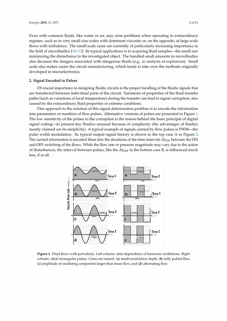
One approach to the solution of this signal deterioration problem is to encode the informationinto parameters or numbers of flow pulses. Alternative versions of pulses are presented in Figure 1.The low sensitivity of the pulses to the corruption is the reason behind the basic principle of digitalsignal coding—in present-day fluidics unusual because of complexity (the advantages of fluidicsmostly claimed are its simplicity). A typical example of signals carried by flow pulses is PWM—thepulse width modulation. Its typical output signal history is shown in the top case A in Figure 2.The carried information is encoded there into the durations of the time intervals ∆tON between the ONand OFF switching of the flows. While the flow rate or pressure magnitude may vary due to the actionof disturbances, the interval between pulses, like the ∆tOFF in the bottom case B, is influenced muchless, if at all.

Figure 1. Fluid flows with periodicity. Left column: time dependence of harmonic oscillations. Rightcolumn: ideal rectangular pulses. Cases are named: (a) small modulation depth, (b) fully pulsed flow,(c) amplitude of oscillating component larger than mean flow, and (d) alternating flow.

Energies 2019, 12, 3071 3 of 21

Figure 2. Examples of signal encoded in properties of rectangular flow pulses. (A) Pulse widthmodulation with a constant relative value of duty cycle ∆tON/∆tOFF. (B) Signal encoded in the frequencyof constant-width pulses.

3. Basic Devices: Amplifiers

Of essential importance for the fluidic pulse generation and shaping is the availability of fluidicamplifiers. It was the invention of the no-moving-part flow amplification that in the middle of sixtiesof the last century [14,15] started fluidics as a separate branch of technology. It is in contrast with theearlier classical hydraulics and pneumatics, which also can amplify liquid or gas flow rate or pressurebut depends on the use of mechanical moved or deformed components. This results in too large size,often a need of maintenance, and complicated (and expensive) manufacturing. In pure fluidics thedevices are simply easily made empty cavities.

There is a number of already used or potentially usable fluidic amplification principles. It maysuffice to name here just the five most important ones: jet deflection [13] (which is most popular),captive vortex generated by tangential inflow into a cavity [6], colliding flows [16,17], separation ofa jet from an attachment wall [14], and transition into turbulence. In the essential principle, fluidicamplification is based on creating inside the amplifier cavity a flowfield characterised by presenceof hydrodynamic instability. This creates a sensitive spot where applying a quite weak input actionresults in a substantial change of the whole flowfield, and in particular, a change in the output terminal.The amplification effect is measured by parameter called gain. It is the ratio of the output (at Y, Figure 3)to the input (at X) values of the same quantity. Amplifiers do exist which for some reason are designedwith unity and even sub-unity gain, but this is extremely extraordinary.

Figure 3. Schematic representation of a signal and power flows in a fluidic amplifier. Top: the simplesamplifier with three terminals. Bottom: the diverter type amplifiers decrease the output flow rate byletting some fluid to flow away through the vent.

Energies 2019, 12, 3071 4 of 21

Typical present day fluidic amplifiers exhibit a flow gain of the order from 10 to 100. The powerused for this amplification effect is delivered from the fluid flow delivered into the supply terminal S.The simplest configuration of an amplifier is schematically presented in the top of Figure 3. The fluidis supplied into the terminal S (usually kept by an external regulator at a constant supplied pressure;though constant flow rate may be also often used). The weak input signal flow is delivered into theinput terminal X. Its presence there creates in the output terminal Y a corresponding powerful outputeffect. What this effect actually is depends on the amplification characteristic of the device. Typical areproportional amplifiers. Their characteristic is linear so that the output is equal to the input multipliedby the value of the gain.

There are—less common—fluidic “turn-down” amplifiers, e.g. as discussed in [17], which decreasethe flow passing through them in proportion to the input signal. Much easier to design and developare the diverter amplifier variants. They need the auxiliary vent terminal V, as shown at the bottom ofFigure 3. Through this terminal escapes the fluid which is diverted by the control input action fromentering the output terminal Y.

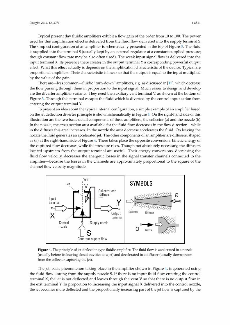
To present an idea about the typical internal configuration, a simple example of an amplifier basedon the jet deflection diverter principle is shown schematically in Figure 4. On the right-hand side of thisillustration are the two basic detail components of these amplifiers, the collector (a) and the nozzle (b).In the nozzle, the cross-section area available for the fluid flow decreases in the flow direction—whilein the diffuser this area increases. In the nozzle the area decrease accelerates the fluid. On leaving thenozzle the fluid generates an accelerated jet. The other components of an amplifier are diffusers, shapedas (a) at the right-hand side of Figure 4. There takes place the opposite conversion: kinetic energy ofthe captured flow decreases while the pressure rises. Though not absolutely necessary, the diffuserslocated upstream from the output terminal are useful. Their energy conversions, decreasing thefluid flow velocity, decreases the energetic losses in the signal transfer channels connected to theamplifier—because the losses in the channels are approximately proportional to the square of thechannel flow velocity magnitude.

Figure 4. The principle of jet-deflection type fluidic amplifier. The fluid flow is accelerated in a nozzle(usually before its leaving closed cavities as a jet) and decelerated in a diffuser (usually downstreamfrom the collector capturing the jet).

The jet, basic phenomenon taking place in the amplifier shown in Figure 4, is generated usingthe fluid flow issuing from the supply nozzle S. If there is no input fluid flow entering the controlterminal X, the jet is not deflected and leaves through the vent V so that there is no output flow inthe exit terminal Y. In proportion to increasing the input signal X delivered into the control nozzle,the jet becomes more deflected and the proportionally increasing part of the jet flow is captured by the

Energies 2019, 12, 3071 5 of 21

collector leading to Y. This jet deflection is a typical case of the flowfield with the weak spot. In this casethe spot is located at the base of the jet, immediately downstream from the exit from the supply nozzle.

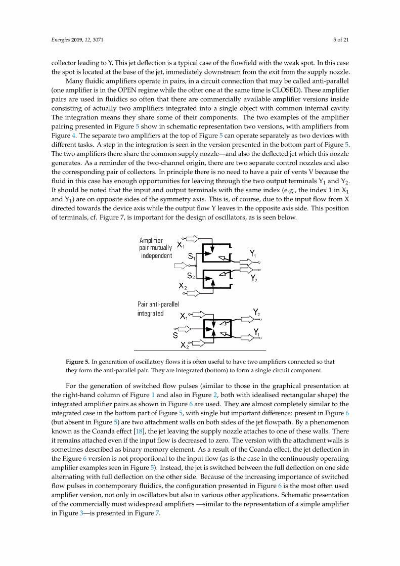
Many fluidic amplifiers operate in pairs, in a circuit connection that may be called anti-parallel(one amplifier is in the OPEN regime while the other one at the same time is CLOSED). These amplifierpairs are used in fluidics so often that there are commercially available amplifier versions insideconsisting of actually two amplifiers integrated into a single object with common internal cavity.The integration means they share some of their components. The two examples of the amplifierpairing presented in Figure 5 show in schematic representation two versions, with amplifiers fromFigure 4. The separate two amplifiers at the top of Figure 5 can operate separately as two devices withdifferent tasks. A step in the integration is seen in the version presented in the bottom part of Figure 5.The two amplifiers there share the common supply nozzle—and also the deflected jet which this nozzlegenerates. As a reminder of the two-channel origin, there are two separate control nozzles and alsothe corresponding pair of collectors. In principle there is no need to have a pair of vents V because thefluid in this case has enough opportunities for leaving through the two output terminals Y1 and Y2.It should be noted that the input and output terminals with the same index (e.g., the index 1 in X1

and Y1) are on opposite sides of the symmetry axis. This is, of course, due to the input flow from Xdirected towards the device axis while the output flow Y leaves in the opposite axis side. This positionof terminals, cf. Figure 7, is important for the design of oscillators, as is seen below.

Figure 5. In generation of oscillatory flows it is often useful to have two amplifiers connected so thatthey form the anti-parallel pair. They are integrated (bottom) to form a single circuit component.

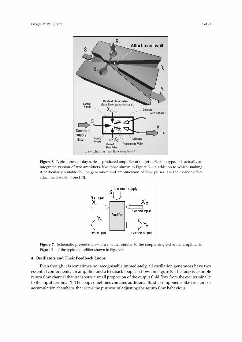
For the generation of switched flow pulses (similar to those in the graphical presentation atthe right-hand column of Figure 1 and also in Figure 2, both with idealised rectangular shape) theintegrated amplifier pairs as shown in Figure 6 are used. They are almost completely similar to theintegrated case in the bottom part of Figure 5, with single but important difference: present in Figure 6(but absent in Figure 5) are two attachment walls on both sides of the jet flowpath. By a phenomenonknown as the Coanda effect [18], the jet leaving the supply nozzle attaches to one of these walls. Thereit remains attached even if the input flow is decreased to zero. The version with the attachment walls issometimes described as binary memory element. As a result of the Coanda effect, the jet deflection inthe Figure 6 version is not proportional to the input flow (as is the case in the continuously operatingamplifier examples seen in Figure 5). Instead, the jet is switched between the full deflection on one sidealternating with full deflection on the other side. Because of the increasing importance of switchedflow pulses in contemporary fluidics, the configuration presented in Figure 6 is the most often usedamplifier version, not only in oscillators but also in various other applications. Schematic presentationof the commercially most widespread amplifiers —similar to the representation of a simple amplifierin Figure 3—is presented in Figure 7.

Energies 2019, 12, 3071 6 of 21

Figure 6. Typical present-day series—produced amplifier of the jet-deflection type. It is actually anintegrated version of two amplifiers, like those shown in Figure 5—in addition to which, makingit particularly suitable for the generation and amplification of flow pulses, are the Coanda-effectattachment walls. From [13].

Figure 7. Schematic presentation—in a manner similar to the simple single-channel amplifier inFigure 3—of the typical amplifier shown in Figure 6.

4. Oscillators and Their Feedback Loops

Even though it is sometimes not recognisable immediately, all oscillation generators have twoessential components: an amplifier and a feedback loop, as shown in Figure 8. The loop is a simplereturn flow channel that transports a small proportion of the output fluid flow from the exit terminal Yto the input terminal X. The loop sometimes contains additional fluidic components like resistors oraccumulation chambers, that serve the purpose of adjusting the return flow behaviour.

Energies 2019, 12, 3071 7 of 21

Figure 8. Schematic representation of flows in a fluidic general feedback loop: a part of the output flowY is returned to the input X.

The idea of the feedback came to fluidics in a direct analogy to the much earlier developments inthe no-moving-part electronics. The amplifiers for amplification of electronic signals were developedfrom the thermionic diode invented by Fleming [19] in 1904. Diodes were developed into a vacuumtube amplifier via the addition of the grid, the third terminal. The idea was patented by DeForest [20].In principle, as seen in top of Figure 3, the roles of the three terminals in the vacuum tube amplifierwere fully analogous to the terminals S, X, and Y of the fluidic amplifiers. It was with this vacuumtube amplifier that the final step to the oscillators by the addition of the feedback loop was made.It was invented by Armstrong [21] in 1913. It should be emphasised that apart from the generationand amplification of periodically oscillating flows, the feedback loop can perform several other usefultasks. As a matter of fact, the simple signal connection from Y to X, as it is shown (with the amplifierfrom Figure 4) in the example presented in Figure 9 would actually not produce the oscillation effect atall. The reason is this simplest case is positive feedback. It operates as schematically represented inFigure 10. Such behaviour may be quite useful for some other tasks but not for the role of the oscillatorsof interest here. The input signal in X would rapidly move the deflected jet towards its full deflection.After that, the conditions would remain stationary, with constant maximum output signal in the exit Yas long as there is a supply flow S.

Figure 9. Positive feedback loop channel added to the simple amplifier from Figure 4.

Figure 10. Use of the positive feedback: The output Y is kept in the ON state even after the input flowpulse X ceases to exist.

Energies 2019, 12, 3071 8 of 21

The desirable feedback generation of pulsating oscillation, as seen in Figure 11, is obtained by twoprocesses taking place in the feedback loop channel. The first one is inversion of the return flow byan invertor as schematically represented in Figure 11. It results in the negative type of the feedback.The second process is the need to secure a certain duration of the generated pulse. This is obtained bythe time delay in the loop.

Figure 11. Use of the negative feedback: generation of the periodic pulse train.

Apart of the oscillators, there is yet another important group of devices in fluidics. They areperhaps less known but certainly not of lesser importance. It is the family of pulse shapers. For correctoperation, the pulses have to show distinct leading and trailing edges. Because of the usually complexfrequency spectrum of the unsteady responses of the amplifier—as well as the various devices thatmay be connected into the feedback loop—the shapes of arriving pulses may be quite far from theideal. The individual components of the signal spectrum travel at different speeds. Also the valuesof the amplifier gain may be different for different frequencies. In fact, some harmonic components,especially those of higher frequencies, may be completely filtered out. Moreover, the shapes of theindividual pulses in a high-frequency pulse train may be deformed differently (due to varied phasetransport effects).

To avoid the unpleasant consequences of these signal deformations, it is useful to run the flowpulses through the pulse shaper device for correction. The device may be based on the schematicallyrepresented system in Figure 12 (even though the actual realisation may be very much different).The desirable pulse correction may be obtained by the use of two parallel feedback loops. One of them,the outer positive loop, generates the properly shaped leading edges of the pulses. The other loop,the inner negative feedback loop with time delay, takes care of the trailing edges. Generated pulse isthus started by the flow in the positive feedback, the same as in Figure 10, but then comes the delayedmore powerful negative feedback that stops the output flow. Its delay defines the pulse trailing edge.The result are pulses having all the same duration ∆tY determined by the properties of the time delay inthe negative feedback, i.e., irrespective of the duration ∆tX of the input pulse that may come corrupted.As it is apparent, the pulse shapers have in principle very much in common with oscillators.

Figure 12. Pulse shaper—schematic representation of its internal flows. The duration ∆tY of the outputpulse is dependent solely on the delay in the inner loop and independent of the input pulses.

Energies 2019, 12, 3071 9 of 21

5. Flip-Flop Circuits

In the early era of electronics, with vacuum tube amplification technology the forefather of fluidics,an interesting pulse generating circuit was invented characterised by a pair of amplifiers arranged inanti-parallel. This circuit, of which a direct analogy was later made in wluidics, is particularly wellsuited for the generation and handling of the rectangular-shaped flow pulses. Its basic configurationis presented in general terms in Figure 13. Inventors were Abraham and Bloch in France, electronicengineers working during WWI on developments in radio transmission. Due to the applied rules ofmilitary secrets, their publication [22] had to be postponed until after the war, and in the meantimeEccless and Jordan in Britain obtained the patent on the same idea [23]. The inventors of [22] called thedevice “multi-vibrateur.” The meaning of this term is obvious in Fouriér analysis of the generated pulse.It spectrum results from generation of many (theoretically infinitely many) multiples of the harmonicmultiples of the base frequency. Eccles and Jordan [23] called their circuit ”flip-flop”. Amplifiers of thepair are switched between their two extreme regimes, OPEN (large output Y) and CLOSED (Y = 0),as shown in the diagram at the bottom of right-hand side in Figure 13. By adjusting the parameters ofthe components in the circuit, it is possible to operate it in three alternative useful operational modes.In the bistable mode, the flows remain stable in either one of two regimes. It may be the regime withthe steady flow in Y1 or the equally stable regime with steady flow in Y2. Othervise, the regime maybe monostable with one of the output channels dominant so that to it the circuit always returns in theabsence of control input. Finally, the self-excited oscillating version is described as astable.

Figure 13. Schematic presentation of the “flip-flop” pair of amplifiers blocking one another. A typicalpresent-day amplifier shown in Figure 6 is actually an integrated version of this pair.

The jet-deflection fluidic amplifier version shown above in Figure 6 operates as the “flip-flop”presented schematically in the Figure 13. It should be noted there that while the mutual blockage ofthe amplifiers in Figure 13 requests a crossing of the signal transfer channels connecting the amplifiers(which would cause manufacturing complication in what is the essentially a single-plane configuration),in the fluidic versions shown in Figure 14, with control nozzles on the opposed locations, no suchspatial crossing of the signal channels is necessary. The inverting character of the negative feedback toget the oscillation is obtained by connecting the terminals Y with X located on the same side of thefluidic amplifier.

Energies 2019, 12, 3071 10 of 21

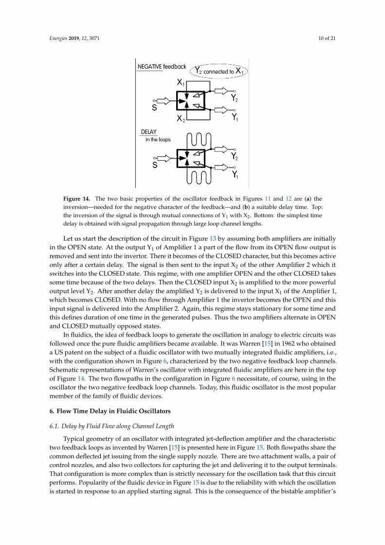
Figure 14. The two basic properties of the oscillator feedback in Figures 11 and 12 are (a) theinversion—needed for the negative character of the feedback—and (b) a suitable delay time. Top:the inversion of the signal is through mutual connections of Y1 with X2. Bottom: the simplest timedelay is obtained with signal propagation through large loop channel lengths.

Let us start the description of the circuit in Figure 13 by assuming both amplifiers are initiallyin the OPEN state. At the output Y1 of Amplifier 1 a part of the flow from its OPEN flow output isremoved and sent into the invertor. There it becomes of the CLOSED character, but this becomes activeonly after a certain delay. The signal is then sent to the input X2 of the other Amplifier 2 which itswitches into the CLOSED state. This regime, with one amplifier OPEN and the other CLOSED takessome time because of the two delays. Then the CLOSED input X2 is amplified to the more powerfuloutput level Y2. After another delay the amplified Y2 is delivered to the input X1 of the Amplifier 1,which becomes CLOSED. With no flow through Amplifier 1 the invertor becomes the OPEN and thisinput signal is delivered into the Amplifier 2. Again, this regime stays stationary for some time andthis defines duration of one time in the generated pulses. Thus the two amplifiers alternate in OPENand CLOSED mutually opposed states.

In fluidics, the idea of feedback loops to generate the oscillation in analogy to electric circuits wasfollowed once the pure fluidic amplifiers became available. It was Warren [15] in 1962 who obtaineda US patent on the subject of a fluidic oscillator with two mutually integrated fluidic amplifiers, i.e.,with the configuration shown in Figure 6, characterized by the two negative feedback loop channels.Schematic representations of Warren’s oscillator with integrated fluidic amplifiers are here in the topof Figure 14. The two flowpaths in the configuration in Figure 6 necessitate, of course, using in theoscillator the two negative feedback loop channels. Today, this fluidic oscillator is the most popularmember of the family of fluidic devices.

6. Flow Time Delay in Fluidic Oscillators

6.1. Delay by Fluid Flow along Channel Length

Typical geometry of an oscillator with integrated jet-deflection amplifier and the characteristictwo feedback loops as invented by Warren [15] is presented here in Figure 15. Both flowpaths share thecommon deflected jet issuing from the single supply nozzle. There are two attachment walls, a pair ofcontrol nozzles, and also two collectors for capturing the jet and delivering it to the output terminals.That configuration is more complex than is strictly necessary for the oscillation task that this circuitperforms. Popularity of the fluidic device in Figure 15 is due to the reliability with which the oscillationis started in response to an applied starting signal. This is the consequence of the bistable amplifier’s

Energies 2019, 12, 3071 11 of 21

separate control of both the beginning and end (leading and trailing edge) of the generated oscillationpulse. The jet is thus reliably switched at exactly the time of the pulse edge.

Figure 15. Typical example of oscillator with flow time delays according to Warren’s U.S. patent [15].The frequency of generated oscillation depends on the lengths of negative feedback loops withthe connecting channels between the control X and output Y terminals of a bistable jet-deflectiontype amplifier.

Capable of generating the pulses in a more simple way, but exhibiting less satisfactory operationalreliability, is the oscillator version with the single-flowpath amplifier an example of which is shownin Figure 16. Its is described as monostable because in the no-input-signal regime the jet alwaysattaches to the single available Coanda-effect wall. The amplifier is supplied by a permanent fluidflow delivered into the input terminal X. Beginning of the attachment wall is located at the exit ofthe supply nozzle. The jet generated in this nozzle attaches to this wall. and leads it to the outputterminal Y. At the downstream end of the wall, the captured flow is divided into two parts. While onepart leaves to the output terminal Y, the rest enters the feedback channel which brings the fluid to thecontrol nozzle, which is oriented perpendicularly to the supply nozzle axis. If there is a flow from thecontrol nozzle, the Coanda effect cannot keep the jet attached to the attachment wall. The suppliedflow separates from this wall and together with the control flow leaves to atmosphere through the ventterminal (at the upper part of the picture). Of course, with the resultant absence of the flow past theattachment wall, the flow through the output terminal Y stops. The switching of the flow into thisregime is not immediate. It is delayed by the duration of the flow past the attachment wall. This delaydefines the time between pulses.

Energies 2019, 12, 3071 12 of 21

Figure 16. Simpler than the two-loop oscillator in Figure 15, this example version has a monostableamplifier and only one feedback loop. Experience shows such pulse generators to be less reliable(sometimes failing to oscillate, sometimes missing a pulse).

The relative width of the generated pulses is characterised by their “duty cycle”, defined as theratio of pulse ON duration to the total time of the oscillation period ∆tp. In the oscillator shown inFigure 16, the duty cycle is constant, determined by the geometry of the device’s internal cavity.

In the bistable amplifier version with two feedback loops in Figure 15, it is possible to adjustthe duty cycle value. This is done by separately adjusting the lengths of the two feedback channels.As seen in Figures 15–17, the pulse widths and duty cycle are determined by three factors. It is thefeedback loops’ lengths, the flow velocities in them, and also the (usually quite small) switching timeof the jet in the amplifier. The most important parameter, propagation velocity in the loop, may beestimated by the relations in Figure 17 (adapted from reference [13]) and in the diagram Figure 18. as afunction of available driving pressure difference. It may be noted that this propagation time delay in asimple channel is a typical example of an effect in which the analogy between fluidics and electriccircuitry fails - because the electrons propagation in a conductor is extremely fast and delays have tobe arranged differently. As a final note on the subject of feedback loops, the device shown in Figure 19may be seen as a proposal for a pulse shaper based directly on the signal flows from Figure 12.

Figure 17. Typical dependence between pressure difference across the nozzle and the exit velocity ina planar fluidic device. The delays in the version in Figure 15 are inversely proportional to the flowvelocity w, which, in turn, increases (here for simplicity neglecting friction losses) with the square rootof the acting pressure difference ∆P. Adapted from [13].

Energies 2019, 12, 3071 13 of 21

Figure 18. Pressure and velocities prevailing in a typical fluid flow channels applicable to generatingthe delay. Higher velocities than shown here might be generated but would result in high energydissipation (friction and conversion into heat). Other limits are stresses in the device body that mayendanger its life and reliability.

Figure 19. An example of pulse shaper with monostable amplifier and two mutually opposed time-delayfeedback loops. (A) Schematic representation of the configuration with both positive and negativeloops. (B) Planar pulse shaper cavity (of constant depth everywhere). Note the secondary feedbackloop missing in Figure 15.

6.2. Achieving Higher Oscillation Frequencie

It should be mentioned that the classical hydraulic and pneumatic devices can actually alsooperate at quite high oscillation frequencies. The problem is not in achieving at such frequencies, butrather the dangerously high pressure levels needed for them. The high pressure force is necessaryfor moving or deforming the mechanical component. For a high natural frequency, this force must

Energies 2019, 12, 3071 14 of 21

be much higher than the inertial forces. As the consequence, the operating conditions occupy in thediagram in Figure 18 the part on the right-hand side, at the high pressure levels. where they canapproach dangerously high mechanical stressing.

One of the advantages of pure fluidics is that the devices, especially when working with gas,occupy the area of low pressure at left in the diagram Figure 18. It is thus possible without high stressesto design operating conditions of high velocities and high frequencies. Of course, in considering thehigh frequencies, there are other aspects to be taken into consideration. An important aspect is theoverall size of the device. Very roughly, with present-day usual devices of overall sizes from 20 mm to200 mm, the operating frequencies of oscillators according to Figure 15 with reasonably long feedbackchannels operate typically between f ≈ 50 Hz and f ≈ 200 Hz.

Somewhat higher frequencies, say ≈ 400 Hz, may be obtained with a different, resonatorfeedback [5,24] operating with compression and expansion waves traveling in a resonant cavity.The limiting factor with the standard design in Figure 15 are the reasonable lengths and turning anglesof the channel flow. In typical methods of fluidic device manufacturing, the circuit components aredistributed in a plane from which are removed those parts in the resultant cavities of which the fluidflows. This, of course, leads to is a problem with the “island” left free according to Figures 16 and 19.

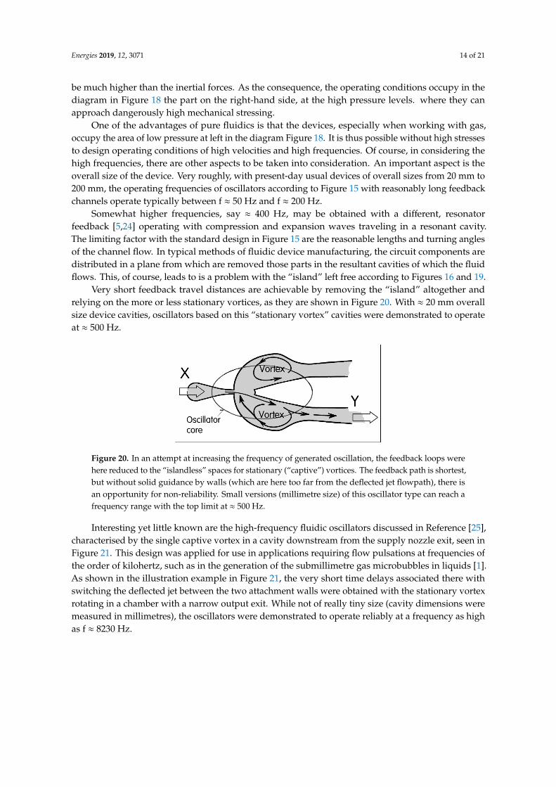
Very short feedback travel distances are achievable by removing the “island” altogether andrelying on the more or less stationary vortices, as they are shown in Figure 20. With ≈ 20 mm overallsize device cavities, oscillators based on this “stationary vortex” cavities were demonstrated to operateat ≈ 500 Hz.

Figure 20. In an attempt at increasing the frequency of generated oscillation, the feedback loops werehere reduced to the “islandless” spaces for stationary (“captive”) vortices. The feedback path is shortest,but without solid guidance by walls (which are here too far from the deflected jet flowpath), there isan opportunity for non-reliability. Small versions (millimetre size) of this oscillator type can reach afrequency range with the top limit at ≈ 500 Hz.

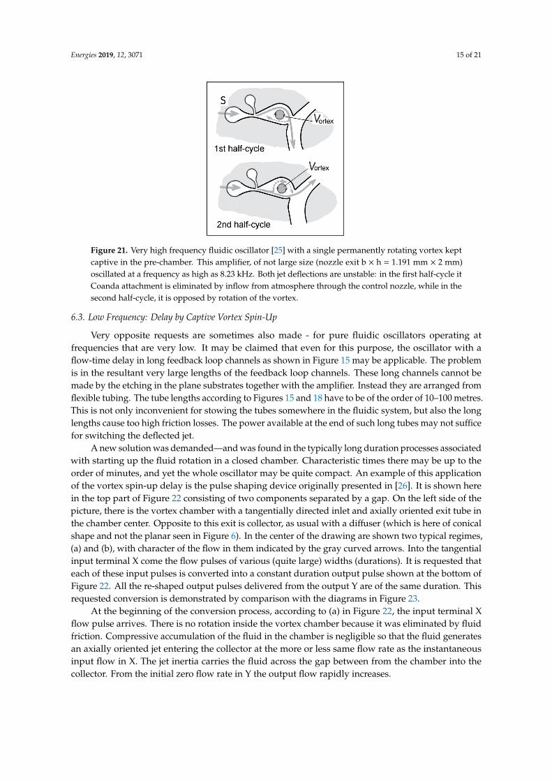
Interesting yet little known are the high-frequency fluidic oscillators discussed in Reference [25],characterised by the single captive vortex in a cavity downstream from the supply nozzle exit, seen inFigure 21. This design was applied for use in applications requiring flow pulsations at frequencies ofthe order of kilohertz, such as in the generation of the submillimetre gas microbubbles in liquids [1].As shown in the illustration example in Figure 21, the very short time delays associated there withswitching the deflected jet between the two attachment walls were obtained with the stationary vortexrotating in a chamber with a narrow output exit. While not of really tiny size (cavity dimensions weremeasured in millimetres), the oscillators were demonstrated to operate reliably at a frequency as highas f ≈ 8230 Hz.

Energies 2019, 12, 3071 15 of 21

Figure 21. Very high frequency fluidic oscillator [25] with a single permanently rotating vortex keptcaptive in the pre-chamber. This amplifier, of not large size (nozzle exit b × h = 1.191 mm × 2 mm)oscillated at a frequency as high as 8.23 kHz. Both jet deflections are unstable: in the first half-cycle itCoanda attachment is eliminated by inflow from atmosphere through the control nozzle, while in thesecond half-cycle, it is opposed by rotation of the vortex.

6.3. Low Frequency: Delay by Captive Vortex Spin-Up

Very opposite requests are sometimes also made - for pure fluidic oscillators operating atfrequencies that are very low. It may be claimed that even for this purpose, the oscillator with aflow-time delay in long feedback loop channels as shown in Figure 15 may be applicable. The problemis in the resultant very large lengths of the feedback loop channels. These long channels cannot bemade by the etching in the plane substrates together with the amplifier. Instead they are arranged fromflexible tubing. The tube lengths according to Figures 15 and 18 have to be of the order of 10–100 metres.This is not only inconvenient for stowing the tubes somewhere in the fluidic system, but also the longlengths cause too high friction losses. The power available at the end of such long tubes may not sufficefor switching the deflected jet.

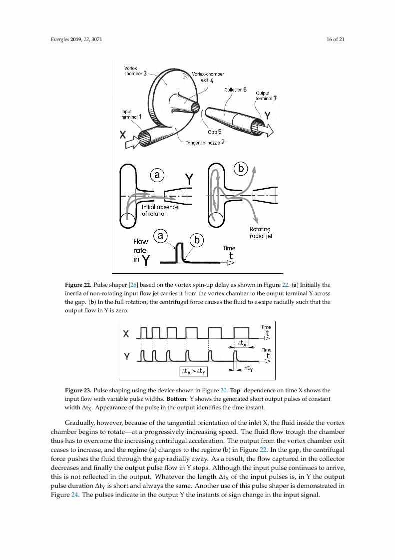
A new solution was demanded—and was found in the typically long duration processes associatedwith starting up the fluid rotation in a closed chamber. Characteristic times there may be up to theorder of minutes, and yet the whole oscillator may be quite compact. An example of this applicationof the vortex spin-up delay is the pulse shaping device originally presented in [26]. It is shown herein the top part of Figure 22 consisting of two components separated by a gap. On the left side of thepicture, there is the vortex chamber with a tangentially directed inlet and axially oriented exit tube inthe chamber center. Opposite to this exit is collector, as usual with a diffuser (which is here of conicalshape and not the planar seen in Figure 6). In the center of the drawing are shown two typical regimes,(a) and (b), with character of the flow in them indicated by the gray curved arrows. Into the tangentialinput terminal X come the flow pulses of various (quite large) widths (durations). It is requested thateach of these input pulses is converted into a constant duration output pulse shown at the bottom ofFigure 22. All the re-shaped output pulses delivered from the output Y are of the same duration. Thisrequested conversion is demonstrated by comparison with the diagrams in Figure 23.

At the beginning of the conversion process, according to (a) in Figure 22, the input terminal Xflow pulse arrives. There is no rotation inside the vortex chamber because it was eliminated by fluidfriction. Compressive accumulation of the fluid in the chamber is negligible so that the fluid generatesan axially oriented jet entering the collector at the more or less same flow rate as the instantaneousinput flow in X. The jet inertia carries the fluid across the gap between from the chamber into thecollector. From the initial zero flow rate in Y the output flow rapidly increases.

Energies 2019, 12, 3071 16 of 21

Figure 22. Pulse shaper [26] based on the vortex spin-up delay as shown in Figure 22. (a) Initially theinertia of non-rotating input flow jet carries it from the vortex chamber to the output terminal Y acrossthe gap. (b) In the full rotation, the centrifugal force causes the fluid to escape radially such that theoutput flow in Y is zero.

Figure 23. Pulse shaping using the device shown in Figure 20. Top: dependence on time X shows theinput flow with variable pulse widths. Bottom: Y shows the generated short output pulses of constantwidth ∆tX. Appearance of the pulse in the output identifies the time instant.

Gradually, however, because of the tangential orientation of the inlet X, the fluid inside the vortexchamber begins to rotate—at a progressively increasing speed. The fluid flow trough the chamberthus has to overcome the increasing centrifugal acceleration. The output from the vortex chamber exitceases to increase, and the regime (a) changes to the regime (b) in Figure 22. In the gap, the centrifugalforce pushes the fluid through the gap radially away. As a result, the flow captured in the collectordecreases and finally the output pulse flow in Y stops. Although the input pulse continues to arrive,this is not reflected in the output. Whatever the length ∆tX of the input pulses is, in Y the outputpulse duration ∆tY is short and always the same. Another use of this pulse shaper is demonstrated inFigure 24. The pulses indicate in the output Y the instants of sign change in the input signal.

Energies 2019, 12, 3071 17 of 21

Figure 24. Another use of the pulse sharper from Figure 22. The output pulse generated in the outputY identifies the instants at which the increasing input flow in X crosses the zero.

6.4. Oscillator with Load-Switched Vortices

Essentially the same principle, the delay caused by gradually increasing rotation of a captivevortex, is also used in a low-frequency generator of periodic pulse trains [26,27], presented in Figures 25and 26. In contrast to the 3D spatial configuration shown in Figure 22, suitable for use in powerfluidics, the oscillator in Figure 26 is of a planar configuration. This is advantageous from the point ofview of contemporary small-scale manufacturing. There are two mutually similar vortex chambers,1 and 2. They both have a tangentially oriented inlet and centrally positioned exit perpendicular tothe illustration plane of Figure 26. The inlets are connected to exits of what is essentially a bistableCoanda-effect jet-deflection flow diverter. It is very much similar to bistable amplifiers, from which itdiffers by the absence of control terminals since it is switched by applying the load switching approach.This is explained in Figure 25. The diverter in this illustration is completely similar to that in Figure 26,but there are no vortex chambers. Their hydraulic resistance is replaced by the more general idea offluidic loads: connection of devices generating a pressure drop. In the initial flow regime, the jet in thetop picture part A of Figure 25 is shown attached to the upper attachment wall leading to the output 1.If the fluidic resistance (dissipance) of the load connected to the upper output 1 is small, there is only aminimal change. The Coanda effect is sufficiently strong for keeping the jet deflected to the upperoutput 1. If, however, the resistance is further increased, at some stage of this increase the Coandaeffect fails. As shown in the bottom part B of Figure 25, the jet simply finds it easier to leave throughthe lower output 2. In Figure 25, this increased load is represented by the connected fluidic resistor,with smaller cross-section area available for the exit fluid from the diverter. In the oscillator shown inFigure 26, the increased load is due to the increased rotation speed inside the vortex chamber and theassociated centrifugal force acting on the rotating fluid.

Figure 25. Oscillator [28,29] with a load-switched bistable diverter and two alternatively rotated vortexchambers, with all components in planar configuration.

Energies 2019, 12, 3071 18 of 21

Figure 26. Switching the jet to the opposite attachment wall (from output 1 to output 2) by the loadthat makes the flow into the output 1 more difficult. Adapted from Reference [27].

6.5. Very Low Frequency “Flip-Flop” Oscillato

Typical use of fluidic oscillators [29] is currently found in their increasing heat and/or masstransfer in various chemical and physical processes. The increase is usually the result of destroying theboundary layer, which behaves as an insulating stationary layer at a transfer surface. In the illustrationFigure 26 is a schematic representation of the case of two parallel heat exchangers with flows fluidicallypulsated [30] in a circuit containing a pair of vortex chambers. The flow, supplied through the supplyinlet S, is divided into two parallel branches. It is pulsated so that a larger flow rate through the firstexchanger is simultaneous with the smaller flow rate through the second exchanger, and vice versa.The negative feedback and delay effects necessary for the oscillator, Figure 13, are here provided by thetube connecting the terminals X1 and X2.

In the next pair of pictures (Figures 27 and 28), the pressure distributions generating the feedbackeffect are explained. For easier explanation, the exchangers as well as vortex chambers are in thesepictures replaced by schematically presented fluidic resistors R (i.e., local cross-section area decreases).The pressure drops across the restrictor are represented by the vertical lengths of the lines and arrowsin Figures 28 and 29.

Figure 27. Oscillator based on the “flip-flop” configuration. Agitation by alternating fast and slowflows in the heat exchangers transport processes according to Reference [29].

Energies 2019, 12, 3071 19 of 21

Figure 28. Explanation of generated delayed fluid flow generating rotation in the vortex chamber 1.For simplicity of explanation the exchanges as well as vortex chambers are replaced by fluidic resistors R.

Figure 29. During the second half of the oscillation cycle, the direction of the control flow is reversed.

In Figure 28 is presented the situation in the first half of the oscillation cycle, with a larger flowrate through the first branch (at left). This larger flow also means a larger pressure drop ∆Pexchang1across the first heat exchanger (in Figure 28 represented by the longer arrow). There is no rotationinside the vortex chamber 1 so that the fluid passes through it radially into its central exit. This resultsin a small pressure drop ∆Pvortex ch.1. At this time the conditions in the second branch (at right) aredifferent. There is a smaller flow rate through the second exchanger (represented in Figure 29 by theshorter vertical arrow), and the pressure drop ∆Pexchang2 is larger because the fluid inside the secondvortex chamber rotates. As a result, the pressure in X2 is larger than the pressure in X1. The fluid thusflows away from vortex chamber 2 into the vortex chamber 1. As it enters this chamber tangentially,the rotation there progressively increases. The large length of the tube connecting the terminals X1 andX2 delaying the rotation. Also the flow away from the second vortex chamber through its center alsostops the rotation. When the rotation intensity in vortex chamber 1 reaches its limit value, the pressuredrop across the chamber 1 increases so that flow in the tube connecting the terminals X1 and X2 reversesits direction. The flow field thus becomes as shown in Figure 29.

7. Conclusions

This paper explains the operating principles of no-moving-part fluidic oscillators, which aredevices currently finding increased application in a number of interesting uses. The principlesare in some cases analogous to the forerunner circuits of electronics—but quite often used are also

Energies 2019, 12, 3071 20 of 21

configurations that differ substantially. In particular, the paper provides an explanation of why thenowadays universally used fluidic amplifiers are the configurations with two mutually integratedflowpaths. The other not obviously analogy are the fluidic “flip-flop” circuits for the extreme conditionsof very high and very low frequencies. Present standard time delays, without which the feedbackloops would not work, are based on duration of axial (lengthwise) flow in the loop channel. Paperpresents also the little known and yet important new ideas of the time delays based on reaching acertain magnitude of rotation speed of a captive vortex.

Funding: Author’s work was supported by grant 17-08218S obtained from GACR—the Grant Agency of theCzech Republic. He was also a recipient of institutional support RVO: 61388998.

Conflicts of Interest: The authors declare no conflict of interest.

References

1. Rehman, F.; Medley, G.J.; Bandulasena, H.; Zimmerman, W.B. Fluidic oscillator-mediated microbubblegeneration to provide cost effective mass transfer and mixing efficiency to the wastewater treatment plants.Environ. Res. 2014, 37, 32–39. [CrossRef] [PubMed]

2. Desai, P.D.; Hines, M.J.; Riaz, Y.; Zimmerman, W.B. Resonant pulsing frequency effect for much smallerbubble formation with fluidic oscillation. Energies 2018, 11, 2680. [CrossRef]

3. Zimmerman, W.B.; Tesar, V.; Butler, S.; Bandulasena, H. Microbubble generation. Recent Pat. Eng. 2008, 2,1–8. [CrossRef]

4. Seifert, A.; Pack, L.G. Active control of separated flow on a wall–mounted hump at high Reynolds numbers.AIAA J. 2002, 40, 1363–1372. [CrossRef]

5. Tesar, V.; Zhong, S.; Fayaz, R. New fluidic oscillator concept for flow separation control. AIAA J. 2013, 51,397–405. [CrossRef]

6. Raghu, S. Fluidic oscillators for flow control. Exp. Fluids 2013, 54, 1455. [CrossRef]7. Ten, J.S.; Povey, T. Self-excited fluidic oscillators for gas turbines cooling enhancement: Experimental and

computational study. J. Thermophys. Heat Transf. 2018, 33, 536–547. [CrossRef]8. Tesar, V. Enhancing impinging-jet heat or mass transfer by fluidically generated flow pulsation. Chem. Eng.

Res. Des. 2009, 87, 181–192. [CrossRef]9. Tesar, V. Fluidic control of molten metal flow. Acta Polytech. J. Adv. Eng. 2003, 43, 15.10. Mairhofer, J.; Roppert, K.; Ertl, P. Microfluidic systems for pathogen sensing: A Review. Sensors (Basel) 2009,

9, 4804–4823. [CrossRef] [PubMed]11. Tesar, V. Role of microfluidics in discovering new marketable substances—A Survey. In Proceedings of the

19th International Conference, Svratka, Czech Republic, 13–16 May 2013; p. 614.12. Tesar, V. Microfluidic Systems for Combinatorial Chemistry. In Encyclopedia of Microfluidics and Nanofluidics;

Li, D., Ed.; Springer Science Business Media: Berlin, Germany, 2008; p. 1221.13. Tesar, V. Pressure-Driven Microfluidics; Artech House Publishers: Norwood, MA, USA, 2007.14. Zalmanzon, L.A. Method of Automatically Controlling Pneumatic or Hydraulic Elements of Instruments

and Other Devices. U.S. Patent 3,295,543, December 1959.15. Warren, R.W. Negative Feedback Oscillator. U.S. Patent 3,158,166, August 1962.16. Tesar, V.; Peszynski, K. Pneumatic sensors based on colliding curved wall-jets. Sens. Actuators A Phys. 2015,

228, 82–94.17. Tesar, V. Microfluidic turn-down valve. J. Vis. 2002, 5, 301–307. [CrossRef]18. Coanda, H. Device for Deflecting a Stream of Elastic Fluid Projected into an Elastic Fluid. U.S. Patent 2,052,869,

1 September 1936.19. Fleming, J.A. Instrument for Converting Alternating Electric Currents into Continuous Currents.

U.S. Patent 803,684, 19 April 1905.20. DeForest, L. Device for Amplifying Feeble Electrical Current. U.S. Patent 841,387, 25 October 1906.21. Armstrong, E. Wireless Receiving System. U.S. Patent 1,113,149, 18 December 1913.22. Abraham, H.; Bloch, E. Mesure en valeur absolue des périodes des oscillations électriques de haute fréquence.

Ann. Phys. 1919, 9, 237–302. [CrossRef]23. Eccles, W.H.; Jordan, F.W. Improvements in Ionic Relais. Patent UK 148,582, 21 June 1918.

Energies 2019, 12, 3071 21 of 21

24. Tesar, V. Fluidic Oscillator with Jet-Type Bistable Amplifier. Patent CZ 303,758, August 2011.25. Tesar, V. High-frequency fluidic oscillator. Sens. Actuators A Phys. 2015, 234, 158–167. [CrossRef]26. Tesar, V. Device for Adjusting Time Dependence of Fluid Flow. Patent CZ 202,898, January 1979.27. Tesar, V. Fluidic Oscillator. Patent CZ 306,064, December 2014.28. Tesar, V.; Smyk, E. Fluidic low-frequency oscillator with vortex spin-up time delay. Chem. Eng. Process.

Process. Intensif. 2015, 90, 6–15. [CrossRef]29. Tesar, V. Taxonomic trees of fluidic oscillators. EPJ Web Conf. 2017, 143, 02128. [CrossRef]30. Tesar, V. Heat Exchanger with Fluidic Device for Transfer Intensification. Patent CZ 262,367, December 1986.

© 2019 by the author. Licensee MDPI, Basel, Switzerland. This article is an open accessarticle distributed under the terms and conditions of the Creative Commons Attribution(CC BY) license (http://creativecommons.org/licenses/by/4.0/).