ABSTRACT

We apply the white noise functional approach in the evaluation of the Feyn-

man propagator of a coupled harmonic oscillators of uniform frequency and mass. The

evaluation is made first by decoupling the oscillators through a coordinate transfor-

mation. With the coordinate transformation, the propagator then becomes separable

and reduces to a one-dimensional harmonic oscillator. The evaluation of each of the

propagator in the language of white noise analysis is done by following the work of Hida

and Streit [15]. The propagator is then expressed in its symmetric form and from it we

obtain the energy spectrum and the wavefunction of the coupled harmonic oscillators.

COUPLED HARMONIC OSCILLATORS :

A WHITE NOISE FUNCTIONAL APPROACH

A Thesis

Presented toThe Faculty of Department of Physics

MSU-Iligan Institute of Technology9200 Iligan City, Philippines

In Partial Fulfillmentof the Requirements for the Degree of

Bachelor of Science in Physics

JEFFERSON R. PABALAYMarch 2008

APPROVAL SHEET

The thesis attached hereto, entitled “COUPLED HARMONIC OSCIL-LATORS : A WHITE NOISE FUNCTIONAL APPROACH”, prepared andsubmitted by JEFFERSON R. PABALAY, in partial fulfillment of the requirementsfor the degree of Bachelor of Science in Physics is hereby submitted for approval:

JINKY B. BORNALES, Ph.D.Adviser

Date

REMIGIO G.TEE, Ph.D. CHRISTINE JOY G. GRAVINOPanel Member Panel Member

Date Date

This thesis is approved in partial fulfillment of the requirements for the degree ofBachelor of Science in Physics:

JINKY B. BORNALES, Ph.DChairman, Physics Department

MSU-Iligan Institute of Technology

Date

ROMULO C. GUERRERO, Ph.D.Dean, College of Science and Mathematics

MSU-Iligan Institute of TechnologyIligan City, Philippines

Date

ACKNOWLEDGEMENTS

Physics is the most interesting secular subject I could ever find and learning it

for these past seven years has been a lot of fun to me. This thesis is one of the proofs

of the knowledge I acquired in studying physics. But along all the process of learning,

I should not fail to acknowledge the Sovereign GOD who is the cradle of all wisdom

and bodies of knowledge.

All that I am and all that I will ever be, I owe to the faithful God who reveals the

truth of all that man call as unknown. I thank the loving Father who is ever merciful

who protects me and provides all my needs, who answers all my cries and carries me

gently when I am tired. Due honor I give to the Dear Holy Spirit who teaches and

guides me, who comforts and strengthens me, and sharpens my senses whenever I cling

to Him. And to the compassionate Saviour Lord Jesus Christ who gave me the free

gift of salvation and cleanses me from all filthiness through His precious blood that was

shed at the cross of calvary, I give my deepest gratitude.

Truly, God makes no mistakes in His dealings in my life. He gave me the best

parents in this world that I could ever have who laid down the foundations of my life,

the best family which is my shelter of love and peace, which also becomes my constant

inspiration to fight a good fight. He gave me my pastor who cares and feeds me with

spiritual things. He placed me to a wonderful church family who does not forget to

include me in their prayers, also, a youth department which serves as my schoolmaster

in both Christian service and leadership. A patient and a hard-working adviser He

provided, who puts up her best efforts to cheer me up to work harder and better. He

also placed me in a physics department which is devoted to provide us the best learning

that they could give and with a student society, the KMP, that always reminds me to

study and work. And a special friend who accompanies me and prepares things for me,

v

He gave to me as a bonus treasure. And there are many wonderful things that God

did which can never be written.

To this end, I may be able to find no more excuses in fulfilling my oath since

God Himself clears the way for me as well as my field of vision. I give back all the

glory and honor to my Precious God and Saviour Jesus Christ.

And unto man He said, Behold, the fear of the Lord, that is wisdom; and to depart

from evil is understanding.

Job 28:28

Author

jefferson

Table of Contents

Page

ABSTRACT i

TITLE PAGE ii

APPROVAL SHEET iii

ACKNOWLEDGEMENTS iv

CHAPTER

1 INTRODUCTION 1

1.1 Objectives of the Study . . . . . . . . . . . . . . . . . . . . . . . . . . . 2

1.2 Significance of the Study . . . . . . . . . . . . . . . . . . . . . . . . . . 2

1.3 Scope and Limitation . . . . . . . . . . . . . . . . . . . . . . . . . . . . 2

2 MATHEMATICAL PRELIMINARIES 3

2.1 Feynman Path Integral . . . . . . . . . . . . . . . . . . . . . . . . . . . 3

2.2 White Noise Analysis . . . . . . . . . . . . . . . . . . . . . . . . . . . . 4

2.3 One-Dimensional Free Particle [4] . . . . . . . . . . . . . . . . . . . . . 6

2.4 One-Dimensional Harmonic Oscillator [15] . . . . . . . . . . . . . . . . 8

3 WHITE NOISE PATH INTEGRATION FOR THE COUPLED HARMONIC

OSCILLATORS 14

3.1 Decoupling the Oscillators . . . . . . . . . . . . . . . . . . . . . . . . . 14

3.2 Harmonic Oscillator . . . . . . . . . . . . . . . . . . . . . . . . . . . . . 16

3.3 Coupled Harmonic Oscillators . . . . . . . . . . . . . . . . . . . . . . . 21

3.4 Energy Spectrum and Wavefunction . . . . . . . . . . . . . . . . . . . . 23

4 CONCLUSION AND RECOMMENDATION 26

REFERENCES 28

APPENDIX 30

A T -transform of Φ(ω) = Nexp[− 1

2〈ω, kω〉

]31

B T -transform of Φ(ω) = N exp[− 1

2〈ω,Kω〉

]exp

[− 1

2〈ω,Lω〉

]33

C Calculation of Matrix Elements [22] 35

CHAPTER 1

INTRODUCTION

In the domain of quantum mechanics, the wavefunction and energy spectrum

give a complete description of a quantum mechanical system, including the time de-

velopment of its quantum states. They provide an idea on the behavior of the system

through time, that is, given a state ψ(t′) at an initial time t’, the state ψ(t′′) at a later

time t” can be easily determined.

Mathematical models have been formulated to solve for these important abstract

entities of quantum problems. Among the well-kown formulations are Heisenberg’s

matrix formulation and Schrodinger’s differential equation.

In 1948, the path integral approach was introduced by Richard Feynman [1].

In this formulation, the quantum propagator is taken as the sum over all the possible

paths that a particle may take from an initial point x′ to a final point x′′. This path

integral method is useful in polymer physics [13], quantum mechanics, and quantum

field theory and has been successfully applied to numerous problems both in relativis-

tic and nonrelativistic quantum mechanics [2]. However, although a large number of

quantum problems were solved using Feynman’s formulation [2, 3], yet it is said to be

lacking a mathematical meaning.

To provide a more solid mathematical foundation to the Feynman path integral

formulation, Hida and Streit introduced the infinite-dimensional Gaussian white noise

calculus [7, 8, 9]. This approach casts the Feynman integral in the language of white

noise analysis and translates the infinite-dimensional ”flat” measure in the Feynman

integral into a well-defined Gaussian white noise measure. This formulation has also

been successfully applied to problems in statistical [5, 6] and quantum mechanics [10,

11, 12].

2

In this study, we consider and present the mathematical details in solving the

propagator of a coupled harmonic oscillators of uniform mass and frequency using the

Gaussian white noise functional approach.

1.1 Objectives of the Study

This study aims to evaluate the propagator of two harmonic oscillators with

the same frequency and mass, each of which having a potential V = 12mΩ2x2, which

are coupled through an arbitrary strength parameter, using the white noise functional

approach. The wavefunctions and energy spectrum will then be extracted from the

symmetrized form of the propagator.

1.2 Significance of the Study

Oscillatory phenomenon pervades physics. Pulsating stars and planetary mo-

tions studied in astrophysics have an oscillatory nature. Electromagnetic fields, atomic

vibrations in lattices, and modes of oscillation of atomic nucleus are also examples of

this phenomenon. Thus, the study of the dynamical behavior of oscillators is a central

issue in physics.

The harmonic oscillator is the simplest and most fundamental theoretical model

of oscillatory phenomena, and also a significant model system in quantum mechanics

since many complex quantum systems can be reduced to it. Therefore, the evaluation of

the propagator of a coupled harmonic oscillators using the mathematically well-defined

white noise functional approach is of considerable significance to many problems in

quantum mechanics.

1.3 Scope and Limitation

This study focuses on the evaluation of the propagator of a coupled harmonic

oscillators of uniform frequency and mass using the white noise functional approach.

CHAPTER 2

MATHEMATICAL PRELIMINARIES

In this section, the Feynman path integral is introduced as well as the basic

idea behind white noise theory. The S− and T− transforms are introduced also. The

mathematical details in solving the propagator of a free particle in one dimension is

also presented in this chapter which will help us learn the basic manipulations of the

white noise analysis as a method in solving quantum mechanical problems.

2.1 Feynman Path Integral

In the Feynman path integral formulation [4], the quantum mechanical propa-

gator, 〈x′′ |exp(−iHt)|x′〉 = K(x′′, x′; t), in nonrelativistic quantum mechanics may be

thought of as a kind of averaging over all the possible paths taken by a particle from

an initial point x(t′) = x′ to a final point x(t′′) = x′′, and is given by [3]

K(x′′, x′;T ) =

∫ x(t′′)=x′′

x(t′)=x′exp

( i~S)D[x] (2.1)

where D[x] is the infinite-dimensional Lebesgue measure and S is the classical action

which serves as an oscillatory weight function, expressed as

S[x] =

∫ t

0

L(x, x) dτ (2.2)

with time element 0 ≤ τ ≤ t. The Lagrangian L of the action, typically, is a sum of

two terms such as

L(x, x) = L0(x) + L1(x) =1

2mx2 − V (x) (2.3)

4

for a particle of mass m moving in a field of potential V . And correspondingly,

S[x] = S0[x]−∫V (x)dτ. (2.4)

2.2 White Noise Analysis

In the discussion of white noise analysis, the involved functionals are defined in

the measure space (S∗, B, µ) of white noise, where S∗ is a space of generalized functions,

B is Wiener’s Brownian motion given by

B(t) =

∫ t

0

ω(τ)dτ = 〈ω, 1[0,t)〉 , (2.5)

and µ is the standard Gaussian measure on S∗, also called the white noise Gaussian

measure, which is determined by the characteristic functional C(ξ) [16],

C(ξ) = exp(− 1

2

∫ξ2dτ

). (2.6)

As can be seen in Eq. (2.5), the white noise variable ω(τ) is the time derivative of a

Brownian motion,

ω(τ) = B(t) =dB(t)

dt. (2.7)

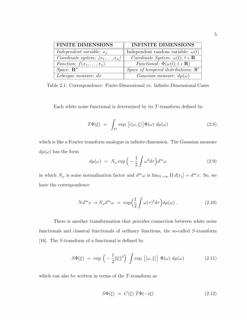
The fundamental idea is to introduce a generalized white noise functional,

Φ(ω(t); t ε R), and to analyze it systematically by taking the collection of infinitely

large number of random white noise variables, ω(t); t ε R, as the complex coordinate

system of an infinite-dimensional space. Thus, the analysis is infinite-dimensional and

does involve important parts that cannot be approximated by finite-dimensional calcu-

lus. The following table shows the correspondence between the finite-dimensional and

infinite-dimensional cases [4].

5

FINITE DIMENSIONS INFINITE DIMENSIONS

Independent variable: xj Independent random variable: ω(t)Coordinate system: (x1,. . . ,xn) Coordinate System: ω(t); t ε RFunction: f(x1, . . . , xn) Functional : Φ(ω(t); t ε R)Space: Rn Space of tempered distributions : S∗

Lebesgue measure: dx Gaussian measure: dµ(ω)

Table 2.1: Correspondence: Finite-Dimensional vs. Infinite-Dimensional Cases

Each white noise functional is determined by its T -transform defined by

TΦ(ξ) =

∫S∗

exp[i〈ω, ξ〉

]Φ(ω) dµ(ω) (2.8)

which is like a Fourier transform analogue in infinite-dimension. The Gaussian measure

dµ(ω) has the form

dµ(ω) = Nω exp(− 1

2

∫ω2dτ

)d∞ω (2.9)

in which Nω is some normalization factor and d∞ω is limN→∞ q d[xj] = d∞x. So, we

have the correspondence

Nd∞x→ Nωd∞ω = exp

(1

2

∫ω(τ)2dτ

)dµ(ω) . (2.10)

There is another transformation that provides connection between white noise

functionals and classical functionals of ordinary functions, the so-called S-transform

[16]. The S-transform of a functional is defined by

SΦ(ξ) = exp(− 1

2‖ξ‖2

) ∫exp

[〈ω, ξ〉

]Φ(ω) dµ(ω) (2.11)

which can also be written in terms of the T -transform as

SΦ(ξ) = C(ξ) TΦ(−iξ) (2.12)

6

and we also have

TΦ(ξ) = C(ξ) SΦ(iξ) . (2.13)

2.3 One-Dimensional Free Particle [4]

For a free particle, the potential is V (x) = 0 and the Lagrangian is given by

L(x, x) =1

2mx2 − V (x) =

1

2mx2 (2.14)

in which it follows that the Feynman propagator is expressed as

K(x′′, x′; t) =

∫exp[ i~

∫(1

2mx2)dt

]D[x] . (2.15)

We will now translate the Feynman propagator, Eq.(2.15), in the language of

white noise analysis. We parametrize the paths of the particle by introducing trajec-

tories x(t) consisting a Brownian fluctuation B(t)

x(t) = x′ +

√~m

∫ t

0

ω(τ)dτ (2.16)

where∫ t

0ω(τ)dτ = B(t). From Eq.(2.16), we get

x(t) =

√~m

ω(τ) . (2.17)

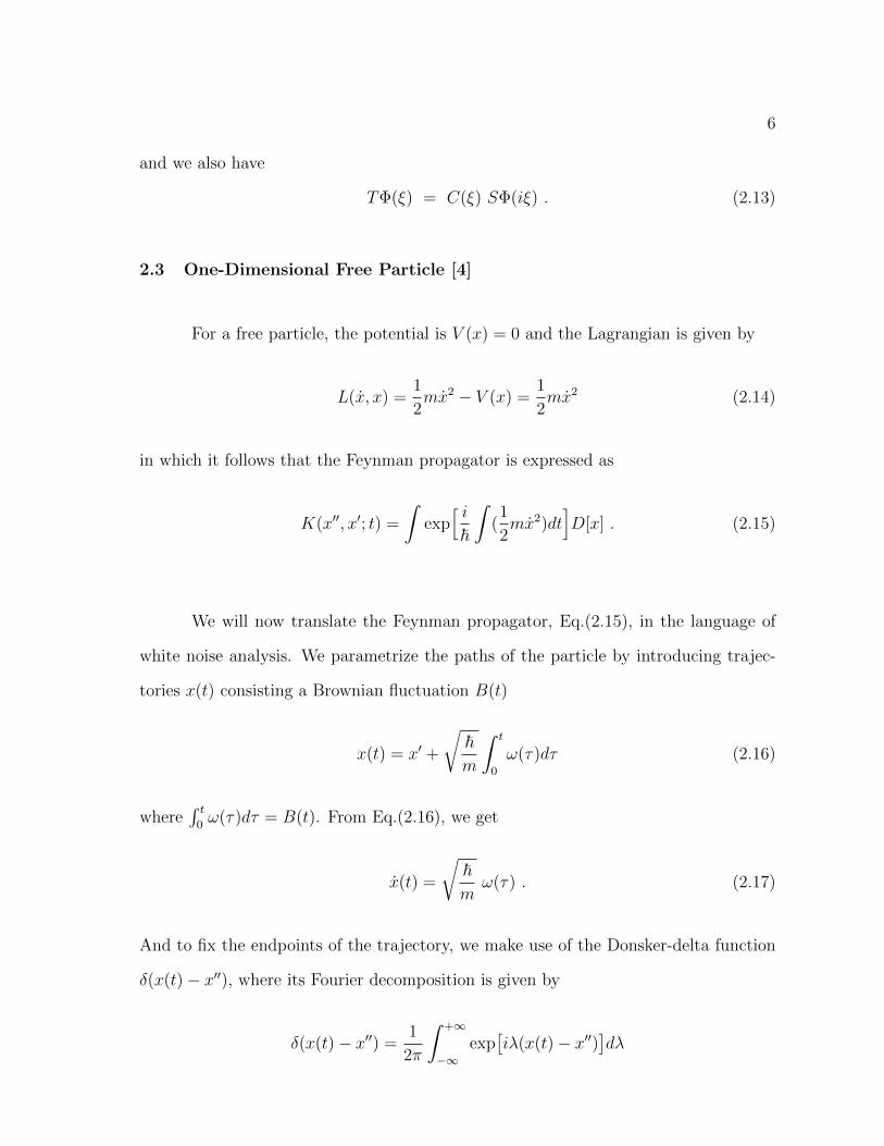
And to fix the endpoints of the trajectory, we make use of the Donsker-delta function

δ(x(t)− x′′), where its Fourier decomposition is given by

δ(x(t)− x′′) =1

2π

∫ +∞

−∞exp[iλ(x(t)− x′′)

]dλ

7

δ(

(x′ − x′′) +

√~m

∫ t

0

ω(τ)dτ)

=1

2π

∫λ

exp[iλ(x′ − x′′)

]exp[iλ

√~m

∫ t

0

ω(τ)2dτ]dλ .

(2.18)

Also, since the Feynman integration is with respect to an infinite-dimensional “flat”

measure, D[x], while the white noise measure, dµ(ω), is Gaussian [15], we need to use

the correspondence given in Eq.(2.10) where D[x] = Nd∞x.

Utilizing Eq.(2.10), Eq.(2.17) and the Donsker-delta function in Eq.(2.18), the

propagator in the language of white noise analysis can then be expressed as

K(x′′, x′; t) =1

2π

∫λ

exp[iλ(x′ − x′′)

]∫I0exp

[i⟨ω, λ

√~m

⟩]dµ(ω)

dλ (2.19)

where I0 is identified as a special case of the Gauss kernel given by

I0 = Nexp[i+ 1

2

∫ω(τ)2dτ

](2.20)

and N is a suitable normalization constant.

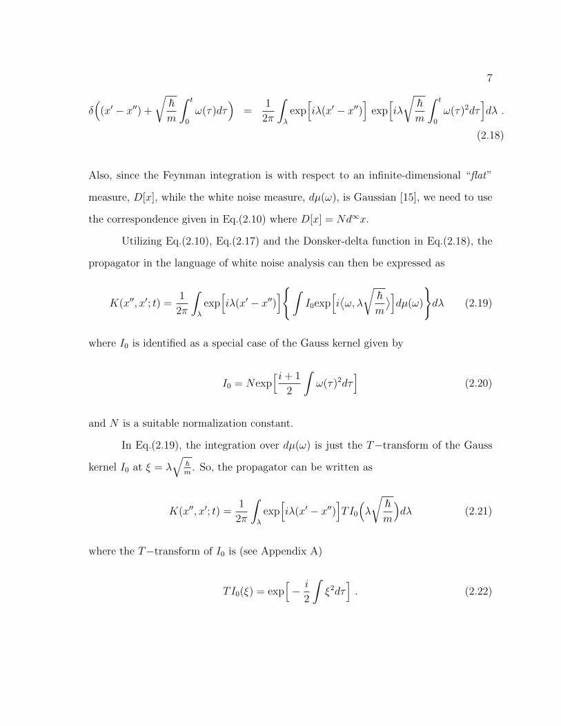
In Eq.(2.19), the integration over dµ(ω) is just the T−transform of the Gauss

kernel I0 at ξ = λ√

~m

. So, the propagator can be written as

K(x′′, x′; t) =1

2π

∫λ

exp[iλ(x′ − x′′)

]TI0

(λ

√~m

)dλ (2.21)

where the T−transform of I0 is (see Appendix A)

TI0(ξ) = exp[− i

2

∫ξ2dτ

]. (2.22)

8

Thus, the propagator becomes

K(x′′, x′; t) =1

2π

∫∞

exp[iλ(x′ − x′′)

]exp[− i

2

∫ t

0

ξ2dτ]dλ

=1

2π

∫∞dλ exp

[iλ(x′ − x′′)

][− i~λ2t

2m

]=

1

2π

∫∞dλ exp

[− i~t

2mλ2 − i(x′′ − x)λ

]. (2.23)

The integral over λ in Eq.(2.23) is just the Gaussian integral (a 0)

∫ +∞

−∞exp(− iap2

2− ibp

)dp =

√2π

iaexp(ib2

2a

)(2.24)

where we identify a = ~tm

and b = (x′′ − x′).

Therefore, the propagator for a free particle in one-dimension is

K(x′′, x′; t) =

√m

2πi~texp[ im

2~t(x′′ − x′)2

]. (2.25)

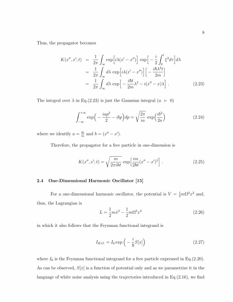
2.4 One-Dimensional Harmonic Oscillator [15]

For a one-dimensional harmonic oscillator, the potential is V = 12mΩ2x2 and,

thus, the Lagrangian is

L =1

2mx2 − 1

2mΩ2x2 (2.26)

in which it also follows that the Feynman functional integrand is

IH.O. = I0 exp(− i

~S[x]

)(2.27)

where I0 is the Feynman functional integrand for a free particle expressed in Eq.(2.20).

As can be observed, S[x] is a function of potential only and as we parametrize it in the

language of white noise analysis using the trajectories introduced in Eq.(2.16), we find

9

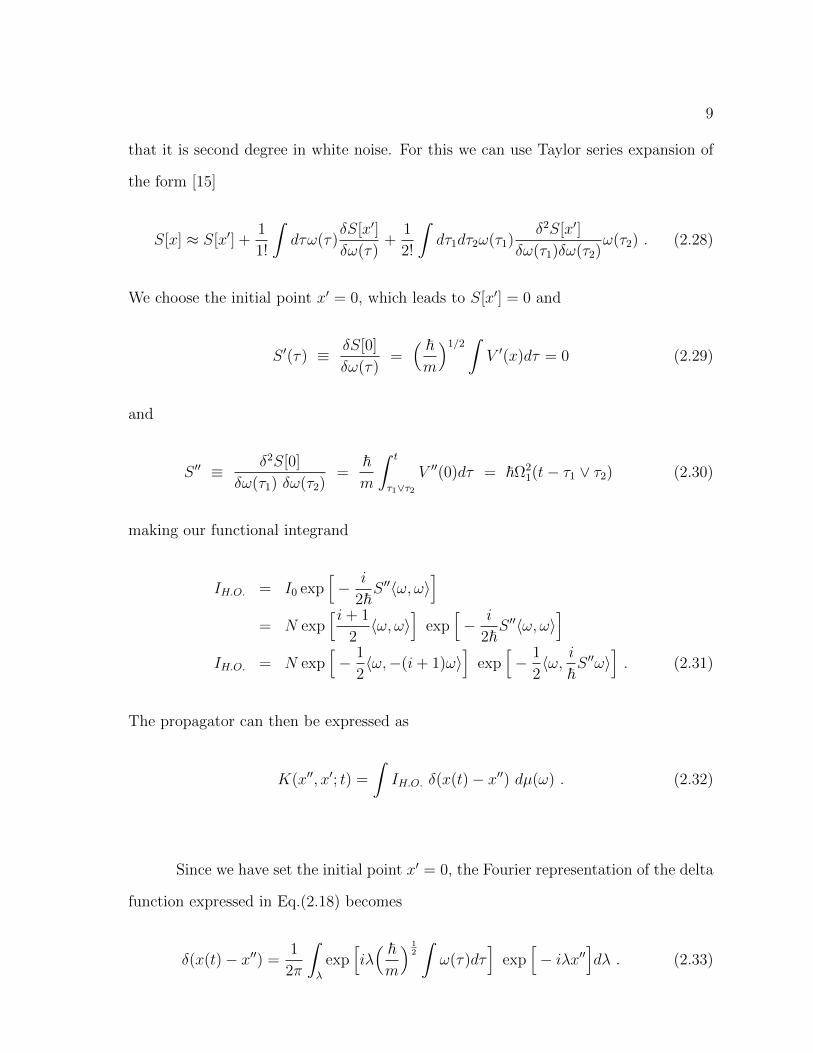
that it is second degree in white noise. For this we can use Taylor series expansion of

the form [15]

S[x] ≈ S[x′] +1

1!

∫dτω(τ)

δS[x′]

δω(τ)+

1

2!

∫dτ1dτ2ω(τ1)

δ2S[x′]

δω(τ1)δω(τ2)ω(τ2) . (2.28)

We choose the initial point x′ = 0, which leads to S[x′] = 0 and

S ′(τ) ≡ δS[0]

δω(τ)=( ~m

)1/2∫V ′(x)dτ = 0 (2.29)

and

S ′′ ≡ δ2S[0]

δω(τ1) δω(τ2)=

~m

∫ t

τ1∨τ2V ′′(0)dτ = ~Ω2

1(t− τ1 ∨ τ2) (2.30)

making our functional integrand

IH.O. = I0 exp[− i

2~S ′′〈ω, ω〉

]= N exp

[i+ 1

2〈ω, ω〉

]exp

[− i

2~S ′′〈ω, ω〉

]IH.O. = N exp

[− 1

2〈ω,−(i+ 1)ω〉

]exp

[− 1

2〈ω, i

~S ′′ω〉

]. (2.31)

The propagator can then be expressed as

K(x′′, x′; t) =

∫IH.O. δ(x(t)− x′′) dµ(ω) . (2.32)

Since we have set the initial point x′ = 0, the Fourier representation of the delta

function expressed in Eq.(2.18) becomes

δ(x(t)− x′′) =1

2π

∫λ

exp[iλ( ~m

) 12

∫ω(τ)dτ

]exp

[− iλx′′

]dλ . (2.33)

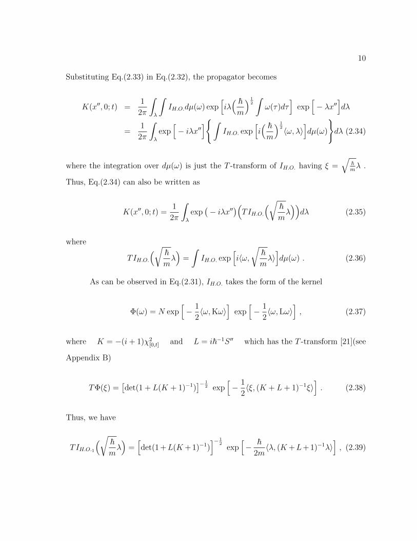
10

Substituting Eq.(2.33) in Eq.(2.32), the propagator becomes

K(x′′, 0; t) =1

2π

∫λ

∫IH.O.dµ(ω) exp

[iλ( ~m

) 12

∫ω(τ)dτ

]exp

[− λx′′

]dλ

=1

2π

∫λ

exp[− iλx′′

]∫IH.O. exp

[i( ~m

) 12 〈ω, λ〉

]dµ(ω)

dλ (2.34)

where the integration over dµ(ω) is just the T -transform of IH.O. having ξ =√

~mλ .

Thus, Eq.(2.34) can also be written as

K(x′′, 0; t) =1

2π

∫λ

exp(− iλx′′

)(TIH.O.

(√ ~mλ))dλ (2.35)

where

TIH.O.

(√ ~mλ)

=

∫IH.O. exp

[i〈ω,

√~mλ〉]dµ(ω) . (2.36)

As can be observed in Eq.(2.31), IH.O. takes the form of the kernel

Φ(ω) = N exp[− 1

2〈ω,Kω〉

]exp

[− 1

2〈ω,Lω〉

], (2.37)

where K = −(i+ 1)χ2[0,t] and L = i~−1S ′′ which has the T -transform [21](see

Appendix B)

TΦ(ξ) =[det(1 + L(K + 1)−1)

]− 12 exp

[− 1

2〈ξ, (K + L+ 1)−1ξ〉

]. (2.38)

Thus, we have

TIH.O.1

(√ ~mλ)

=[det(1 +L(K+ 1)−1)

]− 12

exp[− ~

2m〈λ, (K+L+ 1)−1λ〉

], (2.39)

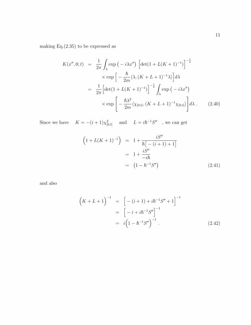
11

making Eq.(2.35) to be expressed as

K(x′′, 0; t) =1

2π

∫λ

exp(− iλx′′

) [det(1 + L(K + 1)−1)

]− 12

× exp[− ~

2m〈λ, (K + L+ 1)−1λ〉

]dλ

=1

2π

[det(1 + L(K + 1)−1)

]− 12

∫λ

exp(− iλx′′

)× exp

[− ~λ2

2m〈χ[0,t], (K + L+ 1)−1χ[0,t]〉

]dλ . (2.40)

Since we have K = −(i+ 1)χ2[0,t] and L = i~−1S ′′ , we can get

(1 + L(K + 1)−1

)= 1 +

iS ′′

~[− (i+ 1) + 1

]= 1 +

iS ′′

−i~=

(1− ~−1S ′′

)(2.41)

and also

(K + L+ 1

)−1

=[− (i+ 1) + i~−1S ′′ + 1

]−1

=[− i+ i~−1S ′′

]−1

= i(

1− ~−1S ′′)−1

. (2.42)

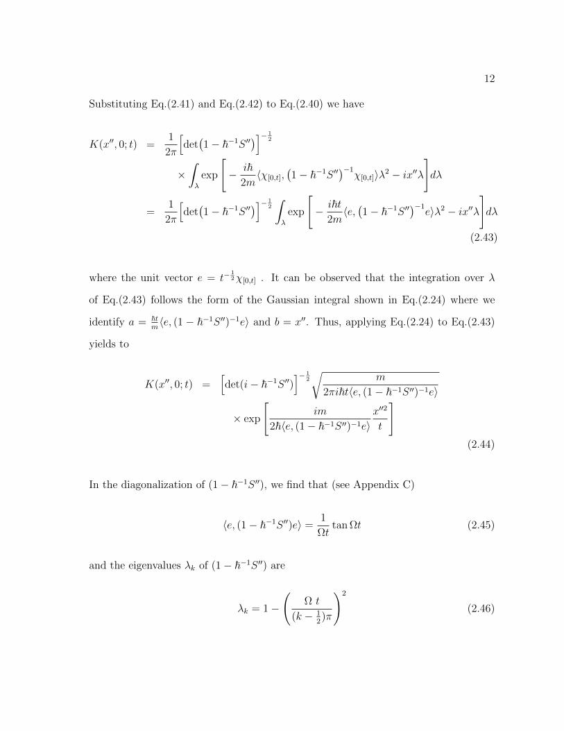
12

Substituting Eq.(2.41) and Eq.(2.42) to Eq.(2.40) we have

K(x′′, 0; t) =1

2π

[det(1− ~−1S ′′

)]− 12

×∫λ

exp

[− i~

2m〈χ[0,t],

(1− ~−1S ′′

)−1χ[0,t]〉λ2 − ix′′λ

]dλ

=1

2π

[det(1− ~−1S ′′

)]− 12

∫λ

exp

[− i~t

2m〈e,(1− ~−1S ′′

)−1e〉λ2 − ix′′λ

]dλ

(2.43)

where the unit vector e = t−12χ[0,t] . It can be observed that the integration over λ

of Eq.(2.43) follows the form of the Gaussian integral shown in Eq.(2.24) where we

identify a = ~tm〈e, (1 − ~−1S ′′)−1e〉 and b = x′′. Thus, applying Eq.(2.24) to Eq.(2.43)

yields to

K(x′′, 0; t) =[det(i− ~−1S ′′)

]− 12

√m

2πi~t〈e, (1− ~−1S ′′)−1e〉

× exp

[im

2~〈e, (1− ~−1S ′′)−1e〉x′′2

t

](2.44)

In the diagonalization of (1− ~−1S ′′), we find that (see Appendix C)

〈e, (1− ~−1S ′′)e〉 =1

Ωttan Ωt (2.45)

and the eigenvalues λk of (1− ~−1S ′′) are

λk = 1−

(Ω t

(k − 12)π

)2

(2.46)

13

which makes [det(1− ~−1S ′′)

]− 12

=(∏

k

λk)− 1

2 =(

cos Ωt)− 1

2 . (2.47)

Thus we have the propagator as

K(x′′, 0; t) =

(mΩ

2πi~ sin Ωt

) 12

exp

[imΩ

2~x′′2 cot Ωt

]. (2.48)

This one-dimensional harmonic oscillator has been solved already by L. Streit and T.

Hida [15] in the language of white noise analysis. In the case of a coupled harmonic

oscillators the Lagrangian is

L =1

2

(x2

1 + x22

)− 1

2mΩ2

(x2

1 + x22

)− λx1x2 . (2.49)

By performing a coordinate transformation using the following matrix [18]

∣∣∣∣∣ x1

x2

∣∣∣∣∣ =

∣∣∣∣∣ cosφ sinφ

− sinφ cosφ

∣∣∣∣∣∣∣∣∣∣ y1

y2

∣∣∣∣∣and taking φ = π

2, we can decouple the oscillators and deal with them independently.

After solving for their respective propagators, the total propagator can then be taken

as the product of their individual propagators, expressed as

K(x′′, x′; t) = K1(x′′1, x′1; t) K2(x′′2, x

′2; t) . (2.50)

We will deal with the details of a coupled harmonic oscillators and its evaluation in the

language of white noise analysis in the next chapter.

CHAPTER 3

WHITE NOISE PATH INTEGRATION FOR THE

COUPLED HARMONIC OSCILLATORS

The Lagrangian for a coupled harmonic oscillators of uniform frequency and

mass is given by

L =1

2m(x2

1 + x22

)− 1

2mΩ2

(x2

1 + x22

)− λx1x2 . (3.1)

As can be seen in the expression above, there is a coupling between the x coordinates

which makes it difficult to deal with, thus, there is a need to decouple the oscillators.

3.1 Decoupling the Oscillators

In order to quantize the potential and map it into that of a pair of independent

oscillators, we will introduce a decoupling transformation [18],

∣∣∣∣∣ x1

x2

∣∣∣∣∣ =

∣∣∣∣∣ cosφ sinφ

− sinφ cosφ

∣∣∣∣∣∣∣∣∣∣ y1

y2

∣∣∣∣∣giving us the new Lagrangian

L′ =1

2m[y2

1 cos2 φ+ 2y1y2 cosφ sinφ+ y22 sin2 φ+ y2

1 sin2 φ− 2y1y2 cosφ sinφ+ y22 cos2 φ

]− 1

2mΩ2

[y2

1 cos2 φ+ 2y1y2 cosφ sinφ+ y22 sin2 φ+ y2

1 sin2 φ− 2y1y2 cosφ sinφ+ y22 cos2 φ

]− λ(y1 cosφ+ y2 sinφ

)(− y1 sinφ+ y2 cosφ

). (3.2)

15

L′ =1

2m[y2

1(cos2 φ+ sin2 φ) + y22(cos2 φ+ sin2 φ)

]−1

2mΩ2

[y2

1(cos2 φ+ sin2 φ) + y22(cos2 φ+ sin2 φ)

]−[− y2

1 cosφ sinφ+ y1y2 cos2 φ− y1y2 sin2 φ+ y22 cosφ sinφ

]. (3.3)

Using the following trigonometric identities,

1 = cos2 φ+ sin2 φ

sin 2φ = 2 sinφ cosφ

cos 2φ = cos2 φ− sin2 φ

we can simplify the new Lagrangian and obtain

L′ =1

2m(y2

1 + y22

)− 1

2mΩ2

(y2

1 + y22

)− λ[− 1

2y2

1 sin 2φ+1

2y2

2 sin 2φ+ y1y2 cos 2φ]

=1

2

(y2

1 + y22

)− y2

1

[1

2mΩ2 − 1

2λ sin 2φ

]− y2

2

[1

2mΩ2 +

1

2λ sin 2φ

]− y1y2λ cos 2φ .

(3.4)

In order to eliminate the coupling between the y coordinates, we impose the

condition that φ = π4, making cos 2φ = 0 and sin 2φ = 1. And so, the decoupled

Lagrangian is

L′ =1

2m[y2

1 + y22

]− y2

1

[mΩ2

2− λ

2

]− y2

2

[mΩ2

2+λ

2

]. (3.5)

16

At this point, the problem has been reduced to that of two harmonic oscillators with

the following Lagrangian

L′1 =m

2y2

1 − y21

[mΩ2

2− λ

2

](3.6)

L′2 =m

2y2

2 − y22

[mΩ2

2+λ

2

](3.7)

with the new frequencies

Ω21 = Ω2 − λ

m(3.8)

Ω22 = Ω2 +

λ

m. (3.9)

3.2 Harmonic Oscillator

Since, the problem has been decoupled already, we can now deal with the os-

cillators independently. For the first harmonic oscillator, the potential is given by

V (y1) = 12mΩ2

1y21, and the effective action can be written as the sum of the free-particle

part and the interaction potential

S[y1] = S0[y1] +

∫V (y1)dτ . (3.10)

The Feynman functional integrand is then expressed as

IH.O.1 = I0 exp(− i

~S[y1]

), (3.11)

where I0 is the Feynman functional integrand for a free particle expressed in Eq.(2.20).

As can be observed, S[y1] is a function of potential only and, as we parametrize the

17

paths using the trajectory

y1(t) = y′1 +

√~m

∫ t

0

ω(τ)dτ , (3.12)

we find that it is second degree in white noise. For this we can use Taylor series

expansion of the form [15]

S[y1] ≈ S[y′1] +1

1!

∫dτω(τ)

δS[y′1]

δω(τ)+

1

2!

∫dτ1dτ2ω(τ1)

δ2S[y′1]

δω(τ1)δω(τ2)ω(τ2) . (3.13)

Choosing the initial point y′1 = 0, leads to S[y′1] = 0 and

S ′(τ) ≡ δS[0]

δω(τ)=( ~m

)1/2∫V ′(y)dτ = 0 (3.14)

and

S ′′ ≡ δ2S[0]

δω(τ1) δω(τ2)=

~m

∫ t

τ1∨τ2V ′′(0)dτ = ~Ω2

1(t− τ1 ∨ τ2) . (3.15)

So, we have

IH.O.1 = I0 exp[− i

2~S ′′〈ω, ω〉

]= N exp

[i+ 1

2〈ω, ω〉

]exp

[− i

2~S ′′〈ω, ω〉

]IH.O.1 = N exp

[− 1

2〈ω,−(i+ 1)ω〉

]exp

[− 1

2〈ω, i

~S ′′ω〉

]. (3.16)

The propagator can then be expressed as

K1(y′′1 , y′1; t) =

∫IH.O.1 δ(y1(t)− y′′1) dµ(ω) . (3.17)

18

We now utilize the Fourier representation of the delta function expressed as

δ(y1(t)− y′′) =1

2π

∫λ

exp[iλ(y1(t)− y′′1)

]dλ

=1

2π

∫λ

exp[iλ(y′1 +

( ~m

) 12

∫ω(τ)dτ − y′′1

)]dλ , (3.18)

but, since we have set the initial point y′1 = 0, the delta function will then be

δ(y1(t)− y′′) =1

2π

∫λ

exp[iλ( ~m

) 12

∫ω(τ)dτ

]exp

[− iλy′′1

]dλ . (3.19)

Substituting Eq.(3.19) in Eq.(3.17), the propagator will then be

K1(y′′1 , 0; t) =1

2π

∫λ

∫IH.O.1dµ(ω) exp

[iλ( ~m

) 12

∫ω(τ)dτ

]exp

[− λy′′1

]dλ

=1

2π

∫λ

exp[− iλy′′1

]∫IH.O.1 exp

[i( ~m

) 12 〈ω, λ〉

]dµ(ω)

dλ(3.20)

where the integration over dµ(ω) is just the T -transform of IH.O.1 having ξ =√

~mλ .

Thus, Eq.(3.20) can also be written as

K1(y′′1 , 0; t) =1

2π

∫λ

exp(− iλy′′1

)(TIH.O.1

(√ ~mλ))dλ (3.21)

where

TIH.O.1

(√ ~mλ)

=

∫IH.O.1 exp

[i〈ω,

√~mλ〉]dµ(ω) . (3.22)

As can be seen in Eq.(3.16), IH.O.1 takes the form of the kernel

Φ(ω) = N exp[− 1

2〈ω,Kω〉

]exp

[− 1

2〈ω,Lω〉

], (3.23)

19

where K = −(i + 1)χ2[0,t] and L = i~−1S ′′ which has the T -transform (see

Appendix B) [21]

TΦ(ξ) =[det(1 + L(K + 1)−1)

]− 12 exp

[− 1

2〈ξ, (K + L+ 1)−1ξ〉

]. (3.24)

Thus, we have

TIH.O.1

(√ ~mλ)

=[det(1 +L(K+ 1)−1)

]− 12

exp[− ~

2m〈λ, (K+L+ 1)−1λ〉

], (3.25)

making Eq.(3.21) to be expressed as

K1(y′′1 , 0; t) =1

2π

∫λ

exp(− iλy′′1

) [det(1 + L(K + 1)−1)

]− 12

× exp[− ~

2m〈λ, (K + L+ 1)−1λ〉

]dλ

=1

2π

[det(1 + L(K + 1)−1)

]− 12

∫λ

exp(− iλy′′1

)× exp

[− ~λ2

2m〈χ[0,t], (K + L+ 1)−1χ[0,t]〉

]dλ . (3.26)

Since we have K = −(i+ 1)χ2[0,t] and L = i~−1S ′′ , we can get

(1 + L(K + 1)−1

)= 1 +

iS ′′

~[− (i+ 1) + 1

]= 1 +

iS ′′

−i~=

(1− ~−1S ′′

)(3.27)

20

and also

(K + L+ 1

)−1

=[− (i+ 1) + i~−1S ′′ + 1

]−1

=[− i+ i~−1S ′′

]−1

= i(

1− ~−1S ′′)−1

. (3.28)

Substituting Eq.(3.27) and Eq.(3.28) to (3.26), we have

K1(y′′1 , 0; t) =1

2π

[det(1− ~−1S ′′

)]− 12

×∫λ

exp

[− i~

2m〈χ[0,t],

(1− ~−1S ′′

)−1χ[0,t]〉λ2 − iy′′1λ

]dλ

=1

2π

[det(1− ~−1S ′′

)]− 12

∫λ

exp

[− i~t

2m〈e,(1− ~−1S ′′

)−1e〉λ2 − iy′′1λ

]dλ

(3.29)

where the unit vector e = t−12χ[0,t] .

It can be observed that the integration over λ of Eq.(3.29) follows the form of

the Gaussian integral shown in Eq.(2.24) where we identify a = ~tm〈e, (1 − ~−1S ′′)−1e〉

and b = y′′1 . Thus, applying Eq.(2.24) to Eq.(3.29) yields to

K1(y′′1 , 0; t) =[det(1− ~−1S ′′)

]− 12

√m

2πi~t〈e, (1− ~−1S ′′)−1e〉

× exp

[im

2~〈e, (1− ~−1S ′′)−1e〉y′′21

t

](3.30)

In the diagonalization of (1− ~−1S ′′), we find that (see Appendix C)

〈e, (1− ~−1S ′′)e〉 =1

Ω1ttan Ω1t (3.31)

21

and the eigenvalues λk of (1− ~−1S ′′) are

λk = 1−

(Ω1t

(k − 12)π

)2

(3.32)

which makes [det(1− ~−1S ′′)

]− 12

=(∏

k

λk)− 1

2 =(

cos Ω1t)− 1

2 . (3.33)

Thus, we have the propagator as

K1(y′′1 , 0; t) =

(mΩ1

2πi~ sin Ω1t

) 12

exp

[imΩ1

2~y′′21 cot Ω1t

]. (3.34)

From here, it also follows that the propagator for the second oscillator can be written

as

K2(y′′2 , 0; t) =

(mΩ2

2πi~ sin Ω2t

) 12

exp

[imΩ2

2~y′′22 cot Ω2t

]. (3.35)

3.3 Coupled Harmonic Oscillators

In solving for the total propagator for the coupled harmonic oscillators, we

simply get the product of the propagators of the individual oscillators (see Eq.(2.50)),

written as

K(y′′, 0; t) = K1(y′′1 , 0; t) K2(y′′2 , 0; t) . (3.36)

With the results given in Eq.(3.34) and Eq.(3.35), we now have

K(y′′, 0; t) =m

2πi~

( Ω1 Ω2

sin Ω1t sin Ω2t

) 12

exp

imΩ1

2~ sin Ω1t

[cos Ω1t(y

′′21 )]

× exp

imΩ2

2~ sin Ω2t

[cos Ω2t(y

′′22 )]

. (3.37)

22

Since, in the decoupling procedure we used a coordinate transformation, the

desired propagator can then be obtained by returning to the original coordinates using

the following transformation

∣∣∣∣∣ y′′1y′′2∣∣∣∣∣ =

∣∣∣∣∣ cosφ − sinφ

sinφ cosφ

∣∣∣∣∣∣∣∣∣∣ x′′1x′′2

∣∣∣∣∣where we get

y′′21 = x′′21 cos2 φ− 2x′′1x′′2 cosφ sinφ+ x′′22 sin2 φ (3.38)

y′′22 = x′′21 sin2 φ+ 2x′′1x′′2 cosφ sinφ+ x′′22 cos2 φ . (3.39)

Also, since we have set φ = π4

, Eq.(3.38) and Eq.(3.39) becomes

y′′21 =1

2(x′′21 + x′′22 − 2x′′1x

′′2) =

1

2(x′′1 − x′′2)2 (3.40)

y′′22 =1

2(x′′21 + x′′22 + 2x′′1x

′′2) =

1

2(x′′1 + x′′2)2 . (3.41)

Finally, the total propagator becomes

K(x′′, 0; t) =m

2πi~

( Ω1 Ω2

sin Ω1t sin Ω2t

) 12

exp

imΩ1

4~ sin Ω1t

[cos Ω1t(x

′′1 − x′′2)2

]

× exp

imΩ2

4~ sin Ω2t

[cos Ω2t(x

′′1 + x′′2)2

](3.42)

which solves the problem for a coupled harmonic oscillators. The resulting propagator

also agrees with the result of the particular case dealt in the work of de Souza Dutra

[18].

23

3.4 Energy Spectrum and Wavefunction

We now express the propagator in Eq.(3.41) in the form

K(x′′, 0; t) =∑

n1,n2∈N

Ψ∗n1,n2(x′′1, x

′′2) Ψn1,n2(0) e−

i~ tEn1,n2 (3.43)

for an initial point x′1 = x′2 = 0 . Using the relations

i sin Ωt =1

2eiΩt(1− e−2iΩt) (3.44)

cos Ωt =1

2eiΩt(1 + e−2iΩt) (3.45)

we can rewrite the propagator as

K(x′′, 0; t) =m

2π~

[4Ω1 Ω2

eit(Ω1+Ω2) (1− e−2iΩ1t) (1− e−2iΩ2t)

] 12

× exp

− mΩ1

4~(x′′1 − x′′2)2 1 + e−2iΩ1t

1− e−2iΩ1t

× exp

− mΩ2

4~(x′′1 + x′′2)2 1− e−2iΩ2t

1− e−2iΩ2t

(3.46)

Now, applying the Mehler formula [20] of the form

1√1− z2

exp[4xyz − (x2 + y2) (1 + z2)

2(1− z2)

]= e

−(x2+y2)2

∞∑n=0

1

n!

(z2

)nHn(x)Hn(y) (3.47)

where the functions Hn are the Hermite polynomials

Hn(y) = (−1)ney2 dn

dyne−y

2

(3.48)

24

we identify x = 0 and

y1 =

√mΩ1

2~(x′′1 − x′′2) ; z1 = e−iΩ1t

y2 =

√mΩ2

2~(x′′1 + x′′2) ; z2 = e−iΩ2t . (3.49)

Thus, we can rewrite the propagator in its symmetric form as

K(x′′, 0; t) =m

π~

[ Ω1 Ω2

eit(Ω1+Ω2)

] 12

× exp[− mΩ1

4~(x′′1 − x′′2)2

] ∞∑n1=0

1

n1!

(e−itΩ1

2

)n1

Hn1

(√mΩ1

2~(x′′1 − x′′2)

)

× exp[− mΩ2

4~(x′′1 + x′′2)2

] ∞∑n2=0

1

n2!

(e−itΩ2

2

)n2

Hn2

(√mΩ2

2~(x′′1 + x′′2)

)

=m

π~(Ω1 Ω2

) 12 exp

− m

4~

[Ω1(x′′1 − x′′2)2 + Ω2(x′′1 + x′′2)2

]

×∑

n1,n2∈N

(2n1n1!)−1(2n2n2!)−1 exp

− it

[1

2(Ω1 + Ω2) + n1Ω1 + n2Ω2

]

×Hn1

(√mΩ1

2~(x′′1 − x′′2)

)Hn2

(√mΩ2

2~(x′′1 + x′′2)

). (3.50)

Re-arranging terms, we get

K(x′′, 0; t) =∑

n1,n2∈N

m(Ω1 Ω2)12

2(n1+n2)π~n1!n2!exp

− m

4~

[Ω1(x′′1 − x′′2)2 + Ω2(x′′1 + x′′2)2

]

×Hn1

(√mΩ1

2~(x′′1 − x′′2)

)Hn2

(√mΩ2

2~(x′′1 + x′′2)

)

× exp

[− i

~t~[1

2(Ω1 + Ω2) + n1Ω1 + n2Ω2

]]. (3.51)

25

From Eq.(3.48), we can extract the energy spectrum, that is,

En1,n2 = ~

[(n1 +

1

2

)Ω1 +

(n2 +

1

2

)Ω2

](3.52)

and the general formula of the wavefunction as

Ψn1,n2 =

√m√

Ω1 Ω2

2(n1+n2)π~n1!n2!exp

− m

4~

[Ω1(x1 − x2)2 + Ω2(x1 + x2)2

]

×Hn1

(√mΩ1

2~(x1 − x2)

)Hn2

(√mΩ2

2~(x1 + x2)

). (3.53)

Thus, we have solved the problem of a coupled harmonic oscillators of uniform

frequency and mass using the white noise functional approach. We have solved the

wavefunction and the energy spectrum of the system. And based on the results, the

energy spectrum is just the sum of the energies of the two harmonic oscillators. Also,

the energies are “quantized” and even at the ground state where n = 0, the energy is

not zero, but ~(Ω1+Ω2)2

. Moreover, the quantum state of the coupled harmonic oscillators

is described completely by its wavefunction.

CHAPTER 4

CONCLUSION AND RECOMMENDATION

With the use of the quantum propagator we obtain the significant abstract

entities of quantum mechanics, specifically, the wavefunction and the energy spectrum.

Contained within these entites are the informations about a quantum physical system,

including the time development of its quantum states. Thus, it is rightful to state

that a quantum problem is solved when we are able to find these abstract entities. To

solve for this entities, one of the methods that was developed is the Feynman path

integral formulation, and in this study we use the white noise functional approach for

its evaluation.

In this thesis, the Feynman propagator for a coupled harmonic oscillators of uni-

form frequency and mass which are coupled through an arbitrary strength parameter

was completely solved using the white noise functional approach. First, we decou-

pled the oscillators by using a coordinate transformation as illustrated by de Souza

Dutra[18]. After the decoupling process, we dealt with the oscillators independently

and evaluated their respective Feynman propagator using the white noise functional

approach. Finally, the total propagator was obtained by multiplying their individual

propagators. However, since we changed coordinates in the decoupling process, the de-

sired total propagator was acquired by shifting back to the original coordinates. Also,

from the symmetrized form of the propagator, the wavefunction and the energy spec-

trum were extracted. Therefore, we have met the objectives of this study. The results

of this study also conforms to the results of the particular case dealt in the work of de

Souza Dutra [18].

The white noise functional approach was successfully applied to solve various

problems in quantum mechanics, and the problem of coupled harmonic oscillators is

27

just one of them. This study could serve as a helpful reference to future studies since

this could be extended to more complicated cases including the varying frequency and

mass, as well as the driven case.

REFERENCES

[1] R.P. Feynman. Space-time Approach to Non-Relativistic Quantum Mechanics. Rev.

Mcd. Phys. 20 (1948) 367.

[2] C. Grosche and F. Steiner: Handbook of Feynman Path Integrals (Springer, Berlin,

1965).

[3] R.P. Feynman and R.P. Hibbs: Quantum Mechanics and Path Integrals. (McGraw-

Hill, New York, 1965).

[4] C.C. Bernido and M.V. Carpio-Bernido: White Noise Analysis and Feynman Path

Integral. In Functional Integrals in Stochastic and Quantum Dynamics. Jagna Bo-

hol, 2001. Ed. by C.C. Bernido, M.V. Carpio-Bernido, and L. Streit, Central

Visayan Institute Foundation, Philippines (2002) 18-31.

[5] C.C. Bernido and M.V. Carpio-Bernido. Entanglement Probabilities in Polymers:

A White Noise Functional Approach. J. Phys. A: Math. Gen. 36 (2003) 1-11.

[6] C.C. Bernido, M.V. Carpio-Bernido an J.B. Bornales. On Chirality and Length-

Dependent Potentials in Polymer Entanglements. Phys. Lett. A 339 (2005) 232-

236.

[7] T. Hida, et. al.: White Noise. An Infinite Dimensional Calculus.(Kluver, Dor-

drecht, 1993).

[8] N. Obata: White Noise Calculus and Fock Space. Lecture Notes in Mathematics,

Vol.1577.(Springer, Berlin, 1994).

[9] H.H. Kuo: White Noise Distribution Theory. (CRC, Boca Raton, 1996).

29

[10] M. de Faria, J. Potthoff, and L. Streit. The Feynman Integrand as a Hida Distri-

bution. J. Math. Phys. 32(1991) 2123-2127.

[11] M. Grothaus, D.C. Khandekar, J.L. da Silva, and L. Streit. The Feynman Integral

for Time-Dependent Anharmonic Oscillators. J. Math. Phys. 38 3278-3299.

[12] T. Kuna, L. Streit, and W. Westerkamp. Feynman Integrals for a Class of Expo-

nentially Growing Potentials. J. Math. Phys. 39 (1999) 4476-4491.

[13] F. Wiegel. Introduction to Path-Integral Methods in Physics and Polymer Sci-

ence.(1986).

[14] R.P. Feynman. Space-Time Approach to Nonrelativistic Quantum Mechanics. Re-

view of Modern Physics 20 (1948) 367-387.

[15] L. Streit and T. Hida. Generalized Brownian Functionals and the Feynman Inte-

gral. Stoch. Proc. Appl. 16 (1983) 55-69.

[16] T. Hida. White Noise Analysis: Part I. Theory in Progress. Taiwanese Journal of

Mathematics, Vol. 7 (2003) 541-556.

[17] H.H. Kuo. On Laplacian Operators of Generalized Brownian Functionals, In

Stochastic Processes and their Applications. LNM 1203, Ed. K. Ito and T. Hida

(Springer-Verlag, Berlin, 1986) 119-128.

[18] A. de Souza Dutra. On the Quantum Mechanical Propagator for a Driven Coupled

Harmonic Oscillators. J. Phys. A.: Math. Gen. 25 (1992) 4189-4198.

[19] G. Arfken. Mathematical Methods for Physicists. 3rd Ed. (Academic Press, New

York, 1985).

[20] I. S. Gradshteyn and I. M. Ryzhik. Table of Integrals, Series, and Products. (Aca-

demic Press, New York, 1980).

30

[21] D. de Falco and D.C. Khandekar. Applications of White Noise Calculus to the

Computation of Feynman Integrals. Stoch. Phys. and Appl. 29 (1988) 257-266.

[22] M. Egot : Harmonic Oscillator: A White Noise Functional Approach. (An un-

dergraduate thesis , Mindanao State University - Iligan Institute of Technology,

Philippines, March 2006).

[23] A. R. Nasir : White Noise Path Integration for a Two-Dimensional Anistrophic

Harmonic Oscillator with Uniform Magnetic Field.(An undergraduate thesis , Min-

danao State University - Iligan Institute of Technology, Philippines, March 2007).

[24] J.P. Manigo : Charged Particle in a Uniform Magnetic Field: A White Noise

Functional Approach. (An undergraduate thesis , Mindanao State University - Ili-

gan Institute of Technology, Philippines, March 2006).

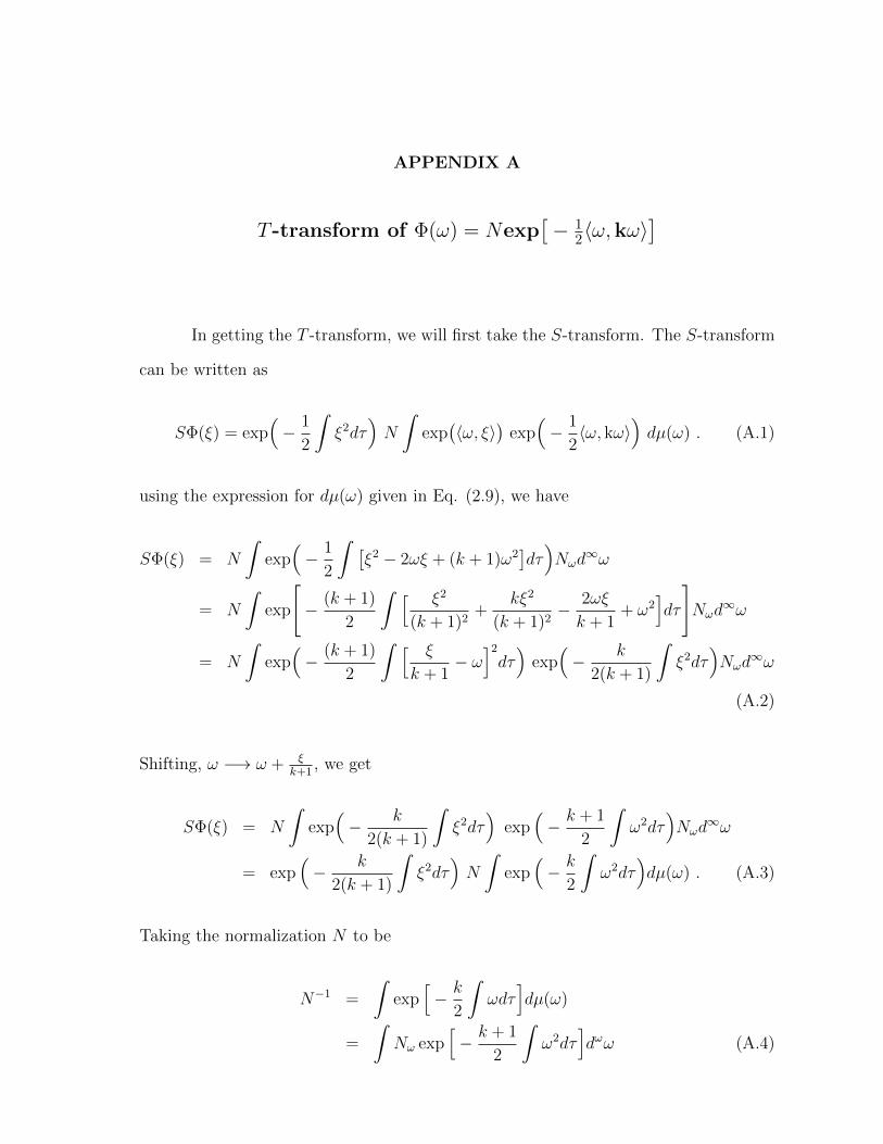
APPENDIX A

T -transform of Φ(ω) = Nexp[− 1

2〈ω,kω〉]

In getting the T -transform, we will first take the S-transform. The S-transform

can be written as

SΦ(ξ) = exp(− 1

2

∫ξ2dτ

)N

∫exp(〈ω, ξ〉

)exp(− 1

2〈ω, kω〉

)dµ(ω) . (A.1)

using the expression for dµ(ω) given in Eq. (2.9), we have

SΦ(ξ) = N

∫exp(− 1

2

∫ [ξ2 − 2ωξ + (k + 1)ω2

]dτ)Nωd

∞ω

= N

∫exp

[− (k + 1)

2

∫ [ ξ2

(k + 1)2+

kξ2

(k + 1)2− 2ωξ

k + 1+ ω2

]dτ

]Nωd

∞ω

= N

∫exp(− (k + 1)

2

∫ [ ξ

k + 1− ω

]2

dτ)

exp(− k

2(k + 1)

∫ξ2dτ

)Nωd

∞ω

(A.2)

Shifting, ω −→ ω + ξk+1

, we get

SΦ(ξ) = N

∫exp(− k

2(k + 1)

∫ξ2dτ

)exp

(− k + 1

2

∫ω2dτ

)Nωd

∞ω

= exp(− k

2(k + 1)

∫ξ2dτ

)N

∫exp

(− k

2

∫ω2dτ

)dµ(ω) . (A.3)

Taking the normalization N to be

N−1 =

∫exp

[− k

2

∫ωdτ

]dµ(ω)

=

∫Nω exp

[− k + 1

2

∫ω2dτ

]dωω (A.4)

32

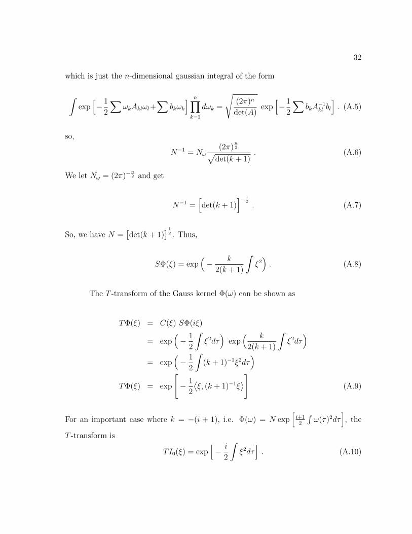
which is just the n-dimensional gaussian integral of the form

∫exp

[− 1

2

∑ωkAklωl+

∑bkωk

] n∏k=1

dωk =

√(2π)n

det(A)exp

[− 1

2

∑bkA

−1kl bl

]. (A.5)

so,

N−1 = Nω(2π)

n2√

det(k + 1). (A.6)

We let Nω = (2π)−n2 and get

N−1 =[det(k + 1)

]− 12. (A.7)

So, we have N =[det(k + 1)

] 12 . Thus,

SΦ(ξ) = exp(− k

2(k + 1)

∫ξ2). (A.8)

The T -transform of the Gauss kernel Φ(ω) can be shown as

TΦ(ξ) = C(ξ) SΦ(iξ)

= exp(− 1

2

∫ξ2dτ

)exp

( k

2(k + 1)

∫ξ2dτ

)= exp

(− 1

2

∫(k + 1)−1ξ2dτ

)TΦ(ξ) = exp

[− 1

2

⟨ξ, (k + 1)−1ξ

⟩](A.9)

For an important case where k = −(i + 1), i.e. Φ(ω) = N exp[i+1

2

∫ω(τ)2dτ

], the

T -transform is

TI0(ξ) = exp[− i

2

∫ξ2dτ

]. (A.10)

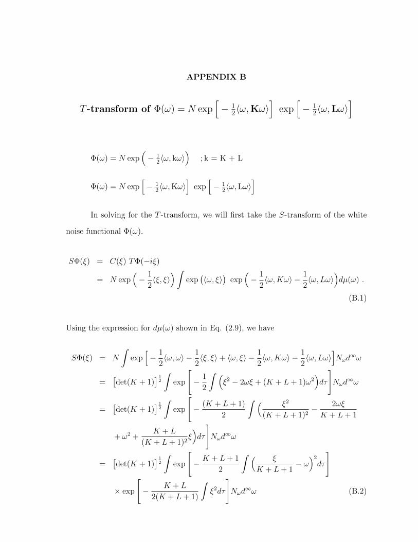
APPENDIX B

T -transform of Φ(ω) = N exp[− 1

2〈ω,Kω〉]

exp[− 1

2〈ω,Lω〉]

Φ(ω) = N exp(− 1

2〈ω, kω〉

); k = K + L

Φ(ω) = N exp[− 1

2〈ω,Kω〉

]exp

[− 1

2〈ω,Lω〉

]In solving for the T -transform, we will first take the S-transform of the white

noise functional Φ(ω).

SΦ(ξ) = C(ξ) TΦ(−iξ)

= N exp(− 1

2〈ξ, ξ〉

)∫exp

(〈ω, ξ〉

)exp

(− 1

2〈ω,Kω〉 − 1

2〈ω, Lω〉

)dµ(ω) .

(B.1)

Using the expression for dµ(ω) shown in Eq. (2.9), we have

SΦ(ξ) = N

∫exp

[− 1

2〈ω, ω〉 − 1

2〈ξ, ξ〉+ 〈ω, ξ〉 − 1

2〈ω,Kω〉 − 1

2〈ω, Lω〉

]Nωd

∞ω

=[det(K + 1)

] 12

∫exp

[− 1

2

∫ (ξ2 − 2ωξ + (K + L+ 1)ω2

)dτ

]Nωd

∞ω

=[det(K + 1)

] 12

∫exp

[− (K + L+ 1)

2

∫ ( ξ2

(K + L+ 1)2− 2ωξ

K + L+ 1

+ ω2 +K + L

(K + L+ 1)2ξ)dτ

]Nωd

∞ω

=[det(K + 1)

] 12

∫exp

[− K + L+ 1

2

∫ ( ξ

K + L+ 1− ω

)2

dτ

]

× exp

[− K + L

2(K + L+ 1)

∫ξ2dτ

]Nωd

∞ω (B.2)

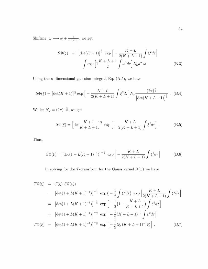
34

Shifting, ω −→ ω + ξK+L+1

, we get

SΦ(ξ) =[det(K + 1)

] 12 exp

[− K + L

2(K + L+ 1)

∫ξ2dτ

]∫

exp[1K + L+ 1

2

∫ω2dτ

]Nωd

∞ω (B.3)

Using the n-dimensional gaussian integral, Eq. (A.5), we have

SΦ(ξ) =[det(K + 1)

] 12 exp

[− K + L

2(K + L+ 1)

∫ξ2dτ

]Nω

(2π)n2[

det(K + L+ 1)] 1

2

. (B.4)

We let Nω = (2π)−n2 , we get

SΦ(ξ) =[det

K + 1

K + L+ 1

] 12

exp[− K + L

2(K + L+ 1)

∫ξ2dτ

]. (B.5)

Thus,

SΦ(ξ) =[det(1 + L(K + 1)−1)

]− 12 exp

[− K + L

2(K + L+ 1)

∫ξ2dτ

](B.6)

In solving for the T -transform for the Gauss kernel Φ(ω) we have

TΦ(ξ) = C(ξ) SΦ(iξ)

=[det(1 + L(K + 1)−1)

]− 12 exp

(− 1

2

∫ξ2dτ

)exp

[ K + L

2(K + L+ 1)

∫ξ2dτ

]=

[det(1 + L(K + 1)−1)

]− 12 exp

[− 1

2

(1− K + L

K + L+ 1

) ∫ξ2dτ

]=

[det(1 + L(K + 1)−1)

]− 12 exp

[− 1

2(K + L+ 1)−1

∫ξ2dτ

]TΦ(ξ) =

[det(1 + L(K + 1)−1)

]− 12 exp

[− 1

2〈ξ, (K + L+ 1)−1ξ〉

]. (B.7)

APPENDIX C

Calculation of Matrix Elements [22]

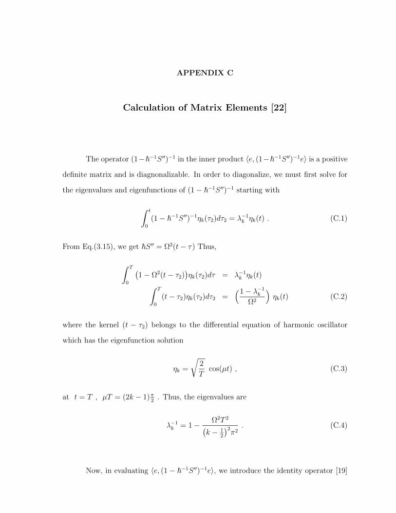
The operator (1−~−1S ′′)−1 in the inner product 〈e, (1−~−1S ′′)−1e〉 is a positive

definite matrix and is diagnonalizable. In order to diagonalize, we must first solve for

the eigenvalues and eigenfunctions of (1− ~−1S ′′)−1 starting with

∫ t

0

(1− ~−1S ′′)−1ηk(τ2)dτ2 = λ−1k ηk(t) . (C.1)

From Eq.(3.15), we get ~S ′′ = Ω2(t− τ) Thus,

∫ T

0

(1− Ω2(t− τ2)

)ηk(τ2)dτ = λ−1

k ηk(t)∫ T

0

(t− τ2)ηk(τ2)dτ2 =(1− λ−1

k

Ω2

)ηk(t) (C.2)

where the kernel (t − τ2) belongs to the differential equation of harmonic oscillator

which has the eigenfunction solution

ηk =

√2

Tcos(µt) , (C.3)

at t = T , µT = (2k − 1)π2

. Thus, the eigenvalues are

λ−1k = 1− Ω2T 2(

k − 12

)2π2

. (C.4)

Now, in evaluating 〈e, (1− ~−1S ′′)−1e〉, we introduce the identity operator [19]

36

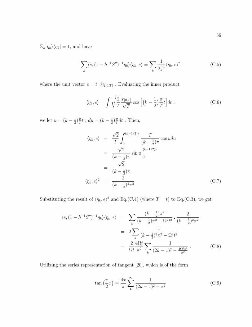
Σk|ηk〉〈ηk| = 1, and have

∑k

〈e, (1− ~−1S ′′)−1ηk〉〈ηk, e〉 =∑k

1

λ−1k

〈ηk, e〉2 (C.5)

where the unit vector e = t−12χ[0,T ] . Evaluating the inner product

〈ηk, e〉 =

∫ √2

T

χ[0,T ]√T

cos[(k − 1

2

)πTt]dt . (C.6)

we let u = (k − 12) πTt ; dµ = (k − 1

2) πTdt . Then,

〈ηk, e〉 =

√2

T

∫ (k−1/2)π

0

T

(k − 12)π

cosudu

=

√2

(k − 12)π

sinu∣∣∣(k−1/2)π

0

=

√2

(k − 12)π

〈ηk, e〉2 =2

(k − 12)2π2

(C.7)

Substituting the result of 〈ηk, e〉2 and Eq.(C.4) (where T = t) to Eq.(C.3), we get

〈e, (1− ~−1S ′′)−1ηk〉〈ηk, e〉 =∑k

(k − 12)π2

(k − 12)π2 − Ω2t2

2

(k − 12)2π2

= 2∑k

1

(k − 12)2π2 − Ω2t2

=2

Ωt

4Ωt

π2

∑k

1

(2k − 1)2 − 4Ω2t2

π2

. (C.8)

Utilizing the series representation of tangent [20], which is of the form

tan(π

2x)

=4x

π

∞∑k

1

(2k − 1)2 − x2(C.9)

37

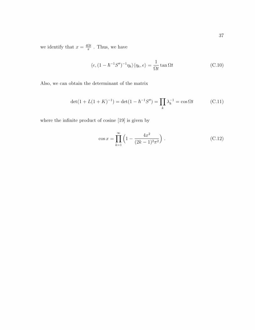
we identify that x = 4Ωtπ

. Thus, we have

〈e, (1− ~−1S ′′)−1ηk〉〈ηk, e〉 =1

Ωttan Ωt (C.10)

Also, we can obtain the determinant of the matrix

det(1 + L(1 +K)−1) = det(1− ~−1S ′′) =∏k

λ−1k = cos Ωt (C.11)

where the infinite product of cosine [19] is given by

cosx =∞∏k=1

(1− 4x2

(2k − 1)2π2

). (C.12)