Harmonic Oscillators and Two-by-two Matrices in Symmetry Problems in Physics

Young Suh Kim

www.mdpi.com/journal/symmetry

Edited by

Printed Edition of the Special Issue Published in Symmetry

Harmonic Oscillators and Two-By-Two Matrices in Symmetry Problems in Physics Special Issue Editor Young Suh Kim

MDPI • Basel • Beijing • Wuhan • Barcelona • Belgrade

Special Issue Editor

Young Suh Kim University of Maryland USA Editorial Office MDPI AG St. Alban-Anlage 66 Basel, Switzerland This edition is a reprint of the Special Issue published online in the open access journal Symmetry (ISSN 2073-8994) from 2014–2017 (available at: http://www.mdpi.com/journal/symmetry/special_issues/physics-matrices). For citation purposes, cite each article independently as indicated on the article page online and as indicated below: Author 1; Author 2. Article title. Journal Name Year, Article number, page range. First Edition 2017 ISBN 978-3-03842-500-7 (Pbk) ISBN 978-3-03842-501-4 (PDF)

Articles in this volume are Open Access and distributed under the Creative Commons Attribution license (CC BY), which allows users to download, copy and build upon published articles even for commercial purposes, as long as the author and publisher are properly credited, which ensures maximum dissemination and a wider impact of our publications. The book taken as a whole is © 2017 MDPI, Basel, Switzerland, distributed under the terms and conditions of the Creative Commons license CC BY-NC-ND (http://creativecommons.org/licenses/by-nc-nd/4.0/).

iii

Table of Contents About the Special Issue Editor ..................................................................................................................... v

Preface to “Harmonic Oscillators and Two-by-two Matrices in Symmetry Problems in Physics” ..................................................................................................................................... vii

Chapter 1 Orlando Panella and Pinaki Roy

Pseudo Hermitian Interactions in the Dirac Equation Reprinted from: Symmetry 2014, 6(1), 103–110; doi: 10.3390/sym6010103............................................. 3 Ettore Minguzzi

Spacetime Metrics from Gauge Potentials Reprinted from: Symmetry 2014, 6(2), 164–170; doi: 10.3390/sym6020164............................................. 9 Andrea Quadri

Quantum Local Symmetry of the D-Dimensional Non-Linear Sigma Model: A Functional Approach Reprinted from: Symmetry 2014, 6(2), 234–255; doi: 10.3390/sym6020234............................................. 15 Lock Yue Chew and Ning Ning Chung

Dynamical Relation between Quantum Squeezing and Entanglement in Coupled Harmonic Oscillator System Reprinted from: Symmetry 2014, 6(2), 295–307; doi: 10.3390/sym6020295............................................. 34 F. De Zela

Closed-Form Expressions for the Matrix Exponential Reprinted from: Symmetry 2014, 6(2), 329–344; doi: 10.3390/sym6020329............................................. 45 Luis L. Sánchez-Soto and Juan J. Monzón

Invisibility and PT Symmetry: A Simple Geometrical Viewpoint Reprinted from: Symmetry 2014, 6(2), 396–408; doi: 10.3390/sym6020396............................................. 59 Sibel Başkal, Young S. Kim and Marilyn E. Noz

Wigner’s Space-Time Symmetries Based on the Two-by-Two Matrices of the Damped Harmonic Oscillators and the Poincaré Sphere Reprinted from: Symmetry 2014, 6(3), 473–515; doi: 10.3390/sym6030473............................................. 70 Chapter 2 Heung-Ryoul Noh

Analytical Solutions of Temporal Evolution of Populations in Optically-Pumped Atoms with Circularly Polarized Light Reprinted from: Symmetry 2016, 8(3), 17; doi: 10.3390/sym8030017 ....................................................... 111 M. Howard Lee

Local Dynamics in an Infinite Harmonic Chain Reprinted from: Symmetry 2016, 8(4), 22; doi: 10.3390/sym8040022 ....................................................... 123

iv

Christian Baumgarten

Old Game, New Rules: Rethinking the Form of Physics Reprinted from: Symmetry 2016, 8(5), 30; doi: 10.3390/sym8050030 ....................................................... 135 Anaelle Hertz, Sanjib Dey, Véronique Hussin and Hichem Eleuch

Higher Order Nonclassicality from Nonlinear Coherent States for Models with Quadratic Spectrum Reprinted from: Symmetry 2016, 8(5), 36; doi: 10.3390/sym8050036 ....................................................... 170 Gabriel Amador, Kiara Colon, Nathalie Luna, Gerardo Mercado, Enrique Pereira and Erwin Suazo

On Solutions for Linear and Nonlinear Schrödinger Equations with Variable Coefficients: A Computational Approach Reprinted from: Symmetry 2016, 8(6), 38; doi: 10.3390/sym8060038 ....................................................... 179 Alexander Rauh

Coherent States of Harmonic and Reversed Harmonic Oscillator Reprinted from: Symmetry 2016, 8(6), 46; doi:10.3390/sym8060046 ...................................................... 195 Sibel Başkal, Young S. Kim and Marilyn E. Noz

Entangled Harmonic Oscillators and Space-Time Entanglement Reprinted from: Symmetry 2016, 8(7), 55; doi: 10.3390/sym8070055 ....................................................... 207 Halina Grushevskaya and George Krylov

Massless Majorana-Like Charged Carriers in Two-Dimensional Semimetals Reprinted from: Symmetry 2016, 8(7), 60; doi: 10.3390/sym8070060 ....................................................... 233 Chapter 3 Young S. Kim and Marilyn E. Noz

Lorentz Harmonics, Squeeze Harmonics and Their Physical Applications Reprinted from: Symmetry 2011, 3, 16–36; doi: 10.3390/sym3010016 ..................................................... 247 Young S. Kim and Marilyn E. Noz

Dirac Matrices and Feynman’s Rest of the Universe Reprinted from: Symmetry 2012, 4, 626–643; doi: 10.3390/sym4040626 ................................................. 266 Young S. Kim and Marilyn E. Noz

Symmetries Shared by the Poincar?Group and the Poincar?Sphere Reprinted from: Symmetry 2013, 5, 233–252; doi: 10.3390/sym5030233 ................................................. 282 Sibel Baskal, Young S. Kim and Marilyn E. Noz

Wigner’s Space-Time Symmetries Based on the Two-by-Two Matrices of the Damped Harmonic Oscillators and the Poincar?Sphere Reprinted from: Symmetry 2014, 6, 473–515; doi: 10.3390/sym6030473 ................................................. 299 Sibel Baskal, Young S. Kim and Marilyn E. Noz

Loop Representation of Wigner’s Little Groups Reprinted from: Symmetry 2017, 9(7), 97; doi: 10.3390/sym9070097 ....................................................... 338

v

About the Special Issue Editor Young Suh Kim Dr. Kim came to the United States from South Korea in 1954 after high school graduation, to become a freshman at the Carnegie Institute of Technology (now called Cernegie Mellon University) in Pittsburgh. In 1958, he went to Princeton University to pursue graduate studies in Physics and received his PhD degree in 1961. In 1962, he became an assistant professor of Physics at the University of Maryland at College Park near Washington, DC. In 2007, Dr. Kim became a professor emeritus at the same university and thus became a full-time physicist. Dr. Kim's thesis advisor at Princeton was Sam Treiman, but he had to go to Eugene Wigner when faced with fundamental problems in physics. During this process, he became interested in Wigner's 1939 paper on internal space-time symmetries of physics. Since 1978, his publications have been based primarily on constructing mathematical formulas for understanding this paper. In 1988, Dr. Kim noted that the same set of mathematical devices is applicable to squeezed states in quantum optics. Since then, he has also been publishing papers on optical and information sciences.

vii

Preface to “Harmonic Oscillators and Two-by-two Matrices in Symmetry Problems in Physics”

This book consists of articles published in the two Special Issues entitled "Physics Based on Two-By-Two Matrices" and "Harmonic Oscillators in Modern Physics", in addition to the articles published by the issue editor that are not in those Special Issues.

With a degree of exaggeration, modern physics is the physics of harmonic oscillators and two-by-two matrices. Indeed, they constitute the basic language for the symmetry problems in physics, and thus the main theme of this journal. There is nothing special about the articles published in these Special Issues. In one way or another, most of the articles published in this Symmetry journal are based on these two mathematical instruments.

What is special is that the authors of these two Special Issues were able to recognize this aspect of the symmetry problems in physics. They are not the first to do this. In 1963, Eugene Wigner was awarded the Nobel prize for introducing group theoretical methods to physical problems. Wigner's basic scientific language consisted of two-by-two matrices.

Paul A. M. Dirac's four-by-four matrices are two-by-two matrices of two-by-two matrices. In addition, Dirac had another scientific language. He was quite fond of harmonic oscillators. He used the oscillator formalism for the Fock space which is essential to second quantification and quantum field theory. The role of Gaussian functions in coherent and squeezed states in quantum optics is well known. In addition, the oscillator wave functions are used as approximations for many complicated wave functions in physics.

Needless to say, spacial relativity and quantum mechanics are two of the greatest achievements in physics of the past century. Dirac devoted lifelong efforts to making quantum mechanics compatible with Einstein's spacial relativity. He was interested in oscillator wave functions that can be Lorentz-boosted.

This journal will be publishing many interesting papers based on two-by-two matrices and harmonic oscillators. The authors will be very happy to acknowledge that they are following the examples of Dirac and Wigner. We all respect them.

Young Suh Kim Special Issue Editor

Chapter 1: Two-By-Two Matrices

symmetryS S

Article

Pseudo Hermitian Interactions in the Dirac Equation

Orlando Panella 1,* and Pinaki Roy 2

1 INFN—Istituto Nazionale di Fisica Nucleare, Sezione di Perugia, Via A. Pascoli, Perugia 06123, Italy2 Physics and Applied Mathematics Unit, Indian Statistical Institute, 203 Barrackpur Trunck Road Kolkata

700108, India; E-Mail: pinaki@isical.ac.in* E-Mail: orlando.panella@pg.infn.it; Tel.: +39-075-585-2762; Fax: +39-075-584-7296.

Received: 31 July 2013; in revised form: 18 December 2013 / Accepted: 23 December 2013 /Published: 17 March 2014

Abstract: We consider a (2 + 1)-dimensional massless Dirac equation in the presence of complexvector potentials. It is shown that such vector potentials (leading to complex magnetic fields) canproduce bound states, and the Dirac Hamiltonians are η-pseudo Hermitian. Some examples havebeen explicitly worked out.

Keywords: pseudo Herimitian Hamiltonians; two-dimensional Dirac Equation; complex magnetic fields

1. Introduction

In recent years, the massless Dirac equation in (2 + 1) dimensions has drawn a lot of attention,primarily because of its similarity to the equation governing the motion of charge carriers in graphene[1,2]. In view of the fact that electrostatic fields alone cannot provide confinement of the electrons,there have been quite a number of works on exact solutions of the relevant Dirac equation withdifferent magnetic field configurations, for example, square well magnetic barriers [3–5], non-zeromagnetic fields in dots [6], decaying magnetic fields [7], solvable magnetic field configurations [8],etc. On the other hand, at the same time, there have been some investigations into the possible role ofnon-Hermiticity and PT symmetry [9] in graphene [10–12], optical analogues of relativistic quantummechanics [13] and relativistic non-Hermitian quantum mechanics [14], photonic honeycomb lattice[15], etc. Furthermore, the (2 + 1)-dimensional Dirac equation with non-Hermitian Rashba and scalarinteraction was studied [16]. Here, our objective is to widen the scope of incorporating non-Hermitianinteractions in the (2 + 1)-dimensional Dirac equation. We shall introduce η pseudo Hermitianinteractions by using imaginary vector potentials. It may be noted that imaginary vector potentialshave been studied previously in connection with the localization/delocalization problem [17,18],as well as PT phase transition in higher dimensions [19]. Furthermore, in the case of the Diracequation, there are the possibilities of transforming real electric fields to complex magnetic fields andvice versa by the application of a complex Lorentz boost [20]. To be more specific, we shall considerη-pseudo Hermitian interactions [21] within the framework of the (2 + 1)-dimensional massless Diracequation. In particular, we shall examine the exact bound state solutions in the presence of imaginarymagnetic fields arising out of imaginary vector potentials. We shall also obtain the η operator, and itwill be shown that the Dirac Hamiltonians are η-pseudo Hermitian.

2. The Model

The (2 + 1)-dimensional massless Dirac equation is given by:

Hψ = Eψ, H = cσ · P = c

(0 P−

P+ 0

), ψ =

(ψ1

ψ2

)(1)

Symmetry 2014, 6, 103–110 3 www.mdpi.com/journal/symmetry

Symmetry 2014, 6, 103–110

where c is the velocity of light and:

P± = (Px ± iPy) = (px + Ax)± i(py + Ay) (2)

In order to solve Equation (1), it is necessary to decouple the spinor components. Applying theoperator, H, from the left in Equation (1), we find:

c2

(P−P+ 0

0 P+P−

)ψ = E2ψ (3)

Let us now consider the vector potential to be:

Ax = 0, Ay = f (x) (4)

so that the magnetic field is given by:Bz(x) = f ′(x) (5)

For the above choice of vector potentials, the component wave functions can be taken of the form:

ψ1,2(x, y) = eikyyφ1,2(x) (6)

Then, from (3), the equations for the components are found to be (in units of h = 1):

[− d2

dx2 + W2(x) + W ′(x)]

φ1(x) = ε2φ1(x)

[− d2

dx2 + W2(x)− W ′(x)]

φ2(x) = ε2φ2(x)(7)

where ε = (E/c), and the function, W(x), is given by:

W(x) = ky + f (x) (8)

2.1. Complex Decaying Magnetic Field

It is now necessary to choose the function, f (x). Our first choice for this function is:

f (x) = −(A + iB) e−x, − ∞ < x < ∞ (9)

where A > 0 and B are constants. This leads to a complex exponentially decaying magnetic field:

Bz(x) = (A + iB)e−x (10)

For B = 0 or a purely imaginary number (such that (A+ iB) > 0), the magnetic field is an exponentiallydecreasing one, and we recover the case considered in [7,8].

Now, from the second of Equation (7), we obtain:

[− d2

dx2 + V2(x)]

φ2 =(

ε2 − k2y

)φ2 (11)

where:V2(x) = k2

y + (A + iB)2 e−2x − (2ky + 1)(A + iB) e−x (12)

4

Symmetry 2014, 6, 103–110

It is not difficult to recognize V2(x) in Equation (12) as the complex analogue of the Morse potentialwhose solutions are well known [22,23]. Using these results, we find:

E2,n = ±c√

k2y − (ky − n)2

φ2,n = tky−ne−t/2L(2ky−2n)n (t), n = 0, 1, 2, .... < [ky]

(13)

where t = 2(A + iB)e−x and L(a)n (t) denote generalized Laguerre polynomials. The first point to

note here is that for the energy levels to be real, it follows from Equation (13) that the correspondingeigenfunctions are normalizable when the condition ky ≥ 0 holds. For ky < 0, the wave functions arenot normalizable, i.e., no bound states are possible.

Let us now examine the upper component, φ1. Since φ2 is known, one can always use theintertwining relation:

cP−ψ2 = Eψ1 (14)

to obtain φ1. Nevertheless, for the sake of completeness, we present the explicit results for φ1. In thiscase, the potential analogous to Equation (12) reads:

V1(x) = k2y + (A + iB)2 e−2x − (2ky − 1)(A + iB) e−x (15)

Clearly, V1(x) can be obtained from V2(x) by the replacement ky → ky − 1, and so, the solutions can beobtained from Equation (13) as:

E1,n = ±c√

k2y − (ky − n − 1)2

φ1,n = tky−n−1e−t/2L(2ky−2n−2)n (t), n = 1, 2, .... < [ky − 1]

(16)

Note that the n = 0 state is missing from the spectrum Equation (16), so that it is a singlet state.Furthermore, E2,n+1 = E1,n, so that the ground state is a singlet, while the excited ones are doublydegenerate. Similarly, the negative energy states are also paired. In this connection, we would like tonote that {H, σ3} = 0, and consequently, except for the ground state, there is particle hole symmetry.The wave functions for the holes are given by σ3ψ. The precise structure of the wave functions of theoriginal Dirac equation are as follows (we present only the positive energy solutions):

E0 = 0, ψ0 =

(0

φ2,0

)

En+1 = c√

k2y − (ky − n − 1)2, ψn+1 =

(φ1,n

φ2,n+1

), n = 0, 1, 2, · · ·

(17)

It is interesting to note that the spectrum does not depend on the magnetic field. Furthermore, thedispersion relation is no longer linear, as it should be in the presence of interactions. It is also easilychecked that when the magnetic field is reversed, i.e., A → −A and B → −B with the simultaneouschange of ky → −ky, the two potentials V1,2(x) = W(x)±W ′(x) go one into each other, V1(x) ↔ V2(x).Therefore, the solutions are correspondingly interchanged, φ1,n ↔ φ2,n and E1,n ↔ E2,n, but retain thesame functional form as in Equations (13) and (16).

Therefore, we find that it is indeed possible to create bound states with an imaginary vectorpotential. We shall now demonstrate the above results for a second example.

5

Symmetry 2014, 6, 103–110

2.2. Complex Hyperbolic Magnetic Field

Here, we choose f (x), which leads to an effective potential of the complex hyperbolicRosen–Morse type:

f (x) = A tanh(x − iα), − ∞ < x < ∞, A and α are real constants (18)

In this case, the complex magnetic field is given by:

Bz(x) = A sech2(x − iα) (19)

Note that for α = 0, we get back the results of [8,24]. Using Equation (18) in the second half ofEquation (7), we find: [

− d2

dx2 + U2(x)]

φ2 = (ε2 − k2y − A2)φ2 (20)

where

U2(x) = k2y − A(A + 1) sech2(x − iα) + 2Aky tanh(x − iα) (21)

This is the Hyperbolic Rosen–Morse potential with known energy values and eigenfunctions. In thepresent case, the eigenvalues and the corresponding eigenfunctions are given by [23,25]:

E2,n = ±c√

A2 + k2y − (A − n)2 − A2k2

y(A−n)2 , n = 0, 1, 2, .... < [A −√

Aky]

φ2,n = (1 − t)s1/2(1 + t)s2/2P(s1,s2)n (t)

(22)

where P(a,b)n (z) denotes Jacobi polynomials and:

t = tanh x, s1,2 = A − n ± Aky

A − n(23)

The energy values corresponding to the upper component of the spinor can be found out by replacingA by (A − 1), and φ1 can be found out using relation Equation (14).

3. η-Pseudo Hermiticity

Let us recall that a Hamiltonian is η-pseudo Hermitian if [21]:

ηHη−1 = H† (24)

where η is a Hermitian operator. It is known that eigenvalues of a η-pseudo Hermitian Hamiltonianare either all real or are complex conjugate pairs [21]. In view of the fact that in the present examples,the eigenvalues are all real, one is tempted to conclude that the interactions are η pseudo Hermitian.To this end, we first consider case 1, and following [26], let us consider the Hermitian operator:

η = e−θpx , θ = arctanBA

(25)

Then, it follows that:

ηcη−1 = c, ηpxη−1 = px, ηV(x)η−1 = V(x + iθ) (26)

6

Symmetry 2014, 6, 103–110

We recall that in both the cases considered here, the Hamiltonian is of the form:

H = cσ · P = c

(0 P−

P+ 0

)(27)

where, for the first example:P± = px ± ipy ± i(A + iB)e−x (28)

Then:

H† = c

(0 P†

+

P†− 0

)(29)

Now, from Equation (28), it follows that:

P†+ = px − ipy − i(A − iB)e−x, P†

− = px + ipy + i(A − iB)e−x (30)

and using Equation (26), it can be shown that:

ηP+η−1 = px + ipy + i(A − iB)e−x = P†−, ηP−η−1 = px − ipy − i(A − iB)e−x = P†

+ (31)

Next, to demonstrate the pseudo Hermiticity of the Dirac Hamiltonian Equation (27), let us considerthe operator η′ = η · I2, where I2 is the (2 × 2) unit matrix. Then, it can be shown that:

η′Hη′−1= H† (32)

Thus, the Dirac Hamiltonian with a complex decaying magnetic field Equation (10) is η-pseudoHermitian.

For the magnetic field given by Equation (19), the operator, η, can be found by using relationsEquation (26). After a straightforward calculation, it can be shown that the η operator is given by:

η = e−2αpx (33)

so that, in this second example, also, the Dirac Hamiltonian is η-pseudo Hermitian.

4. Conclusions

Here, we have studied the (2 + 1)-dimensional massless Dirac equation (we note that if a massiveparticle of mass m is considered, the energy spectrum in the first example would become En =

c√

k2y + m2c2 − (ky − n)2. Similar changes will occur in the second example, too). in the presence of

complex magnetic fields, and it has been shown that such magnetic fields can create bound states.It has also been shown that Dirac Hamiltonians in the presence of such magnetic fields are η-pseudoHermitian. We feel it would be of interest to study the generation of bound states using other types ofmagnetic fields, e.g., periodic magnetic fields.

Acknowledgments: One of us (P. R.) wishes to thank INFN Sezione di Perugia for supporting a visit duringwhich part of this work was carried out. He would also like to thank the Physics Department of the University ofPerugia for its hospitality.

Conflicts of Interest: The authors declare no conflict of interest.

References

1. Novoselov, K.S.; Geim, A.K.; Morozov, S.V.; Jiang, D.; Zhang, Y.; Dubonos, S.V.; Grigorieva, I.V.; Firsov, A.A.Electric field effect in atomically thin carbon films. Science 2004, 306, 666–669.

2. Novoselov, K.S.; Geim, A.K.; Morozov, S.V.; Jiang, D.; Katsnelson, M.I.; Grigorieva, I.V.; Dubonos, S.V.;Firsov, A.A. Two-dimensional gas of massless Dirac fermions in graphene. Nature 2005, 438, 197–200.

7

Symmetry 2014, 6, 103–110

3. De Martino, A.; Dell’Anna, L.; Egger, R. Magnetic confinement of massless dirac fermions in graphene.Phys. Rev. Lett. 2007, 98, 066802:1–066802:4.

4. De Martino, A.; Dell’Anna L.; Eggert, R. Magnetic barriers and confinement of Dirac-Weyl quasiparticles ingraphene. Solid State Commun. 2007, 144, 547–550.

5. Dell’Anna, L.; de Martino, A. Multiple magnetic barriers in graphene. Phys. Rev. B 2009, 79,045420:1–045420:9.

6. Wang, D.; Jin, G. Bound states of Dirac electrons in a graphene-based magnetic quantum dot. Phys. Lett. A2009, 373, 4082–4085.

7. Ghosh, T.K. Exact solutions for a Dirac electron in an exponentially decaying magnetic field. J. Phys. Condens.Matter 2009, 21, doi:10.1088/0953-8984/21/4/045505.

8. Kuru, S; Negro, J.M.; Nieto, L.M. Exact analytic solutions for a Dirac electron moving in graphene undermagnetic fields. J. Phys. Condens. Matter 2009, 21, doi:10.1088/0953-8984/21/45/455305.

9. Bender, C.M.; Boettcher, S. Real spectra in non-hermitian hamiltonians having PT symmetry. Phys. Rev. Lett.1988, 80, 5243–5246.

10. Fagotti, M; Bonati, C.; Logoteta, D.; Marconcini, P.; Macucci, M. Armchair graphene nanoribbons:PT-symmetry breaking and exceptional points without dissipation. Phys. Rev. B 2011, 83, 241406:1–241406:4.

11. Szameit, A.; Rechtsman, M.C.; Bahat-Treidel, O.; Segev, M. PT-Symmetry in heoneycomeb photonic lattices.Phys. Rev. A 2011, 84, 021806(R):1–021806(R):5.

12. Esaki, K.; Sato, M.; Hasebe, K.; Kohmoto, M. Edge states and topological phases in non-Hermitian systems.Phys. Rev. B 2011, 84, 205128:1–205128:19.

13. Longhi, S. Classical simulation of relativistic quantum mechanics in periodic optical structures. Appl. Phys. B2011, 104, 453–468.

14. Longhi, S. Optical realization of relativistic non-hermitian quantum mechanics. Phys. Rev. Lett. 2010, 105,013903:1–013903:4.

15. Ramezani, H.; Kottos, T.; Kovanis, V.; Christodoulides, D.N. Exceptional-point dynamics in photonihoneycomb lattices with PT-symmetry. Phys. Rev. A 2012, 85, 013818:1–013818:6.

16. Mandal, B.P.; Gupta, S. Pseudo-hermitian interactions in Dirac theory: Examples. Mod. Phys. Lett. A 2010, 25,1723–1732.

17. Hatano, N.; Nelson, D. Localization transitions in non-hermitian quantum mechanics. Phys. Rev. Lett. 1996,77, 570–573.

18. Feinberg, J.; Zee, A. Non-Hermitian localization and delocalization. Phys. Rev. E 1999, 59, 6433–6443.19. Mandal, B.P.; Mourya, B.K.; Yadav, R.K. PT phase transition in higher-dimensional quantum systems.

Phys. Lett. A 2013, 377, 1043–1046.20. Tan, L.Z.; Park, C.-H.; Louie, S.G. Graphene Dirac fermions in one dimensional field profiles; Tansforming

magnetic to electric field. Phys. Rev. B 2010, 81, 195426:1–195426:8.21. Mostafazadeh, A. Pseudo-hermiticity versus PT-symmetry III: Equivalence of pseudo-Hermiticity and the

presence of antilinear symmetries. J. Math. Phys. 2002, 43, 3944–3951.22. Flügge, S. Practical Quantum Mechanics; Springer-Verlag: Berlin, Germany, 1974.23. Cooper, F.; Khare, A; Sukhatme, U. Supersymmetry in Quantum Mechanics; World Scientific Publishing Co.

Pte. Ltd.: Singapore, 2001.24. Milpas, E.; Torres, M.; Murguía, G. Magnetic field barriers in graphene: An analytically solvable model.

J. Phys. Condens. Matter 2011, 23, 245304:1–245304:7.25. Rosen, N.; Morse, P.M. On the vibrations of polyatomic molecules. Phys. Rev. 1932, 42, 210–217.26. Ahmed, Z. Pseudo-hermiticity of hamiltonians under imaginary shift of the coordinate: Real spectrum of

complex potentials. Phys. Lett. A 2001, 290, 19–22.

c© 2014 by the authors. Licensee MDPI, Basel, Switzerland. This article is an open accessarticle distributed under the terms and conditions of the Creative Commons Attribution(CC BY) license (http://creativecommons.org/licenses/by/4.0/).

8

symmetryS S

Article

Spacetime Metrics from Gauge Potentials

Ettore Minguzzi

Dipartimento di Matematica e Informatica “U. Dini”, Università degli Studi di Firenze, Via S. Marta 3, I-50139Firenze, Italy; E-Mail: ettore.minguzzi@unifi.it; Tel./Fax: +39-055-4796-253

Received: 27 January 2014; in revised form: 21 March 2014 / Accepted: 24 March 2014 /Published: 27 March 2014

Abstract: I present an approach to gravity in which the spacetime metric is constructed from anon-Abelian gauge potential with values in the Lie algebra of the group U(2) (or the Lie algebra ofquaternions). If the curvature of this potential vanishes, the metric reduces to a canonical curvedbackground form reminiscent of the Friedmann S3 cosmological metric.

Keywords: gauge theory; G-structure; teleparallel theory

1. Introduction

The observational evidence in favor of Einstein’s general theory of relativity has clarified thatthe spacetime manifold is not flat, and hence that it can be approximated by the flat Minkowskispacetime only over limited regions. Quantum Field Theory, and in particular the perturbative approachthrough the Feynman’s integral, has shown the importance of expanding near a “classical" backgroundconfiguration. Although we do not have at our disposal a quantum theory of gravity, it would be naturalto take a background configuration which approximates as much as possible the homogeneous curvedbackground that is expected to take place over cosmological scales accordingly to the cosmologicalprinciple. Therefore, it is somewhat surprising that most classical approaches to quantum gravity startfrom a perturbation of Minkowski’s metric in the form gμν = ημν + hμν. This approach is ill definedin general unless the manifold is asymptotically flat. Indeed, the expansion depends on the chosencoordinate system, a fact which is at odds with the principle of general covariance.

Expanding over the flat metric is like Taylor expanding a function by taking the first linearapproximation near a point. It is clear that the approximation cannot be good far from the pointand that no firm global conclusion can be drawn from similar approaches. A good global expansionshould be performed in a different way, taking into account the domain of definition of the function.So, a function defined over an interval would be better approximated with a Fourier series than witha Taylor expansion. Despite of these simple analogies, much research has been devoted to quantumgravity by means of expansions of the form g = η + h, possibly because of the lack of alternatives.

Actually, some years ago [1] I proposed a gauge approach to gravity that solves this problem in aquite simple way and which, I believe, deserves to be better known.

To start with let us observe that general relativity seems to privilege in its very formalism the flatbackground. Indeed, the Riemann curvature R measures the extent by which the spacetime is far fromflat, namely far from the background

R = 0 ⇔ (M, g) is flat.

If the true background is not the flat Minkowski space then as a first step one would have to constructa different curvature F with the property that

F = 0 ⇔ (M, g) takes the canonical background shape.

It is indeed possible to accomplish this result. Let us first introduce some notations.

Symmetry 2014, 6, 164–170 9 www.mdpi.com/journal/symmetry

Symmetry 2014, 6, 164–170

2. Some Notations from Gauge Theory

Gauge theories were axiomatized in the fifties by Ehresmann [2] as connections over principalbundles. Since I need to fix the notation, here I shortly review that setting. A principal bundle is givenby a differentiable manifold (the bundle) P, a differentiable manifold (the base) M, a projection

π : P → M (1)

a Lie group G, and a right action of G on P

p → pg p ∈ P, g ∈ G (2)

such that M = P/G, i.e., M is the orbit space. Moreover, the fiber bundle P is locally the productP = M × G. To be more precise, given a point m ∈ M there is an open set U of m, such that π−1(U) isdiffeomorphic to U × G and the diffeomorphism preserves the right action. If this property holds alsoglobally the principal bundle is called trivial. The set π−1(m) is the fiber of m and it is diffeomorphicto G. Let G be the Lie algebra of G, and let τa be a base of generators

[τa, τb] = f cabτc (3)

Let p ∈ P be a point of the principal bundle; it can be considered as an application p : G → P whichacts as g → pg. The fundamental fields (We follow mostly the conventions of Kobayashi-Nomizu.The upper star ∗ indicates the pull-back when applied to a function, the fundamental field whenapplied to a generator, and the horizontal lift when applied to a curve or a tangent vector on the base.)τ∗

a over P are defined in p as the push-forward of the group generators: τ∗a = p∗τa. They are vertical

fields in the sense that they are in the ker of π: π∗(τ∗a ) = 0. They form a base of the vertical tangent

space at p.A connection over P is a 1-form ω : P → G with the following properties

(a) ω(X∗) = X X ∈ G(b) R∗

gω = g−1ωg

The tangent space at p is split into the sum of two subspaces: the vertical space, that is the ker of π,and the horizontal space, that is the ker of ω

TpP = Hp ⊕ Vp (4)

Let U be an open set of M. A section σ is a function σ : U → π−1(U) such that π ◦ σ = IU . The gaugepotential depends on the section and is defined by

A = τa Aaμdxμ = σ∗ω (5)

where {xμ} are coordinates on the base. A change of section is sometimes called gauge transformation.The curvature is defined by (The exterior product is defined through α ∧ β = α ⊗ β − β ⊗ α where α

and β are 1-forms. As a consequence ω ∧ ω = [ω, ω])

Ω = dωh = dω + ω ∧ ω (6)

where h projects the vector arguments to the horizontal space [2]. The field strength is defined byF = τaFa

μνdxμdxν = σ∗Ω. In other words

Faμν = ∂μ Aa

ν − ∂ν Aaμ + f a

bc Abμ Ac

ν (7)

10

Symmetry 2014, 6, 164–170

Given a section one can construct a system of coordinates over P in a canonical way. Simply let (x, g)be the coordinates of the point p = σ(x)g. In this coordinates the connection can be rewritten

ω = g−1dg + g−1 Ag (8)

and the curvature can be rewrittenΩ = g−1Fg (9)

indeed the form of the connection given here satisfies both the requirements above and A = σ∗ω.From these last equations one easily recovers the gauge transformation rules after a change of sectionσ′ = σu(x) (g′ = u−1(x)g), that is

A′μ = u−1 Aμu + u−1∂μu (10)

F′μν = u−1Fμνu (11)

3. The Background Metric

We are used to define a manifold through charts φ : U → R4, U ⊂ M, taking values on R

4.Let us instead take them with value in a four-dimensional canonical manifold with enough structureto admit some natural metric. We shall use a matrix Lie group G, but we do not really want to giveany special role to the identity of G. We shall see later how to solve this problem. The metric g hasto be constructed as a small departure from that naturally present in G and which plays the role ofbackground metric.

We take as background metric the expression

gB = Ig(θ, θ) (12)

where θ is the Maurer-Cartan form of the group [2], that is θ = g−1dg, and Ig is an adjoint invariantquadratic form on the Lie algebra G, which might depend on g ∈ G. The Maurer-Cartan form has theeffect of mapping an element v ∈ TgG to the Lie algebra element whose fundamental vector field at gis v.

Of course, we demand that gB be a Lorentzian metric in a four-dimensional Lie group,and furthermore we want it to represent an isotropic cosmological background, thus G has to containthe SO(3) subgroup. We are lead to the Abelian group of translations T4 or to the group U(2)(or equivalently the group of quaternions since it shares with U(2) the Lie algebra). In what followswe shall only consider the latter group, the case of the Abelian translation group being simpler.

Thus let us consider the group U(2). Every matrix of this group reads u = eiλr with 0 ≤ λ ≤ π

where r ∈ SU(2) (while a quaternion reads eλr, λ ∈ R)

r =

(r0 + ir3 r2 + ir1

−r2 + ir1 r0 − ir3

),

3

∑μ=0

r2μ = 1 (13)

The Lie algebra of U(2) is that of anti-hermitian matrices A which read

A = i

(a0 + a3 a1 − ia2

a1 + ia2 a0 − a3

)(14)

By adjoint invariance of Ig we mean Iu′gu′†(uAu†, uAu†) = Ig(A, A), for any u, u′ ∈ U(2).Clearly, the adjoint invariance for the Abelian subgroup U(1) is guaranteed because for u ∈ U(1),uAu† = A, u′gu′† = g. The expressions that satisfy this invariance property are

Ig(A, A) =α(λ)

2(tr A)2 − β(λ)

2tr(A2) (15)

11

Symmetry 2014, 6, 164–170

Ig(A, A) = −2α(λ)(a0)2 + β(λ)[(a0)2 + (a1)2 + (a2)2 + (a3)2] (16)

where α and β are functions of the phase of g = eiλr, r ∈ SU(2) (which is left invariant under adjointtransformations). We get a Lorentzian metric for 2α > β and β > 0. With the simple choice α = β = 1we get

Ig(A, A) = detA = −(a0)2 + (a1)2 + (a2)2 + (a3)2 (17)

Notice that tr(r†dr) = 0 and

tr(r†dr r†dr) = −tr(dr†dr) = −2 det(r†dr) = −23

∑μ=0

dr2μ (18)

Let us recall that θ = φ†dφ where the group element φ reads φ = reiλ. Thus using tr(r†dr) = 0 wefind for the background metric

gB = Ig(θ, θ) = I(

r†dr + idλ, r†dr + idλ)=

= −I (dλ, dλ) + I(r†dr, r†dr) = −(2α − β)dλ2 − β

2tr(r†dr r†dr) =

= −(2α − β)dλ2 + β(dr20 + dr2

1 + dr22 + dr2

3)

Recalling the constraint ∑3μ=0 r2

μ = 1 we find a background metric which coincides with Friedmann’swith a S3 section.

More specifically, let σ0 = I, and let σi, i = 1, 2, 3, be the Pauli matrices. Let τμ = iσμ be a base forthe Lie algebra of U(2). Let us parametrize φ ∈ U(2) through

φ = eiλσ0 r = eiλσ0eiχ(τ1 sin θ cos ϕ+τ2 sin θ sin ϕ+τ3 cos θ) (19)

then the background metric reads

gB = −dt2 + a2(t)(

dχ2 + sin2 χ(dθ2 + sin2 θ dϕ2))

(20)

where

t =∫ λ

0dλ′

√2α(λ′)− β(λ′) (21)

anda2(t) = β (λ(t)) (22)

These calculations, first presented in [1], show that the Friedmann metric appears rather naturallyfrom the study of the U(2) group. Of course, since this argument depends only on the Lie algebrarather that the group structure, it can be repeated for the group of quaternions [3].

4. Perturbing the Background

In this section we shall suppose that Ig does not depend on g, namely that α and β are constants,this means that we ignore the time dependence of the cosmological background.

We mentioned that we wish to use charts φ : U → G, U ⊂ M, with value in a group G but thatwe do not want to assign to the identity of G any special role. To that end, let us assume for simplicitythat M is simply connected, and let us introduce a trivial bundle P endowed with a flat connection ω.The connection being flat is integrable, thus given an horizontal section σ : M → P, and parametrizingevery point of P through p(x, g) = σ(x)g, we obtain a splitting P ∼ M × G. In this way the identityof G does not play any special role since it refers to different points of P depending on the choice ofsection σ.

12

Symmetry 2014, 6, 164–170

A second section σ : M → P is now related to the former by σ(x)φ−1(x) = σ(x), where φ : M → Gis the chart we were looking for. In order to be interpreted as a chart, φ has to be injective. The idea isto define the metric

g = I(A − A, A − A)

where A = σ∗ω is the potential of the flat connection and A = σ∗ω is the potential of a possiblynon-trivial connection. From the transformation rule for the potential (10) we obtain

A = φ−1(x)dφ(x)

Let us show that the metric so defined satisfies the property F = 0 ⇒ background metric. Suppose thatF = 0 then σ can be chosen in such a way that A = 0, thus the metric becomes

F = 0 ⇒ g = I(φ−1(x)dφ(x), φ−1(x)dφ(x)) = I(φ∗θ, φ∗θ) = φ∗gB (23)

that is, up to a coordinate change the metric coincides with the background metric.We observe that A = τa Aa

μdxμ has 16 components, namely the same number of components asthe metric. However, we have an additional degree of freedom given by φ(x). This function can becompletely removed using the invertibility of this map, namely using the coordinates φμ on the Liegroup to parametrize M. In this way the metric reads

g = I(φ−1dφ − τa Aaμ(φ)dφμ, φ−1dφ − τa Aa

μ(φ)dφμ)

these coordinates are referred as internal coordinates. In internal coordinates any gauge transformationinduces a coordinate transformation. For instance, the gauge potential transforms as

τa A′ac = {u−1τa Aa

bu + u−1∂bu} ∂φb

∂φ′c (24)

and the transformation law for the curvature becomes

F′ab = u−1Fcd u

∂φc

∂φ′a∂φd

∂φ′b (25)

where σ′ = σu and the matrix u(φ) is related to the transformation φ′a(φb) by the product φ′ = φ u(φ).In the same way it can be shown, for example, that the spacetime metric transforms as a tensorunder (24).

One can further ask whether the Einstein equations can be rephrased as dynamical equationsfor the potential A. The answer is affirmative and passes through the vierbein reformulation of theEinstein-Hilbert Lagrangian.

We recall that a tetrad field (vierbein) ea = eμa ∂μ, is a set of four vector fields ea such that

gμν = ηabeaμeb

ν. The inverse eaμ is defined through eμ

a eaν = δ

μν . The Einstein Lagrangian can be rewritten

−√−g16π

R =1

8πvν

, ν +

√−g16π

{14

CabcCabc − CaacCb c

b +12

CabcCbac

}(26)

where the first term on the right-hand side is a total divergence and

Ccab = ec

α(∂aeαb − ∂beα

a ) = eμa eν

b(∂νecμ − ∂μec

ν) (27)

In order to obtain a dynamics for A we select a base τa for the Lie algebra such that

I(τa, τb) = ηab

13

Symmetry 2014, 6, 164–170

where ηab is the Minkowski metric. Then we make a gauge transformation so as to send the flatpotential A to zero. This gauge is called the OT gauge. Since g = I(τa Aa

μdxμ, τa Aaμdxμ), the vierbein

becomes coincident with the potentialea

μ = Aaμ

so the field equations can be ultimately expressed in terms of Aaμ. We have observed above that with

F = 0 the metric becomes that of the Einstein static Universe which is not a solution of the dynamicalequations (without cosmological constant). One could wish to obtain a realistic cosmological solutionfor F = 0. At the moment I do not known how to modify the theory so as to accomplish thisresult (but observe that we never changed the dynamics which is always that given by the Einstein’sequations). However, our framework might not need any modification. It can be shown [1] that thescale factor a in front of the Einstein static Universe metric is actually the coupling constant for thistheory so the expansion of the Universe could be an effect related to the renormalization of the theory.

In the Abelian case T4 (not in the U(2) case) the Lagrangian can also be expressed in terms of thecurvature (7). Indeed, since f c

ab = 0 the curvature becomes coincident with the tensors Cabc entering the

above expression of the Lagrangian (however, observe that the potential still enters the metric and thevierbeins which are used to raise the indices of the curvature). The final expression is quadratic in thecurvature F and is related to the teleparallel approach to general relativity [4–7]. Issues related to therenormalizability of the dynamics determined by (26) have yet to be fully studied.

The OT gauge approach has been used to infer the dynamics and is complementary to theinternal coordinates approach mentioned above. Indeed, while the latter allows us to interpret the mapφ : U → G, U ⊂ M, as a chart with values in G, the OT frame approach sends φ to the identity, so inthe new gauge the non-injective map φ cannot be interpreted as a chart. Thus, after having developedthe dynamics in the OT gauge we would have to make a last gauge transformation to reformulate it ininternal coordinates.

Acknowledgments: This work has been partially supported by GNFM of INDAM.

Conflicts of Interest: The author declares no conflicts of interest.

References

1. Minguzzi, E. Gauge invariance in teleparallel gravity theories: A solution to the background structureproblem. Phys. Rev. D 2002, 65, 084048. doi:10.1103/PhysRevD.65.084048.

2. Kobayashi, S.; Nomizu, K. Foundations of Differential Geometry. In Interscience Tracts in Pure and AppliedMathematics; Interscience Publishers: New York, NY, USA, 1963; Volume I.

3. Trifonov, V. Natural Geometry of Nonzero Quaternions. Int. J. Theor. Phys. 2007, 46, 251–257.4. Cho, Y.M. Einstein Lagrangian as the translational Yang-Mills Lagrangian. Phys. Rev. D 1976, 14, 2521–2525.5. Hayashi, K.; Shirafuji, T. New general relativity. Phys. Rev. D 1979, 19, 3524–3553.6. Rodrigues, W.A., Jr.; de Souza, Q.A.G.; da Rocha, R. Conservation Laws on Riemann-Cartan, Lorentzian and

Teleparallel Spacetimes. Bull. Soc. Sci. Lett. Lodz. Ser. Rech. Deform. 2007, 52, 37–65, 66–77.7. Aldrovandi, R.; Pereira, J.G. Teleparallel Gravity. In Fundamental Theories of Physics; Springer: Berlin, Germany,

2013; Volume 173.

c© 2014 by the author. Licensee MDPI, Basel, Switzerland. This article is an open accessarticle distributed under the terms and conditions of the Creative Commons Attribution(CC BY) license (http://creativecommons.org/licenses/by/4.0/).

14

symmetryS S

Review

Quantum Local Symmetry of the D-DimensionalNon-Linear Sigma Model: A Functional Approach

Andrea Quadri 1,2

1 Istituto Nazionale di Fisica Nucleare (INFN), Sezione di Milano, via Celoria 16, I-20133 Milano, Italy;E-Mail: andrea.quadri@mi.infn.it; Tel.: +39-2-5031-7287; Fax: +39-2-5031-7480

2 Dipartimento di Fisica, Università di Milano, via Celoria 16, I-20133 Milano, Italy

Received: 27 February 2014; in revised form: 31 March 2014 / Accepted: 11 April 2014 /Published: 17 April 2014

Abstract: We summarize recent progress on the symmetric subtraction of the Non-Linear SigmaModel in D dimensions, based on the validity of a certain Local Functional Equation (LFE) encodingthe invariance of the SU(2) Haar measure under local left transformations. The deformation ofthe classical non-linearly realized symmetry at the quantum level is analyzed by cohomologicaltools. It is shown that all the divergences of the one-particle irreducible (1-PI) amplitudes(both on-shell and off-shell) can be classified according to the solutions of the LFE. Applications tothe non-linearly realized Yang-Mills theory and to the electroweak theory, which is directly relevantto the model-independent analysis of LHC data, are briefly addressed.

Keywords: Non-Linear Sigma Model; quantum symmetries; renormalization;Becchi–Rouet–Stora–Tyutin (BRST)

1. Introduction

The purpose of this paper is to provide an introduction to the recent advances in the study ofthe renormalization properties of the SU(2) Non-Linear Sigma Model (NLSM) and of the quantumdeformation of the underlying non-linearly realized classical SU(2) local symmetry. The resultsreviewed here are based mainly on References [1–19].

The linear sigma model was originally proposed a long time ago in [20] in the context ofelementary particle physics. In this model the pseudoscalar pion fields �φ form a chiral multiplettogether with a scalar field σ, with (σ, �φ) transforming linearly as a vector under O(4) ∼ SU(2)×SU(2)/Z2. If one considers instead the model on the manifold defined by

σ2 + �φ2 = f 2π , σ > 0 (1)

one obtains a theory where the chiral group SO(4) ∼ SU(2) × SU(2) (with SO(4) selected bythe positivity condition on σ) is spontaneously broken down to the isotopic spin group SU(2).The composite field σ has a non-vanishing expectation value fπ (to be identified with the piondecay constant), while the pions are massless. Despite the fact that this is only an approximatedescription (since in reality the pions are massive and chiral SU(2)× SU(2) is not exact, even beforebeing spontaneously broken), the approach turned out to be phenomenologically quite successful andpaved the way to the systematic use of effective field theories as a low energy expansion.

The first step in this direction was to obtain a phenomenological lagrangian directly, by makinguse of a pion field with non-linear transformation properties dictated by chiral symmetry from thebeginning. After the seminal work of Reference [21] for the chiral SU(2)× SU(2) group, non-linearlyrealized symmetries were soon generalized to arbitrary groups in [22,23] and have since then becomea very popular tool [24].

Symmetry 2014, 6, 234–255 15 www.mdpi.com/journal/symmetry

Symmetry 2014, 6, 234–255

Modern applications involve, e.g., Chiral Perturbation Theory [25–28], low energy electroweaktheories [29] as well as gravity [30].

Effective field theories usually exhibit an infinite number of interaction terms, that canbe organized according to the increasing number of derivatives. By dimensional arguments,the interaction terms must then be suppressed by some large mass scale M (so that one expectsthat the theory is reliable at energies well below M) (For a modern introduction to the problem,see e.g., [31]). In the spirit of the phenomenological lagrangians, the tree-level effective action isused to compute physical quantities up to a given order in the momentum expansion. Only a finitenumber of derivative interaction vertices contribute to that order, thus allowing to express the physicalobservables one is interested in through a finite number of parameters (to be eventually fixed bycomparison with experimental data). Then the theory can be used to make predictions at the givenorder of accuracy in the low-energy expansion.

The problem of the mathematically consistent evaluation of quantum corrections in this classof models has a very long history. On general grounds, the derivative couplings tend to worsenthe ultraviolet (UV) behavior of the theory, since UV divergent contributions arise in the Feynmanamplitudes that cannot be compensated by a multiplicative renormalization of the fields and aredefinition of the mass parameters and the coupling constants in the classical action (truncated atsome given order in the momentum expansion). Under these circumstances, one says that the theory isnon-renormalizable (A compact introduction to renormalization theory is given in [32]).

It should be stressed that the key point here is the instability of the classical action: no matter howmany terms are kept in the derivative expansion of the tree-level action, there exists a sufficiently highloop order where UV divergences appear that cannot be reabsorbed into the classical action. On theother hand, if in a non-anomalous and non-renormalizable gauge theory one allows for infinitelymany terms in the classical action (all those compatible with the symmetries of the theory), then UVdivergences can indeed be reabsorbed by preserving the Batalin-Vilkovisky master equation [33] andthe model is said to be renormalizable in the modern sense [34].

Sometimes symmetries are so powerful in constraining the UV divergences that the non-lineartheory proves to be indeed renormalizable (although not by power-counting), like for instance theNLSM in two dimensions [35,36] (For a more recent introduction to the subject, see e.g., [37]).

In four dimensions the situation is much less favorable. It has been found many years agothat already at one loop level in the four-dimensional NLSM there exists an infinite number ofone-particle irreducible (1-PI) divergent pion amplitudes. Many attempts were then made in theliterature in order to classify such divergent terms. Global SU(2) chiral symmetry is not preservedalready at one loop level [38–40]. Moreover it turns out that some of the non-symmetric terms can bereabsorbed by a redefinition of the fields [40–43], however in the off-shell four-point φa amplitudessome divergent parts arise that cannot be reabsorbed by field redefinitions unless derivatives areallowed [40]. These technical difficulties prevented such attempts to evolve into a mathematicallyconsistent subtraction procedure.

More recently it has been pointed out [1] that one can get the full control on the ultravioletdivergences of the φ’s-amplitudes by exploiting the constraints stemming from the presence of acertain local symmetry, associated with the introduction of a SU(2) background field connection intothe theory. This symmetry in encoded in functional form in the so-called Local Functional Equation(LFE) [1]. It turns out that the fundamental divergent amplitudes are not those associated with thequantum fields of the theory, namely the pions, but those corresponding to the background connectionand to the composite operator implementing the non-linear constraint [1,2]. These amplitudes arenamed ancestor amplitudes.

At every order in the loop expansion there is only a finite number of divergent ancestor amplitudes.They uniquely fix the divergent amplitudes involving the pions. Moreover, non-renormalizabilityof this theory in four dimensions can be traced back to the instability of the classical non-linear

16

Symmetry 2014, 6, 234–255

local symmetry, that gets deformed by quantum corrections. These results hold for the full off-shellamplitudes [3].

A comment is in order here. In Reference [4] it has been argued that Minimal Subtraction is asymmetric scheme, fulfilling all the symmetries of the NLSM in the LFE approach. This in particularentails that all finite parts of the needed higher order counterterms are consistently set to zero. It shouldbe stressed that this is not the most general solution compatible with the symmetries and the WPC, that iscommonly used in the spirit of the most popular effective field theory point of view. Indeed, these finiteparts are constrained neither by the LFE nor by the WPC and thus, mathematically, they can be freelychosen, as far as they are introduced at the order prescribed by the WPC and without violating the LFE.

The four dimensional SU(2) NLSM provides a relatively simple playground where to test theapproach based on the LFE, that can be further generalized to the SU(N) case (and possibly even to amore general Lie group).

Moreover, when the background vector field becomes dynamical, the SU(2) NLSM action allowsone to generate a mass term for the gauge field à la Stückelberg [44,45]. The resulting non-linearimplementation of the spontaneous symmetry breaking mechanism (as opposed to the linear Higgsmechanism) is widely used in the context of electroweak low energy effective field theories, that are avery important tool in the model-independent analysis of LHC data [46–49].

2. The Classical Non-Linear Sigma Model

The classical SU(2) NLSM in D dimensions is defined by the action

S0 =∫

dDxm2

D4

Tr(

∂μΩ†∂μΩ)

(2)

where the matrix Ω is a SU(2) group element given by

Ω =1

mD(φ0 + iφaτa) , Ω†Ω = 1 , det Ω = 1 , φ2

0 + φ2a = m2

D (3)

In the above equation τa, a = 1, 2, 3 are the Pauli matrices and mD = mD/2−1 is the mass scale of thetheory. m has mass dimension 1. φa are the three independent fields parameterizing the matrix Ω,while we choose the positive solution of the non-linear constraint, yielding

φ0 =√

m2D − φ2

a (4)

In components one finds

S0 =∫

dDx(1

2∂μφa∂μφa +

12

φa∂μφaφb∂μφb

φ20

)(5)

The model therefore contains non-polynomial, derivative interactions for the massless scalars φa.Equation (2) is invariant under a global SU(2)L × SU(2)R chiral transformation

Ω′ = UΩV† , U ∈ SU(2)L , V ∈ SU(2)R (6)

We notice that such a global transformation is non-linearly realized, as can be easily seen bylooking at its infinitesimal version. E.g., for the left transformation one finds:

δφa =12

αφ0(x) +12

εabcφb(x)αc , δφ0(x) = −12

αφa(x) (7)

Since φ0 is given by Equation (4), the first term in the r.h.s. of δφa is non-linear (and evennon-polynomial) in the quantum fields.

17

Symmetry 2014, 6, 234–255

Perturbative quantization of the NLSM requires to carry out the path-integral

Z[J] =∫

Dφa exp(

iS0[φa] + i∫

dDx Jaφa

)(8)

by expanding around the free theory and by treating the second term in the r.h.s. of Equation (5) asan interaction. Notice that in Equation (8) the sources Ja are coupled to the fields φa over which thepath-integral is performed. In momentum space the propagator for the φa fields is

Δφaφb = iδabp2 (9)

The mass dimension of the φa is therefore D/2 − 1, in agreement with Equation (3).The presence of two derivatives in the interaction term is the cause (in dimensions greater than 2)

of severe UV divergences, leading to the non-renormalizability of the theory.

3. The Approach based on the Local Functional Equation

Some years ago it was recognized that the most effective classification of the UV divergences(both for on-shell and off-shell amplitudes) of the NLSM cannot be achieved in terms of thequantized fields φa, as it usually happens in power-counting renormalizable theories, but ratherthrough the so-called ancestor amplitudes, i.e., the Green’s functions of certain composite operators,whose knowledge completely determines the amplitudes involving at least one φa-leg. This propertyfollows as a consequence of the existence of an additional local functional identity, the so-called LocalFunctional Equation (LFE) [1].

The LFE stems from the local SU(2)L-symmetry that can be established from the gaugetransformation of the flat connection Fμ associated with the matrix Ω:

Fμ = iΩ∂μΩ† =12

Faμτa (10)

i.e., the local SUL(2)-transformation of Ω

Ω′ = UΩ (11)

induces a gauge transformation of the flat connection, namely

F′μ = UFμU† + iU∂μU† (12)

S0 in Equation (2) is not invariant under local SU(2)L transformations; however it is easy to made itinvariant, once one realizes that it can be written as

S0 =∫

dDxm2

D4

Tr(F2μ) (13)

Since Fμ transforms as a gauge connection, one can introduce an additional external classical vectorsource Jμ = 1

2 Jaμτa and replace S0 with

S =∫

dDxm2

D4

Tr(Fμ − Jμ)2 (14)

18

Symmetry 2014, 6, 234–255

If one requires that Jaμ transforms as a gauge connection under the local SU(2)L group, S inEquation (14) is invariant under a local SU(2)L symmetry given by

δφa =12

αaφ0 +12

εabcφbαc , δφ0 = −12

αaφa

δ Jaμ = ∂μαa + εabc Jbμαc (15)

Notice that in the above equation αa is a local parameter.In order to implement the classical local SU(2)L invariance at the quantum level, one needs to

define the composite operator φ0 in Equation (4) by coupling it in the classical action to an externalsource K0 through the term

Sext =∫

dDx K0φ0 (16)

K0 is invariant under δ.The important observation now is that the variation of full one-particle irreducible (1-PI) vertex

functional Γ(0) = S + Sext is linear in the quantized fields φa, i.e.,

δΓ(0) = −12

∫dDx αa(x)K0(x)φa(x) (17)

By taking a derivative of both sides of the above equation w.r.t. αa(x) one obtains the LFE for thetree-level vertex functional Γ(0):

Wa(Γ(0)) = −∂μδΓ(0)

δ Jaμ+ εacb Jcμ

δΓ(0)

δ Jbμ

+12

δΓ(0)

δK0(x)δΓ(0)

δφa(x)+

12

εabcφc(x)δΓ(0)

δφb(x)= −1

2K0(x)φa(x) (18)

Notice that the φ0-term, entering in the variation of the φa field, is generated by δΓ(0)

δK0(x) . The advantageof this formulation resides in the fact that it is suitable to be promoted at the quantum level. Indeed bydefining the composite operator φ0 by taking functional derivatives w.r.t. its source K0, one is able tocontrol its renormalization, once radiative corrections are included [50].

In the following Section we are going to give a compact and self-contained presentation of thealgebraic techniques used to deal with bilinear functional equations like the LFE in Equation (18).

4. Ancestor Amplitudes and the Weak Power-Counting

We are going to discuss in this Section the consequences of the LFE for the full vertex functional.The imposition of a quantum symmetry in a non-power-counting renormalizable theory is a subtleproblem, since in general there is no control on the dimensions of the possible breaking terms as strongas the one guaranteed by the Quantum Action Principle (QAP) in the renormalizable case. Let usdiscuss the latter case first.

4.1. Renormalizable Theories and the Quantum Action Principle

If the tree-level functional Γ(0) is power-counting renormalizable, the renormalizationprocedure [51] provides a way to compute all higher-order terms in the loop expansion of the fullvertex functional Γ[Φ, χ] = ∑∞

n=0 hnΓ(n)[Φ, χ], depending on the set of quantized fields Φ and externalsources collectively denoted by χ, by fixing order by order only a finite set of action-like normalizationconditions. One says that the classical action is therefore stable under radiative corrections, namely thenumber of free parameters does not increase with the loop order.

This procedure is a recursive one, since it allows to construct Γ(n) once Γ(j), j < n are known.From a combinatorial point of view, it turns out that Γ is the generating functional of the 1-PIrenormalized Feynman amplitudes.

19

Symmetry 2014, 6, 234–255

A desirable feature of power-counting renormalizable theories is that the dependence of 1-PIGreen’s functions under an infinitesimal variations of the quantized fields and of the parametersof the model is controlled by the so-called Quantum Action Principle (QAP) [52–55] and can beexpressed as the insertion of certain local operators with UV dimensions determined by their tree-levelapproximation (i.e., a polynomial in the fields, the external sources and derivatives thereof).

Let us now consider a certain symmetry δ of the tree-level Γ(0) classical action. Under the conditionthat the symmetry δ is non-anomalous [56], it can be extended to the full vertex functional Γ. In manycases of physical interest the proof that the symmetry is non-anomalous can be performed by makinguse of cohomological tools. Namely one writes the functional equation associated with the δ-invarianceof the tree-level vertex functional as follows:

S(Γ(0)) ≡∫

dDx ∑Φ

δΓ(0)

δΦ(x)δΓ(0)

δΦ∗(x)= 0 (19)

where Φ∗ is an external source coupled in the tree-level vertex functional to the δ-transformation of Φand the sum is over the quantized fields. Φ∗ are known as antifields [33]. If δ is nilpotent (as it happens,e.g., for the Becchi–Rouet–Stora–Tyutin (BRST) operator [57–59] in gauge theories), the recursive proofof the absence of obstructions to the fulfillment of Equation (19) works as follows. Suppose thatEquation (19) is satisfied up to order n − 1 in the loop expansion. Then by the QAP the n-th orderbreaking

Δ(n) ≡∫

dDx ∑Φ

( δΓ(0)

δΦ(x)δΓ(n)

δΦ∗(x)+

δΓ(n)

δΦ(x)δΓ(0)

δΦ∗(x)+

n−1

∑j=1

δΓ(j)

δΦ(x)δΓ(n−j)

δΦ∗(x)

)(20)

is a polynomial in the fields, the external sources and their derivatives. The term involving Γ(n) inEquation (20) allows to define the linearized operator S0 according to

S0(Γ(n)) ≡∫

dDx ∑Φ

( δΓ(0)

δΦ(x)δΓ(n)

δΦ∗(x)+

δΓ(n)

δΦ(x)δΓ(0)

δΦ∗(x)

)(21)

S0 is also nilpotent, as a consequence of the nilpotency of δ and of the tree-level invariance inEquation (19). By exploiting this fact and by applying S0 on both sides of Equation (20) one finds

S0(Δ(n)) = 0 (22)

provided that the Wess-Zumino consistency condition [60]

S0

( n−1

∑j=1

δΓ(j)

δΦ(x)δΓ(n−j)

δΦ∗(x)

)= 0 (23)

holds. This is the case, e.g., for the BRST symmetry and the associated master Equation (19),since Equation (23) turns out to be a consequence of a generalized Jacobi identity for theBatalin-Vilkovisky bracket for the conjugated variables (Φ, Φ∗) [33].

The problem of establishing whether the functional identity

S(Γ) = 0 (24)

holds at order n then boils down to prove that the most general solution to Equation (22) is of the form

Δ(n) = −S0(Ξ(n)) (25)

20

Symmetry 2014, 6, 234–255

since then Γ′(n) ≡ Γ(n) + Ξ(n) will fulfill Equation (24) at order n in the loop expansion.

I.e., the problem reduces to the computation of the cohomology H(S0) of the operator S0 in the space ofintegrated local polynomials in the fields, the external sources and their derivatives. Two S0-invariantintegrated local polynomials J1 and J2 belong to the same cohomology class in H(S0) if and only if

J1 = J2 + S0(K) (26)

for some integrated local polynomial K. In particular, H(S0) is empty if the only cohomology class isthe one of the zero element, so that the condition that J1 is S0-invariant implies that

J1 = S0(K) (27)

for some K. Hence if one can prove that the cohomology of the operator S0 is empty in the space ofbreaking terms, then Equation (25) must be fulfilled by some choice of the functional Ξ(n). Moreover itmust be checked that the UV dimensions of the possible counterterms Ξ(n) are compatible with theaction-like condition, so that renormalizability of the theory is not violated. An extensive review ofBRST cohomologies for gauge theories is given in [61].

4.2. Non-Renormalizable Theories

The QAP does not in general hold for non-renormalizable theories. This does not come as asurprise, since the appearance of UV divergences with higher and higher degree, as one goes up withthe loop order, prevents to characterize the induced breaking of a functional identity in terms of apolynomial of a given finite degree (independent of the loop order).

Moreover for the NLSM another important difference must be stressed: the basic Green’s functionsof the theory are not those of the quantized fields φa, but those of the flat connection coupled to theexternal vector source Jaμ and of the non-linear constraint φ0 (coupled to K0). This result follows fromthe invertibility of

δΓδK0

= φ0 + O(h)

as a formal power series in h (since φ0|φa=0 = mD). Then the LFE for the vertex functional Γ

Wa(Γ) = −12

K0(x)φa(x) (28)

can be seen as a first-order functional differential equation controlling the dependence of Γ on thefields φa. Provided that a solution exists (as will be proven in Section 5), Equation (28) determines allthe amplitudes involving at least one external φa-leg in terms of the boundary condition provided bythe functional Γ[ J, K0] = Γ[φ, J, K0]

∣∣φa=0.

Γ[ J, K0] is the generating functional of the so called ancestor amplitudes, i.e., the 1-PI amplitudesinvolving only external J and K0 legs.

It is therefore reasonable to assume the LFE in Equation (28) as the starting point for thequantization of the theory.

From a path-integral point of view, Equation (28) implies that one is performing an integrationover the SU(2)-invariant Haar measure of the group, namely one is computing

Z[J, Jμ, K0] =∫

DΩ(φ) exp(

iΓ(0)[φ, Jμ, K0] + i∫

dDx Jaφa

)(29)

where we denote by DΩ(φ) the SU(2) Haar measure (in the coordinate representation spanned by thefields φa). This clarifies the geometrical meaning of the LFE.

21

Symmetry 2014, 6, 234–255

4.3. Weak Power-Counting

As we have already noticed, in four dimensions the NLSM is non power-counting renormalizable,since already at one loop level an infinite number of divergent φ-amplitudes exists. One may wonderwhether the UV behavior of the ancestor amplitudes (the boundary conditions to the LFE) is better.It turns out that this is indeed the case and one finds that in D dimensions a n-th loop Feynmanamplitude G with NK0 external K0-legs and NJ external J-legs has superficial degree of divergencegiven by [2]

d(G) ≤ (D − 2)n + 2 − NJ − 2NK0 (30)

The proof is straightforward although somehow lengthy and will not be reported here. It can be foundin [2]. Equation (30) establishes the Weak Power-Counting (WPC) condition: at every loop order onlya finite number of superficially divergent ancestor amplitudes exist.

For instance, in D = 4 and at one loop order, Equation (30) reduces to

d(G) ≤ 4 − NJ − 2NK0 (31)

i.e., UV divergent amplitudes involve only up to four external Jμ legs or two K0-legs.By taking into account Lorentz-invariance and global SU(2)R symmetry, the list of UV divergent

amplitudes reduces to∫

d4x ∂μ Jaν∂μ Jνa ,

∫d4x (∂ Ja)

2 ,∫

d4x εabc∂μ Jaν Jμb Jν

c ,∫

d4x ( Ja)2( Jb)

2

∫d4x Jaμ Jμ

b Jaν Jνb ,

∫d4x J2

aμ ,∫

d4x K20 ,

∫d4x K0 J2

a (32)

Notice that the counterterms are local.It should be emphasized that the model is not power-counting renormalizable, even when ancestor

amplitudes are considered, since according to Equation (30) the number of UV divergent amplitudesincreases as the loop order n grows.

A special case is the 2-dimensional NLSM. For D = 2 Equation (30) yields

d(G) ≤ 2 − NJ − 2NK0 (33)

i.e., at every loop order there can be only two UV divergent ancestor amplitudes, namely∫

d2x J2 and∫

d2x K0

These are precisely of the same functional form as the ancestor amplitudes entering in the tree-levelvertex functional and, in this sense, the model shares the stability property of the classical action typicalof power-counting renormalizable models. Renormalizability of the 2-dimensional NLSM can also beestablished by relying on the Ward identity of global SU(2) symmetry (see e.g., [37]).

A comment is in order here. In References [24,25] the external fields are the sources of connectedGreen’s functions of certain quark-antiquark currents. The ancestor amplitudes in the NLSM, in theapproach based on the LFE, do not have a direct physical interpretation of this type, however they havea very clear geometrical meaning. First of all, Jμ is the source coupled to the flat connection naturallyassociated with the group element Ω. On the other hand, K0 is the unique scalar source required, in thespecial case of the SU(2) group, in order to control the renormalization of the non-linear classical SU(2)transformation of the φa’s and thus plays the role of the so-called antifields [33,50]. The extension to ageneral Lie group G is addressed at the end of Section 5.

22

Symmetry 2014, 6, 234–255

5. Cohomological Analysis of the LFE

In order to study the properties of the LFE, it is very convenient to introduce a fictious BRSToperator s by promoting the gauge parameters αa(x) to classical anticommuting ghosts ωa(x).I.e., one sets

s Jaμ = ∂μωa + εabc Jbμωc , sφa =12

ωaφ0 +12

εabcφbωc , sφ0 = −12

ωaφa

sK0 =12

ωaδΓ(0)

δφa(x), sωa = −1

2εabcωbωc (34)

Some comments are in order here. First of all the BRST operator s acts also on the external source K0.Moreover, the BRST transformation of ωa is fixed by nilpotency, namely s2 = 0.

The introduction of the ghosts allows to define a grading w.r.t. the conserved ghost number. ω hasghost number +1, while all the other fields and sources have ghost number zero. (The ghost numberwas called the Faddeev-Popov (ΦΠ) charge in [2].)

In terms of the operator s we can write the n-th order projection (n ≥ 1) of the LFE in Equation (28)as follows:

[ ∫dDx ωaWa(Γ)

](n)= sΓ(n) +

n−1

∑j=1

∫dDx

12

ωaδΓ(j)

δK0

δΓ(n−j)

δφa= 0 (35)

Notice that the bilinear term in the LFE manifests itself into the presence of the mixed δΓ(j)

δK0δΓ(n−j)

δφacontribution. Moreover in the r.h.s. there is no contribution from the breaking term linear in φa inEquation (18) since the latter remains classical.

Suppose now that all divergences have been recursively subtracted up to order n − 1. At the n-thorder the UV divergent part can only come from the term involving Γ(n) in Equation (35) and therefore,if the LFE holds, one gets a condition on the UV divergent part Γ(n)

pol of Γ(n):

sΓ(n)pol = 0 (36)

To be specific, one can use Dimensional Regularization and subtract only the pole part of the ancestoramplitudes (after the proper normalization of the ancestor background connection amplitudes

mmD

δ(n)Γδ Jμ1

a1 . . . δ Jμnan

The LFE then fixes the correct factor for the normalization of amplitudes involving K0). This subtractionprocedure has been shown to be symmetric [2,4], i.e., to preserve the LFE. The pole parts beforesubtraction obey the condition in Equation (36).

By the nilpotency of s, solving Equation (36) is equivalent to computing the cohomology of theBRST operator s in the space of local functionals in J, φ, K0 and their derivatives with ghost numberzero. This can be achieved by using the techniques developed in [62].

One first builds invariant combinations in one-to-one correspondence with the ancestor variablesJaμ and K0. For that purpose it is more convenient to switch back to matrix notation. The differenceIμ ≡ Fμ − Jμ transforms in the adjoint representation of SU(2), being the difference of two gaugeconnections. Thus the conjugate of such a difference w.r.t. Ω

jμ = jaμτa

2= Ω† IμΩ (37)

23

Symmetry 2014, 6, 234–255

is invariant under s. By direct computation one finds

m2D jaμ = m2

D Iaμ − 2φ2b Iaμ + 2φb Ibμφa + 2φ0εabcφb Icμ

≡ m2DRba Ibμ (38)

The matrix Rba is an element of the adjoint representation of SU(2) and therefore the mapping Jaμ → jaμ

is invertible.One can also prove that the following combination

K0 ≡ m2DK0

φ0− φa

δSδφa

(39)

is invariant [2]. At φa = 0 one gets

K0∣∣φa=0 = mDK0 (40)

and therefore the transformation K0 → K0 is also invertible.In terms of the new variables K0 and jμ and by differentiating Equation (36) w.r.t. ωa one gets

ΘabδΓ(n)

pol [j, K, φ]

δφb= 0 (41)

where sφb = ωaΘab, i.e.,

Θab =12

φ0δab +12

εabcφc (42)

Θab is invertible and thus Equation (41) yields

δΓ(n)pol [j, K0, φ]

δφb= 0 (43)

This equation is a very powerful one. It states that the n-th order divergences (after the theory hasbeen made finite up to order n − 1) of the φ-fields can only appear through the invariant combinationsK0 and jaμ. These invariant variables have been called bleached variables and they are in one-to-onecorrespondence with the ancestor variables K0 and Jaμ.

The subtraction strategy is thus the following. One computes the divergent part of the properlynormalized ancestor amplitudes that are superficially divergent at a given loop order according to theWPC formula in Equation (30). Then the replacement Jaμ → jaμ and K0 → K0 is carried out. This givesthe full set of counterterms required to make the theory finite at order n in the loop expansion.

As an example, we give here the explicit form of the one-loop divergent counterterms for theNLSM in D = 4 [2] (notice that we have set g = 1 according to our conventions in this paper):

Γ(1) =1

D − 4

[− 1

121

(4π)2m2

Dm2

(I1 − I2 − I3

)+

1(4π)2

148

m2D

m2

(I6 + 2I7

)

+1

(4π)232

1m2m2

DI4 +

1(4π)2

12

1m2 I5

](44)

By projecting the above equation on the relevant monomial in the φa fields one can get the divergencesof the descendant amplitudes. As an example, for the four point φa function one gets by explicit

24

Symmetry 2014, 6, 234–255

computation that the contribution from the combination I1 − I2 − I3 is zero, while the remaininginvariants give

Γ(1)[φφφφ] = − 1D − 4

1m2

Dm2(4π)2∫dDx

(− 1

3∂μφa∂μφa∂νφb∂νφb −

23

∂μφa∂νφa∂μφb∂νφb

− 32

φa�φaφb�φb − 2φa�φa∂μφb∂μφb

)(45)

The invariants in the combination I6 + 2I7 generate the counterterms in the first line betweensquare brackets; these counterterms are globally SU(2) invariant. The other terms are generatedby invariants involving the source K0. In [39,40] they were constructed by means of a (non-locallyinvertible) field redefinition of φa. The full set of mixed four point amplitudes involving at least one φa

legs and the external sources Jμ and K0 can be found in [2].The correspondence with the linear sigma model in the large coupling limit has been studied

in [5].The massive NLSM in the LFE formulation has been studied in [15], while the symmetric

subtraction procedure for the LFE associated with polar coordinates in the simplest case of the freecomplex scalar field has been given in [16].

In the SU(2) NLSM just one scalar source K0 is sufficient in order to formulate the LFE. For anarbitrary Lie group G the LFE can always be written if one introduces a full set of antifields φ∗

I ,as follows. Let us denote by Ω(φI) the group element belonging to G, parameterized by localcoordinates φI . Then under an infinitesimal left G-transformation of parameters αJ

δΩ = iαJ TJΩ (46)

where TJ are the generators of the group G, one has

δφI = SI J(φ)αJ (47)

It is convenient to promote the local left invariance to a BRST symmetry by upgrading the parametersαJ to local classical anticommuting ghosts CJ . Then one can introduce in the usual way the couplingswith the antifields φ∗

I through

Sext =∫

dDx φ∗I SI J(φ)CJ (48)

and then write the corresponding BV master equation [33]. This is the generalization of the LFE validfor the group G. The cohomology of the linearized BV operator (which is the main tool for identifyingthe bleached variables, as shown above) has been studied for any Lie group G in [62].

6. Higher Loops

At orders n > 1 the LFE for Γ(n) is an inhomogeneous equation

sΓ(n) = Δ(n) ≡ −12

∫dDx ωa

n−1

∑j=1

δΓ(j)

δK0

δΓ(n−j)

δφa(49)

The above equation can be explicitly integrated by using the techniques of the Slavnov-Taylor(ST) parameterization of the effective action [63–65] (originally developed in order to provide astrategy for the restoration of the ST identity of non-anomalous gauge theories in the absence of asymmetric regularization).

25

Symmetry 2014, 6, 234–255

For that purpose it is convenient to redefine the ghost according to

ωa = Θabωb (50)

where Θab is given in Equation (42). The action of s then reduces to

sK0 = sjaμ = 0 , sφa = ωa , sωa = 0 (51)

This means that the variables K0 and jaμ are invariant, while the pair (φa, ωa) is a BRST doublet(i.e., a pair of variables u, v such that s u = v, s v = 0) [33,66].

By the nilpotency of s the following consistency condition must hold for Δ(n):

sΔ(n) = 0 (52)

The fulfillment of the above equation as a consequence of the validity of the LFE up to order n − 1 isproven in [63]. In terms of the new variables Equation (49) reads

∫dDx ωa

δΓ(n)

δφa= Δ(n)[ωa, φa, K0, jaμ] (53)

By noticing that Δ(n) is linear in ωa and by differentiating Equation (53) w.r.t. ωa we arrive at

δΓ(n)

δφa(x)=

δΔ(n)

δωa(x)(54)

The above equation controls the explicit dependence of the n-th order vertex functional on φa (there isin addition an implicit dependence on φa through the variables jaμ and K0).

The explicit dependence on φa only appears through lower order terms. Hence it does notinfluence the n-th order ancestor amplitudes.

The solution of Equation (49) can be written in compact form by using a homotopy operator.Indeed Γ(n) will be the sum of a n-th order contribution A(n), depending only on jaμ and K0, plus alower order term:

Γ(n)[φa, K0, Jaμ] = A(n)[K0, jaμ]

+∫

dDx∫ 1

0dt φa(x)λt

δΔ(n)

δωa(x)(55)

The operator λt acts as follows on a generic functional X[φa, ωa, K0, jaμ]:

λtX[φa, ωa, K0, jaμ] = X[tφa, tωa, K0, jaμ] (56)

The homotopy operator κ for the BRST differential s in the second line of Equation (55) is thereforegiven by

κ =∫

dDx∫ 1

0dt φa(x)λt

δ

δωa(x)(57)

and satisfies the condition

{s, κ} = 1 (58)

where 1 denotes the identity on the space of functionals spanned by ωa, φa.

26

Symmetry 2014, 6, 234–255

An important remark is in order here. The theory remains finite and respects the LFE if one addsto Γ(n) some integrated local monomials in jaμ and K0 and ordinary derivatives thereof (with finitecoefficients), compatible with Lorentz symmetry and global SU(2) invariance, while respecting theWPC condition in Equation (30):

Γ(n)f inite = ∑

j

∫dDx Mj(jaμ, K0) (59)

This is a consequence of the non power-counting renormalizability of the theory: one can introduceorder by order in the loop expansion an increasing number of finite parameters that do not appearin the classical action. Notice that they cannot be inserted back at tree-level: if one performs such anoperation, the WPC condition is lost.

This observation suggests that these finite parameters cannot be easily understood as physicalfree parameters of the theory, since they cannot appear in the tree-level action. It was then proposedto define the model by choosing the symmetric subtraction scheme discussed in Section 5 and byconsidering as physical parameters only those present in the classical action plus the scale of theradiative corrections Λ [4]. While acceptable on physical grounds, from the mathematical point of viewone may wonder whether there is some deeper reason justifying such a strategy. We will commentbriefly on this point in the Conclusions.

7. Applications to Yang-Mills and the Electroweak Theory

When the vector source Jaμ becomes a dynamical gauge field, the NLSM action gives rise to theStückelberg mass term [67].

The subtraction procedure based on the LFE has been used to implement a mathematicallyconsistent formulation of non-linearly realized massive Yang-Mills theory. SU(2) Yang-Mills in the LFEformalism has been formulated in [6]. The pseudo-Goldstone fields take over the role of the φa fieldsof the NLSM. Their Green’s functions are fixed by the LFE. The WPC proves to be very restrictive,since by imposing the WPC condition it turns out that the only allowed classical solution is the usualYang-Mills theory plus the Stückelberg mass term.

This is a very powerful (and somehow surprising) result. Indeed all possible monomialsconstructed out of jaμ and ordinary derivatives thereof are gauge-invariant and therefore they couldbe used as interaction vertices in the classical action.

Otherwise said, the peculiar structure of the Yang-Mills action

SYM = −∫

d4x14

GaμνGμνa (60)

where Gaμν denotes the field strength of the gauge field Aaμ

Gaμν = ∂μ Aaν − ∂ν Aaμ + fabc Abμ Acν

is not automatically enforced by the requirement of gauge invariance if the gauge group is non-linearlyrealized. However if the WPC condition is satisfied, the only admissible solution becomes Yang-Millstheory plus the Stückelberg mass term:

SnlYM = SYM +∫

d4xM2

2(Aaμ − Faμ)

2 (61)

Massive Yang-Mills theory in the presence of a non-linearly realized gauge group is physicallyunitary [67] (despite the fact that it violates the Froissart bound [68–74] at tree-level). The countertermsin the Landau gauge have been computed at one loop level in [7]. The formulation of the theory in ageneral ’t Hooft gauge has been given in [8].

27

Symmetry 2014, 6, 234–255

The approach based on the LFE can also be used for non-perturbative studies of Yang-Mills theoryon the lattice. The phase diagram of SU(2) Yang-Mills has been considered in [17]. Emerging evidenceis being accumulated about the formation of isospin scalar bound states [18] in the supposedly confinedphase of the theory [19].

An analytic approach based on the massless bound-state formalism for the implementation of theSchwinger mechanism in non-Abelian gauge theories has been presented in [75–77].

A very important physical application of non-linearly realized gauge theories is the formulationof a non-linearly realized electroweak theory, based on the group SU(2)× U(1). The set of gauge fieldscomprises the SU(2) fields Aaμ and the hypercharge U(1) gauge connection Bμ. By using the techniqueof bleached variables one can first construct SU(2) invariant variables in one-to-one correspondencewith Aμ = Aaμ

τa2 [8]:

wμ = Ω†gAμΩ − g′τ3

2Bμ + iΩ†∂μΩ ≡ waμ

τa

2(62)

In the above equation we have reinserted back for later convenience the SU(2) and U(1) couplingconstants g and g′. Since wμ is SU(2) invariant, the hypercharge generator coincides with the electriccharge generator. w3μ is then the bleached counterpart of the Zμ field, since

Zμ =1√

g2 + g′2w3μ

∣∣∣∣∣∣φa=0

= cW A3μ − sW Bμ (63)

where sW and cW are the sine and cosine of the Weinberg angle

sW =g′√

g2 + g′2, cW =

g√g2 + g′2

(64)

The photon Aμ is described by the combination orthogonal to Zμ, namely

Aμ = sW A3μ + cW Bμ (65)

One can built out of A1μ and A2μ the charged W± field

W±μ =

1√2(A1μ ∓ iA2μ) (66)

whose bleached counterpart is simply

w±μ =

1√2(w1μ ∓ iw2μ) (67)

The WPC allows for the same symmetric couplings of the Standard Model and for two independentmass invariants [9–11]

M2Ww+w− +

M2Z

2w2

3μ (68)

where the mass of the Z and W bosons are not related by the Weinberg relation

MZ =MWcW

28

Symmetry 2014, 6, 234–255

This is a peculiar signature of the mass generation mechanism à la Stückelberg, that is not presentin the linearly realized theory à la Brout-Englert-Higgs [78–80] (even if one discards the condition ofpower-counting renormalizability in favour of the WPC) [12].

The inclusion of physical scalar resonances in the non-linearly realized electroweak model,while respecting the WPC, yields some definite prediction for the Beyond the Standard Model (BSM)sector. Indeed it turns out that it is impossible to add a scalar singlet without breaking the WPCcondition. The minimal solution requires a SU(2) doublet of scalars, leading to a CP-even physical field(to be identified with the recently discovered scalar resonance at 125.6 GeV) and to three additionalheavier physical states, one CP-odd and neutral and two charged ones [13]. The proof of the WPC inthis model and the BRST identification of physical states has been given in [14].

The WPC and the symmetries of the theory select uniquely the tree-level action of the non-linearlyrealized electroweak model. As in the NLSM case, mathematically additional finite counterterms areallowed at higher orders in the loop expansion. In [4] it has been argued that they cannot be interpretedas additional physical parameters (unlike in the effective field theory approach), on the basis of theobservation that they are forbidden at tree-level by the WPC, and this strategy has been consistentlyapplied in [7,11].

The question remains open of whether a Renormalization Group equation exists, involving afinite change in the higher order subtractions, in such a way to compensate the change in the slidingscale Λ of the radiative corrections. We notice that in this case the finite higher order countertermswould be a function of the tree-level parameters only (unlike in the conventional effective field theoryapproach, where they are treated as independent extra free parameters). This issue deserves furtherinvestigation, since obviously the possibility of running the scale Λ in a mathematically consistentway would allow to obtain physical predictions of the same observables applicable in different energyregimes.

8. Conclusions

The LFE makes it apparent that the independent amplitudes of the NLSM are not those ofthe quantum fields, over which the path-integral is carried out, but rather those of the backgroundconnection Jμ and of the source K0, coupled to the solution of the non-linear constraint φ0. The WPCcan be formulated only for these ancestor amplitudes; the LFE in turn fixes the descendant amplitudes,involving at least one pion external leg. Within this formulation, the minimal symmetric subtractiondiscussed in Section 5 is natural, since it provides a way to implement the idea that the number ofancestor interaction vertices, appearing in the classical action and compatible with the WPC, must befinite.

However, it should be stressed that the most general solution to the LFE, compatible with theWPC, does not forbid to choose different finite parts of the higher order symmetric counterterms (as inthe most standard view of effective field theories, where such arbitrariness is associated with extra freeparameters of the non-renormalizable theory), as far as they are introduced at the order prescribed bythe WPC condition and without violating the LFE.

In this connection it should be noticed that the addition of the symmetric finite renormalizationsin Equation (59), that are allowed by the symmetries of the theory, is equivalent to a change in the Hopfalgebra [81,82] of the model. This is because the finite counterterms in Equation (59) modify the set of1-PI Feynman diagrams on which the Hopf algebra is constructed, as a dual of the enveloping algebraof the Lie algebra of Feynman graphs. The approach to renormalization based on Hopf algebras isknown to be equivalent [83] to the traditional approach based on the Bogoliubov recursive formula andits explicit solution through the Zimmermann’s forest formula [84]. For models endowed with a WPCit might provide new insights into the structure of the UV divergences of the theory. This connectionseems to deserve further investigations.

Acknowledgments: It is a pleasure to acknowledge many enlightening discussions with R. Ferrari. Useful commentsand a careful reading of the manuscript by D. Bettinelli are also gratefully acknowledged.

29

Symmetry 2014, 6, 234–255

Appendix

One-Loop Invariants

We report here the invariants controlling the one-loop divergences of the NLSM in D = 4 [2].

I1 =∫

dDx[

Dμ(F − J)ν

]a

[Dμ(F − J)ν

]a

,

I2 =∫

dDx[

Dμ(F − J)μ]

a

[Dν(F − J)ν

]a

,

I3 =∫

dDx εabc

[Dμ(F − J)ν

]a

(Fμ

b − Jμb

)(Fν

c − Jνc

),

I4 =∫

dDx(m2

DK0

φ0− φa

δSδφa

)2,

I5 =∫

dDx(m2

DK0

φ0− φa

δSδφa

)(Fμ

b − Jμb

)2,

I6 =∫

dDx(

Fμa − Jμ

a

)2(Fν

b − Jνb

)2,

I7 =∫

dDx(

Fμa − Jμ

a

)(Fν

a − Jνa

)(Fbμ − Jbμ

)(Fbν − Jbν

)(A1)

In the above equation Dμ[F] stands for the covariant derivative w.r.t. Faμ

Dμ[F]ab = δab∂μ + εacbFcμ (A2)

Conflicts of Interest: The author declares no conflict of interest.

References

1. Ferrari, R. Endowing the nonlinear sigma model with a flat connection structure: A way to renormalization.JHEP 2005, doi:10.1088/1126-6708/2005/08/048.

2. Ferrari, R.; Quadri, A. A Weak power-counting theorem for the renormalization of the non-linear sigmamodel in four dimensions. Int. J. Theor. Phys. 2006, 45, 2497–2515.

3. Bettinelli, D.; Ferrari, R.; Quadri, A. Path-integral over non-linearly realized groups and Hierarchysolutions. JHEP 2007, doi:10.1088/1126-6708/2007/03/065.

4. Bettinelli, D.; Ferrari, R.; Quadri, A. Further Comments on the Symmetric Subtraction of the NonlinearSigma Model. Int. J. Mod. Phys. 2008, A23, 211–232.

5. Bettinelli, D.; Ferrari, R.; Quadri, A. The Hierarchy principle and the large mass limit of the linear sigmamodel. Int. J. Theor. Phys. 2007, 46, 2560–2590.

6. Bettinelli, D.; Ferrari, R.; Quadri, A. A Massive Yang-Mills Theory based on the Nonlinearly RealizedGauge Group. Phys. Rev. D 2008, 77, doi:10.1103/PhysRevD.77.045021.

7. Bettinelli, D.; Ferrari, R.; Quadri, A. One-loop self-energy and counterterms in a massive Yang-Mills theorybased on the nonlinearly realized gauge group. Phys. Rev. D 2008, 7, doi:10.1103/PhysRevD.77.105012.

8. Bettinelli, D.; Ferrari, R.; Quadri, A. Gauge Dependence in the Nonlinearly Realized Massive SU(2) GaugeTheory. J. General. Lie Theor. Appl. 2008, 2, 122–126.

9. Bettinelli, D.; Ferrari, R.; Quadri, A. The SU(2) × U(1) Electroweak Model based on the NonlinearlyRealized Gauge Group. Int. J. Mod. Phys. 2009, A24, 2639–2654.

10. Bettinelli, D.; Ferrari, R.; Quadri, A. The SU(2) × U(1) Electroweak Model based on the NonlinearlyRealized Gauge Group. II. Functional Equations and the Weak Power-Counting. Acta Phys. Polon. 2010,B41, 597–628.

11. Bettinelli, D.; Ferrari, R.; Quadri, A. One-loop Self-energies in the Electroweak Model with NonlinearlyRealized Gauge Group. Phys. Rev. D 2009, 79, doi:10.1103/PhysRevD.79.125028.

30

Symmetry 2014, 6, 234–255

12. Quadri, A. The Algebra of Physical Observables in Nonlinearly Realized Gauge Theories. Eur. Phys. J.2010, C70, 479–489.

13. Binosi, D.; Quadri, A. Scalar Resonances in the Non-linearly Realized Electroweak Theory. JHEP 2013,1302, doi:10.1007/JHEP02(2013)020.

14. Bettinelli, D.; Quadri, A. The Stueckelberg Mechanism in the presence of Physical Scalar Resonances.Phys. Rev. D 2013, 88, doi:10.1103/PhysRevD.88.065023.

15. Ferrari, R. A Symmetric Approach to the Massive Nonlinear Sigma Model. J. Math. Phys. 2011,52, 092303:1–092303:16.

16. Ferrari, R. On the Renormalization of the Complex Scalar Free Field Theory. J. Math. Phys. 2010,51, 032305:1–032305:20.

17. Ferrari, R. On the Phase Diagram of Massive Yang-Mills. Acta Phys. Polon. 2012, B43, 1965–1980.18. Ferrari, R. On the Spectrum of Lattice Massive SU(2) Yang–Mills. Acta Phys. Polon. 2013, B44, 1871–1885.19. Ferrari, R. Metamorphosis versus Decoupling in Nonabelian Gauge Theories at Very High Energies.

Acta Phys. Polon. 2012, B43, 1735–1767.20. Gell-Mann, M.; Levy, M. The axial vector current in beta decay. Nuovo Cim. 1960, 16, 705–726.21. Weinberg, S. Nonlinear realizations of chiral symmetry. Phys. Rev. 1968, 166, 1568–1577.22. Coleman, S.R.; Wess, J.; Zumino, B. Structure of phenomenological Lagrangians. 1. Phys. Rev. 1969,

177, 2239–2247.23. Callan, C.G., Jr.; Coleman, S.R.; Wess, J.; Zumino, B. Structure of phenomenological Lagrangians. 2.

Phys. Rev. 1969, 177, 2247–2250.24. Weinberg, S. Phenomenological Lagrangians. Physica 1979, A96, 327–340.25. Gasser, J.; Leutwyler, H. Chiral Perturbation Theory to One Loop. Ann. Phys. 1984, 158, 142–210.26. Gasser, J.; Leutwyler, H. Chiral Perturbation Theory: Expansions in the Mass of the Strange Quark.

Nucl. Phys. B 1985, 250, 465–516.27. Bijnens, J.; Colangelo, G.; Ecker, G. Renormalization of chiral perturbation theory to order p**6. Ann. Phys.

2000, 280, 100–139.28. Ecker, G.; Gasser, J.; Leutwyler, H.; Pich, A.; de Rafael, E. Chiral Lagrangians for Massive Spin 1 Fields.

Phys. Lett. B 1989, 223, 425–432.29. Buchmuller, W.; Wyler, D. Effective Lagrangian Analysis of New Interactions and Flavor Conservation.

Nucl. Phys. B 1986, 268, 621–653.30. Donoghue, J.F. Introduction to the effective field theory description of gravity. Available online:

http://arxiv.org/abs/grqc/9512024 (accessed on 15 April 2014).31. Weinberg, S. The Quantum Theory of Fields. Vol. 2: Modern Applications; Cambridge University Press:

Cambridge, UK, 1996.32. Itzykson, C.; Zuber, J. Quantum Field Theory; McGraw-Hill: New York, NY, USA, 1980.33. Gomis, J.; Paris, J.; Samuel, S. Antibracket, antifields and gauge theory quantization. Phys. Rep. 1995,

259, 1–145.34. Gomis, J.; Weinberg, S. Are nonrenormalizable gauge theories renormalizable? Nucl. Phys. B 1996,

469, 473–487.35. Brezin, E.; Zinn-Justin, J.; Le Guillou, J. Renormalization of the Nonlinear Sigma Model in (Two + Epsilon)

Dimension. Phys. Rev. D 1976, 14, 2615–2621.36. Becchi, C.; Piguet, O. On the Renormalization of Two-dimensional Chiral Models. Nucl. Phys. B 1989,

315, 153–165.37. Zinn-Justin, J. Quantum Field Theory and Critical Phenomena; International Series of Monographs on Physics;

Oxford University Press: Oxford, UK, 2002.38. Ecker, G.; Honerkamp, J. Application of invariant renormalization to the nonlinear chiral invariant pion

lagrangian in the one-loop approximation. Nucl. Phys. B 1971, 35, 481–492.39. Appelquist, T.; Bernard, C.W. The Nonlinear σ Model in the Loop Expansion. Phys. Rev. D 1981, 23,

doi:10.1103/PhysRevD.23.425.40. Tataru, L. One Loop Divergences of the Nonlinear Chiral Theory. Phys. Rev. D 1975, 12, 3351–3352.41. Gerstein, I.; Jackiw, R.; Weinberg, S.; Lee, B. Chiral loops. Phys. Rev. D 1971, 3, 2486–2492.42. Charap, J. Closed-loop calculations using a chiral-invariant lagrangian. Phys. Rev. D 1970, 2, 1554–1561.43. Honerkamp, J.; Meetz, K. Chiral-invariant perturbation theory. Phys. Rev. D 1971, 3, 1996–1998.

31

Symmetry 2014, 6, 234–255

44. Stueckelberg, E. Interaction forces in electrodynamics and in the field theory of nuclear forces. Helv. Phys.Acta 1938, 11, 299–328.

45. Ruegg, H.; Ruiz-Altaba, M. The Stueckelberg field. Int. J. Mod. Phys. 2004, A19, 3265–3348.46. Altarelli, G.; Mangano, M.L. Electroweak Physics. In Proceedings of CERN Workshop on Standard Model

Physics (and More) at the LHC, CERN, Geneva, Switzerland, 25–26 May 1999.47. Azatov, A.; Contino, R.; Galloway, J. Model-Independent Bounds on a Light Higgs. JHEP 2012, 1204,

doi:10.1007/JHEP04(2012)127.48. Contino, R. The Higgs as a Composite Nambu-Goldstone Boson. Available online:

http://arxiv.org/abs/1005.4269 (accessed on 15 April 2014).49. Espinosa, J.; Grojean, C.; Muhlleitner, M.; Trott, M. First Glimpses at Higgs’ face. JHEP 2012, 1212,

doi:DOI:10.1007/JHEP12(2012)045.50. Zinn-Justin, J. Renormalization of Gauge Theories—Unbroken and broken. Phys. Rev. D 1974, 9, 933–946.51. Velo, G.; Wightman, A. Renormalization Theory. In Proceedings of the NATO Advanced Study Institute,

Erice, Sicily, Italy, 17–31 August 1975.52. Breitenlohner, P.; Maison, D. Dimensional Renormalization and the Action Principle. Commun. Math. Phys.

1977, 52, 11–38.53. Lam, Y.M.P. Perturbation Lagrangian theory for scalar fields: Ward-Takahasi identity and current algebra.

Phys. Rev. D 1972, 6, 2145–2161.54. Lam, Y.M.P. Perturbation lagrangian theory for Dirac fields—Ward-Takahashi identity and current algebra.

Phys. Rev. D 1972, 6, 2161–2167.55. Lowenstein, J. Normal product quantization of currents in Lagrangian field theory. Phys. Rev. D 1971,

4, 2281–2290.56. Piguet, O.; Sorella, S. Algebraic renormalization: Perturbative renormalization, symmetries and anomalies.

Lect. Notes Phys. 1995, M28, 1–134.57. Becchi, C.; Rouet, A.; Stora, R. Renormalization of Gauge Theories. Ann. Phys. 1976, 98, 287–321.58. Becchi, C.; Rouet, A.; Stora, R. Renormalization of the Abelian Higgs-Kibble Model. Commun. Math. Phys.

1975, 42, 127–162.59. Becchi, C.; Rouet, A.; Stora, R. The Abelian Higgs-Kibble Model. Unitarity of the S Operator. Phys. Lett. B

1974, 52, 344–346.60. Wess, J.; Zumino, B. Consequences of anomalous Ward identities. Phys. Lett. B 1971, 37, 95–97.61. Barnich, G.; Brandt, F.; Henneaux, M. Local BRST cohomology in gauge theories. Phys. Rep. 2000,

338, 439–569.62. Henneaux, M.; Wilch, A. Local BRST cohomology of the gauged principal nonlinear sigma model.

Phys. Rev. D 1998, 58, 025017:1–025017:14.63. Quadri, A. Slavnov-Taylor parameterization of Yang-Mills theory with massive fermions

in the presence of singlet axial-vector currents. JHEP 2005, 0506, doi:10.1088/1126-6708/2005/06/068.

64. Quadri, A. Higher order nonsymmetric counterterms in pure Yang-Mills theory. J. Phys. G 2004, 30,677–689.

65. Quadri, A. Slavnov-Taylor parameterization for the quantum restoration of BRST symmetries in anomalyfree gauge theories. JHEP 2003, 0304, doi:10.1088/1126-6708/2003/04/017.

66. Quadri, A. Algebraic properties of BRST coupled doublets. JHEP 2002, 0205, doi:10.1088/1126-6708/2002/05/051.

67. Ferrari, R.; Quadri, A. Physical unitarity for massive non-Abelian gauge theories in the Landau gauge:Stueckelberg and Higgs. JHEP 2004, 0411, doi:10.1088/1126-6708/2004/11/019.

68. Froissart, M. Asymptotic behavior and subtractions in the Mandelstam representation. Phys. Rev. 1961,123, 1053–1057.

69. Cornwall, J.M.; Levin, D.N.; Tiktopoulos, G. Derivation of Gauge Invariance from High-Energy UnitarityBounds on the s Matrix. Phys. Rev. D 1974, 10, 1145–1167.

70. Lee, B.W.; Quigg, C.; Thacker, H. Weak Interactions at Very High-Energies: The Role of the Higgs BosonMass. Phys. Rev. D 1977, 16, 1519–1531.

71. Weldon, H.A. The Effects of Multiple Higgs Bosons on Tree Unitarity. Phys. Rev. D 1984, 30, 1547–1558.

32

Symmetry 2014, 6, 234–255

72. Chanowitz, M.S.; Gaillard, M.K. The TeV Physics of Strongly Interacting W’s and Z’s. Nucl. Phys. B 1985,261, 379–431.

73. Gounaris, G.; Kogerler, R.; Neufeld, H. Relationship Between Longitudinally Polarized Vector Bosons andtheir Unphysical Scalar Partners. Phys. Rev. D 1986, 34, 3257–3259.

74. Bettinelli, D.; Ferrari, R.; Quadri, A. Of Higgs, Unitarity and other Questions. Proc. Steklov Inst. Math.2011, 272, 22–38.

75. Aguilar, A.; Ibanez, D.; Mathieu, V.; Papavassiliou, J. Massless bound-state excitations and the Schwingermechanism in QCD. Phys. Rev. D 2012, 85, doi:10.1103/PhysRevD.85.014018 .

76. Aguilar, A.; Binosi, D.; Papavassiliou, J. The dynamical equation of the effective gluon mass. Phys. Rev. D2011, 84, doi:10.1103/PhysRevD.84.085026.

77. Ibañez, D.; Papavassiliou, J. Gluon mass generation in the massless bound-state formalism. Phys. Rev. D2013, 87, doi:10.1103/PhysRevD.87.034008.

78. Higgs, P.W. Broken symmetries, massless particles and gauge fields. Phys. Lett. 1964, 12, 132–133.79. Higgs, P.W. Broken Symmetries and the Masses of Gauge Bosons. Phys. Rev. Lett. 1964, 13, 508–509.80. Englert, F.; Brout, R. Broken Symmetry and the Mass of Gauge Vector Mesons. Phys. Rev. Lett. 1964, 13,

321–323.81. Connes, A.; Kreimer, D. Renormalization in quantum field theory and the Riemann-Hilbert problem. 1.

The Hopf algebra structure of graphs and the main theorem. Commun. Math. Phys. 2000, 210, 249–273.82. Connes, A.; Kreimer, D. Renormalization in quantum field theory and the Riemann-Hilbert problem.

2. The beta function, diffeomorphisms and the renormalization group. Commun. Math. Phys. 2001,216, 215–241.

83. Ebrahimi-Fard, K.; Patras, F. Exponential renormalization. Ann. Henri Poincare 2010, 11, 943–971.84. Zimmermann, W. Convergence of Bogolyubov’s method of renormalization in momentum space.

Commun. Math. Phys. 1969, 15, 208–234.

c© 2014 by the author. Licensee MDPI, Basel, Switzerland. This article is an open accessarticle distributed under the terms and conditions of the Creative Commons Attribution(CC BY) license (http://creativecommons.org/licenses/by/4.0/).

33

symmetryS S

Article

Dynamical Relation between Quantum Squeezingand Entanglement in Coupled Harmonic OscillatorSystem

Lock Yue Chew 1,* and Ning Ning Chung 2

1 Division of Physics and Applied Physics, School of Physical and Mathematical Sciences, NanyangTechnological University, Singapore 637371, Singapore

2 Department of Physics, National University of Singapore, Singapore 117542, Singapore;E-Mail: phycnn@nus.edu.sg

* E-Mail: lockyue@ntu.edu.sg; Tel.: +65-6316-2968; +65-6316-6984.

Received: 27 February 2014; in revised form: 14 April 2014 / Accepted: 18 April 2014 /Published: 23 April 2014

Abstract: In this paper, we investigate into the numerical and analytical relationship between thedynamically generated quadrature squeezing and entanglement within a coupled harmonic oscillatorsystem. The dynamical relation between these two quantum features is observed to vary monotically,such that an enhancement in entanglement is attained at a fixed squeezing for a larger couplingconstant. Surprisingly, the maximum attainable values of these two quantum entities are foundto consistently equal to the squeezing and entanglement of the system ground state. In addition,we demonstrate that the inclusion of a small anharmonic perturbation has the effect of modifyingthe squeezing versus entanglement relation into a nonunique form and also extending the maximumsqueezing to a value beyond the system ground state.

Keywords: quantum entanglement; squeezed state; coupled harmonic oscillators

PACS: 03.65.Ge, 31.15.MD

1. Introduction

Entanglement is a fundamental resource for non-classical tasks in the field of quantuminformation [1]. It has been shown to improve communication and computation capabilities viathe notion of quantum dense coding [2], quantum teleportation [3], unconditionally secured quantumcryptographic protocols [4,5], and quantum algorithms for integer factorization [6]. For any quantumalgorithm operating on pure states, it has been proven that the presence of multi-partite entanglementis necessary if the quantum algorithm is to offer an exponential speed-up over classical computation[7]. Note, however, that a non-zero value of entanglement might not be the necessary condition forquantum computational speed up of algorithm operating on mixed states [8]. In addition, in order toachieve these goals practically, it is necessary to maintain the entanglement within the quantum stateswhich are fragile against the decohering environment. An approach would be to employ an entangledstate with as large an entanglement as possible, and the idea is that the production of such entangledstate could be tuned through the operation of quantum squeezing.

Indeed, the relation between quantum squeezing and quantum entanglement has been activelypursued in recent years [9–18]. Notably, the creation of entanglement is shown experimentally to beable to induce spin squeezing [9,10]. Such entanglement-induced squeezing has the important outcomeof producing measuring instruments that go beyond the precision of current models. In addition,quantum squeezing is found to be able to induce, enhance and even preserve entanglement indecohering environments [11–13]. Previously, we have investigated the relation between the squeezing

Symmetry 2014, 6, 295–307 34 www.mdpi.com/journal/symmetry

Symmetry 2014, 6, 295–307

and entanglement of the ground state of the coupled harmonic oscillator system [16,17]. The groundstate entanglement entropy was found to increase monotonically with an increase in quadraturesqueezing within this system. When a small anharmonic perturbing potential is added to the system,a further enhancement in quadrature squeezing is observed. While the entropy-squeezing curve shiftsto the right in this case, we realized that the entanglement entropy is still a monotonically increasingfunction in terms of quadrature squeezing.

In this paper, we have extended our earlier work discussed above by investigating into the dynamicalrelation between quadrature squeezing and entanglement entropy of the coupled harmonic oscillatorsystem. Coupled harmonic oscillator system has served as useful paradigm for many physical systems,such as the field modes of electromagnetic radiation [19–21], the vibrations in molecular systems [22],and the formulation of the Lee model in quantum field theory [23]. It was shown that the coupledharmonic oscillator system possesses the symmetry of the Lorentz group O(3, 3) or SL(4, r) classically,and that of the symmetry O(3, 2) or Sp(4) quantum mechanically [24]. In addition, the physics of coupledharmonic oscillator system can be conveniently represented by the mathematics of two-by-two matrices,which have played a role in clarifying the physical basis of entanglement [25]. In Section 2 of this paper,we first described the coupled harmonic oscillator model. It is then followed by a discussion on therelation between the dynamically generated squeezing and entanglement of the coupled oscillator systems,which we have determined quantitatively via numerical computation. In Section 3 of the paper, we presentanalytical results in support of the numerical results obtained in Section 2. Here, we illustrate how theproblem can be solved in terms of two-by-two matrices. Then, in Section 4 of the paper, we study how theinclusion of anharmonicity can influence the relation between the dynamically generated squeezing andentanglement. Finally, we give our conclusion in Section 5 of the paper.

2. Dynamical Relation of Quantum Squeezing and Entanglement in Coupled HarmonicOscillator System

The Hamiltonian of the coupled harmonic oscillator system is described as follow:

H =p2

12m1

+12

m1ω21x2

1 +p2

22m2

+12

m2ω22x2

2 + λ(x2 − x1)2 (1)

where x1 and x2 are the position co-ordinates, while p1 and p2 are the momenta of the oscillators.The interaction potential between the two oscillators is assumed to depend quadratically on thedistance between the oscillators, and is proportional to the coupling constant λ. For simplicity, we haveset m1 = m2 = m and ω1 = ω2 = ω. This Hamiltonian is commonly used to model physical systemssuch as the vibrating molecules or the squeezed modes of electromagnetic field. In fact, the modelhas been widely explored [26–28] and is commonly used to elucidate the properties of quantumentanglement in continuous variable systems [29–35].

Next, let us discuss on the relation between the squeezing and entanglement of the lowest energyeigenstate of this coupled harmonic oscillator system. Note that

H |g〉 = E0 |g〉 (2)

with |g〉 being the ground state and E0 being the lowest eigen-energy of the coupled oscillator systemwith Hamiltonian given by Equation (1). Entanglement between the two oscillators can be quantifiedby the von Neumann entropy:

SvN = −Tr [ρl ln ρl ] (3)

where ρl is the reduced density matrix. For squeezing parameter, we shall adopt the dimensionless definition:

Sx = − lnσx1

σ(0)x1

(4)

35

Symmetry 2014, 6, 295–307

with σx1 =√〈x2

1〉 − 〈x1〉2 being the uncertainty associated with the first oscillator’s position and

the normalization constant σ(0)x1 =

√h/2mω being the uncertainty associated with the harmonic

oscillator’s position. For simplicity, we shall evaluate only the position squeezing in the first oscillator.Indeed, the position uncertainty squeezing and the entanglement entropy of the ground state of

this oscillator have been solved analytically by previous studies [36,37] as follows:

Sx = − ln

√h

2mω1+γ

2√h

2mω

= − ln

√1 + γ

2(5)

where γ = 1/√

1 + 4λ/mω2; and

SvN = cosh2(

ln γ

4

)ln

[cosh2

(ln γ

4

)]− sinh2

(ln γ

4

)ln

[sinh2

(ln γ

4

)](6)

As shown in Reference [17], by eliminating γ between Equations (5) and (6), the relation between thesqueezing parameter and the von Neumann entropy of the ground state of the coupled harmonicoscillators is obtained as follow:

SvN =(ξ + 1)2

4ξln

((ξ + 1)2

4ξ

)− (ξ − 1)2

4ξln

((ξ − 1)2

4ξ

)(7)

withξ =

√2e−2Sx − 1 (8)

This relation is shown as a solid line in Figure 1.

−0.05 0 0.05 0.1 0.15 0.2 0.25 0.3 0.35−0.2

0

0.2

0.4

0.6

0.8

1

1.2

1.4

Sx

SvN

Figure 1. A plot on the dynamical relation between entanglement and squeezing obtained numericallyfor coupled harmonic oscillator system with the coupling constant λ = 0.75 (squares), 2 (triangles),3.75 (circles) and 6 (crosses). Note that the ground state entanglement-squeezing curve given byEquation (7) is plotted as a solid curve for comparison. In addition, the values of the maximumattainable squeezing and entanglement for various λ have been plotted as stars.

In this paper, we have gone beyond the static relation between squeezing and entanglementbased on the stationary ground state. In particular, we have explored numerically into the dynamicalgeneration of squeezing and entanglement via the quantum time evolution, with the initial statebeing the tensor product of the vacuum states (|0, 0〉) of the oscillators. Note that the obtained results

36

Symmetry 2014, 6, 295–307

hold true for any initial coherent states (|α1, α2〉) since the entanglement dynamics of the coupledharmonic oscillator system is independent of initial states [38]. In general, the system dynamics iseither two-frequency periodic or quasi-periodic depending on whether the ratio of the two frequencies,f1 = 1 and f2 =

√1 + 4λ, are rational or irrational. By yielding the values of the squeezing parameter

and the entanglement entropy at the same time point within their respective dynamical evolution,we obtained the dynamical relations between the squeezing and entanglement for different couplingconstants λ = 0.75, 2, 3.75 and 6, as shown in Figure 1. Interestingly, the results show a smoothmonotonic increase of the dynamically generated entanglement entropy as the quadrature squeezingincreases for each λ. In addition, the dynamically generated entanglement entropy is observed tobe larger for a fixed squeezing as λ increases. It is surprising that the maximum attainable valuesof these two quantum entities determined dynamically are found to fall consistently on the systemground states’ squeezing and entanglement relation as given by Equations (7) and (8) for all values ofλ. More importantly, this relation also serve as a bound to the entanglement entropy and squeezingthat are generated dynamically.

3. Analytical Derivation on the Dynamical Relation between Quantum Squeezingand Entanglement

In this section, we shall perform an analytical study on the dynamical relationship betweenquantum squeezing and the associated entanglement production. We first yield the second quantizedform of the Hamiltonian of the coupled harmonic oscillator system as follow:

H = a†1a1 + a†

2a2 + 1 +λ

2{(a†

1 + a1)− (a†2 + a2)}2 (9)

Then, the time evolution of the annihilation operator aj (as well as the creation operator a†j ) can be

determined according to the following Heisenberg equation of motion:

ddt

aj =1i[aj, H] (10)

From this, we obtain:ddt

a = Aa (11)

with a = (a1 a†1 a2 a†

2)T and

A =

(B CC B

)(12)

Note that

B = i

(−(1 + λ) −λ

λ 1 + λ

)(13)

and

C = i

(λ λ

−λ −λ

)(14)

Due to the symmetry in the coupled oscillator system, the matrix A is symmetric in the form of atwo-by-two matrix although it is not symmetric in its full four-by-four matrix form. This symmetricproperty enables a simple evaluation of the time dependent annihilation and creation operators ofthe oscillators:

a(t) = Fa(0) (15)

where

F =12

(JeD1t J − KeD2tK−1 JeD1t J + KeD2tK−1

JeD1t J + KeD2tK−1 JeD1t J − KeD2tK−1

)(16)

37

Symmetry 2014, 6, 295–307

J =

(0 11 0

)(17)

D1 =

(i 00 −i

)(18)

D2 =

(iΩ 00 −iΩ

)(19)

and

K =

(1 β

β 1

)(20)

with Ω = f2 =√

1 + 4λ and β = (1 + Ω)/(1 − Ω). We then have:

a1(t) =

(12

e−it − η1 + η2

)a1(0) + η3 a†

1(0) +(

12

e−it + η1 − η2

)a2(0)− η3 a†

2(0)

(21)

a†1(t) = −η3 a1(0) +

(12

eit − η∗1 + η∗

2

)a†

1(0) + η3 a2(0) +

(12

eit + η∗1 − η∗

2

)a†

2(0)

(22)

a2(t) =

(12

e−it + η1 − η2

)a1(0)− η3 a†

1(0) +(

12

e−it − η1 + η2

)a2(0) + η3 a†

2(0)

(23)

a†2(t) = η3 a1(0) +

(12

eit + η∗1 − η∗

2

)a†

1(0)− η3 a2(0) +

(12

eit − η∗1 + η∗

2

)a†

2(0)

(24)

where

η1 =(1 − Ω)2

8ΩeiΩt

η2 =(1 + Ω)2

8Ωe−iΩt

η3 =i(1 − Ω)(1 + Ω)

4Ωsin(Ωt)

With these results, we are now ready to determine the analytical expressions of both the quantumentanglement and squeezing against time. For entanglement, we shall employ the criterion developedby Duan et al. [39] for quantification since it leads to simplification of the analytical expression whileremaining valid as a measure of entanglement in coupled harmonic oscillator systems. According tothis criterion, as long as

SD = 2 − (Δu)2 − (Δv)2 > 0 (25)

the state of the quantum system is entangled. Note that u = x1 + x2 and v = p1 − p2 are two EPR-typeoperators, whereas Δu and Δv are the corresponding quantum fluctuation. This allows us to expressthe entanglement measure SD as follow:

SD(t) = 2(〈a†1a1〉 − 〈a†

1〉〈a1〉+ 〈a†2a2〉 − 〈a†

2〉〈a2〉+〈a†

1a†2〉 − 〈a†

1〉〈a†2〉+ 〈a1a2〉 − 〈a1〉〈a2〉) (26)

Note that the short form 〈O〉 used in Equation (26) implies 〈α1, α2|O(t)|α1, α2〉, where |α1, α2〉 representsa tensor product of arbitrary initial coherent states. Recall that the subsequent results are indepedent of

38

Symmetry 2014, 6, 295–307

the initial states as mentioned in the last section. After substituting Equations (21)–(24) into Equation(26), we obtain the analytical expression of entanglement against time:

SD(t) = (Ω2 − 1) sin2 Ωt (27)

In coupled harmonic oscillator systems, SD has a unique monotonic relation with SvN (see Figure 2).For squeezing, we have

Sx(t) = − ln

√〈x2

1〉 − 〈x1〉2

0.5

= − ln√〈a†2

1 〉 − 〈a†1〉2 + 〈a2

1〉 − 〈a1〉2 + 〈a†1a1〉 − 〈a†

1〉〈a1〉+ 〈a1a†1〉 − 〈a1〉〈a†

1〉(28)

Then, by substituting Equations (21)–(24) into Equation (28) as before, we obtain the analyticalexpression of squeezing against time:

Sx(t) = − ln

√1 − Ω2 − 1

2Ω2 sin2 Ωt (29)

We can also obtain an analytical expression between SD and Sx by substituting Equation (27) intoEquation (29) with some rearrangement:

SD = 2Ω2 (1 − e−2Sx ) (30)

It is important to note that Sx can only span a range of values 0 ≤ Sx ≤ S(m)x , where S(m)

x =

− ln√(Ω2 + 1)/2Ω2. Furthermore, for a coupled harmonic oscillator system with a fixed value of

λ, the dynamically generated squeezing can be higher than the squeezing in the system’s ground state.The analytical result given by Equation (30) is plotted in Figure 3 for λ = 0.75, 2, 3.75, 6 and 10, with eachcurve begins at Sx = 0, SD = 0 and ends at Sx = S(m)

x , SD = S(m)D = Ω2 − 1. In fact, the set of end

points given by Sx = S(m)x , SD = S(m)

D gives rise to the solid curve in Figure 3. Specifically, the maximumentanglement and the maximum squeezing parameter relates as follow:

S(m)D =

1 − ξ2

ξ2 (31)

with

ξ =

√2e−2S(m)

x − 1 (32)

Note that Equation (32) is the same as Equation (8), and Equation (31) corresponds to the groundstate solid curve of Figure 1. This allows us to deduce the monotonic relation between SD and SvN,

which is performed by evaluating the relation between SD of the maximum entangled state andSvN of the ground state at equal amount of squeezing. Indeed, the resulting derived relationshipshown as solid line in Figure 2 is valid due to the fact that the link between SD(t) and SvN(t) is foundto be expressible by precisely the same curve. Thus, we have concretely affirmed the one to onecorrespondence between SD and SvN through this relationship. More importantly, we have clearlydemonstrated that the maximum entanglement attained dynamically is the same as the degree ofentanglement of a ground state with the same squeezing.

39

Symmetry 2014, 6, 295–307

0 0.5 1 1.50

5

10

15

20

25

30

35

40

45

SvN

SD

Figure 2. This plot shows the monotonic relation between SD and SvN in coupled harmonic oscillatorsystems. SD(t) and SvN(t) are plotted as squares (λ = 0.75), triangles (λ = 2), circles (λ = 3.75)and crosses (λ = 6). The relation between the ground state von Neuman entropy given by SvN =(ξ+1)2

4ξ ln((ξ+1)2

4ξ

)− (ξ−1)2

4ξ ln((ξ−1)2

4ξ

)and the maximum dynamically generated entanglement given

by S(m)D = 1−ξ2

ξ2 is plotted as solid curve. Note that both SvN and S(m)D are functions of the squeezing

parameter Sx and ξ =√

2e−2Sx − 1.

0 0.05 0.1 0.15 0.2 0.25 0.3 0.350

5

10

15

20

25

30

35

40

Sx

SD

Figure 3. A plot on the dynamical relation between entanglement and squeezing given by Equation(30) for coupled harmonic oscillator system. The relation is dependent on λ and the curves from topto bottom are with respect to λ = 10, 6, 3.75, 2, and 0.75 respectively. Note that the thick solid curverepresents the values of the maximum attainable squeezing and entanglement for the range 0 < λ < 10.

When projected into the x1 − p2 or x2 − p1 plane, the initial coherent state can be represented bya circular distribution with equal uncertainty in both x and p direction. During the time evolution,the circular distribution is being rotated and squeezed. As a result, squeezing and entanglement aregenerated such that the distribution becomes elliptical in the x1 − p2 or x2 − p1 plane with rotationof the ellipse’s major axis away from the x- or p-axis which creates entanglement. The generation ofsqueezing and entanglement reaches their maximum values at the same time when the major axis ofthe elliptical distribution has rotated 45◦ away from the x- or p-axis. Note that at this point, squeezingis merely in the collective modes. On the other hand, as discussed in Reference [37], the ground statewave function of the coupled harmonic oscillator system is separable in their collective modes. In bothcases, entanglement and squeezing relates uniquely as given by Equation (7) and (31).

40

Symmetry 2014, 6, 295–307

4. Quantum Squeezing and Entanglement in Coupled Anharmonic Oscillator Systems

Next, let us investigate the effect of including an anharmonic potential on the dynamical relationbetween squeezing and entanglement through the following Hamiltonian systems:

H =p2

12m1

+12

m1ω21x2

1 +p2

22m2

+12

m2ω22x2

2 + λ(x2 − x1)2 + ε(x4

1 + x42) (33)

For simplicity, we consider only the quartic perturbation potential. For previous studies ofentanglement in coupled harmonic oscillators with quartic perturbation, see Reference [40] andthe references therein. Again, we choose the initial state to be the tensor product of the vacuumstates. We then evolve the state numerically through the Hamiltonian given by Equation (33). For thenumerical simulation, we consider only a small anharmonic perturbation, i.e., ε = 0.1 and 0.2. Note thatwe have truncated the basis size at M = 85 at which the results are found to converge.

With a small anharmonic perturbation, the dynamically generated entanglement entropy is nolonger a smooth monotonically increasing function of the quadrature squeezing as before (see Figure 4).This implies that for coupled anharmonic oscillator systems, the dynamically generated degree ofentanglement cannot be characterized through a measurement of the squeezing parameter. In addition,when the anharmonic potential is included, the maximum attainable squeezing is much enhanced.This effect is clearly shown in Figure 4, where we observe that the maximum dynamical squeezingextends far beyond the largest squeezing given by the coupled anharmonic oscillator system’s groundstate at different λ. In addition, as we increase the anharmonic perturbation from 0.1 to 0.2, we foundthat the maximum attainable squeezing continues to grow with extension going further beyond thelargest squeezing given by the ground state of the coupled anharmonic oscillator system.

0 0.2 0.4 0.60

0.2

0.4

0.6

0.8

1

1.2

Sx

SvN

0 0.2 0.4 0.60

0.2

0.4

0.6

0.8

1

1.2

Sx

SvN

0 0.2 0.4 0.60

0.2

0.4

0.6

0.8

1

1.2

Sx

SvN

0 0.2 0.4 0.60

0.2

0.4

0.6

0.8

1

1.2

Sx

SvN

(a)

(c)

(b)

(d)

Figure 4. The effect of anharmonicity (ε = 0.1) on the dynamical relation between quadrature squeezingand entanglement. Note that we have employed the following parameter: (a) λ = 0.75; (b) λ = 2;(c) λ = 3.75; and (d) λ = 6. We have plotted the ground state entanglement-squeezing curve of thecoupled anharmonic oscillator system with ε = 0.1 as solid curve for comparison.

41

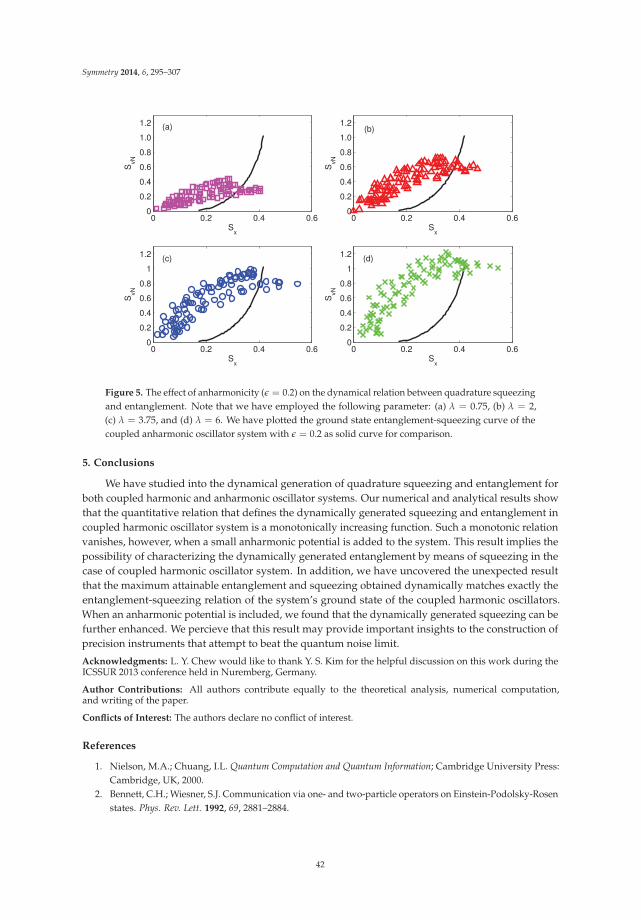
Symmetry 2014, 6, 295–307

0 0.2 0.4 0.60

0.2

0.4

0.6

0.8

1.0

1.2

Sx

SvN

0 0.2 0.4 0.60

0.2

0.4

0.6

0.8

1.0

1.2

Sx

SvN

0 0.2 0.4 0.60

0.2

0.4

0.6

0.8

1

1.2

Sx

SvN

0 0.2 0.4 0.60

0.2

0.4

0.6

0.8

1

1.2

Sx

SvN

(a)

(c)

(b)

(d)

Figure 5. The effect of anharmonicity (ε = 0.2) on the dynamical relation between quadrature squeezingand entanglement. Note that we have employed the following parameter: (a) λ = 0.75, (b) λ = 2,(c) λ = 3.75, and (d) λ = 6. We have plotted the ground state entanglement-squeezing curve of thecoupled anharmonic oscillator system with ε = 0.2 as solid curve for comparison.

5. Conclusions

We have studied into the dynamical generation of quadrature squeezing and entanglement forboth coupled harmonic and anharmonic oscillator systems. Our numerical and analytical results showthat the quantitative relation that defines the dynamically generated squeezing and entanglement incoupled harmonic oscillator system is a monotonically increasing function. Such a monotonic relationvanishes, however, when a small anharmonic potential is added to the system. This result implies thepossibility of characterizing the dynamically generated entanglement by means of squeezing in thecase of coupled harmonic oscillator system. In addition, we have uncovered the unexpected resultthat the maximum attainable entanglement and squeezing obtained dynamically matches exactly theentanglement-squeezing relation of the system’s ground state of the coupled harmonic oscillators.When an anharmonic potential is included, we found that the dynamically generated squeezing can befurther enhanced. We percieve that this result may provide important insights to the construction ofprecision instruments that attempt to beat the quantum noise limit.

Acknowledgments: L. Y. Chew would like to thank Y. S. Kim for the helpful discussion on this work during theICSSUR 2013 conference held in Nuremberg, Germany.

Author Contributions: All authors contribute equally to the theoretical analysis, numerical computation,and writing of the paper.

Conflicts of Interest: The authors declare no conflict of interest.

References

1. Nielson, M.A.; Chuang, I.L. Quantum Computation and Quantum Information; Cambridge University Press:Cambridge, UK, 2000.

2. Bennett, C.H.; Wiesner, S.J. Communication via one- and two-particle operators on Einstein-Podolsky-Rosenstates. Phys. Rev. Lett. 1992, 69, 2881–2884.

42

Symmetry 2014, 6, 295–307

3. Bennett, C.H.; Brassard, G.; Crépeau, C.; Jozsa, R.; Peres, A.; Wooters, W.K. Teleporting an unknownquantum state via dual classical and Einstein-Podolsky-Rosen channels. Phys. Rev. Lett. 1993, 70, 1895–1899.

4. Bennett, C.H.; Brassard, G. Quantum cryptography: Public key distribution and coin tossing. In Proceedingsof the IEEE International Conference on Computers, Systems and Signal Processing, IEEE Computer Society,New York, NY, USA, 1984; pp. 175–179.

5. Ekert, A.K. Quantum cryptography based on Bell’s theorem. Phys. Rev. Lett. 1991, 67, 661–663.6. Shor, P.W. Polynomial-time algorithms for prime factorization and discrete logarithms on a quantum

computer. SIAM J. Comput. 1997, 26, 1484–1509.7. Jozsa, R.; Linden, N. On the role of entanglement in quantum-computational speed-up. Proc. R. Soc. Lond.

A 2003, 459, 2011–2032.8. Lanyon, B.P.; Barbieri, M.; Almeida, M.P.; White, A.G. Experimental quantum computing without

entanglement. Phys. Rev. Lett. 2008, 101, 200501:1–200501:4.9. Sørensen, A.; Duan, L.M.; Cirac, J.I.; Zoller, P. Many-particle entanglement with Bose-Einstein condensates.

Nature 2001, 409, 63–66.10. Bigelow, N. Squeezing Entanglement. Nature 2001, 409, 27–28.11. Furuichi, S.; Mahmoud, A.A. Entanglement in a squeezed two-level atom. J. Phys. A Math. Gen. 2001, 34,

6851–6857.12. Xiang, S.; Shao, B.; Song, K. Quantum entanglement and nonlocality properties of two-mode Gaussian

squeezed states. Chin. Phys. B 2009, 18, 418–425.13. Galve, F.; Pachón, L.A.; Zueco, D. Bringing entanglement to the high temperature limit. Phys. Rev. Lett.

2010, 105, doi:10.1103/PhysRevLett.105.180501.14. Ulam-Orgikh, D.; Kitagawa, M. Spin squeezed and decoherence limit in Ramsey spectroscopy. Phys. Rev. A

2001, 64, doi:10.1103/PhysRevA.64.052106.15. Wolf, M.M.; Eisert, J.; Plenio, M.B. Entangling power of passive optical elements. Phys. Rev. Lett. 2003, 90,

047904:1–047904:4.16. Chung, N.N.; Er, C.H.; Teo, Y.S.; Chew, L.Y. Relation of the entanglement entropy and uncertainty product

in ground states of coupled anharmonic oscillators. Phys. Rev. A 2010, 82, doi:10.1103/PhysRevA.82.014101.17. Chew, L.Y.; Chung, N.N. Quantum entanglement and squeezing in coupled harmonic and anharmonic

oscillators systems. J. Russ. Laser Res. 2011, 32, 331–337.18. Er, C.H.; Chung, N.N.; Chew, L.Y. Threshold effect and entanglement enhancement through local

squeezing of initial separable states in continuous-variable systems. Phys. Scripta 2013, 87,doi:10.1088/0031-8949/87/02/025001.

19. Han, D.; Kim, Y.S.; Noz, M.E. Linear canonical transformations of coherent and squeezed states in theWigner phase space. Phys. Rev. A 1988, 37, 807–814.

20. Han, D.; Kim, Y.S.; Noz, M.E. Linear canonical transformations of coherent and squeezed states in theWigner phase space. II. Quantitative analysis. Phys. Rev. A 1989, 40, 902–912.

21. Han, D.; Kim, Y.S.; Noz, M.E. Linear canonical transformations of coherent and squeezed states in theWigner phase space. III. Two-mode states. Phys. Rev. A 1990, 41, 6233–6244.

22. Wilson, E.B.; Decius, J.C.; Cross, P.C. Molecular Vibration; McGraw-Hill: New York, NY, USA, 1955.23. Schweber, S.S. An Introduction to Relativistic Quantum Field Theory; Row-Peterson: New York, NY, USA, 1961.24. Han, D.; Kim, Y.S.; Noz, M.E. O(3,3)-like symmetries of coupled harmonic-oscillators. J. Math. Phys. 1995,

36, 3940–3954.25. Kim, Y.S.; Noz, M.E. Coupled oscillators, entangled oscillators, and Lorentz-covariant harmonic oscillators.

J. Opt. B Quantum Semiclass. Opt. 2005, 7, S458–S467.26. Eisert, J.; Plenio, M.B.; Bose, S.; Hartley, J. Towards quantum entanglement in nanoelectromechanical

devices. Phys. Rev. Lett. 2004, 93, 190402:1–190402:4.27. Joshi, C.; Jonson, M.; Öhberg, P.; Andersson, E. Constructive role of dissipation for driven coupled bosonic

modes. Phys. Rev. A 2013, 87, 062304:1–062304:4.28. Joshi, C.; Hutter, A.; Zimmer, F.E.; Jonson, M.; Andersson, E.; Öhberg, P. Quantum entanglement of

nanocantilevers. Phys. Rev. A 2010, 82, doi:10.1103/PhysRevA.82.043846.29. Ikeda, S.; Fillaux, F. Incoherent elastic-neutron-scattering study of the vibrational dynamics and spin-related

symmetry of protons in the KHCO3 crystal. Phys. Rev. B 1999, 59, 4134–4145.

43

Symmetry 2014, 6, 295–307

30. Fillaux, F. Quantum entanglement and nonlocal proton transfer dynamics in dimers of formic acid andanalogues. Chem. Phys. Lett. 2005, 408, 302–306.

31. Audenaert, K.; Eisert, J.; Plenio, M.B.; Werner, R.F. Symmetric qubits from cavity states. Phys. Rev. A 2002,66, 042327:1–042327:6.

32. Martina, L.; Soliani, G. Hartree-Fock approximation and entanglement. Available online:http://arxiv.org/abs/0704.3130 (accessed on 18 April 2014).

33. Chung, N.N.; Chew, L.Y. Energy eigenvalues and squeezing properties of general systems of coupledquantum anharmonic oscillators. Phys. Rev. A 2007, 76, doi:10.1103/ PhysRevA.76.032113.

34. Chung, N.N.; Chew, L.Y. Two-step approach to the dynamics of coupled anharmonic oscillators. Phys. Rev.A 2009, 80, doi:10.1103/PhysRevA.80.012103.

35. Jellal, A.; Madouri, F.; Merdaci, A. Entanglement in coupled harmonic oscillators studied using a unitarytransformation. J. Stat. Mech. 2011, doi:10.1088/1742-5468/2011/09/P09015.

36. McDermott, R.M.; Redmount, I.H. Coupled classical and quantum oscillators. Available online:http://arxiv.org/abs/quant-ph/0403184 (accessed on 18 April 2014).

37. Han, D.; Kim, Y.S.; Noz, M.E. Illustrative example of Feymann’s rest of the universe. Am. J. Phys. 1999, 67,61–66.

38. Chung, N.N.; Chew, L.Y. Dependence of entanglement dynamics on the global classical dynamical regime.Phys. Rev. E 2009, 80, 016204:1–016204:7.

39. Duan, L.M.; Giedke, G.; Cirac, J.I.; Zoller, P. Inseparable criterion for continuous variable systems. Phys.Rev. Lett. 2000, 84, 2722–2725.

40. Joshi, C.; Jonson, M.; Andersson, E.; Öhberg, P. Quantum entanglement of anharmonic oscillators. J. Phys. BAt. Mol. Opt. Phys. 2011, 44, doi:10.1088/0953-4075/44/24/245503.

c© 2014 by the authors. Licensee MDPI, Basel, Switzerland. This article is an open accessarticle distributed under the terms and conditions of the Creative Commons Attribution(CC BY) license (http://creativecommons.org/licenses/by/4.0/).

44

symmetryS S

Article

Closed-Form Expressions for the Matrix Exponential

F. De Zela

Departamento de Ciencias, Sección Física, Pontificia Universidad Católica del Perú, Ap.1761, Lima L32, Peru;E-Mail: fdezela@pucp.edu.pe; Tel.: +51-1-6262000; Fax: +51-1-6262085

Received: 28 February 2014; in revised form: 16 April 2014 / Accepted: 17 April 2014 / Published: 29 April 2014

Abstract: We discuss a method to obtain closed-form expressions of f (A), where f is an analyticfunction and A a square, diagonalizable matrix. The method exploits the Cayley–Hamilton theoremand has been previously reported using tools that are perhaps not sufficiently appealing to physicists.Here, we derive the results on which the method is based by using tools most commonly employedby physicists. We show the advantages of the method in comparison with standard approaches,especially when dealing with the exponential of low-dimensional matrices. In contrast to otherapproaches that require, e.g., solving differential equations, the present method only requires theconstruction of the inverse of the Vandermonde matrix. We show the advantages of the method byapplying it to different cases, mostly restricting the calculational effort to the handling of two-by-twomatrices.

Keywords: matrix exponential; Cayley–Hamilton theorem; two-by-two representations;Vandermonde matrices

PACS: 02.30.Tb, 42.25.Ja, 03.65.Fd

1. Introduction

Physicists are quite often faced with the task of calculating f (A), where A is an n × n matrix andf an analytic function whose series expansion generally contains infinitely many terms. The mostprominent example corresponds to exp A. Usual approaches to calculate f (A) consist in eithertruncating its series expansion, or else finding a way to “re-summate” terms so as to get a closed-formexpression. There is yet another option that can be advantageously applied when dealing with ann × n matrix, and which derives from the Cayley–Hamilton theorem [1]. This theorem states thatevery square matrix satisfies its characteristic equation. As a consequence of this property, any seriesexpansion can be written in terms of the first n powers of A. While this result is surely very wellknown among mathematicians, it appears to be not so widespread within the physicists’ community[2]. Indeed, most textbooks on quantum mechanics still resort to the Baker–Hausdorff lemma orto special properties of the involved matrices, in order to obtain closed-form expressions of seriesexpansions [3–5]. This happens even when dealing with low-dimensional matrices, i.e., in cases inwhich exploiting the Cayley–Hamilton theorem would straightforwardly lead to the desired result.Such a state of affairs probably reflects a lack of literature on the subject that is more palatable tophysicists than to mathematicians. The present paper aims at dealing with the subject matter by usinglanguage and tools that are most familiar to physicists. No claim of priority is made; our purpose isto show how well the derived results fit into the repertoire of tools that physicists routinely employ.To this end, we start addressing the simple, yet rich enough case of 2 × 2 matrices.

An archetypical example is the Hamiltonian H = kσ · B that rules the dynamics of a spin-1/2particle subjected to a magnetic field B. Here, σ = (σx, σy, σz) denotes the Pauli spin operator and k isa parameter that provides the above expression with appropriate units. The upsurge of research inseveral areas of physics—most notably in quantum optics—involving two-level systems, has made a

Symmetry 2014, 6, 329–344 45 www.mdpi.com/journal/symmetry

Symmetry 2014, 6, 329–344

Hamiltonian of the above type quite ubiquitous. Indeed, the dynamics of any two-level system is ruledby a Hamiltonian that can be written in such a form. Hence, one often requires an explicit, closed-formexpression for quantities such as exp(iαn · σ), where n is a unit vector. This closed-form expressioncan be obtained as a generalization of Euler’s formula exp iα = cos α + i sin α. It reads

exp(iαn · σ) = cos αI + i sin αn · σ (1)

with I denoting the identity operator.Let us recall how most textbooks of quantum mechanics proceed to demonstrate Equation (1)

(see, e.g., [3–5]). The demonstration starts by writing the series expansion exp A = ∑k Ak/k! for thecase A = iαn · σ. Next, one invokes the following relationship:

(a · σ) (b · σ) = (a · b)I + i (a × b) · σ (2)

whose proof rests on σiσj = δij I + iεijkσk (summation over repeated indices being understood).Equation (2) implies that (n · σ)2n = I, and hence (n · σ)2n+1 = n · σ. This allows one to splitthe power series of exp(iαn · σ) in two parts, one constituted by even and the other by odd powers ofiαn · σ:

exp(iαn · σ) =∞

∑n=0

(iα)2n

2n!I +

∞

∑n=0

(iα)2n+1

(2n + 1)!n · σ (3)

By similarly splitting Euler’s exponential, i.e.,

exp iα = cos α + i sin α =∞

∑n=0

(iα)2n

2n!+

∞

∑n=0

(iα)2n+1

(2n + 1)!(4)

one sees that Equation (3) is the same as Equation (1).Although this standard demonstration is a relatively simple one, it seems to be tightly related

to the particular properties of the operator n · σ, as well as to our ability to “re-summate” the seriesexpansion so as to obtain a closed-form expression. There are several other cases [6] in which a relationsimilar to Equation (1) follows as a consequence of generalizing some properties of the group SU(2)and its algebra to the case SU(N), with N > 2. Central to these generalizations and to their associatedtechniques are both the Cayley–Hamilton theorem and the closure of the Lie algebra su(N) undercommutation and anti-commutation of its elements [6]. As already recalled, the Cayley–Hamiltontheorem states that any n × n matrix A satisfies its own characteristic equation p(A) = 0, where

p(λ) = Det(λI − A) = λn + cn−1λn−1 + . . . + c1λ + c0 (5)

is A’s characteristic polynomial. From p(A) = 0 it follows that any power Ak, with k ≥ n, can bewritten in terms of the matrices I = A0, A, . . . , An−1. Thus, any infinite series, such as the onecorresponding to exp A, may be rewritten in terms of the n powers A0, A, . . . , An−1. By exploiting thisfact one can recover Equation (1). Reciprocally, given A, one can construct a matrix B that satisfiesexp B = A, as shown by Dattoli, Mari and Torre [2]. These authors used essentially the same tools aswe do here and presented some of the results that we will show below, but leaving them in an implicitform. The aforementioned authors belong to a group that has extensively dealt with our subjectmatter and beyond it [7], applying the present techniques to cases of current interest [8]. A somewhatdifferent approach was followed by Leonard [9], who related the Cayley–Hamilton theorem to thesolution of ordinary differential equations, in order to get closed expressions for the matrix exponential.This technique can be applied to all n × n matrices, including those that are not diagonalizable.Untidt and Nielsen [10] used this technique when addressing the groups SU(2), SU(3) and SU(4).Now, especially when addressing SU(2), Leonard’s approach seems to be unnecessarily involved.This is because there is a trade-off between the wide applicability of the method and its tailoring to a

46

Symmetry 2014, 6, 329–344

special case. When dealing with diagonalizable matrices, the present approach may prove more useful.Thus, one exploits not only the Cayley–Hamilton theorem, but the diagonalizability of the involvedmatrices as well. As a result, we are provided with a straightforward way to obtain closed-formexpressions for the matrix exponential. There are certainly many other ways that are either moregeneral [9,11] or else better suited to specific cases [12–16], but the present method is especially usefulfor physical applications.

The rest of the paper is organized as follows. First, we present Leonard’s technique in a way thatsomewhat differs from the approach used in [9]. Thereafter, we show how to obtain Equation (1) byusing a technique that can be generalized to diagonalizable n × n matrices, thereby introducingthe method that is the main subject of the present work. As an illustration of this technique,we address some representative cases that were taken from the repertoire of classical mechanics,quantum electrodynamics, quantum optics and from the realm of Lorentz transformations. While theresults obtained are known, their derivations should serve to demonstrate the versatility of the method.Let us stress once again that our aim has been to present this method by following an approach thatcould be appealing to most physicists, rather than to mathematically oriented readers.

2. Closed Form of the Matrix Exponential via the Solution of Differential Equations

Consider the coupled system of differential equations, given by

Dx ≡ dxdt

= Ax (6)

with x = (x1, . . . , xn)T and A a constant, n × n matrix. The matrix exponential appears in the solutionof Equation (6), when we write it as x(t) = eAtx(0). By successive derivation of this exponentialwe obtain DkeAt = AkeAt. Hence, p(D)eAt ≡ (Dn + cn−1Dn−1 + . . . + c1D + c0)eAt = p(A)eAt = 0,on account of p(A) = 0, i.e., the Cayley–Hamilton theorem. Now, as already noted, this implies that eAt

can be expressed in terms of A0, A, . . . , An−1. Let us consider the matrix M(t) := ∑n−1k=0 yk(t)Ak, with

the yk(t) being n independent solutions of the differential equation p(D)y(t) = 0. That is, the yk(t)solve this equation for n different initial conditions that will be conveniently chosen. We have thus thatp(D)M(t) = ∑n−1

k=0 p(D)yk(t)Ak = 0. Our goal is to choose the yk(t) so that eAt = M(t). To this end,we note that DkeAt |t=0= AkeAt |t=0= Ak. That is, eAt solves p(D)Φ(t) = 0 with the initial conditionsΦ(0) = A0, . . . , Dn−1Φ(0) = An−1. It is then clear that we must take the following initial conditions:Djyk(0) = δ

jk, with j, k ∈ {0, . . . , n − 1}. In such a case, eAt and M(t) satisfy both the same differential

equation and the same initial conditions. Hence, eAt = M(t).Summarizing, the method consists in solving the n-th order differential equation p(D)y(t) = 0

for n different initial conditions. These conditions read Djyk(0) = δjk, with j, k ∈ {0, . . . , n − 1}.

The matrix exponential is then given by eAt = ∑n−1k=0 yk(t)Ak. The standard procedure for solving

p(D)y(t) = 0 requires finding the roots of the characteristic equation p(λ) = 0. Each root λ withmultiplicity m contributes to the general solution with a term (a0 + a1t + . . . + am−1tm−1)eλt, the akbeing fixed by the initial conditions. As already said, this method applies even when the matrix A isnot diagonalizable. However, when the eigenvalue problem for A is a solvable one, another approachcan be more convenient. We present such an approach in what follows.

3. Closed Form of the Matrix Exponential via the Solution of Algebraic Equations

Let us return to Equation (1). We will derive it anew, this time using standard tools of quantummechanics. Consider a Hermitian operator A, whose eigenvectors satisfy A |ak〉 = ak |ak〉 and span theHilbert space on which A acts. Thus, the identity operator can be written as I = ∑k |ak〉 〈ak|. One canalso write A = A · I = ∑k ak |ak〉 〈ak|. Moreover, Am = ∑k am

k |ak〉 〈ak|, from which it follows that

F(A) = ∑k

F(ak) |ak〉 〈ak| (7)

47

Symmetry 2014, 6, 329–344

for any function F(A) that can be expanded in powers of A.Let us consider the 2 × 2 case A = n · σ, with n a unit vector. This matrix has the eigenvalues

±1 and the corresponding eigenvectors |n±〉. That is, n · σ |n±〉 = ± |n±〉. We need no more thanthis to get Equation (1). Indeed, from n · σ = |n+〉 〈n+| − |n−〉 〈n−| and I = |n+〉 〈n+|+ |n−〉 〈n−|,it follows that |n±〉 〈n±| = (I ± n · σ) /2. Next, we consider F(A) = exp A = ∑k exp ak |ak〉 〈ak|,with A = iαn · σ. The operator iαn · σ has eigenvectors |n±〉 and eigenvalues ±iα. Thus,

exp(iαn · σ) = eiα |n+〉 〈n+|+ e−iα |n−〉 〈n−| (8)

=12

eiα (I + n · σ) +12

e−iα (I − n · σ) (9)

=

(eiα + e−iα

2

)I +

(eiα − e−iα

2

)n · σ (10)

which is Equation (1). Note that it has not been necessary to know the eigenvectors of A = iαn · σ.It is a matter of convenience whether one chooses to express exp (iαn · σ) in terms of the projectors|n±〉 〈n±|, or in terms of I and n · σ.

Let us now see how the above method generalizes when dealing with higher-dimensional spaces.To this end, we keep dealing with rotations. The operator exp (iαn · σ) is a rotation operator acting onspinor space. It is also an element of the group SU(2), whose generators can be taken as Xi = iσi/2,i = 1, 2, 3. They satisfy the commutation relations

[Xi, Xj

]= εijkXk that characterize the rotation

algebra. The rotation operator can also act on three-dimensional vectors r. In this case, one often usesthe following formula, which gives the rotated vector r′ in terms of the rotation angle θ and the unitvector n that defines the rotation axis:

r′ = r cos θ + n (n · r) [1 − cos θ] + (n × r) sin θ (11)

Equation (11) is usually derived from vector algebra plus some geometrical considerations [17].We can derive it, alternatively, by the method used above. To this end, we consider the rotationgenerators Xi for three-dimensional space, which can be read off from the next formula, Equation (12).The rotation matrix is then obtained as exp (θn · X), with

n · X =

⎛⎜⎝ 0 −n3 n2

n3 0 −n1

−n2 n1 0

⎞⎟⎠ ≡ M (12)

It is straightforward to find the eigenvalues of the non-Hermitian, antisymmetric matrix M. They are 0and ±i. Let us denote the corresponding eigenvectors as |n0〉 and |n±〉, respectively. Similarly to thespin case, we have now

I = |n+〉 〈n+|+ |n−〉 〈n−|+ |n0〉 〈n0| (13)

M = i |n+〉 〈n+| − i |n−〉 〈n−| (14)

We need a third equation, if we want to express the three projectors |nk〉 〈nk|, k = ±, 0, in terms of Iand M. This equation is obtained by squaring M:

M2 = − |n+〉 〈n+| − |n−〉 〈n−| (15)

From Equations (13)–(15) we immediately obtain |n±〉 〈n±| =(∓iM − M2) /2, and |n0〉 〈n0| = I + M2.

Thus, we have

exp(θM) = eiθ |n+〉 〈n+|+ e−iθ |n−〉 〈n−|+ e0 |n0〉 〈n0| (16)

= I + M sin θ + M2 [1 − cos θ] (17)

48

Symmetry 2014, 6, 329–344

By letting M, as given in Equation (12), act on r = (x, y, z)T , we easily see that Mr = n × r andM2r = n × (n × r) = n (n · r)− r. Thus, on account of Equation (17), r′ = exp(θM)r reads the sameas Equation (11).

The general case is now clear. Consider an operator A whose matrix representation is anN × N matrix. Once the eigenvalues ak of A (which we assume nondegenerate) have beendetermined, we can write the N equations: A0 = I = ∑k |ak〉 〈ak|, A = ∑k ak |ak〉 〈ak|, A2 =

∑Nk=1 a2

k |ak〉 〈ak| , . . . , AN−1 = ∑Nk=1 aN−1

k |ak〉 〈ak|, from which it is possible to obtain the N projectors|ak〉 〈ak| in terms of I, A, A2, . . . , AN−1. To this end, we must solve the system

⎛⎜⎜⎜⎜⎜⎜⎝

1 1 . . . 1a1 a2 . . . aNa2

1 a22 a2

N...

......

aN−11 aN−1

2 aN−1N

⎞⎟⎟⎟⎟⎟⎟⎠

⎛⎜⎜⎜⎜⎜⎜⎝

|a1〉 〈a1||a2〉 〈a2||a3〉 〈a3|

...|aN〉 〈aN |

⎞⎟⎟⎟⎟⎟⎟⎠

=

⎛⎜⎜⎜⎜⎜⎜⎝

IAA2

...AN−1

⎞⎟⎟⎟⎟⎟⎟⎠

(18)

The matrix in Equation (18), with components Vk,i = ak−1i (k, i ∈ {1, . . . , N}), is a Vandermonde

matrix, whose inverse can be explicitly given [18]. Once we have written the |ak〉 〈ak| in terms ofI, A, . . . AN−1, we can express any analytic function of A in terms of these N powers of A, in particularexp A = ∑N

k=1 exp(ak) |ak〉 〈ak|. For the case N = 4, for instance, we have the following result:

|a1〉 〈a1| =A3 − A2(a2 + a3 + a4) + A(a2a3 + a2a4 + a3a4)− a2a3a4

(a1 − a2)(a1 − a3)(a1 − a4)(19)

|a2〉 〈a2| =A3 − A2(a1 + a3 + a4) + A(a1a3 + a1a4 + a3a4)− a1a3a4

(a2 − a1)(a2 − a3)(a2 − a4)(20)

|a3〉 〈a3| =A3 − A2(a1 + a2 + a4) + A(a1a2 + a1a4 + a2a4)− a1a2a4

(a3 − a1)(a3 − a2)(a3 − a4)(21)

|a4〉 〈a4| =A3 − A2(a1 + a2 + a3) + A(a1a2 + a1a3 + a2a3)− a1a3a4

(a4 − a1)(a4 − a2)(a4 − a3)(22)

The general solution can be written in terms of the inverse of the Vandermonde matrix V. To this end,consider a system of equations that reads like (18), but with the operators entering the column vectorsbeing replaced by numbers, i.e.,

∣∣aj⟩ ⟨

aj∣∣ → wj, with j = 1, . . . , N, and Ak → qk+1, with k = 0, . . . , N − 1.

The solution of this system is given by wj = ∑N−1k=0 Uj,kqk, with U = V−1, the inverse of the Vandermonde

matrix. This matrix inverse can be calculated as follows [18]. Let us define a polynomial Pj(x) of degreeN − 1 as

Pj(x) =N

∏n=1n =j

x − an

aj − an=

N

∑k=1

Uj,kxk−1 (23)

The coefficients Uj,k of the last equality follow from expanding the preceding expression and collectingequal powers of x. These Uj,k are the components of V−1. Indeed, setting x = ai and observingthat Pj(ai) = δji = ∑N

k=1 Uj,kak−1i = (UV)j,i, we see that U is the inverse of the Vandermonde

matrix. The projectors∣∣aj

⟩ ⟨aj∣∣ in Equation (18) can thus be obtained by replacing x → A in

Equation (23).We get in this way the explicit solution

∣∣aj⟩ ⟨

aj∣∣ = N

∑k=1

Uj,k Ak−1 =N

∏n=1n =j

A − an

aj − an(24)

The above expression can be inserted into Equation (7), if one wants to write F(A) in terms of the firstN powers of A.

49

Symmetry 2014, 6, 329–344

So far, we have assumed that the eigenvalues of A are all nondegenerate. Let us now considera matrix M with degenerate eigenvalues. As before, we deal with a special case, from which thegeneral formalism can be easily inferred. Let M be of dimension four and with eigenvalues λ1 and λ2,which are two-fold degenerate. We can group the projectors as follows:

I = (|e1〉 〈e1|+ |e2〉 〈e2|) + (|e3〉 〈a3|+ |e4〉 〈e4|) (25)

M = λ1 (|e1〉 〈e1|+ |e2〉 〈e2|) + λ2 (|e3〉 〈a3|+ |e4〉 〈e4|) (26)

It is then easy to solve the above equations for the two projectors associated with the two eigenvalues.We obtain

|e1〉 〈e1|+ |e2〉 〈e2| =λ2 I − Mλ2 − λ1

(27)

|e3〉 〈a3|+ |e4〉 〈e4| =λ1 I − Mλ1 − λ2

(28)

We can then writeeM =

1λ1 − λ2

[(λ1eλ2 − λ2eλ1

)I +

(eλ1 − eλ2

)M

](29)

We will need this result for the calculation of the unitary operator that defines the Foldy–Wouthuysentransformation, our next example. It is now clear that in the general case of degenerate eigenvalues,we can proceed similarly to the nondegenerate case, but solving n < N equations.

4. Examples

Let us now see how the method works when applied to some well-known cases. Henceforth, werefer to the method as the Cayley–Hamilton (CH)-method, for short. Our aim is to show the simplicityof the required calculations, as compared with standard techniques.

4.1. The Foldy–Wouthuysen Transformation

The Foldy–Wouthuysen transformation is introduced [19] with the aim of decoupling the upper(ϕ) and lower (χ) components of a bispinor ψ = (ϕ, χ)T that solves the Dirac equation ih∂ψ/∂t = Hψ,where H = −ihcα ·∇+ βmc2. Here, β and α = (αx, αy, αz) are the 4 × 4 Dirac matrices:

β =

(1 0

0 −1

), α =

(0 σ

σ 0

)(30)

The Foldy–Wouthuysen transformation is given by ψ′ = Uψ, with [19]

U = exp(

θ

2βα · p

)(31)

We can calculate U by applying Equation (29) for M = θβα · p/2 = (θ |p|/2)βα ·n, where n = p/ |p|.The eigenvalues of the 4 × 4 matrix βα · n are ±i, each being two-fold degenerate. This follows fromnoting that the matrices

βα · n =

(0 σ · n

−σ · n 0

)and

(0 1−1 0

)(32)

50

Symmetry 2014, 6, 329–344

have the same eigenvalues. Indeed, because (σ · n)2 = 1, the above matrices share the characteristicequation λ2 + 1 = 0. Their eigenvalues are thus ±i. The eigenvalues of M = θβα · p/2 are thenλ1,2 = ±iθ |p| /2. Replacing these values in Equation (29) we obtain

exp(

θ

2βα · p

)=

1iθ |p|

[iθ |p|

2

(e−iθ|p|/2 + eiθ|p|/2

)I +

(eiθ|p|/2 − e−iθ|p|/2

) θ |p|2

βα · n]

(33)

= cos (|p| θ/2) + sin (|p| θ/2) βα · p|p| (34)

The standard way to get this result requires developing the exponential in a power series.Thereafter, one must exploit the commutation properties of α and β in order to group together oddand even powers of θ. This finally leads to the same closed-form expression that we have arrived atafter some few steps.

4.2. Lorentz-Type Equations of Motion

The dynamics of several classical and quantum systems is ruled by equations that can be castas differential equations for a three-vector S. These equations often contain terms of the form Ω×.An example of this is the ubiquitous equation

dSdt

= Ω × S (35)

Equation (35) and its variants have been recently addressed by Babusci, Dattoli and Sabia [20],who applied operational methods to deal with them. Instead of writing Equation (35) in matrixform, these authors chose to exploit the properties of the vector product by defining the operatorΩ := Ω×. The solution for the case ∂Ω/∂t = 0, for instance, was obtained by expanding exp(tΩ) asan infinite series and using the cyclical properties of the vector product in order to get S(t) in closedform. This form is nothing but Equation (11) with the replacements r′ → S(t), r → S(0) and θ → Ωt,where Ω := |Ω|. We obtained Equation (11) without expanding the exponential and without usingany cyclic properties. Our solution follows from writing Equation (35) in matrix form, i.e.,

dSdt

= ΩMS (36)

where M is given by Equation (12) with n = Ω/Ω. The solution S(t) = exp(MΩt)S(0) is theneasily written in closed form by applying the CH-method, as in Equation (11). The advantagesof this method show up even more sharply when dealing with some extensions of Equation (36).Consider, e.g., the non-homogeneous version of Equation (35):

dSdt

= Ω × S + N = ΩMS + N (37)

This is the form taken by the Lorentz equation of motion when the electromagnetic field is given byscalar and vector potentials reading Φ = −E · r and A = B × r/2, respectively [20]. The solution ofEquation (37) is easily obtained by acting on both sides with the “integrating (operator-valued) factor”exp(−ΩMt). One then readily obtains, for the initial condition S(0) = S0,

S(t) = eΩMtS0 +

ˆ t

0eΩM(t−s)Nds (38)

The matrix exponentials in Equation (38) can be expressed in their eigenbasis, as in Equation (16).For a time-independent N, the integral in Equation (38) is then trivial. An equivalent solution isgiven in [20], but written in terms of the evolution operator U(t) = exp(tΩ) and its inverse. Inverseoperators repeatedly appear within such a framework [20] and are often calculated with the help of

51

Symmetry 2014, 6, 329–344

the Laplace transform identity: A−1 =´ ∞

0 exp(−sA)ds. Depending on A, this could be not such astraightforward task as it might appear at first sight. Now, while vector notation gives us additionalphysical insight, vector calculus can rapidly turn into a messy business. Our strategy is therefore toavoid vector calculus and instead rely on the CH-method as much as possible. Only at the end we writedown our results, if we wish, in terms of vector products and the like. That is, we use Equations (13)–(17)systematically, in particular Equation (16) when we need to handle exp(θM), e.g., within integrals.The simplification comes about from our working with the eigenbasis of exp(θM), i.e., with the eigenbasisof M. Writing down the final results in three-vector notation amounts to expressing these results in thebasis in which M was originally defined, cf. Equation (12). Let us denote this basis by {|x〉, |y〉, |z〉}.The eigenvectors |n±〉 and |n0〉 of M are easily obtained from those of X3, cf. Equation (12). Theeigenvectors of X3 are, in turn, analogous to those of Pauli’s σy, namely |±〉 = (|x〉 ∓ i|y〉)/

√2, plus

a third eigenvector that is orthogonal to the former ones, that is, |0〉 = |z〉. In order to obtain theeigenvectors of n · X, with n = (sin θ cos φ, sin θ sin φ, cos θ), we apply the rotation exp(φX3) exp(θX2)

to the eigenvectors |±〉 and |0〉, thereby getting |n±〉 and |n0〉, respectively. All these calculations areeasily performed using the CH-method.

Once we have |n±〉 and |n0〉, we also have the transformation matrix T that brings M into diagonalform: T−1MT = MD = diag(−i, 0, i). Indeed, T’s columns are just |n−〉, |n0〉 and |n+〉. After we havecarried out all calculations in the eigenbasis of M, by applying T we can express the final result in thebasis {|x〉, |y〉, |z〉}, thereby obtaining the desired expressions in three-vector notation. Let us illustratethis procedure by addressing the evolution equation

dSdt

= Ω × S + λΩ × (Ω × S) (39)

In matrix form, such an equation reads

dSdt

= ΩMS + λ(ΩM)2S = [ΩM + λ(ΩM)2]S ≡ AS (40)

The solution is given by S(t) = exp(At)S0. The eigenbasis of A is the same as that of M. We have thus

exp(At) = e(iΩ−λΩ2)t|n+〉〈n+|+ e(−iΩ−λΩ2)t|n−〉〈n−|+ |n0〉〈n0| (41)

The projectors |nk〉〈nk| can be written in terms of the powers of A by solving the system

I = |n+〉 〈n+|+ |n−〉 〈n−|+ |n0〉 〈n0| (42)

A = (iΩ − λΩ2) |n+〉 〈n+| − (iΩ + λΩ2) |n−〉 〈n−| (43)

A2 = (iΩ − λΩ2)2 |n+〉 〈n+|+ (iΩ + λΩ2)2 |n−〉 〈n−| (44)

Using A = ΩM + λ(ΩM)2 and A2 = −2λΩ3M + (1 − λ2Ω2)(ΩM)2, and replacing the solution ofthe system (42)–(44) in Equation (41) we get

exp(At) = I + e−λΩ2t sin(Ωt)M + [1 − e−λΩ2t cos(Ωt)]M2 (45)

Finally, we can write the solution S(t) = exp(At)S0 in the original basis {|x〉, |y〉, |z〉}, something thatin this case amounts to writing MS0 = n × S0 and M2S0 = n (n · S0)− S0. Equation (39) was alsoaddressed in [20], but making use of the operator method. The solution was given in terms of a seriesexpansion for the evolution operator. In order to write this solution in closed form, it is necessaryto introduce sin- and cos-like functions [20]. These functions are defined as infinite series involvingtwo-variable Hermite polynomials. The final expression reads like Equation (11), but with sin and cosreplaced by the aforementioned functions containing two-variable Hermite polynomials. Now, one canhardly unravel from such an expression the physical features that characterize the system’s dynamics.

52

Symmetry 2014, 6, 329–344

On the other hand, a solution given as in Equation (45) clearly shows such dynamics, in particularthe damping effect stemming from the λ-term in Equation (39), for λ > 0. Indeed, Equation (45)clearly shows that the state vector S(t) = exp(At)S0 asymptotically aligns with Ω while performing adamped Larmor precession about the latter.

The case ∂Ω/∂t = 0 is more involved and generally requires resorting to Dyson-like seriesexpansions, e.g., time-ordered exponential integrations. While this subject lies beyond the scope of thepresent work, it should be mentioned that the CH-method can be advantageously applied also in thiscontext. For instance, time-ordered exponential integrations involving operators of the form A + B(t)do require the evaluation of exp A. Likewise, disentangling techniques make repeated use of matrixexponentials of single operators [21]. In all these cases, the CH-method offers a possible shortcut.

4.3. The Jaynes–Cummings Hamiltonian

We address now a system composed by a two-level atom and a quantized (monochromatic)electromagnetic field. Under the dipole and the rotating-wave approximations, the Hamiltonian ofthis system reads (in standard notation)

H =h2

ω0σz + hωa†a + hg(

a†σ− + aσ+)

(46)

Let us denote the upper and lower states of the two-level atom by |a〉 and |b〉, respectively, and theFock states of the photon-field by |n〉. The Hilbert space of the atom-field system is spanned by thebasis B = {|a, n〉 , |b, n〉 , n = 0, 1, . . .}. The states |a, n〉 and |b, n〉 are eigenstates of the unperturbedHamiltonian H0 = hω0σz/2 + hωa†a. The interaction Hamiltonian V = hg

(a†σ− + aσ+

)couples the

states |a, n〉 and |b, n + 1〉 alone. Hence, H can be split into a sum: H = ∑n Hn, with each Hn acting onthe subspace Span{|a, n〉 , |b, n + 1〉}. Within such a subspace, Hn is represented by the 2 × 2 matrix

Hn = hω

(n +

12

)I + h

(δ/2 g

√n + 1

g√

n + 1 −δ/2

)(47)

where δ = ω0 − ω.A standard way [22] to calculate the evolution operator U = exp(−iHt/h) goes as follows.

One first writes the Hamiltonian in the form H = H1 + H2, with H1 = hω(a†a + σz/2

)and

H2 = hδσz/2 + hg(a†σ− + aσ+

). Because [H1, H2] = 0, the evolution operator can be factored as

U = U1U2 = exp(−iH1t/h) exp(−iH2t/h). The first factor is diagonal in SpanB. The second factor canbe expanded in a Taylor series. As it turns out, one can obtain closed-form expressions for the even andthe odd powers of the expansion. Thus, a closed-form for U2 can be obtained as well. As can be seen,this method depends on the realization that Equation (46) can be written in a special form, which rendersit possible to factorize U.

Let us now calculate U by the CH-method. We can exploit the fact that H splits as H = ∑n Hn,with [Hn, Hm] = 0, and write U = ∏n Un = ∏n exp(−iHnt/h). Generally, a 2 × 2 Hamiltonian H haseigenvalues of the form E± = h(λ0 ± λ). We have thus

I = |+〉 〈+|+ |−〉 〈−| (48)

H/h = (λ0 + λ) |+〉 〈+|+ (λ0 − λ) |−〉 〈−| (49)

so that

exp(−iHt/h) = exp(−iλ+t) |+〉 〈+|+ exp(−iλ−t) |−〉 〈−| (50)

=e−iλ0t

λ

[(iλ0 sin λt + λ cos λt) I − i(sin λt)

Hh

](51)

53

Symmetry 2014, 6, 329–344

In our case, Hn has eigenvalues E±n = hω(n + 1/2)± h

√δ2/4 + g2(n + 1) ≡ hω(n + 1/2)± hRn.

Whence,

exp(−iHnt/h) =e−iω(n+1/2)t

Rn

[(iω(n +

12) sin (Rnt) + Rn cos (Rnt)

)I − i sin(Rnt)

Hn

h

](52)

Replacing Hn from Equation (47) in the above expression we get

exp(−iHnt/h) = e−iω(n+1/2)t

[cos (Rnt) I − i sin (Rnt)

2Rn

(δ 2g

√n + 1

2g√

n + 1 −δ

)](53)

This result enables a straightforward calculation of the evolved state |ψ(t)〉 out of a general initial state

|ψ(0)〉 = ∑n

Ca,n |a, n〉+ Cb,n+1 |b, n + 1〉 (54)

Equation (53) refers to a matrix representation in the two-dimensional subspaceSpan{|a, n〉 , |b, n + 1〉}. Let us focus on

cos (Rnt) I =

(cos (Rnt) 0

0 cos (Rnt)

)(55)

This matrix is a representation in subspace Span{|a, n〉 , |b, n + 1〉} of the operator

cos(

t√

ϕ + g2)|a〉〈a|+ cos

(t√

ϕ

)|b〉〈b| (56)

where ϕ := g2a†a + δ2/4. Proceeding similarly with the other operators that enter Equation (53)and observing that sin (Rnt) R−1

n√

n + 1 = 〈n| i sin(t√

ϕ + g2)(√

ϕ + g2)−1a |n + 1〉, etc., we readilyobtain

exp(−iHt/h) = e−iω(a†a+ 12 )t

⎛⎜⎜⎝

cos(

t√

ϕ + g2)−

iδ sin(

t√

ϕ+g2)

2√

ϕ+g2− ig sin(t

√ϕ+g2)√

ϕ+g2a

−ig sin

(t√

ϕ)

√ϕ

a† cos(t√

ϕ)+

iδ sin(

t√

ϕ)

2√

ϕ

⎞⎟⎟⎠ (57)

where the 2 × 2 matrix refers now to the atomic subspace Span{|a〉, |b〉}. One can see that theCH-method reduces the amount of calculational effort invested to get Equation (53), as compared withother approaches [22].

4.4. Bispinors and Lorentz Transformations

As a further application, let us consider the representation of Lorentz transformations in the spaceof bispinors. In coordinate space, Lorentz transformations are given by xμ = Λμ

ν xν (Greek indicesrun from 0 to 3), with the Λμ

ν satisfying Λμν Λτ

σηνσ = ημτ . Here, ημν represents the metric tensor ofMinkowsky space (η00 = −η11 = −η22 = η33 = 1, ημν = 0 for μ = ν). A bispinor ψ(x) transformsaccording to [19]

ψ(x) = ψ(Λx) = S(Λ)ψ(x) (58)

with

S(Λ) = exp B (59)

B = −14

Vμνγμγν (60)

54

Symmetry 2014, 6, 329–344

The Vμν = −Vνμ are the components of an antisymmetric tensor, which has thus six independentcomponents, corresponding to the six parameters defining a Lorentz transformation. The quantitiesγμ = ημνγν satisfy γμγν + γμγν = 2ημν. The quantities γμγν are the generators of the Lorentz group.S(Λ) is not a unitary transformation, but satisfies

S−1 = γ0S†γ0 (61)

For the following, it will be advantageous to define

pi = γ0γi, i = 1, 2, 3 (62)

q1 = γ2γ3, q2 = γ3γ1, q3 = γ1γ2 (63)

We call the pi Pauli generators and the qi quaternion generators. The pseudoscalar γ5 := γ0γ1γ2γ3

satisfies γ25 = −1, γ5γμ = − γμγ5, so that it commutes with each generator of the Lorentz group:

γ5 (γμγν) = (γμγν) γ5 (64)

This means that quantities of the form α + βγ5 (α, β ∈ R) behave like complex numbers uponmultiplication with pi and qi . We denote the subspace spanned by such quantities as the complex-likesubspace Ci and set i ≡ γ5. Noting that i pi = qi and i qi = −pi, the following multiplication rules areeasily derived:

qiqj = εijkqk − δij (65)

pi pj = −εijkqk + δij = −qiqj = −iεijk pk + δij (66)

piqj = εijk pk + iδij = i(−εijkqk + δij) (67)

The following commutators can then be straightforwardly obtained:

[qi, qj

]= 2εijkqk (68)[

pi, pj]

= −2εijkqk = −2iεijk pk (69)[pi, qj

]= 2εijk pk (70)

They make clear why we dubbed the pi as Pauli generators. Noting that they furthermore satisfy

pi pj + pj pi = 2δij (71)

we see the correspondence i → i, pk → −σk, with i being the imaginary unit and σk the Paulimatrices. These matrices, as is well-known, satisfy

[σi, σj

]= 2iεijkσk and the anticommutation relations

σiσj + σjσi = 2δij, which follow from σiσj = iεijkσk + δij.We can write now S(Λ) = exp(− 1

4 Vμνγμγν) in terms of pi and qi:

B =3

∑i=1

(αi pi + βiqi) (72)

Here, we have set αi = −V0i/4 and βkεijk = −Vij/4. We can write B in terms of the Pauli-generatorsalone:

B =3

∑i=1

(αi + iβi )pi ≡3

∑i=1

zi pi (73)

55

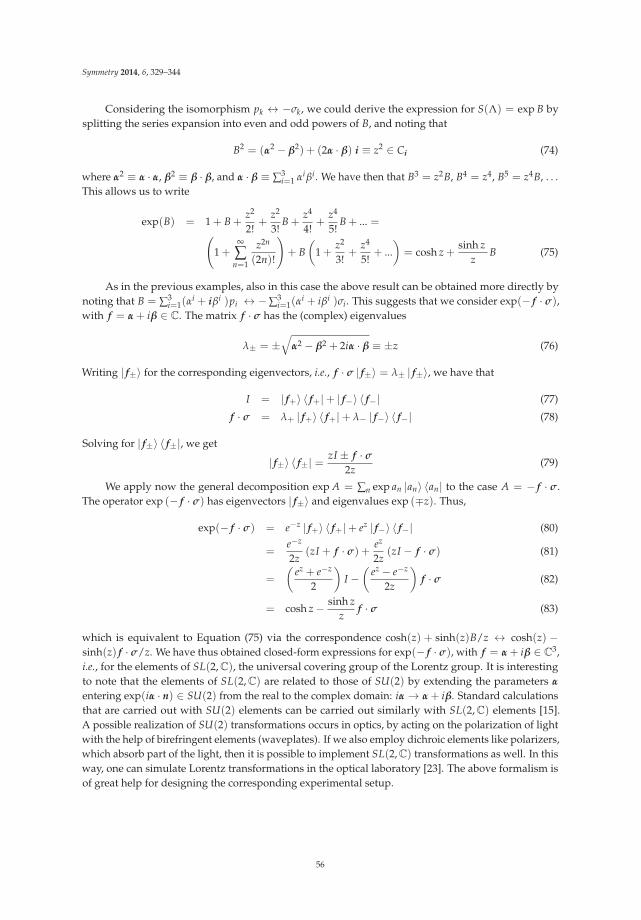
Symmetry 2014, 6, 329–344

Considering the isomorphism pk ↔ −σk, we could derive the expression for S(Λ) = exp B bysplitting the series expansion into even and odd powers of B, and noting that

B2 = (α2 − β2) + (2α · β) i ≡ z2 ∈ Ci (74)

where α2 ≡ α · α, β2 ≡ β · β, and α · β ≡ ∑3i=1 αiβi. We have then that B3 = z2B, B4 = z4, B5 = z4B, . . .

This allows us to write

exp(B) = 1 + B +z2

2!+

z2

3!B +

z4

4!+

z4

5!B + ... =(

1 +∞

∑n=1

z2n

(2n)!

)+ B

(1 +

z2

3!+

z4

5!+ ...

)= cosh z +

sinh zz

B (75)

As in the previous examples, also in this case the above result can be obtained more directly bynoting that B = ∑3

i=1(αi + iβi )pi ↔ −∑3

i=1(αi + iβi )σi. This suggests that we consider exp(− f · σ),

with f = α + iβ ∈ C. The matrix f · σ has the (complex) eigenvalues

λ± = ±√

α2 − β2 + 2iα · β ≡ ±z (76)

Writing | f±〉 for the corresponding eigenvectors, i.e., f · σ | f±〉 = λ± | f±〉, we have that

I = | f+〉 〈 f+|+ | f−〉 〈 f−| (77)

f · σ = λ+ | f+〉 〈 f+|+ λ− | f−〉 〈 f−| (78)

Solving for | f±〉 〈 f±|, we get

| f±〉 〈 f±| =zI ± f · σ

2z(79)

We apply now the general decomposition exp A = ∑n exp an |an〉 〈an| to the case A = − f · σ.The operator exp (− f · σ) has eigenvectors | f±〉 and eigenvalues exp (∓z). Thus,

exp(− f · σ) = e−z | f+〉 〈 f+|+ ez | f−〉 〈 f−| (80)

=e−z

2z(zI + f · σ) +

ez

2z(zI − f · σ) (81)

=

(ez + e−z

2

)I −

(ez − e−z

2z

)f · σ (82)

= cosh z − sinh zz

f · σ (83)

which is equivalent to Equation (75) via the correspondence cosh(z) + sinh(z)B/z ↔ cosh(z) −sinh(z) f · σ/z. We have thus obtained closed-form expressions for exp(− f · σ), with f = α + iβ ∈ C

3,i.e., for the elements of SL(2,C), the universal covering group of the Lorentz group. It is interestingto note that the elements of SL(2,C) are related to those of SU(2) by extending the parameters α

entering exp(iα · n) ∈ SU(2) from the real to the complex domain: iα → α + iβ. Standard calculationsthat are carried out with SU(2) elements can be carried out similarly with SL(2,C) elements [15].A possible realization of SU(2) transformations occurs in optics, by acting on the polarization of lightwith the help of birefringent elements (waveplates). If we also employ dichroic elements like polarizers,which absorb part of the light, then it is possible to implement SL(2,C) transformations as well. In thisway, one can simulate Lorentz transformations in the optical laboratory [23]. The above formalism isof great help for designing the corresponding experimental setup.

56

Symmetry 2014, 6, 329–344

5. Conclusions

The method presented in this paper—referred to as the Cayley–Hamilton method—provesadvantageous for calculating closed-form expressions of analytic functions f (A) of an n × n matrix A,in particular matrix exponentials. The matrix A is assumed to be a diagonalizable one, even though onlyits eigenvalues are needed, not its eigenvectors. We have recovered some known results from classicaland quantum mechanics, including Lorentz transformations, by performing the straightforwardcalculations that the method prescribes. In most cases, the problem at hand was reshaped so as tosolve it by dealing with two-by-two matrices only.

Acknowledgments: The author gratefully acknowledges the Research Directorate of the Pontificia UniversidadCatólica del Perú (DGI-PUCP) for financial support under Grant No. 2014-0064.

Conflicts of Interest: The author declares no conflict of interest.

References

1. Gantmacher, F.R. The Theory of Matrices; Chelsea Publishing Company: New York, NY, USA, 1960; p. 83.2. Dattoli, G.; Mari, C.; Torre, A. A simplified version of the Cayley-Hamilton theorem and exponential forms

of the 2 × 2 and 3 × 3 matrices. Il Nuovo Cimento 1998, 180, 61–68.3. Cohen-Tannoudji, C.; Diu, B.; Laloë, F. Quantum Mechanics; John Wiley & Sons: New York, NY, USA, 1977;

pp. 983–989.4. Sakurai, J.J. Modern Quantum Mechanics; Addison-Wesley: New York, NY, USA, 1980; pp. 163–168.5. Greiner, W.; Müller, B. Quantum Mechanics, Symmetries; Springer: New York, NY, USA, 1989; p. 68.6. Weigert, S. Baker-Campbell-Hausdorff relation for special unitary groups SU(N). J. Phys. A 1997, 30,

8739–8749.7. Dattoli, G.; Ottaviani, P.L.; Torre, A.; Vásquez, L. Evolution operator equations: Integration with algebraic

and finite-difference methods. Applications to physical problems in classical and quantum mechanics andquantum field theory. Riv. Nuovo Cimento 1997, 20, 1–133.

8. Dattoli, G.; Zhukovsky, K. Quark flavour mixing and the exponential form of the Kobayashi–Maskawamatrix. Eur. Phys. J. C 2007, 50, 817–821.

9. Leonard, I. The matrix exponential. SIAM Rev. 1996, 38, 507–512.10. Untidt, T.S.; Nielsen, N.C. Closed solution to the Baker-Campbell-Hausdorff problem: Exact effective

Hamiltonian theory for analysis of nuclear-magnetic-resonance experiments. Phys. Rev. E 2002, 65,doi:10.1103/PhysRevE.65.021108.

11. Moore, G. Orthogonal polynomial expansions for the matrix exponential. Linear Algebra Appl. 2011, 435,537–559.

12. Ding, F. Computation of matrix exponentials of special matrices. Appl. Math. Comput. 2013, 223, 311–326.13. Koch, C.T.; Spence, J.C.H. A useful expansion of the exponential of the sum of two non-commuting matrices,

one of which is diagonal. J. Phys. A Math. Gen. 2003, 36, 803–816.14. Ramakrishna, V.; Zhou, H. On the exponential of matrices in su(4). J. Phys. A Math. Gen. 2006, 39, 3021–3034.15. Tudor, T. On the single-exponential closed form of the product of two exponential operators. J. Phys. A Math.

Theor. 2007, 40, 14803–14810.16. Siminovitch, D.; Untidt, T.S.; Nielsen, N.C. Exact effective Hamiltonian theory. II. Polynomial expansion of

matrix functions and entangled unitary exponential operators. J. Chem. Phys. 2004, 120, 51–66.17. Goldstein, H. Classical Mechanics, 2nd ed.; Addison-Wesley: New York, NY, USA, 1980; pp. 164–174.18. Press, W.H.; Teukolsky, S.A.; Vetterling, W.T.; Flannery, B.P. Numerical Recipees in FORTRAN, The Art of

Scientific Computing, 2nd ed.; Cambridge University Press: Cambridge, UK, 1992; pp. 83–84.19. Bjorken, J.D.; Drell, S.D. Relativistic Quantum Mechanics; McGraw-Hill: New York, NY, USA, 1965.20. Babusci, D.; Dattoli, G.; Sabia, E. Operational methods and Lorentz-type equations of motion. J. Phys. Math.

2011, 3, 1–17.21. Puri, R.R. Mathematical Methods of Quantum Optics; Springer: New York, NY, USA, 2001; pp. 8–53.

57

Symmetry 2014, 6, 329–344

22. Meystre, P.; Sargent, M. Elements of Quantum Optics, 2nd ed.; Springer: Berlin, Germany, 1999, pp. 372–373.23. Kim, Y.S.; Noz, M.E. Symmetries shared by the Poincaré group and the Poincaré sphere. Symmetry 2013, 5,

233–252.

c© 2014 by the author. Licensee MDPI, Basel, Switzerland. This article is an open accessarticle distributed under the terms and conditions of the Creative Commons Attribution(CC BY) license (http://creativecommons.org/licenses/by/4.0/).

58

symmetryS S

Article

Invisibility and PT Symmetry: A SimpleGeometrical Viewpoint

Luis L. Sánchez-Soto * and Juan J. Monzón

Departamento de Óptica, Facultad de Física, Universidad Complutense, 28040 Madrid, Spain; E-Mail:jjmonzon@opt.ucm.es* E-Mail: lsanchez@fis.ucm.es; Tel.: +34-91-3944-680; Fax: +34-91-3944-683.

Received: 24 February 2014; in revised form: 12 May 2014 / Accepted: 14 May 2014 /Published: 22 May 2014

Abstract: We give a simplified account of the properties of the transfer matrix for a complexone-dimensional potential, paying special attention to the particular instance of unidirectionalinvisibility. In appropriate variables, invisible potentials appear as performing null rotations,which lead to the helicity-gauge symmetry of massless particles. In hyperbolic geometry, this can beinterpreted, via Möbius transformations, as parallel displacements, a geometric action that has noEuclidean analogy.

Keywords: PT symmetry; SL(2, C); Lorentz group; Hyperbolic geometry

1. Introduction

The work of Bender and coworkers [1–6] has triggered considerable efforts to understand complexpotentials that have neither parity (P) nor time-reversal symmetry (T ), yet they retain combinedPT invariance. These systems can exhibit real energy eigenvalues, thus suggesting a plausiblegeneralization of quantum mechanics. This speculative concept has motivated an ongoing debate inseveral forefronts [7,8].

Quite recently, the prospect of realizing PT -symmetric potentials within the framework of opticshas been put forward [9,10] and experimentally tested [11]. The complex refractive index takes on herethe role of the potential, so they can be realized through a judicious inclusion of index guiding andgain/loss regions. These PT -synthetic materials can exhibit several intriguing features [12–14], one ofwhich will be the main interest of this paper, namely, unidirectional invisibility [15–17].

In all these matters, the time-honored transfer-matrix method is particularly germane [18].However, a quick look at the literature immediately reveals the different backgrounds and habits inwhich the transfer matrix is used and the very little cross talk between them.

To remedy this flaw, we have been capitalizing on a number of geometrical concepts to gain furtherinsights into the behavior of one-dimensional scattering [19–26]. Indeed, when one think in a unifyingmathematical scenario, geometry immediately comes to mind. Here, we keep going this program andexamine the action of the transfer matrices associated to invisible scatterers. Interestingly enough,when viewed in SO(1, 3), they turn to be nothing but parabolic Lorentz transformations, also callednull rotations, which play a crucial role in the determination of the little group of massless particles.Furthermore, borrowing elementary techniques of hyperbolic geometry, we reinterpret these matricesas parallel displacements, which are motions without Euclidean counterpart.

We stress that our formulation does not offer any inherent advantage in terms of efficiency insolving practical problems; rather, it furnishes a general and unifying setting to analyze the transfermatrix for complex potentials, which, in our opinion, is more than a curiosity.

Symmetry 2014, 6, 396–408 59 www.mdpi.com/journal/symmetry

Symmetry 2014, 6, 396–408

2. Basic Concepts on Transfer Matrix

To be as self-contained as possible, we first briefly review some basic facts on the quantumscattering of a particle of mass m by a local complex potential V(x) defined on the real line R [27–34].Although much of the renewed interest in this topic has been fuelled by the remarkable case of PTsymmetry, we do not use this extra assumption in this Section.

The problem at hand is governed by the time-independent Schrödinger equation

HΨ(x) =[− d2

dx2 + U(x)]

Ψ(x) = ε Ψ(x) (1)

where ε = 2mE/h2 and U(x) = 2mV(x)/h2, E being the energy of the particle. We assume thatU(x) → 0 fast enough as x → ±∞, although the treatment can be adapted, with minor modifications,to cope with potentials for which the limits U± = limx→±∞ U(x) are different.

Since U(x) decays rapidly as |x| → ∞, solutions of (1) have the asymptotic behavior

Ψ(x) =

{A+e+ikx + A−e−ikx x → −∞B+e+ikx + B−e−ikx x → ∞

(2)

Here, k2 = ε, A± and B± are k-dependent complex coefficients (unspecified, at this stage), and thesubscripts + and − distinguish right-moving modes exp(+ikx) from left-moving modes exp(−ikx),respectively.

The problem requires to work out the exact solution of (1) and invoke the appropriate boundaryconditions, involving not only the continuity of Ψ(x) itself, but also of its derivative. In this way,one has two linear relations among the coefficients A± and B±, which can be solved for any amplitudepair in terms of the other two; the result can be expressed as a matrix equation that translates thelinearity of the problem. Frequently, it is more advantageous to specify a linear relation between thewave amplitudes on both sides of the scatterer, namely,(

B+

B−

)= M

(A+

A−

)(3)

M is the transfer matrix, which depends in a complicated way on the potential U(x). Yet one canextract a good deal of information without explicitly calculating it: let us apply (3) successively toa right-moving [(A+ = 1, B− = 0)] and to a left-moving wave [(A+ = 0, B− = 1)], both of unitamplitude. The result can be displayed as(

T�

0

)= M

(1

R�

),

(Rr

1

)= M

(0Tr

)(4)

where T�,r and R�,r are the transmission and reflection coefficients for a wave incoming at the potentialfrom the left and from the right, respectively, defined in the standard way as the quotients of thepertinent fluxes [35].

With this in mind, Equation (4) can be thought of as a linear superposition of the two independentsolutions

Ψ�k(x) =

{e+ikx + R�(k) e−ikx x → −∞ ,

T�(k) e+ikx x → ∞ ,Ψr

k(x) =

{Tr(k) e−ikx x → −∞

e−ikx + Rr(k) e+ikx x → ∞(5)

which is consistent with the fact that, since ε > 0, the spectrum of the Hamiltonian (1) is continuousand there are two linearly independent solutions for a given value of ε. The wave function Ψ�

k(x)represents a wave incident from −∞ [exp(+ikx)] and the interaction with the potential produces a

60

Symmetry 2014, 6, 396–408

reflected wave [R�(k) exp(−ikx)] that escapes to −∞ and a transmitted wave [T�(k) exp(+ikx)] thatmoves off to +∞. The solution Ψr

k(x) can be interpreted in a similar fashion.Because of the Wronskian of the solutions (5) is independent of x, we can compute W(Ψ�

k, Ψrk) =

Ψ�kΨr ′

k − Ψ� ′k Ψr

k first for x → −∞ and then for x → ∞; this gives

i2k

W(Ψ�k, Ψr

k) = Tr(k) = T�(k) ≡ T(k) (6)

We thus arrive at the important conclusion that, irrespective of the potential, the transmission coefficientis always independent of the input direction.

Taking this constraint into account, we go back to the system (4) and write the solution for M as

M11(k) = T(k)− R�(k)Rr(k)T(k)

, M12(k) =Rr(k)T(k)

, M21(k) = −R�(k)T(k)

, M22(k) =1

T(k)(7)

A straightforward check shows that det M = +1, so M ∈ SL(2, C); a result that can be drawn from anumber of alternative and more elaborate arguments [36].

One could also relate outgoing amplitudes to the incoming ones (as they are often the magnitudesone can externally control): this is precisely the scattering matrix, which can be concisely formulated as(

B+

A−

)= S

(A+

B−

)(8)

with matrix elements

S11(k) = T(k) , S12(k) = Rr(k) , S21(k) = R�(k) , S22(k) = T(k) (9)

Finally, we stress that transfer matrices are very convenient mathematical objects. Suppose that V1

and V2 are potentials with finite support, vanishing outside a pair of adjacent intervals I1 and I2. If M1

and M2 are the corresponding transfer matrices, the total system (with support I1 ∪ I2) is described by

M = M1 M2 (10)

This property is rather helpful: we can connect simple scatterers to create an intricate potentiallandscape and determine its transfer matrix by simple multiplication. This is a common instance inoptics, where one routinely has to treat multilayer stacks. However, this important property doesnot seem to carry over into the scattering matrix in any simple way [37,38], because the incomingamplitudes for the overall system cannot be obtained in terms of the incoming amplitudes for everysubsystem.

3. Spectral Singularities

The scattering solutions (5) constitute quite an intuitive way to attack the problem and they arewidely employed in physical applications. Nevertheless, it is sometimes advantageous to look at thefundamental solutions of (1) in terms of left- and right-moving modes, as we have already used in (2).

Indeed, the two independent solutions of (1) can be formally written down as [39]

Ψ(+)k (x) = e+ikx +

∫ ∞

xK+(x, x′)e+ikx′dx′

(11)

Ψ(−)k (x) = e−ikx +

∫ x

−∞K−(x, x′)e−ikx′dx′

61

Symmetry 2014, 6, 396–408

The kernels K±(x, x′) enjoy a number of interesting properties. What matters for our purposes is thatthe resulting Ψ(±)

k (x) are analytic with respect to k in C+ = {z ∈ C| Im z > 0} and continuous on thereal axis. In addition, it is clear that

Ψ(+)k (x) = e+ikx x → ∞ , Ψ(−)

k (x) = e−ikx x → −∞ (12)

that is, they are the Jost functions for this problem [31].Let us look at the Wronskian of the Jost functions W(Ψ(−)

k , Ψ(+)k ), which, as a function of k,

is analytical in C+. A spectral singularity is a point k∗ ∈ R+ of the continuous spectrum of theHamiltonian (1) such that

W(Ψ(−)k∗

, Ψ(+)k∗

) = 0 (13)

so Ψ(±)k (x) become linearly dependent at k∗ and the Hamiltonian is not diagonalizable. In fact, the set of

zeros of the Wronskian is bounded, has at most a countable number of elements and its limit points canlie in a bounded subinterval of the real axis [40]. There is an extensive theory of spectral singularitiesfor (1) that was started by Naimark [41]; the interested reader is referred to, e.g., Refs. [42–46] forfurther details.

The asymptotic behavior of Ψ±k (x) at the opposite extremes of R with respect to those in (12) can

be easily worked out by a simple application of the transfer matrix (and its inverse); viz,

Ψ(−)k (x) = M12e+ikx + M22e−ikx x → ∞

(14)

Ψ(+)k (x) = M22e+ikx − M21e−ikx x → −∞

Using Ψ±k (x) in (12) and (14), we can calculate

i2k

W(Ψ(−)k , Ψ(+)

k ) = M22(k) (15)

Upon comparing with the definition (13), we can reinterpret the spectral singularities as the real zerosof M22(k) and, as a result, the reflection and transmission coefficients diverge therein. The converseholds because M12(k) and M21(k) are entire functions, lacking singularities. This means that, in anoptical scenario, spectral singularities correspond to lasing thresholds [47–49].

One could also consider the more general case that the Hamiltonian (1) has, in addition to acontinuous spectrum corresponding to k ∈ R+, a possibly complex discrete spectrum. The lattercorresponds to the square-integrable solutions of that represent bound states. They are also zerosof M22(k), but unlike the zeros associated with the spectral singularities these must have a positiveimaginary part [36].

The eigenvalues of S are

s± =1

M22(k)

[1 ±

√1 − M11(k)M22(k)

](16)

At a spectral singularity, s+ diverges, while s− → M11(k)/2, which suggests identifying spectralsingularities with resonances with a vanishing width.

4. Invisibility and PT Symmetry

As heralded in the Introduction, unidirectional invisibility has been lately predicted in PTmaterials. We shall elaborate on the ideas developed by Mostafazadeh [50] in order to shed light intothis intriguing question.

The potential U(x) is called reflectionless from the left (right), if R�(k) = 0 and Rr(k) �= 0[Rr(k) = 0 and R�(k) �= 0]. From the explicit matrix elements in (7) and (9), we see that unidirectional

62

Symmetry 2014, 6, 396–408

reflectionlessness implies the non-diagonalizability of both M and S. Therefore, the parameters of thepotential for which it becomes reflectionless correspond to exceptional points of M and S [51,52].

The potential is called invisible from the left (right), if it is reflectionless from left (right) and inaddition T(k) = 1. We can easily express the conditions for the unidirectional invisibility as

M12(k) �= 0 , M11(k) = M22(k) = 1 (left invisible)

(17)

M21(k) �= 0 , M11(k) = M22(k) = 1 (right invisible)

Next, we scrutinize the role of PT -symmetry in the invisibility. For that purpose, we first brieflyrecall that the parity transformation “reflects” the system with respect to the coordinate origin, so thatx → −x and the momentum p → −p. The action on the wave function is

Ψ(x) → (PΨ)(x) = Ψ(−x) (18)

On the other hand, the time reversal inverts the sense of time evolution, so that x → x, p → −p andi → −i. This means that the operator T implementing such a transformation is antiunitary and itsaction reads

Ψ(x) → (T Ψ)(x) = Ψ∗(x) (19)

Consequently, under a combined PT transformation, we have

Ψ(x) → (PT Ψ)(x) = Ψ∗(−x) (20)

Let us apply this to a general complex scattering potential. The transfer matrix of thePT -transformed system, we denote by M(PT ), fulfils(

A∗+

A∗−

)= M(PT )

(B∗+

B∗−

)(21)

Comparing with (3), we come to the result

M(PT ) = (M−1)∗ (22)

and, because det M = 1, this means

M11PT−→ M∗

22 , M12PT−→ −M∗

12 , M21PT−→ −M∗

21 , M22PT−→ M∗

11 (23)

When the system is invariant under this transformation [M(PT ) = M], it must hold

M−1 = M∗ (24)

a fact already noticed by Longhi [48] and that can be also recast as [53]

Re

(R�

T

)= Re

(Rr

T

)= 0 (25)

This can be equivalently restated in the form

ρ� − τ = ±π/2 , ρr − τ = ±π/2 (26)

with τ = arg(T) and ρ�,r = arg(R�,r). Hence, if we look at the complex numbers R�, Rr, and Tas phasors, Equation (26) tell us that R� and Rr are always collinear, while T is simultaneously

63

Symmetry 2014, 6, 396–408

perpendicular to them. We draw the attention to the fact that the same expressions have been derivedfor lossless symmetric beam splitters [54]: we have shown that they hold true for any PT -symmetricstructure.

A direct consequence of (23) is that there are particular instances of PT -invariant systems that areinvisible, although not every invisible potential is PT invariant. In this respect, it is worth stressing,that even (P-symmetric) potentials do not support unidirectional invisibility and the same holds forreal (T -symmetric) potentials.

In optics, beam propagation is governed by the paraxial wave equation, which is equivalentto a Schrödinger-like equation, with the role of the potential played here by the refractive index.Therefore, a necessary condition for a complex refractive index to be PT invariant is that its real partis an even function of x, while the imaginary component (loss and gain profile) is odd.

5. Relativistic Variables

To move ahead, let us construct the Hermitian matrices

X =

(X+

X−

)⊗(

X∗+ X∗

−)=

(|X+|2 X+X∗

−X∗+X− |X−|2

)(27)

where X± refers to either A± or B±; i.e., the amplitudes that determine the behavior at each side of thepotential. The matrices X are quite reminiscent of the coherence matrix in optics or the density matrixin quantum mechanics.

One can verify that M acts on X by conjugation

X′ = M X M† (28)

The matrix X′ is associated with the amplitudes B± and X with A±.Let us consider the set σμ = (11, σ), with Greek indices running from 0 to 3. The σμ are the identity

and the standard Pauli matrices, which constitute a basis of the linear space of 2 × 2 complex matrices.For the sake of covariance, it is convenient to define σμ ≡ σμ = (11,−σ), so that [55]

Tr(σμσν) = 2δμν (29)

and δμν is the Kronecker delta. To any Hermitian matrix X we can associate the coordinates

xμ = 12 Tr(Xσμ) (30)

The congruence (28) induces in this way a transformation

x′ μ = Λμν(M) xν (31)

where Λμν(M) can be found to be

Λμν(M) = 1

2 Tr(σμMσνM†) (32)

This equation can be solved to obtain M from Λ. The matrices M and −M generate the same Λ, so thishomomorphism is two-to-one. The variables xμ are coordinates in a Minkovskian (1+3)-dimensionalspace and the action of the system can be seen as a Lorentz transformation in SO(1, 3).

Having set the general scenario, let us have a closer look at the transfer matrix corresponding toright invisibility (the left invisibility can be dealt with in an analogous way); namely,

M =

(1 R0 1

)(33)

64

Symmetry 2014, 6, 396–408

where, for simplicity, we have dropped the superscript from Rr, as there is no risk of confusion.Under the homomorphism (32) this matrix generates the Lorentz transformation

Λ(M) =

⎛⎜⎜⎜⎝

1 + |R|2/2 Re R − Im R −|R|2/2Re R 1 0 −Re R

− Im R 0 1 Im R|R|2/2 Re R − Im R 1 − |R|2/2

⎞⎟⎟⎟⎠ (34)

According to Wigner [56], the little group is a subgroup of the Lorentz transformations under whicha standard vector sμ remains invariant. When sμ is timelike, the little group is the rotation groupSO(3). If sμ is spacelike, the little group are the boosts SO(1, 2). In this context, the matrix (34) is aninstance of a null rotation; the little group when sμ is a lightlike or null vector, which is related to E(2),the symmetry group of the two-dimensional Euclidean space [57].

If we write (34) in the form Λ(M) = exp(iN), we can easily work out that

N =

⎛⎜⎜⎜⎝

0 Re R − Im R 0Re R 0 0 −Re R

− Im R 0 0 Im R0 Re R − Im R 0

⎞⎟⎟⎟⎠ (35)

This is a nilpotent matrix and the vectors annihilated by N are invariant by Λ(M). In terms of the Liealgebra so(1, 3), N can be expressed as

N = Re R (K1 + J2)− Im R (K2 + J1) (36)

where Ki generate boosts and Ji rotations (i = 1, 2, 3) [58]. Observe that the rapidity of the boost andthe angle of the rotation have the same norm. The matrix N define a two-parameter Abelian subgroup.

Let us take, for the time being, Re R = 0, as it happens for PT -invariant invisibility. We canexpress K2 + J1 as the differential operator

K2 + J1 → (x2∂0 + x0∂2) + (x2∂3 − x3∂2) = x2(∂0 + ∂3) + (x0 − x3)∂2 (37)

As we can appreciate, the combinations

x2 , x0 − x3 , (x0)2 − (x1)2 − (x3)2 (38)

remain invariant. Suppressing the inessential coordinate x2, the flow lines of the Killing vector (37) isthe intersection of a null plane, x0 − x3 = c2 with a hyperboloid (x0)2 − (x1)2 − (x3)2 = c3. The casec3 = 0 has the hyperboloid degenerate to a light cone with the orbits becoming parabolas lying incorresponding null planes.

6. Hyperbolic Geometry and Invisibility

Although the relativistic hyperboloid in Minkowski space constitute by itself a model of hyperbolicgeometry (understood in a broad sense, as the study of spaces with constant negative curvature), it isnot the best suited to display some features.

Let us consider the customary tridimensional hyperbolic space H3, defined in terms of the upper

half-space {(x, y, z) ∈ R3|z > 0}, equipped with the metric [59]

ds2 =

√dx2 + dy2 + dz2

z(39)

The geodesics are the semicircles in H3 orthogonal to the plane z = 0.

65

Symmetry 2014, 6, 396–408

We can think of the plane z = 0 in R3 as the complex plane C with the natural identification

(x, y, z) → w = x + iy. We need to add the point at infinity, so that C = C ∪ ∞, which is usuallyreferred to as the Riemann sphere and identify C as the boundary of H3.

Every matrix M in SL(2, C) induces a natural mapping in C via Möbius (or bilinear)transformations [60]

w′ =M11w + M12

M21w + M22(40)

Note that any matrix obtained by multiplying M by a complex scalar λ gives the same transformation,so a Möbius transformation determines its matrix only up to scalar multiples. In other words, we needto quotient out SL(2, C) by its center {11,−11}: the resulting quotient group is known as the projectivelinear group and is usually denoted PSL(2, C).

Observe that we can break down the action (40) into a composition of maps of the form

w → w + λ , w → λw , w → −1/w (41)

with λ ∈ C. Then we can extend the Möbius transformations to all H3 as follows:

(w, z) → (w + λ, z) , (w, z) → (λw, |λ|z) , (w, z) →(− w∗

|w2|+ z2 ,z

|w2|+ z2

)(42)

The expressions above come from decomposing the action on C of each of the elements of PSL(2, C) inquestion into two inversions (reflections) in circles in C. Each such inversion has a unique extensionto H3 as an inversion in the hemisphere spanned by the circle and composing appropriate pairs ofinversions gives us these formulas.

In fact, one can show that PSL(2, C) preserves the metric on H3. Moreover every isometry of H3 canbe seen to be the extension of a conformal map of C to itself, since it must send hemispheres orthogonalto C to hemispheres orthogonal to C, hence circles in C to circles in C. Thus all orientation-preservingisometries of H3 are given by elements of PSL(2, C) acting as above.

In the classification of these isometries the notion of fixed points is of utmost importance.These points are defined by the condition w′ = w in (40), whose solutions are

w f =(M11 − M22)±

√[Tr(M)]2 − 4

2M21(43)

So, they are determined by the trace of M. When the trace is a real number, the induced Möbiustransformations are called elliptic, hyperbolic, or parabolic, according [Tr(M)]2 is lesser than, greater than,or equal to 4, respectively. The canonical representatives of those matrices are [61](

eiθ/2 00 e−iθ/2

)︸ ︷︷ ︸

elliptic

,

(eξ/2 0

0 e−ξ/2

)︸ ︷︷ ︸

hyperbolic

,

(1 λ

0 1

)︸ ︷︷ ︸

parabolic

(44)

while the induced geometrical actions are

w′ = weiθ , w′ = weξ , w′ = w + λ (45)

that is, a rotation of angle θ (so fixes the axis z), a squeezing of parameter ξ (it has two fixed points inC, no fixed points in H3, and every hyperplane in H3 that contains the geodesic joining the two fixedpoints in C is invariant); and a parallel displacement of magnitude λ, respectively. We emphasize thatthis later action is the only one without Euclidean analogy. Indeed, in view of (33), this is preciselythe action associated to an invisible scatterer. The far-reaching consequences of this geometricalinterpretation will be developed elsewhere.

66

Symmetry 2014, 6, 396–408

7. Concluding Remarks

We have studied unidirectional invisibility by a complex scattering potential, which is characterizedby a set of PT invariant equations. Consequently, the PT -symmetric invisible configurations are quitespecial, for they possess the same symmetry as the equations.

We have shown how to cast this phenomenon in term of space-time variables, having in this waya relativistic presentation of invisibility as the set of null rotations. By resorting to elementary notionsof hyperbolic geometry, we have interpreted in a natural way the action of the transfer matrix in thiscase as a parallel displacement.

We think that our results are yet another example of the advantages of these geometrical methods:we have devised a geometrical tool to analyze invisibility in quite a concise way that, in addition,can be closely related to other fields of physics.

Acknowledgments: We acknowledge illuminating discussions with Antonio F. Costa, José F. Cariñena and JoséMaría Montesinos. Financial support from the Spanish Research Agency (Grant FIS2011-26786) is gratefullyacknowledged.

Author Contributions: Both authors contributed equally to the theoretical analysis, numerical calculations,and writing of the paper.

Conflicts of Interest: The authors declare no conflict of interest.

References

1. Bender, C.M.; Boettcher, S. Real spectra in non-Hermitian Hamiltonians having PT symmetry. Phys. Rev.Lett. 1998, 80, 5243–5246.

2. Bender, C.M.; Boettcher, S.; Meisinger, P.N. PT -symmetric quantum mechanics. J. Math. Phys. 1999,40, 2201–2229.

3. Bender, C.M.; Brody, D.C.; Jones, H.F. Complex extension of quantum mechanics. Phys. Rev. Lett. 2002, 89,doi:10.1103/PhysRevLett.89.270401.

4. Bender, C.M.; Brody, D.C.; Jones, H.F. Must a Hamiltonian be Hermitian? Am. J. Phys. 2003, 71, 1095–1102.5. Bender, C.M. Making sense of non-Hermitian Hamiltonians. Rep. Prog. Phys. 2007, 70, 947–1018.6. Bender, C.M.; Mannheim, P.D. PT symmetry and necessary and sufficient conditions for the reality of

energy eigenvalues. Phys. Lett. A 2010, 374, 1616–1620.7. Assis, P. Non-Hermitian Hamiltonians in Field Theory: PT -symmetry and Applications; VDM: Saarbrücken,

Germany, 2010.8. Moiseyev, N. Non-Hermitian Quantum Mechanics; Cambridge University Press: Cambridge, UK, 2011.9. El-Ganainy, R.; Makris, K.G.; Christodoulides, D.N.; Musslimani, Z.H. Theory of coupled optical

PT -symmetric structures. Opt. Lett. 2007, 32, 2632–2634.10. Bendix, O.; Fleischmann, R.; Kottos, T.; Shapiro, B. Exponentially fragile PT symmetry in lattices with

localized eigenmodes. Phys. Rev. Lett. 2009, 103, doi:10.1103/PhysRevLett.103.030402.11. Ruter, C.E.; Makris, K.G.; El-Ganainy, R.; Christodoulides, D.N.; Segev, M.; Kip, D. Observation of parity-time

symmetry in optics. Nat. Phys. 2010, 6, 192–195.12. Makris, K.G.; El-Ganainy, R.; Christodoulides, D.N.; Musslimani, Z.H. Beam dynamics in PT symmetric

optical lattices. Phys. Rev. Lett. 2008, 100, 103904:1–103904:4.13. Longhi, S. Bloch oscillations in complex crystals with PT symmetry. Phys. Rev. Lett. 2009, 103,

123601:1–123601:4.14. Sukhorukov, A.A.; Xu, Z.; Kivshar, Y.S. Nonlinear suppression of time reversals in PT -symmetric optical

couplers. Phys. Rev. A 2010, 82, doi:10.1103/PhysRevA.82.043818.15. Ahmed, Z.; Bender, C.M.; Berry, M.V. Reflectionless potentials and PT symmetry. J. Phys. A 2005,

38, L627–L630.16. Lin, Z.; Ramezani, H.; Eichelkraut, T.; Kottos, T.; Cao, H.; Christodoulides, D.N. Unidirectional

invisibility dnduced by PT -symmetric periodic structures. Phys. Rev. Lett. 2011, 106,doi:10.1103/PhysRevLett.106.213901.

17. Longhi, S. Invisibility in PT -symmetric complex crystals. J. Phys. A 2011, 44, doi:10.1088/1751-8113/44/48/485302.

67

Symmetry 2014, 6, 396–408

18. Sánchez-Soto, L.L.; Monzón, J.J.; Barriuso, A.G.; Cariñena, J. The transfer matrix: A geometrical perspective.Phys. Rep. 2012, 513, 191–227.

19. Monzón, J.J.; Sánchez-Soto, L.L. Lossles multilayers and Lorentz transformations: More than an analogy.Opt. Commun. 1999, 162, 1–6.

20. Monzón, J.J.; Sánchez-Soto, L.L. Fullly relativisticlike formulation of multilayer optics. J. Opt. Soc. Am. A1999, 16, 2013–2018.

21. Monzón, J.J.; Yonte, T.; Sánchez-Soto, L.L. Basic factorization for multilayers. Opt. Lett. 2001, 26, 370–372.22. Yonte, T.; Monzón, J.J.; Sánchez-Soto, L.L.; Cariñena, J.F.; López-Lacasta, C. Understanding multilayers from

a geometrical viewpoint. J. Opt. Soc. Am. A 2002, 19, 603–609.23. Monzón, J.J.; Yonte, T.; Sánchez-Soto, L.L.; Cariñena, J.F. Geometrical setting for the classification of

multilayers. J. Opt. Soc. Am. A 2002, 19, 985–991.24. Barriuso, A.G.; Monzón, J.J.; Sánchez-Soto, L.L. General unit-disk representation for periodic multilayers.

Opt. Lett. 2003, 28, 1501–1503.25. Barriuso, A.G.; Monzón, J.J.; Sánchez-Soto, L.L.; Cariñena, J.F. Vectorlike representation of multilayers. J.

Opt. Soc. Am. A 2004, 21, 2386–2391.26. Barriuso, A.G.; Monzón, J.J.; Sánchez-Soto, L.L.; Costa, A.F. Escher-like quasiperiodic heterostructures. J.

Phys. A 2009, 42, 192002:1–192002:9.27. Muga, J.G.; Palao, J.P.; Navarro, B.; Egusquiza, I.L. Complex absorbing potentials. Phys. Rep. 2004,

395, 357–426.28. Levai, G.; Znojil, M. Systematic search for PT -symmetric potentials with real spectra. J. Phys. A 2000,

33, 7165–7180.29. Ahmed, Z. Schrödinger transmission through one-dimensional complex potentials. Phys. Rev. A 2001,

64, 042716:1–042716:4.30. Ahmed, Z. Energy band structure due to a complex, periodic, PT -invariant potential. Phys. Lett. A 2001,

286, 231–235.31. Mostafazadeh, A. Spectral singularities of complex scattering potentials and infinite reflection and

transmission coefficients at real energies. Phys. Rev. Lett. 2009, 102, 220402:1–220402:4.32. Cannata, F.; Dedonder, J.P.; Ventura, A. Scattering in PT -symmetric quantum mechanics. Ann. Phys. 2007,

322, 397–433.33. Chong, Y.D.; Ge, L.; Stone, A.D. PT -symmetry breaking and laser-absorber modes in optical scattering

systems. Phys. Rev. Lett. 2011, 106, doi:10.1103/PhysRevLett.106.093902.34. Ahmed, Z. New features of scattering from a one-dimensional non-Hermitian (complex) potential. J. Phys.

A 2012, 45, doi:10.1088/1751-8113/45/3/032004.35. Boonserm, P.; Visser, M. One dimensional scattering problems: A pedagogical presentation of the relationship

between reflection and transmission amplitudes. Thai J. Math. 2010, 8, 83–97.36. Mostafazadeh, A.; Mehri-Dehnavi, H. Spectral singularities, biorthonormal systems and a two-parameter

family of complex point interactions. J. Phys. A 2009, 42, doi:10.1088/1751-8113/ 42/12/125303.37. Aktosun, T. A factorization of the scattering matrix for the Schrödinger equation and for the wave equation

in one dimension. J. Math. Phys. 1992, 33, 3865–3869.38. Aktosun, T.; Klaus, M.; van der Mee, C. Factorization of scattering matrices due to partitioning of potentials

in one-dimensional Schrödinger-type equations. J. Math. Phys. 1996, 37, 5897–5915.39. Marchenko, V.A. Sturm-Liouville Operators and Their Applications; AMS Chelsea: Providence, RI, USA, 1986.40. Tunca, G.; Bairamov, E. Discrete spectrum and principal functions of non-selfadjoint differential operator.

Czech J. Math. 1999, 49, 689–700.41. Naimark, M.A. Investigation of the spectrum and the expansion in eigenfunctions of a non-selfadjoint

operator of the second order on a semi-axis. AMS Transl. 1960, 16, 103–193.42. Pavlov, B.S. The nonself-adjoint Schrödinger operators. Topics Math. Phys. 1967, 1, 87–114.43. Naimark, M.A. Linear Differential Operators: Part II; Ungar: New York, NY, USA, 1968.44. Samsonov, B.F. SUSY transformations between diagonalizable and non-diagonalizable Hamiltonians.

J. Phys. A 2005, 38, L397–L403.45. Andrianov, A.A.; Cannata, F.; Sokolov, A.V. Spectral singularities for non-Hermitian one-dimensional

Hamiltonians: Puzzles with resolution of identity. J. Math. Phys. 2010, 51, 052104:1–052104:22.

68

Symmetry 2014, 6, 396–408

46. Chaos-Cador, L.; García-Calderón, G. Resonant states for complex potentials and spectral singularities.Phys. Rev. A 2013, 87, doi:10.1103/PhysRevA.87.042114.

47. Schomerus, H. Quantum noise and self-sustained radiation of PT -symmetric systems. Phys. Rev. Lett. 2010,104, doi:10.1103/PhysRevLett.104.233601.

48. Longhi, S. PT -symmetric laser absorber. Phys. Rev. A 2010, 82, doi:10.1103/ PhysRevA.82.031801.49. Mostafazadeh, A. Nonlinear spectral singularities of a complex barrier potential and the lasing threshold

condition. Phys. Rev. A 2013, 87, doi:10.1103/PhysRevA.87.063838.50. Mostafazadeh, A. Invisibility and PT symmetry. Phys. Rev. A 2013, 87, doi:10.1103/ PhysRevA.87.012103.51. Müller, M.; Rotter, I. Exceptional points in open quantum systems. J. Phys. A 2008, 41, 244018:1–244018:15.52. Mehri-Dehnavi, H.; Mostafazadeh, A. Geometric phase for non-Hermitian Hamiltonians and its holonomy

interpretation. J. Math. Phys. 2008, 49, 082105:1–082105:17.53. Monzón, J.J.; Barriuso, A.G.; Montesinos-Amilibia, J.M.; Sánchez-Soto, L.L. Geometrical aspects of

PT -invariant transfer matrices. Phys. Rev. A 2013, 87, doi:10.1103/PhysRevA.87.012111.54. Mandel, L.; Wolf, E. Optical Coherence and Quantum Optics; Cambridge University Press: Cambridge,

UK, 1995.55. Barut, A.O.; Raczka, R. Theory of Group Representations and Applications; PWN: Warszaw, Poland, 1977;

Section 17.2.56. Wigner, E. On unitary representations of the inhomogeneous Lorentz group. Ann. Math. 1939, 40, 149–204.57. Kim, Y.S.; Noz, M.E. Theory and Applications of the Poincaré Group; Reidel: Dordrecht, The Netherlands, 1986.58. Weinberg, S. The Quantum Theory of Fields; Cambridge University Press: Cambridge, UK, 2005; Volume 1.59. Iversen, B. Hyperbolic Geometry; Cambridge University Press: Cambridge, UK, 1992; Chapter VIII.60. Ratcliffe, J.G. Foundations of Hyperbolic Manifolds; Springer: Berlin, Germany, 2006; Section 4.3.61. Anderson, J.W. Hyperbolic Geometry; Springer: New York, NY, USA, 1999; Chapter 3.

c© 2014 by the authors. Licensee MDPI, Basel, Switzerland. This article is an open accessarticle distributed under the terms and conditions of the Creative Commons Attribution(CC BY) license (http://creativecommons.org/licenses/by/4.0/).

69

symmetryS S

Article

Wigner’s Space-Time Symmetries Based on theTwo-by-Two Matrices of the Damped HarmonicOscillators and the Poincaré Sphere

Sibel Baskal 1, Young S. Kim 2,* and Marilyn E. Noz 3

1 Department of Physics, Middle East Technical University, Ankara 06800, Turkey;E-Mail: baskal@newton.physics.metu.edu.tr

2 Center for Fundamental Physics, University of Maryland, College Park, MD 20742, USA3 Department of Radiology, New York University, New York, NY 10016, USA; E-Mail: marilyne.noz@gmail.com* E-Mail: yskim@umd.edu; Tel.: +1-301-937-1306.

Received: 28 February 2014; in revised form: 28 May 2014 / Accepted: 9 June 2014 / Published: 25 June 2014

Abstract: The second-order differential equation for a damped harmonic oscillator can be convertedto two coupled first-order equations, with two two-by-two matrices leading to the group Sp(2). It isshown that this oscillator system contains the essential features of Wigner’s little groups dictatingthe internal space-time symmetries of particles in the Lorentz-covariant world. The little groups arethe subgroups of the Lorentz group whose transformations leave the four-momentum of a givenparticle invariant. It is shown that the damping modes of the oscillator correspond to the littlegroups for massive and imaginary-mass particles respectively. When the system makes the transitionfrom the oscillation to damping mode, it corresponds to the little group for massless particles.Rotations around the momentum leave the four-momentum invariant. This degree of freedomextends the Sp(2) symmetry to that of SL(2, c) corresponding to the Lorentz group applicable to thefour-dimensional Minkowski space. The Poincaré sphere contains the SL(2, c) symmetry. In addition,it has a non-Lorentzian parameter allowing us to reduce the mass continuously to zero. It is thuspossible to construct the little group for massless particles from that of the massive particle byreducing its mass to zero. Spin-1/2 particles and spin-1 particles are discussed in detail.

Keywords: damped harmonic oscillators; coupled first-order equations; unimodular matrices; Wigner’slittle groups; Poincaré sphere; Sp(2) group; SL(2, c) group; gauge invariance; neutrinos; photons

PACS: 03.65.Fd, 03.67.-a, 05.30.-d

1. Introduction

We are quite familiar with the second-order differential equation

md2ydt2 + b

dydt

+ Ky = 0 (1)

for a damped harmonic oscillator. This equation has the same mathematical form as

Ld2Qdt2 + R

dQdt

+1C

Q = 0 (2)

for electrical circuits, where L, R, and C are the inductance, resistance, and capacitance respectively.These two equations play fundamental roles in physical and engineering sciences. Since they startfrom the same set of mathematical equations, one set of problems can be studied in terms of the other.For instance, many mechanical phenomena can be studied in terms of electrical circuits.

Symmetry 2014, 6, 473–515 70 www.mdpi.com/journal/symmetry

Symmetry 2014, 6, 473–515

In Equation (1), when b = 0, the equation is that of a simple harmonic oscillator with thefrequency ω =

√K/m. As b increases, the oscillation becomes damped. When b is larger than 2

√Km,

the oscillation disappears, as the solution is a damping mode.Consider that increasing b continuously, while difficult mechanically, can be done electrically

using Equation (2) by adjusting the resistance R. The transition from the oscillation mode to thedamping mode is a continuous physical process.

This b term leads to energy dissipation, but is not regarded as a fundamental force. It isinconvenient in the Hamiltonian formulation of mechanics and troublesome in transition to quantummechanics, yet, plays an important role in classical mechanics. In this paper this term will help usunderstand the fundamental space-time symmetries of elementary particles.

We are interested in constructing the fundamental symmetry group for particles in theLorentz-covariant world. For this purpose, we transform the second-order differential equation ofEquation (1) to two coupled first-order equations using two-by-two matrices. Only two linearlyindependent matrices are needed. They are the anti-symmetric and symmetric matrices

A =

(0 −ii 0

), and S =

(0 ii 0

)(3)

respectively. The anti-symmetric matrix A is Hermitian and corresponds to the oscillation part,while the symmetric S matrix corresponds to the damping.

These two matrices lead to the Sp(2) group consisting of two-by-two unimodular matrices withreal elements. This group is isomorphic to the three-dimensional Lorentz group applicable to twospace-like and one time-like coordinates. This group is commonly called the O(2, 1) group.

This O(2, 1) group can explain all the essential features of Wigner’s little groups dictating internalspace-time symmetries of particles [1]. Wigner defined his little groups as the subgroups of the Lorentzgroup whose transformations leave the four-momentum of a given particle invariant. He observedthat the little groups are different for massive, massless, and imaginary-mass particles. It has been achallenge to design a mathematical model which will combine those three into one formalism, but weshow that the damped harmonic oscillator provides the desired mathematical framework.

For the two space-like coordinates, we can assign one of them to the direction of the momentum,and the other to the direction perpendicular to the momentum. Let the direction of the momentumbe along the z axis, and let the perpendicular direction be along the x axis. We therefore study thekinematics of the group within the zx plane, then see what happens when we rotate the system aroundthe z axis without changing the momentum [2].

The Poincaré sphere for polarization optics contains the SL(2, c) symmetry isomorphic to thefour-dimensional Lorentz group applicable to the Minkowski space [3–7]. Thus, the Poincaré sphereextends Wigner’s picture into the three space-like and one time-like coordinates. Specifically, thisextension adds rotations around the given momentum which leaves the four-momentum invariant [2].

While the particle mass is a Lorentz-invariant variable, the Poincaré sphere contains an extravariable which allows the mass to change. This variable allows us to take the mass-limit of thesymmetry operations. The transverse rotational degrees of freedom collapse into one gauge degree offreedom and polarization of neutrinos is a consequence of the requirement of gauge invariance [8,9].

The SL(2, c) group contains symmetries not seen in the three-dimensional rotation group.While we are familiar with two spinors for a spin-1/2 particle in nonrelativistic quantum mechanics,there are two additional spinors due to the reflection properties of the Lorentz group. There are thus16 bilinear combinations of those four spinors. This leads to two scalars, two four-vectors, and oneantisymmetric four-by-four tensor. The Maxwell-type electromagnetic field tensor can be obtained asa massless limit of this tensor [10].

In Section 2, we review the damped harmonic oscillator in classical mechanics, and note thatthe solution can be either in the oscillation mode or damping mode depending on the magnitude of

71

Symmetry 2014, 6, 473–515

the damping parameter. The translation of the second order equation into a first order differentialequation with two-by-two matrices is possible. This first-order equation is similar to the Schrödingerequation for a spin-1/2 particle in a magnetic field.

Section 3 shows that the two-by-two matrices of Section 2 can be formulated in terms of theSp(2) group. These matrices can be decomposed into the Bargmann and Wigner decompositions.Furthermore, this group is isomorphic to the three-dimensional Lorentz group with two space and onetime-like coordinates.

In Section 4, it is noted that this three-dimensional Lorentz group has all the essential featuresof Wigner’s little groups which dictate the internal space-time symmetries of the particles in theLorentz-covariant world. Wigner’s little groups are the subgroups of the Lorentz group whosetransformations leave the four-momentum of a given particle invariant. The Bargmann Wignerdecompositions are shown to be useful tools for studying the little groups.

In Section 5, we note that the given momentum is invariant under rotations around it. The additionof this rotational degree of freedom extends the Sp(2) symmetry to the six-parameter SL(2, c) symmetry.In the space-time language, this extends the three dimensional group to the Lorentz group applicableto three space and one time dimensions.

Section 6 shows that the Poincaré sphere contains the symmetries of SL(2, c) group. In addition,it contains an extra variable which allows us to change the mass of the particle, which is not allowedin the Lorentz group.

In Section 7, the symmetries of massless particles are studied in detail. In addition to rotationaround the momentum, Wigner’s little group generates gauge transformations. While gaugetransformations on spin-1 photons are well known, the gauge invariance leads to the polarization ofmassless spin-1/2 particles, as observed in neutrino polarizations.

In Section 8, it is noted that there are four spinors for spin-1/2 particles in the Lorentz-covariantworld. It is thus possible to construct 16 bilinear forms, applicable to two scalars, and two vectors,and one antisymmetric second-rank tensor. The electromagnetic field tensor is derived as the masslesslimit. This tensor is shown to be gauge-invariant.

2. Classical Damped Oscillators

For convenience, we write Equation (1) as

d2ydt2 + 2μ

dydt

+ ω2y = 0 (4)

with

ω =

√Km

, and μ =b

2m(5)

The damping parameter μ is positive when there are no external forces. When ω is greater than μ,the solution takes the form

y = e−μt [C1 cos(ω′t) + C2 sin(ω′t)]

(6)

whereω′ =

√ω2 − μ2 (7)

and C1 and C2 are the constants to be determined by the initial conditions. This expression is for adamped harmonic oscillator. Conversely, when μ is greater than ω, the quantity inside the square-rootsign is negative, then the solution becomes

y = e−μt [C3 cosh(μ′t) + C4 sinh(μ′t)]

(8)

withμ′ =

√μ2 − ω2 (9)

72

Symmetry 2014, 6, 473–515

If ω = μ, both Equations (6) and (8) collapse into one solution

y(t) = e−μt [C5 + C6 t] (10)

These three different cases are treated separately in textbooks. Here we are interested in thetransition from Equation (6) to Equation (8), via Equation (10). For convenience, we start from μ greaterthan ω with μ′ given by Equation (9).

For a given value of μ, the square root becomes zero when ω equals μ. If ω becomes larger,the square root becomes imaginary and divides into two branches.

± i√

ω2 − μ2 (11)

This is a continuous transition, but not an analytic continuation. To study this in detail, we translatethe second order differential equation of Equation (4) into the first-order equation with two-by-twomatrices.

Given the solutions of Equations (6) and (10), it is convenient to use ψ(t) defined as

ψ(t) = eμty(t), and y = e−μtψ(t) (12)

Then ψ(t) satisfies the differential equation

d2ψ(t)dt2 + (ω2 − μ2)ψ(t) = 0 (13)

2.1. Two-by-Two Matrix Formulation

In order to convert this second-order equation to a first-order system, we introduce ψ1(t) andψ2(t) satisfying two coupled differential equations

dψ1(t)dt

= (μ − ω)ψ2(t) (14)

dψ2(t)dt

= (μ + ω)ψ1(t) (15)

which can be written in matrix form as

ddt

(ψ1

ψ2

)=

(0 μ − ω

μ + ω 0

)(ψ1

ψ2

)(16)

Using the Hermitian and anti-Hermitian matrices of Equation (3) in Section 1, we construct thelinear combination

H = ω

(0 −ii 0

)+ μ

(0 ii 0

)(17)

We can then consider the first-order differential equation

i∂

∂tψ(t) = Hψ(t) (18)

While this equation is like the Schrödinger equation for an electron in a magnetic field, the two-by-twomatrix is not Hermitian. Its first matrix is Hermitian, but the second matrix is anti-Hermitian.It is of course an interesting problem to give a physical interpretation to this non-Hermitian matrix

73

Symmetry 2014, 6, 473–515

in connection with quantum dissipation [11], but this is beyond the scope of the present paper.The solution of Equation (18) is

ψ(t) = exp

{(0 −ω + μ

ω + μ 0

)t

}(C7

C8

)(19)

where C7 = ψ1(0) and C8 = ψ2(0) respectively.

2.2. Transition from the Oscillation Mode to Damping Mode

It appears straight-forward to compute this expression by a Taylor expansion, but it is not.This issue was extensively discussed in the earlier papers by two of us [12,13]. The key idea is to writethe matrix (

0 −ω + μ

ω + μ 0

)(20)

as a similarity transformation of

ω′(

0 −11 0

)(ω > μ) (21)

and as that of

μ′(

0 11 0

)(μ > ω) (22)

with ω′ and μ′ defined in Equations (7) and (9), respectively.Then the Taylor expansion leads to(

cos(ω′t) −√(ω − μ)/(ω + μ) sin(ω′t)√

(ω + μ)/(ω − μ) sin(ω′t) cos(ω′t)

)(23)

when ω is greater than μ. The solution ψ(t) takes the form(C7 cos(ω′t)− C8

√(ω − μ)/(ω + μ) sin(ω′t)

C7√(ω + μ)/(ω − μ) sin(ω′t) + C8 cos(ω′t)

)(24)

If μ is greater than ω, the Taylor expansion becomes(cosh(μ′t)

√(μ − ω)/(μ + ω) sinh(μ′t)√

(μ + ω)/(μ − ω) sinh(μ′t) cosh(μ′t)

)(25)

When ω is equal to μ, both Equations (23) and (25) become(1 0

2ωt 1

)(26)

If ω is sufficiently close to but smaller than μ, the matrix of Equation (25) becomes(1 + (ε/2)(2ωt)2 +ε(2ωt)

(2ωt) 1 + (ε/2)(2ωt)2

)(27)

withε =

μ − ω

μ + ω(28)

74

Symmetry 2014, 6, 473–515

If ω is sufficiently close to μ, we can let

μ + ω = 2ω, and μ − ω = 2με (29)

If ω is greater than μ, ε defined in Equation (28) becomes negative, the matrix of Equation (23) becomes(1 − (−ε/2)(2ωt)2 −(−ε)(2ωt)

2ωt 1 − (−ε/2)(2ωt)2

)(30)

We can rewrite this matrix as(1 − (1/2)

[(2ω

√−ε)

t]2 −√−ε

[(2ω

√−ε)

t]

2ωt 1 − (1/2)[(

2ω√−ε

)t]2)

(31)

If ε becomes positive, Equation (27) can be written as(1 + (1/2)

[(2ω

√ε)

t]2 √

ε[(

2ω√

ε)

t]

2ωt 1 + (1/2)[(

2ω√

ε)

t]2)

(32)

The transition from Equation (31) to Equation (32) is continuous as they become identical whenε = 0. As ε changes its sign, the diagonal elements of above matrices tell us how cos(ω′t) becomescosh(μ′t). As for the upper-right element element, − sin(ω′t) becomes sinh(μ′t). This non-analyticcontinuity is discussed in detail in one of the earlier papers by two of us on lens optics [13]. This typeof continuity was called there “tangential continuity.” There, the function and its first derivative arecontinuous while the second derivative is not.

2.3. Mathematical Forms of the Solutions

In this section, we use the Heisenberg approach to the problem, and obtain the solutions in theform of two-by-two matrices. We note that

1. For the oscillation mode, the trace of the matrix is smaller than 2. The solution takes the form of(cos(x) −e−η sin(x)

eη sin(x) cos(x)

)(33)

with trace 2 cos(x). The trace is independent of η.2. For the damping mode, the trace of the matrix is greater than 2.(

cosh(x) e−η sinh(x)eη sinh(x) cosh(x)

)(34)

with trace 2 cosh(x). Again, the trace is independent of η.3. For the transition mode, the trace is equal to 2, and the matrix is triangular and takes the form of(

1 0γ 1

)(35)

When x approaches zero, the Equations (33) and (34) take the form(1 − x2/2 −xe−η

xeη 1 − x2/2

), and

(1 + x2/2 xe−η

xeη 1 + x2/2

)(36)

75

Symmetry 2014, 6, 473–515

respectively. These two matrices have the same lower-left element. Let us fix this element to be apositive number γ. Then

x = γe−η (37)

Then the matrices of Equation (36) become(1 − γ2e−2η/2 −γe−2η

γ 1 − γ2e−2η/2

), and

(1 + γ2e−2η/2 γe−2η

γ 1 + γ2e−2η/2

)(38)

If we introduce a small number ε defined as

ε =√

γe−η (39)

the matrices of Equation (38) become(e−η/2 0

0 eη/2

)(1 − γε2/2

√γε√

γε 1 − γε2/2

)(eη/2 0

0 e−η/2

)

(e−η/2 0

0 eη/2

)(1 + γε2/2

√γε√

γε 1 + γε2/2

)(eη/2 0

0 e−η/2

) (40)

respectively, with e−η = ε/√

γ.

3. Groups of Two-by-Two Matrices

If a two-by-two matrix has four complex elements, it has eight independent parameters. If thedeterminant of this matrix is one, it is known as an unimodular matrix and the number of independentparameters is reduced to six. The group of two-by-two unimodular matrices is called SL(2, c).This six-parameter group is isomorphic to the Lorentz group applicable to the Minkowski spaceof three space-like and one time-like dimensions [14].

We can start with two subgroups of SL(2, c).

1. While the matrices of SL(2, c) are not unitary, we can consider the subset consisting of unitarymatrices. This subgroup is called SU(2), and is isomorphic to the three-dimensional rotationgroup. This three-parameter group is the basic scientific language for spin-1/2 particles.

2. We can also consider the subset of matrices with real elements. This three-parameter groupis called Sp(2) and is isomorphic to the three-dimensional Lorentz group applicable to twospace-like and one time-like coordinates.

In the Lorentz group, there are three space-like dimensions with x, y, and z coordinates.However, for many physical problems, it is more convenient to study the problem in thetwo-dimensional (x, z) plane first and generalize it to three-dimensional space by rotating the systemaround the z axis. This process can be called Euler decomposition and Euler generalization [2].

First, we study Sp(2) symmetry in detail, and achieve the generalization by augmenting thetwo-by-two matrix corresponding to the rotation around the z axis. In this section, we study in detailproperties of Sp(2) matrices, then generalize them to SL(2, c) in Section 5.

There are three classes of Sp(2) matrices. Their traces can be smaller or greater than two, or equalto two. While these subjects are already discussed in the literature [15–17] our main interest iswhat happens as the trace goes from less than two to greater than two. Here we are guided by themodel we have discussed in Section 2, which accounts for the transition from the oscillation mode tothe damping mode.

76

Symmetry 2014, 6, 473–515

3.1. Lie Algebra of Sp(2)

The two linearly independent matrices of Equation (3) can be written as

K1 =12

(0 ii 0

), and J2 =

12

(0 −ii 0

)(41)

However, the Taylor series expansion of the exponential form of Equation (23) or Equation (25) requiresan additional matrix

K3 =12

(i 00 −i

)(42)

These matrices satisfy the following closed set of commutation relations.

[K1, J2] = iK3, [J2, K3] = iK1, [K3, K1] = −i J2 (43)

These commutation relations remain invariant under Hermitian conjugation, even though K1 and K3

are anti-Hermitian. The algebra generated by these three matrices is known in the literature as thegroup Sp(2) [17]. Furthermore, the closed set of commutation relations is commonly called the Liealgebra. Indeed, Equation (43) is the Lie algebra of the Sp(2) group.

The Hermitian matrix J2 generates the rotation matrix

R(θ) = exp (−iθ J2) =

(cos(θ/2) − sin(θ/2)sin(θ/2) cos(θ/2)

)(44)

and the anti-Hermitian matrices K1 and K2, generate the following squeeze matrices.

S(λ) = exp (−iλK1) =

(cosh(λ/2) sinh(λ/2)sinh(λ/2) cosh(λ/2)

)(45)

and

B(η) = exp (−iηK3) =

(exp (η/2) 0

0 exp (−η/2)

)(46)

respectively.Returning to the Lie algebra of Equation (43), since K1 and K3 are anti-Hermitian, and J2 is

Hermitian, the set of commutation relation is invariant under the Hermitian conjugation. In otherwords, the commutation relations remain invariant, even if we change the sign of K1 and K3,while keeping that of J2 invariant. Next, let us take the complex conjugate of the entire system.Then both the J and K matrices change their signs.

3.2. Bargmann and Wigner Decompositions

Since the Sp(2) matrix has three independent parameters, it can be written as [15](cos (α1/2) − sin (α1/2)sin (α1/2) cos (α1/2)

)(cosh χ sinh χ

sinh χ cosh χ

)(cos (α2/2) − sin (α2/2)sin (α2/2) cos (α2/2)

)(47)

This matrix can be written as(cos(δ/2) − sin(δ/2)sin(δ/2) cos(δ/2)

)(a bc d

)(cos(δ/2) sin(δ/2)− sin(δ/2) cos(δ/2)

)(48)

77

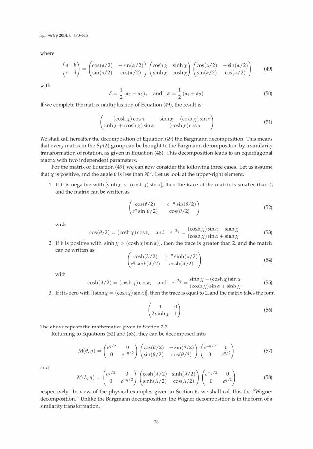
Symmetry 2014, 6, 473–515

where (a bc d

)=

(cos(α/2) − sin(α/2)sin(α/2) cos(α/2)

)(cosh χ sinh χ

sinh χ cosh χ

)(cos(α/2) − sin(α/2)sin(α/2) cos(α/2)

)(49)

withδ =

12(α1 − α2) , and α =

12(α1 + α2) (50)

If we complete the matrix multiplication of Equation (49), the result is((cosh χ) cos α sinh χ − (cosh χ) sin α

sinh χ + (cosh χ) sin α (cosh χ) cos α

)(51)

We shall call hereafter the decomposition of Equation (49) the Bargmann decomposition. This meansthat every matrix in the Sp(2) group can be brought to the Bargmann decomposition by a similaritytransformation of rotation, as given in Equation (48). This decomposition leads to an equidiagonalmatrix with two independent parameters.

For the matrix of Equation (49), we can now consider the following three cases. Let us assumethat χ is positive, and the angle θ is less than 90◦. Let us look at the upper-right element.

1. If it is negative with [sinh χ < (cosh χ) sin α], then the trace of the matrix is smaller than 2,and the matrix can be written as(

cos(θ/2) −e−η sin(θ/2)eη sin(θ/2) cos(θ/2)

)(52)

with

cos(θ/2) = (cosh χ) cos α, and e−2η =(cosh χ) sin α − sinh χ

(cosh χ) sin α + sinh χ(53)

2. If it is positive with [sinh χ > (cosh χ) sin α)], then the trace is greater than 2, and the matrixcan be written as (

cosh(λ/2) e−η sinh(λ/2)eη sinh(λ/2) cosh(λ/2)

)(54)

with

cosh(λ/2) = (cosh χ) cos α, and e−2η =sinh χ − (cosh χ) sin α

(cosh χ) sin α + sinh χ(55)

3. If it is zero with [(sinh χ = (cosh χ) sin α)], then the trace is equal to 2, and the matrix takes the form(1 0

2 sinh χ 1

)(56)

The above repeats the mathematics given in Section 2.3.Returning to Equations (52) and (53), they can be decomposed into

M(θ, η) =

(eη/2 0

0 e−η/2

)(cos(θ/2) − sin(θ/2)sin(θ/2) cos(θ/2)

)(e−η/2 0

0 eη/2

)(57)

and

M(λ, η) =

(eη/2 0

0 e−η/2

)(cosh(λ/2) sinh(λ/2)sinh(λ/2) cos(λ/2)

)(e−η/2 0

0 eη/2

)(58)

respectively. In view of the physical examples given in Section 6, we shall call this the “Wignerdecomposition.” Unlike the Bargmann decomposition, the Wigner decomposition is in the form of asimilarity transformation.

78

Symmetry 2014, 6, 473–515

We note that both Equations (57) and (58) are written as similarity transformations. Thus

[M(θ, η)]n =

(cos(nθ/2) −e−η sin(nθ/2)

eη sin(nθ/2) cos(nθ/2)

)(59)

[M(λ, η)]n =

(cosh(nλ/2) eη sinh(nλ/2)

e−η sinh(nλ/2) cosh(nλ/2)

)(60)

[M(γ)]n =

(1 0

nγ 1

)(61)

These expressions are useful for studying periodic systems [18].The question is what physics these decompositions describe in the real world. To address this,

we study what the Lorentz group does in the real world, and study isomorphism between the Sp(2)group and the Lorentz group applicable to the three-dimensional space consisting of one time andtwo space coordinates.

3.3. Isomorphism with the Lorentz Group

The purpose of this section is to give physical interpretations of the mathematical formulas given inSection 3.2. We will interpret these formulae in terms of the Lorentz transformations which are normallydescribed by four-by-four matrices. For this purpose, it is necessary to establish a correspondencebetween the two-by-two representation of Section 3.2 and the four-by-four representations of theLorentz group.

Let us consider the Minkowskian space-time four-vector

(t, z, x, y) (62)

where(t2 − z2 − x2 − y2) remains invariant under Lorentz transformations. The Lorentz group

consists of four-by-four matrices performing Lorentz transformations in the Minkowski space.In order to give physical interpretations to the three two-by-two matrices given in

Equations (44)–(46), we consider rotations around the y axis, boosts along the x axis, and boostsalong the z axis. The transformation is restricted in the three-dimensional subspace of (t, z, x). It isthen straight-forward to construct those four-by-four transformation matrices where the y coordinateremains invariant. They are given in Table 1. Their generators also given. Those four-by-four generatorssatisfy the Lie algebra given in Equation (43).

Table 1. Matrices in the two-by-two representation, and their corresponding four-by-four generatorsand transformation matrices.

Matrices Generators Four-by-Four Transform matrices

R(θ) J2 = 12

(0 −ii 0

) ⎛⎜⎜⎝

0 0 0 00 0 −i 00 i 0 00 0 0 0

⎞⎟⎟⎠

⎛⎜⎜⎝

1 0 0 00 cos θ − sin θ 00 sin θ cos θ 00 0 0 1

⎞⎟⎟⎠

B(η) K3 = 12

(i 00 −i

) ⎛⎜⎜⎝

0 i 0 0i 0 0 00 0 0 00 0 0 0

⎞⎟⎟⎠

⎛⎜⎜⎝

cosh η sinh η 0 0sinh η cosh η 0 0

0 0 1 00 0 0 1

⎞⎟⎟⎠

S(λ) K1 = 12

(0 ii 0

) ⎛⎜⎜⎝

0 0 i 00 0 0 0i 0 0 00 0 0 0

⎞⎟⎟⎠

⎛⎜⎜⎝

cosh λ 0 sinh λ 00 1 0 0

sinh λ 0 cosh λ 00 0 0 1

⎞⎟⎟⎠

79

Symmetry 2014, 6, 473–515

4. Internal Space-Time Symmetries

We have seen that there corresponds a two-by-two matrix for each four-by-four Lorentztransformation matrix. It is possible to give physical interpretations to those four-by-four matrices.It must thus be possible to attach a physical interpretation to each two-by-two matrix.

Since 1939 [1] when Wigner introduced the concept of the little groups many papers have beenpublished on this subject, but most of them were based on the four-by-four representation. In thissection, we shall give the formalism of little groups in the language of two-by-two matrices. In sodoing, we provide physical interpretations to the Bargmann and Wigner decompositions introducedin Section 3.2.

4.1. Wigner’s Little Groups

In [1], Wigner started with a free relativistic particle with momentum, then constructed subgroupsof the Lorentz group whose transformations leave the four-momentum invariant. These subgroups thusdefine the internal space-time symmetry of the given particle. Without loss of generality, we assumethat the particle momentum is along the z direction. Thus rotations around the momentum leavethe momentum invariant, and this degree of freedom defines the helicity, or the spin parallel tothe momentum.

We shall use the word “Wigner transformation” for the transformation which leaves thefour-momentum invariant:

1. For a massive particle, it is possible to find a Lorentz frame where it is at rest withzero momentum. The four-momentum can be written as m(1, 0, 0, 0), where m is the mass.This four-momentum is invariant under rotations in the three-dimensional (z, x, y) space.

2. For an imaginary-mass particle, there is the Lorentz frame where the energy componentvanishes. The momentum four-vector can be written as p(0, 1, 0, 0), where p is the magnitude ofthe momentum.

3. If the particle is massless, its four-momentum becomes p(1, 1, 0, 0). Here the first and secondcomponents are equal in magnitude.

The constant factors in these four-momenta do not play any significant roles. Thus we writethem as (1, 0, 0, 0), (0, 1, 0, 0), and (1, 1, 0, 0) respectively. Since Wigner worked with these three specificfour-momenta [1], we call them Wigner four-vectors.

All of these four-vectors are invariant under rotations around the z axis. The rotation matrix is

Z(φ) =

⎛⎜⎜⎜⎝

1 0 0 00 1 0 00 0 cos φ − sin φ

0 0 sin φ cos φ

⎞⎟⎟⎟⎠ (63)

In addition, the four-momentum of a massive particle is invariant under the rotation around the yaxis, whose four-by-four matrix was given in Table 1. The four-momentum of an imaginary particle isinvariant under the boost matrix S(λ) given in Table 1. The problem for the massless particle is morecomplicated, but will be discussed in detail in Section 7. See Table 2.

80

Symmetry 2014, 6, 473–515

Table 2. Wigner four-vectors and Wigner transformation matrices applicable to two space-like andone time-like dimensions. Each Wigner four-vector remains invariant under the application of itsWigner matrix.

Mass Wigner Four-Vector Wigner Transformation

Massive (1, 0, 0, 0)

⎛⎜⎜⎝

1 0 0 00 cos θ − sin θ 00 sin θ cos θ 00 0 0 1

⎞⎟⎟⎠

Massless (1, 1, 0, 0)

⎛⎜⎜⎝

1 + γ2/2 −γ2/2 γ 0γ2/2 1 − γ2/2 γ 0−γ γ 1 00 0 0 1

⎞⎟⎟⎠

Imaginary mass (0, 1, 0, 0)

⎛⎜⎜⎝

cosh λ 0 sinh λ 00 1 0 0

sinh λ 0 cosh λ 00 0 0 1

⎞⎟⎟⎠

4.2. Two-by-Two Formulation of Lorentz Transformations

The Lorentz group is a group of four-by-four matrices performing Lorentz transformations on theMinkowskian vector space of (t, z, x, y), leaving the quantity

t2 − z2 − x2 − y2 (64)

invariant. It is possible to perform the same transformation using two-by-two matrices [7,14,19].In this two-by-two representation, the four-vector is written as

X =

(t + z x − iy

x + iy t − z

)(65)

where its determinant is precisely the quantity given in Equation (64) and the Lorentz transformationon this matrix is a determinant-preserving, or unimodular transformation. Let us consider thetransformation matrix as [7,19]

G =

(α β

γ δ

), and G† =

(α∗ γ∗

β∗ δ∗

)(66)

withdet (G) = 1 (67)

and the transformationX′ = GXG† (68)

Since G is not a unitary matrix, Equation (68) not a unitary transformation, but rather we call thisthe “Hermitian transformation”. Equation (68) can be written as(

t′ + z′ x′ − iy′

x + iy t′ − z′

)=

(α β

γ δ

)(t + z x − iy

x + iy t − z

)(α∗ γ∗

β∗ δ∗

)(69)

It is still a determinant-preserving unimodular transformation, thus it is possible to write this as afour-by-four transformation matrix applicable to the four-vector (t, z, x, y) [7,14].

Since the G matrix starts with four complex numbers and its determinant is one by Equation (67),it has six independent parameters. The group of these G matrices is known to be locally isomorphic

81

Symmetry 2014, 6, 473–515

to the group of four-by-four matrices performing Lorentz transformations on the four-vector (t, z, x, y).In other words, for each G matrix there is a corresponding four-by-four Lorentz-transform matrix [7].

The matrix G is not a unitary matrix, because its Hermitian conjugate is not always its inverse.This group has a unitary subgroup called SU(2) and another consisting only of real matrices calledSp(2). For this later subgroup, it is sufficient to work with the three matrices R(θ), S(λ), and B(η)given in Equations (44)–(46) respectively. Each of these matrices has its corresponding four-by-fourmatrix applicable to the (t, z, x, y). These matrices with their four-by-four counterparts are tabulated inTable 1.

The energy-momentum four vector can also be written as a two-by-two matrix. It can be writtenas

P =

(p0 + pz px − ipy

px + ipy p0 − pz

)(70)

withdet (P) = p2

0 − p2x − p2

y − p2z (71)

which meansdet (P) = m2 (72)

where m is the particle mass.The Lorentz transformation can be written explicitly as

P′ = GPG† (73)

or (p′0 + p′z p′x − ip′yp′x + ip′y E′ − p′z

)=

(α β

γ δ

)(p0 + pz px − ipy

px + ipy p0 − pz

)(α∗ γ∗

β∗ δ∗

)(74)

This is an unimodular transformation, and the mass is a Lorentz-invariant variable. Furthermore, it wasshown in [7] that Wigner’s little groups for massive, massless, and imaginary-mass particles can beexplicitly defined in terms of two-by-two matrices.

Wigner’s little group consists of two-by-two matrices satisfying

P = WPW† (75)

The two-by-two W matrix is not an identity matrix, but tells about the internal space-time symmetryof a particle with a given energy-momentum four-vector. This aspect was not known when Einsteinformulated his special relativity in 1905, hence the internal space-time symmetry was not an issue atthat time. We call the two-by-two matrix W the Wigner matrix, and call the condition of Equation (75)the Wigner condition.

If determinant of W is a positive number, then P is proportional to

P =

(1 00 1

)(76)

corresponding to a massive particle at rest, while if the determinant is negative, it is proportional to

P =

(1 00 −1

)(77)

82

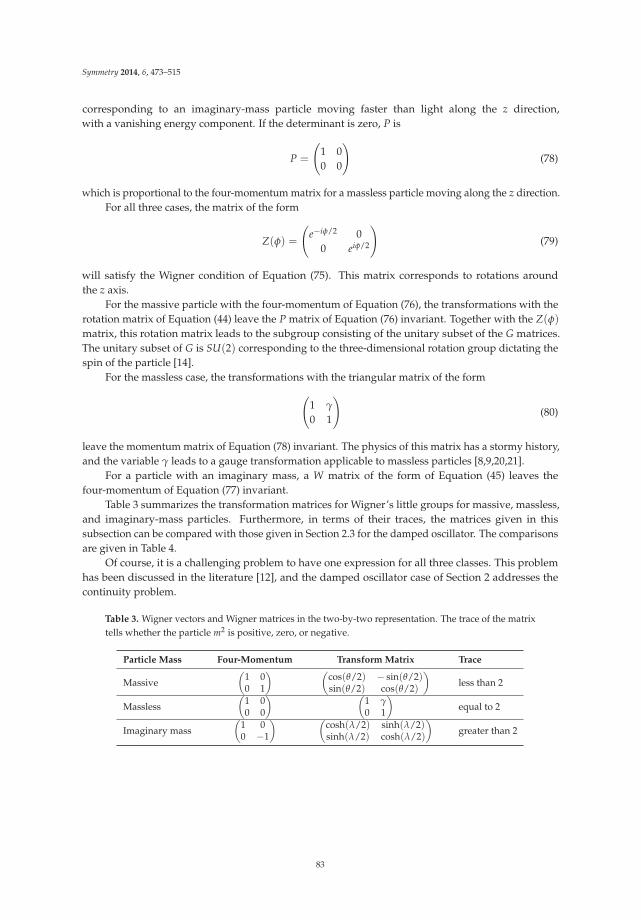
Symmetry 2014, 6, 473–515

corresponding to an imaginary-mass particle moving faster than light along the z direction,with a vanishing energy component. If the determinant is zero, P is

P =

(1 00 0

)(78)

which is proportional to the four-momentum matrix for a massless particle moving along the z direction.For all three cases, the matrix of the form

Z(φ) =

(e−iφ/2 0

0 eiφ/2

)(79)

will satisfy the Wigner condition of Equation (75). This matrix corresponds to rotations aroundthe z axis.

For the massive particle with the four-momentum of Equation (76), the transformations with therotation matrix of Equation (44) leave the P matrix of Equation (76) invariant. Together with the Z(φ)matrix, this rotation matrix leads to the subgroup consisting of the unitary subset of the G matrices.The unitary subset of G is SU(2) corresponding to the three-dimensional rotation group dictating thespin of the particle [14].

For the massless case, the transformations with the triangular matrix of the form(1 γ

0 1

)(80)

leave the momentum matrix of Equation (78) invariant. The physics of this matrix has a stormy history,and the variable γ leads to a gauge transformation applicable to massless particles [8,9,20,21].

For a particle with an imaginary mass, a W matrix of the form of Equation (45) leaves thefour-momentum of Equation (77) invariant.

Table 3 summarizes the transformation matrices for Wigner’s little groups for massive, massless,and imaginary-mass particles. Furthermore, in terms of their traces, the matrices given in thissubsection can be compared with those given in Section 2.3 for the damped oscillator. The comparisonsare given in Table 4.

Of course, it is a challenging problem to have one expression for all three classes. This problemhas been discussed in the literature [12], and the damped oscillator case of Section 2 addresses thecontinuity problem.

Table 3. Wigner vectors and Wigner matrices in the two-by-two representation. The trace of the matrixtells whether the particle m2 is positive, zero, or negative.

Particle Mass Four-Momentum Transform Matrix Trace

Massive(

1 00 1

) (cos(θ/2) − sin(θ/2)sin(θ/2) cos(θ/2)

)less than 2

Massless(

1 00 0

) (1 γ0 1

)equal to 2

Imaginary mass(

1 00 −1

) (cosh(λ/2) sinh(λ/2)sinh(λ/2) cosh(λ/2)

)greater than 2

83

Symmetry 2014, 6, 473–515

Table 4. Damped Oscillators and Space-time Symmetries. Both share Sp(2) as their symmetry group.

Trace Damped Oscillator Particle Symmetry

Smaller than 2 Oscillation Mode Massive ParticlesEqual to 2 Transition Mode Massless Particles

Larger than 2 Damping Mode Imaginary-mass Particles

5. Lorentz Completion of Wigner’s Little Groups

So far we have considered transformations applicable only to (t, z, x) space. In order to study thefull symmetry, we have to consider rotations around the z axis. As previously stated, when a particlemoves along this axis, this rotation defines the helicity of the particle.

In [1], Wigner worked out the little group of a massive particle at rest. When the particle gainsa momentum along the z direction, the single particle can reverse the direction of momentum, the spin,or both. What happens to the internal space-time symmetries is discussed in this section.

5.1. Rotation around the z Axis

In Section 3, our kinematics was restricted to the two-dimensional space of z and x, and thusincludes rotations around the y axis. We now introduce the four-by-four matrix of Equation (63)performing rotations around the z axis. Its corresponding two-by-two matrix was given inEquation (79). Its generator is

J3 =12

(1 00 −1

)(81)

If we introduce this additional matrix for the three generators we used in Sections 3 and 3.2, we endup the closed set of commutation relations

[Ji, Jj] = iεijk Jk, [Ji, Kj] = iεijkKk, [Ki, Kj] = −iεijk Jk (82)

withJi =

12

σi, and Ki =i2

σi (83)

where σi are the two-by-two Pauli spin matrices.For each of these two-by-two matrices there is a corresponding four-by-four matrix generating

Lorentz transformations on the four-dimensional Lorentz group. When these two-by-two matricesare imaginary, the corresponding four-by-four matrices were given in Table 1. If they are real,the corresponding four-by-four matrices were given in Table 5.

84

Symmetry 2014, 6, 473–515

Table 5. Two-by-two and four-by-four generators not included in Table 1. The generators giventhere and given here constitute the set of six generators for SL(2, c) or of the Lorentz group given inEquation (82).

Generator Two-by-Two Four-by-Four

J312

(1 00 −1

) ⎛⎜⎜⎝

0 0 0 00 0 0 00 0 0 −i0 0 i 0

⎞⎟⎟⎠

J112

(0 11 0

) ⎛⎜⎜⎝

0 0 0 00 0 0 i0 0 0 00 −i 0 0

⎞⎟⎟⎠

K212

(0 1−1 0

) ⎛⎜⎜⎝

0 0 0 i0 0 0 00 0 0 0i 0 0 0

⎞⎟⎟⎠

This set of commutation relations is known as the Lie algebra for the SL(2, c), namely the group oftwo-by-two elements with unit determinants. Their elements are complex. This set is also the Lorentzgroup performing Lorentz transformations on the four-dimensional Minkowski space.

This set has many useful subgroups. For the group SL(2, c), there is a subgroup consisting only ofreal matrices, generated by the two-by-two matrices given in Table 1. This three-parameter subgroupis precisely the Sp(2) group we used in Sections 3 and 3.2. Their generators satisfy the Lie algebragiven in Equation (43).

In addition, this group has the following Wigner subgroups governing the internal space-timesymmetries of particles in the Lorentz-covariant world [1]:

1. The Ji matrices form a closed set of commutation relations. The subgroup generated by theseHermitian matrices is SU(2) for electron spins. The corresponding rotation group does not changethe four-momentum of the particle at rest. This is Wigner’s little group for massive particles.If the particle is at rest, the two-by-two form of the four-vector is given by Equation (76).The Lorentz transformation generated by J3 takes the form(

eiφ/2 00 e−iφ/2

)(1 00 1

)(e−iφ/2 0

0 eiφ/2

)=

(1 00 1

)(84)

Similar computations can be carried out for J1 and J2.2. There is another Sp(2) subgroup, generated by K1, K2, and J3. They satisfy the commutation

relations[K1, K2] = −i J3, [J3, K1] = iK2, [K2, J3] = iK1. (85)

The Wigner transformation generated by these two-by-two matrices leave the momentumfour-vector of Equation (77) invariant. For instance, the transformation matrix generated by K2

takes the form

exp (−iξK2) =

(cosh(ξ/2) i sinh(ξ/2)i sinh(ξ/2) cosh(ξ/2)

)(86)

and the Wigner transformation takes the form(cosh(ξ/2) i sinh(ξ/2)

−i sinh(ξ/2) cosh(ξ/2)

)(1 00 −1

)(cosh(ξ/2) i sinh(ξ/2)

−i sinh(ξ/2) cosh(ξ/2)

)=

(1 00 −1

)(87)

Computations with K2 and J3 lead to the same result.

85

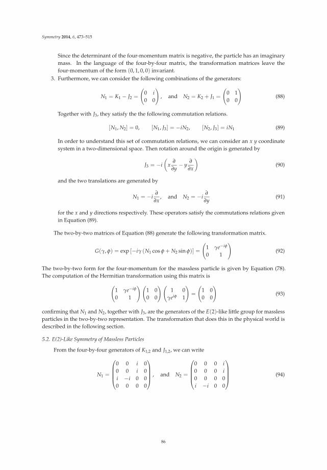
Symmetry 2014, 6, 473–515

Since the determinant of the four-momentum matrix is negative, the particle has an imaginarymass. In the language of the four-by-four matrix, the transformation matrices leave thefour-momentum of the form (0, 1, 0, 0) invariant.

3. Furthermore, we can consider the following combinations of the generators:

N1 = K1 − J2 =

(0 i0 0

), and N2 = K2 + J1 =

(0 10 0

)(88)

Together with J3, they satisfy the the following commutation relations.

[N1, N2] = 0, [N1, J3] = −iN2, [N2, J3] = iN1 (89)

In order to understand this set of commutation relations, we can consider an x y coordinatesystem in a two-dimensional space. Then rotation around the origin is generated by

J3 = −i(

x∂

∂y− y

∂

∂x

)(90)

and the two translations are generated by

N1 = −i∂

∂x, and N2 = −i

∂

∂y(91)

for the x and y directions respectively. These operators satisfy the commutations relations givenin Equation (89).

The two-by-two matrices of Equation (88) generate the following transformation matrix.

G(γ, φ) = exp [−iγ (N1 cos φ + N2 sin φ)] =

(1 γe−iφ

0 1

)(92)

The two-by-two form for the four-momentum for the massless particle is given by Equation (78).The computation of the Hermitian transformation using this matrix is(

1 γe−iφ

0 1

)(1 00 0

)(1 0

γeiφ 1

)=

(1 00 0

)(93)

confirming that N1 and N2, together with J3, are the generators of the E(2)-like little group for masslessparticles in the two-by-two representation. The transformation that does this in the physical world isdescribed in the following section.

5.2. E(2)-Like Symmetry of Massless Particles

From the four-by-four generators of K1,2 and J1,2, we can write

N1 =

⎛⎜⎜⎜⎝

0 0 i 00 0 i 0i −i 0 00 0 0 0

⎞⎟⎟⎟⎠ , and N2 =

⎛⎜⎜⎜⎝

0 0 0 i0 0 0 i0 0 0 0i −i 0 0

⎞⎟⎟⎟⎠ (94)

86

Symmetry 2014, 6, 473–515

These matrices lead to the transformation matrix of the form

G(γ, φ) =

⎛⎜⎜⎜⎝

1 + γ2/2 −γ2/2 γ cos φ γ sin φ

γ2/2 1 − γ2/2 γ cos φ γ sin φ

−γ cos φ γ cos φ 1 0−γ sin φ γ sin φ 0 1

⎞⎟⎟⎟⎠ (95)

This matrix leaves the four-momentum invariant, as we can see from

G(γ, φ)

⎛⎜⎜⎜⎝

1100

⎞⎟⎟⎟⎠ =

⎛⎜⎜⎜⎝

1100

⎞⎟⎟⎟⎠ (96)

When it is applied to the photon four-potential

G(γ, φ)

⎛⎜⎜⎜⎝

A0

A3

A1

A2

⎞⎟⎟⎟⎠ =

⎛⎜⎜⎜⎝

A0

A3

A1

A2

⎞⎟⎟⎟⎠+ γ (A1 cos φ + A2 sin φ)

⎛⎜⎜⎜⎝

1100

⎞⎟⎟⎟⎠ (97)

with the Lorentz condition which leads to A3 = A0 in the zero mass case. Gauge transformationsare well known for electromagnetic fields and photons. Thus Wigner’s little group leads to gaugetransformations.

In the two-by-two representation, the electromagnetic four-potential takes the form(2A0 A1 − iA2

A1 + iA2 0

)(98)

with the Lorentz condition A3 = A0. Then the two-by-two form of Equation (97) is(1 γe−iφ

0 1

)(2A0 A1 − iA2

A1 + iA2 0

)(1 0

γeiφ 1

)(99)

which becomes (A0 A1 − iA2

A1 + iA2 0

)+

(2γ (A1 cos φ − A2 sin φ) 0

0 0

)(100)

This is the two-by-two equivalent of the gauge transformation given in Equation (97).For massless spin-1/2 particles starting with the two-by-two expression of G(γ, φ) given in

Equation (92), and considering the spinors

u =

(10

), and v =

(01

)(101)

for spin-up and spin-down states respectively,

Gu = u, and Gv = v + γe−iφu (102)

This means that the spinor u for spin up is invariant under the gauge transformation while v is not.Thus, the polarization of massless spin-1/2 particle, such as neutrinos, is a consequence of the gaugeinvariance. We shall continue this discussion in Section 7.

87

Symmetry 2014, 6, 473–515

5.3. Boosts along the z Axis

In Sections 4.1 and 5.1, we studied Wigner transformations for fixed values of the four-momenta.The next question is what happens when the system is boosted along the z direction, with thetransformation (

t′

z′

)=

(cosh η sinh η

sinh η cosh η

)(tz

)(103)

Then the four-momenta become

(cosh η, sinh η, 0, 0), (sinh η, cosh η, 0, 0), eη(1, 1, 0, 0) (104)

respectively for massive, imaginary, and massless particles cases. In the two-by-two representation,the boost matrix is (

eη/2 00 e−η/2

)(105)

and the four-momenta of Equation (104) become(eη 00 e−η

),

(eη 00 −e−η

),

(eη 00 0

)(106)

respectively. These matrices become Equations (76)–(78) respectively when η = 0.We are interested in Lorentz transformations which leave a given non-zero momentum invariant.

We can consider a Lorentz boost along the direction preceded and followed by identical rotationmatrices, as described in Figure 1 and the transformation matrix as(

cos(α/2) − sin(α/2)sin(α/2) cos(α/2)

)(cosh χ − sinh χ

− sinh χ cosh χ

)(cos(α/2) − sin(α/2)sin(α/2) cos(α/2)

)(107)

which becomes ((cos α) cosh χ − sinh χ − (sin α) cosh χ

− sinh χ + (sin α) cosh χ (cos α) cosh χ

)(108)

(a) (b)

Figure 1. Bargmann and Wigner decompositions. (a) Bargmann decomposition; (b) Wignerdecomposition. In the Bargmann decomposition, we start from a momentum along the z direction. Wecan rotate, boost, and rotate to bring the momentum to the original position. The resulting matrix is theproduct of one boost and two rotation matrices. In the Wigner decomposition, the particle is boostedback to the frame where the Wigner transformation can be applied. Make a Wigner transformationthere and come back to the original state of the momentum. This process also can also be written as theproduct of three simple matrices.

88

Symmetry 2014, 6, 473–515

Except the sign of χ, the two-by-two matrices of Equations (107) and (108) are identical with thosegiven in Section 3.2. The only difference is the sign of the parameter χ. We are thus ready to interpretthis expression in terms of physics.

1. If the particle is massive, the off-diagonal elements of Equation (108) have opposite signs,and this matrix can be decomposed into(

eη/2 00 e−η/2

)(cos(θ/2) − sin(θ/2)sin(θ/2) cos(θ/2)

)(eη/2 0

0 e−η/2

)(109)

with

cos(θ/2) = (cosh χ) cos α, and e2η =cosh(χ) sin α + sinh χ

cosh(χ) sin α − sinh χ(110)

ande2η =

p0 + pz

p0 − pz(111)

According to Equation (109) the first matrix (far right) reduces the particle momentum to zero.The second matrix rotates the particle without changing the momentum. The third matrix booststhe particle to restore its original momentum. This is the extension of Wigner’s original idea tomoving particles.

2. If the particle has an imaginary mass, the off-diagonal elements of Equation (108) have thesame sign, (

eη/2 00 e−η/2

)(cosh(λ/2) − sinh(λ/2)sinh(λ/2) cosh(λ/2)

)(eη/2 0

0 e−η/2

)(112)

with

cosh(λ/2) = (cosh χ) cos α, and e2η =sinh χ + cosh(χ) sin α

cosh(χ) sin α − sinh χ(113)

ande2η =

p0 + pz

pz − p0(114)

This is also a three-step operation. The first matrix brings the particle momentum to thezero-energy state with p0 = 0. Boosts along the x or y direction do not change thefour-momentum. We can then boost the particle back to restore its momentum. This operationis also an extension of the Wigner’s original little group. Thus, it is quite appropriate to call theformulas of Equations (109) and (112) Wigner decompositions.

3. If the particle mass is zero with

sinh χ = (cosh χ) sin α (115)

the η parameter becomes infinite, and the Wigner decomposition does not appear to be useful.We can then go back to the Bargmann decomposition of Equation (107). With the condition ofEquations (115) and (108) becomes (

1 −γ

0 1

)(116)

withγ = 2 sinh χ (117)

The decomposition ending with a triangular matrix is called the Iwasawa decomposition [16,22]and its physical interpretation was given in Section 5.2. The γ parameter does not depend on η.

89

Symmetry 2014, 6, 473–515

Thus, we have given physical interpretations to the Bargmann and Wigner decompositions givenin Section (3.2). Consider what happens when the momentum becomes large. Then η becomes largefor nonzero mass cases. All three four-momenta in Equation (106) become

eη

(1 00 0

)(118)

As for the Bargmann-Wigner matrices, they become the triangular matrix of Equation (116), with γ =

sin(θ/2)eη and γ = sinh(λ/2)eη , respectively for the massive and imaginary-mass cases.In Section 5.2, we concluded that the triangular matrix corresponds to gauge transformations.

However, particles with imaginary mass are not observed. For massive particles, we can start withthe three-dimensional rotation group. The rotation around the z axis is called helicity, and remainsinvariant under the boost along the z direction. As for the transverse rotations, they become gaugetransformation as illustrated in Table 6.

Table 6. Covariance of the energy-momentum relation, and covariance of the internal space-timesymmetry. Under the Lorentz boost along the z direction, J3 remains invariant, and this invariantcomponent of the angular momentum is called the helicity. The transverse component J1 and J2 collapseinto a gauge transformation. The γ parameter for the massless case has been studied in earlier papersin the four-by-four matrix formulation of Wigner’s little groups [8,21].

Massive, Slow Covariance Massless, Fast

E = p2/2m Einstein’s E = mc2 E = cpJ3 Helicity

Wigner’s Little GroupJ1, J2 Gauge Transformation

5.4. Conjugate Transformations

The most general form of the SL(2, c) matrix is given in Equation (66). Transformation operatorsfor the Lorentz group are given in exponential form as:

D = exp

{−i

3

∑i=1

(θi Ji + ηiKi)

}(119)

where the Ji are the generators of rotations and the Ki are the generators of proper Lorentz boosts.They satisfy the Lie algebra given in Equation (43). This set of commutation relations is invariantunder the sign change of the boost generators Ki. Thus, we can consider “dot conjugation” defined as

D = exp

{−i

3

∑i=1

(θi Ji − ηiKi)

}(120)

Since Ki are anti-Hermitian while Ji are Hermitian, the Hermitian conjugate of the above expression is

D† = exp

{−i

3

∑i=1

(−θi Ji + ηiKi)

}(121)

while the Hermitian conjugate of G is

D† = exp

{−i

3

∑i=1

(−θi Ji − ηiKi)

}(122)

90

Symmetry 2014, 6, 473–515

Since we understand the rotation around the z axis, we can now restrict the kinematics to thezt plane, and work with the Sp(2) symmetry. Then the D matrices can be considered as Bargmanndecompositions. First, D and D, and their Hermitian conjugates are

D(α, χ) =

((cos α) cosh χ sinh χ − (sin α) cosh χ

sinh χ + (sin α) cosh χ (cos α) cosh χ

)(123)

D(α, χ) =

((cos α) cosh χ − sinh χ − (sin α) cosh χ

− sinh χ + (sin α) cosh χ (cos α) cosh χ

)(124)

These matrices correspond to the “D loops” given in Figure 2a,b respectively. The “dot” conjugationchanges the direction of boosts. The dot conjugation leads to the inversion of the space which is calledthe parity operation.

We can also consider changing the direction of rotations. Then they result in the Hermitianconjugates. We can write their matrices as

D†(α, χ) =

((cos α) cosh χ sinh χ + (sin α) cosh χ

sinh χ − (sin α) cosh χ (cos α) cosh χ

)(125)

D†(α, χ) =

((cos α) cosh χ − sinh χ + (sin α) cosh χ

− sinh χ − (sin α) cosh χ (cos α) cosh χ

)(126)

From the exponential expressions from Equation (119) to Equation (122), it is clear that

D† = D−1, and D† = D−1 (127)

The D loop given in Figure 1 corresponds to D. We shall return to these loops in Section 7.

(b) (a)

(d) (c)

Figure 2. Four D-loops resulting from the Bargmann decomposition. (a) Bargmann decomposition fromFigure 1; (b) Direction of the Lorentz boost is reversed; (c) Direction of rotation is reversed; (d) Bothdirections are reversed. These operations correspond to the space-inversion, charge conjugation, andthe time reversal respectively.

91

Symmetry 2014, 6, 473–515

6. Symmetries Derivable from the Poincaré Sphere

The Poincaré sphere serves as the basic language for polarization physics. Its underlyinglanguage is the two-by-two coherency matrix. This coherency matrix contains the symmetry of SL(2, c)isomorphic to the the Lorentz group applicable to three space-like and one time-like dimensions [4,6,7].

For polarized light propagating along the z direction, the amplitude ratio and phase difference ofelectric field x and y components traditionally determine the state of polarization. Hence, the polarizationcan be changed by adjusting the amplitude ratio or the phase difference or both. Usually, the opticaldevice which changes amplitude is called an “attenuator” (or “amplifier”) and the device which changesthe relative phase a “phase shifter”.

Let us start with the Jones vector:(ψ1(z, t)ψ2(z, t)

)=

(a exp [i(kz − ωt)]a exp [i(kz − ωt)]

)(128)

To this matrix, we can apply the phase shift matrix of Equation (79) which brings the Jones vector to(ψ1(z, t)ψ2(z, t)

)=

(a exp [i(kz − ωt − iφ/2)]a exp [i(kz − ωt + iφ/2)]

)(129)

The generator of this phase-shifter is J3 given Table 5.The optical beam can be attenuated differently in the two directions. The resulting matrix is

e−μ

(eη/2 0

0 e−η/2

)(130)

with the attenuation factor of exp (−μ0 + η/2) and exp (−μ − η/2) for the x and y directionsrespectively. We are interested only the relative attenuation given in Equation (46) which leadsto different amplitudes for the x and y component, and the Jones vector becomes(

ψ1(z, t)ψ2(z, t)

)=

(aeμ/2 exp [i(kz − ωt − iφ/2)]

ae−μ/2 exp [i(kz − ωt + iφ/2)]

)(131)

The squeeze matrix of Equation (46) is generated by K3 given in Table 1.The polarization is not always along the x and y axes, but can be rotated around the z axis using

Equation (79) generated by J2 given in Table 1.Among the rotation angles, the angle of 45◦ plays an important role in polarization optics. Indeed,

if we rotate the squeeze matrix of Equation (46) by 45◦, we end up with the squeeze matrix ofEquation (45) generated by K1 given also in Table 1.

Each of these four matrices plays an important role in special relativity, as we discussed inSections 3.2 and 6. Their respective roles in optics and particle physics are given in Table 7.

92

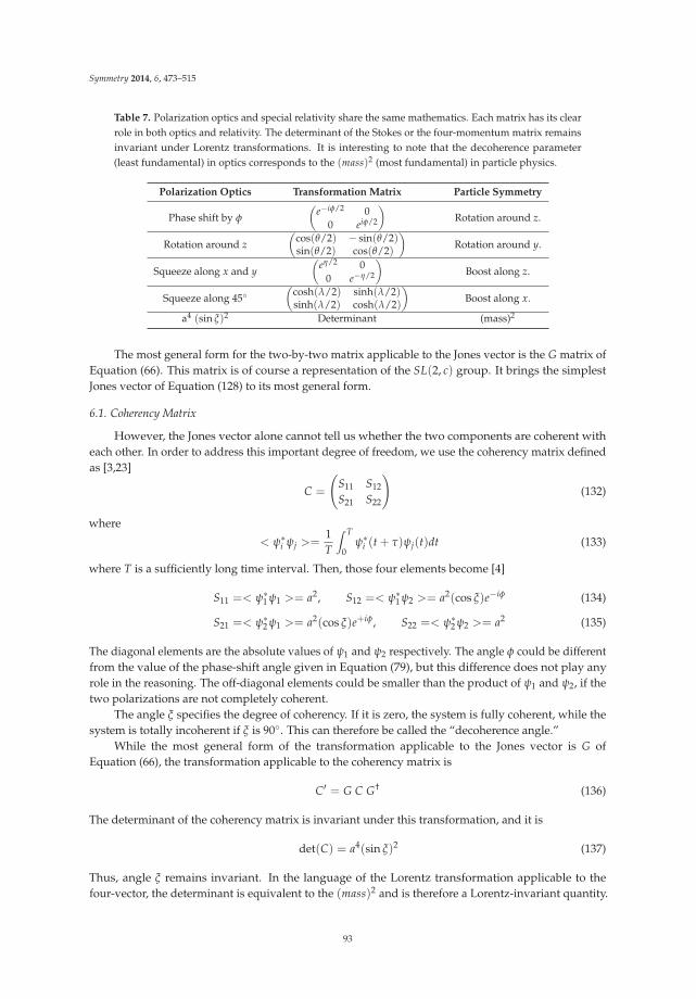
Symmetry 2014, 6, 473–515

Table 7. Polarization optics and special relativity share the same mathematics. Each matrix has its clearrole in both optics and relativity. The determinant of the Stokes or the four-momentum matrix remainsinvariant under Lorentz transformations. It is interesting to note that the decoherence parameter(least fundamental) in optics corresponds to the (mass)2 (most fundamental) in particle physics.

Polarization Optics Transformation Matrix Particle Symmetry

Phase shift by φ

(e−iφ/2 0

0 eiφ/2

)Rotation around z.

Rotation around z(

cos(θ/2) − sin(θ/2)sin(θ/2) cos(θ/2)

)Rotation around y.

Squeeze along x and y(

eη/2 00 e−η/2

)Boost along z.

Squeeze along 45◦(

cosh(λ/2) sinh(λ/2)sinh(λ/2) cosh(λ/2)

)Boost along x.

a4 (sin ξ)2 Determinant (mass)2

The most general form for the two-by-two matrix applicable to the Jones vector is the G matrix ofEquation (66). This matrix is of course a representation of the SL(2, c) group. It brings the simplestJones vector of Equation (128) to its most general form.

6.1. Coherency Matrix

However, the Jones vector alone cannot tell us whether the two components are coherent witheach other. In order to address this important degree of freedom, we use the coherency matrix definedas [3,23]

C =

(S11 S12

S21 S22

)(132)

where

< ψ∗i ψj >=

1T

∫ T

0ψ∗

i (t + τ)ψj(t)dt (133)

where T is a sufficiently long time interval. Then, those four elements become [4]

S11 =< ψ∗1 ψ1 >= a2, S12 =< ψ∗

1 ψ2 >= a2(cos ξ)e−iφ (134)

S21 =< ψ∗2 ψ1 >= a2(cos ξ)e+iφ, S22 =< ψ∗

2 ψ2 >= a2 (135)

The diagonal elements are the absolute values of ψ1 and ψ2 respectively. The angle φ could be differentfrom the value of the phase-shift angle given in Equation (79), but this difference does not play anyrole in the reasoning. The off-diagonal elements could be smaller than the product of ψ1 and ψ2, if thetwo polarizations are not completely coherent.

The angle ξ specifies the degree of coherency. If it is zero, the system is fully coherent, while thesystem is totally incoherent if ξ is 90◦. This can therefore be called the “decoherence angle.”

While the most general form of the transformation applicable to the Jones vector is G ofEquation (66), the transformation applicable to the coherency matrix is

C′ = G C G† (136)

The determinant of the coherency matrix is invariant under this transformation, and it is

det(C) = a4(sin ξ)2 (137)

Thus, angle ξ remains invariant. In the language of the Lorentz transformation applicable to thefour-vector, the determinant is equivalent to the (mass)2 and is therefore a Lorentz-invariant quantity.

93

Symmetry 2014, 6, 473–515

6.2. Two Radii of the Poincaré Sphere

Let us write explicitly the transformation of Equation (136) as(S′

11 S′12

S′21 S′

22

)=

(α β

γ δ

)(S11 S12

S21 S22

)(α∗ γ∗

β∗ δ∗

)(138)

It is then possible to construct the following quantities,

S0 =S11 + S22

2, S3 =

S11 − S22

2(139)

S1 =S12 + S21

2, S2 =

S12 − S21

2i(140)

These are known as the Stokes parameters, and constitute a four-vector (S0, S3, S1, S2) under theLorentz transformation.

In the Jones vector of Equation (128), the amplitudes of the two orthogonal components are equal.Thus, the two diagonal elements of the coherency matrix are equal. This leads to S3 = 0, and theproblem is reduced from the sphere to a circle. In the resulting two-dimensional subspace, we canintroduce the polar coordinate system with

R =√

S21 + S2

2 (141)

S1 = R cos φ (142)

S2 = R sin φ (143)

The radius R is the radius of this circle, and is

R = a2 cos ξ (144)

The radius R takes its maximum value S0 when ξ = 0◦. It decreases as ξ increases and vanisheswhen ξ = 90◦. This aspect of the radius R is illustrated in Figure 3.

R

0S

Figure 3. Radius of the Poincaré sphere. The radius R takes its maximum value S0 when thedecoherence angle ξ is zero. It becomes smaller as ξ increases. It becomes zero when the anglereaches 90◦.

94

Symmetry 2014, 6, 473–515

In order to see its implications in special relativity, let us go back to the four-momentum matrix ofm(1, 0, 0, 0). Its determinant is m2 and remains invariant. Likewise, the determinant of the coherencymatrix of Equation (132) should also remain invariant. The determinant in this case is

S20 − R2 = a4 sin2 ξ (145)

This quantity remains invariant under the Hermitian transformation of Equation (138), which is aLorentz transformation as discussed in Sections 3.2 and 6. This aspect is shown on the last row ofTable 7.

The coherency matrix then becomes

C = a2

(1 (cos ξ)e−iφ

(cos ξ)eiφ 1

)(146)

Since the angle φ does not play any essential role, we can let φ = 0, and write the coherency matrix as

C = a2

(1 cos ξ

cos ξ 1

)(147)

The determinant of the above two-by-two matrix is

a4(

1 − cos2 ξ)= a4 sin2 ξ (148)

Since the Lorentz transformation leaves the determinant invariant, the change in this ξ variable isnot a Lorentz transformation. It is of course possible to construct a larger group in which this variableplays a role in a group transformation [6], but here we are more interested in its role in a particlegaining a mass from zero or the mass becoming zero.

6.3. Extra-Lorentzian Symmetry

The coherency matrix of Equation (146) can be diagonalized to

a2

(1 + cos ξ 0

0 1 − cos ξ

)(149)

by a rotation. Let us then go back to the four-momentum matrix of Equation (70). If px = py = 0,and pz = p0 cos ξ , we can write this matrix as

p0

(1 + cos ξ 0

0 1 − cos ξ

)(150)

Thus, with this extra variable, it is possible to study the little groups for variable masses, including thesmall-mass limit and the zero-mass case.

For a fixed value of p0, the (mass)2 becomes

(mass)2 = (p0 sin ξ)2 , and (momentum)2 = (p0 cos ξ)2 (151)

resulting in(energy)2 = (mass)2 + (momentum)2 (152)

This transition is illustrated in Figure 4. We are interested in reaching a point on the light conefrom mass hyperbola while keeping the energy fixed. According to this figure, we do not have to make

95

Symmetry 2014, 6, 473–515

an excursion to infinite-momentum limit. If the energy is fixed during this process, Equation (152) tellsthe mass and momentum relation, and Figure 5 illustrates this relation.

(a) (b)

Figure 4. Transition from the massive to massless case. (a) Transition within the framework of theLorentz group; (b) Trasnsition allowed in the symmetry of the Poincaré sphere. Within the frameworkof the Lorentz group, it is not possible to go from the massive to massless case directly, because itrequires the change in the mass which is a Lorentz-invariant quantity. The only way is to move toinfinite momentum and jump from the hyperbola to the light cone, and come back. The extra symmetryof the Poincaré sphere allows a direct transition

Momentum

Ma

ss

Energy

ξangle

Figure 5. Energy-momentum-mass relation. This circle illustrates the case where the energy is fixed,while the mass and momentum are related according to the triangular rule. The value of the angle ξ

changes from zero to 180◦. The particle mass is negative for negative values of this angle. However, inthe Lorentz group, only (mass)2 is a relevant variable, and negative masses might play a role fortheoretical purposes.

96

Symmetry 2014, 6, 473–515

Within the framework of the Lorentz group, it is possible, by making an excursion to infinitemomentum where the mass hyperbola coincides with the light cone, to then come back to thedesired point. On the other hand, the mass formula of Equation (151) allows us to go there directly.The decoherence mechanism of the coherency matrix makes this possible.

7. Small-Mass and Massless Particles

We now have a mathematical tool to reduce the mass of a massive particle from its positive valueto zero. During this process, the Lorentz-boosted rotation matrix becomes a gauge transformation forthe spin-1 particle, as discussed Section 5.2. For spin-1/2 particles, there are two issues.

1. It was seen in Section 5.2 that the requirement of gauge invariance lead to a polarization ofmassless spin-1/2 particle, such as neutrinos. What happens to anti-neutrinos?

2. There are strong experimental indications that neutrinos have a small mass. What happens tothe E(2) symmetry?

7.1. Spin-1/2 Particles

Let us go back to the two-by-two matrices of Section 5.4, and the two-by-two D matrix. For amassive particle, its Wigner decomposition leads to

D =

(cos(θ/2) −e−η sin(θ/2)

eη sin(θ/2) cos(θ/2)

)(153)

This matrix is applicable to the spinors u and v defined in Equation (101) respectively for the spin-upand spin-down states along the z direction.

Since the Lie algebra of SL(2, c) is invariant under the sign change of the Ki matrices, we canconsider the “dotted” representation, where the system is boosted in the opposite direction, while thedirection of rotations remain the same. Thus, the Wigner decomposition leads to

D =

(cos(θ/2) −eη sin(θ/2)

e−η sin(θ/2) cos(θ/2)

)(154)

with its spinors

u =

(10

), and v =

(01

)(155)

For anti-neutrinos, the helicity is reversed but the momentum is unchanged. Thus, D† is theappropriate matrix. However, D† = D−1 as was noted in Section 5.4. Thus, we shall use D foranti-neutrinos.

When the particle mass becomes very small,

e−η =m2p

(156)

becomes small. Thus, if we let

eη sin(θ/2) = γ, and e−η sin(θ/2) = ε2 (157)

then the D matrix of Equation (153) and the D of Equation (154) become(1 − γε2/2 −ε2

γ 1 − γε2

), and

(1 − γε2/2 −γ

ε2 1 − γε2

)(158)

97

Symmetry 2014, 6, 473–515

respectively where γ is an independent parameter and

ε2 = γ

(m2p

)2(159)

When the particle mass becomes zero, they become(1 0γ 1

), and

(1 −γ

0 1

)(160)

respectively, applicable to the spinors (u, v) and (u, v) respectively.For neutrinos, (

1 0γ 1

)(10

)=

(1γ

), and

(1 0γ 1

)(01

)=

(01

)(161)

For anti-neutrinos, (1 −γ

0 1

)(10

)=

(10

), and

(1 −γ

0 1

)(01

)=

(−γ

1

)(162)

It was noted in Section 5.2 that the triangular matrices of Equation (160) perform gaugetransformations. Thus, for Equations (161) and (162) the requirement of gauge invariance leads tothe polarization of neutrinos. The neutrinos are left-handed while the anti-neutrinos are right-handed.Since, however, nature cannot tell the difference between the dotted and undotted representations,the Lorentz group cannot tell which neutrino is right handed. It can say only that the neutrinos andanti-neutrinos are oppositely polarized.

If the neutrino has a small mass, the gauge invariance is modified to(1 − γε2/2 −ε2

γ 1 − γε2/2

)(01

)=

(01

)− ε2

(1

γ/2

)(163)

and (1 − γε2/2 −γ

ε2 1 − γε2

)(10

)=

(10

)+ ε2

(−γ/2

1

)(164)

respectively for neutrinos and anti-neutrinos. Thus the violation of the gauge invariance in both casesis proportional to ε2 which is m2/4p2.

7.2. Small-Mass Neutrinos in the Real World

Whether neutrinos have mass or not and the consequences of this relative to the Standard Modeland lepton number is the subject of much theoretical speculation [24,25], and of cosmology [26],nuclear reactors [27], and high energy experimentations [28,29]. Neutrinos are fast becoming animportant component of the search for dark matter and dark radiation [30]. Their importance withinthe Standard Model is reflected by the fact that they are the only particles which seem to exist withonly one direction of chirality, i.e., only left-handed neutrinos have been confirmed to exist so far.

It was speculated some time ago that neutrinos in constant electric and magnetic fields wouldacquire a small mass, and that right-handed neutrinos would be trapped within the interaction field [31].Solving generalized electroweak models using left- and right-handed neutrinos has been discussedrecently [32]. Today these right-handed neutrinos which do not participate in weak interactions arecalled “sterile” neutrinos [33]. A comprehensive discussion of the place of neutrinos in the schemeof physics has been given by Drewes [30]. We should note also that the three different neutrinos,namely νe, νμ, and ντ , may have different masses [34].

98

Symmetry 2014, 6, 473–515

8. Scalars, Four-Vectors, and Four-Tensors

In Sections 5 and 7, our primary interest has been the two-by-two matrices applicable to spinors forspin-1/2 particles. Since we also used four-by-four matrices, we indirectly studied the four-componentparticle consisting of spin-1 and spin-zero components.

If there are two spin 1/2 states, we are accustomed to construct one spin-zero state, and onespin-one state with three degeneracies.

In this paper, we are confronted with two spinors, but each spinor can also be dotted. For thisreason, there are 16 orthogonal states consisting of spin-one and spin-zero states. How many spin-zerostates? How many spin-one states?

For particles at rest, it is known that the addition of two one-half spins result in spin-zero andspin-one states. In this paper, we have two different spinors behaving differently under the Lorentzboost. Around the z direction, both spinors are transformed by

Z(φ) = exp (−iφJ3) =

(e−iφ/2 0

0 eiφ/2

)(165)

However, they are boosted by

B(η) = exp (−iηK3) =

(eη/2 0

0 e−η/2

)(166)

B(η) = exp (iηK3) =

(e−η/2 0

0 eη/2

)(167)

applicable to the undotted and dotted spinors respectively. These two matrices commute with eachother, and also with the rotation matrix Z(φ) of Equation (165). Since K3 and J3 commute with eachother, we can work with the matrix Q(η, φ) defined as

Q(η, φ) = B(η)Z(φ) =

(e(η−iφ)/2 0

0 e−(η−iφ)/2

)(168)

Q(η, φ) = B(η)Z(φ) =

(e−(η+iφ)/2 0

0 e(η+iφ)/2

)(169)

When this combined matrix is applied to the spinors,

Q(η, φ)u = e(η−iφ)/2u, Q(η, φ)v = e−(η−iφ)/2v (170)

Q(η, φ)u = e−(η+iφ)/2u, Q(η, φ)v = e(η+iφ)/2v (171)

If the particle is at rest, we can construct the combinations

uu,1√2(uv + vu), vv (172)

to construct the spin-1 state, and1√2(uv − vu) (173)

for the spin-zero state. There are four bilinear states. In the SL(2, c) regime, there are two dotted spinors.If we include both dotted and undotted spinors, there are 16 independent bilinear combinations.They are given in Table 8. This table also gives the effect of the operation of Q(η, φ).

99

Symmetry 2014, 6, 473–515

Table 8. Sixteen combinations of the SL(2, c) spinors. In the SU(2) regime, there are two spinorsleading to four bilinear forms. In the SL(2, c) world, there are two undotted and two dotted spinors.These four spinors lead to 16 independent bilinear combinations.

Spin 1 Spin 0

uu, 1√2(uv + vu), vv, 1√

2(uv − vu)

uu, 1√2(uv + vu), vv, 1√

2(uv − vu)

uu, 1√2(uv + vu), vv, 1√

2(uv − vu)

uu, 1√2(uv + vu), vv, 1√

2(uv − vu)

After the Operation of Q(η, φ) and Q(η, φ)

e−iφeηuu, 1√2(uv + vu), eiφe−ηvv, 1√

2(uv − vu)

e−iφe−η uu, 1√2(uv + vu), eiφeη vv, 1√

2(uv − vu)

e−iφuu, 1√2(eηuv + e−ηvu), eiφvv, 1√

2(eηuv − e−ηvu)

e−iφuu, 1√2(uv + vu), eiφ vv, 1√

2(e−η uv − eη vu)

Among the bilinear combinations given in Table 8, the following two are invariant under rotationsand also under boosts.

S =1√2(uv − vu), and S = − 1√

2(uv − vu) (174)

They are thus scalars in the Lorentz-covariant world. Are they the same or different? Let us considerthe following combinations

S+ =1√2

(S + S

), and S− =

1√2

(S − S

)(175)

Under the dot conjugation, S+ remains invariant, but S− changes its sign.Under the dot conjugation, the boost is performed in the opposite direction. Therefore it is the

operation of space inversion, and S+ is a scalar while S− is called the pseudo-scalar.

8.1. Four-Vectors

Let us consider the bilinear products of one dotted and one undotted spinor as uu, uv, uv, vv,and construct the matrix

U =

(uv vvuu vu

)(176)

Under the rotation Z(φ) and the boost B(η) they become(eηuv e−iφvveiφuu e−ηvu

)(177)

Indeed, this matrix is consistent with the transformation properties given in Table 8, and transformslike the four-vector (

t + z x − iyx + iy t − z

)(178)

This form was given in Equation (65), and played the central role throughout this paper. Under thespace inversion, this matrix becomes (

t − z −(x − iy)−(x + iy) t + z

)(179)

100

Symmetry 2014, 6, 473–515

This space inversion is known as the parity operation.The form of Equation (176) for a particle or field with four-components, is given by (V0, Vz, Vx, Vy).

The two-by-two form of this four-vector is

U =

(V0 + Vz Vx − iVy

Vx + iVy V0 − Vz

)(180)

If boosted along the z direction, this matrix becomes(eη (V0 + Vz) Vx − iVy

Vx + iVy e−η (V0 − Vz)

)(181)

In the mass-zero limit, the four-vector matrix of Equation (181) becomes(2A0 Ax − iAy

Ax + iAy 0

)(182)

with the Lorentz condition A0 = Az. The gauge transformation applicable to the photon four-vectorwas discussed in detail in Section 5.2.

Let us go back to the matrix of Equation (180), we can construct another matrix U. Since the dotconjugation leads to the space inversion,

U =

(uv vvuu vu

)(183)

Then

uv � (t − z), vu � (t + z) (184)

vv � −(x − iy), uu � −(x + iy) (185)

where the symbol � means “transforms like”.Thus, U of Equation (176) and U of Equation (183) used up 8 of the 16 bilinear forms. Since there

are two bilinear forms in the scalar and pseudo-scalar as given in Equation (175), we have to giveinterpretations to the six remaining bilinear forms.

8.2. Second-Rank Tensor

In this subsection, we are studying bilinear forms with both spinors dotted and undotted.In Section 8.1, each bilinear spinor consisted of one dotted and one undotted spinor. There arealso bilinear spinors which are both dotted or both undotted. We are interested in two sets of threequantities satisfying the O(3) symmetry. They should therefore transform like

(x + iy)/√

2, (x − iy)/√

2, z (186)

which are likeuu, vv, (uv + vu)/

√2 (187)

respectively in the O(3) regime. Since the dot conjugation is the parity operation, they are like

− uu, −vv, −(uv + vu)/√

2 (188)

In other words,(uu) = −uu, and (vv) = −vv (189)

101

Symmetry 2014, 6, 473–515

We noticed a similar sign change in Equation (184).In order to construct the z component in this O(3) space, let us first consider

fz =12[(uv + vu)− (uv + vu)] , gz =

12i

[(uv + vu) + (uv + vu)] (190)

where fz and gz are respectively symmetric and anti-symmetric under the dot conjugation or the parityoperation. These quantities are invariant under the boost along the z direction. They are also invariantunder rotations around this axis, but they are not invariant under boost along or rotations around thex or y axis. They are different from the scalars given in Equation (174).

Next, in order to construct the x and y components, we start with g± as

f+ =1√2(uu − uu) g+ =

1√2i

(uu + uu) (191)

f− =1√2(vv − vv) g− =

1√2i

(vv + vv) (192)

Then

fx =1√2( f+ + f−) =

12[(uu − uu) + (vv − vv)] (193)

fy =1√2i

( f+ − f−) =12i

[(uu − uu)− (vv − vv)] (194)

and

gx =1√2(g+ + g−) =

12i

[(uu + uu) + (vv + vv)] (195)

gy =1√2i

(g+ − g−) = −12[(uu + uu)− (vv + vv)] (196)

Here fx and fy are symmetric under dot conjugation, while gx and gy are anti-symmetric.Furthermore, fz, fx, and fy of Equations (190) and (193) transform like a three-dimensional

vector. The same can be said for gi of Equations (190) and (195). Thus, they can grouped into thesecond-rank tensor

T =

⎛⎜⎜⎜⎝

0 −gz −gx −gy

gz 0 − fy fx

gx fy 0 − fz

gy − fx fz 0

⎞⎟⎟⎟⎠ (197)

whose Lorentz-transformation properties are well known. The gi components change their signs underspace inversion, while the fi components remain invariant. They are like the electric and magneticfields respectively.

If the system is Lorentz-booted, fi and gi can be computed from Table 8. We are now interestedin the symmetry of photons by taking the massless limit. According to the procedure developed inSection 6, we can keep only the terms which become larger for larger values of η. Thus,

fx → 12(uu − vv) , fy → 1

2i(uu + vv) (198)

gx → 12i

(uu + vv) , gy → −12(uu − vv) (199)

in the massless limit.

102

Symmetry 2014, 6, 473–515

Then the tensor of Equation (197) becomes

F =

⎛⎜⎜⎜⎝

0 0 −Ex −Ey

0 0 −By Bx

Ex By 0 0Ey −Bx 0 0

⎞⎟⎟⎟⎠ (200)

with

Bx � 12(uu − vv) , By � 1

2i(uu + vv) (201)

Ex =12i

(uu + vv) , Ey = −12(uu − vv) (202)

The electric and magnetic field components are perpendicular to each other. Furthermore,

Ex = By, Ey = −Bx (203)

In order to address this question, let us go back to Equation (191). In the massless limit,

B+ � E+ � uu, B− � E− � vv (204)

The gauge transformation applicable to u and v are the two-by-two matrices(1 −γ

0 1

), and

(1 0−γ 1

)(205)

respectively as noted in Sections 5.2 and 7.1. Both u and v are invariant under gauge transformations,while u and v do not.

The B+ and E+ are for the photon spin along the z direction, while B− and E− are for the oppositedirection. In 1964 [35], Weinberg constructed gauge-invariant state vectors for massless particlesstarting from Wigner’s 1939 paper [1]. The bilinear spinors uu and and vv correspond to Weinberg’sstate vectors.

8.3. Possible Symmetry of the Higgs Mechanism

In this section, we discussed how the two-by-two formalism of the group SL(2, c) leads thescalar, four-vector, and tensor representations of the Lorentz group. We discussed in detail how thefour-vector for a massive particle can be decomposed into the symmetry of a two-component masslessparticle and one gauge degree of freedom. This aspect was studied in detail by Kim and Wigner [20,21],and their results are illustrated in Figure 6. This decomposition is known in the literature as the groupcontraction.

The four-dimensional Lorentz group can be contracted to the Euclidean and cylindrical groups.These contraction processes could transform a four-component massive vector meson into a masslessspin-one particle with two spin components, and one gauge degree of freedom.

Since this contraction procedure is spelled out detail in [21], as well as in the present paper,its reverse process is also well understood. We start with one two-component massless particle withone gauge degree of freedom, and end up with a massive vector meson with its four components.

The mathematics of this process is not unlike the Higgs mechanism [36,37], where one masslessfield with two degrees of freedom absorbs one gauge degree freedom to become a quartet of bosons,namely that of W, Z± plus the Higgs boson. As is well known, this mechanism is the basis for thetheory of electro-weak interaction formulated by Weinberg and Salam [38,39].

103

Symmetry 2014, 6, 473–515

Figure 6. Contractions of the three-dimensional rotation group. (a) Contraction in terms of thetangential plane and the tangential cylinder [20]; (b) Contraction in terms of the expansion andcontraction of the longitudinal axis [21]. In both cases, the symmetry ends up with one rotation aroundthe longitudinal direction and one translational degree along the longitudinal axis. The rotation andtranslation corresponds to the helicity and gauge degrees of freedom.

The word “spontaneous symmetry breaking” is used for the Higgs mechanism. It could bean interesting problem to see that this symmetry breaking for the two Higgs doublet model can beformulated in terms of the Lorentz group and its contractions. In this connection, we note an interestingrecent paper by Dée and Ivanov [40].

9. Conclusions

The damped harmonic oscillator, Wigner’e little groups, and the Poincaré sphere belong to thethree different branches of physics. In this paper, it was noted that they are based on the samemathematical framework, namely the algebra of two-by-two matrices.

The second-order differential equation for damped harmonic oscillators can be formulated interms of two-by-two matrices. These matrices produce the algebra of the group Sp(2). While thereare three trace classes of the two-by-two matrices of this group, the damped oscillator tells us how tomake transitions from one class to another.

It is shown that Wigner’s three little groups can be defined in terms of the trace classes of theSp(2) group. If the trace is smaller than two, the little group is for massive particles. If greater thantwo, the little group is for imaginary-mass particles. If the trace is equal to two, the little group is formassless particles. Thus, the damped harmonic oscillator provides a procedure for transition from onelittle group to another.

The Poincaré sphere contains the symmetry of the six-parameter SL(2, c) group. Thus, the sphereprovides the procedure for extending the symmetry of the little group defined within the Lorentz groupof three-dimensional Minkowski space to its full Lorentz group in the four-dimensional space-time. Inaddition, the Poincaré sphere offers the variable which allows us to change the symmetry of a massiveparticle to that of a massless particle by continuously decreasing the mass.

In this paper, we extracted the mathematical properties of Wigner’s little groups from the dampedharmonic oscillator and the Poincaré sphere. In so doing, we have shown that the transition from onelittle group to another is tangentially continuous.

This subject was initiated by Inönü and Wigner in 1953 as the group contraction [41]. In theirpaper, they discussed the contraction of the three-dimensional rotation group becoming contracted tothe two-dimensional Euclidean group with one rotational and two translational degrees of freedom.While the O(3) rotation group can be illustrated by a three-dimensional sphere, the plane tangential at

104

Symmetry 2014, 6, 473–515

the north pole is for the E(2) Euclidean group. However, we can also consider a cylinder tangential atthe equatorial belt. The resulting cylindrical group is isomorphic to the Euclidean group [20]. Whilethe rotational degree of freedom of this cylinder is for the photon spin, the up and down translationson the surface of the cylinder correspond to the gauge degree of freedom of the photon, as illustratedin Figure 6.

It was noted also that the Bargmann decomposition of two-by-two matrices, as illustrated inFigure 1 and Figure 2, allows us to study more detailed properties of the little groups, including spaceand time reflection reflection properties. Also in this paper, we have discussed how the scalars,four-vectors, and four-tensors can be constructed from the two-by-two representation in theLorentz-covariant world.

In addition, it should be noted that the symmetry of the Lorentz group is also contained in thesqueezed state of light [14] and the ABCD matrix for optical beam transfers [18]. We also mentionedthe possibility of understanding the mathematics of the Higgs mechanism in terms of the Lorentzgroup and its contractions.

Acknowledgements

In his 1939 paper [1], Wigner worked out the subgroups of the Lorentz group whosetransformations leave the four momentum of a given particle invariant. In so doing, he workedout their internal space-time symmetries. In spite of its importance, this paper remains as one of themost difficult papers to understand. Wigner was eager to make his paper understandable to youngerphysicists.

While he was the pioneer in introducing the mathematics of group theory to physics, he wasalso quite fond of using two-by-two matrices to explain group theoretical ideas. He asked one of thepresent authors (Young S. Kim) to rewrite his 1939 paper [1] using the language of those matrices.This is precisely what we did in the present paper.

We are grateful to Eugene Paul Wigner for this valuable suggestion.

Author Contributions

This paper is largely based on the earlier papers by Young S. Kim and Marilyn E. Noz, and thoseby Sibel Baskal and Young S. Kim. The two-by-two formulation of the damped oscillator in Section 2was jointly developed by Sibel Baskal and Yound S. Kim during the summer of 2012. Marilyn E. Nozdeveloped the idea of the symmetry of small-mass neutrinos in Section 7. The limiting process in thesymmetry of the Poincaré sphere was formulated by Young S. Kim. Sibel Baskal initially constructedthe four-by-four tensor representation in Section 8.

The initial organization of this paper was conceived by Young S. Kim in his attempt to followWigner’s suggestion to translate his 1939 paper into the language of two-by-two matrices. Sibel Baskaland Marilyn E. Noz tightened the organization and filled in the details.

Conflicts of Interest

The authors declare no conflicts of interest.

References

1. Wigner, E. On unitary representations of the inhomogeneous Lorentz Group. Ann. Math. 1939, 40, 149–204.2. Han, D.; Kim, Y.S.; Son, D. Eulerian parametrization of Wigner little groups and gauge transformations in

terms of rotations in 2-component spinors. J. Math. Phys. 1986, 27, 2228–2235.3. Born, M.; Wolf, E. Principles of Optics, 6th ed.; Pergamon: Oxford, UK, 1980.

105

Symmetry 2014, 6, 473–515

4. Han, D.; Kim, Y.S.; Noz, M.E. Stokes parameters as a Minkowskian four-vector. Phys. Rev. E 1997, 56,6065–6076.

5. Brosseau, C. Fundamentals of Polarized Light: A Statistical Optics Approach; John Wiley: New York, NY, USA,1998.

6. Baskal, S.; Kim, Y.S. De Sitter group as a symmetry for optical decoherence. J. Phys. A 2006, 39, 7775–7788.7. Kim, Y.S.; Noz, M.E. Symmetries shared by the Poincaré Group and the Poincaré Sphere. Symmetry 2013, 5,

233–252.8. Han, D.; Kim, Y.S.; Son, D. E(2)-like little group for massless particles and polarization of neutrinos. Phys. Rev.

D 1982, 26, 3717–3725.9. Han, D.; Kim, Y.S.; Son, D. Photons, neutrinos and gauge transformations. Am. J. Phys. 1986, 54, 818–821.10. Baskal, S.; Kim, Y.S. Little groups and Maxwell-type tensors for massive and massless particles. Europhys.

Lett. 1997, 40, 375–380.11. Leggett, A.; Chakravarty, S.; Dorsey, A.; Fisher, M.; Garg, A.; Zwerger, W. Dynamics of the dissipative 2-state

system. Rev. Mod. Phys. 1987, 59, 1–85.12. Baskal, S.; Kim, Y.S. One analytic form for four branches of the ABCD matrix. J. Mod. Opt. 2010, 57, 1251–1259.13. Baskal, S.; Kim, Y.S. Lens optics and the continuity problems of the ABCD matrix. J. Mod. Opt. 2014, 61,

161–166.14. Kim, Y.S.; Noz, M.E. Theory and Applications of the Poincaré Group; Reidel: Dordrecht, The Netherlands, 1986.15. Bargmann, V. Irreducible unitary representations of the Lorentz group. Ann. Math. 1947, 48, 568–640.16. Iwasawa, K. On some types of topological groups. Ann. Math. 1949, 50, 507–558.17. Guillemin, V.; Sternberg, S. Symplectic Techniques in Physics; Cambridge University Press: Cambridge, UK,

1984.18. Baskal, S.; Kim, Y.S. Lorentz Group in Ray and Polarization Optics. In Mathematical Optics:

Classical, Quantum and Computational Methods; Lakshminarayanan, V., Calvo, M.L., Alieva, T., Eds.; CRC Taylor andFrancis: New York, NY, USA, 2013; Chapter 9, pp. 303–340.

19. Naimark, M.A. Linear Representations of the Lorentz Group; Pergamon: Oxford, UK, 1964.20. Kim, Y.S.; Wigner, E.P. Cylindrical group and masless particles. J. Math. Phys. 1987, 28, 1175–1179.21. Kim, Y.S.; Wigner, E.P. Space-time geometry of relativistic particles. J. Math. Phys. 1990, 31, 55–60.22. Georgieva, E.; Kim, Y.S. Iwasawa effects in multilayer optics. Phys. Rev. E 2001, 64,

doi:10.1103/PhysRevE.64.026602.23. Saleh, B.E.A.; Teich, M.C. Fundamentals of Photonics, 2nd ed.; John Wiley: Hoboken, NJ, USA, 2007.24. Papoulias, D.K.; Kosmas, T.S. Exotic Lepton Flavour Violating Processes in the Presence of Nuclei. J. Phys.:

Conf. Ser. 2013, 410, 012123:1–012123:5.25. Dinh, D.N.; Petcov, S.T.; Sasao, N.; Tanaka, M.; Yoshimura, M. Observables in neutrino mass spectroscopy

using atoms. Phys. Lett. B. 2013, 719, 154–163.26. Miramonti, L.; Antonelli, V. Advancements in Solar Neutrino physics. Int. J. Mod. Phys. E. 2013, 22, 1–16.27. Li, Y.-F.; Cao, J.; Jun, Y.; Wang, Y.; Zhan, L. Unambiguous determination of the neutrino mass hierarchy using

reactor neutrinos. Phys. Rev. D. 2013, 88, 013008:1–013008:9.28. Bergstrom, J. Combining and comparing neutrinoless double beta decay experiments using different 584

nuclei. J. High Energy Phys. 2013, 02, 093:1–093:27.29. Han, T.; Lewis, I.; Ruiz, R.; Si, Z.-G. Lepton number violation and W ′ chiral couplings at the LHC. Phys. Rev.

D 2013, 87, 035011:1–035011:25.30. Drewes, M. The phenomenology of right handed neutrinos. Int. J. Mod. Phys. E 2013, 22, 1330019:1–1330019:75.31. Barut, A.O.; McEwan, J. The four states of the massless neutrino with pauli coupling by spin-gauge invariance.

Lett. Math. Phys. 1986, 11, 67–72.32. Palcu, A. Neutrino Mass as a consequence of the exact solution of 3-3-1 gauge models without exotic electric

charges. Mod. Phys. Lett. A 2006, 21, 1203–1217.33. Bilenky, S.M. Neutrino. Phys. Part. Nucl. 2013, 44, 1–46.34. Alhendi, H. A.; Lashin, E. I.; Mudlej, A. A. Textures with two traceless submatrices of the neutrino mass

matrix. Phys.Rev. D 2008, 77, 013009.1–013009.1-13.35. Weinberg, S. Photons and gravitons in S-Matrix theory: Derivation of charge conservation and equality of

gravitational and inertial mass. Phys. Rev. 1964, 135, B1049–B1056.36. Higgs, P.W. Broken symmetries and the masses of gauge bosons. Phys. Rev. Lett. 1964, 13, 508–509.

106

Symmetry 2014, 6, 473–515

37. Guralnik, G.S.; Hagen, C.R.; Kibble, T.W.B. Global conservation laws and massless particles. Phys. Rev. Lett.1964, 13, 585–587.

38. Weinberg, S. A model of leptons. Phys. Rev. Lett. 1967, 19, 1265–1266.39. Weinberg, S. Quantum Theory of Fields, Volume II, Modern Applications; Cambridge University Press: Cambridge,

UK, 1996.40. Dée, A.; Ivanov, I.P. Higgs boson masses of the general two-Higgs-doublet model in the Minkowski-space

formalism. Phys. Rev. D 2010, 81, 015012:1–015012:8.41. Inönü, E.; Wigner, E.P. On the contraction of groups and their representations. Proc. Natl. Acad. Sci. USA 1953,

39, 510–524.

c© 2014 by the authors. Licensee MDPI, Basel, Switzerland. This article is an open accessarticle distributed under the terms and conditions of the Creative Commons Attribution(CC BY) license (http://creativecommons.org/licenses/by/4.0/).

107

Chapter 2: Harmonic Oscillators in Modern Physics

symmetryS S

Article

Analytical Solutions of Temporal Evolution ofPopulations in Optically-Pumped Atoms withCircularly Polarized Light

Heung-Ryoul Noh

Department of Physics, Chonnam National University, Gwangju 500-757, Korea; hrnoh@chonnam.ac.kr;Tel.: +82-62-530-3366

Academic Editor: Young Suh KimReceived: 10 December 2015; Accepted: 14 March 2016 ; Published: 19 March 2016

Abstract: We present an analytical calculation of temporal evolution of populations for opticallypumped atoms under the influence of weak, circularly polarized light. The differential equations forthe populations of magnetic sublevels in the excited state, derived from rate equations, are expressedin the form of inhomogeneous second-order differential equations with constant coefficients.We present a general method of analytically solving these differential equations, and obtain explicitanalytical forms of the populations of the ground state at the lowest order in the saturation parameter.The obtained populations can be used to calculate lineshapes in various laser spectroscopies,considering transit time relaxation.

Keywords: second-order differential equations; optical pumping; analytical solutions

PACS: 02.30.Hq; 32.80.Xx; 32.30.-r

1. Introduction

When an atom is illuminated by single-mode laser light, the populations of the magnetic sublevelsand coherences between them exhibit complicated temporal variations. This phenomenon is calledoptical pumping, which is widely used in the preparation of internal atomic states of interest [1,2].It has recently been observed that optical pumping affects the lineshapes in saturated absorptionspectroscopy (SAS) [3], electromagnetically induced transparency (EIT) [4], and absorption of coldatoms with a Λ-type three-level scheme [5]. Nonlinear effects in optical pumping have also beeninvestigated [6,7].

The temporal dynamics of the internal states of an atom are accurately described by densitymatrix equations [8,9]. In some special cases, however, a simpler method can be employed to solve forthe dynamics of the internal states of the atom, using rate equations [10,11]. Furthermore, when theintensity of light is weak, the rate equations can be solved analytically [12–15]. These analyticalsolutions are practically very useful; once they are obtained, it is readily possible to obtain analyticallycomputed quantities such as the absorption coefficient of a probe beam and lineshape functions innonlinear laser spectroscopy. We have previously reported analytical solutions for SAS [16,17] andpolarization spectroscopy (PS) [18].

Interestingly, the equations governing the temporal dynamics of populations at the weakintensity limit are homogeneous or inhomogeneous second-order linear differential equations (DEs)with constant coefficients [12–15]. Unlike the harmonic oscillator in mechanics, where under- orover-damped motions are observed [19], the equations for optical pumping show only over-dampedbehaviors. However, this system exhibits a variety of inhomogeneous DEs. In a recent publication,we reported the method of solving these equations analytically, in the context of a pedagogical

Symmetry 2016, 8, 17 111 www.mdpi.com/journal/symmetry

Symmetry 2016, 8, 17

description of the method of solving inhomogeneous DEs [15]. Although the method is straightforwardin principle, it is not easy to obtain analytical solutions for complicated atomic structures, such as Cs.Extending the previous study [15], in this paper, we present a general method of analytically solvingthe DEs for such a complicated atom.

2. Theory

The energy level diagram under consideration is shown in Figure 1. Since alkali-metal atomsare considered, there are two ground states with Fg = I + 1/2 and Fg = I − 1/2 (I: nuclear spinangular momentum quantum number). We consider a σ+ polarized weak laser beam, whose Rabifrequency is Ω and optical frequency is ω = ω0 + δ (ω0 is the resonance frequency and δ is the laserfrequency detuning). We assume that the laser frequency is tuned to the transition from one of the twoground states (in Figure 1, the state Fg = I + 1/2). Then, the other ground state (in Figure 1, the stateFg = I − 1/2) is not excited by laser light, and can be populated by spontaneous emission from theexcited state when the optical transition is not cycling. The populations (and the states themselves) ofthe magnetic sublevels in the excited, upper ground, and lower ground states are labeled, respectively,as gi, fi, and hi with i = 1, 2, · · · .

g1 g3

f1f2 f3 fi-2

g2

�

gi-2 gi

fi-1 fi

gi-1

h1h2 h3 hi-2

hi-1 hi

�0

Groundstates

Excitedstates

�g

Figure 1. An energy level diagram for an optically pumped atom under the influence of circularlypolarized light.

The internal dynamics of the atom can be described by the density matrix equation in the framerotating with frequency ω:

ρ = − (i/h) [H, ρ] + ρsp, (1)

where ρ is the density operator. In Equation (1), the Hamiltonian, H, is given by

H = −∑j

hδ∣∣gj

⟩ ⟨gj∣∣− ∑

jhΔg

∣∣hj⟩ ⟨

hj∣∣− hΩ

2 ∑j

Cjj

∣∣gj⟩ ⟨

f j∣∣+ h.c., (2)

where Δg is the hyperfine splitting between the two ground states and h.c. denotes the harmonicconjugate. In Equation (2), the first two terms in the right-hand side represent the bare atomicHamiltonian and the rest terms denote the atom-photon interaction Hamiltonian [20]. Cj

i is

the normalized transition strength between the states fi and gj, and Rji ≡

(Cj

i

)2is given

below (Equation (13)). In Equation (1), ρsp represents spontaneous emission term, whose matrixrepresentations are given by:

〈gi| ρsp∣∣gj

⟩= −Γ 〈gi| ρ

∣∣gj⟩

,〈gi| ρsp

∣∣ f j⟩= − Γ

2 〈gi| ρ∣∣ f j

⟩, 〈gi| ρsp

∣∣hj⟩= − Γ

2 〈gi| ρ∣∣hj

⟩,

〈 fi| ρsp∣∣ f j

⟩= Γ ∑0

ε=−2 Ci+εi Cj+ε

j 〈gi+ε| ρ∣∣gj+ε

⟩,

〈hi| ρsp∣∣hj

⟩= Γ ∑0

ε=−2 Di+εi Dj+ε

j 〈gi+ε| ρ∣∣gj+ε

⟩,

(3)

112

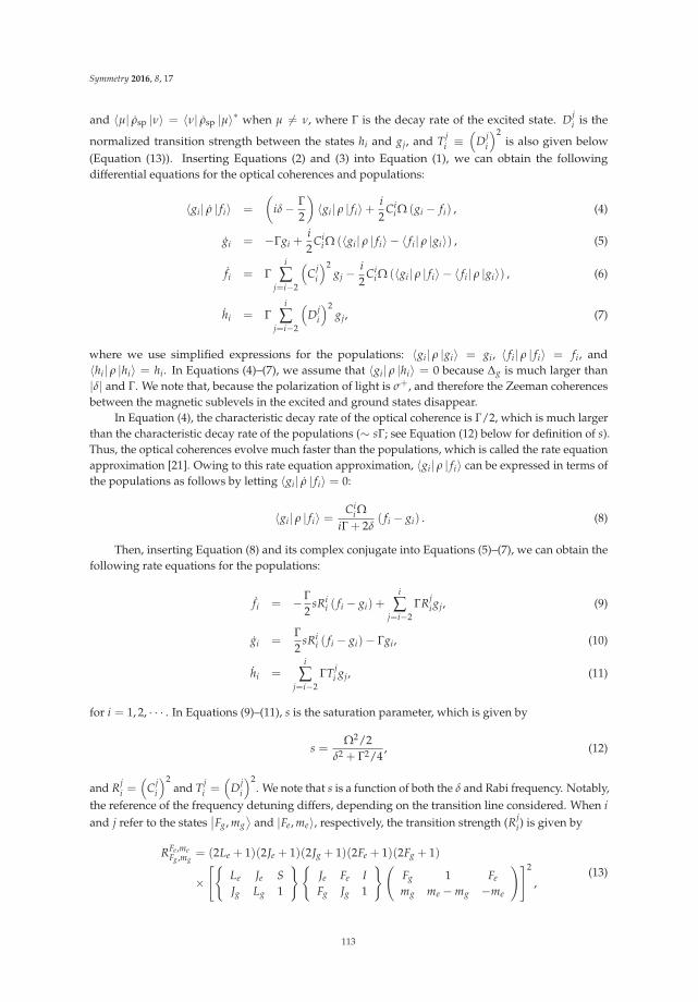
Symmetry 2016, 8, 17

and 〈μ| ρsp |ν〉 = 〈ν| ρsp |μ〉∗ when μ �= ν, where Γ is the decay rate of the excited state. Dji is the

normalized transition strength between the states hi and gj, and Tji ≡

(Dj

i

)2is also given below

(Equation (13)). Inserting Equations (2) and (3) into Equation (1), we can obtain the followingdifferential equations for the optical coherences and populations:

〈gi| ρ | fi〉 =

(iδ − Γ

2

)〈gi| ρ | fi〉+

i2

Cii Ω (gi − fi) , (4)

gi = −Γgi +i2

Cii Ω (〈gi| ρ | fi〉 − 〈 fi| ρ |gi〉) , (5)

fi = Γi

∑j=i−2

(Cj

i

)2gj −

i2

Cii Ω (〈gi| ρ | fi〉 − 〈 fi| ρ |gi〉) , (6)

hi = Γi

∑j=i−2

(Dj

i

)2gj, (7)

where we use simplified expressions for the populations: 〈gi| ρ |gi〉 = gi, 〈 fi| ρ | fi〉 = fi, and〈hi| ρ |hi〉 = hi. In Equations (4)–(7), we assume that 〈gi| ρ |hi〉 = 0 because Δg is much larger than|δ| and Γ. We note that, because the polarization of light is σ+, and therefore the Zeeman coherencesbetween the magnetic sublevels in the excited and ground states disappear.

In Equation (4), the characteristic decay rate of the optical coherence is Γ/2, which is much largerthan the characteristic decay rate of the populations (∼ sΓ; see Equation (12) below for definition of s).Thus, the optical coherences evolve much faster than the populations, which is called the rate equationapproximation [21]. Owing to this rate equation approximation, 〈gi| ρ | fi〉 can be expressed in terms ofthe populations as follows by letting 〈gi| ρ | fi〉 = 0:

〈gi| ρ | fi〉 =Ci

i ΩiΓ + 2δ

( fi − gi) . (8)

Then, inserting Equation (8) and its complex conjugate into Equations (5)–(7), we can obtain thefollowing rate equations for the populations:

fi = −Γ2

sRii ( fi − gi) +

i

∑j=i−2

ΓRji gj, (9)

gi =Γ2

sRii ( fi − gi)− Γgi, (10)

hi =i

∑j=i−2

ΓTji gj, (11)

for i = 1, 2, · · · . In Equations (9)–(11), s is the saturation parameter, which is given by

s =Ω2/2

δ2 + Γ2/4, (12)

and Rji =

(Cj

i

)2and Tj

i =(

Dji

)2. We note that s is a function of both the δ and Rabi frequency. Notably,

the reference of the frequency detuning differs, depending on the transition line considered. When iand j refer to the states

∣∣Fg, mg⟩

and |Fe, me〉, respectively, the transition strength (Rji) is given by

RFe ,meFg ,mg

= (2Le + 1)(2Je + 1)(2Jg + 1)(2Fe + 1)(2Fg + 1)

×[{

Le Je SJg Lg 1

}{Je Fe IFg Jg 1

}(Fg 1 Fe

mg me − mg −me

)]2

,(13)

113

Symmetry 2016, 8, 17

where L and S denote the orbital and electron spin angular momenta, respectively, and the curly(round) brackets represent the 6J (3J) symbol. Tj

i are similarly obtained by using different Fg values inEquation (13).

The explicit form of Equation (9) is given by

fi =Γ2

sRii (gi − fi) + Γ

(Ri−2

i gi−2 + Ri−1i gi−1 + Ri

igi

), (14)

and fi can be expressed in terms of gi and gi from Equation (10) at the lowest order in s as follows:

fi =2

ΓsRii(gi + Γgi) . (15)

Insertion of Equations (10) and (15) into Equation (14) yields the following DE for gi:

gi + Γ(

1 +s2

Rii

)gi +

s2

Γ2Rii

(1 − Ri

i

)gi

=s2

Γ2Ri−2i Ri

igi−2 +s2

Γ2Ri−1i Ri

igi−1. (16)

when i = 1, the right-hand side of Equation (16) vanishes. Therefore, Equation (16) becomes ahomogeneous DE. In contrast, when i �= 1, Equation (16) becomes an inhomogeneous DE because theright-hand side terms are functions of gi.

We solve Equation (16) from i = 1 consecutively. As is well-known, the solution of Equation (16)consists of two parts: a homogeneous solution and a particular solution. We first find the solutions ofthe homogeneous equation by inserting the equation gi ∼ eλΓt into Equation (16). Then, we have twovalues (λ2i−1, λ2i) for λ as follows:

λ2i−1(2i) =14

(−2 − sRi

i − (+)

√4 − 4sRi

i + s(8 + s)(

Rii)2)

,

which can be approximated as follows in the weak intensity limit:

λ2i−1 � −1 − s2

(Ri

i

)2, λ2i � − s

2Ri

i

(1 − Ri

i

).

We consider the case of i = 1 in Equation (16). Then, the solution is given by

g1 = C1,1eλ1Γt + C1,2eλ2Γt,

where the coefficients C1,1 and C1,2 should be determined using the initial conditions. In the case ofi = 2, the right-hand side in Equation (16) contains the terms of eλ1Γt and eλ2Γt. Therefore, g2 has fourexponential terms:

g2 = C2,1eλ1Γt + C2,2eλ2Γt + C2,3eλ3Γt + C2,4eλ4Γt,

where the coefficients should also be determined. Therefore, we can express gj generally as follows:

gj =2j

∑k=1

Cj,keλkΓt. (17)

114

Symmetry 2016, 8, 17

We find Cj,k with k = 1, 2, · · · , 2j by means of recursion relations; i.e., Cj,k are expressed in termsof Ci,l with i < j and l = 1, 2, · · · , 2i. Inserting Equation (17) into Equation (16), we obtain

gi = Ci,2i−1eλ2i−1Γt + Ci,2ieλ2iΓt

+ ∑2(i−1)k=1

(s/2)Ri−1i Ri

iCi−1,k

λ2k+λk+

s2 Ri

i(1+λk−Rii)

eλkΓt

+ ∑2(i−2)k=1

(s/2)Ri−2i Ri

iCi−2,k

λ2k+λk+

s2 Ri

i(1+λk−Rii)

eλkΓt.

(18)

Comparing Equations (17) and (18) gives

Ci,k =(s/2)Ri

i

(Ri−1

i Ci−1,k + Ri−2i Ci−2,k

)λ2

k + λk +s2 Ri

i(1 + λk − Ri

i) , (19)

for k = 1, 2, · · · , 2(i − 2),

Ci,k =(s/2)Ri−1

i RiiCi−1,k

λ2k + λk +

s2 Ri

i(1 + λk − Ri

i) , (20)

for k = 2i − 3 and 2(i − 1).

The remaining two coefficients, Ci,2i−1 and Ci,2i, can be derived from Equation (18) using twoinitial conditions for gi(0) and gi(0):

gi(0) = 0, gi(0) =s2

p0Rii,

where p0 is the population of each sublevel in the ground state at equilibrium, which is equal to1/[2(2I + 1)]. Then, the results are given by

Ci,2i−1 = 12Qi

[2(

Ai + 2A′i + Bi + 2B′

i)

+ (Ai + Bi − 2p0) sRii]− Ai+Bi

2 ,(21)

Ci,2i = − 12Qi

[2(

Ai + 2A′i + Bi + 2B′

i)

+ (Ai + Bi − 2p0) sRii]− Ai+Bi

2 ,(22)

where

Qi =√

4 + sRii(−4 + (8 + s) Ri

i),

Ai =2(i−1)

∑k=1

(s/2)Ri−1i Ri

iCi−1,k

λ2k + λk +

s2 Ri

i(1 + λk − Ri

i) , for i ≥ 2

Bi =2(i−2)

∑k=1

(s/2)Ri−2i Ri

iCi−2,k

λ2k + λk +

s2 Ri

i(1 + λk − Ri

i) , for i ≥ 3,

A′i =

2(i−1)

∑k=1

(s/2)Ri−1i Ri

iλkCi−1,k

λ2k + λk +

s2 Ri

i(1 + λk − Ri

i) , for i ≥ 2

B′i =

2(i−2)

∑k=1

(s/2)Ri−2i Ri

iλkCi−2,k

λ2k + λk +

s2 Ri

i(1 + λk − Ri

i) , for i ≥ 3,

andA1 = 0, A′

1 = 0, B1 = B2 = 0, and B′1 = B′

2 = 0.

115

Symmetry 2016, 8, 17

The coefficients in gi from g1 can be obtained by successively using the recursion relations inEquations (19)–(22). Once gi are obtained, fi can be obtained using Equation (15). Up to the lowestorder in s, the result is given by

fi =i

∑k=1

2Ci,2k

sRii

eλ2kΓt. (23)

Since λk ∼ −1 for odd k, gi can be expressed as follows:

gi =i

∑k=1

(Ci,2k−1e−Γt + Ci,2keλ2kΓt

). (24)

Taking the derivative of Equation (24) with respect to time and letting t = 0, we have

gi(0) = −i

∑k=1

Ci,2k−1,

up to the first order in s, since λ2k (k = 1, 2, · · · , i) are already in the first order in s. Because one ofthe initial conditions is gi(0) = sp0Ri

i/2, and gi(0) = ∑ik=1 (Ci,2k−1 + Ci,2k) = 0 from the other initial

condition, we obtain the following equations:

i

∑k=1

Ci,2k−1 = −i

∑k=1

Ci,2k = − s2

p0Rii. (25)

Using the relations in Equations (23) and (25), we find the simplified form of gi as follows:

gi =Ri

is2

(fi − p0e−Γt

). (26)

We obtain the populations of the sublevels in the ground state, which are not excited by laser light.The one or two magnetic sublevels with higher magnetic quantum numbers correspond to this case.We can easily obtain analytical populations by integrating the populations spontaneously transferredfrom the excited state, and the result is given by

fi = p0 +i−2

∑k=1

Ri−2i Ci−2,2k

eλ2kΓt − 1λ2k

+i−1

∑k=1

Ri−1i Ci−1,2k

eλ2kΓt − 1λ2k

. (27)

In several cases of atomic transition systems, λk can duplicate, and the method of solving particularsolutions given in Equation (18) no longer holds. We may solve for the particular solutions using themethod presented in our previous paper [15]. However, it is also possible to solve by intentionallymodifying λk to satisfy the conditions that all λk are unique. One possible method is setting Rj

i →Rj

i + δi,j jε, where ε is a constant that is taken as zero at the final stage of the calculation. Although thismethod is not novel, it is very efficient.

The populations (hi) of the sublevels in the ground state, which are not excited by laser light,can be easily obtained analytically by integrating the populations spontaneously transferred from theexcited state (Equation (11)), and the result is given by

hi = p0 +0

∑l=−2

i+l

∑k=1

Ti+li Ci+l,2k

eλ2kΓt − 1λ2k

. (28)

116

Symmetry 2016, 8, 17

3. Calculated Results

Based on the method developed in Section 2, here we present the calculated results of thepopulations for the two transition schemes: (i) Fg = 4 → Fe = 5 and (ii) Fg = 3 → Fe = 3 for the D2line of Cs. The energy level diagram for the Cs-D2 line is shown in Figure 2a, and the energy leveldiagrams for these two transitions are shown in Figure 2b,c. Owing to the large hyperfine splitting inthe excited states, it is justifiable to neglect the off-resonant transitions; i.e., the Fg = 4 → Fe = 4 andFg = 4 → Fe = 3 transitions can be neglected when the laser light is tuned to the Fg = 4 → Fe = 5transition line. Although it is in principle possible to include the off-resonant transitions in theanalytical calculation of the populations [13], the complicated analytical solutions may not be practicallyuseful.

F =4g

9192 MHz

F =5e

6S1/2

6P3/2

f1 f2 f3f4 f5

f6 f7 f8f9

g1 g2g3 g4 g5

g6 g7 g8g9

m =-5 -4 -3 -2 -1 0 1 2 3 4 5e

F =4e

F =3e

F =2e

f1 f2 f3f4 f5

f6 f7

h1 h2h3

h4 h5h6 h7 h8

g1 g2g3 g4 g5

g6

m = -3 -2 -1 0 1 2 3e

F =4g

F =5e

F =3g F =3g

F =4g

F =3e

F =3g

(a) (b) (c)

251 MHz

201 MHz

151 MHz

Figure 2. (a) Energy level diagram of the Cs-D2 line. (b) Energy level diagrams for theFg = 4 → Fe = 5 cycling transition line and (c) for the Fg = 3 → Fe = 3 transition lineilluminated by σ+ polarized laser light.

3.1. Results for the Fg = 4 → Fe = 5 Transition

The Fg = 4 → Fe = 5 transition shown in Figure 2b is cycling, and is used in many experiments,such as laser cooling and trapping [22]. Because σ+ polarized laser light is illuminated, the sublevelswith me = −5 and −4 are not optically excited. The normalized transition strengths, for the transitionspresented in Figure 2b, are given by

(R1

1, R22, R3

3, R44, R5

5, R66, R7

7, R88, R9

9

)=

(145

,1

15,

215

,29

,13

,7

15,

2845

,45

, 1)

.

For the transition for i = 1, we obtain λ1 � −1 and λ2 � − 222025 s, and

C1,1 = − s1440

, C1,2 =s

1440.

Thus, using Equation (23), we obtain

f1 =116

e−22sΓt/2025.

117

Symmetry 2016, 8, 17

The λ4 for the transition for i = 2 is approximately given by − 7225 s, and the coefficients are

given by

C2,1 =s

240, C2,2 =

s2460

,

C2,3 = − s160

, C2,4 =11

6560s.

Therefore, we have

f2 =182

e−22sΓt/2025 +33

656e−7sΓt/225.

The remaining λ2k (k = 2, · · · , 9) values are given by

(λ6, λ8, λ10, λ12, λ14, λ16, λ18)

=

(− 13

225s, − 7

81s, − s

9, − 28

225s, − 238

2025s, − 2

25s, 0

),

and the remaining populations are explicitly given by

f3 =413

31 160e−22τ/2025 +

772624

e−7τ/225 +121

6080e−13τ/225,

f4 =2317

264 860e−22τ/2025 +

69320 992

e−7τ/225 +1089

44 080e−13τ/225 − 1001

252416e−7τ/81,

f5 =25 577

3 072 376e−22τ/2025 +

4235125 952

e−7τ/225 +5203

141 056e−13τ/225

− 5005504 832

e−7τ/81 − 14322 272

e−τ/9,

f6 =148 693

17 666 162e−22τ/2025 +

192547 232

e−7τ/225 +2057

35 264e−13τ/225

− 162563 104

e−7τ/81 − 71516 704

e−τ/9 +13552

e−28τ/225,

f7 =921 751

89 260 608e−22τ/2025 +

251941 984

e−7τ/225 +8917424

e−13τ/225

− 49 075504 832

e−7τ/81 − 55557424

e−τ/9 − 273736

e−28τ/225 +209192

e−238τ/2025,

f8 =39 041 249

2 119 939 440e−22τ/2025 +

156110 496

e−7τ/225 +225 071352 640

e−13τ/225 +219 275126 208

e−7τ/81

+99553712

e−τ/9 +33673680

e−28τ/225 − 7724

e−238τ/2025 − 459160

e−2τ/25,

f9 =916

− 1 205 666 2818 479 757 760

e−22τ/2025 − 74 771188 928

e−7τ/225 − 316 701352 640

e−13τ/225

−404 009252 416

e−7τ/81 − 62 95333 408

e−τ/9 − 31335520

e−28τ/225 +407192

e−238τ/2025 +459160

e−2τ/25,

where we use a simplified notation: τ ≡ sΓt. Since the Fg = 4 → Fe = 5 transition is cycling,the populations in the magnetic sublevels in the Fg = 3 ground state remain at their equilibrium value,1/16. It should be also noted that the sum of the ground state populations is conserved, i.e.,

9

∑i=1

fi =916

.

118

Symmetry 2016, 8, 17

From Equation (26), the populations of the sublevels in the excited state can be expressed in termsof the populations in the ground state as follows:

gi =Ri

is2

(fi −

116

e−Γt)

.

The constants in f9 and g9 can be accurately calculated using Equation (10). In the steady-stateregime, all the populations except f9 and g9 vanish, and these satisfy the following equations:

Γ2

s [ f9(∞)− g9(∞)]− Γg9(∞) = 0, f9(∞) + g9(∞) =916

,

with R99 = 1. Then, we have

f9(∞) =9(2 + s)32(1 + s)

, g9(∞) =9s

32(1 + s),

which can be used in a more accurate calculation of the SAS spectrum.

3.2. Results for the Fg = 3 → Fe = 3 Transition

Now we present the calculated results of the populations for the Fg = 3 → Fe = 3 transition ofthe D2 line of Cs. The energy level diagram for the transition is shown in Figure 2c. The sublevel ofthe excited state with me = −3 is not optically excited, and thus the sublevel of the upper-ground statewith mg = −4 is not filled by spontaneous emission. We also obtain the solutions for the populations inthe other ground state (Fg = 4). To prevent the duplication of the transition strengths in this transition,we introduce ε so that the transition strengths are given explicitly by

(R1

1, R22, R3

3, R44, R5

5, R66

)=

(316

+ ε,516

+ 2ε,38+ 3ε,

38+ 4ε,

516

+ 5ε,316

+ 6ε

).

We take ε → 0 at the final stage of the calculation. The λ2k (k = 1, · · · , 6) values at ε → 0 aregiven by

(λ2, λ4, λ6, λ8, λ10, λ12)

=

(− 39

512s, − 55

512s, − 15

128s, − 15

128s, − 55

512s, − 39

512s)

.

We first find various Cik values using the recursion relations in Equations (19)–(22). For thetransition for i = 1, we obtain

C1,1 = − 3512

s, C1,2 =3

512s;

thus, using Equation (23), we obtain

f1 =116

e−39sΓt/512.

Using a similar method, we can obtain f2 and f3 as follows:

f2 =364

e−39τ/512 +164

e−55τ/512,

f3 =25448

e−39τ/512 +164

e−55τ/512 − 1112

e−15τ/128,

119

Symmetry 2016, 8, 17

where the simplified notation, τ ≡ sΓt, is used. In the calculation of f4, because λ6 and λ8 are equal, f4

may contain the term ∼ τe−15τ/128. However, because the transition between g3 and f4 is prohibited,the particular solution for f4 does not contain the term ∼ τe−15τ/128. In contrast, f5, f6, and f7 containthe terms proportional to τ. The results for f4, f5, and f6 are explicitly given by

f4 =15224

e−39τ/512 +332

e−55τ/512 − 11112

e−15τ/128,

f5 =135896

e−39τ/512 +

(−173

640+

9τ

4096

)e−55τ/512 +

51280

e−15τ/128,

f6 =

(269

12 544+

1125τ

114 688

)e−39τ/512

+

(19256

− 45τ

16 384

)e−55τ/512 − 13

392e−15τ/128.

Since f7 is not excited by laser light, using Equation (27) yields,

f7 =68 971327 184

−(

343 3232 119 936

+10 125τ

1 490 944

)e−39τ/512

+

(1371

30 976+

135τ

180 224

)e−55τ/512 − 3

98e−15τ/128.

The populations of the sublevels in the excited state, using Equation (26), can be expressed asfollows:

gi =Ri

is2

(fi −

116

e−Γt)

.

The populations of the sublevels in the ground state Fg = 4 can be obtained using Equation (28),and are presented in the appendix.

4. Conclusions

We have presented a general method of solving homogeneous or inhomogeneous second-orderDEs corresponding to the optical pumping phenomenon with σ+ polarized laser light. Unlike theharmonic oscillator in mechanics or electrical circuits, this system only exhibits over-damped behavior.Although the method of solving inhomogeneous DEs with constant coefficients is straightforwardin principle, obtaining accurate analytical solutions for the equations related to optically pumpedatoms, in particular, those with complicated atomic structures, such as Cs, is cumbersome. Our methodof solving the DEs provides an easy way to obtain analytical solutions at the weak intensity limit.This method is general and applicable to most atoms. As stated in Section 1, the obtained analyticalform of the populations can be used in the calculation of spectroscopic lineshapes such as in saturatedabsorption spectroscopy (SAS) [16,17] and polarization spectroscopy (PS) [18]. Calculations of SASand PS for Cs atoms are in progress.

Acknowledgments: This research was supported by Basic Science Research Program through the NationalResearch Foundation of Korea (NRF) funded by the Ministry of Science, ICT and future Planning(2014R1A2A2A01006654).

Conflicts of Interest: The authors declare no conflict of interest.

Appendix

When the laser frequency is tuned to the Fg = 3 → Fe = 3 transition (Figure 2c), the populationsof the sublevels in the ground state Fg = 4 are given by

120

Symmetry 2016, 8, 17

h1 =23312

− 7624

e−39τ/512,

h2 =93

1144− 41

2496e−39τ/512 − 5

2112e−55τ/512,

h3 =895

10 296− 1109

52 416e−39τ/512 − 3

704e−55τ/512 +

11008

e−15τ/128,

h4 =2352574

− 68526 208

e−39τ/512 − 191760

e−55τ/512 +41

5040e−15τ/128,

h5 =10 727113 256

− 3475104 832

e−39τ/512

−(

2641232 320

+3τ

45 056

)e−55τ/512 +

312520

e−15τ/128,

h6 =143 477

1 472 328−

(843 497

19 079 424+

125τ

1 490 944

)e−39τ/512

+

(401

30 976− 45τ

180 224

)e−55τ/512 − 13

3528e−15τ/128,

h7 =293 731

2 944 656−

(147 347

2 725 632+

125τ

212 992

)e−39τ/512

+

(7889

154 880− 63τ

180 224

)e−55τ/512 − 43

1260e−15τ/128,

h8 =299 023

2 944 656−

(24 497

681 408+

125τ

53 248

)e−39τ/512

+

(− 959

116 160+

21τ

45 056

)e−55τ/512 +

132520

e−15τ/128.

Finally, we note that the sum of the populations is conserved, i.e.,

116

+7

∑i=1

fi +8

∑i=1

hi = 1,

where 1/16 is the population at the sublevel mg = −4 in the upper ground state.

References

1. Happer, W. Optical pumping. Rev. Mod. Phys. 1972, 44, 169–249.2. McClelland, J.J. Optical State Preparation of Atoms. In Atomic, Molecular, and Optical Physics: Atoms and

Molecules; Dunning, F.B., Hulet, R.G., Eds; Academic Press: San Diego, CA, USA, 1995; pp. 145–170.3. Smith, D.A.; Hughes, I.G. The role of hyperfine pumping in multilevel systems exhibiting saturated

absorption. Am. J. Phys. 2004, 72, 631–637.4. Magnus, F.; Boatwright, A.L.; Flodin, A.; Shiell, R.C. Optical pumping and electromagnetically induced

transparency in a lithium vapour. J. Opt. B: Quantum Semiclass. Opt. 2005, 7, 109–118.5. Han, H.S.; Jeong, J.E.; Cho, D. Line shape of a transition between two levels in a three-level Λ configuration.

Phys. Rev. A 2011, 84, doi:10.1103/PhysRevA.84.032502.6. Sydoryk, I.; Bezuglov, N.N.; Beterov, I.I.; Miculis, K.; Saks, E.; Janovs, A.; Spels, P.; Ekers, A. Broadening and

intensity redistribution in the Na(3p) hyperfine excitation spectra due to optical pumping in the weakexcitation limit. Phys. Rev. A 2008, 77, doi:10.1103/PhysRevA.77.042511.

7. Porfido, N.; Bezuglov, N.N.; Bruvelis, M.; Shayeganrad, G.; Birindelli, S.; Tantussi, F.; Guerri, I.; Viteau, M.;Fioretti, A.; Ciampini, D.; et al. Nonlinear effects in optical pumping of a cold and slow atomic beam.Phys. Rev. A 2015, 92, doi:10.1103/PhysRevA.92.043408.

8. McClelland, J.J.; Kelley, M.H. Detailed look at aspects of optical pumping in sodium. Phys. Rev. A 1985, 31,3704–3710.

121

Symmetry 2016, 8, 17

9. Farrell, P.M.; MacGillivary, W.R.; Standage, M.C. Quantum-electrodynamic calculation of hyperfine-statepopulations in atomic sodium. Phys. Rev. A 1988, 37, 4240–4251.

10. Balykin, V.I. Cyclic interaction of Na atoms with circularly polarized laser radiation. Opt. Commun. 1980, 33,31–36.

11. Liu, S.; Zhang, Y.; Fan, D.; Wu, H.; Yuan, P. Selective optical pumping process in Doppler-broadened atoms.Appl. Opt. 2011, 50, 1620–1624.

12. Moon, G.; Shin, S.R.; Noh, H.R. Analytic solutions for the populations of an optically-pumped multilevelatom. J. Korean Phys. Soc. 2008, 53, 552–557.

13. Moon, G.; Heo, M.S.; Shin, S.R.; Noh, H.R.; Jhe, W. Calculation of analytic populations for a multilevel atomat low laser intensity. Phys. Rev. A 2008, 78, doi:10.1103/PhysRevA.78.015404.

14. Won, J.Y.; Jeong, T.; Noh, H.R. Analytical solutions of the time-evolution of the populations for D1 transitionline of the optically-pumped alkali-metal atoms with I = 3/2. Optik 2013, 124, 451–455.

15. Noh, H.R. Analytical Study of Optical Pumping for the D1 Line of 85Rb Atoms. J. Korean Phys. Soc. 2104, 64,1630–1635.

16. Moon, G.; Noh, H.R. Analytic solutions for the saturated absorption spectra. J. Opt. Soc. Am. B 2008, 25,701–711.

17. Moon, G.; Noh, H.R. Analytic Solutions for the Saturated Absorption Spectrum of the 85Rb Atom with aLinearly Polarized Pump Beam. J. Korean Phys. Soc. 2009, 54, 13–22.

18. Do, H.D.; Heo, M.S.; Moon, G.; Noh, H.R.; Jhe, W. Analytic calculation of the lineshapes in polarizationspectroscopy of rubidium. Opt. Commun. 2008, 281, 4042–4047.

19. Thornton, T.; Marion, J.B. Classical Dynamics of Particles and Systems, 5th ed.; Brooks/Cole: New York, NY,USA, 2004.

20. Cohen-Tannoudji, C.; Dupont-Roc, J.; Grynberg, G. Atom–Photon Interactions Basic Processes and Applications;Wiley: New York, NY, USA, 1992.

21. Meystre, P.; Sargent, M., III. Elements of Quantum Optics; Springer: New York, NY, USA, 2007.22. Metcalf, H.J.; van der Straten, P. Laser Cooling and Trapping; Springer: New York, NY, USA, 1999.

c© 2016 by the author. Licensee MDPI, Basel, Switzerland. This article is an open accessarticle distributed under the terms and conditions of the Creative Commons Attribution(CC BY) license (http://creativecommons.org/licenses/by/4.0/).

122

Article

Local Dynamics in an Infinite Harmonic Chain

M. Howard Lee

Department of Physics and Astronomy, University of Georgia, Athens, GA 30602, USA; mhlee@uga.edu

Academic Editor: Young Suh KimReceived: 26 February 2016; Accepted: 6 April 2016; Published: 15 April 2016

Abstract: By the method of recurrence relations, the time evolution in a local variable in a harmonicchain is obtained. In particular, the autocorrelation function is obtained analytically. Using thisresult, a number of important dynamical quantities are obtained, including the memory functionof the generalized Langevin equation. Also studied are the ergodicity and chaos in a localdynamical variable.

Keywords: recurrence relations; harmonic chain; local dynamics; ergodicity; chaos

1. Introduction

A harmonic chain has been a useful model for a variety of dynamical phenomena, such as thelattice vibrations in solids, Brownian motion and diffusion. It has also been a useful model for testingtheoretical concepts, such as the thermodynamic limit, irreversibility and ergodicity. One can studythese properties in a harmonic chain. In this work, we shall touch on most of these issues analytically.

The dynamics in a chain of nearest-neighbor (nn) coupled monatomic oscillators (defined inSection 3) has been studied in the past almost exclusively by means of normal modes [1]. If there areN oscillators in a chain, the single-particle or individual coordinates of the oscillators qi, i = 1, 2, ..N,are replaced by the total or collective coordinates Qj, j = 1, 2, ..N. In the space of the collectivecoordinates, the “collective” oscillators are no longer coupled. As a result, their motions are simplyperiodic. Each collective oscillator would have a unique frequency associated with it (if degeneracydue to symmetry could be ignored).

On the one hand, this collective picture is very helpful in understanding the dynamics of aharmonic chain by avoiding what might be a complicated picture due to a set of motions of coupledsingle particles. If only the collective behavior is required, this approach is certainly sufficient.

On the other hand, if one wishes to know the dynamics of a single oscillator in a chain,the traditional approach becomes cumbersome. Why would one wish to know the dynamics ofone oscillator in a chain? There may be a defect in a chain, for example. It may be a heavier or lightermass than its neighbors’. Diffusivity is attributed to the motions of single oscillators. For these andother physical reasons that will become apparent, there is a need to study how a single oscillatorembedded in a chain evolves in time. We shall term it local dynamics to be distinguished fromtotal dynamics.

In the 1980s, a new method of calculating the time evolution in a Hermitian system was developed,known as the method of recurrence relations [2]. It solves the Heisenberg equation of motion for adynamical variable of physical interest, which may be the momentum of a single particle, the numberor current density. Although it was intended to deal with dynamical variables of quantum origin,i.e., operators, it was found to be applicable to classical variables by replacing commutators withPoisson brackets. During the past three decades, this method has been widely applied to a variety ofdynamical issues emanating from the electron gas, lattice spins, lattice vibrations and classical fluids.For reviews, see [3–7]. For a partial list of recent papers, see [8–21].

Symmetry 2016, 8, 22 123 www.mdpi.com/journal/symmetry

Symmetry 2016, 8, 22

Formally, this method shows what types of solutions are admissible [22]. It provides a deeperinsight into the memory function and the Langevin equation. It has also provided a basis from whichto developed the ergometric theory of the ergodic hypothesis.

In Section 2, we will briefly introduce the method of recurrence relations, mostly by assertion,referring the proofs to the original sources and review articles. In Section 3, the dynamics of a localvariable (a single particle) in an infinite harmonic chain will be solved by the method of recurrencerelations. Some useful physical applications will follow to complete this work.

2. Method of Recurrence Relations

Let A be a dynamical variable, e.g., a spin operator, and H(A) an N-body Hamiltonian.The number of particles N is not restricted initially. The Hamiltonian H must however be Hermitian,which means that there is to be no dissipation in the dynamics of A. The time evolution of A is to begiven by the Heisenberg equation of motion:

A(t) = i[H, A(t)] (1)

with h = 1 and [H, A] = HA − AH. If A is a classical variable, the rhs of Equation (1) is to be replacedby the Poisson brackets.

A formal solution for Equation (1) may be viewed in geometrical terms. Let A(t) be a vector in aninner product space S of d dimensions. This space is spanned by d basis vectors fk, k = 0, 1, ..d − 1, d≥2.These basis vectors are mutually orthogonal:

( fk, fk′) = 0 i f k′ �=k (2)

where ( , ) denotes an inner product, which defines the space S. Observe that they are time independent.In terms of these, A(t) may be expressed as:

A(t) = ∑kak(t) fk (3)

where ak, k = 0, 1, ..d − 1, is a set of functions or basis functions conjugate to the basis vectors.They carry time dependence.

As t evolves, this vector A(t) evolves in this space S. Its motion in S is governed by Equation (1),so that it is H specific. Since ||A(t)|| = ||A||, that is (A(t), A(t)) = (A, A), the “length” of A(t) in S isan invariant of time. As t evolves, A(t) may only rotate in S. This means that there is a Bessel equality,which limits what kind of rotation is allowed.

Since both the basis vectors and functions are only formally stated, Equation (3) is not yet useful.One does not know what is d, the dimensionality of S. To make it useful, we need to realize S,an abstract space by defining the inner product in a physically-useful way.

2.1. Kubo Scalar Product

We shall realize S by the Kubo scalar product (KSP) as follows: let X and Y be two vectors in S.The inner product of X and Y is defined as:

(X, Y) = 1/β∫0

βdλ < X(λ)Y∗ > − < X >< Y∗ > (4)

where β = 1/kBT, T temperature, < .. > means an ensemble average, ∗ means Hermitianconjugation and:

X(λ) = eλHXe−λH (5)

Equation (4) is known as KSP in many body theory [23]. There is a deep physical reason for usingKSP to realize S [24]. When realized by KSP, it shall be denoted S.

124

Symmetry 2016, 8, 22

2.2. Basis Vectors

We have proved that the basis vectors in S satisfy the following recurrence relation, known as RR I:

fk+1 = fk + Δk fk−1, k = 0, 1, 2, .., d − 1 (6)

where fk = i[H, fk], Δk = || fk||/|| fk−1||, with f−1 = 0 and Δ0 = 1.If k = 0 in Equation (6), f1 = f0. With f0 = A (by choice), f1 is obtained and, therewith, Δ1.Given Δ1, by setting k = 1 in Equation (6), one can calculate f2, therewith Δ2. If proceeding in

this manner, fd = 0 for some finite value of d giving a finite dimensional S or fd �=0 as d→∞ giving aninfinite dimensional S. By RR I, we can determine d and, thus, generate all of the basis vectors neededto span A(t) in S for a particular H. In addition, we can construct the hypersurface σ:

σ = (Δ1, Δ2, ..Δd−1) (7)

As we shall see, the dynamics is governed by σ. The Δ’s known as the recurrants are successiveratios of the norms of fk. They are static quantities, so that they are in principle calculable as a functionof parameters, such as temperature, wave vectors, etc., for a given H. They collectively define theshape of S, constraining what kind of trajectory is possible for A(t).

2.3. Basis Functions

If RR I is applied to Equation (1), it yields a recurrence relation for the basis functions: with a−1 = 0,

Δk+1ak+1 = −ak + ak−1, k = 0, 1, ..d − 1 (8)

where ak = d/dt ak. Equation (8) is known as RR II. It is actually composed of two recurrence relations,one for k = 0 (because of a−1 = 0) and another for the rest k = 1, 2, ..d − 1.

There is an important boundary condition on ak. By Equation (3), A(t = 0) = A = f0. Thus,a0(t = 0) = 1 and ak(t = 0) = 0, k �=0. These basis functions are autocorrelation functions.For example, a0 = (A(t), A)/(A, A), a1 = (A(t), f1)/( f1, f1) = (A(t), A)/(A, A), etc. Hence, thestatic and dynamic information is to be contained in them.

2.4. Continued Fractions

If a0 is known, the rest of the basis functions can be obtained one by one by RR II. To obtainit, let Lzak(t) = ak(z), k = 0, 1, ..d − 1, where Lz is the Laplace transform operator. The RR II istransformed to:

1 = za0 + Δ1 a1 (9)

ak−1 = zak + Δk+1 ak+1, k = 1, 2, ..d − 1 (10)

From Equation (9), a0 is obtained in terms of b1 = a1/a0. By setting k = 1 in Equation (10), b1 interms of b2 = a2/a1. Proceeding term by term, we obtain the continued fraction form for a0:

a0(z) = 1/(z + Δ1/(z + ... + Δd−1/z))..) (11)

If the hypersurface is determined, the continued fraction may be summable. By taking L−1z on

Equation (11), we can obtain a0(t):

a0(t) = 1/2πi∫

ca0(z)eztdz, Re z > 0 (12)

where by c, we mean that the contour is to be on the right of all singularities contained in the rhs ofEquation (11). If a0(t) is thus determined, the rest of the basis functions can be obtained one by one by

125

Symmetry 2016, 8, 22

RR II. Hence, A(t) (see Equation (3)) is completed solved if formally. This recurrence relation analysiscan be implemented for a harmonic chain, described in Section 3.

3. Local Dynamics in a Harmonic Chain

Consider a classical harmonic chain of N equal masses in periodic boundary conditions (N evennumber, m mass and κ the coupling constant) defined by the Hamiltonian:

H =N/2−1

∑−N/2

p2i /2m + 1/2κ (qi − qi+1)

2 (13)

where pi and qi are the momentum and the coordinate of mass m at site i, and sites −N/2 and N/2− 1are nns. Let A = p0 the momentum of mass m at Site 0. The time evolution of p0 follows from themethod of recurrence relations: in units m = κ = 1,

p0(t) = a0(t) p0 + a1(t) ((q−1 + q1)/2 − q0) + a2(t) (p−1 + p1) + ... (14)

Let HC denote a harmonic chain of N masses defined by Equation (13). It has been shown that forHC, d = N + 1 and that there are N recurrants in the hypersurface [25]. If the recurrants are expressedin our dimensionless units, the hypersurface has a symmetric structure in the form: σ(N = 2) = (2, 2),σ(N = 4) = (2, 1, 1, 2), σ(N = 6) = (2, 1, 1, 1, 1, 2), etc. We can conclude that for N oscillators (N evennumber), Δ1 and ΔN = 2 and Δk = 1, k = 2, 3, ..N − 1, giving a general form:

σ(N) = (2, 1, 1, , ..1, 1, 2) (15)

If these recurrants are substituted in Equation (11), they will realize Equation (11).If N→∞(d→∞),

σ = (2, 1, 1, ....) (16)

Taking this limit breaks the front-end symmetry. Equation (11) is summable:

a0(z) =1√

4 + z2(17)

By taking the inverse transform, see Equation (12), we obtain:

a0(t) = J0(2t) (18)

where J is the Bessel function. This is a known result [26,27]. By RR II, we obtain:

ak(t) = Jk(2t), k = 1, 2, .. (19)

Therewith, we have obtained the complete time evolution of p0 in an infinite HC.Observe that a0(t→∞) = 0. The vanishing of the autocorrelation function at t = ∞ is an indication

of irreversibility. It is possible in a Hermitian system only by the thermodynamic limit being taken.This property is an important consideration for the ergodicity of the dynamical variable A = p0, to beconsidered later [28].

Langevin Dynamics

The equation of motion for A may also be expressed by the generalized Langevin equation [29]:

d/dt A(t) +∫0

tM(t − t′)A(t′)dt′ = F(t) (20)

126

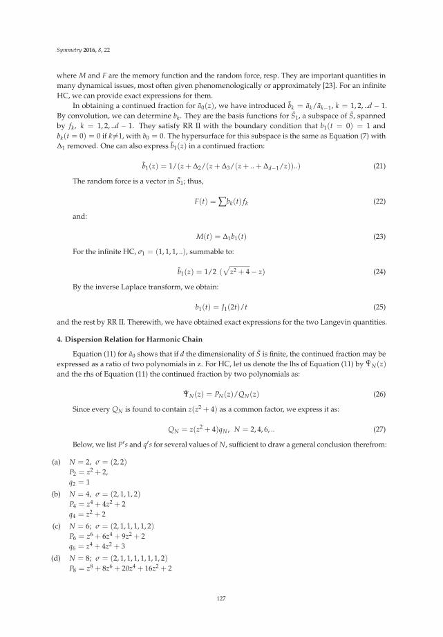
Symmetry 2016, 8, 22

where M and F are the memory function and the random force, resp. They are important quantities inmany dynamical issues, most often given phenomenologically or approximately [23]. For an infiniteHC, we can provide exact expressions for them.

In obtaining a continued fraction for a0(z), we have introduced bk = ak/ak−1, k = 1, 2, ..d − 1.By convolution, we can determine bk. They are the basis functions for S1, a subspace of S, spannedby fk, k = 1, 2, ..d − 1. They satisfy RR II with the boundary condition that b1(t = 0) = 1 andbk(t = 0) = 0 if k �=1, with b0 = 0. The hypersurface for this subspace is the same as Equation (7) withΔ1 removed. One can also express b1(z) in a continued fraction:

b1(z) = 1/(z + Δ2/(z + Δ3/(z + .. + Δd−1/z))..) (21)

The random force is a vector in S1; thus,

F(t) = ∑bk(t) fk (22)

and:

M(t) = Δ1b1(t) (23)

For the infinite HC, σ1 = (1, 1, 1, ..), summable to:

b1(z) = 1/2 (√

z2 + 4 − z) (24)

By the inverse Laplace transform, we obtain:

b1(t) = J1(2t)/t (25)

and the rest by RR II. Therewith, we have obtained exact expressions for the two Langevin quantities.

4. Dispersion Relation for Harmonic Chain

Equation (11) for a0 shows that if d the dimensionality of S is finite, the continued fraction may beexpressed as a ratio of two polynomials in z. For HC, let us denote the lhs of Equation (11) by ΨN(z)and the rhs of Equation (11) the continued fraction by two polynomials as:

ΨN(z) = PN(z)/QN(z) (26)

Since every QN is found to contain z(z2 + 4) as a common factor, we express it as:

QN = z(z2 + 4)qN , N = 2, 4, 6, .. (27)

Below, we list P′s and q′s for several values of N, sufficient to draw a general conclusion therefrom:

(a) N = 2, σ = (2, 2)P2 = z2 + 2,q2 = 1

(b) N = 4, σ = (2, 1, 1, 2)P4 = z4 + 4z2 + 2q4 = z2 + 2

(c) N = 6; σ = (2, 1, 1, 1, 1, 2)P6 = z6 + 6z4 + 9z2 + 2q6 = z4 + 4z2 + 3

(d) N = 8; σ = (2, 1, 1, 1, 1, 1, 1, 2)P8 = z8 + 8z6 + 20z4 + 16z2 + 2

127

Symmetry 2016, 8, 22

q8 = z6 + 6z4 + 10z2 + 4

(e) N = 10; σ = (2, 1, 1, 1, 1, 1, 1, 1, 1, 2)P10 = z10 + 10z8 + 35z6 + 50z4 + 25z4 + 2q10 = z8 + 8z6 + 21z4 + 20z2 + 5

(f) N = 12; σ = (2, 1, 1, 1, 1, 1, 1, 1, 1, 1, 1, 2)P12 = z12 + 12z10 + 54z8 + 112z6 + 105z4 + 36z2 + 2q12 = z10 + 10z8 + 36z6 + 56z4 + 35z2 + 6

If z = 2isinα, α �=0, the above polynomials have simple expressions for all orders of N:

PN = 2cosNα (28)

qN = sinNα/sin2α, sin2α �=0 (29)

4.1. Zeros of qN

The dispersion relation can be deduced from zk the zeros of qN :

qN(z) = Π(z − zk) (30)

From Equation (29),

sinNαk = 0 (31)

with sin2αk �=0 and αk �=0. Hence,

αk = (π/N)k, k = ±1,±2, ..±(N/2 − 1) (32)

Hence, with k given above,

zk = 2isinαk (33)

One may also write:

Π(z − zk)|z=2isinα = sinNα/sin2α (34)

Since QN = z(z2 + 4)qN (see Equation (26)), the prefactor contributes to the zeros of QN . They maybe included in Equation (32) if the range of k is made to includes zero and N/2.

4.2. a0(t) for Finite N

Given the zeros of QN , it is now straightforward to obtain a0(t) by Equation (12). For example,if N = 6,

a0(t) = 1/6[1 + 2cost + 2cos√

3t + cos2t] (35)

A general expression would be:

a0(t) = 1/N∑k

cosωkt (36)

where:ωk = 2|sin(πνk)|, νk = k/N (37)

k = −N/2, .,−1, 0, 1, ..N/2. Since Equation (36) is a dispersion relation, ν′s will be termed“wave vectors”.

128

Symmetry 2016, 8, 22

4.3. a0(t) When N→∞

If N→∞, the sum in Equation (36) may be converted to an integral:

rhs o f Equation(36) = 1/2π∫−π

πe2itsinθdθ (38)

The rhs of Equation (38) is an integral representation of J0(2t). Hence, a0(t) = J0(2t), the same asEquation (18).

It is worth noting here that the zeros of J0(2t) can thus be obtained from Equation (36) by takingN→∞ by the condition:

ωkt = π/2(2n + 1), n = 0, 1, 2, .. (39)

If we write J0(2t) = Π(2t − 2tk), by Equation (37):

2tk = π(2n + 1)/|2sinπk/N|, k/N = (−1/2, 1/2) (40)

Evidently, there are infinitely many zeros in J0 [30]. This result will be significant in Section 6.

4.4. a0(z) = ΨN(z) When N →∞

By Equations (26)–(29),

ΨN(z) = VcosNα/sinNα (41)

where V = 2sin2α/(z(z2 + 4)) = dα/dz (by z = 2isinα). Furthermore:

cosNα/sinNα = 1/N d/dα(logsinNα)

= 1/N d/dα[log(sinNα/sin2α) + logsin2α] (42)

The second term on the rhs of Equation (42) may be dropped if N→∞. For the first term,by Equations (28) and (29),

rhs o f Equation(42) = dz/dα d/dz logΠ(z − zk) = dz/dα ∑1/(z − zk) (43)

The prefactor dz/dα = 1/V. Since N→∞, we can convert the above sum into an integral:writing Ψ = ΨN , N→∞,

Ψ(z) =1π

∫−π/2

π/2 dθ

z − 2isinθ=

1√4 + z2

(44)

The above result is the same as Equation (17).The asymptotic results Equations (16) and (17) were obtained by taking the N→∞ limit first on

the hypersurface. What is shown in Section 4 is that the same results are also obtained from finite Nsolutions for a0(t).

5. Ergodicity of Dynamical Variable A = p0

If A is a variable of a Hermitian system of N particles, N→∞, it is possible to determine whetherit is ergodic. According to the ergometric theory of the ergodic hypothesis [31], A is ergodic if WA �=0or ∞, where:

WA =∫0

∞rA(t) dt (45)

129

Symmetry 2016, 8, 22

where rA(t) = (A(t), A)/(A, A) = a0(t), the autocorrelation function of A. By Equation (12),

WA = rA(z = 0) (46)

If d→∞ as N→∞, which is the case of HC, z→0 on Equation (11) yields an infinite product of thefollowing form:

WA =Δ2×Δ4×...Δ2n

Δ1×Δ3×...Δ2n+1, n→∞ (47)

Ordinarily, infinite products are difficult to evaluate, as they seem to require product rules thatdiffer from those for finite products. However, they can be determined by Equation (45) or Equation (46)as illustrated below.

5.1. Infinite Harmonic Chain

If A = p0 of HC, we can determine whether A is ergodic by evaluating Equations (45)–(47).If N→∞, σ = (2, 1, 1, ...) (see (16)), and Ψ(t) = J0(2t) (see Equation (18)). Hence, by Equation (45),WA = 1/2.

It was shown that Ψ(z) = 1/√

z2 + 4; see Equation (17). Hence, by Equation (46), WA = 1/2.Finally, by σ, we can write down the infinite product:

WA =1×1×1×....2×1×1×...

=12

(48)

in agreement with the previous results. As noted above, computing infinite products is a delicate matter.The order of terms in an infinite product may not be altered, nor the terms themselves. In Equation(48), such a nicety did not enter since all elements are one but one. Compare with another example inSection 5.2 below.

5.2. Infinite Harmonic Chain with One End Attached to a Wall

We shall now change HC defined by Equation (13) slightly. Let the coupling between the oscillatorsat q−2 and q−1 be cut. Furthermore, let the mass of the oscillator at q−1 be infinitely heavy, so that theoscillator at q0 is attached as if to a wall. The rest of the chain is unchanged. The oscillators in thisnew configuration are labeled 0, 1, 2..N − 1, with one end attached to a wall and the other end free.Finally, let N→∞.

If A = p0, the recurrants are found to have the following form [27,32]:Δ1 = 2/1, Δ3 = 3/2, Δ5 = 4/3, .. Δ2 = 1/2, Δ4 = 2/3, Δ6 = 3/4, ...Evidently, they may be put in the form: Δ2n−1 = (n + 1)/n and Δ2n = n/(n + 1), n = 1, 2, 3,...

These recurrants imply that for A = p0 [27,32],

a0(t) = J0(2t)− J4(2t) (49)

a0(z) = 1/√(z2 + 4) [1 − 1/16 (

√z2 + 4 − z)4] (50)

By Equation (47),

WA =1/2×2/3×3/4×...×n/(n + 1)2/1×3/2×4/3×...×(n + 1)/n

, n→∞ (51)

Each term in the numerator is less than one, while each term in the denominator greater than one.If the terms and the order are preserved, WA→0. By Equations (45) and (46), it may be tested usingEquations (49) and (50). In both cases, we obtain WA = 0 verifying the infinite product.

130

Symmetry 2016, 8, 22

Since WA = 0, A = p0 is not ergodic in this chain. For this variable, the phase space isnot transitive. If mass at Site 0 is slightly perturbed, the perturbed energy is not delocalizedeverywhere [33].

6. Harmonic Chain and Logistic Map

The logistic map (LM) is sometimes called the Ising model of chaos for being possibly the simplestmodel exhibiting chaos [34]. If x is a real number in an interval (0,1), the map is defined by:

f (x) = ax(1 − x), x = (0, 1) (52)

where a is a control parameter, a real number limited to 1 < a≤4. Thus, the map is real and boundedas x. If there exists x = x∗, such that f (x∗) = x∗, it is termed a fixed point of f (x). If f n is an n-foldnested function of f , i.e., f n(x) = f ( f n−1) = f ( f (... f (x)...), with f 1≡ f , there may be fixed points forf n : f n(x∗) = x∗. The values of the fixed points and the number of the fixed points will depend on thesize of the control parameter a.

If a < 3, there is only one fixed point for any n. There is a remarkable theorem due toSharkovskii [35] on 1d continuous maps on the interval, such as LM. As applied to this map,this theorem says that if a≥1 +

√8, there are infinitely many fixed points as n→∞. This implies

that a trajectory starting from almost any point in (0,1) is chaotic. At a = 4 (the largest possiblevalue), the fixed points fill the interval x = (0, 1) densely with a unique distribution ρx,

∫ρxdx = 1.

This distribution is known as the invariant density of fixed points, first deduced by Ulam [36,37]:

ρx =1

π√

x(1 − x), 0 < x < 1 (53)

The invariant density refers to the spectrum of fixed points in (0,1). The square-root singularity inEquation (53), a branch cut from 0–1, indicates that the spectrum is dense. If μ is a Lebesgue measure,dμ(x) = ρxdx. Hence, μ = 1.

We wish to see whether ρx, a distribution of fixed points, bears a relationship to ρω, the powerspectrum of frequencies in HC. For this purpose, consider the following transformations of variables:

x = 1/2 + 1/4 ω (54)

and:ρxdx = ρωdω (55)

By substituting Equation (54) in (53), we obtain by Equation (55):

ρω =1

π√

4 − ω2, − 2 < ω < 2 (56)

= 0 if otherwise.For an infinite HC, a0(z = iω) = πρω . By Equation (17), or Equation (44), the rhs of Equation (56)

is precisely the power spectrum for A = p0. Equation (56) shows that the fixed points of LM ata = 4 (LM4) correspond to the frequencies of HC.

Since the frequencies in the power spectrum are positive quantities, let us express Equation (54) as:

ω = 2|1 − 2x|, 0 < x < 1 (57)

For LM4,

x = sin2πy/2 (58)

y/2 = l/(2N + 1), l = 1, 2.., N (59)

131

Symmetry 2016, 8, 22

y being the pre-fixed points of x the fixed points. If Equation (59) is substituted in Equation (57)and y replaced by ν + 1/2:

ω = 2|sinπν| (60)

The above is identical to Equation (37), the dispersion relation for HC. In the limit N→∞, both ν

and y lie in the same interval (−1/2, 1/2). This property shows that the pre-fixed points of LM4 alsocorrespond to the wave vectors of HC.

The correspondence between x and ω and also between y and ν indicate that the iterationdynamics of LM4 and the time evolution in HC are isomorphic in their local variables. This impliesthat if a variable in HC is ergodic, a corresponding variable in LM4 is also ergodic. If the trajectory ofan initial value in LM4 is chaotic, we must also conclude that the trajectory of a local variable in HCmust also be chaotic.

Chaos in HC? Let us first examine chaos in LM4. According to Sharkovskii, chaos is impliedwhere there are infinitely many periods. By our work, they form a set of uncountable pre-fixed pointsof Lebesgue measure 1. This results in an aleph cycle, which can never return to the initial point [34].In an infinite HC, there are also infinitely many periods. See Equation (40). Thus, the HC has thenecessary and possibly sufficient property for chaos.

In an infinite HC attached to a wall (see Section 5.2), there is chaos also, as there are infinitely manyperiods. However, as was already shown, its variables are not ergodic. This indicates that ergodicity isa subtler property than chaos. In a continuous map, there may be chaos, but not ergodicity.

7. Concluding Remarks

In this work, we have dwelt with the dynamics of a monatomic chain with which to illustratesome of the finer points of the dynamics contained in it. This simplest of harmonic chains can be madericher in a variety of ways. One can make one oscillator to have a different mass than its neighbors [25].It would be a model for an impurity or a defect. One could make it a periodic diatomic chain [8] oreven an aperiodic diatomic chain [8]. We are providing a list of recent advances made by the methodof recurrence relations on others [38–44]. For related studies on HC by Fokker–Planck dynamics andnon-exponential decay, see [7,45,46].

Acknowledgments: I thank Joao Florencio for having kindled my interest in the dynamics of harmonic chainsthrough our collaboration in the 1980s. I thank the University of Georgia Franklin College for supporting myresearch through the regents professorship. This work is dedicated to the memory of Bambi Hu.

Conflicts of Interest: The author declares no conflict of interest.

References

1. Mazur, P.; Montroll, E. Poincaré cycles, ergodicity, and irreversibility in assemblies of coupled harmonicoscillators. J. Math. Phys. 1960, 1, 70–84.

2. Lee, M.H. Solutions of the generalized Langevin equation by a method of recurrence relations. Phys. Rev. B1982, 26, 2547–2551.

3. Pires, A.S.T. The memory function formalism in the study of the dynamics of a many body system. Helv. Phys.Acta 1988, 61, 988.

4. Viswanath, V.S.; Mueller, G. Recursion Method; Springer-Verlag: Berlin, Germany, 1994.5. Balucani, U.; Lee, M.H.; Tognetti, V. Dynamical correlations. Phys. Rep. 2003, 373, 409–492.6. Mokshin, A.V. Self-consistent approach to the description of relaxation processes in classical

multiparticle systems. Theory Math. Phys. 2015, 183, 449–477.7. Sen, S. Solving the Liouville equation for conservative systems: Continued fraction formalism and a simple

application. Phys. A 2006, 360, 304–324.8. Kim, J.; Sawada, I. Dynamics of a harmonic oscillator on the Bethe lattice. Phys. Rev. E 2000, 61, R2172–R2175.9. Sawada, I. Dynamics of the S = 1/2 alternating chains at T = ∞. Phys. Rev. Lett. 1999, 83, 1668–1671.

132

Symmetry 2016, 8, 22

10. Sen, S. Exact solution of the Heisenberg equation of motion for the surface spin in a semi-infinite S=1/2 XYchain at infinite temperatures. Phys. Rev. B 1991, 44, 7444–7450.

11. Florencio, J.; Sá Barreto, F.C.S. Dynamics of the random one-dimensional transverse Ising model. Phys. Rev. B1999, 60, 9555–9560.

12. Silva Nunez, M.E.; Florencio, J. Effects of disorder on the dynamics of the XY chain. Phys. Rev. B 2003,68, 144061–114065.

13. Daligault, J.; Murillo, M.S. Continued fraction matrix representation of response functions in multicomponentsystems. Phys. Rev. E 2003, 68, 154011–154014.

14. Mokshin, A.V.; Yulmatyev, R.M.; Hanggi, P. Simple measure of memory for dynamical processes describedby a generalized langevin equation. Phys. Rev. Lett. 2005, 95, 200601.

15. Hong, J.; Kee, H.Y. Analytic treatment of Mott-Hubbard transition in the half-filled Hubbard model and itsthermodynamics. Phys. Rev. B 1995, 52, 2415–2421.

16. Liu, Z.-Q.; Kong, X.-M.; Chen, X.-S. Effects of Gaussian disorder on the dynamics of the random transverseIsing model. Phys. Rev. B 2006, 73, 224412.

17. Chen, X.-S.; Shen, Y.-Y.; Kong, X.-M. Crossover of the dynamical behavior in two-dimensional randomtransverse Ising model. Phys. Rev. B 2010, 82, 174404.

18. De Mello Silva, E. Time evolution in a two-dimensional ultrarelativistic-like electron gas by recurrencerelations method. Acta Phys. Pol. B 2015, 46, 1135–1141.

19. De Mello Silva, E. Dynamical class of a two-dimensional plasmonic Dirac system. Phys. Rev. E 2015,92, 042146.

20. Guimaraes, P.R.C.; Plascak, J.A.; de Alcantara Bonfim, O.F.; Florencio, J. Dynamics of the transverse Isingmodel with next-nearest-neighbor interactions. Phys. Rev. E 2015, 92, 042115.

21. Sharma, N.L. Response and relaxation of a dense electron gas in D dimensions at long wavelengths.Phys. Rev. B 1992, 45, 3552–3556.

22. Lee, M.H. Can the velocity autocorrelation function decay exponentially? Phys. Rev. Lett. 1983, 51, 1227–1230.23. Kubo, R. The fluctuation-dissipation theorem. Rep. Prog. Phys. 1966, 29, 255–284.24. Lee, M.H. Orthogonalization process by recurrence relations. Phys. Rev. Lett. 1982, 49, 1072–1075.25. Lee, M.H.; Florencio, J., Jr.; Hong, J. Dynamic equivalence of a two-dimensional quantum electron gas and a

classical harmonic oscillator chain with an impurity mass. J. Phys. A 1989, 22, L331–L335.26. Fox, R.F. Long-time tails and diffusion. Phys. Rev. A 1983, 27, 3216–3233.27. Florencio, J., Jr.; Lee, M.H. Exact time evolution of a classical harmonic-oscillator chain. Phys. Rev. A 1985, 31,

3231–3236.28. Lee, M.H. Why Irreversibility is not a sufficient condition for ergodicity. Phys. Rev. Lett. 2007, 98, 190601.29. Lee, M.H. Derivation of the generalized Langevin equation by a method of recurrence relations. J. Math. Phys.

1983, 24, 2512–2514.30. Watson, G.N. A Treatise on the Theory of Bessel Functions; Cambridge U.P.: London, UK, 1980; Chapter 15.31. Lee, M.H. Ergodic theory, infinite products, and long time behavior in Hermitian models. Phys. Rev. Lett.

2001, 87, 250601/1–250601/4.32. Pestana Marino, E. Ph.D. Thesis, University of Georgia, Athens, GA, USA, 2011, unpublished.33. Lee, M.H. Birkhoff’s theorem, many-body response functions, and the ergodic condition. Phys. Rev. Lett.

2007, 98, 110403.34. Lee, M.H. Solving for the fixed points of 3-cycle in the logistic map and toward realizing chaos by the

theorems of Sharkovskii and Li-Yorke. Commu. Theor. Phys. 2014, 62, 485–496.35. Sharkovskii, A.N. Coexistence of cycles of a continuous transformation of a line into itself. Ukrainian Math. J.

1964, 16, 61–71 (in Russian); English transt.: Int. J. Bifurc. Chaos 1995, 5, 1363–1273.36. Ulam, S.M. A Collection of Mathematical Problems; Interscience: New York, NY, USA, 1960; pp. 73–74.37. Lee, M.H. Cyclic solutions in chaos and the Sharkowskii theorem. Acta Phys. Pol. B 2012, 43, 1053–1063.38. Yu, M.B. Momentum autocorrelation function of Fibonacci chains with finite number oscillators. Eur. J. Phys.

B 2012, 85, 379.39. Yu, M.B. Momentum autocorrelation function of a classical oscillator chain with alternating masses. Eur. J.

Phys. B 2013, 86, 57.40. Yu, M.B. Momentum autocorrelation function of an impurity in a classical oscillator chain with alternating

masses - I. General theory. Phys. A 2014, 398, 252–263.

133

Symmetry 2016, 8, 22

41. Yu, M.B. Momentum autocorrelation function of an impurity in a classical oscillator chain with alternatingmasses II. Illustrations. Phys. A 2015, 438, 469–486.

42. Yu, M.B. Momentum autocorrelation function of an impurity in a classical oscillator chain with alternatingmasses III. Some limiting cases. Phys. A 2016, 447, 411–421.

43. Wierling, A.; Sawada, I. Wave-number dependent current correlation for a harmonic oscillator. Phys. Rev. E2010, 82, 051107.

44. Wierling, A. Dynamic structure factor of linear harmonic chain - A recurrence relation approach. Eur. J. Phys.B 2012, 85, 20.

45. Vitali, D.; Grigolini, P. Subdynamics, Fokker-Planck equation, and exponential decay of relaxation processes.Phys. Rev. A 1989, 39, 1486–1499.

46. Grigolini, P. Quantum Mechanical Irreversibility and Measurement; World Scientific: Singapore, Singapore, 1993.

c© 2016 by the author. Licensee MDPI, Basel, Switzerland. This article is an open accessarticle distributed under the terms and conditions of the Creative Commons Attribution(CC BY) license (http://creativecommons.org/licenses/by/4.0/).

134

symmetryS S

Essay

Old Game, New Rules: Rethinking the Formof Physics

Christian Baumgarten

5244 Birrhard, Switzerland; christian-baumgarten@gmx.net

Academic Editor: Young Suh KimReceived: 26 February 2016; Accepted: 28 April 2016; Published: 6 May 2016

Abstract: We investigate the modeling capabilities of sets of coupled classical harmonic oscillators(CHO) in the form of a modeling game. The application of the simple but restrictive rules of the gamelead to conditions for an isomorphism between Lie-algebras and real Clifford algebras. We showthat the correlations between two coupled classical oscillators find their natural description in theDirac algebra and allow to model aspects of special relativity, inertial motion, electromagnetism andquantum phenomena including spin in one go. The algebraic properties of Hamiltonian motionof low-dimensional systems can generally be related to certain types of interactions and hence tothe dimensionality of emergent space-times. We describe the intrinsic connection between phasespace volumes of a 2-dimensional oscillator and the Dirac algebra. In this version of a phase spaceinterpretation of quantum mechanics the (components of the) spinor wavefunction in momentumspace are abstract canonical coordinates, and the integrals over the squared wave function representssecond moments in phase space. The wave function in ordinary space-time can be obtained viaFourier transformation. Within this modeling game, 3+1-dimensional space-time is interpreted asa structural property of electromagnetic interaction. A generalization selects a series of Cliffordalgebras of specific dimensions with similar properties, specifically also 10- and 26-dimensional realClifford algebras.

Keywords: Hamiltonian mechanics; coupled oscillators; Lorentz transformation; Dirac equation

PACS: 45.20.Jj, 47.10.Df, 41.75, 41.85, 03.65.Pm, 05.45.Xt, 03.30.+p, 03.65.-w,29.27.-a

1. Introduction

D. Hestenes had the joyful idea to describe physics as a modeling game [1]. We intend to play amodeling game with (ensembles of) classical harmonic oscillators (CHO). The CHO is certainly one ofthe most discussed and analyzed systems in physics and one of the few exactly solveable problems.One would not expect any substantially new discoveries related to this subject. Nevertheless there areaspects that are less well-known than others. One of these aspects concerns the transformation group ofthe symplectic transformations of n coupled oscillators, Sp(2n). We invite the reader to join us playing“a modeling game” and to discover some fascinating features related to possible reinterpretations ofsystems of two (or more) coupled oscillators. We will show that special relativity can be reinterpreted asa transformation theory of the second moments of the abstract canonical variables of coupled oscillatorsystems (The connection of the Dirac matrices to the symplectic group has been mentioned by Dirac inReference [2]. For the connection of oscillators and Lorentz transformations (LTs) see also the papersof Kim and Noz [3–5] and references therein. The use of CHOs to model quantum systems has beenrecently described-for instance-by Briggs and Eisfeld [6–8]). We extend the application beyond pureLTs and show that the Lorentz force can be reinterpreted by the second moments of two coupledoscillators in proper time. Lorentz transformations can be modeled as symplectic transformations [4].We shall show how Maxwell’s equations find their place within the game.

Symmetry 2016, 8, 30 135 www.mdpi.com/journal/symmetry

Symmetry 2016, 8, 30

The motivation for this game is to show that many aspects of modern physics can be understood onthe basis of the classical notions of harmonic oscillation if these notions are appropriately reinterpreted.

In Section 2 we introduce the rules of our game, in Section 3 we introduce the algebraic notionsof the Hamilton formalism. In Section 4 we describe how geometry emerges from coupled oscillatorsystems, in Section 5 we describe the use of symplectic transformations and introduce the Pauli- andDirac algebra. In Section 6 we introduce a physical interpretation of oscillator moments and inSection 7 we relate the phase space of coupled oscillators to the real Dirac algebra. Section 8 contains ashort summary.

2. The Rules Of The Game

The first rule of our game is the principle of reason (POR): No distinction without reason-we shouldnot add or remove something specific (an asymmetry, a concept, a distinction) from our model withouthaving a clear and explicite reason. If there is no reason for a specific asymmetry or choice, then allpossibilities are considered equivalently.

The second rule is the principle of variation (POV): We postulate that change is immanent to allfundamental quantities in our game. From these two rules, we take that the mathematical object of ourtheory is a list (n-tuple) of quantities (variables) ψ, each of which varies at all times.

The third rule is the principle of objectivity (POO): Any law within this game refers tomeasurements, defined as comparison of quantities (object properties) in relation to other objectproperties of the same type (i.e., unit). Measurements require reference standards (rulers).A measurement is objective if it is based on (properties of) the objects of the game. This apparentself-reference is unavoidable, as it models the real situation of physics as experimental science. Since allfundamental objects (quantities) in our model vary at all times, the only option to construct a constantquantity that might serve as a ruler, is given by constants of motion (COM). Hence the principle ofobjectivity requires that measurement standards are derived from constants of motion.

This third rule implies that the fundamental variables can not be directly measured, but onlyfunctions of the fundamental variables of the same dimension (unit) of a COM. Thus the model hastwo levels: The level of the fundamental variable list ψ, which is experimentally not directly accessibleand a level of observables which are (as we shall argue) even moments of the fundamental variables ψ.

2.1. Discussion of the Rules

E.T. Jaynes wrote that “Because of their empirical origins, QM and QED are not physical theoriesat all. In contrast, Newtonian celestial mechanics, Relativity, and Mendelian genetics are physicaltheories, because their mathematics was developed by reasoning out the consequences of clearly statedphysical principles from which constraint the possibilities”. And he continues “To this day we haveno constraining principle from which one can deduce the mathematics of QM and QED; [...] In otherwords, the mathematical system of the present quantum theory is [...] unconstrained by any physicalprinciple” [9]. This remarkably harsh criticism of quantum mechanics raises the question of what weconsider to be a physical principle. Are the rules of our game physical principles? We believe thatthey are no substantial physical principles but formal first principles, they are preconditions of a sensibletheory. They contain no immediate physical content, but they define the form or the idea of physics.

It is to a large degree immanent to science and specifically to physics to presuppose the existenceof reason: Apples do not fall down by chance—there is a reason for this tendency. Usually this believe inreason implies the believe in causality, i.e., that we can also (at least in principle) explain why a specificapple falls at a specific time, but practically this latter believe can rarely be confirmed experimentallyand therefore remains to some degree metaphysical. Thus, if, as scientists, we postulate that thingshave reason, then this is not a physical principle but a precondition, a first principle.

The second rules (POV), is specific to the form (or idea) of physics, e.g., that it is the sense ofphysics to recognize the pattern of motion and to predict future. Therefore the notion of time in the formof change is indeed immanent to the physical description of reality.

136

Symmetry 2016, 8, 30

The principle of objectivity (POO) is immanent to the very idea of physics: A measurement isthe comparison of properties of objects with compatible properties of reference objects, e.g., requires“constant” rulers. Hence the rules of the game are to a large degree unavoidable: They follow fromthe very form of physics and therefore certain laws of physics are not substantial results of a physicaltheory. For instance a consistent “explanation” of the stability of matter is impossible as we presumedit already within the idea of measurement. More precisely: if this presumption does not follow withinthe framework of a physical theory, then the theory is flawed, since it can not reproduce it’s ownpresumptions.

Einstein wrote with respect to relativity that “It is striking that the theory (except for thefour-dimensional space) introduces two kinds of things, i.e., (1) measuring rods and clocks; (2) all otherthings, e.g., the electromagnetic field, the material point, etc. This, in a certain sense, is inconsistent;strictly speaking, measuring rods and clocks should emerge as solutions of the basic equations [...],not, as it were, as theoretically self-sufficient entities”. [10]. The more it may surprise that the stabilityof matter can not be obtained from classical physics as remarked by Elliott H. Lieb: “A fundamentalparadox of classical physics is why matter, which is held together by Coulomb forces, does notcollapse” [11]. This single sentence seems to rule out the possibility of a fundamental classical theoryand uncovers the uncomfortable situation of theoretical physics today: Despite the overwhelmingexperimental and technological success, there is a deep-seated confusion concerning the theoreticalfoundations. Our game is therefore a meta-experiment. It is not the primary goal to find “new” lawsof nature or new experimental predictions, but it is a conceptional “experiment” that aims to furtherdevelop our understanding of the consequences of principles: which ones are really required to derivecentral “results” of contemporary physics. In this short essay final answers can not be given, butmaybe some new insights are possible.

2.2. What about Space-Time?

A theory has to make the choice between postulate and proof. If a 3+1 dimensional space-time ispresumed, then it cannot be proven within the same theoretical framework. More precisely, the valueof such a proof remains questionable. This is a sufficient reason to avoid postulates concerning thedimensionality of space-time. Another, even stronger, reason to avoid a direct postulate of space-timeand its geometry has been given above: The fundamental variables that we postulated, can not bedirectly measured. This excludes space-time coordinates as primary variables (which can be directlymeasured), but with it almost all other apriori assumed concepts like velocity, acceleration, momentum,energy and so on. At some point these concepts certainly have to be introduced, but we suggest anapproach to the formation of concepts that differs from the Newtonian axiomatic method. The PORdoes not allow to introduce distinctions between the fundamental variables into coordinates andmomenta without reason. Therefore we are forced to use an interpretational method, which one mightsummarize as function follows form. We shall first derive equations and then we shall interpret theequations according to some formal criteria. This implies that we have to refer to already existingnotions if we want to identify quantities according to their appearance within a certain formalism.The consequence for the game is, that we have to show how to give rise to geometrical notions: If we donot postulate space-time then we have to suggest a method to construct it.

A consequence of our conception is that both, objects and fields have to be identified withdynamical structures, as there is simply nothing else available. This fits to the framework of structurepreserving (symplectic) dynamics that we shall derive from the described principles.

137

Symmetry 2016, 8, 30

3. Theory of Small Oscillations

In this section we shall derive the theory of coupled oscillators from the rules of our game.According to the POO there exists a function (COM) H(ψ) such that ( Let us first (for simplicity)assume that ∂H

∂t = 0.):dHdt

= ∑k

∂H∂ψk

ψk = 0 (1)

or in vector notationdHdt

= (∇ψ H) · ψ = 0 (2)

The simplest solution is given by an arbitrary skew-symmetric matrix X :

ψ = X ∇ψ H (3)

Note that it is only the skew-symmetry of X , which ensures that it is always a solution to Equation (2)and which ensures that H is constant. If we now consider a state vector ψ of dimension k, thenthere is a theorem in linear algebra, which states that for any skew-symmetric matrix X there exists anon-singular matrix Q such that we can write [12]:

QT X Q = diag(η0, η0, η0, . . . , 0, 0, 0) (4)

where η0 is the matrix

η0 =

(0 1−1 0

)(5)

If we restrict us to orthogonal matrices Q, then we may still write

QT X Q = diag(λ0 η0, λ1 η0, λ2 η0, . . . , 0, 0, 0) (6)

In both cases we may leave away the zeros, since they correspond to non-varying variables, whichwould be in conflict with the second rule of our modeling game. Hence k = 2n must be even and thesquare matrix X has the dimension 2n × 2n. As we have no specific reason to assume asymmetriesbetween the different degrees of freedom (DOF), we have to choose all λk = 1 in Equation (6) andreturn to Equation (4) without zeros and define the block-diagonal so-called symplectic unit matrix(SUM) γ0:

QT X Q = diag(η0, η0, . . . , η0) ≡ γ0 (7)

These few basic rules thus lead us directly to Hamiltonian mechanics: Since the state vector has evendimension and due to the form of γ0, we can interpret ψ as an ensemble of n classical DOF-each DOFrepresented by a canonical pair of coordinate and momentum: ψ = (q1, p1, q2, p2, . . . , qn, pn)T . In thisnotation and after the application of the transformation Q, Equation (3) can be written in form of theHamiltonian equations of motion (HEQOM):

qi = ∂H∂pi

pi = − ∂H∂qi

(8)

The validity of the HEQOM is of fundamental importance as it allows for the use of the resultsof Hamiltonian mechanics, of statistical mechanics and thermodynamics-but without the intrinsicpresupposition that the qi have to be understood as positions in real space and the pi as thecorresponding canonical momenta. This is legitimate as the theory of canonical transformations isindependent from any specific physical interpretation of what the coordinates and momenta represent physically.As no other interpretation is at hand, we say that these canonical pairs are coordinates qi, pi in an

138

Symmetry 2016, 8, 30

abstract phase space and they are canonical coordinates and momenta only due to the form of theHEQOM. The choice of the specific form of γ0 is for n > 1 DOF not unique. It could for instance bewritten as

γ0 ≡ η0 ⊗ 1n×n (9)

which corresponds a state vector of the form

ψ = (q1, . . . , qn, p1, . . . , pn, )T

or byγ0 ≡ 1n×n ⊗ η0 (10)

as in Equation (7). Therefore we are forced to make an arbitrary choice (But we should keep in mind,that other “systems” with a different choice are possible. If we can not exclude their existence, then theyshould exist as well. With respect to the form of the SUM, we suggest that different “particle” types(different types of fermions for instance) have a different SUM). But in all cases the SUM γ0 must beskew-symmetric and have the following properties:

γT0 = −γ0

γ20 = −1

(11)

which also implies that γ0 is orthogonal and has unit determinant. Note also that all eigenvalues ofγ0 are purely imaginary. However, once we have chosen a specific form of γ0, we have specified aset of canonical pairs (qi, pi) within the state vector. This choice fixes the set of possible canonical(structure preserving) transformations.

Now we write the Hamiltonian H(ψ) as a Taylor series, we remove the rule-violating constantterm and cut it after the second term. We do not claim that higher terms may not appear, but wedelay the discussion of higher orders to a later stage. All this is well-known in the theory of smalloscillations. There is only one difference to the conventional treatment: We have no direct macroscopicinterpretation for ψ and following our first rule we have to write the second-order Hamiltonian H(ψ)

in the most general form:

H(ψ) =12

ψT Aψ (12)

where A is only restricted to be symmetric as all non-symmetric terms do not contribute to H. Since itis not unlikely to find more than a single constant of motion in systems with multiple DOFs, wedistinguish systems with singular matrix A from those with a positive or negative definite matrix A.Positive definite matrices are favoured in the sense that they allow to identify H with the amount of asubstance or an amount of energy (It is immanent to the concept of substance that it is understood assomething positive semidefinite).

Before we try to interprete the elements in A, we will explore some general algebraic propertiesof the Hamiltonian formalism. If we plug Equations (12) into (3), then the equations of motion can bewritten in the general form

ψ = γ0 Aψ = F ψ (13)

The matrix F = γ0 A is the product of the symmetric (positive semi-definite) matrix A and theskew-symmetric matrix γ0. As known from linear algebra, the trace of such products is zero:

Tr(F) = 0 (14)

Pure harmonic oscillation of ψ is described by matrices F with purely imaginary eigenvalues and thoseare the only stable solutions [12]. Note that Equation (13) may represent a tremendous amount ofdifferent types of systems-all linearily coupled systems in any dimension, chains or d-dimensional

139

Symmetry 2016, 8, 30

lattices of linear coupled oscillators and wave propagation (However the linear approximation doesnot allow for the description of the transport of heat).

One quickly derives from the properties of γ0 and A that

FT = AT γT0 = −A γ0 = γ2

0 A γ0 = γ0 F γ0 (15)

Since any square matrix can be written as the sum of a symmetric and a skew-symmetric matrix, it isnearby to also consider the properties of products of γ0 with a skew-symmetric real square matrices B.If C = γ0 B, then

CT = BT γT0 = B γ0 = −γ2

0 B γ0 = −γ0 C γ0 (16)

Symmetric 2n × 2n-matrices contain 2n (2n + 1)/2 different matrix elements and skew-symmetricones 2n (2n − 1)/2 elements, so that there are νs linear independent matrix elements in A

νs = n (2n + 1) (17)

and νc matrix elements in B withνc = n (2n − 1) (18)

In the theory of linear Hamiltonian dynamics, matrices of the form of F are known as “Hamiltonian” or“infinitesimal symplectic” and those of the form of C as “skew-Hamiltonian” matrices. This conventionis a bit odd as F does not appear in the Hamiltonian and it is in general not symplectic. Furthermorethe term “Hamiltonian matrix” has a different meaning in quantum mechanics - in close analogy to A.But it is known that this type of matrix is closely connected to symplectic matrices as every symplecticmatrix is a matrix exponential of a matrix F [12]. We consider the matrices as defined by Equations (15)and (16) as too important and fundamental to have no meaningful and unique names: Therefore wespeak of a symplex (plural symplices), if a matrix holds Equation (15) and of a cosymplex if it holdsEquation (16).

Symplectic Motion and Second Moments

So what is a symplectic matrix anyway? The concept of symplectic transformations is a specificformulation of the theory of canonical transformations. Consider we define a new state vector (or newcoordinates) φ(ψ)-with the additional requirement, that the transformation is reversible. Then theJacobian matrix of the transformation is given by

Jij =

(∂φi∂ψj

)(19)

and the transformation is said to be symplectic, if the Jacobian matrix holds [12]

J γ0 JT = γ0 (20)

Let us see what this implies in the linear case:

J ψ = J F J−1 J ψ

ψ = J ψ˙ψ = J F J−1 ψ˙ψ = F ψ

(21)

140

Symmetry 2016, 8, 30

and-by the use of Equation (20) one finds that F is still a symplex:

FT = (J−1)T FT JT

FT = (J−1)T γ0 F γ0 JT

FT = −γ20 (J

−1)T γ0 F J−1 γ0

FT = −γ0 J γ20 F J−1 γ0

FT = γ0 J F J−1 γ0

FT = γ0 F γ0

(22)

Hence a symplectic transformation is first of all a similarity transformation, but secondly, it preservesthe structure of all involved equations. Therefore the transformation is said to be canonical or structurepreserving. The distinction between canonical and non-canonical transformations can therefore betraced back to the skew-symmetry of γ0 and the symmetry of A- both of them consequences of therules of our physics modeling game.

Recall that we argued that the matrix A should be symmetric because skew-symmetric terms donot contribute to the Hamiltonian. Let us have a closer look what this means. Consider the matrix ofsecond moments Σ that can be build from the variables ψ:

Σ ≡ 〈ψ ψT〉 (23)

in which the angles indicate some (yet unspecified) sort of average. The equation of motion of thismatrix is given by

Σ = 〈ψ ψT〉+ 〈ψ ψT〉Σ = 〈F ψ ψT〉+ 〈ψ ψT FT〉 (24)

Now, as long as F does not depend on ψ, we obtain

Σ = F Σ + Σ FT

Σ = F Σ + Σ γ0 F γ0

(Σ γ0) = F (Σ γ0)− (Σ γ0) F

S = F S − S F

(25)

where we defined the new matrix S ≡ Σ γ0. For completeness we introduce the “adjunct” spinorψ = ψT γ0 so that we may write

S = 〈ψψ 〉 (26)

Note that S is also a symplex. The matrix S (i.e., all second moments) is constant, iff S and F commute.Now we define an observable to be an operator O with a (potentially) non-vanishing expectation

value, defined by:〈O〉 ≡ 〈ψOψ〉 = 〈ψT γ0 Oψ〉 (27)

Thus, if the product γ0 O is not skew-symmetric, i.e., contains a product of γ0 with a symmetric matrixB, then the expectation value is potentially non-zero:

〈O〉 ≡ 〈ψT γ0 (γ0 B)ψ〉 = −〈ψT B ψ〉 (28)

This means that only the symplex-part of an operator is “observable”, while cosymplices yield avanishing expectation value. Hence Equation (25) delivers the blueprint for the general definition ofobservables. Furthermore we find in the last line the constituting equation for Lax pairs [13]. Peter Laxhas shown that for such pairs of operators S and F that obey Equation (25) there are the followingconstants of motion

Tr(Sk) = const (29)

141

Symmetry 2016, 8, 30

for arbitrary integer k > 0. Since S is a symplex and therefore by definition the product of a symmetricmatrix and the skew-symmetric γ0, Equation (29) is always zero and hence trivially true for k = 1.The same is true for any odd power of S, as it can be easily shown that any odd power of a symplexis again a symplex (see Equation (35)), so that the only non-trivial general constants of motioncorrespond to even powers of S, which implies that all observables are functions of even powers of thefundamental variables.

To see the validity for k > 1 we have to consider the general algebraic properties of the traceoperator. Let λ be an arbitrary real constant and τ be a real parameter, then

Tr(A) = Tr(AT)

Tr(λ A) = λ Tr(A)d

dτ Tr(A(τ)) = Tr( dAdτ )

Tr(A + B) = Tr(A) + Tr(B)Tr(A B) = Tr(B A)

(30)

It follows that0 = Tr(A B − B A)

0 = Tr(An B − An−1 B A)

0 = Tr[An−1 (A B − B A)

] (31)

From the last line of Equation (31) it follows with dAdτ = λ (A B − B A)

ddτ

Tr(An) = 0 (32)

Remark: This conclusion is not limited to symplices.However for single spinors ψ and the corresponding second moments S = Σ γ0 = ψψT γ0 we

find:Tr(Sk) = Tr[ψ ψT γ0 · · ·ψ ψT γ0]

= Tr[ψ (ψT γ0 · · ·ψ ψT γ0)]

= Tr[(ψT γ0 · · ·ψ ψT γ0)ψ]

= Tr[(ψT γ0 ψ) · · · (ψTγ0ψ)

]= 0

(33)

since each single factor (ψT γ0 ψ) vanishes due to the skew-symmetry of γ0. Therefore the constants ofmotion as derived from Equation (29) are non-zero only for even k and after averaging over some kind ofdistribution such that S = 〈ψψT γ0〉 has non-zero eigenvalues as in Equation (34) below.

The symmetric matrix 2n × 2n-matrix Σ (and also A) is positive definite, if it can be written as aproduct Σ = ΨΨT , where Ψ is a non-singular matrix of size 2n × m with m ≥ 2n.

For n = m/2 = 1, the form of Ψ may be chosen as

Ψ = 1√q2+p2

(q −pp q

)= 1√

q2+p2(1ψ, η0 ψ)

⇒ Σ = ΨΨT = ΨT Ψ = 1

S = γ0

(34)

so that for k = 2 the average of two “orthogonal” column-vectors ψ and η0 ψ gives a non-zero constantof motion via Lax pairs as γ2

0 = −1.These findings have some consequences for the modeling game. The first is that we have found

constants of motion-though some of them are physically meaningful only for a non-vanishing volumein phase space, i.e., by the combination of several spinors ψ. Secondly, a stable state S = 0 impliesthat the matrix operators forming the Lax pair have the same eigenvectors: a density distribution inphase space (as described by the matrix of second moments) is stable if it is adapted or matched to the

142

Symmetry 2016, 8, 30

symplex F. The phase space distribution as represented by S and the driving terms (the components ofF) must fit to each other in order to obtain a stable “eigenstate”. But we also found a clear reason, whygenerators (of symplectic transformations) are always observables and vice versa: Both, the generatorsas well as the observables are symplices of the same type. There is a one-to-one correspondencebetween them, not only as generators of infinitesimal transformations, but also algebraically.

Furthermore, we may conclude that (anti-) commutators are an essential part of “classical”Hamiltonian mechanics and secondly that the matrix S has the desired properties of observables:Though S is based on continuously varying fundamental variables, it is constant, if it commutes withF, and it varies otherwise (In accelerator physics, Equation (25) describes the envelope of a beam inlinear optics. The matrix of second moments Σ is a covariance matrix-and therefore our modelinggame is connected to probability theory exactly when observables are introduced).

Hence it appears sensible to take a closer look on the (anti-) commutation relations of (co-)symplices and though the definitions of (co-) symplices are quite plain, the (anti-) commutator algebrathat emerges from them has a surprisingly rich structure. If we denote symplices by Sk and cosymplicesby Ck, then the following rules can quickly be derived:

S1 S2 − S2 S1

C1 C2 − C2 C1

C S + S C

S2 n+1

⎫⎪⎪⎪⎬⎪⎪⎪⎭ ⇒ symplex

S1 S2 + S2 S1

C1 C2 + C2 C1

C S − S C

S2 n

Cn

⎫⎪⎪⎪⎪⎪⎬⎪⎪⎪⎪⎪⎭

⇒ cosymplex

(35)

This Hamiltonian algebra of (anti-)commutators is of fundamental importance insofar as we derivedit in a few steps from first principles (i.e., the rules of the game) and it defines the structure ofHamiltonian dynamics in phase space. The distinction between symplices and cosymplices is also thedistinction between observables and non-observables. It is the basis of essential parts of the followingconsiderations.

4. Geometry from Hamiltonian Motion

In the following we will demonstrate the geometrical content of the algebra of (co-)symplices(Equation (35)) which emerges for specific numbers of DOF n. As shown above, pairs of canonicalvariables (DOFs) are a direct consequence of the abstract rules of our game. Though single DOFsare poor “objects”, it is remarkable to find physical structures emerging from our abstract rules at all.This suggests that there might be more structure to discover when n DOF are combined, for instancegeometrical structures. The following considerations obey the rules of our game, since they arebased purely on symmetry considerations like those that guided us towards Hamiltonian dynamics.The objects of interest in our algebraic interpretation of Hamiltonian dynamics are matrices. The firstmatrix (besides A) with a specific form that we found, is γ0. It is a symplex:

γT0 = −γ0 = γ0 γ0 γ0 (36)

According to Equation (17) there are νs = n (2 n + 1) (i.e., νs ≥ 3) symplices. Hence it is nearby toask if other symplices with similar properties like γ0 exist-and if so, what the relations between thesematrices are. According to Equation (35) the commutator of two symplices is again a symplex, while theanti-commutator is a cosymplex. As we are primarily interested in observables and components of the

143

Symmetry 2016, 8, 30

Hamiltonian (i.e., symplices), respectively, we look for further symplices that anti-commute with γ0

and with each other. In this case, the product of two such matrices is also a symplex, i.e., anotherpotential contribution to the general Hamiltonian matrix F.

Assumed we had a set of N mutually anti-commuting orthogonal symplices γ0 and γk withk ∈ [1 . . . N − 1], then a Hamiltonian matrix F might look like

F =N−1∑

k=0fk γk + . . . (37)

The γk are symplices and anti-commute with γ0:

γ0 γk + γk γ0 = 0 (38)

Multiplication from the left with γ0 gives:

− γk + γ0 γk γ0 = −γk + γTk = 0 (39)

so that all other possible symplices γk, which anticommute with γ0, are symmetric and square to 1.This is an important finding for what follows, as it can (within our game) be interpreted as a classicalproof of the uniqueness of (observable) time-dimension: Time is one-dimensional as there is no otherskew-symmetric symplex that anti-commutes with γ0. We can choose different forms for γ0, but theemerging algebra allows for no second “direction of time”.

The second order derivative of ψ is (for constant F) given by ψ = F2 ψ which yields:

F2 =N−1∑

i=0f 2i γ2

i + ∑i �=j

fi f j (γi γj + γj γi) (40)

Since the anti-commutator on the right vanishes by definition, we are left with:

F2 =

(N−1∑

k=1f 2k − f 2

0

)1 (41)

Thus-we find a set of (coupled) oscillators, if

f 20 >

N−1

∑k=1

f 2k (42)

such thatψ = −ω2 ψ (43)

Given such matrix systems exist-then they generate a Minkowski type “metric” as in Equation (41)(Indeed it appears that Dirac derived his system of matrices from the this requirement [14]).The appearance of this metric shows how a Minkowski type geometry emerges from the drivingterms of oscillatory motion. This is indeed possible- at least for symplices of certain dimensionsas we will show below. The first thing needed is some kind of measure to define the length of a“vector”. Since the length is a measure that is invariant under certain transformations, specificallyunder rotations, we prefer to use a quantity with certain invariance properties to define a length.The only one we have at hand is given by Equation (29). Accordingly we define the (squared) lengthof a matrix representing a “vector” by

‖A‖2 ≡ 12 n

Tr(A2) (44)

144

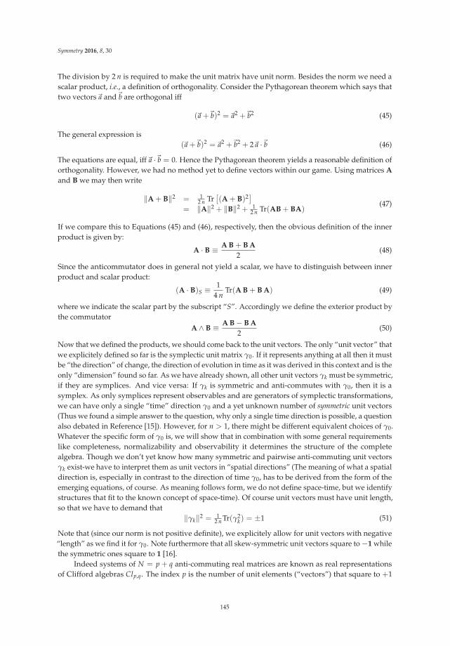
Symmetry 2016, 8, 30

The division by 2 n is required to make the unit matrix have unit norm. Besides the norm we need ascalar product, i.e., a definition of orthogonality. Consider the Pythagorean theorem which says thattwo vectors�a and�b are orthogonal iff

(�a +�b)2 =�a2 +�b2 (45)

The general expression is(�a +�b)2 =�a2 +�b2 + 2�a ·�b (46)

The equations are equal, iff�a ·�b = 0. Hence the Pythagorean theorem yields a reasonable definition oforthogonality. However, we had no method yet to define vectors within our game. Using matrices A

and B we may then write

‖A + B‖2 = 12 n Tr

[(A + B)2]

= ‖A‖2 + ‖B‖2 + 12 n Tr(AB + BA)

(47)

If we compare this to Equations (45) and (46), respectively, then the obvious definition of the innerproduct is given by:

A · B ≡ A B + B A

2(48)

Since the anticommutator does in general not yield a scalar, we have to distinguish between innerproduct and scalar product:

(A · B)S ≡ 14 n

Tr(A B + B A) (49)

where we indicate the scalar part by the subscript “S”. Accordingly we define the exterior product bythe commutator

A ∧ B ≡ A B − B A

2(50)

Now that we defined the products, we should come back to the unit vectors. The only “unit vector” thatwe explicitely defined so far is the symplectic unit matrix γ0. If it represents anything at all then it mustbe “the direction” of change, the direction of evolution in time as it was derived in this context and is theonly “dimension” found so far. As we have already shown, all other unit vectors γk must be symmetric,if they are symplices. And vice versa: If γk is symmetric and anti-commutes with γ0, then it is asymplex. As only symplices represent observables and are generators of symplectic transformations,we can have only a single “time” direction γ0 and a yet unknown number of symmetric unit vectors(Thus we found a simple answer to the question, why only a single time direction is possible, a questionalso debated in Reference [15]). However, for n > 1, there might be different equivalent choices of γ0.Whatever the specific form of γ0 is, we will show that in combination with some general requirementslike completeness, normalizability and observability it determines the structure of the completealgebra. Though we don’t yet know how many symmetric and pairwise anti-commuting unit vectorsγk exist-we have to interpret them as unit vectors in “spatial directions” (The meaning of what a spatialdirection is, especially in contrast to the direction of time γ0, has to be derived from the form of theemerging equations, of course. As meaning follows form, we do not define space-time, but we identifystructures that fit to the known concept of space-time). Of course unit vectors must have unit length,so that we have to demand that

‖γk‖2 = 12 n Tr(γ2

k) = ±1 (51)

Note that (since our norm is not positive definite), we explicitely allow for unit vectors with negative“length” as we find it for γ0. Note furthermore that all skew-symmetric unit vectors square to −1 whilethe symmetric ones square to 1 [16].

Indeed systems of N = p + q anti-commuting real matrices are known as real representationsof Clifford algebras Clp,q. The index p is the number of unit elements (“vectors”) that square to +1

145

Symmetry 2016, 8, 30

and q is the number of unit vectors that square to −1. Clifford algebras are not necessarily connectedto Hamiltonian motion, rather they can be regarded as purely mathematical “objects”. They canbe defined without reference to matrices whatsoever. Hence in mathematics, sets of matrices aremerely “representations” of Clifford algebras. But our game is about physics and due to the provenone-dimensionality of time we concentrate on Clifford algebras ClN−1,1 which link CHOs in thedescribed way with the generators of a Minkowski type metric. Further below it will turn out that therepresentation by matrices is-within the game-indeed helpful, since it leads to an overlap of certainsymmetry structures. The unit elements (or unit “vectors”) of a Clifford algebra, ek, are called thegenerators of the Clifford algebra. They pairwise anticommute and they square to ±1 (The role asgenerator of the Clifford algebra should not be confused with the role as generators of symplectictransformations (i.e., symplices). Though we are especially interested in Clifford algebras in whichall generators are symplices, not all symplices are generators of the Clifford algebra. Bi-vectors forinstance are symplices, but not generators of the Clifford algebra). Since the inverse of the unit elementsek of a Clifford algebra must be unique, the products of different unit vectors form new elements andall possible products including the unit matrix form a group. There are

(Nk

)possible combinations

(products without repetition) of k elements from a set of N generators. We therefore find(

N2

)bi-vectors,

which are products of two generators,(

N3

)trivectors) and so on. The product of all N basic matrices is

called pseudoscalar. The total number of all k-vectors then is (We identify k = 0 with the unit matrix 1.):

N

∑k=0

(Nk

)= 2N (52)

If we desire to construct a complete system, then the number of variables of the Clifford algebra has tomatch the number of variables of the used matrix system:

2N = (2n)2 (53)

Note that the root of this equation gives an even integer 2N/2 = 2 n so that N must be even. Hence allHamiltonian Clifford algebras have an even dimension. Of course not all elements of the Cliffordalgebra may be symplices. The unit matrix (for instance) is a cosymplex. Consider the Clifford algebraCl1,1 with N = 2, which has two generators, say γ0 with γ2

0 = −1 and γ1 with γ21 = 1. Since these two

anticommute (by definition of the Clifford algebra), so that we find (besides the unit matrix) a fourthmatrix formed by the product γ0 γ1:

γ0 γ1 = −γ1 γ0

(γ0 γ1)2 = γ0 γ1 γ0 γ1

= −γ0 γ0 γ1 γ1 = 1

(54)

The completeness of the Clifford algebras as we use them here implies that any 2 n × 2 n-matrix M

with (2n)2 = 2N can be written as a linear combination of all elements of the Clifford algebra:

M =4n2−1

∑k=0

mk γk (55)

The coefficients can be computed from the scalar product of the unit vectors with the matrix M:

mk = (γk · M)S =sk4n

Tr(γk M + M γk) (56)

Recall that skew-symmetric γk have a negative length and therefore we included a factor sk whichrepresents the “signature” of γk, in order to get the correct sign of the coefficients mk.

146

Symmetry 2016, 8, 30

Can we derive more properties of the constructable space-times? One restriction resultsfrom representation theory: A theorem from the theory of Clifford algebras states that Clp,q hasa representation by real matrices if (and only if) [17]

p − q = 0 or 2 mod 8 (57)

The additional requirement that all generators must be symplices so that p = N − 1 and q = 1 thenrestricts N to

N − 2 = 0 or 2 mod 8 (58)

Hence the only matrix systems that have the required symmetry properties within our modeling gameare those that represent Clifford algebras with the dimensions 1 + 1, 3 + 1, 9 + 1, 11 + 1, 17 + 1, 19 + 1,25 + 1, 27 + 1 and so on. These correspond to matrix representations of size 2 × 2, 4 × 4, 32 × 32,64 × 64, 512 × 512 and so on. The first of them is called Pauli algebra, the second one is the Dirac algebra.Do these two have special properties that the higher-dimensional algebras do not have? Yes, indeed.

Firstly, since dynamics is based on canonical pairs, the real Pauli algebra describes the motionof a single DOF and the Dirac algebra decribes the simplest system with interaction between twoDOF. This suggests the interpretation that within our game, objects (Dirac-particles) are not located“within space-time”, since we did not define space at all up to this point, but that space-time can bemodeled as an emergent phenomenon. Space-time is in between particles.

Secondly, if we equate the number of fundamental variables (2 n) of the oscillator phase spacewith the dimension of the Clifford space N, then Equation (53) leads to

2N = N2 (59)

which allows for N = 2 and N = 4 only. But why should it be meaningful to assume N = 2 n?The reason is quite simple: If 2 n > N as for all higher-dimensional state vectors, there are lessgenerators of the algebra than independent variables. This discrepancy increases with n. Hence thedescribed objects can not be pure vectors anymore, but must contain tensor-type components (k-vectors)(For a deeper discussion of the dimensionality of space-time, see Reference [16] and references therein).

But before we describe a formal way to interprete Equation (59), let us first investigate the physicaland geometrical implications of the game as described so far.

Matrix Exponentials

We said that the unit vectors γ0 and γk are symplices and therefore generators of symplectictransformations. All symplectic matrices are matrix exponentials of symplices [12]. The computationof matrix exponentials is in the general case non-trivial. However, in the special case of matrices thatsquare to ±1 (e.g., along the “axis” γk of the coordinate system), the exponentials are readily evaluated:

exp (γa τ) =∞∑

k=0

(γa τ)k

k!

exp (γa τ) =∞∑

k=0sk τ2k

(2 k)! + γa∞∑

k=0sk τ2k+1

(2 k+1)!

(60)

where s = ±1 is the sign of the matrix square of γa. For s = −1 (γ2a = −1), it follows that

Ra(τ) = exp (γa τ) = cos (τ) + γa sin (τ) (61)

and for s = 1 (γ2a = 1):

Ba(τ) = exp (γa τ) = cosh (τ) + γa sinh (τ) (62)

We can indentify skew-symmetric generators with rotations and (as we will show in more detail below)symmetric generators with boosts.

147

Symmetry 2016, 8, 30

The (hyperbolic) sine/cosine structure of symplectic matrices are not limited to the generatorsbut are a general property of the matrix exponentials of the symplex F (These properties are the mainmotivation to choose the nomenclature of “symplex” and “cosymplex”.):

M(t) = exp (F t) = C + S (63)

where the (co-) symplex S (C) is given by:

S = sinh (F t)C = cosh (F t)

(64)

since (the linear combination of) all odd powers of a symplex is again a symplex and the sum of alleven powers is a cosymplex. The inverse transfer matrix M−1(t) is given by:

M−1(t) = M(−t) = C − S (65)

The physical meaning of the matrix exponential results from Equation (13), which states that (forconstant symplices F) the solutions are given by the matrix exponential of F:

ψ(t) = M(t)ψ(0) (66)

A symplectic transformation can be regarded as the result of a possible evolution in time. There is noproof that non-symplectic processes are forbidden by nature, but that only symplectic transformationsare structure preserving. Non-symplectic transformations are then structure defining. Both play afundamental role in the physics of our model reality, because fundamental particles are-according toour model-represented by dynamical structures. Therefore symplectic transformations describe thoseprocesses and interactions, in which structure is preserved, i.e., in which the type of the particle is notchanged. The fundamental variables are just “carriers” of the dynamical structures. Non-symplectictransformations can be used to transform the structure. This could also be described by a rotation ofthe direction of time. Another interpretation is that of a gauge-transformation [18].

5. The Significance of (De-)Coupling

In physics it is a standard technique to reduce complexity of problems by a suitable changeof variables. In case of linear systems, the change of variables is a linear canonical transformation.The goal of such transformations is usually to substitute the solution of a complicated problem bythe solution of multiple simpler problems. This technique is known under various names, one ofthese names is decoupling, but it is also known as principal component analysis or (as we will later show)transformation into the “rest frame”. In other branches of science one might refer to it as patternrecognition.

In the following we investigate, how to transform a general oscillatory 2n × 2n-dimensionalsymplex to normal form. Certainly it would be preferable to find a “physical method”, i.e., a methodthat matches to the concepts that we introcuded so far and that has inherently physical significance.Or at least significance and explanatory power with respect to our modeling game. Let us start fromthe simplest systems, i.e., with the Pauli and Dirac algebras which correspond to matrices of size 2 × 2and 4 × 4, respectively.

148

Symmetry 2016, 8, 30

5.1. The Pauli Algebra

The fundamental significance of the Pauli algebra is based on the even dimensionality of (classical)phase space. The algebra of 2 × 2 matrices describes the motion of a single (isolated) DOF. Besides η0,the real Pauli algebra includes the following three matrices:

η1 =

(0 11 0

)

η2 = η0 η1 =

(1 00 −1

)

η3 = 1 =

(1 00 1

) (67)

All except the unit matrix η3 are symplices. If η0 and η1 are chosen to represent the generators of thecorresponding Clifford algebra Cl1,1, then η2 is the only possible bi-vector. A general symplex hasthe form:

F = a η0 + b η1 + c η2

=

(c a + b

−a + b −c

)(68)

The characteristic equation is given by Det(F − λ 1) = 0

0 = (c − λ)(−c − λ)− (a + b)(−a + b)λ = ±

√c2 + b2 − a2 (69)

The eigenvalues λ± are both either real for a2 < c2 + b2 or both imaginary a2 > c2 + b2 (or both zero).Systems in stable oscillation have purely imaginary eigenvalues. This case is most interesting for ourmodeling game.

Decoupling is usually understood in the more general sense to treat the interplay of several(at least two) DOF, but here we ask, whether all possible oscillating systems of n = 1 are isomorphic tonormal form oscillators. Since there are 3 parameters in F and only one COM, namely the frequencyω, we need at least two parameters in the transformation matrix. Let us see, if we can choose thesetwo transformations along the axis of the Clifford algebra. In this case we apply subsequentially twosymplectic transformations along the axis η0 and η2. Applying the symplectic transformation matrixexp (η0 τ/2) we obtain:

F1 = exp (η0 τ/2) F exp (−η0 τ/2)= a′ η0 + b′ η1 + c′ η2

(70)

(The “half-angle” argument is for convenience). The transformed coefficients a′, b′ and c′ are given by

a′ = ab′ = b cos τ − c sin τ

c′ = c cos τ + b sin τ

(71)

so that-depending on the “duration of the pulse”, we can chose to transform into a coordinate systemin which either b′ = 0 or c′ = 0. If we choose t = arctan (−c/b), then c′ = 0, so that

F′ = a η0 +√

b2 + c2 η1 = a′ η0 + b′ η1 (72)

If we chose the next generator to be η2, then:

a′′ = a′ cosh τ − b′ sinh τ

b′′ = b′ cosh τ − a′ sinh τ(73)

149

Symmetry 2016, 8, 30

In this case we have to dinstinguish between the case, where a′ > b′ and a′ < b′. The former is theoscillatory system and in this case the transformation with τ = artanh(b′/a′) leads to the normal formof a 1-dim. oscillator:

a′′ =√

a2 − b2 − c2

b′′ = 0c′′ = 0

(74)

and the matrix F′′ has the formF′′ =

√a2 − b2 − c2 η0 (75)

If the eigenvalues are imaginary, then λ = ± i ω and hence

F′′ = ω η0 (76)

so that the solution is-for constant frequency-given by the matrix exponential:

ψ(t) = exp (ω η0 t)ψ(0)= (1 cos (ω t) + η0 sin (ω t)) ψ(0)

(77)

This shows that in the context of stable oscillator algebras-the real Pauli algebra can be reduced to thecomplex number system: This becomes evident, if we consider possible representations of the complexnumbers. Clearly we need two basic elements- the unit matrix and η0, i.e., a matrix that commuteswith the unit matrix and squares to −1. If we write “i” instead of η0, then it is easily verified that(See also References [17,19] and Equation (34) in combination with Reference [20].):

z = x + i y = Z =

(x y−y x

)z = x − i y = ZT = x 1 + ηT

0 yexp (i φ) = cos (φ) + i sin (φ)

‖z‖2 = Z ZT = z z = x2 + y2

(78)

The theory of holomorphic functions is based on series expansions and can be equally well formulatedwith matrices. Viewed from our perspective the complex numbers are a special case of the realPauli algebra- since we have shown above that any one-dimensional oscillator can be canonicallytransformed into a system of the form of Equation (76). Nevertheless we emphasize that the complexnumbers interpreted this way can only represent the normal form of an oscillator. The normal formexcludes a different scaling of coordinates and momenta as used in classical mechanics, i.e., it avoidsintrinsically the appearance of different “spring constants” and masses (There have been severalattempts to explain the appearance of the complex numbers in quantum mechanics [21–27]. A generaldiscussion of the use of complex numbers in physics is beyond the scope of this essay, thereforewe add just a remark. Gary W. Gibbons wrote that “In particular there can be no evolution if ψ isreal” [24]. We agree with Gibbons that the unit imaginary can be related to evolution in time as itimplies oscillation, but we do not agree with his conclusion. Physics was able to describe evolution intime without imaginaries before quantum mechanics and it still is. The unconscious use of the unitimaginary did not prevent quantum mechanics from being experimetally successful. But it preventsphysicists from understanding its structure).

5.2. The Dirac Algebra

In this subsection we consider the oscillator algebra for two coupled DOF, the algebra of4 × 4 matrices. In contrast to the real Pauli algebra, where the parameters a, b and c did notsuggest a specific physical meaning, the structure of the Dirac algebra bears geometrical significance

150

Symmetry 2016, 8, 30

as has been pointed out by David Hestenes and others [28–30]. The (real) Dirac algebra is thesimplest real algebra that enables for a description of two DOF and the interaction between them.Furthermore the eigenfrequencies of a Dirac symplex F may be complex, while the spectrum of thePauli matrices does not include complex numbers off the real and imaginary axis. The spectrum ofgeneral 2n× 2n-symplices has a certain structure - since the coefficients of the characteristic polynomialare real: If λ is an eigenvalue of F, then its complex conjugate λ as well as λ and −λ are also eigenvalues.As we will show, this is the spectrum of the Dirac algebra and therefore any 2n × 2n-system can, atleast in principle, be block-diagonalized using 4 × 4-blocks. The Dirac algebra is therefore the simplestalgebra that covers the general case.

The structure of Clifford algebras follows Pascal’s triangle. The Pauli algebra has the structure1 − 2 − 1 (scalar-vector-bivector), the Dirac algebra has the structure 1 − 4 − 6 − 4 − 1, standing forunit element (scalar), vectors, bi-vectors, tri-vectors and pseudoscalar. The vector elements are byconvention indexed with γμ with μ = 0 . . . 3, i.e., the generators of the algebra (According to Pauli’sfundamental theorem of the Dirac algebra, all possible choices of the Dirac matrices are, as long as the“metric tensor” gμν remains unchanged, equivalent [31]. ):

γ0 =

⎛⎜⎜⎜⎝

0 1 0 0−1 0 0 00 0 0 10 0 −1 0

⎞⎟⎟⎟⎠ γ1 =

⎛⎜⎜⎜⎝

0 −1 0 0−1 0 0 00 0 0 10 0 1 0

⎞⎟⎟⎟⎠

γ2 =

⎛⎜⎜⎜⎝

0 0 0 10 0 1 00 1 0 01 0 0 0

⎞⎟⎟⎟⎠ γ3 =

⎛⎜⎜⎜⎝

−1 0 0 00 1 0 00 0 −1 00 0 0 1

⎞⎟⎟⎟⎠

(79)

We define the following numbering scheme for the remaining matrices (The specific choice of thematrices is not unique. A table of the different systems can be found in Reference ([32]).):

γ14 = γ0 γ1 γ2 γ3; γ15 = 1

γ4 = γ0 γ1; γ7 = γ14 γ0 γ1 = γ2 γ3

γ5 = γ0 γ2; γ8 = γ14 γ0 γ2 = γ3 γ1

γ6 = γ0 γ3; γ9 = γ14 γ0 γ3 = γ1 γ2

γ10 = γ14 γ0 = γ1 γ2 γ3

γ11 = γ14 γ1 = γ0 γ2 γ3

γ12 = γ14 γ2 = γ0 γ3 γ1

γ13 = γ14 γ3 = γ0 γ1 γ2

(80)

According to Equation (17) we expect 10 symplices and since the 4 vectors and 6 bi-vectors aresymplices, all other elements are cosymplices. With this ordering, the general 4 × 4-symplex F can bewritten as (instead of Equation (55)):

F =9

∑k=0

fk γk (81)

In Reference [32] we presented a detailed survey of the Dirac algebra with respect to symplecticHamiltonian motion. The essence of this survey is the insight that the real Dirac algebra describesHamiltonian motion of an ensembles of two-dimensional oscillators, but as well the motion of a“point particle” in 3-dimensional space, i.e., that Equation (25) is, when expressed by the real Diracalgebra, isomorphic to the Lorentz force equation as we are going to show in Section 6.3. Or, in other words,the Dirac algebra allows to model a point particle and its interaction with the electromagnetic field interms of the classical statistical ensemble of abstract oscillators.

151

Symmetry 2016, 8, 30

6. Electromechanical Equivalence (EMEQ)

The number and type of symplices within the Dirac algebra (80) suggests to use the followingvector notation for the coefficients [32,33] of the observables:

E ≡ f0�P ≡ ( f1, f2, f3)

T

�E ≡ ( f4, f5, f6)T

�B ≡ ( f7, f8, f9)T

(82)

where the “clustering” of the coefficients into 3-dimensional vectors will be explained in the following.The first four elements E and �P are the coefficients of the generators of the Clifford algebra and theremaining symplices are 3 symmetric bi-vectors �E and skew-symmetric bi-vectors �B. As explainedabove, the matrix exponentials of pure Clifford elements are readily evaluated (Equations (61) and (62)).The effect of a symplectic similarity transformation on a symplex

ψ = R(τ/2)ψ

F = R(τ/2) F R−1(τ/2)= R(τ/2) F R(−τ/2)

(83)

can then be computed component-wise as in the following case of a rotation (using Equation (81)):

F =9∑

k=0fk Ra γk R−1

a

Ra γk R−1a = (cos(τ/2) + γa sin(τ/2)) γk (cos(τ/2)− γa sin(τ/2))

= γk cos2(τ/2)− γa γk γa sin2(τ/2) + (γa γk − γk γa) cos(τ/2) sin(τ/2))

(84)

Since all Clifford elements either commute or anti-commute with each other, we have two possiblesolutions. The first (γk and γa commute) yields with γ2

a = −1:

Ra γk R−1a = γk cos2(τ/2)− γ2

a γk sin2(τ/2) = γk (85)

but if (γk and γa anti-commute) we obtain a rotation:

Ra γk R−1a = γk (cos2(τ/2)− sin2(τ/2)) + γa γk 2 cos(τ/2) sin(τ/2))

= γk cos(τ) + γa γk sin(τ)(86)

For a = 9 (γa = γ1 γ2) for instance we find:

γ1 = γ1 cos(τ) + γ1 γ2 γ1 sin(τ) = γ1 cos(τ)− γ2 sin(τ)γ2 = γ2 cos(τ) + γ1 γ2 γ2 sin(τ) = γ2 cos(τ) + γ1 sin(τ)γ3 = γ3 ,

(87)

which is formally equivalent to a rotation of �P about the “z-axis”. If the generator γa of thetransformation is symmetric, we obtain:

Ra γk R−1a = (cosh(τ/2) + γa sinh(τ/2)) γk (cosh(τ/2)− γa sinh(τ/2))

= γk cosh2(τ/2)− γa γk γa sinh2(τ/2) + (γa γk − γk γa) cosh(τ/2) sinh(τ/2))(88)

so that (if γa and γk commute):

γk = γk cosh2(τ/2)− γ2a γk sinh2(τ/2)

γk = γk (cosh2(τ/2)− sinh2(τ/2)) = γk(89)

152

Symmetry 2016, 8, 30

and if γa and γk anticommute:

γk = γk (cosh2(τ/2) + sinh2(τ/2)) + 2 γa γk cosh(τ/2) sinh(τ/2))= γk cosh(τ) + γa γk sinh(τ) ,

(90)

which is equivalent to a boost when the following parametrization of “rapidity” τ is used:

tanh (τ) = β

sinh (τ) = β γ

cosh (τ) = γ

γ = 1√1−β2

(91)

A complete survey of these transformations and the (anti-) commutator tables can be found inReference [32] (This formalism corresponds exactly to the relativistic invariance of a Dirac spinor inQED as described for instance in Reference [34], although the Dirac theory uses complex numbersand a different sign-convention for the metric tensor). The “spatial” rotations are generated by thebi-vectors associated with �B and Lorentz boosts by the components associated with �E. The remaining4 generators of symplectic transformations correspond to E and �P. They where named phase-rotation(generated by γ0) and phase-boosts (generated by �γ = (γ1, γ2, γ3)) and have been used for instance forsymplectic decoupling as described in Reference [33].

It is nearby (and already suggested by our notation) to consider the possibility that the EMEQ(Equation (82)) allows to model a relativistic particle as represented by energy E and momentum P

either in an external electromagnetic field given by �E and �B or-alternatively-in an accelerating and/orrotating reference frame, where the elements �E and �B correspond to the axis of acceleration androtation, respectively. We assumed, that all components of the state vector ψ are equivalent in meaningand unit. Though we found that the state vector is formally composed of canonical pairs, the unitsare unchanged and identical for all elements of ψ. From Equation (13) we take, that the simplex F

(and also A) have the unit of a frequency. If the Hamiltonian H is supposed to represent energy, thenthe components of ψ have the unit of the square root of action.

If the coefficients are supposed to represent the electromagnetic field, then we need to expressthese fields in the unit of frequency. This can be done, but it requires to involve natural conversionfactors like h, charge e, velocity c and a mass, for instance the electron mass me. The magnetic field(for instance) is related to a “cyclotron frequency” ωc by ωc ∝ e

meB.

However, according to the rules of the game, the distinction between particle properties and“external” fields requires a reason, an explanation. Especially as it is physically meaningless formacroscopic coupled oscillators. In References [32,33] this nomenclature was used in a merely formalway, namely to find a descriptive scheme to order the symplectic generators, so to speak an equivalentcircuit to describe the general possible coupling terms for two-dimensional coupled linear optics asrequired for the description of charged particles beams.

Here we play the reversed modeling game: Instead of using the EMEQ as an equivalent circuitto describe ensembles of oscillators, we now use ensembles of oscillators as an equivalent circuitto describe point particles. The motivation for Equation (82) is nevertheless similar, i.e., it followsfrom the formal structure of the Dirac Clifford algebra. The grouping of the coefficients comes alongwith the number of vector- and bi-vector-elements, 4 and 6, respectively. The second criterium is todistinguish between generators of rotations and boost, i.e., between symmetric and skew-symmetricsymplices, which separates energy from momentum and electric from magnetic elements. Third of all,we note that even (Even k-vectors are those with even k = 2 m, where m is a natural number) elements(scalar, bi-vectors, 4-vectors etc.) of even-dimensional Clifford algebras form a sub-algebra. This meansthat we can generate the complete Clifford algebra from the vector-elements by matrix multiplication(this is why we call them generators), but we can not generate vectors from bi-vectors by multiplication.And therefore the vectors are the particles (which are understood as the sources of fields) and the

153

Symmetry 2016, 8, 30

bi-vectors are the fields, which are generated by the objects and influence their motion. The full Diracsymplex-algebra includes the description of a particle (vector) in a field (bi-vector). But why would thefield be external? Simply, because it is impossible to generate bi-vectors from a single vector-type object,since any single vector-type object written as E γ0 + �P · �γ squares to a scalar. Therefore, the fields mustbe the result of interaction with other particles and hence we call them “external”. This is in someway a “first-order” approach, since there might be higher order processes that we did not consideryet. But in the linear approach (i.e., for second-order Hamiltonians), this distinction is reasonable andhence a legitimate move in the game.

Besides the Hamiltonian structure (symplices vs. co-symplices) and the Clifford algebraic structure(distinguishing vectors, bi-vectors, tri-vectors etc.) there is a third essential symmetry, which isconnected to the real matrix representation of the Dirac algebra and to the fact that it describes thegeneral Hamiltonian motion of coupled oscillators: To distinguish the even from the odd elementswith respect to the block-diagonal matrix structure. We used this property in Reference [33] to developa general geometrical decoupling algorithm (see also Section 6.2).

Now it may appear that we are cheating somehow, as relativity is usually “derived” from theconstancy of the speed of light, while in our modeling game, we did neither introduce spatial notionsnor light at all. Instead we directly arrive at notions of quantum electrodynamics (QED). How can thisbe? The definition of “velocity” within wave mechanics usually involves the dispersion relation ofwaves, i.e., the velocity of a wave packet is given by the group velocity �vgr defined by

�vgr ≡ �∇�k ω(�k) (92)

and the so-called phase velocity vph defined by

vph =ω

k(93)

It is then typically mentioned that the product of these two velocities is a constant vgr vph = c2. By theuse of the EMEQ and Equation (29), the eigenvalues of F can be written as:

K1 = −Tr(F2)/4K2 = Tr(F4)/16 − K2

1/4ω1 =

√K1 + 2

√K2

ω2 =√

K1 − 2√

K2

ω21 ω2

2 = K21 − 4 K2 = Det(F)

K1 = E2 + �B2 − �E2 − �P2

K2 = (E �B + �E × �P)2 − (�E · �B)2 − (�P · �B)2

(94)

Since symplectic transformations are similarity transformations, they do not alter the eigenvalues ofthe matrix F and since all possible evolutions in time (which can be described by the Hamiltonian)are symplectic transformations, the eigenvalues (of closed systems) are conserved. If we consider a“free particle”, the we obtain from Equation (94):

ω1,2 = ±√E2 − �P2 (95)

As we mentioned before both, energy and momentum, have (within this game) the unit of frequencies.If we take into account that ω1,2 ≡ m is fixed, then the dispersion relation for “the energy” E = ω is

E = ω =

√m2 + �P2 (96)

154

Symmetry 2016, 8, 30

which is indeed the correct relativistic dispersion. But how do we make the step from pure oscillationsto waves? (The question if Quantum theory requires Planck’s constant h, has been answered negativeby John P. Ralston [35]).

6.1. Moments and The Fourier Transform

In case of “classical” probability distribution functions (PDFs) φ(x) we may use the Taylor termsof the characteristic function φx(t) = 〈exp i t x〉x, which is the Fourier transform of φ(x), at the origin.The k-th moment is then given by

〈xk〉 = ik φ(k)(0) (97)

where φ(k) is the k-th derivative of φx(t).A similar method would be of interest for our modeling game. Since a (phase space-) density is

positive definite, we can always take the square root of the density instead of the density itself: φ =√

ρ.The square root can also defined to be a complex function, so that the density is ρ = φφ� = ‖φ‖2 and,if mathematically well-defined (convergent), we can also define the Fourier transform of the complexroot, i.e.,

φ(ω,�k) = N∫

φ(t,�x) exp (i ω t − i�k�x) dt d3x (98)

and vice versa:φ(t,�x) = N

∫φ(ω,�k) exp (−i ω t + i�k�x) dωd3k (99)

In principle, we may define the density no only by real and imaginary part, but by an arbitrary numberof components. Thus, if we consider a four-component spinor, we may of course mathematicallydefine its Fourier transform. But in order to see, why this might be more than a mathematical“trick”, but physically meaningful, we need to go back to the notions of classical statistical mechanics.Consider that we replace the single state vector by an “ensemble”, where we leave the question open,if the ensemble should be understood as a single phase space trajectory, averaged over time, or as some(presumably large) number of different trajectories. It is well-known, that the phase space densityρ(ψ) is stationary, if it depends only on constants of motion, for instance if it depends only on theHamiltonian itself. With the Hamiltonian of Equation (12), the density could for example have theform

ρ(H) ∝ exp (−βH) = exp (−β ψAψ/2) (100)

which corresponds to a multivariate Gaussian. But more important is the insight, that the densityexclusively depends on the second moments of the phase space variables as given by the Hamiltonian,i.e., in case of a “free particle” it depends on E and �P. And therefore we should be able to use energyand momentum as frequency ω and wave-vector�k.

But there are more indications in our modeling game that suggest the use of a Fourier transformas we will show in the next section.

6.2. The Geometry of (De-)Coupling

In the following we give a (very) brief summary of Reference [33]. As already mentioned,decoupling is meant-despite the use of the EMEQ-first of all purely technical-mathematical. Let usdelay the question, if the notions that we define in the following have any physical relevance. Here we

155

Symmetry 2016, 8, 30

refer first of all to block-diagonalization, i.e., we treat the symplex F just as a “Hamiltonian” matrix.From the definition of the real Dirac matrices we obtain F in explicit 4 × 4 matrix form:

F =

⎛⎜⎜⎜⎝

−Ex Ez + By Ey − Bz Bx

Ez − By Ex −Bx −Ey − Bz

Ey + Bz Bx Ex Ez − By

−Bx −Ey + Bz Ez + By −Ex

⎞⎟⎟⎟⎠

+

⎛⎜⎜⎜⎝

−Pz E − Px 0 Py

−E − Px Pz Py 00 Py −Pz E + Px

Py 0 −E + Px Pz

⎞⎟⎟⎟⎠

(101)

If we find a (sequence of) symplectic similarity transformations that would allow to reduce the4 × 4-form to a block-diagonal form, then we would obtain two separate systems of size 2 × 2 and wecould continue with the transformations of Section 5.1.

Inspection of Equation (101) unveils that F is block-diagonal, if the coefficents Ey, Py, Bx and Bz

vanish. Obviously this implies that �E · �B = 0 and �P · �B = 0. Or vice versa, if we find a symplecticmethod that transforms into a system in which �E · �B = 0 and �P · �B = 0, then we only need to applyappropriate rotations to achieve block-diagonal form. As shown in Reference [33] this can be donein different ways, but in general it requires the use of the “phase rotation” γ0 and “phase boosts”�γ. Within the conceptional framework of our game, the application of these transformationsequals the use of “matter fields”. But furthermore, this shows that block-diagonalization has alsogeometric significance within the Dirac algebra and, with respect to the Fourier transformation,the requirement �P · �B = 0 indicates a divergence free magnetic field, as the replacement of �P by�∇ yields �∇ · �B = 0. The additional requirement �E · �B = 0 also fits well to our physical picture ofe.m. waves. Note furthermore, that there is no analogous requirement to make �P · �E equal to zero.Thus (within this analogy) we can accept �∇ · �E �= 0.

But this is not everything to be taken from this method. If we analyze in more detail, whichexpressions are required to vanish and which may remain, then it appears that �P · �B is explicitelygiven by

Px Bx γ1 γ2 γ3 + Py By γ2 γ3 γ1 + Pz Bz γ3 γ1 γ2 = (�P · �B) γ10

Ex Bx γ4 γ2 γ3 + Ey By γ5 γ3 γ1 + Ez Bz γ6 γ1 γ2 = (�E · �B) γ14

Px Ex γ1 γ4 γ3 + Py Ey γ2 γ5 γ1 + Pz Ez γ3 γ6 γ2 = −(�P · �E) γ0

(102)

That means that exactly those products have to vanish which yield cosymplices. This can be interpretedvia the structure preserving properties of symplectic motion. Since within our game, the particle typecan only be represented by the structure of the dynamics, and since electromagnetic processes do notchange the type of a particle, then they are quite obviously structure preserving which then impliesthe non-appearance of co-symplices. Or-in other words-electromagnetism is of Hamiltonian nature.We will come back to this point in Section 6.4.

6.3. The Lorentz Force

In the previous section we constituted the distinction between the “mechanical” elementsP = E γ0 + �γ · �P of the general matrix F and the electrodynamical elements F = γ0 �γ · E + γ14 γ0 �γ · �B.Since the matrix S = Σ γ0 is a symplex, let us assume to be equal to P and apply Equation (25). We thenfind (with the appropriate relative scaling between P and F as explained above):

dP

dτ= P =

q2 m

(F P − P F) (103)

which yields written with the coefficients of the real Dirac matrices:

156

Symmetry 2016, 8, 30

dEdτ = q

m�P · �E

d�Pdτ = q

m

(E �E + �P × �B

)(104)

where τ is the proper time. If we convert to the lab frame time t using dt = dτγ Equation (103) yields

(setting c = 1):γ dE

dt = q γ�v · �Eγ d�P

dt = qm

(m γ �E + m γ�v × �B

)dEdt = q�v · �Ed�Pdt = q

(�E +�v × �B

) (105)

which is the Lorentz force. Therefore the Lorentz force acting on a charged particle in 3 spatialdimensions can be modeled by an ensemble of 2-dimensional CHOs. The isomorphism between theobservables of the perceived 3-dimensional world and the second moments of density distributions inthe phase space of 2-dimensional oscillators is remarkable.

In any case, Equation (103) clarifies two things within the game. Firstly, that both, energy Eand momentum �p, have to be interpreted as mechanical energy and momentum (and not canonical),secondly the relative normalization between fields and mechanical momentum is fixed and last, but notleast, it clarifies the relation between the time related to mass (proper time) and the time related to γ0

and energy, which appears to be the laboratory time.

6.4. The Maxwell Equations

As we already pointed out, waves are (within this game) the result of a Fourier transformation(FT). But there are different ways to argue this. In Reference [16] we argued that Maxwell’s equationscan be derived within our framework by (a) the postulate that space-time emerges from interaction,i.e., that the fields �E and �B have to be constructed from the 4-vectors. X = t γ0 +�x · �γ, J = ρ γ0 +�j · �γand A = Φ γ0 + �A · �γ with (b) the requirement that no co-symplices emerge. But we can also arguewith the FT of the density (see Section 6.1).

If we introduce the 4-derivative

∂ ≡ −∂t γ0 + ∂x γ1 + ∂y γ2 + ∂z γ3 (106)

The non-abelian nature of matrix multiplication requires to distinguish differential operators acting to

the right and to the left, i.e., we have ∂ as defined in Equation (106),→∂ and

←∂ which is written to the

right of the operand (thus indicating the order of the matrix multiplication) so that

H←∂ ≡ −∂t H γ0 + ∂x H γ1 + ∂y H γ2 + ∂z H γ3

→∂ H ≡ −γ0 ∂t H + γ1 ∂x H + γ2 ∂y H + γ3 ∂z H

(107)

The we find the following general rules (see Equation (35)) that prevent from non-zero cosymplices:

12

(→∂ vector − vector

←∂

)⇒ bi-vector

12

(→∂ bi-vector − bi-vector

←∂

)⇒ vector

12

(→∂ bi-vector + bi-vector

←∂

)⇒ axial vector = 0

12

(→∂ vector + vector

←∂

)⇒ scalar = 0

(108)

157

Symmetry 2016, 8, 30

Application of these derivatives yields:

F = 12

(→∂ A − A

←∂

)4 π J = 1

2

(→∂ F − F

←∂

)0 =

→∂ F + F

←∂

0 = 12

(→∂ A + A

←∂

)0 = 1

2

(→∂ J + J

←∂

)(109)

The first row of Equation (109) corresponds to the usual definition of the bi-vector fields from a vectorpotential A and is (written by components) given by

�E = −�∇φ − ∂t �A�B = �∇× �A

(110)

The second row of Equation (109) corresponds to the usual definition of the 4-current J as sourcesof the fields and the last three rows just express the impossibility of the appearance of cosymplices.They explicitely represent the homogenuous Maxwell equations

�∇ · �B = 0�∇× �E + ∂t�B = 0

(111)

the continuity equation∂tρ + �∇ ·�j = 0 (112)

and the so-called “Lorentz gauge”∂tΦ + �∇ · �A = 0 (113)

The simplest idea about the 4-current within QED is to assume that it is proportional to the“probability current”, which is within our game given by the vector components of S = Σ γ0.

7. The Phase Space

Up to now, our modeling game referred to the second moments and the elements of S are secondmoments such that the observables are given by (averages over) the following quadratic forms:

E ∝ ψT ψ = q21 + p2

1 + q22 + p2

2px ∝ −q2

1 + p21 + q2

2 − p22

py ∝ 2 (q1 q2 − p1 p2)

pz ∝ 2 (q1 p1 + q2 p2)

Ex ∝ 2 (q1 p1 − q2 p2)

Ey ∝ −2 (q1 p2 + q2 p1)

Ez ∝ q21 − p2

1 + q22 − p2

2Bx ∝ 2 (q1 q2 + p1 p2)

By ∝ q21 + p2

1 − q22 − p2

2Bz ∝ 2 (q1 p2 − p1 q2)

(114)

If we analyze the real Dirac matrix coefficents of S = ψ ψT γ0 in terms of the EMEQ and evaluate thequadratic relations between those coefficients, then we obtain:

158

Symmetry 2016, 8, 30

�P2 = �E2 = �B2 = E2

0 = �E2 − �B2

E2 = 12 (

�E2 + �B2)

E �P = �E × �BE3 = �P · (�E × �B)m2 ∝ E2 − �P2 = 0

�P · �E = �E · �B = �P · �B = 0

(115)

Besides a missing renormalization these equations describe an object without mass but with thegeometric properties of light as decribed by electrodynamics, e.g., by the electrodynamic descriptionof electromagnetic waves, which are �E · �B = 0, �P ∝ �E × �B, �E2 = �B2 and so on. Hence single spinors arelight-like and can not represent massive particles.

Consider the spinor as a vector in a four-dimensional Euclidean space. We write the symmetricmatrix A (or Σ, respectively) as a product in the form of a Gramian:

A = BT B (116)

or-componentwise:Aij = ∑k (BT)ik Bkj

= ∑k Bki Bkj (117)

The last line can be read such that matrix element Aij is the conventional 4-dimensional scalar productof column vector Bi with column vector Bj.

From linear algebra we know that Equation (116) yields a non-singular matrix A, iff thecolumn-vectors of the matrix B are linearily independent. In the orthonormal case, the matrix Asimply is the pure form of a non-singular matrix, i.e., the unit matrix. Hence, if we want to construct amassive object from spinors, we need several spinors to fill the columns of B. The simplest case is theorthogonal case: the combination of four mutual orthogonal vectors. Given a general 4-componentHamiltonian spinor ψ = (q1, p1, q2, p2), how do we find a spinor that is orthogonal to this one?In 3 (i.e., odd) space dimensions, we know that there are two vectors that are perpendicular to anyvector (x, y, z)T , but without fixing the first vector, we can’t define the others. In even dimensionsthis is different: it suffices to find a non-singular skew-symmetric matrix like γ0 to generate a vectorthat is orthogonal to ψ, namely γ0 ψ. As in Equation (3), it is the skew-symmetry of the matrix thatensures the orthogonality. A third vector γk ψ must then be orthogonal to ψ and to γ0 ψ. It must beskew-symmetric and it must hold ψTγT

k γ0 ψ = 0. This means that the product γTk γ0 must also be

skew-symmetric and hence that γk must anti-commute with γ0:

(γTk γ0)

T = γT0 γk = −γT

k γ0

⇒ γT0 γk + γT

k γ0 = 00 = γ0 γk + γk γ0

(118)

Now let us for a moment return to the question of dimensionality. There are in general 2 n (2 n − 1)/2non-zero independent elements in a skew-symmetric square 2n × 2n matrix. But how many matricesare there in the considered phase space dimensions, i.e., in 1+ 1, 3+ 1 and 9+ 1 (etc.) dimensions whichanti-commute with γ0? We need at least 2 n − 1 skew-symmetric anti-commuting elements to obtaina diagonal A. However, this implies at least N − 1 anticommuting elements of the Clifford algebrathat square to −1. Hence the ideal case is 2n = N, which is only true for the Pauli and Dirac algebra.For the Pauli algebra, there is one skew-symmetric element, namely η0. In the Dirac algebra thereare 6 skew-symmetric generators that contain two sets of mutually anti-commuting skew-symmetric

159

Symmetry 2016, 8, 30

matrices: γ0, γ10 and γ14 on the one hand and γ7, γ8 and γ9 on the other hand. The next consideredClifford algebra with N = 9+ 1 dimensions requires a representation by 2n = 32 =

√210 -dimensional

real matrices. Hence this algebra may not represent a Clifford algebra with more than 10 unitelements-certainly not 2 n. Hence, we can not use the algebra to generate purely massive objects(e.g., diagonal matrices) without further restrictions (i.e., projections) of the spinor ψ.

But what exactly does this mean? Of course we can easily find 32 linearily independent spinors togenerate an orthogonal matrix B. So what exactly is special in the Pauli- and Dirac algebra? To seethis, we need to understand, what it means that we can use the matrix B of mutually orthogonalcolumn-spinors

B = (ψ, γ0 ψ, γ10 ψ, γ14 ψ) (119)

This form implies that we can define the mass of the “particle” algebraically, and since we have N − 1 = 3anticommuting skew-symmetric matrices in the Dirac algebra, we can find a multispinor B for anyarbitrary point in phase space. This does not seem to be sensational at first sight, since this appearsto be a property of any Euclidean space. The importance comes from the fact that ψ is a “point” in avery special space-a point in phase space. In fact, we will argue in the following that this possibility tofactorize ψ and the density ρ is everything but self-evident.

If we want to simulate a phase space distribution, we can either define a phase space densityρ(ψ) or we use the technique of Monte-Carlo simulations and represent the phase space by (a hugenumber of random) samples. If we generate a random sample and we like to implement a certain exactsymmetry of the density in phase space, then we would (for instance) form a symmetric sample byappending not only a column-vector to B, but also its negative −ψ. In this way we obtain a samplewith an exact symmetry. In a more general sense: If a phase space symmetry can be represented bya matrix γs that allows to associate to an arbitrary phase space point ψ a second point γs ψ whereγs is skew-symmetric, then we have a certain continuous linear rotational symmetry in this phasespace. As we have shown, phase-spaces are intrinsically structured by γ0 and insofar much morerestricted than Euclidean spaces. This is due to the distinction of symplectic from non-symplectictransformations and due to the intrinsic relation to Clifford algebras: Phase spaces are spaces structuredby time. Within our game, the phase space is the only possible fundamental space.

We may imprint the mentioned symmetry to an arbitrary phase space density ρ by taking all phasespace samples that we have so far and adding the same number of samples, each column multipliedby γs. Thus, we have a single rotation in the Pauli algebra and two of them in the Dirac algebra:

B0 = ψ

γ0 → B1 = (ψ, γ0 ψ)

γ14 → B2 = (ψ, γ0 ψ, γ14 ψ, γ14 γ0 ψ)

= (ψ, γ0 ψ, γ14 ψ, γ10 ψ)

(120)

or:B0 = ψ

γ7 → B1 = (ψ, γ7 ψ)

γ8 → B2 = (ψ, γ7 ψ, γ8 ψ, γ8 γ7 ψ)

= (ψ, γ7 ψ, γ8 ψ,−γ9 ψ)

(121)

Note that order and sign of the column-vectors in B are irrelevant—at least with respect to theautocorrelation matrix B BT . Thus we find that there are two fundamental ways to represent a positivemass in the Dirac algebra and one in the Pauli-algebra. The 4-dimensional phase space of the Diracalgebra is in two independent ways self-matched.

160

Symmetry 2016, 8, 30

Our starting point was the statement that 2 n linear independent vectors are needed to generatemass. If we can’t find 2 n vectors in the way described above for the Pauli and Dirac algebra, then thisdoes (of course) not automatically imply that there are not 2 n linear independent vectors.

But what does it mean that the dimension of the Clifford algebra of observables (N) does not matchthe dimension of the phase space (2 n) in higher dimensions? There are different physical descriptionsgiven. Classically we would say that a positive definite 2 n-component spinor describes a system of n(potentially) coupled oscillators with n frequencies. If B is orthogonal, then all oscillators have the samefrequency, i.e., the system is degenerate. But for n > 2 we find that not all eigenmodes can involvethe complete 2 n-dimensional phase space. This phenomenon is already known in 3 dimensions:The trajectory of the isotropic three-dimensional oscillator always happens in a 2-dimensional plane,i.e., in a subspace. If it did not, then the angular momentum would not be conserved. In this case theisotropy of space would be broken. Hence one may say in some sense that the isotropy of space is thereason for a 4-dimensional phase-space and hence the reason for the 3 + 1-dimensional observablespace-time of objects. Or in other words: higher-dimensional spaces are incompatible with isotropy,i.e., with the conservation of angular momentum. There is an intimate connection of these findingsto the impossibility of Clifford algebras Clp,1 with p > 3 to create a homogeneous “Euclidean” space:Let γ0 represent time and γk with k ∈ [1, . . . , N − 1] the spatial coordinates. The spatial rotators areproducts of two spatial basis vectors. The generator of rotations in the (1, 2)-plane is γ1 γ2. Then wehave 6 rotators in 4 “spatial” dimensions:

γ1 γ2, γ1 γ3, γ1 γ4, γ2 γ3, γ2 γ4, γ3 γ4 (122)

However, we find that some generators commute and while others anticommute and it can be takenfrom combinatorics that only sets of 3 mutual anti-commuting rotators can be formed from a set ofsymmetric anti-commuting γk. The 3 rotators

γ1 γ2, γ2 γ3, γ1 γ3 (123)

mutually anticommute, but γ1 γ2 and γ3 γ4 commute. Furthermore, in 9 + 1 dimensions, the spinorsare either projections into 4-dimensional subspaces or there are non-zero off-diagonal terms in A,i.e., there is “internal interaction”.

Another way to express the above considerations is the following: Only in 4 phase spacedimensions we may construct a massive object from a matrix B that represents a multispinor Ψof exactly N = 2n single spinors and construct a wave-function according to

Ψ = φB (124)

where ρ = φ2 is the phase space density.It is easy to prove and has been shown in Reference [16] that the elements γ0, γ10 and γ14 represent

parity, time reversal and charge conjugation. The combination of these operators to form a multispinor,may lead (with normalization) to the construction of symplectic matrices M. Some examples are:

M = (1 ψ, γ0 ψ,−γ14 ψ,−γ10 ψ)/√

ψT ψ

M γ0 MT = γ0

M = (1 ψ,−γ14 ψ,−γ10 ψ, γ0 ψ)/√

ψT ψ

M γ10 MT = γ10

M = (γ10 ψ,−1 ψ,−γ14 ψ, γ0 ψ)/√

ψT ψ

M γ14 MT = γ14

(125)

161

Symmetry 2016, 8, 30

Hence the combination of the identity and CPT-operators can be arranged such that the multispinorM is symplectic with respect to the directions of time γ0, γ10 and γ14, but not with respect to γ7, γ8

or γ9. As we tried to explain, the specific choice of the skew-symmetric matrix γ0 is determined by astructure defining transformation. Since particles are nothing but dynamical structures in this game,the 6 possible SUMs should stand for 6 different particle types. However, for each direction of time,there are also two choices of the spatial axes. For γ0 we have chosen γ1, γ2 and γ3, but we could haveused γ4 = γ0 γ1, γ5 = γ0 γ2 and γ6 = γ0 γ3 as well.

Thus, there should be either 6 or 12 different types of structures (types of fermions) that canbe constructed within the Dirac algebra. The above construction allows for three different typescorresponding to three different forms of the symplectic unit matrix, further three types are expectedto be related to γ7, γ8 and γ9:

M = (1 ψ,−γ9 ψ,−γ8 ψ,−γ7 ψ)/√

ψT ψ

M γ7 MT = γ7

M = (1 ψ,−γ8 ψ,−γ7 ψ,−γ9 ψ)/√

ψT ψ

M γ8 MT = γ8

M = (γ7 ψ,−1 ψ,−γ8 ψ,−γ9 ψ)/√

ψT ψ

M γ9 MT = γ9

(126)

These matrices describe specific symmetries of the 4-dimensional phase space, i.e., geometric objectsin phase space. Therefore massive multispinors can be described as volumes in phase space. If wedeform the figure by stretching parameters a, b, c, d such that

M = (a 1 ψ,−b γ0 ψ,−c γ14 ψ,−d γ10 ψ)/√

ψT ψ (127)

then one obtains with fk taken from Equation (114):

M MT γ0 =9∑

k=0gk fk γk/

√ψT ψ

g0 = a2 + b2 + c2 + d2

g1 = −g2 = g3 = a2 − b2 + c2 − d2

g4 = −g5 = g6 = a2 − b2 − c2 + d2

g7 = g8 = g9 = a2 + b2 − c2 − d2

(128)

This result reproduces the quadratic forms fk of Equation (114), but furthermore the phase space radiia, b, c and d reproduce the structure of the Clifford algebra, i.e., the classification into the 4 types ofobservables E , �P, �E and �B. This means that a deformation of the phase space “unit cell” representsmomenta and fields, i.e., the dimensions of the phase space unit cell are related to the appearance ofcertain symplices:

(a = b)AND (c = d) ⇒ �P = �E = 0(a = c)AND (b = d) ⇒ �E = �B = 0(a = d)AND (b = c) ⇒ �P = �B = 0

(129)

while for a = b = c = d all vectors but E vanish. Only in this latter case, the matrix M is symplectic fora = b = c = d = 1. These relations confirm the intrinsic connection between a classical 4-dimensionalHamiltonian phase space and Clifford algebras in dimension 3+1.

162

Symmetry 2016, 8, 30

8. Summary and Discussion

Based on three fundamental principles, which describe the form of physics, we have shown thatthe algebraic structure of coupled classical degrees of freedom is (depending on the number of theDOFs) isomorph to certain Clifford algebras that allow to explain the dimensionality of space-time,to model Lorentz-transformations, the relativistic energy-momentum relation and even Maxwell’sequations.

It is usually assumed that we have to define the properties of space-time in the first place:“In Einstein’s theory of gravitation matter and its dynamical interaction are based on the notion ofan intrinsic geometric structure of the space-time continuum” [36]. However, as we have shownwithin this “game”, it has far more explanatory power to derive and explain space-time from theprinciples of interaction. Hence we propose to reverse the above statement: The intrinsic geometricstructure of the space-time continuum is based on the dynamical interaction of matter. A rigorousconsequence of this reversal of perspective is that “space-time” does not need to have a fixed andunique dimensionality at all. It appears that the dimensionality is a property of the type of interaction.However, supposed higher-dimensional space-times (see Reference [16]) would emerge in analogyto the method presented here, for instance in nuclear interaction, then these space-times would notsimply be Euclidean spaces of higher dimension. Clifford algebras, especially if they are restricted bysymplectic conditions by a Hamiltonian function, have a surprisingly complicated intrinsic structure.As we pointed out, if all generators of a Clifford algebra are symplices, then in 9+ 1 dimensions, we findk-vectors with k ∈ [0..10] but k-vectors generated from symplices are themselves symplices only fork ∈ [1, 2, 5, 6, 9, 10, . . . ]. However, if space-time is constraint by Hamiltonian motion, then ensemblesof oscillators may also clump together to form “objects” with 9 + 1 or 25 + 1-dimensional interactions,despite the fact that we gave strong arguments for the fundamentality of the 3 + 1-dimensionalHamiltonian algebra.

There is no a priori reason to exclude higher order terms-whenever they include constants ofmotion. However, as the Hamiltonian then involves terms of higher order, we might then need toconsider higher order moments of the phase space distribution. In this case we would have to inventan action constant in order to scale ψ.

Our game is based a few general rules and symmetry considerations. The math used in ourderivation-taken the results of representation theory for granted-is simple and can be understoodon an undergraduate level. And though we never intended to find a connection to stringtheory, we found-besides the 3 + 1-dimensional interactions a list of possible higher-dimensionalcandidates, two of which are also in the focus of string theories, namely 9 + 1 = 10-dimensional and25 + 1 = 26-dimensional theories [37].

We understand this modeling game as a contribution to the demystification (and unification) ofour understanding of space-time, relativity, electrodynamics and quantum mechanics. Despite the factthat it has become tradition to write all equations of motion of QED and QM in a way that requires theuse of the unit imaginary, our model seems to indicate that it does not have to be that way. Though itis frequently postulated that evolution in time has to be unitary within QM, it appears that symplecticmotion does not only suffice, but is superior as it yields the correct number of relevant operators.While in the unitary case, one should expect 16 (15) unitary (traceless) operators for a 4-componentspinor, but the natural number of generators in the corresponding symplectic treatment is 10 as foundby Dirac himself in QED [2,38]. If a theory contains things which are not required, then we have addedsomething arbitrary and artificial. The theory as we described it indicates that in momentum space,which is used here, there is no immediate need for the use of the unit imaginary and no need for morethan 10 fundamental generators. The use of the unit imaginary however appears unavoidable whenwe switch via Fourier transform to the “real space”.

There is a dichotomy in physics. On the one hand all causes are considered to inhabit space-time(local causality), but on the other hand the physical reasoning mostly happens in energy-momentumspace: There are no Feyman-graphs, no scattering amplitudes, no fundamental physical relations, that

163

Symmetry 2016, 8, 30

do not refer in some way to energy or momentum (-conservation). We treat problems in solid statephysics as well as in high energy physics mostly in Fourier space (reciprocal lattice).

We are aware that the rules of the game are, due to their rigour, difficult to accept. However, maybeit does not suffice to speculate that the world might be a hologram (As t’Hooft suggested [39] andLeonard Susskind sketched in his celebrated paper, Reference [40])-we really should play modelinggames that might help to decide, if and how it could be like that.

Conflicts of Interest: “The author declares no conflict of interest.”

Appendix Microcanonical Ensemble

Einstein once wrote that “A theory is the more impressive the greater the simplicity of its premises,the more different kinds of things it relates, and the more extended its area of applicability. Hence thedeep impression that classical thermodynamics made upon me. It is the only physical theory ofuniversal content concerning which I am convinced that, within the framework of the applicability ofits basic concepts, it will never be overthrown [...]” [10]. We agree with him and we will try to show inthe following that this holds also for the branch of thermodynamics that is called statistical mechanics.

By the use of the EMEQ it has been shown, that the expectation values

fk =Tr(γ2

k)

16ψ γk ψ (A1)

can be associated with energy E and momentum �p of and with the electric (magnetic) field �E and �Bas seen by a relativistic charged particle. It has also been shown that stable systems can always betransformed in such a way as to bring H into a diagonal form:

F =

⎛⎜⎜⎜⎝

0 ω1 0 0−ω1 0 0 0

0 0 0 ω2

0 0 −ω2 0

⎞⎟⎟⎟⎠ (A2)

In the following we will use the classical model of the microcanonical ensemble to compute somephase space averages. Let the constant value of the Hamiltonian be H = U where U is some energy,the volume in phase space Φ� that is limited by the surface of constant energy U is given by [41]:

Φ� =∫

H<U

dq1 dp1 dq2 dp2 (A3)

and the partition function ω� is the derivative

ω� =dΦ�

dU(A4)

which is the phase space integral over all states of constant energy U. The average value of any phasespace function f (p, q) is then given by

f (p, q) =1

ω�

ddU

∫H<U

f (p, q) dq1 dp1 dq2 dp2 (A5)

164

Symmetry 2016, 8, 30

In case of a 2-dimensional harmonic oscillator, for instance, we may take the following parametrizationof the phase space:

q1 = r cos (α) cos (β)

p1 = r cos (α) sin (β)

q2 = r sin (α) cos (γ)p2 = r sin (α) sin (γ)

(A6)

Note that Equation (A6) describes a solution of the equations of motion

ψ = F ψ (A7)

when we replaceβ → −ω1 tγ → −ω2 t

(A8)

This means that the (normalized) integration over β and γ is mathematically identical to an integrationover all times (time average). From Equation (A5) one would directly conclude

f (p, q) =1

ω�

ddU

∫H<U

f (p, q)√

g dr dα dβ dγ (A9)

where g is the Gramian determinant. However the relative amplitude controlled by the parameterα can not be changed by symplectic transformations and hence remains constant in a closed system.Therefore the phase space trajectory of the oscillator can not cover the complete 3-dim. energy surface,but only a 2-dim. subset thereof. This is known very well in accelerator physics as the emittancepreservation of decoupled DOF. And we have shown in Reference [33] that all stable harmonicoscillators are symplectically similar to a decoupled system. Consequently α has to be excluded fromthe integration of a “single particle” average and has to be treated instead as an additional parameteror “boundary condition”:

f (p, q) =1

ω�

ddU

∫H<U

f (p, q)√

g dr dβ dγ (A10)

The Gramian determinant hence is given by:

g = Det(GT G)

G =

⎛⎜⎜⎜⎜⎜⎝

∂q1∂r

∂q1∂β

∂q1∂γ

∂p1∂r

∂p1∂β

∂p1∂γ

∂q2∂r

∂q2∂β

∂q2∂γ

∂p2∂r

∂p2∂β

∂p2∂γ

⎞⎟⎟⎟⎟⎟⎠

(A11)

so that one finds √g = r2 cos (α) sin (α) (A12)

Accordingly, Equation (A3) has to be written as

Φ� =∫

H<U

√g dr dβ dγ (A13)

165

Symmetry 2016, 8, 30

We use the abbreviationsω = ω1+ω2

2Δω = ω1−ω2

2Ω = ω + Δω cos (2 α)

(A14)

The Hamilton function is given in the new coordinates by

H =r2 Ω

2(A15)

so that the condition H < U translates into

r ≤√

2 ε (A16)

where ε = U/Ω. The integration over β and γ is taken from 0 to 2 π. The complete integrationresults in

Φ� = 2 π2

3 sin (2 α)(

2 UΩ

)3/2

ω� = 32 U Φ�

(A17)

The following average values are computed from Equation (A10):

H = UH2 = U2

fk =

⎧⎪⎨⎪⎩

ε for k = 0ε cos (2 α) for k = 80 for k ∈ {1 − 7, 9}

f 2k =

⎧⎪⎨⎪⎩

fk2

for k = 0, 814 ε2 (1 + cos2 (2 α)) for k ∈ {1, 3, 4, 6}12 ε2 sin2 (2 α) for k ∈ {2, 5, 7, 9}

(A18)

Hence we find that f0 (energy), f8 (one spin component) and H (mass) are “sharp” (i.e., operators withan eigenvalue), while the other “expectation values” have a non-vanishing variance. The fact that spinalways has a “direction of quantization”, i.e., that only one single “sharp” component, can thereforebe modelled within our game. It is a consequence of symplectic motion. Note also that the squaredexpectation values of all even (γ1, γ3, γ4 and γ6, except γ0 and γ8) and all odd (γ2, γ5, γ7 and γ9)operators are equal (The even Dirac matrices are block-diagonal, the odd ones not. There are six evensymplices and four odd (γ2, γ5, γ7 and γ9) ones [32]. Obviously this pattern is the reason for thegrouping in Equation (A18)).

Consider the coordinates are given by the fields (�E ∝ �x) �Q = ( f4, f5, f6)T and the momenta as

usual by �P = ( f1, f2, f3)T , then the angular momentum�L should be given by�L = �Q × �P. We obtain

the following expectation values from the microcanonical ensemble:

Lx = Lz = 0L2

x = L2z = 1

2 ε4 sin2 (2 α)

Ly = ε2 cos (2 α)

L2y = ε4 cos2 (2 α)

(A19)

That is-up to a common scale factor of ε (or ε2, respectively)-we have the same results as inEquation (A18). Consider now the quantum mechanical postulate that the spin component of afermion is sz = ±s = ± 1

2 and |�s|2 = s2x + s2

y + s2z = s(s + 1) = 3

4 . We can “derive” this result(up to a factor) from an isotropy requirement for the 4th order moments, i.e., from the condition that〈P2

x 〉 = 〈P2y 〉 = 〈P2

z 〉:sin2 (2 α) = 2 cos2 (2 α) (A20)

166

Symmetry 2016, 8, 30

so thatα =

12

arctan√

2 = 27.3678◦ (A21)

or equivalently with1 + 3 cos2 (2 α) = 0 (A22)

we obtaincos (2 α) = ± 1√

3(A23)

With respect to the symplex F as defined in Equation (A2), we have

F = ω γ0 + Δω γ8 (A24)

so that with Equation (A18) one finds

f8/ f0 = f8/ f0 = cos (2 α) (A25)

The total spin would then be given by the 4th order moments as�S2 = ε2, so that for a spin- 12 -particle we

would have to normalize to ε2 = (s(s + 1))h2 = 34 h2 and hence f8 =

√34 h 1√

3= h

2 . However, the massformula (Equation (94)), refers to the second moments, so that in linear theory we would have

H = m = ω0

√f 20 + f 2

8 = ω0

√ε2 +

13

ε2 = ω0

√43

ε = ω0 h (A26)

In order to relate this to a frequency difference, we use Equation (A25):

f8f0

= Δωω = ω1−ω2

ω1+ω2= cos (2 α) = 1√

3⇒ω1ω2

= 2 +√

3Ω = 4 Δω = 4√

3ω

(A27)

Then from r =√

2 ε and Equation (A15) we find

H = r2 Ω2 = ε Ω =

√34 h Ω =

√34 h 4√

3ω

= 2 h ω = h(ω1 + ω2)(A28)

To conclude, classical statistical mechanics allows for a description of spin, if the rules of symplecticmotion are taken into account. This alone is remarkable. Secondly, assumed that the microcanonicalensemble is the right approach, then the isotropy of the emergent 3+1-dimensional space-time(with respect to 4th-order moments) apparently requires a certain ratio between the frequenciesand amplitudes of the two coupled oscillators, i.e., an asymmetry on the fundamental level.

Appendix .1 Entropy and Heat Capacity

The entropy S of the microcanonical ensemble can be written as [41]:

S = k log Φ� (A29)

The temperature T of the system is given by

∂S∂U = 1

T =∂(k log Φ�)

∂U = k ω�

Φ�

= 3 k2 U

(A30)

167

Symmetry 2016, 8, 30

so that energy as a function of temperature is

U =32

k T (A31)

and the heat capacity CV = ∂U∂T is (per particle)

CV =32

k (A32)

This important result demonstrates—according to statistical mechanics— that the 3-dimensionality ofthe “particle” as the energy per DOF is k T

2 : a two-dimensional harmonic oscillator of fundamentalvariables is equivalent to an free 3-dimensional “point particle”. To our knowledge this is the first realphysical model of a relativistic point particle.

References

1. Hestenes, D. Modeling games in the Newtonian World. Am. J. of Phys. 1992, 60, 732–748.2. Dirac, P.A.M. A remarkable representation of the 3 + 2 de Sitter group. J. Math. Phys. 1963, 4, 901–909.3. Kim, Y.S.; Noz, M.E. Symplectic formulation of relativistic quantum mechanics. J. Math. Phys. 1981, 22,

2289–2293.4. Kim, Y.S.; Noz, M.E. Dirac’s light—Cone coordinate system. Am. J. Phys. 1982, 50, 721–724.5. Kim, Y.S.; Noz, M.E. Coupled oscillators, entangled oscillators, and Lorentz-covariant harmonic oscillators.

J. Opt. B Quantum Semiclass. Opt. 2005, 7, S458–S467.6. Briggs, J.; Eisfeld, A. Equivalence of quantum and classical coherence in electronic energy transfer.

Phys. Rev. E 2011, 83, 051911, doi:10.1103/PhysRevE.83.051911.7. Briggs, J.; Eisfeld, A. Coherent quantum states from classical oscillator amplitudes. Phys. Rev. A 2012, 85,

052111, doi:10.1103/PhysRevA.85.052111.8. Briggs, J.; Eisfeld, A. Quantum dynamics simulations with classical oscillators. Phys. Rev. A 2013, 88, 062104,

doi:10.1103/PhysRevA.88.062104.9. Jaynes, E.T. The Electron; Hestenes, D., Weingartshofer, A., Eds; Kluwer Academic Publishers: Dordrecht,

Holland, 1991.10. Schilpp, P.A. Albert Einstein: Autobiographical Notes; Open Court Publishing Company: Chicago, IL,

USA, 1979.11. Lieb, E.H. The stability of matter, Rev. Mod. Phys. 1976, 48, 553–569.12. Meyer, K.R.; Hall, G.R.; Offin, D. Introduction to Hamiltonian Dynamical Systems and the N-Body Problem,

2nd ed.; Springer, New York, NY, USA, 2000.13. Lax, P.D. Integrals of Nonlinear Equations of Evolution and Solitary Waves. Comm. Pure Appl. Math. 1968,

21, 467–490.14. Dirac, P.A.M. The Quantum Theory of the Electron. Proc. R. Soc. A 1928, 117, 610–624.15. Borstnik, N.M.; Nielson, H.B.; Why odd-space and odd-time dimensions in even-dimensional spaces?

Phys. Lett. B 2000, 486, 314–321.16. Baumgarten, C. Minkowski Spacetime and QED from Ontology of Time. Kastner, R.E., Jeknic-Dugic, J.,

Jaroszkiewicz, G., Eds; 2014/2015. arXiv:1409.5338v5; to appear in Quantum Structural Studies, forthcomingfrom World Scientific.

17. Lounesto, P. Clifford Algebras and Spinors, 2nd ed.; Cambridge University Press: New York, NY, USA, 2001.18. Baumgarten, C. A new look at linear (non-?) symplectic ion beam optics in magnets. Nucl. Instr. Meth. A

2014, 735, 546–551.19. Dyson, F.J. The Threefold Way. Algebraic Structure of Symmetry Groups and Ensembles in Quantum

Mechanics. J. Math. Phys. 1962, 3, 1199–1215.20. Ralston, J.P. Berrys phase and the symplectic character of quantum time evolution. Phys. Rev. A 1989, 40,

4872–4884.21. Hestenes, D. Observables, Operators, and Complex Numbers in the Dirac Theory. J. Math. Phys. 1975, 16,

556–572.

168

Symmetry 2016, 8, 30

22. Baylis, W.E.; Huschlit, J.; Wei, J. Why i? Am. J. Phys. 1992, 60, 788–796.23. Horn, M.E. Living in a world without imaginaries. J. Phys.: Conf. Ser. 2012, 380, 012006,

doi:10.1088/1742-6596/380/1/012006.24. Gibbons, G.W. The Emergent Nature of Time and the Complex Numbers in Quantum Cosmology. In The

Arrows of Time: A debate in Cosmology; Mersini-Houghton, L., Vass, R., Eds; Springer Berlin Heidelberg: Berlin,Germany, 2012; pp. 109–148.

25. Schiff, J.; Poirier, B. Communication: Quantum mechanics without wavefunctions. J. Chem. Phys. 2012, 136,031102, doi:10.1063/1.3680558.

26. Strocchi, F. Complex coordinates and quantum mechanics. Rev. Mod. Phys. 1966, 38, 36–40.27. Stückelberg, E.C.G. Quantum theory in real Hilbert space. Helv. Phys. Acta 1960, 33, 727–752.28. Hestenes, D. Space-Time-Algebra; Gordon and Breach: New York, NY, USA, 1966.29. Hestenes, D. Spacetime Physics with Geometric Algebra. Am. J. Phys. 2003, 71, 691–714.30. Gull, S.; Lasenby, A.; Doran, C. Imaginary numbers are not real—The geometric algebra of spacetime.

Found. Phys. 1993, 23, 1175–1201.31. Pauli, W. Elementary Particles and Their Interactions: Concepts and Phenomena. Ann. de l’Inst.

Henry Poincare 1936, 6, 109–136.32. Baumgarten, C. Use of real Dirac matrices in two-dimensional coupled linear optics. Phys. Rev. ST

Accel. Beams. 2011, 14, 114002, doi:10.1103/PhysRevSTAB.15.124001.33. Baumgarten, C. Geometrical method of decoupling. Phys. Rev. ST Accel. Beams 2012, 15, 124001,

doi:10.1103/PhysRevSTAB.15.124001.34. Schmüser, P. Feynman-Graphen und Eichtheorien für Experimentalphysiker (Lecture Notes in Physics No. 295);

Springer-Verlag: Heidelburg, Germany, 1988. (in German)35. Ralston, J.P. Quantum Theory without Planck’s Constant. 2012, arXiv:1203.5557.36. Schrödinger, E. Space-Time Structure; Cambridge University Press: New York, NY, USA, 1950,

ISBN 0-521-31520-4.37. Blumenhagen, R.; Lüst, D.; Theissen, S. Basic Concepts of String Theory; Springer-Verlag Berlin Heidelberg:

Berlin, Germany, 2013.38. Dirac, P.A.M. Forms of Relativistic Dynamics. Rev. Mod. Phys. 1949, 21, 392–399.39. ’t Hooft, G. Dimensional Reduction in Quantum Gravity. 2009, arxiv:gr-qc/9310026.40. Susskind, L. The world as a hologram. J. Math. Phys. 1995, 36, 6377-6396.41. Becker, R. Theory of Heat, 2nd ed.; Springer-Verlag Berlin Heidelberg: Berlin, Germany, 1967.

c© 2016 by the author. Licensee MDPI, Basel, Switzerland. This article is an open accessarticle distributed under the terms and conditions of the Creative Commons Attribution(CC BY) license (http://creativecommons.org/licenses/by/4.0/).

169

symmetryS S

Article

Higher Order Nonclassicality from NonlinearCoherent States for Models with Quadratic Spectrum

Anaelle Hertz 1, Sanjib Dey 2,3,∗, Véronique Hussin 2,4 and Hichem Eleuch 5,6

1 Centre for Quantum Information and Communication, École Polytechnique, Université Libre de Bruxelles,Bruxelles 1050, Belgium; ahertz@ulb.ac.be

2 Centre de Recherches Mathématiques, Université de Montréal, Montréal, QC H3C 3J7, Canada;dey@crm.umontreal.ca (S.D.); veronique.hussin@umontreal.ca (V.H.)

3 Department of Mathematics and Statistics, Concordia University, Montréal, QC H3G 1M8, Canada4 Department de Mathématiques et de Statistique, Université de Montréal, Montréal, QC H3C 3J7, Canada5 Department of Physics, McGill University, Montréal, QC H3A 2T8, Canada; heleuch@fulbrightmail.org6 Institute for Quantum Science and Engineering, Texas A&M University, College Station, Texas 77843, USA* Correspondence: dey@crm.umontreal.ca; Tel.: +1-514-343-6111 (ext. 4731)

Academic Editor: Young Suh KimReceived: 29 February 2016; Accepted: 13 May 2016; Published: 19 May 2016

Abstract: Harmonic oscillator coherent states are well known to be the analogue of classical states.On the other hand, nonlinear and generalised coherent states may possess nonclassical properties.In this article, we study the nonclassical behaviour of nonlinear coherent states for generalised classesof models corresponding to the generalised ladder operators. A comparative analysis among themindicates that the models with quadratic spectrum are more nonclassical than the others. Our centralresult is further underpinned by the comparison of the degree of nonclassicality of squeezed states ofthe corresponding models.

Keywords: nonlinear coherent states; nonclassicality; squeezed states; entanglement entropy

1. Introduction

In 1926, Erwin Schrödinger first introduced coherent states while searching for classical likestates [1]. In the very first proposal, coherent states were interpreted as nonspreading wavepacketswhen they move in the harmonic oscillator potential. They minimise the Heisenberg’s uncertaintyrelation, with equal uncertainties in each quadrature. Thus, they are the best quantum mechanicalrepresentation of a point in phase space, or in other words, they are the closest possible quantummechanical states whose behaviour resemble that of classical particles. Coherent states were introducedlater by Glauber and Sudarshan [2,3] as a starting point of nonclassicality in terms of the P-functionfor arbitrary density matrices ρ,

ρ =∫

P(z)|z〉〈z|dRez dImz∫

P(z)dRez dImz = 1 (1)

For coherent states, the weight function P(z) can be interpreted as a probability density, as inthis case the P-function is a delta function. Glauber defined the nonclassical states as those for whichthe P-distribution fails to be a probability density. More specifically, if the singularities of P-functionsare either of types stronger than those of the delta functions or they are negative, the correspondingstates have no classical analogue. A different argument is given in [4], where the author says thata quantum state may be nonclassical even though the P-distribution is a probability density, rather,the nonclassicality is associated with the failure of the Margenau-Hill distribution to be a probabilitydistribution. Nevertheless, we will stick to the convention of Glauber throughout our discussion. It is

Symmetry 2016, 8, 36 170 www.mdpi.com/journal/symmetry

Symmetry 2016, 8, 36

important to know that while the coherent states play important roles in various branches of physicsdue to their classical like behaviour, the nonclassical states also have several interesting characteristicsfor the purpose of quantum information processing. Over last few decades, there have been numerousexperimental attempts in search of nonclassical states [5,6]. The underlying inspiration behind all theseefforts is that the nonclassical states are the prerequisites for creating entangled states [7], which arethe most fundamental requirements for quantum teleportation.

There exist different types of nonclassical states in the literature; such as, squeezed states [8,9],photon added coherent states [10], Schrödinger cat states [11], pair coherent states [12], photonsubtracted squeezed states [13] and many more. For a concrete review on the subject, one can follow;for instance, [14]. Apart from the aforementioned nonclassical states, the nonclassical properties ofdifferent type of coherent states have also been explored, for instance, for Gazeau-Klauder coherentstates [15], nonlinear coherent states [16–20] and coherent states in noncommutative space [21,22].In this article, we explore the comparative analysis of nonclassical nature of nonlinear coherent statesfor two different type of models associated to the nonlinear ladder operators, and realise that themodels with quadratic spectrum produce higher amount of nonclassicality than the others.

Our manuscript is organised as follows: In Section 2, we discuss the general constructionprocedure of nonlinear coherent and squeezed states. In Section 3, we revisit a well known techniqueof computing quantum entanglement from nonclassical states by utilising a quantum beam splitter.In Section 4, nonclassical properties of nonlinear coherent states for two general classes of models areanalysed. Our conclusions are stated in Section 5.

2. Nonlinear Coherent and Squeezed States

We start with a brief review of coherent states |z〉, which are defined as the eigenstates of theboson annihilation operator a|z〉 = z|z〉, with z being complex eigenvalues [2]. In terms of Fock statesthey are represented in a compact form by

|z〉 =1

N (z)

∞

∑n=0

zn√

n!|n〉 N (z) = e

|z|22 (2)

It was shown that the above expression is equivalent to the one obtained by applying the Glauber’sunitary displacement operator, D(z) = exp(za† − z∗a), on the vacuum |0〉. The striking featureof coherent states is that they minimise the uncertainty relation, i.e., Δx2Δp2 = 1/4, with equaluncertainties in each coordinate and, therefore, exhibit reduced noise in optical communications [23].On the other hand, it is well known that for squeezed states the uncertainty in one of the coordinatesx, p becomes squeezed, so that they produce much lower noise in the corresponding quadraturein comparison to the coherent states [8,9]. Squeezed states |z, γ〉 are constructed in two equivalentways as for coherent states. First, from the eigenvalue definition, (a + γa†)|z, γ〉 = z|z, γ〉 [24,25]and, second, by acting the squeezing operator, S(γ) = exp[(γa†a† − γ∗aa)/2], on the coherent state,i.e., |z, γ〉 = S(γ)D(z)|0〉, with z, γ ∈ C, |γ| < 1. Consequently, one can express the squeezed states inthe number state basis as follows

|z, γ〉 =1

N (z, γ)

∞

∑n=0

1√n!

(γ

2

)n/2Hn

(z√2γ

)|n〉 (3)

where, Hn(α) are the Hermite polynomials in the complex variable α. Therefore, the coherent statesEquation (2) appear to be a special solution of squeezed states Equation (3) for γ = 0. A directgeneralisation of the above formalism is carried out by the replacement of boson creation andannihilation operators a, a† with the generalised ladder operators A, A†, such that

A = a f (a†a) = f (a†a + 1)a (4)

A† = f (a†a)a† = a† f (a†a + 1) (5)

171

Symmetry 2016, 8, 36

with f (a†a) being an operator valued function of the number operator [25,26]. For the choice off (a†a) = 1, the generalised ladder operators A, A† fall into the canonical creation and annihilationoperators a, a†. Note that, the operator valued function f (a†a) can be associated with the eigenvaluesen of a system composed of the ladder operators A and A†, as follows

A† A = f (a†a)a†a f (a†a) = f 2(a†a)a†a ∼ f 2(n)n = en (6)

which holds in general for the function f (n). The appearance of additional constant terms in theeigenvalues can be realised by rescaling the composite system of A and A† correspondingly. In thegeneralised framework, the coherent states Equation (2) are modified according to the eigenvaluedefinition, A|z, f 〉 = z|z, f 〉, to

|z, f 〉 =1

N (z, f )

∞

∑n=0

zn√

n! f (n)!|n〉 f (0)! = 1 (7)

which are familiar as the nonlinear coherent states [27–29], with the nonlinearity arising from thefunction f (n). The normalisation constant N (z, f ) can be computed by the requirement 〈z, f |z, f 〉 = 1.For more informations regarding the generalisation of the coherent states, we refer the readers to [14,30].By following Equation (6), also it is possible to express the coherent states Equation (7) in terms of theeigenvalues of the corresponding systems as given below [21,31]

|z, f 〉 =1

N (z, f )

∞

∑n=0

zn√

en!|n〉 e0 = 0 (8)

Construction of squeezed states in the generalised formalism is more involved. Indeed, one requiresto expand the squeezed states |z, γ, f 〉 in terms of Fock states

|z, γ, f 〉 = 1N (z, γ, f )

∞

∑n=0

I(z, γ, n)√n! f (n)!

|n〉 = 1N (z, γ, f )

∞

∑n=0

I(z, γ, n)√en!

|n〉 (9)

followed by the substitution into the corresponding eigenvalue equation, (A + γA†)|z, γ, f 〉 = z|z, γ, f 〉,to yield a three term recurrence relation [21,26]

I(z, γ, n + 1)− z I(z, γ, n) + γn f 2(n)I(z, γ, n − 1) = 0 (10)

with I(z, γ, 0) = 1 and I(z, γ, 1) = z. It is worthwhile to mention that due to the inadequacy of generalformalism in the literature, one requires to solve the recurrence relation Equation (10) each time toobtain the squeezed states for the model corresponding to the particular value of f (n). To this end,we would like to mention that the nonlinear coherent Equation (7) and squeezed states Equation (9)are very interesting areas of research in recent days. Let us mention, for example, oscillating motion ofa particle in a quadratic potential is described by the coherent states. For a non-quadratic confiningpotential, the nonlinear coherent state could be a good model for such motion states. Also, the nonlinearcoherent state could be an adapted model for studying several physical systems with a non-harmonicpotential; such as, the Bose-Einstein condensate [32], Hall effects [33], nonlinear field theories [34], etc.Experimentally, the nonlinearity can be realised by the optical pumping (with a laser) of nonlinearmediums; such as, the Kerr medium inside a cavity [35]. The emitted light from such nonlinearmediums can be modelled as a nonlinear coherent light, which are nonclassical in nature [35,36].The existence of squeezed states in nonlinear mediums have also been found experimentally; see, forexample [37].

172

Symmetry 2016, 8, 36

3. Nonclassicality via Entanglement

The modern quantum optics is undergoing through an extensive research of detecting variousnonclassical states and analysing the qualitative behaviour among them. A well known fact is that interms of nonclassicality the coherent states define a boundary, where the nonclassical effects are absent.There exist several approaches of examining the nonclassicality of states, for instance, by analysingquadrature and photon number squeezing [8,9] or higher order squeezing [38], by examiningthe negativity of the Wigner function [39], by testing the separability with the Peres-Horodeckicriterion [12,40,41], etc. Here, we would like to implement a well established protocol, i.e., the quantumbeam splitter [7,21,42]. The output states of a beam splitter are realised by acting a unitary operator Bon the input states:

|out〉 = B|in〉 = eθ2 (a†beiφ−ab†e−iφ)|in〉 |in〉 = |ψ1〉 ⊗ |ψ2〉 (11)

with a, a† and b, b† being the sets of canonical ladder operators operating on the input fields |ψ1〉 and|ψ2〉, respectively. φ is the phase difference between the reflected and transmitted fields and θ ∈ [0, π]

denotes the angle of the beam splitter. For more details on the device we refer the readers to [42].It is well known that when we pass the coherent state Equation (2) through one of the input portsand a vacuum state |0〉 through the other, we obtain two coherent states at the output ports with theintensity in each of the outputs being halved. However, passing nonclassical states through the inputscreate inseparable/entangled states at the output. Thus it can be utilised as a simple and efficienttool to test the nonclassicality of the input states by checking whether the output states are entangledor not. Let us briefly review the detailed procedure of computing the outputs for arbitrary inputs.Consider, for instance, the generalised squeezed states Equation (9) at one of the inputs, such that theoutput states become

|out〉 = B(|z, γ, f 〉 ⊗ |0〉) = 1N (z, γ, f )

∞

∑n=0

I(z, γ, n)√n! f (n)!

B(|n〉 ⊗ |0〉) (12)

where the action of the beam splitter on the Fock state is known [7]

B(|n〉 ⊗ |0〉

)=

n

∑q=0

(nq

)1/2

tqrn−q(|q〉 ⊗ |n − q〉)

(13)

with t = cos(θ/2) and r = −eiφ sin(θ/2) being the transmission and reflection coefficients, respectively.By substituting Equation (13) into Equation (12) and following the similar steps as in [21], we obtain thelinear entropy of the output states, S = 1 − Tr(ρ2

a), with ρ2a being the reduced density matrix of system

a obtained by performing a trace over system b of the density matrix ρab = |out〉〈out|, as follows

S = 1 − 1N 4(z, γ, f )

∞

∑q=0

∞

∑s=0

∞

∑m=0

∞

∑n=0

|t|2(q+s)|r|2(m+n)

×I(z, γ, m + q)I∗(z, γ, m + s)I(z, γ, n + s)I∗(z, γ, n + q)q!s!m!n! f (m + q)! f (m + s)! f (n + s)! f (n + q)!

(14)

The linear entropy S, which varies between 0 and 1 is used to measure entanglement, 0corresponding to the case of a pure state while 1 refers to a maximally entangled state. Note thatthe phase φ between the transmitted and reflected fields is not relevant for the present case as theyappear with their square of their norms in Equation (14). We always work on 50:50 beam splitter,i.e., with θ = π/2. The reason is that the symmetric beam splitter produces the highest amount ofentanglement among all other cases. Moreover, we perform a comparative study between differentmodels so that the angle of the beam splitter, θ, also becomes irrelevant to us.

173

Symmetry 2016, 8, 36

4. Nonclassical Models

In this section, we construct coherent states and squeezed states of several types of modelsassociated to the operators A, A† and compare their qualitative behaviour in terms of nonclassicality.To start with, let us recall some well known facts of the harmonic oscillator along with a deformedversion of it.

4.1. Linear versus Quadratic Spectrum

The general form of coherent and squeezed states associated with the model correspondingto f (n) are given in Equations (8) and (9), respectively. The harmonic oscillator is the limit of thegeneralised expressions for f (n) = 1. For the case when f (n) =

√n, the corresponding eigenvalues

of A† A are en = f 2(n)n = n2, which we call a deformed version of the harmonic oscillator withquadratic spectrum. Let us first study the squeezing properties of the above two systems in thequadrature components

x =12(a + a†) p =

12i(a − a†) (15)

which are nothing but dimensionless position and momentum operators, respectively. It is well knownthat for the coherent states of harmonic oscillator the uncertainty relation is saturated, i.e., ΔxΔp = 1/2,with Δx = Δp = 1/

√2. When we consider the quadratic case, i.e., f (n) =

√n, one of the quadratures

Δx becomes squeezed while the the other one Δp is expanded correspondingly. Quadrature squeezingis a well known phenomenon, which indicates the nonclassical nature of a quantum state [8,9].A comparative analysis of the two cases in Figure 1 shows that the quadratic case is nonclassical, whilethe harmonic oscillator resembles the classical behaviour.

Figure 1. Dispersion in position (Δx)2, momentum (Δp)2 and product of dispersionsΔ(z, 0) = (Δx)2(Δp)2 for the usual (solid lines) and quadratic (dashed lines) coherent states of theharmonic oscillator.

Next we compare the density probabilities between the two cases, which are shown in Figure 2.For the harmonic oscillator case, the probability density in x remains uniform for all values of z.Whereas, in the quadratic case it becomes narrower with the increase of the value of z. This providesus an additional evidence of nonclassicality of the states.

174

Symmetry 2016, 8, 36

Figure 2. Density probabilities |ψ(z, f )|2 for usual (left) versus the quadratic (right) coherent states ofthe harmonic oscillator.

Let us now move on to the squeezed states. We first solve the recurrence relation Equation (10)for f (n) =

√n, in terms of the Gauss hypergeometric function 2F1 as follows

I(z, γ, n) = inγn/2n! 2F1

[− n,

12+

iz2√

γ; 1; 2

](16)

which, when substituted in Equation (9), we obtain the explicit form of the squeezed states for thecorresponding model. We know that the squeezed states of any model are always nonclassical [8,9].However, from the previous analysis we can claim that the squeezed states in the quadratic case aremore nonclassical than those of the harmonic oscillator. To verify, we utilise the protocol discussedin Section 3. We compute the linear entropies of the output states for the input states |z, γ〉 ⊗ |0〉 and|z, γ, f 〉 ⊗ |0〉, respectively, corresponding to the two different cases. The comparison of the outcomesare demonstrated in Figure 3 for different values of the squeezing parameter γ. Although for verysmall values of z, we obtain lower amount of entropy in the quadratic case than in the case of harmonicoscillator. It may happen because of the fact that the lower value of z corresponds to the case when theuncertainties are almost same for both of the cases. However, we do not have a concrete argumenthere behind this limitation, and we leave it as an open problem. Nevertheless, our results are valid forhigher values of z.

Figure 3. Linear entropy for squeezed states of harmonic oscillator (dashed lines) versus quadraticspectrum (solid lines).

175

Symmetry 2016, 8, 36

4.2. Linear Plus Quadratic Spectrum

In this section, we would like to explore the nonclassical behaviour of the models with eigenvaluesof type en = An + Bn2, such that f (n) =

√A + Bn, where A, B being some parameters, B = 0.

Note that there exists various models which belong to this class of eigenvalues for different parameters,for instance, the Pöschl-Teller model [43], the harmonic oscillator in noncommutative space [44], etc.The squeezed states for the corresponding class of models are constructed by solving the recurrencerelation Equation (10)

I(z, γ, n) = in (γB)n/2(

1 +AB

)(n)

2F1

[− n,

12+

A2B

+iz

2√

γB; 1 +

AB

; 2]

(17)

and computing

f 2(n)! = Bn(

1 +AB

)(n)(18)

where Q(n) := ∏n−1k=0 (Q + k) denotes the Pochhammer symbol with the raising factorial. We calculate

the entanglement of the coherent and squeezed states of the corresponding models for differentvalues of A and B, as shown in Figure 4a,b, respectively. Note that, the expression of linear entropyEquation (14) contains infinite sums and, therefore, it is not an easy task to compute the entanglement.In addition, one needs to be careful when one deals with the entropy for finite number of levels.We have carefully investigated the minimum requirement of the number of levels for the convergenceof the series for the corresponding values of the parameters that we have chosen in our computation.For instance, in case of Figure 3, we have considered the number of levels equals to 40 and in case ofFigure 4 it is 30.

Figure 4. Linear entropy for (a) coherent states; (b) squeezed states for γ = 0.5.

As indicated in the previous section, apart from the case of the harmonic oscillator we obtain finiteamount of entropies for coherent states in each case corresponding to different values of the functionf (n) as shown in Figure 4a. This suggests the general nonclassical nature of the nonlinear coherentstates. In addition, we observe that the quadratic case, f (n) =

√n, produces the highest amount of

entanglement among all other cases. The similar effects are also found for the case of squeezed statesas demonstrated in Figure 4b.

5. Conclusions

We have studied the nonclassical behaviour of nonlinear coherent states for several classes ofmodels. We observed that the nonclassicality depends on the nature of the function f (n). By comparingthe entanglement properties of the coherent states and the squeezed states for different models

176

Symmetry 2016, 8, 36

corresponding to different values of f (n), we showed that the model with quadratic spectrum producesthe highest amount of entanglement. Thus, our analysis might help someone to find out the rightmodels, whose degree of nonclassicality may be higher and, therefore, may produce more entanglementin comparison to other models. For further investigations, one can study few other nonclassicalproperties [8,9,45] as discussed in Section 3 of our models to confirm our findings. One can alsoperform a similar analysis as presented here, or utilise any other powerful techniques available inthe literature to verify whether the quadratic spectrum of other classes of models delivers the highestnonclassicality and entanglement, which we leave as open problems.

Acknowledgments: Anaelle Hertz acknowledges the support from the Canadian NSERC research fellowshipand from the Belgian FNRS research fellowship. Sanjib Dey is supported by the Postdoctoral Fellowship jointlyfunded by the Laboratory of Mathematical Physics of the Centre de Recherches Mathématiques and by SyedTwareque Ali, Marco Bertola and Véronique Hussin. Veronique Hussin acknowledges the support of researchgrants from NSERC of Canada.

Author Contributions: All of the authors contributed equally to this article.

Conflicts of Interest: The authors declare no conflict of interest.

References

1. Schrödinger, E. Der stetige übergang von der mikro-zur makromechanik. Naturwissenschaften 1926, 14,664–666.

2. Glauber, R.J. Coherent and incoherent states of the radiation field. Phys. Rev. 1963, 131, 2766,doi:10.1103/PhysRev.131.2766.

3. Sudarshan, E.C.G. Equivalence of semiclassical and quantum mechanical descriptions of statistical lightbeams. Phys. Rev. Lett. 1963, 10, 277–279.

4. Johansen, L.M. Nonclassical properties of coherent states. Phys. Lett. A 2004, 329, 184–187.5. Meekhof, D.M.; Monroe, C.; King, B.E.; Itano, W.M.; Wineland, D.J. Generation of nonclassical motional

states of a trapped atom. Phys. Rev. Lett. 1996, 76, 1796, doi:10.1103/PhysRevLett.76.1796.6. Bose, S.; Jacobs, K.; Knight, P.L. Preparation of nonclassical states in cavities with a moving mirror.

Phys. Rev. A 1997, 56, 4175, doi:10.1103/PhysRevA.56.4175.7. Kim, M.S.; Son, W.; Bužek, V.; Knight, P.L. Entanglement by a beam splitter: Nonclassicality as a prerequisite

for entanglement, Phys. Rev. A 2002, 65, 032323.8. Walls, D.F. Squeezed states of light. Nature 1983, 306, 141–146.9. Loudon, R.; Knight, P.L. Squeezed light. J. Mod. Opt. 1987, 34, 709–759.10. Agarwal, G.S.; Tara, K. Nonclassical properties of states generated by the excitations on a coherent state.

Phys. Rev. A 1991, 43, 492, doi:10.1103/PhysRevA.43.492.11. Xia, Y.; Guo, G. Nonclassical properties of even and odd coherent states. Phys. Lett. A 1989, 136, 281–283.12. Agarwal, G.S.; Biswas, A. Quantitative measures of entanglement in pair-coherent states. J. Opt. B 2005, 7,

350–354.13. Wakui, K.; Takahashi, H.; Furusawa, A.; Sasaki, M. Photon subtracted squeezed states generated with

periodically poled KTiOPO4. Opt. Exp. 2007, 15, 3568–3574.14. Dodonov, V.V. Nonclassical states in quantum optics: A squeezed review of the first 75 years. J. Opt. B 2002,

4, R1.15. Roy, B.; Roy, P. Gazeau-Klauder coherent state for the Morse potential and some of its properties. Phys. Lett. A

2002, 296, 187–191.16. Roy, B.; Roy, P. New nonlinear coherent states and some of their nonclassical properties. J. Phys. B 2000,

2, 65.17. Choquette, J.J.; Cordes, J.G.; Kiang, D. Nonlinear coherent states: Nonclassical properties. J. Opt. B 2003,

5, 56.18. Obada, A.S.; Darwish, M.; Salah, H.H. Some non-classical properties of a class of new nonlinear coherent

states. J. Mod. Opt. 2005, 52, 1263–1274.19. Récamier, J.; Gorayeb, M.; Mochán, W.L.; Paz, J.L. Nonlinear coherent states and some of their properties.

Int. J. Theor. Phys. 2008, 47, 673–683.

177

Symmetry 2016, 8, 36

20. Tavassoly, M.K. On the non-classicality features of new classes of nonlinear coherent states. Opt. Commun.2010, 283, 5081–5091.

21. Dey, S.; Hussin, V. Entangled squeezed states in noncommutative spaces with minimal length uncertaintyrelations. Phys. Rev. D 2015, 91, 124017.

22. Dey, S.; Fring, A.; Hussin, V. Nonclassicality versus entanglement in a noncommutative space.arXiv:1506.08901.

23. Gerry, C.; Knight, P. Introductory Quantum Optics; Cambridge University Press: Cambridge, UK, 2005.24. Fu, H.-C.; Sasaki, R. Exponential and Laguerre squeezed states for su(1, 1) algebra and the Calogero-Sutherland

model. Phys. Rev. A 1996, 53, 3836.25. Alvarez-Moraga, N.; Hussin, V. Generalized coherent and squeezed states based on the h(1)⊕ su(2) algebra.

J. Math. Phys. 2002, 43, 2063–2096.26. Angelova, M.; Hertz, A.; Hussin, V. Squeezed coherent states and the one-dimensional Morse quantum

system. J. Phys. A 2012, 45, 244007.27. Man’ko, V.I.; Marmo, G.; Solimeno, S.; Zaccaria, F. Physical nonlinear aspects of classical and quantum

q-oscillators. Int. J. Mod. Phys. A 1993, 8, 3577–3597.28. Filho, R.L.M.; Vogel, W. Nonlinear coherent states. Phys. Rev. A 1996, 54, 4560.29. Sivakumar, S. Studies on nonlinear coherent states. J. Opt. B 2000, 2, R61.30. Perelomov, A. Generalized Coherent States and Their Applications; Springer-Verlag: Berlin, Germany, 2012.31. Gazeau, J.P.; Klauder, J.R. Coherent states for systems with discrete and continuous spectrum. J. Phys. A

1999, 32, 123.32. Greiner, M.; Mandel, O.; Hänsch, T.W.; Bloch, I. Collapse and revival of the matter wave field of

a Bose-Einstein condensate. Nature 2002, 419, 51–54.33. Ezawa, Z.F. Quantum Hall Effects: Field Theoretical Approach and Related Topics; World Scientific:

Singapore, 2008.34. Ashtekar, A.; Lewandowski, J.; Marolf, D.; Mourao, J.; Thiemann, T. Coherent State Transforms for Spaces of

Connections. J. Funct. Anal. 1996, 135, 519–551.35. Ourjoumtsev, A.; Kubanek, A.; Koch, M.; Sames, C.; Pinkse, P.W.H.; Rempe, G.; Murr, K. Observation of

squeezed light from one atom excited with two photons. Nature 2011, 474, 623–626.36. Baas, A.; Karr, J.P.; Eleuch, H.; Giacobino, E. Optical bistability in semiconductor microcavities. Phys. Rev. A

2004, 69, 023809.37. Huang, K.; Le Jeannic, H.; Ruaudel, J.; Verma, V.B.; Shaw, M.D.; Marsili, F.; Nam, S.W.; Wu, E.; Zeng, H.;

Jeong, Y.-C.; et al. Optical synthesis of large-amplitude squeezed coherent-state superpositions with minimalresources. Phys. Rev. Lett. 2015, 115, 023602.

38. Hong, C.K.; Mandel, L. Higher-order squeezing of a quantum field. Phys. Rev. Lett. 1985, 54, 323,doi:10.1103/PhysRevLett.54.323.

39. Wigner, E. On the quantum correction for thermodynamic equilibrium. Phys. Rev. 1932, 40, 749,doi:10.1103/PhysRev.40.749.

40. Duan, L.M.; Giedke, G.; Cirac, J.I.; Zoller, P. Inseparability criterion for continuous variable systems.Phys. Rev. Lett. 2000, 84, 2722, doi:10.1103/PhysRevLett.84.2722.

41. Simon, R. Peres-Horodecki separability criterion for continuous variable systems. Phys. Rev. Lett. 2000, 84,2726, doi:10.1103/PhysRevLett.84.2726.

42. Campos, R.A.; Saleh, B.E.A.; Teich, M.C. Quantum-mechanical lossless beam splitter: SU(2) symmetry andphoton statistics. Phys. Rev. A 1989, 40, 1371–1384.

43. Antoine, J.P.; Gazeau, J.P.; Monceau, P.; Klauder, J.R.; Penson, K.A. Temporally stable coherent states forinfinite well and Pöschl-Teller potentials. J. Math. Phys. 2001, 42, 2349–2387.

44. Dey, S.; Fring, A.; Khantoul, B. Hermitian versus non-Hermitian representations for minimal lengthuncertainty relations. J. Phys. A 2013, 46, 335304.

45. Dey, S. q-deformed noncommutative cat states and their nonclassical properties. Phys. Rev. D 2015, 91, 044024.

c© 2016 by the authors. Licensee MDPI, Basel, Switzerland. This article is an open accessarticle distributed under the terms and conditions of the Creative Commons Attribution(CC BY) license (http://creativecommons.org/licenses/by/4.0/).

178

symmetryS S

Article

On Solutions for Linear and Nonlinear SchrödingerEquations with Variable Coefficients: AComputational Approach

Gabriel Amador 1, Kiara Colon 1, Nathalie Luna 1, Gerardo Mercado 1, Enrique Pereira 1 and

Erwin Suazo 2,*

1 Department of Mathematical Sciences, University of Puerto Rico at Mayagüez, Mayagüez, Puerto Rico, PR00681-9018, USA; gabriel.amador@upr.edu (G.A.); kiara.colon1@upr.edu (K.C.);nathalie.luna@upr.edu (N.L.); gerardo.mercado1@upr.edu (G.M.); enrique.pereira@upr.edu (E.P.)

2 School of Mathematical and Statistical Sciences, University of Texas at Rio Grande Valley, Edinburg, TX78539-2999, USA

* Correspondence: erwin.suazo@utrgv.edu; Tel.: +1-956-665-7087

Academic Editor: Young Suh KimReceived: 2 March 2016; Accepted: 6 May 2016; Published: 27 May 2016

Abstract: In this work, after reviewing two different ways to solve Riccati systems, we are ableto present an extensive list of families of integrable nonlinear Schrödinger (NLS) equations withvariable coefficients. Using Riccati equations and similarity transformations, we are able to reducethem to the standard NLS models. Consequently, we can construct bright-, dark- and Peregrine-typesoliton solutions for NLS with variable coefficients. As an important application of solutions forthe Riccati equation with parameters, by means of computer algebra systems, it is shown that theparameters change the dynamics of the solutions. Finally, we test numerical approximations for theinhomogeneous paraxial wave equation by the Crank-Nicolson scheme with analytical solutionsfound using Riccati systems. These solutions include oscillating laser beams and Laguerre andGaussian beams.

Keywords: generalized harmonic oscillator; paraxial wave equation; nonlinear schrödinger-typeequations; riccati systems; solitons

PACS: J0101

1. Introduction

In modern nonlinear sciences, some of the most important models are the variable coefficientnonlinear Schrödinger-type ones. Applications include long distance optical communications,optical fibers and plasma physics, (see [1–25] and references therein).

In this paper, we first review a generalized pseudoconformal transformation introduced in [26](lens transform in optics [27] see also [28]). As the first main result, we will use this generalizedlens transformation to construct solutions of the general variable coefficient nonlinear Schrödingerequation (VCNLS):

iψt = −a(t)ψxx +(

b(t)x2 − f (t)x + G(t))

ψ − ic(t)xψx − id(t)ψ + ig(t)ψx + h(t)|ψ|2sψ, (1)

extending the results in [1]. If we make a(t) = Λ/4πn0, Λ being the wavelength of the optical sourcegenerating the beam, and choose c(t) = g(t) = 0, then Equation (??) models a beam propagation insideof a planar graded-index nonlinear waveguide amplifier with quadratic refractive index representedby b(t)x2 − f (t)x + G(t), and h(t) represents a Kerr-type nonlinearity of the waveguide amplifier,

Symmetry 2016, 8, 38 179 www.mdpi.com/journal/symmetry

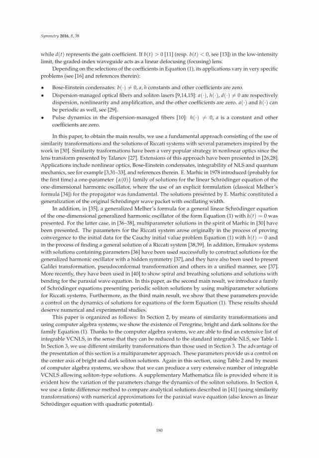
Symmetry 2016, 8, 38

while d(t) represents the gain coefficient. If b(t) > 0 [11] (resp. b(t) < 0, see [13]) in the low-intensitylimit, the graded-index waveguide acts as a linear defocusing (focusing) lens.

Depending on the selections of the coefficients in Equation (1), its applications vary in very specificproblems (see [16] and references therein):

• Bose-Einstein condensates: b(·) �= 0, a, h constants and other coefficients are zero.• Dispersion-managed optical fibers and soliton lasers [9,14,15]: a(·), h(·), d(·) �= 0 are respectively

dispersion, nonlinearity and amplification, and the other coefficients are zero. a(·) and h(·) canbe periodic as well, see [29].

• Pulse dynamics in the dispersion-managed fibers [10]: h(·) �= 0, a is a constant and othercoefficients are zero.

In this paper, to obtain the main results, we use a fundamental approach consisting of the use ofsimilarity transformations and the solutions of Riccati systems with several parameters inspired by thework in [30]. Similarity trasformations have been a very popular strategy in nonlinear optics since thelens transform presented by Talanov [27]. Extensions of this approach have been presented in [26,28].Applications include nonlinear optics, Bose-Einstein condensates, integrability of NLS and quantummechanics, see for example [3,31–33], and references therein. E. Marhic in 1978 introduced (probably forthe first time) a one-parameter {α(0)} family of solutions for the linear Schrödinger equation of theone-dimensional harmonic oscillator, where the use of an explicit formulation (classical Melher’sformula [34]) for the propagator was fundamental. The solutions presented by E. Marhic constituted ageneralization of the original Schrödinger wave packet with oscillating width.

In addition, in [35], a generalized Melher’s formula for a general linear Schrödinger equationof the one-dimensional generalized harmonic oscillator of the form Equation (1) with h(t) = 0 waspresented. For the latter case, in [36–38], multiparameter solutions in the spirit of Marhic in [30] havebeen presented. The parameters for the Riccati system arose originally in the process of provingconvergence to the initial data for the Cauchy initial value problem Equation (1) with h(t) = 0 andin the process of finding a general solution of a Riccati system [38,39]. In addition, Ermakov systemswith solutions containing parameters [36] have been used successfully to construct solutions for thegeneralized harmonic oscillator with a hidden symmetry [37], and they have also been used to presentGalilei transformation, pseudoconformal transformation and others in a unified manner, see [37].More recently, they have been used in [40] to show spiral and breathing solutions and solutions withbending for the paraxial wave equation. In this paper, as the second main result, we introduce a familyof Schrödinger equations presenting periodic soliton solutions by using multiparameter solutionsfor Riccati systems. Furthermore, as the third main result, we show that these parameters providea control on the dynamics of solutions for equations of the form Equation (1). These results shoulddeserve numerical and experimental studies.

This paper is organized as follows: In Section 2, by means of similarity transformations andusing computer algebra systems, we show the existence of Peregrine, bright and dark solitons for thefamily Equation (1). Thanks to the computer algebra systems, we are able to find an extensive list ofintegrable VCNLS, in the sense that they can be reduced to the standard integrable NLS, see Table 1.In Section 3, we use different similarity transformations than those used in Section 3. The advantage ofthe presentation of this section is a multiparameter approach. These parameters provide us a control onthe center axis of bright and dark soliton solutions. Again in this section, using Table 2 and by meansof computer algebra systems, we show that we can produce a very extensive number of integrableVCNLS allowing soliton-type solutions. A supplementary Mathematica file is provided where it isevident how the variation of the parameters change the dynamics of the soliton solutions. In Section 4,we use a finite difference method to compare analytical solutions described in [41] (using similaritytransformations) with numerical approximations for the paraxial wave equation (also known as linearSchrödinger equation with quadratic potential).

180

Symmetry 2016, 8, 38

Table 1. Families of NLS with variable coefficients.

# Variable Coefficient NLS Solutions (j=1,2,3)

1iψt = l0ψxx − bmtm−1+b2t2m

4l0x2ψ

−ibtmxψx − λl0e−btm+1

m+1 |ψ|2ψ

ψj(x, t) = 1√e−btm+1

m+1

ei( btm4 l0x2)uj(x, t)

2iψt = l0ψxx − t−2

2l0x2ψ

+i 1t xψx − λl0t|ψ|2ψ

ψj(x, t) = 1√tei( −1

4t l0x2)uj(x, t)

3iψt = l0ψxx −

(c2

4 l0)

x2ψ

+icxψx − λl0ect|ψ|2ψψj(x, t) = 1√

ect ei( −c4 l0x2)uj(x, t)

4iψt = l0ψxx − b2

4l0tkx2ψ

+ibxψx − λl0ebt|ψ|2ψψj(x, t) = 1√

ebtei( −b

4 l0x2)uj(x, t)

5iψt = l0ψxx − abebt+a2e2bt

4l0x2ψ

−iaebtxψx − λl0ea−aebt

b |ψ|2ψ

ψj(x, t) = 1√e

a−aebtb

ei( aebt4 l0x2)uj(x, t)

6iψt = l0ψxx − 1

4l0x2ψ

−icoth(t)xψx − λl0csch(t)|ψ|2ψψj(x, t) = 1√

csch(t)ei( coth(t)

4 l0x2)uj(x, t)

7iψt = l0ψxx − 1

4l0x2ψ

−itan(t)xψx − λl0cos(t)|ψ|2ψψj(x, t) = 1√

cos(t)ei( tan(t)

4 l0x2)uj(x, t)

8iψt = l0ψxx − bt−1+b2 ln2(t)

4l0x2ψ

−ibln(t)xψx − λl0t−btebt|ψ|2ψψj(x, t) = 1√

−t−btebt ei( bln(t)4 l0x2)uj(x, t)

9iψt = l0ψxx +

14l0

x2ψ + icot(−t)xψx

−λl0csc(t)|ψ|2ψψj(x, t) = 1√

csc(t)ei( −cot(−t)

4 l0x2)uj(x, t)

10iψt = l0ψxx +

14l0

x2ψ − itan(−t)xψx

−λl0sec(t)|ψ|2ψψj(x, t) = 1√

sec(t)ei( tan(−t)

4 l0x2)uj(x, t)

11iψt = l0ψxx − 2abtebt2+a2e2bt2

4l0x2ψ

−iaebt2xψx − λl0e

−a2

√πb er f i(

√bt)|ψ|2ψ

ψj(x, t) = 1√e−a2

√πb er f i(

√bt)

eaebt2

4 l0x2uj(x, t)

12iψt = l0ψxx +

atanh2(bt)(b−a)−ab4l0

x2ψ

−iatanh(bt)xψx − λl0|cosh(bt)|ab |ψ|2ψ

ψj(x, t) = 1√|cosh(bt)|

ab

ei( atanh(bt)4 l0x2)uj(x, t)

13iψt = l0ψxx +

acoth2(bt)(b−a)−ab4l0

x2ψ

−iacoth(bt)xψx − λl0|sinh(bt)|ab |ψ|2ψ

ψj(x, t) = 1√|sinh(bt)|

ab

ei( acoth(bt)4 l0x2)uj(x, t)

14iψt = l0ψxx −

(a2+absinh(bt)+a2sinh2(bt)

4l0

)x2ψ

−iacosh(bt)xψx − λl0e−asinh(bt)

b |ψ|2ψ

ψj(x, t) = 1√e−asinh(bt)

b

ei( acosh(bt)4 l0x2)uj(x, t)

15iψt = l0ψxx −

(a2+absin(bt)−a2sin2(bt)

4l0

)x2ψ

+iacos(bt)xψx − λl0easin(bt)

b |ψ|2ψ

ψj(x, t) = 1√e

asin(bt)b

ei( −acos(bt)4 l0x2)uj(x, t)

16iψt = l0ψxx −

(a2+abcos(bt)−a2cos2(bt)

4l0

)x2ψ

−iasin(bt)xψx + λl0eacos(bt)

b |ψ|2ψ

ψj(x, t) = 1√e

acos(bt)b

ei( −asin(bt)4 l0x2)uj(x, t)

17iψt = l0ψxx − atan2(bt)(a+b)+ab

4l0x2ψ

−iatan(bt)xψx − λl0|cos(bt)|ab |ψ|2ψ

ψj(x, t) = 1√|cos(bt)|

ab

ei( atan(bt)4 l0x2)uj(x, t)

18iψt = l0ψxx − acot2(bt)(a+b)+ab

4l0x2ψ

+iacot(bt)xψx − λl0|sin(bt)|ab |ψ|2ψ

ψj(x, t) = 1√|sin(bt)|

ab

ei( acot(bt)4 l0x2)uj(x, t)

181

Symmetry 2016, 8, 38

Table 2. Riccati equations used to generate the similarity transformations.

# Riccati Equation Similarity Transformation from Table 1

1 y′x = axny2 + bmxm−1 − ab2xn+2m 1

2 (axn + b)y′x = by2 + axn−2 2

3 y′x = axny2 + bxmy + bcxm − ac2xn 3

4 y′x = axny2 + bxmy + ckxk−1 − bcxm+k − ac2xn+2k 1

5 xy′x = axny2 + my − ab2xn+2m 3

6 (axn + bxm + c)y′x = αxky2 + βxsy − αb2xk + βbxs 4

7 y′x = beμxy2 + acecx − a2be(μ+2c)x 5

8 y′x = aeμxy2 + cy − ab2e(μ+2c)x 3

9 y′x = aecxy2 + bnxn−1 − ab2ecxx2n 1

10 y′x = axny2 + bcecx − ab2xne2cx 8

11 y′x = axny2 + cy − ab2xne2cx 3

12 y′x =[

a sinh2(cx)− c]y2 − a sinh2(cx) + c − a 6

13 2y′x = [a − b + a cosh(bx)]y2 + a + b − a cosh(bx) 7

14 y′x = a(ln x)ny2 + bmxm−1 − ab2x2m(ln x)n 1

15 xy′x = axny2 + b − ab2xn ln2 x 8

16 y′x =[b + a sin2(bx)

]y2 + b − a + a sin2(bx) 9

17 2y′x = [b + a + a cos(bx)]y2 + b − a + a cos(bx) 10

18 y′x =[b + a cos2(bx)

]y2 + b − a + a cos2(bx) 10

19 y′x = c(arcsin x)ny2 + ay + ab − b2c(arcsin x)n 3

20 y′x = a(arcsin x)ny2 + βmxm−1 − aβ2x2m(arcsin x)n 1

21 y′x = c(arccos x)ny2 + ay + ab − b2c(arccos x)n 3

22 y′x = a(arccos x)ny2 + βmxm−1 − aβ2x2m(arccos x)n 1

23 y′x = c(arctan x)ny2 + ay + ab − b2c(arctan x)n 3

24 y′x = a(arctan x)ny2 + bmxm−1 − ab2x2m(arctan x)n 1

25 y′x = c(arccot x)ny2 + ay + ab − b2c(arccot x)n 3

26 y′x = a(arccot x)ny2 + bmxm−1 − ab2x2m(arccot x)n 1

27 y′x = f y2 + ay − ab − b2 f 3

28 y′x = f y2 + anxn−1 − a2x2n f 1

29 y′x = f y2 + gy − a2 f − ag 3

30 y′x = f y2 + gy + anxn−1 − axng − a2 f x2n 1

31 y′x = f y2 − axngy + anxn−1 − a2x2n(g − f ) 1

32 y′x = f y2 + abebx − a2e2bx f 5

33 y′x = f y2 + gy + abebx − aebxg − a2e2bx f 5

34 y′x = f y2 − aebxgy + abebx + a2e2bx(g − f ) 5

35 y′x = f y2 + 2abxebx2 − a2 f e2bx2 11

36 y′x = f y2 − a tanh2(bx)(a f + b) + ab 12

37 y′x = f y2 − a coth2(bx)(a f + b) + ab 13

38 y′x = f y2 − a2 f + ab sinh(bx)− a2 f sinh2(bx) 14

39 y′x = f y2 − a2 f + ab sin(bx) + a2 f sin2(bx) 15

40 y′x = f y2 − a2 f + ab cos(bx) + a2 f cos2(bx) 16

41 y′x = f y2 − a tan2(bx)(a f − b) + ab 17

42 y′x = f y2 − a cot2(bx)(a f − b) + ab 18

182

Symmetry 2016, 8, 38

2. Soliton Solutions for VCNLS through Riccati Equations and Similarity Transformations

In this section, by means of a similarity transformation introduced in [42], and using computeralgebra systems, we show the existence of Peregrine, bright and dark solitons for the family Equation(1). Thanks to the computer algebra systems, we are able to find an extensive list of integrablevariable coefficient nonlinear Schrödinger equations (see Table 1). For similar work and applications toBose-Einstein condensates, we refer the reader to [1]

Lemma 1. ([42]) Suppose that h(t) = −l0λμ(t) with λ ∈ R, l0 = ±1 and that c(t), α(t), δ(t), κ(t), μ(t)and g(t) satisfy the equations:

α(t) = l0c(t)

4, δ(t) = −l0

g(t)2

, h(t) = −l0λμ(t), (2)

κ(t) = κ(0)− l04

∫ t

0g2(z)dz, (3)

μ(t) = μ(0)exp(∫ t

0(2d(z)− c(z))dz

)μ(0) �= 0, (4)

g(t) = g(0)− 2l0exp(−

∫ t

0c(z)dz

) ∫ t

0exp

(∫ z

0c(y)dy

)f (z)dz. (5)

Then,

ψ(t, x) =1√μ(t)

ei(α(t)x2+δ(t)x+κ(t))u(t, x) (6)

is a solution to the Cauchy problem for the nonautonomous Schrödinger equation

iψt − l0ψxx − b(t)x2ψ + ic(t)xψx + id(t)ψ + f (t)xψ − ig(t)ψx − h(t)|ψ|2ψ = 0, (7)

ψ(0, x) = ψ0(x), (8)

if and only if u(t, x) is a solution of the Cauchy problem for the standard Schrödinger equation

iut − l0uxx + l0λ|u|2u = 0, (9)

with initial datau(0, x) =

√μ(0)e−i(α(0)x2+δ(0)x+κ(0))ψ0(x). (10)

Now, we proceed to use Lemma 1 to discuss how we can construct NLS with variable coefficientsequations that can be reduced to the standard NLS and therefore be solved explicitly. We startrecalling that

u1(t, x) = A exp(

2iA2t)(3 + 16iA2t − 16A4t2 − 4A2x2

1 + 16A4t2 + 4A2x2

), A ∈ R (11)

is a solution for (l0 = −1 and λ = −2)

iut + uxx + 2|u|2u = 0, t, x ∈ R. (12)

In addition,u2(ξ, τ) = A tanh(Aξ)e−2iA2τ (13)

is a solution of (l0 = −1 and λ = 2)

iuτ + uξξ − 2|u|2u = 0, (14)

183

Symmetry 2016, 8, 38

andu3(τ, ξ) =

√v sech

(√vξ

)exp(−ivτ), v > 0 (15)

is a solution of (l0 = 1 and λ = −2),

iuτ − uξξ − 2|u|2u = 0. (16)

Example 1. Consider the NLS:

iψt + ψxx −c2

4x2ψ − icxψx ± 2ect|ψ|2ψ = 0. (17)

Our intention is to construct a similarity transformation from Equation (17) to standard NLSEquation (9) by means of Lemma 1. Using the latter, we obtain

b(t) =c2

4, c(t) = c, μ(t) = ect,

andα(t) = − c

4, h(t) = ±2ect.

Therefore,

ψ(x, t) =e−i c

4 x2

√ect

uj(x, t), j = 1, 2

is a solution of the form Equation (6), and uj(x, t) are given by Equations (12) and (13).

Example 2. Consider the NLS:

iψt + ψxx −1

2t2 x2ψ − i1t

xψx ± 2t|ψ|2ψ = 0. (18)

By Lemma 1, a Riccati equation associated to the similarity transformation is given by

dcdt

+ c(t)2 − 2t−2 = 0, (19)

and we obtain the functionsb(t) =

12t2 , c(t) = −1

t, μ(t) = t,

α(t) = − 14t

, h1(t) = −2t, h2(t) = 2t.

Using uj(x, t), j = 1 and 2, given by Equations (12) and (13), we get the solutions

ψj(x, t) =e−i 1

4t x2

√t

ui(x, t). (20)

Table 1 shows integrable variable coefficient NLS and the corresponding similarity transformationto constant coefficient NLS. Table 2 lists some Riccati equations that can be used to generatethese transformations.

184

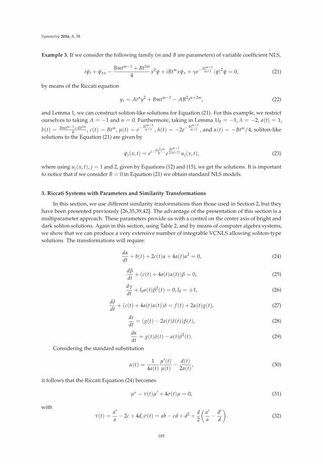
Symmetry 2016, 8, 38

Example 3. If we consider the following family (m and B are parameters) of variable coefficient NLS,

iψt + ψxx −Bmtm−1 + Bt2m

4x2ψ + iBtmxψx + γe−

Btm+1m+1 |ψ|2ψ = 0, (21)

by means of the Riccati equation

yt = Atny2 + Bmtm−1 − AB2tn+2m, (22)

and Lemma 1, we can construct soliton-like solutions for Equation (21). For this example, we restrictourselves to taking A = −1 and n = 0. Furthermore, taking in Lemma 1l0 = −1, λ = −2, a(t) = 1,

b(t) = Bmtm−1+Bt2m

4 , c(t) = Btm, μ(t) = e−Btm+1

m+1 , h(t) = −2e−Btm+1

m+1 , and α(t) = −Btm/4, soliton-likesolutions to the Equation (21) are given by

ψj(x, t) = ei −Bx2tm4 e

Btm+12(m+1) uj(x, t), (23)

where using uj(x, t), j = 1 and 2, given by Equations (12) and (15), we get the solutions. It is importantto notice that if we consider B = 0 in Equation (21) we obtain standard NLS models.

3. Riccati Systems with Parameters and Similarity Transformations

In this section, we use different similarity trasformations than those used in Section 2, but theyhave been presented previously [26,35,39,42]. The advantage of the presentation of this section is amultiparameter approach. These parameters provide us with a control on the center axis of bright anddark soliton solutions. Again in this section, using Table 2, and by means of computer algebra systems,we show that we can produce a very extensive number of integrable VCNLS allowing soliton-typesolutions. The transformations will require:

dα

dt+ b(t) + 2c(t)α + 4a(t)α2 = 0, (24)

dβ

dt+ (c(t) + 4a(t)α(t))β = 0, (25)

dγ

dt+ l0a(t)β2(t) = 0, l0 = ±1, (26)

dδ

dt+ (c(t) + 4a(t)α(t))δ = f (t) + 2α(t)g(t), (27)

dε

dt= (g(t)− 2a(t)δ(t))β(t), (28)

dκ

dt= g(t)δ(t)− a(t)δ2(t). (29)

Considering the standard substitution

α(t) =1

4a(t)μ′(t)μ(t)

− d(t)2a(t)

, (30)

it follows that the Riccati Equation (24) becomes

μ′′ − τ(t)μ′ + 4σ(t)μ = 0, (31)

with

τ(t) =a′

a− 2c + 4d, σ(t) = ab − cd + d2 +

d2

(a′

a− d′

d

). (32)

185

Symmetry 2016, 8, 38

We will refer to Equation (31) as the characteristic equation of the Riccati system. Here, a(t),b(t), c(t), d(t), f (t) and g(t) are real value functions depending only on the variable t. A solution ofthe Riccati system Equations (24)–(29) with multiparameters is given by the following expressions(with the respective inclusion of the parameter l0) [26,35,39]:

μ(t) = 2μ(0)μ0(t)(α(0) + γ0(t)), (33)

α(t) = α0(t)−β2

0(t)4(α(0) + γ0(t))

, (34)

β(t) = − β(0)β0(t)2(α(0) + γ0(t))

=β(0)μ(0)

μ(t)w(t), (35)

γ(t) = l0γ(0)− l0β2(0)4(α(0) + γ0(t))

, l0 = ±1, (36)

δ(t) = δ0(t)−β0(t)(δ(0) + ε0(t))

2(α(0) + γ0(t)), (37)

ε(t) = ε(0)− β(0)(δ(0) + ε0(t))2(α(0) + γ0(t))

, (38)

κ(t) = κ(0) + κ0(t)−(δ(0) + ε0(t))

2

4(α(0) + γ0(t)), (39)

subject to the initial arbitrary conditions μ(0), α(0), β(0) �= 0, γ(0), δ(0), ε(0) and κ(0). α0, β0, γ0, δ0,ε0 and κ0 are given explicitly by:

α0(t) =1

4a(t)μ′

0(t)μ0(t)

− d(t)2a(t)

, (40)

β0(t) = − w(t)μ0(t)

, w(t) = exp(−

∫ t

0(c(s)− 2d(s))ds

), (41)

γ0(t) =d(0)2a(0)

+1

2μ1(0)μ1(t)μ0(t)

, (42)

δ0(t) =w(t)μ0(t)

∫ t

0

[(f (s)− d(s)

a(s)g(s)

)μ0(s) +

g(s)2a(s)

μ′0(s)

]ds

w(s), (43)

ε0(t) = − 2a(t)w(t)μ′

0(t)δ0(t) + 8

∫ t0

a(s)σ(s)w(s)

(μ′0(s))

2 (μ0(s)δ0(s))ds

+2∫ t

0a(s)w(s)

μ′0(s)

[f (s)− d(s)

a(s) g(s)]ds,

(44)

κ0(t) = a(t)μ0(t)μ′

0(t)δ2

0(t)− 4∫ t

0a(s)σ(s)

(μ′0(s))

2 (μ0(s)δ0(s))2ds

−2∫ t

0a(s)

μ′0(s)

(μ0(s)δ0(s))[

f (s)− d(s)a(s) g(s)

]ds,

(45)

with δ0(0) = g0(0)/(2a(0)), ε0(0) = −δ0(0), κ0(0) = 0. Here, μ0 and μ1 represent the fundamentalsolution of the characteristic equation subject to the initial conditions μ0(0) = 0, μ′

0(0) = 2a(0) �= 0and μ1(0) �= 0, μ′

1(0) = 0.Using the system Equations (34)–(39), in [26], a generalized lens transformation is presented.

Next, we recall this result (here we use a slight perturbation introducing the parameter l0 = ±1 inorder to use Peregrine type soliton solutions):

186

Symmetry 2016, 8, 38

Lemma 2 (l0 = 1, [26]). Assume that h(t) = λa(t)β2(t)μ(t) with λ ∈ R. Then, the substitution

ψ(t, x) =1√μ(t)

ei(α(t)x2+δ(t)x+κ(t))u(τ, ξ), (46)

where ξ = β(t)x + ε(t) and τ = γ(t), transforms the equation

iψt = −a(t)ψxx + b(t)x2ψ − ic(t)xψx − id(t)ψ − f (t)xψ + ig(t)ψx + h(t)|ψ|2ψ

into the standard Schrödinger equation

iuτ − l0uξξ + l0λ|u|2u = 0, l0 = ±1, (47)

as long as α, β, γ, δ, ε and κ satisfy the Riccati system Equations (24)–(29) and also Equation (30).

Example 4. Consider the NLS:

iψt = ψxx −x2

4ψ + h(0) sech(t)|ψ|2ψ. (48)

It has the associated characteristic equation μ′′ + aμ = 0, and, using this, we will obtain the functions:

α(t) =coth(t)

4− 1

2csch(t) sech(t), δ(t) = − sech(t), (49)

κ(t) = 1 − tanh(t)2

, μ(t) = cosh(t), (50)

h(t) = h(0) sech(t), β(t) =1

cosh(t), (51)

ε(t) = −1 + tanh(t), γ(t) = 1 − tanh(t)2

. (52)

Then, we can construct solution of the form

ψj(t, x) =1√μ(t)

ei(α(t)x2+δ(t)x+κ(t))uj

(1 − tanh(t)

2,

xcosh(t)

− 1 + tanh(t))

, (53)

with uj, j = 1 and 2, given by Equations (12) and (13).

Example 5. Consider the NLS:

iψt(x, t) = ψxx(x, t) +h(0)β(0)2μ(0)1 + α(0)2c2t

|ψ(x, t)|2ψ(x, t).

It has the characteristic equation μ′′ + aμ = 0, and, using this, we will obtain the functions:

α(t) =14t

− 12 + α(0)4c2

2t2, δ(t) =

δ(0)1 + α(0)2c2t

, (54)

κ(t) = κ(0)− δ(0)2c2t2 + 4α(0)c2t

, h(t) =h(0)β(0)2μ(0)1 + α(0)2c2t

, (55)

μ(t) = (1 + α(0)2c2t)μ(0), β(t) =β(0)

1 + α(0)2c2t,

187

Symmetry 2016, 8, 38

γ(t) = γ(0)− β(0)2c2t2 + 4α(0)c2t

, ε(t) = ε(0)− β(0)δ(0)c2t1 + 2α(0)c2t

.

Then, we can construct a solution of the form

ψj(t, x) = 1√μ(t)

ei(α(t)x2+δ(t)x+κ(t))

uj

(γ(0)− β(0)2c2t

2+4α(0)c2t , β(0)x1+α(0)2c2t + ε(0)− β(0)δ(0)c2t

1+2α(0)c2t

),

(56)

with uj, j = 1 and 2, Equations (12) and (13).

Following Table 2 of Riccati equations, we can use Equation (24) and Lemma 2 to construct anextensive list of integrable variable coefficient nonlinear Schrödinger equations.

4. Crank-Nicolson Scheme for Linear Schrödinger Equation with Variable CoefficientsDepending on Space

In addition, in [35], a generalized Melher’s formula for a general linear Schrödinger equationof the one-dimensional generalized harmonic oscillator of the form Equation (1) with h(t) = 0 waspresented. As a particular case, if b = λ ω2

2 ; f = b, ω > 0, λ ∈ {−1, 0, 1}, c = g = 0, then the evolutionoperator is given explicitly by the following formula (note—this formula is a consequence of Mehler’sformula for Hermite polynomials):

ψ(x, t) = UV(t) f :=1√

2iπμj(t)

∫Rn

eiSV (x,y,t) f (y)dy, (57)

where

SV(x, y, t) =1

μj(t)

(x2

j + y2j

2lj(t)− xjyj

),

{μj(t), lj(t)

}=

⎧⎪⎪⎪⎪⎨⎪⎪⎪⎪⎩

(58)Using Riccati-Ermakov systems in [41], it was shown how computer algebra systems can be used

to derive the multiparameter formulas (33)–(45). This multi-parameter study was used also to studysolutions for the inhomogeneous paraxial wave equation in a linear and quadratic approximationincluding oscillating laser beams in a parabolic waveguide, spiral light beams, and more familiesof propagation-invariant laser modes in weakly varying media. However, the analytical methodis restricted to solve Riccati equations exactly as the ones presented in Table 2. In this section,we use a finite differences method to compare analytical solutions described in [41] with numericalapproximations. We aim (in future research) to extend numerical schemes to solve more general casesthat the analytical method exposed cannot. Particularly, we will pursue to solve equations of thegeneral form:

iψt = −Δψ + V(x, t)ψ, (59)

using polynomial approximations in two variables for the potential function V(x, t) (V(x, t) ≈b(t)

(x2

1 + x22)+ f (t)x1 + g(t)x2 + h(t)). For this purpose, it is necessary to analyze stability of different

methods applied to this equation.

188

Symmetry 2016, 8, 38

We also will be interested in extending this process to nonlinear Schrödinger-type equations withpotential terms dependent on time, such as

iψt = −Δψ + V(x, t)ψ + s|ψ|2ψ. (60)

In this section, we show that the Crank-Nicolson scheme seems to be the best method to deal withreconstructing numerically the analytical solutions presented in [41].

Numerical methods arise as an alternative when it is difficult to find analytical solutions of theSchrödinger equation. Despite numerical schemes not providing explicit solutions to the problem,they do yield approaches to the real solutions which allow us to obtain some relevant properties of theproblem. Most of the simplest and often-used methods are those based on finite differences.

In this section, the Crank-Nicolson scheme is used for linear Schrödinger equation in the case ofcoefficients depending only on the space variable because it is absolutely stable and the matrix of theassociate system does not vary for each iteration.

A rectangular mesh (xm, tn) is introduced in order to discretize a bounded domain Ω × [0, T] inspace and time. In addition, τ and h represent the size of the time step and the size of space step,respectively. xm and h are in R if one-dimensional space is considered; otherwise, they are in R

2.The discretization is given by the matrix system

(I +

iaτ

2h2 Δ +iτ2

V(x)

)ψn+1 =

(I − iaτ

2h2 Δ − iτ2

V(x)

)ψn, (61)

where I is the identity matrix, Δ is the discrete representation of the Laplacian operator in space, andV(x) is the diagonal matrix that represents the operator of the external potential depending on x.

The paraxial wave equation (also known as harmonic oscillator)

2iψt + Δψ − r2ψ = 0, (62)

where r = x for x ∈ R or r =√

x21 + x2

2 for x ∈ R2, describes the wave function for a laser beam [40].

One solution for this equation can be presented as Hermite-Gaussian modes on a rectangulardomain:

ψnm(x, t) = Anmexp[i(κ1+κ2)+2i(n+m+1)γ]√

2n+mn!m!πβ

× exp[i(αr2 + δ1x1 + δ2x2

)− (βx1 + ε1)

2/2 − (βx2 + ε2)2/2

]× Hn(βx1 + ε1)Hm(βx2 + ε2),

(63)

where Hn(x) is the n-th order Hermite polynomial in the variable x, see [40,41].In addition, some solutions of the paraxial equation may be expressed by means of

Laguerre–Gaussian modes in the case of cylindrical domains (see [43]):

ψmn (x, t) = Am

n

√n!

π(n+m)! β

× exp[i(αr2 + δ1x1 + δ2x2 + κ1 + κ2

)− (βx1 + ε1)

2/2 − (βx2 + ε2)2/2

]× exp[i(2n + m + 1)γ](β(x1 ± ix2) + ε1 ± iε2)

m

× Lmn

((βx1 + ε1)

2 + (βx2 + ε2)2)

,

(64)

with Lmn (x) being the n-th order Laguerre polynomial with parameter m in the variable x.

α, β, γ, δ1, δ2, ε1, ε2, κ1 and κ2 given by Equations (34)–(39) for both Hermite-Gaussian andLaguerre-Gaussian modes.

Figures 1 and 2 show two examples of solutions of the one-dimensional paraxial equation withΩ = [−10, 10] and T = 12. The step sizes are τ = 10

200 and h = 10200 .

189

Symmetry 2016, 8, 38

(a) (b)

Figure 1. (a) corresponding approximation for the one-dimensional Hermite-Gaussian beam with t = 10.

The initial condition is√

23√

πe(

23 x)2/2; (b) the exact solution for the one-dimensional Hermite-Gaussian

beam with t = 10, An = 1, μ0 = 1, α0 = 0, β0 = 49 , n0 = 0, δ0 = 0, γ0 = 0, ε0 = 0, κ0 = 0.

(a) (b)

Figure 2. (a) corresponding approximation for the one-dimensional Hermite-Gaussian beam with t = 10.

The initial condition is√

23√

πe(

23 x)2/2+ix; (b) the exact solution for the one-dimensional Hermite-Gaussian

beam with t = 10, An = 1, μ0 = 1, α0 = 0, β0 = 49 , n0 = 0, δ0 = 1, γ0 = 0, ε0 = 0, κ0 = 0.

Figure 3 shows four profiles of two-dimensional Hermite-Gaussian beams considering Ω =

[−6, 6]× [−6, 6] and T = 10. The corresponding step sizes are τ = 1040 and h =

(1248 , 12

48

).

190

Symmetry 2016, 8, 38

(a)

(b)

(c)

(d)

Figure 3. (Left): corresponding approximations for the two-dimensional Hermite-Gaussian beams

with t = 10. The initial conditions are (a) 1√8π

e−(x2+y2); (b) 1√2π

e−(x2+y2)x; (c)√

2π e−(x2+y2)xy;

(d) 14√

32πe−(x2+y2)

(8x2 − 2

)(8y2 − 2

). (Right): the exact solutions for the two-dimensional

Hermite-Gaussian beams with t = 10 and parameters Anm = 14 , α0 = 0, β0 =

√2, δ0,1 = 1, γ0,1 =

0, ε0,1 = 0, κ0,1 = 0. For (a) n = 0 and m = 0, for (b) n = 1 and m = 0, for (c) n = 1 and m = 1, for (d)n = 2 and m = 2.

191

Symmetry 2016, 8, 38

Figure 4 shows two profiles of two-dimensional Laguerre–Gaussian beams considering Ω =

[−6, 6]× [−6, 6] and T = 10. The corresponding step sizes are τ = 1040 and h =

(1248 , 12

48

).

(a)

(b)

Figure 4. (Left): corresponding approximations for the two-dimensional Laguerre–Gaussian beamswith t = 10. The initial conditions are (a) 1√

4πe−(x2+y2)(x + iy); (b) 1√

2πe−(x2+y2)(x + iy)

(1 − x2 − y2).

(Right): the exact solutions for the two-dimensional Laguerre–Gaussian beams with t = 10 andparameters Am

n = 14 , α0 = 0, β0 =

√2, δ0,1 = 1, γ0,1 = 0, ε0,1 = 0, κ0,1 = 0.

5. Conclusions

Rajendran et al. in [1] used similarity transformations introduced in [28] to show a list of integrableNLS equations with variable coefficients. In this work, we have extended this list, using similaritytransformations introduced by Suslov in [26], and presenting a more extensive list of families ofintegrable nonlinear Schrödinger (NLS) equations with variable coefficients (see Table 1 as a primarylist. In both approaches, the Riccati equation plays a fundamental role. The reader can observethat, using computer algebra systems, the parameters (see Equations (33)–(39)) provide a change ofthe dynamics of the solutions; the Mathematica files are provided as a supplement for the readers.Finally, we have tested numerical approximations for the inhomogeneous paraxial wave equationby the Crank-Nicolson scheme with analytical solutions. These solutions include oscillating laserbeams and Laguerre and Gaussian beams. The explicit solutions have been found previously thanksto explicit solutions of Riccati-Ermakov systems [41].

Supplementary Materials: The following are available online at http://www.mdpi.com/2073-8994/8/5/38/s1,Mathematica supplement file.

Acknowledgments: The authors were partially funded by the Mathematical American Association through NSF(grant DMS-1359016) and NSA (grant DMS-1359016). Also, the authors are thankful for the funding receivedfrom the Department of Mathematics and Statistical Sciences and the College of Liberal Arts and Sciences atUniversity of Puerto Rico, Mayagüez. E. S. is funded by the Simons Foundation Grant # 316295 and by theNational Science Foundation Grant DMS-1440664. E.S is also thankful for the start up funds and the “Faculty

192

Symmetry 2016, 8, 38

Development Funding Program Award" received from the School of Mathematics and Statistical Sciences and theCollege of Sciences at University of Texas, Rio Grande Valley.

Author Contributions: The original results presented in this paper are the outcome of a research collaborationstarted during the Summer 2015 and continuous until Spring 2016. Similarly, the selection of the examples,tables, graphics and extended bibliography is the result of a continuous long interaction between the authors.

Conflicts of Interest: The authors declare no conflict of interest.

References

1. Rajendran, S.; Muruganandam, P.; Lakshmanan, M. Bright and dark solitons in a quasi-1D Bose–Einsteincondensates modelled by 1D Gross–Pitaevskii equation with time-dependent parameters. Phys. D NonlinearPhenom. 2010, 239, 366–386. [CrossRef]

2. Agrawal, G.-P. Nonlinear Fiber Optics, 4th ed.; Academic Press: New York, NY, USA, 2007.3. Al Khawaja, U. A comparative analysis of Painlevé, Lax Pair and similarity transformation methods in

obtaining the integrability conditions of nonlinear Schrödinger equations. J. Phys. Math. 2010, 51. [CrossRef]4. Brugarino, T.; Sciacca, M. Integrability of an inhomogeneous nonlinear Schrödinger equation in Bose-Einstein

condensates and fiber optics. J. Math. Phys. 2010, 51. [CrossRef]5. Chen, H.-M.; Liu, C.S. Solitons in nonuniform media. Phys. Rev. Lett. 1976, 37, 693–697. [CrossRef]6. He, X.G.; Zhao, D.; Li, L.; Luo, H.G. Engineering integrable nonautonomous nonlinear Schrödinger equations.

Phys. Rev. E. 2009, 79. [CrossRef] [PubMed]7. He, J.; Li, Y. Designable inegrability of the variable coefficient nonlinear Schrödinger equations. Stud. Appl.

Math. 2010, 126, 1–15. [CrossRef]8. He, J.S.; Charalampidis, E.G.; Kevrekidis, P.G.; Frantzeskakis, D.J. Rogue waves in nonlinear Schrödinger

models with variable coefficients: Application to Bose-Einstein condensates. Phys. Lett. A 2014, 378, 577–583.[CrossRef]

9. Kruglov, V.I.; Peacock, A.C.; Harvey, J.D. Exact solutions of the generalized nonlinear Schrödinger equationwith distributed coefficients. Phys. Rev. E 2005, 71. [CrossRef] [PubMed]

10. Marikhin, V.G.; Shabat, A.B.; Boiti, M.; Pempinelli, F. Self-similar solutions of equations of the nonlinearSchrödinger type. J. Exp. Theor. Phys. 2000, 90, 553–561. [CrossRef]

11. Ponomarenko, S.A.; Agrawal, G.P. Do Solitonlike self-similar waves exist in nonlinear optical media?Phys. Rev. Lett. 2006, 97. [CrossRef] [PubMed]

12. Ponomarenko, S.A.; Agrawal, G.P. Optical similaritons in nonlinear waveguides. Opt. Lett. 2007, 32,1659–1661. [CrossRef] [PubMed]

13. Raghavan, S.; Agrawal, G.P. Spatiotemporal solitons in inhomogeneous nonlinear media. Opt. Commun.2000, 180, 377–382. [CrossRef]

14. Serkin, V.N.; Hasegawa, A. Novel Soliton solutions of the nonlinear Schrödinger Equation model. Phys. Rev.Lett. 2000, 85. [CrossRef] [PubMed]

15. Serkin, V.; Matsumoto, M.; Belyaeva, T. Bright and dark solitary nonlinear Bloch waves in dispersionmanaged fiber systems and soliton lasers. Opt. Commun. 2001, 196, 159–171. [CrossRef]

16. Tian, B.; Shan, W.; Zhang, C.; Wei, G.; Gao, Y. Transformations for a generalized variable-coefficient nonlinearSchrödinger model from plasma physics, arterial mechanics and optical fibers with symbolic computation.Eur. Phys. J. B 2005, 47, 329–332. [CrossRef]

17. Dai, C.-Q.; Wang, Y.-Y. Infinite generation of soliton-like solutions for complex nonlinear evolution differentialequations via the NLSE-based constructive method. Appl. Math. Comput. 2014, 236, 606–612. [CrossRef]

18. Wang, M.; Shan, W.-R.; Lü, X.; Xue, Y.-S.; Lin, Z.-Q.; Tian, B. Soliton collision in a general coupled nonlinearSchrödinger system via symbolic computation. Appl. Math. Comput. 2013, 219, 11258–11264. [CrossRef]

19. Yu, F.; Yan, Z. New rogue waves and dark-bright soliton solutions for a coupled nonlinear Schrödingerequation with variable coefficients. Appl. Math. Comput. 2014, 233, 351–358. [CrossRef]

20. Fibich, G. The Nonlinear Schrödinger Equation, Singular Solutions and Optical Collapse; Springer:Berlin/Heidelberg, Germany, 2015.

21. Kevrekidis, P.G.; Frantzeskakis, D.J.; Carretero-Gonzáles, R. Emergent Nonlinear Phenomena in Bose-EinsteinCondensates: Theory and Experiment; Springer Series of Atomic, Optical and Plasma Physics; Springer:Berlin/Heidelberg, Germany, 2008; Volume 45.

193

Symmetry 2016, 8, 38

22. Suazo, E.; Suslov, S.-K. Soliton-Like solutions for nonlinear Schrödinger equation with variable quadraticHamiltonians. J. Russ. Laser Res. 2010, 33, 63–83. [CrossRef]

23. Sulem, C.; Sulem, P.L. The Nonlinear Schrödinger Equation; Springer: New York, NY, USA, 1999.24. Tao, T. Nonlinear dispersive equations: Local and global analysis. In CBMS Regional Conference Series in

Mathematics; American Mathematical Society: Providence, RI, USA, 2006.25. Zakharov, V.-E.; Shabat, A.-B. Exact theory of two-dimensional self-focusing and one-dimensional

self-modulation of waves in nonlinear media. Soviet. Phys. JETP 1972, 34, 62–69.26. Suslov, S.-K. On integrability of nonautonomous nonlinear Schrödinger equations. Proc. Am. Math. Soc.

2012, 140, 3067–3082. [CrossRef]27. Talanov, V.I. Focusing of light in cubic media. JETP Lett. 1970, 11, 199–201.28. Perez-Garcia, V.M.; Torres, P.J.; Konotop, V.K. Similarity transformations for nonlinear Schrödinger equations

with time-dependent coefficients. Physica D 2006, 221, 31–36. [CrossRef]29. Ablowitz, M.; Hooroka, T. Resonant intrachannel pulse interactions in dispersion-managed transmission

systems. IEEE J. Sel. Top. Quantum Electron. 2002, 8, 603–615. [CrossRef]30. Marhic, M.E. Oscillating Hermite-Gaussian wave functions of the harmonic oscillator. Lett. Nuovo Cim. 1978,

22, 376–378. [CrossRef]31. Carles, R. Nonlinear Schrödinger equation with time dependent potential. Commun. Math. Sci. 2010, 9,

937–964. [CrossRef]32. López, R.M.; Suslov, S.K.; Vega-Guzmán, J.M. On a hidden symmetry of quantum harmonic oscillators.

J. Differ. Equ. Appl. 2013, 19, 543–554. [CrossRef]33. Aldaya, V.; Cossío, F.; Guerrero, J.; López-Ruiz, F.F. The quantum Arnold transformation. J. Phys. A Math.

Theor. 2011, 44, 1–6. [CrossRef]34. Feynman, R.P.; Hibbs, A.R. Quantum Mechanics and Path Integrals; McGraw-Hill: New York, NY, USA, 1965.35. Cordero-Soto, R.; Lopez, R.M.; Suazo, E.; Suslov, S.K. Propagator of a charged particle with a spin in uniform

magnetic and perpendicular electric fields. Lett. Math. Phys. 2008, 84, 159–178. [CrossRef]36. Lanfear, N.; López, R.M.; Suslov, S.K. Exact wave functions for a generalized harmonic oscillators. J. Russ.

Laser Res. 2011, 32, 352–361. [CrossRef]37. López, R.M.; Suslov, S.K.; Vega-Guzmán, J.M. Reconstructing the Schrödinger groups. Phys. Scr. 2013, 87,

1–6. [CrossRef]38. Suazo, E.; Suslov, S.K. Cauchy problem for Schrödinger equation with variable quadratic Hamiltonians.

2011. to be submitted.39. Suazo, E. Fundamental Solutions of Some Evolution Equations. Ph.D. Thesis, Arizona State University,

Tempe, AZ, USA, September 2009.40. Mahalov, A.; Suazo, E.; Suslov, S.K. Spiral laser beams in inhomogeneous media. Opt. Lett. 2013, 38,

2763–2766. [CrossRef] [PubMed]41. Koutschan, C.; Suazo, E.; Suslov, S.K. Fundamental laser modes in paraxial optics: From computer algebra

and simulations to experimental observation. Appl. Phys. B 2015, 121, 315–336. [CrossRef]42. Escorcia, J.; Suazo, E. Blow-up results and soliton solutions for a generalized variable coefficient nonlinear

Schrödinger equation. Available online: http://arxiv.org/abs/1605.07554 (accessed on 24 May 2016).43. Andrews, L.C.; Phillips, R.L. Laser Beam Propagation through Random Media, 2nd ed.; SPIE Press: Bellingham,

WA, USA, 2005.

© 2016 by the authors. Licensee MDPI, Basel, Switzerland. This article is an open accessarticle distributed under the terms and conditions of the Creative Commons Attribution(CC BY) license (http://creativecommons.org/licenses/by/4.0/).

194

symmetryS S

Article

Coherent States of Harmonic and ReversedHarmonic Oscillator

Alexander Rauh

Department of Physics, University of Oldenburg, Oldenburg D-26111, Germany;alexander.rauh@uni-oldenburg.de; Tel.:+49-441-798-3460

Academic Editor: Young Suh KimReceived: 16 January 2016; Accepted: 3 June 2016; Published: 13 June 2016

Abstract: A one-dimensional wave function is assumed whose logarithm is a quadratic form inthe configuration variable with time-dependent coefficients. This trial function allows for generaltime-dependent solutions both of the harmonic oscillator (HO) and the reversed harmonic oscillator(RO). For the HO, apart from the standard coherent states, a further class of solutions is derived witha time-dependent width parameter. The width of the corresponding probability density fluctuates,or "breathes" periodically with the oscillator frequency. In the case of the RO, one also obtainsnormalized wave packets which, however, show diffusion through exponential broadening with time.At the initial time, the integration constants give rise to complete sets of coherent states in the threecases considered. The results are applicable to the quantum mechanics of the Kepler-Coulombproblem when transformed to the model of a four-dimensional harmonic oscillator with a constraint.In the classical limit, as was shown recently, the wave packets of the RO basis generate thehyperbolic Kepler orbits, and, by means of analytic continuation, the elliptic orbits are also obtainedquantum mechanically.

Keywords: inverted harmonic oscillator; harmonic trap; Kepler-Coulomb problem;Kustaanheimo-Stiefel transformation

1. Introduction

Coherent states of the harmonic oscillator (HO) were introduced already at the beginning ofwave mechanics [1]. Much later, such states were recognized as being useful as a basis to describeradiation fields [2] and optical correlations [3]. The reversed harmonic oscillator (RO) refers to a modelwith repulsive harmonic forces, and was discussed in [4] in the context of irreversibility. Recently, in [5],which also communicates historical remarks, the RO was applied to describe nonlinear optical phenomena.As mentioned in [5], the term “inverted harmonic oscillator” (IO) originally refers to a model withnegative kinetic and potential energy, as proposed in [6]. Nevertheless, most articles under the headlineIO, actually consider the RO model, see, e.g., [7–9].

The RO model formally can be obtained by assuming a purely imaginary oscillator frequency. It isthen not anymore possible to construct coherent states by means of creation and annihilation operators;for a text book introduction see [10]. In [9], the RO was generalized by the assumption of a time-dependentmass and frequency. The corresponding Schrödinger equation was solved by means of an algebraicmethod with the aim to describe quantum tunneling.

In the present study, emphasis is laid on the derivation of complete sets of coherent states both forthe HO and the RO model, together with their time evolution. In the case of the HO, in addition tothe standard coherent states, a further function set is found with a time-dependent width parameter.Both in the HO and RO case, the integration constants of the time-dependent solutions induce completefunction sets which, at time t = 0, are isomorphic to the standard coherent states of the HO.

Symmetry 2016, 8, 46 195 www.mdpi.com/journal/symmetry

Symmetry 2016, 8, 46

In Section 6, an application to the quantum mechanics of the Kepler-Coulomb problem will bebriefly discussed. As has first been observed by Fock [11], the underlying four-dimensional rotationsymmetry of the non-relativistic Hamiltonian of the hydrogen atom permits the transformation tothe problem of four isotropic harmonic oscillators with a constraint; for applications see, e.g., [12–14].The transformation proceeds conveniently by means of the Kustaanheimo-Stiefel transformation [15].In [14], the elliptic Kepler orbits were derived in the classical limit on the basis of coherent HO states.By means of coherent RO states, the classical limit for hyperbolic Kepler orbits was achieved in [16,17],whereby the elliptic regime could be obtained by analytic continuation from the hyperbolic side.Recently, by means of the same basis, a first order quantum correction to Kepler’s equation wasderived in [18], whereby the smallness parameter was defined by the reciprocal angular momentum inunits of h.

As compared to the classical elliptic Kepler orbits, the derivation of hyperbolic orbits fromquantum mechanics was accomplished quite recently [16,17]. For this achievement, it was crucial todevise a suitable time-dependent ansatz for the wave function, see (1) below, in order to constructcoherent RO states. As it turns out, the wave function (1) contains also the usual coherent HOstates, and, unexpectedly, a further set of coherent states, which we call type-II states. The latterare characterized by a time-dependent width parameter and are solutions of the time-dependentSchrödinger equation of the HO. Section 4 contains the derivation. Essentially, the type-II states offer adisposable width parameter which allows us, for instance, to describe arbitrarily narrowly peaked initialstates together with their time evolution in a harmonic potential. In this paper, a unified derivationis presented of coherent states of the HO, RO, and type-II HO states. Furthermore, the connection ofHO and RO with the quantum mechanics of the Kepler-Coulomb problem is briefly discussed in thecontext of the derivation of the classical Kepler orbits from quantum mechanics.

2. Introducing a Trial Wave Function

In order to solve the Schrödinger equation for the harmonic oscillator (HO) and the reversedoscillator (RO), a trial wave function of Gaussian type is assumed as follows

ψ(x, t) = C0 exp[C(t) + B(t)x − Γ(t)x2

], x ∈ R, Real(Γ) > 0, (1)

where C, B, Γ are complex functions of time t and C0 the time-independent normalization constant.When the Schrödinger operator [i h∂t − H] is applied to ψ for a Hamiltonian with harmonic potential,then the wave function ψ is reproduced up to a factor which is a quadratic polynomial and mustvanish identically in the configuration variable x:

0 = p0(t) + p1(t)x + p2(t)x2. (2)

The conditions p0 = 0, p1 = 0, and p2 = 0, give rise to three first-order differential equationsfor the functions C(t), B(t), and Γ(t). In the following we examine two cases for the HO: type-I andtype-II are characterized by a constant and time-dependent function Γ, respectively. In the case of theRO, only a time-dependent Γ leads to a solution. By a suitable choice of the parameters, the ansatz (1)solves the time-dependent Schrödinger equation both for the HO and the RO Hamiltonian

H = p2/(2m) + (mω2/2)x2 and HΩ = p2/(2m)− (mΩ2/2)x2, ω, Ω > 0,

respectively.

3. Standard (Type-I) Coherent States of the HO

In the following, the time-dependent solutions are derived, within the trial function scheme,for the Hamiltonian

H = p2/(2m) + (mω2/2)x2 = (hω/2)[−∂2

ζ + ζ2]

, (3)

196

Symmetry 2016, 8, 46

where ζ = αx is dimensionless with α2 = mω/h. For later comparison, we list the standard definitionof coherent states from the textbook [10], see Equations (4.72) and (4.75):

|z〉 = exp[−1

2zz∗

] ∞

∑n=0

zn√

n!|n〉, (4)

ψz(ζ) = π−1/4 exp[−1

2(zz∗ + z2)

]exp

[−1

2ζ2 +

√2ζz

], ζ = αx, α2 =

mω

h, (5)

where ψz(ζ) = 〈ζ|z〉, |n〉 denotes the n-th energy eigenvector, and the star superscript meanscomplex conjugation. The time evolution gives rise to, see [10],

|z, t〉 = exp[−i ωt/2] |z exp[−i ωt]〉, (6)

ψz(ζ, t) = exp[−i ωt/2]ψ(z exp[−i ωt])(ζ). (7)

The state |z〉 is minimal with respect to the position-momentum uncertainty product Δx Δp,and there exists the following completeness property, see [3],

1π

∫ ∞

0udu

∫ 2π

0dϕ |z〉〈z| = ∑

n|n〉〈n|, z = u exp[i ϕ]. (8)

The relation (8) follows immediately from the definition (4). An equivalent statement is

1π

∫ ∞

0udu

∫ 2π

0dϕ 〈ζ2|z〉〈z|ζ1〉 = δ(ζ2 − ζ1), (9)

which corresponds to the completeness of the energy eigenfunctions of the harmonic oscillator.In Appendix B, we reproduce a proof of (9), which is appropriate, since the proof has to be extended tothe modified coherent states in the type-II HO and the RO cases.

In terms of the scaled variables ζ and τ = tω, the trial ansatz reads

ψ(ζ, τ) = C0 exp[c(τ) + β(τ)ζ − γ(τ)ζ2/2

], (10)

where c, β, γ are dimensionless functions of τ, and the re-scaling factor of the probability density,1/

√α, is taken into the normalization constant C0.We assume that γ = γ0 = const. Then, the polynomial (2) gives rise to the equations

γ20 = 1, i β′(τ) = β(τ), 2i c′(t) = 1 − β2(t), (11)

which implies that γ0 = 1 is fixed. The further solutions emerge easily as

β(τ) = C2 exp[−i τ], c(τ) = −i τ/2 − (C22/4) exp[−2i τ] + C3, (12)

where C2 and C3 are complex integration constants. A comparison with (5), at t = 0, suggests to set

C2 =√

2 z, C3 = −(1/2)zz∗, (13)

which specifies the functions β and c as follows

β(τ) =√

2 (z exp[−i τ)], c(t) = −i τ/2 − (1/2)[zz∗ + (z exp[−i τ])2

]. (14)

197

Symmetry 2016, 8, 46

The normalization integral with respect to ζ amounts to the condition

C20√

π exp[zz∗] = 1; (15)

hence (7) with (5) is reproduced.

4. Type-II Solutions of the Harmonic Oscillator

With γ being a function of time, one obtains the following differential equations with primedenoting the derivative with respect to the scaled time τ:

i γ′ = γ2 − 1, i β′ = γ β; 2i c′ = γ − β2. (16)

The solution for γ is

γ(τ) =exp(2i τ)− C1

exp(2i τ) + C1C1 =

1 − γ0

1 + γ0. γ0 = γ(0). (17)

Splitting γ into its real and imaginary parts, one can write

γ(τ) = γR + i γI ; γR = (1 − C21)N−1

1 , γI = 2 C1N−11 sin(2τ),

N1(τ) = 1 + C21 + 2C1 cos(2τ) = 4(1 + γ0)

−2[1 + (γ2

0 − 1) sin2(τ)]

. (18)

In order that the wave function is square integrable, γR has to be positive, which implies that

C21 < 1 or γ0 > 0. (19)

The initial value γ(t = 0) ≡ γ0 > 0 emerges as a disposable parameter.The probability density, P = |ψ(ζ, τ)|2, is characterized by a width of order of magnitude

d = 1/√

γR:

d(τ) =√[

1 + (γ20 − 1) sin2(τ)

]/γ0. (20)

Obviously, the width fluctuates, or "breathes", periodically with time. Of course, this is not abreathing mode as observed in systems of confined interacting particles, see [19,20], e.g.,

Integration of the β equation leads to

β = C2 exp(i τ) [exp(2i τ) + C1]−1 = C2N−1

1 [exp(−i τ) + exp(i τ)C1] . (21)

Later on, the complex integration constant C2 ≡ A2 + i B2 will serve as a state label. The thirddifferential equation of (16) amounts to

c(τ) = i τ/2 − C22 [4 (exp(2i τ) + C1)]

−1 − (1/2) ln(√

exp(2i τ) + C1

)+ C3. (22)

By reasons explained in Appendix A, we dispose of the integration constant C3 as follows

C3 = −(1 + γ0)(8γ0)−1(A2

2 + γ0B22), C2 = A2 + i B2. (23)

In Appendix A, the probability density P is derived in the following form

P(ξ, τ) =C2

0√N1

exp[−γR (ξ − βR/γR)

2]

, (24)

198

Symmetry 2016, 8, 46

where the time-dependent functions γR and N1 are defined through (17) and (18), and βR comes out as

βR(τ) = (1/8)(1 + γ0)−1N−1

1 [A2 cos(τ) + B2 sin(τ)] . (25)

The complex integration constant C2 corresponds to the familiar complex quantum number z inthe case of the standard coherent states; hence, the real numbers A2, B2 characterize different states.The normalization constant C0 obeys the following condition, see Appendix A,

1 = (1/2)C20

√π/γ0(1 + γ0). (26)

4.1. Completeness of Type-II States

Combining the above results, we write the time-dependent wave function as follows

ψ(ξ, τ) =C0√

exp(2i τ) + C1exp

[C3 −

C22 (exp(−2i τ) + C1)

4N1+ β(τ)ξ − γ(τ)ξ2/2

], (27)

where γ, β, and C3 are defined in (18), (21), and (23), respectively. Let us consider ψ at zero time:

ψ(ξ, 0) =C0√

1 + C1exp

[C3 −

C22

4(1 + C1)+ C2(1 + γ0) ξ/2 − γ0ξ2/2

]. (28)

In (28), we set ξ = ξ/√

γ0 to write

ψ(ξ, 0) =C0γ−1/4

0√1 + C1

exp

[C3 −

C22

4(1 + C1)+ C2(1 + γ0)/

√γ0 ξ/2 − ξ2/2

]. (29)

Now we substitute the complex variable z for the integration constant C2 as follows

C21 + γ0

2√

γ0=

√2 z (30)

and obtain

ψ(ξ, 0) =C0√

1 + C1exp

[C3 − z2 γ0

1 + γ0+√

2 z ξ − ξ2/2]

. (31)

In C3, given in (23), we make the following replacements which are induced by (30):

A2 → κ(z + z∗), B2 → −i κ(z − z∗), κ =√

2γ0/(1 + γ0). (32)

There occur some nice cancelations, and one obtains

ψz(ξ) =C0γ−1/4

0√1 + C1

exp[−1

2

(zz∗ + z2

)+ i D +

√2 z ξ − ξ2/2

], D =

1 − γ0

2(1 + γ0)Im(z2). (33)

Comparison with (5) shows that the wave function (33) has the same structure apart from thepurely imaginary phase i D. The latter drops out in the completeness proof, see (A15) in Appendix B.As a consequence, the states (33) form a complete set of states with respect to the state label z.

At τ = 0, the states (33) differ from the standard coherent states (5) by the state dependent phaseD, through the variables ζ and ζ which denote the differently scaled space variable x, and also throughthe different definition of the quantum number z, which for simplicity was denoted by the samesymbol in (30). Essentially, type-I and type-II states differ by their time evolution and width parameterγ0 which is equal to α2 = mω/h and to an arbitrary positive number, respectively.

199

Symmetry 2016, 8, 46

4.2. Mean Values and Uncertainty Product

In the following, we list mean values for the time-dependent states (27) including the positionmomentum uncertainty product Δxp. They are periodic in time with the oscillator angular frequencyω ≡ 2π/T. The uncertainty product is minimal at the discrete times tn = (1/4)nT, n = 0, 1, . . . .For comparison, the traditional coherent states are always minimal [10]. We use the abbreviations(Δx)2 = 〈x2〉 − 〈x〉2 and (Δv)2 = 〈v2〉 − 〈v〉2 for the mean square deviations of position andvelocity, respectively.

〈x(τ)〉 = (1/α)(1 + γ0)(2γ0)−1 [A2 cos(τ) + B2γ0 sin(τ)] ; (34)

〈v(τ)〉 = hα(2mγ0)−1 [−A2 sin(τ) + γ0B2 cos(τ)] ; (35)

(Δx)2 = (4α2γ0)

−1[1 + γ2

0 + (1 − γ20) cos(2τ)

]; (36)

(Δv)2 = h2α2(4m2γ0)

−1[1 + γ2

0 + (γ20 − 1) cos(2τ)

]; (37)

〈H〉 = hω(8γ20)

−1[(1 + γ0)

2(

A22 + γ2

0B22

)+ 2γ0(1 + γ2

0)]

. (38)

It is noticed that the mean square deviations do not depend on the state label (A2, B2).The uncertainty product follows immediately from (36) and (37) as

Δxp := (Δx)2(Δp)

2 ≡ m2(Δx)2(Δv)2 =h2

16γ20

[(1 + γ2

0)2 − (1 − γ2

0)2 cos2(2τ)

]. (39)

In the special case γ0 = 1, the product is always minimal. As a matter of fact, γ0 = 1 is the type-Icase of Section 3.

By (38), the mean energy does not depend on time and is positive definite, as it must be. The limitto the standard case with γ0 = 1, gives the known result

〈H〉γ0=1 = hω(zz∗ + 1/2). (40)

and the state with z = 0 is the ground state of the HO with zero point energy hω/2.

5. Wave Packet Solutions for the RO

For convenience, we will keep the same symbols for the trial functions γ(τ), β(τ), and c(τ).Setting ω = i Ω with Ω > 0, implies that α2 = −mΩ/h. In the coherent state (5), the exponential part,−ζ2/2 ≡ −(mω/h)x2/2, is then replaced by +(mΩ/h)x2/2, which precludes normalization.

We introduce 1/αΩ as the new length parameter and define the dimensionless magnitudes

ζ = αΩx, τ = t Ω, with α2Ω = mΩ/h. (41)

The Schrödinger equation, with the ansatz (10), has to be solved for the RO Hamiltonian

HΩ = p2/(2m)− mΩ2/2 x2 = −hΩ/2[∂2

ζ + ζ2]

. (42)

From (2), the following differential equations result:

i γ′(τ) = 1 + γ2(τ), i β′(τ) = γ(τ)β(τ), 2i c′(τ) = γ(τ)− β2(τ), (43)

200

Symmetry 2016, 8, 46

where, as compared with the HO case in (16), only the equation for γ differs. Beginning with γ,one successively obtains the following solutions

γ(τ) = −i tanh(τ + i C1), (44)

β(τ) = C2/ cosh(τ + i C1), (45)

c(τ) = C3 − (1/2) ln (cosh(τ + i C1)) + (i /2)C22 tanh(τ + i C1), (46)

where C1, C2, C3 are integration constants. We assume that

γ0 ≡ γ(0) = tan(C1) > 0, 0 < C1 < π/2, (47)

which implies thatcos(C1) = (1 + γ2

0)−1/2, sin(C1) = γ0(1 + γ2

0)−1/2. (48)

In order to decompose the functions c(τ), β(τ), γ(τ) into their real and imaginary parts, we takeover the following abbreviations from [16]

f (τ) = cosh(τ)− i γ0 sinh(τ), h(τ) = [ f f ∗]−1. (49)

After the decompositions β = βR + i β I , γ = γR + i γI , C2 = A2 + i B2, we infer from (44) to (46):

γR = h(τ)γ0, γI = − (h(τ)/2) (1 + γ20) sinh(2τ); (50)

βR = h(τ)√

1 + γ20 [A2 cosh(τ) + γ0B2 sinh(τ)] ,

β I = h(τ)√

1 + γ20 [B2 cosh(τ)− γ0 A2 sinh(τ)] ; (51)

exp[c(τ)] = [cosh(τ + i C1)]−1/2 exp

[C3 − C2

2γ(τ)/2]

. (52)

According to (50), γR is larger zero, which makes the wave function (10) a normalizable wave packet.The probability density reads:

P(ζ, τ) = C20 exp

[c + c∗ + 2βRζ − γRζ2

]. (53)

Integration with respect to ζ leads to the normalization condition

1 = C20

√π/γR exp

[c(τ) + c∗(τ) + β2

R/γR

]. (54)

The normalization constant C0 was determined in [16] for real constants C2. With C2 = A2 + i B2,we dispose of the integration constant C3 as

C3 = −(1/2)(A22/γ0 + B2

2γ0) (55)

to obtain in a straightforward manner

C20 =

√π(γ−1

0 + γ0), (56)

which is a time independent condition as it must be.With the aid of elementary trigonometric manipulations and the normalization constant C0 given

in (56), the wave function can be written as follows

ψ(ζ, τ) = (γ0/π)1/4√

h(τ) f (τ) exp[C3 − (1/2)C2

2γ(τ) + β(τ)ζ − γ(τ)ζ2/2]

. (57)

201

Symmetry 2016, 8, 46

5.1. Coherent States of the RO

As before, let us consider the wave function at time t = 0, where in particular h = f = 1:

ψ(ζ, 0) ≡ ψ(ζ, τ = 0) = (γ0/π)1/4 exp[

C3 − 1/2C22γ0 + C2

√1 + γ2

0 ζ − γ0ζ2/2]

. (58)

After the re-scaling ζ → ζ with ζ =√

γ0 ζ, one obtains

Ψ(ζ, 0) = π−1/4 exp[

C3 − 1/2C22γ0 + C2

√(1 + γ2

0)/γ0 ζ − ζ2/2]

. (59)

In view of the standard HO wave function (5), we replace the integration constant C2 by z:

C2

√(1 + γ2

0)/γ0 =√

2 z (60)

and obtainΨz(ζ) = π−1/4 exp

[C3 − γ2

0 z2/(1 + γ20) +

√2 z ζ − ζ2/2

]. (61)

In C3, given in (55), the relation (60) gives rise to the substitutions

A2 → κ1(z + z∗), B2 → −i κ1(z − z∗), κ1 = (1/2)√

2γ0/(1 + γ20), (62)

and hence toC3 =

[4(1 + γ2

0)]−1 [

(γ20 − 1)(z2 + z∗z∗)− 2(1 + γ2

0)zz∗]

. (63)

After some elementary re-arrangements, one finds

Ψz(ζ) =1

π1/4 exp[−1

2(zz∗ + z2) + i D1 +

√2 z ζ − ζ2

2

], D1 =

1 − γ20

2(1 + γ20)

Im(z2). (64)

Apart from the purely imaginary phase i D1, the wave functions Ψz are the same as the standardcoherent states (5). Since in the completeness proof the D1 phase drops out, see (A15) in Appendix B,the states Ψz form a complete function set.

5.2. Mean Values

With the aid of Mathematica [21], we get the following mean values for position x, velocity v,their mean square deviations (Δx)2, (Δv)2, and the mean energy 〈HΩ〉:

〈x〉 = (αΩ)−1√

1 + γ−20 [A2 cosh(τ) + γ0B2 sinh(τ)] ; (65)

(Δx)2 =(

2α2Ωγ0

)−1 [cosh2(τ) + γ2

0 sinh2(τ)]

; (66)

〈v〉 = (hαΩ/m)√

1 + γ−20 [A2 sinh(τ) + γ0B2 cosh(τ)] ; (67)

(Δv)2 = (hαΩ/(2m))2 γ−10

[γ2

0 − 1 + (1 + γ20) cosh(2τ)

]; (68)

〈HΩ〉 = hΩ(4γ0)−1

[γ2

0 − 1 + 2(γ0 + γ−10 )

(γ2

0B22 − A2

2

)]. (69)

The mean energy does not depend on time, as it must be. With the aid of (62), the mean energycould also be expressed in terms of the complex state label z. Since A2 and B2 are arbitrary real

202

Symmetry 2016, 8, 46

numbers, the mean energy can have any positive or negative value. From (66) and (68) one infers theposition-momentum uncertainty product Δxp as

Δ2xp(τ) = h2/(8γ2

0)[cosh2(τ) + γ2

0 sinh(τ)] [

γ20 − 1 + (1 + γ2

0) cosh(2τ)]

. (70)

This product obeys the inequality

Δ2xp(τ) > Δ2

xp(0) = h2/4, τ > 0. (71)

Obviously, the uncertainty product is minimal at τ = 0, which means for the coherent states (64).By (66), the wave packets broaden exponentially with time.

6. Application to the Kepler-Coulomb Problem

The connection of the non-relativistic Hamiltonian for the hydrogen atom with the modelof a four-dimensional oscillator is conveniently achieved by means of the Kustaanheimo-Stiefeltransformation [15], which we write as follows [16,22]

u1 =√

r cos(θ/2) cos(ϕ − Φ); u2 =√

r cos(θ/2) sin(ϕ − Φ);u3 =

√r sin(θ/2) cos(Φ); u4 =

√r sin(θ/2) sin(Φ),

(72)

where r, θ, ϕ are three-dimensional polar coordinates with r > 0, 0 < θ < π, 0 ≤ ϕ < 2π,and 0 ≤ Φ < 2π generates the extension to the fourth dimension. The vector u = {u1, u2, u3, u3}covers the R4 and the volume elements are related as [16]

du1du2du3du4 = (1/8)r sin(θ)drdθdϕdΦ. (73)

The stationary Schrödinger equation Hψ = Eψ for the Hamiltonian H = p2/(2m) − λ/r istransformed into the following form of a four-dimensional harmonic oscillator [14]:

HuΨ(u) = λΨ(u), Hu = −h2/(8m)Δu − E u · u, Δu = ∂2u1+ ...∂2

u4(74)

with the constraint∂ΦΨ(u) = 0. (75)

It should be noticed that, by (72), the components u2i have the dimension of a length rather than

length square. As a consequence, in the evolution equation i h∂σΨ = HuΨ, the parameter σ, which hasthe dimension time/length, is not the time parameter of the original problem. For negative energieswith E < 0, four-dimensional coherent oscillator states (of type-I) were used in [14] to show that ellipticorbits emerge in the classical limit whereby σ turns out being proportional to the eccentric anomaly.

In the spectrum of positive energies (ionized states of the hydrogen atom) with E > 0,coherent states of the RO were constructed in [16] and gave rise to hyperbolic orbits in the classical limit;by analytic continuation, also the elliptic orbits were derived from the RO states in the classicallimit [17]. In addition, Kepler’s equation was obtained by the assumption that time-dependence entersthrough the curve parameter σ only. Recently [18], based on the coherent RO states, the first orderquantum correction to Kepler’s equation could be established for the smallness parameter ε = h/Lwhere L denotes the orbital angular momentum.

7. Conclusions

Besides the standard coherent states of the harmonic oscillator (H0), a further solution family ofthe time-dependent Schrödinger equation was derived with the following properties: (i) The functionsare normalizable of Gaussian type and contain a disposable width parameter. The latter allows us,for instance, to use arbitrarily concentrated one-particle states independently of the parameters of

203

Symmetry 2016, 8, 46

a harmonic trap; (ii) The functions are complete and isomorphic to the standard coherent states attime t = 0; (iii) The states minimize the position-momentum uncertainty product at the discrete timesTn = n π/(2ω), n = 0, 1, . . . ; (iv) The width of the wave packets “breathes” periodically with periodT/2 = π/ω. (v) There is no diffusion, T = 2π/ω is the recurrence time of the states.

In the case of the reversed harmonic oscillator (RO), there exists only one family of time-dependentsolutions. They share the properties (i) and (ii) of the type-II HO states, and (iii) is fulfilled at time t = 0,only. There is no recurrence, instead there is diffusion with a broadening which increases exponentiallywith time. The application to the Kepler-Coulomb problem was briefly discussed. The HO coherentstates of type-I and the RO coherent states served as basis to derive, in the classical limit, the ellipticKepler orbits [14] and the hyperbolic ones [16,17], respectively.

Acknowledgments: The author expresses his gratitude to Jürgen Parisi for his constant encouragement andsupport. He also profited from his critical reading of the manuscript.

Conflicts of Interest: The author declares no conflict of interest.

Appendix. Probability Density for Type-II States

We have to decompose the functions β(τ) and c(τ), as given by (21)and (22), into their real andimaginary parts. To this end, we set C2 = A2 + i B2 with real constants A2 and B2 and β = βR + i β I .Using the definitions of N1 and C1 in terms of γ0, we obtain

βR =1 + γ0

2A2 cos(τ) + B2γ0 sin(τ)

1 + (γ20 − 1) sin2(τ)

,

β I =1 + γ0

2B2 cos(τ)− A2γ0 sin(τ)

1 + (γ20 − 1) sin2(τ)

. (A1)

In view of the function c(τ), we make use of the following auxiliary relations

Fc ≡ −C22 [4 (exp(2i τ) + C1)]

−1 = FR + i FI ,

FR = (1/(4N1))[(B2

2 − A22) cos(2τ)− 2A2B2 sin(2τ) + (B2

2 − A22)C1

],

FI = (1/(4N1))[(A2

2 − B22) sin(2τ)− 2A2B2 cos(2τ)− 2A2B2C1

], (A2)

exp [c(τ) + c∗(τ)] = (1/√

N1) exp [2C3 + 2FR] , (A3)

where the integration constant C3 is assumed being real and the star suffix means complex conjugation.The probability density P results from the wave function (10) in the form

P(ξ, τ) =C2

0√N1

exp[2C3 + 2FR + 2βRξ − γRξ2

], (A4)

where C0 is defined through the normalization integral

1 =∫ ∞

−∞dξ P(ξ, τ) =

C20√

π√N1γR

exp(G), G = 2C3 + 2FR + β2R/γR. (A5)

From the expression of G, it is not obvious that C0 is independent of τ which was assumed in (10).Clearly, since Φ := ψ/C0 obeys the Schrödinger equation and H is hermitian, one has the property

∂τ〈Φ|Φ〉 = 0. (A6)

As a matter of fact, it is straightforward to show that

2FR + β2R/γR =

[B2

2(C1 − 1)− A22(1 + C1)

] [2(C2

1 − 1)]−1

(A7)

204

Symmetry 2016, 8, 46

does not depend on τ. We now dispose of the integration constant C3 such that the exponentG vanishes:

C3 = −[

B22(C1 − 1)− A2

2(1 + C1)] [

4(C21 − 1)

]−1. (A8)

In view of G = 0, we replace 2C3 + 2FR by −β2R/γR, so that

P(ξ, τ) =C2

0√N1

exp[−γR (ξ − βR/γR)

2]

, (A9)

which is the result (24). The normalization condition comes out immediately in the form

1 =C2

0√

π√N1γR

=C2

0√

π√1 − C2

1

=C2

0√

π(1 + γ0)

2√

γ0. (A10)

Appendix. Proof of Completeness

In order to prove the completeness of the functions (5), i.e., for the type-I HO case, we takeadvantage of the following generating function of the Hermite polynomials [23]:

exp[2XZ − Z2

]=

∞

∑n=0

Zn

n!Hn(X). (A11)

In the function (5), we replace z by√

2 Z to obtain

ψz(ζ) = π−1/4 exp[−ZZ∗ − (1/2)ζ2

]exp

[−Z2 + 2ζZ

]. (A12)

With the aid of (A11), one can write

ψz(ζ) = exp [−(1/2)zz∗]∞

∑n=0

zn√

n!ϕn(ζ), (A13)

whereϕn(ζ) =

1√n!2n

√π

Hn(ζ) exp[−(1/2)ζ2

]. (A14)

By means of (A13) and setting z = u exp[i ϕ], we obtain

〈ζ2|z〉〈z|ζ1〉 = exp[−u2

] ∞

∑m,n=0

un+m exp [i (m − n)ϕ]√m!n!

ϕm(ζ2)ϕn(ζ1). (A15)

In (A15), the ϕ integration projects out the terms n = m with the result

1π

∫ ∞

0udu

∫ 2π

0dϕ 〈ζ2|z〉〈z|ζ1〉 = 2

∫ ∞

0udu exp[−u2]

∞

∑n=0

u2n

n!ϕn(ζ2)ϕn(ζ1). (A16)

After changing the integration variable u → v with v = u2 with udu = dv/2, one uses

∫ ∞

0dv

vn

n!exp[−v] = 1, n = 0, 1, . . . (A17)

and, in view of the completeness of the Hermite polynomials, arrives at

1π

∫ ∞

0udu

∫ 2π

0dϕ 〈ζ2|z〉〈z|ζ1〉 =

∞

∑n=0

ϕn(ζ2)ϕn(ζ1) = δ (ζ2 − ζ1) . (A18)

205

Symmetry 2016, 8, 46

In the type-II HO and the RO cases, there appear additional purely imaginary phases in thewave function, which do not depend on ζ1, ζ2, and drop out at the step (A15) of the completenessproof above.

References

1. Schrödinger, E. Der stetige Übergang von der Mikro-zur Makromechanik. Naturwissenschaften 1926, 14,664–666.

2. Glauber, R.J. Coherent and incoherent states of the radiation field. Phys. Rev. 1963, 131, 2766.3. Glauber, R.J. Photon Correlations. Phys. Rev. Lett. 1963, 10, 84.4. Antoniou, I.E.; Progogine, I. Intrinsic irreversibility and integrability of dynamics. Phys. A Stat. Mech. Appl.

1993, 192, 443–464.5. Gentilini, S.; Braidotti, M.C.; Marcucci, G.; DelRe, E.; Conti, C. Physical realization of the Glauber

quantum oscillator. Sci. Rep. 2015, 5, 15816.6. Glauber, R.J. Amplifiers, attenuators, and schrödinger’s cat. Ann. N. Y. Acad. Sci. 1986, 480, 336–372.7. Barton, G. Quantum mechanis of the inverted oscillator potential. Ann. Phys. 1986, 166, 322–363.8. Bhaduri, R.K.; Khare, A.; Reimann, S.M.; Tomisiek, E.L. The riemann zeta function and the inverted harmonic

oscillator. Ann. Phys. 1997, 264, 25–40.9. Guo, G.-J.; Ren, Z.-Z.; Ju, G.-X.; Guo, X.-Y. Quantum tunneling effect of a time-dependent inverted

harmonic oscillator. J. Phys. A Math. Theor. 2011, 44, 185301.10. Galindo, A.; Pascual, P. Quantum Mechanics I; Springer: Berlin, Germany, 1990.11. Fock, V.A. Zur Theorie des Wassenstoffatoms. Z. Phys. 1935, 98, 145–154.12. Chen, A.C. Hydrogen atom as a four-dimensional oscillator. Phys. Rev. A 1980, 22, 333–335.13. Gracia-Bondia, J.M. Hydrogen atom in the phase-space formulation of quantum mechanics. Phys. Rev. A

1984, 30, 691–697.14. Gerry, C.C. Coherent states and the Kepler-Coulomb problem. Phys. Rev. A 1986, 33, 6–11.15. Kustaanheimo, P.; Stiefel, E. Perturbation theory of Kepler motion based on spinor regularization. J. Reine

Angew. Math. 1965, 218, 204–219.16. Rauh, A.; Parisi, J. Quantum mechanics of hyperbolic orbits in the Kepler problem. Phys. Rev. A 2011,

83, 042101.17. Rauh, A.; Parisi, J. Quantum mechanics of Kepler orbits. Adv. Stud. Theor. Phys. 2014, 8, 889–938.18. Rauh, A.; Parisi, J. Quantum mechanical correction to Kepler’s equation. Adv. Stud. Theor. Phys. 2016, 10,

1–22.19. Baletto, F.; Riccardo, F. Structural properties of nanoclusters: Energetic, thermodynamic, and kinetic effects.

Rev. Mod. Phys. 2015, 77, 371–423.20. Bauch, S.; Balzer, K.; Bonitz, M. Quantum breathing mode of trapped bosons and fermions at arbitrary coupling.

Phys. Rev. B 2009, 80, 054515.21. Wolfram Research, Inc. Mathematica; Version 10.1.0.0; Wolfram Research, Inc.: Champaign, IL, USA, 2015.22. Chen, C.; Kibler, M. Connection between the hydrogen atom and the four-dimensional oscillator. Phys. Rev. A

1985, 31, 3960–3963.23. Gradshteyn, I.S.; Ryzhik, I.M. Table of Integrals, Series, and Products; Academic Press: New York, NY, USA, 1965.

c© 2016 by the author. Licensee MDPI, Basel, Switzerland. This article is an open accessarticle distributed under the terms and conditions of the Creative Commons Attribution(CC BY) license (http://creativecommons.org/licenses/by/4.0/).

206

symmetryS S

Article

Entangled Harmonic Oscillators andSpace-Time Entanglement

Sibel Baskal 1, Young S. Kim 2,* and Marilyn E. Noz 3

1 Department of Physics, Middle East Technical University, 06800 Ankara, Turkey;baskal@newton.physics.metu.edu.tr

2 Center for Fundamental Physics, University of Maryland College Park, College Park, MD 20742, USA3 Department of Radiology, New York University School of Medicine, New York, NY 10016, USA;

marilyn.noz@med.nyu.edu* Correspondence: yskim@umd.edu; Tel.: +1-301-937-6306

Academic Editor: Sergei D. OdintsovReceived: 26 February 2016; Accepted: 20 June 2016; Published: 28 June 2016

Abstract: The mathematical basis for the Gaussian entanglement is discussed in detail, as well as itsimplications in the internal space-time structure of relativistic extended particles. It is shown that theGaussian entanglement shares the same set of mathematical formulas with the harmonic oscillatorin the Lorentz-covariant world. It is thus possible to transfer the concept of entanglement to theLorentz-covariant picture of the bound state, which requires both space and time separations betweentwo constituent particles. These space and time variables become entangled as the bound state moveswith a relativistic speed. It is shown also that our inability to measure the time-separation variableleads to an entanglement entropy together with a rise in the temperature of the bound state. As wasnoted by Paul A. M. Dirac in 1963, the system of two oscillators contains the symmetries of the O(3, 2)de Sitter group containing two O(3, 1) Lorentz groups as its subgroups. Dirac noted also that thesystem contains the symmetry of the Sp(4) group, which serves as the basic language for two-modesqueezed states. Since the Sp(4) symmetry contains both rotations and squeezes, one interesting caseis the combination of rotation and squeeze, resulting in a shear. While the current literature is mostlyon the entanglement based on squeeze along the normal coordinates, the shear transformation is aninteresting future possibility. The mathematical issues on this problem are clarified.

Keywords: Gaussian entanglement; two coupled harmonic oscillators; coupled Lorentz groups;space-time separation; Wigner’s little groups; O(3, 2) group; Dirac’s generators for twocoupled oscillators

PACS: 03.65.Fd, 03.65.Pm, 03.67.-a, 05.30.-d

1. Introduction

Entanglement problems deal with fundamental issues in physics. Among them, the Gaussianentanglement is of current interest not only in quantum optics [1–4], but also in other dynamicalsystems [3,5–8]. The underlying mathematical language for this form of entanglement is that ofharmonic oscillators. In this paper, we present first the mathematical tools that are and may be usefulin this branch of physics.

The entangled Gaussian state is based on the formula:

1cosh η ∑

k(tanh η)kχk(x)χk(y) (1)

where χn(x) is the nth excited-state oscillator wave function.

Symmetry 2016, 8, 55 207 www.mdpi.com/journal/symmetry

Symmetry 2016, 8, 55

In Chapter 16 of their book [9], Walls and Milburn discussed in detail the role of this formula inthe theory of quantum information. Earlier, this formula played the pivotal role for Yuen to formulatehis two-photon coherent states or two-mode squeezed states [10]. The same formula was used byYurke and Patasek in 1987 [11] and by Ekert and Knight [12] for the two-mode squeezed state whereone of the photons is not observed. The effect of entanglement is to be seen from the beam splitterexperiments [13,14].

In this paper, we point out first that the series of Equation (1) can also be written as a squeezedGaussian form:

1√π

exp{−1

4

[e−2η(x + y)2 + e2η(x − y)2

]}(2)

which becomes:1√π

exp{−1

2

(x2 + y2

)}(3)

when η = 0.We can obtain the squeezed form of Equation (2) by replacing x and y by x′ and y′,

respectively, where: (x′

y′

)=

(cosh η − sinh η

− sinh η cosh η

)(xy

)(4)

If x and y are replaced by z and t, Equation (4) becomes the formula for the Lorentz boost along the zdirection. Indeed, the Lorentz boost is a squeeze transformation [3,15].

The squeezed Gaussian form of Equation (2) plays the key role in studying boosted bound statesin the Lorentz-covariant world [16–20], where z and t are the space and time separations between twoconstituent particles. Since the mathematics of this physical system is the same as the series given inEquation (1), the physical concept of entanglement can be transferred to the Lorentz-covariant boundstate, as illustrated in Figure 1.

Figure 1. One mathematics for two branches of physics. Let us look at Equations (1) and (2) applicableto quantum optics and special relativity, respectively. They are the same formula from the Lorentzgroup with different variables as in the case of the Inductor-Capacitor-Resistor (LCR) circuit and themechanical oscillator sharing the same second-order differential equation.

We can approach this problem from the system of two harmonic oscillators. In 1963, Paul A. M.Dirac studied the symmetry of this two-oscillator system and discussed all possible transformations

208

Symmetry 2016, 8, 55

applicable to this oscillator [21]. He concluded that there are ten possible generators of transformationssatisfying a closed set of commutation relations. He then noted that this closed set corresponds to theLie algebra of the O(3, 2) de Sitter group, which is the Lorentz group applicable to three space-like andtwo time-like dimensions. This O(3, 2) group has two O(3, 1) Lorentz groups as its subgroups.

We note that the Lorentz group is the language of special relativity, while the harmonicoscillator is one of the major tools for interpreting bound states. Therefore, Dirac’s two-oscillatorsystem can serve as a mathematical framework for understanding quantum bound systems in theLorentz-covariant world.

Within this formalism, the series given in Equation (1) can be produced from the ten-generatorDirac system. In discussing the oscillator system, the standard procedure is to use the normalcoordinates defined as:

u =x + y√

2, and v =

x − y√2

(5)

In terms of these variables, the transformation given in Equation (4) takes the form:(u′

v′

)=

(e−η 0

0 eη

)(uv

)(6)

where this is a squeeze transformation along the normal coordinates. While the normal-coordinatetransformation is a standard procedure, it is interesting to note that it also serves as a Lorentz boost [18].

With these preparations, we shall study in Section 2 the system of two oscillators and coordinatetransformations of current interest. It is pointed out in Section 3 that there are ten different generatorsfor transformations, including those discussed in Section 2. It is noted that Dirac derived ten generatorsof transformations applicable to these oscillators, and they satisfy the closed set of commutationrelations, which is the same as the Lie algebra of the O(3, 2) de Sitter group containing two Lorentzgroups among its subgroups. In Section 4, Dirac’s ten-generator symmetry is studied in the Wignerphase-space picture, and it is shown that Dirac’s symmetry contains both canonical and Lorentztransformations.

While the Gaussian entanglement starts from the oscillator wave function in its ground state,we study in Section 5 the entanglements of excited oscillator states. We give a detailed explanation ofhow the series of Equation (1) can be derived from the squeezed Gaussian function of Equation (2).

In Section 6, we study in detail how the sheared state can be derived from a squeezed state.It appears to be a rotated squeezed state, but this is not the case. In Section 7, we study what happenswhen one of the two entangled variables is not observed within the framework of Feynman’s rest ofthe universe [22,23].

In Section 8, we note that most of the mathematical formulas in this paper have been usedearlier for understanding relativistic extended particles in the Lorentz-covariant harmonic oscillatorformalism [20,24–28]. These formulas allow us to transport the concept of entanglement from thecurrent problem of physics to quantum bound states in the Lorentz-covariant world. The timeseparation between the constituent particles is not observable and is not known in the present formof quantum mechanics. However, this variable effects the real world by entangling itself with thelongitudinal variable.

2. Two-Dimensional Harmonic Oscillators

The Gaussian form: [1√π

]1/4exp

(− x2

2

)(7)

is used for many branches of science. For instance, we can construct this function by throwing dice.

209

Symmetry 2016, 8, 55

In physics, this is the wave function for the one-dimensional harmonic oscillator in the groundstate. This function is also used for the vacuum state in quantum field theory, as well as the zero-photonstate in quantum optics. For excited oscillator states, the wave function takes the form:

χn(x) =[

1√π2nn!

]1/2Hn(x) exp

(−x2

2

)(8)

where Hn(x) is the Hermite polynomial of the nth degree. The properties of this wave function arewell known, and it becomes the Gaussian form of Equation (7) when n = 0.

We can now consider the two-dimensional space with the orthogonal coordinate variables x andy and the same wave function with the y variable:

χm(y) =[

1√π2mm!

]1/2Hm(y) exp

(−y2

2

)(9)

and construct the function:ψn,m(x, y) = [χn(x)] [χm(y)] (10)

This form is clearly separable in the x and y variables. If n and m are zero, the wave function becomes:

ψ0,0(x, y) =1√π

exp{−1

2

(x2 + y2

)}(11)

Under the coordinate rotation: (x′

y′

)=

(cos θ − sin θ

sin θ cos θ

)(xy

)(12)

this function remains separable. This rotation is illustrated in Figure 2. This is a transformation veryfamiliar to us.

We can next consider the scale transformation of the form:(x′

y′

)=

(eη 00 e−η

)(xy

)(13)

This scale transformation is also illustrated in Figure 2. This area-preserving transformation is knownas the squeeze. Under this transformation, the Gaussian function is still separable.

If the direction of the squeeze is rotated by 45◦, the transformation becomes the diagonaltransformation of Equation (6). Indeed, this is a squeeze in the normal coordinate system. This form ofsqueeze is most commonly used for squeezed states of light, as well as the subject of entanglements.It is important to note that, in terms of the x and y variables, this transformation can be written asEquation (4) [18]. In 1905, Einstein used this form of squeeze transformation for the longitudinal andtime-like variables. This is known as the Lorentz boost.

In addition, we can consider the transformation of the form:(x′

y′

)=

(1 2α

0 1

)(xy

)(14)

This transformation shears the system as is shown in Figure 2.After the squeeze or shear transformation, the wave function of Equation (10) becomes

non-separable, but it can still be written as a series expansion in terms of the oscillator wave functions.It can take the form:

ψ(x, y) = ∑n,m

An,mχn(x)χm(y) (15)

210

Symmetry 2016, 8, 55

with:

∑n,m

|An,m|2 = 1

if ψ(x, y) is normalized, as was the case for the Gaussian function of Equation (11).

2.1. Squeezed Gaussian Function

Under the squeeze along the normal coordinate, the Gaussian form of Equation (11) becomes:

ψη(x, y) =1√π

exp{−1

4

[e−2η(x + y)2 + e2η(x − y)2

]}(16)

which was given in Equation (2). This function is not separable in the x and y variables. These variablesare now entangled. We obtain this form by replacing, in the Gaussian function of Equation (11), the xand y variables by x′ and y′, respectively, where:

x′ = (cosh η)x − (sinh η)y, and y′ = (cosh η)y − (sinh η)x (17)

This form of squeeze is illustrated in Figure 3, and the expansion of this squeezed Gaussian functionbecomes the series given in Equation (1) [20,26]. This aspect will be discussed in detail in Section 5.

y y

yy

Rotation

Squeeze Shear

x

xx

Start

x

Figure 2. Transformations in the two-dimensional space. The object can be rotated, squeezed orsheared. In all three cases, the area remains invariant.

x

squeezed

y

.

Figure 3. Squeeze along the 45 ◦C direction, discussed most frequently in the literature.

211

Symmetry 2016, 8, 55

In 1976 [10], Yuen discussed two-photon coherent states, often called squeezed states of light.This series expansion served as the starting point for two-mode squeezed states. More recently, in 2003,Giedke et al. [1] used this formula to formulate the concept of the Gaussian entanglement.

There is another way to derive the series. For the harmonic oscillator wave functions, there arestep-down and step-up operators [17]. These are defined as:

a =1√2

(x +

∂

∂x

), and a† =

1√2

(x − ∂

∂x

)(18)

If they are applied to the oscillator wave function, we have:

a χn(x) =√

n χn−1(x), and a† χn(x) =√

n + 1 χn+1(x) (19)

Likewise, we can introduce b and b† operators applicable to χn(y):

b =1√2

(y +

∂

∂y

), and b† =

1√2

(y − ∂

∂y

)(20)

Thus (a†)n

ψ0(x) =√

n! χn(x)(b†)n

ψ0(y) =√

n!χn(y) (21)

and:a χ0(x) = b χ0(y) = 0 (22)

In terms of these variables, the transformation leading the Gaussian function of Equation (11) to itssqueezed form of Equation (16) can be written as:

exp{η

2

(a†b† − a b

)}(23)

which can also be written as:

exp{−η

(x

∂

∂y+ y

∂

∂x

)}(24)

Next, we can consider the exponential form:

exp{(tanh η)a†b†)

}(25)

which can be expanded as:

∑n

1n!(tanh η)n

(a†b†

)n(26)

If this operator is applied to the ground state of Equation (11), the result is:

∑n(tanh η)nχn(x)χn(y) (27)

This form is not normalized, while the series of Equation (1) is. What is the origin of this difference?There is a similar problem with the one-photon coherent state [29,30]. There, the series comes

from the expansion of the exponential form:

exp{

αa†}

(28)

212

Symmetry 2016, 8, 55

which can be expanded to:

∑n

1n!

αn(

a†)n

(29)

However, this operator is not unitary. In order to make this series unitary, we consider theexponential form:

exp(

αa† − α∗a)

(30)

which is unitary. This expression can then be written as:

e−αα∗/2[exp

(αa†)]

[exp (α∗a)] (31)

according to the Baker–Campbell–Hausdorff (BCH) relation [31,32]. If this is applied to the groundstate, the last bracket can be dropped, and the result is:

e−αα∗/2 exp[αa†]

(32)

which is the unitary operator with the normalization constant:

e−αα∗/2

Likewise, we can conclude that the series of Equation (27) is different from that of Equation (1)due to the difference between the unitary operator of Equation (23) and the non-unitary operator ofEquation (25). It may be possible to derive the normalization factor using the BCH formula, but itseems to be intractable at this time. The best way to resolve this problem is to present the exactcalculation of the unitary operator leading to the normalized series of Equation (11). We shall return tothis problem in Section 5, where squeezed excited states are studied.

2.2. Sheared Gaussian Function

In addition, there is a transformation called “shear,” where only one of the two coordinates istranslated, as shown in Figure 2. This transformation takes the form:(

x′

y′

)=

(1 2α

0 1

)(xy

)(33)

which leads to: (x′

y′

)=

(x + 2αy

y

)(34)

This shear is one of the basic transformations in engineering sciences. In physics, this transformationplays the key role in understanding the internal space-time symmetry of massless particles [33–35].This matrix plays the pivotal role during the transition from the oscillator mode to the damping modein classical damped harmonic oscillators [36,37].

Under this transformation, the Gaussian form becomes:

ψshr(x, y) =1√π

exp{−1

2

[(x − 2αy)2 + y2

]}(35)

It is possible to expand this into a series of the form of Equation (15) [38].The transformation applicable to the Gaussian form of Equation (11) is:

exp(−2αy

∂

∂x

)(36)

213

Symmetry 2016, 8, 55

and the generator is:

− iy∂

∂x(37)

It is of interest to see where this generator stands among the ten generators of Dirac.However, the most pressing problem is whether the sheared Gaussian form can be regarded as

a rotated squeezed state. The basic mathematical issue is that the shear matrix of Equation (33) istriangular and cannot be diagonalized. Therefore, it cannot be a squeezed state. Yet, the Gaussianform of Equation (35) appears to be a rotated squeezed state, while not along the normal coordinates.We shall look at this problem in detail in Section 6.

3. Dirac’s Entangled Oscillators

Paul A. M. Dirac devoted much of his life-long efforts to the task of making quantum mechanicscompatible with special relativity. Harmonic oscillators serve as an instrument for illustrating quantummechanics, while special relativity is the physics of the Lorentz group. Thus, Dirac attempted toconstruct a representation of the Lorentz group using harmonic oscillator wave functions [17,21].

In his 1963 paper [21], Dirac started from the two-dimensional oscillator whose wave functiontakes the Gaussian form given in Equation (11). He then considered unitary transformations applicableto this ground-state wave function. He noted that they can be generated by the following tenHermitian operators:

L1 =12

(a†b + b†a

), L2 =

12i

(a†b − b†a

)

L3 =12

(a†a − b†b

), S3 =

12

(a†a + bb†

)

K1 = −14

(a†a† + aa − b†b† − bb

)

K2 =i4

(a†a† − aa + b†b† − bb

)

K3 =12

(a†b† + ab

)

Q1 = − i4

(a†a† − aa − b†b† + bb

)

Q2 = −14

(a†a† + aa + b†b† + bb

)

Q3 =i2

(a†b† − ab

)(38)

He then noted that these operators satisfy the following set of commutation relations.

[Li, Lj] = iεijkLk, [Li, Kj] = iεijkKk, [Li, Qj] = iεijkQk

[Ki, Kj] = [Qi, Qj] = −iεijkLk, [Li, S3] = 0

[Ki, Qj] = −iδijS3, [Ki, S3] = −iQi, [Qi, S3] = iKi (39)

Dirac then determined that these commutation relations constitute the Lie algebra for the O(3, 2)de Sitter group with ten generators. This de Sitter group is the Lorentz group applicable to three space

214

Symmetry 2016, 8, 55

coordinates and two time coordinates. Let us use the notation (x, y, z, t, s), with (x, y, z) as the spacecoordinates and (t, s) as two time coordinates. Then, the rotation around the z axis is generated by:

L3 =

⎛⎜⎜⎜⎜⎜⎝

0 −i 0 0 0i 0 0 0 00 0 0 0 00 0 0 0 00 0 0 0 0

⎞⎟⎟⎟⎟⎟⎠ (40)

The generators L1 and L2 can also be constructed. The K3 and Q3 generators will take the form:

K3 =

⎛⎜⎜⎜⎜⎜⎝

0 0 0 0 00 0 0 0 00 0 0 i 00 0 i 0 00 0 0 0 0

⎞⎟⎟⎟⎟⎟⎠ , Q3 =

⎛⎜⎜⎜⎜⎜⎝

0 0 0 0 00 0 0 0 00 0 0 0 i0 0 0 0 00 0 i 0 0

⎞⎟⎟⎟⎟⎟⎠ (41)

From these two matrices, the generators K1, K2, Q1, Q2 can be constructed. The generator S3 can bewritten as:

S3 =

⎛⎜⎜⎜⎜⎜⎝

0 0 0 0 00 0 0 0 00 0 0 0 00 0 0 0 −i0 0 0 i 0

⎞⎟⎟⎟⎟⎟⎠ (42)

The last five-by-five matrix generates rotations in the two-dimensional space of (t, s). If we introducethese two time variables, the O(3, 2) group leads to two coupled Lorentz groups. The particle mass isinvariant under Lorentz transformations. Thus, one Lorentz group cannot change the particle mass.However, with two coupled Lorentz groups, we can describe the world with variable masses, such asthe neutrino oscillations.

In Section 2, we used the operators Q3 and K3 as the generators for the squeezed Gaussianfunction. For the unitary transformation of Equation (23), we used:

exp (−iηQ3) (43)

However, the exponential form of Equation (25) can be written as:

exp {−i(tanh η) (Q3 + iK3)} (44)

which is not unitary, as was seen before.From the space-time point of view, both K3 and Q3 generate Lorentz boosts along the z direction,

with the time variables t and s, respectively. The fact that the squeeze and Lorentz transformationsshare the same mathematical formula is well known. However, the non-unitary operator iK3 does notseem to have a space-time interpretation.

As for the sheared state, the generator can be written as:

Q3 − L2 (45)

leading to the expression given in Equation (37). This is a Hermitian operator leading to the unitarytransformation of Equation (36).

215

Symmetry 2016, 8, 55

4. Entangled Oscillators in the Phase-Space Picture

Also in his 1963 paper, Dirac states that the Lie algebra of Equation (39) can serve as thefour-dimensional symplectic group Sp(4). This group allows us to study squeezed or entangledstates in terms of the four-dimensional phase space consisting of two position and two momentumvariables [15,39,40].

In order to study the Sp(4) contents of the coupled oscillator system, let us introduce the Wignerfunction defined as [41]:

W(x, y; p, q) =(

1π

)2 ∫exp

{−2i(px′ + qy′)

}× ψ∗(x + x′, y + y′)ψ(x − x′, y − y′)dx′dy′ (46)

If the wave function ψ(x, y) is the Gaussian form of Equation (11), the Wigner function becomes:

W(x, y : p, q) =(

1π

)2exp

{−(

x2 + p2 + y2 + q2)}

(47)

The Wigner function is defined over the four-dimensional phase space of (x, p, y, q) just as in thecase of classical mechanics. The unitary transformations generated by the operators of Equation (38)are translated into Wigner transformations [39,40,42]. As in the case of Dirac’s oscillators, there are tencorresponding generators applicable to the Wigner function. They are:

L1 = +i2

{(x

∂

∂q− q

∂

∂x

)+

(y

∂

∂p− p

∂

∂y

)}

L2 = − i2

{(x

∂

∂y− y

∂

∂x

)+

(p

∂

∂q− q

∂

∂p

)}

L3 = +i2

{(x

∂

∂p− p

∂

∂x

)−(

y∂

∂q− q

∂

∂y

)}

S3 = − i2

{(x

∂

∂p− p

∂

∂x

)+

(y

∂

∂q− q

∂

∂y

)}(48)

and:

K1 = − i2

{(x

∂

∂p+ p

∂

∂x

)−(

y∂

∂q+ q

∂

∂y

)}

K2 = − i2

{(x

∂

∂x+ y

∂

∂y

)−(

p∂

∂p+ q

∂

∂q

)}

K3 = +i2

{(x

∂

∂q+ q

∂

∂x

)+

(y

∂

∂p+ p

∂

∂y

)}

Q1 = +i2

{(x

∂

∂x+ q

∂

∂q

)−(

y∂

∂y+ p

∂

∂p

)}

Q2 = − i2

{(x

∂

∂p+ p

∂

∂x

)+

(y

∂

∂q+ q

∂

∂y

)}

Q3 = − i2

{(y

∂

∂x+ x

∂

∂y

)−(

q∂

∂p+ p

∂

∂q

)}(49)

216

Symmetry 2016, 8, 55

These generators also satisfy the Lie algebra given in Equations (38) and (39). Transformations generatedby these generators have been discussed in the literature [15,40,42].

As in the case of Section 3, we are interested in the generators Q3 and K3. The transformationgenerated by Q3 takes the form:[

exp{

η

(x

∂

∂y+ y

∂

∂x

)}] [exp

{−η

(p

∂

∂q+ q

∂

∂p

)}](50)

This exponential form squeezes the Wigner function of Equation (47) in the x y space, as well as in theircorresponding momentum space. However, in the momentum space, the squeeze is in the oppositedirection, as illustrated in Figure 4. This is what we expect from canonical transformation in classicalmechanics. Indeed, this corresponds to the unitary transformation, which played the major role inSection 2.

xx

q q

pp

y y

Q

K

3

3Transform

Figure 4. Transformations generated by Q3 and K3. As the parameter η becomes larger, both the spaceand momentum distribution becomes larger.

Even though shown insignificant in Section 2, K3 had a definite physical interpretation in Section 3.The transformation generated by K3 takes the form:[

exp{

η

(x

∂

∂q+ q

∂

∂x

)}] [exp

{η

(y

∂

∂p+ p

∂

∂y

)}](51)

This performs the squeeze in the x q and y p spaces. In this case, the squeezes have the same sign,and the rate of increase is the same in all directions. We can thus have the same picture of squeezefor both x y and p q spaces, as illustrated in Figure 4. This parallel transformation corresponds to theLorentz squeeze [20,25].

As for the sheared state, the combination:

Q3 − L2 = −i(

y∂

∂x+ q

∂

∂p

)(52)

generates the same shear in the p q space.

217

Symmetry 2016, 8, 55

5. Entangled Excited States

In Section 2, we discussed the entangled ground state and noted that the entangled state ofEquation (1) is a series expansion of the squeezed Gaussian function. In this section, we are interestedin what happens when we squeeze an excited oscillator state starting from:

χn(x)χm(y) (53)

In order to entangle this state, we should replace x and y, respectively, by x′ and y′ given inEquation (17).

The question is how the oscillator wave function is squeezed after this operation. Let us note firstthat the wave function of Equation (53) satisfies the equation:

12

{(x2 − ∂2

∂x2

)−(

y2 − ∂2

∂y2

)}χn(x)χm(y) = (n − m)χn(x)χm(y) (54)

This equation is invariant under the squeeze transformation of Equation (17), and thus, the eigenvalue(n − m) remains invariant. Unlike the usual two-oscillator system, the x component and the y componenthave opposite signs. This is the reason why the overall equation is squeeze-invariant [3,25,43].

We then have to write this squeezed oscillator in the series form of Equation (15). The mostinteresting case is of course for m = n = 0, which leads to the Gaussian entangled state givenin Equation (16). Another interesting case is for m = 0, while n is allowed to take all integervalues. This single-excitation system has applications in the covariant oscillator formalism where notime-like excitations are allowed. The Gaussian entangled state is a special case of this single-excitedoscillator system.

The most general case is for nonzero integers for both n and m. The calculation for this case isavailable in the literature [20,44]. Seeing no immediate physical applications of this case, we shall notreproduce this calculation in this section.

For the single-excitation system, we write the starting wave function as:

χn(x)χ0(y) =[

1π 2nn!

]1/2Hn(x) exp

{−(

x2 + y2

2

)}(55)

There are no excitations along the y coordinate. In order to squeeze this function, our plan is to replacex and y by x′ and y′, respectively, and write χn(x′)χ0(y′) as a series in the form:

χn(x′)χ0(y′) = ∑k′ ,k

Ak′ ,k(n)χk′(x)χk(y) (56)

Since k′ − k = n or k′ = n + k, according to the eigenvalue of the differential equation given inEquation (54), we write this series as:

χn(x′)χ0(y′) = ∑k′ ,k

Ak(n)χ(k+n)(x)χk(y) (57)

with:

∑k|Ak(n)|2 = 1 (58)

This coefficient is:Ak(n) =

∫χk+n(x)χk(y)χn(x′)χ0(y′) dx dy (59)

This calculation was given in the literature in a fragmentary way in connection with a Lorentz-covariantdescription of extended particles starting from Ruiz’s 1974 paper [45], subsequently by Kim et al. in

218

Symmetry 2016, 8, 55

1979 [26] and by Rotbart in 1981 [44]. In view of the recent developments of physics, it seems necessaryto give one coherent calculation of the coefficient of Equation (59).

We are now interested in the squeezed oscillator function:

Ak(n) =[

1π2 2nn!(k + n)2(n + k)!k2k!

]1/2

×∫

Hn+k(x)Hk(y)Hn(x′) exp{−(

x2 + y2 + x′2 + y′2

2

)}dxdy (60)

As was noted by Ruiz [45], the key to the evaluation of this integral is to introduce the generatingfunction for the Hermite polynomials [46,47]:

G(r, z) = exp(−r2 + 2rz

)= ∑

m

rm

m!Hm(z) (61)

and evaluate the integral:

I =∫

G(r, x)G(s, y)G(r′, x′) exp{−(

x2 + y2 + x′2 + y′2

2

)}dxdy (62)

The integrand becomes one exponential function, and its exponent is quadratic in x and y.This quadratic form can be diagonalized, and the integral can be evaluated [20,26]. The result is:

I =[

π

cosh η

]exp (2rs tanh η) exp

(2rr′

cosh η

)(63)

We can now expand this expression and choose the coefficients of rn+k, sk, r′n for H(n+k)(x), Hn(y) andHn(z′), respectively. The result is:

An;k =

(1

cosh η

)(n+1) [ (n + k)!n!k!

]1/2

(tanh η)k (64)

Thus, the series becomes:

χn(x′)χ0(y′) =(

1cosh η

)(n+1)

∑k

[(n + k)!

n!k!

]1/2

(tanh η)kχk+n(x)χk(y) (65)

If n = 0, it is the squeezed ground state, and this expression becomes the entangled state ofEquation (16).

6. E(2)-Sheared States

Let us next consider the effect of shear on the Gaussian form. From Figures 3 and 5, it is clear thatthe sheared state is a rotated squeezed state.

In order to understand this transformation, let us note that the squeeze and rotation are generatedby the two-by-two matrices:

K =

(0 ii 0

), J =

(0 −ii 0

)(66)

219

Symmetry 2016, 8, 55

which generate the squeeze and rotation matrices of the form:

exp (−iηK) =

(cosh η sinh η

sinh η cosh η

)

exp (−iθ J) =

(cos θ − sin θ

sin θ cos θ

)(67)

respectively. We can then consider:

S = K − J =

(0 2i0 0

)(68)

This matrix has the property that S2 = 0. Thus, the transformation matrix becomes:

exp (−iαS) =

(1 2α

0 1

)(69)

Since S2 = 0, the Taylor expansion truncates, and the transformation matrix becomes the triangularmatrix of Equation (34), leading to the transformation:(

xy

)→

(x + 2αy

y

)(70)

The shear generator S of Equation (68) indicates that the infinitesimal transformation is a rotationfollowed by a squeeze. Since both rotation and squeeze are area-preserving transformations, the shearshould also be an area-preserving transformations.

x

y

Shear

Figure 5. Sear transformation of the Gaussian form given in Equation (11).

In view of Figure 5, we should ask whether the triangular matrix of Equation (69) can be obtainedfrom one squeeze matrix followed by one rotation matrix. This is not possible mathematically. It canhowever, be written as a squeezed rotation matrix of the form:(

eλ/2 00 e−λ/2

)(cos ω sin ω

− sin ω cos ω

)(e−λ/2 0

0 eλ/2

)(71)

resulting in: (cos ω eλ sin ω

−e−λ sin ω cos ω

)(72)

If we let:(sin ω) = 2αe−λ (73)

220

Symmetry 2016, 8, 55

Then: (cos ω 2α

−2αe−2λ cos ω

)(74)

If λ becomes infinite, the angle ω becomes zero, and this matrix becomes the triangular matrix ofEquation (69). This is a singular process where the parameter λ goes to infinity.

If this transformation is applied to the Gaussian form of Equation (11), it becomes:

ψ(x, y) =1√π

exp{−1

2

[(x − 2αy)2 + y2

]}(75)

The question is whether the exponential portion of this expression can be written as:

exp{−1

2

[e−2η(x cos θ + y sin θ)2 + e2η(x sin θ − y cos θ)2

]}(76)

The answer is yes. This is possible if:

tan(2θ) =1α

e2η = 1 + 2α2 + 2α√

α2 + 1

e−2η = 1 + 2α2 − 2α√

α2 + 1 (77)

In Equation (74), we needed a limiting case of λ becoming infinite. This is necessarily a singulartransformation. On the other hand, the derivation of the Gaussian form of Equation (75) appears tobe analytic. How is this possible? In order to achieve the transformation from the Gaussian form ofEquations (11) to (75), we need the linear transformation:(

cos θ − sin θ

sin θ cos θ

)(eη 00 e−η

)(78)

If the initial form is invariant under rotations as in the case of the Gaussian function of Equation (11),we can add another rotation matrix on the right-hand side. We choose that rotation matrix to be:(

cos(θ − π/2) − sin(θ − π/2)sin(θ − π/2) cos(θ − π/2)

)(79)

write the three matrices as:(cos θ′ − sin θ′

sin θ′ cos θ′

)(cosh η sinh η

sinh η cosh η

)(cos θ′ − sin θ′

sin θ′ cos θ′

)(80)

with:θ′ = θ − π

4The multiplication of these three matrices leads to:(

(cosh η) sin(2θ) sinh η + (cosh η) cos(2θ)

sinh η − (cosh η) cos(2θ) (cosh η) sin(2θ)

)(81)

221

Symmetry 2016, 8, 55

The lower-left element can become zero when sinh η = cosh(η) cos(2θ), and consequently,this matrix becomes: (

1 2 sinh η

0 1

)(82)

Furthermore, this matrix can be written in the form of a squeezed rotation matrix given inEquation (72), with:

cos ω = (cosh η) sin(2θ)

e−2λ =cos(2θ)− tanh η

cos(2θ) + tanh η(83)

The matrices of the form of Equations (72) and (81) are known as the Wigner and Bargmanndecompositions, respectively [33,36,48–50].

7. Feynman’s Rest of the Universe

We need the concept of entanglement in quantum systems of two variables. The issue is how themeasurement of one variable affects the other variable. The simplest case is what happens to the firstvariable while no measurements are taken on the second variable. This problem has a long historysince von Neumann introduced the concept of the density matrix in 1932 [51]. While there are manybooks and review articles on this subject, Feynman stated this problem in his own colorful way. In hisbook on statistical mechanics [22], Feynman makes the following statement about the density matrix.

When we solve a quantum-mechanical problem, what we really do is divide the universe into two parts—thesystem in which we are interested and the rest of the universe. We then usually act as if the system in which weare interested comprised the entire universe. To motivate the use of density matrices, let us see what happenswhen we include the part of the universe outside the system.

Indeed, Yurke and Potasek [11] and also Ekert and Knight [12] studied this problem in thetwo-mode squeezed state using the entanglement formula given in Equation (16). Later in 1999,Han et al. studied this problem with two coupled oscillators where one oscillator is observed whilethe other is not and, thus, is in the rest of the universe as defined by Feynman [23].

Somewhat earlier in 1990 [27], Kim and Wigner observed that there is a time separation whereverthere is a space separation in the Lorentz-covariant world. The Bohr radius is a space separation.If the system is Lorentz-boosted, the time-separation becomes entangled with the space separation.However, in the present form of quantum mechanics, this time-separation variable is not measuredand not understood.

This variable was mentioned in the paper of Feynman et al. in 1971 [43], but the authors say theywould drop this variable because they do not know what to do with it. While what Feynman et al. didwas not quite respectable from the scientific point of view, they made a contribution by pointing outthe existence of the problem. In 1990, Kim and Wigner [27] noted that the time-separation variablebelongs to Feynman’s rest of the universe and studied its consequences in the observable world.

In this section, we first reproduce the work of Kim and Wigner using the x and y variables andthen study the consequences. Let us introduce the notation ψn

η (x, y) for the squeezed oscillator wavefunction given in Equation (65):

ψnη (x, y) = χn(x′)χ0(y′) (84)

with no excitations along the y direction. For η = 0, this expression becomes χn(x)χ0(y).From this wave function, we can construct the pure-state density matrix as:

ρnη(x, y; r, s) = ψn

η (x, y)ψnη (r, s) (85)

222

Symmetry 2016, 8, 55

which satisfies the condition ρ2 = ρ, which means:

ρnη(x, y; r, s) =

∫ρn

η(x, y; u, v)ρnη(u, v; r, s)dudv (86)

As illustrated in Figure 6, it is not possible to make measurements on the variable y. We thus haveto take the trace of this density matrix along the y axis, resulting in:

ρnη(x, r) =

∫ψn

η (x, y)ψnη (r, y)dy

=

(1

cosh η

)2(n+1)

∑k

(n + k)!n!k!

(tanh η)2kχn+k(x)χk+n(r) (87)

The trace of this density matrix is one, but the trace of ρ2 is:

Tr(

ρ2)=∫

ρnη(x, r)ρn

η(r, x)drdx

=

(1

cosh η

)4(n+1)

∑k

[(n + k)!

n!k!

]2

(tanh η)4k (88)

which is less than one. This is due to the fact that we are not observing the y variable. Our knowledgeis less than complete.

x

y

Measurable

No

t M

easu

rab

le

Rest

of t

he

Un

iver

se

tanh(η) = 0 tanh(η) = 0.8

Figure 6. Feynman’s rest of the universe. As the Gaussian function is squeezed, the x and y variablesbecome entangled. If the y variable is not measured, it affects the quantum mechanics of the x variable.

The standard way to measure this incompleteness is to calculate the entropy defined as [51–53]:

S = −Tr (ρ(x, r) ln[ρ(x, r)]) (89)

which leads to:

S = 2(n + 1)[(cosh η)2 ln(cosh η)− (sinh η)2 ln(sinh η)]

−(

1cosh η

)2(n+1)

∑k

(n + k)!n!k!

ln[(n + k)!

n!k!

](tanh η)2k (90)

Let us go back to the wave function given in Equation (84). As is illustrated in Figure 6,its localization property is dictated by its Gaussian factor, which corresponds to the ground-state wave

223

Symmetry 2016, 8, 55

function. For this reason, we expect that much of the behavior of the density matrix or the entropy forthe nth excited state will be the same as that for the ground state with n = 0. For this state, the densitymatrix is:

ρη(x, r) =(

1π cosh(2η)

)1/2exp

{−1

4

[(x + r)2

cosh(2η)+ (x − r)2 cosh(2η)

]}(91)

and the entropy is:Sη = 2

[(cosh η)2 ln(cosh η)− (sinh η)2 ln(sinh η)

](92)

The density distribution ρη(x, x) becomes:

ρη(x, x) =(

1π cosh(2η)

)1/2exp

( −x2

cosh(2η)

)(93)

The width of the distribution becomes√

cosh(2η), and the distribution becomes wide-spread as η

becomes larger. Likewise, the momentum distribution becomes wide-spread as can be seen in Figure 4.This simultaneous increase in the momentum and position distribution widths is due to our inabilityto measure the y variable hidden in Feynman’s rest of the universe [22].

In their paper of 1990 [27], Kim and Wigner used the x and y variables as the longitudinaland time-like variables respectively in the Lorentz-covariant world. In the quantum world, it is awidely-accepted view that there are no time-like excitations. Thus, it is fully justified to restrict the ycomponent to its ground state, as we did in Section 5.

8. Space-Time Entanglement

The series given in Equation (1) plays the central role in the concept of the Gaussian orcontinuous-variable entanglement, where the measurement on one variable affects the quantummechanics of the other variable. If one of the variables is not observed, it belongs to Feynman’s rest ofthe universe.

The series of the form of Equation (1) was developed earlier for studying harmonic oscillatorsin moving frames [20,24–28]. Here, z and t are the space-like and time-like separations between thetwo constituent particles bound together by a harmonic oscillator potential. There are excitationsalong the longitudinal direction. However, no excitations are allowed along the time-like direction.Dirac described this as the “c-number” time-energy uncertainty relation [16]. Dirac in 1927 was talkingabout the system without special relativity. In 1945 [17], Dirac attempted to construct space-time wavefunctions using harmonic oscillators. In 1949 [18], Dirac introduced his light-cone coordinate systemfor Lorentz boosts, demonstrating that the boost is a squeeze transformation. It is now possible tocombine Dirac’s three observations to construct the Lorentz covariant picture of quantum bound states,as illustrated in Figure 7.

If the system is at rest, we use the wave function:

ψn0 (z, t) = χn(z)χ0(t) (94)

which allows excitations along the z axis, but no excitations along the t axis, according to Dirac’sc-number time-energy uncertainty relation.

If the system is boosted, the z and t variables are replaced by z′ and t′ where:

z′ = (cosh η)z − (sinh η)t, and t′ = −(sinh η)z + (cosh η)t (95)

This is a squeeze transformation as in the case of Equation (17). In terms of these space-time variables,the wave function of Equation (84), can be written as:

ψnη (z, t) = χn(z′)χ0(t′) (96)

224

Symmetry 2016, 8, 55

and the series of Equation (65) then becomes:

ψnη (z, t) =

(1

cosh η

)(n+1)

∑k

[(n + k)!

n!k!

]1/2

(tanh η)kχk+n(z)χk(t) (97)

Figure 7. Dirac’s form of Lorentz-covariant quantum mechanics. In addition to Heisenberg’suncertainty relation, which allows excitations along the spatial direction, there is the “c-number”time-energy uncertainty without excitations. This form of quantum mechanics can be combined withDirac’s light-cone picture of Lorentz boost, resulting in the Lorentz-covariant picture of quantummechanics. The elliptic squeeze shown in this figure can be called the space-time entanglement.

Since the Lorentz-covariant oscillator formalism shares the same set of formulas with the Gaussianentangled states, it is possible to explain some aspects of space-time physics using the concepts andterminologies developed in quantum optics, as illustrated in Figure 1.

The time-separation variable is a case in point. The Bohr radius is a well-defined spatial separationbetween the proton and electron in the hydrogen atom. However, if the atom is boosted, this radiuspicks up a time-like separation. This time-separation variable does not exist in the Schrödinger pictureof quantum mechanics. However, this variable plays the pivotal role in the covariant harmonicoscillator formalism. It is gratifying to note that this “hidden or forgotten” variable plays a role in thereal world while being entangled with the observable longitudinal variable. With this point in mind,let us study some of the consequences of this space-time entanglement.

First of all, does the wave function of Equation (96) carry a probability interpretation in theLorentz-covariant world? Since dzdt = dz′dt′, the normalization:∫

|ψnη (z, t)|2dtdz = 1 (98)

This is a Lorentz-invariant normalization. If the system is at rest, the z and t variables are completelydis-entangled, and the spatial component of the wave function satisfies the Schrödinger equationwithout the time-separation variable.

However, in the Lorentz-covariant world, we have to consider the inner product:

(ψn

η (z, t), ψmη′(z, t)

)=∫ [

ψnη (z, t)]∗ψm

η′(z, t))

dzdt (99)

225

Symmetry 2016, 8, 55

The evaluation of this integral was carried out by Michael Ruiz in 1974 [45], and the result was:

(1

| cosh(η − η′)|

)n+1δnm (100)

In order to see the physical implications of this result, let us assume that one of the oscillators is atrest with η′ = 0 and the other is moving with the velocity β = tanh(η). Then, the result is:

(ψn

η (z, t), ψm0 (z, t)

)=

(√1 − β2

)n+1δnm (101)

Indeed, the wave functions are orthonormal if they are in the same Lorentz frame. If one of them isboosted, the inner product shows the effect of Lorentz contraction. We are familiar with the contraction√

1 − β2 for the rigid rod. The ground state of the oscillator wave function is contracted like a rigid rod.The probability density |ψ0

η(z)|2 is for the oscillator in the ground sate, and it has one hump.For the nth excited state, there are (n + 1) humps. If each hump is contracted like

√1 − β2, the net

contraction factor is(√

1 − β2)n+1

for the nth excited state. This result is illustrated in Figure 8.

n = 2

n = 0

Lorentz Contractions

Qu

an

tum

Excit

ati

on

s

Figure 8. Orthogonality relations for two covariant oscillator wave functions. The orthogonalityrelation is preserved for different frames. However, they show the Lorentz contraction effect for twodifferent frames.

With this understanding, let us go back to the entanglement problem. The ground state wavefunction takes the Gaussian form given in Equation (11):

ψ0(z, t) =1√π

exp{−1

2

(z2 + t2

)}(102)

where the x and y variables are replaced by z and t, respectively. If Lorentz-boosted, this Gaussianfunction becomes squeezed to [20,24,25]:

ψ0η(z, t) =

1√π

exp{−1

4

[e−2η(z + t)2 + e2η(z − t)2

]}(103)

leading to the series:1

cosh η ∑k(tanh η)kχk(z)χk(t) (104)

According to this formula, the z and t variables are entangled in the same way as the x and y variablesare entangled.

226

Symmetry 2016, 8, 55

Here, the z and t variables are space and time separations between two particles bound togetherby the oscillator force. The concept of the space separation is well defined, as in the case of the Bohrradius. On the other hand, the time separation is still hidden or forgotten in the present form ofquantum mechanics. In the Lorentz-covariant world, this variable affects what we observe in the realworld by entangling itself with the longitudinal spatial separation.

In Chapter 16 of their book [9], Walls and Milburn wrote down the series of Equation (1) anddiscussed what would happen when the η parameter becomes infinitely large. We note that the seriesgiven in Equation (104) shares the same expression as the form given by Walls and Milburn, as wellas other papers dealing with the Gaussian entanglement. As in the case of Wall and Milburn, we areinterested in what happens when η becomes very large.

As we emphasized throughout the present paper, it is possible to study the entanglement seriesusing the squeezed Gaussian function given in Equation (103). It is then possible to study this problemusing the ellipse. Indeed, we can carry out the mathematics of entanglement using the ellipse shownFigure 9. This figure is the same as that of Figure 6, but it illustrates the entanglement of the space andtime separations, instead of the x and y variables. If the particle is at rest with η = 0, the Gaussianform corresponds to the circle in Figure 9. When the particle gains speed, this Gaussian functionbecomes squeezed into an ellipse. This ellipse becomes concentrated along the light cone with t = z,as η becomes very large.

The point is that we are able to observe this effect in the real world. These days, the velocityof protons from high-energy accelerators is very close to that of light. According to Gell-Mann [54],the proton is a bound state of three quarks. Since quarks are confined in the proton, they have neverbeen observed, and the binding force must be like that of the harmonic oscillator. Furthermore, theobserved mass spectra of the hadrons exhibit the degeneracy of the three-dimensional harmonicoscillator [43]. We use the word “hadron” for the bound state of the quarks. The simplest hadron isthus the bound state of two quarks.

In 1969 [55], Feynman observed that the same proton, when moving with a velocity close to thatof light, can be regarded as a collection of partons, with the following peculiar properties.

1. The parton picture is valid only for protons moving with velocity close to that of light.2. The interaction time between the quarks becomes dilated, and partons are like free particles.3. The momentum distribution becomes wide-spread as the proton moves faster. Its width is

proportional to the proton momentum.4. The number of partons is not conserved, while the proton starts with a finite number of quarks.

Figure 9. Feynman’s rest of the universe. This figure is the same as Figure 6. Here, the space variable zand the time variable t are entangled.

227

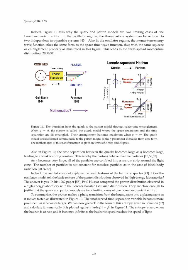
Symmetry 2016, 8, 55

Indeed, Figure 10 tells why the quark and parton models are two limiting cases of oneLorentz-covariant entity. In the oscillator regime, the three-particle system can be reduced totwo independent two-particle systems [43]. Also in the oscillator regime, the momentum-energywave function takes the same form as the space-time wave function, thus with the same squeezeor entanglement property as illustrated in this figure. This leads to the wide-spread momentumdistribution [20,56,57].

Figure 10. The transition from the quark to the parton model through space-time entanglement.When η = 0, the system is called the quark model where the space separation and the timeseparation are dis-entangled. Their entanglement becomes maximum when η = ∞. The quarkmodel is transformed continuously to the parton model as the η parameter increases from zero to ∞.The mathematics of this transformation is given in terms of circles and ellipses.

Also in Figure 10, the time-separation between the quarks becomes large as η becomes large,leading to a weaker spring constant. This is why the partons behave like free particles [20,56,57].

As η becomes very large, all of the particles are confined into a narrow strip around the lightcone. The number of particles is not constant for massless particles as in the case of black-bodyradiation [20,56,57].

Indeed, the oscillator model explains the basic features of the hadronic spectra [43]. Does theoscillator model tell the basic feature of the parton distribution observed in high-energy laboratories?The answer is yes. In his 1982 paper [58], Paul Hussar compared the parton distribution observed ina high-energy laboratory with the Lorentz-boosted Gaussian distribution. They are close enough tojustify that the quark and parton models are two limiting cases of one Lorentz-covariant entity.

To summarize, the proton makes a phase transition from the bound state into a plasma state asit moves faster, as illustrated in Figure 10. The unobserved time-separation variable becomes moreprominent as η becomes larger. We can now go back to the form of this entropy given in Equation (92)and calculate it numerically. It is plotted against (tanh η)2 = β2 in Figure 11. The entropy is zero whenthe hadron is at rest, and it becomes infinite as the hadronic speed reaches the speed of light.

228

Symmetry 2016, 8, 55

Figure 11. Entropy and temperature as functions of [tanh(η)]2 = β2. They are both zero when thehadron is at rest, but they become infinitely large when the hadronic speed becomes close to that oflight. The curvature for the temperature plot changes suddenly around [tanh(η)]2 = 0.8, indicating aphase transition.

Let us go back to the expression given in Equation (87). For this ground state, the densitymatrix becomes:

ρη(z, z′) =(

1cosh η

)2

∑k(tanh η)2kχk(z)χk(z′) (105)

We can now compare this expression with the density matrix for the thermally-excited oscillatorstate [22]:

ρη(z, z′) =(

1 − e−1/T)

∑k

[e−1/T

]kχk(z)χk(z′) (106)

By comparing these two expressions, we arrive at:

[tanh(η)]2 = e−1/T (107)

and thus:T =

−1ln [(tanh η)2]

(108)

This temperature is also plotted against (tanh η)2 in Figure 11. The temperature is zero if the hadron isat rest, but it becomes infinite when the hadronic speed becomes close to that of light. The slope ofthe curvature changes suddenly around (tanh η)2 = 0.8, indicating a phase transition from the boundstate to the plasma state.

In this section, we have shown how useful the concept of entanglement is in understanding therole of the time-separation in high energy hadronic physics including Gell–Mann’s quark model andFeynman’s parton model as two limiting cases of one Lorentz-covariant entity.

9. Concluding Remarks

The main point of this paper is the mathematical identity:

1√π

exp{−1

4

[e−2η(x + y)2 + e2η(x − y)2

]}=

1cosh η ∑

k(tanh η)kχk(x)χk(y) (109)

which says that the series of Equation (1) is an expansion of the Gaussian form given in Equation (2).

229

Symmetry 2016, 8, 55

The first derivation of this series was published in 1979 [26] as a formula from the Lorentz group.Since this identity is not well known, we explained in Section 5 how this formula can be derived fromthe generating function of the Hermite polynomials.

While the series serves useful purposes in understanding the physics of entanglement,the Gaussian form can be used to transfer this idea to high-energy hadronic physics. The hadron, suchas the proton, is a quantum bound state. As was pointed out in Section 8, the squeezed Gaussianfunction of Equation (109) plays the pivotal role for hadrons moving with relativistic speeds.

The Bohr radius is a very important quantity in physics. It is a spatial separation between theproton and electron in the the hydrogen atom. Likewise, there is a space-like separation betweenconstituent particles in a bound state at rest. When the bound state moves, it picks up a time-likecomponent. However, in the present form of quantum mechanics, this time-like separation is notrecognized. Indeed, this variable is hidden in Feynman’s rest of the universe. When the system isLorentz-boosted, this variable entangles itself with the measurable longitudinal variable. Our failureto measure this entangled variable appears in the form of entropy and temperature in the real world.

While harmonic oscillators are applicable to many aspects of quantum mechanics, Paul A. M.Dirac observed in 1963 [21] that the system of two oscillators contains also the symmetries of theLorentz group. We discussed in this paper one concrete case of Dirac’s symmetry. There are differentlanguages for harmonic oscillators, such as the Schrödinger wave function, step-up and step-downoperators and the Wigner phase-space distribution function. In this paper, we used extensively apictorial language with circles and ellipses.

Let us go back to Equation (109); this mathematical identity was published in 1979 as textbookmaterial in the American Journal of Physics [26], and the same formula was later included in a textbookon the Lorentz group [20]. It is gratifying to note that the same formula serves as a useful tool for thecurrent literature in quantum information theory [59,60].

Author Contributions: Each of the authors participated in developing the material presented in this paper and inwriting the manuscript.

Conflicts of Interest: The authors declare that no conflict of interest exists.

References

1. Giedke, G.; Wolf, M.M.; Krueger, O.; Werner, R.F.; Cirac, J.J. Entanglement of formation for symmetricGaussian states. Phys. Rev. Lett. 2003, 91, 10790.1–10790.4.

2. Braunstein, S.L.; van Loock, P. Quantum information with continuous variables. Rev. Mod. Phys. 2005, 28,513–676.

3. Kim, Y.S.; Noz, M.E. Coupled oscillators, entangled oscillators, and Lorentz-covariant Oscillators. J. Opt. BQuantum Semiclass. 2003, 7, s459–s467.

4. Ge, W.; Tasgin, M.E.; Suhail Zubairy, S. Conservation relation of nonclassicality and entanglement forGaussian states in a beam splitter. Phys. Rev. A 2015, 92, 052328.

5. Gingrigh, R.M.; Adami, C. Quantum Engtanglement of Moving Bodies. Phys. Rev. Lett. 2002, 89, 270402.6. Dodd, P.J.; Halliwell, J.J. Disentanglement and decoherence by open system dynamics. Phys. Rev. A 2004,

69, 052105.7. Ferraro, A.; Olivares, S.; Paris, M.G.A. Gaussian States in Continuous Variable Quantum Information.

EDIZIONI DI FILOSOFIA E SCIENZE (2005). Available online: http://arxiv.org/abs/quant-ph/0503237(accessed on 24 June 2016).

8. Adesso, G.; Illuminati, F. Entanglement in continuous-variable systems: Recent advances and currentperspectives. J. Phys. A 2007, 40, 7821–7880.

9. Walls, D.F.; Milburn, G.J. Quantum Optics, 2nd ed.; Springer: Berlin, Germany, 2008.10. Yuen, H.P. Two-photon coherent states of the radiation field. Phys. Rev. A 1976, 13, 2226–2243.11. Yurke, B.; Potasek, M. Obtainment of Thermal Noise from a Pure State. Phys. Rev. A 1987, 36, 3464–3466.12. Ekert, A.K.; Knight, P.L. Correlations and squeezing of two-mode oscillations. Am. J. Phys. 1989, 57, 692–697.

230

Symmetry 2016, 8, 55

13. Paris, M.G.A. Entanglement and visibility at the output of a Mach-Zehnder interferometer. Phys. Rev. A1999, 59, 1615.

14. Kim, M.S.; Son, W.; Buzek, V.; Knight, P.L. Entanglement by a beam splitter: Nonclassicality as a prerequisitefor entanglement. Phys. Rev. A 2002, 65, 02323.

15. Han, D.; Kim, Y.S.; Noz, M.E. Linear Canonical Transformations of Coherent and Squeezed States in theWigner phase Space III. Two-mode States. Phys. Rev. A 1990, 41, 6233–6244.

16. Dirac, P.A.M. The Quantum Theory of the Emission and Absorption of Radiation. Proc. Roy. Soc. (Lond.)1927, A114, 243–265.

17. Dirac, P.A.M. Unitary Representations of the Lorentz Group. Proc. Roy. Soc. (Lond.) 1945, A183, 284–295.18. Dirac, P.A.M. Forms of relativistic dynamics. Rev. Mod. Phys. 1949, 21, 392–399.19. Yukawa, H. Structure and Mass Spectrum of Elementary Particles. I. General Considerations. Phys. Rev.

1953, 91, 415–416.20. Kim, Y.S.; Noz, M.E. Theory and Applications of the Poincaré Group; Reidel: Dordrecht, The Netherlands, 1986.21. Dirac, P.A.M. A Remarkable Representation of the 3 + 2 de Sitter Group. J. Math. Phys. 1963, 4, 901–909.22. Feynman, R.P. Statistical Mechanics; Benjamin Cummings: Reading, MA, USA, 1972.23. Han, D.; Kim, Y.S.; Noz, M.E. Illustrative Example of Feynman’s Rest of the Universe. Am. J. Phys. 1999, 67,

61–66.24. Kim, Y.S.; Noz, M.E. Covariant harmonic oscillators and the quark model. Phys. Rev. D 1973, 8, 3521–3627.25. Kim, Y.S.; Noz, M.E.; Oh, S.H. Representations of the Poincaré group for relativistic extended hadrons.

J. Math. Phys. 1979, 20, 1341–1344.26. Kim, Y.S.; Noz, M.E.; Oh, S.H. A simple method for illustrating the difference between the homogeneous

and inhomogeneous Lorentz groups. Am. J. Phys. 1979, 47, 892–897.27. Kim, Y.S.; Wigner, E.P. Entropy and Lorentz Transformations. Phys. Lett. A 1990, 147, 343–347.28. Kim, Y.S.; Noz, M.E. Lorentz Harmonics, Squeeze Harmonics and Their Physical Applications. Symmerty

2011, 3, 16–36.29. Klauder, J.R.; Sudarshan, E.C.G. Fundamentals of Quantum Optics; Benjamin: New York, NY, USA, 1968.30. Saleh, B.E.A.; Teich, M.C. Fundamentals of Photonics, 2nd ed.; John Wiley and Sons: Hoboken, NJ, USA, 2007.31. Miller, W. Symmetry Groups and Their Applications; Academic Press: New York, NY, USA, 1972.32. Hall, B.C. Lie Groups, Lie Algebras, and Representations: An Elementary Introduction, 2nd ed.; Springer

International: Cham, Switzerland, 2015.33. Wigner, E. On Unitary Representations of the Inhomogeneous Lorentz Group. Ann. Math. 1939, 40, 149–204.34. Weinberg, S. Photons and gravitons in S-Matrix theory: Derivation of charge conservation and equality of

gravitational and inertial mass. Phys. Rev. 1964, 135, B1049–B1056.35. Kim, Y.S.; Wigner, E.P. Space-time geometry of relativistic-particles. J. Math. Phys. 1990, 31, 55–60.36. Baskal, S.; Kim, Y.S.; Noz, M.E. Wigner’s Space-Time Symmetries Based on the Two-by-Two Matrices of the

Damped Harmonic Oscillators and the Poincaré Sphere. Symmetry 2014, 6, 473–515.37. Baskal, S.; Kim, Y.S.; Noz, M.E. Physics of the Lorentz Group; IOP Science; Morgan & Claypool Publishers:

San Rafael, CA, USA, 2015.38. Kim, Y.S.; Yeh, Y. E(2)-symmetric two-mode sheared states. J. Math. Phys. 1992, 33, 1237–124639. Kim, Y.S.; Noz, M.E. Phase Space Picture of Quantum Mechanics; World Scientific Publishing Company:

Singapore, Singapore, 1991.40. Kim, Y.S.; Noz, M.E. Dirac Matrices and Feynman’s Rest of the Universe. Symmetry 2012, 4, 626–643.41. Wigner, E. On the Quantum Corrections for Thermodynamic Equilibrium. Phys. Rev. 1932, 40, 749–759.42. Han, D.; Kim, Y.S.; Noz, M.E. O(3, 3)-like Symmetries of Coupled Harmonic Oscillators. J. Math. Phys. 1995,

36, 3940–3954.43. Feynman, R.P.; Kislinger, M.; Ravndal, F. Current Matrix Elements from a Relativistic Quark Model.

Phys. Rev. D 1971, 3, 2706–2732.44. Rotbart, F.C. Complete orthogonality relations for the covariant harmonic oscillator. Phys. Rev. D 1981, 12,

3078–3090.45. Ruiz, M.J. Orthogonality relations for covariant harmonic oscillator wave functions. Phys. Rev. D 1974, 10,

4306–4307.46. Magnus, W.; Oberhettinger, F.; Soni, R.P. Formulas and Theorems for the Special Functions of Mathematical Physics;

Springer-Verlag: Heidelberg, Germany, 1966.

231

Symmetry 2016, 8, 55

47. Doman, B.G.S. The Classical Orthogonal Polynomials; World Scientific: Singapore, Singapore, 2016.48. Bargmann, V. Irreducible unitary representations of the Lorentz group. Ann. Math. 1947, 48, 568–640.49. Han, D.; Kim, Y.S. Special relativity and interferometers. Phys. Rev. A 1988, 37, 4494–4496.50. Han, D.; Kim, Y.S.; Noz, M.E. Wigner rotations and Iwasawa decompositions in polarization optics.

Phys. Rev. E 1999, 1, 1036–1041.51. Von Neumann, J. Die mathematische Grundlagen der Quanten-Mechanik; Springer: Berlin, Germany, 1932.

(von Neumann, I. Mathematical Foundation of Quantum Mechanics; Princeton University: Princeton, NJ,USA, 1955.)

52. Fano, U. Description of States in Quantum Mechanics by Density Matrix and Operator Techniques.Rev. Mod. Phys. 1957, 29, 74–93.

53. Wigner E.P.; Yanase, M.M. Information Contents of Distributions. Proc. Natl. Acad. Sci. USA 1963, 49,910–918.

54. Gell-Mann, M. A Schematic Model of Baryons and Mesons. Phys. Lett. 1964, 8, 214–215.55. Feynman, R.P. Very High-Energy Collisions of Hadrons. Phys. Rev. Lett. 1969, 23, 1415–1417.56. Kim, Y.S.; Noz, M.E. Covariant harmonic oscillators and the parton picture. Phys. Rev. D 1977, 15, 335–338.57. Kim, Y.S. Observable gauge transformations in the parton picture. Phys. Rev. Lett. 1989, 63, 348–351.58. Hussar, P.E. Valons and harmonic oscillators. Phys. Rev. D 1981, 23, 2781–2783.59. Leonhardt, U. Essential Quantum Optics; Cambridge University Press: London, UK, 2010.60. Furusawa, A.; Loock, P.V. Quantum Teleportation and Entanglement: A Hybrid Approach to Optical Quantum

Information Processing; Wiley-VCH: Weinheim, Germany, 2010.

c© 2016 by the authors. Licensee MDPI, Basel, Switzerland. This article is an open accessarticle distributed under the terms and conditions of the Creative Commons Attribution(CC BY) license (http://creativecommons.org/licenses/by/4.0/).

232

symmetryS S

Article

Massless Majorana-Like Charged Carriers inTwo-Dimensional Semimetals

Halina Grushevskaya † and George Krylov †,∗

Physics Department, Belarusian State University, 4 Nezaleznasti Ave., 220030 Minsk, Belarus;grushevskaja@bsu.by* Correspondence: krylov@bsu.by; Tel.: +375-296-62-44-97† These authors contributed equally to this work.

Academic Editor: Young Suh KimReceived: 29 February 2016; Accepted: 1 July 2016; Published: 8 July 2016

Abstract: The band structure of strongly correlated two-dimensional (2D) semimetal systems isfound to be significantly affected by the spin-orbit coupling (SOC), resulting in SOC-inducedFermi surfaces. Dirac, Weyl and Majorana representations are used for the description of differentsemimetals, though the band structures of all these systems are very similar. We develop a theoreticalapproach to the band theory of two-dimensional semimetals within the Dirac–Hartree–Fockself-consistent field approximation. It reveals partially breaking symmetry of the Dirac cone affectedby quasi-relativistic exchange interactions for 2D crystals with hexagonal symmetry. Fermi velocitybecomes an operator within this approach, and elementary excitations have been calculated in thetight-binding approximation when taking into account the exchange interaction of π(pz)-electronwith its three nearest π(pz)-electrons. These excitations are described by the massless Majoranaequation instead of the Dirac one. The squared equation for this field is of the Klein–Gordon–Focktype. Such a feature of the band structure of 2D semimetals as the appearance of four pairs of nodesis shown to be described naturally within the developed formalism. Numerical simulation of bandstructure has been performed for the proposed 2D-model of graphene and a monolayer of Pb atoms.

Keywords: 2D semimetals; Dirac–Hartree–Fock self-consistent field approximation; Majorana-likefield; Weyl-like nodes; Fermi velocity operator

PACS: 73.22.-f, 81.05.Bx

1. Introduction

Strongly correlated materials, such as two-dimensional (2D) complex oxides of transition metals,graphene, oxides with a perovskite structure, and IV–VI semiconductors being three-dimensional(3D) analogues of graphene, can demonstrate unusual electronic and magnetic properties, such ase.g., half-metallicity. The linear dispersion law for such materials is stipulated by the simultaneousexistence of positively and negatively charged carriers [1]. Conical singularities are generic in thequantum crystals having honeycomb lattice symmetry [2]. Bipolarity of the material suggests that thestate of an excitonic insulator is possible for it. Since an electron-hole pair is at the same time its ownantiparticle, the Majorana representation has been used [3,4] to describe the interaction of pseudospinswith the valley currents in a monolayer graphene.

The electron is a complex fermion, so if one decomposes it into its real and imaginary parts,which would be Majorana fermions, they are rapidly re-mixed by electromagnetic interactions.However, such a decomposition could be reasonable for a superconductor where, because of effectiveelectrostatic screening, the Bogoliubov quasi-fermions behave as if they are neutral excitations [5].

Symmetry 2016, 8, 60 233 www.mdpi.com/journal/symmetry

Symmetry 2016, 8, 60

A helical magnetic ordering (commensurate magnetism) occurs due to strong spin-orbit coupling(SOC) between Fe and Pb atoms in the system where a chain of ferromagnetic Fe atoms is placed onthe surface of conventional superconductor composed of Pb atoms [6]. In this case, the imposition ofSOC results in the appearance of Majorana-like excitations at the ends of the Fe atom chain.

The discovered p-wave function pairing in this Fe-chain is allowed to assume that there existsa new mechanism of superconductivity in high-temperature superconductors through the exchangeof Majorana particles rather than phonons in the Bardeen–Cooper–Schrieffer theory. Such a novelsuperconducting state emerges, for example, in compound CeCoIn5 in strong magnetic fields inaddition to ordinary superconducting state, [7]. It has been shown [8–10] that the coupling of electronsinto Cooper pairs in pnictides (LiFeAs with slabs FeAs) is mediated by the mixing of d-electron orbitalssurrounding the atomic cores of transition metal. The new state is mediated by an anti-ferromagneticorder, and its fluctuations appear due to strong spin-orbit coupling [8,9,11]. It has been experimentallyconfirmed in [10] for LiFeAs. For antiferromagnetic itinerant-electron system LaFe12B6, ultrasharpmagnetization steps have been observed [12]. The last can be only explained by the existence ofanti-ferromagnetic order, and its fluctuations appear due to strong spin-orbit coupling.

Thus, there is a strong evidence that SOC may control the spin ordering in the absence of externalmagnetic fields. However, the mechanism that leads to such, commensurate magnetism has not beenyet established.

The phenomenon of the contraction of electron density distribution in one direction is callednematicity. It is observed in pnictides BaFe2(As1−xPx)2 placed in a magnetic field, and such aphenomenon remains in the superconducting state [13]. The nematicity is coupled with considerablestripe spin fluctuations in FeSe [14]. The very strong spin orbit coupling leads to contraction in afactor of about 10% and rotation on 30◦ of the hexagonal Brillouin zone of delafossite oxide PtCoO2,belonging to yet another class of topological insulators in which atoms of metal are in layers withtriangular lattices [15].

Other topological insulators, namely so-called Weyl materials with a linear dispersion law,are close in properties with layered perovskite-like materials (see [16] and references therein).Currently, the first candidate for such a material has been found, namely TaAs, whose Brillouinzone has Weyl-like nodes and Fermi arcs [17–19].

Moreover, the experimental evidence of the similarities between the Fermi surfaces of insulatorSmB6 and metallic rare earth hexaborides (PrB6 and LaB6) has been presented in [20]. To explain theaccompanying ordering phenomena, each associated with different symmetry breaking, it is necessaryto develop a unified theory as it has been pointed out in [9].

Electrically charged carriers in the strongly correlated semimetallic systems with half-filled bandsare massless fermions [15,21,22].

In a low-dimensional system, the exciton binding energy turns out to be high [23] and, respectively,the transition to the state of excitonic insulator is possible. Therefore, the Majorana rather than Weylrepresentation is preferable for the description of 2D semimetals. An attempt to represent the transitionto the state of excitonic insulator as the appearance of Majorana zero-modes solution in graphenewith trigonal warping [24] contradicts experimental data on the absence of a gap in band structureof graphene [25] and on diminishing of charged carriers mobility [26] and minimal conductivity [27].However, at the present time, there exist experimental signatures of graphene Majorana states ingraphene-superconductor junctions without the need for spin-orbit coupling [28]. However, modernQuantum Field Theory of pseudo-Dirac quasiparticles in random phase approximation predicts astrong screening that destroys the excitonic pairing instability if the fermion dynamic mass m(p)dependent on momentum p is small in comparison with the chemical potential μ: m(p) ≤ μ [29].

In the paper, we would like to show how the above described features of the layered materials canbe formalized in 2D models, where the charged carriers are the quasiparticles of Majorana rather thanof the Weyl type. We also show that, under certain conditions, these quasiparticles reveal themselvesas Weyl-like states or massless Dirac pseudofermions.

234

Symmetry 2016, 8, 60

However, the use of the well-known Majorana representations to describe a semimetal as amassless-quasiparticle system is encountered with such a puzzle as the absence of harmonic oscillatorysolutions in ultrarelativistic limit for Majorana particles of zero mass [30]. The equations are knownfor massive Majorana particles only [31–33].

In the paper, we reveal different aspects of appearance of Majorana-like quasiparticle states inthe band structure of semimetals. 2D Hartree–Fock approximation for graphene, however, predictsexperimentally observable increase of the Fermi velocity value vF(�p) at small momenta p [25] butleads to logarithmically divergent vF(�p) at p → 0 [34]. To take into account this effect of long rangeCoulomb interactions correctly, our calculation is based on the quasi-relativistic Dirac–Hartree–Fockself-consistent field approach developed earlier [35,36].

The goal is to construct a 2D-semimetal model in which a motion equation is a pseudo-relativisticmassless Majorana-like one. We show that the squared equation for this field is of a Klein–Gordon–Focktype, and therefore the charged carriers in such 2D-semimetal models can be assumed masslessMajorana-like quasiparticles.

We study quasiparticle excitations of the electronic subsystem of a hexagonal monoatomic layer(monolayer) of light or heavy atoms in tight-binding approximation. The simulations are performedfor the atoms of C and Pb on the assumption that sp2-hybridization for s- and p-electron orbitals isalso possible for the atoms of Pb.

We demonstrate that the band-structure features for the hexagonal monolayers are similar to eachother due to the similarity of external electronic shells of their atoms. Despite the similarity of the bandstructure, the charged carriers in such 2D-semimetal models can possess different features, e.g., thecharged carriers in the monolayer of the atoms of C can be thought of as massless Dirac pseudofermions,whereas in the monolayer from the atoms of Pb, they reveal themselves as Weyl-like states.

The paper is organized as follows. In Section 2, we propose a semimetal model with couplingbetween pseudospin and valley currents and prove the pseudo-helicity conservation law. In Section 3,we briefly introduce the approach [3,35–37] and use it in a simple tight-binding approximation toobtain the system of equations for a Majorana secondary quantized field. In Section 4, we support thestatement that the squared equation for the constructed field is of the Klein–Gordon–Fock type fordifferent model exchange operators. We also discuss features of our model manifesting in the bandstructure of real semimetals. In Section 5, we discuss the proposed approximations for the exchangeinteractions in 2D semimetals and summarize our findings.

2. Monolayer Semimetal Model with Partial Unfolding of Dirac Bands

Semimetals are known to be bipolar materials with half-filled valence and conduction bands.A distinctive feature of the graphene band structure is the existence of Dirac cones in the Diracpoints (valleys) K, K′ of the Brillouin zone. In the present paper, these Dirac points are designated asKA, KB. We assume that pseudo-spins of hexagonally packed carbon atoms in the monoatomic layer(monolayer) graphene are anti-ordered, as it is shown schematically in Figure 1a. The fact that thepseudo-helicity (chirality) conservation law forbids massless charged carriers to be in lattice sites withthe opposite signs of pseudo-spin, makes possible the existence of valley currents due to jumps throughthe forbidden sites. This is shown schematically in Figure 1a. Coupling between the pseudo-spin andthe valley current in the Majorana representation of bispinors can be determined in the following way.

235

Symmetry 2016, 8, 60

(a) (b)

Figure 1. (a) graphene lattice, comprised of two sublattices {A} with spin “up” and {B} with spin“down” . Right and left valley currents JR

v and JLv are shown as circular curves with arrows. Double

arrows from site A to site BL and from A to BR indicate clockwise and anti-clockwise directions.The axis of mirror reflection from AR to BL is marked by dash-dotted line; (b) transformations of aq-circumference into ellipses under an action of exchange operators

(Σx

rel)

AB and(Σx

rel)

BA (in color).

According to Figure 1a, a particle can travel from a lattice site A to e.g., a lattice site AR throughright or left sites BR or BL, respectively. Since the particle is symmetrical, its description in the rightand left reference frames has to be equivalent. Therefore, a bispinor wave function Ψ′ of graphenehas to be chosen in the Majorana representation, and its upper and lower spin components ψ′, ψ′ aretransformed by left and right representations of the Lorentz group:

Ψ′ =

(ψ′

σ

ψ′−σ

)=

(e

κ2�σ·�nψσ

eκ2 (−�σ)·�nψ−σ

). (1)

The wave-function χ†σ(�rA) |0,+σ〉 of a particle (in our case of an electron-hole pair) located on the

site A, behaves as a component ψσ, while the wave-function χ†−σ(�rB) |0,−σ〉 of a particle located on

the site B behaves as a component ψ−σ of the bispinor (1).Relativistic particles with non-zero spin possess the helicity h, which is the projection of the

particle’s spin to the direction of motion [32]:

h ≡ �p · �S =12

pi

(σi 00 σi

), (2)

where �p is the particle momentum, �S is the spin operator for a particle, �σ is the vector of the Paulimatrices σi, and i = x, y. In quantum relativistic field theory, the value of the helicity of a masslessparticle is preserved in the transition from one reference frame moving with the velocity v1, to anotherone moving with the velocity v2 [32,38].

Let us designate the two-dimensional spin of the quasi-particle in valleys KA and KB as�SAB = h�σAB/2 and �SBA = h�σBA/2, respectively.

Let us introduce two-dimensional pseudospin �SAB and �SBA of quasi-particles in valleys KAand KB through the transformed vector �σ of the Pauli matrices σi, i = x, y as �SAB = h�σAB/2 and�SBA = h�σBA/2. The explicit form of this transformation is given in Section 3.

A valley current JRv or JL

v , on the right or left closed contour {A → BR → AR → B → AL → BL → A}or {A → BL → AL → B → AR → BR → A}, respectively, in Figure 1, is created by an electron (hole)with pseudo-angular momentum�lABR and momentum �pABR or by an electron (hole) with�lABL and

236

Symmetry 2016, 8, 60

�pABL . Pseudo-helicity of bispinors (1), describing the particles right or left the from lattice site A, isdefined by the expressions, which are analogous to (2):

hBR A ≡ �pABR · �SBR A, (3)

hBL A ≡ �pABL · �SBL A. (4)

Let us use the parity operator P, which mirrors the bispinor (1) with respect to the line passingthrough the points A and B. Pseudo-helicity of the mirrored bispinor is defined by the expression:

PhBR AR P = hALBL = �pBL AL · �SALBL . (5)

Pseudo-helicity hAB does not change its value while the valley momentum and the pseudo-spinchange signs: �pALBL = −�pBR AR and �SALBL = −�SBR AR .

The pseudo-helicity hAB is expressed through the projection MAB =�σBA ·(�lAB + h�σBA/2

)of the

total angular momentum on the direction of the spin�σBA as [39,40]:

�σBA · �pAB = σrBA

(pr, BA + ı

MABr

− h/2)= σr

BA

(pr, BA + ı

�σBA ·�lABr

), (6)

where σrBA and pr, BA are radial components of the spin and the momentum, respectively. According to

Equation (6), the pseudo-spin-orbit scalar�σBA ·�lAB describes the coupling (interaction) of the spinwith the valley currents flowing along a closed loop clockwise or in opposite directions, as is shownin Figure 1a. Hence, there exists a preferred direction along which the spin projection of the bispinor(1) is not changed after transition from one moving reference frame into another. At this, the spinof a particle precesses. Transformation of the electron and hole into each other in an exciton is apseudo-precession.

As a result, the coupling of pseudo-spin and valley currents stipulates the spin precession ofexciton charged carriers in graphene. In our model, the orientation of non-equilibrium spin of the statesof monolayer graphene in electromagnetic fields may be retained for a long time due to prohibitionof change for exciton pseudo-helicity. Pseudo-precession is possible, if spins of pz -electrons areanti-ordered (pseudo-antiferromagnetic ordering). Therefore, the pseudo-spin precession of the excitoncan be implemented through the exchange interaction. Furthermore, we determine the operators�σBA(AB), �pAB(BA) and describe the effects of pseudo-spin and valley current coupling.

3. Effects of Coupling between Pseudo-Spin and Valley Current

In quasi-relativistic approximation (c−1 expansion), the eigenproblem for the equation of motionof the secondary quantized field χ†

−σAin the model shown in Figure 1a has the form: [35–37]

{�σ · �p vqu

F − 1c(iΣx

rel)AB (iΣxrel)BA

}χ†−σA

(�r) |0,−σ〉 (7)

= Equ(p)χ†−σA

(�r) |0,−σ〉 ,

where the Fermi velocity operator vquF is defined as

vquF =

[(Σx

rel)BA + ch�σ · (�KA + �KB)]

.

237

Symmetry 2016, 8, 60

(Σx

rel)

BA ,(Σx

rel)

AB are determined through an ordinary exchange interaction contribution,for example [39,40]:

(Σxrel)AB χ†

σB(�r) |0, σ〉 =

Nv N

∑i=1

∫d�riχ

†σi

B(�r) |0, σ〉

×〈0,−σi|χ†−σA

i(�ri)V(�ri −�r)χ−σB(�ri)|0,−σi′ 〉.

V(�ri −�r) is the Coulomb interaction between two valent electrons with radius-vectors�ri and�r; Nis a total number of atoms in the system, Nv is a number of valent electrons in an atom, c is the speedof light.

After applying the non-unitary transformation to the wave function in the form

˜χ†−σA

|0,−σ〉 = (Σxrel)BA χ†

−σA|0,−σ〉 ,

we obtain (neglecting mixing of the states for the Dirac points) the equation that is similar to the onein 2D quantum field theory (QFT) [41–43], but it describes the motion of a particle with pseudo-spin�SAB = h�σAB/2:{

�σAB2D · �pBA − c−1 ˜ΣBAΣAB

}˜χ†−σA

(�r) |0,−σ〉 = Equ(p) ˜χ†−σA

(�r) |0,−σ〉 , (8)

with a transformed 2D vector �σAB2D of the Pauli matrices, which are determined as

�σAB2D =

(Σx

rel)

BA�σ(Σx

rel)−1

BA. The following notions are introduced: �pBA ˜χ†−σA

=(Σx

rel)

BA �p(Σx

rel)−1

BA ˜χ†−σA

≡[(

Σxrel

)BA �p

]χ†−σA

, Equ = Equ/vBAF , vBA

F =(Σx

rel)

BA, ˜ΣBAΣAB ≡(Σx

rel)

BA

(iΣx

rel)

AB

(iΣx

rel)

BA

(Σx

rel)−1

BA =(iΣx

rel)

BA

(iΣx

rel)

AB; and the product of two capital sigma, asone sees from the last chain of formulas, behaves like a scalar mass term.

Further simulations are performed in nearest neighbor tight-binding approximation [44,45].This approximation correctly predicts the graphene band structure in the energy range ±1 eV [46].This turns out to be sufficient for our purposes. We use the expressions for the exchange betweenπ(pz)-electrons only. One can find the explicit form of these expressions in [4].

The action of the matrices(Σx

rel)

BA ,(Σx

rel)

AB in the momentum space is shown in Figure 1b.As

(Σx

rel)

BA =(Σx

rel)

AB, the vector �pBA is rotated with respect to �pAB and stretched. According toFigure 1b, ellipses in momentum spaces of electrons and holes are rotated 90◦ with respect to eachother. With an account of the hexagonal symmetry of the system, the last explains the experimentallyobserved rotation in 30◦ of the hexagonal Brillouin zone of PtCoO2 [15].

Thus, the sequence of exchange interactions(Σx

rel)

AB

(Σx

rel)

BA

(Σx

rel)

AB for valley currents makesrotation initially of the electron Brillouin zone and Dirac band into the hole Brillouin zone andDirac band, and then vice-versa. Thus, the exchange

(Σx

rel)

AB(AB) ≡ ΣAB(BA) changes the sublatticeswave functions:

|ψAB〉 = ΣAB |ψ∗BA〉 .

Owing to it and neglecting a very small mass term c−1 ˜ΣBAΣAB, the equation in which the operatorof the Fermi velocity enters, can be rewritten as follows:

�σBA2D · �pAB |ψAB〉 = Equ |ψ∗

BA〉 . (9)

Taking into account that E → i ∂∂t and �p = −i�∇, we transform the system of equations for the

Majorana bispinor (ψ†AB, (ψ∗

BA)†):

238

Symmetry 2016, 8, 60

�σBA2D · �pAB |ψAB〉 = i

∂

∂t|ψ∗

BA〉 , (10)

�σAB2D · �p ∗

BA |ψ∗BA〉 = −i

∂

∂t|ψAB〉 , (11)

into the wave equation of the form:

(�σAB2D · �p ∗

BA)(�σBA2D · �pAB) |ψAB〉 =

∂2

∂t2 |ψAB〉 . (12)

Equation (12) describes an oscillator with the energy operator ω(�p)

ω(�p) =1√2

[(�σAB

2D · �pBA)(�σBA2D · �pAB) + (�σBA

2D · �pAB)(�σAB2D · �pBA)

]1/2. (13)

Now, one can really see that the obtained equation is the equation of motion for a Majoranabispinor wave function of the semimetal charged carriers.

Thus, the Fermi velocity becomes an operator within this approach, and elementary excitationsare fermionic excitations described by the massless Majorana-like equation rather than Dirac-like one.

4. Harmonic Analysis of the Problem

Equation (13) can be rewritten in the following form:

ω2(�p) =12(

HABHBA + HBA HAB)

. (14)

In order to describe the proposed secondary quantized field by a set of harmonic oscillators, itis necessary to show that the squared Equation (14), obtained by the symmetrization of the productof the Hamiltonians HAB and HBA, is the Klein–Gordon–Fock operator. This will be the case if thenon-diagonal matrix elements of the operator vanish identically, and therefore the components of theequation are independent. Then, ω2(�p) can be considered as a “square of energy operator”.

Unfortunately, because of the complex form of the exchange operator, the statement is difficult toprove in the general case. Therefore, we do this for several approximations of the exchange interactionand demonstrate that the Equation (14) is a Klein–Gordon–Fock one.

As a first particular case, when the proposed Majorana-like field is proven to be a harmonicoscillators set, we consider ε-neighborhood (ε → 0) of the Dirac point KA(KB).

Let us designate the momentum of a particle in a valley as �q. The momentum �q is determinedas �q = �p − h�KA. In the case of very small values of �q, q → 0 the exchange operator ΣAB(BA) isapproximated by a power series expansion up to the fourth order in q. Then, an analytical calculationof non-diagonal elements of the operator ω2(�p) performed in the Mathematica system proves thatthey are identically zero.

Band structures for monolayer graphene and monolayer of atoms of Pb are shown in Figure 2a,b.One can see that the Weyl nodes in graphene are located far enough from the Dirac point. The Weylnodes are shifted to the Dirac point for the Pb-monolayer. Therefore, Weyl-like character in thebehavior of charged carriers may be exhibited for the Pb-monolayer under the condition that thecontributions up to 4-th order in q are prevailing in the exchange. In accordance with Figure 1b, theexchange operator matrices transform a circumference in the momentum space into a highly stretchedellipse that allows us to assume the presence of nematicity in the model.

For a given �q, where the eigenfunction of Equation (9) represents 2D spinor Ψ, we choose itsnormalization in the form Ψ(�q) = (ψ(�q), 1)† with lower component equal to unity. Then, as it canbe easily shown for the massless Dirac pseudo-fermion model [47], the absolute value of the uppercomponent |ψ(�q)| does not depend upon the wave vector �q, demonstrating the equivalence of all

239

Symmetry 2016, 8, 60

directions in �q space. We construct |ψ(�q)|2 for Equation (9) in q4-approximation for the exchange.The results are shown in Figure 2c. The isotropy of |ψ(�q)|2 is broken for our model due to theappearance of the preferable directions in the momentum space.

As one can see from Figure 2c, the existence of almost one-dimensional regions with sharp jumpin |ψ(�q)|2 should probably lead to some anisotropy already in the configuration space for the carriersthat we consider as manifestation of nematicity.

The approximation q4 for the exchange operator expression presents a particular interest forsystems with strong damping of quasi-particle excitations.

(a) (b) (c)

Figure 2. A splitting of Dirac cone replicas: for graphene (a) and Pb monolayer (b). One of the six pairsof Weyl-like nodes: source and sink are indicated; (c) the square of the absolute value of the upperspinor component |ψ|2 of�q−eigenstate in the 2D semimetal model. �q = �p − �KA. (in color)

The second approximation of the exchange, for which we can prove the harmonic origin of theproposed Majorana-like field, is the model exchange with full exponential factors taken into account,but with the phase-difference between π(p)z-electrons wavefunction chosen to be identically zero(see Ref. [4] for detail). Numeric simulation of ω2(�p) with this model exchange has been performedon a discrete lattice in the Brillouin zone. It has been demonstrated that the operator ω2(�p) is alwaysdiagonal in this case.

Now, we perform the simulations with the exact expression for the exchange term.In this general case, the exchange between π(pz)-electron and its three nearest π(pz)-electrons

has been calculated based on the method proposed in [4]. Band structure of the 2D semimetal hasthe form of a degenerated Dirac cone in the neighborhood of the Dirac point. Then, the emergence ofunfolding leads to replica appearance, and further splitting of these replicas gives the octagonalsymmetry of the problem, as one can see in Figure 3. Hyperbolic points (saddle points) arelocated between nodes and at the apex of the Dirac cone (Van-Hove singularities) as one can see inFigure 2a,b [3,48–50]. Therefore, a fractal-like set of Fermi arcs which are shown in Figure 4, isformed in the absence of damping in the system. Contrary to the graphene case, the splitting ofthe Dirac bands for the Pb-monolayer occurs at sufficiently small q, and therefore, can be observedexperimentally. In addition, for the Pb-monolayer, there exist regions with huge numbers of Fermiarcs, and, respectively, regions with strong fluctuations of antiferromagnetic ordering.

Thus, the secondary quantized field described by Equation (9) represents a field in which quantamanifest themselves as Dirac pseudo-fermions in the apex of the Dirac cone and as Weyl-like particlesfor sufficiently large q at the presence of the dumping in the system. For an ideal system ( m ε(�q) = 0),such a behavior is similar to that of the mathematical pendulum in the vicinity of the separatrix [51,52].

240

Symmetry 2016, 8, 60

(a) (b)

Figure 3. A band structure in the graphene model with partial unfolding of Dirac cone: real (a) andimaginary (b) parts of ε(�q); range of high momenta. �q = �p − �KA (in color).

Figure 4. Density of Fermi arcs sets in graphene (a) and Pb-monolayer bands for values of momentum

q in the range 0 ≥ q/∣∣∣�KA

∣∣∣ ≤ 10−4,�q = �p − �KA.

5. Discussion

Discussing the obtained results, we have to point out, firstly, that the excitations of the constructedsecondary-quantized pseudo-fermionic field are Majorana-like massless quasiparticles.

The set of Fermi arcs in our model shows that the splitting of Dirac replicas on a huge number ofWeyl-like states occurs in the momentum space except for the Dirac cone apex.

In contrast to known massless Dirac and Weyl models, in the proposed model, there is a partialremoving of the degeneracy of the Dirac cone, and the octagonal symmetry of the bands emerges forsufficiently large q. Thus, Majorana particles in our model can be represented as a wave package ofinfinitely large number of Weyl-like states.

Secondly, the Dirac cone for the proposed 2D-semimetal model is degenerated in a very smallneighborhood of the Dirac point KA(KB) at q → 0.

Thirdly, the first-approximation with damping demonstrates that sufficiently strong decay leadsto diminishing the number of the Weyl states and formation of bands having hexagonal symmetry.In accordance with the obtained results, in the system with strong damping, only six pairs of Weylnodes survive. In this case, each Dirac hole (electron) cone is surrounded by three electron (hole) bandsrelating to three Weyl pairs. Provided the lifetime of the Weyl-like states is sufficiently large (small butfinite damping) to preserve the octagonal symmetry of the bands, each Dirac hole (electron) cone willbe surrounded by four electron (hole) bands relating to four Weyl pairs.

Important features of the proposed model are that the fractal set of Fermi arches manifestspseudospin fluctuations and the phenomenon of nematicity is possible.

241

Symmetry 2016, 8, 60

6. Conclusions

In conclusion, contrary to known Dirac and Weyl models, the constructed 2D-semimetal modelallows for description, in a general formalism, the band structure of a wide class of existing strongly.

Acknowledgments: This work has been supported in part by Research grant No. 2.1.01.1 within the BasicResearch Program “Microcosm and Universe” of the Republic of Belarus.

Author Contributions: Both authors equally contributed to this work.

Conflicts of Interest: The authors declare no conflict of interest.

References

1. Grushevskaya, H.V.; Hurski, L.I. Coherent charge transport in strongly correlated electron systems:Negatively charged exciton. Quantum Matter 2015, 4, 384–386.

2. Fefferman, C.L.; Weinstein, M.I. Honeycomb lattice potentials and Dirac points. J. Am. Math. Soc. 2012, 25,1169–1220.

3. Grushevskaya, H.V.; Krylov, G. Quantum field theory of graphene with dynamical partial symmetry breaking.J. Mod. Phys. 2014, 5, 984–994.

4. Grushevskaya, H.V.; Krylov, G. Semimetals with Fermi Velocity Affected by Exchange Interactions: TwoDimensional Majorana Charge Carriers. J. Nonlinear Phenom. Complex Syst. 2015, 18, 266–283.

5. Semenoff, G.W.; Sodano, P. Stretched quantum states emerging from a Majorana medium. J. Phys. B: At. Mol.Opt. Phys. 2007, 40, 1479–1488.

6. Nadj-Perge, S.; Drozdov, I.K.; Li, J.; Chen, H.; Jeon, S.; Seo, J.; MacDonald, A.H.; Bernevig, A.; Yazdani, A.Observation of Majorana fermions in ferromagnetic atomic chains on a superconductor. Science 2014, 346,602–607.

7. Gerber, S.; Bartkowiak, M.; Gavilano, J.L.; Ressouche, E.; Egetenmeyer, N.; Niedermayer, C.; Bianchi,A.D.; Movshovich, R.; Bauer, E.D.; Thompson, J.D.; et al. Switching of magnetic domains reveals spatiallyinhomogeneous superconductivity. Nat. Phys. 2014, 10, 126–129.

8. Shimojima, T.; Sakaguchi, F.; Ishizaka, K.; Ishida, Y.; Kiss, T.; Okawa, M.; Togashi, T.; Chen, C.-T.; Watanabe, S.;Arita, M.; et al. Orbital-independent superconducting gaps in iron-pnictides. Science 2011, 332, 564–567.

9. Davis, J.C.S.; Lee, D.-H. Concepts relating magnetic interactions, intertwined electronic orders, and stronglycorrelated superconductivity. Proc. Natl. Acad. Sci. USA 2013, 110, 17623–17630.

10. Borisenko, S.V.; Evtushinsky, D.V.; Liu, Z.-H.; Morozov, I.; Kappenberger, R.; Wurmehl, S.; Büchner, B.;Yaresko, A.N.; Kim, T.K.; Hoesch, M.; et al. Direct observation of spin-orbit coupling in iron-basedsuperconductors. Nat. Phys. 2015, doi:10.1038/nphys3594.

11. Hurski, L.I.; Grushevskaya, H.V.; Kalanda, N.A. Non-adiabatic paramagnetic model of pseudo-gap state inhigh-temperature cuprate superconductors. Dokl. Nat. Acad. Sci. Belarus 2010, 54, 55–62. (In Russian)

12. Diop, L.V.B.; Isnard, O.; Rodriguez-Carvajal, J. Ultrasharp magnetization steps in the antiferromagneticitinerant-electron system LaFe12B6. Phys. Rev. 2016, B93, 014440.

13. Kasahara, S.; Shi, H.J.; Hashimoto, K.; Tonegawa, S.; Mizukami, Y.; Shibauchi, T.; Sugimoto, K.; Fukuda, T.;Terashima, T.; Nevidomskyy, A.H.; et al. Electronic nematicity above the structural and superconductingtransition in BaFe2(As1−xPx)2. Nature 2012, 486, 382–385.

14. Wang, Q.; Shen, Y.; Pan, B.; Hao, Y.; Ma, M.; Zhou, F.; Steffens, P.; Schmalzl, K.; Forrest, T.R.; Abdel-Hafiez, M.;et al. Strong interplay between stripe spin fluctuations, nematicity and superconductivity in FeSe. Nat. Mater.2016, 15, 159–163.

15. Kushwaha, P.; Sunko, V.; Moll, Ph.J.W.; Bawden, L.; Riley, J.M.; Nandi, N.; Rosner, H.; Schmidt, M.P.;Arnold, F.; Hassinger, E.; et al. Nearly free electrons in a 5d delafossite oxide metal. Sci. Adv. 2015,1, e1500692.

16. Lv, M.; Zhang, S.-C. Dielectric function, Friedel oscillation and plasmons in Weyl semimetals. Int. J. Mod. Phys.B 2013, 27, 1350177.

17. Xu, S.-Y.; Belopolski, I.; Alidoust, N.; Neupane, M.; Bian, G.; Zhang, C.; Sankar, R.; Chang, G.; Yuan, Z.;Lee, C.-C.; et al. Discovery of a Weyl Fermion semimetal and topological Fermi arcs. Science 2015, 349,613–617.

242

Symmetry 2016, 8, 60

18. Lv, B.Q.; Xu, N.; Weng, H.M.; Ma, J.Z.; Richard, P.; Huang, X.C.; Zhao, L.X.; Chen, G.F.; Matt, C.E.; Bisti, F.;et al. Observation of Weyl nodes in TaAs. Nat. Phys. 2015, 11, 724–727.

19. Huang, S.-M.; Xu, S.-Y.; Belopolski, I.; Lee, C.-C.; Chang, G.; Wang, B.K.; Alidoust, N.; Bian, G.; Neupane, M.;Zhang, C.; et al. A Weyl Fermion semimetal with surface Fermi arcs in the transition metal monopnictideTaAs class. Nat. Commun. 2015, 6, 7373.

20. Tan, B.S.; Hsu, Y.-T.; Zeng, B.; Ciomaga Hatnean, M.; Harrison, N.; Zhu, Z.; Hartstein, M.; Kiourlappou, M.;Srivastava, A.; Johannes, M.D.; et al. Unconventional Fermi surface in an insulating state. Science 2015, 349,287–290.

21. Falkovsky, L.A. Optical properties of graphene and IV–VI semiconductors. Phys.-Uspekhi 2008, 51, 887–897.22. Novoselov, K.S.; Jiang, D.; Schedin, F.; Booth, T.J.; Khotkevich, V.V.; Morozov, S.V.; Geim, A.K.

Two-dimensional atomic crystals. Proc. Natl. Acad. Sci. USA 2005, 102, 10451–10453.23. Keldysh, L.V. Coulomb interaction in thin semiconductor and semimetal films. Lett. J. Exper. Theor. Phys.

1979, 29, 716–719.24. Dora, B.; Gulacsi, M.; Sodano, P. Majorana zero modes in graphene with trigonal warping. Phys. Status

Solidi RRL 2009, 3, 169–171.25. Elias, D.C.; Gorbachev, R.V.; Mayorov, A.S.; Morozov, S.V.; Zhukov, A.A.; Blake, P.; Ponomarenko, L.A.;

Grigorieva, I.V.; Novoselov, K.S.; Guinea, F.; et al. Dirac cones reshaped by interaction effects in suspendedgraphene. Nat. Phys. 2012, 8, 172.

26. Du, X.; Skachko, I.; Barker, A.; Andrei, E.Y. Approaching ballistic transport in suspended graphene.Nat. Nanotechnol. 2008, 3, 491–495.

27. Cooper, D.R.; D’Anjou, B.; Ghattamaneni, N.A.; Harack, B.; Hilke, M.; Horth, A.; Majlis, N.; Massicotte, M.;Vandsburger, L.; Whiteway, E.; et al. Experimental Review of Graphene. ISRN Condensed Matter Phys. 2012,2012, Article ID 501686.

28. San-Jose, P.; Lado, J. L.; Aguado, R.; Guinea, F.; Fernandez-Rossier, J. Majorana Zero Modes in Graphene.Phys. Rev. X 2015, 5, 041042.

29. Wang, J.R.; Liu, G.Z. Eliashberg theory of excitonic insulating transition in graphene. J. Phys. Condensed Matter2011, 23, 155602.

30. Pessa, E. The Majorana Oscillator. Electr. J. Theor. Phys. 2006, 3, 285–292.31. Majorana, E. Theory of Relativistic Particles with Arbitrary Intrinsic Moment. Nuovo Cimento 1932, 9, 335.32. Peskin, M.E.; Schroeder, D.V. An Introduction to Quantum Field Theory; Addison-Wesley Publishing Company:

Oxford, UK, 1995.33. Simpao, V.A. Exact Solution of Majorana Equation via Heaviside Operational Ansatz. Electr. J. Theor. Phys.

2006, 3, 239–247.34. Hainzl, C.; Lewin, M.; Sparber, C. Ground state properties of graphene in Hartree-Fock theory. J. Math. Phys.

2012, 53, 095220.35. Grushevskaya, H.V.; Krylov, G.G. Charge Carriers Asymmetry and Energy Minigaps in Monolayer Graphene:

Dirac–Hartree–Fock approach. Int. J. Nonliner Phenom. Complex Syst. 2013, 16, 189–208.36. Grushevskaya, H.V.; Krylov, G.G. Nanotechnology in the Security Systems, NATO Science for Peace and Security

Series C: Environmental Security; Bonca, J., Kruchinin, S., Eds.; Springer: Dordrecht, The Netherlands, 2015;Chapter 3.

37. Grushevskaya, H.V.; Krylov, G.G. Electronic Structure and Transport in Graphene: QuasiRelativisticDirac–Hartree–Fock Self-Consistent Field Approximation. In Graphene Science Handbook. Vol. 3: Electrical andOptical Properties; Aliofkhazraei, M., Ali, N., Milne, W.I., Ozkan, C.S., Mitura, S., Gervasoni, J.L., Eds.; CRCPress—Taylor&Francis Group: Boca Raton, FL, USA, 2016.

38. Gribov, V.N. Quantum Electrodynamics; R & C Dynamics: Izhevsk, Russia, 2001. (In Russian)39. Fock, V.A. Principles of Quantum Mhechanics; Science: Moscow, Russia, 1976. (In Russian)40. Krylova, H.; Hursky, L. Spin Polarization in Strong-Correlated Nanosystems; LAP LAMBERT Academic

Publishing, AV Akademikerverlag GmbH & Co.: Saarbrüken, Germany, 2013.41. Semenoff, G.W. Condensed-matter simulation of a three-dimensional anomaly. Phys. Rev. Lett. 1984, 53, 2449.42. Abergel, D.S.L.; Apalkov, V.; Berashevich, J.; Ziegler, K.; Chakraborty, T. Properties of graphene: A theoretical

perspective. Adv. Phys. 2010, 59, 261.43. Gusynin, V.P.; Sharapov, S.G.; Carbotte, J.P. AC Conductivity of Graphene: From Tight-binding model to 2 +

1-dimensional quantum electrodynamics. Int. J. Mod. Phys. B 2007, 21, 4611.

243

Symmetry 2016, 8, 60

44. Wallace, P.R. The band theory of graphite. Phys. Rev. 1971, 71, 622–634.45. Saito, R.; Dresselhaus, G.; Dresselhaus, M.S. Physical Properties of Carbon Nanotubes; Imperial: London,

UK, 1998.46. Reich, S.; Maultzsch, J.; Thomsen, C.; Ordejón, P. Tight-binding description of graphene. Phys. Rev. B 2002,

66, 035412.47. Castro Neto, A.H.; Guinea, F.; Peres, N.M.; Novoselov, K.S.; Geim, A.K. The electronic properties of graphene.

Rev. Mod. Phys. 2009, 81, 109.48. Brihuega, I.; Mallet, P.; González-Herrero, H.; Trambly de Laissardière, G.; Ugeda, M.M.; Magaud, L.;

Gomez-Rodríguez, J.M.; Ynduráin, F.; Veuillen, J.-Y. Unraveling the Intrinsic and Robust Nature of van HoveSingularities in Twisted Bilayer Graphene by Scanning Tunneling Microscopy and Theoretical Analysis.Phys. Rev. Lett. 2012, 109, 196802; Erratum in 2012, 109, 209905.

49. Andrei, E.Y.; Li, G.; Du, X. Electronic properties of graphene: A perspective from scanning tunnelingmicroscopy and magnetotransport. Rep. Prog. Phys. 2012, 75, 056501.

50. Grushevskaya, H.V.; Krylov, G.; Gaisyonok, V.A.; Serow, D.V. Symmetry of Model N = 3 for Graphene withCharged Pseudo-Excitons. J. Nonliner Phenom. Complex Sys. 2015, 18, 81–98.

51. Zaslavsky, G. M.; Sagdeev, R.Z.; Usikov, D.A.; Chernikov, A.A. Weak Chaos and Quasi-Regular Patterns;Cambridge University Press: New York, NY, USA, 1991.

52. Guckenheimer, J.; Holmes, P. Nonlinear Oscillations, Dynamical Systems, and Bifurcations of Vector Fields;Springer-Verlag: New York, NY, USA, 1990; Volume 42.

c© 2016 by the authors. Licensee MDPI, Basel, Switzerland. This article is an open accessarticle distributed under the terms and conditions of the Creative Commons Attribution(CC BY) license (http://creativecommons.org/licenses/by/4.0/).

244

Chapter 3: Papers Published by This Issue Editior in Symmetry

symmetryS S

Article

Lorentz Harmonics, Squeeze Harmonics and TheirPhysical Applications

Young S. Kim 1,� and Marilyn E. Noz 2

1 Center for Fundamental Physics, University of Maryland, College Park, MD 20742, USA2 Department of Radiology, New York University, New York, NY 10016, USA* E-Mail: yskim@umd.edu; Tel.: 301-405-6024.

Received: 6 January 2011; in revised form: 7 February 2011 / Accepted: 11 February 2011 /Published: 14 February 2011

Abstract: Among the symmetries in physics, the rotation symmetry is most familiar to us.It is known that the spherical harmonics serve useful purposes when the world is rotated.Squeeze transformations are also becoming more prominent in physics, particularly in optical sciencesand in high-energy physics. As can be seen from Dirac’s light-cone coordinate system, Lorentzboosts are squeeze transformations. Thus the squeeze transformation is one of the fundamentaltransformations in Einstein’s Lorentz-covariant world. It is possible to define a complete set oforthonormal functions defined for one Lorentz frame. It is shown that the same set can be used forother Lorentz frames. Transformation properties are discussed. Physical applications are discussed inboth optics and high-energy physics. It is shown that the Lorentz harmonics provide the mathematicalbasis for squeezed states of light. It is shown also that the same set of harmonics can be used forunderstanding Lorentz-boosted hadrons in high-energy physics. It is thus possible to transmit physicsfrom one branch of physics to the other branch using the mathematical basis common to them.

Keywords: Lorentz harmonics; relativistic quantum mechanics; squeeze transformation; Dirac’s efforts;hidden variables; Lorentz-covariant bound states; squeezed states of light

Classification: PACS 03.65.Ge, 03.65.Pm

1. Introduction

In this paper, we are concerned with symmetry transformations in two dimensions, and we areaccustomed to the coordinate system specified by x and y variables. On the xy plane, we know how tomake rotations and translations. The rotation in the xy plane is performed by the matrix algebra

(x′

y′

)=

(cos θ − sin θ

sin θ cos θ

)(x

y

)(1)

but we are not yet familiar with

(z′

t′

)=

(cosh η sinh η

sinh η cosh η

)(z

t

)(2)

Symmetry 2011, 3, 16–36 247 www.mdpi.com/journal/symmetry

Symmetry 2011, 3, 16–36

We see this form when we learn Lorentz transformations, but there is a tendency in the literature toavoid this form, especially in high-energy physics. Since this transformation can also be written as

(u′

v′

)=

(exp (η) 0

0 exp (−η)

)(u

v

)(3)

withu =

z + t√2

, v =z − t√

2(4)

where the variables u and v are expanded and contracted respectively, we call Equation (2) orEquation (3) squeeze transformations [1].

From the mathematical point of view, the symplectic group Sp(2) contains both the rotationand squeeze transformations of Equations (1) and (2), and its mathematical properties have beenextensively discussed in the literature [1,2]. This group has been shown to be one of the essential toolsin quantum optics. From the mathematical point of view, the squeezed state in quantum optics is aharmonic oscillator representation of this Sp(2) group [1].

We are interested in this paper in “squeeze transformations” of localized functions. We are quitefamiliar with the role of spherical harmonics in three dimensional rotations. We use there the same setof harmonics, but the rotated function has different linear combinations of those harmonics. Likewise,we are interested in a complete set of functions which will serve the same purpose for squeezetransformations. It will be shown that harmonic oscillator wave functions can serve the desiredpurpose. From the physical point of view, squeezed states define the squeeze or Lorentz harmonics.

In 2003, Giedke et al. used the Gaussian function to discuss the entanglement problems ininformation theory [3]. This paper allows us to use the oscillator wave functions to address manyinteresting current issues in quantum optics and information theory. In 2005, the present authors notedthat the formalism of Lorentz-covariant harmonic oscillators leads to a space-time entanglement [4].We developed the oscillator formalism to deal with hadronic phenomena observed in high-energylaboratories [5]. It is remarkable that the mathematical formalism of Giedke et al. is identical with thatof our oscillator formalism.

While quantum optics or information theory is a relatively new branch of physics, the squeezetransformation has been the backbone of Einstein’s special relativity. While Lorentz, Poincaré, andEinstein used the transformation of Equation (2) for Lorentz boosts, Dirac observed that the sameequation can be written in the form of Equation (3) [6]. Unfortunately, this squeeze aspect of Lorentzboosts has not been fully addressed in high-energy physics dealing with particles moving withrelativistic speeds.

Thus, we can call the same set of functions “squeeze harmonics” and “Lorentz harmonics” inquantum optics and high-energy physics respectively. This allows us to translate the physics ofquantum optics or information theory into that of high-energy physics.

The physics of high-energy hadrons requires a Lorentz-covariant localized quantum system.This description requires one variable which is hidden in the present form of quantum mechanics. It isthe time-separation variable between two constituent particles in a quantum bound system like thehydrogen atom, where the Bohr radius measures the separation between the proton and the electron.What happens to this quantity when the hydrogen atom is boosted and the time-separation variablestarts playing its role? The Lorentz harmonics will allow us to address this question.

In Section 2, it is noted that the Lorentz boost of localized wave functions can be described interms of one-dimensional harmonic oscillators. Thus, those wave functions constitute the Lorentzharmonics. It is also noted that the Lorentz boost is a squeeze transformation.

In Section 3, we examine Dirac’s life-long efforts to make quantum mechanics consistent withspecial relativity, and present a Lorentz-covariant form of bound-state quantum mechanics. In Section 4,

248

Symmetry 2011, 3, 16–36

we construct a set of Lorentz-covariant harmonic oscillator wave functions, and show that they can begiven a Lorentz-covariant probability interpretation.

In Section 5, the formalism is shown to constitute a mathematical basis for squeezed states of light,and for quantum entangled states. In Section 6, this formalism can serve as the language for Feynman’srest of the universe [7]. Finally, in Section 7, we show that the harmonic oscillator formalism can beapplied to high-energy hadronic physics, and what we observe there can be interpreted in terms ofwhat we learn from quantum optics.

2. Lorentz or Squeeze Harmonics

Let us start with the two-dimensional plane. We are quite familiar with rigid transformationssuch as rotations and translations in two-dimensional space. Things are different for non-rigidtransformations such as a circle becoming an ellipse.

We start with the well-known one-dimensional harmonic oscillator eigenvalue equation

12

[−

(∂

∂x

)2+ x2

]χn(x) =

(n +

12

)χn(x) (5)

For a given value of integer n, the solution takes the form

χn(x) =[

1√π2nn!

]1/2Hn(x) exp

(−x2

2

)(6)

where Hn(x) is the Hermite polynomial of the n-th degree. We can then consider a set of functionswith all integer values of n. They satisfy the orthogonality relation

∫χn(x)χn′(x) = δnn′ (7)

This relation allows us to define f (x) as

f (x) = ∑n

Anχn(x) (8)

withAn =

∫f (x)χn(x)dx (9)

Let us next consider another variable added to Equation (5), and the differential equation

12

{[−

(∂

∂x

)2+ x2

]+

[−

(∂

∂y

)2+ y2

]}φ(x, y) = λφ(x, y) (10)

This equation can be re-arranged to

12

{−

(∂

∂x

)2−

(∂

∂y

)2+ x2 + y2

}φ(x, y) = λφ(x, y) (11)

This differential equation is invariant under the rotation defined in Equation (1). In terms of thepolar coordinate system with

r =√

x2 + y2, tan θ =( y

x

)(12)

this equation can be written:

12

{− ∂2

∂r2 − 1r

∂

∂r− 1

r2∂2

∂θ2 + r2}

φ(r, θ) = λφ(r, θ) (13)

249

Symmetry 2011, 3, 16–36

and the solution takes the form

φ(r, θ) = e−r2/2Rn,m(r) {Am cos(mθ) + Bn sin(mθ)} (14)

The radial equation should satisfy

12

{− ∂2

∂r2 − 1r

∂

∂r+

m2

r2 + r2}

Rn,m(r) = (n + m + 1)Rn,m(r) (15)

In the polar form of Equation (14), we can achieve the rotation of this function by changing the anglevariable θ.

On the other hand, the differential equation of Equation (10) is separable in the x and y variables.The eigen solution takes the form

φnx ,ny(x, y) = χnx (x)χny(y) (16)

withλ = nx + ny + 1 (17)

If a function f (x, y) is sufficiently localized around the origin, it can be expanded as

f (x, y) = ∑nx ,ny

Anx ,ny χnx (x)χny(y) (18)

withAnx ,ny =

∫f (x, y)χnx (x)χny(y) dx dy (19)

If we rotate f (x, y) according to Equation (1), it becomes f (x∗, y∗), with

x∗ = (cos θ)x − (sin θ)y, y∗ = (sin θ)x + (cos θ)y (20)

This rotated function can also be expanded in terms of χnx (x) and χny(y):

f (x∗, y∗) = ∑nx ,ny

A∗nx ,ny χnx (x)χny(y) (21)

withA∗

nx ,ny =∫

f (x∗, y∗)χnx (x)χny(y) dx dy (22)

Next, let us consider the differential equation

12

{−

(∂

∂z

)2+

(∂

∂t

)2+ z2 − t2

}ψ(z, t) = λψ(z, t) (23)

Here we use the variables z and t, instead of x and y. Clearly, this equation can be also separated in thez and t coordinates, and the eigen solution can be written as

ψnz ,nt(z, t) = χnz(z)χnt(z, t) (24)

withλ = nz − nt. (25)

The oscillator equation is not invariant under coordinate rotations of the type given in Equation (1).It is however invariant under the squeeze transformation given in Equation (2).

250

Symmetry 2011, 3, 16–36

The differential equation of Equation (23) becomes

14

{− ∂

∂u∂

∂v+ uv

}ψ(u, v) = λψ(u, v) (26)

Both Equation (11) and Equation (23) are two-dimensional differential equations. They areinvariant under rotations and squeeze transformations respectively. They take convenient formsin the polar and squeeze coordinate systems respectively as shown in Equation (13) and Equation (26).

The solutions of the rotation-invariant equation are well known, but the solutions of thesqueeze-invariant equation are still strange to the physics community. Fortunately, both equations areseparable in the Cartesian coordinate system. This allows us to study the latter in terms of the familiarrotation-invariant equation. This means that if the solution is sufficiently localized in the z and t plane,it can be written as

ψ(z, t) = ∑nz ,nt

Anz ,nt χnz(z)χnt(t) (27)

withAnz ,nt =

∫ψ(z, t)χnz(z)χnt(t) dz dt (28)

If we squeeze the coordinate according to Equation (2),

ψ(z∗, t∗) = ∑nz ,nt

A∗nz ,nt χnz(z)χnt(t) (29)

withA∗

nz ,nt =∫

ψ(z∗, t∗)χnz(z)χnt(t) dz dt (30)

Here again both the original and transformed wave functions are linear combinations of the wavefunctions for the one-dimensional harmonic oscillator given in Equation (6).

The wave functions for the one-dimensional oscillator are well known, and they play importantroles in many branches of physics. It is gratifying to note that they could play an essential role insqueeze transformations and Lorentz boosts, see Table (1). We choose to call them Lorentz harmonicsor squeeze harmonics.

Table 1. Cylindrical and hyperbolic equations. The cylindrical equation is invariant under rotationwhile the hyperbolic equation is invariant under squeeze transformation

Equation Invariant under EigenvalueCylindrical Rotation λ = nx + ny + 1Hyperbolic Squeeze λ = nx − ny

3. The Physical Origin of Squeeze Transformations

Paul A. M. Dirac made it his life-long effort to combine quantum mechanics with special relativity.We examine the following four of his papers.

• In 1927 [8], Dirac pointed out the time-energy uncertainty should be taken into consideration forefforts to combine quantum mechanics and special relativity.

• In 1945 [9], Dirac considered four-dimensional harmonic oscillator wave functions with

exp{−1

2

(x2 + y2 + z2 + t2

)}(31)

and noted that this form is not Lorentz-covariant.

251

Symmetry 2011, 3, 16–36

• In 1949 [6], Dirac introduced the light-cone variables of Equation (4). He also noted that theconstruction of a Lorentz-covariant quantum mechanics is equivalent to the construction of arepresentation of the Poncaré group.

• In 1963 [10], Dirac constructed a representation of the (3 + 2) deSitter group using two harmonicoscillators. This deSitter group contains three (3 + 1) Lorentz groups as its subgroups.

In each of these papers, Dirac presented the original ingredients which can serve as buildingblocks for making quantum mechanics relativistic. We combine those elements using Wigner’s littlegroups [11] and and Feynman’s observation of high-energy physics [12–14].

First of all, let us combine Dirac’s 1945 paper and his light-cone coordinate system given in his1949 paper. Since x and y variables are not affected by Lorentz boosts along the z direction in Equation(31), it is sufficient to study the Gaussian form

exp{−1

2

(z2 + t2

)}(32)

This form is certainly not invariant under Lorentz boost as Dirac noted. On the other hand, it can bewritten as

exp{−1

2

(u2 + v2

)}(33)

where u and v are the light-cone variables defined in Equation (4). If we make the Lorentz-boost orLorentz squeeze according to Equation (3), this Gaussian form becomes

exp{−1

2

(e−2ηu2 + e2ηv2

)}(34)

If we write the Lorentz boost as

z′ =z + βt√1 − β2

t′ =t + βz√1 − β2

(35)

where β is the the velocity parameter v/c, then β is related to η by

β = tanh(η) (36)

Let us go back to the Gaussian form of Equation (32), this expression is consistent with Dirac’s earlierpaper on the time-energy uncertainty relation [8]. According to Dirac, this is a c-number uncertaintyrelation without excitations. The existence of the time-energy uncertainty is illustrated in the first partof Figure 1.

In his 1927 paper, Dirac noted the space-time asymmetry in uncertainty relations. While there areno time-like excitations, quantum mechanics allows excitations along the z direction. How can we takecare of problem?

If we suppress the excitations along the t coordinate, the normalized solution of this differentialequation, Equation (24), is

ψ(z, t) =(

1π2nn!

)1/2Hn(z) exp

{−

(z2 + t2

2

)}(37)

252

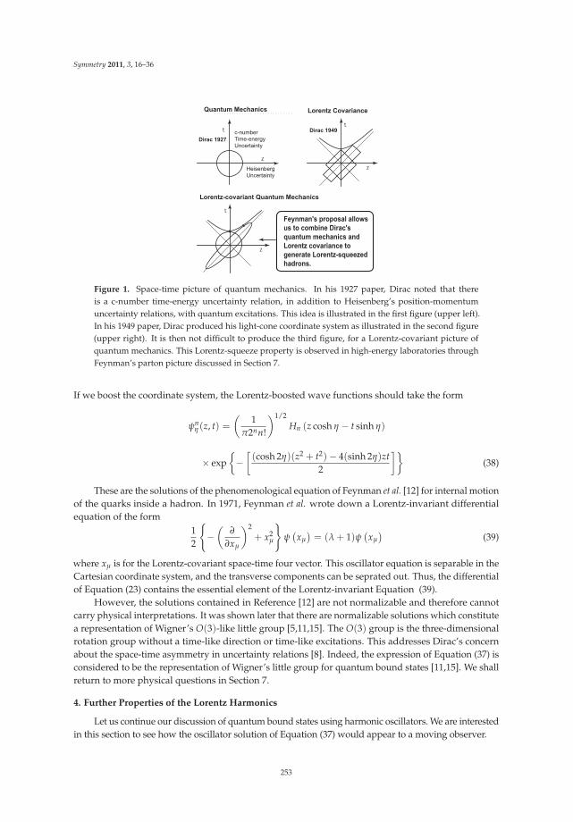
Symmetry 2011, 3, 16–36

t

z

z

z

t

t

Dirac 1927

Dirac 1949c-number

Time-energy

Uncertainty

Heisenberg

Uncertainty

Quantum Mechanics Lorentz Covariance

Lorentz-covariant Quantum Mechanics

Feynman's proposal allows

us to combine Dirac's

quantum mechanics and

Lorentz covariance to

generate Lorentz-squeezed

hadrons.

Figure 1. Space-time picture of quantum mechanics. In his 1927 paper, Dirac noted that thereis a c-number time-energy uncertainty relation, in addition to Heisenberg’s position-momentumuncertainty relations, with quantum excitations. This idea is illustrated in the first figure (upper left).In his 1949 paper, Dirac produced his light-cone coordinate system as illustrated in the second figure(upper right). It is then not difficult to produce the third figure, for a Lorentz-covariant picture ofquantum mechanics. This Lorentz-squeeze property is observed in high-energy laboratories throughFeynman’s parton picture discussed in Section 7.

If we boost the coordinate system, the Lorentz-boosted wave functions should take the form

ψnη (z, t) =

(1

π2nn!

)1/2Hn (z cosh η − t sinh η)

× exp{−

[(cosh 2η)(z2 + t2)− 4(sinh 2η)zt

2

]}(38)

These are the solutions of the phenomenological equation of Feynman et al. [12] for internal motionof the quarks inside a hadron. In 1971, Feynman et al. wrote down a Lorentz-invariant differentialequation of the form

12

{−

(∂

∂xμ

)2+ x2

μ

}ψ(

xμ

)= (λ + 1)ψ

(xμ

)(39)

where xμ is for the Lorentz-covariant space-time four vector. This oscillator equation is separable in theCartesian coordinate system, and the transverse components can be seprated out. Thus, the differentialof Equation (23) contains the essential element of the Lorentz-invariant Equation (39).

However, the solutions contained in Reference [12] are not normalizable and therefore cannotcarry physical interpretations. It was shown later that there are normalizable solutions which constitutea representation of Wigner’s O(3)-like little group [5,11,15]. The O(3) group is the three-dimensionalrotation group without a time-like direction or time-like excitations. This addresses Dirac’s concernabout the space-time asymmetry in uncertainty relations [8]. Indeed, the expression of Equation (37) isconsidered to be the representation of Wigner’s little group for quantum bound states [11,15]. We shallreturn to more physical questions in Section 7.

4. Further Properties of the Lorentz Harmonics

Let us continue our discussion of quantum bound states using harmonic oscillators. We are interestedin this section to see how the oscillator solution of Equation (37) would appear to a moving observer.

253

Symmetry 2011, 3, 16–36

The variable z and t are the longitudinal and time-like separations between the two constituentparticles. In terms of the light-cone variables defined in Equation (4), the solution of Equation (37)takes the form

ψn0 (z, t) =

[1

πn!2n

]1/2Hn

(u + v√

2

)exp

{−

(u2 + v2

2

)}(40)

and

ψnη (z, t) =

[1

πn!2n

]1/2Hn

(e−ηu + eηv√

2

)exp

{−

(e−2ηu2 + e2ηv2

2

)}(41)

for the rest and moving hadrons respectively.It is mathematically possible to expand this as [5,16]

ψnη (z, t) =

(1

cosh η

)(n+1)

∑k

[(n + k)!

n!k!

]1/2

(tanh η)kχn+k(z)χn(t) (42)

where χn(z) is the n-th excited state oscillator wave function which takes the familiar form

χn(z) =[

1√π2nn!

]1/2Hn(z) exp

(−z2

2

)(43)

as given in Equation (6). This is an expansion of the Lorentz-boosted wave function in terms of theLorentz harmonics.

If the hadron is at rest, there are no time-like oscillations. There are time-like oscillations fora moving hadron. This is the way in which the space and time variable mix covariantly. This alsoprovides a resolution of the space-time asymmetry pointed out by Dirac in his 1927 paper [8]. We shallreturn to this question in Section 6. Our next question is whether those oscillator equations can begiven a probability interpretation.

Even though we suppressed the excitations along the t direction in the hadronic rest frame, it isan interesting mathematical problem to start with the oscillator wave function with an excited state inthe time variable. This problem was adressed by Rotbart in 1981 [17].

4.1. Lorentz-Invariant Orthogonality Relations

Let us consider two wave functions ψnη (z, t). If two covariant wave functions are in the same

Lorentz frame and have thus the same value of η, the orthogonality relation

(ψn′

η , ψnη

)= δnn′ (44)

is satisfied.If those two wave functions have different values of η, we have to start with

(ψn′

η′ , ψnη

)=

∫ (ψn′

η′ (z, t))∗

ψnη (z, t)dzdt (45)

Without loss of generality, we can assume η′ = 0 in the system where η = 0, and evaluate the integration.The result is [18]

(ψn′

0 , ψnη

)=

∫ (ψn′

0 (z, t))2

ψnη (z, t)dxdt =

(√1 − β2

)(n+1)δn,n′ (46)

where β = tanh(η), as given in Equation (36). This is like the Lorentz-contraction property of a rigidrod. The ground state is like a single rod. Since we obtain the first excited state by applying a step-upoperator, this state should behave like a multiplication of two rods, and a similar argument can be giveto n rigid rods. This is illustrated in Figure 2.

254

Symmetry 2011, 3, 16–36

Figure 2. Orthogonality relations for the covariant harmonic oscillators. The orthogonality remainsinvariant. For the two wave functions in the orthogonality integral, the result is zero if they havedifferent values of n. If both wave functions have the same value of n, the integral shows the Lorentzcontraction property.

With these orthogonality properties, it is possible to give quantum probability interpretation inthe Lorentz-covariant world, and it was so stated in our 1977 paper [19].

4.2. Probability Interpretations

Let us study the probability issue in terms of the one-dimensional oscillator solution of Equation (6)whose probability interpretation is indisputable. Let us also go back to the rotationally invariantdifferential equation of Equation (11). Then the product

χnx (x)χny(y) (47)

also has a probability interpretation with the eigen value(nx + ny + 1

). Thus the series of the form [1,5]

φnη (x, y) =

(1

cosh η

)(n+1)

∑k

[(n + k)!

n!k!

]1/2

(tanh η)kχn+k(x)χn(y) (48)

also has its probability interpretation, but it is not in an eigen state. Each term in this series has aneigenvalue (2n + k + 1). The expectation value of Equation (11) is

(1

cosh η

)2(n+1)

∑k

(2n + k + 1)(n + k)!n!k!

(tanh η)2k (49)

If we replace the variables x and y by z and t respectively in the above expression of Equation(48), it becomes the Lorentz-covariant wave function of Equation (42). Each term χn+k(z)χk(t) in theseries has the eigenvalue n. Thus the series is in the eigen state with the eigenvalue n.

This difference does not prevent us from importing the probability interpretation from that ofEquation (48).

In the present covariant oscillator formalism, the time-separation variable can be separatedfrom the rest of the wave function, and does not requite further interpretation. For a moving

255

Symmetry 2011, 3, 16–36

hadron, time-like excitations are mixed with longitudinal excitations. Is it possible to give a physicalinterpretation to those time-like excitations? To address this issue, we shall study in Section 5 two-modesqueezed states also based on the mathematics of Equation (48). There, both variables have theirphysical interpretations.

5. Two-Mode Squeezed States

Harmonic oscillators play the central role also in quantum optics. There the nth excited oscillatorstate corresponds to the n-photon state |n >. The ground state means the zero-photon or vacuum state|0 >. The single-photon coherent state can be written as

|α >= e−αα∗/2 ∑n

αn√

n!|n > (50)

which can be written as [1]

|α >= e−αα∗/2 ∑n

αn

n!

(a†

)n|0 >=

{e−αα∗/2

}exp

{αa†

}|0 > (51)

This aspect of the single-photon coherent state is well known. Here we are dealing with one kind ofphoton, namely with a given momentum and polarization. The state |n > means there are n photonsof this kind.

Let us next consider a state of two kinds of photons, and write |n1, n2 > as the state of n1 photonsof the first kind, and n2 photons of the second kind [20]. We can then consider the form

1cosh η

exp{(tanh η)a†

1 a†2

}|0, 0 > (52)

The operator a†1 a†

2 was studied by Dirac in connection with his representation of the deSitter group, aswe mentioned in Section 3. After making a Taylor expansion of Equation (52), we arrive at

1cosh η ∑

k(tanh η)k|k, k > (53)

which is the squeezed vacuum state or two-photon coherent state [1,20]. This expression is the wavefunction of Equation (48) in a different notation. This form is also called the entangled Gaussian stateof two photons [3] or the entangled oscillator state of space and time [4].

If we start with the n-particle state of the first photon, we obtain

[1

cosh η

](n+1)exp

{(tanh η)a†

1 a†2

}|n, 0 >

=

[1

cosh η

](n+1)

∑k

[(n + k)!

n!k!

]1/2

(tanh η)k|k + n, k > (54)

which is the wave function of Equation (42) in a different notation. This is the n-photonsqueezed state [1].

Since the two-mode squeezed state and the covariant harmonic oscillators share the same setof mathematical formulas, it is possible to transmit physical interpretations from one to the other.For two-mode squeezed state, both photons carry physical interpretations, while the interpretation isyet to be given to the time-separation variable in the covariant oscillator formalism. It is clear fromEquation (42) and Equation (54) that the time-like excitations are like the second-photon states.

What would happen if the second photon is not observed? This interesting problem was addressedby Yurke and Potasek [21] and by Ekert and Knight [22]. They used the density matrix formalism and

256

Symmetry 2011, 3, 16–36

integrated out the second-photon states. This increases the entropy and temperature of the system.We choose not to reproduce their mathematics, because we will be presenting the same mathematicsin Section 6.

6. Time-Separation Variable in Feynman’s Rest of the Universe

As was noted in the previous section, the time-separation variable has an important role in thecovariant formulation of the harmonic oscillator wave functions. It should exist wherever the spaceseparation exists. The Bohr radius is the measure of the separation between the proton and electronin the hydrogen atom. If this atom moves, the radius picks up the time separation, according toEinstein [23].

On the other hand, the present form of quantum mechanics does not include this time-separationvariable. The best way we can interpret it at the present time is to treat this time-separation as avariable in Feynman’s rest of the universe [24]. In his book on statistical mechanics [7], Feynman states

When we solve a quantum-mechanical problem, what we really do is divide the universe into twoparts - the system in which we are interested and the rest of the universe. We then usually act as ifthe system in which we are interested comprised the entire universe. To motivate the use of densitymatrices, let us see what happens when we include the part of the universe outside the system.

The failure to include what happens outside the system results in an increase of entropy.The entropy is a measure of our ignorance and is computed from the density matrix [25]. The densitymatrix is needed when the experimental procedure does not analyze all relevant variables to themaximum extent consistent with quantum mechanics [26]. If we do not take into account thetime-separation variable, the result is an increase in entropy [27,28].

For the covariant oscillator wave functions defined in Equation (42), the pure-state density matrix is

ρnη(z, t; z′, t′) = ψn

η (z, t)ψnη (z

′, t′) (55)

which satisfies the condition ρ2 = ρ :

ρnη(z, t; x′, t′) =

∫ρn

η(z, t; x”, t”)ρnη(z”, t”; z′, t′)dz”dt” (56)

However, in the present form of quantum mechanics, it is not possible to take into account thetime separation variables. Thus, we have to take the trace of the matrix with respect to the t variable.Then the resulting density matrix is

ρnη(z, z′) =

∫ψn

η (z, t)ψnη (z

′, t)dt

=

(1

cosh η

)2(n+1)

∑k

(n + k)!n!k!

(tanh η)2kψn+k(z)ψ∗n+k(z

′) (57)

The trace of this density matrix is one, but the trace of ρ2 is less than one, as

Tr(

ρ2)=

∫ρn

η(z, z′)ρnη(z

′, z)dzdz′

=

(1

cosh η

)4(n+1)

∑k

[(n + k)!

n!k!

]2

(tanh η)4k (58)

which is less than one. This is due to the fact that we do not know how to deal with the time-likeseparation in the present formulation of quantum mechanics. Our knowledge is less than complete.

257

Symmetry 2011, 3, 16–36

The standard way to measure this ignorance is to calculate the entropy defined as

S = −Tr (ρ ln(ρ)) (59)

If we pretend to know the distribution along the time-like direction and use the pure-state densitymatrix given in Equation (55), then the entropy is zero. However, if we do not know how to deal withthe distribution along t, then we should use the density matrix of Equation (57) to calculate the entropy,and the result is

S = 2(n + 1){(cosh η)2 ln(cosh η)− (sinh η) ln(sinh η)

}

−(

1cosh η

)2(n+1)

∑k

(n + k)!n!k!

ln[(n + k)!

n!k!

](tanh η)2k (60)

In terms of the velocity v of the hadron,

S = −(n + 1){

ln[

1 −(v

c

)2]+

(v/c)2 ln(v/c)2

1 − (v/c)2

}

−[

1 −(

1v

)2]

∑k

(n + k)!n!k!

ln[(n + k)!

n!k!

] (vc

)2k(61)

Let us go back to the wave function given in Equation (41). As is illustrated in Figure 3,its localization property is dictated by the Gaussian factor which corresponds to the ground-state wavefunction. For this reason, we expect that much of the behavior of the density matrix or the entropy forthe nth excited state will be the same as that for the ground state with n = 0. For this state, the densitymatrix and the entropy are

ρ(z, z′) =(

1π cosh(2η)

)1/2exp

{−1

4

[(z + z′)2

cosh(2η)+ (z − z′)2 cosh(2η)

]}(62)

andS = 2

{(cosh η)2 ln(cosh η)− (sinh η)2 ln(sinh η)

}(63)

respectively. The quark distribution ρ(z, z) becomes

ρ(z, z) =(

1π cosh(2η)

)1/2exp

( −z2

cosh(2η)

)(64)

The width of the distribution becomes√

cosh η, and becomes wide-spread as the hadronic speedincreases. Likewise, the momentum distribution becomes wide-spread [5,29]. This simultaneousincrease in the momentum and position distribution widths is called the parton phenomenon inhigh-energy physics [13,14]. The position-momentum uncertainty becomes cosh η. This increase inuncertainty is due to our ignorance about the physical but unmeasurable time-separation variable.

Let us next examine how this ignorance will lead to the concept of temperature. For theLorentz-boosted ground state with n = 0, the density matrix of Equation (62) becomes that of theharmonic oscillator in a thermal equilibrium state if (tanh η)2 is identified as the Boltzmann factor [29].For other states, it is very difficult, if not impossible, to describe them as thermal equilibrium states.Unlike the case of temperature, the entropy is clearly defined for all values of n. Indeed, the entropy inthis case is derivable directly from the hadronic speed.

The time-separation variable exists in the Lorentz-covariant world, but we pretend not to knowabout it. It thus is in Feynman’s rest of the universe. If we do not measure this time-separation,it becomes translated into the entropy.

258

Symmetry 2011, 3, 16–36

β = 0

z

t

Measurable

No

t M

easu

rab

le

β = 0.8Feynman's

Rest of the

Universe

t

z

First Photon

Second photon

Figure 3. Localization property in the zt plane. When the hadron is at rest, the Gaussian formis concentrated within a circular region specified by (z + t)2 + (z − t)2 = 1. As the hadron gainsspeed, the region becomes deformed to e−2η(z + t)2 + e2η(z − t)2 = 1. Since it is not possible to makemeasurements along the t direction, we have to deal with information that is less than complete.

z

p

Quantum

Uncertainty

Statistical

Uncertainty

Figure 4. The uncertainty from the hidden time-separation coordinate. The small circle indicates theminimal uncertainty when the hadron is at rest. More uncertainty is added when the hadron moves.This is illustrated by a larger circle. The radius of this circle increases by

√cosh(2η).

We can see the uncertainty in our measurement process from the Wigner function defined as

W(z, p) =1π

∫ρ(z + y, z − y)e2ipydy (65)

After integration, this Wigner function becomes

W(z, p) =1

π cosh(2η)exp

{−

(z2 + p2

cosh(2η)

)}(66)

This Wigner phase distribution is illustrated in Figure 4. The smaller inner circle corresponds to theminimal uncertainty of the single oscillator. The larger circle is for the total uncertainty includingthe statistical uncertainty from our failure to observe the time-separation variable. The two-modesqueezed state tells us how this happens. In the two-mode case, both the first and second photons areobservable, but we can choose not to observe the second photon.

7. Lorentz-Covariant Quark Model

The hydrogen atom played the pivotal role while the present form of quantum mechanics wasdeveloped. At that time, the proton was in the absolute Galilean frame of reference, and it wasthinkable that the proton could move with a speed close to that of light.

Also, at that time, both the proton and electron were point particles. However, the discoveryof Hofstadter et al. changed the picture of the proton in 1955 [30]. The proton charge has its internal

259

Symmetry 2011, 3, 16–36

distribution. Within the framework of quantum electrodynamics, it is possible to calculate theRutherford formula for the electron-proton scattering when both electron and proton are point particles.Because the proton is not a point particle, there is a deviation from the Rutherford formula. We describethis deviation using the formula called the “proton form factor” which depends on the momentumtransfer during the electron-proton scattering.

Indeed, the study of the proton form factor has been and still is one of the central issues inhigh-energy physics. The form factor decreases as the momentum transfer increases. Its behavior iscalled the “dipole cut-off” meaning an inverse-square decrease, and it has been a challenging problemin quantum field theory and other theoretical models [31]. Since the emergence of the quark model in1964 [32], the hadrons are regarded as quantum bound states of quarks with space-time wave functions.Thus, the quark model is responsible for explaining this form factor. There are indeed many paperswritten on this subject. We shall return to this problem in Subsection 7.2.

Another problem in high-energy physics is Feynman’s parton picture [13,14]. If the hadron isat rest, we can approach this problem within the framework of bound-state quantum mechanics.If it moves with a speed close to that of light, it appears as a collection of an infinite number ofpartons, which interact with external signals incoherently. This phenomenon raises the question ofwhether the Lorentz boost destroys quantum coherence [33]. This leads to the concept of Feynman’sdecoherence [34]. We shall discuss this problem first.

7.1. Feynman’s Parton Picture and Feynman’s Decoherence

In 1969, Feynman observed that a fast-moving hadron can be regarded as a collection of many“partons” whose properties appear to be quite different from those of the quarks [5,14]. For example,the number of quarks inside a static proton is three, while the number of partons in a rapidly movingproton appears to be infinite. The question then is how the proton looking like a bound state of quarksto one observer can appear different to an observer in a different Lorentz frame? Feynman made thefollowing systematic observations.

a. The picture is valid only for hadrons moving with velocity close to that of light.b. The interaction time between the quarks becomes dilated, and partons behave as free independent

particles.c. The momentum distribution of partons becomes widespread as the hadron moves fast.d. The number of partons seems to be infinite or much larger than that of quarks.

Because the hadron is believed to be a bound state of two or three quarks, each of the above phenomenaappears as a paradox, particularly (b) and (c) together. How can a free particle have a wide-spreadmomentum distribution?

In order to address this question, let us go to Figure 5, which illustrates the Lorentz-squeezeproperty of the hadron as the hadron gains its speed. If we use the harmonic oscillator wave function,its momentum-energy wave function takes the same form as the space-time wave function. As thehadron gains its speed, both wave functions become squeezed.

As the wave function becomes squeezed, the distribution becomes wide-spread, the springconstant appear to become weaker. Consequently, the constituent quarks appear to become freeparticles.

If the constituent particles are confined in the narrow elliptic region, they become like masslessparticles. If those massless particles have a wide-spread momentum distribution, it is like a black-bodyradiation with infinite number of photon distributions.

We have addressed this question extensively in the literature, and concluded Gell-Mann’s quarkmodel and Feynman’s parton model are two different manifestations of the same Lorentz-covariantquantity [19,35,36]. Thus coherent quarks and incoherent partons are perfectly consistent withinthe framework of quantum mechanics and special relativity [33]. Indeed, this defines Feynman’sdecoherence [34].

260

Symmetry 2011, 3, 16–36

Ene

rgy

dist

ribut

ion

β=0.8β=0

z

t

z

BOOST

SPACE-TIME

DEFORMATION

Weaker springconstant

Quarks become(almost) free

Tim

e di

latio

n

TIM

E-E

NE

RG

Y U

NC

ER

TA

INT

Y

t

( (

β=0.8β=0

qz

qo

qz

BOOST

MOMENTUM-ENERGY

DEFORMATION

Parton momentumdistribution

becomes wider

qo

( (

(

(

QUARKS PARTONS

Figure 5. Lorentz-squeezed space-time and momentum-energy wave functions. As the hadron’s speedapproaches that of light, both wave functions become concentrated along their respective positivelight-cone axes. These light-cone concentrations lead to Feynman’s parton picture.

More recently, we were able to explain this decoherence problem in terms of the interaction timeamong the constituent quarks and the time required for each quark to interact with external signals [4].

7.2. Proton Form Factors and Lorentz Coherence

As early as in 1970, Fujimura et al. calculated the electromagnetic form factor of the protonusing the wave functions given in this paper and obtained the so-called “dipole” cut-off of the formfactor [37]. At that time, these authors did not have a benefit of the differential equation of Feynmanand his co-authors [12]. Since their wave functions can now be given a bona-fide covariant probabilityinterpretation, their calculation could be placed between the two limiting cases of quarks and partons.

Even before the calculation of Fujimura et al. in 1965, the covariant wave functions werediscussed by various authors [38–40]. In 1970, Licht and Pagnamenta also discussed this problem withLorentz-contracted wave functions [41].

In our 1973 paper [42], we attempted to explain the covariant oscillator wave function in terms ofthe coherence between the incoming signal and the width of the contracted wave function. This aspectwas explained in terms of the overlap of the energy-momentum wave function in our book [5].

In this paper, we would like to go back to the coherence problem we raised in 1973, and follow-upon it. In the Lorentz frame where the momentum of the proton has the opposite signs before and afterthe collision, the four-momentum transfer is

(p, E)− (−p, E) = (2p, 0) (67)

where the proton comes along the z direction with its momentum p, and its energy√

p2 + m2.

261

Symmetry 2011, 3, 16–36

Then the form factor becomes

F(p) =∫

e2ipz (ψη(z, t))∗

ψ−η(z, t) dz dt (68)

If we use the ground-state oscillator wave function, this integral becomes

1π

∫e2ipz exp

{− cosh(2η)

(z2 + t2

)}dz dt (69)

After the t integration, this integral becomes

1√π cosh(2η)

∫e2ipz exp

{−z2 cosh(2η)

}dz (70)

The integrand is a product of a Gaussian factor and a sinusoidal oscillation. The width of the Gaussianfactor shrinks by 1/

√cosh(2η), which becomes exp (−η) as η becomes large. The wave length of the

sinusoidal factor is inversely proportional to the momentum p. The wave length decreases also atthe rate of exp (−η). Thus, the rate of the shrinkage is the same for both the Gaussian and sinusoidalfactors. For this reason, the cutoff rate of the form factor of Equation (68) should be less than that for

∫e2ipz (ψ0(z, t))∗ ψ0(z, t) dz dt =

1√π

∫e2ipz exp

(−z2

)dz (71)

which corresponds to the form factor without the squeeze effect on the wave function. The integrationof this expression lead to exp

(−p2), which corresponds to an exponential cut-off as p2 becomes large.

Let us go back to the form factor of Equation (68). If we complete the integral, it becomes

F(p) =1

cosh(2η)exp

{ −p2

cosh(2η)

}(72)

As p2 becomes large, the Gaussian factor becomes a constant. However, the factor 1/ cosh(2η) leadsthe form factor decrease of 1/p2, which is a much slower decrease than the exponential cut-off withoutsqueeze effect.

There still is a gap between this mathematical formula and the observed experimental data.Before looking at the experimental curve, we have to realize that there are three quarks inside thehadron with two oscillator mode. This will lead to a

(1/p2)2 cut-off, which is commonly called the

dipole cut-off in the literature.There is still more work to be done. For instance, the effect of the quark spin should be

addressed [43,44]. Also there are reports of deviations from the exact dipole cut-off [45]. There havebeen attempts to study the form factors based on the four-dimensional rotation group [46], and also onthe lattice QCD [47].

Yet, it is gratifying to note that the effect of Lorentz squeeze lead to the polynomial decrease inthe momentum transfer, thanks to the Lorentz coherence illustrated in Figure 6. We started our logicfrom the fundamental principles of quantum mechanics and relativity.

8. Conclusions

In this paper, we presented one mathematical formalism applicable both to the entanglementproblems in quantum optics [3] and to high-energy hadronic physics [4]. The formalism is basedon harmonic oscillators familiar to us. We have presented a complete orthonormal set with aLorentz-covariant probability interpretation.

Since both branches of physics share the same mathematical base, it is possible to translatephysics from one branch to the other. In this paper, we have given a physical interpretation to the

262

Symmetry 2011, 3, 16–36

Incr

easi

ng

Fre

qu

ency

Incr

easi

ng

Mo

men

tum

Tra

nsf

er

without Contraction

with Contraction

LorentzCoherence

withoutCoherence

Figure 6. Coherence between the wavelength and the proton size. As the momentum transfer increases,the external signal sees Lorentz-contracting proton distribution. On the other hand, the wavelength ofthe signal also decreases. Thus, the cutoff is not as severe as the case where the proton distribution isnot contracted.

time-separation variable as a hidden variable in Feynman’s rest of the universe, in terms of thetwo-mode squeezed state where both photons are observable.

This paper is largely a review paper with an organization to suit the current interest in physics.For instance, the concepts of entanglement and decoherecne did not exist when those original paperswere written. Furthermore, the probability interpretation given in Subsection 4.2 has not beenpublished before.

The rotation symmetry plays its role in all branches of physics. We noted that the squeezesymmetry plays active roles in two different subjects of physics. It is possible that the squeezetransformation can serve useful purposes in many other fields, although we are not able to specifythem at this time.

References

1. Kim, Y.S.; Noz, M.E. Phase Space Picture of Quantum Mechanics; World Scientific Publishing Company:Singapore, 1991.

2. Guillemin, V.; Sternberg, S. Symplectic Techniques in Physics; Cambridge University: Cambridge, UK, 1984.3. Giedke, G.; Wolf, M.M.; Krger, O; Werner, R.F.; Cirac, J.J. Entanglement of formation for symmetric Gaussian

states. Phys. Rev. Lett. 2003, 91, 107901-107904.4. Kim, Y.S.; Noz, M.E. Coupled oscillators, entangled oscillators, and Lorentz-covariant harmonic oscillators.

J. Opt. B: Quantum Semiclass. Opt. 2005, 7, S458-S467.5. Kim, Y.S.; Noz, M.E. Theory and Applications of the Poincaré Group D; Reidel Publishing Company: Dordrecht,

The Netherlands, 1986.6. Dirac, P.A.M. Forms of Relativistic Dynamics. Rev. Mod. Phys. 1949, 21, 392-399.7. Feynman, R.P. Statistical Mechanics; Benjamin/Cummings: Reading, MA, USA, 1972.8. Dirac, P.A.M. The Quantum Theory of the Emission and Absorption of Radiation. Proc. Roy. Soc. (London)

1927, A114, 243-265.9. Dirac, P.A.M. Unitary Representations of the Lorentz Group. Proc. Roy. Soc. (London) 1945, A183, 284-295.10. Dirac, P.A.M. A Remarkable Representation of the 3 + 2 de Sitter Group. J. Math. Phys. 1963, 4, 901-909.11. Wigner, E. On Unitary Representations of the Inhomogeneous Lorentz Group. Ann. Math. 1939, 40, 149-204.

263

Symmetry 2011, 3, 16–36

12. Feynman, R.P.; Kislinger, M.; Ravndal F. Current Matrix Elements from a Relativistic Quark Model.Phys. Rev. D 1971, 3, 2706-2732.

13. Feynman, R.P. Very High-Energy Collisions of Hadrons. Phys. Rev. Lett. 1969, 23, 1415-1417.14. Feynman, R.P. The Behavior of Hadron Collisions at Extreme Energies in High-Energy Collisions.

In Proceedings of the Third International Conference; Gordon and Breach: New York, NY, USA, 1969; pp. 237-249.15. Kim, Y.S.; Noz, M.E.; Oh, S.H. Representations of the Poincaré group for relativistic extended hadrons.

J. Math. Phys. 1979, 20, 1341-1344.16. Kim, Y.S.; Noz, M.E.; Oh, S.H.; A Simple Method for Illustrating the Difference between the Homogeneous

and Inhomogeneous Lorentz Groups. Am. J. Phys. 1979, 47, 892-897.17. Rotbart, F.C. Complete orthogonality relations for the covariant harmonic oscillator. Phys. Rev. D 1981, 12,

3078-3090.18. Ruiz, M.J. Orthogonality relations for covariant harmonic oscillator wave functions. Phys. Rev. D 1974, 10,

4306-4307.19. Kim, Y.S.; Noz, M.E. Covariant Harmonic Oscillators and the Parton Picture. Phys. Rev. D 1977, 15, 335-338.20. Yuen, H.P. Two-photon coherent states of the radiation field. Phys. Rev. A 1976, 13, 2226-2243.21. Yurke, B.; Potasek, M. Obtainment of Thermal Noise from a Pure State. Phys. Rev. A 1987, 36, 3464-3466.22. Ekert, A.K.; Knight, P.L. Correlations and squeezing of two-mode oscillations. Am. J. Phys. 1989, 57, 692-697.23. Kim, Y.S.; Noz, M.E. The Question of Simultaneity in Relativity and Quantum Mechanics. In Quantum Theory:

Reconsideration of Foundations–3; Adenier, G., Khrennikov, A., Nieuwenhuizen, T.M., Eds.; AIP ConferenceProceedings 180, American Institute of Physics, College Park, MD, USA, 2006; pp. 168-178.

24. Han, D.; Kim, Y.S.; Noz, M.E. Illustrative Example of Feynman’s Rest of the Universe. Am. J. Phys. 1999, 67,61-66.

25. von Neumann, J. Die Mathematische Grundlagen der Quanten-mechanik; Springer: Berlin, Germany, 1932.26. Fano, U. Description of States in Quantum Mechanics by Density Matrix and Operator Techniques. Rev. Mod.

Phys. 1967, 29, 74-93.27. Kim, Y.S.; Wigner, E.P. Entropy and Lorentz Transformations. Phys. Lett. A 1990, 147, 343-347.28. Kim, Y.S. Coupled oscillators and Feynman’s three papers. J. Phys. Conf. Ser. 2007, 70, 012010: 1-19.29. Han, D.; Kim, Y.S.; Noz, M.E. Lorentz-Squeezed Hadrons and Hadronic Temperature. Phys. Lett. A 1990, 144,

111-115.30. Hofstadter, R.; McAllister, R.W. Electron Scattering from the Proton. Phys. Rev. 1955, 98, 217-218.31. Frazer, W.; Fulco, J. Effect of a Pion-Pion Scattering Resonance on Nucleon Structure. Phys. Rev. Lett. 1960, 2,

365-368.32. Gell-Mann, M. Nonleptonic Weak Decays and the Eightfold Way. Phys. Lett. 1964, 12, 155-156.33. Kim, Y.S. Does Lorentz Boost Destroy Coherence? Fortschr. der Physik 1998, 46, 713-724.34. Kim, Y.S.; Noz, M.E. Feynman’s Decoherence. Optics Spectro. 2003, 47, 733-740.35. Hussar, P.E. Valons and harmonic oscillators. Phys. Rev. D 1981, 23, 2781-2783.36. Kim, Y.S. Observable gauge transformations in the parton picture. Phys. Rev. Lett. 1989, 63, 348-351.37. Fujimura, K.; Kobayashi, T.; Namiki, M. Nucleon Electromagnetic Form Factors at High Momentum Transfers

in an Extended Particle Model Based on the Quark Model. Prog. Theor. Phys. 1970, 43, 73-79.38. Yukawa, H. Structure and Mass Spectrum of Elementary Particles. I. General Considerations. Phys. Rev.

1953, 91, 415-416.39. Markov, M. On Dynamically Deformable Form Factors in the Theory Of Particles. Suppl. Nuovo Cimento

1956, 3, 760-772.40. Ginzburg, V.L.; Man’ko, V.I. Relativistic oscillator models of elementary particles. Nucl. Phys. 1965, 74,

577-588.41. Licht, A.L.; Pagnamenta, A. Wave Functions and Form Factors for Relativistic Composite Particles I.

Phys. Rev. D 1970, 2, 1150-1156.42. Kim, Y.S.; Noz, M.E. Covariant harmonic oscillators and the quark model. Phys. Rev. D 1973, 8, 3521-3627.43. Lipes, R. Electromagnetic Excitations of the Nucleon in a Relativistic Quark Model. Phys. Rev. D 1972, 5,

2849-2863.44. Henriques, A.B.; Keller, B.H.; Moorhouse, R.G. General three-spinor wave functions and the relativistic

quark model. Ann. Phys. (NY) 1975, 93, 125-151.

264

Symmetry 2011, 3, 16–36

45. Punjabi, V.; Perdrisat, C.F.; Aniol, K.A.; Baker, F.T.; Berthot, J.; Bertin, P.Y.; Bertozzi, W.; Besson, A.; Bimbot, L.;Boeglin, W.U.; et al. Proton elastic form factor ratios to Q2 = 3.5 GeV2 by polarization transfer. Phys. Rev. C2005, 71, 055202-27.

46. Alkofer, R.; Holl, A.; Kloker, M.; Karssnigg A.; Roberts, C.D. On Nucleon Electromagnetic Form Factors.Few-Body Sys. 2005, 37, 1-31.

47. Matevosyan, H.H.; Thomas, A.W.; Miller, G.A. Study of lattice QCD form factors using the extendedGari-Krumpelmann model. Phys. Rev. C 2005, 72, 065204-5.

c© 2011 by the authors. Licensee MDPI, Basel, Switzerland. This article is an open accessarticle distributed under the terms and conditions of the Creative Commons Attribution(CC BY) license (http://creativecommons.org/licenses/by/4.0/).

265

symmetryS S

Article

Dirac Matrices and Feynman’s Rest of the Universe

Young S. Kim 1,* and Marilyn E. Noz 2

1 Center for Fundamental Physics, University of Maryland, College Park, MD 20742, USA2 Department of Radiology, New York University, New York, NY 10016, USA; marilyne.noz@gmail.com* Author to whom correspondence should be addressed; yskim@umd.edu; Tel.: +1-301-937-6306.

Received: 25 June 2012; in revised form: 6 October 2012; Accepted: 23 October 2012; Published: 30 October 2012

Abstract: There are two sets of four-by-four matrices introduced by Dirac. The first set consistsof fifteen Majorana matrices derivable from his four γ matrices. These fifteen matrices can alsoserve as the generators of the group SL(4, r). The second set consists of ten generators of the Sp(4)group which Dirac derived from two coupled harmonic oscillators. It is shown possible to extendthe symmetry of Sp(4) to that of SL(4, r) if the area of the phase space of one of the oscillators isallowed to become smaller without a lower limit. While there are no restrictions on the size of phasespace in classical mechanics, Feynman’s rest of the universe makes this Sp(4)-to-SL(4, r) transitionpossible. The ten generators are for the world where quantum mechanics is valid. The remainingfive generators belong to the rest of the universe. It is noted that the groups SL(4, r) and Sp(4) arelocally isomorphic to the Lorentz groups O(3, 3) and O(3, 2) respectively. This allows us to interpretFeynman’s rest of the universe in terms of space-time symmetry.

Keywords: Dirac gamma matrices; Feynman’s rest of the universe; two coupled oscilators;Wigner’s phase space; non-canonical transformations; group generators; SL(4, r) isomorphic O(3, 3);quantum mechanics interpretation

1. Introduction

In 1963, Paul A. M. Dirac published an interesting paper on the coupled harmonic oscillators [1].Using step-up and step-down operators, Dirac was able to construct ten operators satisfying a closedset of commutation relations. He then noted that this set of commutation relations can also be usedas the Lie algebra for the O(3, 2) de Sitter group applicable to three space and two time dimensions.He noted further that this is the same as the Lie algebra for the four-dimensional symplectic groupSp(4).

His algebra later became the fundamental mathematical language for two-mode squeezed states inquantum optics [2–5]. Thus, Dirac’s ten oscillator matrices play a fundamental role in modern physics.

In the Wigner phase-space representation, it is possible to write the Wigner function in termsof two position and two momentum variables. It was noted that those ten operators of Dirac can betranslated into the operators with these four variables [4,6], which then can be written as four-by-fourmatrices. There are thus ten four-by-four matrices. We shall call them Dirac’s oscillator matrices.They are indeed the generators of the symplectic group Sp(4).

We are quite familiar with four Dirac matrices for the Dirac equation, namely γ1, γ2, γ3, and γ0.They all become imaginary in the Majorana representation. From them we can construct fifteen linearlyindependent four-by-four matrices. It is known that these four-by-four matrices can serve as thegenerators of the SL(4, r) group [6,7]. It is also known that this SL(4, r) group is locally isomorphic tothe Lorentz group O(3, 3) applicable to the three space and three time dimensions [6,7].

There are now two sets of the four-by-four matrices constructed by Dirac. The first set consists ofhis ten oscillator matrices, and there are fifteen γ matrices coming from his Dirac equation. There is

Symmetry 2012, 4, 626–643 266 www.mdpi.com/journal/symmetry

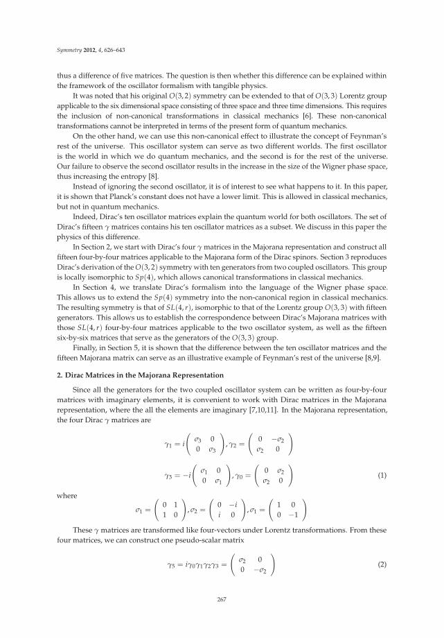
Symmetry 2012, 4, 626–643

thus a difference of five matrices. The question is then whether this difference can be explained withinthe framework of the oscillator formalism with tangible physics.

It was noted that his original O(3, 2) symmetry can be extended to that of O(3, 3) Lorentz groupapplicable to the six dimensional space consisting of three space and three time dimensions. This requiresthe inclusion of non-canonical transformations in classical mechanics [6]. These non-canonicaltransformations cannot be interpreted in terms of the present form of quantum mechanics.

On the other hand, we can use this non-canonical effect to illustrate the concept of Feynman’srest of the universe. This oscillator system can serve as two different worlds. The first oscillatoris the world in which we do quantum mechanics, and the second is for the rest of the universe.Our failure to observe the second oscillator results in the increase in the size of the Wigner phase space,thus increasing the entropy [8].

Instead of ignoring the second oscillator, it is of interest to see what happens to it. In this paper,it is shown that Planck’s constant does not have a lower limit. This is allowed in classical mechanics,but not in quantum mechanics.

Indeed, Dirac’s ten oscillator matrices explain the quantum world for both oscillators. The set ofDirac’s fifteen γ matrices contains his ten oscillator matrices as a subset. We discuss in this paper thephysics of this difference.

In Section 2, we start with Dirac’s four γ matrices in the Majorana representation and construct allfifteen four-by-four matrices applicable to the Majorana form of the Dirac spinors. Section 3 reproducesDirac’s derivation of the O(3, 2) symmetry with ten generators from two coupled oscillators. This groupis locally isomorphic to Sp(4), which allows canonical transformations in classical mechanics.

In Section 4, we translate Dirac’s formalism into the language of the Wigner phase space.This allows us to extend the Sp(4) symmetry into the non-canonical region in classical mechanics.The resulting symmetry is that of SL(4, r), isomorphic to that of the Lorentz group O(3, 3) with fifteengenerators. This allows us to establish the correspondence between Dirac’s Majorana matrices withthose SL(4, r) four-by-four matrices applicable to the two oscillator system, as well as the fifteensix-by-six matrices that serve as the generators of the O(3, 3) group.

Finally, in Section 5, it is shown that the difference between the ten oscillator matrices and thefifteen Majorana matrix can serve as an illustrative example of Feynman’s rest of the universe [8,9].

2. Dirac Matrices in the Majorana Representation

Since all the generators for the two coupled oscillator system can be written as four-by-fourmatrices with imaginary elements, it is convenient to work with Dirac matrices in the Majoranarepresentation, where the all the elements are imaginary [7,10,11]. In the Majorana representation,the four Dirac γ matrices are

γ1 = i

(σ3 00 σ3

), γ2 =

(0 −σ2

σ2 0

)

γ3 = −i

(σ1 00 σ1

), γ0 =

(0 σ2

σ2 0

)(1)

where

σ1 =

(0 11 0

), σ2 =

(0 −ii 0

), σ1 =

(1 00 −1

)These γ matrices are transformed like four-vectors under Lorentz transformations. From these

four matrices, we can construct one pseudo-scalar matrix

γ5 = iγ0γ1γ2γ3 =

(σ2 00 −σ2

)(2)

267

Symmetry 2012, 4, 626–643

and a pseudo vector iγ5γμ consisting of

iγ5γ1 = i

(−σ1 0

0 σ1

), iγ5γ2 = −i

(0 II 0

)

iγ5γ0 = i

(0 I−I 0

), iγ5γ3 = i

(−σ3 0

0 +σ3

)(3)

In addition, we can construct the tensor of the γ as

Tμν =i2(γμγν − γνγμ

)(4)

This antisymmetric tensor has six components. They are

iγ0γ1 = −i

(0 σ1

σ1 0

), iγ0γ2 = −i

(−I 00 I

), iγ0γ3 = −i

(0 σ3

σ3 0

)(5)

and

iγ1γ2 = i

(0 −σ1

σ1 0

), iγ2γ3 = −i

(0 −σ3

σ3 0

), iγ3γ1 =

(σ2 00 σ2

)(6)

There are now fifteen linearly independent four-by-four matrices. They are all traceless and theircomponents are imaginary [7]. We shall call these Dirac’s Majorana matrices.

In 1963 [1], Dirac constructed another set of four-by-four matrices from two coupled harmonicoscillators, within the framework of quantum mechanics. He ended up with ten four-by-four matrices.It is of interest to compare his oscillator matrices and his fiftteen Majorana matrices.

3. Dirac’s Coupled Oscillators

In his 1963 paper [1], Dirac started with the Hamiltonian for two harmonic oscillators. It can bewritten as

H =12

(p2

1 + x21

)+

12

(p2

2 + x22

)(7)

The ground-state wave function for this Hamiltonian is

ψ0(x1, x2) =1√π

exp{−1

2

(x2

1 + x22

)}(8)

We can now consider unitary transformations applicable to the ground-state wave function ofEquation (8), and Dirac noted that those unitary transformations are generated by [1]

L1 = 12(a†

1a2 + a†2a1), L2 = 1

2i(a†

1a2 − a†2a1)

L3 = 12(a†

1a1 − a†2a2), S3 = 1

2(a†

1a1 + a2a†2)

K1 = − 14(a†

1a†1 + a1a1 − a†

2a†2 − a2a2

)K2 = i

4(a†

1a†1 − a1a1 + a†

2a†2 − a2a2

)K3 = 1

2(a†

1a†2 + a1a2

)Q1 = − i

4(a†

1a†1 − a1a1 − a†

2a†2 + a2a2

)Q2 = − 1

4(a†

1a†1 + a1a1 + a†

2a†2 + a2a2

)Q3 = i

2(a†

1a†2 − a1a2

)(9)

where a† and a are the step-up and step-down operators applicable to harmonic oscillator wavefunctions. These operators satisfy the following set of commutation relations.

268

Symmetry 2012, 4, 626–643

[Li, Lj

]= iεijkLk,

[Li, Kj

]= iεijkKk,

[Li, Qj

]= iεijkQk[

Ki, Kj]=[Qi, Qj

]= −iεijkLk, [Li, S3] = 0[

Ki, Qj]= −iδijS3, [Ki, S3] = −iQi, [Qi, S3] = iKi (10)

Dirac then determined that these commutation relations constitute the Lie algebra for the O(3, 2)de Sitter group with ten generators. This de Sitter group is the Lorentz group applicable to threespace coordinates and two time coordinates. Let us use the notation (x, y, z, t, s), with (x, y, z) as spacecoordinates and (t, s) as two time coordinates. Then the rotation around the z axis is generated by

L3 =

⎛⎜⎜⎜⎜⎜⎝0 −i 0 0 0i 0 0 0 00 0 0 0 00 0 0 0 00 0 0 0 0

⎞⎟⎟⎟⎟⎟⎠ (11)

The generators L1 and L2 can be also be constructed. The K3 and Q3 will take the form

K3 =

⎛⎜⎜⎜⎜⎜⎝0 0 0 0 00 0 0 0 00 0 0 i 00 0 i 0 00 0 0 0 0

⎞⎟⎟⎟⎟⎟⎠, Q3 =

⎛⎜⎜⎜⎜⎜⎝0 0 0 0 00 0 0 0 00 0 0 0 i0 0 0 0 00 0 i 0 0

⎞⎟⎟⎟⎟⎟⎠ (12)

From these two matrices, the generators K1, K2, Q1, Q2 can be constructed. The generator S3 can bewritten as

S3 =

⎛⎜⎜⎜⎜⎜⎝0 0 0 0 00 0 0 0 00 0 0 0 00 0 0 0 −i0 0 0 i 0

⎞⎟⎟⎟⎟⎟⎠ (13)

The last five-by-five matrix generates rotations in the two-dimensional space of (t, s).In his 1963 paper [1], Dirac states that the Lie algebra of Equation (10) can serve as the

four-dimensional symplectic group Sp(4). In order to see this point, let us go to the Wigner phase-spacepicture of the coupled oscillators.

3.1. Wigner Phase-Space Representation

For this two-oscillator system, the Wigner function is defined as [4,6]

W(x1, x2; p1, p2) =(

1π

)2 ∫exp{−2i(p1y1 + p2y2)}

×ψ∗(x1 + y1, x2 + y2)ψ(x1 − y1, x2 − y2)dy1dy2(14)

Indeed, the Wigner function is defined over the four-dimensional phase space of (x1, p1, x2, p2) just asin the case of classical mechanics. The unitary transformations generated by the operators of Equation(9) are translated into linear canonical transformations of the Wigner function [4]. The canonicaltransformations are generated by the differential operators [4]:

L1 = + i2

{(x1

∂∂p2

− p2∂

∂x1

)+(

x2∂

∂p1− p1

∂∂x2

)}

269

Symmetry 2012, 4, 626–643

L2 = − i2

{(x1

∂∂x2

− x2∂

∂x1

)+(

p1∂

∂p2− p2

∂∂p1

)}L3 = + i

2

{(x1

∂∂p1

− p1∂

∂x1

)−(

x2∂

∂p2− p2

∂∂x2

)}S3 = − i

2

{(x1

∂∂p1

− p1∂

∂x1

)+(

x2∂

∂p2− p2

∂∂x2

)}(15)

andK1 = − i

2

{(x1

∂∂p1

+ p1∂

∂x1

)−(

x2∂

∂p2+ p2

∂∂x2

)}K2 = − i

2

{(x1

∂∂x1

− p1∂

∂p1

)+(

x2∂

∂x2− p2

∂∂p2

)}K3 = + i

2

{(x1

∂∂p2

+ p2∂

∂x1

)+(

x2∂

∂p1+ p1

∂∂x2

)}Q1 = + i

2

{(x1

∂∂x1

− p1∂

∂p1

)−(

x2∂

∂x2− p2

∂∂p2

)}Q2 = − i

2

{(x1

∂∂p1

+ p1∂

∂x1

)+(

x2∂

∂p2+ p2

∂∂x2

)}Q3 = − i

2

{(x2

∂∂x1

+ x1∂

∂x2

)−(

p2∂

∂p1+ p1

∂∂p2

)}(16)

3.2. Translation into Four-by-Four Matrices

For a dynamical system consisting of two pairs of canonical variables x1, p1 and x2, p2, we canuse the coordinate variables defined as [6]

(η1, η2, η3, η4) = (x1, p1, x2, p2) (17)

Then the transformation of the variables from ηi to ξi is canonical if [12,13]

MJM = J (18)

where M is a four-by-four matrix defined by

Mij =∂

∂ηjξi

and

J =

⎛⎜⎜⎜⎝0 1 0 0−1 0 0 00 0 0 10 0 −1 0

⎞⎟⎟⎟⎠ (19)

According to this form of the J matrix, the area of the phase space for x1 and p1 variables remainsinvariant, and the story is the same for the phase space of x2 and p2.

We can then write the generators of the Sp(4) group as

L1 =−12

(0 σ2

σ2 0

), L2 =

i2

(0 −II 0

)

L3 =12

(−σ2 0

0 σ2

), S3 =

12

(σ2 00 σ2

)(20)

and

K1 =i2

(σ1 00 −σ1

), K2 =

i2

(σ3 00 σ3

), K3 = − i

2

(0 σ1

σ1 0

)

270

Symmetry 2012, 4, 626–643

and

Q1 =i2

(−σ3 0

0 σ3

), Q2 =

i2

(σ1 00 σ1

), Q3 =

i2

(0 σ3

σ3 0

)(21)

These four-by-four matrices satisfy the commutation relations given in Equation (10). Indeed, the deSitter group O(3, 2) is locally isomorphic to the Sp(4) group. The remaining question is whether theseten matrices can serve as the fifteen Dirac matrices given in Section 2. The answer is clearly no. How canten matrices describe fifteen matrices? We should therefore add five more matrices.

4. Extension to O(3, 3) Symmetry

Unlike the case of the Schrödinger picture, it is possible to add five non-canonical generators tothe above list. They are

S1 = + i2

{(x1

∂∂x2

− x2∂

∂x1

)−(

p1∂

∂p2− p2

∂∂p1

)}S2 = − i

2

{(x1

∂∂p2

− p2∂

∂x1

)+(

x2∂

∂p1− p1

∂∂x2

)}(22)

as well as three additional squeeze operators:

G1 = − i2

{(x1

∂∂x2

+ x2∂

∂x1

)+(

p1∂

∂p2+ p2

∂∂p1

)}G2 = i

2

{(x1

∂∂p2

+ p2∂

∂x1

)−(

x2∂

∂p1+ p1

∂∂x2

)}G3 = − i

2

{(x1

∂∂x1

+ p1∂

∂p1

)+(

x2∂

∂p1+ p1

∂∂x2

)}(23)

These five generators perform well-defined operations on the Wigner function. However, the questionis whether these additional generators are acceptable in the present form of quantum mechanics.

In order to answer this question, let us note that the uncertainty principle in the phase-spacepicture of quantum mechanics is stated in terms of the minimum area in phase space for a given pairof conjugate variables. The minimum area is determined by Planck’s constant. Thus we are allowed toexpand the phase space, but are not allowed to contract it. With this point in mind, let us go back toG3 of Equation (23), which generates transformations that simultaneously expand one phase spaceand contract the other. Thus, the G3 generator is not acceptable in quantum mechanics even though itgenerates well-defined mathematical transformations of the Wigner function.

If the five generators of Equations (22) and (23) are added to the ten generators given in Equations(15) and (16), there are fifteen generators. They satisfy the following set of commutation relations.

[Li, Lj

]= iεijkLk,

[Si, Sj

]= iεijkSk,

[Li, Sj

]= 0[

Li, Kj]= iεijkKk,

[Li, Qj

]= iεijkQk,

[Li, Gj

]= iεijkGk[

Ki, Kj]=[Qi, Qj

]=[Qi, Qj

]= −iεijkLk[

Ki, Qj]= −iδijS3,

[Qi, Gj

]= −iδijS1,

[Gi, Kj

]= −iδijS2

[Ki, S3] = −iQi, [Qi, S3] = iKi, [Gi, S3] = 0

[Ki, S1] = 0, [Qi, S1] = −iGi, [Gi, S1] = iQi

[Ki, S2] = iGi, [Qi, S2] = 0, [Gi, S2] = −iKi (24)

As we shall see in Section 4.2, this set of commutation relations serves as the Lie algebra for the groupSL(4, r) and also for the O(3, 3) Lorentz group.

271

Symmetry 2012, 4, 626–643

These fifteen four-by-four matrices are written in terms of Dirac’s fifteen Majorana matrices,and are tabulated in Table 1. There are six anti-symmetric and nine symmetric matrices.These anti-symmetric matrices were divided into two sets of three rotation generators in thefour-dimensional phase space. The nine symmetric matrices can be divided into three sets of threesqueeze generators. However, this classification scheme is easier to understand in terms the groupO(3, 3), discussed in Section 4.2.

Table 1. SL(4, r) and Dirac matrices. Two sets of rotation generators and three sets of boost generators.There are 15 generators.

First component Second component Third component

Rotation L1 = −i2 γ0 L2 = −i

2 γ5γ0 L3 = −12 γ5

Rotation S1 = i2 γ2γ3 S2 = i

2 γ1γ2 S3 = i2 γ3γ1

Boost K1 = −i2 γ5γ1 K2 = 1

2 γ1 K3 = i2 γ0γ1

Boost Q1 = i2 γ5γ3 Q2 = −1

2 γ3 Q3 = − i2 γ0γ3

Boost G1 = −i2 γ5γ2 G2 = 1

2 γ2 G3 = i2 γ0γ2

4.1. Non-Canonical Transformations in Classical Mechanics

In addition to Dirac’s ten oscillator matrices, we can consider the matrix

G3 =i2

(I 00 −I

)(25)

which will generate a radial expansion of the phase space of the first oscillator, while contracting thatof the second phase space [14], as illustrated in Figure 1. What is the physical significance of thisoperation? The expansion of phase space leads to an increase in uncertainty and entropy [8,14].

p p

x x

1

1

2

2

Figure 1. Expanding and contracting phase spaces. Canonical transformations leave the area of eachphase space invariant. Non-canonical transformations can change them, yet the product of these twoareas remains invariant.

The contraction of the second phase space has a lower limit in quantum mechanics, namely itcannot become smaller than Planck’s constant. However, there is no such lower limit in classicalmechanics. We shall go back to this question in Section 5.

272

Symmetry 2012, 4, 626–643

In the meantime, let us study what happens when the matrix G3 is introduced into the set of matricesgiven in Equations (20) and (21). It commutes with S3, L3, K1, K2, Q1, and Q2. However, its commutatorswith the rest of the matrices produce four more generators:

[G3, L1] = iG2, [G3, L2] = −iG1, [G3, K3] = iS2, [G3, Q3] = −iS1 (26)

where

G1 = i2

(0 II 0

), G2 = 1

2

(0 −σ2

σ2 0

)

S1 = i2

(0 σ3

−σ3 0

), S2 = i

2

(0 −σ1

σ1 0

)(27)

If we take into account the above five generators in addition to the ten generators of Sp(4), there arefifteen generators. These generators satisfy the set of commutation relations given in Equation (24).

Indeed, the ten Sp(4) generators together with the five new generators form the Lie algebra forthe group SL(4, r). There are thus fifteen four-by-four matrices. They can be written in terms of thefifteen Majorana matrices, as given in Table 1.

4.2. Local Isomorphism between O(3,3) and SL(4,r)

It is now possible to write fifteen six-by-six matrices that generate Lorentz transformations on thethree space coordinates and three time coordinates [6]. However, those matrices are difficult to handleand do not show existing regularities. In this section, we write those matrices as two-by-two matricesof three-by-three matrices.

For this purpose, we construct four sets of three-by-three matrices given in Table 2. There are twosets of rotation generators

Li =

(Ai 00 0

), Si =

(0 00 Ai

)(28)

applicable to the space and time coordinates respectively.There are also three sets of boost generators. In the two-by-two representation of the matrices

given in Table 2, they are

Ki =

(0 BiBi 0

), Qi =

(0 CiCi 0

), Gi =

(0 Di

Di 0

)(29)

where the three-by-three matrices Ai, Bi, Ci, and Di are given in Table 2, and Ai, Bi, Ci, Di are theirtransposes respectively.

273

Symmetry 2012, 4, 626–643

Table 2. Three-by-three matrices constituting the two-by-two representation of generators of theO(3, 3) group.

i = 1 i = 2 i = 3

Ai

⎛⎝ 0 0 00 0 −i0 i 0

⎞⎠ ⎛⎝ 0 0 i0 0 0−i 0 0

⎞⎠ ⎛⎝ 0 −i 0i 0 00 0 0

⎞⎠Bi

⎛⎝ i 0 00 0 00 0 0

⎞⎠ ⎛⎝ 0 0 0i 0 00 0 0

⎞⎠ ⎛⎝ 0 0 00 0 0i 0 0

⎞⎠Ci

⎛⎝ 0 i 00 0 00 0 0

⎞⎠ ⎛⎝ 0 0 00 i 00 0 0

⎞⎠ ⎛⎝ 0 0 00 0 00 i 0

⎞⎠Di

⎛⎝ 0 0 i0 0 00 0 0

⎞⎠ ⎛⎝ 0 0 00 0 i0 0 0

⎞⎠ ⎛⎝ 0 0 00 0 00 0 i

⎞⎠

There is a four-by-four Majorana matrix corresponding to each of these fifteen six-by-six matrices,as given in Table 1.

There are of course many interesting subgroups. The most interesting case is the O(3, 2)subgroup, and there are three of them. Another interesting feature is that there are three timedimensions. Thus, there are also O(2, 3) subgroups applicable to two space and three time coordinates.This symmetry between space and time coordinates could be an interesting future investigation.

5. Feynman’s Rest of the Universe

In his book on statistical mechanics [9], Feynman makes the following statement. When we solvea quantum-mechanical problem, what we really do is divide the universe into two parts - the system in whichwe are interested and the rest of the universe. We then usually act as if the system in which we are interestedcomprised the entire universe. To motivate the use of density matrices, let us see what happens when we includethe part of the universe outside the system.

We can use two coupled harmonic oscillators to illustrate what Feynman says about his rest of theuniverse. One of the oscillators can be used for the world in which we make physical measurements,while the other belongs to the rest of the universe [8].

Let us start with a single oscillator in its ground state. In quantum mechanics, there are manykinds of excitations of the oscillator, and three of them are familiar to us. First, it can be excited toa state with a definite energy eigenvalue. We obtain the excited-state wave functions by solving theeigenvalue problem for the Schrödinger equation, and this procedure is well known.

Second, the oscillator can go through coherent excitations. The ground-state oscillator can beexcited to a coherent or squeezed state. During this process, the minimum uncertainty of the groundstate is preserved. The coherent or squeezed state is not in an energy eigenstate. This kind of excitedstate plays a central role in coherent and squeezed states of light, which have recently become astandard item in quantum mechanics.

Third, the oscillator can go through thermal excitations. This is not a quantum excitation but astatistical ensemble. We cannot express a thermally excited state by making linear combinations ofwave functions. We should treat this as a canonical ensemble. In order to deal with this thermal state,we need a density matrix.

For the thermally excited single-oscillator state, the density matrix takes the form [9,15,16].

ρ(x, y) =(

1 − e−1/T)

∑k

e−k/Tφk(x)φ∗k (x) (30)

where the absolute temperature T is measured in the scale of Boltzmann’s constant, and φk(x) is thek-th excited state wave oscillator wave function. The index ranges from 0 to ∞.

274

Symmetry 2012, 4, 626–643

We also use Wigner functions to deal with statistical problems in quantum mechanics. The Wignerfunction for this thermally excited state is [4,9,15]

WT(x, p) =1π

∫e−2ipzρ(x − z, x + z)dz (31)

which becomes

WT =

[tanh(1/2T)

π

]exp[−(

x2 + p2)

tanh(1/2T)]

(32)

This Wigner function becomes

W0 =1π

exp[−(

x2 + p2)]

(33)

when T = 0. As the temperature increases, the radius of this Gaussian form increases from one to [14].

1√tanh(1/2T)

(34)

The question is whether we can derive this expanding Wigner function from the concept of Feynman’srest of the universe. In their 1999 paper [8], Han et al. used two coupled harmonic oscillators to illustratewhat Feynman said about his rest of the universe. One of their two oscillators is for the world in whichwe do quantum mechanics and the other is for the rest of the universe. However, these authors did notuse canonical transformations. In Section 5.1, we summarize the main point of their paper using thelanguage of canonical transformations developed in the present paper.

Their work was motivated by the papers by Yurke et al. [17] and by Ekert et al. [18], and theBarnett–Phoenix version of information theory [19]. These authors asked the question of what happenswhen one of the photons is not observed in the two-mode squeezed state.

In Section 5.2, we introduce another form of Feynman’s rest of the universe, based onnon-canonical transformations discussed in the present paper. For a two-oscillator system, we candefine a single-oscillator Wigner function for each oscillator. Then non-canonical transformations allowone Wigner function to expand while forcing the other to shrink. The shrinking Wigner function has alower limit in quantum mechanics, while there is none in classical mechanics. Thus, Feynman’s rest ofthe universe consists of classical mechanics where Planck’s constant has no lower limit.

In Section 5.3, we translate the mathematics of the expanding Wigner function into the physicallanguage of entropy.

5.1. Canonical Approach

Let us start with the ground-state wave function for the uncoupled system. Its Hamiltonian isgiven in Equation (7), and its wave function is

ψ0(x1, x2) =1√π

exp[−1

2

(x2

1 + x22

)](35)

We can couple these two oscillators by making the following canonical transformations. First, let usrotate the coordinate system by 45◦ to get

1√2(x1 + x2),

1√2(x1 − x2) (36)

Let us then squeeze the coordinate system:

eη

√2(x1 + x2),

e−η

√2(x1 − x2) (37)

275

Symmetry 2012, 4, 626–643

Likewise, we can transform the momentum coordinates to

e−η

√2(p1 + p2),

eη

√2(p1 − p2) (38)

Equations (37) and (38) constitute a very familiar canonical transformation. The resulting wavefunction for this coupled system becomes

ψη(x1, x2) =1√π

exp{−1

4

[eη(x1 − x2)

2 + e−η(x1 + x2)2]}

(39)

This transformed wave function is illustrated in Figure 2.As was discussed in the literature for several different purposes [4,20–22], this wave function can

be expanded as

ψη(x1, x2) =1

cosh η ∑k

(tanh

η

2

)kφk(x1)φk(x2) (40)

where the wave function φkφ(x) and the range of summation are defined in Equation (30). From thiswave function, we can construct the pure-state density matrix

ρ(

x1, x2; x′1, x′2)= ψη(x1, x2)ψη

(x′1, x′2

)(41)

which satisfies the condition ρ2 = ρ:

ρ(

x1, x2; x′1, x′2)=∫

ρ(

x1, x2; x′′1 , x′′

2)ρ(

x′′1 , x′′

2 ; x′1, x′2)dx′′

1 dx′′2 (42)

x

x

Measurable

No

t M

easu

rab

le

Rest

of t

he

Un

iver

se

tanh(η) = 0 tanh(η) = 0.8

2

1

Figure 2. Two-dimensional Gaussian form for two-coupled oscillators. One of the variables isobservable while the second variable is not observed. It belongs to Feynman’s rest of the universe.

If we are not able to make observations on the x2, we should take the trace of the ρ matrix withrespect to the x2 variable. Then the resulting density matrix is

ρ(

x, x′)=∫

ψη(x, x2){

ψη

(x′, x2

)}∗dx2 (43)

276

Symmetry 2012, 4, 626–643

Here, we have replaced x1 and x′1 by x and x′ respectively. If we complete the integration over the x2

variable,

ρ(

x, x′)=

(1

π cosh η

)1/2exp

{−[(x + x′)2 + (x − x′)2 cosh2 η

4 cosh η

]}(44)

The diagonal elements of the above density matrix are

ρ(x, x) =(

1π cosh η

)1/2exp(−x2/ cosh η

)(45)

With this expression, we can confirm the property of the density matrix: Tr(ρ) = 1.As for the trace of ρ2, we can perform the integration

Tr(

ρ2)=∫

ρ(

x, x′)ρ(

x′, x)dx′dx =

1cosh η

(46)

which is less than one for nonzero values of η.The density matrix can also be calculated from the expansion of the wave function given in

Equation (40). If we perform the integral of Equation (43), the result is

ρ(

x, x′)=

(1

cosh(η/2)

)2

∑k

(tanh

η

2

)2kφk(x)φ∗

k(

x′)

(47)

which leads to Tr(ρ) = 1. It is also straightforward to compute the integral for Tr(ρ2). The calculation

leads to

Tr(

ρ2)=

(1

cosh(η/2)

)4

∑k

(tanh

η

2

)4k(48)

The sum of this series becomes to (1/ cosh η), as given in Equation (46).We can approach this problem using the Wigner function. The Wigner function for the two

oscillator system is [4]

W0(x1, p1; x2, p2) =

(1π

)2exp[−(

x21 + p2

1 + x22 + p2

2

)](49)

If we pretend not to make measurement on the second oscillator coordinate, the x2 and p2 variableshave to be integrated out [8]. The net result becomes the Wigner function for the first oscillator.

The canonical transformation of Equations (37) and (38) changes this Wigner function to

W (x1, x2; p1, p2) =(1

π

)2

exp{−1

2

[eη(x1 − x2)

2 + e−η(x1 + x2)2

+e−η(p1 − p2)2 + eη(p1 + p2)

2]}

(50)

If we do not observe the second pair of variables, we have to integrate this function over x2 andp2:

Wη(x1, p1) =∫

W(x1, x2; p1, p2)dx2dp2 (51)

and the evaluation of this integration leads to [8]

Wη(x, p) =1

π cosh ηexp[−(

x2 + p2

cosh η

)](52)

where we use x and p for x1 and p1 respectively.

277

Symmetry 2012, 4, 626–643

This Wigner function is of the form given in Equation (32) for the thermal excitation, if we identifythe squeeze parameter η as [23]

cosh η =1

tanh(1/2T)(53)

The failure to make measurement on the second oscillator leads to the radial expansion of the Wignerphase space as in the case of the thermal excitation.

5.2. Non-Canonical Approach

As we noted before, among the fifteen Dirac matrices, ten of them can be used for canonicaltransformations in classical mechanics, and thus in quantum mechanics. They play a special role inquantum optics [2–5].

The remaining five of them can have their roles if the change in the phase space area is allowed.In quantum mechanics, the area can be increased, but it has a lower limit called Plank’s constant.In classical mechanics, this constraint does not exist. The mathematical formalism given in this paperallows us to study this aspect of the system of coupled oscillators.

Let us choose the following three matrices from those in Equations (20) and (21).

S3 =12

(σ2 00 σ2

), K2 =

i2

(σ3 00 σ3

), Q2 =

i2

(σ1 00 σ1

)(54)

They satisfy the closed set of commutation relations:

[S3, K2] = iQ2, [S3, Q2] = −iQ3, [K2, Q2] = −iS3 (55)

This is the Lie algebra for the Sp(2) group, This is the symmetry group applicable to the single-oscillatorphase space [4], with one rotation and two squeezes. These matrices generate the same transformationfor the first and second oscillators.

We can choose three other sets with similar properties. They are

S3 =12

(σ2 00 σ2

), Q1 =

i2

(σ3 00 −σ3

), K1 =

i2

(σ1 00 −σ1

)(56)

L3 =12

(−σ2 0

0 σ2

), K2 =

i2

(σ3 00 σ3

), K1 =

i2

(−σ1 0

0 σ1

)(57)

and

L3 =12

(−σ2 0

0 σ2

),−Q2 =

i2

(−σ3 0

0 σ3

), Q2 =

i2

(σ1 00 σ1

)(58)

These matrices also satisfy the commutation relations given in Equation (55). In this case,the squeeze transformations take opposite directions in the second phase space.

Since all these transformations are canonical, they leave the area of each phase space invariant.However, let us look at the non-canonical generator G3 of Equation (25). It generates the transformationmatrix of the form (

eη 00 e−η

)(59)

If η is positive, this matrix expands the first phase space while contracting the second. This contraction ofthe second phase space is allowed in classical mechanics, but it has a lower limit in quantum mechanics.

The expansion of the first phase space is exactly like the thermal expansion resulting from ourfailure to observe the second oscillator that belongs to the rest of the universe. If we expand the systemof Dirac’s ten oscillator matrices to the world of his fifteen Majorana matrices, we can expand and

278

Symmetry 2012, 4, 626–643

contract the first and second phase spaces without mixing them up. We can thus construct a modelwhere the observed world and the rest of the universe remain separated. In the observable world,quantum mechanics remains valid with thermal excitations. In the rest of the universe, since the areaof the phase space can decrease without lower limit, only classical mechanics is valid.

During the expansion/contraction process, the product of the areas of the two phase spacesremains constant. This may or may not be an extended interpretation of the uncertainty principle,but we choose not to speculate further on this issue.

Let us turn our attention to the fact that the groups SL(4, r) and Sp(4) are locally isomorphicto O(3, 3) and O(3, 2) respectively. This means that we can do quantum mechanics in one of theO(3, 2) subgroups of O(3, 3), as Dirac noted in his 1963 paper [1]. The remaining generators belong toFeynman’s rest of the universe.

5.3. Entropy and the Expanding Wigner Phase Space

We have seen how Feynman’s rest of the universe increases the radius of the Wigner function.It is important to note that the entropy of the system also increases.

Let us go back to the density matrix. The standard way to measure this ignorance is to calculatethe entropy defined as [16,24–27].

S = −Tr(ρ ln(ρ)) (60)

where S is measured in units of Boltzmann’s constant. If we use the density matrix given in Equation(44), the entropy becomes

S = 2{

cosh2(η

2

)ln(

coshη

2

)− sinh2

(η

2

)ln(

sinhη

2

)}(61)

In order to express this equation in terms of the temperature variable T, we write Equation (53) as

cosh η =1 + e−1/T

1 − e−1/T (62)

which leads to

cosh2(η

2

)=

11 + e−1/T , sinh2

(η

2

)=

e−1/T

1 + e−1/T (63)

Then the entropy of Equation (61) takes the form [8]

S =

(1T

){1

exp(1/T)− 1

}− ln

(1 − e−1/T

)(64)

This familiar expression is for the entropy of an oscillator state in thermal equilibrium. Thus, for thisoscillator system, we can relate our ignorance of the Feynman’s rest of the universe, measured by ofthe coupling parameter η, to the temperature.

6. Concluding Remarks

In this paper, we started with the fifteen four-by-four matrices for the Majorana representationof the Dirac matrices, and the ten generators of the Sp(4) group corresponding to Dirac’s oscillatormatrices. Their explicit forms are given in the literature [6,7], and their roles in modern physics arewell-known [3,4,11]. We re-organized them into tables.

The difference between these two representations consists of five matrices. The physics ofthis difference is discussed in terms of Feynman’s rest of the universe [9]. According to Feynman,this universe consists of the world in which we do quantum mechanics, and the rest of the universe.In the rest of the universe, our physical laws may or may not be respected. In the case of coupledoscillators, without the lower limit on Planck’s constant, we can do classical mechanics but notquantum mechanics in the rest of the universe.

279

Symmetry 2012, 4, 626–643

In 1971, Feynman et al. [28] published a paper on the oscillator model of hadrons, where theproton consists of three quarks linked up by oscillator springs. In order to treat this problem, they usea three-particle symmetry group formulated by Dirac in his book on quantum mechanics [29,30].An interesting problem could be to see what happens to the two quarks when one of them is notobserved. Another interesting question could be to see what happens to one of the quarks when twoof them are not observed.

Finally, we note here that group theory is a very powerful tool in approaching problems inmodern physics. Different groups can share the same set of commutation relations for their generators.Recently, the group SL(2, c) through its correspondence with the SO(3, 1) has been shown to bethe underlying language for classical and modern optics [4,31]. In this paper, we exploited thecorrespondence between SL(4, r) and O(3, 3), as well as the correspondence between Sp(4) andO(3, 2), which was first noted by Paul A. M. Dirac [1].

There could be more applications of group isomorphisms in the future. A comprehensive list ofthose correspondences is given in Gilmore’s book on Lie groups [32].

Acknowledgments: We would like to thank Christian Baumgarten for telling us about the Sp(2) symmetry inclassical mechanics.

References

1. Dirac, P.A.M. A remarkable representation of the 3 + 2 de Sitter Group. J. Math. Phys. 1963, 4, 901–909.[CrossRef]

2. Yuen, H.P. Two-photon coherent states of the radiation field. Phys. Rev. A 1976, 13, 2226–2243. [CrossRef]3. Yurke, B.S.; McCall, S.L.; Klauder, J.R. SU(2) and SU(1,1) interferometers. Phys. Rev. A 1986, 33, 4033–4054.

[CrossRef] [PubMed]4. Kim, Y.S.; Noz, M.E. Phase Space Picture of Quantum Mechanics; World Scientific Publishing Company:

Singapore, 1991.5. Han, D.; Kim, Y.S.; Noz, M.E.; Yeh, L. Symmetries of two-mode squeezed states. J. Math. Phys. 1993, 34,

5493–5508. [CrossRef]6. Han, D.; Kim, Y.S.; Noz, M.E. O(3,3)-like symmetries of coupled harmonic oscillators. J. Math. Phys. 1995, 36,

3940–3954. [CrossRef]7. Lee, D.-G. The Dirac gamma matrices as “relics” of a hidden symmetry?: As fundamental representation of

the algebra Sp(4,r). J. Math. Phys. 1995, 36, 524–530. [CrossRef]8. Han, D.; Kim, Y.S.; Noz, M.E. Illustrative example of Feynman’s rest of the universe. Am. J. Phys. 1999, 67,

61–66. [CrossRef]9. Feynman, R.P. Statistical Mechanics; Benjamin/Cummings: Reading, MA, USA, 1972.10. Majorana, E. Relativistic theory of particles with arbitrary intrinsic angular momentum. Nuovo Cimento 1932,

9, 335–341. [CrossRef]11. Itzykson, C.; Zuber, J.B. Quantum Field Theory; MaGraw-Hill: New York, NY, USA, 1980.12. Goldstein, H. Classical Mechanics, 2nd ed.; Addison-Wesley: Reading, MA, USA, 1980.13. Abraham, R.; Marsden, J.E. Foundations of Mechanics, 2nd ed.; Benjamin/Cummings: Reading, MA, USA,

1978.14. Kim, Y.S.; Li, M. Squeezed states and thermally excited states in the Wigner phase-space picture of quantum

mechanics. Phys. Lett. A 1989, 139, 445–448. [CrossRef]15. Davies, R.W.; Davies, K.T.R. On the Wigner distribution function for an oscillator. Ann. Phys. 1975, 89,

261–273. [CrossRef]16. Landau, L.D.; Lifshitz, E.M. Statistical Physics; Pergamon Press: London, UK, 1958.17. Yurke, B.; Potasek, M. Obtainment of thermal noise from a pure state. Phys. Rev. A 1987, 36, 3464–3466.

[CrossRef] [PubMed]18. Ekert, A.K.; Knight, P.L. Correlations and squeezing of two-mode oscillations. Am. J. Phys. 1989, 57, 692–697.

[CrossRef]19. Barnett, S.M.; Phoenix, S.J.D. Information theory, squeezing and quantum correlations. Phys. Rev. A 1991, 44,

535–545. [CrossRef] [PubMed]

280

Symmetry 2012, 4, 626–643

20. Kim, Y.S.; Noz, M.E.; Oh, S.H. A simple method for illustrating the difference between the homogeneousand inhomogeneous Lorentz Groups. Am. J. Phys. 1979, 47, 892–897. [CrossRef]

21. Kim, Y.S.; Noz, M.E. Theory and Applications of the Poincaré Group; Reidel: Dordrecht, the Netherlands, 1986.22. Giedke, G.; Wolf, M.M.; Krueger, O.; Werner, R.F.; Cirac, J.J. Entanglement of formation for symmetric

Gaussian states. Phys. Rev. Lett. 2003, 91, 107901–107904. [CrossRef] [PubMed]23. Han, D.; Kim, Y.S.; Noz, M.E. Lorentz-squeezed hadrons and hadronic temperature. Phys. Lett. A 1990, 144,

111–115. [CrossRef]24. von Neumann, J. Mathematical Foundation of Quantum Mechanics; Princeton University: Princeton, NJ, USA, 1955.25. Fano, U. Description of states in quantum mechanics by density matrix and operator techniques. Rev. Mod.

Phys. 1957, 29, 74–93. [CrossRef]26. Blum, K. Density Matrix Theory and Applications; Plenum: New York, NY, USA, 1981.27. Kim, Y.S.; Wigner, E.P. Entropy and Lorentz transformations. Phys. Lett. A 1990, 147, 343–347. [CrossRef]28. Feynman, R.P.; Kislinger, M.; Ravndal, F. Current matrix elements from a relativistic Quark Model. Phys. Rev.

D 1971, 3, 2706–2732. [CrossRef]29. Dirac, P.A.M. Principles of Quantum Mechanics, 4th ed.; Oxford University: London, UK, 1958.30. Hussar, P.E.; Kim, Y.S.; Noz, M.E. Three-particle symmetry classifications according to the method of Dirac.

Am. J. Phys. 1980, 48, 1038–1042. [CrossRef]31. Baskal, S.; Kim, Y.S. Lorentz Group in ray and polarization optics. In Mathematical Optics: Classical, Quantum and

Imaging Methods; Lakshminarayanan, V., Calvo, M.L., Alieva, T., Eds.; CRC Press: New York, NY, USA, 2012.32. Gilmore, R. Lie Groups, Lie Algebras, and Some of Their Applications; Wiley: New York, NY, USA, 1974.

© 2012 by the authors. Licensee MDPI, Basel, Switzerland. This article is an open accessarticle distributed under the terms and conditions of the Creative Commons Attribution(CC BY) license (http://creativecommons.org/licenses/by/4.0/).

281

symmetryS S

Article

Symmetries Shared by the Poincaré Group and thePoincaré Sphere

Young S. Kim 1,* and Marilyn E. Noz 2

1 Center for Fundamental Physics, University of Maryland, College Park, MD 20742, USA2 Department of Radiology, New York University, New York, NY 10016, USA; marilyne.noz@gmail.com* Author to whom correspondence should be addressed; yskim@umd.edu; Tel.: +1-301-937-1306.

Received: 29 May 2013; in revised form: 9 June 2013; Accepted: 9 June 2013; Published: 27 June 2013

Abstract: Henri Poincaré formulated the mathematics of Lorentz transformations, known as thePoincaré group. He also formulated the Poincaré sphere for polarization optics. It is shown that thesetwo mathematical instruments can be derived from the two-by-two representations of the Lorentzgroup. Wigner’s little groups for internal space-time symmetries are studied in detail. While theparticle mass is a Lorentz-invariant quantity, it is shown to be possible to address its variations interms of the decoherence mechanism in polarization optics.

Keywords: Poincaré group; Poincaré sphere; Wigner’s little groups; particle mass; decoherencemechanism; two-by-two representations; Lorentz group

1. Introduction

It was Henri Poincaré who worked out the mathematics of Lorentz transformations before Einsteinand Minkowski, and the Poincaré group is the underlying language for special relativity. In order toanalyze the polarization of light, Poincaré also constructed a graphic illustration known as the Poincarésphere [1–3].

It is of interest to see whether the Poincaré sphere can also speak the language of special relativity.In that case, we can study the physics of relativity in terms of what we observe in optical laboratories.For that purpose, we note first that the Lorentz group starts as a group of four-by-four matrices, while thePoincaré sphere is based on the two-by-two matrix consisting of four Stokes parameters. Thus, it isessential to find a two-by-two representation of the Lorentz group. Fortunately, this representationexists in the literature [4,5], and we shall use it in this paper.

As for the problems in relativity, we shall discuss here Wigner’s little groups dictating the internalspace-time symmetries of relativistic particles [6]. In his original paper of 1939 [7], Wigner consideredthe subgroups of the Lorentz group, whose transformations leave the four-momentum of a givenparticle invariant. While this problem has been extensively discussed in the literature, we proposehere to study it using Naimark’s two-by-two representation of the Lorentz group [4,5].

This two-by-two representation is useful for communicating with the symmetries of the Poincarésphere based on the four Stokes parameters, which can take the form of two-by-two matrices. We shallprove here that the Poincaré sphere shares the same symmetry property as that of the Lorentz group,particularly in approaching Wigner’s little groups. By doing this, we can study the Lorentz symmetriesof elementary particles from what we observe in optical laboratories.

The present paper starts from an unpublished note based on an invited paper presented by one ofthe authors (YSK) at the Fedorov Memorial Symposium: Spins and Photonic Beams at Interface heldin Minsk (2011) [8]. To this, we have added a detailed discussion of how the decoherence mechanismin polarization optics is mathematically equivalent to a massless particle gaining mass to become amassive particle. We are particularly interested in how the variation of mass can be accommodated inthe study of internal space-time symmetries.

Symmetry 2013, 5, 233–252 282 www.mdpi.com/journal/symmetry

Symmetry 2013, 5, 233–252

In Section 2, we define the symmetry problem we propose to study in this paper. We are interested inthe subgroups of the Lorentz group, whose transformations leave the four-momentum of a given particleinvariant. This is an old problem and has been repeatedly discussed in the literature [6,7,9]. In thispaper, we discuss this problem using the two-by-two formulation of the Lorentz group. This two-by-twolanguage is directly applicable to polarization optics and the Poincaré sphere.

While Wigner formulated his little groups for particles in their given Lorentz frames, we givea formalism applicable to all Lorentz frames. In his 1939 paper, Wigner pointed out that his littlegroups are different for massive, massless and imaginary-particles. In Section 3, we discuss thepossibility of deriving the symmetry properties for massive and imaginary-mass particles from that ofthe massless particle.

In Section 4, we assemble the variables in polarization optics, and define the matrix operatorscorresponding to transformations applicable to those variables. We write the Stokes parameters in theform of a two-by-two matrix. The Poincaré sphere can be constructed from this two-by-two Stokesmatrix. In Section 5, we note that there can be two radii for the Poincaré sphere. Poincaré’s originalsphere has one fixed radius, but this radius can change, depending on the degree of coherence. Basedon what we studied in Section 3, we can associate this change of the radius to the change in mass ofthe particle.

2. Poincaré Group and Wigner’s Little Groups

Poincaré formulated the group theory of Lorentz transformations applicable to four-dimensionalspace consisting of three space coordinates and one time variable. There are six generators for thisgroup consisting of three rotation and three boost generators.

In addition, Poincaré considered translations applicable to those four space-time variables,with four generators. If we add these four generators to the six generators for the homogenousLorentz group, the result is the inhomogeneous Lorentz group [7] with ten generators. This largergroup is called the Poincaré group in the literature.

The four translation generators produce space-time four-vectors consisting of the energy andmomentum. Thus, within the framework of the Poincaré group, we can consider the subgroup ofthe Lorentz group for a fixed value of momentum [7]. This subgroup defines the internal space-timesymmetry of the particle. Let us consider a particle at rest. Its momentum consists of its mass as itstime-like variable and zero for the three momentum components.

(m, 0, 0, 0) (1)

For convenience, we use the four-vector convention, (t, z, x, y) and(E, pz, px, py

).

This four-momentum of Equation (1) is invariant under three-dimensional rotations applicableonly to the z, x, y coordinates. The dynamical variable associated with this rotational degree of freedomis called the spin of the particle.

We are then interested in what happens when the particle moves with a non-zero momentum.If it moves along the z direction, the four-momentum takes the value:

m(cosh η, sinh η, 0, 0) (2)

which means:

p0 = m(cosh η)pz = m(sinh η)eη =

√p0 + pz

p0 − pz(3)

Accordingly, the little group consists of Lorentz-boosted rotation matrices. This aspect of the littlegroup has been discussed in the literature [6,9]. The question then is whether we could carry out thesame logic using two-by-two matrices

283

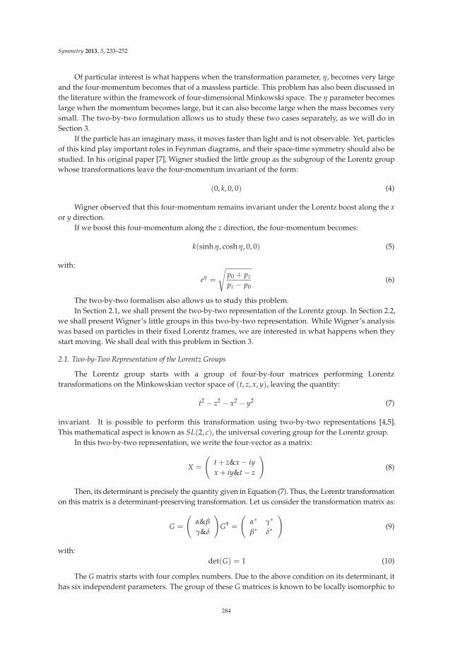
Symmetry 2013, 5, 233–252

Of particular interest is what happens when the transformation parameter, η, becomes very largeand the four-momentum becomes that of a massless particle. This problem has also been discussed inthe literature within the framework of four-dimensional Minkowski space. The η parameter becomeslarge when the momentum becomes large, but it can also become large when the mass becomes verysmall. The two-by-two formulation allows us to study these two cases separately, as we will do inSection 3.

If the particle has an imaginary mass, it moves faster than light and is not observable. Yet, particlesof this kind play important roles in Feynman diagrams, and their space-time symmetry should also bestudied. In his original paper [7], Wigner studied the little group as the subgroup of the Lorentz groupwhose transformations leave the four-momentum invariant of the form:

(0, k, 0, 0) (4)

Wigner observed that this four-momentum remains invariant under the Lorentz boost along the xor y direction.

If we boost this four-momentum along the z direction, the four-momentum becomes:

k(sinh η, cosh η, 0, 0) (5)

with:

eη =

√p0 + pz

pz − p0(6)

The two-by-two formalism also allows us to study this problem.In Section 2.1, we shall present the two-by-two representation of the Lorentz group. In Section 2.2,

we shall present Wigner’s little groups in this two-by-two representation. While Wigner’s analysiswas based on particles in their fixed Lorentz frames, we are interested in what happens when theystart moving. We shall deal with this problem in Section 3.

2.1. Two-by-Two Representation of the Lorentz Groups

The Lorentz group starts with a group of four-by-four matrices performing Lorentztransformations on the Minkowskian vector space of (t, z, x, y), leaving the quantity:

t2 − z2 − x2 − y2 (7)

invariant. It is possible to perform this transformation using two-by-two representations [4,5].This mathematical aspect is known as SL(2, c), the universal covering group for the Lorentz group.

In this two-by-two representation, we write the four-vector as a matrix:

X =

(t + z&x − iyx + iy&t − z

)(8)

Then, its determinant is precisely the quantity given in Equation (7). Thus, the Lorentz transformationon this matrix is a determinant-preserving transformation. Let us consider the transformation matrix as:

G =

(α&β

γ&δ

)G† =

(α∗ γ∗

β∗ δ∗

)(9)

with:det(G) = 1 (10)

The G matrix starts with four complex numbers. Due to the above condition on its determinant, ithas six independent parameters. The group of these G matrices is known to be locally isomorphic to

284

Symmetry 2013, 5, 233–252

the group of four-by-four matrices performing Lorentz transformations on the four-vector (t, z, x, y).In other words, for each G matrix, there is a corresponding four-by-four Lorentz-transform matrix, asis illustrated in the Appendix A.

The matrix, G, is not a unitary matrix, because its Hermitian conjugate is not always its inverse.The group can have a unitary subgroup, called SU(2), performing rotations on electron spins. As faras we can see, this G-matrix formalism was first presented by Naimark in 1954 [4]. Thus, we call thisformalism the Naimark representation of the Lorentz group. We shall see first that this representationis convenient for studying space-time symmetries of particles. We shall then note that this Naimarkrepresentation is the natural language for the Stokes parameters in polarization optics.

With this point in mind, we can now consider the transformation:

X′ = GXG† (11)

Since G is not a unitary matrix, it is not a unitary transformation. In order to tell this difference, we callthis the “Naimark transformation”. This expression can be written explicitly as:

(t′ + z′ x′ − iy′

x + iy t′ − z′

)=

(α β

γ δ

)(t + z x − iy

x + iy t − z

)(α∗ γ∗

β∗ δ∗

)(12)

For this transformation, we have to deal with four complex numbers. However, for all practicalpurposes, we may work with two Hermitian matrices:

Z(δ) =

(eiδ/2 0

0 e−iδ/2

)R(δ) =

(cos(θ/2) − sin(θ/2)sin(θ/2) cos(θ/2)

)(13)

and two symmetric matrices:

B(η) =

(eη/2 0

0 e−η/2

)S(λ) =

(cosh(λ/2) sinh(λ/2)sinh(λ/2) cosh(λ/2)

)(14)

whose Hermitian conjugates are not their inverses. The two Hermitian matrices in Equation (13) leadto rotations around the z and y axes, respectively. The symmetric matrices in Equation (14) performLorentz boosts along the z and x directions, respectively.

Repeated applications of these four matrices will lead to the most general form of the G matrix ofEquation (9) with six independent parameters. For each two-by-two Naimark transformation, there isa four-by-four matrix performing the corresponding Lorentz transformation on the four-componentfour-vector. In the Appendix A, the four-by-four equivalents are given for the matrices of Equations (13)and (14).

It was Einstein who defined the energy-momentum four-vector and showed that it also has thesame Lorentz-transformation law as the space-time four-vector. We write the energy-momentumfour-vector as:

P =

(E + pz px − ipy

px + ipy E − pz

)(15)

with:det(P) = E2 − p2

x − p2y − p2

z (16)

which means:det(P) = m2 (17)

where m is the particle mass.

285

Symmetry 2013, 5, 233–252

Now, Einstein’s transformation law can be written as:

P′ = GPG† (18)

or explicitly:

(E′ + p′z p′x − ip′yp′x + ip′y E′ − p′z

)=

(α β

γ δ

)(E + pz px − ipy

px + ipy E − pz

)(α∗ γ∗β∗

δ∗

)(19)

2.2. Wigner’s Little Groups

Later in 1939 [7], Wigner was interested in constructing subgroups of the Lorentz group whosetransformations leave a given four-momentum invariant. He called these subsets “little groups”.Thus, Wigner’s little group consists of two-by-two matrices satisfying:

P = WPW† (20)

This two-by-two W matrix is not an identity matrix, but tells about the internal space-timesymmetry of a particle with a given energy-momentum four-vector. This aspect was not known whenEinstein formulated his special relativity in 1905. The internal space-time symmetry was not an issueat that time.

If its determinant is a positive number, the P matrix can be brought to a form proportional to:

P =

(1 00 1

)(21)

corresponding to a massive particle at rest.If the determinant is negative, it can be brought to a form proportional to:

P =

(1 00 −1

)(22)

corresponding to an imaginary-mass particle moving faster than light along the z direction, with itsvanishing energy component.

If the determinant is zero, we may write P as:

P =

(1 00 0

)(23)

which is proportional to the four-momentum matrix for a massless particle moving along the zdirection.

For all three of the above cases, the matrix of the form:

Z(δ) =

(eiδ/2 0

0 e−iδ/2

)(24)

will satisfy the Wigner condition of Equation (20). This matrix corresponds to rotations around the zaxis, as is shown in the Appendix A.

For the massive particle with the four-momentum of Equation (21), the Naimark transformationswith the rotation matrix of the form:

R(θ) =

(cos(θ/2) − sin(θ/2)sin(θ/2) cos(θ/2)

)(25)

286

Symmetry 2013, 5, 233–252

also leave the P matrix of Equation (21) invariant. Together with the Z(δ) matrix, this rotation matrixleads to the subgroup consisting of the unitary subset of the G matrices. The unitary subset of G isSU(2), corresponding to the three-dimensional rotation group dictating the spin of the particle [9].

For the massless case, the transformations with the triangular matrix of the form:

(1 γ

0 1

)(26)

leave the momentum matrix of Equation (23) invariant. The physics of this matrix has a stormy history,and the variable, γ, leads to gauge transformation applicable to massless particles [6,10].

For a particle with its imaginary mass, the W matrix of the form:

S(λ) =

(cosh(λ/2) sinh(λ/2)sinh(λ/2) cosh(λ/2)

)(27)

will leave the four-momentum of Equation (22) invariant. This unobservable particle does not appearto have observable internal space-time degrees of freedom.

Table 1 summarizes the transformation matrices for Wigner’s subgroups for massive, masslessand imaginary-mass particles. Of course, it is a challenging problem to have one expression for allthose three cases, and this problem has been addressed in the literature [11].

Table 1. Wigner’s Little Groups. The little groups are the subgroups of the Lorentz group, whosetransformations leave the four-momentum of a given particle invariant. Thus, the little groups define theinternal space-time symmetries of particles. The four-momentum remains invariant under the rotationaround it. In addition, the four-momentum remains invariant under the following transformations.These transformations are different for massive, massless and imaginary-mass particles.

Particle mass Four-momentum Transform matrices

Massive(

1 00 1

) (cos(θ/2) − sin(θ/2)sin(θ/2) cos(θ/2)

)

Massless(

1 00 0

) (1 γ0 1

)

Imaginary mass(

1 00 −1

) (cosh(λ/2) sinh(λ/2)sinh(λ/2) cosh(λ/2)

)

3. Lorentz Completion of Wigner’s Little Groups

In his original paper [7], Wigner worked out his little groups for specific Lorentz frames. For themassive particle, he constructed his little group in the frame where the particle is at rest. For theimaginary-mass particle, the energy-component of his frame is zero.

For the massless particle, it moves along the z direction with a nonzero momentum. There are nospecific frames particularly convenient for us. Thus, the specific frame can be chosen for an arbitraryvalue of the momentum, and the triangular matrix of Equation (26) should remain invariant underLorentz boosts along the z direction.

For the massive particle, let us Lorentz-boost the four-momentum matrix of Equation (21) byperforming a Naimark transformation:

(eη/2 0

0 e−η/2

)(1 00 1

)(eη/2 0

0 e−η/2

)(28)

which leads to: (eη 00 e−η

)(29)

287

Symmetry 2013, 5, 233–252

This resulting matrix corresponds to the Lorentz-boosted four-momentum given in Equation (2).For simplicity, we let m = 1 hereafter in this paper. The Lorentz transformation applicable to thefour-momentum matrix is not a similarity transformation, but it is a Naimark transformation, as definedin Equation (11).

On the other hand, the rotation matrix of Equation (25) is Lorentz-boosted as a similarity transformation:

(eη/2 0

0 e−η/2

)(cos(θ/2) − sin(θ/2)sin(θ/2) cos(θ/2)

)(e−η/2 0

0 eη/2

)(30)

and it becomes: (cos(θ/2) −eη sin(θ/2)

e−η sin(θ/2) cos(θ/2)

)(31)

If we perform the Naimark transformation of the four-momentum matrix of Equation (29) withthis Lorentz-boosted rotation matrix:(

cos(θ/2) −eη sin(θ/2)e−η/2 sin(θ/2) cos(θ/2)

)(eη 00 e−η

)(cos(θ/2) eη sin(θ/2)

−e−η sin(θ/2) cos(θ/2)

)(32)

the result is the four-momentum matrix of Equation (29). This means that the Lorentz-boosted rotationmatrix of Equation (31) represents the little group, whose transformations leave the four-momentummatrix of Equation (29) invariant.

For the imaginary-mass case, the Lorentz boosted four-momentum matrix becomes:

(eη 00 −e−η

)(33)

The little group matrix is:

(cosh(λ/2) eη sinh(λ/2)

e−η sinh(λ/2) cosh(λ/2)

)(34)

where η is given in Equation (6).For the massless case, if we boost the four-momentum matrix of Equation (23), the result is:

eη

(1 00 0

)(35)

Here, the η parameter is an independent variable and cannot be defined in terms of the momentumor energy.

The remaining problem is to see whether the massive and imaginary-mass cases collapse to themassless case in the large η limit. This variable becomes large when the momentum becomes large orthe mass becomes small. We shall discuss these two cases separately.

3.1. Large-Momentum Limit

While Wigner defined his little group for the massive particle in its rest frame in his originalpaper [7], the little group represented by Equation (31) is applicable to the moving particle,whose four-momentum is given in Equation (29). This matrix can also be written as:

eη

(1 00 e−2η

)(36)

288

Symmetry 2013, 5, 233–252

In the limit of large η, we can change the above expression into:

eη

(1 00 0

)(37)

This process is continuous, but not necessarily analytic [11]. After making this transition, we cancome back to the original frame to obtain the four momentum matrix of Equation (23).

The remaining problem is the Lorentz-boosted rotation matrix of Equation (31). If this matrixis going to remain finite as η approaches infinity, the upper-right element should be finite for largevalues of η. Let it be γ. Then:

− eη sin(θ/2) = γ (38)

This means that angle θ has to become zero. As a consequence, the little group matrix ofEquation (31) becomes the triangular matrix given in Equation (26) for massless particles.

Imaginary-mass particles move faster than light, and they are not observable. On the other hand,the mathematics applicable to Wigner’s little group for this particle has been useful in the two-by-twobeam transfer matrix in ray and polarization optics [12].

Let us go back to the four-momentum matrix of Equation (22). If we boost this matrix, it becomes:

(eη 00 −e−η

)(39)

which can be written as:

eη

(1 00 −e−2η

)(40)

This matrix can be changed to form Equation (37) in the limit of large η.Indeed, the little groups for massive, massless and imaginary cases coincide in the large-η limit.

Thus, it is possible to jump from one little group to another, and it is a continuous process, but notnecessarily analytic [12].

The η parameter can become large as the momentum becomes large or the mass becomes small.In this subsection, we considered the case for large momentum. However, it is of interest to see thelimiting process when the mass becomes small, especially in view of the fact that neutrinos havesmall masses.

3.2. Small-Mass Limit

Let us start with a massive particle with fixed energy, E. Then, p0 = E, and pz = E cos χ.The four-momentum matrix is

E

(1 + cos χ 0

0 1 − cos χ

)(41)

The determinant of this matrix is E2(sin χ)2. In the regime of the Lorentz group, this is the (mass)2

and is a Lorentz-invariant quantity. There are no Lorentz transformations that change the angle, χ.Thus, with this extra variable, it is possible to study the little groups for variable masses, including thesmall-mass limit and the zero-mass case.

If χ = 0, the matrix of Equation (41) becomes that of the four-momentum matrix for a masslessparticle. As it becomes a positive small number, the matrix of Equation (41) can be written as:

E(sin χ)

(eη 00 e−η

)(42)

289

Symmetry 2013, 5, 233–252

with

eη =

√1 + cos χ

1 − cos χ(43)

Here, again, the determinant of Equation (42) is E2(sin χ)2. With this matrix, we can constructWigner’s little group for each value of the angle, χ. If χ is not zero, even if it is very small, the littlegroup is O(3)-like, as in the case of all massive particles. As the angle, χ, varies continuously fromzero to 90◦, the mass increases from zero to its maximum value.

It is important to note that the little groups are different for the small-mass limit and for thezero-mass case. In this section, we studied the internal space-time symmetries dictated by Wigner’slittle groups, and we are able to present their Lorentz-covariant picture in Table 2.

Table 2. Covariance of the energy-momentum relation and covariance of the internal space-timesymmetry groups. The γ parameter for the massless case has been studied in earlier papers in thefour-by-four matrix formulation [6]. It corresponds to a gauge transformation. Among the three spincomponents, S3 is along the direction of the momentum and remains invariant. It is called the “helicity".

Massive, Slow Covariance Massless, Fast

E = p2/2m Einstein’s E = mc2 E = cpS3 Helicity

Wigner’s Little GroupS1, S2 Gauge Transformation

4. Jones Vectors and Stokes Parameters

In studying polarized light propagating along the z direction, the traditional approach is toconsider the x and y components of the electric fields. Their amplitude ratio and the phase differencedetermine the state of polarization. Thus, we can change the polarization either by adjusting theamplitudes, by changing the relative phase or both. For convenience, we call the optical device thatchanges amplitudes an “attenuator” and the device that changes the relative phase a “phase shifter”.

The traditional language for this two-component light is the Jones-vector formalism, which isdiscussed in standard optics textbooks [13]. In this formalism, the above two components are combinedinto one column matrix, with the exponential form for the sinusoidal function:

(ψ1(z, t)ψ2(z, t)

)=

(a exp{i(kz − ωt + φ1)}b exp{i(kz − ωt + φ2)}

)(44)

This column matrix is called the Jones vector.When the beam goes through a medium with different values of indexes of refraction for the x

and y directions, we have to apply the matrix:

(eiδ1 00 eiδ2

)= ei(δ1+δ2)/2

(e−iδ/2 0

0 eiδ/2

)(45)

with δ = δ1 − δ2. In measurement processes, the overall phase factor, ei(δ1+δ2)/2, cannot be detectedand can therefore be deleted. The polarization effect of the filter is solely determined by the matrix:

Z(δ) =

(eiδ/2 0

0 e−iδ/2

)(46)

which leads to a phase difference of δ between the x and y components. The form of this matrix isgiven in Equation (13), which serves as the rotation around the z axis in the Minkowski space and time.

290

Symmetry 2013, 5, 233–252

Also along the x and y directions, the attenuation coefficients could be different. This will lead tothe matrix [14]: (

e−η1 00 e−η2

)= e−(η1+η2)/2

(eη/2 0

0 e−η/2

)(47)

with η = η2 − η1 . If η1 = 0 and η2 = ∞, the above matrix becomes:

(1 00 0

)(48)

which eliminates the y component. This matrix is known as a polarizer in the textbooks [13] and is aspecial case of the attenuation matrix of Equation (47).

This attenuation matrix tells us that the electric fields are attenuated at two different rates.The exponential factor, e−(η1+η2)/2, reduces both components at the same rate and does not affect thestate of polarization. The effect of polarization is solely determined by the squeeze matrix [14]:

B(η) =

(eη/2 0

0 e−η/2

)(49)

This diagonal matrix is given in Equation (14). In the language of space-time symmetries, this matrixperforms a Lorentz boost along the z direction.

The polarization axes are not always the x and y axes. For this reason, we need the rotation matrix:

R(θ) =

(cos(θ/2) − sin(θ/2)sin(θ/2) cos(θ/2)

)(50)

which, according to Equation (13), corresponds to the rotation around the y axis in the space-timesymmetry.

Among the rotation angles, the angle of 45◦ plays an important role in polarization optics.Indeed, if we rotate the squeeze matrix of Equation (49) by 45◦, we end up with the squeeze matrix:

R(θ) =

(cosh(λ/2) sinh(λ/2)sinh(λ/2) cosh(λ/2)

)(51)

which is also given in Equation (14). In the language of space-time physics, this matrix leads to aLorentz boost along the x axis.

Indeed, the G matrix of Equation (9) is the most general form of the transformation matrixapplicable to the Jones vector. Each of the above four matrices plays its important role in specialrelativity, as we discussed in Section 2. Their respective roles in optics and particle physics are given inTable 3.

However, the Jones vector alone cannot tell us whether the two components are coherent witheach other. In order to address this important degree of freedom, we use the coherency matrix [1,2]:

C =

(S11 S12

S21 S22

)(52)

with:

< ψ∗i ψj >=

1T

∫ T

0ψ∗

i (t + τ)ψj(t)dt (53)

291

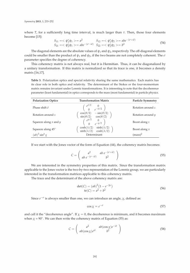
Symmetry 2013, 5, 233–252

where T, for a sufficiently long time interval, is much larger than τ. Then, those four elementsbecome [15]:

S11 =< ψ∗1 ψ1 >= a2 S12 =< ψ∗

1 ψ2 >= abe−(σ+iδ)

S21 =< ψ∗2 ψ1 >= abe−(σ−iδ) S22 =< ψ∗

2 ψ2 >= b2 (54)

The diagonal elements are the absolute values of ψ1 and ψ2, respectively. The off-diagonal elementscould be smaller than the product of ψ1 and ψ2, if the two beams are not completely coherent. The σ

parameter specifies the degree of coherency.This coherency matrix is not always real, but it is Hermitian. Thus, it can be diagonalized by

a unitary transformation. If this matrix is normalized so that its trace is one, it becomes a densitymatrix [16,17].

Table 3. Polarization optics and special relativity sharing the same mathematics. Each matrix hasits clear role in both optics and relativity. The determinant of the Stokes or the four-momentummatrix remains invariant under Lorentz transformations. It is interesting to note that the decoherenceparameter (least fundamental) in optics corresponds to the mass (most fundamental) in particle physics.

Polarization Optics Transformation Matrix Particle Symmetry

Phase shift δ

(eδ/2 0

0 e−iδ/2

)Rotation around z

Rotation around z(

cos(θ/2) − sin(θ/2)sin(θ/2) cos(θ/2)

)Rotation around y

Squeeze along x and y(

eη/2 00 e−η/2

)Boost along z

Squeeze along 45◦(

cosh(λ/2) sinh(λ/2)sinh(λ/2) cosh(λ/2)

)Boost along x

(ab)2 sin2 χ Determinant (mass)2

If we start with the Jones vector of the form of Equation (44), the coherency matrix becomes:

C =

(a2 ab e−(σ+iδ)

ab e−(σ−iδ) b2

)(55)

We are interested in the symmetry properties of this matrix. Since the transformation matrixapplicable to the Jones vector is the two-by-two representation of the Lorentz group, we are particularlyinterested in the transformation matrices applicable to this coherency matrix.

The trace and the determinant of the above coherency matrix are:

det(C) = (ab)2(1 − e−2σ)

tr(C) = a2 + b2 (56)

Since e−σ is always smaller than one, we can introduce an angle, χ, defined as:

cos χ = e−σ (57)

and call it the “decoherence angle”. If χ = 0, the decoherence is minimum, and it becomes maximumwhen χ = 90◦. We can then write the coherency matrix of Equation (55) as:

C =

(a2 ab(cos χ)e−iδ

ab(cos χ)eiδ b2

)(58)

292

Symmetry 2013, 5, 233–252

The degree of polarization is defined as [13]:

f =

√1 − 4 det(C)

(tr(C))2 =

√√√√1 − 4(ab)2 sin2 χ

(a2 + b2)2 (59)

This degree is one if χ = 0. When χ = 90◦, it becomes:

a2 − b2

a2 + b2 (60)

Without loss of generality, we can assume that a is greater than b. If they are equal, this minimumdegree of polarization is zero.

Under the influence of the Naimark transformation given in Equation (11), this coherency matrixis transformed as:

(61)It is more convenient to make the following linear combinations:

S0 = S11+S222 S3 = S11−S22

2S1 = S12+S21

2 S2 = S12−S212i

(62)

These four parameters are called Stokes parameters, and four-by-four transformations applicableto these parameters are widely known as Mueller matrices [1,3]. However, if the Naimarktransformation given in Equation (61) is translated into the four-by-four Lorentz transformationsaccording to the correspondence given in the Appendix A, the Mueller matrices constitute arepresentation of the Lorentz group.

Another interesting aspect of the two-by-two matrix formalism is that the coherency matrix canbe formulated in terms of quarternions [18–20]. The quarternion representation can be translatedinto rotations in four-dimensional space. There is a long history between the Lorentz group and thefour-dimensional rotation group. It would be interesting to see what the quarternion representation ofpolarization optics will add to this history between those two similar, but different, groups.

As for earlier applications of the two-by-two representation of the Lorentz group, we note thevector representation by Fedorov [21,22]. Fedorov showed that it is easier to carry out kinematicalcalculations using his two-by-two representation. For instance, the computation of the Wigner rotationangle is possible in the two-by-two representation [23]. Earlier papers on group theoretical approachesto polarization optics include also those on Mueller matrices [24] and on relativistic kinematics andpolarization optics [25].

5. Geometry of the Poincaré Sphere

We now have the four-vector, (S0, S3, S1, S2), which is Lorentz-transformed like the space-timefour-vector, (t, z, x, y), or the energy-momentum four-vector of Equation (15). This Stokes four-vectorhas a three-component subspace, (S3, S1, S2), which is like the three-dimensional Euclidean subspace

293

Symmetry 2013, 5, 233–252

in the four-dimensional Minkowski space. In this three-dimensional subspace, we can introduce thespherical coordinate system with:

R =√

S23 + S2

1 + S22

S3 = R cos ξ

S1 = R(sin ξ) cos δS2 = R(sin ξ) sin δ

(63)

The radius, R, is the radius of this sphere, and is:

R =12

√(a2 − b2)

2 + 4(ab)2 cos2 χ (64)

with:

S3 =a2 − b2

2(65)

This spherical picture is traditionally known as the Poincaré sphere [1–3]. Without loss ofgenerality, we assume a is greater than b, and S3 is non-negative. In addition, we can consider anothersphere with its radius:

S0 =a2 + b2

2(66)

according to Equation (62).The radius, R, takes its maximum value, S0, when χ = 0◦. It decreases and reaches its minimum

value, S3, when χ = 90◦. In terms of R, the degree of polarization given in Equation (59) is:

f =RS0

(67)

This aspect of the radius R is illustrated in Figure 1a. The minimum value of R is S3 of Equation (64).

Figure 1. Radius of the Poincaré sphere. The radius, R, takes its maximum value, S0, when thedecoherence angle, χ, is zero. It becomes smaller as χ increases. It becomes minimum when the anglereaches 90◦. Its minimum value is S3, as is illustrated in Figure 1a. The degree of polarization ismaximum when R = S0 and is minimum when R = S3. According to Equation (65), S3 becomes zerowhen a = b, and the minimum value of R becomes zero, as is indicated in Figure 1b. Its maximumvalue is still S0. This maximum radius can become larger because b becomes larger to make a = b.

294

Symmetry 2013, 5, 233–252

Let us go back to the four-momentum matrix of Equation (15). Its determinant is m2 and remainsinvariant. Likewise, the determinant of the coherency matrix of Equation (58) should also remaininvariant. The determinant in this case is:

S20 − R2 = (ab)2 sin2 χ (68)

This quantity remains invariant. This aspect is shown on the last row of Table 3.Let us go back to Equation (49). This matrix changes the relative magnitude of the amplitudes,

a and b. Thus, without loss of generality, we can study the Stokes parameters with a = b. The coherencymatrix then becomes:

C = a2

(1 (cos χ)e−iδ

(cos χ)eiδ 1

)(69)

Since the angle, δ, does not play any essential roles, we can let δ = 0 and write the coherencymatrix as:

C = a2

(1 cos χ

cos χ 1

)(70)

Then, the minimum radius, S3 = 0, and S0 of Equation (62) and R of Equation (64) become:

S0 = a2R = a2(cos χ) (71)

respectively. The Poincaré sphere becomes simplified to that of Figure 1b. This Poincaré sphere allowsR to decrease to zero.

The determinant of the above two-by-two matrix is:

a4(

1 − cos2 χ)= a4 sin2 χ (72)

Since the Lorentz transformation leaves the determinant invariant, the change in this χ variable isnot a Lorentz transformation. It is of course possible to construct a larger group in which this variableplays a role in a group transformation [23], but in this paper, we are more interested in its role in aparticle gaining a mass. With this point in mind, let us diagonalize the coherency matrix of Equation(69). Then it takes the form:

a2

(1 + cos χ 0

0 1 − cos χ

)(73)

This form is the same as the four-momentum matrix given in Equation (41). There, we werenot able to associate the variable, χ, with any known physical process or symmetry operations ofthe Lorentz group. Fortunately, in this section, we noted that this variable comes from the degree ofdecoherence in polarization optics.

6. Concluding Remarks

In this paper, we noted first that the group of Lorentz transformations can be formulated interms of two-by-two matrices. This two-by-two formalism can also be used for transformations of thecoherency matrix in polarization optics consisting of four Stokes parameters.

Thus, this set of the four parameters is like a Minkowskian four-vector under four-by-four Lorentztransformations. In order to accommodate all four Stokes parameters, we noted that the radius of thePoincaré sphere should be allowed to vary from its maximum value to its minimum, corresponding tothe fully and minimal coherent cases.

As in the case of the particle mass, the decoherence parameter in the Stokes formalism is invariantunder Lorentz transformations. However, the Poincaré sphere, with a variable radius, provides the

295

Symmetry 2013, 5, 233–252

mechanism for the variations of the decoherence parameter. It was noted that this variation gives aphysical process whose mathematics correspond to that of the mass variable in particle physics.

As for polarization optics, the traditional approach has been to work with two polarizermatrices, like: (

1 00 0

)(0 00 1

)(74)

We have replaced these two matrices by one attenuation matrix of Equation (47). This replacementenables us to formulate the Lorentz group for the Stokes parameters [15]. Furthermore, this attenuationmatrix makes it possible to make a continuous transformation from one matrix to another by adjustingthe attenuation parameters in optical media. It could be interesting to design optical experimentsalong this direction.

Acknowledgments: This paper is in part based on an invited paper presented by one of the authors (YSK) at theFedorov Memorial Symposium: International Conference “Spins and Photonic Beams at Interface”, dedicated tothe 100th anniversary of F.I. Fedorov (1911–1994) (Minsk, Belarus, 2011). He would like to thank Sergei Kilin forinviting him to the conference.

In addition to numerous original contributions in optics, Fedorov wrote a book on two-by-two representationsof the Lorentz group based on his own research on this subject. It was, therefore, quite appropriate for him (YSK) topresent a paper on applications of the Lorentz group to optical science. He would like to thank V. A. Dluganovichand M. Glaynskii for bringing the papers and the book written by Academician Fedorov, as well as their ownpapers to his attention.

Conflicts of Interest: The authors declare no conflict of interest.

Appendix Appendix

In Section 2, we listed four two-by-two matrices whose repeated applications lead to the mostgeneral form of the two-by-two matrix, G. It is known that every G matrix can be translated into afour-by-four Lorentz transformation matrix through [4,9,15]:

⎛⎜⎜⎜⎝

t′ + z′

x′ − iy′

x′ + iy′

t′ − z′

⎞⎟⎟⎟⎠ =

⎛⎜⎜⎜⎝

αα∗ αβ∗ βα∗ ββ∗

αγ∗ αδ∗ βγ∗ βδ∗

γα∗ γβ∗ δα∗ δβ∗

γγ∗ γδ∗ δγ∗ δδ∗

⎞⎟⎟⎟⎠⎛⎜⎜⎜⎝

t + zx − iyx + iyt − z

⎞⎟⎟⎟⎠ (75)

and: ⎛⎜⎜⎜⎝

tzxy

⎞⎟⎟⎟⎠ =

12

⎛⎜⎜⎜⎝

1 0 0 11 0 0 −10 1 1 00 i −i 0

⎞⎟⎟⎟⎠⎛⎜⎜⎜⎝

t + zx − iyx + iyt − z

⎞⎟⎟⎟⎠ (76)

These matrices appear to be complicated, but it is enough to study the matrices of Equation (13)and Equation (14) to cover all the matrices in this group. Thus, we give their four-by-four equivalentsin this Appendix A:

Z(δ) =

(eiδ/2 0

0 e−iδ/2

)(77)

leads to the four-by-four matrix: ⎛⎜⎜⎜⎝

1 0 0 01 0 0 00 1 cos δ − sin δ

0 0 sin δ cos δ

⎞⎟⎟⎟⎠ (78)

296

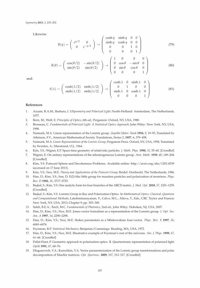
Symmetry 2013, 5, 233–252

Likewise:

B(η) =

(eη/2 0

0 e−η/2

)→

⎛⎜⎜⎜⎝

cosh η sinh η 0 0sinh η cosh η 0 0

0 0 1 00 0 0 1

⎞⎟⎟⎟⎠ (79)

R(θ) =

(cos(θ/2) − sin(θ/2)sin(θ/2) sin(θ/2)

)→

⎛⎜⎜⎜⎝

1 0 0 00 cos θ − sin θ 00 sin θ cos θ 00 0 0 1

⎞⎟⎟⎟⎠ (80)

and:

S(λ) =

(cosh(λ/2) sinh(λ/2)sinh(λ/2) sinh(λ/2)

)→

⎛⎜⎜⎜⎝

cosh λ 0 sinh λ 00 1 0 0

sinh λ 0 cosh λ 00 0 0 1

⎞⎟⎟⎟⎠ (81)

References

1. Azzam, R.A.M.; Bashara, I. Ellipsometry and Polarized Light; North-Holland: Amsterdam, The Netherlands,1977.

2. Born, M.; Wolf, E. Principles of Optics, 6th ed.; Pergamon: Oxford, NY, USA, 1980.3. Brosseau, C. Fundamentals of Polarized Light: A Statistical Optics Approach; John Wiley: New York, NY, USA,

1998.4. Naimark, M.A. Linear representation of the Lorentz group. Uspekhi Mater. Nauk 1954, 9, 19–93, Translated by

Atkinson, F.V., American Mathematical Society Translations, Series 2, 1957, 6, 379–458.5. Naimark, M.A. Linear Representations of the Lorentz Group; Pergamon Press: Oxford, NY, USA, 1958; Translated

by Swinfen, A.; Marstrand, O.J., 1964.6. Kim, Y.S.; Wigner, E.P. Space-time geometry of relativistic particles. J. Math. Phys. 1990, 31, 55–60. [CrossRef]7. Wigner, E. On unitary representations of the inhomogeneous Lorentz group. Ann. Math. 1939, 40, 149–204.

[CrossRef]8. Kim, Y.S. Poincaré Sphere and Decoherence Problems. Available online: http://arxiv.org/abs/1203.4539

(accessed on 17 June 2013).9. Kim, Y.S.; Noz, M.E. Theory and Applications of the Poincaré Group; Reidel: Dordrecht, The Netherlands, 1986.10. Han, D.; Kim, Y.S.; Son, D. E(2)-like little group for massless particles and polarization of neutrinos. Phys.

Rev. D 1982, 26, 3717–3725.11. Baskal, S.; Kim, Y.S. One analytic form for four branches of the ABCD matrix. J. Mod. Opt. 2010, 57, 1251–1259.

[CrossRef]12. Baskal, S.; Kim, Y.S. Lorentz Group in Ray and Polarization Optics. In Mathematical Optics: Classical, Quantum

and Computational Methods; Lakshminarayanan, V., Calvo, M.L., Alieva, T., Eds.; CRC Taylor and Francis:New York, NY, USA, 2013; Chapter 9; pp. 303–349.

13. Saleh, B.E.A.; Teich, M.C. Fundamentals of Photonics, 2nd ed.; John Wiley: Hoboken, NJ, USA, 2007.14. Han, D.; Kim, Y.S.; Noz, M.E. Jones-vector formalism as a representation of the Lorentz group. J. Opt. Soc.

Am. A 1997, 14, 2290–2298.15. Han, D.; Kim, Y.S.; Noz, M.E. Stokes parameters as a Minkowskian four-vector. Phys. Rev. E 1997, 56,

6065–6076.16. Feynman, R.P. Statistical Mechanics; Benjamin/Cummings: Reading, MA, USA, 1972.17. Han, D.; Kim, Y.S.; Noz, M.E. Illustrative example of Feynman’s rest of the universe. Am. J. Phys. 1999, 67,

61–66. [CrossRef]18. Pellat-Finet, P. Geometric approach to polarization optics. II. Quarternionic representation of polarized light.

Optik 1991, 87, 68–76.19. Dlugunovich, V.A.; Kurochkin, Y.A. Vector parameterization of the Lorentz group transformations and polar

decomposition of Mueller matrices. Opt. Spectrosc. 2009, 107, 312–317. [CrossRef]

297

Symmetry 2013, 5, 233–252

20. Tudor, T. Vectorial Pauli algebraic approach in polarization optics. I. Device and state operators. Optik 2010,121, 1226–1235. [CrossRef]

21. Fedorov, F.I. Vector parametrization of the Lorentz group and relativistic kinematics. Theor. Math. Phys. 1970,2, 248–252. [CrossRef]

22. Fedorov, F.I. Lorentz Group; [in Russian]; Global Science, Physical-Mathematical Literature: Moscow, Russia,1979.

23. Baskal, S.; Kim, Y.S. De Sitter group as a symmetry for optical decoherence. J. Phys. A 2006, 39, 7775–7788.24. Dargys, A. Optical Mueller matrices in terms of geometric algebra. Opt. Commun. 2012, 285, 4785–4792.

[CrossRef]25. Pellat-Finet, P.; Basset, M. What is common to both polarization optics and relativistic kinematics? Optik

1992, 90, 101–106.

© 2013 by the authors. Licensee MDPI, Basel, Switzerland. This article is an open accessarticle distributed under the terms and conditions of the Creative Commons Attribution(CC BY) license (http://creativecommons.org/licenses/by/4.0/).

298

symmetryS S

Article

Wigner’s Space-Time Symmetries Based on theTwo-by-Two Matrices of the Damped HarmonicOscillators and the Poincaré Sphere

Sibel Baskal 1, Young S. Kim 2,* and Marilyn E. Noz 3

1 Department of Physics, Middle East Technical University, Ankara 06800, Turkey; E-Mail:baskal@newton.physics.metu.edu.tr

2 Center for Fundamental Physics, University of Maryland, College Park, MD 20742, USA3 Department of Radiology, New York University, New York, NY 10016, USA; E-Mail: marilyne.noz@gmail.com* E-Mail: yskim@umd.edu; Tel.: +1-301-937-1306.

Received: 28 February 2014; in revised form: 28 May 2014 / Accepted: 9 June 2014 / Published: 25 June 2014

Abstract: The second-order differential equation for a damped harmonic oscillator can be convertedto two coupled first-order equations, with two two-by-two matrices leading to the group Sp(2). It isshown that this oscillator system contains the essential features of Wigner’s little groups dictatingthe internal space-time symmetries of particles in the Lorentz-covariant world. The little groups arethe subgroups of the Lorentz group whose transformations leave the four-momentum of a givenparticle invariant. It is shown that the damping modes of the oscillator correspond to the littlegroups for massive and imaginary-mass particles respectively. When the system makes the transitionfrom the oscillation to damping mode, it corresponds to the little group for massless particles.Rotations around the momentum leave the four-momentum invariant. This degree of freedomextends the Sp(2) symmetry to that of SL(2, c) corresponding to the Lorentz group applicable to thefour-dimensional Minkowski space. The Poincaré sphere contains the SL(2, c) symmetry. In addition,it has a non-Lorentzian parameter allowing us to reduce the mass continuously to zero. It is thuspossible to construct the little group for massless particles from that of the massive particle byreducing its mass to zero. Spin-1/2 particles and spin-1 particles are discussed in detail.

Keywords: damped harmonic oscillators; coupled first-order equations; unimodular matrices; Wigner’slittle groups; Poincaré sphere; Sp(2) group; SL(2, c) group; gauge invariance; neutrinos; photons

PACS: 03.65.Fd, 03.67.-a, 05.30.-d

1. Introduction

We are quite familiar with the second-order differential equation

md2ydt2 + b

dydt

+ Ky = 0 (1)

for a damped harmonic oscillator. This equation has the same mathematical form as

Ld2Qdt2 + R

dQdt

+1C

Q = 0 (2)

for electrical circuits, where L, R, and C are the inductance, resistance, and capacitance respectively.These two equations play fundamental roles in physical and engineering sciences. Since they startfrom the same set of mathematical equations, one set of problems can be studied in terms of the other.For instance, many mechanical phenomena can be studied in terms of electrical circuits.

Symmetry 2014, 6, 473–515 299 www.mdpi.com/journal/symmetry

Symmetry 2014, 6, 473–515

In Equation (1), when b = 0, the equation is that of a simple harmonic oscillator with thefrequency ω =

√K/m. As b increases, the oscillation becomes damped. When b is larger than 2

√Km,

the oscillation disappears, as the solution is a damping mode.Consider that increasing b continuously, while difficult mechanically, can be done electrically

using Equation (2) by adjusting the resistance R. The transition from the oscillation mode to thedamping mode is a continuous physical process.

This b term leads to energy dissipation, but is not regarded as a fundamental force. It isinconvenient in the Hamiltonian formulation of mechanics and troublesome in transition to quantummechanics, yet, plays an important role in classical mechanics. In this paper this term will help usunderstand the fundamental space-time symmetries of elementary particles.

We are interested in constructing the fundamental symmetry group for particles in theLorentz-covariant world. For this purpose, we transform the second-order differential equationof Equation (1) to two coupled first-order equations using two-by-two matrices. Only two linearlyindependent matrices are needed. They are the anti-symmetric and symmetric matrices

A =

(0 −ii 0

), and S =

(0 ii 0

)(3)

respectively. The anti-symmetric matrix A is Hermitian and corresponds to the oscillation part, whilethe symmetric S matrix corresponds to the damping.

These two matrices lead to the Sp(2) group consisting of two-by-two unimodular matrices withreal elements. This group is isomorphic to the three-dimensional Lorentz group applicable to twospace-like and one time-like coordinates. This group is commonly called the O(2, 1) group.

This O(2, 1) group can explain all the essential features of Wigner’s little groups dictating internalspace-time symmetries of particles [1]. Wigner defined his little groups as the subgroups of the Lorentzgroup whose transformations leave the four-momentum of a given particle invariant. He observedthat the little groups are different for massive, massless, and imaginary-mass particles. It has been achallenge to design a mathematical model which will combine those three into one formalism, but weshow that the damped harmonic oscillator provides the desired mathematical framework.

For the two space-like coordinates, we can assign one of them to the direction of the momentum,and the other to the direction perpendicular to the momentum. Let the direction of the momentumbe along the z axis, and let the perpendicular direction be along the x axis. We therefore study thekinematics of the group within the zx plane, then see what happens when we rotate the system aroundthe z axis without changing the momentum [2].

The Poincaré sphere for polarization optics contains the SL(2, c) symmetry isomorphic to thefour-dimensional Lorentz group applicable to the Minkowski space [3–7]. Thus, the Poincaré sphereextends Wigner’s picture into the three space-like and one time-like coordinates. Specifically, thisextension adds rotations around the given momentum which leaves the four-momentum invariant [2].

While the particle mass is a Lorentz-invariant variable, the Poincaré sphere contains an extravariable which allows the mass to change. This variable allows us to take the mass-limit of thesymmetry operations. The transverse rotational degrees of freedom collapse into one gauge degree offreedom and polarization of neutrinos is a consequence of the requirement of gauge invariance [8,9].

The SL(2, c) group contains symmetries not seen in the three-dimensional rotation group.While we are familiar with two spinors for a spin-1/2 particle in nonrelativistic quantum mechanics,there are two additional spinors due to the reflection properties of the Lorentz group. There are thus16 bilinear combinations of those four spinors. This leads to two scalars, two four-vectors, and oneantisymmetric four-by-four tensor. The Maxwell-type electromagnetic field tensor can be obtained asa massless limit of this tensor [10].

In Section 2, we review the damped harmonic oscillator in classical mechanics, and note thatthe solution can be either in the oscillation mode or damping mode depending on the magnitude of

300

Symmetry 2014, 6, 473–515

the damping parameter. The translation of the second order equation into a first order differentialequation with two-by-two matrices is possible. This first-order equation is similar to the Schrödingerequation for a spin-1/2 particle in a magnetic field.

Section 3 shows that the two-by-two matrices of Section 2 can be formulated in terms of theSp(2) group. These matrices can be decomposed into the Bargmann and Wigner decompositions.Furthermore, this group is isomorphic to the three-dimensional Lorentz group with two space and onetime-like coordinates.

In Section 4, it is noted that this three-dimensional Lorentz group has all the essential featuresof Wigner’s little groups which dictate the internal space-time symmetries of the particles in theLorentz-covariant world. Wigner’s little groups are the subgroups of the Lorentz group whosetransformations leave the four-momentum of a given particle invariant. The Bargmann Wignerdecompositions are shown to be useful tools for studying the little groups.

In Section 5, we note that the given momentum is invariant under rotations around it. Theaddition of this rotational degree of freedom extends the Sp(2) symmetry to the six-parameter SL(2, c)symmetry. In the space-time language, this extends the three dimensional group to the Lorentz groupapplicable to three space and one time dimensions.

Section 6 shows that the Poincaré sphere contains the symmetries of SL(2, c) group. In addition,it contains an extra variable which allows us to change the mass of the particle, which is not allowedin the Lorentz group.

In Section 7, the symmetries of massless particles are studied in detail. In addition to rotationaround the momentum, Wigner’s little group generates gauge transformations. While gaugetransformations on spin-1 photons are well known, the gauge invariance leads to the polarization ofmassless spin-1/2 particles, as observed in neutrino polarizations.

In Section 8, it is noted that there are four spinors for spin-1/2 particles in the Lorentz-covariantworld. It is thus possible to construct 16 bilinear forms, applicable to two scalars, and two vectors, andone antisymmetric second-rank tensor. The electromagnetic field tensor is derived as the masslesslimit. This tensor is shown to be gauge-invariant.

2. Classical Damped Oscillators

For convenience, we write Equation (1) as

d2ydt2 + 2μ

dydt

+ ω2y = 0 (4)

with

ω =

√Km

, and μ =b

2m(5)

The damping parameter μ is positive when there are no external forces. When ω is greater than μ,the solution takes the form

y = e−μt [C1 cos(ω′t) + C2 sin(ω′t)]

(6)

whereω′ =

√ω2 − μ2 (7)

and C1 and C2 are the constants to be determined by the initial conditions. This expression is for adamped harmonic oscillator. Conversely, when μ is greater than ω, the quantity inside the square-rootsign is negative, then the solution becomes

y = e−μt [C3 cosh(μ′t) + C4 sinh(μ′t)]

(8)

withμ′ =

√μ2 − ω2 (9)

301

Symmetry 2014, 6, 473–515

If ω = μ, both Equations (6) and (8) collapse into one solution

y(t) = e−μt [C5 + C6 t] (10)

These three different cases are treated separately in textbooks. Here we are interested in thetransition from Equation (6) to Equation (8), via Equation (10). For convenience, we start from μ greaterthan ω with μ′ given by Equation (9).

For a given value of μ, the square root becomes zero when ω equals μ. If ω becomes larger, thesquare root becomes imaginary and divides into two branches.

± i√

ω2 − μ2 (11)

This is a continuous transition, but not an analytic continuation. To study this in detail, we translatethe second order differential equation of Equation (4) into the first-order equation with two-by-twomatrices.

Given the solutions of Equations (6) and (10), it is convenient to use ψ(t) defined as

ψ(t) = eμty(t), and y = e−μtψ(t) (12)

Then ψ(t) satisfies the differential equation

d2ψ(t)dt2 + (ω2 − μ2)ψ(t) = 0 (13)

2.1. Two-by-Two Matrix Formulation

In order to convert this second-order equation to a first-order system, we introduce ψ1(t) andψ2(t) satisfying two coupled differential equations

dψ1(t)dt

= (μ − ω)ψ2(t) (14)

dψ2(t)dt

= (μ + ω)ψ1(t) (15)

which can be written in matrix form as

ddt

(ψ1

ψ2

)=

(0 μ − ω

μ + ω 0

)(ψ1

ψ2

)(16)

Using the Hermitian and anti-Hermitian matrices of Equation (3) in Section 1, we construct thelinear combination

H = ω

(0 −ii 0

)+ μ

(0 ii 0

)(17)

We can then consider the first-order differential equation

i∂

∂tψ(t) = Hψ(t) (18)

While this equation is like the Schrödinger equation for an electron in a magnetic field, the two-by-twomatrix is not Hermitian. Its first matrix is Hermitian, but the second matrix is anti-Hermitian.It is of course an interesting problem to give a physical interpretation to this non-Hermitian matrix

302

Symmetry 2014, 6, 473–515

in connection with quantum dissipation [11], but this is beyond the scope of the present paper.The solution of Equation (18) is

ψ(t) = exp

{(0 −ω + μ

ω + μ 0

)t

}(C7

C8

)(19)

where C7 = ψ1(0) and C8 = ψ2(0) respectively.

2.2. Transition from the Oscillation Mode to Damping Mode

It appears straight-forward to compute this expression by a Taylor expansion, but it is not.This issue was extensively discussed in the earlier papers by two of us [12,13]. The key idea is to writethe matrix (

0 −ω + μ

ω + μ 0

)(20)

as a similarity transformation of

ω′(

0 −11 0

)(ω > μ) (21)

and as that of

μ′(

0 11 0

)(μ > ω) (22)

with ω′ and μ′ defined in Equations (7) and (9), respectively.Then the Taylor expansion leads to(

cos(ω′t) −√(ω − μ)/(ω + μ) sin(ω′t)√

(ω + μ)/(ω − μ) sin(ω′t) cos(ω′t)

)(23)

when ω is greater than μ. The solution ψ(t) takes the form(C7 cos(ω′t)− C8

√(ω − μ)/(ω + μ) sin(ω′t)

C7√(ω + μ)/(ω − μ) sin(ω′t) + C8 cos(ω′t)

)(24)

If μ is greater than ω, the Taylor expansion becomes(cosh(μ′t)

√(μ − ω)/(μ + ω) sinh(μ′t)√

(μ + ω)/(μ − ω) sinh(μ′t) cosh(μ′t)

)(25)

When ω is equal to μ, both Equations (23) and (25) become(1 0

2ωt 1

)(26)

If ω is sufficiently close to but smaller than μ, the matrix of Equation (25) becomes(1 + (ε/2)(2ωt)2 +ε(2ωt)

(2ωt) 1 + (ε/2)(2ωt)2

)(27)

withε =

μ − ω

μ + ω(28)

303

Symmetry 2014, 6, 473–515

If ω is sufficiently close to μ, we can let

μ + ω = 2ω, and μ − ω = 2με (29)

If ω is greater than μ, ε defined in Equation (28) becomes negative, the matrix of Equation (23) becomes(1 − (−ε/2)(2ωt)2 −(−ε)(2ωt)

2ωt 1 − (−ε/2)(2ωt)2

)(30)

We can rewrite this matrix as(1 − (1/2)

[(2ω

√−ε)

t]2 −√−ε

[(2ω

√−ε)

t]

2ωt 1 − (1/2)[(

2ω√−ε

)t]2)

(31)

If ε becomes positive, Equation (27) can be written as(1 + (1/2)

[(2ω

√ε)

t]2 √

ε[(

2ω√

ε)

t]

2ωt 1 + (1/2)[(

2ω√

ε)

t]2)

(32)

The transition from Equation (31) to Equation (32) is continuous as they become identical whenε = 0. As ε changes its sign, the diagonal elements of above matrices tell us how cos(ω′t) becomescosh(μ′t). As for the upper-right element element, − sin(ω′t) becomes sinh(μ′t). This non-analyticcontinuity is discussed in detail in one of the earlier papers by two of us on lens optics [13]. This typeof continuity was called there “tangential continuity.” There, the function and its first derivative arecontinuous while the second derivative is not.

2.3. Mathematical Forms of the Solutions

In this section, we use the Heisenberg approach to the problem, and obtain the solutions in theform of two-by-two matrices. We note that

1. For the oscillation mode, the trace of the matrix is smaller than 2. The solution takes the form of(cos(x) −e−η sin(x)

eη sin(x) cos(x)

)(33)

with trace 2 cos(x). The trace is independent of η.2. For the damping mode, the trace of the matrix is greater than 2.(

cosh(x) e−η sinh(x)eη sinh(x) cosh(x)

)(34)

with trace 2 cosh(x). Again, the trace is independent of η.3. For the transition mode, the trace is equal to 2, and the matrix is triangular and takes the form of(

1 0γ 1

)(35)

When x approaches zero, the Equations (33) and (34) take the form(1 − x2/2 −xe−η

xeη 1 − x2/2

), and

(1 + x2/2 xe−η

xeη 1 + x2/2

)(36)

304

Symmetry 2014, 6, 473–515

respectively. These two matrices have the same lower-left element. Let us fix this element to be apositive number γ. Then

x = γe−η (37)

Then the matrices of Equation (36) become(1 − γ2e−2η/2 −γe−2η

γ 1 − γ2e−2η/2

), and

(1 + γ2e−2η/2 γe−2η

γ 1 + γ2e−2η/2

)(38)

If we introduce a small number ε defined as

ε =√

γe−η (39)

the matrices of Equation (38) become(e−η/2 0

0 eη/2

)(1 − γε2/2

√γε√

γε 1 − γε2/2

)(eη/2 0

0 e−η/2

)

(e−η/2 0

0 eη/2

)(1 + γε2/2

√γε√

γε 1 + γε2/2

)(eη/2 0

0 e−η/2

) (40)

respectively, with e−η = ε/√

γ.

3. Groups of Two-by-Two Matrices

If a two-by-two matrix has four complex elements, it has eight independent parameters. If thedeterminant of this matrix is one, it is known as an unimodular matrix and the number of independentparameters is reduced to six. The group of two-by-two unimodular matrices is called SL(2, c).This six-parameter group is isomorphic to the Lorentz group applicable to the Minkowski spaceof three space-like and one time-like dimensions [14].

We can start with two subgroups of SL(2, c).

1. While the matrices of SL(2, c) are not unitary, we can consider the subset consisting of unitarymatrices. This subgroup is called SU(2), and is isomorphic to the three-dimensional rotationgroup. This three-parameter group is the basic scientific language for spin-1/2 particles.

2. We can also consider the subset of matrices with real elements. This three-parameter groupis called Sp(2) and is isomorphic to the three-dimensional Lorentz group applicable to twospace-like and one time-like coordinates.

In the Lorentz group, there are three space-like dimensions with x, y, and z coordinates.However, for many physical problems, it is more convenient to study the problem in thetwo-dimensional (x, z) plane first and generalize it to three-dimensional space by rotating the systemaround the z axis. This process can be called Euler decomposition and Euler generalization [2].

First, we study Sp(2) symmetry in detail, and achieve the generalization by augmenting thetwo-by-two matrix corresponding to the rotation around the z axis. In this section, we study in detailproperties of Sp(2) matrices, then generalize them to SL(2, c) in Section 5.

There are three classes of Sp(2) matrices. Their traces can be smaller or greater than two, or equalto two. While these subjects are already discussed in the literature [15–17] our main interest iswhat happens as the trace goes from less than two to greater than two. Here we are guided by themodel we have discussed in Section 2, which accounts for the transition from the oscillation mode tothe damping mode.

305

Symmetry 2014, 6, 473–515

3.1. Lie Algebra of Sp(2)

The two linearly independent matrices of Equation (3) can be written as

K1 =12

(0 ii 0

), and J2 =

12

(0 −ii 0

)(41)

However, the Taylor series expansion of the exponential form of Equation (23) or Equation (25) requiresan additional matrix

K3 =12

(i 00 −i

)(42)

These matrices satisfy the following closed set of commutation relations.

[K1, J2] = iK3, [J2, K3] = iK1, [K3, K1] = −i J2 (43)

These commutation relations remain invariant under Hermitian conjugation, even though K1 and K3

are anti-Hermitian. The algebra generated by these three matrices is known in the literature as thegroup Sp(2) [17]. Furthermore, the closed set of commutation relations is commonly called the Liealgebra. Indeed, Equation (43) is the Lie algebra of the Sp(2) group.

The Hermitian matrix J2 generates the rotation matrix

R(θ) = exp (−iθ J2) =

(cos(θ/2) − sin(θ/2)sin(θ/2) cos(θ/2)

)(44)

and the anti-Hermitian matrices K1 and K2, generate the following squeeze matrices.

S(λ) = exp (−iλK1) =

(cosh(λ/2) sinh(λ/2)sinh(λ/2) cosh(λ/2)

)(45)

and

B(η) = exp (−iηK3) =

(exp (η/2) 0

0 exp (−η/2)

)(46)

respectively.Returning to the Lie algebra of Equation (43), since K1 and K3 are anti-Hermitian, and J2 is

Hermitian, the set of commutation relation is invariant under the Hermitian conjugation. In otherwords, the commutation relations remain invariant, even if we change the sign of K1 and K3,while keeping that of J2 invariant. Next, let us take the complex conjugate of the entire system.Then both the J and K matrices change their signs.

3.2. Bargmann and Wigner Decompositions

Since the Sp(2) matrix has three independent parameters, it can be written as [15](cos (α1/2) − sin (α1/2)sin (α1/2) cos (α1/2)

)(cosh χ sinh χ

sinh χ cosh χ

)(cos (α2/2) − sin (α2/2)sin (α2/2) cos (α2/2)

)(47)

This matrix can be written as(cos(δ/2) − sin(δ/2)sin(δ/2) cos(δ/2)

)(a bc d

)(cos(δ/2) sin(δ/2)− sin(δ/2) cos(δ/2)

)(48)

306

Symmetry 2014, 6, 473–515

where (a bc d

)=

(cos(α/2) − sin(α/2)sin(α/2) cos(α/2)

)(cosh χ sinh χ

sinh χ cosh χ

)(cos(α/2) − sin(α/2)sin(α/2) cos(α/2)

)(49)

withδ =

12(α1 − α2) , and α =

12(α1 + α2) (50)

If we complete the matrix multiplication of Equation (49), the result is((cosh χ) cos α sinh χ − (cosh χ) sin α

sinh χ + (cosh χ) sin α (cosh χ) cos α

)(51)

We shall call hereafter the decomposition of Equation (49) the Bargmann decomposition. This meansthat every matrix in the Sp(2) group can be brought to the Bargmann decomposition by a similaritytransformation of rotation, as given in Equation (48). This decomposition leads to an equidiagonalmatrix with two independent parameters.

For the matrix of Equation (49), we can now consider the following three cases. Let us assumethat χ is positive, and the angle θ is less than 90◦. Let us look at the upper-right element.

1. If it is negative with [sinh χ < (cosh χ) sin α], then the trace of the matrix is smaller than 2,and the matrix can be written as(

cos(θ/2) −e−η sin(θ/2)eη sin(θ/2) cos(θ/2)

)(52)

with

cos(θ/2) = (cosh χ) cos α, and e−2η =(cosh χ) sin α − sinh χ

(cosh χ) sin α + sinh χ(53)

2. If it is positive with [sinh χ > (cosh χ) sin α)], then the trace is greater than 2, and the matrixcan be written as (

cosh(λ/2) e−η sinh(λ/2)eη sinh(λ/2) cosh(λ/2)

)(54)

with

cosh(λ/2) = (cosh χ) cos α, and e−2η =sinh χ − (cosh χ) sin α

(cosh χ) sin α + sinh χ(55)

3. If it is zero with [(sinh χ = (cosh χ) sin α)], then the trace is equal to 2, and the matrix takes the form(1 0

2 sinh χ 1

)(56)

The above repeats the mathematics given in Section 2.3.Returning to Equations (52) and (53), they can be decomposed into

M(θ, η) =

(eη/2 0

0 e−η/2

)(cos(θ/2) − sin(θ/2)sin(θ/2) cos(θ/2)

)(e−η/2 0

0 eη/2

)(57)

and

M(λ, η) =

(eη/2 0

0 e−η/2

)(cosh(λ/2) sinh(λ/2)sinh(λ/2) cos(λ/2)

)(e−η/2 0

0 eη/2

)(58)

respectively. In view of the physical examples given in Section 6, we shall call this the “Wignerdecomposition.” Unlike the Bargmann decomposition, the Wigner decomposition is in the form of asimilarity transformation.

307

Symmetry 2014, 6, 473–515

We note that both Equations (57) and (58) are written as similarity transformations. Thus

[M(θ, η)]n =

(cos(nθ/2) −e−η sin(nθ/2)

eη sin(nθ/2) cos(nθ/2)

)(59)

[M(λ, η)]n =

(cosh(nλ/2) eη sinh(nλ/2)

e−η sinh(nλ/2) cosh(nλ/2)

)(60)

[M(γ)]n =

(1 0

nγ 1

)(61)

These expressions are useful for studying periodic systems [18].The question is what physics these decompositions describe in the real world. To address this,

we study what the Lorentz group does in the real world, and study isomorphism between the Sp(2)group and the Lorentz group applicable to the three-dimensional space consisting of one time andtwo space coordinates.

3.3. Isomorphism with the Lorentz Group

The purpose of this section is to give physical interpretations of the mathematical formulas given inSection 3.2. We will interpret these formulae in terms of the Lorentz transformations which are normallydescribed by four-by-four matrices. For this purpose, it is necessary to establish a correspondencebetween the two-by-two representation of Section 3.2 and the four-by-four representations of theLorentz group.

Let us consider the Minkowskian space-time four-vector

(t, z, x, y) (62)

where(t2 − z2 − x2 − y2) remains invariant under Lorentz transformations. The Lorentz group

consists of four-by-four matrices performing Lorentz transformations in the Minkowski space.In order to give physical interpretations to the three two-by-two matrices given in Equations (44)–(46),

we consider rotations around the y axis, boosts along the x axis, and boosts along the zaxis.The transformation is restricted in the three-dimensional subspace of (t, z, x). It is thenstraight-forward to construct those four-by-four transformation matrices where the y coordinate remainsinvariant. They are given in Table 1. Their generators also given. Those four-by-four generators satisfy theLie algebra given in Equation (43).

Table 1. Matrices in the two-by-two representation, and their corresponding four-by-four generatorsand transformation matrices.

Matrices Generators Four-by-Four Transform matrices

R(θ) J2 = 12

(0 −ii 0

) ⎛⎜⎜⎝

0 0 0 00 0 −i 00 i 0 00 0 0 0

⎞⎟⎟⎠

⎛⎜⎜⎝

1 0 0 00 cos θ − sin θ 00 sin θ cos θ 00 0 0 1

⎞⎟⎟⎠

B(η) K3 = 12

(i 00 −i

) ⎛⎜⎜⎝

0 i 0 0i 0 0 00 0 0 00 0 0 0

⎞⎟⎟⎠

⎛⎜⎜⎝

cosh η sinh η 0 0sinh η cosh η 0 0

0 0 1 00 0 0 1

⎞⎟⎟⎠

S(λ) K1 = 12

(0 ii 0

) ⎛⎜⎜⎝

0 0 i 00 0 0 0i 0 0 00 0 0 0

⎞⎟⎟⎠

⎛⎜⎜⎝

cosh λ 0 sinh λ 00 1 0 0

sinh λ 0 cosh λ 00 0 0 1

⎞⎟⎟⎠

308

Symmetry 2014, 6, 473–515

4. Internal Space-Time Symmetries

We have seen that there corresponds a two-by-two matrix for each four-by-four Lorentztransformation matrix. It is possible to give physical interpretations to those four-by-four matrices.It must thus be possible to attach a physical interpretation to each two-by-two matrix.

Since 1939 [1] when Wigner introduced the concept of the little groups many papers have beenpublished on this subject, but most of them were based on the four-by-four representation. In thissection, we shall give the formalism of little groups in the language of two-by-two matrices. In sodoing, we provide physical interpretations to the Bargmann and Wigner decompositions introducedin Section 3.2.

4.1. Wigner’s Little Groups

In [1], Wigner started with a free relativistic particle with momentum, then constructed subgroupsof the Lorentz group whose transformations leave the four-momentum invariant. These subgroupsthus define the internal space-time symmetry of the given particle. Without loss of generality, weassume that the particle momentum is along the z direction. Thus rotations around the momentumleave the momentum invariant, and this degree of freedom defines the helicity, or the spin parallel tothe momentum.

We shall use the word “Wigner transformation” for the transformation which leaves thefour-momentum invariant:

1. For a massive particle, it is possible to find a Lorentz frame where it is at rest with zeromomentum. The four-momentum can be written as m(1, 0, 0, 0), where m is the mass. Thisfour-momentum is invariant under rotations in the three-dimensional (z, x, y) space.

2. For an imaginary-mass particle, there is the Lorentz frame where the energy componentvanishes. The momentum four-vector can be written as p(0, 1, 0, 0), where p is the magnitude ofthe momentum.

3. If the particle is massless, its four-momentum becomes p(1, 1, 0, 0). Here the first and secondcomponents are equal in magnitude.

The constant factors in these four-momenta do not play any significant roles. Thus we writethem as (1, 0, 0, 0), (0, 1, 0, 0), and (1, 1, 0, 0) respectively. Since Wigner worked with these three specificfour-momenta [1], we call them Wigner four-vectors.

All of these four-vectors are invariant under rotations around the z axis. The rotation matrix is

Z(φ) =

⎛⎜⎜⎜⎝

1 0 0 00 1 0 00 0 cos φ − sin φ

0 0 sin φ cos φ

⎞⎟⎟⎟⎠ (63)

In addition, the four-momentum of a massive particle is invariant under the rotation around the yaxis, whose four-by-four matrix was given in Table 1. The four-momentum of an imaginary particle isinvariant under the boost matrix S(λ) given in Table 1. The problem for the massless particle is morecomplicated, but will be discussed in detail in Section 7. See Table 2.

309

Symmetry 2014, 6, 473–515

Table 2. Wigner four-vectors and Wigner transformation matrices applicable to two space-like and onetime-like dimensions. Each Wigner four-vector remains invariant under the application of its Wignermatrix.

Mass Wigner Four-Vector Wigner Transformation

Massive (1, 0, 0, 0)

⎛⎜⎜⎝

1 0 0 00 cos θ − sin θ 00 sin θ cos θ 00 0 0 1

⎞⎟⎟⎠

Massless (1, 1, 0, 0)

⎛⎜⎜⎝

1 + γ2/2 −γ2/2 γ 0γ2/2 1 − γ2/2 γ 0−γ γ 1 00 0 0 1

⎞⎟⎟⎠

Imaginary mass (0, 1, 0, 0)

⎛⎜⎜⎝

cosh λ 0 sinh λ 00 1 0 0

sinh λ 0 cosh λ 00 0 0 1

⎞⎟⎟⎠

4.2. Two-by-Two Formulation of Lorentz Transformations

The Lorentz group is a group of four-by-four matrices performing Lorentz transformations on theMinkowskian vector space of (t, z, x, y), leaving the quantity

t2 − z2 − x2 − y2 (64)

invariant. It is possible to perform the same transformation using two-by-two matrices [7,14,19].In this two-by-two representation, the four-vector is written as

X =

(t + z x − iy

x + iy t − z

)(65)

where its determinant is precisely the quantity given in Equation (64) and the Lorentz transformationon this matrix is a determinant-preserving, or unimodular transformation. Let us consider thetransformation matrix as [7,19]

G =

(α β

γ δ

), and G† =

(α∗ γ∗

β∗ δ∗

)(66)

withdet (G) = 1 (67)

and the transformationX′ = GXG† (68)

Since G is not a unitary matrix, Equation (68) not a unitary transformation, but rather we call thisthe “Hermitian transformation”. Equation (68) can be written as(

t′ + z′ x′ − iy′

x + iy t′ − z′

)=

(α β

γ δ

)(t + z x − iy

x + iy t − z

)(α∗ γ∗

β∗ δ∗

)(69)

It is still a determinant-preserving unimodular transformation, thus it is possible to write this as afour-by-four transformation matrix applicable to the four-vector (t, z, x, y) [7,14].

Since the G matrix starts with four complex numbers and its determinant is one by Equation (67),it has six independent parameters. The group of these G matrices is known to be locally isomorphic

310

Symmetry 2014, 6, 473–515

to the group of four-by-four matrices performing Lorentz transformations on the four-vector (t, z, x, y).In other words, for each G matrix there is a corresponding four-by-four Lorentz-transform matrix [7].

The matrix G is not a unitary matrix, because its Hermitian conjugate is not always its inverse.This group has a unitary subgroup called SU(2) and another consisting only of real matrices calledSp(2). For this later subgroup, it is sufficient to work with the three matrices R(θ), S(λ), and B(η)given in Equations (44)–(46) respectively. Each of these matrices has its corresponding four-by-fourmatrix applicable to the (t, z, x, y). These matrices with their four-by-four counterparts are tabulated inTable 1.

The energy-momentum four vector can also be written as a two-by-two matrix. It can be writtenas

P =

(p0 + pz px − ipy

px + ipy p0 − pz

)(70)

withdet (P) = p2

0 − p2x − p2

y − p2z (71)

which meansdet (P) = m2 (72)

where m is the particle mass.The Lorentz transformation can be written explicitly as

P′ = GPG† (73)

or (p′0 + p′z p′x − ip′yp′x + ip′y E′ − p′z

)=

(α β

γ δ

)(p0 + pz px − ipy

px + ipy p0 − pz

)(α∗ γ∗

β∗ δ∗

)(74)

This is an unimodular transformation, and the mass is a Lorentz-invariant variable. Furthermore, itwas shown in [7] that Wigner’s little groups for massive, massless, and imaginary-mass particles canbe explicitly defined in terms of two-by-two matrices.

Wigner’s little group consists of two-by-two matrices satisfying

P = WPW† (75)

The two-by-two W matrix is not an identity matrix, but tells about the internal space-time symmetryof a particle with a given energy-momentum four-vector. This aspect was not known when Einsteinformulated his special relativity in 1905, hence the internal space-time symmetry was not an issue atthat time. We call the two-by-two matrix W the Wigner matrix, and call the condition of Equation (75)the Wigner condition.

If determinant of W is a positive number, then P is proportional to

P =

(1 00 1

)(76)

corresponding to a massive particle at rest, while if the determinant is negative, it is proportional to

P =

(1 00 −1

)(77)

311

Symmetry 2014, 6, 473–515

corresponding to an imaginary-mass particle moving faster than light along the z direction, witha vanishing energy component. If the determinant is zero, P is

P =

(1 00 0

)(78)

which is proportional to the four-momentum matrix for a massless particle moving along the z direction.For all three cases, the matrix of the form

Z(φ) =

(e−iφ/2 0

0 eiφ/2

)(79)

will satisfy the Wigner condition of Equation (75). This matrix corresponds to rotations aroundthe z axis.

For the massive particle with the four-momentum of Equation (76), the transformations with therotation matrix of Equation (44) leave the P matrix of Equation (76) invariant. Together with the Z(φ)matrix, this rotation matrix leads to the subgroup consisting of the unitary subset of the G matrices.The unitary subset of G is SU(2) corresponding to the three-dimensional rotation group dictating thespin of the particle [14].

For the massless case, the transformations with the triangular matrix of the form(1 γ

0 1

)(80)

leave the momentum matrix of Equation (78) invariant. The physics of this matrix has a stormy history,and the variable γ leads to a gauge transformation applicable to massless particles [8,9,20,21].

For a particle with an imaginary mass, a W matrix of the form of Equation (45) leaves thefour-momentum of Equation (77) invariant.

Table 3 summarizes the transformation matrices for Wigner’s little groups for massive, massless,and imaginary-mass particles. Furthermore, in terms of their traces, the matrices given in thissubsection can be compared with those given in Section 2.3 for the damped oscillator. The comparisonsare given in Table 4.

Of course, it is a challenging problem to have one expression for all three classes. This problemhas been discussed in the literature [12], and the damped oscillator case of Section 2 addresses thecontinuity problem.

Table 3. Wigner vectors and Wigner matrices in the two-by-two representation. The trace of the matrixtells whether the particle m2 is positive, zero, or negative.

Particle Mass Four-Momentum Transform Matrix Trace

Massive(

1 00 1

) (cos(θ/2) − sin(θ/2)sin(θ/2) cos(θ/2)

)less than 2

Massless(

1 00 0

) (1 γ0 1

)equal to 2

Imaginary mass(

1 00 −1

) (cosh(λ/2) sinh(λ/2)sinh(λ/2) cosh(λ/2)

)greater than 2

312

Symmetry 2014, 6, 473–515

Table 4. Damped Oscillators and Space-time Symmetries. Both share Sp(2) as their symmetry group.

Trace Damped Oscillator Particle Symmetry

Smaller than 2 Oscillation Mode Massive ParticlesEqual to 2 Transition Mode Massless Particles

Larger than 2 Damping Mode Imaginary-mass Particles

5. Lorentz Completion of Wigner’s Little Groups

So far we have considered transformations applicable only to (t, z, x) space. In order to study thefull symmetry, we have to consider rotations around the z axis. As previously stated, when a particlemoves along this axis, this rotation defines the helicity of the particle.

In [1], Wigner worked out the little group of a massive particle at rest. When the particle gainsa momentum along the z direction, the single particle can reverse the direction of momentum, the spin,or both. What happens to the internal space-time symmetries is discussed in this section.

5.1. Rotation around the z Axis

In Section 3, our kinematics was restricted to the two-dimensional space of z and x, and thusincludes rotations around the y axis. We now introduce the four-by-four matrix of Equation (63)performing rotations around the z axis. Its corresponding two-by-two matrix was given inEquation (79). Its generator is

J3 =12

(1 00 −1

)(81)

If we introduce this additional matrix for the three generators we used in Sections 3 and 3.2, we endup the closed set of commutation relations

[Ji, Jj] = iεijk Jk, [Ji, Kj] = iεijkKk, [Ki, Kj] = −iεijk Jk (82)

withJi =

12

σi, and Ki =i2

σi (83)

where σi are the two-by-two Pauli spin matrices.For each of these two-by-two matrices there is a corresponding four-by-four matrix generating

Lorentz transformations on the four-dimensional Lorentz group. When these two-by-two matricesare imaginary, the corresponding four-by-four matrices were given in Table 1. If they are real,the corresponding four-by-four matrices were given in Table 5.

313

Symmetry 2014, 6, 473–515

Table 5. Two-by-two and four-by-four generators not included in Table 1. The generators giventhere and given here constitute the set of six generators for SL(2, c) or of the Lorentz group given inEquation (82).

Generator Two-by-Two Four-by-Four

J312

(1 00 −1

) ⎛⎜⎜⎝

0 0 0 00 0 0 00 0 0 −i0 0 i 0

⎞⎟⎟⎠

J112

(0 11 0

) ⎛⎜⎜⎝

0 0 0 00 0 0 i0 0 0 00 −i 0 0

⎞⎟⎟⎠

K212

(0 1−1 0

) ⎛⎜⎜⎝

0 0 0 i0 0 0 00 0 0 0i 0 0 0

⎞⎟⎟⎠

This set of commutation relations is known as the Lie algebra for the SL(2, c), namely the group oftwo-by-two elements with unit determinants. Their elements are complex. This set is also the Lorentzgroup performing Lorentz transformations on the four-dimensional Minkowski space.

This set has many useful subgroups. For the group SL(2, c), there is a subgroup consisting only ofreal matrices, generated by the two-by-two matrices given in Table 1. This three-parameter subgroupis precisely the Sp(2) group we used in Sections 3 and 3.2. Their generators satisfy the Lie algebragiven in Equation (43).

In addition, this group has the following Wigner subgroups governing the internal space-timesymmetries of particles in the Lorentz-covariant world [1]:

1. The Ji matrices form a closed set of commutation relations. The subgroup generated by theseHermitian matrices is SU(2) for electron spins. The corresponding rotation group does not changethe four-momentum of the particle at rest. This is Wigner’s little group for massive particles.If the particle is at rest, the two-by-two form of the four-vector is given by Equation (76).The Lorentz transformation generated by J3 takes the form(

eiφ/2 00 e−iφ/2

)(1 00 1

)(e−iφ/2 0

0 eiφ/2

)=

(1 00 1

)(84)

Similar computations can be carried out for J1 and J2.2. There is another Sp(2) subgroup, generated by K1, K2, and J3. They satisfy the commutation relations

[K1, K2] = −i J3, [J3, K1] = iK2, [K2, J3] = iK1. (85)

The Wigner transformation generated by these two-by-two matrices leave the momentumfour-vector of Equation (77) invariant. For instance, the transformation matrix generated by K2

takes the form

exp (−iξK2) =

(cosh(ξ/2) i sinh(ξ/2)i sinh(ξ/2) cosh(ξ/2)

)(86)

and the Wigner transformation takes the form(cosh(ξ/2) i sinh(ξ/2)

−i sinh(ξ/2) cosh(ξ/2)

)(1 00 −1

)(cosh(ξ/2) i sinh(ξ/2)

−i sinh(ξ/2) cosh(ξ/2)

)=

(1 00 −1

)(87)

Computations with K2 and J3 lead to the same result.

314

Symmetry 2014, 6, 473–515

Since the determinant of the four-momentum matrix is negative, the particle has an imaginarymass. In the language of the four-by-four matrix, the transformation matrices leave thefour-momentum of the form (0, 1, 0, 0) invariant.

3. Furthermore, we can consider the following combinations of the generators:

N1 = K1 − J2 =

(0 i0 0

), and N2 = K2 + J1 =

(0 10 0

)(88)

Together with J3, they satisfy the the following commutation relations.

[N1, N2] = 0, [N1, J3] = −iN2, [N2, J3] = iN1 (89)

In order to understand this set of commutation relations, we can consider an x y coordinatesystem in a two-dimensional space. Then rotation around the origin is generated by

J3 = −i(

x∂

∂y− y

∂

∂x

)(90)

and the two translations are generated by

N1 = −i∂

∂x, and N2 = −i

∂

∂y(91)

for the x and y directions respectively. These operators satisfy the commutations relations givenin Equation (89).

The two-by-two matrices of Equation (88) generate the following transformation matrix.

G(γ, φ) = exp [−iγ (N1 cos φ + N2 sin φ)] =

(1 γe−iφ

0 1

)(92)

The two-by-two form for the four-momentum for the massless particle is given by Equation (78). Thecomputation of the Hermitian transformation using this matrix is(

1 γe−iφ

0 1

)(1 00 0

)(1 0

γeiφ 1

)=

(1 00 0

)(93)

confirming that N1 and N2, together with J3, are the generators of the E(2)-like little group for masslessparticles in the two-by-two representation. The transformation that does this in the physical world isdescribed in the following section.

5.2. E(2)-Like Symmetry of Massless Particles

From the four-by-four generators of K1,2 and J1,2, we can write

N1 =

⎛⎜⎜⎜⎝

0 0 i 00 0 i 0i −i 0 00 0 0 0

⎞⎟⎟⎟⎠ , and N2 =

⎛⎜⎜⎜⎝

0 0 0 i0 0 0 i0 0 0 0i −i 0 0

⎞⎟⎟⎟⎠ (94)

315

Symmetry 2014, 6, 473–515

These matrices lead to the transformation matrix of the form

G(γ, φ) =

⎛⎜⎜⎜⎝

1 + γ2/2 −γ2/2 γ cos φ γ sin φ

γ2/2 1 − γ2/2 γ cos φ γ sin φ

−γ cos φ γ cos φ 1 0−γ sin φ γ sin φ 0 1

⎞⎟⎟⎟⎠ (95)

This matrix leaves the four-momentum invariant, as we can see from

G(γ, φ)

⎛⎜⎜⎜⎝

1100

⎞⎟⎟⎟⎠ =

⎛⎜⎜⎜⎝

1100

⎞⎟⎟⎟⎠ (96)

When it is applied to the photon four-potential

G(γ, φ)

⎛⎜⎜⎜⎝

A0

A3

A1

A2

⎞⎟⎟⎟⎠ =

⎛⎜⎜⎜⎝

A0

A3

A1

A2

⎞⎟⎟⎟⎠+ γ (A1 cos φ + A2 sin φ)

⎛⎜⎜⎜⎝

1100

⎞⎟⎟⎟⎠ (97)

with the Lorentz condition which leads to A3 = A0 in the zero mass case. Gauge transformationsare well known for electromagnetic fields and photons. Thus Wigner’s little group leads to gaugetransformations.

In the two-by-two representation, the electromagnetic four-potential takes the form(2A0 A1 − iA2

A1 + iA2 0

)(98)

with the Lorentz condition A3 = A0. Then the two-by-two form of Equation (97) is(1 γe−iφ

0 1

)(2A0 A1 − iA2

A1 + iA2 0

)(1 0

γeiφ 1

)(99)

which becomes (A0 A1 − iA2

A1 + iA2 0

)+

(2γ (A1 cos φ − A2 sin φ) 0

0 0

)(100)

This is the two-by-two equivalent of the gauge transformation given in Equation (97).For massless spin-1/2 particles starting with the two-by-two expression of G(γ, φ) given in

Equation (92), and considering the spinors

u =

(10

), and v =

(01

)(101)

for spin-up and spin-down states respectively,

Gu = u, and Gv = v + γe−iφu (102)

This means that the spinor u for spin up is invariant under the gauge transformation while v is not.Thus, the polarization of massless spin-1/2 particle, such as neutrinos, is a consequence of the gaugeinvariance. We shall continue this discussion in Section 7.

316

Symmetry 2014, 6, 473–515

5.3. Boosts along the z Axis

In Sections 4.1 and 5.1, we studied Wigner transformations for fixed values of the four-momenta.The next question is what happens when the system is boosted along the z direction, with thetransformation (

t′

z′

)=

(cosh η sinh η

sinh η cosh η

)(tz

)(103)

Then the four-momenta become

(cosh η, sinh η, 0, 0), (sinh η, cosh η, 0, 0), eη(1, 1, 0, 0) (104)

respectively for massive, imaginary, and massless particles cases. In the two-by-two representation,the boost matrix is (

eη/2 00 e−η/2

)(105)

and the four-momenta of Equation (104) become(eη 00 e−η

),

(eη 00 −e−η

),

(eη 00 0

)(106)

respectively. These matrices become Equations (76)–(78) respectively when η = 0.We are interested in Lorentz transformations which leave a given non-zero momentum invariant.

We can consider a Lorentz boost along the direction preceded and followed by identical rotationmatrices, as described in Figure 1 and the transformation matrix as(

cos(α/2) − sin(α/2)sin(α/2) cos(α/2)

)(cosh χ − sinh χ

− sinh χ cosh χ

)(cos(α/2) − sin(α/2)sin(α/2) cos(α/2)

)(107)

which becomes ((cos α) cosh χ − sinh χ − (sin α) cosh χ

− sinh χ + (sin α) cosh χ (cos α) cosh χ

)(108)

317

Symmetry 2014, 6, 473–515

(a) (b)

Figure 1. Bargmann and Wigner decompositions. (a) Bargmann decomposition; (b) Wignerdecomposition. In the Bargmann decomposition, we start from a momentum along the z direction. Wecan rotate, boost, and rotate to bring the momentum to the original position. The resulting matrix is theproduct of one boost and two rotation matrices. In the Wigner decomposition, the particle is boostedback to the frame where the Wigner transformation can be applied. Make a Wigner transformationthere and come back to the original state of the momentum. This process also can also be written as theproduct of three simple matrices.

Except the sign of χ, the two-by-two matrices of Equations (107) and (108) are identical with thosegiven in Section 3.2. The only difference is the sign of the parameter χ. We are thus ready to interpretthis expression in terms of physics.

1. If the particle is massive, the off-diagonal elements of Equation (108) have opposite signs,and this matrix can be decomposed into(

eη/2 00 e−η/2

)(cos(θ/2) − sin(θ/2)sin(θ/2) cos(θ/2)

)(eη/2 0

0 e−η/2

)(109)

with

cos(θ/2) = (cosh χ) cos α, and e2η =cosh(χ) sin α + sinh χ

cosh(χ) sin α − sinh χ(110)

ande2η =

p0 + pz

p0 − pz(111)

According to Equation (109) the first matrix (far right) reduces the particle momentum to zero.The second matrix rotates the particle without changing the momentum. The third matrix booststhe particle to restore its original momentum. This is the extension of Wigner’s original idea tomoving particles.

2. If the particle has an imaginary mass, the off-diagonal elements of Equation (108) have thesame sign, (

eη/2 00 e−η/2

)(cosh(λ/2) − sinh(λ/2)sinh(λ/2) cosh(λ/2)

)(eη/2 0

0 e−η/2

)(112)

318

Symmetry 2014, 6, 473–515

with

cosh(λ/2) = (cosh χ) cos α, and e2η =sinh χ + cosh(χ) sin α

cosh(χ) sin α − sinh χ(113)

ande2η =

p0 + pz

pz − p0(114)

This is also a three-step operation. The first matrix brings the particle momentum to thezero-energy state with p0 = 0. Boosts along the x or y direction do not change thefour-momentum. We can then boost the particle back to restore its momentum. This operationis also an extension of the Wigner’s original little group. Thus, it is quite appropriate to call theformulas of Equations (109) and (112) Wigner decompositions.

3. If the particle mass is zero with

sinh χ = (cosh χ) sin α (115)

the η parameter becomes infinite, and the Wigner decomposition does not appear to be useful.We can then go back to the Bargmann decomposition of Equation (107). With the condition ofEquations (115) and (108) becomes (

1 −γ

0 1

)(116)

withγ = 2 sinh χ (117)

The decomposition ending with a triangular matrix is called the Iwasawa decomposition [16,22]and its physical interpretation was given in Section 5.2. The γ parameter does not depend on η.

Thus, we have given physical interpretations to the Bargmann and Wigner decompositions givenin Section (3.2). Consider what happens when the momentum becomes large. Then η becomes largefor nonzero mass cases. All three four-momenta in Equation (106) become

eη

(1 00 0

)(118)

As for the Bargmann-Wigner matrices, they become the triangular matrix of Equation (116), with γ =

sin(θ/2)eη and γ = sinh(λ/2)eη , respectively for the massive and imaginary-mass cases.In Section 5.2, we concluded that the triangular matrix corresponds to gauge transformations.

However, particles with imaginary mass are not observed. For massive particles, we can start withthe three-dimensional rotation group. The rotation around the z axis is called helicity, and remainsinvariant under the boost along the z direction. As for the transverse rotations, they become gaugetransformation as illustrated in Table 6.

Table 6. Covariance of the energy-momentum relation, and covariance of the internal space-timesymmetry. Under the Lorentz boost along the z direction, J3 remains invariant, and this invariantcomponent of the angular momentum is called the helicity. The transverse component J1 and J2 collapseinto a gauge transformation. The γ parameter for the massless case has been studied in earlier papersin the four-by-four matrix formulation of Wigner’s little groups [8,21].

Massive, Slow Covariance Massless, Fast

E = p2/2m Einstein’s E = mc2 E = cpJ3 Helicity

Wigner’s Little GroupJ1, J2 Gauge Transformation

319

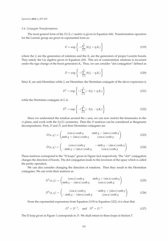
Symmetry 2014, 6, 473–515

5.4. Conjugate Transformations

The most general form of the SL(2, c) matrix is given in Equation (66). Transformation operatorsfor the Lorentz group are given in exponential form as:

D = exp

{−i

3

∑i=1

(θi Ji + ηiKi)

}(119)

where the Ji are the generators of rotations and the Ki are the generators of proper Lorentz boosts.They satisfy the Lie algebra given in Equation (43). This set of commutation relations is invariantunder the sign change of the boost generators Ki. Thus, we can consider “dot conjugation” defined as

D = exp

{−i

3

∑i=1

(θi Ji − ηiKi)

}(120)

Since Ki are anti-Hermitian while Ji are Hermitian, the Hermitian conjugate of the above expression is

D† = exp

{−i

3

∑i=1

(−θi Ji + ηiKi)

}(121)

while the Hermitian conjugate of G is

D† = exp

{−i

3

∑i=1

(−θi Ji − ηiKi)

}(122)

Since we understand the rotation around the z axis, we can now restrict the kinematics to thezt plane, and work with the Sp(2) symmetry. Then the D matrices can be considered as Bargmanndecompositions. First, D and D, and their Hermitian conjugates are

D(α, χ) =

((cos α) cosh χ sinh χ − (sin α) cosh χ

sinh χ + (sin α) cosh χ (cos α) cosh χ

)(123)

D(α, χ) =

((cos α) cosh χ − sinh χ − (sin α) cosh χ

− sinh χ + (sin α) cosh χ (cos α) cosh χ

)(124)

These matrices correspond to the “D loops” given in Figure 2a,b respectively. The “dot” conjugationchanges the direction of boosts. The dot conjugation leads to the inversion of the space which is calledthe parity operation.

We can also consider changing the direction of rotations. Then they result in the Hermitianconjugates. We can write their matrices as

D†(α, χ) =

((cos α) cosh χ sinh χ + (sin α) cosh χ

sinh χ − (sin α) cosh χ (cos α) cosh χ

)(125)

D†(α, χ) =

((cos α) cosh χ − sinh χ + (sin α) cosh χ

− sinh χ − (sin α) cosh χ (cos α) cosh χ

)(126)

From the exponential expressions from Equation (119) to Equation (122), it is clear that

D† = D−1, and D† = D−1 (127)

The D loop given in Figure 1 corresponds to D. We shall return to these loops in Section 7.

320

Symmetry 2014, 6, 473–515

(b) (a)

(d) (c)

Figure 2. Four D-loops resulting from the Bargmann decomposition. (a) Bargmann decompositionfrom Figure 1; (b) Direction of the Lorentz boost is reversed; (c) Direction of rotation is reversed; (d)Both directions are reversed. These operations correspond to the space-inversion, charge conjugation,and the time reversal respectively.

6. Symmetries Derivable from the Poincaré Sphere

The Poincaré sphere serves as the basic language for polarization physics. Its underlyinglanguage is the two-by-two coherency matrix. This coherency matrix contains the symmetry of SL(2, c)isomorphic to the the Lorentz group applicable to three space-like and one time-like dimensions [4,6,7].

For polarized light propagating along the z direction, the amplitude ratio and phase difference ofelectric field x and y components traditionally determine the state of polarization. Hence, the polarizationcan be changed by adjusting the amplitude ratio or the phase difference or both. Usually, the opticaldevice which changes amplitude is called an “attenuator” (or “amplifier”) and the device which changesthe relative phase a “phase shifter”.

Let us start with the Jones vector:(ψ1(z, t)ψ2(z, t)

)=

(a exp [i(kz − ωt)]a exp [i(kz − ωt)]

)(128)

321

Symmetry 2014, 6, 473–515

To this matrix, we can apply the phase shift matrix of Equation (79) which brings the Jones vector to(ψ1(z, t)ψ2(z, t)

)=

(a exp [i(kz − ωt − iφ/2)]a exp [i(kz − ωt + iφ/2)]

)(129)

The generator of this phase-shifter is J3 given Table 5.The optical beam can be attenuated differently in the two directions. The resulting matrix is

e−μ

(eη/2 0

0 e−η/2

)(130)

with the attenuation factor of exp (−μ0 + η/2) and exp (−μ − η/2) for the x and y directionsrespectively. We are interested only the relative attenuation given in Equation (46) which leadsto different amplitudes for the x and y component, and the Jones vector becomes(

ψ1(z, t)ψ2(z, t)

)=

(aeμ/2 exp [i(kz − ωt − iφ/2)]

ae−μ/2 exp [i(kz − ωt + iφ/2)]

)(131)

The squeeze matrix of Equation (46) is generated by K3 given in Table 1.The polarization is not always along the x and y axes, but can be rotated around the z axis using

Equation (79) generated by J2 given in Table 1.Among the rotation angles, the angle of 45◦ plays an important role in polarization optics. Indeed,

if we rotate the squeeze matrix of Equation (46) by 45◦, we end up with the squeeze matrix ofEquation (45) generated by K1 given also in Table 1.

Each of these four matrices plays an important role in special relativity, as we discussed inSections 3.2 and 6. Their respective roles in optics and particle physics are given in Table 7.

Table 7. Polarization optics and special relativity share the same mathematics. Each matrix has its clearrole in both optics and relativity. The determinant of the Stokes or the four-momentum matrix remainsinvariant under Lorentz transformations. It is interesting to note that the decoherence parameter (leastfundamental) in optics corresponds to the (mass)2 (most fundamental) in particle physics.

Polarization Optics Transformation Matrix Particle Symmetry

Phase shift by φ

(e−iφ/2 0

0 eiφ/2

)Rotation around z.

Rotation around z(

cos(θ/2) − sin(θ/2)sin(θ/2) cos(θ/2)

)Rotation around y.

Squeeze along x and y(

eη/2 00 e−η/2

)Boost along z.

Squeeze along 45◦(

cosh(λ/2) sinh(λ/2)sinh(λ/2) cosh(λ/2)

)Boost along x.

a4 (sin ξ)2 Determinant (mass)2

The most general form for the two-by-two matrix applicable to the Jones vector is the G matrix ofEquation (66). This matrix is of course a representation of the SL(2, c) group. It brings the simplestJones vector of Equation (128) to its most general form.

322

Symmetry 2014, 6, 473–515

6.1. Coherency Matrix

However, the Jones vector alone cannot tell us whether the two components are coherent witheach other. In order to address this important degree of freedom, we use the coherency matrix definedas [3,23]

C =

(S11 S12

S21 S22

)(132)

where

< ψ∗i ψj >=

1T

∫ T

0ψ∗

i (t + τ)ψj(t)dt (133)

where T is a sufficiently long time interval. Then, those four elements become [4]

S11 =< ψ∗1 ψ1 >= a2, S12 =< ψ∗

1 ψ2 >= a2(cos ξ)e−iφ (134)

S21 =< ψ∗2 ψ1 >= a2(cos ξ)e+iφ, S22 =< ψ∗

2 ψ2 >= a2 (135)

The diagonal elements are the absolute values of ψ1 and ψ2 respectively. The angle φ could be differentfrom the value of the phase-shift angle given in Equation (79), but this difference does not play anyrole in the reasoning. The off-diagonal elements could be smaller than the product of ψ1 and ψ2, if thetwo polarizations are not completely coherent.

The angle ξ specifies the degree of coherency. If it is zero, the system is fully coherent, while thesystem is totally incoherent if ξ is 90◦. This can therefore be called the “decoherence angle.”

While the most general form of the transformation applicable to the Jones vector is G ofEquation (66), the transformation applicable to the coherency matrix is

C′ = G C G† (136)

The determinant of the coherency matrix is invariant under this transformation, and it is

det(C) = a4(sin ξ)2 (137)

Thus, angle ξ remains invariant. In the language of the Lorentz transformation applicable to thefour-vector, the determinant is equivalent to the (mass)2 and is therefore a Lorentz-invariant quantity.

6.2. Two Radii of the Poincaré Sphere

Let us write explicitly the transformation of Equation (136) as(S′

11 S′12

S′21 S′

22

)=

(α β

γ δ

)(S11 S12

S21 S22

)(α∗ γ∗

β∗ δ∗

)(138)

It is then possible to construct the following quantities,

S0 =S11 + S22

2, S3 =

S11 − S22

2(139)

S1 =S12 + S21

2, S2 =

S12 − S21

2i(140)

These are known as the Stokes parameters, and constitute a four-vector (S0, S3, S1, S2) under theLorentz transformation.

In the Jones vector of Equation (128), the amplitudes of the two orthogonal components are equal.Thus, the two diagonal elements of the coherency matrix are equal. This leads to S3 = 0, and the

323

Symmetry 2014, 6, 473–515

problem is reduced from the sphere to a circle. In the resulting two-dimensional subspace, we canintroduce the polar coordinate system with

R =√

S21 + S2

2 (141)

S1 = R cos φ (142)

S2 = R sin φ (143)

The radius R is the radius of this circle, and is

R = a2 cos ξ (144)

The radius R takes its maximum value S0 when ξ = 0◦. It decreases as ξ increases and vanisheswhen ξ = 90◦. This aspect of the radius R is illustrated in Figure 3.

R

0S

Figure 3. Radius of the Poincaré sphere. The radius R takes its maximum value S0 when thedecoherence angle ξ is zero. It becomes smaller as ξ increases. It becomes zero when the anglereaches 90◦.

In order to see its implications in special relativity, let us go back to the four-momentum matrix ofm(1, 0, 0, 0). Its determinant is m2 and remains invariant. Likewise, the determinant of the coherencymatrix of Equation (132) should also remain invariant. The determinant in this case is

S20 − R2 = a4 sin2 ξ (145)

This quantity remains invariant under the Hermitian transformation of Equation (138), which is aLorentz transformation as discussed in Sections 3.2 and 6. This aspect is shown on the last row ofTable 7.

The coherency matrix then becomes

C = a2

(1 (cos ξ)e−iφ

(cos ξ)eiφ 1

)(146)

324

Symmetry 2014, 6, 473–515

Since the angle φ does not play any essential role, we can let φ = 0, and write the coherency matrix as

C = a2

(1 cos ξ

cos ξ 1

)(147)

The determinant of the above two-by-two matrix is

a4(

1 − cos2 ξ)= a4 sin2 ξ (148)

Since the Lorentz transformation leaves the determinant invariant, the change in this ξ variable isnot a Lorentz transformation. It is of course possible to construct a larger group in which this variableplays a role in a group transformation [6], but here we are more interested in its role in a particlegaining a mass from zero or the mass becoming zero.

6.3. Extra-Lorentzian Symmetry

The coherency matrix of Equation (146) can be diagonalized to

a2

(1 + cos ξ 0

0 1 − cos ξ

)(149)

by a rotation. Let us then go back to the four-momentum matrix of Equation (70). If px = py = 0,and pz = p0 cos ξ , we can write this matrix as

p0

(1 + cos ξ 0

0 1 − cos ξ

)(150)

Thus, with this extra variable, it is possible to study the little groups for variable masses, includingthe small-mass limit and the zero-mass case.

For a fixed value of p0, the (mass)2 becomes

(mass)2 = (p0 sin ξ)2 , and (momentum)2 = (p0 cos ξ)2 (151)

resulting in(energy)2 = (mass)2 + (momentum)2 (152)

This transition is illustrated in Figure 4. We are interested in reaching a point on the light conefrom mass hyperbola while keeping the energy fixed. According to this figure, we do not have to makean excursion to infinite-momentum limit. If the energy is fixed during this process, Equation (152) tellsthe mass and momentum relation, and Figure 5 illustrates this relation.

325

Symmetry 2014, 6, 473–515

(a) (b)

Figure 4. Transition from the massive to massless case. (a) Transition within the framework of theLorentz group; (b) Trasnsition allowed in the symmetry of the Poincaré sphere. Within the frameworkof the Lorentz group, it is not possible to go from the massive to massless case directly, because itrequires the change in the mass which is a Lorentz-invariant quantity. The only way is to move toinfinite momentum and jump from the hyperbola to the light cone, and come back. The extra symmetryof the Poincaré sphere allows a direct transition

Momentum

Ma

ss

Energy

ξangle

Figure 5. Energy-momentum-mass relation. This circle illustrates the case where the energy is fixed,while the mass and momentum are related according to the triangular rule. The value of the angle ξ

changes from zero to 180◦. The particle mass is negative for negative values of this angle. However, inthe Lorentz group, only (mass)2 is a relevant variable, and negative masses might play a role fortheoretical purposes.

Within the framework of the Lorentz group, it is possible, by making an excursion to infinitemomentum where the mass hyperbola coincides with the light cone, to then come back to thedesired point. On the other hand, the mass formula of Equation (151) allows us to go there directly.The decoherence mechanism of the coherency matrix makes this possible.

326

Symmetry 2014, 6, 473–515

7. Small-Mass and Massless Particles

We now have a mathematical tool to reduce the mass of a massive particle from its positive valueto zero. During this process, the Lorentz-boosted rotation matrix becomes a gauge transformation forthe spin-1 particle, as discussed Section 5.2. For spin-1/2 particles, there are two issues.

1. It was seen in Section 5.2 that the requirement of gauge invariance lead to a polarization ofmassless spin-1/2 particle, such as neutrinos. What happens to anti-neutrinos?

2. There are strong experimental indications that neutrinos have a small mass. What happens tothe E(2) symmetry?

7.1. Spin-1/2 Particles

Let us go back to the two-by-two matrices of Section 5.4, and the two-by-two D matrix. For amassive particle, its Wigner decomposition leads to

D =

(cos(θ/2) −e−η sin(θ/2)

eη sin(θ/2) cos(θ/2)

)(153)

This matrix is applicable to the spinors u and v defined in Equation (101) respectively for the spin-upand spin-down states along the z direction.

Since the Lie algebra of SL(2, c) is invariant under the sign change of the Ki matrices, we canconsider the “dotted” representation, where the system is boosted in the opposite direction, while thedirection of rotations remain the same. Thus, the Wigner decomposition leads to

D =

(cos(θ/2) −eη sin(θ/2)

e−η sin(θ/2) cos(θ/2)

)(154)

with its spinors

u =

(10

), and v =

(01

)(155)

For anti-neutrinos, the helicity is reversed but the momentum is unchanged. Thus, D† is theappropriate matrix. However, D† = D−1 as was noted in Section 5.4. Thus, we shall use D foranti-neutrinos.

When the particle mass becomes very small,

e−η =m2p

(156)

becomes small. Thus, if we let

eη sin(θ/2) = γ, and e−η sin(θ/2) = ε2 (157)

then the D matrix of Equation (153) and the D of Equation (154) become(1 − γε2/2 −ε2

γ 1 − γε2

), and

(1 − γε2/2 −γ

ε2 1 − γε2

)(158)

respectively where γ is an independent parameter and

ε2 = γ

(m2p

)2(159)

327

Symmetry 2014, 6, 473–515

When the particle mass becomes zero, they become(1 0γ 1

), and

(1 −γ

0 1

)(160)

respectively, applicable to the spinors (u, v) and (u, v) respectively.For neutrinos, (

1 0γ 1

)(10

)=

(1γ

), and

(1 0γ 1

)(01

)=

(01

)(161)

For anti-neutrinos, (1 −γ

0 1

)(10

)=

(10

), and

(1 −γ

0 1

)(01

)=

(−γ

1

)(162)

It was noted in Section 5.2 that the triangular matrices of Equation (160) perform gaugetransformations. Thus, for Equations (161) and (162) the requirement of gauge invariance leads tothe polarization of neutrinos. The neutrinos are left-handed while the anti-neutrinos are right-handed.Since, however, nature cannot tell the difference between the dotted and undotted representations,the Lorentz group cannot tell which neutrino is right handed. It can say only that the neutrinos andanti-neutrinos are oppositely polarized.

If the neutrino has a small mass, the gauge invariance is modified to(1 − γε2/2 −ε2

γ 1 − γε2/2

)(01

)=

(01

)− ε2

(1

γ/2

)(163)

and (1 − γε2/2 −γ

ε2 1 − γε2

)(10

)=

(10

)+ ε2

(−γ/2

1

)(164)

respectively for neutrinos and anti-neutrinos. Thus the violation of the gauge invariance in both casesis proportional to ε2 which is m2/4p2.

7.2. Small-Mass Neutrinos in the Real World

Whether neutrinos have mass or not and the consequences of this relative to the Standard Modeland lepton number is the subject of much theoretical speculation [24,25], and of cosmology [26],nuclear reactors [27], and high energy experimentations [28,29]. Neutrinos are fast becoming animportant component of the search for dark matter and dark radiation [30]. Their importance withinthe Standard Model is reflected by the fact that they are the only particles which seem to exist withonly one direction of chirality, i.e., only left-handed neutrinos have been confirmed to exist so far.

It was speculated some time ago that neutrinos in constant electric and magnetic fields wouldacquire a small mass, and that right-handed neutrinos would be trapped within the interaction field [31].Solving generalized electroweak models using left- and right-handed neutrinos has been discussedrecently [32]. Today these right-handed neutrinos which do not participate in weak interactions arecalled “sterile” neutrinos [33]. A comprehensive discussion of the place of neutrinos in the scheme ofphysics has been given by Drewes [30]. We should note also that the three different neutrinos, namelyνe, νμ, and ντ , may have different masses [34].

328

Symmetry 2014, 6, 473–515

8. Scalars, Four-Vectors, and Four-Tensors

In Sections 5 and 7, our primary interest has been the two-by-two matrices applicable to spinors forspin-1/2 particles. Since we also used four-by-four matrices, we indirectly studied the four-componentparticle consisting of spin-1 and spin-zero components.

If there are two spin 1/2 states, we are accustomed to construct one spin-zero state, and onespin-one state with three degeneracies.

In this paper, we are confronted with two spinors, but each spinor can also be dotted. For thisreason, there are 16 orthogonal states consisting of spin-one and spin-zero states. How many spin-zerostates? How many spin-one states?

For particles at rest, it is known that the addition of two one-half spins result in spin-zero andspin-one states. In this paper, we have two different spinors behaving differently under the Lorentzboost. Around the z direction, both spinors are transformed by

Z(φ) = exp (−iφJ3) =

(e−iφ/2 0

0 eiφ/2

)(165)

However, they are boosted by

B(η) = exp (−iηK3) =

(eη/2 0

0 e−η/2

)(166)

B(η) = exp (iηK3) =

(e−η/2 0

0 eη/2

)(167)

applicable to the undotted and dotted spinors respectively. These two matrices commute with eachother, and also with the rotation matrix Z(φ) of Equation (165). Since K3 and J3 commute with eachother, we can work with the matrix Q(η, φ) defined as

Q(η, φ) = B(η)Z(φ) =

(e(η−iφ)/2 0

0 e−(η−iφ)/2

)(168)

Q(η, φ) = B(η)Z(φ) =

(e−(η+iφ)/2 0

0 e(η+iφ)/2

)(169)

When this combined matrix is applied to the spinors,

Q(η, φ)u = e(η−iφ)/2u, Q(η, φ)v = e−(η−iφ)/2v (170)

Q(η, φ)u = e−(η+iφ)/2u, Q(η, φ)v = e(η+iφ)/2v (171)

If the particle is at rest, we can construct the combinations

uu,1√2(uv + vu), vv (172)

to construct the spin-1 state, and1√2(uv − vu) (173)

for the spin-zero state. There are four bilinear states. In the SL(2, c) regime, there are two dotted spinors.If we include both dotted and undotted spinors, there are 16 independent bilinear combinations.They are given in Table 8. This table also gives the effect of the operation of Q(η, φ).

329

Symmetry 2014, 6, 473–515

Table 8. Sixteen combinations of the SL(2, c) spinors. In the SU(2) regime, there are two spinorsleading to four bilinear forms. In the SL(2, c) world, there are two undotted and two dotted spinors.These four spinors lead to 16 independent bilinear combinations.

Spin 1 Spin 0

uu, 1√2(uv + vu), vv, 1√

2(uv − vu)

uu, 1√2(uv + vu), vv, 1√

2(uv − vu)

uu, 1√2(uv + vu), vv, 1√

2(uv − vu)

uu, 1√2(uv + vu), vv, 1√

2(uv − vu)

After the Operation of Q(η, φ) and Q(η, φ)

e−iφeηuu, 1√2(uv + vu), eiφe−ηvv, 1√

2(uv − vu)

e−iφe−η uu, 1√2(uv + vu), eiφeη vv, 1√

2(uv − vu)

e−iφuu, 1√2(eηuv + e−ηvu), eiφvv, 1√

2(eηuv − e−ηvu)

e−iφuu, 1√2(uv + vu), eiφ vv, 1√

2(e−η uv − eη vu)

Among the bilinear combinations given in Table 8, the following two are invariant under rotationsand also under boosts.

S =1√2(uv − vu), and S = − 1√

2(uv − vu) (174)

They are thus scalars in the Lorentz-covariant world. Are they the same or different? Let us considerthe following combinations

S+ =1√2

(S + S

), and S− =

1√2

(S − S

)(175)

Under the dot conjugation, S+ remains invariant, but S− changes its sign.Under the dot conjugation, the boost is performed in the opposite direction. Therefore it is the

operation of space inversion, and S+ is a scalar while S− is called the pseudo-scalar.

8.1. Four-Vectors

Let us consider the bilinear products of one dotted and one undotted spinor as uu, uv, uv, vv,and construct the matrix

U =

(uv vvuu vu

)(176)

Under the rotation Z(φ) and the boost B(η) they become(eηuv e−iφvveiφuu e−ηvu

)(177)

Indeed, this matrix is consistent with the transformation properties given in Table 8, and transformslike the four-vector (

t + z x − iyx + iy t − z

)(178)

This form was given in Equation (65), and played the central role throughout this paper. Under thespace inversion, this matrix becomes (

t − z −(x − iy)−(x + iy) t + z

)(179)

330

Symmetry 2014, 6, 473–515

This space inversion is known as the parity operation.The form of Equation (176) for a particle or field with four-components, is given by (V0, Vz, Vx, Vy).

The two-by-two form of this four-vector is

U =

(V0 + Vz Vx − iVy

Vx + iVy V0 − Vz

)(180)

If boosted along the z direction, this matrix becomes(eη (V0 + Vz) Vx − iVy

Vx + iVy e−η (V0 − Vz)

)(181)

In the mass-zero limit, the four-vector matrix of Equation (181) becomes(2A0 Ax − iAy

Ax + iAy 0

)(182)

with the Lorentz condition A0 = Az. The gauge transformation applicable to the photon four-vectorwas discussed in detail in Section 5.2.

Let us go back to the matrix of Equation (180), we can construct another matrix U. Since the dotconjugation leads to the space inversion,

U =

(uv vvuu vu

)(183)

Then

uv � (t − z), vu � (t + z) (184)

vv � −(x − iy), uu � −(x + iy) (185)

where the symbol � means “transforms like”.Thus, U of Equation (176) and U of Equation (183) used up 8 of the 16 bilinear forms. Since there

are two bilinear forms in the scalar and pseudo-scalar as given in Equation (175), we have to giveinterpretations to the six remaining bilinear forms.

8.2. Second-Rank Tensor

In this subsection, we are studying bilinear forms with both spinors dotted and undotted.In Section 8.1, each bilinear spinor consisted of one dotted and one undotted spinor. There arealso bilinear spinors which are both dotted or both undotted. We are interested in two sets of threequantities satisfying the O(3) symmetry. They should therefore transform like

(x + iy)/√

2, (x − iy)/√

2, z (186)

which are likeuu, vv, (uv + vu)/

√2 (187)

respectively in the O(3) regime. Since the dot conjugation is the parity operation, they are like

− uu, −vv, −(uv + vu)/√

2 (188)

In other words,(uu) = −uu, and (vv) = −vv (189)

331

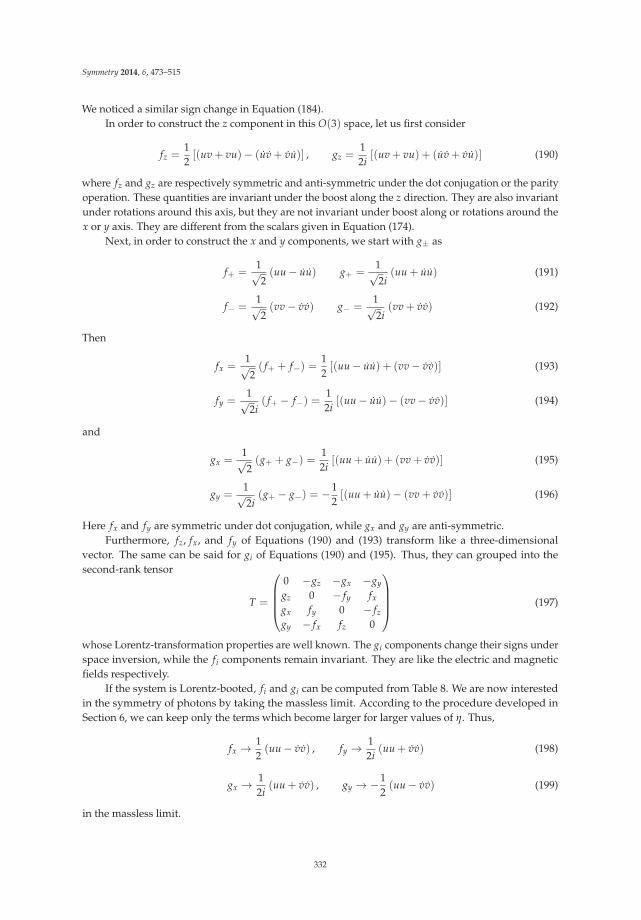
Symmetry 2014, 6, 473–515

We noticed a similar sign change in Equation (184).In order to construct the z component in this O(3) space, let us first consider

fz =12[(uv + vu)− (uv + vu)] , gz =

12i

[(uv + vu) + (uv + vu)] (190)

where fz and gz are respectively symmetric and anti-symmetric under the dot conjugation or the parityoperation. These quantities are invariant under the boost along the z direction. They are also invariantunder rotations around this axis, but they are not invariant under boost along or rotations around thex or y axis. They are different from the scalars given in Equation (174).

Next, in order to construct the x and y components, we start with g± as

f+ =1√2(uu − uu) g+ =

1√2i

(uu + uu) (191)

f− =1√2(vv − vv) g− =

1√2i

(vv + vv) (192)

Then

fx =1√2( f+ + f−) =

12[(uu − uu) + (vv − vv)] (193)

fy =1√2i

( f+ − f−) =12i

[(uu − uu)− (vv − vv)] (194)

and

gx =1√2(g+ + g−) =

12i

[(uu + uu) + (vv + vv)] (195)

gy =1√2i

(g+ − g−) = −12[(uu + uu)− (vv + vv)] (196)

Here fx and fy are symmetric under dot conjugation, while gx and gy are anti-symmetric.Furthermore, fz, fx, and fy of Equations (190) and (193) transform like a three-dimensional

vector. The same can be said for gi of Equations (190) and (195). Thus, they can grouped into thesecond-rank tensor

T =

⎛⎜⎜⎜⎝

0 −gz −gx −gy

gz 0 − fy fx

gx fy 0 − fz

gy − fx fz 0

⎞⎟⎟⎟⎠ (197)

whose Lorentz-transformation properties are well known. The gi components change their signs underspace inversion, while the fi components remain invariant. They are like the electric and magneticfields respectively.

If the system is Lorentz-booted, fi and gi can be computed from Table 8. We are now interestedin the symmetry of photons by taking the massless limit. According to the procedure developed inSection 6, we can keep only the terms which become larger for larger values of η. Thus,

fx → 12(uu − vv) , fy → 1

2i(uu + vv) (198)

gx → 12i

(uu + vv) , gy → −12(uu − vv) (199)

in the massless limit.

332

Symmetry 2014, 6, 473–515

Then the tensor of Equation (197) becomes

F =

⎛⎜⎜⎜⎝

0 0 −Ex −Ey

0 0 −By Bx

Ex By 0 0Ey −Bx 0 0

⎞⎟⎟⎟⎠ (200)

with

Bx � 12(uu − vv) , By � 1

2i(uu + vv) (201)

Ex =12i

(uu + vv) , Ey = −12(uu − vv) (202)

The electric and magnetic field components are perpendicular to each other. Furthermore,

Ex = By, Ey = −Bx (203)

In order to address this question, let us go back to Equation (191). In the massless limit,

B+ � E+ � uu, B− � E− � vv (204)

The gauge transformation applicable to u and v are the two-by-two matrices(1 −γ

0 1

), and

(1 0−γ 1

)(205)

respectively as noted in Sections 5.2 and 7.1. Both u and v are invariant under gauge transformations,while u and v do not.

The B+ and E+ are for the photon spin along the z direction, while B− and E− are for the oppositedirection. In 1964 [35], Weinberg constructed gauge-invariant state vectors for massless particlesstarting from Wigner’s 1939 paper [1]. The bilinear spinors uu and and vv correspond to Weinberg’sstate vectors.

8.3. Possible Symmetry of the Higgs Mechanism

In this section, we discussed how the two-by-two formalism of the group SL(2, c) leads thescalar, four-vector, and tensor representations of the Lorentz group. We discussed in detail how thefour-vector for a massive particle can be decomposed into the symmetry of a two-component masslessparticle and one gauge degree of freedom. This aspect was studied in detail by Kim and Wigner [20,21],and their results are illustrated in Figure 6. This decomposition is known in the literature as the groupcontraction.

The four-dimensional Lorentz group can be contracted to the Euclidean and cylindrical groups.These contraction processes could transform a four-component massive vector meson into a masslessspin-one particle with two spin components, and one gauge degree of freedom.

Since this contraction procedure is spelled out detail in [21], as well as in the present paper,its reverse process is also well understood. We start with one two-component massless particle withone gauge degree of freedom, and end up with a massive vector meson with its four components.

The mathematics of this process is not unlike the Higgs mechanism [36,37], where one masslessfield with two degrees of freedom absorbs one gauge degree freedom to become a quartet of bosons,namely that of W, Z± plus the Higgs boson. As is well known, this mechanism is the basis for thetheory of electro-weak interaction formulated by Weinberg and Salam [38,39].

333

Symmetry 2014, 6, 473–515

Figure 6. Contractions of the three-dimensional rotation group. (a) Contraction in terms of thetangential plane and the tangential cylinder [20]; (b) Contraction in terms of the expansion andcontraction of the longitudinal axis [21]. In both cases, the symmetry ends up with one rotation aroundthe longitudinal direction and one translational degree along the longitudinal axis. The rotation andtranslation corresponds to the helicity and gauge degrees of freedom.

The word “spontaneous symmetry breaking” is used for the Higgs mechanism. It could bean interesting problem to see that this symmetry breaking for the two Higgs doublet model can beformulated in terms of the Lorentz group and its contractions. In this connection, we note an interestingrecent paper by Dée and Ivanov [40].

9. Conclusions

The damped harmonic oscillator, Wigner’e little groups, and the Poincaré sphere belong to thethree different branches of physics. In this paper, it was noted that they are based on the samemathematical framework, namely the algebra of two-by-two matrices.

The second-order differential equation for damped harmonic oscillators can be formulated interms of two-by-two matrices. These matrices produce the algebra of the group Sp(2). While thereare three trace classes of the two-by-two matrices of this group, the damped oscillator tells us how tomake transitions from one class to another.

It is shown that Wigner’s three little groups can be defined in terms of the trace classes of theSp(2) group. If the trace is smaller than two, the little group is for massive particles. If greater thantwo, the little group is for imaginary-mass particles. If the trace is equal to two, the little group is formassless particles. Thus, the damped harmonic oscillator provides a procedure for transition from onelittle group to another.

The Poincaré sphere contains the symmetry of the six-parameter SL(2, c) group. Thus, the sphereprovides the procedure for extending the symmetry of the little group defined within the Lorentz groupof three-dimensional Minkowski space to its full Lorentz group in the four-dimensional space-time.In addition, the Poincaré sphere offers the variable which allows us to change the symmetry of amassive particle to that of a massless particle by continuously decreasing the mass.

In this paper, we extracted the mathematical properties of Wigner’s little groups from the dampedharmonic oscillator and the Poincaré sphere. In so doing, we have shown that the transition from onelittle group to another is tangentially continuous.

This subject was initiated by Inönü and Wigner in 1953 as the group contraction [41]. In theirpaper, they discussed the contraction of the three-dimensional rotation group becoming contracted tothe two-dimensional Euclidean group with one rotational and two translational degrees of freedom.While the O(3) rotation group can be illustrated by a three-dimensional sphere, the plane tangential at

334

Symmetry 2014, 6, 473–515

the north pole is for the E(2) Euclidean group. However, we can also consider a cylinder tangential atthe equatorial belt. The resulting cylindrical group is isomorphic to the Euclidean group [20]. While therotational degree of freedom of this cylinder is for the photon spin, the up and down translations onthe surface of the cylinder correspond to the gauge degree of freedom of the photon, as illustrated inFigure 6.

It was noted also that the Bargmann decomposition of two-by-two matrices, as illustrated inFigure 1 and Figure 2, allows us to study more detailed properties of the little groups, includingspace and time reflection reflection properties. Also in this paper, we have discussed how thescalars, four-vectors, and four-tensors can be constructed from the two-by-two representation inthe Lorentz-covariant world.

In addition, it should be noted that the symmetry of the Lorentz group is also contained in thesqueezed state of light [14] and the ABCD matrix for optical beam transfers [18]. We also mentionedthe possibility of understanding the mathematics of the Higgs mechanism in terms of the Lorentzgroup and its contractions.

Acknowledgements

In his 1939 paper [1], Wigner worked out the subgroups of the Lorentz group whosetransformations leave the four momentum of a given particle invariant. In so doing, he workedout their internal space-time symmetries. In spite of its importance, this paper remains as one of themost difficult papers to understand. Wigner was eager to make his paper understandable to youngerphysicists.

While he was the pioneer in introducing the mathematics of group theory to physics, he wasalso quite fond of using two-by-two matrices to explain group theoretical ideas. He asked one of thepresent authors (Young S. Kim) to rewrite his 1939 paper [1] using the language of those matrices. Thisis precisely what we did in the present paper.

We are grateful to Eugene Paul Wigner for this valuable suggestion.

Author Contributions

This paper is largely based on the earlier papers by Young S. Kim and Marilyn E. Noz, and thoseby Sibel Baskal and Young S. Kim. The two-by-two formulation of the damped oscillator in Section 2was jointly developed by Sibel Baskal and Yound S. Kim during the summer of 2012. Marilyn E. Nozdeveloped the idea of the symmetry of small-mass neutrinos in Section 7. The limiting process in thesymmetry of the Poincaré sphere was formulated by Young S. Kim. Sibel Baskal initially constructedthe four-by-four tensor representation in Section 8.

The initial organization of this paper was conceived by Young S. Kim in his attempt to followWigner’s suggestion to translate his 1939 paper into the language of two-by-two matrices. Sibel Baskaland Marilyn E. Noz tightened the organization and filled in the details.

Conflicts of Interest

The authors declare no conflicts of interest.

References

1. Wigner, E. On unitary representations of the inhomogeneous Lorentz Group. Ann. Math. 1939, 40, 149–204.2. Han, D.; Kim, Y.S.; Son, D. Eulerian parametrization of Wigner little groups and gauge transformations in

terms of rotations in 2-component spinors. J. Math. Phys. 1986, 27, 2228–2235.3. Born, M.; Wolf, E. Principles of Optics, 6th ed.; Pergamon: Oxford, UK, 1980.

335

Symmetry 2014, 6, 473–515

4. Han, D.; Kim, Y.S.; Noz, M.E. Stokes parameters as a Minkowskian four-vector. Phys. Rev. E 1997, 56,6065–6076.

5. Brosseau, C. Fundamentals of Polarized Light: A Statistical Optics Approach; John Wiley: New York, NY, USA,1998.

6. Baskal, S.; Kim, Y.S. De Sitter group as a symmetry for optical decoherence. J. Phys. A 2006, 39, 7775–7788.7. Kim, Y.S.; Noz, M.E. Symmetries shared by the Poincaré Group and the Poincaré Sphere. Symmetry 2013, 5,

233–252.8. Han, D.; Kim, Y.S.; Son, D. E(2)-like little group for massless particles and polarization of neutrinos. Phys. Rev.

D 1982, 26, 3717–3725.9. Han, D.; Kim, Y.S.; Son, D. Photons, neutrinos and gauge transformations. Am. J. Phys. 1986, 54, 818–821.10. Baskal, S.; Kim, Y.S. Little groups and Maxwell-type tensors for massive and massless particles. Europhys. Lett.

1997, 40, 375–380.11. Leggett, A.; Chakravarty, S.; Dorsey, A.; Fisher, M.; Garg, A.; Zwerger, W. Dynamics of the dissipative 2-state

system. Rev. Mod. Phys. 1987, 59, 1–85.12. Baskal, S.; Kim, Y.S. One analytic form for four branches of the ABCD matrix. J. Mod. Opt. 2010, 57, 1251–1259.13. Baskal, S.; Kim, Y.S. Lens optics and the continuity problems of the ABCD matrix. J. Mod. Opt. 2014, 61,

161–166.14. Kim, Y.S.; Noz, M.E. Theory and Applications of the Poincaré Group; Reidel: Dordrecht, The Netherlands, 1986.15. Bargmann, V. Irreducible unitary representations of the Lorentz group. Ann. Math. 1947, 48, 568–640.16. Iwasawa, K. On some types of topological groups. Ann. Math. 1949, 50, 507–558.17. Guillemin, V.; Sternberg, S. Symplectic Techniques in Physics; Cambridge University Press: Cambridge, UK,

1984.18. Baskal, S.; Kim, Y.S. Lorentz Group in Ray and Polarization Optics. In Mathematical Optics:

Classical, Quantum and Computational Methods; Lakshminarayanan, V., Calvo, M.L., Alieva, T., Eds.; CRC Taylor andFrancis: New York, NY, USA, 2013; Chapter 9, pp. 303–340.

19. Naimark, M.A. Linear Representations of the Lorentz Group; Pergamon: Oxford, UK, 1964.20. Kim, Y.S.; Wigner, E.P. Cylindrical group and masless particles. J. Math. Phys. 1987, 28, 1175–1179.21. Kim, Y.S.; Wigner, E.P. Space-time geometry of relativistic particles. J. Math. Phys. 1990, 31, 55–60.22. Georgieva, E.; Kim, Y.S. Iwasawa effects in multilayer optics. Phys. Rev. E 2001, 64,

doi:10.1103/PhysRevE.64.026602.23. Saleh, B.E.A.; Teich, M.C. Fundamentals of Photonics, 2nd ed.; John Wiley: Hoboken, NJ, USA, 2007.24. Papoulias, D.K.; Kosmas, T.S. Exotic Lepton Flavour Violating Processes in the Presence of Nuclei. J. Phys.:

Conf. Ser. 2013, 410, 012123:1–012123:5.25. Dinh, D.N.; Petcov, S.T.; Sasao, N.; Tanaka, M.; Yoshimura, M. Observables in neutrino mass spectroscopy

using atoms. Phys. Lett. B. 2013, 719, 154–163.26. Miramonti, L.; Antonelli, V. Advancements in Solar Neutrino physics. Int. J. Mod. Phys. E. 2013, 22, 1–16.27. Li, Y.-F.; Cao, J.; Jun, Y.; Wang, Y.; Zhan, L. Unambiguous determination of the neutrino mass hierarchy using

reactor neutrinos. Phys. Rev. D. 2013, 88, 013008:1–013008:9.28. Bergstrom, J. Combining and comparing neutrinoless double beta decay experiments using different 584

nuclei. J. High Energy Phys. 2013, 02, 093:1–093:27.29. Han, T.; Lewis, I.; Ruiz, R.; Si, Z.-G. Lepton number violation and W ′ chiral couplings at the LHC. Phys. Rev.

D 2013, 87, 035011:1–035011:25.30. Drewes, M. The phenomenology of right handed neutrinos. Int. J. Mod. Phys. E 2013, 22, 1330019:1–1330019:75.31. Barut, A.O.; McEwan, J. The four states of the massless neutrino with pauli coupling by spin-gauge invariance.

Lett. Math. Phys. 1986, 11, 67–72.32. Palcu, A. Neutrino Mass as a consequence of the exact solution of 3-3-1 gauge models without exotic electric

charges. Mod. Phys. Lett. A 2006, 21, 1203–1217.33. Bilenky, S.M. Neutrino. Phys. Part. Nucl. 2013, 44, 1–46.34. Alhendi, H. A.; Lashin, E. I.; Mudlej, A. A. Textures with two traceless submatrices of the neutrino mass

matrix. Phys.Rev. D 2008, 77, 013009.1–013009.1-13.35. Weinberg, S. Photons and gravitons in S-Matrix theory: Derivation of charge conservation and equality of

gravitational and inertial mass. Phys. Rev. 1964, 135, B1049–B1056.36. Higgs, P.W. Broken symmetries and the masses of gauge bosons. Phys. Rev. Lett. 1964, 13, 508–509.

336

Symmetry 2014, 6, 473–515

37. Guralnik, G.S.; Hagen, C.R.; Kibble, T.W.B. Global conservation laws and massless particles. Phys. Rev. Lett.1964, 13, 585–587.

38. Weinberg, S. A model of leptons. Phys. Rev. Lett. 1967, 19, 1265–1266.39. Weinberg, S. Quantum Theory of Fields, Volume II, Modern Applications; Cambridge University Press: Cambridge,

UK, 1996.40. Dée, A.; Ivanov, I.P. Higgs boson masses of the general two-Higgs-doublet model in the Minkowski-space

formalism. Phys. Rev. D 2010, 81, 015012:1–015012:8.41. Inönü, E.; Wigner, E.P. On the contraction of groups and their representations. Proc. Natl. Acad. Sci. USA 1953,

39, 510–524.

c© 2014 by the authors. Licensee MDPI, Basel, Switzerland. This article is an open accessarticle distributed under the terms and conditions of the Creative Commons Attribution(CC BY) license (http://creativecommons.org/licenses/by/4.0/).

337

symmetryS S

Article

Loop Representation of Wigner’s Little Groups

Sibel Baskal 1, Young S. Kim 2,* and Marilyn E. Noz 3

1 Department of Physics, Middle East Technical University, 06800 Ankara, Turkey;baskal@newton.physics.metu.edu.tr

2 Center for Fundamental Physics, University of Maryland College Park, Maryland, MD 20742, USA3 Department of Radiology, New York University, New York, NY 10016, USA; marilyn.noz@med.nyu.edu* Correspondence: yskim@umd.edu; Tel.: +1-301-937-6306

Academic Editor: Sergei D. OdintsovReceived: 12 May 2017; Accepted: 15 June 2017; Published: 23 June 2017

Abstract: Wigner’s little groups are the subgroups of the Lorentz group whose transformations leavethe momentum of a given particle invariant. They thus define the internal space-time symmetriesof relativistic particles. These symmetries take different mathematical forms for massive and formassless particles. However, it is shown possible to construct one unified representation using agraphical description. This graphical approach allows us to describe vividly parity, time reversal,and charge conjugation of the internal symmetry groups. As for the language of group theory,the two-by-two representation is used throughout the paper. While this two-by-two representation isfor spin-1/2 particles, it is shown possible to construct the representations for spin-0 particles, spin-1particles, as well as for higher-spin particles, for both massive and massless cases. It is shown alsothat the four-by-four Dirac matrices constitute a two-by-two representation of Wigner’s little group.

Keywords: Wigner’s little groups; Lorentz group; unified picture of massive and massless particles;two-by-two representations; graphical approach to internal space-time symmetries

PACS: 02.10.Yn; 02.20.Uw; 03.65.Fd

1. Introduction

In his 1939 paper [1], Wigner introduced subgroups of the Lorentz group whose transformationsleave the momentum of a given particle invariant. These subgroups are called Wigner’s little groupsin the literature and are known as the symmetry groups for internal space-time structure.

For instance, a massive particle at rest can have spin that can be rotated in three-dimensional space.The little group in this case is the three-dimensional rotation group. For a massless particle movingalong the z direction, Wigner noted that rotations around the z axis do not change the momentum.In addition, he found two more degrees of freedom, which together with the rotation, constitute asubgroup locally isomorphic to the two-dimensional Euclidean group.

However, Wigner’s 1939 paper did not deal with the following critical issues.

1. As for the massive particle, Wigner worked out his little group in the Lorentz frame where theparticle is at rest with zero momentum, resulting in the three-dimensional rotation group. He couldhave Lorentz-boosted the O(3)-like little group to make the little group for a moving particle.

2. While the little group for a massless particle is like E(2), it is not difficult to associate the rotationaldegree of freedom to the helicity. However, Wigner did not give physical interpretations to thetwo translation-like degrees of freedom.

3. While the Lorentz group does not allow mass variations, particles with infinite momentum shouldbehave like massless particles. The question is whether the Lorentz-boosted O(3)-like little groupbecomes the E(2)-like little group for particles with infinite momentum.

Symmetry 2017, 9, 97 338 www.mdpi.com/journal/symmetry

Symmetry 2017, 9, 97

These issues have been properly addressed since then [2–5]. The translation-like degrees offreedom for massless particles collapse into one gauge degree of freedom, and the E(2)-like littlegroup can be obtained as the infinite-momentum limit of the O(3)-like little group. This history issummarized in Figure 1.

Rotation

y

x

z

Ga

ug

e t

ran

sfo

rma

tio

n

y

x

Translation

Top view

Side

view

Tangential plane

at the north pole

Cylinder tangential

around the equator

Sphere with

O(3) symmetry

ISOMORPHIC

E(2)

Cylindrical

Group

Figure 1. O(3)-like and E(2)-like internal space-time symmetries of massive and massless particles.The sphere corresponds to the O(3)-like little group for the massive particle. There is a plane tangentialto the sphere at its north pole, which is E(2). There is also a cylinder tangent to the sphere at itsequatorial belt. This cylinder gives one helicity and one gauge degree of freedom. This figure thusgives a unified picture of the little groups for massive and massless particles [5].

In this paper, we shall present these developments using a mathematical language moretransparent than those used in earlier papers.

1. In his original paper [1], Wigner worked out his little group for the massive particle when itsmomentum is zero. How about moving massive particles? In this paper, we start with a movingparticle with non-zero momentum. We then perform rotations and boosts whose net effectdoes not change the momentum [6–8]. This procedure can be applied to the massive, massless,and imaginary-mass cases.

2. By now, we have a clear understanding of the group SL(2, c) as the universal covering group of theLorentz group. The logic with two-by-two matrices is far more transparent than the mathematicsbased on four-by-four matrices. We shall thus use the two-by-two representation of the Lorentzgroup throughout the paper [5,9–11].

The purpose of this paper is to make the physics contained in Wigner’s original paper moretransparent. In Section 2, we give the six generators of the Lorentz group. It is possible to write themin terms of coordinate transformations, four-by-four matrices, and two-by-two matrices. In Section 3,we introduce Wigner’s little groups in terms of two-by-two matrices. In Section 4, it is shown possibleto construct transformation matrices of the little group by performing rotations and a boost resultingin a non-trivial matrix, which leaves the given momentum invariant.

Since we are more familiar with Dirac matrices than the Lorentz group, it is shown in Section 5 thatDirac matrices are a representation of the Lorentz group, and his four-by-four matrices are two-by-two

339

Symmetry 2017, 9, 97

representations of the two-by-two representation of Wigner’s little groups. In Section 6, we constructspin-0 and spin-1 particles for the SL(2,c) spinors. We also discuss massless higher spin particles.

2. Lorentz Group and Its Representations

The group of four-by-four matrices, which performs Lorentz transformations on the four-dimensionalMinkowski space leaving invariant the quantity

(t2 − z2 − x2 − y2), forms the starting point for the

Lorentz group. As there are three rotation and three boost generators, the Lorentz group is a six-parametergroup.

Einstein, by observing that this Lorentz group also leaves invariant(E, pz, px, py

), was able to derive

his Lorentz-covariant energy-momentum relation commonly known as E = mc2. Thus, the particle massis a Lorentz-invariant quantity.

The Lorentz group is generated by the three rotation operators:

Ji = −i

(xj

∂

∂xk− xk

∂

∂xj

), (1)

where i, j, k = 1, 2, 3, and three boost operators:

Ki = −i(

t∂

∂xi+ xi

∂

∂t

). (2)

These generators satisfy the closed set of commutation relations:

[Ji, Jj

]= iεijk Jk,

[Ji, Kj

]= iεijkKk,

[Ki, Kj

]= −iεijk Jk, (3)

which are known as the Lie algebra for the Lorentz group.Under the space inversion, xi → −xi, or the time reflection, t → −t, the boost generators Ki

change sign. However, the Lie algebra remains invariant, which means that the commutation relationsremain invariant under Hermitian conjugation.

In terms of four-by-four matrices applicable to the Minkowskian coordinate of (t, z, x, y),the generators can be written as:

J3 =

⎛⎜⎜⎜⎝

0 0 0 00 0 0 00 0 0 −i0 0 i 0

⎞⎟⎟⎟⎠ , K3 =

⎛⎜⎜⎜⎝

0 i 0 0i 0 0 00 0 0 00 0 0 0

⎞⎟⎟⎟⎠ , (4)

for rotations around and boosts along the z direction, respectively. Similar expressions can be writtenfor the x and y directions. We see here that the rotation generators Ji are Hermitian, but the boostgenerators Ki are anti-Hermitian.

We can also consider the two-by-two matrices:

Ji =12

σi, and Ki =i2

σi, (5)

where σi are the Pauli spin matrices. These matrices also satisfy the commutation relations given inEquation (3).

There are interesting three-parameter subgroups of the Lorentz group. In 1939 [1], Wigner consideredthe subgroups whose transformations leave the four-momentum of a given particle invariant. First of all,consider a massive particle at rest. The momentum of this particle is invariant under rotations inthree-dimensional space. What happens for the massless particle that cannot be brought to a restframe? In this paper we shall consider this and other problems using the two-by-two representation ofthe Lorentz group.

340

Symmetry 2017, 9, 97

3. Two-by-Two Representation of Wigner’s Little Groups

The six generators of Equation (5) lead to the group of two-by-two unimodular matrices of the form:

G =

(α β

γ δ

), (6)

with det(G) = 1, where the matrix elements are complex numbers. There are thus six independentreal numbers to accommodate the six generators given in Equation (5). The groups of matrices of thisform are called SL(2, c) in the literature. Since the generators Ki are not Hermitian, the matrix G is notalways unitary. Its Hermitian conjugate is not necessarily the inverse.

The space-time four-vector can be written as [5,9,11]:

(t + z x − iy

x + iy t − z

), (7)

whose determinant is t2 − z2 − x2 − z2, and remains invariant under the Hermitian transformation:

X′ = G X G†. (8)

This is thus a Lorentz transformation. This transformation can be explicitly written as:

(t′ + z′ x′ − iy′

x′ + iy′ t′ − z′

)=

(α β

γ δ

)(t + z x − iy

x + iy t − z

)(α∗ γ∗

β∗ δ∗

). (9)

With these six independent real parameters, it is possible to construct four-by-four matrices forLorentz transformations applicable to the four-dimensional Minkowskian space [5,12]. For the purposeof the present paper, we need some special cases, and they are given in Table 1.

Table 1. Two-by-two and four-by-four representations of the Lorentz group.

Generators Two-by-Two Four-by-Four

J3 = 12

(1 00 −1

) (exp (iφ/2) 0

0 exp (−iφ/2)

) ⎛⎝1 0 0 0

0 1 0 00 0 cos φ − sin φ0 0 sin φ cos φ

⎞⎠

K3 = 12

(i 00 −i

) (exp (η/2) 0

0 exp (−η/2)

) ⎛⎝cosh η sinh η 0 0

sinh η cosh η 0 00 0 1 00 0 0 1

⎞⎠

J1 = 12

(0 11 0

) (cos(θ/2) i sin(θ/2)i sin(θ/2) cos(θ/2)

) ⎛⎝1 0 0 0

0 cos θ 0 sin θ0 0 1 00 − sin θ 0 cos θ

⎞⎠

K1 = 12

(0 ii 0

) (cosh(λ/2) sinh(λ/2)sinh(λ/2) cosh(λ/2)

) ⎛⎝cosh λ 0 sinh λ 0

0 1 0sinh λ 0 cosh λ 0

0 0 0 1

⎞⎠

J2 = 12

(0 −ii 0

) (cos(θ/2) − sin(θ/2)sin(θ/2) cos(θ/2)

) ⎛⎝1 0 0 0

0 cos θ − sin θ 00 sin θ cos θ 00 0 0 1

⎞⎠

K2 = 12

(0 1−1 0

) (cosh(λ/2) −i sinh(λ/2)i sinh(λ/2) cosh(λ/2)

) ⎛⎝cosh λ 0 0 sinh λ

0 1 0 00 0 1 0

sinh λ 0 0 cosh λ

⎞⎠

341

Symmetry 2017, 9, 97

Likewise, the two-by-two matrix for the four-momentum takes the form:

P =

(p0 + pz px − ipy

px + ipy p0 − pz

), (10)

with p0 =√

m2 + p2z + p2

x + p22. The transformation property of Equation (9) is applicable also to this

energy-momentum four-vector.In 1939 [1], Wigner considered the following three four-vectors.

P+ =

(1 00 1

), P0 =

(1 00 0

), P− =

(1 00 −1

). (11)

whose determinants are 1, 0, and −1, respectively, corresponding to the four-momenta of massive,massless, and imaginary-mass particles, as shown in Table 2.

Table 2. The Wigner momentum vectors in the two-by-two matrix representation together with thecorresponding transformation matrix. These four-momentum matrices have determinants that arepositive, zero, and negative for massive, massless, and imaginary-mass particles, respectively.

Particle Mass Four-Momentum Transform Matrix

Massive(

1 00 1

) (cos(θ/2) − sin(θ/2)sin(θ/2) cos(θ/2)

)

Massless(

1 00 0

) (1 −γ0 1

)

Imaginary mass(

1 00 −1

) (cosh(λ/2) sinh(λ/2)sinh(λ/2) cosh(λ/2)

)

He then constructed the subgroups of the Lorentz group whose transformations leave thesefour-momenta invariant. These subgroups are called Wigner’s little groups in the literature. Thus, thematrices of these little groups should satisfy:

W Pi W† = Pi, (12)

where i = +, 0,−. Since the momentum of the particle is fixed, these little groups define the internalspace-time symmetries of the particle. For all three cases, the momentum is invariant under rotationsaround the z axis, as can be seen from the expression given for the rotation matrix generated by J3

given in Table 1.For the first case corresponding to a massive particle at rest, the requirement of the subgroup is:

W P+ W† = P+. (13)

This requirement tells that the subgroup is the rotation subgroup with the rotation matrix aroundthe y direction:

R(θ) =

(cos(θ/2) − sin(θ/2)sin(θ/2) cos(θ/2)

). (14)

For the second case of P0, the triangular matrix of the form:

Γ(ξ) =

(1 −ξ

0 1

), (15)

342

Symmetry 2017, 9, 97

satisfies the Wigner condition of Equation (12). If we allow rotations around the z axis, the expression becomes:

Γ(ξ, φ) =

(1 −ξ exp (−iφ)0 1

). (16)

This matrix is generated by:

N1 = J2 − K1 =

(0 −i0 0

), and N2 = J1 + K2 =

(0 10 0

). (17)

Thus, the little group is generated by J3, N1, and N2. They satisfy the commutation relations:

[N1, N2] = 0, [J3, N1] = iN2, [J3, K2] = −iN1. (18)

Wigner in 1939 [1] observed that this set is the same as that of the two-dimensional Euclideangroup with one rotation and two translations. The physical interpretation of the rotation is easy tounderstand. It is the helicity of the massless particle. On the other hand, the physics of the N1 and N2

matrices has a stormy history, and the issue was not completely settled until 1990 [4]. They generategauge transformations.

For the third case of P−, the matrix of the form:

S(λ) =

(cosh(λ/2) sinh(λ/2)sinh(λ/2) cosh(λ/2)

), (19)

satisfies the Wigner condition of Equation (12). This corresponds to the Lorentz boost along the xdirection generated by K1 as shown in Table 1. Because of the rotation symmetry around the z axis,the Wigner condition is satisfied also by the boost along the y axis. The little group is thus generatedby J3, K1, and K2. These three generators:

[J3, K1] = iK2, [J3, K2] = −iK1, [K1, K2] = −i J3 (20)

form the little group O(2, 1), which is the Lorentz group applicable to two space-like and onetime-like dimensions.

Of course, we can add rotations around the z axis. Let us Lorentz-boost these matrices along the zdirection with the diagonal matrix:

B(η) =

(exp (η/2) 0

0 exp (−η/2)

). (21)

Then, the matrices of Equations (14), (15), and (19) become:

B(η)R(θ)B(−η) =

(cos(θ/2) −eη sin(θ/2)

e−η sin(θ/2) cos(θ/2)

), (22)

B(η)Γ(ξ)B(−η) =

(1 −eηξ

0 1

), (23)

B(η)S(−λ)B(−η) =

(cosh(λ/2) −eη sinh(λ/2)

−e−η sinh(λ/2) cosh(λ/2)

), (24)

respectively. We have changed the sign of λ for future convenience.

343

Symmetry 2017, 9, 97

When η becomes large, θ, ξ, and λ should become small if the upper-right elements of the thesethree matrices are to remain finite. In that case, the diagonal elements become one, and all threematrices become like the triangular matrix:

(1 −γ

0 1

). (25)

Here comes the question of whether the matrix of Equation (24) can be continued fromEquation (22), via Equation (23). For this purpose, let us write Equation (22) as:

(1 − (γε)2/2 −γ

γε2 1 − (γε)2/2

), (26)

for small θ = 2γε, with ε = e−η . For Equation (24), we can write:

(1 + (γε)2/2 −γ

−γε2 1 + (γε)2/2

), (27)

with λ = −2γε. Both of these expressions become the triangular matrix of Equation (25) when ε = 0.For small values of ε, the diagonal elements change from cos(θ/2) to cosh(λ/2) while sin(θ/2)

becomes − sinh(λ/2). Thus, it is possible to continue from Equation (22) to Equation (24).The mathematical details of this process have been discussed in our earlier paper on this subject [13].

We are then led to the question of whether there is one expression that will take care of all threecases. We shall discuss this issue in Section 4.

4. Loop Representation of Wigner’s Little Groups

It was noted in Section 3 that matrices of Wigner’s little group take different forms for massive,massless, and imaginary-mass particles. In this section, we construct one two-by-two matrix thatworks for all three different cases.

In his original paper [1], Wigner constructs those matrices in specific Lorentz frames. For instance, for amoving massive particle with a non-zero momentum, Wigner brings it to the rest frame and works out theO(3) subgroup of the Lorentz group as the little group for this massive particle. In order to complete thelittle group, we should boost this O(3) to the frame with the original non-zero momentum [4].

In this section, we construct transformation matrices without changing the momentum. Let usassume that the momentum is along the z direction; the rotation around the z axis leaves themomentum invariant. According to the Euler decomposition, the rotation around the y axis, inaddition, will accommodate rotations along all three directions. For this reason, it is enough to studywhat happens in transformations within the xz plane [14].

It was Kupersztych [6] who showed in 1976 that it is possible to construct a momentum-preservingtransformation by a rotation followed by a boost as shown in Figure 2. In 1981 [7], Han and Kimshowed that the boost can be decomposed into two components as illustrated in Figure 2. In 1988 [8],Han and Kim showed that the same purpose can be achieved by one boost preceded and followed bythe same rotation matrix, as shown also in Figure 2. We choose to call this loop the “D loop” and writethe transformation matrix as:

D(α, χ) = R(α)S(−2χ)R(α). (28)

344

Symmetry 2017, 9, 97

Figure 2. Evolution of the Wigner loop. In 1976 [6], Kupersztych considered a rotation followed bya boost whose net result will leave the momentum invariant. In 1981 [7], Han and Kim consideredthe same problem with simpler forms for boost matrices. In 1988, Han and Kim [8] constructed theLorentz kinematics corresponding to the Bargmann decomposition [10] consisting of one boost matrixsandwiched by two rotation matrices. In the present case, the two rotation matrices are identical.

The D matrix can now be written as three matrices. This form is known in the literature as theBargmann decomposition [10]. This form gives additional convenience. When we take the inverse orthe Hermitian conjugate, we have to reverse the order of matrices. However, this particular form doesnot require re-ordering.

The D matrix of Equation (28) becomes:

D(α, χ) =

((cos α) cosh χ − sinh χ − (sin α) cosh χ

− sinh χ + (sin α) cosh χ (cos α) cosh χ

). (29)

If the diagonal element is smaller than one with ((cos α) cosh χ) < 1, the off-diagonal elementshave opposite signs. Thus, this D matrix can serve as the Wigner matrix of Equation (22) for massiveparticles. If the diagonal elements are one, one of the off-diagonal elements vanishes, and thismatrix becomes triangular like Equation (23). If the diagonal elements are greater than one with((cos α) cosh χ) > 1, this matrix can become Equation (24). In this way, the matrix of Equation (28) canaccommodate the three different expressions given in Equations (22)–(24).

4.1. Continuity Problems

Let us go back to the three separate formulas given in Equations (22)–(24). If η becomes infinity,all three of them become triangular. For the massive particle, tanh η is the particle speed, and:

tanh η =pp0

, (30)

where p and p0 are the momentum and energy of the particle, respectively.When the particle is massive with m2 > 0, the ratio:

lower-left elementupper-right element

, (31)

is negative and is:

− e−2η =1 −

√1 + m2/p2

1 +√

1 + m2/p2. (32)

345

Symmetry 2017, 9, 97

If the mass is imaginary with m2 < 0, the ratio is positive and:

e−2η =1 −

√1 + m2/p2

1 +√

1 + m2/p2. (33)

This ratio is zero for massless particles. This means that when m2 changes from positive tonegative, the ratio changes from −e−2η to e−2η . This transition is continuous, but not analytic.This aspect of non-analytic continuity has been discussed in one of our earlier papers [13].

The D matrix of Equation (29) combines all three matrices given in Equations (22)–(24) into onematrix. For this matrix, the ratio of Equation (31) becomes:

tanh χ − sin α

tanh χ + sin α=

1 −√

1 + (m/p)2

1 +√

1 + (m/p2). (34)

Thus,m2

p2 =

(sin α

tanh χ

)2− 1. (35)

For the D loop of Figure 2, both tanh χ and sin α range from 0–1, as illustrated in Figure 3.For small values of the mass for a fixed value of the momentum, this expression becomes:

− m2

4p2 . (36)

Thus, the change from positive values of m2 to negative values is continuous and analytic.For massless particles, m2 is zero, while it is negative for imaginary-mass particles.

We realize that the mass cannot be changed within the frame of the Lorentz group and that both α

and η are parameters of the Lorentz group. On the other hand, their combinations according to the Dloop of Figure 2 can change the value of m2 according to Equation (35) and Figure 3.

fig.a fig.b

Figure 3. Non-Lorentzian transformations allowing mass variations. The D matrix of Equation (29)allows us to change the χ and α analytically within the square region in (a). These variations allow themass variations illustrated in (b), not allowed in Lorentz transformations. The Lorentz transformationsare possible along the hyperbolas given in this figure.

4.2. Parity, Time Reversal, and Charge Conjugation

Space inversion leads to the sign change in χ:

D(α,−χ) =

((cos α) cosh χ sinh χ − (sin α) cosh χ

sinh χ + (sin α) cosh χ (cos α) cosh χ

), (37)

346

Symmetry 2017, 9, 97

and time reversal leads to the sign change in both α and χ:

D(−α,−χ) =

((cos α) cosh χ sinh χ + (sin α) cosh χ

sinh χ − (sin α) cosh χ (cos α) cosh χ

). (38)

If we space-invert this expression, the result is a change only in the direction of rotation,

D(−α, χ) =

((cos α) cosh χ − sinh χ + (sin α) cosh χ

− sinh χ − (sin α) cosh χ (cos α) cosh χ

). (39)

The combined transformation of space inversion and time reversal is known as the “charge conjugation”.All of these transformations are illustrated in Figure 4.

Time Reflection

Sp

ac

e I

nv

ers

ion

Time

Reversal

Parity Charge

Conjugation

Figure 4. Parity, time reversal, and charge conjugation of Wigner’s little groups in the loop representation.

Let us go back to the Lie algebra of Equation (3). This algebra is invariant under Hermitianconjugation. This means that there is another set of commutation relations,

[Ji, Jj

]= iεijk Jk,

[Ji, Kj

]= iεijkKk,

[Ki, Kj

]= −iεijk Jk, (40)

where Ki is replaced with Ki = −Ki. Let us go back to the expression of Equation (2). This transition tothe dotted representation is achieved by the space inversion or by the parity operation.

On the other hand, the complex conjugation of the Lie algebra of Equation (3) leads to:

[J∗i , J∗j

]= −iεijk J∗k ,

[J∗i , K∗

j

]= −iεijkK∗

k ,[K∗

i , K∗j

]= iεijk J∗k . (41)

347

Symmetry 2017, 9, 97

It is possible to restore this algebra to that of the original form of Equation (3) if we replace J∗i by−Ji and K∗

i by −Ki. This corresponds to the time-reversal process. This operation is known as theanti-unitary transformation in the literature [15,16].

Since the algebras of Equations (3) and (41) are invariant under the sign change of Ki and K∗i ,

respectively, there is another Lie algebra with J∗i replaced by −Ji and K∗i by −Ki. This is the parity

operation followed by time reversal, resulting in charge conjugation. With the four-by-four matricesfor spin-1 particles, this complex conjugation is trivial, and J∗i = −Ji, as well as K∗

i = −Ki.On the other hand, for spin 1/2 particles, we note that:

J∗1 = J1, J∗2 = −J2, J∗3 = J3,

K∗1 = −K1, K∗

2 = K2, K∗3 = −K3. (42)

Thus, J∗i should be replaced by σ2 Jiσ2, and K∗i by -σ2Kiσ2.

5. Dirac Matrices as a Representation of the Little Group

The Dirac equation, Dirac matrices, and Dirac spinors constitute the basic language for spin-1/2particles in physics. Yet, they are not widely recognized as the package for Wigner’s little group. Yes,the little group is for spins, so are the Dirac matrices.

Let us write the Dirac equation as:

(p · γ − m)ψ(�x, t) = λψ(�x, t). (43)

This equation can be explicitly written as:

(−iγ0

∂

∂t− iγ1

∂

∂x− iγ2

∂

∂y− iγ3

∂

∂z− m

)ψ(�x, t) = λψ(�x, t), (44)

where:

γ0 =

(0 II 0

), γ1 =

(0 σ1

−σ1 0

), γ2 =

(0 σ2

−σ2 0

), γ3 =

(0 σ3

−σ3 0

), (45)

where I is the two-by-two unit matrix. We use here the Weyl representation of the Dirac matrices.The Dirac spinor has four components. Thus, we write the wave function for a free particle as:

ψ(�x, t) = U± exp [i (�p ·�x − p0t)], (46)

with the Dirac spinor:

U+ =

(uu

), U− =

(vv

), (47)

where:

u = u =

(10

), and v = v =

(01

). (48)

In Equation (46), the exponential form exp [i (�p ·�x − p0t)] defines the particle momentum, and thecolumn vector U± is for the representation space for Wigner’s little group dictating the internalspace-time symmetries of spin-1/2 particles.

In this four-by-four representation, the generators for rotations and boosts take the form:

Ji =12

(σi 00 σi

), and Ki =

i2

(σi 00 −σi

). (49)

348

Symmetry 2017, 9, 97

This means that both dotted and undotted spinor are transformed in the same way under rotation,while they are boosted in the opposite directions.

When this γ0 matrix is applied to U±:

γ0U+ =

(0 II 0

)(uu

)=

(uu

), and γ0U− =

(0 II 0

)(vv

)=

(vv

). (50)

Thus, the γ0 matrix interchanges the dotted and undotted spinors.The four-by-four matrix for the rotation around the y axis is:

R44(θ) =

(R(θ) 0

0 R(θ)

), (51)

while the matrix for the boost along the z direction is:

B44(η) =

(B(η) 0

0 B(−η)

), (52)

with:

B(±η) =

(e±η/2 0

0 e∓η/2

). (53)

These γ matrices satisfy the anticommutation relations:

{γμ, γν

}= 2gμν, (54)

where:

g00 = 1, g11 = g22 = g22 = −1,

gμν = 0 if μ �= ν. (55)

Let us consider space inversion with the exponential form changing to exp [i (−�p ·�x − p0t)].For this purpose, we can change the sign of x in the Dirac equation of Equation (44). It then becomes:

(−iγ0

∂

∂t+ iγ1

∂

∂x+ iγ2

∂

∂y+ iγ3

∂

∂z− m

)ψ(−�x, t) = λψ(−�x, t). (56)

Since γ0γi = −γiγ0 for i = 1, 2, 3,(−iγ0

∂

∂t− iγ1

∂

∂x− iγ2

∂

∂y− iγ3

∂

∂z− m

)[γ0ψ(−�x · �p, p0t)] = λ[γ0ψ(−�x · �p, p0t)]. (57)

This is the Dirac equation for the wave function under the space inversion or the parity operation.The Dirac spinor U± becomes γ0U±, according to Equation (50). This operation is illustrated in Table 3and Figure 4.

Table 3. Parity, charge conjugation, and time reversal in the loop representation.

Start Time Reflection

Start Start withR(α)S(−2χ)R(α)

Time ReversalR(−α)S(2χ)R(−α)

SpaceInversion

ParityR(α)S(2χ)R(α)

Charge ConjugationR(−α)S(−2χ)R(−α)

349

Symmetry 2017, 9, 97

We are interested in changing the sign of t. First, we can change both space and time variables,and then, we can change the space variable. We can take the complex conjugate of the equation first.Since γ2 is imaginary, while all others are real, the Dirac equation becomes:

(iγ0

∂

∂t+ iγ1

∂

∂x− iγ2

∂

∂y+ iγ3

∂

∂z− m

)ψ∗(�x, t) = λψ∗(�x, t). (58)

We are now interested in restoring this equation to the original form of Equation (44). In order toachieve this goal, let us consider (γ1γ3) . This form commutes with γ0 and γ2 and anti-commutes withγ1 and γ3. Thus,(

−iγ0∂

∂t− iγ1

∂

∂x− iγ2

∂

∂y− iγ3

∂

∂z− m

)(γ1γ3)ψ∗(�x,−t) = λ (γ1γ3)ψ∗(�x,−t). (59)

Furthermore, since:

γ1γ3 =

(iσ2 00 iσ2

), (60)

this four-by-four matrix changes the direction of the spin. Indeed, this form of time reversal isconsistent with Table 3 and Figure 4.

Finally, let us change the signs of both�x and t. For this purpose, we go back to the complex-conjugatedDirac equation of Equation (43). Here, γ2 anti-commutes with all others. Thus, the wave function:

γ2ψ(−�x · �p,−p0t), (61)

should satisfy the Dirac equation. This form is known as the charge-conjugated wave function, and itis also illustrated in Table 3 and Figure 4.

5.1. Polarization of Massless Neutrinos

For massless neutrinos, the little group consists of rotations around the z axis, in addition to Niand Ni applicable to the upper and lower components of the Dirac spinors. Thus, the four-by-fourmatrix for these generators is:

N44(i) =

(Ni 00 Ni

). (62)

The transformation matrix is thus:

D44(α, β) = exp(−iαN44(1) − iβN44(2)

)=

(D(α, β) 0

0 D(α, β)

), (63)

with:

D(α, β) =

(1 α − iβ0 1

), D(α, β)

(1 0

−α − iβ 1

). (64)

As is illustrated in Figure 1, the D transformation performs the gauge transformation on masslessphotons. Thus, this transformation allows us to extend the concept of gauge transformationsto massless spin-1/2 particles. With this point in mind, let us see what happens when this Dtransformation is applied to the Dirac spinors.

D(α, β)u = u, D(α, β)v = v. (65)

Thus, u and v are invariant gauge transformations.

350

Symmetry 2017, 9, 97

What happens to v and u?

D(α, β)v = v + (α − iβ)u, D(α, β)u = u − (α + iβ)v. (66)

These spinors are not invariant under gauge transformations [17,18].Thus, the Dirac spinor:

Uinv =

(uv

), (67)

is gauge-invariant while the spinor

Unon =

(vu

), (68)

is not. Thus, gauge invariance leads to the polarization of massless spin-1/2 particles. Indeed, this iswhat we observe in the real world.

5.2. Small-Mass Neutrinos

Neutrino oscillation experiments presently suggest that neutrinos have a small, but finite mass [19].If neutrinos have mass, there should be a Lorentz frame in which they can be brought to rest withan O(3)-like SU(2) little group for their internal space-time symmetry. However, it is not likely thatat-rest neutrinos will be found anytime soon. In the meantime, we have to work with the neutrinowith a fixed momentum and a small mass [20]. Indeed, the present loop representation is suitable forthis problem.

Since the mass is so small, it is appropriate to approach this small-mass problem as a departurefrom the massless case. In Section 5.1, it was noted that the polarization of massless neutrinos is aconsequence of gauge invariance. Let us start with a left-handed massless neutrino with the spinor:

v =

(01

), (69)

and the gauge transformation applicable to this spinor:

Γ(γ) =

(1 0γ 1

). (70)

Since: (1 0γ 1

)(01

)=

(01

), (71)

the spinor of Equation (69) is invariant under the gauge transformation of Equation (70).If the neutrino has a small mass, the transformation matrix is for a rotation. However, for a small

non-zero mass, the deviation from the triangular form is small. The procedure for deriving the Wignermatrix for this case is given toward the end of Section 3. The matrix in this case is:

D(γ) =

(1 − (γε)2/2 −γε2

γ 1 − (γε)2/2

), (72)

with ε2 = m/p, where m and p are the mass and momentum of the neutrino, respectively. This matrixbecomes the gauge transformation of Equation (70) for ε = 0. If this matrix is applied to the spinor ofEquation (69), it becomes:

˙D(γ)v =

(−γε2

1

). (73)

351

Symmetry 2017, 9, 97

In this way, the left-handed neutrino gains a right-handed component. We took into account that(γε)2 is much smaller than one.

Since massless neutrinos are gauge independent, we cannot measure the value of γ. For thesmall-mass case, we can determine this value from the measured values of m/p and the density ofright-handed neutrinos.

6. Scalars, Vectors, and Tensors

We are quite familiar with the process of constructing three spin-1 states and one spin-0 state fromtwo spinors. Since each spinor has two states, there are four states if combined.

In the Lorentz-covariant world, for each spin-1/2 particle, there are two additional two-componentspinors coming from the dotted representation [12,21–23]. There are thus four states. If two spinorsare combined, there are 16 states. In this section, we show that they can be partitioned into

1. scalar with one state,2. pseudo-scalar with one state,3. four-vector with four states,4. axial vector with four states,5. second-rank tensor with six states.

These quantities contain sixteen states. We made an attempt to construct these quantities in ourearlier publication [5], but this earlier version is not complete. There, we did not take into account theparity operation properly. We thus propose to complete the job in this section.

For particles at rest, it is known that the addition of two one-half spins result in spin-zero andspin-one states. Hence, we have two different spinors behaving differently under the Lorentz boost.Around the z direction, both spinors are transformed by:

Z(φ) = exp (−iφJ3) =

(e−iφ/2 0

0 eiφ/2

). (74)

However, they are boosted by:

B(η) = exp (−iηK3) =

(eη/2 0

0 e−η/2

),

B(η) = exp (iηK3),=

(e−η/2 0

0 eη/2

), (75)

which are applicable to the undotted and dotted spinors, respectively. These two matrices commutewith each other and also with the rotation matrix Z(φ) of Equation (74). Since K3 and J3 commute witheach other, we can work with the matrix Q(η, φ) defined as:

Q(η, φ) = B(η)Z(φ) =

(e(η−iφ)/2 0

0 e−(η−iφ)/2

),

Q(η, φ) = B(η)Z(φ) =

(e−(η+iφ)/2 0

0 e(η+iφ)/2

). (76)

When this combined matrix is applied to the spinors,

Q(η, φ)u = e(η−iφ)/2u, Q(η, φ)v = e−(η−iφ)/2v,

Q(η, φ)u = e−(η+iφ)/2u, Q(η, φ)v = e(η+iφ)/2v. (77)

352

Symmetry 2017, 9, 97

If the particle is at rest, we can explicitly construct the combinations:

uu,1√2(uv + vu), vv, (78)

to obtain the spin-1 state and:1√2(uv − vu), (79)

for the spin-zero state. This results in four bilinear states. In the SL(2, c) regime, there are two dottedspinors, which result in four more bilinear states. If we include both dotted and undotted spinors,there are sixteen independent bilinear combinations. They are given in Table 4. This table also givesthe effect of the operation of Q(η, φ).

Table 4. Sixteen combinations of the SL(2, c) spinors. In the SU(2) regime, there are two spinorsleading to four bilinear forms. In the SL(2, c) world, there are two undotted and two dotted spinors.These four-spinors lead to sixteen independent bilinear combinations.

Spin 1 Spin 0

uu, 1√2(uv + vu), vv, 1√

2(uv − vu)

uu, 1√2(uv + vu), vv, 1√

2(uv − vu)

uu, 1√2(uv + vu), vv, 1√

2(uv − vu)

uu, 1√2(uv + vu), vv, 1√

2(uv − vu)

After the operation of Q(η, φ) and Q(η, φ)e−iφeηuu, 1√

2(uv + vu), eiφe−ηvv, 1√

2(uv − vu)

e−iφe−η uu, 1√2(uv + vu), eiφeη vv, 1√

2(uv − vu)

e−iφuu, 1√2(eηuv + e−ηvu), eiφvv, 1√

2(eηuv − e−ηvu)

e−iφuu, 1√2(uv + vu), eiφ vv, 1√

2(e−η uv − eη vu)

Among the bilinear combinations given in Table 4, the following two equations are invariantunder rotations and also under boosts:

S =1√2(uv − vu), and S = − 1√

2(uv − vu). (80)

They are thus scalars in the Lorentz-covariant world. Are they the same or different? Let usconsider the following combinations

S+ =1√2

(S + S

), and S− =

1√2

(S − S

). (81)

Under the dot conjugation, S+ remains invariant, but S− changes sign. The boost is performed inthe opposite direction and therefore is the operation of space inversion. Thus, S+ is a scalar, while S−is called a pseudo-scalar.

6.1. Four-Vectors

Let us go back to Equation (78) and make a dot-conjugation on one of the spinors.

uu,1√2(uv + vu), vv,

1√2(uv − vu),

uu,1√2(uv + vu), vv,

1√2(uv − vu). (82)

353

Symmetry 2017, 9, 97

We can make symmetric combinations under dot conjugation, which lead to:

1√2(uu + uu) ,

12[(uv + vu) + (uv + vu)],

1√2(vv + vv), for spin 1,

12[(uv − vu) + (uv − vu)], for spin 0, (83)

and anti-symmetric combinations, which lead to:

1√2(uu − uu) ,

12[(uv + vu)− (uv + vu)],

1√2(vv − vv), for spin 1,

12[(uv − vu)− (uv − vu)], for spin 0. (84)

Let us rewrite the expression for the space-time four-vector given in Equation (7) as:

(t + z x − iy

x + iy t − z

), (85)

which, under the parity operation, becomes

(t − z −x + iy

−x − iy t + z

). (86)

If the expression of Equation (85) is for an axial vector, the parity operation leads to:

(−t + z x − iyx + iy −t − z

), (87)

where only the sign of t is changed. The off-diagonal elements remain invariant, while the diagonalelements are interchanged with sign changes.

We note here that the parity operation corresponds to dot conjugation. Then, from the expressionsgiven in Equations (83) and (84), it is possible to construct the four-vector as:

V =

(uv − vu vv − vvuu − uu uv − vu

), (88)

where the off-diagonal elements change their signs under the dot conjugation, while the diagonalelements are interchanged.

The axial vector can be written as:

A =

(uv + vu vv + vvuu + uu −uv − vu

). (89)

Here, the off-diagonal elements do not change their signs under dot conjugation, and the diagonalelements become interchanged with a sign change. This matrix thus represents an axial vector.

6.2. Second-Rank Tensor

There are also bilinear spinors, which are both dotted or both undotted. We are interested in twosets of three quantities satisfying the O(3) symmetry. They should therefore transform like:

(x + iy)/√

2, (x − iy)/√

2, z, (90)

354

Symmetry 2017, 9, 97

which are like:uu, vv, (uv + vu)/

√2, (91)

respectively, in the O(3) regime. Since the dot conjugation is the parity operation, they are like:

− uu, −vv, −(uv + vu)/√

2. (92)

In other words,(uu) = −uu, and (vv) = −vv. (93)

We noticed a similar sign change in Equation (86).In order to construct the z component in this O(3) space, let us first consider:

fz =12[(uv + vu)− (uv + vu)] , gz =

12i

[(uv + vu) + (uv + vu)] . (94)

Here, fz and gz are respectively symmetric and anti-symmetric under the dot conjugation or theparity operation. These quantities are invariant under the boost along the z direction. They are alsoinvariant under rotations around this axis, but they are not invariant under boosts along or rotationsaround the x or y axis. They are different from the scalars given in Equation (80).

Next, in order to construct the x and y components, we start with f± and g± as:

f+ =1√2(uu − uu) , f− =

1√2(vv − vv) ,

g+ =1√2i

(uu + uu) , g− =1√2i

(vv + vv) . (95)

Then:

fx =1√2( f+ + f−) =

12[(uu + vv)− (uu + vv)] ,

fy =1√2i

( f+ − f−) =12i

[(uu − vv)− (uu − vv)] , (96)

and:

gx =1√2(g+ + g−) =

12[(uu + vv) + (uu + vv)] ,

gy =1√2i

(g+ − g−) =12i

[(uu − vv) + (uu − vv)] . (97)

Here, fx and fy are symmetric under dot conjugation, while gx and gy are anti-symmetric.Furthermore, fz, fx and fy of Equations (94) and (96) transform like a three-dimensional vector. The same

can be said for gi of Equations (94) and (97). Thus, they can be grouped into the second-rank tensor:

⎛⎜⎜⎜⎝

0 − fz − fx − fy

fz 0 −gy gx

fx gy 0 −gz

fy −gx gz 0

⎞⎟⎟⎟⎠ , (98)

whose Lorentz-transformation properties are well known. The gi components change their signs underspace inversion, while the fi components remain invariant. They are like the electric and magneticfields, respectively.

355

Symmetry 2017, 9, 97

If the system is Lorentz-boosted, fi and gi can be computed from Table 4. We are now interestedin the symmetry of photons by taking the massless limit. Thus, we keep only the terms that becomelarger for larger values of η. Thus,

fx → 12(uu − vv) , fy → 1

2i(uu + vv) ,

gx → 12i

(uu + vv) , gy → −12(uu − vv) , (99)

in the massless limit.Then, the tensor of Equation (98) becomes:

⎛⎜⎜⎜⎝

0 0 −Ex −Ey

0 0 −By Bx

Ex By 0 0Ey −Bx 0 0

⎞⎟⎟⎟⎠ , (100)

with:

Ex � 12(uu − vv) , Ey � 1

2i(uu + vv) ,

Bx =12i

(uu + vv) , By = −12(uu − vv) . (101)

The electric and magnetic field components are perpendicular to each other. Furthermore,

Bx = Ey, By = −Ex. (102)

In order to address symmetry of photons, let us go back to Equation (95). In the massless limit,

B+ � E+ � uu, B− � E− � vv. (103)

The gauge transformations applicable to u and v are the two-by-two matrices:

(1 −γ

0 1

), and

(1 0γ 1

), (104)

respectively. Both u and v are invariant under gauge transformations, while u and v are not.The B+ and E+ are for the photon spin along the z direction, while B− and E− are for the

opposite direction.

6.3. Higher Spins

Since Wigner’s original book of 1931 [24,25], the rotation group, without Lorentz transformations,has been extensively discussed in the literature [22,26,27]. One of the main issues was how to constructthe most general spin state from the two-component spinors for the spin-1/2 particle.

Since there are two states for the spin-1/2 particle, four states can be constructed from two spinors,leading to one state for the spin-0 state and three spin-1 states. With three spinors, it is possible toconstruct four spin-3/2 states and two spin-1/2 states, resulting in six states. This partition process ismuch more complicated [28,29] for the case of three spinors. Yet, this partition process is possible forall higher spin states.

In the Lorentz-covariant world, there are four states for each spin-1/2 particle. With two spinors,we end up with sixteen (4 × 4) states, and they are tabulated in Table 4. There should be 64 states for

356

Symmetry 2017, 9, 97

three spinors and 256 states for four spinors. We now know how to Lorentz-boost those spinors. Wealso know that the transverse rotations become gauge transformations in the limit of zero-mass orinfinite-η. It is thus possible to bundle all of them into the table given in Figure 5.

Figure 5. Unified picture of massive and massless particles. The gauge transformation is aLorentz-boosted rotation matrix and is applicable to all massless particles. It is possible to constructhigher-spin states starting from the four states of the spin-1/2 particle in the Lorentz-covariant world.

In the relativistic regime, we are interested in photons and gravitons. As was noted inSections 6.1 and 6.2, the observable components are invariant under gauge transformations. They are alsothe terms that become largest for large values of η.

We have seen in Section 6.2 that the photon state consists of uu and vv for those whose spins areparallel and anti-parallel to the momentum, respectively. Thus, for spin-2 gravitons, the states must beuuuu and vvvv, respectively.

In his effort to understand photons and gravitons, Weinberg constructed his states for masslessparticles [30], especially photons and gravitons [31]. He started with the conditions:

N1|state >= 0, and N2|state >= 0, (105)

where N1 and N2 are defined in Equation (17). Since they are now known as the generators of gaugetransformations, Weinberg’s states are gauge-invariant states. Thus, uu and vv are Weinberg’s statesfor photons, and uuuu are vvvv are Weinberg’s states for gravitons.

7. Concluding Remarks

Since the publication of Wigner’s original paper [1], there have been many papers written on thesubject. The issue is how to construct subgroups of the Lorentz group whose transformations do notchange the momentum of a given particle. The traditional approach to this problem has been to workwith a fixed mass, which remains invariant under Lorentz transformation.

In this paper, we have presented a different approach. Since, we are interested in transformationsthat leave the momentum invariant, we do not change the momentum throughout mathematicalprocesses. Figure 3 tells the difference. In our approach, we fix the momentum, and we allow transitionsfrom one hyperbola to another analytically with one transformation matrix. It is an interesting futureproblem to see what larger group can accommodate this process.

Since the purpose of this paper is to provide a simpler mathematics for understanding the physicsof Wigner’s little groups, we used the two-by-two SL(2, c) representation, instead of four-by-fourmatrices, for the Lorentz group throughout the paper. During this process, it was noted in Section 5that the Dirac equation is a representation of Wigner’s little group.

We also discussed how to construct higher-spin states starting from four-component spinorsfor the spin-1/2 particle. We studied how the spins can be added in the Lorentz-covariant world,as illustrated in Figure 5.

Author Contributions: Each of the authors participated in developing the material presented in this paper and inwriting the manuscript.

357

Symmetry 2017, 9, 97

Conflicts of Interest: The authors declare no conflict of interest.

References

1. Wigner, E. On unitary representations of the inhomogeneous Lorentz group. Ann. Math. 1939, 40, 149–204.2. Han, D.; Kim, Y.S.; Son, D. Gauge transformations as Lorentz-boosted rotations. Phys. Lett. B 1983, 131, 327–329.3. Kim, Y.S.; Wigner, E.P. Cylindrical group and massless particles. J. Math. Phys. 1987, 28, 1175–1179.4. Kim, Y.S.; Wigner, E.P. Space-time geometry of relativistic-particles. J. Math. Phys. 1990, 31, 55–60.5. Baskal, S.; Kim, Y.S.; Noz, M.E. Physics of the Lorentz Group, IOP Concise Physics; Morgan & Claypool Publishers:

San Rafael, CA, USA, 2015.6. Kupersztych, J. Is there a link between gauge invariance, relativistic invariance and Electron Spin?

Nuovo Cimento 1976, 31B, 1–11.7. Han, D.; Kim, Y.S. Little group for photons and gauge transformations. Am. J. Phys. 1981, 49, 348–351.8. Han, D.; Kim, Y.S. Special relativity and interferometers. Phys. Rev. A 1988, 37, 4494–4496.9. Dirac, P.A.M. Applications of quaternions to Lorentz transformations. Proc. R. Irish Acad. 1945, A50, 261–270.10. Bargmann, V. Irreducible unitary representations of the Lorentz group. Ann. Math. 1947, 48, 568–640.11. Naimark, M.A. Linear Representations of the Lorentz Group; Pergamon Press: Oxford, UK, 1954.12. Kim, Y.S.; Noz, M.E. Theory and Applications of the Poincaré Group; Reidel: Dordrecht, The Netherlands, 1986.13. Baskal, S.; Kim, Y.S.; Noz, M.E. Wigner’s space-time symmetries based on the two-by-two matrices of the

damped harmonic oscillators and the poincaré sphere. Symmetry 2014, 6, 473–515.14. Han, D.; Kim, Y.S.; Son, D. Eulerian parametrization of Wigner little groups and gauge transformations in

terms of rotations in 2-component spinors. J. Math. Phys. 1986, 27, 2228–2235.15. Wigner, E.P. Normal form of antiunitary operators. J. Math. Phys. 1960, 1, 409–413.16. Wigner, E.P. Phenomenological distinction between unitary and antiunitary symmetry operators. J. Math. Phys.

1960, 1, 413–416.17. Han, D.; Kim, Y.S.; Son, D. E(2)-like little group for massless particles and polarization of neutrinos.

Phys. Rev. D 1982, 26, 3717–3725.18. Han, D.; Kim, Y.S.; Son, D. Photons, neutrinos, and gauge transformations. Am. J. Phys. 1986, 54, 818–821.19. Mohapatra, R.N.; Smirnov, A.Y. Neutrino mass and new physics. Ann. Rev. Nucl. Part. Sci. 2006, 56, 569–628.20. Kim, Y.S.; Maguire, G.Q., Jr.; Noz, M.E. Do small-mass neutrinos participate in gauge transformations?

Adv. High Energy Phys. 2016, 2016, 1847620, doi:10.1155/2016/1847620.21. Berestetskii, V.B.; Pitaevskii, L.P.; Lifshitz, E.M. Quantum Electrodynamics, Volume 4 of the Course of Theoretical

Physics, 2nd ed.; Pergamon Press: Oxford, UK, 1982.22. Gel’fand, I.M.; Minlos, R.A.; Shapiro, A. Representations of the Rotation and Lorentz Groups and their Applications;

MacMillan: New York, NY, USA, 1963.23. Weinberg, S. Feynman rules for any spin. Phys. Rev. 1964, 133, B1318–B1332.24. Wigner, E. Gruppentheorie und ihre Anwendungen auf die Quantenmechanik der Atomspektren;

Friedrich Vieweg und Sohn: Braunsweig, Germany, 1931. (In German)25. Wigner, E.P. Group Theory and Its Applications to the Quantum Mechanics of Atomic Spectra, Translated from the German;

Griffin, J.J., Ed.; Academic Press: New York, NY, USA, 1959.26. Condon, E.U.; Shortley, G.H. The Theory of Atomic Spectra; Cambridge University Press: London, UK, 1951.27. Hamermesh, M. Group Theory and Application to Physical Problems; Addison-Wesley: Reading, MA, USA, 1962.28. Feynman, R.P.; Kislinger, M.; Ravndal, F. Current matrix elements from a relativistic quark model. Phys. Rev. D

1971, 3, 2706–2732.29. Hussar, P.E.; Kim, Y.S.; Noz, M.E. Three-particle symmetry classifications according to the method of Dirac.

Am. J. Phys. 1980, 48, 1038–1042.30. Weinberg, S. Feynman rules for any spin II. massless particles. Phys. Rev. 1964, 134, B882–B896.31. Weinberg, S. Photons and gravitons in S-Matrix theory: Derivation of charge conservation and equality of

gravitational and inertial mass. Phys. Rev. 1964, 135, B1049–B1056.

© 2017 by the authors. Licensee MDPI, Basel, Switzerland. This article is an open accessarticle distributed under the terms and conditions of the Creative Commons Attribution(CC BY) license (http://creativecommons.org/licenses/by/4.0/).

358

MDPI AG

St. Alban-Anlage 66

4052 Basel, Switzerland

Tel. +41 61 683 77 34

Fax +41 61 302 89 18

http://www.mdpi.com

Symmetry Editorial Office

E-mail: symmetry@mdpi.com

http://www.mdpi.com/journal/symmetry

MDPI AG St. Alban-Anlage 66 4052 Basel Switzerland

Tel: +41 61 683 77 34 Fax: +41 61 302 89 18

www.mdpi.com ISBN 978-3-03842-501-4