arX

iv:c

ond-

mat

/030

3576

v1 [

cond

-mat

.mtr

l-sci

] 27

Mar

200

3

Oscillatory wave fronts in chains of coupled nonlinear oscillators

A. Carpio[*]

Departamento de Matematica Aplicada, Universidad Complutense de Madrid, 28040 Madrid, Spain

L. L. Bonilla[**]

Departamento de Matematicas, Universidad Carlos III de Madrid, Avda. Universidad 30, E-28911 Leganes, Spain

(Dated: January 13, 2014)

Wave front pinning and propagation in damped chains of coupled oscillators are studied. There

are two important thresholds for an applied constant stress F : for |F | < Fcd (dynamic Peierls stress),

wave fronts fail to propagate, for Fcd < |F | < Fcs stable static and moving wave fronts coexist, and

for |F | > Fcs (static Peierls stress) there are only stable moving wave fronts. For piecewise linear

models, extending an exact method of Atkinson and Cabrera’s to chains with damped dynamics

corroborates this description. For smooth nonlinearities, an approximate analytical description is

found by means of the active point theory. Generically for small or zero damping, stable wave front

profiles are non-monotone and become wavy (oscillatory) in one of their tails.

PACS numbers: 45.05.+x; 05.45.-a; 83.60.Uv

I. INTRODUCTION

Wave fronts and pulses play important roles in many

physical systems. Examples abound: the motion of dislo-

cations [1, 2] or cracks [3] in crystalline materials, atoms

adsorbed on a periodic substrate [4], the motion of elec-

tric field domains and domain walls in semiconductor su-

perlattices [5, 6], pulse propagation through myelinated

nerves [7], pulse propagation through cardiac cells [8],

etc. Furthermore, these localized waves often play an

important role in Statistical Mechanics [9] or Quantum

Field Theory [10]. When wave fronts or pulses are solu-

tions of spatially discrete systems, they often fail to prop-

agate unless an external force or parameter surpasses a

critical value [11]. Wave front pinning in discrete sys-

tems may be related to such different physical phenom-

ena as the existence of Peierls stresses in continuum me-

chanics [12] or the relocation of electric field domains in

semiconductor superlattices [6]. In the continuum limit,

the width of the pinning interval (range of the exter-

nal force for which wave fronts fail to propagate) tends

to zero exponentially fast and many authors have calcu-

lated the critical force for different models in this limit

[2, 13, 14, 15].

Not surprisingly, wave front motion and pinning are

different depending on the dynamics describing the

model at hand. To be precise, let us consider a chain

2

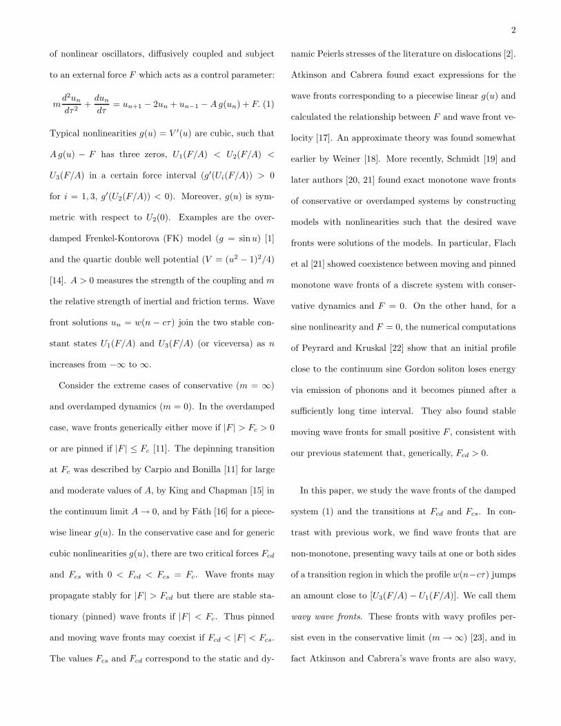
of nonlinear oscillators, diffusively coupled and subject

to an external force F which acts as a control parameter:

md2un

dτ2+

dun

dτ= un+1 − 2un + un−1 − Ag(un) + F. (1)

Typical nonlinearities g(u) = V ′(u) are cubic, such that

Ag(u) − F has three zeros, U1(F/A) < U2(F/A) <

U3(F/A) in a certain force interval (g′(Ui(F/A)) > 0

for i = 1, 3, g′(U2(F/A)) < 0). Moreover, g(u) is sym-

metric with respect to U2(0). Examples are the over-

damped Frenkel-Kontorova (FK) model (g = sin u) [1]

and the quartic double well potential (V = (u2 − 1)2/4)

[14]. A > 0 measures the strength of the coupling and m

the relative strength of inertial and friction terms. Wave

front solutions un = w(n − cτ) join the two stable con-

stant states U1(F/A) and U3(F/A) (or viceversa) as n

increases from −∞ to ∞.

Consider the extreme cases of conservative (m = ∞)

and overdamped dynamics (m = 0). In the overdamped

case, wave fronts generically either move if |F | > Fc > 0

or are pinned if |F | ≤ Fc [11]. The depinning transition

at Fc was described by Carpio and Bonilla [11] for large

and moderate values of A, by King and Chapman [15] in

the continuum limit A → 0, and by Fath [16] for a piece-

wise linear g(u). In the conservative case and for generic

cubic nonlinearities g(u), there are two critical forces Fcd

and Fcs with 0 < Fcd < Fcs = Fc. Wave fronts may

propagate stably for |F | > Fcd but there are stable sta-

tionary (pinned) wave fronts if |F | < Fc. Thus pinned

and moving wave fronts may coexist if Fcd < |F | < Fcs.

The values Fcs and Fcd correspond to the static and dy-

namic Peierls stresses of the literature on dislocations [2].

Atkinson and Cabrera found exact expressions for the

wave fronts corresponding to a piecewise linear g(u) and

calculated the relationship between F and wave front ve-

locity [17]. An approximate theory was found somewhat

earlier by Weiner [18]. More recently, Schmidt [19] and

later authors [20, 21] found exact monotone wave fronts

of conservative or overdamped systems by constructing

models with nonlinearities such that the desired wave

fronts were solutions of the models. In particular, Flach

et al [21] showed coexistence between moving and pinned

monotone wave fronts of a discrete system with conser-

vative dynamics and F = 0. On the other hand, for a

sine nonlinearity and F = 0, the numerical computations

of Peyrard and Kruskal [22] show that an initial profile

close to the continuum sine Gordon soliton loses energy

via emission of phonons and it becomes pinned after a

sufficiently long time interval. They also found stable

moving wave fronts for small positive F , consistent with

our previous statement that, generically, Fcd > 0.

In this paper, we study the wave fronts of the damped

system (1) and the transitions at Fcd and Fcs. In con-

trast with previous work, we find wave fronts that are

non-monotone, presenting wavy tails at one or both sides

of a transition region in which the profile w(n−cτ) jumps

an amount close to [U3(F/A) − U1(F/A)]. We call them

wavy wave fronts. These fronts with wavy profiles per-

sist even in the conservative limit (m → ∞) [23], and in

fact Atkinson and Cabrera’s wave fronts are also wavy,

3

as these authors would have found out had they depicted

their exact expression graphically. In the overdamped

limit m → 0, Fcd → Fc and the wave front profiles be-

come monotone. We have thus arrived to a general pic-

ture of wave fronts in discrete chains of coupled nonlinear

oscillators with m > 0.

The rest of the paper is organized as follows. Section

II considers Eq. (1) with a piecewise linear g(u). We

find exact formulas for the wave front profiles in the gen-

eral damped case following the method of Atkinson and

Cabrera’s [17]. These profiles are often wavy and they are

asymptotically stable in the damped case. It is important

to obtain them for two reasons: (i) there are very few ex-

act wave front solutions that are non-monotone, and (ii)

in the limit of large inertia, it is hard to discriminate

numerically between wavy wave fronts traveling with dif-

ferent velocities or having different profiles. Exact so-

lutions make good benchmarks for numerical methods.

The results for the damped model with a generic cubic

nonlinearity are presented in Section III. We calculate

the static and dynamic Peierls stresses for typical values

of A and m. A characterization of these stresses is given

in terms of our active point theory. Sec. IV contains a

discussion of our results.

II. EXPLICIT CONSTRUCTION OF WAVE

FRONT PROFILES

Let us rescale time in Eq. (1), so that t = τ/√

m, and

consider a piecewise linear g(u):

d2un

dt2+ α

dun

dt= un+1 − 2un + un−1 − Ag(un) + F, (2)

g(un) =

un + 1, for un < 0,

un − 1, for un ≥ 0,

(3)

where α = 1/√

m. Notice that g(u) = u + 1 − 2 H(u),

where H(x) = 1 for x > 0 and H(x) = 0 for x < 0 is the

Heaviside unit step function. Let us consider a smooth

wave front profile un = w(x) ≡ v(x) − 1, x = n − ct,

moving rigidly with velocity c. We center the wave front

so as to have w(0) = 0. Taking into account that g(u)

is an odd function and using the front profile un(t) =

w(n − ct), we can see that the following transformations

leave Eq. (2) for w(x) invariant:

(x, w, c, F ) → (−x, w,−c, F )

(x, w, c, F ) → (x,−w, c,−F )

(x, w, c, F ) → (−x,−w,−c,−F ). (4)

Let us consider now the case F > 0, c > 0 and w′(0) < 0,

i.e., a wave front profile that decreases in the transition

region about x = 0. The transformations (4) yield a

profile with: (i) c < 0, F > 0 increasing in the transition

region, (ii) c > 0, F < 0 increasing in the transition

region, and (iii) c < 0, F < 0 decreasing in the transition

region. Thus we find that sgnw = −sgn(xcF ), g(w) =

w + 1 − 2 H(−xsgn(cF )), and we can restrict ourselves

to considering the case F > 0, c > 0 and w′(0) < 0:

4

-20 0 20-1

-0.5

0

0.5

1

z

w(z

)

-20 0 20-1

-0.5

0

0.5

1

zw

(-z)

-20 0 20

-1

-0.5

0

0.5

1

z

-w(z

)

-20 0 20

-1

-0.5

0

0.5

1

z

-w(-

z)

c > 0 -c < 0

-c < 0 c > 0

F > 0 F > 0

- F < 0 - F < 0

(a) (b)

(c) (d)

x

x x

w(x

)

w(-

x)

-w(x

)

-w(-

x)x

FIG. 1: Symmetries in the wavefront solutions for A = 0.25,

α = 0, c = 0.5. and F = 0.009.

All other three possible cases can be obtained from our

results by using Eq. (4); see Figure 1.

The wave front profile v(x) = w(x) + 1 satisfies:

c2v′′(x) − αcv′(x) − [v(x + 1) − 2v(x) + v(x − 1)]

+Av(x) = 2AH(−sgn(cF )x) + F, (5)

with v(0) = 1. We can calculate v(x) by using the con-

tour integral expression for the step function:

H(−x) = − 1

2πi

∫

C

eik x

kdk. (6)

Here C runs over the real axis in the complex k plane

passing above the pole at k = 0 as in Fig. 2. For x > 0

(resp. x < 0), C is closed by a semicircle in the upper

(resp. lower) half plane oriented counterclockwise (resp.

clockwise).

Then the solution of Eq. (5) is

v(x) =F

A− A

πi

∫

C

exp[ik sgn(cF )x] dk

k L(k, α), (7)

Re(k)

Im(k)

k=0

FIG. 2: Contour for the Heaviside step function (6) and the

integral formula (7)-(8) when α 6= 0.

L(k, α) = A + 4 sin2

(

k

2

)

− k2c2 − ik|c|α sgn(F ). (8)

All the zeros of the function L(k, α) given by (7) are

complex for α > 0, and they correspond to exponentially

localized modes. The nonzero poles of the integrand in

Eq. (7) can be found graphically by plotting the curves

ReL(k, α) = 0 and ImL(k, α) = 0 in the complex k-plane,

as depicted in Fig 3. When α → 0, a finite number of

poles tend to the real axis, whereas infinitely many keep

a nonzero imaginary part even at α = 0. The poles on

the real axis correspond to radiation modes, cause os-

cillations in the wave front tails, and their number in-

creases as c decreases; see Figs. 4(a) and (b). The purely

imaginary poles of Figures 3 and 4(c) yield the central

monotone part of the wave front profiles. For α = 0, the

integration contour in Eq. (7) avoids poles on the real

axis according to a criterion due to Atkinson and Cabrera

[17], shown in Figure 5 and derived later on this Section.

5

10 20 30 40-4

-2 0 2 4

(a)

Re(k)

Im(k

)

10 20 30 40-4

-2 0 2 4

(b)

Re(k)

Im(k

)

10 20 30 40-4

-2 0 2 4

(c)

Re(k)

Im(k

)

Re(k)

FIG. 3: Complex poles as intersection of the curves

ReL(k, α) = 0 and ImL(k, α) = 0 when c = 0.2, A = 0.25

and: (a) α = 0, (b) α = 0.1, (c) α = 1.

We will use (7) and the method of residues to construct

profiles satisfying v(x) > 1 for x < 0 and v(x) < 1 for

x > 0. Notice that we can obtain a complex dispersion

relation between ω = kc and k from L(k, α) = 0. The

contour choice and the fact that α > 0 give rise to an ex-

ponential decay of v(x) to its asigned values at x = ±∞.

When α = 0, the wave fronts may exhibit undamped

oscillations extending all the way to infinity.

The condition v(0) = 1 yields a relationship between

the wave front velocity c and the external force F :

1 =F

A− A

πi

∫

C

dk

kL(k, α)

=F

A−

∑

L(p,α)=0,Im(p)>0

2A

p Lk(p, α), (9)

where we have assumed that cF > 0 and v′(1) < 0. The

resulting function F (c) can be calculated by computing

this series of residues numerically. Once F (c) is known,

Eq. (7) can be used to compute the wave front profiles for

0 1 2 3 4 5 6 7 80

10

20

Re(k)

(a) A+4 sin(Re(k)/2)2

c2 Re(k)2

0 50 100 150 200 2500

5

10

Re(k)

(b) A+4 sin(Re(k)/2)2

c2 Re(k)2

0 0.5 1 1.5

-2

-1

0

Im(k)

(c)A+2-2cosh(Im(k))-c 2 Im(k)2- α c Im(k)

Re(k)

Re(k)

Im(k)

FIG. 4: Real poles in the conservative case α = 0 with A =

0.25: (a) c = 0.5 (b) c = 0.01; Purely imaginary poles when

A = 0.25 (c) c = 0.5, α = 1

Re(k)

Im(k)

k=0

kL'(k)<0kL'(k)<0

kL'(k)>0 kL'(k)>0

FIG. 5: Contour for the integral formula (7)-(8) in the con-

servative case α = 0 for c > 0 and F > 0.

a pair (c, F (c)). We shall now show how this construction

works out for α = 0, α = ∞ and for α finite.

6

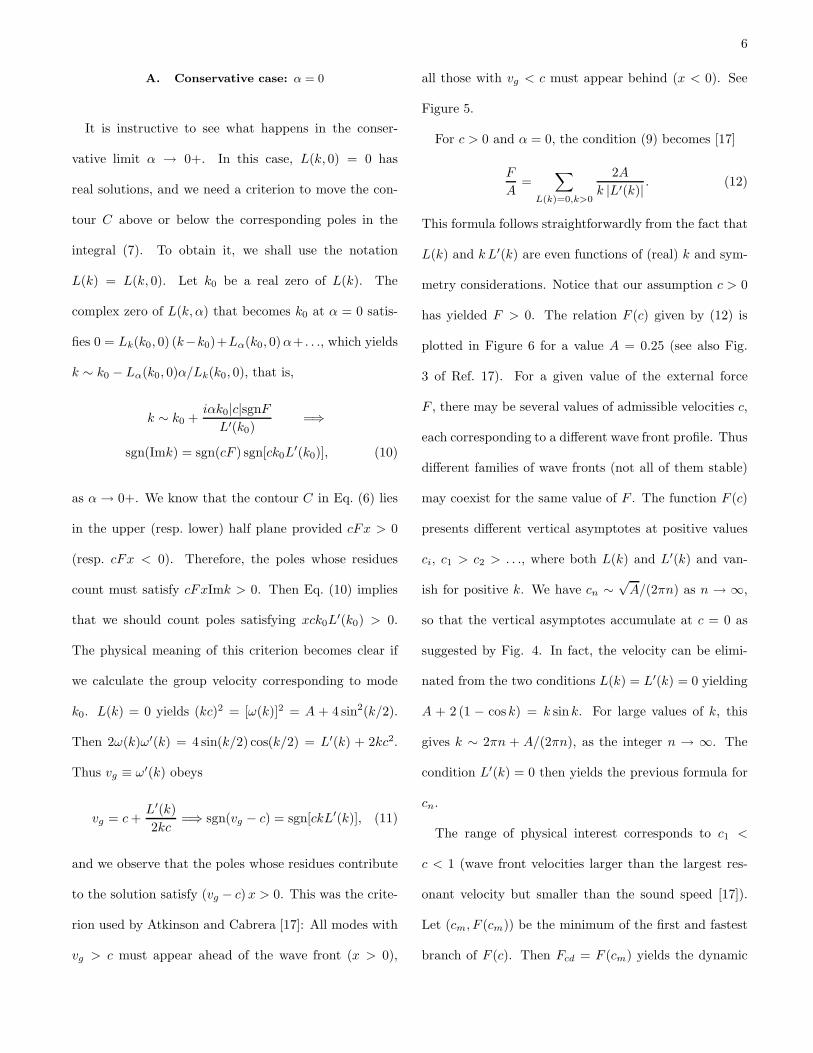
A. Conservative case: α = 0

It is instructive to see what happens in the conser-

vative limit α → 0+. In this case, L(k, 0) = 0 has

real solutions, and we need a criterion to move the con-

tour C above or below the corresponding poles in the

integral (7). To obtain it, we shall use the notation

L(k) = L(k, 0). Let k0 be a real zero of L(k). The

complex zero of L(k, α) that becomes k0 at α = 0 satis-

fies 0 = Lk(k0, 0) (k−k0)+Lα(k0, 0)α+ . . ., which yields

k ∼ k0 − Lα(k0, 0)α/Lk(k0, 0), that is,

k ∼ k0 +iαk0|c|sgnF

L′(k0)=⇒

sgn(Imk) = sgn(cF ) sgn[ck0L′(k0)], (10)

as α → 0+. We know that the contour C in Eq. (6) lies

in the upper (resp. lower) half plane provided cFx > 0

(resp. cFx < 0). Therefore, the poles whose residues

count must satisfy cFxImk > 0. Then Eq. (10) implies

that we should count poles satisfying xck0L′(k0) > 0.

The physical meaning of this criterion becomes clear if

we calculate the group velocity corresponding to mode

k0. L(k) = 0 yields (kc)2 = [ω(k)]2 = A + 4 sin2(k/2).

Then 2ω(k)ω′(k) = 4 sin(k/2) cos(k/2) = L′(k) + 2kc2.

Thus vg ≡ ω′(k) obeys

vg = c +L′(k)

2kc=⇒ sgn(vg − c) = sgn[ckL′(k)], (11)

and we observe that the poles whose residues contribute

to the solution satisfy (vg − c)x > 0. This was the crite-

rion used by Atkinson and Cabrera [17]: All modes with

vg > c must appear ahead of the wave front (x > 0),

all those with vg < c must appear behind (x < 0). See

Figure 5.

For c > 0 and α = 0, the condition (9) becomes [17]

F

A=

∑

L(k)=0,k>0

2A

k |L′(k)| . (12)

This formula follows straightforwardly from the fact that

L(k) and k L′(k) are even functions of (real) k and sym-

metry considerations. Notice that our assumption c > 0

has yielded F > 0. The relation F (c) given by (12) is

plotted in Figure 6 for a value A = 0.25 (see also Fig.

3 of Ref. 17). For a given value of the external force

F , there may be several values of admissible velocities c,

each corresponding to a different wave front profile. Thus

different families of wave fronts (not all of them stable)

may coexist for the same value of F . The function F (c)

presents different vertical asymptotes at positive values

ci, c1 > c2 > . . ., where both L(k) and L′(k) and van-

ish for positive k. We have cn ∼√

A/(2πn) as n → ∞,

so that the vertical asymptotes accumulate at c = 0 as

suggested by Fig. 4. In fact, the velocity can be elimi-

nated from the two conditions L(k) = L′(k) = 0 yielding

A + 2 (1 − cos k) = k sink. For large values of k, this

gives k ∼ 2πn + A/(2πn), as the integer n → ∞. The

condition L′(k) = 0 then yields the previous formula for

cn.

The range of physical interest corresponds to c1 <

c < 1 (wave front velocities larger than the largest res-

onant velocity but smaller than the sound speed [17]).

Let (cm, F (cm)) be the minimum of the first and fastest

branch of F (c). Then Fcd = F (cm) yields the dynamic

7

0 0.5 1 1.50

0.1

0.2

c

F(c

)

(a)

0 0.05 0.1 0.15 0.20

0.1

0.2

c

F(c

)

(b)

c=0.2c=0.23c=0.5

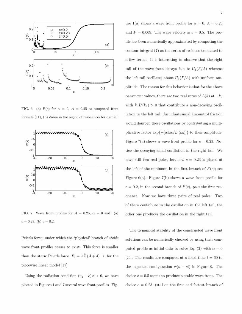
FIG. 6: (a) F (c) for α = 0, A = 0.25 as computed from

formula (11), (b) Zoom in the region of resonances for c small.

-30 -20 -10 0 10 20-1

-0.5

0

0.5

1

x

w(x

)

(a)

-30 -20 -10 0 10 20-1

-0.5

0

0.5

1

x

w(x

)

(b)

FIG. 7: Wave front profiles for A = 0.25, α = 0 and: (a)

c = 0.23, (b) c = 0.2.

Peierls force, under which the ‘physical’ branch of stable

wave front profiles ceases to exist. This force is smaller

than the static Peierls force, Fc = A3

2 (A + 4)−1

2 , for the

piecewise linear model [17].

Using the radiation condition (vg − c)x > 0, we have

plotted in Figures 1 and 7 several wave front profiles. Fig-

ure 1(a) shows a wave front profile for α = 0, A = 0.25

and F = 0.009. The wave velocity is c = 0.5. The pro-

file has been numerically approximated by computing the

contour integral (7) as the series of residues truncated to

a few terms. It is interesting to observe that the right

tail of the wave front decays fast to U1(F/A) whereas

the left tail oscillates about U3(F/A) with uniform am-

plitude. The reason for this behavior is that for the above

parameter values, there are two real zeros of L(k) at ±k0

with k0L′(k0) > 0 that contribute a non-decaying oscil-

lation to the left tail. An infinitesimal amount of friction

would dampen these oscillations by contributing a multi-

plicative factor exp{−[αk0c/L′(k0)]} to their amplitude.

Figure 7(a) shows a wave front profile for c = 0.23. No-

tice the decaying small oscillation in the right tail. We

have still two real poles, but now c = 0.23 is placed at

the left of the minimum in the first branch of F (c); see

Figure 6(a). Figure 7(b) shows a wave front profile for

c = 0.2, in the second branch of F (c), past the first res-

onance. Now we have three pairs of real poles. Two

of them contribute to the oscillation in the left tail, the

other one produces the oscillation in the right tail.

The dynamical stability of the constructed wave front

solutions can be numerically checked by using their com-

puted profile as initial data to solve Eq. (2) with α = 0

[24]. The results are compared at a fixed time t = 60 to

the expected configuration w(n − ct) in Figure 8. The

choice c = 0.5 seems to produce a stable wave front. The

choice c = 0.23, (still on the first and fastest branch of

8

-40 -20 0 20 40 60-1

0

1

(a) c=0.5, F=0.009, t=60

n

un(t

),w

(n-c

t)

-50 0 50-1

0

1

(b) c=0.23, F=0.01, t=60

n

un(t

),w

(n-c

t)

-40 -20 0 20 40 60 80-1

0

1

(c) c=0.2, F=0.029, t=60

n

un(t

),w

(n-c

t)

1

1

1

(b) c=0.23, F=0.01, t=60

(a) c=0.5, F=0.009, t=60

(c) c=0.2, F=0.029, t=60

n

n

n

FIG. 8: Dynamical stability when A = 0.25, α = 0. We

compare un(t) (solid line) to w(n − ct) (dot-dashed line) for

(a) c = 0.5, (b) c = 0.23, (c) c = 0.2.

F (c) but to the left of its minimum), evolves towards a

static front. The choice c = 0.2 (on the second branch of

F (c)), evolves towards a wave front moving faster than

expected, with a speed on the first branch of F (c). Thus

our numerical results seem to indicate that stable wave

fronts have velocities on the first and fastest branch of

F (c) with F ′(c) > 0, to the left of the minimum speed

on this branch, cm > 0. Then Fcd = F (cm), and stable

wave fronts with v′(1) < 0 have speeds larger or equal

than cm.

We have found wave front profiles with oscillatory tails

that seem stable under small disturbances. One question

that comes to mind is whether these profiles occur in

models with smooth nonlinearities. The answer is yes:

See an explicit construction in Appendix A.

-30 -20 -10 0 10 20 30

-0.5

0

0.5

1

x

w(x

)

(a)

0 0.5 1 1.5 2 2.5 30

0.1

0.2

c

F(c

)

(b)

FIG. 9: Overdamped limit when A = 0.25. (a) Wave front

profile for c = 0.02. (b) F (c) as computed from formula (9).

B. Overdamped limit: α = ∞

The results in the overdamped limit m = 0 are consis-

tent with previous work [11, 15, 16]: there are one wave

front profile and one c for each fixed F above a threshold,

Fc. Wave front profiles are monotone, and they resemble

staircases for c small. See Figure 9.

C. Finite damping: α > 0

The results for finite damping interpolate between the

conservative and overdamped cases. For small α, the

function F (c) and the wave front profiles are non mono-

tone although their oscillations decay as n → ±∞; see

Fig. 10. Fig. 11 shows a comparison between un(t) for

α = 0 (for the same values as in Fig. 8). We observe that,

for this small damping, the corresponding wave fronts

have the same stability properties as in the conservative

case: dynamically stable for c > cm, and unstable for

9

-100 -80 -60 -40 -20 0 20-1

-0.5

0

0.5

1

x

w(x

)(a)

0 0.5 1 1.5 20

0.1

0.2

c

F(c

)

(b)

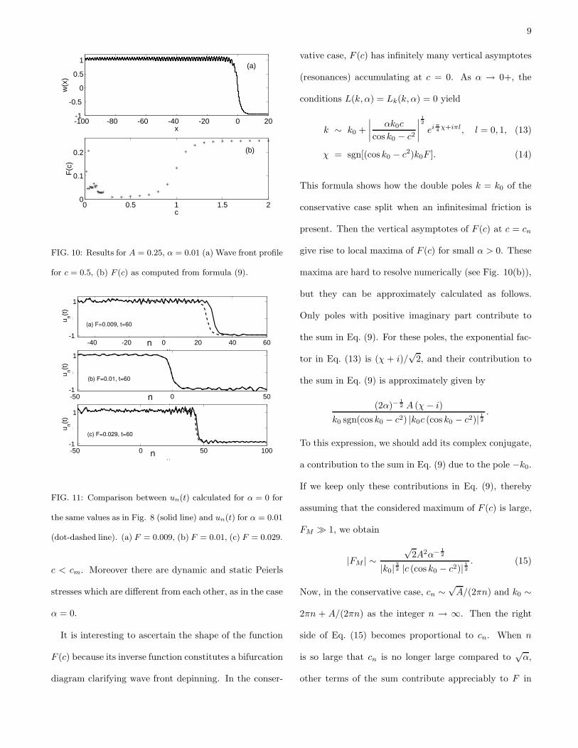
FIG. 10: Results for A = 0.25, α = 0.01 (a) Wave front profile

for c = 0.5, (b) F (c) as computed from formula (9).

-40 -20 0 20 40 60-1

0

1

(a) F=0.009, t=60

n

un(t

)

-50 0 50-1

0

1

(b) F=0.01, t=60

n

un(t

)

-50 0 50 100-1

0

1

(c) F=0.029, t=60

n

un(t

)

(a) F=0.009, t=60

(b) F=0.01, t=60

(c) F=0.029, t=60

n

n

n

FIG. 11: Comparison between un(t) calculated for α = 0 for

the same values as in Fig. 8 (solid line) and un(t) for α = 0.01

(dot-dashed line). (a) F = 0.009, (b) F = 0.01, (c) F = 0.029.

c < cm. Moreover there are dynamic and static Peierls

stresses which are different from each other, as in the case

α = 0.

It is interesting to ascertain the shape of the function

F (c) because its inverse function constitutes a bifurcation

diagram clarifying wave front depinning. In the conser-

vative case, F (c) has infinitely many vertical asymptotes

(resonances) accumulating at c = 0. As α → 0+, the

conditions L(k, α) = Lk(k, α) = 0 yield

k ∼ k0 +

∣

∣

∣

∣

αk0c

cos k0 − c2

∣

∣

∣

∣

1

2

ei π

4χ+iπl, l = 0, 1, (13)

χ = sgn[(cos k0 − c2)k0F ]. (14)

This formula shows how the double poles k = k0 of the

conservative case split when an infinitesimal friction is

present. Then the vertical asymptotes of F (c) at c = cn

give rise to local maxima of F (c) for small α > 0. These

maxima are hard to resolve numerically (see Fig. 10(b)),

but they can be approximately calculated as follows.

Only poles with positive imaginary part contribute to

the sum in Eq. (9). For these poles, the exponential fac-

tor in Eq. (13) is (χ + i)/√

2, and their contribution to

the sum in Eq. (9) is approximately given by

(2α)−1

2 A (χ − i)

k0 sgn(cos k0 − c2) |k0c (cos k0 − c2)| 12.

To this expression, we should add its complex conjugate,

a contribution to the sum in Eq. (9) due to the pole −k0.

If we keep only these contributions in Eq. (9), thereby

assuming that the considered maximum of F (c) is large,

FM ≫ 1, we obtain

|FM | ∼√

2A2α− 1

2

|k0|3

2 |c (cos k0 − c2)| 12. (15)

Now, in the conservative case, cn ∼√

A/(2πn) and k0 ∼

2πn + A/(2πn) as the integer n → ∞. Then the right

side of Eq. (15) becomes proportional to cn. When n

is so large that cn is no longer large compared to√

α,

other terms of the sum contribute appreciably to F in

10

the formula (9). We conjecture that these contributions

add to Fcs,

|FM | − Fcs ∼√

2

αA

5

4 cn, cn ∼√

A2πn

, (16)

so that the maxima of F (c) accumulate near c = 0 as the

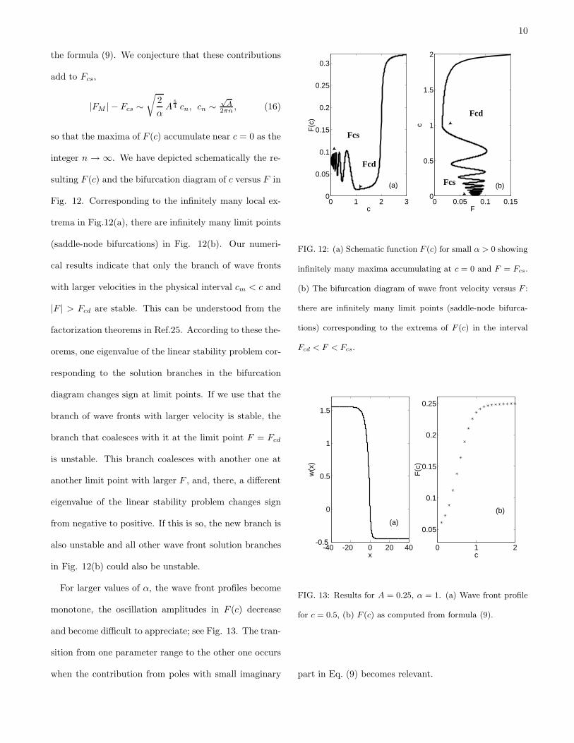
integer n → ∞. We have depicted schematically the re-

sulting F (c) and the bifurcation diagram of c versus F in

Fig. 12. Corresponding to the infinitely many local ex-

trema in Fig.12(a), there are infinitely many limit points

(saddle-node bifurcations) in Fig. 12(b). Our numeri-

cal results indicate that only the branch of wave fronts

with larger velocities in the physical interval cm < c and

|F | > Fcd are stable. This can be understood from the

factorization theorems in Ref.25. According to these the-

orems, one eigenvalue of the linear stability problem cor-

responding to the solution branches in the bifurcation

diagram changes sign at limit points. If we use that the

branch of wave fronts with larger velocity is stable, the

branch that coalesces with it at the limit point F = Fcd

is unstable. This branch coalesces with another one at

another limit point with larger F , and, there, a different

eigenvalue of the linear stability problem changes sign

from negative to positive. If this is so, the new branch is

also unstable and all other wave front solution branches

in Fig. 12(b) could also be unstable.

For larger values of α, the wave front profiles become

monotone, the oscillation amplitudes in F (c) decrease

and become difficult to appreciate; see Fig. 13. The tran-

sition from one parameter range to the other one occurs

when the contribution from poles with small imaginary

0 1 2 30

0.05

0.1

0.15

0.2

0.25

0.3

c

F(c

)

(a)

0 0.05 0.1 0.150

0.5

1

1.5

2

F

c

(b)

Fcs

Fcd

Fcd

Fcs

FIG. 12: (a) Schematic function F (c) for small α > 0 showing

infinitely many maxima accumulating at c = 0 and F = Fcs.

(b) The bifurcation diagram of wave front velocity versus F :

there are infinitely many limit points (saddle-node bifurca-

tions) corresponding to the extrema of F (c) in the interval

Fcd < F < Fcs.

-40 -20 0 20 40-0.5

0

0.5

1

1.5

x

w(x

)

(a)

0 1 2

0.05

0.1

0.15

0.2

0.25

c

F(c

)

(b)

FIG. 13: Results for A = 0.25, α = 1. (a) Wave front profile

for c = 0.5, (b) F (c) as computed from formula (9).

part in Eq. (9) becomes relevant.

11

0 1 2 34.8

5

5.2

5.4

5.6

5.8

6

6.2

6.4

α

Fcd

(α)

(a)

5 5.5 60

0.1

0.2

0.3

0.4

0.5

0.6

F

|c(F

)|

(b)

5.6

F (

α)cd |c(F

)|

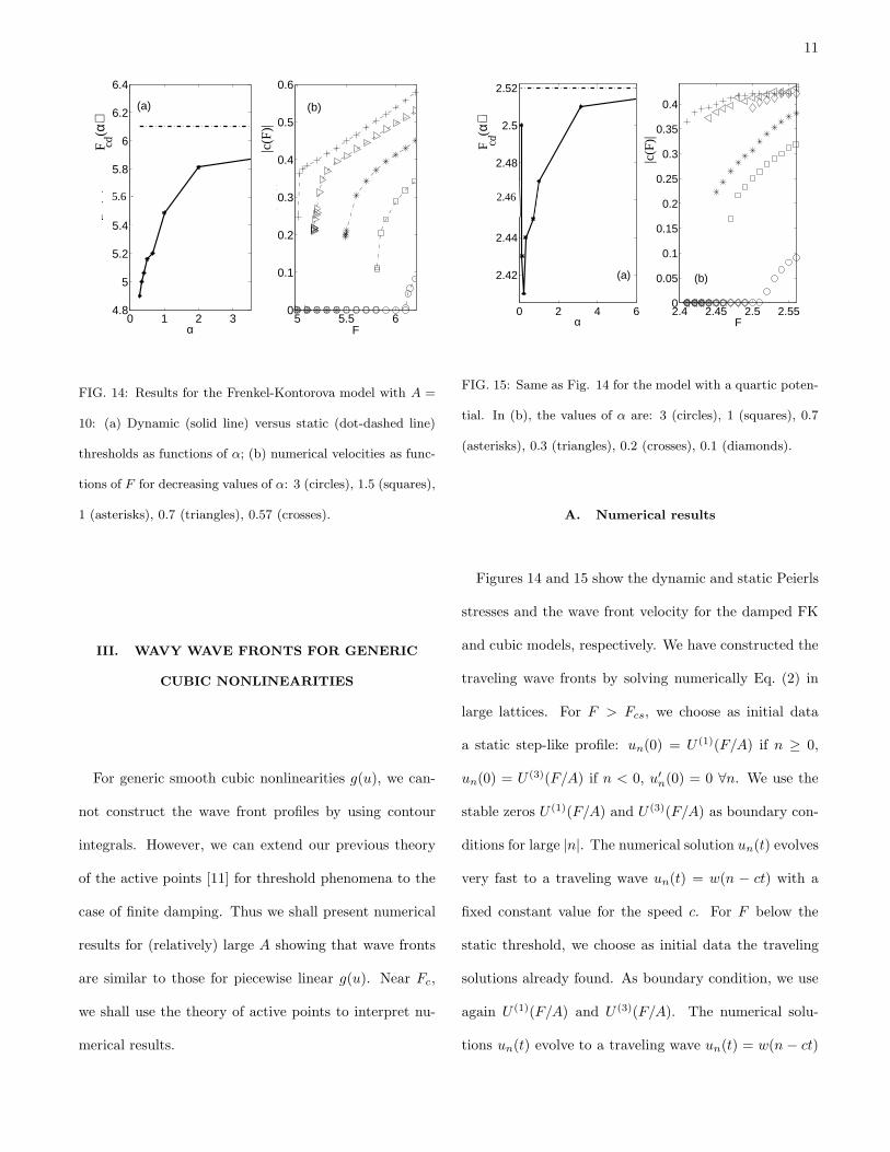
FIG. 14: Results for the Frenkel-Kontorova model with A =

10: (a) Dynamic (solid line) versus static (dot-dashed line)

thresholds as functions of α; (b) numerical velocities as func-

tions of F for decreasing values of α: 3 (circles), 1.5 (squares),

1 (asterisks), 0.7 (triangles), 0.57 (crosses).

III. WAVY WAVE FRONTS FOR GENERIC

CUBIC NONLINEARITIES

For generic smooth cubic nonlinearities g(u), we can-

not construct the wave front profiles by using contour

integrals. However, we can extend our previous theory

of the active points [11] for threshold phenomena to the

case of finite damping. Thus we shall present numerical

results for (relatively) large A showing that wave fronts

are similar to those for piecewise linear g(u). Near Fc,

we shall use the theory of active points to interpret nu-

merical results.

0 2 4 6

2.42

2.44

2.46

2.48

2.5

2.52

α

Fcd

(α)

(a)

2.4 2.45 2.5 2.550

0.05

0.1

0.15

0.2

0.25

0.3

0.35

0.4

F

|c(F

)|

(b)

2.46

F (

α)cd

|c(F

)|

FIG. 15: Same as Fig. 14 for the model with a quartic poten-

tial. In (b), the values of α are: 3 (circles), 1 (squares), 0.7

(asterisks), 0.3 (triangles), 0.2 (crosses), 0.1 (diamonds).

A. Numerical results

Figures 14 and 15 show the dynamic and static Peierls

stresses and the wave front velocity for the damped FK

and cubic models, respectively. We have constructed the

traveling wave fronts by solving numerically Eq. (2) in

large lattices. For F > Fcs, we choose as initial data

a static step-like profile: un(0) = U (1)(F/A) if n ≥ 0,

un(0) = U (3)(F/A) if n < 0, u′n(0) = 0 ∀n. We use the

stable zeros U (1)(F/A) and U (3)(F/A) as boundary con-

ditions for large |n|. The numerical solution un(t) evolves

very fast to a traveling wave un(t) = w(n − ct) with a

fixed constant value for the speed c. For F below the

static threshold, we choose as initial data the traveling

solutions already found. As boundary condition, we use

again U (1)(F/A) and U (3)(F/A). The numerical solu-

tions un(t) evolve to a traveling wave un(t) = w(n − ct)

12

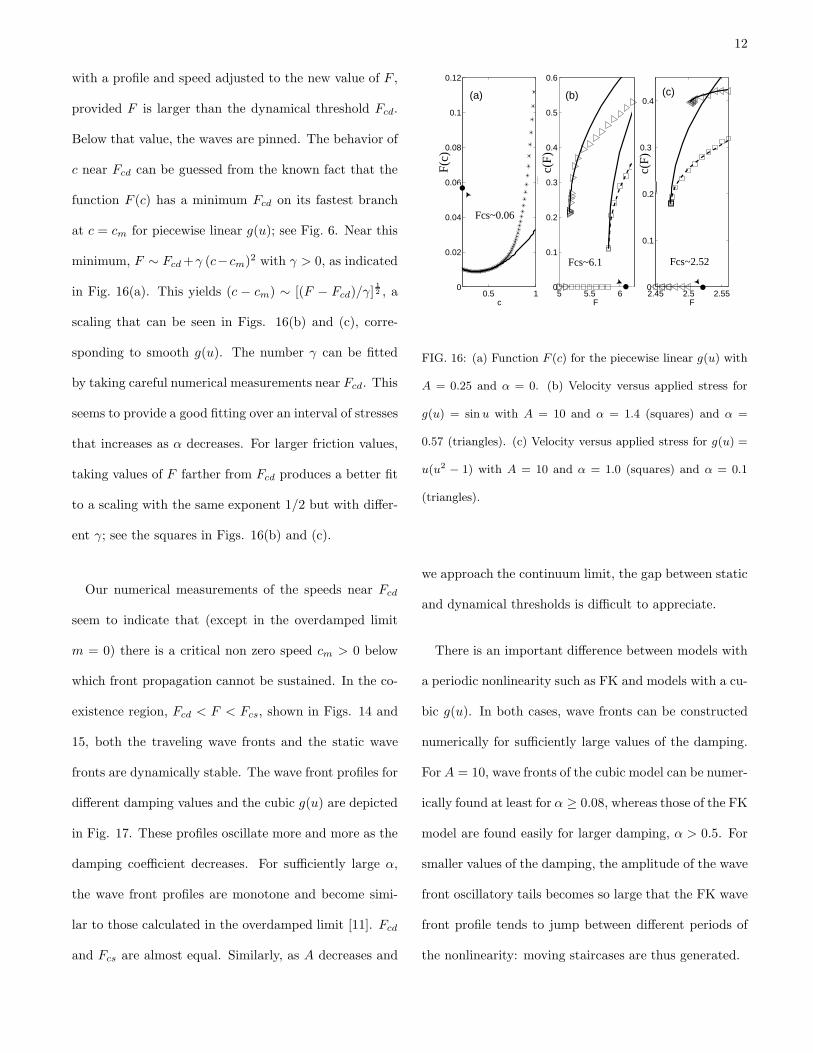
with a profile and speed adjusted to the new value of F ,

provided F is larger than the dynamical threshold Fcd.

Below that value, the waves are pinned. The behavior of

c near Fcd can be guessed from the known fact that the

function F (c) has a minimum Fcd on its fastest branch

at c = cm for piecewise linear g(u); see Fig. 6. Near this

minimum, F ∼ Fcd +γ (c−cm)2 with γ > 0, as indicated

in Fig. 16(a). This yields (c − cm) ∼ [(F − Fcd)/γ]1

2 , a

scaling that can be seen in Figs. 16(b) and (c), corre-

sponding to smooth g(u). The number γ can be fitted

by taking careful numerical measurements near Fcd. This

seems to provide a good fitting over an interval of stresses

that increases as α decreases. For larger friction values,

taking values of F farther from Fcd produces a better fit

to a scaling with the same exponent 1/2 but with differ-

ent γ; see the squares in Figs. 16(b) and (c).

Our numerical measurements of the speeds near Fcd

seem to indicate that (except in the overdamped limit

m = 0) there is a critical non zero speed cm > 0 below

which front propagation cannot be sustained. In the co-

existence region, Fcd < F < Fcs, shown in Figs. 14 and

15, both the traveling wave fronts and the static wave

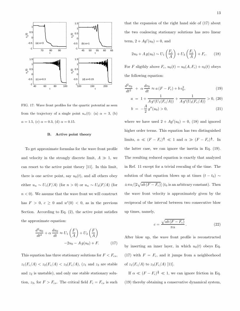
fronts are dynamically stable. The wave front profiles for

different damping values and the cubic g(u) are depicted

in Fig. 17. These profiles oscillate more and more as the

damping coefficient decreases. For sufficiently large α,

the wave front profiles are monotone and become simi-

lar to those calculated in the overdamped limit [11]. Fcd

and Fcs are almost equal. Similarly, as A decreases and

2.45 2.5 2.550

0.1

0.2

0.3

0.4(c)

F

c(F

)

5 5.5 60

0.1

0.2

0.3

0.4

0.5

0.6

F

c(F

)

(b)

0.5 10

0.02

0.04

0.06

0.08

0.1

0.12

c

F(c

)

(a)

c(F

)

c(F

)

F(c

)

Fcs~6.1 Fcs~2.52

Fcs~0.06

FIG. 16: (a) Function F (c) for the piecewise linear g(u) with

A = 0.25 and α = 0. (b) Velocity versus applied stress for

g(u) = sin u with A = 10 and α = 1.4 (squares) and α =

0.57 (triangles). (c) Velocity versus applied stress for g(u) =

u(u2 − 1) with A = 10 and α = 1.0 (squares) and α = 0.1

(triangles).

we approach the continuum limit, the gap between static

and dynamical thresholds is difficult to appreciate.

There is an important difference between models with

a periodic nonlinearity such as FK and models with a cu-

bic g(u). In both cases, wave fronts can be constructed

numerically for sufficiently large values of the damping.

For A = 10, wave fronts of the cubic model can be numer-

ically found at least for α ≥ 0.08, whereas those of the FK

model are found easily for larger damping, α > 0.5. For

smaller values of the damping, the amplitude of the wave

front oscillatory tails becomes so large that the FK wave

front profile tends to jump between different periods of

the nonlinearity: moving staircases are thus generated.

13

70 80 90-1

-0.5

0

0.5

1

t

u n(t)

(a) α=3

45 50 55 60 65-1

-0.5

0

0.5

1

1.5

t

u n(t)

(b) α=1

40 60 80 100-1

-0.5

0

0.5

1

1.5

t

(c) α=0.3

u n(t)

100 150 200-1

-0.5

0

0.5

1

1.5

t

(d) α=0.15

u n(t)

FIG. 17: Wave front profiles for the quartic potential as seen

from the trajectory of a single point un(t): (a) α = 3, (b)

α = 1.5, (c) α = 0.3, (d) α = 0.15.

B. Active point theory

To get approximate formulas for the wave front profile

and velocity in the strongly discrete limit, A ≫ 1, we

can resort to the active point theory [11]. In this limit,

there is one active point, say u0(t), and all others obey

either un ∼ U1(F/A) (for n > 0) or un ∼ U3(F/A) (for

n < 0). We assume that the wave front we will construct

has F > 0, c ≥ 0 and w′(0) < 0, as in the previous

Section. According to Eq. (2), the active point satisfies

the approximate equation:

d2u0

dt2+ α

du0

dt≈ U1

(

F

A

)

+ U3

(

F

A

)

−2u0 − Ag(u0) + F. (17)

This equation has three stationary solutions for F < Fcs,

z1(Fc/A) < z2(Fc/A) < z3(Fc/A), (z1 and z3 are stable

and z2 is unstable), and only one stable stationary solu-

tion, z3, for F > Fcs. The critical field Fc = Fcs is such

that the expansion of the right hand side of (17) about

the two coalescing stationary solutions has zero linear

term, 2 + Ag′(u0) = 0, and

2u0 + Ag(u0) ∼ U1

(

Fc

A

)

+ U3

(

Fc

A

)

+ Fc. (18)

For F sligthly above Fc, u0(t) = u0(A, Fc) + v0(t) obeys

the following equation:

d2v0

dt2+ α

dv0

dt≈ a (F − Fc) + b v2

0 , (19)

a = 1 +1

Ag′(U1(Fc/A))+

1

Ag′(U3(Fc/A))> 0, (20)

b = −A

2g′′(u0) > 0, (21)

where we have used 2 + Ag′(u0) = 0, (18) and ignored

higher order terms. This equation has two distinguished

limits, α ≪ (F − Fc)1

4 ≪ 1 and α ≫ (F − Fc)1

4 . In

the latter case, we can ignore the inertia in Eq. (19).

The resulting reduced equation is exactly that analyzed

in Ref. 11 except for a trivial rescaling of the time. The

solution of that equation blows up at times (t − t0) ∼

±πα/[2√

ab (F − Fc)] (t0 is an arbitrary constant). Then

the wave front velocity is approximately given by the

reciprocal of the interval between two consecutive blow

up times, namely,

c =

√

ab (F − Fc)

πα. (22)

After blow up, the wave front profile is reconstructed

by inserting an inner layer, in which u0(t) obeys Eq.

(17) with F = Fc, and it jumps from a neighborhood

of z1(Fc/A) to z3(Fc/A) [11].

If α ≪ (F − Fc)1

4 ≪ 1, we can ignore friction in Eq.

(19) thereby obtaining a conservative dynamical system,

14

Eq. (19) with α = 0, as our reduced equation. Its tra-

jectories also blow up and the wave front velocity can be

straightforwardly calculated as

c =

(

ab (F−Fc)3

)1

4

2√

2K(

1√2

) =

√2π

(

ab (F−Fc)3

)1

4

[

Γ(

14

)]2 , (23)

where K(1/√

2) = 1.854075 is the complete elliptic inte-

gral of the first kind with module k = 1/√

2 [26]. Con-

trary to the overdamped case, a consistent inner layer

connecting blowing up trajectories of the reduced equa-

tion and trajectories of Eq. (17) for F = Fc and α = 0

does not exist. This points out to a breakdown of the

active point theory as α → 0+, which is consistent with

our conjectured bifurcation diagram in Fig. 12(b) for the

piecewise linear model. Assuming that Fig. 12(b) is also

the bifurcation diagram of models with smooth nonlin-

earities, a succession of infinitely many saddle-node bifur-

cations (that accumulate at c = 0, F = Fcs) connect the

branch of stable wave fronts and that of stationary front

solutions between Fcd and Fcs. If this is the case, seeking

a description in terms of standard normal forms as (19)

and scaling is rather hopeless. Not surprisingly, the sus-

picious scaling (23) is hard to check numerically (the sta-

ble branch of moving wave fronts ends at F = Fcd < Fc),

whereas the scaling (22) can be easily checked (Fcd ≈ Fc

in the overdamped limit) [11].

Let us now come back to Eq. (17) to explain the

coexistence of moving and stationary wave fronts for

Fcd < F < Fc. In Fig. 18, we have depicted the

phase plane associated to Eq. (17) for the cubic non-

-1 -0.5 0 0.5 1 1.5-2

-1.5

-1

-0.5

0

0.5

1

1.5

2

u0

du0

FIG. 18: Phase plane of Eq. (17) with the cubic nonlinearity

for A = 10, α = 0.5 and F = 2.45.

0 1 2 32

2.2

2.4

α

Fcd

(a)

Fcd

(α)F

cda(α)

0 1 2 30

0.05

0.1

0.15

0.2

α

Rel

ativ

e er

ror

(b)

1 2 3

5

5.5

6

α

Fcd

(c)F

cd(α)

Fcda

(α)

1 2 30.02

0.03

0.04

0.05

α

Rel

ativ

e er

ror

(d)

FIG. 19: Comparison of Fcda ≡ Fc2 and Fcd as functions of

the damping α for A = 10 and: (a) the cubic nonlinearity, (b)

its relative error, (c) the FK nonlinearity, and (d) its relative

error.

linearity g(u) = u (u2 − 1). The profiles in Fig. 17

correspond to one active point jumping from a neigh-

borhood of U1(F/A) to a neighborhood of U3(F/A).

The right side of Eq. (17) has three zeros in the inter-

val [U1(F/A), U3(F/A)] for F < Fc1, corresponding to

15

two stable spiral points or centers (zi(F/A), 0), i = 1, 3,

and one saddle point (z2(F/A), 0). At F = Fc1two

of the zeros coalesce and for F > Fc1only the spi-

ral point (z3(F/A), 0) remains. For α > 0, there is

a new critical value of F , Fc2, such that the initial

datum (U1(F/A), 0), which is close to the spiral point

(z1(F/A), 0), may evolve to the other stable spiral point,

(z3(F/A), 0), for F ∈ (Fc2, Fc1

); see Fig. 18. The tra-

jectory leaving a neighborhood of (z1(F/A), 0) and en-

tering (z3(F/A), 0) defines the wave front profile. For

F < Fc2, the initial datum (U1(F/A), 0) evolves toward

(z1(F/A), 0) and no wave front is generated. Thus Fc2

yields an approximation to the dynamical Peierls stress,

Fcd. Fig. 19 compares Fc2 to Fcd, which has been cal-

culated numerically by solving the complete system (2).

Notice that our approximation worsens as α decreases to-

wards zero indicating break down of the one active point

approximation. We shall explain below why this is so.

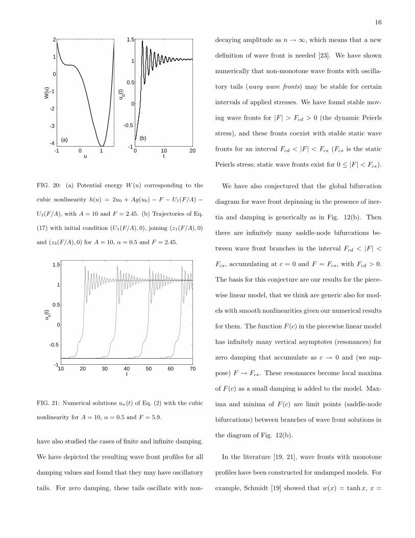
The dynamic critical Peierls stress can be intuitively

explained as follows. The potential energy associated to

the nonlinearity h(u) = 2u0 + Ag(u0) − F − U1(F/A) −

U3(F/A) on the right side of Eq. (17) is depicted in Fig.

20(a). An initial condition (U1(F/A), 0) is close to the

left minimum of W (u0). If the energy corresponding to

the initial condition is slightly higher than that of the

left minimum, the solution of (17) evolves toward it be-

cause of friction. On the other hand, larger energies can-

not be dissipated by the friction term and the trajectory

surpasses the maximum of W (u0) with nonzero veloc-

ity. Then the trajectory falls in the basin of the right

minimum of the potential, performing a damped oscil-

lation about it before reaching z3(F/A), 0). Once u0(t)

has reached a neighborhood of the second spiral point,

u−1(t) takes its place and performes a similar motion.

The resulting trajectory is depicted in Fig. 20(b). The

solution of the complete system (2) is shown in Fig. 21.

The wave front velocity is approximately given by the

reciprocal of the time u0(t) takes to jump from z1(F/A)

to z3(F/A). Notice that the oscillations about z3(F/A)

persist a longer time as α decreases and may have fi-

nite amplitude. Then we cannot approximate sufficiently

well u1(t) by the constant value U3(F/A) for small val-

ues of the friction and the one active point approximation

breaks down. This explains the discrepancies in Fig. 19

for small α. Since the difference [U3(F/A) − U1(F/A)]

is larger for the FK than for the cubic nonlinearity, the

approximation u1(t) ≈ U3(F/A) is better for the FK non-

linearity as shown in Fig. 19.

IV. DISCUSSION

We have studied wave front solutions in chains of non-

linear oscillators with inertia and damping. Two ana-

lytical methods have been used to construct the wave

fronts and their velocities. For piecewise linear mod-

els, exact formulas can be found for the wave fronts and

the relation between their velocity and the applied stress

F as Atkinson and Cabrera did already in 1965 for the

conservative case [17]. Different from these authors, we

16

-1 0 1-4

-3

-2

-1

0

1

2

u

W(u

)

(a)

0 10 20-1

-0.5

0

0.5

1

1.5

t

u 0(t)

(b)

FIG. 20: (a) Potential energy W (u) corresponding to the

cubic nonlinearity h(u) = 2u0 + Ag(u0) − F − U1(F/A) −

U3(F/A), with A = 10 and F = 2.45. (b) Trajectories of Eq.

(17) with initial condition (U1(F/A), 0), joining (z1(F/A), 0)

and (z3(F/A), 0) for A = 10, α = 0.5 and F = 2.45.

10 20 30 40 50 60 70-1

-0.5

0

0.5

1

1.5

t

u n(t)

FIG. 21: Numerical solutions un(t) of Eq. (2) with the cubic

nonlinearity for A = 10, α = 0.5 and F = 5.9.

have also studied the cases of finite and infinite damping.

We have depicted the resulting wave front profiles for all

damping values and found that they may have oscillatory

tails. For zero damping, these tails oscillate with non-

decaying amplitude as n → ∞, which means that a new

definition of wave front is needed [23]. We have shown

numerically that non-monotone wave fronts with oscilla-

tory tails (wavy wave fronts) may be stable for certain

intervals of applied stresses. We have found stable mov-

ing wave fronts for |F | > Fcd > 0 (the dynamic Peierls

stress), and these fronts coexist with stable static wave

fronts for an interval Fcd < |F | < Fcs (Fcs is the static

Peierls stress; static wave fronts exist for 0 ≤ |F | < Fcs).

We have also conjectured that the global bifurcation

diagram for wave front depinning in the presence of iner-

tia and damping is generically as in Fig. 12(b). Then

there are infinitely many saddle-node bifurcations be-

tween wave front branches in the interval Fcd < |F | <

Fcs, accumulating at c = 0 and F = Fcs, with Fcd > 0.

The basis for this conjecture are our results for the piece-

wise linear model, that we think are generic also for mod-

els with smooth nonlinearities given our numerical results

for them. The function F (c) in the piecewise linear model

has infinitely many vertical asymptotes (resonances) for

zero damping that accumulate as c → 0 and (we sup-

pose) F → Fcs. These resonances become local maxima

of F (c) as a small damping is added to the model. Max-

ima and minima of F (c) are limit points (saddle-node

bifurcations) between branches of wave front solutions in

the diagram of Fig. 12(b).

In the literature [19, 21], wave fronts with monotone

profiles have been constructed for undamped models. For

example, Schmidt [19] showed that w(x) = tanhx, x =

17

n + t/2, is a wave front solution for Eq. (2) with α =

F = 0, A = 1 and a potential V (u) = −3u2/4 − u4/8 −

(sinh 1)−2 ln(1−u2 tanh2 1), with g(u) = V ′(u). For this

model, Fcs > 0 [21]. Solving numerically this model for

F 6= 0, wave fronts with one oscillatory tail on x > 0

are found for F > 0, similar to those in Fig. 1(b). For

F < 0, wave fronts with one oscillatory tail on x < 0 are

found instead; see Fig. 1(c). Both types of fronts have

|c| > 1/2. This shows that wavy wave fronts are generic

and that Schmidt’s monotone wave front is a non-generic

limiting case separating branches of wavy wave fronts and

corresponding to Fcd = 0. A possible bifurcation diagram

|c| vs. F for this example could be that in Fig. 12(b) with

Fcs > 0, Fcd = 0 and |cm| = 1/2: numerical solution

of the model seems to be consistent with a bifurcation

diagram having a limit point at F = 0, |c| = 1/2, and

with reflection symmetry with respect to the |c| axis (|c|

in the diagram is even in F ).

Acknowledgments

This work has been supported by the Spanish MCyT

through grants BFM2002-04127-C02, by the Third Re-

gional Research Program of the Autonomous Region of

Madrid (Strategic Groups Action), and by the European

Union under grant HPRN-CT-2002-00282.

APPENDIX A: NONLINEAR MODEL HAVING A

EXPLICIT WAVY WAVE FRONT PROFILE

It is fairly easy to find smooth g(u) having wave front

solutions with undamped oscillatory tails provided their

dynamics is conservative. Let us choose a profile of the

form:

w(x) =

−1 + k1eax x ≤ 0

1 + k2 cos(bx + c) x ≥ 0

This profile is continuous if −1 + k1 = 1 + k2 cos c,

differentiable if k1a = −k2b sin d and twice differen-

tiable if k1a2 = −k2b

2 cos c. We set c = tan−1(b/a),

k1 = 2/(1 + a2/b2) and k2 = −k1a/(b sin c). The only

restriction on a and b is b + tan−1(b/a) < π/2, a, b > 0

to ensure that cos(bx+ c) is monotone in 0 < x < 1. The

profile w(x) satisfies:

wxx =

a2(w + 1) for w < k1 − 1,

−b2(w + 1) for w > k1 − 1,

w(x + 1) − 2w(x) + w(x − 1) = f(w(x)),

with:

f(w) =

2(w + 1)(cosha − 1) w < w1

(w + 1)e−a + Y − 2w (w1, w2)

k2 cos(W + b) + k1ea

b(W−b−c) − 2w (w2, w3)

2(w − 1)(cos b − 1) w > w3

Here, W = k−12 cos−1(w − 1), Y = k2 cos{ba−1 ln[(w +

1)/k1] + b + c}, w1 = e−ak1 − 1, w2 = k1 − 1, and w3 =

k2 cos(b+ c)−1. The continuous function f(w) is convex

but, for a certain interval of values of c2, the function

gc(u) = c2uxx − f(u) has three zeroes and is strongly

18

asymmetric. For these values of c, the system d2un/dt2 =

un+1−2un +un−1−gc(un) has a traveling wave solution

un(t) = w(n − ct).

[*] E-address ana−carpio@mat.ucm.es.

[**] E-address bonilla@ing.uc3m.es.

[1] J. Frenkel and T. Kontorova, J. Phys. USSR, 13, 1

(1938). O.M. Braun and Yu.S. Kivshar, Phys. Rep. 306,

1 (1998).

[2] F.R.N. Nabarro, Theory of Crystal Dislocations (Oxford

University Press, Oxford, UK, 1967).

[3] L.I. Slepyan, Sov. Phys. Dokl. 26, 538 (1981).

[4] P. M. Chaikin and T. C. Lubensky, Principles of con-

densed matter physics (Cambridge University Press,

Cambridge, 1995). Chapter 10.

[5] A. Carpio, L.L. Bonilla and G. Dell’Acqua, Phys. Rev.

E, 64, 036204 (2001).

[6] L.L. Bonilla, J. Phys. Condensed Matter 14, R341

(2002).

[7] A.R.A. Anderson and B.D. Sleeman, Int. J. Bif. Chaos,

5, 63 (1995). A. Carpio and L.L. Bonilla, SIAM J. Appl.

Math. 63, 619 (2002).

[8] J.P. Keener and J. Sneyd, Mathematical Physiology

(Springer, New York, 1998). Chapter 9.

[9] D.R. Nelson, Defects and Geometry in Condensed Matter

Physics (Cambridge U.P., Cambridge, UK, 2002).

[10] C. Rebbi and J. Soliani (eds.), Solitons and Particles,

(World Sci., Singapore, 1984).

[11] A. Carpio and L.L. Bonilla, Phys. Rev. Lett. 86, 6034

(2001) and SIAM J. Appl. Math. 63, 1056 (2003).

[12] R. Hobart, J. Appl. Phys. 36, 1948 (1965).

[13] V.L. Indenbom, Soviet Phys. - Crystallogr. 3, 193 (1959)

[Kristallografiya 3, 197 (1958)].

[14] J. W. Cahn, Acta Metallurgica 8, 554 (1960).

[15] J.R. King and S.J. Chapman, Eur. J. Appl. Math. 12,

433 (2001).

[16] G. Fath, Physica D, 116, 176 (1998).

[17] W. Atkinson and N. Cabrera, Phys. Rev. 138, A763

(1965).

[18] J. H. Weiner, Phys. Rev. 136, A863 (1964).

[19] V.H. Schmidt, Phys. Rev. B 20, 4397 (1979).

[20] P.C. Bressloff and G. Rowlands, Physica D 106, 255

(1997).

[21] S. Flach, Y. Zolotaryuk and K. Kladko, Phys. Rev. E 59,

6105 (1999).

[22] M. Peyrard and M.D. Kruskal, Physica D 14, 88 (1984).

[23] In the conservative limit m → ∞, the oscillations at one

of both tails of the wave front do not decay as n → ±∞.

This means that a slightly more general definition of

wave front solution is needed in the conservative case:

un(τ ) = w(n − cτ ) joins the neighborhoods of U1(F/A)

and U3(F/A) (or viceversa) as n increases from −∞ to

∞. An infinitesimal amount of damping causes the oscil-

latory tails of the wave front to decay to either U1(F/A)

or U3(F/A) as n → ±∞.

[24] We would like to point out that the numerical solution

of Eq. (2) should be calculated by using a scheme of

sufficiently high order and small tolerance for the cases

α = 0 or α > 0 small (typically a standard Rung-Kutta-

Fehlberg scheme of orders 4/5 with tolerance 10−5 would

19

do). Schemes with lower order or larger tolerances have

been found to produce spurious traveling waves. For the

purpose of checking the appropriatedness of a given nu-

merical scheme, the exact solutions we have discussed are

invaluable.

[25] G. Iooss and D.D. Joseph, Elementary stability and bi-

furcation theory (Springer, New York, 1980).

[26] I.S. Gradshteyn and I.M. Ryzhik, Table of integrals, se-

ries, and products (Academic Press, New York, 1980).

Chapter 8.