Oscillatory instabilities of intracellular fiber networks - eDiss
115
Oscillatory instabilities of intracellular fiber networks Dissertation for the award of the degree “Doctor rerum naturalium” of the Georg-August-Universität Göttingen within the doctoral program IMPRS Physics of Biological and Complex Systems of the Georg-August University School of Science (GAUSS) submitted by Hsin-Fang Hsu from Taiwan Göttingen, 2015
-
Upload
khangminh22 -
Category
Documents
-
view
1 -
download
0
Transcript of Oscillatory instabilities of intracellular fiber networks - eDiss

Oscillatory instabilitiesof intracellular fiber networks
Dissertationfor the award of the degree“Doctor rerum naturalium”
of the Georg-August-Universität Göttingen
within the doctoral programIMPRS Physics of Biological and Complex Systems
of the Georg-August University School of Science (GAUSS)
submitted byHsin-Fang Hsufrom Taiwan
Göttingen, 2015

Thesis Committee:Prof. Dr. Eberhard BodenschatzDepartment of Fluid Dynamics, Pattern Formation and BiocomplexityMax Planck Institute for Dynamics and Self-OrganizationInstitute for Nonlinear DynamicsGeorg-August-Universität GöttingenProf. Dr. Jörg EnderleinIII. Physical Institute Biophysics / Complex SystemsGeorg-August-Universität GöttingenProf. Dr. Andreas JanshoffInstitute for Physical ChemistryGeorg-August-Universität Göttingen
Members of Examination Board:Prof. Dr. Thomas BurgBiological Micro- and NanotechnologyMax Planck Institute for Biophysical ChemistryDr. Marco TarantolaDepartment of Fluid Dynamics, Pattern Formation and BiocomplexityMax Planck Institute for Dynamics and Self-OrganizationProf. Dr. Jörg GroßhansDepartment Developmental BiochemistryInstitute of Biochemistry and Molecular Cell BiologyUniversity Medical Center Göttingen
Date of oral examination: 2015/05/19


Contents
1 Introduction 91.1 Dictyostelium discoideum . . . . . . . . . . . . . . . . . . . . . . . . . 9
1.2 Actin cytoskeleton . . . . . . . . . . . . . . . . . . . . . . . . . . . . 14
1.3 Myosin II . . . . . . . . . . . . . . . . . . . . . . . . . . . . . . . . . 20
1.4 Self-organization and oscillations . . . . . . . . . . . . . . . . . . . . 26
1.5 Aim and outline . . . . . . . . . . . . . . . . . . . . . . . . . . . . . . 27
2 Material and methods 282.1 Cell culture and development . . . . . . . . . . . . . . . . . . . . . . 28
2.2 Microfluidics . . . . . . . . . . . . . . . . . . . . . . . . . . . . . . . 30
2.3 Experimental design . . . . . . . . . . . . . . . . . . . . . . . . . . . 34
2.4 Image processing and data analysis . . . . . . . . . . . . . . . . . . . 35
3 Self-sustained oscillations 433.1 Motivation . . . . . . . . . . . . . . . . . . . . . . . . . . . . . . . . . 43
3.2 Determining self-oscillations . . . . . . . . . . . . . . . . . . . . . . . 43
3.3 Properties of self-oscillations . . . . . . . . . . . . . . . . . . . . . . . 47
3.4 Impact of various cell properties on self-oscillations . . . . . . . . . . 50
3.5 Proposed underlying mechanism . . . . . . . . . . . . . . . . . . . . 52
3.6 Pseudopod formation and self-oscillations . . . . . . . . . . . . . . . 54
3.7 Conclusion . . . . . . . . . . . . . . . . . . . . . . . . . . . . . . . . 59
– 3 –
Contents
4 Actin dynamics is stimulation strength dependent 604.1 Motivation . . . . . . . . . . . . . . . . . . . . . . . . . . . . . . . . . 60
4.2 Responses of self-oscillating cells to external stimuli . . . . . . . . . . 62
4.3 Effects of different strengths of stimulation . . . . . . . . . . . . . . . 64
4.4 Single cell experiments . . . . . . . . . . . . . . . . . . . . . . . . . . 67
4.5 Proposed underlying mechanism . . . . . . . . . . . . . . . . . . . . 71
4.6 Nonlinear properties of responses . . . . . . . . . . . . . . . . . . . . 75
4.7 Conclusion . . . . . . . . . . . . . . . . . . . . . . . . . . . . . . . . 80
5 Myosin II sets the optimal response time scale 825.1 Motivation . . . . . . . . . . . . . . . . . . . . . . . . . . . . . . . . . 82
5.2 Myosin II dynamics in the absence of external stimulation . . . . . . 83
5.3 The dynamics of myosin II in the presence of cAMP stimulation . . . 85
5.4 Myosin II helps the recovery of cortical actin filaments. . . . . . . . . 88
5.5 The role of myosin II before its translocation to the cortex . . . . . . 91
5.6 Conclusion . . . . . . . . . . . . . . . . . . . . . . . . . . . . . . . . 96
Conclusion and Outlook 97
Bibliography 99
Acknowledgments 113
Curriculum Vitae 114
– 4 –
List of Figures
1.1 Social cycle of D. discoideum. . . . . . . . . . . . . . . . . . . . . . . 10
1.2 Morphogenesis in the mound. . . . . . . . . . . . . . . . . . . . . . . 11
1.3 Comparison of cytoskeleton related proteins in different species. . . . 13
1.4 Examples of actin-based cytoskeleton function. . . . . . . . . . . . . 14
1.5 The structure of an actin monomer. . . . . . . . . . . . . . . . . . . . 15
1.6 Formation of actin filaments: nucleation and extension. . . . . . . . . 16
1.7 Actin filament elongation and ATP hydrolysis. . . . . . . . . . . . . . 17
1.8 Formation of dendritic actin network and the key regulation proteins. 18
1.9 Key actin related proteins in different cells. . . . . . . . . . . . . . . . 19
1.10 Schematic representation of the myosins in D. discoideum. . . . . . . 21
1.11 The structure of non-muscle myosin II. . . . . . . . . . . . . . . . . . 22
1.12 ATPase cycle of myosin. . . . . . . . . . . . . . . . . . . . . . . . . . 23
1.13 Assembly pathways of myosin II filament in D. discoideum. . . . . . . 24
1.14 The structure of myosin II. . . . . . . . . . . . . . . . . . . . . . . . . 25
2.1 The growth of D. discoideum cells. . . . . . . . . . . . . . . . . . . . . 29
2.2 Summary of the fabrication of microfluidic channels. . . . . . . . . . 31
2.3 Flow chart of photoresist fabrication. . . . . . . . . . . . . . . . . . . 32
2.4 Structures of caged cAMP. . . . . . . . . . . . . . . . . . . . . . . . . 35
2.5 A schematic diagram of the experimental setup. . . . . . . . . . . . . 36
2.6 Method of finding preliminary threshold. . . . . . . . . . . . . . . . . 37
2.7 Image processing. . . . . . . . . . . . . . . . . . . . . . . . . . . . . . 38
2.8 Process to obtain optimal cytosolic signal. . . . . . . . . . . . . . . . 40
2.9 Homogeneous cytosolic signal. . . . . . . . . . . . . . . . . . . . . . 41
2.10 Local analysis of fluorescence intensity in different regions inside a cell. 42
3.1 Examples of cytosolic intensity in the absence of external stimulation. 44
3.2 Autocorrelation with fixed-size window can reveal the varying proper-
ties of the oscilations. . . . . . . . . . . . . . . . . . . . . . . . . . . 45
– 5 –

List of Figures
3.3 Self-oscillating cells are synchronized as cells respond to uniform
stimulation. . . . . . . . . . . . . . . . . . . . . . . . . . . . . . . . . 46
3.4 Cytosolic signal and cortical signal oscillate out of phase in cells show-
ing self-oscillation. . . . . . . . . . . . . . . . . . . . . . . . . . . . . 47
3.5 Distribution of self-oscillation periods. . . . . . . . . . . . . . . . . . 48
3.6 To determine self-oscillations by autocorrelation function. . . . . . . 49
3.7 Analysis of oscillation dwell time. . . . . . . . . . . . . . . . . . . . . 50
3.8 Impact of different passage numbers, starvation times and cell sizes in
the distribution of self-oscillations. . . . . . . . . . . . . . . . . . . . 51
3.9 Capping protein and actin peaked in the cortex at the same time. . . 52
3.10 Learn the time of capping protein binding from the response to cAMP. 53
3.11 Self-oscillating signals show symmetric oscillations. . . . . . . . . . . 55
3.12 Arp2/3 is activated by external stimulation. . . . . . . . . . . . . . . 56
3.13 Self-oscillations in the absence of external cAMP was related to the
membrane undulation of the cells. . . . . . . . . . . . . . . . . . . . 57
3.14 D. discoideum cells show constant protrusion rate. . . . . . . . . . . . 58
4.1 Effects of self-oscillations on cAMP response. . . . . . . . . . . . . . . 61
4.2 The impact of periodic stimulation on self-oscillation. . . . . . . . . . 63
4.3 Response to external stimulation depends on the strength of excitation. 65
4.4 Resonance peak shifts for different stimulation strength. . . . . . . . 66
4.5 A schematic diagram illustrating the experiments that apply different
doses of cAMP to single cells. . . . . . . . . . . . . . . . . . . . . . . 67
4.6 Threshold for cAMP responses varies a lot among cells. . . . . . . . . 68
4.7 Intrinsic noise causes the scattering of response amplitude. . . . . . . 69
4.8 Tp and Td at diverse stimulation strength in different cells. . . . . . 70
4.9 Global parameters that determine the behavior of cells. . . . . . . . . 71
4.10 The dependence of Amp on polymerization and depolymerization. . 72
4.11 The relation between Amp and Td on a log-log scale. . . . . . . . . . 73
4.12 Amp–Td relation of Aip1-null cells. . . . . . . . . . . . . . . . . . . . 74
4.13 Simulated resonance curves of damped oscillators. . . . . . . . . . . 75
4.14 Effect of altering the strength of stimulation on the resonance curve. 76
4.15 Simulations of resonance curves with different stimulation strengths. 77
4.16 Simulation of Amp versus Tp and Amp versus Td at different strengths
of external stimulation. . . . . . . . . . . . . . . . . . . . . . . . . . . 78
4.17 Amount of Aip1 is limited with the increasing of LimE. . . . . . . . . 79
– 6 –
List of Figures
5.1 Oscillations of myosin II and LimE were independent of each other. . 83
5.2 Properties of self-oscillations in myosin II-null cells. . . . . . . . . . . 84
5.3 Responses of LimE and myosin II to a single 1 s pulse of cAMP. . . . . 85
5.4 Schematic diagram showing how myosin II in D. discoideum cells
changes its localization in response to cAMP. . . . . . . . . . . . . . . 86
5.5 Periodic stimuli were applied to verify the release of myosin II from
the cortical region right after stimulation. . . . . . . . . . . . . . . . 87
5.6 Comparison of LimE dynamics in wild-type and myosin II-null cells. . 88
5.7 Translocation of myosin II to the cortex relies on the dynamics of the
actin filaments. . . . . . . . . . . . . . . . . . . . . . . . . . . . . . . 89
5.8 Myosin II-null cells cannot contract after stimulation by cAMP. . . . . 90
5.9 Effect of myosin II on filamentous actin dynamics before its transloca-
tion to the cortex. . . . . . . . . . . . . . . . . . . . . . . . . . . . . . 92
5.10 Logarithm fitting of relation between Amp and Td. . . . . . . . . . . 93
5.11 Effect of starvation time on actin dynamics in myosin II-null cells. . . 94
5.12 Correlation analysis between cell size and the time cells stay on the
solid surface. . . . . . . . . . . . . . . . . . . . . . . . . . . . . . . . 94
5.13 Effect of cell sizes on the actin dynamics in myosin II-null and wild-
type cells. . . . . . . . . . . . . . . . . . . . . . . . . . . . . . . . . . 95
– 7 –

List of Abbreviations
Aip1 . . . . . . . . . . . . . . . actin-interacting protein 1
ATP . . . . . . . . . . . . . . . . Adenosine-5’-triphosphate
BCMCM . . . . . . . . . . . [6,7- Bis(carboxymethoxy)coumarin-4-yl]methyladenosine
cAMP . . . . . . . . . . . . . . 3’-5’ cyclic adenosine monophosphate
cAR . . . . . . . . . . . . . . . . cAMP receptor
CLSM . . . . . . . . . . . . . . confocal laser scanning microscopy
DDE . . . . . . . . . . . . . . . delay differential equation
Dictyostelium . . . . . . Dictyostelium discoideumDMNB . . . . . . . . . . . . . 4,5-dimethoxy-2-nitrobenzyl
DMSO . . . . . . . . . . . . . dimethyl sulfoxide
ELC . . . . . . . . . . . . . . . . essential light chains of myosin II
F-actin . . . . . . . . . . . . . filamentous actin
G-actin . . . . . . . . . . . . monomeric actin, global actin
GFP . . . . . . . . . . . . . . . green fluorescent protein
MHC . . . . . . . . . . . . . . heavy chains of myosin II
MHCK . . . . . . . . . . . . . myosin heavy chain kinase
NPFs . . . . . . . . . . . . . . . nucleation promoting factors
PB . . . . . . . . . . . . . . . . . phosphate buffer
PDMS . . . . . . . . . . . . . polydimethylsiloxane
PI3K . . . . . . . . . . . . . . . phospho-inositol-3-kinase
PIP2 . . . . . . . . . . . . . . . phosphatidylinositol 4,5-bisphosphate
PIP3 . . . . . . . . . . . . . . . phosphatidylinositol 3,4,5-trisphosphate
pst . . . . . . . . . . . . . . . . . prestalk
RLC . . . . . . . . . . . . . . . regulatory light chains of myosin II
SCAR . . . . . . . . . . . . . . suppressor of cAMP receptor mutation
TIRFM . . . . . . . . . . . . . total internal reflection fluorescence Microscopy
WASP . . . . . . . . . . . . . . Wiskott-Aldrich syndrome protein
– 8 –
CHAPTER 1
Introduction
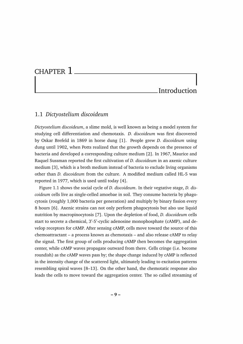
1.1 Dictyostelium discoideum
Dictyostelium discoideum, a slime mold, is well known as being a model system for
studying cell differentiation and chemotaxis. D. discoideum was first discovered
by Oskar Brefeld in 1869 in horse dung [1]. People grew D. discoideum using
dung until 1902, when Potts realized that the growth depends on the presence of
bacteria and developed a corresponding culture medium [2]. In 1967, Maurice and
Raquel Sussman reported the first cultivation of D. discoideum in an axenic culture
medium [3], which is a broth medium instead of bacteria to exclude living organisms
other than D. discoideum from the culture. A modified medium called HL-5 was
reported in 1977, which is used until today [4].
Figure 1.1 shows the social cycle of D. discoideum. In their vegtative stage, D. dis-coideum cells live as single-celled amoebae in soil. They consume bacteria by phago-
cytosis (roughly 1,000 bacteria per generation) and multiply by binary fission every
8 hours [6]. Axenic strains can not only perform phagocytosis but also use liquid
nutrition by macropinocytosis [7]. Upon the depletion of food, D. discoideum cells
start to secrete a chemical, 3’-5’-cyclic adenosine monophosphate (cAMP), and de-
velop receptors for cAMP. After sensing cAMP, cells move toward the source of this
chemoattractant – a process known as chemotaxis – and also release cAMP to relay
the signal. The first group of cells producing cAMP then becomes the aggregation
center, while cAMP waves propagate outward from there. Cells cringe (i.e. become
roundish) as the cAMP waves pass by; the shape change induced by cAMP is reflected
in the intensity change of the scattered light, ultimately leading to excitation patterns
resembling spiral waves [8–13]. On the other hand, the chemotatic response also
leads the cells to move toward the aggregation center. The so called streaming of
– 9 –

1.1. Dictyostelium discoideum
Figure 1.1: Social cycle of D. discoideum. Spores can germinate when the environment issuitable for growth. However, upon deprivation of food, cells start to movetoward each other via chemotaxis. They aggregate to become multicellular,starting from a mound and then differentiate through a slug into a fruitingbody. Adapted by permission from Macmillan Publishers Ltd: Nature ReviewsMolecular Cell Biology [5], copyright (2004).
– 10 –

Chapter 1. Introduction
cells is represented by a series of radial arms and ends up with the formation of a
multicellular organism. The structure is known as a mound and is composed of up
to 105 cells. Cells change their behaviors in the mound according to their starvation
history: cells starved in the S and the early G2 phase differentiate into prestalk cells,
whereas cells starved in the late G2 phase become prespore cells[5, 14–16].
Figure 1.2: Morphogenesis in the mound. To form the stalk of a fruiting body, prestalk cellspstA and pstO move upwards to the tip and pstB cells move downwards to thebottom. Republished with permission of Company of Biologists Ltd., from [17];permission conveyed through Copyright Clearance Center, Inc.
It is the different chemotatic responses between prestalk and prespore cells that
mediates the differentiation: prestalks cells move faster so the prestalk A and the
prestalk O (pstA and pstO) cells rotate toward the tip and the prestalk B (pstB) cells
move to the base, while the slower moving prespore cells stay in the central mound
(Figure 1.2). The tip can further elongate to form a finger-like structure, which
becomes the slug. The slug can migrate to find the ideal environmental conditions,
failing which it transforms into a fruiting body. During the process of fruiting body
formation – known as culmination – prestalk cells differentiate into the stalk and
the basal disk and raise the prespore cells to the top. The stalk cells die afterwards
but the remaining spore cells are stored in the spherical structure called sorus and
can be dispersed as spores. The name D. discoideum actually reflects the observation
of fruiting body production. Dicty means "net-like" structure of many aggregating
cells while -stelium means "tower", representing the standing stalk [1]. D. discoideumcan also incorporate bacteria into their fruiting bodies so that they can be carried
away as new food source during dispersion of the spores [18]. Spores are resistant to
heating, freezing or drying. Once the environment is suitable for growing, the spores
will germinate, D. discoideum cells emerge and the life cycle starts again [19, 20]. It
is the ability to switch between the single and the multicellular forms that justifies
calling D. discoideum in this part of its life cycle, "social" [21].
– 11 –

1.1. Dictyostelium discoideum
D. discoideum cells are easy to culture and genetically modify [21, 22]. Unlike
mammalian cells, D. discoideum cells grow at room temperature and under atmo-
spheric CO2 levels. Moreover, D. discoideum is haploid (i.e., D. discoideum has only
one set of chromosomes). So genes need to be knocked out just once to create
mutants. This property is very helpful in the creation of mutations. Protocols for
genetic modifications with methods like targeted gene disruption [23], restriction
enzyme mediated integration (REMI) [24] or RNA interference inhibition [25] have
been developed over the years. Furthermore, the recently sequenced D. discoideumgenome supports genetic modifications and the evolutional comparison to other
species [26].
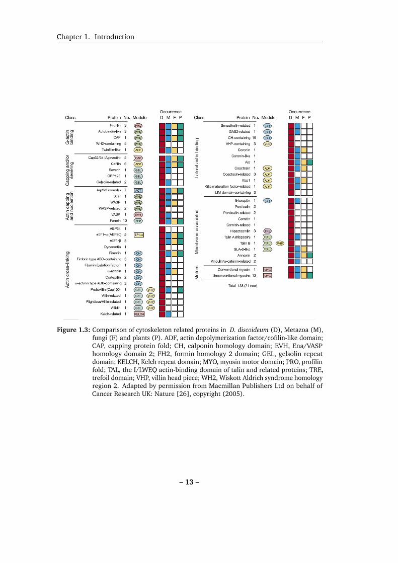
Besides the experimental advantages, the genome sequence shows that despite the
fact that D. discoideum diverged from metazoa earlier than fungus (D. discoideumdiverges right after the split of animal-plant), D. discoideum preserved more cy-
toskeleton related proteins that are similar to metazoa than to fungus and plants
(Figure 1.3) [26]. The cytoskeleton of eukaryotic cells is essential to maintain the
integrity of cells as well as to resist forces. It also plays important roles in self-
organization for migration, division during cytokinesis as well as transport of vesicles
inside cells. Cytoskeleton also drives ubiquitous and significant reactions such as
phargocytosis and chemotaxis. Also, the morphogenesis of D. discoideum cells is
triggered by physiological stimuli, which enables the direct study of chemotaxis.
Taken together, D. discoideum is a well established model system for the study of
eukaryotic cytoskeleton and chemotaxis.
– 12 –
Chapter 1. Introduction
Figure 1.3: Comparison of cytoskeleton related proteins in D. discoideum (D), Metazoa (M),fungi (F) and plants (P). ADF, actin depolymerization factor/cofilin-like domain;CAP, capping protein fold; CH, calponin homology domain; EVH, Ena/VASPhomology domain 2; FH2, formin homology 2 domain; GEL, gelsolin repeatdomain; KELCH, Kelch repeat domain; MYO, myosin motor domain; PRO, profilinfold; TAL, the I/LWEQ actin-binding domain of talin and related proteins; TRE,trefoil domain; VHP, villin head piece; WH2, Wiskott Aldrich syndrome homologyregion 2. Adapted by permission from Macmillan Publishers Ltd on behalf ofCancer Research UK: Nature [26], copyright (2005).
– 13 –
1.2. Actin cytoskeleton
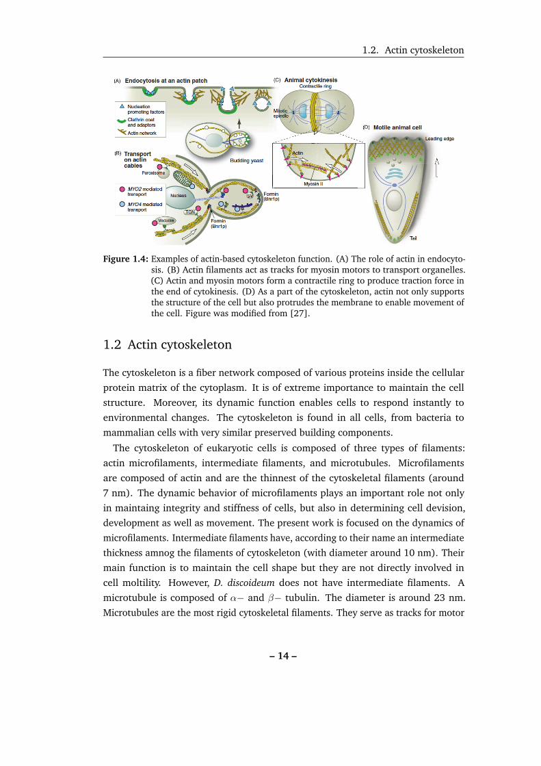
Figure 1.4: Examples of actin-based cytoskeleton function. (A) The role of actin in endocyto-sis. (B) Actin filaments act as tracks for myosin motors to transport organelles.(C) Actin and myosin motors form a contractile ring to produce traction force inthe end of cytokinesis. (D) As a part of the cytoskeleton, actin not only supportsthe structure of the cell but also protrudes the membrane to enable movement ofthe cell. Figure was modified from [27].
1.2 Actin cytoskeleton
The cytoskeleton is a fiber network composed of various proteins inside the cellular
protein matrix of the cytoplasm. It is of extreme importance to maintain the cell
structure. Moreover, its dynamic function enables cells to respond instantly to
environmental changes. The cytoskeleton is found in all cells, from bacteria to
mammalian cells with very similar preserved building components.
The cytoskeleton of eukaryotic cells is composed of three types of filaments:
actin microfilaments, intermediate filaments, and microtubules. Microfilaments
are composed of actin and are the thinnest of the cytoskeletal filaments (around
7 nm). The dynamic behavior of microfilaments plays an important role not only
in maintaing integrity and stiffness of cells, but also in determining cell devision,
development as well as movement. The present work is focused on the dynamics of
microfilaments. Intermediate filaments have, according to their name an intermediate
thickness amnog the filaments of cytoskeleton (with diameter around 10 nm). Their
main function is to maintain the cell shape but they are not directly involved in
cell moltility. However, D. discoideum does not have intermediate filaments. A
microtubule is composed of α− and β− tubulin. The diameter is around 23 nm.
Microtubules are the most rigid cytoskeletal filaments. They serve as tracks for motor
– 14 –
Chapter 1. Introduction
proteins such as kinesins and dyneins which transport organelles inside the cells.
Microtubules also form the mitotic spindle and thus are of great importance in cell
division.
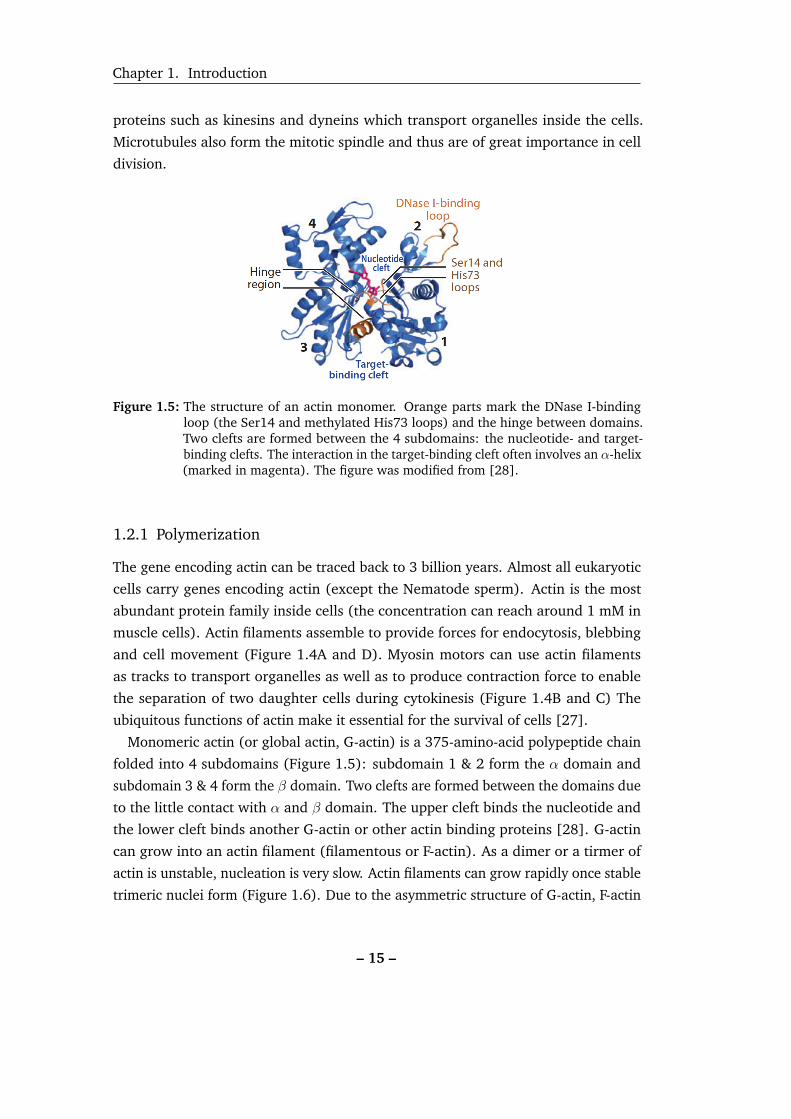
Figure 1.5: The structure of an actin monomer. Orange parts mark the DNase I-bindingloop (the Ser14 and methylated His73 loops) and the hinge between domains.Two clefts are formed between the 4 subdomains: the nucleotide- and target-binding clefts. The interaction in the target-binding cleft often involves an α-helix(marked in magenta). The figure was modified from [28].
1.2.1 Polymerization
The gene encoding actin can be traced back to 3 billion years. Almost all eukaryotic
cells carry genes encoding actin (except the Nematode sperm). Actin is the most
abundant protein family inside cells (the concentration can reach around 1 mM in
muscle cells). Actin filaments assemble to provide forces for endocytosis, blebbing
and cell movement (Figure 1.4A and D). Myosin motors can use actin filaments
as tracks to transport organelles as well as to produce contraction force to enable
the separation of two daughter cells during cytokinesis (Figure 1.4B and C) The
ubiquitous functions of actin make it essential for the survival of cells [27].
Monomeric actin (or global actin, G-actin) is a 375-amino-acid polypeptide chain
folded into 4 subdomains (Figure 1.5): subdomain 1 & 2 form the α domain and
subdomain 3 & 4 form the β domain. Two clefts are formed between the domains due
to the little contact with α and β domain. The upper cleft binds the nucleotide and
the lower cleft binds another G-actin or other actin binding proteins [28]. G-actin
can grow into an actin filament (filamentous or F-actin). As a dimer or a tirmer of
actin is unstable, nucleation is very slow. Actin filaments can grow rapidly once stable
trimeric nuclei form (Figure 1.6). Due to the asymmetric structure of G-actin, F-actin
– 15 –

1.2. Actin cytoskeleton
is polar, with one end called the barbed end and the other called the pointed end.
The barbed end containing ATP grows faster and orients toward the cell membrane.
The fresh growing F-actins further push the membrane forward.
Figure 1.6: Formation of actin filaments: nucleation and extension. To grow from monomericactin is very difficult and slow. Even dimers and trimers are unstable. However,the elongation by adding new monomeric actin on to the existing nucleus israpid and stable. The growth is much faster at the barbed end than the pointedend. The figure is modified from [27].
1.2.2 Depolymerization
The hydrolysis of ATP by F-actin changes the confirmation and leads to disassembly:
the Ser14 β-hairpin loop forms an hydrogen bond with the γ-phosphate in ATP. After
ATP hydrolysis, the γ-phosphate is released, Ser14 changes orientation to form a
contact with the β-phosphate and the His73 loop move toward the nucleotide to
occupy the space released the γ-phosphate [28]. Both the barbed end and the pointed
end can grow and disassemble. Figure 1.7 shows the association and dissociation
rate constants as well as the equilibrium constants K1 of both the F-actin ends. As the
equilibrium constant determines the critical concentration for actin polymerization,
the difference in the equilibrium constatnt for ATP-actin at the barbed end (K=0.12)
and the pointed end (K=0.6) causes growth on the barbed end and depolymerization
on the pointed end – known as treadmilling.
1.2.3 Role of actin binding proteins
Actin dynamics requires the regulation of a variety of proteins. Figure 1.8 shows how
an actin network forms a dendritic structure via the treadmilling process. We first
introduce the essential proteins shown here in detail and then talk about two other
proteins (Aip1 and coronin) that help in depolymerization.
Besides elongating the existing F-actin, new filaments can grow on the side of
existing filaments to form branches. The nucleation of a branch is initiated by active
Arp2/3, a protein complex composed of seven subunits. Usually less than 1% of
Arp2/3 is in the active form [30]. In the inactive form, the Arp2/3 complex is loosely
1the ratio between dissociation and association rate constant (k-/k+).
– 16 –

Chapter 1. Introduction
Figure 1.7: Actin filament elongation and ATP hydrolysis. The unit of association rateconstants are µM−1s−1. The unit of dissociation rate constants are s−1. Theratio of the dissociation rate constant to the association rate constant is K,the dissociation equilibrium constant with units of µM. Reprinted from [29],Copyright (2003), with permission from Elsevier.
packed. Together with actin filaments and actin monomers, regulating proteins called
nucleation promoting factors (NPFs) such as WASp and Scar, Arp2/3 can be activated
by a conformational change: all subunits are brought together to form a compact
structure wrapping around the helix of actin filament [31]. It is the coorperation of
NPFs, actin filaments, actin monomers that activates Arp2/3 and then initiates the
formation of new branches. None of them can activate Arp2/3 on their own. The
binding of the activated Arp2/3 to the mother filaments thus forms branch junctions
and the barbed end of a new filament (known as a daughter filament) can grow from
here. The angle between these two filaments is 70o [32, 33].
The keratocyte and D. discoideum cells can move their body length (10 µm) in one
minute. However, pure actin filaments are intrinsically stable: exchange of subunits
at the ends is around 0.04µm/min [29]. Therefore, it is the role of actin binding
proteins that enables the rapid turnover of actin networks. Rapid turnover requires
an abundant pool of actin monomers, efficient polymerization and fast deploymer-
ization to replenish the pool of actin monomers. Under physiological conditions,
the unpolymerized pool of G-actin usually has 2 to 3 orders of magnitude more
actin monomers than the critical concentration2 (though it varies among different
species) (Figure 1.9). However, not all G-actin can be directly polymerized to F-actin.
2Critical concentration here is defined as the equilibrium dissociation constant (Kd). Under physiolog-ical conditions, Kd for ATP-actin is 0.1 µM at barbed-end and 0.6 µM at pointed-end [34].
– 17 –

1.2. Actin cytoskeleton
Figure 1.8: Formation of dendritic actin network and the key regulation proteins. Nucleationpromoting factors like WASp/Scar bring Arp2/3 and an actin monomer togetherto the side of an existing filament to form a branch. The pool of ATP-actin boundto profilin bind to barbed ends to elongate the actin filament. Elongation isterminated by the binding of a capping protein. The ATP-actin on the actinfilament is gradually hydrolyzed into ADP-actin (aging). ADF/cofilin can severand dissociate ADP-actin filaments. The ADP-actin then rapidly exchanges anucleotide to become ATP-actin with the help of Profilin. The profilin boundATP-actin is then again ready to elongate barbed ends. The growing filamentscan push the membrane forward. The figure was modified from [27]
.
– 18 –

Chapter 1. Introduction
Figure 1.9: Key actin related proteins in different cells. The table was adapted from [34].
Profilin and Thymosin-β4 compete with each other to bind ATP-actin monomers.
Thymosin-β4 cannot participate in actin filament nucleation or elongation, whereas
profilin helps to effectively add subunits to F-actin. Profilin can exchange ADP for
ATP on G-actin and then add subunits only to the barbed ends (but cannot add them
to the pointed ends).
As G-actin is abundant and Profilin can only elongate the barbed end of F-actin,
the amount of F-actin itself determines the growth of F-actin. Profilin can also
inhibit filament nucleation to prevent elongation along the new F-actin. To terminate
polymerization, a capping protein binds tightly on the barbed end with extremely
slow dissociation rates3: 5 × 10⁻⁴s−1; on the other hand, binding of ADF/cofilin
to ADP-actin monomers changes the twist of actin helix and promotes severing of
the filaments into short segments. It is the higher affinity of ADF/cofilin for ADP-
actin monomers that drives the severing process; ADP-actin very quickly turns into
ATP-actin due to the high concentration of ATP in living cells; profilin can bind to
ATP-actin and polymerize the filaments again owing to higher affinity of profilin for
ATP-actin than ADF/cofilin. Capping proteins and cofilin are of extreme importance
to cell as lacking the associated regulating genes are lethal to cells [35, 36].
3The half-time of uncapping is > 1000 s, much longer than the lifetime of actin dynamics (tens ofseconds).
– 19 –

1.3. Myosin II
Besides cofilin, proteins such as Aip1 (actin-interacting protein 1) and coronin
also help regulate actin depolymerization. Aip1 can not only enhance fragmentation
of actin filaments mediated by cofilin [37–40] but also cap the barbed ends of
those severed fragments [41, 42]. Aip1 translocates dynamically to regions that are
enriched in filamentous actin (such as pseudopodia, lammellipodia and phagocytic
cups) [43–45]. Coronin is named after its localization in crownlike extensions of
cell surfaces [46]. Coronin plays two different roles in the front and the back of the
cell. At the front of the cell, coronin not only binds to the ATP-actin filaments with
high affinity [47–54] but also recruits Arp2/3 complex to the sides of filaments to
form new nucleation sites and branch [53, 55–57]. Besides promoting the growth
of actin filaments, coronin can inhibit depolymerization in the front as well. The
coiled-coil domain of coronin has high affinity toward ATP-actin. Coronin can thus
bind ATP-actin to block cofilin binding and prevent the severing of ATP-actin filaments.
On the contrary, at the rear of the cell, the coiled-coil domain no longer inhibits the
binding of cofilin but allows the β− propeller domain to recruit cofilin to disassemble
and sever actin filaments [52, 58]. After the disassembly of actin filaments, Arp2/3
complex and coronin dissociate and then diffuse to the front of the cell. Taken
together, the mechanism regenerates fresh actin monomer pool to supply the rapid
turnover of moving cells.
Both Aip1 and coronin are important for cytokinesis, development and movement.
In cells lacking either Aip1 or coronin, cytokinesis is prolonged and cells are usually
multinucleated. The reduced endocytosis and phagocytosis rates in Aip1-null or
coronin-null cells result in slower growth rates [45, 58, 59].
1.3 Myosin II
To date, 13 types of myosin have been discovered from the genome sequence of
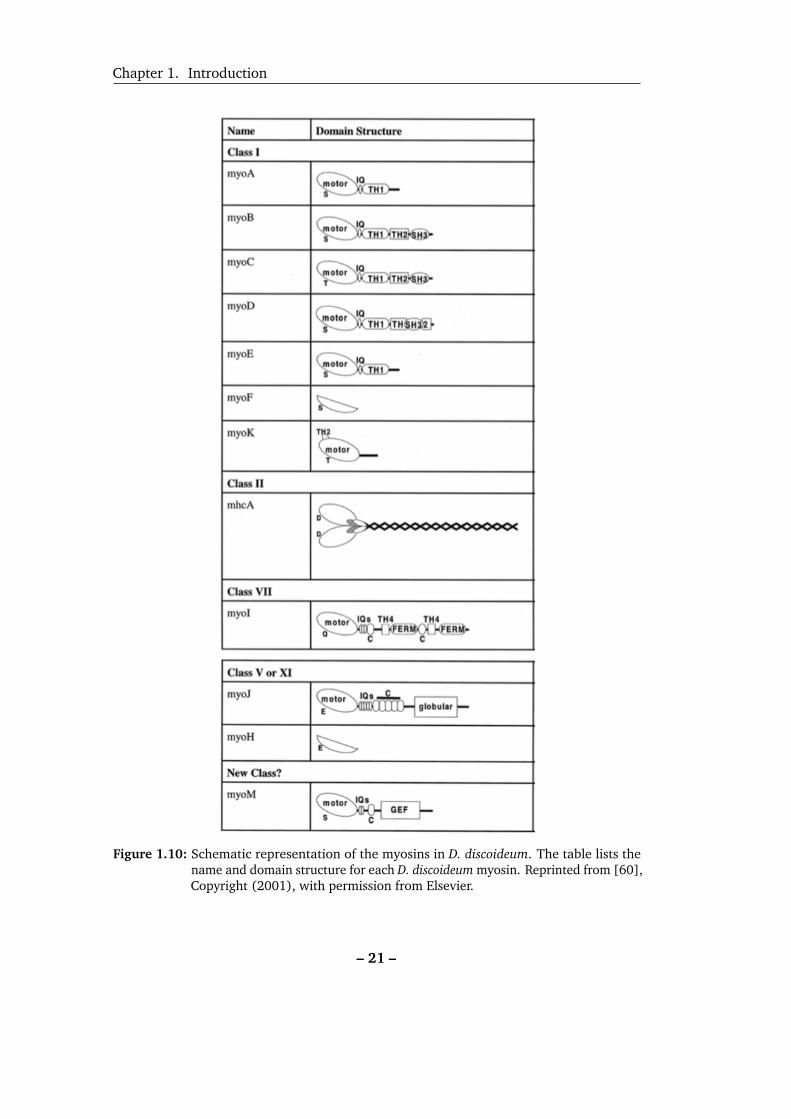
D. discoideum cells [26]. Figure 1.10 shows the conceptional structure of them [60].
Based on the structure, myosin can be categorized into several types. Most myosins
belong to class II (from now on we will call it myosin II). Myosin II is also the protein
responsible for the contration in cardiac, skeletal and smooth muscles. Myosin II,
due to its significance, is well studied and known as conventional myosin. The other
types of myosin are thus called unconventional myosin. Myosin II molecules with
similar function and structure as their conterparts in muscle are are present in all
non-muscle eukaryotic cells [61]. We thus call them non-muscle myosin. In this
study, we will focus on the non-muscle myosin in D. discoideum cells.
– 20 –
Chapter 1. Introduction
Figure 1.10: Schematic representation of the myosins in D. discoideum. The table lists thename and domain structure for each D. discoideum myosin. Reprinted from [60],Copyright (2001), with permission from Elsevier.
– 21 –

1.3. Myosin II
Figure 1.11: The structure of non-muscle myosin II. The global head domain binds to theactin filament. With the hydrolysis of ATP, myosin II can move on actin filamentso it is also regarded as motor domain. The regulatory light chains (RLC)can regulate the activity of myosin II and the essential light chains (ELC) canstabilize heavy chain. They bind to the heavy chains at the neck part that linkthe head and tail domains. Adapted by permission from Macmillan PublishersLtd: Nature Reviews Molecular Cell Biology [61], copyright (2009)
.
Myosin II is a hexamer composed of two myosin heavy chains (MHC), two regula-
tory light chains and two essential light chains (Figure 1.11). Each subunit is encoded
by a single gene. The heavy chain can be divided into a globular head domain that
binds to actin filaments, a neck region that binds two light chains and a long tail
domain. The light chains are essential to stabilize the neck region and make the neck
a rigid lever arm that can swing on an actin filament (Figure 1.12) [62, 63]. Myosin II
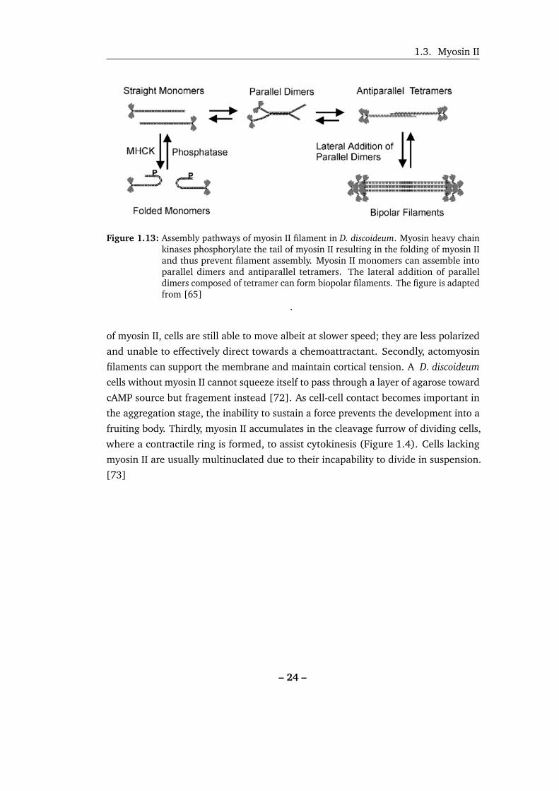
can self-assemble via the long heavy chain tail to form bipolar filaments: two myosin II
tails minimize the electrostatic interactions of repeating hydrophobic and alternating
negtively and positively charged residues in the tail domain by staggering 14 residues
and forming a coiled-coil structure [64]. With electrostatic interactions, the hexamer
myosin II can further form parallel dimers, antiparallel tetramers and grow thicker
by lateral addition of parallel dimers [65]. Immunoelectron microscopy shows that
myosin II bipolar filaments are composed of 10–20 molecules and are about 0.5 µm
long and 12 nm thick in D. discoideum cells [66]. Since the electrostatic forces hold
bipolar filaments together, the formation of myosin II filament highly depends on the
ionic strength.
Besides ionic strength, phosphorylation of the heavy chain also regulates the assem-
bly of myosin II filament. Myosin heavy chain kinase A (MHCK A) can phosphorylate
threonine at positions 1823, 1833 and 2029. The bending structure of phosphory-
lated myosin heavy chain observed from electron micrographs postulates that due
to the stabilization from the negative phosphate groups and the positively charged
– 22 –

Chapter 1. Introduction
Figure 1.12: Schematic diagram to show the interaction between actin and myosin and thecorresponding ATPase cycle of myosin. Myosin in red shows the bound stateto actin filament, whereas myosin in blue shows the detached state. Adaptedby permission from Macmillan Publishers Ltd: [Nature Cell Biology] [63],copyright (2001)
.
residues, myosin II monomers can form folded structure (Folded monomers in Fig-
ure 1.13) and inhibit the assembly of bipolar filaments [67, 68]. The motor domain
enables myosin II to bind on actin filaments and form actomyosin. By hydrolyzing
ATP, myosin II motor head can slide on actin filaments and induce contraction (Fig-
ure 1.14) [69]. In Figure 1.12, the ATPase cycle of myosin shows that myosin first
hydrolyzes ATP without binding to actin. The following attachment to actin triggers
the release of phosphate and induces the force-generating stroke [70, 71]. The tight
coupling between hydrolysis of ATP and the interaction of actin-myosin prevents
unnecessary ATP consumption [63]. As myosin II is only functional as filaments,
the lack of myosin II heavy chain thus inhibits the entire function of the myosin II
molecule[61].
Myosin II plays an important role in cell migration, cell shape maintance, and
cytokinesis: regarding the first role, in a migrating cell, actin filaments polymerize in
the front and push the membrane forward; meanwhile myosin II accumulates in the
rear and leads to contractile forces. In response to a chemoattractant, the localization
of myosin II can surpress lateral pseudopod formation to maintain the polarity of the
cells, resulting in persistent movement towards the chemoattractant. In the absence
– 23 –
1.3. Myosin II
Figure 1.13: Assembly pathways of myosin II filament in D. discoideum. Myosin heavy chainkinases phosphorylate the tail of myosin II resulting in the folding of myosin IIand thus prevent filament assembly. Myosin II monomers can assemble intoparallel dimers and antiparallel tetramers. The lateral addition of paralleldimers composed of tetramer can form biopolar filaments. The figure is adaptedfrom [65]
.
of myosin II, cells are still able to move albeit at slower speed; they are less polarized
and unable to effectively direct towards a chemoattractant. Secondly, actomyosin
filaments can support the membrane and maintain cortical tension. A D. discoideumcells without myosin II cannot squeeze itself to pass through a layer of agarose toward
cAMP source but fragement instead [72]. As cell-cell contact becomes important in
the aggregation stage, the inability to sustain a force prevents the development into a
fruiting body. Thirdly, myosin II accumulates in the cleavage furrow of dividing cells,
where a contractile ring is formed, to assist cytokinesis (Figure 1.4). Cells lacking
myosin II are usually multinuclated due to their incapability to divide in suspension.
[73]
– 24 –

Chapter 1. Introduction
Figure 1.14: Myosin II is a hexamer composed of two regulatory light chains (RLC), twoessential light chains (ELC) and two myosin heavy chains (MHC). Each heavychain has a head domain and a tail domain. Myosin heavy chain kinases(MHCKs) can phosphorylate three threonines of the tail to prevent the assemblyof myosin II filaments. Actomyosin refers to the structure formed when myosin IIbinds to actin filaments via the interaction of motor domain. With the hydrolysisof ATP, myosin can show its motor activity. Reprinted from [69], Copyright(2006), with permission from Elsevier.
.
– 25 –

1.4. Self-organization and oscillations
1.4 Self-organization and oscillations
Self-organization is a process where global order emerges from local interactions
between the components of a disordered system. Schools of fish, flocks of birds, and
patterns on animal fur are classic examples of biological pattern formation driven
by self-organization. Self-organization also plays an important role in the structure
formation of a cell. The local dynamics of actin filaments enables cell movement by
forming pseudopodia, blebbs, filopodia, membrane ruffling and other structures. It is
the self-organization of various molecules inside the cell that determines the dynamic
behavior of cells.
One of the well-known examples is the actin comet tail of the bacteria Listeriamonocytogenes. It uses the actin system of the cell it infects to propel itself within
the cytoplasm of the host as well as to invade adjacent cells. The actin tail initiates
from the asymmetric distribution of the protein ActA on the surface of Listeria. ActA
protein not only interacts with monomeric ATP-actin, but also activates and recruits
anchoring proteins such as Arp2/3 and VASP to support elongation. The insertion
of actin thus produces force for propulsion [74–78]. Another intriguing example of
cytoskeletal self-organization are actin waves, which propagate at the substrated-
attached surface by constantly polymerizing in the front and depolymerizing in the
back. It was proposed that D. discoideum cells use actin wave to scan the surface for
particles to intake [79]. The three-dimentional ordered self-organization follows the
signal of PIP3 and is operated by actin binding proteins: Arp2/3 is associated with
actin throughout the wave, whereas myosin IB is enriched in the front and coronin is
recruited at the back for disassembly [80–83].
In particular cases, collective behavior of many interacting components can result in
systems with an intrinsic potential to oscillate. Oscillatory systems are known to play
important roles in biology [84, 85]: circadian clocks circle between day and night to
coordinate behavior with daily and seasonal changes [86–88], Min protein systems
recycle inside Escherichia coli to determine the division site [89, 90] and cilia beat to
sense factors such as frequency of mechanical sources in the environment [91, 92].
The most well-known oscillation of D. discoideum cells is the periodic emission of
cAMP (with a period around 6 min) during their starvation stage, which enables them
to stimulate each other and then accumulate to develop into fruiting bodies [93, 94].
The periodicity manifested itself in experiments such as (1) light scattering by
cells observed by dark-field microscopy (2) contact among cells observed by bright-
field microscopy and (3) cell-surface contact observed by total internal reflection
– 26 –

Chapter 1. Introduction
fluorescence microscopy (TIRFM) [95, 96]. In addition, cAMP also triggers the
uptake of calcium, resulting in oscillations of Ca2+ [97, 98].
Besides the oscillations of cAMP, oscillations of several different components have
been found in D. discoideum in the absence of a chemoattractant: PIP3 (PtdIns 3,4,5-
trisphosphate) has been found to spontaneously oscillate on the membrane with a
period of around 200 s [99, 100]; protrusion of a pseudopod formed with a frequency
of around 3.5/min [101–108]; SCAR/WAVE, coronin and LimE were recently found
to oscillate with a period of around 10 s [109, 110].
1.5 Aim and outline
D. discoideum shares many common features of actin dynamics and essential responses
with eukaryotic cells and cancer cells. Therefore, most properties of the oscillations
are well studied in the simpler biological model system. However, the properties and
the underlying mechanisms of the recently found autonomous cytoskeletal oscillations
are still unexpolred. Questions such as what the roles of this autonomous oscillation
in chemotaxis are, and how external stimulation affects autonomous oscillations are
intriguing but unanswered.
This study will start by investigating actin dynamics of cells in the absence of
external stimuli. We analyze thousands of cells to get a stochastically significant
mean. In the part on intrinsic oscillations, we report on the properties like the
distribution of oscillations, role of actin regulating proteins such as Aip1, coronin
and myosin II and propose an underlying mechanism. In the second chapter, we
investigated how external stimulation alters the intrinsic frequency. With dose
dependence experiments and careful examination of the different sections of the
actin polymerization, depolymerization and recovery, we extend our model to account
for the chemotatic responses. We also use the experimental data to verify an existing
model of actin dynamics and modify it according to our experimental results. Finally,
we investigate the role of myosin II in actin dynamics. Although myosin II is not
directly invovled in actin regulation, it is essential for effective cellular functions
such as movement, chemotaxis and cytokinesis. Here we first study the dynamics
of myosin II to understand not only how myosin II regulates actin dynamics but
also how the self-organized actin network influences the dynamics of myosin II.
Myosin II-knockout cells are further studied to reveal the significance of myosin II in
regulating the chemotatic relevance in actin dynamics as well as cellular functions.
– 27 –

CHAPTER 2
Material and methods
2.1 Cell culture and development
Dictyostelium discoideum cells were cryopreserved in vials in the form of spores at
−80 ◦C for long-term storage. For mutants that cannot form spores, the cells were
direrctly frozen in liquid nitrogen. The first step to grow cells is to thaw the frozen
cells. Vials from freezer or liquid nitrogen were first thawed at room temperature.
Cells were grown at 22 ◦C in HL-5 medium on Petri dishes. To germinate cells from
spores, 100 µM spores were cultured on a Petri dish with 10 mL HL-5 medium
(14 g/L peptone, 7 g/L yeast extract, 13.5 g/L glucose, 0.5 g/L KH2PO4, 0.5 g/L
Na2HPO4, Formedium, Norwich, England). To obtain cells from frozen cells, the
cryopreservation medium containing DMSO was first replaced by fresh HL-5 medium
and then put into a Petri dish.
To be free of asepsis, all the reagents (e.g. buffer and medium), glassware,
disposable plastic wares were sterilized. The working area and the exterior of
equipment were always cleaned with 70% ethanol. Depending on the cell lines,
antibiotics were supplemented as selection markers to protect the integrity of cell
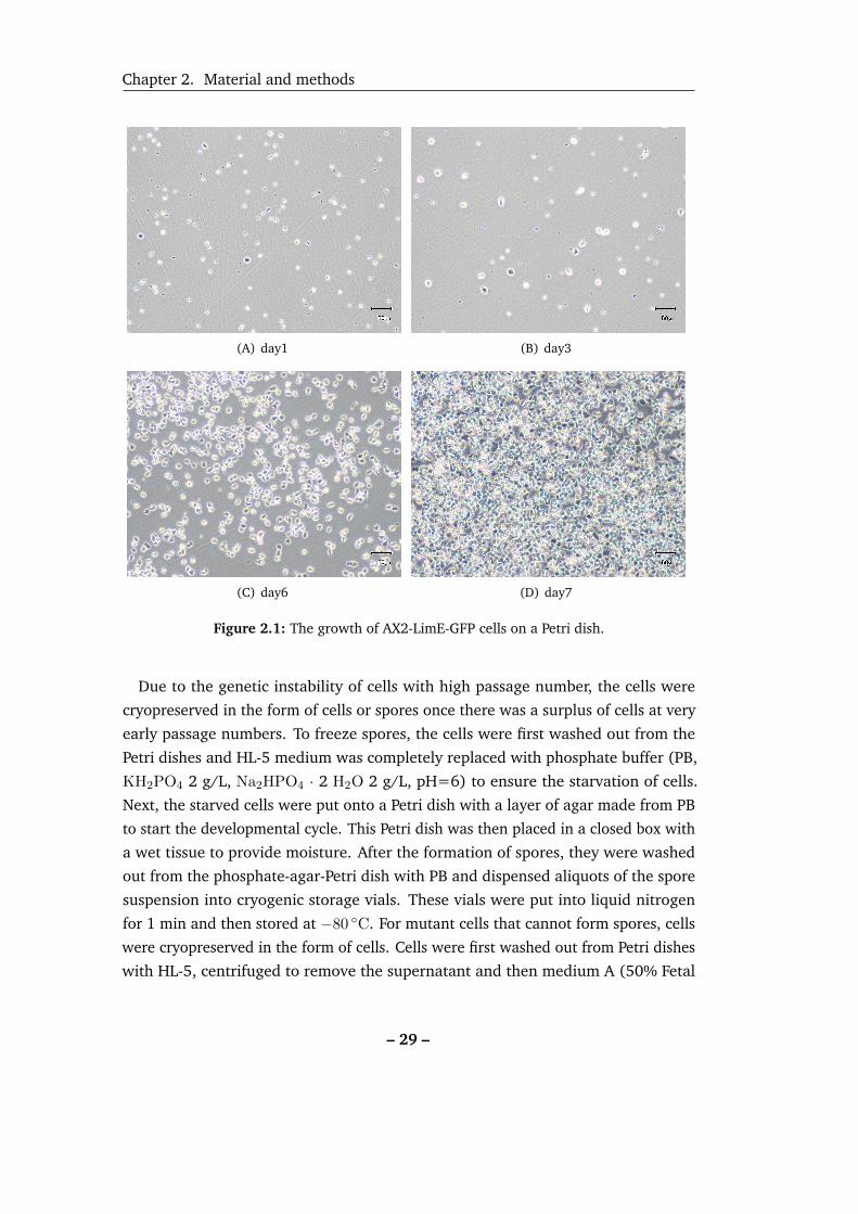
culture from the second day of thawing. Figure 2.1 shows the growth of AX2-LimE-
GFP cell from the first day of thawing. After the cells occupied all the available
substrate on the Petri dish (i.e., reached confluence, Figure 2.1D), we subcultured the
cells by transferring some of the cells to a new Petri dish with fresh medium to grow
(i.e., a new passage). Every subculture step increased the passage number of cells by
one. Depending on the density and growth rate of different cell lines, the cell culture
was passaged within 3 days. Since cell lines in continuous cultures are likely to be
genetically unstable as the passage number increases, cells were discarded when the
passage number reached 15.
– 28 –
Chapter 2. Material and methods
(A) day1 (B) day3
(C) day6 (D) day7
Figure 2.1: The growth of AX2-LimE-GFP cells on a Petri dish.
Due to the genetic instability of cells with high passage number, the cells were
cryopreserved in the form of cells or spores once there was a surplus of cells at very
early passage numbers. To freeze spores, the cells were first washed out from the
Petri dishes and HL-5 medium was completely replaced with phosphate buffer (PB,
KH2PO4 2 g/L, Na2HPO4 · 2 H2O 2 g/L, pH=6) to ensure the starvation of cells.
Next, the starved cells were put onto a Petri dish with a layer of agar made from PB
to start the developmental cycle. This Petri dish was then placed in a closed box with
a wet tissue to provide moisture. After the formation of spores, they were washed
out from the phosphate-agar-Petri dish with PB and dispensed aliquots of the spore
suspension into cryogenic storage vials. These vials were put into liquid nitrogen
for 1 min and then stored at −80 ◦C. For mutant cells that cannot form spores, cells
were cryopreserved in the form of cells. Cells were first washed out from Petri dishes
with HL-5, centrifuged to remove the supernatant and then medium A (50% Fetal
– 29 –

2.2. Microfluidics
calf serum (FCS, Invitrogen), 50% HL-5) was added to dispense the cells. These
cells were counted with a hemocytometer and then diluted with 50% medium A and
50% medium B (40% medium A, 40% FCS, 20% DMSO as a cryoprotective agent)
in order to be aliquoted with a concentration of 107 cells/mL. The aliquoted cells
in cryovials were then put into a controlled freezing rate apparatus (Mr. FrostyTM
Freezing Container) to cool at the rate of −1 ◦C/min. This optimal cooling rate for
cell preservation was achieved by filling the container chamber with 100% isopropyl
alcohol. The freezing apparatus with cryovial containing cells was first stored at
−20 ◦C for 1–2 hours and then −80 ◦C overnight. Finally the frozen cells were
transferred to and stored in liquid nitrogen.
2.2 Microfluidics
The microfluidic channels used in the experiments were fabricated using soft lithogra-
phy. A master wafer was first made by photolithography and then ploy(dimethylsiloxane)
(PDMS, SylgardTM 184, Dow Corning Europe SA, Houdeng-Goegnies, Belgium) was
poured over the master to get an elastomeric block. Finally, the patterned block was
bound to a glass slide and was ready for use. Figure 2.2 summarizes the steps of
fabrication while the next three subchapters outline the details of the procedure.
2.2.1 Mask Design
The pattern of the channels were designed with a computer-aided design (CAD)
software and then printed on a mask. The mask design was printed on chrome/quartz
with a resolution of 1.8 µm. Figure 2.2 shows the geometry of channels used in the
experiments.
2.2.2 Photoresist
Photolithography generates patterns on a surface. The surface coated with photoresist
is selectively irradiated by UV light through the transparent part of the predesigned
mask. After the chemical reaction induced by exposure to UV light changes the
properties of the photoresist, the following developing process washes out either the
exposed part (positive photoresist) or the unexposed part (negative photoresist). In
our case, negative photoresist is used.
The designed mask was then used in photolithography to create the master wafer.
The high contrast, epoxy based SU-8 was used as the photoresist and the procedure
– 30 –

Chapter 2. Material and methods
Figure 2.2: Summary of the fabrication of microfluidic channels. Soft lithography removesonly the masked part and leaves the designed channels unchanged. PDMS wasused for replica molding. Finally, the device is sealed by binding PDMS to a glasscover slide. The geometry of the microfluidic channels used is shown as a topview: channel height: 26 µm; channel width: 500 µm.
followed the protocol of MICROCHEM [111]. The process includes wafer cleaning,
spin coating, soft baking, UV exposure, post exposure baking, developing, rinsing,
drying and finally measuring the height based on interferometry (Figure 2.3).
1. Cleaning. The polished silicon master wafer (diameter 100 mm, SiMat) was
first baked at 200 ◦C for 5 min to evaporate residual organic solvents on the
surface.
2. Spin coating. After the wafer cooled down, it was placed on a spin coater.
Approximately 1 ml SU-8 was then poured onto the center of the wafer. The
viscosity of SU-8 and the spin speed are vital to the final thickness of the
channel. For a channel with a height of 26 µm, SU-8 25 (viscosity=2500 cSt)
was used. The coating was done in two steps. The first spread cycle took 5 s
to ramp to 500 rpm with an acceleration of 100 rpm/s. The second spin cycle
ramped to 2000 rpm with an acceleration of 300 rpm/s and was held for a
total of 30 s.
– 31 –

2.2. Microfluidics
Figure 2.3: Flow chart of photoresist fabrication. The process includes clean, spin coating ofSU8, soft bake, UV exposure, post exposure bake (PEB), and finally development.
– 32 –

Chapter 2. Material and methods
3. Soft baking. After the resist spread onto the substrate, the wafer was placed
on a hotplate to evaporate the solvents and densify the film. Stepwise heating
was used to make the photoresist adhere to the substrate better. The wafer was
first heated on a hotplate at 65 ◦C for 3 min and then at 95 ◦C for 7 min.
4. UV exposure. The plate was cooled down before exposure to UV. A mercury
arc lamp with a power of 350 W and intensity of 14 mW/cm2 was used as the
light source for 14 s to provide 200 J/cm2 exposure energy. The exposure to
UV light was carried out in a EVG620 mask alignment system (EVG, St. Florian
am Inn, Austria).
5. PEB. The exposure of SU-8 to UV light solidifies the material by cross-linking the
long molecular chains. This epoxy cross-linking is acid-initiated and thermally
driven. As strong acid was formed during UV exposure, the post exposure
baking provides heat for the process of epoxy cross-linking. To reduce the
stress resulting from the cross-linking of SU-8, the wafer was first heated on a
hotplate at 65 ◦C for 1 min, then at 95 ◦C for 3 min and finally gradually cooled
down to room temperature.
6. Development. The wafer was then immersed in the developer of SU-8 (1-
Methoxy-2-propanol acetate) until all non-cross-linked SU-8 was washed out.
Finally, we rinse the wafer with isopropyl alcohol and dry it with nitrogen. The
height can be verified by white light interferometry (Wyko NT 1100, Veeco,
Plainview, NY).
2.2.3 Soft lithograpghy
The key to soft lithography is the patterned structures on the surface of an elastomeric
block. PDMS is a fluid at room temperature but can be readily converted into solid
elastomers by cross-linking. A liquid silicon rubber base (i.e. a vinyl-terminated
PDMS) and a curing agent (i.e. a mixture of a platinum complex and copolymers
of methylhydrosiloxane and dimethylsiloxane) were first mixed in a 10:1 ratio,
degassed in a vacuum desiccator and finally cured for 1 to 2 hours at 75 ◦C. The
hydrosilyation reaction between vinyl groups (SiCH−−CH2) and hydrosilane groups
(SiH) transformed the liquid into a solid cross-linked elastomer [112, 113].
Inlet and outlet holes were punched into the replica mold of PDMS with a 0.75 mm
puncher (Harris Uni-CoreTM). The PDMS and a cover glass (No.1, 24 × 60mm,
Menzel Gläser, Braunschweig, Germany) were then placed into a plasma vacuum
chamber (PDC 002, Harrick Plasma, Ithaca, NY). The vacuum pump was connected
to the outlet of the reaction chamber and air was used as the process gas to generate
– 33 –

2.3. Experimental design
plasma. After a 30 s treatment with a violet plasma, the PDMS and the cover glass
were taken out and bound together. The oxidization of PDMS in air plasma enables
etching of hydrocarbons leaving silanol groups (SiOH) on the surface, rendering
the surface hydrophilic. Immediate contact of PDMS and cover glass enables an
irreversible seal by formation of Si-O-Si covalent bond1. The hydrophilic surface after
the treatment of plasma also helps the spreading of buffer in microfluidic channels.
Finally, the inlet of the microfulidic channel was connected to a a glass syringe
(McMaster, Hamilton, Ontario) via a PTFE microtube (Novodirect, Kehl, Germany).
2.3 Experimental design
To investigate the actin dynamics of migrating D. discoideum cells in the presence
and absence of external chemotatic stimuli, we took advantage of the fact that
D. discoideum cells respond to cAMP when they are starved, and that the microfluidic
devices can be used to apply and remove cAMP with high spatiotemporal precision.
The preparation of cells was started one day previous to the experiment. Cells
were first washed out of the Petri dish with HL-5 and then centrifuged to remove the
supernatant. The number of cells was estimated by a hemacytometer. Around 5× 10⁵
cells were then collected in a Erlenmeyer flask with a final volume of 25 mL and
shaken at 150 rpm for one day. To start the starvation, cells in the log phase (where
cells proliferate exponentially) were collected from the Erlenmeyer flask and the
HL-5 medium was replaced with PB. The process of removing the supernatant after
centrifuge was repeated twice to ensure the complete removal of nutrients from cells.
Finally, a drop of 50 nM cAMP was applied to the cells every 6 min continuously for
6 hours via a peristaltic pump. The cells were then centrifuged to replace the buffer
and resuspended in a final volume of 2 mL fresh PB.
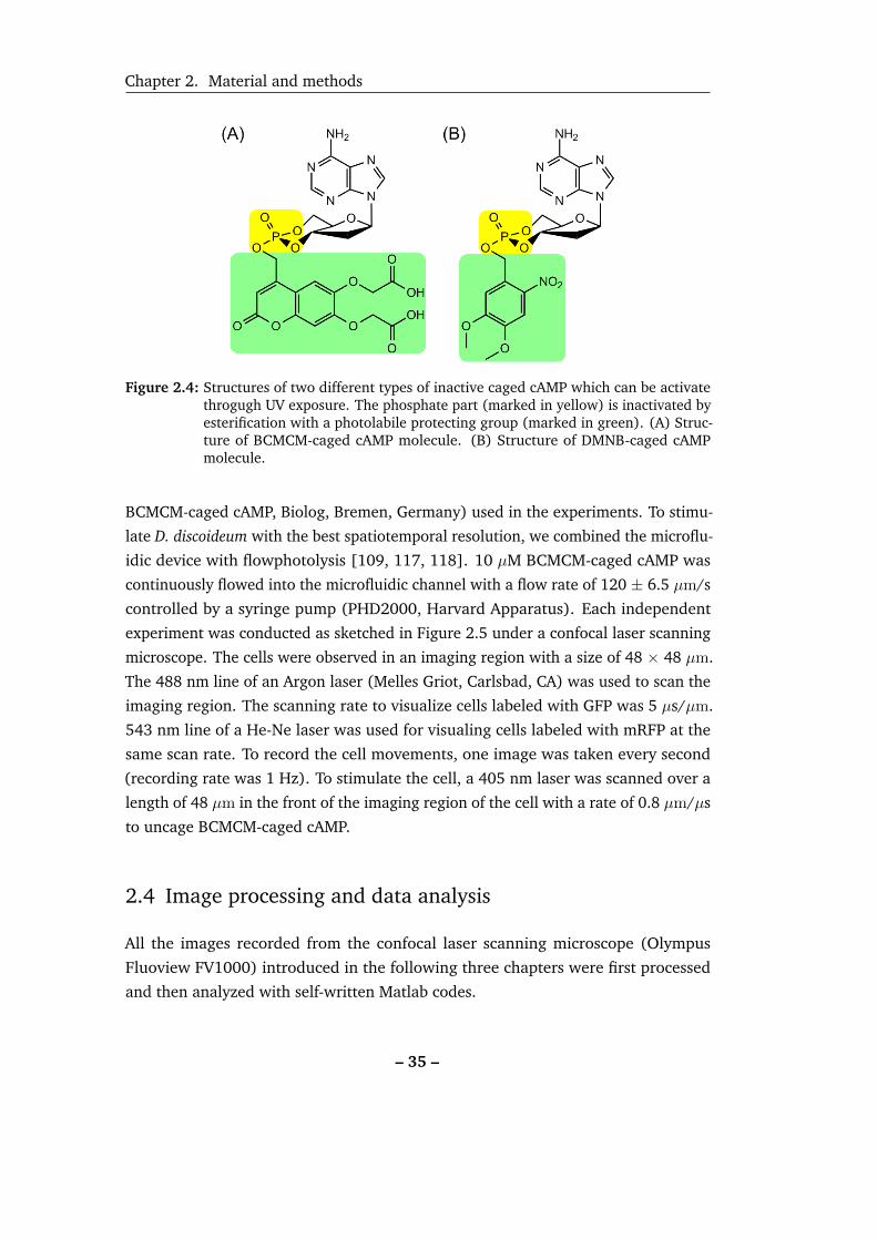
The interaction between cAMP receptors and cAMP enables D. discoideum cells
to recognize cAMP. As binding to cAMP causes receptor phosphorylation [114],
caged cAMP was designed by esterification of the phosphate moiety (marked yel-
low in Figure 2.4) with a protecting group (marked green in Figure 2.4). This
protecting group is photolabile. Application of a flash of light removes the protect-
ing group and turns the inactive caged cAMP into active cAMP to evoke biological
responses [115, 116]. The equatorial isomers of [6,7- Bis(carboxymethoxy)coumarin-
4-yl]methyladenosine-3’,5’-cyclic monophosphate was the caged cAMP (Figure 2.4A.
1The website of harrick plasma provides more details (http://www.harrickplasma.com/applications-microfluidic.php).
– 34 –
Chapter 2. Material and methods
Figure 2.4: Structures of two different types of inactive caged cAMP which can be activatethrogugh UV exposure. The phosphate part (marked in yellow) is inactivated byesterification with a photolabile protecting group (marked in green). (A) Struc-ture of BCMCM-caged cAMP molecule. (B) Structure of DMNB-caged cAMPmolecule.
BCMCM-caged cAMP, Biolog, Bremen, Germany) used in the experiments. To stimu-
late D. discoideum with the best spatiotemporal resolution, we combined the microflu-
idic device with flowphotolysis [109, 117, 118]. 10 µM BCMCM-caged cAMP was
continuously flowed into the microfluidic channel with a flow rate of 120 ± 6.5 µm/s
controlled by a syringe pump (PHD2000, Harvard Apparatus). Each independent
experiment was conducted as sketched in Figure 2.5 under a confocal laser scanning
microscope. The cells were observed in an imaging region with a size of 48 × 48 µm.
The 488 nm line of an Argon laser (Melles Griot, Carlsbad, CA) was used to scan the
imaging region. The scanning rate to visualize cells labeled with GFP was 5 µs/µm.
543 nm line of a He-Ne laser was used for visualing cells labeled with mRFP at the
same scan rate. To record the cell movements, one image was taken every second
(recording rate was 1 Hz). To stimulate the cell, a 405 nm laser was scanned over a
length of 48 µm in the front of the imaging region of the cell with a rate of 0.8 µm/µs
to uncage BCMCM-caged cAMP.
2.4 Image processing and data analysis
All the images recorded from the confocal laser scanning microscope (Olympus
Fluoview FV1000) introduced in the following three chapters were first processed
and then analyzed with self-written Matlab codes.
– 35 –

2.4. Image processing and data analysis
Figure 2.5: A schematic diagram of the experimental setup. BCMCM-caged cAMP wascontinuously flowed into the microfluidic channel with a rate of 110 µm/s. Theuncaging laser is always applied right in front of the cell to release functionalcAMP.
2.4.1 Pre-processing filters
We first remove noise from the fluorescence images by setting a threshold to separate
the actual signal from the background noise (binary thresholding). We set the
threshold intensity as follows: (1) All pixels from one image (i.e., one cell at one
observation time) were classified into one of 10 groups based on their intensity.
Group 1 (k=1) was composed of pixels with the lowest intensity, whereas the
brightest pixels were collected in group 10 (k=10). (2) The mean intensity was
calculated in each group (< Ik >). (3) The intensity differences between adjacent
groups were determined (< Ik+1 > − < Ik >). (4) When the difference between a
pair of adjacent groups was significantly larger than others, then the mean of the
lower-intensity group was defined as the background threshold. Figure 2.6 shows
that the difference between groups 9 and 10 is significantly larger than the rest. So
in this case, the mean intensity of the ninth group was taken as threshold.
Secondly, binary thresholding was performed using this calculated threshold.
The pixels with intensities higher than the threshold were defined as 1 (plotted as
red in Figure 2.7B) and those below the threshold were defined as 0 (plotted as
– 36 –

Chapter 2. Material and methods
0 2 4 6 8 100
50
100
150
200
250
300
Groupk+1
− Groupk
< I
>k+
1 − <
I >
k
Figure 2.6: Method of finding preliminary threshold. Each pixel from one image (i.e., onecell at one observation time) was classified into 10 group according to its intensity.The intensity differences between adjacent groups were determined (< Ik+1 >− < Ik >) and plotted here. Group 9 and Group 10 show distinct difference sothe mean intensity of Group 9 was taken as the preliminary threshold.
blue in Figure 2.7B). All the small spots in the background area were then further
removed by performing the so-called morphological opening using a disk with the
radius of 1 pixel as a structuring element. Figure 2.7C shows the image after the
performance of morphological opening2 Finally, a median filtering of the image using
a 3 pixel-by-3 pixel window was performed to remove small noise around the image
(Figure 2.7D).
2.4.2 Intenisty of cytosol and cortex
Actin dynamics mainly happens in the region close to membrane, where the main
mechanical support of the cell comes from. Traditionally, this region is called cell
cortex and the inner fluidic part is called cytosol. Confocal microscopy takes images
from one focal plane of the cell. If the focal plane is in the middle of the cell, then
the inner part of the image is the cytosol whereas the outer region is the cortex. On
the contrary, if the focal plane is in the bottom of the cell, then only the cell cortex is
captured. Therefore, to obtain information from both cytosol and cortex, the focal
plane was always carefully choosen to be in the middle of the cell (or at least far
from top and bottom of the cell).
To define an optimal region of cortex and cytosol for each cell, the following
analysis was always performed: each processed image was first eroded using a disk
as a structuring element object. For a given radius of the disk, the total intensity and
2If some larger holes escaped the filtering routine, the function imfill(mask,’holes’) in Matlab wasapplied to remove those holes.
– 37 –

2.4. Image processing and data analysis
x (um)
y (u
m)
(A)
0 8 16 24 32 40 480
8
16
24
32
40
48
x (um)
y (u
m)
(B)
0 8 16 24 32 40 480
8
16
24
32
40
48
x (um)
y (u
m)
(C)
0 8 16 24 32 40 480
8
16
24
32
40
48
x (um)
y (u
m)
(D)
0 8 16 24 32 40 480
8
16
24
32
40
48
Figure 2.7: Image processing. (A) Original image. (B) Image after removing pixels belowthe threshold. (C) Image after removing noise with small sized dots (<1 µM).(D) Image after removing noise around the edge of the cell (i.e. median filteredimage).
– 38 –

Chapter 2. Material and methods
size of the eroded image (i.e., the cortical region of the cell) and the remaining image
(i.e., the cytosolic region of the cell) were calculated. The white line in Figure 2.8A
shows the boundary of the cell and the yellow line shows the result of an erosion
process using a disk with radius of 1.6 µm. The region inside the yellow line is
the cytosol and that between yellow and white line is the cortex. Secondly, this
procedure was run at different erosion radii to get the average intensity of the cytosol,
the average intensity of the cortex and the size of the whole cell for further area
extension analysis.
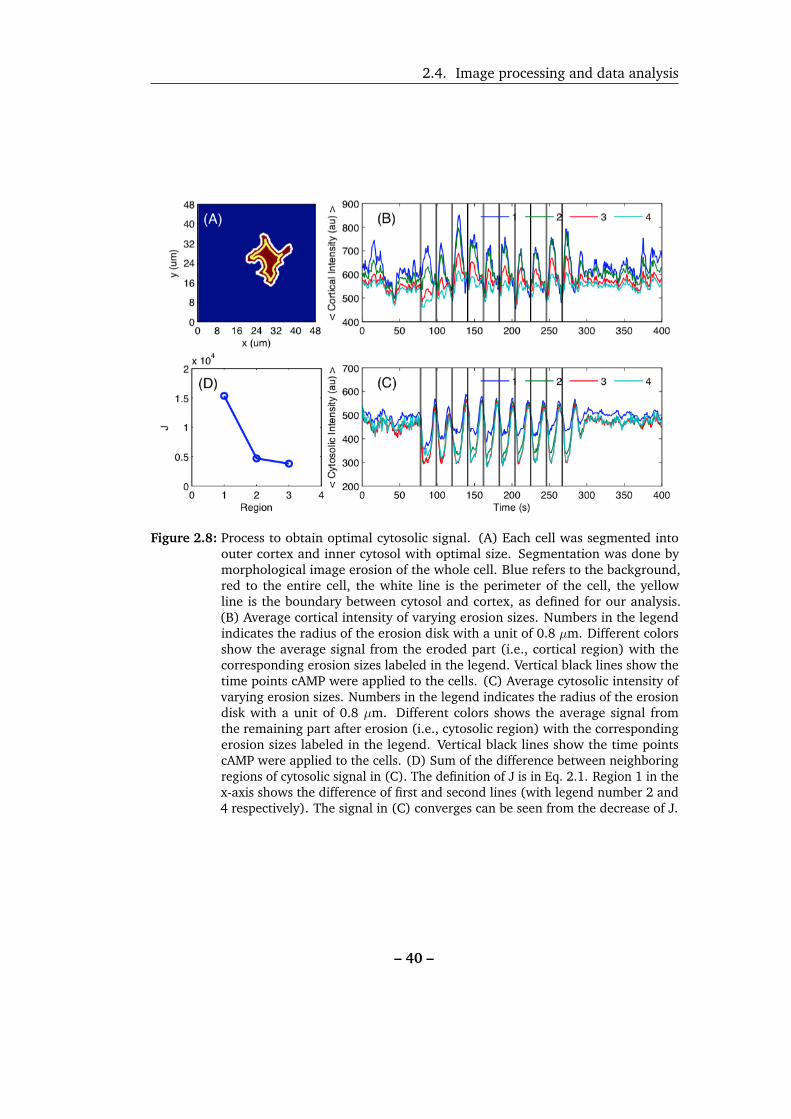
Figures 2.8B and 2.8C show the average intensity of cytosolic and cortical regions
with different size of the erosion disk. The temporal information from different
regions of the cell are independent of the size of the erosion region. The intensity
of the cytosolic signal converged once no cortical signal was included. In order to
quantify the convergence, we calculated:
J =N∑t=1
|(Icytosol(r + 1,t)− Icytosol(r,t))| (2.1)
Icytosol(r,t) is the cytosolic intensity eroded using a disk with radius of r pixels at
frame t and N is the total number of frames recorded. The cytosolic intensity from the
region with minimum value of J (Figures 2.8D) was then chosen for further analysis.
2.4.3 Homogeneous cytosolic signal
Cells usually form localized structures in the cortical region, such as pseudopodia. As
only one focal plane is observed with confocal microscope, usually more pixels are
included in the cytosolic region (compared to the cortical region) and thus lowers
the variability in the extracted structure analysis of cytosolic dynamics. Moreover,
the signal of the cytosol is more homogeneous and thus less sensitive to reactions
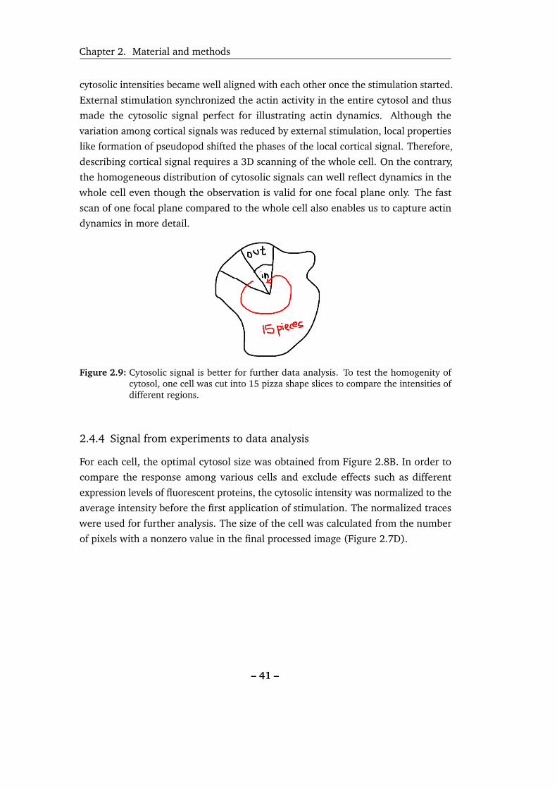
happening in other focal planes. This can be proven by comparing the local intensities
in different regions of cytosol and cortex. The image of one cell was cut into
15 radially extending pieces (Figure 2.9, from here on referenced as pizza pieces) and
the intensity-time traces of cortex and cytosol from different regions were plotted.
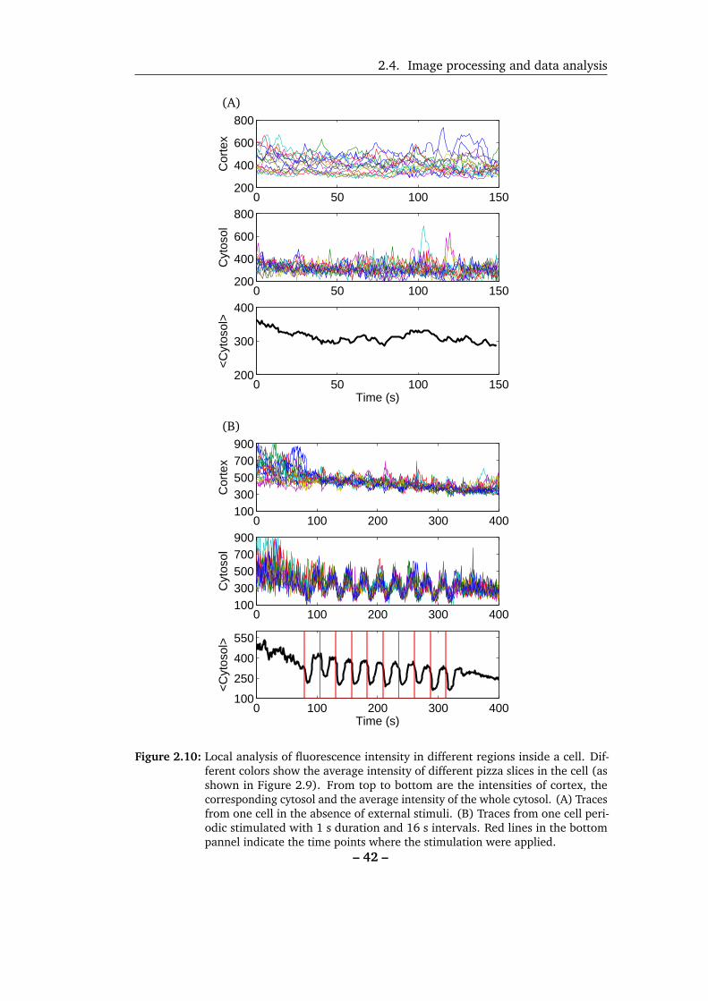
In the absence of external stimulation, the signal from cortex and from cytosol
varied inside the cell (Figure 2.10A) but the variation among different regions of
cytosol was smaller than that of cortex. As one part of our study is to investigate
the cellular responses to external stimulation, we next examined the cytosolic and
cortical signals under external stimulation. Figure 2.10B shows that the overlaid
– 39 –
2.4. Image processing and data analysis
Figure 2.8: Process to obtain optimal cytosolic signal. (A) Each cell was segmented intoouter cortex and inner cytosol with optimal size. Segmentation was done bymorphological image erosion of the whole cell. Blue refers to the background,red to the entire cell, the white line is the perimeter of the cell, the yellowline is the boundary between cytosol and cortex, as defined for our analysis.(B) Average cortical intensity of varying erosion sizes. Numbers in the legendindicates the radius of the erosion disk with a unit of 0.8 µm. Different colorsshow the average signal from the eroded part (i.e., cortical region) with thecorresponding erosion sizes labeled in the legend. Vertical black lines show thetime points cAMP were applied to the cells. (C) Average cytosolic intensity ofvarying erosion sizes. Numbers in the legend indicates the radius of the erosiondisk with a unit of 0.8 µm. Different colors shows the average signal fromthe remaining part after erosion (i.e., cytosolic region) with the correspondingerosion sizes labeled in the legend. Vertical black lines show the time pointscAMP were applied to the cells. (D) Sum of the difference between neighboringregions of cytosolic signal in (C). The definition of J is in Eq. 2.1. Region 1 in thex-axis shows the difference of first and second lines (with legend number 2 and4 respectively). The signal in (C) converges can be seen from the decrease of J.
– 40 –
Chapter 2. Material and methods
cytosolic intensities became well aligned with each other once the stimulation started.
External stimulation synchronized the actin activity in the entire cytosol and thus
made the cytosolic signal perfect for illustrating actin dynamics. Although the
variation among cortical signals was reduced by external stimulation, local properties
like formation of pseudopod shifted the phases of the local cortical signal. Therefore,
describing cortical signal requires a 3D scanning of the whole cell. On the contrary,
the homogeneous distribution of cytosolic signals can well reflect dynamics in the
whole cell even though the observation is valid for one focal plane only. The fast
scan of one focal plane compared to the whole cell also enables us to capture actin
dynamics in more detail.
Figure 2.9: Cytosolic signal is better for further data analysis. To test the homogenity ofcytosol, one cell was cut into 15 pizza shape slices to compare the intensities ofdifferent regions.
2.4.4 Signal from experiments to data analysis
For each cell, the optimal cytosol size was obtained from Figure 2.8B. In order to
compare the response among various cells and exclude effects such as different
expression levels of fluorescent proteins, the cytosolic intensity was normalized to the
average intensity before the first application of stimulation. The normalized traces
were used for further analysis. The size of the cell was calculated from the number
of pixels with a nonzero value in the final processed image (Figure 2.7D).
– 41 –
2.4. Image processing and data analysis
0 50 100 150200
400
600
800
Cor
tex
0 50 100 150200
400
600
800C
ytos
ol
0 50 100 150200
300
400
Time (s)
<C
ytos
ol>
(A)
0 100 200 300 400100300500700900
Cor
tex
0 100 200 300 400100300500700900
Cyt
osol
0 100 200 300 400100
250
400
550
Time (s)
<C
ytos
ol>
(B)
Figure 2.10: Local analysis of fluorescence intensity in different regions inside a cell. Dif-ferent colors show the average intensity of different pizza slices in the cell (asshown in Figure 2.9). From top to bottom are the intensities of cortex, thecorresponding cytosol and the average intensity of the whole cytosol. (A) Tracesfrom one cell in the absence of external stimuli. (B) Traces from one cell peri-odic stimulated with 1 s duration and 16 s intervals. Red lines in the bottompannel indicate the time points where the stimulation were applied.
– 42 –
CHAPTER 3
Self-sustained oscillations
3.1 Motivation
Besides the well known periodic secretion of cAMP [119], it has been reported that
Dictyostelium discoideum cells also show non-random oscillations in various other
components: the key signaling mediators, Phosphatidylinositol 3,4,5-triphosphate,
shape [99, 100], locomotion and pseudopodia dynamics in the absence of cAMP [120].
The time period of these oscillations are in the range of serveal minutes. Recently,
oscillations of actin cytoskeleton in the range of ten seconds were also found in
D. discoideum [109, 110, 117, 121]. As the properties of self-oscillations have not
yet been fully investigated, we characterized the oscillation periods, duration and
occurrence of self-oscillations. Cells with different passage numbers, starvation times
and sizes were also investigated. The aim is to explore the underlying mechanism and
understand if there is any role of the self-oscillations in the life cycle of D. discoideumcells.
3.2 Determining self-oscillations
The occurrence and the disappearance of self-sustained oscillations are unpredictable
and the duration of the oscillations is usually short (less than 5 oscillations). Due to
the intrinsic noise and intensity variations from cell movement, it is very difficult to
determine self-oscillations (Figure 3.1). Here we use an autocorrelation function to
remove uncorrelated noise sources and characterize the oscillation periods. If the
cytoskeleton shows more than two regular oscillations in the absence of chemoattrac-
tant stimulation, we call it self-sustained oscillation or self-oscillation. Considering
the fact that the oscillation periods range from 8 s to 22 s [109, 110, 117, 121] and
– 43 –

3.2. Determining self-oscillations
0 50 100 150 200−200
0
200
Inte
nsity
0 50 100 150 200−200
0
200
Inte
nsity
0 50 100 150 200−100
0
100
Inte
nsity
Time (s)
Figure 3.1: Examples of cytosolic intensity of three different cells in the absence of externalstimulaion.
the definition of autonomous oscillations requires more than 2 oscillations, a fixed
window with a length of 60 s was used to run autocorrelation. The fixed window
was slid across the data to find the autocorrelation at different time. As sudden
changes in phase or frequency of the signals affect the analysis of autocorrelation,
to run autocorrelation with a fixed length of the window (which is shorter than
the whole observation time) not only reduces this effect in the unpredictable signal
of self-oscillations but also allows reliable comparison between different cells and
different observation times. Figure 3.2A & 3.2F shows that this method can capture
the oscillation periods of regular oscillations (red and green traces) and distinguish
the traces without oscillations (blue trace), suggesting that the autocorrelation with
fixed-size window can reveal the varying properties of the oscillations.
The autocorrelation function from the fixed window was considered to be a
regular oscillation only when it satisfied the following conditions: first, the amplitude
difference of neighboring peaks and valleys was larger than 0.02. Second, the
variation of the time differences between peaks (i.e. detected oscillation period) was
less than 2 s. Finally, at least two continuous and regular oscillations were detected.
– 44 –

Chapter 3. Self-sustained oscillations
0 50 100 150 200150
200
250
300
350
400
Time (s)
Inte
nsity
(A)
0 10 20 30 40 50 60
−0.5
0
0.5
1
Time (s)
Aut
oCor
rela
tion
(F)
0 50 100 150 200150
200
250
300
350
400
450
Time (s)
Inte
nsity
(B)
0 10 20 30 40 50 60−0.5
0
0.5
1
Time (s)A
utoC
orre
latio
n
(G)
0 50 100 150 200150
200
250
300
350
400
Time (s)
Inte
nsity
(C)
0 10 20 30 40 50 60−0.2
0
0.2
0.4
0.6
0.8
1
Time (s)
Aut
oCor
rela
tion
(H)
0 50 100 150 200200
250
300
350
400
450
500
Time (s)
Inte
nsity
(D)
0 10 20 30 40 50 60
−0.5
0
0.5
1
Time (s)
Aut
oCor
rela
tion
(I)
0 50 100 150 200 250 300150
200
250
300
350
400
450
500
Time (s)
Inte
nsity
(E)
0 10 20 30 40 50 60−0.5
0
0.5
1
Time (s)
Aut
oCor
rela
tion
(J)
Figure 3.2: Autocorrelation with fixed-size window can reveal the varying properties ofthe oscilations. (A–E) Examples of different traces of cytosolic signal. (F–J) Autocorrelation analysis. Different colors show the autocorrelation function ofthe corresponding colored part in the figure of its left hand side. The peaks aremarked when the criteria of regular oscillations are met.
– 45 –

3.2. Determining self-oscillations
0 50 100 150 2000
200
400
600
800
1000
Time (s)
Cor
tex
(A)
0 50 100 150 2000
100
200
300
400
500
Time (s)
Cyt
osol
(C)
0 50 100 150 200100
200
300
400
Time (s)
<C
ytos
ol>
(D)
0 50 100 150 200300
400
500
600
700
Time (s)
<C
orte
x>
(B)
0 100 200 300 400300
500
700
900
1100
Time (s)
Cor
tex
(E)
0 100 200 300 400200
350
500
650
800
Time (s)
Cyt
osol
(F)
0 100 200 300 400200
300
400
500
600
Time (s)
<C
ytos
ol>
(H)
0 100 200 300 400400
500
600
700
Time (s)
<C
orte
x>
(G)
Figure 3.3: Self-oscillating cells are synchronized as cells respond to uniform stimulation.(A)–(D) Intensity analysis of one cell in the absence of external stimulation.(A) Cortical intensity of different regions inside the cell. Different colors showthe average intensity of the cortical region in one pizza piece (as described inFigure 2.9). (B) Intensity average over the whole cortex of the cell. (C) Cytosolicintensity of different regions inside the cell. Different colors show the corre-sponding intensity of the cytosolic region as in (A). (D) Intensity average overthe whole cytosol of the cell. (E)–(H) Intensity analysis of one cell in response touniform and periodic external stimuli (each stimulus lasted 1 s and the intervalbetween two stimuli was 21 s). (E) Cortical intensity of different regions insidethe cell. Different colors show the average intensity of the cortical region inone pizza piece. External stimulations were omitted for better visualization.(F) Cytosolic intensity of different regions inside the cell. Different colors showthe corresponding intensity of the cytosolic region as in (E). External stimulationwere omitted for better visualization. (G) Cortical intensity average over thewhole cortex of the cell. Red vertical lines indicate the time when cAMP wasapplied. (H) Cytosolic intensity average over the whole cytosol of the cell. Redlines indicate the time when cAMP was applied.
– 46 –
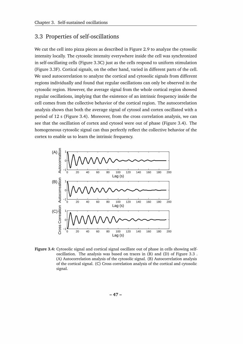
Chapter 3. Self-sustained oscillations
3.3 Properties of self-oscillations
We cut the cell into pizza pieces as described in Figure 2.9 to analyze the cytosolic
intensity locally. The cytosolic intensity everywhere inside the cell was synchronized
in self-oscillating cells (Figure 3.3C) just as the cells respond to uniform stimulation
(Figure 3.3F). Cortical signals, on the other hand, varied in different parts of the cell.
We used autocorrelation to analyze the cortical and cytosolic signals from different
regions individually and found that regular oscillations can only be observed in the
cytosolic region. However, the average signal from the whole cortical region showed
regular oscillations, implying that the existence of an intrinsic frequency inside the
cell comes from the collective behavior of the cortical region. The autocorrelation
analysis shows that both the average signal of cytosol and cortex oscillated with a
period of 12 s (Figure 3.4). Moreover, from the cross correlation analysis, we can
see that the oscillation of cortex and cytosol were out of phase (Figure 3.4). The
homogeneous cytosolic signal can thus perfectly reflect the collective behavior of the
cortex to enable us to learn the intrinsic frequency.
0 20 40 60 80 100 120 140 160 180 200−1
0
1
Lag (s)
Aut
ocor
real
tion
(A)
0 20 40 60 80 100 120 140 160 180 200−1
0
1
Lag (s)
Aut
ocor
real
tion
(B)
0 20 40 60 80 100 120 140 160 180 200−1
0
1
Lag (s)Cro
ss C
orre
altio
n
(C)
Figure 3.4: Cytosolic signal and cortical signal oscillate out of phase in cells showing self-oscillation. The analysis was based on traces in (B) and (D) of Figure 3.3 .(A) Autocorrelation analysis of the cytosolic signal. (B) Autocorrelation analysisof the cortical signal. (C) Cross correlation analysis of the cortical and cytosolicsignal.
– 47 –
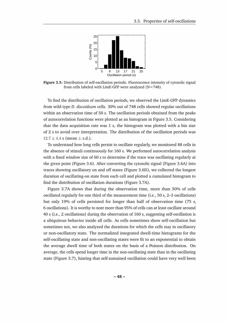
3.3. Properties of self-oscillations
5 9 13 17 21 250
5
10
15
20
25
Cou
nts
(%)
Oscillation period (s)
Figure 3.5: Distribution of self-oscillation periods. Fluorescence intensity of cytosolic signalfrom cells labeled with LimE-GFP were analyzed (N=748).
To find the distribution of oscillation periods, we observed the LimE-GFP dynamics
from wild-type D. discoideum cells. 30% out of 748 cells showed regular oscillations
within an observation time of 50 s. The oscillation periods obtained from the peaks
of autocorrelation functions were plotted as an histogram in Figure 3.5. Considering
that the data acquisition rate was 1 s, the histogram was plotted with a bin size
of 2 s to avoid over interpretation. The distribution of the oscillation periods was
12.7± 4.4 s (mean ± s.d.).
To understand how long cells persist to oscillate regularly, we monitored 88 cells in
the absence of stimuli continuously for 160 s. We performed autocorrelation analysis
with a fixed window size of 60 s to determine if the trace was oscillating regularly at
the given point (Figure 3.6). After converting the cytosolic signal (Figure 3.6A) into
traces showing oscillatory on and off states (Figure 3.6D), we collected the longest
duration of oscillating-on state from each cell and plotted a cumulated histogram to
find the distribution of oscillation durations (Figure 3.7A).
Figure 3.7A shows that during the observation time, more than 50% of cells
oscillated regularly for one third of the measurement time (i.e., 50 s, 2–3 oscillations)
but only 19% of cells persisted for longer than half of observation time (75 s,
6 oscillations). It is worthy to note more than 95% of cells can at least oscillate around
40 s (i.e., 2 oscillations) during the observation of 160 s, suggesting self-oscillation is
a ubiquitous behavior inside all cells. As cells sometimes show self-oscillation but
sometimes not, we also analyzed the durations for which the cells stay in oscillatory
or non-oscillatory state. The normalized integrated dwell-time histograms for the
self-oscillating state and non-oscillating states were fit to an exponential to obtain
the average dwell time of both states on the basis of a Poisson distribution. On
average, the cells spend longer time in the non-oscillating state than in the oscillating
state (Figure 3.7), hinting that self-sustained oscillation could have very well been
– 48 –
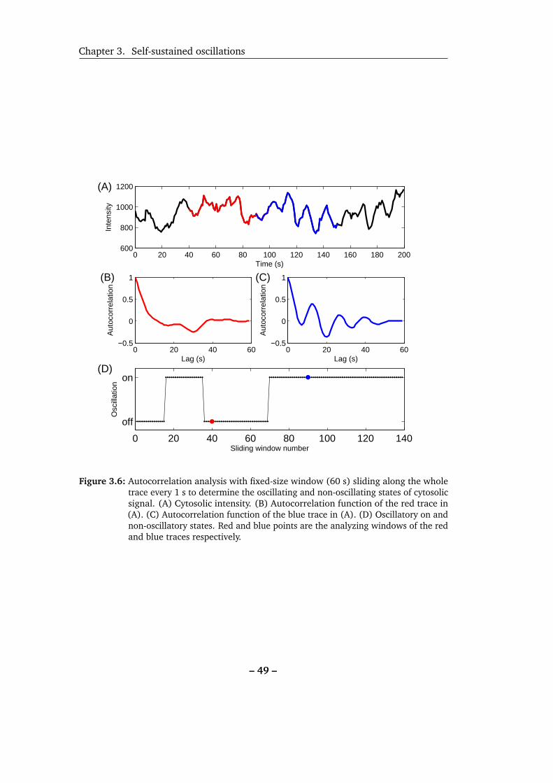
Chapter 3. Self-sustained oscillations
0 20 40 60 80 100 120 140 160 180 200600
800
1000
1200
Time (s)
Inte
nsity
(A)
0 20 40 60 80 100 120 140
off
on
Sliding window number
Osc
illat
ion
(D)
0 20 40 60−0.5
0
0.5
1
Lag (s)
Aut
ocor
rela
tion
(B)
0 20 40 60−0.5
0
0.5
1
Lag (s)
Aut
ocor
rela
tion
(C)
Figure 3.6: Autocorrelation analysis with fixed-size window (60 s) sliding along the wholetrace every 1 s to determine the oscillating and non-oscillating states of cytosolicsignal. (A) Cytosolic intensity. (B) Autocorrelation function of the red trace in(A). (C) Autocorrelation function of the blue trace in (A). (D) Oscillatory on andnon-oscillatory states. Red and blue points are the analyzing windows of the redand blue traces respectively.
– 49 –
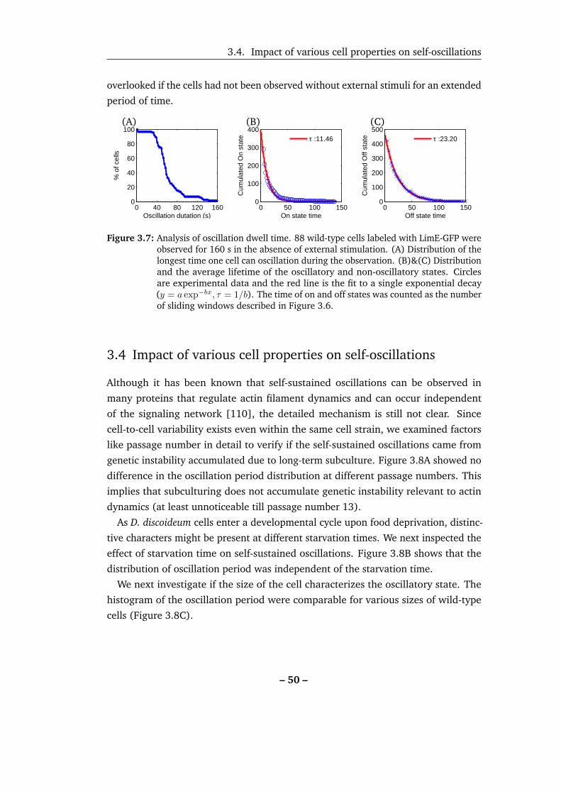
3.4. Impact of various cell properties on self-oscillations
overlooked if the cells had not been observed without external stimuli for an extended
period of time.
0 40 80 120 1600
20
40
60
80
100
% o
f cel
ls
Oscillation dutation (s)
(A)
0 50 100 1500
100
200
300
400
On state time
Cum
ulat
ed O
n st
ate
τ :11.46
(B)
0 50 100 1500
100
200
300
400
500
Off state time
Cum
ulat
ed O
ff st
ate
τ :23.20
(C)
Figure 3.7: Analysis of oscillation dwell time. 88 wild-type cells labeled with LimE-GFP wereobserved for 160 s in the absence of external stimulation. (A) Distribution of thelongest time one cell can oscillation during the observation. (B)&(C) Distributionand the average lifetime of the oscillatory and non-oscillatory states. Circlesare experimental data and the red line is the fit to a single exponential decay(y = a exp−bx, τ = 1/b). The time of on and off states was counted as the numberof sliding windows described in Figure 3.6.
3.4 Impact of various cell properties on self-oscillations
Although it has been known that self-sustained oscillations can be observed in
many proteins that regulate actin filament dynamics and can occur independent
of the signaling network [110], the detailed mechanism is still not clear. Since
cell-to-cell variability exists even within the same cell strain, we examined factors
like passage number in detail to verify if the self-sustained oscillations came from
genetic instability accumulated due to long-term subculture. Figure 3.8A showed no
difference in the oscillation period distribution at different passage numbers. This
implies that subculturing does not accumulate genetic instability relevant to actin
dynamics (at least unnoticeable till passage number 13).
As D. discoideum cells enter a developmental cycle upon food deprivation, distinc-
tive characters might be present at different starvation times. We next inspected the
effect of starvation time on self-sustained oscillations. Figure 3.8B shows that the
distribution of oscillation period was independent of the starvation time.
We next investigate if the size of the cell characterizes the oscillatory state. The
histogram of the oscillation period were comparable for various sizes of wild-type
cells (Figure 3.8C).
– 50 –

Chapter 3. Self-sustained oscillations
0 5 10 15 20 25 300
10
20
30
40
50
Cou
nts
(%)
Oscillation Period (s)
Passage # 1, N = 25Passage # 2, N = 190Passage # 3, N = 30Passage # 4, N = 41Passage # 5, N = 43Passage # 8, N = 112Passage # 12, N = 147Passage # 13, N = 124
(A)
0 5 10 15 20 25 300
10
20
30
40
Cou
nts
(%)
Oscillation Period (s)
Starve:4−5 hr, N = 14Starve:5−6 hr, N = 66Starve:6−7 hr, N = 178Starve:7−8 hr, N = 262Starve:8−9 hr, N = 152Starve:9−10 hr, N = 41
(B)
0 5 10 15 20 25 300
20
40
60
80
Cou
nts
(%)
Oscillation Period (s)
0−69 µm2, N = 27
69−137 µm2, N = 272
137−206 µm2, N = 258
206−274 µm2, N = 96
274−343 µm2, N = 32
411−480 µm2, N = 8
480−548 µm2, N = 3
(C)
Figure 3.8: Impact of different passage numbers, starvation times and cell sizes in thedistribution of self-oscillations. Legend shows the number of cells under differentcondition. (A) Distribution of oscillation period for self-oscillating cells withdifferent passage numbers, (B) different starvation times and (C) with differentcell sizes.
– 51 –
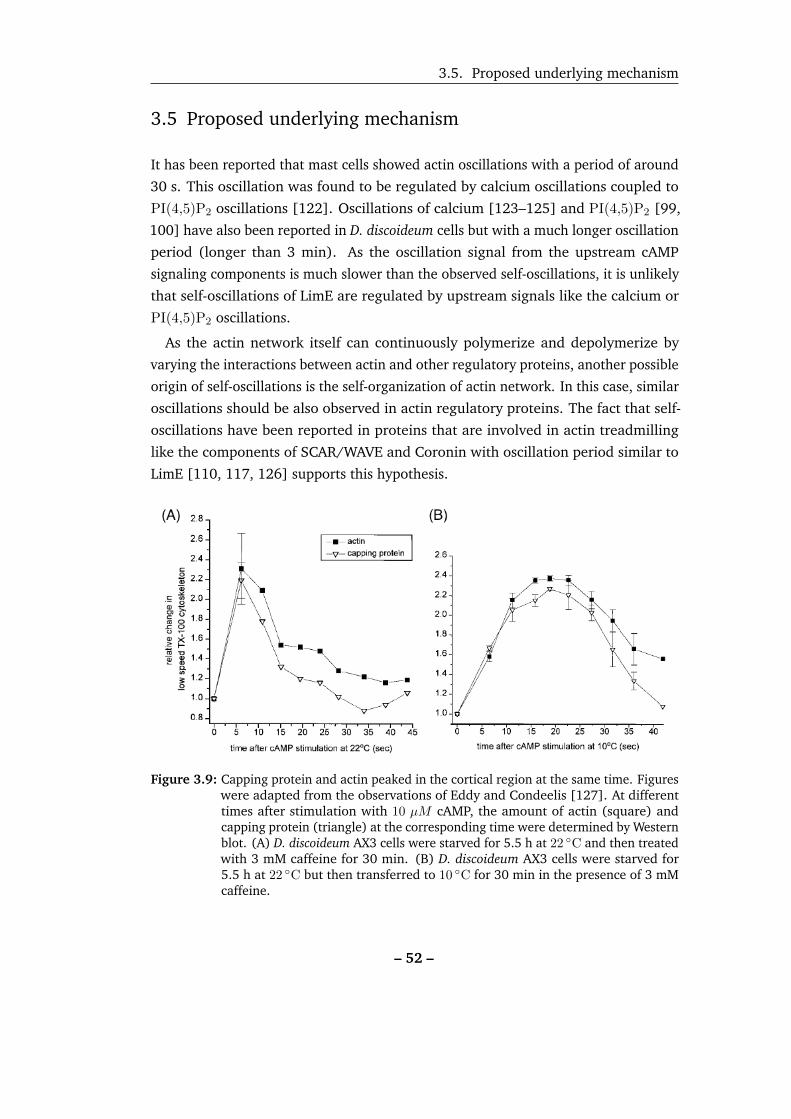
3.5. Proposed underlying mechanism
3.5 Proposed underlying mechanism
It has been reported that mast cells showed actin oscillations with a period of around
30 s. This oscillation was found to be regulated by calcium oscillations coupled to
PI(4,5)P2 oscillations [122]. Oscillations of calcium [123–125] and PI(4,5)P2 [99,
100] have also been reported in D. discoideum cells but with a much longer oscillation
period (longer than 3 min). As the oscillation signal from the upstream cAMP
signaling components is much slower than the observed self-oscillations, it is unlikely
that self-oscillations of LimE are regulated by upstream signals like the calcium or
PI(4,5)P2 oscillations.
As the actin network itself can continuously polymerize and depolymerize by
varying the interactions between actin and other regulatory proteins, another possible
origin of self-oscillations is the self-organization of actin network. In this case, similar
oscillations should be also observed in actin regulatory proteins. The fact that self-
oscillations have been reported in proteins that are involved in actin treadmilling
like the components of SCAR/WAVE and Coronin with oscillation period similar to
LimE [110, 117, 126] supports this hypothesis.
Figure 3.9: Capping protein and actin peaked in the cortical region at the same time. Figureswere adapted from the observations of Eddy and Condeelis [127]. At differenttimes after stimulation with 10 µM cAMP, the amount of actin (square) andcapping protein (triangle) at the corresponding time were determined by Westernblot. (A) D. discoideum AX3 cells were starved for 5.5 h at 22 ◦C and then treatedwith 3 mM caffeine for 30 min. (B) D. discoideum AX3 cells were starved for5.5 h at 22 ◦C but then transferred to 10 ◦C for 30 min in the presence of 3 mMcaffeine.
– 52 –
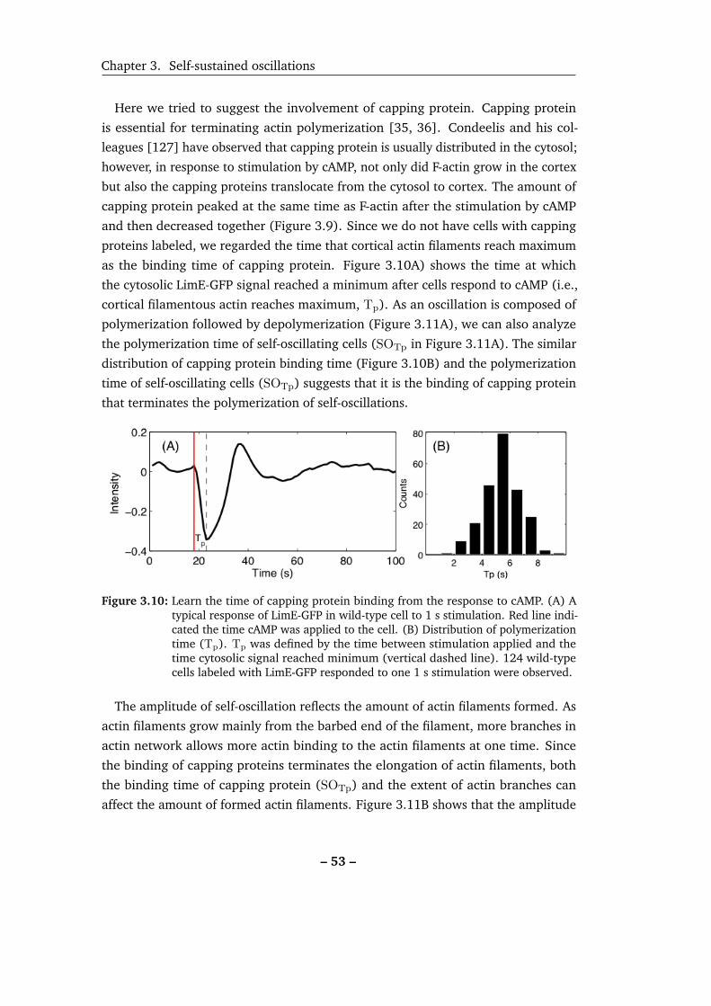
Chapter 3. Self-sustained oscillations
Here we tried to suggest the involvement of capping protein. Capping protein
is essential for terminating actin polymerization [35, 36]. Condeelis and his col-
leagues [127] have observed that capping protein is usually distributed in the cytosol;
however, in response to stimulation by cAMP, not only did F-actin grow in the cortex
but also the capping proteins translocate from the cytosol to cortex. The amount of
capping protein peaked at the same time as F-actin after the stimulation by cAMP
and then decreased together (Figure 3.9). Since we do not have cells with capping
proteins labeled, we regarded the time that cortical actin filaments reach maximum
as the binding time of capping protein. Figure 3.10A) shows the time at which
the cytosolic LimE-GFP signal reached a minimum after cells respond to cAMP (i.e.,
cortical filamentous actin reaches maximum, Tp). As an oscillation is composed of
polymerization followed by depolymerization (Figure 3.11A), we can also analyze
the polymerization time of self-oscillating cells (SOTp in Figure 3.11A). The similar
distribution of capping protein binding time (Figure 3.10B) and the polymerization
time of self-oscillating cells (SOTp) suggests that it is the binding of capping protein
that terminates the polymerization of self-oscillations.
Figure 3.10: Learn the time of capping protein binding from the response to cAMP. (A) Atypical response of LimE-GFP in wild-type cell to 1 s stimulation. Red line indi-cated the time cAMP was applied to the cell. (B) Distribution of polymerizationtime (Tp). Tp was defined by the time between stimulation applied and thetime cytosolic signal reached minimum (vertical dashed line). 124 wild-typecells labeled with LimE-GFP responded to one 1 s stimulation were observed.
The amplitude of self-oscillation reflects the amount of actin filaments formed. As
actin filaments grow mainly from the barbed end of the filament, more branches in
actin network allows more actin binding to the actin filaments at one time. Since
the binding of capping proteins terminates the elongation of actin filaments, both
the binding time of capping protein (SOTp) and the extent of actin branches can
affect the amount of formed actin filaments. Figure 3.11B shows that the amplitude
– 53 –

3.6. Pseudopod formation and self-oscillations
of self-oscillation is not related to the amount of Arp2/3, the main protein that
enabling branches formation. Considering the fact that SCAR/WAVE, the main
protein that activates Arp2/3, is activated through external stimulation [128–131],
it is possible that only few active Arp2/3 in cells in the absence of external stimuli
and thus shows no effect on the formation of actin filaments. This is confirmed by
comparing the amount of Arp2/3 translocate to the cortical region in the presence
and absence of stimulation (Figure 3.12). On the other hand, the binding time of
capping proteins controls the amount of actin formation: the later the binding of
capping proteins occurs (larger SOTp), the longer the actin filaments can grow (larger
PAmp, Figure 3.11B). Due to the fact that depolymerization can only initiate from the
pointed end of actin filament, longer filaments requires longer time to depolymerize,
as seen by Figure 3.11E. As an oscillation is composed of polymerization followed
by depolymerization (Figure 3.11A), it is the binding time of capping protein that
determines the frequency of self-oscillation.
It is worthy to note that the distribution of polymerization (SOTp) and depolymer-
ization times (SOTd) are indistinguishable (D and F in Figure 3.11), suggesting that
the traces of self-oscillation were very symmetric.
3.6 Pseudopod formation and self-oscillations
Different time scales have been observed in D. discoideum before: adenylate cyclase
produces cAMP every 6 min, phosphatase and tensin homolog (PTEN) periodically
oscillate out of phase with phosphoinositide-3-kinase (PI3K) with a period around
200 s. Pseudopod grows with a period of around 12 s [101]. The recent observations
of rapid oscillations in the cytoskeleton network have a period around 10 s [109, 110,
117]. Although the time scale of this rapid oscillation is close to that of pseudopod
growth, the link between self-oscillations and pseudopod formation is still unclear.
Based on previous studies, we know that the growth period of a pseudopod [101]
is comparable with the period of self-oscillation. Secondly, Van Haastert and his
colleagues found that D. discoideum cells formed pseudopod with the same frequency
at different starvation times [132]. Thirdly, cells lacking myosin II, moved less
efficiently toward cAMP because myosin II is essential for inhibiting lateral protrusions
to polarize the cell and enables persistent directional movement. However, cells were
still able to extend pseudopod or ruffled membranes even without myosin II [133–
136].
– 54 –

Chapter 3. Self-sustained oscillations
2 4 6 80
0.1
0.2
0.3
SOTp
(s)
PA
mp
(C)
2 4 6 80
10
20
30C
ount
s (%
)
SOTp
(s)
(D)
2 4 6 80
0.1
0.2
0.3
SOTd
(s)
DA
mp
(E)
2 4 6 80
10
20
30
Cou
nts
(%)
SOTd
(s)
(F)
SOTp
SOTd
PAmp
DAmp
Time
Inte
nsity
(A)
0.02 0.04 0.06 0.08 0.10
0.01
0.02
0.03
0.04
Am
p of
Arp
3
Amp of LimE
(B)
Figure 3.11: Self-oscillating signals show symmetric oscillations. 266 self-oscillating wild-type cells labeled with LimE-GFP were observed in the absence of externalstimulation. SO stands for self-oscillation. (A) Definition of polymerizationtime (SOTp), polymerization amplitude (PAmp), depolymerization time (SOTd)and depolymerization amplitude (DAmp). (B) Amp from self-oscillating cellsco-express Arp3-GFP and LimE-mRFP. Each red dot shows the analysis fromone self-oscillating cell. (C) SOTp v.s. PAmp. Each dot shows the average SOTp
and PAmp from one cell. (D) The distribution of SOTp. (E) SOTd v.s. DAmp.Each dot shows the average SOTd and DAmp from one cell. (F) The distributionof SOTd.
– 55 –
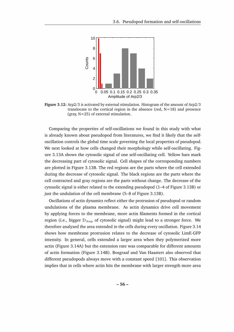
3.6. Pseudopod formation and self-oscillations
0 0.05 0.1 0.15 0.2 0.25 0.3 0.350
2
4
6
8
10
Amplitude of Arp2/3
Cou
nts
Figure 3.12: Arp2/3 is activated by external stimulation. Histogram of the amount of Arp2/3translocate to the cortical region in the absence (red, N=18) and presence(gray, N=25) of external stimulation.
Comparing the properties of self-oscillations we found in this study with what
is already known about pseudopod from literatures, we find it likely that the self-
oscillation controls the global time scale governing the local properties of pseudopod.
We next looked at how cells changed their morphology while self-oscillating. Fig-
ure 3.13A shows the cytosolic signal of one self-oscillating cell. Yellow bars mark
the decreasing part of cytosolic signal. Cell shapes of the corresponding numbers
are plotted in Figure 3.13B. The red regions are the parts where the cell extended
during the decrease of cytosolic signal. The black regions are the parts where the
cell contracted and gray regions are the parts without change. The decrease of the
cytosolic signal is either related to the extending pseudopod (1–4 of Figure 3.13B) or
just the undulation of the cell membrane (5–8 of Figure 3.13B).
Oscillations of actin dynamics reflect either the protrusion of pseudopod or random
undulations of the plasma membrane. As actin dynamics drive cell movement
by applying forces to the membrane, more actin filaments formed in the cortical
region (i.e., bigger DAmp of cytosolic signal) might lead to a stronger force. We
therefore analyzed the area extended in the cells during every oscillation. Figure 3.14
shows how membrane protrusion relates to the decrease of cytosolic LimE-GFP
intensity. In general, cells extended a larger area when they polymerized more
actin (Figure 3.14A) but the extension rate was comparable for different amounts
of actin formation (Figure 3.14B). Bosgraaf and Van Haastert also observed that
different pseudopods always move with a constant speed [101]. This observation
implies that in cells where actin hits the membrane with larger strength more area
– 56 –
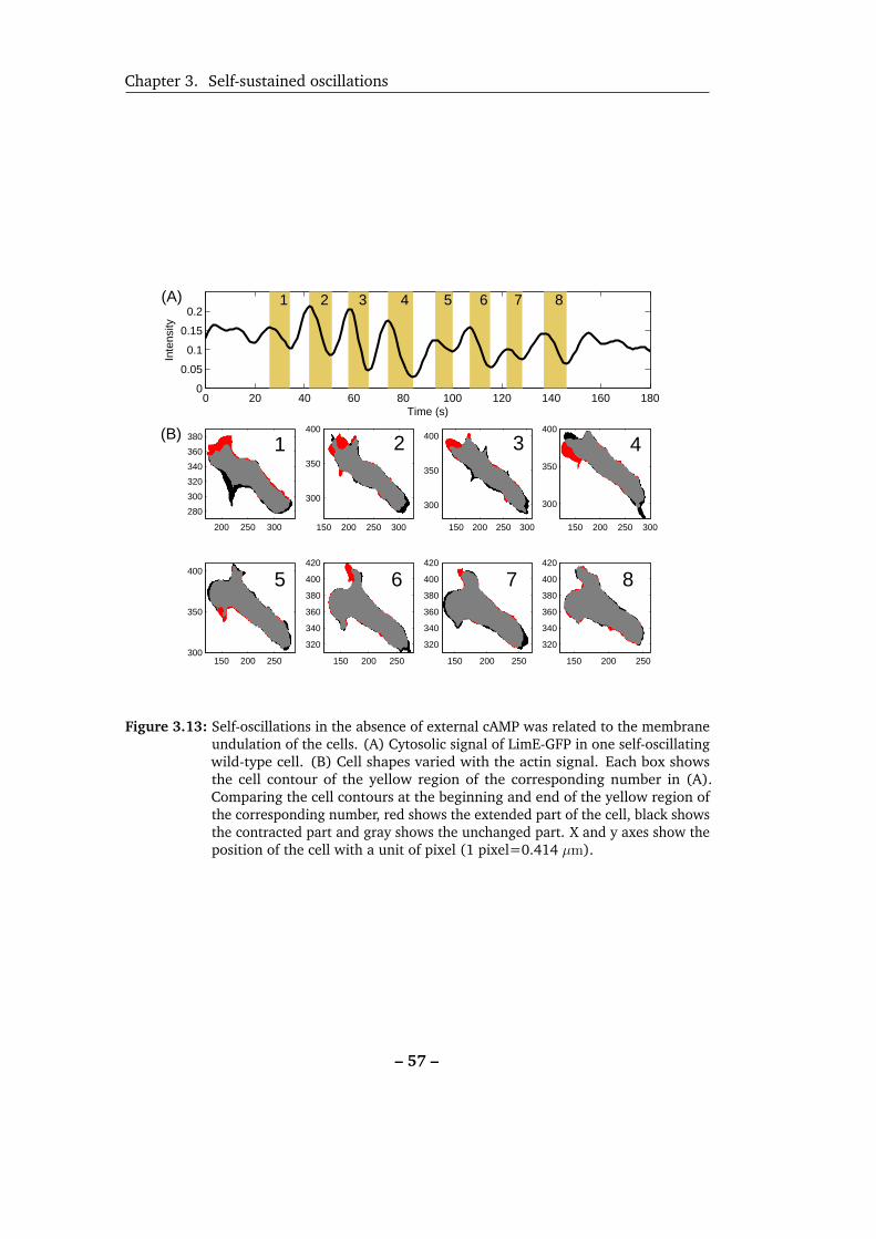
Chapter 3. Self-sustained oscillations
1(B)
200 250 300
280
300
320
340
360
380 2
150 200 250 300
300
350
400
3
150 200 250 300
300
350
4004
150 200 250 300
300
350
400
5
150 200 250300
350
4006
150 200 250
320
340
360
380
400
420
7
150 200 250
320
340
360
380
400
420
8
150 200 250
320
340
360
380
400
420
0 20 40 60 80 100 120 140 160 1800
0.05
0.1
0.15
0.21 2 3 4 5 6 7 8
Time (s)
Inte
nsity
(A)
Figure 3.13: Self-oscillations in the absence of external cAMP was related to the membraneundulation of the cells. (A) Cytosolic signal of LimE-GFP in one self-oscillatingwild-type cell. (B) Cell shapes varied with the actin signal. Each box showsthe cell contour of the yellow region of the corresponding number in (A).Comparing the cell contours at the beginning and end of the yellow region ofthe corresponding number, red shows the extended part of the cell, black showsthe contracted part and gray shows the unchanged part. X and y axes show theposition of the cell with a unit of pixel (1 pixel=0.414 µm).
– 57 –

3.6. Pseudopod formation and self-oscillations
is protruded but then actin hits the membrane less often. The frequency of hitting
the membrane was controlled by the fact that it takes longer to depolymerize more
actin filament (Figure 3.11D). Therefore, by simply manipulating the polymerization
and depolymerization, the self-organization of the actin network might result in a
constant extension rate of pseudopod to explore the surrounding for food during
starvation.
0 0.1 0.2 0.30
5
10
15
20
25
30
35
DAmp
Ext
ende
d A
rea
(% c
ell s
ize) (A)
0 0.1 0.2 0.3 0.4−1
0
1
2
3
4
5
DAmp
Ext
ende
d R
ate
(% c
ell s
ize/
s)
(B)
Figure 3.14: D. discoideum cells show constant protrusion rate. 266 self-oscillating wild-type cells labeled with LimE-GFP were observed in the absence of externalstimulation. (A) Extended area during the depolymerization time of oneoscillation was plotted against the corresponding depolymerization amplitude(DAmp). (B) Extension rates at different DAmp. Extension rates were calculatedby dividing depolymerization time (SOTd in Figure 3.11) into the correspondingextended area (Extended area in (A)).
However, by looking at only one focal plane, we lost the three dimensional in-
formation of pseudopods. The correlation between area and response amplitude
(Figure 3.14A) was thus not as obvious as the amplitude-time relation observed in
Figure 3.11D. A clearer trend might be found in experiments that can better capture
pseudopod dynamics, like scanning the whole cell faster in 3D or using microfluidic
techniques to flatten cells into a two dimensional plane [137].
– 58 –

Chapter 3. Self-sustained oscillations
3.7 Conclusion
In this study, we examined the properties of self-oscillations: by systematically
examining the oscillation period of more than 700 cells, we first confirmed that
the distribution of the self-oscillation period peaks around 12 s (Figure 3.5). As
asynchronous signals average each other out, we can describe the properties of
the oscillations only when the whole actin network is synchronized. This intrinsic
frequency governing the actin dynamics and its property is robust; cells with different
passage numbers, starvation times and different sizes oscillate with similar periods.
This oscillation relates either to the local protrusions of pseudopods for directional
movement or to the formation of patches for membrane undulations. By considering
the roles of proteins regulating the actin network, we concluded that (i) the frequency
of self-oscillations are determined by the binding time of capping proteins, (ii) the
binding time of capping proteins determines the amplitude of self-oscillations, and
(iii) the amplitude controls the following depolymerization time.
Considering the facts that oscillatory and non-oscillatory states alternated inside
every cell and that the oscillation amplitude and frequency vary with time, it is
possible that the self-oscillation is just a consequence of random synchronization of
many local oscillators inside a cell. It has been reported that oscillations at different
spots (local oscillators) within the same cell could oscillate with a phase shift or
different frequencies [110]. This observation is consistent with Figure 3.3B, which
shows that self-oscillations originate from the collective behavior of the whole actin
network. Taken together, the self-oscillations just reflect the synchronization of rapid
turnover in the self-organized cytoskeletal network.
– 59 –
CHAPTER 4
Actin dynamics is stimulation strength dependent
4.1 Motivation
In the previous chapter, we learned the dynamics of filamentous actin in the absence
of external stimulation. Careful analysis showed that the intrinsic oscillation period
centered around 12.7 s with a standard deviation of about 4.5 s (Figure 3.5). The
oscillations show the same time scale as the rapid oscillations of cytoskeletal network
observed in [110]. Westendorf et al., found a resonance peak at 20 s when they
stimulated the cells periodically [109]. The resonance period is close but does not
coincide with the intrinsic oscillation period of self-oscillations. It is still unknown if
this difference is significant. Is this a reasonable error based on cell-to-cell variability
or are there other controlling mechanisms?
The key to link the two time scales relies on experiments that can observe the
transition of actin dynamics from self-oscillation to controlled cAMP response. D. dis-coideum cells were starved to become chemotatic so that cAMP can be used as
chemoattractant. To have precise control of the application of cAMP, we com-
bined photolysis with microfluidics: a caged cAMP compound was continuously
flowed into the microfluidic channel, as described in chapter 3. We visualized the
dynamical behavior of the actin cytoskeleton by expressing fluorescently tagged
LimE∆coil (LimE-GFP), which is known to co-localize with freshly polymerized actin
filaments [80, 138]. By comparing the responses before and after the application of
stimuli, we learn not only how the external stimuli change the self-oscillations but
also how self-oscillations affect the responses to cAMP stimulation.
– 60 –

Chapter 4. Actin dynamics is stimulation strength dependent
Figure 4.1: Effects of self-oscillations on actin dynamics in response to a single 1 s stimulation.LimE-GFP signal from wild-type cells were observed. Vertical red line marks thetime of cAMP application. Tp was defined as the time between the stimulationapplied (i.e., vertical red lines) and the intensity reached minimum (i.e., verticaldashed lines). Td was defined as the time between the minimum (valley, alsoindicated by vertical dashed lines) and the maximum (peak) of cytosolic intensity.Amp was defined as the corresponding intensity difference. Tr was defined asthe time starting from the maximum (peak) to the rest of the response. (A) Anexemplary response of cells without self-oscillation before stimulation. (B) Anexemplary response of cells showing self-oscillations before stimulation. (C)–(E) Histograms of analysis of Amp, Tp and Td from cells that did not showoscillations 50 s before stimulation. (F)–(H) Histograms of analysis of Amp, Tp
and Td from cells showing oscillations 50 s before stimulation..
– 61 –
4.2. Responses of self-oscillating cells to external stimuli
4.2 Responses of self-oscillating cells to external stimuli
The sensing of cAMP initiates a large amount of actin filaments formation everywhere
in the cortical region of D. discoideum cells, resulting in a depletion in the cytosolic
signal. The following excessive disassembly of actin filaments brings the system
back to the basal state (Figure 4.1A). To investigate the influence of the existence of
self-oscillation on cAMP responses, we analyzed the responses to stimulation from
all cells and examined if the response dynamics depends on whether or not the
cells were self-oscillating before stimulation. Considering the fact that the response
after stimulation is composed of polymerization, depolymerization and final recovery,
the response dynamics was dissected into three successive intervals (Figure 4.1A):
Tp (where polymerization dominates), Td (where depolymerization dominates)
and Tr (the remaining relaxation time). Since the signal becomes unrecognizable
after the depolymerization dominated region, we will focus on Tp and Td. The
amplitude (Amp), defined as the difference between the maximum and minimum of
the cytosolic signal, will also be investigated to know the amount of depolymerized
actin. Figure 4.1C–4.1E shows the analysis for the cells that did not self-oscillate
50 s before stimulation was applied and F–H shows the analysis for the cells that
oscillated regularly 50 s before stimulation. Self-oscillations seems to have no impact
on the actin dynamics of cAMP responses.
To gain further insight into the influence of stimulation on the occurrence of self-
oscillations, we applied periodic stimuli to self-oscillating cells. Figure 4.2 shows
that the external stimulation always immediately replaced the rhythm of the self-
oscillating cell. This property was independent of myosin II. Self-oscillations of cells
genetically lacking myosin II were also replaced by cAMP responses immediately
after the stimulation of cAMP. Cells can re-establish self-oscillation once the impact
of stimulation is gone (Figure 4.2C). However, external stimuli can neither eliminate
nor trigger the occurrence of self-oscillation: after 10 pulses of periodic stimuli,
self-oscillations of cells can either be restored (Figure 4.2D) or stopped (Figure 4.2B)
whereas non-self-oscillating cells can either remain non-oscillating (Figure 4.2A) or
begin to oscillate (Figure 4.2C).
– 62 –

Chapter 4. Actin dynamics is stimulation strength dependent
0 50 100 150 200 250 300 350−0.5
−0.25
0
0.25
0.5(A)
Inte
nsity
0 50 100 150 200 250 300 350−0.5
−0.25
0
0.25
0.5(B)
Inte
nsity
0 50 100 150 200 250 300 350−0.6
−0.3
0
0.3
0.6(C)
Inte
nsity
0 50 100 150 200 250 300
−0.25
0
0.25(D)
Time (s)
Inte
nsity
Figure 4.2: The impact of periodic stimulation on self-oscillation. Wild-type cells labeledLimE-GFP were observed. Black traces show the cytosolic signal of LimE-GFP. Redlines show the time when cAMP was applied to the cell. (A) Periodic stimuli wereapplied with an interval of 24 s. The cell neither shows self-oscillation beforenor after the periodic stimulation. (B) Periodic stimuli were applied with aninterval of 24 s. The cytosolic signal self-oscillates before the periodic stimulationbut ceases after the periodic pulses. (C) Periodic stimuli were applied with aninterval of 27 s. The cell did not show self-oscillation before the stimulation butoscillated after the periodic excitation. (D) Periodic stimuli were applied withan interval of 16 s. The cell shows self-oscillations both before and after theperiodic stimulation.
– 63 –

4.3. Effects of different strengths of stimulation
4.3 Effects of different strengths of stimulation
As the cytoskeletal network of D. discoideum is known to be a nonlinear dynamical
system [110] and one of the characteristics of nonlinear systems is the dependence
of the response frequency on the excitation strength [139], we decided to stimulate
the cells with different doses of cAMP to understand the effect of perturbation. The
stimulation strengths were controlled by adjusting the concentration of BCMCM-
caged cAMP flowed in and with the power of uncaging laser fixed. Figure 4.3 shows
that the response amplitude only increases with the stimulation strengths in a very
narrow region. This implies that there is a threshold, or a narrow concentration range
of cAMP, at which the cell becomes responsive. It has been observed that the upstream
PH-Crac signals increased monotonically with increasing cAMP concentration only
within a very limited range (around 10−9 − 10−8 M), below which the cells were
essentially nonresponsive. Above 10−8 M, the responses were rather scattered,
although the average values seemed to indicate a plateau [140]. Considering the
fact that the uncaging efficiency of BCMCM-caged cAMP is around 1% [115, 116],
the response threshold seems to be well preserved from signaling pathways to actin
networks.
We next want to know if stimulation strength has any effect on the response
frequency. However, it is difficult to precisely determine the time at which the
first oscillation after the stimulation ends. The best way to capture the oscillation
frequency is to stimulate the cells periodically to find the resonance frequency. As
the response amplitude reaches maximum when the intrinsic frequency matches the
frequency of external stimulation, the intrinsic frequency (resonance frequency) can
be extracted by recording the amplitude of cellular responses to stimulation with
different periods. With this method, Westendorf et al., found that the resonance
period of actin dynamics is at 20 s [109]. To confirm the resonance shift due to
external stimulation, we stimulated the cells periodically with stronger stimulation
strength. As the caged cAMP used here (BCMCM-caged cAMP) releases active cAMP
more efficiently than that used in [109] (DMNB-caged cAMP) [115, 116], BCMCM-
caged cAMP released more functional cAMP than DMNB-caged cAMP at identical
concentrations (10 µM). Figure 4.4 shows that the resonance peak from stronger
stimulation has a bigger amplitude as well as a longer period.
– 64 –
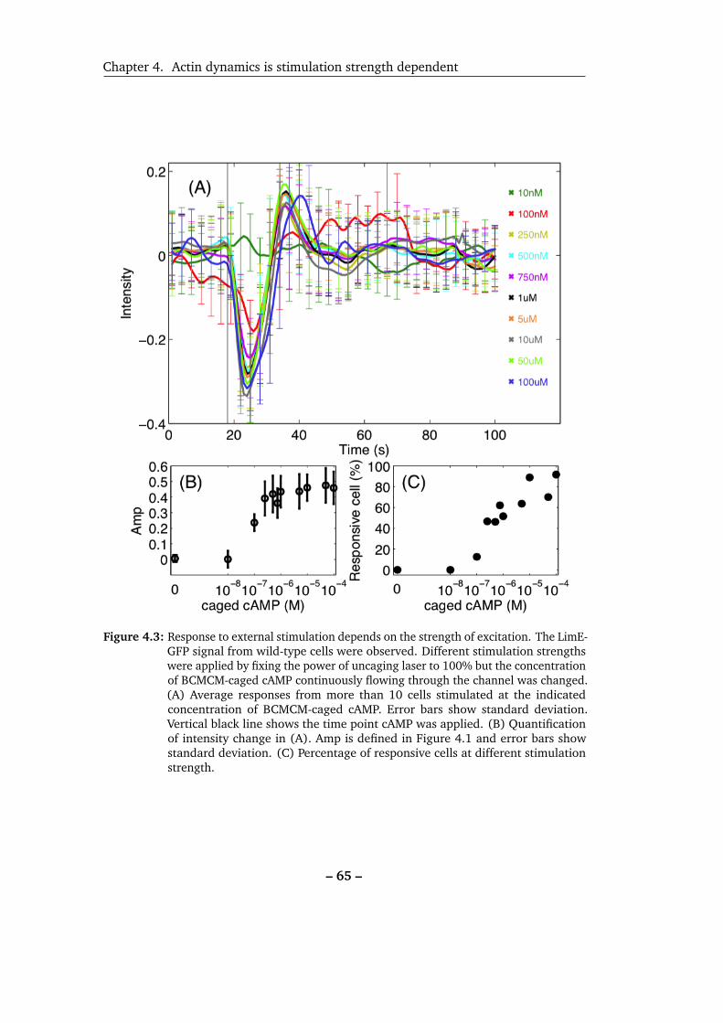
Chapter 4. Actin dynamics is stimulation strength dependent
Figure 4.3: Response to external stimulation depends on the strength of excitation. The LimE-GFP signal from wild-type cells were observed. Different stimulation strengthswere applied by fixing the power of uncaging laser to 100% but the concentrationof BCMCM-caged cAMP continuously flowing through the channel was changed.(A) Average responses from more than 10 cells stimulated at the indicatedconcentration of BCMCM-caged cAMP. Error bars show standard deviation.Vertical black line shows the time point cAMP was applied. (B) Quantificationof intensity change in (A). Amp is defined in Figure 4.1 and error bars showstandard deviation. (C) Percentage of responsive cells at different stimulationstrength.
– 65 –

4.3. Effects of different strengths of stimulation
10 20 30 40 50 600.2
0.3
0.4
0.5
0.6
0.7
0.8
0.9
1
Interval (s)
Am
p
Figure 4.4: Resonance peak shifts for different stimulation strength. At the specified intervalwe applied 10 stimuli to each cell and analyzed the amplitude of individualresponsive traces. At least 20 cells were observed for every interval. Black lineshows the resonance curve for strong stimulation (10 µM BCMCM). Circles referto stimulation intervals done in the experiment and the error bars show thestandard deviation of the response amplitude in different cells. Gray line showsthe resonance curve at weak stimulation (10 µM DMNB)1
Transition of the actin dynamics in self-oscillating cells to a cAMP response induced
by external stimulation of cAMP shows that self-oscillation is immediately replaced by
stimulated response, which requires longer time to finish one oscillation compared to
self-oscillations (Figure 4.1B). Therefore, when we stimulated the cells periodically,
the resonance period peaks at a time longer than the period of self-oscillations.
1As the data from [109] were analyzed differently (e.g. traces of cells were not normalized accordingto the intensity before stimulation to exclude the effect from different expression levels amongcells; all responsive traces were averaged first and then analyzed so the information about variationamong cells cannot be seen from the resonance curve.) We took the data and reanalyzed it basedon the scope of analysis used here.
– 66 –

Chapter 4. Actin dynamics is stimulation strength dependent
4.4 Single cell experiments
The error bars on the resonance points are due to the variations among cells. It is
known that even under the same strength of stimulation, the responses from different
cells vary a lot [141]. To gain more insight into the cell-cell diversity, we designed a
new experiment where we successively apply cAMP at different concentrations to
the same cell by adjusting the power of the uncaging laser with an interval of 4 min
between sequential stimuli to allow the cells to fully recover from the previous cAMP
exposure. The stimulation was always started with 100% laser power and gradually
decreased to the point where the cells no longer responded; the laser intensity was
then increased again to confirm that the unresponsive signal was due to the weak
stimulation rather than cellular damages. This design enables us to explore questions
like "Do all cells have the same threshold?" and "Does the response stay constant
after reaching the plateau?"
Figure 4.5: A schematic diagram illustrating the experiments that apply different dosesof cAMP to single cells. The concentration of BCMCM-caged cAMP flowed inthe channel was fixed to 100 nM. By altering the power of the uncaging laser,different doses of cAMP can be applied to the same cell. The stimulation alwaysstarted from 100% power of uncaging laser and then gradually decreased till thepoint the cell did not respond anymore. We then increased the power of uncaginglaser again to make sure that the reason the cell did not respond was due toweak stimulation rather than cell damages. The laser power shown here is justto illustrate the idea of decrease and then increase again. The actual values oflaser power were adjusted appropriately for each individual cell. Every stimuluswas separated 4 min to make sure the cell was fully recovered from previousstimulation. The green regions mark the time cells were under recording whereasthe gray regions mark the time without any recording.
– 67 –
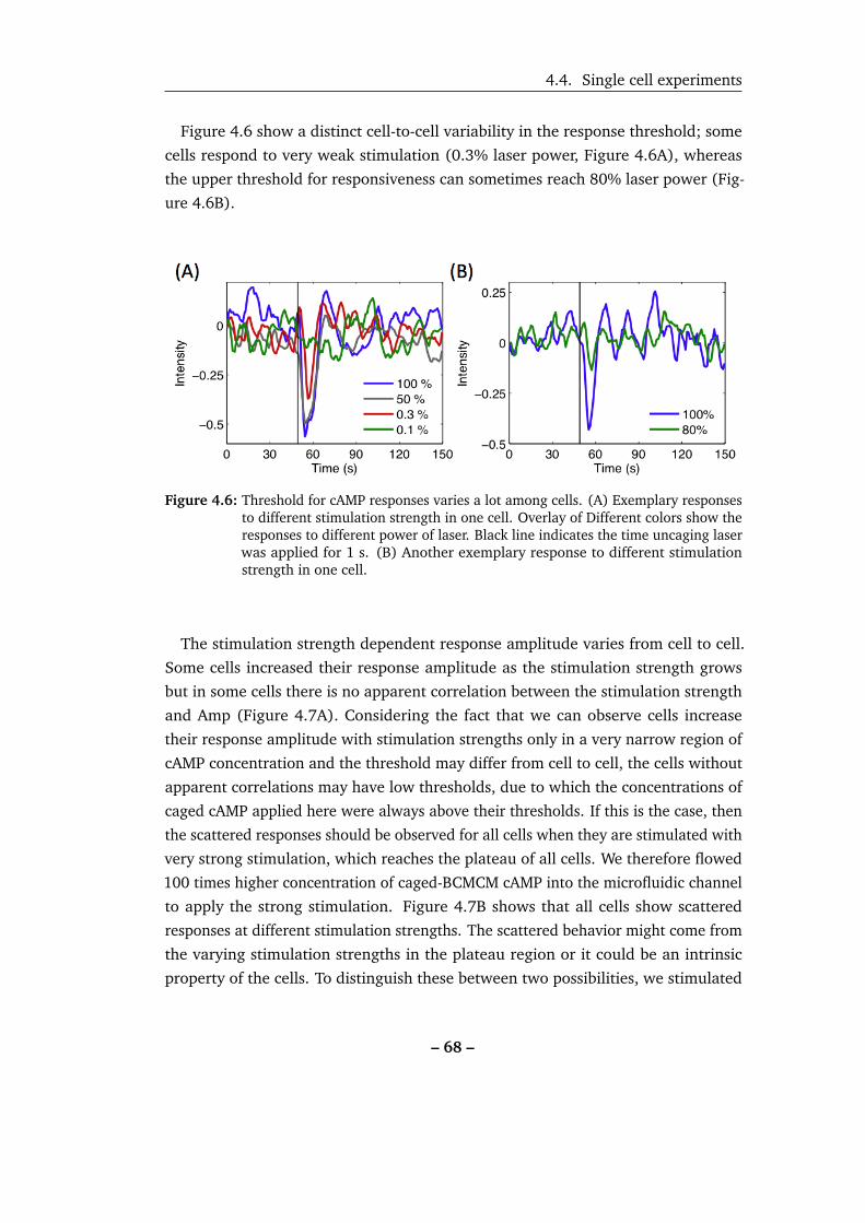
4.4. Single cell experiments
Figure 4.6 show a distinct cell-to-cell variability in the response threshold; some
cells respond to very weak stimulation (0.3% laser power, Figure 4.6A), whereas
the upper threshold for responsiveness can sometimes reach 80% laser power (Fig-
ure 4.6B).
Figure 4.6: Threshold for cAMP responses varies a lot among cells. (A) Exemplary responsesto different stimulation strength in one cell. Overlay of Different colors show theresponses to different power of laser. Black line indicates the time uncaging laserwas applied for 1 s. (B) Another exemplary response to different stimulationstrength in one cell.
The stimulation strength dependent response amplitude varies from cell to cell.
Some cells increased their response amplitude as the stimulation strength grows
but in some cells there is no apparent correlation between the stimulation strength
and Amp (Figure 4.7A). Considering the fact that we can observe cells increase
their response amplitude with stimulation strengths only in a very narrow region of
cAMP concentration and the threshold may differ from cell to cell, the cells without
apparent correlations may have low thresholds, due to which the concentrations of
caged cAMP applied here were always above their thresholds. If this is the case, then
the scattered responses should be observed for all cells when they are stimulated with
very strong stimulation, which reaches the plateau of all cells. We therefore flowed
100 times higher concentration of caged-BCMCM cAMP into the microfluidic channel
to apply the strong stimulation. Figure 4.7B shows that all cells show scattered
responses at different stimulation strengths. The scattered behavior might come from
the varying stimulation strengths in the plateau region or it could be an intrinsic
property of the cells. To distinguish these between two possibilities, we stimulated
– 68 –

Chapter 4. Actin dynamics is stimulation strength dependent
one cell 5 times using an identical amount of cAMP. Figure 4.7C shows that the
responses scattered in a similar range once cells crossed the response threshold,
confirming that the scattering of amplitude response originates from the intrinsic
noise of the cells.
Figure 4.7: Intrinsic noise causes the scattering of response amplitude. Wild-type cellslabeled with LimE-GFP were observed with the method shown in Figure 4.5.Different symbols show the response from different cells. (A) The variation ofamplitude response at different strengths of external stimulation. Experimentswere done with 100 nM BCMCM-caged cAMP continuously flowing in the chan-nel. Laser intensity was adjusted according to the x-axis. (B) The variation ofamplitude response at different strength of external stimulation. Experimentswere done with 10 µM BCMCM-caged cAMP continuously flowing in the channel.Laser intensity was adjusted according to the x-axis. (C) The variation of ampli-tude response when cells were stimulated with the same strength of externalstimulation is shown. Experiments were done with 10 µM BCMCM-caged cAMPcontinuously flowing in the channel and the laser intensity was always 100%.Interval between successive stimulation was 100 s.
To explore the mechanism that governs the response frequency at different stimu-
lation strengths, we analyzed how the polymerization and depolymerization times
change with stimulation strength in different cells. Figures 4.8A & 4.8B shows that
under all ranges of stimulation, polymerization time remains scattered around a
constant value without a clear trend of variation with stimulation strength. The
polymerization time was also scattered in cells responding to the same stimulation
(Figure 4.8C), suggesting it is an intrinsic propertyof the cells. On the other hand,
depolymerization time shows a trend similar to the response amplitude (Figure 4.8D
to 4.8E); depolymerization time grows with the stimulation strength in some cells,
whereas in some cells no clear trend was observed.
– 69 –
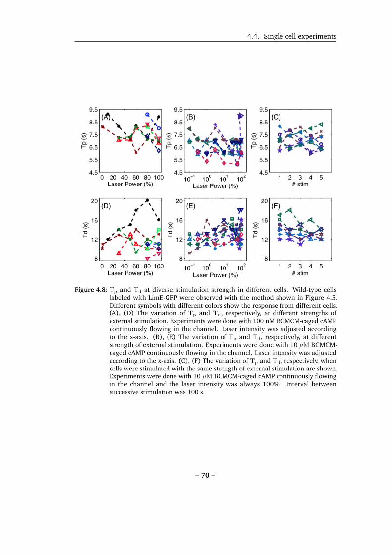
4.4. Single cell experiments
Figure 4.8: Tp and Td at diverse stimulation strength in different cells. Wild-type cellslabeled with LimE-GFP were observed with the method shown in Figure 4.5.Different symbols with different colors show the response from different cells.(A), (D) The variation of Tp and Td, respectively, at different strengths ofexternal stimulation. Experiments were done with 100 nM BCMCM-caged cAMPcontinuously flowing in the channel. Laser intensity was adjusted accordingto the x-axis. (B), (E) The variation of Tp and Td, respectively, at differentstrength of external stimulation. Experiments were done with 10 µM BCMCM-caged cAMP continuously flowing in the channel. Laser intensity was adjustedaccording to the x-axis. (C), (F) The variation of Tp and Td, respectively, whencells were stimulated with the same strength of external stimulation are shown.Experiments were done with 10 µM BCMCM-caged cAMP continuously flowingin the channel and the laser intensity was always 100%. Interval betweensuccessive stimulation was 100 s.
– 70 –

Chapter 4. Actin dynamics is stimulation strength dependent
4.5 Proposed underlying mechanism
In spite of the variations inside every cell and the prominent variability among cells,
responses from all cells reveal the same trend when we plotted the polymerization
time and the depolymerization time with the corresponding response amplitude:
responses with scattered amplitudes have their polymerization times scattered around
a constant value (Figure 4.9A), whereas responses with larger amplitudes also show
longer depolymerization times (Figure 4.9B).
It has been observed that the amount of capping protein peaked at the same
time as F-actin after the stimulation by cAMP and their amounts then decreased
together [127], suggesting that it is the binding of capping protein that terminates
the polymerization process. We therefore regarded Tp as the binding time of capping
protein.
0 4 8 12 16 200
0.2
0.4
0.6
0.8
1
Td (s)
Am
p
(B)
0 4 8 12 16 200
0.2
0.4
0.6
0.8
1
Tp (s)
Am
p
(A)
Figure 4.9: Global parameters that determine the behavior of cells. Wild-type cells labeledwith LimE-GFP were observed. Black dots show the analysis from 314 self-oscillating cells and gray crosses show the analysis from 95 cells responding to asingle 1 s stimulus at 100% laser power to uncage 10 µM BCMCM-caged cAMP.Black stars show the analysis from 136 cells responding to a single 1 s stimulusof different concentrations. The stimulus was applied with 100% laser power touncage different concentration of BCMCM-caged cAMP (from 30 nM to 100 µM).(A) Relation between Amp and Tp. (B) Relation between Amp and Td.
– 71 –
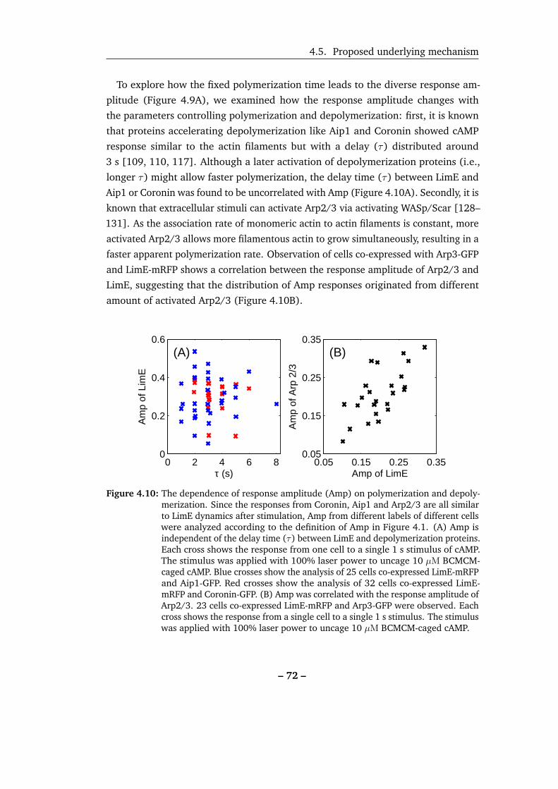
4.5. Proposed underlying mechanism
To explore how the fixed polymerization time leads to the diverse response am-
plitude (Figure 4.9A), we examined how the response amplitude changes with
the parameters controlling polymerization and depolymerization: first, it is known
that proteins accelerating depolymerization like Aip1 and Coronin showed cAMP
response similar to the actin filaments but with a delay (τ) distributed around
3 s [109, 110, 117]. Although a later activation of depolymerization proteins (i.e.,
longer τ) might allow faster polymerization, the delay time (τ) between LimE and
Aip1 or Coronin was found to be uncorrelated with Amp (Figure 4.10A). Secondly, it is
known that extracellular stimuli can activate Arp2/3 via activating WASp/Scar [128–
131]. As the association rate of monomeric actin to actin filaments is constant, more
activated Arp2/3 allows more filamentous actin to grow simultaneously, resulting in a
faster apparent polymerization rate. Observation of cells co-expressed with Arp3-GFP
and LimE-mRFP shows a correlation between the response amplitude of Arp2/3 and
LimE, suggesting that the distribution of Amp responses originated from different
amount of activated Arp2/3 (Figure 4.10B).
0.05 0.15 0.25 0.350.05
0.15
0.25
0.35
Am
p of
Arp
2/3
Amp of LimE
(B)
0 2 4 6 80
0.2
0.4
0.6
τ (s)
Am
p of
Lim
E
(A)
Figure 4.10: The dependence of response amplitude (Amp) on polymerization and depoly-merization. Since the responses from Coronin, Aip1 and Arp2/3 are all similarto LimE dynamics after stimulation, Amp from different labels of different cellswere analyzed according to the definition of Amp in Figure 4.1. (A) Amp isindependent of the delay time (τ) between LimE and depolymerization proteins.Each cross shows the response from one cell to a single 1 s stimulus of cAMP.The stimulus was applied with 100% laser power to uncage 10 µM BCMCM-caged cAMP. Blue crosses show the analysis of 25 cells co-expressed LimE-mRFPand Aip1-GFP. Red crosses show the analysis of 32 cells co-expressed LimE-mRFP and Coronin-GFP. (B) Amp was correlated with the response amplitude ofArp2/3. 23 cells co-expressed LimE-mRFP and Arp3-GFP were observed. Eachcross shows the response from a single cell to a single 1 s stimulus. The stimuluswas applied with 100% laser power to uncage 10 µM BCMCM-caged cAMP.
– 72 –
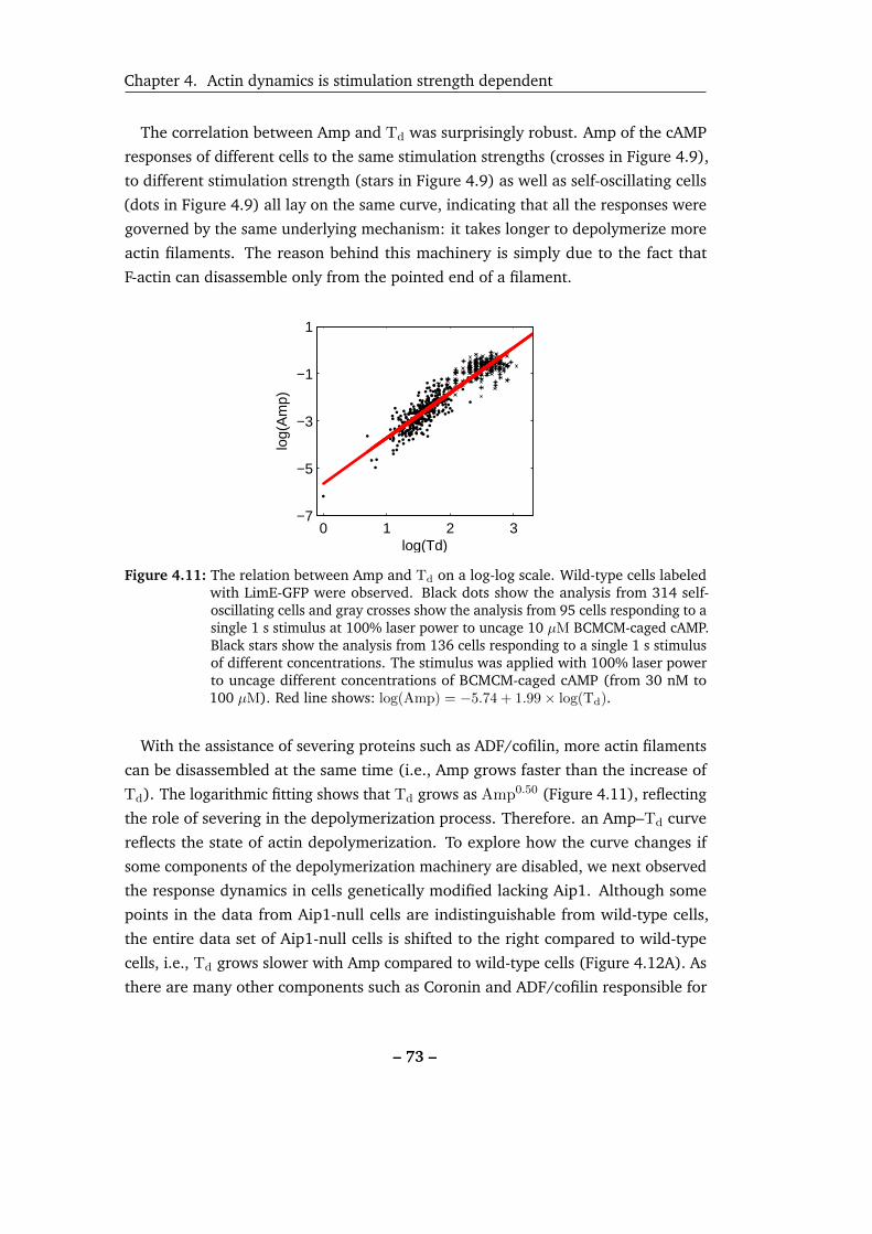
Chapter 4. Actin dynamics is stimulation strength dependent
The correlation between Amp and Td was surprisingly robust. Amp of the cAMP
responses of different cells to the same stimulation strengths (crosses in Figure 4.9),
to different stimulation strength (stars in Figure 4.9) as well as self-oscillating cells
(dots in Figure 4.9) all lay on the same curve, indicating that all the responses were
governed by the same underlying mechanism: it takes longer to depolymerize more
actin filaments. The reason behind this machinery is simply due to the fact that
F-actin can disassemble only from the pointed end of a filament.
0 1 2 3−7
−5
−3
−1
1
log(
Am
p)
log(Td)
Figure 4.11: The relation between Amp and Td on a log-log scale. Wild-type cells labeledwith LimE-GFP were observed. Black dots show the analysis from 314 self-oscillating cells and gray crosses show the analysis from 95 cells responding to asingle 1 s stimulus at 100% laser power to uncage 10 µM BCMCM-caged cAMP.Black stars show the analysis from 136 cells responding to a single 1 s stimulusof different concentrations. The stimulus was applied with 100% laser powerto uncage different concentrations of BCMCM-caged cAMP (from 30 nM to100 µM). Red line shows: log(Amp) = −5.74 + 1.99× log(Td).
With the assistance of severing proteins such as ADF/cofilin, more actin filaments
can be disassembled at the same time (i.e., Amp grows faster than the increase of
Td). The logarithmic fitting shows that Td grows as Amp0.50 (Figure 4.11), reflecting
the role of severing in the depolymerization process. Therefore. an Amp–Td curve
reflects the state of actin depolymerization. To explore how the curve changes if
some components of the depolymerization machinery are disabled, we next observed
the response dynamics in cells genetically modified lacking Aip1. Although some
points in the data from Aip1-null cells are indistinguishable from wild-type cells,
the entire data set of Aip1-null cells is shifted to the right compared to wild-type
cells, i.e., Td grows slower with Amp compared to wild-type cells (Figure 4.12A). As
there are many other components such as Coronin and ADF/cofilin responsible for
– 73 –
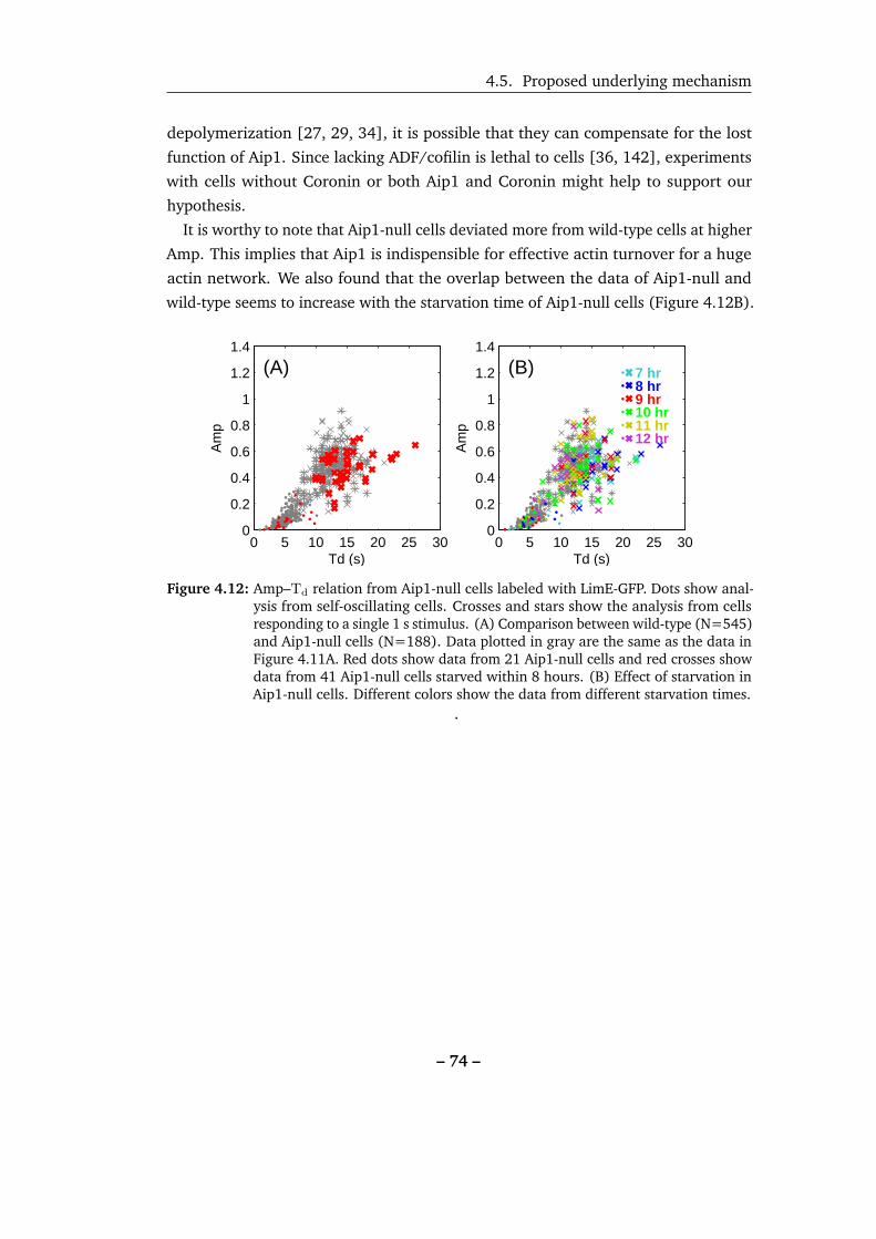
4.5. Proposed underlying mechanism
depolymerization [27, 29, 34], it is possible that they can compensate for the lost
function of Aip1. Since lacking ADF/cofilin is lethal to cells [36, 142], experiments
with cells without Coronin or both Aip1 and Coronin might help to support our
hypothesis.
It is worthy to note that Aip1-null cells deviated more from wild-type cells at higher
Amp. This implies that Aip1 is indispensible for effective actin turnover for a huge
actin network. We also found that the overlap between the data of Aip1-null and
wild-type seems to increase with the starvation time of Aip1-null cells (Figure 4.12B).
0 5 10 15 20 25 300
0.2
0.4
0.6
0.8
1
1.2
1.4
Td (s)
Am
p
(A)
0 5 10 15 20 25 300
0.2
0.4
0.6
0.8
1
1.2
1.4
Td (s)
Am
p
7 hr8 hr9 hr10 hr11 hr12 hr
(B)
Figure 4.12: Amp–Td relation from Aip1-null cells labeled with LimE-GFP. Dots show anal-ysis from self-oscillating cells. Crosses and stars show the analysis from cellsresponding to a single 1 s stimulus. (A) Comparison between wild-type (N=545)and Aip1-null cells (N=188). Data plotted in gray are the same as the data inFigure 4.11A. Red dots show data from 21 Aip1-null cells and red crosses showdata from 41 Aip1-null cells starved within 8 hours. (B) Effect of starvation inAip1-null cells. Different colors show the data from different starvation times.
.
– 74 –

Chapter 4. Actin dynamics is stimulation strength dependent
4.6 Nonlinear properties of responses
As the cAMP responses resemble the oscillation of a damped oscillator, we next tried
to describe the response with the dynamics of a damped oscillator:
x+ 2ξx+ kx = F (t), (4.1)
We regarded the amplitude x of damped oscillators as the response amplitude of
the cytosolic signal after the stimulation of cAMP; the application of cAMP to the
system was considered as the application of a force F with a Heaviside step function
that stays at a constant value for 1 s; ξ is the damping coefficient.
Simulations of periodic stimuli shows that the position of the resonance peak did
not change under the stimulation of different strength (Figure 4.14).
Figure 4.13: Simulated resonance curves of damped oscillators. Simulations were conductedwith equation 4.1. Frequency of stimuli shown in the x-axis was normalized tothe resonance frequency when γ = 0 (Natural frequency). Different symbolsdisplay different amplitude of applied force (F).
To reproduce the nonlinear phenomena observed in the experiments that response
frequency is dependent on the stimulation strength, a cubic term was added to the
damped oscillator. It is also known as duffing oscillators [139]. γ is the parameter
introducing nonlinearity:
x+ 2ξx+ kx+ γx3 = F (t), (4.2)
– 75 –

4.6. Nonlinear properties of responses
Simulations with periodic stimuli support the nonlinear nature of the phenomenon
observed in experiments (Figure 4.4). Different strengths of the external stimuli
always changed the responsive amlitude but the resonance frequency only varied
when γ was nonzero (Figure 4.14A). γ shifts the resonance peak by introducing a
nonlinearity to the damped oscillators: the magnitude of γ (along with F) reflects
the extent of resonance peak shift and the sign of γ reflects the direction of the shift
(Figure 4.14C).
Figure 4.14: Effect of altering the strength of stimulation on the resonance curve. Sim-ulations were conducted with equation 4.2. Frequency of stimuli shown inthe x-axis was normalized to the resonance frequency when γ = 0 (Naturalfrequency). (A) Simulated resonance curves of duffing oscillators (γ = 0.4) atdifferent forces of stimulation. Different symbols display different amplitudeof applied force. (B) Effect of altering the values of γ on the resonance curve.Different colors show resonance curves with different γ values.
However, the parameters of duffing oscillators have no identifiable physiologi-
cal counterparts in terms of actin dynamics as they were not made to study actin
dynamics in the first place. A time delayed feedback model has been proposed to
explain the actin dynamics based on a time-delay between the polymerization and
depolymerization [109]:
dA(t)
dt= k+(t)A(t)− k−A(t)A(t− τ), (4.3)
k+(t) = k0+ + ks(t), (4.4)
where k+(t) is the overall polymerization rate which is regulated by intrinsic polymer-
ization (k0+), external stimulation (ks(t)) and adaptation; A(t) is the concentration of
actin filaments (i.e., the cortical fluorescence intensity observed in our experiment);
k− is the overall depolymerization rate of the system; τ is the delay time between
– 76 –

Chapter 4. Actin dynamics is stimulation strength dependent
polymerization and depolymerization. The solutions (fixed points) are stable when
k0+τ < π/2, where the oscillations decrease amplitude with time; solutions become
unstable as k0+τ > π/2, where the oscillations increase amplitude with time and
finally enter time-periodic limit cycle oscillations. The system thus encounters a Hopf
bifurcation at k0+τ = π/2, where the solutions oscillate with constant amplitude.
This model reproduces several characteristic features of the in vivo situation: first,
it has been shown that four times the delay time is the oscillation period when the
parameters are at the bifurcation point [143]. Secondly, we were able to reproduce
the stimulation strength dependence of the resonance curve in the frame work of this
model (Figure 4.15).
10 20 300
0.5
1
1.5x 10
−3
Stimulation Interval
Am
plitu
de
Figure 4.15: Simulations of resonance curves with different stimulation strengths. Resonancecurves simulated by time delayed feedback model (Eq. 4.2) with k0+ = 0.3 andτ = 4. Stimulation (ks(t)) was applied as Gaussian function with maximumvalue of 1.5 (black curve) and 0.6 (gray curve).
Here we further examined the model by comparing simulations with our experi-
mental results. First, oscillating solutions last longer as the parameters come close to
the bifurcation point, implying the intrinsic parameters of self-oscillating cells are
close to the bifurcation point, where the oscillation period is close to four times the
delay time (τ). The distribution we report here in Figure 3.5 agrees well with four
times of the delay time observed by Huang et. al (3.39±1.2 s) [110]. Secondly, we
observed that the resonance frequencies depend on the strength of external stimu-
lation; simulation at different strength of the stimulation reveals a shift to longer
period in the resonance curve (Figure 4.4).
However, we would like to stress that Eq. 4.3 is based on the assumption that
the amount of depolymerization proteins always increase with the polymerized
filamentous actin but without a limit. According to Eq. 4.3, increasing the amount
of depolymerization proteins not only increases the depolymerization rate but also
– 77 –

4.6. Nonlinear properties of responses
depletes the actin pool, resulting in an extremely slow growth rate and prolongs
the recovery time tremendously. As a result, this model failed in predicting how
the deploymerization time (Td) changes with response amplitude (gray lines with
triangles in Figure 4.16C).
0 5 10 15 20 25 30 350
2
4
6
8
10
TdA
mp
(B)
0 2 4 6 8 100
2
4
6
8
10
Tp
Am
p
(A)
Figure 4.16: Simulation of Amp versus Tp and Amp versus Td at different strengths ofexternal stimulation. Gray lines show simulations from time-delayed modelproposed in reference [109] (Eq. 4.2) with k0+ = 0.3 and τ = 4. Black linesshow simulations from the model with depolymerization threshold (Eq. 4.6)using k0+ = 0.3 and τ = 4. Stimulation (ks(t)) was applied as Gaussian functionwith a maximum value of 0.3, 0.4, 0.5, 1.0, 1.5, 2.0, 2.5, 3.0, 3.5, and 4.0.(A) Amp versus Tp. (B) Amp versus Td
To include the limited increase of the depolymerization proteins, we modify the
time delayed model by setting a threshold to the depolymerization part of Eq. 4.3:
dA(t)
dt= k+(t) +A(t)− k−A(t)B(t),
B(t) =
{A(t− τ) : A(t− τ) < Cthre,
Cthre : A(t− τ) ≥ Cthre.
(4.5)
An upper limit was set for the maximum amount of depolymerization proteins that
can participate in disassembling actin filaments (Cthre). Below the threshold concen-
tration, the amount of depolymerization proteins was A(t− τ), namely, proportional
to the amount of actin filaments A(t). Under a strong excitation, A(t) increases
according to the time delayed model but instead of growing without limit, the maxi-
mum amount of depolymerization protein can be used is the threshold. Simulations
show that this modification lead to results consistent with our experimental observa-
tion: Td grows with increasing Amp, whereas Tp remains constant (black lines with
circular symbols in Figure 4.16).
– 78 –

Chapter 4. Actin dynamics is stimulation strength dependent
0 0.1 0.2 0.3 0.40
0.1
0.2
0.3
0.4
Am
p of
Aip
1
Amp of LimE
Figure 4.17: Amount of Aip1 is limited with the increasing of LimE. Stimulation was ap-plied at 100% laser power to uncage 10 µM BCMCM-caged cAMP. Responseamplitudes from 24 cells co-expressing LimE-mRFP and Aip1-GFP to a sin-gle 1 s stimulation were analyzed. Amp is defined as in Figure 4.1 from thecorresponding signal.
It is worthy to note that the diverse amount of activated Arp2/3 can be related to
the different polymerization rates (k0+) in the model, resulting in various response
amplitude among cells even under the same stimulation strength. If the modification
of the model was correct, then under very strong stimulation, the amount of depoly-
merization protein will reach a constant value for all cells with various response
amplitude. Therefore, we examined the amplitude response of cells co-expressed with
LimE-mRFP and Aip1-GFP experimentally. We stimulated cells with a stimulation
strength strong enough for all cells to be in the plateau region (i.e., the same stimula-
tion strength as Figure 4.7B). Figure 4.17 shows that cells with varying Amp of LimE
all have Aip1 responses in the similar range, supporting the modification of the model.
– 79 –

4.7. Conclusion
4.7 Conclusion
By applying cAMP to individual cells, we found that external stimulation leads to
a rapid increase in filamentous actin formation in the cortex. As it also required a
longer time to depolymerize more actin filaments, the time to finish one oscillation
was thus prolonged compared to the actin self-oscillation cycle (Figure 4.1B). This
prolongation accounts for the difference between the frequency of the self-oscillations
and the forcing resonance peak (Figure 4.4). Comparisons between actin dynamics
before and after stimulation suggest that self-oscillations have no effect on cAMP
responses and the external stimuli can either trigger or inhibit the occurrence of
self-oscillation (Figure 4.2).
To investigate the underlying mechanism, we analyzed how external stimuli change
the different parts of the cAMP response. First, the time for actin to polymerize
(Tp) was the same in self-oscillations as well as responses to external simulation
(Figure 3.11 and Figure 3.10), suggesting that this process was controlled by the
binding of capping protein. As Arp2/3 can be activated through extracellular stimuli
and the consequent actin branch structure enables more actin to bind, simultaneously,
during the same polymerization time (Tp), cells responding to the stimulation grew
actin filaments much faster than self-oscillating cells (compare the distribution of
Amp between crosses and dots in Figure 4.9B). Second, the time for filamentous
actin to depolymerize prolonged a lot compared to self-oscillating cells (compare the
distribution of Td between crosses and dots in Figure 4.9B). It is the prolongation
of depolymerization time that accounts for the difference between the frequency of
self-oscillations and the forcing resonance peak.
The correlation between Amp and Td is very robust. Responses from self-oscillating
cells, cells stimulated with different stimulation strengths and different frequencies
all lay on the same curve. This suggests that the Amp and Td are good measures to
describe the underlying mechanism of depolymerization. The growth of Amp as the
square of Td, represents the core properties of actin depolymerization: first, as actin
dissociates only from the pointed end of actin filaments, a longer time is required
to disassemble more actin. Second, severing enhances the depolymerization rate
by creating more pointed ends of actin filaments. As the bigger Amp comes from
the more branched network, the role of severing becomes more significant at higher
Amp.
– 80 –
Chapter 4. Actin dynamics is stimulation strength dependent
Experiments with cells simultaneously labeled LimE and Arp2/3 provided us the
information about how Amp varies with the amount of activated Arp2/3. A further
evidence to support the hypothesis would be the verification of the capping protein
as the major factor determining Tp. Experiments comparing Tp of normal cells and
cells lacking capping protein can strongly support the hypothesis. However, deleting
capping protein is lethal to cells. Although experiments with cells with simultaneously
labeled LimE and capping protein to see the correlation between the peak of capping
protein in the cortex and actin filaments in response to stimulation would provide
similar information as what was done before [127], there is no evidence yet that
oscillations of actin in self-oscillating cells is also controlled by the binding of capping
protein.
In conclusion, the regulation of polymerization and depolymerization controls
not only the strength but also the frequency of actin dynamics. Moreover, even for
cAMP stimulation responses involving a much more complicated cascade of enzyme
reactions, the underlying mechanism of the self-organization of actin dynamics is the
same in the presence and absence of stimuli.
– 81 –
CHAPTER 5
Myosin II sets the optimal response time scale
5.1 Motivation
So far we have described actin dynamics in the absence of external stimulation
(chapter 3) as well as how cAMP triggers the actin responses (chapter 4). We also
investigated and proposed the leading roles of the associated proteins involved in the
processes of polymerization and depolymerization of actin filaments. Besides actin
binding proteins, the motor protein myosin II also binds to filamentous actin and is
indispensible for maintaining the normal functioning of cell movement and develop-
ment. By walking unidirectionally towards the barbed end (usually designated as
the plus end.) of actin filaments, myosin II bundles enable contraction. Cells lacking
myosin II show reduced stiffness and decreased cortical tension, they diminish their
translocation speed and terminate cell division in suspension [72, 144–146]. Despite
the significance of myosin II, whether myosin II is required for the rapid oscillations
of actin cytoskeleton has not yet been studied.
Here we simultaneously observed the dynamics of myosin II and LimE in D. dis-coideum cells by co-expressing myosin II-GFP and LimE-mRFP to investigate the
coupling between the dynamics of myosin II and actin in the absence of stimulation.
Considering the fact that myosin II is functionally active only as filaments, the lack of
heavy chain inhibits the entire function of myosin II [61, 69]. To elucidate the role
of myosin II in self-oscillations, we examined the dynamics of LimE in cells without
myosin II heavy chains (which, from here on will be referenced to as myosin II-null
or myosin II knock-out cells). We further explored the interplay between actin and
myosin II in the presence of stimulation. Besides the actin dynamics itself, we also in-
spected how the interplay between actin and myosin II influences the cell morphology,
especially the cringing phenomena in response to cAMP [95].
– 82 –

Chapter 5. Myosin II sets the optimal response time scale
5.2 Myosin II dynamics in the absence of external stimulation
Cells simultaneously labeled myosin II-GFP and LimE-mRFP showing various types
of oscillations in the absence of external stimulation: regular oscillations of both
myosin II and LimE, regular oscillations only in myosin II but not in LimE, and
regular oscillations only in LimE but not in myosin II, and also neither myosin II
nor LimE oscillating. The occurrence of LimE and myosin II oscillate together
(1489 oscillations observed from 387 cells) is higher than only LimE (764 oscillations
observed from 387 cells) or myosin II (604 oscillations observed from 387 cells)
oscillates. We further examined the oscillation period distributions for the cases
mentioned above. Histograms are indistinguishable in all cases (Figure 5.1), implying
that the oscillations of myosin II and LimE are independent of each other. Moreover,
although it has been found that LimE-mRFP and LimE-GFP localized at different
positions of the cell cortex [147], the distribution of oscillation periods did not
change at different LimE labels (Figure 5.1A and Figure 3.5).
Figure 5.1: Oscillations of myosin II and LimE were independent of each other. 387 cellslabeled both myosin II-GFP and LimE-mRFP were observed. Histograms ofthe oscillation period of (A) LimE in cells that only show oscillations in LimE(N=764). (B) LimE in cells showing oscillations in both LimE and myosin II(N=1489). (C) Myosin II in cells that only show oscillations in myosin II(N=604). (D) Myosin II in cells showing oscillations in both LimE and myosin II(N=1489).
– 83 –

5.2. Myosin II dynamics in the absence of external stimulation
We further confirmed that myosin II is not necessary for self-oscillations by looking
at the oscillation period of myosin II knock-out cells. Cells without myosin II showed
comparable oscillation periods of LimE as found in wild-type cells (Figure 5.2A and
Figure 3.5). Moreover, the occurrence as well as the duration of self-oscillations are
also indepedent of myosin II (Figure 5.2B to 5.2D and Figure 3.7).
Figure 5.2: Properties of self-oscillations in LimE-GFP labeled myosin II-null cells. (A) Dis-tribution of self-oscillation periods (N=655). (B)–(D) 224 myosin II-null cellslabeled with LimE-GFP were observed for 160 s in the absence of externalstimulation. (B) Distribution of the longest time for which a cell can oscillate.(C) Distribution and average life time of oscillating and non-oscillating states.Circles display experimental data and the red line is the fit to a single exponen-tial decay (y = a exp−bx, τ = 1/b). (D) Distribution and average life time ofnon-oscillating states. Crosses are experimental data and the red line displaysthe fit to a single exponential decay (y = a exp−bx, τ = 1/b)
– 84 –
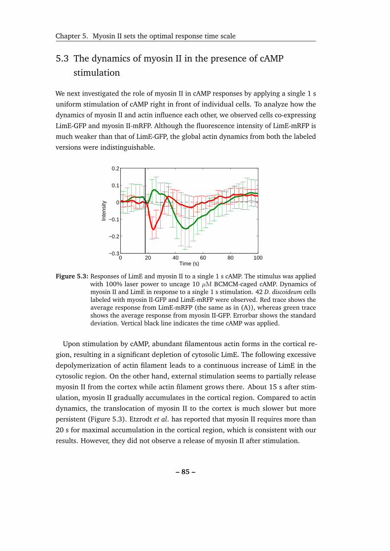
Chapter 5. Myosin II sets the optimal response time scale
5.3 The dynamics of myosin II in the presence of cAMP
stimulation
We next investigated the role of myosin II in cAMP responses by applying a single 1 s
uniform stimulation of cAMP right in front of individual cells. To analyze how the
dynamics of myosin II and actin influence each other, we observed cells co-expressing
LimE-GFP and myosin II-mRFP. Although the fluorescence intensity of LimE-mRFP is
much weaker than that of LimE-GFP, the global actin dynamics from both the labeled
versions were indistinguishable.
0 20 40 60 80 100−0.3
−0.2
−0.1
0
0.1
0.2
Time (s)
Inte
nsity
Figure 5.3: Responses of LimE and myosin II to a single 1 s cAMP. The stimulus was appliedwith 100% laser power to uncage 10 µM BCMCM-caged cAMP. Dynamics ofmyosin II and LimE in response to a single 1 s stimulation. 42 D. discoideum cellslabeled with myosin II-GFP and LimE-mRFP were observed. Red trace shows theaverage response from LimE-mRFP (the same as in (A)), whereas green traceshows the average response from myosin II-GFP. Errorbar shows the standarddeviation. Vertical black line indicates the time cAMP was applied.
Upon stimulation by cAMP, abundant filamentous actin forms in the cortical re-
gion, resulting in a significant depletion of cytosolic LimE. The following excessive
depolymerization of actin filament leads to a continuous increase of LimE in the
cytosolic region. On the other hand, external stimulation seems to partially release
myosin II from the cortex while actin filament grows there. About 15 s after stim-
ulation, myosin II gradually accumulates in the cortical region. Compared to actin
dynamics, the translocation of myosin II to the cortex is much slower but more
persistent (Figure 5.3). Etzrodt et al. has reported that myosin II requires more than
20 s for maximal accumulation in the cortical region, which is consistent with our
results. However, they did not observe a release of myosin II after stimulation.
– 85 –

5.3. The dynamics of myosin II in the presence of cAMP stimulation
It is known that in the presence of a chemical gradient, myosin II localizes in the
rear of the cell. Moreover, myosin II can rapidly redistribute according to the direction
of the gradient, involving a rapid release from the cortical region (Figure 5.4B). But
a release of myosin II from the cortex in response to a uniform stimulus of cAMP has
not been reported. From the increase and the subsequent decrease in the amount
of myosin II observed in our experiments (Figure 5.3), it is possible that the release
of myosin II in response to a uniform stimulation of cAMP was overlooked so far
(Figure 5.4A).
Figure 5.4: Schematic diagram showing myosin II of D. discoideum cells changes its localiza-tion in response to cAMP. (A) In response to a uniform stimulation, myosin II istranslocated isotropically around the cortex. (B) Myosin II always localizes tothe rear part of the cell on a local stimulation with a microcapillary (↗ showsthe direction of cell movement). Upon changing the direction of the stimuli,myosin II is released from the original rear-end of the cortex and is translocatedto the new position opposite to where the stimulation is applied (↙ shows thedirection of cell movement under the new gradient). The figure is adaptedfrom [148].
We next verified if a uniform stimulation of cAMP can also trigger the release of
myosin II from the cortex but the main challenge is that the signal of the released
myosin II is too weak to be distinguished from noise. Our goal is thus to enhance the
amount of cortical myosin II. Considering the fact that myosin II starts to translocate
to the cortex around 15 s after stimulation by cAMP and starts to disassemble
and return to the cytosol around 25 s after stimulation, the application of another
stimulation about 10–25 s after the first stimulation can achieve our goal without
any genetic modification of the cell. The periodic increases of myosin II-GFP signal
– 86 –
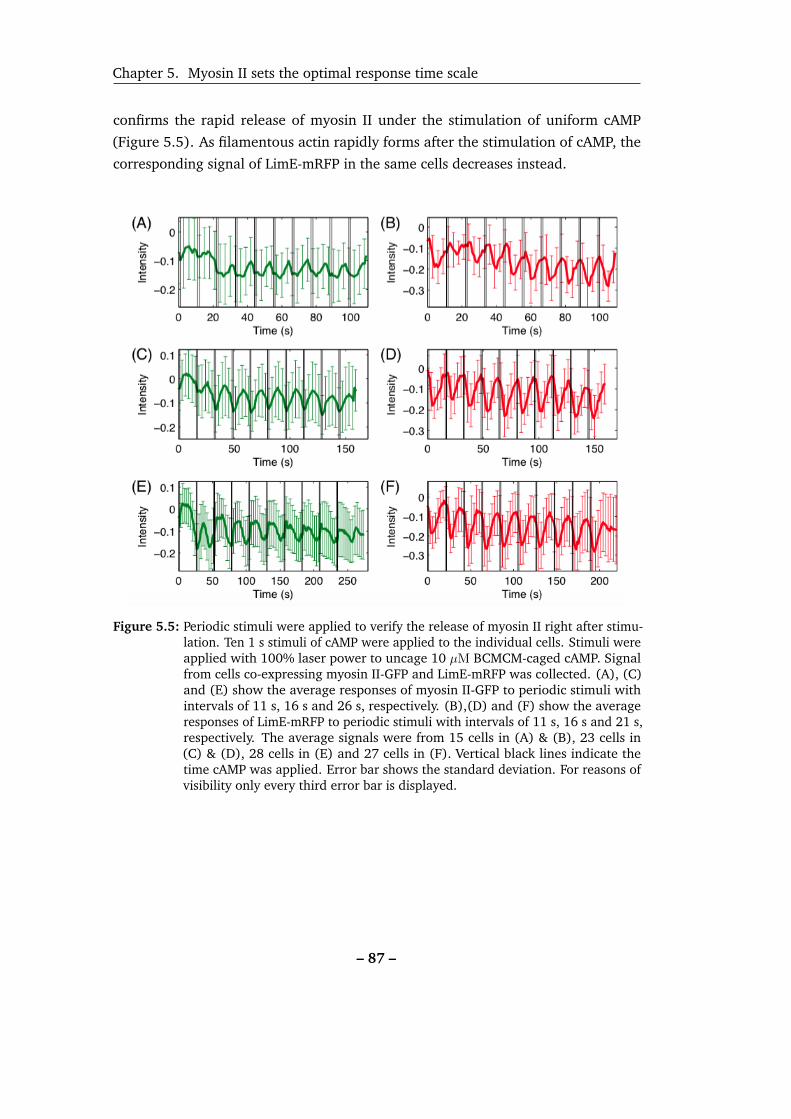
Chapter 5. Myosin II sets the optimal response time scale
confirms the rapid release of myosin II under the stimulation of uniform cAMP
(Figure 5.5). As filamentous actin rapidly forms after the stimulation of cAMP, the
corresponding signal of LimE-mRFP in the same cells decreases instead.
Figure 5.5: Periodic stimuli were applied to verify the release of myosin II right after stimu-lation. Ten 1 s stimuli of cAMP were applied to the individual cells. Stimuli wereapplied with 100% laser power to uncage 10 µM BCMCM-caged cAMP. Signalfrom cells co-expressing myosin II-GFP and LimE-mRFP was collected. (A), (C)and (E) show the average responses of myosin II-GFP to periodic stimuli withintervals of 11 s, 16 s and 26 s, respectively. (B),(D) and (F) show the averageresponses of LimE-mRFP to periodic stimuli with intervals of 11 s, 16 s and 21 s,respectively. The average signals were from 15 cells in (A) & (B), 23 cells in(C) & (D), 28 cells in (E) and 27 cells in (F). Vertical black lines indicate thetime cAMP was applied. Error bar shows the standard deviation. For reasons ofvisibility only every third error bar is displayed.
– 87 –
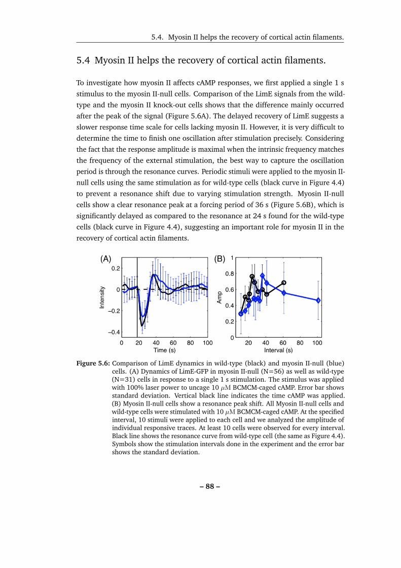
5.4. Myosin II helps the recovery of cortical actin filaments.
5.4 Myosin II helps the recovery of cortical actin filaments.
To investigate how myosin II affects cAMP responses, we first applied a single 1 s
stimulus to the myosin II-null cells. Comparison of the LimE signals from the wild-
type and the myosin II knock-out cells shows that the difference mainly occurred
after the peak of the signal (Figure 5.6A). The delayed recovery of LimE suggests a
slower response time scale for cells lacking myosin II. However, it is very difficult to
determine the time to finish one oscillation after stimulation precisely. Considering
the fact that the response amplitude is maximal when the intrinsic frequency matches
the frequency of the external stimulation, the best way to capture the oscillation
period is through the resonance curves. Periodic stimuli were applied to the myosin II-
null cells using the same stimulation as for wild-type cells (black curve in Figure 4.4)
to prevent a resonance shift due to varying stimulation strength. Myosin II-null
cells show a clear resonance peak at a forcing period of 36 s (Figure 5.6B), which is
significantly delayed as compared to the resonance at 24 s found for the wild-type
cells (black curve in Figure 4.4), suggesting an important role for myosin II in the
recovery of cortical actin filaments.
Figure 5.6: Comparison of LimE dynamics in wild-type (black) and myosin II-null (blue)cells. (A) Dynamics of LimE-GFP in myosin II-null (N=56) as well as wild-type(N=31) cells in response to a single 1 s stimulation. The stimulus was appliedwith 100% laser power to uncage 10 µM BCMCM-caged cAMP. Error bar showsstandard deviation. Vertical black line indicates the time cAMP was applied.(B) Myosin II-null cells show a resonance peak shift. All Myosin II-null cells andwild-type cells were stimulated with 10 µM BCMCM-caged cAMP. At the specifiedinterval, 10 stimuli were applied to each cell and we analyzed the amplitude ofindividual responsive traces. At least 10 cells were observed for every interval.Black line shows the resonance curve from wild-type cell (the same as Figure 4.4).Symbols show the stimulation intervals done in the experiment and the error barshows the standard deviation.
– 88 –
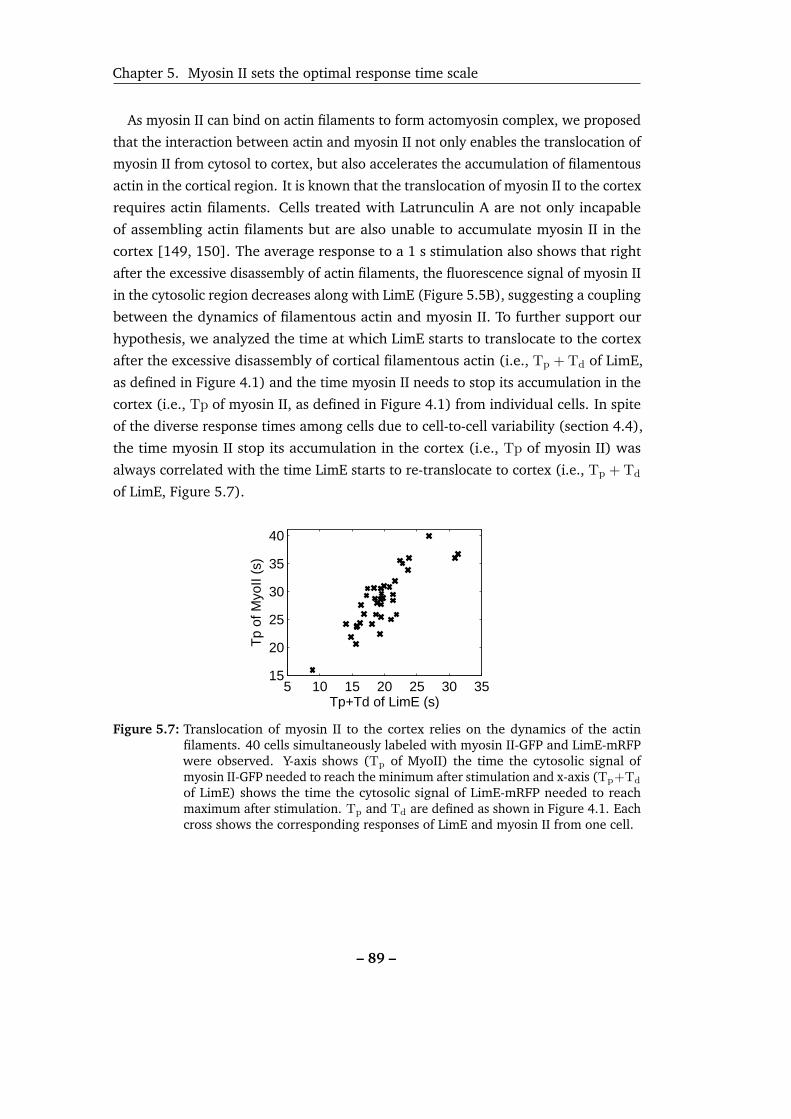
Chapter 5. Myosin II sets the optimal response time scale
As myosin II can bind on actin filaments to form actomyosin complex, we proposed
that the interaction between actin and myosin II not only enables the translocation of
myosin II from cytosol to cortex, but also accelerates the accumulation of filamentous
actin in the cortical region. It is known that the translocation of myosin II to the cortex
requires actin filaments. Cells treated with Latrunculin A are not only incapable
of assembling actin filaments but are also unable to accumulate myosin II in the
cortex [149, 150]. The average response to a 1 s stimulation also shows that right
after the excessive disassembly of actin filaments, the fluorescence signal of myosin II
in the cytosolic region decreases along with LimE (Figure 5.5B), suggesting a coupling
between the dynamics of filamentous actin and myosin II. To further support our
hypothesis, we analyzed the time at which LimE starts to translocate to the cortex
after the excessive disassembly of cortical filamentous actin (i.e., Tp + Td of LimE,
as defined in Figure 4.1) and the time myosin II needs to stop its accumulation in the
cortex (i.e., Tp of myosin II, as defined in Figure 4.1) from individual cells. In spite
of the diverse response times among cells due to cell-to-cell variability (section 4.4),
the time myosin II stop its accumulation in the cortex (i.e., Tp of myosin II) was
always correlated with the time LimE starts to re-translocate to cortex (i.e., Tp + Td
of LimE, Figure 5.7).
5 10 15 20 25 30 3515
20
25
30
35
40
Tp+Td of LimE (s)
Tp
of M
yoII
(s)
Figure 5.7: Translocation of myosin II to the cortex relies on the dynamics of the actinfilaments. 40 cells simultaneously labeled with myosin II-GFP and LimE-mRFPwere observed. Y-axis shows (Tp of MyoII) the time the cytosolic signal ofmyosin II-GFP needed to reach the minimum after stimulation and x-axis (Tp+Td
of LimE) shows the time the cytosolic signal of LimE-mRFP needed to reachmaximum after stimulation. Tp and Td are defined as shown in Figure 4.1. Eachcross shows the corresponding responses of LimE and myosin II from one cell.
– 89 –
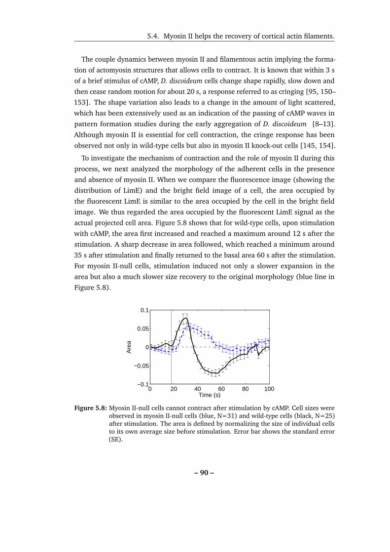
5.4. Myosin II helps the recovery of cortical actin filaments.
The couple dynamics between myosin II and filamentous actin implying the forma-
tion of actomyosin structures that allows cells to contract. It is known that within 3 s
of a brief stimulus of cAMP, D. discoideum cells change shape rapidly, slow down and
then cease random motion for about 20 s, a response referred to as cringing [95, 150–
153]. The shape variation also leads to a change in the amount of light scattered,
which has been extensively used as an indication of the passing of cAMP waves in
pattern formation studies during the early aggregation of D. discoideum [8–13].
Although myosin II is essential for cell contraction, the cringe response has been
observed not only in wild-type cells but also in myosin II knock-out cells [145, 154].
To investigate the mechanism of contraction and the role of myosin II during this
process, we next analyzed the morphology of the adherent cells in the presence
and absence of myosin II. When we compare the fluorescence image (showing the
distribution of LimE) and the bright field image of a cell, the area occupied by
the fluorescent LimE is similar to the area occupied by the cell in the bright field
image. We thus regarded the area occupied by the fluorescent LimE signal as the
actual projected cell area. Figure 5.8 shows that for wild-type cells, upon stimulation
with cAMP, the area first increased and reached a maximum around 12 s after the
stimulation. A sharp decrease in area followed, which reached a minimum around
35 s after stimulation and finally returned to the basal area 60 s after the stimulation.
For myosin II-null cells, stimulation induced not only a slower expansion in the
area but also a much slower size recovery to the original morphology (blue line in
Figure 5.8).
0 20 40 60 80 100−0.1
−0.05
0
0.05
0.1
Time (s)
Are
a
Figure 5.8: Myosin II-null cells cannot contract after stimulation by cAMP. Cell sizes wereobserved in myosin II-null cells (blue, N=31) and wild-type cells (black, N=25)after stimulation. The area is defined by normalizing the size of individual cellsto its own average size before stimulation. Error bar shows the standard error(SE).
– 90 –

Chapter 5. Myosin II sets the optimal response time scale
The rapid growth of filamentous actin everywhere around the cortex pushes the
membrane to instigates the increase of area as well as transforms the irregular cell
shape into a circular morphology, resulting in a reduction of scattered light [155].
Since myosin II-null cells also grow actin filament in the cortical region in response
to stimulation (blue trace in Figure 5.6A), a morphology change and thus a reduction
in the scattered light can still be observed without myosin II. It is worth to note that
myosin II-null cells show a delay in the expansion of area (blue trace in Figure 5.8).
Considering the fact that the cross-linking of myosin II stablizes the actin cortex [72],
myosin II-null cells lose their cortical integrity and thus may expand their membrane
less effectively.
5.5 The role of myosin II before its translocation to the cortex
So far, the main differences happened around the time myosin II translocated to
the cortical region. To investigate if the cortical release of myosin II additionally
influences the actin dynamics, we dissected the time before the translocation of
myosin II to the cortex into two parts: Tp (time for which polymerization dominates,
as defined in Figure 4.1), Td (time when depolymerization dominates, as defined in
Figure 4.1). The amplitude (Amp) defines the difference between the maximum and
minimum of cytosolic signal was investigated to know the amount of depolymerized
actin as well. Wild-type and myosin II-null cells show comparable distribution
of Tp (Figure 5.9A & 5.9B), suggesting a resemblance of actin dynamics during
polymerization. As more myosin II-null cells distributed in the long depolymerization
times than wild-type cells (Figure 5.9D & 5.9E), we further plotted Amp against Td to
verify if the broader distribution implying a different depolymerization mechanism or
due to larger cell-to-cell variability. We found that data from wild-type and myosin II-
null cells lay on the same curve. The logarithmic fitting also shows comparable results
in myosin II-null cells (Figure 5.10B, Td grows with Amp0.56) and in wild-type cells
(Figure 4.11, Td grows as Amp0.50). The plot of Amp against Tp was also examined
and all responses from wild-type and myosin II-null cells again lay on the same curve,
suggesting a similar underlying mechanism controlling the dynamics of filamentous
actin even in the absence of myosin II: the length of the polymerization dominated
time is independent of stimulation strength (Figure 5.9C) but more filamentous actin
(larger Amp) requires a longer depolymerization time (Figure 5.9F).
– 91 –
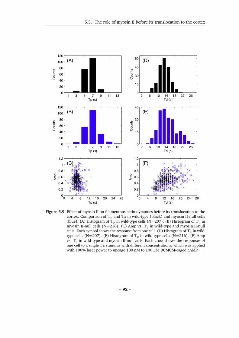
5.5. The role of myosin II before its translocation to the cortex
Figure 5.9: Effect of myosin II on filamentous actin dynamics before its translocation to thecortex. Comparison of Tp and Td in wild-type (black) and myosin II-null cells(blue). (A) Histogram of Tp in wild-type cells (N=207). (B) Histogram of Tp inmyosin II-null cells (N=216). (C) Amp vs. Tp in wild-type and myosin II-nullcells. Each symbol shows the response from one cell. (D) Histogram of Td in wild-type cells (N=207). (E) Histogram of Tp in wild-type cells (N=216). (F) Ampvs. Td in wild-type and myosin II-null cells. Each cross shows the responses ofone cell to a single 1 s stimulus with different concentrations, which was appliedwith 100% laser power to uncage 100 nM to 100 µM BCMCM-caged cAMP.
– 92 –

Chapter 5. Myosin II sets the optimal response time scale
−1 0 1 2 3 4−7
−5
−3
−1
1
log(
Am
p)
log(Td)
Figure 5.10: Logarithm fitting of relation between Amp and Td. Myosin II-null cells labeledLimE-GFP were observed. Dots show the analysis from 502 self-oscillatingcells and crosses show the analysis from 232 cells responding to one 1 sstimulus. The stimulus was applied with 100% laser power to uncage differentconcentrations of BCMCM-caged cAMP (from 30 nM to 100 µM). Red lineshows: log(Amp) = −5.4 + 1.78× log(Td).
The data from myosin II-null cells is scattered over a larger area than the wild-
type cells, suggesting a substantial cell-to-cell variability in myosin II-null cells
(Figure 5.9C & 5.9F). To inspect the origin of the significant variations among
myosin II-null cells, we first examined how different starvation times change the
properties of Amp and Td. Self-oscillating cells scattered more as they starved longer
than 9 hours (Figure 5.11B). However, cells starved between 6 and 13 hours seem to
show similar scattering in Amp and Td in response to stimulation (Figure 5.11A).
Due the fact that cells lacking myosin II have a disturbed cell division in suspension,
the sizes of myosin II-null cells are in general much bigger (as shown in histograms
in Figure 5.12) [156–159]. However, myosin II-null cells can divide through an
adhesion dependent mechanism once they are on a solid surface [160–163]. Here
we looked at the wild-type and myosin II-null cells to see how they change their sizes
during the experimental time on the solid surface (Figure 5.12): myosin II-null cells
were much larger than wild-type cells. Some myosin II-null cells tend to decrease
their sizes with extended measurement time on the solid surface but the majority of
myosin II-null cells did not change their size during the experiment, just like wild-type
cells. Detailed analysis of Amp, Td and Tp reveals that dynamics of filamentous actin
is independent of the size of the cells (Figure 5.13).
– 93 –

5.5. The role of myosin II before its translocation to the cortex
0 5 10 15 200
0.2
0.4
0.6
0.8
1
1.2
(A)
Td (s)
Am
p
0 1 2 3 4 5 6 7 8 90
0.1
0.2
0.3
0.4
0.5
0.6
6−7 hr7−8 hr8−9 hr9−10 hr10−11 hr11−12 hr12−13 hr
(B)
Td (s)
Am
p
Figure 5.11: Effect of starvation time on actin dynamics in myosin II-null cells (N=734).Amp and Td of cytosolic signals were analyzed. Dots show the analysis ofself-oscillating cells (N=502). Crosses show the analysis of cells respondingto a single 1 s stimulus (N=232). The stimulus was applied with 100% laserpower to uncage BCMCM-caged cAMP with concentration ranging from 100 nMto 100 µM. (A) Different colors show the data from different starvation times.(B) A magnification of (A) to see the data of self-oscillating cells more clearly.
Figure 5.12: Correlation analysis between cell size and the time cells stay on the solid surface.Sizes were observed in wild-type cells (A) and myosin II-null cells (B). Insetshows the histogram of the sizes from all corresponding cells. Dots show theanalysis of self-oscillating cells. Crosses show the analysis of cells respondingto a single 1 s stimulus. The stimulus was applied with 100% laser powerto uncage BCMCM-caged cAMP with concentration ranging from 100 nM to100 µM. Each symbol shows the size of one cell at the corresponding time. Bluedots, N=502; blue crosses, N=232; black dots, N=300; black crosses, N=231.
– 94 –

Chapter 5. Myosin II sets the optimal response time scale
Figure 5.13: Effect of cell sizes on actin dynamics in myosin II-null (N=734, A,C,E. Sizesshown in the legend apply also to (C) and (E).) and wild-type cells (N=531,B,D,F. Sizes shown in the legend apply also to (D) and (F).). Amp, Tp andTd were defined as Figure 4.1. Dots show the analysis of self-oscillating cells.Crosses show the analysis of cells responding to a single 1 s stimulus. Thestimulus was applied with 100% laser power to uncage BCMCM-caged cAMPwith concentration ranged from 100 nM to 100 µM. (A)&(B) Amp vs. Td inself-oscillating cells. (C)&(D) Amp vs. Td in self-oscillating cells as well ascells responding to stimulation. (E)&(F) Amp vs. Tp in cells responding tostimulation.
– 95 –
5.6. Conclusion
5.6 Conclusion
Here we investigated the role of myosin II in rapid oscillations of the cytoskeletal
network in the absence of external stimulation. We found no correlation between
the self-oscillations of actin and any observable dynamics of myosin II or even its
presence, suggesting that myosin II is not necessary for the rapid oscillations in the
cytoskeletal networks.
However, immediately after the stimulation of cAMP, actin filaments grow in
the cortical region whereas myosin II is released from the cortex (out-of-phase
signals). As myosin II is indispensable for inhibiting the formation of pseudopods [72,
144–146], the release of myosin II enables the freshly formed filamentous actin to
induce membrane protrusions. Most proteins in the signaling pathway stimulation
or regulating actin network are translocated to the cortex within 10 s after the
stimulation of cAMP (such as PHcrac, Ras, Aip1, Coronin, etc.) [109, 110, 140, 164].
In contrast, previous studies claimed that myosin II responded to the stimulation in
a much later time scale (around 30 s after stimulation) [165]. Our finding points
out that myosin II is in fact responsive, though less pronounced, within 10 s, but is
released from the cortex into the cytosol (Figure 5.5).
The later translocation of myosin II to the cortical region (30 s cf. 10 s) is due to
the fact that the translocation of myosin II requires filamentous actin. We confirmed
the coupling between the dynamics of myosin II and LimE during their translocation
to the cortical region (Figure 5.7). The delay in the recovery of cortical filamentous
actin in myosin II-null cells (Figure 5.6A) suggests that the interaction between
myosin II and actin filaments not only carries myosin II from the cytosol to the cortex
but also enhances the efficiency of actin accumulation in the cortical region.
The main difference between the morphology of wild-type and myosin II mutant
cells is also found during the time that myosin II and filamentous actin translocate to
the cortex together: wild-type cells rapidly shrink their size to 10% smaller of their
size before stimualtion and then gradually recover, whereas myosin II-null cells slowly
returned to their original sizes (Figure 5.8), suggesting that they lose the property
to contract rapidly. Considering the fact that myosin II walking on actin filaments
enables contraction, the accumulation of actomyosin filaments in the cortex thus lead
to a significant decrease in the imaged area. Cells without myosin II decreases their
size much more slowly, implying the indispensible role of myosin II in maintaining
cell morphology.
– 96 –

Conclusion and Outlook
In this work, we investigated the actin network dynamics of D. discoideum in the
absence and presence of external stimulation of cAMP. We quantified first the self-
oscillations: the actin networks of cells oscillate with a period around 12 s and this
property is independent of the passage number, starvation time, cell sizes and even
regulatory proteins like myosin II. We discovered that self-oscillations originate from
the global synchronization of actin polymerization and depolymerization in the cell
cortex and can be observed in all cells. The oscillation periods are controlled by
the binding time of the capping protein: as filamentous actin shows little branching
owing to the small amount of activated Arp2/3 (branching protein), the binding time
of capping protein determines the number of polymerized actin filaments. Since the
following depolymerization only happens from the pointed end of actin filaments,
it takes longer to depolymerize more actin filaments. Considering the fact that one
oscillation period includes both the polymerization and depolymerization process,
the binding time of capping protein therefore controls the oscillation period through
determining the amount of polymerized filamentous actin.
It is the synchronizations that enable us to learn the frequency of the intrinsic
cytoskeletal dynamics. However, cells spend more time in the non-oscillatory state
and it is still unknown what initiates the global synchronization. Since it has been
found in the actin dynamics of cancer cells that calcium is responsible for oscillations
with periods of around 30 s [122], examination of the influence of calcium on
self-oscillations should be a good start.
Second, we investigated the effect of stimulation strength on actin dynamics.
We found that the response amplitude grows with stimulation strength only in a
very narrow region of stimulation, after which the response amplitude reaches a
plateau. This threshold varies a lot among cells. Moreover, the response amplitudes
are scattered not only with respect to different stimulation strength at the plateau
but also to the same stimulation. In spite of the large cell-to-cell variability, when
plotting the single response amplitudes against the corresponding polymerization
and depolymerization times, a nearly constant and quadratic relationship are visible,
respectively, suggesting an universal underlying mechanism.
– 97 –
5.6. Conclusion
It has been reported that actin patches can form randomly anywhere in the cell
cortex [166, 167]. Pseudopods grow from the regions with the highest density of
actin patches [132]. Cells have a basal cycle for the extension of pseudopod, which
is a non-random probabilistic process [103, 107]. Shallow gradients does not change
the dynamics of patch formation but can bias the probabilities of patch formation to
enhance the density of patches aligned with the direction of the gradient [102, 105].
This corroborates our finding that the response upon external stimulation can be
well described by the same mechanism and components of self-oscillations, while the
larger response amplitude are ascribed to an increased amount of Arp2/3.
It is still unclear what the factor controlling the amount of activated Arp2/3
after stimulation is. Besides examining the dynamics of proteins involved in the
signaling pathways upstream of Arp2/3, it is worthwhile to check whether genetic
variations play a role on the differences among individuals. To uncover the underlying
determinant, a new method that enables simultaneous stimulation and recording of
a large number of cells is required for an efficient systematic screening.
Finally, we investigated the interplay between actin and myosin II. There is no
correlation between the self-oscillations of actin and any observable dynamics of
myosin II or even its presence. However, immediately after the stimulation of cAMP,
actin filaments grow in the cortical region whereas myosin II is released from the
cortex (out-of-phase signals). As myosin II inhibits the formation of pseudopods,
the release of myosin II enables the freshly formed filamentous actin to induce
membrane protrusions. Most proteins in the signaling pathway or regulating actin
network are translocated to the cortex within 10 s after the stimulation of cAMP
(such as PHcrac, Ras, Aip1, Coronin, etc.). In contrast, previous studies claimed that
myosin II responded to the stimulation in a much later time scale (around 30 s after
stimulation) [165]. Our finding points out that myosin II is in fact responsive, though
less pronounced, within 10 s, but is released from the cortex into the cytosol. The
later translocation of myosin II to the cortical region (30 s cf. 10 s) is due to the
fact that the translocation of myosin II requires filamentous actin. The interaction
between myosin II and actin filaments not only carries myosin II from the cytosol
to the cortex but also enhances the efficiency of actin accumulation in the cortical
region. The actomyosin complex further enables rapid cell contraction. Myosin II-null
cells show a delay in the recovery of cortical actin filaments as well as incapability
of contractions, revealing the essence of myosin II in regulating actin dynamics and
maintaining cell morphology.
– 98 –

Bibliography
[1] Ludwig Eichinger & Francisco Rivero, editor. Dictyostelium discoideum proto-cols. Humana press, 2006.
[2] G. Potts. Zur physiologie des dictyostelium mucoroides. Flora (Jena), 1902.
[3] R. Sussman and M. Sussman. Physical charaterization of deoxyribonucleicacids in dictyostelium discoideum. Arch. Biochem. Biophys, 1971.
[4] J. Franke and R. Kessin. Adefined minimal medium for axenic strains ofdictyostelium discoideum. Proc. Natl. Acad. Sci USA, 1977.
[5] R. L. Chisholm and R. A. Firtel. Insights into morphogenesis from a simpledevelopmental system. Nat. Rev. Mol. Cell Biol., 5(7):531–541, July 2004.
[6] I. M. Zadahames and J. M. Ashworth. Cell-cycle during vegetative stage ofdictyostelium-discoideum and its response to temperature-change. J. Cell Sci.,32(AUG):1–20, 1978.
[7] M. Clarke. Recent insights into host-pathogen interactions from dictyostelium.Cell. Microbiol., 12(3):283–291, March 2010.
[8] K. J. Tomchik and P. N. Devreotes. Adenosine-3’,5’-monophosphate waves indictyostelium-discoideum - a demonstration by isotope dilution-fluorography.Science, 212(4493):443–446, 1981.
[9] S. Sawai, P. A. Thomason, and E. C. Cox. An autoregulatory circuitfor long-range self-organization in dictyostelium cell populations. Nature,433(7023):323–326, January 2005.
[10] D. Dormann, J. Y. Kim, P. N. Devreotes, and C. J. Weijer. camp receptor affinitycontrols wave dynamics, geometry and morphogenesis in dictyostelium. J.Cell Sci., 114(13):2513–2523, July 2001.
[11] E. Ben-Jacob, I. Cohen, and H. Levine. Cooperative self-organization ofmicroorganisms. Adv. Phys., 49(4):395–554, June 2000.
[12] P. N. Devreotes, M. J. Potel, and S. A. Mackay. Quantitative-analysis of cyclic-amp waves mediating aggregation in dictyostelium-discoideum. Dev. Biol.,96(2):405–415, 1983.
– 99 –

Bibliography
[13] E. Palsson, K. J. Lee, R. E. Goldstein, J. Franke, R. H. Kessin, and E. C. Cox.Selection for spiral waves in the social amoebae dictyostelium. Proc. Natl.Acad. Sci. U. S. A., 94(25):13719–13723, December 1997.
[14] C. J. Weijer, G. Duschl, and C. N. David. Dependence of cell-type proportioningand sorting on cell-cycle phase in dictyostelium-discoideum. J. Cell Sci.,70(AUG):133–145, 1984.
[15] M. Wang, R. J. Aerts, W. Spek, and P. Schaap. Cell-cycle phase in dictyostelium-discoideum is correlated with the expression of cyclic-amp production, detec-tion, and degradation - involvement of cyclic-amp signaling in cell sorting.Dev. Biol., 125(2):410–416, February 1988.
[16] R. H. Gomer and R. A. Firtel. Cell-autonomous determination of cell-type choice in dictyostelium development by cell-cycle phase. Science,237(4816):758–762, August 1987.
[17] J. C. Coates and A. J. Harwood. Cell-cell adhesion and signal transductionduring dictyostelium development. J. Cell Sci., 114(24):4349–4358, December2001.
[18] D. A. Brock, T. E. Douglas, D. C. Queller, and J. E. Strassmann. Primitiveagriculture in a social amoeba. Nature, 469(7330):393–+, January 2011.
[19] D. A. Cotter and K. B. Raper. Properties of germinating spores of dictyosteliumdiscoideum. J. Bacteriol., 96(5):1680–&, 1968.
[20] D. A. Cotter and K. B. Raper. Factors affecting rate of heat-induced sporegermination in dictyostelium discoideum. J. Bacteriol., 96(1):86–&, 1968.
[21] M. J. Carnell and R. H. Insall. Actin on disease - studying the pathobiology ofcell motility using dictyostelium discoideum. Sem. Cell Dev. Biol., 22(1):82–88,February 2011.
[22] P. Cosson and T. Soldati. Eat, kill or die: when amoeba meets bacteria. Curr.Opin. Microbiol., 11(3):271–276, June 2008.
[23] J. King and R. H. Insall. Parasexual genetics of dictyostelium gene disruptions:identification of a ras pathway using diploids. Bmc Genet., 4:12, July 2003.
[24] A. Kuspa and W. F. Loomis. Tagging developmental genes in dictyostelium byrestriction enzyme-mediated integration of plasmid dna. Proc. Natl. Acad. Sci.U. S. A., 89(18):8803–8807, September 1992.
[25] H. Martens, J. Novotny, J. Oberstrass, T. L. Steck, P. Postlethwait, andW. Nellen. Rnai in dictyostelium: The role of rna-directed rna polymerasesand double-stranded rnase. Mol. Biol. Cell, 13(2):445–453, February 2002.
– 100 –

Bibliography
[26] L. Eichinger, J. A. Pachebat, G. Glockner, M. A. Rajandream, R. Sucgang,M. Berriman, J. Song, R. Olsen, K. Szafranski, Q. Xu, B. Tunggal, S. Kummer-feld, M. Madera, B. A. Konfortov, F. Rivero, A. T. Bankier, R. Lehmann, N. Ham-lin, R. Davies, P. Gaudet, P. Fey, K. Pilcher, G. Chen, D. Saunders, E. Sodergren,P. Davis, A. Kerhornou, X. Nie, N. Hall, C. Anjard, L. Hemphill, N. Bason,P. Farbrother, B. Desany, E. Just, T. Morio, R. Rost, C. Churcher, J. Cooper,S. Haydock, N. van Driessche, A. Cronin, I. Goodhead, D. Muzny, T. Mourier,A. Pain, M. Lu, D. Harper, R. Lindsay, H. Hauser, K. James, M. Quiles, M. M.Babu, T. Saito, C. Buchrieser, A. Wardroper, M. Felder, M. Thangavelu, D. John-son, A. Knights, H. Loulseged, K. Mungall, K. Oliver, C. Price, M. A. Quail,H. Urushihara, J. Hernandez, E. Rabbinowitsch, D. Steffen, M. Sanders, J. Ma,Y. Kohara, S. Sharp, M. Simmonds, S. Spiegler, A. Tivey, S. Sugano, B. White,D. Walker, J. Woodward, T. Winckler, Y. Tanaka, G. Shaulsky, M. Schleicher,G. Weinstock, A. Rosenthal, E. C. Cox, R. L. Chisholm, R. Gibbs, W. F. Loomis,M. Platzer, R. R. Kay, J. Williams, P. H. Dear, A. A. Noegel, B. Barrell, andA. Kuspa. The genome of the social amoeba dictyostelium discoideum. Nature,435(7038):43–57, May 2005.
[27] T. D. Pollard and J. A. Cooper. Actin, a central player in cell shape andmovement. Science, 326(5957):1208–1212, November 2009.
[28] R. Dominguez and K. C. Holmes. Actin structure and function. Annu. Rev.Biophys., 40:169–186, 2011.
[29] T. D. Pollard and G. G. Borisy. Cellular motility driven by assembly anddisassembly of actin filaments (vol 112, pg 453, 2002). Cell, 113(4):549–549,May 2003.
[30] T. D. Pollard. Regulation of actin filament assembly by arp2/3 complex andformins. Annu. Rev. Biophys. Biomol. Struct., 36:451–477, 2007.
[31] R. C. Robinson, K. Turbedsky, D. A. Kaiser, J. B. Marchand, H. N. Higgs,S. Choe, and T. D. Pollard. Crystal structure of arp2/3 complex. Science,294(5547):1679–1684, November 2001.
[32] K. J. Amann and T. D. Pollard. The arp2/3 complex nucleates actin filamentbranches from the sides of pre-existing filaments. Nat. Cell Biol., 3(3):306–310,March 2001.
[33] T. M. Svitkina and G. G. Borisy. Arp2/3 complex and actin depolymerizingfactor cofilin in dendritic organization and treadmilling of actin filament arrayin lamellipodia. J. Cell Biol., 145(5):1009–1026, May 1999.
[34] T. D. Pollard, L. Blanchoin, and R. D. Mullins. Molecular mechanisms control-ling actin filament dynamics in nonmuscle cells. Annu. Rev. Biophys. Biomol.Struct., 29:545–576, 2000.
– 101 –

Bibliography
[35] H. Aizawa, Y. Fukui, and I. Yahara. Live dynamics of dictyostelium cofilinsuggests a role in remodeling actin latticework into bundles. J. Cell Sci.,110:2333–2344, October 1997.
[36] H. Aizawa, K. Sutoh, S. Tsubuki, S. Kawashima, A. Ishii, and I. Yahara.Identification, characterization, and intracellular-distribution of cofilin indictyostelium-discoideum. J. Biol. Chem., 270(18):10923–10932, May 1995.
[37] H. Aizawa, M. Katadae, M. Maruya, M. Sameshima, K. Murakami-Murofushi,and I. Yahara. Hyperosmotic stress-induced reorganization of actin bundles indictyostelium cells over-expressing cofilin. Genes Cells, 4(6):311–324, June1999.
[38] K. Okada, T. Obinata, and H. Abe. Xaip1: a xenopus homologue of yeast actininteracting protein 1 (aip1), which induces disassembly of actin filamentscooperatively with adf cofilin family proteins. J. Cell Sci., 112(10):1553–1565,May 1999.
[39] S. Ono. Regulation of actin filament dynamics by actin depolymerizing fac-tor/cofilin and actin-interacting protein 1: New blades for twisted filament.Biochemistry (Mosc.), 42(46):13363–13370, November 2003.
[40] S. Ono, K. Mohri, and K. Ono. Microscopic evidence that actin-interactingprotein 1 actively disassembles actin-depolymerizing factor/cofilin-boundactin filaments. J. Biol. Chem., 279(14):14207–14212, April 2004.
[41] K. Okada, L. Blanchoin, H. Abe, H. Chen, T. D. Pollard, and J. R. Bamburg.Xenopus actin-interacting protein 1 (xaip1) enhances cofilin fragmentationof filaments by capping filament ends. J. Biol. Chem., 277(45):43011–43016,November 2002.
[42] K. Okada, H. Ravi, E. M. Smith, and B. L. Goode. Aip1 and cofilin promoterapid turnover of yeast actin patches and cables: A coordinated mechanismfor severing and capping filaments. Mol. Biol. Cell, 17(7):2855–2868, July2006.
[43] A. Rodal, J. Tetrault, D. Amberg, and D. Drubin. Aip1p functionally interactswith cofilin in vivo and in vitro. Mol. Biol. Cell, 9:15A–15A, November 1998.
[44] A. A. Rodal, J. W. Tetreault, P. Lappalainen, D. G. Drubin, and D. C. Am-berg. Aip1p interacts with cofilin to disassemble actin filaments. J. Cell Biol.,145(6):1251–1264, June 1999.
[45] A. Konzok, I. Weber, E. Simmeth, U. Hacker, M. Maniak, and A. Muller-Taubenberger. Daip1, a dictyostelium homologue of the yeast actin-interactingprotein 1, is involved in endocytosis, cytokinesis, and motility. J. Cell Biol.,146(2):453–464, July 1999.
– 102 –
Bibliography
[46] E. L. Dehostos, B. Bradtke, F. Lottspeich, R. Guggenheim, and G. Gerisch.Coronin, an actin binding-protein of dictyostelium-discoideum localized tocell-surface projections, has sequence similarities to g-protein beta-subunits.EMBO J., 10(13):4097–4104, December 1991.
[47] B. L. Goode, J. J. Wong, A. C. Butty, M. Peter, A. L. McCormack, J. R. Yates,D. G. Drubin, and G. Barnes. Coronin promotes the rapid assembly and cross-linking of actin filaments and may link the actin and microtubule cytoskeletonsin yeast. J. Cell Biol., 144(1):83–98, January 1999.
[48] L. Cai, Al. M. Makhov, and J. E. Bear. F-actin binding is essential for coronin1b function in vivo. J. Cell Sci., 120(10):1779–1790, May 2007.
[49] Z. Spoerl, M. Stumpf, A. A. Noegel, and A. Hasse. Oligomerization, f-actininteraction, and membrane association of the ubiquitous mammalian coronin3 are mediated by its carboxyl terminus. J. Biol. Chem., 277(50):48858–48867,December 2002.
[50] T. Oku, S. Itoh, R. Ishii, K. Suzuki, W. M. Nauseef, S. Toyoshima, and T. Tsuji.Homotypic dimerization of the actin-binding protein p57/coronin-1 mediatedby a leucine zipper motif in the c-terminal region. Biochem. J., 387:325–331,April 2005.
[51] J. Gatfield, I. Albrecht, B. Zanolari, M. O. Steinmetz, and J. Pieters. Associationof the leukocyte plasma membrane with the actin cytoskeleton through coiledcoil-mediated trimeric coronin 1 molecules. Mol. Biol. Cell, 16(6):2786–2798,June 2005.
[52] M. Gandhi, V. Achard, L. Blanchoin, and B. L. Goode. Coronin switches rolesin actin disassembly depending on the nucleotide state of actin. Mol. Cell,34(3):364–374, May 2009.
[53] C. L. Humphries, H. I. Balcer, J. L. D’Agostino, B. Winsor, D. G. Drubin,G. Barnes, B. J. Andrews, and B. L. Goode. Direct regulation of arp2/3complex activity and function by the actin binding protein coronin. J. CellBiol., 159(6):993–1004, December 2002.
[54] C. Z. Liu, Y. Chen, and S. F. Sui. The identification of a new actin-bindingregion in p57. Cell Res., 16(1):106–112, January 2006.
[55] M. Gandhi and B. L. Goode. Coronin: The double-edged sword of actindynamics. Subcell. Biochem., 48:72–87, 2008.
[56] N. Foeger, L. Rangell, D. M. Danilenko, and A. C. Chan. Requirement forcoronin 1 in t lymphocyte trafficking and cellular homeostasis. Science,313(5788):839–842, August 2006.
– 103 –

Bibliography
[57] L. Cai, N. Holoweckyj, M. D. Schaller, and J. E. Bear. Phosphorylation ofcoronin 1b by protein kinase c regulates interaction with arp2/3 and cellmotility. J. Biol. Chem., 280(36):31913–31923, September 2005.
[58] E. L. Dehostos, C. Rehfuess, B. Bradtke, D. R. Waddell, R. Albrecht, J. Murphy,and G. Gerisch. Dictyostelium mutants lacking the cytoskeletal protein coroninare defective in cytokinesis and cell motility. J. Cell Biol., 120(1):163–173,January 1993.
[59] A. A. Noegel and M. Schleicher. The actin cytoskleleton of dictyostelium: astory told by mutants. J. Cell Sci., 113(5):759–766, March 2000.
[60] M. A. de la Roche and G. P. Cote. Regulation of dictyostelium myosin i and ii.Biochim. Biophys. Acta, 1525(3):245–261, March 2001.
[61] M. Vicente-Manzanares, X. Ma, R. S. Adelstein, and A. R. Horwitz. Non-musclemyosin ii takes centre stage in cell adhesion and migration. Nat. Rev. Mol. CellBiol., 10(11):778–790, November 2009.
[62] T. Q. P. Uyeda, P. D. Abramson, and J. A. Spudich. The neck region of themyosin motor domain acts as a lever arm to generate movement. Proc. Natl.Acad. Sci. U. S. A., 93(9):4459–4464, April 1996.
[63] C. T. Murphy, R. S. Rock, and J. A. Spudich. A myosin ii mutation uncouplesatpase activity from motility and shortens step size. Nat. Cell Biol., 3(3):311–315, March 2001.
[64] A. D. Mclachlan and J. Karn. Periodic charge-distributions in the myosinrod amino-acid-sequence match cross-bridge spacings in muscle. Nature,299(5880):226–231, 1982.
[65] M. A. De la Roche, J. L. Smith, V. Betapudi, T. T. Egelhoff, and G. P. Cote.Signaling pathways regulating dictyostelium myosin ii. J. Muscle Res. CellMotil., 23(7-8):703–718, October 2002.
[66] S. Yumura and T. Kitanishiyumura. Immunoelectron microscopic studies ofthe ultrastructure of myosin-filaments in dictyostelium-discoideum. Cell Struct.Funct., 15(6):343–354, December 1990.
[67] C. Pasternak, J. A. Spudich, and E. L. Elson. Capping of surface-receptors andconcomitant cortical tension are generated by conventional myosin. Nature,341(6242):549–551, October 1989.
[68] W. C. Liang, H. M. Warrick, and J. A. Spudich. A structural model for phos-phorylation control of dictyostelium myosin ii thick filament assembly. J. CellBiol., 147(5):1039–1047, November 1999.
[69] L. Bosgraaf and P. J. M. van Haastert. The regulation of myosin ii in dic-tyostelium. Eur. J. Cell Biol., 85(9-10):969–979, September 2006.
– 104 –
Bibliography
[70] Y. E. Goldman. Wag the tail: Structural dynamics of actomyosin. Cell, 93(1):1–4, April 1998.
[71] R. J. Barsotti, J. A. Dantzig, and Y. E. Goldman. Myosin isoforms show differentstrokes for different blokes. Nat. Struct. Biol., 3(9):737–739, September 1996.
[72] G. Laevsky and D. A. Knecht. Cross-linking of actin filaments by myosinii is a major contributor to cortical integrity and cell motility in restrictiveenvironments. J. Cell Sci., 116(18):3761–3770, September 2003.
[73] T. T. Egelhoff, D. J. Manstein, and J. A. Spudich. Complementation of myosinnull mutants in dictyostelium-discoideum by direct functional selection. Dev.Biol., 137(2):359–367, February 1990.
[74] L. A. Cameron, P. A. Giardini, F. S. Soo, and J. A. Theriot. Secrets of actin-based motility revealed by a bacterial pathogen. Nat. Rev. Mol. Cell Biol.,1(2):110–119, November 2000.
[75] P. Cossart and A. Toledo-Arana. Listeria monocytogenes, a unique model ininfection biology: an overview. Microbes Infect., 10(9):1041–1050, July 2008.
[76] M. Kaksonen, C. P. Toret, and D. G. Drubin. Harnessing actin dynamics forclathrin-mediated endocytosis. Nat. Rev. Mol. Cell Biol., 7(6):404–414, June2006.
[77] V. Laurent, T. P. Loisel, B. Harbeck, A. Wehman, L. Grobe, B. M. Jockusch,J. Wehland, F. B. Gertler, and M. F. Carlier. Role of proteins of the ena/-vasp family in actin-based motility of listeria monocytogenes. J. Cell Biol.,144(6):1245–1258, March 1999.
[78] S. M. Rafelski and J. A. Theriot. Mechanism of polarization of listeria mono-cytogenes surface protein acta. Mol. Microbiol., 59(4):1262–1279, February2006.
[79] G. Gerisch. Self-organizing actin waves that simulate phagocytic cup structures.PMC Biophys, 3(1):7–7, March 2010.
[80] T. Bretschneider, S. Diez, K. Anderson, J. Heuser, M. Clarke, A. Muller-Taubenberger, J. Kohler, and G. Gerisch. Dynamic actin patterns and arp2/3assembly at the substrate-attached surface of motile cells. Curr. Biol., 14(1):1–10, January 2004.
[81] Y. Asano, A. Nagasaki, and T. Q. P. Uyeda. Correlated waves of actin filamentsand pip(3) in dictyostelium cells. Cell Motil. Cytoskeleton, 65(12):923–934,December 2008.
[82] G. Gerisch, T. Bretschneider, A. Muller-Taubenberger, E. Simmeth, M. Ecke,S. Diez, and K. Anderson. Mobile actin clusters and traveling waves in
– 105 –
Bibliography
cells recovering from actin depolymerization. Biophys. J., 87(5):3493–3503,November 2004.
[83] G. Gerisch, M. Ecke, D. Wischnewski, and B. Schroth-Diez. Different modes ofstate transitions determine pattern in the phosphatidylinositide-actin system.BMC Cell Biol., 12:42, October 2011.
[84] A. Goldbeter, C. Gerard, D. Gonze, J. C. Leloup, and G. Dupont. Systemsbiology of cellular rhythms. FEBS Lett., 586(18):2955–2965, August 2012.
[85] K. Kruse and F. Julicher. Oscillations in cell biology. Curr. Opin. Cell Biol.,17(1):20–26, February 2005.
[86] A. Goldbeter, C. Gerard, and J. C. Leloup. Circadian rhythms and systemsbiology. Med. Sci., 26(1):49–56, January 2010.
[87] C. L. Partch, C. B. Green, and J. S. Takahashi. Molecular architecture of themammalian circadian clock. Trends Cell Biol., 24(2):90–99, February 2014.
[88] C. Dibner, U. Schibler, and U. Albrecht. The mammalian circadian timingsystem: Organization and coordination of central and peripheral clocks. Annu.Rev. Physiol., 72:517–549, 2010.
[89] G. Meacci and K. Kruse. Min-oscillations in escherichia coli induced by inter-actions of membrane-bound proteins. Phys. Biol., 2(2):89–97, June 2005.
[90] M. Loose, K. Kruse, and P. Schwille. Protein self-organization: Lessons fromthe min system. Annu. Rev. Biophys., 40:315–336, 2011.
[91] C. Shingyoji, H. Higuchi, M. Yoshimura, E. Katayama, and T. Yanagida. Dyneinarms are oscillating force generators. Nature, 393(6686):711–714, June 1998.
[92] A. C. Crawford and R. Fettiplace. The mechanical-properties of ciliary bundlesof turtle cochlear hair-cells. J. Physiol. (Lond.), 364(JUL):359–&, 1985.
[93] G. Gerisch, D. Hulser, D. Malchow, and U. Wick. Cell communication byperiodic cyclic-amp pulses. Phil. Trans. R. Soc. B, 272(915):181–&, 1975.
[94] B. M. Shaffer. Secretion of cyclic-amp induced by cyclic-amp in cellularslime-mold dictyostelium-discoideum. Nature, 255(5509):549–552, 1975.
[95] R. P. Futrelle, J. Traut, and W. G. Mckee. Cell behavior in dictyostelium-discoideum - pre-aggregation response to localized cyclic-amp pulses. J. CellBiol., 92(3):807–821, 1982.
[96] E. Schaefer, D. Aue, M. Tarantola, E. Polo, C. Westendorf, N. Oikawa,E. Bodenschatz, B. Geil, and A. Janshoff. Collective behavior of dic-tyostelium discoideum monitored by impedance analysis. Commun. Integr.Biol., 6(3):e23894–e23894, May 2013.
– 106 –
Bibliography
[97] D. Malchow, R. Bohme, and U. Gras. On the role of calcium in chemotaxis andoscillations of dictyostelium cells. Biophys. Struct. Mech., 9(2):131–136, 1982.
[98] J. Bumann, B. Wurster, and D. Malchow. Attractant-induced changes andoscillations of the extracellular ca++ concentration in suspensions of differ-entiating dictyostelium cells. J. Cell Biol., 98(1):173–178, 1984.
[99] Y. Arai, T. Shibata, S. Matsuoka, M. J. Sato, T. Yanagida, and M. Ueda. Self-organization of the phosphatidylinositol lipids signaling system for randomcell migration. Proc. Natl. Acad. Sci. U. S. A., 107(27):12399–12404, July2010.
[100] T. Shibata, A. Yoshiyuki, M. Satomi, S. J. Masayuki, and U. Masahiro. Self-organization of the phosphatidylinositol lipids signaling system for randomcell migration. Biophys. J., 100(3):Biophys Soc, February 2011.
[101] L. Bosgraaf and P. J. M. Van Haastert. Quimp3, an automated pseudopod-tracking algorithm. Cell Adh. Migr., 4(1):46–55, January 2010.
[102] P. J. M. Van Haastert. Chemotaxis: insights from the extending pseudopod. J.Cell Sci., 123(18):3031–3037, September 2010.
[103] P. J. M. Van Haastert. A stochastic model for chemotaxis based on the orderedextension of pseudopods. Biophys. J., 99(10):3345–3354, November 2010.
[104] A. Kortholt, I. Keizer-Gunnink, R. Kataria, and P. J. M. Van Haastert. Rasactivation and symmetry breaking during dictyostelium chemotaxis. J. CellSci., 126(19):4502–4513, October 2013.
[105] P. J. M. Van Haastert. How cells use pseudopods for persistent movement andnavigation. Sci. Signal., 4(159):pe6, February 2011.
[106] P. J. M. van Haastert and M. Postma. Biased random walk by stochasticfluctuations of chemoattractant-receptor interactions at the lower limit ofdetection. Biophys. J., 93(5):1787–1796, September 2007.
[107] P. J. M. Van Haastert and L. Bosgraaf. The local cell curvature guides pseu-dopodia towards chemoattractants. HFSP J, 3(4):282–286, August 2009.
[108] L. Bosgraaf and P. J. M. Van Haastert. Navigation of chemotactic cells by paral-lel signaling to pseudopod persistence and orientation. Plos One, 4(8):e6842,August 2009.
[109] C. Westendorf, J. Negrete, A. J. Bae, R. Sandmann, E. Bodenschatz, andC. Beta. Actin cytoskeleton of chemotactic amoebae operates close to theonset of oscillations. Proc. Natl. Acad. Sci. U. S. A., 110(10):3853–3858, March2013.
– 107 –
Bibliography
[110] C.-H. Huang, M. Tang, C. Shi, P. A. Iglesias, and P. N. Devreotes. An ex-citable signal integrator couples to an idling cytoskeletal oscillator to drivecell migration. Nat. Cell Biol., 15(11):1307–U108, November 2013.
[111] Nano SU-8 Negative tone photoresist formulations 2-25.
[112] Y. N. Xia and G. M. Whitesides. Soft lithography. Annu. Rev. Mater. Sci.,28:153–184, 1998.
[113] S. J. Clarson and J. A. Semlyen. Siloxane Polymers. Englewood Cliffs,NJ:Prentice Hall, 1993.
[114] R. H. Kessin. Dictyostelium: evolution, cell biology, and the development ofmulticellularity. Developmental and Cell Biology Series, 38:i–xiv„ 2001.
[115] V. Hagen, J. Bendig, S. Frings, T. Eckardt, S. Helm, D. Reuter, and U. B. Kaupp.Highly efficient and ultrafast phototriggers for camp and cgmp by using long-wavelength uv/vis-activation. Angew. Chem. Int. Ed., 40(6):1046–+, 2001.
[116] V. Hagen, S. Frings, J. Bendig, D. Lorenz, B. Wiesner, and U. B. Kaupp.Fluorescence spectroscopic quantification of the release of cyclic nucleotidesfrom photocleavable [bis(carboxymethoxy)coumarin-4-yl]methyl esters insidecells. Angew. Chem. Int. Ed., 41(19):3625–3628, 2002.
[117] C. Westendorf. Oscillatory dynamics of the actin Cytoskeleton. PhD thesis,Georg-August-Universität Göttingen, 2013.
[118] C. Beta, D. Wyatt, W.-J. Rappel, and E. Bodenschatz. Flow photolysis forspatiotemporal stimulation of single cells. Anal. Chem., 79(10):3940–3944,May 2007.
[119] D. Malchow, V. Nanjundiah, and G. Gerisch. Ph oscillations in cell-suspensionsof dictyostelium-discoideum - their relation to cyclic-amp signals. J. Cell Sci.,30(APR):319–330, 1978.
[120] T. Killich, P. J. Plath, E. C. Hass, W. Xiang, H. Bultmann, L. Rensing, andM. G. Vicker. Cell-movement and shape are nonrandom and determined byintracellular, oscillatory rotating waves in dictyostelium amebas. Biosystems,33(2):75–87, 1994.
[121] H. C. Ishikawa-Ankerhold. Functional Organization of the Actin System inDictyostelium. PhD thesis, Technischen Universität München, 2008.
[122] M. Wu, X. Wu, and P. De Camilli. Calcium oscillations-coupled conversion ofactin travelling waves to standing oscillations. Proc. Natl. Acad. Sci. U. S. A.,110(4):1339–1344, January 2013.
– 108 –

Bibliography
[123] J. Bumann, D. Malchow, and B. Wurster. Oscillations of ca++ concentrationduring the cell-differentiation of dictyostelium-discoideum - their relation tooscillations in cyclic-amp and other components. Differentiation, 31(2):85–91,1986.
[124] A. Goldbeter. Oscillations and waves of cyclic amp in dicyostelium: A prototypefor spatio-temporal organization and pulsatile intercellular communication.Bull. Math. Biol., 68(5):1095–1109, July 2006.
[125] V. Nanjundiah. Cyclic amp oscillations in dictyostelium discoideum: modelsand observations. Biophys. Chem., 72(1-2):1–8, May 1998.
[126] J. Negrete. Fluctuations and Oscillatory Instabilities of Intracellular FiberNetworks. PhD thesis, Georg-August-Universität Göttingen, 2014.
[127] R. J. Eddy, J. Han, and J. S. Condeelis. Capping protein terminates but doesnot initiate chemoattractant-induced actin assembly in dictyostelium. J. CellBiol., 139(5):1243–1253, December 1997.
[128] D. Yarar, W. To, A. Abo, and M. D. Welch. The wiskott-aldrich syndromeprotein directs actin-based motility by stimulating actin nucleation with thearp2/3 complex. Curr. Biol., 9(10):555–558, May 1999.
[129] D. Winter, T. Lechler, and R. Li. Activation of the yeast arp2/3 complex bybee1p, a wasp-family protein. Curr. Biol., 9(9):501–504, May 1999.
[130] R. Rohatgi, L. Ma, H. Miki, M. Lopez, T. Kirchhausen, T. Takenawa, and M. W.Kirschner. The interaction between n-wasp and the arp2/3 complex linkscdc42-dependent signals to actin assembly. Cell, 97(2):221–231, April 1999.
[131] L. M. Machesky, R. D. Mullins, H. N. Higgs, D. A. Kaiser, L. Blanchoin, R. C.May, M. E. Hall, and T. D. Pollard. Scar, a wasp-related protein, activatesnucleation of actin filaments by the arp2/3 complex. Proc. Natl. Acad. Sci. U.S. A., 96(7):3739–3744, March 1999.
[132] P. J. M. Van Haastert and L. Bosgraaf. Food searching strategy of amoeboidcells by starvation induced run length extension. Plos One, 4(8):e6814, August2009.
[133] D. Wessels, D. R. Soll, D. Knecht, W. F. Loomis, A. Delozanne, and J. Spudich.Cell motility and chemotaxis in dictyostelium amebae lacking myosin heavy-chain. Dev. Biol., 128(1):164–177, July 1988.
[134] J. A. Spudich. In pursuit of myosin function. Cell Regul., 1(1):1–11, November1989.
[135] D. Wessels and D. R. Soll. Myosin-ii heavy-chain null mutant of dictyosteliumexhibits defective intracellular particle movement. J. Cell Biol., 111(3):1137–1148, September 1990.
– 109 –

Bibliography
[136] P. J. Heid, D. Wessels, K. J. Daniels, P. Gibson, H. Zhang, E. Voss, and D. R.Soll. The role of myosin heavy chain phosphorylation in dictyostelium motil-ity, chemotaxis and f-actin localization. J. Cell Sci., 117(20):4819–4835,September 2004.
[137] C. Westendorf, A. J. Bae, C. Erlenkamper, E. Galland, C. Franck, E. Boden-schatz, and C. Beta. Live cell flattening - traditional and novel approaches.PMC Biophys, 3(1):9–9, April 2010.
[138] I. Sadler, A. W. Crawford, J. W. Michelsen, and M. C. Beckerle. Zyxin and ccrp- 2 interactive lim domain proteins associated with the cytoskeleton. J. CellBiol., 119(6):1573–1587, December 1992.
[139] I. Kovacic and M. J. Brennan, editors. The Duffing Equation: NonlinearOscillators and their Behaviour. John Wiley & Sons, Ltd., 2011.
[140] C. J. Wang, A. Bergmann, B. Lin, K. Kim, and A. Levchenko. Diverse sensitivitythresholds in dynamic signaling responses by social amoebae. Sci. Signal.,5(213):ra17, February 2012.
[141] A. Samadani, J. Mettetal, and A. van Oudenaarden. Cellular asymmetry and in-dividuality in directional sensing. Proc. Natl. Acad. Sci. U. S. A., 103(31):11549–11554, August 2006.
[142] P. Lappalainen, E. V. Fedorov, A. A. Fedorov, S. C. Almo, and D. G. Drubin.Essential functions and actin-binding surfaces of yeast cofilin revealed bysystematic mutagenesis. EMBO J., 16(18):5520–5530, September 1997.
[143] J. D. Murray. Mathematical Biology. Springer, 2004.
[144] E. Shelden and D. A. Knecht. Dictyostelium cell shape generation requiresmyosin ii. Cell Motil. Cytoskeleton, 35(1):59–67, 1996.
[145] P. A. Clow and J. G. McNally. In vivo observations of myosin ii dynamicssupport a role in rear retraction. Mol. Biol. Cell, 10(5):1309–1323, May 1999.
[146] E. Shelden and D. A. Knecht. Mutants lacking myosin-ii cannot resist forcesgenerated during multicellular morphogenesis. J. Cell Sci., 108:1105–1115,March 1995.
[147] M. G. Lemieux, D. Janzen, R. Hwang, J. Roldan, and D. A. Jarchum,I.and Knecht. Visualization of the actin cytoskeleton: Different f-actin-bindingprobes tell different stories. Cytoskeleton, 71(3):157–169, March 2014.
[148] S. Yumura. How does myosin ii localize within a dictyostelium cell? J. PlantRes., 110(1100):501–510, December 1997.
– 110 –

Bibliography
[149] R. K. Mahajan, K. T. Vaughan, J. A. Johns, and J. D. Pardee. Actin-filamentsmediate dictyostelium myosin assembly invitro. Proc. Natl. Acad. Sci. U. S. A.,86(16):6161–6165, August 1989.
[150] S. Levi, M. V. Polyakov, and T. T. Egelhoff. Myosin ii dynamics in dictyostelium:Determinants for filament assembly and translocation to the cell cortex duringchemoattractant responses. Cell Motil. Cytoskeleton, 53(3):177–188, Novem-ber 2002.
[151] V. T. Nachmias, Y. Fukui, and J. A. Spudich. Chemoattractant-elicited transloca-tion of myosin in motile dictyostelium. Cell Motil. Cytoskeleton, 13(3):158–169,1989.
[152] A. Ryter, C. Klein, and P. Brachet. Dictyostelium-discoideum surface changeselicited by high-concentrations of camp. Exp. Cell Res., 119(2):373–380, 1979.
[153] J. Condeelis, A. Hall, A. Bresnick, V. Warren, R. Hock, H. Bennett, and S. Ogi-hara. Actin polymerization and pseudopod extension during ameboid chemo-taxis. Cell Motil. Cytoskeleton, 10(1-2):77–90, 1988.
[154] L. Haviv, D. Gillo, Fr. Backouche, and A. Bernheim-Groswasser. A cytoskeletaldemolition worker: Myosin ii acts as an actin depolymerization agent. J. Mol.Biol., 375(2):325–330, January 2008.
[155] P. Latimer. Light-scattering vs microscopy for measuring average cell-size andshape. Biophys. J., 27(1):117–126, 1979.
[156] D. A. Knecht and W. F. Loomis. Antisense rna inactivation of myosin heavy-chain gene-expression in dictyostelium-discoideum. Science, 236(4805):1081–1086, May 1987.
[157] G. Gerisch and I. Weber. Cytokinesis without myosin ii. Curr. Opin. Cell Biol.,12(1):126–132, February 2000.
[158] A. De Lozanne and J. A. Spudich. Disruption of the dictyostelium myosinheavy-chain gene by homologous recombination. Science, 236(4805):1086–1091, May 1987.
[159] D. J. Manstein, M. A. Titus, A. De Lozanne, and J. A. Spudich. Gene re-placement in dictyostelium - generation of myosin null mutants. EMBO J.,8(3):923–932, March 1989.
[160] J. H. Zang, G. Cavet, J. H. Sabry, P. Wagner, S. L. Moores, and J. A. Spudich.On the role of myosin-ii in cytokinesis: Division of dictyostelium cells underadhesive and nonadhesive conditions. Mol. Biol. Cell, 8(12):2617–2629,December 1997.
[161] T. Q. P. Uyeda, A. Nagasaki, and S. Yumura. Multiple parallelisms in animalcytokinesis. Int. Rev. Cytol., 240:377–+, 2004.
– 111 –

Bibliography
[162] R. Neujahr, C. Heizer, and G. Gerisch. Myosin ii-independent processes inmitotic cells of dictyostelium discoideum: Redistribution of the nuclei, re-arrangement of the actin system and formation of the cleavage furrow. J. CellSci., 110:123–137, January 1997.
[163] I. Weber, R. Neujahr, A. P. Du, J. Kohler, J. Faix, and G. Gerisch. Two-steppositioning of a cleavage furrow by cortexillin and myosin ii. Curr. Biol.,10(9):501–506, May 2000.
[164] C. Janetopoulos and R. A. Firtel. Directional sensing during chemotaxis. FEBSLett., 582(14):2075–2085, June 2008.
[165] M. Etzrodt, H. C. F. Ishikawa, J. Dalous, A. Mueller-Taubenberger,T. Bretschneider, and G. Gerisch. Time-resolved responses to chemoattrac-tant, characteristic of the front and tall of dictyostelium cells. FEBS Lett.,580(28-29):6707–6713, December 2006.
[166] M. Postma, J. Roelofs, J. Goedhart, H. M. Loovers, A. J. W. G. Visser, and P. J. M.Van Haastert. Sensitization of dictyostelium chemotaxis by phosphoinositide-3-kinase-mediated self-organizing signalling patches. J. Cell Sci., 117(14):2925–2935, June 2004.
[167] M. Postma, J. Roelofs, J. Goedhart, T. W. J. Gadella, A. J. W. G. Visser, andP. J. M. Van Haastert. Uniform camp stimulation of dictyostelium cells induceslocalized patches of signal transduction and pseudopodia. Mol. Biol. Cell,14(12):5019–5027, December 2003.
– 112 –
Acknowledgments
The thesis cannot be finished without the support from many people. First, I would
like to thank my advisor Prof. Dr. Eberhard Bodenschatz for giving me the chance to
work here. His support and advices make the work better. I would like to thank my
second advisor Prof. Dr. Carsten Beta for all the support and discussions to improve
the work. Many thanks Prof. Dr. Andreas Janshoff and Prof. Dr. Jörg Enderlein for
being my thesis committee members to help me finish on the right track. I would
also like to thank Prof. Dr. Alain Pumir for his discussions and valuable opinions. I
would like to thank Prof. Dr. Thomas Burg, Prof. Dr. Gregor Eichele and Prof. Dr.
Jörg Großhans for being the member of the examination board of my thesis defense.
I really appreciate all the great help Katharina, Maren, Marion and Tina in taking
care of numerous cells. I am grateful to have nice colleagues. It’s really enjoyable to
work together with Alexei, Azam, Brian, Christoph, Christian, Isabella, Jose, Kaumudi,
Laura, Marco, Noriko and Vladimir. Thanks to Fabio, Garrett, Jennifer, Holly, Michael,
Prasanth and Simon for being my roommates. It’s very nice to have their accompany
and all the helps. Especially thanks to Azam, Isabella, Kaumudi and Laura for taking
care of me like my sisters. Jenny is always super helpful. Thanks to Angela for solving
all the administration matters and making my life in Germany much easier. Thanks
to Andreas Kopp, Andreas Renner, Artur, Dennis, Florian, Gerhard, Haitao, Holger,
Sabrina and Xiaozhou for their helps in the past years. Thanks to Antje, Frauke and
Tina (PBCS office) to help me cope with administrative matters from the school.Finally, thanks to Chao-Chen for all the support in life as well as in work. Life
would be more difficult and boring without him. Thanks to my family. Their supporthelps me get through the hard times. Thanks God, I finished!
– 113 –

Curriculum Vitae
Academic Background2011/10-present PhD in Physics
Max Planck Institute for Dynamics and Self-OrganizationGeorg-August-Universität Göttingen
Thesis topic:Oscillatory instabilities of intracellular fiber networksAdvisor: Prof. Dr. Eberhard Bodenschatz
2010/08-2011/09 Research assistantNational Taiwan University, Department of Chemistry
2008/09-2010/07 M.S., Department of ChemistryNational Taiwan University
Thesis topic:Investigating RecA filament formation of Escherichia coli andDeinococcus radiodurans along duplex DNAAdvisor: Prof. Dr. Hung-Wen Li• Master thesis awarded as top 5 in the department.• Dissertation award: Annual meeting of the Chinese chemicalsociety.
2004/09-2008/06 B.S., Department of ChemistryNational Taiwan University
Publications1. Hsu, H.-F., Ngo, K. N., Chitteni-Pattu, S., Cox, M. M. & Li, H.-W., "Investigating
Deinococcus radiodurans RecA protein filament formation by real-time single-molecule approaches" Biochemistry 2011, 50, 8270-8280
2. Piechura, J. R., Tseng, T.-L., Hsu, H.-F., Byrne, R.T., Battista, J. R., Li, H.-W. &Cox, M. M.,"Directed Evolution of Extreme Resistance to Ionizing Radiation:How RecA Protein Adaptation Contributes." DNA Repair 2015, 26, 30-43.
3. Hsu, H.-F., Westendorf, C., Tarantola, M., Zykov, V., Bodenschatz, E., Beta, C.,"Cell-to-cell variability in the actin polymerization rate controls the intrinsicfrequency of a nonlinear cytoskeletal oscillator." (in preparation)
4. Hsu, H.-F., Tarantola, M., Beta, C., Bodenschatz, E., "Myosin II sets the optimalresponse time scale of chemotatic amoeba." (in preparation)
– 114 –