
Numerical study of pump-turbine instabilities
154
HAL Id: tel-01272738 https://tel.archives-ouvertes.fr/tel-01272738 Submitted on 23 Feb 2016 HAL is a multi-disciplinary open access archive for the deposit and dissemination of sci- entific research documents, whether they are pub- lished or not. The documents may come from teaching and research institutions in France or abroad, or from public or private research centers. L’archive ouverte pluridisciplinaire HAL, est destinée au dépôt et à la diffusion de documents scientifiques de niveau recherche, publiés ou non, émanant des établissements d’enseignement et de recherche français ou étrangers, des laboratoires publics ou privés. Numerical study of pump-turbine instabilities : pumping mode off-design conditions Uroš Ješe To cite this version: Uroš Ješe. Numerical study of pump-turbine instabilities : pumping mode off-design conditions. Fluids mechanics [physics.class-ph]. Université Grenoble Alpes, 2015. English. NNT : 2015GREAI090. tel- 01272738
-
Upload
khangminh22 -
Category
Documents
-
view
2 -
download
0
Transcript of Numerical study of pump-turbine instabilities

HAL Id: tel-01272738https://tel.archives-ouvertes.fr/tel-01272738
Submitted on 23 Feb 2016
HAL is a multi-disciplinary open accessarchive for the deposit and dissemination of sci-entific research documents, whether they are pub-lished or not. The documents may come fromteaching and research institutions in France orabroad, or from public or private research centers.
L’archive ouverte pluridisciplinaire HAL, estdestinée au dépôt et à la diffusion de documentsscientifiques de niveau recherche, publiés ou non,émanant des établissements d’enseignement et derecherche français ou étrangers, des laboratoirespublics ou privés.
Numerical study of pump-turbine instabilities : pumpingmode off-design conditions
Uroš Ješe
To cite this version:Uroš Ješe. Numerical study of pump-turbine instabilities : pumping mode off-design conditions. Fluidsmechanics [physics.class-ph]. Université Grenoble Alpes, 2015. English. �NNT : 2015GREAI090�. �tel-01272738�

THÈSEPour obtenir le grade de
DOCTEUR DE L’UNIVERSITÉ GRENOBLE ALPESSpécialité : Mécanique des fluides, Procédés, Énergétique
Arrêté ministériel : 7 août 2006
Présentée par
Uroš JEŠE
Thèse dirigée par Regiane FORTES-PATELLAet codirigée par Matevž DULAR
préparée au sein du Laboratoire des Ecoulements Géophysiques etIndustriels (LEGI)et de l’École Doctorale I-MEP2
Numerical study of pump-turbineinstabilities: Pumping mode off-design conditions
Thèse soutenue publiquement le 13/11/2015,devant le jury composé de :
M, Stéphane AUBERTProf., EC Lyon, Président du jury
M, François AVELLANProf., EPFL (Switzerland), Rapporteur
M, Antoine DAZINMaître de conférences, ENSAM Lille, Rapporteur
Mme, Regiane FORTES-PATELLAProf., Grenoble-INP, Directrice de thèse
M, Matevž DULARAssoc. Prof., University of Ljubljana (Slovenia), Codirecteur de thèse

ii
Laboratory for Geophysical and Industrial Flows (LEGI)

Acknowledgements
Presented PhD study wouldn’t be possible without my supervisors Prof. Regiane Fortes-Patella and Asst. Prof. Matevž Dular. Funding has been provided by Slovene HumanResources Development and Scholarship Fund and Laboratory for Geophysical and In-dustrial Flows (LEGI).
I would like to start my thankyou-list with Regiane Fortes-Patella. Not only that shewas the best scientific supervisor one could only wish for, she was much more than thatto me. When I came to France, I couldn’t speak any French (except merci, oui, non,bonjour and maybe a few words more). She helped me with the assimilation, she hasbeen honestly concerned about how I feel and if I’m happy in Grenoble...and it meant alot to me. She was supportive, honest, fair and enthusiastic during the whole studies. Ireally appreciated all the discussions related or not related to the PhD work. As I said,much more than just a supervisor. Thank you, Regiane.
I would like to thank also my thesis co-director Matevž Dular. He introduced meto scientific work during my master studies and he shared with me important comments,suggestions and views during my PhD thesis. Moreover, he showed me that science can bevery funny and very interesting as well as the life of a scientist. Without him, I probablywouldn’t start my PhD studies. Thank you, Matevž.
Beside my supervisors, I need to thank also the other members of the thesis jury:Prof. Stéphane Aubert, Prof. François Avellan and Assoc. Prof. Antoine Dazin for theirremarks, opinions, demanding question and most of all for the interesting and indepthdebate during the thesis defence. Thank you.
Next ones on the list are all my friends from LEGI and from Grenoble. You knowexactly who you are. Because of you, I really enjoyed my 3 years in Grenoble. I lovedplaying football for LEGI team and drinking coffee in LEGI cafeteria. I loved spendingtime outside in the mountains and I enjoyed Grenoble city life, especially on Friday orSaturday evenings. We spent incredible time together. Without all of you, my life wouldbe so much emptier. Thank you, all.
Finally, I would like to thank also my dearest. Firstly, Tina, that supported methree years from another country and spent hours and days during these years on visitingGrenoble. As a consequence, I need to thank Gaia that didn’t cry the night before thethesis defense...quite an achievement for a 6 weeks old baby. Thank you.
Some of you know the story about Schrödinger’s cat (named after Erwin Schrödinger,quantum physicist). It’s a thought experiment, so no actual cats have been injured duringthe experiment. The experiment setup contains a cat that is placed in a sealed box alongwith a radioactive sample, a Geiger counter and a bottle of poison. If the Geiger counterdetects that the radioactive material has decayed, it will trigger the smashing of the bot-tle of poison and the cat will be killed. If radioactive material could have simultaneouslydecayed and not decayed in the sealed environment (according to Copenhagen interpre-tation), then it follows the cat too is both alive and dead until the box is opened. It is a
iii

iv
bit similar to the PhD work, since the PhD work is a process and is validated only at theend with the PhD defense. Therefore, we can not know during the process what will bethe output of the work. I believe that it is worth trying, despite all the uncertainties ofthe work and unknown results. It is why I love science, because of the process, becauseI like to be curious and sometimes even uncertain. However, now, at the end, when thebox is opened, I’m still very happy that to see that the cat is alive. If by any coincidence,any younger PhD students will read this text, I could offer an advise. Stay curious, keepmoving forward and never forget why you started with this uncertain period of your life.
Laboratory for Geophysical and Industrial Flows (LEGI)

Abstract
Flexibility and energy storage seem to be the main challenges of the energy industry atthe present time. Pumped Storage Power Plants (PSP), using reversible pump-turbines,are among the most cost-efficient solutions to answer these needs. To provide a rapidadjustment to the electrical grid, pump-turbines are subjects of quick switching betweenpumping and generating modes and to extended operation under off-design conditions.To maintain the stability of the grid, the continuous operating area of reversible pump-turbines must be free of hydraulic instabilities.
Two main sources of pumping mode instabilities are the presence of the cavitation andthe rotating stall, both occurring at the part load. Presence of cavitation can lead intovibrations, loss of performance and sometimes erosion. Moreover, due to rotating stall thatcan be observed as periodic occurrence and decay of recirculation zones in the distributorregions, the machine can be exposed to uncontrollable shift between the operating pointswith the significant discharge modification and the drop of the efficiency. Both phenomenaare very complex, three-dimensional and demanding for the investigation. Especiallyrotating stall in the pump-turbines is poorly addressed in the literature. First objective ofthe presented PhD study has been to develop the cost-efficient numerical methodology inorder to enable the accurate prediction and analysis of the off-design part load phenomena.
The investigations have been made on the reduce-scaled high head pump-turbine de-sign (nq = 27) provided by Alstom Hydro. Steady and unsteady numerical calculationshave been performed using code FINE/TurboTM with barotropic cavitation model imple-mented and developed before in the laboratory. Some of the numerical results have beencompared to the experimental data. Cavitating flow analysis has been made for variousflow rates and wide range of cavitation levels. Flow investigation has been focused onthe cavitation influence on the flow behavior and on the performance of the machine.Main analyses include incipient cavitation values, head drop curves and cavitation formsprediction for wide ranges of flow rates and NPSH values. Special attention has beenput on the interaction between cavitation forms and the performance drop (hump zone)caused by the rotating stall. Cavitation results showed good agreement with the providedexperimental data.
Second part of the thesis has been focused on the prediction and analysis of the ro-tating stall flow patterns. Computationally fast steady simulations have been presentedand used to predict stable and unstable operating regions. The analyses have been doneon 4 different guide vanes openings and 2 guide vanes geometries. In order to get detailedinformation about the unsteady flow patterns related to the rotating stall, more exactunsteady simulations have been performed. Local flow study has been done to describein details the governing mechanisms of the rotating stall. The analyses enable the inves-tigations of the rotating stall frequencies, number of stalled cells and the intensity of therotating stall. Moreover, the unsteady calculations give very good prediction of the pump-turbine performance for both, stable and unstable operating regions. Numerical results
v

vi
give very good qualitative and quantitative agreement with the available experimentaldata.
The approach appears to be very reliable, robust and precise. Even though the numer-ical results (rotating stall frequencies, number of cells...) on the actual geometry shouldbe confirmed experimentally, author believes that the methodology could be used on anyother pump-turbine (or centrifugal pump) geometry. Moreover, the simulations can beused industrially to study the effects of the guide vanes geometries, guide vanes openingangles and influence of the gap between the impeller and the distributor in order to reduceor even eliminate the negative effects of the rotating stall.
Keywords: Pump-turbine, Instabilities, CFD, Rotating Stall, Cavitation, Hump zone,Off-design, Part load
Laboratory for Geophysical and Industrial Flows (LEGI)

Résumé
Actuellement, la flexibilité et le stockage de l’énergie sont parmi les principaux défis del’industrie de l’énergie. Les stations de transfert d’énergie par pompage (STEP), en util-isant des turbines-pompes réversibles, comptent parmi les solutions les plus rentables pourrépondre à ces besoins. Pour assurer un réglage rapide du réseau électrique, les turbines-pompes sont sujettes à de rapides changements entre modes pompage et turbinage. Ellessont souvent exposées à un fonctionnement prolongé dans des conditions hors nominal.Pour assurer la stabilité du réseau, la zone d’exploitation continue de turbines-pompesréversibles doit être libre de toute instabilité hydraulique.
Deux sources principales d’instabilités en mode pompage peuvent limiter la plage defonctionnement continu. Il s’agit de la présence de cavitation et de décollement tournant,tous deux survenant à charge partielle. La cavitation peut conduire à des vibrations,des pertes de performance et parfois même à l’érosion de la turbine-pompe. En outre,en raison de décollements tournants (apparition et décomposition périodique de zones derecirculation dans les régions du distributeur), la machine peut être exposée à un change-ment incontrôlable entre les points de fonctionnement, avec une modification de charge etune baisse significative des performances. Les deux phénomènes sont très complexes, tri-dimensionnels et délicats à étudier. Surtout le phénomène de décollement tournant dansles turbines-pompes est peu abordé dans la littérature. Le premier objectif de l’étude dudoctorat présenté a été d’utiliser un code numérique, testé au laboratoire, et de dévelop-per une méthodologie de calcul pour permettre la prévision des phénomènes à chargepartielle.
L’étude a été faite sur une géométrie à échelle réduite d’une turbine-pompe de hautechute (nq = 27) fournie par Alstom Hydro. Des calculs numériques ont été effectuésen utilisant le code FINE/TurboTM avec le modèle de cavitation barotrope qui a étédéveloppé au laboratoire. L’analyse des écoulements cavitants a été faite pour des débitset de niveaux de cavitation différents. Les principales analyses portent sur des valeursnaissantes de cavitation, des courbes de chute de performance et sur la prédiction desformes de cavitation pour différents débits et valeurs de NPSH. Une attention particulièrea été portée sur l’interaction entre les formes de cavitation à l’entrée de la roue et la baissede performance (zone de feston), causée par le décollement tournant qui apparaît dansla région du distributeur. Les résultats numériques ont montré un bon accord avec lesdonnées expérimentales disponibles.
La deuxième partie de la thèse a concerné la prédiction et l’analyse de décollementstournants. Des simulations ont été utilisées pour prédire les régions d’exploitation stableset instables de la machine. La méthodologie mentionnée pourrait fournir des résultatsglobaux précis pour différents points de fonctionnement avec un faible coût de calcul.
Afin d’obtenir des informations détaillées sur les écoulements instables, des simulationsinstationnaires plus précises ont été réalisées. L’analyse locale des écoulements a permisla description des mécanismes gouvernant le phénomène de décollement tournant. Les
vii

viii
analyses permettent l’étude du nombre, de l’intensité et des fréquences de rotation descellules tournants. En outre, les calculs instationnaires donnent une très bonne prédictionde la performance de la turbine-pompe.
L’approche proposée est fiable, robuste et précise. La méthodologie de calcul proposéepeut être utilisée sur plusieurs géométries de turbine-pompe (ou pompe centrifuge), pourune large gamme de débits et de géométries de directrices. Les simulations proposéespeuvent être utilisées à l’échelle industrielle pour étudier les effets de géométrie, d’anglesd’ouverture de directrices ou de l’influence du jeu entre la roue et le distributeur afin deréduire ou même éliminer les effets négatifs des décollements tournants.
Mots-clés: Turbine-pompe, Instabilitiés, CFD, Décollement tournant, Feston, Cavita-tion, Hors nominal, Charge partielle
Laboratory for Geophysical and Industrial Flows (LEGI)

Contents
I Introduction 1
1 Overview 31.1 Energy industry . . . . . . . . . . . . . . . . . . . . . . . . . . . . . . . . . 31.2 Pumped-storage power plants (PSP) . . . . . . . . . . . . . . . . . . . . . 51.3 Reversible pump-turbine . . . . . . . . . . . . . . . . . . . . . . . . . . . . 71.4 Pumping mode instabilities . . . . . . . . . . . . . . . . . . . . . . . . . . 7
1.4.1 Centrifugal pump characteristic . . . . . . . . . . . . . . . . . . . . 71.4.2 Part load flows in centrifugal pumps . . . . . . . . . . . . . . . . . 101.4.3 Flow separation and rotating stall . . . . . . . . . . . . . . . . . . . 111.4.4 Hump shaped performance curve . . . . . . . . . . . . . . . . . . . 12
1.5 Cavitation . . . . . . . . . . . . . . . . . . . . . . . . . . . . . . . . . . . . 141.5.1 History of cavitation . . . . . . . . . . . . . . . . . . . . . . . . . . 151.5.2 Cavitation origins . . . . . . . . . . . . . . . . . . . . . . . . . . . . 151.5.3 Hydrodynamic cavitation . . . . . . . . . . . . . . . . . . . . . . . . 161.5.4 Non-dimensional parameters . . . . . . . . . . . . . . . . . . . . . . 181.5.5 Cavitation in turbines . . . . . . . . . . . . . . . . . . . . . . . . . 181.5.6 Cavitation in pumps . . . . . . . . . . . . . . . . . . . . . . . . . . 21
1.6 Numerical simulation overview . . . . . . . . . . . . . . . . . . . . . . . . . 241.6.1 CFD approaches . . . . . . . . . . . . . . . . . . . . . . . . . . . . 251.6.2 CFD tradition in LEGI . . . . . . . . . . . . . . . . . . . . . . . . . 26
1.7 Thesis objectives . . . . . . . . . . . . . . . . . . . . . . . . . . . . . . . . 261.8 Document organization . . . . . . . . . . . . . . . . . . . . . . . . . . . . . 27
II Tools and Methodology 29
2 Physical and numerical modeling 312.1 Navier-Stokes’ equations . . . . . . . . . . . . . . . . . . . . . . . . . . . . 32
2.1.1 Unsteady RANS . . . . . . . . . . . . . . . . . . . . . . . . . . . . 332.2 Turbulence modeling . . . . . . . . . . . . . . . . . . . . . . . . . . . . . . 33
2.2.1 Turbulence model k − ǫ . . . . . . . . . . . . . . . . . . . . . . . . 342.2.2 Turbulence model k − ω . . . . . . . . . . . . . . . . . . . . . . . . 35
2.3 Cavitation modeling . . . . . . . . . . . . . . . . . . . . . . . . . . . . . . 352.3.1 Homogeneous approach . . . . . . . . . . . . . . . . . . . . . . . . . 352.3.2 Barotropic model . . . . . . . . . . . . . . . . . . . . . . . . . . . . 362.3.3 Bubble dynamic models . . . . . . . . . . . . . . . . . . . . . . . . 37
2.4 Scaled pump-turbine numerical domain . . . . . . . . . . . . . . . . . . . . 382.5 Meshing . . . . . . . . . . . . . . . . . . . . . . . . . . . . . . . . . . . . . 392.6 Boundary conditions . . . . . . . . . . . . . . . . . . . . . . . . . . . . . . 41
ix

x CONTENTS
2.6.1 Rotating blocks . . . . . . . . . . . . . . . . . . . . . . . . . . . . . 422.7 Convergence criteria and time discretization . . . . . . . . . . . . . . . . . 43
2.7.1 Steady simulations . . . . . . . . . . . . . . . . . . . . . . . . . . . 432.7.2 Unsteady simulations . . . . . . . . . . . . . . . . . . . . . . . . . . 44
2.8 Applied numerical scheme . . . . . . . . . . . . . . . . . . . . . . . . . . . 452.8.1 Computational resources . . . . . . . . . . . . . . . . . . . . . . . . 45
2.9 Comparison of experimental and numerical data . . . . . . . . . . . . . . . 472.9.1 Hysteresis effect . . . . . . . . . . . . . . . . . . . . . . . . . . . . . 47
III Results 49
3 Global results 51
3.1 Global results for non-cavitating regime . . . . . . . . . . . . . . . . . . . . 513.1.1 Turbulence model tests . . . . . . . . . . . . . . . . . . . . . . . . . 523.1.2 Tests of the rotor/stator interfaces and the rotating blocks . . . . . 53
3.2 Validation of the cavitation model . . . . . . . . . . . . . . . . . . . . . . . 563.2.1 Incipient cavitation . . . . . . . . . . . . . . . . . . . . . . . . . . . 56
3.3 NPSH head drop curves . . . . . . . . . . . . . . . . . . . . . . . . . . . . 573.4 Cavitation forms . . . . . . . . . . . . . . . . . . . . . . . . . . . . . . . . 583.5 Comparison to the visualization data . . . . . . . . . . . . . . . . . . . . . 633.6 Cavitation influence on the hump zone . . . . . . . . . . . . . . . . . . . . 633.7 Chapter discussion . . . . . . . . . . . . . . . . . . . . . . . . . . . . . . . 65
4 Steady partial load flow analysis 67
4.1 Guide vane opening 14◦ . . . . . . . . . . . . . . . . . . . . . . . . . . . . 674.1.1 Hump zone analysis . . . . . . . . . . . . . . . . . . . . . . . . . . . 69
4.2 Guide vane opening 12◦ . . . . . . . . . . . . . . . . . . . . . . . . . . . . 704.3 Guide vane opening 16◦ . . . . . . . . . . . . . . . . . . . . . . . . . . . . 714.4 Guide vane opening 18◦ . . . . . . . . . . . . . . . . . . . . . . . . . . . . 734.5 Analysis discussions . . . . . . . . . . . . . . . . . . . . . . . . . . . . . . . 744.6 Guide vanes geometry GV II . . . . . . . . . . . . . . . . . . . . . . . . . . 74
4.6.1 Experimental comparison . . . . . . . . . . . . . . . . . . . . . . . 744.6.2 GV II, opening 12◦ . . . . . . . . . . . . . . . . . . . . . . . . . . . 754.6.3 GV II, opening 14◦ . . . . . . . . . . . . . . . . . . . . . . . . . . . 764.6.4 GV II, opening 16◦ . . . . . . . . . . . . . . . . . . . . . . . . . . . 774.6.5 GV II, opening 18◦ . . . . . . . . . . . . . . . . . . . . . . . . . . . 77
4.7 Chapter discussion . . . . . . . . . . . . . . . . . . . . . . . . . . . . . . . 78
5 Rotating stall analysis 79
5.1 Global results 14◦ . . . . . . . . . . . . . . . . . . . . . . . . . . . . . . . . 795.2 Global results 16◦ . . . . . . . . . . . . . . . . . . . . . . . . . . . . . . . . 815.3 Local flow analysis at Φ = 0, 0313, GV opening 14◦ . . . . . . . . . . . . . 83
5.3.1 Impeller blades pressure distribution . . . . . . . . . . . . . . . . . 835.3.2 Draft tube conditions . . . . . . . . . . . . . . . . . . . . . . . . . . 845.3.3 Distributor time-depending analysis . . . . . . . . . . . . . . . . . . 84
5.4 Evolution of the rotating stall . . . . . . . . . . . . . . . . . . . . . . . . . 905.5 Chapter discussion . . . . . . . . . . . . . . . . . . . . . . . . . . . . . . . 91
Laboratory for Geophysical and Industrial Flows (LEGI)

CONTENTS xi
IV Conclusions and perspectives 93
6 Conclusions and perspectives 956.1 Conclusions . . . . . . . . . . . . . . . . . . . . . . . . . . . . . . . . . . . 956.2 Perspectives . . . . . . . . . . . . . . . . . . . . . . . . . . . . . . . . . . . 97
Bibliography 99
Appendices 107
A Experimental data 107A.1 Experimental test rig . . . . . . . . . . . . . . . . . . . . . . . . . . . . . . 107
B Résumé prolongé 111B.1 Introduction . . . . . . . . . . . . . . . . . . . . . . . . . . . . . . . . . . . 111
B.1.1 Les stations de transfert d’énergie par pompage (STEP) . . . . . . 112B.1.2 Les instabilités en mode pompage . . . . . . . . . . . . . . . . . . . 114B.1.3 Séparation d’écoulement et décollement tournant . . . . . . . . . . 115B.1.4 Feston cadre et courbe de performance . . . . . . . . . . . . . . . . 116
B.2 La cavitation . . . . . . . . . . . . . . . . . . . . . . . . . . . . . . . . . . 117B.2.1 Cavitation dans les pompes . . . . . . . . . . . . . . . . . . . . . . 118
B.3 Objectifs de la thèse . . . . . . . . . . . . . . . . . . . . . . . . . . . . . . 121B.4 Modélisation physique et numérique . . . . . . . . . . . . . . . . . . . . . . 121
B.4.1 Les approches CFD . . . . . . . . . . . . . . . . . . . . . . . . . . . 122B.4.2 Schéma numérique appliqué . . . . . . . . . . . . . . . . . . . . . . 122B.4.3 Moyens de calcul . . . . . . . . . . . . . . . . . . . . . . . . . . . . 123
B.5 Les résultats globaux . . . . . . . . . . . . . . . . . . . . . . . . . . . . . . 124B.5.1 Validation du modèle de cavitation . . . . . . . . . . . . . . . . . . 125B.5.2 Cavitation naissante . . . . . . . . . . . . . . . . . . . . . . . . . . 125B.5.3 Courbes de NPSH . . . . . . . . . . . . . . . . . . . . . . . . . . . 126B.5.4 Formes de cavitation, débit φ = 0, 0348 . . . . . . . . . . . . . . . . 127B.5.5 Influence de la cavitation sur le feston cadre . . . . . . . . . . . . . 128
B.6 Analyse stationnaire à débit partiel . . . . . . . . . . . . . . . . . . . . . . 129B.6.1 GV ouverture 14◦ . . . . . . . . . . . . . . . . . . . . . . . . . . . . 129
B.7 Analyse du décollement tournant . . . . . . . . . . . . . . . . . . . . . . . 131B.7.1 Résultats globaux 14◦ . . . . . . . . . . . . . . . . . . . . . . . . . 131B.7.2 Évolution du décollement tournant . . . . . . . . . . . . . . . . . . 133
B.8 Conclusions . . . . . . . . . . . . . . . . . . . . . . . . . . . . . . . . . . . 133B.9 Perspectives . . . . . . . . . . . . . . . . . . . . . . . . . . . . . . . . . . . 134
Laboratory for Geophysical and Industrial Flows (LEGI)

List of Figures
1.1 Global primary energy consumption (www.eia.gov) . . . . . . . . . . . . . 31.2 Global primary energy sources (www.eia.gov) . . . . . . . . . . . . . . . . 41.3 Electricity produced by wind and solar power plants (Germany, 4/9 -
5/9/14, www.eex.com) . . . . . . . . . . . . . . . . . . . . . . . . . . . . . 51.4 Pumped-storage power plant (Alstom Hydro) . . . . . . . . . . . . . . . . 61.5 Pumped-storage power plant (Alstom Hydro) . . . . . . . . . . . . . . . . 71.6 Velocity triangles at the inlet/outlet of the pump impeller; outlet triangles
comparison for three flow rates . . . . . . . . . . . . . . . . . . . . . . . . 81.7 Specific energy transformation inside the pump-turbine, pumping mode [90] 91.8 Optimal types of pumps related to specific speed . . . . . . . . . . . . . . . 91.9 Possible part load recirculation zones in centrifugal pump [9] . . . . . . . . 101.10 Flow separation on the airfoil, depending on the attack angle . . . . . . . . 111.11 Schematic representation of the rotating stall in the pump-turbine (isosur-
face Vm = 4m/s) . . . . . . . . . . . . . . . . . . . . . . . . . . . . . . . . 111.12 Pumping mode unstable characteristic due to distributor hump . . . . . . . 131.13 Operating point control: a) Increasing system losses, b) Variation of static
head, c) Pump speed variation. . . . . . . . . . . . . . . . . . . . . . . . . 141.14 p− T and p− v phase diagrams . . . . . . . . . . . . . . . . . . . . . . . 151.15 Parsons’ cavitation tunnel (1895) [90] . . . . . . . . . . . . . . . . . . . . . 161.16 Types of cavitation a) Traveling bubble cavitation b) Sheet cavitation c)
Cloud cavitation d) Supercavitation e) and f) Cavitating vortices [33] . . . 171.17 Cavitation number for turbine characteristics (Q = const.) . . . . . . . . . 191.18 Types of cavitation, depending on operating point (hill chart) [60], [90] . . 201.19 a) trailing edge cavitation; b) leading edge cavitation; d) cavitation vortices
[33] . . . . . . . . . . . . . . . . . . . . . . . . . . . . . . . . . . . . . . . . 201.20 Cavitation vortex and outlet velocity triangles [33] . . . . . . . . . . . . . 211.21 Velocity triangles . . . . . . . . . . . . . . . . . . . . . . . . . . . . . . . . 211.22 Cavitation in centrifugal pump [90] . . . . . . . . . . . . . . . . . . . . . . 221.23 Position of the pump-turbine system . . . . . . . . . . . . . . . . . . . . . 231.24 Typical pump-turbine NPSHR characteristics for Q = const. (head drop
curve) . . . . . . . . . . . . . . . . . . . . . . . . . . . . . . . . . . . . . . 231.25 Flow rate influence on the NPSHR values . . . . . . . . . . . . . . . . . . 24
2.1 Barotropic state law . . . . . . . . . . . . . . . . . . . . . . . . . . . . . . 372.2 Numerical pump-turbine domain; left: 3D view, right: Meridional view . . 392.3 Mesh and y+ value at the inlet of the impeller (left) and at the distributor
(right) . . . . . . . . . . . . . . . . . . . . . . . . . . . . . . . . . . . . . . 402.4 Boundary conditions - meridional view . . . . . . . . . . . . . . . . . . . . 412.5 Convergence criteria, RMS, steady simulations . . . . . . . . . . . . . . . . 44
xii

LIST OF FIGURES xiii
2.6 Convergence criteria, RMS, unsteady simulations . . . . . . . . . . . . . . 452.7 Schematic representation of the hysteresis effect on the performance curve . 48
3.1 Global pump-turbine performance, losses in the distributor - lossOUT(Opening 14◦, basic GV geometry, non-cavitating regime) . . . . . . . . . . 52
3.2 Comparison between turbulence models k − ǫ (Extended wall functions)and k − ω (SST) . . . . . . . . . . . . . . . . . . . . . . . . . . . . . . . . 53
3.3 Influence and definition of the rotating blocks . . . . . . . . . . . . . . . . 543.4 (left) Influence of the different types of interface; (right) Position of the
interface . . . . . . . . . . . . . . . . . . . . . . . . . . . . . . . . . . . . . 543.5 Comparison of the data transfer for the used interface and the mixing plane
interface at the entrance of the impeller . . . . . . . . . . . . . . . . . . . . 553.6 Incipient cavitation values . . . . . . . . . . . . . . . . . . . . . . . . . . . 563.7 NPSH head drop curves . . . . . . . . . . . . . . . . . . . . . . . . . . . . 583.8 Suction side cavitation forms for φ = 0, 0348 (α = 0, 05) . . . . . . . . . . . 593.9 Provided energy along the impeller blade for φ = 0, 0348 and various NPSH
values . . . . . . . . . . . . . . . . . . . . . . . . . . . . . . . . . . . . . . 593.10 Suction side cavitation forms for φ = 0, 0278 (α = 0, 05) . . . . . . . . . . . 603.11 β1 and β2 for 3 different NPSH values for φ = 0, 0278 . . . . . . . . . . . . 603.12 Suction side cavitation forms for φ = 0, 0435 (α = 0, 05) . . . . . . . . . . . 613.13 Suction side cavitation forms for φ = 0, 0487 (α = 0, 05) . . . . . . . . . . . 623.14 Pressure side cavitation forms for φ = 0, 0487 (α = 0, 05) . . . . . . . . . . 623.15 Stagnation point for 3 different discharges . . . . . . . . . . . . . . . . . . 623.16 Comparison of cavitation forms to visualization data (Alstom Hydro) for
φ = 0, 0304 . . . . . . . . . . . . . . . . . . . . . . . . . . . . . . . . . . . 633.17 Cavitation influence on the hump zone . . . . . . . . . . . . . . . . . . . . 643.18 Changed losses in the distributor and changed performance of the impeller
due to cavitation, compared to the non-cavitating regime . . . . . . . . . . 64
4.1 Pumping performance curve for GV opening 14◦, GV I geometry; flowpatterns analysis . . . . . . . . . . . . . . . . . . . . . . . . . . . . . . . . 68
4.2 a) Investigated area between the GV channels for mass flow analysis; b)Hump zone performance curve, GV I, opening 14◦; c) Flow rate variationbetween various GV channels (GVC) around the distributor (normalizedby average flow rate Qavg) . . . . . . . . . . . . . . . . . . . . . . . . . . . 69
4.3 Static pressure guide vanes loading: a) Guide vanes numbers; b)-f) Staticpressure on suction and pressure side of the guide vanes . . . . . . . . . . . 70
4.4 Pumping performance curve for GV opening 12◦, GV I geometry; flowpatterns analysis . . . . . . . . . . . . . . . . . . . . . . . . . . . . . . . . 71
4.5 Pumping performance curve for GV opening 16◦, GV I geometry; flowpatterns analysis . . . . . . . . . . . . . . . . . . . . . . . . . . . . . . . . 72
4.6 Pumping performance curve for GV opening 18◦, GV I geometry; flowpatterns analysis . . . . . . . . . . . . . . . . . . . . . . . . . . . . . . . . 73
4.7 Experimental comparison of performance curve between guide vanes ge-ometries GV I and GV II for 4 different openings . . . . . . . . . . . . . . 75
4.8 Guide vanes geometry GV II, opening 12◦, compared to the experimentaldata (a) and to the guide vane geometry GV I (b) . . . . . . . . . . . . . . 76
4.9 Guide vanes geometry GV II, opening 14◦, compared to the experimentaldata (a) and to the guide vane geometry GV I (b) . . . . . . . . . . . . . . 76
Laboratory for Geophysical and Industrial Flows (LEGI)
xiv LIST OF FIGURES
4.10 Guide vanes geometry GV II, opening 16◦, compared to the experimentaldata (a) and to the guide vane geometry GV I (b) . . . . . . . . . . . . . . 77
4.11 Guide vanes geometry GV II, opening 18◦, compared to the experimentaldata (a) and to the guide vane geometry GV I (b) . . . . . . . . . . . . . . 78
5.1 Pumping performance curve for GV opening 14◦, rotating stall analysis . . 805.2 Pumping performance curve for GV opening 16◦, rotating stall analysis . . 825.3 Pressure distribution around 4 consecutive impeller blades at a given time 835.4 a) Static pressure at the draft tube; b) Tangential velocity in the draft tube 845.5 a) Flow rate fluctuations through one guide vanes channel b)-j) Mid-span
vorticity with velocity vectors inside the guide vane channel for varioustime steps . . . . . . . . . . . . . . . . . . . . . . . . . . . . . . . . . . . . 85
5.6 a) Flow rate fluctuations through one guide vanes channel b)-j) Mid-spanstatic pressure distribution inside the guide vane channel for various timesteps . . . . . . . . . . . . . . . . . . . . . . . . . . . . . . . . . . . . . . . 87
5.7 a) Flow rate fluctuations through guide vanes channel b)-i) Radial velocityat D/Dout = 1, 127 (GV leading edge) for various time steps . . . . . . . 88
5.8 a) Flow rate fluctuations through guide vanes channel b)-i) Radial velocityat D/Dout = 1, 156 for various time steps . . . . . . . . . . . . . . . . . . 89
5.9 a) Flow rate fluctuations through guide vanes channel b)-i) Radial velocityat D/Dout = 1, 195 for various time steps . . . . . . . . . . . . . . . . . . 90
5.10 a) Flow rate fluctuations through guide vanes channel b)-i) Radial velocityat D/Dout = 1, 233 (GV trailing edge) for various time steps . . . . . . . 91
6.1 Mesh size (N◦ of cells) and CPU time for various types of simulations . . . 96
A.1 Schematic closed test rig for pump-turbines (pumping mode) . . . . . . . . 107A.2 Position of the sensors during the measurements (Alstom Hydro) . . . . . . 109
B.1 Sources mondiales d’énergie primaire (www.eia.gov) . . . . . . . . . . . . . 111B.2 Station de transfert d’énergie par pompage (Alstom Hydro) . . . . . . . . . 113B.3 Triangles de vitesse . . . . . . . . . . . . . . . . . . . . . . . . . . . . . . . 115B.4 Séparation d’écoulement sur le profil d’aile, en fonction de l’angle d’attaque 116B.5 Représentation schématique du décollement tournant . . . . . . . . . . . . 116B.6 Caractéristique instable en mode pompage à cause du feston . . . . . . . . 117B.7 p− T et p− v dans les diagrammes de phase . . . . . . . . . . . . . . . . 118B.8 Cavitation dans les pompes centrifuges [90] . . . . . . . . . . . . . . . . . . 119B.9 Caractéristique NPSHR typique pour Q = const. . . . . . . . . . . . . . . 120B.10 Influence du débit sur les valeurs de NPSHR . . . . . . . . . . . . . . . . 120B.11 La performance globale, les pertes dans le distributeur - lossOUT (ouver-
ture 14◦, géométrie GV I, régime non-cavitant) . . . . . . . . . . . . . . . . 125B.12 Valeurs de cavitation naissante . . . . . . . . . . . . . . . . . . . . . . . . . 126B.13 Courbes de NPSH . . . . . . . . . . . . . . . . . . . . . . . . . . . . . . . . 127B.14 Formes de cavitation de côté aspiration pour φ = 0, 0348 (α = 0, 05) . . . . 128B.15 Influence de la cavitation sur le feston cadre . . . . . . . . . . . . . . . . . 128B.16 Variations des pertes dans le distributeur et des performances de la roue
dues à la cavitation, par rapport au régime non-cavitant . . . . . . . . . . 129B.17 Courbe de performance pour GV ouverture 14◦; la géométrie GV I; analyse
des configurations d’écoulement . . . . . . . . . . . . . . . . . . . . . . . . 130
Laboratory for Geophysical and Industrial Flows (LEGI)

LIST OF FIGURES xv
B.18 Courbe de performance pour GV ouverture 14◦, analyse du décollementtournant . . . . . . . . . . . . . . . . . . . . . . . . . . . . . . . . . . . . . 132
Laboratory for Geophysical and Industrial Flows (LEGI)

Nomenclature
Latin
A guide vane opening [◦]AS system area [m2]cmin minimal sound velocity [m/s]cp pressure coefficient [/]C critical point of water [/]C loss coefficient [/]Cµ turbulent model constant [/]D diameter [m]f external forces [N ]fN nominal frequency [min−1]g gravitational constant [m/s2]H head difference [m]Hn net head [m]H0 nominal head [m]H3% 3% head drop [m]Hloss head losses in the system [m]k turbulent kinetic energy [m2/s2]KS system curve characteristic [m]L characteristic length [m]n rotating speed [min−1]nq specific speed number [min−1 · s−1/2 ·m3/4]NPSH net positive suction head [m]NPSHA available net positive suction head [m]NPSHR required net positive suction head [m]p pressure [Pa]P power [W ]Ph hydraulic power [W ]Pm mechanical power [W ]Q discharge [m3/s]Q∗ normalized discharge [m3/s]R radius [m]Re Reynolds number [/]t time [s]T temperature [K]T torque [N ·m]Tr triple point of water [/]
xvi

LIST OF FIGURES xvii
u velocity component [m/s]U circumferential velocity [m/s]v velocity [m/s]V absolute velocity [m/s]Vm meridional velocity [m/s]Vr radial velocity [m/s]Vt tangential velocity [m/s]W relative velocity [m/s]y+ non-dimensional wall distance [/]z position [m]Z position [m]
Greek
α void ratio [/]α absolute flow angle [◦]β relative flow angle [◦]ǫ turbulent dissipation rate [m2/s3]η efficiency [/]η0 nominal efficiency [/]µ dynamic viscosity [kg/(s ·m)]µt turbulent viscosity [kg/(s ·m)]π constant [/]ρ density [kg/m3]σ cavitation number [/]σi incipient cavitation number [/]σp allowed cavitation number [/]σ1% cavitation number at 1% efficiency drop [/]τ shear stress [Pa]τ time needed for one impeller revolution [s]φ flow rate coefficient [/]ψ specific energy coefficient [/]ω rotating speed [rad/s]ω turbulent frequency [1/s]ωS rotating stall speed [rad/s]
Subscripts
0 reference, nominal1 pump inlet2 pump outletavg averagedi incipientinl inletl liquidm mixture
Laboratory for Geophysical and Industrial Flows (LEGI)

xviii LIST OF FIGURES
min minimalref referenceout outletv vaporisation
Abbreviations
BEP Best Efficiency PointCFD Computational Fluid DynamicsCPU Central Processing UnitDNS Direct Numerical SimulationsEPFL Ecole Polytechnique Fédérale de LausanneGV Guide VanesLDV Laser Doppler MeasurementsLEGI Laboratory for Geophysical and Industrial FlowsLES Large Eddy SimulationsPIV Particle Image VelocimetryPS Pressure SidePSP Pumped Storage Power PlantsRANS Reynolds Averaged Navier-StokesSAS Scale-Adaptive SimulationSS Suction SideSST Shear Stress TransportSV Stay VanesURANS Unsteady Reynolds Averaged Navier-Stokes
Definitions
NPSH net positive suction head NPSH(m) =pref − pvρl g
φ flow rate coefficient φ =Q
πωR3
ψ specific energy coefficient ψ =2gH
ω2R2
Laboratory for Geophysical and Industrial Flows (LEGI)

Part I
Introduction
1


Chapter 1
Overview
1.1 Energy industry
In the last five decades, the population of our planet has increased by more than 100%to around 7,2 million in year 2014. The growth seems to be exponential, which means itwill not stop for some time. Global primary energy consumption during the same periodhas increased by 338% to around 148 PWh (1015 Watt hour). The growth is very strong,therefore we will need more and more energy, especially in the developing countries withvery fast economy growth (Figure 1.1, BRIC - Brazil, Russia, India, China).
Figure 1.1: Global primary energy consumption (www.eia.gov)
The second problem related to the increasing energy consumption is the origin ofenergy. Figure 1.2 shows the dependence on oil, coal and natural gas. Together theyrepresent 87% of all primary energy sources. Their combustion has low efficiency, more-over, as a side product we get the so called greenhouse gases that are harmful to localand global environment. Since all of them are non-renewable, the stocks are limited andmostly estimated to less than one century. Another important source of energy are nu-clear power plants. However, due to its possible effect on the environment and on thesafety of the people, many countries decided to reduce and abandon this energy source.
Traditionally, hydroelectricity represents the major part in renewable sources. It isflexible and clean. Using water potential energy with the efficiency of over 90% it is also

4 CHAPTER 1. OVERVIEW
Figure 1.2: Global primary energy sources (www.eia.gov)
considered as the most efficient way to produce electricity. Around 17% (3,7 PWh/year)of the world electrical energy is currently generated by hydropower. According to IEA(International Energy Agency), the technical potential for hydropower is estimated toaround 16 PWh/year, therefore we are using approximately 23% of the available potential(in 2013). The countries with the highest technical potential for hydroelectricity areChina, US, Russia, Brazil and Canada.
Another advantage of hydro power plants is their durability. The expected life timeof a plant is estimated to be around 40 years, however, there are many hydro powerplants that were built more than 50 or even 100 years ago. Therefore, some upgradesand renovation can significantly extend the lifetime of power plants and consequentlyreduce the price of the electricity provided by hydropower. Moreover, the renovation cansignificantly improve the overall efficiency of the hydro power plants and increase theelectricity production.
Besides hydroelectricity, the most widely used renewable energy sources are solar andwind power plants. The global percentage of the mentioned sources is still low, however,in several western European countries, the wind and solar power plants together alreadyprovide more than 20% of electricity demands. Indeed, in 2013, Spain became the firstcountry in the world where the leading source of energy is wind. It accounted for 20,9%of the country electricity, according to Spanish Wind Energy Association (AEE).
The drawback of the wind and solar power plants is the negative effect on the electricalgrid stability. As seen on figure 1.3, the electricity generated by solar and wind powerplants can change every hour, even every minute. The electrical grids nowadays arenot very flexible, which means that there can not be significant variation between thedemand and the supply side of the grid. On the supply side, the sudden decrease of windintensity or/and unpredicted cloud can cause the decrease of electrical power in the gridand therefore cause instabilities. On the other hand, the main instabilities on the demandside are caused during industrial operating hours. To balance and adjust the electricalgrid system, a fast and reliable solution must be provided in order to store the energyduring the production peak and use the same energy, when the energy consumption ishigher than the production. So far, the pumped-storage power plants are the best solutionthat enable us flexibility.
Moreover, the provided energy storage can be enormous, since it depends only on the
Laboratory for Geophysical and Industrial Flows (LEGI)

CHAPTER 1. OVERVIEW 5
Figure 1.3: Electricity produced by wind and solar power plants (Germany, 4/9 - 5/9/14,www.eex.com)
size of the upper reservoir. This kind of energy storage is very efficient compared to theother types of storage, because is does not lose the stored energy as in case of the thermalor other kinds of energy storage.
1.2 Pumped-storage power plants (PSP)
Generally, we can divide hydro power plants into several groups. The most typical ap-proach is to build a dam to store and accumulate water. Usually in the lower part ofthe dam, one or several turbines are connected by penstock to the water storage behindthe dam and to the generator that transforms mechanical energy of the turbine to elec-tricity. This kind of hydro power plants are called storage power plants and they can bepartly regulated depending on the available water supply and energy requirements of theelectrical grid.
The other approach is used on so called ’Run-of-river’ schemes. The dam on the riveris still necessary, however, there is low or no capacity for water storage behind the dam.The turbine uses almost constant flow rate of the river and therefore produces a constantamount of electricity.
The third type of hydro power plants are called Pumped-storage power plants. Aspresented on figure 1.4, they consist of two reservoirs connected by penstock. The lowerone can be part of classical hydro power plant as described above. The conventionalsystems normally contain two separate hydraulic systems. One with a pump that pumpswater to the higher reservoir and the other one with a turbine that, through a generator,generates electricity. Another option is to have one hydraulic system, but still separatepump and turbine machine [5], [68]. In that case, the pump can help regulating thepressure around the turbine in the generating mode, which is especially useful in the caseof Pelton turbines.
However, due to the reduction of the cost and the technology improvement, we usuallynowadays use just one system with reverse pump-turbine machine (figure 1.4). When wehave too much energy available, the machine works in the pumping mode, therefore itpumps water in the higher reservoir. On the contrary, when we have a lack of electricity
Laboratory for Geophysical and Industrial Flows (LEGI)

6 CHAPTER 1. OVERVIEW
Figure 1.4: Pumped-storage power plant (Alstom Hydro)
in the grid, the machine rotates in the other direction and generates electricity.The overall efficiency of the process of pumping water into a higher reservoir and using
potential energy of water to generate electricity is up to 80%. However, pump-turbinesare economically cost-effective as well. Indeed, when the demand of electricity is lowerthan supply, usually during the night, the price of electricity is low. On the contrary,when the supply is lower than the demand, typically in the morning, the electricity priceincreases. The daily difference between the highest and the lowest price can be evenmore than 100%. To use the availability of the pumped-storage power plant as well aspossible, regular switching from pumping to generating mode and vice versa is mandatory.Pumped-storage power plant systems have been originally built to use and store the extraenergy during the night provided by nuclear power plants. The switching between thegenerating and pumping mode occurred around 3 - 4 times per day. During the last years,the described switching increased to more than 10 times, since the main role of the PSPis to provide the stability of the grid, that is strongly influenced by the unstable energysources, such as solar and wind power plants.
Like the other turbomachines, reversible pump-turbines are also designed for one op-timal constant flow rate Q and net head H, that are given by the geographical position ofboth reservoirs. However, the regular changing between pumping and generating regimeand the specific electricity demands of the grid, are the reasons that in reality, the pump-turbine needs to operate regularly at off-design conditions. Extended operating at off-design conditions can cause a significant efficiency drop, vibrations and can even seriouslydamage the machine. To avoid this scenario, it is essential to extend the operating range,therefore to study the origins of the instabilities.
Laboratory for Geophysical and Industrial Flows (LEGI)
CHAPTER 1. OVERVIEW 7
1.3 Reversible pump-turbine
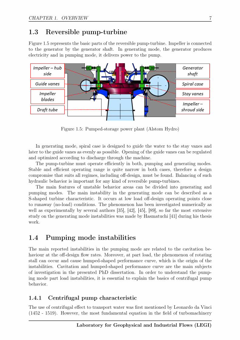
Figure 1.5 represents the basic parts of the reversible pump-turbine. Impeller is connectedto the generator by the generator shaft. In generating mode, the generator produceselectricity and in pumping mode, it delivers power to the pump.
Figure 1.5: Pumped-storage power plant (Alstom Hydro)
In generating mode, spiral case is designed to guide the water to the stay vanes andlater to the guide vanes as evenly as possible. Opening of the guide vanes can be regulatedand optimized according to discharge through the machine.
The pump-turbine must operate efficiently in both, pumping and generating modes.Stable and efficient operating range is quite narrow in both cases, therefore a designcompromise that suits all regimes, including off-design, must be found. Balancing of suchhydraulic behavior is important for any kind of reversible pump-turbines.
The main features of unstable behavior areas can be divided into generating andpumping modes. The main instability in the generating mode can be described as aS-shaped turbine characteristic. It occurs at low load off-design operating points closeto runaway (no-load) conditions. The phenomenon has been investigated numerically aswell as experimentally by several authors [35], [42], [45], [89], so far the most extensivestudy on the generating mode instabilities was made by Hasmatuchi [41] during his thesiswork.
1.4 Pumping mode instabilities
The main reported instabilities in the pumping mode are related to the cavitation be-haviour at the off-design flow rates. Moreover, at part load, the phenomenon of rotatingstall can occur and cause humped-shaped performance curve, which is the origin of theinstabilities. Cavitation and humped-shaped performance curve are the main subjectsof investigation in the presented PhD dissertation. In order to understand the pump-ing mode part load instabilities, it is essential to explain the basics of centrifugal pumpbehavior.
1.4.1 Centrifugal pump characteristic
The use of centrifugal effect to transport water was first mentioned by Leonardo da Vinci(1452 - 1519). However, the most fundamental equation in the field of turbomachinery
Laboratory for Geophysical and Industrial Flows (LEGI)
8 CHAPTER 1. OVERVIEW
was presented by Leonhard Euler (1707 - 1783). Euler’s equation for turbomachines isbased on the conservation of angular momentum. The simplified linear Euler equationfor specific hydraulic energy of the pump can be written as:
gH = U2V2u − U1V1u. (1.1)
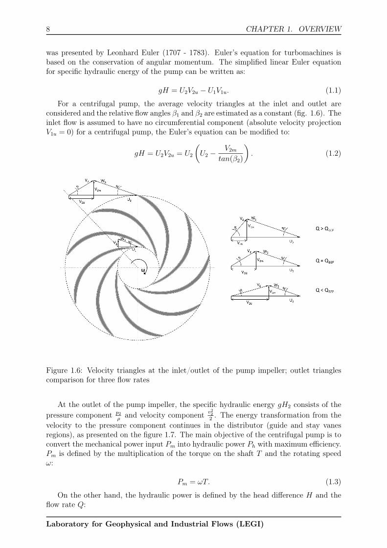
For a centrifugal pump, the average velocity triangles at the inlet and outlet areconsidered and the relative flow angles β1 and β2 are estimated as a constant (fig. 1.6). Theinlet flow is assumed to have no circumferential component (absolute velocity projectionV1u = 0) for a centrifugal pump, the Euler’s equation can be modified to:
gH = U2V2u = U2
(
U2 −V2m
tan(β2)
)
. (1.2)
Figure 1.6: Velocity triangles at the inlet/outlet of the pump impeller; outlet trianglescomparison for three flow rates
At the outlet of the pump impeller, the specific hydraulic energy gH2 consists of thepressure component p2
ρand velocity component v2
2
2. The energy transformation from the
velocity to the pressure component continues in the distributor (guide and stay vanesregions), as presented on the figure 1.7. The main objective of the centrifugal pump is toconvert the mechanical power input Pm into hydraulic power Ph with maximum efficiency.Pm is defined by the multiplication of the torque on the shaft T and the rotating speedω:
Pm = ωT. (1.3)
On the other hand, the hydraulic power is defined by the head difference H and theflow rate Q:
Laboratory for Geophysical and Industrial Flows (LEGI)

CHAPTER 1. OVERVIEW 9
H =p
ρ+v2
2g+ z; (1.4)
Ph = Qρ(gH2 − gH1). (1.5)
Figure 1.7: Specific energy transformation inside the pump-turbine, pumping mode [90]
In order to provide the maximum efficiency, the appropriate shape of the pump shouldbe chosen. The typical criteria is a specific speed number nq. Since the specific speednumber definition can vary a lot in literature, it is important to define it clearly. In ourcase and in most industrial cases, the units are as follows: n(min−1); Q(m3/s); H(m).
nq = n
√Q
H3/4. (1.6)
Regardless of the definition, the lower specific speed value always represents a morecentrifugal shape of the pump and on the contrary, higher values represent more axialvane shapes. Generally, the pumps can be divided into four groups, depending on thevane shape, as presented on the figure 1.8.
Figure 1.8: Optimal types of pumps related to specific speed
The other important non-dimensional numbers, widely used in literature, are the flowrate coefficient φ and the specific energy coefficient ψ that are defined as:
φ =Q
πωR3; (1.7)
ψ =2gH
ω2R2. (1.8)
Laboratory for Geophysical and Industrial Flows (LEGI)
10 CHAPTER 1. OVERVIEW
Another important factor that must be taken into account to achieve high efficiencyand low losses is the energy transformation inside the machine. It must be as smoothas possible (fig. 1.7). Therefore, the flow from the impeller must be adapted to thedistributor. In case of a pump-turbine, the distributor contains two parts. On one hand,the guide vanes opening angle can be modified and adapted to the flow and on the otherhand, the stay vanes are fixed.
The importance of adapting angle of guide vanes opening is even clearer, because thetriangles of velocity at the outlet of impeller are changing significantly, depending on theflow rate. Figure 1.6 shows the difference in absolute flow angle α2 at the outlet of theimpeller for three different flow rates. In order to reduce the losses in the distributor, theα2 angle should match the opening angle of the guide vanes.
However, that is not the case at part flow rate, where unadapted attack angle at theinlet of the distributor causes the flow separation and consequently rotating stalls.
1.4.2 Part load flows in centrifugal pumps
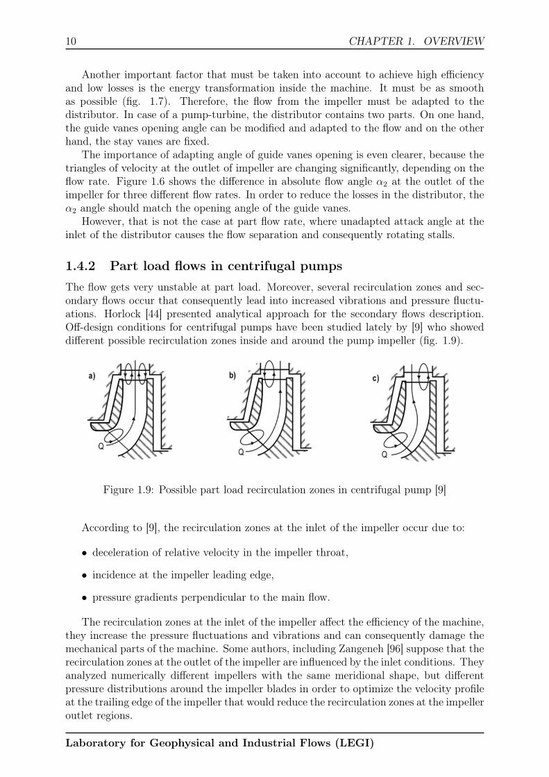
The flow gets very unstable at part load. Moreover, several recirculation zones and sec-ondary flows occur that consequently lead into increased vibrations and pressure fluctu-ations. Horlock [44] presented analytical approach for the secondary flows description.Off-design conditions for centrifugal pumps have been studied lately by [9] who showeddifferent possible recirculation zones inside and around the pump impeller (fig. 1.9).
Figure 1.9: Possible part load recirculation zones in centrifugal pump [9]
According to [9], the recirculation zones at the inlet of the impeller occur due to:
• deceleration of relative velocity in the impeller throat,
• incidence at the impeller leading edge,
• pressure gradients perpendicular to the main flow.
The recirculation zones at the inlet of the impeller affect the efficiency of the machine,they increase the pressure fluctuations and vibrations and can consequently damage themechanical parts of the machine. Some authors, including Zangeneh [96] suppose that therecirculation zones at the outlet of the impeller are influenced by the inlet conditions. Theyanalyzed numerically different impellers with the same meridional shape, but differentpressure distributions around the impeller blades in order to optimize the velocity profileat the trailing edge of the impeller that would reduce the recirculation zones at the impelleroutlet regions.
Laboratory for Geophysical and Industrial Flows (LEGI)

CHAPTER 1. OVERVIEW 11
1.4.3 Flow separation and rotating stall
Kline [54] gave the first explanations about the stall origins. It is defined as a recirculationzone on the internal or external walls. The initial flow separation can be caused by severalflow phenomena, such as:
• an obstacle on the flow path,
• an unadapted attack angle on the leading edge of the blade (fig. 1.10),
• strong pressure gradients, normal to the flow direction.
Figure 1.10: Flow separation on the airfoil, depending on the attack angle
The first detailed explanation of the rotating stall was given by Emmons [27] in 1959.At the beginning, the phenomenon was studied in a case of axial and centrifugal com-pressors ([34], [43], [46], [62]). Indeed, the rotating stall investigations on the centrifugalpump geometry were performed much later. Around 1990, Arndt [2], [3] was investigatingthe rotor stator interactions, and the study showed that the pressure fluctuations werestrongly influenced by a radial gap between the trailing edge of the impeller and the lead-ing edge of the diffuser. Moreover, the pressure fluctuations have been much higher onthe suction side of the diffuser vanes.
Figure 1.11: Schematic representation of the rotating stall in the pump-turbine (isosurfaceVm = 4m/s)
Laboratory for Geophysical and Industrial Flows (LEGI)

12 CHAPTER 1. OVERVIEW
Rotating stall is usually seen as cells of increased and decreased flow rate inside thedistributor. Figure 1.11 represents the rotating stall inside a pump-turbine. 4 cells ofincreased flow rate are rotating around the distributor in the same direction as the impellerwith the frequency ωS from 2% to 6% of the operating frequency of the impeller ω. Forthe centrifugal pump applications, the rotating stall can also have the opposite directionthan the pump. Studies on the radial gap influence on the forward/backward rotatingstall have been made by Sano et al. [81], [82] in 2002. They state that a larger radialclearance between the impeller and the diffuser causes an easier occurrence of the diffuserrotating stall due to the decoupling of the impeller/diffuser flow.
Most of the experimental studies of the rotating stall in pumps and pump-turbinestook place in the last 20 years. The main approach was to use PIV (Particle ImageVelocimetry) method and was firstly used by Sinha et al. [86], [87]. The radial clearancebetween the impeller and the diffuser was around 10% of the impeller diameter. Heassumed that a larger clearance would increase the stall intensity and the probability ofstall occurrence as it was originally stated by Yoshida [94]. Similar experimental studies,using PIV method, were performed later by [72] and [91].
The most extensive project regarding the pump-turbine geometry in pumping modewas set up in Lausanne during Hydrodyna project. Part-load flow behavior in the cen-trifugal pumps as well as in the pump-turbines was investigated numerically and ex-perimentally by Braun [10] during his thesis. The LDV (Laser Doppler Measurements)method was used in order to analyze the velocity components between the guide vanechannels and in the vaneless gap between the impeller and the distributor. During thevisual observation of the experiment, confirmed by noise analysis, some kind of cavitationvortex appeared in the region of the guide vanes, despite the fact that it is located in thehigh pressure area. Similar behaviors were observed in some cases of industrial centrifugalpumps. Braun assumed that the origin of the vortex is the flow separation on the hub sideof the distributor and can reach the area of the impeller as well. Another study about thecavitation influence on the hump shaped performance curve was made by Amblard [1] in1985.
Numerically, steady and unsteady 3-dimensional simulations were performed usingRANS (Reynolds Averaged Navier-Stokes) equations [10], [93]. Additional numerical stud-ies were performed lately in the EPFL by Pacot [69], [70], who used LES (Large EddySimulation) to investigate the rotating stall behavior. The global rotating stall behaviorin one operating point was caught quite well, including the area and the frequency of thestall. Those kind of calculations are very demanding regarding computational time. Theywere done on one of today’s fastest supercomputers (more than 700000 cores), called Kcomputer, which is located in Japan.
1.4.4 Hump shaped performance curve
The appearance of the described rotating stall phenomena significantly increases the lossesin the distributor and, therefore, causes a positive differential slope on the performancecurve as presented on the figure 1.12. The green and the red lines represent the char-acteristics of the system. The normal, stable operating range for the pump-turbine isbetween the green lines. In a stable area, the pump-turbine provides one correspondingflow rate for every given net head of the system. On the contrary, in the area of theunstable characteristics due to the phenomenon of the rotating stall, the pump-turbinecan provide three different flow rates for the given system characteristic, as shown bythe red curve. In reality, that means that the flow rate through the pump-turbine varies
Laboratory for Geophysical and Industrial Flows (LEGI)

CHAPTER 1. OVERVIEW 13
completely uncontrollably. Behavior like this drastically increases the losses. Moreover,it also causes very strong vibrations that can damage and in the worst case even destroythe machine.
Figure 1.12: Pumping mode unstable characteristic due to distributor hump
Obviously, the pump-turbine should not operate in the area of the distributor hump.However, since the pump-turbine needs to change the regime several times per day andmust be as adaptable as possible, there is no possibility to completely avoid the problem-atic unstable area. Some of the general control options of the operating point for pumpingsystem are presented on figure 1.13. The system curve characteristic is proportional tothe squared flow rate and to a loss coefficient C:
KS ∝ CQ2
AS
. (1.9)
The first option is to increase or decrease the losses in the system. It is often usedin the industrial application to control the provided head. In pump-turbine systems it ispartly used during the start-ups and the shut-downs for the changing from pumping togenerating mode and vice versa. It is not used for normal operating.
The second option is the variation of the static head. This kind of control is veryuseful in tidal application, where the relative difference between the water levels can belarge. For PSP system that means the variation of the water level between the upper andthe lower reservoir, which is relatively small. The head variation in case of PSP must betaken into account, but can not be used to control the operating points.
The third option is to control the speed of the pump-turbine. The technology is calledvariable speed technology for the pump-turbines. It is a rather new approach in the fieldof the PSP. Detailed description and advantages were provided by [11]. The technologyis already used by Alstom Hydro in several installations around the world. It enablesthe variation of the pump-turbine rotating speed and consequently different performancecurves as seen on the part c) of the figure 1.13. Several advantages of the variable speedtechnology comparing to fixed speed are:
• For a fixed static head (water level of the reservoirs), the absorbed power can vary(up to 30%). Therefore, it can be used for the grid regulation when necessary.
Laboratory for Geophysical and Industrial Flows (LEGI)

14 CHAPTER 1. OVERVIEW
Figure 1.13: Operating point control: a) Increasing system losses, b) Variation of statichead, c) Pump speed variation.
• Optimizing the efficiency. For a single speed machine the BEP (Best efficiencypoint) is a point at a given head and a given discharge. If the rotating speed of themachine is changed, the BEP also changes, which means that we can achieve betterefficiency for the non-optimal flow rates, especially at the part load flow.
• Since the technology enables for higher flexibility, depending on the grid demands,the pump-turbine can operate longer. Therefore, the economic amortization timeof the whole PSP system is shorter.
• Variable speed technology can be used to avoid the unstable operating points, suchas the described distributor hump region and regimes, where the cavitation phe-nomenon is present.
1.5 Cavitation
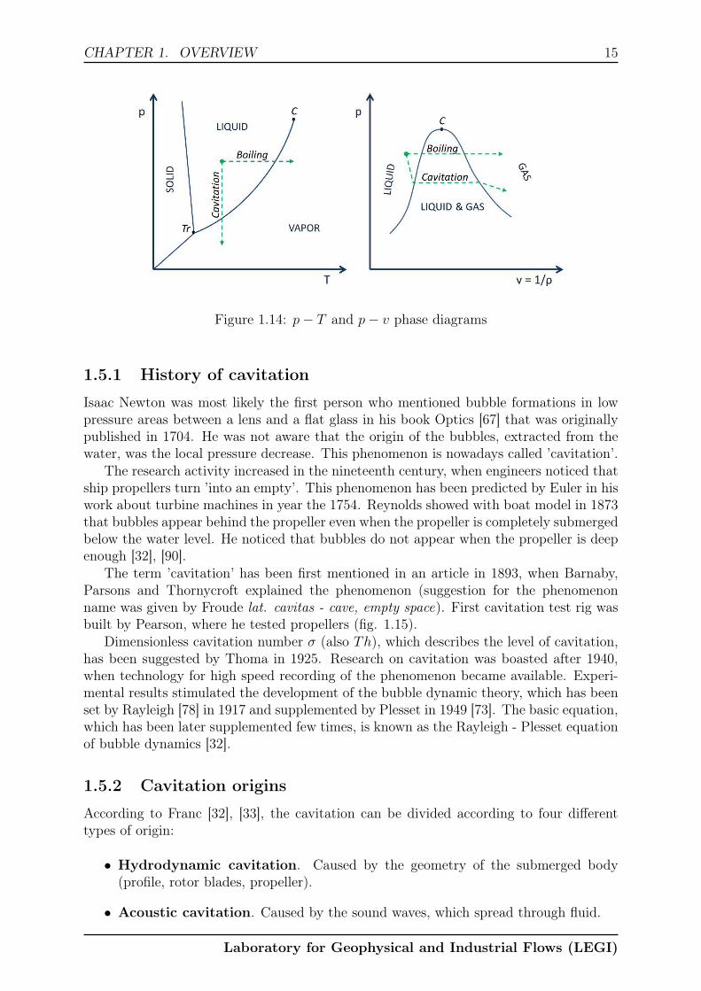
The most common description of the term ’cavitation’ is the appearance of vapor bubblesinside an initially homogeneous liquid medium. Usually, it is seen as a transition from theliquid to the vapor phase and again back to the liquid. The reason for the appearance ofcavitation is a local decrease of pressure, where the temperature remains approximatelyconstant. The vapor pressure can be explained in a classical thermodynamic point ofview. On the p− T phase diagram for water (fig. 1.14), the line between the triple pointof water Tr and the critical point C separates the liquid phase from the vapor phase. Thevapor pressure pv means that crossing the curve under static conditions causes the changeof the phase (in our case, evaporation). As seen from figure 1.14, the vapor pressure pv isa function of the temperature. As mentioned before, the cavitation in cold water usuallyoccurs at the almost constant temperature, when local pressure is decreased and laterincreased again. A similar phenomenon is called boiling, where the vaporisation occursat the constant pressure when the temperature is increased.
The last stage of the cavitation process occurs when the pressure returns back to theinitial one (above the pv) and the bubbles start to implode. The bubble ’void’ is filledagain with the surrounding liquid. During the bubble collapse, strong pressure waves canbe emitted, and one of the consequences can be serious damage of the nearby solid walls.
Laboratory for Geophysical and Industrial Flows (LEGI)
CHAPTER 1. OVERVIEW 15
Figure 1.14: p− T and p− v phase diagrams
1.5.1 History of cavitation
Isaac Newton was most likely the first person who mentioned bubble formations in lowpressure areas between a lens and a flat glass in his book Optics [67] that was originallypublished in 1704. He was not aware that the origin of the bubbles, extracted from thewater, was the local pressure decrease. This phenomenon is nowadays called ’cavitation’.
The research activity increased in the nineteenth century, when engineers noticed thatship propellers turn ’into an empty’. This phenomenon has been predicted by Euler in hiswork about turbine machines in year the 1754. Reynolds showed with boat model in 1873that bubbles appear behind the propeller even when the propeller is completely submergedbelow the water level. He noticed that bubbles do not appear when the propeller is deepenough [32], [90].
The term ’cavitation’ has been first mentioned in an article in 1893, when Barnaby,Parsons and Thornycroft explained the phenomenon (suggestion for the phenomenonname was given by Froude lat. cavitas - cave, empty space). First cavitation test rig wasbuilt by Pearson, where he tested propellers (fig. 1.15).
Dimensionless cavitation number σ (also Th), which describes the level of cavitation,has been suggested by Thoma in 1925. Research on cavitation was boasted after 1940,when technology for high speed recording of the phenomenon became available. Experi-mental results stimulated the development of the bubble dynamic theory, which has beenset by Rayleigh [78] in 1917 and supplemented by Plesset in 1949 [73]. The basic equation,which has been later supplemented few times, is known as the Rayleigh - Plesset equationof bubble dynamics [32].
1.5.2 Cavitation origins
According to Franc [32], [33], the cavitation can be divided according to four differenttypes of origin:
• Hydrodynamic cavitation. Caused by the geometry of the submerged body(profile, rotor blades, propeller).
• Acoustic cavitation. Caused by the sound waves, which spread through fluid.
Laboratory for Geophysical and Industrial Flows (LEGI)

16 CHAPTER 1. OVERVIEW
Figure 1.15: Parsons’ cavitation tunnel (1895) [90]
• Optic cavitation. Caused by the photons or laser light.
• Cavitation of particles. Caused by other elementary particles, e.g. protons.
The hydrodynamic and the acoustic cavitation commence because of the tensions inthe fluid; on the other hand, the optical cavitation and the cavitation of particles startbecause of a local energy input into the fluid. In the field of hydraulic machines, thehydrodynamic cavitation is the most important, and therefore deserves an additionalanalysis.
1.5.3 Hydrodynamic cavitation
Hydrodynamic cavitation occurs due to one or several effects that increase the possibilityof cavitation:
• Geometry of the submerged body, which causes an increase of local velocityand an indirect decrease of the local static pressure.
• Boundary layer between flows with two different speed.
• Surface roughness.
• Vibrations of submerged bodies, when the fluid can not follow high speedfrequencies of the body.
Different types of cavitation can be observed depending on the flow conditions andthe geometry of the submerged body. It is common to distinguish between the differenttypes of cavitation, each having its distinctive characteristics. Franc [32], Knapp [55] andYoung [95] describe five different types of cavitation as presented on the figure 1.16.
• Transient isolated bubbles. A type of cavitation where individual bubbles formin the liquid and move with the flow. They appear in low pressure regions, travelwith the flow and implode in the regions with high pressure. (fig. 1.16, part a)
Laboratory for Geophysical and Industrial Flows (LEGI)
CHAPTER 1. OVERVIEW 17
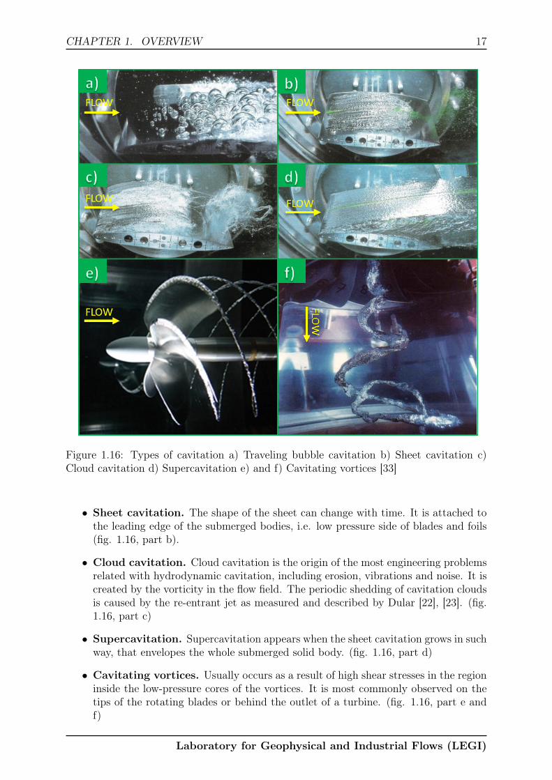
Figure 1.16: Types of cavitation a) Traveling bubble cavitation b) Sheet cavitation c)Cloud cavitation d) Supercavitation e) and f) Cavitating vortices [33]
• Sheet cavitation. The shape of the sheet can change with time. It is attached tothe leading edge of the submerged bodies, i.e. low pressure side of blades and foils(fig. 1.16, part b).
• Cloud cavitation. Cloud cavitation is the origin of the most engineering problemsrelated with hydrodynamic cavitation, including erosion, vibrations and noise. It iscreated by the vorticity in the flow field. The periodic shedding of cavitation cloudsis caused by the re-entrant jet as measured and described by Dular [22], [23]. (fig.1.16, part c)
• Supercavitation. Supercavitation appears when the sheet cavitation grows in suchway, that envelopes the whole submerged solid body. (fig. 1.16, part d)
• Cavitating vortices. Usually occurs as a result of high shear stresses in the regioninside the low-pressure cores of the vortices. It is most commonly observed on thetips of the rotating blades or behind the outlet of a turbine. (fig. 1.16, part e andf)
Laboratory for Geophysical and Industrial Flows (LEGI)

18 CHAPTER 1. OVERVIEW
1.5.4 Non-dimensional parameters
The basic condition for cavitation occurrence is when local minimal static pressure pmin
reaches the vaporisation pressure pv:
pmin = pv. (1.10)
If we use a reference point where the pressure and velocity equals p0 and v0, thepressure coefficient cp(~r, t) for a random local point and a random time can be defined as:
cp(~r, t) =p(~r, t)− p0
ρv20
2
. (1.11)
On the other hand, the cavitation number σ can be written as a relation between areference and a vaporisation pressure:
σ =p0 − pv(T )
ρv20
2
. (1.12)
When the cavitation number σ is low enough for the cavitation occurrence, it can bemarked as an incipient cavitation number σi. Normally, a simplified explanation statesthat the vaporisation commences when the local static pressure reaches the vaporisationpressure. However, in reality, the vaporisation conditions are much more difficult to define.The fact is that cp is influenced by several other factors such as friction, turbulence level,boundary layers and others. Moreover, even σi is influenced by some parameters suchas amount of dissolved gas in the water. Still, in many circumstances, including theones presented in this document, especially for numerical modeling of cavitating flows,following estimation is taken for σi:
σi = −cp,min. (1.13)
1.5.5 Cavitation in turbines
Cavitation behavior in different types of hydraulic machines has been studied and pre-sented by [4], [28]. As mentioned before, the cavitation in the turbine occurs when thelocal pressure drops under the critical vaporisation pressure. To characterize the levelof cavitation, the cavitation number σ is used. Lower cavitation number means moreintensive cavitation, however it does not tell us about the forms of cavitation that arepresent inside the turbine.
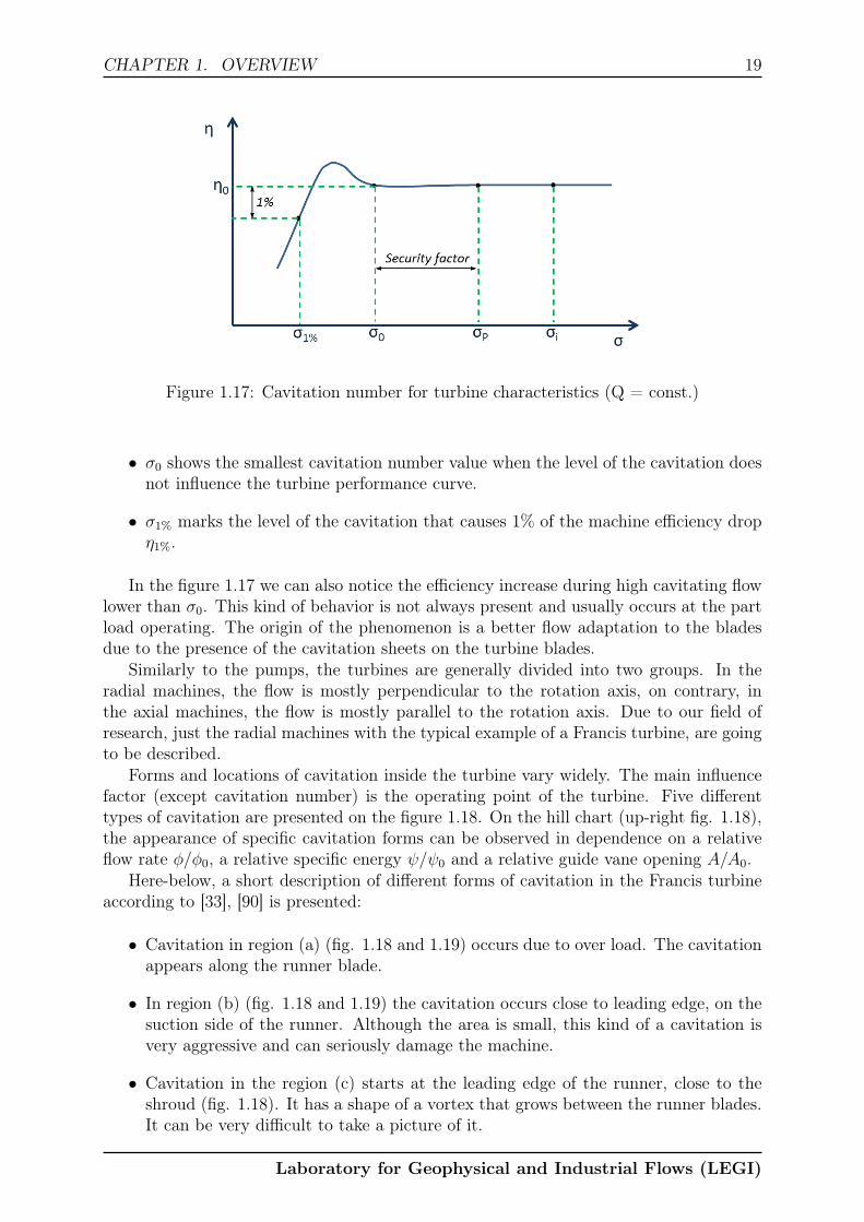
On the figure 1.17 we can observe how the cavitation level influences the turbineperformance. Several typical values of the cavitation number are marked on the chartaccording to IEC 60193 [12]:
• σi represents the incipient cavitation value. Experimentally, it is set by a visualobservation; numerically, usually by the comparison of the lowest local pressure inthe domain and a vaporisation pressure. Incipient cavitation value is lower whenthe flow is close to optimal value Q/QBEP = 1, therefore the attack angle is welladapted to the blades. On the contrary, for increased or decreased flow rate, thevalue increases due to either too high or too low attack angles.
• σp represents the lowest value of the cavitation number when the machine is stillallowed to operate.
Laboratory for Geophysical and Industrial Flows (LEGI)
CHAPTER 1. OVERVIEW 19
Figure 1.17: Cavitation number for turbine characteristics (Q = const.)
• σ0 shows the smallest cavitation number value when the level of the cavitation doesnot influence the turbine performance curve.
• σ1% marks the level of the cavitation that causes 1% of the machine efficiency dropη1%.
In the figure 1.17 we can also notice the efficiency increase during high cavitating flowlower than σ0. This kind of behavior is not always present and usually occurs at the partload operating. The origin of the phenomenon is a better flow adaptation to the bladesdue to the presence of the cavitation sheets on the turbine blades.
Similarly to the pumps, the turbines are generally divided into two groups. In theradial machines, the flow is mostly perpendicular to the rotation axis, on contrary, inthe axial machines, the flow is mostly parallel to the rotation axis. Due to our field ofresearch, just the radial machines with the typical example of a Francis turbine, are goingto be described.
Forms and locations of cavitation inside the turbine vary widely. The main influencefactor (except cavitation number) is the operating point of the turbine. Five differenttypes of cavitation are presented on the figure 1.18. On the hill chart (up-right fig. 1.18),the appearance of specific cavitation forms can be observed in dependence on a relativeflow rate φ/φ0, a relative specific energy ψ/ψ0 and a relative guide vane opening A/A0.
Here-below, a short description of different forms of cavitation in the Francis turbineaccording to [33], [90] is presented:
• Cavitation in region (a) (fig. 1.18 and 1.19) occurs due to over load. The cavitationappears along the runner blade.
• In region (b) (fig. 1.18 and 1.19) the cavitation occurs close to leading edge, on thesuction side of the runner. Although the area is small, this kind of a cavitation isvery aggressive and can seriously damage the machine.
• Cavitation in the region (c) starts at the leading edge of the runner, close to theshroud (fig. 1.18). It has a shape of a vortex that grows between the runner blades.It can be very difficult to take a picture of it.
Laboratory for Geophysical and Industrial Flows (LEGI)

20 CHAPTER 1. OVERVIEW
Figure 1.18: Types of cavitation, depending on operating point (hill chart) [60], [90]
Figure 1.19: a) trailing edge cavitation; b) leading edge cavitation; d) cavitation vortices[33]
• In the region (d), both, the specific energy and flow rate factor are low. The attackangle is not well adapted and causes the flow separation and consequently somecavitation vortices (fig. 1.18 and 1.19). This type of cavitation results in increasedvibrations of the machine.
• At part load region (e), the cavitation vortex occurs in the draft tube (fig. 1.18 and1.20) as a result of a water circulation at the turbine outlet. It causes strong, low-frequency vibrations and changes the hydraulic condition. The size of the vortexdepends mostly on the cavitation number. On the other hand, the vortex shapedepends on the relative flow rate φ/φ0. For high flow rates, the shape is almost axi-symmetric and the rotation is opposite to the turbine rotation (fig. 1.20, left). Onthe contrary, for low flow rates, the rotation has the same direction as the turbine
Laboratory for Geophysical and Industrial Flows (LEGI)

CHAPTER 1. OVERVIEW 21
and the vortex is rotating around the draft tube (fig. 1.20, right). Typical rotatingvortex frequency is between 25% and 35% of the turbine rotation frequency.
Figure 1.20: Cavitation vortex and outlet velocity triangles [33]
1.5.6 Cavitation in pumps
Cavitation in pumps occurs mostly on both sides of the impeller blades, depending on theattack angle at the impeller leading edge. As seen on the figure 1.21, in the case of thereduced flow rate, the cavitation appears firstly on the suction side of the blade. On thecontrary, when the flow rate is increased, the cavitation typically occurs on the pressureside.
Figure 1.21: Velocity triangles
On the figure 1.22 we can see all different forms of cavitation in the centrifugal pump.The cavitation forms (on the suction side (a) and on the pressure side of the blade)originate in the non-adapted flow attack angle. On the other hand, the cavitation in the
Laboratory for Geophysical and Industrial Flows (LEGI)

22 CHAPTER 1. OVERVIEW
(c) region (sealing gap) occurs due to secondary flows that cause local pressure decrease.In special cases of increased flow rate, the cavitation can be present also in the region (d),on the spiral case tongue (centrifugal pumps) [6]. Similarly, in the case of the increasedflow rate in the pump-turbine, the cavitation can occur on the pressure side of guidevanes, if the guide vanes opening angle is not adapted to the flow.
Figure 1.22: Cavitation in centrifugal pump [90]
Generally, the presence of the developed cavitation forms in a pump can lead into:
• reducing the pump performance (reducing net head Hn), if the flow rate Q androtating speed n remain constant;
• decrease of the efficiency η;
• changing the velocity and the pressure profile inside the pump;
• damage of the pump due to cavitation erosion.
The intensity and effects of the cavitation depend mostly on the NPSH (net positivesuction head) number, which is comparable parameter to the cavitation number σ for thecase of the turbines of single profiles.
NPSH number definition
Net positive suction head number can be given for the system as well as for the machine.When we try to describe and compare the system probability for the cavitation occurrence,available NPSH number (NPSHA) can be calculated as:
NPSHA(m) =p0 − pvρg
+v202g
+∆Z −Hloss. (1.14)
Index 1 in the equation 1.14 refers to conditions at the lower reservoir. It is importantto stress that ∆Z has positive value, if the level of the pump-turbine is lower than thelower reservoir of the PSP system, as seen on the figure 1.23. Hloss represents the lossesin the system between the machine and the lower reservoir. Kinetic energy component isusually estimated to 0, since the water level in the reservoirs changes very slowly.
Laboratory for Geophysical and Industrial Flows (LEGI)

CHAPTER 1. OVERVIEW 23
Figure 1.23: Position of the pump-turbine system
According to the equation 1.14 and the figure 1.23, the level of the water in thelower reservoir influences the cavitation level in the pump-turbine. Therefore, in order tominimize or avoid cavitation, the position of the pump-turbine is generally significantlyunder the level of the lower reservoirs.
On the other hand, the required NPSH value (NPSHR) is used to define various levelsof developed cavitation inside the machine. Some of the typical values are presented onthe figure 1.24 and are defined as:
Figure 1.24: Typical pump-turbine NPSHR characteristics for Q = const. (head dropcurve)
• NPSHR−i represents the incipient cavitation value. Experimentally, it can be ob-tained by the visualization measurements in the pump (pump-turbine).
Laboratory for Geophysical and Industrial Flows (LEGI)

24 CHAPTER 1. OVERVIEW
• NPSHR−ero represents the value, where the cavitation intensity is high enough tocause the erosion on the blades of the pump.
• NPSHR−3% represents the cavitation value, when the head drop, due to presence ofthe cavitation, reaches 3% of reference no-cavitation headH0. NPSHR−3% value canbe obtained by the global measurements of the pump (pump-turbine) performancethat are described in the international standard IEC 60193 [12].
Slight increase of the performance can be sometimes observed on NPSHR head dropcurve for a reduced flow rate, similar as for the turbine cavitation characteristics (fig.1.17). Also the origin of the improvement is the same. Therefore, an attack angle atthe leading edge of the blade is optimized due to the cavitation sheet, attached to theblade. As mentioned, the NPSHR values are usually obtained through measurementsand visualization. However, numerical simulations can be as well used to predict theNPSH values and forms of cavitation for certain values, which is also one of the severalobjectives of the presented PhD work.
NPSHR values are significantly influenced by the flow rate. The incipient cavitationvalue curve has the lowest value at the optimal flow rate, as presented on the figure 1.25.Due to velocity triangles (fig. 1.21), the incipient cavitation at the reduced flow rateoccurs on the suction side of the blades. On the contrary, at the increased flow rate itoccurs on the pressure side of the blade. Cavitation on the pressure side of the blade hasa more significant effect on the performance of the pump-turbine than the cavitation onthe suction side. Indeed, the NPSHR−3% value is higher for the increased flow rate thanfor the part load as seen on the figure 1.25.
Figure 1.25: Flow rate influence on the NPSHR values
Several times in the presented PhD work, NPSH value is mentioned without indica-tors R (required) or A (available). It should be underlined that since one of the objectivesof the work is to study numerically the influence of the cavitation intensity inside thepump-turbine, NPSH value always represents required NPSH value (NPSHR).
1.6 Numerical simulation overview
Computational fluid dynamics (CFD) is taking a strong part in the field of fluid mechanics.Development of the computers and the software provided the academics and the industry
Laboratory for Geophysical and Industrial Flows (LEGI)

CHAPTER 1. OVERVIEW 25
with useful tools to analyze, predict and improve the flow behavior. Comparing to theexperiments, CFD approach is normally cheaper and can provide more detailed informa-tion about the phenomena that scientists and engineers are interested in. However, it stillhas its limits in the computational power and the accuracy of the given results, thereforean evaluation of the calculated data is always necessary. Typically, a good combinationof the experimental and the numerical studies gives the best and the most cost-efficientresults.
1.6.1 CFD approaches
To achieve good results from the numerical simulations, it is important to know whichtypes of simulations are available and what are their limitations. Generally, three differentapproaches are available to simulate the flow behavior. Direct Numerical Simulation(DNS) solves unsteady Navier-Stokes equations and computes the turbulence forms on allscales. If the time and space discretization are good enough, the DNS simulations shouldprovide the most exact results. Kolmogorov [56] made a study on the appropriate spatialdiscretization for high Reynolds turbulent flows in 1941. However, when performing DNS,the limits are set with the available computational time. So far, even the fastest andthe largest supercomputers are capable to calculate only the simple geometries with lowReynolds numbers. Taking into account the expected development of the computationalpower, the DNS simulations for complex geometries with high Reynolds number will notbe available for a few decades.
Second approach is known as a Large Eddy Simulation (LES). It is a compromisebetween DNS and RANS simulations. It computes the turbulent forms, but not on allscales. Therefore, with a filter selection, one must choose the size of the turbulent struc-tures that will still be calculated. The challenge is to find a good compromise betweenthe accuracy and the discretization. The turbulence production occurs on the large scale,but dissipates on the small scales, therefore, it is essential to find the appropriate timeand spatial discretization. Additionally, the modeling of the boundary layers may be verydemanding due to need for very dense mesh close to the walls. Feasibility study on themesh size should be performed before actual numerical simulations. LES approach isgetting more and more popular in last years in academics, however it is not completelyready yet to be used for industrial applications. The most extensive study in the fieldof the turbomachinery was recently performed by Pacot [69]. The computation for oneoperating point lasted around 12 days for 40 impeller revolutions on an about 10000 com-putational cores. It is clear that this amount of computational capacity is not widelyavailable. On the other hand, the LES simulations have shown potential for predictingthe flow behavior.
The only remaining approach is to solve Reynolds Averaged Navier-Stokes (RANS)equations. So far it is extensively used in the industry as well as in the academics. Theapproach is economical, since it can be used for a wide range of application even on a casualPC. The drawback is that the RANS approach provides statistically averaged solutions forthe turbulent behavior. Choosing appropriate turbulent model is very important. TheRANS equations can be modified to Unsteady RANS (URANS) equations to performthe unsteady calculations. More about the RANS and URANS approach follows in thechapter 2.
Laboratory for Geophysical and Industrial Flows (LEGI)

26 CHAPTER 1. OVERVIEW
1.6.2 CFD tradition in LEGI
Tradition of the numerical simulations in the LEGI laboratory has a long history, espe-cially in the field of the cavitation modeling. The initial model was based on a barotropiclaw approach and developed for 2D non-viscous flows [21]. Successive improvements ofthe 2D numerical and physical models were carried out during the last decades, concern-ing mainly the turbulence modeling and the compressibility effects on turbulence [14],[19]. The application of the numerical tool to study different unsteady cavitating flowconfigurations allowed very reliable experimental validation [30], [31], [61], [79], [80].
To analyse 3D complex flows, especially in the field of the turbomachinery, the cav-itation model was implemented in the 3D URANS code Fine/TURBOTM in the scopeof a very fruitful collaboration between the LEGI and Numeca International [15], [16].Mainly during the thesis works of Pouffary [74] and Coutier-Delgosha [13], many steadyand unsteady calculations were performed for cavitating inducers, in collaboration withthe CNES and the rocket engine division of SNECMA-Moteurs, with successful experi-mental validation in cold water applications [18], [37], [75], [76] . The final objective wasproviding assistance to the design and prevision of operating range of rocket engine tur-bopumps, taking into account the hydrodynamic instabilities of cavitating flows. Otherapplications of unsteady cavitation modeling have also been investigated in the researchteam, for example in the field of cavitation erosion [29], [57].
The presented work is part of this overall context. It took into account the previousresearch team’s know-how on numerical calculations and flow analyses in turbomachines.Based on this know-how, the code Fine/TURBOTM and the barotropic cavitating modelhave been applied to study the flows inside of the considered pump-turbine geometry.
For the research team, it was the first time that this type of machine and the as-sociated unsteady and instable phenomena were studied. The methodology developedduring this thesis to mesh, to calculate and to analyze these complex mechanisms is amajor contribution to the future works, mainly in the scope of the storage program at theSupergrid institute.
1.7 Thesis objectives
CFD simulations provide us a useful, cost-efficient tool for analyzing the flow phenomenain hydraulic machines. Presented study focuses on the predicting and analyzing the flowunder the complex, part load pumping mode off-design conditions. The studied geometryis a reduced-scale high head pump-turbine model (nq = 27). At the part load regimes,the continuous operation of the machine can be limited by the rotating stall and thecavitation. The objectives of the thesis are the following:
• The first objective is to use a commercial code, tested before in the laboratory, todevelop a numerical simulations approach allowing the accurate prediction of off-design part load phenomena in pumping mode operating regions. The main goal isto predict accurately the cavitation forms, drop of performance due to cavitationand to carry out local analysis of the flow patterns in cavitating flow. Moreover, aglobal analysis of the cavitation impact on the rotating stall flow patterns will beperformed. The code should give an accurate global prediction of the hump zoneon the performance curve caused by the rotating stall. It should also enable theanalysis of the unsteady flow pattern for wide range of the flow rates and the NPSH
Laboratory for Geophysical and Industrial Flows (LEGI)

CHAPTER 1. OVERVIEW 27
values. Therefore, the simulations should be numerically stable and robust, but stillaccurate.
• Another objective is to develop the computationally cheap global methodology usingsteady RANS equations that will detect the stable and the unstable pumping modeoperating regions. Mentioned methodology can be very useful for fast, practical flowanalysis of the variables such as guide vane opening angles, guide and stay vanesgeometry, the size of the radial gap between the impeller and the distributor andothers. It should provide accurate global results for a large amount of the operatingpoints for a relatively low computational cost.
• The final objective is to make a detailed analysis of the rotating stall behavior andorigins by performing full geometry unsteady simulations. The analysis should in-clude the investigations of the velocity and pressure fields in the distributor regions.Moreover, the influence of the flow rate, guide vanes opening angles, guide vanesgeometry and radial clearance gaps should be studied in detail in order to givethe global image about the phenomenon. The analysis, the developed tools andmethodology could be an important basis for the future studies of the unsteadyoff-design flow phenomena, not only on the presented pump-turbine geometry, buton the other kind of pump-turbines and centrifugal pumps as well.
1.8 Document organization
The document consists of three parts. Part I has described the background of the study.It started with the introduction to the energy sector challenges, showed the importance ofthe pumped storage power plants (PSP) for the electrical grid and presents the rentabilityof the PSP systems. The operation of the reversible pump-turbine has been explained bypresenting the basic laws, principles and classifications for centrifugal pumps and pump-turbines. Additionally, the unsteady, off-design flow phenomena has been presented andexplained. An important part of the Part I was the presentation of the cavitation thatstarts with a basic explanation of the phenomenon and continues with describing theappearance in the hydraulic machines and the related challenges.
Part II will describe the used tools and methodologies. It will start with a shortdescription of the background of the experimental measurements that have been done inthe Alstom Hydro laboratory in Grenoble. It presents the possible sources of discrep-ancies between the experimental and the numerical data. Part II continues with thepresentation of the numerical setup. Numerical domain and methodology is presentedstarting with the governing equations and continuing with the turbulence and cavitationmodeling, meshing and a brief description of the applied numerical scheme.
Part III presents the results. These are divided into three chapters. The first oneis focused on global results of the steady simulations on the periodic mesh including theanalysis of the cavitating flow. The second one presents the approach to detect the stableand the unstable operating points that depend on the guide vane openings and geometry.The third chapter shows the results of the unsteady simulations followed by the detailedanalysis of the rotating stall phenomenon.
Laboratory for Geophysical and Industrial Flows (LEGI)

28 CHAPTER 1. OVERVIEW
Laboratory for Geophysical and Industrial Flows (LEGI)

Part II
Tools and Methodology
29


Chapter 2
Physical and numerical modeling
The idea behind the CFD simulations is to have a tool that can provide us with detailedinformation about the flow behavior in reasonable time and computational cost. Moreover,the cost and the time of the computations are the biggest CFD advantage compared to theexperiments. The constant development of the computers enables us larger and cheapercomputations in a shorter time. Indeed, for the field of hydraulic turbomachines, we canalready obtain a great amount of reliable results in one or a few days, using just a normalpersonal computer. On the other side, preparing and performing an experiment can takelot of time (weeks), large testing rigs, expensive equipment and great amount of workinghours. The experiments are also limited by the amount and the position (mostly on solidwalls) of the measuring points, whereas numerically we can get the data in all calculateddomains. However, if performed accurately, the experimental results are probably stillmore reliable than the numerical ones.
CFD simulations consist of three important parts:
• Preprocessing is used to define the problem. During the procedure, one needs to:
– define the physical bounds (geometry),
– set the spatial discretization (mesh),
– choose the governing equations,
– define the boundary conditions.
• Simulation is the longest part of the CFD, when the equations are solved iterativelyfor a steady state or a transient solution.
• Postprocessing is used for analyzing and visualizing the obtained results.
Important part of the CFD simulation is also the evaluation of the results. Smalldifference in the settings can lead into completely different results. Therefore, one needsto evaluate if the results are physical or they are affected by some numerical error orinaccuracy. When choosing the best models to describe the certain problems, extensivestudy of the literature can play an important role. Moreover, the comparison with theexperimental data is always very welcome. Firstly, to confirm the numerical results andsecondly, to confirm the numerical code that enables to provide the data for variousoperating points in a short time.
31

32 CHAPTER 2. PHYSICAL AND NUMERICAL MODELING
2.1 Navier-Stokes’ equations
The motion of the fluid is governed by the mass (eq. 2.1) and the momentum (eq. 2.2,derived from Newton’s second law) conservation laws. The flow is a result of the externalforces, such as gravity, pressure, the shear stress that origins in the movement of thesolid surface close to the fluid and the rotation induced body forces, such as Coriolisforce. Governing equations are known as Navier-Stokes equations. For incompressibleNewtonian fluid with a constant density in a Cartesian coordinate system, they can bewritten in the following way:
∂ui∂xi
= 0, (2.1)
∂ui∂t
+ uj∂ui∂xj
=1
ρ
(
−∂p
∂xi+∂τij∂xj
)
+ fi. (2.2)
For a viscous Newtonian fluid, the shear stress τ can be expressed by the strain ratetensor Dij and the dynamic viscosity µ:
τij = 2µDij ; Dij =1
2
(
−∂ui∂xj
+∂uj∂xi
)
. (2.3)
By introducing τ into the equation 2.2 we get the incompressible Navier-Stokes equa-tion for Newtonian fluids:
∂ui∂t
+ uj∂ui∂xj
=1
ρ
(
−∂p
∂xi+ µ
∂2ui∂xi∂xj
)
+ fi. (2.4)
Navier-Stokes equations can be solved analytically for the laminar flow. The valuethat defines if the flow is laminar or turbulent flow is a dimensionless Reynolds numberRe. On one hand, the laminar flow occurs at the low Reynolds numbers, where the viscousforces are dominant. It can be observed as a smooth, constant fluid motion. On the otherhand, the turbulent flow occurs at high Reynolds numbers, where the inertial forces aredominant. It is characterized as chaotic and it produces vortices, eddies of various sizesand other flow instabilities. Reynolds number is therefore defined as a relation betweenthe inertial and the viscous forces and can be written as:
Re =inertial forces
viscous forces=ρvL
µ=ρU2D2
µ. (2.5)
For the case of the pump-turbines, the velocity component v can be substituted withU2 (figure 1.6) and characteristic length L with an outer diameter D2. The critical value,where the laminar flow changes into turbulent inside the pipes, is between Re = 1700and Re = 2300, according to the literature [25]. In our pump-turbine case the Re reachesaround Re = 3, 6 · 106, which means that the turbulence is fully developed.
Modeling the turbulent flow becomes much more demanding than the laminar. Asalready mentioned, the DNS and mostly also the LES approaches are still computationallytoo expensive. The remaining and most widely used is therefore the RANS approach. Theidea is to use Reynolds decomposition and separate the flow variable u (in case of velocity)into the mean component u and the fluctuating component u′:
Laboratory for Geophysical and Industrial Flows (LEGI)

CHAPTER 2. PHYSICAL AND NUMERICAL MODELING 33
u(~x, t) = u(~x) + u′(~x, t). (2.6)
By introducing the equation 2.6 into the incompressible Navier-Stokes equation (eq.2.4) we can get the Reynolds averaged Navier-Stokes equations:
∂ui∂t
+ uj∂ui∂xj
=1
ρ
(
−∂p
∂xi+ µ
∂2ui∂2xj
)
−∂u′iu
′
j
∂xj+ fi. (2.7)
For the steady RANS equations there is no time dependence, therefore, the timedepending part equals 0:
∂ui∂t
= 0. (2.8)
Due to Reynolds stress term u′iu′
j we get 6 new unknowns, which means that thesystem of the equations is not anymore closed. At that point it is necessary to involveturbulence modeling that can be done by several approaches.
2.1.1 Unsteady RANS
The difference between the classical RANS equations and the Unsteady RANS equationsis the definition of the Reynolds decomposition. The mean component u is in the case ofthe URANS equations, not only function of the space, but also of the time. Therefore,Reynolds decomposition can be written as:
u(~x, t) = u(~x, t) + u′(~x, t). (2.9)
Mean value u can be defined as:
u(~x, t) =1
∆t
∫ t+∆t
t
u(~x, t)dt. (2.10)
It is important to define correctly the integral time ∆t. It should be long enoughto have representative mean value, and on the other hand it should be short enough tocalculate the changing of the flow behavior.
Final URANS equation is therefore eq. 2.7 with the space and time depending variablesui = ui(~x, t), p = p(~x, t) and u′iu
′
j = u′iu′
j(~x, t).
2.2 Turbulence modeling
Choosing the right turbulent model might be one of the most important decision duringthe process of CFD preprocessing. Different approaches of modeling the turbulence havebeen tested and developed through the last decades. The typical approach for RANSequations is to substitute the Reynolds stress term in equation 2.7 with the eddy viscosityexpression (eq. 2.11).
∂u′iu′
j
∂xj= µT
(
∂ui∂xj
+∂uj∂xi
)
. (2.11)
Laboratory for Geophysical and Industrial Flows (LEGI)

34 CHAPTER 2. PHYSICAL AND NUMERICAL MODELING
However, in the literature one can find several different ways of modeling the eddyviscosity. Turbulent models are usually divided into groups, depending on the number ofthe additional equations they are using. Some of the turbulent model groups are:
• Algebric (0-equation) models are typically used, when fast and numerically stablecalculations are required. However, to simulate more precisely the turbulent quan-tities with good rate of convergence, the higher level turbulence models are advised.Typical example of the algebric model is Baldwin-Lomax model [7].
• 1-equation models, like Spalart-Allmaras model [88], are widely used due to theirrobustness and ability to treat complex flows. They can be seen as a good compro-mise between the 0-equation and the 2-equations models. According to [63], theyare a very popular choice for simulating aerodynamic external flows.
• 2-equations models are the most widely chosen options in the last decades. Twoadditional transport equations are used to define the turbulence intensity and lengthscale. Most famous groups of models for the industrial and academic applicationsare based on the k − ǫ and the k − ω models.
• Reynolds Stress Models (RSM), also known as a second order closure models, arethe most complex classical turbulence models. Six separate transport equationsare used for the Reynolds stress term. It is the most general of all turbulencemodels that works relatively well for a wide range of engineering problems. However,it is computationally very expensive and requires high mesh quality. Moreover,comparing to 2-equations models, it is more demanding to achieve the satisfyingconverged solution.
According to the literature and the previous know-how of the laboratory, the bestturbulence modeling compromise for the application of turbomachinery seems to be oneof the 2-equations models.
2.2.1 Turbulence model k − ǫ
The standard model has been initially proposed by [50]. Turbulent eddy viscosity µt isexpressed as a function of turbulent kinetic energy k and the dissipation ǫ (eq. 2.12):
µt = ρCµk2
ǫ; Cµ = 0, 09. (2.12)
When the production and the dissipation of turbulent kinetic energy k are balanced,it can be assumed that the dissipation rate ǫ is related to the turbulent kinetic energy bythe turbulent length scale L:
ǫ ≈k3/2
L. (2.13)
The model gives typically good results for industrial application, especially in the freestream areas away from the walls. However, the weakness of the model is the turbulenceprediction and therefore the flow separation in the boundary layers close to the walls. Inorder to avoid the problem, several modifications were proposed to model the boundaryregions [71], [84], [92].
Laboratory for Geophysical and Industrial Flows (LEGI)

CHAPTER 2. PHYSICAL AND NUMERICAL MODELING 35
The model used in the present PhD study has been developed and presented in 2000by Hakimi et al. [40] and is implemented in the Numeca CFD solver FINETM/Turbo. Itis a improved k− ǫ model that uses a novel set of wall functions for the turbulent kineticenergy and the turbulent dissipation based on DNS data of Kim et al. [53]. This k − ǫmodel with wall functions uses a single damping function for the eddy viscosity similar tothat used in the low Reynolds k − ǫ model of Yang and Shih [92] and wall functions forthe shear stress and the heat flux similar to those used in the standard model with wallfunctions. The derived model insures that k, ǫ and the Reynolds stress term u′iu
′
j fit tothe DNS data.
To sum up, the difference between the used model and a classic low Reynolds modelis that in the used k− ǫ (Extended wall function) model, the turbulent equations are notsolved in the first layer next to the wall. Instead, wall functions derived from DNS dataare used to define the values of k and ǫ in the first cell next to the wall.
2.2.2 Turbulence model k − ω
The standard k − ω model uses turbulent frequency ω to define turbulent viscosity µt:
µt = ρk
ω; ω =
√k
CµL. (2.14)
The model gives better results than standard k − ǫ in the boundary regions but isless exact in the free stream flow. Considering that, the combined model that uses k − ωapproach in the boundary regions and the k−ǫ in the free stream flow away from the wallshas been developed. It is known as a k − ω (SST ). The advantages and experiences aredescribed by [65]. Nowadays, k − ω (SST ) is probably the most widely used turbulencemodel in the field of turbomachinery, especially with the optimization of the turbulentviscosity called SST-SAS model that enables resolving more detailed structures of theflow patterns (introduced by Menter [64] and Egorov [26]).
Both, k − ω (SST ) and k − ǫ (Extended wall function), have been tested during thepresent work. The comparison between the models is presented in the chapter 3.
2.3 Cavitation modeling
Numerical modeling of the cavitating flow can be done in several different ways. Most ofthe cavitation models consider two aggregate phases (liquid and vapour) as a homogeneousliquid-vapour mixture.
2.3.1 Homogeneous approach
Cavitating flow is a mixture of liquid and vapour phases. Since hydrodynamic cavitationoccurs at high velocities, one can assume that there is a negligible velocity slip [52] on theborder between the phases, which means that the flow can be considered as homogeneous.The properties of the flow depend on the local void ratio α:
α =vapour volume
cell volume. (2.15)
The density and dynamic viscosity of the mixture phase can be simply expressed asinitially proposed by [8]. Index m represents mixture, l liquid phase and v vapour phase:
Laboratory for Geophysical and Industrial Flows (LEGI)

36 CHAPTER 2. PHYSICAL AND NUMERICAL MODELING
ρ = ρm = αρv + (1− α)ρl, (2.16)
µ = µm = αµv + (1− α)µl. (2.17)
Modeling of the cavitating flow using homogeneous approach requires to modify theNavier-Stokes equation for mass conservation (2.1). Since the density is not constantanymore, it can be written as:
∂ρ
∂t+∂(ρui)
∂xi= 0. (2.18)
Mass and momentum conservation equations have to be solved by using variablesfor mixture flow (ρm, µm, um). The difference between the cavitation models is in themodeling of the evaporation and the condensation process. Two different approaches havebeen proposed through the last decades. Moreover, they have been extensively tested inthe laboratory.
• Barotropic model defines the mixture density by local pressure.
• Bubble dynamic models use source terms and are usually based on Rayleigh-Plesset equation for bubble dynamics. Similar approaches are based on the massconservation for vapour and liquid phase.
2.3.2 Barotropic model
Barotropic model was initially proposed by Delannoy and Kueny [21] and was also usedby Coutier-Delgosha [13] [14], Fortes-Patella [31], Pouffary [74], [75], [76], Reboud [79],Hofmann [17] and others to study steady and unsteady cavitating flows in turbomachin-ery.
Fluid is defined by density ρ that is calculated for each cell. If the mixture density ρequals to the density of the liquid ρl, we can suppose that the full cell is filled by liquid.On the contrary, if the density in the cell ρ equals the density of the vapour phase ρv, thecell is filled by vapour. The law that defines the density variation in the cells is calledbarotropic state law and is presented on the figure 2.1.
Density in the cell is directly related to the local pressure p. When the local pressurep is lower than pv −∆p/2, the whole cell is filled with vapour. On the contrary, when thelocal pressure is higher than pv +∆p/2, the whole cell is filled with liquid.
The mixture region pv − ∆p/2 < p < pv + ∆p/2 is defined by the minimal soundvelocity in the liquid-vapour mixture cmin that can be written as c2min = ∂p
∂ρ. To provide a
smooth density transition from the liquid to the vapour phase, the density ρ is describedby a sinus function (eq. 2.19):
ρ =ρl + ρv
2+ρl + ρv
2sin
(
p− pvc2min
2
ρl − ρv
)
. (2.19)
The size of mixture zone is therefore defined by the value 1
cmin
. A smaller cmin rep-resents smaller mixture region. However, during the modeling one does not have directaccess to the parameter cmin. If the density ratio between the liquid and the vapour phase
Laboratory for Geophysical and Industrial Flows (LEGI)

CHAPTER 2. PHYSICAL AND NUMERICAL MODELING 37
Figure 2.1: Barotropic state law
is considered very high (ρv << ρl), then the parameter Amin is used instead of cmin andcan be calculated as (eq. 2.20):
Amin =
√
ρl − ρv2
c2min. (2.20)
Local void ratio α is defined by the local density of the mixture (eq. 2.21):
α =ρ− ρlρv − ρl
. (2.21)
The density of the vapour ρv changes significantly with the temperature. The typicalvalue for 20◦C and 100 % humidity is ρv = 17, 3g/m3. However, authors have often useddifferent values for the vapour pressure ρv, everything between 1g/m3 < ρv < 100g/m3 inorder to increase the robustness of the simulations. Detailed analysis and influence studyof the parameters have been described by Pouffary during his PhD thesis work [74].
Working with barotropic state law for the modeling of cavitation has normally shownvery good matching with the experimental data. However, there was often the problem ofthe numerical robustness and stability that could lead into a not satisfying convergenceor even non-converged solution. To set good parameters, it often requires knowledge andsome experience with the parameters. Pouffary [74] and Coutier [13] have also shownthat turbulence models based on k − ǫ work better with the barotropic state law thanturbulence models based on k − ω.
In the presented work, the barotropic model is used in all cases of the cavitatingflow with the constant cmin = 1m/s as it has been proposed by Reboud [80] and laterthermodynamically proved by Goncalves and Fortes-Patella [36]. Additionally, the ratiobetween the vapour and the liquid density has been set to 0,01 and Amin to 23. Thevalues remained constant for all the cavitating simulations.
2.3.3 Bubble dynamic models
The model is typically based on the Rayleigh-Plesset equation and has been initially usedby Kubota [58]. It describes the radius of the bubbles in relation to the local pressure.
Laboratory for Geophysical and Industrial Flows (LEGI)

38 CHAPTER 2. PHYSICAL AND NUMERICAL MODELING
The radius is defined by the void ratio and therefore the density. A similar approach,based on more complex relation between the bubble radius and local pressure, has beenproposed by Schnerr and Sauer [83]. Both cases and several others as well include thepredefined parameters such as the density of the bubbles and the bubble radius that arehard or even impossible to estimate. The simulations based on the described modelstherefore depend on the input parameters that can give very wide range of results.
Void ratio transport equation models
The approach is based on the mass conservation for the vapour or the liquid phase. Theadvantage is that the model takes into account the time influence on the mass transportthrough the empirical equation for the source term. It also enables for the modeling ofthe internal forces influence on the cavitation structures, which can affect the extensionand the transport of the cavitation bubbles and clouds. The approach has been developedand used by Merkle [66], Kunz [59] and Singhal [85]. Optimization of the model for therapidly changing pressure field has been proposed by [98].
Another advantage of the model is that we don’t need to estimate the parametersabout the density of the bubbles or bubble radius, however, we still need to estimate theconstants regarding appearance and sink of the bubbles, which might be a difficult taskas well and may vary from case to case.
For a detailed information about the available cavitation models, see [20].
2.4 Scaled pump-turbine numerical domain
Numerical geometry for the presented PhD work has been provided by Alstom Hydrotogether with some available experimental data. The investigated machine is a reduced-scale high head pump-turbine model with the presented characteristics (tab. 2.1). Moredetailed information about the geometry are not available due to confidential aspects. Allthe presented calculations have been done in a pumping mode regime.
Specific speed nq 27Number of impeller blades 9
Number of guide vanes 20Number of stay vanes 20Rotational speed n 1000 rpmOperating range φ 0,034 - 0,045
Table 2.1: Pump-turbine characteristics
As presented on figure 2.2, the domain consists of a draft tube cone, an impeller with9 blades, 20 guide vanes, 20 stay vanes and a convergent expansion instead of a spiralcase. Two main advantages of the convergent expansion are to enable the periodicitycondition for whole domain (if necessary) and due to convergent shape avoiding numericalinstabilities at the outlet of the domain. The draft tube (cone) length is around 3 timeslonger than inlet diameter D1.
Probably one of the most important information about the geometry is the radial gapbetween the outlet of the impeller and the inlet of the distributor. Various opening angles(12◦, 14◦, 16◦, 18◦) and 2 different guide vane geometries have been studied and the radial
Laboratory for Geophysical and Industrial Flows (LEGI)

CHAPTER 2. PHYSICAL AND NUMERICAL MODELING 39
Figure 2.2: Numerical pump-turbine domain; left: 3D view, right: Meridional view
gap has changed for each opening as well. The gap sizes, relative to the outer impellerdiameter D2 for all used opening and both geometries could be seen in the table 2.2.
opening angle GV I - basic geometry GV II - new geometry12◦ 13,3 % 12,9 %14◦ 12,6 % 12,2 %16◦ 11,3 % 11,6 %18◦ 10,7 % 11,0 %
Table 2.2: Relative gap size for 2 guide vane geometries and 4 guide vane openings
It can be seen from table 2.2 that the relative gap size changes significantly with theopening angle. For the basic geometry the changing of the GV opening angle from 18◦ to12◦ leads into increasing the size of the gap for 24,3%. The influence of the gap size onthe flow behavior will be additionally presented and analyzed in the results.
2.5 Meshing
Meshing, together with the boundary conditions, represents one of the most essentialparts in CFD. In our case, the Numeca’s software AutoGRID 5 has been used to create afully structured mesh that consists of only hexahedral cells. Several feasibility studies andoptimizations have been made to find an adequate mesh. The mesh in our case has to berefined in distributor region to give accurate results in zone of hump-shaped performancecurve and rotating stall. Nevertheless, it must be coarse enough in the cavitating regionsto enable robust simulations and converged results. Moreover, the number of mesh cellsshould not be too high in order to avoid the computationally too expensive simulations.
Another important aspect of meshing is to keep the same (or very similar) mesh duringall the studies to enable reliable comparison of all the obtained results. Several parts ofthe mesh have been changed during the studies in our case due to changed guide vanes
Laboratory for Geophysical and Industrial Flows (LEGI)

40 CHAPTER 2. PHYSICAL AND NUMERICAL MODELING
opening angle, guide vanes geometry and the periodicity conditions between the blades.However, the quality of mesh remained almost the same for all the presented cases.
Mesh characteristic in table 2.3 refers to the initial periodic mesh for guide vanesopening 14◦ and for basic guide vane geometry (GV I).
When the periodicity has not been used as a boundary condition between the eitherimpeller blades or distributor vanes, one needs to multiply the number of nodes by 9 inthe impeller and by 20 in the distributor.
Component Number of nodes Min. skewness Max. expansion ratio y+mean
Impeller 320’000 35◦ 1, 76 7, 4Distributor 520’000 27◦ 1, 52 8, 7Draft tube 30’000 41◦ 1, 06 6, 0
Total 870’000 27◦ 1, 76 7, 5
Table 2.3: Periodic mesh characteristics
Dimensionless number y+ is a widely used criteria for the estimation of the meshquality close to the walls. It depends on the size of the first cell on the wall y, thekinematic viscosity ν and the friction velocity uτ at the nearest wall (eq. 2.22).
y+ =y uτν
(2.22)
Mean y+ value for the whole domain is below 10 (tab. 2.3). The highest value isreached between the outlet of the impeller and the inlet of the guide vanes (fig. 2.3 -right), where the flow has the highest velocity. However, even in that region the value isbelow 30, which is still sufficient for the applied turbulence model.
Figure 2.3: Mesh and y+ value at the inlet of the impeller (left) and at the distributor(right)
As already mentioned, the mesh in the distributor region has to be finer than in theimpeller region in order to get exact detection of the flow separation on the guide vanes.The reason is related to the higher velocities (Re numbers) in this region. If the mesh is
Laboratory for Geophysical and Industrial Flows (LEGI)

CHAPTER 2. PHYSICAL AND NUMERICAL MODELING 41
too coarse, the first flow separation that leads into the rotating stall phenomenon doesnot occur at the correct flow rate.
On the other hand, at the inlet of the impeller, where the cavitation typically occurs,mesh should be coarser in order to be coherent with the homogeneous cavitation model.The applied model is robust and can give good converged results about the average cav-itation forms (cavitation clouds) and the loss of the performance due to the cavitation.Nevertheless, the model is not capable to calculate very small forms, such as individualcavitation bubbles. Therefore, if the mesh in the cavitating region is too fine, the codewill not reach the convergence that is necessary for reliable results.
2.6 Boundary conditions
Boundary conditions are very important for the stability of the simulations. Moreover, insome cases they have also significant influence on the obtained results, especially at thenon-optimal flow conditions, such as part load.
In our case, constant mass flow rate Q has always been set at the inlet of the domain,and at the outlet of the domain, static pressure ps has been imposed. It is also veryimportant to define correctly rotating and stationary walls of the machine that shouldbe set as similarly as possible to the actual physical conditions, otherwise they can affectthe obtained solution, especially at the part load. In our case it was necessary to modifyseveral blocks to get a good definition of the rotating and the stationary no-slip walls asseen on the figure 2.4.
Figure 2.4: Boundary conditions - meridional view
Laboratory for Geophysical and Industrial Flows (LEGI)
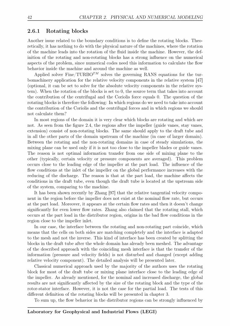
42 CHAPTER 2. PHYSICAL AND NUMERICAL MODELING
2.6.1 Rotating blocks
Another issue related to the boundary conditions is to define the rotating blocks. Theo-retically, it has nothing to do with the physical nature of the machines, where the rotationof the machine leads into the rotation of the fluid inside the machine. However, the def-inition of the rotating and non-rotating blocks has a strong influence on the numericalaspects of the problem, since numerical codes need this information to calculate the flowbehavior inside the machine and around the machine as well.
Applied solver Fine/TURBOTM solves the governing RANS equations for the tur-bomachinery application for the relative velocity components in the relative system [47](optional, it can be set to solve for the absolute velocity components in the relative sys-tem). When the rotation of the blocks is set to 0, the source term that takes into accountthe contribution of the centrifugal and the Coriolis force equals 0. The question of therotating blocks is therefore the following: In which regions do we need to take into accountthe contribution of the Coriolis and the centrifugal forces and in which regions we shouldnot calculate them?
In most regions of the domain it is very clear which blocks are rotating and which arenot. As seen from the figure 2.4, the regions after the impeller (guide vanes, stay vanes,extension) consist of non-rotating blocks. The same should apply to the draft tube andin all the other parts of the domain upstream of the machine (in case of larger domain).Between the rotating and the non-rotating domains in case of steady simulations, themixing plane can be used only if it is not too close to the impeller blades or guide vanes.The reason is not optimal information transfer from one side of mixing plane to theother (typically, certain velocity or pressure components are averaged). This problemoccurs close to the leading edge of the impeller at the part load. The influence of theflow conditions at the inlet of the impeller on the global performance increases with thereducing of the discharge. The reason is that at the part load, the machine affects theconditions in the draft tube, even though the draft tube is located at the upstream sideof the system, comparing to the machine.
It has been shown recently by Zhang [97] that the relative tangential velocity compo-nent in the region before the impeller does not exist at the nominal flow rate, but occursat the part load. Moreover, it appears at the certain flow rates and then it doesn’t changesignificantly for even lower flow rates. Zhang also claimed that the rotating stall, whichoccurs at the part load in the distributor region, origins in the bad flow conditions in theregion close to the impeller inlet.
In our case, the interface between the rotating and non-rotating part coincide, whichmeans that the cells on both sides are matching completely and the interface is adaptedto the mesh and not the inverse. This kind of interface has been created by splitting theblocks in the draft tube after the whole domain has already been meshed. The advantageof the described approach with the coinciding mesh interface is that the transfer of theinformation (pressure and velocity fields) is not disturbed and changed (except addingrelative velocity component). The detailed analysis will be presented later.
Classical numerical approach used by the majority of the authors uses the rotatingblock for most of the draft tube or mixing plane interface close to the leading edge ofthe impeller. As already mentioned, for the nominal and increased discharge, the globalresults are not significantly affected by the size of the rotating block and the type of therotor-stator interface. However, it is not the case for the partial load. The tests of thisdifferent definition of the rotating blocks will be presented in chapter 3.
To sum up, the flow behavior in the distributor regions can be strongly influenced by
Laboratory for Geophysical and Industrial Flows (LEGI)

CHAPTER 2. PHYSICAL AND NUMERICAL MODELING 43
conditions at the inlet of the impeller. Therefore, setting the interface that divides therotating and non-rotating blocks seems to be very important, especially at the part loadoperating points. The best way seems to be to create an unite mesh for the impeller andthe draft tube (cone) and later split the blocks and create coinciding interface. The rotat-ing and non-rotating regions can therefore be defined without interfering the information(pressure, velocity fields) transfer close to the leading edge of the impeller blades.
2.7 Convergence criteria and time discretization
Steady and unsteady simulations have been performed during the studies. In both casesit is necessary to have good convergence in order to obtain reliable results, which is notvery hard for the operating points close to the BEP in non-cavitating regime. However, itgets much more complicated in the cavitation regime and especially at the unstable partload conditions.
2.7.1 Steady simulations
Global residuals are typically used as a convergence criteria for a steady simulations. Itdepends a lot on the initial conditions, therefore the convergence level cannot be com-pletely quantified. What is more important than the value of the global residuals is thestability of the convergence curve. The simulation reached the convergent solution whenit is stable and does not fluctuate too much.
Other criteria that might be even more important than the global residuals are:
• Mass flow convergence. The difference between the inlet and the outlet massflow. For the stable operating points the difference is lower than 0, 003%. On theother hand, for a very unstable operating points, the difference below 1% is stillacceptable.
• Head convergence. The numerical head is defined as the total pressure differencebetween the inlet and the outlet of the numerical domain. The fluctuations of theconverged solution are negligible at stable operating points. However, they mightappear in unstable off-design regions. For the regions with stalled cells, it oftenoccurs to have ’periodical’ fluctuations in a range of a few percent, even for thesteady simulations.
• Torque convergence. For stable operating points the fluctuations are less than0, 01% and for unstable points, the satisfying convergence is less than 0, 1% of thefluctuations.
• Efficiency convergence can be difficult to estimate. For stable points, the conver-gence curve is usually very stable with less than 0, 01%. However, for the cavitatingregimes and if the rotating stall is present, the fluctuations can reach up to 1%.
The convergence difference between stable and unstable operating can be seen on thefigure 2.5. Both curves represent a converged solution. However, the global residuals forthe operating point with the rotating stall finishes with the ’periodic repetitions’. Similarbehaviors could be seen also on the mass flow convergence curve, head convergence curveand others. It means that we have an unsteady phenomenon, which cannot be simulatedcorrectly by the steady approach. The solution may slightly vary depending on the final
Laboratory for Geophysical and Industrial Flows (LEGI)

44 CHAPTER 2. PHYSICAL AND NUMERICAL MODELING
iteration. This kind of analysis can help us to detect the stable and the unstable operatingregions. Additional analysis on the convergence will be shown in the Part III.
Figure 2.5: Convergence criteria, RMS, steady simulations
2.7.2 Unsteady simulations
Choosing the time step can significantly influence the length of the simulations and alsothe precision of the results at the end of the simulations. Typical time discretizationchoices for hydraulic machines are 1◦ or 2◦ of the rotation of the machine. One must beaware that the discretization of 1◦ would result in a calculation twice as long as in thecase of 2◦.
In the case of unsteady simulations it is important to know, before the simulations,which kind of results are we interested in. The time step choice depends on this infor-mation. For example, if we are interested in the pressure fluctuations around the regionbetween the impeller and the distributor, the critical effect would be the interaction be-tween the impeller blades and the guide vanes. In our case of 9 impeller blades and 20guide vanes it would mean 180 interactions per revolution of the machine. Therefore, thediscretization should be 1◦ (360 time steps per revolution) or even 0, 5◦ (720 time stepsper revolution). Similar conclusions have been proposed by [10] and [41]. They showedthat the discretization of 1◦ is enough to simulate precisely pressure fluctuations in theregion between the impeller and the distributor.
On the other hand, if the goal is to detect, predict and analyze the rotating stall,the time step can be different. The frequency of the stall is usually around 3% of therotating frequency of the machine, which means that the time discretization of 2◦ shouldbe enough to catch the correct frequency and forms of the rotating stall.
No matter which discretization time is used, one still needs to provide good convergencefor each time step. The approach is called Dual Time Stepping and is similar to the steadysimulations for each time step. The number of so called internal iterations can be definedby setting the satisfying convergence level (global residuals) or by limiting the number ofiterations for each time step. The convergence is good, when several consecutive iterations
Laboratory for Geophysical and Industrial Flows (LEGI)
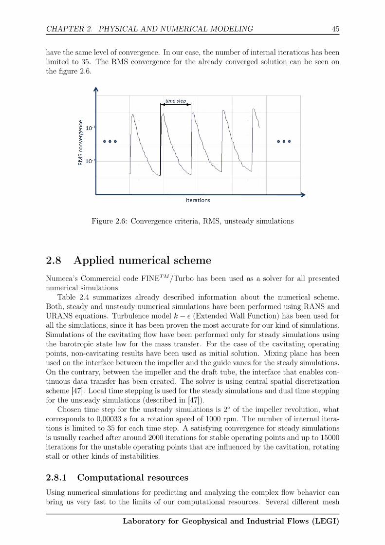
CHAPTER 2. PHYSICAL AND NUMERICAL MODELING 45
have the same level of convergence. In our case, the number of internal iterations has beenlimited to 35. The RMS convergence for the already converged solution can be seen onthe figure 2.6.
Figure 2.6: Convergence criteria, RMS, unsteady simulations
2.8 Applied numerical scheme
Numeca’s Commercial code FINETM/Turbo has been used as a solver for all presentednumerical simulations.
Table 2.4 summarizes already described information about the numerical scheme.Both, steady and unsteady numerical simulations have been performed using RANS andURANS equations. Turbulence model k − ǫ (Extended Wall Function) has been used forall the simulations, since it has been proven the most accurate for our kind of simulations.Simulations of the cavitating flow have been performed only for steady simulations usingthe barotropic state law for the mass transfer. For the case of the cavitating operatingpoints, non-cavitating results have been used as initial solution. Mixing plane has beenused on the interface between the impeller and the guide vanes for the steady simulations.On the contrary, between the impeller and the draft tube, the interface that enables con-tinuous data transfer has been created. The solver is using central spatial discretizationscheme [47]. Local time stepping is used for the steady simulations and dual time steppingfor the unsteady simulations (described in [47]).
Chosen time step for the unsteady simulations is 2◦ of the impeller revolution, whatcorresponds to 0,00033 s for a rotation speed of 1000 rpm. The number of internal itera-tions is limited to 35 for each time step. A satisfying convergence for steady simulationsis usually reached after around 2000 iterations for stable operating points and up to 15000iterations for the unstable operating points that are influenced by the cavitation, rotatingstall or other kinds of instabilities.
2.8.1 Computational resources
Using numerical simulations for predicting and analyzing the complex flow behavior canbring us very fast to the limits of our computational resources. Several different mesh
Laboratory for Geophysical and Industrial Flows (LEGI)

46 CHAPTER 2. PHYSICAL AND NUMERICAL MODELING
Type of Simulation Steady UnsteadyPhysical model RANS URANS
Turbulence model k − ǫ (Ext. Wall Function) k − ǫ (Ext. Wall Function)Cavitation model Barotropic /
Spatial discretization Central (2nd order) Central (2nd order)Temporal discretization Local time stepping Dual time stepping
Time step / 2◦ of the revolutionMax iterations/time steps 2000 - 15000 iterations up to 2700 time steps
Table 2.4: Numerical scheme
settings were analyzed during the presented work. However, for the final analysis andresults only one type of mesh has been used in order to have a good comparison betweenthe various boundary conditions and different types of simulation. In other words, inall cases the mesh density does not change, the numerical domain does not change, theperiodicity between the blades changes and the type of simulations (steady and unsteady)changes as well.
Approximate estimation of the necessary computational resources for non-cavitatingoperating points are presented in the table 2.5. Column ’periodic’ represents fully peri-odical mesh that is typically used in the field of turbomachinery. It means that just onechannel of the impeller and one channel of the distributor are calculated. The ’combined’mesh consists of one meshed channel in the region of the impeller and a fully mesheddistributor. The term ’Full mesh’ or ’full domain’ represents the type of mesh whereperiodicity was not used at all. The entire domain (impeller, draft tube and distributor)is 360◦ meshed and calculated.
periodic combined full domain full domaintype steady steady steady unsteady
mesh cells 0,87 M 10,7 M 13,4 M 13,4 MCPU h 7 - 20 250 320 270/revOutput 0,2 Gb 1,9 Gb 2,3 Gb 1,7 Gb/ts
Table 2.5: Mesh analysis, CPU time, data size
Simulations of the cavitating flow require from 2 - 5 times more CPU hours, comparingto non-cavitating operating points. The calculation time depends significantly on theintensity of the cavitation, therefore, it is difficult to make a general estimation.
As seen from the table 2.5, the size of mesh differs significantly. On one hand, thecalculations on the periodic mesh can be easily performed on the normal personal com-puter, since only 7 - 20 CPU hours are necessary to reach good convergence for thenon-cavitating flow. On the other hand, for the combined and for the full domain, oneneeds several additional processors and more than 250 CPU hours for steady simulations.Moreover, the typical size of random-access memory (RAM) in a personal computer isnot sufficient anymore.
Optimal type of simulation for the exact prediction of the rotating stall is most likelyunsteady simulation with a full-meshed geometry. However, in that case, the computa-tional requirements become very demanding. For good stall detection, one needs to userotating angle 2◦ of impeller revolution or less, this means at least 180 time steps per onerevolution of the machine. Since every time step provides us around 1,7 Gb of data, we
Laboratory for Geophysical and Industrial Flows (LEGI)

CHAPTER 2. PHYSICAL AND NUMERICAL MODELING 47
need around 300 Gb of storage to save data and around 270 CPU computational hoursper one revolution of the pump-turbine. Nevertheless, to detect the stall characteristicfrequency, which is normally between 2% and 6% of the nominal frequency of the machine,more than 10 revolutions should be calculated for each operating point. By multiplyingthe numbers, it becomes clear that the computational cost and demanding data storagefor that kind of simulation is high and not easily affordable.
One of the goals of the study is to find cost-efficient computational approach to simu-late part load unstable operating points in pumping mode. Therefore, all our calculationshave been performed on the server in LEGI on the maximum of the 12 cores. The cal-culation time of the longest of the presented simulations has been around 2 weeks. Itmeans that all the calculations in the presented work are fast and repeatable on widelyaccessible computers.
To conclude, it is necessary to estimate which kind of simulations do we need for goodresults at each operating point. Moreover, one needs to be aware of the advantages anddisadvantages of each type of simulation.
2.9 Comparison of experimental and numerical data
To validate the numerical simulations, they have been compared to the provided experi-mental data. Comparison was mostly based on the global performance. Head differencehas been evaluated numerically as the average total pressure difference between the outletand the inlet of the numerical domain. Gravitation has been neglected.
Experimentally, the head difference information comes from the pressure sensors thathave been installed upstream and downstream of the machine. Position of the pressuresensors on the test rig can be seen in the Appendix 1 (fig. A.2). Comparison of theexperimental and numerical (fig. 2.4) position of the pressure reference sections showsthat in the numerical domain the spiral case and the draft tube elbow are not taken intoaccount. On the other side, the convergent extension exists only in the numerical domain.It means that the calculated performance cannot be completely the same, because thelosses depend also on the domain.
Another effect that has not been taken into account numerically is the leakage flow.In physical machines there is small part of the flow that go around the machine from thehigh pressure region of the pump-turbine to the low pressure region. It is considered asa loss and it can slightly affect the pump-turbine performance curve. The leakage flow inthe centrifugal pump has been studied experimentally and numerically by [24].
However, despite all the mentioned differences, the comparison between the numericaland the experimental data is still possible. If the goal is to have a detailed quantitativecomparison of the results, then additional impact factors (leakage, sensors position,...)including mentioned losses and differences should be considered and taken into account.However, since the main idea in our case is to have a good qualitative description of thepart load flow phenomena, those factors have not been taken into account. Nevertheless,even in our case, various quantitative comparisons and conclusions have been done andare presented in the thesis Part III.
2.9.1 Hysteresis effect
Hysteresis phenomenon represents the differences in the performance curve dependingif the flow rate is decreasing or increasing. It occurs typically during the experiments.
Laboratory for Geophysical and Industrial Flows (LEGI)

48 CHAPTER 2. PHYSICAL AND NUMERICAL MODELING
Especially the hump zone can be significantly influenced by the hysteresis. Figure 2.7shows the difference in the hump zone position. If one starts to measure the pump-turbine performance at the increased discharge and than gradually reduces it, the humpzone might occur at a lower discharge than if the measurements are performed at lowerdischarge first, which is later gradually increased.
Figure 2.7: Schematic representation of the hysteresis effect on the performance curve
The hysteresis effect has been studied experimentally and numerically on the cen-trifugal pump geometry by [51] and on the pump-turbine geometry (pumping mode) by[77]. In their cases, the difference between the increasing and the decreasing performancecurve do not exceed 3% of the nominal discharge.
During the experiment in the Alstom Hydro’s laboratory, the hysteresis effect hasnot been taken into account. It means that we should take into account the appropriatetolerance for the measured position of the hump zone. Nevertheless, as already mentioned,the aims of the presented study are more qualitative than quantitative. Therefore, thementioned tolerance is acceptable for the comparison with the numerical simulations andas well for the final analysis and the conclusions.
Laboratory for Geophysical and Industrial Flows (LEGI)

Part III
Results
49


Chapter 3
Global results
This chapter focuses mainly on the analysis of the cavitation phenomenon. All the per-formed calculations represent steady simulations and have been performed on the de-scribed periodic mesh. Applied guide vanes opening angle is 14◦ in all cases. Most of theresults have been presented in [48].
The beginning of the chapter also includes the tests of the already presented turbulencemodels and the chosen boundary conditions. The cavitation analysis is mostly focused onthe prediction of the incipient cavitation values, head drop curves, cavitation forms andon the effects of the cavitation appearance on the performance curve.
3.1 Global results for non-cavitating regime
The first global results, presented on the figure 3.1, have been obtained for steady non-cavitating regime. The comparison between the experimental and the numerical data canbe analyzed qualitatively and quantitatively as well. The curve is a basis for all furtheranalysis of the cavitating flow. The first source of difference between the experimentaland the numerical performance values occurs due to different total pressure (net head)measurement spots between the experimental and the numerical domain. The position ofsensors in the experiment are marked on the figure A.2 (Appendix A). On the other hand,the numerical reference points are defined as a inlet and outlet of the numerical domain.Additionally, mechanical and volumetric losses have not been estimated and taken intoaccount numerically.
As shown on the figure 3.1, the position of the hump zone can be detected numericallyby the accuracy of 2% on flow rate value. It is a good matching considering the possiblehysteresis effect on the experimental curve that has not been taken into account since theinformation about it has not been provided. The hump amplitude prediction matcheswell; in the cases of the experimental and numerical curve the specific energy coefficientψ drops for around 1%.
The comparison between the experimental and the numerical performance curvesshows good matching for all the operating points at the normal operating range closeto BEP and for the increased discharge as well (for φ = 0, 0315 and higher). The discrep-ancy between the experimental and the numerical curve is around 1%.
The performance decrease, known as a hump zone (fig. 3.1; φ = 0, 031, numerically;φ = 0, 032, experimentally) occurs due to the flow separation in the distributor area,which later leads into the phenomenon called the rotating stall. The phenomenon will bedescribed in detail in the next two chapters. However, it is important to stress that ac-
51

52 CHAPTER 3. GLOBAL RESULTS
Figure 3.1: Global pump-turbine performance, losses in the distributor - lossOUT (Open-ing 14◦, basic GV geometry, non-cavitating regime)
cording to the performed calculations, the head decrease occurs due to the increased lossesin the distributor regions (line lossOUT, fig. 3.1, represents the losses in the distributorregions).
The flow behavior at the significantly decreased discharge (around φ = 0, 026) is verycomplex and 3-dimensional in the distributor regions. Using a periodicity as a boundarycondition between the guide and the stay vane channels might not be appropriate. Un-steady simulations that have been performed on full mesh will be analyzed in the chapter5.
3.1.1 Turbulence model tests
Comparison of the k − ǫ (Extended wall functions) turbulence model and the k − ω(SST) model (fig. 3.2) shows that the k− ǫ (Extended wall functions) model predicts theglobal performance curve more accurately than the k − ω (SST) model comparing to theexperimental data.
Even though our comparisons are more qualitative than quantitative, there are stilltwo main differences between the models. One is the trend of the line for all the flow rateshigher than hump zone, where the trend of the performance curve is more exact in thecase of the k−ǫ (Extended wall functions) model. The other indicator is the prediction ofthe hump zone. On one hand, the zone is predicted at almost the same discharge and hasa similar amplitude for the case of the k − ǫ (Extended wall functions) and experimentaldata. On the other side, the k−ω (SST) model predicts the hump zone at the around 12%lower discharge and has smaller amplitude. The prediction of the hump zone seems to bestrongly related to the accuracy of the prediction of the flow separation in the distributorregion. From this point, for all presented simulations, turbulence model k − ǫ (Extendedwall functions) has been used.
Laboratory for Geophysical and Industrial Flows (LEGI)

CHAPTER 3. GLOBAL RESULTS 53
Figure 3.2: Comparison between turbulence models k − ǫ (Extended wall functions) andk − ω (SST)
3.1.2 Tests of the rotor/stator interfaces and the rotating blocks
The definition of the rotating blocks and the interfaces around the impeller influence theglobal prediction of the pump-turbine performance, including the prediction of the humpzone. In our case, the blocks have been defined as shown on the figure 2.4. Figure 3.3shows the influence of the rotation of the blocks on the global performance comparison andcorresponding definitions of the rotating blocks. Definition of rotating and non-rotatingblocks is mathematically related to the calculation of the Coriolis and centrifugal forces.If the rotation speed of the block is defined as 0, then the possible Coriolis and centrifugalforces will not be calculated in this block.
If the border between the rotating and the non-rotating blocks is set very close tothe leading edge of the impeller (No prerotation - fig. 3.3), the performance prediction isnot good for any operating points. It gets worse with reducing the discharge, moreover,hump zone cannot be predicted. On the other hand, if the border is set far away fromthe impeller (Full prerotation - fig. 3.3), the prediction is good at optimal discharge andat increased discharge. At the part load, the discrepancies increase significantly and thetrend of the performance curve is not well predicted. The hump zone still occurs, but atthe lower discharge and with a higher hump amplitude.
For comparison, the blue line (Partial prerotation - fig. 3.3) represents the results,where the border between the rotating and non-rotating blocks is set at the distance ofaround Dinl/4 from the leading edge of the impeller. The border (interface) is almostparallel to the leading edge as seen on the figure 3.4. As mentioned before, the interfacebetween the rotating and non-rotating part match perfectly, which means that the cellson both sides are matching completely and the interface is adapted to the mesh and notthe inverse. This kind of interface has been created by splitting the blocks in the drafttube after the whole domain has been already meshed. Prediction of the performancecurve is in this case relatively good for all discharges, the prediction of the hump zone isaccurate as well.
The advantage of the described approach with the coinciding mesh interface is that the
Laboratory for Geophysical and Industrial Flows (LEGI)

54 CHAPTER 3. GLOBAL RESULTS
Figure 3.3: Influence and definition of the rotating blocks
Figure 3.4: (left) Influence of the different types of interface; (right) Position of theinterface
transfer of the information (pressure and velocity fields) is not disturbed and changed (ex-cept adding relative velocity component). For comparison, using mixing plane approach
Laboratory for Geophysical and Industrial Flows (LEGI)
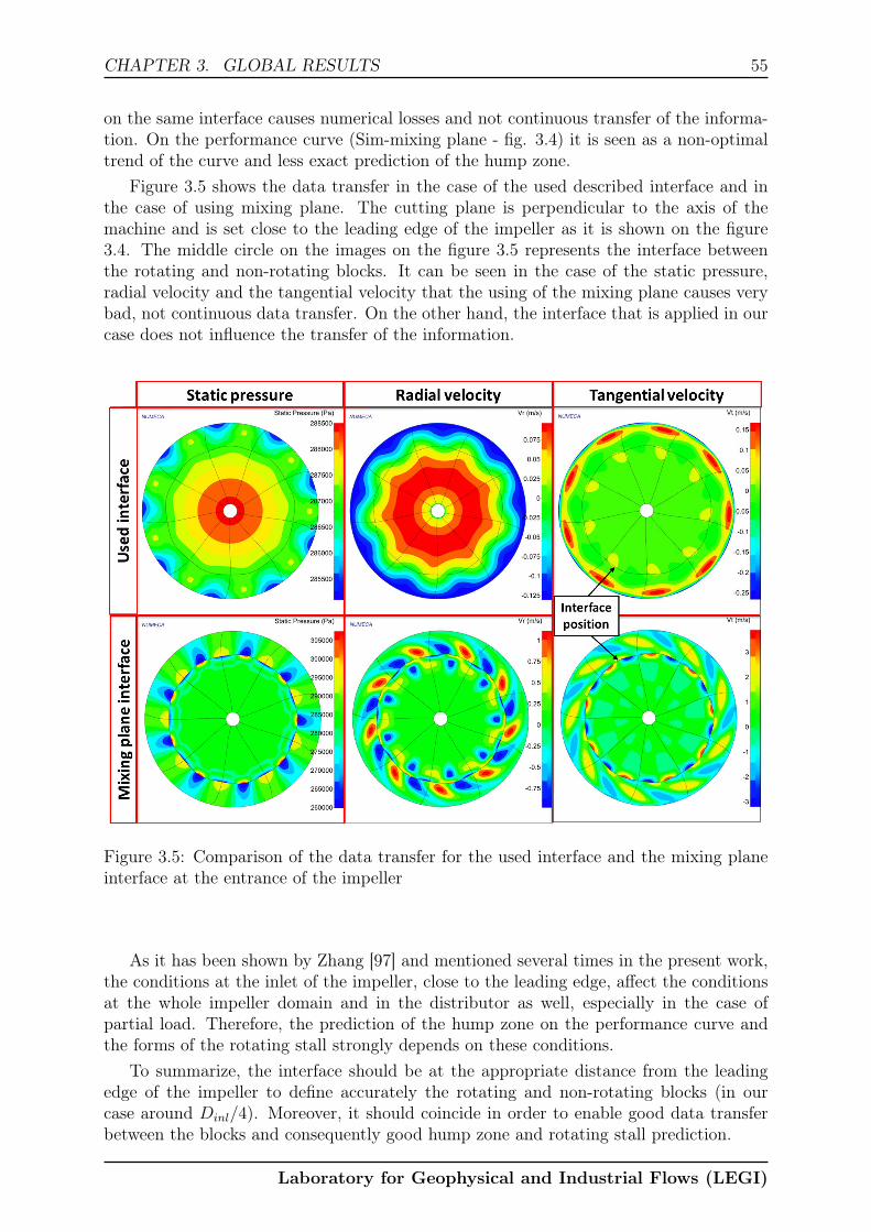
CHAPTER 3. GLOBAL RESULTS 55
on the same interface causes numerical losses and not continuous transfer of the informa-tion. On the performance curve (Sim-mixing plane - fig. 3.4) it is seen as a non-optimaltrend of the curve and less exact prediction of the hump zone.
Figure 3.5 shows the data transfer in the case of the used described interface and inthe case of using mixing plane. The cutting plane is perpendicular to the axis of themachine and is set close to the leading edge of the impeller as it is shown on the figure3.4. The middle circle on the images on the figure 3.5 represents the interface betweenthe rotating and non-rotating blocks. It can be seen in the case of the static pressure,radial velocity and the tangential velocity that the using of the mixing plane causes verybad, not continuous data transfer. On the other hand, the interface that is applied in ourcase does not influence the transfer of the information.
Figure 3.5: Comparison of the data transfer for the used interface and the mixing planeinterface at the entrance of the impeller
As it has been shown by Zhang [97] and mentioned several times in the present work,the conditions at the inlet of the impeller, close to the leading edge, affect the conditionsat the whole impeller domain and in the distributor as well, especially in the case ofpartial load. Therefore, the prediction of the hump zone on the performance curve andthe forms of the rotating stall strongly depends on these conditions.
To summarize, the interface should be at the appropriate distance from the leadingedge of the impeller to define accurately the rotating and non-rotating blocks (in ourcase around Dinl/4). Moreover, it should coincide in order to enable good data transferbetween the blocks and consequently good hump zone and rotating stall prediction.
Laboratory for Geophysical and Industrial Flows (LEGI)

56 CHAPTER 3. GLOBAL RESULTS
3.2 Validation of the cavitation model
To evaluate the level of the cavitation in the pumping regime, definition of the requiredNPSH value is important. In our case, it is calculated for each operating point as:
NPSH(m) =pref − pvρl g
. (3.1)
In the equation 3.1, pref represents the total pressure value at the inlet of the domain,pv the vaporization pressure of the water at 20◦C, ρl the density of the water and g is thegravitational constant. Numerical NPSH value has been calculated after each calculation.
Since the conditions at the inlet and the outlet of the numerical domain have beenfixed, the NPSH value has been modified by changing the value of vaporization pressurepv in order to keep the stability of simulations and similar level of the convergence, whichplays even more important role in the calculations with the cavitation model and unstableoperating points. A similar approach has been used and described in the thesis work byPouffary [74] and Coutier-Delgosha [13].
3.2.1 Incipient cavitation
It is important that the numerical simulations in the cavitating regime can be validatedand compared to the experimental results. The incipient cavitation value (fig. 3.6) ispresented for the numerical simulations as well as for the experiment. Experimentally,the value is obtained by the visual observation of the pump-turbine impeller inlet. Thevalue at different flow rates is defined as the appearance of the first cavitation bubbles.
Figure 3.6: Incipient cavitation values
Classical numerical industrial approach does not use the cavitation model to predictthe incipient cavitation value. It is simplified by defining the reference pressure pref(eq. 3.1) by the difference between the total pressure at the inlet of the domain andthe minimal static pressure in the studied domain. The approach has been proved quite
Laboratory for Geophysical and Industrial Flows (LEGI)

CHAPTER 3. GLOBAL RESULTS 57
precise to predict the incipient cavitation value. Nevertheless, it cannot give us anyadditional information if the cavitation is more developed.
When using the cavitation model, the criteria for the incipient cavitation conditioncan be defined by the void ratio α. In our case, when the void ratio in the first cavitatingcell reached the value α = 0, 2 (20% of vapor in the cell), the corresponding NPSH valuehas been taken as the incipient cavitation value. The agreement between the industrialapproach without cavitation model and the approach using the cavitation model for themass transfer is very good. However, the simulations with the cavitation model can giveus lots of additional information about the cavitating flow behavior comparing to theindustrial numerical approach.
As presented on the figure 3.6, the matching between the numerical and the experi-mental values is good for the wide range of flow rates. The precision for both, numericaland experimental NPSHi values, is estimated to ± 0, 5m. Some deviation can be ob-served for the increased flow rate at the operating point around φ = 0, 048. The reasonis most likely the experimental methodology for estimating the occurrence of the firstbubble. In most of our studied operating points, the first cavitation bubble occurs atthe leading on the suction side of the impeller blade. On contrary, at the φ = 0, 048,the cavitation firstly occurs on the pressure side of blade, which is experimentally moredifficult to observe, which could explain the higher discrepancy in this area.
3.3 NPSH head drop curves
The robustness of the cavitation model allows us to provide results for a wide range offlow rates and a wide range of NPSH values.
The NPSH head drop curves could be made for various flow conditions. Figure 3.7shows four different NPSH head drop curves for the four different operating regimes (flowrates). Curve φ = 0, 0348 represents the operating regime, close to the best efficiencypoint for the guide vane opening of 14◦, which is also relatively close to the hump zone.φ = 0, 0278 represents the part load operating regime, which is at lower discharge thanthe hump zone. The curve at φ = 0, 0435 is close to the upper operational limit of thenormal operating regime and the curve φ = 0, 0487 represents the operation point at theincreased discharge. In these three cases, we can see experimental results for 1% headdrop due to cavitation occurrence. Numerical results are in relatively good agreementwith the experimental data.
As seen from the figure 3.7, the simulated head drop can reach up to 10% due to thecavitation on the pressure side of the impeller blades. All the points where the head dropoccurs are considered dangerous, since the machine can be exposed to strong vibrations,erosion and non-controllable switching of the operating points due to the presence of thecavitation phenomenon.
In the case of the reduced discharge, a performance increase can be observed beforethe head drop at around NPSH = 2 m. The cavitation sheet at this point increases theincidence at the leading edge of the impeller blade and improves the performance.
It is known that the cavitation cloud at the low NPSH values is not a steady phe-nomenon. However, steady simulations enable us to get average size of cavitation sheetfor each NPSH value and the estimated head drop. To evaluate the size of the cavita-tion clouds and the frequency of the cloud separation, high-cost unsteady simulations arerequired and have not been performed in these studies.
Laboratory for Geophysical and Industrial Flows (LEGI)

58 CHAPTER 3. GLOBAL RESULTS
Figure 3.7: NPSH head drop curves
3.4 Cavitation forms
Discharge φ = 0, 0348 (close to BEP)
Related to figure 3.7, we can observe the cavitation forms for different flow rates. Figure3.8 represents three different levels of cavitation inside the pump-turbine at the dischargeφ = 0, 0348, which corresponds to the operating point close to the BEP for the consideredopening. The incipient cavitation value for that case is around NPSHi = 4, 8m. Thecavitation firstly occurs on the suction side of the impeller blade. By lowering the NPSHvalue, the cavitation is seen mostly on the large area on the suction side of the blade,closer to the shroud. At extremely low NPSH values (NPSH = 1, 78m), one can observethe vapour sheets also on the pressure side of the blade. In case of NPSH = 1, 78m thehead drop reaches around 5% of the nominal head for the corresponding discharge andguide vanes opening.
The cavitation forms in the channels between the impeller blades have an importantimpact on the provided energy by the impeller. The impeller blade has been divided intoseven (D1 - D7, fig. 3.9, left) regions in order to observe the energy distribution along theimpeller blade.
Line ’total’ (3.9, right) represents the performance of the pump-turbine for the corre-sponding NPSH value including the losses in the distributor. At very low NPSH values,we can see that the regions closer to the leading edge of the impeller blades provide lessenergy because of the cavitation appearance. However, the blade regions D3 and D4 par-tially compensate the bad distribution at region D1. Provided energy in the regions D3and D4 is even higher than in cases with higher NPSH values. It is interesting that evenin the region D7, which is at the outlet of the impeller, the performance fluctuates formore than 10%. In fact, the performance in the region D7 is the best in the case of theNPSH = 1, 83m.
Overall, as expected, the presence of the cavitation has negative influence on the per-
Laboratory for Geophysical and Industrial Flows (LEGI)
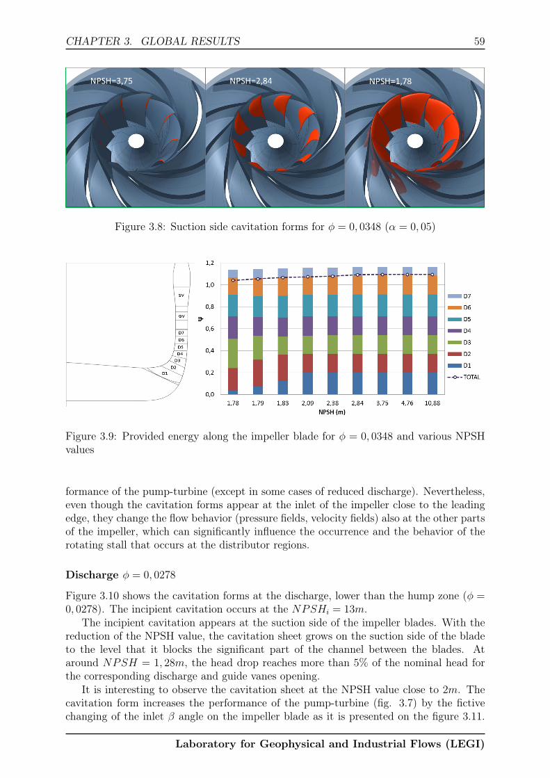
CHAPTER 3. GLOBAL RESULTS 59
Figure 3.8: Suction side cavitation forms for φ = 0, 0348 (α = 0, 05)
Figure 3.9: Provided energy along the impeller blade for φ = 0, 0348 and various NPSHvalues
formance of the pump-turbine (except in some cases of reduced discharge). Nevertheless,even though the cavitation forms appear at the inlet of the impeller close to the leadingedge, they change the flow behavior (pressure fields, velocity fields) also at the other partsof the impeller, which can significantly influence the occurrence and the behavior of therotating stall that occurs at the distributor regions.
Discharge φ = 0, 0278
Figure 3.10 shows the cavitation forms at the discharge, lower than the hump zone (φ =0, 0278). The incipient cavitation occurs at the NPSHi = 13m.
The incipient cavitation appears at the suction side of the impeller blades. With thereduction of the NPSH value, the cavitation sheet grows on the suction side of the bladeto the level that it blocks the significant part of the channel between the blades. Ataround NPSH = 1, 28m, the head drop reaches more than 5% of the nominal head forthe corresponding discharge and guide vanes opening.
It is interesting to observe the cavitation sheet at the NPSH value close to 2m. Thecavitation form increases the performance of the pump-turbine (fig. 3.7) by the fictivechanging of the inlet β angle on the impeller blade as it is presented on the figure 3.11.
Laboratory for Geophysical and Industrial Flows (LEGI)

60 CHAPTER 3. GLOBAL RESULTS
Figure 3.10: Suction side cavitation forms for φ = 0, 0278 (α = 0, 05)
The attached cavitation sheet can be assumed as a part of the impeller blade that has, inthis case, a changed geometry and optimized operating conditions.
Figure 3.11: β1 and β2 for 3 different NPSH values for φ = 0, 0278
Figure 3.11 represents the impeller inlet and the outlet β angle for corresponding NPSHvalues presented on the figure 3.10. The operating point of the improved performance(NPSH = 1, 91m) has lower beta value close to the hub, comparing to the case of smallcavitation (with no influence on the performance).
It is clear that the cavitation changes the flow attack angle on the leading edge ofthe blade and changes the performance of the impeller. However, what is important isthe changing of the beta angle at the trailing edge of the impeller. It proves that theconditions at the leading edge of the impeller affect the condition at the trailing edge ofthe impeller and consequently at the inlet of the distributor.
Similar conclusions have been made by [97]. This is very important for the study andthe prediction of the rotating stall. Not only that it can be affected by the cavitationforms, but also by the velocity profile at the inlet of the impeller that must be thereforesimulated as exactly as possible.
Laboratory for Geophysical and Industrial Flows (LEGI)

CHAPTER 3. GLOBAL RESULTS 61
Discharge φ = 0, 0435
Figure 3.12 represents the cavitation forms for an operating point close to the upperoperating limit. The incipient cavitation occurs at the value NPSHi = 3, 6m, which ismore than 1m lower than in the case of operating point close to BEP (φ = 0, 0348). Thecavitation occurs almost at the same time on the pressure and suction side of the impellerblades, which shows us that the flow attack angle is well adapted to the angle of theleading edge of the impeller blade.
Figure 3.12: Suction side cavitation forms for φ = 0, 0435 (α = 0, 05)
On the suction side, cavitation firstly occurs far away from the leading edge of theimpeller blade close to the shroud side of the impeller. At around NPSH = 2, 85m,the cavitation sheets from the suction side and the pressure side join together at theshroud and at that point strong pressure drop occurs, because the cavitation alreadyoccupies significant part in the channel between the impeller blades. Operating point atthe NPSH = 2, 82m represents the head drop of around 7% comparing to the nominalhead for the considered discharge.
Discharge φ = 0, 0487
Figures 3.13 and 3.14 represent the cavitation forms at the suction and the pressure sideof the impeller blade for the significantly increased discharge (φ = 0, 0487) and differentNPSH values. The incipient cavitation appears at the NPSHi = 10, 9m close to theleading edge on the pressure side of the impeller blade. At around NPSH = 5m, thecavitation occurs also on the suction side of the blade close to the shroud and far awayfrom the leading edge of the impeller blade. With the lowering of the NPSH value, thecavitation sheet grows mostly on the shroud side of the impeller on both, pressure andsuction side of the blade. Around the NPSH = 4m the sheets from pressure and suctionside of the blade join on the shroud side of the impeller.
Meanwhile, small cavitation forms occur also on the suction side of the guide vanes(fig. 3.14). Even though the guide vanes are in the high pressure region of the machine,the unadapted guide vane opening angle results in the position of the stagnation pointfar from the leading edge of the guide vane on the pressure side of the vane. Figure 3.15represents the stagnation points close to the leading edge of the guide vanes for 3 differentdischarges. The static pressure scale is the same for all 3 figures.
In case of the operating point close to the BEP (φ = 0, 0435), the stagnation pointalmost matches the leading edge of the guide vane. Therefore, the pressure gradients are
Laboratory for Geophysical and Industrial Flows (LEGI)

62 CHAPTER 3. GLOBAL RESULTS
Figure 3.13: Suction side cavitation forms for φ = 0, 0487 (α = 0, 05)
Figure 3.14: Pressure side cavitation forms for φ = 0, 0487 (α = 0, 05)
Figure 3.15: Stagnation point for 3 different discharges
low on both sides of the vane. At the part load (φ = 0, 0278), the attack angle of the flowchanges and the stagnation point moves a bit towards the suction side of the guide vane.However, even though the local pressure on the pressure side reduces, it is still too high forthe cavitation occurrence. On the other hand, for the increased discharge (φ = 0, 0487),the stagnation point moves towards the pressure side of the guide vanes. Consequently, thelocal pressure on the suction side of the guide vanes decreases significantly and reaches the
Laboratory for Geophysical and Industrial Flows (LEGI)

CHAPTER 3. GLOBAL RESULTS 63
vaporization pressure as seen on the figure 3.15. Nevertheless, the form of the cavitationin the guide vane region does not change a lot with the NPSH value due to surroundinghigh pressure regions.
3.5 Comparison to the visualization data
The direct comparison of the cavitation forms between the numerical images and theexperimental visualization has been possible for the discharge φ = 0, 0304, but (due tolimited visualization data) only for two NPSH values. As seen from the figure 3.16, thecavitation structures for NPSH = 6m and NPSH = 7m match the forms, observed byvisualization of the suction side of the pump-turbine impeller.
Figure 3.16: Comparison of cavitation forms to visualization data (Alstom Hydro) forφ = 0, 0304
3.6 Cavitation influence on the hump zone
Cavitation influence on the hump region has been investigated phenomenologically underthe same numerical conditions for the same opening as previous cavitation analyses. Fig-ure 3.17 presents the hump zone for non-cavitating conditions and under relatively strong,but constant cavitating conditions (constant NPSH values). Non-cavitating performancecurve has been compared to the two constant NPSH performance curves. Both NPSHvalues (NPSH = 2, 7m and NPSH = 2m) affect the hump zone significantly.
The presence of the strong cavitation reduces the hump amplitude and the positivedH/dQ slope is not observed anymore for the cavitating regimes at NPSH = 2, 7m and
Laboratory for Geophysical and Industrial Flows (LEGI)

64 CHAPTER 3. GLOBAL RESULTS
Figure 3.17: Cavitation influence on the hump zone
NPSH = 2m. Similar results have been presented by [1]. As already seen, in the case ofφ = 0, 0278 and NPSH = 2m, the performance improves due to the optimized conditionsin the impeller. Similar experimental and numerical results have been recently presentedby [38], [39].
It could be expected that the developed cavitation forms increase the losses in theimpeller. However, it is not obvious for the case of the distributor. The losses in thedistributor and decreased performance in the impeller have been investigated for thecavitating operating points (NPSH = 2, 7m and NPSH = 2m) and have been comparedto the non-cavitating regime (fig. 3.18). Negative values represent the increase of thelosses (∆Ψ, fig. 3.18).
Figure 3.18: Changed losses in the distributor and changed performance of the impellerdue to cavitation, compared to the non-cavitating regime
Cavitation effects on the performance are higher when the flow rate is higher. Some-times, at the part load (φ = 0, 0278), the presence of the cavitation even improves theperformance curve due to better conditions in the distributor, as seen on the figure 3.18.
Laboratory for Geophysical and Industrial Flows (LEGI)

CHAPTER 3. GLOBAL RESULTS 65
Analysis also shows that in most cases, the cavitation appearance increases losses in theimpeller and in the distributor as well, even though the cavitation occurs at the leadingedge of the impeller blade.
3.7 Chapter discussion
To conclude, the effects of the cavitation and generally the conditions at the inlet of theimpeller seem to be very complex. They have influence on the pressure and velocity fieldsin the parts of the domain that are very far from the region of actual cavitation appearance.It also means that the other unstable phenomena, such as the rotating stall, are stronglyinfluenced by it. The detailed analyses and comparisons of the pressure and velocity fieldsshould be made in the future for the cases of the cavitating and non-cavitating operatingpoints.
Influence of the cavitation on the hump region can be improved by the unsteadycalculations of the cavitating operating points. The simulations would be computationallymore demanding, but would give detailed insights about the interaction between the twotypes of instabilities, rotating stall and cavitation.
Laboratory for Geophysical and Industrial Flows (LEGI)

66 CHAPTER 3. GLOBAL RESULTS
Laboratory for Geophysical and Industrial Flows (LEGI)

Chapter 4
Steady partial load flow analysis
The results in the first part of this chapter have been analyzed for 4 different guidevanes openings and guide vanes geometry GV I (the opening is related to the relativeangle to tangential direction). All the presented calculations are steady simulations fornon-cavitating regime, performed on the periodic and on the combined mesh, where theperiodicity has been applied in the impeller and not in the distributor. Results have beenpartly presented in [49].
Analyses have been focused on a global prediction of the hump position, on the ampli-tude of the hump and on the flow patterns in the distributor area. Moreover, the analysishas been used to predict the stable, fully unstable and slightly unstable operating pointsin relation with the corresponding guide vanes openings and flow rates.
The last part of the chapter presents the global performance curves for the changedguide vanes geometry GV II. Results have been obtained on the fully periodic mesh andsteady simulations. They have been compared to the experimental curves and to thenumerical results for the guide vanes geometry GV I.
4.1 Guide vane opening 14◦
The line titled ’Sim-periodic 14◦’ (fig. 4.1) represents the calculations with the periodicmesh. The hump zone position has been detected with an accuracy of 2% on the flow rateaxis. Head drop amplitude reaches around 1% in both cases, numerical and experimentalone.
In chapter 3, it has been shown that the head drop in the hump zone was related tothe losses which occur due to flow behavior inside the distributor. To study the effects ofthe periodicity, the combined mesh has been created (Sim-combined 14◦, fig. 4.1), usinga periodicity in the impeller area and full distributor mesh. The difference between thenumerical results occurs only at the part load for the flow rates around Φ = 0, 025. Incase of periodic mesh, flow separation can be detected only on one guide vane, which isnot enough to represent the behavior in those operating points.
Several analyses of the flow patterns in the distributor of the combined mesh have beenmade on the mid-span cutting plane by comparing the meridional velocity distributions.The analysis showed a symmetrical distribution of the flow for all flow rates higher thanΦ = 0, 0317 (i.e., case a, Φ = 0, 0348, fig. 4.1). On the contrary, for the part load at thehump region (Φ = 0, 0313), the instability is seen as an unsymmetrically distributed flowas shown on the fig. 4.1, case b. Moreover, the flow analysis shows 4 cells of the decreasedflow rate next to the regions of the increased flow rate. The detected phenomenon is
67

68 CHAPTER 4. STEADY PARTIAL LOAD FLOW ANALYSIS
Figure 4.1: Pumping performance curve for GV opening 14◦, GV I geometry; flow patternsanalysis
related to an unsteady phenomenon of rotating stall that will be presented in details inthe next chapter.
By reducing the flow rate, different shapes and number of the flow cells could be pre-dicted. Between Φ = 0, 0275 and Φ = 0, 0304 the flow seems again almost symmetricallydistributed around the distributor. Performance is slightly underpredicted as in all casesof stable operating regime. On the other hand, flow seems to be very unstable lower thanΦ = 0, 027, which can be seen as 5 to 7 cells of increased flow rate (case c, Φ = 0, 0261,fig. 4.1).
Stable regions are marked on the figure 4.1. Stability is defined as a symmetricaldistributed flow in the regions of the guide vanes and stay vanes. Operating regions thatare not marked as stable are considered unstable. Therefore, there is high probabilitythat the rotating stall will occur there.
Numerical steady results calculated on the combined mesh overpredict the performancefor the very unstable part load operating points (Φ < 0, 028). For these points, theunsteady calculations should be performed, since the unsteadiness of the flow in thedistributor plays an important role in the prediction of the losses in this part of thedomain.
Laboratory for Geophysical and Industrial Flows (LEGI)

CHAPTER 4. STEADY PARTIAL LOAD FLOW ANALYSIS 69
4.1.1 Hump zone analysis
The unstable region around the hump was additionally investigated by mass flow variationanalysis through 20 channels between the guide vanes for three different operating pointsas shown on the figure 4.2b. Figure 4.2a shows the cutting plane though the guide vanechannels close to the leading edge, at which the flow rate has been investigated.
Figure 4.2: a) Investigated area between the GV channels for mass flow analysis; b) Humpzone performance curve, GV I, opening 14◦; c) Flow rate variation between various GVchannels (GVC) around the distributor (normalized by average flow rate Qavg)
Non homogeneous distribution of the flow rate, which can physically lead to the vibra-tions and uncontrollable changing of the operating points, are negligible for the dischargeΦ = 0, 0317 and all higher flow rates. On the contrary, the flow rate fluctuations at thehump zone (Φ = 0, 0313) reach up to ± 10%, as seen on the figure 4.2 c. When the valueof the dH/dQ on the performance curve is again negative (Φ = 0, 0304 and lower), thefluctuations decrease significantly (Φ = 0, 0304). They change less than 1% of the averageflow rate between the channels.
Additional hump zone study has been done by analyzing the pressure distributionsaround the guide vanes. Static pressure distributions on 5 consecutive guide vanes (fig.4.3a) have been analyzed for the discharge Φ = 0, 0313. Figures 4.3 show static pressuredistributions for suction and pressure sides of guide vanes in three different positions(close to hub, in the middle, close to shroud). Meridional velocity distribution shows aflow separation that blocks an important part of the channel between the guide vanes 3and 4. Consequently, the static pressure on the pressure side of GV 4 and on the suctionside of GV 3 is increased. The flow deviation close to the leading edge of the GV 3 causes
Laboratory for Geophysical and Industrial Flows (LEGI)

70 CHAPTER 4. STEADY PARTIAL LOAD FLOW ANALYSIS
an increased flow rate in the channel between the GV 2 and GV 3. Therefore, low pressureregions could be observed in the pressure side of GV 3 and in the suction side of GV 2.
Figure 4.3: Static pressure guide vanes loading: a) Guide vanes numbers; b)-f) Staticpressure on suction and pressure side of the guide vanes
To sum up, a steady, fully periodic mesh can give a good prediction of the humpshaped performance curve. Steady simulations on the combined mesh appear to be veryuseful to detect the stable and the unstable operating regions on the performance curve.Moreover, they can be used for several different steady analyses of the flow patterns in thedistributor zone. In case of very unstable operating points, unsteady simulations shouldbe performed in order to get more precise information about the distributor losses andconsequently about the net head for corresponding discharge.
4.2 Guide vane opening 12◦
The numerical hump detection for the 12◦ opening occurs at the same flow rate as ex-perimental one, also the hump amplitude is similar, as seen on the figure 4.4. Flow issymmetrically distributed for the flow rates higher than Φ = 0, 0325 (fig. 4.4a). The humpseems to be less intensive comparing to the 14◦ opening. 4 cells of slightly increased flowrate can be observed at the hump zone (Φ = 0, 0322, fig. 4.4b). Between the Φ = 0, 027and Φ = 0, 0313, the flow seems to be symmetrically distributed around the distributor(fig. 4.4c). By a considerable decrease of the flow rate, 6 cells of increased flow rate areformed between the Φ = 0, 024 and the Φ = 0, 027, as seen on figure 4.4d.
The difference between the periodic mesh and the combined mesh occurs at veryunstable operating points, where the rotating stall seems to be very strong. The origin
Laboratory for Geophysical and Industrial Flows (LEGI)

CHAPTER 4. STEADY PARTIAL LOAD FLOW ANALYSIS 71
Figure 4.4: Pumping performance curve for GV opening 12◦, GV I geometry; flow patternsanalysis
of the discrepancies with the experimental results lies in the unsteadiness of the rotatingstall that can not be simulated by the steady simulations. Same as for other openings,the periodic mesh in these cases can predict only flow separation on the guide vanes,the combined mesh can be used to predict the stall forms in the distributor. However,for detailed performance prediction and for the analysis of the unsteady components,unsteady simulations should be performed.
4.3 Guide vane opening 16◦
Guide vane opening 16◦ shows experimental performance curve almost without hump (fig.4.5). The tendency of the curve changes at around Φ = 0, 0332, where small hump occurs.
Laboratory for Geophysical and Industrial Flows (LEGI)

72 CHAPTER 4. STEADY PARTIAL LOAD FLOW ANALYSIS
The tendency of the numerical curve is slightly different for the operating points higherthan Φ = 0, 0332, compared to the experimental one. The difference occurs most likelydue to the applied conditions on the rotor-stator interface between the impeller and thedistributor. The influence of the applied mixing plane in the interface on the flow ishigher, when the gap between the impeller and the guide vanes is lower. Moreover, theimpact of the mixing plane and periodicity on the performance curve increases with thelowering of the discharge.
Figure 4.5: Pumping performance curve for GV opening 16◦, GV I geometry; flow patternsanalysis
Numerically, the flow seems to be stable and symmetrical for all the flow rates, as seenon the figure 4.5. The numerical hump occurs at the operating point Φ = 0, 0313. Forthis opening, around the hump zone, the full domain mesh should be used, preferably incombination with unsteady simulations. The reason is the reduction of the vaneless gap,which causes increased influence of the used mixing plane and the periodicity comparingto the smaller openings, where the gap is bigger.
The stall in case of opening 16◦ seems to be less intensive than in case of smalleropenings. On the other hand, the losses in the distributor increase due to a less adaptedangle of attack at the part load. The difference between the numerical simulations on theperiodic mesh and on the combined mesh is very small. It occurs at the part load. Theperformance from the combined mesh is slightly under-predicted at the part load as in allcases of a stable behavior.
Laboratory for Geophysical and Industrial Flows (LEGI)

CHAPTER 4. STEADY PARTIAL LOAD FLOW ANALYSIS 73
4.4 Guide vane opening 18◦
The largest analyzed opening 18◦ does not have a very intensive hump region as seen on thefigure 4.6. The stable regions with the symmetrical distribution occur at Φ ≥ 0, 0313 (fig.4.6a). For all the other part load discharges we can observe slightly unstable distributionsthat is seen as a high number of stalled cells ( fig. 4.6b, c, d). In case of Φ = 0, 0304,Φ = 0, 0278 and Φ = 0, 0244 we can see around 8 cells of increased and decreased flowrate.
Figure 4.6: Pumping performance curve for GV opening 18◦, GV I geometry; flow patternsanalysis
The issue with the results for guide vane opening 18◦ is the same as with the opening16◦. The gap between the impeller and the distributor becomes very small and is thereforevery sensitive to the rotor-stator conditions. That is the origin of the slight differencebetween the numerical and the experimental performance curve tendency. Probably, itwould be more appropriate to use full impeller geometry in this case, since the flow
Laboratory for Geophysical and Industrial Flows (LEGI)

74 CHAPTER 4. STEADY PARTIAL LOAD FLOW ANALYSIS
patterns in the guide vane regions might affect the flow at the outlet of the impeller.Moreover, using mixing plane and steady simulations is probably not the optimal solutionfor the calculations with the small gap between the impeller and the distributor.
Apart the mentioned issues, the simulations still seem to be very useful for the pre-diction of the stable and the unstable operating points. This kind of simulations confirmsthe finding that the stall appears to be more intensive for the smaller opening and highergaps. On the other hand, the higher openings increase the losses in the distributor dueto unadapted angle of attack at the leading edge of the guide vanes.
4.5 Analysis discussions
General findings about the presented analysis are that the code detects well the stableand the unstable operating regions. However, some discrepancies occur at the predictionof the performance for certain operating points. For all 4 different guide vanes openings,numerically the performance is a bit over predicted in the case of unstable, very low partload regions (where cells of increased and decreased flow rate occur) and a bit underpre-dicted in stable part load regions. The difference between the periodical mesh and thecombined mesh results are seen only in the unstable, part load regions, where rotatingstall presumably appears.
For the higher openings, the using of the mixing plane on the rotor-stator interfaceand the periodicity at the impeller regions seems to be a bit problematic. The influenceof the aforementioned parameters on the flow prediction increases due to the reduced gapbetween the impeller and the distributor. For the cases of a small gap, the flow from theguide vane regions influences the flow in the impeller and not only the inverse.
In any case, the presented results imply very cost-efficient solution that provides ampleinformation about the flow behavior at the part load. In order to obtain more detailedresults and improved analysis, steady and unsteady calculations in the full domain shouldbe used.
4.6 Guide vanes geometry GV II
The results in this section demonstrate the comparison between the guide vanes geometryGV I and the modified geometry GV II. All the calculations in this section are steadysimulations that have been made on the fully periodic mesh for 4 different guide vanesopenings. The information about the relative gap size between the impeller and thedistributor can be found in the table 2.2 in the chapter 2.
The analysis in this section is only global and can provide us information about theposition of the hump zone. Moreover, it can be used to detect safe stable operating regionsthat are mostly located at the discharges higher than the hump zone and where the stallis not present. It is worth to note that stalled cells can still occur even though in somecases the hump zone is not experimentally seen as a positive value of the dH/dQ on theperformance curve.
4.6.1 Experimental comparison
Figure 4.7 presents experimental comparison between guide vanes geometries GV I andGV II for 4 different openings. In all cases geometry GV II shows better performance atpartial load comparing to the geometry GV I. Hump zone position, defined as a changing
Laboratory for Geophysical and Industrial Flows (LEGI)

CHAPTER 4. STEADY PARTIAL LOAD FLOW ANALYSIS 75
of the performance curve tendency, is located at lower discharge in case of GV II for all4 openings. Indeed, in case of 12◦, it occurs at 6% lower discharge, in case of 14◦ at 7%lower discharge, in case of 16◦ at 3,5% lower discharge and in case of 18◦ at 1,5% lowerdischarge as seen on the figure 4.7.
In the case of the GV I and GV II, opening 12◦, we can observe another strong humpzone on the experimental curve at very low discharge (Φ = 0, 025, fig. 4.7a). However,this hump is not related to the flow behavior in the distributor, but, according to severalrecent studies, it is related to the backflow in the impeller inlet, it occurs for some openingsand should be investigated additionally in detail in a further study. On the contrary, socalled distributor hump zone is located at the discharge around Φ = 0, 03 for GV II andis seen as a changed tendency of the performance curve.
Figure 4.7: Experimental comparison of performance curve between guide vanes geome-tries GV I and GV II for 4 different openings
The performance is improved also from the hump amplitude point of view. We canobserve a positive dH/dQ value on the performance curve for geometry GV I and openings12◦ and 14◦. On the other hand, in case of geometry GV II, dH/dQ value remainsnegative, which means that each net head value corresponds to exactly one discharge.Consequently, there is no uncontrollable changing of the operating points that mightdamage the machine.
4.6.2 GV II, opening 12◦
In the case of the GV II, opening 12◦, numerical distributor hump occurs at around Φ =0, 03 and is seen as a strong increase of the losses. The tendency of the curve for the flow
Laboratory for Geophysical and Industrial Flows (LEGI)

76 CHAPTER 4. STEADY PARTIAL LOAD FLOW ANALYSIS
rates higher than hump zone is predicted correctly. Comparing to the guide vane geometryGV I (fig. 4.8b), the distributor hump zone occurs at an around 3% lower discharge, whichis a correct trend, even though the difference is a bit higher experimentally. It shouldbe stressed that the gap between the impeller and the GV is smaller in case of GV II(tab. 2.2), comparing to GV I. Results presented in the next chapter will show therelations and the trends between the steady simulations with periodic geometry and theunsteady simulations with the full meshed geometry. We can assume that, in this case, theprediction of the hump zone position and the size of the hump zone would be significantlyimproved if we perform the unsteady simulations on full domain.
Figure 4.8: Guide vanes geometry GV II, opening 12◦, compared to the experimental data(a) and to the guide vane geometry GV I (b)
4.6.3 GV II, opening 14◦
Experimental performance curve for the opening 14◦ shows a distributor hump as a chang-ing of the curve tendency at discharge around Φ = 0, 03, as seen from the figure 4.9a.The tendency of the numerical curve for the flow rates higher than hump zone matchesthe experimental one. Numerically, we can observe the distributor hump at the samedischarge as experimentally, but the amplitude is higher.
Figure 4.9: Guide vanes geometry GV II, opening 14◦, compared to the experimental data(a) and to the guide vane geometry GV I (b)
Laboratory for Geophysical and Industrial Flows (LEGI)

CHAPTER 4. STEADY PARTIAL LOAD FLOW ANALYSIS 77
Numerical calculations with the modified guide vanes geometry GV II have been com-pared to the guide vane geometry GV I (fig. 4.9b). Gap size between the impeller andthe GV is smaller in case of GV II (tab. 2.2), comparing to GV I. The distributor humpfor geometry GV II occurs at around 5% lower discharge comparing to the case of thegeometry GV I, which is a correct prediction according to the experimental data.
4.6.4 GV II, opening 16◦
Hump zone for the guide vanes opening 16◦ for geometry GV II can be seen as thechanging of the experimental performance curve tendency at around Φ = 0, 032 (fig.4.10a). Comparing to the experimental curve for the guide vane geometry GV I, thecurve tendency changes at the discharge 3% lower than in case of geometry GV I (fig.4.7c).
Figure 4.10: Guide vanes geometry GV II, opening 16◦, compared to the experimentaldata (a) and to the guide vane geometry GV I (b)
Numerically, we can observe distributor hump at Φ = 0, 0305, which is lower thanexperimentally. However, it should be stressed again that with the higher guide vanesopenings, the gap between the impeller and the distributor reduces. This indicates thatthe influence of the conditions, such as the mixing plane at the rotor-stator interface andthe periodicity, increases. Gap is higher in case of GV II compared to the GV I. The gapsize also explains the slight change of the numerical performance curve tendency for flowrates higher than the hump zone, comparing to the experimental curve.
Comparison of the numerical curves for both guide vane geometries (fig. 4.10b) showsa similar behavior as for the other openings. The hump zone for modified geometry GV IIoccurs at an around 3% lower discharge compared to the guide vane geometry GV I.
4.6.5 GV II, opening 18◦
Experimentally at the guide vanes opening 18◦, the hump zone occurs at around Φ = 0, 033and is seen as a changing of the experimental performance curve tendency. The differencebetween the experimental performance curves for guide vane geometries GV I and GV IIis only in the part load losses as seen on the fig. 4.7d. Numerically, the hump is predictedat discharge Φ = 0, 0304 as shown on fig. 4.11. Numerical comparison of the geometriesGV I and GV II does not show significant differences. Gap is higher in case of GV II,
Laboratory for Geophysical and Industrial Flows (LEGI)

78 CHAPTER 4. STEADY PARTIAL LOAD FLOW ANALYSIS
comparing to the GV I (tab. 2.2). However, we can assume that the differences mightoccur if we would not use periodicity as boundary condition. Behavior like this can beseen for the geometry GV I and simulations made on the combined mesh (fig. 4.6).
Figure 4.11: Guide vanes geometry GV II, opening 18◦, compared to the experimentaldata (a) and to the guide vane geometry GV I (b)
4.7 Chapter discussion
To conclude, it should be pointed out that the presented steady simulations on the periodicmesh predict relatively well the position of the hump zone for both guide vanes geometries,GV I and GV II. The approach is completely satisfying for all the discharges higher thanthe hump zone. The simulations are computationally very cheap and robust, which meansthat we can obtain results for a wide range of operating points in a short time. Theaccuracy is better for smaller openings, where the size of the gap between the impellertrailing edge and the guide vanes leading edge is larger. It means that the influence of thedistributor flow on the flow inside the impeller is lower. The advantage of the simulationson the combined mesh is the fast stability detection for each operating point. In otherwords, using low-cost simulations, each operating point can be defined as stable, unstableor slightly unstable.
The issue related to the steady simulations and the vaneless gap size is using themixing plane on the rotor-stator interface between the impeller and the distributor. Theinfluence of the mixing plane is higher in case of partial flow rate and in case of smallergap. The impact is seen as a slightly changed performance curve tendency for largeropenings and less exact prediction of the hump zone. All of the described issues can beavoided by using full geometry mesh and unsteady simulations. However, they are lesscost-efficient, which means that it need to be determined firstly, which kind of informationabout flow behavior and results precision needs to be obtained.
Laboratory for Geophysical and Industrial Flows (LEGI)

Chapter 5
Rotating stall analysis
The results in this chapter have been obtained by performing the unsteady simulationson fully meshed domain for a non-cavitating regime. The time step is the same for allpresented simulations and is defined as 2◦ of the impeller revolution. The number of inneriterations has been fixed to 35 for each time step. All calculations have been initializedfrom steady simulations on the full mesh geometry. From 2 to 3 revolutions have beennecessary to stabilize the calculations, after that around 10 - 15 revolutions have beenperformed to analyze the rotating stall phenomenon.
Simulations have been performed for guide vanes geometry GV I and guide vanesopenings 14◦ and 16◦. Unsteady flow behaviors such as rotating stall frequency androtating stall intensity have been investigated and analyzed. Rotating stall intensity hasbeen mentioned several times in this chapter. It should be stressed that the parameter’intensity’ is qualitative and up to interpretation. However, the author assume that therotating stall is more intensive if the size of stalled cells is bigger and thus the numberof cells is lower. Moreover, it is also assumed that the higher rotating stall frequencycorresponds to a higher intensity of the rotating stall. The assumption should be verifiedexperimentally. In the future, a dimensionless number could be proposed to quantify therotating stall intensity.
The detailed analysis of the time dependent local flow has been made for the dischargeΦ = 0, 0313 and opening 14◦ in order to analyze the governing instability phenomena.
5.1 Global results 14◦
Global unsteady results for the GV opening 14◦ have been compared to the experimentaldata and to the already presented steady simulations as seen on the figure 5.1. Addi-tionally, we can see that the steady results on the full mesh geometry do not differ fromthe steady results on the combined mesh. The finding shows that for the presented GVopening and geometry, periodicity in the impeller region can be applied for the steadysimulations. Unsteady results show significant improvement in the prediction of the per-formance curve, comparing to the steady simulation. Moreover, the comparison betweenthe experimental data and the unsteady simulations shows very good agreement in bothstable and unstable operating regions.
Flow analysis for unsteady calculations shows slightly different results for some points,comparing to the already presented steady results on the combined mesh (fig. 4.1).Flow distribution analyses have been made on the mid-span cutting plane by comparingthe meridional velocity patterns. Figure 5.1a shows symmetrically distributed flow for
79

80 CHAPTER 5. ROTATING STALL ANALYSIS
the discharge Φ = 0, 0348. Similar behavior has been observed for the operating pointΦ = 0, 0325 and according to the other results, we can assume that the same symmetricaldistribution could be observed for all discharges higher than the hump zone.
In the hump zone (fig. 5.1b; Φ = 0, 0313), 4 rotating cells of increased and decreasedflow rate have been observed. The cells seem to be more developed than in case of thesteady simulations. The rotating frequency of the cells is around 3,5% of the operatingfrequency of the pump-turbine (tab. 5.1). The discharge Φ = 0, 0313 has been chosenfor a detailed local flow analysis of the rotating stall that will be presented later in thischapter. Specific energy fluctuations for this discharge reach around ±0, 5% and indicatean unstable, potentially dangerous operating point.
Figure 5.1: Pumping performance curve for GV opening 14◦, rotating stall analysis
By additional lowering of the discharge, we can observe 8 rotating stall cells at Φ =0, 0296. Rotating stall frequency is lower, comparing to Φ = 0, 0313 and reaches around
Laboratory for Geophysical and Industrial Flows (LEGI)

CHAPTER 5. ROTATING STALL ANALYSIS 81
Discharge N◦ of cells Frequency IntensityΦ = 0, 0348 / / 0Φ = 0, 0325 / / 0Φ = 0, 0313 4 3,5% ++Φ = 0, 0296 8 2% +Φ = 0, 0261 3 5,5% +++
Table 5.1: Rotating stall cells, frequency and intensity for opening 14◦
2% of the operational frequency (fig. 5.1c; tab. 5.1). Moreover, the rotating cells also seemto be less intensive for this case and there are no performance fluctuations. Comparingto the steady simulations on the combined mesh (fig. 4.1), the flow at Φ = 0, 0296 showsslightly more unstable behavior. The findings are the same for most of the operatingpoints.
The flow becomes even more unstable at the very low partial load at Φ = 0, 0261.Three rotating cells of the strongly increased and decreased flows can be observed (fig.5.1d). The frequency of the rotating stall cells reaches 5.5% of the operational frequency(tab. 5.1). The fluctuation of the specific energy coefficient Ψ are around ±0, 5%, which isanother indicator of a very unstable operating point. Steady simulations for this discharge(fig. 4.1d) showed a higher number and smaller stalled cells, which confirms the generalfindings that the unsteady simulations on the full mesh geometry predict slightly moreunstable flow patterns. Therefore, they are required for a precise prediction of the rotatingstall.
5.2 Global results 16◦
Global unsteady results for the GV opening 16◦ around the hump zone have been com-pared to the experimental data and to the already presented steady simulations, as seen onthe figure 5.2. Steady results on the full mesh geometry do not show significant improve-ment in the performance prediction, comparing to the steady results on the combinedmesh. Similar as for the GV opening 14◦, the unsteady results show very good agreementwith the experimental data for all simulated operating points. The improvement in theprediction of the performance curve is significant, comparing to the steady simulations.Hump zone position and amplitude, seen as a changed tendency of the performance curve,matches the experimental data almost completely. Comparisons of the flow patterns havebeen made on the mid-span cutting plane by analyzing the meridional velocity profile forseveral different discharges.
At the discharge Φ = 0, 0348, symmetrical flow distribution that corresponds to astable operating point can be observed (fig. 5.2a). The flow is stable until the dis-charge Φ = 0, 0330, where the performance curve changes its tendency. At the dischargeΦ = 0, 0322 (fig. 5.2b), we can see that the flow starts to be slightly unsymmetricallydistributed, but still very stable.
By additional flow rate lowering, we can observe 4 cells of the locally increased anddecreased flow rate at the discharge Φ = 0, 0313 (fig. 5.2c). It is interesting to comparethis point to the same discharge at the GV opening 14◦ (fig. 5.1b). We can see the samenumber of rotating stall cells, but intensity at the GV 14◦ seems to be much higher. Itconfirms our hypothesis that the increase of GV opening causes a smaller gap betweenthe impeller and the distributor, which consequently leads into the less intensive rotating
Laboratory for Geophysical and Industrial Flows (LEGI)
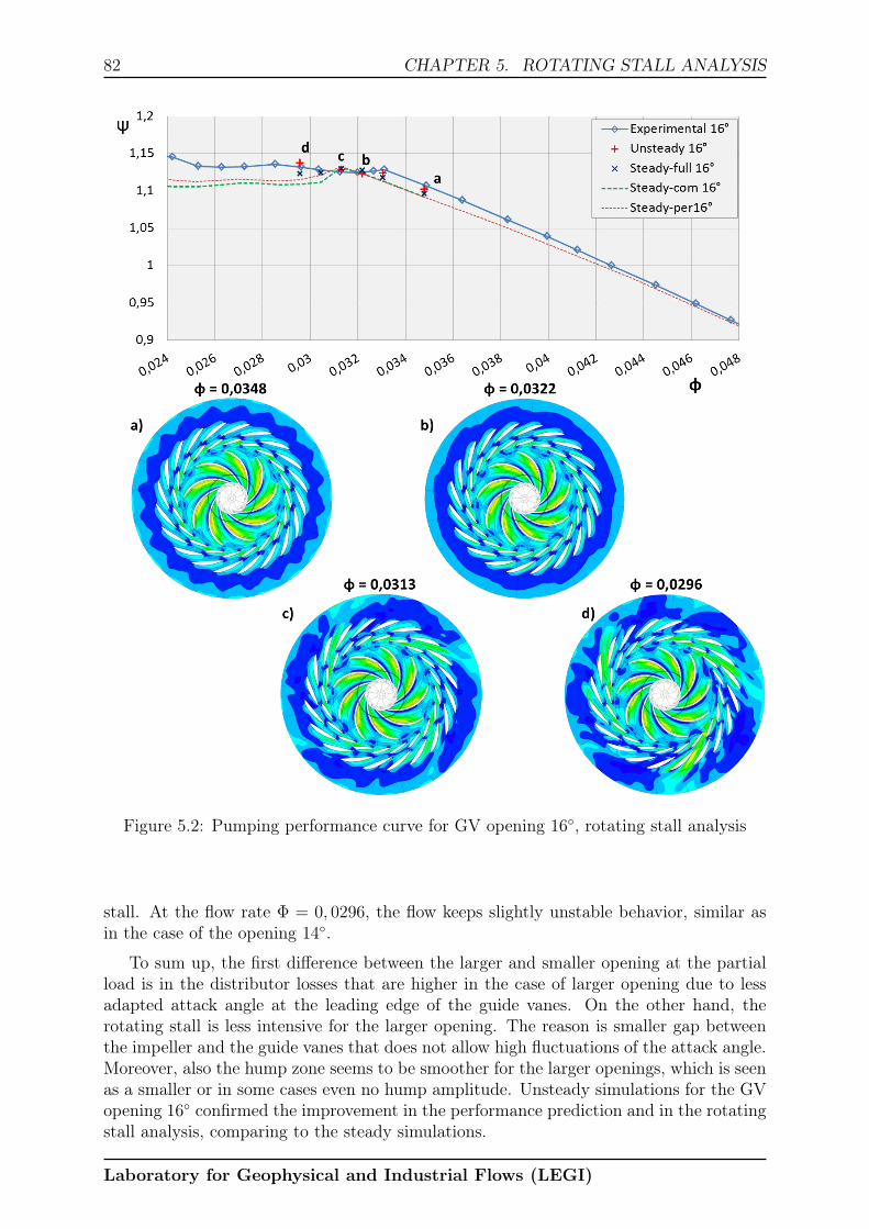
82 CHAPTER 5. ROTATING STALL ANALYSIS
Figure 5.2: Pumping performance curve for GV opening 16◦, rotating stall analysis
stall. At the flow rate Φ = 0, 0296, the flow keeps slightly unstable behavior, similar asin the case of the opening 14◦.
To sum up, the first difference between the larger and smaller opening at the partialload is in the distributor losses that are higher in the case of larger opening due to lessadapted attack angle at the leading edge of the guide vanes. On the other hand, therotating stall is less intensive for the larger opening. The reason is smaller gap betweenthe impeller and the guide vanes that does not allow high fluctuations of the attack angle.Moreover, also the hump zone seems to be smoother for the larger openings, which is seenas a smaller or in some cases even no hump amplitude. Unsteady simulations for the GVopening 16◦ confirmed the improvement in the performance prediction and in the rotatingstall analysis, comparing to the steady simulations.
Laboratory for Geophysical and Industrial Flows (LEGI)

CHAPTER 5. ROTATING STALL ANALYSIS 83
5.3 Local flow analysis at Φ = 0, 0313, GV opening 14◦
Detailed flow analyses have been made for opening 14◦, guide vane geometry GV I anddischarge Φ = 0, 0313 that represents an operating point at the hump zone, where therotating stall occurs. After stabilization period, around 15 revolutions of the pump-turbineimpeller have been calculated and analyzed.
5.3.1 Impeller blades pressure distribution
Static pressure distributions have been analyzed on 4 consecutive impeller blades. Thisanalysis is important because it can show us the impact of the developed rotating stallon the flow patterns in the upstream regions such as impeller and even draft tube. Staticpressure has been analyzed on the mid-span cutting plane on the impeller blades (fig.5.3a). Figure 5.3b shows the difference in the static pressure distribution on both, pressureand suction sides of the blades. It should be taken into account that the relative positionof the 4 impeller blades is not the same and can influence the pressure distribution aroundthe blade, but it is estimated that it is lower than the rotating stall influence.
Figure 5.3: Pressure distribution around 4 consecutive impeller blades at a given time
Rotating stall influence, seen as a change in pressure distribution, is the highest closeto the trailing edge of the impeller blades. However, the difference can be observed alsoon the suction side of the blades and even close to the impeller blades leading edges, whichare located very far from actual occurrence of the rotating stall in the distributor regions.Pressure fields around the blades have a strong influence on the velocity fields in theimpeller channel. It should be stressed that the influence can also be inverse, therefore,the conditions close to the leading edge of the impeller can have an impact on the rotatingstall patterns in the distributor.
Laboratory for Geophysical and Industrial Flows (LEGI)
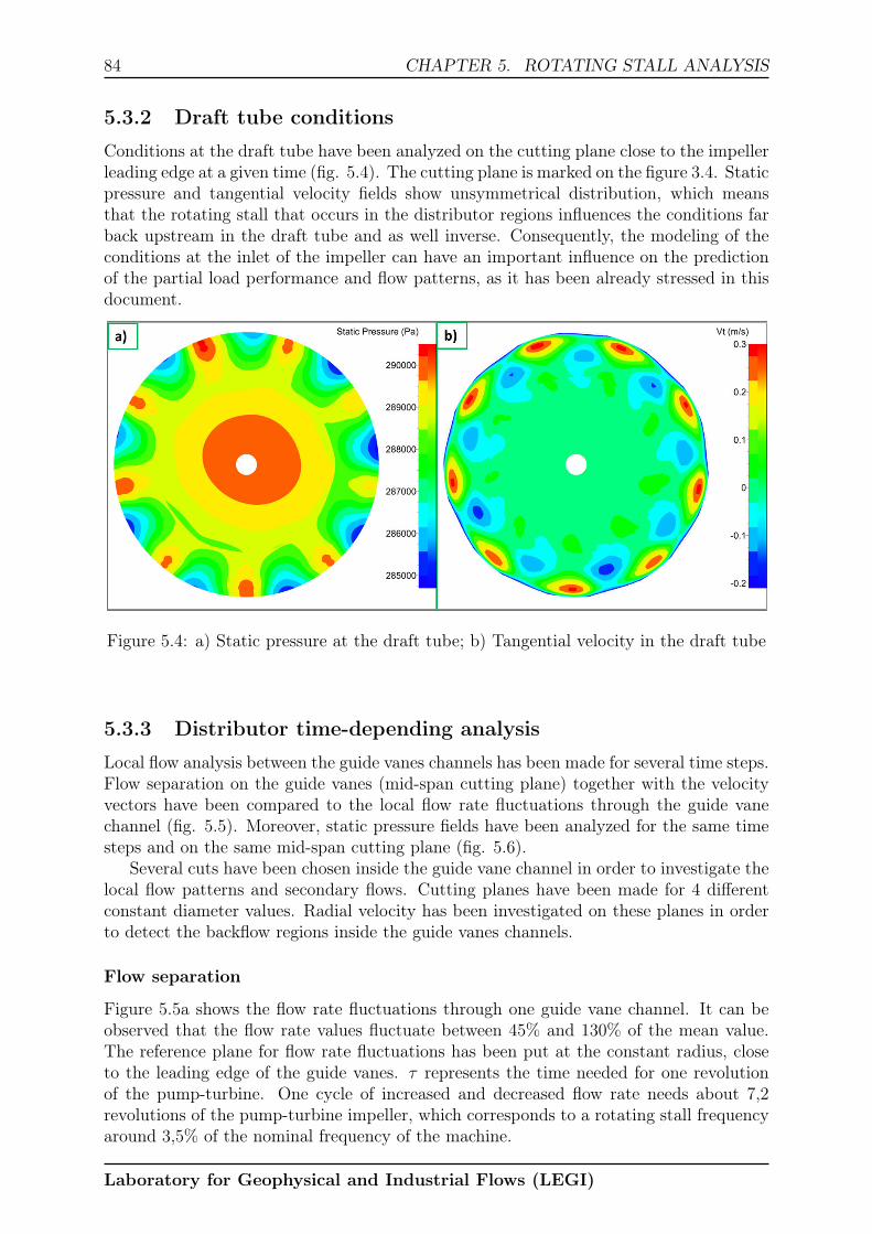
84 CHAPTER 5. ROTATING STALL ANALYSIS
5.3.2 Draft tube conditions
Conditions at the draft tube have been analyzed on the cutting plane close to the impellerleading edge at a given time (fig. 5.4). The cutting plane is marked on the figure 3.4. Staticpressure and tangential velocity fields show unsymmetrical distribution, which meansthat the rotating stall that occurs in the distributor regions influences the conditions farback upstream in the draft tube and as well inverse. Consequently, the modeling of theconditions at the inlet of the impeller can have an important influence on the predictionof the partial load performance and flow patterns, as it has been already stressed in thisdocument.
Figure 5.4: a) Static pressure at the draft tube; b) Tangential velocity in the draft tube
5.3.3 Distributor time-depending analysis
Local flow analysis between the guide vanes channels has been made for several time steps.Flow separation on the guide vanes (mid-span cutting plane) together with the velocityvectors have been compared to the local flow rate fluctuations through the guide vanechannel (fig. 5.5). Moreover, static pressure fields have been analyzed for the same timesteps and on the same mid-span cutting plane (fig. 5.6).
Several cuts have been chosen inside the guide vane channel in order to investigate thelocal flow patterns and secondary flows. Cutting planes have been made for 4 differentconstant diameter values. Radial velocity has been investigated on these planes in orderto detect the backflow regions inside the guide vanes channels.
Flow separation
Figure 5.5a shows the flow rate fluctuations through one guide vane channel. It can beobserved that the flow rate values fluctuate between 45% and 130% of the mean value.The reference plane for flow rate fluctuations has been put at the constant radius, closeto the leading edge of the guide vanes. τ represents the time needed for one revolutionof the pump-turbine. One cycle of increased and decreased flow rate needs about 7,2revolutions of the pump-turbine impeller, which corresponds to a rotating stall frequencyaround 3,5% of the nominal frequency of the machine.
Laboratory for Geophysical and Industrial Flows (LEGI)
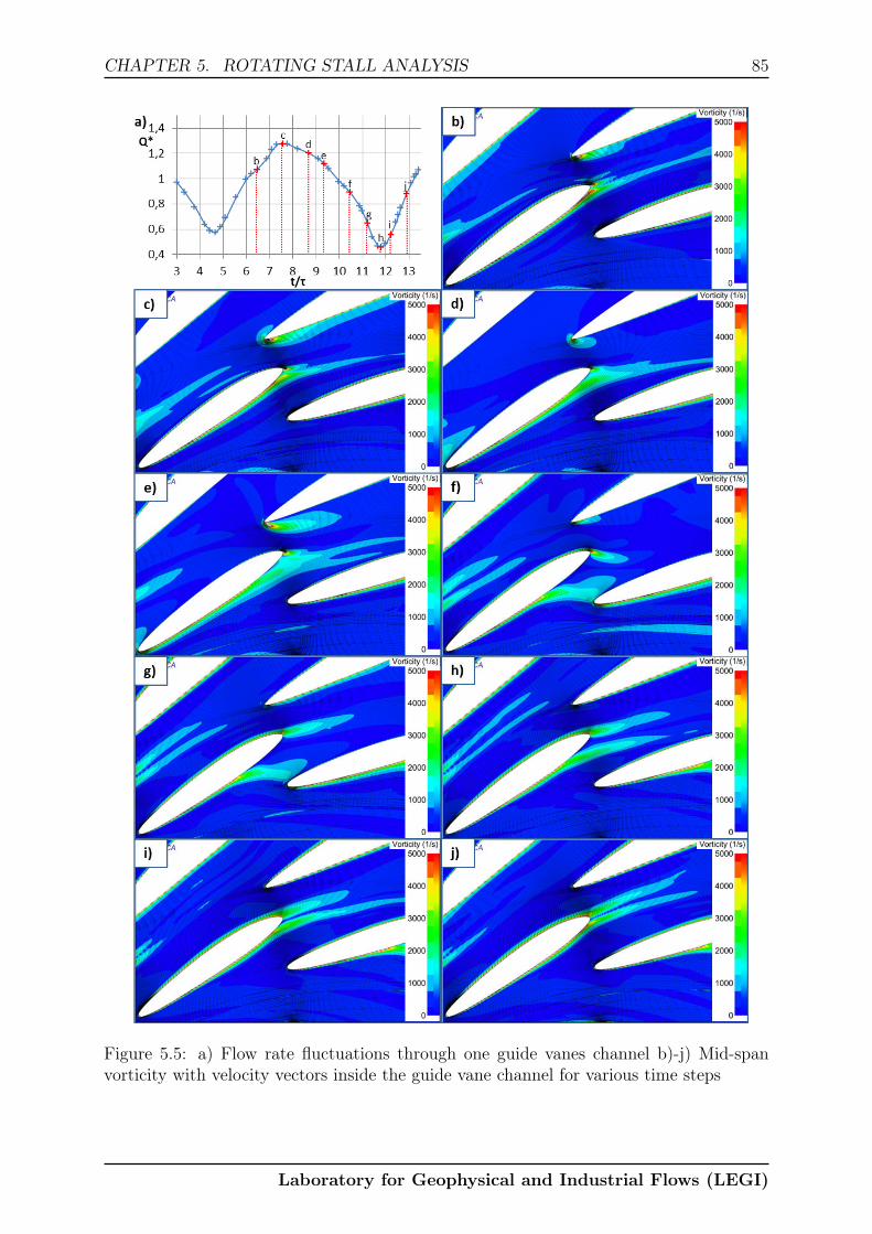
CHAPTER 5. ROTATING STALL ANALYSIS 85
Figure 5.5: a) Flow rate fluctuations through one guide vanes channel b)-j) Mid-spanvorticity with velocity vectors inside the guide vane channel for various time steps
Laboratory for Geophysical and Industrial Flows (LEGI)
86 CHAPTER 5. ROTATING STALL ANALYSIS
Figure 5.5’b’-’j’ shows the vorticity and velocity vectors on the mid-span cutting plane.Flow rate through the channel is the highest at the time step ’c’. At this time, theseparation occurs only at the trailing edge of the guide vane. Time steps ’d’ - ’g’ show thegrowing region of the flow recirculation inside the guide vanes channel. Velocity vectorsshow the deviation of the flow to the downstream channel. At the time step ’e’, we canobserve increased separation and flow deviation on the pressure side of the stay vane,which leads the flow back to the guide vanes regions and consequently causes increasedbackflow close to the guide vane leading edge. Flow recirculation on the mid-span seemsto be the highest in the time steps ’f’ and ’g’. However, the flow rate continues to reducedue to unfavorable conditions.
The flow rate is the lowest at the time step ’h’, even though the recirculation zonealready starts to reduce on the mid-span cutting plane. It means that the flow patternsare very complex and three-dimensional. Since, only mid-spans are shown on the figure5.5, additional analyses have been done to verify that the tendency of the flow is differentcloser to the hub and the shroud. At the time steps ’i’ and ’j’, the recirculation zone inthe guide vane channel continues to reduce and also the flow rate inside the channel startsto increase again.
As expected, it seems that the flow rate through the guide vane channel depends onthe size of the flow separation and recirculation zone between the two consecutive guidevanes. However, the dependence is not completely linear. It seems that there is a delaybetween the size of the recirculation zone and flow rate, which is caused by the flowbehavior closer to the hub and shroud side of the machine.
Static pressure fields
Under normal, stable operating points, static pressure distribution along the guide vaneschannel should not change in time. However, at the partial load, when the rotating stallis present, the pressure distribution can vary significantly and is related to the flow rateinside the channel. Moreover, the relation between the static pressure and the velocityalong the channel can be described by the Bernoulli’s principle (eq. 5.1) as the frictionby viscous forces can be negligible.
v2
2+ gZ +
p
ρ= const. (5.1)
The relation can be applied to any reference point on the streamlines inside the chan-nel. Still, when explaining the phenomenon, we need to pay lots of attention, since theflow is 3-dimensional and the recirculation zones can cause complex flow patterns alongthe channels.
Figure 5.6 represents the static pressure fields on the mid-span cutting plane insidethe guide vanes channels for various time steps. Time steps and cutting plane are thesame as on the figure 5.5, where the vorticity is presented and can therefore be directlycompared. Time step ’c’ represents the highest flow rate in the guide vane channel. Thestatic pressure value in the channel is very low, which is to be expected, according toBernoulli’s principle. A small static pressure peak can be seen close to the trailing edge ofthe guide vane at the time steps ’b’, ’c’ and ’d’. It corresponds to the small recirculationzone that has been observed also on the figure 5.5.
At the time steps from ’d’ to ’f’, the flow rate in the channel reduces, the recirculationzone increases and consequently the static pressure increases. Increasing of the staticpressure in the channel causes strong adverse pressure gradient around the downstream
Laboratory for Geophysical and Industrial Flows (LEGI)

CHAPTER 5. ROTATING STALL ANALYSIS 87
Figure 5.6: a) Flow rate fluctuations through one guide vanes channel b)-j) Mid-spanstatic pressure distribution inside the guide vane channel for various time steps
Laboratory for Geophysical and Industrial Flows (LEGI)

88 CHAPTER 5. ROTATING STALL ANALYSIS
guide vane leading edge that even increases the flow deviation to the downstream channelas seen at the time step ’f’. Consequently, the flow rate continues to reduce even more.Slowly, adverse gradient starts to neutralize and with some delay (time step ’h’ and ’i’),the flow rate starts to increase again. The stall meanwhile moves to the downstreamchannel as it can be seen on the right side of figures 5.5j and 5.6j. At time step ’j’, asmall static pressure peak can be observed close to the trailing edge of the guide vanes,which means that the recirculation zone is reduced again to a very small region close tothe trailing edge.
Guide vanes channel sections
Radial velocity has been investigated on 4 different cuts in the GV regions (fig. 5.7 - fig.5.10). The cuts have been made on the constant diameter values along the GV channels.The diameters are defined relatively to the outer diameter of the impellerDout. Time stepsremain the same as for the figures 5.5 and 5.6. Since the radial velocity is proportionalto the flow rate, the analysis provides an insight of the flow distribution between the hubside and the shroud side of the machine.
Figure 5.7: a) Flow rate fluctuations through guide vanes channel b)-i) Radial velocity atD/Dout = 1, 127 (GV leading edge) for various time steps
Figure 5.7 shows the radial velocity profile at the leading edge of the guide vane channelfor five different time steps. Time step ’b’ shows the region of increasing flow rate throughthe channel. The flow rate increases mostly at the hub and shroud side of the channel.Later it also increases close to the downstream guide vane and it reaches maximum at thetime step ’c’.
Time step ’f’ represents the highest recirculation zone seen on figure 5.5f. Flow rateis still high close to the hub and the shroud. Small backflow region can be observed close
Laboratory for Geophysical and Industrial Flows (LEGI)
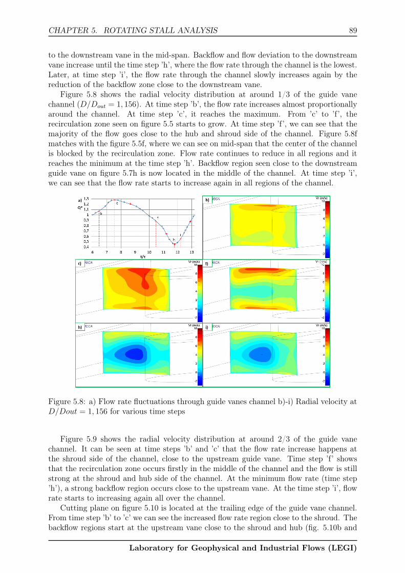
CHAPTER 5. ROTATING STALL ANALYSIS 89
to the downstream vane in the mid-span. Backflow and flow deviation to the downstreamvane increase until the time step ’h’, where the flow rate through the channel is the lowest.Later, at time step ’i’, the flow rate through the channel slowly increases again by thereduction of the backflow zone close to the downstream vane.
Figure 5.8 shows the radial velocity distribution at around 1/3 of the guide vanechannel (D/Dout = 1, 156). At time step ’b’, the flow rate increases almost proportionallyaround the channel. At time step ’c’, it reaches the maximum. From ’c’ to ’f’, therecirculation zone seen on figure 5.5 starts to grow. At time step ’f’, we can see that themajority of the flow goes close to the hub and shroud side of the channel. Figure 5.8fmatches with the figure 5.5f, where we can see on mid-span that the center of the channelis blocked by the recirculation zone. Flow rate continues to reduce in all regions and itreaches the minimum at the time step ’h’. Backflow region seen close to the downstreamguide vane on figure 5.7h is now located in the middle of the channel. At time step ’i’,we can see that the flow rate starts to increase again in all regions of the channel.
Figure 5.8: a) Flow rate fluctuations through guide vanes channel b)-i) Radial velocity atD/Dout = 1, 156 for various time steps
Figure 5.9 shows the radial velocity distribution at around 2/3 of the guide vanechannel. It can be seen at time steps ’b’ and ’c’ that the flow rate increase happens atthe shroud side of the channel, close to the upstream guide vane. Time step ’f’ showsthat the recirculation zone occurs firstly in the middle of the channel and the flow is stillstrong at the shroud and hub side of the channel. At the minimum flow rate (time step’h’), a strong backflow region occurs close to the upstream vane. At the time step ’i’, flowrate starts to increasing again all over the channel.
Cutting plane on figure 5.10 is located at the trailing edge of the guide vane channel.From time step ’b’ to ’c’ we can see the increased flow rate region close to the shroud. Thebackflow regions start at the upstream vane close to the shroud and hub (fig. 5.10b and
Laboratory for Geophysical and Industrial Flows (LEGI)

90 CHAPTER 5. ROTATING STALL ANALYSIS
Figure 5.9: a) Flow rate fluctuations through guide vanes channel b)-i) Radial velocity atD/Dout = 1, 195 for various time steps
c). Recirculation region starts to grow in the middle of the channel, close to the upstreamvane (time step ’f’). At this time, the most of the flow passes close to the shroud and hubsides. Minimum flow rate is reached at the time step ’h’, when also the flow rates at thehub and shroud sides reduce. At time step ’i’, the flow rate through the channel starts togrow again by reducing the recirculation zone close to the upstream guide vane.
5.4 Evolution of the rotating stall
Evolution of the rotating stall can be described in a simplified way as an occurrence anda decay of the stalled cells.
• Phase 1. Flow increases in the channel due to favorable conditions, such as lowpressure in the middle of the channel (fig. 5.6b) and angle of attack adapted to theguide vanes (fig. 5.5b). Slowly, it reaches maximum value of around 130% of thenominal flow through the channel.
• Phase 2. Angle of attack at the entrance of the channel (seen as velocity vectors)starts to turn slowly to the downstream channel (fig. 5.5d). Meanwhile, staticpressure in the channel starts to increase and causes strong adverse pressure gradientbetween the middle region of the channel and the region close to the leading edgeof the downstream guide vane on the pressure side of the vane (fig. 5.6d, e, f). Itleads into strong flow separation in the channel, growth of the recirculation zoneand deviation of the flow towards the downstream channel (fig. 5.5d, e, f, g). Flowrate reduction starts firstly in the middle of the channel and after that it reduces
Laboratory for Geophysical and Industrial Flows (LEGI)

CHAPTER 5. ROTATING STALL ANALYSIS 91
Figure 5.10: a) Flow rate fluctuations through guide vanes channel b)-i) Radial velocityat D/Dout = 1, 233 (GV trailing edge) for various time steps
also at the hub side and shroud side of the channel, which leads into additional flowrate reduction (fig. 5.9f, h). It reaches minimum of around 45% of the nominal flowrate.
• Phase 3. Adverse pressure gradients start to reduce, together with the size of therecirculation zone and cause gradually more favorable conditions that lead moreflow rate into the channel. The stalled cell moves to the downstream channel, whichcauses additional fast flow rate increase in the channel.
5.5 Chapter discussion
In this chapter it was shown that unsteady simulations can give very precise results.Accuracy of performance prediction has been improved significantly, comparing to thesteady simulations. Additionally, the simulations are robust enough to give good resultsat very unstable operating points, where the rotating stall occurs. Various shapes of therotating stall have been detected. Results and trends of rotating stall behavior appears tobe similar to the experimental work of [10]. However, they cannot be compared directly,since the pump-turbine geometry is different in their case. It is important to say thatthe intensity of the rotating stall can vary. It could be parametrized by the number ofrotating stall cells, rotating stall frequency and by the flow variation through the guidevane channel. As a perspective, non-dimensional parameter could be proposed in orderto evaluate the rotating stall intensity for various geometries and openings.
Unsteady simulations presented in this chapter showed the relation between the num-ber of rotating stall cells and the rotating stall frequency (tab. 5.1). At lower number
Laboratory for Geophysical and Industrial Flows (LEGI)

92 CHAPTER 5. ROTATING STALL ANALYSIS
of cells results in higher stall frequency. Moreover, the discharge fluctuations are higherin the cases of lower number of cells. Even though the statement should be verified ex-perimentally, it can be assumed that the conditions with less rotating stall cells are lessfavorable (more dangerous) for the machine, comparing to the more rotating stall cells orfully symmetrical distribution of the flow around the distributor.
Local flow analysis showed the mechanisms of the rotating stall. In a simplified way,the rotating stall can be described with the growth and decay of the stalled cell. Mostimportant parameters for the stall evolution are the size of the flow separation and recir-culation zones that completely change the flow conditions at the leading edge of the guidevanes. Pressure fields, especially the direction and magnitude of adverse pressure gradi-ent, cause the deviation of the flow to the downstream channel, which consequently leadsthe rotation of the stalled cells around the distributor with its characteristic frequency.
Laboratory for Geophysical and Industrial Flows (LEGI)

Part IV
Conclusions and perspectives
93


Chapter 6
Conclusions and perspectives
6.1 Conclusions
CFD tools have been used in the presented work to predict and analyze pumping modepart load instabilities. All presented simulations have been performed in LEGI on maxi-mum 12 processors, which is nowadays widely accessible computational power.
The first goal of the project has been to perform and to develop simulations of thecavitation phenomena in a pump-turbine geometry. Steady calculations on periodic meshhave been performed for various discharges and various NPSH values. Reliable resultshave been obtained even for very unstable off-design operating points. The agreementbetween the (unfortunately limited) experimental data and simulations is very good. Thecode is capable to predict accurately the incipient cavitation values, the NPSH head dropcurves and the average cavitation forms in reasonably short time (max. 20 CPU hours).
Steady simulations on the periodic and combined mesh give good insight on the stabil-ity of the operating points. Calculations on the periodic mesh are very fast and relativelygood in the prediction of the global performance curve. They are accurate enough to beused to analyze the global position of the hump zone and the influence of the variousguide vanes geometries. Combined mesh with the periodicity in the impeller regions andfull mesh at the distributor regions can be additionally used for the analysis of the stalledforms in the distributor. Stable, slightly unstable and fully unstable operating points canbe detected by using this approach. It is a compromised solution between more costly, un-steady simulations on fully-meshed domain and steady simulations on the periodic mesh.However, they have their limits. The prediction of the hump zone is better if the gapbetween the impeller and the distributor is larger. The origins of the discrepancies arethe periodicity in the impeller regions and using the mixing plane at the border betweenthe impeller and the distributor. Indeed, for the case of larger guide vanes openings(smaller gaps), the flow patterns at the distributor regions influence the flow behaviorat the impeller regions. Author would suggest to put special attention on the modelingof rotor-stator interactions, when the gaps between the impeller and the distributor arerelatively small and the operating points are at the partial load. Moreover, for smallergaps and partial loads, the periodicity between the blades would not be suggested in orderto minimize the discrepancies between the numerical and the experimental results.
The results obtained by unsteady simulations, using URANS equations, are very goodcomparing to the results in the literature. Moreover, they prove that the developedCFD tools can be very exact in the prediction of the performance even under off-designconditions, such as partial load. Additionally, CFD simulations give us a detailed insight
95
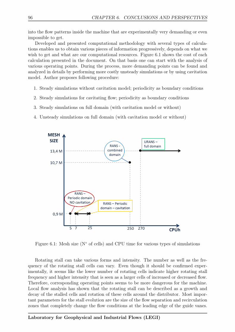
96 CHAPTER 6. CONCLUSIONS AND PERSPECTIVES
into the flow patterns inside the machine that are experimentally very demanding or evenimpossible to get.
Developed and presented computational methodology with several types of calcula-tions enables us to obtain various pieces of information progressively, depends on what wewish to get and what are our computational resources. Figure 6.1 shows the cost of eachcalculation presented in the document. On that basis one can start with the analysis ofvarious operating points. During the process, more demanding points can be found andanalyzed in details by performing more costly unsteady simulations or by using cavitationmodel. Author proposes following procedure:
1. Steady simulations without cavitation model; periodicity as boundary conditions
2. Steady simulations for cavitating flow; periodicity as boundary conditions
3. Steady simulations on full domain (with cavitation model or without)
4. Unsteady simulations on full domain (with cavitation model or without)
Figure 6.1: Mesh size (N◦ of cells) and CPU time for various types of simulations
Rotating stall can take various forms and intensity. The number as well as the fre-quency of the rotating stall cells can vary. Even though it should be confirmed exper-imentally, it seems like the lower number of rotating cells indicate higher rotating stallfrequency and higher intensity that is seen as a larger cells of increased or decreased flow.Therefore, corresponding operating points seems to be more dangerous for the machine.Local flow analysis has shown that the rotating stall can be described as a growth anddecay of the stalled cells and rotation of these cells around the distributor. Most impor-tant parameters for the stall evolution are the size of the flow separation and recirculationzones that completely change the flow conditions at the leading edge of the guide vanes.
Laboratory for Geophysical and Industrial Flows (LEGI)

CHAPTER 6. CONCLUSIONS AND PERSPECTIVES 97
Pressure fields, especially the direction and magnitude of adverse pressure gradient, causethe deviation of the flow to the downstream channels and are responsible for the so calledrotation of the stalled cells. Taking into account all mentioned rotating stall mechanisms,we can highlight several possible ways to modify the effects of the rotating stall.
• Decreasing GV opening angle would increase the gap between the impeller andguide vanes and the gap between the guide vanes and stay vanes as well. Angle ofattack would be in that case more adapted at the GV leading edge, but would beable to fluctuate more due to larger gap between the impeller and GV leading edge.Increased gap between the GV and the SV would make the flow deviation and therotation of the cells around the distributor easier.
• Increasing GV opening angle would reduce the gap between the impeller andthe guide vanes. Even though the attack angle would become less adapted, also thepossible fluctuations of local attack angle would reduce. The losses in the distributorwould increase, but the rotating stall intensity would reduce, which is good for theoperating points stability.
• Changing GV geometry would change the velocity and pressure fields in thedistributor regions, which could change completely the position and the amplitudeof the hump zone as it has been shown also in this document. It should be stressedthat the GV design around the GV leading edge can influence the ratio betweenthe gap size and the opening angle, which is not linear. Design of the guide vanesis therefore a strong tool that can be used to modify rotating stall conditions atvarious operating points.
• Reducing the impeller-distributor gap size would reduce the intensity of therotating stall. However, the relative gap size would change even more with thechanging of the guide opening, if the guide vanes are positioned closer to the impeller.It should be mentioned that other kind of instabilities, such as strong pressurefluctuations due to rotor-stator interactions might appear in case of very smallradial gap between the impeller and the guide vanes.
• Changing impeller geometry might have an influence on the rotating stall mech-anisms. It was shown in this document that pressure and velocity fields in theimpeller might have a strong influence on the rotating stall. Moreover, the flowangle at the trailing edge of the impeller seems to be a useful way to control and toinfluence the rotating stall conditions.
6.2 Perspectives
First of all, experimental tests should be performed to evaluate the precision of the pre-sented numerical simulations. Accuracy of the rotating stall frequency and number of ro-tating stall cells prediction should be validated by the experimental measurements for thesame geometry under the same operating conditions. Furthermore, in order to increaseprecision and enable various frequency analyses, additional revolutions of the machineshould be simulated.
The presented results, especially unsteady calculations, demonstrate big potential todevelop a general, widely accessible numerical tool that gives reliable results for a widerange of discharges, even under demanding off-design conditions, such as the appearance
Laboratory for Geophysical and Industrial Flows (LEGI)

98 CHAPTER 6. CONCLUSIONS AND PERSPECTIVES
of the cavitation and the rotating stall. To achieve that, unsteady simulations could bemade also for the cavitating conditions. More importantly, the simulations should bevalidated for additional GV openings, GV geometries and even for completely differentpump-turbine geometries.
Another perspective could be a more detailed analysis of the unsteady flow phenomenainside the impeller and the distributor. The phenomenon known as a runner hump existsfor some geometries and is related with the partial load recirculation zones close to theleading edge of the impeller. In literature it has been poorly addressed, therefore it shouldbe additionally investigated. Presented work can be a good basis to address this unstablebehavior.
Finally, the main idea of the presented study was the investigation of the hump zoneand related rotating stall in order to minimize its effects on the pump-turbine performance.At this moment, all the numerical tools to achieve this are available and can be used forany geometry that is facing the problem of the rotating stall. Additional study fromindustrial or academic point of view should be performed in order to propose practicalsolutions for reducing or eliminating the negative effects of the rotating stall on the pump-turbine performance and stability of the operating points.
Laboratory for Geophysical and Industrial Flows (LEGI)

Bibliography
[1] *H Amblard, P Henry, G Borciani, G Martin, P Guiton, and R Thalmann. Com-portement des turbines Francis et des pompes-turbines à débit partiel. La HouilleBlanche, (5):435–440, 1985.
[2] N Arndt, A J Acosta, C E Brennen, and T K Caughey. Rotor–stator interaction ina diffuser pump. Journal of Turbomachinery, 111(3):213–221, 1989.
[3] N Arndt, A J Acosta, C E Brennen, and T K Caughey. Experimental investigationof rotor-stator interaction in a centrifugal pump with several vaned diffusers. Journalof Turbomachinery, 112(1):98–108, 1990.
[4] F Avellan. Introduction to cavitation in hydraulic machinery. In The 6th InternationalConference on Hydraulic Machinery and Hydrodynamics, Timisoara, Romania, 2004.
[5] F Avellan. Evolution des groupes de pompage-turbinage. Bulletin des SEV VSEIncluding Jahresheft, 103(2):37, 2012.
[6] R Bachert, B Stoffel, and M Dular. Unsteady cavitation at the tongue of the voluteof a centrifugal pump. Journal of Fluids Engineering, 132(6):061301, 2010.
[7] *B S Baldwin and H Lomax. Thin layer approximation and algebraic model forseparated turbulent flows. American Institute of Aeronautics and Astronautics, 1978.
[8] *S G Bankoff. A variable density single-fluid model for two-phase flow with particularreference to steam-water flow. Journal of Heat Transfer, 82(4):265–272, 1960.
[9] S Berten. Hydrodynamics of high specific power pumps for off-design operating con-ditions. PhD thesis, EPFL, 2010.
[10] O Braun. Part load flow in radial centrifugal pumps. PhD thesis, EPFL, 2009.
[11] G D Ciocan, O Teller, and F Czerwinski. Variable speed pump-turbines technol-ogy. University" Politehnica" of Bucharest Scientific Bulletin, Series D: MechanicalEngineering, 74(1):33–42, 2012.
[12] International Electrotechnical Commission et al. Iec 60193. Hydraulic turbines, stor-age pumps and pump-turbines - model acceptance tests. Chap. Dimensional Checkof Model and Prototype, 1999.
[13] O Coutier-Delgosha. Modélisation des écoulements cavitants: étude des comporte-ments instationnaires et application tridimensionnelle aux turbomachines. PhD the-sis, Grenoble, INPG, 2001.
99

100 BIBLIOGRAPHY
[14] O Coutier-Delgosha, R Fortes-Patella, and J-L Reboud. Evaluation of the turbulencemodel influence on the numerical simulations of unsteady cavitation. Journal ofFluids Engineering, 125(1):38–45, 2003.
[15] O Coutier-Delgosha, R Fortes-Patella, J-L Reboud, N Hakimi, and C Hirsch. Nu-merical simulation of cavitating flow in 2d and 3d inducer geometries. InternationalJournal for Numerical Methods in Fluids, 48(2):135–167, 2005.
[16] O Coutier-Delgosha, R Fortes-Patella, J-L Reboud, N Hakimi, and C Hirsch. Sta-bility of preconditioned navier–stokes equations associated with a cavitation model.Computers & Fluids, 34(3):319–349, 2005.
[17] O Coutier-Delgosha, R Fortes-Patella, J-L Reboud, M Hofmann, and B Stoffel. Ex-perimental and numerical studies in a centrifugal pump with two-dimensional curvedblades in cavitating condition. Journal of Fluids Engineering, 125(6):970–978, 2003.
[18] O Coutier-Delgosha, P Morel, R Fortes-Patella, and J-L Reboud. Numerical simu-lation of turbopump inducer cavitating behavior. International Journal of RotatingMachinery, 2005(2):135–142, 2005.
[19] O Coutier-Delgosha, J L Reboud, and Y Delannoy. Numerical simulation of theunsteady behaviour of cavitating flows. International Journal for Numerical Methodsin Fluids, 42(5):527–548, 2003.
[20] J Decaix. Modélisation et simulation de la turbulence compressible en milieudiphasique: application aux écoulements cavitants instationnaires. PhD thesis, Greno-ble, INPG, 2012.
[21] Y Delannoy and J-L Kueny. Two phase flow approach in unsteady cavitation mod-elling. In ASME Cavitation and Multiphase flow forum, pages 153–158, 1990.
[22] M Dular, R Bachert, C Schaad, and B Stoffel. Investigation of a re-entrant jetreflection at an inclined cavity closure line. European Journal of Mechanics-B/Fluids,26(5):688–705, 2007.
[23] M Dular, R Bachert, B Stoffel, and B Širok. Experimental evaluation of numeri-cal simulation of cavitating flow around hydrofoil. European Journal of Mechanics-B/Fluids, 24(4):522–538, 2005.
[24] P Dupont, A-C Bayeul-Lainé, A Dazin, G Bois, O Roussette, and Q Si. Leakageflow simulation in a specific pump model. In IOP Conference Series: Earth andEnvironmental Science, volume 22, page 012012. IOP Publishing, 2014.
[25] B Eckhardt, T M Schneider, B Hof, and J Westerweel. Turbulence transition in pipeflow. Annu. Rev. Fluid Mech., 39:447–468, 2007.
[26] Y Egorov, F R Menter, R Lechner, and D Cokljat. The scale-adaptive simulationmethod for unsteady turbulent flow predictions. part 2: Application to complex flows.Flow, Turbulence and Combustion, 85(1):139–165, 2010.
[27] *H W Emmons. A surway of stall propagation: experiment and theory. Journal ofBasic Engineering, 81:409–416, 1959.
Laboratory for Geophysical and Industrial Flows (LEGI)

BIBLIOGRAPHY 101
[28] X Escaler, E Egusquiza, M Farhat, F Avellan, and M Coussirat. Detection of cavi-tation in hydraulic turbines. Mechanical Systems and Signal Processing, 20(4):983–1007, 2006.
[29] R Fortes-Patella, A Archer, and C Flageul. Numerical and experimental investiga-tions on cavitation erosion. In IOP Conference Series: Earth and EnvironmentalScience, volume 15, page 022013. IOP Publishing, 2012.
[30] R Fortes-Patella, S Barre, and J-L Reboud. Experiments and modelling of cavitatingflows in venturi. part II: unsteady cavitation. In CAV 2006 Symposium, 2006.
[31] R Fortes-Patella, O Coutier-Delgosha, J Perrin, and J-L Reboud. Numerical modelto predict unsteady cavitating flow behavior in inducer blade cascades. Journal ofFluids Engineering, 129(2):128–135, 2007.
[32] J-P Franc and J-M Michel. Fundamentals of cavitation, volume 76. Springer, 2006.
[33] J-P Franc et al. La cavitation: mécanismes physiques et aspects industriels. PressesUniversitaires Grenoble, 1995.
[34] *P Frigne and R Van den Braembussche. Distinction between different types ofimpeller and diffuser rotating stall in a centrifugal compressor with vaneless diffuser.Journal of Engineering for Gas Turbines and Power, 106(2):468–474, 1984.
[35] C Gentner, M Sallaberger, C Widmer, O Braun, and T Staubli. Numerical andexperimental analysis of instability phenomena in pump turbines. In IOP ConferenceSeries: Earth and Environmental Science, volume 15, page 032042. IOP Publishing,2012.
[36] E Goncalves and R Fortes-Patella. Numerical simulation of cavitating flows withhomogeneous models. Computers & Fluids, 38(9):1682–1696, 2009.
[37] N Gonzalo-Flores, E Goncalvès, R Fortes-Patella, J Rolland, and C Rebattet. Headdrop of a spatial turbopump inducer. Journal of Fluids Engineering, 130(11):111301,2008.
[38] L Gros, A Couzinet, and D Pierrat. Part load flow and hydrodynamic instabilities ofa centrifugal pump–Part I: experimental investigations. In Paper 33444, AJK JointFluid Engineering Conference 2015, 2015.
[39] L Gros, A Couzinet, and D Pierrat. Part load flow and hydrodynamic instabilitiesof a centrifugal pump–Part II: Numerical simulations. In Paper 33445, AJK JointFluid Engineering Conference 2015, 2015.
[40] N Hakimi, C Hirsch, and S Pierret. Presentation and application of a new extendedk–ε model with wall functions. ECCOMAS, Barcelona, 2000.
[41] V Hasmatuchi. Hydrodynamics of a pump-turbine operating at off-design conditionsin generating mode. PhD thesis, EPFL, 2012.
[42] V Hasmatuchi, M Farhat, S Roth, F Botero, and F Avellan. Experimental evidence ofrotating stall in a pump-turbine at off-design conditions in generating mode. Journalof Fluids Engineering, 133(5):051104, 2011.
Laboratory for Geophysical and Industrial Flows (LEGI)

102 BIBLIOGRAPHY
[43] *U Haupt, U Seidel, A N Abdel-Hamid, and M Rautenberg. Unsteady flow in acentrifugal compressor with different types of vaned diffusers. Journal of Turboma-chinery, 110(3):293–302, 1988.
[44] *J H Horlock and B Lakshminarayana. Secondary flows: theory, experiment, andapplication in turbomachinery aerodynamics. Annual Review of Fluid Mechanics,5(1):247–280, 1973.
[45] J-B Houdeline, J Liu, S Lavigne, Y Laurant, and L Balara. Start-up improvementin turbine mode for high head PSP machine. In IOP Conference Series: Earth andEnvironmental Science, volume 15, page 042022. IOP Publishing, 2012.
[46] M Inoue, M Kuroumaru, S Yoshida, and M Furukawa. Short and long length-scaledisturbances leading to rotating stall in an axial compressor stage with differentstator/rotor gaps. Journal of Turbomachinery, 124(3):376–384, 2002.
[47] NUMECA International. Theoretical manual FINETM/Turbo v8.9. 2011.
[48] U Ješe, R Fortes-Patella, and S Antheaume. High head pump-turbine: Pumpingmode numerical simulations with a cavitation model for off-design conditions. InIOP Conference Series: Earth and Environmental Science, volume 22, page 032048.IOP Publishing, 2014.
[49] U Ješe, R Fortes-Patella, and M Dular. Numerical study of pump-turbine instabil-ities under pumping mode off-design conditions. In Paper 33501, AJK Joint FluidEngineering Conference 2015, 2015.
[50] W P Jones and B Launder. The prediction of laminarization with a two-equationmodel of turbulence. International Journal of Heat and Mass Transfer, 15(2):301–314, 1972.
[51] K A Kaupert, P Holbein, and T Staubli. A first analysis of flow field hysteresis in apump impeller. Journal of Fluids Engineering, 118(4):685–691, 1996.
[52] I Khlifa, O Coutier-Delgosha, S Fuzier, M Hočevar, A Vabre, and K Fezzaa. Velocitymeasurements in cavitating flows using fast X-ray imaging. In Congrés Français deMécanique (21; 2013; Bordeaux), 2013.
[53] J Kim, P Moin, and R Moser. Turbulence statistics in fully developed channel flowat low Reynolds number. Journal of fluid mechanics, 177:133–166, 1987.
[54] S J Kline. On the nature of stall. Stanford University, Dept. of Mechanical Engi-neering, 1958.
[55] R T Knapp, J W Daily, and F G Hammitt. Cavitation. Institute of hydraulic research,University of Iowa, 1979.
[56] A N Kolmogorov. The local structure of turbulence in incompressible viscous fluid forvery large Reynolds numbers. In Dokl. Akad. Nauk SSSR, volume 30, pages 299–303,1941.
[57] L Krumenacker, R Fortes-Patella, and A Archer. Numerical estimation of cavitationintensity. In IOP Conference Series: Earth and Environmental Science, volume 22,page 052014. IOP Publishing, 2014.
Laboratory for Geophysical and Industrial Flows (LEGI)

BIBLIOGRAPHY 103
[58] A Kubota, H Kato, and H Yamaguchi. A new modelling of cavitating flows: Anumerical study of unsteady cavitation on a hydrofoil section. Journal of FluidMechanics, 240(1):59–96, 1992.
[59] R F Kunz, J W Lindau, M L Billet, and David R Stinebring. Multiphase CFD mod-eling of developed and supercavitating flows. Defense Technical Information Center,2001.
[60] *S C Li. Cavitation of hydraulic machinery, volume 1. Imperial College Press London,2000.
[61] H Lohrberg, B Stoffel, R Fortes-Patella, O Coutier-Delgosha, and J L Reboud. Nu-merical and experimental investigations on the cavitating flow in a cascade of hydro-foils. Experiments in fluids, 33(4):578–586, 2002.
[62] N M McDougall, N A Cumpsty, and T P Hynes. Stall inception in axial compressors.Journal of Turbomachinery, 112(1):116–123, 1990.
[63] F R Menter. Eddy viscosity transport equations and their relation to the k-ε model.Journal of Fluids Engineering, 119(4):876–884, 1997.
[64] F R Menter and Y Egorov. The scale-adaptive simulation method for unsteadyturbulent flow predictions. part 1: theory and model description. Flow, Turbulenceand Combustion, 85(1):113–138, 2010.
[65] F R Menter, M Kuntz, and R Langtry. Ten years of industrial experience with thesst turbulence model. Turbulence, Heat and Mass Transfer, 4(1), 2003.
[66] C L Merkle, J Feng, and P E Buelow. Computational modeling of the dynamics ofsheet cavitation. In 3rd International Symposium on Cavitation, Grenoble, France,volume 2, pages 47–54, 1998.
[67] *I Newton. Opticks or, a Treatise of the reflexions, refractions, inflexions and coloursof light. Also two treatises of the species and magnitude of curvilinear figures. London,printed for Sam. Smith and Benj. Walford, 1704.
[68] C Nicolet, Y Vaillant, B Kawkabani, P h Allenbach, J J Simond, and F Avellan.Pumped storage units to stabilize mixed islanded power network: a transient analysis.Proceedings of HYDRO, pages 6–9, 2008.
[69] O Pacot. Large scale computation of the rotating stall in a pump-turbine using anoverset finite element large eddy simulation numerical code. PhD thesis, EPFL, 2014.
[70] O Pacot, C Kato, and F Avellan. High-resolution les of the rotating stall in a reducedscale model pump-turbine. In IOP Conference Series: Earth and EnvironmentalScience, volume 22, page 022018. IOP Publishing, 2014.
[71] V C Patel, W Rodi, and G Scheuerer. Turbulence models for near-wall and lowreynolds number flows-a review. AIAA Journal, 23(9):1308–1319, 1985.
[72] N Pedersen, P S Larsen, and C B Jacobsen. Flow in a centrifugal pump impeller atdesign and off-design conditions–part I: particle image velocimetry (PIV) and laserDoppler velocimetry (LDV) measurements. Journal of Fluids Engineering, 125(1):61–72, 2003.
Laboratory for Geophysical and Industrial Flows (LEGI)

104 BIBLIOGRAPHY
[73] M S Plesset. The dynamics of cavitation bubbles. Journal of Applied Mechanics,16:277, 1949.
[74] B Pouffary. Simulation numérique d’écoulements 2d/3d cavitants, stationnaires etinstationnaires: analyse spécifique pour les turbomachines. PhD thesis, Grenoble,INPG, 2004.
[75] B Pouffary, R Fortes-Patella, J-L Reboud, and P-A Lambert. Numerical analysisof cavitation instabilities in inducer blade cascade. Journal of Fluids Engineering,130(4):041302, 2008.
[76] B Pouffary, R Fortes-Patella, J-L Reboud, and P-A Lambert. Numerical simulationof 3d cavitating flows: analysis of cavitation head drop in turbomachinery. Journalof Fluids Engineering, 130(6):061301, 2008.
[77] H J Ran, X W Luo, Y L Chen, H Y Xu, and M Farhat. Hysteresis phenomenain hydraulic measurement. In IOP Conference Series: Earth and EnvironmentalScience, volume 15, page 062048. IOP Publishing, 2012.
[78] L Rayleigh. On the pressure developed in a liquid during the collapse of a sphericalcavity. The London, Edinburgh, and Dublin Philosophical Magazine and Journal ofScience, 34(200):94–98, 1917.
[79] J-L Reboud, R Fortes-Patella, M Hofmann, H Lohrberg, G Ludwig, and B Stoffel.Numerical and experimental investigations on the self oscillating behavior of cloudcavitation. In ASME Paper FEDSM99-7259, Proceedings of 3rd ASME/JSME JointFluids Engineering Conference, 1999.
[80] J-L Reboud, B Stutz, and Olivier Coutier-Delgosha. Two-phase flow structure ofcavitation: experiment and modelling of unsteady effects. In 3rd International Sym-posium on Cavitation CAV1998, Grenoble, France, volume 26, 1998.
[81] T Sano, Y Nakamura, Y Yoshida, and Y Tsujimoto. Alternate blade stall and rotatingstall in a vaned diffuser. JSME International Journal Series B, 45(4):810–819, 2002.
[82] T Sano, Y Yoshida, Y Tsujimoto, Y Nakamura, and T Matsushima. Numerical studyof rotating stall in a pump vaned diffuser. Journal of Fluids Engineering, 124(2):363–370, 2002.
[83] *G H Schnerr and J Sauer. Physical and numerical modeling of unsteady cavitationdynamics. In Fourth International Conference on Multiphase Flow, New Orleans,USA, volume 1, 2001.
[84] *T-H Shih, W W Liou, A Shabbir, Z Yang, and J Zhu. A new k-epsilon eddy viscositymodel for high Reynolds number turbulent flows: Model development and validation.1994.
[85] A K Singhal, M M Athavale, H Li, and Y Jiang. Mathematical basis and validationof the full cavitation model. Journal of Fluids Engineering, 124(3):617–624, 2002.
[86] M Sinha and J Katz. The onset and development of rotating stall within a centrifugalpump with a vaned diffuser. In Paper FEDSM99-7198, The 3rd ASME/JSME JointFluid Engineering Conference, pages 1–7, 1999.
Laboratory for Geophysical and Industrial Flows (LEGI)

BIBLIOGRAPHY 105
[87] M Sinha, A Pinarbasi, and J Katz. The flow structure during onset and developedstates of rotating stall within a vaned diffuser of a centrifugal pump. Journal ofFluids Engineering, 123(3):490–499, 2001.
[88] P R Spalart and S R Allmaras. A one-equation turbulence model for aerodynamicflows. AIAA Journal, 1992.
[89] T Staubli, F Senn, and M Sallaberger. Instability of pump-turbines during start-upin turbine mode. Hydro2008, Ljubljana, Slovenia, Paper, (9.6), 2008.
[90] B Širok, M Dular, and B Stoffel. Kavitacija. Ljubljana, 2006.
[91] G Wuibaut, G Bois, P Dupont, G Caignaert, and M Stanislas. PIV measurements inthe impeller and the vaneless diffuser of a radial flow pump in design and off-designoperating conditions. Journal of Fluids Engineering, 124(3):791–797, 2002.
[92] *Z Yang and T H Shih. New time scale based k-epsilon model for near-wall turbu-lence. AIAA Journal, 31(7):1191–1198, 1993.
[93] Y Yangyang, X Yexiang, Z Wei, Z Liming, A S Hwang, and W Zhengwei. Numericalanalysis of a model pump-turbine internal flow behavior in pump hump district. InIOP Conference Series: Earth and Environmental Science, volume 22, page 032040.IOP Publishing, 2014.
[94] Y Yoshida, Y Murakami, T Tsurusaki, and Y Tsujimoto. Rotating stalls in cen-trifugal impeller/vaned diffuser systems. In Proc. First ASME/JSME Joint FluidsEngineering Conference, pages 125–130, 1991.
[95] F R Young. Cavitation. World Scientific, 1999.
[96] M Zangeneh, A Goto, and H Harada. On the design criteria for suppression ofsecondary flows in centrifugal and mixed flow impellers. Journal of Turbomachinery,120(4):723–735, 1998.
[97] Z Zhang. Rotating stall mechanism and stability control in the pump flows. In IOPConference Series: Earth and Environmental Science, volume 12, page 012010. IOPPublishing, 2010.
[98] A Žnidarčič, R Mettin, and M Dular. Modeling cavitation in a rapidly changingpressure field–application to a small ultrasonic horn. Ultrasonics Sonochemistry,22:482–492, 2015.
(*) Marked references have not been read by author directly (or only partly)
Laboratory for Geophysical and Industrial Flows (LEGI)

106 BIBLIOGRAPHY
Laboratory for Geophysical and Industrial Flows (LEGI)

Appendix A
Experimental data
A.1 Experimental test rig
All the experimental data used in the presented studies have been provided by AlstomHydro. The measurements have been carried out on the test rig in Alstom’s laboratory inGrenoble according to international standard IEC 60193 [12]. Schematic representationof the closed test rig components can be seen on the figure A.1.
Figure A.1: Schematic closed test rig for pump-turbines (pumping mode)
The test rig consists of following components:
• Circulation pumps that take care for the flow circulation and compensate thelosses in the closed loop. They are also used to control the operating points.
• Valve, which regulates the flow rate in the loop.
• Water tank, where the pump-turbine upstream pressure can be defined.
• Scaled pump-turbine model equipped with the experimental setup for the per-formance measurements and the visualization.
107

108 APPENDIX A. EXPERIMENTAL DATA
During the experiment on the closed test rig, one can set, measure and observe severalsystem parameters that define the operating points of the machines. In the presentedstudy, we used experimental data provided by the following instrumentation:
• Flow meters that are situated on the test rig away from the machine. Two differenttechnologies are used at the same time to cross check measurements, when it ispossible. The accuracy of the measurements is around 0,15%.
– Electromagnetic flow meters: Water velocity through a magnetic fieldcauses a difference of the potential in the water.
– Propeller flow meters: The rotating speed of the propellers is proportionalto the velocity of the flow.
• Pressure sensors on the draft tube and on the spiral case. On each side of themachine, there are four differential pressure sensors that measure static and dynamiccomponents of the total pressure.
– Manometers are used to measure the static pressure difference. Their preci-sion is around 0,05%.
– Piezoelectric sensors are used to measure the dynamic component of thepressure. The accuracy of the sensors is around 1%.
• Shaft torque measurement equipment is situated on the generator shaft.
• High speed camera close to the draft cone. Draft cone is made of Plexiglas,therefore it is possible to observe the cavitation forms on the suction side of theimpeller blades, close to the leading edge.
Position of the pressure sensors section at the high and low pressure area is veryimportant for the evaluation of the numerical results, since the numerical domain is notcompletely the same as the experimental one. Figure A.2 shows the position of the sensorsand instrumentation.
Laboratory for Geophysical and Industrial Flows (LEGI)
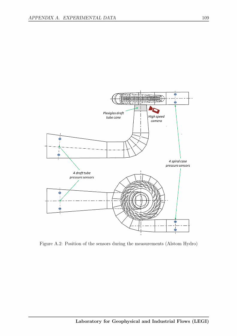
APPENDIX A. EXPERIMENTAL DATA 109
Figure A.2: Position of the sensors during the measurements (Alstom Hydro)
Laboratory for Geophysical and Industrial Flows (LEGI)

110 APPENDIX A. EXPERIMENTAL DATA
Laboratory for Geophysical and Industrial Flows (LEGI)
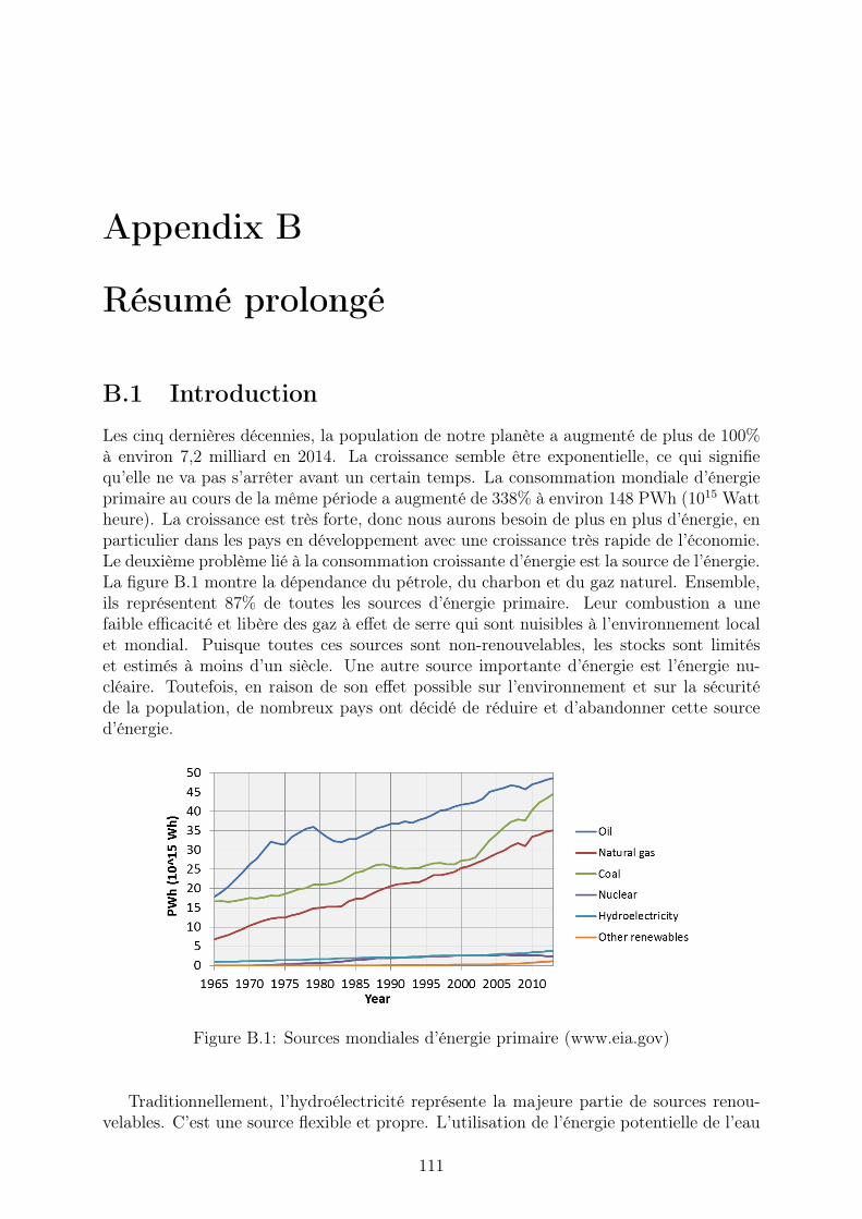
Appendix B
Résumé prolongé
B.1 Introduction
Les cinq dernières décennies, la population de notre planète a augmenté de plus de 100%à environ 7,2 milliard en 2014. La croissance semble être exponentielle, ce qui signifiequ’elle ne va pas s’arrêter avant un certain temps. La consommation mondiale d’énergieprimaire au cours de la même période a augmenté de 338% à environ 148 PWh (1015 Wattheure). La croissance est très forte, donc nous aurons besoin de plus en plus d’énergie, enparticulier dans les pays en développement avec une croissance très rapide de l’économie.Le deuxième problème lié à la consommation croissante d’énergie est la source de l’énergie.La figure B.1 montre la dépendance du pétrole, du charbon et du gaz naturel. Ensemble,ils représentent 87% de toutes les sources d’énergie primaire. Leur combustion a unefaible efficacité et libère des gaz à effet de serre qui sont nuisibles à l’environnement localet mondial. Puisque toutes ces sources sont non-renouvelables, les stocks sont limitéset estimés à moins d’un siècle. Une autre source importante d’énergie est l’énergie nu-cléaire. Toutefois, en raison de son effet possible sur l’environnement et sur la sécuritéde la population, de nombreux pays ont décidé de réduire et d’abandonner cette sourced’énergie.
Figure B.1: Sources mondiales d’énergie primaire (www.eia.gov)
Traditionnellement, l’hydroélectricité représente la majeure partie de sources renou-velables. C’est une source flexible et propre. L’utilisation de l’énergie potentielle de l’eau
111

112 APPENDIX B. RÉSUMÉ PROLONGÉ
d’une efficacité supérieure à 90%, est également considérée comme le moyen le plus effi-cace pour produire de l’électricité. Autour de 17% (3,7 PWh/an) de l’énergie électriquemondiale est actuellement générée par l’énergie hydroélectrique. Selon l’AIE (Agence in-ternationale de l’énergie), le potentiel technique de l’hydroélectricité est estimé à environ16 PWh/an. Nous utilisons donc environ 23% du potentiel disponible (en 2013). Les paysavec le plus haut potentiel technique pour l’hydroélectricité sont la Chine, les États-Unis,la Russie, le Brésil et le Canada.
Un autre avantage des centrales hydroélectriques est leur durabilité. La durée devie moyenne est estimée à environ 40 ans. Cependant, il y a beaucoup de centrales hy-droélectriques qui ont été construites il y a plus de 50 ou même 100 ans. Par conséquent,certaines mises à niveau et rénovations peuvent prolonger considérablement la durée devie des centrales et réduire par conséquent les coûts de l’électricité fournie par l’énergie hy-droélectrique. Par ailleurs, la rénovation peut améliorer de manière significative l’efficacitéglobale des centrales hydroélectriques et augmenter leur production électrique.
Autre que l’hydroélectricité, les sources d’énergie renouvelable les plus largement util-isés sont les sources solaires et éoliennes. Le pourcentage global des sources mentionnéesest encore faible, mais dans plusieurs pays d’Europe de l’Ouest, le vent et les centralessolaires fournissent ensemble déjà plus de 20% de la demande d’électricité.
L’inconvénient du vent et des centrales solaires est l’effet négatif sur la stabilité duréseau électrique. La quantité d’électricité produite par les centrales solaires et éoliennespeut changer toutes les heures, même à chaque minute. Les réseaux électriques ne sontaujourd’hui pas très flexibles, ce qui signifie qu’il ne peut y avoir de variation significativeentre la demande et l’offre du réseau. Concernant l’offre, une baisse soudaine de l’intensitédu vent et/ou l’apparition d’un nuage imprévu peut provoquer la diminution de l’énergieélectrique dans le réseau et donc provoquer des instabilités. D’autre part, les principalesinstabilités sur la demande sont remarquées pendant les heures d’exploitation industrielles.Pour équilibrer et ajuster le système de réseau électrique, une solution rapide et fiable doitêtre fournie afin de stocker l’énergie pendant le pic de production et d’utiliser la mêmeénergie, lorsque la consommation est plus élevée que la production. Jusqu’à présent, lesstations de transfert d’énergie par pompage (STEP) sont la meilleure solution qui nouspermet la flexibilité et le stockage d’énergie à grande échelle.
B.1.1 Les stations de transfert d’énergie par pompage (STEP)
Généralement, nous pouvons diviser les centrales hydroélectriques en plusieurs catégories.L’approche la plus classique consiste à construire un barrage pour stocker et accumuler del’eau. Habituellement, dans la partie inférieure du barrage, une ou plusieurs turbines sontreliées par une conduite forcée, au stockage de l’eau derrière le barrage, et au générateurqui transforme l’énergie mécanique de la turbine en l’électricité. Ces centrales hydroélec-triques sont appelées les centrales de stockage et elles peuvent être en partie réglées enfonction des besoins du réseau électrique et de l’approvisionnement en eau.
Les centrales au fil-de-l’eau sont un autre exemple d’aménagement hydraulique. Lebarrage sur la rivière est toujours nécessaire, cependant, il n’y a que peu ou pas de capacitéde stockage de l’eau derrière le barrage. La turbine utilise le débit presque constant de larivière et produit donc une quantité constante d’électricité.
Le troisième type de centrales hydroélectriques est la station de transfert d’énergie parpompage (STEP). Comme présenté sur la figure B.2, il se compose de deux réservoirs,reliés par une conduite forcée. Celui du bas peut être une partie de l’usine hydroélectriqueclassique comme décrit ci-dessus. En raison de la réduction des coûts et de l’amélioration
Laboratory for Geophysical and Industrial Flows (LEGI)

APPENDIX B. RÉSUMÉ PROLONGÉ 113
de la technologie, nous avons l’habitude d’utiliser de nos jours, un seul système avec lamachine turbine-pompe réversible (fig. B.2). Quand on a trop d’énergie disponible, lamachine fonctionne en mode de pompage, et pompe donc l’eau dans le réservoir supérieur.Le contraire se passe quand nous avons un manque d’électricité dans le réseau, la machinetourne dans l’autre sens et génère de l’électricité.
Figure B.2: Station de transfert d’énergie par pompage (Alstom Hydro)
L’efficacité globale du processus de pompage/turbinage de l’eau pour produire del’électricité est au maximum de 80%. Cependant, les pompes-turbines sont aussi économique-ment rentable. En effet, lorsque la demande d’électricité est inférieure à l’offre, générale-ment au cours de la nuit, le prix de l’électricité est faible. Au contraire, lorsque l’offre estinférieure à la demande, généralement dans la matinée, les prix de l’électricité augmente.La différence quotidienne entre le plus haut et le prix le plus bas peut être même plusde 100%. Pour utiliser la disponibilité des centrales STEP au mieux, il est obligatoired’assurer une commutation régulière du mode pompage au mode génération et vice versa.Les systèmes d’une centrale STEP ont été construits à l’origine pour utiliser et stockerl’énergie supplémentaire fournie par les centrales nucléaires pendant la nuit. Initialement,la commutation entre le mode de production et de pompage survenait autour de 3 - 4fois par jour. Au fils des dernières années, la commutation a augmenté de plus de 10 fois,puisque le rôle principal de la STEP est d’assurer la stabilité du réseau, qui est forte-ment influencée par les sources d’énergie intermittentes, telles que les centrales solaires etéoliennes.
Comme les autres turbomachines, les turbines-pompes réversibles sont également conçuespour un débit constant Q optimal, et une chute nette H optimale, qui sont donnés parla position géographique des deux réservoirs. Cependant, le changement régulier entre
Laboratory for Geophysical and Industrial Flows (LEGI)

114 APPENDIX B. RÉSUMÉ PROLONGÉ
le pompage et le régime de génération électrique, ainsi que les exigences spécifiques del’électricité du réseau, sont les raisons pour lesquelles, en réalité, la turbine-pompe fonc-tionne régulièrement sous des conditions hors nominales. Un long fonctionnement sousdes conditions de ce genre peut provoquer une chute importante de l’efficacité, des vi-brations, ainsi que des dommages sévères sur la machine. Pour éviter ce scénario, il estessentiel d’étudier les origines des instabilités.
B.1.2 Les instabilités en mode pompage
Les principales instabilités remarquées dans le mode de pompage sont liées au comporte-ment de cavitation lors des débits non-optimaux. De plus, à charge partielle, le phénomènedu décollement tournant peut se produire et provoquer une forme de bosse sur la courbede performance (phénomène appelé ’feston’), ce qui est à l’origine des instabilités. L’étudede la cavitation et du feston sont les principaux objectifs de la thèse de doctorat ici présen-tée. Afin de comprendre les instabilités du mode de pompage en charge partielle, il estessentiel d’expliquer les bases du comportement d’une pompe centrifuge.
L’utilisation de l’effet centrifuge pour transporter de l’eau a été proposée pour lapremière fois par Leonard de Vinci (1452 à 1519). Cependant, l’équation la plus fonda-mentale dans le domaine des turbomachines a été présentée par Leonhard Euler (1707 à1783). L’équation d’Euler pour turbomachines est basée sur la conservation du momentangulaire. L’équation linéaire d’Euler simplifiée pour l’énergie hydraulique spécifique dela pompe peut être écrite comme:
gH = U2V2u − U1V1u. (B.1)
Pour une pompe centrifuge, les triangles de vitesse moyens à l’entrée et à la sortie sontpris en compte et le rapport des angles d’écoulement β1 et β2 sont considérés constants(fig. B.3). L’écoulement d’entrée est supposé n’avoir aucune composante circonférentielle(projection de vitesse absolue V1u = 0) pour une pompe centrifuge, l’équation d’Eulerpeut être modifiée en:
gH = U2V2u = U2
(
U2 −V2m
tan(β2)
)
. (B.2)
A la sortie de la turbine, l’énergie hydraulique spécifique gH2 se compose de la pressionp2ρ
et de la vitesse v22
2. La transformation de l’énergie de vitesse en pression continue dans
le distributeur. L’objectif principal de la pompe centrifuge est de convertir la puissancemécanique Pm en puissance hydraulique Ph avec une efficacité maximale. Pm est définiepar la multiplication du couple T sur l’arbre et la vitesse de rotation ω de:
Pm = ωT. (B.3)
D’autre part, la puissance hydraulique est définie par la différence de chute H et ledébit Q:
H =p
ρ+v2
2g+ z; (B.4)
Ph = Qρ(gH2 − gH1). (B.5)
Les autres nombres adimensionnels importants, très utilisés dans la littérature, sontle coefficient débit φ et le coefficient d’énergie spécifique ψ qui sont définis comme suit:
Laboratory for Geophysical and Industrial Flows (LEGI)

APPENDIX B. RÉSUMÉ PROLONGÉ 115
Figure B.3: Triangles de vitesse
φ =Q
πωR3; (B.6)
ψ =2gH
ω2R2. (B.7)
Afin d’atteindre un rendement élevé et de faibles pertes, la transformation de l’énergieà l’intérieur de la machine doit être aussi progressive que possible. Par conséquent, ledébit de la turbine doit être adapté au distributeur. Dans le cas d’une turbine-pompe, ledistributeur comporte deux parties. D’une part, l’angle d’ouverture des aubes directricespeut être modifié et adapté à l’écoulement et, d’autre part, les aubes avant-directrices sontfixes. L’adaptation de l’angle d’ouverture des aubes directrices est nécessaire parce queles triangles de vitesse à la sortie de la roue changent de façon considérable, en fonctionde la vitesse d’écoulement. La figure B.3 montre la différence de l’ angle d’écoulementabsolu α2 à la sortie de la roue pour trois débits différents. Afin de réduire les pertes dansle distributeur, l’angle α2 doit correspondre à l’ouverture de l’angle des aubes directrices.
B.1.3 Séparation d’écoulement et décollement tournant
La séparation est définie comme une zone de recirculation sur les parois solides de la ma-chine. La séparation de l’écoulement initial peut être provoquée par plusieurs phénomènesd’écoulement, tels que:
• un obstacle sur le trajet d’écoulement,
• un angle d’attaque inadapté au bord d’attaque de l’aube (fig. B.4),
Laboratory for Geophysical and Industrial Flows (LEGI)
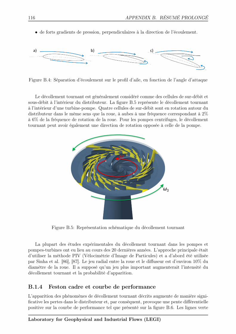
116 APPENDIX B. RÉSUMÉ PROLONGÉ
• de forts gradients de pression, perpendiculaires à la direction de l’écoulement.
Figure B.4: Séparation d’écoulement sur le profil d’aile, en fonction de l’angle d’attaque
Le décollement tournant est généralement considéré comme des cellules de sur-débit etsous-débit à l’intérieur du distributeur. La figure B.5 représente le décollement tournantà l’intérieur d’une turbine-pompe. Quatre cellules de sur-débit sont en rotation autour dudistributeur dans le même sens que la roue, à aubes à une fréquence correspondant à 2%à 6% de la fréquence de rotation de la roue. Pour les pompes centrifuges, le décollementtournant peut avoir également une direction de rotation opposée à celle de la pompe.
Figure B.5: Représentation schématique du décollement tournant
La plupart des études expérimentales du décollement tournant dans les pompes etpompes-turbines ont eu lieu au cours des 20 dernières années. L’approche principale étaitd’utiliser la méthode PIV (Vélocimétrie d’Image de Particules) et a d’abord été utiliséepar Sinha et al. [86], [87]. Le jeu radial entre la roue et le diffuseur est d’environ 10% dudiamètre de la roue. Il a supposé qu’un jeu plus important augmenterait l’intensité dudécollement tournant et la probabilité d’apparition.
B.1.4 Feston cadre et courbe de performance
L’apparition des phénomènes de décollement tournant décrits augmente de manière signi-ficative les pertes dans le distributeur et, par conséquent, provoque une pente différentiellepositive sur la courbe de performance tel que présenté sur la figure B.6. Les lignes verte
Laboratory for Geophysical and Industrial Flows (LEGI)

APPENDIX B. RÉSUMÉ PROLONGÉ 117
et rouge représentent les caractéristiques du circuit hydraulique. La plage de fonction-nement stable normale pour la turbine-pompe est entre les lignes vertes. Dans une zonestable, la turbine-pompe fournit pour chaque hauteur de chute nette du système un débitcorrespondant. Par ailleurs, dans la zone des caractéristiques instables causées par lephénomène de décollement tournant, la turbine-pompe peut fournir trois débits différentspour la caractéristique du circuit donnée, comme indiqué par la courbe rouge. En réal-ité, cela signifie que le débit à travers la turbine-pompe varie de manière complètementincontrôlable. Un tel comportement augmente considérablement les pertes. De plus, elleprovoque de très fortes vibrations qui peuvent endommager et dans le pire des cas, mêmedétruire la machine. De toute évidence, la turbine-pompe ne doit pas opérer dans la zonedu feston cadre.
Figure B.6: Caractéristique instable en mode pompage à cause du feston
B.2 La cavitation
La description la plus commune du terme ’cavitation’ est l’apparition de bulles de vapeurà l’intérieur d’un milieu liquide initialement homogène. Habituellement, c’est considérécomme un passage du liquide à la phase vapeur et puis de nouveau à la phase liquide.La raison de l’apparition de la cavitation est la diminution de la pression locale, avec unetempérature qui reste sensiblement constante. La pression de vapeur peut être expliquéed’un point de vue thermodynamique classique. Sur le diagramme de phase p − T del’eau (fig. B.7), la ligne entre le point triple de l’eau Tr et le point critique C sépare laphase liquide de la phase vapeur. La pression de vapeur pv indique la limite à partir delaquelle une diminution supplémentaire de pression statique (à température constante)provoquerait le changement de la phase (dans notre cas, l’évaporation). Comme le mon-tre la figure B.7, la pression de vapeur pv est une fonction de la température. Commementionné précédemment, la cavitation dans l’eau froide se produit généralement à tem-pérature à peu près constante, lorsque la pression locale diminue et ensuite augmentede nouveau. Un phénomène similaire arrive au point d’ébullition, où la vaporisation seproduit à pression constante quand la température augmente.
Laboratory for Geophysical and Industrial Flows (LEGI)

118 APPENDIX B. RÉSUMÉ PROLONGÉ
Figure B.7: p− T et p− v dans les diagrammes de phase
La dernière étape du processus de cavitation se produit lorsque la pression retourneà sa valeur initiale (au-dessus de la pv) et les bulles commencent à imploser. La bullede vapeur se remplit à nouveau avec le liquide environnant. Lors de l’implosion de labulle, des ondes de pression de forte amplitude peuvent être émises, pouvant induire àl’endommagement des parois solides environnantes.
B.2.1 Cavitation dans les pompes
La cavitation dans les pompes se produit généralement sur les deux côtés des pales, enfonction de l’angle de l’écoulement au bord d’attaque de la roue. Dans le cas d’une vitessed’écoulement réduite, la cavitation apparaît en premier sur le côté d’aspiration de la pale.En revanche, lorsque le débit augmente, la cavitation se produit généralement sur le côtépression de la pale.
Sur la figure B.8, nous pouvons voir toutes les différentes formes de cavitation dansla pompe centrifuge. Les formes de cavitation (sur le côté d’aspiration (a) et sur le côtépression de la pale) proviennent de l’angle d’attaque de l’écoulement non-adapté. D’autrepart, la cavitation dans la région (c) (jeu) est due à des écoulements secondaires quiprovoquent la diminution de la pression locale. Dans des cas particuliers de débit partiel,la cavitation peut être présente aussi dans la zone (d), dans la région du bec de volute(pompes centrifuges) [6]. De même, dans le cas de l’augmentation du débit de la turbine-pompe, la cavitation peut se produire du côté pression des aubes directrices, si l’ouverturede l’angle des aubes directrices n’est pas adaptée à l’écoulement.
Généralement, la présence de formes de cavitation développées dans une pompe peutconduire à:
• la réduction de la performance de la pompe (en réduisant la chute nette Hn), si ledébit Q et la vitesse de rotation n restent constants;
• la diminution du rendement;
• la modification de la vitesse et du profil de pression à l’intérieur de la pompe;
• l’endommagement de la pompe dû à l’érosion de cavitation.
Laboratory for Geophysical and Industrial Flows (LEGI)

APPENDIX B. RÉSUMÉ PROLONGÉ 119
Figure B.8: Cavitation dans les pompes centrifuges [90]
Définition du nombre NPSH
La charge nette absolue à l’aspiration (NPSH) peut être attribuée au circuit ainsi qu’àla machine. Quand nous essayons de décrire et de comparer la probabilité de l’apparitionde la cavitation dans un circuit, le nombre NPSH présent (NPSHA) peut être calculécomme suit:
NPSHA(m) =p0 − pvρg
+v202g
+∆Z −Hloss. (B.8)
L’index 1 dans l’équation B.8 se réfère aux conditions dans le réservoir inférieur. Il estimportant de souligner que ∆Z est positif si le niveau de la turbine-pompe est inférieurau réservoir inférieur de la centrale. Hloss représente les pertes dans le système entre lamachine et le réservoir inférieur. L’énergie cinétique est généralement estimée à 0, car leniveau d’eau dans les réservoirs change très lentement. Selon l’équation B.8, le niveau del’eau dans le réservoir inférieur influe sur le niveau de cavitation dans la turbine-pompe.Par conséquent, afin de réduire au minimum ou d’éviter la cavitation, la position de laturbine-pompe est en général nettement inférieure au niveau des réservoirs inférieurs.
D’autre part, la valeur du NPSH requise (NPSHR) est utilisée pour définir différentsniveaux de cavitation développée à l’intérieur de la machine. Certaines des valeurs typ-iques sont présentées sur la figure B.9 et sont définies de la sorte:
• NPSHR−i représente la valeur de cavitation naissante. Expérimentalement, il peutêtre obtenu par les mesures de visualisation dans la pompe (turbine-pompe).
• NPSHR−ero représente la valeur où l’intensité de la cavitation est suffisammentélevée pour provoquer l’érosion sur les aubes de la pompe.
• NPSHR−3% représente le niveau de cavitation pour lequel la chute de performances,en raison de la présence de la cavitation, atteint 3% de la chute de référence sanscavitation H0. NPSHR−3% peut être obtenu par les mesures globales des perfor-mances de la pompe (turbine-pompe) qui sont décrites dans la norme internationaleIEC 60193 [12].
Une légère augmentation de la performance peut être parfois observée sur la courbe dechute principale NPSHR pour un débit réduit. L’angle d’écollement au bord d’attaque
Laboratory for Geophysical and Industrial Flows (LEGI)
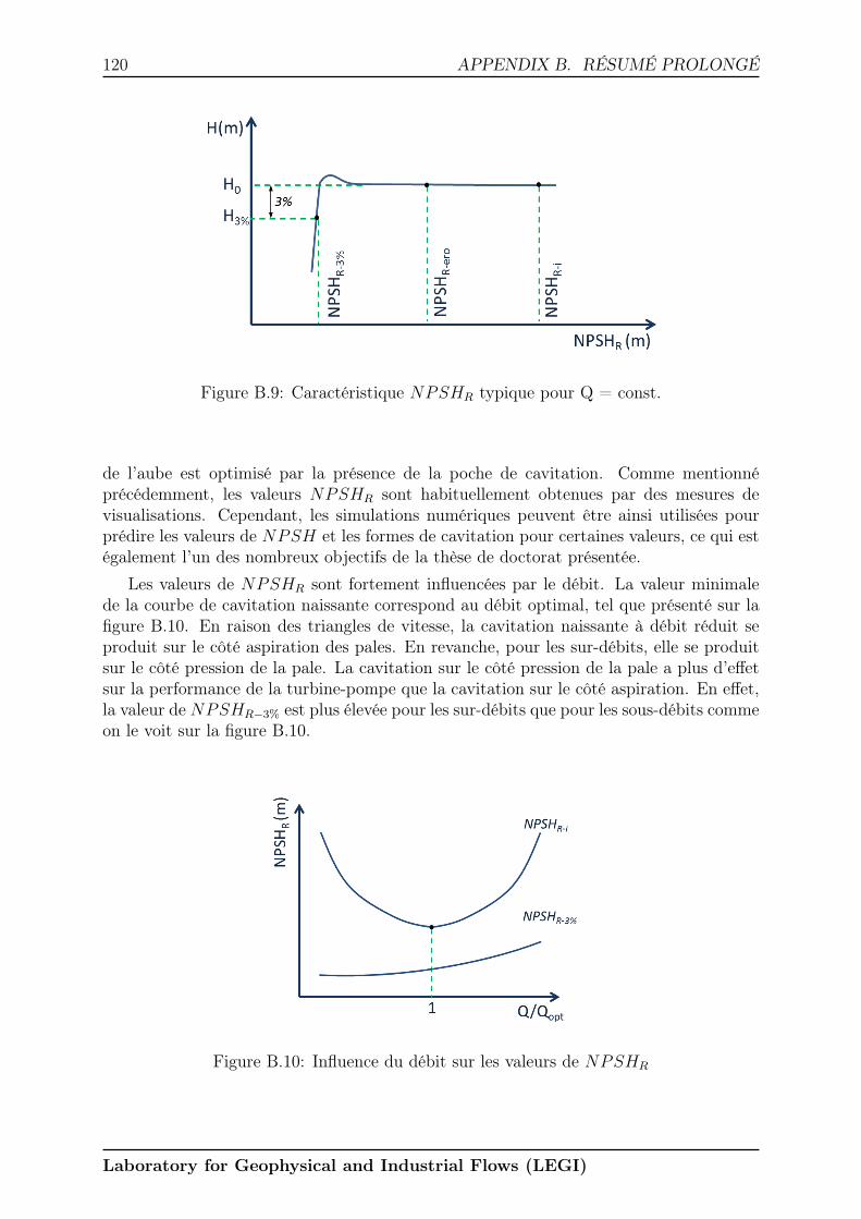
120 APPENDIX B. RÉSUMÉ PROLONGÉ
Figure B.9: Caractéristique NPSHR typique pour Q = const.
de l’aube est optimisé par la présence de la poche de cavitation. Comme mentionnéprécédemment, les valeurs NPSHR sont habituellement obtenues par des mesures devisualisations. Cependant, les simulations numériques peuvent être ainsi utilisées pourprédire les valeurs de NPSH et les formes de cavitation pour certaines valeurs, ce qui estégalement l’un des nombreux objectifs de la thèse de doctorat présentée.
Les valeurs de NPSHR sont fortement influencées par le débit. La valeur minimalede la courbe de cavitation naissante correspond au débit optimal, tel que présenté sur lafigure B.10. En raison des triangles de vitesse, la cavitation naissante à débit réduit seproduit sur le côté aspiration des pales. En revanche, pour les sur-débits, elle se produitsur le côté pression de la pale. La cavitation sur le côté pression de la pale a plus d’effetsur la performance de la turbine-pompe que la cavitation sur le côté aspiration. En effet,la valeur de NPSHR−3% est plus élevée pour les sur-débits que pour les sous-débits commeon le voit sur la figure B.10.
Figure B.10: Influence du débit sur les valeurs de NPSHR
Laboratory for Geophysical and Industrial Flows (LEGI)

APPENDIX B. RÉSUMÉ PROLONGÉ 121
B.3 Objectifs de la thèse
Les simulations CFD nous fournissent un outil utile et rentable pour analyser les phénomènesd’écoulement dans les machines hydrauliques. L’étude présentée porte sur la prédictionet l’analyse de l’écoulement dans des conditions complexes en régime hors-nominal enmode de pompage. La géométrie étudiée est le modéle réduit d’une turbine-pompe àhaute chute (nq = 27). A des régimes de charge partielle, le fonctionnement continu de lamachine peut être limité par le décollement tournant et la cavitation. Les objectifs de lathèse sont les suivants:
• Le premier objectif est d’utiliser un code commercial, testé auparavant dans le lab-oratoire, pour développer une approche numérique afin de permettre la prédictionprécise des phénomènes observés en régime hors-nominal. Le but est d’utiliser lecode et de proposer une méthodologie numérique pour prédire avec précision lesrégimes de cavitation, les chutes de performance dues à la cavitation, et effectuerdes analyses locales des écoulements cavitants. Des analyses globales de l’impact dela cavitation sur les découlements tournants et le feston seront également proposées.Le code devra donner une prévision globale et précise de la zone de feston cadresur la courbe de performance de la machine. Il devra également permettre l’analysede l’écoulements instables observés pour une large gamme de débits et de valeursde NPSH. Par conséquent, les simulations doivent être numériquement stables etrobustes, tout en restant précises.
• Un autre objectif est de développer une méthodologie globale de calcul à bas coûtqui permet de détecter les zones d’exploitation stables et instables. Les méthodolo-gies mentionnées peuvent être très utiles pour une analyse rapide et pratique desécoulements et pour l’évaluation de l’influence de différents paramétres tels les anglesd’ouverture des aubes, la géométrie des aubes directrices et des avant-directrices, lataille de jeu radial entre la roue et le distributeur entre autres. Il devra fournir derésultats globaux précis pour un grand nombre de points de fonctionnement pourun coût de calcul relativement faible.
• L’objectif final est de faire une analyse détaillée du comportement et des originesde décollement tournant en effectuant des simulations instationnaires sur toute lagéométrie. L’analyse inclura l’étude des champs de vitesse et de pression dans le dis-tributeur. De plus, l’influence de la vitesse d’écoulement, les angles d’ouverture desaubes directrices, la géométrie des aubes directrices et la taille de jeu radial serontétudiées en détail afin de donner une image globale de le phénomène. L’analyse pro-posée, ainsi que les outils et des méthodologies développés pourront être une baseimportante pour les futures études sur les phénomènes d’écoulement instables enrégime hors-nominal, pas seulement pour la géométrie de turbine-pompe présentée,mais aussi pour d’autres géométries de turbine-pompe et de pompes centrifuges.
B.4 Modélisation physique et numérique
Les études numériques basées sur la CFD sont devenues fréquentes dans le domaine dela mécanique des fluides. Le développement des ordinateurs et des logiciels a assuréaux universitaires et industries des outils utiles pour analyser, prévoir et améliorer lecomportement de l’écoulement au sein des circuits et machines hydrauliques. En com-paraison aux études expérimentales, l’approche CFD est normalement moins couteuse
Laboratory for Geophysical and Industrial Flows (LEGI)

122 APPENDIX B. RÉSUMÉ PROLONGÉ
et peut fournir des informations plus détaillées sur les phénomènes auxquels les scien-tifiques et les ingénieurs sont intéressés. Cependant, cette approche a encore ses limitesen termes de puissance de calcul et de précision des résultats obtenus. C’est pourquoi, lavalidation de ces résultats est toujours nécessaire. Typiquement, la combinaison d’étudesexpérimentales et numériques donne les résultats les plus efficaces.
B.4.1 Les approches CFD
Pour obtenir de bons résultats des simulations numériques, il est important de savoir quelstypes de simulations sont disponibles et quelles sont leurs limites. En règle générale, troisapproches différentes sont disponibles pour simuler le comportement d’un écoulement. Lasimulation numérique directe (DNS) résout des équations instationnaires de Navier-Stokeset calcule les structures turbulents sur toutes les échelles. Si la discrétisation en temps eten l’espace est adéquate, les DNS doivent fournir les résultats les plus exactes. Jusqu’àprésent, les plus grands et plus rapides superordinateurs ne sont capables de calculer quede géométries simples avec d’écoulements à faibles nombres de Reynolds. Compte tenude l’évolution attendue de la puissance de calcul, les DNS pour des géométries complexesavec grand nombre de Reynolds ne seront pas disponibles avant quelques décennies.
La deuxième approche est connue par le nom Large Eddy Simulation (LES). C’est uncompromis entre les DNS et les simulations RANS. Cette approche calcule les structuresturbulentes, mais pas sur toutes les échelles. Par conséquent, avec une sélection de filtres,il faut choisir la taille des structures turbulentes qui seront calculées. Le défi est de trouverun bon compromis entre l’exactitude et la discrétisation. Les turbulences se produisentsur une grande échelle, mais se dissipent sur les petites échelles. Par conséquent, il estessentiel de trouver une discrétisation spatiale adéquate. En outre, la modélisation descouches limites peut être très exigeante en raison des besoins de maillage très dense prèsdes bords. Une étude de faisabilité sur le maillage doit être effectuée avant les simulationsnumériques réelles. La méthode LES a gagné en popularité ces dernières années dans ledomaine académique, mais elle n’est pas encore utilisée fréquemment pour les applicationsindustrielles.
La seule approche restante est de résoudre les équations de Navier-Stokes moyennéesà l’aide de la décomposition de Reynolds (RANS). Jusqu’à présent, elle est largementutilisée dans l’industrie ainsi que par les universitaires. L’approche est économique, carelle peut être utilisée pour une large gamme d’applications, sans besoin de moyens decalculs importants. L’inconvénient est que l’approche RANS nous fournit des solutionsstatistiquement moyennes pour le comportement turbulent. Choisir le bon modèle turbu-lent est très important. Les équations RANS peuvent être modifiées comme des équationsRANS instationnaire (URANS) pour effectuer les calculs instationnaires.
B.4.2 Schéma numérique appliqué
Le code FINETM/Turbo de Numeca a été utilisé pour toutes les simulations numériquesprésentées.
Le tableau B.1 résume les informations sur le schéma numérique. Les deux types desimulations, stationnaire et instationnaire, ont été effectuées en utilisant les équationsRANS et URANS. Le modèle de turbulence k − ǫ (Extended Wall Function) a été utilisépour toutes les simulations, car il a été validé comme étant le plus précis pour notregenre de simulations. Les simulations de l’écoulement de cavitation ont été effectuéesuniquement pour des simulations stationnaires en utilisant la loi d’état barotrope pour
Laboratory for Geophysical and Industrial Flows (LEGI)

APPENDIX B. RÉSUMÉ PROLONGÉ 123
le transfert de masse. Dans le cas de régimes de fonctionnement cavitants, des résultatsnon cavitants ont été utilisés comme solution initiale. Un plan de mélange a été utilisésur l’interface entre le rotor et les directrices pour les simulations stationnaires. Entrela roue et le tube d’aspiration, le plan de mélange n’a pas été appliqué et une interfacepermettant le bon transfert de données fut créée. Le solveur utilise un schéma centrépour la discrétisation spatiale [47]. Un pas de temps local est utilisé pour les simulationsstationnaires. L’approche par pas de temps dual a été appliquée pour les simulationsinstationnaires (voir description dans [47]).
Type de Simulation Stationnaire InstationnaireModèle physique RANS URANS
Modèle de turbulence k − ǫ (Ext. Wall Function) k − ǫ (Ext. Wall Function)Modèle de cavitation Barotrope /Discrétisation spatiale Central (2nd order) Central (2nd order)
Discrétisation temporelle Local time stepping Dual time steppingPas de temps / 2◦ de tour
Max iter/pas de temps 2000 - 15000 iter 2700 pas de temps
Table B.1: Schéma numérique
Le pas de temps choisi pour les simulations instationnaires est 2◦ de la révolutionde la roue, ce qui correspond à 0, 00033s pour une vitesse de rotation de 1000 tourspar minute. Le nombre d’itérations internes est limité à 35 pour chaque pas de temps.Une convergence satisfaisante pour les simulations stationnaires est généralement atteinteaprès environ 2000 itérations pour des points de fonctionnement stables et jusqu’à 15000itérations pour les points de fonctionnement instables qui sont influencés par la cavitation,le décollement tournant ou par d’autres types d’instabilités.
B.4.3 Moyens de calcul
Plusieurs paramètres de maillage différents ont été analysés au cours de l’étude présentée.Cependant, pour l’analyse finale et les résultats, un seul type de maillage a été utilisédans le but d’avoir une bonne comparaison entre les différentes conditions aux limites etles différents types de simulations. En d’autres termes, dans tous les cas la densité dumaillage ne change pas, le domaine numérique ne change pas, la périodicité entre les paleschange, et le type de simulations (stationnaires et instationnaires) change aussi.
Une estimation des ressources informatiques nécessaires pour des points de fonction-nement non-cavitant est présentée dans le tableau B.2. Colonne ’periodic’ indique quedes conditions de périodicité ont été appliquées dans le roue et dans le distributeur. Celasignifie que seulement un canal de la roue mobile et un canal du distributeur sont calculés.Le maillage ’combined’ se compose d’une chaîne à mailles dans la zone de la roue à aubeset un distributeur entièrement maillé. Le ’full mesh’ représente le type de maillage où lapériodicité n’a pas été utilisée et pour lequel la machine a été maillée complétement.
Les simulations de l’écoulement de cavitation exige 2 à 5 fois plus de temps de calcul, encomparaison aux calculs non cavitant. Le temps de calcul dépend beaucoup de l’intensitéde la cavitation, par conséquent, il est difficile de faire une estimation générale.
Comme le montre le tableau B.2, la taille de maille diffère de manière significative.D’une part, les calculs sur le maillage périodique peuvent être facilement effectués sur unordinateur personnel normal, puisque seuls 7 à 20 heures de calcul sont nécessaires pour
Laboratory for Geophysical and Industrial Flows (LEGI)
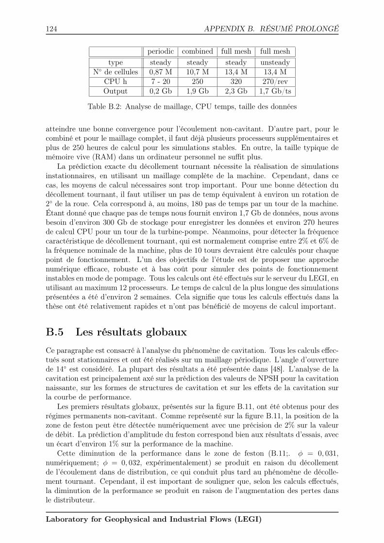
124 APPENDIX B. RÉSUMÉ PROLONGÉ
periodic combined full mesh full meshtype steady steady steady unsteady
N◦ de cellules 0,87 M 10,7 M 13,4 M 13,4 MCPU h 7 - 20 250 320 270/revOutput 0,2 Gb 1,9 Gb 2,3 Gb 1,7 Gb/ts
Table B.2: Analyse de maillage, CPU temps, taille des données
atteindre une bonne convergence pour l’écoulement non-cavitant. D’autre part, pour lecombiné et pour le maillage complet, il faut déjà plusieurs processeurs supplémentaires etplus de 250 heures de calcul pour les simulations stables. En outre, la taille typique demémoire vive (RAM) dans un ordinateur personnel ne suffit plus.
La prédiction exacte du décollement tournant nécessite la réalisation de simulationsinstationnaires, en utilisant un maillage complète de la machine. Cependant, dans cecas, les moyens de calcul nécessaires sont trop important. Pour une bonne détection dudécollement tournant, il faut utiliser un pas de temp équivalent à environ un rotation de2◦ de la roue. Cela correspond à, au moins, 180 pas de temps par un tour de la machine.Étant donné que chaque pas de temps nous fournit environ 1,7 Gb de données, nous avonsbesoin d’environ 300 Gb de stockage pour enregistrer les données et environ 270 heuresde calcul CPU pour un tour de la turbine-pompe. Néanmoins, pour détecter la fréquencecaractéristique de décollement tournant, qui est normalement comprise entre 2% et 6% dela fréquence nominale de la machine, plus de 10 tours devraient être calculés pour chaquepoint de fonctionnement. L’un des objectifs de l’étude est de proposer une approchenumérique efficace, robuste et à bas coût pour simuler des points de fonctionnementinstables en mode de pompage. Tous les calculs ont été effectués sur le serveur du LEGI, enutilisant au maximum 12 processeurs. Le temps de calcul de la plus longue des simulationsprésentées a été d’environ 2 semaines. Cela signifie que tous les calculs effectués dans lathèse ont été relativement rapides et n’ont pas bénéficié de moyens de calcul important.
B.5 Les résultats globaux
Ce paragraphe est consacré à l’analyse du phénomène de cavitation. Tous les calculs effec-tués sont stationnaires et ont été réalisés sur un maillage périodique. L’angle d’ouverturede 14◦ est considéré. La plupart des résultats a été présentée dans [48]. L’analyse de lacavitation est principalement axé sur la prédiction des valeurs de NPSH pour la cavitationnaissante, sur les formes de structures de cavitation et sur les effets de la cavitation surla courbe de performance.
Les premiers résultats globaux, présentés sur la figure B.11, ont été obtenus pour desrégimes permanents non-cavitant. Comme représenté sur la figure B.11, la position de lazone de feston peut être détectée numériquement avec une précision de 2% sur la valeurde débit. La prédiction d’amplitude du feston correspond bien aux résultats d’essais, avecun écart d’environ 1% sur la performance de la machine.
Cette diminution de la performance dans le zone de feston (B.11;. φ = 0, 031,numériquement; φ = 0, 032, expérimentalement) se produit en raison du décollementde l’écoulement dans de distribution, ce qui conduit plus tard au phénomène de décolle-ment tournant. Cependant, il est important de souligner que, selon les calculs effectués,la diminution de la performance se produit en raison de l’augmentation des pertes dansle distributeur.
Laboratory for Geophysical and Industrial Flows (LEGI)

APPENDIX B. RÉSUMÉ PROLONGÉ 125
Figure B.11: La performance globale, les pertes dans le distributeur - lossOUT (ouverture14◦, géométrie GV I, régime non-cavitant)
B.5.1 Validation du modèle de cavitation
Afin d’évaluer le niveau de la cavitation dans le régime de pompage, la définition numériquede la valeur de NPSH requis est importante. Dans notre cas, il est calculé pour chaquepoint que d’exploitation:
NPSH(m) =pref − pvρl g
. (B.9)
Dans l’équation B.9, pref représente la valeur totale de pression à l’entrée du domaine,pv la pression de vaporisation de l’eau à 20◦C, ρl la densité de l’eau, tandis que g estl’accélération gravitationnelle. Puisque les conditions à l’entrée et à la sortie du domainenumérique ont été fixées, la valeur NPSH a été modifiée en changeant la valeur de lapression de vaporisation pv dans le but de maintenir la stabilité de la simulation ainsiqu’un bon niveau de convergence.
B.5.2 Cavitation naissante
La possibilité de pouvoir valider les simulations numériques en régime cavitant par com-parison avec les résultats expérimentaux est d’une importance considérable. La valeurde cavitation naissante (fig. B.12) fait référence aux simulations numériques ainsi qu’àl’expérience. Expérimentalement, la valeur est obtenue par l’observation visuelle d’entréede roue de turbine-pompe. La valeur à différents débits est définie comme l’apparitiondes premières bulles de cavitation.
L’approche industrielle numérique classique ne se sert pas du modèle de cavitationpour prédire la valeur de cavitation naissante. Il est simplifié, définissant la pression deréférence pref (eq. B.9) par la différence entre la pression totale à l’entrée du domaineet la pression statique minimale dans le domaine étudié. Bien que cette approche se soitrévélée assez précise pour prédire la valeur de cavitation naissante, il ne peut pas nousoffrir d’informations supplémentaires si la cavitation est plus développée.
Laboratory for Geophysical and Industrial Flows (LEGI)

126 APPENDIX B. RÉSUMÉ PROLONGÉ
Figure B.12: Valeurs de cavitation naissante
Lorsqu’on utilise le modéle de cavitation, les critères pour définir la cavitation naissantepeuvent être définis par le taux de vide α. Dans notre cas, quand le taux de vide est deα = 0, 2 (20% de la vapeur dans la cellule), la valeur NPSH correspondante a été prisecomme valeur de cavitation naissante. L’accord entre l’approche industrielle sans modèlede cavitation et l’approche se servant du modèle de cavitation pour le transfert de masseest très bon. Les simulations avec le modèle de cavitation peuvent toutefois nous fournirassez d’informations supplémentaires sur le comportement des ecoulements cavitants parrapport à l’approche numérique industrielle.
Comme la figure B.12 l’indique, la mise en correspondance entre les valeurs numériqueset expérimentales fonctionne bien dans une gamme considérable de débits. L’écart estestimé à ±0, 5m. Un écart plus important peut être observé dans le cas du point defonctionnement de φ = 0, 048. Cela est probablement dû à la méthodologie expérimentaleappliquée pour estimer l’apparition de la première bulle. Dans la plupart des points defonctionnement que nous avons étudiés, la première bulle de cavitation s’est produite surle côté aspiration de la pale de la roue. En revanche, pour φ = 0, 048, la cavitationsurvient en premier lieu sur le côté pression de la pale, ce qui est plus difficile à observerexpérimentalement et pourrait expliquer l’écart observé.
B.5.3 Courbes de NPSH
Les courbes de NPSH peuvent être produites pour diverses conditions de débit. La figureB.13 montre quatre courbes NPSH différentes, correspondant aux quatre différents débits.La courbe φ = 0, 0348 représente le régime de fonctionnement, à proximité du meilleurpoint de rendement pour GV ouverture 14◦, ce qui est également relativement proche dela zone de feston. φ = 0, 0278 représente le débit partiel. La courbe φ = 0, 0435 estproche de la limite maximale de fonctionnement normal, tandis que la courbe φ = 0, 0487représente le point de fonctionnement à sur-débit. Dans trois cas, nous pouvons observerles résultats expérimentaux pour 1% de perte de performance qui est due à l’occurrence dela cavitation. Les résultats numériques sont en relativement bon accord avec les données
Laboratory for Geophysical and Industrial Flows (LEGI)

APPENDIX B. RÉSUMÉ PROLONGÉ 127
expérimentales.
Figure B.13: Courbes de NPSH
Comme la figure B.13 le montre, la perte de chute simulée peut atteindre 10% à causede la cavitation sur le côté pression de la pale de la roue. Tous les points où la perte deperformance se produit sont considérés comme dangereux puisque la machine peut êtreexposée à de fortes vibrations, à l’érosion et à des points de fonctionnement instables.Tout cela est provoqué par le phénomène de la cavitation.
Dans le cas de débit réduit, une performance augmentée peut être observée avantla chute de pression à environ NPSH = 2m. À ce point-là, la cavitation augmentel’incidence de l’écoulement au bord d’attaque de la pale de la roue et améliore la perfor-mance.
Il est connu que la cavitation n’est pas un phénomène stationnaire quand les valeursNPSH sont basses. Toutefois, les simulations stationnaires nous permettent d’obtenir laforme et la taille moyen de poches de cavitation pour chaque valeur de NPSH ainsi quela perte estimée. Pour évaluer la fréquence de lâcher des structures de cavitation, desimulations instationnaires couteuses sont nécessaires et n’ont pas été effectuées dans lacadre de cette thèse.
B.5.4 Formes de cavitation, débit φ = 0, 0348
Sur la figure B.13, nous pouvons observer les formes de cavitations correspondant à dif-férents débits. La figure B.14 indique les trois niveaux de cavitation dans la turbine-pompeà débit de φ = 0, 0348, ce qui correspond au point de fonctionnement de meilleur ren-dement pour l’ouverture considérée. La valeur de cavitation naissante dans ce cas-là estd’environ NPSHi = 4, 8m. Tout d’abord, la cavitation survient sur le côté aspiration dela roue. Quand la valeur de NPSH baisse, la cavitation est présente principalement surune grande surface du côté aspiration de la pale, plus près de carter. Quand les valeursNPSH sont extrêmement faibles (NPSH = 1, 78m), les poches de cavitation se forment
Laboratory for Geophysical and Industrial Flows (LEGI)

128 APPENDIX B. RÉSUMÉ PROLONGÉ
sur le côté pression de la pale également. Quand NPSH = 1, 78m, la chute de pressionparvient à 5% environ de la hauteur d’élévation nominale correspondant au débit et àl’ouverture de directrice considérés.
Figure B.14: Formes de cavitation de côté aspiration pour φ = 0, 0348 (α = 0, 05)
B.5.5 Influence de la cavitation sur le feston cadre
L’influence de cavitation sur le feston a été étudiée dans les mêmes conditions numériqueset pour la même ouverture que dans les analyses de cavitation précédentes. La figureB.15 illustre la zone de feston sous conditions non-cavitantes, ainsi que sous conditionsde cavitation relativement fortes (valeurs NPSH constantes). La courbe de performancepour l’ecoulement non-cavitatnt a été comparée aux deux courbes de performance à NPSHconstant. Dans les deux cas (NPSH = 2, 7m et NPSH = 2m), les valeurs de NPSH ontun effet important sur le feston cadre.
Figure B.15: Influence de la cavitation sur le feston cadre
La présence d’une cavitation forte réduit l’amplitude de feston et l’inclinaison positivedH/dQ n’est plus observée dans le cas des régimes de cavitation aux valeurs de NPSH =2, 7m et NPSH = 2m. Comme déjà constaté, dans le cas de φ = 0, 0278 et NPSH = 2m,la performance s’améliore grâce aux conditions optimisées dans la roue.
Laboratory for Geophysical and Industrial Flows (LEGI)

APPENDIX B. RÉSUMÉ PROLONGÉ 129
On peut anticiper que les formes développées de cavitation causent des pertes plusimportantes dans la roue, cependant, cela n’est pas évident dans le cas du distributeur. Lespertes dans le distributeur et la baisse de performance dans la roue ont été étudiées pour lespoints de fonctionnement cavitant (NPSH = 2, 7m etNPSH = 2m) et ont été comparéesau régime non-cavitant (fig. B.16). Les valeurs négatives désignent l’augmentation despertes (∆Ψ, fig. B.16).
Figure B.16: Variations des pertes dans le distributeur et des performances de la rouedues à la cavitation, par rapport au régime non-cavitant
Les effets de la cavitation sur la performance sont plus considérables lorsque le débitest plus élevé. Quelques fois, à débit partiel (φ = 0, 0278), la présence de cavitationaméliore la courbe de performance grâce aux meilleures conditions dans le distributeur,comme l’indique la figure B.16. En outre, l’analyse montre que dans la majorité des cas,la cavitation augmente les pertes dans la roue ainsi que dans le distributeur, bien que lacavitation se produise sur le bord d’attaque de la pale de la roue.
B.6 Analyse stationnaire à débit partiel
Tous les calculs analysés dans ce paragraphe sont stationnaires et non-cavitant. Lesanalyses se concentrent sur la prédiction globale de la position du feston, sur l’amplitudedu feston et sur l’écoulement dans la zone du distributeur. L’analyse a servi à prédireles zones de fonctionnement stables, complètement instables et légèrement instables enfonction des ouvertures de distributeur et des débits considérés.
B.6.1 GV ouverture 14◦
La ligne intitulée ’Sim-periodic 14◦’ (fig. B.17) comporte les calculs avec maillage péri-odique. La position de feston a été détectée avec une précision de 2% sur l’axe de débit.L’amplitude de chute parvient à plus ou moins 1% dans les deux cas - numérique ainsi queexpérimentale. Il a été montré que la chute de performance dans le région de feston estliée aux pertes qui se produisissent à cause du comportement de l’écoulement à l’intérieurdu distributeur.
Laboratory for Geophysical and Industrial Flows (LEGI)
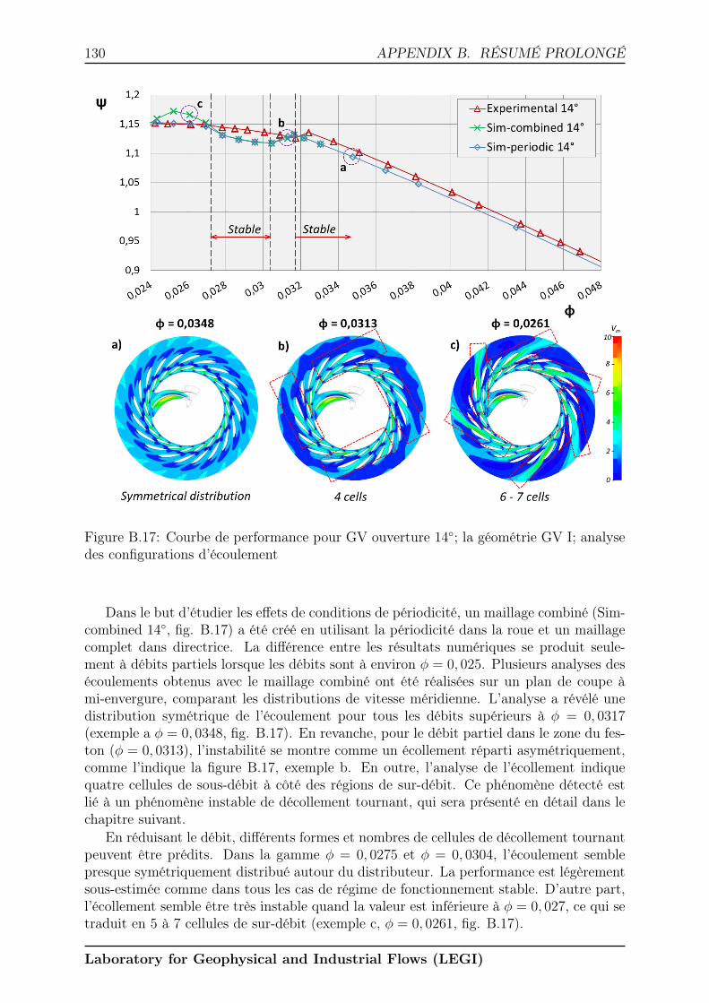
130 APPENDIX B. RÉSUMÉ PROLONGÉ
Figure B.17: Courbe de performance pour GV ouverture 14◦; la géométrie GV I; analysedes configurations d’écoulement
Dans le but d’étudier les effets de conditions de périodicité, un maillage combiné (Sim-combined 14◦, fig. B.17) a été créé en utilisant la périodicité dans la roue et un maillagecomplet dans directrice. La différence entre les résultats numériques se produit seule-ment à débits partiels lorsque les débits sont à environ φ = 0, 025. Plusieurs analyses desécoulements obtenus avec le maillage combiné ont été réalisées sur un plan de coupe àmi-envergure, comparant les distributions de vitesse méridienne. L’analyse a révélé unedistribution symétrique de l’écoulement pour tous les débits supérieurs à φ = 0, 0317(exemple a φ = 0, 0348, fig. B.17). En revanche, pour le débit partiel dans le zone du fes-ton (φ = 0, 0313), l’instabilité se montre comme un écollement réparti asymétriquement,comme l’indique la figure B.17, exemple b. En outre, l’analyse de l’écollement indiquequatre cellules de sous-débit à côté des régions de sur-débit. Ce phénomène détecté estlié à un phénomène instable de décollement tournant, qui sera présenté en détail dans lechapitre suivant.
En réduisant le débit, différents formes et nombres de cellules de décollement tournantpeuvent être prédits. Dans la gamme φ = 0, 0275 et φ = 0, 0304, l’écoulement semblepresque symétriquement distribué autour du distributeur. La performance est légèrementsous-estimée comme dans tous les cas de régime de fonctionnement stable. D’autre part,l’écollement semble être très instable quand la valeur est inférieure à φ = 0, 027, ce qui setraduit en 5 à 7 cellules de sur-débit (exemple c, φ = 0, 0261, fig. B.17).
Laboratory for Geophysical and Industrial Flows (LEGI)

APPENDIX B. RÉSUMÉ PROLONGÉ 131
Les régions stables sont marquées sur la figure B.17. La stabilité est définie comme unedistribution symétrique de l’écollement dans les régions de directrice et avant-directrice.Les régions de fonctionnement qui ne sont pas marquées comme stables sont considéréesinstables. Il est donc fort probable que le décollement tournant se produira dans cesrégions instables. Les résultats stationnaires calculés sur maillage combiné surestime laperformance aux points fortement instables (φ < 0, 028). Des calculs instationnairesdevraient être effectués pour ces points, vu que l’instabilité de l’écollement dans le dis-tributeur joue un rôle important dans la prédiction des pertes dans cette partie de lamachine.
B.7 Analyse du décollement tournant
Nous avons obtenus les résultats ci-dessous en effectuant des simulations instationnairessur la géométrie complète en le régime non-cavitant. Entre 2 et 3 tours de roue ont éténécessaires pour stabiliser les calculs, et puis environ 10 à 15 révolutions ont été effectuéespour analyser le phénomène de décollement tournant. Les comportements et les carac-téristiques des écoulements instables tels que la fréquence et l’intensité de décollementtournant ont été étudiés et analysés. Dans le but d’étudier ces phénomènes d’instabilité,une analyse détaillée de ecoulement local pour le débit φ = 0, 0313 et l’ouverture de 14◦,a été réalisée.
B.7.1 Résultats globaux 14◦
Nous avons comparé les résultats instables globaux pour l’ouverture GV de 14◦ aux don-nées expérimentales et aux simulations stationnaires présentées ci-dessus, comme le mon-tre la figure B.18. En plus, nous pouvons voir que les résultats stationnaires sur lagéométrie compléte ne diffèrent pas des résultats stationnaires sur le maillage combiné.Cela indique que dans le cas de l’ouverture et la géométries considérées, la périodicitédans la région de roue peut être appliquée pour les simulations stationnaires. Les résul-tats instationnaires révèlent une amélioration importante de la prédiction de la courbede performance par rapport aux simulations stationnaires. Par ailleurs, la comparaisonentre les données expérimentales et les simulations instables indique un très bon accorddans les deux régions de fonctionnement, stable ainsi qu’instable.
Dans la zone du feston (fig. B.18b; φ = 0, 0313), quatre cellules de sur-débit etsous-débit ont été observées. Les cellules semblent plus développées que dans le cas dessimulations stationnaires. La fréquence de rotation des cellules est d’environ 3,5% de lafréquence de rotation de la turbine-pompe (tab. B.3). Les fluctuations d’énergie spéci-fiques pour ce débit atteignent environ ±0, 5% et indiquent un point de fonctionnementinstable, potentiellement dangereux.
Alors que le débit continue à décroître, nous pouvons observer huit cellules de dé-collement tournant à φ = 0, 0296. La fréquence de décollement tournant est inférieurepar rapport à φ = 0, 0313 et parvient à environ 2% de la fréquence de fonctionnement(fig. B.18c; tab.B.3). En outre, les cellules paraissent moins intenses dans ce cas-là et laperformance ne fluctue pas. En comparaison aux simulations stationnaires sur le mail-lage combiné (fig. B.17), le comportement est un peu plus instable quand le flux est àφ = 0, 0296. Cela est le cas dans la plupart de points de fonctionnement.
L’écoulement devient encore plus instable au débit très faible de φ = 0, 0261. Troiscellules de décollement tournant peuvent être observées (fig. B.18d). La fréquence de
Laboratory for Geophysical and Industrial Flows (LEGI)

132 APPENDIX B. RÉSUMÉ PROLONGÉ
Figure B.18: Courbe de performance pour GV ouverture 14◦, analyse du décollementtournant
Débit N◦ des cellules Fréquence IntensitéΦ = 0, 0348 / / 0Φ = 0, 0325 / / 0Φ = 0, 0313 4 3,5% ++Φ = 0, 0296 8 2% +Φ = 0, 0261 3 5,5% +++
Table B.3: Cellules de décollement tournant, la fréquence and l’intensité pour ouverture14◦
décollement tournant parvient à 5,5% de la fréquence de fonctionnement de la turbine-pompe. La fluctuation du coefficient d’énergie spécifique φ atteint environ ±0, 5%, ce qui
Laboratory for Geophysical and Industrial Flows (LEGI)

APPENDIX B. RÉSUMÉ PROLONGÉ 133
est un autre indicateur d’un point de fonctionnement fortement instable. Les simulationsstationnaires pour ce débit ont abouti à un nombre plus élevé et de cellules décollées deformat réduit. Cela confirme les conclusions générales que les simulations instationnairessur la géométrie complet prédisent des écoulements légèrement plus instables. Ils sontdonc nécessaires pour une prédiction précise du décollement tournant.
B.7.2 Évolution du décollement tournant
L’évolution du décollement tournant peut être décrite de manière simplifiée comme unedécomposition des cellules bloquées.
• Phase 1. Le débit augmente dans le canal en raison de conditions favorables, tellesque la basse pression au milieu du canal et angle d’attaque adapté aux GV. Il atteintprogressivement la valeur maximale de l’ordre de 130% du débit nominal à traversle canal.
• Phase 2. L’angle d’attaque à l’entrée du canal (décrit à l’aide des vecteurs devitesse) commence à tourner doucement vers le canal aval. Entre temps, la pressionstatique dans le canal commence à augmenter, ce qui provoque une gradient depression adverse forte entre le milieu du canal et la région près du bord d’attaquede la prochaine GV sur le côté pression de l’aube. Cela aboutit à une forte sépara-tion de l’écoulement dans le canal, à la croissance de la zone de séparation et à ladéviation de l’écoulement vers le canal aval. Le débit diminue d’abord au milieu ducanal et baisse ensuite sur le moyeu et carter du canal, provoquant une réductionsupplémentaire de débit à environ 45% du débit nominal.
• Phase 3. Gradient de pression adverse commence à diminuer conjointement avecla zone de recirculation, entraînant progressivement des conditions plus favorableset en augmentant le débit dans le canal. La cellule bloquée se déplace vers canalaval, ce qui entraine une augmentation supplémentaire de débit dans le canal.
B.8 Conclusions
Des outils de calcul ont été utilisés dans le travail ci-présent pour prédire et analyser desinstabilities en mode pompage. Toutes les simulations décrites ont été effectuées au LEGIavec au maximum 12 processeurs, ce qui constitue aujourd’hui une puissance de calcullargement accessible.
Le premier objectif du projet a été de réaliser et de développer des simulations desphénomènes de cavitation dans la géométrie de turbine-pompe considérée. Les calculsstationnaires sur maillage périodique ont été réalisés pour différents débits et valeurs deNPSH. Même dans le cas des points de fonctionnement hors nominaux et fortement in-stables, nous avons obtenu des résultats fiables. Les données expérimentales (bien quelimitées) s’accordent bien avec les simulations. Le code est capable de prédire avec préci-sion les valeurs de cavitation naissante, les courbes de NPSH et les formes de cavitationmoyennes avec de temps de calcul raisonnables (20 heures CPU au maximum).
Les simulations stationnaires offrent un bon aperçu de la stabilité des points de fonc-tionnement. Des maillage du type ’combiné’ peuvent également être appliqués aux anal-yses de décollement tournant dans le distributeur. Les points de fonctionnement stables,
Laboratory for Geophysical and Industrial Flows (LEGI)
134 APPENDIX B. RÉSUMÉ PROLONGÉ
légèrement instables et fortement instables peuvent être détectés en utilisant cette ap-proche. Cela constitue une solution de compromis entre des simulations instationnairesplus coûteuses sur la géométrie complète et des simulations stationnaires sur le maillagepériodique. L’auteur souligne le besoin d’une attention particulière sur la modélisation desinteractions entre le roue et le distributeur lorsque les jeux entre la roue et le distributeursont relativement faibles et les points de fonctionnement sont à débits partiels.
Les résultats obtenus par les simulations instationnaires, en utilisant les équationsURANS, se comparent bien aux résultats dans la littérature. D’ailleurs, ils prouventque les outils CFD peuvent être très exacts en prédisant la performance, même dans desconditions hors nominales, par exemple adébit partiel. En outre, des simulations CFDnous donnent un aperçu détaillé des écoulements dans la machine qui nécessitent desétudes expérimentales très exigeantes, quelques fois même impossibles à réaliser.
Les décollement tournants peuvent être caractérisés par de formes et intensités di-verses. Le nombre ainsi que la fréquence du décollement tournant peuvent varier. Bienque cela doive être confirmé par des expériences, il semble que le nombre faible de cellulesindique une fréquence de décollement tournant plus élevée. Par conséquent, un tel pointde fonctionnement semble être plus dangereux pour la machine. L’analyse de l’écoulementlocal montre que le décollement tournant peut être décrit par l’augmentation ou la décom-position de cellules bloquées ainsi que par la rotation de ces cellules autour du distributeur.La forme de zones de recirculation et de séparation de l’écoulement, qui changent com-plètement les conditions au bord d’attaque des directrices sont les paramètres qui jouentle rôle le plus important sur l’evolution du décollement tournant. Les champs de pres-sion, en particulier la direction et la magnitude du gradient pression adverse, entraînentune déviation de l’écoulement vers canal aval et causent ce que l’on appelle la rotationde cellules. Tenant compte de tous les mécanismes de décollement tournant mentionnés,nous pouvons souligner plusieurs façons possibles de modifier les effets du décollementtournant:
• Diminution/augementation de l’angle d’ouverture des directrices
• Modification de la géométrie de directrices
• Réduction du jeu roue-distributeur
• Modification de la géométrie de la roue
B.9 Perspectives
Premièrement, des expériences devraient être effectuées pour que la précision de simula-tions numériques présentées puisse être évaluée. L’exactitude de la fréquence de décolle-ment tournant et le nombre de cellules devraient être validés par mesures expérimentalespour la même géométrie dans les mêmes conditions de fonctionnement.
Les résultats présentés, particulièrement les calculs instationnaires, offrent des grandespossibilités pour le développement d’un outil général et accessible qui donnerait des ré-sultats fiables pour une large gamme de débits, même dans des conditions de fonction-nement hors nominales, avec l’apparition de la cavitation et de décollement tournant.Pour y parvenir, des simulations instationnaires pourraient être effectuées également sousdes conditions de cavitation.
Laboratory for Geophysical and Industrial Flows (LEGI)

APPENDIX B. RÉSUMÉ PROLONGÉ 135
Finalement, l’idée principale de cette étude était d’étudier le feston cadre et le dé-collement tournant dans le but de minimaliser leurs effets sur la performance de turbine-pompe. Les outils numériques maintenant disponibles peuvent être utilisés pour toutegéométrie exposée au problème de décollements tournants. Des études supplémentairesdu point de vue industriel et/ou académique devraient être réalisées afin de proposer dessolutions pratiques pour réduire ou éliminer les effets négatifs de décollement tournantsur les performances et la stabilité de machines hydrauliques.
Laboratory for Geophysical and Industrial Flows (LEGI)