On the onset of postshock flow instabilities over concave surfaces
Shear instabilities in shallow-water
magnetohydrodynamics
Julian Mak
Submitted in accordance with the requirements for the degree of Doctor of Philosophy
The University of Leeds
Department of Applied Mathematics
July 2013
The candidate confirms that the work submitted is his own and that appropriate credit
has been given where reference has been made to the work of others. This copy has been
supplied on the understanding that it is copyright materialand that no quotation from the
thesis may be published without proper acknowledgment.
c©2013 The University of Leeds and Julian Mak

ii
AbstractThe interaction of horizontal shear flows and magnetic fieldsin stably stratified layers is central
to many problems in astrophysical fluid dynamics. Motions insuch stratified systems, such
as the solar tachocline, may be studied within the shallow-water approximation, valid when
the horizontal length scales associated with the motion arelong compared to the vertical
scales. Shallow-water systems have the advantage that it captures the fundamental dynamics
resulting from stratification, but there is no explicit dependence on the vertical co-ordinate,
and is thus mathematically simpler than the continuously stratified, three-dimensional fluid
equations. Here, we study the shear instability problem within the framework of shallow-water
magnetohydrodynamics.
A standard linear analysis is first carried out, where we derive theorems satisfied by general basic
states (growth rate bounds, semi-circle theorems, stability criteria, parity results), investigate the
instabilities associated with idealised, piecewise-constant profiles (the vortex sheet and rectangular
jet), and investigate the instabilities associated with two prototypical smooth profiles (hyperbolic-
tangent shear-layer and Bickley jet); these are studied viaanalytical, numerical and asymptotic
methods. The nonlinear development of the instabilities associated with the smooth profiles is
then investigated numerically, focussing first on the changes to the nonlinear evolution arising from
MHD effects, before investigating the differences arisingfrom shallow-water effects. We finally
investigate the interplay between MHD and shallow-water effects on the nonlinear evolution.

iii
子曰 : “學而不思則罔,思而不學則殆”〈〈論語 ·為政〉〉
0“He who learns but does not think is lost; he who thinks but does not learn is in danger” – Confucius,Analects2.15

iv

v
AcknowledgementsFirst and foremost I would like to thank my supervisors, David Hughes and Stephen Griffiths, for
introducing me to this interesting research topic, as well as their continued support, guidance and
patience with this thesis and my academic development over the past four years. I would also like
to thank my undergraduate supervisors, Djoko Wirosoetisno, Miguel Moyers-Gonzalez, and my
pastoral advisor John Bolton for encouraging me to pursue PhD studies fives years ago.
I further extend my thanks to the following people for discussions and contribution that have
improved parts of this thesis: Steve Tobias and Sam Hunter for discussions of the properties
possessed by shallow-water systems; Eyal Heifetz for comments on the counter-propgating
Rossby wave mechanism that appears in Chapter 5; Andrew Gilbert for discussions that improved
Chapter 5, and for the anti-dynamo result in Chapter 7; Ben Hepworth and Laura Burgess, for a
template of their nonlinear code that served as a starting point of the nonlinear code I wrote to
generate the results in Chapter 6 and 7; and my examiners David Dritschel and Chris Jones for
comments that clarified some technical points and improved the presentation of the thesis. I would
also like to thank Pat Diamond, Nic Brummell, Pascale Garaud, as well as Yusuke Kosuga, Erica
Rosenblum, Toby Wood, CJ Donnelly and other participants ofthe six week 2010 International
Summer Institute for Modelling in Astrophysics summer programme that contributed significantly
to my early academic development.
On a more personal note, I would like to thank my family, staffand student members at Leeds
mathematics department, and my friends from outside the department for their continued support
and encouragement during my time at Leeds.
This work was supported by the STFC doctoral training grant ST/F006934/1.

vi
vii
NotationB3 three-dimensional magnetic field,B3 = (bx, by, bz)
b two-dimensional magnetic field,b = (bx, by)
B magnetic flux in shallow-water,B = (htbx, htby)
c phase speed,c = cr + ici
F Froude number,F = U/√gHg gravitational acceleration
H equilibrium fluid depth
h the free surface displacement
hB bottom topography
ht total fluid heightht = H0 + F 2h
j vertical component of current,j = ez · (∇×B3)
M inverse Alfven-Mach number,M = B/UP total pressure
p gas pressure
Q, q potential vorticity,q = ω/ht
U0 the basic state velocity
u3 three-dimensional velocity field,u3 = (u, v, w)
u two-dimensional velocity field,u = (u, v)
U momentum in shallow-water,U = (htu, htv)
α streamwise wavenumber
ρ density
ω vertical component of vorticity,ω = ez · (∇× u3)
∇ gradient operator
∇z gradient operator withz-component omitted
D/Dt material derivative
(·)′ d(·)/dy

viii
ix
Contents
Abstract . . . . . . . . . . . . . . . . . . . . . . . . . . . . . . . . . . . . . . . . . . ii
Acknowledgements . . . . . . . . . . . . . . . . . . . . . . . . . . . . . . . . . . .. v
Notation . . . . . . . . . . . . . . . . . . . . . . . . . . . . . . . . . . . . . . . . . . vii
Contents . . . . . . . . . . . . . . . . . . . . . . . . . . . . . . . . . . . . . . . . . . ix
List of figures . . . . . . . . . . . . . . . . . . . . . . . . . . . . . . . . . . . . . . .xiv
List of tables . . . . . . . . . . . . . . . . . . . . . . . . . . . . . . . . . . . . . . .. xxv
1 Introduction 1
2 The shallow-water MHD equations 7
2.1 Derivation . . . . . . . . . . . . . . . . . . . . . . . . . . . . . . . . . . . . . . 7
2.2 Properties . . . . . . . . . . . . . . . . . . . . . . . . . . . . . . . . . . . . . .10
2.2.1 Non-dimensional form . . . . . . . . . . . . . . . . . . . . . . . . . . .10
2.2.2 Conserved quantities . . . . . . . . . . . . . . . . . . . . . . . . . . .. 12
2.2.3 Waves . . . . . . . . . . . . . . . . . . . . . . . . . . . . . . . . . . . . 16
3 Linear theory: eigenvalue problem and general theorems 19
3.1 Linearisation and eigenvalue problem . . . . . . . . . . . . . . .. . . . . . . . 19
3.2 Growth rate bound . . . . . . . . . . . . . . . . . . . . . . . . . . . . . . . . .21
3.3 Semicircle theorems . . . . . . . . . . . . . . . . . . . . . . . . . . . . . .. . . 22

CONTENTS x
3.3.1 Stability criteria . . . . . . . . . . . . . . . . . . . . . . . . . . . . .. . 24
3.4 Parity results . . . . . . . . . . . . . . . . . . . . . . . . . . . . . . . . . . .. 24
3.5 Discussion . . . . . . . . . . . . . . . . . . . . . . . . . . . . . . . . . . . . . .25
4 Instabilities of piecewise-constant profiles 31
4.1 Vortex sheet . . . . . . . . . . . . . . . . . . . . . . . . . . . . . . . . . . . . .32
4.1.1 Asymptotic analysis:M ≈ 1 . . . . . . . . . . . . . . . . . . . . . . . . 34
4.2 Rectangular jet . . . . . . . . . . . . . . . . . . . . . . . . . . . . . . . . . .. 34
4.2.1 Vortex sheet like behaviour at largeα . . . . . . . . . . . . . . . . . . . 36
4.2.2 Long-wave cutoff due to the magnetic field . . . . . . . . . . .. . . . . 38
4.2.3 Preferred mode of instability: even versus odd modes.. . . . . . . . . . 40
4.2.4 Miscellaneous features . . . . . . . . . . . . . . . . . . . . . . . . .. . 43
4.3 Summary and discussion . . . . . . . . . . . . . . . . . . . . . . . . . . . .. . 43
4.4 Appendix: Expressions for eigenfunctions . . . . . . . . . . .. . . . . . . . . . 45
5 Linear instabilities of smooth profiles 49
5.1 Numerical method . . . . . . . . . . . . . . . . . . . . . . . . . . . . . . . . .49
5.2 Hyperbolic-tangent shear layer . . . . . . . . . . . . . . . . . . . .. . . . . . . 50
5.3 Instability mechanism in terms of counter-propagatingRossby waves . . . . . . . 52
5.3.1 Modifications in the SWMHD case . . . . . . . . . . . . . . . . . . . .56
5.4 Bickley jet . . . . . . . . . . . . . . . . . . . . . . . . . . . . . . . . . . . . . . 62
5.5 Long-wave asymptotics . . . . . . . . . . . . . . . . . . . . . . . . . . . .. . . 65
5.5.1 Hyperbolic-tangent shear layer . . . . . . . . . . . . . . . . . .. . . . . 68
5.5.2 Long-wave asymptotics for jets . . . . . . . . . . . . . . . . . . .. . . 70
5.5.3 Consistency issues of long-wave asymptotics for jets. . . . . . . . . . . 72

CONTENTS xi
5.6 Summary and discussion . . . . . . . . . . . . . . . . . . . . . . . . . . . .. . 74
5.7 Appendix: Recovering fields from the eigenfunctionG . . . . . . . . . . . . . . 76
6 Nonlinear evolution: two-dimensional incompressible MHD 79
6.1 Mathematical formulation and numerical methods . . . . . .. . . . . . . . . . . 79
6.2 Numerical methods: Fourier–Chebyshev pseudo-spectral method . . . . . . . . . 82
6.2.1 Pseudo-spectral methods . . . . . . . . . . . . . . . . . . . . . . . .. . 83
6.2.2 Fourier modes . . . . . . . . . . . . . . . . . . . . . . . . . . . . . . . 83
6.2.3 Chebyshev modes . . . . . . . . . . . . . . . . . . . . . . . . . . . . . 85
6.3 Numerical methods: time-stepping by linear multi-stepmethods . . . . . . . . . 88
6.4 Hydrodynamic evolution: a review . . . . . . . . . . . . . . . . . . .. . . . . . 90
6.4.1 Hyperbolic-tangent shear layer . . . . . . . . . . . . . . . . . .. . . . . 90
6.4.2 Bickley jet . . . . . . . . . . . . . . . . . . . . . . . . . . . . . . . . . 97
6.5 MHD evolution: hyperbolic-tangent shear layer . . . . . . .. . . . . . . . . . . 99
6.5.1 Regime boundary estimation . . . . . . . . . . . . . . . . . . . . . .. . 110
6.5.2 Regime classification . . . . . . . . . . . . . . . . . . . . . . . . . . .. 111
6.5.3 Dependence of evolution on Re . . . . . . . . . . . . . . . . . . . . .. 115
6.5.4 The cases with largerM . . . . . . . . . . . . . . . . . . . . . . . . . . 117
6.6 MHD evolution: Bickley jet . . . . . . . . . . . . . . . . . . . . . . . . .. . . 117
6.6.1 Regime classification . . . . . . . . . . . . . . . . . . . . . . . . . . .. 124
6.6.2 The cases with largerM . . . . . . . . . . . . . . . . . . . . . . . . . . 125
6.7 Summary and discussion . . . . . . . . . . . . . . . . . . . . . . . . . . . .. . 126
6.7.1 Dependence on viscosity . . . . . . . . . . . . . . . . . . . . . . . . .. 129
6.7.2 Arresting mechanism: tearing instabilities? . . . . . .. . . . . . . . . . 129
6.7.3 Validating and improving on the disruption estimate .. . . . . . . . . . 132
CONTENTS xii
6.8 Appendix A: Differentiation and quadrature routines inFourier–Chebyshev
spectral space . . . . . . . . . . . . . . . . . . . . . . . . . . . . . . . . . . . . 134
6.8.1 Fast Fourier Transform (FFT) . . . . . . . . . . . . . . . . . . . . .. . 134
6.8.2 Integration of quadratic quantities . . . . . . . . . . . . . .. . . . . . . 135
6.8.3 Quasi-TriDiagonal Solver (QTS) . . . . . . . . . . . . . . . . . .. . . . 136
6.9 Appendix B: Derivation of AB/BD3 . . . . . . . . . . . . . . . . . . . .. . . . 138
7 Nonlinear evolution: shallow-water MHD 143
7.1 Numerical and mathematical formulation of SWMHD . . . . . .. . . . . . . . . 143
7.1.1 The choice of dissipation and conservation problems .. . . . . . . . . . 143
7.1.2 Arguments for employing (7.10) . . . . . . . . . . . . . . . . . . .. . . 149
7.1.3 Presence of fast waves . . . . . . . . . . . . . . . . . . . . . . . . . . .152
7.2 Hydrodynamic evolution . . . . . . . . . . . . . . . . . . . . . . . . . . .. . . 156
7.2.1 Hyperbolic-tangent shear layer . . . . . . . . . . . . . . . . . .. . . . . 157
7.2.2 Bickley jet . . . . . . . . . . . . . . . . . . . . . . . . . . . . . . . . . 163
7.3 MHD evolution . . . . . . . . . . . . . . . . . . . . . . . . . . . . . . . . . . . 168
7.3.1 Hyperbolic-tangent shear layer:F = 0.1 . . . . . . . . . . . . . . . . . 168
7.3.2 Hyperbolic-tangent shear layer:F = 0.5 . . . . . . . . . . . . . . . . . 174
7.3.3 Bickley jet:F < 1 . . . . . . . . . . . . . . . . . . . . . . . . . . . . . 178
7.4 The case ofF ≥ 1 . . . . . . . . . . . . . . . . . . . . . . . . . . . . . . . . . 180
7.5 Summary and discussion . . . . . . . . . . . . . . . . . . . . . . . . . . . .. . 182
7.6 Appendix A: Other forms of magnetic dissipation in SWMHD. . . . . . . . . . 188
7.6.1 Anti-dynamo result . . . . . . . . . . . . . . . . . . . . . . . . . . . . .188
7.7 Appendix B: Numerical scheme whenF = 0 . . . . . . . . . . . . . . . . . . . 189

CONTENTS xiii
8 Conclusions and further work 191
8.1 Summary of results . . . . . . . . . . . . . . . . . . . . . . . . . . . . . . . .. 191
8.2 Conclusions . . . . . . . . . . . . . . . . . . . . . . . . . . . . . . . . . . . . .193
8.3 Some possible further work . . . . . . . . . . . . . . . . . . . . . . . . .. . . . 193
Bibliography 199

List of figures xiv

xv
List of Figures
1.1 Angular velocity profile inferred from helioseismology,
taken from the LSV group at HAO, NCAR
(http://www.hao.ucar.edu/research/lsv/lsv.php, convection
page). 450nHz and 325 nHz translates roughly to rotation periods of 26 and 36
days. The tachocline is indicated by the dashed line. . . . . . .. . . . . . . . . . 4
2.1 Physical set up of the problem. . . . . . . . . . . . . . . . . . . . . . .. . . . . 8
3.1 Four possible regimes for the semicircle bounds (3.17) and (3.19). They could:
(a) completely overlap;(b) partially overlap;(c) shrink to a point;(d) be disjoint.
For the latter two cases, the intersection region is empty, so there are no normal
mode instabilities. . . . . . . . . . . . . . . . . . . . . . . . . . . . . . . . . .. 24
4.1 Contours of Im(cv) given by the expression (4.8), with stability boundaries (4.9). 33
4.2 Comparison between the exact results (4.8), given by crosses, and the asymptotic
results (4.11) and (4.12), given by the dot-dashed line and solid line respectively.
Note the use of different axes here. . . . . . . . . . . . . . . . . . . . . .. . . . 35
4.3 Contours ofci, computed numerically for the even mode (equation (4.16), left
column) and the odd mode (equation (4.17), right column) of the rectangular jet at
some selectedα. Note the different choice of axes used in the bottom panels.The
stability boundary according to computed results is the contour labelled by ‘0’.
The stability boundaries (4.20), (4.24) and (4.26) are plotted also in the appropriate
panels. . . . . . . . . . . . . . . . . . . . . . . . . . . . . . . . . . . . . . . . . 37

LIST OF FIGURES xvi
4.4 Comparison of the computed growth rates and the predicted growth rates from
the asymptotic results, for the even mode of the rectangularjet atM = 0.1. The
computed results are given by crosses (and circles when the computed result is
smaller than what may be displayed at this axis choice),α×(4.23) is given by the
dot-dashed line (cutoff plotted as vertical dotted line) and α×(4.24) is given by
the solid line (cutoff plotted as vertical dashed line). Thecorresponding growth
rate as predicted by the largeα asymptotics (4.18) is plotted as squares when this
growth rate is non-zero. . . . . . . . . . . . . . . . . . . . . . . . . . . . . . .. 39
4.5 Comparison of the computed growth rates and the predicted growth rates from
the asymptotic results, for the odd mode of the rectangular jet atM = 0.1. The
computed results are given by crosses (and circles when the computed result is
smaller than what may be displayed at this axis choice),α×(4.26) is given by the
dot-dashed line (cutoff plotted as vertical dotted line). The corresponding growth
rate as predicted by the largeα asymptotics (4.18) is plotted as squares when this
growth rate is non-zero. . . . . . . . . . . . . . . . . . . . . . . . . . . . . . .. 41
4.6 A plot over(α,F ) space showing the different scenarios for the rectangular jet.
Here, ce = Im(ce) and co = Im(co); see legend for the corresponding regime
denoted by I–VI. The cutoff atF = 0 due to the magnetic field (4.30) is labelled
asαc0 and is plotted as the dot-dashed line. The change of regime, i.e. where the
even and odd mode are equally unstable, as predicted by the small F asymptotic
analysis (4.32), is labelled asαc1 and plotted as the dashed line in the diagrams. . 42
4.7 A zoomed in version of Figure 4.6. . . . . . . . . . . . . . . . . . . . .. . . . . 43
5.1 Contours ofci overF andM parameter space at selectedα. The results have been
filtered so that only modes with|cr| < 10−3 are plotted. Figure 4.1 is reproduced
here as panel(d) for comparison purposes. . . . . . . . . . . . . . . . . . . . . . 51
5.2 Contours ofci over F and M parameter space at selectedα. Inflection
point instabilities with|cr| < 10−3 are plotted as solid lines while supersonic
instabilities with|cr| > 10−3 are plotted as dashed lines. . . . . . . . . . . . . . 53

LIST OF FIGURES xvii
5.3 The growth rate over the unstable bandwidth at selected parameter values for
U0(y) = tanh(y). The inflection-point mode is plotted as lines and the
supsersonic mode as markers. . . . . . . . . . . . . . . . . . . . . . . . . . .. . 53
5.4 Basic CRW mechanism in schematic form, for the background velocity profile of
U0 = tanh(y), so the background vorticity profile isΩ0 = −sech2(y). Solid
lines here depict the dynamics for the incompressible, hydrodynamic case. The
contours are of the vorticity. Vorticity anomalies are shown by the closed solid
curves, and the effect of these on the other contours, leading to instability, is shown
by solid arrows. . . . . . . . . . . . . . . . . . . . . . . . . . . . . . . . . . . . 54
5.5 Vorticity eigenfunction of the most unstable mode ofU0(y) = tanh(y) at some
selected parameters. Here and in subsequent diagrams of this type, red is positive
and blue is negative. Notice the larger shift between the pair of waves asM is
increased, and a slight tilting whenF is increased. . . . . . . . . . . . . . . . . . 55
5.6 Height (pressure) eigenfunction of the most unstable mode ofU0(y) = tanh(y)
at some selected parameters. Notice an increased tilting with increasingF . . . . . 55
5.7 Vorticity contributions associated with the most unstable mode atF = 0,M = 0;
panel(a) is also Figure 5.5(c). The small relativeL2 error given by (5.9) indicates
that the vorticity anomalies come solely from deformation of the material contours. 57
5.8 Vorticity contributions associated with the most unstable mode atF = 0, M =
0.25. Notice that unlike the hydrodynamic shallow-water case, the vorticity
contribution due the MHD effects is the same order as the contribution due to
the displacement of the material contour. Note also the bottom panels are zoomed
in than the other panels. . . . . . . . . . . . . . . . . . . . . . . . . . . . . . .. 58
5.9 Modified CRW mechanism in pictorial form, with the background velocity profile
U0 = tanh(y). The solid contours are associated with the basic CRW mechanism,
as in Figure 5.4. The closed dashed curves represent the additional vorticity
anomalies due to the extra physical effects. The (stabilising) effect of these extra
vorticity anomalies are shown by the dashed arrows. . . . . . . .. . . . . . . . . 59
LIST OF FIGURES xviii
5.10 Vorticity contributions associated with the most unstable mode atF = 0.5, M =
0. Notice that the vorticity contribution due the presence ofa free surface is much
smaller than the contribution due to the displacement of thematerial contour. . . 60
5.11 Vorticity contributions implied by the velocity eigenfunction calculated atF = 0,
M = 0. . . . . . . . . . . . . . . . . . . . . . . . . . . . . . . . . . . . . . . . 60
5.12 Vorticity contributions associated with the most unstable mode atF = 0.5, M =
0.25. Notice that, as observed before, the vorticity contribution from the MHD
term is larger than the contribution from the shallow-waterterm, and both are
such that they counteract the contribution from the deformation of the material
contour. . . . . . . . . . . . . . . . . . . . . . . . . . . . . . . . . . . . . . . . 61
5.13 Contours ofci over theF andM parameter space at selectedα, for the even
mode (left column) and the odd mode (right column) ofU0(y) = sech2(y). The
predicted cut off from the asymptotic result (5.38) is plotted in panel (e). . . . . . 63
5.14 The growth rate over the unstable bandwidth at selectedparameter values for
U0(y) = sech2(y). The even mode is plotted as lines and the odd mode as markers.63
5.15 Vorticity eigenfunction of the most unstable even modeof U0(y) = sech2(y), at
some selected parameters. . . . . . . . . . . . . . . . . . . . . . . . . . . . .. 64
5.16 Height (pressure) eigenfunction of the most unstable even mode ofU0(y) =
sech2(y), at some selected parameters. . . . . . . . . . . . . . . . . . . . . . . . 65
5.17 Vorticity eigenfunction of the most unstable odd mode of U0(y) = sech2(y), at
some selected parameters. . . . . . . . . . . . . . . . . . . . . . . . . . . . .. 65
5.18 Height (pressure) eigenfunction of the most unstable odd mode ofU0(y) =
sech2(y), at some selected parameters. . . . . . . . . . . . . . . . . . . . . . . . 66
5.19 Line graphs ofc = cr+ ici atα = 0.01, varying withF for some values ofM , for
the shear layer. The crosses are computed results, solid line is the asymptotic result
cv + αc1 with c1 given by (5.31), and the dot-dashed line is the inner expansion
given by the relevant solution to the cubic (5.32). . . . . . . . .. . . . . . . . . 71
LIST OF FIGURES xix
5.20 Comparison of the computed growth rates (crosses) and the predicted growth rates
from the asymptotic results forU(y) = sech2(y), atM = 0.1: α×(5.37) is given
by the dot-dashed line (cutoff plotted as vertical dotted line) andα×(5.38) is given
by the solid line (cutoff plotted as vertical dashed line). Circles denote the modes
stabilised by the magnetic field. . . . . . . . . . . . . . . . . . . . . . . .. . . . 72
5.21 L∞ error of the inverted eigenfunctions for the caseF = 0.7, M = 0.2 andα =
0.26, when the numerical solutions are substituted into the linearised SWMHD
equations given by (3.3). This diagram is typical of the behaviour of the errors,
with the largest errors in they-momentum equation. . . . . . . . . . . . . . . . . 77
6.1 Snapshots of vorticity for the shear layer run, at Re= 500. Left column shows the
full vorticity, whilst the right column shows vorticity with thek = 0 Fourier mode
removed. . . . . . . . . . . . . . . . . . . . . . . . . . . . . . . . . . . . . . . 92
6.2 Snapshots ofu for the shear layer run at Re= 500. . . . . . . . . . . . . . . . . 93
6.3 Time-series of the energy for the shear layer run at Re= 500 (solid= perturbation
state; dashed= mean state; black dot-dashed= total energy). Most of the energy
still resides in the mean so the total energy and mean energy curve lie on top of
each other. . . . . . . . . . . . . . . . . . . . . . . . . . . . . . . . . . . . . . . 94
6.4 A time-series of the dissipation rateǫRe for the shear layer run at Re= 500. . . . 95
6.5 Snapshots of vorticity for the Bickley jet, at Re= 500. . . . . . . . . . . . . . . 97
6.6 Snapshots of theu for the Bickley jet run at Re= 500. Notice that there is some
back flow at the later times. . . . . . . . . . . . . . . . . . . . . . . . . . . . .. 98
6.7 Time-series of energy for the Bickley jet run at Re= 500 (blue= kinetic; solid=
perturbation state; dashed= mean state; black dot-dashed= total energy). . . . . 99
6.8 Time-series of the dissipation rateǫRe for the Bickey jet run at Re= 500. . . . . 99
6.9 Snapshots of vorticity for the shear layer at different field strengths (at Rm=
Re= 500). . . . . . . . . . . . . . . . . . . . . . . . . . . . . . . . . . . . . . 102
6.10 Snapshots of field lines for the shear layer runs at several field strengths (at Rm=
Re= 500). . . . . . . . . . . . . . . . . . . . . . . . . . . . . . . . . . . . . . 104

LIST OF FIGURES xx
6.11 Magnetic tension, plotted as arrows, with magnitude proportional to their length,
superimposed on a field line plot. The arrow lengths have beenmagnified by a
factor of four for clarity. . . . . . . . . . . . . . . . . . . . . . . . . . . . .. . 105
6.12 Snapshots of current for the shear layer run (at Rm= Re= 500, M = 0.05). . . 105
6.13 Field line configuration from a tearing unstable initialisation, with no background
flow. . . . . . . . . . . . . . . . . . . . . . . . . . . . . . . . . . . . . . . . . . 106
6.14 Snapshots ofu for the shear layer runs at different field strengths (at Rm= Re=
500). . . . . . . . . . . . . . . . . . . . . . . . . . . . . . . . . . . . . . . . . . 107
6.15 Time-series of the energies (blue= kinetic; red= magnetic; solid= perturbation
state; dashed= mean state; black dot-dashed line= total energy) for the shear
layer runs at different field strengths (at Rm= Re= 500). . . . . . . . . . . . . 108
6.16 Domain-integrated dissipation rateǫRe (blue curve),ǫRm (red curve) andǫ = ǫRe+
ǫRm (black dashed curve) for the shear layer runs, at Rm= Re= 500. . . . . . . 109
6.17 Vorticity field truncated spectrally at several levels, for thet = 100 snapshot (third
row of Figure 6.9). The enstrophy capture ratio given by the left hand side of (6.54)
at various truncation levels is also given. . . . . . . . . . . . . . .. . . . . . . . 113
6.18 Regime diagram, as measured by the spectral truncationwavenumberkcut
(maximised over time) and via the shear layer width expansion factor f (taken
at end time). The suggested boundary given by (6.53) is plotted for several values
of C. . . . . . . . . . . . . . . . . . . . . . . . . . . . . . . . . . . . . . . . . . 116
6.19 Snapshots of vorticity for the shear layer at some larger values ofM (at Rm=
Re= 500). Note the use of a wider colour scale compared to Figure 6.9,and the
simulations were initialised with a larger perturbation than the ones presented in
Figure 6.19. . . . . . . . . . . . . . . . . . . . . . . . . . . . . . . . . . . . . . 118
6.20 Snapshots of vorticity for the Bickley jet at differentfield strengths (at Rm=
Re= 500). . . . . . . . . . . . . . . . . . . . . . . . . . . . . . . . . . . . . . 120
6.21 Snapshots of field lines for the Bickley jet runs at several field strengths (at Rm=
Re= 500). . . . . . . . . . . . . . . . . . . . . . . . . . . . . . . . . . . . . . 121

LIST OF FIGURES xxi
6.22 Snapshots of electric current for the Bickley jet (at Rm= Re= 500, M = 0.05). 122
6.23 Snapshots ofu for the Bickley jet runs at different field strengths (at Rm= Re=
500). . . . . . . . . . . . . . . . . . . . . . . . . . . . . . . . . . . . . . . . . . 122
6.24 Time-series of energies (blue= kinetic; red= magnetic; solid= perturbation
state; dashed= mean state; black dot-dashed line= total energy) for the Bickley
jet runs (at Rm= Re= 500). . . . . . . . . . . . . . . . . . . . . . . . . . . . . 123
6.25 Domain-integrated dissipation rateǫRe (blue curve),ǫRm (red curve) andǫ = ǫRe+
ǫRm (black dashed curve) for the Bickley jet runs. . . . . . . . . . . . .. . . . . 124
6.26 Regime diagram, as measured by the reduction of the peakvalue ofu at end time
as a relative factor to the equivalent hydrodynamic case. Again,M2Rm = C is
plotted for some values ofC. . . . . . . . . . . . . . . . . . . . . . . . . . . . . 126
6.27 Snapshots of vorticity for the Bickley jet run atM = 0.25 (at Rm= Re= 500). . 126
6.28 Comparison between two shear layer runs atM = 0.05, Rm = 1000 at two
different values of Re. Displayed are the energy time-series (blue= kinetic; red
= magnetic), dissipation rates (blue= viscous; red= Ohmic) and snapshots ofu. 130
6.29 Snapshots of current for the shear layer run (at Rm= Re= 500, M = 0.05), in a
small box centred around the stagnation point. A pinching ofthe current sheet is
observed. . . . . . . . . . . . . . . . . . . . . . . . . . . . . . . . . . . . . . . 131
6.30 Computation time scaling for the FFT commands, averaged over 100 calculations.
The computed times for the relevant routines are divided by the theoretical
scalings, so the data should fit to a constant function. . . . . .. . . . . . . . . . 134
6.31 Computation time scaling for the commands to evaluate the integrals of quadratic
quantities, averaged over 20 calculations. The computed times for the relevant
routines have been divided by the theoretical scalings, so the data should fit to a
constant function. . . . . . . . . . . . . . . . . . . . . . . . . . . . . . . . . . .135
6.32 Computation time scalings for the linear system solverroutines, averaged over 20
calculations. . . . . . . . . . . . . . . . . . . . . . . . . . . . . . . . . . . . . . 139
6.33 (Discrete)L2 error at the final time of the semi-implicit schemes given by the
variable versions of AB/BD2, AB/BD3, and AB3/BD1. . . . . . . . .. . . . . . 141
LIST OF FIGURES xxii
7.1 Numerical stability boundaries of various time-marching schemes for the one-
dimensional, linear, hydrodynamic shallow-water equations, plotted at severalF
values. The schemes are stable forz values left of the contours. . . . . . . . . . . 154
7.2 RelativeL2 errors for a two-dimensional, linear SWMHD evolution of a single
gravity wave initialisation, at severalF values;U0 = 1, M = 0.1, wavenumber
(k, l) = (6, 1) and(Lx, Ly) = (2π, 1), withNx = Ny = 32. . . . . . . . . . . . 155
7.3 Snapshots of potential vorticity at some different values ofF for the shear layer
runs (at Re= 500). TheF = 0 case may be compared to Figure 6.1. . . . . . . . 158
7.4 Snapshots of the height field for theF = 0.5 run at some early times, for the shear
layer run (at Re= 500). The left column has the mean height (H = 1) removed,
while the right column has the mean and first Fourier harmonicremoved. . . . . 159
7.5 Snapshots ofu for the shear layer runs (at Re= 500). . . . . . . . . . . . . . . . 160
7.6 Time-series of energies (blue= kinetic; magenta= potential; solid= perturbation
state; dashed= mean state; black dot-dashed line= total energy), for the shear
layer runs (at Re= 500). . . . . . . . . . . . . . . . . . . . . . . . . . . . . . . 161
7.7 Domain-integrated dissipation rateǫRe (solid curve) and contribution from the
cross term (dashed curve) for the shear layer runs. . . . . . . . .. . . . . . . . . 162
7.8 Domain-integrated momentum for the shear layer runs. The red curve represents
the domain-integratedy-momentum (which is not expected to be conserved). The
blue curve, which represents the domain-integratedx-momentum (also should be
zero) has variations that are not visible at this axis scale.. . . . . . . . . . . . . 162
7.9 Snapshots of potential vorticity at various values ofF for the Bickley jet profile
(at Re= 500). TheF = 0 case may be compared to Figure 6.5. . . . . . . . . . 164
7.10 Snapshots of the height field for theF = 0.5 run at some early times, for the
Bickley jet profile (at Re= 500). The left column has the background height field
H = 1 removed, while the right column has both the background height field and
first Fourier mode removed. . . . . . . . . . . . . . . . . . . . . . . . . . . . .. 165
7.11 Snapshots ofu for the Bickley jet runs (at Re= 500). . . . . . . . . . . . . . . . 166
LIST OF FIGURES xxiii
7.12 Time-series of energies (blue= kinetic; magenta= potential; solid= perturbation
state; dashed= mean state; black dot-dashed line= total energy) for the Bickley
jet runs (at Re= 500). . . . . . . . . . . . . . . . . . . . . . . . . . . . . . . . 166
7.13 Domain-integrated dissipation rateǫRe (solid curve) and contribution from the
cross term (dashed curve) for the Bickley jet runs. The crossterm contribution
increases in magnitude with increasingF . . . . . . . . . . . . . . . . . . . . . . 167
7.14 Domain-integrated pertubation momentum for the Bickley jet profile. The red
curve represents the domain-integratedy-momentum (which is not formally
conserved), and the blue curve represented the domain-integratedx-momentum
with the background state removed. . . . . . . . . . . . . . . . . . . . . .. . . 167
7.15 Snapshots of potential vorticity atF = 0.1 and different values ofM for the shear
layer (at Re= Rm= 500). Compare this to Figure 6.9. . . . . . . . . . . . . . . 169
7.16 Snapshots ofu with F = 0.1 for the shear layer runs (at Re= Rm = 500).
Compare this to Figure 6.14. . . . . . . . . . . . . . . . . . . . . . . . . . . .. 170
7.17 Time-series of energies (blue= kinetic; red= magnetic; magenta= potential;
solid = perturbation state; dashed= mean state; black dot-dashed line= total
energy) for the shear layer runs (at Rm= Re= 500, F = 0.1). . . . . . . . . . . 171
7.18 Domain-integrated dissipation rateǫRe (solid curve) and contribution from the
cross term (dashed curve), for the shear layer atF = 0.1; blue represents the terms
associated with momentum dissipation, and red represents the terms associated
with flux dissipation. . . . . . . . . . . . . . . . . . . . . . . . . . . . . . . . .172
7.19 Regime diagram for the shear layer runs atF = 0.1, as measured by the spectral
truncation parameterkcut and via the shear layer width at the end of the run.
The suggested boundaries given byM2Rm = C are plotted for several values
of C. The colours are as before, with blue denoting non-disruptive cases, magenta
denoting mildly disruptive cases, and red denoting strongly disruptive cases. . . . 173
7.20 Snapshots of vorticity atF = 0.5 at some different values ofM for the shear layer
(at Re= Rm= 500). . . . . . . . . . . . . . . . . . . . . . . . . . . . . . . . . 174
7.21 Snapshots ofu with F = 0.5 for the shear layer runs (at Re= Rm= 500). . . . 176

LIST OF FIGURES xxiv
7.22 Time-series of energies (blue= kinetic; red= magnetic; magenta= potential;
solid = perturbation state; dashed= mean state; black dot-dashed line= total
energy) for the shear layer runs (at Rm= Re= 500, F = 0.5). . . . . . . . . . . 177
7.23 Domain-integrated dissipation rateǫRe (solid curve) and contribution from the
cross term (dashed curve) for the shear layer runs atF = 0.5 blue represents
the momentum dissipation terms, and red represents the flux dissipation terms. . . 178
7.24 Regime diagram for the shear layer atF = 0.5, as measured by the spectral
truncation parameterkcut and via the shear layer width at the end of the run. The
suggested boundaries given byM2Rm= C are plotted for several values ofC. . 179
7.25 Snapshots of potential vorticity atF = 0.5 and different values ofM for the
Bickley jet profile (at Re= Rm= 500). . . . . . . . . . . . . . . . . . . . . . . 180
7.26 Perturbed free surface plotsh for the shear layer atM = 0, F =√2, at a snapshot
taken a short while before the numerical routine crashes.(a) and(b) shows cross-
sections ofh, and(c) shows a surface plot ofh. For image rendering purposes,
(c) is produced using only a fifth of the total data points. . . . . . .. . . . . . . 181

xxv
List of Tables
1.1 Some physical parameters given in Gough (2007) for the Sun atR = 0.7Rsun. . . 4
6.1 Parameter values employed in our investigation for the shear layer profile. . . . . 101
6.2 Regime classification for the shear layer in the incompressible case, using the
spectral truncation measure. . . . . . . . . . . . . . . . . . . . . . . . . .. . . 112
6.3 Raw data from the set of calculations at Re= 500 for the shear layer, with
numbers denoting the truncation wavenumberkcut maximised over time. The
hydrodynamic case haskcut = 7. . . . . . . . . . . . . . . . . . . . . . . . . . . 114
6.4 Regime classification for the shear layer in the incompressible case, using the
shear layer width measure. . . . . . . . . . . . . . . . . . . . . . . . . . . . .. 114
6.5 Raw data from the set of calculations at Re= 500 for the shear layer. The numbers
denote the shear layer width expansion factor (relative to the hydrodynamic run at
Re= 500, taken at end time). The expansion factor for the hydrodynamic case is
defined to bef = 1. . . . . . . . . . . . . . . . . . . . . . . . . . . . . . . . . . 115
6.6 Parameter values employed in our investigation for the Bickley jet profile. . . . . 119
6.7 Regime classification for the Bickley jet in the incompressible case, using the peak
jet strength reduction factor. . . . . . . . . . . . . . . . . . . . . . . . .. . . . 125
6.8 Raw data from the set of calculations at Re= 500 for the Bickley jet. The numbers
denote the peak jet strength reduction factor relative to the hydrodynamic case. . 125

LIST OF TABLES xxvi
7.1 Parameter values used in our investigation of the nonlinear SWMHD equations for
the shear layer profile. . . . . . . . . . . . . . . . . . . . . . . . . . . . . . . .. 157
7.2 Raw data from the set of calculations at Re= 500 for the shear layer runs atF =
0.1. The numbers denote the truncation wavenumberkcut (taking the maximum
over time). The hydrodynamic case atF = 0.1 haskcut = 7. See Figure 7.19 for
colour codes. . . . . . . . . . . . . . . . . . . . . . . . . . . . . . . . . . . . . 172
7.3 Raw data from the set of calculations at Re= 500 for the shear layer runs atF =
0.1. The numbers denote the shear layer width expansion factor (relative to the
hydrodynamic run at Re= 500 andF = 0.1, taken at end time). The expansion
factor for the hydrodynamic case is defined to bef = 1. See Figure 7.19 for
colour codes. . . . . . . . . . . . . . . . . . . . . . . . . . . . . . . . . . . . . 173
7.4 Raw data from the set of calculations at Re= 500 for the shear layer atF = 0.5.
The numbers denote the truncation wavenumberkcut (taking the maximum over
time). The hydrodynamic case haskcut = 5. . . . . . . . . . . . . . . . . . . . . 176
7.5 Raw data from the set of calculations at Re= 500 for the shear layer atF =
0.5. The numbers denote the shear layer width expansion factor (relative to the
hydrodynamic run at Re= 500, taken at end time). The expansion factor for the
hydrodynamic case is defined to bef = 1. . . . . . . . . . . . . . . . . . . . . . 177

1
Chapter 1
Introduction
Geophysical and astrophysical systems are often density stratified, with flows characterised by
motions that have a long horizontal length scale compared with the vertical scale. The dynamics
of such systems are often studied under the shallow-water approximation (e.g., Pedlosky 1987,
§3; Salmon 1998,§2; Vallis 2006,§3; Buhler 2009,§1); this constitutes a set of two-dimensional
equations with no explicit dependence on the vertical co-ordinate, a mathematical simplification
compared with the continuously stratified three-dimensional system. The shallow-water equations
capture the fundamental dynamics of density stratification, supporting slow, vortical motions as
well as fast, wave motions, and interactions thereof.
The hydrodynamic shallow-water equations have often been used as a model for geophysical and
astrophysical systems, such as the Earth’s ocean (e.g., Vallis, 2006, part IV) or Jupiter’s weather
layer (e.g., Cho & Polvani, 1996a; Showman, 2007). They are also used as a simplified model for
exploring the fundamental fluid dynamics underlying geophysical and astrophysical systems, for
example: vortex and wave dynamics in uniformly rotating systems (e.g., Sadourny, 1975; Young,
1986; Ripa, 1987; Farge & Sadourny, 1989; Ford, 1994; Polvani et al., 1994; Stegner & Dritschel,
2000; Fordet al., 2000; Mohebalhojeh & Dritschel, 2001; Lahaye & Zeitlin, 2012; Plotka &
Dritschel, 2012); jet formation in differentially rotating systems (e.g., Cho & Polvani, 1996a,b;
Showman, 2007; Scott & Polvani, 2008; Dritschel & Scott, 2011; Showman & Polvani, 2011);
wave-wave or wave-mean flow interaction (e.g., Ripa, 1982; Buhler & McIntyre, 1998; Buhler,
2000; Buhler & McIntyre, 2003; Buhler, 2009); shear instabilities (e.g., Satomura, 1981; Griffiths
et al., 1982; Paldor, 1983; Ripa, 1983; Hayashi & Young, 1987; Balmforth, 1999; Dritschelet al.,
Chapter 1. Introduction 2
1999; Mohebalhojeh & Dritschel, 2000; Poulin & Flierl, 2003; Dritschel & Vanneste, 2006).
In this thesis we shall be concentrating on shear instabilities. To study the behaviour of shear
flows at a fundamental level, we shall investigate instabilities of parallel shear flows in planar
geometry. Instability of parallel shear flows in the hydrodynamic (not necessarily shallow-water)
setting is by now a well-established topic, often included as chapters in monographs dedicated to
instabilities (Lin, 1955; Betchov & Criminale, 1967; Chandrasekhar, 1981; Drazin & Reid, 1981;
Schmid & Henningson, 2001; Criminaleet al., 2003) or geophysical fluid dynamics (e.g., Pedlosky
1987,§7; Vallis 2006,§6; Buhler 2009,§7). Instabilities associated with shear flows leads to the
breakdown of the flow, formation of coherent structures, andeventual transition into turbulence
via secondary instabilities (e.g., Schmid & Henningson, 2001). The breakdown of the flow and
transition to turbulence has implications for mixing of momentum, vorticity, passive scalars,
density (if stratification is present) and so forth, so it is of theoretical as well as physical interest
to study shear flow instabilities. For example, see the recent review by Smyth & Moum (2012)
for recent advances in shear instability research in geophysical fluid dynamics. Shear instabilities
in the hydrodynamic shallow-water setting have been investigated by numerous authors. It is
known that instability may result from the basic flow profile possessing non-monotonic (potential)
vorticity gradients (e.g., Ripa, 1983; Ford, 1994; Balmforth, 1999; Dritschelet al., 1999; Poulin
& Flierl, 2003; Dritschel & Viudez, 2007), as in the incompressible system, but also from gravity
wave interaction (e.g., Satomura, 1981; Griffithset al., 1982; Paldor, 1983; Ripa, 1983; Hayashi &
Young, 1987; Balmforth, 1999; Dritschel & Vanneste, 2006).The formation of vortices resulting
from the instability then also emit gravity waves (e.g., Dritschelet al. 1999; Mohebalhojeh &
Dritschel 2000; Poulin & Flierl 2003; Dritschel & Vanneste 2006; see also Ford 1994; Polvani
et al. 1994; Fordet al. 2000 for example on gravity wave emission by shallow-water vortices),
something that is absent in the incompressible setting.
Many astrophysical systems are stratified, thin in terms of aspect ratios, and are ionised. The
interaction of the fluid motion with a background magnetic field in such systems require the
magnetohydrodynamic (MHD) description; one interest thenis a MHD analogue of the shallow-
water equations as a simplified model for investigating the interplay between stratification and
MHD effects. To this end, the shallow-water MHD system (SWMHD) was derived by Gilman
(2000), and we shall be investigating the dynamics of shear flows in the SWMHD system.
Often we shall have in mind the solar tachocline as an exampleof such an astrophysical system.

Chapter 1. Introduction 3
From helioseismology (see, for example, the review by Christensen-Dalsgaard & Thompson
2007), it was inferred from observational data relatively recently that, in the Sun, the latitudinal
differential rotation (faster at the equator and slower at the poles) holds true along radial lines
throughout the convection zone, whilst the inner radiativezone rotates roughly in solid body
rotation; a representation of this inversion for the angular rotational period is given in Figure 1.1.
This naturally leads to a thin transition region (of depth approximately 0.03Rsun) of strong shear
located at approximately 0.7Rsun; this region was termed the tachocline by Spiegel & Zahn (1992).
In particular, the lower portion of the tachocline that is within the radiative zone is known to be
strongly stratified, and the assumptions that go into the shallow-water description are well satisfied
in this region. For completeness, some data estimated by Gough at 0.7Rsun are reproduced here
in Table 1.1; this will be used to estimate the magnitude of certain non-dimensional parameters
in Chapter 2. The tachocline is regarded as an important piece of the jigsaw in understanding
the global solar dynamics. Its mere existence has led to a re-assessment of the underlying fluid
dynamical behaviour due to fluid/magnetic coupling, leading to questions on how the tachocline
is maintained, generally known as the tachocline confinement problem (e.g., Spiegel & Zahn,
1992; Gough & McIntyre, 1998; Garaud, 2007; Wood & McIntyre,2011; Woodet al., 2011). The
tachocline is generally seen as the seat of the solar dynamo,contributing to the strengthening of
the magnetic field via differential rotation (e.g., Tobias &Weiss, 2007). The issue of instabilities
associated with the differential rotation profile and its physical consequences is also of relevance
(e.g Gilman & Cally, 2007; Dikpatiet al., 2009; Zaqarashiviliet al., 2010). We refer the reader to
the book “The solar tachocline” (edited by Hughes, Rosner & Weiss, 2007) for a comprehensive
and relatively recent review of the current research problems associated with the tachocline.
Since the derivation by Gilman (2000), the SWMHD equations have been studied both from a
theoretical and modelling point of view. They have been shown to possess a hyperbolic as well
as Hamiltonian structure (De Sterck, 2001; Dellar, 2002, 2003b; Rossmanith, 2002). The MHD
modifications to wave motions supported by the hydrodynamicshallow-water system have also
been derived (Schecteret al., 2001; Zaqarashiviliet al., 2008; Heng & Spitkovsky, 2009). To date,
the principal aim of studies of shear flow instabilities in SWMHD have been to investigate in detail
the global aspect of the instability, employing spherical geometry and model differential rotation
profiles as the basic shear flow (Dikpati & Gilman, 2001; Rempel & Dikpati, 2003; Dikpatiet al.,
2003; Dikpati & Gilman, 2005). These authors considered basic state profiles that only depend
on latitude, and they investigated the effects of differentmagnetic field strengths, varying physical

Chapter 1. Introduction 4
Figure 1.1: Angular velocity profile inferred from helioseismology, taken from the LSV group at HAO,
NCAR (http://www.hao.ucar.edu/research/lsv/lsv.php, convection page). 450nHz and
325 nHz translates roughly to rotation periods of 26 and 36 days. The tachocline is indicated by the dashed
line.
Quantity meaning value atR = 0.7Rsun units (cgs units)
Rsun Solar radius 6.95 × 1010 cm
Ωpole angular frequency at pole 2.0× 10⁻⁶ s−1
Ωequator angular frequency at equator 2.9× 10⁻⁶ s−1
ρ density 0.21 g cm−3
N buoyancy frequency 8× 10⁻⁴ s−1
c sound speed 2.3 × 107 cm s−1
g gravitational acceleration 5.4 × 104 cm s−2
µ0 magnetic permeability 1
η magnetic diffusivity 4.1 × 102 cm2 s−1
ν kinematic viscosity 2.7 × 101 cm2 s−1
κ thermal diffusivity 1.4 × 107 cm2 s−1
Table 1.1: Some physical parameters given in Gough (2007) for the Sun atR = 0.7Rsun.
Chapter 1. Introduction 5
structure of the background magnetic field, and the dependence on the gravity parameter (theirG,
which will be seen to be related to our Froude numberF asG ∼ F−2; see Dikpati & Gilman
2001; Rempel & Dikpati 2003; Dikpatiet al.2003).
These previous studies of shear instabilities have focussed on the global instabilities. To
complement these previous studies, we focus here on local instabilities, with the aim to examine
the shear flow instability problem in a more general context.For this, we consider here the
instability problem of plane parallel shear flows in the single-layer SWMHD system. We ask the
general question: how are the well known fluid instabilitiesof plane parallel shear flows modified
by MHD and shallow-water effects?
We begin in Chapter 2 with a derivation of the SWMHD equations, and, in planar geometry with
appropriate boundary conditions, highlight the conservation laws and wave modes possessed by
this system. We study the onset of instability via a linear analysis, and derive in Chapter 3 the
governing eigenvalue equation, as well as some general results valid for suitably differentiable
profiles. At a sufficiently local level, most flows may be modelled as either a shear layer or a
jet. In Chapter 4 we consider the instability characteristics of idealised versions of these shear
layer and jet profiles, namely, the vortex sheet and the rectangular jet. It is known such piecewise-
constant profiles reveal features that have analogues in thecorresponding smooth cases, and the
resulting problem benefit from the fact the problem may be solved completely or asymptotically.
In Chapter 5 we consider two prototypical flow profiles often employed for studying the instability
characteristics of shear layers and jets, the hyperbolic-tangent shear layer and the Bickley jet.
To highlight several features of interest, we first solve theeigenvalue problem numerically. We
consider the instability mechanism, where there is an interpretation of the instability mechanism
in terms of a pair of counter-propagating Rossby waves; we see how this paradigm is modified
when MHD and shallow water effects are present. The long-wave asymptotic procedure of Drazin
& Howard (1962) is generalised to the SWMHD system, and theseanalytical, asymptotic results
complement the numerical results presented earlier. The nonlinear evolution of unstable smooth
shear flows is then studied numerically. Chapter 6 focusses on the incompressible cases, with a
review of the numerical techniques and known results in the literature. It is known that the vortices
normally formed from the hydrodynamic evolution may be destroyed by MHD effects, depending
on the field strength and on the size of the magnetic diffusivity parameter. An investigation of
the disruption on the dependence of the background field strength and dissipation parameter is

Chapter 1. Introduction 6
carried out, and we provide estimates of the boundaries between the different regimes. Chapter
7 deals with the modifications introduced by shallow-water effects. Some numerical issues are
highlighted, before an investigation into the parameter dependence of the nonlinear evolution.
Detailed conclusion and discussion are given at the end of each chapter, and a brief conclusion
and suggestions for future work are given in Chapter 8.

7
Chapter 2
The shallow-water MHD equations
For self-containment purposes, we reproduce here a derivation of the shallow-water MHD
(SWMHD) equations (see also Gilman, 2000; Dellar, 2003a). Anticipating the discussions in
the later chapters, we also provide derivations of the conservations laws and wave solutions for
this system.
2.1 Derivation
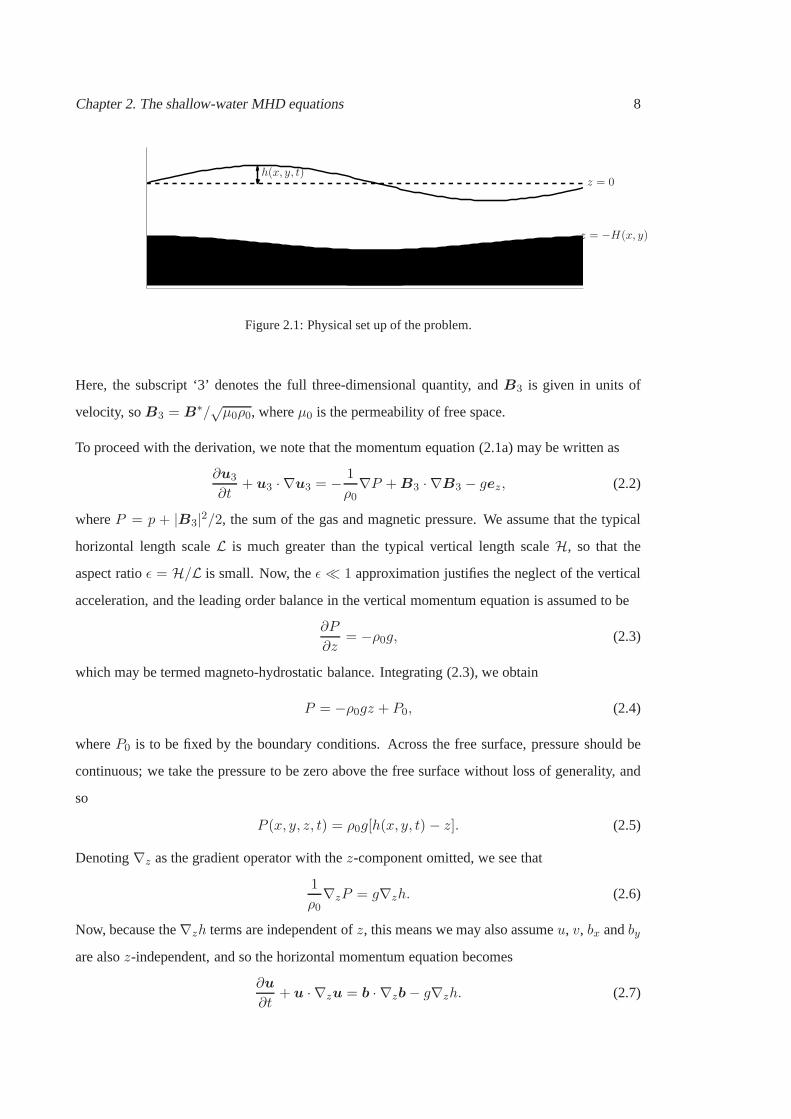
We consider a magneto-fluid with a free surface atz = h(x, y, t) with undisturbed free surface at
z = 0, lying over some topography (describing real topography, underlying dynamical effects or
otherwise)z = −H(x, y). The total fluid column height is given byht = H + h; see Figure 2.1.
We focus on dynamics at a sufficiently local level so that the Rossby number (measuring the
relative importance between inertia and rotational effects) is large, so that the Coriolis term is
relatively small and may be neglected as a simplification. The three-dimensional incompressible,
ideal MHD equations describing the dynamics of a thin layer of electrically conducting fluid of
constant densityρ, with gravitational acceleration, are given by
∂u3
∂t+ u3 · ∇u3 = − 1
ρ0∇p+ (∇×B3)×B3 − gez, (2.1a)
∂B3
∂t+ u3 · ∇B3 = B3 · ∇u3, (2.1b)
∇ · u3 = 0, (2.1c)
∇ ·B3 = 0. (2.1d)
Chapter 2. The shallow-water MHD equations 8
h(x, y, t)
z = −H(x, y)
z = 0
Figure 2.1: Physical set up of the problem.
Here, the subscript ‘3’ denotes the full three-dimensionalquantity, andB3 is given in units of
velocity, soB3 = B∗/√µ0ρ0, whereµ0 is the permeability of free space.
To proceed with the derivation, we note that the momentum equation (2.1a) may be written as
∂u3
∂t+ u3 · ∇u3 = − 1
ρ0∇P +B3 · ∇B3 − gez, (2.2)
whereP = p + |B3|2/2, the sum of the gas and magnetic pressure. We assume that the typical
horizontal length scaleL is much greater than the typical vertical length scaleH, so that the
aspect ratioǫ = H/L is small. Now, theǫ ≪ 1 approximation justifies the neglect of the vertical
acceleration, and the leading order balance in the verticalmomentum equation is assumed to be
∂P
∂z= −ρ0g, (2.3)
which may be termed magneto-hydrostatic balance. Integrating (2.3), we obtain
P = −ρ0gz + P0, (2.4)
whereP0 is to be fixed by the boundary conditions. Across the free surface, pressure should be
continuous; we take the pressure to be zero above the free surface without loss of generality, and
so
P (x, y, z, t) = ρ0g[h(x, y, t) − z]. (2.5)
Denoting∇z as the gradient operator with thez-component omitted, we see that
1
ρ0∇zP = g∇zh. (2.6)
Now, because the∇zh terms are independent ofz, this means we may also assumeu, v, bx andby
are alsoz-independent, and so the horizontal momentum equation becomes
∂u
∂t+ u · ∇zu = b · ∇zb− g∇zh. (2.7)
Chapter 2. The shallow-water MHD equations 9
Hereu = (u, v) andb = (bx, by). The dependency in the vertical co-ordinatez does not appear
explicitly, which highlights an important feature of the shallow-water equations: if the fields are
initially depth independent, they will remain so for all subsequent time (e.g.,§2.3 of Salmon 1998
or §3.1 of Vallis 2006).
Now, integrating∇ · u3 = 0 over the fluid depth gives
[w]z=hz=−H = −ht∇z · u, (2.8)
with ht = H + h. Sincew is just the material derivative of the position of a particular element,
we have
[w]z=hz=−H =
(
∂
∂t+ u3 · ∇
)
[H + h(x, y, t)] =
(
∂
∂t+ u · ∇z
)
ht. (2.9)
Putting the two together, we obtain
∂ht∂t
+∇z · (htu) = 0. (2.10)
For the induction equation (2.1b), assumingbz is small compared tobx andby, there is only explicit
evolution of the horizontal magnetic field, with the governing equation given by
∂b
∂t+ u · ∇zb = b · ∇zu. (2.11)
Finally, from the condition∇ ·B3 = 0,
∂bz∂z
= −∇z · b. (2.12)
Integrating over the fluid depth gives
[bz]z=hz=−H = −ht∇z · b. (2.13)
We make two further additional assumptions. The lower boundary is taken to be a perfect
conductor, and it is assumed that the free surface starts offas a field line. By Alfven’s theorem,
field lines are frozen into the fluid, and the free surface thusremains a field line. The full three-
dimensional field should be locally parallel to the verticalboundaries. So, lettingn be the normal
vector to the vertical boundaries, we requireB3 · n = 0, and hence
(bx, by,−ht∇z · b) · (−∂h/∂x,−∂h/∂y, 1) = −∇z · (htb) = 0. (2.14)

Chapter 2. The shallow-water MHD equations 10
In summary, the single layer SWMHD equations in Cartesian co-ordinates are given by
∂u
∂t+ u · ∇u = b · ∇b− g∇h, (2.15a)
∂b
∂t+ u · ∇b = b · ∇u, (2.15b)
∂h
∂t+∇ · (htu) = 0, (2.15c)
∇ · (htb) = 0, (2.15d)
where the subscript on the gradient operator has been dropped. It will be seen later that the
divergence-free condition (2.15d), if satisfied initially, is preserved by the dynamics, and thus
serves as a constraint for the initial condition; hence we dohave five equations for five variables,
subject to a constraint. Note that it is∂h/∂t that appears sinceh is the only quantity inht =
H+h(x, y, t) that is time dependent. This set of equations is only dependent on the two horizontal
variables, but there is a vertical structure in thatw andbz are not necessarily zero, but are related
to the horizontal divergence ofu andb respectively.
It should be noted that a vector identity may be used to rewrite the induction equation (2.15b) in
the form
∂b
∂t= ∇× (u× b) + (∇ · u)b− (∇ · b)u. (2.16)
Neitheru or b are divergence-free by themselves; rather, it isu3 andB3, reconstructed from the
relations (2.8) and (2.13), that are divergence-free.
2.2 Properties
For completeness we provide an overview of the basic properties satisfied by the SWMHD
equations, highlighting some important points that will bediscussed in the later chapters.
2.2.1 Non-dimensional form
A common approach is to rescale the problem to obtain a non-dimensional set of equations. Taking
then
u → Uu, b → Bb, h→ Hh, (2.17)
Chapter 2. The shallow-water MHD equations 11
we shall also choose to scale time by the advective time rather than the Alfven time, so we also
have∂
∂t→ 1
T∂
∂t=
UL∂
∂t, ∇ → 1
L∇. (2.18)
Rescaling accordingly gives
∂u
∂t+ u · ∇u =M2
b · ∇b− 1
F 2∇h, (2.19a)
∂b
∂t+ u · ∇b = b · ∇u, (2.19b)
∂h
∂t+∇ · (htu) = 0, (2.19c)
∇ · (htb) = 0. (2.19d)
The two non-dimensional parameters are then the inverse Alfven-Mach numberM = B/U , a
measure of the relative importance of the Lorentz force termand the fluid inertia term, and the
Froude numberF = U/√gH, a measure of how strong gravity is (it will be seen thatF is related
to the speed of gravity waves). A further rescaling ofh→ F 2h results in the set of equations
∂u
∂t+ u · ∇u =M2
b · ∇b−∇h, (2.20a)
∂b
∂t+ u · ∇b = b · ∇u, (2.20b)
F 2 ∂h
∂t+∇ · (htu) = 0, (2.20c)
∇ · (htb) = 0, (2.20d)
whereht = H+F 2h is the total fluid depth. The Froude number now appears in the mass and flux
conservation equations rather than the momentum equations. The two-dimensional incompressible
MHD equations are recovered whenF = 0, H = 1 (with h identified with the pressurep).
Furthermore, the hydrodynamic equations are obtained whenM = 0.
To get a rough estimate ofM andF for the tachocline we use the parameters given in Table 1.1.
We take the typical velocity and length scales as
T =Ωpole+Ωequator
2, L = 2π × 0.7Rsun ⇒ U =
L
T≈ 1.3× 105 cm s−1 (2.21)
We first estimateM . There is some uncertainty in the magnetic field strengthB∗ in the tachocline,
but a likely range is103G . B∗ . 105G. This leads to
B =B∗
√µ0ρ0
cm s−1 ≈ 2.2× 10³−5 cm s−1, (2.22)
Chapter 2. The shallow-water MHD equations 12
and so we have
0.01 .M . 1. (2.23)
For the Froude number, instead of just takingH and work outF = U/√gH, we consider a
slightly different approach that is often employed in geophysical fluid dynamics; this approach
was also the one adopted by, for example, Dikpati & Gilman (2001). In the hydrodynamic case,
there is a formal analogy between linearised shallow-watersystem and the linearised primitive
equations, and the shallow-water gravity waves√gH0 correspond to the fastest gravity waves in
the continuously stratified case, given byNH1/π (e.g., Gill, 1982,§6.11). TakingH1 = 0.03Rsun,
this impliesNH1/π ≈ 5× 105 cm s−1, and thus giving
F ≈ 0.25. (2.24)
The equivalent depthH0 in this case is approximately5× 106 cm (or50 km).
This implies that the large-scale magnetic field is weak relative to the large-scale flow, and that
the system is strongly constrained by stratification effects. Although we have estimates forF and
M for the tachocline, we will not restrict ourselves to these parameters as we are interested in the
more general shear flow instability problem.
2.2.2 Conserved quantities
In line with the domain set up considered later, we consider the case where the domain is periodic
in x and bounded by perfectly conducting impermeable walls iny, with no underlying topography
(soH = 1). Now we haveht = 1 + F 2h, we first note that integrating the divergence-free
condition (2.20d) over the domain leads to the restriction
[htby]y=Ly
y=−Ly= 0. (2.25)
This is satisfied for example if we take no normal flux boundaryconditions
by = 0 on y = ±Ly. (2.26)
This, together with no normal flow boundary conditions
v = 0 on y = ±Ly, (2.27)

Chapter 2. The shallow-water MHD equations 13
implies the condition∂h
∂y= 0 on y = ±Ly (2.28)
from they-component of the momentum equation. We then have the following conservation laws:
Mass conservation
d
dt
∫∫
ht dxdy = −∫∫
∇ · (htu) dxdy = 0, (2.29)
since the domain is periodic inx andv = 0 on they-boundaries.
Momentum conservation
d
dt
∫∫
htu dxdy =−∫∫ [
∇ · (htuu) + ht∂h
∂x
]
dxdy −M2
∫∫
bx∇ · (htb) dxdy
=−∫∫
∂
∂x
(
F 2h2
2+ h
)
dxdy = 0,
(2.30)
owing to periodicity inx, andv = 0 as well asby = 0 on they-boundaries. Note that the
divergence-free condition (2.15d) is required for momentum conservation.
d
dt
∫∫
htv dxdy =−∫∫ [
∇ · (htvu) + ht∂h
∂y
]
dxdy −M2
∫∫
by∇ · (htb) dxdy
=−∫∫
∂
∂y
(
F 2h2
2+ h
)
dxdy
=−∫ [
F 2h2
2+ h
]+Ly
−Ly
dx,
(2.31)
again, owing to periodicity, andv = 0 as well asby = 0 on they-boundaries. As above, the
divergence-free condition (2.15d) is again required for conservation. The loss ofy-momentum
conservation here is related to the fact that we no longer have translational invariance iny. In
the incompressible limitF = 0, the extra contribution happens to vanish as long as there isno
net difference in the mean pressure on the side walls. We notein passing that the presence of
underlying topography also results in extra contributionsto the momentum budget.
Flux conservation
Similar to the above manipulations, we have
d
dt
∫∫
htbx dxdy = −∫∫
∇ · (htbxu) dxdy −∫∫
u∇ · (htb) dxdy = 0, (2.32)
Chapter 2. The shallow-water MHD equations 14
and
d
dt
∫∫
htby dxdy = −∫∫
∇ · (htbyu) dxdy −∫∫
v∇ · (htb) dxdy = 0, (2.33)
using periodicity inx, v = 0 andby = 0 on they-boundaries. The divergence-free condition
(2.15d) is again necessary for conservation.
Total energy conservation
The total energy of the system evolves as
1
2
d
dt
∫∫
[
ht(|u|2 +M2|b|2) + F 2h2]
dxdy
=−∫∫
∇ ·
htu
( |u|2 +M2|b|22
+ h
)
dxdy
+M2
∫∫
htb · ∇ (ubx + vby) dxdy,
(2.34)
where the energy contributions on the left hand side of (2.34) are the kinetic energy, the magnetic
energy, and the potential energy; notice that the kinetic and magnetic energy is multiplied by the
total height and is cubic in nature, whereas the potential energy only involves the deviation from
the rest state. In the incompressible limitF = 0, the potential energy contribution disappears,
whilst in the hydrodynamic limitM = 0, the magnetic contribution disappears. The first integral
vanishes because of periodicity andv = 0 on the boundaries. Performing an integration by parts
on the second integral,
∫∫[
htbx∂
∂x(ubx + vby)
]
dxdy = [htbx(ubx + vby)]x=Lx
x=0 + [htby(ubx + vby)]y=Ly
y=−Ly
−∫∫
(ubx + vby)∇ · (htb) dxdy = 0,
(2.35)
owing to periodicity,by = 0 on the boundary, and the divergence free condition. Thus thetotal
energy is conserved.
Divergence-free condition
All of the above conservation laws as written depend crucially on the fact that the divergence-free
condition of the magnetic field (2.20d) holds for all time. Itis therefore important to verify that
the governing equation preserves this divergence-free condition during the evolution. This may
Chapter 2. The shallow-water MHD equations 15
be shown by a brute force calculation by considering the timederivative of∇ · (htb) and using
the remaining equations as appropriate (index notation here is useful). A cleaner way to show this
(due to Sam Hunter, private communication) is to observe that
∇× (u× htb) = htb · ∇u− htb(∇ · u)− u · ∇(htb) + u[∇ · (htb)]
= htb · ∇u− htu · ∇b− b[∇ · (htu)] + u[∇ · (htb)]
= ht∂b
∂t+ b
∂ht∂t
+ u[∇ · (htb)]
=∂
∂t(htb) + u[∇ · (htb)],
(2.36a)
so∂
∂t∇ · (htb) = ∇ · [∇× (· · · ) + u(∇ · (htb))]. (2.36b)
The divergence of a curl is zero, and so ifhtb is divergence free att = 0, the subsequent evolution
will keep the fields divergence free. Another way to show thisproperty is to observe that the
induction equation may be written as
∂(htb)
∂t+∇ · (htub− htbu) = 0, (2.37)
as in De Sterck (2001), using the tensor notation(ub)ij = uibj . Taking a divergence also shows
that the divergence-free condition is preserved in time by the dynamics.
Equations in transport variables
Another equivalent and potentially useful way of writing the SWMHD equations is in terms of the
transport variables(U ,B, h) = (htu, htb, h). Equations given by (2.20) may then be written as
∂U
∂t+∇ ·
(
UU
ht−M2BB
ht
)
+ ht∇h = 0, (2.38a)
∂B
∂t+∇ ·
(
UB
ht− BU
ht
)
= 0, (2.38b)
F 2 ∂h
∂t+∇ ·U = 0, (2.38c)
∇ ·B = 0. (2.38d)
We have used the divergence-free condition implicitly whenwriting the equations in this form.
The remainingh terms may also be included in the divergence term if there is no underlying
topography. Then it may be checked that mass, momentum, flux and energy conservation are as

Chapter 2. The shallow-water MHD equations 16
before by using the analogous boundary conditions given by
V = 0, By = 0 and∂h
∂y= 0 on y = ±Ly. (2.39)
This shows that, at least in the ideal case, we have the expected conservation laws. We will be
interested in solving the SWMHD equations numerically to investigate the nonlinear evolution in
due course. It will be seen that there are some subtle issues regarding the choice of solving the
equations in velocity or transport variables and the dissipation terms that are to be inserted. In the
ideal case there is no big difference between the two formulations; we will use the velocity variable
formulation in the linear analysis and discuss why we might want to use the transport variable
formulation over the velocity variable formulation in the numerical investigation in Chapter 7.
Other quantities and their associated conservation laws
In the shallow-water system withM = 0, the potential vorticity
q =ω
ht, ω =
∂v
∂x− ∂u
∂y, (2.40)
is materially conserved, satisfyingDq/Dt = 0, with D/Dt = ∂/∂t + u · ∇. WhenM 6= 0
however this is no longer true, as the Lorentz force term is generally rotational. Instead, it is the
flux functionhtb = ez ×∇A that is materially conserved, satisfyingDA/Dt = 0.
The SWMHD system also possesses a Hamiltonian structure, asdemonstrated by Dellar (2002).
Choosing the state variables, constructing the Hamiltonian and equipping it with a Poisson bracket
(with associated Poisson tensor), conserved quantities may be derived in a systematic manner.
Furthermore, the representation is in fact a non-canonicalone, and as such there are extra Casimir
invariants that corresponds to non-trivial conservation laws; in this case the Casimir invariants are
related to the flux functionA. One notable invariant that the Hamiltonian formulation reveals is
the global cross-helicity given by∫∫
htu · b dxdy, (2.41)
again, the condition (2.20d) is necessary for conservation.
2.2.3 Waves
The type of waves supported by the SWMHD equations, including the effect of rotation, have
been previously investigated (Schecteret al., 2001; Zaqarashiviliet al., 2008; Heng & Spitkovsky,
Chapter 2. The shallow-water MHD equations 17
2009). To obtain the dispersion relation governing wave motion, we consider again the simplified
case where the equations are posed in a channel, with no topography, and take as basic state
u0 = ex, b0 = ex, h = 0. (2.42)
Linearising about this basic state, we obtain
∂u
∂t+∂u
∂x−M2 ∂bx
∂x+∂h
∂x= 0, (2.43a)
∂v
∂t+∂v
∂x−M2∂by
∂x+∂h
∂y= 0, (2.43b)
∂bx∂t
+∂bx∂x
− ∂u
∂x= 0, (2.43c)
∂by∂t
+∂by∂x
− ∂v
∂x= 0, (2.43d)
F 2
(
∂h
∂t+∂h
∂x
)
+∂u
∂x+∂v
∂y= 0. (2.43e)
The boundary conditionsv = by = ∂h/∂y = 0 suggest we consider solutions of the form
(u, bx, h) = (u0, bx,0, h0) cos(nπy
L
)
ei(kx−ωt), (2.44a)
(v, by) = (v0, by,0) sin(nπy
L
)
ei(kx−ωt), (2.44b)
which leads to the algebraic system
k − ω 0 −kM2 0 k
0 k − ω 0 −kM2 inπ/L
−k 0 k − ω 0 0
0 −k 0 k − ω 0
k −inπ/L 0 0 F 2(k − ω)
u0
v0
bx,0
by,0
h0
= 0. (2.45)
The dispersion relation is then
(k − ω)[(k − ω)2 − k2M2]
[
F 2(k − ω)2 − F 2k2M2 − k2 − n2π2
L2
]
= 0. (2.46)
The first bracket corresponds to theu0 = v0 = 0 case which is not a wave mode of interest
here. The second bracket is associated with the Alfven branch which has dispersion relation and
eigenfunctions given by
ωA = k ±Mk, u = ∓bx, v = ∓by, h = 0. (2.47)

Chapter 2. The shallow-water MHD equations 18
The last bracket is associated with magneto-gravity waves.The dispersion relation is given by
ωmg = k ±√
k2 + F 2M2k2 + n2π2/L2
F, (2.48a)
and the eigenfunctions are given by
u =± h0Fk√
k2 + F 2M2k2 + n2π2/L2
k2 + n2π2/L2cos(nπy
L
)
cos(kx− ωt),
v =∓ h0F (nπ/L)
√
k2 + F 2M2k2 + n2π2/L2
k2 + n2π2/L2sin(nπy
L
)
sin(kx− ωt),
bx =− h0k2F 2M
k2 + n2π2/L2cos(nπy
L
)
cos(kx− ωt),
by =h0k(nπ/L)F 2M
k2 + n2π2/L2sin(nπy
L
)
sin(kx− ωt),
h =h0 cos(nπy
L
)
cos(kx− ωt).
(2.48b)
WhenF → 0, we see that the gravity waves become infinitely fast and are effectively filtered out
of the system. These exact wave solutions are used later in Chapter 7 as a check for the numerical
routines.

19
Chapter 3
Linear theory: eigenvalue problem and
general theorems
3.1 Linearisation and eigenvalue problem
The non-dimensional SWMHD equations are given by
∂u
∂t+ u · ∇u = −∇h+M2
b · ∇b, (3.1a)
∂b
∂t+ u · ∇b = b · ∇u, (3.1b)
F 2∂h
∂t+∇ · (htu) = 0, (3.1c)
∇ · (htb) = 0, (3.1d)
whereht = H + F 2h is the total fluid depth. For the linear problem considered here, the basic
state and perturbation are chosen to satisfy the divergencefree condition (3.1d), so it need not be
considered explicitly. Above a topography of the formH(y), we consider a basic state
h = 0, u = U0(y)ex and b = B0(y)ex, (3.2)
so that the basic magnetic field profile is initially aligned with the basic flow profile. We then
consider perturbations inh, u = (u, v) andb = (bx, by) to this basic state. The linear evolution is
Chapter 3. Linear theory: eigenvalue problem and general theorems 20
then described by
(
∂
∂t+ U0
∂
∂x
)
u+ U ′0v = −∂h
∂x+M2
(
B0∂bx∂x
+B′0by
)
, (3.3a)(
∂
∂t+ U0
∂
∂x
)
v = −∂h∂y
+M2B0∂by∂x
, (3.3b)(
∂
∂t+ U0
∂
∂x
)
bx +B′0v = U ′
0by +B0∂u
∂x, (3.3c)
(
∂
∂t+ U0
∂
∂x
)
by = B0∂v
∂x, (3.3d)
F 2
(
∂
∂t+ U0
∂
∂x
)
h+H
(
∂u
∂x+∂v
∂y
)
+H ′v = 0, (3.3e)
where a prime denotes differentiation with respect toy.
Since the coefficients of the system of linear PDEs given by (3.3) are only functions ofy, we may
consider modal solutions of the form
ξ(x, y, t) = Reξ(y) exp[iα(x− ct)], (3.4)
whereα is the (real) wavenumber andc is the phase speed, so thatω = αc is the wave frequency.
We shall be considering a temporal analysis in whichα is real andc = cr+ ici is complex; we then
observe that such a modal solution grows likeexp(αcit). Equations (3.3) reduce to an eigenvalue
problem given by the following system of equations, after dropping the hatted notation,
iα(U0 − c)u+ vU ′0 = −iαh+M2(B′
0by + iαB0bx), (3.5a)
iα(U0 − c)v = −h′ + iαM2B0by, (3.5b)
iα(U0 − c)bx − U ′0by = iαB0u−B′
0v, (3.5c)
iα(U0 − c)by = iαB0v, (3.5d)
iα(U0 − c)F 2h+ iαu+ (Hv)′ = 0. (3.5e)
This system may in fact be reduced to a single second order ODE. Eliminating in favour ofv gives
a single governing differential equation given by
[
S2(Hv)′
(U0 − c)2HK2
]′
−[
α2S2
H(U0 − c)2− U ′
0
H(U0 − c)
(
S2
(U0 − c)2K2
)′
+Q′
0S2
(U0 − c)3K2
]
Hv = 0,
(3.6)
whereQ0 = −U ′0/H is the background potential vorticity, and
S2(y) = (U0(y)− c)2 −M2B20(y), K2(y) = 1− F 2S2(y). (3.7)

Chapter 3. Linear theory: eigenvalue problem and general theorems 21
We note that equation (3.6) remains unchanged underα → −α, so we may therefore takeα ≥ 0
without loss of generality; thus unstable modes haveci > 0. The ODE (3.6) may be singular in
the domain ifc is purely real; here, we shall be interested only in instabilities, so this will not be
an issue.
The eigenvalue equation (3.6) may be cast into a more compactform. Following Howard (1961),
we consider the transformationHv = (U0 − c)nG. Equation (3.6) then becomes[
(U0 − c)2nΣ2
HK2G′
]′
− α2(U0 − c)2nΣ2G
H
+ (n − 1)
[
U ′0(U0 − c)2n−1Σ2
(K2)′+ n
(U ′0)
2(U0 − c)2n−2Σ2
K2− Q′
0(U0 − c)2n−1Σ2
HK2
]
G
H= 0.
(3.8)
We see that takingn = 1 gives us the much simplified equation[
S2
K2
G′
H
]′
− α2S2G
H= 0, (3.9)
which we shall use for the remainder of the linear analysis. In the shallow-water, hydrodynamic
limit (M = 0), equation (3.6) reduces to equation (3.4) of Balmforth (1999). In the two-
dimensional incompressible MHD limit (F = 0 andH = 1), (3.9) reduces to equation (3.5)
of Hughes & Tobias (2001).
We will consider equation (3.9) in either an unbounded domain, for which |G| → 0 as|y| → ∞,
or in a bounded domain with rigid side walls, whereG = 0. Either way, for given realα, (3.9) is
then an eigenvalue problem for the unknown phase speedc = cr + ici.
In the hydrodynamic case (M = 0), there is an analogy between the shallow-water equations and
the compressible Euler equations (e.g., Vallis 2006,§3.1, or Buhler 2009,§1.6). We may thus draw
on the previous results of shear instabilities in the compressible hydrodynamic system in order to
compare with our results.
3.2 Growth rate bound
A bound on the instability growth rate may be obtained by manipulating equations (3.3) in a
manner analogous to that adopted by, for example, Griffiths (2008). The rate of change of the total
disturbance energy is given by the combination
Hu∗ × (3.3a)+Hv∗ × (3.3b)+ (M2Hb∗x)× (3.3c)+ (M2Hb∗y)× (3.3d)+ h× (3.3e),

Chapter 3. Linear theory: eigenvalue problem and general theorems 22
where∗ denotes complex conjugate. On adopting the form (3.4) for the perturbations, the real part
of this expression gives
αci[
H(
|u|2 + |v|2 +M2|bx|2 +M2|by|2)
+ F 2|h|2]
=
− Re[
HU ′0
(
vu∗ −M2b∗xby)
+M2HB′0 (vbx − u∗by)
]
− Re∂
∂y(Hvh∗).
(3.10)
On integrating over they domain, employing the boundary condition onv, and manipulating the
remaining terms on the right hand side using the fact that±2Re(pq∗) ≤ |p|2 + |q|2 yields
αci
∫
E dy ≤ 1
2(max |U ′
0|+M max |B′0|)∫
H(
|u|2 + |v|2 +M2|bx|2 +M2|by|2)
dy (3.11)
with E is equal to the square bracket quantity on the left hand side of equation (3.10). Adding an
extraF 2|h|2 term to the integrand on the right hand side respects the inequality, so we obtain the
following bound on the growth rate:
αci ≤1
2(max |U ′
0|+M max |B′0|). (3.12)
Thus the growth rate of a modal solution is bounded above by the average of the maximum shear
and the maximum current. In the absence of a magnetic field, this reduces to the well-known
bound in hydrodynamics (Høiland, 1953; Howard, 1961).
3.3 Semicircle theorems
In a classic paper, Howard (1961) proved that, for incompressible, hydrodynamic parallel shear
flows, the wave speedc of any unstable mode must lie within a semi-circle in the complex
plane determined by properties of the basic state flow. Subsequently, semi-circle theorems have
been derived for several other hydrodynamical and hydromagnetic systems (e.g., Kochar & Jain,
1979a,b; Collings & Grimshaw, 1980; Watson, 1981; Hayashi &Young, 1987; Shivamoggi &
Debnath, 1987; Thuburn & Haynes, 1996; Hughes & Tobias, 2001; Zaqarashiviliet al., 2010). In
a similar manner, semi-circle theorems may be derived for the SWMHD system.
Multiplying equation (3.9) byG∗, integrating overy and using the boundary conditions gives the∫
S2
K2
|G′|2H
dy + α2
∫
S2|G|2H
dy = 0. (3.13)
The imaginary part of (3.13) gives
ci
∫
(U0 − cr)χ dy = 0, where χ =|G′|2H|K|4 + α2 |G|2
H≥ 0. (3.14)

Chapter 3. Linear theory: eigenvalue problem and general theorems 23
Equation (3.14) immediately yields Rayleigh’s result that, for unstable modes,cr lies in the range
of U0 (i.e.U0,min ≤ cr ≤ U0,max). Note this formal bound is independent ofF .
On using equation (3.14), the real part of (3.13) gives
(c2r + c2i )
∫
χ dy =
∫
χ(
U20 −M2B2
0
)
dy − F 2
∫ |S|4H|K|4 |G
′|2 dy, (3.15)
which implies that
0 ≤ (c2r + c2i )
∫
χ dy ≤(
U20 −M2B2
0
)
max
∫
χ dy. (3.16)
Thus the complex wave speedc of an unstable eigenfunction must lie within the semi-circle
defined by
(c2r + c2i ) ≤(
U20 −M2B2
0
)
max. (3.17)
Another semi-circle bound may be obtained, by using the inequality
0 ≥∫
(U0 − U0,max)(U0 − U0,min)χ dy.
Substituting from (3.14), deriving an inequality from (3.15) and dropping the integral multiplying
F 2 leads to the expression
0 ≥[
c2r + c2i − (U0,min + U0,max)cr + U0,minU0,max +M2(B2)min
]
∫
χ dy, (3.18)
which gives another semi-circle bound: the speedc of an unstable eigenfunction must lie within
the region defined by
[
cr −U0,min + U0,max
2
]2
+ c2i ≤[
U0,max − U0,min
2
]2
−M2(B2)min. (3.19)
Thus, taking these results together, the eigenvaluec of an unstable mode must lie within the
intersection of the two semi-circles defined by (3.17) and (3.19). In the absence of magnetic field,
semi-circle (3.19) lies wholly within semi-circle (3.17),and we recover the well-known result of
Howard (1961).
A drawback of the above approach is that the bounds do not contain the Froude numberF . It
is possible to includeF into the semi-circle bounds using similar manipulations tothat used by
Pedlosky (1964), but this does not tighten the bounds; see the Section 3.5 for details.
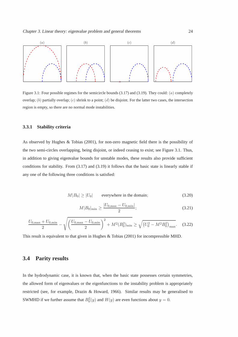
Chapter 3. Linear theory: eigenvalue problem and general theorems 24
(a) (b) (c) (d)
Figure 3.1: Four possible regimes for the semicircle bounds(3.17) and (3.19). They could:(a) completely
overlap;(b) partially overlap;(c) shrink to a point;(d) be disjoint. For the latter two cases, the intersection
region is empty, so there are no normal mode instabilities.
3.3.1 Stability criteria
As observed by Hughes & Tobias (2001), for non-zero magneticfield there is the possibility of
the two semi-circles overlapping, being disjoint, or indeed ceasing to exist; see Figure 3.1. Thus,
in addition to giving eigenvalue bounds for unstable modes,these results also provide sufficient
conditions for stability. From (3.17) and (3.19) it followsthat the basic state is linearly stable if
any one of the following three conditions is satisfied:
M |B0| ≥ |U0| everywhere in the domain; (3.20)
M |B0|min ≥ |U0,max − U0,min|2
; (3.21)
U0,max + U0,min
2−
√
(
U0,max − U0,min
2
)2
+M2(B20)min ≥
√
(
U20 −M2B2
0
)
max. (3.22)
This result is equivalent to that given in Hughes & Tobias (2001) for incompressible MHD.
3.4 Parity results
In the hydrodynamic case, it is known that, when the basic state possesses certain symmetries,
the allowed form of eigenvalues or the eigenfunctions to theinstability problem is appropriately
restricted (see, for example, Drazin & Howard, 1966). Similar results may be generalised to
SWMHD if we further assume thatB20(y) andH(y) are even functions abouty = 0.

Chapter 3. Linear theory: eigenvalue problem and general theorems 25
Following Howard (1963), whenU(y) is odd abouty = 0, we notice that (3.9) is unchanged
underc → −c andG(y) → G(−y). By considering the conjugate equation, we see that an
unstable eigenfunction must be accompanied by eigenvaluesof the formc = ±cr± ici, so unstable
solutions are either standing waves (cr = 0) or a pair of counter-propagating waves with the same
phase speed. As argued by Howard (1963), the symmetry in the basic state implies there is no
preferred direction for wave propagation, consistent withthe form the eigenvalues are allowed to
take.
Now consider the case whenU(y) is even abouty = 0. Then it is seen that
Ge(y) =1
2[G(y) +G(−y)] and Go(y) =
1
2[G(y)−G(−y)] (3.23)
are also eigenfunctions of (3.9). If we now takeGo multiplied by (3.9) withG = Ge, and subtract
fromGe multiplied by (3.9) withG = Go, integrating over they-domain gives
[G′eGo −G′
oGe]Ly
−Ly= 0, (3.24)
owing to the imposed boundary conditions on the eigenfunction. The Wronskian ofGe andGo is
equal to zero implies that the two functions are linearly dependent throughout the domain. This
cannot be the case so one of them is identically zero, and therefore we conclude the eigenfunction
corresponding to a particular eigenvalue is either an even or odd function abouty = 0.
3.5 Discussion
Equation (3.8) for other values ofn
Here and in later chapters, we consider then = 1 case in equation (3.8), leading to equation (3.9)
from which we obtain the semi-circle theorems and parity results. Howard (1961) noticed that
by taking different values ofn, notably then = 0 andn = 1/2 cases, different results could be
obtained.
In the absence of MHD effects, then = 0 case does indeed give us a generalisation of Rayleigh’s
criterion for theF = 0 case, as noted already by Balmforth (1999). When MHD effectsare
present, the usual manoeuvre (e.g., Drazin & Reid, 1981,§22) gives an expression involvingc
which needs to change sign over the domain for there to be an instability (e.g., Hughes & Tobias,

Chapter 3. Linear theory: eigenvalue problem and general theorems 26
2001). This is of minimal use since we need to solve the full problem before we can use the
criterion.
A different approach may yet give stability theorems. A method due initially to Arnol’d (1966a)
considers using wave activity invariants and deducing formal stability results that can, in certain
cases, be extended to nonlinear stability. Briefly, following Shepherd (1990), we consider the non-
canonical Hamiltonian representation of a system (fluid systems written in the Eulerian formalism
generally require the non-canonical representation), given by
∂u
∂t= J
δHδu, (3.25)
whereu is the state vector,H is the Hamiltonian functional, andJ is the symplectic (Poisson)
operator. In the canonical representation,u = (p, q), wherep and q are the generalised co-
ordinates (usually momentum and position), and we see that
J =
−1 0
0 1
. (3.26)
The benefit with using the non-canonical representation is that it makes explicit the Casimir
invariants associated with the kernel ofJ. For example, in two-dimensional incompressible
hydrodynamics, the Casimirs are functions of vorticity. ByNoether’s theorem, conservation laws
are associated with symmetries (and vice-versa), and in theincompressible hydrodynamic system,
the Casimirs are associated with the particle relabelling symmetry (e.g., Salmon, 1998,§7). In the
hydrodynamic shallow-water system, the Casimirs areC =∫
f(q) dS, wheref is an arbitrary
function of the potential vorticityq (e.g., Shepherd, 1990); in the SWMHD system, the Casimirs
are of the form
C =
∫
[f(A) + htg(A)] dS, (3.27)
whereht = H + F 2h, andf and g are arbitrary functions of the flux functionA, defined as
htb = e×∇A (Dellar, 2002).
The observation then is that, for a steady basic stateU0, we have
∂U0
∂t= J
δHδu
∣
∣
∣
∣
u=U0
= 0. (3.28)
Now, the Hamiltonian functionalH and the Casimir functionalC are both invariants of the system,
and so we haveδHδu
∣
∣
∣
∣
u=U0
= − δCδu
∣
∣
∣
∣
u=U0
(3.29)

Chapter 3. Linear theory: eigenvalue problem and general theorems 27
where the minus sign is by convention, and from this we may work out the Casimir functionalsC.
Then we construct the wave activity functional
A(u) = H(u)−H(U0) + C(u)− C(U0), (3.30)
which is an invariant of the dynamics;A here is sometimes called the pseudo-energy.Amay be further augmented by other conserved functionals, such as along-stream momentum
(relevant here for the shear flow problem). The point is that,under the small amplitude
approximation, this quantity can serve as a Hamiltonian forthe linearised dynamics, act as
a norm to measure disturbance growth, and hence provide a means to obtain formal stability
criteria for linear stability. Furthermore, it is usually quadratic, and so in certain cases, additional
convexity estimates can result in nonlinear, Lyapunov-type stability criteria. In the incompressible
hydrodynamic case for plane parallel shear flows, it was shown that Rayleigh’s condition comes
from considering the pseudo-energy (e.g., Salmon, 1998,§7), whilst the Rayleigh–Fjørtoft
condition comes from augmenting the pseudo-energy with an additional momentum functional.
These may also be promoted to nonlinear stability conditions and appear as special cases of
Arnol’d’s theorems.
The idea of using wave activity invariants in various disguises has been employed previously by
various authors (e.g., Taylor, 1915; Blumen, 1970; Satomura, 1981; Eliassen, 1983; Ripa, 1983).
The advantage of using the Hamiltonian structure is that wave activities may be derived in a
systematic manner, as well as making obvious the links with the underlying structure of the system
of equations and its associated symmetries/conservation laws. There have been several works that
invoke the Hamiltonian structure explicitly (e.g., Holmet al., 1985; McIntyre & Shepherd, 1987;
Dritschel, 1988; Shepherd, 1990, 1992; Vladimirov & Moffatt, 1995; Vladimirovet al., 1996;
Nycander, 2003; Shepherd, 2003), and it would certainly be worth investigating whether such a
procedure can yield a result for the SWMHD system.
For then = 1/2 case, using manipulations similar to Chimonas (1970), the growth rate bound
(3.12) may be obtained. The method used in the main body of this chapter is substantially cleaner
and more intuitive, and since we do not obtain a new result, a presentation of the working has been
omitted.
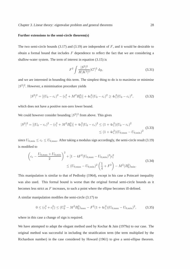
Chapter 3. Linear theory: eigenvalue problem and general theorems 28
Further extensions to the semi-circle theorem(s)
The two semi-circle bounds (3.17) and (3.19) are independent of F , and it would be desirable to
obtain a formal bound that includesF dependence to reflect the fact that we are considering a
shallow-water system. The term of interest in equation (3.15) is
F 2
∫ |S2|2H|K2|2 |G
′|2 dy, (3.31)
and we are interested in bounding this term. The simplest thing to do is to maximise or minimise
|S2|2. However, a minimisation procedure yields
|S2|2 = [(U0 − cr)2 − (c2i +M2B2
0)] + 4c2i (U0 − cr)2 ≥ 4c2i (U0 − cr)
2, (3.32)
which does not have a positive non-zero lower bound.
We could however consider bounding|S2|2 from above. This gives
|S2|2 = [(U0 − cr)2 − (c2i +M2B2
0)] + 4c2i (U0 − cr)2 ≤ (1 + 4c2i )(U0 − cr)
2
≤ (1 + 4c2i )(U0,max − U0,min)2
(3.33)
sinceU0,min ≤ cr ≤ U0,max. After taking a modulus sign accordingly, the semi-circle result (3.19)
is modified to(
cr −U0,max + U0,min
2
)2
+ [1− 4F 2(U0,max − U0,min)2]c2i
≤ (U0,max − U0,min)2
(
1
4+ F 2
)
−M2(B20)min.
(3.34)
This manipulation is similar to that of Pedlosky (1964), except in his case a Poincare inequality
was also used. This formal bound is worse than the original formal semi-circle bounds as it
becomes less strict asF increases, to such a point where the ellipse becomes ill-defined.
A similar manipulation modifies the semi-circle (3.17) to
0 ≤ (c2r + c2i ) ≤ (U20 −M2B2
0)max − F 2(1 + 4c2i )(U0,max − U0,min)2, (3.35)
where in this case a change of sign is required.
We have attempted to adapt the elegant method used by Kochar &Jain (1979a) to our case. The
original method was successful in including the stratification term (the term multiplied by the
Richardson number) in the case considered by Howard (1961) to give a semi-ellipse theorem.
Chapter 3. Linear theory: eigenvalue problem and general theorems 29
Similar approaches have been tried here and we were unsuccessful in generating something similar
for the shallow-water or MHD cases. The method of Barston (1980) has also been attempted
(working in the Lagrangian formulation and considering relevant supremum or infimum of the
associated operators) but nothing new has been derived fromemploying that formalism.

Chapter 3. Linear theory: eigenvalue problem and general theorems 30

31
Chapter 4
Instabilities of piecewise-constant
profiles
There are many variations of the shear flow instability problem that may be studied, with different
profiles of the magnetic field, parameter values, and so forth. We restrict ourselves to the simpler
case where there is no topography (H = 1) and the background magnetic field is uniform (B0 = 1,
so thatM is now our measure of the field strength). This simplifies the problem somewhat and in
certain limits reduces to problems that have been previously studied in the incompressible and/or
hydrodynamic case. With these restrictions, equation (3.9) becomes[
S2
K2G′
]′
− α2S2G = 0, (4.1)
where, again,S2 = (U0 − c)2 −M2, andK2 = 1 − F 2S2. We seek solutions in an unbounded
domain, with
|G| → 0 as |y| → ∞. (4.2)
We consider velocity profilesU0(y) that are piecewise-constant. In addition to allowing for the
problem to be solved analytically, such profiles usually reveal some features that are present in the
analogous smooth profiles, which we consider in Chapter 5.
If U0(y) is discontinuous aty = y0, then the eigenfunctionG must satisfy two jump conditions
at y = y0. In the usual way (e.g., Drazin & Reid, 1981,§23), denotingη to be the cross-stream
displacement (sov = Dη/Dt), the (linearised) kinematic boundary condition implies
[η]y+0
y−0
=
[
v
U0 − c
]y+0
y−0
= [G]y+0
y−0
= 0. (4.3a)

Chapter 4. Instabilities of piecewise-constant profiles 32
The free surface displacement (and so pressure) must also becontinuous aty = y0. The
corresponding condition onG is most easily derived by integrating (4.1) acrossy = y0, yielding
[
S2
K2G′
]y+0
y−0
= 0. (4.3b)
4.1 Vortex sheet
We first consider the velocity profile
U0(y) =
+1, y > 0,
−1, y < 0.
Then, fory 6= 0, (4.1) becomesG′′ − α2K2G = 0. Using (4.2) and (4.3a), we thus find
G(y) =
exp (−αK+y) , y > 0,
exp (+αK−y) , y < 0,
(4.4)
where
K± =√
1− F 2[(1∓ c)2 −M2], Re(K±) > 0. (4.5)
The second jump condition (4.3b) then implies an eigenvaluerelation forc:
(1− c)2 −M2
K++
(1 + c)2 −M2
K−= 0. (4.6)
Note thatc is independent of wavenumberα, so any unstable mode withci > 0 has an unbounded
growth rate asα → ∞. This is an artefact of considering ideal fluids; viscosity will act
preferentially on small scales and remove this unphysical behaviour.
There are several special cases. WhenF = M = 0, we recover the classical Kelvin–Helmholtz
instability with c = ±i. WhenF = 0 but M 6= 0, (4.6) reduces to the incompressible MHD
case withc2 = −(1 −M2), a result due to Michael (1953). The Kelvin–Helmholtz instability
is stabilized whenM ≥ 1, which might be expected physically as the disturbance has to do
work to bend the field lines. WhenM = 0 but F 6= 0, we obtain the classical hydrodynamic
shallow-water case, which is analogous to two-dimensionalcompressible hydrodynamics. The
Kelvin–Helmholtz instability is stabilized whenF ≥√2 (Bazdenkov & Pogutse, 1983; Miles,
1958), which might be expected physically as the disturbance has to do work to move the free
surface against gravity. Thus, increasingF orM in the absence of the other is stabilising.

Chapter 4. Instabilities of piecewise-constant profiles 33
F
M
ci
(4.9)(4.9)
000
1
1
1
√2
2
3
4
5
0.1
0.20.3
0.4
0.5
0.5
0.5
0.6 0.70.80.9
Figure 4.1: Contours of Im(cv) given by the expression (4.8), with stability boundaries (4.9).
In the general case whereF andM are both non-zero, (4.6) can be rearranged and squared to yield
c2(1 + c2 −M2)− F 2[(1− c)2 −M2][(1 + c)2 −M2] = 0. (4.7)
Here we will ignore the degenerate case withc = 0 that occurs whenM = 1. We have checked
numerically that only two roots of (4.7) also satisfy (4.6);they arec = ±cv, where
cv = i
[√1 + 4F 2 + 4F 4M2 − (1 + F 2 + F 2M2)
F 2
]1/2
. (4.8)
Note that Re(cv) = 0. A contour plot of Im(cv) is shown in Figure 4.1. Using (4.8), we see that
there is instability only if
M < 1 and F <
√
2
1−M2. (4.9)
Although, at fixedM , increasingF is always stabilising, the critical value ofF above which the
flow is stable increases asM increases towards1. Thus, although magnetic field and free surface
effects are stabilising in isolation, together they can lead to instabilities at large values ofF .
We have also solved the full equation (4.6) numerically via aNewton iteration scheme, and the
roots associated with instability are described bycv given by (4.8). No other modes of instability
were found from solving numerically (4.6).

Chapter 4. Instabilities of piecewise-constant profiles 34
4.1.1 Asymptotic analysis:M ≈ 1
The tongue region of instability atM . 1 may be further investigated via an asymptotic analysis.
Writing µ = (1−M2) ≪ 1 andF 2 = O(1), equation (4.7) is given by
0 = c4 − 2
[
1
F 2+ 2− µ
]
c2 − µ
[
2
F 2− µ
]
. (4.10)
We know the roots are stable whenµ is non-positive, i.e.M ≥ 1. The two dominant balances are
c2 = O(1) andc2 = O(µ). TheO(1) roots are real both at the leading order and at the next order
correction and hence are ignored. TheO(µ) roots take the form
c ∼ i
√
1−M2
1 + 2F 2as (1−M2) → 0+, F 2 = O(1). (4.11)
As expected, this root is stable whenM ≥ 1, in accordance with the stability criterion. For the
caseF 2 = ǫ−1 ≫ 1, if µ ≪ ǫ, then we have (4.11) to leading order, and ifµ ≫ ǫ, we can show
that the roots are real, so we consider the caseµ = λǫ with λ = O(1). The dominant balance
gives eitherc2 = O(1) or c2 = O(ǫ2), and again theO(1) roots are real at leading order and at
the next order correction so will be ignored. TheO(ǫ) roots take the form
c2 ∼ ǫ(1−M2)21− 2λ
4.
Notice that we requireλ > 1/2 for instability, i.e.
F <
√
2
1−M2,
and we recover one of our conditions in (4.9). Restoring the scalings of relevant terms, we have
c ∼ i
√
1−M2
2F 2− (1−M2)2
4as F−2 ∼ (1−M2) → 0+. (4.12)
The exact result (4.8) and the asymptotic results (4.11) and(4.12) are plotted in Figure 4.2, and
the quantitative agreement between the asymptotics and exact results is apparent.
4.2 Rectangular jet
We now consider the velocity profile
U0(y) =
1, |y| < 1,
0, |y| > 1.
(4.13)

Chapter 4. Instabilities of piecewise-constant profiles 35
M
c i(a) F = 0.5 (b) F = 1.5
(c) F = 2 (d) F = 5
0.85
0.850.85
0.90.9
0.90.9
0.950.95
0.950.95
11
11
1.051.05
1.051.05
00
00
0.25
0.5
0.15
0.3
0.1
0.2
0.01
0.02
Figure 4.2: Comparison between the exact results (4.8), given by crosses, and the asymptotic results (4.11)
and (4.12), given by the dot-dashed line and solid line respectively. Note the use of different axes here.
Then, (4.1) and (4.2) imply
G =
C+ exp (−αK0(y − 1)) , y > 1,
Ce cosh(αK1y) + Co sinh(αK1y), |y| < 1,
C− exp (+αK0(y + 1)) , y < −1,
(4.14)
for someC+, C−, Ce andCo, where
K0 =√
1− F 2(c2 −M2), K1 =√
1− F 2[(1 − c)2 −M2]. (4.15)
We consider modes that satisfy Re(K0) > 0, i.e. modes that decay at infinity.
Since the profile is even abouty = 0, we may follow Rayleigh’s formulation (e.g., Drazin & Reid,
1981, Q1.7) and consider eigenfunctions that are either even or odd. For the even mode, we have
Co = 0, and the matching conditions gives
c2 −M2
K0+
(1− c)2 −M2
K1tanh(αK1) = 0. (4.16)
For the odd mode, we haveCe = 0, and matching gives
c2 −M2
K0+
(1− c)2 −M2
K1coth(αK1) = 0. (4.17)
When there is no magnetic field, these equations reduce to special cases of results given
by Gill (1965), who considered corresponding instabilities for two-dimensional compressible
hydrodynamics.
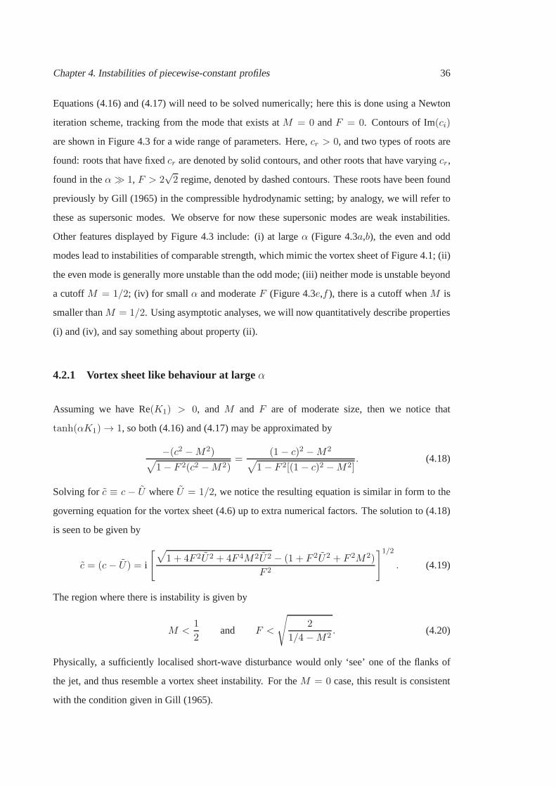
Chapter 4. Instabilities of piecewise-constant profiles 36
Equations (4.16) and (4.17) will need to be solved numerically; here this is done using a Newton
iteration scheme, tracking from the mode that exists atM = 0 andF = 0. Contours of Im(ci)
are shown in Figure 4.3 for a wide range of parameters. Here,cr > 0, and two types of roots are
found: roots that have fixedcr are denoted by solid contours, and other roots that have varying cr,
found in theα ≫ 1, F > 2√2 regime, denoted by dashed contours. These roots have been found
previously by Gill (1965) in the compressible hydrodynamicsetting; by analogy, we will refer to
these as supersonic modes. We observe for now these supersonic modes are weak instabilities.
Other features displayed by Figure 4.3 include: (i) at largeα (Figure 4.3a,b), the even and odd
modes lead to instabilities of comparable strength, which mimic the vortex sheet of Figure 4.1; (ii)
the even mode is generally more unstable than the odd mode; (iii) neither mode is unstable beyond
a cutoffM = 1/2; (iv) for smallα and moderateF (Figure 4.3e,f ), there is a cutoff whenM is
smaller thanM = 1/2. Using asymptotic analyses, we will now quantitatively describe properties
(i) and (iv), and say something about property (ii).
4.2.1 Vortex sheet like behaviour at largeα
Assuming we have Re(K1) > 0, andM and F are of moderate size, then we notice that
tanh(αK1) → 1, so both (4.16) and (4.17) may be approximated by
−(c2 −M2)√
1− F 2(c2 −M2)=
(1− c)2 −M2
√
1− F 2[(1 − c)2 −M2]. (4.18)
Solving for c ≡ c− U whereU = 1/2, we notice the resulting equation is similar in form to the
governing equation for the vortex sheet (4.6) up to extra numerical factors. The solution to (4.18)
is seen to be given by
c = (c− U) = i
[√
1 + 4F 2U2 + 4F 4M2U2 − (1 + F 2U2 + F 2M2)
F 2
]1/2
. (4.19)
The region where there is instability is given by
M <1
2and F <
√
2
1/4 −M2. (4.20)
Physically, a sufficiently localised short-wave disturbance would only ‘see’ one of the flanks of
the jet, and thus resemble a vortex sheet instability. For theM = 0 case, this result is consistent
with the condition given in Gill (1965).

Chapter 4. Instabilities of piecewise-constant profiles 37
M
F
ci(a) α = 15 (b) α = 15
(c) α = 0.7 (d) α = 0.7
(e) α = 0.1 (f) α = 0.1
000
00
00
00
0
00
0
00
0
0.5
0.5
0.5 0.5
0.5 0.5
0.5
2.5 2.5
5
5 5
5 5
5
10
10 10
10
0.05
0.05
0.05
0.05
0.05
0.150.15
0.15
0.15
0.25
0.250.25
0.25
0.25
0.25
0.25
0.25
0.25
0.25
0.25
0.25
0.25
0.35 0.35
0.35
0.45 0.45
0.45 0.45
0.01 0.010.02 0.02
(4.20)(4.20)
(4.24)
(4.26)
Figure 4.3: Contours ofci, computed numerically for the even mode (equation (4.16), left column) and
the odd mode (equation (4.17), right column) of the rectangular jet at some selectedα. Note the different
choice of axes used in the bottom panels. The stability boundary according to computed results is the
contour labelled by ‘0’. The stability boundaries (4.20), (4.24) and (4.26) are plotted also in the appropriate
panels.
Returning briefly to these supersonic instabilities that exists in the region beyond the cutoff given
by conditions in (4.20), the interpretation by Gill (1965) is that, even though the modes are
effectively isolated vortex sheet instabilities whenα ≫ 1, when the stability boundary given
by (4.20) is crossed, the isolated modes on one flank become radiating, interact with the mode
on the other flank, and leading to instability. Such instabilities arising from interacting radiating
waves is termed resonant over-reflection (e.g., McIntyre & Weissman, 1978; Benilov & Lapin,
2013)1. Although these instabilities exist, we observe that thesehave growth rates that are small,
and thus have not investigated them in great detail here.
1This is in contrast to over-reflection, which does not necessarily lead to instability (e.g., Acheson, 1976).

Chapter 4. Instabilities of piecewise-constant profiles 38
4.2.2 Long-wave cutoff due to the magnetic field
Even mode
We consider the even mode first. Assuming that
Re(K1) > 0, α≪ 1, and αF ≪ 1, (4.21)
we havetanh(αK1) ≈ αK1, and (4.16) becomes
−(c2 −M2)√
1− F 2(c2 −M2)= α[(1 − c)2 −M2]. (4.22)
Suppose thatF 2 = O(1). If M = O(1) also, thenc = ±M at leading order, andc is real at the
next correction. LettingM2 = µ ≪ 1, the interesting results comes from takingα ∼ µ, which
gives, at leading order inµ,
c ∼ i√
α−M2 as M2 ∼ α→ 0+, F 2 = O(1). (4.23)
Whenµ =M2 ≪ α, we recover the result of Gill (1965). The presence of the magnetic field is to
reduce the strength of the instability, and in this case to introduce a long-wave cutoff. The Froude
number dependence comes in at the next correction.
Consider nowF 2 = ǫ−1 ≫ 1. We letα ∼ ǫs; to be consistent with the assumptions stated in
(4.21), we needs > 1/2. Again,M2 = O(1) results in a realc, so we considerM2 = µ ≪ 1.
It may be checked that the balance that gives a non-zeroci at leading order isµ ∼ ǫ ∼ α. This
impliesc ∼ ǫ1/2 ∼ α1/2, with the corresponding result
c ∼ i
[
α2F 2
2−M2 +
√
α4F 4
4+ α2
]1/2
as M2 ∼ F−2 ∼ α→ 0+. (4.24)
We see that there is a long-wave cutoff due to the presence of amagnetic field. Notice also that,
whenF is small, expression (4.24) reduces formally to (4.23).
Figure 4.4 shows the computed growth rates over a range ofα compared with the corresponding
asymptotic results. The computed results are found by solving the full eigenvalue equation (4.16)
with a Newton root finding method. Notice that the domain of validity of (4.24) requiresαF−2 =
O(1), consistent also with the numerical results given in the bottom panels of Figure 4.3. In both
cases, we note thatc ∼ iα1/2; we will see that the scaling is different for the odd mode.
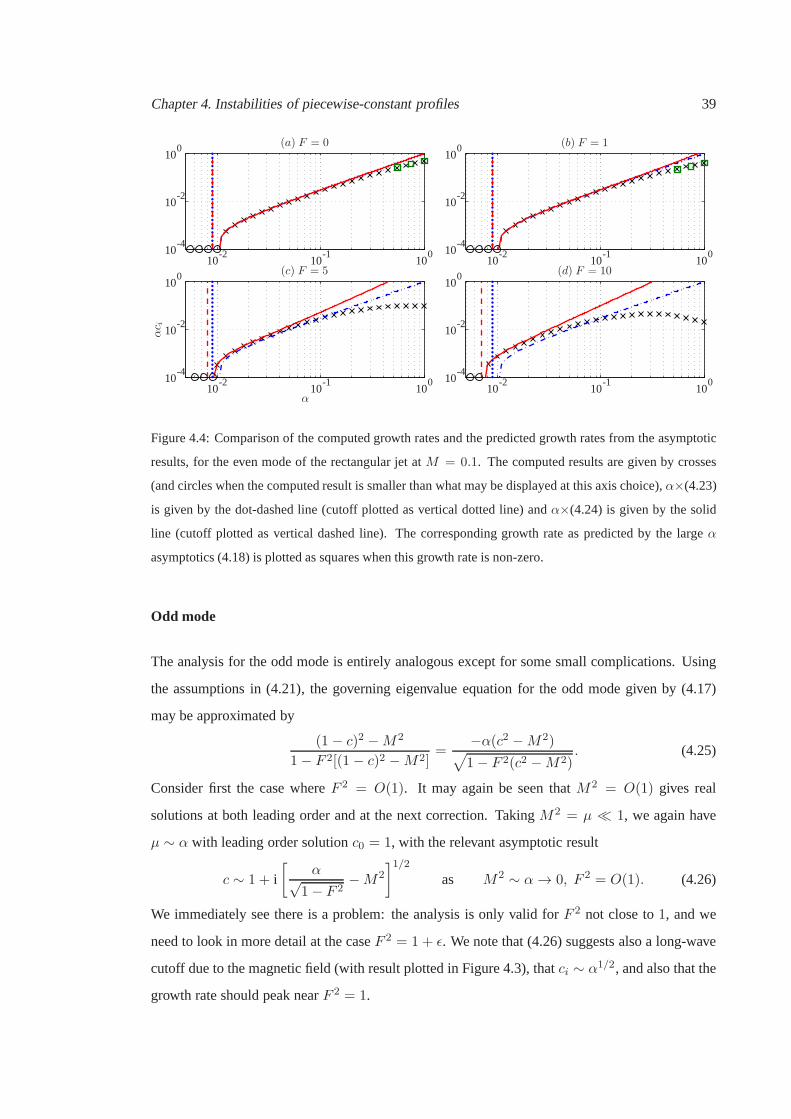
Chapter 4. Instabilities of piecewise-constant profiles 39replacements
α
αc i
(a) F = 0 (b) F = 1
(c) F = 5 (d) F = 1010
10
10101010
10
10
10101010
10
10
10101010
10
10
10101010
0
0
0
0
0
0
0
0
-1-1
-1-1
-2
-2
-2
-2
-2
-2
-2
-2
-4-4
-4-4
Figure 4.4: Comparison of the computed growth rates and the predicted growth rates from the asymptotic
results, for the even mode of the rectangular jet atM = 0.1. The computed results are given by crosses
(and circles when the computed result is smaller than what may be displayed at this axis choice),α×(4.23)
is given by the dot-dashed line (cutoff plotted as vertical dotted line) andα×(4.24) is given by the solid
line (cutoff plotted as vertical dashed line). The corresponding growth rate as predicted by the largeα
asymptotics (4.18) is plotted as squares when this growth rate is non-zero.
Odd mode
The analysis for the odd mode is entirely analogous except for some small complications. Using
the assumptions in (4.21), the governing eigenvalue equation for the odd mode given by (4.17)
may be approximated by
(1− c)2 −M2
1− F 2[(1− c)2 −M2]=
−α(c2 −M2)√
1− F 2(c2 −M2). (4.25)
Consider first the case whereF 2 = O(1). It may again be seen thatM2 = O(1) gives real
solutions at both leading order and at the next correction. TakingM2 = µ ≪ 1, we again have
µ ∼ α with leading order solutionc0 = 1, with the relevant asymptotic result
c ∼ 1 + i
[
α√1− F 2
−M2
]1/2
as M2 ∼ α→ 0, F 2 = O(1). (4.26)
We immediately see there is a problem: the analysis is only valid for F 2 not close to1, and we
need to look in more detail at the caseF 2 = 1 + ǫ. We note that (4.26) suggests also a long-wave
cutoff due to the magnetic field (with result plotted in Figure 4.3), thatci ∼ α1/2, and also that the
growth rate should peak nearF 2 = 1.

Chapter 4. Instabilities of piecewise-constant profiles 40
ForF 2 = 1 + ǫ, to get an instability we need to takec = 1 + ǫc1, with µ1/2 ∼ α2/5 ∼ ǫ where
M2 = µ ≪ 1; the other choice isǫ ∼ µ, which gives a realc1. The equation forc1 is then given
by the quintic equation
(c21 − ν)2(2c1 + 1) = −λ2, (4.27)
whereν andλ areO(1) constants withµ = νǫ2 andα = λǫ2/5. This unfortunately has no
closed form solution. Even though we cannot solve forc1 in closed form, we can say thatc1 is
expected to be complex because of the numerical results presented in Figure 4.3. We observe that
c = 1 + α2/5c1 with Im(c1) > 0, which suggests the odd mode may be more unstable than the
even mode at thisF ≈ 1 regime. We will revisit the possibility of the odd mode dominating in the
next subsection.
For larger values ofF , we letF 2 = ǫ−1 ≫ 1. On takingM2 = µ≪ 1, we obtain the result
c ∼ 1 +
√
iαF
+M2 as1
F 2∼M4/(2s+1) ∼ α1/s → 0+ (s > 1/2), (4.28)
wheres may be left as a free parameter, and this result now suggests there is no cutoff due to the
magnetic field, asci is small but non-zero. The fact that there is no longer a cutoff at smallα
suggests also that in this highF smallα regime, the odd modes are preferred over the even mode.
We also notice that this result is formally equivalent to theresult (4.26) in the largeF limit.
We compare the numerical results from the full equation (4.17) to the asymptotic results given
by equation (4.26) – equation (4.28) is the largeF limit of (4.26) so has been omitted. We plot
in Figure 4.5 the growth rateαci againstα, and the agreement between the numerical and the
asymptotic results is apparent. The scaling suggested by theF 2 = 1 + ǫ analysis has also been
checked and agreement is observed.
4.2.3 Preferred mode of instability: even versus odd modes.
As we have noted, the odd mode may be the preferred mode of instability in certain regimes.
To investigate this more thoroughly, we carried out a scan over (M,F,α) space, computing the
eigenvalues corresponding to the even and the odd modes. This is converted into the regime
diagram given by Figures 4.6 and 4.7, showing the regions in parameter space where one or the
other mode is preferred.
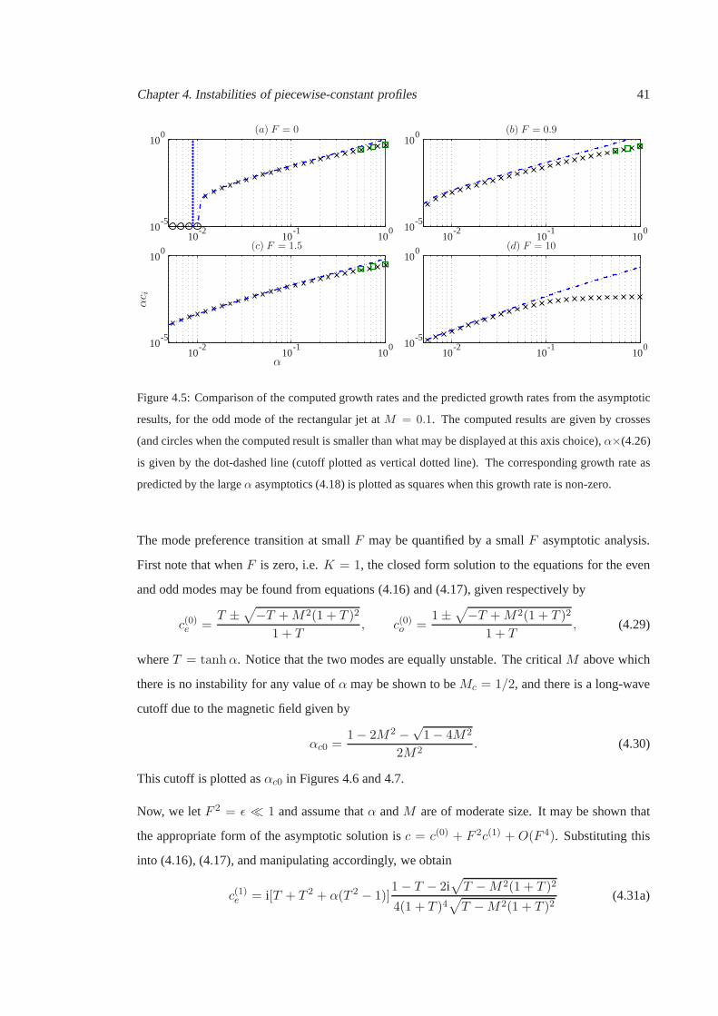
Chapter 4. Instabilities of piecewise-constant profiles 41replacements
α
αc i
(a) F = 0 (b) F = 0.9
(c) F = 1.5 (d) F = 1010
10101010
10
10101010
10
10101010
10
10101010
0
0
0
0
0
0
0
0
-1-1
-1-1
-2-2
-2-2
-5-5
-5-5
Figure 4.5: Comparison of the computed growth rates and the predicted growth rates from the asymptotic
results, for the odd mode of the rectangular jet atM = 0.1. The computed results are given by crosses
(and circles when the computed result is smaller than what may be displayed at this axis choice),α×(4.26)
is given by the dot-dashed line (cutoff plotted as vertical dotted line). The corresponding growth rate as
predicted by the largeα asymptotics (4.18) is plotted as squares when this growth rate is non-zero.
The mode preference transition at smallF may be quantified by a smallF asymptotic analysis.
First note that whenF is zero, i.e.K = 1, the closed form solution to the equations for the even
and odd modes may be found from equations (4.16) and (4.17), given respectively by
c(0)e =T ±
√
−T +M2(1 + T )2
1 + T, c(0)o =
1±√
−T +M2(1 + T )2
1 + T, (4.29)
whereT = tanhα. Notice that the two modes are equally unstable. The critical M above which
there is no instability for any value ofα may be shown to beMc = 1/2, and there is a long-wave
cutoff due to the magnetic field given by
αc0 =1− 2M2 −
√1− 4M2
2M2. (4.30)
This cutoff is plotted asαc0 in Figures 4.6 and 4.7.
Now, we letF 2 = ǫ ≪ 1 and assume thatα andM are of moderate size. It may be shown that
the appropriate form of the asymptotic solution isc = c(0) + F 2c(1) + O(F 4). Substituting this
into (4.16), (4.17), and manipulating accordingly, we obtain
c(1)e = i[T + T 2 + α(T 2 − 1)]1 − T − 2i
√
T −M2(1 + T )2
4(1 + T )4√
T −M2(1 + T )2(4.31a)
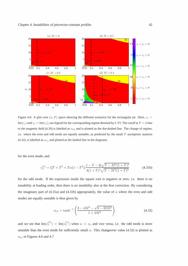
Chapter 4. Instabilities of piecewise-constant profiles 42
α
F
(a)M = 0 (b)M = 0.1
(c)M = 0.2 (d)M = 0.4
αc1 = 0.173
αc0 = 0
αc1 = 0.183
αc0 = 0.0102
αc1 = 0.217
αc0 = 0.436
αc1 = 0.429
αc0 = 0.25
ce = co = 0
ce = co > 0
co > ce = 0
ce > co = 0
co > ce > 0
ce > co > 0
I
II
I
I
II II
IIII
II
III III
III
III
IV
IV
VV
VV
V
VI
VI
0.050.05
0.050.05
0.20.2
0.20.2
0.40.4
0.40.4
0.60.6
0.60.6
0.80.8
0.80.8
11
11
00
00
55
55
1010
1010
1515
1515
2020
2020
Figure 4.6: A plot over(α, F ) space showing the different scenarios for the rectangular jet. Here,ce =
Im(ce) andco = Im(co); see legend for the corresponding regime denoted by I–VI. The cutoff atF = 0 due
to the magnetic field (4.30) is labelled asαc0 and is plotted as the dot-dashed line. The change of regime,
i.e. where the even and odd mode are equally unstable, as predicted by the smallF asymptotic analysis
(4.32), is labelled asαc1 and plotted as the dashed line in the diagrams.
for the even mode, and
c(1)o = i[T + T 2 + Tα(1 − T 2)]1− T − 2i
√
T −M2(1 + T )2
4(1 + T )4√
T −M2(1 + T )2(4.31b)
for the odd mode. If the expression inside the square root is negative or zero, i.e. there is no
instability at leading order, then there is no instability also at the first correction. By considering
the imaginary part of (4.31a) and (4.31b) appropriately, the value ofα where the even and odd
modes are equally unstable is then given by
αc1 = tanh−1
(
3− 4M2 −√8− 32M2
1 + 4M2
)
, (4.32)
and we see that Im(c(1)e ) < Im(c(1)o ) whenα < αc and vice versa, i.e. the odd mode is more
unstable than the even mode for sufficiently smallα. This changeover value (4.32) is plotted as
αc1 in Figures 4.6 and 4.7
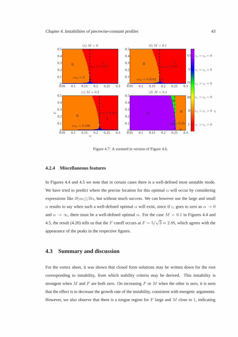
Chapter 4. Instabilities of piecewise-constant profiles 43
α
α
F
(a)M = 0 (b)M = 0.1
(c)M = 0.2 (d)M = 0.4
αc1 = 0.173
αc0 = 0
αc1 = 0.183
αc0 = 0.0102
αc1 = 0.217
αc0 = 0.436αc0 = 0.25
ce = co = 0
ce = co > 0
co > ce = 0
ce > co = 0
co > ce > 0
ce > co > 0
I
I I
I
II
II II
II II
IIIIV
IV
V
VV
V
V
VI
VI
00
00
0.050.05
0.050.05
0.1
0.1
0.1
0.1
0.1
0.1
0.1
0.1
0.150.15
0.150.15
0.2
0.2
0.2
0.2
0.2
0.2
0.2
0.2
0.250.25
0.250.25
0.3
0.3
0.3
0.3
0.3
0.3
0.3
0.3
0.40.4
0.40.4
0.50.5
0.50.5
Figure 4.7: A zoomed in version of Figure 4.6.
4.2.4 Miscellaneous features
In Figures 4.4 and 4.5 we note that in certain cases there is a well-defined most unstable mode.
We have tried to predict where the precise location for this optimal α will occur by considering
expressions like∂(αci)/∂α, but without much success. We can however use the large and small
α results to say when such a well-defined optimalα will exist, since ifci goes to zero asα → 0
andα → ∞, there must be a well-defined optimalα. For the caseM = 0.1 in Figures 4.4 and
4.5, the result (4.20) tells us that theF cutoff occurs atF = 5/√3 ≈ 2.88, which agrees with the
appearance of the peaks in the respective figures.
4.3 Summary and discussion
For the vortex sheet, it was shown that closed form solutionsmay be written down for the root
corresponding to instability, from which stability criteria may be derived. This instability is
strongest whenM andF are both zero. On increasingF orM when the other is zero, it is seen
that the effect is to decrease the growth rate of the instability, consistent with energetic arguments.
However, we also observe that there is a tongue region forF large andM close to1, indicating
Chapter 4. Instabilities of piecewise-constant profiles 44
that somehow the individual stabilisation effects cancel each other out. An asymptotic analysis
was carried out near the stability boundaryM = 1 to investigate the behaviour of the instability
in this tongue region.
For the rectangular jet, there were several features of notethat we have found. Forα ≫ 1, we
found two types of instability, one that is like a vortex sheet instability, and the other is what we
termed supersonic instabilities, previously found by Gill(1965) and now attributed to resonant
over-reflection. We focussed on the vortex sheet instabilities, and found analytical expressions
for these instabilities via an asymptotic analysis. The supersonic instabilities were observed to
be weak instabilities so have not been investigated in greatdetail; it is certainly possible however
to investigate them via an asymptotic procedure, as was donein Gill (1965). Numerically it was
found that there are no instabilities whenM > 1/2. For α ≪ 1, it was seen that there is a
cutoff due to the magnetic field, and the locations of these cutoffs were found by an asymptotic
procedure. Although it was found that the even mode is generally more unstable that the odd
mode, via numerical and asymptotic procedures, we were ableto find regions in parameter space
where the odd mode is the strongest instability.

Chapter 4. Instabilities of piecewise-constant profiles 45
4.4 Appendix: Expressions for eigenfunctions
When the profile is piecewise-constant, the eigenfunction may be written down explicitly, given
below. Note that theF dependence appears inK2 = 1− F 2S2 = 1− F 2[(U0 − c)2 −M2], and
in the caseF = 0, h is identified withp, the pressure term in the incompressible case. Note the
expressions forh remain formally atO(1) in the limit of F tending to zero, and this is because
of the rescalingh = h/F 2 we employed when we wrote down the full SWMHD equations in
Chapter 2.
Note in these cases there are no vorticity or current perturbations except at the discontinuities.
Vortex sheet
U0 =
+1, y > 0
−1, y < 0
(4.33a)
G =
e−αK+y, y > 0
e+αK−y, y < 0
(4.33b)
v =
+(1− c)e−αK+y, y > 0
−(1 + c)e+αK−y, y < 0
(4.33c)
by =
Me−αK+y, y > 0
Me+αK−y, y < 0
(4.33d)
u =
−i(1− c)K−1+ e−αK+y, y > 0
−i(1 + c)K−1− e+αK
−y, y < 0
(4.33e)
bx =
−iMK−1+ e−αK+y, y > 0
+iMK−1− e+αK
−y, y < 0
(4.33f)
h =
+iS2+K
−1+ e−αK+y, y > 0
−iS2−K
−1− e+αK
−y, y < 0
(4.33g)

Chapter 4. Instabilities of piecewise-constant profiles 46
Rectangular jet: even mode
U0 =
0, y > 1
1, |y| < 1
0, y < −1
(4.34a)
G =
+e−αK0(y−1), y > 1
+ cosh(αK1y)/ cosh(αK1), |y| < 1
+e+αK0(y+1), y < −1
(4.34b)
v =
−ce−αK0(y−1), y > 1
+(1− c) cosh(αK1y)/ cosh(αK1), |y| < 1
−ce+αK0(y+1), y < −1
(4.34c)
by =
+Me−αK0(y−1), y > 1
+M cosh(αK1y)/ cosh(αK1), |y| < 1
+Me+αK0(y+1), y < −1
(4.34d)
u =
+ice−αK0(y−1), y > 1
+i(1− c) sinh(αK1y)/ cosh(αK1), |y| < 1
−ice+αK0(y+1), y < −1
(4.34e)
bx =
−iMe−αK0(y−1), y > 1
+iM sinh(αK1y)/ cosh(αK1), |y| < 1
+iMe+αK0(y+1), y < −1
(4.34f)
h =
+iS20e
−αK0(y−1), y > 1
−iS21 sinh(αK1y)/ cosh(αK1), |y| < 1
−iS20e
+αK0(y+1), y < −1
(4.34g)

Chapter 4. Instabilities of piecewise-constant profiles 47
Rectangular jet: odd mode
U0 =
0, y > 1
1, |y| < 1
0, y < −1
(4.35a)
G =
+e−αK0(y−1), y > 1
+ sinh(αK1y)/ sinh(αK1), |y| < 1
−e+αK0(y+1), y < −1
(4.35b)
v =
−ce−αK0(y−1), y > 1
+(1− c) sinh(αK1y)/ sinh(αK1), |y| < 1
−ce+αK0(y+1), y < −1
(4.35c)
by =
+Me−αK0(y−1), y > 1
+M sinh(αK1y)/ sinh(αK1), |y| < 1
−Me+αK0(y+1), y < −1
(4.35d)
u =
+ice−αK0(y−1), y > 1
+i(1− c) cosh(αK1y)/ sinh(αK1), |y| < 1
+ice+αK0(y+1), y < −1
(4.35e)
bx =
−iMe−αK0(y−1), y > 1
+iM cosh(αK1y)/ sinh(αK1), |y| < 1
−iMe+αK0(y+1), y < −1
(4.35f)
h =
+iS20e
−αK0(y−1), y > 1
−iS21 cosh(αK1y)/ sinh(αK1), |y| < 1
+iS20e
+αK0(y+1), y < −1.
(4.35g)

Chapter 4. Instabilities of piecewise-constant profiles 48

49
Chapter 5
Linear instabilities of smooth profiles
As a model for more realistic profiles, we consider in this chapter the instabilities associated with
the hyperbolic-tangent shear layer and the Bickley jet. Again, for simplicity, we limit ourselves to
the case of a uniform background magnetic field with no underlying topography. Linear instability
calculations involving these two profiles are well documented in the literature in a wide variety of
contexts (e.g., Lipps, 1962; Howard, 1963; Michalke, 1964;Drazin & Howard, 1966; Hazel, 1972;
Drazin & Reid, 1981; Sutherland & Peltier, 1992, 1994; Hughes & Tobias, 2001) and provide a
comparison and check on our results.
5.1 Numerical method
We seek a numerical solution of the eigenvalue equation (4.1), written as
G′′ +
[
(S2)′
S2− (K2)′
K2
]
G′ − α2K2G = 0, (5.1)
where, again,S2 = (U0 − c)2 − M2 andK2 = 1 − F 2S2. Although the velocity profiles
are technically defined over the entire real line, we solve the equation on the finite domainy ∈[−Ly, Ly]. We will consider solutions that decay exponentially as|y| becomes large, namely
G ∼ exp[−αKy], Re(K) > 0 as |y| → ∞, (5.2)
and the size ofLy chosen depends on the decay properties of the eigenfunction; we will
be doublingLy until the change in the computed eigenvalue is suitably small, such that

Chapter 5. Linear instabilities of smooth profiles 50
|c(2Ly)|/|c(Ly)| < ǫ, for some choice ofǫ. We solve the second order ODE (5.1) by a shooting
method, with matching imposed aty = 0, employing a generalised Newton method as the root-
finding algorithm; the integration is started from±Ly, taking
G′
G
∣
∣
∣
∣
−Ly
= −αK−,G′
G
∣
∣
∣
∣
Ly
= −AαK+, (5.3)
as the initialisation, whereK± = 1 − F 2[(U(±∞) − c)2 −M2], with U(±∞) = ±1 for the
shear layer andU(±∞) = 0 for the jet. The constantA and the eigenvaluec accordingly until the
matching errors aty = 0 are sufficiently small. To avoid singularities in the governing equation,
we seek only unstable modes. The routines were written in MATLAB, using routineode113
as the integrator (an Adams-Bashforth type method with adaptive grid). Although the boundary
conditions are functions ofc, changing at every iteration, we generally have no problemswith
convergence provided that the initial guess is close to the true value. Solutions are initialised from
F = 0, M = 0 at some fixedα using a known numerical result documented in, for example,
Drazin & Reid (1981). Runs at new parameter values are then initialised using an estimate for
the eigenvalue from previously calculated eigenvalues at nearby parameter values. The Bickley
jet is even abouty = 0 and hence the parity result of Section 3.4 holds, i.e. the eigenfunctions are
either even or odd. In this case we need integrate only up toy = 0, with the imposition of either
G′(0) = 0 (even mode) orG(0) = 0 (odd mode).
5.2 Hyperbolic-tangent shear layer
In this subsection, we consider the basic state velocity defined by
U0(y) = tanh(y), −∞ < y <∞. (5.4)
From inequality (3.12) we know that the growth ratesαci associated with any instability are
bounded above bymax |U ′0|/2 = 1/2; furthermore, from the stability criteria (3.20) or (3.21), this
profile is stable whenM ≥ 1 . From the parity results in Section 3.4, the eigenvalues associated
with unstable eigenfunctions take the formc = ±cr + ici. In the hydrodynamic case, instability
exists only within the bandwidth0 < α < 1, with a neutral mode atα = 1 (e.g., Drazin & Reid,
1981,§31.10).
Figure 5.1 shows contours ofci over theF andM parameter space at selectedα, reflecting: (i) a
relatively short wave disturbance (Figure 5.1a); (ii) the most unstable mode in the hydrodynamic

Chapter 5. Linear instabilities of smooth profiles 51
0.4
F
M
ci(a) α = 0.70 (b) α = 0.44
(c) α = 0.01 (d) vortex sheet
000
00
00
00
0.20.2
1
1
1
1
1
1
1
1
1
2
22
2
3
33
3
0.1
0.10.1
0.10.3
0.3
0.3
0.5
0.5
0.5
0.50.5
0.5
0.50.7 0.7
0.9 0.9
0.01
0.010.01
0.01
Figure 5.1: Contours ofci overF andM parameter space at selectedα. The results have been filtered so
that only modes with|cr| < 10−3 are plotted. Figure 4.1 is reproduced here as panel(d) for comparison
purposes.
incompressible case (Figure 5.1b); (iii) a long wave disturbance in panel (Figure 5.1c). Figure 4.1,
the corresponding diagram for the vortex sheet profile, is reproduced here as the Figure 5.1(d)
for comparison purposes. We should note that the results have been filtered so that only the low-
frequency modes (here those with|cr| < 10−3) have been displayed; as explained below, there
is also a distinct second mode of instability (with larger|cr|), which is manifest at higher values
of F . Figure 5.1(c) and (d) are remarkably similar, suggesting that long-wave instabilities for this
velocity profile resemble the instabilities of a vortex sheet. This resemblance will be quantified
via a long-wave asymptotic analysis in Section 5.5, in whichwe derive the more general result
that long-wave instabilities of any shear layer profile resemble vortex sheet instabilities.
As described above, figure 5.1 is compiled by tracking the evolution of a particular mode
of instability, using the incompressible hydrodynamic case (F = M = 0) as the starting
point. It is therefore important to ask whether there are additional, distinct modes of instability.
Indeed, it is known that for both two-dimensional compressible hydrodynamics and shallow-water
hydrodynamics, there is a second mode of instability, foundby Blumenet al.(1975) and Satomura
(1981) respectively. Compared to the first modes (those of Figure 5.1), which may be referred
to as inflection point instabilities, these second modes (orsupersonic modes for compressible
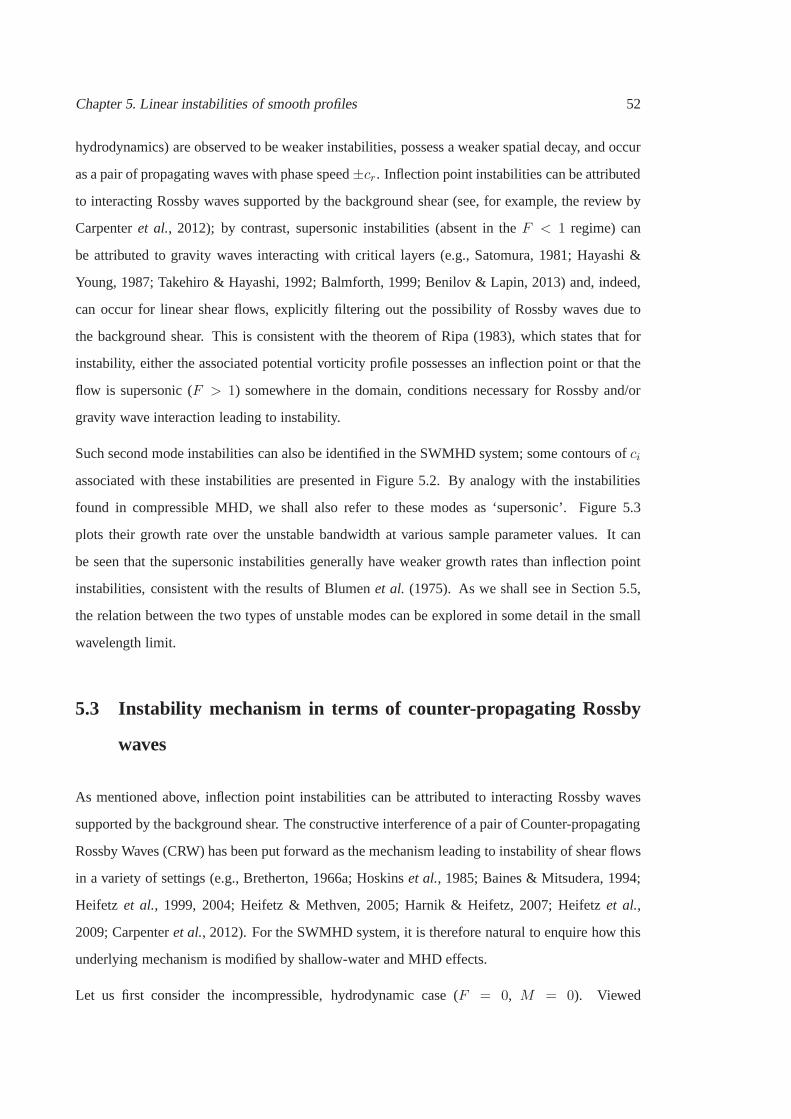
Chapter 5. Linear instabilities of smooth profiles 52
hydrodynamics) are observed to be weaker instabilities, possess a weaker spatial decay, and occur
as a pair of propagating waves with phase speed±cr. Inflection point instabilities can be attributed
to interacting Rossby waves supported by the background shear (see, for example, the review by
Carpenteret al., 2012); by contrast, supersonic instabilities (absent in the F < 1 regime) can
be attributed to gravity waves interacting with critical layers (e.g., Satomura, 1981; Hayashi &
Young, 1987; Takehiro & Hayashi, 1992; Balmforth, 1999; Benilov & Lapin, 2013) and, indeed,
can occur for linear shear flows, explicitly filtering out thepossibility of Rossby waves due to
the background shear. This is consistent with the theorem ofRipa (1983), which states that for
instability, either the associated potential vorticity profile possesses an inflection point or that the
flow is supersonic (F > 1) somewhere in the domain, conditions necessary for Rossby and/or
gravity wave interaction leading to instability.
Such second mode instabilities can also be identified in the SWMHD system; some contours ofci
associated with these instabilities are presented in Figure 5.2. By analogy with the instabilities
found in compressible MHD, we shall also refer to these modesas ‘supersonic’. Figure 5.3
plots their growth rate over the unstable bandwidth at various sample parameter values. It can
be seen that the supersonic instabilities generally have weaker growth rates than inflection point
instabilities, consistent with the results of Blumenet al. (1975). As we shall see in Section 5.5,
the relation between the two types of unstable modes can be explored in some detail in the small
wavelength limit.
5.3 Instability mechanism in terms of counter-propagatingRossby
waves
As mentioned above, inflection point instabilities can be attributed to interacting Rossby waves
supported by the background shear. The constructive interference of a pair of Counter-propagating
Rossby Waves (CRW) has been put forward as the mechanism leading to instability of shear flows
in a variety of settings (e.g., Bretherton, 1966a; Hoskinset al., 1985; Baines & Mitsudera, 1994;
Heifetz et al., 1999, 2004; Heifetz & Methven, 2005; Harnik & Heifetz, 2007; Heifetz et al.,
2009; Carpenteret al., 2012). For the SWMHD system, it is therefore natural to enquire how this
underlying mechanism is modified by shallow-water and MHD effects.
Let us first consider the incompressible, hydrodynamic case(F = 0, M = 0). Viewed
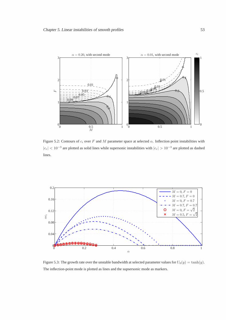
Chapter 5. Linear instabilities of smooth profiles 53
F
M
ciα = 0.20, with second mode α = 0.01, with second mode
000
00
0.5
0.50.5
1
1
1
1
1
22
33
0.1
0.1
0.2
0.2
0
0
0.01
0.01 0.030.03
0.05
0.050.07
0.07
0.09
0.09
Figure 5.2: Contours ofci overF andM parameter space at selectedα. Inflection point instabilities with
|cr| < 10−3 are plotted as solid lines while supersonic instabilities with |cr| > 10−3 are plotted as dashed
lines.
α
αc i
M = 0, F = 0
M = 0.7, F = 0
M = 0, F = 0.7
M = 0.7, F = 0.7
M = 0, F =√2
M = 0.5, F =√2
00
0.2
0.2 0.4 0.6 0.8 1
0.04
0.08
0.12
0.16
Figure 5.3: The growth rate over the unstable bandwidth at selected parameter values forU0(y) = tanh(y).
The inflection-point mode is plotted as lines and the supsersonic mode as markers.

Chapter 5. Linear instabilities of smooth profiles 54
− −
+− −
+ +
Ω0(y)
Figure 5.4: Basic CRW mechanism in schematic form, for the background velocity profile ofU0 = tanh(y),
so the background vorticity profile isΩ0 = −sech2(y). Solid lines here depict the dynamics for the
incompressible, hydrodynamic case. The contours are of thevorticity. Vorticity anomalies are shown
by the closed solid curves, and the effect of these on the other contours, leading to instability, is shown by
solid arrows.
individually, the Rossby waves are neutral. Its direction of propagation is determined by the
vorticity profile, which in this case is related to the background flow. This in turn is seen to imply
a wave propagation that is in the opposite direction to the background flow. A pair of CRW may
then be held stationary by the background flow, become phase locked, and, depending on the
phase shift, interfere constructively, leading to mutual amplification and hence instability. This is
the scenario depicted in, for example, Figure 1 of Heifetz & Methven (2005). Schematically, these
CRW are represented by the solid curves in figure 5.4, where each of the vorticity anomalies has
an associated velocity, and where the configuration is such that the mutual influence of the two
Rossby waves acts to increase the wave amplitude.
We plot in Figures 5.5 and 5.6 the relevant eigenfunctions for the most unstable mode at
some sample values ofF andM , with the Rossby waves represented by vorticity anomalies;
the incompressible hydrodynamic case is displayed in panel(c) in the figures. Looking at
Figure 5.5(c), the pattern is consistent with the schematic in Figure 5.4. So, at the simplest level,
we observe that increasingF orM perturbs the patterns away from the optimal configuration for
instability, thus leading to the observed stabilisation. We now quantify how the extra physics of

Chapter 5. Linear instabilities of smooth profiles 55
y
αx/2π
(d) F = 0,M = 0 (c) F = 0,M = 0.75
(b) F = 0.75, M = 0 (a) F = 0.75, M = 0.75
0
0
0 0.5
1
1-1
3
-3
Figure 5.5: Vorticity eigenfunction of the most unstable mode of U0(y) = tanh(y) at some selected
parameters. Here and in subsequent diagrams of this type, red is positive and blue is negative. Notice
the larger shift between the pair of waves asM is increased, and a slight tilting whenF is increased.
y
αx/2π
(d) F = 0,M = 0 (c) F = 0,M = 0.75
(b) F = 0.75, M = 0 (a) F = 0.75, M = 0.75
0
0
0 0.5
1
1-1
5
-5
Figure 5.6: Height (pressure) eigenfunction of the most unstable mode ofU0(y) = tanh(y) at some selected
parameters. Notice an increased tilting with increasingF .
the SWMHD system perturbs the patterns away from the optimumconfiguration.
So since Rossby waves are associated with vorticity anomalies, we consider the vorticity
equation and see what can be inferred. The vorticity equation in two-dimensional incompressible

Chapter 5. Linear instabilities of smooth profiles 56
hydrodynamics isDω
Dt≡ ∂ω
∂t+ u · ∇ω = 0. (5.5)
Then, linearising about a basic shear flowU0(y) gives(
∂
∂t+ U0
∂
∂x
)
ω = −vΩ′0. (5.6)
Now, we note thatv is related to the cross-stream displacement of the materialcontourη as(
∂
∂t+ U0
∂
∂x
)
η = v, (5.7)
and so taking modal solutions of the form (3.4) then gives
ω = −ηΩ0. (5.8)
This says that, in the incompressible hydrodynamic case, any vorticity anomalies are tied to the
deformation of the material contour.
Here we work out the eigenfunction forω andη associated with the most unstable mode fromG,
and compare the two in Figure 5.7. As a measure of the error, wecalculate the relativeL2 error:
rel. L2 error=||ω − (−ηΩ′
0)||L2
||ω||L2
, ||(·)||L2=
√
∫∫
(·)2 dxdy. (5.9)
As we can see, the relative error is small, less than 1%; thus we can say with confidence that the
vorticity budget equation captures all the vorticity contributions.
5.3.1 Modifications in the SWMHD case
The SWMHD vorticity equation is given by
Dω
Dt= −(∇ · u)ω +M2
b · ∇j +M2(∇ · b)j, (5.10)
whereω and j are thez-components of the vorticity,∇ × u, and electric current,∇ × b,
respectively. Using equations (3.1c) and (3.1d), this can be written as
Dω
Dt= F 2ω
Dh
Dt+ F 2hω∇ · u+M2(1− F 2j)b · ∇j −M2hj∇ · b. (5.11)
On linearising about the basic stateU0 = U0(y)ex, B0 = 1ex, taking modal solutions of the
form (3.4), we obtain the following expression for the vorticity budget:
ω = −ηΩ′ + F 2hΩ+M2 j
U0 − c, (5.12)

Chapter 5. Linear instabilities of smooth profiles 57
y
αx/2π
(a) ω (b) ω − (−ηΩ′0)
(c) − ηΩ′0
L2 rel. error= 0.0058579
0
0
0
0
0
0
0
0
0
0.5
0.50.5
1
1
11
-3
-3-3
3
33
-1
0.1
0.1
-0.1
-0.1
×10-3
Figure 5.7: Vorticity contributions associated with the most unstable mode atF = 0, M = 0; panel(a) is
also Figure 5.5(c). The small relativeL2 error given by (5.9) indicates that the vorticity anomaliescome
solely from deformation of the material contours.
whereΩ0 = −U ′0 is the basic state vorticity. These three terms represent contributions due
respectively to the deformation of the cross-stream displacement, to shallow-water and magnetic
effects. Inspection of Figure 5.1 shows that the instability is most vigorous whenM = F = 0
and that increasing eitherM or F when the other parameter is zero is stabilising; we therefore
expect that the vorticity anomalies from the magnetic and shallow-water effects will counteract
that associated with the deformation of the material contour.
CRWs modification when one ofF or M is zero
Consider first the case whereF = 0 (the incompressible MHD case). Equation (5.12) is given by
ω = −ηΩ′0 +M2 j
U0 − c. (5.13)
We show in Figure 5.8 a typical result forF = 0 showing the physical form of the respective
components associated with the most unstable mode at the particular parameter values.
We notice that the positive contribution to vorticity whenM 6= 0 has a centre that straddles the two
negative vorticity anomalies associated with the deformation of the material contour, and the same
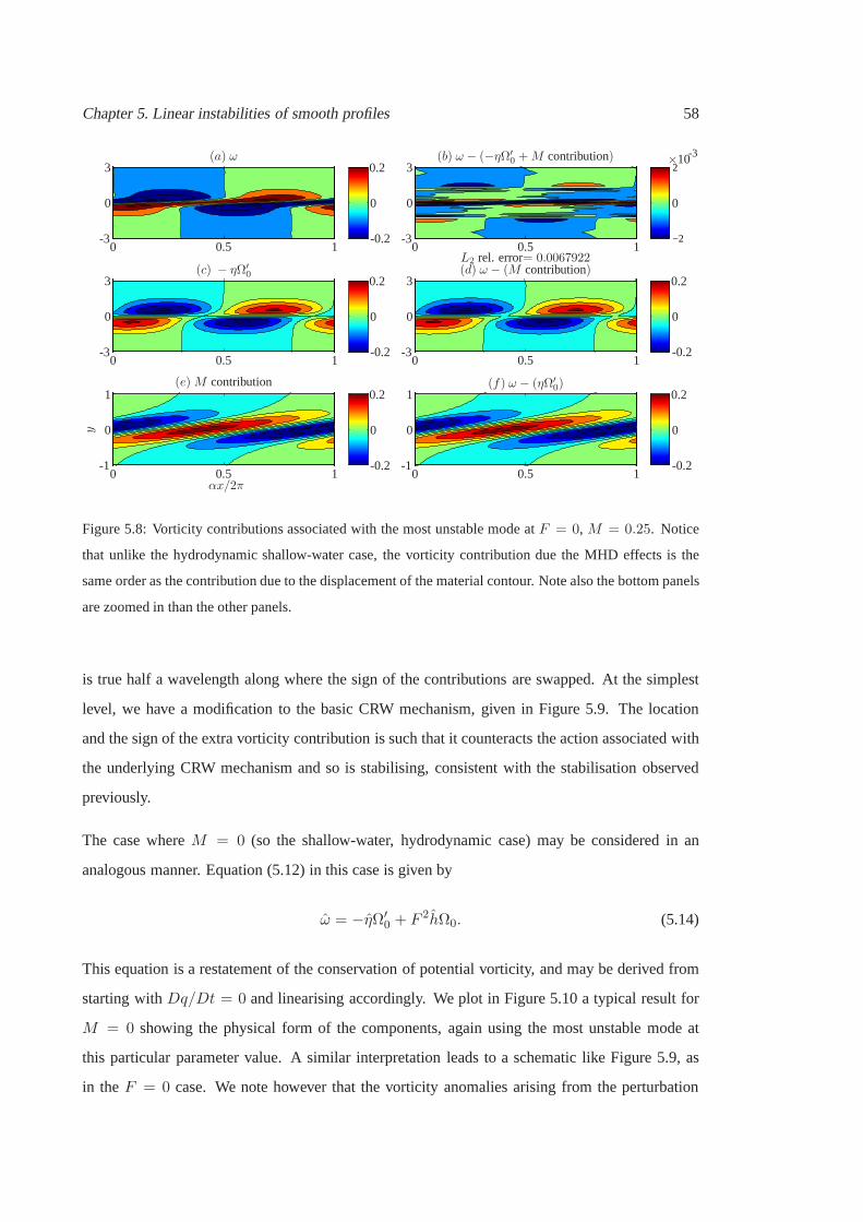
Chapter 5. Linear instabilities of smooth profiles 58
−2
2
y
αx/2π
(a) ω (b) ω − (−ηΩ′0 +M contribution)
(c) − ηΩ′0 (d) ω − (M contribution)
(e)M contribution (f) ω − (ηΩ′0)
L2 rel. error= 0.0067922
0
0
0
0
0
00
0
0
0
0
0
0
0
0
0
0
0
0.5
0.5
0.50.5
0.5
0.5
1
1
1
1
1
1
1
1
-3
-3
-3
-3
3
3
3
3
-1-1
0.2
0.2
0.2 0.2
0.2
-0.2
-0.2
-0.2 -0.2
-0.2
×10-3
Figure 5.8: Vorticity contributions associated with the most unstable mode atF = 0, M = 0.25. Notice
that unlike the hydrodynamic shallow-water case, the vorticity contribution due the MHD effects is the
same order as the contribution due to the displacement of thematerial contour. Note also the bottom panels
are zoomed in than the other panels.
is true half a wavelength along where the sign of the contributions are swapped. At the simplest
level, we have a modification to the basic CRW mechanism, given in Figure 5.9. The location
and the sign of the extra vorticity contribution is such thatit counteracts the action associated with
the underlying CRW mechanism and so is stabilising, consistent with the stabilisation observed
previously.
The case whereM = 0 (so the shallow-water, hydrodynamic case) may be considered in an
analogous manner. Equation (5.12) in this case is given by
ω = −ηΩ′0 + F 2hΩ0. (5.14)
This equation is a restatement of the conservation of potential vorticity, and may be derived from
starting withDq/Dt = 0 and linearising accordingly. We plot in Figure 5.10 a typical result for
M = 0 showing the physical form of the components, again using themost unstable mode at
this particular parameter value. A similar interpretationleads to a schematic like Figure 5.9, as
in theF = 0 case. We note however that the vorticity anomalies arising from the perturbation
Chapter 5. Linear instabilities of smooth profiles 59
− −
+− −
+ − +
+ +
Ω0(y)
Figure 5.9: Modified CRW mechanism in pictorial form, with the background velocity profileU0 =
tanh(y). The solid contours are associated with the basic CRW mechanism, as in Figure 5.4. The closed
dashed curves represent the additional vorticity anomalies due to the extra physical effects. The (stabilising)
effect of these extra vorticity anomalies are shown by the dashed arrows.
of the material contour is the dominant contribution to the whole vorticity, larger than the extra
contribution by an order of magnitude.
As a further verification of these ideas, we have also adopteda perturbative approach to the
analysis of expression (5.12), approximating the shallow-water and magnetic contributions using
the eigenfunction forF = M = 0. It can be readily seen that calculatingF 2hΩ0 using h
is consistent with that obtained from the full linear equations (see Figure 5.11a, b). To obtain
an estimate of the magnetic contribution, it is necessary tocalculate j using the governing
equations (3.3c) – (3.3d) with the velocity obtained whenF = M = 0. This is slightly more
involved than forh, but can be shown to provide a consistent vorticity contribution; see for
example Figure 5.11(c) and the numerically calculated contribution given in Figure 5.11(d). Thus
the idea that shallow-water and magnetic effects act to shift the vorticity distribution from an
optimal configuration for instability is confirmed.

Chapter 5. Linear instabilities of smooth profiles 60
y
αx/2π
(a) ω (b) ω − (−ηΩ′0 + F 2hΩ0)
(c) − ηΩ′0 (d) ω − (F 2hΩ0)
(e) F 2hΩ0 (f) ω − (ηΩ′0)
L2 rel. error=0.0059802
0
0
0
0
0
00
0
0
0
0
0
0
0
0
0
0
0
1
1
1 1
1
1
-3
-3
-3 -3
-3
-3
3
3
3 3
3
3
-0.5-0.5
-0.5
0.50.5
0.5
0.5
0.5
0.5 0.5
0.5
0.5
-5
5
-0.05-0.05
0.050.05
×10-3
Figure 5.10: Vorticity contributions associated with the most unstable mode atF = 0.5, M = 0. Notice
that the vorticity contribution due the presence of a free surface is much smaller than the contribution due
to the displacement of the material contour.
y
αx/2π
(a) Impliedh atF = 0.1, M = 0 (b) Implied−F 2hΩ0
(c) Implied j atF = 0,M = 0.1 (d) ImpliedM contribution
0
0 0
0
0
0
0
0
0
0
0
0
0.50.5
0.50.5
1
1
1
1
1
11
33
-3-3 -0.1
-0.1
-0.05
0.05
-1
-1-1
×10-3
-0.2
0.10.2
Figure 5.11: Vorticity contributions implied by the velocity eigenfunction calculated atF = 0,M = 0.
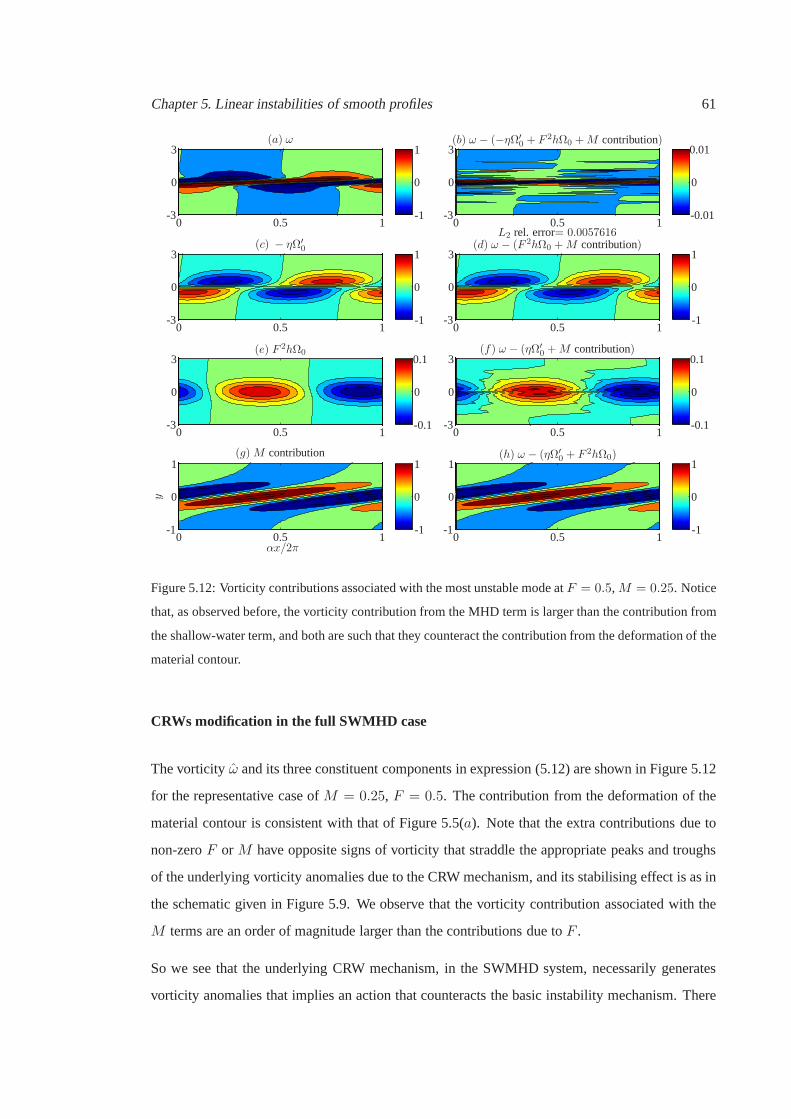
Chapter 5. Linear instabilities of smooth profiles 61
y
αx/2π
(a) ω (b) ω − (−ηΩ′0 + F 2hΩ0 +M contribution)
(c) − ηΩ′0 (d) ω − (F 2hΩ0 +M contribution)
(e) F 2hΩ0 (f) ω − (ηΩ′0 +M contribution)
(g)M contribution (h) ω − (ηΩ′0 + F 2hΩ0)
L2 rel. error= 0.0057616
0
0
0
0
00
0
00
0
00
0
0
0
0
0
0
0
00
0
0
0
0.5
0.5
0.5
0.5
0.5
0.5
0.50.5
1
1
1
11
1
1
1
1
1
1
1
1
11
-3
-3
-3
-3
-3-3
3
3
3
3
33
-1
-1
-1
-1-1
-1
-1
0.1 0.1
-0.1 -0.1
0.01
-0.01
Figure 5.12: Vorticity contributions associated with the most unstable mode atF = 0.5,M = 0.25. Notice
that, as observed before, the vorticity contribution from the MHD term is larger than the contribution from
the shallow-water term, and both are such that they counteract the contribution from the deformation of the
material contour.
CRWs modification in the full SWMHD case
The vorticityω and its three constituent components in expression (5.12) are shown in Figure 5.12
for the representative case ofM = 0.25, F = 0.5. The contribution from the deformation of the
material contour is consistent with that of Figure 5.5(a). Note that the extra contributions due to
non-zeroF orM have opposite signs of vorticity that straddle the appropriate peaks and troughs
of the underlying vorticity anomalies due to the CRW mechanism, and its stabilising effect is as in
the schematic given in Figure 5.9. We observe that the vorticity contribution associated with the
M terms are an order of magnitude larger than the contributions due toF .
So we see that the underlying CRW mechanism, in the SWMHD system, necessarily generates
vorticity anomalies that implies an action that counteracts the basic instability mechanism. There
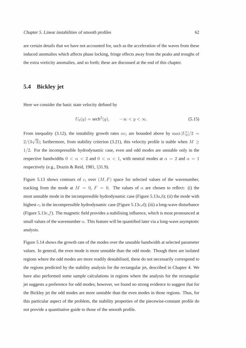
Chapter 5. Linear instabilities of smooth profiles 62
are certain details that we have not accounted for, such as the acceleration of the waves from these
induced anomalies which affects phase locking, fringe effects away from the peaks and troughs of
the extra vorticity anomalies, and so forth; these are discussed at the end of this chapter.
5.4 Bickley jet
Here we consider the basic state velocity defined by
U0(y) = sech2(y), −∞ < y <∞. (5.15)
From inequality (3.12), the instability growth ratesαci are bounded above bymax |U ′0|/2 =
2/(3√3); furthermore, from stability criterion (3.21), this velocity profile is stable whenM ≥
1/2. For the incompressible hydrodynamic case, even and odd modes are unstable only in the
respective bandwidths0 < α < 2 and0 < α < 1, with neutral modes atα = 2 andα = 1
respectively (e.g., Drazin & Reid, 1981,§31.9).
Figure 5.13 shows contours ofci over (M,F ) space for selected values of the wavenumber,
tracking from the mode atM = 0, F = 0. The values ofα are chosen to reflect: (i) the
most unstable mode in the incompressible hydrodynamic case(Figure 5.13a,b); (ii) the mode with
highestci in the incompressible hydrodynamic case (Figure 5.13c,d); (iii) a long-wave disturbance
(Figure 5.13e,f ). The magnetic field provides a stabilising influence, whichis most pronounced at
small values of the wavenumberα. This feature will be quantified later via a long-wave asymptotic
analysis.
Figure 5.14 shows the growth rate of the modes over the unstable bandwidth at selected parameter
values. In general, the even mode is more unstable than the odd mode. Though there are isolated
regions where the odd modes are more readily destabilised, these do not necessarily correspond to
the regions predicted by the stability analysis for the rectangular jet, described in Chapter 4. We
have also performed some sample calculations in regions where the analysis for the rectangular
jet suggests a preference for odd modes; however, we found nostrong evidence to suggest that for
the Bickley jet the odd modes are more unstable than the even modes in those regions. Thus, for
this particular aspect of the problem, the stability properties of the piecewise-constant profile do
not provide a quantitative guide to those of the smooth profile.

Chapter 5. Linear instabilities of smooth profiles 63
F
M
ci(a) α = 0.90 (b) α = 0.52
(c) α = 0.30 (d) α = 0.23
(e) α = 0.05 (f) α = 0.05
000
00
00
00
00
00
0.5
0.5
0.50.5
0.5
0.5
1
1
1
2
2
2
5
5
5
10
10
10
0.05
0.1
0.15
0.2
0.25
0.25
0.25
0.250.25
0.25
0.25
0.01
0.01
0.01
0.01
0.01
0.01
0.04
0.04
0.04
0.07
0.07
0.070.07
0.07
0.07
0.140.
14
0.140.21
0.17 (5.35)
Figure 5.13: Contours ofci over theF andM parameter space at selectedα, for the even mode (left
column) and the odd mode (right column) ofU0(y) = sech2(y). The predicted cut off from the asymptotic
result (5.38) is plotted in panel (e).
α
αc i
00 0.4 0.8 1.2 1.6 2
0.04
0.08
0.12
0.16 even,M = 0, F = 0even,M = 0.2, F = 0even,M = 0, F = 5even,M = 0.2, F = 5odd,M = 0, F = 0odd,M = 0.2, F = 0odd,M = 0, F = 0.5oddM = 0.2, F = 0.5
Figure 5.14: The growth rate over the unstable bandwidth at selected parameter values forU0(y) =
sech2(y). The even mode is plotted as lines and the odd mode as markers.
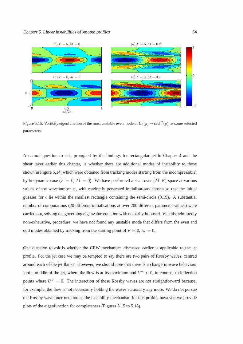
Chapter 5. Linear instabilities of smooth profiles 64
y
αx/2π
(d) F = 0,M = 0 (c) F = 0,M = 0.2
(b) F = 5,M = 0 (a) F = 5,M = 0.2
0
0
0 0.5
1
1-1
2
-2
Figure 5.15: Vorticity eigenfunction of the most unstable even mode ofU0(y) = sech2(y), at some selected
parameters.
A natural question to ask, prompted by the findings for rectangular jet in Chapter 4 and the
shear layer earlier this chapter, is whether there are additional modes of instability to those
shown in Figure 5.14, which were obtained from tracking modes starting from the incompressible,
hydrodynamic case (F = 0, M = 0). We have performed a scan over(M,F ) space at various
values of the wavenumberα, with randomly generated initialisations chosen so that the initial
guesses forc lie within the smallest rectangle containing the semi-circle (3.19). A substantial
number of computations (20 different initialisations at over 200 different parameter values) were
carried out, solving the governing eigenvalue equation with no parity imposed. Via this, admittedly
non-exhaustive, procedure, we have not found any unstable mode that differs from the even and
odd modes obtained by tracking from the starting point ofF = 0,M = 0.
One question to ask is whether the CRW mechanism discussed earlier is applicable to the jet
profile. For the jet case we may be tempted to say there are two pairs of Rossby waves, centred
around each of the jet flanks. However, we should note that there is a change in wave behaviour
in the middle of the jet, where the flow is at its maximum andU ′′ < 0, in contrast to inflection
points whereU ′′ = 0. The interaction of these Rossby waves are not straightforward because,
for example, the flow is not necessarily holding the waves stationary any more. We do not pursue
the Rossby wave interpretation as the instability mechanism for this profile, however, we provide
plots of the eigenfunction for completeness (Figures 5.15 to 5.18).
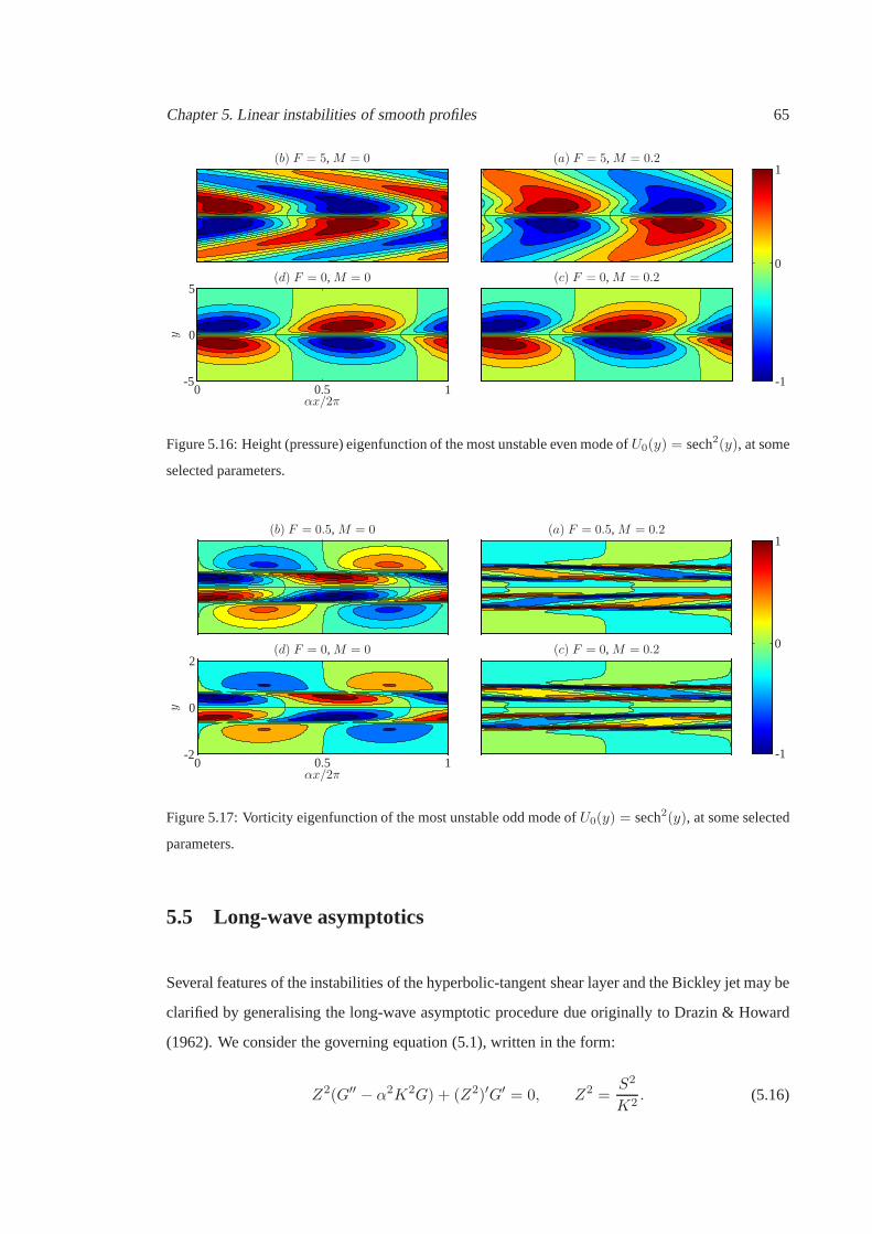
Chapter 5. Linear instabilities of smooth profiles 65
y
αx/2π
(d) F = 0,M = 0 (c) F = 0,M = 0.2
(b) F = 5,M = 0 (a) F = 5,M = 0.2
0
0
0 0.5
1
1-1-5
5
Figure 5.16: Height (pressure) eigenfunction of the most unstable even mode ofU0(y) = sech2(y), at some
selected parameters.
y
αx/2π
(d) F = 0,M = 0 (c) F = 0,M = 0.2
(b) F = 0.5, M = 0 (a) F = 0.5,M = 0.2
0
0
0 0.5
1
1-1
2
-2
Figure 5.17: Vorticity eigenfunction of the most unstable odd mode ofU0(y) = sech2(y), at some selected
parameters.
5.5 Long-wave asymptotics
Several features of the instabilities of the hyperbolic-tangent shear layer and the Bickley jet may be
clarified by generalising the long-wave asymptotic procedure due originally to Drazin & Howard
(1962). We consider the governing equation (5.1), written in the form:
Z2(G′′ − α2K2G) + (Z2)′G′ = 0, Z2 =S2
K2. (5.16)
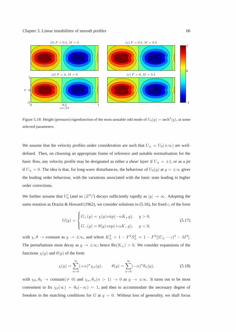
Chapter 5. Linear instabilities of smooth profiles 66
y
αx/2π
(d) F = 0,M = 0 (c) F = 0,M = 0.2
(b) F = 0.5, M = 0 (a) F = 0.5, M = 0.2
0
0
0 0.5
1
1-1-5
5
Figure 5.18: Height (pressure) eigenfunction of the most unstable odd mode ofU0(y) = sech2(y), at some
selected parameters.
We assume that the velocity profiles under consideration aresuch thatU± = U0(±∞) are well-
defined. Then, on choosing an appropriate frame of referenceand suitable normalisation for the
basic flow, any velocity profile may be designated as either ashear layerif U± = ±1, or as ajet
if U± = 0. The idea is that, for long-wave disturbances, the behaviour of U0(y) at y = ±∞ gives
the leading order behaviour, with the variations associated with the basic state leading to higher
order corrections.
We further assume thatU ′0 (and so(Z2)′) decays sufficiently rapidly as|y| → ∞. Adopting the
same notation as Drazin & Howard (1962), we consider solutions to (5.16), for fixedc, of the form
G(y) =
G+(y) = χ(y) exp(−αK+y), y > 0,
G−(y) = θ(y) exp(+αK−y), y < 0,
(5.17)
with χ, θ → constant asy → ±∞, and whereK2± = 1 − F 2S2
± = 1 − F 2[(U± − c)2 −M2].
The perturbations must decay asy → ±∞; hence Re(K±) > 0. We consider expansions of the
functionsχ(y) andθ(y) of the form
χ(y) =
∞∑
n=0
(+α)nχn(y), θ(y) =
∞∑
n=0
(−α)nθn(y), (5.18)
with χ0, θ0 → constant(6= 0) andχn, θn(n > 1) → 0 asy → ±∞. It turns out to be most
convenient to fixχ0(∞) = θ0(−∞) = 1, and then to accommodate the necessary degree of
freedom in the matching conditions forG at y = 0. Without loss of generality, we shall focus

Chapter 5. Linear instabilities of smooth profiles 67
on the equations forχ; those forθ follow in a similar fashion. On substituting expressions (5.17)
(with the expansions (5.18)) into (5.16), equating the coefficients at each order ofα gives
0 = [Z2χ′0]′, (5.19a)
0 = [Z2χ′1]′ −K+[(Z
2χ0)′ + Z2χ′
0], (5.19b)
0 = [Z2χ′n+2]
′ −K+[(Z2χn+1)
′ + Z2χn+1] + Z2(K2+ −K2), n ≥ 0. (5.19c)
Equation (5.19a) integrates toZ2χ′0 = C, with the conditions at infinity then givingC = 0. Thus
χ0 = constant= 1 through our choice ofχ0(∞). Integration of equations (5.19b) – (5.19c) then
gives, after some algebra,
χ1 =
∫ y
∞
(
1− Z2+
Z2
)
dy1,
χ2 =
∫ y
∞
[
1
Z2
∫ y1
∞(S2 − S2
+) dy2 +K2+
∫ y1
∞
(
1− Z2+
Z2
)
dy2
]
dy1.
(5.20)
Analogously, we have
θ0 = 1,
θ1 = K−
∫ y
−∞
(
1− Z2−
Z2
)
dy1,
θ2 =
∫ y
−∞
[
1
Z2
∫ y1
−∞(S2 − S2
−) dy2 +K2−
∫ y1
−∞
(
1− Z2−
Z2
)
dy2
]
dy1.
(5.21)
Having normalisedχ andθ, the matching conditions aty = 0 become
G+(0) = ΓG−(0), and G′+(0) = ΓG′
−(0), (5.22)
for some constantΓ. Consistency thus impliesG+(0)G′−(0) = G−(0)G
′+(0), which gives
0 =
[
S2+
K++S2−
K−
]
+ α
[∫ ∞
0(S2 − S2
+) dy +
∫ 0
−∞(S2 − S2
−) dy
− S2+
K+K−
∫ 0
−∞
(
1− S2−
S2
)
dy − S2−
K+K−
∫ ∞
0
(
1− S2+
S2
)
dy
]
+O(α2),
(5.23)
where the factor of−1/Z2 multiplying the whole of the right hand side has been removed.
Although we have focussed on the case of uniform background magnetic field, it is possible to
include a non-uniform background magnetic field in our derivation, subject to imposing conditions
analogous to those for the background velocity profile. For the case where there is a underlying
topography, we refer the reader to the article of Collings & Grimshaw (1980) for the assumptions
required.

Chapter 5. Linear instabilities of smooth profiles 68
5.5.1 Hyperbolic-tangent shear layer
For a shear layer,U± = ±1, the leading order term of expression (5.23) gives
(1− c(0))2 −M2
√
1− F 2[(1− c(0))2 −M2]+
(1 + c(0))2 −M2
√
1− F 2[(1 + c(0))2 −M2]= 0, (5.24)
which is exactly the eigenvalue equation of the vortex sheet(4.6). Hence, for any shear layer,
c → cv in (4.8) asα → 0. This is perhaps not entirely surprising: sufficiently longwaves will, at
least to leading order, see the shear layer as a discontinuity. This also suggests that the tongue of
instability (cf. Figure 5.1c) is a generic feature of shear layer profiles since long wavesare unstable
in the tongue region.
Information about the second mode of instability may be obtained at the next order. From
the discussion of the vortex sheet in Chapter 4, we know that whenF is sufficiently high, the
eigenvaluecv becomes real. Following Blumenet al. (1975), we considerc = cv + αc(1) + · · · .Choosingcv ∈ R
+, we note that
K+,0K−,0 =√
1− F 2[(1− cv)2 −M2√
1− F 2[(1 + cv)2 −M2 = 1 (5.25)
upon writing outcv in full using (4.8). Assuming(1−M2) = O(1), to proceed, we need to obtain
theO(α) correction to this first term in the square bracket in (5.23),and evaluate the remaining
integrals.
Takingc = cv + αc(1) and Taylor expand accordingly, we use theO(1) relation that
S2+,0
K2+,0
= −S2−,0
K2−,0
(5.26)
to eliminate terms accordingly. This yields in our case
S2+
K2+
+S2−
K2−
= · · · + α
[
c(1)
K+,0
2
S2−,0
4cv
√
1 + 4F 2 + 4F 4M2
]
. (5.27)
In theM = 0 case this is an equivalent form to that obtained by Blumenet al. (1975).
Now, to evaluate the integrals on the right hand side of (5.23). WhenU0 = tanh(y),
∫ ∞
0(S2 − S2
+) dy +
∫ 0
−∞(S2 − S2
−) dy = −2. (5.28)
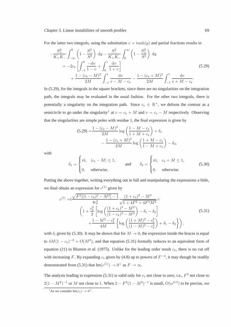
Chapter 5. Linear instabilities of smooth profiles 69
For the latter two integrals, using the substitutionv = tanh(y) and partial fractions results in
− S2+
K+K−
∫ 0
−∞
(
1− S2−
S2
)
dy − S2−
K+K−
∫ ∞
0
(
1− S2+
S2
)
dy
= −2cv
[∫ 0
−1
−dv
1− v+
∫ 1
0
dv
1 + v
]
+1− (cv −M)2
2M
∫ 1
−1
dv
v −M − cv− 1− (cv +M)2
2M
∫ 1
−1
dv
v +M − cv.
(5.29)
In (5.29), for the integrals in the square brackets, since there are no singularities on the integration
path, the integrals may be evaluated in the usual fashion. For the other two integrals, there is
potentially a singularity on the integration path. Sincecv ∈ R+, we deform the contour as a
semicircle to go under the singularity1 at v = cv +M andv = cv −M respectively. Observing
that the singularities are simple poles with residue 1, the final expression is given by
(5.29)=1− (cv −M)2
2Mlog
(
1−M − cv
1 +M + cv
)
+ δ1
− 1− (cv +M)2
2Mlog
(
1 +M − cv
1−M + cv
)
− δ2,
with
δ1 =
πi, |cv −M | ≤ 1,
0, otherwise,and δ2 =
πi, cv +M ≤ 1,
0, otherwise.(5.30)
Putting the above together, writing everything out in full and manipulating the expressions a little,
we final obtain an expression forc(1) given by
c(1) =i
√
F 2[(1− cv)2 −M2]− 1
4c2v
(1 + cv)2 −M2
√1 + 4F 2 + 4F 4M2
×(
1 +c2v2
[
log
(
(1 + cv)2 −M2
(1− cv)2 −M2
)
− δ1 − δ2
]
+1−M2 − c2v
4M
log
(
(1 +M)2 − c2v(1−M)2 − c2v
)
+ δ1 − δ2
)
,
(5.31)
with δi given by (5.30). It may be shown that forM → 0, the expression inside the braces is equal
to 4M(1 − cv)−2 + O(M2), and that equation (5.31) formally reduces to an equivalentform of
equation (21) in Blumenet al. (1975). Unlike for the leading order resultcv, there is no cut off
with increasingF . By expandingcv given by (4.8) up to powers ofF−4, it may though be readily
demonstrated from (5.31) that Im(c(1)) → 0+ asF → ∞.
The analysis leading to expression (5.31) is valid only forcv not close to zero, i.e.,F 2 not close to
2(1−M2)−1 orM not close to1. When2− F 2(1−M2)−1 is small,O(α2/3) to be precise, we
1As we consider Im(cv) → 0+.

Chapter 5. Linear instabilities of smooth profiles 70
havecv ∼ αc(1) ∼ α1/3. Performing appropriate rescaling and choosing the appropriate branch
so that Re(√· · ·) > 0, givesc(1) as the solution of the cubic equation
6 + 2M2
(1−M2)3c3 +
(
2
1−M2− F 2
)
c− iα
[
1
1−M2+
1
2Mlog
1 +M
1−M
]
= 0, (5.32)
for α2/3 ∼ 2(1−M2)−1−F 2 → 0. Equation (5.32) formally reduces to equation (23) in Blumen
et al.(1975). There is an inadmissible rootc = −ici, and two roots that are either purely imaginary
(c = ici) or complex (c = ±cr + ici) depending onF 2. Considering the expansion
(5.32)= (c− iA)2(c− iB),
the transition to non-zerocr may be seen to occur at
F 2cusp=
2
1−M2− 3
[
α2
4
6 + 2M2
(1−M2)3
(
1
1−M2+
1
2Mlog
1 +M
1−M
)2]1/3
. (5.33)
This expression reduces toF 2cusp= 2−3(6α2)1/3 whenM → 0, as given by Blumenet al.(1975).
The leading order result with, separately, corrections from the outer and inner expansions, together
with the full numerical results, are presented in figure 5.19. The asymptotic results, including the
location of the cusp given by equation (5.33), show excellent agreement with the numerically
computed values.
5.5.2 Long-wave asymptotics for jets
A general velocity profile is defined as a jet if, in an appropriate frame,U± = 0. In this case,
expression (5.23) simplifies to
0 =2S2
0
K0+ α
[∫ ∞
−∞(S2 − S2
0) dy −S20
K20
∫ ∞
−∞
(
1− S20
S2
)
dy
]
+O(α2), (5.34)
whereS20 = (0 − c)2 −M2. Here, for a fixed value ofF , we need to consider different regimes
for M . ForF 2 = O(1), if M2 = O(1) thenc is real at both leading order and at the next order
correction. The marginal case isM2 ∼ α, but this givesc(0) = 0 at leading order. At the next
order correction, we choose to balance the first two terms on the right hand side of (5.34). On
letting M2 = µα and definingE =∫ +∞−∞ U2/2 dy, whereE may be assumed to beO(1) via
rescaling, we obtain
c ∼ i√
αE −M2 as M2 ∼ α→ 0, F 2 = O(1). (5.35)

Chapter 5. Linear instabilities of smooth profiles 71
(a)M = 0 (b)M = 0.25 (c)M = 0.5
(d)M = 0 (e)M = 0.25 (f)M = 0.5
F
c ic r
111
111
1.51.51.5
1.51.51.5
222
222
000
000
0.20.20.2
0.20.20.2
0.40.40.4
0.40.40.4
Figure 5.19: Line graphs ofc = cr + ici atα = 0.01, varying withF for some values ofM , for the shear
layer. The crosses are computed results, solid line is the asymptotic resultcv +αc1 with c1 given by (5.31),
and the dot-dashed line is the inner expansion given by the relevant solution to the cubic (5.32).
The corresponding result for the compressible hydrodynamic case was derived by Gill & Drazin
(1965), and for the incompressible MHD case by Gedzelman (1973).
For largeF , we letF 2 = ǫ−1 ≫ 1. Then the interesting case is whenM2 = O(ǫ) andα ∼ ǫ.
Considering the same balance as above gives the following result:
c ∼ i
[
α2F 2E2
2−M2 +
√
α2E2 +α4F 4E4
4
]1/2
as1
F 2∼M2 ∼ α→ 0. (5.36)
This result reduces formally to (5.34) in the limit of smallF .
For the Bickley jet,∫ +∞−∞ (sech2y)2 dy = 4/3. The corresponding long-wave asymptotic results
are therefore given by
c ∼ i
√
2
3α−M2 as M2 ∼ α→ 0, F 2 = O(1), (5.37)
and
c ∼ i
[
2
9α2F 2 −M2 +
2
3
√
α2 +α4F 4
9
]1/2
as1
F 2∼M2 ∼ α→ 0. (5.38)

Chapter 5. Linear instabilities of smooth profiles 72
(a) F = 0 (b) F = 1
(c) F = 5 (d) F = 10
α
αc i
10
10
10101010
10
10
10101010
10
10
10101010
10
10
10101010
0
0
0
0
0
0
0
0
-2
-2
-2
-2
-2
-2
-2
-2
-4-4
-4-4
-1-1
-1-1
Figure 5.20: Comparison of the computed growth rates (crosses) and the predicted growth rates from the
asymptotic results forU(y) = sech2(y), atM = 0.1: α×(5.37) is given by the dot-dashed line (cutoff
plotted as vertical dotted line) andα×(5.38) is given by the solid line (cutoff plotted as verticaldashed
line). Circles denote the modes stabilised by the magnetic field.
The growth rate as predicted by (5.37) and (5.38) is plotted against the computed growth rates
(of the even mode) in Figure 5.20; it can be seen that the cutoffs due to the magnetic field are
accurately predicted.
5.5.3 Consistency issues of long-wave asymptotics for jets
One potential concern is that we have assumed that the secondintegral in the square brackets in
expression (5.34) is negligible in the leading order balance. We show here that
c2 −M2
1− F 2(c2 −M2)
∫ +∞
−∞
[
1− c2 −M2
(U0 − c)2 −M2
]
dy = O(ǫ log ǫ), (5.39)
whereǫ is some small parameter related to the regime of interest. Thus the asymptotic scheme is
indeed consistent.
Following Drazin & Howard (1962), we shall assume that|U0| ≤ Ae−a|y|, which is satisfied
for the Bickley jet considered. This condition may be relaxed: choosing|U0| ≤ A/(1 + y2n),
wheren is an integer, provides a modified version of (5.39) using theapproach below. Drazin
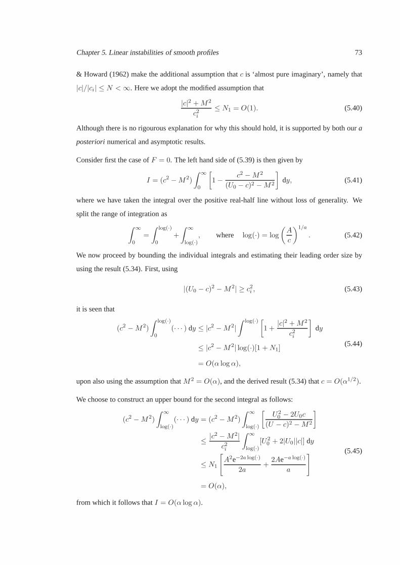
Chapter 5. Linear instabilities of smooth profiles 73
& Howard (1962) make the additional assumption thatc is ‘almost pure imaginary’, namely that
|c|/|ci| ≤ N <∞. Here we adopt the modified assumption that
|c|2 +M2
c2i≤ N1 = O(1). (5.40)
Although there is no rigourous explanation for why this should hold, it is supported by both oura
posteriorinumerical and asymptotic results.
Consider first the case ofF = 0. The left hand side of (5.39) is then given by
I = (c2 −M2)
∫ ∞
0
[
1− c2 −M2
(U0 − c)2 −M2
]
dy, (5.41)
where we have taken the integral over the positive real-halfline without loss of generality. We
split the range of integration as
∫ ∞
0=
∫ log(·)
0+
∫ ∞
log(·), where log(·) = log
(
A
c
)1/a
. (5.42)
We now proceed by bounding the individual integrals and estimating their leading order size by
using the result (5.34). First, using
|(U0 − c)2 −M2| ≥ c2i , (5.43)
it is seen that
(c2 −M2)
∫ log(·)
0(· · · ) dy ≤ |c2 −M2|
∫ log(·) [
1 +|c|2 +M2
c2i
]
dy
≤ |c2 −M2| log(·)[1 +N1]
= O(α log α),
(5.44)
upon also using the assumption thatM2 = O(α), and the derived result (5.34) thatc = O(α1/2).
We choose to construct an upper bound for the second integralas follows:
(c2 −M2)
∫ ∞
log(·)(· · · ) dy = (c2 −M2)
∫ ∞
log(·)
[
U20 − 2U0c
(U − c)2 −M2
]
≤ |c2 −M2|c2i
∫ ∞
log(·)[U2
0 + 2|U0||c|] dy
≤ N1
[
A2e−2a log(·)
2a+
2Ae−a log(·)
a
]
= O(α),
(5.45)
from which it follows thatI = O(α log α).
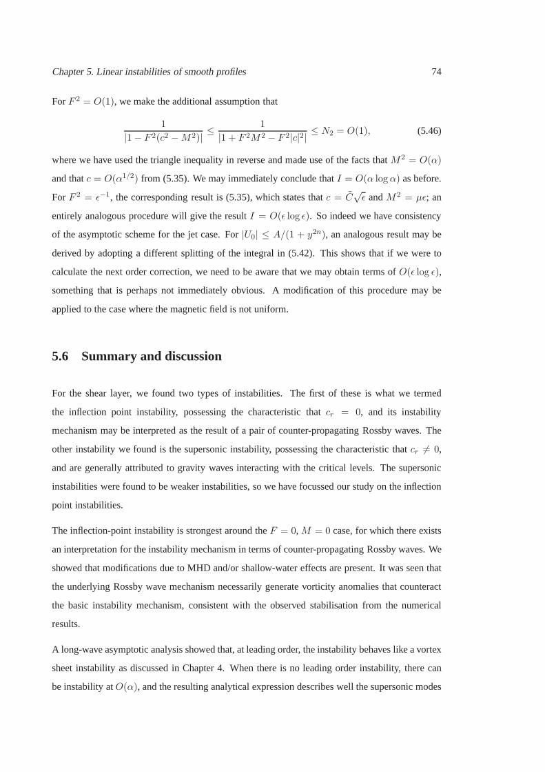
Chapter 5. Linear instabilities of smooth profiles 74
ForF 2 = O(1), we make the additional assumption that
1
|1− F 2(c2 −M2)| ≤1
|1 + F 2M2 − F 2|c|2| ≤ N2 = O(1), (5.46)
where we have used the triangle inequality in reverse and made use of the facts thatM2 = O(α)
and thatc = O(α1/2) from (5.35). We may immediately conclude thatI = O(α logα) as before.
ForF 2 = ǫ−1, the corresponding result is (5.35), which states thatc = C√ǫ andM2 = µǫ; an
entirely analogous procedure will give the resultI = O(ǫ log ǫ). So indeed we have consistency
of the asymptotic scheme for the jet case. For|U0| ≤ A/(1 + y2n), an analogous result may be
derived by adopting a different splitting of the integral in(5.42). This shows that if we were to
calculate the next order correction, we need to be aware thatwe may obtain terms ofO(ǫ log ǫ),
something that is perhaps not immediately obvious. A modification of this procedure may be
applied to the case where the magnetic field is not uniform.
5.6 Summary and discussion
For the shear layer, we found two types of instabilities. Thefirst of these is what we termed
the inflection point instability, possessing the characteristic that cr = 0, and its instability
mechanism may be interpreted as the result of a pair of counter-propagating Rossby waves. The
other instability we found is the supersonic instability, possessing the characteristic thatcr 6= 0,
and are generally attributed to gravity waves interacting with the critical levels. The supersonic
instabilities were found to be weaker instabilities, so we have focussed our study on the inflection
point instabilities.
The inflection-point instability is strongest around theF = 0,M = 0 case, for which there exists
an interpretation for the instability mechanism in terms ofcounter-propagating Rossby waves. We
showed that modifications due to MHD and/or shallow-water effects are present. It was seen that
the underlying Rossby wave mechanism necessarily generatevorticity anomalies that counteract
the basic instability mechanism, consistent with the observed stabilisation from the numerical
results.
A long-wave asymptotic analysis showed that, at leading order, the instability behaves like a vortex
sheet instability as discussed in Chapter 4. When there is noleading order instability, there can
be instability atO(α), and the resulting analytical expression describes well the supersonic modes
Chapter 5. Linear instabilities of smooth profiles 75
from the numerical calculations. The criticalF for which that supersonic instability becomes the
preferred mode of instability was also derived from this asymptotic analysis.
For the Bickley jet, the parity result dictates that the eigenfunction is either even or odd about
y = 0. The even mode is generally found to be more unstable than theodd mode, although there
are isolated regions in parameter space where the converse is true. A cutoff of the instability due
to the magnetic field atα ≪ 1 is again observed, and the locations of the cutoffs may be found
using an asymptotic analysis.
With regards to the Rossby wave mechanism, there were details that we have not taken into
account, such as the changes in the phase-locking mechanism(the induced vorticity anomalies
from extra effects accelerates the underlying Rossby waves), or whether it would be applicable
even in the tongue region of instability for the shear layer.The mathematical basis appears to
be well developed for an extended investigation (e.g., Heifetzet al., 1999, 2004, 2009; Carpenter
et al., 2012), and it would be interesting to investigate the modifications to the wave dynamics,
potentially revealing the more subtle features possessed by the instability. Since we know that,
in the hydrodynamic case, the stability criteria may be interpreted as conditions that allow the
relevant mechanisms to occur, one question we may ask is that, if we know the precise details
associated with the instability mechanism, can we deduce from this stability criteria (e.g., Heifetz
et al., 2009)? This would be particularly interesting since we have not managed to derive stability
conditions for this system of equations, and this may provide another avenue to derive stability
theorems.
With regards to the supersonic instabilities, it would alsobe interesting to consider a further
investigation into the characteristic of these instabilities, using tools employed by previous works
(e.g., Satomura, 1981; Hayashi & Young, 1987; Takehiro & Hayashi, 1992; Balmforth, 1999). It
was mentioned also in Balmforth (1999) that one interpretation of these supersonic instabilities
is via over-reflection (e.g., Acheson, 1976; Lindzen & Tung,1978; McIntyre & Weissman, 1978;
Lindzen, 1988; Harnik & Heifetz, 2007; Bakas & Farrell, 2010; Benilov & Lapin, 2013), and
it would be interesting to derive the modifications to over-reflection in SWMHD to further our
understanding on phenomena involving magneto-gravity waves. Furthermore, in the work of
Harnik & Heifetz (2007), an attempt was made to reconcile over-reflection and the Rossby wave
action-at-a-distance mechanism, and it would also be interesting to see how over-reflection leading
to instability may be interpreted in this formalism.

Chapter 5. Linear instabilities of smooth profiles 76
5.7 Appendix: Recovering fields from the eigenfunctionG
The quantities(u, v, bx, by, h) may be recovered from knowledge of the eigenfunctionG. It may
be shown that, for the case whereH ≡ 1 andv = (U0 − c)G
v =(U0 − c)G, (5.47a)
by =MB0G, (5.47b)
u =v′ + F 2M [B′
0(U0 − c) +B0U′0]by − F 2[(U0 − c)U ′
0 +M2B0B′0]v
−iα[1− F 2[(U0 − c)2 −M2B20 ]]
, (5.47c)
bx =b′y + F 2[(U0 − c)U ′
0 +MB0U′0]by − F 2M [B0U
′0 + (U0 − c)B′
0)]v
−iα[1 − F 2[(U0 − c)2 −M2B20 ]]
, (5.47d)
h =M(B′
0(U0 − c) +B0U′0)by − [(U0 − c)U ′
0 +M2B0B′0]v + [(U − c)2 −M2B2
0 ]v′
iα(U − c)[1− F 2[(U0 − c)2 −M2B20 ]]
.
(5.47e)
In the investigation presented here, the numerical derivatives were calculated by a fourth-order
accurate finite-difference approximation using theweights routine given in Fornberg (1998).
We observe hereh remains formally atO(1) because of the rescalingh =ˆh/F 2 employed
when we wrote down the full non-dimensionalised SWMHD equations. Indeed, sinceh is to
be identified withp whenF = 0, it may be shown that we recover the above expression if we start
with the equations withF = 0 and reconstructp from (u, v, bx, by). The perturbation displacement
η, vorticity ω, potential vorticityq and currentj are seen to satisfy
Dη
Dt= v ⇒ η =
v
iα(U0 − c), (5.48a)
ω =∂v
∂x− ∂u
∂y⇒ ω = iαv − u′, (5.48b)
Q+ q =Ω0 + ω
1 + F 2h⇒ q = ω − F 2Ω0h+O(small2), (5.48c)
j =∂by∂x
− ∂bx∂y
⇒ j = iαby − b′x. (5.48d)
Working out vorticity and current fromω andj is found to be more accurate than taking derivatives
of the full u andv fields. It is found that by taking the numerical solution and inserting it back
into the linearised equations (3.3), the largest error as measured by theL∞ norm is ofO(10−2)
for the choice of numerical tolerance we used for working outG. This occurs in they-momentum
equation; typical diagrams for the errors from an inversionis given in Figure 5.21.
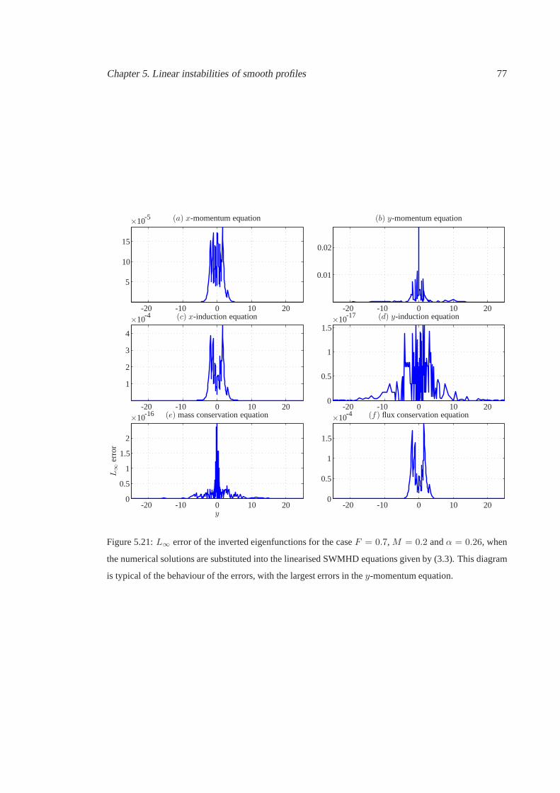
Chapter 5. Linear instabilities of smooth profiles 77
(a) x-momentum equation (b) y-momentum equation
(c) x-induction equation (d) y-induction equation
(e) mass conservation equation (f) flux conservation equation
y
×10×10
×10×10
×10
L∞
erro
r
-20-20
-20-20
-20-20
-10-10
-10-10
-10-10
00
00
000
00
1010
1010
10
10
10
2020
2020
2020
0.50.5
0.5
11
1
1
1.5
1.5
1.5
2
2
3
4
5
15
0.01
0.02
-5
-4
-4 -17
-16
Figure 5.21:L∞ error of the inverted eigenfunctions for the caseF = 0.7,M = 0.2 andα = 0.26, when
the numerical solutions are substituted into the linearised SWMHD equations given by (3.3). This diagram
is typical of the behaviour of the errors, with the largest errors in they-momentum equation.

Chapter 5. Linear instabilities of smooth profiles 78

79
Chapter 6
Nonlinear evolution: two-dimensional
incompressible MHD
In the previous chapter the instability characteristics ofthe shear layer and the Bickley jet profile
were investigated. A natural progression now is to investigate the nonlinear evolution of unstable
shear flows. In this chapter, we consider the incompressiblelimit (F = 0) to highlight the
dynamics due to MHD effects, before moving on to an investigation of the full SWMHD system
in Chapter 7. We start by reviewing in some detail the numerical methods we employ. We then
review the hydrodynamic case before proceeding to an investigation of the MHD case. A summary
and discussion of the results are given at the end of the chapter.
6.1 Mathematical formulation and numerical methods
As in the previous chapter, we consider the case with no topography and a uniform background
magnetic field given byB0 = 1, and we will consider eitherU0(y) = tanh(y) or U0(y) =
sech2(y); M = B/U is then our measure of the field strength. We shall be investigating the
nonlinear evolution numerically. Since we only have finite resolution and we expect the evolution
to generate small-scales, we need something to damp these small-scale features, in a physical
manner, to stabilise our numerical routines. To this end, wereinstate the viscous and Ohmic
dissipation. The (two-dimensional) incompressible MHD equations (F = 0) in non-dimensional

Chapter 6. Nonlinear evolution: two-dimensional incompressible MHD 80
form are then given by
∂u
∂t+ u · ∇u−∇p−M2
b · ∇b =1
Re∇2
u, (6.1a)
∂b
∂t+ u · ∇b− b · ∇u =
1
Rm∇2
b, (6.1b)
∇ · u = 0, (6.1c)
∇ · b = 0. (6.1d)
The Reynolds numbers are defined using the velocity and length scales associated with the basic
flow, so
Re=ULν, Rm=
ULη, (6.2)
whereν is the kinematic viscosity, andη is the coefficient of magnetic diffusivity.
We shall be interested in the temporal evolution of the dynamics, and we consider a domain that is
periodic inx and wall bounded iny. A domain of lengthLx = 2π/α will support one wavelength
of the instability with wavenumberα, doubling this gives two wavelengths of the instability, and
so forth. Although the basic flow profiles are technically defined on an unbounded domain, it is
found that by taking they-boundaries located aty = ±Ly for Ly sufficiently large, together with
appropriate boundary conditions, the dynamical influence of the boundaries can be minimised.
Sinceu andb are both divergence-free, we write the equations in terms ofa streamfunctionψ and
a magnetic potentialA, here defined as
u = ez ×∇ψ, b = ez ×∇A. (6.3)
The vorticityω and currentj are then given by
ω = ∇2ψ, j = ∇2A. (6.4)
The divergence-free conditions are automatically satisfied, and the set of equations (6.1) have the
equivalent formulation given by
∂ω
∂t+ ∂(ψ, ω) −M2∂(A,∇2A) =
1
Re∇2ω, (6.5a)
∂A
∂t+ ∂(ψ,A) =
1
Rm∇2A, (6.5b)
∇2ψ = ω, (6.5c)
where
∂(α, β) =∂α
∂x
∂β
∂y− ∂α
∂y
∂β
∂x(6.6)

Chapter 6. Nonlinear evolution: two-dimensional incompressible MHD 81
is the usual Jacobian term. The corresponding basic states are then given by
Ψ0(y) =
− log cosh(y),
− tanh(y),
A0(y) = −y. (6.7)
This set up is convenient in that we do not have to worry about imposing the divergence-free
condition at every time step via, for example, splitting methods, projection methods, or semi-
implicit methods (e.g., Peyret, 2002).
In our channel geometry, boundary conditions iny need to be imposed accordingly. The no-normal
flow condition impliesv = ∂ψ/∂x = 0 on y = ±Ly, soψ is a constant function inx. Then,
because momentum is conserved,
∫∫
u dxdy =
∫∫
∂ψ
∂ydxdy = Lx[ψ(t)]
Ly
−Ly= constant, (6.8)
so we must have
[ψ(t)]Ly
−Ly= [ψ(0)]
Ly
−Ly. (6.9)
This is satisfied if
ψ(t,±Ly) = ψ(0,±Ly). (6.10a)
The same argument applies to the no-normal flux conditionby = 0, giving
A(t,±Ly) = A(0,±Ly). (6.10b)
To mimic a free shear flow, we use stress-free boundary conditions rather than no-slip, so
∂u
∂y= 0 ⇒ ∂2ψ
∂y2= ω(±Ly) = 0. (6.10c)
The above conditions are then to be enforced at each time-step accordingly.
Additionally, we split the above quantities as a basic stateplus a perturbation, i.e.
ψ = Ψ0(y) + ψ, A = A0(y) + A, (6.11)
and also
ω = Ω0(y) +∇2ψ = −U ′0(y) +∇2ψ, j = J0(y) +∇2A = 0 +∇2A. (6.12)
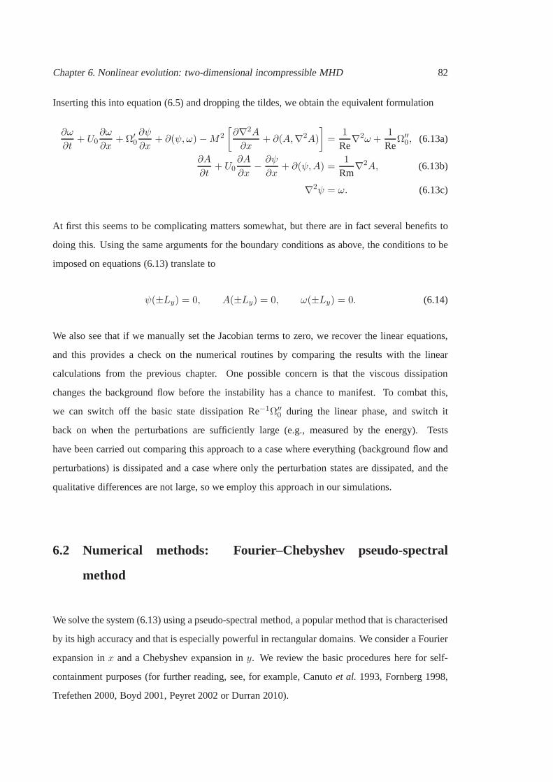
Chapter 6. Nonlinear evolution: two-dimensional incompressible MHD 82
Inserting this into equation (6.5) and dropping the tildes,we obtain the equivalent formulation
∂ω
∂t+ U0
∂ω
∂x+Ω′
0
∂ψ
∂x+ ∂(ψ, ω) −M2
[
∂∇2A
∂x+ ∂(A,∇2A)
]
=1
Re∇2ω +
1
ReΩ′′0, (6.13a)
∂A
∂t+ U0
∂A
∂x− ∂ψ
∂x+ ∂(ψ,A) =
1
Rm∇2A, (6.13b)
∇2ψ = ω. (6.13c)
At first this seems to be complicating matters somewhat, but there are in fact several benefits to
doing this. Using the same arguments for the boundary conditions as above, the conditions to be
imposed on equations (6.13) translate to
ψ(±Ly) = 0, A(±Ly) = 0, ω(±Ly) = 0. (6.14)
We also see that if we manually set the Jacobian terms to zero,we recover the linear equations,
and this provides a check on the numerical routines by comparing the results with the linear
calculations from the previous chapter. One possible concern is that the viscous dissipation
changes the background flow before the instability has a chance to manifest. To combat this,
we can switch off the basic state dissipation Re−1Ω′′0 during the linear phase, and switch it
back on when the perturbations are sufficiently large (e.g.,measured by the energy). Tests
have been carried out comparing this approach to a case whereeverything (background flow and
perturbations) is dissipated and a case where only the perturbation states are dissipated, and the
qualitative differences are not large, so we employ this approach in our simulations.
6.2 Numerical methods: Fourier–Chebyshev pseudo-spectral
method
We solve the system (6.13) using a pseudo-spectral method, apopular method that is characterised
by its high accuracy and that is especially powerful in rectangular domains. We consider a Fourier
expansion inx and a Chebyshev expansion iny. We review the basic procedures here for self-
containment purposes (for further reading, see, for example, Canutoet al. 1993, Fornberg 1998,
Trefethen 2000, Boyd 2001, Peyret 2002 or Durran 2010).
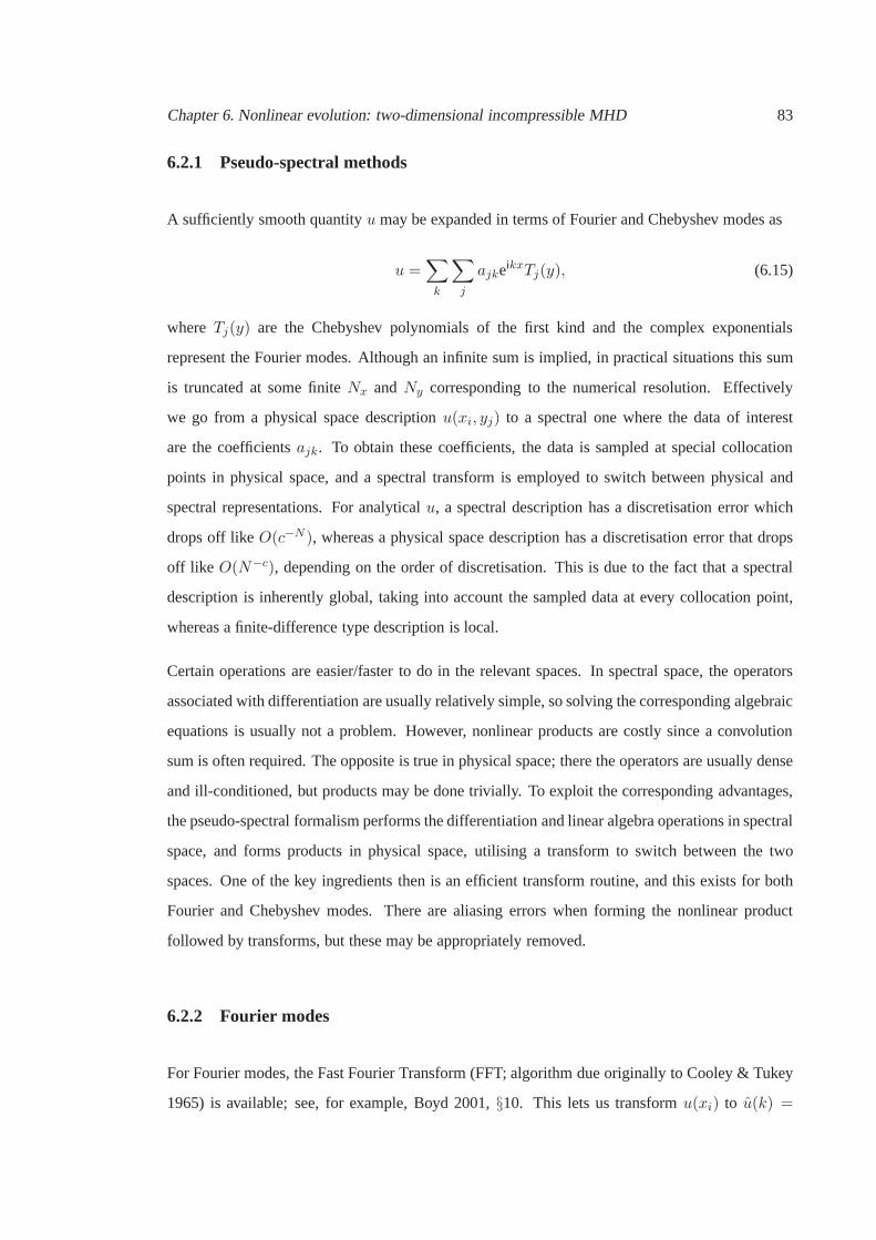
Chapter 6. Nonlinear evolution: two-dimensional incompressible MHD 83
6.2.1 Pseudo-spectral methods
A sufficiently smooth quantityu may be expanded in terms of Fourier and Chebyshev modes as
u =∑
k
∑
j
ajkeikxTj(y), (6.15)
where Tj(y) are the Chebyshev polynomials of the first kind and the complex exponentials
represent the Fourier modes. Although an infinite sum is implied, in practical situations this sum
is truncated at some finiteNx andNy corresponding to the numerical resolution. Effectively
we go from a physical space descriptionu(xi, yj) to a spectral one where the data of interest
are the coefficientsajk. To obtain these coefficients, the data is sampled at specialcollocation
points in physical space, and a spectral transform is employed to switch between physical and
spectral representations. For analyticalu, a spectral description has a discretisation error which
drops off likeO(c−N ), whereas a physical space description has a discretisationerror that drops
off like O(N−c), depending on the order of discretisation. This is due to thefact that a spectral
description is inherently global, taking into account the sampled data at every collocation point,
whereas a finite-difference type description is local.
Certain operations are easier/faster to do in the relevant spaces. In spectral space, the operators
associated with differentiation are usually relatively simple, so solving the corresponding algebraic
equations is usually not a problem. However, nonlinear products are costly since a convolution
sum is often required. The opposite is true in physical space; there the operators are usually dense
and ill-conditioned, but products may be done trivially. Toexploit the corresponding advantages,
the pseudo-spectral formalism performs the differentiation and linear algebra operations in spectral
space, and forms products in physical space, utilising a transform to switch between the two
spaces. One of the key ingredients then is an efficient transform routine, and this exists for both
Fourier and Chebyshev modes. There are aliasing errors whenforming the nonlinear product
followed by transforms, but these may be appropriately removed.
6.2.2 Fourier modes
For Fourier modes, the Fast Fourier Transform (FFT; algorithm due originally to Cooley & Tukey
1965) is available; see, for example, Boyd 2001,§10. This lets us transformu(xi) to u(k) =

Chapter 6. Nonlinear evolution: two-dimensional incompressible MHD 84
∑
i akeikxi , where the collocation points are given by
xi =2πi
Nx, i = 0, 1, · · · , Nx − 1. (6.16)
The transform is fast in that the number of operations required isO(Nx logNx), as opposed
to standard discrete Fourier transform algorithms that typically requiresO(N2x) operations.
Differentiation in spectral space is especially simple, given by
∂
∂x→ ik. (6.17)
Numerical tests of the FFT routines used are given in§6.8.
There are errors from using this pseudo-spectral approach,arising from the fact that there is some
ambiguity when sampling a function at a finite number of collocation points. For example, suppose
we havexi = (0, π, 2π), the sampled valuesu(xi) = (0, 0, 0) may well describeu = sin(nx) for
n ∈ Z; here, the resolution limits the highest harmonic that may be properly described. Normally
this is not an issue, but spurious errors do arise when FFTs ofnonlinear products are taken, since
the combination of the lower harmonics may result in unphysical higher harmonics that are below
the truncation level set by the resolution, so introducing spurious oscillations. There are several
methods to remove these errors, with Orszag’s 2/3 rule (Orszag, 1971) being particularly simple
to implement. During the transform stage, we simply set the coefficients of the highest third of the
harmonics to zero. In a Fourier representation of the above,we should bear in mind thatNx points
give modes fromk = −Nx/2, · · · 0, 1, · · ·Nx/2, so in the transform routine, all coefficients with
wavenumbers satisfying
|k| ≥ ⌈(Nx/2)(2/3)⌉ = ⌈Nx/3⌉ (6.18)
are set to zero, where⌈(·)⌉ is the ceiling function. We have found that dealiased runs are better
behaved, especially when the run appears to only be marginally resolved. Another point to note
is that the discretised version of the differential equations do not necessarily conserve discretely
the physical quantities such as those mentioned in Chapter 2. One way to ensure the discretised
equations inherit the conservations laws from the continuous case is to remove the dealiasing
errors (e.g., Boyd, 2001,§11). All runs reported here are dealiased using Orszag’s 2/3rule.
The Fourier description allows spatial integration to be done in a particularly convenient fashion.
We note that∫ Lx
0akeikx dx =
Lxa0, k = 0,
0, k = 2πn/Lx, n ∈ N.
(6.19)

Chapter 6. Nonlinear evolution: two-dimensional incompressible MHD 85
with Lx the length of the periodic domain. So to integrate in thex-direction, we simply need to
pick out thek = 0 Fourier mode and multiply it byLx. This method of numerical integration is
spectrally accurate.
We have also the standard Parseval’s theorem given by
∫ Lx
0u2 dx = Lx
∑
k
|ak|2. (6.20)
This follows from the fact that the Fourier modes are orthogonal with respect to the corresponding
inner product on this domain of interest. Indeed, expandingu2 in Fourier modes automatically
gives the result, assuming the order of integration and summation may be exchanged. This allows
us for example to work out the global and modal decompositionof quadratic quantities (such as
energy) whilst maintaining spectral accuracy.
6.2.3 Chebyshev modes
Chebyshev polynomials of the first kind ony ∈ [−1, 1] may be defined by the recurrence relation
T0(y) = 1, T1(y) = y, Tj+1(y) = 2yTj(y)− Tj−1(y). (6.21)
Alternatively, they may be defined as polynomials satisfying
Tj(y) = cos(j arccos y), j = 0, 1, · · · . (6.22)
A clear description of this is given in the book of Trefethen (2000), where Chebyshev polynomials
are seen as the cosine function wrapped around a cylinder. With this description, there is a clear
relationship between the Chebyshev modes and cosine functions, so an adapted FFT serves as the
transform.
The collocation points we employ in this case are the Gauss-Lobatto points given by
yj = cos
(
πj
Ny
)
, j = 0, · · ·Ny. (6.23)
Aliasing errors will be present if we use the pseudo-spectral approach, but again may be removed
by setting to zero the highest third of the wavenumbers.
Differentiation in Chebyshev spectral space is not as straightforward as in Fourier space; however
the matrices are still relatively sparse. These differentiation matrices are evaluated via recurrence
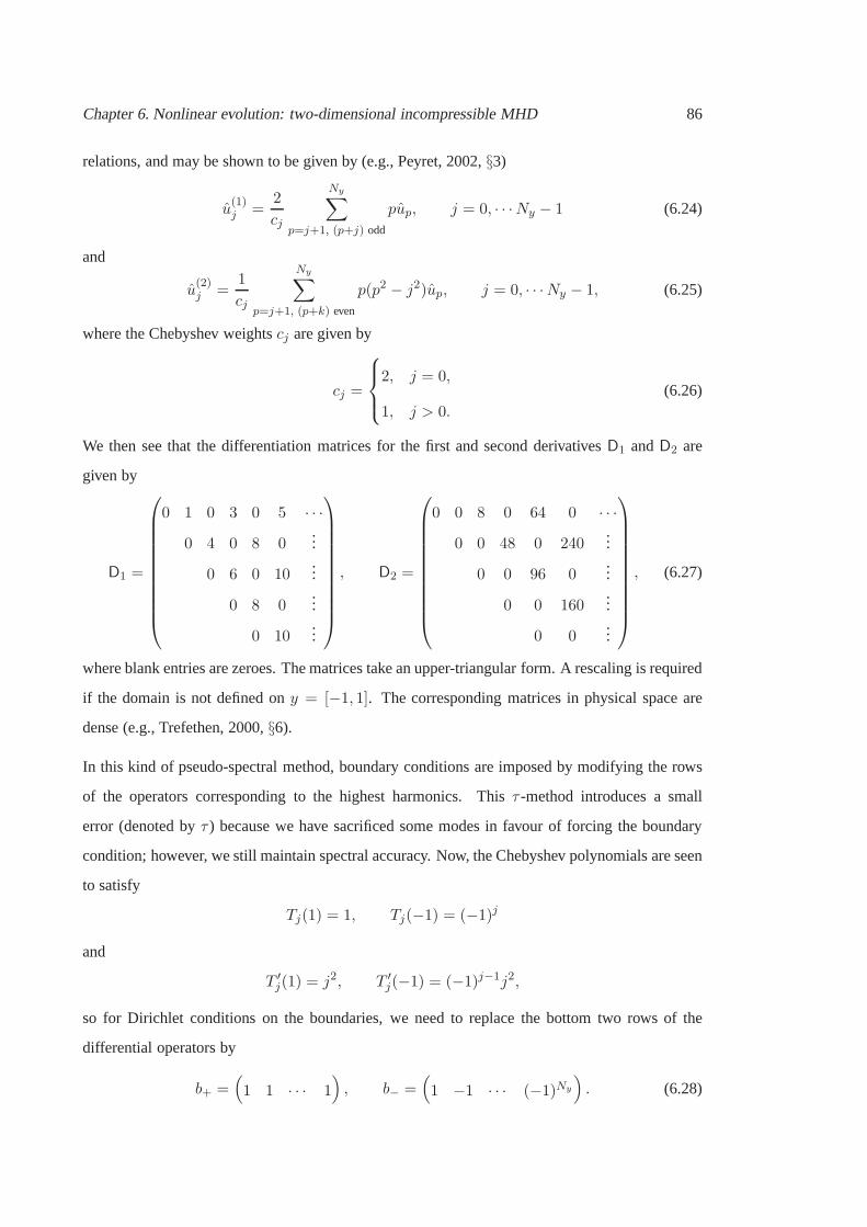
Chapter 6. Nonlinear evolution: two-dimensional incompressible MHD 86
relations, and may be shown to be given by (e.g., Peyret, 2002, §3)
u(1)j =
2
cj
Ny∑
p=j+1, (p+j) odd
pup, j = 0, · · ·Ny − 1 (6.24)
and
u(2)j =
1
cj
Ny∑
p=j+1, (p+k) even
p(p2 − j2)up, j = 0, · · ·Ny − 1, (6.25)
where the Chebyshev weightscj are given by
cj =
2, j = 0,
1, j > 0.
(6.26)
We then see that the differentiation matrices for the first and second derivativesD1 andD2 are
given by
D1 =
0 1 0 3 0 5 · · ·
0 4 0 8 0...
0 6 0 10...
0 8 0...
0 10...
, D2 =
0 0 8 0 64 0 · · ·
0 0 48 0 240...
0 0 96 0...
0 0 160...
0 0...
, (6.27)
where blank entries are zeroes. The matrices take an upper-triangular form. A rescaling is required
if the domain is not defined ony = [−1, 1]. The corresponding matrices in physical space are
dense (e.g., Trefethen, 2000,§6).
In this kind of pseudo-spectral method, boundary conditions are imposed by modifying the rows
of the operators corresponding to the highest harmonics. This τ -method introduces a small
error (denoted byτ ) because we have sacrificed some modes in favour of forcing the boundary
condition; however, we still maintain spectral accuracy. Now, the Chebyshev polynomials are seen
to satisfy
Tj(1) = 1, Tj(−1) = (−1)j
and
T ′j(1) = j2, T ′
j(−1) = (−1)j−1j2,
so for Dirichlet conditions on the boundaries, we need to replace the bottom two rows of the
differential operators by
b+ =(
1 1 · · · 1)
, b− =(
1 −1 · · · (−1)Ny
)
. (6.28)

Chapter 6. Nonlinear evolution: two-dimensional incompressible MHD 87
For Neumann conditions, we need to replace the last two rows by
b+ =(
0 1 · · · N2y
)
, b− =(
0 −1 · · · (−1)Ny−1N2y
)
. (6.29)
When the operators are modified by the rows enforcing the boundary conditions, the resulting
matrix appears to be of a form where appropriate manipulations should result in uncoupled systems
that may be solved separately. This is indeed the case when the resulting equation of the form of
a constant-coefficient Helmholtz equation, where only second and zero derivatives are involved.
For purely Dirichlet or purely Neumann conditions, the resulting system is of the quasi-tridiagonal
form, for which a fast solver exists (Thual, 1986). Most equations we need to solve are of this
Helmholtz type, and as such we may use the fast solver. The fast solver requiresO(N) operations,
compared to the standardLU-decomposition with a back-substitution, which typicallyrequires
O(N3) operations. For more details of this fast solver, see Section 6.8.
Spatial integration may be performed via the Clenshaw–Curtis quadrature (Clenshaw & Curtis
1960; see also Trefethen 2000,§12). This is given by
∫ 1
−1u dy ≈ w
Ta, w =
2
0
2
1− 22
0...
2
1−N2y
=
c0 × 1
c1 × 0
c2 ×2
1− 22
0...
cNy×
1
1−N2y
, (6.30)
wherea = (aj) are the Chebyshev coefficients ofu. Observe that only the even coefficients make
a contribution, since an odd function integrated over an even domain is identically zero.
To calculate the integrals of quadratic quantities, we cannot rely on an analogous Parseval’s
theorem as the Chebyshev modes are not orthogonal to the weight functionw(y) = 1. Instead, the
relationship between the coefficients ofu andu2 is given by
u =
Ny∑
j=0
ajTj ⇒ u2 =
Ny∑
j=0
Ny∑
k=0
ajakTjTk
=
Ny∑
j=0
Ny∑
k=0
ajak2
(Tj+k + T|k−j|),
(6.31)

Chapter 6. Nonlinear evolution: two-dimensional incompressible MHD 88
upon using a standard relation for Chebyshev polynomials. So then
∫ 1
−1u dy ≈
Ny∑
j=0
Ny∑
k=0
ajak2
∫ 1
−1(Tj+k + T|k−j|) dy, (6.32)
and we can evaluate the integral by summing the coefficients multiplied by the relevant Clenshaw–
Curtis weights, but truncating when(j + k) > Ny. However, we expect this method to be
extremely inefficient since we have to performO(N2y ) elementary operations. Alternatively, one
could take a FFT ofu2 and use the Clenshaw–Curtis quadrature as before. It was found that both
methods are comparable in accuracy but the summation methodis overly expensive except for
relatively small values ofNy; see Section 6.8 for more details.
6.3 Numerical methods: time-stepping by linear multi-stepmethods
The spatial discretisation turns the system of PDEs into a set of differential equations taking the
symbolic form∂u
∂t= N(u) + L(u). (6.33)
Here, u is the state vector of interest, and we will denote the nonlinear and linear operators
associated with the problem asN and L respectively. For example, in the one-dimensional
advection-diffusion equation,N(u) = −u∂u/∂x andL(u) = ν∂2u/∂x2.
Perhaps the first ‘obvious’ thing to do is to consider a fully explicit discretisation; that is,
something of the form
un+1 = A(∆t, un, un−1, · · · ,N(un),N(un−1), · · · , L(un), L(un−1), · · · ), (6.34)
where the superscript denotes the state variable at the relevant time level, and the precise form of
A depends on the time-step method used. The important thing isthat only information from the
previous time levels are required. When the temporal discretisation is done this way, the time-step
required for numerical stability is subject to the CFL condition (e.g., Boyd, 2001,§12)
∆t
[
uN + uL∆x
]
≤ Ccfl = O(1), (6.35)
whereCcfl is a method dependent number (we refer to this as the CFL number here), and the
subscripts denote the relevant terms associated with the physics described byN andL. Physically,
this condition places a necessary restriction on the time-step size associated with the phenomenon
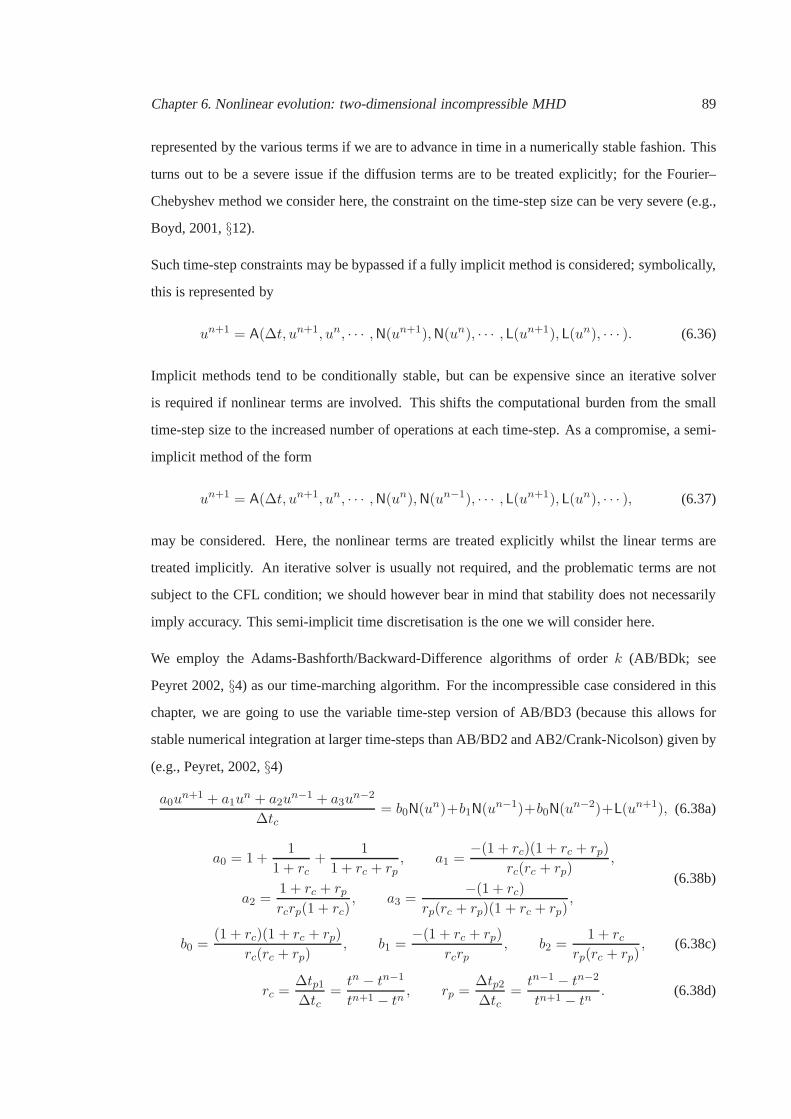
Chapter 6. Nonlinear evolution: two-dimensional incompressible MHD 89
represented by the various terms if we are to advance in time in a numerically stable fashion. This
turns out to be a severe issue if the diffusion terms are to be treated explicitly; for the Fourier–
Chebyshev method we consider here, the constraint on the time-step size can be very severe (e.g.,
Boyd, 2001,§12).
Such time-step constraints may be bypassed if a fully implicit method is considered; symbolically,
this is represented by
un+1 = A(∆t, un+1, un, · · · ,N(un+1),N(un), · · · , L(un+1), L(un), · · · ). (6.36)
Implicit methods tend to be conditionally stable, but can beexpensive since an iterative solver
is required if nonlinear terms are involved. This shifts thecomputational burden from the small
time-step size to the increased number of operations at eachtime-step. As a compromise, a semi-
implicit method of the form
un+1 = A(∆t, un+1, un, · · · ,N(un),N(un−1), · · · , L(un+1), L(un), · · · ), (6.37)
may be considered. Here, the nonlinear terms are treated explicitly whilst the linear terms are
treated implicitly. An iterative solver is usually not required, and the problematic terms are not
subject to the CFL condition; we should however bear in mind that stability does not necessarily
imply accuracy. This semi-implicit time discretisation isthe one we will consider here.
We employ the Adams-Bashforth/Backward-Difference algorithms of orderk (AB/BDk; see
Peyret 2002,§4) as our time-marching algorithm. For the incompressible case considered in this
chapter, we are going to use the variable time-step version of AB/BD3 (because this allows for
stable numerical integration at larger time-steps than AB/BD2 and AB2/Crank-Nicolson) given by
(e.g., Peyret, 2002,§4)
a0un+1 + a1u
n + a2un−1 + a3u
n−2
∆tc= b0N(u
n)+b1N(un−1)+b0N(u
n−2)+L(un+1), (6.38a)
a0 = 1 +1
1 + rc+
1
1 + rc + rp, a1 =
−(1 + rc)(1 + rc + rp)
rc(rc + rp),
a2 =1 + rc + rprcrp(1 + rc)
, a3 =−(1 + rc)
rp(rc + rp)(1 + rc + rp),
(6.38b)
b0 =(1 + rc)(1 + rc + rp)
rc(rc + rp), b1 =
−(1 + rc + rp)
rcrp, b2 =
1 + rcrp(rc + rp)
, (6.38c)
rc =∆tp1∆tc
=tn − tn−1
tn+1 − tn, rp =
∆tp2∆tc
=tn−1 − tn−2
tn+1 − tn. (6.38d)

Chapter 6. Nonlinear evolution: two-dimensional incompressible MHD 90
The time-step size∆t is set by the maximum allowable value satisfying
∆t
[
max(U0 + u)
∆x+max
(
v
∆y
)]
≤ Ccfl, (6.39)
whereu = (u, v) in (6.39), and the CFL number is an input parameter. See Section 6.9 for a
derivation and some of the related numerical tests carried out for the AB/BD3 algorithm.
There are other methods, such as Integrating Factor or Exponential Time Differencing, that could
act as an alternative to a semi-implicit discretisation butthese all have other associated problems
when a Chebyshev discretisation is employed; see, for example, Livermore (2007) for a review
and comparison of such methods in the spherical MHD context.
Our subsequent parameter choices for the simulations are chosen after doing convergence tests on
the time-step size and spatial resolution, by comparing runs at half the time-step and/or increased
resolution (twice the resolution where possible) and looking at, for example, the energy and
dissipation time-series. Energy power spectrum for the runs presented here show the energy
content at the higher modes are small (below10−5), indicating our runs are well-resolved;
spectrum diagrams have been omitted here.
6.4 Hydrodynamic evolution: a review
We first review what is known about the nonlinear evolution ofunstable shear flows in the
incompressible, hydrodynamic limit. Although the resultspresented are not new, we reproduce
them here for self-containment, and to demonstrate that ournumerical routines are able to
reproduce known, well-established results. For the hydrodynamic case, we setM to zero in the
governing equation (6.13), and solve only for the vorticityand streamfunction.
6.4.1 Hyperbolic-tangent shear layer
For this flow profile we focus on the case where the domain supports exactly one wavelength of
the most unstable mode predicted by the linear theory, so we takeLx = 2π/α, with α = 0.44
(Michalke 1964, and Chapter 5 here). Test runs have found that Ly = 10 is sufficiently large
for finite-domain effects to be negligible. For this case we choose a resolution ofNx = 256 and
Ny = 512, at Re= 500, a compromise between having well-resolved runs and the runs not being
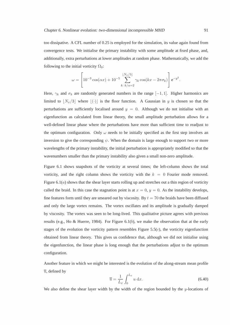
Chapter 6. Nonlinear evolution: two-dimensional incompressible MHD 91
too dissipative. A CFL number of 0.25 is employed for the simulation, its value again found from
convergence tests. We initialise the primary instability with some amplitude at fixed phase, and,
additionally, extra perturbations at lower amplitudes at random phase. Mathematically, we add the
following to the initial vorticityΩ0:
ω =
10−3 cos(αx) + 10−5
⌊Nx/3⌋∑
k: k/α=2
γk cos(kx− 2πσk)
e−y2 .
Here, γk andσk are randomly generated numbers in the range[−1, 1]. Higher harmonics are
limited to ⌊Nx/3⌋ where ⌊(·)⌋ is the floor function. A Gaussian iny is chosen so that the
perturbations are sufficiently localised aroundy = 0. Although we do not initialise with an
eigenfunction as calculated from linear theory, the small amplitude perturbation allows for a
well-defined linear phase where the perturbations have morethan sufficient time to readjust to
the optimum configuration. Onlyω needs to be initially specified as the first step involves an
inversion to give the correspondingψ. When the domain is large enough to support two or more
wavelengths of the primary instability, the initial perturbation is appropriately modified so that the
wavenumbers smaller than the primary instability also given a small non-zero amplitude.
Figure 6.1 shows snapshots of the vorticity at several times; the left-column shows the total
vorticity, and the right column shows the vorticity with thek = 0 Fourier mode removed.
Figure 6.1(a) shows that the shear layer starts rolling up and stretches out a thin region of vorticity
called the braid. In this case the stagnation point is atx = 0, y = 0. As the instability develops,
fine features form until they are smeared out by viscosity. Byt = 70 the braids have been diffused
and only the large vortex remains. The vortex oscillates andits amplitude is gradually damped
by viscosity. The vortex was seen to be long-lived. This qualitative picture agrees with previous
results (e.g., Ho & Huerre, 1984). For Figure 6.1(b), we make the observation that at the early
stages of the evolution the vorticity pattern resembles Figure 5.5(c), the vorticity eigenfunction
obtained from linear theory. This gives us confidence that, although we did not initialise using
the eigenfunction, the linear phase is long enough that the perturbations adjust to the optimum
configuration.
Another feature in which we might be interested is the evolution of the along-stream mean profile
u, defined by
u =1
Lx
∫ Lx
0u dx. (6.40)
We also define the shear layer width by the width of the region bounded by they-locations of

Chapter 6. Nonlinear evolution: two-dimensional incompressible MHD 92
(a) (b)
t=
20t=
35t=
45t=
70
1
0
0
-1
-0.045
0.045
0.4
-0.1
-0.1
-0.2
-0.5
-0.6
-0.6
0.8
0.9
Figure 6.1: Snapshots of vorticity for the shear layer run, at Re= 500. Left column shows the full vorticity,
whilst the right column shows vorticity with thek = 0 Fourier mode removed.
which the difference betweenu and its free-stream value (u±∞ = ±1 in this case) is smaller than
some tolerance. Another possible way to define this width would be by they-location whereω
is sufficiently close to its free-stream value (ω = 0 in this case). Snapshots ofu are shown in
Figure 6.2.
Here, we see that as the instability develops and the shear layer rolls up, the shear flattens out,
leading to an increase of the shear layer width. There does not appear to be much more broadening
after the roll-up stage, and any small increases in shear layer width after the roll-up stage we
attribute to viscous effects. Although there is still an inflection point, the parallel flow assumption
no longer applies, and so to say anything about the stabilityof the saturated state we would need
to consider a linear instability analysis of this state via,for example, a Floquet analysis (e.g.,
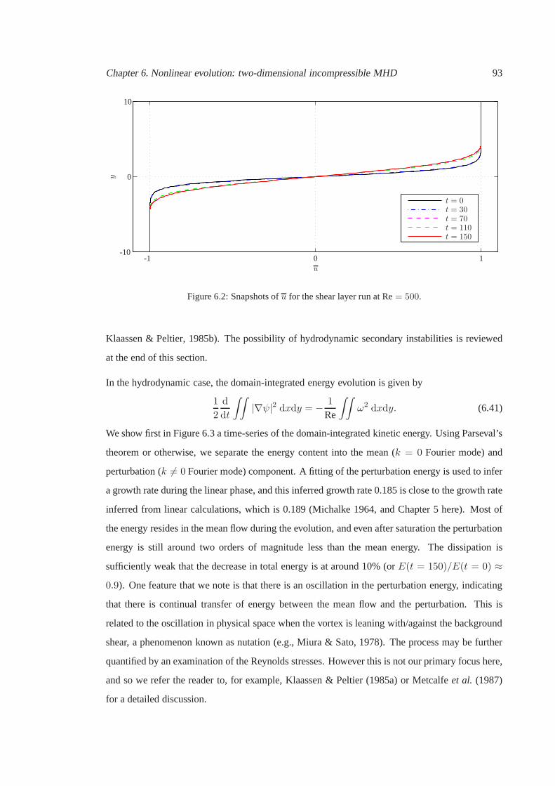
Chapter 6. Nonlinear evolution: two-dimensional incompressible MHD 93
y
u-1
0
0 1-10
10
t = 0t = 30t = 70t = 110t = 150
Figure 6.2: Snapshots ofu for the shear layer run at Re= 500.
Klaassen & Peltier, 1985b). The possibility of hydrodynamic secondary instabilities is reviewed
at the end of this section.
In the hydrodynamic case, the domain-integrated energy evolution is given by
1
2
d
dt
∫∫
|∇ψ|2 dxdy = − 1
Re
∫∫
ω2 dxdy. (6.41)
We show first in Figure 6.3 a time-series of the domain-integrated kinetic energy. Using Parseval’s
theorem or otherwise, we separate the energy content into the mean (k = 0 Fourier mode) and
perturbation (k 6= 0 Fourier mode) component. A fitting of the perturbation energy is used to infer
a growth rate during the linear phase, and this inferred growth rate 0.185 is close to the growth rate
inferred from linear calculations, which is 0.189 (Michalke 1964, and Chapter 5 here). Most of
the energy resides in the mean flow during the evolution, and even after saturation the perturbation
energy is still around two orders of magnitude less than the mean energy. The dissipation is
sufficiently weak that the decrease in total energy is at around 10% (orE(t = 150)/E(t = 0) ≈0.9). One feature that we note is that there is an oscillation in the perturbation energy, indicating
that there is continual transfer of energy between the mean flow and the perturbation. This is
related to the oscillation in physical space when the vortexis leaning with/against the background
shear, a phenomenon known as nutation (e.g., Miura & Sato, 1978). The process may be further
quantified by an examination of the Reynolds stresses. However this is not our primary focus here,
and so we refer the reader to, for example, Klaassen & Peltier(1985a) or Metcalfeet al. (1987)
for a detailed discussion.

Chapter 6. Nonlinear evolution: two-dimensional incompressible MHD 94
t
Ek
0 50 100 150
10
10
10
10
10
2
0
-2
-4
-6
growth≈ 0.185
Figure 6.3: Time-series of the energy for the shear layer runat Re= 500 (solid= perturbation state; dashed
= mean state; black dot-dashed= total energy). Most of the energy still resides in the mean sothe total
energy and mean energy curve lie on top of each other.
We show in Figure 6.4 the dissipation rateǫRe defined by
ǫRe =1
Re
∫∫
ω2 dxdy. (6.42)
We observe thatǫRe is bounded above by its initial value in the diagram; this is because enstrophy
(and in fact any function of vorticity) is an ideal invariantof two-dimensional hydrodynamics, and
there can be no net enstrophy production in this set up. This is however not the case when MHD
effects are present, since the Lorentz force feedback violates the conservation of vorticity, leading
to a dissipation rate exceeding the initial rate.
We have also checked that the numerical method conservesx- andy-momentum. The initialisation
has no momentum to begin with, as the basic state has zero net momentum, and the disturbances
are periodic with zero mean. The numerical integration shows that, for the course of the run,
domain-integrated momentum remains at machine level magnitudes.
Hydrodynamic secondary instabilities
Although the primary focus of this flow is the single wavelength case, we have also carried out runs
at two wavelengths, and test cases at four wavelengths. It isknown that a configuration of a row
of like-signed vortices is unstable, and is most unstable toan instability at twice the wavelength

Chapter 6. Nonlinear evolution: two-dimensional incompressible MHD 95
ǫ
t0 50 100 150
10
10
-1
-2
Figure 6.4: A time-series of the dissipation rateǫRe for the shear layer run at Re= 500.
of the primary instability (i.e. at wavenumberα/2), a result first demonstrated for point vortices
by von Karman (e.g., Lamb, 1932,§7). This subharmonic pairing instability has been investigated
analytically (Kelly, 1967; Stuart, 1967) and numerically (Corcos & Sherman, 1984; Metcalfe
et al., 1987; Klaassen & Peltier, 1989, 1991; Staquet, 1995; Mashayek & Peltier, 2012a,b) for
the shear layer. As the name suggests, this secondary instability causes like-signed vortices to pair
up and merge into larger vortices, further broadening the mean profile. We have performed some
simulations where only the fundamental wavenumberα receives a non-zero amplitude, but the
domain is large enough to support two vortices initially forming, and we find that the vortices do
not merge at least for the run duration (up tot = 200, wheret = 50 is approximately the time
when the primary instability starts saturating). If instead we initialise in a ‘generic’ fashion, with
non-zero amplitudes at wavenumbers in the subharmonic and higher harmonics, the vortices do
merge. Measuring the growth rate numerically at each Fourier mode as (e.g., Klaassen & Peltier
1989)
σ(k, t) =1
2E(k, t)
dE(k, t)
dt(6.43)
shows that, as a function of time,σ(α, t) is initially the largest, then it is superseded byσ(α/2, t∗)
at some later timet∗. This merging generates further small scale activity as maybe seen by an
increase in dissipation rate at the time around the merging.
Even in the single-wavelength case, the vortex core formed may be unstable to several secondary
instabilities, although most of these are ruled out in our setting; we mention them however for
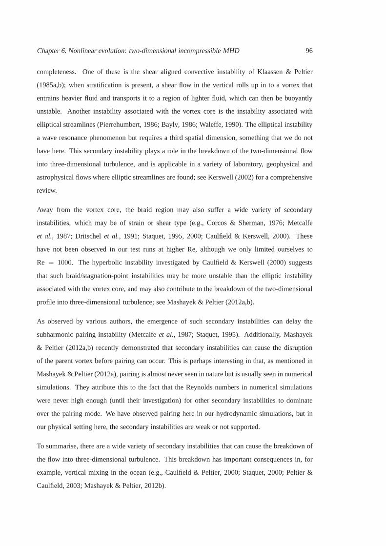
Chapter 6. Nonlinear evolution: two-dimensional incompressible MHD 96
completeness. One of these is the shear aligned convective instability of Klaassen & Peltier
(1985a,b); when stratification is present, a shear flow in thevertical rolls up in to a vortex that
entrains heavier fluid and transports it to a region of lighter fluid, which can then be buoyantly
unstable. Another instability associated with the vortex core is the instability associated with
elliptical streamlines (Pierrehumbert, 1986; Bayly, 1986; Waleffe, 1990). The elliptical instability
a wave resonance phenomenon but requires a third spatial dimension, something that we do not
have here. This secondary instability plays a role in the breakdown of the two-dimensional flow
into three-dimensional turbulence, and is applicable in a variety of laboratory, geophysical and
astrophysical flows where elliptic streamlines are found; see Kerswell (2002) for a comprehensive
review.
Away from the vortex core, the braid region may also suffer a wide variety of secondary
instabilities, which may be of strain or shear type (e.g., Corcos & Sherman, 1976; Metcalfe
et al., 1987; Dritschelet al., 1991; Staquet, 1995, 2000; Caulfield & Kerswell, 2000). These
have not been observed in our test runs at higher Re, althoughwe only limited ourselves to
Re = 1000. The hyperbolic instability investigated by Caulfield & Kerswell (2000) suggests
that such braid/stagnation-point instabilities may be more unstable than the elliptic instability
associated with the vortex core, and may also contribute to the breakdown of the two-dimensional
profile into three-dimensional turbulence; see Mashayek & Peltier (2012a,b).
As observed by various authors, the emergence of such secondary instabilities can delay the
subharmonic pairing instability (Metcalfeet al., 1987; Staquet, 1995). Additionally, Mashayek
& Peltier (2012a,b) recently demonstrated that secondary instabilities can cause the disruption
of the parent vortex before pairing can occur. This is perhaps interesting in that, as mentioned in
Mashayek & Peltier (2012a), pairing is almost never seen in nature but is usually seen in numerical
simulations. They attribute this to the fact that the Reynolds numbers in numerical simulations
were never high enough (until their investigation) for other secondary instabilities to dominate
over the pairing mode. We have observed pairing here in our hydrodynamic simulations, but in
our physical setting here, the secondary instabilities areweak or not supported.
To summarise, there are a wide variety of secondary instabilities that can cause the breakdown of
the flow into three-dimensional turbulence. This breakdownhas important consequences in, for
example, vertical mixing in the ocean (e.g., Caulfield & Peltier, 2000; Staquet, 2000; Peltier &
Caulfield, 2003; Mashayek & Peltier, 2012b).
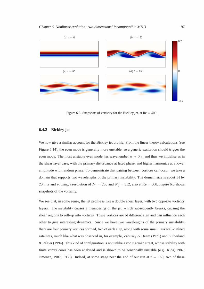
Chapter 6. Nonlinear evolution: two-dimensional incompressible MHD 97
(a) t = 0 (b) t = 50
(c) t = 85 (d) t = 150
-0.7
0
0.7
Figure 6.5: Snapshots of vorticity for the Bickley jet, at Re= 500.
6.4.2 Bickley jet
We now give a similar account for the Bickley jet profile. Fromthe linear theory calculations (see
Figure 5.14), the even mode is generally more unstable, so a generic excitation should trigger the
even mode. The most unstable even mode has wavenumberα ≈ 0.9, and thus we initialise as in
the shear layer case, with the primary disturbance at fixed phase, and higher harmonics at a lower
amplitude with random phase. To demonstrate that pairing between vortices can occur, we take a
domain that supports two wavelengths of the primary instability. The domain size is about14 by
20 in x andy, using a resolution ofNx = 256 andNy = 512, also at Re= 500. Figure 6.5 shows
snapshots of the vorticity.
We see that, in some sense, the jet profile is like a double shear layer, with two opposite vorticity
layers. The instability causes a meandering of the jet, which subsequently breaks, causing the
shear regions to roll-up into vortices. These vortices are of different sign and can influence each
other to give interesting dynamics. Since we have two wavelengths of the primary instability,
there are four primary vortices formed, two of each sign, along with some small, less well-defined
satellites, much like what was observed in, for example, Zabusky & Deem (1971) and Sutherland
& Peltier (1994). This kind of configuration is not unlike a von Karman street, whose stability with
finite vortex cores has been analysed and is shown to be generically unstable (e.g., Kida, 1982;
Jimenez, 1987, 1988). Indeed, at some stage near the end of our run at t = 150, two of these
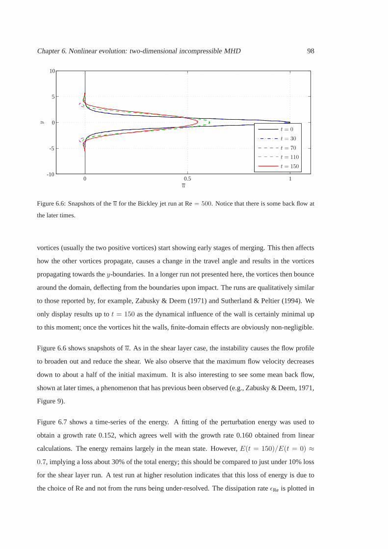
Chapter 6. Nonlinear evolution: two-dimensional incompressible MHD 98
u
y
t = 0
t = 30
t = 70
t = 110
t = 150
0
0-10
-5
5
10
0.5 1
Figure 6.6: Snapshots of theu for the Bickley jet run at Re= 500. Notice that there is some back flow at
the later times.
vortices (usually the two positive vortices) start showingearly stages of merging. This then affects
how the other vortices propagate, causes a change in the travel angle and results in the vortices
propagating towards they-boundaries. In a longer run not presented here, the vortices then bounce
around the domain, deflecting from the boundaries upon impact. The runs are qualitatively similar
to those reported by, for example, Zabusky & Deem (1971) and Sutherland & Peltier (1994). We
only display results up tot = 150 as the dynamical influence of the wall is certainly minimal up
to this moment; once the vortices hit the walls, finite-domain effects are obviously non-negligible.
Figure 6.6 shows snapshots ofu. As in the shear layer case, the instability causes the flow profile
to broaden out and reduce the shear. We also observe that the maximum flow velocity decreases
down to about a half of the initial maximum. It is also interesting to see some mean back flow,
shown at later times, a phenomenon that has previous been observed (e.g., Zabusky & Deem, 1971,
Figure 9).
Figure 6.7 shows a time-series of the energy. A fitting of the perturbation energy was used to
obtain a growth rate 0.152, which agrees well with the growthrate 0.160 obtained from linear
calculations. The energy remains largely in the mean state.However,E(t = 150)/E(t = 0) ≈0.7, implying a loss about 30% of the total energy; this should becompared to just under 10% loss
for the shear layer run. A test run at higher resolution indicates that this loss of energy is due to
the choice of Re and not from the runs being under-resolved. The dissipation rateǫRe is plotted in
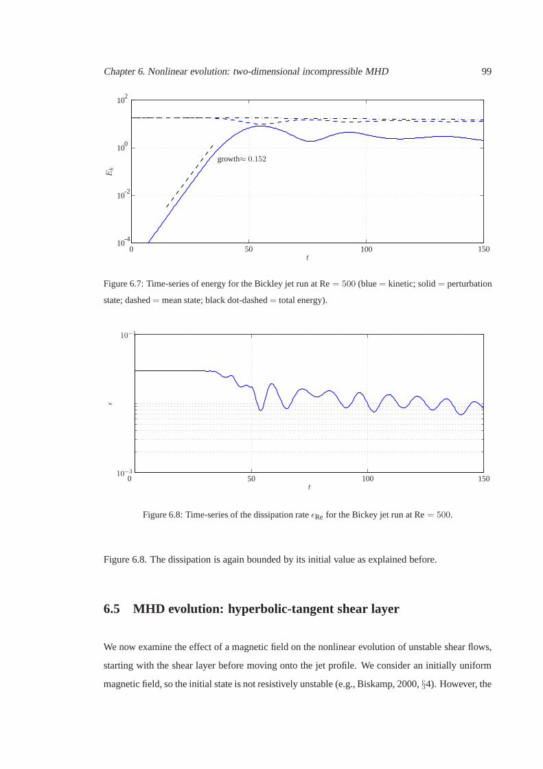
Chapter 6. Nonlinear evolution: two-dimensional incompressible MHD 99
t
Ek
0 50 100 150
10
10
10
10
2
0
-2
-4
growth≈ 0.152
Figure 6.7: Time-series of energy for the Bickley jet run at Re= 500 (blue= kinetic; solid= perturbation
state; dashed= mean state; black dot-dashed= total energy).
ǫ
t0 50 100 150
10−1
10−3
Figure 6.8: Time-series of the dissipation rateǫRe for the Bickey jet run at Re= 500.
Figure 6.8. The dissipation is again bounded by its initial value as explained before.
6.5 MHD evolution: hyperbolic-tangent shear layer
We now examine the effect of a magnetic field on the nonlinear evolution of unstable shear flows,
starting with the shear layer before moving onto the jet profile. We consider an initially uniform
magnetic field, so the initial state is not resistively unstable (e.g., Biskamp, 2000,§4). However, the

Chapter 6. Nonlinear evolution: two-dimensional incompressible MHD 100
evolved state may be resistively unstable, and the dynamicsmay be altered by resistive instabilities.
A priori, we might envisage three MHD regimes:
1. MHD effects are ‘strong’, so that although the initial state is linearly stable, it could be
nonlinearly stable (e.g., suppression of shear layer roll-up);
2. MHD effects are ‘weak’, and the evolution is much like the hydrodynamic case;
3. some intermediate case between the two, where the vortical motion can wind up the field
lines, build up MHD feedback, and modify the nonlinear development.
It is this intermediate case (3) we are particularly interested in; although the field is initially weak
(measured by energy ratios for example), MHD effects may notbe negligible when the nonlinear
evolution is concerned. Naturally, we expect the degree of feedback to depend on the field strength
M , the magnetic diffusivity as measured by Rm, and, on the viscosity as measured by Re.
The nonlinear development of the MHD shear layer case has been studied previously (Miura, 1982;
Malagoliet al., 1996; Franket al., 1996; Joneset al., 1997; Keppenset al., 1999; Jeonget al., 2000;
Baty et al., 2003; Palottiet al., 2008). However, all these authors have used routines designed for
solving compressible MHD. Furthermore, all these works, apart from Palottiet al. (2008), rely on
resolution dependent numerical dissipation. Palottiet al. (2008) investigated the dependence of
the evolution on Rm but not on the field strengthM , whilst the other works investigated the effects
of M and the sonic Mach number on the evolution.
The account we present here is new in that we numerically solve the incompressible MHD system
rather than a small Mach number run of compressible MHD, and,furthermore, we investigate the
simultaneous dependence of the nonlinear evolution on bothM and Rm. The former is perhaps
not that significant, as it appears that the more striking aspect of the nonlinear evolution stems from
MHD rather than compressible effects (Malagoliet al., 1996; Joneset al., 1997). The nonlinear
evolution can result in secondary resistive instabilitiessince finite Rm leads to reconnection events,
which release magnetic stresses back onto the flow, alteringthe dynamics. The theory of classical
resistive instabilities relies on Ohmic dissipation (e.g., Biskamp, 2000,§4), so we argue that, for
any attempt to reconcile the numerical results and the theory, employing explicit Ohmic dissipation
rather than some numerical artefact is essential. Further,being able to control the strength of

Chapter 6. Nonlinear evolution: two-dimensional incompressible MHD 101
parameter value
α 0.44
Ccfl 0.2
Lx × Ly [0, 2π/α] × [−10, 10]
Re 500
M 0.01, 0.02, 0.03, 0.04, 0.05, 0.06, 0.07, 0.1
Rm 50, 250, 500, 750, 1000
Nx ×Ny 512× 1024 for Rm= 1000
384 × 768 for Rm= 750
256 × 512 otherwise
Table 6.1: Parameter values employed in our investigation for the shear layer profile.
Ohmic dissipation is important in a systematic explorationof parameter space, something that is
not possible with resolution-dependent dissipation.
For our investigation, we fix Re= 500, and consider several values of Rm ranging from50 to
1000 (or, effectively, several values of the magnetic Prandtl number Pm= Rm/Re ranging from
0.1 to 2), and a wide range of basic field strengths measured byM . All runs are dealised, and, as
a reminder,M = 1 guarantees linear stability (from Chapter 5 here). We have focused on small
values ofM , where the linear growth rates and eigenfunctions are only small perturbations away
from the hydrodynamic case. We use the same fundamental wavenumberα = 0.44, chosen so that
only a single wavelength of the primary instability is supported. Calculations have been carried
out at the parameter values given in Table 6.1.
For illustrative purposes, we focus on three sample runs, where Rm= 500, andM = 0.01, 0.03,
and0.05. At these values ofM , the initial magnetic energy is no more than 1% of the initial
kinetic energy. Figure 6.9 shows snapshots of vorticity from these runs.
Figure 6.9(a) shows the run atM = 0.01, a truly weak field case, for which the evolution
resembles the hydrodynamic evolution. In this case there isstretching and shearing of the magnetic
field, but the resulting magnetic forces are never strong enough to alter the macro-dynamics in any
significant way. This should be contrasted to theM = 0.03 run given in Figure 6.9(b). As the
shear layer rolls up, the stretched field is now strong enoughto feed back on the flow, resulting

Chapter 6. Nonlinear evolution: two-dimensional incompressible MHD 102
(a)M = 0.01 (b)M = 0.03 (c)M = 0.05
t=
50t=
75t=
100
t=
150
-1
0
1
Figure 6.9: Snapshots of vorticity for the shear layer at different field strengths (at Rm= Re= 500).
in positive vorticity filaments in the peripheral regions ofthe vortex. This build up of filaments
with strong vorticity however is not sustained, and byt = 150 the filaments have been smoothed
out by dissipative effects. The final frame of Figure 6.9(b) still bears some resemblance to the
corresponding frame for theM = 0.01 case, with a clear signature of the vortex, although it
has diminished in size. This would perhaps be termed a ‘mildly disruptive’ case. Figure 6.9(c)
shows a ‘severely disruptive’ case, whenM = 0.05. The initial roll-up is similar to the other two
cases; however very strong regions of vorticity are created. At t = 100 the vortex seems to have
suffered some elongation and shearing due to the MHD feedback onto the flow. By the end frame,
although there are still traces of the vortex remaining, it has been substantially reduced in size, and
the dominant features in the domain are now strong vorticityfilaments.

Chapter 6. Nonlinear evolution: two-dimensional incompressible MHD 103
For theM = 0.1, Rm= 500 case (not presented here), what little remains of the parentvortex is
destroyed byt = 150, and vorticity filaments litter the computational domain. In increasing Rm
for the above runs, the behaviour becomes more violent and the observed disruption is stronger.
For example, theM = 0.03, Rm = 1000 run is more like the severely disruptive run presented
here in Figure 6.9(c), in contrast to the mildly disruptive run at the sameM but Rm= 500 shown
in Figure 6.9(b). This indicates that there is stronger disruption with increasingM and Rm.
It is informative to see the magnetic field line configuration. This may be done by plotting contours
of the magnetic potentialA; snapshots of the field lines are given in Figure 6.10 for the three cases
presented here. The contours are chosen so that the field lines thread the regiony ∈ [−2, 2] at
t = 0, with a 0.5 spacing; the field line threadingy = 0 is omitted for clarity. We see that in
Figure 6.10(a), for the non-disruptive case, the field lines are wound up bythe vortical motion
and form concentrated flux regions on the edges of the vortex;such regions should also be seen as
current sheets, which are expected to be resistively unstable. In such a situation with curved field
lines, the magnetic tension, given byT = b · ∇b, has a component directed into the vortex. The
idea is that the vortical motion winds up the field lines and builds up magnetic stresses, which are
then released at a major reconnection event, and act on the vortex. In this weak field case the force
is not strong enough to disrupt the vortex in any significant way. By the end time, the magnetic
loops inside the vortex have largely been diffused and magnetic flux has been expelled from the
centre to the edges of the vortex. This process of flux expulsion has previously been described by
Weiss (1966), who, via dimensional arguments, also predicted the strength to which fields could
grow. Although his numerical computations were carried outin the kinematic regime, with no
feedback on the velocity field via the Lorentz force in the momentum eqauation, theM = 0.01
case here is comparable to his results in that the Lorentz force is never significant compared to the
fluid inertia even locally, and the kinematic assumptions are well satisfied.
Now we compare the weak case ofM = 0.01 to the mildly disruptive case ofM = 0.03 in
Figure 6.10(b). The magnetic stresses are now strong enough to cause some disruption. The parent
vortex is still present after the mild disruption and a flux expelled state is reached. TheM = 0.03
case suffers no further disruption events aftert = 150 in a longer test run we have carried out.
This may be explained by the fact that, since the vortex is able to maintain its integrity after the
initial disruption, most of the field lines that thread the vortex end up being expelled, so there is
nothing left for the surviving vortex to wind up. For theM = 0.05 case in Figure 6.10(c), the

Chapter 6. Nonlinear evolution: two-dimensional incompressible MHD 104
(a)M = 0.01 (b)M = 0.03 (c)M = 0.05
t=
50t=
75t=
100
t=
150
Figure 6.10: Snapshots of field lines for the shear layer runsat several field strengths (at Rm= Re= 500).
stresses released are even stronger and distort the vortex significantly. The evolution is completely
different, with clear signs of magnetic islands, and a flux expelled state is not achieved.
We observe that disruption is a fast phenomenon, occurring in no more than an eddy turnover
time. One key point we want to highlight is that the disruption, when it does happen, affects the
dynamics well before the flux expelled state has been reached. Also, to demonstrate further that the
magnetic tension does act to distort the vortex, we plot in Figure 6.11 the field line configuration
with the tension force overlaid as arrows, at a time before a major disruption event has occurred.
There is indeed a component directed towards the centre of the vortex.

Chapter 6. Nonlinear evolution: two-dimensional incompressible MHD 105
M = 0.05, t = 60
Figure 6.11: Magnetic tension, plotted as arrows, with magnitude proportional to their length, superimposed
on a field line plot. The arrow lengths have been magnified by a factor of four for clarity.
(a) t = 50 (b) t = 75
(c) t = 100 (d) t = 150
4
0
-4
Figure 6.12: Snapshots of current for the shear layer run (atRm= Re= 500,M = 0.05).
Figure 6.12 shows snapshots of the current densityj for theM = 0.05 run. The configuration is
consistent with the field line plots in Figure 6.10(c), in that strong current layers are formed on the
fringes of the vortex. Such thin layers of current are known to be resistively unstable. Note also
that it is not a single current layer, but a double current layer that exists on the edges of the vortex.
One other feature to note in the more violent disruptive cases is that the current distribution
bears a noticeable visual resemblance with the vorticity distribution, as has been observed in

Chapter 6. Nonlinear evolution: two-dimensional incompressible MHD 106
(a) B0 = tanh(y) (b) B0(y) = sech2(y)
x
y
33
0
0
0
0-3-3
2525 5050
Figure 6.13: Field line configuration from a tearing unstable initialisation, with no background flow.
two-dimensional MHD turbulence simulations (e.g., Biskamp & Welter, 1989; Biskamp, 2003;
Dritschel & Tobias, 2012). The shearing of the field lines is strongest at regions with non-zero
vorticity so perhaps it is not entirely unexpected that the current is largest around these regions
and implying a vorticity-current correlation.
It is known that, in thin current layers, the tearing type instabilities are usually the fastest
growing instabilities (e.g., Furthet al. 1963; Biskamp 2000,§4; Priest & Forbes 2000,§6). In
Figure 6.13 we show the field line configuration from nonlinear simulations, initialising with
B0(y) = tanh(y) (the single current layer, Figure 6.13a) andB0(y) = sech2(y) (a double current
layer, Figure 6.13b), with no background flow. The tearing instability causes a pinching of the field
lines and forms magnetic islands. In other nonlinear simulations in vortical flows (e.g., Biskamp &
Welter, 1989), the break up of current layers is often attributed to tearing instabilities, and, in those
cases, the break up is often accompanied by balloon like structures in the electric current. These
balloon like structures have been observed in some of our nonlinear simulations of shear flows
with background magnetic field, so, given that tearing instabilities are usually the most unstable
resistive instability in a thin current layer configuration, it seems plausible that these are also in
play here. We give some details of our attempt at providing more evidence for pinning down the
exact resistive instability at play in the discussion section at the end of the chapter.
Going back to the shear layer case, we show snapshots ofu for the sample runs in Figure 6.14.
Compared to the hydrodynamic cases, we make the observationthat disruption events encourage a
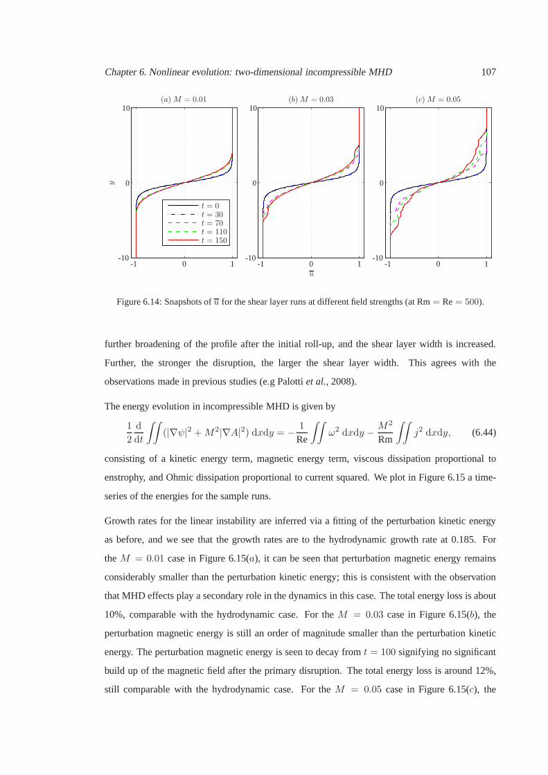
Chapter 6. Nonlinear evolution: two-dimensional incompressible MHD 107
(a)M = 0.01 (b)M = 0.03 (c)M = 0.05
t = 0t = 30t = 70t = 110t = 150
u
y 0
0
0
0
0
0-10-10-10
101010
111 -1-1-1
Figure 6.14: Snapshots ofu for the shear layer runs at different field strengths (at Rm= Re= 500).
further broadening of the profile after the initial roll-up,and the shear layer width is increased.
Further, the stronger the disruption, the larger the shear layer width. This agrees with the
observations made in previous studies (e.g Palottiet al., 2008).
The energy evolution in incompressible MHD is given by
1
2
d
dt
∫∫
(|∇ψ|2 +M2|∇A|2) dxdy = − 1
Re
∫∫
ω2 dxdy − M2
Rm
∫∫
j2 dxdy, (6.44)
consisting of a kinetic energy term, magnetic energy term, viscous dissipation proportional to
enstrophy, and Ohmic dissipation proportional to current squared. We plot in Figure 6.15 a time-
series of the energies for the sample runs.
Growth rates for the linear instability are inferred via a fitting of the perturbation kinetic energy
as before, and we see that the growth rates are to the hydrodynamic growth rate at 0.185. For
theM = 0.01 case in Figure 6.15(a), it can be seen that perturbation magnetic energy remains
considerably smaller than the perturbation kinetic energy; this is consistent with the observation
that MHD effects play a secondary role in the dynamics in thiscase. The total energy loss is about
10%, comparable with the hydrodynamic case. For theM = 0.03 case in Figure 6.15(b), the
perturbation magnetic energy is still an order of magnitudesmaller than the perturbation kinetic
energy. The perturbation magnetic energy is seen to decay from t = 100 signifying no significant
build up of the magnetic field after the primary disruption. The total energy loss is around 12%,
still comparable with the hydrodynamic case. For theM = 0.05 case in Figure 6.15(c), the

Chapter 6. Nonlinear evolution: two-dimensional incompressible MHD 108
(a)M = 0.01
(b)M = 0.03
(c)M = 0.05
growth≈ 0.180
growth≈ 0.180
growth≈ 0.179
E
t0
0
0
50
50
50
100
100
100
150
150
150
10
10
10
10
10
10
10
10
10
10
10
10
2
2
2
0
0
0
-2
-2
-2
-4
-4
-4
Figure 6.15: Time-series of the energies (blue= kinetic; red= magnetic; solid= perturbation state; dashed
= mean state; black dot-dashed line= total energy) for the shear layer runs at different field strengths (at
Rm= Re= 500).
perturbation magnetic energy is comparable with the perturbation kinetic energy, and this certainly
indicates that the dynamics are significantly influenced by MHD effects. The total energy loss here
is higher, at around 17%.
The increase in energy loss observed in Figure 6.15 is perhaps expected; since the Ohmic
dissipation rate given by
ǫRm =M2
Rm
∫∫
j2 dxdy (6.45)
is related to the current density, and we have already observed that strong current sheets appear
as a result of the vortical motion, this implies that extra dissipation is present, leading to higher
energy loss. We plot in Figure 6.16 the viscous dissipation rateǫRe, the Ohmic dissipation rate
ǫRm and the total dissipation for the three sample cases. Indeed, it is seen that the more disruptive
case atM = 0.05 has a much higher Ohmic dissipation, so much so that Ohmic dissipation is the
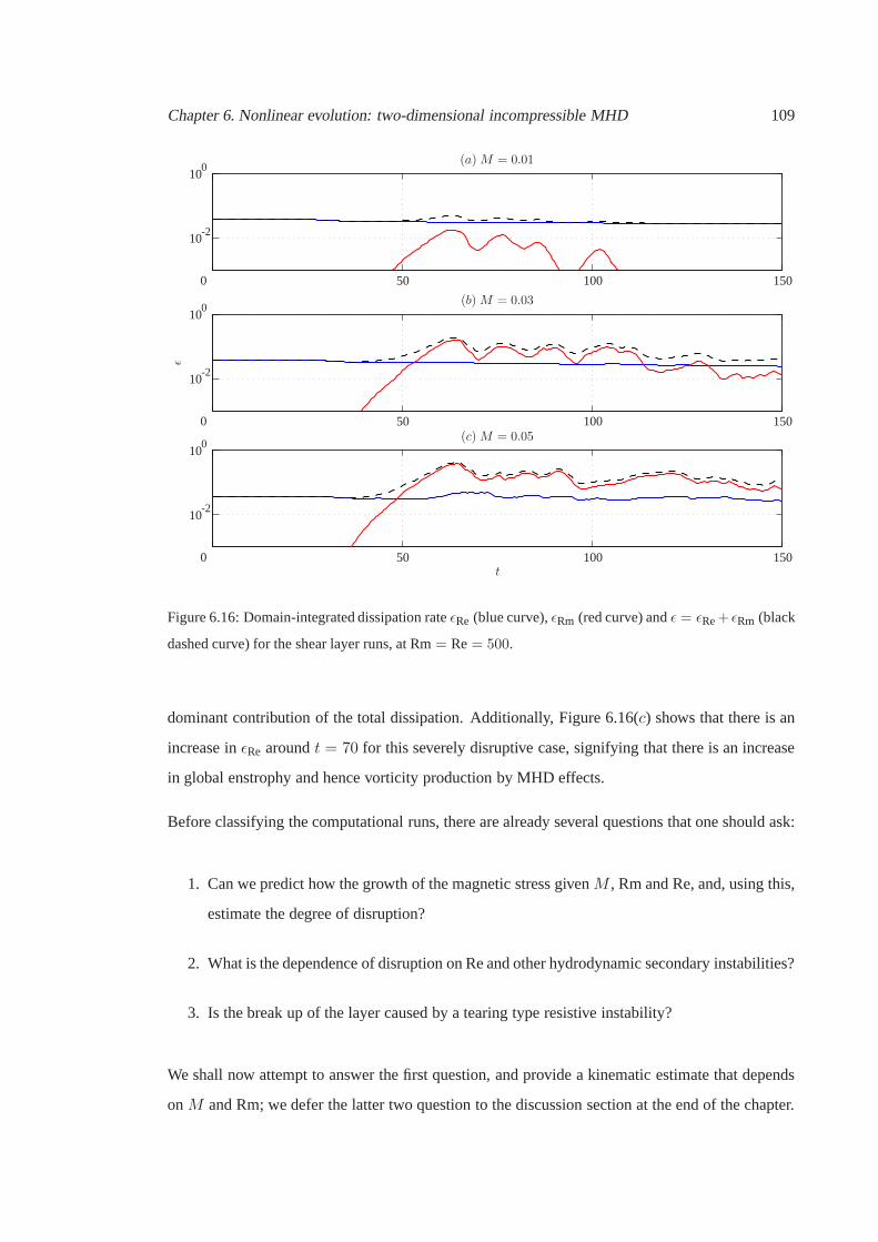
Chapter 6. Nonlinear evolution: two-dimensional incompressible MHD 109
(a)M = 0.01
(b)M = 0.03
(c)M = 0.05
t
ǫ
0
0
0
50
50
50
100
100
100
150
150
150
10
10
10
10
10
10
0
0
0
-2
-2
-2
Figure 6.16: Domain-integrated dissipation rateǫRe (blue curve),ǫRm (red curve) andǫ = ǫRe+ ǫRm (black
dashed curve) for the shear layer runs, at Rm= Re= 500.
dominant contribution of the total dissipation. Additionally, Figure 6.16(c) shows that there is an
increase inǫRe aroundt = 70 for this severely disruptive case, signifying that there isan increase
in global enstrophy and hence vorticity production by MHD effects.
Before classifying the computational runs, there are already several questions that one should ask:
1. Can we predict how the growth of the magnetic stress givenM , Rm and Re, and, using this,
estimate the degree of disruption?
2. What is the dependence of disruption on Re and other hydrodynamic secondary instabilities?
3. Is the break up of the layer caused by a tearing type resistive instability?
We shall now attempt to answer the first question, and providea kinematic estimate that depends
onM and Rm; we defer the latter two question to the discussion section at the end of the chapter.

Chapter 6. Nonlinear evolution: two-dimensional incompressible MHD 110
6.5.1 Regime boundary estimation
We know that if the magnetic stresses built up by the vorticalmotion are significant before the
major reconnection event occurs, then we can expect disruption to occur. The question then is
how to quantify the size of the stresses.
The circular motion of the vortex has associated with it a centripetal force. For a fluid with density
ρ and permeabilityµ0, if a uniform vortex has length scaleLe and velocityUe, then the centripetal
force scales likeρU2e /Le. So we expect there to be significant disruption if the tension forceT is
comparable to the centripetal force, i.e.
T ∼ |ρb · ∇b| ∼ ρU2e
Le, (6.46)
where againb = b∗/√ρµ0 is in units of velocity. Then it remains to estimate how largeT can
get. For this purpose, we employ a kinematic argument similar to that given in Weiss (1966). A
kinematic argument should at least give us a first estimate ofhow largeT can grow until it is
arrested by dissipative effects.
We start from the (dimensional) induction equation
∂b
∂t= ∇× (u× b) + η∇2
b. (6.47)
Now, the initial large-scale fieldB0 at length scaleLe may be amplified to a stronger small-scale
field b at a smaller length scaleℓ. Away from dissipation scales, flux conservation implies that we
have
B0Le = bℓ ⇒ b =B0Le
ℓ. (6.48)
This amplification is arrested when the advection term∇× (u× b) is comparable to the diffusive
termη∇2b, i.e.
UeB0
Le∼ ηb
ℓ2, (6.49)
implying
b ∼(
UeLe
η
)1/3
B0. (6.50)
This is the first part of the argument in Weiss (1966), and ourb here is hisB1.
Now, sinceb≫ B0 andℓ≪ Le, we have, using (6.48) and (6.50)
T ∼ |ρb · ∇b| ∼ ρb2
ℓ∼ ρ
b3
B0Le∼ ρUe
B20
η. (6.51)

Chapter 6. Nonlinear evolution: two-dimensional incompressible MHD 111
This suggests we are in the disruptive regime when
ρUeB2
0
η∼ ρU2
e
Le⇒ B2
0
η∼ Ue
Le∼ Ωe, (6.52)
whereΩe is the typical scale for vorticity in two-dimensions.
Going back to our non-dimensional set up, a constant field implies that
B0 →M,1
η→ Rm,
so the expected disruption condition (6.46) becomes
M2Rm∼ Ωe. (6.53)
For the shear layer profile considered here,Ωe ∼ 1. The severely disruptive case of(M,Rm) =
(0.05, 500) hasM2Rm = 1.25, the mildly disruptive case of(M,Rm) = (0.03, 500) has
M2Rm = 0.45, and the non-disruptive case of(M,Rm) = (0.01, 500) hasM2Rm = 0.05,
so this kinematic prediction is then at least consistent with the observed disruption for these three
sample cases.
As argued before, the disruption event occurs well before any flux expulsion regime is reached
(approximately half to one turnover time compared with three or four turnover times for flux
expulsion), so we use the above estimate, which takes into account how much the field lines may
be amplified before it is arrested by finite magnetic dissipation. We will test our kinematic estimate
here, and discuss the possibilities of a dynamic estimate inthe discussion section at the end of the
chapter.
6.5.2 Regime classification
We now proceed to classify our set of runs in(M,Rm) space. To do this we need some way of
measuring the degree of disruption. There are several features correlated with the observed degree
of disruption, such as the dominance of filamentary vorticity structures and the increase of shear
layer width. We construct measures that make use of these twoobservations.
More filamentary structures implies more small-scale activity. In a spectral representation this
implies that more modes are required to reconstruct the original profile. Using vorticity as
an example, since we have data for vorticity collocated at the relevant points, we consider a

Chapter 6. Nonlinear evolution: two-dimensional incompressible MHD 112
case kcut marker
severely disruptive kcut ≥ 25 mildly disruptive 10 < kcut < 25 no visible disruption kcut ≤ 10 ×
Table 6.2: Regime classification for the shear layer in the incompressible case, using the spectral truncation
measure.
spectral representation of the data. We then take some truncation wavenumberkcut, and a spectral
truncation is carried out by setting to zero the coefficientswith wavenumberskcut < ky ≤ Ny
for Chebyshev modes andkcut < kx ≤ Nx/2 for Fourier modes. The enstrophy associated with
ω(k = kcut) is calculated for increasingkcut until some large percentage of the total enstrophy is
recovered, and we record thekcut that achieves this; vorticity fields possessing more filamentary
structure will have a higherkcut. As a demonstration, reconstructions of the spectrally truncated
vorticity at several values ofkcut are given in Figure 6.17, using thet = 100 frames of Figure 6.9.
The enstrophy capture percentage, given by‖ωcut‖2/‖ωfull‖2, where‖ · ‖ is interpreted in theL2
sense, is given underneath the panels. As expected, for a runwhere the main feature is the parent
vortex, only a few modes are needed to capture most of the enstrophy and reproduce the original
profile. More modes are required when filamentary structuresare present.
For our purpose we choose thekcut that recovers 99% of the enstrophy, i.e.
‖ωcut‖2‖ωfull‖2
> 0.99, (6.54)
and we takekcut maximised over the run time at each(M,Rm). We choose to use enstrophy over
the current squared because in our case Re is fixed whilst Rm isnot, and a larger Rm allows for
thinner current sheets, naturally resulting in a largerkcut. Enstrophy is used over energy because
enstrophy provides a sharper measure, asω is one derivative higher than∇ψ. The maximum over
the run is taken because this takes into account when the activity is at its most vigorous, compared
to, say, takingkcut at the end time when diffusion may have already smoothed out some features.
Using Figure 6.17 as a rough visual guide and with some calibration using some sample runs,
we classify the runs as in Table 6.2. The raw data from our set of runs is given in Table 6.3; for
comparison, the hydrodynamic run at Re= 500 haskcut = 7.
Another measure of the disruption that we consider is the width of the shear layer. As observed
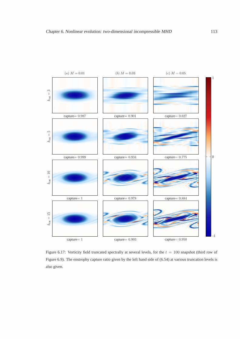
Chapter 6. Nonlinear evolution: two-dimensional incompressible MHD 113
(a)M = 0.01 (b)M = 0.03 (c)M = 0.05
kcu
t=
3k
cut=
5k
cut=
10k
cut=
15
capture= 0.987
capture= 0.999
capture= 1
capture= 1
capture= 0.901
capture= 0.934
capture= 0.978
capture= 0.993
capture= 0.627
capture= 0.775
capture= 0.884
capture= 0.950-1
0
1
Figure 6.17: Vorticity field truncated spectrally at several levels, for thet = 100 snapshot (third row of
Figure 6.9). The enstrophy capture ratio given by the left hand side of (6.54) at various truncation levels is
also given.

Chapter 6. Nonlinear evolution: two-dimensional incompressible MHD 114
Rm
M0.01 0.02 0.03 0.04 0.05 0.06 0.07 0.1
1000 7 17 37 25 55 54 60 60
750 7 14 30 34 34 41 45 60
500 7 7 24 31 33 31 33 46
250 7 7 7 22 27 29 28 31
50 7 7 7 7 8 9 11 14
Table 6.3: Raw data from the set of calculations at Re= 500 for the shear layer, with numbers denoting the
truncation wavenumberkcut maximised over time. The hydrodynamic case haskcut = 7.
case layer expansion factorf marker
severely disruptive f ≥ 1.5 mildly disruptive 1.15 < f < 1.5 no visible disruption 1.15 ≤ f ×
Table 6.4: Regime classification for the shear layer in the incompressible case, using the shear layer width
measure.
in Figure 6.14, the more disruptive the run, the larger the shear layer width. To measure the shear
layer width, we find the location where|u − u∞| < 0.01, with u∞ the free-stream value of the
profile (u∞ = 1 for the shear layer profile). To give a measure, we fix a snapshot time, and
calculate the shear layer width, normalised by the shear layer width in the hydrodynamic case at
the corresponding time. For our purposes, we took the layer width at the end timet = 150, so
f =layer width of run att = 150
layer width of hydrodynamic run att = 150. (6.55)
From this, we classify the runs as in Table 6.4. The raw data isgiven in Table 6.5. The
hydrodynamic case has a factor of1, with an initial layer width of about 5.9 and an end layer
width of 7.65.
Using the two classifications, we plot in Figure 6.18 regime diagrams in(M,Rm) space based
on the two measures given, for the single wavelength case at Re = 500. Lines ofM2Rm = C,
consistent with (6.53), for several values ofC are overlaid onto the diagram. There was some
calibration required for classifying the simulations; this has been done so that the essentially
hydrodynamic runs and the severely disruptive runs are captured as best as possible. There are
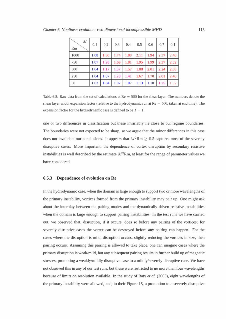
Chapter 6. Nonlinear evolution: two-dimensional incompressible MHD 115
Rm
M0.1 0.2 0.3 0.4 0.5 0.6 0.7 0.1
1000 1.08 1.30 1.74 1.88 2.11 1.94 2.37 2.46
750 1.07 1.28 1.69 1.81 1.95 1.99 2.37 2.52
500 1.04 1.17 1.37 1.57 1.88 2.01 2.24 2.56
250 1.04 1.07 1.20 1.41 1.67 1.78 2.01 2.40
50 1.03 1.04 1.07 1.07 1.13 1.10 1.25 1.52
Table 6.5: Raw data from the set of calculations at Re= 500 for the shear layer. The numbers denote the
shear layer width expansion factor (relative to the hydrodynamic run at Re= 500, taken at end time). The
expansion factor for the hydrodynamic case is defined to bef = 1.
one or two differences in classification but these invariably lie close to our regime boundaries.
The boundaries were not expected to be sharp, so we argue thatthe minor differences in this case
does not invalidate our conclusions. It appears thatM2Rm ≥ 0.5 captures most of the severely
disruptive cases. More important, the dependence of vortexdisruption by secondary resistive
instabilities is well described by the estimateM2Rm, at least for the range of parameter values we
have considered.
6.5.3 Dependence of evolution on Re
In the hydrodynamic case, when the domain is large enough to support two or more wavelengths of
the primary instability, vortices formed from the primary instability may pair up. One might ask
about the interplay between the pairing modes and the dynamically driven resistive instabilities
when the domain is large enough to support pairing instabilities. In the test runs we have carried
out, we observed that, disruption, if it occurs, does so before any pairing of the vortices; for
severely disruptive cases the vortex can be destroyed before any pairing can happen. For the
cases where the disruption is mild, disruption occurs, slightly reducing the vortices in size, then
pairing occurs. Assuming this pairing is allowed to take place, one can imagine cases where the
primary disruption is weak/mild, but any subsequent pairing results in further build up of magnetic
stresses, promoting a weakly/mildly disruptive case to a mildly/severely disruptive case. We have
not observed this in any of our test runs, but these were restricted to no more than four wavelengths
because of limits on resolution available. In the study of Baty et al. (2003), eight wavelengths of
the primary instability were allowed, and, in their Figure 15, a promotion to a severely disruptive
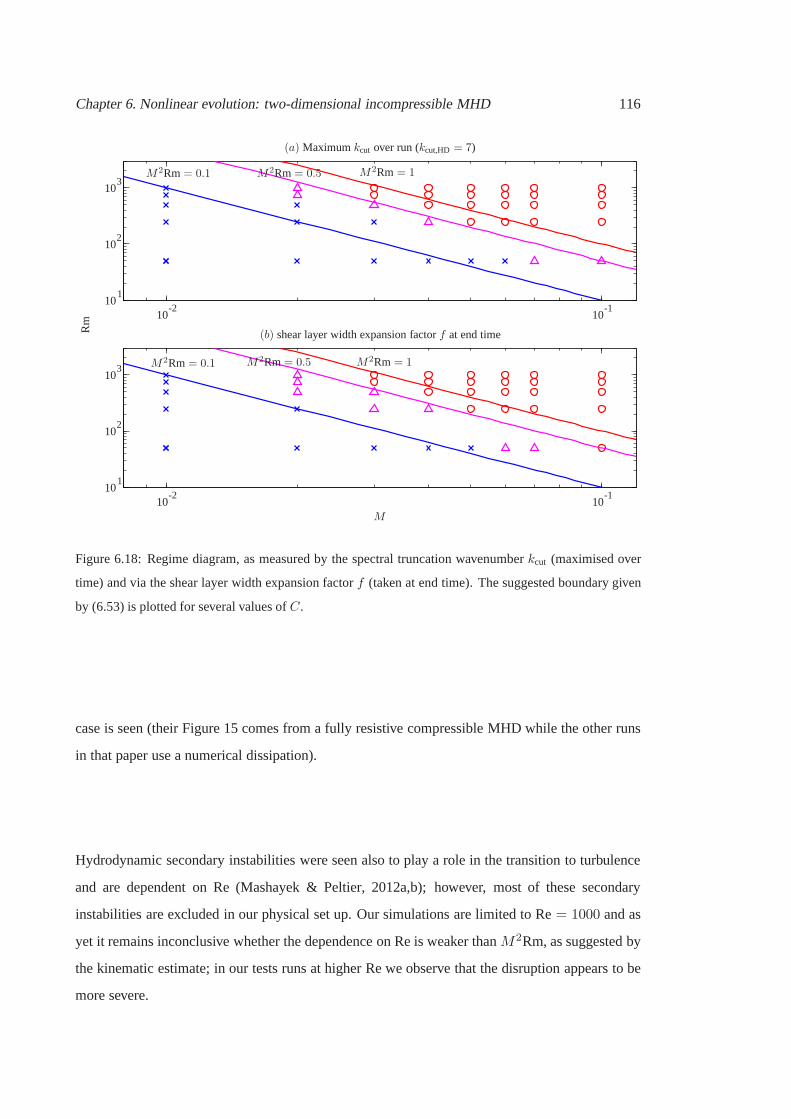
Chapter 6. Nonlinear evolution: two-dimensional incompressible MHD 116
(a) Maximumkcut over run (kcut,HD = 7)
M
Rm
M2Rm= 0.1
M2Rm= 0.1
M2Rm= 0.5
M2Rm= 0.5
M2Rm= 1
M2Rm= 1
10
10
101010
10
10
101010
-1
-1
-2
-2
1
1
2
2
3
3
(b) shear layer width expansion factorf at end time
Figure 6.18: Regime diagram, as measured by the spectral truncation wavenumberkcut (maximised over
time) and via the shear layer width expansion factorf (taken at end time). The suggested boundary given
by (6.53) is plotted for several values ofC.
case is seen (their Figure 15 comes from a fully resistive compressible MHD while the other runs
in that paper use a numerical dissipation).
Hydrodynamic secondary instabilities were seen also to play a role in the transition to turbulence
and are dependent on Re (Mashayek & Peltier, 2012a,b); however, most of these secondary
instabilities are excluded in our physical set up. Our simulations are limited to Re= 1000 and as
yet it remains inconclusive whether the dependence on Re is weaker thanM2Rm, as suggested by
the kinematic estimate; in our tests runs at higher Re we observe that the disruption appears to be
more severe.

Chapter 6. Nonlinear evolution: two-dimensional incompressible MHD 117
6.5.4 The cases with largerM
For completeness, Figure 6.19 shows snapshots of the vorticity for runs with larger values ofM
than those considered previously; recall, from Chapter 5, thatM ≥ 1 guarantees linear stability
of this basic state. A larger perturbation to the vorticity was given to compensate for the slower
growth rates. We should note that the time snapshots are not comparable to those in Figure 6.9
since the perturbation is of a different magnitude.
For theM = 0.2 case in Figure 6.19(a), we observe severe disruption, with regions of very strong
vorticity generated even before the vortex has completely formed. The disruption is very rapid
and strong filaments litter the domain. Even in this slightlyshorter run, the shear layer is observed
to have spread to the boundary. For theM = 0.4 case in Figure 6.19(b), we perhaps still observe
some disruption, but now the background field appears to be strong enough to suppress fluid
motion, and by the end frame, we have what would be deemed a laminar state. For theM = 0.6
case in Figure 6.19(c), nothing that is characteristic of disruption is observed, and it would appear
that even the rolling up motion has been suppressed.
We note then that the disruption estimateM2Rm ∼ Ωe only predicts the degree of disruption
where there is a rolling up of the shear layer. The transitionlocation between the disruptive regime
and the nonlinearly stable regime has not been investigatedhere.
6.6 MHD evolution: Bickley jet
We now consider an analogous investigation for the Bickley jet profile. In planar geometry, the
evolution of this profile in the incompressible MHD system has been investigated by Biskamp
et al. (1998); jet-like profiles in the compressible MHD regime have been investigated by, for
example, Min (1997a,b) and Baty & Keppens (2006). All these authors find that vortices may
be disrupted, and that weak vorticity bands become the dominant feature in the domain. As in
the shear layer case, we consider values ofM that, according to linear theory, result in growth
rates and eigenfunctions that are comparable to the hydrodynamic case. As was done previously,
we takeα = 0.9, with a domain that supports two wavelengths of the primary instability, partly
for consistency, and partly to demonstrate that complete disruption may happen before pairing of
vortices occur. A summary of the run parameters is given in Table 6.6.

Chapter 6. Nonlinear evolution: two-dimensional incompressible MHD 118
(a)M = 0.2 (b)M = 0.4 (c)M = 0.6
t=
50t=
75t=
100
t=
150
-3
0
3
Figure 6.19: Snapshots of vorticity for the shear layer at some larger values ofM (at Rm= Re = 500).
Note the use of a wider colour scale compared to Figure 6.9, and the simulations were initialised with a
larger perturbation than the ones presented in Figure 6.19.
As before, we take three representative runs, carried out atRm = 500 andM = 0.01, 0.03,
and0.05; as a reminder,M = 0.5 implies linear stability (see Chapter 5). In Figure 6.20 we
show snapshots of the vorticity for these three runs. In all cases, the primary instability causes a
meandering and break up of the jet, as in the hydrodynamic case displayed in Figure 6.5. For the
M = 0.01 case in Figure 6.20(a), at t = 100, we see that there is some sort of distortion to the
vortices, due to the release of built up magnetic stresses, and the vortices take an almost triangular
shape in this frame. The stresses built up in this case however are evidently not very strong, and
the vortices are able to recover their elliptical shapes byt = 150; at this time, we also see early
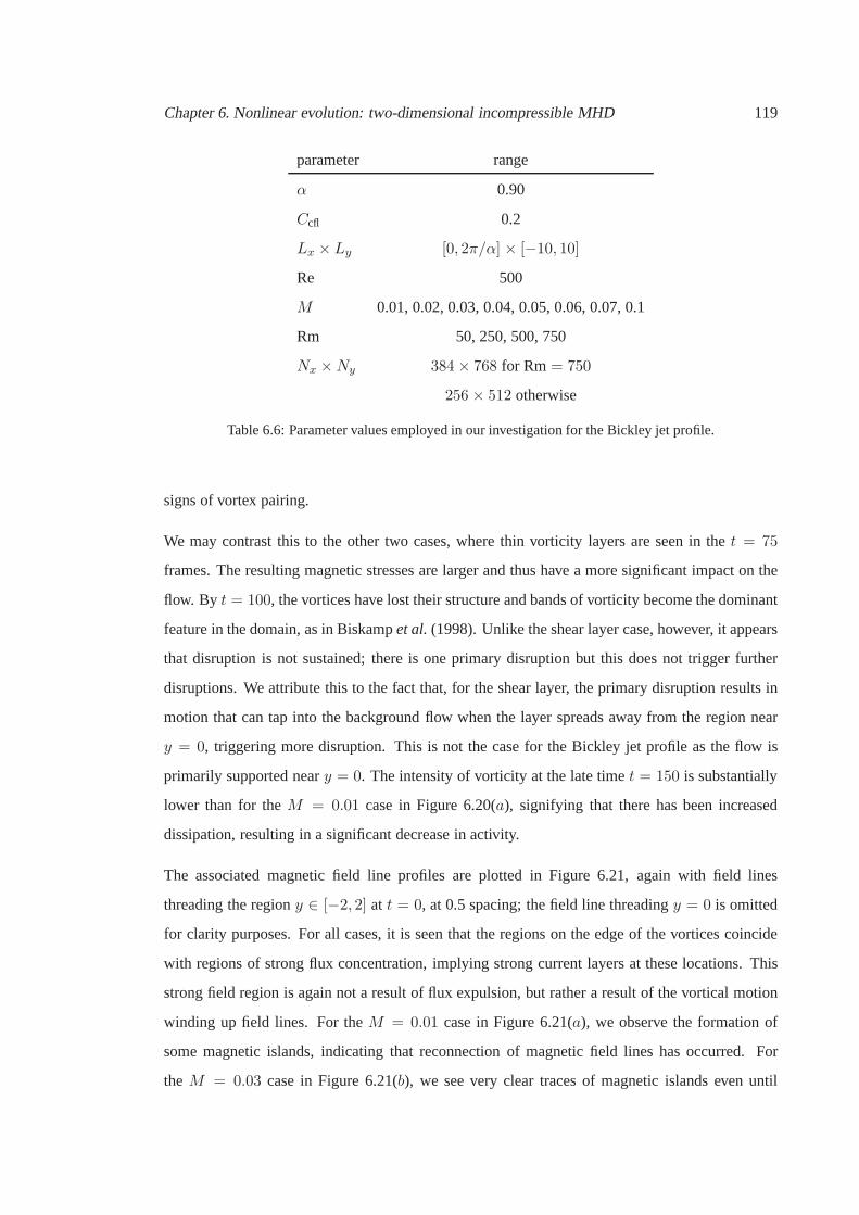
Chapter 6. Nonlinear evolution: two-dimensional incompressible MHD 119
parameter range
α 0.90
Ccfl 0.2
Lx × Ly [0, 2π/α] × [−10, 10]
Re 500
M 0.01, 0.02, 0.03, 0.04, 0.05, 0.06, 0.07, 0.1
Rm 50, 250, 500, 750
Nx ×Ny 384 × 768 for Rm= 750
256 × 512 otherwise
Table 6.6: Parameter values employed in our investigation for the Bickley jet profile.
signs of vortex pairing.
We may contrast this to the other two cases, where thin vorticity layers are seen in thet = 75
frames. The resulting magnetic stresses are larger and thushave a more significant impact on the
flow. By t = 100, the vortices have lost their structure and bands of vorticity become the dominant
feature in the domain, as in Biskampet al.(1998). Unlike the shear layer case, however, it appears
that disruption is not sustained; there is one primary disruption but this does not trigger further
disruptions. We attribute this to the fact that, for the shear layer, the primary disruption results in
motion that can tap into the background flow when the layer spreads away from the region near
y = 0, triggering more disruption. This is not the case for the Bickley jet profile as the flow is
primarily supported neary = 0. The intensity of vorticity at the late timet = 150 is substantially
lower than for theM = 0.01 case in Figure 6.20(a), signifying that there has been increased
dissipation, resulting in a significant decrease in activity.
The associated magnetic field line profiles are plotted in Figure 6.21, again with field lines
threading the regiony ∈ [−2, 2] at t = 0, at 0.5 spacing; the field line threadingy = 0 is omitted
for clarity purposes. For all cases, it is seen that the regions on the edge of the vortices coincide
with regions of strong flux concentration, implying strong current layers at these locations. This
strong field region is again not a result of flux expulsion, butrather a result of the vortical motion
winding up field lines. For theM = 0.01 case in Figure 6.21(a), we observe the formation of
some magnetic islands, indicating that reconnection of magnetic field lines has occurred. For
theM = 0.03 case in Figure 6.21(b), we see very clear traces of magnetic islands even until
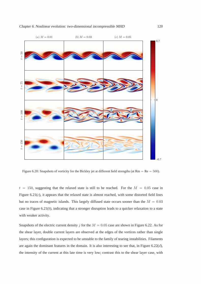
Chapter 6. Nonlinear evolution: two-dimensional incompressible MHD 120
(a)M = 0.01 (b)M = 0.03 (c)M = 0.05
t=
50t=
75t=
100
t=
150
0
-0.7
0.7
Figure 6.20: Snapshots of vorticity for the Bickley jet at different field strengths (at Rm= Re= 500).
t = 150, suggesting that the relaxed state is still to be reached. For theM = 0.05 case in
Figure 6.21(c), it appears that the relaxed state is almost reached, with some distorted field lines
but no traces of magnetic islands. This largely diffused state occurs sooner than theM = 0.03
case in Figure 6.21(b), indicating that a stronger disruption leads to a quicker relaxation to a state
with weaker activity.
Snapshots of the electric current densityj for theM = 0.05 case are shown in Figure 6.22. As for
the shear layer, double current layers are observed at the edges of the vortices rather than single
layers; this configuration is expected to be unstable to the family of tearing instabilities. Filaments
are again the dominant features in the domain. It is also interesting to see that, in Figure 6.22(d),
the intensity of the current at this late time is very low; contrast this to the shear layer case, with

Chapter 6. Nonlinear evolution: two-dimensional incompressible MHD 121
(a)M = 0.01 (b)M = 0.03 (c)M = 0.05t=
50t=
75t=
100
t=
150
Figure 6.21: Snapshots of field lines for the Bickley jet runsat several field strengths (at Rm= Re= 500).
its current profile given in Figure 6.12(d).
In Figure 6.23 we show snapshots ofu. As with the shear layer, there is broadening ofu as the
primary instability saturates and the jet breaks up into vortices. In contrast to the shear layer case
however, the jet widths (computed using either|u− u∞| or |ω− ω∞| as the measure) for the runs
at different field strengths at the end timet = 150 are in fact comparable with each other. This
seems to be because there is really only one significant disruption event, in contrast to the shear
layer case where a cascade of disruptions may occur, leadingto a substantial increase of the shear
layer width. We do observe, however, that the decrease in peak flow value, given bymax |u(y)|,is correlated with increasing disruption, with more disruptive runs leading to a larger decrease in
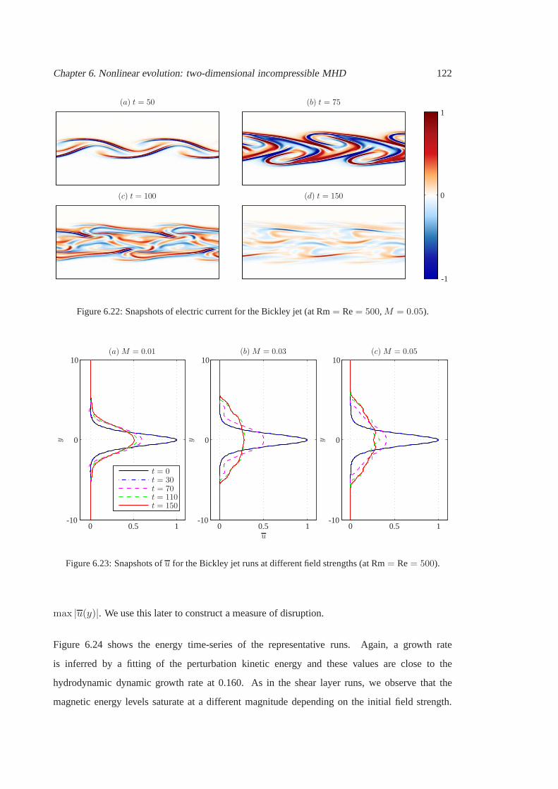
Chapter 6. Nonlinear evolution: two-dimensional incompressible MHD 122
(a) t = 50 (b) t = 75
(c) t = 100 (d) t = 150 0
-1
1
Figure 6.22: Snapshots of electric current for the Bickley jet (at Rm= Re= 500,M = 0.05).
(a)M = 0.01 (b)M = 0.03 (c)M = 0.05
t = 0t = 30t = 70t = 110t = 150
u
yyy 0
0
0
0
0
0-10-10-10
101010
111 0.50.50.5
Figure 6.23: Snapshots ofu for the Bickley jet runs at different field strengths (at Rm= Re= 500).
max |u(y)|. We use this later to construct a measure of disruption.
Figure 6.24 shows the energy time-series of the representative runs. Again, a growth rate
is inferred by a fitting of the perturbation kinetic energy and these values are close to the
hydrodynamic dynamic growth rate at 0.160. As in the shear layer runs, we observe that the
magnetic energy levels saturate at a different magnitude depending on the initial field strength.

Chapter 6. Nonlinear evolution: two-dimensional incompressible MHD 123
(a)M = 0.01
(b)M = 0.03
(c)M = 0.05
growth≈ 0.151
growth≈ 0.150
growth≈ 0.149
E
t0
0
0
50
50
50
100
100
100
150
150
150
10
10
10
10
10
10
10
10
10
10
10
10
0
0
0
-2
-2
-2
2
2
2
-4
-4
-4
Figure 6.24: Time-series of energies (blue= kinetic; red= magnetic; solid= perturbation state; dashed=
mean state; black dot-dashed line= total energy) for the Bickley jet runs (at Rm= Re= 500).
The disruptive cases have the perturbation magnetic and kinetic energies comparable at some point
during the run. There is a noticeable loss of total energy; theM = 0.01 case in Figure 6.24(a) has
a loss of around 30%, comparable with the hydrodynamic case,whilst in theM = 0.05 case in
Figure 6.24(c), this is around 40%.
In Figure 6.25 we plot the dissipation rates for the three runs. Unlike the shear layer runs, Ohmic
dissipation is not necessarily several orders of magnitudehigher than the viscous dissipation;
however in all three runs they are at some point comparable. The Ohmic dissipation increases
to a peak value but then generally decreases afterwards; contrast this to the shear layer case in
Figure 6.16 where multiple well-defined peaks in the Ohmic dissipation are observed. This is
consistent with the observation that the disruption eventsare not sustained, and there is really only
one primary disruption event.
In this multiple wavelength case there is the possibility ofpairing of like-signed vortices; however
in the runs where we observe disruption, the destruction of vortices occurs before any vortex
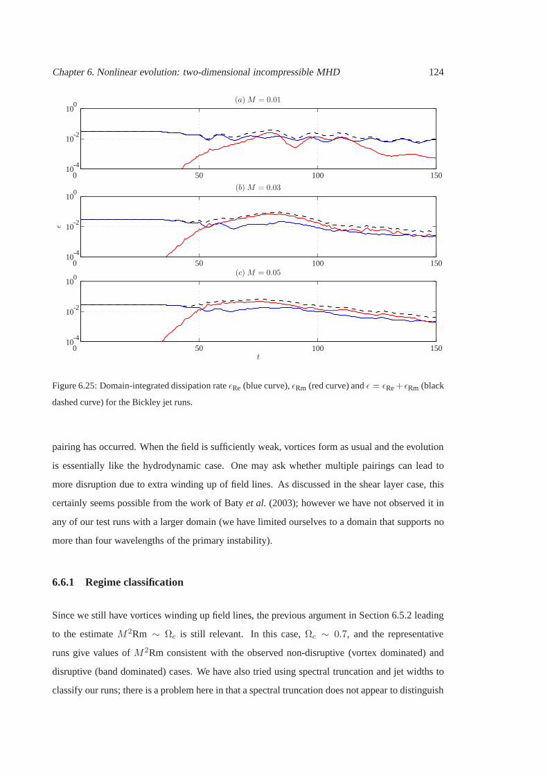
Chapter 6. Nonlinear evolution: two-dimensional incompressible MHD 124
(a)M = 0.01
(b)M = 0.03
(c)M = 0.05
t
ǫ
0
0
0
50
50
50
100
100
100
150
150
150
10
10
10
10
10
10
10
10
10
0
0
0
-2
-2
-2
-4
-4
-4
Figure 6.25: Domain-integrated dissipation rateǫRe (blue curve),ǫRm (red curve) andǫ = ǫRe+ ǫRm (black
dashed curve) for the Bickley jet runs.
pairing has occurred. When the field is sufficiently weak, vortices form as usual and the evolution
is essentially like the hydrodynamic case. One may ask whether multiple pairings can lead to
more disruption due to extra winding up of field lines. As discussed in the shear layer case, this
certainly seems possible from the work of Batyet al. (2003); however we have not observed it in
any of our test runs with a larger domain (we have limited ourselves to a domain that supports no
more than four wavelengths of the primary instability).
6.6.1 Regime classification
Since we still have vortices winding up field lines, the previous argument in Section 6.5.2 leading
to the estimateM2Rm ∼ Ωe is still relevant. In this case,Ωe ∼ 0.7, and the representative
runs give values ofM2Rm consistent with the observed non-disruptive (vortex dominated) and
disruptive (band dominated) cases. We have also tried usingspectral truncation and jet widths to
classify our runs; there is a problem here in that a spectral truncation does not appear to distinguish

Chapter 6. Nonlinear evolution: two-dimensional incompressible MHD 125
case peaku reduction factor marker
disruptive/bands < 0.75 not disruptive/vortices ≥ 0.75 ×
Table 6.7: Regime classification for the Bickley jet in the incompressible case, using the peak jet strength
reduction factor.
Rm
M0.01 0.02 0.03 0.04 0.05 0.06 0.07 0.1
750 0.90 0.64 0.48 0.45 0.52 0.52 0.57 0.65
500 0.93 0.69 0.51 0.45 0.51 0.56 0.51 0.65
250 0.96 0.89 0.67 0.51 0.51 0.53 0.51 0.29
50 0.96 0.96 0.93 0.80 0.80 0.40 0.26 0.29
Table 6.8: Raw data from the set of calculations at Re= 500 for the Bickley jet. The numbers denote the
peak jet strength reduction factor relative to the hydrodynamic case.
between relatively wide bands of vorticity and compact vortices, and we have already made the
observation that the jet widths of the saturated states appear to be comparable to each other in our
runs. One measure that does seem to be well correlated with the degree of disruption is the peak
jet strength valuemax |u(y)|. We will thus takemax |u(y)| at the end of the MHD simulations
at t = 150 and divide this by the peak value of the equivalent hydrodynamic run to give us a
reduction factor. We classify the runs using the conditionsgiven in Table 6.7; the corresponding
hydrodynamic case of course has a reduction factor of 1, withmax |u(y)| = 0.55 at t = 150 in
this case. The raw data is given in Table 6.8 and a regime diagram is given in Figure 6.26.
We see thatM2Rm ≥ 0.1 appears to capture all the disruptive cases. More importantly, the
dependence of disruption on the combinationM2Rm appears to be well captured.
6.6.2 The cases with largerM
For completeness, we plot in Figure 6.27 snapshots of the vorticity of a run at largerM , here at
M = 0.25 (M = 0.5 implies linear stability), with Rm= Re= 500. The jet appears to meander a
little but does not break up into vortices; compare this to the shear layer case where the vortex does
not form at largerM . Again, the estimateM2Rm ∼ Ωe requires that we have vortices forming

Chapter 6. Nonlinear evolution: two-dimensional incompressible MHD 126
M
Jet peak value expansion factor at end time
Rm
M2Rm= 0.1 M2Rm= 0.710
10
101010
-1-2
1
2
3
Figure 6.26: Regime diagram, as measured by the reduction ofthe peak value ofu at end time as a relative
factor to the equivalent hydrodynamic case. Again,M2Rm= C is plotted for some values ofC.
t = 50 t = 75 t = 100 t = 150
-0.7
0
0.7
Figure 6.27: Snapshots of vorticity for the Bickley jet run at M = 0.25 (at Rm= Re= 500).
in the first place; the transition between the disruptive andnonlinear stable regime has not been
investigated.
6.7 Summary and discussion
To summarise, we have investigated the nonlinear evolutionof shear flow instabilities in
incompressible MHD, takingF = 0. Even for weak background field (in the sense that the initial
magnetic energy is much smaller than the initial kinetic energy), it is known from previous work
that the vortical motion arising from the hydrodynamic evolution can amplify the magnetic field,
Chapter 6. Nonlinear evolution: two-dimensional incompressible MHD 127
feedback onto the flow, and cause disruption to the coherent structures that would otherwise form.
Our work here appears to be the first to investigate the simultaneous dependence of disruption on
the basic field strengthM and the dissipation parameter, in this case measured by the magnetic
Reynolds number Rm, as well as provide an estimate for the dependence of the degree of disruption
on the parameter values.
For the shear layer, we focussed on the case where the domain supports a single wavelength of
the most unstable mode. In the hydrodynamic case, the shear layer rolls up into a vortex, and in
our physical setting, there are no observable hydrodynamicsecondary instabilities (e.g., pairing,
braid, convective etc.) that affect the stability of the vortex, and the vortex was seen to be long-
lived. When a background magnetic field was included, three cases were observed: the case
where MHD effects are truly weak, the evolution being essentially hydrodynamic, with the field
lines advected passively and eventually reaching a flux expelled regime; the mildly disruptive
case, where the vortical motion stretched field lines, releasing stresses, but the vortex survives this
disruption, retains its integrity, and a flux expelled regime was also reached; the severely disruptive
case, where the MHD feedback was sufficiently strong, disrupting the vortex significantly, a flux
expelled regime is not reached, and the resulting dominant features in the domain are vorticity
filaments rather than a coherent vortex. The degree of disruption was seen to become more severe
on increasing Rm and/orM (assuming that we are still in the nonlinearly unstable regime). It was
also seen that the increase of the shear layer width was correlated with the degree of disruption.
With regards to the disruption mechanism, vortical motion winds up magnetic field lines,
stretching out a thin current sheet and building up magneticstresses. This build up is arrested when
the current sheet becomes sufficiently thin and breaks (probably due to a resistive instability). This
releases the magnetic stress that feeds back onto the flow, potentially causing disruption. With
this in mind, we provided an estimate for the degree of observed disruption using a kinematic,
dimensional argument. The resulting estimate,M2Rm ∼ Ωe, was tested against the numerical
data overM and Rm space, with the degree of disruption measured by a spectral truncation
wavenumber (maximised over the run) and a shear layer width expansion factor (taken at end
of the run). It was seen that, for the shear layer case,M2Rm ≥ 0.5 appears to capture all of
the severely disruptive runs, but, more importantly, the degree of disruption exhibited by the data
conformed well to the parameter combinationM2Rm.
For the Bickley jet, we focussed on the case where the domain supports two wavelengths of the
Chapter 6. Nonlinear evolution: two-dimensional incompressible MHD 128
most unstable mode. In the hydrodynamic case, it was seen that the jets undergoes a kinking
motion before breaking up into vortices, which then subsequently pair up. In the MHD case, either
the vortices survive the disruption event, and the evolution proceeds as in the hydrodynamic case,
or the vortices are completely disrupted, and vorticity bands form instead. The disruption was
observed to be less violent than for the shear layer, in that there appears to be only one significant
disruption event, rather than a continued cascade of disruptions. This was attributed to the fact that,
in the shear layer, the resulting motion can further tap intothe background flow energy away from
y = 0 for trigger more disruption events, whilst this is not the case for the jet profile as the flow is
largely supported aroundy = 0. It was observed from profiles ofu that the peak value ofu, rather
than the jet width or the spectral truncation wavenumber, was better correlated with the disruption
observed. Since the physical mechanism leading to disruption is similar to the shear layer case,
we also tested theM2Rm∼ Ωe estimate against the data. It was seen thatM2Rm≥ 0.1 appears
to capture all the disruptive runs, and, furthermore, the dependence on the combinationM2Rm
was seen in the regime diagram.
For completeness, we have also performed some runs with largerM , where it appears that we have
nonlinear stability, with no rolling up of the shear layer orbreaking up of the jet. Our estimate for
disruption then requires that we do in fact have vortices forming. The transition location between
the disruptive and nonlinearly stable regime has not been investigated here.
Generally, disruption is a fast process, typically occurring in no more than an eddy turnover time.
For the shear layer, disruption occurs before a flux expelledregime is reached, and for the jet,
disruption can occur before there is any pairing between thevortices. Our estimate, stemming
from a particularly simple kinematic and dimensional argument, also highlights that some care is
needed when the term ‘weak field’ is used; in our shear flow problem using our estimate, it isM
and Rm in the combinationM2Rm≪ 1 that results in an evolution that is essentially unmodified
by MHD effects. The fact that disruption by MHD effects is fast and depends onM2Rm
indicates that this phenomenon will be a robust feature in the nonlinear development of shear
flows in astrophysical systems, since Rm is typically very large. This disruption mechanism from
MHD effects also provides another route for transition to turbulence without resorting to other
hydrodynamic instabilities that require, for example, stratification effects, and so can operate even
in strongly stratified systems where the fluid motion is predominantly horizontal and secondary
hydrodynamic instabilities may be weak. This potentially has impact on, for example, mixing

Chapter 6. Nonlinear evolution: two-dimensional incompressible MHD 129
properties in such electrically conducting fluid systems, something that we have not investigated
here.
We now discuss some other points relating to the disruption mechanism that were mentioned in
the main body of the text.
6.7.1 Dependence on viscosity
All the numerical results presented here were for both the shear layer and the Bickley jet were
performed at Re= 500, and one might wonder about the effects of increasing Re. We have also
conducted some test runs at Re= 750 and1000; one comparison for the shear layer is given in
Figure 6.28, where we plot side by side some quantities obtained from the simulations. There are
some differences, and it is certainly true that the runs at larger Re appear to result in a more severe
disruption, with more vorticity filaments appearing. Sincewe are restricted here in computing
resources, we are unable to probe the parameter region at higher Re, although we do observe that
larger Re increases the life-time of the vorticity filamentsformed from the shredding of the vortex.
We also suspect that, in other systems where other secondaryhydrodynamic instabilities operate
(e.g., Mashayek & Peltier, 2012a,b), the increase in Re willalso lead to a stronger disruption of the
vortices formed, except in this case the disruption is due toa combination of both hydrodynamic
and resistive secondary instabilities. Larger simulations (or ones employing a different formalism;
Dritschel & Tobias 2012) would allow for an investigation ofthe dynamical dependence on
increasing Re and also Rm.
6.7.2 Arresting mechanism: tearing instabilities?
The cause of the major reconnection event in the shear layer runs has largely been attributed to
tearing instabilities by previous investigations (e.g., Joneset al., 1997; Keppenset al., 1999; Baty
et al., 2003), although we suspect a similar mechanism is at play for the jet runs. In particular,
these authors observe in their simulations the appearance of structures that are consistent with the
onset of tearing instabilities, such as magnetic islands and chains of plasmoids (e.g., Figure 11 of
Keppenset al. 1999; Figure 15 of Batyet al. 2003). Tearing-type instabilities are generally the
most unstable in such a current sheet setting (§4 of Biskamp 2000;§6 of Priest & Forbes 2000).
However, we also observe current sheet pinching before current sheet break up in regions centred

Chapter 6. Nonlinear evolution: two-dimensional incompressible MHD 130
(a) Re= 500 (b) Re= 1000
EE
ǫǫ
yy
tt
tt
uu
0
0
0
0
0
0
0
0
0
0
0
0
10
10
10
10
10
10
10
10
10
10
10
10
10
10
1010
5050
5050
100100
100100
150150
150150
22
-2-2
-2-2
-4-4
-4-4
-10-10-1-1 11
Figure 6.28: Comparison between two shear layer runs atM = 0.05, Rm = 1000 at two different values
of Re. Displayed are the energy time-series (blue= kinetic; red= magnetic), dissipation rates (blue=
viscous; red= Ohmic) and snapshots ofu.
around the stagnation point; Figure 6.29 shows snapshots ofthe current in a higher resolution
run, Re= Rm = 500 but at512 × 1024, with M = 0.05, centred around the stagnation point.
This pinching is presumably due to the combined effect of theinflow pushing the current sheets
together, and the instability causing the sheet to pinch. Itwould be beneficial if we could separate
the effect due to the background flow, and provide more evidence for us to conclude the exact type
of resistive instability causing the major reconnection event.
In the time-series of energies shown in Figure 6.15, after the initial peak of perturbation kinetic
energy, the perturbation magnetic energy continues to growa little. One might be convinced that
the perturbation magnetic energy grows at a smaller rate purely by observation of the relevant
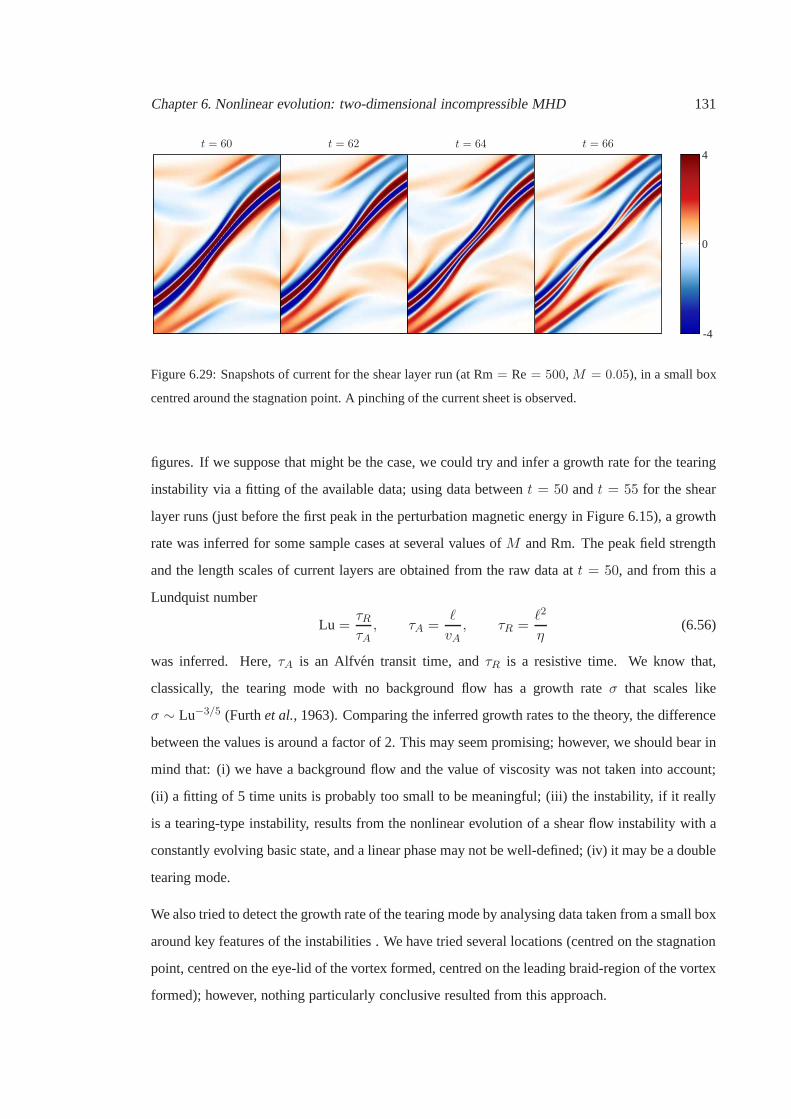
Chapter 6. Nonlinear evolution: two-dimensional incompressible MHD 131
t = 60 t = 62 t = 64 t = 66
-4
0
4
Figure 6.29: Snapshots of current for the shear layer run (atRm = Re= 500, M = 0.05), in a small box
centred around the stagnation point. A pinching of the current sheet is observed.
figures. If we suppose that might be the case, we could try and infer a growth rate for the tearing
instability via a fitting of the available data; using data betweent = 50 andt = 55 for the shear
layer runs (just before the first peak in the perturbation magnetic energy in Figure 6.15), a growth
rate was inferred for some sample cases at several values ofM and Rm. The peak field strength
and the length scales of current layers are obtained from theraw data att = 50, and from this a
Lundquist number
Lu =τRτA, τA =
ℓ
vA, τR =
ℓ2
η(6.56)
was inferred. Here,τA is an Alfven transit time, andτR is a resistive time. We know that,
classically, the tearing mode with no background flow has a growth rateσ that scales like
σ ∼ Lu−3/5 (Furthet al., 1963). Comparing the inferred growth rates to the theory, the difference
between the values is around a factor of 2. This may seem promising; however, we should bear in
mind that: (i) we have a background flow and the value of viscosity was not taken into account;
(ii) a fitting of 5 time units is probably too small to be meaningful; (iii) the instability, if it really
is a tearing-type instability, results from the nonlinear evolution of a shear flow instability with a
constantly evolving basic state, and a linear phase may not be well-defined; (iv) it may be a double
tearing mode.
We also tried to detect the growth rate of the tearing mode by analysing data taken from a small box
around key features of the instabilities . We have tried several locations (centred on the stagnation
point, centred on the eye-lid of the vortex formed, centred on the leading braid-region of the vortex
formed); however, nothing particularly conclusive resulted from this approach.

Chapter 6. Nonlinear evolution: two-dimensional incompressible MHD 132
We also carried out simulations for the nonlinear evolutionof tearing modes with a background
flow, as in, for example, Ofmanet al. (1993), Chenet al. (1997), Otto & Fairfield (2000). Both
single current layers (e.g.,B0(y) = tanh(y)) and double current layers (e.g.,B0(y) = sech2(y))
have been tried with and without a background shear layer flowat different shear layer widths.
The code manages to reproduce what has been documented previously but does not seem to give
any extra information that is relevant to our case here. In particular, we never observe the violent
evolution associated with the shear layer profile that is reported here, for several values of Re
ranging from500 to 1000.
Knowing exactly what the arresting mechanism is would complete the dynamical picture
concerning disruption induced by vortical motion, as well as provide some explicit suggestions
to the parameter dependence we might want to look out for in the regime estimations. It certainly
seems plausible that the tearing-type instability acts as the arresting mechanism, but we can not be
sure about this until there is more evidence available. We conjecture that it is probably a tearing
mode supplemented by the straining experienced by the braid-region/current-layer centred around
the stagnation point that ultimately leads to the current layer break up. The interplay between
these two mechanisms however is not clear. There are techniques to investigate this but we have
not looked at this in much detail.
6.7.3 Validating and improving on the disruption estimate
Supposing for the moment that the dependence of disruption on Re is weak, one interesting
and fairly straight forward thing to do would be to see how farthe kinematic regime estimation
M2Rm∼ Ωe extends into(M,Rm) space. This would simply involve running larger simulations
at higher Rm, possibly using theM2Rm∼ Ωe estimate as a guide for where to look in parameter
space. This may also help clarify the resistive instabilitypoint made previously, giving us more
evidence towards pinning down the exact type of resistive instability causing the disruption.
One possible and more involved investigation would be to go beyond a kinematic argument
and obtain an estimate that takes into account the dynamic feedback. This has been done in
the magneto-convection setting by Gallowayet al. (1978) and Galloway & Moore (1979) via a
matched asymptotic technique. It would be interesting to extend those arguments to this perhaps
simpler case, since we do not have thermal driving. Perhaps an even simpler case would be to
revisit the problem of Weiss (1966), with a vortex in a two-dimensional doubly periodic box and

Chapter 6. Nonlinear evolution: two-dimensional incompressible MHD 133
a uniform background magnetic field, but taking into accountthe dynamical feedback. Some test
simulations we have carried out shows similar disruptive behaviour as those observed here, but we
have not studied the parameter dependence in nearly as much detail1.
1(At time of final correction) Dritschel & Tobias (private communication) have also reported similar results for the
vortex-in-a-box problem.
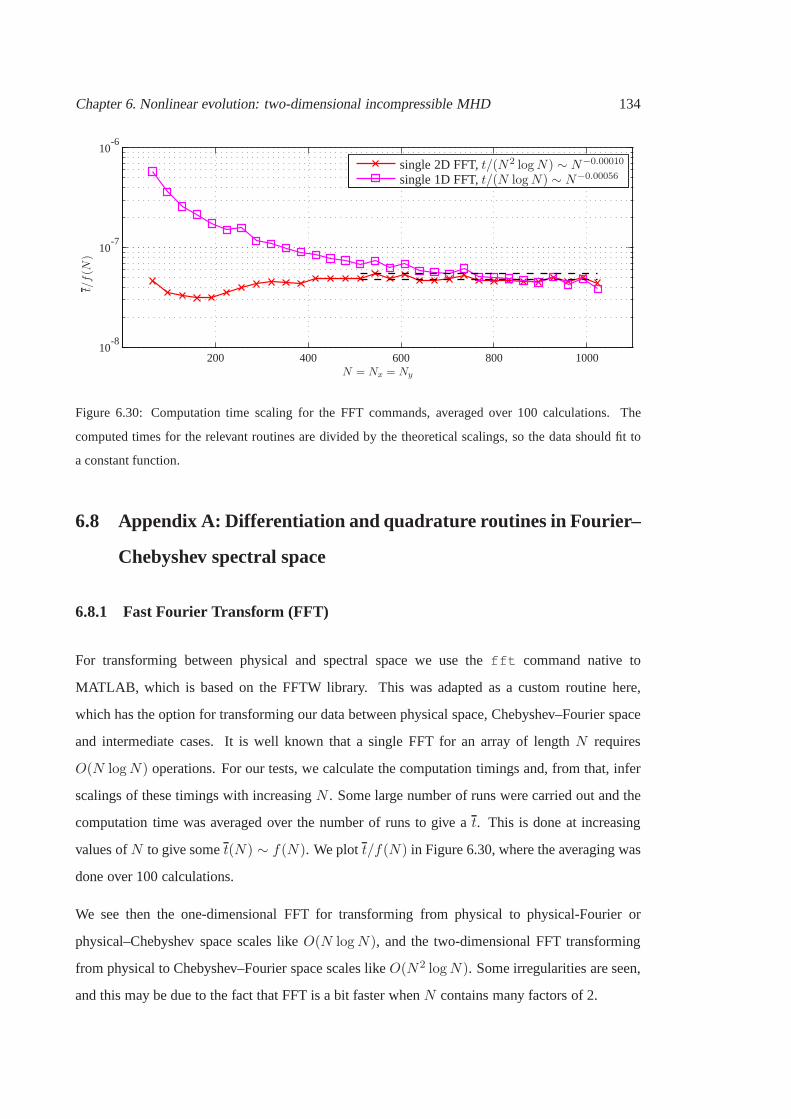
Chapter 6. Nonlinear evolution: two-dimensional incompressible MHD 134
N = Nx = Ny
t/f(N
)
single 2D FFT,t/(N2 logN) ∼ N−0.00010
single 1D FFT,t/(N logN) ∼ N−0.00056
10
10
10
-6
-7
-8
200 400 600 800 1000
Figure 6.30: Computation time scaling for the FFT commands,averaged over 100 calculations. The
computed times for the relevant routines are divided by the theoretical scalings, so the data should fit to
a constant function.
6.8 Appendix A: Differentiation and quadrature routines in Fourier–
Chebyshev spectral space
6.8.1 Fast Fourier Transform (FFT)
For transforming between physical and spectral space we usethe fft command native to
MATLAB, which is based on the FFTW library. This was adapted as a custom routine here,
which has the option for transforming our data between physical space, Chebyshev–Fourier space
and intermediate cases. It is well known that a single FFT foran array of lengthN requires
O(N logN) operations. For our tests, we calculate the computation timings and, from that, infer
scalings of these timings with increasingN . Some large number of runs were carried out and the
computation time was averaged over the number of runs to givea t. This is done at increasing
values ofN to give somet(N) ∼ f(N). We plott/f(N) in Figure 6.30, where the averaging was
done over 100 calculations.
We see then the one-dimensional FFT for transforming from physical to physical-Fourier or
physical–Chebyshev space scales likeO(N logN), and the two-dimensional FFT transforming
from physical to Chebyshev–Fourier space scales likeO(N2 logN). Some irregularities are seen,
and this may be due to the fact that FFT is a bit faster whenN contains many factors of 2.
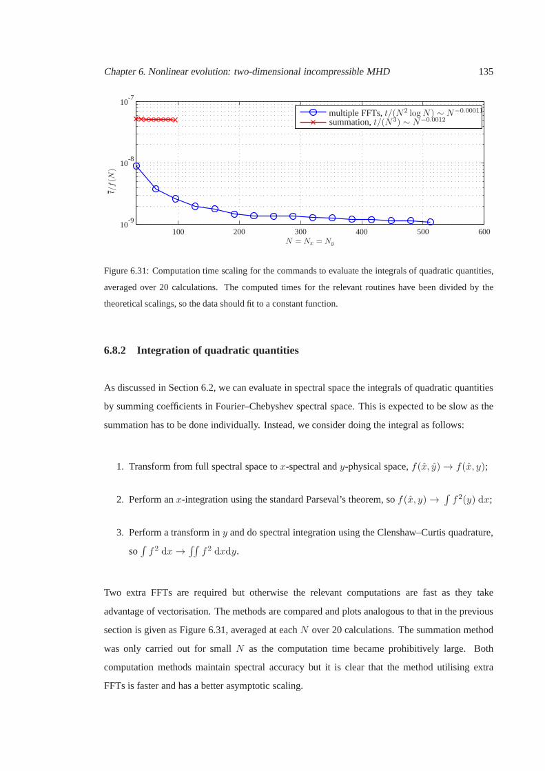
Chapter 6. Nonlinear evolution: two-dimensional incompressible MHD 135
N = Nx = Ny
t/f(N
)multiple FFTs,t/(N2 logN) ∼ N−0.00011
summation,t/(N3) ∼ N−0.0012
10
10
10
-7
-8
-9
100 200 300 400 500 600
Figure 6.31: Computation time scaling for the commands to evaluate the integrals of quadratic quantities,
averaged over 20 calculations. The computed times for the relevant routines have been divided by the
theoretical scalings, so the data should fit to a constant function.
6.8.2 Integration of quadratic quantities
As discussed in Section 6.2, we can evaluate in spectral space the integrals of quadratic quantities
by summing coefficients in Fourier–Chebyshev spectral space. This is expected to be slow as the
summation has to be done individually. Instead, we considerdoing the integral as follows:
1. Transform from full spectral space tox-spectral andy-physical space,f(x, y) → f(x, y);
2. Perform anx-integration using the standard Parseval’s theorem, sof(x, y) →∫
f2(y) dx;
3. Perform a transform iny and do spectral integration using the Clenshaw–Curtis quadrature,
so∫
f2 dx→∫∫
f2 dxdy.
Two extra FFTs are required but otherwise the relevant computations are fast as they take
advantage of vectorisation. The methods are compared and plots analogous to that in the previous
section is given as Figure 6.31, averaged at eachN over 20 calculations. The summation method
was only carried out for smallN as the computation time became prohibitively large. Both
computation methods maintain spectral accuracy but it is clear that the method utilising extra
FFTs is faster and has a better asymptotic scaling.

Chapter 6. Nonlinear evolution: two-dimensional incompressible MHD 136
6.8.3 Quasi-TriDiagonal Solver (QTS)
The fast Helmholtz solver we use is due to Thual (1986); see Appendix B of Peyret (2002) and
§4.1 of Canutoet al. (1993). Using the inversion step∇2ψ = ω as an example, we note that in
our case the linear system takes the following form in spectral space:
· · · D2 − k2I · · ·· · · b+ · · ·· · · b− · · ·
ψ =
ω
g+
g−
, (6.57)
whereb± andg± are the vectors and scalars for enforcing the boundary conditions. Now, there
is a recurrence relationship between the second derivativeand the zero derivative Chebyshev
coefficients, given by
Pj u(2)j−2 +Qju
(2)j +Rju
(2)j+2 = uj , j = 2, 3 · · ·Ny, (6.58a)
with
Pj =cj−2
4j(j − 1), Qj =
−ej+2
2(j2 − 1), Rj =
ej+4
4j(j + 1), (6.58b)
wherecj andej are given by
cj =
2, j = 0,
1, otherwise,ej =
1, j ≤ Ny,
0 j > Ny.
(6.58c)
We then observe that (6.57) may be written as
ψ(2)k − k2ψk = ωk, k = 0, 1, · · ·Ny − 2,
∑
k
b+k = g+,
∑
k
b−k = g−,
(6.59)
so eliminating accordingly, it may be seen that the system given by (6.57) takes the alternative
form
P ′jψj−2 +Q′
jψj +R′jψj+2 = fj, j = 2, . . . , Ny, (6.60a)
where
P ′j = k2Pj , Q′
j = −k2Qj − 1, R′j = k2Rj, (6.60b)

Chapter 6. Nonlinear evolution: two-dimensional incompressible MHD 137
and
fj = −(Pj ωj−2 +Qj ωj +Rjωj+2). (6.60c)
Notice that there are no primes onP , Q andR in the definition off . The system decouples, and
the even and odd coefficients may be solved separately. The resulting decoupled system is of the
form
b0 b2 · · · · · · · · · bNy
P ′2 Q′
2 R′2
P ′4 Q′
4 R′4
. . . . . . . . .
P ′Ny−2 Q′
Ny−2 R′Ny−2
P ′Ny
Q′Ny
ψ0
ψ2
ψ4
...
...
ψNy
=
g
f2
f4......
fNy
(6.61)
where b and g denotes the boundary condition vector and the boundary value appropriately
modified, and similarly for the odd coefficients; this systemis of quasi-tridiagonal form (a
tridiagonal system with one extra row). An analogue of the Thomas algorithm for the tridiagonal
system is given as follows:
1. LetI be the length ofbeven/odd. Definep = P ′even/odd, and analogously forQ, R, andf . Let
ψ = ψeven/odd, so we solve forψ and then extract the relevant information to getψeven/odd.
2. Construct
XI−1 = −pIqI, YI−1 =
fIqI, (6.62)
Xi−1 =−pi
qi + riXi, Yi−1 =
fi − riYiqi + riXi
, i = I − 1, . . . , 1. (6.63)
3. Construct
θi = Xi−1θi−1, λi = Xi−1λi−1 + Yi−1, i = 1, . . . , I, (6.64)
with θ0 = 1, λ0 = 0.
4. Evaluate
ψ0 =geven/odd− Λ
Θ, Θ =
∑
i
biθi, Λ =∑
i
biλi. (6.65)
From this, compute
ψi = Xi−1ψi + Yi, i = 0, . . . , I − 1, (6.66)
and extract the data accordingly.
Chapter 6. Nonlinear evolution: two-dimensional incompressible MHD 138
For the inversion problem∇2ψ = ω, we impose theψ = 0 condition, so
beven=(
1 1 · · · 1)
, geven=g+ + g−
2= 0,
bodd =(
1 1 · · · 1)
, godd =g+ − g−
2= 0.
This algorithm is stable if the system satisfies a diagonallydominant condition given by
|qi|
≥ |pi|+ |ri| if ri 6= 0,
> |pi|+ |ri| if ri = 0.
(6.67)
This method may be used if Dirichlet or Neumann boundary conditions are used on both
boundaries, but needs to be modified if mixed boundary conditions are used. If the boundary
conditions are inhomogeneous and when the domain is not on[−1, 1], extra prefactors will appear
in geven/odd.
As for the Thomas algorithm, the number of operations required isO(N), which is substantially
smaller than usingLU−decomposition and a back-substitution, which typically requiresO(N3)
operations. In Figure 6.32 we plot the computation time for arepresentative problem (solving for
the inversion step of the vorticity for the streamfunction at the first time-step), averaged over 20
calculations, required by the QTS routine as compared to other native commands in MATLAB,
namely (i)linsolve with no options invoked (denoted as Linsolve in Figure 6.32), and (ii)
lu followed bylinsolve with options for solving strictly upper- and lower-triangular systems
(denoted as LU in the Figure Figure 6.32). The numerical differences between the computed
solutions are ofO(10−8); however, it is seen that the actual computation time and thesuggested
asymptotic behaviour of the scaling of the QTS routine compares favourably tolinsolve and
lu commands in MATLAB.
6.9 Appendix B: Derivation of AB/BD3
We first derive the BDk algorithms. We discretise∂un+1/∂t by a backward difference formula,
knowing the data at three levels before. Chapter 3 of Fornberg (1998) provides the formula
for finding the appropriate weights for an arbitrary spaced stencil, essentially rearranging the
appropriate Lagrange polynomial and tracing its coefficients. We have
Fij(x) =
i∑
k=0
ckijk!xk, f (k)(x) = ci0f(x0) + ∆tcci1f(x1) + · · · , (6.68)

Chapter 6. Nonlinear evolution: two-dimensional incompressible MHD 139
N = Nx = Ny
t
t ∼ N3.426
t ∼ N3.3962
t ∼ N1.6408
LinsolveLUQTS
10
10
10
10
0
-1
-2
-3
50 100 150 200 250
Figure 6.32: Computation time scalings for the linear system solver routines, averaged over 20 calculations.
wherek is the derivative required andFij is the Lagrange polynomial given by
Fij =(x− x0) · · · (x− xj−1)(x− xj+1) · · · (x− xi)
(xj − x0) · · · (xj − xj−1)(xj − xj+1) · · · (xj − xi). (6.69)
For our case,k = 3, and we seek(c13,0, c13,1, c
13,2, c
13,3) with
(x0, x1, x2, x3) = (0,−∆tc,−∆tc −∆tp1,−∆tc −∆tp1 −∆tp2), (6.70)
where∆t with subscripts are defined in Section 6.3.
The Lagrange polynomials are respectively
F30 =(x+∆tc)(x+∆tc +∆tp1)(x+∆tc +∆tp1 +∆tp2)
∆tc(∆tc +∆tp1)(∆tc +∆tp1 +∆tp2), (6.71a)
F31 =x(x+∆tc +∆tp1)(x+∆tc +∆tp1 +∆tp2)
−∆tc∆tp1(∆tp1 +∆tp2), (6.71b)
F32 =x(x+∆tc)(x+∆tc +∆tp1 +∆tp2)
−(∆tp1 +∆tp2)(−∆tp1)∆tp2, (6.71c)
F33 =x(x+∆tc)(x+∆tc +∆tp1)
−(∆tc +∆tp1 +∆tp2)(−∆tp1 −∆tp2)(−∆tp2). (6.71d)
The coefficient ofx1 gives
∂u
∂t≈ a0u
n+1 + a1un + a2u
n−1 + a3un−2
∆tc, (6.72)
with the coefficientsai given by (6.38).

Chapter 6. Nonlinear evolution: two-dimensional incompressible MHD 140
It then remains to turn this into a AB/BDk scheme by approximating thef(un+1) term by known
data. We observe that
f(un+1) = f(un) + ∆tcf′(un) +
(∆tc)2
2f ′′(un) + · · · , (6.73)
so we consider approximating the derivative terms using a one sided difference that is third order
accurate. Using the same formula, we seek(c12,0, c12,1, c
12,2) and(c22,0, c
22,1, c
22,2) with
(x0, x1, x2) = (0,−∆tp1,−∆tp1 −∆tp2), (6.74)
and we obtain
F20 =(x+∆tp1)(x+∆tp1 +∆tp2)
∆tp1(∆tp1 +∆tp2), (6.75a)
F21 =x(x+∆tp1 +∆tp2)
−∆tp1∆tp2, (6.75b)
F22 =(x+∆tp1)x
−∆tp1(−∆tp1 −∆tp2). (6.75c)
This gives
∆tcc120 =
2rc + rprc(rc + rp)
, ∆tcc121 = −(rc + rp)
rcrp, ∆tcc
122 =
rcrp(rc + rp)
, (6.76)
and
(∆tc)2
2c220 =
1
rc(rc + rp),
(∆tc)2
2c221 = − 1
rcrp,
(∆tc)2
2c222 =
1
rp(rc + rp),
(6.77)
which in turn gives us
f(un+1) ≈f(un) + ∆tcf′(un) +
(∆tc)2
2f ′′(un)
=f(un) + ∆tc(c120f(u
n) + c121f(un−1) + c122f(u
n−2))
+(∆tc)
2
2(c220f(u
n) + c221f(un−1) + c222f(u
n−2))
=b0f(un) + b1f(u
n−1) + b2f(un−2),
(6.78)
with coefficients given by (6.38). When the step size is constant, these reduce to known formulas
(e.g., Peyret, 2002,§4).
To test the time-marching algorithm and the semi-implicit treatment, we use the example given in
§4.5 of Peyret (2002), a one-dimensional advection-diffusion problem with forcing where the exact
solution is known, and test the AB/BD3 algorithm withL = ∂2/∂y2 in (6.38) against AB/BD2

Chapter 6. Nonlinear evolution: two-dimensional incompressible MHD 141
log(‖u−u
true‖ L
2)
log(∆taverage)
error∼ h0.99832
error∼ h1.9991
error∼ h2.9895
AB/BD2AB/BD3
AB3/BD1
-5
-5-6-7
-10
-15
-20
Figure 6.33: (Discrete)L2 error at the final time of the semi-implicit schemes given by the variable versions
of AB/BD2, AB/BD3, and AB3/BD1.
and AB3/BD1 withL similarly treated. To generate the time grid, we specify a step size mean and
randomly generate spacings that have Gaussian distribution with small variance (typically around
a quarter of the mean); the grid is different at eacht, but all three methods use the same randomly
generated grid at the samet. The results are shown in Figure 6.33, plotted against a measure of
the error with mean time-step size. The theoretical decrease in error with decrease in mean-step
size is confirmed by the numerical results.
Chapter 6. Nonlinear evolution: two-dimensional incompressible MHD 142

143
Chapter 7
Nonlinear evolution: shallow-water
MHD
Following on from the investigation withF = 0 in the previous chapter, we now study the
nonlinear evolution of the shear layer and the jet profiles inthe SWMHD system whereF > 0.
There are some difficulties with regards to the numerical implementation in the shallow-water
case, and we address these first before presenting the results from the simulations. Our focus here
is on theF < 1 case, and the associated non-zero Froude number modification to the processes
highlighted in the previous chapter. Some details with regards to theF > 1 cases are given
towards the end of the chapter.
7.1 Numerical and mathematical formulation of SWMHD
7.1.1 The choice of dissipation and conservation problems
The SWMHD equations were derived in the ideal setting, but since we expect small-scale features
to appear as part of the nonlinear evolution, some sort of diffusion will be required to stabilise
the routines. The problem of the form of dissipation to take in the hydrodynamic shallow-water
equations has been previously discussed (e.g., Gent, 1993;Ochoaet al., 2011; Gilbertet al., 2013).
As an illustrative example, suppose we consider a SWMHD system with dissipation that looks
Chapter 7. Nonlinear evolution: shallow-water MHD 144
similar to the incompressible MHD equations given in (6.1),given by
∂u
∂t+ u · ∇u−M2
b · ∇b+∇h =1
Re∇2
u, (7.1a)
∂b
∂t+ u · ∇b− b · ∇u =
1
Rm∇2
b, (7.1b)
F 2 ∂h
∂t+∇ · [(1 + F 2h)u] =
F 2
R∇2h, (7.1c)
∇ · [(1 + F 2h)b] = 0. (7.1d)
Here, R denotes an associated dissipation onh (not necessarily physical). For numerical purposes,
there is no reason why we cannot take this form of dissipation; it turns out though that there are
physical reasons why the choice of dissipation in (7.1) is a particularly bad one. Regardless of this,
there is a fundamental issue that does need to be addressed, and that is the self-consistency of the
derivation of the SWMHD equations when finite magnetic dissipation is present. The derivation
leading to the SWMHD system assumes there is no magnetic dissipation, and so the free surface
is initially and remains a field line. In the ideal case, this is justified, leading to the modified
divergence-free condition of the magnetic field, but this isno longer necessarily true when finite
magnetic dissipation is present. How do we reconcile this?
For the moment, we argue that for short-time phenomena at large Rm, the frozen-in condition is
a reasonable assumption. We then need to be careful with maintaining the equivalent divergence-
free condition as well as the conservation laws. As we have noted already in Chapter 2, the
equivalent divergence-free condition is absolutely required for the absence of extra sources in the
conserved quantities. This frozen-in assumption may be plausible for phenomena on dynamic
time-scales, such as shear flow instabilities, but is most certainly not valid for phenomena on
dissipative time-scales that occur in, for example, turbulence or dynamo studies. A justification
into this fundamental problem of self-consistency must be addressed if the SWMHD equations are
to be used for such studies. We revisit this point in the discussion section later.
Suppose we use formulation (7.1). We now show what else can gowrong in terms of conservation
laws. In Chapter 2 we already demonstrated the various conservation properties of the ideal
SWMHD system (on the left hand side of 7.1), so here we focus onthe modifications of the
conservation properties resulting from the dissipation terms on the right hand side of (7.1).
Chapter 7. Nonlinear evolution: shallow-water MHD 145
Mass conservation
d
dt
∫∫
ht dxdy =F 2
R
∫∫(
∂2
∂x2+
∂2
∂y2
)
h dxdy. (7.2)
If we have periodicity inx, then we needF 2R−1 = 0 or ∂h/∂y = 0 on the boundaries for mass
conservation.
Momentum conservation violation
Assuming that the divergence-free condition is satisfied for all time, thex-momentum evolution is
given byd
dt
∫∫
htu dxdy =
∫∫ (
1
Reht∇2u+
F 2
Ru∇2h
)
dxdy
=− F 2
(
1
Re+
1
R
)∫∫
∇ht · ∇u dxdy,
(7.3)
where we use periodicity inx, v = 0, by = 0 and additionally∂u/∂y = 0 as y-boundary
conditions. So there is no momentum conservation since the extra terms are not generically zero.
Similarly, for they-momentum equation,
d
dt
∫∫
htv dxdy =
∫∫ (
1
Reht∇2v +
F 2
Rv∇2h
)
dxdy
=− F 2
(
1
Re+
1
R
)∫∫
∇h · ∇v dxdy −∫ [
F 2h2
2+ h
]y=Ly
y=−Ly
dx,
(7.4)
and we encounter a similar problem.
Flux conservation violation
In addition to problems with momentum conservation, there is also a problem with magnetic flux
conservation. Again, assuming the divergence-free condition holds,
d
dt
∫∫
htbx dxdy =
∫∫(
1
Rmht∇2bx +
F 2
Rbx∇2h
)
dxdy
=− F 2
(
1
Rm+
1
R
)∫∫
∇h · ∇bx dxdy,
(7.5)
where periodicity inx, v = 0, by = 0 and additionally∂bx/∂y = 0 asy-boundary conditions
have been used. Observe also that
d
dt
∫∫
htby dxdy =
∫∫ (
1
Rmht∇2by +
F 2
Rby∇2h
)
dxdy
=− F 2
(
1
Rm+
1
R
)∫∫
∇h · ∇by dxdy,(7.6)
Chapter 7. Nonlinear evolution: shallow-water MHD 146
so again there are extra contributions to global magnetic flux from extra terms.
Total energy conservation in velocity variables
Constructing the energy budget as before, we see that
1
2
d
dt
∫∫
[
ht(|u|2 +M2|b|2) + F 2h2]
dxdy
=
∫∫[
1
Re(htu) · ∇2
u+M2
Rm(htb) · ∇2
b+F 2
R
( |u|2 +M2|b|22
∇2h
)
+ hF 2
R∇2h
]
dxdy
=−∫∫
ht
[
1
Re
(
∂uj∂xi
)2
+M2
Rm
(
∂bj∂xi
)2]
+F 2
R
(
∂h
∂xi
)2
dxdy
− F 2
∫∫ [(
1
Re+
1
R
)
uj∂h
∂xi
∂uj∂xi
+M2
(
1
Rm+
1
R
)
bj∂h
∂xi
∂bj∂xi
]
dxdy.
(7.7)
Thus we do not have a formally negative-definite dissipationwhenF 6= 0.
Divergence free condition violation
Finally, we observe that
∂
∂t(htb) = ∇× (u× htb) +
1
Rmht∇2
b+F 2
Rb∇2h, (7.8)
and so∂
∂t∇ · (htb) = ∇ ·
[
1
Rmht∇2
b+F 2
Rb∇2h
]
6= 0, (7.9)
unless Rm−1 = R−1 = 0 or F = 0. This is particularly problematic, as the divergence-free
condition was used implicitly in the calculations of the other conservation laws.
So now we have seen what could go wrong, we consider an alternative implementation of
dissipation using the SWMHD equations written in transportvariables with (U ,B, h) =
(htu, htb, h):
∂U
∂t+∇ ·
(
UU
ht−M2BB
ht
)
+ ht∇h =1
Re∇2
U , (7.10a)
∂B
∂t+∇ ·
(
UB
ht− BU
ht
)
=1
Rm∇2
B, (7.10b)
F 2∂h
∂t+∇ ·U =
F 2
R∇2h, (7.10c)
∇ ·B = 0. (7.10d)

Chapter 7. Nonlinear evolution: shallow-water MHD 147
Here, tensor notation is used, with(UB)ij = UiBj . Also note that the form of the dissipation
employed in (7.10) is different to that in (7.1). Before going through the same arguments using
conservation laws, we first make the observation that they-component of the momentum equation
is given by
∂V
∂t+
∂
∂x
(
UV −M2BxBy
ht
)
+∂
∂y
(
V 2 −M2B2y
ht
)
+ ht∂h
∂y=
1
Re∇2V. (7.11)
If we takeV = 0 andBy = 0 as boundary conditions, then, on they-boundaries, we have
ht∂h
∂y
∣
∣
∣
∣
y=±Ly
=1
Re∂2V
∂y2
∣
∣
∣
∣
y=±Ly
. (7.12)
Substituting for∂V/∂y using the continuity equation, also evaluated at they-boundaries, we have
ht∂h
∂y
∣
∣
∣
∣
y=±Ly
=1
Re∂
∂y
(
F 2
R∇2h− F 2∂h
∂t− ∂U
∂x
)∣
∣
∣
∣
y=±Ly
. (7.13)
Upon swapping the derivatives for theU term and further assuming∂U/∂y = 0 on the y-
boundaries, this gives
F 2
Re∂
∂t
∂h
∂y
∣
∣
∣
∣
y=±Ly
=
(
1
ReF 2
R∇2 − ht
)
∂h
∂y
∣
∣
∣
∣
y=±Ly
. (7.14)
For the simulations presented later, we will takeR−1 = 0, and so if∂h/∂y = 0 initially, then
∂h/∂y = 0 on the boundaries for all subsequent time.
Mass conservation
The continuity equation has not been modified, so periodicity in x and ∂h/∂y = 0 on the
boundaries leads again to mass conservation.
Momentum conservation
Assuming the divergence-free condition forB holds,
d
dt
∫∫
U dxdy =1
Re
∫∫
∇2U dxdy = 0, (7.15)
since we have periodicity,V = 0, By = 0 and if we take∂U/∂y = 0 on they-boundaries.
Similarly,
d
dt
∫∫
V dxdy =1
Re
∫∫
∇2V dxdy −∫ [
F 2h2
2+ h
]y=Ly
y=−Ly
dx (7.16)
using the same set of boundary conditions. No extra terms appear in this setting.

Chapter 7. Nonlinear evolution: shallow-water MHD 148
Flux conservation
Again, assuming the divergence-free condition holds,
d
dt
∫∫
Bx dxdy =1
Rm
∫∫
∇2Bx dxdy = 0, (7.17)
using periodicity,V = 0, By = 0, and if we take∂Bx/∂y = 0 on they-boundaries. Similarly,
d
dt
∫∫
By dxdy =1
Rm
∫∫
∇2By dxdy
=1
Rm
∫∫
∂2By
∂y2dxdy − 1
Rm
∫∫
∂
∂x
∂Bx
∂ydxdy = 0,
(7.18)
upon using the same set of boundary conditions.
Total energy conservation
Since the equations are formulated forU andB, we first need to work out what the implied
dissipation operators foru andb are. Suppose that
∂u
∂t+ · · · = DRe, (7.19)
then we have∂(htu)
∂t+ · · · = htDRe+
F 2
Ru∇2h. (7.20)
The right hand side must be equivalent to Re−1∇2U in (7.10a), so
DRe =1
Re∇2
U
ht− F 2
Ru
ht∇2h. (7.21)
A similar manipulation implies that
DRm =1
Rm∇2
B
ht− F 2
Rb
ht∇2h. (7.22)
Then the energy equation is
1
2
d
dt
∫∫
[
ht(|u|2 +M2|b|2) + F 2h2]
dxdy
=1
2
d
dt
∫∫
[
(U · u+M2B · b) + F 2h2
]
dxdy
=
∫∫[
1
Reu · ∇2
U +M2
Rmb · ∇2
B +F 2
R
( |u|2 +M2|b|22
)
∇2h+ hF 2
R∇2h
]
dxdy
=−∫∫
ht
[
1
Re
(
∂uj∂xi
)2
+M2
Rm
(
∂bj∂xi
)2]
+F 2
R
(
∂h
∂xi
)2
dxdy
+ F 2
∫∫[(
1
R− 1
Re
)
uj∂h
∂xi
∂uj∂xi
+M2
(
1
R− 1
Rm
)
bj∂h
∂xi
∂bj∂xi
]
dxdy.
(7.23)
Chapter 7. Nonlinear evolution: shallow-water MHD 149
So, in the hydrodynamic shallow-water system, we can in factobtain a negative-definite
dissipation if we choose Re= R (as in Poulin & Flierl 2003). We will be takingR−1 = 0, so we
do not end up with negative-definite disspation; however, itwill be seen the extra contributions
arising from this choice is small compared to negative-definite contribution for all theF < 1
results we present.
Divergence-free condition
We see that∂B
∂t= ∇×
(
U
ht×B
)
+1
Rm∇2
B, (7.24)
and so∂
∂t(∇ ·B) = ∇ ·
[
∇× (· · · ) + u(∇ ·B) +1
Rm∇2∇ ·B
]
. (7.25)
Thus an initially divergence-free field remains divergence-free in the continuous time setting. So
certainly formulation (7.10) in transport variables maintains more (but not all) of the conservation
laws than formulation (7.1) in velocity variables. In particular, the divergence-free condition
(7.10d) is maintained by the formulation of the SWMHD equations given by (7.10).
7.1.2 Arguments for employing(7.10)
Despite some of the flaws that are present with formulation (7.10), namely the lack of negative-
definite energy dissipation in the general case with R, Re andRm distinct, we will be using this
formulation and here we give our reasons for this.
With regards to momentum dissipation, several other possibilities have been given in Ochoaet al.
(2011) and Gilbertet al. (2013); our choice here is option III of Ochoaet al. (2011). Some of
the other possibilities, used in the absence of a dissipation term in the continuity equation, have
the property that they give a negative-definite dissipationand maintain other conservation laws.
However, the forms of these dissipation terms are not particularly convenient to treat numerically
in our pseudo-spectral, semi-implicit-in-time formalism, mainly because the associated dissipation
terms involve nonlinear combinations ofh andU .
There is of course the possibility of taking Re= R in (7.10), which does give a negative-definite
dissipation of energy (as in Poulin & Flierl, 2003). We have not done this here and for the results

Chapter 7. Nonlinear evolution: shallow-water MHD 150
presented later, we have R−1 = 0. This is partly because, when R−1 6= 0, the resulting equation
for h to be solved is of fourth rather than second order iny. The fast solver does not appear to
have a generalisation to the fourth order problem, and thus another solver needs to be used. In the
test runs at some values ofF , we compared the case where R= Re (usingLU for inversion ofh)
and R−1 = 0 (using the fast solver). The runs were qualitatively comparable, but the routine using
LU takes anything upwards of five times the amount of time to run compared to the routine using
the fast solver.
With regards to the other dissipative terms when R−1 = 0, given in the hydrodynamic case by
F 2∫∫
uj(∂ih)(∂iuj) dxdy, we see that these terms are contains factors ofF 2 and involve∇h.
We expect that, forF small, steepening should not be an issue so∇h is small, and hence the extra
contributions to dissipation are also going to be small. As amatter of convenience, we numerically
implement (7.10) with R−1 = 0, and trackF 2∫∫
uj(∂ih)(∂iuj) dxdy. In our test runs, we found
that, in this particular shear flow problem and at the values of F at which we focussed most of
our attention (F < 1), the absolute value of the extra contributions is only a small percentage
of the total dissipation. There were some issues with test runs atF > 1, which we defer to
later discussions. So this choice of dissipation is unlikely to cause major problems, using thisa
posteriorivalidation.
For the MHD case, if we bypass the fundamental issue of field-line slippage and insist on satisfying
this divergence-free condition, then we need a magnetic dissipation that maintains this condition.
There are several possible choices (Andrew Gilbert, private communication), with ours being one
of them; see Section 7.6 for more details. The alternative choices are such that, in the absence of
dissipation in the continuity equation, a negative-definite dissipation may be achieved. However,
the terms are nonlinear and are problematic to treat in our formalism. So, again mainly for
simplicity and also because we expect the extra contributions to be small in theF < 1 regime, we
employ the setting as in (7.10) and track the extra contributions to magnetic dissipation, here given
by F 2∫∫
bj(∂ih)(∂ibj) dxdy; these are again seen to be small compared to the total dissipation
in our test runs.
In summary, we numerically solve for the SWMHD equations given in (7.10), with R−1 = 0. This
formulation is an improvement over the formulation in velocity variables as more conservation
laws are maintained. In particular, the divergence-free condition is maintained. We should note,
however, that energy dissipation in this set up is not negative-definite; tests have shown that, in
Chapter 7. Nonlinear evolution: shallow-water MHD 151
this particular problem and at the values ofF we consider, the fact that we do not formally have
negative-definite dissipation is unlikely to be a significant problem since the extra contribution is
only a small percentage of the total dissipation, demonstrated later for some representative cases.
We note in passing that there is also a possibility to employ the vorticityω, divergenceδ (with the
associated potentials) and the height fieldh as fundamental variables (e.g., Polvaniet al., 1994;
Cho & Polvani, 1996a,b; Scott & Polvani, 2008). This is in fact the preferred method when the
domain is doubly periodic, since a spectral method employing either Fourier modes or spherical
harmonics allows for a straightforward solution of the resulting Poisson equation. For the channel
geometry we have here, there is the added complication of lateral boundary conditions that need to
be imposed. In this case the formulation in terms of(ω, δ, h) leads to a coupled elliptic system to
be solved at the inversion step at every time-step (Salmon, 2009). This is expensive as an iterative
solver will then be required; this formalism has not been tested here.
To maintain the divergence-free condition, we employ a flux function such that
B = ez ×∇A. (7.26)
This reduces to the magnetic potential in two-dimensional incompressible MHD whenF = 0.
The equations that we will be solving are given by
∂U
∂t+
∂
∂x
(
U2 −M2B2x
1 + F 2h+F 2h2
2
)
+∂
∂y
(
UV −M2BxBy
1 + F 2h
)
+∂h
∂x=
1
Re∇2U, (7.27a)
∂V
∂t+
∂
∂x
(
UV −M2BxBy
1 + F 2h
)
+∂
∂y
(
V 2 −M2B2y
1 + F 2h+F 2h2
2
)
+∂h
∂y=
1
Re∇2V, (7.27b)
∂A
∂t+
U
1 + F 2h
∂A
∂x+
V
1 + F 2h
∂A
∂y=
1
Rm∇2A, (7.27c)
F 2 ∂h
∂t+∂U
∂x+∂V
∂y= 0, (7.27d)
where we have taken R−1 = 0. WhenF = 0, the above equations formally reduce to that of
incompressible MHD. In two-dimensional planar MHD, it is well-known that there is no dynamo
action (Zel’dovich, 1957); an anti-dynamo result may be shown (due to Andrew Gilbert, private
communication); see Section 7.6. We once again the choice ofdissipation is anad hocchoice and
does not stem from a self-consistent derivation from the Boussinesq MHD equations; we comment
on the possibility of deriving a set of thin-layer equationsin a self-consistent way at the end of this
chapter.

Chapter 7. Nonlinear evolution: shallow-water MHD 152
To satisfy as many of the conservation properties as possible, the take the boundary conditions
V = 0,∂U
∂y= 0,
∂h
∂y= 0, A = 0 on y = ±Ly. (7.28)
From (7.27c), we observe that the boundary conditionA = 0 implies that, on the boundaries, all
terms on the left hand side and∂2A/∂x2 are zero, and so this implies∂2A/∂y2 = ∂Bx/∂y = 0
on the boundaries. With such boundary conditions, waves hitting the boundaries will be reflected
back into the domain. Test runs have shown that the gravity waves generated forF < 1 are
small in amplitude and do not appear to have a significant effect on the macro-dynamics. There
are methods to absorb impacting gravity waves, such as inserting sponge-layers or modifying the
boundary conditions (e.g., Durran, 2010,§8), but these are not employed here.
7.1.3 Presence of fast waves
Unlike the incompressible case, fast gravity waves are supported in shallow-water systems. If we
were to consider an explicit treatment of all terms except the dissipation terms, then we would
have a restriction on∆t of the form
∆t×max
(
uN∆x
+vN∆y
)
,
(
uG∆x
+vG∆y
)
≤ Ccfl = O(1). (7.29)
For numerical stability,∆t needs to be small enough so that the fastest process supported by the
system is evolved in a stable fashion. From Chapter 2, we expect that(uG, vG) ∼ O(F−1), and
this places severe restrictions on the time-step, particularly for smallF .
There are several ways around this restriction, for exampleby employing splitting methods or
semi-implicit treatments (see e.g., Peyret, 2002; Durran,2010). We will consider here a semi-
implicit treatment of the relevant terms, namely the∇h terms in equations (7.27a) and (7.27b),
and the divergence terms in equation (7.27d).
Another issue we address before giving the full details of the time discretisation is the stability
properties of the time-marching scheme for wave propagation. To illustrate this, it is perhaps
easiest to consider the one-dimensional, inviscid, hydrodynamic shallow-water equations, with
a uniform background flow; in the ideal case, there is no difference between using velocity or
Chapter 7. Nonlinear evolution: shallow-water MHD 153
transport variables, so we use velocity variables temporarily. The linearised equations are
∂u
∂t+∂u
∂x+∂h
∂x= 0, (7.30a)
F 2
[
∂h
∂t+∂h
∂x
]
+∂u
∂x= 0. (7.30b)
To analyse the stability of the scheme, we carry out a von Neumann stability analysis (e.g., Durran,
2010,§3), using the AB/BD2 method, rather than AB/BD3 employed in the previous chapter, to
demonstrate the differences in the stability properties between this second and third order time-
marching scheme. A discretisation with∂h/∂x and∂u/∂x treated implicitly then gives
a0un+1 + a1u
n + a2un−1 +∆tU0
∂
∂x(b0u
n + b1un−1) + ∆t
∂hn+1
∂x= 0, (7.31a)
F 2(a0hn+1 + a1h
n + a2hn−1) + F 2∆tU0
∂
∂x(b0h
n + b1hn−1) +
∂un+1
∂x= 0, (7.31b)
where the AB/BD2 coefficients are given by (Peyret, 2002,§4)
a0 =2 + rc1 + rc
, a1 = −1− 1
rc, a2 =
1
1 + rc, (7.32a)
b0 = 1 +1
rc, b1 = − 1
rc, (7.32b)
rc =∆tp1∆tc
=tn − tn−1
tn+1 − tn. (7.32c)
Now, since the system given by (7.31) is a function ofx only, we consider solutions ofh andu
of the form(un, hn) ∼ An exp(ikx), whereA ∈ C. If |A| > 1, then the numerical solution will
grow at each time-step and thus be numerically unstable. Denotingz = ik∆t, we obtain the linear
system
VAB/BD2(A,U0, z) zA2
zA2 F 2VAB/BD2
u
h
= 0, (7.33)
where we have used the shorthand
VAB/BD2 = a0A2 + (a1 + U0b0z)A+ (a2 + U0b1z). (7.34)
ChoosingF andU0, we can solve this system forA on a z = zr + izi grid. Choosing the
appropriate branch of solutions, we can plot the stability contour |A| = 1 in the complexz
plane, with numerical stability (|A| < 1) to the left of the contour, and instability otherwise.
In Figure 7.1 we plot the stability region of AB/BD2 along with the corresponding results for
AB/BD3, AB3/Crank-Nicolson, and AB2/Crank-Nicolson, forseveralF values. Sincez = ik∆t,

Chapter 7. Nonlinear evolution: shallow-water MHD 154
(a) AB/BD3 (b) AB3/CN
(c) AB2/CN (d) AB/BD2
zr =Re(ik∆t)zr =Re(ik∆t)
zr =Re(ik∆t)zr =Re(ik∆t)
z i=
Im(ik∆t)
z i=
Im(ik∆t)
z i=
Im(ik∆t)
z i=
Im(ik∆t)
F = 0.1F = 0.1
F = 0.1F = 0.1
F = 0.25F = 0.25
F = 0.25F = 0.25
F = 0.5F = 0.5
F = 0.5F = 0.5
F = 0.75F = 0.75
F = 0.75F = 0.75
0
0
0
0
0
0
0
0
0.020.02
0.020.02
0.040.04
0.040.04
-0.02-0.02
-0.02-0.02
-0.04-0.04
-0.04-0.04
0.20.2
0.20.2
0.40.4
0.40.4
-0.2-0.2
-0.2-0.2
-0.4-0.4
-0.4-0.4
Figure 7.1: Numerical stability boundaries of various time-marching schemes for the one-dimensional,
linear, hydrodynamic shallow-water equations, plotted atseveralF values. The schemes are stable forz
values left of the contours.
if the scheme is unstable on some of thezr = 0 line then we have a restriction on∆t. We see that
when AB3 schemes are employed in this setting, we have a severe restriction on∆t whenF ≪ 1,
whilst the AB2 scheme does not appear to exhibit this undesirable behaviour. The AB/BD3 version
of the code is easily adapted to AB/BD2 since the only things that needs changing are the relevant
coefficientsaj andbj , given in equation (7.32); thus we employ the AB/BD2 scheme as the time-
marching algorithm in this chapter.
As a final test of the AB/BD2 scheme, we solve numerically the two-dimensional linearised
SWMHD equations. These are solved with the AB/BD2 scheme using the semi-implicit formalism
presented earlier, appropriately initialised with exact gravity wave solutions given by (2.48).
First an elliptic equation forh is solved, thenu and v are updated at each time-step, with a
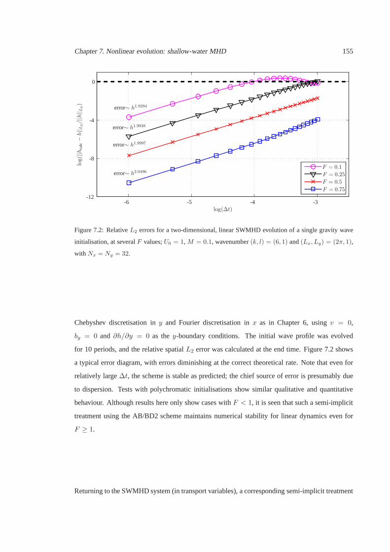
Chapter 7. Nonlinear evolution: shallow-water MHD 155
error∼ h1.9294
error∼ h1.9938
error∼ h1.9997
error∼ h2.0496
log(||h
calc−h|| L
2/||h|| L
2)
log(∆t)
F = 0.1
F = 0.25
F = 0.5
F = 0.75
-3
-4
-4-5-6
0
-8
-12
Figure 7.2: RelativeL2 errors for a two-dimensional, linear SWMHD evolution of a single gravity wave
initialisation, at severalF values;U0 = 1, M = 0.1, wavenumber(k, l) = (6, 1) and(Lx, Ly) = (2π, 1),
with Nx = Ny = 32.
Chebyshev discretisation iny and Fourier discretisation inx as in Chapter 6, usingv = 0,
by = 0 and ∂h/∂y = 0 as they-boundary conditions. The initial wave profile was evolved
for 10 periods, and the relative spatialL2 error was calculated at the end time. Figure 7.2 shows
a typical error diagram, with errors diminishing at the correct theoretical rate. Note that even for
relatively large∆t, the scheme is stable as predicted; the chief source of erroris presumably due
to dispersion. Tests with polychromatic initialisations show similar qualitative and quantitative
behaviour. Although results here only show cases withF < 1, it is seen that such a semi-implicit
treatment using the AB/BD2 scheme maintains numerical stability for linear dynamics even for
F ≥ 1.
Returning to the SWMHD system (in transport variables), a corresponding semi-implicit treatment
Chapter 7. Nonlinear evolution: shallow-water MHD 156
in time using the AB/BD2 discretisation results in the scheme(
a0 −∆t
Re∇2
)
Un+1 = N(U) −∆t∂hn+1
∂x, (7.35a)
(
a0 −∆t
Re∇2
)
V n+1 = N(V )−∆t∂hn+1
∂y, (7.35b)
(
a0 −∆t
Rm∇2
)
An+1 = N(A), (7.35c)
a0F2hn+1 +∆t
(
∂Un+1
∂x+∂V n+1
∂y
)
= F 2N(h), (7.35d)
whereN denotes the relevant terms that are evaluated at the levels below n + 1. Taking the
divergence of the momentum equation then gives(
a0 −∆t
Re∇2
)(
∂Un+1
∂x+∂V n+1
∂y
)
=
(
∂N(U)
∂x+∂N(V )
∂y
)
−∆t∇2hn+1, (7.36)
and so we have the following elliptic equation to solve forh:[
(∆t)2∇2 − a0F2
(
a0 −∆t
Re∇2
)]
hn+1
= ∆t
(
∂N(U)
∂x+∂N(V )
∂y
)
− F 2(a0 − ν∆t∇2)N(h).
(7.37)
Oncehn+1 is known, the other equations may be appropriately advancedin time. Since this is
a second order scheme, the first time-step is taken using an Euler/Crank-Nicolson scheme with a
similar semi-implicit treatment.
Note that the algorithm also works forF = 0, and in this caseh is to be identified with the
pressure fieldp. There is however a subtlety in the inversion step forh when solving the Poisson
equation (7.37); see Section 7.7 for details. The shallow-water program may be used to solve
for incompressible dynamics, and results from this programhave been checked against those
obtained from the program employing the streamfunction-vorticity formulation. The qualitative
and quantitative results (e.g., agreement of shear layer width at end time, general behaviour of
energy time-series and dissipation rates) from the two programs agree with each other, but the
program using the streamfunction-vorticity formulation runs faster because it has one less equation
to solve.
7.2 Hydrodynamic evolution
We focus first on cases withF < 1. We have found that, for the nonlinear runs using AB/BD2, the
CFL number needs to be reduced from around 0.15 for the smallF cases to about 0.05 for largerF

Chapter 7. Nonlinear evolution: shallow-water MHD 157
in order to retain numerical stability, with the transitionat aroundF ≈ 0.4. In these shallow-water
runs, we initialise with a linear eigenfunction (appropriately scaled) at specifiedα, and add to this
higher wavenumber perturbations at lower amplitude with random phase. The initial total energy
of the perturbations is fixed at10−5. As before, we switch off the dissipation of the basic state
until the perturbations are sufficiently large, using the same energy criteria as in Chapter 6.
7.2.1 Hyperbolic-tangent shear layer
Table 7.1 shows a summary of the parameter values employed for the shear layer runs. Again, we
focus on the case where the domain supports a single wavelength of the primary instability. The
optimalα for these cases are close toα = 0.44. We will focus our investigation onF = 0, 0.1
and0.5; the runs atF = 0.25 andF = 0.75 are comparable to those atF = 0.1 andF = 0.5
respectively.
parameter range
F 0, 0.1, 0.25, 0.5, 0.75
Re 500
Nx ×Ny 256 × 512
Ccfl 0.15 forF < 0.5
0.05 forF ≥ 0.5
α 0.44
Table 7.1: Parameter values used in our investigation of thenonlinear SWMHD equations for the shear
layer profile.
We show in Figure 7.3 snapshots of the potential vorticityq = ω/ht (this reduces to the regular
vorticity whenF = 0). Figure 7.3(a) is the case withF = 0, i.e. the incompressible case; the
evolution for this case has already been described in the previous chapter. The vortex does not lie
in the centre of domain as in Figure 6.1 because of a phase difference in the initialisation. For the
case withF = 0.1 in Figure 7.3(b), the evolution is largely similar to the incompressible case. For
F = 0.5 in Figure 7.3(c), the rolling up stage is delayed somewhat but otherwise theevolution
is similar to the other two cases. The saturated state at thislargeF value is a slightly elongated
vortex compared to the smallF cases.
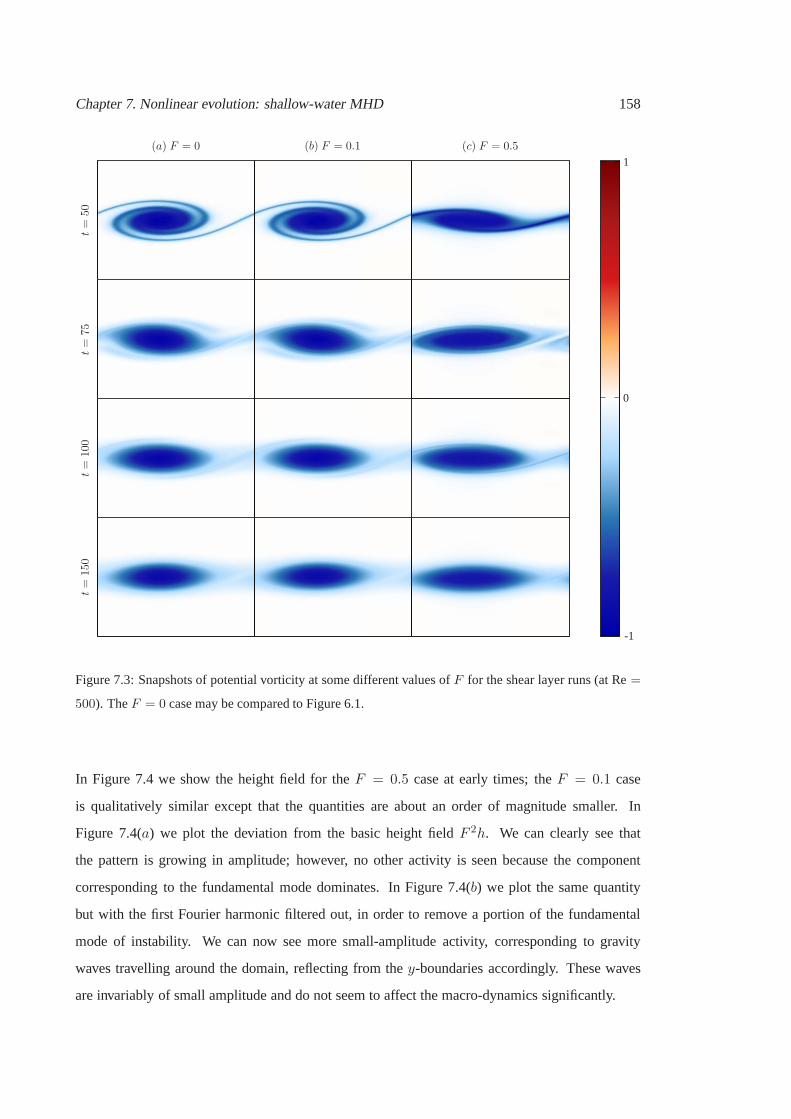
Chapter 7. Nonlinear evolution: shallow-water MHD 158
t=
50t=
75t=
100
t=
150
(a) F = 0 (b) F = 0.1 (c) F = 0.5
0
-1
1
Figure 7.3: Snapshots of potential vorticity at some different values ofF for the shear layer runs (at Re=
500). TheF = 0 case may be compared to Figure 6.1.
In Figure 7.4 we show the height field for theF = 0.5 case at early times; theF = 0.1 case
is qualitatively similar except that the quantities are about an order of magnitude smaller. In
Figure 7.4(a) we plot the deviation from the basic height fieldF 2h. We can clearly see that
the pattern is growing in amplitude; however, no other activity is seen because the component
corresponding to the fundamental mode dominates. In Figure7.4(b) we plot the same quantity
but with the first Fourier harmonic filtered out, in order to remove a portion of the fundamental
mode of instability. We can now see more small-amplitude activity, corresponding to gravity
waves travelling around the domain, reflecting from they-boundaries accordingly. These waves
are invariably of small amplitude and do not seem to affect the macro-dynamics significantly.
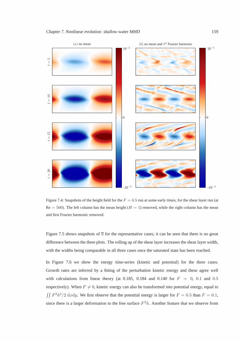
Chapter 7. Nonlinear evolution: shallow-water MHD 159
(a) no mean (b) no mean and1st Fourier harmonict=
5t=
10t=
15t=
20
00
-10−3
10−3
-10−5
10−5
Figure 7.4: Snapshots of the height field for theF = 0.5 run at some early times, for the shear layer run (at
Re= 500). The left column has the mean height (H = 1) removed, while the right column has the mean
and first Fourier harmonic removed.
Figure 7.5 shows snapshots ofu for the representative cases; it can be seen that there is no great
difference between the three plots. The rolling up of the shear layer increases the shear layer width,
with the widths being comparable in all three cases once the saturated state has been reached.
In Figure 7.6 we show the energy time-series (kinetic and potential) for the three cases.
Growth rates are inferred by a fitting of the perturbation kinetic energy and these agree well
with calculations from linear theory (at 0.185, 0.184 and 0.140 for F = 0, 0.1 and 0.5
respectively). WhenF 6= 0, kinetic energy can also be transformed into potential energy, equal to∫∫
F 2h2/2 dxdy. We first observe that the potential energy is larger forF = 0.5 thanF = 0.1,
since there is a larger deformation to the free surfaceF 2h. Another feature that we observe from

Chapter 7. Nonlinear evolution: shallow-water MHD 160
(a) F = 0 (b) F = 0.1 (c) F = 0.5
t = 0
t = 30
t = 70
t = 110
t = 150
u
y 0
0
0
0
0
0-10-10-10
101010
111 -1-1-1
Figure 7.5: Snapshots ofu for the shear layer runs (at Re= 500).
the energy plots is that the evolution of the perturbation potential energy largely follows that of
the perturbation kinetic energy. The oscillations in the kinetic energy are again related to vortex
nutation, and the similarity in the evolution of the two energy profiles is due to the height field
adjusting to the oscillations in velocity accordingly. Thetotal energy loss for all three cases is
comparable to the incompressible case, at around 10%.
The right hand side of the energy balance equation (7.23) is given by
ǫRe =1
Re
∫∫
[
ht
(
∂uj∂xi
)2
+ F 2uj∂h
∂xi
∂uj∂xi
]
dxdy. (7.38)
In Figure 7.7 we show the time-series of the domain-integrated terms representing dissipation.
The solid curve is a time-series ofǫRe, whilst the dashed line is the absolute value of
Re−1F 2∫∫
uj(∂ih)(∂iuj) dxdy. It turns out thatǫRe is positive definite whilst the cross term,
which may be of either sign (but tends to be negative) is much smaller than the sign-definite term.
As we can see, for the purely incompressible case withF = 0, there is no extra contribution
since the cross term is multiplied by a factor ofF 2. For the other two cases, the size of the cross
term increases withF ; however it is still only a small percentage of the total contribution. We
conclude therefore that, even though we do not have sign-definite dissipation of energy, the effects
of this choice of dissipation operator on this particular shear instability problem are unlikely to be
significant.
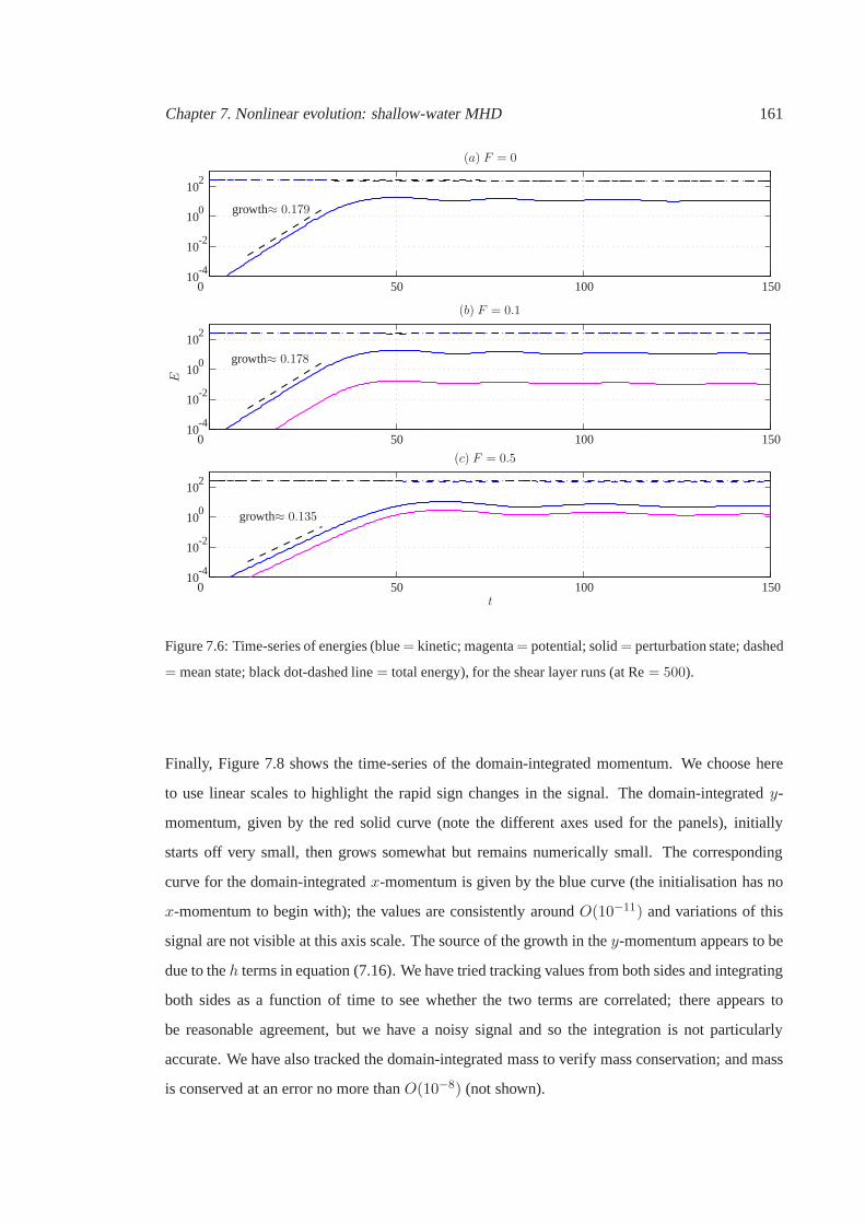
Chapter 7. Nonlinear evolution: shallow-water MHD 161replacements
(a) F = 0
(b) F = 0.1
(c) F = 0.5
growth≈ 0.179
growth≈ 0.178
growth≈ 0.135
E
t0
0
0
50
50
50
100
100
100
150
150
150
10
10
10
10
10
10
10
10
10
10
10
10
2
2
2
0
0
0
-2
-2
-2
-4
-4
-4
Figure 7.6: Time-series of energies (blue= kinetic; magenta= potential; solid= perturbation state; dashed
= mean state; black dot-dashed line= total energy), for the shear layer runs (at Re= 500).
Finally, Figure 7.8 shows the time-series of the domain-integrated momentum. We choose here
to use linear scales to highlight the rapid sign changes in the signal. The domain-integratedy-
momentum, given by the red solid curve (note the different axes used for the panels), initially
starts off very small, then grows somewhat but remains numerically small. The corresponding
curve for the domain-integratedx-momentum is given by the blue curve (the initialisation hasno
x-momentum to begin with); the values are consistently around O(10−11) and variations of this
signal are not visible at this axis scale. The source of the growth in they-momentum appears to be
due to theh terms in equation (7.16). We have tried tracking values fromboth sides and integrating
both sides as a function of time to see whether the two terms are correlated; there appears to
be reasonable agreement, but we have a noisy signal and so theintegration is not particularly
accurate. We have also tracked the domain-integrated mass to verify mass conservation; and mass
is conserved at an error no more thanO(10−8) (not shown).

Chapter 7. Nonlinear evolution: shallow-water MHD 162
(a) F = 0
(b) F = 0.1
(c) F = 0.5
t
ǫ
0
0
0
50
50
50
100
100
100
150
150
150
10
10
10
10
10
10
10
10
10
0
0
0
-5
-5
-5
-10
-10
-10
Figure 7.7: Domain-integrated dissipation rateǫRe (solid curve) and contribution from the cross term
(dashed curve) for the shear layer runs.
(a) F = 0 (b) F = 0.1 (c) F = 0.5
t
∫∫
Udxdy
000 505050 100100100 150150150
×10×10×101
-1
55
-5-5
000
-6-8-10
Figure 7.8: Domain-integrated momentum for the shear layerruns. The red curve represents the domain-
integratedy-momentum (which is not expected to be conserved). The blue curve, which represents the
domain-integratedx-momentum (also should be zero) has variations that are not visible at this axis scale.

Chapter 7. Nonlinear evolution: shallow-water MHD 163
We have also considered the case of multiple wavelengths; pairing occurs as in the incompressible
case without substantial difference.
7.2.2 Bickley jet
For the Bickley jet, the calculations in Chapter 5 indicate that the even mode is more unstable than
the odd mode for anyα within the unstable bandwidth, so we initialise the nonlinear simulation
with the even eigenfunction, normalised so that the total initial energy is fixed at10−5. We use
the same parameter values as in the shear layer case except wetakeα = 0.9, with the domain
large enough to support two wavelengths of the primary instability, as in Chapter 6. Linear theory
tells us that, at the values ofF we are considering, the even mode has a growth rate similar
to the incompressible case, with hardly any noticeable perturbation of the eigenfunctions. The
question then is whether the nonlinear evolution is significantly different. From our investigation
of the shear layer, we might suspect that the evolution will not be noticeably different to the
incompressible case providedF < 1.
Figure 7.9 shows snapshots of the potential vorticity at thethree different values ofF we are
considering; it would appear in this case that there is almost no difference in the evolution, with
all the panels being visually identical to each other. Although not our focus here, when rotational
effects are present, it is well known that there is an asymmetry between the stability properties
of cyclones and anti-cyclones (vortices of positive and negative vorticity respectively), where
modifyingF can have a more noticeable effect (e.g., Polvaniet al., 1994; Poulin & Flierl, 2003).
In Figure 7.10 we show the height field for theF = 0.5 case, to show that there is small-
amplitude activity in the height field and thus the presence of small amplitude gravity waves.
The corresponding diagram forF = 0.1 is similar but the plotted quantities are at least an order
of magnitude smaller.
In Figure 7.11 we show snapshots ofu for the jet profile. Once again, the profiles are virtually
indistinguishable from each other, with the same behaviouras in the incompressible hydrodynamic
case. The jet profile broadens and reduces in magnitude, withsome reverse flow observed.
The time-series of the energy for the Bickley jet profile is plotted in Figure 7.12. Growth rates are
inferred from a fit of the perturbation kinetic energy, and these agree well with the linear theory
(which are 0.160, 0.160 and 0.157 forF = 0, 0.1 and0.5 respectively). The growth rates are

Chapter 7. Nonlinear evolution: shallow-water MHD 164
(a) F = 0 (b) F = 0.1 (c) F = 0.5
t=
50t=
75t=
100
t=
150
0
-0.7
0.7
Figure 7.9: Snapshots of potential vorticity at various values ofF for the Bickley jet profile (at Re= 500).
TheF = 0 case may be compared to Figure 6.5.
also comparable to each other, with a slight difference for the F = 0.5 case. We see that the
perturbation potential energy is a few orders of magnitude smaller than the kinetic energy, but the
potential energy increases withF . The total loss of energy is comparable to the incompressible
case, at around 30%.
Figure 7.13 shows the dissipation rates represented by the terms in (7.38). Again, we notice that
the extra contribution from the cross term is several ordersof magnitude less than the sign-definite
dissipation, and thus our choice of dissipation is unlikelyto cause a significant problem in this
shear instability problem, even though it is not formally sign-definite.
The domain-integrated perturbation momentum is plotted inFigure 7.14. In this case there is a

Chapter 7. Nonlinear evolution: shallow-water MHD 165
(a) no mean (b) no mean and1st Fourier harmonict=
5t=
10t=
15t=
20
00
-10−3
10−3
-10−5
10−5
Figure 7.10: Snapshots of the height field for theF = 0.5 run at some early times, for the Bickley jet profile
(at Re= 500). The left column has the background height fieldH = 1 removed, while the right column
has both the background height field and first Fourier mode removed.
background flow with non-zerox-momentum; the momentum contribution of this was removed
to give a deviation from momentum conservation. Even when this has been done, we see that the
largest deviation from zero comes from they-momentum signal, given by the red curve. The blue
curve representing thex-momentum has been overlaid for visibility purposes, and atthis scale any
variations are not visible. The errors are small and should have a negligible effect on the overall
dynamics. A similar integration of the signal as discussed for the shear layer case has been tried
and the conclusions are broadly similar.

Chapter 7. Nonlinear evolution: shallow-water MHD 166
(a) F = 0 (b) F = 0.1 (c) F = 0.5
t = 0t = 30t = 70t = 110t = 150
u
yyy 0
0
0
0
0
0-10-10-10
101010
111 0.50.50.5
Figure 7.11: Snapshots ofu for the Bickley jet runs (at Re= 500).
(a) F = 0
(b) F = 0.1
(c) F = 0.5
growth≈ 0.155
growth≈ 0.155
growth≈ 0.151
E
t0
0
0
50
50
50
100
100
100
150
150
150
10
10
10
10
10
10
10
10
10
10
10
10
2
2
2
0
0
0
-2
-2
-2
-4
-4
-4
Figure 7.12: Time-series of energies (blue= kinetic; magenta= potential; solid= perturbation state;
dashed= mean state; black dot-dashed line= total energy) for the Bickley jet runs (at Re= 500).

Chapter 7. Nonlinear evolution: shallow-water MHD 167replacements
(a) F = 0
(b) F = 0.1
(c) F = 0.5
t
ǫ
0
0
0
50
50
50
100
100
100
150
150
150
10
10
10
10
10
10
10
10
10
0
0
0
-5
-5
-5
-10
-10
-10
Figure 7.13: Domain-integrated dissipation rateǫRe (solid curve) and contribution from the cross term
(dashed curve) for the Bickley jet runs. The cross term contribution increases in magnitude with increasing
F .
(a) F = 0 (b) F = 0.1 (c) F = 0.5
t
∫∫
Udxdy
000 505050 100100100 150150150
×10×10×101
-1
55
-5-5
000
-6-8-10
Figure 7.14: Domain-integrated pertubation momentum for the Bickley jet profile. The red curve represents
the domain-integratedy-momentum (which is not formally conserved), and the blue curve represented the
domain-integratedx-momentum with the background state removed.

Chapter 7. Nonlinear evolution: shallow-water MHD 168
7.3 MHD evolution
We now turn to the cases withM > 0, again with a uniform background magnetic field. We first
discuss the evolution of the shear layer profile with increasing F before moving on to the Bickley
jet profile.
7.3.1 Hyperbolic-tangent shear layer:F = 0.1
At such a small value ofF we do not expect a large deviation from the conclusions drawnfrom
theF = 0 incompressible case. As such, we will not go into so much detail as we have done
previously, but concentrate on highlighting the differences that do arise. We focus on the regime
of smallM as before and use the Re= 500, Rm= 500 andM = 0.01, 0.03 and0.05 runs as our
three representative cases.
Figure 7.15 shows snapshots of the potential vorticity at different values ofM . These are
comparable to the corresponding diagrams for the incompressible case (Figure 6.9). The three
cases show various degrees of disruption as before, with increased disruption with increasingM
and Rm. The vortex winds up field lines, builds magnetic stresses, and stretches out thin current
sheets that are resistively unstable. The breakup of the current layer releases the stresses, impacts
back on the vortex, and potentially causes disruption. In the weakly disruptive cases, the surviving
vortex would expel field lines to the edges of the vortex as before. We will use the spectral
truncation parameter later to measure the severity of disruption for the runs at different parameter
values.
The plots related to the magnetic quantities are largely similar to those given in the incompressible
case and have been omitted. Plotting the height field shows traces of small-amplitude waves, but
we omit this here also as it does not appear to show any particularly interesting features that are
obviously associated with MHD effects.
Figure 7.16 shows snapshots ofu; we see again that the degree of disruption is correlated with the
resulting shear layer width. Later on we will use the layer width expansion factor to quantify the
degree of disruption, as was done previously for the incompressible case.
Figure 7.17 shows the time-series of the energy for these sample runs. The behaviour of the
magnetic energy is largely as observed in Figure 6.15 for theincompressible case, with a different
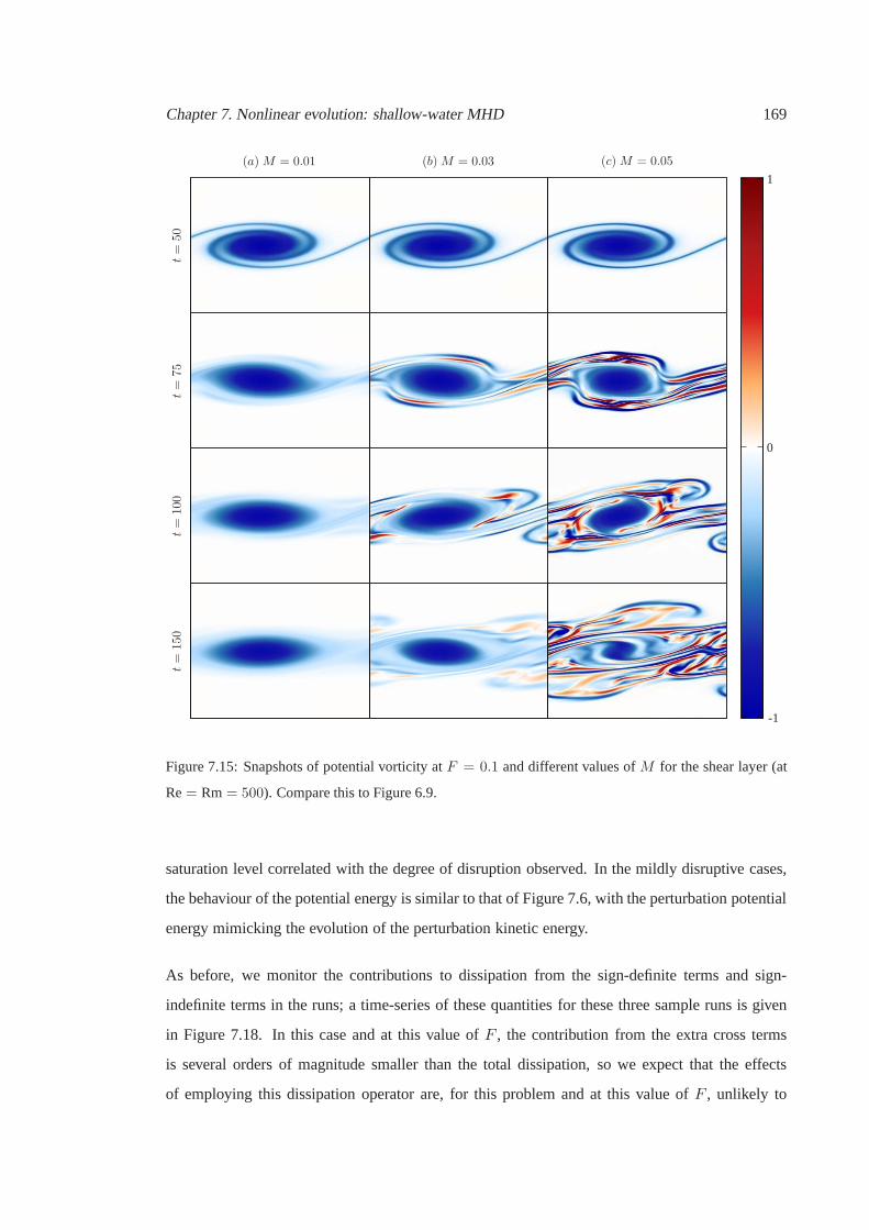
Chapter 7. Nonlinear evolution: shallow-water MHD 169
(a)M = 0.01 (b)M = 0.03 (c)M = 0.05t=
50t=
75t=
100
t=
150
0
-1
1
Figure 7.15: Snapshots of potential vorticity atF = 0.1 and different values ofM for the shear layer (at
Re= Rm= 500). Compare this to Figure 6.9.
saturation level correlated with the degree of disruption observed. In the mildly disruptive cases,
the behaviour of the potential energy is similar to that of Figure 7.6, with the perturbation potential
energy mimicking the evolution of the perturbation kineticenergy.
As before, we monitor the contributions to dissipation fromthe sign-definite terms and sign-
indefinite terms in the runs; a time-series of these quantities for these three sample runs is given
in Figure 7.18. In this case and at this value ofF , the contribution from the extra cross terms
is several orders of magnitude smaller than the total dissipation, so we expect that the effects
of employing this dissipation operator are, for this problem and at this value ofF , unlikely to
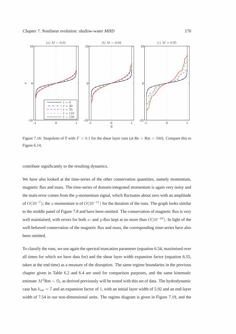
Chapter 7. Nonlinear evolution: shallow-water MHD 170
(a)M = 0.01 (b)M = 0.03 (c)M = 0.05
t = 0t = 30t = 70t = 110t = 150
u
y 0
0
0
0
0
0-10-10-10
101010
111 -1-1-1
Figure 7.16: Snapshots ofu with F = 0.1 for the shear layer runs (at Re= Rm = 500). Compare this to
Figure 6.14.
contribute significantly to the resulting dynamics.
We have also looked at the time-series of the other conservation quantities, namely momentum,
magnetic flux and mass. The time-series of domain-integrated momentum is again very noisy and
the main error comes from they-momentum signal, which fluctuates about zero with an amplitude
ofO(10−7); thex-momentum is ofO(10−11) for the duration of the runs. The graph looks similar
to the middle panel of Figure 7.8 and have been omitted. The conservation of magnetic flux is very
well maintained, with errors for bothx- andy-flux kept at no more thanO(10−10). In light of the
well-behaved conservation of the magnetic flux and mass, thecorresponding time-series have also
been omitted.
To classify the runs, we use again the spectral truncation parameter (equation 6.54, maximised over
all times for which we have data for) and the shear layer widthexpansion factor (equation 6.55,
taken at the end time) as a measure of the disruption. The sameregime boundaries in the previous
chapter given in Table 6.2 and 6.4 are used for comparison purposes, and the same kinematic
estimateM2Rm∼ Ωe as derived previously will be tested with this set of data. The hydrodynamic
case haskcut = 7 and an expansion factor of1, with an initial layer width of 5.92 and an end layer
width of 7.54 in our non-dimensional units. The regime diagram is given in Figure 7.19, and the

Chapter 7. Nonlinear evolution: shallow-water MHD 171
(a)M = 0.01
(b)M = 0.03
(c)M = 0.05
growth≈ 0.176
growth≈ 0.176
growth≈ 0.176
E
t0
0
0
50
50
50
100
100
100
150
150
150
10
10
10
10
10
10
10
10
10
10
10
10
2
2
2
0
0
0
-2
-2
-2
-4
-4
-4
Figure 7.17: Time-series of energies (blue= kinetic; red= magnetic; magenta= potential; solid=
perturbation state; dashed= mean state; black dot-dashed line= total energy) for the shear layer runs
(at Rm= Re= 500, F = 0.1).
raw data in Tables 7.2 and 7.3.
The raw data may be compared with the data for theF = 0 case given in Tables 6.3 and 6.5, and
only one of the runs has been classified differently. This particular run is on the borderline of the
regime boundary in theF = 0 case anyway so this discrepancy is not a concern. Consequently,
the regime diagram given in Figure 7.19 is largely similar tothat for the caseF = 0 (given by
Figure 6.18, without the Rm= 1000 data and with one marker changed). We see again that
the degree of disruption is well described by the suggested parameter dependenceM2Rm, with
M2Rm≥ 0.5 capturing the runs that are classified as severely disrupted.

Chapter 7. Nonlinear evolution: shallow-water MHD 172
(a)M = 0.01
(b)M = 0.03
(c)M = 0.05
t
ǫ
0
0
0
50
50
50
100
100
100
150
150
150
10
10
10
10
10
10
10
10
10
0
0
0
-5
-5
-5
-10
-10
-10
Figure 7.18: Domain-integrated dissipation rateǫRe (solid curve) and contribution from the cross term
(dashed curve), for the shear layer atF = 0.1; blue represents the terms associated with momentum
dissipation, and red represents the terms associated with flux dissipation.
Rm
M0.01 0.02 0.03 0.04 0.05 0.06 0.07 0.1
750 7 18 35 47 42 38 48 54
500 7 7 23 36 44 36 36 44
250 7 7 8 18 25 31 32 26
50 7 7 7 8 8 10 11 13
Table 7.2: Raw data from the set of calculations at Re= 500 for the shear layer runs atF = 0.1. The
numbers denote the truncation wavenumberkcut (taking the maximum over time). The hydrodynamic case
atF = 0.1 haskcut = 7. See Figure 7.19 for colour codes.

Chapter 7. Nonlinear evolution: shallow-water MHD 173
(a) Maximumkcut over run (kcut,HD = 7)
M
Rm
M2Rm= 0.1
M2Rm= 0.1
M2Rm= 0.5
M2Rm= 0.5
M2Rm= 1
M2Rm= 1
10
10
101010
10
10
101010
-1
-1
-2
-2
1
1
2
2
3
3
(b) shear layer width expansion factor at end time
Figure 7.19: Regime diagram for the shear layer runs atF = 0.1, as measured by the spectral truncation
parameterkcut and via the shear layer width at the end of the run. The suggested boundaries given by
M2Rm = C are plotted for several values ofC. The colours are as before, with blue denoting non-
disruptive cases, magenta denoting mildly disruptive cases, and red denoting strongly disruptive cases.
Rm
M0.1 0.2 0.3 0.4 0.5 0.6 0.7 0.1
750 1.02 1.19 1.60 1.80 1.94 2.42 2.33 2.57
500 1.02 1.16 1.43 1.71 1.97 2.00 2.14 2.65
250 1.02 1.05 1.26 1.49 1.64 1.86 2.04 2.42
50 1.00 1.02 1.03 1.05 1.07 1.10 1.16 1.36
Table 7.3: Raw data from the set of calculations at Re= 500 for the shear layer runs atF = 0.1. The
numbers denote the shear layer width expansion factor (relative to the hydrodynamic run at Re= 500 and
F = 0.1, taken at end time). The expansion factor for the hydrodynamic case is defined to bef = 1. See
Figure 7.19 for colour codes.
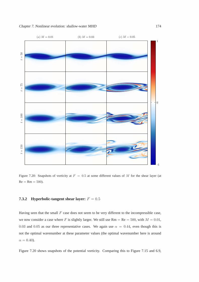
Chapter 7. Nonlinear evolution: shallow-water MHD 174
(a)M = 0.01 (b)M = 0.03 (c)M = 0.05
t=
50t=
75t=
100
t=
150
0
-1
1
Figure 7.20: Snapshots of vorticity atF = 0.5 at some different values ofM for the shear layer (at
Re= Rm= 500).
7.3.2 Hyperbolic-tangent shear layer:F = 0.5
Having seen that the smallF case does not seem to be very different to the incompressiblecase,
we now consider a case whereF is slightly larger. We still use Rm= Re= 500, withM = 0.01,
0.03 and 0.05 as our three representative cases. We again useα = 0.44, even though this is
not the optimal wavenumber at these parameter values (the optimal wavenumber here is around
α = 0.40).
Figure 7.20 shows snapshots of the potential vorticity. Comparing this to Figure 7.15 and 6.9,

Chapter 7. Nonlinear evolution: shallow-water MHD 175
we see that the runs appear less disruptive. TheM = 0.01 case in Figure 7.20(a) resembles the
hydrodynamic case, with the vorticity concentrated in the (if somewhat slightly more elongated)
vortex. For theM = 0.03 case in Figure 7.20(b), there are some hints of vorticity regions outside
the vortex but these are distinctly fainter than in the correspondingF = 0.1 or F = 0 case. The
vortex here is of a similar size to the smallerM case, in contrast to theF = 0.1 case, where the
resulting vortex forM = 0.03 is smaller than that forM = 0.01. For theM = 0.05 case in
Figure 7.20(c), this was previously a severely disruptive case at this value ofM and Rm, but now
the disruption is noticeably milder. Although strong vorticity filaments are seen and the vortex
appears to have reduced in size, it retains its integrity up to the end timet = 150. A longer
run shows that, for thisM = 0.05 case, the filaments eventually get smeared out but the vortex
remains, unlike the analogous case whenF is smaller, with the vortex completely destroyed. The
equivalent diagrams for current and height do not appear to show any new features and have been
omitted.
There are some plausible explanations for this decrease in the observed disruption. One possibility
is that the magnetic stresses build up as before, and any stresses that are released act on the fluid
column. However, now that the fluid column is also allowed to move vertically, a portion of this
built up stress ends up as work done against gravity, and thiscushioning effect results in a milder
disruption. The suppression of filamentation due to the shorter range of interaction whenF > 0
has been previously reported by, for example, Waugh & Dritschel (1991).
Figure 7.21 shows snapshots ofu for these runs. We note that the final time shear layer width of
theM = 0.03 case is not noticeably different to that ofM = 0.01, unlike the equivalent diagrams
for smallerF given in Figures 7.16 and 6.14. The shear layer width forM = 0.05 is also only
marginally larger than for the other two cases, unlike the smallerF cases. If we use the shear layer
width as a measure of the disruption then we again conclude that, keeping(M,Rm,Re, α) fixed,
we expect runs to be classified as having suffered a milder disruption with increasingF .
The time-series of the energies are plotted in Figure 7.22. The growth rates are again inferred
and these are consistent with the growth rates obtained fromthe linear calculation. The potential
energy for all three runs here is larger than in the equivalent diagram in Figure 7.17, forF = 0.1.
In Figure 7.23 we show the domain-integrated dissipation terms. The sign-indefinite contribution
is larger here than forF = 0.1; however, it is still only a small percentage of the total dissipation.
The conservation properties of other quantities have been checked and are well-maintained by the
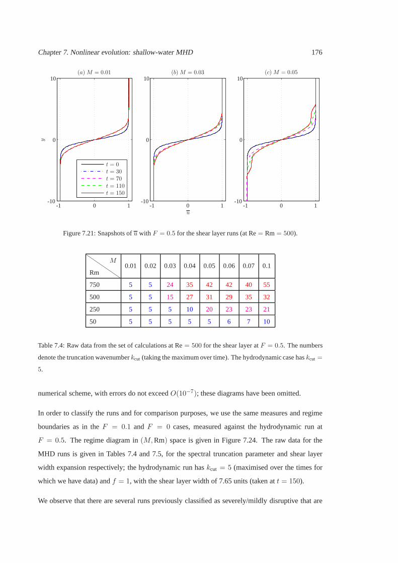
Chapter 7. Nonlinear evolution: shallow-water MHD 176
(a)M = 0.01 (b)M = 0.03 (c)M = 0.05
t = 0t = 30t = 70t = 110t = 150
u
y 0
0
0
0
0
0-10-10-10
101010
111 -1-1-1
Figure 7.21: Snapshots ofu with F = 0.5 for the shear layer runs (at Re= Rm= 500).
Rm
M0.01 0.02 0.03 0.04 0.05 0.06 0.07 0.1
750 5 5 24 35 42 42 40 55
500 5 5 15 27 31 29 35 32
250 5 5 5 10 20 23 23 21
50 5 5 5 5 5 6 7 10
Table 7.4: Raw data from the set of calculations at Re= 500 for the shear layer atF = 0.5. The numbers
denote the truncation wavenumberkcut (taking the maximum over time). The hydrodynamic case haskcut =
5.
numerical scheme, with errors do not exceedO(10−7); these diagrams have been omitted.
In order to classify the runs and for comparison purposes, weuse the same measures and regime
boundaries as in theF = 0.1 andF = 0 cases, measured against the hydrodynamic run at
F = 0.5. The regime diagram in(M,Rm) space is given in Figure 7.24. The raw data for the
MHD runs is given in Tables 7.4 and 7.5, for the spectral truncation parameter and shear layer
width expansion respectively; the hydrodynamic run haskcut = 5 (maximised over the times for
which we have data) andf = 1, with the shear layer width of 7.65 units (taken att = 150).
We observe that there are several runs previously classifiedas severely/mildly disruptive that are

Chapter 7. Nonlinear evolution: shallow-water MHD 177
(a)M = 0.01
(b)M = 0.03
(c)M = 0.05
growth≈ 0.135
growth≈ 0.135
growth≈ 0.134
E
t0
0
0
50
50
50
100
100
100
150
150
150
10
10
10
10
10
10
10
10
10
10
10
10
2
2
2
0
0
0
-2
-2
-2
-4
-4
-4
Figure 7.22: Time-series of energies (blue= kinetic; red= magnetic; magenta= potential; solid=
perturbation state; dashed= mean state; black dot-dashed line= total energy) for the shear layer runs
(at Rm= Re= 500, F = 0.5).
Rm
M0.1 0.2 0.3 0.4 0.5 0.6 0.7 0.1
750 1.00 1.02 1.13 1.47 1.63 1.60 1.74 2.61
500 1.00 1.01 1.10 1.29 1.48 1.63 1.61 2.09
250 1.00 1.01 1.03 1.15 1.26 1.40 1.53 1.82
50 1.00 1.00 1.00 1.00 1.00 1.01 1.01 1.03
Table 7.5: Raw data from the set of calculations at Re= 500 for the shear layer atF = 0.5. The numbers
denote the shear layer width expansion factor (relative to the hydrodynamic run at Re= 500, taken at end
time). The expansion factor for the hydrodynamic case is defined to bef = 1.

Chapter 7. Nonlinear evolution: shallow-water MHD 178
(a)M = 0.01
(b)M = 0.03
(c)M = 0.05
t
ǫ
0
0
0
50
50
50
100
100
100
150
150
150
10
10
10
10
10
10
10
10
10
0
0
0
-5
-5
-5
-10
-10
-10
Figure 7.23: Domain-integrated dissipation rateǫRe (solid curve) and contribution from the cross term
(dashed curve) for the shear layer runs atF = 0.5 blue represents the momentum dissipation terms, and
red represents the flux dissipation terms.
now classified as mildly/non-disruptive. There are also some discrepancies between the two
measures. Considering that the regime boundaries were calibrated using only data from the
incompressible case, this discrepancy is perhaps not unexpected. The regime changeovers still
appear to closely follow the dependenceM2Rm = C well, at least for the coverage of(M,Rm)
space we have here. The regionM2Rm ≥ 0.5 now contains some runs that are classified as
mildly disruptive, in contrast to the smallerF cases, consistent with the runs generally suffering a
weaker disruption at higherF (compared to Figure 7.19). In conclusion, we expect the disruption
to follow the dependenceM2Rm= f(F ), with f a decreasing function ofF .
7.3.3 Bickley jet: F < 1
We have already observed in Section 7.2.2 that the effects ofF ≤ 1 appear to be weak for the
nonlinear evolution of the Bickley jet in the hydrodynamic,shallow-water case. In Figure 7.25 we
show snapshots of the potential vorticity atF = 0.5, again for Rm= Re= 500, andM = 0.01,

Chapter 7. Nonlinear evolution: shallow-water MHD 179
(a) Maximumkcut over run (kcut,HD = 7)
M
Rm
M2Rm= 0.1
M2Rm= 0.1
M2Rm= 0.5
M2Rm= 0.5
M2Rm= 1
M2Rm= 1
10
10
101010
10
10
101010
-1
-1
-2
-2
1
1
2
2
3
3
(b) shear layer width expansion factor at end time
Figure 7.24: Regime diagram for the shear layer atF = 0.5, as measured by the spectral truncation
parameterkcut and via the shear layer width at the end of the run. The suggested boundaries given by
M2Rm= C are plotted for several values ofC.
0.03, and0.05 as our representative cases.
We observe here that, compared to Figure 6.20, there are somedifferences in the transients for the
more disruptive cases; however the end result is qualitatively similar, with the appearance of weak
bands of vorticity. What is slightly different in this case is that, in the end frame of theM = 0.05
case, there appears to be slightly more activity compared tothe correspondingM = 0.03 case,
contrary to the corresponding comparison whenF = 0 given in Figure 6.20. For the weak field
case, the disruption is slight, only deforming the vorticesslightly but not destroying them, and the
vortices recover their elliptical shape by the end frame. A reduction in the amplitude and spreading
of the jet may also be seen in the profiles ofu.
The other diagrams (profiles ofu, time-series of energies, dissipation and conservation of
quantities) and the regime diagram are virtually indistinguishable to those given for the
incompressible case in Chapter 6 and have been omitted. So itwould appear that the effect of

Chapter 7. Nonlinear evolution: shallow-water MHD 180
(a)M = 0.01 (b)M = 0.03 (c)M = 0.05
t=
50t=
75t=
100
t=
150
0
-0.7
0.7
Figure 7.25: Snapshots of potential vorticity atF = 0.5 and different values ofM for the Bickley jet profile
(at Re= Rm= 500).
F ≤ 1 on the evolution of the Bickley is relatively weak. Again, this may not be true when
rotational effects are present, since we then expect vortexasymmetry to play a role in the dynamics.
7.4 The case ofF ≥ 1
It would appear that the nonlinear dynamics in theF < 1 regime is not significantly different
to theF = 0 limit, so it is of interest to investigate theF ≥ 1 regime where, for example,
supersonic instabilities are present. However, we ran intosome serious numerical problems when
considering theF ≥ 1 cases. In Figure 7.26 we plot the perturbed free surface for ashear layer

Chapter 7. Nonlinear evolution: shallow-water MHD 181
(a) x = −7.65
(b) y = 25.65
(c) F =√2
x
x
yy
h
hh
0
0
0
0
0
0
0
-10
-101010
10
10
20
20
30
30
-0.2
-0.2
-0.2 0.2
0.2
0.2 0.4
0.4
0.4
Figure 7.26: Perturbed free surface plotsh for the shear layer atM = 0, F =√2, at a snapshot taken a
short while before the numerical routine crashes.(a) and(b) shows cross-sections ofh, and(c) shows a
surface plot ofh. For image rendering purposes,(c) is produced using only a fifth of the total data points.
test run, atM = 0 andF =√2, initialised using the eigenfunction calculated from linear theory.
It can be seen that there is nonlinear steepening of the free surface. Steepening was also observed
for the Bickley jet simulations withF ≥ 1. It is during the nonlinear phase of the instability,
where the background flow starts being modified by the perturbations, that we start seeing this
steepening. It should be noted that, for the linear shallow-water case, our time-stepping scheme at
this CFL number is stable forF ≥ 1; we still observe steepening when the CFL number has been
decreased. The code crashes shortly after this time-snapshot. Overturning of the free surface and
shock formation has been observed in previous shallow-water simulations of shear instabilities
(e.g., Chu, 2010, and references within), so we believe thissteepening is a generic feature arising
from the dynamics and is not a numerical artefact.
As shallow-water theory is a long-wave theory (dynamics have a small aspect ratio), shock
formation leads to the breakdown of the assumption of hydrostatic balance, and therefore
breakdown of shallow-water theory. There are methods to deal with steepening (numerical,
modifying or augmenting shallow-water theory) and these are discussed in the discussion section

Chapter 7. Nonlinear evolution: shallow-water MHD 182
at the end of this chapter.
7.5 Summary and discussion
We assumed that the free surface is forced to stay a field line,resulting in the condition∇· (hb) =0. Putting to one-side the validity of this assumption for themoment, it was seen that seen that
the SWMHD equations written in terms of the transport variablesU = htu andB = htb, with a
Laplacian operator acting onU andB to mimic dissipation, maintain more conservation laws than
the analogous approach employing velocity variables. A particularly important point is that our
approach here maintains the divergence-free condition∇ ·B = 0, implicitly required in deriving
the conservation laws even in the ideal case. The approach weemploy is particularly convenient
to implement in our pseudo-spectral, semi-implicit-in-time approach, but it does not provide a
formally negative-definite dissipation. We have though tracked the formally sign-indefinite term
in our simulations and have found this extra contribution tobe only a small percentage of the total
dissipation for ourF < 1 simulations, so is unlikely to play a significant role in the dynamics.
We conjecture that there should be mathematically consistent way of deriving shallow-water with
magnetic dissipation, and we suspect that, for our problem,our approach is a good approximation
to the ‘exact’ theory since the errors introduced appear to be small. As fast waves are present,
certain terms in the shallow-water system were treated implicitly to relieve the CFL condition. It
was also found, via a von Neumann analysis, that the AB/BD2 scheme possessed better stability
properties than AB/BD3, so numerical routines for the shallow-water system used AB/BD2 as the
time-marching scheme.
We focussed on theF < 1 cases. For the shear layer, we again considered the case where the
domain supports a single wavelength of the primary instability. We first investigated the effect of
increasingF whenM = 0. At small values ofF , small-amplitude gravity waves are present;
however, they do not seem to affect the nonlinear dynamics very much, and the evolution was
largely like the incompressible case, with a long-lived vortex forming. For larger values ofF ,
small-amplitude gravity waves are again present, althoughthese are at a larger amplitude than the
small F cases. The vortex formed is more elongated than for the incompressible and smallF
cases, but is also seen to be long-lived. When a magnetic fieldis included, the degree of disruption
observed in the smallF cases was comparable to the incompressible case. For largerF , however,

Chapter 7. Nonlinear evolution: shallow-water MHD 183
the disruption is seen to be milder. One explanation for thisis that when the magnetic stresses
are released on the fluid column, some of this is converted into deforming the free surface and
thus does work against gravity. Like the incompressible case, disruption, when it occurs, is a fast
phenomenon, occurring within one or two eddy turnover timesafter the formation of the vortex.
We also tested our kinematic regime estimateM2Rm ∼ Ωe against the data from the shallow-
water runs. We classified the runs using the same regime boundaries as those used in the
incompressible case. It is seen that, for smallF , the classifications are largely the same as the
incompressible case. For largerF , the runs appear to suffer a milder disruption, with some
runs that were previously severe/mildly disruptive classified as mildly/non-disruptive. Thus our
estimateM2Rm ∼ Ωe over-estimates the degree of disruption at the ranges ofM and Rm we
covered. The data points still follow theM2Rm = f(F ) dependence reasonably well, withf a
decreasing function ofF .
For the Bickley jet, whenF < 1 in both the hydrodynamic and MHD regime, the evolution is still
effectively like the incompressible case, except for the fact that the presence of small-amplitude
gravity waves, although these do not appear to influence the vortex dynamics very much. The
transients are slightly different but the disruption observed appears to depend mainly onM and
Rm and only weakly onF . The regime classifications are also largely similar to the incompressible
case and so the results were not presented.
OnceF exceedsO(1), there are numerical difficulties for both profiles, where overturning of
the free surface was observed. This points to a breakdown of shallow-water theory as the small
aspect ratio and hydrostatic balance assumption becomes invalid, and further numerical and/or
mathematical modification or a different model is required to investigate the dynamics.
We now provide a discussion of several issues that arose during this investigation, in decreasing
order of severity.
Numerical treatment of gravity wave terms
One not so crippling numerical issue we had was that the CFL number required for numerical
stability was somewhat low whenF 6= 0. As a reminder, the nonlinear term(1 + F 2h)∇h was
split into a linear term that was treated implicitly, whilstthe nonlinear term was treated explicitly.
We suspect this decrease in CFL number is due to this explicittreatment of the nonlinear terms,

Chapter 7. Nonlinear evolution: shallow-water MHD 184
and it might be an idea to try for a more implicit treatment to give a larger stable time-step. We
could treat the nonlinear term as implicitly as possible whilst maintaining linearity at leveln+ 1.
To do this, we observe that
hn+1∇hn+1 ≈(
hn +∆t∂h
∂t
∣
∣
∣
∣
n
+ · · ·)
∇hn+1, (7.39)
so taking an approximation of the time derivative term usingdata from leveln andn− 1 (but not
leveln+ 1 in order to maintain linearity at leveln+ 1) gives
ht∇h ≈ 1 + F 2[(1 + b0∆t)hn + b1∆th
n−1]∇hn+1, (7.40)
where thebi coefficients are given in (7.32). If we then form the equationfor h in our semi-
implicit approach, we observe that we need to take a divergence of ht∇h, and we will end up
with an inversion forh that involves operators involving second as well as first derivatives. Not
only can we not use the fast solver as we no longer have a Helmholtz equation to solve, we also
have spatially varying coefficients multiplying the differential operators. So, in the shallow-water
cases, finite-difference/volume methods are perhaps more suitable since no spectral representation
(so no convolution sums) is required. Other formulations (in vorticity-divergence or otherwise)
may also lead to other numerical schemes (e.g., Mohebalhojeh & Dritschel, 2000, 2001; Dritschel
& Viudez, 2007).
Although we have not considered inserting sponge-layers toabsorb outgoing gravity waves (e.g.,
Durran, 2010,§8), this may be done in principle, to better mimic the free-shear flow problem. In
this shear instability problem it is possibly not a major concern as the gravity waves are small-
amplitude and do not seem to alter the vortex dynamics all that much. Although not our focus
here, in studies of gravity wave generation by shear flows where the outward flux is of concern
(e.g., Sutherlandet al., 1994; Sutherland & Peltier, 1994; Staquet & Sommeria, 2002; Bakas &
Farrell, 2009a,b), ways to stop waves reflecting from the boundaries are required.
Nonlinear steepening whenF ≥ 1
Our investigation was restricted to the regimeF < 1 where we do not appear to encounter
steepening that causes the routines to crash. TheF ≥ 1 region contains, for the shear layer,
the portion of parameter space where supersonic modes are unstable, as well as the tongue region
(when MHD effects are present), and, for the Bickley jet, theregion where perhaps the nonlinear
dynamics would be more different than theF < 1 case we have considered here.
Chapter 7. Nonlinear evolution: shallow-water MHD 185
Steepening points to the breakdown of shallow-water theory, which is a system of equation
obtained at leading order in the aspect ratio. Going to the next order in aspect ratio, the equations
obtained includes dispersion effects that can counter the steepening; the set of equations are known
as the Green–Naghdi equations (Green & Naghdi 1976; see alsoDellar 2003b and Pearce & Esler
2010). This may perhaps be required for investigating the dynamics in the region where wave
steepening occurs.
There are several numerical methods that deal with nonlinear steepening and shock formation, but
we have not tested any of these in any detail to judge their relative merits. One possibility is to
employ a dissipation ofh as in Poulin & Flierl (2003); such a dissipation may represent physical
mechanism (e.g., radiative damping), and its additional consequences on the conservation laws
have already been discussed. A second possibility is to employ shock capturing methods used in
compressible or shallow-water dynamics (e.g., Toro, 2001;Chu, 2010), and these would involve
using a finite-difference/volume method. One other possibility that prevents nonlinear steepening
in shallow-water is to modify the pressure term∇h in the momentum equation appropriately, as
in Buhler (1998).
Form of the dissipation
We have already highlighted that finite magnetic diffusivity implies field line slippage, something
that is not entirely consistent with the derivation of the SWMHD equations as we have here.
Another potential problem is that the dissipation that we did employ does not guarantee a sign-
definite energy dissipation. We discuss the latter point before the more fundamental question of
the self-consistency of the SWMHD system when finite magnetic diffusion is present.
We consider first the form of momentum dissipation. The problems associated with the form of
momentum dissipation in the hydrodynamic case have been previously discussed in the literature
(e.g., Ochoaet al., 2011; Gilbertet al., 2013). The recent papers of Ochoaet al. (2011) and
Gilbert et al. (2013) conclude that, to ensure momentum conservation, thedissipation should be
expressed in terms of the divergence of a symmetric stress tensor, with the correct factors ofh
to account for the fact that momentum in shallow-water is given byU = hu (see also Buhler,
2000). It then remains to check whether we have negative-definite energy dissipation. The form
of dissipation employed here, given by∇2U in the transport variable formulation (corresponding
to option III of Ochoaet al.2011) satisfies the momentum condition, but does not give a formally
Chapter 7. Nonlinear evolution: shallow-water MHD 186
negative-definite dissipation. Other forms of the dissipation that do maintain momentum and
negative-definite dissipation are given in Ochoaet al. (2011) and Gilbertet al. (2013). None of
these are particularly well suited to a pseudo-spectral, semi-implicit-in-time treatment, because the
terms are nonlinear in the fundamental variables, so finite-difference/volume methods are perhaps
better suited for this line of investigation.
With regards to the form of the magnetic dissipation, we havenoted that, if we were to enforce
the frozen-in property, then we would need a magnetic dissipation that maintains the divergence-
free condition in the magnetic field. A general form of magnetic dissipation that satisfies this
property was suggested by Andrew Gilbert (private communication); see Section 7.6. The main
point is although there is the possibility for a magnetic diffusion that also gives negative-definite
dissipation of magnetic energy, the dissipation terms appear in nonlinear combinations, much like
the issue encountered in the choice of momentum dissipation. Again, a finite-difference/volume
approach is perhaps more suitable to implement these types of dissipation.
Returning to the more fundamental question of self-consistency, we argued that, for phenomena
on short dynamical time-scales such as shear flow instabilities, the frozen-in approximation is
perhaps a plausible one. Although our method isad hoc, we conjecture that it is perhaps a good
approximation to the ‘exact’ theory, to be derived self-consistently starting from the Boussinesq
three-dimensional MHD equations, because the errors introduced with our approach is small and
our integration times are short. The same argument is almostcertainly not going to be true
for studies that require dynamics to be simulated on resistive time-scales, such as turbulence
or dynamo problems (overlooking the possibility of an anti-dynamo theorem for the moment).
Studies that do utilise the SWMHD equations with finite magnetic diffusivity and the frozen-in
approximation need to justify not only the form of the dissipation used, but also the validity of
the underlying approximations on a case by case basis. As a case in point, we feel that this issue
has not been appropriately addressed in the article by Lilloet al. (2005), who study the possibility
of dynamo action in some sort of system resembling the SWMHD system here. As we have
alluded to already, there is also the possibility of anti-dynamo results depending on the form of the
dissipation if the frozen-in approximation is used (see Section 7.6).
It should be possible to derive a self-consistent form of theSWMHD equations with dissipation
included in the derivation by, for example, matching the magnetic field in the fluid layer onto some
external magnetic field profile. The question then is whetherthe approximations that are required

Chapter 7. Nonlinear evolution: shallow-water MHD 187
are realistic, and whether one actually gains anything fromdoing an approximation, as some of the
advantages of employing the shallow-water system (such as the system being explicitly dependent
on only two spatial dimensions) may be lost. The derivation of the SWMHD system with field-line
slippage has not been investigated in much detail here, but is a fundamental question that needs
to be addressed, especially if the SWMHD system is to be employed for modelling nonlinear
physical phenomena, such as global tachocline or hot exoplanet dynamics.

Chapter 7. Nonlinear evolution: shallow-water MHD 188
7.6 Appendix A: Other forms of magnetic dissipation in SWMHD
In the absence of dissipation in the continuity equation, consider
∂B
∂t+∇ ·
(
UB
ht− BU
ht
)
=htRm
D, (7.41)
with
htD = −∇× (hpt∇× (hqtb)), (7.42)
wherep andq are free parameters for the moment andht is the total fluid column (Andrew Gilbert,
private communication). The factor ofht multiplying D is to account for dissipation of the total
fluid column. It is obvious that this form of dissipation maintains the divergence-free condition of
the magnetic field, and reduces accordingly in the incompressible case. The case that we used in
(7.10), in transport variables with∇2B (where only energy dissipation was an issue), is the case
wherep = 0 andq = 1. In general, we have
1
2
d
dt
∫∫
ht|b|2 dxdy = · · ·+∫∫
htb ·∂b
∂tdxdy
= · · ·+ 1
Rm
∫∫
htb · D dxdy
= · · · − 1
Rm
∫∫
hpt (∇× b) · (∇× (hqb)) dxdy.
(7.43)
Then we see that, for our case (p = 0 andq = 1), the energy dissipation is not negative-definite,
as observed already. If instead we takep = 1 and q = 0, then we have a negative-definite
dissipation, with the dissipation related to the domain integrated current∫∫
htj2 dxdy. The
numerical advantage of thep = 0, q = 1 case is that it leads to terms that are particularly easy to
treat in our pseudo-spectral formalism. Thep = 1, q = 0 case contains nonlinear terms which may
be treated accordingly in the finite-difference/volume approach, in contrast to the pseudo-spectral
approach we employed here.
7.6.1 Anti-dynamo result
The following results are also due to Andrew Gilbert (private communication), included here for
completeness. In the ideal SWMHD system, the induction equation in terms of the flux function
(with ht = 1 + F 2h)
htb = ez ×∇A (7.44)
Chapter 7. Nonlinear evolution: shallow-water MHD 189
is given by (Dellar, 2002)∂A
∂t+ u · ∇A = 0. (7.45)
With our choice of dissipation,p = 0 andq = 1 in equation (7.42), we have
∂A
∂t+ u · ∇A =
1
Rm∇2A. (7.46)
In the shallow-water case, the argument is that the maximum point A = Amax cannot increase in
time and so there is no dynamo, at least in terms of magnetic flux. In full, suppose we have
Amax(t) = A(xmax(t), t)). (7.47)
Then
∇A|xmax
= 0, ∇2A∣
∣
xmax≤ 0, (7.48)
and sodAmax
dt=dxmax
dt· ∇A|
xmax+∂Amax
∂t
=− u · ∇A|xmax
+1
Rm∇2A
∣
∣
xmax≤ 0.
(7.49)
The maximumAmax cannot increase, so a dynamo that has increasing magnetic flux with time is
impossible.
For the casep = 1 andq = 0 which gives negative-definite dissipation, it may be shown that the
induction equation in terms of the streamfunction is given (in our notation) by
∂A
∂t+ u · ∇A =
1
Rm∇2A− 1
RmF 2
1 + F 2h(∇h) · (∇A). (7.50)
WhenF = 0 this reduces to the incompressible case. A similar anti-dynamo result may be shown
since the extra term has a∇A contribution, which is zero atxmax.
7.7 Appendix B: Numerical scheme whenF = 0
WhenF = 0, the inversion forh in (7.37) becomes ill-defined whenk = 0 since we have a
second order differential equation with two Neumann boundary conditions. This corresponds to
the issue that, in the incompressible case, pressure effectively acts as a Lagrange multiplier to
ensure incompressibility at every time-step, but since it only appears through a derivative (unlike
the shallow-water case where there is a specific evolution equation forh), the mean component

Chapter 7. Nonlinear evolution: shallow-water MHD 190
of the pressure is defined up to a constant. Although this meancomponent plays no role in the
dynamics, it does however lead to a non-unique inversion. Tofix this constant, we observe that, in
the incompressible case, the Poisson equation forp is given by
∇2p = ∇ · (u · ∇u−M2b · ∇b) +
1
Re∇2
u. (7.51)
Taking anx-average, using the divergence-free conditions foru andb, and the condition∂u/∂y =
0 on they-boundaries, we end up with
∂2p
∂y2=
∂2
∂y2(v2 +M2b2y). (7.52)
Integrating once gives∂p
∂y= 2
(
v∂v
∂y+M2by
∂by∂y
)
+ C. (7.53)
The constantC is zero since∂p/∂y, v andby are zero on they-boundaries. Integrating once again
gives another constant that is irrelevant for the dynamics,hence may be set to zero. We notice then
sincev andby are zero on the boundaries, thenp = 0 on the boundaries also. To implement this
in our numerical routine, an extra option was written in so that, whenF = 0 andk = 0, instead
of implementing homogeneous Neumann conditions on both walls (solved using the fast solver),
one of the boundary conditions was changed to a homogeneous Dirichlet condition (to take into
account we set the constant to be zero) and solved usingLU decomposition.
191
Chapter 8
Conclusions and further work
8.1 Summary of results
We have investigated the problem of shear flow instabilitiesin the single layer SWMHD system,
in planar geometry with no rotation. General properties of the SWMHD system were reviewed,
paying particular attention to the conservation properties.
For the onset of the instabilities, the linearised problem was first formulated in the usual manner,
looking at the temporal evolution of normal mode solutions and formulating an eigenvalue
problem. Some results for general basic states were derived. We then focussed on the simpler
problem with no underlying topography and a uniform background magnetic field. Instability
characteristics of two piecewise-constant profiles, the vortex sheet and the rectangular jet, and
two smooth profiles, the hyperbolic-tangent shear layer andthe Bickley jet, were investigated
via numerical and asymptotic methods. For the shear layer, two modes of instabilities were
identified, the inflection-point and supersonic instabilities. The inflection-point instabilities have
larger growth rates, are standing waves, resemble the vortex sheet instability at smallα, and their
associated instability mechanism is normally attributed to the constructive interference of a pair
of counter-propagating Rossby waves. The supersonic instabilities are found whenF > 1, have
growth rates that are smaller than the inflection-point modes, arise as a pair of propagating waves,
and the associated instability mechanism is normally attributed to gravity wave interaction with
critical layers. The Bickley jet was found to possess two modes of instability, classified as either
even or odd abouty = 0. For the shear layer, the instabilities close to theF = 0, M = 0
Chapter 8. Conclusions and further work 192
case are normally attributed to counter-propagating Rossby waves, and here we also investigated
modifications to this mechanism introduced by shallow-water and MHD effects. It was seen that
the underlying Rossby wave action-at-a-distance mechanism generates vorticity anomalies that
counteract the basic mechanism, leading to stabilisation of the instability. A long-wave asymptotic
procedure was employed to provide analytical expressions to complement the numerical results.
For the nonlinear evolution, it was seen that vortices that form as the shear layer rolls up or as
the jet profile breaks up may suffer disruption when MHD effects were present. Focussing first
on the incompressible case, this disruption was seen to depend on the basic field strengthM and
the magnetic dissipation parameter, here characterised bythe magnetic Reynolds number Rm.
An estimate from a kinematic argument suggests that the dependence of the disruption on the
parameter values scales asM2Rm ∼ Ωe, whereΩe is the typical vorticity magnitude of the
vortices formed. A range of runs from both profiles were classified accordingly and it was seen
that the data conforms well to theM2Rm dependence. Although we have restricted ourselves
to studying the dependence ofM and Rm, some tests runs at larger Re suggests that disruption
is more severe also at increasing Re; this is perhaps expected as the dissipation acts less on the
vorticity filaments, prolonging it’s lifetime, contribution to the amount of small-scale activity. In
the shallow-water case, we focussed on theF < 1 case asF & 1 appears to lead to overturning of
the free surface, and thus leads to the breakdown of shallow-water theory as the initial assumptions
used in deriving the set of equations becomes invalid. For small values ofF , the evolution was
essentially like the incompressible case. For the shear layer at moderate values ofF , it was
seen that the disruption appears to be milder. For the Bickley jet, all F < 1 cases appear to be
qualitatively similar, with minimal differences between theseF < 1 runs and the incompressible
runs, except for the presence of small-amplitude gravity waves, which do not seem to interact
significantly with the vortical motions. The kinematic estimateM2Rm ∼ Ωe was tested against
the numerical data from the shallow-water runs, and the degree of disruption appears still to depend
closely onM2Rm.
More in-depth summaries and relevant discussions may be found at the end of the individual
chapters.
Chapter 8. Conclusions and further work 193
8.2 Conclusions
We have provided a thorough investigation into the characteristics of shear instabilities associated
with free-shear flows, focusing on shear layer and jet profiles. In particular, we have attempted to
provide an investigation into the underlying instability mechanism and its modifications by other
physical effects.
With regards to disruption by MHD effects, since Rm is typically large in astrophysical systems of
interest and the fact that disruption occurs on dynamical time-scales (no more than a few eddy
turnover times), we expect disruption to be a robust featurein unstable shear flows, causing
the breakdown of coherent structures and the transition of laminar flows into chaotic, turbulent
motion. The key feature of these secondary resistive instabilities is that they may operate in
strongly stratified systems with large Richardson number when other secondary hydrodynamic
instabilities are comparatively weak.
Our disruption estimateM2Rm ∼ Ωe is a kinematic one, relying only on the fact that vortices
wind up the magnetic field. It should therefore serve as a firstestimate even for shear flows in
other physical systems, for example, where the system is stratified and velocity shear is in the
vertical, i.e. the Kelvin–Helmholtz scenario. The extent to which the kinematic estimate is true
has not been investigated for the large Rm region as larger runs are required.
Understanding the breakdown of coherent structures into turbulent motion is not only interesting
from a fluid dynamical point of view, but it also has importantphysical consequences. One such
example is in turbulent mixing, physically relevant in bothgeophysical and astrophysical systems.
We have not looked at the consequences on mixing in this case,but it is certainly an interesting
problem to consider in the future.
8.3 Some possible further work
Extension of Ripa’s theorem
As mentioned in Chapter 3 and 5, one result in shallow-water that we have not managed to
generalise to the SWMHD system is an analogue of Ripa’s theorem (Ripa, 1983). Ripa’s
theorem states that, for the rotating, hydrodynamic shallow-water system in planar geometry,
Chapter 8. Conclusions and further work 194
if the Rayleigh–Fjørtoft condition (for potential vorticity) and a subsonic condition is satisfied,
then the basic state is formally stable, i.e. linearly stable to infinitesimal disturbances. The
approach adopted in the derivation is to make use of the underlying symmetries possessed by
the equations to construct a norm and to find the extremal states via a variational problem, an
idea dating back to Arnol’d (1965a,b, 1966a,b). These normsmay be constructed directly from
the governing equations although some ingenuity may be required (e.g., Taylor, 1915; Drazin &
Howard, 1966; Bretherton, 1966b; Blumen, 1971; Satomura, 1981; Eliassen, 1983), or may be
constructed more systematically for general ideal fluid systems by making use of the underlying
Hamiltonian structure (e.g., Holmet al., 1985; Shepherd, 1990). For the shallow-water system,
Ripa’s theorem may be derived via this method (Shepherd 1990, 1992; see also Ripa 1991 for the
multi-layer case), while in the incompressible MHD case, Rayleigh–Fjørtoft type stability criteria
have been derived previously via similar methods (e.g., Holm et al., 1985; Vladimirov & Moffatt,
1995; Vladimirovet al., 1996). The SWMHD system has been shown to possess a Hamiltonian
structure (Dellar, 2002, 2003a), and it remains to derive stability conditions for this system; this is
currently being investigated.
Modification to the Rossby wave mechanism by other physical effects
In Chapter 5 we attributed the inflection-point instabilities to interacting Rossby waves, and
considered modifications to the underlying mechanism when other physical effects were involved.
It should be possible to quantify in more detail the modification of the Rossby waves by MHD
effects. One approach is to consider the piecewise-linear mixing layer profile (sometimes known
as the Rayleigh strip), which may be solved exactly in the hydrodynamic case. The mathematical
basis appears to be well established (e.g., Heifetzet al., 1999, 2004; Heifetz & Methven, 2005;
Heifetz et al., 2006; Harnik & Heifetz, 2007; Heifetzet al., 2009; Carpenteret al., 2012),
employing, for example: the Generalised Stability Theory formalism of Farrell & Ioannou
(1996a,b) to obtain information about the optimum configuration and information about transient
growth; pseudo-energy/momentum (related also to the Hamiltonian formalism discussed earlier)
to quantify wave activity responsible for instability in simulations; wave kernels (or Green’s
functions) to described the wave-interaction effects. It would be informative to see how the
inclusion of a background magnetic field would alter the underlying Rossby (or Rossby-Alfven)
wave dynamics and its role in generating the instability.
Chapter 8. Conclusions and further work 195
Supersonic modes, gravity wave interaction, and over-reflection
As demonstrated in the shallow-water system, instability can also arise owing to gravity wave
interaction with critical layers in the system (e.g., Satomura, 1981; Hayashi & Young, 1987;
Takehiro & Hayashi, 1992; Balmforth, 1999). It would be interesting to further investigate
these supersonic modes via the WKB/numerical approach of Takehiro & Hayashi (1992) and
the matched asymptotics approach of Balmforth (1999) in theSWMHD system. Related to
wave interaction is the process of over-reflection (e.g., Acheson, 1976; Lindzen & Tung, 1978;
Lindzen, 1988; Benilov & Lapin, 2013). There have also been attempts to interpret the over-
reflection phenomenon by an analogous Rossby wave action-at-a-distance mechanism (Harnik
& Heifetz, 2007). It would also be interesting to see in detail the MHD modifications to the
underlying mechanisms associated with gravity waves, in order to provide a better understanding
of phenomena associated with magneto-gravity waves.
Disruption mechanism and regime estimates
A fairly simple extension of the work carried out here would be to test the kinematic estimate
M2Rm∼ Ωe with larger runs at higher Rm and Re, and to see how well this estimate extends into
parameter space. The probing of parameter space would employ the kinematic estimate as a guide
to where to look, and to see whether theM2Rm dependence holds true for more extreme values
in parameter space.
Going beyond the kinematic estimate, it would be desirable to obtain estimates that consider the
full dynamical problem so that effects in the incompressible and shallow-water regimes are taken
into account. A dynamical estimate was previously given forthe magneto-convection by Galloway
et al. (1978); see also the numerical investigation in Galloway & Moore (1979). Although the
physical settings are different, it should be possible to adapt their asymptotic techniques to our
problem in order to provide estimates of the magnetic field strength before disruption occurs. An
even simpler problem may be to consider a vortex in a doubly-periodic box (as in Weiss 1966),
but with dynamical feedback. Some test runs of this vortex-in-a-box problem have shown that the
vortex may also be disrupted by MHD effects, so this problem would complement our shear flow
study in understanding the underlying mechanism, as well asproviding another testing ground for
our theoretical predictions.
Chapter 8. Conclusions and further work 196
One component in the disruption mechanism that we have not been able to clarify is the resistive
instability leading to release of magnetic stresses. We suspect that it is a tearing-type instability,
since tearing instabilities tend to be the fastest growing instabilities in thin currents. Larger
resolution runs should provide more data and possibly show clearer signatures of the resistive
instabilities in these thin current sheets. We also have theshear flow as well as vortex-in-a-box
problem as testing grounds to investigate the nature of the resistive instabilities in current sheets
arising from vortical motion.
A complementary approach to the pseudo-spectral method we have employed here would be to
consider the vortex in a box problem and/or the shear flow problem using contour dynamics, such
as the Contour Advective Semi-Lagrangian algorithm (CASL;e.g., Mohebalhojeh & Dritschel,
2009) or the newer version, the Combined Lagrangian Advection Method (CLAM; e.g., Dritschel
& Fontane, 2010). The routines are based on semi-Lagrangianmethods advecting (potential)
vorticity contours, and are formally Re= ∞ methods (the process of contour surgery removes
small-scale, sharp features not covered by the numerical resolution). The CASL/CLAM codes
have been tested in various settings and are known to be able to reproduce results obtained via, for
example, pseudospectral methods, at an impressive fraction of the cost in terms of both time and
computing power (e.g., Dritschel & Scott, 2009). The MHD version of CLAM has been employed
in a recent study of two-dimensional MHD turbulence (Dritschel & Tobias, 2012) and it was seen
that the results are comparable to runs performed using pseudospectral methods, for low magnetic
Prandtl number (ν ≪ η ≪ 1), again at a tiny fraction of the cost. This would provide another
approach for investigating the dependence of the dynamics on Re.
F ≥ 1 regime and shallow-water with dissipation
We have not been able to investigate the nonlinear evolutionof shear flows in theF ≥ 1 regime
because of nonlinear steepening leading to overturning of the free surface. Shock formation
is something that our numerical routines cannot deal with atthe moment, but also points to
the breakdown of shallow-water theory, since the initial assumptions (small-aspect ratio and
hydrostatic balance) become invalid. Other models, such asshallow-water theory with dispersion
(Green–Naghdi equations for example), will be required forprobing the dynamics at the regimes
where steepening occurs.
As discussed already in Chapter 8, the forms of dissipation that provide the desired conservation

Chapter 8. Conclusions and further work 197
properties (such as momentum and magnetic flux conservation, negative-definite dissipation
of energy, maintenance of the divergence-free conditions)occur in nonlinear combinations
of the fundamental variable, which causes problems in a pseudo-spectral but not in a finite-
difference/volume approach. Our choice of dissipation in theF < 1 regime led to extra sign-
indefinite contributions to energy dissipation (although these were seen to be small for this
dynamical problem), and it would certainly be more satisfactory if we use something that gives us
the desired physics, including conservation of various quantities and dissipation being negative-
definite.
At a more fundamental level, the self-consistency issue of SWMHD with finite magnetic
dissipation needs to be addressed if the SWMHD system is to beused as model of, for example,
the solar tachocline. It should be possible to include finitemagnetic dissipation in the derivation,
starting from the Boussinesq incompressible MHD equations, perhaps by matching onto some
sort of external magnetic field profile, leading to some otherset of equations. It then remains to
see whether we can do the approximation in such a way as to preserve certain conservation laws,
and whether such an approximation is in fact beneficial as we may lose, for example, the two-
dimensional aspect of shallow-water. On the other hand, since we expect there to be no dynamo
when magnetic flux is conserved in the layer of fluid, we may have the possibility of dynamo
action when the flux conservation is relaxed.
Other physical effects: stratification, rotation, geometry, etc.
Beyond our simple case of a single-layer, non-rotating, shallow-water system in planar geometry,
various extensions are possible. For example, multi-layermodels may be considered to mimic
stratification; a derivation of the multi-layer models has been achieved (Sam Hunter, private
communication), assuming that magnetic flux is conserved ineach layer. This system should
serve as a simplified model for investigating the interplay between stratification and MHD effects.
Rotation effects may also be considered, and, in particular, an analogue of the quasi-geostrophic
(QG) equations is of particular interest due to its simplicity, and some provisional work has been
performed. Taking a different route to Gilman (1967a,b,c),who considered taking an analogue of
the QG limit of the continuously stratified MHD equations before taking layers, we started from
the layered shallow-water models under the frozen-in approximation, took an analogue of the QG
limit, and we derived the same set of equations given in Gilman (1967a,b,c). The difference is

Chapter 8. Conclusions and further work 198
that, done this way, it was clear why there is no explicit coupling of the magnetic field in the
different layers in the momentum or induction equation. Theinitial idea of using this magneto-
quasi-geostrophic model (mQG perhaps; see also Umurhan, 2013, on arXiV) was to investigate
the jet formation problem in MHD (e.g., Tobiaset al., 2007); this is however beyond the scope of
this study and will be developed elsewhere.
The shear flow problem in the spherical case has been considered already, as mentioned in
Chapter 1 (Dikpati & Gilman, 2001; Rempel & Dikpati, 2003; Dikpati et al., 2003; Dikpati &
Gilman, 2005). These works are linear studies, and it would be interesting to consider the nonlinear
behaviour, bearing in mind the discussion we presented withregards to the form of the dissipation
employed.
Going beyond shallow-water, the shear flow problem with MHD effects in the Kelvin–Helmholtz
problem, i.e. vertical shear with vertical stratification (and possibly with a third spatial dimension)
would merit an investigation. This would then introduce theother well-known hydrodynamic
secondary instabilities into play, alongside the expecteddisruption arising from MHD effects.
These would presumably contribute to the breakdown of coherent structures into turbulence, with
implications for turbulent mixing, for example. This is an important area of study as it would have
implications for the mixing properties in stratified MHD systems, such as the tachocline.
It is hoped that this study contributes to the larger study ofMHD by investigating in some detail
the dynamics in a simpler setting, highlighting some fundamental features that should be present
even when other physical effects might be in play. Shear instabilities play an important role in
the transition into turbulence, and this investigation waskept sufficiently theoretical to provide
a fundamental understanding to the underlying dynamics that forms part of this larger physical
problem.

199
Bibliography
ACHESON, D. J. 1976. On over-reflexion.J. Fluid Mech., 77, 433–472.
ARNOL’ D, V. I. 1965a. Conditions for nonlinear stability of stationary plane curvilinear flows of
an ideal fluid.Soviet Math., 6, 773–777.
ARNOL’ D, V. I. 1965b. Variational principle for three-dimensionalsteady-state flows of an ideal
fluid. J. Appl. Math. Mech., 29, 1002–1008.
ARNOL’ D, V. I. 1966a. On ana priori estimate in the theory of hydrodynamical stability.Amer.
Math. Soc. Transl. Ser., 79, 267–269.
ARNOL’ D, V. I. 1966b. Sur la geometrie differentielle des groups de Lie de dimension infinie et
ses applications a l’hydrodynamique des fluids parfaits.Ann. Inst. Fourier 16, 1, 316–361.
BAINES, P. G., & MITSUDERA, H. 1994. On the mechanism of shear instabilities.J. Fluid
Mech., 276, 327–342.
BAKAS, N. A., & FARRELL, B. F. 2009a. Gravity waves in a horizontal shear flow. Part I:
Growth mechanisms in the absence of potential vorticity perturbations.J. Phys. Oceanogr., 39,
481–496.
BAKAS, N. A., & FARRELL, B. F. 2009b. Gravity waves in a horizontal shear flow. Part II:
Interaction between gravity waves and potential vorticityperturbations.J. Phys. Oceanogr., 39,
497–511.
BAKAS, N. A., & FARRELL, B. F. 2010. The role of nonnormality in overreflection theory. J.
Atmos. Sci., 67, 2547–2558.
BALMFORTH, N. J. 1999. Shear instability in shallow water.J. Fluid Mech., 387, 97–127.

BIBLIOGRAPHY 200
BARSTON, E. M. 1980. Circle theorems for inviscid steady flows.Int. J. Engng Sci., 18, 477–489.
BATY, H., & K EPPENS, R. 2006. Kelvin-Helmholtz disruptions in extended magnetized jet flows.
Astron. Astrophys., 447, 9–22.
BATY, H., KEPPENS, R., & COMTE, P. 2003. The two-dimensional magnetohydrodynamic
Kelvin-Helmholtz instability: Compressibility and large-scale coalescence effects.Phys. of
Plasmas, 10, 4661–4674.
BAYLY , B. J. 1986. Three-dimensional instability of elliptical flow. Phys. Rev. Lett., 57, 2160–
2163.
BAZDENKOV, S. V., & POGUTSE, O. P. 1983. Supersonic stabilization of a tangential shearin a
thin atmosphere.JETP Lett., 37, 375–377.
BENILOV, E. S., & LAPIN, V. N. 2013. On resonant over-reflection of waves by jets.Geophys.
Astrophys. Fluid Dyn., 107, 304–327.
BETCHOV, R., & CRIMINALE , W. O. 1967. Stability of parallel flows.Applied Math. and Mech.,
10.
BISKAMP, D. 2000.Magnetic reconnection in plasmas. Cambridge University Press.
BISKAMP, D. 2003.Magnetohydrodynamic turbulence. Cambridge University Press.
BISKAMP, D., & WELTER, H. 1989. Dynamics of decaying two-dimensional
magnetohydrodynamic turbulence.Phys. Fluids B, 1, 1964–1979.
BISKAMP, D., SCHWARZ, E., & ZEILER, A. 1998. Instability of a magnetized plasma jet.Phys.
Plasmas, 5, 2485–2488.
BLUMEN , W. 1970. Shear layer instability of an inviscid compressible fluid. J. Fluid Mech., 40,
769–781.
BLUMEN , W. 1971. On the stability of plane flow with horizontal shearto three-dimensional
nondivergent disturbances.Geophys. Astrophys. Fluid Dyn., 2, 189–200.
BLUMEN , W., DRAZIN , P. G., & BILLINGS, D. F. 1975. Shear layer instability of an inviscid
compressible fluid. Part 2.J. Fluid Mech., 71, 305–316.

BIBLIOGRAPHY 201
BOYD, J. P. 2001.Chebyshev and Fourier Spectral Methods. Dover, New York.
BRETHERTON, F. P. 1966a. Baroclinic instability and the short wavelength cut-off in terms of
potential vorticity.Q. J. Roy. Met. Soc., 92, 335–345.
BRETHERTON, F. P. 1966b. Critical layer instability in baroclinic flows. Q. J. Roy. Met. Soc., 92,
325–334.
BUHLER, O. 1998. A shallow-water model that prevents nonlinear steepening of gravity waves.
J. Atmos. Sci., 55, 2884–2891.
BUHLER, O. 2000. On the vorticity transport due to dissipating or breaking waves in shallow-
water flow.J. Fluid Mech., 407, 235–263.
BUHLER, O. 2009.Waves and mean flows. Cambridge University Press.
BUHLER, O., & MCINTYRE, M. E. 1998. On non-dissipative wave-mean interactions in the
atmopsheres or oceans.J. Fluid Mech., 354, 301–343.
BUHLER, O., & MCINTYRE, M. E. 2003. Remote recoil: a new wave-mean interaction effect. J.
Fluid Mech., 492, 207–230.
CANUTO, C., HUSSAINI, M. Y., QUARTERONI, A., & Z ANG, T. A. 1993.Spectral Methods In
Fluid Dynamics. Springer.
CARPENTER, J. R., TEDFORD, E. W., HEIFETZ, E., & LAWRENCE, G. A. 2012. Instability
in stratified shear flow: Review of a physical interpretationbased on interacting waves.Appl.
Mech. Rev., 64, 061001.
CAULFIELD , C. P., & KERSWELL, R. R. 2000. The nonlinear development of three-dimensional
disturbances at hyperbolic stagnations points: A model of the braid region in mixing layers.
Phys. Fluids, 12, 1032–1043.
CAULFIELD , C. P., & PELTIER, W. R. 2000. The anatomy of the mixing transition in
homogeneous and stratified free shear layers.J. Fluid Mech., 413, 1–47.
CHANDRASEKHAR, S. 1981. Hydrodynamic and Hydromagnetic Stability. Dover edn. Dover
Publications Inc.
BIBLIOGRAPHY 202
CHEN, Q., OTTO, A., & L EE, L. C. 1997. Tearing instability, Kelvin-Helmholtz instability, and
magnetic reconnection.J. Geophys. Res., 102, 151–161.
CHIMONAS, G. 1970. The extension of the Miles-Howard theorem to compressible fluids. J.
Fluid Mech., 43, 833–836.
CHO, J. Y.-K., & POLVANI , L. M. 1996a. The formation of jets and vortices from freely-evolving
shallow water turbulence on the surface of a sphere.Phys. Fluids, 8, 1531–1552.
CHO, J. Y.-K., & POLVANI , L. M. 1996b. The morphogenesis of bands and zonal winds in the
atmospheres on the giant outer planets.Science, 273, 335–337.
CHRISTENSEN-DALSGAARD, J., & THOMPSON, M. J. 2007. Observational results and issues
concerning the tachocline.In: HUGHES, D. W., ROSNER, R., & WEISS, N. O. (eds),The
Solar Tachocline. Cambridge University Press.
CHU, V. H. 2010. Shear instability, wave and turbulence simulations using shallow-water
equations.J. Hydro-environ. Res., 3, 173–178.
CLENSHAW, C. W., & CURTIS, A. R. 1960. A method for numerical integration on an automatic
computer.Numerische Mathematik, 2, 197–205.
COLLINGS, I. L., & GRIMSHAW, R. H. J. 1980. The effect of topography on the stability of a
barotropic coastal current.Dyn. Atmos. Ocean., 5, 83–106.
COOLEY, J. W., & TUKEY, J. W. 1965. An algorithm for the machine calculation of complex
Fourier series.Math. Comput., 19, 297–301.
CORCOS, G. M., & SHERMAN, F. S. 1976. Vorticity concentration and the dynamics of unstable
free shear layers.J. Fluid Mech., 73, 241–264.
CORCOS, G. M., & SHERMAN, F. S. 1984. The mixing layer: Deterministic models of a turbulent
flow. Part 1. Introduction and the two-dimensional flow.J. Fluid Mech., 139, 29–65.
CRIMINALE , W. O., JACKSON, T. L., & JOSLIN, R. D. 2003. Theory and computation in
hydrodynamic stability. Cambridge University Press.
DE STERCK, H. 2001. Hyperbolic theory of the “shallow water” magnetohydrodynamics
equations.Phys. Plasmas, 8, 3293–3304.

BIBLIOGRAPHY 203
DELLAR , P. J. 2002. Hamiltonian and symmetric hyperbolic structures of shallow water
magnetohydrodynamics.Phys. Plasmas, 9, 1130–1136.
DELLAR , P. J. 2003a. Common Hamiltonian structure of the shallow water equations with
horizontal temperature gradients and magnetic fields.Phys. Fluids, 15, 292–297.
DELLAR , P. J. 2003b. Dispersive shallow water magnetohydrodynamics. Phys. Plasmas, 10,
581–590.
DIKPATI , M., & G ILMAN , P. A. 2001. Analysis of hydrodynamic stability of solar tachocline
latitudinal differential rotation using a shallow-water model. Astrophys. J., 551, 536–564.
DIKPATI , M., & G ILMAN , P. A. 2005. A shallow-water theory for the Sun’s active longitudes.
Astrophys. J. Lett., 635, L193–L196.
DIKPATI , M., GILMAN , P. A., & REMPEL, M. 2003. Stability analysis of tachocline latitudinal
differential rotation and coexisting toroidal band using ashallow-water model.Astrophys. J.,
596, 680–697.
DIKPATI , M., GILMAN , P. A., CALLY , P. S., & MIESCH, M. S. 2009. Axisymmetric MHD
instabilities in solar/stellar tachoclines.Astrophys. J., 692, 1421–1431.
DRAZIN , P. G., & HOWARD, L. N. 1962. The instability to long waves of unbounded parallel
inviscid flow. J. Fluid Mech., 14, 257–283.
DRAZIN , P. G., & HOWARD, L. N. 1966. Hydrodynamic stability of parallel flow of inviscid
fluid. Advan. Appl. Mech., 9, 1–89.
DRAZIN , P. G., & REID, W. H. 1981.Hydrodynamic Stability. 2nd edn. Cambridge University
Press.
DRITSCHEL, D. G. 1988. Nonlinear stability bounds for inviscid, two-dimensional, parallel or
circular flows with monotonic vorticity, and the analogous three-dimensional quasi-geostrophic
flows. J. Fluid Mech., 191, 575–581.
DRITSCHEL, D. G., & FONTANE, J. 2010. The combined Lagrangian advection method.J.
Comput. Phys., 229, 5408–5417.

BIBLIOGRAPHY 204
DRITSCHEL, D. G., & SCOTT, R. K. 2009. On the simulation of nearly inviscid two-dimensional
turbulence.J. Comput. Phys., 228, 2707–2711.
DRITSCHEL, D. G., & SCOTT, R. K. 2011. Jet sharpening by turbulent mixing.Phil. Tran. Roy.
Soc. A, 369, 754–770.
DRITSCHEL, D. G., & TOBIAS, S. M. 2012. Two-dimensional magnetohydrodynamic turbulence
in the small magnetic Prandtl number limit.J. Fluid Mech., 703, 85–98.
DRITSCHEL, D. G., & VANNESTE, J. 2006. The instability of a potential vorticity front.J. Fluid
Mech., 561, 237–254.
DRITSCHEL, D. G., & VI UDEZ, A. 2007. The persistence of balance in geophysical flows.J.
Fluid Mech., 570, 365–383.
DRITSCHEL, D. G., HAYNES, P. H., JUCKES, M. N., & SHEPHERD, T. G. 1991. The stability
of a two-dimensional vorticity filament under uniform strain. J. Fluid Mech., 230, 647–665.
DRITSCHEL, D. G., POLVANI , L. M., & M OHEBALHOJEH, A. R. 1999. The contour-advective
semi-Lagrangian algorithm for the shallow water equations. Mon. Weather Rev., 127, 1551–
1564.
DURRAN, D. R. 2010.Numerical methods for fluid dynamics. 2nd edn. Springer.
ELIASSEN, A. 1983. The Charney-Stern theorem on barotropic-baroclinic instability. Pure Appl.
Geophys., 121, 563–572.
FARGE, M., & SADOURNY, R. 1989. Wave-vortex dynamics in rotating shallow water.J. Fluid.
Mech., 206, 433–462.
FARRELL, B. F., & IOANNOU, P. J. 1996a. Generalized stability theory. Part I: Autonomous
operators.J. Atmos. Sci., 53, 2025–2040.
FARRELL, B. F., & IOANNOU, P. J. 1996b. Generalized stability theory. Part II: Non-autonomous
operators.J. Atmos. Sci., 53, 2041–2053.
FORD, R. 1994. The instability of an axisymmetric vortex with monotonic potential vorticity in
rotating shallow water.J. Fluid Mech., 280, 303–334.
BIBLIOGRAPHY 205
FORD, R., MCINTYRE, M. E., & NORTON, W. A. 2000. Balance and the slow quasimanifold:
Some explicit results.J. Atmos. Sci., 57, 1236–1254.
FORNBERG, B. 1998.A practical guide to pseudospectral methods. Cambridge University Press.
FRANK , A., JONES, T. W., RYU , D., & GAALAAS , J. B. 1996. The MHD Kelvin-Helmholtz
instability: A two-dimensional numerical study.Astrophys. J., 460, 777–793.
FURTH, H. P., KILLEEN , J., & ROSENBLUTH, M. N. 1963. Finite resistivity instabilities of a
sheet pinch.Phys. Fluids, 6, 459–484.
GALLOWAY , D. J., & MOORE, D. R. 1979. Axisymmetric convection in the presence of a
magnetic field.Geophys. Astrophys. Fluid Dyn., 12, 73–105.
GALLOWAY , D. J., PROCTOR, M. R. E., & WEISS, N. O. 1978. Magnetic flux ropes and
convection.J. Fluid Mech., 87, 243–261.
GARAUD , P. 2007. Magnetic confinement of the solar tachocline.In: HUGHES, D. W., ROSNER,
R., & WEISS, N. O. (eds),The solar tachocline. Cambridge University Press.
GEDZELMAN , S. D. 1973. Hydromagnetic stability of parallel flow of an ideal heterogeneous
fluid. J. Fluid Mech., 58, 777–794.
GENT, P. R. 1993. The energetically consistent shallow-water equations. J. Atmos. Sci., 50,
1323–1325.
GILBERT, A. D., RIEDINGER, X., & T HUBURN, J. 2013. Note on the form of the viscous term
for two dimensional Navier-Stokes flows.Submitted to Quart J. Mech. Appl. Math.
GILL , A. E. 1965. Instabilities of “top-hat” jets and wakes in compressible fluids.Phys. Fluids,
1428–1430.
GILL , A. E. 1982.Atmospheric-Ocean Dynamics. Academic Press.
GILL , A. E., & DRAZIN , P. G. 1965. Note on instability of compressible jets and wakes to
long-wave disturbance.J. Fluids Mech., 22, 415.
GILMAN , P. A. 1967a. Stability of baroclinic flows in a zonal magnetic field: Part I. J. Atmos.
Sci., 24, 101–118.

BIBLIOGRAPHY 206
GILMAN , P. A. 1967b. Stability of baroclinic flows in a zonal magnetic field: Part II. J. Atmos.
Sci., 24, 119–129.
GILMAN , P. A. 1967c. Stability of baroclinic flows in a zonal magnetic field: Part III. J. Atmos.
Sci., 24, 130–143.
GILMAN , P. A. 2000. Magnetohydrodynamic “shallow water” equations for the solar tachocline.
Astrophys. J., 544, L79–L82.
GILMAN , P. A., & CALLY , P. S. 2007. Global MHD instabilities of the tachocline.In: HUGHES,
D. W., ROSNER, R., & WEISS, N. O. (eds),The Solar Tachocline. Cambridge University
Press.
GOUGH, D. O. 2007. An introduction to the solar tachocline.In: HUGHES, D. W., ROSNER, R.,
& W EISS, N. O. (eds),The Solar Tachocline. Cambridge University Press.
GOUGH, D. O., & MCINTYRE, M. E. 1998. Inevitability of a magnetic field in the Sun’s radiative
interior. Nature, 394, 755–757.
GREEN, A. E., & NAGHDI , P. M. 1976. A derivation of equations for wave propagation in water
of variable depth.J. Fluid Mech., 78, 237–246.
GRIFFITHS, R. W., KILLWORTH , P. D., & STERN, M. E. 1982. Ageostrophic instability of
ocean currents.J. Fluid Mech., 117, 343–377.
GRIFFITHS, S. D. 2008. The limiting form of inertial instability in geophysical flows.J. Fluid
Mech., 605, 115–143.
HARNIK , N., & HEIFETZ, E. 2007. Relating overreflection and wave geometry to the counter-
propagating Rossby wave perspective: Toward a deeper mechanistic understanding of shear
instability. J. Atmos. Sci., 64, 2238–2261.
HAYASHI , Y.-Y., & Y OUNG, W. R. 1987. Stable and unstable shear modes of rotating parallel
flows in shallow water.J. Fluid Mech., 184, 477–504.
HAZEL, P. 1972. Numerical studies of the stability of inviscid stratified shear flows.J. Fluid
Mech., 51, 39–61.

BIBLIOGRAPHY 207
HEIFETZ, E., & METHVEN, J. 2005. Relating optimal growth to counter-propagating Rossby
Waves in shear instability.Phys. Fluids, 17, 064107.
HEIFETZ, E., BISHOP, C. H., & ALPERT, P. 1999. Counter-propagating Rossby waves in the
barotropic Rayleigh model of shear instability.Q. J. Roy. Met. Soc., 125, 2835–2853.
HEIFETZ, E., BISHOP, C. H., HOSKINS, B. J., & METHVEN, J. 2004. The counter-propagating
Rossby-wave perspective on baroclinic instability. I: Mathematical basis.Q. J. Roy. Met. Soc.,
130, 211–231.
HEIFETZ, E., REUVENI, Y., GELFGAT, A., K IT, E., & METHVEN, J. 2006. The
counterpropagating Rossby wave perspective on Kelvin Helmholtz instability as a limiting case
of a Rayleigh shear layer with zero width.Phys. Fluids, 18, 018101.
HEIFETZ, E., HARNIK , N., & TAMARIN , T. 2009. Canonical Hamiltonian representation of
pseudoenergy in shear flows using counter-propagating Rossby Waves. Q. J. Roy. Met. Soc.,
135, 2161–2167.
HENG, K., & SPITKOVSKY, A. 2009. Magnetohydrodynamic shallow water waves: Linear
analysis.Astrophys. J., 703, 1819–1831.
HO, C-. M., & HUERRE, P. 1984. Perturbed free shear layers.Annu. Rev. Fluid Mech., 16,
365–424.
HØILAND , E. 1953. On two-dimensional perturbation of linear flow.Geopfys. Publ., 18, 333–342.
HOLM , D.D., MARSDEN, J.E., RATIU , T.S., & WEINSTEIN, A. 1985. Nonlinear stability of
fluid and plasma equilibria.Phys. Rep., 123, 1–116.
HOSKINS, B. J., MCINTYRE, M. E., & ROBERTSON, A. W. 1985. On the use and significance
of isentropic potential vorticity maps.Q. J. Roy. Met. Soc., 111, 877–946.
HOWARD, L. N. 1961. Note on a paper of John W. Miles.J. Fluid Mech., 10, 509–512.
HOWARD, L. N. 1963. Neutral curves and stability boundaries in stratified flow. J. Fluid Mech.,
16, 333–342.
HUGHES, D. W., & TOBIAS, S. M. 2001. On the instability of magnetohydrodynamic shear
flows. Proc. R. Soc. Lond. A, 457, 1365–1384.
BIBLIOGRAPHY 208
HUGHES, D. W., ROSNER, R., & WEISS, N. O. 2007. The Solar Tachocline. Cambridge
University Press.
JEONG, H., RYU , D., JONES, T. W., , & FRANK , A. 2000. The magnetohydrodynamic Kelvin-
Helmholtz instability. III. The role of sheared magnetic field in planar flows.Astrophys. J., 529,
536–547.
JIMENEZ, J. 1987. On the linear stability of the inviscid Karman vortex street.J. Fluid Mech.,
178, 177–194.
JIMENEZ, J. 1988. Linear stability of a non-asymmetric, inviscid, Karman street of small uniform
vortices.J. Fluid Mech., 189, 337–348.
JONES, T. W., GAALAAS , J. B., RYU , D., & FRANK , A. 1997. The MHD Kelvin-Helmholtz
instability. II. The role of weak and oblique fields in planarflows. Astrophys. J., 482, 230–244.
KELLY, R. E. 1967. On the stability of an invsicid shear layer whichis periodic in space and time.
J. Fluid Mech., 27, 657–689.
KEPPENS, R., TOTH, G., WESTERMANN, R. H. J., & GOEDBLOED, J. P. 1999. Growth and
saturation of the Kelvin-Helmholtz instability with parallel and anti-parallel magnetic fields.J.
Plasma Phys., 61, 1–19.
KERSWELL, R. R. 2002. Elliptical instability.Annu. Rev. Fluid Mech., 34, 83–113.
K IDA , S. 1982. Stabilizing effects of finite core on Karman vortex street.J. Fluid Mech., 122,
487–504.
KLAASSEN, G. P., & PELTIER, W. R. 1985a. Evolution of finite amplitude Kelvin-Helmholtz
billows in two spatial dimensions.J. Atmos. Sci., 42, 1321–1339.
KLAASSEN, G. P., & PELTIER, W. R. 1985b. The onset of turbulence in finite-amplitude Kelvin-
Helmholtz billows.J. Fluid Mech., 155, 1–35.
KLAASSEN, G. P., & PELTIER, W. R. 1989. The role of transverse secondary instabilitiesin the
evolution of free shear layers.J. Fluid Mech., 202, 367–402.
KLAASSEN, G. P., & PELTIER, W. R. 1991. The influence of stratification on secondary
instability in free shear layers.J. Fluid Mech., 227, 71–106.

BIBLIOGRAPHY 209
KOCHAR, G. T., & JAIN , R. K. 1979a. Note on Howard’s semicircle theorem.J. Fluid Mech.,
91, 489–491.
KOCHAR, G. T., & JAIN , R. K. 1979b. On Howard’s semi-circle theorem in hydromagnetics. J.
Phys. Soc. Jpn., 47, 654–658.
LAHAYE , N., & ZEITLIN , V. 2012. Decaying vortex and wave turbulence in rotating shallow
water model, as follows from high-resolution direct numerical simulations.Phys. Fluids, 24,
115106.
LAMB , H. 1932.Hydrodynamics. 6th edn. Cambridge University Press.
L ILLO , R., MININNI , P. D., & GOMEZ, D. O. 2005. Toward a dynamo model for the solar
tachocline.Physica A, 349, 667–674.
L IN , C. C. 1955.The theory of hydrodynamics stability. Cambridge University Press.
L INDZEN, R. S. 1988. Instability of plane parallel shear flow (Towards a mechanistic picture of
how it works).PAGEOPH, 16, 103–121.
L INDZEN, R. S., & TUNG, K. K. 1978. Wave overreflection and shear instability.J. Atmos. Sci.,
35, 1626–1632.
L IPPS, F. B. 1962. The barotropic stability of the mean winds in theatmosphere.J. Fluid Mech.,
12, 397–407.
L IVERMORE, P. W. 2007. An implementation of the exponential time differencing scheme to the
magnetohydrodynamic equations in a spherical shell.J. Comput. Phys., 220, 824–838.
MALAGOLI , A., BODO, G., & ROSNER, R. 1996. On the nonlinear evolution of
magnetohydrodynamic Kelvin-Helmholtz instabilities.Astrophys. J., 456, 708–716.
MASHAYEK , A., & PELTIER, W. R. 2012a. The ‘zoo’ of secondary instabilities precursory to
stratified shear flow transition. Part 1 Shear aligned convection, pairing, and braid instabilities.
J. Fluid Mech, 708, 5–44.
MASHAYEK , A., & PELTIER, W. R. 2012b. The ‘zoo’ of secondary instabilities precursory to
stratified shear flow transition. Part 2 The influence of stratification. J. Fluid Mech, 708, 45–70.
BIBLIOGRAPHY 210
MCINTYRE, M. E., & SHEPHERD, T. G. 1987. An exact local conservation theorem for finite-
amplitude disturbances to non-parallel shear flows, with remarks on Hamiltonian structure and
on Arnol’d’s stability theorems.J. Fluid Mech., 181, 527–565.
MCINTYRE, M. E., & WEISSMAN, M. A. 1978. On radiating instabilities and resonant
overreflection.J. Atmos. Sci., 35, 1190–1196.
METCALFE, R. W., ORSZAG, S. A., BRACHET, M. E., & RILEY, J. J. 1987. Secondary
instability of a temporally growing mixing layer.J. Fluid Mech., 184, 207–243.
M ICHAEL, D. H. 1953. Stability of a combined current and vortex sheetin a perfectly conducting
fluid. Proc. Camb. Phil. Soc., 51, 528–532.
M ICHALKE , A. 1964. On the inviscid instability of the hyperbolic-tangent velocity profile. J.
Fluid Mech., 19, 543–556.
M ILES, J. W. 1958. On the disturbed motion of a vortex sheet.J. Fluid Mech., 4, 538–552.
M IN , K. W. 1997a. Numerical simulation of the individual mode evolution in a slab jet.Mon.
Not. R. Astron. Soc., 285, 191–200.
M IN , K. W. 1997b. Simulation of the Kelvin-Helmholtz instability in the magnetized jet.
Astrophys. J., 482, 733–746.
M IURA , A. 1982. Nonlinear evolution of the magnetohydrodynamic Kelvin-Helmholtz instability.
Phys. Rev. Lett., 49, 779–782.
M IURA , A., & SATO, T. 1978. Theory of vortex nutation and amplitude oscillation in an inviscid
shear instability.J. Fluid Mech., 86, 33–47.
MOHEBALHOJEH, A. R., & DRITSCHEL, D. G. 2000. On the representation of gravity waves in
numerical models of the shallow water equations.Q. J. Roy. Met. Soc., 126, 669–688.
MOHEBALHOJEH, A. R., & DRITSCHEL, D. G. 2001. Hierarchies of balance conditions for the
f -plane shallow water equations.J. Atmos. Sci., 58, 2411–2426.
MOHEBALHOJEH, A. R., & DRITSCHEL, D. G. 2009. The diabatic contour-advective semi-
Lagrangian algorithms for the spherical shallow water equations. Mon. Weather Rev., 137,
2979–2994.

BIBLIOGRAPHY 211
NYCANDER, J. 2003. Stable vortices as maximum or minimum energy flows.In: O. U. VELASCO
FUENTES, J. SHEINBAUM , J. OCHOA (ed), Nonlinear Processes in Geophysical Fluid
Dynamics. Kluwer.
OCHOA, J., SHEINBAUM , J., & JIM ENEZ, A. 2011. Lateral friction in reduced-gravity models:
Parametrizations consistent with energy dissipation and conservation of angular momenum.J.
Phys. Oceanogr., 41, 1894–1901.
OFMAN , L., MORRISON, P. J., & STEINOLFSON, R. S. 1993. Nonlinear evolution of resistive
tearing mode instability with shear flow and viscosity.Phys. Fluids B, 2, 376–387.
ORSZAG, S. A. 1971. On the elimination of aliasing in finite-difference schemes by filtering
high-wavenumber components.J. Atmos. Sci., 28, 1074.
OTTO, A., & FAIRFIELD , D. H. 2000. Kelvin-Helmholtz instability at the magnetotail boundary:
MHD simulation and comparison with geotail observations.J. Geophys. Res., 105, 21175–
21190.
PALDOR, N. 1983. Linear stability and stable modes of geostrophic fronts. Geophys. Astrophys.
Fluid Dyn., 24, 299–326.
PALOTTI , M. L., HEITSCH, F., ZWEIBEL, E. G., & HUANG, Y. M. 2008. Evolution of
unmagnetized and magnetized shear layers.Astrophys. J., 678, 234–244.
PEARCE, J. D., & ESLER, J. G. 2010. A pseudo-spectral algorithm and test cases for the
numerical solution of the two-dimensional rotating Green-–Naghdi shallow water equations.
J. Comput. Phys., 229, 7594–7608.
PEDLOSKY, J. 1964. The stability of currents in the atmosphere and theocean: Part I.J. Atmos.
Sci., 21, 201–219.
PEDLOSKY, J. 1987.Geophysical Fluid Dynamics. 2nd edn. Springer-Verlag.
PELTIER, W. R., & CAULFIELD , C. P. 2003. Mixing efficiency in stratified shear flows.Annu.
Rev. Fluid Mech., 35, 135–167.
PEYRET, R. 2002.Spectral methods for incompressible viscous flow. Springer AMS.
BIBLIOGRAPHY 212
PIERREHUMBERT, R. T. 1986. Universal short-wave instability of two-dimensional eddies in an
inviscid fluid. Phys. Rev. Lett., 57, 2157–2159.
PLOTKA , H., & DRITSCHEL, D. G. 2012. Quasi-geostrophic shallow-water vortex-patch
equilibria and their stability.Geophys. Astrophys. Fluid Dyn., 106, 574–595.
POLVANI , L. M., MCWILLIAMS , J. C., SPALL, M., & FORD, R. 1994. The coherent structures
of shallow water turbulence: Deformation radius effects, cyclone/anticyclone asymmetry and
gravity wave generation.Chaos, 4, 177–186.
POULIN , F. J., & FLIERL, G. R. 2003. The nonlinear evolution of barotropically unstable jets.J.
Phys. Oceanogr., 33, 2173–2192.
PRIEST, E. R., & FORBES, T. G. 2000.Magnetic reconnection: MHD theory and applications.
Cambridge University Press.
REMPEL, M., & D IKPATI , M. 2003. Storage and equilibrium of toroidal magnetic fields in
the solar tachocline: A comparison between MHD shallow-water and full MHD approaches.
Astrophys. J., 584, 524–527.
RIPA, P. 1982. Nonlinear wave-wave interactions in a one-layer reduced-gravity model on the
equatorialβ plane.J. Phys. Oceanogr., 12, 97–111.
RIPA, P. 1983. General stability conditions for zonal flows in a one-layer model on theβ-plane or
the sphere.J. Fluid Mech., 126, 463–489.
RIPA, P. 1987. On the stability of elliptical vortex solution of the shallow-water equations.J.
Fluid Mech., 183, 343–363.
RIPA, P. 1991. General stability conditions for a multi-layer model. J. Fluids Mech., 222, 119–
137.
ROSSMANITH, J. A. 2002.A wave propagation method with constrained transport for ideal and
shallow water magnetohydrodynamics. Ph.D. thesis, University of Washington.
SADOURNY, R. 1975. The dynamics of finite-difference models of the shallow-water equations.
J. Atmos. Sci., 32, 680–689.
SALMON , R. 1998.Lectures on Geophysical Fluid Dynamics. Oxford University Press.

BIBLIOGRAPHY 213
SALMON , R. 2009. A shallow water model conserving energy and potential enstrophy in the
presence of boundaries.J. Mar. Res., 67, 779–814.
SATOMURA , T. 1981. An investigation of shear instability in a shallowwater.J. Met. Soc. Japan,
59, 148–170.
SCHECTER, D. A., BOYD, J. F., & GILMAN , P. A. 2001. “Shallow-water”
magnetohydrodynamic waves in the Solar tachocline.Astrophys. J., 551, L185–L188.
SCHMID , P. J., & HENNINGSON, D. S. 2001.Stability and Transition In Shear Flows. Applied
Mathematical Sciences, vol. 142. Springer.
SCOTT, R. K., & POLVANI , L. M. 2008. Equatorial superrotation in shallow atmospheres.
Geophys. Res. Lett., 35, L24202.
SHEPHERD, T. G. 1990. Symmetries, conservation laws, and Hamiltonian structure in
geophysical fluid dynamics.Adv. Geophys., 287–338.
SHEPHERD, T. G. 1992. Arnold stability applied to fluid flow: Successesand failures.
In: CARNEVALE, G.F., & R.T. PIERREHUMBERT, EDS. (eds), Nonlinear Phenomena In
Atmospheric and Oceanic Sciences. Springer-Verlag.
SHEPHERD, T. G. 2003. Ripa’s theorem and its relatives.In: O. U. VELASCO FUENTES,
J. SHEINBAUM , J. OCHOA (ed),Nonlinear Processes in Geophysical Fluid Dynamics. Kluwer.
SHIVAMOGGI , B. K., & DEBNATH, L. 1987. Stability of magnetohydrodynamic stratified shear
flows. Acta Mech., 68, 33–42.
SHOWMAN , A. P. 2007. Numerical simulations of forced shallow-waterturbulence: Effects of
moist convection on the large-scale on circulation of Jupiter and Saturn.J. Atmos. Sci., 64,
3132–3157.
SHOWMAN , A. P., & POLVANI , L. M. 2011. Equatorial superrotation on tidally locked
exoplanets.Astrophys. J., 738, 71–94.
SMYTH , W. D., & MOUM, J. N. 2012. Ocean mixing by Kelvin-Helmholtz instability.
Oceanography, 25, 140–149.
SPIEGEL, E. A., & ZAHN , J. P. 1992. The Solar tachocline.Astron. Astrophys., 265, 106–114.
BIBLIOGRAPHY 214
STAQUET, C. 1995. Two-dimensional secondary instabilities in a strongly stratified shear layer.
J. Fluid Mech., 296, 73–126.
STAQUET, C. 2000. Mixing in a stably stratified shear layer: Two- and three-dimensional
numerical experiments.Fluid Dyn. Res., 27, 367–404.
STAQUET, C., & SOMMERIA , J. 2002. Internal gravity waves: From instabilities to turbulence.
Annu. Rev. Fluid Mech., 34, 559–593.
STEGNER, A., & D RITSCHEL, D. G. 2000. A numerical investigation of the stability of isolated
vortices beyond the quasi-geostrophic regime.J. Phys. Oceanogr., 30, 2562–2573.
STUART, J. T. 1967. On finite amplitude oscillations in laminar mixing layers.J. Fluid Mech.,
29, 417–440.
SUTHERLAND, B. R., & PELTIER, W. R. 1992. The stability of stratified jets.Geophys.
Astrophys. Fluid Dyn., 66, 101–131.
SUTHERLAND, B. R., & PELTIER, W. R. 1994. Turbulence transition and internal wave
generation in density stratified jets.Phys. Fluids, 6, 1267–1284.
SUTHERLAND, B. R., CAULFIELD , C. P., & PELTIER, W. R. 1994. Internal gravity wave
generation and hydrodynamic instability.J. Atmos. Sci., 51, 3261–3280.
TAKEHIRO, S. I., & HAYASHI , Y. Y. 1992. Over-reflection and shear instability in a shallow-
water model.J. Fluid Mech., 236, 259–279.
TAYLOR , G. I. 1915. Eddy motion in the atmosphere.Phil. Trans. Roy. Soc. Lond. A, 115, 1–26.
THUAL , O. 1986. Transition vers la turbulence dans des systeemes dynamique apparentes a la
convection. Ph.D. thesis, Univresite de Nice-Sophia Antipolis.
THUBURN, J., & HAYNES, P. H. 1996. Bounds on the growth rate and phase velocity of
instabilities in non-divergent barotropic flow on a sphere:A semicircle theorem.Q. J. Roy.
Met. Soc., 122, 779–787.
TOBIAS, S. M., & WEISS, N. O. 2007. The solar dynamo and the tachocline.In: HUGHES,
D. W., ROSNER, R., & WEISS, N. O. (eds),The solar tachocline. Cambridge University
Press.

BIBLIOGRAPHY 215
TOBIAS, S. M., DIAMOND , P. H., & HUGHES, D. W. 2007. β-plane magnetohydrodynamic
turbulence in the Solar tachocline.Astrophys. J., 667, L113–L116.
TORO, E. F. 2001.Shock-Capturing Methods for Free-Surface Shallow Flows. Wiley.
TREFETHEN, L. N. 2000.Spectral Methods in MATLAB. SIAM.
VALLIS , G. K. 2006.Atmospheric and Oceanic Fluid Dynamics. Cambridge University Press.
VLADIMIROV , V. A., & M OFFATT, H. K. 1995. On general transformations and variational
principles for the magnetohydrodynamics of ideal fluids. Part 1. Fundamental principles.J.
Fluid Mech., 283, 125–139.
VLADIMIROV , V. A., MOFFATT, H. K., & I LIN , K. I. 1996. On general transformations and
variational principles for the magnetohydrodynamics of ideal fluids. Part 2. Stability criteria for
two-dimensional flows.J. Fluid Mech., 329, 187–205.
WALEFFE, F. 1990. On the three-dimensional instability of strainedvortices. Phys. Fluids A, 2,
76–80.
WATSON, M. 1981. Shear instability of differential rotation in stars. Geophys. Astrophys. Fluid
Dyn., 16, 285–298.
WAUGH, D. W., & DRITSCHEL, D. G. 1991. The stability of filamentary vorticity in two-
dimensional geophysical vortex-dynamics models.J. Fluid Mech., 231, 575–598.
WEISS, N. O. 1966. The expulsion of magnetic flux by eddies.Proc. Roy. Soc. Lond. A, 293,
310–328.
WOOD, T., & M CINTYRE, M. E. 2011. Polar confinement of the Sun’s interior magneticfield
by laminar magnetostrophic flow.J. Fluid Mech., 677, 445–482.
WOOD, T., MCCASLIN , J., & GARAUD , P. 2011. The Sun’s meridional circulation and interior
magnetic field.Astrophys. J., 738, 47.
YOUNG, W. R. 1986. Elliptical vortices in shallow water.J. Fluid Mech., 171, 101–119.
ZABUSKY, N. J., & DEEM, G. S. 1971. Dynamical evolution of two-dimensional unstable shear
flows. J. Fluid Mech., 47, 353–379.
BIBLIOGRAPHY 216
ZAQARASHIVILI , T. V., OLIVER , R., BALLESTER, J. L., & SHERGELASHVILI, B. M. 2008.
Rossby waves in “shallow water” magnetohydrodynamics.A. & A., 470, 815–820.
ZAQARASHIVILI , T. V., CARBONELL, M., OLIVER , R., & BALLESTER, J. L. 2010. Magnetic
Rossby waves in the solar tachocline and Rieger-type periodicities. Astrophys. J., 709, 749–758.
ZEL’ DOVICH, YA . B. 1957. The mangetic field in the two-dimensional motion ofa conducting
turbulent fluid.Sov. Physics JETP, 4, 460–462.
Copyright © 2022 FDOKUMEN