Hydrodynamic instabilities of miscible and immiscible ...
179
HAL Id: tel-00007716 https://tel.archives-ouvertes.fr/tel-00007716v1 Submitted on 10 Dec 2004 (v1), last revised 27 Dec 2004 (v2) HAL is a multi-disciplinary open access archive for the deposit and dissemination of sci- entific research documents, whether they are pub- lished or not. The documents may come from teaching and research institutions in France or abroad, or from public or private research centers. L’archive ouverte pluridisciplinaire HAL, est destinée au dépôt et à la diffusion de documents scientifiques de niveau recherche, publiés ou non, émanant des établissements d’enseignement et de recherche français ou étrangers, des laboratoires publics ou privés. Hydrodynamic instabilities of miscible and immiscible magnetic fluids in a Hele-Shaw cell Maksim Igonin To cite this version: Maksim Igonin. Hydrodynamic instabilities of miscible and immiscible magnetic fluids in a Hele- Shaw cell. Condensed Matter [cond-mat]. Université Paris-Diderot - Paris VII, 2004. English. tel- 00007716v1
-
Upload
khangminh22 -
Category
Documents
-
view
2 -
download
0
Transcript of Hydrodynamic instabilities of miscible and immiscible ...

HAL Id: tel-00007716https://tel.archives-ouvertes.fr/tel-00007716v1
Submitted on 10 Dec 2004 (v1), last revised 27 Dec 2004 (v2)
HAL is a multi-disciplinary open accessarchive for the deposit and dissemination of sci-entific research documents, whether they are pub-lished or not. The documents may come fromteaching and research institutions in France orabroad, or from public or private research centers.
L’archive ouverte pluridisciplinaire HAL, estdestinée au dépôt et à la diffusion de documentsscientifiques de niveau recherche, publiés ou non,émanant des établissements d’enseignement et derecherche français ou étrangers, des laboratoirespublics ou privés.
Hydrodynamic instabilities of miscible and immisciblemagnetic fluids in a Hele-Shaw cell
Maksim Igonin
To cite this version:Maksim Igonin. Hydrodynamic instabilities of miscible and immiscible magnetic fluids in a Hele-Shaw cell. Condensed Matter [cond-mat]. Université Paris-Diderot - Paris VII, 2004. English. tel-00007716v1

UNIVERSITE PARIS 7 – DENIS DIDEROT
INSTITUT DE PHYSIQUE DE L’UNIVERSITE DE LETTONIE
2004/2005 Numero attribue par la bibliotheque
THESE
de Doctorat en Cotutelle
pour l’obtention du Diplome de
DOCTEUR DE L’UNIVERSITE PARIS 7
ET DE L’UNIVERSITE DE LETTONIE
SPECIALITE: Physique des liquides
presentee et soutenue publiquement par
Maksim IGONIN
le 29 novembre 2004
Sujet de la these :
Instabilites hydrodynamiques
des liquides magnetiques miscibles et non miscibles
dans une cellule de Hele-Shaw
Jury :
M. Jean-Claude BACRI Directeur de these
M. Andrejs CEBERS Directeur de these
M. Agris GAILITIS Rapporteur
M. Pascal KUROWSKI Examinateur
M. Jean-Pierre BRANCHER Rapporteur

.

Parızes 7. Universitate
Latvijas Universitates Fizikas Instituts
Maksims IGONINS
Samaisosos un nesamaisosos magnetisko skidrumu
hidrodinamiskas nestabilitates
Hele-Sou suna
Doktora disertacija
Zinatniskie vadıtaji:
Zans-Klods BAKRI un Andrejs CEBERS
University Paris 7 – Denis Diderot
Institute of Physics, University of Latvia
Maksim IGONIN
Hydrodynamic instabilities
of miscible and immiscible magnetic fluids
in a Hele-Shaw cell
PhD thesis
Supervised by
Jean-Claude BACRI and Andrejs CEBERS

ii
Acknowledgements
This work en cotutelle has been done at the University of Latvia (in theInstitute of Physics in Salaspils and at the Chair of theoretical physics) and inthe Laboratoire des Milieux Desordonnes et Heterogenes (Groupe ferrofluide)of the University Paris 6 – Pierre et Marie Curie.
I am indebted to Professor Jean-Pierre Brancher and Professor AgrisGailıtis, who did an honour to me agreeing to referee my thesis.
I would like to thank my Latvian supervisor Professor Andrejs Cebers forsuggesting interesting and challenging problems for the thesis. I am gratefulto my French supervisor Professor Jean-Claude Bacri for his generous hospi-tality and patience. My understanding of the subject owes much, of course,to their vast experience gained during decades of a front-line research. It ismy pleasure to acknowledge also the attention of Professor Regine Perzynskito my studies and her valuable comments. I appreciate very much the en-couragement and support provided by Dr. Martin Devaud and Dr. SandrisLacis.
I am grateful to Valentin Leroy (and Julie) and to Evelyne Kolb for theirhelp, advice, and for making my studies in Paris particularly pleasant. Ithank Gregory Pacitto for showing me what a ferrofluid is and for his helpin my desperate attempts to learn some French. For creating a friendly andmotivating atmosphere in the Laboratory, I thank also Eric Janiaud, FlorenceElias, Florence Gazeau, Claire Wilhelm, Peter Lee, Marcelo Sousa, and manyothers.
In Riga, I am thankful to Ansis Mezulis for cooperation and for the intro-duction into experimental techniques. I would like to thank Ivars Drikis forhis continuous effort to develop the local computing infrastructure availableto colleagues, and for the qualified advice on software. I also thank M. M.Maiorov, G. Kronkalns, V. A. Ivin, and Andrei for discussions and help.
I owe the debt of sincere gratitude to my teachers in the Moscow Instituteof Physics and Technology, my alma mater, for having shaped my mind andhaving sustained my interest in hydrodynamics.
I gratefully acknowledge the financial support of my studies in France(nine months) by the Embassy of France in Latvia, without which this workwould have been impossible. Financial support provided under the EU FP5project G1MA-CT-2002-04046 (six months of PhD training) is gratefullyacknowledged as well.
Above all, I thank my parents for their support, patience, and love.
Contents
Contents iii
Introduction 1
1 Governing equations 4
1.1 About ferrofluids . . . . . . . . . . . . . . . . . . . . . . . . . 41.2 Gap-averaging, diffusion, and stresses . . . . . . . . . . . . . . 51.3 The Darcy law and the Brinkman equation . . . . . . . . . . . 131.4 Magnetic ponderomotive force . . . . . . . . . . . . . . . . . . 19
2 Stability of a miscible interface 24
2.1 Miscible interfaces in a Hele-Shaw cell . . . . . . . . . . . . . 242.2 Miscible problem and continuous spectrum . . . . . . . . . . . 272.3 Labyrinthine instability . . . . . . . . . . . . . . . . . . . . . . 33
2.3.1 Derivation of the dispersion relation . . . . . . . . . . . 342.3.2 Stability diagram and asymptotic analysis . . . . . . . 382.3.3 Physical mechanism of oscillations . . . . . . . . . . . . 442.3.4 Labyrinthine instability of a diffused interface . . . . . 48
2.4 Peak instability in a Hele-Shaw cell . . . . . . . . . . . . . . . 572.4.1 Perturbations and sharp interface: normal field . . . . 582.4.2 A periodic stripe pattern in the normal field. . . . . . . 622.4.3 A diffused interface in the normal field . . . . . . . . . 652.4.4 A comparison to FRS experiments . . . . . . . . . . . 70
3 ST instability with an immiscible MF 73
3.1 The free-boundary problem . . . . . . . . . . . . . . . . . . . 733.1.1 The context of the problem . . . . . . . . . . . . . . . 733.1.2 Formulation of the problem . . . . . . . . . . . . . . . 763.1.3 Alternative formulations . . . . . . . . . . . . . . . . . 813.1.4 Integral equation . . . . . . . . . . . . . . . . . . . . . 833.1.5 Magnetic force and finger . . . . . . . . . . . . . . . . 86
iii

iv
3.2 The numerical method . . . . . . . . . . . . . . . . . . . . . . 903.2.1 Modelling with BIE . . . . . . . . . . . . . . . . . . . . 903.2.2 Interface and curvature . . . . . . . . . . . . . . . . . . 973.2.3 Discretization of integrals . . . . . . . . . . . . . . . . 1013.2.4 Characterization and validation . . . . . . . . . . . . . 105
3.3 Numerical results for the perpendicular field . . . . . . . . . . 1123.3.1 Magnetic Saffman–Taylor fingers . . . . . . . . . . . . 1123.3.2 Dendritic patterns . . . . . . . . . . . . . . . . . . . . 126
3.4 Numerical results for the normal field . . . . . . . . . . . . . . 138
Conclusion 144
List of Figures 146
List of Tables 148
Bibliography 149
Introduction
The work treats theoretically the dynamics of magnetic fluids in a Hele-Shawcell.
As the magnetic fluid (MF, or a ferrofluid) is a suspension of magneticnanoparticles in a carrier liquid, its nature is twofold. On the one hand, it isa fluid with peculiar body and interfacial forces acting upon it; on the otherhand, diverse diffusion phenomena occur in magnetic colloids. In some situ-ations it is possible that both qualities come into play. Namely, the particleensemble subjected to a macroscopically non-potential force can entrain thecarrier liquid, thus exciting a convective instability. The applied field beinguniform, the instability is due to the self-magnetic (demagnetizing) field of aninhomogeneous ferrofluid: a “superparamagnetic” MF parcel is entrained intoa stronger resulting field, i.e. where the demagnetizing influence of the MFsample diminishes. Advection by the MF motion and diffusion redistributethe particles and, in their turn, affect the self-magnetic field.
In a thin plane layer with rigid transparent walls (a Hele-Shaw cell), mis-cible instabilities with MF’s can be observed directly (with a microscope). Inthe field applied perpendicularly to the cell, an intricate labyrinthine pattern(Fig. 1) developed [1] at a narrow straight “diffusion front” between MF andits pure carrier liquid. A peak pattern was observed for another field ori-entation. The pattern length scale was approximately as small as the layerthickness (less than 10−2 cm). Having formed rapidly, both patterns weregradually blurred out by diffusion.
In the forced Rayleigh scattering experiments [2] with transient opticalgratings induced in thin MF layers, very recently reported was the first ex-perimental evidence of a microconvection [3]. That the subject requires in-vestigation is further exemplified by the controversy [4] around the nature ofthe effects observed in a MF layer heated by a perpendicular laser beam.
We cautiously adopt the approach of averaging across the gap in ourwork. We note that even the linear stability of miscible interfaces was al-most unexplored until recently. However, a careful analysis of this sort canreveal a lot. In many known miscible and immiscible instabilities in a Hele-
1
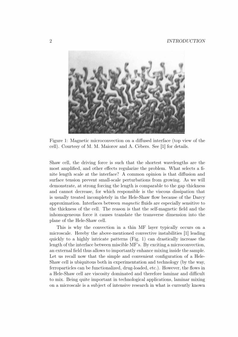
2 INTRODUCTION
Figure 1: Magnetic microconvection on a diffused interface (top view of thecell). Courtesy of M. M. Maiorov and A. Cebers. See [1] for details.
Shaw cell, the driving force is such that the shortest wavelengths are themost amplified, and other effects regularize the problem. What selects a fi-nite length scale at the interface? A common opinion is that diffusion andsurface tension prevent small-scale perturbations from growing. As we willdemonstrate, at strong forcing the length is comparable to the gap thicknessand cannot decrease, for which responsible is the viscous dissipation thatis usually treated incompletely in the Hele-Shaw flow because of the Darcyapproximation. Interfaces between magnetic fluids are especially sensitive tothe thickness of the cell. The reason is that the self-magnetic field and theinhomogeneous force it causes translate the transverse dimension into theplane of the Hele-Shaw cell.
This is why the convection in a thin MF layer typically occurs on amicroscale. Hereby the above-mentioned convective instabilities [1] leadingquickly to a highly intricate patterns (Fig. 1) can drastically increase thelength of the interface between miscible MF’s. By exciting a microconvection,an external field thus allows to importantly enhance mixing inside the sample.Let us recall now that the simple and convenient configuration of a Hele-Shaw cell is ubiquitous both in experimentation and technology (by the way,ferroparticles can be functionalized, drug-loaded, etc.). However, the flows ina Hele-Shaw cell are viscosity dominated and therefore laminar and difficultto mix. Being quite important in technological applications, laminar mixingon a microscale is a subject of intensive research in what is currently known

INTRODUCTION 3
as “microfluidics” [5].Until recently, in studies of interfacial instabilities in Hele-Shaw cells im-
miscible magnetic fluids forming sharp, well-defined interfaces were a subjectof theoretical analysis (e.g. [6]) and experimental treatment (e.g. [7]). How-ever, the notions of the miscible “interface” and the true immiscible one turnout to be not completely antagonistic. Under discussion [8, 9] is the role ofthe non-conventional Korteweg stresses that emerge at high concentrationgradients and reduce to the classical surface tension in the limit of vanishinginterface thickness. Although our particular results do not concern this is-sue, important analogy between the miscible and immiscible interfaces shouldindeed take place and be traceable.
In the second half of our study, we model the non-linear dynamics ofimmiscible MF interfaces in the same configuration as before. This is theclassical problem [10] modified by the presence of a magnetostatic force dueto the self-magnetic field of a ferrofluid. Historically, the interest to theoriginal problem of “viscous fingering” was motivated by its relation to theoil-extraction process. Later (in 1980’s), it proved to be interesting in itsown right for both physicists and mathematicians, for the interface was ob-served to form beautiful complex patterns. The Hele-Shaw flow is currentlyrecognized as the simplest physical process capable of pattern formation [11].In ferrofluids, the evolving patterns are modified substantially by the long-range magnetostatic repulsion to become interesting “dendritic” structures[12, 7], different from both the viscous fingers and the crystalline dendrites.Theoretically, some of their features can be explained using the notion ofthe effective surface tension [6, 13]. Nevertheless, numerical modelling is in-dispensable for providing a complete understanding of the process. Efficientmodelling in the Darcy approximation is possible owing to the fact that theimmiscible problem can be rendered one-dimensional in effect, and we de-scribe the corresponding computational techniques. Of course, in a systemthat complex, it is difficult even to pose a question that can be answered,but we have made a try to get some insight into the physics.

Chapter 1
Governing equations
1.1 About ferrofluids
The particular subject of the present work is a magnetic fluid (MF, alsoknown as ferrofluid). For a general reference on MF’s, see [14, 15]. Here wegive only a superficial account of some most basic ideas.
Conceptually, ferrofluid is a colloidal suspension of magnetic particles.In order to prevent the dipolar particles from agglomeration, the energy oftheir dipole-dipole interaction should not exceed the thermal one, for whichthe particles should be small enough. The upper bound for particle sizes isof the order of 10 nm, so that the volume of a particle is a single magneticdomain. Besides, as in any colloid, the van der Waals attraction should becounteracted, which is achieved by adsorbing either a surfactant coat (thesteric stabilization), or ions of the same sign (the charge stabilization) on thesurface of a particle. For details, see texts on the physical chemistry of col-loids. The size of a particle should not be too small, however, to facilitate thepreparation and to have an acceptable magnetic susceptibility. Sometimeswe will distinguish between the magnetic and hydrodynamic radii of a par-ticle; the latter is somewhat higher because the surface layer of the materialis non-magnetic, and besides, particles can be coated with a surfactant.
Being both a magnetic media and a fluid, MF can exhibit peculiar featuresnot known for other existing materials. Thus, its free horizontal surface ina (strong enough) perpendicular magnetic field undergoes the static “peak”instability. The peaks form either a hexagonal or square lattice [14, 15],which was a subject of intensive theoretical analysis [16]. The known fluid-mechanical instabilities are also modified in the case of magnetized ferrofluids,as we will see. One more peculiarity is associated with the possibility tomaterialize, by ferrofluids in rapidly rotating fields, the hydrodynamics “with
4

1.2. GAP-AVERAGING, DIFFUSION, AND STRESSES 5
a spin” (or internal rotations), when the stress tensor is non-symmetric. Thereason is that the magnetization of a particle requires certain time to alignwith the applied field, either by rotating with respect to the material of theparticle, or by rotating the particle as a whole in the viscous fluid. We,however, will be dealing solely with a quasi-static field.
We will not give any further generalities on magnetic fluids. We mentionnow only some facts that are of immediate relevance to our subject. (Latersome more information about ferrofluids will also be given.)
The field interacts with MF through the magnetic ponderomotive force.(The force will be addressed in detail in §1.4.) Now consider the fact theforce, in fact, acts upon the particles. A particle moves with some velocityrelative to the carrier liquid, and the Stokes drag on it equals, on the average,the force exerted upon the particle. However, the particles can also drive thecarrier, in which case an overall MF flow results. Its velocity is determinedby the friction at the walls of the cell (according to the Darcy law, §1.3).The friction experienced by a given MF volume at the walls is (more or less)balanced by the force that all particles in the volume exert on the carrier.It gives the ratio of two velocities: the one of MF relative to the walls andthe one of particles relative to the carrier. The ratio is very large unlessthe concentration is very low. Specifically, for the magnetophoretic particletransport to be neglected with respect to the advective one, the condition
ϕ≫ (a/h)2 (1.1)
must hold [17], where a is the average radius of a particle, ϕ is the vol-ume fraction of the suspended matter, and h is the gap spacing. Obviously,the condition is not restrictive at all, given the concentration of normallyemployed ferrofluids. The estimate is only a necessary condition since it as-sumes that the force on magnetic particles entrains MF, for which it mustbe non-potential. Otherwise, the pressure gradient can counter-balance theparticle force, which is the case, by the way, for the one-dimensional MFconcentration distributions whose stability (against two-dimensional convec-tion) we will analyze later (§§2.3, 2.4). Nevertheless, in the present studythe magnetodiffusion will not be taken into account.
1.2 Gap-averaging, diffusion, Korteweg stresses
In this paragraph we will discuss the process of mixing by diffusion in aHele-Shaw geometry. This material refers to general miscible fluids.
Let us consider the Brownian diffusion of ferromagnetic particles in MF.The velocity ~v will be that of the center of mass of the suspension (i.e. of

6 CHAPTER 1. GOVERNING EQUATIONS
MF as a whole). Then for the velocity the equation of continuity holds
∂ρ/∂t+ div(ρ~v) = 0 , (1.2)
ρ being the density of MF, and the momentum equation (see §1.3 later) canbe written down for the mixture in the same form as it is for a single fluid(Chapter VI of [18]). In addition, the conservation of species gives
∂(ρC)/∂t+ div(ρC~v) + div~ = 0 ,
where C is the mass fraction of magnetic particles, ~ is the density of thediffusive mass flux associated with the diffusive fluxes ~0, ~1 of the carrierliquid and magnetic particles, respectively, [18]. Then
dc/dt+ c div~v + (1/mp) div~ = 0 , (1.3)
where c is the number of magnetic particles per unit volume, and mp is themass of a particle. It is reasonable to assume that the density ρ of MF varieslinearly with c (a “simple mixture”):
ρ(c) = ρ0
(
1 +c
c∗
)
,
where ρ0, ρ1 are the densities of the carrier liquid and the magnetic material,respectively, and
1
c∗= mp
(
1
ρ0
− 1
ρ1
)
.
(I.e. by introducing a particle into a certain volume, the mass of the volumeincreases by dρ/dn = Vp(ρ1 − ρ0), Vp being the volume of a particle.) Thenfrom Eq.(1.2) it follows that
dc/dt+ (c+ c∗) div~v = 0 .
Finally, comparing with Eq.(1.3), we obtain
div~v =
(
1
ρ0
− 1
ρ1
)
div~ . (1.4)
Thus a very basic argument, involving only conservation laws and a simpleρ(c) dependence, reveals an obvious but usually forgotten fact that even ifboth components of a flowing inhomogeneous mixture are incompressible,the mass-averaged flow velocity does not satisfy div~v = 0. (In the presentcontext, the mixture is called “incompressible” if the density of none of the

1.2. GAP-AVERAGING, DIFFUSION, AND STRESSES 7
constituents varies with pressure.) The velocity is divergence-free (solenoidal)only if the densities ρ0 and ρ1 are equal.
Nevertheless, we still will assume that variations in the particle concen-tration throughout MF result in a negligible change in the density. Puttingdiv~v = 0 leads to a considerable simplification of the further analysis.
Among several variables any of which can describe the composition of amixture (such as the mass or molar concentration, volume fraction, etc.), itis the mass fraction C that is associated to our reference frame of the centerof mass (§§4.3, 4.17 of [19]). The first Fick’s law introduces the diffusioncoefficient D in the usual way if the fluxes (taken relative to our reference
frame) are expressed through C: div~ = −ρD~∇C. (However, the range ofvalidity of the first Fick’s law remains unclear to us.) But in dilute ferrofluids,and since the density difference will anyway be neglected, the compositionvariables are interchangeable, e.g. we can write the equations in terms of thevolumic molar concentration c (i.e. the number of particles per unit volume,as defined above). The incurred error will be indeed negligible. For example,from Eqs.(1.3), (1.4) we have
dc
dt+
1
mp
[
1 + ϕ
(
ρ1
ρ0
− 1
)]
div~ = 0 , (1.5)
which simplifies to the standard convection–diffusion equation
dc
dt+
1
mp
div~ = 0
if the ferrofluid is dilute enough:
1
ϕ≫ ρ1
ρ0
− 1 . (1.6)
Of course, the volume-averaged velocity is solenoidal without any approx-imations, as noted in [20, 21]. As the Hele-Shaw flow that will be of interestto us is free from inertia, it may seem appealing to reformulate the problemin terms of the volume-averaged velocity. However, the advantage is quiteillusory. For example, the correct boundary conditions for mixtures are notknown as yet [22]. (The no-slip of which velocity holds?) This uncertainty af-fects the friction term involving velocity in the averaged equations of motion(§1.3). So one anyway resorts to approximations of the above sort.
That the assumption div~v = 0 is generally wrong for mixtures and, inparticular, for miscible fluids, was studied extensively by D. D. Joseph withcollaborators. (Our simple Eq.(1.4) is essentially Eq.(2.30) of [23].) Anotherclosely related issue are the so-called gradient stresses that may arise in

8 CHAPTER 1. GOVERNING EQUATIONS
the regions of high concentration and density (not present in the Navier–Stokes stress tensor of a Newtonian fluid). In the work [24] the history ofthe subject is presented over more than a century with many excerpts andexperimental illustrations. It appears that many researchers recognized theexistence of what can phenomenologically be described as a transient surfacetension at the miscible “interface.” Back in 1901, Korteweg composed ageneral stress tensor for compressible and incompressible fluids and showedthat it leads to boundary conditions mimicing those at a curved interface withsurface tension. This “capillary” tensor is a second order tensor composednon-linearly of the first and second gradients of density and/or concentration;for details, see the works cited below. In [25], by introducing a modifiedvelocity that turns out to be divergence-free, the momentum equation isrepresented in the form of the Navier–Stokes equation with two viscosities, anon-trivial driving force, and a modified pressure (a conventional one plus a“concentration pressure”). Under some assumptions (of constant coefficients),four of the five Korteweg coefficients entering the stress tensor effectively dropout. Non-linear stability of a vertically stratified fluid is analyzed by energymethods. It is suggested that the Taylor dispersion problem (see below) andthe Hele-Shaw problems with miscible fluids be reworked to take the gradientstresses and the non-solenoidality into account. The Hele-Shaw case is indeedinvestigated in [20], where a linear analysis of a Rayleigh–Taylor instabilityis carried out. The effect of div~v 6= 0 proved to be minor if the diffusioncoefficient is small. The step-like concentration distribution in the Hele-Shaw geometry does not evolve into the one-dimensional error-function oneif the non-solenoidal velocity due to mixing is taken into account [22]. In[25, 20] some constraints are obtained on the coefficients appearing in theKorteweg stress tensor to avoid, on the one hand, the ill-posedness and, onthe other hand, an unconditional non-linear stability. Let us note that eventhe signs of the Korteweg coefficients are not yet established, although theorder of magnitude of the transient surface tension is more or less clear fromexperiments, [24]. In [23], the (in-)validity of putting div~v = 0 is discussedfurther. The pressure difference across a plane mixing layer is found to bezero even allowing for the Korteweg stresses; the diffusion in a pipe is alsoconsidered. For the spherical diffusion fronts, the t−1/2 scaling is obtained.
In a review [8], the diffuse-interface models are presented in several situ-ations. For a single-component fluid, of interest can be the behaviour near acritical point (that the interface thickness grows without bound was shownalready by van der Waals with a simpler model) or at the contact line (asof a droplet creeping along the wall). For the binary fluid, the modifiedCahn–Hilliard equation enters the governing equations, the spinodal decom-position being a typical application. Interestingly, the question about the

1.2. GAP-AVERAGING, DIFFUSION, AND STRESSES 9
non-solenoidality of the velocity arises in this context as well and has strongconsequences: it is argued by some authors that the thermodynamical role ofpressure changes. It is also demonstrated how the classical Laplace–Youngcondition with a variable surface tension is recovered in the sharp-interfacelimit.1 (See also [26].) The work also identifies some “subtle differences”between the applicable models. Another important point elucidated in [8]is the connection between the Korteweg stress tensor and the Cahn–Hilliardterm in the density of the free energy f = f0(c, T, . . .) + β(~∇c)2 [this is aspatial development of f ; the shape of f0(c, . . .) is responsible for the (im-)miscibility]. In [27, 28], the diffuse-interface models are also reviewed. Fora Hele-Shaw flow, the Hele-Shaw–Cahn–Hilliard model (HSCH) is analyzedin particular. The average velocity being non-solenoidal is taken into ac-count, non-conventional stresses enter the Darcy equation (§1.3), and theconcentration is governed by the Cahn–Hilliard equation that becomes theconvection–diffusion equation (CDE) in the limit of a slow concentrationvariation. (Note that Joseph et al. use CDE in the above-cited works.)
Above we have discussed the still somewhat exotic Korteweg stresses.The classical approach due to Taylor, however, would be to treat the par-ticles as a passive scalar, i.e. as an admixture having no influence on theflow. This results in the convection–diffusion equation for the velocity andconcentration averaged across the flow, but with an effective diffusion co-efficient Deff that exceeds the molecular one D: for a capillary tube [29],Deff − D = (Ur)2/(48D), where U is the average velocity and r is the ra-dius, while for a Hele-Shaw cell of a thickness h the result is Deff − D =(Uh)2/(210D). The higher the diffusivity, the lower the difference, since thediffusion spreads the scalar away from the center into the near-wall regionof low advection velocity. However, normally the fluid viscosity is stronglyconcentration dependent.
At this point we would like to present a brief overview of the past the-oretical work on miscible flows in a Hele-Shaw cell and porous media. (Seethe next paragraph on the relation between the two types of flow. Themechanical dispersion is the porous-media counterpart of the diffusion in aHele-Shaw cell.) A review of the early results can be found in [30]. We wouldnote in particular the asymptotic stability analysis of [31] of a vertical misci-ble displacement and the study [32] (discussed later on p. 17). Much of theresearch concentrated around the porous-media flow. The work [33] becameseminal for much of the research that followed. There, a popular approxi-mate framework (so-called QSSA, also of use in the present work, see p. 27)
1As the second part of the present work concerns immiscible ferrofluids, the Kortewegstresses could serve as a common basis for the whole work.

10 CHAPTER 1. GOVERNING EQUATIONS
for the stability analysis of time-dependent flows with diffusion (dispersion)is established. It is partially validated by the comparison to the solutionof the initial-value stability problem (§2.2). The anisotropy of the disper-sion is taken into account in [33]. The radial geometry is analyzed in [34].Velocity-dependent dispersion is found to have a destabilizing effect in [35].An asymptotic solution for thin diffused interfaces (but still with QSSA) isfound. It is stated explicitly that the sharp-interface stability result dependson the jump of the concentration derivative of the viscosity rather than onthe jump in viscosity (the latter is the case for an immiscible interface). Theconditions are found at which there is no short-wave cutoff (i.e. however largethe wavenumbers, they all are unstable despite the transversal dispersion).In [36, 37], the gravity effect is in addition taken into account, the density ofthe fluid being an arbitrary function of the concentration; the dispersion isconsidered an arbitrary function of velocity. In [37] the cross-over betweenthe diffusive regime (no instability) and the convective one (fingers) is tracedexperimentally. The presence of a tangential velocity discontinuous at theinterface is found to stabilize the displacement in the presence of gravity in[38]. In [39] the effect of the non-monotonic concentration–viscosity depen-dence (“profile”), such as that of a water solution of propanols, is investigated.At some conditions, the diffusive smearing of a stable basic state can ren-der it unstable. Asymptotic analysis of [35] for almost sharp interfaces isextended for any concentration–viscosity dependence. However, this workis also important for stressing the presence of the continuous spectrum inthe stability problem (we will develop this subject in §2.2). Identified is thephysical reason why it is the concentration derivative of the viscosity, and notthe viscosity itself, that determines stability. In this regard, let us note thatin the review [30] referenced above, the viscosity difference (in the form ofthe viscosity Atwood ratio, Eq.(3.18)) is erroneously listed among the para-meters that determine stability. In [21] the conditions for the equivalence ofthe flow under gravity, on the one hand, and by displacement, on the other,are established with respect to the concentration dependence of viscosity anddensity. (Note that with immiscible interfaces, the two flows are equivalent,see references in [21] and, for the flow in a Hele-Shaw cell, see §3.1.2.) Numer-ical simulations are presented e.g. in [40, 21, 41]. The above studies mainlyconcern the porous-media flows. The interest to the Hele-Shaw miscible flowas such was sporadic ([42, 32, 20]) until the late 1990’s.
At the moment, the miscible interfaces are a subject of growing inter-est, as exemplified by [9]. In [43] (extended in [44]), miscible displacementsare studied experimentally in capillaries. If the finger of the less-viscous dis-placing fluid, whose thickness is the main concern of the work, occupies morethan half of the cross-section of the capillary, a thin spike (needle) is observed

1.2. GAP-AVERAGING, DIFFUSION, AND STRESSES 11
to grow from its tip. (The intruding finger exists at large Peclet numbersPe = Uh/D and for a finite time because of mixing; U is e.g. the averagedisplacement velocity.) The flow structure (recirculations) giving rise to thespike is investigated (Fig. 12 of [43]). In the accompanying numerical study[45], where a constant diffusion coefficient, the linear concentration–densitydependence, and the exponential concentration–viscosity one are assumed, ananalogous protrusion is obtained in simulations for the geometry of a Hele-Shaw cell as well. In this work, a noteworthy argument is presented that,contrary to intuition and if viscosity is concentration dependent, the conven-tional viscous stresses can mask the velocity-independent Korteweg stressesat high Peclet numbers. The numerical analysis is extended to include thenew effects in [46], where it was found that taking the Korteweg stresses, butnot the velocity non-solenoidality, into account allows to reproduce the ex-perimental observations. The results of simulations by a different numericaltechnique [47] are in good agreement with [45] (under the same assumptions,but at no gravity). The Stokes [45] or even Navier-Stokes [47] equations areused in these simulations of a Hele-Shaw flow; see [48, 28] for the numericalmodelling of the gap-averaged Darcy flow with the Korteweg stresses. Apartfrom the above-cited earlier works (see [24] and references therein), manyattempts are made to conduct, with miscible fluids, the classical experimentsknown for the immiscible case, with the aim to establish the effective surfacetension. Thus, Rayleigh–Taylor fingers, drop formation, and other phenom-ena with miscible interfaces are analysed in [49]. The interfaces vibratedhorizontally or vertically and the known interfacial singularity above a pairof horizontal parallel immersed counter-rotating cylinders, are carefully stud-ied experimentally [50, 51] in the miscible case. Direct measurements of theeffective surface tension are also done [52].
For the concentration-dependent fluid viscosity, when the velocity profileat displacement deviates from parabolic, an asymptotic integro-differentialequation is obtained for the velocity in [53] by making use of the small ratioof the gap width to the extension of the mixing region along the cell. At finitePeclet numbers, having adopted the “quarter-power” concentration–viscositydependence and constant diffusivity, they [53] study the distribution of theconcentration across the cell at various viscosity ratios. It is established thatif Pe . 10δ, then the angle between the isolines of concentration and thenormal to the cell will not exceed δ ≪ 1. In the limit of zero diffusion,regardless of the (monotonic, however) concentration–viscosity relation, thegap-averaged concentration develops a “shock,” i.e. at the tip of the tongueits thickness changes abruptly to zero, which possibility is noted already in[42]. The necessary condition for this not to happen is that M < 3/2, whereM is the ratio of displaced fluid’s viscosity to that of the injected fluid. The

12 CHAPTER 1. GOVERNING EQUATIONS
asymptotic analysis is checked against the simulations [47, 46].In an experimental study [54] of a miscible Saffman–Taylor instability in
a vertical Hele-Shaw cell, the theory [53] finds an unexpected outcome. Theexperiment is conducted with the heavier fluid resting below the lighter one,which stabilizes the interface at no displacement. Then the upper fluid ispumped into the gap, and a downward displacement occurs. The heavierfluid is also the more viscous one. The Peclet number is quite high, > 104,so that the diffusion can be neglected. If M exceeds ≈ 2 and, in addition, ifthe non-dimensional injection rate is above critical Uc(M) [Uc(M) decreaseswith M ], then the horizontal, in the plane of the cell, uniformity of the dis-placement gets broken, and thin jets of the lower fluid divide the falling oneinto plane fingers. The width of the fingers is found to be ≈ 5h (see thenext paragraph on what we believe is the reason for this relation), and theyresemble in shape the “deep cells” occurring at directional solidification ofbinary liquids (e.g. [55]). The distribution of the gap-averaged concentrationc of the upper fluid is recorded in [54]. Obviously, c gives also the thickness ofthe downward tongue. After short transients, the concentration field propa-gates downwards in a self-similar manner and in some cases indeed decreasesin a non-smooth manner along the vertical. Found in [54] is an unexpectedrelation between the occurrence of the fingering in the plane of the cell andthe occurrence of the shock at the vertical c curve (i.e. of the jump in thetongue thickness measured across the gap). Namely, the fingering instabilitysets in if, and only if, the tongue thickness abruptly goes to zero (a “frontal”shock). Thus, the flow in the perpendicular direction remains uniform ifthe thickness varies smoothly downwards or if it changes abruptly, but to anon-zero value (an “internal” shock). The latter case refers to the protru-sion simulated numerically in [45]. In [56] the theory of [53] is extended toinclude the buoyancy effects. A theoretical diagram in M–U coordinates isdelineated which distinguishes between the three cases. The diagram showsa satisfactory agreement with the experimental data. However, the origin ofthe correlation between the shape of the concentration isolines in the verticalperpendicular section of the cell and the onset of convection in the plane of thecell remains practically unexplained; a three-dimensional stability analysis isrequired to understand the instability. Using some experimental relations,an ad-hoc analysis is attempted in their later note [57].
As for the object of our study, although we routinely call it a “misci-ble magnetic fluid” (“miscible” in all proportions), it is essentially a singlefluid with an inhomogeneous concentration of suspended ferroparticles. Thesurface-tension-like effects are due to attractive dipole–dipole particle inter-actions at concentration gradients and discontinuities. The same effects arein operation at field-induced phase separation of MF’s in thin layers at a
1.3. THE DARCY LAW AND THE BRINKMAN EQUATION 13
diffused boundary between the concentrated and dilute MF phases (see e.g.[58, 59, 60, 61, 62, 63, 64]). In [58, 65, 66] a general model of magneticsuspensions is developed where the free energy of the suspension containsthe Cahn–Hilliard term. However, we will eventually adopt the simplest MFmodel in which interparticle interactions are neglected. Hence it would be in-consequent to take the Korteweg stresses into account and, at the same time,use the Langevin law for the MF magnetization. Very recently, a miscibleradial gap-averaged MF flow in the perpendicular field was simulated withthe Korteweg stresses [67]; for the same problem simulated without them,see [68]. The subject of these works is particularly close to ours. Now thelack of the quantitative experimental data for ferrofluids becomes apparent.
As this paragraph has shown, the common reduction of the problemto a two-dimensional one by averaging the concentration and the assumedPoiseuille velocity profile across the gap simplifies the analysis at the costof leaving possibly important effects out of account. The suspended parti-cles can be a “very active” scalar. In our further analysis, we will put asidenon-conventional Korteweg stresses, neglect the Taylor dispersion, and inmost cases we will neglect the concentration dependence of the viscosity; Dwill be a constant isotropic diffusion coefficient. Thus, analyzing a miscibleHele-Shaw flow in a technically tractable way and interpreting the results ofsuch analysis requires known caution for the reasons clear from the aboveexposition. In the next paragraph we will consider the conventional viscousstresses; even their treatment in the Hele-Shaw context is commonly incom-plete, but our results will prove the necessity to take them fully into account.So, having said all the above, we eventually adopt for the concentration thesimplest CDE with the gap-averaged variables and the solenoidal averagevelocity field.2
1.3 The Darcy law and the Brinkman equation
for a Hele-Shaw flow
Let us consider an incompressible fluid of a constant viscosity η flowing be-tween parallel plates at a velocity ~v = (vx, vy, vz), the plates being z = ±h/2.It is well-known and simple to check that the equations vy = vz = 0,
vx(z) = − 1
2η
dp
dx
(
h2
4− z2
)
, (1.7)
2 “Presumably the practitioners of these arts know what they are doing and recognizethat they are making an approximation . . . ” (D. D. Joseph, [23].)
14 CHAPTER 1. GOVERNING EQUATIONS
describe the planar Poiseuille flow driven by a constant pressure gradientdp/dx. At any gradient, this is a solution to the full stationary Navier–Stokes equations (NSE) with the no-slip conditions at the plates (we layaside the question of its stability).
Now imagine that the flow for some reason is not unidirectional. Theexact solution becomes prohibitively complicated, if feasible at all, becauseof the non-linear term in NSE. However, at low enough velocity the termis negligible throughout the entire flow domain (§2.7 of [69]), so that NSEsimplifies to the linear Stokes equation:
−~∇p+ η∆~v = 0 . (1.8)
With some reservations, this equation admits an important reduction thatwe are going to describe now.
Consider a flow that approaches the Poiseuille one at infinity. Let us trythe possibility of the same kind of z dependence in the entire flow domain:
vx =6
h2
(
h2
4− z2
)
ux(x, y) ,
vy =6
h2
(
h2
4− z2
)
uy(x, y) ,
(1.9)
where the coefficient is so chosen that ~u is the z-averaged velocity (vx, vy).In addition, let us demand that
div⊥ ~u = 0 , ~u = ~∇⊥φ , (1.10)
where φ(x, y) is some sufficiently smooth function, and the index “⊥” refersto an operator in two dimensions x, y. Physically, the assumption is that theflow responds to the local pressure gradient as if it were globally constant.Then by the continuity
0 = div~v =6
h2
(
h2
4− z2
)
div⊥ ~u+∂vz
∂z
we have vz = 0, and p = inv(z) from Eq.(1.8). Substituting Eq.(1.9) intoEq.(1.8), we obtain
−∂p∂x
+6η
h2
(
h2
4− z2
)
∆⊥ux −12η
h2ux = 0 , (1.11)
and analogously for ∂p/∂y, uy. The term in the middle vanishes, for Eqs.(1.10)lead to ∆⊥ux = ∆⊥uy = 0. Thus,
−∂p∂x
− 12η
h2ux = 0 ,
−∂p∂y
− 12η
h2uy = 0 .
(1.12)

1.3. THE DARCY LAW AND THE BRINKMAN EQUATION 15
It is remarkable that the pressure gradients are indeed independent of z.Besides, this relation proves that ~u can be potential.
We have demonstrated that Eqs.(1.9), (1.10) solve the incompressibleStokes equation (1.8). A z-independent potential force density can be addedto Eq.(1.8) and absorbed into the pressure gradient, changing nothing in theanalysis. Essentially, we have found that with such driving force, a three-dimensional laterally unbounded flow exactly reduces, by the substitution(1.9), to a two-dimensional one at a gap-averaged velocity. The unbounded-ness is essential for the following reason. Imagine a cylindric obstacle situatedbetween the plates perpendicularly to them, filling the gap entirely; at theboundary of the obstacle some conditions are posed in terms of the velocity ~v(§4.8 of [70]). Then, apart from reducing the number of dimensions, the sub-stitution also effectively reduces the order of the differential equation. Notall boundary conditions posed for the Stokes equation (1.8) can be satisfiedat solving the reduced Eq.(1.10). (The exact analogy can also break at freesurfaces and discontinuities.) The no-flux (non-permeability) condition canbe satisfied, but not together with the no-slip condition. However, the flow“feels” the presence of the no-slip condition only within a thin belt of thickness∼ h around the obstacle. Indeed, if vx and vy are required to vanish at theboundary as well as at the plates, their second derivatives in Eq.(1.8) acrossthe gap and along the plates can be estimated to relate as (l/h)2, where l isa distance from the boundary. Therefore at l ≫ h the boundary conditionhas no impact on the pressure gradient and, by Eq.(1.12), on velocity. Thesame result is valid near the lateral sides of a Hele-Shaw cell [71].
Eq.(1.12) for the gap-averaged velocity is exactly (to within the coeffi-cient) a two-dimensional version of the Darcy law that is widely used todescribe, at coarse enough scales, the groundwater flow [72] in porous mediawith permeability α = 12η/h2 (we will call it the friction coefficient). Dueto this direct analogy, the Hele-Shaw device (cell) was often employed tomodel the percolation processes. However, originally it was introduced byH. J. S. Hele-Shaw back in 1898 to model steady two-dimensional incom-pressible potential inviscid flows around various obstacles (§330 of [73]; seephotos in [74]). At a sufficiently narrow separation between the plates (com-pared to the dimensions L of the obstacle in the x, y plane, L ≫ h), thedifference in the boundary conditions is negligible and the above approachcan indeed be reverted. Of course, the pressure p of the Hele-Shaw flow willhave nothing in common with the pressure piv of the inviscid flow (see §3.9in [75]) that is calculated from the velocity through a non-linear relation:
ρ(~u · ~∇)~u = −~∇piv ,
ρ being the density. Phenomena such as a flow with non-zero circulation

16 CHAPTER 1. GOVERNING EQUATIONS
around the obstacle (i.e. with a multiple-valued potential) and flow detach-ment cannot be reproduced in a Hele-Shaw cell (§3.9 of [75], §4.8 of [70]).About a century ago, A. N. Krylov suggested to use the device to modelstresses in 2D elasticity problems arising in shipbuilding, while Hele-Shawhimself employed the device to solve some potential problems in electrody-namics.
As for the criterion to neglect inertia in NSE, a simple comparison of thenon-linear term in NSE against the friction at the plates in Eq.(1.12) givesRe∗ ≪ 1, where Re∗ is the “reduced” Reynolds number calculated with h2/Las the length scale [76, 70]. Another issue regarding the validity of Eq.(1.12)is the possibility to omit the non-stationary term ρ ∂~u/∂t (or ρ ∂~v/∂t in NSE)while preserving the ∂c/∂t term in the convection–diffusion equation. It isnot difficult to retain both and solve, e.g., the stability problem. Then itturns out that the reverse time scale of the flow (e.g. the instability growthincrement) λ must remain sufficiently small in the sense that λρ0 ≪ α, i.e.λh2/D ≪ η/(ρD) = Sc (the Schmidt number Sc is of the order of 107 inthe typical case). Such rapid processes are of no interest for us. Were λ notsmall, the non-stationary term ∂~u/∂t would become significant, and besides,the vorticity would have no time to diffuse in the transverse direction to formthe stationary velocity profile.
What happens at a general driving force not satisfying the above condi-tions – at a non-potential and/or z-dependent one? Then the reduction doesnot take place. For example, if the force is z-independent but non-potential,neither is the average velocity ~u, cf. Eq.(1.12). The middle term in Eq.(1.11)no longer vanishes at an arbitrary z, while the other terms are z-independent,so there is no solution. This indicates that the velocity profile in fact devi-ates from the parabolic one. Of course, if the spatial scale L of the flow inthe plane of the cell is large compared to h, the term can be neglected withrespect to the friction at walls, and the Darcy law is recovered. Without theassumption that L≫ h, averaging the Stokes equation across the gap gives
−∂ < p >
∂x+ η∆⊥ux − αux + fx = 0 (1.13)
(and analogously for the y-components), where ~f is a gap-averaged drivingforce. Here it is assumed that it is possible to introduce a friction coefficientα such that η < ∂2vx/∂z
2 >= −αux, where ux =< vx >. Although thisis generally not the case, and Eq.(1.13) cannot be justified in this way, theequation looks rather reasonable from the physical point of view. The near-wall friction is the only viscous effect that is allowed for by the Darcy law.The Brinkman term η∆⊥ux in Eq.(1.13) describes the viscous dissipationdue to the flow non-uniformity in the plane of the cell and the associated
1.3. THE DARCY LAW AND THE BRINKMAN EQUATION 17
additional shear stresses. Like the Darcy law, Eq.(1.13) is known in thecontext of porous media flows, where it is named after Brinkman (sometimesit is referred to as the Darcy-Stokes equation). It describes both a free fluidflow and a flow in porous media and is useful at analyzing flows bounded bypermeable walls.
For the Hele-Shaw flow, however, a rigorous argument for Eq.(1.13) wasmissing until recently. In [77] a unidirectional Stokes flow in a Hele-Shaw cellwas analyzed in several particular situations. In one of them, the flow in avertical Hele-Shaw cell was directed along the gravity force, and the densitywas non-uniformly distributed perpendicularly to the flow, but was constantalong the flow and across the gap. Then the volume-averaged gravity forceis non-potential (as can be seen by taking its curl). Still, the gap-averagedStokes equation was demonstrated to reduce indeed to Eq.(1.13), but at longenough wavelength and with the Brinkman term multiplied by a constantprefactor 12/π2 ≈ 1.2. The exact form of the Brinkman term is compli-cated and non-local (integral) [77]. The prefactor is not known in the morecomplicated cases involving magnetic forces that will be under consideration.Moreover, we don’t know the shape of the velocity profile when the magneticforces are in operation; one cannot expect it to be the Poiseuille one, so theexpression for α in Eq.(1.13) is also not known exactly. Therefore we willfollow the previous research and leave the Brinkman term equal to unity inEq.(1.13).
In another case studied in [77], it was viscosity that varied perpendicularlyto the flow. Note that our equations presented in this paragraph hold atconstant viscosity. The case of a variable viscosity will be modelled in thepresent work only with the Darcy law (1.12). Nevertheless, it is noteworthythat the same conclusions as stated above hold in this case as well [77].
The Darcy law was conventional at describing the Hele-Shaw flow. How-ever, the Brinkman equation is more adequate to describe the microconvec-tion occurring on the scale of the gap width of the Hele-Shaw cell. First of all,one recalls the early work [32], both analytical and experimental one, wherethe viscous shear in the plane of the Hele-Shaw cell is considered as the onlydissipation mechanism in the radial miscible flow (i.e neither surface tensionnor diffusion are in operation). At a large radius, when the interface becomesalmost straight, the most unstable mode is found to scale linearly with thegap width, which conclusion is substantiated by experimental results [32].In [78] the same miscible Hele-Shaw experiment is conducted with a recti-linear displacement; again, the results (Fig. 11(a) of [78]) give (1 . . . 3)h forthe finger width. (As for the immiscible case, let us note the experimentallyobserved [79] saturation of the radius of curvature of the anomalous Saffman–Taylor fingers at the value of (2.2±0.1)h at high capillary numbers.) In some

18 CHAPTER 1. GOVERNING EQUATIONS
other situations [80, 81, 82, 83, 84, 85] the introduction of the Brinkman termin Eq.(1.13) was considered essential for a Hele-Shaw flow. In the contextof the Rayleigh–Taylor instability with non-magnetic miscible or immisciblefluids in a Hele-Shaw cell, recently a comparison [86, 87] was done betweenthe stability results given by experiments, a three-dimensional numerical lin-ear analysis and non-linear simulations (all with the Stokes equation and the3D CDE), on the one hand, and the stability results of [88] for the sharpinterface (based on the Brinkman equation and the 2D CDE), on the otherhand. (Contrary to the works discussed in §1.2, the concentration was as-sumed viscosity independent in these studies.) In [88, 89], a linear stabilityanalysis of a sharp interface was conducted analytically in both the misci-ble and immiscible cases, and the Brinkman equation was found to render
the most dangerous wavenumber of the instability equal to√
6(√
5 − 1)
/
h
(the corresponding wavelength is ≈ 2.3h) in the limit of large Peclet orcapillary (§3.1.2) numbers. A slightly more general dispersion relation wasobtained, using different characteristic time and space scales, in [90] [theirEqs.(6), (9)] for an arbitrary Schmidt number Sc, and verified using their 3Dlattice-gas code [47]. The comparison [88, 86, 87] of the Brinkman results tothe more general Stokes ones revealed a “somewhat surprising” [86] generalability of the Brinkman formulation to capture stability details – despite itsgap-averaging (and QSSA, see p. 27 later). The non-linear simulations [86]demonstrated the transition between the two-dimensional Hele-Shaw mode ofinstability with a gap-invariant concentration field to the three-dimensionalregime with a strongly z-dependent driving force and non-Poiseuille velocityprofile. (We have already discussed on p. 11 the velocity profile at the vis-cously driven displacement.) Naturally, the transition occurs at high valuesof the dimensionless group (∆ρ)gh/(αD), ∆ρ being the density differenceand g being the free-fall acceleration.
The effect of the wavelength “saturation” at ∼ h was also found and like-wise attributed to the additional viscous stresses in our early communication[91] in the context of miscible MF’s (see §2.3.4, Figs. 2.10, 2.11 later). It isnoteworthy that an analogous effect for chemical fronts in a Hele-Shaw cellis contained in Eq.(16) of [81] as their driving parameter tends to infinity,which is due to the adopted Brinkman equation (cf. [92]). We would like tonote here also the analytical work [93] which explored the Rayleigh–Taylorinstability of a horizontal mixing front in an unbounded three-dimensionalgeometry (see also [94]). It was found that a new type of dissipation (vis-cosity) added into a stability problem with another stabilizing mechanism(diffusion), can couple with the latter, seriously modifying the behaviour ofthe most unstable mode by introducing a short-wavelength cut-off. [Note

1.4. MAGNETIC PONDEROMOTIVE FORCE 19
that our dimensionless Cm number (Eq.(2.19)) that will govern the stabilityof our problem also involves a product ηD.]
We would like to stress once again that h being the length scale of anunstable interface in a Hele-Shaw cell at high Peclet or capillary numbers isconsistent with the experimental evidence (for more references, see [88, 87]).Significant part of the forthcoming results are obtained assuming the flow isgoverned by the Brinkman equation.
1.4 The magnetic ponderomotive force
In this paragraph we will present the expressions for magnetic ponderomotiveforce and magnetic field that will be used throughout the following work.
In the approximation of magnetostatics for a non-conducting ferrofluidthe Maxwell equations give
div ~B = 0 , (1.14)
rot ~H = 0 . (1.15)
Relaxation of the magnetization ~M will be considered instantaneous, so that~M ‖ ~H.
The general formula for the ponderomotive-force density in a liquid mag-netic reads (Eq.(4.33) of [14] in Gaussian units3)
~fm = −~∇[
∫ H
0
(
∂(Mv)
∂v
)
H,T
dH
]
+M~∇H , (1.16)
where v = 1/ρ is the reverse density. This expression was derived in mid-sixties, since before the advent of magnetic fluids it would have had no practi-cal applications. If M = ((µ− 1)/4π)H with µ = const, the simpler classicalexpression due to Korteweg and Helmholtz is recovered:
~fm =1
8π~∇[
H2ρ
(
∂µ
∂ρ
)
T
]
− H2
8π~∇µ (1.17)
(Eq.(4.47) of [14], Eq.(35.3) of [95]). However, Eq.(1.16) was derived for asingle-phase media, and is not obviously valid for a multi-phase dispersedmedia such as magnetic fluids. Indeed, the variables T , ρ, and H are nolonger enough to define the thermodynamic state of MF; for example, theconcentration c can also vary independently, while in the approach of Cowley& Rosensweig the product cv is effectively fixed. Then M becomes a function
3The CGS system of units is in use throughout the present work.

20 CHAPTER 1. GOVERNING EQUATIONS
of the following three variables: c, T , and H. This point was made in [96],
where the expression for ~fm was derived in the form of Eq.(1.16), but withthe fragment
(
∂(Mv)
∂v
)
H,T
= M − ρ
(
∂M
∂ρ
)
H,T
replaced by the expression
M − c
(
∂M
∂c
)
H,T
.
The two formulations of the magnetic force were apparently in contradic-tion. However, it was reconciled by V. V. Gogosov and his collaborators (seeGogosov’s footnote comment at pp. 130–131 of [14], pp. 90–91 of [97], andreferences therein). It turns out that
ρ
(
∂M
∂ρ
)
H,T
= c
(
∂M
∂c
)
H,T
, (1.18)
where the derivative in the left-hand side is taken also at a constant massconcentration of the magnetic phase (equal to cv times particle mass), whichcondition is implicit in Eq.(1.16). We assume again that MF is quite dilute sothat the particle dipole-dipole interaction may be neglected: cm2
∗/kBT ≪ 1,where m∗ is the magnetic moment of a particle, kB is Boltzmann’s constant,and T is the temperature. (Equivalently, ϕ≪ kBT/(M
2SVp), where MS is the
magnetization of the particle material, and Vp is the volume of a particle,cVp = ϕ; usually the inequality is close to ϕ ≪ 1.) Consequently, the MFmagnetization M in the field H obeys the Langevin law (with M ≪ H)and is directly proportional to the concentration c. Then by Eq.(1.18) theintegral term in Eq.(1.16) vanishes, and one obtains simply
~fm = M~∇H . (1.19)
(Of course, the integral term in Eq.(1.16), entering as a gradient, can beabsorbed into the pressure and forgotten in the absence of discontinuities.)
That the result (1.19) is not trivial becomes evident if one attempts to
calculate ~fm statistically as the volume-averaged force on the gas of dipoles(magnetic particles) in an external field. The force on a single dipole is indeeda scalar product of its momentum and the gradient of some microscopic field.The analogous problem of computing the “effective” or “local” field arises inthe long-developed and quite subtle theories of dielectric media with dipolarmolecules. The analogy is formal though (cf. §31 of [95]), e.g. averaging

1.4. MAGNETIC PONDEROMOTIVE FORCE 21
the microscopic magnetic field gives the magnetic induction ~B, while theaveraged electric field gives the intensity ~E. Here we only note that Eq.(1.19)was obtained by a macroscopic thermodynamical argument. (See also §8 of[98].)
Eq.(1.15) allows us to introduce the potential of the self-magnetic (de-
magnetizing) field ~H− ~H0 = −~∇ψs of the MF volume in the uniform applied
field ~H0. Since ~B = ~H + 4π ~M , Eq.(1.14) gives the Poisson equation in threedimensions for ψs:
∆ψs = 4π div ~M
with appropriate conditions at infinity. Its solution is
ψs(~r0) = −∫
R3
div ~M(~r)
|~r0 − ~r| dV . (1.20)
At the boundary S between magnetic and non-magnetic media there is ajump in the magnetization ~M , and div ~M becomes a delta function there.Equivalently, instead of integrating the delta functions, a corresponding in-tegral over S can be added to the right-hand side of Eq.(1.20):
ψs(~r0) = −∫
R3\S
div ~M(~r)
|~r0 − ~r| dV +
∫
S
Mn(~r)
|~r0 − ~r| dS , (1.21)
where ~n(~r) is the normal to S outward with respect to the magnetic media.The formulas for the magnetostatic potential can be found in many bookson electromagnetism [99]; interestingly, they were first obtained by Poisson,who, apart from all other, was interested in the magnetostatics and foundedits mathematical theory. In the electric terminology, if ψs were the electro-static potential, then −div ~M and Mn would be, respectively, the volume andsurface densities of charge, both free and induced ones.
The field, potential, magnetization, and force density can be formallyexpanded in, e.g., volume fraction ϕ→ 0: ~H = ~H0 +ϕ ~H1 + . . .. Then in thelowest order ~M is directed along ~H0 (or equivalently, along ~B0) and
~M =ϕm0
Vp
~H0
H0
+O(ϕ2) ,
where m0 6 m∗ is the average magnetic moment in the direction of ~H0. Since~H0 is uniform,
div ~M =
(
~∇ϕm0
Vp
·~H0
H0
)
+O(ϕ2) =
(
~H0
H0
· ~∇M)
+O(ϕ2) .
22 CHAPTER 1. GOVERNING EQUATIONS
This expression allows to rewrite Eq.(1.21) as
ψs(~r0) = ψ∗(~r0) +O(ϕ2) , (1.22)
where
ψ∗(~r0) = −∫
(
~H0
H0
· ~∇M)
dV
|~r0 − ~r| +
∫
H0nM dS
H0 |~r0 − ~r| = O(ϕ) (1.23)
(ϕ ~H1 = −~∇ψ∗). Now we calculate
H =
√
H20 + 2ϕ( ~H0 · ~H1) +O(ϕ2) = H0 + ϕ
(
~H0
H0
· ~H1
)
+O(ϕ2) .
Let us adopt the following notation: the magnetic media (MF) will occupy
the layer z = 0 . . . h (a Hele-Shaw cell), while ~H0 will be directed eitheralong the z axis (the “perpendicular” field), or along the x axis (the “normal”field; this notation is adopted from [100]). The properties of the media willbe further assumed to be constant across the layer: ϕ, M = inv(z). Thenthe gap-averaged density of the magnetostatic ponderomotive force (1.19)becomes
< ~fm >= −Mh
∫ h
0
~∇(
~H0
H0
· ~∇ψ∗
)
dz +O(ϕ3) . (1.24)
In the case of the normal field, the surface integral in Eq.(1.23) vanishesdue to H0n = 0. Then
ψ∗(~r) = −∫
∂M
∂x ′
dV ′
|~r − ~r ′| , (1.25)
< ~fm >= −Mh
∫ h
0
~∇∂ψ∗
∂xdz +O(ϕ3) = −M
h~∇⊥
∂
∂x
∫ h
0
ψ∗ dz +O(ϕ3) ,
(1.26)
where ~∇⊥ is the two-dimensional Laplacian, and it is assumed possible todifferentiate outside the integral. Further transformations will be undertakenin §2.4.1.
In the case of the perpendicular field we have ( ~H0 · ~∇M) = 0 and it is thevolume integral that vanishes in Eq.(1.23):
ψ∗(~r) =
(∫
S2
−∫
S1
)
M dS ′
|~r − ~r ′| , (1.27)

1.4. MAGNETIC PONDEROMOTIVE FORCE 23
where S2 and S1 are the upper (z = h) and lower (z = 0) walls of the cell,respectively. The gap-averaged density of the force follows as
< ~fm > = −Mh~∇⊥
∫ h
0
∂ψ∗
∂zdz +O(ϕ3) = −M
h~∇⊥ (ψ∗|z=h − ψ∗|z=0) +O(ϕ3)
= −2M
h~∇⊥ ψ∗|z=h +O(ϕ3) . (1.28)
For future reference, we expand Eq.(1.27):
ψ∗|z=h =
∫
S2
(
1√
(x− x′)2 + (y − y′)2− 1√
(x− x′)2 + (y − y′)2 + h2
)
M dS ′ .
(1.29)This approximation for the magnetic force was also employed by others
(e.g. [101], §4.6 of [15], [102]). Note that M = m0c in our description witha constant m0. The degree of magnetic saturation is not important. Theforces (1.26), (1.28) and the resulting flow are in general not potential in themiscible case owing to the inhomogeneity of c.

Chapter 2
Linear stability analysis
of a miscible interface
in a Hele-Shaw cell
2.1 Miscible interfaces in a Hele-Shaw cell:
an overview and model
In a magnetic fluid, the transport processes allow an extra control parameter:the applied magnetic field. They attract scientific interest because of theirspecific cooperative nature, since the self-magnetic field of the colloid as awhole influences the magnetophoretic motion of colloidal particles and leadsto the field-dependent anisotropic effective diffusion.
However, as we have discussed in the Introduction, even if the externalfield is uniform, the self-magnetic field can give rise to a convective instabil-ity.1 In a thin plane layer with rigid transparent walls (a Hele-Shaw cell),miscible instabilities with MF’s can be observed directly with a microscope.In the experiment [1] MF and its pure carrier liquid were brought into con-tact in a Hele-Shaw cell forming a narrow straight “diffusion front.” In theperpendicular (to the cell) external field, the interface developed an intricatelabyrinthine pattern, while a peak pattern was obtained in the normal field(i.e. in the field applied along the cell perpendicularly to the front). Thepattern length scale was approximately as small as the layer thickness (lessthan 10−2 cm). Having quickly formed, the patterns were gradually blurredout by diffusion.
1This term should be understood in our context as an instability of a quiescent statewith respect to convection and not as the opposite to the “absolute” instability of a flow.
24

2.1. MISCIBLE INTERFACES IN A HELE-SHAW CELL 25
Recently, the diffusion in magnetic fluids under an applied magnetic fieldwas investigated [2, 103, 104, 105] by the forced Rayleigh scattering (FRS)on the optical gratings induced in thin layers (between transparent plates)of MF’s heated by an intensive non-uniform illumination (“pumping”) [106].By exposing the layer for a long enough time, a stationary grating – usu-ally a periodic array of parallel stripes – was created. After the pumpingis switched off, thermal inhomogeneities relax almost immediately, whereasthe concentration grating decays gradually. This allowed to determine theeffective diffusion coefficient of magnetic particles. If the magnetic field wasapplied along the layer parallel to the concentration gradients (in the “peak”configuration with respect to the stripes), the effective diffusion coefficientwas observed to increase up to several times as the field increased. This ef-fect was attributed [2, 103] to the magnetophoresis in the self-magnetic field.However, the mixing might have also been enhanced through breaking theone-dimensionality of the concentration distribution. The magnetophoresisalone is hardly capable of producing this effect [107]. Even though the oc-currence of microconvection was not checked in these FRS experiments, suchpossibility should be investigated. And indeed, very recently, reported werethe first experimental indications of a microconvection in the FRS setup[3, 108].
In this regard the experiments [109] also deserve mentioning; their in-terpretation was controversial [109, 110, 4]. An MF layer was heated by afocused perpendicular laser beam. The diffraction pattern was observed toloose its axisymmetric shape if the perpendicular magnetic field was raisedabove a critical value. Further on, if in addition a field was applied alongthe cell, the diffraction pattern would oscillate. While the authors of theexperiment believe that a convection sets in there, it is argued in [110] thatthe circular symmetry is lost owing to a static instability akin to that of mag-netic bubbles in a Hele-Shaw cell, with the concentration gradients playingthe role of an effective surface tension (§1.2). The nature of observed effectsremains unclear. (See also [111].)
In a circular geometry, a miscible MF flow in a Hele-Shaw cell under aperpendicular field was recently simulated in [68] and an intensive fingeringwas reported.
An instability of the Darcy flow of magnetic fluids in porous media in thefield applied along the concentration gradients (the peak configuration) wasstudied in [112]. To extend these results to the case of a Hele-Shaw cell, itsfinite thickness must be taken into account at deriving the self-magnetic fieldof MF. We will consider several concentration distributions along the cell inorder to be close to real experimental conditions. The case of an isolatedmiscible interface admits a pen-and-paper analysis for both orientations of

26 CHAPTER 2. STABILITY OF A MISCIBLE INTERFACE
x
zy
0
h
Ur
cc0~
= 0c0 =
Hr
(norm)
0Hr
(perp)
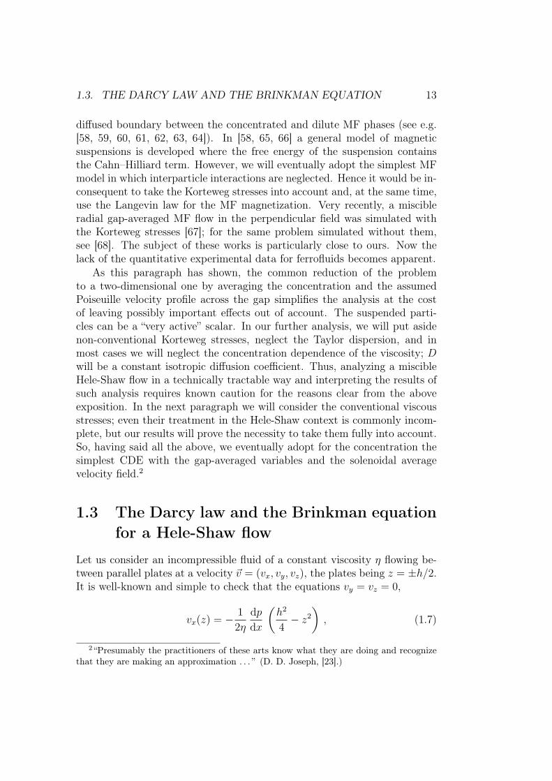
Figure 2.1: A sketch of a Hele-Shaw cell with a perturbed step-like concen-tration distribution.
the field. Studying the smoothed step-like and Gaussian (an isolated stripe;it will be studied only in the normal field) distributions allows to assessthe impact of smearing on stability. Besides, the continuous formulation ofthe problem makes it possible to incorporate the Brinkman (Darcy–Stokes)equation for the Hele-Shaw flow that is an improvement over the conventionalDarcy law (§1.3). The array of sharp parallel stripes specifically reproducesthe periodicity of the FRS grating.
We will consider a MF confined in a horizontal Hele-Shaw cell of spacing h.An inhomogeneous gap-invariant concentration of magnetic particles servesto model a particular case of a miscible MF pair in contact. (Indeed, generallyone would expect two MF’s to have e.g. different diffusion coefficients, etc.)The MF concentration c(x, y) (the number of magnetic particles per unitvolume) is assumed constant across the cell, and the whole problem is to berendered two-dimensional by averaging across the cell gap.
According to §1.2, we take the two-dimensional mass-averaged MF veloc-ity field ~v to satisfy
div~v = 0 , (2.1)
and the convection–diffusion equation holds:
∂c
∂t+ (~v · ~∇)c = D∆c , (2.2)
where D is a constant diffusion coefficient. According to §1.1, the magne-tophoresis is not taken into account.

2.2. MISCIBLE PROBLEM AND CONTINUOUS SPECTRUM 27
The flow is governed by the Brinkman (Darcy–Stokes) equation for thegap-averaged variables [see Eq.(1.13) in §1.3]:
−~∇p+ (η∆ − α)~v + ~fm = 0 , (2.3)
where p is the pressure, ~v is the velocity (relative to the walls), η is the vis-cosity, and α = 12η/h2 is the friction coefficient estimated for the Poiseuillevelocity profile. We remind (§1.3) that we can expect the full Eq.(2.3) tobe valid for η = const; however, in the Darcy case it holds also at theconcentration-dependent viscosity η = η(c). ~fm stands for the gap-averageddensity of the magnetostatic body force that depends on the field orienta-tion.
2.2 The miscible stability problem
and the continuous spectrum2
Let us consider the linear stability of some one-dimensional concentrationdistribution c0(x, t0). The miscible basic flow is time-dependent due to dif-fusion so that a quasi-steady-state approximation (QSSA) must be adoptedto study the linear stability by means of the normal-mode analysis at somemoment t0 [33]. Hereby we discard the further diffusion of the basic state asthe flow perturbations evolve; their diffusion is taken into account, however.Technically, this amounts to “freezing” the time-dependent coefficients in thelinearized perturbation equations. QSSA is considered [33] valid for diffusedenough interfaces. Non-QSSA attempts were an exception [31], though re-cently a quite general QSSA-free approach to the long-wave linear stabilityof miscible interfaces was suggested [113]. Note also the boundary condi-tions introduced in [20] that render the basic flow with diffusion steady andcan perhaps be used experimentally to create a controlled diffusion front (thesolute spreads by diffusion upwards into a vertical Hele-Shaw cell whose openbottom side is immersed into a large reservoir, with a downward flow of thesolvent opposing the spreading). In principle, a time-independent basic statecan be maintained also by a chemical reaction [114].
Keeping in mind the situation of slow displacement and weak externalfield, we introduce h and h2/D as space and time scales, respectively, to
2 “It should be kept in mind that the subject of instabilities in an infinite domainis intrinsically difficult, in particular because of the appearance of problems related tothe continuous spectrum. Many seemingly innocent questions have, to date, not eventhe beginning of a satisfactory mathematical answer. . . ” (P. Collet and J.-P. Eckmann,Instabilities and Fronts in Extended Systems, Princeton University Press, 1990.)

28 CHAPTER 2. STABILITY OF A MISCIBLE INTERFACE
render our independent variables dimensionless. Further on, we scale theconcentration, velocity, magnetic potential, viscosity, friction coefficient, andpressure with their respective reference values c, D/h, cm0h, η, α = 12η/h2,and αD. We preserve the same notation for the dimensionless variables.
Now we take the curl of Eq.(2.3) and linearize it along with Eq.(2.2) aboutthe basic state. Since the coefficients of the linearized equations depend onlyon x (and on the “frozen” time t0 which enters as a parameter), we can sep-arate out the variables t and y, as one would do if no integral terms werepresent. Thus we expand a velocity disturbance into discrete Fourier modes
v′x(x; k), v′y(x; k)
exp(iky + λ(k)t) (and likewise we expand the perturba-tions of c and ψ), where λ is a temporal growth increment of the mode of adimensionless wavenumber k. We proceed with a singled out mode.
The linearized Eq.(2.2) becomes now
d2c′
dx2− (k2 + λ) c′ = v′x
∂c0∂x
, (2.4)
The flow incompressibility immediately yields
ikv′y = −dv′xdx
. (2.5)
In the next paragraphs we will present the further steps of the stabilityanalysis in the case of magnetic fluids. In the rest of the present paragraph,we will explore some general issues concerning the stability analysis. Thismatter will be of no direct use further in the work. In particular, let us con-sider now in some detail the occurrence of the continuous spectrum, since wewill encounter later (in §2.3) a linearized problem that can possess no dis-crete spectrum. In order to clarify the issue without technical complications,we temporarily set ~fm = 0, omit the Brinkman term in Eq.(2.3), and takeα = const.
Making use of the incompressibility, one obtains now the linearized Eq.(2.3)simply as
d2v′xdx2
− k2v′x = 0 . (2.6)
The equations (2.4) and (2.6) together with the boundary conditions (thatc′ and v′x vanish) at infinity compose an eigenvalue problem.
However, it can be readily seen that at any λ the boundary conditionsare not satisfied. Thus there are no normal modes. Under some conditions,we will meet the same difficulty in our analysis of complete MF equations.However, it is the behaviour of infinitesimal perturbations that is of inter-est to us. Their dynamics is nevertheless governed by the linearized system.

2.2. MISCIBLE PROBLEM AND CONTINUOUS SPECTRUM 29
The decomposition into normal modes [115] is only a convenient way, but notalways an appropriate one, to reduce the problem for an arbitrary pertur-bation into a simpler problem for the single-mode solutions, whose temporalbehaviour is given by a compact dispersion relation.
Let us outline briefly a not rigorous argument (ch. 4 of [116], §7.10 of[117]) by which a generalization of the usual normal-mode approach can beobtained. Many assumptions, reservations, etc. will be omitted to make theidea clear. Consider a linear operator L whose set of eigenfunctions uk(x),Luk = λkuk, is complete:
u =∑
k
αkuk
for an arbitrary u(x). Then
Lu =∑
k
αkλkuk ,
and we can introduce other operators by the following formal definition:
f(L)u =∑
k
αkf(λk)uk .
Let us consider f(t) = 1/(λ− t):
f(L)u =∑
k
αkuk
λ− λk
. (2.7)
Obviously, this f(L) is the inverse of −(L − λE), E being the identityoperator. Now if L is a differential operator, the inverse is expressed througha Green’s function G:
f(L)u = −∫
G(x, ξ, λ)u(ξ) dξ . (2.8)
Integrating Eqs.(2.7) and (2.8) over a large circle in the λ plane and takingthe residues at the poles in Eq.(2.7), we obtain
u(x) = − 1
2πi
∮
dλ
∫
G(x, ξ, λ)u(ξ) dξ . (2.9)
Thus the decomposition of a function in terms of the eigenfunctions of L isrelated to the Green’s function of L− λE. From Eq.(2.9) it follows that
− 1
2πi
∮
G(x, ξ, λ) dλ = δ(x− ξ) . (2.10)
30 CHAPTER 2. STABILITY OF A MISCIBLE INTERFACE
The resulting formulas hold in fact for a wider class of situations than onemight think.
To be more specific, let us write down our system (2.4), (2.6). We havea generalized eigenvalue problem:
L
(
c′
v′x
)
= λB
(
c′
v′x
)
,
where
B =
(
1 00 0
)
and
L =
d2
dx2 − k2 −∂c0∂x
0 d2
dx2 − k2
.
In this case the Green’s function becomes a Green’s matrix (§16.5 of [118]).For illustration purposes let us consider, however, the trivial case ∂c0/∂x =
0. Then the equations for c′ and v′x decouple so that the Green’s function forthe concentration given by
(L11 − λE)G(x, ξ, λ) = δ(x− ξ)
can be easily found as
G =−1
2√k2 + λ
exp(
−|x− ξ|√k2 + λ
)
.
Now we want to integrate G over the circle of an infinite radius. G is analyticin λ with the exception of a branch cut λ ∈ (−∞,−k2), on the upper sideof which we choose ℑm
√k2 + λ > 0. The sum of the integral over the circle
and the integral over the branch cut (both paths are followed in the samedirection) equals zero by Cauchy’s theorem. The integral over the branchcut is easy to evaluate, and we obtain the following formula:
− 1
2πi
∮
G(x, ξ, λ) dλ =1
2π
−k2∫
−∞
cos(
|x− ξ|√
−(k2 + λ))
√
−(k2 + λ)dλ , (2.11)
where the square root takes on its arithmetic value. In accordance withEq.(2.10), the right-hand side indeed reduces to a delta-function by a well-known representation
∫ +∞
−∞
exp(ikx) dk = 2πδ(x) .

2.2. MISCIBLE PROBLEM AND CONTINUOUS SPECTRUM 31
Eq.(2.9) takes on the form
c′(x) =1
2π
−k2∫
−∞
dλ√
−(k2 + λ)
+∞∫
−∞
cos(
|x− ξ|√
−(k2 + λ))
c′(ξ) dξ =
−k2∫
−∞
dλ
2πσ
cos (σx)
+∞∫
−∞
c′(ξ) cos (σξ) dξ + sin (σx)
+∞∫
−∞
c′(ξ) sin (σξ) dξ
(2.12)
(here σ =√
−(k2 + λ)). This is nothing else but the desired decompositionof (the k-th y-mode of) an arbitrary instantaneous concentration field interms of functions of a prescribed temporal behaviour ∼ exp(λt). If theGreen’s function had pole singularities in addition to the branch cut, therewould appear a sum of residues in Eqs.(2.11), (2.12) corresponding to thedecomposition into the conventional normal modes. The inner integration inEq.(2.12) would still give the coefficients of the decomposition. We remindthat usually the expansion is implicit, and normal modes are analyzed fromthe beginning. However, we have a decomposition in terms of functions thatdo not satisfy the boundary conditions at infinity, where the functions areonly bounded but do not vanish. The corresponding eigenvalues λ are saidto belong to the so-called continuous spectrum of the stability operator asopposed to the discrete spectrum (§12 in [118]). (Indeed, one has to integrateover the continuous spectrum but sum over the enumerable set of discreteeigenvalues.) Although every eigenfunction of the continuous spectrum isnot admissible in the sense of the boundary conditions, their continuousinfinite set can represent a valid vanishing perturbation. The situation is thesame as with the Fourier integral (our illustration (2.12) is a version of theFourier decomposition). Infinity of the domain is a root of the continuousspectrum. Indeed, shift the boundary conditions to finite points, and thecontinuous spectrum will usually condense into a countable set of discreteeigenvalues. (Another common cause for the continuous spectrum to emergeis the singularity of coefficients.)
A by-product of our analysis (2.12) is that λ ≤ −k2, i.e. every perturba-tion belonging to the continuous spectrum will disappear. Of course, withour simplifications, it follows directly from the diffusion equation that anydisturbance will. Thus the continuous spectrum can be neglected if one asksabout the instability. How general is this conclusion?
Later we will study situations where the analogue of Eq.(2.6) will containadditional, integral terms related to the magnetic field, which will render thestability operator integro-differential. Analysis of the inverse operator andits singularities seems to be intractable. A finite number of discrete modes
32 CHAPTER 2. STABILITY OF A MISCIBLE INTERFACE
will appear; the discrete eigenvalues will have either ℜeλ > −k2 or ℑmλ 6= 0(it is easy to see that complex-valued eigenvalues come in conjugate pairs).
Nevertheless, Eq.(2.4) remains valid and has the following property. Asin our problems ∂c0/∂x and other variable coefficients vanish at infinity,the convection–diffusion equation (2.2) and the analogue of Eq.(2.6) alwaysdecouple at infinity. Thus we will have the same behaviour of the eigen-functions at infinity. If the conditions of vanishing are imposed there, thediscrete eigenfunctions result that can be real or complex valued, while thecorresponding eigenvalues can be stable or unstable. If we demand that thesolutions be only bounded, the continuum eigenfunctions result. In this caseit is guaranteed, by virtue of Eq.(2.4), that λ is real and negative. Of coursewe realize that this argument, extended from [39], is not rigorous, still webelieve the conclusion is right.
In the spectral theory ([119, 120]) the exact definitions of the discrete,continuous, and the so-called residual spectrum are given. The linear or-dinary differential operators do not possess the residual spectrum (p.184 of[117], p.200 of [116]). The spectral theory for the self-adjoint operators is es-pecially well developed. We will obtain complex-valued eigenvalues though,which automatically implies that the problem is not self-adjoint. For theSturm-Liouville problem, there are many simple criteria allowing to judgeupon the spectrum merely by coefficients. The continuous spectrum of theboundary-value problems is quite important in quantum mechanics [121].
In hydrodynamics, the most studied stability problem is that of the in-ertial instability (governed by the Orr-Sommerfeld equation) of the viscousparallel shear flow, and its inviscid limit. The continuous spectrum of theproblem in the unbounded domain is discussed, e.g., in [122, 123, 124]. Thecomplete and mathematically rigorous approach to the linear stability prob-lem with time-invariant coefficients is to solve the initial-boundary-valueproblem for an arbitrary perturbation, which allows to take the continuousspectrum into account in a natural way. This is usually achieved throughthe one-sided Laplace transform of the equations in time combined with theFourier transform in those spacial variables of which the coefficients are in-dependent ([125, 126, 127, 128]; see also [129], §2.3.2 in [130]). At invertingthe solution obtained in the transform space, the poles in the variable of theLaplace transform correspond to the discrete eigenmodes, while the branchcuts correspond to the continuum eigenfunctions, much the same as for theabove-demonstrated technique employing the Green’s function. Indeed, thehomogeneous linear stability equations such as Eq.(2.4) for c′ exp(λt + . . .),etc, are exactly the equations for the Laplace-transformed Fourier modes oflinear perturbations of c(t, . . .), etc, but without the inhomogeneous termsdue to initial conditions. Integrating over the unstable part of the contin-

2.3. LABYRINTHINE INSTABILITY 33
uous spectrum, one obtains that the associated temporal behaviour is non-exponential (§47.1 in [131]).
We would like to touch briefly the so-called transient-growth phenomena[132, 133, 134]. It turns out that the notion of linear stability must be gen-eralized to describe the observed phenomena more adequately. Consider thecase of non-orthogonal eigenfunctions, all of them decaying monotonically intime (a linearly stable situation). Then possible are their linear combinationssuch that they, being initially small, grow temporarily because of the differ-ence in growth rates between individual modes. A simplistic analogue is theearly behaviour of exp(−t) − exp(−2t) ∼ t. The transient growth can be sosubstantial (orders of magnitude) that the disturbance enters the non-linearregime, where its fate is no longer controlled by the linear theory.
We also just mention the so-called energy methods in (non-linear) stabil-ity theory that are based on the estimates of solutions to differential equations(§§VI.8–9 in [135], [136], [137]). If the flow is found to be non-linearly sta-ble, it is of course stable with respect to infinitesimal disturbances as well.Hydrodynamic stability problems are treated from the stand-point of thenon-equilibrium thermodynamics in [138].
The theory of the hydrodynamic stability is a respectable but demandingfield3 at the interface between fluid mechanics and applied mathematics. Asa reference, we would recommend [131]; for a detailed overview of inertialinstabilities and transition, see Chapter 2 of [139].
2.3 The labyrinthine instability
In the next four paragraphs,4 we will consider the magnetic field appliedperpendicularly to the cell and the “labyrinthine” instability it causes. Thenthe gap-averaged density of the magnetostatic body force ~fm is given byEq.(1.28) as
~fm = −2h−1m0c~∇ψ . (2.13)
Herem0 is an average particle moment component along ~H0, and by Eq.(1.29),
ψ(~r, t) = m0
∫
c(~r ′, t)K (~r ′ − ~r) dS ′ (2.14)
with K(~ρ) = 1/ρ− 1/√
ρ2 + h2.
3 “Research on hydrodynamic stability has been deep but narrow. . . ” (P. G. Drazinand W. H. Reid, [131].)
4Results of §2.3 were mostly published in [140] and communicated in part as [141, 91]and at [9].

34 CHAPTER 2. STABILITY OF A MISCIBLE INTERFACE
2.3.1 Derivation of the dispersion relation
We investigate the linear stability of the initially step-like concentration dis-tribution (i.e. of the straight “front” separating half-planes each occupied byits respective MF). For the sake of generality, a steady displacement of thefluid perpendicularly to the front with the velocity U relative to the walls isalso allowed for, which, at the concentration-dependent viscosity, allows usto take the Saffman–Taylor mechanism of instability into account. We canallow for viscosity variations only in the Darcy case.
We adopt the (x,y) Cartesian rectilinear reference frame that moves with
the velocity ~U , the x axis being directed along the ~U vector (Fig. 2.1). Thequiescent state is then as follows:
~v0 = 0 , (2.15)
∂c0/∂t = ∂2c0/∂x2 , (2.16)
−∂p0/∂x− Peα− 2 Cm c0 ∂ψ0/∂x = 0 , (2.17)
ψ0 =
∫ +∞
−∞
c0(ξ + x, t0) ln(
1 + ξ−2)
dξ , (2.18)
where Pe = Uh/D is the Peclet number.5 The dimensionless group
Cm =(cm0)
2
αD(2.19)
is the ratio of the time h2/D it takes for diffusion to act over the character-istic distance h to the time h2α/(cm0)
2 of the advection due to the magneticforce. In fact, the gap width h is introduced as the characteristic length bythe magnetic field – through the dimensional form of Eq.(2.18). The drivingforce being due to a self-magnetic field, Cm is quadratic in magnetization.Hence Cm parallels the magnetic Rayleigh number ∼ (∂M/∂T )2(∆T/h)2h4
characterizing a thermomagnetic instability [142] of a thin MF layer in a uni-form perpendicular field with a temperature difference ∆T imposed acrossthe layer. However, even though Cm resembles the magnetic concentration(solute) Rayleigh number, it has nothing to do with gradients across the cell.Cm is essentially independent of the viscosity, for the Stokes drag enteringthe Einstein formula for D and the friction coefficient α both vary linearlywith η (so that Cm ∼ (cm0)
2h2a/(kBT ), where kB is the Boltzmann con-stant). As MF saturates, a field increase cannot yield an arbitrarily high Cmwith a given MF sample (unless a thicker cell is taken). For the only available
5Everywhere we use “ ln” for the natural logarithm and “lg” for the decimal one.
2.3. LABYRINTHINE INSTABILITY 35
experimental situation [1] (h = 0.01 cm, H0 = 100 Oe, MF saturated mag-netization of 10 G) we substitute reasonable guesses for the missing values(a = 5 × 10⁻⁷ cm for the radius of a particle, and 500 G for the particlematerial magnetization), which yields Cm ≈ 104.
Interestingly, the dimensional analysis of the problem (the Π-theorem[143]) with constant coefficients reveals that only one more dimensionlessparameter could in principle emerge: h3c. Obviously, we are working in thelimit h3c≫ 1 (moreover, h3c≫ h/a by Eq.(1.1)).
As described in §2.2, we expand all disturbances into discrete Fouriermodes ∼ exp(iky + λ(k)t). Then, introducing the McDonald (modifiedBessel) function
K0(x) =
∫ ∞
0
cos(xt)dt√t2 + 1
, (2.20)
the perturbation of the potential is expressed as
ψ′ = 2
∫ +∞
−∞
c′(ξ + x)(
K0(k |ξ|) −K0(k√
ξ2 + 1))
dξ . (2.21)
The linearized CDE has already been obtained as Eq.(2.4). Taking intoaccount the incompressibility of the flow, Eq.(2.5), one obtains the linearizedcurl of Eq.(2.3) as
1
k2
d
dx
[
− η
12
d3v′xdx3
+(
k2 η
12+ α
) dv′xdx
]
+η
12
(
d2v′xdx2
− k2v′x
)
− αv′x
−Pedα
dcc′ − 2 Cm
(
c′∂ψ0
∂x− ψ′∂c0
∂x
)
= 0 .
(2.22)
The appearance of Eq.(2.22) is somewhat misleading, since it is valid, in itsfull form, only at η = const, when the term with the Pe factor vanishes.However, a varying viscosity is allowed in the Darcy approximation when(h/L)2 = k2 + ‖d2/dx2‖≪ 1, where L is the two-dimensional (in the planeof the cell) flow scale. Recalling the definition of α we find that the termsexplicitly containing η should be omitted to have the Darcy case.
Equations (2.21)–(2.22) compose a system of linear ordinary differentialand integro-differential equations. Imposing the relevant boundary condi-tions
c′ = v′x = 0 (2.23)
at x = ±∞ yields an eigenvalue problem for the system (these conditionsrefer to the eigenfunctions of the discrete spectrum, §2.2).
We start with the Darcy case L2 ≫ h2 in the formal limit t0 = 0 when theconcentration distribution is step-like. This linear stability problem can be

36 CHAPTER 2. STABILITY OF A MISCIBLE INTERFACE
solved analytically. Let c, α, and dα/dc be equal 1, a1, and b1, respectively,if x < 0 and 0, a2, and b2 if x > 0. From Eq.(2.18) we calculate the magneticpotential ψ0 of the basic state:
∂ψ0(x, 0)/∂x = − ln(
1 + x−2)
. (2.24)
Equations (2.4), (2.22) in both half-planes x < 0 and x > 0 take on the form
d2c′/dx2 = (k2 + λ) c′ , (2.25)
k−2 d2v′x/dx2 − v′x = a−1
1,2 c′(
b1,2 Pe − 2 Cm ln(
1 + x−2))
. (2.26)
Now, we demand that the discrete perturbation modes vanish at infinity andintroduce the following conditions at the discontinuity:
[v′x]+0−0 = 0 , (2.27)
[dc′/dx]+0−0 = v′x(0) [c0]
+0−0 , (2.28)
[c′]+0−0 = 0 , (2.29)
[α(c0)dv′x/dx]
+0−0 = −2 Cm k2ψ′(0) [c0]
+0−0 . (2.30)
The jump conditions (2.27), (2.28), and (2.30) are obtained from the inte-gral form of Eqs.(2.1)–(2.3) and essentially represent, respectively, the con-servation of mass, species, and momentum (the latter amounts here to thepressure continuity). Condition (2.29) corresponds to a phenomenologicallaw (the first Fick’s law) and perhaps has no immediately apparent physicalinterpretation in the sharp-interface limit. It may be deduced from Eq.(2.4)e.g. by “balancing” the delta functions (p. 41 in [144]). Even though thereduced Eqs.(2.25), (2.26) are purely differential, the non-local nature of theproblem survives through the boundary condition (2.30).
From Eqs.(2.25) and (2.29) it follows that
c′(x) = A exp(−sk|x|) , (2.31)
where A is the dimensionless amplitude of the perturbation mode, and
s =√
1 + λ/k2 . (2.32)
For the concentration to vanish at infinity we suppose (§2.2)
ℜe s > 0 . (2.33)

2.3. LABYRINTHINE INSTABILITY 37
The perturbation of the field is found from Eq.(2.21) as ψ′(0) = 4AJ(s, k)/k,where
J(p, q) =
∫ +∞
0
exp(−pz)(
K0(z) −K0(√
z2 + q2))
dz .
From Eq.(2.26) we obtain (s 6= 1)
v′x = C1,2 exp (k|x|) +D1,2 exp (−k|x|) + Aa−11,2 b1,2 Pe (s2 − 1)−1 exp (−sk|x|)
−Aa−11,2 Cm k [exp (+k|x|) g (|x|, k(s+ 1)) − exp (−k|x|) g (|x|, k(s− 1))] ,
(2.34)
where
g(z, a) =
∫ z
0
exp(−aζ) ln(
1 + ζ−2)
dζ ,
and C1,2, D1,2 are the dimensionless amplitudes in their respective domains.(For a neutral perturbation, s = 1, the necessary expressions are the recov-ered as the limit of the written ones.) In order for the velocity to vanish atinfinity we demand
C1,2 = Aa−11,2 Cm k f(k(s+ 1)) , (2.35)
where
f (a) ≡ g (+∞, a) = 2 (γ + ln a− ci a cos a− si a sin a) /a , (2.36)
γ = 0.5772 . . . is the Euler constant, and
si x = −∫ +∞
x
sin t
tdt , ci x = −
∫ +∞
x
cos t
tdt
are the integral sine and cosine functions. Conditions (2.27)–(2.30) now yield
D1,2/A = 2ks− a−11,2 Cm k f(k(s+ 1)) − a−1
1,2 b1,2 Pe/(s2 − 1) (2.37)
and the dispersion relation
a1 + a2
2ks+ Cm [2J(s, k) − k f(k(s+ 1))] +
b1 + b24
Pe
s+ 1= 0 . (2.38)
Equation (2.38), solved for λ, in a zero field agrees with the expressionsobtained previously by other authors (e.g. [36] at a constant isotropic disper-sion). However, it is now obvious that the dispersion relation and Eq.(2.33)should preferably be written in terms of s rather than λ. In dimensionalvariables, the gap width h at Cm = 0 drops out of Eq.(2.38), as it should do.
38 CHAPTER 2. STABILITY OF A MISCIBLE INTERFACE
Given that b1,2 > 0, an unstable displacement occurs for the non-magneticfluid at negative Peclet numbers (Fig. 2.1). Concentration–viscosity profileis often [33] assumed exponential, η ∼ exp(Rc), in which case (b1 + b2)/(a1 +a2) = R. Note that contrary to the immiscible case, the dispersion relation(2.38) does not involve the viscosity contrast a2 − a1 due to a different natureof perturbations and boundary conditions (see p. 10).
At any Cm only the solutions of Eq.(2.38) that satisfy the condition(2.33) correspond to admissible, vanishing at infinity perturbations and thuscomprise a discrete eigenvalue spectrum. (A similar observation was madein [39]; see §2.2.) Obviously, an arbitrary initial data cannot be decomposedin terms of a finite set of discrete normal modes alone. The continuous partof the perturbation spectrum (ℜe s = 0) consists of improper eigenfunctionsthat are only bounded as x → ±∞. These elementary perturbations arestationary (ℑmλ = 0) and stable (λ 6 −k2).
In the case when both the applied field and the displacement favour theinstability, the dispersion relation (2.38) may lead to a double-humped λ(k)curve. The presence of two preferred wavelengths may result in an interestingmode competition and interaction. But further on in the present article werestrict ourselves to the case α(c) = α = const, i.e. in the dispersion relation(2.38) we set
a1 = a2 = 1 , b1 = b2 = 0 . (2.39)
This renders the system insensitive to the displacement and Pe is no longera control parameter. For a sharp interface, however, conditions (2.39) arenot as restrictive as for a diffused one. Indeed, according to Eq.(2.38), anarbitrary α(c) at no displacement can be absorbed in a rescaled Cm, in whichcase there is no loss of generality in imposing a1 = a2 = 1. This way or that,relation (2.38) implicitly defines the possibly multiple-valued λ = λ(k,Cm)dependence to be explored in detail in the next paragraph.
2.3.2 The stability diagram and the asymptotic analysis
of the dispersion relation6
At Cm = 0 (the pure convective diffusion) no discrete modes are present.For small Cm the following expression may be derived from Eq.(2.38) bydifferentiating the implicit function s = s(Cm):
λ = −k2 + Cm2 (k f(k) − 2J(0, k))2 +O(Cm3) , (2.40)
6 “Divergent series are the invention of the devil, and it is shameful to base on them anydemonstration whatsoever. . . by using them one can draw any conclusion he pleases. . . ”(Niels Henrik Abel, 1828).

2.3. LABYRINTHINE INSTABILITY 39
where J(0, q) = 12π (1 − e−q). Owing to Eq.(2.33), the parentheses in Eq.(2.40)
must be positive, which condition is equivalent to k > k0 = 1.673.For an arbitrary Cm the number of eigenvalues was checked by applying
the Cauchy principle of argument [145] to the left-hand side of Eq.(2.38),with the latter being regarded as a function h(s) of a complex variable s inthe half-plane (2.33). Consider a semicircle C of a large radius in the half-plane ℜe s > 0, closed by a segment ℜe s = 0. Then the number of zeroes theleft-hand side of Eq.(2.38) has within the semicircle is equal, in the absenceof poles, to the number of winds the image h(C) makes around the origin.7
The dispersion curves are presented in Fig. 2.3 (k > k0) and Fig. 2.4(k < k0). We begin with the case k > k0, when just one solution to Eq.(2.38)for a given Cm exists. This mode is stationary. The value Cmcr = 5.572appears to be critical, with the mode losing its stability at kcr = 5.343.The most dangerous wavenumber quickly increases with Cm, which is to bediscussed below. At k = k0 the value s = 0 satisfies the dispersion relation(2.38) with any Cm. As k varies slightly, the solution to Eq.(2.38) departsfrom zero and either becomes admissible in the sense of Eq.(2.33) or not.Indeed, as soon as k gets smaller than k0, one discrete mode disappears (ifCm < Cm0 = 7.135) or emerges (Cm > Cm0). In general, if k < k0, eitherno solutions or two (complex-conjugate or real distinct) solutions exist. Theoccurrence of two modes is illustrated by Fig. 2.4 (which extends Fig. 2.3). Ifthe pair is stationary, we term “dominant” the mode with larger increment,referring to the other one as “secondary.” Fig. 2.5 presents the classificationof solutions in the k, Cm plane. There is a long-wave region on the parameterplane that corresponds to the absence of the discrete modes.8 If Cm < Cm0,the region spans over the whole 0 < k < k0 range, but it contracts at largerCm (the region h of Fig. 2.5). Further on, the dispersion relation (2.38)subject to the constraint (2.33) has two complex-conjugate solutions in theregions f , g (with the frequency of oscillations tending to zero on the bordercurves 3 and 4); these two solutions are real in c–e; at entering the regions a,b the secondary mode disappears. Closing the path of the clockwise circular“walk” over the stability map, we observe a disappearance of the only modeon the a–h boundary. On the whole, the complexity of Fig. 2.5 is largely dueto the condition (2.33), for there always are two solutions to the standalonedispersion relation (2.38), either real or complex.
The neutral curves for oscillatory and stationary modes intersect in the
7The idea of this beautiful application of the complex analysis is due to ProfessorA. Cebers.
8 “What happens then with a small disturbance?” – this apparently simple question,asked by Professor J.-C. Bacri, has in fact motivated us to investigate the issue of thecontinuous spectrum (§2.2).

40 CHAPTER 2. STABILITY OF A MISCIBLE INTERFACE
0
(b) k = 1.70, Cm = 30: 1 mode.
0
(c) k = 1.65, Cm = 30: 2 modes.
0
(g) k = 1.0, Cm = 15: 2 modes.
0
(h) k = 1.0, Cm = 9: no modes.
Figure 2.2: The number of discrete modes as the number of winds aroundthe origin: an application of the Cauchy principle of argument. Plotted isthe image of a large semicircle in the half-plane ℜe s > 0 under the complextransform generated by the dispersion relation (2.38), (2.39). The plots arelabelled according to the lettering of the stability diagram (Fig. 2.5).

2.3. LABYRINTHINE INSTABILITY 41
λ
2 4 6 8k
- 5
0
5
k=k0 0.0 4.872
5.572
6.47.135
15.0
Figure 2.3: The growth rate – wavenumber dependence for short wavelengthsk > k0. Numbers near the curves indicate the corresponding Cm values. Thedotted curve is the zero-field limit λ = −k2. Only the Cm = 15.0 curveextends leftwards beyond k0 (where a ℜeλ segment is visible).
Re
λ
1.2 1.4 1.6 1.8k
- 2
0
2
4
k=k0
1234
31.68
15.0
Figure 2.4: The growth rate – wavenumber dependence for k < k0. 1 – thepair of real increments; 2 – the real part of two complex-conjugate increments;3 – along this curve the two increments converge; 4 – the secondary incrementin the infinite field.

42 CHAPTER 2. STABILITY OF A MISCIBLE INTERFACE
0 0.5 1.0 1.5 2.0k
25
50
75
Cm
k0
a
bc
d
ef
g
h
12345
Figure 2.5: The stability diagram and classification of modes. 1, 2 – theneutral curves for the stationary and oscillatory instabilities, respectively;3 – the boundary of the domain of the oscillatory instability; 4 – the lowerboundary (ℜe s = 0, ℑm s 6= 0) of the region of the discrete spectrum; 5 –k = k0 (s = 0). There is one stationary mode in the regions a, b; twostationary modes in c–e; two complex-conjugate oscillatory modes in f , g;no admissible modes in h.

2.3. LABYRINTHINE INSTABILITY 43
point k = 1.443, Cm = 31.68. To the right of this point along the realneutral curve (curve 1 in Fig. 2.5), a perturbation mode (the dominant onein d or the only one in a) loses its stability as Cm increases. On the contrary,since the secondary increment diminishes with the field (see Fig. 2.4), tothe left of the point (in e) along the real neutral curve the secondary modeacquires stability as Cm increases. This branch of the neutral curve has anasymptote k = 1.225 (i.e. however intense, the field cannot stabilize a long-wave secondary mode, see the curve 4 in Fig. 2.4). The field destabilizes thecomplex-conjugate modes: the neutral curve 2 in Fig. 2.5 corresponds to along-wave cutoff. Two complex-conjugate modes imply the presence of anoscillatory convection. Its physical origin will be addressed in §2.3.3. Herewe just remark that the convective self-oscillations sought in [146, 147] arevery different in that they involve temperature and concentration gradientsacross the cell (as well as additional diffusive effects).
The dispersion relation (2.38) calls for an approximate representationthat would enable us to derive simple, explicit asymptotic formulas for somerelationships found above. The structure of Eq.(2.38) suggests exploringthe limit of large increments rather than a common long-wave expansion.Specifically, the left-hand side of relation (2.38) is asymptotically expandedin s in the limiting case
|s| → ∞ , |s| ≫ 1/k . (2.41)
The senior terms of the expanded equation read:
ks/(2 Cm) − s−1F (k) + s−2 (ln(ks) + γ − 1) + . . . = 0 , (2.42)
where F (q) = ln(q/2) +K0(q) + γ. The first two terms in Eq.(2.42) immedi-ately give a single mode
λ = −k2 + 2 Cm kF (k) . (2.43)
The diffusive smearing of the perturbations is responsible here for the −k2
term that replaces the known for the immiscible case cubic-in-k dampingterm in Eq.(3.36) due to the surface tension. Relation (2.43) also revealsthe fact that the diffusion is of no influence when Cm → ∞ (for the −k2
term becomes negligible) and that the diffusion coefficient D drops out fromthe dimensional growth increment – magnetization dependence. In otherwords, h2/(CmD) = h2α/(cm0)
2 should be chosen as a true time scale of theinstability. In a strong field the new scale becomes much less than severalhours (the typical value of h2/D). In the Cm → ∞ limit from Eq.(2.43)one recovers the result of [101] for the comb-like instability in zero gravity

44 CHAPTER 2. STABILITY OF A MISCIBLE INTERFACE
and with zero surface tension. (The only difference is a factor of 2, which isdue to the inviscid nature of the non-magnetic ambient liquid used in [101],i.e. a2 = 0.) It can be inferred also that the QSSA validity must improveas Cm → ∞, since the time scale of perturbations varies inversely withCm, whereas the basic distribution is Cm independent. The results of [101]required no QSSA at all.
In the second approximation we solve the three-term Eq.(2.42) to find ata small k some important corrections to Eq.(2.43). If Cm is large enoughfor the given k, another real s to satisfy Eq.(2.42) exists (the secondarymode). As Cm increases, this s asymptotically approaches from above aconstant value 4/k2 (which corresponds to the curve 4 of Fig. 2.4), while thedominant eigenvalue (2.43) increases without bound. On the contrary, if thefield decreases, the two roots approach one another and converge at s = 6/k2
(curve 3 of Fig. 2.4) with 1/CmB = (1/216)k5(− ln k) (curve 3 of Fig. 2.5).The roots become complex-valued and conjugate. As the field decreasesfurther, the frequency of oscillations grows rapidly and attains a maximumof ℑmλ ≈ 20/k2 at about half the CmB. The pair of oscillatory modes gainsstability at (2/27)CmB, having ℑm s ≈ ℜe s = 2/k2 (i.e. the frequency ofthe neutral oscillations is asymptotically ℑmλ = 8/k2), which correspondsto the curve 2 of Fig. 2.5. Thus, given a fixed k ≪ 1, the range of unstableoscillations covers about a decade in Cm. (However, the oscillatory mode isnot dominant at a fixed large Cm.) Finally, at much lower Cm values, thesolutions fail to satisfy the conditions (2.41); indeed, on the boundary of thedomain of the discrete spectrum (curve 4 of Fig. 2.5) we have kℑm s ∼ 1(λ ∼ −1).
The validity of the presented asymptotic analysis was verified, amongmany other means, by direct evaluation of the dispersion relation.
2.3.3 Physical mechanism of oscillations9
In this paragraph we attempt to explain the mechanism of the instability inphysical terms. To this end, a feedback is established between a driving forceand the motion it causes. For clarity, we analyze the case of no displacement.We will be using primed capitals to denote a fully qualified perturbation:c − c0 ∼ C ′(x, y, t) = ℜe [c′(x) exp(λt)] cos(ky), etc. Let us consider the
9 “The apparent indication of some form of instability or growth by the linearized planewave analysis requires rather more by way of interpretation than might at first sightbe supposed.” (P. C. Clemmow and J. P. Dougherty, Electrodynamics of Particles and
Plasmas, Addison-Wesley, 1969, §6.1.1.)
2.3. LABYRINTHINE INSTABILITY 45
linearized dimensionless Eqs.(2.3) and (2.13):
−~∇P ′ − α~V ′ + ~F ′1 + ~F ′
2 = 0 , (2.44)
where ~F ′1 = −2 CmC ′~∇ψ0, ~F
′2 = −2 Cm c0~∇Ψ′, and ~V ′ =
V ′x, V
′y
. The
perturbation ~F ′2 of the magnetic force is peculiar to plane layers of polariz-
able media in a perpendicular field, and we are not aware of instabilities ofdifferent origin driven by an analogous force. We note that F ′
1 y = 0, and atx = 0 additionally F ′
2 x = 0 (eigenfunctions V ′x, C
′, and Ψ′ have all been foundto be even in x). Importantly, it is only at the interface that the velocityfield has direct influence upon the concentration and thus is of interest forour purposes.
If the stationary instability sets in, the mechanism seems rather clear.Close enough to the interface, a positive concentration perturbation C ′ givesrise to a force in the x-direction: F ′
1 x > 0. The force naturally induces alikewise-directed velocity disturbance (V ′
x > 0). This velocity advects inho-mogeneous basic concentration at x = 0 (Eq.(2.28)) so as to increase the con-centration perturbation. Diffusive smearing competes the self-intensification(as expressed by Cm). All in all, a “superparamagnetic” ferrofluid parcelis entrained into a stronger resulting field, i.e. into the region of smallerdemagnetizing influence of MF. (This is the case for the above-mentionedthermomagnetic instability [142] as well.)
Now we turn to the intriguing nature of a self-sustained oscillatory con-vection that is also predicted for the system. We begin with establishingan overall pattern of the normal modes that is exemplified by Fig. 2.6. Anoscillating x-component of the velocity causes by turns positive and negativeconcentration variations at the interface. The variations are spread outwardsby diffusion and form two semi-infinite sequences of vanishing spots. Thespots are alternately either rich or deficient in suspended matter, with newspots being continuously “born” at x = 0 (as shown in Fig. 2.6). The processreminds one of “heat waves”, or also of a one-dimensional diffusion over asemi-axis with an oscillating source at the end-point. Specifically, accordingto Eq.(2.31),
C ′ = A exp(µt− ak|x|) cos(bk|x| − ωt) cos(ky) , (2.45)
where s = a + ib and λ = k2(s2 − 1) = µ + iω. Essential is that thesequences propagate away from x = 0 (in both directions) at a velocity
w = ω/(bk) = 2ak > 0. As for the velocity ~V ′, from the curl of Eq.(2.44) it
may be seen that concentration spots at x 6= 0 owing to ~F ′1 are associated
with the local flow vorticity rotz(α~V′) = 2 Cm (∂ψ0/∂x) ∂C
′/∂y. According

46 CHAPTER 2. STABILITY OF A MISCIBLE INTERFACE
x
y
0
Figure 2.6: Example of an oscillatory perturbation mode (t0 = 0, the Darcyapproximation, k = 1.2, Cm = 53.88, neutral, of a period T = 1.246) plottedover k|y| 6 π, k|x| 6 3π/4. Upper panels: concentration (contours) and ve-locity (arrows). Lower panels: the field potential (contours) and the density
of the magnetic force ~F ′1 + ~F ′
2 (arrows). Light and dark areas correspond topositive and negative values, respectively. Arrow lengths depend non-linearlyon vector magnitudes. Left to right: t = 0; T/4; T/3. By t = T/2, the t = 0pattern is exactly inverted throughout. The basic concentration is non-zeroat the left-hand side of every panel (x < 0).

2.3. LABYRINTHINE INSTABILITY 47
to Eq.(2.30), the velocity component V ′y is discontinuous at the interface (it
changes sign), so it is set to zero at x = 0 when plotting Fig. 2.6.
What is the restoring force reversing the velocity at x = 0? Such reversalis evidently important for the overall pattern inversion. As stated above, thedirect action of the magnetic force at x = 0 is always to amplify the concen-tration perturbation. Then Eq.(2.44) leaves the only possibility: the pressuregradient across the interface may oppose the force, and ∂P ′/∂x is periodi-cally larger in magnitude than F ′
1 x. (The latter was never the case with thestationary instability). One local origin of the counter-pressure may be easilyidentified. By ensuring the flow incompressibility, the pressure involves they-component F ′
2 y of the force into balance. This F ′2 y is zero outside MF, but
inside MF it is directed against ~∇Ψ′ (Fig. 2.6), i.e. approximately against~∇C ′ (since Ψ′ is a smoothed version of C ′). Along this side of the interface,the force tends to stretch y-wise the region of positive C ′, thereby creating adepression inside MF that favours an inward motion and hence the transportof negative C ′. In like manner, if C ′ is negative, an excess pressure inducedinside MF would provide a positive ∂C ′/∂t. Thus the oscillatory regime isindirectly enabled by F ′
2 y.
In the above analysis a weak divergence of F ′1 x at x = 0 has been left
out of account. However, an integrable force density may be redistributedover an arbitrarily narrow stripe containing the interface line, which wouldnot affect our conclusions. This applies also to the counter-pressure gradient.Note that F ′
1 x − ∂P ′/∂x remains finite as x→ 0.
Obviously, oscillations are possible so far as certain phase relations existbetween the velocity, competing forces, and concentration. The eigenfunc-tions are out of phase even if taken at the same point. Indeed, Eq.(2.45) aty = 0 and x = 0 becomes simply C ′ = A exp(µt) cos(ωt). However, from thejump condition (2.28) it follows that at this point V ′
x = 2Akℜe [s exp(λt)] =2Ak|s| exp(µt) cos(ωt + arg s). The velocity disturbance is always ahead ofthe concentration (with the time difference (arg s)/ω). This may be noticedin Fig. 2.6: at a quarter period, the concentration must be exactly zero atx = 0, but the velocity has the “negative” direction already and has workedfor some time to decrease C ′ locally. This phase shift must also be attributedto the pressure, for the x-component of the magnetic force oscillates in phasewith the concentration. Since ∂P ′/∂x and αV ′
x sum to make a force of a zerolag, it is quite evident that the pressure must fall behind with C ′. (Strictlyspeaking, since the force is divergent at x = 0, the pressure gradient is asum of an unbounded part that must be in phase with the force, and a fi-nite part that lags behind.) The importance of the F ′
2 y contribution to thepressure at x = 0 has been established above. The force F ′
2 y is determined

48 CHAPTER 2. STABILITY OF A MISCIBLE INTERFACE
by the perturbation of the field potential Ψ′. But Ψ′ must lag behind theconcentration at x = 0 for the following simple reason: it is defined througha smoothing (over x) integral operator acting upon a specific time-dependentconcentration distribution. Namely, the concentration inhomogeneities travelaway from x = 0, so that averaging across the interface involves the earlier-delivered ones. Therefore the potential at x = 0 falls behind with C ′, andthe time lag may be easily expressed as −[arg J(s, k)]/ω > 0. In particular,at a quarter period the potential at the interface is non-zero yet. In short,after ~F ′
1 and diffusion have worked to produce a large enough concentration
spot, ~F ′2 takes over and initiates the reversion.
On the whole, self-oscillations occur through the spatial and temporal in-terplay between diffusion and advection, with the latter being driven by con-centration inhomogeneity (via the magnetic force). Since diffusion is crucialfor such oscillations to occur, they are absent in the well-studied immisciblecase.
2.3.4 Labyrinthine instability of a diffused interface:
numerical stability analysis
One might expect the stability features found for small k in §2.3.2 to persistin the case of the more general Brinkman equation. Unfortunately, it isfor the weakly diffused interfaces that our numerical results for the Darcyapproximation prove rather different from those obtained without it.
The case t0 > 0 is studied both in the Darcy approximation (L2 ≫ h2)and without it. The viscosity is assumed constant. To obtain an algebraiceigenvalue problem from Eqs.(2.4), (2.21)–(2.23), the spatial derivatives areapproximated (with the second order) with finite differences, while the in-volved integral operator with a logarithmically singular kernel is handled asfollows. The logarithm is subtracted from the kernel and a simple quadra-ture rule based on it as a weight function is constructed; the rule is exactfor piecewise-linear integrand functions; a smooth remainder is integratedby the trapezoidal rule. To be resolved are several spatial scales: of thebasic concentration distribution; of the basic field [which vanishes as 1/x2
for |x| ≫ max(1,√t0)]; of the perturbations [in a weak field these extend
beyond 1/k, see Eq.(2.31)]. This is partially achieved by adopting a non-uniform grid. Grid points are uniformly distributed along the z axis, wherez = x/
√x2 + a2 is a transform of the physical coordinate x (along the basic-
state gradients). In the present calculations we take a =√t0 + 5 + 5/k with
N grid points. The results are checked against the change in N . Normallywe focus upon the dominant mode. The spectrum of the resulting matrix

2.3. LABYRINTHINE INSTABILITY 49
Cm Wavenumber k
0.14 0.2 0.3 0.5 0.7 1.0 1.4 2.0 3.0
300 2* 2* 2* / 2 3 3 / 2 3 / 2 3 / 2 3 / 2 3 / 2
150 2* 2* 2* 2 3 / 2 2 2 3 / 2 3 / 2
100 2* 2* 2* 2* / 2 3 / 1 2 2 2 3 / 2
75 2* 2* 2* 2* / 2 2 / 1 2 / 1 2 2 2
50 0 2* 2* 2* / 2 2 / 1 1 2 / 1 2 2
30 0 0 2* 2* / 2 2 / 1 1 1 2 / 1 2 / 1
20 0 0 0 2* 2* / 1 1 1 1 2 / 1
10 0 0 0 0 2* / 1 1 1 1 1
5 0 0 0 0 0 / 1 1 1 1 1
3 0 0 0 0 0 / 1 1 1 1 1
Table 2.1: The number of numerical modes at t0 = 0.01 for various k, Cmvalues. The Darcy and Brinkman results, where different, are separated bya slash. An asterisk denotes two complex-conjugate modes (counted bothin the preceding number). The case k = 0.14 is computed with N=320; forother columns N=288. To compare with Fig. 2.5 (p. 42).
becomes quite “dense” for t0 > 1, which prevents from efficient solving bypower method for just this mode alone. We resort to a standard eigenvaluefinder to calculate the whole discrete spectrum. The cases explored includet0=0.01; 0.03; 0.1; 0.3; 1; 3; 10; 30; 100 with k in the range 0.05 . . . 20 (17values) and Cm in the range 3 . . . (3 × 10⁴) (32 values). Many Figures to beintroduced in this paragraph are curve fits of the pointwise data.
For the smallest t0 values we numerically obtain a satisfactory agreementwith our Darcy analytic findings. In particular, the absence of the discretemodes (region h in Fig. 2.5) indeed manifests itself as an absence of thematrix eigenvalues satisfying ℜe s > 0. The number of eigenvalues given byboth numerical codes is listed in Table 2.1 for the smallest t0 tried.
Given fixed t0, k, and Cm, a rough threshold value of N exists suchthat the number of modes does not change upon further grid refinement.The smaller t0 and k, the higher the threshold, which makes the respec-tive results computationally more expensive. As t0 increases, the oscillatory“tongue” on the k, Cm plane (regions f , g in Fig. 2.5) shrinks and shifts tosmaller wavenumbers, and the domain of no modes (region h) behaves cor-respondingly. As early as at t0 = 1, even with our best resolution N = 320,we could locate neither oscillatory modes nor the absence of any modes inthe whole k range, while both were still present at t0 = 0.3, k 6 0.2. Exam-

50 CHAPTER 2. STABILITY OF A MISCIBLE INTERFACE
0 5 10 15 20−400
−300
−200
−100
0
100
200
300
400
500
600Re λ
k
t0=1, Cm=1000
0 5 10 15 20−400
−300
−200
−100
0
100
200
300
Re λ
k
t0=1, Cm=1000
Figure 2.7: An example of the full (discrete) spectrum of growth increments:the Darcy law (top) and the Brinkman equation (bottom). N=160, t0 = 1,Cm = 1000.

2.3. LABYRINTHINE INSTABILITY 51
ining the numerical oscillatory modes, and both Darcy and Brinkman ones,suggests that at t0 > 0 the presented mechanism of oscillations does notchange essentially. For t0 > 1 all the numerical modes are stationary, andtheir number increases with t0 and Cm (being artificially limited by N). Forthe Darcy case, the number also increases with k. As to the Brinkman case,the number follows more or less the Darcy pattern for small k, but attainsa maximum at some k value, being at larger k well lower than it is in theDarcy case (Fig. 2.7).
The growth increment of the dominant mode is plotted in Figs. 2.8, 2.9.For the Darcy approximation we observe an unlimited shift of the most dan-gerous wavelength towards the successively shorter scales as the field in-creases, which invalidates the approximation for a weak field already. Besides,large-k concentration being gap-invariant contradicts intuition, especially inthe miscible case. Relaxing the Darcy approximation inhibits the instabil-ity at shorter scales and leads to a new effect: as Cm increases, the mostdangerous wavelength tends to a limiting value that is of the order of h, orunity in the dimensionless notation (Fig. 2.10), and that weakly depends onthe thickness of the diffused interface (Fig. 2.11). It remains to be seen howthis wavelength dynamics is related to finger coarsening at early stages (cf.[113] for the Darcy case). The linearly most dangerous wavelength is oftencompared against the typical length of a non-linear pattern. Unfortunately,the latter cannot be recovered with certainty from the experimental pho-tographs [1]. However, if we admit that they all are of the same scale, thetypical length may be estimated to be as small as about one third of the gapwidth (thus considerably smaller than allowed by Figs. 2.10, 2.11). In thiscase the assumption of a gap-invariant concentration is questionable, thoughit may be argued that the apparent length scale might have decreased by atip-splitting at a non-linear stage.
For both the Darcy and the Brinkman cases, the growth rates are asymp-totically (Cm → ∞) linear in Cm for any fixed k value. As a function of k,the rescaled by Cm growth rate in the Brinkman case approaches a limitingcurve as Cm → ∞ (plotted in Fig. 2.12; cf. Fig. 3 of [88]), while the growthincrement of the most dangerous wavelength roughly scales as Cm/t0 for t0 >
1 (Fig. 2.13). Relative to QSSA it deserves mentioning that the rate of changeof the basic state (1/c0) ∂c0/∂t0 is independent of Cm and decreases as 1/t0 at
x =√t0, but not slower than t
−3/20 for any fixed x. Strictly speaking, we can
expect QSSA to hold if 1/|λ| ≪ c0/ (∂c0/∂t0) =√πt0 erfcx(ξ)/ξ for all range
of ξ = x/(2√t0) wherein the solution is localized (which is obviously not the
case with a sharp interface). The function erfcx(z) is defined as erfcx(z) =exp(z2) (1 − erf(z)) and thus asymptotically erfcx(z)/z ∼ 1/(
√πz2) as z →

52 CHAPTER 2. STABILITY OF A MISCIBLE INTERFACE
05
1015
20
0
1
2
3
x 104
−0.5
0
0.5
1
1.5
2
2.5
x 104
t0=1
kCm
λ
−2−1
01
2
1
2
3
4
50
0.2
0.4
0.6
0.8
t0=1
lg klg Cm
(k2+λ)/Cm
Figure 2.8: The dominant mode for the Darcy equation. N=160, t0 = 1.

2.3. LABYRINTHINE INSTABILITY 53
05
1015
20
0
1
2
3
x 104
−2000
0
2000
4000
6000
8000
t0=1
k
Cm
λ
−2−1
01
2
1
2
3
4
50
0.05
0.1
0.15
0.2
0.25
t0=1
lg klg Cm
(k2+λ)/Cm
Figure 2.9: The dominant mode for the Brinkman equation. N=160, t0 = 1.
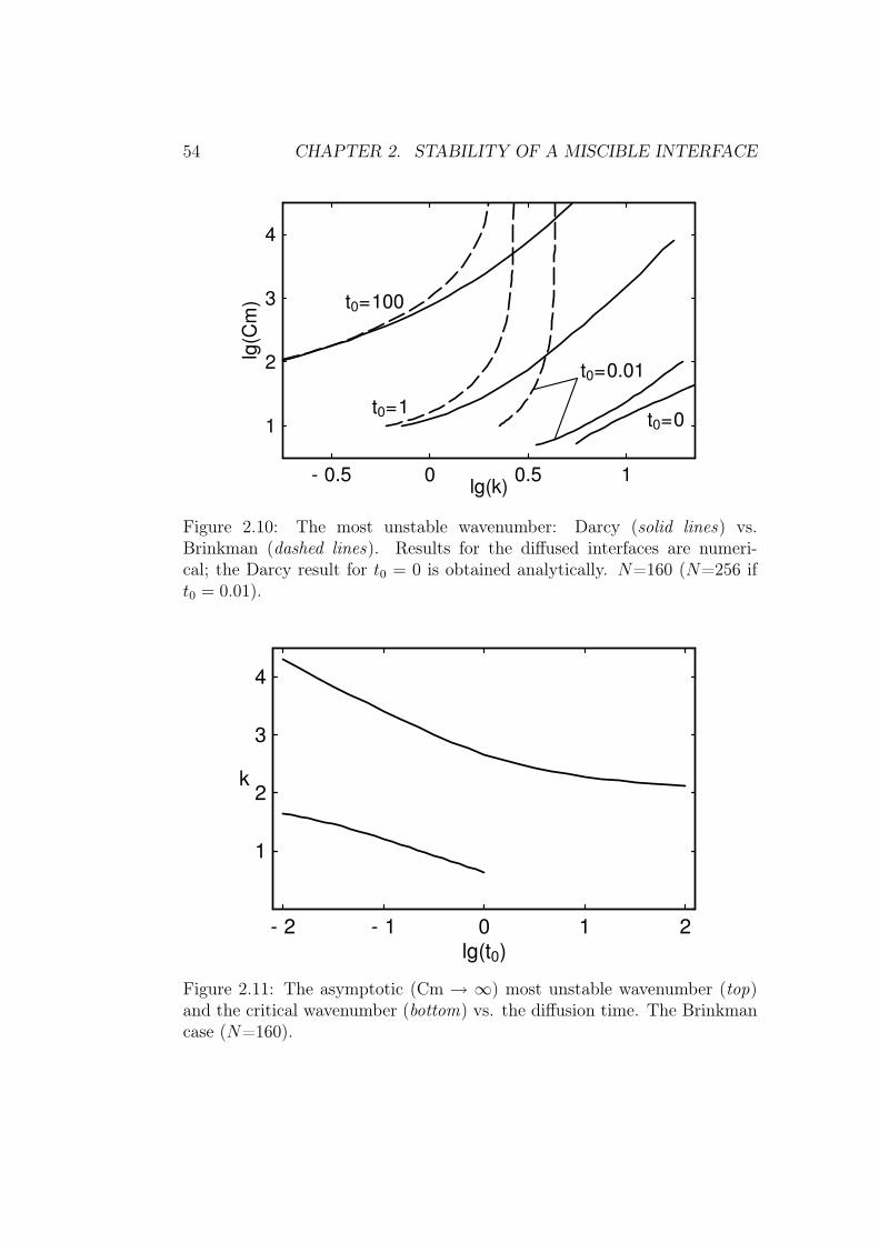
54 CHAPTER 2. STABILITY OF A MISCIBLE INTERFACE
- 0.5 0 0.5 1
1
2
3
4lg
(Cm
)
lg(k)
t0=0
t0=0.01
t0=1
t0=100
Figure 2.10: The most unstable wavenumber: Darcy (solid lines) vs.Brinkman (dashed lines). Results for the diffused interfaces are numeri-cal; the Darcy result for t0 = 0 is obtained analytically. N=160 (N=256 ift0 = 0.01).
- 2 - 1 0 1 2lg(t0)
1
2
3
4
k
Figure 2.11: The asymptotic (Cm → ∞) most unstable wavenumber (top)and the critical wavenumber (bottom) vs. the diffusion time. The Brinkmancase (N=160).

2.3. LABYRINTHINE INSTABILITY 55
λ
- 0.5 0 0.5 1lg(k)
- 3
- 2
- 1
0
lg ––––Cm
t0=0.01
t0=1
t0=100
Figure 2.12: The asymptotic (Cm → ∞) growth increment – wavenumberdependence in the Brinkman case. N=160 (N=256 if t0 = 0.01).
λ
- 1 0 1 2lg(t0)
lg ––––Cm
- 2
- 1
0
Figure 2.13: Variation of the asymptotic (Cm → ∞) increment of the mostunstable mode with the diffusion time t0 in the Brinkman case (solid line,N=160); the 1/t0 apparent scaling (dashed line).

56 CHAPTER 2. STABILITY OF A MISCIBLE INTERFACE
- 0.5 0 0.5 1
1
2
3
4
lg(C
m)
lg(k)
t0=0
t0=0.01
t0=1
t0=100
Figure 2.14: Evolution of the Darcy neutral curves (solid lines) vs. Brinkmanones (dashed lines) as the interface diffuses. The t0 = 0 Darcy curve isobtained analytically (Fig. 2.5). On the t0 = 0.01 curves (N=256), emptycircles denote a stationary mode, while the filled ones stand for an oscillatorypair. The other neutral curves (N=160) correspond to stationary modes.

2.4. PEAK INSTABILITY IN A HELE-SHAW CELL 57
+∞ and erfcx(z)/z ∼ 1/z as z → +0.
As the basic state diffuses out, the critical wavenumber decreases some-what (Fig. 2.11). Fig. 2.14 presents the neutral curves and leads to the follow-ing conclusions about the long-wave perturbations (k < 1). First, it is onlywhen t0 is not small that the inequality ‖d/dx‖≪ 1 holds for the eigenfunc-tions, so that the Brinkman case reduces to the Darcy one. Fig. 2.10 bringsmore evidence to this point. Conversely, when the interface is sharp enough,higher velocity derivatives in Eq.(2.22) (and additional boundary conditionsfor the discontinuous problem) come into play if the Brinkman formulationis employed. Table 2.1 (t0 = 0.01) also exhibits the difference in the numberof modes between the cases. Secondly, Fig. 2.14 demonstrates that the in-terface smearing at an early stage diminishes the stability of the long-waveperturbations. Moreover, they are more unstable for the Brinkman-governedsystem than for the Darcy-governed one, i.e. adding more dissipation reducesstability. This is not impossible, a celebrated example, though distant one,being the inertial instability (governed by the Orr-Sommerfeld equation) ofthe viscous planar Poiseuille flow which is stable in the inviscid limit (bythe Rayleigh’s inflection-point theorem). In the case of the Rayleigh–Taylorinstability with miscible fluids, however, analytical dispersion relations areavailable at t0 = 0 for both Brinkman and Darcy formulations [88], andin the Darcy case the increment appears to be always higher than in theBrinkman case. Finally, we note that the numerically obtained critical Cmfor t0 = 0.01 in the Darcy approximation is somewhat lower than the an-alytically obtained Cmcr for the sharp interface. The possibly destabilizingeffect of the basic-state diffusion at its early rapid phase was also observed,and also with QSSA, in [39, 38] (cf. also Fig. 18 of [87]). The critical Cm –t0 dependence will be shown later (Fig. 2.21).
2.4 The peak instability in a Hele-Shaw cell
In the next four paragraphs,10 we will consider the uniform external magneticfield ~H0 applied in the plane of the cell normally to the interface (along thex-axis, Fig. 2.1). The equations of §2.1 hold, but the gap-averaged density
of the magnetostatic body force ~fm is now given by Eq.(1.26) as
~fm = −m0c~∇∂ψ
∂x, (2.46)
10The results of §2.4.1 were mostly published in [148], the results of §§2.4.2–2.4.4 werepublished as [149]. Besides, all this was presented as [150].

58 CHAPTER 2. STABILITY OF A MISCIBLE INTERFACE
where m0 is the average magnetic moment of a particle along ~H0. (Theparticles are non-interacting.) The gap-averaged potential ψ of the self-
magnetic field of MF ( ~H = ~H0 − ~∇Ψ, ψ =< Ψ >) reads by Eq.(1.25):
ψ = −m0
h
h∫
0
dz
h∫
0
dz′+∞∫
−∞
+∞∫
−∞
∂c(x′, y′)
∂x′dx′ dy′
((x− x′)2 + (y − y′)2 + (z − z′)2)1/2.
(2.47)
2.4.1 Perturbation analysis and a sharp interface in the
normal field
In this paragraph, we undertake the stability analysis for a sharp interfaceunder the normal field. The analysis follows largely the lines of §2.3.1 (and§2.2). We again non-dimensionalize Eqs.(2.2), (2.3), (2.46), and (2.47) intro-ducing h and h2/D as space and time scales, respectively. The concentration,magnetic potential, viscosity, friction coefficient, and pressure are scaled withtheir respective reference values c, cm0h, η, α, and αD. The existing notationis kept for the dimensionless variables.
Let us consider the linear stability of the quiescent state for some con-centration distribution c = c0(x, t0) in the external field ~H0. We again em-ploy the quasi-stationary-state approximation (QSSA) and “freeze” the co-efficients of linearized equations to simplify significantly the analysis. Weintroduce two-dimensional normal modes: c(x, y) = c0(x, t0) + c′(x) eıky+λt,~v = ~v ′(x)eıky+λt, etc. The linearized Eqs.(2.3), (2.46) are
−v′x −dp′
dx− Cm c′
∂2ψ0
∂x2− Cm c0
d2ψ′
dx2= 0 , (2.48)
−v′y − ikp′ − Cm ikc0dψ′
dx= 0 . (2.49)
Expressing v′y by incompressibility from Eq.(2.5) and the pressure perturba-tion p′ from Eq.(2.49), one rewrites Eq.(2.48) as
1
k2
d
dx
[
− 1
12
d3v′xdx3
+
(
k2
12+ 1
)
dv′xdx
]
+1
12
(
d2v′xdx2
− k2v′x
)
− v′x−
Cm
(
c′∂2ψ0
∂x2− ∂c0∂x
dψ′
dx
)
= 0 .
(2.50)
Eq.(2.4) is the linearized equation for the concentration perturbation. From

2.4. PEAK INSTABILITY IN A HELE-SHAW CELL 59
Eq.(2.47) the derivative of the potential follows as
∂ψ
∂x= 2
+∞∫
−∞
+∞∫
−∞
(x− x′)∂c
∂x′J(
√
(x− x′)2 + (y − y′)2)
dx′ dy′ (2.51)
with J(ρ) = (√
ρ2 + 1 − ρ)/
ρ2 . Then the magnetic potential ψ0 induced by
the basic distribution c0(x, t0) is given by
∂ψ0
∂x= 2
+∞∫
−∞
∂c0∂x′
[
2 arctan1
x− x′− (x− x′) ln
(
1 +1
(x− x′)2
)]
dx′ ,
(2.52)so that
∂2ψ0
∂x2= 4π
∂c0∂x
− 2
+∞∫
−∞
∂c0(ξ + x)
∂ξln
(
1 +1
ξ2
)
dξ . (2.53)
The field perturbation is also calculated from Eq.(2.51) as
dψ′
dx= 4
+∞∫
−∞
(x− x′)dc′
dx′J0(x− x′, k) dx′ = 4πc′ + 4
+∞∫
−∞
c′(ξ + x)J1(ξ, k) dξ ,
(2.54)where J1(η, k) = d (ηJ0(η, k))/ dη − πδ(η) is only logarithmically singular,and
J0(ξ, k) =
∫ ∞
0
cos(kζ) J(
√
ζ2 + ξ2)
dζ .
Now we are in position to solve analytically the stability problem fora straight sharp interface if the simpler Darcy law is assumed for the flowinstead of Eq.(2.3). The corresponding version of Eq.(2.50) is recovered byomitting the terms that involve division by 12, while other equations of thisparagraph remain valid.
Let us consider a step-like concentration distribution: ∂c0/∂x = −δ(x).Then Eqs.(2.52), (2.53) immediately give
[
∂ψ0
∂x
]+0
−0
= −4π ,∂2ψ0
∂x2= 4π
∂c0∂x
+ 2 ln
(
1 +1
x2
)
. (2.55)
At the discontinuity of c0 additional conditions hold [cf. Eqs.(2.27)–(2.30) in§2.3.1]. Three of them are the same as in the case of the perpendicular field:the continuity of c′ and v′x and [dc′/dx] = v′x [c0] . Only the condition for the

60 CHAPTER 2. STABILITY OF A MISCIBLE INTERFACE
jump of the pressure differs. It can be derived by integrating Eq.(2.50) overx along the interval (−δ,+δ) and taking the limit δ → 0:
1
k2
[
dv′xdx
]+0
−0
= Cm
(
c′(0)
[
∂ψ0
∂x
]+0
−0
− dψ′(0)
dx[c0]
+0−0
)
. (2.56)
This relation can also be derived as a balance of pressures in the same wayas it has been done for the perpendicular field. If one wishes not to deal withmagnetic forces divergent at the interface where magnetic properties change,the “magnetic pressure” (§5.2 of [14]) can be introduced instead. Indeed,Eq.(5.23) of [14] translated into the CGS units reads [p] = 2πM2
n , where Mn
is the magnetization normal to the interface. Upon linearization and non-dimensionalization we obtain [p′] = 4πCm c′. We also have from Eqs.(2.49),(2.5) at x 6= 0:
p′ = − 1
k2
dv′xdx
− Cm c0dψ′
dx.
Now with Eq.(2.55) we recover Eq.(2.56).The solution of Eq.(2.4) is again simply
c′ = A exp(−sk|x|) , (2.57)
where s =√
1 + λ/k2 as before. Eq.(2.50) at x 6= 0 becomes
1
k2
d2v′xdx2
− v′x = 2ACm exp(−sk|x|) ln
(
1 +1
x2
)
.
The solution of this equation that vanishes at infinity and is continuous atx = 0 reads
v′x = C exp(−k|x|)
− AkCm exp(+k|x|)+∞∫
|x|
exp(−kx′(s+ 1)) ln
(
1 +1
x′2
)
dx′
− AkCm exp(−k|x|)|x|∫
0
exp(−kx′(s− 1)) ln
(
1 +1
x′2
)
dx′ , (2.58)
The boundary conditions on the derivatives of the velocity and concentrationthen give, respectively,
−2Ck − 2Ak2 Cm f (k(s+ 1)) = −4πAk2 Cm + k2 Cmdψ′(0)
dx, (2.59)

2.4. PEAK INSTABILITY IN A HELE-SHAW CELL 61
2As = C − AkCm f (k(s+ 1)) , (2.60)
where f (a) is defined by Eq.(2.36).To obtain a dispersion relation from Eqs.(2.59), (2.60), the field pertur-
bation dψ′(0)/dx must be found from Eq.(2.54):
dψ′(0)
dx= 4A(π + J(s, k)) (2.61)
with
J(s, k) =
+∞∫
−∞
exp(−sk|ξ|)J1(ξ, k) dξ . (2.62)
Then the dispersion relation for the growth increment follows as
s/Cm + J(s, k) + f (k(s+ 1)) = 0 . (2.63)
It yields a single monotonous perturbation mode. After some manipulations,it is possible to obtain the neutral curve in the following form:
1
Cm=π
2+
2
3k− 2 − k2
3K1(k)−
k
3K0(k)+
(
1 − k2
3
)
Ki1 (k)− f (2k) , (2.64)
where K0 is the Macdonald function (2.20),
Ki1 (k) =
∫ ∞
k
K0(t)dt ,
and K1 = −K0′
. The neutral curve is shown in Fig. 2.15. For k → 0 it maybe expanded as
1
Cm= k(5
2− γ − ln (8k) +O(k)
)
. (2.65)
This approximation becomes unsatisfactory at k ≈ 0.3 already where itfalsely predicts a minimum (Fig. 2.15). For k → ∞ the neutral curve behavesasymptotically as follows:
1
Cm∼ π
2+
1
k
(
2
3− γ − ln(2k)
)
. (2.66)
The critical field is Cmcr = 2/π. Our dispersion relation and neutral curveshould be compared against that of [112] for the case of porous media,which at zero displacement read 2s2 = Cm + 1 −
√1 + 2 Cm = inv(k) and
Cm = 4 = inv(k), respectively. Nevertheless the critical Cm’s are compara-ble. Despite the finite thickness of the Hele-Shaw cell, the critical wavenum-ber is infinite. This indicates of course that at small scales our analysis
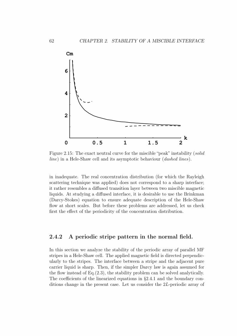
62 CHAPTER 2. STABILITY OF A MISCIBLE INTERFACE
0.5 1 1.5 2k
2
4
6
Cm
0
Figure 2.15: The exact neutral curve for the miscible “peak” instability (solidline) in a Hele-Shaw cell and its asymptotic behaviour (dashed lines).
in inadequate. The real concentration distribution (for which the Rayleighscattering technique was applied) does not correspond to a sharp interface;it rather resembles a diffused transition layer between two miscible magneticliquids. At studying a diffused interface, it is desirable to use the Brinkman(Darcy-Stokes) equation to ensure adequate description of the Hele-Shawflow at short scales. But before these problems are addressed, let us checkfirst the effect of the periodicity of the concentration distribution.
2.4.2 A periodic stripe pattern in the normal field.
In this section we analyze the stability of the periodic array of parallel MFstripes in a Hele-Shaw cell. The applied magnetic field is directed perpendic-ularly to the stripes. The interface between a stripe and the adjacent purecarrier liquid is sharp. Then, if the simpler Darcy law is again assumed forthe flow instead of Eq.(2.3), the stability problem can be solved analytically.The coefficients of the linearized equations in §2.4.1 and the boundary con-ditions change in the present case. Let us consider the 2L-periodic array of

2.4. PEAK INSTABILITY IN A HELE-SHAW CELL 63
- 1.5 - 1 0 0.5
0
1
2
3
lg k
lg Cm
Figure 2.16: The neutral curves for the instability of the periodic array ofsharp stripes in the Darcy flow. Dotted lines : L = 2, l = 1; dash-dottedlines : L = 10, l = 1; dashed lines: L = 10, l = 5; solid line (from Fig. 2.15):L→ ∞, l → ∞.
stripes, the stripe width being 2l (l < L). Then
∂c0∂x
=+∞∑
m=−∞
[δ(x− 2mL+ l) − δ(x− 2mL− l)] ,
which, according to Eq.(2.53), gives
∂2ψ0
∂x2− 4π
∂c0∂x
= −2 lnΦ(x+ l)
Φ(x− l),
where Φ(y) = 1 + sinh2(π/(2L))/
sin2(πy/(2L)) .With the exception of the magnetic potential, whose perturbation ψ′
needs to be evaluated numerically through an infinite sum, the due pro-cedure is much the same as in the previous paragraph. Writing down generalsolutions of linear homogeneous Eqs.(2.50), (2.4) for every domain where c0is constant, one makes use of the jump conditions and periodicity to obtaina linear algebraic system for the amplitudes of eigenmodes. The dispersionrelation follows as the zero determinant of this system. Lengthy details ofthis straightforward derivation are omitted. The resulting dispersion relationis of the form F (s,Cm, k, L, l) = 0, where s =
√
1 + λ/k2. In fact, F is poly-nomial in Cm, which facilitates finding the roots of the dispersion relation.As common [15] for the problems with the self-magnetic field, a kind of “reci-procity” relation holds: F (s,Cm, k, L, l) = F (s,Cm, k, L, L− l), i.e. inverting

64 CHAPTER 2. STABILITY OF A MISCIBLE INTERFACE
- 1.5 - 1 - 0.5 0.5 1lg k
1
2
3
4
0
lg Cm
Figure 2.17: The neutral curves for the instability of the periodic array ofnarrow (l = 0.1) sharp stripes in the Darcy flow. Dotted lines : L = 0.2;dashed lines: L = 2; solid lines : L = 10.
the underlying stripe pattern (MF ↔ non-MF) does not change the flow andits stability. Indeed, for an arbitrary concentration distribution c(x, y), theformal change of sign and the shift by a constant (here c) together modifyour initial Eqs.(2.3), (2.46), (2.47), and (2.2) only insignificantly. (The mod-ification consists in the addition to the pressure that further drops out bothfrom the equations and from the jump conditions.)
Computing the neutral curves (ℜeλ = 0), we found no oscillatory neutralmodes, so that the “exchange of stabilities” takes place at the threshold. Forall values L, l that we tried, the neutral curves appear to have two branches.The upper branch corresponds to the undulation (bending) mode, in whichthe perturbed velocity at the opposite edges of each stripe is of the samedirection. The critical mode is the “peristaltic” one, in which the edges of astripe spread away in the opposite directions or move toward one another.As l increases (along with L), the mutual influence of the edges vanishes.Therefore, at l → ∞ the branches converge (the higher the wavenumber k,the faster) to the neutral curve for the instability of the sharp discontinuityobtained in the preceding paragraph. At fixed L, l the convergence also seemsto be the case as k → ∞ (Figs. 2.16, 2.17). In fact, since we evaluated thedispersion relation only approximately, it cannot be excluded that at somepoint the two modes fully coalesce into a single one.
We note in conclusion that in the periodical stripe pattern a second per-turbation mode exists. This peristaltic mode becomes unstable at finite (andrather low) Cm values even in the limit of large wavelength (Figs. 2.16, 2.17).
A comparison of several sharp-interface neutral curves obtained in the
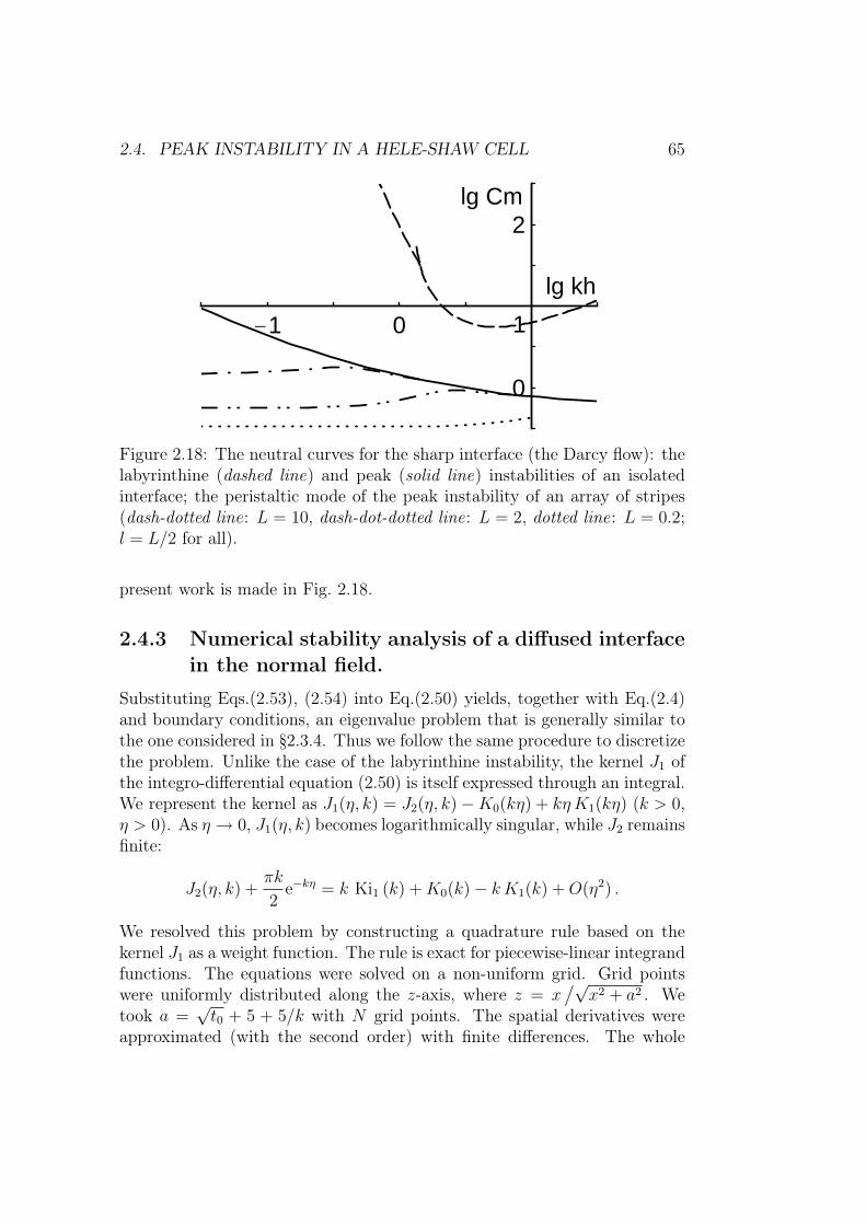
2.4. PEAK INSTABILITY IN A HELE-SHAW CELL 65
-1 0
0
2
1
lg Cm
lg kh
Figure 2.18: The neutral curves for the sharp interface (the Darcy flow): thelabyrinthine (dashed line) and peak (solid line) instabilities of an isolatedinterface; the peristaltic mode of the peak instability of an array of stripes(dash-dotted line: L = 10, dash-dot-dotted line: L = 2, dotted line: L = 0.2;l = L/2 for all).
present work is made in Fig. 2.18.
2.4.3 Numerical stability analysis of a diffused interface
in the normal field.
Substituting Eqs.(2.53), (2.54) into Eq.(2.50) yields, together with Eq.(2.4)and boundary conditions, an eigenvalue problem that is generally similar tothe one considered in §2.3.4. Thus we follow the same procedure to discretizethe problem. Unlike the case of the labyrinthine instability, the kernel J1 ofthe integro-differential equation (2.50) is itself expressed through an integral.We represent the kernel as J1(η, k) = J2(η, k) −K0(kη) + kη K1(kη) (k > 0,η > 0). As η → 0, J1(η, k) becomes logarithmically singular, while J2 remainsfinite:
J2(η, k) +πk
2e−kη = k Ki1 (k) +K0(k) − kK1(k) +O(η2) .
We resolved this problem by constructing a quadrature rule based on thekernel J1 as a weight function. The rule is exact for piecewise-linear integrandfunctions. The equations were solved on a non-uniform grid. Grid pointswere uniformly distributed along the z-axis, where z = x
/√x2 + a2 . We
took a =√t0 + 5 + 5/k with N grid points. The spatial derivatives were
approximated (with the second order) with finite differences. The whole

66 CHAPTER 2. STABILITY OF A MISCIBLE INTERFACE
- 1 - 0.5 0 0.5 1lg k
1
2
3
4
lg Cm
Figure 2.19: The neutral curves for the instability of the originally step-like concentration distribution in the Brinkman flow (solid lines, t0 = 0.03;0.1; 0.3; 1; 3; 10; 30 bottom to top) and in the Darcy flow (dashed lines,t0 = 0.03 for the upper curve, t0 = 0 for the lower analytical one repeatedfrom Fig. 2.15).
- 1 - 0.5 0 0.5 1lg k
1
2
3
4
lg Cm
Figure 2.20: The neutral curves for the instability of the Gaussian concen-tration distribution in the Brinkman flow. Right to left: t0 = 0.03; 0.1; 0.3;1; 3; 10; 30.

2.4. PEAK INSTABILITY IN A HELE-SHAW CELL 67
-2 -1 10
1
2
lg t0
lg Cm
Figure 2.21: The critical Cm number as the basic concentration distributiondiffuses out in the Brinkman flow: the labyrinthine (dashed line) and peak(solid line) instabilities of a single initially step-like interface c1(x); the peakinstability of a Gaussian stripe c2(x) (dash-dotted line).
spectrum of the algebraic system for a given (k, Cm) pair was obtained bya standard eigenvalue finder. Since eigenfunctions of the discrete spectrumare required to vanish at infinity, numerical real eigenvalues λ ≤ −k2 must bediscarded [see §2.2, Eqs.(2.4), (2.33)]. In many cases several valid eigenvalueswere obtained. However, we traced only the highest (dominant) one. All theresults presented correspond to N = 512 but were checked against the changein resolution.
We did the numerical stability analysis for two basic concentration distri-butions c0(x, t0): c1 = 0.5 erfc (0.5x/
√t0) and c2 = exp (−0.25x2/ t0), where t0
is the time elapsed since the distribution was step-like or delta-function-like,respectively. Both distributions are normalized by the maximum concentra-tion value, which for the Gaussian one (c2) implies a progressive scaling downof the Cm number as the diffusion process evolves. Generally, t0 in our analy-sis may just parametrize a family of instantaneous “frozen” distributions thatnot necessarily result from the diffusion of a definite initial one. The casesexplored include t0 = 0.03; 0.1; 0.3; 1; 3; 10; 30 with 17 k values withinthe range 0.05 . . . 20 and 18 Cm values such that 4πt0 Cm ranged from 0.2to (1 × 10⁵). (For t0 = 10, 30 additional series of computations with higherCm numbers were undertaken as well).
For both concentration distributions the dominant normal mode wasfound to be stationary. The neutral curves of the instability are plotted

68 CHAPTER 2. STABILITY OF A MISCIBLE INTERFACE
- 0.5 0 0.5lg k
1
2
3
4
5
- 1
lg Cm
t0=30
t0=1
t0=0.03
Figure 2.22: The Cm dependence of the most unstable wavenumber for theinitially step-like concentration distribution (solid lines) and for the Gaussianone (dashed lines) in the Brinkman flow. Black circles correspond to λ = 10.
- 1.5 - 1 - 0.5 0.5 1 1.5lg t0
- 1
- 0.5
0.5
0
lg k
Figure 2.23: The most unstable wavelength at infinite Cm (top) and the crit-ical wavelength (bottom) for the initially step-like concentration distribution(solid lines) and for the Gaussian one (dashed lines) at various t0 values inthe Brinkman flow.

2.4. PEAK INSTABILITY IN A HELE-SHAW CELL 69
- 1.5 - 1 - 0.5 0.5 1 1.5lg t0
- 3
- 2
- 1
0
lg λ /Cm
Figure 2.24: The asymptotic (Cm → ∞) value of the λ/Cm ratio for theinitially step-like (solid line) and Gaussian (dashed line) concentration dis-tributions in the Brinkman flow.
in Figs. 2.19, 2.20 for the originally step-like concentration distribution andfor the Gaussian one, respectively. Along with the curves for the Brinkmanflow at various t0 values, two neutral curves for the Darcy flow are also plot-ted in Fig. 2.19: the one obtained analytically in §2.4.1 for t0 = 0 and thenumerical one for t0 = 0.03. These curves demonstrate that numerical resultsare consistent with earlier analytic findings. Besides, the Darcy critical Cmnumbers are just a little lower than the Brinkman ones. In the rest of theSection we will consider the Brinkman flow only. The critical Cm numbersprovided by Fig. 2.21 generally increase as the concentration gradients getsmoother (even though their amplitude is fixed). Therefore, to verify experi-mentally the onset of convection, it may be appropriate to switch on the fieldas soon as the desired distribution develops and not earlier. The Gaussiandistribution proves to be less stable than the c1 one for all t0’s tried. TheCm dependence of the most dangerous wavenumber is presented in Fig. 2.22.As Cm increases, the most unstable wavelength tends to the limit of severalgap widths, as summarized in Fig. 2.23. While being typical for the mi-croconvection in a Hele-Shaw cell, such behaviour is not reproduced by theDarcy law (see §2.3.4). It should be noted that the limiting (“saturation”)wavelength is almost the same for both distributions and weakly dependson t0. The growth increment λ increases along the curves (upwards) plot-ted in Fig. 2.22. Their lower end-points correspond to λ = 0 (and thus tothe minimum of the neutral curves in Figs. 2.19, 2.20). Since the validityof QSSA improves as the instability growth rate increases, the Cm numbersthat correspond to λ = 10 are also given in Fig. 2.22. For large Cm the

70 CHAPTER 2. STABILITY OF A MISCIBLE INTERFACE
increment of the most unstable wavenumber is asymptotically linear in Cm.This indicates that the proper time scale of the problem becomes h2/(CmD)(p. 43). The limit of the λ/Cm ratio is given in Fig. 2.24.
2.4.4 A comparison to FRS experiments
In the FRS case the developed models concern the situation when the ther-mal variations have relaxed already after the light source was switched off.Though thermodiffusion is no longer in action, the concentration structureis still present, because it requires much longer time to vanish [106]. Notethat only the experiment [3] specifically concerned the convection in the FRSsetup. We begin with discussing other cases, where the instability was nei-ther sought nor detected; its presence can now be judged upon by evaluatingthe corresponding Cm number. As for t0 for the diffused distributions, it willbe taken to be unity, since the pattern period is comparable to h.
Let us estimate the maximum Cm number attained in works [2, 103].The magnetization of the particle material (maghemite) is MS = 4 × 10² G,while the magnetic radius of particles is am = 6 nm. In the highest fieldH0 = 1.4 × 10³ Oe used, the magnetization of such paramagnetic colloidbecomes almost saturated. The diffusion coefficient D of particles of thehydrodynamic radius ah = 15 nm may be found by the Einstein–Stokesformula. Then, if the average MF concentration cav is substituted for c inthe Cm definition (p. 34), for the colloid of the volume fraction ϕav = 0.09in a h = 0.01 mm thick cell one obtains Cm = 7 × 10⁴.
However, it is the concentration modulation (and not cav) that is respon-sible for the instability. The concentration difference δc between the darkand bright fringes in the developed grating was in fact introduced above asc and may differ considerably from the average concentration; unfortunately,it was not measured [2, 103]. Nevertheless it may be estimated consideringthe preceding stage of the FRS experiment. Refs. [147, 151, 106] analyze thissteady-state regime, when the light source is still on, and the non-uniformheating sustains the concentration pattern through thermodiffusion (assum-ing the absence of any convection at this stage). In particular, in these worksthe amplitudes of the spatial Fourier modes of the temperature are derived inthe framework of the two-timescale model. In our case the formulas for thefirst mode of the time-averaged temperature T0 would be T0 = θ cos qx+constwith
θ =2I[1 − exp(−aph)]
Sh(q2χ+ ρcp/τ0)
where I is the average power of the pumping laser, S is the overall area of theperiodic interference pattern, q = 2π/Λ, Λ is the fringe pattern period, ap,

2.4. PEAK INSTABILITY IN A HELE-SHAW CELL 71
χ, ρ, and cp are the MF absorption coefficient, thermal conductivity, density,and specific heat capacity, respectively. (At 532 nm ap/ϕ = 2 × 104 cm−1
[152], so for exp(−aph) ≪ 1 the constant mean value at ϕ = ϕav may beused.) The τ0 constant is the characteristic time of the thermal decay due tothe heat flux through the walls. Since in the steady state the net diffusive fluxis zero, we have dϕ0/dx = −S∗
Tϕ0 dT0/dx, where the Soret coefficient S∗T is
employed. Integrating this relation between the adjacent minimum and max-imum, one derives the variation of the relative volume fraction as δϕ/ϕav =2 sinh (|S∗
T|θ)/ I0 (|S∗T|θ), where I0 is the modified Bessel function of the first
kind. Substituting I ≤ 0.2 W, S = 3 × 10⁻⁷ m2, and Λ = (2 . . . 6.5) × 10−5 m[2, 103], τ0 = 1.9 × 10⁻⁴ s [152], S∗
T = −9 × 10⁻² K−1 [153] and taking χ,ρ, and cp values to equal those of water, we obtain θ = (1.5 . . . 4) K andδϕ/ϕav = 0.3 . . . 0.7. This corresponds to Cm = (0.5 . . . 4)× 104.
Then from Fig. 2.21 it may be inferred that the instability indeed developsin the circumstances of the FRS experiment [2, 103] as soon as the pumpingis switched off. However, the microconvection intensifies mixing and thusdestroys the concentration inhomogeneity that feeds the instability. Thoughthe non-linear stage of the process in the periodical concentration structureis unclear, it is possible that having disturbed the original structure, themicroconvection vanishes soon after its onset (similar to what was observedin [1]). Subsequently, only the diffusion is in operation, which could havehindered the identification of the convection phenomenon. We remind thatRefs. [2, 103, 154] attributed the increase of the diffusion coefficient in theapplied magnetic field solely to the transport effects. It should be noted alsothat convection may be in fact essentially three-dimensional, so that our 2Dapproach cannot describe it correctly. Anyway, the convective instability,if present, impacts the FRS measurements of the diffusion coefficient in theapplied magnetic field. The onset of the threshold convection will be probablymarked by a break on the Deff(H0) (effective diffusion coefficient – appliedfield) curve, which makes more detailed measurements desirable.
The Cm number was much lower in the experiment [105], mostly owing toa less powerful light source. For the MF magnetization of 7.8 G, ϕ = 2.14%,h = 0.1 mm, D = 6.1 × 10⁻¹¹ m2/s, η = 4.2 × 10⁻⁴ kg/(m s) (toluene at50C), and δϕ = 0.126% (also found [105, 155] from the two-timescale model)we have Cm = 7 × 10². Still this value probably exceeds the critical one.
Let us also estimate the Cm number attained in [1], where an instabilitywas observed directly at a diffusion front in the normal field. Given h =0.1 mm, H0 = 200 Oe, and ϕMS = 10 G and substituting reasonable guessesfor the missing values am = 5 nm, ah = 8 nm, and MS = 500 G, one obtainsCm = 4 × 10⁴. This value is indeed high enough for the instability to develop.
Finally, we turn to a very recent FRS experiment [3, 108], where a con-

72 CHAPTER 2. STABILITY OF A MISCIBLE INTERFACE
vection is detected in the field parallel to the temperature gradient while thelight source is on. The temporal behaviour of the intensity of the diffractedpattern cannot be explained by diffusive processes alone. In particular, inthe steady-state regime the intensity is observed to fluctuate about a meanvalue. The results [3] are presented in terms of the magnetic solute Rayleighnumber Rm = 48π(L/h)2 Cm/µ, where µ is the permeability (we will takeµ = 1), and the variation of the diffusion coefficient with the field is ne-glected. At 2L = 3 × 10⁻³ cm and h = 1 × 10⁻² cm, the observed criticalRm ≈ 1.7 translates into Cm ≈ 0.5. This value is in a remarkably goodaccordance with our prediction (the dotted line in Figs. 2.17, 2.18) despitethe fact that temperature inhomogeneities are not allowed for in our model.To our knowledge, this experiment is the only one that provides a directquantitative test for our theory.

Chapter 3
The Saffman–Taylor instability
with immiscible ferrofluids
3.1 The free-boundary problem
3.1.1 The context of the problem
The phenomenon of viscous fingering in a Hele-Shaw cell became widelyknown thanks to the classical paper by Saffman and Taylor [10]. We are notgoing to present the overview of this vast field [156, 157, 30, 158, 11, 159],mentioning only the basic facts. In [10], as a less viscous fluid displaced amore viscous one, the former was observed to penetrate the latter taking on,in the plane of the cell, the shape of a finger. The finger shape was registeredfor several fluid pairs; as the surface tension (the reverse capillary number)tended to zero, the finger width was observed to decrease approaching onehalf of the cell width. The asymptotic shapes observed at a small surfacetension were found to fit closely the analytically obtained solution, providedone substitutes 1/2 for the relative width of the finger. The analytical solu-tion at zero surface tension (Eq.(3.35)) involves the relative finger width λ asan undetermined parameter. Many other exact solutions are known at zerosurface tension, e.g. [160], but this problem is ill-posed and some solutionsbecome singular in finite time. (Few known exact solutions for a non-zerosurface tension describe quite artificial flows, e.g. [161].) The surface tensionregularizes the problem in the sense that, e.g., at a finite capillary number Ca(defined on p. 79), the amplitude of the disturbance required for a secondaryinstability of the tip of the finger is ∼ exp(−
√Ca · const) ([11], §IX.6). How
and why does a small but non-zero surface tension select the λ = 1/2 shapefrom all other? The problem attracted an extreme interest in 1980’s, andtremendous mathematical and experimental effort was exerted in order to
73

74 CHAPTER 3. ST INSTABILITY WITH AN IMMISCIBLE MF
understand the “selection” problem. In the work [162], the problem of widthselection by surface tension was addressed along with the issue of stability ofsteady fingers. For steady-state ST fingers with surface tension a system ofnon-linear integro-differential equations was obtained which allowed to finda unique finger width for any given surface tension. (Later it turned outthat in fact, there is a discrete set of solutions, but other ones are unsta-ble. It is also noteworthy that the analysis in [162] of the finger stabilitywas inconclusive.) The solvability condition for the equations of McLean &Saffman gave a mathematical understanding of how a shape gets selected atsmall surface tensions (§§VIII.2–VIII.4 of [11]). The main complication inthe selection problem is that apparently small effects are not negligible andlead to a qualitatively different behaviour. Analytically, it turned out thatexponentially small terms are of primary importance in certain asymptoticexpansions (“asymptotics beyond all orders”). This is the reason why manyearlier analytic attempts failed (cf. the “undetected inconsistency” in [162],etc.). The surface tension, however small it be, is crucial for the selectionsince it comes with interfacial curvature and is a singular perturbation (astructurally unstable problem). A classical analogue, also from fluid me-chanics, is the relation between viscous and inviscid flows as distinguishedby viscosity that comes with higher velocity derivatives. Experimentally, fin-gers were observed to undergo some instabilities such as tip-splitting and tobe “pathologically” sensitive to various artificial perturbations, transforminginto strikingly beautiful patterns. Thus, fractal patterns were obtained at theviscous displacement of non-Newtonian fluids, both miscible and immiscible[163, 164, 165]. These examples are particularly relevant to our case sincewe also study a “complex fluid.”
The immiscible Hele-Shaw flow with magnetic fluids under the influenceof the perpendicular magnetic field was extensively analyzed and modelled byA. Cebers with collaborators. Their first work on the subject [166] developsa so-called boundary-integral formulation of the problem for an MF dropletconfined in a Hele-Shaw cell. The method was applied [166, 167, 168] to theanalysis of the over-extension (i.e. peristaltic) and bending (i.e. undulation)instabilities of MF drops as well as multi-lobe shapes. The treatment ofthe integral terms describing magnetic interactions was improved in [168].These and some other numerical results are accumulated in §4.7 of [15]. Fora later work, see [169], where modelled was vertex-splitting and a long-timebehaviour of a drop similar to the rearrangement of the Steiner trees, and[170]. Rising bubbles in a vertical Hele-Shaw cell filled with a ferrofluid weresimulated by the algorithm e.g. in [171]. However, these works dealt withthe radial geometry (for experimental results, see e.g. [172]). In [173], asingle MF stripe was modelled, and its undulations and side-branching were

3.1. THE FREE-BOUNDARY PROBLEM 75
obtained. The rupture of a MF layer in a vertical cell was simulated in [174].Of interest to us is the rectilinear geometry that was modelled in [175, 176].Our treatment of magnetic terms (§3.1.5) will be quite close to that of [175],which, in its turn, was adapted from [168]. Tip-splitting under artificialperturbations was studied in [175]. In [176] a longer magnetic Saffman–Taylor finger was simulated as well as a branched structure.
Now let us mention very briefly the analyses of the labyrinthine instabilityand related issues (for a general presentation, see §4.6 of [15]). In [177], thethreshold of instability was obtained. In [178], a variational formalism isdeveloped for the dynamics of dipolar domains. In [179], a weakly non-linear analysis of the viscous fingering with MF’s in a perpendicular fieldwas undertaken, while in [100], the Kelvin–Helmholtz instability in a Hele-Shaw cell is addressed and some other results are summarized. In [6], theimportant notion of the effective surface tension (p. 133) is overviewed.
All the above research on the immiscible Hele-Shaw flow with ferrofluidswas undertaken for the magnetic field perpendicular to the cell, in which “per-pendicular” configuration a labyrinthine instability was known to be possiblesince mid-1970’s. Of the three physically selected mutually perpendicularorientations of the magnetic field, the one tangential to the straight interfaceand parallel to the cell is known to be stabilizing (e.g. [100], or Refs. 6, 7of [175]). The other potentially destabilizing configuration is the “normal”one, when the field is directed parallel to the cell, but normally to the inter-face line. Then a (Hele-Shaw version of the) peak pattern can be observed[180, 7, 181]. The interface dynamics in this case has not yet been simu-lated. In the present work, we report such preliminary simulations for thefirst time. The study of the normal-field instability will be deferred to §3.4,and we begin with the perpendicular configuration.
However, a systematic study of the immiscible labyrinthine instability ina rectilinear geometry is also lacking. In this second half of our work, we willdevelop the approach of the above-cited work [176]. It requires elaboration(e.g., in terms of accuracy) and extension to enable the computation of richlybranched, highly ramified in the long run “dendritic” structures.
The latter motivation emerges in the light of the new experimental data[12, 7, 181]. In [12], the Rayleigh–Taylor instability was explored in theperpendicular field. A comparison of the observed near-critical (in the senseof stability) behaviour to the linear stability theory was undertaken. Somereported [12] features of the far-from-threshold pattern will be commentedupon in §3.3.2. In [7], the viscous fingering with ferrofluids was investigatedin both perpendicular and normal configurations, and the relative width ofthe magnetic ST finger was measured (in the perpendicular case). Finger-like patterns will be simulated in §3.3.1. For further details about these

76 CHAPTER 3. ST INSTABILITY WITH AN IMMISCIBLE MF
experiments, we refer the reader to these original works [12, 7]. To be closein our simulations to the experimental conditions, let now us estimate therelevant values of the dimensionless parameters. (For their definitions, seep. 79 and p. 84 later). For the Saffman–Taylor experiment [12, 181], the Hele-Shaw cell used was T = 2 cm wide and its gap was h = 0.1 cm thick. Themagnetic Bond number Bm was of the order of unity. MF of the dynamicviscosity coefficient η2 = 0.35 g/(cm · s) was displaced by air of a negligibleviscosity ∼ 10−3η2, so that At = 1. The surface tension at the interface wasevaluated to be σ = 60 g/s2. Then the flow rate Q = u0hT of 600 ml/hcorresponded to Ca ≈ 12u0η2/σ = 7/120. Experiments were done in therange of flow rates (0.1 . . . 10)Q, i.e. Ca did not exceed unity there. As forthe Rayleigh–Taylor experiments [7, 181], T = 14 cm, h = 5 × 10⁻² cm.An MF of the dynamic viscosity coefficient η2 = 1.4 g/(cm · s) and densityρ2 = 1.7 g/cm3 rests on top of white spirit, whose viscosity is η1 = η2/140,and density is ρ1 = 0.8 g/cm3. Therefore 1 − At ≈ 2η1/η2 ≈ 1.4 × 10⁻².Besides, taking into account the surface tension at the interface, σ = 12 g/s2,one obtains the gravitational Bond number as Bg ≈ 0.18 (we will use laterthe value 3/16). The magnetization curve presented in Fig. 3.4 of [181] allowsto determine that at the external field of 23 kA/m the MF magnetizationwas about 21 kA/m (21 G), while at 40 kA/m it becomes M = 24 kA/m(24 G). (By the way, these values question the validity of our approximationof a magnetization negligibly small with respect to the applied field.) Thiscorresponds to the magnetic Bond numbers Bm = 3.675 and 4.8, respectively.
3.1.2 Formulation of the problem
Consider a vertical Hele-Shaw cell filled with two fluids (Fig. 3.1).1 Each ofthem may be magnetic. The cell is supposed infinite in both directions. Letus reference the two fluids by an index i. Their viscosity, density, and mag-netization are denoted by ηi, ρi, and Mi, respectively. As with the misciblefluids, we may describe the gap-averaged flow in a cell of the thickness h bythe Darcy law or by the Brinkman equation. The latter option, however, willnot be explored in this Chapter, as it complicates the problem substantially.In each fluid, the Darcy law reads:
−~∇p− αi(~v + ~u0) + ρi~g + ~fm = 0 , (3.1)
where p is the pressure, αi = 12ηi/h2 is the friction coefficient, ~u0 is the
constant injection velocity at infinity relative to the cell walls, ~v is the velocityin the reference frame moving with ~u0, and ~g is the free-fall acceleration.
1Please observe that we interchange the x and y axes relative to the previous definition.
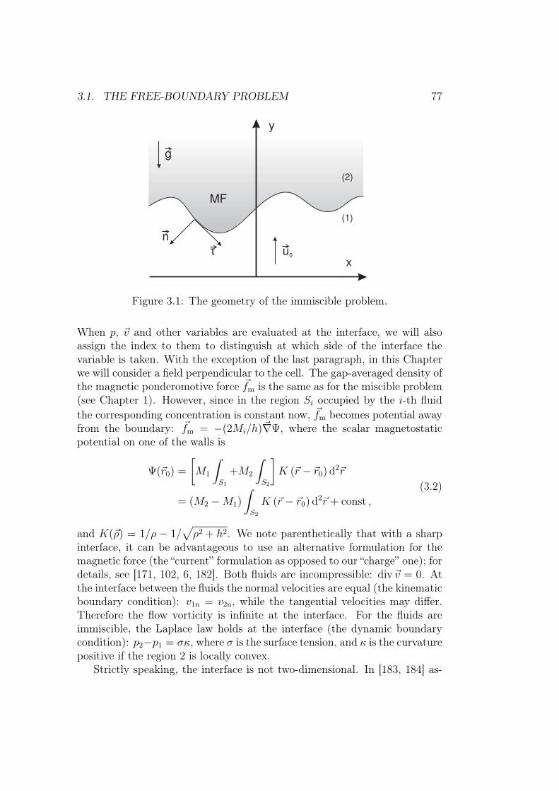
3.1. THE FREE-BOUNDARY PROBLEM 77
x
y
τn
(1)
(2)
g
u0
MF
Figure 3.1: The geometry of the immiscible problem.
When p, ~v and other variables are evaluated at the interface, we will alsoassign the index to them to distinguish at which side of the interface thevariable is taken. With the exception of the last paragraph, in this Chapterwe will consider a field perpendicular to the cell. The gap-averaged density ofthe magnetic ponderomotive force ~fm is the same as for the miscible problem(see Chapter 1). However, since in the region Si occupied by the i-th fluid
the corresponding concentration is constant now, ~fm becomes potential awayfrom the boundary: ~fm = −(2Mi/h)~∇Ψ, where the scalar magnetostaticpotential on one of the walls is
Ψ(~r0) =
[
M1
∫
S1
+M2
∫
S2
]
K (~r − ~r0) d2~r
= (M2 −M1)
∫
S2
K (~r − ~r0) d2~r + const ,
(3.2)
and K(~ρ) = 1/ρ − 1/√
ρ2 + h2. We note parenthetically that with a sharpinterface, it can be advantageous to use an alternative formulation for themagnetic force (the “current” formulation as opposed to our “charge” one); fordetails, see [171, 102, 6, 182]. Both fluids are incompressible: div~v = 0. Atthe interface between the fluids the normal velocities are equal (the kinematicboundary condition): v1n = v2n, while the tangential velocities may differ.Therefore the flow vorticity is infinite at the interface. For the fluids areimmiscible, the Laplace law holds at the interface (the dynamic boundarycondition): p2−p1 = σκ, where σ is the surface tension, and κ is the curvaturepositive if the region 2 is locally convex.
Strictly speaking, the interface is not two-dimensional. In [183, 184] as-

78 CHAPTER 3. ST INSTABILITY WITH AN IMMISCIBLE MF
ymptotic boundary conditions at the immiscible interface in a Hele-Shawcell were derived that took into account the film of a viscous fluid that isleft during the displacement at the walls, and the transverse variations of themeniscus shape. According to this theory, owing to the meniscus, σ shouldhave been replaced with (π/4)σ plus a presumably constant term [10]. How-ever, since the reference experiments [7, 181, 12, 180] are conducted withprewetted cell walls and surface tension was measured in situ there in a cer-tain way, we will assume that σ is already rescaled, and ignore other effectsdue to the contact angle being dependent upon the displacement velocity,etc.
Then from (3.1) it is obvious that the Saffman–Taylor and Rayleigh–Taylor problems for a vertical cell are identical in the Hele-Shaw approxima-tion and transform one into another by substitution ρi~g ↔ −αi~u0. The flowis unbounded but we demand that it is periodic in the lateral direction (i.e.perpendicularly to ~u0), the period being T (T ≫ h). Note that owing to the
non-locality of ~fm, the stated problem is different from that of a laterallybounded flow, while for non-magnetic fluids one problem is typically substi-tuted by the other. The issue of the horizontally bounded cell will be touchedin §3.1.5. The Hele-Shaw flow with the magnetic ponderomotive force (3.1)was first studied by Cebers [101].
As in the miscible problem, the gap-averaged magnetic force translatesthe transverse dimension h through the length scale of the magnetic forceinto the 2D problem. Now we will render the problem dimensionless by in-troducing h and h3(α1 + α2)/σ as length and time scales, correspondingly.The time scale is characteristic for the relaxation of an interfacial perturba-tion of dimension h by the surface tension alone. If a viscosity difference,buoyancy, or magnetic effects dominate, then thus non-dimensionalized timescan be far from unity for a physically selected phase of the process (e.g. whennon-linear effects come into play, etc.). Other choices for the scales are alsopossible and are used in the literature, but neither of them is universally con-venient and physical in every limit. For example, at studying the “dendriticstructures” (§3.3), whose scale is much less than T , it is reasonable not tointroduce T into the dimensionless parameters that will enter the equations.Quite similar solutions may be expected for the dendritic problems that indimensional variables differ only in the value of the imposed period T , andthis similarity should remain evident in the dimensionless formulation. Tonon-dimensionalize the “dynamical” variables containing the unit of mass,we use the surface tension that is almost always required anyway to regu-larize the problem (see §3.2.1). Then we arrive at the following equation in
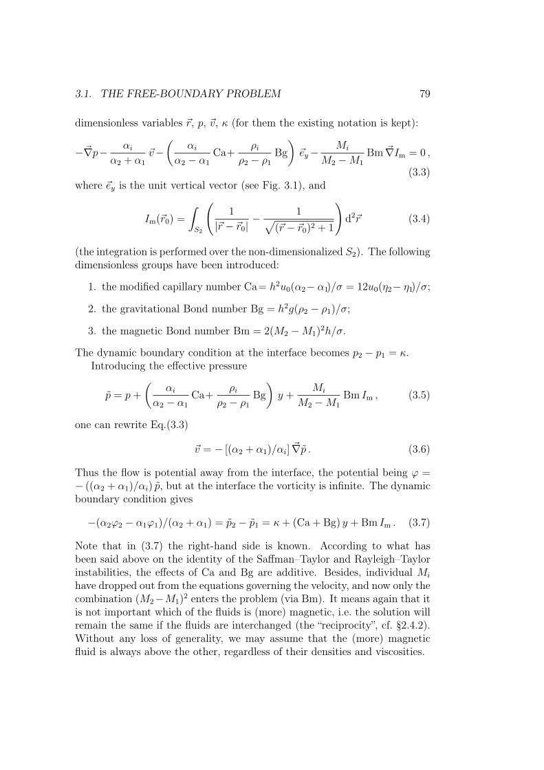
3.1. THE FREE-BOUNDARY PROBLEM 79
dimensionless variables ~r, p, ~v, κ (for them the existing notation is kept):
−~∇p− αi
α2 + α1
~v−(
αi
α2 − α1
Ca+ρi
ρ2 − ρ1
Bg
)
~ey −Mi
M2 −M1
Bm ~∇Im = 0 ,
(3.3)where ~ey is the unit vertical vector (see Fig. 3.1), and
Im(~r0) =
∫
S2
(
1
|~r − ~r0|− 1√
(~r − ~r0)2 + 1
)
d2~r (3.4)
(the integration is performed over the non-dimensionalized S2). The followingdimensionless groups have been introduced:
1. the modified capillary number Ca= h2u0(α2− α1)/σ = 12u0(η2− η1)/σ;
2. the gravitational Bond number Bg = h2g(ρ2 − ρ1)/σ;
3. the magnetic Bond number Bm = 2(M2 −M1)2h/σ.
The dynamic boundary condition at the interface becomes p2 − p1 = κ.Introducing the effective pressure
p = p+
(
αi
α2 − α1
Ca+ρi
ρ2 − ρ1
Bg
)
y +Mi
M2 −M1
Bm Im , (3.5)
one can rewrite Eq.(3.3)
~v = − [(α2 + α1)/αi] ~∇p . (3.6)
Thus the flow is potential away from the interface, the potential being ϕ =− ((α2 + α1)/αi) p, but at the interface the vorticity is infinite. The dynamicboundary condition gives
−(α2ϕ2 − α1ϕ1)/(α2 + α1) = p2 − p1 = κ+ (Ca + Bg) y + Bm Im . (3.7)
Note that in (3.7) the right-hand side is known. According to what hasbeen said above on the identity of the Saffman–Taylor and Rayleigh–Taylorinstabilities, the effects of Ca and Bg are additive. Besides, individual Mi
have dropped out from the equations governing the velocity, and now only thecombination (M2−M1)
2 enters the problem (via Bm). It means again that itis not important which of the fluids is (more) magnetic, i.e. the solution willremain the same if the fluids are interchanged (the “reciprocity”, cf. §2.4.2).Without any loss of generality, we may assume that the (more) magneticfluid is always above the other, regardless of their densities and viscosities.

80 CHAPTER 3. ST INSTABILITY WITH AN IMMISCIBLE MF
The flow being two-dimensional, the stream function2 can also be intro-duced:
vx = ∂ψ/∂y, vy = −∂ψ/∂x . (3.8)
The kinematic boundary condition at the interface may be expressed via thestream function as ∂(ψ2 − ψ1)/∂τ = 0, where ~τ is the unit tangent vector ofthe interface, or, adjusting the unimportant constant, simply
ψ2 = ψ1 . (3.9)
Given the initial interface, the above equations allow to compute the in-stantaneous “material” (Lagrangian) velocity at the interface. The velocitycomponent normal to the interface gives the rate of deformation of the inter-face. This allows to integrate the system with respect to time to obtain theshape evolution. Note that the boundary conditions hold at the boundarythroughout the process without change, while the boundary itself evolves andits determination is the aim of the analysis. Thus our problem falls into thecategory of moving-boundary problems that are rather common in fluid me-chanics – groundwater and free-surface flows, water waves (such problems arecommented upon in §3.2.1), etc. Interestingly, if the evolution is expectedto end up with a certain final stationary state, determining this unknownstate is a free-boundary problem [185]. (There is some confusion in the liter-ature regarding what the free-boundary problem and the moving-boundaryone precisely are; sometimes the terms are used interchangeably.)
On the other hand, at a given moment of time, we have a boundary-value problem (BVP). We have established that the two-dimensional flow inconsideration is incompressible and potential within both domains. Then itfollows immediately that both the potential and ψ are harmonic, i.e. we havean elliptic BVP for one of these unknown functions that needs to be solveda large number of times in the course of the domain evolution.
The BVP will indeed be solved, step by step, in the present work. How-ever, before turning to the issue of how this should be done, let us mentionbriefly a moving-boundary problem of a quite different origin that turns outto be equivalent to computing a Hele-Shaw flow. The problem naturally ad-mits a very different approach not requiring to solve the Laplace equation (itis “generated” instead) and resolve the boundary conditions explicitly. We arespeaking of the so-called diffusion-limited aggregation (DLA) and stochasticmethods stemming from it [11]. The DLA process was originally understoodas the Brownian motion of tiny particles released far from the first fixed oneeither one by one or as a steady flux; if a particle doesn’t escape to infin-ity, it sooner or later touches and sticks to some of the particles that have
2Avoid confusing it with the magnetic potential.

3.1. THE FREE-BOUNDARY PROBLEM 81
“aggregated” earlier. The probability density for a particle to be at a givenpoint away form the cluster obeys the Laplace equation but equals zero at theboundary of the aggregate. The boundary moves at a velocity proportionalto the gradient of the probability density. The growing aggregates turned outfascinating [186] and having a fractal dimension (≈ 1.7 for a planar case),which raised extreme interest [187] to this apparently simple model. Veryquickly the exact analogy was noticed between DLA and the pattern forma-tion in viscous displacements in porous media [188]. It also became possibleto incorporate the effect of surface tension [157] into a two-dimensional DLAto have a complete analogy with a Hele-Shaw model as well. Here we regardthe DLA model as suggesting another point of view on our problem. Thediscrete “random-walk” methods were indeed used to model the Hele-Shawflow (e.g. [189, 190]).
3.1.3 Alternative formulations of BVP
In principle, it is possible to solve the Laplace equation directly in both do-mains e.g. by finite differences, satisfying the somehow approximated bound-ary conditions. For the elliptic BVP’s in two dimensions, however, a numberof alternative mathematical formulations is available, some of which offernumerically more efficient treatment. In this paragraph we will give a brief(and incomplete) account of these analytical approaches.
The first such example is the restatement of BVP as the variational prob-lem for the functional for which the original PDE is the Euler-Lagrangeequation (the “Dirichlet principle”). This can always be done for self-adjointproblems. This variational problem may be solved by the Galerkin (or otherprojection) method with basis functions of local support, which constitutesthe finite-element method [191].
Another example are the powerful complex-analytic methods whose appli-cation to fluid dynamics in two dimensions is long established. The conformalmapping technique reduces BVP to the computation of the conformal map ofthe unit disk onto the given domain or vice versa, which leads to an integralequation for the map (§§V.8, V.9, VI.4 in [192]). (The map is simply relatedto the Green’s function of BVP, e.g. [145].) Moreover, if for some domain themap is known, the map for a slightly deformed domain at the next time stepmay be approximated by special efficient methods [145]. On the applicationof such methods to the Hele-Shaw flow (also with surface tension), see §3.2.1.
Yet another example from this theory are the methods of singular integralequations with Cauchy-type kernels (further referred to as the Cauchy-type,or singular, integral equations) [193, 194] – the main tool for studying variousBVP’s of the theory of analytic functions. Interestingly, our problem can also

82 CHAPTER 3. ST INSTABILITY WITH AN IMMISCIBLE MF
be posed in the form studied in the literature on the Cauchy-type integralequations. Indeed, for the complex potential Φ = ϕ+iψ our kinematic bound-
ary condition may be rewritten as ℑm(
d(Φ2−Φ1)dz
(τx + iτy))
= v2n − v1n = 0.
The dynamic condition at α1 = α2 is ℜe(
d(Φ2−Φ1)dz
(τx + iτy))
= v2τ − v1τ =
−2 ddτ
(p2− p1), and this latter function is known for a given interface (3.7). Inother words, known is the jump of (τx + iτy)
dΦdz
. This problem is a particularcase of the following problem solved analytically in [194]: find a piecewise-analytical function (i.e. the one analytical away from some contour in thecomplex plane) by a given jump at the contour of a linear combination (withcontinuous complex-valued coefficients) of the sought function, its derivativesof given orders, and contour integrals of the function multiplied by some Fred-holm kernels (zeroes in our case). For the exact formulation see §35 of [194],where this problem is called “the boundary problem of the Riemann typewith the boundary condition that contains derivatives”; a variety of otherBVP’s are considered there as well.
The theory of BVP’s for analytic functions is closely related to (and moregeneral than) the classical potential theory. Indeed, consider the Cauchy-typeintegral defined as
Φ(z) =1
2πi
∮
C
µ(t)dt
t− z. (3.10)
Away from the contour C parametrized by a real s and defined by t = t(s),Φ(z) is an analytic function of a complex variable z, µ being the density ofthe Cauchy-type integral. If z ∈ C, the contour integral is taken in the senseof the principal value [193, 194, 145]. Then it is easy to demonstrate ([193],§10 in [194]) that the imaginary part of the Cauchy-type integral with thereal density µ(t(c)) is the single-layer logarithmic potential
1
2π
∮
C
dµ
dsln |t− z|ds , (3.11)
with density dµ/ds, while the real part of the Cauchy-type integral is exactlythe double-layer potential. In like manner, the formulas for the jump atthe contour of potentials and their derivatives are related to the Sokhotski-Plemelj formulas for the Cauchy-type integral, etc.
Employing a potential to resolve the boundary condition results again inan integral equation on the potential density (the equation is real, however).The potential is usually chosen so as to avoid the ill-posed Fredholm equationsof the first kind, while welcome are the Fredholm equations of the second kindand, to a certain extent, the singular integral equations (“sometimes blessingsin disguise” [195]). Having obtained the density, the harmonic function in

3.1. THE FREE-BOUNDARY PROBLEM 83
question is found at any point from the definition of the potential (i.e. byintegration). It is this technique that is called the boundary-integral method.More precisely, it is an indirect boundary-integral method, since the problemis solved through an intermediate function: the potential density. The directboundary-integral methods involve only the functions that are contained inthe original formulation and are obtained usually as follows. According tothe main Green’s identity for the contour C : ~ρ = ~ρ(s) and an arbitraryharmonic function u [196],
Ωu(~r) =1
2π
∮
C
(
u(~ρ)∂
∂nρ
ln |~ρ− ~r| − ∂u(~ρ)
∂nρ
ln |~ρ− ~r|)
ds ,
where ∂/∂nρ = (~n, ∂/∂~ρ), and Ω = 2π (Ω = 0) if ~r points inside (outside) C,and Ω = π if ~r ∈ C. This formula allows to take into account the Dirichlet orNeumann boundary conditions, leading immediately to an integral equation.
3.1.4 The integral equation
In this paragraph we will present the boundary-integral formulation of theproblem developed by Cebers [175, 176]. We will use the single-layer potentialto present the stream function in both domains:
ψ(~r) =1
2π
∫ −∞
−∞
γ(s′) ln |~ρ(s′) − ~r|ds′ , (3.12)
where s′ is the arclength parameter. The integration is carried out along theinfinitely long interface that is a closed curve on the Riemann sphere. Eq.(3.9)is satisfied automatically by the single-layer representation. To determine γand solve the problem, we have to satisfy now only the dynamic boundarycondition (3.7). To express the condition through ψ, we differentiate Eq.(3.7)along the interface and take into account one of the Cauchy-Riemann condi-tions for the complex potential (∂ϕ/∂τ = −∂ψ/∂n, ∂/∂n = (~n, ∂/∂~r)):
(∂/∂n)(α2ψ2−α1ψ1)/(α2+α1) = (∂/∂τ) [κ+ (Ca + Bg) y + Bm Im] . (3.13)
Now we need the formula for the normal derivative of the single-layer poten-tial at the contour. The formula is in our notation as follows (e.g. §II.6 of[197], §IV.1 of [135], §IV.5 of [196]):
(
∂
∂n
∫ −∞
−∞
γ(s′) ln |~ρ(s′) − ~r|ds′)∣
∣
∣
∣
~r→~ρ(s)
=
± πγ(s) +
∫ −∞
−∞
γ(s′)
(
∂
∂nln |~ρ(s′) − ~r|
)∣
∣
∣
∣
~r=~ρ(s)
ds′ , (3.14)

84 CHAPTER 3. ST INSTABILITY WITH AN IMMISCIBLE MF
where the upper (lower) sign holds if ~r points to the domain for which ~n isthe inward (outward, respectively) unit normal. Let us introduce
(
∂ψ
∂n
)
0
=1
2π
∫ −∞
−∞
γ(s′)
(
∂
∂nln |~ρ(s′) − ~r|
)∣
∣
∣
∣
~r=~ρ(s)
ds′ . (3.15)
Then Eq.(3.14) gives
∂ψ1
∂n= +
γ
2+
(
∂ψ
∂n
)
0
,∂ψ2
∂n= −γ
2+
(
∂ψ
∂n
)
0
. (3.16)
Substituting these equations into (3.13) finally yields
−γ2
+ At
(
∂ψ
∂n
)
0
=∂
∂τ[κ+ (Ca + Bg) y + Bm Im] , (3.17)
where the dimensionless viscosity Atwood ratio is introduced:
At =α2 − α1
α2 + α1
=η2 − η1
η2 + η1
. (3.18)
The three parameters listed on p. 79, At, the dimensionless period T , andthe initial conditions determine our problem completely.
As soon as this integral equation is solved for γ, the velocities at eachside of the interface can be obtained by differentiating ψ by definition (3.8).Essentially we need only the normal velocity that is equal to ∂ψ/∂τ . Theactual tangential velocity is discontinuous at the interface according to (3.14),but we may take whatever value is convenient; we take the average velocity,though other choices are also used in the literature. Then the differentiationof the single-layer potential can be carried out effectively inside the integral(3.12).
vx
vy
=1
2πv.p.
∫ −∞
−∞
γ(s′)
(
+∂/∂y
−∂/∂x
ln |~ρ(s′) − ~r|)∣
∣
∣
∣
~r=~ρ(s)
ds′ . (3.19)
This equation completes the formal solution for a given time step.To obtain computable formulas, let us first expand Eqs. (3.15) and (3.19).
We introduce complex variables z = x+ iy, z′(s′) = ρx + iρy. Then(
∂
∂xln |~ρ(s′) − ~r|
)∣
∣
∣
∣
~r=~ρ(s)
=1
2
∂
∂x[ln(z′ − z) + ln(z′∗ − z∗)] = −ℜe
1
z′ − z,
and analogously(
∂
∂yln |~ρ(s′) − ~r|
)∣
∣
∣
∣
~r=~ρ(s)
= +ℑm1
z′ − z.

3.1. THE FREE-BOUNDARY PROBLEM 85
Therefore
vx − ivy =1
2πi
∮
C
γ(z′)dz′
z′ − z. (3.20)
Employing the formula of integration by parts in the Cauchy-type integral(§3.5 in [194]), this equation could have also been derived immediately owingto the connection (3.10), (3.11) between the complex flow potential Φ, theflow function ℑm Φ (3.12), and velocities. In fact, Eq.(3.20) solves the equa-tion ∆ψ = −ω, where ω is the vorticity concentrated along C as a vortexsheet.
Now let us make use of the periodicity: γ(z′+mT ) = γ(z′) for any integerm. Then, if C ′ is a part of C that comprises the full period,
vx − ivy =1
2πi
+∞∑
m=−∞
∮
C
γ(z′)dz′
z′ − z +mT
=1
2πi
∫
C′
γ(z′)dz′+∞∑
m=−∞
1
z′ − z +mT
=1
2Ti
∫
C′
γ(z′) cotπ(z′ − z)
Tdz′ .
(3.21)
The just-used formula+∞∑
m=−∞
1
z +mπ= cot z
is cited in [145] (p.402) as known to Leonard Euler back in 1742.
The obtained expressions follow in the real form:
vx(s) = − 1
2Tv.p.
∫ L
0
γ(s′)sinh b cosh b
sin2 a+ sinh2 bds′ ,
vy(s) = +1
2Tv.p.
∫ L
0
γ(s′)sin a cos a
sin2 a+ sinh2 bds′ .
(3.22)
Here a = π (x(s′) − x(s)) /T , b = π(y(s′)−y(s))/T , and L is the length of theinterface. We remind that the principal value of the singular Cauchy-typeintegral (3.20) must be taken.
Eq.(3.15) can be represented in the same manner since
(
∂ψ
∂n
)
0
= −nxvy + nyvx = −(τxvx + τyvy) .

86 CHAPTER 3. ST INSTABILITY WITH AN IMMISCIBLE MF
It enables us to obtain the final form of the integral equation on γ:
γ(s) +At
T
∫ L
0
γ(s′)τy(s) sin a cos a− τx(s) sinh b cosh b
sin2 a+ sinh2 bds′
= −2∂
∂τ[κ+ (Ca + Bg) y + Bm Im] . (3.23)
Note that the limiting value of the fraction in the integrand as s′ → s is
T
2π
(
τyd2x
ds2− τx
d2y
ds2
)
.
The kernel of the integral equation is non-singular and smooth, so thatEq.(3.23) is the Fredholm integral equation of the second kind.
We end up this paragraph with a remark that the case of negative Atnumbers needs not to be studied separately – owing to a symmetry presentin our equations, it reduces to that of positive At’s. Indeed, consider twointerfaces, one of which is a reflection of the other with respect to y = 0axis. For clarity, let us set Ca = 0. The first interface has the more viscousand heavy fluid above and the less viscous and light one below, so thatAt = At∗ > 0, Bg = Bg∗ > 0. The second interface is formed by two otherfluids: on the top there is a heavier but less viscous fluid, while a light andmore viscous one is below, and their properties are such that At = −At∗ < 0,and Bg = Bg∗. We also demand that the magnetic Bond number be thesame. Now consider Eq.(3.23) for the two cases. Its right-hand sides differonly in sign, since so do y and κ, while the Im’s in sum give a constant, cf.Eq.(3.2). If we now demand that γ also take on the exactly opposite value,so will do the integral term of Eq.(3.23), so that the latter equation in bothcases will be equivalent. Then it is easy to see from Eq.(3.22) that vx will bethe same in both cases, but vy will have different signs, thus preserving therelation between the interfaces. In other words, the solution of a problemwith At = −At∗ is exactly the solution of the same problem with At = +At∗
but turned upside down. Therefore it suffices to study only non-negative At’sin the range 0 . . . 1.
3.1.5 The magnetic force and the ST finger
in a laterally bounded cell
Let us carry out some analytical work on transforming the expression (3.4)for the magnetic integral Im. First we transform it by Green’s formula
∫
G
(
∂Q
∂x− ∂P
∂y
)
dx dy =
∮
∂G+
Pdx+Qdy :
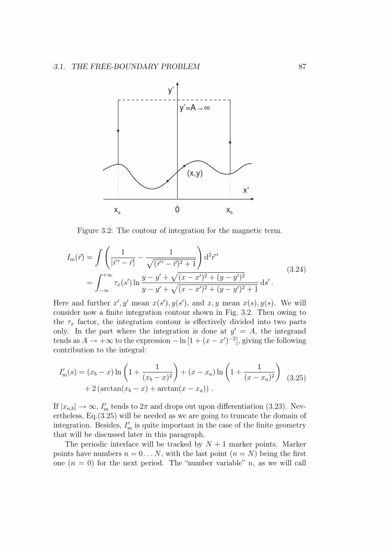
3.1. THE FREE-BOUNDARY PROBLEM 87
y’
x’
xbxa
y’=A→∞
(x,y)
0
Figure 3.2: The contour of integration for the magnetic term.
Im(~r) =
∫
(
1
|~r ′ − ~r| −1
√
(~r ′ − ~r)2 + 1
)
d2~r ′
=
∫ +∞
−∞
τx(s′) ln
y − y′ +√
(x− x′)2 + (y − y′)2
y − y′ +√
(x− x′)2 + (y − y′)2 + 1ds′ .
(3.24)
Here and further x′, y′ mean x(s′), y(s′), and x, y mean x(s), y(s). We willconsider now a finite integration contour shown in Fig. 3.2. Then owing tothe τx factor, the integration contour is effectively divided into two partsonly. In the part where the integration is done at y′ = A, the integrandtends as A→ +∞ to the expression − ln [1 + (x− x′)−2], giving the followingcontribution to the integral:
I ′m(s) = (xb − x) ln
(
1 +1
(xb − x)2
)
+ (x− xa) ln
(
1 +1
(x− xa)2
)
+ 2 (arctan(xb − x) + arctan(x− xa)) .
(3.25)
If |xa,b| → ∞, I ′m tends to 2π and drops out upon differentiation (3.23). Nev-ertheless, Eq.(3.25) will be needed as we are going to truncate the domain ofintegration. Besides, I ′m is quite important in the case of the finite geometrythat will be discussed later in this paragraph.
The periodic interface will be tracked by N + 1 marker points. Markerpoints have numbers n = 0 . . . N , with the last point (n = N) being the firstone (n = 0) for the next period. The “number variable” n, as we will call

88 CHAPTER 3. ST INSTABILITY WITH AN IMMISCIBLE MF
it, may be regarded as a curve parameter another than the arclength s(n).Taking then the periodicity into account, we represent Eq.(3.24) as
Im(s) =
∫ n+N/2
n−N/2
τx(s′) lnF
(
x− x′
T,y − y′
T
)
ds′
dn′dn′−T lnT +I ′m(s)+I ′′m(s) ,
(3.26)where only one logarithm evaluation is needed per point s′,
F (u, v) =1
v +√u2 + v2 + 1
+∞∏
m=−∞m6=0
v +√
(u−m)2 + v2
v +√
(u−m)2 + v2 + 1, (3.27)
and
I ′′m(s) =
∫ n+N/2
n−N/2
τx(s′) ln
(
y − y′ +√
(x− x′)2 + (y − y′)2) ds′
dn′dn′ . (3.28)
Note that with our moving limits of integration in Eq.(3.26), the periodicityof the magnetic force is ensured. The integrand in Eq.(3.26) is always smooth,while in I ′′m it is logarithmically singular at s′ = s, so we integrate it by partsto obtain
I ′′m(s) =
∫ n+N/2
n−N/2
τx(s′)(y − y′) − τy(s
′)(x− x′)√
(x− x′)2 + (y − y′)2
ds′
dn′dn′ − T
+ (x− xA) ln(
y − yA +√
(x− xA)2 + (y − yA)2)
− (x− xB) ln(
y − yB +√
(x− xB)2 + (y − yB)2)
.
(3.29)
Here xA = x(n−N/2), xB = x(n+N/2), and yA = yB = y(n±N/2).In general, the product (3.27) cannot be calculated in a closed form.
Although it may be evaluated numerically using the series transformation andconvergence acceleration techniques, in the calculations that will be presentedhere we will satisfy ourselves with taking a finite number of termsM = maxmand truncating the rest. This corresponds to xa = xA −MT , xb = xB +MTin Eq.(3.25). This formulation of the magnetic force is not identical to thatof [175, 176].
Now our problem is fully determined by the integral equation (3.23),its right-hand side (3.26), (3.25), (3.29), and the velocity integrals (3.22).Now we are in position to develop the numerical procedure of solving theseequations. But before, it is convenient now to analyze an important propertyof the magnetic force that has direct consequences for computations of alaterally bounded flow.

3.1. THE FREE-BOUNDARY PROBLEM 89
Up to now in this Chapter, under study was a flow with periodic boundaryconditions, while the real conditions are at least that of no flux (no normalflow). (The more realistic no-slip condition cannot be generally satisfiedwith the Darcy equation.) With non-magnetic fluids, as long as symmetricshapes are studied, both conditions are related (but not equivalent). Indeed,vx(−T/2) = vx(+T/2) by periodicity, while from symmetry it follows thatvx(−T/2) = −vx(+T/2). Therefore vx(±T/2) = 0, and every symmetricperiodic Hele-Shaw flow is necessarily a valid laterally confined one. Thereverse statement is true only with one reservation: the symmetric interfacemust approach the sides (x = ±T/2) at a straight angle. Otherwise, in theperiodic problem we effectively have an interface with corners, for which ourequations are not valid. This is easy to see.
For example, the integrand
τy(s) sin a cos a− τx(s) sinh b cosh b
sin2 a+ sinh2 b
in Eq.(3.23) at s′ = L − s takes on the value τy cot(2πx/T ) if the interfaceis symmetric. At x = 0, thanks to the symmetry and smoothness, we haveτy = 0 and the indeterminate form may be resolved to produce a finite result.However, as x → ±T/2, the limit is generally (τy 6= 0) infinity. To establishthe sort of singularity, it is necessary to investigate two independent limits:s → 0 and s′ → L − s. We failed to adapt the algorithm developed for theperiodic boundary conditions to the non-periodic case.
Therefore we see the only tractable way to make the periodic boundaryconditions work: to demand that τy = 0 at x = ±T/2. In other words, theinterface should approach the sides of the cell at a straight angle. This isindeed a common, often implicit though, assumption. For such an interface,both types of boundary conditions are shown above to be equivalent.
Unfortunately, with magnetic fluids the situation is worse. It is likely thata magnetic fluid cannot, at least in our description, develop any corners. Theabsence of MF in the adjacent periods leads to a singularity of magnetic forceat the end-points of the interface. In order to have the non-periodic situationin these transformations, one should set xa = xA = −T/2, xb = xB = +T/2,and use the fixed limits of integration 0 . . . L. The following exact expressioncan be easily obtained for the magnetic integral Im (3.24) if the interface isplanar:
dImdx
=1
2ln
1 + (T/2 + x)−2
1 + (T/2 − x)−2(3.30)
This function is logarithmically divergent at the end-points. (We remarkhere that with a planar interface, the whole problem may be solved by sepa-ration of variables, which was done to check our boundary-integral results.)

90 CHAPTER 3. ST INSTABILITY WITH AN IMMISCIBLE MF
Note that Im enters the effective pressure p (3.5), where its singularity can-not be compensated by infinite dp/dτ , the “real” pressure gradient alongthe interface. Indeed, dp/dτ can have only a finite jump given by the dy-namic boundary condition at a regular interface, while the jump of dIm/dτis infinite anyway. Therefore, according to Eq.(3.6), as the effective pressuregradient goes infinite, so does the tangential velocity (at least at one side ofthe interface). We also observed the non-convergent behaviour of numericalvelocities for other (non-planar) interfaces that approached the sides of thecell at a straight angle.
If the boundary of the domain occupied by MF has corners, the problemhas no bounded solutions in our model and, of course, cannot be simulatednumerically. We stress that this fact has physical grounds rather than numer-ical ones. The more promontory the element of the interface, the strongerindeed it is pushed outwards by the rest of the MF volume. This can beseen from the dispersion relation (3.36) for a planar interface, where the Bmcontribution to the growth increment varies asymptotically as k ln k for largewavenumbers k. Therefore the physical model must be changed in order tosimulate the interfaces that are not tangent to the sides of the cell. Perhaps,the Darcy law and the two-dimensional approach to the magnetic force mustbe abandoned.
However, if the task is to simulate a magnetic ST finger (see §3.2.4), thenthe precise conditions at the sides of the cell can be not very important. Thenone can demand that the interface comes always tangent to the sides and sim-ulate a long finger that will not “feel” this condition. The periodic algorithmis incompatible with it, as we have shown above. Still the boundary-integraltechnique can be applied to the non-periodic situation with a slight modifi-cation. Apart from the way the magnetic force is computed, the kernel of theintegral equation and the velocity integrals (3.21)–(3.23) are modified. Be-sides, the non-periodic case requires that γ be distributed not only along theinterface, but also along the sides of the cell. In principle, with such methodit is also possible to model an infinite interface that does not approach thesides of the cell at all. This algorithm can be developed in the future.
3.2 The numerical method
3.2.1 Numerical modelling
with boundary integral equations
In this paragraph we present an overview of applications of the boundary-integral method introduced above in §3.1.3 – the method that will ultimately

3.2. THE NUMERICAL METHOD 91
serve us to obtain physical results. The review is method-oriented ratherthan subject-oriented. As we will see, a considerable amount of research wasdevoted by computational physicists to “taming” the boundary integrals. Nu-merical instabilities inherent to the method have considerably complicatedand limited its use, and not only in the past. Nevertheless, the job is worthdoing thanks to important features shared by some of the approaches, includ-ing the boundary-integral method, touched upon in §3.1.3. They lead to anintegral equation that involves only the values at the boundary, thus reduc-ing the dimension of the problem by unity. Discontinuities of fluid quantitiesat the interface are easy to take into account; besides, infinite domains arehandled naturally. These features are of course an important advantage boththeoretically and for modelling.
Elliptic BVP’s are among the most common problem types in physicsand engineering, emerging in a very wide range of disciplines. Thus theboundary-integral approach has found its application, for example, in dif-fraction problems in electromagnetism [198], acoustics, to solve the appliedproblems of elasticity and viscoplasticity theories [199, 200], etc. The ap-proach is natural and especially effective in the problems where only valuesat the boundaries are in fact important or wanted, e.g. in the analysis ofcracks in the elasticity theory (according to the maximum principle, extremalvalues of the stress are attained at the boundary). In engineering computa-tions, even the complex-variable formulation via the Cauchy-type integralsis in use [201]. On the evolution of the so-called “method of boundary el-ements” (BEM) in applied mechanics, see [202]. (BEM essentially is theboundary-integral method coupled with a special approach to the boundarydiscretization.) Aero- and hydrodynamical applications of boundary inte-grals are also numerous: Stokes flow [203, 200], scattering of surface gravitywaves [199], point-vortex [204] and 3D panel [205] methods in aerodynamics,groundwater flow, inviscid non-linear surface waves, the Kelvin–Helmholtzand Rayleigh–Taylor instabilities. For a recent overview on the boundaryintegral methods for interfacial flows, see [206]. The first (to our knowl-edge) numerical simulation of a Hele-Shaw flow with surface tension by theboundary-integral method dates back to 1961 [207]. (On further progress,see later in this paragraph.) Owing to the Darcy law, especially close to ourproblem are the moving-boundary problems (oil extraction by displacement)of the groundwater filtration (percolation) theory (§XVII.6 of [72], [208],§12.3 in [200]). The conditions at the water–air “interface” in porous mediaare not quite clear (see references in [209]), but are often assumed to be justthose of a continuous pressure. The groundwater problems were solved em-ploying the boundary integrals, sometimes employing the jump of the normalderivative of the single-layer potential (§§XVII.6, XIX.6 in [72], [208]). Of

92 CHAPTER 3. ST INSTABILITY WITH AN IMMISCIBLE MF
common use in that field, however, are the complex-analytic methods [72]).See a review [157] on the application of the complex-analytic methods to theHele-Shaw flow with surface tension; on the recent developments and refer-ences, see [159, 210] and §X.3 of [11]. As for the numerical solution of theboundary-integral equations of potential theory, see [211] for a general sur-vey. Remember however that we have an indirect boundary-integral method,with velocity being linked to γ through a singular integral, even though theintegral equation per se is perfectly Fredholmic. Besides, in our case we needto solve a large number of the BVP’s, with solution of the preceding problembeing used by the following one.
At this point it is necessary to identify and analyze the problem associatedwith boundary integrals. A singular integral, in general, can be very sensitiveto small changes in its density. Consider
f(x) = v.p.
∫ π
0
[g(x+ α) + g(x− α)] cotα
2dα = v.p.
∫ x+π
x−π
g(α) cotα− x
2dα
and its “singular part” obtained by replacing cot z with 1/z. Then it can berigorously proved that an arbitrarily large change in the principal value f canbe caused by an arbitrarily small variation of the density g, provided thatthe variation is only continuous; if the variation is square-integrable, however,this effect is guaranteed not to take place and f is itself square-integrable inx. The example of the first situation was built, and the statement for thesecond situation was proved in [212] (§69 and comment 113). The sensitivityof a singular integral to the small change in its density is also discussedin [213] (§§5.1, 5.2, 7.1, 7.2), where special approximations to the densityare developed that are not subject to the sensitivity and can be used toevaluate the integrals. In [204] (§13.1) it is pointed out that the sensitivitycan reveal itself, upon discretization, as numerical instability in the so-calledpoint-vortex method (see below in this paragraph). It is further suggestedin [204] that in order to avoid the instability, the point vortices should beplaced approximately halfway between the points where the equation is tobe satisfied.
Let us recall now that the very boundary-value problem may be ill-posed(the solution to BVP might not continuously depend on the boundary con-ditions). For an elliptical operator in a bounded domain, boundary-valueproblems are ill-posed unless boundary values are specified on all boundariesof the domain. A relevant here example of an ill-posed problem is the Cauchyproblem for the Laplace equation for which J. Hadamard constructed his cel-ebrated illustration of ill-posedness (e.g. §III.6 of [135], [214]). In the numer-ical solution of BVP, the ill-posedness appears as a numerical instability, andthe finer the mesh, the worse the result. In an advanced text on numerical

3.2. THE NUMERICAL METHOD 93
analysis [215] it is shown that the two-dimensional Rayleigh–Taylor instabil-ity (RTI) with ideal fluids without surface tension is an ill-posed numericalproblem, and it is quite difficult even to soften the ill-posedness. It turnsout that some boundary conditions must be given with the exponentiallysmall round-off error; high spatial resolution requires multiple-precision ma-chine arithmetics. It is also pointed out that the application of an arbitrarysmoothing is a poor practice. In the dispersion relation for the instabilitymodes of a planar interface, the ill-posedness manifests itself as the unlimitedgrowth of the increment as the wavelength vanishes. (Indeed, as Ca → ∞in Eqs.(3.36), (3.40) introduced later, the −k3 term becomes insignificantleading to λ → ∞ at k → ∞. The same applies even more to the ef-fect of Bm → ∞ for both perpendicular and normal field orientations.) Inthe discretized equations, k may not be infinite; instead, the fastest-growingwavenumber corresponds to the numerical mode of smallest wavelength (2grid points per period – the “sawtooth” mode).
Many physically meaningful and important problems are ill-posed (in anidealized description). We should mention the Kelvin–Helmholtz instability(KHI) that occurs at the flat interface between ideal irrotational incompress-ible fluids across which the tangential velocity is discontinuous. Under thegravity, surface or internal water waves develop at a horizontal interface. Ifthe configuration is gravitationally unstable, and there is no velocity jumpat the interface at infinity, the Rayleigh–Taylor instability ensues, and anon-uniform shear develops even though it was not present initially. Theproblems of KHI, RTI, and the Saffman–Taylor instability are known to beill-posed at zero surface tension and to lead to curvature singularities, wavebreak-ups, etc. in finite time; ill-posedness manifests itself in the correspond-ing dispersion relations (e.g. §13.7 in [144]) as an unbounded growth rate atlarge wavenumbers [214]. Note that RTI and ill-posedness can develop evenif the upper fluid is of zero density, in the regions of the deformed interfacewhere the local acceleration exceeds the free-fall one [216]. The numericalapproximations to these problems proved difficult to obtain even during theregular stage.
Historically, advances in modelling these important problems numericallyby the boundary-integral method were ahead of and drove the understandingof the similar method for Hele-Shaw flows. The velocity integrals in theseproblems of interfaces between two ideal incompressible fluids in two dimen-sions (referred to as the Birkhoff–Rott integrals in the case of the vortexsheet) are exactly the same as in the Hele-Shaw problem, but the integralequation differs from ours and is related to the Bernoulli’s law.
Vortex sheet and point-vortex arrays are a classical subject (e.g. §151 of[73], §§13.62–13.71 of [217], §2.6 of [70]). The first simulation of the dynamics

94 CHAPTER 3. ST INSTABILITY WITH AN IMMISCIBLE MF
of the vortex sheet discretized into point vortices, was undertaken in early1930’s by Rosenhead. Even at a low spatial resolution the instability lead toa chaotic motion of the vortices. In 1960’s, G. Birkhoff could not obtain theconvergence of his results as N → ∞ because of the instability. A commonopinion formed that the point-vortex approach is inadequate. In 1965 (pub-lished in 1980), the handling of the velocity integrals was improved in thework [218] to take into account the “self-induction” of point vortices (the “vande Vooren correction” discussed later). A real point vortex can drive othervortices but not itself, as known from the hydrodynamics of two-dimensionalirrotational flows, e.g. [219]. Thus the (accurately) discretized problem for acontinuous vortex sheet indeed differs from the originally discrete problem fora point-vortex array, though the formulas look almost identical. The numberof point vortices was kept low [218] to avoid the instability. Nevertheless, inlate 1970’s – early 1980’s, some new numerical results were obtained with themethod. In many works, an arbitrary smoothing was applied, whose effect onconvergence was hardly predictable. For later developments, important werethe works [220, 221] (no numerical instability was noticed there). Finally, inmid-1980’s a correct numerical regularization was developed [222]. Namely,high-wavenumber Fourier modes must be filtered out completely from thesolution at every time step if their amplitude is below a certain limit. (Thisis referred to as “the Krasny filtering”. Since the solution, while it exists, andthe initial conditions should be analytic, the Fourier coefficients must any-way decay quickly with wavenumber.) At small N it may be practical just todo the computations in a higher precision. The filtering allowed to simulatethe vortex-sheet evolution from the initial conditions leading to a cusp up tothe time of singularity [222]. Yet later, a spectrally accurate quadrature wasapplied in this problem [223] based upon the results of [224] (the spectralaccuracy is discussed in §3.2.3).
For quite a time, also under consideration were various more or less phys-ical regularizations to render the above-mentioned problems well-posed, e.g.,by taking into account the surface tension, (additional effects of) viscosity,etc. [214]. In [225], e.g., rigorously proved was the well-posedness of a generalinterface with surface tension between two ideal irrotational incompressiblefluids of different tangential velocities and densities. However, through nu-merous attempts made by many researchers, a very unpleasant fact becameevident in this context that even a physically well-posed continuous problemmay upon discretization become an ill-posed one! Many early studies suf-fered, e.g. [226], from purely numerical high-wavenumber instabilities, and itwas not clear why the surface tension cannot damp them. Some early simula-tions [227, 228] of the Hele-Shaw flow with surface tension were performed bythe “vortex-in-cell” (VIC) method, which differs from the point-vortex one
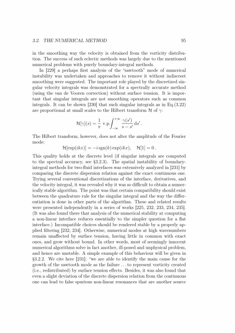
3.2. THE NUMERICAL METHOD 95
in the smoothing way the velocity is obtained from the vorticity distribu-tion. The success of such eclectic methods was largely due to the mentionednumerical problems with purely boundary-integral methods.
In [229] a perhaps first analysis of the “sawtooth” mode of numericalinstability was undertaken and approaches to remove it without indiscreetsmoothing were suggested. The important role played by the discretized sin-gular velocity integrals was demonstrated for a spectrally accurate method(using the van de Vooren correction) without surface tension. It is impor-tant that singular integrals are not smoothing operators such as commonintegrals. It can be shown [230] that such singular integrals as in Eq.(3.22)are proportional at small scales to the Hilbert transform H of γ:
H[γ](s) =1
πv.p.
∫ +∞
−∞
γ(s′)
s− s′ds′ .
The Hilbert transform, however, does not alter the amplitude of the Fouriermode:
H[exp(ikx)] = −i sgn(k) exp(ikx), H[1] = 0 .
This quality holds at the discrete level (if singular integrals are computedto the spectral accuracy, see §3.2.3). The spatial instability of boundary-integral methods for two-fluid interfaces was extensively analyzed in [231] bycomparing the discrete dispersion relation against the exact continuous one.Trying several conventional discretizations of the interface, derivatives, andthe velocity integral, it was revealed why it was so difficult to obtain a numer-ically stable algorithm. The point was that certain compatibility should existbetween the quadrature rule for the singular integral and the way the differ-entiation is done in other parts of the algorithm. These and related resultswere presented independently in a series of works [225, 232, 233, 234, 235].(It was also found there that analysis of the numerical stability at computinga non-linear interface reduces essentially to the simpler question for a flatinterface.) Incompatible choices should be rendered stable by a properly ap-plied filtering [232, 234]. Otherwise, numerical modes at high wavenumbersremain unaffected by surface tension, having little in common with exactones, and grow without bound. In other words, most of seemingly innocentnumerical algorithms solve in fact another, ill-posed and unphysical problem,and hence are unstable. A simple example of this behaviour will be given in§3.2.2. We cite here [231]: “we are able to identify the main cause for thegrowth of the sawtooth mode as the failure . . . to represent vorticity created(i.e., redistributed) by surface tension effects. Besides, it was also found thateven a slight deviation of the discrete dispersion relation from the continuousone can lead to false spurious non-linear resonances that are another source

96 CHAPTER 3. ST INSTABILITY WITH AN IMMISCIBLE MF
of numerical instability (see [229, 231] on Moore’s works). These results referto the case of a vortex sheet with surface tension. Unfortunately, so detailedand delicate numerical analysis is not, to our knowledge, available for theHele-Shaw flow. Rather, a single spectral method of choice is being adver-tised in [230] and subsequent works of their group, while stability of otherdiscretizations is poorly covered in the literature.
Described above is a specific sort of numerical instability, sometimes re-ferred to as the “spatial” one. It should not be confused with the “temporal”instability of time integration that we will discuss now. The “spatial” insta-bility remains present even if time integration is carried out exactly (withtime continuous). Time integration is numerically stable unless the Courant-Friedrichs-Levy (CFL) constraint on the time step is violated. Observing theconstraint guarantees that the round-off errors do not amplify in the courseof simulation. The constraint is very stringent for the explicit methods – theones that use the explicit discrete expression for new marker position solelyin terms of old ones. If time marching instead uses implicit formulas fora new position that involve new positions for other markers, the constraintbecomes much less restrictive. (In finite-difference methods for partial differ-ential equations, the notions of explicit and implicit templates are extremelyimportant as well.) For our set of equations and explicit method, the CFLcondition is [225, 230]
(∆t)max ∼ (∆s)3min . (3.31)
It is (∆s)min, the minimum separation of markers in arclength, that con-strains the maximum time step (∆t)max for which the explicit time integra-tion is still numerically stable according to (3.31). The constraint is so severebecause of the curvature that introduces high-order derivatives. It has alsolimited seriously the previous research. An implicit method is difficult toobtain, but it allows to choose the time step from considerations of approx-imation only. Nevertheless, in [230] an effectively implicit time-integrationmethod was developed. In this approach, the interface is represented notin the Cartesian coordinates but in the tangent angle – arclength ones, inorder to have simple “linear” expression for the curvature. Further on, the“small-scale decomposition” is applied to the velocity integral, which revealsthat at short scales, it behaves essentially like a Hilbert transform on thedensity of the potential. The latter admits implicit treatment in the Fourierspace. The equations are set up in such way that the arclength remain equalautomatically. For details, we refer the reader to [230, 182]. (But mind theremark in [231] that in order to have high accuracy, the low-order implicittime-stepping of [230] can in fact require a yet smaller time step than a high-order explicit marching would do.) Though this technique is a significant

3.2. THE NUMERICAL METHOD 97
advance, allowing to compute the evolution in quite large time steps, we willnot employ it, being satisfied with an explicit time-marching.
It is worth mentioning that it is possible to solve the integral equationand compute the velocity integrals at the computational cost of O(N) in-stead of the standard O(N2) if fast summation methods are used, such asthe method of local corrections or a fast multipole method, and if specialinterface parametrization is used. Such methods are used (e.g. [230]) occa-sionally in computations with large N . The overall computational cost ofa method hereby becomes only O(N lnN) per time step. (In our problemsuch effectiveness is more difficult to achieve, if possible at all, because ofmagnetic integrals.)
The boundary-integral methods discussed in this paragraph are indirect,i.e. some auxiliary function (the density γ of potential) must be computedfirst, enabling one to have further two velocity components. However, directboundary-integral methods for Hele-Shaw flows with surface tension also ex-ist and deserve mentioning. The integral equation is originally formulated forthe normal velocity in these methods (the tangential velocity being not im-portant). We refer the reader to [236] for a working example of such methodand for references to other such formulations.
In conclusion, we note that the boundary-integral method cannot tackleproblems involving topological changes and may require modifications tomodel singularity formation at the interface. Such problems are treated withease employing the level-set approach [233], where a two-dimensional inter-face is considered to be an isoline of level (i.e. height) of a three-dimensionaland rather smooth shape. For this and other related computational tech-niques, see also [8].
3.2.2 Interface and curvature
The periodic interface is tracked by N+1 marker points and is in fact definedby their coordinates x, y. A general interface requires a parametric represen-tation. Markers are always uniformly distributed in the “number variable”(this quality is important at dicretizing the integrals, see §3.2.3). The ar-clength, or natural, parametrization of the interface will also be needed.
To have the arclength s, every time step of the algorithm begins with com-puting the lengths of the interface curvilinear segments between the markers.This is done through the spline representation of the interface.
A cubic spline is a special case of the cubic Hermite interpolating func-tion. The latter function is a piecewise-polynomial (cubic) interpolant withcontinuous first derivative [237]. In general, di – the values of the derivativeat the knots – must also be supplied. However, they may be uniquely defined
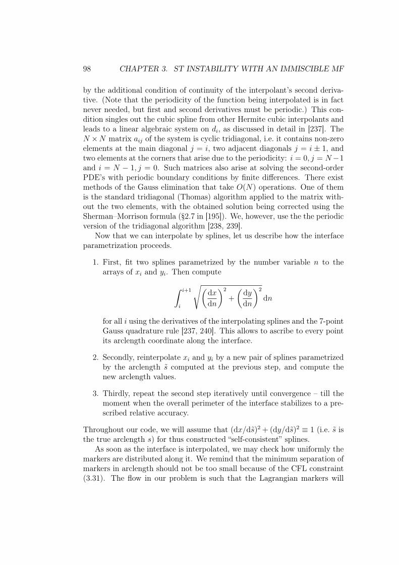
98 CHAPTER 3. ST INSTABILITY WITH AN IMMISCIBLE MF
by the additional condition of continuity of the interpolant’s second deriva-tive. (Note that the periodicity of the function being interpolated is in factnever needed, but first and second derivatives must be periodic.) This con-dition singles out the cubic spline from other Hermite cubic interpolants andleads to a linear algebraic system on di, as discussed in detail in [237]. TheN ×N matrix aij of the system is cyclic tridiagonal, i.e. it contains non-zeroelements at the main diagonal j = i, two adjacent diagonals j = i ± 1, andtwo elements at the corners that arise due to the periodicity: i = 0, j = N−1and i = N − 1, j = 0. Such matrices also arise at solving the second-orderPDE’s with periodic boundary conditions by finite differences. There existmethods of the Gauss elimination that take O(N) operations. One of themis the standard tridiagonal (Thomas) algorithm applied to the matrix with-out the two elements, with the obtained solution being corrected using theSherman–Morrison formula (§2.7 in [195]). We, however, use the the periodicversion of the tridiagonal algorithm [238, 239].
Now that we can interpolate by splines, let us describe how the interfaceparametrization proceeds.
1. First, fit two splines parametrized by the number variable n to thearrays of xi and yi. Then compute
∫ i+1
i
√
(
dx
dn
)2
+
(
dy
dn
)2
dn
for all i using the derivatives of the interpolating splines and the 7-pointGauss quadrature rule [237, 240]. This allows to ascribe to every pointits arclength coordinate along the interface.
2. Secondly, reinterpolate xi and yi by a new pair of splines parametrizedby the arclength s computed at the previous step, and compute thenew arclength values.
3. Thirdly, repeat the second step iteratively until convergence – till themoment when the overall perimeter of the interface stabilizes to a pre-scribed relative accuracy.
Throughout our code, we will assume that (dx/ds)2 + (dy/ds)2 ≡ 1 (i.e. s isthe true arclength s) for thus constructed “self-consistent” splines.
As soon as the interface is interpolated, we may check how uniformly themarkers are distributed along it. We remind that the minimum separation ofmarkers in arclength should not be too small because of the CFL constraint(3.31). The flow in our problem is such that the Lagrangian markers will

3.2. THE NUMERICAL METHOD 99
Figure 3.3: The differential clustering of initially equidistant markers as theinterface evolves.
cluster into crowded groups in the course of interface evolution, leading toprohibitively short time steps and leaving other parts of the interface under-resolved (Fig. 3.3). It is necessary to redistribute the markers from time totime, which is done in the code as follows. As soon as the interface is inter-polated, we check if the minimum and maximum arclength separations arewithin the prescribed margins. If any is not, the new positions are calculatedat an equal (and allowed) distance one from another, possibly changing thenumber of markers. Then the interface is reinterpolated (as described above)again using the new markers.
In our code the redistribution is a relatively rare event; most time stepsare performed without it. Sometimes the redistribution can have a smooth-ing effect on solution [241]. Another possible approach is to use a non-Lagrangian tangential velocity that can be chosen to automatically keepmarkers uniformly distributed. On this and other approaches to redistri-bution and/or new marker deletion and insertion, see e.g. [209], Appendix Bof [242], [243, 230], and §6.3 in [203].
The curvature is given by
κ = (y′′x′ − x′′y′)/(x′2 + y′2)3/2 ,
where primes denote the differentiation with respect to a curve parameter.If the interface is parametrized by arclength, the curvature simplifies to κ =

100 CHAPTER 3. ST INSTABILITY WITH AN IMMISCIBLE MF
(d2y/ds2)/τx (where τx = dx/ds as before). However, we observed this formto lead to numerical instability, so in the code we used
κ = τx d2y/ds2 − τy d2x/ds2 .
To have the curvature, we need to accurately and reliably compute the deriv-atives of the interface-defining functions.
It is well-known ([244], §4.12 in [237]) that the cubic spline interpola-tion of a smooth enough function offers the accuracy of O(h4), h being the(maximum) distance between the knots. The n-th derivative of the spline ap-proximates the n-th derivative of the function to the order (4−n). However,in the special case of a periodical function interpolated over its period (i.e. ifthe spline boundary conditions are periodic), the accuracy of the spline deriv-atives can be improved owing to the fact (see [245] and references therein)that the asymptotic error of the first derivative of a periodic cubic splineremains O(h4) at a knot. Higher derivatives may be had to the same orderthrough the following procedure. First, one fits a spline to the function andcomputes the spline’s first derivatives at the knots. To these values, anotherspline is fit then; its derivative will be an excellent, O(h4) approximation tothe second derivative of the original function. (Note that the second deriva-tive of the original spline would be only h2 accurate.) Yet higher derivativesmay be obtained in the like manner. This technique was referred to as the“spline-on-spline” method (§2.5 in [244]), later as the “successive” or “iterated”splines. It was used in the boundary-integral problems already in [226]; withquintic splines it was used in [242].
We have just discussed the behaviour of the approximation error for agiven function and its derivatives as the mesh is refined. However, a compu-tation is generally done once with a predefined number of markers, the meshbeing refined (doubled) for the purpose of stability rather than approxima-tion. Thus the reverse situation is also of interest: the mesh is fixed, andone tests how good the approximation is for the derivatives of various trialfunctions, for which the Fourier modes exp(ikx) are naturally chosen. Thework [231] analyzed several ways to interpolate a function uniformly sam-pled over a period of 2π. It was demonstrated that the quality of the splinerepresentation deteriorates as k approaches the “Nyquist frequency” which isdefined as the highest wavenumber kmax = N/2 visible to the N -point mesh(the period being 2π). The derivatives of the interpolating spline at the knotsare underestimated, and the smoothing is characterized by the error factor[233, 234, 231]
Es(kh) =3
2 + cos(kh)
sin(kh)
kh,

3.2. THE NUMERICAL METHOD 101
where h = 2π/N is the uniform spacing. In a sense, even the periodic-splineapproximation to the derivative is local like the one by finite differences. Incompliance with the previous passage, 1 − Es ∼ (kh)4/180 as h → 0. The“sawtooth” (Nyquist) mode has 2 sampling points per period that are thepoints of extremum for the interpolating spline, whose derivative thereforevanishes at the knots, Es(π) = 0. This property is a difficulty [231] fora straightforward spline-on-spline procedure. The sawtooth mode does notcontribute to the computed interface curvature and is not damped by thesurface tension. Thus it can be a source of the numerical instability (of asimple “spatial” one); as we have discussed already, the surface tension shouldbe enabled to act upon high numerical wavenumbers (see Section 3.2.1).
3.2.3 Discretization of integrals
Integral operators enter the formulation of our problem three times:
• in the magnetic force (quadrature);
• in the potential density (an integral equation);
• in the velocity (singular quadrature).
We shall consider these cases one by one.The first issue are the numerically accurate quadratures in the magnetic
force (3.26), (3.29). Essentially we have our data in the tabular form: thevalues of the integrand are known at the marker points, the markers beingequispaced in the number variable. Then it is natural and convenient to usethe Hermite cubic quadrature [237]. Consider the Hermite cubic interpolatingfunction (see §3.2.2) with equidistant knots of spacing h – a piecewise-cubicpolynomial c(x) with continuous first derivative. It is fully defined by twoarrays: the one of function values yi and the one of derivatives di. Since theerror of the Hermite interpolation of a smooth function is O(h4) (see above),the original integral can be approximated by the integral of c(x) yielding aninterpolatory quadrature rule of the polynomial degree 4. The integral ofc(x) is given by a remarkably simple formula (§5.8 in [237]):
∫ xn
x1
c(x)dx =n∑
i=1
αiyi + (d1 − dn)h2/12 , (3.32)
where
αi =
h/2 if i = 1 or i = n,
h otherwise.

102 CHAPTER 3. ST INSTABILITY WITH AN IMMISCIBLE MF
Obviously, the sum in Eq.(3.32) is the standard compound rectangle rule,while the other term is a correction that improves the accuracy. Note thatthe correction term involves the derivatives only at the ends of the segment ofintegration. In our code the derivatives of the integrand functions at the end-points are computed analytically from the expressions (3.26), (3.29). Notethat in order to evaluate (3.29), the segment should be divided into two partsat the point s′ = 0 because the integrand is non-smooth there, and the rule(3.32) should be applied to both parts separately.
The second task is to solve the integral equation (3.23) for the potentialdensity γ. There are several methods available for the numerical solution ofthe Fredholm integral equations of the second kind. In [166, 167, 168, 175,176] the Galerkin method is used. The simplest yet efficient method consists,however, in replacing the integral operator with a quadrature rule:
f(s) = γ(s) +
∫ b
a
γ(s′)K(s, s′)ds′ ≈ γ(s) +∑
j
wjγ(sj)K(s, sj) , (3.33)
where K is the kernel of Eq.(3.23) including the prefactor At/T , f is itsright-hand side, wj are the quadrature weights, and sj are the quadraturenodes. The formula (3.33) evaluated at the nodes s = si reduces the problemto a system of linear algebraic equations. This direct approach to solve anintegral equation is usually called the (mechanical) quadrature method andoccasionally is referred to as the Nystrom method. The latter term shouldpreferably be used if on obtaining γ(si) the values of γ at an arbitrary point sare found through Eq.(3.33) used as an interpolation formula (the “Nystrominterpolation”). For our purposes it suffices to have γ at the nodes si only.
Next, which quadrature rule should be chosen? The advice of the “Nu-merical Recipes” [195] is that “for smooth, non-singular problems, nothingbeats Gaussian quadrature. . . ”. Indeed, it is obvious that the dimensional-ity of the algebraic system should be kept as low as possible, the accuracybeing fixed. The Gauss quadrature rules are generally the most efficient inthis sense – for a given number or nodes, they provide the highest algebraicaccuracy (i.e. they exactly integrate algebraic polynomials of the highest or-der) among other interpolatory rules. However, our case is not a general one.The kernel is periodic, the right-hand side and γ are periodic as well, and themarkers are equidistant in the number variable. Then there exists an appeal-ing alternative that we will employ [211]. The following result is important(§6.4 in [215]; also formulated in other textbooks on numerical analysis, in[223], etc.). For a periodic function being integrated over its period, the N -point compound rectangle rule is exact for trigonometric polynomials of theorder N−1, which is the highest possible order for a N -point rule. Such algo-

3.2. THE NUMERICAL METHOD 103
rithms are called spectrally accurate, of infinite accuracy ∼ exp(−const ·N),or saturation-free.
The system of linear algebraic equations is solved for γ(si) by simpleiterations (this method is sometimes referred to as Richardson’s one, §2.3in [246], the fixed-point iteration, or as successive substitutions, since thesystem originates from the Fredholm equation of the second kind):
γi+1(s) = f(s) −∑
j
wjγi(sj)K(s, sj) . (3.34)
The initial guess γ0 is taken from the previous time step. In [233] it issuggested to use the γ0 extrapolated from several previous time steps. If aredistribution has occurred at the beginning of the step, the old γ at newmarker positions is found by the spline interpolation. At the first time step,the right-hand side is taken as the initial guess. On convergence of theiterations, see [221, 216, 233, 243]. The condition to stop the process is thatthe relative change (as compared to the previous iteration) of the absolutevalue of any γ component no longer exceeds the prescribed threshold (i.e.the error should be small in the “continuous” norm). More effective iterativemethods such as GMRES [182, 247] can also be applied.
Now let us turn to the third question – how the principal-value integrals(3.22) can be computed numerically. They have the form
I(∞) = v.p.
∫ N
0
g(n, n′) dn′ ,
where n, n′ are the number variables, g is N-periodic in both variables andsingular but Cauchy-integrable at n′ = n. At the marker points n ∈ [0 . . . N)takes the values 0 ≤ ni = i < N . A possible approach is to resolve thesingularity, which leads to the “van de Vooren correction” [218] to the rec-tangle quadrature rule with the singular point omitted. The accuracy of thecorrected rule is determined by the way the derivatives that enter the correc-tion term are computed; with the Fourier differentiation, the corrected rulebecomes spectrally accurate. Equivalently, the singularity can be subtracted[218], leading to the spectral accuracy [223]. However, there exists a simplervery accurate method. Integrating by the (compound) rectangle rule, let ussimply omit the node that corresponds to s′ = s (the “point vortex method”)
I(∞) ≈ I(N) =N−1∑
j=0j 6=i
g(si, sj) ,

104 CHAPTER 3. ST INSTABILITY WITH AN IMMISCIBLE MF
Then it turns out that the relative (and hence absolute) error introducedhereby is not just O(1/N), but, in addition, does not contain any algebraicterms of higher order [224, 223]. Then this O(1/N) term can be exactly elim-inated by the classical Richardson extrapolation [238] restoring the spectralaccuracy [224, 223]. The Richardson extrapolation in this case consists inthe following. Let N + 1 be odd; the error term to eliminate is C/N , whereC is a constant. Consider the same rule with a halved number N/2 + 1 ofpoints, i.e. the point with j = i is omitted as before, but starting with itevery other point is skipped as well:
I(N/2) = 2N−1∑
j=0j 6=i
i+j even
g(si, sj) ,
Here the term is 2C/N . Then it follows that in the combination
2 I(N) − I(N/2) = 2N−1∑
j=0i+j odd
g(si, sj) ,
the error terms cancel out, which leads to a spectrally accurate approximationof I(∞). This is known as the alternate-point (or alternating) trapezoidal(or rectangle) rule. We will use this rule, for which, we remind, N should beeven.
Yet another issue is an efficient evaluation of the trigonometric functionsin Eqs.(3.22), (3.23). Indeed, at every time step there are approximately N2
pairs of xj − xi and yj − yi of which trigonometric or hyperbolic functionsmust be computed. However, it is possible to decrease the count of functionevaluations down to N using the formulas [229]
sinh(z − z′) = sinh z cosh z′ − sinh z′ cosh z ,
cosh(z − z′) = cosh z cosh z′ − sinh z sinh z′ ,
and analogous trigonometric identities. The functions in the right-hand sideare computed once during a time step. The tables of these values are usedsubsequently in Eqs.(3.22), (3.23).
Note that the form of denominator in Eq.(3.22) is so chosen as to avoidthe cancellation of digits as s′ → s that would occur if it were replaced withcosh2 b− cos2 a. This point was made in [218].

3.2. THE NUMERICAL METHOD 105
3.2.4 Characterization and validation
In the previous paragraphs we have described a single time step of the algo-rithm. Before turning to its verification, we must complete the definition ofthe algorithm by specifying how the problem is integrated in time. Operationcount per time step is O(N2) for the equation setup (magnetic force, matrixto solve the integral equation), solving for γ (operations with the matrix),and evaluation of the velocity integrals. Then, if the perimeter increasesapproximately linearly with model time (Saffman–Taylor fingers) (and sincemarkers are distributed approximately evenly along the interface), a com-puting time needed to calculate up to a certain model time is a cube of themodel time. This imposes a practical prohibition to compute further than acertain model time.
Given the expenses of computing the velocities of the markers, we performthe time integration of the system by the explicit two-step Adams-Bashfortmethod. At the first time step or after a redistribution of markers has oc-curred, the second order Runge–Kutta method is employed. Both methodsare of the second order of approximation in the time step ∆t. The time stepis fixed throughout the run. Higher temporal convergence is not reasonablebecause it is the stability constraint (3.31), and not the approximation, thatreally limits from above the time step ∆t ∼ 1/N3 in our computations. Sincethe error of the spatial approximation will be found to be asymptotically1/N4, the error of the second-order time integration behaving as (1/N3)2 isnegligible at high N .
The program is written portably in the C programming language andcompiled with the free Digital Mars compiler [248]. Throughout the code,we compute indiscriminately in the 80-bit “long-double” floating-point arith-metic (ca. 20 decimal digits). With an Intelr PC, this is anyway thelowest (or the only) hardware precision. Multiple precision defers the onsetof numerical instabilities and is good for computing nearly ill-posed problems(§3.2.1). The algorithm requires O(N2) memory at At 6= 0 because of thematrix of the integral operator. The matrix is computed once per time stepand stored to be reused several times as the corresponding linear system isiterated. With N = 3000 markers the matrix takes about 100 Mbytes ofRAM.
Now we will verify the correctness of our implementation of the algorithmto prove its suitability for the modelling. This will be done in a number ofways. The code of course passes simple “internal-consistency” checks. Itpasses the periodicity test (a comparison of results obtained with shiftedinitial conditions). Doubling the period also gives consistent results, i.e. twoequal patterns are obtained side by side, each being equal to the pattern

106 CHAPTER 3. ST INSTABILITY WITH AN IMMISCIBLE MF
obtained with a single period. The volume of each fluid must conserve byformulation; the numerically computed volume is of course non-zero andincreases with time, but is checked to remain reasonably low. (Other integralinvariants should also be constant and can be checked [218, 226].)
Note that we don’t use any explicit filtering. Smoothing other than thatnaturally associated with the spline approximation (p. 100) is not present inthe presented computations. We were able to do many computations withoutany visible signs of instability or irregularity in the plots of the interface, theright-hand side (rhs) of the integral equation Eq.(3.23), its solution γ, orvelocities. However, in some rare cases we did observe that, independentlyof the time step size, the (κ + Ca y + Bm Im) combination entering the rhs,or rhs itself, developed a small-amplitude zigsaw pattern over some segmentsof the interface. The amplitude of the zigsaw grew quite slowly with time orsaturated at a constant, quite low value. Usually we had to change the spatialresolution to avoid this. We also noticed that too loose marker redistributionconditions could provoke the zigsaw. There was also another, more serioussort of numerical problem. With highly ramified and convoluted interfaces,a numerical blow-up would occur quickly at a very localized segment of highinterfacial curvature: say, a dozen consequent markers would have irregularrhs value, velocities, etc. The iterations of the integral equation on γ would nolonger converge. This problem caused the computation to stop, and we couldnot find a remedy against it. By analogy to the two-dimensional interfacialproblems for ideal fluids, we may expect that full “spatial” numerical stabilitycan be achieved by application of a certain filter [232, 234]. Other possibilitiesare also being tried, which is a subject of our ongoing work.
In Fig. 3.4 some numerically computed non-magnetic shapes are com-pared to the ST finger of a relative width λ. The asymptotic shape of aninfinitely long finger with the tip at x = y = 0 is given by the formula
expπy
(1 − λ)T= cos
πx
λT. (3.35)
At any λ, the ST finger is an exact solution of the problem at zero surfacetension (Ca = ∞; §3.1.1). As the surface tension is non-zero but small, λtends to 1/2. Even at larger surface tensions the observed and modelledshapes not predicted by the surface-tension-free theory, are well describedby Eq.(3.35) with a suitably adjusted λ (the problem of the finger-width“selection”). If not specified otherwise, for λ we will take the first widthmaximum, counting from the tip of the finger. As illustrated by Fig. 3.4, theshapes with surface tension near tips are narrower than the ST finger, butalready at Ca as small as unity, the correspondence becomes quite close.
A common verification test for a Hele-Shaw numerical code is the compar-

3.2. THE NUMERICAL METHOD 107
-10
10
-80 -60 -40 -20 0 20 40 60y
x
-6
-4
-2
0
2
4
6
38 40 42 44 46 48y
x
(a) Ca = 0.2, t = 500: λ = 0.59979.
-10
10
-60 -20 20 60y
x
-4
-2
0
2
4
62 64 66 68 70 72 y
x
(b) Ca = 1, t = 100: λ = 0.53447.
-10
10
-80 -40 0 40 80y
x
-4
-2
0
2
4
70 72 74 76 78 80 82y
x
(c) Ca = 5, t = 20: λ = 0.51181.
Figure 3.4: A comparison of the computed finger shape to the classical STsolution. Upper panels: A non-magnetic finger computed with At = 1,T = 20, and the initial data y = 0.02 cos(2πx/T ). Lower panels: Themagnified tip of the computed finger (boxes) versus the Ca = ∞ ST finger(solid line) of a relative width λ, which is defined by two points marked (solidboxes) in the corresponding upper panel.

108 CHAPTER 3. ST INSTABILITY WITH AN IMMISCIBLE MF
Ca λ by [162] λ = b
1.339824 0.515 0.51538
0.062976 0.640 0.646
Table 3.1: The ST finger width λ – capillary number Ca dependence. Center:results from Table I of [162]. Right: our corresponding numerical results(Bm = 0, At = 1, T = 31.75, M = 3, y = 0.03 cos(2πx/T ) and N = 65initially).
ison of the computed λ to the benchmark steady-state results of [162] (§3.1.1).where a unique finger width for a given surface tension was computed. Wecompute the ST fingers at several Ca, starting with a small cosine-like initialinterface perturbation. However, with a time-dependent model the limitingλ can be difficult to recover. Even an apparently developed finger in factcontinues to deform. Namely, the lateral segments of its interface can un-dulate slightly in a symmetric fashion, with humps emerging not far fromthe tip, travelling slowly away from the nose, and increasing in amplitudein the meanwhile. The distance between the extrema of symmetric humpsis natural to be taken for λ. Thus a convention is needed, when and whichhump should be used. On the other hand, the amplitude of the undula-tion being rather small (about the last decimal place in lambda by [162]),we can merely neglect the difference. In Fig. 3.5 this situation is shown forCa = 0.062976 (the undulations take place at small Ca). We assume thatthe width of a hump follows approximately the model λ(t) = a/(t− t0) + b,where a, b, and t0 are determined from λ values at several t. This b may bethought of as the steady-state λ, though its precise value can be appreciablymodel-dependent and should not be attributed too much importance in suchcases. Thus, it is clear from Fig. 3.5 that the computed λ may well tendto the McLean&Saffman’s limit 0.640 instead of the value λ = b = 0.646given by the fit. (Fit parameters were determined by a non-linear estimationprocedure available in [249], where the non-linear least-squares Marquardt-Levenberg algorithm is implemented). Note that minute oscillations of thetip curvature were reported in [250], where it was also shown that the theseoscillations can grow in amplitude with time leading to a late tip-splitting ofa seemingly stationary finger.
Table 3.1 lists two entries of Table I of [162] that were chosen here forbeing extremal among those given by [162] – the first one corresponds to thesmallest surface tension, while the other corresponds to the largest surfacetension at which the interface is still linearly unstable. (Lower part of theirTable refers to the linearly stable situation.)

3.2. THE NUMERICAL METHOD 109
0.58
0.59
0.6
0.61
0.62
0.63
0.64
0.65
1400 1800 2200 2600 3000
t
λ
Figure 3.5: Computed finger width λ vs time. Black and empty boxes cor-respond to two different “humps” (see text). The dotted curve is a fit to apart of the data, and the solid line is curve’s asymptote λ = b.
Now let us compare the computed growth increment to the theoreticaldispersion relation [176]
λ = −k3 + k
[
Ca + Bg + 2 Bm
(
K0(k) + γ + lnk
2
)]
. (3.36)
(We use the same letter for the growth increment and finger width, whichshould not lead to confusion; the Macdonald functionK0 is given by Eq.(2.20).)Note that if y ∼ exp(λt), then vy/y = λ. Let us choose the parameter val-ues with which the summands in Eq.(3.36) are of the same order: Ca = 1,Bm = 1, T = 2π, i.e. k = 1, and λ = 0.610187. Besides, take M = 10, thenumber of markers as low as N = 65, and the interface that was initiallyjust slightly perturbed: y = 2π × 10−7 cos(2πx/T ). Then for the marker inthe middle (x = 0, y = 2π × 10−7) the computed vertical velocity is foundto be vy = 3.833196 × 10⁻⁷, so that vy/y = 0.610072. Comparing this valueagainst the theoretical one, we recover a rather small error in the computedvalue: 0.02%.
Now let us investigate the quality of the spatial approximation offeredby our algorithm. Specifically, we will find the actual rate of convergenceof the computed solution to the limit as the grid is refined (N → ∞). Weremind that the numerical algorithm was so constructed as to enable the

110 CHAPTER 3. ST INSTABILITY WITH AN IMMISCIBLE MF
fourth-order convergence. To check this feature, let us fix the following pa-rameters: Ca = 7/120, Bm = 1.14, At = 1, T = 20, M = 3, and the initialcondition y = 7 cos(2πx/T ). The initial condition is non-linear in the sensethat its amplitude is comparable to the period T , so that the non-linear inte-gral term in Eq.(3.23) can manifest itself. We distribute markers uniformlyin x, hence unevenly in arclength, to have the most general case possible.The test consists in running the code with different numbers of markers andcomparing the results computed in the first time step (marker redistributionbeing disabled). Namely, we will pick out several markers that are presentat any N and compare their computed velocities as N varies. “By construc-tion,” the values are expected to be of the algebraic asymptotic behaviour:v|N ∼ A+B/Nα, where v|N is either vx or vy computed with N markers perperiod. Hopefully we should observe α = 4. To verify this, let us multiply Nrepeatedly by a factor of 2, carrying out the computation with each value.Now notice that
v|2N − v|Nv|4N − v|2N
N→∞∼ 1/(2N)α − 1/Nα
1/(4N)α − 1/(2N)α= 2α . (3.37)
Thus the “apparent” order of convergence is easy to compute having theresults for 2N and 4N along with the ones for N . The results of such testwith our code are given in the Table 3.2 for 3 markers: far from the end of theinterface, close to it, and immediately at it. The reader may quickly verify,for example, that the ratio (3.37) for vx at the marker with coordinatesx = −1.875, y = 7 cos(2πx/T ) ≈ +5.820 and for N as high as 1024, is8550/519 ≈ 16.5. (The deviation from the exact power of two must beattributed to the finite value of N .) The same behaviour is the case forother markers and other quantities (γ, etc.). Hereby the so-called “apparent”spatial convergence of the algorithm is proved to be of the fourth order. Eventhough we won’t necessarily compute at that high resolutions, this property isquite satisfying, for lower (and usually unchecked and unreported) precisionof existing previously algorithms was one of their serious drawbacks. In fact,the ultimate goal in this direction might be to construct a (even better)spectrally accurate algorithm for the Hele-Shaw flow with MF’s.
In the same manner we can verify the temporal convergence as the timestep is diminished. Specifically, the following was done (with the redistribu-tion feature disabled):
• 4n time steps, each being equal ∆t;
• 2n time steps 2∆t;
• n time steps ∆t.
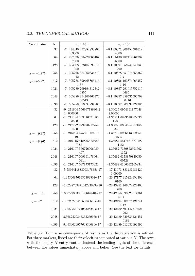
3.2. THE NUMERICAL METHOD 111
Coordinates N vx × 102 vy × 102
x = −1.875,
y ≈ +5.820
32
64
128
256
512
1024
2048
4096
-7. 234440 45298483880463000
-7. 297826 6952205664677000
-7. 304908 078187593675360
-7. 305266 38406283671022
-7. 305288 3994658651151 37
-7. 305289 7691943123420855
-7. 305289 85470076637600519
-7. 305289 859894237968
+8.1 00871 9064525810124300
+8.1 05130 4824149612375500
+8.1 10591 558746343030290
+8.1 10878 55191685636217 7
+8.1 10896 1933740662521 10
+8.1 10897 2910157521100685
+8.1 10897 35953559670200416
+8.1 10897 363694727385
x = +9.375,
y ≈ −6.865
32
64
128
256
512
1024
2048
4096
-0. 271664 55696778630421. 000000
-1. 211184 1094164713836500
-1. 217722 2294902127541500
-1. 216234 375601009210119
-1. 216115 4188355726807 85
-1. 216107 566726906089497
-1. 216107 0693914780640314
-1. 216107 037973773322
-2.30025 09543911776482.00000
-4.34511 68935183650331500
-4.36056 0334594867185340
-4.35712 095644300965127 5
-4.35684 55176516770881 82
-4.35682 73308623915621152
-4.35682 617887082095000728
-4.35682 6106092765834
x = +10,
y = −7
32
64
128
256
512
1024
2048
4096
+5.583641188300347835e-17
-1.253608761936364502e-17
+1.022876987104293089e-16
+3.272935308190616510e-17
-1.322027848250830612e-16
-1.905082977493328250e-17
-3.368252984536326996e-17
-9.493402997760839080e-17
+17.41071 8834816834203.00000
+20.37177 2152249533036100
+20.43251 766074224400700
+20.42555 39392851436161 4
+20.42494 0093781247414 12
+20.42489 891147713024262
+20.42489 6293341244570164
+20.42489 612932692596
Table 3.2: Pointwise convergence of results as the discretization is refined.For three markers, listed are their velocities computed at variousN . The rowswith the empty N entry contain instead the leading digits of the differencebetween the values immediately above and below. See the text for details.

112 CHAPTER 3. ST INSTABILITY WITH AN IMMISCIBLE MF
The temporal convergence proved to be of the second order.
However, another issue may become important in this regard. As anexample, two competing fingers that have developed from the “symmetric”initial conditions (i.e. that have been absolutely identical at the first timestep) and have preserved their resemblance to high accuracy till some mo-ment, suddenly can break the symmetry. Which of the two will dominate isdetermined essentially by the numerical noise, so that computing the sameproblem with two different time steps (or other numerical parameters) canlead to rather different shapes. This question will be explored in more detaillater (§3.3); now we just remark that for the purposes of establishing theconvergence, such events must be avoided.
Our code will be further checked in the following paragraph along withpresenting the results obtained with it. In particular, we will reproduce andextend the results of Cebers [176] regarding non-linear patterns exhibited bymagnetic fluids in a Hele-Shaw cell.
3.3 Numerical results for the perpendicular field3
In this paragraph we will present the results of our numerical simulations.They will be split into two parts: the Saffman–Taylor fingers and the “den-dritic” patterns, although the division is not strict. A small-amplitude per-turbation, mostly one harmonic of a period T , will be taken as the initialcondition. In most cases the initial number of markers will be equal toN = 32or N = 64; however, as the interface evolves and its perimeter increases, thenumber of markers will vary directly, reaching in some cases several thou-sands. The time step is chosen to be close to the largest one compatible withnumerical stability.
3.3.1 Magnetic Saffman–Taylor fingers
We begin with repeating the simulation [176] of a magnetic ST finger. InFig. 3.6 we present our results obtained with the same physical parameters asin [176]. In particular, Fig. 3.6(a) corresponding to t = 0.44 shows excellentagreement with the last panel in Fig.2b of [176] that corresponds to t = 0.4375in our notation (note that gravity was directed upwards in [176]; aspect ratiosof the plots are the same). At a later stage, the characteristic “peristaltic”
3 “. . . du fait de la difficulte mathematique des modeles de croissance, l’analyse del’evolution des formes de croissance ne peut se faire en general que de facon numerique.”(P. Pelce, [11], p. 19.)

3.3. NUMERICAL RESULTS FOR THE PERPENDICULAR FIELD 113
-6
-4
-2
0
2
4
6
-1 0 1
(a) t = 0.44.
-10
-5
0
5
10
-1 0 1
(b) t = 0.85.
Figure 3.6: Magnetic fingers computed with Ca = 12, Bm = 7, At = 29/31,T = π, M = 3, and the initial data y = −0.05 cos(2πx/T ).

114 CHAPTER 3. ST INSTABILITY WITH AN IMMISCIBLE MF
Bm
Ca Bmcr 0.24 0.61 0.93 1.14
7/1200 0.821403 stable stable 0.521 nonstat.
7/240 0.615011 stable stable 0.5469 0.508
7/120 0.357022 stable 0.59805 0.54230 0.5117
7/40 0 0.58850 0.55736 0.53107 0.51468
7/12 0 0.54173 0.52999 0.51984 0.51325
Table 3.3: The finger width λ as a function of Ca and Bm. Other parameters:At = 1, T = 20, M = 3, the initial condition is y = 0.02 cos(2πx/T ),average spacing between markers ∆s = 0.61. Bmcr is a critical magneticBond number at the given Ca. The entry “nonstat.” refers to a non-stationaryfinger whose sides continuously deform and tip width oscillates too much.
deformations near tips of MF tongues falling down become more pronounced(Fig. 3.6(b)).
Now we will present the width of simulated fingers at various Ca andBm. The initial condition is set to be a single small-amplitude harmonicsof a period T . As in §3.2.4, the relative width λ is measured by the widthmaximum that is nearest to the tip. The results are listed in Table 3.3 and arealso plotted in Fig. 3.7 in the fashion of the experimental Fig. 2.31 of [181] andFig. 4 of [7]. The fingers are allowed to develop until their width converges toseveral decimal places, except for the case shown in Fig. 3.8, where the sameextrapolation is used as in §3.2.4 (Fig. 3.5, p. 108). However, at low Ca andhigh Bm numbers the fingers continuously deform “peristaltically” causing thetip width to oscillate. This limits the accuracy of our computed λ. In one case(Ca = 7/1200 and Bm = 1.14), the deformations are so large in amplitudethat no meaningful steady width can be ascribed to the finger (besides, thefinger spontaneously looses symmetry after a while and starts undulating,cf. later). That at Bm > 0.9 fingers become unstable was mentioned in[7, 181]. Comparing Fig. 3.7 to the above-mentioned experimental figures,one can notice that in the experiment, but not in our simulations, it waspossible to obtain steadily propagating non-linear fingers in linearly stablesituations. From our experience with large-amplitude initial conditions andalso with finger-shaped ones, we tend to think that this discrepancy cannot beattributed to the difference in initial conditions. Rather, the non-periodicityof the experimental pattern should lead to different stability properties (seethe end of §3.1.5; it is likely that the non-periodic situation is more unstable).On the other hand, some qualitative features are reproduced well with oursimulation: for a given Ca, λ generally decreases with Bm, and the higher
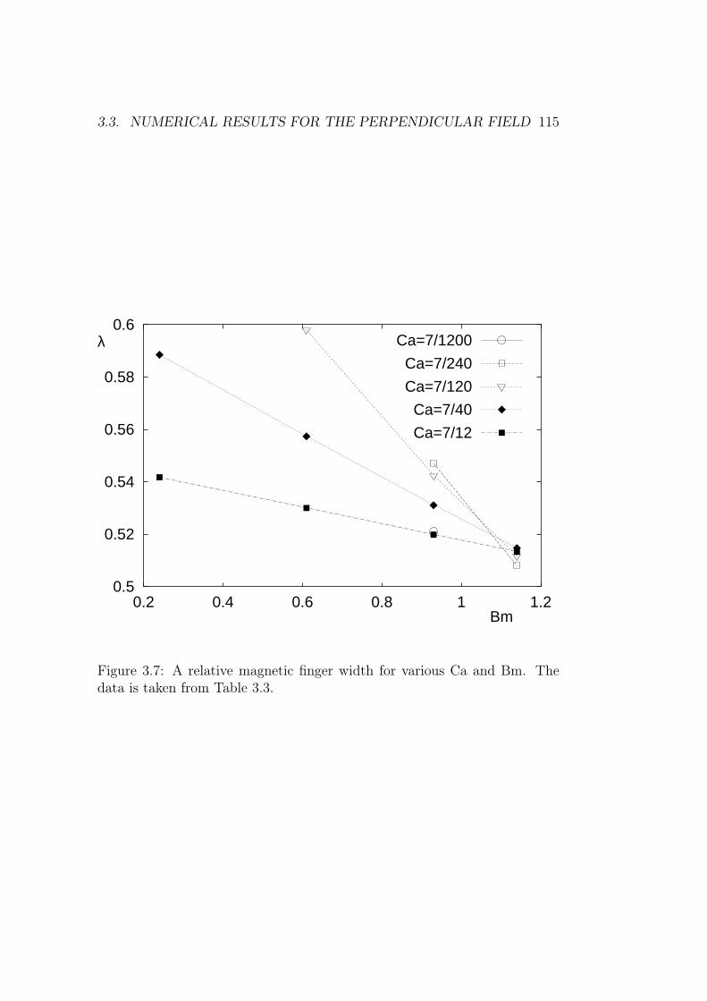
3.3. NUMERICAL RESULTS FOR THE PERPENDICULAR FIELD 115
0.5
0.52
0.54
0.56
0.58
0.6
0.2 0.4 0.6 0.8 1 1.2
λ
Bm
Ca=7/1200
Ca=7/240
Ca=7/120
Ca=7/40
Ca=7/12
Figure 3.7: A relative magnetic finger width for various Ca and Bm. Thedata is taken from Table 3.3.

116 CHAPTER 3. ST INSTABILITY WITH AN IMMISCIBLE MF
0.520
0.522
0.524
0.526
0.528
0.530
0.532
5000 6000 7000 8000 9000 10000 11000
λ
t
Figure 3.8: Computed magnetic finger width λ versus time. Ca = 7/1200,Bm = 0.93; other parameters are as in Table 3.3. The solid line is curve’sasymptote.
Ca, the slower. Note also that at some Bm values, the finger width is a non-monotonous function of Ca having its maximum at an intermediate Ca value.The quantitative agreement with the experiments [181, 7] of the Bacri groupis unfortunately not satisfactory, the discrepancy in λ being at low Ca as highas 0.08. We attribute this to the assumed periodicity of the magnetic force(§3.1.5) and to a high magnetization that is in fact not negligible with respectto the applied field (p. 76). None of the computed fingers had λ < 1/2.
Now we repeat another simulation by Cebers – the one of a magneticbranched pattern [176]. We find it convenient to present most patterns overa period and a half, having the x-axis horizontal and the y-axis – vertical, ifnot specified otherwise. Our pattern presented in Fig. 3.9 should be comparedagainst Fig. 3 of [176]. In comparing, we remember that in that simulationof [176], the length scale was twice as long as ours (we preserve the sameaspect ratio in Fig. 3.9 though), their time scale was two thirds of ours, theircapillary number was defined in a different manner, and their gravity was di-rected upwards. As early as at t = 0.5, our pattern shown in Fig. 3.9(a) looksalready quite different from that shown in the panel of [176] correspondingto t = 0.75 in their notation. Namely, there are two tongues of falling MF(fingers) per period in [176], with the wider one having started to tip-splitalready, while Fig. 3.9(a) displays a single three-lobe tongue. A second fin-

3.3. NUMERICAL RESULTS FOR THE PERPENDICULAR FIELD 117
-6
-3
0
3
6
-3 0 3 6(a) t = 0.5.
-6
-3
0
3
6
-3 0 3 6(b) t = 1.33.
-15
-12
-9
-6
-3
0
3
6
9
12
15
-3 0 3 6(c) t = 2.
-15
-12
-9
-6
-3
0
3
6
9
12
15
-3 0 3 6(d) t = 3.3.
Figure 3.9: An interface computed with Ca = 3, Bm = 7, At = 29/31,T = 2π, M = 3, and the initial data y = −0.1 cos(2πx/T ).

118 CHAPTER 3. ST INSTABILITY WITH AN IMMISCIBLE MF
ger appears at a later stage, but remains weaker than the finger appearing in[176]. Nevertheless, the later structures bear much resemblance to those in[176]. This is evidenced by comparing Fig. 3.9(b) against the correspondingresult of [176] (t = 2 in their notation, which corresponds to our t = 4/3).Indeed, in both cases there are two (long) fingers of emerging non-magneticfluid. Of the two magnetic fingers, one is split into two (three, in our simula-tion) lobes and exhibits two (one) “peristaltic” deformations, while the otheris partially (completely) shielded. In this regard the conjecture made in [250]may be pointed out that two-lobe and three-lobe tip-splittings are caused bythe same instability mechanism and can substitute one another (three-lobesplittings are indeed observed in experiments). As simulation goes on, theperistaltic deformations increase in number and amplitude, becoming sidebranches. About t = 2.1 the symmetry of the interface gets broken. Strictlyspeaking, broken gets the parity of the interface (its evenness with respectto the x = 0 line.) We are able to progress further with the simulation up tot = 3.3 (Fig. 3.9(d)). To assess the accuracy of this result obtained with ini-tial N = 32, we computed with a twice as high resolution (N = 64 initially)up to t = 2, which is shortly before the symmetry breaks up. In Fig. 3.9(c),we try to plot the low-resolution results in dots, while the higher-resolutionones are plotted in solid. The two curves are almost indistinguishable, whichproves that the accuracy is high enough. Turning back to Fig. 3.9(d), we seethat the central finger has shifted towards one of its neighbours. We interpretthis as follows: the symmetric position has lost its stability. We believe thatthe symmetry break-up and the emergence of bifurcation is indeed present inthe model. Which of the two new stable positions is selected? This of courseis determined by the noise, be it numerical or experimental (later we will seean example of the noise effect). The event can be described physically asthe four-arm vertex (located at (x, y) = (0, 0) in Fig. 3.9(c)) being separatedinto two 3-arm vertices (Fig. 3.9(d)). Such events were previously reportedand analyzed for the same problem in the radial geometry [169, 182] and areanalogous to the behaviour of two-dimensional foam films attached to sev-eral pins. The vertex-splitting is believed to prevent the rupture of shapesby the overextension mechanism. Later we will see a vertex-splitting in otherpatterns as well.
Simulating another magnetic structure (Fig. 3.10), we will check the ef-fect on the results of the time step size and that of changing the markerredistribution criteria. Surprisingly, the latter effect is quite appreciable(still not drastic). Besides, at plotting the pattern after the loss of sym-metry (Fig. 3.10(b)), the interface computed at a decreased time step in factdemanded a reflection with respect to x = 0 axis, which shows that small per-turbations (noise) can determine which of the two new stable configurations

3.3. NUMERICAL RESULTS FOR THE PERPENDICULAR FIELD 119
-80
-40
0
40
80
-10 0 10 20
(a) t = 500.
-80
-40
0
40
80
-10 0 10 20
(b) t = 990.
Figure 3.10: An interface computed with Ca = 0.224/π ≈ 7.13 × 10⁻²,Bm = 4.56/π ≈ 1.45, At = 0.92, T = 20, M = 3, and the initial datay = 0.02 cos(2πx/T ). In Fig. 3.10(b), plotted with a dashed line is theinterface computed at a decreased time step (∆t = 0.020 instead of 0.025),the interface plotted with dots is obtained at a tighter arclength spacingconstraint: 0.607 < ∆s < 0.613 (instead of 0.60 < ∆s < 0.62).
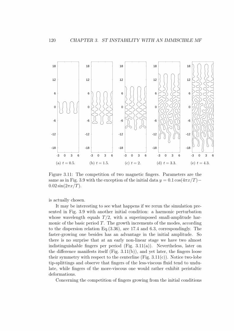
120 CHAPTER 3. ST INSTABILITY WITH AN IMMISCIBLE MF
-18
-12
-6
0
6
12
18
-3 0 3 6
(a) t = 0.5.
-18
-12
-6
0
6
12
18
-3 0 3 6
(b) t = 1.5.
-18
-12
-6
0
6
12
18
-3 0 3 6
(c) t = 2.
-18
-12
-6
0
6
12
18
-3 0 3 6
(d) t = 3.3.
-18
-12
-6
0
6
12
18
-3 0 3 6
(e) t = 4.3.
Figure 3.11: The competition of two magnetic fingers. Parameters are thesame as in Fig. 3.9 with the exception of the initial data y = 0.1 cos(4πx/T )−0.02 sin(2πx/T ).
is actually chosen.
It may be interesting to see what happens if we rerun the simulation pre-sented in Fig. 3.9 with another initial condition: a harmonic perturbationwhose wavelength equals T/2, with a superimposed small-amplitude har-monic of the basic period T . The growth increments of the modes, accordingto the dispersion relation Eq.(3.36), are 17.4 and 6.3, correspondingly. Thefaster-growing one besides has an advantage in the initial amplitude. Sothere is no surprise that at an early non-linear stage we have two almostindistinguishable fingers per period (Fig. 3.11(a)). Nevertheless, later onthe difference manifests itself (Fig. 3.11(b)), and yet later, the fingers loosetheir symmetry with respect to the centerline (Fig. 3.11(c)). Notice two-lobetip-splittings and observe that fingers of the less-viscous fluid tend to undu-late, while fingers of the more-viscous one would rather exhibit peristalticdeformations.
Concerning the competition of fingers growing from the initial conditions

3.3. NUMERICAL RESULTS FOR THE PERPENDICULAR FIELD 121
-15
-10
-5
0
5
10
15
-1 0 1 2 3
(a)
-15
-10
-5
0
5
10
15
-1 0 1 2 3
(b)
Figure 3.12: Shielding: absent or present? (a): t = 1.18, initial shapey = −0.05 cos(4πx/T ) + 0.01 cos(2πx/T ); (b): t = 0.48, initial shape y =−0.05 cos(4πx/T ) − 0.0005 sin(2πx/T ). The initial shapes are schematicallyshown below. Ca = 12, Bm = 7, At = 29/31, T = π, and M = 3 for both.
122 CHAPTER 3. ST INSTABILITY WITH AN IMMISCIBLE MF
of the above sort, we note the important role played by the phase differ-ence between the interacting harmonics. Indeed, compare Figs. 3.12(a) and3.12(b). In the first case, the (downward) humps of the more-viscous fluiddiffer in amplitude, while the humps of the less-viscous one do not. Thestronger downward finger does not shield with time the shorter one, theirdifference in length remains small, as if there were some stabilizing mecha-nism. In the other case, the crests of the wavy interface differ just a littlebit, while the hollows are exactly the same. Nevertheless, the higher crestquickly wins over the lower one (Fig. 3.12(b)). Thus we can cautiously inferthat fingers of the less-viscous fluid are more susceptible to mutual shieldingthan fingers of the more-viscous one.
In Fig. 3.13 we present a long finger undergoing repetitive “peristaltic”deformations. In Figs. 3.13(h)–3.13(k) it is shown how the finger looses itssymmetry with respect to the centerline. It occurs through the characteristicvertex-splitting already described above.
One more pattern is shown in Fig. 3.14. Contrary to what one mightthink, the strange shape of the downward finger proves stable.
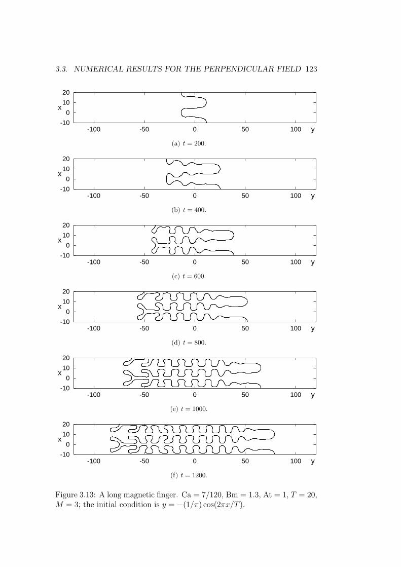
3.3. NUMERICAL RESULTS FOR THE PERPENDICULAR FIELD 123
-10
0
10
20
-100 -50 0 50 100
x
y
(a) t = 200.
-10
0
10
20
-100 -50 0 50 100
x
y
(b) t = 400.
-10
0
10
20
-100 -50 0 50 100
x
y
(c) t = 600.
-10
0
10
20
-100 -50 0 50 100
x
y
(d) t = 800.
-10
0
10
20
-100 -50 0 50 100
x
y
(e) t = 1000.
-10
0
10
20
-100 -50 0 50 100
x
y
(f) t = 1200.
Figure 3.13: A long magnetic finger. Ca = 7/120, Bm = 1.3, At = 1, T = 20,M = 3; the initial condition is y = −(1/π) cos(2πx/T ).

124 CHAPTER 3. ST INSTABILITY WITH AN IMMISCIBLE MF
-10
0
10
20
-100 -50 0 50 100
x
y
(g) t = 1400.
-10
0
10
20
-100 -50 0 50 100
x
y
(h) t = 1450.
-10
0
10
20
-100 -50 0 50 100
x
y
(i) t = 1500.
-10
0
10
20
-100 -50 0 50 100
x
y
(j) t = 1550.
-10
0
10
20
-100 -50 0 50 100
x
y
(k) t = 1600.
Figure 3.13: A long magnetic finger (continued). A vertex-splitting event.
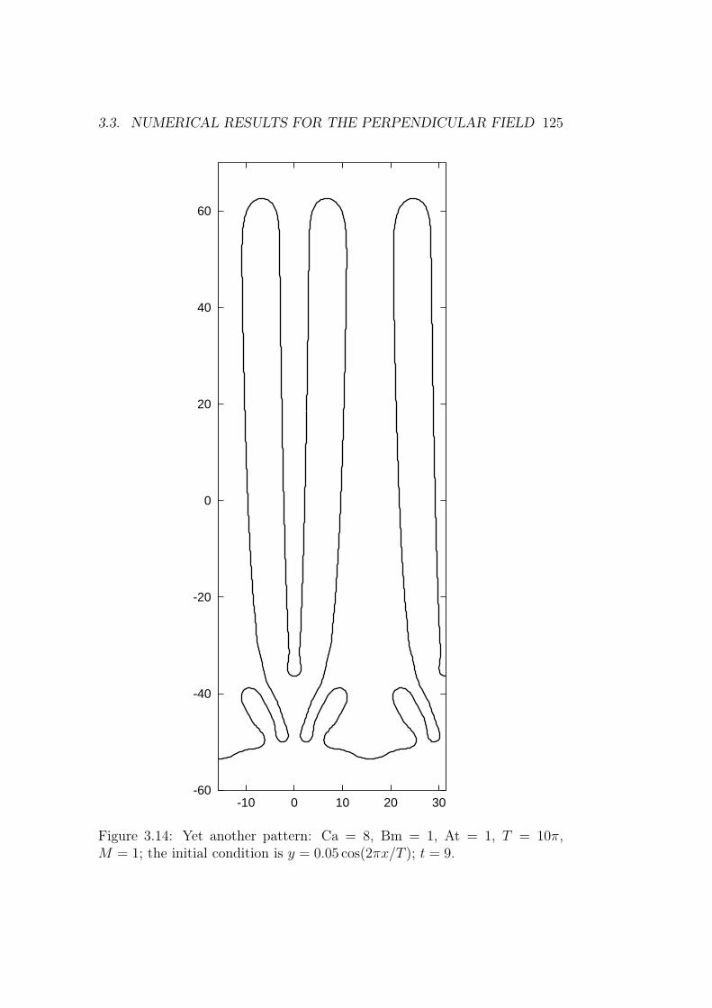
3.3. NUMERICAL RESULTS FOR THE PERPENDICULAR FIELD 125
-60
-40
-20
0
20
40
60
-10 0 10 20 30
Figure 3.14: Yet another pattern: Ca = 8, Bm = 1, At = 1, T = 10π,M = 1; the initial condition is y = 0.05 cos(2πx/T ); t = 9.

126 CHAPTER 3. ST INSTABILITY WITH AN IMMISCIBLE MF
3.3.2 Dendritic patterns
Now we will study the development of a highly convoluted interface thatdevelops at a relatively low capillary number Ca, high Bm, and high viscositycontrast. We will call the more-viscous upper (At > 0) fluid just “liquid”, andthe less-viscous fluid will be called “air”. Tracing the evolution of the interface(Fig. 3.15) reveals some scenarios of pattern formation. Perhaps the mostcommon is the tip-splitting that is the first secondary instability to occur(Figs. 3.15(a), 3.15(b)), both with liquid and air fingers. Some fingers exhibitalready the “peristaltic” deformations. At about t = 14 the pattern loosesits symmetry, and another instability sets in: A peristaltic bulge on a liquidfinger flattens out on one side, jutting out on the other (Fig. 3.15(c)). Theprocess ends up with a single side branch (Fig. 3.15(d); the pattern fragmentsunder consideration are marked by a rectangular contour). Thus a retractionof a side branch is possible, which is indeed observed [12]. In parallel, adjacentair fingers also develop corresponding branches, usually upon undulation, asexemplified by Figs. 3.15(e)–3.15(g). Many fingers become shielded and stopevolving shortly after appearing. Interpenetrating side branches form the“hairpin” details [251]. Later stages are marked by the avalanche of tip-splittings by air fingers. Interestingly, liquid fingers never tip-split again,as was noted and explained by the unfavourable (for instability) viscositycontrast in [12]. Near the tips, air tongues are thicker than liquid ones areat their tips. Note that the top-bottom asymmetry in the pattern is causedby a non-zero At (at a non-zero surface tension). We remind (see p. 86) thatwere At opposite (negative), the pattern would exactly turn upside down towithin the noise effect. The sensitivity of patterns to small perturbations isdemonstrated by Fig. 3.16, we simulate two patterns that differ only in thesign of At and should coincide in precise arithmetics. However, the numericalresults are slightly yet appreciably different because of the numerical errorthat differs between the two simulations (mostly because of the magneticintegrals being taken over different domains). Inside the contour, one cannotice that some side-branchings that have occurred in one case, have notin the other, etc. We stress our belief that this sensitivity is a physicaleffect and not numerical one. The same numerical observation is made in[178] where it is conjectured that the energy functional has multiple localminima in the space of accessible shapes. The final picture that we wereable to obtain without the numerical instability resembles rather closely thepatterns observed in the experiments [12, 181].
At Bm = 4.8, the pattern formed is shown in Fig. 3.17.
It is interesting to note that the number of fingers per period in Fig. 3.15 isn = 5 . . . 6 long fingers of the same direction, while the period 2π/k = 3.5092

3.3. NUMERICAL RESULTS FOR THE PERPENDICULAR FIELD 127
-5
0
5
-10 0 10 20
(a) t = 9.
-5
0
5
-10 0 10 20
(b) t = 14.
-10
-5
0
5
10
-10 0 10 20
(c) t = 16.
-10
-5
0
5
10
-10 0 10 20
(d) t = 19.
-15
-10
-5
0
5
10
15
-10 0 10 20
(e) t = 26.
-15
-10
-5
0
5
10
15
-10 0 10 20
(f) t = 29.
Figure 3.15: The development of a magnetic dendrite: Ca = 3/16, Bm =3.675, At = 0.986, T = 24, M = 3, and the initial data y = −0.5 sin(2πx/T ).

128 CHAPTER 3. ST INSTABILITY WITH AN IMMISCIBLE MF
-15
-10
-5
0
5
10
15
20
-10 0 10 20
(g) t = 32.
-15
-10
-5
0
5
10
15
20
-10 0 10 20
(h) t = 36.
-30
-25
-20
-15
-10
-5
0
5
10
15
20
25
30
35
-10 0 10 20
(i) t = 48.
-30
-25
-20
-15
-10
-5
0
5
10
15
20
25
30
35
-10 0 10 20
(j) t = 60.
Figure 3.15: The development of a magnetic dendrite (continued).

3.3. NUMERICAL RESULTS FOR THE PERPENDICULAR FIELD 129
-30
-25
-20
-15
-10
-5
0
5
10
15
20
25
30
35
40
-10 0 10 20
(k) t = 72.
Figure 3.15: The development of a magnetic dendrite (continued).

130 CHAPTER 3. ST INSTABILITY WITH AN IMMISCIBLE MF
-10
-5
0
5
10
-10 0 10 20
(a) t = 22.
-15
-10
-5
0
5
10
15
-10 0 10 20
(b) t = 32.
-25
-20
-15
-10
-5
0
5
10
15
20
25
30
-10 0 10 20
-30
-25
-20
-15
-10
-5
0
5
10
15
20
25
-10 0 10 20
(c) t = 55.
Figure 3.16: The sensitivity of pattern formation to small perturbations.The pattern shown in Fig. 3.15 is reproduced in solid lines. The patternobtained under the same conditions except for the opposite At = −0.986and the opposite initial data y = +0.5 sin(2πx/T ) is plotted upside down indots. (In the last panel the y-axis is reversed explicitly.) While the exactsolutions coincide, numerical noise in the two runs was different, which leadto appreciably distinct patterns.

3.3. NUMERICAL RESULTS FOR THE PERPENDICULAR FIELD 131
-40
-30
-20
-10
0
10
20
30
40
50
-10 0 10 20
Figure 3.17: A magnetic dendrite at a higher Bm (t = 64): Ca = 3/16, Bm =4.8, At = 0.986, T = 24, M = 3, and the initial data y = −0.5 sin(2πx/T ).

132 CHAPTER 3. ST INSTABILITY WITH AN IMMISCIBLE MF
0.1 0.2 0.5 1 2 5 10 20 50 100δ
0.512
51020
50100200
500Bm
Figure 3.18: The equilibrium width δ of straight magnetic stripes as a func-tion of Bm. Solid line: a stripe in a 2δ-periodic pattern [59]; dotted line: anisolated stripe [252].
of the most dangerous linear mode (for a planar interface) is some 7 timesless than T = 24. In the same time, the width δ of long fingers measured inthe middle of the structure (far from top and bottom) is about 1.2 . . . 1.4 forthe fingers of both sorts. (The closer to the tip, the thinner the finger, unlessthe distance from the tip is less than several widths.) The deviation of thewidth from T/(2n) is due to the “defects” of the structure (side branches,undulation, shielded fingers). Judging by late panels of Fig. 3.15, apart fromthe drift as a whole, the middle of the structure stops to evolve, which meansthat internally this region has arrived to a static equilibrium. In this regardlet us note that it is possible to compute the magnetic energy (per unit length)of the pattern of long parallel MF stripes [253, 59]. This energy summed withthe energy due to surface tension can be minimized at a constant stripe areato yield the equilibrium parameters of the pattern. From formula (11) of[59], in the case when stripes of both kinds are of the same length, it followsthat (in our notations)
(
2δ
π
)2 ∫ π/(2δ)
0
y ln
(
1 +1
sinh2 y
)
dy =2
Bm. (3.38)
Another particular case of that formula in [59] is the equilibrium width4 of
4Bm is defined in [59, 252] to be one half of ours. Our Bm in SI units is(µ0/(4π)) 2(∆M)2h/σ, where µ0 is the “permeability of vacuum.”

3.3. NUMERICAL RESULTS FOR THE PERPENDICULAR FIELD 133
a single straight stripe [252]:
δ2 ln(1 + δ−2) + ln(1 + δ2) = 4/Bm . (3.39)
These relations are plotted in Fig. 3.18. It may be seen that at Bm = 3.675,δ = 1.36 for the system of parallel straight stripes, which agrees well withour measured finger width of 1.2 . . . 1.4. We point out that our fingers areappreciably narrower than the half-period π/k = 1.75 of the most unstablemode of a planar interface. At Bm = 4.8, the obtained finger width is1.0 . . . 1.1, also in agreement with δ = 1.12 given by Fig. 3.18, and alsoless than the half-period π/k = 1.40 of the most unstable mode. Thus thepatterns evolve by adapting to the change of preferred spatial scales thattakes place in the course of their evolution.
On the other hand, a larger width that the fingers inherit from the linearstage of instability is the equilibrium one for a pattern of parallel stripes ata lower Bm. It is remarkable that the energy of magnetostatic interactionsacross an undulating stripe (or stripe pattern) undergoing large-wavelengthundulations scales with wavelength (at large wavelength where it is more im-portant) the same way the energy due to surface tension does. This allows tointroduce [254] the notion of an effective surface tension. This quantity is zeroat the critical Bm (see [177], §4.6 of [15] for a single stripe), which is equiva-lently the equilibrium one defined by Eqs.(3.38), (3.39). The effective surfacetension becomes negative at larger Bm values, leading to long-wavelength un-dulations (cf. simulations of a single stripe in [173]). For the analogy of MFstripe patterns to liquid-crystal smectics, see [6, 13]. Thus it can be expectedthat a magnetic Bond number too high for a given period will force the fingersto undulate. “Chevrons” and “hairpins” should [254, 255, 62] develop fromthe undulations in the non-linear regime, as indeed observed experimentallyin [13, 251]. Now we can add to this our numerically obtained hairpin-likeside branches in Fig. 3.15 and, especially, Fig. 3.17, where they are ratherpronounced and regular.
Fig. 3.19 shows the effect of viscosity contrast on the pattern shown inFig. 3.15 – At = 0 for this simulation, other parameters being the same asin Fig. 3.15. Though the basic mechanisms (tip-splitting, side-branching)are still in operation, the resulting differences are obvious. Notice that thepattern no longer transforms into itself by reflection about the x-axis com-bined with a translation by a half-period. (In precise arithmetics, the patternshould so transform as long as the initial conditions do.)
Now let us determine how long-range the magnetic interactions betweenthe parts of a branched pattern are. In other words, how small M = maxmin Eq.(3.27) is sufficient at calculating the magnetic force? Fig. 3.20 proves
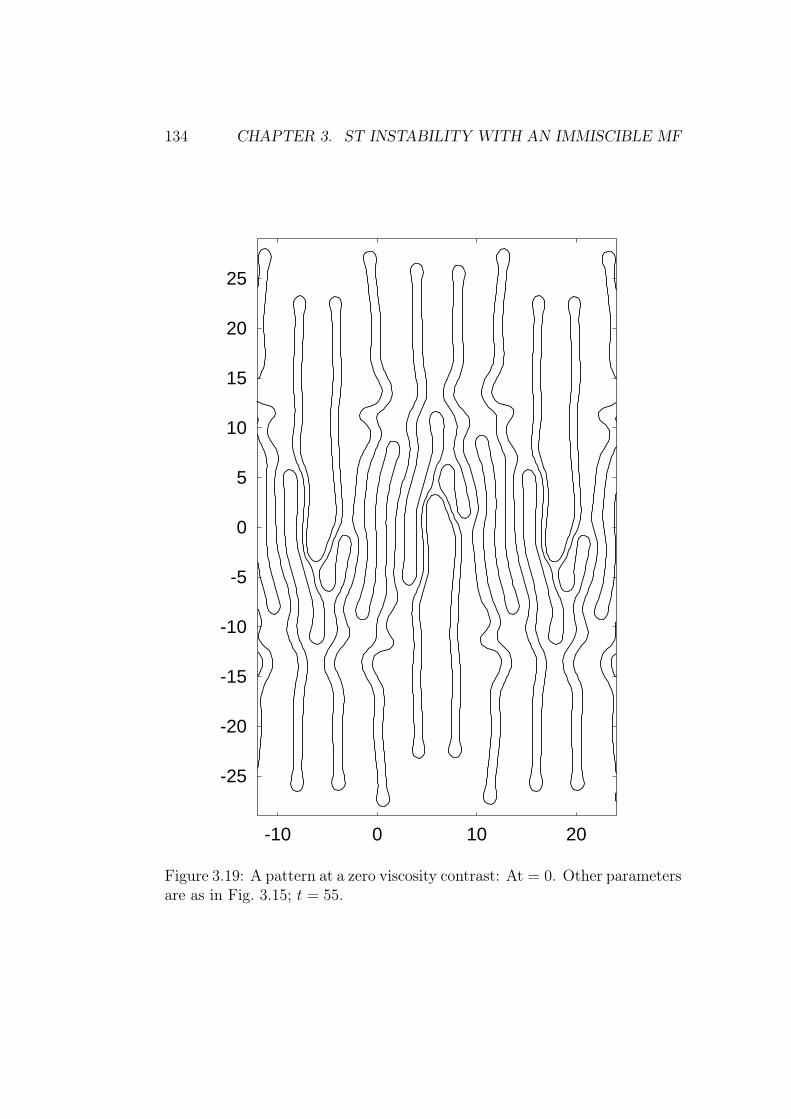
134 CHAPTER 3. ST INSTABILITY WITH AN IMMISCIBLE MF
-25
-20
-15
-10
-5
0
5
10
15
20
25
-10 0 10 20
Figure 3.19: A pattern at a zero viscosity contrast: At = 0. Other parametersare as in Fig. 3.15; t = 55.

3.3. NUMERICAL RESULTS FOR THE PERPENDICULAR FIELD 135
-10
-5
0
5
10
-10 0 10
Figure 3.20: On the effective range of magnetic interactions in Fig. 3.15(t = 19). The pattern interface computed at M = 0 is plotted with a dottedline. The shapes at M = 3 (usual) and M = 1, both plotted in solid, areindistinguishable.
that in the case under review just above, M = 1 is already a very goodapproximation, while M = 0 is perhaps not. (We remind that M = 0means that interactions with about a half of the period in any direction aretaken into account, M = 1 implies one period more, etc.) Nevertheless,since anyway not much computing time would be gained (10–20 %), we willnormally proceed with M = 3 as before.
At low surface tension, we observe other interesting events such as theformation of a pending viscous drop and the air-bubble trapping. Pinchingand rupture of the necks cannot be modelled with the present algorithm (cf.[174]); other approaches are capable of handling topological changes, e.g. thelevel-set algorithm (see p. 97).
In Fig. 3.22 we demonstrate that while the interface can be quite branchedand convoluted, it adapts to the driving forces in such a way that they vary ina rather regular manner along the interface. This includes not only verticalsegments, but also the side branches.
In Fig. 3.23 we compare the early dynamics of the perimeter in the case ofa single finger (Fig. 3.6) against the case of a branched interface (Fig. 3.15).Rapid growth of the interface length in Fig. 3.23(b) at about t = 6 . . . 9 is ex-plained by higher harmonics generated (Fig. 3.15(a)) by the initial imposed

136 CHAPTER 3. ST INSTABILITY WITH AN IMMISCIBLE MF
-15
-10
-5
0
5
10
15
-1 0 1 2 3
(a) Bm = 10, t = 0.162.
-8
-6
-4
-2
0
2
4
6
8
-1 0 1 2 3
(b) Bm = 30, t = 0.062.
Figure 3.21: Drops and trapped bubbles. Ca = 100, At = 0, T = π, M = 3,and initially y = +0.05 cos(4πx/T ) − 0.01 sin(2πx/T ) for both figures.

3.3. NUMERICAL RESULTS FOR THE PERPENDICULAR FIELD 137
-10
0
10
20
0 200 400 600 800 1000s
Figure 3.22: The dynamical structure of the branched interface shown inFig. 3.15(k). The combination 2(κ+ Ca y + Bm Im) + const, the “forcing” ofthe integral Eq.(3.23), is plotted versus arclength.
0.001
0.01
0.1
1
10
100
0 0.1 0.2 0.3 0.4 0.5 0.6 0.7 0.8
L / T
- 1
t
(a) The case of a finger (Fig. 3.6).
0.001
0.01
0.1
1
10
100
0 10 20 30 40 50 60 70
L / T
- 1
t
(b) The case of a branched pattern (Fig. 3.15).
Figure 3.23: Evolution of the perimeter. Solid line: the scaled surplusperimeter L/T − 1; dotted line: its early asymptotics exp(2λt).

138 CHAPTER 3. ST INSTABILITY WITH AN IMMISCIBLE MF
mode of the basic period T in the non-linear regime, with the higher har-monics being more unstable than the initial mode. (It is easy to see that thesurplus perimeter, L−T , of a sinusoidal deformation whose amplitude growsexponentially with rate λ, grows as exp(2λt) in the linear regime and slowsdown afterwards to exp(λt).) In both cases T is larger than the period of themost unstable wavelength. However, the growth rate at the imposed periodin the case of the finger is only 1.6 times lower than the growth rate of themost unstable mode, while in the case of the branched interface the ratio isabout 24. This explains the difference between Figs. 3.23(a) and 3.23(b) aswell as why the imposed mode dominates in the finger case but not in thecase of the branched pattern. Later, the perimeter of the branched structureevolves rather smoothly, but somewhat slower that linearly with time. Onthe contrary, the interfacial length of a developed finger varies linearly withtime to an excellent precision, as might be expected.
In conclusion we mention the so-called comb-like instability [256] that es-sentially is the Rayleigh–Taylor instability of MF’s with stable density strat-ification, Bg < 0. We have made some runs for this situation, finding theobtained patterns to be very similar to the usual case Bg > 0 (Ca > 0). Weremark that the present algorithm enables us to verify the non-linear analysisof [257] of the type of bifurcation in the near-critical conditions.
3.4 Numerical results for the normal field
In fact, at this point we have all the ingredients necessary to easily derive theequations of the evolution of an initially straight interface in the “normal”field (i.e. in the “peak” configuration, where the field is perpendicular tothe interface and parallel to the plane of the Hele-Shaw cell). The dispersionrelation for linearized perturbations of a planar interface [180] can be writtenin our notation as
λ = −k3 + k (Ca + Bg + 2 Bm Inorm(k)) , (3.40)
where
Inorm(k) =
∫ +∞
0
1 − cos(kt)
t2
(√t2 + 1 − t
)
dt .
Both perpendicular (Eq.(3.36)) and normal fields tend to destabilize everywavelength of a perturbed immiscible interface (and the shorter the wave-length, the higher the tendency towards its destabilization by the fields).
Let the field be directed along the y-axis in the geometry of Fig. 3.1.Then to use the formulas derived in §1.4 and Chapter 2.4, we only have to

3.4. NUMERICAL RESULTS FOR THE NORMAL FIELD 139
substitute there x with −y and y with x. Indeed, Eq.(2.46) for the magneticforce at a constant magnetization becomes
~fm = Mi~∇∂ψ
∂y. (3.41)
The (gap-averaged) magnetic potential ψ is written according to the dimen-sional form of Eq.(2.51) as
∂ψ
∂y= −2
h
+∞∫
−∞
+∞∫
−∞
(y − y′)∂M
∂y′Jh
(
√
(x− x′)2 + (y − y′)2)
dx′ dy′ (3.42)
with Jh(ρ) = (√
ρ2 + h2 − ρ)/
ρ2 . Since we have now two domains of con-
stant magnetization, the derivative of the latter in Eq.(3.42) is zero awayfrom the interface, being in fact a delta function. This allows to perform oneof integrations in Eq.(3.42). First imagine that the interface is such that yis a single-valued function of x. Then we immediately obtain (whatever theslope of the interface)
∂ψ
∂y= −2(M2 −M1)
h
+∞∫
−∞
(y − y′)Jh
(
√
(x− x′)2 + (y − y′)2)
dx′
= −2(M2 −M1)
h
+∞∫
−∞
(y − y′)Jh
(
√
(x− x′)2 + (y − y′)2)
τx(s′) ds′ ,
(3.43)
where s′ is the arclength variable parametrizing the infinite interface. Ifwe remove the limitation of single-valuedness, it suffices to split the (x′, y′)domain into the pieces where x′ can be used as a curve parameter and sumthe resulting integrals, obtaining the same final result. If we now proceedwith the same further manipulations as we have done for the case of theperpendicular field in §3.3, we will obtain exactly the same equations exceptfor Im (see Eq.(3.24)) which needs to be replaced with
Im =
v.p.
+∞∫
−∞
√
(x− x′)2 + (y − y′)2 + 1 −√
(x− x′)2 + (y − y′)2
(x− x′)2 + (y − y′)2(y − y′)τx(s
′) ds′ .
(3.44)

140 CHAPTER 3. ST INSTABILITY WITH AN IMMISCIBLE MF
Unlike Eq.(3.24), Eq.(3.44) involves a principal-value integral. We will againtruncate the infinite path of integration in same manner as it has been done in§3.1.5. Our ability to simulate extensively the normal-field instability turnsout to be seriously limited by violent numerical instabilities. To have a stablermethod, some special desingularization of Eq.(3.44) is perhaps needed. Nev-ertheless we are able to produce a preliminary result presented in Figs. 3.24,3.25. (Keep in mind that these Figures are stretched y-wise unlike most pre-vious ones.) Interestingly, it proves possible to reproduce the experimentallyobserved behaviour noted in [7, 181] at Ca = 7/720, Bm = 0.84, At = 1, andT = 20, although some our parameter values differ from the experimentalones. Namely, in the transient regime several peaks per period can developfrom the initial perturbation of a period T . At this stage, the developmentis quite fast (Figs. 3.24(a), 3.24(b)). Then the evolution of the dominantpeak and its smaller neighbours slows down, as shown in Fig. 3.24(c), withthe interfacial period being quite constant. After a while the dominant peakresumes advancing fast, absorbing the smaller ones that recede. Then thereis only one peak with straight slopes that develops into a finger with highcurvature at the tip. Fig. 3.25 shows the case of the maximum viscositycontrast. The transition from a multiple-peak interface to a single peak oc-curs in a slightly different way, while the preceding stage shows no differencebetween the At = 0 and At = 1 cases. We note also that the At = 1 pat-tern almost restores its symmetry with respect to the y = 0 line by aboutt = 90 . . . 100. In the long run, the fingers take on a typical “fish-like” shape.
The development of the boundary-integral method is under way.
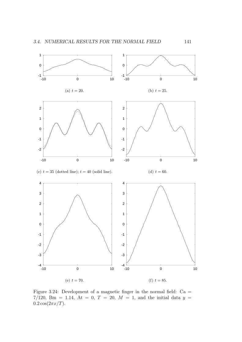
3.4. NUMERICAL RESULTS FOR THE NORMAL FIELD 141
-1
0
1
-10 0 10
(a) t = 20.
-1
0
1
-10 0 10
(b) t = 25.
-2
-1
0
1
2
-10 0 10
(c) t = 35 (dotted line); t = 40 (solid line).
-2
-1
0
1
2
-10 0 10
(d) t = 60.
-4
-3
-2
-1
0
1
2
3
4
-10 0 10
(e) t = 70.
-4
-3
-2
-1
0
1
2
3
4
-10 0 10
(f) t = 85.
Figure 3.24: Development of a magnetic finger in the normal field: Ca =7/120, Bm = 1.14, At = 0, T = 20, M = 1, and the initial data y =0.2 cos(2πx/T ).

142 CHAPTER 3. ST INSTABILITY WITH AN IMMISCIBLE MF
-2
-1
0
1
2
3
-10 0 10
(a) t = 35 (dotted line); t = 40 (solid line).
-2
-1
0
1
2
3
-10 0 10
(b) t = 60.
-4
-3
-2
-1
0
1
2
3
4
5
-10 0 10
(c) t = 70.
-4
-3
-2
-1
0
1
2
3
4
5
-10 0 10
(d) t = 90.
Figure 3.25: Development of a magnetic finger in the normal field at infiniteviscosity contrast. Parameters are the same as in Fig. 3.24 except for At = 1.
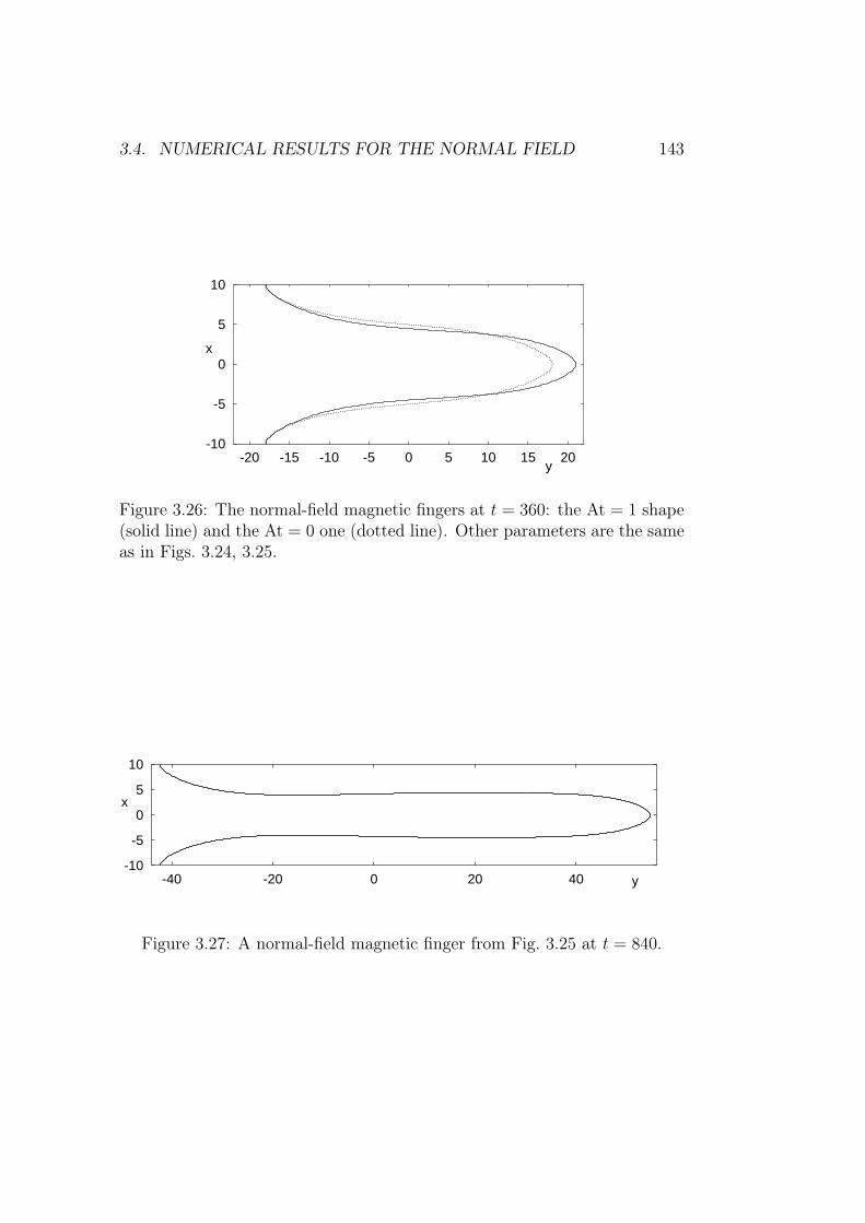
3.4. NUMERICAL RESULTS FOR THE NORMAL FIELD 143
-10
-5
0
5
10
-20 -15 -10 -5 0 5 10 15 20
x
y
Figure 3.26: The normal-field magnetic fingers at t = 360: the At = 1 shape(solid line) and the At = 0 one (dotted line). Other parameters are the sameas in Figs. 3.24, 3.25.
-10
-5
0
5
10
-40 -20 0 20 40
x
y
Figure 3.27: A normal-field magnetic finger from Fig. 3.25 at t = 840.

Conclusion
In conclusion, the present work analyzes some fluid-mechanical instabilitiesexhibited by isothermal magnetized ferrofluids in a Hele-Shaw cell. The non-potential driving force of the instability is due to the self-magnetic field of theferrofluid. By taking the approach of averaging across the gap, we considerboth the case of a single fluid with an inhomogeneous (possibly discontinuous)concentration of magnetic particles, and the case of two immiscible magneticfluids forming a sharp interface with surface tension. Two orientations of theuniform external field are considered: “perpendicular” and “normal” ones.
In the first part, an extensive linear stability analysis is performed for themiscible case with selected basic concentration distributions along the cellthat model experimental conditions reported in the literature. For a step-likeconcentration distribution, we obtain analytically the neutral curves alongwith the critical wavelength and the critical magnetization. In the perpen-dicular field, an oscillatory instability and the absence of discrete instabilitymodes are found possible under certain conditions, and the stability diagramis presented. A mechanism of the oscillatory instability mode is explainedphysically. Self-oscillations occur through the interplay between diffusion andadvection driven via a magnetic body force by concentration inhomogene-ity. An asymptotic treatment of the dispersion relation is presented as well.These results refer to the known experimental situation when a ferrofluid isbrought into contact with its pure carrier liquid, and convective instabilities(the miscible labyrinthine and peak ones) are observed at the diffusion frontbetween the fluids. In the normal field, we additionally consider the stabilityof a periodic pattern of sharp parallel stripes and find that the peristalticmode is critical. These results apply to the forced Rayleigh scattering ex-periments, and our threshold conditions for the onset of microconvection areconsistent with recent experimental observations.
The above analysis is carried out with the assumption that the flow isgoverned by the conventional Darcy law that takes into account only thenear-wall friction. The Brinkman equation offers a much better gap-averagedapproximation of viscous stresses if the typical flow length scale is expected
144

CONCLUSION 145
to be as small as the gap width. It is the simplest equation that allows toreproduce realistically such Hele-Shaw flows. With both the Brinkman equa-tion and the Darcy law, we undertake the numerical stability analysis of thefamily of smoothed step-like concentration distributions (in both fields) andof the Gaussian concentration distributions (in the normal field only). TheDarcy results for the smoothed step-like distributions are proven to convergeto the analytical ones as the interface gets sharper. With the Brinkmanequation, we find that it is viscosity (and not diffusion, as one might think)that determines the scale of the instability at strong forcing by renderingthe most unstable wavelength comparable to several gap widths. This resultproves to be robust, being quite weakly dependent on the basic concentra-tion gradient. We trace the evolution of the neutral curves as the step-likeconcentration distribution diffuses out. Although the wavelength selectionis seriously modified, the critical magnetization is not much affected by theadoption of the Brinkman equation.
In the second half of our study, we model the non-linear dynamics, gov-erned by the Darcy equation, of an immiscible interface between ferrofluids.The boundary-integral method makes modelling efficient by rendering theproblem effectively one-dimensional. We describe the corresponding compu-tational technique, indicate some associated pitfalls, and pay proper attentionto the validity of the developed algorithm. We note that the Saffman–Taylorfinger in a laterally bounded cell cannot be modelled with our approach,although the same problem in the laterally infinite periodic geometry is han-dled with ease. In the latter case, we observe the decrease of the fingerwidth as the magnetization increases. We also obtain picturesque “dendritic”structures close to those observed experimentally and analyze some aspectsof pattern formation such as two-lobe and three-lobe tip-splittings, vertex-splitting, side-branching, and finger shielding. We notice the intrinsic sensi-tivity of the patterns to small perturbations. The change of the preferablelength scale in the course of the pattern evolution is identified as a reason forthe complexity of patterns. These results concern the case of the perpendicu-lar field. We also present, here for the first time, some numerical simulationsfor the normal field. In particular, we obtain a typical finger shape.
As for perspectives, an obvious extension is to unify the miscible and im-miscible problems by following the current trend and allowing for the Korte-weg stresses at the concentration gradients. The non-linear simulations of theBrinkman-governed miscible and immiscible flows might also be interesting;modelling in three dimensions is an ideal. However, these options would com-plicate any treatment considerably. Without any doubt, more experimentsare needed for the development of the subject. The general context for this isquite favourable thanks to the technological trend towards miniaturization.
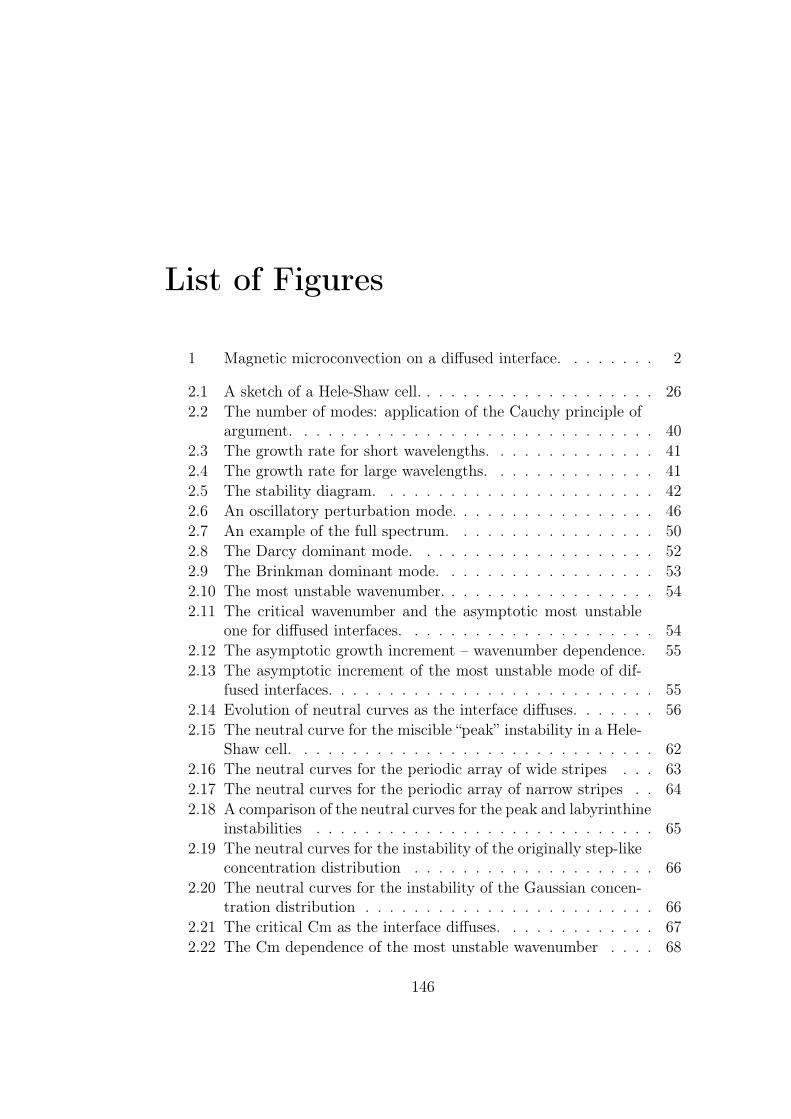
List of Figures
1 Magnetic microconvection on a diffused interface. . . . . . . . 2
2.1 A sketch of a Hele-Shaw cell. . . . . . . . . . . . . . . . . . . . 26
2.2 The number of modes: application of the Cauchy principle ofargument. . . . . . . . . . . . . . . . . . . . . . . . . . . . . . 40
2.3 The growth rate for short wavelengths. . . . . . . . . . . . . . 41
2.4 The growth rate for large wavelengths. . . . . . . . . . . . . . 41
2.5 The stability diagram. . . . . . . . . . . . . . . . . . . . . . . 42
2.6 An oscillatory perturbation mode. . . . . . . . . . . . . . . . . 46
2.7 An example of the full spectrum. . . . . . . . . . . . . . . . . 50
2.8 The Darcy dominant mode. . . . . . . . . . . . . . . . . . . . 52
2.9 The Brinkman dominant mode. . . . . . . . . . . . . . . . . . 53
2.10 The most unstable wavenumber. . . . . . . . . . . . . . . . . . 54
2.11 The critical wavenumber and the asymptotic most unstableone for diffused interfaces. . . . . . . . . . . . . . . . . . . . . 54
2.12 The asymptotic growth increment – wavenumber dependence. 55
2.13 The asymptotic increment of the most unstable mode of dif-fused interfaces. . . . . . . . . . . . . . . . . . . . . . . . . . . 55
2.14 Evolution of neutral curves as the interface diffuses. . . . . . . 56
2.15 The neutral curve for the miscible “peak” instability in a Hele-Shaw cell. . . . . . . . . . . . . . . . . . . . . . . . . . . . . . 62
2.16 The neutral curves for the periodic array of wide stripes . . . 63
2.17 The neutral curves for the periodic array of narrow stripes . . 64
2.18 A comparison of the neutral curves for the peak and labyrinthineinstabilities . . . . . . . . . . . . . . . . . . . . . . . . . . . . 65
2.19 The neutral curves for the instability of the originally step-likeconcentration distribution . . . . . . . . . . . . . . . . . . . . 66
2.20 The neutral curves for the instability of the Gaussian concen-tration distribution . . . . . . . . . . . . . . . . . . . . . . . . 66
2.21 The critical Cm as the interface diffuses. . . . . . . . . . . . . 67
2.22 The Cm dependence of the most unstable wavenumber . . . . 68
146
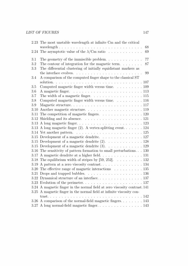
LIST OF FIGURES 147
2.23 The most unstable wavelength at infinite Cm and the criticalwavelength . . . . . . . . . . . . . . . . . . . . . . . . . . . . . 68
2.24 The asymptotic value of the λ/Cm ratio . . . . . . . . . . . . 69
3.1 The geometry of the immiscible problem. . . . . . . . . . . . . 773.2 The contour of integration for the magnetic term. . . . . . . . 873.3 The differential clustering of initially equidistant markers as
the interface evolves. . . . . . . . . . . . . . . . . . . . . . . . 993.4 A comparison of the computed finger shape to the classical ST
solution. . . . . . . . . . . . . . . . . . . . . . . . . . . . . . . 1073.5 Computed magnetic finger width versus time. . . . . . . . . . 1093.6 A magnetic finger. . . . . . . . . . . . . . . . . . . . . . . . . 1133.7 The width of a magnetic finger. . . . . . . . . . . . . . . . . . 1153.8 Computed magnetic finger width versus time. . . . . . . . . . 1163.9 Magnetic structure. . . . . . . . . . . . . . . . . . . . . . . . . 1173.10 Another magnetic structure. . . . . . . . . . . . . . . . . . . . 1193.11 The competition of magnetic fingers. . . . . . . . . . . . . . . 1203.12 Shielding and its absence. . . . . . . . . . . . . . . . . . . . . 1213.13 A long magnetic finger. . . . . . . . . . . . . . . . . . . . . . . 1233.13 A long magnetic finger (2). A vertex-splitting event. . . . . . . 1243.14 Yet another pattern. . . . . . . . . . . . . . . . . . . . . . . . 1253.15 Development of a magnetic dendrite. . . . . . . . . . . . . . . 1273.15 Development of a magnetic dendrite (2). . . . . . . . . . . . . 1283.15 Development of a magnetic dendrite (3). . . . . . . . . . . . . 1293.16 The sensitivity of pattern formation to small perturbations. . . 1303.17 A magnetic dendrite at a higher field. . . . . . . . . . . . . . . 1313.18 The equilibrium width of stripes by [59, 252]. . . . . . . . . . 1323.19 A pattern at a zero viscosity contrast. . . . . . . . . . . . . . . 1343.20 The effective range of magnetic interactions . . . . . . . . . . 1353.21 Drops and trapped bubbles. . . . . . . . . . . . . . . . . . . . 1363.22 Dynamical structure of an interface. . . . . . . . . . . . . . . . 1373.23 Evolution of the perimeter. . . . . . . . . . . . . . . . . . . . . 1373.24 A magnetic finger in the normal field at zero viscosity contrast. 1413.25 A magnetic finger in the normal field at infinite viscosity con-
trast. . . . . . . . . . . . . . . . . . . . . . . . . . . . . . . . . 1423.26 A comparison of the normal-field magnetic fingers. . . . . . . . 1433.27 A long normal-field magnetic finger. . . . . . . . . . . . . . . . 143
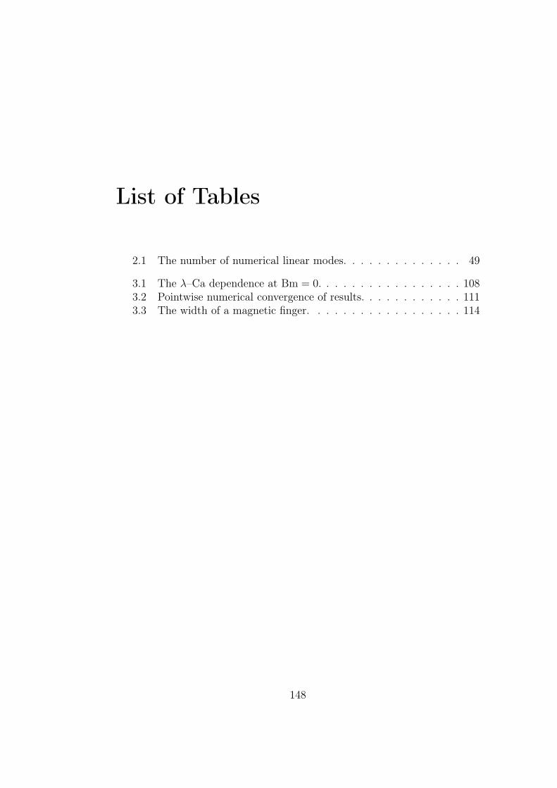
List of Tables
2.1 The number of numerical linear modes. . . . . . . . . . . . . . 49
3.1 The λ–Ca dependence at Bm = 0. . . . . . . . . . . . . . . . . 1083.2 Pointwise numerical convergence of results. . . . . . . . . . . . 1113.3 The width of a magnetic finger. . . . . . . . . . . . . . . . . . 114
148

Bibliography
[1] M. M. Maiorov and A. O. Tsebers. Magnetic microconvection on thediffusion front of ferroparticles. Magnetohydrodynamics5, 19(4):376–380, 1983.
[2] J.-C. Bacri, A. Cebers, A. Bourdon, G. Demouchy, B.M. Heegaard, andR. Perzynski. Forced Rayleigh experiment in a magnetic fluid. Phys.Rev. Lett., 74:5032–5035, 1995.
[3] A. Mezulis and E. Blums. Experimental investigations on the micro-convective instability in optically induced gratings. In NanoMag2004[258], pages 35–36.
[4] W. Luo, T. Du, and J. Huang. Phys. Rev. Lett., 87, 059802, 2001.Reply to [110].
[5] J. M. Ottino and S. Wiggins. Introduction: mixing in micro-fluidics. Phil. Trans. R. Soc. Lond. A, 362:923–935, 2004. Full textis available as: <mixing.chem-eng.northwestern.edu/papers/philtrans/Phil_Trans_OttiWigg.pdf>.
[6] A. Cebers and I. Drikis. Labyrinthine pattern formation in magneticliquids. In I. Athanasopoulos, G. Makrakis, and J. F. Rodrigues, ed-itors, Free boundary problems: theory and applications, volume 409 ofResearch Notes in Mathematics, pages 14–38. Chapman & Hall /CRC,1999.
[7] G. Pacitto, C. Flament, and J.-C. Bacri. Viscous fingering in a magneticfluid. II. Linear Hele-Shaw flow. Phys. Fluids, 13(11):3196–3203, 2001.
5We reference only the English translation of the journal Magnitnaya Gidrodinamika[Магнитная гидродинамика]. The original Russian reference (prior to 2002) can be re-covered at the site of the journal <www.mhd.sal.lv/index.html>.
149

150 BIBLIOGRAPHY
[8] D. M. Anderson, G. B. McFadden, and A. A. Wheeler. Diffuse-interface methods in fluid mechanics. Ann. Rev. Fluid Mech., 30:139–165, 1998. Full text is available as: <math.gmu.edu/˜dmanders/WEBDAN/ann_rev.ps>.
[9] Ecole Superieure de Physique et de Chimie Industrielles. Proceedings ofthe International Workshop on Miscible Interfaces, Paris, France, July2001.
[10] P. G. Saffman and G. Taylor. The penetration of a fluid into a porousmedium or Hele-Shaw cell containing a more viscous liquid. Proc. R.Soc. London, Ser. A, 245:312–329, 1958.
[11] P. Pelce. Theorie des formes de croissance. Digitations, dendrites etflammes. EDP Sciences – CNRS Editions, Les Ulis, Paris, 2000. InFrench.
[12] G. Pacitto, C. Flament, J.-C. Bacri, and M. Widom. Rayleigh–Taylorinstability with magnetic fluids: Experiment and theory. Phys. Rev.E, 62(6):7941–7948, 2000.
[13] C. Flament, J.-C. Bacri, A. Cebers, F. Elias, and R. Perzynski. Parallelstripes of ferrofluid as a macroscopic bidimensional smectic. Europhys.Lett., 34(3):225–230, 1996.
[14] R. E. Rosensweig. Ferrohydrodynamics. Cambridge University Press,Cambridge, 1985. References are made to the revised Russian edition.
[15] E. J. Blums, A. Cebers, and M. M. Maiorov. Magnetic Fluids. Walterde Gruyter, Berlin, 1997.
[16] A. Gailıtis. Formation of the hexagonal pattern on the surface of aferromagnetic fluid in an applied magnetic field. J. Fluid Mech., 82:401–413, 1977.
[17] M. I. Shliomis. Magnetic fluids. Soviet Physics – Uspekhi, 17:153, 1974.
[18] L. D. Landau and E. M. Lifshitz. Fluid Mechanics. Pergamon, Oxford,1987.
[19] R. Haase. Thermodynamik der irreversiblen Prozesse. Steinkopff,Darmstadt, 1963. In German.
BIBLIOGRAPHY 151
[20] H. H. Hu and D. D. Joseph. Miscible displacement in a Hele-Shaw cell.Z. Angew. Math. Phys., 43(4):626–644, 1992. Full text is available at[259].
[21] O. Manickam and G. M. Homsy. Fingering instabilities in verticalmiscible displacement flows in porous media. J. Fluid Mech., 288:75–102, 1995.
[22] T. Y. Liao and D. D. Joseph. Sidewall effects in the smoothing of aninitial discontinuity of concentration. J. Fluid Mech., 342:37–51, 1997.Full text is available at [259].
[23] D. Joseph, A. Huang, and H. Hu. Non-solenoidal velocity effects andKorteweg stresses in simple mixture of incompressible liquids. PhysicaD, 97:104–125, 1996. Full text is available at [259].
[24] D. Joseph. Fluid dynamics of two miscible liquids with diffusion andgradient stresses. Eur. J. Mech. B / Fluids, 9:565–596, 1990. Full textis available at [259].
[25] P. Galdi, D. D. Joseph, L. Preziosi, and S. Rionero. Mathematicalproblems for miscible, incompressible fluids with Korteweg stresses.Eur. J. Mech. B / Fluids, 10:253–267, 1991. Full text is available at[259].
[26] N. Alikakos, P. Bates, and X. Chen. Convergence of the Cahn–Hilliardequations to the Hele-Shaw model. Arch. Rat. Mech. Anal., 128:165–205, 1994.
[27] H.-G. Lee, J. S. Lowengrub, and J. Goodman. Modeling pinchoff andreconnection in a Hele-Shaw cell. I. The models and their calibration.Phys. Fluids, 14(2):492–513, 2002.
[28] H.-G. Lee, J. S. Lowengrub, and J. Goodman. Modeling pinchoff andreconnection in a Hele-Shaw cell. II. Analysis and simulation in thenonlinear regime. Phys. Fluids, 14(2):514–545, 2002.
[29] G. I. Taylor. Dispersion of soluble mater in solvent flowing slowlythrough a tube. Proc. R. Soc. London Ser. A, 219:186–203, 1953.
[30] G. M. Homsy. Viscous fingering in porous media. Annu. Rev. FluidMech., 19:271–311, 1987.
[31] R. A. Wooding. The stability of an interface between miscible fluids ina porous medium. Z. Angew. Math. Phys., 13:255–266, 1962.

152 BIBLIOGRAPHY
[32] L. Paterson. Fingering with miscible fluids in a Hele-Shaw cell. Phys.Fluids, 28(1):26–30, 1985.
[33] C. T. Tan and G. M. Homsy. Stability of miscible displacements inporous media: Rectilinear flow. Phys. Fluids, 29:3549–3556, 1986.
[34] C. T. Tan and G. M. Homsy. Stability of miscible displacements inporous media: Radial source flow. Phys. Fluids, 30(5):1239–1245, 1987.
[35] Y. C. Yortsos and M. Zeybek. Dispersion driven instability in miscibledisplacement in porous media. Phys. Fluids, 31(12):3511–3518, 1988.
[36] J.-C. Bacri, D. Salin, and Y. C. Yortsos. Analyse lineaire de la stabilitede l’ecoulement de fluides miscibles en milieux poreux. C. R. Acad. Sci.Paris, Ser. II, 314:139–144, 1992. In French.
[37] J.-C. Bacri, N. Rakotomalala, D. Salin, and R. Woumeni. Miscible vis-cous fingering: Experiments versus continuum approach. Phys. FluidsA, 4(8):1611–1619, 1992.
[38] A. Rogerson and E. Meiburg. Shear stabilization of miscible displace-ment processes in porous media. Phys. Fluids A, 5(6):1344–1355, 1993.
[39] O. Manickam and G. M. Homsy. Stability of miscible displacementsin porous media with nonmonotonic viscosity profiles. Phys. Fluids A,5:1356–1367, 1993.
[40] C. T. Tan and G. M. Homsy. Simulation of nonlinear viscous fingeringin miscible displacement. Phys. Fluids, 31(6):1330–1338, 1988.
[41] C.-Y. Chen and E. Meiburg. Miscible porous media displacements inthe quarter five-spot configuration. Part 1. The homogeneous case. J.Fluid Mech., 371:233–268, 1998.
[42] R. A. Wooding. Growth of fingers at an unstable diffusing interface ina porous medium or Hele-Shaw cell. J. Fluid Mech., 39:477–495, 1969.
[43] P. Petitjeans and T. Maxworthy. Miscible displacements in capillarytubes. Part 1. Experiments. J. Fluid Mech., 326:37–56, 1996.
[44] J. Kuang, T. Maxworthy, and P. Petitjeans. Miscible displacementsbetween silicone oils in capillary tubes. Eur. J. Mech. B / Fluids,22:271–277, 2003.

BIBLIOGRAPHY 153
[45] C.-Y. Chen and E. Meiburg. Miscible displacements in capillary tubes.Part 2. Numerical simulations. J. Fluid Mech., 326:57–90, 1996.
[46] C.-Y. Chen and E. Meiburg. Miscible displacements in a capillary tube:Influence of Korteweg stresses and divergence effects. Phys. Fluids,14(7):2052–2058, 2002.
[47] N. Rakotomalala, D. Salin, and P. Watzky. Miscible displacement be-tween two parallel plates: BGK lattice gas simulations. J. Fluid Mech.,338:277–297, 1997.
[48] C.-Y. Chen, L. Wang, and E. Meiburg. Miscible droplets in a porousmedium and the effects of Korteweg stresses. Phys. Fluids, 13:2447–2456, 2001.
[49] P. Petitjeans and P. Kurowski. Fluides non miscibles / fluides miscibles:des similitudes interessantes. C. R. Acad. Sci. Paris, Ser. II B, 325:587–592, 1997. In French.
[50] M. Legendre, P. Petitjeans, and P. Kurowski. Instabilites a l’interfaceentre fluides miscibles par forcage oscillant horizontal. C. R. Acad. Sci.Paris, Ser. II B, 331 (9):617–622, 2003. In French.
[51] M. Legendre. Fluides sous vibrations et singularites d’interface. PhDthesis, Universite Paris 6 – Pierre et Marie Curie, Paris, 2003. InFrench.
[52] P. Petitjeans. Une tension de surface pour les fluides miscibles. C. R.Acad. Sci. Paris, Ser. II B, 322:673–679, 1996. In French.
[53] Z. Yang and Y. C. Yortsos. Asymptotic solutions of miscible displace-ments in geometries of large aspect ratio. Phys. Fluids, 9(2):286–298,1997.
[54] E. Lajeunesse, J. Martin, N. Rakotomalala, and D. Salin. 3d insta-bility of miscible displacements in a Hele-Shaw cell. Phys. Rev. Lett.,79(26):5254–5257, 1997.
[55] S. H. Davis. Hydrodynamic interactions in directional solidification. J.Fluid Mech., 212:241–262, 1990.
[56] E. Lajeunesse, J. Martin, N. Rakotomalala, D. Salin, and Y. C. Yortsos.Miscible displacement in a Hele-Shaw cell at high rates. J. Fluid Mech.,398:299–319, 1999.

154 BIBLIOGRAPHY
[57] E. Lajeunesse, J. Martin, N. Rakotomalala, D. Salin, and Y. C. Yortsos.The threshold of the instability in miscible displacements in a Hele-Shaw cell at high rates. Phys. Fluids, 13(3):799–801, 2001.
[58] A. O. Tsebers. Role of surface interactions in stratification of magneticfluids. Magnetohydrodynamics, 18(4):345–350, 1982.
[59] A. Cebers. Transformations of the concentration domain structures ofliquid magnetics in plane layers 1. The energetic approach. Magneto-hydrodynamics, 31(1):58–64, 1995.
[60] A. Cebers. Transformations of the concentration domain structures ofliquid magnetics in plane layers 2. Kinetics and the numerical experi-ment. Magnetohydrodynamics, 31(1):65–72, 1995.
[61] A. Cebers. Two-dimensional concentration domain patterns in mag-netic suspensions: Energetical and kinetic approach. Progr. ColloidPolym. Sci., 100:101–106, 1996.
[62] A. Cebers. Instabilities of concentration stripe patterns in ferrocolloids.Phys. Rev. E, 61(1):700–708, 2000.
[63] D. Lacoste and T. C. Lubensky. Phase transitions in a ferrofluidat magnetic-field-induced microphase separation. Phys. Rev. E, 64,041506, 2001. See also <arxiv.org/abs/cond-mat/0103429>.
[64] A. Cebers. The anisotropy of the surface tension at the magnetic-field-induced phase transformations. J. Magn. Magn. Mat., 252:259–261,2002.
[65] A. O. Tsebers. Three-dimensional structures in planar ferrocolloid lay-ers. Magnetohydrodynamics, 24(2):184–188, 1988.
[66] A. O. Tsebers. A general diffusion model of magnetized suspensionsand dissipative vortex structures in rotating magnetic fields. 1. Mag-netohydrodynamics, 25(3):281–285, 1989.
[67] C.-Y. Chen. Numerical simulations of fingering instabilities in misciblemagnetic fluids in a Hele-Shaw cell and the effects of Korteweg stresses.Phys. Fluids, 15(4):1086–1089, 2003.
[68] C.-Y. Chen and C.-Y. Wen. Numerical simulations of miscible mag-netic flows in a Hele-Shaw cell. Radial flows. J. Magn. Magn. Mater.,252:296–298, 2002.

BIBLIOGRAPHY 155
[69] J. Happel and H. Brenner. Low Reynolds Number Hydrodynamics:With Special Applications to Particulate Media. Prentice-Hall, Engle-wood Cliffs, N. J., 1965.
[70] G. K. Batchelor. An Introduction to Fluid Dynamics. Cambridge Uni-versity Press, Cambridge, 1970.
[71] P. Gondret, N. Rakotomalala, M. Rabaud, D. Salin, and P. Watzky.Viscous parallel flows in a finite aspect ratio Hele-Shaw cell: Analyticaland numerical results. Phys. Fluids, 9:1841–1843, 1997.
[72] P. Ya. Polubarinova-Kochina. Theory of Groundwater Movement.Nauka, Moscow, 2nd edition, 1977. In Russian. English translationfrom the 1st edition was printed by Princeton University Press, Prince-ton, N. J., 1962.
[73] H. Lamb. Hydrodynamics. Cambridge University Press, Cambridge,6th edition, 1993.
[74] M. van Dyke. An Album of Fluid Motion. Parabolic Press, Stanford,California, 1982.
[75] L. Prandtl. Fuhrer durch die Stromungslehre. 2nd edition.
[76] H. Schlichting. Boundary-Layer Theory. McGraw-Hill, N. Y., L., 6thedition, 1968.
[77] J. Zeng, Y. C. Yortsos, and D. Salin. On the Brinkman correction inunidirectional Hele-Shaw flows. Phys. Fluids, 15:3829–3836, 2003.
[78] D. Snyder and S. Tait. A flow-front instability in viscous gravity cur-rents. J. Fluid Mech., 369:1–21, 1998.
[79] M. Rabaud, Y. Couder, and N. Gerard. Dynamics and stability ofanomalous Saffman–Taylor fingers. Phys. Rev. A, 37:935–947, 1988.
[80] W. Boos and A. Thess. Thermocapillary flow in a Hele-Shaw cell. J.Fluid Mech., 352:305–330, 1997.
[81] J. Huang and B. F. Edwards. Pattern formation and evolution nearautocatalytic reaction fronts in a narrow vertical slab. Phys. Rev. E,54:2620–2627, 1996.
[82] M. Bockmann and S. C. Muller. Growth rates of the buoyancy-driveninstability of an autocatalytic reaction front in a narrow cell. Phys.Rev. Lett., 85(12):2506–2509, 2000.

156 BIBLIOGRAPHY
[83] D. A. Vasquez and A. De Wit. Dispersion relations for the convec-tive instability of an acidity front in Hele-Shaw cells. J. Chem. Phys.,121(2):935–941, 2004.
[84] A. A. Predtechensky, W. D. McCormick, J. B. Swift, A. G. Rossberg,and Harry L. Swinney. Traveling wave instability in sustained double-diffusive convection. Phys. Fluids, 6:3923–3935, 1994.
[85] W. Schoepf. Convection onset for a binary mixture in a porous mediumand in a narrow cell: a comparison. J. Fluid Mech., 245:263–278, 1992.
[86] J. Fernandez, P. Kurowski, P. Petitjeans, and E. Meiburg. Density-driven unstable flows of miscible fluids in a Hele-Shaw cell. J. FluidMech., 451:239–260, 2002.
[87] F. Graf, E. Meiburg, and C. Hartel. Density-driven instabilities ofmiscible fluids in a Hele-Shaw cell: Linear stability analysis of thethree-dimensional Stokes equations. J. Fluid Mech., 451:261–282, 2002.
[88] J. Fernandez, P. Kurowski, L. Limat, and P. Petitjeans. Wavelengthselection of fingering instability inside Hele-Shaw cells. Phys. Fluids,13:3120–3125, 2001.
[89] P. Kurowski, J. Fernandez, L. Limat, and P. Petitjeans. Instabilitegravitationnelle entre fluides miscibles dans une cellule de Hele-Shaw:des petits nombres de Peclet aux grands nombres de Peclet. J. Phys.IV (France), 11:247–253, 2001. In French.
[90] J. Martin, N. Rakotomalala, and D. Salin. Gravitational instability ofmiscible fluids in a Hele-Shaw cell. Phys. Fluids, 14(2):902–905, 2002.
[91] M. Igonin and A. Cebers. Labyrinthine instability of miscible magneticfluids. J. Magn. Magn. Mat., 252:293–295, 2002. [Proceedings of the9th International Conference on Magnetic Fluids, Bremen, Germany,July 2001].
[92] J. Huang, D. A. Vasquez, and B. F. Edwards. Onset of convection forautocatalytic reaction fronts in a vertical slab. Phys. Rev. E, 48:4378–4386, 1993.
[93] P. Kurowski, C. Misbah, and S. Tchourkine. Gravitational instabilityof a fictitious front during mixing of miscible fluids. Europhys. Lett.,29:309–314, 1995.

BIBLIOGRAPHY 157
[94] G. K. Batchelor and J. M. Nitsche. Instability of stationary unboundedstratified fluid. J. Fluid Mech., 227:357, 1991.
[95] L. D. Landau, E. M. Lifshitz, and L. P. Pitaevskii. Electrodynamics ofContinuous Media. Pergamon, Oxford, 1984. Translated from the 2ndRussian edition.
[96] I. G. Shaposhnikov and M. I. Shliomis. Hydrodynamics of magnetizablemedia. Magnetohydrodynamics, 11(1):37–46, 1975.
[97] V. V. Gogosov, V. A. Naletova, and G. A. Shaposhnikova. Hy-drodynamics of magnetizable fluids, volume 16 of Progress in Sci-ence and Technology, Ser. Mechanics of Fluid and Gas, pages 76–208. VINITI, Moscow, 1981. In Russian. [Гогосов В. В., НалетоваВ. А., Шапошникова Г. А. Гидродинамика намагничивающихсяжидкостей. Итоги науки и техники. Мех. жидк. и газа. – М.:ВИНИТИ, 1981, т. 16, сс. 76–208].
[98] S. R. de Groot and L. G. Suttorp. Electrodynamics of ContinuousMedia. North Holland, Amsterdam, 1972.
[99] W. K. H. Panofsky and M. Phillips. Classical Electricity and Mag-netism. Addison-Wesley, N. Y., 1962.
[100] J. A. Miranda and M. Widom. Parallel flow in Hele-Shaw cells withferrofluids. Phys. Rev. E, 61:2114–2117, 2000.
[101] A. O. Tsebers. Dynamics of magnetostatic instabilities. Magnetohy-drodynamics, 17(2):113–121, 1981.
[102] D. P. Jackson, R. E. Goldstein, and A. O. Cebers. Hydrodynamics offingering instabilities in dipolar fluids. Phys. Rev. E, 50(1):298–307,1994.
[103] J.-C. Bacri, A. Cebers, A. Bourdon, G. Demouchy, B.M. Heegaard,B. Kashevsky, and R. Perzynski. Transient grating in a ferrofluid un-der magnetic field: Effect of magnetic interactions on the diffusioncoefficient of translation. Phys. Rev. E, 52:3936–3942, 1995.
[104] G. Demouchy, A. Bourdon, J.-C. Bacri, F. da Cruz, A. Mezulis, andE. Blums. Forced Rayleigh scattering determination of the Soret coef-ficient and of the thermodiffusion mobility of ferrofluids under appliedmagnetic field. In Pamir2000 [260], pages 433–438.

158 BIBLIOGRAPHY
[105] A. Mezulis and E. Blums. Two-dimensional determining the transportcoefficients under applied magnetic field. In Proceedings of the FifthInternational Pamir Conference on Fundamental and Applied MHD,volume 2, pages (IV) 63–68, Ramatuelle, France, September 2002.
[106] J. Lenglet, A. Bourdon, J.-C. Bacri, and G. Demouchy. Thermodif-fusion in magnetic colloids evidenced and studied by forced Rayleighscattering experiments. Phys. Rev. E, 65, 031408, 2002.
[107] A. O. Tsebers. Nonlinear magnetodiffusion problems in the intrinsicfield of a particle ensemble. Magnetohydrodynamics, 27(2):123–128,1991.
[108] A. Mezulis and E. Blums. Experimental investigations on the micro-convective instability in optically induced gratings. Magnetohydrody-namics, 2004. Submitted.
[109] W. Luo, T. Du, and J. Huang. Novel convective instabilities in amagnetic fluid. Phys. Rev. Lett., 82:4134–4137, 1999.
[110] M. I. Shliomis. Phys. Rev. Lett., 87, 059801, 2001. Comment on [109].
[111] A. Cebers, T. Du, and W. Luo. Temperature-concentration (activator-inhibitor) model of magnetic fluid free surface autooscillations inducedby absorption of light. Magnetohydrodynamics, 32(3):303–314, 1996.
[112] A. Cebers. Stability of diffusion fronts of magnetic particles in porousmedia (Hele-Shaw cell) under the action of an external magnetic field.Magnetohydrodynamics, 33(1):48–55, 1997.
[113] Yu. Ben, E. A. Demekhin, and H.-C. Chang. A spectral theory forsmall-amplitude miscible fingering. Phys. Fluids, 14:999–1010, 2002.
[114] A. De Wit. Fingering of chemical fronts in porous media. Phys. Rev.Lett., 87, 054502, 2001.
[115] S. Chandrasekhar. Hydrodynamic and Hydromagnetic Stability. Dover,N. Y., 1961.
[116] B. Friedman. Principles and Techniques of Applied Mathematics. Wi-ley, N. Y., 1956.
[117] G. F. Roach. Green’s Functions. Cambridge University Press, Cam-bridge, 2nd edition, 1982.

BIBLIOGRAPHY 159
[118] R. Courant and D. Hilbert. Methoden der mathematischen Physik,volume 1. Springer-Verlag, Berlin, 2nd edition, 1931. In German.
[119] N. Dunford and J. T. Schwartz. Linear Operators. Parts I–III. Inter-science, N. Y., 1958–71.
[120] R. G. Cooke. Linear Operators: Spectral Theory and Some Other Ap-plications. Macmillan, London, 1953.
[121] L. D. Landau and E. M. Lifshitz. Quantum Mechanics: Non-Relativistic Theory. Pergamon, Oxford, 1977.
[122] C. C. Lin. Some mathematical problems in the theory of the stabilityof parallel flows. J. Fluid Mech., 10(3):430–438, 1961.
[123] C. E. Grosch and H. Salwen. Continuous spectrum of Orr–Sommerfeldequation. 1. Spectrum and eigenfunctions. J. Fluid Mech., 87(1):33–54,1978.
[124] H. Salwen and C. E. Grosch. The continuous spectrum of Orr–Sommerfeld equation. 2. Eigenfunction expansions. J. Fluid Mech.,104:445–465, 1981.
[125] K. M. Case. Stability of inviscid plane Couette flow. Phys. Fluids,3(2):143–148, 1960.
[126] L. A. Dikii. The stability of plane parallel flows of an ideal fluid.Dokl. Akad. Nauk SSSR, 135(5):1068–1071, 1960. In Russian. [ДикийЛ. А. Об устойчивости плоскопараллельных потоков идеальнойжидкости, Доклады АН СССР, т. 135, N5, сс. 1068–1071 (1960)].
[127] K. M. Case. Hydrodynamic instability and the inviscid limit. J. FluidMech., 10(3):420–429, 1961.
[128] L. H. Gustavsson. Initial-value problem for boundary layer flows. Phys.Fluids, 22(9):1602–1605, 1979.
[129] R. Menikoff, R. C. Mjolsness, D. H. Sharp, C. Zemach, and B. J. Doyle.The initial value problem for Rayleigh–Taylor instability of viscousfluids. Phys. Fluids, 21(10):1674–1687, 1978.
[130] A. Georgescu. Hydrodynamic Stability Theory. Nijhoff, Dordrecht,1985.

160 BIBLIOGRAPHY
[131] P. G. Drazin and W. H. Reid. Hydrodynamic Stability. CambridgeUniversity Press, Cambridge, 1981.
[132] L. N. Trefethen, A. E. Trefethen, S. C. Reddy, and T. A. Driscoll. Hy-drodynamic stability without eigenvalues. Science, 261:578–584, 1993.
[133] W. O. Criminale, T. L. Jackson, and D. G. Lasseigne. The initial-value problem for viscous channel flows. Technical Report NASACR-195034 ICASE No. 95-6, Institute for Computer Applications inScience and Engineering, NASA Langley Research Center, Hamp-ton, VA 23681-0001, USA, February 1995. Full text is available as:<techreports.larc.nasa.gov/icase/1995/icase-1995-6.pdf>.
[134] P. J. Schmid and D. S. Henningson. Stability and Transition in ShearFlows. Springer, N. Y., 2001.
[135] R. Courant and D. Hilbert. Methods of Mathematical Physics, volume2 (Partial Differential Equations, by R. Courant). Interscience, N. Y.,1962.
[136] G. P. Galdi and S. Rionero. Weighted Energy Method in Fluid Dynamicsand Elasticity, volume 1134 of Lecture Notes in Mathematics. Springer,Berlin, 1985.
[137] D. D. Joseph. Stability of Fluid Motions I, II, volume 27, 28 of SpringerTracts in Natural Philosophy. Springer, Berlin, 1976.
[138] P. Glansdorf and I. Prigogine. Thermodynamic Theory of Structure,Stability and Fluctuations. Wiley, N. Y., 1971.
[139] A. S. Monin and A. M. Yaglom. Statistical Hydromechanics, volume 1.Gidrometeoizdat, Saint-Petersburg, 2nd edition, 1992. In Russian.[Монин А. С., Яглом А. М. Статистическая гидромеханика, т. 1.2-е изд. – СПб.: Гидрометеоиздат, 1992].
[140] M. Igonin and A. Cebers. Labyrinthine instability of miscible magneticfluids. Phys. Fluids, 15:1734–1744, 2003.
[141] M. Igonin and A. Cebers. Labyrinthine instability of miscible magneticfluids. In Proceedings of the 9th Plyos Conference on Magnetic Fluids,pages 190–195, Plyos, Ivanovo region, Russia, September 2000. InRussian. [Игонин М. Д., Цеберс А. О. Лабиринтная неустойчивостьсмешивающихся магнитных жидкостей. – В кн.: 9-я Международ-ная Плёсская конференция по магнитным жидкостям (сентябрь2000 г.). Сборник научных трудов, т. 1, сс. 190–195].

BIBLIOGRAPHY 161
[142] B. A. Finlayson. Convective instability of ferromagnetic fluids. J. FluidMech., 40:753–767, 1970.
[143] G. I. Barenblatt. Scaling, Self-similarity, and Intermediate Asymptot-ics. Cambridge University Press, Cambridge, 1996.
[144] G. B. Whitham. Linear and Nonlinear Waves. Interscience, N. Y.,1974.
[145] M. A. Lavrentiev and B. V. Shabat. Methods of the Theory of Functionsof Complex Variable. Nauka, Moscow, 1987. In Russian. [ЛаврентьевМ. А., Шабат Б. В. Методы теории функций комплексногопеременного. – М.: Наука, 1987].
[146] M. I. Shliomis. Convective instability of magnetized ferrofluids: Influ-ence of magnetophoresis and Soret effect, 2001. Full text is availableas: <arxiv.org/abs/cond-mat/0106413>.
[147] A. Mezulis. Mass transport phenomenon in non-isothermic magneticcolloids. PhD thesis, Universite Paris 7 – Denis Diderot, Paris, 1999.
[148] A. Cebers and M. Igonin. Convective instability of magnetic colloidand forced Rayleigh scattering experiments. Magnetohydrodynamics,38(3):265–270, 2002.
[149] M. Igonin. On the microconvective instability of an inhomogeneousmagnetic fluid in a Hele-Shaw cell. Magnetohydrodynamics, 40(1):53–64, 2004.
[150] M. Igonin and A. Cebers. Magnetic microconvective instabilities inplane layers. In NanoMag2004 [258], pages 37–38.
[151] A. Mezulis, E. Blums, A. Bourdon, and G. Demouchy.Thermodiffusion-induced optical index grating in ferrocolloids:Determination of transport coefficients. In Pamir2000 [260], pages781–786.
[152] J. Lenglet. Generation de second harmonique et diffusion Rayleighforcee dans les colloıdes magnetiques. PhD thesis, Universite Paris 7 –Denis Diderot, Paris, 1996. In French.
[153] A. Mezulis, M. Maiorov, and E. Blums. Transport properties of an ionicmagnetic colloid: Experimental study of increasing the ionic strength.In Proceedings of the 9th International Conference on Magnetic Fluids,Bremen, Germany, July 2001.

162 BIBLIOGRAPHY
[154] K. I. Morozov. Gradient diffusion in concentrated ferrocolloids underthe influence of a magnetic field. Phys. Rev. E, 53:3841–3846, 1996.
[155] A. Mezulis. Private communication, 2003.
[156] P. G. Saffman. Viscous fingering in a Hele-Shaw cell. J. Fluid Mech.,173:73–94, 1986.
[157] D. Bensimon, L. P. Kadanoff, S. D. Liang, B. I. Shraiman, andC. Tang. Viscous flows in two dimensions. Reviews of Modern Physics,58(4):977–999, 1986.
[158] K. V. McCloud and J. V. Maher. Experimental perturbations toSaffman–Taylor flow. Phys. Reports, 260:139–185, 1995.
[159] S. Tanveer. Surprises in viscous fingering. J. Fluid Mech., 409:273–308,2000.
[160] S. D. Howison. Fingering in Hele-Shaw cells. J. Fluid Mech., 167:439–453, 1986.
[161] D. G. Crowdy. Hele-Shaw flows and water waves. J. Fluid Mech.,409:223–242, 2000.
[162] J. W. McLean and P. G. Saffman. The effect of surface tension on theshape of fingers in a Hele-Shaw cell. J. Fluid Mech., 102:455–469, 1981.
[163] J. Nittman, G. Daccord, and H. E. Stanley. In Pietronero and Tosatti[187].
[164] L. M. Sander. In Pietronero and Tosatti [187].
[165] H. Van Damme, C. Laroche, L. Gatineau, and P. Levitz. Viscoelasticeffects in fingering between miscible fluids. J. Physique, 48:1121–1133,1987.
[166] A. O. Tsebers and A. A. Zemitis. Numerical simulation of MHD insta-bility in the free surface of a gripped drop of magnetic liquid. Part 1.Magnetohydrodynamics, 19(4):360–368, 1983.
[167] A. O. Tsebers. A numerical experiment on simulating the MHD insta-bility of the free surface in a trapped drop of magnetic liquid. Part 2.Magnetohydrodynamics, 20(2):140–143, 1984.

BIBLIOGRAPHY 163
[168] A. O. Tsebers. Simulating MHD instability in the free surface ofa trapped drop magnetic liquid. Part 3. Magnetohydrodynamics,21(2):142–147, 1985.
[169] A. Cebers and I. Drikis. A numerical study of the evolution ofquasi-two-dimensional magnetic fluid shapes. Magnetohydrodynamics,32(1):8–17, 1997.
[170] I. Drikis and A. Cebers. Viscous fingering in magnetic fluids: numericalsimulation of radial Hele-Shaw flow. J. Magn. Magn. Mater., 201:339–342, 1999.
[171] A. Cebers. Numerical simulation of the bubble dynamics in a Hele-Shaw cell containing a magnetic fluid. 2. Magnetostatic instabilities.Magnetohydrodynamics, 29(2):128–133, 1993.
[172] C. Flament, G. Pacitto, J.-C. Bacri, I. Drikis, and A. Cebers. Viscousfingering in a magnetic fluid. I. Radial Hele-Shaw flow. Phys. Fluids,10:2464–2472, 1998.
[173] A. Cebers. A numerical simulation of the dynamics of bending defor-mations of the magnetized stripes in Hele-Shaw cells. Magnetohydro-dynamics, 30(1):20–26, 1994.
[174] A. Cebers. Topological instability of stripes in Hele-Shaw cells. 1. Vis-cous instability. Magnetohydrodynamics, 33(2):107–115, 1997.
[175] A. O. Tsebers. Numerical simulation of the Saffman–Taylor instabilityof magnetized liquids. Magnetohydrodynamics, 23(1):13–19, 1987.
[176] A. Cebers. Numerical simulation of Rayleigh–Taylor instability of mag-netic fluids. Magnetohydrodynamics, 33(2):99–106, 1997.
[177] A. O. Tsebers and M. M. Maiorov. Magnetostatic instabilities in planelayers of magnetizable fluids. Magnetohydrodynamics, 16(1):21–27,1980.
[178] S. A. Langer, R. E. Goldstein, and D. P. Jackson. Dynamics oflabyrinthine pattern formation in magnetic fluids. Phys. Rev. A,46(8):4894–4904, 1992.
[179] M. Widom and J. A. Miranda. Viscous fingering patterns in ferroflu-ids. J. Stat. Phys., 93:411–426, 1998. See also <arxiv.org/abs/cond-mat/9802194>.

164 BIBLIOGRAPHY
[180] C. Flament, S. Lacis, J.-C. Bacri, A. Cebers, S. Neveu, and R. Perzyn-ski. Measurement of ferrofluid surface tension in confined geometry.Phys. Rev. E, 53(5):4801–4806, 1996.
[181] G. Pacitto. Instabilites hydrodynamiques a l’interface de ferrofluidesen geometrie confinee. PhD thesis, Universite Paris 7 – Denis Diderot,Paris, 2001. In French.
[182] I. Drikis. Dynamique non-lineaire de la surface libre d’un liquidemagnetique dans une cellule de Hele-Shaw. PhD thesis, UniversiteParis 7 – Denis Diderot, Paris, 1999.
[183] C.-W. Park and G. M. Homsy. Two-phase displacement in Hele-Shawcells: theory. J. Fluid Mech., 139:291–308, 1984.
[184] D. A. Reinelt. The effect of thin film variations and transverse curvatureon the shape of fingers in a Hele-Shaw cell. Phys. Fluids, 30(9):2617–2623, 1987.
[185] P. N. Vabischevich. Numerical Methods of Solution of Free-boundaryProblems. MGU Press, Moscow, 1987. In Russian. [Вабищевич П. Н.Численные методы решения задач со свободной границей. – М.:Изд-во МГУ, 1987].
[186] T. C. Halsey. Diffusion-limited aggregation: A model for pattern for-mation. Phys. Today, 53(11):36–42, 2000. Full text is available as:<www.aip.org/pt/vol-53/iss-11/p36.html>.
[187] L. Pietronero and E. Tosatti, editors. Fractals in Physics. Proceedingsof the Sixth Trieste International Symposium, 9–12 July 1985. North-Holland, Amsterdam, 1986.
[188] L. Paterson. Diffusion-limited aggregation and two-fluid displacementsin porous media. Phys. Rev. Lett., 52(18):1621–1624, 1984.
[189] S. Liang. Random-walk simulations of flow in Hele-Shaw cells. Phys.Rev. A, 33(4):2663–2674, 1986.
[190] A. Arneodo, Y. Couder, G. Grasseau, V. Hakim, and M. Rabaud.Uncovering the analytical Saffman–Taylor finger in unstable viscousfingering and diffusion-limited aggregation. Phys. Rev. Lett., 63(9):984–987, 1989.
[191] G. Strang and G. J. Fix. An Analysis of the Finite Element Method.Prentice-Hall, 1973.
BIBLIOGRAPHY 165
[192] L. V. Kantorovich and V. I. Krylov. Approximate Methods of HigherAnalysis. Interscience, N. Y., 1958. Translated from the 3rd Russianedition.
[193] N. I. Muskhelishvili. Singular Integral Equations: Boundary Problemsof Function Theory and Their Applications to Mathematical Physics.Noordhoff, Groningen, 1953. Translated from the 1st Russian edition.
[194] F. D. Gakhov. Boundary Value Problems. Pergamon Press, Oxford,1966. Translated from the 2nd Russian edition.
[195] W. H. Press, S. A. Teukolsky, W. T. Vetterling, , and B. P. Flannery.Numerical Recipes in C: The Art of Scientific Computing. CambridgeUniversity Press, Cambridge, 1992. Full text is available as: <lib-www.lanl.gov/numerical/bookcpdf.html>.
[196] A. N. Tikhonov and A. A. Samarski. Equations of Mathemati-cal Physics. Nauka, Moscow, 1977. In Russian. [Тихонов А. Н.,Самарский А. А. Уравнения математической физики. – М.: Наука,1977].
[197] N. M. Gunther. La theorie du potentiel et ses applications auxproblemes fondamentaux de la physique mathematique. Gauthier-Villars, Paris, 1934. In French.
[198] D. Colton and R. Kress. Integral Equation Methods in Scattering The-ory. Wiley, N. Y., 1983.
[199] T. A. Cruse and F. J. Rizzo, editors. Boundary-Integral EquationMethod: Computational Applications in Applied Mechanics. The Amer-ican Society of Mechanical Engineers, N. Y., 1975.
[200] C. A. Brebbia, J. C. F. Telles, and L. C. Wrobel. Boundary ElementTechniques: Theory and Applications in Engineering. Springer, Berlin,Heidelberg, 1984.
[201] T. V. Hromadka II and C. Lai. The Complex Variable Boundary Ele-ment Method in Engineering Analysis. Springer, N. Y., 1987.
[202] J. O. Watson. Boundary elements from 1960 to the present day. Elec-tronic J. Boundary Elem., 1(1):34–46, 2003.
[203] C. Pozrikidis. Boundary Integral and Singularity Methods for Lin-earized Viscous Flow. Cambridge University Press, Cambridge, 1992.

166 BIBLIOGRAPHY
[204] S. M. Belotserkovsky and I. K. Lifanov. Method of Discrete Vortices.CRC Press, Boca Raton, Fl., 1992. Paragraphs are cited by the originalRussian edition: Белоцерковский С. М., Лифанов И. К. Численныеметоды в сингулярных интегральных уравнениях (и их применениев аэродинамике, теории упругости, электродинамике). – М.: Наука,1985.
[205] Boundary element methods in aerodynamics. Lecture courseof the Institut fur Aerodynamik und Gasdynamik, Univer-sitat Stuttgart. <www.iag.uni-stuttgart.de/luftfahrzeugaerodynamik/download/bem/lecture.pdf>.
[206] T. Y. Hou, J. S. Lowengrub, and M. J. Shelley. Boundary in-tegral methods for multicomponent fluids and multiphase materi-als. J. Comp. Phys., 169:302–362, 2001. Full text is available as:<www.acm.caltech.edu/˜hou/papers/jcpreview.pdf>.
[207] V. L. Danilov. On the motion of the interface of viscous fluids in anarrow gap. Dokl. Akad. Nauk SSSR, 137(2):299–302, 1961. In Russian.[Данилов В. Л. О движении границы раздела вязких жидкостей вузкой щели, Доклады АН СССР, т. 137, N2, сс. 299–302 (1961)].
[208] A. Begmatov. Problems of Non-Stationary Filtration in Domains withMoving Boundary. Fan, Tashkent, 1991. In Russian. [Бегматов А.Задачи нестационарной фильтрации в областях с подвижнойграницей. – Ташкент: Фан, 1991].
[209] A. J. DeGregoria and L. W. Schwartz. A boundary-integral method for2-phase displacement in Hele–Shaw cells. J. Fluid Mech., 164:383–400,1986.
[210] B. Gustafsson and A. Vasil’ev. Conformal and potential analy-sis in Hele-Shaw cells, 2004. <docencia.mat.utfsm.cl/∼avassili/BOOK2.pdf>.
[211] K. E. Atkinson. The numerical solution of boundary integral equations.In I. Duff and G. Watson, editors, The State of the Art in NumericalAnalysis, pages 223–259. Clarendon Press, Oxford, 1997. Full text isavailable as: <www.math.uiowa.edu/ftp/atkinson/bie_survey.pdf>.
[212] N. N. Lusin. An Integral and the Trigonometric Series. GITTL,Moscow, Leningrad, 1951. Edited and commented by N. K.Bari and D. E. Men’shov. In Russian. [Лузин Н. Н. Интеграл итригонометрический ряд. – М., Л.: ГИТТЛ, 1951].
BIBLIOGRAPHY 167
[213] G. N. Pihteev. Approximate Methods for Computing the Cauchy-typeIntegrals of a Special Kind. Nauka, Novosibirsk, 1982. In Russian.[Пыхтеев Г. Н. Приближенные методы вычисления интеграловтипа Коши специального вида. – Новосибирск: Наука, 1982].
[214] D. D. Joseph and J. C. Saut. Short wave instabilities and ill-posedinitial value problems. Theoret. Comp. Fluid Dynamics, 1:191–227,1990. Full text is available at [259].
[215] K. I. Babenko. Fundamentals of Numerical Analysis. Nauka, Moscow,1986. In Russian. [Бабенко К. И. Основы численного анализа. – М.:Наука, 1986].
[216] J. T. Beale, T. Y. Hou, and J. S. Lowengrub. Growth rates for thelinear motion of fluid interfaces far from equilibrium. Comm. PureAppl. Math., 46:1269–1301, 1993.
[217] L. M. Milne-Thomson. Theoretical Hydrodynamics. Macmillan, Lon-don, 4th edition, 1960.
[218] A. I. van de Vooren. A numerical investigation of the rolling-up ofvortex sheets. Proc. Roy. Soc. London Ser. A, 373:67–91, 1980.
[219] P. Ya. Kochina. Selected Works: Hydrodynamics and Percolation The-ory. Nauka, Moscow, 1991. In Russian. [Кочина П. Я. Гидродинамикаи теория фильтрации: Избранные труды. – М.: Наука, 1991].
[220] G. R. Baker, D. I. Meiron, and S. A. Orszag. Vortex simulations of theRayleigh–Taylor instability. Phys. Fluids, 23:1485–1490, 1980.
[221] G. R. Baker, D. I. Meiron, and S. A. Orszag. Generalized vortex meth-ods for free-surface flow problems. J. Fluid Mech., 123:477–501, 1982.
[222] R. Krasny. A study of singularity formation in a vortex sheet by thepoint-vortex approximation. J. Fluid Mech., 167:65–93, 1986.
[223] M. J. Shelley. A study of singularity formation in vortex-sheet motionby a spectrally accurate vortex method. J. Fluid Mech., 244:493–526,1992.
[224] A. Sidi and M. Israeli. Quadrature methods for periodic singular andweakly singular Fredholm integral equations. J. Sci. Comput., 3:201–231, 1988.

168 BIBLIOGRAPHY
[225] J. T. Beale, T. Y. Hou, and J. S. Lowengrub. On the well-posednessof two fluid interfacial flows with surface tension. In R. E. Caflischand G. C. Papanicolaou, editors, Singularities in Fluids, Plasmas andOptics, Nato Adv. Sci. Inst. Ser. A, pages 11–38. Kluwer, Amsterdam,1993.
[226] D. I. Pullin. Numerical studies of surface-tension effects in nonlinearKelvin–Helmholtz and Rayleigh–Taylor instabilities. J. Fluid Mech.,119:507–532, 1982.
[227] G. Tryggvason and H. Aref. Numerical experiments on Hele-Shaw flowwith a sharp interface. J. Fluid Mech., 136:1–30, 1983.
[228] G. Tryggvason and H. Aref. Finger-interaction mechanisms in stratifiedHele-Shaw flow. J. Fluid Mech., 154:287–301, 1985.
[229] A. J. Roberts. A stable and accurate numerical method to calculatethe motion of a sharp interface between fluids. IMA J. Appl. Math.,31:13–35, 1983.
[230] T. Y. Hou, J. S. Lowengrub, and M. J. Shelley. Removing the stiff-ness from interfacial flows with surface tension. J. Comput. Phys.,114(2):312–338, 1997.
[231] G. Baker and A. Nachbin. Stable methods for vortex sheet motion inthe presence of surface tension. SIAM J. Sci. Comput., 19(5):1737–1766, 1998.
[232] J. T. Beale, T. Y. Hou, J. S. Lowengrub, and M. J. Shelley. Spatialand temporal stability issues for interfacial flows with surface tension.Mathematical and Computer Modelling, 20(10/11):1–27, 1994.
[233] T. Y. Hou. Numerical solutions to free boundary problems. ActaNumerica, pages 335–415, 1995.
[234] J. T. Beale, T. Y. Hou, and J. Lowengrub. Convergence of a boundaryintegral method for water waves. SIAM J. Numer. Anal., 33(5):1797–1843, 1996.
[235] H. D. Ceniceros and T. Y. Hou. Convergence of a non-stiff boundaryintegral method for interfacial flows with surface tension. Mathemat-ics of Computation, 67(221):137–182, 1998. Full text is available as:<www.ams.org/journal-getitem?pii=S0025-5718-98-00911-9>.
BIBLIOGRAPHY 169
[236] E. B. Hansen and H. Rasmussen. A numerical study of unstable Hele-Shaw flow. Computers & Mathematics With Applications, 38:217–230,1999.
[237] D. Kahaner, C. Moler, and S. Nash. Numerical Methods and Software.Prentice-Hall, Englewood Cliffs, N. J., 1989.
[238] R. P. Fedorenko. Introduction to Computational Physics. MFTIPress, Moscow, 1994. In Russian. [Федоренко Р. П. Введение ввычислительную физику. – М.: Изд-вo MФTИ, 1994].
[239] H. Kalis. Methods of Approximate Solution of Differential Equations[Diferencialvienadojumu tuvinatas risinasanas metodes]. Zvaigzne,Riga, 1986. In Latvian.
[240] A. Stroud and D. Secrest. Gaussian Quadrature Formulas. Prentice-Hall, Englewood Cliffs, N. J., 1966.
[241] G. R. Baker. A test of the method of Fink and Soh for following vortexsheet motion. J. Fluid Mech., 100:209–220, 1980.
[242] G. R. Baker and M. J. Shelley. On the connection between thin vortexlayers and vortex sheets. J. Fluid Mech., 215:161–194, 1990.
[243] W. S. Dai and M. J. Shelley. A numerical study of the effect of surfacetension and noise on an expanding Hele-Shaw bubble. Phys. Fluids A,5(9):2131–2146, 1993.
[244] J. H. Ahlberg, E. N. Nilson, and J. L. Walsh. The Theory of Splinesand their Applications. Academic Press, N. Y., 1967.
[245] M. J. Shelley and G. R. Baker. Order-preserving approximations tosuccessive derivatives of periodic functions by iterated splines. SIAMJ. Numer. Anal., 25(6):1442–1452, 1988.
[246] L. A. Hageman and D. M. Young. Applied Iterative Methods. AcademicPress, N. Y., 1981.
[247] I. Drikis. Some aspects of the numerical simulation of the magneticfluid pattern formation by the boundary integral equation technique.Magnetohydrodynamics, 36(1):1–15, 2000.
[248] W. Bright. Digital Mars C and C++ Compilers, 1999–2004.<www.digitalmars.com>.

170 BIBLIOGRAPHY
[249] T. Williams and C. Kelley. GNUPLOT, 1986–1993, 1998, 2004.<www.ucc.ie/gnuplot/>.
[250] E. Meiburg and G. M. Homsy. Nonlinear unstable viscous fingers inHele-Shaw flows. II: Numerical simulation. Phys. Fluids, 31(3):429–439, 1988.
[251] F. Elias, C. Flament, J.-C. Bacri, and S. Neveu. Macro-organizedpatterns in ferrofluid layer: Experimental studies. J. Phys. I (France),7:711–728, 1997.
[252] F. Elias, I. Drikis, A. Cebers, C. Flament, and J.-C. Bacri. Undulationinstability in two-dimensional foams of magnetic fluid. Eur. Phys. J.B, 3:203–209, 1998.
[253] A. Tsebers. Quantitative relationship governing the appearance ofand unique features in the magnetic properties of concentrated domainstructures of magnetic colloids in plane slots. Magnetohydrodynamics,26(3):309–313, 1990.
[254] A. Cebers. On elastic properties of stripe structures of a magnetic fluid.Magnetohydrodynamics, 30(2):148–155, 1994.
[255] A. Cebers. Liquid magnetic stripe patterns and undulation instabilities.J. Magn. Magn. Mater., 149(1–2):93–96, 1995.
[256] A. O. Tsebers and M. M. Maiorov. Comblike instability in thin layersof magnetic fluid. Magnetohydrodynamics, 16(2):126–130, 1980.
[257] A. O. Tsebers. Nature of comb instability. Magnetohydrodynamics,16(3):236–239, 1980.
[258] Institute of Physics, University of Latvia. Proceedings of the Work-shop “Magnetic Forces in Nano- and Biotechnologies”, Riga, Latvia,September 2004.
[259] D. D. Joseph. Online archive of publications: <www.aem.umn.edu/people/faculty/joseph/archive/life.html>.
[260] Proceedings of the Fourth International Pamir Conference on Magne-tohydrodynamics at Dawn of Third Millennium, volume 2, Presqu’ilede Giens, France, September 2000.

ABSTRACT
The dissertation treats analytically and numerically the instabilities exhibitedby magnetic fluids in a Hele-Shaw cell under a uniform magnetic field. Consideredare both two immiscible magnetic fluids whose interface is a well-defined planarcurve and a single fluid with an inhomogeneous gap-averaged concentration ofmagnetic particles (or a diffused interface between miscible ferrofluids). The in-homogeneous demagnetizing field of a ferrofluid sample excites a two-dimensionalconvection or modifies the existing flow. In the first part, we undertake a detailedlinear stability analysis in the miscible case for selected concentration distribu-tions along the cell. The results apply also to the periodical grating induced inthe forced Rayleigh scattering experiments. We demonstrate that the Brinkmanequation better describes the viscous dissipation in a Hele-Shaw flow than the con-ventional Darcy law. We find that viscosity, and not diffusion, renders the lengthscale of the flow comparable to the cell thickness at strong forcing. In the secondhalf of our study, we model the non-linear dynamics of an immiscible interfacebetween ferrofluids by a boundary-integral method. We describe the modificationof the Saffman–Taylor finger by the magnetostatic force. We also obtain “den-dritic” structures close to those observed experimentally and analyze some aspectsof pattern formation.
KEYWORDS: Ferrofluid – Stability analysis – Mixing – Convection–diffusion– Viscous fingering – Boundary integral equations

RESUME
Ce manuscrit decrit analytiquement et numeriquement les instabilites d’unfluide magnetique dans une cellule de Hele-Shaw. On considere l’interface entreun fluide magnetique et un autre fluide non magnetique, miscible ou non, soumisea un champ magnetique homogene normal a la cellule ou a l’interface. Le champdemagnetisant est inhomogene a cette interface et genere un mouvement convectifdes fluides. Dans la premiere partie, nous avons utilise une analyse lineaire destabilite entre deux liquides miscibles pour une distribution donnee de concentra-tion a l’interface. Les resultats s’appliquent aussi a la stabilite d’un reseau deconcentration induit par une experience de Rayleigh force. Nous avons demontreque l’equation de Brinkman decrit mieux la dissipation visqueuse dans une cellulede Hele-Shaw que celle de Darcy. Nous avons trouve que la viscosite (et non ladiffusion massique) donnait a l’ecoulement une echelle de longueur de l’ordre del’epaisseur de la cellule dans le cas des forcages eleves. Dans la seconde partie denotre etude, nous avons modelise la dynamique non lineaire de l’interface avec unetension superficielle par la methode des equations integrales de frontiere. Nousavons decrit la modification des doigts de Saffman–Taylor par les forces magneto-statiques. Nous avons obtenu des structures dendritiques proches de celles ob-servees experimentalement et analyse quelques aspects de la formation des motifs.
MOTS CLES: Liquide magnetique – Analyse de stabilite – Melange – Convection–diffusion – Digitation visqueuse – Equations integrales de frontiere
KOPSAVILKUMS
Disertacija analıtiski un skaitliski tiek analizetas magnetisko skidrumu nestabili-tates Hele-Sou slanıtı homogena magnetiska lauka. Aplukots ka divu nesamaisososmagnetisku skidrumu gadıjums, robeza starp kuriem ir gluda plakana lıkne, ganskidruma gadıjums ar nehomogenu pa slanısa biezumu videjoto magnetisku dalinukoncentraciju. Lielu koncentracijas gradientu gadıjuma pedejo situaciju var apraks-tıt ar asu robezvirsmu starp diviem samaisosiem feroskidrumiem. Feroskidruma at-magnetizejosa lauka nehomogenitate izsauc divdimensionalu konvekciju vai modificeesoso plusmu. Disertacijas pirmaja dala veikta izsmelosa linearas stabilitates analızesamaisosos skidrumu gadıjuma izveletiem koncentracijas sadalıjumiem Hele-Souslanısa plakne. Rezultati piemeroti arı periodiskam koncentracijas sadalıjumam,kurs tiek radıts uzspiestas Releja izkliedes eksperimentos. Mes paradam, ka Brink-mana vienadojums labak apraksta viskozo disipaciju Hele-Sou plusmas neka tradici-onali apskatıtais Darsı likums. Tika atrasts, ka viskozitate (bet ne difuzija) nosakaplusmas telpisko merogu, kurs stipru iedarbıbu gadıjuma ir samerojams ar slanısabiezumu. Darba otraja dala ar robezintegralvienadojumu metodi tiek modeletanesamaisosos feroskidrumu robezas nelineara dinamika. Tiek aprakstıtas Safmena–Teilora pirkstu izmainas, ko izsauc magnetostatiskie speki. Mes iegustam arı dend-rıttipa strukturas, kuras ir tuvas eksperimentos noverojamam un analizejam dazusstrukturu veidosanas aspektus.
ATSLEGAS VARDI: Feroskidrums – Stabilitates analıze – Samaisısanas –Konvekcija–difuzija – Viskoza pirkstu veidosanas – Robezintegralvienadojumi