Science in the Sandbox: Fluctuations, Friction and Instabilities

Science in the Sandbox:Fluctuations, Friction and Instabilities

Robert P. Behringer1, Eric Clement2, Junfei Geng1, Dan Howell∗1,Ljubinko Kondic3, Guy Metcalfe4, Corey O’Hern∗∗1, Guillaume Reydellet2,Sarath Tennakoon1, Loic Vanel∗∗2, and Christian Veje†5

1 Department of Physics and Center for Nonlinear and Complex Systems, DukeUniversity, Durham NC, 27708-0305, USA

2 L. M. D. H.-UMR 7603, Universite de Pierre et Marie Curie, Boite 86, 4 PlaceJussieu, F-75252, Paris, France

3 New Jersey Institute of Technology, Mathematics Department, Newark, NJ 07102,USA

4 CSIRO, Melbourne VIC 3190, Australia5 PMMH E.S.P.C.I. 10 rue Vauquelin, 75231 Paris Cedex 05, France

Abstract. The study of granular materials is a novel and rapidly growing field. Thesematerials are interest for a number of reasons, both practical and theoretical. Theyexhibit a rich of novel dyanamical states, and they exhibit ‘phases’–solid, liquid, andgas–that resemble conventional thermodynamic phases. However, the presence of strongdissipation through friction and inelasticity places these systems well outside the usualclass of systems that can be explained by equilibrium thermodynamics. Thus, thereare important challenges to create new kinds of statistical physics and new analyticaldescriptions for the mean and fluctuating behavior of these materials. We explorerecent work that focuses on several important issues. These include force propagationand fluctuations in static and driven systems. It is well known that forces propagatethrough granular structures along networks–force chains, whose structure is a functionof history. It is much less clear how to describe this process, and even what kindof structures evolve in physical experiments. After a brief overview of the field, weconsider models of force propagation and recent experiments to test these models.Among the latter are experiments that probe force profiles at the base of sandpiles,and experiments that determine the Green’s function response to point perturbationsin granular systems. We also explore the nature of force fluctuations in slowly evolvingsystems, particulary sheared granular systems. These can be very strong–with rmsfluctuations in the force that are as strong as the mean force. Finally, we pursue theanalogy between conventional phases of matter, where we particularly focus on thetransition between fluid and solid granular states in the presence of sustained horizontalshaking.

1 Introduction

Granular systems have captured much recent interest because of their rich phe-nomenology and important applications[1]. Despite their mundane appearance,granular materials are at the heart of many industrial processes, and are as-sociated with a major portion of the economy[2]. These materials also appearroutinely in nature. Catastrophes associated with granular materials are only too

D. Reguera, L.L. Bonilla, and J.M. Rubı (Eds.): LNP 567, pp. 351–391, 2001.c© Springer-Verlag Berlin Heidelberg 2001

352 Robert P. Behringer et al.

common, both in industrial contexts[19], and in such phenomena as mudslides,avalanches and other destructive natural events that often lead to loss of life andproperty damage.Granular materials are collections of macroscopic particles that interact via

dissipative contacts. Thus, a granular system will lose all its kinetic energy in ashort time, either through frictional interactions or through inelastic collisionsor both. The typical energy associated with moving or accelerating a single grain(say in a gravatational field) is vastly greater than thermal energies, kBT . Thus,granular materials are a-thermal: energy is lost by dissipation to heat which ismore or less irrelevant to the properties of the grains, and the thermal energybath does not couple to the motion of the grains.Although granular materials are not thermodynamic systems, they neverthe-

less display different ‘phases’ that resemble liquids, dense fluids, and gases[1]. Inthis work, I will focus on the denser phases, granular solids and fluids. However,there has been much recent work on the gas-like phase as well[4,5].The salient features of each of the granular phases are roughly as follows.

In the solid state, the stress is carried on a spatially tenuous network of stresschains, as in Fig. 1. Such networks have a complex and at best partially under-stood structure. The contacts between grains are long-lived, and typically involvefriction. In the dense fluid-like state, spatio-temporal fluctuations can be verylarge, with a finite probablility that there is a local fluctuation exceeding themean by an order of magnitude or more. In the gas-like regime, models[4] basedon analogies to kinetic theories are reasonably successful in predicting some, butnot all properties, such as the pressure, viscosity or ‘thermal’ conductivity[5]. Al-though granular systems are a-thermal in the sense that energy transfer betweentrue thermal modes of the solid particles is irrelevant to the state of the system,in the case of granular ‘gases’, it is possible to define a ‘granular temperature’that is given by the rms of the fluctuating part of the particle kinetic energy:Tg ≡< (v − v)2 >.Although there are parallels between the granular phases and their thermo-

dynamic counterparts, there are fundamentally important differences too. Thekey feature that separates granular and thermodynamic systems is the pres-ence of dissipation, through inelasticity and friction in the granular case. Forthe gas-like phase, inelasticity of the collisions is thought to lead to a spatialinhomogeneity, known as clustering[6]. Also, in this phase, a number of recentstudies have shown some agreement, but also some deviations from the analogyto thermodynamic gases[4] (via Chapman-Enskog theories). For instance, typ-ical velocity distributions are often roughly gaussian, but the exponent of thevelocity may not be exactly 2, equipartition is often violated, and some transportproperties are far from the predicted value[5].On laboratory scales of length and time, fluctuations in the denser phases can

be much stronger than in conventional thermodynamic systems, and we are onlybeginning to get a handle on their properties[7,8,9,10,11]. The role of friction inthis phase is still an open question[13]. Typically, the mean forces and the rms ofthe force fluctuations are comparable in magnitude. The strength of these fluctu-

Science in the Sandbox: Fluctuations, Friction and Instabilities 353

ations makes it difficult to obtain the appropriate long-wavelength dynamics fordense granular systems. At present, it is not clear under what conditions or scalesfluctuations cease to be important, and when/if a long-wavelength descriptionis guaranteed to work. Perhaps the most fundamental unresolved issue for densegranular systems is the determination of the appropriate statistical description.Necessarily, this description is different from the statistical mechanics of thermalsystems, because ergodicity often does not apply. Thus, it is possible that wemay be able to predict the probability of a given force distribution within a gran-ular system. However, it is an experimental fact that various realizations of aflow or even a static configuration of grains developed under nominally identicalmacroscopic conditions can show significant differences.Even in the absence of strong spatial disorder of the grains, dense granular

arrays show inhomogeneous spatial stress profiles called stress chains[14], whereforces are carried primarily by a small fraction, perhaps a third, of the totalnumber of grains (see Fig. 1). Under slow deformation, such as that which oc-curs due to shearing, changes in the stress chains lead to the strong temporalfluctuations[8,10] noted above. We have explored this feature in several differentexperiments which we discuss below.There are two concepts that are particularly relevant to deformation of dense

granular materials: Reynolds dilatancy, and Coulomb friction. If shear is appliedto a densely packed sample of hard frictional grains, the system must dilate(Reynolds dilatancy) so that the grains can move around each other[15]. Undersustained shearing, the dilation and displacement of grains is often limited to aregion that is ∼ 5 − 10 grains wide called a shear band. The second concept,Coulomb friction, is actually two concepts: first, solid-on-solid (S-o-S) friction,which was first considered by Amontons[16]; and second, Mohr-Coulomb fail-ure, which refers to the onset of slipping within a granular solid. The union ofReynolds dilatancy and granular friction rules is at the heart of modern soilmechanics[17,18].S-o-S friction, which is still the topic of modern research[19], is epitomized in

the introductory physics problem of a block on an inclined plane: the block willslide when the tangential forces FT exceed µFN , where FN is the normal force,and µ is the coefficient of static friction. In the granular analogue, slipping orMohr-Coulomb failure, occurs along surfaces where the ratio of shear and normalstresses exceeds the corresponding friction coefficient. The interesting (and a bitmurky) aspect of friction in granular materials is that individual grains interactthrough S-o-S friction, but in addition, onset of failure within a granular solidis also reasonably well described by Mohr-Coulomb frictional rules.It is important to note that S-o-S friction within a collection of granular

particles is indeterminate for all but very simple cases. This is demonstrated inFig. 2, which contrasts three cases: a) a block on a plane, b) two disks on a plane,and c) three disks on a plane. Assuming a static state, it possible to determineall the frictional forces in cases a and b, but not for c, or more generally formulti-paricle states. Specifically, for case c, there is one more unknown forcecomponent than there are constraints, so there is a one-parameter family of


solutions that satisfy force and torque balance. The addition of more particlestypically leads to additional undetermined degrees of freedom, depending on thenumber of contacts added. In the absence of friction, i.e. if only normal forces areallowed, the forces are uniquely determined. When all there are exactly the samenumber of constraints and degrees of freedom, this is refered to as isostaticity[20].To the extent that real granular systems involve fricitonal forces, the resultingindeterminacy of static granular arrays, implies that these systems are sensitivenot just to the external applied constrains, but also to the way in which thesystem evolved. The challenge is then to relate control parameters and historyto the statistical and mean properties of the system.

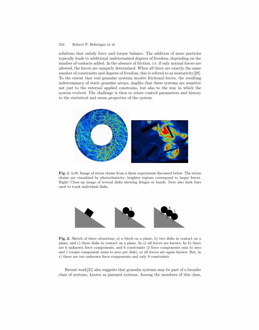
Fig. 1. Left: Image of stress chains from a shear experiment discussed below. The stresschains are visualized by photoelasticity: brighter regions correspond to larger forces.Right: Close-up image of several disks showing fringes or bands. Note also dark barsused to track individual disks.

12

31

23

45

Fig. 2. Sketch of three situations: a) a block on a plane, b) two disks in contact on aplane, and c) three disks in contact on a plane. In a) all forces are known. In b) thereare 6 unknown force components, and 6 constraints (2 force components sum to zeroand 1 torque component sums to zero per disk), so all forces are again known. But, inc) there are ten unknown force components and only 9 constraints.

Recent work[21] also suggests that granular systems may be part of a broaderclass of systems, known as jammed systems. Among the members of this class,


in addition to granular materials, are fluids near the glass transition, foams,colloids, and suspensions. The unifying feature of these systems is that theyundergo a transition from a mobile to a constrained state or vice versa as someparameter or set of parameters changes. In the case of the glass transition, therelevant parameter is the temperature, T , and for granular materials the relevantparameters include both stress and density. That is, under shear, dense granularsystems dilate (change density) and become mobile.Several recent theoretical works[7,22,23,24,25] have provided a context for un-

derstanding static stress distributions in granular materials. The first of these,the q-model[7] of Coppersmith et al, predicts a force distribution for static sys-tems P (F ) ∝ FN−1 exp(−F/Fo), where N is the system dimension. This modelassumes a regular array of grains, nominally subject to gravity, neglects torques,and considers the force balance in one direction only. It introduces randomnessby assuming that the force on a grain in one layer is balanced by transmitingfractions qi, with ΣN

1 qi = 1, to the N supporting grains in the next layer of anordered dense packing, assuming an N-dimensional system. The qi are randomnumbers uniformly distributed in 0 ≤ qi ≤ 1, with the summation constraintabove. For concreteness, it is useful to imagine the 2D case, where the ‘grains’are disks. Then, a fraction, q and 1 − q of the force on a grain is transmit-ted to the two lower neighbors. In addition to an exponential distribution oflarge forces, the q-model predicts that forces between neighboring grains areuncorrelated and that in the long-wavelength limit, the stresses follow a diffu-sion equation, with the time axis along the direction of gravity. Various otherlattice models[22,23,24] contain features that guarantee torque and vector forcebalance, the possibility of correlated stress chains, or other features of randompacking.A rather different approach is embodied by the Oriented Stress Linearity

(OSL) model of Bouchaud, Cates, Witmer and Claudin[26]. The OSL picturesupposes an anisotropic friction-like consitutive law for the components of thestress: σxx = ησzz + µσxz, that is based on an intuitive picture of the robust-ness of stress chains under different directions of applied stress. The quantitiesη and µ are constants that are expected to depend on the history of the sam-ple preparation. When this consitutive rule is combined with the conditionsof stress balance: ∇iσij = ρgj , where ρ is the material density and gi is theappropriate component of the gravitational acceleration, the result is a purelywave-like hyperbolic equation for stress propagation throughout the material:(∇z + c+∇x)(∇z + c−∇x)σij = 0. The creators of the OSL model have alsodiscussed how such a continuum limit might occur in the context of a latticemodel that they dub the Three-Leg Model[26].The contrast between the q-model and the OSL model is dramatic. In the

long-wavelength limit of the q-model, information is lost rapidly through diffu-sion, whereas in the OSL model, information propagates through the medium.The difference in the models is also apparent in the effects of the boundaries onthe possible solutions. For instance, less boundary information is needed for ahyperbolic equation than for an elliptic equation.


Kenkre et al.[27] have proposed a continuum model that can, in essence,interpolate between the q-model and OSL. The overarching principle of theirmodel is the idea of a memory function, such that the response of the granularmaterial is obtain as a convolution of applied stresses with the memory function.Either a diffusion equation, a wave equation, or the telegraph equation resultsfrom an appropriate from the memory function.An alternative approach, contact dynamics[25], has been developed by Mo-

reau, Radjai, and Roux. This scheme provides an algorithm to lift the frictionaldegeneracy of the contacts for hard frictional particles. These authors have con-sidered a number of different granular systems, included systems under compres-sion and shear. For the present purposes, we note that this model also predictsP (F ) ∝ exp(−F/Fo) for large forces.

2 Experimental Tests of Static Models

There have been several attempts recently, some ongoing, to test predictionsof the models described above. We will focus on three of these, 1) tests of thestatic force distributions, 2) measurements of force profiles under sandpiles, and3) measurements of the Greens function, i.e. the stress response function of agranular material to a local force.

2.1 Force Distributions

An important measure of the statistical properties of granular materials is P (F ),the distribution of forces on individual particles. Both the q-model, a number ofrelated lattice models, and contact dynamics, make the striking prediction thatthis distribution will fall off exponentially at large F , although the predictions donot agree about what happens for small F . For instance, in the q-model at smallF , P ∝ FN−1 where N is the dimension, and in contact dynamics simulations,the exponent N − 1 is replaced by another exponent that is nearly zero.The large-F prediction has been tested by the University of Chicago group,

using a novel ‘carbon paper’ technique[7,9]. The forces at the boundaries of acontainer of material were measured by placing a sheet of carbon paper againstthe boundary. The size of the mark left after compaction was a monotonic func-tion of the applied force. From these measurements, the authors showed clearlythat the contact forces followed an exponential distribution at large F .Several other groups have also reported an exponential distribution, but typ-

ically in time-evolving rather than simply static systems[8,10,11]. In both 2Dand 3D Couette-like sheared systems[8,11] (discussed below), we have observedthis large-F exponential distribution. ( See also Shiffer et al. who have carriedout experiments in which a rod was driven through a granular sample[12].)Thus, an exponential form for the large-F part of the distribution seems to

be a recurrent theme. A less well established issue is the nature of the small-Fpart of the distribution, and the nature of spatial correlations. We discuss thisfurther below.


2.2 Force Profiles under Sandpiles

The OSL model has been used to interpret a classic problem in granular mechan-ics, specifically, the force profile at the base of a granular heap, or sandpile[29,26].Experimenters have variably reported that the force under a conical heap of ma-terial has a minimum or a minimum under the peak of the pile (see Fig. 3). Aminimum under the tallest part of the heap is counterintuitive, since we normallyexpect that forces propagate hydrostatically. A key insight of the OSL model isto note that stresses can propagate through stress chains much as stresses prop-agate through butresses of a cathedral. If the history of the heap preparationleads to organized arches down the slope of of the heap, then the force mightbe a maximum on a ring of radius Rm > 0. The OSL model was constructedin such a way that this property was manifest, depending on the choice of theparameters η and µ.

0 0.2 0.4 0.6 0.8 1r/R

0

0.2

0.4

0.6

0.8

1

Sca

led

Pre

ssur

e (P

/ρ g

H)

Experiment Φ=33o

IFE Φ=32.6o

OSL η=0.96, Φ=33o

OSL η=0.88, Φ=33o

0 0.2 0.4 0.6 0.8 1r/R

0

0.2

0.4

0.6

0.8

1

Sca

led

Pre

ssur

e (P

/ρ g

H)

Experiment Φ=33o

IFE Φ=32.6o

OSL η=0.47, Φ=33o

OSL η=0.40, Φ=33o

Fig. 3. Data for the force at the base of a sandpile vs. distance from the center for top:piles formed by pouring from a localized source–a funnel, and bottom: piles formed bypouring from a distributed source–a seive. After Vanel et al.


In yet a different direction, Savage[28] has pointed out that classical soilmechanics models, based on the concept of incipient failure everywhere (IFE),can also explain differences in the force profiles under heaps. The idea is that theinner layers of the pile undergo an elastic deformation because of gravity, but thatthe outer part of the heap is arbitrarily close to slipping, i.e. Coulomb failure.Savage also pointed out that past experiments may be subject to significanterrors because even very tiny deflections of the surface on which the piles formare sufficient to disturb the stress chains/stress profiles.Several experimental groups have set out to explore this issue recently[29,30].

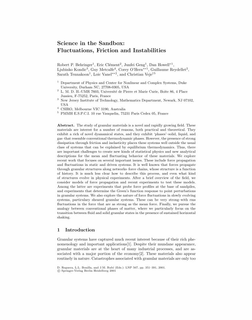
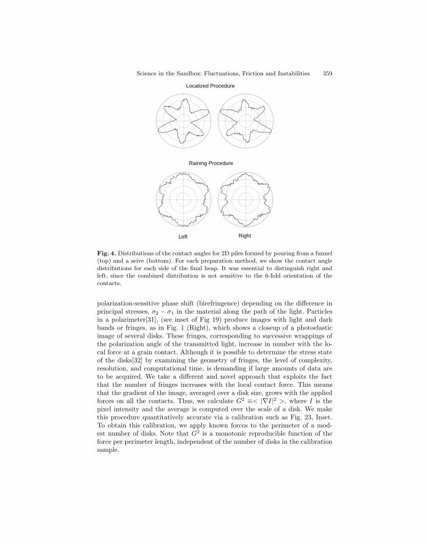
Here, we focus on the work of Vanel et al[29]. Using very sensitive transducersand very stiff surfaces, we found a clear variation of the force profile under sandheaps, depending on how the heap was prepared. If the heap was poured from afunnel, thus creating arches down the slope of the heap, there was an undebat-able minimum at the center of the heap. If the heap was prepared by pouringfrom a sieve, there was a weak maximum at the the center of the heap. Wecontrast the force profiles for these two methods in Fig. 3. Similar, although notas dramatic, results occur for wedge-shaped piles. Recently, we have pursued theissue of history dependence in the context of 2D ‘sandpiles’ using photoelasticdisks[11] (photoelasticity allows us to measure local forces on the disks, as dis-cussed below). Using preparation techniques that are the 2D analogies of funnelsand sieves, we find that the most dramatic difference occurs in the structuralnature of the piles, as evidenced in Fig. 4. This figure shows the contact anglesbetween nearest neighbor disks in mutual contact. In the case of the pile formedfrom a funnel, there is strong anisotropy; in the case of the pile formed from asieve, there is much weaker anisotropy of the grain contact angles.

2.3 Greens Function Measurements

There is a diverse spread in predictions for the large-wavelength behavior ofstatic granular systems. Thus, the q-model predicts diffusion–hence a parabolicPDE; the OSL model predicts a wave equation, hence a hyperbolic PDE, andthe occurence of ‘light cones’. Conventional models predicts an ellasto-plasticresponse, hence for part of the material an elliptic PDE. The models of Kenkre etal. provide both a hyperbolic interpolation between the parabolic and wave cases,and more generally, a mechanism to examine other possible response functions.This means that a fundamentally important experiment to carry out is the

determination of the Green’s function, i.e. the response of a granular systemto a localized point-like perturbation. Ideally, we would like to know in detailthe change in the forces on each grain as a function of position, following theaddition of the perturbation. The average over an ensemble of realizations isthen a representation of the continuum behavior.We are carrying out such experiments on a 2D sample consisting of pho-

toelastic particles. The ideas behind the technique are simple: photoelastic ma-terials are birefringent under stess. Because the particles are photoelastic, wecan obtain information on the stress state of the particles by means of a sim-ple polarimeter. As polarized light traverses a photoelastic material, there is a


Raining Procedure

Localized Procedure

Left Right

Fig. 4. Distributions of the contact angles for 2D piles formed by pouring from a funnel(top) and a seive (bottom). For each preparation method, we show the contact angledistributions for each side of the final heap. It was essential to distinguish right andleft, since the combined distribution is not sensitive to the 6-fold orientation of thecontacts.

polarization-sensitive phase shift (birefringence) depending on the difference inprincipal stresses, σ2 − σ1 in the material along the path of the light. Particlesin a polarimeter[31], (see inset of Fig 19) produce images with light and darkbands or fringes, as in Fig. 1 (Right), which shows a closeup of a photoelasticimage of several disks. These fringes, corresponding to successive wrappings ofthe polarization angle of the transmitted light, increase in number with the lo-cal force at a grain contact. Although it is possible to determine the stress stateof the disks[32] by examining the geometry of fringes, the level of complexity,resolution, and computational time, is demanding if large amounts of data areto be acquired. We take a different and novel approach that exploits the factthat the number of fringes increases with the local contact force. This meansthat the gradient of the image, averaged over a disk size, grows with the appliedforces on all the contacts. Thus, we calculate G2 ≡< |∇I|2 >, where I is thepixel intensity and the average is computed over the scale of a disk. We makethis procedure quantitatively accurate via a calibration such as Fig. 23, Inset.To obtain this calibration, we apply known forces to the perimeter of a mod-est number of disks. Note that G2 is a monotonic reproducible function of theforce per perimeter length, independent of the number of disks in the calibrationsample.


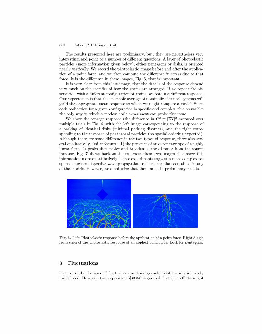
The results presented here are preliminary, but, they are nevertheless veryinteresting, and point to a number of different questions. A layer of photoelasticparticles (more information given below), either pentagons or disks, is orientednearly vertically. We record the photoelastic image before and after the applica-tion of a point force, and we then compute the difference in stress due to thatforce. It is the difference in these images, Fig. 5, that is important.It is very clear from this last image, that the details of the response depend

very much on the specifics of how the grains are arranged. If we repeat the ob-servation with a different configuration of grains, we obtain a different response.Our expectation is that the ensemble average of nominally identical systems willyield the appropriate mean response to which we might compare a model. Sinceeach realization for a given configuration is specific and complex, this seems likethe only way in which a modest scale experiment can probe this issue.We show the average response (the difference in G2 ≡ |∇I|2 averaged over

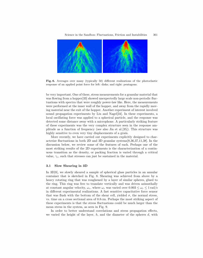
multiple trials in Fig. 6, with the left image corresponding to the response ofa packing of identical disks (minimal packing disorder), and the right corre-sponding to the response of pentagonal particles (no spatial ordering expected).Although there are some difference in the two types of response, there also sev-eral qualitatively similar features: 1) the presence of an outer envelope of roughlylinear form, 2) peaks that evolve and broaden as the distance from the sourceincrease. Fig. 7 shows horizontal cuts across these two images that show thisinformation more quantitatively. These experiments suggest a more complex re-sponse, such as dispersive wave propagation, rather than that contained in anyof the models. However, we emphasize that these are still preliminary results.

Fig. 5. Left: Photoelastic response before the application of a point force. Right Singlerealization of the photoelastic response of an applied point force. Both for pentagons.

3 Fluctuations

Until recently, the issue of fluctuations in dense granular systems was relativelyunexplored. However, two experiments[33,34] suggested that such effects might


Fig. 6. Averages over many (typically 50) different realizations of the photoelasticresponse of an applied point force for left: disks; and right: pentagons.

be very important. One of these, stress measurements for a granular material thatwas flowing from a hopper[33] showed unexpectedly large scale non-periodic fluc-tuations with spectra that were roughly power-law like. Here, the measurementswere performed at the inner wall of the hopper, and away from the rapidly mov-ing material near the exit of the hopper. Another experiment of interest involvedsound propagation experiments by Liu and Nagel[34]. In these experiments, alocal oscillating force was applied to a spherical particle, and the response wasdetected some distance away with a microphone. A particularly striking featureof these experiments was the very complex structure seen in the response am-plitude as a function of frequency (see also Jia et al.[35]). This structure washighly sensitive to even very tiny displacements of a grain.More recently, we have carried out experiments explicitly designed to char-

acterize fluctuations in both 2D and 3D granular systems[8,36,37,11,38]. In thediscussion below, we review some of the features of each. Perhaps one of themost striking results of the 2D experiments is the characterization of a contin-uous transition as the density, or packing fraction is varied through a criticalvalue, γc, such that stresses can just be sustained in the material.

3.1 Slow Shearing in 3D

In 3D[8], we slowly sheared a sample of spherical glass particles in an annularcontainer that is sketched in Fig. 8. Shearing was achieved from above by aheavy rotating ring that was roughened by a layer of similar spheres, glued tothe ring. This ring was free to translate vertically and was driven azimuthallyat constant angular velocity, ωr, where ωr was varied over 0.003 ≤ ωr ≤ 1 rad/sin different experimental realizations. A fast sensitive capacitative force sensorthat was flush with the bottom of the shear cell, yielded σ, the normal stress,vs. time on a cross sectional area of 0.8 cm. Perhaps the most striking aspect ofthese experiments is that the stress fluctuations could be much larger than themean stress in the system, as seen in Fig. 9.In order to better understand correlations and stress propagation effects,

we varied the height of the layer, h, and the diameter of the spheres d, with


Fig. 7. Quantitative realizations of the previous figure: above: disks; and below: pen-tagons. Each curve is the value of the difference in G2 along horizontal lines transverseto the direction of the applied load.

1.0 cm ≤ h ≤ 4.1 cm, and 0.1 cm ≤ d ≤ 0.5 cm. Since the area of the detector wasfixed, by changing the sphere diameter, we were able to change n, the number ofspheres contacting the detector from ∼ 4 to ∼ 100. If the forces on nearby grainswere uncorrelated, then we would expect to see a narrowing of the distribution


Fig. 8. Schematic of apparatus used for 3D shearing experiments. The figure is avertical cross section of a system with cylindrical symmetry (excepting the transducers).Glass spheres lying in an annular channel are sheared from above by a rotating ringon which spheres are glued. Normal stresses are measured vs. time at the base of thechannel by the transducers.

by n−1/2, the number of particles contacting the transducer, i.e. the distributionwould be narrowest for the smallest particle diameters.Returning to the time series of Fig 9, we note that, the probability of having

a fluctuation an order of magnitude greater than the mean is non-negligible (seebelow). An important question that remains to be addressed is what happens asthe system size becomes very large.Power spectra resulting from such stress time series provide useful informa-

tion. Fig. 10, left shows spectra at various rotation rates, ωr, of the shearingwheel, where the particle diameter is d = 2.0mm. At high spectral frequency, ω,P falls off as P (ω) ∝ ω−2 for a given ωr. The spectra vary more weakly with ωat low ω, but in this range, P (ω) ∝ ω−α, with 0 < α < 2. The high frequencydependence is easily explained by assuming a series of random jumps in σ(t)occuring at least as fast as a crossover time ∼ 1/ω∗, corresponding to a shearingring displacement of ∼ 1 particle diameter. The low frequency behavior is per-haps more interesting, since α > 0, would imply processes at slow time scales. Apossible source for such a slow process may be long-time rearrangements of thegrains.These spectra also show a kind of rate invariance. To place this in context,

many continuum models of slow granular flow[39,18] assume rate invariance forthe mean flow properties. The rate invariance shown here is interesting because itapplies to the fluctuations. To interpret this result, we note that if the grains werealmost always close to static equilibrium, we would expect that the time seriesfor the measured force fluctuation would have the form F (t) = g(ωrt). Here,g(z) might depend on the history of the system, but not on ωr except throughthe term ωrt. If we sampled over a long time interval, T , any history dependencewould be removed as the system explored a large collection of the possible nearly


4mm Beads 2cm Fill Helght 2OmHz Rotatton Rate

20

F

10

Mean ->

n

Seconds

Fig. 9. Time series showing stress fluctuations for grains sheared in the 3D annular channel. Stresses are normalized by the static stress, a ~ c , measured at the beginning of the run. The small bar at the lower left indicates the mean stress.

quasi-static states. In that event, a power spectrum for the fluctuations would have the form

where T = Tw,, and z = w,t. Eq. 1 indicates that the scaled power, Pw, , whould depend only on the dimensionless spectral frequency wlw,. Alternatively, w, sets the time scale for the fluctuations. This expectation is borne out in these experiments, as typified by Fig. 10, right. This figure shows an excellent collapse of all the data for the scaled power vs. the scaled frequency for two different particle sizes. Similar collapse was found in all cases. This result is interesting for at least two reasons: first because this is the first demonstration to our knowledge of rate invariance for the fluctuations, and second, because data for two very different size grains show nearly the same scaled power spectra.

A final interesting aspect of these experiments is the distributions of forces (stresses) without regard to time. Thus, the shearing creates a sequence of stress that are members of an ensemble. Since that the time series show rate invariance, it is meaningful to compare the measured force distributions to models and experiments for static situations. Fig. 11 shows such distributions for four different particle sizes. For the smallest (1 mm) particles, roughly n = 100 particles contacted the stress transducer; for the largest particles, roughly n = 6 contacted the transducer. For all cases, the distributions are roughly exponential


Power Spectra 2 0 -

- 0 a,

? -- - 0 0 -

E 2 t k 1L - m 4 - 2 0 -

Fig. 10. Above: Typical power spectra for normal stress fluctuations in the 3D shearing experiments for 2 mm particles that half-fill the 4 cm deep channel. Rotation rates, wT/27r are indicated in the box. Below: Scaled power spectra, w T P ( w / w T ) vs. w/wT for normal stress fluctuations in the 3D shearing experiments. Results are given for two different sphere sizes and for the indicated rotation rates of the shearing ring. The 4 cm deep channel was filled to a depth of 2 cm in these experiments.

for large forces, as in the models discused above. Ir~terestingly, the distributions of Fig. 11 do not show the np1I2 narrowing that would occur if the force on each grain were totally uncorrelated with its neighbors. Thus, for n uncorrelated grains described by the q-model, the total force F, summed over these grains is distributed as p~ = [f0(3n - 1)!Ip1(F/ fo)3np1exp(-F/ f a ) , where fa is an appropriate normalization constant. The multi-particle distribution of forces for n particles at a time then narrows as np1I2, as sketched in Fig. 12. For the experimental distributions in Fig. 11, the mean number of particles in contact with


the transducer changes by a factor of 16 as the particle size changes from 4mmto 1mm. Although the distributions change qualitatively over this size range,they do not show a narrowing by a factor of 4, as would occur in the absenceof correlations. Within the scatter, there does not appear to be as strong a nar-rowing as one would expect for totally uncorrelated forces. Interestingly, in thecarbon paper experiments of Mueth et al.[9], no spatial correlations were found.This difference in the two experiments is unresolved at the moment.

0.0 1.0 2.0 3.0σ/<σ>

-2.0

-1.0

0.0

1.0

Log[

P(σ

) ]

0.0 1.0 2.0 3.0σ/<σ>

-2.0

-1.0

0.0

1.0

Log[

P(σ

) ]

0.0 1.0 2.0 3.0σ/<σ>

-2.0

-1.0

0.0

1.0

Log[

P(σ

) ]

0.0 1.0 2.0 3.0σ/<σ>

-2.0

-1.0

0.0

1.0

Log[

P(σ

) ]

2mm : 3cm FH : 42mHz1mm : 1cm FH : 42mHz

3mm : 4cm FH : 20mHz 4mm : 2cm FH : 20mHz

Fig. 11. Stress distributions, ρ(σ), from the 3D shearing experiments for four differ-ent particle sizes. A small positive quantity has been added to ρ to ensure that thelogarithm always exists.

3.2 Slow Shearing in 2D

Experiments in 3D cannot provide detailed information about the internal forcesor movement of the particles. However, this kind of information is available via2D measurements in which the particles are constructed of photoelastic material.Thus, in a second set of experiments[37,40,11], we have characterized fluctuationsin a 2D granular system consisting of either circular disks or pentagonal particlesconfined to a plane and subject to shearing. In this system, we were able tomeasure forces, displacments, and rotations of the individual particles.The experimental arrangement is sketched in Fig. 13. The disks slide on a

smooth powder-lubricated sheet of Plexiglas. They are confined radially by a

https://www.researchgate.net/publication/235483934_Kinematics_of_two-dimensional_granular_Couette_experiment_at_the_transition_to_shearing?el=1_x_8&enrichId=rgreq-e3d28434047bf247e23489340f6c6cfe-XXX&enrichSource=Y292ZXJQYWdlOzI1MTI5Njk3NDtBUzoxMDE5Mzc4MTkxNjA1NzdAMTQwMTMxNTI3ODE2MQ==


0.0 1.0 2.0 3.0 σ/n

0.0

1.0

2.0

Pn(

σ)

n=1n=2n=3n=4n=5n=6

Pn(σ) = Aσ3n-1e

-3nσ

Fig. 12. Narrowing of force distributions for collections of N uncorrelated grains. Thedistributions are calculated for the collective force of N grains satisfying the 3D q-modelsingle-particle distribution ρ = (2fo)−1(f/fo)2 exp(−f/fo).

wheel at the inner radius, r = Ri, and by a ring at the outer radius r = Ro,where the surfaces of the wheel and ring contacting the grains are roughened,as sketched in Fig. 13. The disks used here are the same as the ones used forthe Greens function experiments. They are cut from a photoelastic[31] polymer,which allows us to determine information on the stress. The diameters, d, of thedisks are either 0.9 cm or 0.74 cm, with ∼ 400 of the former and ∼ 2500 ofthe latter. All disks are 0.62 cm thick. Two sizes of disks were used to reducethe possibility of crystalline ordering. Another concern, segregation by size doesnot occur in these experiments. The pentagons had the same thickness, and were0.64 cm on a side. Additional details can be found in several references[37,40,11].Here, we consider shearing only from the inner wheel, although it is possible

to shear from the outer ring as well. The rate of shearing is set by Ω = 2π/τ ,the angular velocity of the inner wheel, where τ is the time for the wheel tocomplete a revolution. An additional control parameter is the density of particles,as specified by the packing fraction, γ. (γ ≡ the area of the annulus occupied byparticles normalized by the total area).In addition to force information, we also determine kinematic properties of

the system by tracking small dark bars placed on each disk (see Fig. 13). A se-quence of video images is digitized by a frame grabber and analyzed to determine



Light Box

Stepper Motor

Video Camera

ShearingRings

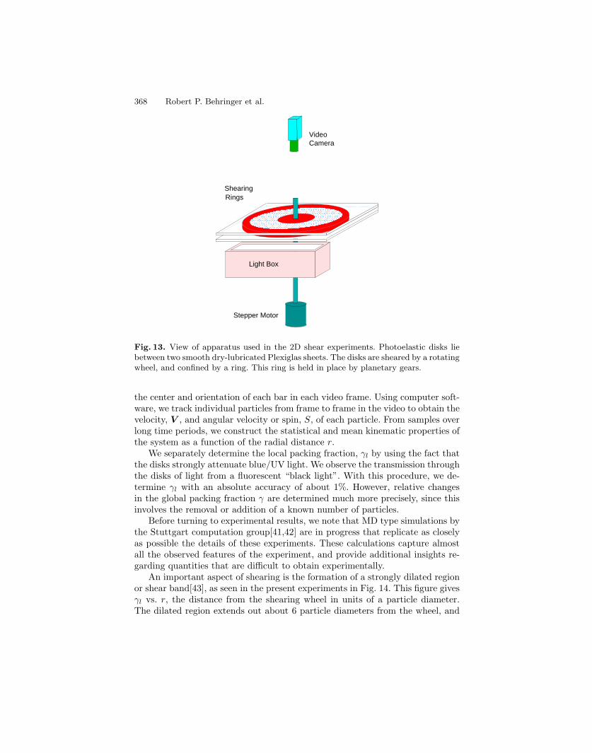
Fig. 13. View of apparatus used in the 2D shear experiments. Photoelastic disks liebetween two smooth dry-lubricated Plexiglas sheets. The disks are sheared by a rotatingwheel, and confined by a ring. This ring is held in place by planetary gears.

the center and orientation of each bar in each video frame. Using computer soft-ware, we track individual particles from frame to frame in the video to obtain thevelocity, V , and angular velocity or spin, S, of each particle. From samples overlong time periods, we construct the statistical and mean kinematic properties ofthe system as a function of the radial distance r.We separately determine the local packing fraction, γl by using the fact that

the disks strongly attenuate blue/UV light. We observe the transmission throughthe disks of light from a fluorescent “black light”. With this procedure, we de-termine γl with an absolute accuracy of about 1%. However, relative changesin the global packing fraction γ are determined much more precisely, since thisinvolves the removal or addition of a known number of particles.Before turning to experimental results, we note that MD type simulations by

the Stuttgart computation group[41,42] are in progress that replicate as closelyas possible the details of these experiments. These calculations capture almostall the observed features of the experiment, and provide additional insights re-garding quantities that are difficult to obtain experimentally.An important aspect of shearing is the formation of a strongly dilated region

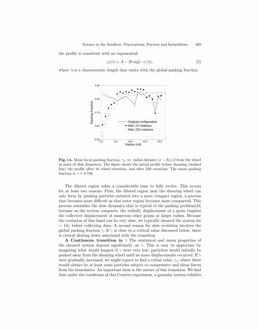
or shear band[43], as seen in the present experiments in Fig. 14. This figure givesγl vs. r, the distance from the shearing wheel in units of a particle diameter.The dilated region extends out about 6 particle diameters from the wheel, and


the profile is consistent with an exponential:

γl(r) = A − B exp(−r/λ), (2)

where λ is a characteristic length that varies with the global packing fraction.

0.0 5.0 10.0 15.0 20.0Radius (r/d)

0.50

0.60

0.70

0.80

0.90

Pac

king

Fra

ctio

n

Original configurationAfter 10 rotationsAfter 220 rotations

Fig. 14. Mean local packing fraction, γl, vs. radial distance (r − Ri)/d from the wheelin units of disk diameters. The figure shows the initial profile before shearing (dashedline) the profile after 10 wheel rotations, and after 220 rotations. The mean packingfraction is γ = 0.788.

The dilated region takes a considerable time to fully evolve. This occursfor at least two reasons. First, the dilated region near the shearing wheel canonly form by pushing particles outward into a more compact region, a processthat becomes more difficult as that outer region becomes more compacted. Thisprocess resembles the slow dynamics that is typical of the parking problem[44]because as the system compacts, the radially displacement of a grain requiresthe collective displacement of numerous other grains at larger radius. Becausethe evolution of this band can be very slow, we typically sheared the system for∼ 1hr before collecting data. A second reason for slow evolution involves theglobal packing fraction γ. If γ is close to a critical value discussed below, thereis critical slowing down associated with the transition.

A Continuous transition in γ The statistical and mean properties ofthe sheared system depend signifciantly on γ. This is easy to appreciate byimagining what would happen if γ were very low: particless would initially bepushed away from the shearing wheel until no more displacements occurred. If γwere gradually increased, we might expect to find a critial value, γc, where therewould always be at least some particles subject to compressive and shear forcesfrom the boundaries. An important issue is the nature of this transition. We findthat under the conditions of this Couette experiment, a granular system exhibits


a number of features that are similar to a continuous phase transition. At γc,the system is very compressible, and in a given part of the system force chainsoccur only intermittently. Most of the grains are close to uncompressed and staticmost of the time. With the addition of more grains, the system strengthens, morechains occur, and grains are dragged more frequently by the shearing wheel. Aconsequence of this last feature is that the system ‘speeds up’. If even moregrains are added, the system becomes very stiff, and disks are subject to largerdeformations. In the extreme limit, brittle materials might fracture. It is thisrange of γ’s, between γc and the strongly compacted regime that we explorehere. It is important to note, however, that the actual change in γ is small; allthe action takes place over a change in γ that corresponds to only about 5%variation.The temporal intermittentency in the stress fluctuations near γc is clear from

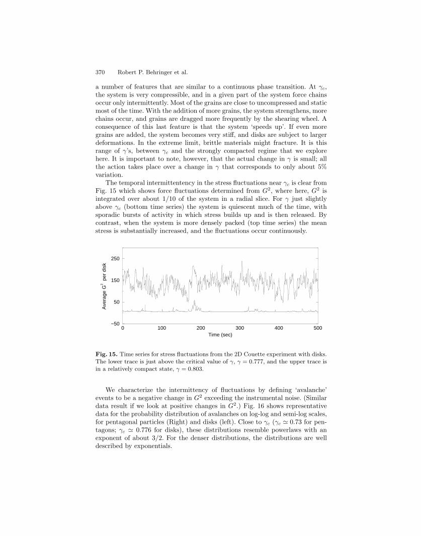
Fig. 15 which shows force fluctuations determined from G2, where here, G2 isintegrated over about 1/10 of the system in a radial slice. For γ just slightlyabove γc (bottom time series) the system is quiescent much of the time, withsporadic bursts of activity in which stress builds up and is then released. Bycontrast, when the system is more densely packed (top time series) the meanstress is substantially increased, and the fluctuations occur continuously.

0 100 200 300 400 500Time (sec)

−50

50

150

250

Ave

rage

G2 p

er d

isk

Fig. 15. Time series for stress fluctuations from the 2D Couette experiment with disks.The lower trace is just above the critical value of γ, γ = 0.777, and the upper trace isin a relatively compact state, γ = 0.803.

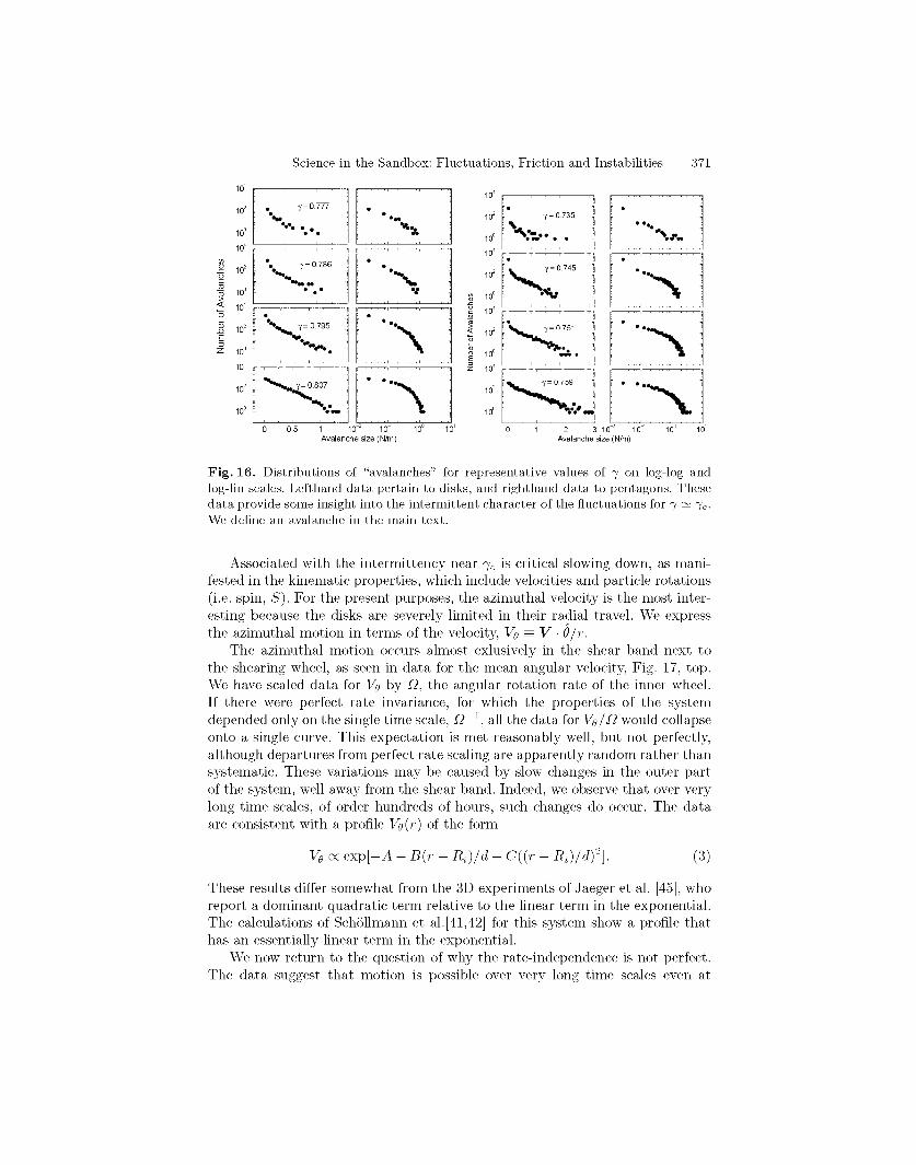
We characterize the intermittency of fluctuations by defining ‘avalanche’events to be a negative change in G2 exceeding the instrumental noise. (Similardata result if we look at positive changes in G2.) Fig. 16 shows representativedata for the probability distribution of avalanches on log-log and semi-log scales,for pentagonal particles (Right) and disks (left). Close to γc (γc 0.73 for pen-tagons; γc 0.776 for disks), these distributions resemble powerlaws with anexponent of about 3/2. For the denser distributions, the distributions are welldescribed by exponentials.


i 0 0 5 1 lo-' 10' 10'

Avalanche slze (Nlm) 0 1 2 3 1 0 - ~ lo-' l o o 10'

Avalanche slze (Nlm)

Fig. 16. Distributions of "avalanches" for representative values of y on log-log and log-lin scales. Lefthand data pertain to disks, and righthand data to pentagons. These data provide some insight into the intermittent character of the fluctuations for y .v y,. We define an avalanche in the main text.

Associated with the intermittency near y, is critical slowing down, as mani- fested in the kinematic properties, which include velocities and particle rotations (i.e. spin, S). For the present purposes, the azimuthal velocity is the most interesting because the disks are severely limited in their radial travel. We express the azimuthal motion in terms of the velocity, V0 = V . Q/T.

The azimuthal motion occurs almost exlusively in the shear band next to the shearing wheel, as seen in data for the mean angular velocity, Fig. 17, top. We have scaled data for V0 by R, the angular rotation rate of the inner wheel. If there were perfect rate invariance, for which the properties of the system depended only on the single time scale, Rpl , all the data for Vs/R would collapse onto a single curve. This expectation is met reasonably well, but not perfectly, although departures from perfect rate scaling are apparently random rather than systematic. These variations may be caused by slow changes in the outer part of the system, well away from the shear band. Indeed, we observe that over very long time scales, of order hundreds of hours, such changes do occur. The data are consistent with a profile Vs(r) of the form

These results differ somewhat from the 3D experiments of Jaeger et al. [45], who report a dominant quadratic term relative to the linear term in the exponential. The calculations of Schollmann et a1.[41,42] for this system show a profile that has an essentially linear term in the exponential.

We now return to the question of why the rate-independence is not perfect. The data suggest that motion is possible over very long time scales even at


0.0 2.0 4.0 6.0 8.0 10.0 12.0 14.0r/d

−0.20

−0.15

−0.10

−0.05

0.00

0.05

0.10

(S/Ω

)(D

/d)

0.0 2.0 4.0 6.0 8.0 10.0 12.0 14.0r/d

10−5

10−4

10−3

10−2

10−1

100

Vθ/Ω

119174245354616114920222022

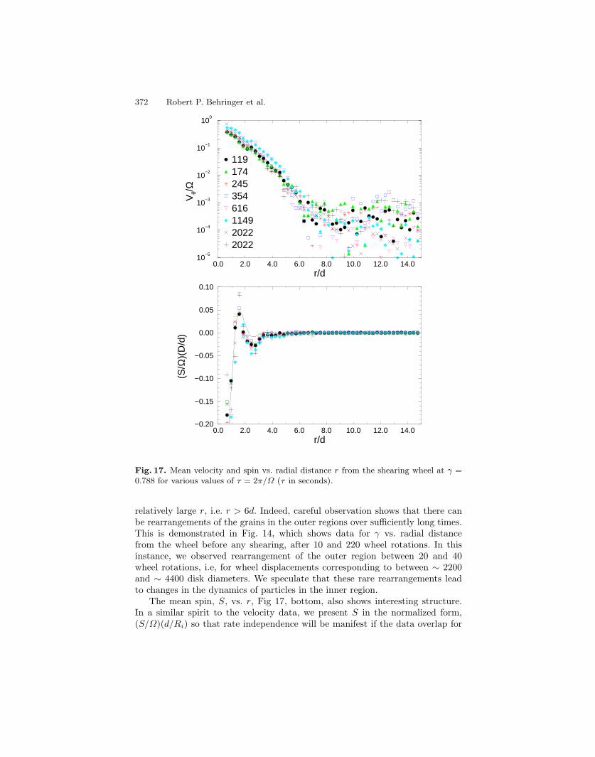
Fig. 17. Mean velocity and spin vs. radial distance r from the shearing wheel at γ =0.788 for various values of τ = 2π/Ω (τ in seconds).

relatively large r, i.e. r > 6d. Indeed, careful observation shows that there canbe rearrangements of the grains in the outer regions over sufficiently long times.This is demonstrated in Fig. 14, which shows data for γ vs. radial distancefrom the wheel before any shearing, after 10 and 220 wheel rotations. In thisinstance, we observed rearrangement of the outer region between 20 and 40wheel rotations, i.e, for wheel displacements corresponding to between ∼ 2200and ∼ 4400 disk diameters. We speculate that these rare rearrangements leadto changes in the dynamics of particles in the inner region.The mean spin, S, vs. r, Fig 17, bottom, also shows interesting structure.

In a similar spirit to the velocity data, we present S in the normalized form,(S/Ω)(d/Ri) so that rate independence will be manifest if the data overlap for


all Ω. Note that a grain that is rolling in place against the inner wheel withoutslipping will have a normalized value of (S/Ω)(d/Ri) = −1. Like the data forVθ, the data for S are nearly but not perfectly rate invariant. Grains adjacent tothe wheel are, on average, rotating backwards, whereas those in the next layerout are rotating in the same sense as the shearing wheel. The fact that theserotations die out quickly with distance from the wheel is quite reasonable, sincethe alternation of rotation with distance from the wheel must compete withfrictional drag and rotational frustration from neighboring grains that are thesame distance from the inner wheel.The distributions for Vθ and S, Fig. 18, contain important information about

the nature of the shear layer, and we return to this point below. These datapertain to disks that are in the first layer contacting the wheel, and data forpentagonal particles are qualitatively similar. There is a large peak near zero forboth Vθ and S, another broad peak for nonzero values, and some hints of a thirdweak peak in Vθ.

-1.5 -0.5 0.5S/(ΩD/d)

0.0

1.0

2.0

3.0

P(S

/ΩD

/d)

-0.5 0.5 1.5Vθ/Ω

0.0

1.0

2.0

P(V

θ/Ω)

11917424535461611492022

Fig. 18. Distributions for Vθ and S for disks within one disk diameter d of the shearingwheel. Different symbols correspond to different values of τ = 2π/Ω. Here, γ = 0.788.


Associated with the strong intermittency near γc is a dramatic variation ofthe kinematic properties with γ as seen in Fig 19 which gives the mean scaledvelocity, Vθ/Ω vs. r. As γ → γc Vθ decreases dramatically, not because of slowermovement of the particles when they actually move, but rather, because thedisks move more sporadically.

0 2 4 6 8 10 12 14r/d

10−6

10−5

10−4

10−2

10−1

100

Vθ/Ω

0.7770.7790.7830.7880.7900.7920.797

LightSource

Plane Polarizer

Plane Polarizer

Sample

Camera1/4 WavePlates

Fig. 19. Velocity vs. distance from the shearing wheel for various γ’s. Inset: schematicof circular polarimeter used for the present photoelasticity measurements.

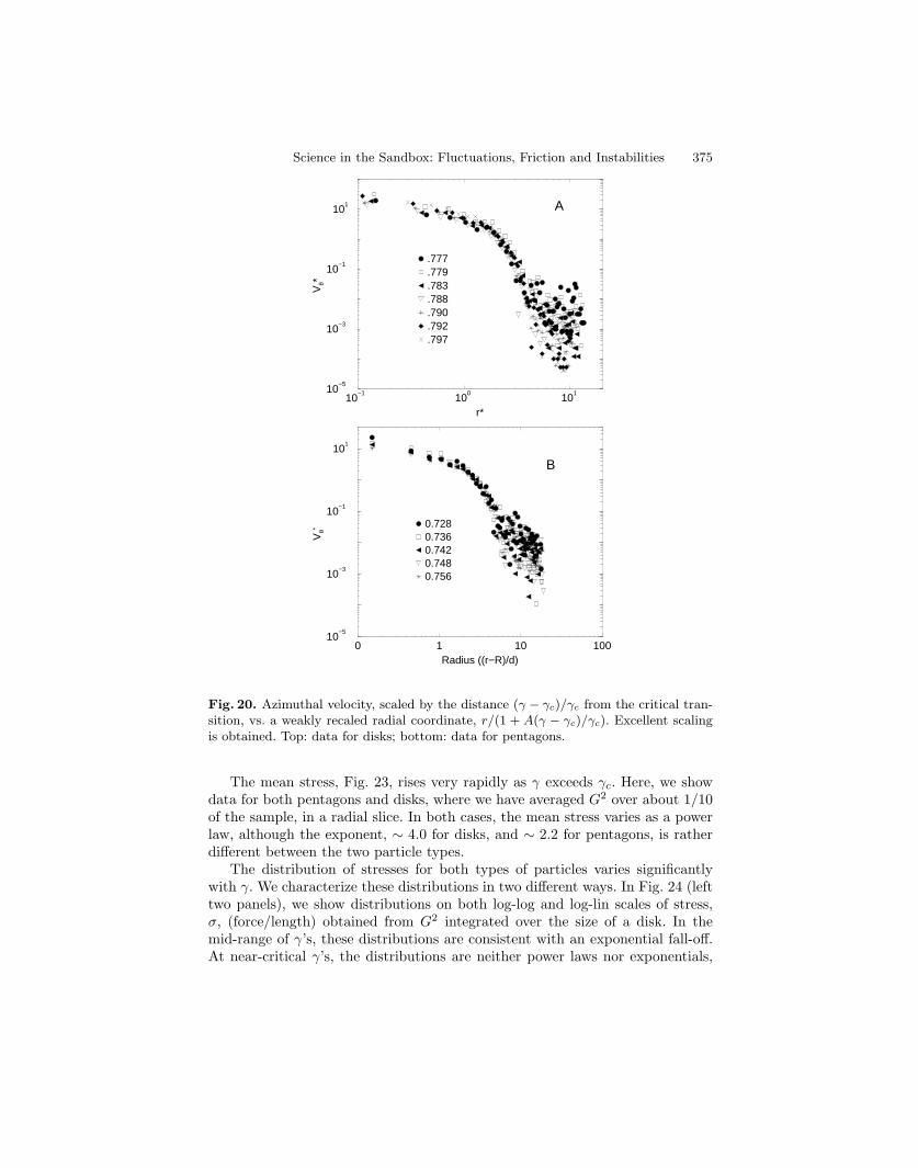
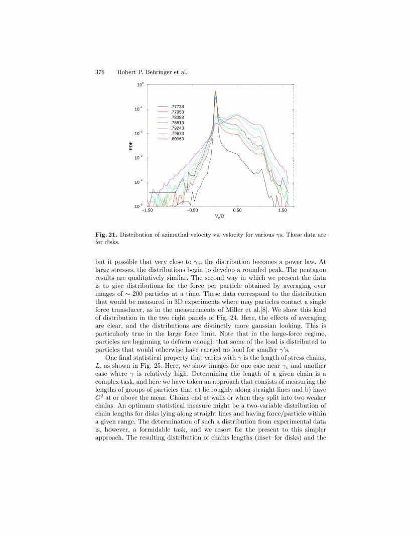
The slowing down as γ → γc satisfies a very clear scaling behavior, as shownin Fig. 20. Here, we have scaled the dimensionless velocity by (γ−γc)/γc, and theradial distance by a slowing varying function of r. The data for all the profilescollapse onto a universal scaling curve for both disks (A) and pentagons (B).The velocity distribution next to the shearing wheel is also affected by chang-

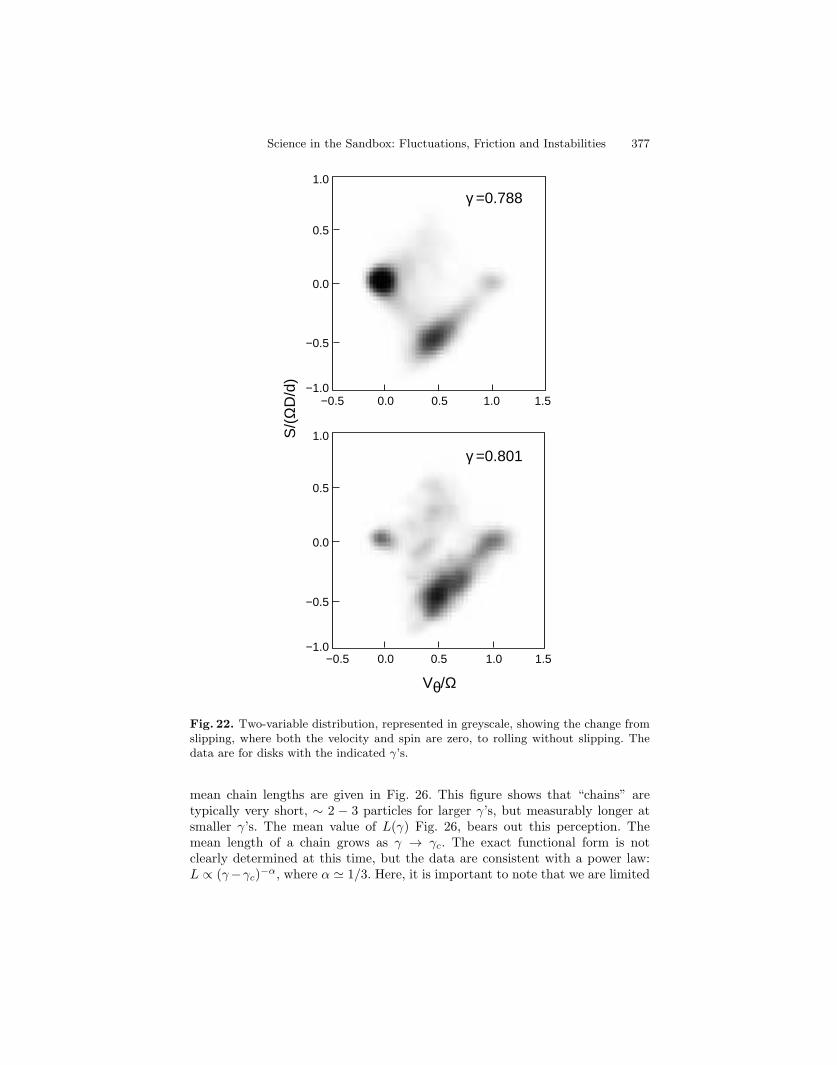
ing γ, Fig 21 shows that the peak near zero velocity increases and the featureat 0.5 decreases as γc is approached from above. This means that as γ growsbeyond γc, grains actually slip less, as captured in Fig. 22. This figure showsgrey-scale representations of the two-variable distributions for velocity and spin,P (Vθ, S) for two different γ’s for the disks that are next to the inner wheel. Forγ γc the preponderance of the weight is near the origin, whereas for a largerγ, much of the statistical weight has moved near the line

Vθ/Ω = 1 + S/(ΩRi/D) (4)

corresponding to the condition that the grains are rolling without slipping againstthe inner wheel. This observation also gives some insight into why Vθ/Ω < 1 atthe shearing wheel (i.e. ¯S < 0.There are also dramatic changes in the statistical properties of the stress as γ

varies, particularly as a result of the critical transition near γc. These propertiessurface in the mean stress, the stress distributions, and in the stress chain lengths.


10−1

100

101

r*

10−5

10−3

10−1

101

Vθ*

.777

.779

.783

.788

.790

.792

.797

0 1 10 100Radius ((r−R)/d)

10−5

10−3

10−1

101

Vθ* 0.728

0.7360.7420.7480.756

A

B

Fig. 20. Azimuthal velocity, scaled by the distance (γ − γc)/γc from the critical tran-sition, vs. a weakly recaled radial coordinate, r/(1 + A(γ − γc)/γc). Excellent scalingis obtained. Top: data for disks; bottom: data for pentagons.

The mean stress, Fig. 23, rises very rapidly as γ exceeds γc. Here, we showdata for both pentagons and disks, where we have averaged G2 over about 1/10of the sample, in a radial slice. In both cases, the mean stress varies as a powerlaw, although the exponent, ∼ 4.0 for disks, and ∼ 2.2 for pentagons, is ratherdifferent between the two particle types.The distribution of stresses for both types of particles varies significantly

with γ. We characterize these distributions in two different ways. In Fig. 24 (lefttwo panels), we show distributions on both log-log and log-lin scales of stress,σ, (force/length) obtained from G2 integrated over the size of a disk. In themid-range of γ’s, these distributions are consistent with an exponential fall-off.At near-critical γ’s, the distributions are neither power laws nor exponentials,


−1.50 −0.50 0.50 1.50Vθ/Ω

10−5

10−4

10−3

10−2

10−1

100

PD

F

.77738

.77953

.78383

.78813

.79243

.79673

.80963

Fig. 21. Distribution of azimuthal velocity vs. velocity for various γs. These data arefor disks.

but it possible that very close to γc, the distribution becomes a power law. Atlarge stresses, the distributions begin to develop a rounded peak. The pentagonresults are qualitatively similar. The second way in which we present the datais to give distributions for the force per particle obtained by averaging overimages of ∼ 200 particles at a time. These data correspond to the distributionthat would be measured in 3D experiments where may particles contact a singleforce transducer, as in the measurements of Miller et al.[8]. We show this kindof distribution in the two right panels of Fig. 24. Here, the effects of averagingare clear, and the distributions are distinctly more gaussian looking. This isparticularly true in the large force limit. Note that in the large-force regime,particles are beginning to deform enough that some of the load is distributed toparticles that would otherwise have carried no load for smaller γ’s.One final statistical property that varies with γ is the length of stress chains,

L, as shown in Fig. 25. Here, we show images for one case near γc and anothercase where γ is relatively high. Determining the length of a given chain is acomplex task, and here we have taken an approach that consists of measuring thelengths of groups of particles that a) lie roughly along straight lines and b) haveG2 at or above the mean. Chains end at walls or when they split into two weakerchains. An optimum statistical measure might be a two-variable distribution ofchain lengths for disks lying along straight lines and having force/particle withina given range. The determination of such a distribution from experimental datais, however, a formidable task, and we resort for the present to this simplerapproach. The resulting distribution of chains lengths (inset–for disks) and the


Vθ/Ω

S/(

ΩD

/d)

−0.5 0.0 0.5 1.0 1.5

γ =0.801

0.0

0.5

−1.0

1.0

−0.5 0.0 0.5 1.0 1.5

−0.5

γ =0.788

−1.0

−0.5

0.5

0.0

1.0

Fig. 22. Two-variable distribution, represented in greyscale, showing the change fromslipping, where both the velocity and spin are zero, to rolling without slipping. Thedata are for disks with the indicated γ’s.

mean chain lengths are given in Fig. 26. This figure shows that “chains” aretypically very short, ∼ 2 − 3 particles for larger γ’s, but measurably longer atsmaller γ’s. The mean value of L(γ) Fig. 26, bears out this perception. Themean length of a chain grows as γ → γc. The exact functional form is notclearly determined at this time, but the data are consistent with a power law:L ∝ (γ−γc)−α, where α 1/3. Here, it is important to note that we are limited


slope = 4 04 / slope = 2 15

, , ,./. (Y-Y,)% lo-' , , ,

Fig. 23. Mean force vs. y in 2D experiments. Left: data for disks; Right: data for pentagons.

Force (Newtons)

0 0 5 1 1 5 2 Force (Newtons)

Forcellength (Newtonslmeter)

1 0' , , , , , , , 4

Forcellength (Newtonslmeter)

Fig. 24. Stress distributions on log-log and log-lin scales for the indicated y's for disks. The left-hand data pertains to the force on a single disk. The right-hand data was obtained by averaging the force over roughly 260 disks.


by the finite size of the system. In future work, we plan to measure chain lengthsfor much larger systems.To sum up briefly, the 2D Couette experiments exhibit a novel continuous

transition for a granular material. This transition, which is intimately relatedto Reynolds dilatancy, is characterized by power laws for a number of prop-erties, such as the mean stress, the velocity, etc. For other properties, such asthe mean chain length, a power law is consistent with the data, even thoughanother mathematical form would also be consistent with the results. Giventhis interesting critical-like behavior, it is interesting to speculate on its rela-tion to other phenomena. One possibility is that this transition is related torigidity percolation[55]. In this regard, we note recent numerical simulations byAharonov and Sparks[54]. These authors report a rigidity phase transition forwhich some properties show discontinuous behavior as a function of density, eventhough the elastic constants undergo a second order transition.

Fig. 25. Images showing stress chains at γ = 0.777, just above γc (left) and at high γ,γ = 0.807, right.

The power spectra associated with the force time series are also of interestsince they give some insight into time scales in the system. The 2D spectra areremarkably like their 3D counterparts, with the exception of the near-criticaldata (not available for 3D). Specific results are presented elsewhere[46,47].

4 Transition to the Fluid State under Shaking

An alternative setting for understanding the transitions between different granu-lar states can be found in shaken systems. A granular material makes the transi-tion from solid to fluid under a variety of different kinds of vibration. Perhaps themost studied case is one of vertical vibrations. Here, the material will flow when


0.00 0.01 0.02 0.03 0.04(γ−γc)/γc

2.0

2.5

3.0

3.5

4.0

Mea

n C

hain

Len

gth

(par

ticle

dia

met

ers)

0 0.01 0.02 0.03 0.04(γ − γc)/γc

2

2.2

2.4

2.6

2.8

Mea

n C

hain

Len

gth

(par

ticle

dia

met

ers)

2 4 6 8 10Chain length (particles/chain)

0

0.2

0.4

0.6

0.8

1

PD

F (

part

icle

s/ch

ain)

.77953

.78383

.78813

.79243

.79673

.80103

.80535

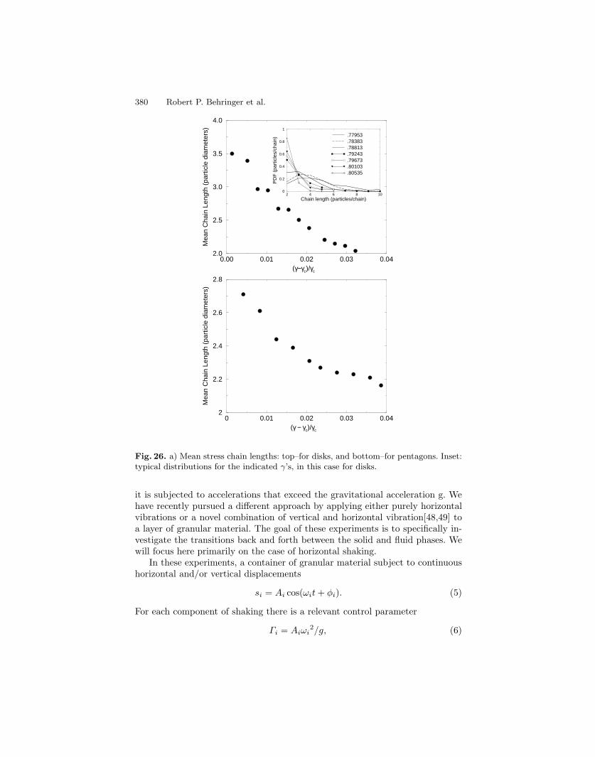
Fig. 26. a) Mean stress chain lengths: top–for disks, and bottom–for pentagons. Inset:typical distributions for the indicated γ’s, in this case for disks.

it is subjected to accelerations that exceed the gravitational acceleration g. Wehave recently pursued a different approach by applying either purely horizontalvibrations or a novel combination of vertical and horizontal vibration[48,49] toa layer of granular material. The goal of these experiments is to specifically in-vestigate the transitions back and forth between the solid and fluid phases. Wewill focus here primarily on the case of horizontal shaking.In these experiments, a container of granular material subject to continuous

horizontal and/or vertical displacements

si = Ai cos(ωit+ φi). (5)

For each component of shaking there is a relevant control parameter

Γi = Aiωi2/g, (6)


where g is the acceleration of gravity, and i = v, h for vertical or horizontal. Ifωv = ωh, the relative phase, φh −φv is also important; otherwise, ∆ω = ωv −ωh

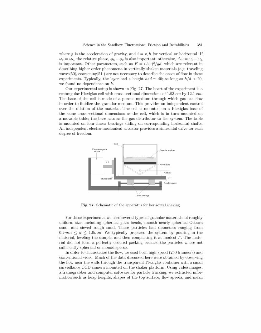
is important. Other parameters, such as E = (Aω)2/gd, which are relevant indescribing higher order phenomena in vertically shaken materials (e.g. travelingwaves[50], coarsening[51]) are not necessary to describe the onset of flow in theseexperiments. Typically, the layer had a height h/d 40; as long as h/d > 20,we found no dependence on h.Our experimental setup is shown in Fig 27. The heart of the experiment is a

rectangular Plexiglas cell with cross-sectional dimensions of 1.93 cm by 12.1 cm.The base of the cell is made of a porous medium through which gas can flowin order to fluidize the granular medium. This provides an independent controlover the dilation of the material. The cell is mounted on a Plexiglas base ofthe same cross-sectional dimensions as the cell, which is in turn mounted ona movable table; the base acts as the gas distributor to the system. The tableis mounted on four linear bearings sliding on corresponding horizontal shafts.An independent electro-mechanical actuator provides a sinusoidal drive for eachdegree of freedom.

Air flow

Porous base

Accelerometer

Granular mediumshakerElectro-magnetic

Cell

Shaker table

Linear bearings

Fig. 27. Schematic of the apparatus for horizontal shaking.

For these experiments, we used several types of granular materials, of roughlyuniform size, including spherical glass beads, smooth nearly spherical Ottawasand, and sieved rough sand. These particles had diameters ranging from0.2mm ≤ d ≤ 1.0mm. We typically prepared the system by pouring in thematerial, leveling the sample, and then compacting it at modest Γ . The mate-rial did not form a perfectly ordered packing because the particles where notsufficiently spherical or monodisperse.In order to characterize the flow, we used both high-speed (250 frames/s) and

conventional video. Much of the data discussed here were obtained by observingthe flow near the walls through the transparent Plexiglas container with a smallsurveillance CCD camera mounted on the shaker platform. Using video images,a framegrabber and computer software for particle tracking, we extracted infor-mation such as heap heights, shapes of the top surface, flow speeds, and mean


flow fields. In a typical run for pure horizontal shaking, we observed the evolu-tion of the system as Ah was increased from zero while keeping ωh fixed. Onceflow was well initiated, we then decreased Ah.For simple horizontal shaking, we are particularly interested in the initial

instability to fluidization. The transition to this flow state is hysteretic in Γh,and leads to a characteristic flow field that consists of sloshing of the grains inthe direction of the shaking, plus slower convective flow, including flow in thedirection transverse to the shaking. Fig 28 shows a sketch of the mean convectiveflow lines (i.e. discounting the sloshing flow) observed from the top and side forΓh somewhat above onset in a cell that is 30 grains wide and 50 grains deep.Grains rise up in the middle of the cell and flow along the surface towards theside walls and then sink at the wall boundaries. The top surface of the liquefiedlayer has a dome shape that is concave down, and the bottom surface of thislayer is concave upwards near the wall boundaries. Thus, the thickness of thefluidized layer is largest in the middle of the cell and smallest at the end walls,as seen previously by Evesque[52].

x

yz

H

Fig. 28. Sketch of convection flow lines in the liquified layer induced by horizontalshaking. Grains rise in the middle of the cell, flow along the surface towards the sidewalls, and then sink at the wall boundaries.

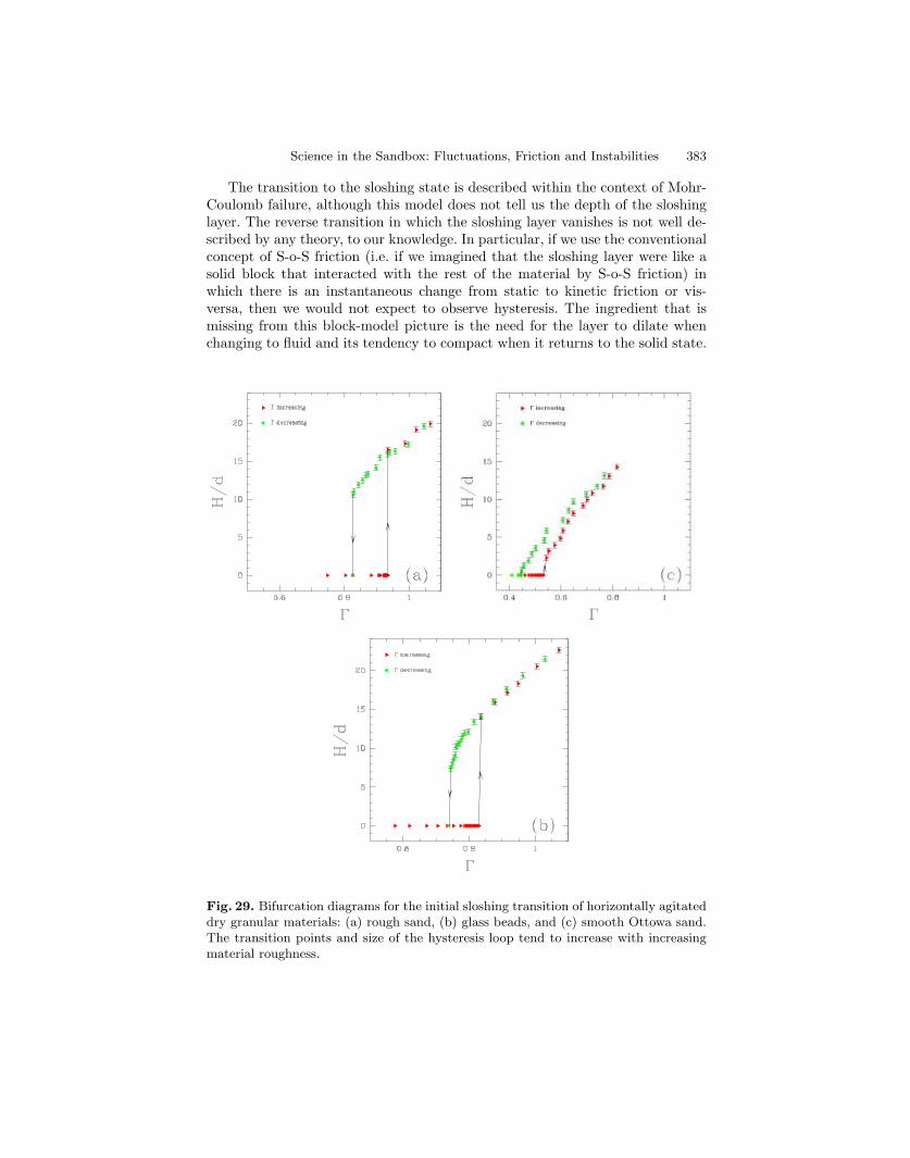
A useful measure of the strength of the flow is the thickness, H, of theliquefied material in the middle of the cell. Fig. 29 shows the typical hystereticbehavior for H as a function of Γh. With increasing Γh, there is a well definedtransition to finite amplitude (i.e. H = 0) flow at Γcu. With Γh decreasingbelow Γcu once flow has begun, the thickness of the layer also decreases but Hnot vanish until Γh reaches a lower critical value Γcd where the relative motioncompletely stops. As Γh is decreased from above towards Γcd, grains near the endwalls stop moving first, while grains in the middle keep moving. Some hysteresiswas present in the 2D studies by Ristow et al.[53], but the hysteresis in theour 3D experiments is larger, particularly for rougher materials. We also notethat below the onset of sloshing there exist a small number of free particles thatslide about on the top of the layer (we refer to these as ‘sliders’). Roughly, theseparticles act like a ‘gas’ in the sense that they have a low density. Yet, they seemto play a surprising role in the solid-to-fluid transition, as noted below.


The transition to the sloshing state is described within the context of Mohr-Coulomb failure, although this model does not tell us the depth of the sloshinglayer. The reverse transition in which the sloshing layer vanishes is not well de-scribed by any theory, to our knowledge. In particular, if we use the conventionalconcept of S-o-S friction (i.e. if we imagined that the sloshing layer were like asolid block that interacted with the rest of the material by S-o-S friction) inwhich there is an instantaneous change from static to kinetic friction or vis-versa, then we would not expect to observe hysteresis. The ingredient that ismissing from this block-model picture is the need for the layer to dilate whenchanging to fluid and its tendency to compact when it returns to the solid state.

Fig. 29. Bifurcation diagrams for the initial sloshing transition of horizontally agitateddry granular materials: (a) rough sand, (b) glass beads, and (c) smooth Ottowa sand.The transition points and size of the hysteresis loop tend to increase with increasingmaterial roughness.


The location of Γcu and Γcd are reproducible for a particular material (withinthe accessible range of these experiments). That is, different ω’s or A’s yield thesame critical Γh’s for a given material and fill height. The values of Γcu and Γcd

are also not affected by the total height of the layer, if that quantity is roughly20 grains or higher. However, these transitions values of Γh do depend on thephysical properties of the material, as shown in Fig 29 (Left). For instance,Γcu and Γcd increase as the roughness of the granular materials increases. Thiscan be attributed to the greater interlocking of rough grains and because roughgrains likely have higher S-o-S friction coefficients. It is also possible to map outthe full bifurcation diagram, including the unstable states, as shown in Fig. 30.Here, the technique that we used involved applying known perturbations to thesystem, and then observing to see whether the fluid or solid was the end statefollowing the perturbation.To obtain additional insight into the relative importance of dilatancy and

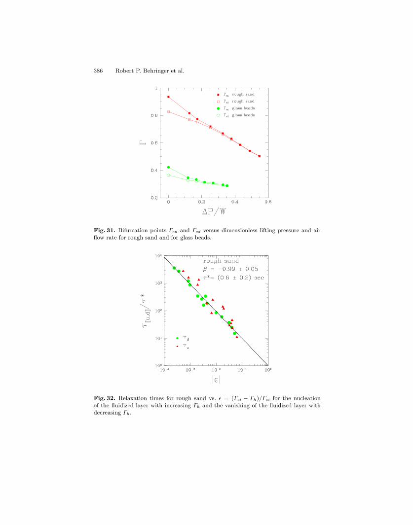
friction, we have carried out two additional experiments. In the first of these, wefluidized the granular bed by passing air through it, using the flow-controlled airsupply (see Fig. 27), where the porous base of the cell acts as the gas distributor.Fig 31, which presents Γcu and Γcd as functions of the air flow through the bed,shows a very strong dependence of these quantities on the air flow. In particular,a modest air flow reduces the critical Γ ’s and ultimately effectively removes thehysteresis in the initial transition. Here, ∆P is the pressure difference acrossthe granular layer, and W is its weight per area. We note that the measureddilation of the bed due to the air flow is small: the maximum dilation for theseexperiments corresponds to less than one granular layer for a bed of 45 layers, i.e.less than 2% dilation. In a second experiment to probe the effects of dilatancy,we placed a small amount of overburden (here a thin piece of plastic of weightcomparable to about half a layer of grains). This small strip of plastic suppressedthe motion of the sliders. Surprisingly, we found that the hysteresis was lifted,and that the transition to flow occured at a slightly reduced value of Γh relative toΓcd, Fig. 30 (Right). This result is particularly striking because we might expectthat the addition of weight would delay the transition, rather than enhance it.An additional point concerns nucleation times. These include the time to

nucleate the fluid layer from the solid when Γh is stepped slightly past Γcu,and the time for all of the fluid phase to decay away if Γh is stepped slightlybelow Γhd. We show representative results for both processes in Fig. 32. Again,there is a surprise: there is a very well defined power law for each process,with the relaxation time always varying as τ = A/ε, where ε = (Γh − Γci)/Γci,(i = u, d). This set of results is striking because it suggests a universal behavior.An interesting and unresolved question is the physics behind the exponent minusone.An important issue concerns the driving mechanism or ‘motors’ for both the

convective flow parallel to the shaker plane and the convective flow perpendicularto the shaker plane. The origin of the sloshing motion is relatively obvious: duringeach half of the shaker cycle grains pile up on one side wall and open a gap nearthe opposite side wall, such that grains near the opening avalanche down to


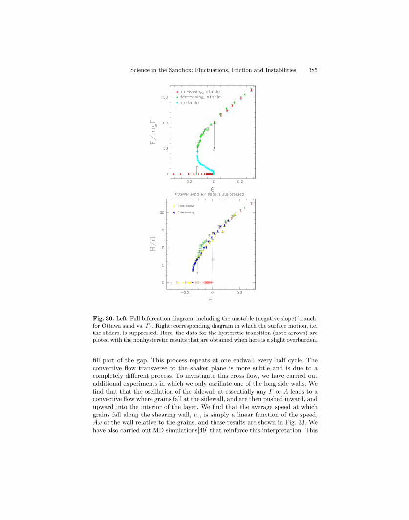
Fig. 30. Left: Full bifurcation diagram, including the unstable (negative slope) branch,for Ottawa sand vs. Γh. Right: corresponding diagram in which the surface motion, i.e.the sliders, is suppressed. Here, the data for the hysteretic transition (note arrows) areploted with the nonhysteretic results that are obtained when here is a slight overburden.

fill part of the gap. This process repeats at one endwall every half cycle. Theconvective flow transverse to the shaker plane is more subtle and is due to acompletely different process. To investigate this cross flow, we have carried outadditional experiments in which we only oscillate one of the long side walls. Wefind that that the oscillation of the sidewall at essentially any Γ or A leads to aconvective flow where grains fall at the sidewall, and are then pushed inward, andupward into the interior of the layer. We find that the average speed at whichgrains fall along the shearing wall, vz, is simply a linear function of the speed,Aω of the wall relative to the grains, and these results are shown in Fig. 33. Wehave also carried out MD simulations[49] that reinforce this interpretation. This


Fig. 31. Bifurcation points Γcu and Γcd versus dimensionless lifting pressure and airflow rate for rough sand and for glass beads.

Fig. 32. Relaxation times for rough sand vs. ε = (Γci − Γh)/Γci for the nucleationof the fluidized layer with increasing Γh and the vanishing of the fluidized layer withdecreasing Γh.


kind of shear-induced convection is likely to occur generally when a 3D materialis sheared in the presence of a gravitational field. We compare the results ofthese calculations with experiment in Fig. 33

0.25 0.5 0.75 1time (period)

-20

-10

0

10

20

30

Px

-1.5

-1

-0.5

0

0.5

1

1.5

2

2.5

Py,

Pz

Px

Py

Pz

(c)

0 10 20 30A (cm/s)

0

0.02

0.04

0.06

0.08

0.1

0.12

0.14

0.16

0.18

0.2

Vy(c

m/s

)f = 2.0 Hz (exp)f = 2.0 Hz (MD)f = 3.0 Hz (exp)f = 3.0 Hz (MD)f = 5.0 Hz (exp)f = 5.0 Hz (MD)fit

ω

(a)|

|

0.2 0.4 0.6 0.8z

-0.001

-0.0008

-0.0006

-0.0004

-0.0002

0

0.0002

Vy

0.40

0.50

0.60

β

(b)

5d

Vy

β

Fig. 33. Comparison of MD calculations and experiment. The left part of the figureshows MD results and experimental results for the downflow of particles along thevertical wall that is induced by shearing. The right part of the figures shosw typicalvelocity profiles obtained from the simulations

When the whole layer of material is now shaken, the following scenario de-scribes the onset of the instability and the mechanism for the cross-convectiveflow. The flow begins when the grains overcome frictional and dilatancy effects.This flow is nucleated at a single point near the solid surface. With the formationof the fluid layer, there is a shear flow of surface grains relative to the long walls(i.e. the direction of shaking) which is a maximum in the longitudinal middle ofthe cell. Near the side walls, there is a strong dilatancy of the moving grains, dueto shearing. The highly dilated grains near the side wall are mobile, and grainsreaching this boundary at the top surface percolate downward. However, grainsfalling along these walls eventually are pushed inwards.

5 Conclusions

We have explored aspects of granular materials that touch on the solid and densefluid phases. Necessarily, we have omitted many interesting results that concernthe gas-like phase. Conventional theories have typically considered only the meanbehavior of granular systems. Recent work has focused on the microscopic struc-ture and statistics of these materials. From this point, the mean behavior isobtained in the long wavelength limit. Several models and techniques addressing


the microscopic structure of granular materials include the q-model (and relatedconstructions), the OSL model, and contact dynamics. In general, these models,as well as experiments, agree that the distribution of forces on individual grainsshould be described at large forces by an exponential: P ∝ exp(−F/Fo). What isstill unclear theorectially is the nature of correlations, their connection to forcechains and how to fold history into the description. Such issues necessarily affectthe long wavelength limit of any description. As a consequence, there are nowcompeting theories that propose an array of very different partial differentialequations for stress fields within a granular material.We have explored these theories through experiments that measure forces at

the base of 3D sand piles, forces and structural information in 2D heaps, andGreen’s function measurements for 2D heaps. The first experiments confirm theimportance of history dependence, and they are consistent with the OSL model.The 2D heap experiments show that structure even more than force profilesis the quantity most strongly affected by history. Finally, the Green’s functionmeasurements, which to date must still be considered preliminary, suggest thatthe mean behavior of a granular system is described by a wave-like process withdispersion.We have also carried out a series of experiments in 3D and in 2D that have

laid out the nature of fluctuations in slowly sheared systems. In 3D, there is aninteresting rate-independence for the fluctuation forces; that is, the shear rateprovides the characteristic time scale for the system, even at the level of theflucutations. Typically, we see force distributions that are consistent with an ex-ponential distribution. But we do not observe the narrowing of the distributionswith increasing number of particles that would be consistent with a total lack ofcorrelation between grains. From the perspective of these experiments, the issuesof correlations is not resolved. In 2D, we also observe exponential distributionsfor a range of densities. However, for densities close to the critical value wherestresses are just maintained in the system, and for highly compressed samples,the distributions differ from exponential. The near-critical regime is particularlyinteresting. Here, a number of quantities, including the compressibility, the char-acteristic length of a stress chain, the distribution of avalanches, and the meanvelocity appear to satisfy powerlaws–in analogy to what one might expect fora fluid near the liquid-gas critical point. This transition is important for densegranular materials because it provides the mechanism for shear deformation. Assuch, it is connected to Reynolds dilatancy, shear bands and similar phenomena.Finally, we have explored the transition between fluid and solid phases

through the use of horizontal and combined horizontal and vertical shaking.Here, we have considered only results for pure horizontal shaking, where we seea hysteretic transition between the fluid and solid states. Interestingly, there ispower law scaling for the time to nucleate either phase, and the hysteresis islifted by either dilating the material slightly or by suppressing the layer of slid-ing particles on the surface. Suppression of the hysteresis with dilation, and thedivergent time scales implies that the dilation process is key to the transition be-tween these phases. It is this process that separtates Coulomb failure of granular


materials from ordinary solid-on-solid frictional failure. The specific and highlyreproducible forms for the nucleation times suggests a global picture should ap-ply to both directions of the phase change, i.e. solid-to-fluid, and fluid-to-solid.Conventional models of Mohr-Coulomb failure treat only the solid-to-fluid tran-sition, and even then do not account for the details of the transition.

Acknowledgments

The work of DH and RPB was supported by the National Science Founda-tion under Grant DMR-9802602, and DMS-9803305, and by NASA under GrantNAG3-1917 and NAG3-2372. The work of E. Clement, G. Reydellet and L. Vanelwas supported under PICS-CNRS no 563.

∗Current address: Argonne National Laboratory, Materials Science Division,9700 Cass AVe. Argonne, IL 60439, USA

∗∗Current address: Dept. of Physics, UCLA, 405 Hilgard Ave. Los Angeles,CA 90095-1547

†Current address: Danish Research Centre for Magnetic Resonance, HvidovreHospital, Dept. 340, Kettegaard Alle 30, DK 2650 Hvigovre, Denmark

References

1. For broad reviews, overviews, and proceedings see: Focus issue of Chaos–R.Behringer, H. Jaeger, and S. Nagel, Chaos 9, 509 (1999); L. P. Kadanof, Rev.Mod. Phys. 71, 435 (1999); Physics of Dry Granular Media, H. J. Herrmann, H.-P.Hovi, and S. Luding, eds. Kluwer, 1998; Proceedings of Powders and Grains, R. P.Behringer and J. T. Jenkins, eds. Balkema (1997); H. M. Jaeger and S. R. Nagel andR. P. Behringer, Physics Today, 49, 32 (1996); Rev. Mod. Phys. 68 1259 (1996);Physics of Granular Media, D. Bideau and J. Dodds, eds. Les Houches Series, Nova(1991); Granular Matter: An Interdisciplinary Approach, A. Mehta, Ed. Springer,NY (1994); R. P. Behringer, Nonlinear Science Today, 3, 1 (1993).

2. B. J. Ennnis, J. Green, and R. Davies, Chem. Eng.Prog. 69, 44 (1994).3. J. Eibl, The Structural Engineer, 62A, 169 (1984).4. A sampling of relevant works includes: S. Ogawa in Proceedings of US-Japan Sem-

inar on Continuum-Mechanical and Statistical Approaches in the Mechanics ofGranular Materials, ed. S. C. Cowin and M. Satake (Gakujutsu Bunker Fukyukai,Tokyo, Japan) 1978; P. K. Haff, J. Fluid Mech. 134, 401 (1983); S. B. Savage, Adv.Appl. Mech. 24, 289 (1984).

5. W. Losert, D.G. W. Cooper , J. Delour, A. Kudrolli, and J. P. Gollub, Chaos 9,682 (1999); M. Shattuck, H. Swinney, private communication.

6. I. Goldhirsch and G. Zanetti, Phys. Rev. Lett. 70, 1619 (1993).7. C.-h.Liu, S. R. Nagel, D. A. Schecter, S. N. Coppersmith, S. Majumdar, O. Narayan

and T. A. Witten, Science 269, 513 (1995), Phys. Rev. E 53, 4673 (1996).8. B. J. Miller, C. O’Hern, and R. P. Behringer, Phys. Rev. Lett. (1996).9. D. K. Mueth H. M. Jaeger, S. R. Nagel, Phys. Rev. E 57, 3164 (1998).10. A. Ngadi and J. Rajchenbach, Phys. Rev. Lett. 80, 273 (1998).11. D. Howell, C. Veje and R. Behringer, Phys. Rev. Lett. 82, 5241 (1999).


12. I. Albert, P. Tegzes, B. Kahng, R. Albert, J. G. Sample, M. Pfeifer, A.-L. Barabasi,T. Vicsek and P. Schiffer, Phys. Rev. Lett. 84 5122 2000; Phys. Rev. Lett 82 205(1999).

13. A. V. Tkachenko and T. A. Witten, to appear.14. P. Dantu, Geotechnique, 18, 50 (1968); A. Drescher and G. De Josselin De Jong,

J.Mech. Phys. Solids, 20, 337 (1972); T. Travers et al. J. Phys. A. 19, L1033.15. R. Jackson, in Theory of Dispersed Multiphase Flow, Ed. Re. E. Meyer (Academic

Press, NY, 1983, p. 29116. G. Amontons, Memoires de l’Academie Royale, A 12, 257 (1699).17. R. M. Nedderman, Statics and Kinematics of Granular Materials, Cambridge,

1992.18. For a review see R. Jackson, In Theory of Dispersed Multiphase Flow ed. R. Meyer,

Academic Press (1983).19. See C. Caroli and P. Nozieres and T. Baumberger in the Proceedings of the Work-

shop on Friction, Arching, Contact Dynamics, D. E. Wolf and P. Grassberger, eds.World Scientific, 1997.

20. S. Ouaguenouni and J.-N. Roux, Europhys. Lett. 32, 449 (1995) and in the Pro-ceedings of the Workshop on Friction, Arching, Contact Dynamics, D. E. Wolf andP. Grassberger, eds. World Scientific, 1997; A. V. Tkachenko and T. A. Witten,Phys. Rev. E 60 687 (1999).

21. A. Liu and S. Nagel, Nature 396, 21 (1998).22. Christophe Eloy and Eric Clement, J. Phys. I France 7, 1541 (1997).23. Joshua Socolar, Phys. Rev. E 57, 3204 (1998).24. Mario Nicodemi, Phys. Rev. Lett. 80, 1340 (1998).25. F. Radjai, M. Jean, J.-J. Moreau, and S. Roux, Phys. Rev. Lett. 77, 274 (1996);

R. Radjai, D. Wolf, M. Jean and J.-J. Moreau, in Friction, Arching and ContactDynamics, ed. D. E. Wlof and P. Grassberger, World Scientific (1997).

26. J. P. Wittmer, P. Claudin, M. E. Cates, and J. -B. Bouchaud, Nature 382, 336(1996); Phys. Rev. E 57, 4441 (1997).

27. V. M. Kenkre, J. E. Scott, E. A. Pease, and A. J. Hurd, Phys. Rev. E 57 5841 and5850 (1998).

28. S. B. Savage, in Physics of Dry Granular Media, H. J. Herrmann, H.-P. Hovi, andS. Luding, eds. Kluwer, 1998.

29. L. Vanel, D. Howell, D. Clark, R. Behringer, and E. Clement, Phys. Rev. E. 60,R5040 (1999).

30. R. Brockbank, J. M. Huntley, and R. Ball, J. Physique I France 10, 1521 (1997).31. R. B. Heywood, Designing by Photoelasticity, Chapman and Hall Ltd, London,

1952.32. S. G. Paikowsky and K. J. DiRocco, Conference on Digital Image Processing: Tech-

niques and Applications in Civil Engineering, Kona, Hawaii, February 28- March5, 1993, ASCE publication 236 (1993).

33. G. W. Baxter and R. P. Behringer, Eur. J. Mech. B, 10, 181 (1991). G. W. Baxter,R. Leone and R. P. Behringer, Europhys. Lett. 21, 569 (1993).

34. C. H. Liu and S. R. Nagel, Phys. Rev. Lett. 68, 3201 (1992).35. X. Jia, C. Caroli and B. Velicky, Phys. Rev. Lett. 82 1863 (1999).36. H. J. Herrmann, S. Luding, J. P. Hovi, eds. Dry Granular Media, Nato ASI series,

Kluver, Amsterdam (1998).37. D. Howell et al. in Proceedings of the Workshop on Friction, Arching and Dilatancy

ed. E. E. Wolf and P. Grassberger, World Scientific, 1997; C. T. Veje, et al. in DryGranular Media, H. J. Herrmann, S. Luding, J. P. Hovi, eds. , Nato ASI series,Kluver, Amsterdam (1998).


38. D. Howell, Ph.D. Thesis, Duke University, 1999, unpublished.39. R. M. Nedderman and C. Laohakul, Powder Technol., 25, 91 (1980).40. C. T. Veje, Daniel W. Howell and R. P. Behringer, Phys. Rev. E 59, 739 (1999).41. S. Schollmann, S. Luding and H. J. Herrmann, to be published.42. C. Veje, D. Howell, R. Behringer, S. Cshollmann, S. Luding and H. Herrmann, in

Physics of Dry Granular Media, H. J. Herrmann, H.-P. Hovi, and S. Luding, eds.Kluwer, 1998.

43. H. Buggisch and G. Loffelmann, Chem. Eng. Processing (1989).44. E. Ben-Naim, J. B. Knight and E. R. Nowak, J. Chem. Phys., 100, 6778 (1996);

Edmund R. Nowak et al., Phys. Rev. E 57, 1971 (1998).45. H. Jaeger, private communication46. D. Howell, R. P. Behringer, and C. T. Veje, Chaos 9, 559 (1999).47. R. P. Behringer, D. Howell, L. Kondic, S. Tennakoon, and C. Veje, Physica D 133,

1 (1999).48. S. G.K. Tennakoon and R. P. Behringer, Phys. Rev. Lett. 81, 794 (1998).49. Europhys. Lett. S. G.K. Tennakoon, L. Kondic, and R. P. Behringer45, 470 (1999).50. H. K. Pak and R. P. Behringer, Phys. Rev. Lett. 71, 1832 (1993).51. E. van Doorn and R. P. Behringer, Phys. Lett. A 235, 469 (1997).52. P. Evesque, Contemp. Phys. 33, 245 (1992).53. G. H. Ristow, G. Strassburger, and I. Rehberg, Phys. Rev. Lett. 79, 833 (1997).54. E. Aharonov and D. Sparks, Phys. Rev. E 60, 6890 (1999).55. S. B. Obuknov, Phys. Rev. Lett. 74, 4472 (1995); C. Moukarzel, P. M. Duxbury,

and P. L. Leath, Phys. Rev. Lett. 78, 1480 (1997).


Science in the Sandbox: Fluctuations, Friction and Instabilities

Documents

Transcript of Science in the Sandbox: Fluctuations, Friction and Instabilities