Two-dimensional angle of arrival fluctuations

Two-dimensional angle of arrival fluctuationsDaniela Di Iorioa) and David M. FarmerInstitute of Ocean Sciences, P.O. Box 6000, Sidney, British Columbia V8L 4B2, Canada

~Received 21 August 1995; accepted for publication 17 December 1995!

Angle of arrival fluctuations are one manifestation of acoustic propagation through a turbulent flow.Here the two-dimensional angle of arrival distribution for a 670-m acoustic path through a highReynolds number flow in a tidal channel is examined and its origin and relationship to the flow fieldis determined. Over scales greater than the variability due to turbulence, a solution of the raypropagation equation explains the effect of advection on the horizontal arrival angle. The rapidlyfluctuating two-dimensional angle of arrival distribution shows a degree of scatter consistent withthe level of turbulent intensity. After removal of effects due to the finite aperture, orthogonalcomponents are correlated during strongly sheared flow implying that the turbulence is weaklyanisotropic over the measured scales. This anisotropy is discussed in terms of the cross streamvelocity gradients]v/]x8 and ]v/]z8, where (x8,z8) are perpendicular diagonal coordinates.© 1996 Acoustical Society of America.

PACS numbers: 43.30.Re, 43.30.Hw@JHM#

INTRODUCTION

The coastal environment is often characterized by en-hanced mixing, increased variability in water properties andstrong tidal effects. Acoustical propagation measurementshave the potential for serving as a sensitive probe of theseprocesses, which can differ markedly from those prevalent inless active waters of the open ocean. Here we describe re-sults of a high-frequency forward scatter experiment in ashallow tidal channel, specifically designed to shed light onsome two-dimensional features of the turbulent environment.

In October 1986 an acoustic propagation experimentwas carried out in Cordova Channel, British Columbia~Fig.1! using two-dimensional arrays of transmitters and receiv-ers. Since the instrumentation uses a high acoustic frequencyand a high sampling rate, and has the ability to measureprecise phase, we are able to make some novel measure-ments of the two-dimensional mean and turbulent structureof the flow and where possible compare them to independentin situ oceanographic measurements.

Although most oceanographic structure is undoubtedlyanisotropic, strongly stirred flows which are fairly commonin the coastal environment can be expected to approach isot-ropy over some range of scales. The existence of anisotropyhowever is essential to the production and dissipation of tur-bulent energy whereas isotropic turbulence can only decaythrough dissipation~see Hinze1!. A knowledge of isotropicturbulence may therefore serve as a starting point for thestudy of anisotropic turbulent flows. Our two-dimensionalacoustic measurements in Cordova Channel provide a checkon the validity of the isotropic assumption.

I. EXPERIMENTAL APPROACH

Cordova Channel, British Columbia is part of a largerarea in which fresh water, primarily from the Fraser River,

mixes with water of higher salinity before reaching the Pa-cific Ocean through the Strait of Juan de Fuca. Except forbrief periods during slack water, Cordova Channel is turbu-lent and this turbulence mixes the variable properties of theinflow. Di Iorio and Farmer2 showed that during the experi-mental period the observed refractive index variability wasdominated by turbulent velocity fluctuations rather than tem-perature and salinity variability when the tidal current wasstrong.

Our experiment made use of a set of four transmitters onthe east side of Cordova Channel operating at a frequency of67 kHz, and four receivers on the west side. Transducerswere rigidly mounted in square arrays of side;1 m on tri-pods@see Fig. 2~a!#. Figure 2~b! labels the receiver array as ifviewed from the channel center. The receiving plane hascoordinate axes (x,z) for horizontal and vertical receivers; arotated coordinate system used later has axes (x8,z8) forperpendicular diagonal receivers. Acoustic propagation isalong they andy8 direction.

Coded sequences~63 bit, phase encodedm sequences!were transmitted from each of the four sources in either acontinuous or block mode~block mode gives a time breakbetween the fourth and the first transmission whereas con-tinuous mode has no time break!, so that for each of thesemodes transmissions cycled through the entire array 17.9 and5.3 times a second, respectively. Table I summarizes the ex-perimental parameters for the data set discussed in this paper.

The signal from each source was detected simulta-neously at each of the four receivers, following which spe-cially built hardware was used for bandpass filtering, com-plex demodulation, and low-pass filtering at the carrierfrequency cutoff, followed by digitization and time-laggedcross correlation with a template of the transmitted code. Thecorrelation score for the inphase (I ) and quadrature (Q)shows a series of nearly triangular peaks, each correspondingto a different path; only the direct path was used. Interpola-tion was carried out across the five highest points in themagnitude

a!Present affiliation: SACLANT Undersea Research Centre, Viale San Bar-tolomeo 400, 19138 La Spezia, Italy.

814 814J. Acoust. Soc. Am. 100 (2), Pt. 1, August 1996 0001-4966/96/100(2)/814/11/$6.00 © 1996 Acoustical Society of America

A~ t !5AI ~ t !21Q~ t !2, ~1!

where t is the travel time, to give the amplitude~A! andarrival time~T !. Interpolation of the inphase and quadrature

at the interpolated peak amplitude location was then used toderive the phase

f5arctanSQ~T !

I ~T ! D . ~2!

This procedure leads to time series of amplitude and phasemeasurements for each receiver, corresponding to the trans-mission from each source. The time of arrival allows resolu-tion of the 2p phase ambiguity inherent in the arctan func-tion of ~2!. Based on a signal-to-noise ratio of 25 dB, theaccuracy in the phase measurement is63.2 deg.

Measurement related noise provides a limit to the usefulresolution of the phase and hence the phase difference at thehighest sampling frequencies. Figure 3 shows twelve 15-minphase spectra taken during a 12-h measurement period. Thevertical spread in the spectral level corresponds to increasedlevels of refractive index variability during stronger flowsand horizontal spread results from the frequency dependenceon mean flowU. An increase in spectral levels at the highestfrequencies corresponds to a truncation of one cycle in thepseudorandom noise~PRN! code on alternating transmis-

FIG. 1. Cordova Channel showing instrument locations, together with trans-mitter ~T! and receiver~R! arrays~m!. Recording current meters at 15- and16-m depth are at station~d! 2; CTD profiles were obtained at stations~j!A and 3.

FIG. 2. ~a! Deployment scheme for the square acoustic array.~b! Schematicshowing the receiver array viewed from the center of the channel. Horizon-tally spaced receivers make use of the top and bottom transducers~x axis!;vertically spaced receivers make use of the left and right transducers~zaxis!. Primed coordinates are for diagonal transducers.

FIG. 3. Twelve experimental phase spectra taken through the measurementperiod. The low-pass filter cutoff point~f c54.5 Hz! is shown.

TABLE I. Acoustic parameters of Cordova Channel scintillation experi-ment.

Parameter Square array

Transducer array depth~m! 15Path lengthL ~m! 670Receiver separation~m! rx51.18 andrz51.03Cycling mode block continuousObservation period~PDT!

23/10/86 12:00 to24/10/86 00:00

24/10/86 00:00 to24/10/86 12:30

Acoustic frequency,f a ~Hz! 69444 67567Acoustic wave numberk ~m21! 293.82 285.89Fresnel radiusAlL ~m! 3.79 3.87Code length@bits ~ms!# 63 ~11! 63 ~14!Bit width @cycles/bit~ms!# 12 ~173! 15 ~222!Phase shift for coding~deg! 180 180Digitization rate@samples/bit~kHz!# 3 ~17.4! 3 ~13.5!Window size@samples~ms!# 21 ~1.211! 11 ~0.814!Repetition rate~Hz! 5.251 17.875

815 815J. Acoust. Soc. Am., Vol. 100, No. 2, Pt. 1, August 1996 D. Di Iorio and D. M. Farmer: Two-dimensional fluctuations

sions used for transmitter identification of continuous modedata. The data were low-pass filtered with a third-order sym-metric Butterworth filter at a cutoff frequency off c54.5 Hz.

II. OCEANOGRAPHIC OBSERVATIONS

Currents were measured with moored instruments at 15and 16 m in the center of the channel~see Fig. 1! with asampling period of 2 min. The current was primarily perpen-dicular to the acoustic path and the resolved component inthis direction is shown in Fig. 4~a! where positive valuescorrespond to flood tide~high water! and negative valuescorrespond to ebb tide~low water!. The Reynolds numberover the average depth of the channel~D528 m! and duringstrong flow~U50.8 m s21! is

Re5UD/n52.23107, ~3!

wheren5131026 m2 s21 is the kinematic viscosity.The current speed from the current meter~solid curve!

can be compared to the acoustically derived speed~seeFarmeret al.3!. The latter is calculated from the scintillationdrift approach using the time delay to the maximum log-amplitude cross-covariance for parallel acoustic paths. Thetime-lagged cross-covariance function is calculated using 4min of log-amplitude data and thus the acoustic current mea-surement is an average over 4 min. The results from theacoustic technique~dots! are shown for comparison in Fig.4~a!. Differences arise because the acoustic method gives apath averaged measurement with uniform weighting alongthe path whereas the current meter is at a point location inthe center of the channel.

The vertical current shear can be measured both with themoored current meters at two depths and the two verticallyspaced propagation paths. The results are shown in Fig. 4~b!.In order to see the difference between the two measurementsthe acoustic results were averaged over 8 min. The shearobtained from the current meters~solid curve! is generally inagreement with that found from the acoustic technique

~dots!. Significant shear~0.04 s21! is measured only duringthe flood. This is a period when turbulence anisotropy ismore pronounced as discussed subsequently.

During the period of these measurements Di Iorio andFarmer2 found the spectrum of refractive index fluctuationsconsistent with the Kolmogorov similarity scaling

Fn~k!50.033Cneff2 k211/3, ~4!

where k is the refractive index wave number andCneff2 is

defined as the effective structure parameter for the refractiveindex fluctuations since it takes into account both scalar andvector contributions and describes the total intensity of thesefluctuations~see Ostacher4!. The effective structure param-eter may be found from the log-amplitude variance

sx250.124Cneff

2 k7/6L11/6, ~5!

wherek is the acoustic wave number andL is the propaga-tion distance.

Figure 5~a! shows measurements ofCneff2 taken through

the tidal cycle shown in Fig. 4~a!. Di Iorio and Farmer2 fur-ther showed that for this period in Cordova Channel the re-fractive index fluctuations are dominated by the velocityfluctuations so that

Fn~k!;Fnv~k!5E~k!/4pc0

2k2, ~6!

where

E~k!51.5e2/3k25/3, ~7!

is the three-dimensional spectrum for the turbulent kineticenergy,e is the turbulent kinetic energy dissipation rate~perunit mass! and c0 is the average sound speed along theacoustic path and converts velocity fluctuations into refrac-tive index fluctuations. Ostachev4 derives the effective struc-ture parameter for refractive index fluctuations dominated byvelocity fluctuations:

Cneff2 5

11

6

Cv2

c02 , ~8!

FIG. 4. ~a! The current speed obtained from a 15-m current meter at station2 ~solid curve! and from acoustic delay to peak method for parallel paths~dots!. ~b! The mean vertical shear]U/]z determined by two verticallyspaced current meters~solid curve! and by the acoustic method~dots!.

FIG. 5. ~a! Effective structure parameterCneff2 ~dots! calculated from the

acoustic log-amplitude variance.~b! Measured turbulent kinetic energy dis-sipation ~1! and the estimated dissipation for a drag coefficient ofCD5331023 ~solid curve!.


whereCv251.97e2/3 is the structure parameter for velocity

fluctuations.Following Di Iorio and Farmer,2 the turbulent kinetic

energy dissipation rate is calculated and shown in Fig. 5~b!.These dissipation rates are used to quantify the magnitude ofthe velocity gradients in Sec. III B 2 to show that they con-tribute to the observed angle of arrival variance. Superim-posed on the measurement is the prediction based on a bal-ance of production and dissipation of turbulent energy for adrag coefficient ofCD5331023 similar to that described inRef. 2.

III. ACOUSTIC ANGLE OF ARRIVAL

As noted previously the rms phase noise is approxi-mately63.2 deg in our acoustical scintillation system. Moreinteresting, however, is the phase difference, and hence themeasurement resolution of the angle of arrival fluctuations.Since the acoustic signal is detected with a two-dimensionalarray, we can determine the horizontal and vertical compo-nents of the arrival angle.

The horizontal and vertical arrival angles,uax and uazrelative to the line perpendicular to the receiver axes, aredefined by

sin uax5~f l2f r !c0

varx5

dfx

krx5

dfx

2p

l

rx, ~9!

sin uaz5~fb2f t!c0

varz5

dfz

krz5

dfz

2p

l

rz, ~10!

where subscriptsl , r , b, and t correspond to the left, right,bottom, and top receivers when viewing the array from thecenter of the channel@see Fig. 2~b!#, f is the phase in radi-ans,c0 is the average sound speed at 15 m depth~;1485m s21!, va52p f a is the angular acoustic frequency,k52p/l is the acoustic wave number, andr is the receiverspacing for the horizontal (x) and the vertical (z) direction.The phase differencedf is taken using diverging acousticpaths ~one transmitter and two receivers!. Even thoughspherical wave propagation is used, it is assumed that in thevicinity of the receivers the waves are plane.

The sensitivity in the angle of arrival measurement relieson three factors: A receiver spacing large enough to accom-modate many wavelengths~i.e., l/r!1!, the ability to re-solve 2p phase ambiguities and the ability to detect phasedifferences within a fraction of a cycle. All these factors aresatisfied in our data and hence we can measure the angle ofarrival with resolution of 0.02 deg for a single transmission.Also, implicit in this calculation is that the phase remaincoherent over the antenna. For a 1-m separation the correla-tion was found to be 0.996.

In a medium where a number of acoustic paths giveapproximately the same travel time, beamforming techniquesare normally applied to resolve the reception angles for eachray. Worcester5 describes such an experiment, using a verti-cal receiving array of four transducers, where the arrivalangle for all paths are obtained and compared to predictedpatterns. We do not have to employ beamforming techniqueswith our data since our first arrival consists of a single path.

Therefore, the arrival angle calculations using~9! and ~10!are carried out both to examine the slow variations associ-ated with ‘‘deterministic’’ deflections of the acoustical path,and also the pattern of rapid fluctuations.

A. Low-frequency fluctuations

Sound traveling across the channel can be modified invarious ways by the intervening water. Changes in the pathaveraged refractive index over time scales of minutes tohours exist because of the gross changes in the mean soundspeed over the path during the tidal cycle. The amplitude orlog-amplitude remains essentially unchanged at these timescales. However, changes in the temperature and salinity re-sulting from mixing and advection, can result in significantphase changes. Horizontal gradients in the sound speed overtime scales.100 s tend to be small~maximum magnitude oforder 531024 s21!, so that horizontal refraction by scalareffects is negligible over the short path length used here.

1. Horizontal angle

Farmer and Di Iorio6 derived the horizontal arrival angleas a result of current using a simple geometric approach.Here we apply a rigorous mathematical solution. The effectof current on the horizontal arrival angle is analysed throughan approximate solution to the wave equation. The time de-pendence for a moving medium isd/dt5]/]t1U–“. Defin-ing the space-time pressure field asP~r ,t)5p~r !e2 iwt foroutward propagation the wave equation reduces to

¹2p~r !1n2~r !k2p~r !522ikn2~r !U–“p~r !

c0, ~11!

where orders ofU2/c2 have been neglected,n~r ! is the re-fractive index of the medium due to scalar changes in thesound speed,k is the acoustic wave number, andc0 is themean sound speed. The transformationC~r !5ln p~r ! gives

¹2C~r !1“C~r !–“C~r !1n2~r !k2

522ikn2~r !U–“C~r !

c0. ~12!

The phase variability can be described by the ray ap-proximation since it is affected by the largest scales. Thisapproach separates the fieldC5ln A1 iS in terms of log-amplitude and phase. This will result in two equations cor-responding to the real and imaginary part. They are, respec-tively,

¹2 ln A1“ ln A–“ ln A2“S–“S1n2k2

52kn2U

c0–“S ~13!

and

¹2S12“ ln A–“S522kn2U

c0–“ ln A. ~14!

Since the Fresnel scale sizel 5 AlL produces the largestamplitude fluctuations~see Tatarskii,7 Di Iorio and Farmer2!we can make the high-frequency approximation, where¹2 ln A1“ ln A–“ ln A5¹2A/A!“S–“S. This result


arises sinceu“Su;k, ¹2A/A;1/l 2 andl! l . Therefore,~13!reduces to

“S–“S5n2k222kn2U

c0–“S. ~15!

We can only solve~14! and ~15! by approximate meth-ods. The amplitude, phase, and refractive index are perturbedinto mean and fluctuating components,

n5n01hs;11hs , ~16!

A5A01A1 , ~17!

S5S01S1 , ~18!

wherehs is the refractive index fluctuation from scalar ef-fects~temperature and salinity!, A0 andS0 are the amplitudeand phase in a medium without motion, andA1 andS1 arethe amplitude and phase fluctuations associated with themoving medium and the refractive index fluctuations. ThusU/c0 has first-order magnitude. This perturbation analysisresults in zeroth- and first-order equations for each of the realand imaginary equations. From the real part

“S0–“S05k2 zeroth order, ~19!

“S0–“S15hsk22k

U

c0–“S0 first order, ~20!

and from the imaginary part

¹2S012“ ln A0–“S050 zeroth order, ~21!

¹2S112“ ln A0–“S112“ ln A1–“S0

522kU

c0–“ ln A0 first order. ~22!

The solutions to the zeroth-order equations are“S05kr /r or S05kr and A05Q/r corresponding to outwardspherical wave propagation in a medium without motion orrandom fluctuations in the refractive index. The solution to~20! for acoustic propagation across the channel and perpen-dicular to the mean flowU5(U,0,0) is

“S15kS hs~r !r

r2U

c0xD , ~23!

where x is the unit vector along thex axis. We neglect thesolution to ~22! since this paper focuses on phase fluctua-tions.

Averaging over the fluctuations of the medium gives

]S1]x

52kU

c0. ~24!

Therefore, the mean horizontal arrival angle for a transmitterand receiver placed atx50 in a moving medium is

ux51

k

]~S01S1!

]x52

U

c0. ~25!

The sign convention for the angle in this derivation is posi-tive clockwise and negative counter clockwise about thepositivey axis. This result shows that the horizontal arrivalangle is independent of path length.

The wavefronts and the rays can be determined for thissolution. Assuming hs50 then “S152kU/c0x andS152kUx/c0 . The resulting phase S5S01S15kr2kUx/c0 gives wavefronts forS5constant. The equationfor the wavefront in the (x,y) plane is then

y5ASAk 1U

c0xD 22x2, ~26!

whereA is a constant in radians. Figure 6 shows the acousticwavefronts propagating outward from the source at the ori-gin. The figure is deliberately exaggerated by setting theMach number,M5U/c050.25, so as to clearly reveal theadvection. This value ofM is 400 times that encountered inCordova Channel. The constantA/k ranges from 0 to 80 m.

The rays perpendicular to the wavefronts in the (x,y)plane are described by the vector equation

“S5kS rr2U

c0xD . ~27!

The equation of the rays is found from the solution to thedifferential equation describing the angle of the ray:

dy

dx5

y

x2Mr, ~28!

wherer 25x21y2. Under the transformationu5y/x,

xdu

dx5

uMA11u2

12MA11u2, ~29!

which may be solved by the method of separation giving

x5y

2 S 1

~By!M2~By!M D , ~30!

where logB is a constant of integration. Figure 6 also showsthe acoustic rays which are refracted due to the current forvalues ofBM ranging nonlinearly from 0.0125 to 4. Thearrival angle deviation is the Mach number of the flow. Thisderivation does not take into account scattering from tem-perature and velocity fluctuations and to first order is inde-

FIG. 6. Acoustic wavefronts and rays as a result of the currentU5Ux. TheMach number is 0.25 in the calculations so that the advection of the wave-fronts and the refraction of the rays can be illustrated.


pendent of path length. If we compute a path-averaged cur-rent speed

U51

L E0

L

U~y!dy ~31!

and setM5U/c0 , the solutions~26! and~30! remain valid tofirst order.

It is interesting to point out that the travel time differ-ence between the refracted ray and the unperturbed ray is asecond-order effect„O(U2/c0

2)… which is negligible. There-fore to first order, the acoustic energy can be assumed totravel along the unperturbed ray~i.e., straight lines! givingan integrated travel time dependent only on the sound-speedchange as a result of the moving medium. R. Pawlowicz~personal communication! has pointed out that this can havesome unique advantages in tomographic measurementswhere the ray path is simplified as the unperturbed ray.

Figure 7~a! shows the horizontal acoustic arrival angle,based on 4-min averages using receivers 4-1@see Fig. 2~b!#together with the arrival angle derived from~25! using thepath averaged current measured by the scintillation drift. Thesign convention for these measured angles is positive counterclockwise and negative clockwise about the line connectingtransmitter and receiver~2y axis!. During peak flow periodsthe acoustic arrival angle overestimates the current.

The measured angular deviations are extremely smalland the array dimensions limit the measurement accuracy.For example, the angular deviation caused by a 1-m s21 cur-rent is 0.038 deg; which is equivalent to the apparent angulardeviation resulting from a displacement of one hydrophone

by only 0.66 mm! Although our supporting structure wasrobust, flow induced mechanical displacements of this mag-nitude would not be surprising. It is worth pointing out thatwith receivers separated by 20 m, the resolution in the arrivalangle is 0.001 degrees resulting in a current speed resolutionof 2.6 cm s21.

Detection of the slowly varying horizontal arrival angleoffers some interesting possibilities for measurement of spa-tially averaged current perpendicular to the acoustic path. Incontrast to the use of scintillation drift~see Farmeret al.3!details of fine scale acoustic scattering are unimportant pro-vided decorrelation of the signal is small over the receiverseparation scale; it is only required that horizontal sound-speed gradients be negligible. This latter requirement mayrestrict application over great distances however, unless aconfiguration is used that allows separation of the horizontalgradient.

2. Vertical angle

The low-frequency variability in the vertical arrivalangleuz depends on the vertical stratification and increaseswith path lengthL. For the short horizontal range~L5670m!, the vertical deflection is~see Brekhovskikh and Lysa-nov8!

tan uz5L

2c0

dc

dz5

L

2c0

Dc

Dz. ~32!

The mean sound-speed gradientDc/Dz is estimated from

FIG. 7. ~a! Horizontal angle of arrival determined by the acoustic method~dots! together with the angle inferred from the measured current speed~solid curve!using~25!. ~b! Vertical arrival angle determined by the acoustic method~dots!, together with the angle inferred from the measured sound-speed gradient~solidcurve! using ~32!.


CTD ~conductivity, temperature, and depth! profiles in thecenter of the channel~see Fig. 1!.

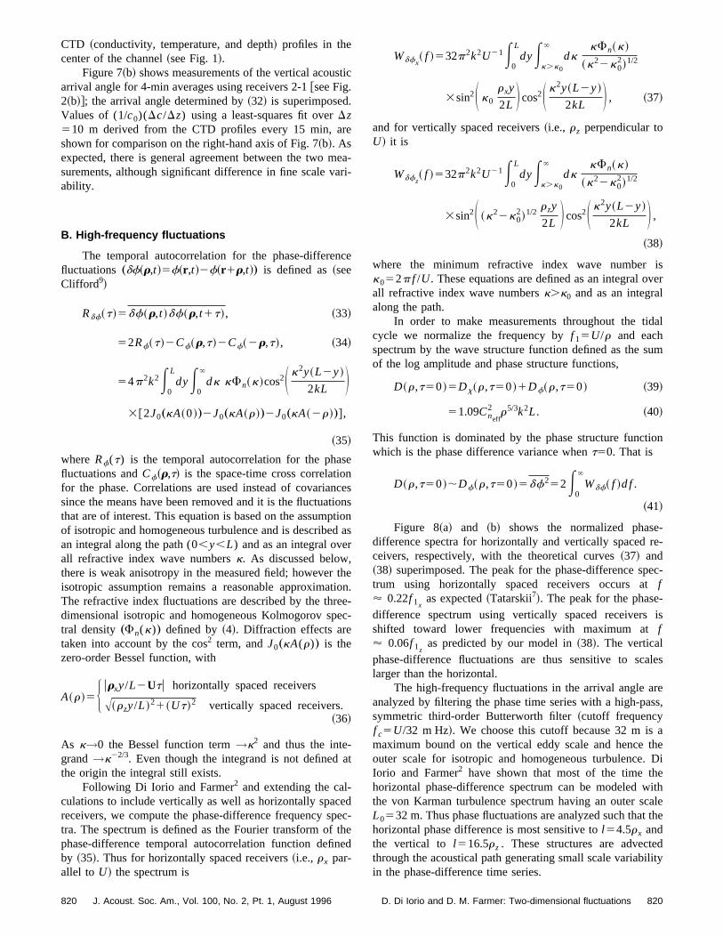
Figure 7~b! shows measurements of the vertical acousticarrival angle for 4-min averages using receivers 2-1@see Fig.2~b!#; the arrival angle determined by~32! is superimposed.Values of (1/c0)(Dc/Dz) using a least-squares fit overDz510 m derived from the CTD profiles every 15 min, areshown for comparison on the right-hand axis of Fig. 7~b!. Asexpected, there is general agreement between the two mea-surements, although significant difference in fine scale vari-ability.

B. High-frequency fluctuations

The temporal autocorrelation for the phase-differencefluctuations„df~r,t!5f~r ,t!2f~r1r,t!… is defined as~seeClifford9!

Rdf~t!5df~r,t !df~r,t1t!, ~33!

52Rf~t!2Cf~r,t!2Cf~2r,t!, ~34!

54p2k2E0

L

dyE0

`

dk kFn~k!cos2S k2y~L2y!

2kL D3@2J0„kA~0!…2J0„kA~r!…2J0„kA~2r!…#,

~35!

whereRf(t) is the temporal autocorrelation for the phasefluctuations andCf~r,t! is the space-time cross correlationfor the phase. Correlations are used instead of covariancessince the means have been removed and it is the fluctuationsthat are of interest. This equation is based on the assumptionof isotropic and homogeneous turbulence and is described asan integral along the path (0,y,L) and as an integral overall refractive index wave numbersk. As discussed below,there is weak anisotropy in the measured field; however theisotropic assumption remains a reasonable approximation.The refractive index fluctuations are described by the three-dimensional isotropic and homogeneous Kolmogorov spec-tral density„Fn(k)… defined by~4!. Diffraction effects aretaken into account by the cos2 term, andJ0„kA(r)… is thezero-order Bessel function, with

A~r!5H urxy/L2Utu horizontally spaced receivers

A~rzy/L !21~Ut!2 vertically spaced receivers.~36!

As k→0 the Bessel function term→k2 and thus the inte-grand→k22/3. Even though the integrand is not defined atthe origin the integral still exists.

Following Di Iorio and Farmer2 and extending the cal-culations to include vertically as well as horizontally spacedreceivers, we compute the phase-difference frequency spec-tra. The spectrum is defined as the Fourier transform of thephase-difference temporal autocorrelation function definedby ~35!. Thus for horizontally spaced receivers~i.e., rx par-allel to U! the spectrum is

Wdfx~ f !532p2k2U21E

0

L

dyEk.k0

`

dkkFn~k!

~k22k02!1/2

3sin2S k0

rxy

2L D cos2S k2y~L2y!

2kL D , ~37!

and for vertically spaced receivers~i.e., rz perpendicular toU! it is

Wdfz~ f !532p2k2U21E

0

L

dyEk.k0

`

dkkFn~k!

~k22k02!1/2

3sin2S ~k22k02!1/2

rzy

2L D cos2S k2y~L2y!

2kL D ,~38!

where the minimum refractive index wave number isk052p f /U. These equations are defined as an integral overall refractive index wave numbersk.k0 and as an integralalong the path.

In order to make measurements throughout the tidalcycle we normalize the frequency byf 15U/r and eachspectrum by the wave structure function defined as the sumof the log amplitude and phase structure functions,

D~r,t50!5Dx~r,t50!1Df~r,t50! ~39!

51.09Cneff2 r5/3k2L. ~40!

This function is dominated by the phase structure functionwhich is the phase difference variance whent50. That is

D~r,t50!;Df~r,t50!5df252E0

`

Wdf~ f !d f .

~41!

Figure 8~a! and ~b! shows the normalized phase-difference spectra for horizontally and vertically spaced re-ceivers, respectively, with the theoretical curves~37! and~38! superimposed. The peak for the phase-difference spec-trum using horizontally spaced receivers occurs atf' 0.22f 1x as expected~Tatarskii

7!. The peak for the phase-difference spectrum using vertically spaced receivers isshifted toward lower frequencies with maximum atf' 0.06f 1z as predicted by our model in~38!. The verticalphase-difference fluctuations are thus sensitive to scaleslarger than the horizontal.

The high-frequency fluctuations in the arrival angle areanalyzed by filtering the phase time series with a high-pass,symmetric third-order Butterworth filter~cutoff frequencyf c5U/32 m Hz!. We choose this cutoff because 32 m is amaximum bound on the vertical eddy scale and hence theouter scale for isotropic and homogeneous turbulence. DiIorio and Farmer2 have shown that most of the time thehorizontal phase-difference spectrum can be modeled withthe von Karman turbulence spectrum having an outer scaleL0532 m. Thus phase fluctuations are analyzed such that thehorizontal phase difference is most sensitive tol54.5rx andthe vertical to l516.5rz . These structures are advectedthrough the acoustical path generating small scale variabilityin the phase-difference time series.


1. Horizontal and vertical arrival angle correlations

In order to observe anisotropy in the scattering, which isrelated to anisotropy in the turbulence, we need to computean average correlation function from our symmetrical array:

uxuz~t! A51

4k2rxrz@Cf~r42,t!1Cf~r24,t!

2Cf~r13,t!2Cf~r31,t!#, ~42!

where the subscriptA denotes that this function is averagedover the array. Figure 9 shows this function normalized bythe variances during ebb and flood.

At zero time lag,

uxuz A51

4k2rxrz@2Cf~r42,0!22Cf~r31,0!#, ~43!

51

4k2rxrz@Df~r31,0!2Df~r42,0!#, ~44!

where stationarity is assumed for the last equality. For theidealized representation of isotropic and homogeneous turbu-lence, the level of the refractive index fluctuations should beindependent of direction and thus zero. This is observed onlypart of the time. During ebb the positive correlation coeffi-cient in Fig. 9~a! at zero time lag is multivalued and thus isunlikely to be significant. At flood, however, the negative

correlation at zero time lag is single-valued suggesting thatthe observed correlation is not random.

The averaged correlation between horizontal and verti-cal arrival angles is the difference between the phase struc-ture function evaluated along two perpendicular diagonal di-rections. Since the diagonal spacings are virtually the same itis the difference in the structure parameterCneff

2 measured

along the two diagonal directions that gives the arrival anglecorrelations. For diverging paths the structure parametermeasured by the wave structure function is weighted towardthe receiver~see Farmeret al.3!; this angle of arrival corre-lation is therefore also weighted towards the receiver.

2. Two-dimensional distribution

The two-dimensional angle of arrival distribution evalu-ated from~44! over a given period can be analyzed by con-touring the number of times the arrival angle has a specificvalue. Figure 10 shows these contours, which correspond toprobability distributions, for 20 min of high-pass filtered datataken through the tidal period shown in Fig. 7~a!. Facing thereceiver array from the center of the channel, a positive hori-zontal ~vertical! angle indicates signals coming from theNorth ~surface!. The degree of scatter is related to the effec-tive refractive index structure parameter,Cneff

2 and hence the

turbulent kinetic energy dissipation ratee which is shown inFig. 5. A large amount of scatter occurs when there is en-hanced turbulence due to the tidal flow and the refractiveindex fluctuations are strong. Little scatter occurs at slackwater. If the turbulence is isotropic we would expect a cir-cular distribution corresponding to equal phase structurefunctions along the diagonals. Under isotropic conditions theacoustic arrival angle distribution would represent a two-dimensional random walk, but this is not observed. More-over, there is a systematic distortion, implying a correlationbetween vertical and horizontal deflections which is morepronounced during maximum flood~frames e to g in Fig.10!.

FIG. 8. Variance preserving plot of the theoretical~solid curve! and experi-mental~dots! phase-difference spectra for~a! horizontally and~b! verticallyspaced receivers. Experimental spectra are taken through a tidal cycle. Nor-malizing frequency is defined asf 1x 5 U/rx and f 1z 5 U/rz for rx51.18 mandrz51.03 m.

FIG. 9. Normalized angle of arrival correlations averaged over the squarearray during~a! strong ebb and~b! strong flood.


The major and minor axes of the distribution are deter-mined by evaluating the eigenvectors of the covariance ma-trix. The eigenvalues of the matrix represent the standarddeviation of the scatter along these axes. Figure 11 shows thestandard deviation along the major and minor axes, the angle

of the major axis and the correlation coefficient based on10-min data sets. The standard deviation, which describesthe magnitude of scatter, is very similar to the effective re-fractive index structure parameterCneff

2 shown in Fig. 5. The

correlation coefficient

r5uxuz A /Aux2 uz

2 ~45!

is positive during ebb, changing to negative when the currentturns to flood. This can also be seen in the change of themajor axis angle. Although, the correlation is small~60.25!,its variability is also small implying a consistent distortion oranisotropic distribution. A 95% confidence interval for thepopulation correlation coefficient is~0.06,0.34! for ebb and~20.38,20.11! for flood. According to the time lag cross-correlation functions, correlations during ebb seem to occurby chance but the correlations during flood are more signifi-cant.

During the flood, the correlation coefficient is negative~20.25! in Fig. 11 which corresponds to a time when theanisotropic distribution observed in the source probabilitydistributions@Fig. 10~e! and ~f!# is greatest; this anisotropyoccurs when the mean shear is significant.

IV. DISCUSSION

Suppose two rays separated byl travel through a dis-tancedy, then the phase-difference between the two paths isdF;k dn dy, wheredn is the refractive index differencealong the two rays~see Tatarskii10!. Since the phase differ-ence is sensitive to scale sizesl , then we can setdy; l andthe arrival angle for a single inhomogeneity isQ;dF/kl;dn. The variances from a single inhomogeneity are thendefined as

dF2;k2l 2dn2, ~46!

Q2;dF2

k2l 2;dn2. ~47!

The total mean-square phase-difference and arrival anglefluctuations due to allN;L/ l inhomogeneities will then beof order

df2;dF2L

l;dn2 k2Ll , ~48!

u2;Q2L

l;dn2

L

l. ~49!

For scale sizes within the inertial subrangel 0! l!L0 ,the refractive index structure function follows the two-thirdslawdn2 ; Cn

2l 2/3and

df25Df~ l ,0!;Cn2l 5/3k2L, ~50!

u25Df~ l ,0!

k2l 2;Cn

2l21/3L, ~51!

where the definition of the phase structure function is givenby the equality~41! and the approximation is consistent withthat derived by theory~40!. Experimental measurements de-fineux

2 ' uz2 ; 2.53 1027 rad2 duringmaximum floodwhich

FIG. 10. Contours showing the number of times the acoustic signal comesfrom a specific direction. Contours are for@5 10 20 40 80 160 320 640 1280#counts and increase toward the center. Each plot represents 20 min of high-pass filtered data taken through the tidal cycle shown in Fig. 7~a!.

FIG. 11. Time series showing the standard deviation of the scatter along themajor and minor axes, the angle of the major axis relative to thex axis, andthe acoustic arrival angle correlation coefficient averaged over the array.


then givesCneff2 ;0.431029 m22/3 for l;rx;rz . This is ap-

proximately a factor of 3 smaller than the observed effectiverefractive index structure parameterCneff

2 measured from the

log-amplitude variance and shown in Fig. 5. Although thefilter cutoff scale used for the phase difference signal is thesame as the effective Fresnel scale filter of the log-amplitudesignal ~i.e., 4 m!, the phase difference filter attenuates thelarger scales more effectively, resulting in the observed fac-tor of three difference.

If dn2 ; sv2/c0

2 for velocity fluctuations along the raypath, then

u2;sv2

c02

L

l. ~52!

Experimental measurements for the angle of arrival varianceduring maximum flood correspond to a rms cross channelvelocity fluctuation ofsv50.03 m s21. This is the correctorder of magnitude for the velocity fluctuations.

Proceeding in a similar fashion, we can writedn2

; (]v/] l )2l 2/c02 for velocity gradients between the two rays

separated by scale sizel . This corresponds to an angle ofarrival variance of

u2;S ]v] l D

2 lL

c02 . ~53!

Angle of arrival variance measurements predict a rms veloc-

ity gradient (A(]v/] l )2) during maximum flood of order0.03 s21 for l;rx;rz .

We can estimate the velocity gradient within the inertialsubrange of the turbulence. If we assume isotropy then]v/]x']v/]z']u/]x and the variance in the gradient has aspectrum~see Tennekes and Lumley11!,

15S ]u

]xD2

52E0

`

k2E~k!dk, ~54!

53.0e2/3E0

k1k1/3 dk, ~55!

where we have used the three-dimensional spectrum for ve-locity fluctuations defined by~7! in the last equality andk1corresponds to the spectral limit for variance calculations.Since our angle of arrival fluctuations~high-pass filteredphase-difference fluctuations! are calculated forl;r, it isappropriate to calculate the variance in the velocity gradientdown to this scale size. Evaluation of~55! is sensitive to thewave number cutoff. For very small scales, the gradientsbecome large so that the energy is dissipated by viscosity.

Integration of~55! leads to

S ]u

]xD2

50.15e2/3k14/3, ~56!

wherek152p/r56.3 rad m21. From Fig. 5~b! the dissipationrate calculated within the isotropic range during flood whenthe mean shear is greatest, and when the anisotropy is mostpronounced, is 231025 m2 s23. This corresponds to an rms]u/]x of order 0.04 s21 which is approximately the same as

the measured rms gradient from the observed arrival anglevariance.

Thus far we have shown that the cross channel velocityfluctuation and velocity gradient can fully account for theobserved angle of arrival variance. More interesting, how-ever, is the angle of arrival correlation which illustrates an-isotropic turbulence at the outer scale of our measurements.This correlation is related to the difference in the phase struc-ture function evaluated along the two perpendicular diago-nals. If we rotate our coordinate system byq5arctan(rz/rx);45° such that x85x cosq1z sinq andz852x sinq1z cosq as shown in Fig. 2, then from~44! itcan be shown that

uxuz A;Lrd4r2

@dnx82

2dnz82

#, ~57!

;Lrd2c0

2 F S ]v]x8

D 22S ]v]z8

D 2G , ~58!

wherer;rx;rz , rd252r2, and the cross channel velocity

gradient is evaluated along the perpendicular diagonal direc-tions (x8,z8). From~58! we conclude that the change in signin the arrival angle correlations apparent in Fig. 11~d! at0500h corresponds to a change in the relative magnitude of(]v/]x8)2 and(]v/]z8)2.

V. CONCLUSIONS

An examination of the two-dimensional arrival angleprovides insight on both the acoustical scattering propertiesof the flow and the underlying fluid dynamical variability.Over scales greater than the variability due to turbulence asolution of the ray propagation equation explains the effectof advection on the horizontal arrival angle. The rapid fluc-tuations in arrival angle have a degree of scatter related tothe intensity of the refractive index fluctuations. This inten-sity is expressed in terms of the turbulent kinetic dissipationrate since velocity fluctuations dominate over temperaturefluctuations during this time.

The properties of the two-dimensional arrival angle areintimately related to the properties of the two-dimensionalturbulent flow. When the vertical shear is strong~0.04 s21!,the turbulence is anisotropic. This anisotropy is detectedthrough differences in the measured structure function alongthe diagonals of our array.

Although this work has primarily been directed towardan explanation of the observed variability, it is apparent thatsuch measurements also have potential for contributing tooceanographic studies. We have already commented~Sec.III A ! on the use of slowly varying horizontal arrival anglesfor path integrated current measurements. The observationsdescribed here and in Di Iorio and Farmer2 illustrate the pathaveraged measurement of turbulence dissipation, and boththis and previous studies demonstrate the measurement ofaveraged current perpendicular to the acoustic path~Farmeret al.3!, vertical current shear using a vertical array, and mea-surement of current along the acoustic path using reciprocaltransmission~Menemenlis and Farmer12!. Spatial aperturefiltering extends this capability to allow measurement as a


function of path position~Farmer and Crawford13!. The two-dimensional analysis discussed here extends this list to in-clude the detection of the two-dimensional properties of theturbulent flow.

ACKNOWLEDGMENTS

This work received support from the Canadian Panel onEnergy Research and Development, and the U.S. Office ofNaval Research. We are grateful to David Lemon and hiscolleagues at ASL Environmental Sciences for their assis-tance with the experiment. The authors wish to thank R. W.Stewart and R. Pawlowicz for insightful discussions. Thefirst author was supported by the Natural Sciences and En-gineering Research Council of Canada and the ScienceCouncil of British Columbia.

1J. O. Hinze,Turbulence: An Introduction to its Mechanism and Theory~McGraw-Hill, New York, 1959!.

2D. Di Iorio and D. M. Farmer, ‘‘Path averaged turbulent dissipation mea-surements using high frequency acoustical scintillation analysis,’’ J.Acoust. Soc. Am.96, 1056–1069~1994!.

3D. M. Farmer, S. F. Clifford, and J. A. Verrall, ‘‘Scintillation structure ofa turbulent tidal flow,’’ J. Geophys. Res.92~C5!, 5369–5382~1985!.

4V. E. Ostachev, ‘‘Sound propagation and scattering in media with random

inhomogeneities of sound speed, density and medium velocity,’’ WavesRandom Media4, 403–428~1994!.

5P. F. Worcester, ‘‘An example of ocean acoustic multipath identificationat long range using both travel time and vertical arrival angle,’’ J. Acoust.Soc. Am.70, 1743–1747~1981!.

6D. M. Farmer and D. Di Iorio, ‘‘Two dimensional acoustical propagationin a stratified shear flow,’’ inNATO Conference on Ocean Variability andAcoustic Propagation, Lerici, Italy, June 1990~Kluwer, Dordrecht, 1990!.

7V. I. Tatarskii,The Effects of the Turbulent Atmosphere on Wave Propa-gation ~translated from Russian by Israel Program for Scientific Transla-tions, Jerusalem, 1971!.

8L. Brekhovskikh and Y. Lysanov,Fundamentals of Ocean Acoustics,Number 8 in Springer Series in Electrophysics, edited by G. Ecker, W.Engl, and L. B. Felsen~Springer-Verlag, Berlin, 1982!.

9S. F. Clifford, ‘‘Temporal-frequency spectra for a spherical wave propa-gating through atmospheric turbulence,’’ J. Opt. Soc. Am.61~10!, 1285–1292 ~1971!.

10V. I. Tatarskii, ‘‘Review of scintillation phenomena,’’ inWave Propaga-tion in Random Media (Scintillation), Seattle, Washington, 3–7 August~SPIE, Bellingham, 1992!.

11H. Tennekes and J. L. Lumley,A First Course in Turbulence~MIT, Cam-bridge, MA, 1972!.

12D. Menemenlis and D. M. Farmer, ‘‘Acoustical measurements of currentand vorticity beneath ice,’’ J. Atmos. Ocean. Technol.9~6!, 827–849~1992!.

13D. M. Farmer and G. B. Crawford, ‘‘Remote sensing of ocean flows byspatial filtering of acoustic scintillations: Observations,’’ J. Acoust. Soc.Am. 90, 1582–1592~1991!.


Two-dimensional angle of arrival fluctuations

Documents

Transcript of Two-dimensional angle of arrival fluctuations