Fluctuations in an aging system: absence of effectivetemperature in the sol-gel transition of a quenched

gelatin sample

Antoine Bérut1, Artyom Petrosyan1,Juan Ruben Gomez-Solano2 and Sergio Ciliberto1

1 Université de Lyon,École Normale Supérieure de Lyon,

Laboratoire de Physique, C.N.R.S. UMR5672,46, Allée d’Italie, 69364 Lyon, France

2 2. Physikalisches Institut, Universität Stuttgart,Pfaffenwaldring 57, 70569 Stuttgart, Germany

October 15, 2018

AbstractWe study the fluctuations of a Brownian micro particle trapped with optical

tweezers in a gelatin solution undergoing a fast local temperature quench belowthe sol-gel transition. Contrary to what was previously reported, we observe noanomalous fluctuations in the particle’s position that could be interpreted in termsof an effective temperature. A careful analysis with ensemble averages shows onlyequilibrium-like properties for the fluctuations, even though the system is clearlyaging. We also provide a detailed discussion on possible artifacts that could havebeen interpreted as an effective temperature, such as the presence of a drift or amixing in time and ensemble averages in data analysis. These considerations are ofgeneral interest when dealing with non-ergodic or non-stationary systems.

Contents1 Introduction and Motivations 2

1.1 Gelatin and the sol-gel transition . . . . . . . . . . . . . . . . . . . . . . . 21.2 Previous work: anomalous variance, heat flux and Fluctuation Dissipation

Theorem violation in an ageing bath . . . . . . . . . . . . . . . . . . . . . 3

2 Experimental set-up 62.1 Gelatin sample preparation . . . . . . . . . . . . . . . . . . . . . . . . . . . 62.2 Optical trapping and controlled gelation . . . . . . . . . . . . . . . . . . . 62.3 Local heating and fast quenching method . . . . . . . . . . . . . . . . . . . 8

1

arX

iv:1

509.

0105

5v1

[co

nd-m

at.s

tat-

mec

h] 3

Sep

201

5

3 Results 103.1 Time evolution of bulk properties and hysteresis . . . . . . . . . . . . . . . 103.2 Difference between ensemble variance and temporal variance in the presence

of a drift . . . . . . . . . . . . . . . . . . . . . . . . . . . . . . . . . . . . . 133.3 Correct Estimation of Position Distribution Function . . . . . . . . . . . . 17

4 What about heat and Fluctuation Dissipation Theorem? 19

5 Conclusion 23

References 23

1 Introduction and Motivations

1.1 Gelatin and the sol-gel transitionGelatin is a thermoreversible gel [1]. It is a heterogeneous mixture of water-soluble de-natured collagen protein chains, extracted by boiling animal by-products (skin, tendons,ligaments, bones, etc.) in water. Collagen molecules are rods of 300 nm length, madeof three strands, with high average molecular weights. This triple-helix structure is sta-bilised by hydrogen bonds and has a diameter of ∼ 1.4 nm. The chemical treatment usedto produce gelatin breaks crosslinks between strands, but can also hydrolyze strands intofragments. Thus a broad molecular weight distribution is obtained for gelatin [2, 3].

Above a temperature Tmelt ∼ 40 ◦C, the gelatin chains are in coil conformation. Thegelatin solution is in a viscous liquid phase, called “sol” phase. Below a temperatureTgel ∼ 30 ◦C renaturation of the native triple helix structure occurs, and chains forma percolating three-dimensional network of helical segments connected by single strandcoils. The gelatin solution is in an arrested state with elastic behaviur, called “gel” phase.The coil-helix transition is completely reversible and the transition from one phase to theother is called the “sol-gel” transition [1].

Physical properties of the sol phase, and of the sol-gel transition are studied in [4, 5]for different gelatin concentrations above 4wt %. In particular, it was seen that thereare at least three successive steps in the transition: monomer to aggregate formation,random-coil-single-helix transition (disorder-order transition), and single-helix-triple-helixtransition (order-order transition). It is then possible to identify different phase states inthe sol domain: the sol state I where the chains have random coil conformations and thesol state II where single and triple helices begin to form (without reaching gelation).

The gel phase was also shown to share properties with glassy materials, which are out-of-equilibrium metastable systems. After a quench at T < Tgel the system is frustrated bytopological constraints because each gelatin chain is involved in at least two helices, andneighbouring helices are competing for the shared portions of non-helical chain. There-fore, the system displays physical ageing: its physical properties slowly evolve with time,through a process known as structural recovery. For example, the small-strain shear mod-ulus of a 5wt % gelatin solution quenched at 20 ◦C increases logarithmically as a functionof the ageing time [6]. And the elasticity of gelatin gels during slow cool and heat cyclesexhibits memory and rejuvenation effects similar to the ones found in spin glasses [7].

Although it is known that mechanical properties of gelatin gels are very sensitive totemperature variations, previous thermal history of the gel, and time, this system has

2

some interesting experimental features:

• The fact that the transition is thermoreversible allows us to do melting/gelationcycles simply by controlling the temperature of the sample.

• The ageing rate can in theory be controlled by changing the quench depth.

• The length-scale of the collagen chains (300 nm) is big enough to be sensed by amicro-particle of 2 µm.

This particular sol-gel transition was chosen for previous works done in our group aboutfluctuations of Brownian particles in quenched gelatin samples [8–10].

A summary of the previous works results and our motivations are presented in thenext section.

1.2 Previous work: anomalous variance, heat flux and Fluctua-tion Dissipation Theorem violation in an ageing bath

Previous works [8–10] showed that a particle trapped with optical tweezers in a liquiddroplet of gelatin solution, quenched at a temperature below Tgel exhibits anomalouslyhigh position fluctuations right after the quench. These anomalous fluctuations couldbe interpreted as an effective temperature, and were consistent with a violation of theFluctuation Dissipation Theorem (FDT) and with an exchange Fluctuation Theorem(xFT) for the heat exchanged between two heat baths at different temperatures [11].

We reproduce here some figures from [8–10] and recall the associated key results:

• The variance of the position σ2x = 〈x2〉 exhibits anomalously high value for short

times (∼ 5 s) right after the quench. It then stabilises at the equipartition valueσ2x eq = kBT/k for ∼ 200 s (where kB is the Boltzmann constant and k the stiffness of

the trap). And it finally decreases logarithmically for long times after the quench.See figure 1a. The anomalously high variances can be interpreted in terms of effectivetemperatures: σ2

x = kBTeff/k > σ2x eq.

• The Probability Distribution Functions of position fluctuations are Gaussian at anytime after the quench, but their variances decreases with time (in agreement withthe variances observed). See figure 1b.

• The Probability Distribution Function of the heat exchanged between the particleand the bath during short times after the quench is asymmetrical. See figure 2.

• The asymmetry function of the heat ρ(q) = ln (P (q)/P (−q)) (where P (q) is theprobability of observing the value q of the heat) satisfies an exchange FluctuationTheorem: ρ(q) = ∆βq, with its slope ∆β directly linked to the effective tempera-tures defined from the variances (see [9]).

• The Fluctuation Dissipation Theorem is violated only for short times after thequench, and this violation can be linked with the amount of heat exchanged betweenthe particle and the bath during the same time. See figure 3.

Unfortunately, none of those key results was found to be reproducible, and we believethat they were only due to an artifact in the data and/or in the analysis method. There-fore, we present in this article a detailed and careful analysis of trajectories of particles

3

100

101

102

103

0

0.5

1

1.5

2

2.5

3

t (s)

kσx(t

)2/ (k BT

)

gelatinglycerol

I II III

(a)

−150 −100 −50 0 50 100 150

10−4

10−3

10−2

x (nm)

Pt(x

) (n

m−

1 )

t = 0.5 st = 60 st = 900 s

(b)

Figure 1: (a) Evolution of the normalised variance kσ2x/kBT of the position fluctuations

of one particle trapped in gelatin solution (10wt %) or glycreol, quenched at 26 ◦C, fordifferent times t after the quench. (b) Evolution of the Probability Distribution Functionof the position fluctuations of the particle trapped in gelatin solution.

−8 −6 −4 −2 0 2 4

10−2

10−1

100

q

Pt(q

τ)

t = 0 st = 5 st = 9 st = 25 s

Figure 2: Probability Density Function of the normalised heat q exchanged during τ = 30 scomputed at different times t after the quench in gelatin.

trapped in a droplet of gelatin solution quenched at a temperature below Tgel. We showthat there is indeed no effective temperature for this system, which surprisingly exhibitsequilibrium-like properties while aging.The article is organized as follow: in the first section we describe our experimental set-up, the gelatin solution preparation, optical trapping system, and local heating for fastquenching method. In the second section, we discuss our experimental results: we showwith some bulk measurements that the system is indeed aging after the quench, we thenanalyze the effect of a slow drift in trajectory and of a mixing between time and ensembleaverages in data analysis to show that there is no anomalous variance of the particle’sposition. We end by discussing the consequences of the absence of effective temperature

4

10−1

100

101

10−18

10−16

f (Hz)

PS

D (

m2

/ Hz)

PassiveActive

(a)

10−1

100

101

10−18

10−16

f (Hz)

PS

D (

m2

/ Hz)

PassiveActive

fc

= (2πτk)−1

(b)

10−1

100

101

10−18

10−16

f (Hz)

PS

D (

m2

/ Hz)

PassiveActive

fc

= (2πτk)−1

(c)

10−1

100

101

10−16

10−18

f (Hz)

PS

D (

m2

/ Hz)

PassiveActive

(d)

Figure 3: Passive Power Spectral Densities of the position fluctuations (color points)and Fourier transform of the active response function (black dashed-lines) computed atdifferent times after the quench. (a) For 0 s < t < 15 s. (b) For 30 s < t < 45 s. (c) For75 s < t < 90 s. (d) For 1200 s < t < 1215 s. If the Fluctuations Dissipation Theoremis verified, the two quantities should be equal, which is not the case for low-frequency in(a).

for the heat exchange, Fluctuation Theorem and Fluctuation Dissipation violation.

5

2 Experimental set-up

2.1 Gelatin sample preparationWe use gelatin powder from porcine skin, produced by Sigma-Aldrichr: gel strength∼ 300 g Bloom, Type A, BioReagent, suitable for cell culture. This gelatin is derivedfrom acid-cured tissue, whereas type B is derived from lime-cured tissue.

We work with gelatin at a weight concentration of 5wt %. The samples are preparedfollowing a standard protocol [12]: the wanted amount of powder is dissolved in bidistilledwater, which is then heated for ∼ 30min at ∼ 60 ◦C while slowly stirred until the solutionis transparent and homogeneous. While the solution is still liquid, ∼ 2mL are filteredusing a Millexr syringe driven filter unit with 0.45 µm pore size mixed cellulose estersmembrane. Then 15 µL of an aqueous solution of silica beads (radius R = 1.00± 0.05 µm)with concentration 107 particlemL−1 are added, and the solution is strongly agitated. Thenon-filtered and final solutions are let gel at room temperature and kept in the refrigeratorfor later use.

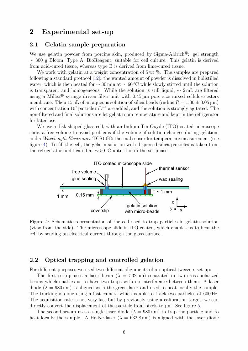
We use a disk-shaped glass cell, with an Indium Tin Oxyde (ITO) coated microscopeslide, a free-volume to avoid problems if the volume of solution changes during gelation,and a Wavelength Electronics TCS10K5 thermal sensor for temperature measurement (seefigure 4). To fill the cell, the gelatin solution with dispersed silica particles is taken fromthe refrigerator and heated at ∼ 50 ◦C until it is in the sol phase.

1 mm 0,15 mm~ 1 mm

thermal sensor

wax sealing

free volume

gelatin solution with micro-beads

glue sealing

coverslip

ITO coated microscope slide

z

xy

Figure 4: Schematic representation of the cell used to trap particles in gelatin solution(view from the side). The microscope slide is ITO-coated, which enables us to heat thecell by sending an electrical current through the glass surface.

2.2 Optical trapping and controlled gelationFor different purposes we used two different alignments of an optical tweezers set-up:

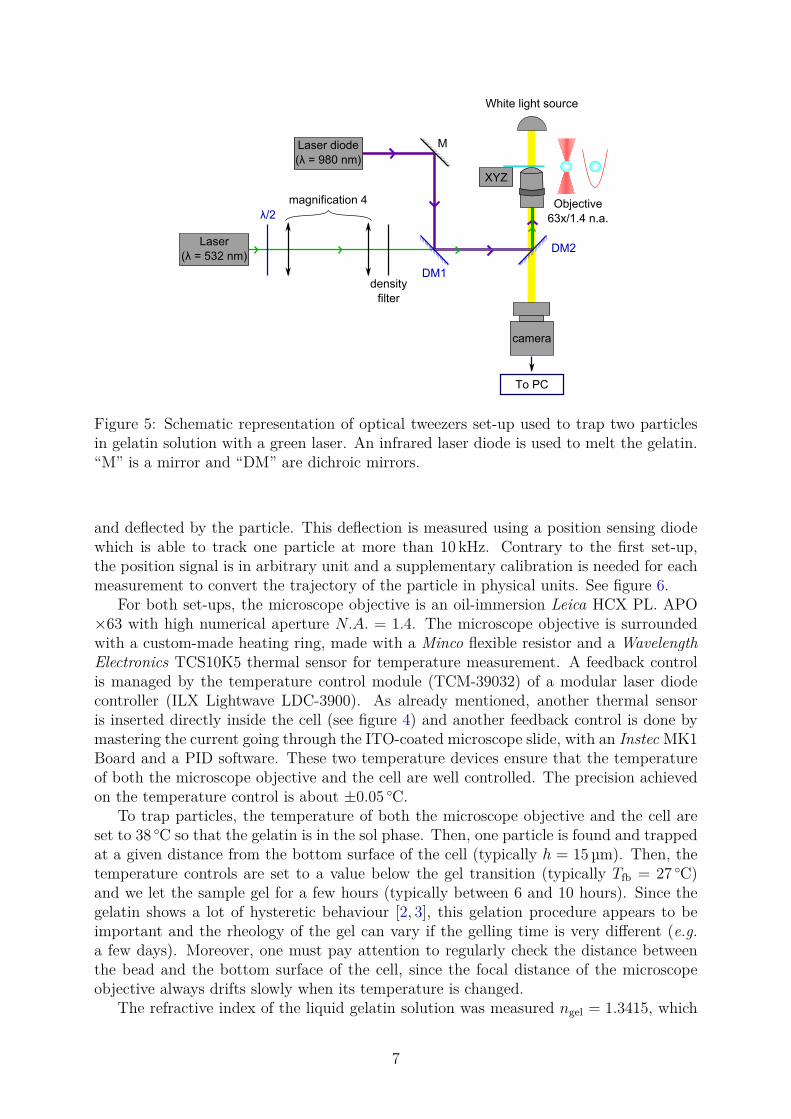
The first set-up uses a laser beam (λ = 532 nm) separated in two cross-polarizedbeams which enables us to have two traps with no interference between them. A laserdiode (λ = 980 nm) is aligned with the green laser and used to heat locally the sample.The tracking is done using a fast camera which is able to track two particles at 600Hz.The acquisition rate is not very fast but by previously using a calibration target, we candirectly convert the displacement of the particle from pixels to µm. See figure 5.

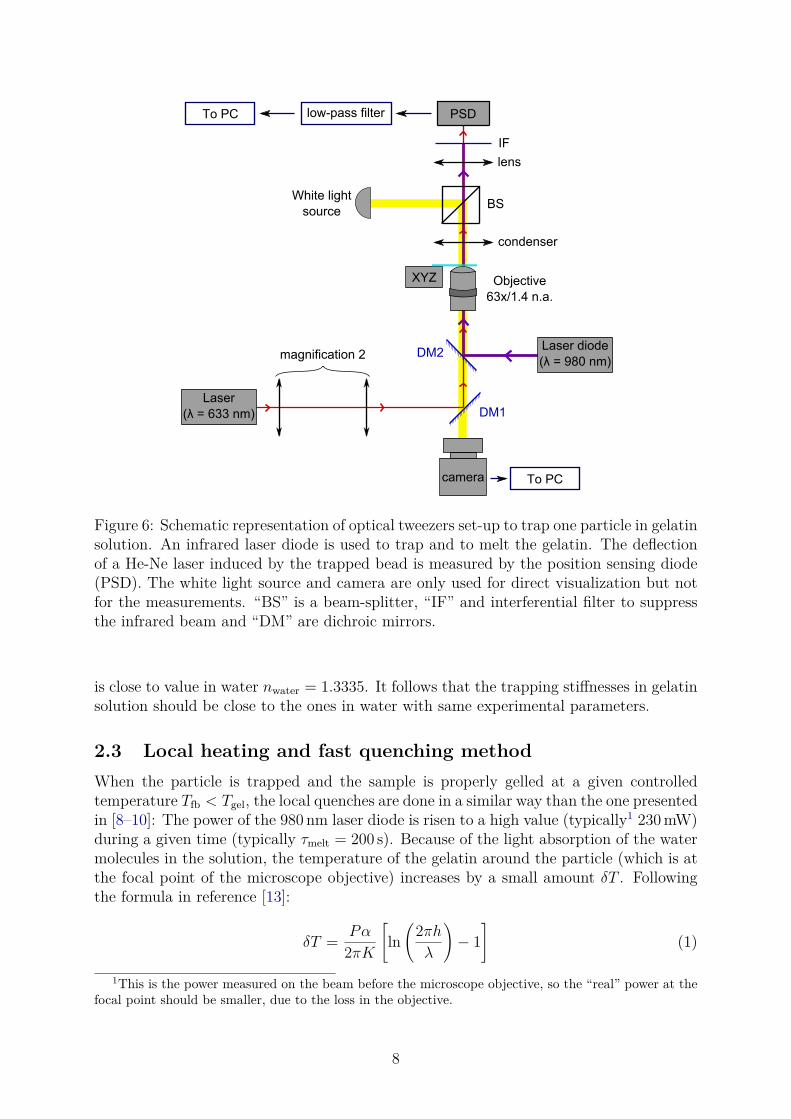
The second set-up uses a single laser diode (λ = 980 nm) to trap the particle and toheat locally the sample. A He-Ne laser (λ = 632.8 nm) is aligned with the laser diode

6

DM2

XYZ

Objective63x/1.4 n.a.

camera

White light source

To PC

Laser (λ = 532 nm)

λ/2magnification 4

densityfilter

Laser diode (λ = 980 nm)

DM1

M

Figure 5: Schematic representation of optical tweezers set-up used to trap two particlesin gelatin solution with a green laser. An infrared laser diode is used to melt the gelatin.“M” is a mirror and “DM” are dichroic mirrors.

and deflected by the particle. This deflection is measured using a position sensing diodewhich is able to track one particle at more than 10 kHz. Contrary to the first set-up,the position signal is in arbitrary unit and a supplementary calibration is needed for eachmeasurement to convert the trajectory of the particle in physical units. See figure 6.

For both set-ups, the microscope objective is an oil-immersion Leica HCX PL. APO×63 with high numerical aperture N.A. = 1.4. The microscope objective is surroundedwith a custom-made heating ring, made with a Minco flexible resistor and a WavelengthElectronics TCS10K5 thermal sensor for temperature measurement. A feedback controlis managed by the temperature control module (TCM-39032) of a modular laser diodecontroller (ILX Lightwave LDC-3900). As already mentioned, another thermal sensoris inserted directly inside the cell (see figure 4) and another feedback control is done bymastering the current going through the ITO-coated microscope slide, with an Instec MK1Board and a PID software. These two temperature devices ensure that the temperatureof both the microscope objective and the cell are well controlled. The precision achievedon the temperature control is about ±0.05 ◦C.

To trap particles, the temperature of both the microscope objective and the cell areset to 38 ◦C so that the gelatin is in the sol phase. Then, one particle is found and trappedat a given distance from the bottom surface of the cell (typically h = 15 µm). Then, thetemperature controls are set to a value below the gel transition (typically Tfb = 27 ◦C)and we let the sample gel for a few hours (typically between 6 and 10 hours). Since thegelatin shows a lot of hysteretic behaviour [2, 3], this gelation procedure appears to beimportant and the rheology of the gel can vary if the gelling time is very different (e.g.a few days). Moreover, one must pay attention to regularly check the distance betweenthe bead and the bottom surface of the cell, since the focal distance of the microscopeobjective always drifts slowly when its temperature is changed.

The refractive index of the liquid gelatin solution was measured ngel = 1.3415, which

7

Laser (λ = 633 nm)

magnification 2

DM1

XYZ Objective63x/1.4 n.a.

camera To PC

Laser diode (λ = 980 nm)

DM2

BS

condenser

PSD

lens

White light source

low-pass filterTo PC

IF

Figure 6: Schematic representation of optical tweezers set-up to trap one particle in gelatinsolution. An infrared laser diode is used to trap and to melt the gelatin. The deflectionof a He-Ne laser induced by the trapped bead is measured by the position sensing diode(PSD). The white light source and camera are only used for direct visualization but notfor the measurements. “BS” is a beam-splitter, “IF” and interferential filter to suppressthe infrared beam and “DM” are dichroic mirrors.

is close to value in water nwater = 1.3335. It follows that the trapping stiffnesses in gelatinsolution should be close to the ones in water with same experimental parameters.

2.3 Local heating and fast quenching methodWhen the particle is trapped and the sample is properly gelled at a given controlledtemperature Tfb < Tgel, the local quenches are done in a similar way than the one presentedin [8–10]: The power of the 980 nm laser diode is risen to a high value (typically1 230mW)during a given time (typically τmelt = 200 s). Because of the light absorption of the watermolecules in the solution, the temperature of the gelatin around the particle (which is atthe focal point of the microscope objective) increases by a small amount δT . Followingthe formula in reference [13]:

δT = Pα

2πK

[ln(

2πhλ

)− 1

](1)

1This is the power measured on the beam before the microscope objective, so the “real” power at thefocal point should be smaller, due to the loss in the objective.

8

where α = 50m−1 is the attenuation coefficient of water at 27 ◦C for wavelength 980 nm [14],and K = 0.61Wm−1K−1 is the thermal conductivity of water. Here, we await:

δT ' 11 ◦C. (2)

This increase in temperature is only roughly estimated. Especially because we don’t reallyknow what is the absorption of the microscope objective for the near infrared, and becauseit is impossible to measure the temperature with a usual probe on this very small scale.But it is seen that the increase is strong enough to melt a small droplet of gelatin (radiusRd ∼ 10 µm) around the bead. Then, the power is quickly decreased to a low value (inthe case where the same laser diode is used to trap and heat) or to zero (in the casewhere another laser is used to trap the particle), and the sample is let gel for a given time(typically τrest = 500 s). Since the thermal diffusivity of water is κ = 0.143× 10−6 m2 s−1

at 25 ◦C, the time τκ needed to dissipate the heat from the droplet to the bulk is short:

τκ ∼R2

dκ∼ 2× 10−4 s. (3)

Hence, the gelatin is believed to experience a fast quench at temperature Tfb < Tgel andshould start ageing2. After the resting time τrest at low temperature Tfb, the power of thelaser diode is risen again, and another quench is done. Note that the exact duration ofτrest was not considered as important, because it was believed that the melting “resets”the gelatin sample and that all the anomalous behavior occurs right after the quench.

The position of the particle trapped in the center of the melted droplet is continuouslymeasured during a succession of several melting and aging. For each measurement thequenching is repeated a few hundred times in order to perform proper ensemble averages.

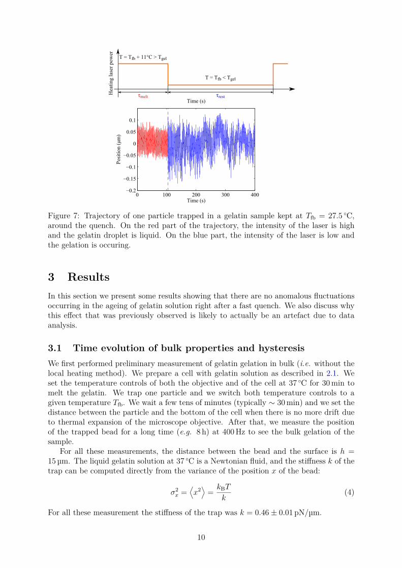
An example of trajectory obtained with the second set-up is presented in figure 7.When the intensity of the laser is high, the gelatin droplet is in the “sol” phase and theparticle fluctuates in an optical trap with a high stiffness. When the intensity of the laseris low, the gelation is occurring and the stiffness of the trap is low (which is the reasonwhy the position fluctuations are bigger).

2Actually, in the case where the same laser diode is used for trapping and melting the droplet, thetemperature of the quench is a little bit above Tfb because of the absorption of the laser. Since thepower of the laser is low, this increase is less than 1 ◦C and can easily be compensated by lowering Tfbaccordingly.

9

0 100 200 300 400−0.2

−0.15

−0.1

−0.05

0

0.05

0.1

Time (s)

Pos

itio

n (µ

m)

Hea

ting

lase

r po

wer

T = Tfb + 11°C > Tgel

τmelt τrestTime (s)

T = Tfb < Tgel

Figure 7: Trajectory of one particle trapped in a gelatin sample kept at Tfb = 27.5 ◦C,around the quench. On the red part of the trajectory, the intensity of the laser is highand the gelatin droplet is liquid. On the blue part, the intensity of the laser is low andthe gelation is occuring.

3 ResultsIn this section we present some results showing that there are no anomalous fluctuationsoccurring in the ageing of gelatin solution right after a fast quench. We also discuss whythis effect that was previously observed is likely to actually be an artefact due to dataanalysis.

3.1 Time evolution of bulk properties and hysteresisWe first performed preliminary measurement of gelatin gelation in bulk (i.e. without thelocal heating method). We prepare a cell with gelatin solution as described in 2.1. Weset the temperature controls of both the objective and of the cell at 37 ◦C for 30min tomelt the gelatin. We trap one particle and we switch both temperature controls to agiven temperature Tfb. We wait a few tens of minutes (typically ∼ 30min) and we set thedistance between the particle and the bottom of the cell when there is no more drift dueto thermal expansion of the microscope objective. After that, we measure the positionof the trapped bead for a long time (e.g. 8 h) at 400Hz to see the bulk gelation of thesample.

For all these measurements, the distance between the bead and the surface is h =15 µm. The liquid gelatin solution at 37 ◦C is a Newtonian fluid, and the stiffness k of thetrap can be computed directly from the variance of the position x of the bead:

σ2x =

⟨x2⟩

= kBT

k(4)

For all these measurement the stiffness of the trap was k = 0.46± 0.01 pN/µm.

10

Since the Tgel is expected to be around 29 ◦C, we varied Tfb from 31 ◦C to 27.5 ◦C. Itwas found that above 28.5 ◦C, the gelation does not occur on the time of the experimentand the solution stays liquid, even if its viscosity increases continuously. Below 28.3 ◦C,the gelation occurs before the end of the experiment. It was estimated that the bulkgelation of the cell volume takes ∼ 260min at 28.3 ◦C and ∼ 120min at 27.5 ◦C.

Estimating the state (“sol” or “gel”) of the gelatin solution, is not trivial, since thefluid can be really viscous without being completely gelled. Qualitatively, the trajectoryof the trapped bead starts to be heckled, and the bead sometimes escapes the trapping(see figure 8). An a posteriori test consists in switching off the laser (resulting in switchingoff the trapping) and letting the sample at Tfb for a few more hours (typically over night)to see if the particle slowly fall to the bottom of the cell. If the particle does not fall, thegelatin solution is considered to be fully gelled.

200 210 220 230 240 250 260 270

1

1.5

2

2.5

3

Time after quench (min)

Pos

ition

(µ

m)

Figure 8: Evolution of the position of one trapped particle, in gelatin solution kept at28.3 ◦C (after being melt at 37 ◦C for 20min). At the end of the trajectory, gelation occursand the particle is moved away from the optical trap.

To estimate the evolution of the viscosity during the gelation process, we used passivemicro-rheology techniques [15]. The trajectories were divided in portions of ∼ 1 h, andthe Power Spectral Density (PSD) was computed for each portion. A long trajectory isrequired because we need low frequencies to correctly estimate the PSD. We explicitlyassume that the bulk aging is slow enough for not perturbing too much the estimationof the PSD when a long trajectory is taken. Or at least, that taking a long time-windowwill only smooth the rheology result.

As seen in figure 9a, shortly after the decrease of temperature, the PSD is stillLorentzian, as awaited for a particle trapped in a Newtonian fluid at equilibrium [16].The viscous drag coefficient γ = 6πRη (with η the dynamical viscosity of the solution)can be estimated from the value of the cut-off frequency fc = k/(2πγ). Here we find:η = 21± 1× 10−3 Pa s. As the gelation occurs, the PSD is less and less Lorentzian (seefigure 9b), which is the sign that the gelatin solution starts to behave as a viscoelasticfluid [17].

We plot in figure 10 the evolution of the fitted cut-off frequency at different timeafter the gelatin solution was set at Tfb = 28.5 ◦C. Even if the spectrum is no longerLorentzian near the end of the measurement, it seems that the cut-off frequency decreasesexponentially. Therefore, the apparent viscosity increase is exponential.

11

10−2

100

102

10−18

10−16

10−14

Frequency (Hz)

Pow

er s

pect

rum

(m

²/H

z)

DataLorenzian fit

(a) 70min after the temperature change.

10−2

100

102

10−18

10−16

10−14

Frequency (Hz)

Pow

er s

pect

rum

(m

²/H

z)

DataLorenzian fit

(b) 320min after the temperature change.

Figure 9: Power Spectral Density of the position of one particle trapped in gelatin solutionkept at 28.5 ◦C (after being melt at 37 ◦C for 30min). The PSD is estimated over a time-window of 1 h. Shortly after switching the temperature the gelatin solution is still aNewtonian fluid and the PSD is Lorentzian. After some time, visco-elastic effects appearand the PSD is no longer Lorentzian.

100 150 200 250 300 350 40010

−2

10−1

Time after quench (min)

Cut

−of

f fre

quen

cy (

Hz)

Figure 10: Evolution of the fitted cut-off frequency fc, in gelatin solution kept at 28.5 ◦C(after being melt at 37 ◦C for 30min).

From these preliminary measurements, we estimate that the Tgel is about 28.3 ◦C forour gelatin solution at 5wt %. We chose to work with Tfb < 28.3 ◦C for all the followingquenching experiments. As mentioned earlier, gelatin solutions have big hysteretic be-haviour [2, 3]. It follows that the viscoelastic properties of the solution in an importanttemperature range around Tgel cannot be known independently of the sample’s history.

Another consequence of the hysteretic behaviour is that the first bulk gelation of thesample must be done in a controlled and reproducible manner. If the sample is let gel fora too long time (generally more than one day), or at a too low temperature (. 22 ◦C),the first melting/regelling cycles used for the quenching experiment will be different fromthe following ones (where a “reproducible” state is reached). Especially, in this case thefirst melting is more difficult to reach. Examples of trajectories are shown in figure 11.One can clearly see some position drifts occurring when the temperature is increased,before reaching a “sol” state where the particle fluctuates in the optical trap. Note that,

12

0 500 1000 1500 2000 2500−1

−0.8

−0.6

−0.4

−0.2

0

0.2

Time (s)

Pos

ition

(µ

m)

(a) First cycles.

0 500 1000 1500 2000 2500−0.4

−0.3

−0.2

−0.1

0

0.1

0.2

Time (s)

Pos

ition

(µ

m)

(b) 3h after starting the cycles.

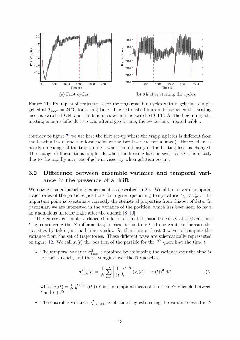
Figure 11: Examples of trajectories for melting/regelling cycles with a gelatine samplegelled at Troom = 24 ◦C for a long time. The red dashed-lines indicate when the heatinglaser is switched ON, and the blue ones when it is switched OFF. At the beginning, themelting is more difficult to reach, after a given time, the cycles look “reproducible”.

contrary to figure 7, we use here the first set-up where the trapping laser is different fromthe heating laser (and the focal point of the two laser are not aligned). Hence, there isnearly no change of the trap stiffness when the intensity of the heating laser is changed.The change of fluctuations amplitude when the heating laser is switched OFF is mostlydue to the rapidly increase of gelatin viscosity when gelation occurs.

3.2 Difference between ensemble variance and temporal vari-ance in the presence of a drift

We now consider quenching experiment as described in 2.3. We obtain several temporaltrajectories of the particles positions for a given quenching temperature Tfb < Tgel. Theimportant point is to estimate correctly the statistical properties from this set of data. Inparticular, we are interested in the variance of the position, which has been seen to havean anomalous increase right after the quench [8–10].

The correct ensemble variance should be estimated instantaneously at a given timet, by considering the N different trajectories at this time t. If one wants to increase thestatistics by taking a small time-window δt, there are at least 3 ways to compute thevariance from the set of trajectories. These different ways are schematically representedon figure 12. We call xi(t) the position of the particle for the ith quench at the time t:

• The temporal variance σ2time is obtained by estimating the variance over the time δt

for each quench, and then averaging over the N quenches:

σ2time(t) = 1

N

N∑i=1

[1δt

∫ t+δt

t(xi(t′)− x̄i(t))2 dt′

](5)

where x̄i(t) = 1δt

∫ t+δtt xi(t′) dt′ is the temporal mean of x for the ith quench, between

t and t+ δt.

• The ensemble variance σ2ensemble is obtained by estimating the variance over the N

13

quenches at a time t and then averaging over the time-window δt:

σ2ensemble(t) = 1

δt

∫ t+δt

t

[1

N − 1

N∑i=1

(xi(t′)− 〈x(t′)〉)2]

dt′ (6)

where 〈x(t′)〉 = 1N

∑Ni=1 xi(t′) is the ensemble mean of the N trajectories xi(t′) at

time t′.

• The boxed variance σ2box is obtained by taking the N segments of trajectory from

xi(t) to xi(t+ δt), and then estimating the variance of the whole set of data:

σ2box(t) = 1

Nδt

N∑i=1

∫ t+δt

t(xi(t′)− x (t))2 dt′ (7)

where x (t) = 1Nδt

∑Ni=1

∫ t+δtt xi(t′) dt′ is the mean computed on the set of data made

of the N segments from xi(t) to xi(t+δt). It is the variance used in references [8–10].

Nota Bene: Here to clearly distinguish the role of the time and the ensemble averageswe have considered the time as a continuous variable and the number of trajectories asdiscrete. But experimentally the time is of course also a discrete variable, since we takemeasurements with a finite sampling frequency.

Time

N tr

ajec

torie

s

δt

Figure 12: Schematic representation of the different ways to estimate the variance for aset of N trajectories with a time-window δt. The temporal variance σ2

time is computedby estimating the variance of the points in the fuschia box, and then averaging over thetrajectories. The ensemble variance σ2

ensemble is computed by estimating the variance of thepoints in the green box, and then averaging over the time-window δt. The boxed varianceσ2box is computed directly by estimating the variance of all the points in the orange box.

If the system is at equilibrium and δt is big enough to correctly take account of thelow-frequency of the motion, all these values should be equal to the equipartition valuekBT/k, with kB the Boltzmann constant, T the temperature and k the trap’s stiffness.

14

Unfortunately, when the system is non-stationary (which is the case for an ageingsystem), these 3 definitions of the variance are not equivalent. Especially, if there’s a slowdrift existing on each trajectory, the estimations that average over time (i.e. temporaland boxed variances) are likely to show a strong artefact.

To illustrate this effect, we have taken a set of 178 quenches done with the first set-up described in 2.2 at 28 ◦C, sampled at 400Hz. The parameters were: melting timeτmelt = 250 s, melting intensity Imelt = 235W, resting time τrest = 305 s and trap stiffness3k = 3.7 pN/µm. One can clearly see on the trajectories that there is a small drift of∼ 40 nm which occurs right after the quench (see figure 13). Such a drift is often seenfor this kind of measurement. We interpret it as a slow relaxation of the gel network,which occurs on a time much smaller than the gelation, but much greater than the heatdissipation. In other words, when the gelation occurs, the particle is trapped in the gelnetwork at a given position. And even if we melt a small droplet, the gelatin networkwill somehow “remind” this position and pull the particle back to its place when it regels.Here the drift is very visible because the position of the trapping laser is not the sameas the position of the locally heating laser. Thus the position where the particle wasduring the first bulk gelation is not the position where the particle is attracted to whenthe gelatin is melted. But even when there is only one laser used for both trapping andheating, this drift can occur. It is indeed impossible to verify that the position where theparticle is when the sample gelled is exactly the position of the laser, and a drift of onlya few nm can be visible. This kind of drift can be avoided by having a more powerfulheating laser to completely melt the gelatin on a larger area, as in [18].

0 5 10 15

0.96

0.98

1

1.02

Time after quench (s)

Pos

ition

(µ

m)

Figure 13: 20 first trajectories for a quench at Tfb = 28 ◦C, sampled at 400Hz. A slowdrift of ∼ 40 nm is clearly visible during the first ∼ 1 s. After that, the position onlyoscillates randomly around a mean value.

We then have three characteristic times :

• τgel the time needed for the gelatin solution to regel completely. It goes from a fewhundreds to more than 1000 s depending on the quench temperature Tfb.

• τdynamics the typical time of the particle motion, which is directly 1fc

and evolvesfrom ∼ 5 to ∼ 100 s during the gelation process.

3The trap stiffness is measured when the gelatin sample is completely melt and kept at constanttemperature T = 37 ◦C, before the first bulk gelation.

15

• τdrift the time where the drift is visible, which is typically 1 s for our experiment.

If we take a δt sufficiently small compared to τdrift, the boxed and ensemble varianceswill give more or less the same result. Whereas, since τdrift < τdynamics, it is clear thatthe temporal variance will dramatically underestimate the variance due to the lack oflow frequencies signal. Indeed, the temporal variance would require a δt of the order ofmagnitude of τdynamics for a correct estimation, which cannot be used because of the driftand the aging. Data are shown on figure 14 for δt = 0.1 s.

100

102

0.8

1

1.2

1.4

1.6

Time after quench (s)

Var

ianc

es /

( k

BT

/k )

σbox2

σensemble2

(a) Ensemble and boxed variances.

100

102

0.1

0.15

0.2

0.25

0.3

0.35

0.4

0.45

Time after quench (s)

σ time

2 /

( k B

T/k

)

(b) Temporal variance.

Figure 14: Different variances computed for δt = 0.1 s and normalised by the equilibriumvalue kBT/k. The ensemble and boxed values are nearly equal and seem to be close tothe equilibrium value at any time after the quench. Whereas the temporal value is clearlybelow the equilibrium value and decreases logarithmically with time after the quench.

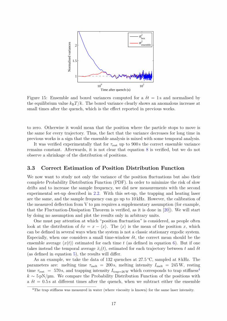
Now, if the chosen δt is too big compared to the characteristic time of the drift, theboxed variances will start to show an anomalous increase. Data are shown on figure 15for δt = 1 s. This increase is not a real non-equilibrium effect due to the sol-gel transition,but only an artefact due to data analysis in presence of a slow drift. However, this slowdrift is due to the fact that the sample is a gelatin solution, where an elastic network iscreated in the “gel” phase.

It is nevertheless interesting to see that the correct ensemble variance seems to satisfythe equilibrium equipartition relation at any time after the fast quench, even though thereis a clear evolution of the visco-elastic properties with time, and even in the presence ofa slow drift at the beginning of the quench:

∀t : σ2ensemble(t) = kBT

k. (8)

Similar results were seen for different quenches temperatures from 28 ◦C to 26 ◦C.In [8–10] it is stated that for longer times after the quench, the variance should decrease

because of the elasticity of the gelatin network (as seen figure 1a). This result is not clear.Of course, the particle dynamics becomes arrested after gelation, and at some point theamplitude of its positional fluctuations must decrease in time. At the gel point, the storagemodulus and the yield stress of the gelatin sample becomes non-zero, and even for a freelysuspended particle the dynamics becomes subdiffusive [19]. Therefore it is clear that thetemporal variance calculated for each trajectory should go to zero at long time. However,the ensemble variance calculated instantaneously over several trajectories should not go

16

100

102

1

1.5

2

Time after quench (s)

Nor

mal

ised

var

ianc

es

σbox2

σensemble2

Figure 15: Ensemble and boxed variances computed for a δt = 1 s and normalised bythe equilibrium value kBT/k. The boxed variance clearly shows an anomalous increase atsmall times after the quench, which is the effect reported in previous works.

to zero. Otherwise it would mean that the position where the particle stops to move isthe same for every trajectory. Thus, the fact that the variance decreases for long time inprevious works is a sign that the ensemble analysis is mixed with some temporal analysis.

It was verified experimentally that for τrest up to 900 s the correct ensemble varianceremains constant. Afterwards, it is not clear that equation 8 is verified, but we do notobserve a shrinkage of the distribution of positions.

3.3 Correct Estimation of Position Distribution FunctionWe now want to study not only the variance of the position fluctuations but also theircomplete Probability Distribution Function (PDF). In order to minimize the risk of slowdrifts and to increase the sample frequency, we did new measurements with the secondexperimental set-up described in 2.2. With this set-up, the trapping and heating laserare the same, and the sample frequency can go up to 10 kHz. However, the calibration ofthe measured deflection from V to µm requires a supplementary assumption (for example,that the Fluctuation-Dissipation Theorem is verified, as it is done in [20]). We will startby doing no assumption and plot the results only in arbitrary units.

One must pay attention at which “position fluctuation” is considered, as people oftenlook at the distribution of δx = x − 〈x〉. The 〈x〉 is the mean of the position x, whichcan be defined in several ways when the system is not a classic stationary ergodic system.Especially, when one considers a small time-window δt, the correct mean should be theensemble average 〈x(t)〉 estimated for each time t (as defined in equation 6). But if onetakes instead the temporal average x̄i(t), estimated for each trajectory between t and δt(as defined in equation 5), the results will differ.

As an example, we take the data of 132 quenches at 27.5 ◦C, sampled at 8 kHz. Theparameters are: melting time τmelt = 200 s, melting intensity Imelt = 245W, restingtime τrest = 570 s, and trapping intensity Itrap=26W which corresponds to trap stiffness4k ∼ 5 pN/µm. We compare the Probability Distribution Function of the positions witha δt = 0.5 s at different times after the quench, when we subtract either the ensemble

4The trap stiffness was measured in water (where viscosity is known) for the same laser intensity.

17

−0.08 −0.06 −0.04 −0.02 0 0.02 0.04 0.06

10−4

10−2

Dis

trib

utio

n (n

orm

alis

ed)

Position (a.u.)

(a) When one subtracts the ensemble average.

−0.08 −0.06 −0.04 −0.02 0 0.02 0.04 0.06

10−4

10−2

Dis

trib

utio

n (n

orm

alis

ed)

Position (a.u.)

(b) When one subtracts the temporal average.

Figure 16: Evolution of the Probability Distribution Function of the position fluctuationδx depending on the definition taken for the subtracted average. The PDFs are computedon a time-window δt = 0.5 s for different times after the quench, going from t = 0 s (bluecurves) to t = 540 s (red curves).

average (figure 16a) or the temporal average (figure 16b). In the first case, the PDFsare nearly always Gaussian and do not evolve in time. In the second case, the PDFs arealways nice gaussians, but with a variance that decreases in time. This is consistent withthe previous results showing that the ensemble variance is constant at any time after thequench, whereas the temporal variance decreases logarithmically with the time after thequench. And the variances estimated by doing a Gaussian fit on the PDFs clearly showsthe same behaviour (see figure 17).

This effect is simple to understand: the trajectories evolve on a time τgel. This time ismuch bigger than τfluc, the typical time of the fluctuations, and δt. On the time-windowδt, each portion of trajectory xi(t) can be written xi(t) = x̄i + δxi(t), where x̄i is the timeaverage of the ith trajectory over the time-window. When one considers the N trajectoryfragments between t and t+δt, the difference between them is mostly due to the averagedvalue x̄i of each trajectory fragment, and not to the fast fluctuations δxi(t). Which meansthat the distribution of all the xi(t) between t and t+δt is nearly the same as the ensembledistribution of the x̄i. Whereas, the distribution of all the δxi(t) is nothing more thanthe distribution of the fast temporal fluctuations of one single trajectory.

This difference is very important, as any kind of high-pass filtering (for example a“detrend” function which is often used to suppress slow drifts) done to the trajectorieswill result in subtracting the temporal average, and thus distort the PDFs estimation.

The experimental results show that the correct estimated PDFs do not evolve in timeafter a fast quench. Since we have already shown that the correct ensemble variance alwaysverifies the equilibrium equipartition relation, we can conclude that the variance of thesePDFs is simply kBT/k. It is again interesting to see that, even if the gelatin solution isaging, its ensemble statistical properties seem to verify relations that are normally verifiedat equilibrium.

It was also verified with some available data from [8–10] that the correct ensemblePDFs are not evolving with time after the quench.

18

10−1

100

101

102

0

1

2

3

4

x 10−4

Time after quench (s)

σ PD

F2

(a.

u.)

EnsembleTemporal

Figure 17: Evolution of the variance estimated by fitting the PDFs with a Gaussian, atdifferent times after the fast quench. When subtracting the correct ensemble averagethe variance is constant. When subtracting the temporal average, the variance decreasesalmost logarithmically with the time after the quench.

4 What about heat and Fluctuation Dissipation The-orem?

In previous works [8–10] the anomalous fluctuations observed right after the quench wereinterpreted in terms of heat exchanges between the bath and the particle. Indeed, theheat exchanged between t and t + τ is equal to the variation of the particle’s energy∆Ut,τ = ∆Ut+τ −∆Ut:

Qt,τ = ∆Ut,τ = k

2(x2(t+ τ)− x2(t)

). (9)

In particular, the decrease of the variance after the quench has been interpreted as thesign of a heat transfer from the particle to the bath :

〈Qt,τ 〉 = k

2(σ2(t+ τ)− σ2(t)

)≤ 0. (10)

The Probability Distribution Functions (PDF) of the Qt,τ were shown to be asymmetricalfor values of t and τ chosen right after the quench (i.e. where the anomalous fluctuationswere observed).

A violation of Fluctuation-Dissipation Relation was also observed for times right afterthe fast quench. It was linked to the non-zero heat exchange by a modification of theHarada-Sasa equality [21,22] for non-stationary systems:

∫ ∞1/∆t

[Sx(t, f)− 2kBT

πfIm{R̂(t, f)}

]df = 2|〈Qt,∆t〉|

k(11)

Where Sx(t, f) is the Power Spectral Density of x and R̂(t, f) is the Fourier transformof the linear response function of the position x to a perturbative time-dependent force(these two quantifies are function of the frequency f , but also of the time t since thesystem is ageing).

19

All these interpretations comes from the fact that the variance was seen anomalouslyhigh right after the quench, and then reduces to the equipartition value after a given time.In particular, the asymmetry and the shape of the PDFs of Qt,τ are simply mathematicalconsequences of the fact that x(t+τ) and x(t) have Gaussian PDFs with different variancesσ2(t + τ) > σ2(t). For example, the exchange Fluctuation Theorem (xFT) that wasretrieved with the asymmetrical PDFs of Q is mathematically verified for any randomvariable defined by y = x1 − x2 where x1 and x2 are random variables with centeredGaussian distribution of different variances: σ2

x1 6= σ2x2 .

Since we have already shown that, if estimated correctly, the PDFs of x show noanomalous behavior and have a constant variance equal to kBT/k, if follows directly thatthe PDFs of Qt,τ are symmetrical. Consequently, in average there is no heat exchangebetween the particle and the bath, for any t and t + τ , and the xFT reduces to a trivialequality because the asymmetry function of a symmetrical distribution is always zero.

Considering the Fluctuation-Dissipation Theorem, one must remind that it is a priorinot a good idea to test it in Fourier space. Indeed it is necessary to assume that thesystem is stationary and ergodic to link the correlation function to the power spectrumwith the Wiener–Khinchin theorem [23,24]. Therefore, when the system is not stationary,one should in theory look at the proper ensemble correlation function:

EnsCorrxx(t, τ) = 1N

N∑i=1

[xi(t)− 〈x(t)〉]× [xi(t+ τ)− 〈x(t+ τ)〉] (12)

instead of the Power Spectral Density (PSD), which is a temporal quantity. Of course,one can always define a PSD of xi on a given time-window δt for each trajectory Sxi

(t, f).And this PSD would be equal to the Fourier Transform (FT) of the temporal correlationof xi computed on the same time-window:

TimeCorrxx(t, τ) = 1δt

∫ t+δt

t[xi(t′)− x̄i]× [xi(t′ + τ)− x̄i] dt′ = FT{Sxi

(t, f)}. (13)

But the system needs to be considered stationary and ergodic on the time-window δt, sothat the ensemble and temporal correlations should be equal.

Here, the assumption of local stationarity is reasonable since the PSD were computedon 15 s long time-windows (which is short compared to the ∼ 900 s necessary to gel).However, it seems probable that the observed violation of Fluctuation-Dissipation Theo-rem was only due to the same kind of artifact already responsible for anomalous varianceincrease (for example: slow drifts for times right after the fast quench), because PSDs aresensible to low-frequency noises. Thus, there is no reason that this apparent violation islinked to an heat exchange, which does not exist anyway.

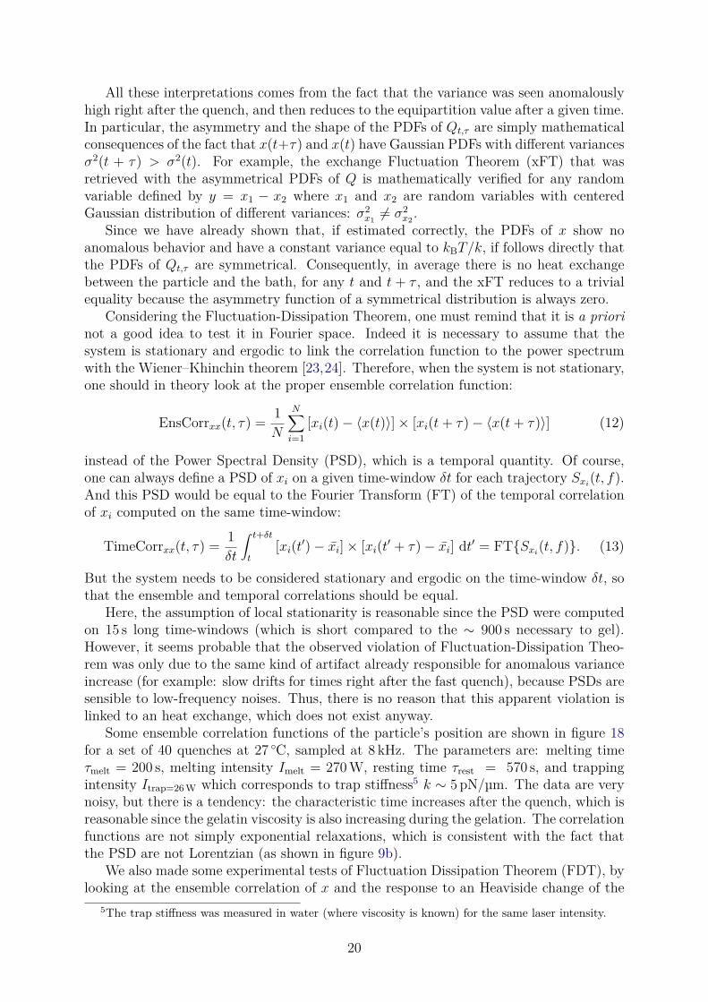
Some ensemble correlation functions of the particle’s position are shown in figure 18for a set of 40 quenches at 27 ◦C, sampled at 8 kHz. The parameters are: melting timeτmelt = 200 s, melting intensity Imelt = 270W, resting time τrest = 570 s, and trappingintensity Itrap=26W which corresponds to trap stiffness5 k ∼ 5 pN/µm. The data are verynoisy, but there is a tendency: the characteristic time increases after the quench, which isreasonable since the gelatin viscosity is also increasing during the gelation. The correlationfunctions are not simply exponential relaxations, which is consistent with the fact thatthe PSD are not Lorentzian (as shown in figure 9b).

We also made some experimental tests of Fluctuation Dissipation Theorem (FDT), bylooking at the ensemble correlation of x and the response to an Heaviside change of the

5The trap stiffness was measured in water (where viscosity is known) for the same laser intensity.

20

t = 10 st = 20 st = 40 st = 70 st = 130 st = 250 st = 370 s

0 2 4 6 8 10

0

0.5

1

1.5

|τ| (seconds)

Ens

Cor

r xx(t

,−τ)

(no

rmal

ised

)

Figure 18: Normalised ensemble correlation function for a quench at 27 ◦C. Here wekeep t fixed and we vary τ from −10 s to 0 s. The normalisation is done by dividingEnsCorrxx(t, τ) by the value of kBT/k extracted from the variance of the position PDFs.

position of the trap. For these measurements, the position of the trap is changed from X1to X2 at a time tR after the first quench, and the sample is let gel with the particle in X2.Then, for the second quench, the position of the trap is moved back to X1 at time tR afterthe quench, and the sample is let gel in X1. The procedure is then repeated alternatively.The perturbation introduced by the change of trapping position allows us to compute anormalized response function, averaged over the trajectories:

χ(tR, τ) = 〈x(tR + τ)−Xinitial〉Xfinal −Xinitial

(14)

where [Xinitial;Xfinal] = [X1;X2] or [X2;X1]. It corresponds to the usual definition of theresponse function:

χ(t) = 〈x(t)perturbed − x(t)unperturbed〉perturbation amplitude . (15)

We useXfinal−Xinitial which is proportional to the perturbation amplitude. And we simplytake Xinitial as the average value of the unperturbed trajectory, because the mean positionof the bead is constant and equal to the position of the trap if there is no perturbation6.If the FDT is verified, the response function should verify:

χ(tR, τ) = 1− k

kBTEnsCorrxx(tR, τ) (16)

Some data are presented in figure 19 for 50 quenches at 26 ◦C, sampled at 8 kHz. Theparameters are: melting time τmelt = 200 s, melting intensity Imelt = 270W, restingtime τrest = 570 s, and trapping intensity Itrap=26W which corresponds to trap stiffness7k ∼ 5 pN/µm. The values of X1 and X2 are estimated by computing the mean positionof the bead when the gelatin is melted (which gives alternatively X1 and X2). The exactvalue of kBT/k was extracted from the variance of the position PDFs computed beforechanging the position of the trap. These measurements are a bit noisy because it requiresa lot of statistics to compute a proper ensemble correlation function, but no apparentviolation of the FDT was found for the times tested.

6One could also take 〈x(tR)〉 to guarantee that χ(tR, 0) = 0, but it wasn’t necessary here.7The trap stiffness was measured in water (where viscosity is known) for the same laser intensity.

21

0 2 4 6 8 100

0.2

0.4

0.6

0.8

1

1.2

Time τ (s)

Res

pons

e an

d C

orre

latio

n (n

orm

alis

ed)

100 s after the quench

1−EnsCorrxx

(tR,τ)/σ2

χ (tR,τ)

Figure 19: Normalised response function χ(tR, τ) and ensemble correlation function fortR = 100 s after the quench, and τ going from 0 to 10 s.

We didn’t test the Fluctuation Dissipation Theorem for times tR taken shortly afterthe quench, because the ensemble correlation shows a characteristic time which is veryshort at this time (see figure 18). It is then more difficult to compute a proper ensemblecorrelation right after the quench, than when the viscosity of gelatin has already startedto increase. We also didn’t compute the response function by varying tR for a fixed tR+τ ,because it would require a lot of time to do the experiments. Indeed, each set of tR requiresone day of measurement to compute χ(tR, τ), and the sample cannot be kept a lot of dayswithout degrading.

22

5 ConclusionIn conclusion, we have locally studied the gel transition of a gelatin solution. We wereunable to reproduce the results of previous works [8–10], but we have identified some ex-perimental and data analysis artifacts which may explain the effects previously observed.In particular we have analyzed the effect of time-windows on proper ensemble averages,which are important to study aging systems.

We have shown that in the hysteresis range of temperature (28.3 ◦C < T < 36 ◦C),bulk gelation can occur on very long times, and viscoelastic properties gradually appear.The characteristic time of the particle trapped in the bulk-gelling sample was seen todecrease exponentially before the gelation (whereas the viscosity evolves logarithmicallyafter the gelation).

For fast quenches of a small droplet of gelatin solution, we have found that the Prob-ability Distribution Functions of the position of the trapped particle do not evolve withtime after the quench, even if the gelatin sample is undergoing aging and the viscoelasticproperties are clearly evolving. Moreover, these PDFs show equilibrium-like properties,being Gaussian with a variance equal to the equipartition value kBT/k. These resultsseem not so surprising a posteriori, since it was already observed in the previous worksthat, after ∼ 15 s the Brownian motion of the trapped particle behaves like in equilibriumwith the thermal motion of the gelatin chains. Only the very first seconds after the quenchshowed anomalous behavior, which was strange, because the complete gelation occurs onmuch larger scales (∼ 900 s). It however remains striking that a system which is clearlynot stationary because of aging has ensemble properties which are stationary.

For systems which are not ergodic or not stationary, time properties can be verydifferent from ensemble properties. And it was also shown that some artifacts (like slowdrifts) or analysis bias (like high-pass filter) can greatly modify the results if ensembleproperties are estimated on time-windows. Therefore, one must be very careful whenstudying statistical properties of an aging system. This kind of problems had alreadyarisen for other aging systems. For example, it was already shown in [25] that increase ineffective temperature previously seen in suspension of Laponite [26] were in fact artifactsdue to analysis methods.

Finally, in agreement with the absence of anomalous position fluctuation after the fastquench, no heat exchange, nor violation of the Fluctuation Dissipation Theorem was seen,as it would be expected in an equilibrium medium.

References[1] K. te Nijenhuis, Thermoreversible networks: viscoelastic properties and structure of

gels. Advances in polymer science, Springer, 1997.

[2] M. Djabourov, J. Leblond, and P. Papon, “Gelation of aqueous gelatin solutions. i.structural investigation,” Journal de physique, vol. 49, no. 2, pp. 319–332, 1988.

[3] M. Djabourov, J. Leblond, and P. Papon, “Gelation of aqueous gelatin solutions. ii.rheology of the sol-gel transition,” Journal de Physique, vol. 49, no. 2, pp. 333–343,1988.

23

[4] H. B. Bohidar and S. S. Jena, “Kinetics of sol–gel transition in thermoreversiblegelation of gelatin,” The Journal of Chemical Physics, vol. 98, no. 11, pp. 8970–8977,1993.

[5] H. B. Bohidar and S. S. Jena, “Study of sol-state properties of aqueous gelatinsolutions,” The Journal of Chemical Physics, vol. 100, no. 9, pp. 6888–6895, 1994.

[6] O. Ronsin, C. Caroli, and T. Baumberger, “Interplay between shear loading andstructural aging in a physical gelatin gel,” Phys. Rev. Lett., vol. 103, p. 138302, Sep2009.

[7] A. Parker and V. Normand, “Glassy dynamics of gelatin gels,” Soft Matter, vol. 6,pp. 4916–4919, 2010.

[8] J. R. Gomez-Solano, Nonequilibrium fluctuations of a Brownian particle. Theses,École normale supérieure de lyon - ENS LYON, Nov. 2011. Available at https://tel.archives-ouvertes.fr/tel-00648099.

[9] J. R. Gomez-Solano, A. Petrosyan, and S. Ciliberto, “Heat fluctuations in a nonequi-librium bath,” Phys. Rev. Lett., vol. 106, p. 200602, May 2011.

[10] J. R. Gomez-Solano, A. Petrosyan, and S. Ciliberto, “Fluctuations, linear responseand heat flux of an aging system,” EPL (Europhysics Letters), vol. 98, no. 1, p. 10007,2012.

[11] C. Jarzynski and D. K. Wójcik, “Classical and quantum fluctuation theorems forheat exchange,” Phys. Rev. Lett., vol. 92, p. 230602, Jun 2004.

[12] V. Normand, S. Muller, J.-C. Ravey, and A. Parker, “Gelation kinetics of gelatin: Amaster curve and network modeling,” Macromolecules, vol. 33, no. 3, pp. 1063–1071,2000.

[13] E. J. Peterman, F. Gittes, and C. F. Schmidt, “Laser-induced heating in opticaltraps,” Biophysical journal, vol. 84, no. 2, pp. 1308–1316, 2003.

[14] K. F. Palmer and D. Williams, “Optical properties of water in the near infrared,” J.Opt. Soc. Am., vol. 64, pp. 1107–1110, Aug 1974.

[15] D. Mizuno, D. A. Head, F. C. MacKintosh, and C. F. Schmidt, “Active and passivemicrorheology in equilibrium and nonequilibrium systems,” Macromolecules, vol. 41,no. 19, pp. 7194–7202, 2008.

[16] K. Berg-Sørensen and H. Flyvbjerg, “Power spectrum analysis for optical tweezers,”Review of Scientific Instruments, vol. 75, no. 3, pp. 594–612, 2004.

[17] G. Pesce, A. C. D. Luca, G. Rusciano, P. A. Netti, S. Fusco, and A. Sasso, “Mi-crorheology of complex fluids using optical tweezers: a comparison with macrorheo-logical measurements,” Journal of Optics A: Pure and Applied Optics, vol. 11, no. 3,p. 034016, 2009.

[18] J. R. Gomez-Solano, V. Blickle, and C. Bechinger, “Nucleation and growth of ther-moreversible polymer gels,” Phys. Rev. E, vol. 87, p. 012308, Jan 2013.

24

[19] T. H. Larsen and E. M. Furst, “Microrheology of the liquid-solid transition duringgelation,” Phys. Rev. Lett., vol. 100, p. 146001, Apr 2008.

[20] M. Fischer, A. C. Richardson, S. N. S. Reihani, L. B. Oddershede, and K. Berg-Sørensen, “Active-passive calibration of optical tweezers in viscoelastic media,” Re-view of Scientific Instruments, vol. 81, no. 1, pp. –, 2010.

[21] T. Harada and S.-i. Sasa, “Equality connecting energy dissipation with a violationof the fluctuation-response relation,” Phys. Rev. Lett., vol. 95, p. 130602, Sep 2005.

[22] G. Verley and D. Lacoste, “Fluctuation theorems and inequalities generalizing thesecond law of thermodynamics out of equilibrium,” Phys. Rev. E, vol. 86, p. 051127,Nov 2012.

[23] N. Wiener, “Generalized harmonic analysis,” Acta Mathematica, vol. 55, no. 1,pp. 117–258, 1930.

[24] A. Khintchine, “Korrelationstheorie der stationären stochastischen prozesse,” Math-ematische Annalen, vol. 109, no. 1, pp. 604–615, 1934.

[25] P. Jop, J. R. Gomez-Solano, A. Petrosyan, and S. Ciliberto, “Experimental studyof out-of-equilibrium fluctuations in a colloidal suspension of laponite using opticaltraps,” Journal of Statistical Mechanics: Theory and Experiment, vol. 2009, no. 04,p. P04012, 2009.

[26] N. Greinert, T. Wood, and P. Bartlett, “Measurement of effective temperatures inan aging colloidal glass,” Phys. Rev. Lett., vol. 97, p. 265702, Dec 2006.

25