1Department of Economics, University of Wisconsin, 1180 Observatory Drive, Madison, WI 53706; jkennan@ssc.wisc.edu. Ithank Daron Acemoglu, V.V. Chari, Kim-Sau Chung, Tryphon Kollintzas, Rody Manuelli, Rob Shimer, Alberto Trejos andparticipants in the Northwestern University Summer Workshop in Macroeconomics, the Tow Conference at the University of Iowa,the HCM conference at K)C!, the NBER Summer Institute, the IZA-WDI conference at INCAE, and seminars at the Universityof Wisconsin, Penn State University, the University of Pennsylvania and Carnegie-Mellon for valuable comments. The NationalScience Foundation provided research support.

Informational Conflict and Employment Fluctuations

John Kennan1

University of Wisconsin-Madison and NBER

November 2003

Abstract

Because it takes time for workers and employers to find each other, a successful match yields a

surplus to be divided between them. This paper analyzes the possibility that conflict over the division of

the surplus might break up the match, either temporarily or permanently. Private information regarding

the size of the surplus provides a rational basis for such conflict. But even if match-specific information

generates employment fluctuations at the micro level, one might expect that these fluctuations would not

survive aggregation. One main finding of the paper is that changes in economic conditions affecting the

size of the surplus in all matches can synchronize bargaining outcomes at the micro level, so that

informational conflict does indeed lead to aggregate employment fluctuations. Informational conflict can

lead to either a temporary disruption in employment, or to a permanent separation, depending on

workers’ ability to commit to punishment outcomes following rejection of a wage demand. This paper

analyzes the case in which workers cannot commit to a permanent separation (from a jointly profitable

match), but can only commit to a temporary suspension of employment, interpreted as a temporary

layoff. The model gives a quantitatively reasonable account of temporary layoffs during a recession.

2See Kennan and Wilson (1993) for an analysis of efficiency in private information bargaining.

3Hall (2003) also treats wage bargaining as a central element in employment fluctuations, but all separations in his model areefficient ex post – there is no private information. Hall focuses on the rate at which matches are made, rather than the rate at whichthey break up; he argues that the job creation rate is very sensitive to how much of the match surplus the employer expects to get.

1

1. Introduction

Because it takes time for workers and employers to find each other, a successful match yields a

surplus to be divided between them. The implications of this observation have been extensively studied,

following the seminal papers of Diamond (1982) and Mortensen (1982). This paper analyzes the

possibility that conflict over the division of the surplus might break up the match, either temporarily or

permanently. Private information regarding the size of the surplus provides a rational basis for such

conflict: indeed, Myerson and Satterthwaite (1983) showed that it is generally impossible to ensure an ex

post efficient outcome unless the size of the surplus is common knowledge2. But even if match-specific

information generates employment fluctuations at the micro level, one might expect that these

fluctuations would not survive aggregation. One main finding of the paper is that changes in economic

conditions affecting the size of the surplus in all matches can synchronize bargaining outcomes at the

micro level, so that informational conflict does indeed lead to aggregate employment fluctuations.

Persistent private information naturally leads to fluctuations in bargaining outcomes. Cyclic

equilibria are analyzed in Kennan (2001): the main idea can be summarized as follows. A worker facing

an employer who has private information about the value of the match has basically two choices: a

pooling demand that ensures immediate agreement, or an aggressive demand that risks a conflict

outcome. Only the aggressive demand reveals information, and persistence implies that information

about current valuations will be valuable in future negotiations. This leads to cycles: a worker who is

aggressive this time and loses will be pessimistic in subsequent negotiations, but the pooling demands

induced by this pessimism do not reveal new information, and the pessimism wears off, so that after

some time the worker becomes optimistic enough to make another aggressive demand, and so on.

Acemoglu (1995) modeled unemployment as the result of conflict over how to divide the match

surplus in an environment where the employers have better information about the size of the surplus.3 A

major difference here is that employers' have private information only about the value of their own

workers' labor, rather than the value of an aggregate shock, as in Acemoglu's model. The role of

aggregate shocks in this paper is to ensure that fluctuations at the level of individual bargaining pairs do

not disappear when averaged over the entire economy. The aggregate shocks do not directly cause

employment fluctuations: if employers had no private information, there would be no conflict, regardless

2

of the aggregate state. But given that the employers do have private information, aggregate shocks cause

aggregate employment fluctuations by synchronizing the workers’ bargaining demands.

Informational conflict can lead to either a temporary disruption in employment, or to a permanent

separation, depending on workers’ ability to commit to punishment outcomes following rejection of a

wage demand. This paper analyzes the case in which workers cannot commit to a permanent separation

(from a jointly profitable match), but can only commit to a temporary suspension of employment,

interpreted as a temporary layoff.

Both Mortensen and Pissarides (1994) and Cole and Rogerson (1999) analyze the extent to which the

Mortensen-Pissarides model can match aggregate data on job flows in U.S. manufacturing, as described

by Davis, Haltiwanger and Schuh (1996). A notable feature of the data is that the onset of a recession is

associated with a burst of job destruction (meaning that establishments report unusually large decreases

in the number of employees on the payroll, relative to the number of workers employed three months

earlier). The Mortensen-Pissarides model explains this as being due to a change in the threshold at which

job matches remain viable: a negative aggregate shock destroys those matches that generate a positive

surplus only while the aggregate state is good. Here, the spike in job destruction at the start of a

recession is explained instead as a burst of temporary layoffs, involving workers who were not optimistic

enough to make tough bargaining demands while the aggregate state was good, but who become more

aggressive when they have less to lose. The model gives a quantitatively reasonable account of

temporary layoffs during a recession, but the dynamics of permanent separations follows the Mortensen-

Pissarides model. In particular, the temporary layoff model does not resolve the unemployment

persistence puzzle discussed by Shimer (2003) and Hall (2003). But an alternative version of the model,

based on a stronger commitment assumption, is capable of generating highly persistent unemployment;

this is discussed further in the Conclusion.

2. A Model of Repeated Negotiations with Private Information and Aggregate Shocks

The flow surplus from a successful job match is modeled as a stochastic process that has an

idiosyncratic component and an “aggregate” component that is common to all jobs. The idiosyncratic

component is observed privately by the employer, while the aggregate component is common knowledge.

Each of these components is a Markov pure jump process with two states. The aggregate states are

labeled “b” and “g” (meaning bad and good), and the idiosyncratic states are labeled “L” and “H” (low

and high, also meaning bad and good). Let ybL be the flow surplus when the economy is in the bad state,

3

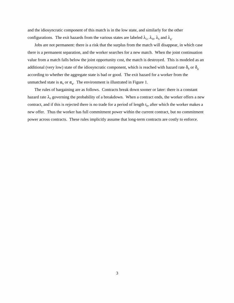
and the idiosyncratic component of this match is in the low state, and similarly for the other

configurations. The exit hazards from the various states are labeled 8L, 8H, 8b and 8g.

Jobs are not permanent: there is a risk that the surplus from the match will disappear, in which case

there is a permanent separation, and the worker searches for a new match. When the joint continuation

value from a match falls below the joint opportunity cost, the match is destroyed. This is modeled as an

additional (very low) state of the idiosyncratic component, which is reached with hazard rate *b or *g

according to whether the aggregate state is bad or good. The exit hazard for a worker from the

unmatched state is "b or "g. The environment is illustrated in Figure 1.

The rules of bargaining are as follows. Contracts break down sooner or later: there is a constant

hazard rate 80 governing the probability of a breakdown. When a contract ends, the worker offers a new

contract, and if this is rejected there is no trade for a period of length t0, after which the worker makes a

new offer. Thus the worker has full commitment power within the current contract, but no commitment

power across contracts. These rules implicitly assume that long-term contracts are costly to enforce.

4

Figure 1: Model Parameters

In the absence of any historical information, the probability of the low idiosyncratic state is that

implied by the invariant distribution of the Markov switching process, i.e.

Let R(t) denote the probability that the employer’s valuation is low at time t, given that it was low at t=0.

Then

5

where 7 = 8L + 8H governs the extent to which successive contract negotiations are linked. If 7 is

infinite, information is completely transitory, so that any inference that the worker might draw from the

current contract negotiation will be irrelevant by the time the next contract is negotiated. At the other

extreme, if 7 = 0 the current information is entirely permanent.

The equilibrium solution used in this paper is based on a discrete-time version of the model, with no

aggregate shocks, which is analyzed in Kennan (2001). The equilibrium is a renewal process based on

the outcome of screening offers made by the worker. If the employer accepts an offer revealing that the

private state is currently high, the continuation game is the same as it was the last time such a revelation

was made, and similarly if a rejected offer convinces the worker that the state is currently low.

In each contract negotiation there are two possibilities from the worker's point of view. If

information is sufficiently persistent and if the worker has inferred from a recent negotiation that the

state was low, it will be optimal to make a pooling offer. Alternatively, if the worker believes that the

high state is sufficiently likely, a screening offer will be worthwhile. Each offer leaves either the high or

low employer type on the margin between acceptance and rejection. A screening offer is just acceptable

to the high type, and unacceptable to the low type. A pooling offer is just acceptable to the low type, and

more than acceptable to the high type.

If the employer accepts a screening offer, the worker will infer that the state is high, and so the

worker will screen again when the next contract is negotiated (unless perpetual pooling is optimal). Of

course the employer knows that acceptance of a screening offer weakens its bargaining position next

time, so the offer must be sufficiently generous to compensate for this. If the employer rejects a

screening offer, on the other hand, the worker infers that the state is currently low, and it may then be

optimal to make a pooling offer next time, and perhaps again the time after that, and so on. Acceptance

of these pooling offers reveals nothing about the state, and so the worker's belief decays toward :. A key

feature of the equilibrium is the length of time needed for the worker to become sufficiently optimistic to

screen again, following rejection of a screening offer. This will depend on the aggregate state, so let Kb

be the length of time during which the worker makes pooling offers even if the aggregate state is bad (so

that the cost of screening is low), and let k be the additional time needed until the worker is optimistic

enough to screen even if the public shock is good, with Kg = Kb + k. It is assumed that t0 < Kb.

6

If the employer accepts an offer revealing a high valuation now, the worker screens again next time,

and so on until a screening offer is rejected. The equilibrium cycle is sketched in Figure 3, which

represents varying degrees of pessimism for the worker. At one extreme, immediately after an

unsuccessful screening offer, the worker believes the employer's valuation is low now for sure. In this

situation the worker pools now, and continues to pool (whenever a contract opportunity arises) until the

probability of the low valuation has decayed past the screening threshold .*b. Beyond this point, the

worker makes pooling offers if the aggregate state is good, and screening offers if the state is bad, until

the probability of the low valuation has decayed past a second screening threshold .*g. At the other

extreme, the worker is sure that the employer's valuation is high immediately after a screening offer is

accepted, and (given that : is below .*g) the worker remains sufficiently optimistic to make only

screening offers until the employer rejects. The relationship between K and .* is given by

7

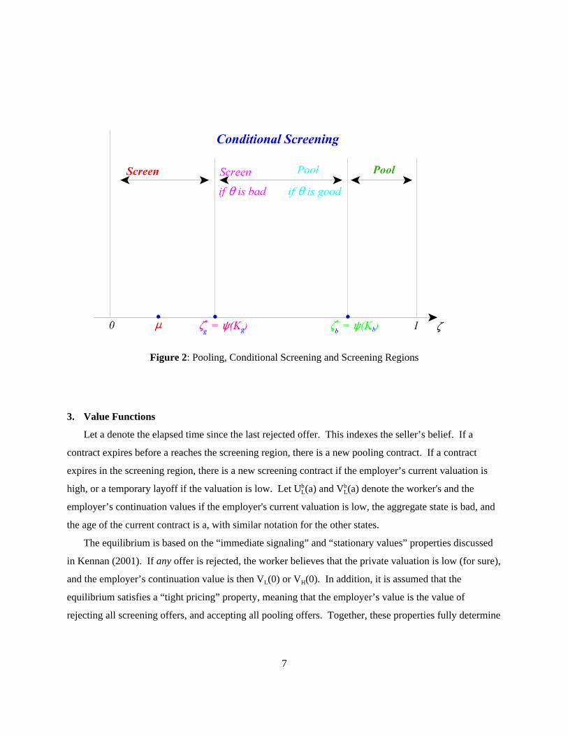
Figure 2: Pooling, Conditional Screening and Screening Regions

3. Value Functions

Let a denote the elapsed time since the last rejected offer. This indexes the seller’s belief. If a

contract expires before a reaches the screening region, there is a new pooling contract. If a contract

expires in the screening region, there is a new screening contract if the employer’s current valuation is

high, or a temporary layoff if the valuation is low. Let ULb(a) and VL

b(a) denote the worker's and the

employer’s continuation values if the employer's current valuation is low, the aggregate state is bad, and

the age of the current contract is a, with similar notation for the other states.

The equilibrium is based on the “immediate signaling” and “stationary values” properties discussed

in Kennan (2001). If any offer is rejected, the worker believes that the private valuation is low (for sure),

and the employer’s continuation value is then VL(0) or VH(0). In addition, it is assumed that the

equilibrium satisfies a “tight pricing” property, meaning that the employer’s value is the value of

rejecting all screening offers, and accepting all pooling offers. Together, these properties fully determine

8

the employer’s continuation values: in particular, the employer’s value function can be determined

independently of the worker’s continuation value in the unmatched state.

Since both sides are risk-neutral, with the same discount factor, the timing of wage payments is

indeterminate: what matters is the expected present value of wage payments over the life of each

contract. It is convenient to summarize these payments as a lump sum paid when the contract begins

(with no flow payments). Define the screening prices PHb and PH

g as the payments that make the high-

valuation employer indifferent between accepting and rejecting the worker’s contract offer, given that

rejection would lead the worker to believe that the current valuation is low, while acceptance would

reveal the high state. Then

Similarly, the pooling prices for a contract of age a are given by

Taking VL (0) and VH (0) as given, consider a contract with beliefs in the screening region (this might

be either a screening contract that was accepted, or a pooling contract that has continued into the

screening region). The continuation values are constant in this region, because the worker will make a

screening offer at the next opportunity, regardless of how much additional time has elapsed. The

employer’s continuation values are determined by the asset pricing equations

9

The worker’s continuation values include the payments received when a screening offer is accepted, and

the continuation value at the start of a temporary layoff if it is rejected. The workers’ values are

determined by the following equations

where U0 is the worker’s value of search for a new match, contingent on the aggregate state.

One way to solve these equations is to solve first for V(Kg ), and then use the results (together with

the screening price equations) to solve for U(Kg ). Alternatively, the continuation values can be stacked

in one 8-dimensional vector V, and the equations can be written as:

where

and the matrix S2 and the vector Y2 are given in the Appendix. Although S2 is determined by the basic

model parameters, Y2 depends on the initial values V(0), and on the worker’s separation values U0 .

Taking these as given (for the moment), the solution is

When the contract age lies between Kb and Kg, the worker makes a screening offer at contract

expiration if the aggregate state is bad, and otherwise makes a pooling offer. The employer’s

continuation values in this conditional screening region are given by

10

(where V0 denotes a time-derivative). These values differ from the corresponding values in the

unconditional screening region in two ways. First, they are not constant. Second, when the aggregate

state is good, the high-valuation employer’s continuation value at contract expiration is the value of

paying the pooling price and continuing with a new contract, rather than the value of rejecting the

contract offer.

The worker’s continuation values in the conditional screening region are given by

Note here that the contract age is reset to Kg following acceptance of a screening offer, with the

interpretation that the worker’s belief lies in the unconditional screening region following acceptance of

a screening offer.

The equations for the employer’s and the worker’s continuation values in the conditional screening

region can be written as

where S1 and Y1 are given in the Appendix. This is a system of linear differential equations, with

terminal conditions given by the solution for V(Kg ) described above. The solution of the differential

equation system can be written using matrix exponential notation as

11

In particular, the continuation values at the start of the conditional screening region are given by

When the contract age is less than Kb, the worker makes pooling offers at contract expiration

regardless of the aggregate state. The continuation values in this pooling region are given by

This differential equation system can be written as

Using V(Kb) as the terminal condition, the solution in this region is

At the end of a temporary layoff, there is a pooling offer, and the continuation values following

acceptance of this offer are given by

12

During the temporary layoff, the continuation values are determined by the following system

Write this as

The solution for the values during a temporary layoff can then be written as

where

13

Thus the continuation values jump at the end of the temporary layoff, by the amount of the relevant

pooling offer; the employer’s values jump up once the pooling payment has been made, and the worker’s

values jump down.

The continuation values following rejection of an offer are then given by

The elements of the vector V(0) were taken as given earlier, so they enter both sides of the above

equation, which must therefore be solved to determine the equilibrium values. Also, the worker’s

separation values were taken as given. These are determined by

where w0 is the income flow for an unmatched worker (including unemployment benefits and the value

of leisure). New matches are found at the rate ", and the worker immediately makes a screening offer

(because the belief according to the invariant distribution is :, and this lies in the screening region by

assumption). If the new employer is in the high state, the screening offer is accepted, and otherwise it is

rejected, and employment starts after a delay of length t0 .

4. Equilibrium

So far, it has been assumed that there are state-contingent thresholds .*b and .*

g governing the worker's

choice between screening and pooling offers. These thresholds determine Kb and Kg, giving the lengths

of the pooling and conditional screening regions, and these in turn determine the continuation values for

the employer and the worker. In particular, the worker's payoffs from screening and pooling are

ultimately determined by the value of .*b and .*

g used in the employer's and worker's strategies. So there

must be a fixed point: using .*b and .*

g to determine the strategies, and computing the worker's payoffs

from screening and pooling as the belief . varies, it must be that screening and pooling yield the same

continuation value for the worker when . = .*b and K = Kb, if the aggregate state is good, and again when

. = .*g and K = Kg, if the aggregate state is bad.

14

When the aggregate state is good, the worker’s expected payoffs from pooling and screening at the

expiration of a contract of age Kg are given by

where . is the worker’s current belief (i.e. the probability that the employer’s current valuation is low).

This yields the following equation for the screening threshold:

meaning that the worker is indifferent between pooling and screening if the aggregate state is good and

the belief is .*g. On the other hand, the worker’s belief when the contract age is Kg is given by

Eliminating .g* from these two equations yields

This equation implicitly involves Kb (as can be seen from the value function derivation in the previous

section).

When the aggregate state is bad, the calculation of the screening threshold is slightly different,

because in this case an accepted screening offer sets the state variable to a = Kg (meaning that there will

be a screening offer at the next opportunity, regardless of the aggregate state). Thus the belief that makes

the worker indifferent between screening and pooling is given by

4Whether this equilibrium is unique is an open question. In the special case where there are no aggregate shocks theequilibrium is unique (i.e. it is the only equilibrium satisfying the stationary value, immediate signaling and tight pricingproperties).

There is an implicit assumption that one rejected offer should be enough to convince the worker that the employer's currentvaluation is low. This will not work if the high valuation is very persistent. In this case, the equilibrium must involve extendedscreening: the worker makes an offer above the screening price, and the employer randomizes in such a way that the worker makesanother screening offer next time following rejection. This problem is analyzed in detail in a model with fixed-length contracts andno aggregate shocks in Kennan (2001), and the results indicate that the equilibrium construction used here will be valid if theopportunity cost of screening is sufficiently large.

15

After substituting for .b*,

This equation can be solved jointly with the above equation for Kg to obtain Kb and Kg in terms of the

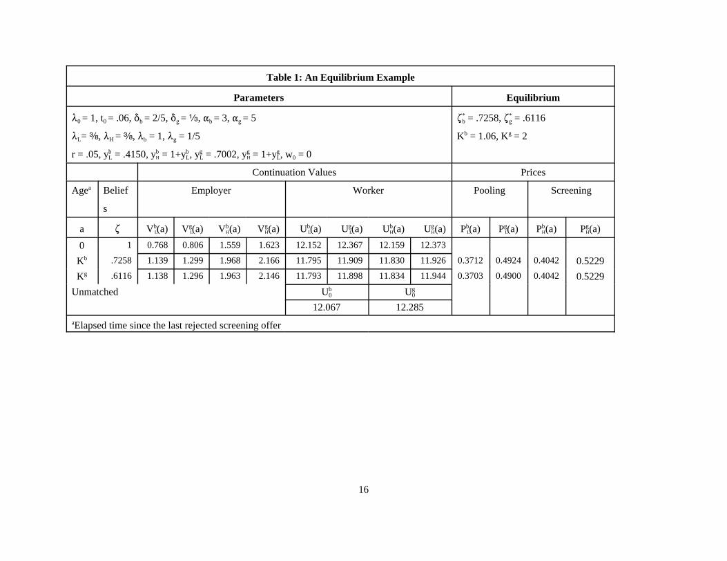
primitive parameters, thus completing the equilibrium calculation4. A numerical example is shown in

Table 1.

16

Table 1: An Equilibrium Example

Parameters Equilibrium

80 = 1, t0 = .06, *b = 2/5, *g = a, "b = 3, "g = 5

8L= d, 8H = d, 8b = 1, 8g = 1/5

r = .05, yLb = .4150, yH

b = 1+yLb, yL

g = .7002, yHg = 1+yL

g, w0 = 0

.b* = .7258, .g

* = .6116

Kb = 1.06, Kg = 2

Continuation Values Prices

Agea Belief

s

Employer Worker Pooling Screening

a . V Lb(a) V L

g(a) VHb(a) VH

g(a) ULb(a) UL

g(a) UHb(a) UH

g(a) PLb(a) PL

g(a) PHb(a) PH

g(a)

0 1 0.768 0.806 1.559 1.623 12.152 12.367 12.159 12.373

Kb .7258 1.139 1.299 1.968 2.166 11.795 11.909 11.830 11.926 0.3712 0.4924 0.4042 0.5229

Kg .6116 1.138 1.296 1.963 2.146 11.793 11.898 11.834 11.944 0.3703 0.4900 0.4042 0.5229

Unmatched U0b U0

g

12.067 12.285aElapsed time since the last rejected screening offer

17

5. Employment Fluctuations

The model has two kinds of unemployment. Some workers are currently unmatched, following a

permanent separation from their previous employers. Others are still matched with an employer, but

unemployed because their contracts have recently broken down; such workers are described as being on

temporary layoff.

Permanent Separations

The process governing job creation and destruction is not affected by temporary layoffs. Let U(t) be

the proportion of unmatched workers. This is determined in the usual way by solving the piecewice-

linear differential equation

where (",*) = ("b,*b ) if the current aggregate state is bad, and otherwise (",*) = ("g,*g ). If the aggregate

state has been good during the interval [T1,t], then

where Ug* is the steady-state level of permanent separations corresponding to the good aggregate state:

Similarly, if the aggregate state has been bad during the interval [T0,t], then

where Ub* is the steady-state level of permanent separations corresponding to the bad aggregate state.

Thus the path of U(t) can be determined for any history of the Markov switching process determining the

aggregate state, by stitching together the segments between switching points.

18

Survival Analysis

In order to determine the aggregate flow of temporary layoffs, it is necessary to keep track of the

distribution of job matches over ages (where age refers to elapsed time since the last rejected offer, rather

than the actual age of the match, which is irrelevant). Let R(t,a) be the density of low-private-valuation

matches aged a at time t, and let L(t,a) be the stock of low-private-valuation matches aged a or greater;

also, let z(t,a) be the density of matches aged a at time t (including both low and high private valuations).

The vector x is defined as

The cohort of matches in which offers were rejected at date t is R(t,0) = z(t,0). This cohort includes the

flow of temporary layoffs and the flow of new matches in the low state.

The size and composition of each cohort as it ages over the interval [0,Kg] are determined by the

following differential equation (with the time variable suppressed):

For a cohort of age a, let ag and ab denote the amount of time spent in the good and bad aggregate states,

with a = ag + ab. Recall that R(a) is the probability that the employer’s valuation is low at date t+a, given

that the valuation was low at date t. Thus the size and composition of the cohort at age a are given by

Steady States

In the good aggregate state, the stock of contracts that have reached the screening age evolves

according to the following system

19

Thus in the good steady state,

This implies

Recession Dynamics

This section considers the path of unemployment during and after a recession. It is assumed that the

economy starts in the good steady state. At date T0 the aggregate state switches from good to bad, and at

date T1 the state switches back. It is assumed that the duration of the recession is less than the length of

the pooling phase in the bad aggregate state, but greater than the difference between this and the length of

the pooling phase in the good state. That is,

The evolution of the age distribution is sketched in Figure 3. The diagonal flow in this diagram

shows the increase in age over time.

20

Figure 3: Survival analysis for cohorts born before the recession.

21

The Risk Set

Contracts are at risk of breakdown when the employer’s current valuation is low, and when the

contract is old enough to have reached the screening region. The set of such contracts is L(K): this will

be called the risk set – meaning L(Kb ) during the recession, and L(Kg ) otherwise. During the recession,

the risk set has two parts. Some contracts are at risk only because the aggregate state is bad. This

“conditional” risk set is denoted by Lc = L(Kg ) - L(Kb ), while the unconditional risk set is denoted by

Lu = L(Kg ).

Expiration of a contract that has reached age K triggers a screening offer. This initiates a temporary

layoff if the employer is currently in the low state, and the age counter is reset to zero in this case. On

the other hand, if the employer is currently in the high state, the screening offer is accepted, and the age

counter is set to Kg, meaning that there will be another screening offer when the new contract expires,

regardless of the aggregate state.

The Conditional Risk Set

The conditional risk set is analyzed in Appendix B: the results are summarized here. For

t 0 [T0 ,T0 + k], the stock of contracts of age a 0 [Kb ,Kg ] is

where ) = *b - *g and

The conditional risk set is

So

where Hc(t) is the set of high-valuation contracts that are in the conditional screening region.

For t 0 [T0 + k, T1],

22

The Unconditional Risk Set

During the recession, the set of contracts in the unconditional screening region evolves according to

The coefficient matrix in this system can be written as A - *b I. Suppose -D1 and -D2 are the roots of A

(the roots are negative, so D1 and D2 are positive). The solution can be written as

where

with J0 = t - T0, and

At date T0 + k, the formula for Hc changes, as described above, and Xi(t) is given by

where J1 = t - T1. After the recession ends, the conditional risk set is no longer relevant, and the job

creation and destruction rates revert to "g and *g. Moreover, after date T0 + Kg, the initial cohort size is

no longer constant. The solution for the risk set is obtained in segments: the first four segments are the

5The worker flow data (which can be found at http://www.bos.frb.org/economic/neer/neer1999/neer499c.htm) are seasonallyadjusted quarterly averages of CPS matched monthly observations.

23

intervals [T0 ,T0+k], [T0+k, T1], [T1, T1+k], [T1+k, T0 +Kg ], and the next four are obtained by shifting

these forward by Kg, and this pattern is repeated ad infinitum. The details of this construction are given

in Appendix C.

Quantitative Implications

In this section the model is used to describe a recession and the subsequent recovery, using realistic

parameter values. The main focus is on the extent to which cyclical variations in worker flows are

influenced by the dynamics of temporary layoffs.

The standard way to judge the empirical relevance of a model of employment fluctuations is to ask

whether it can match selected moments of the data, using reasonable parameter values, as in Mortensen

and Pissarides (1994), Cole and Rogerson (1999) and Merz (1999). The question addressed here is more

narrowly focused: what does a recession look like in the model, relative to the data? This question is

interesting in part because it leads to a more concrete analysis of what actually happens in the model. In

addition, the moments usually considered in the standard method miss an important feature of the data: a

recession is best described as an unusual and short-lived aberration from the normal state of the

economy. This feature is well captured by the Markov jump process used here (when 8b is substantially

larger than 8g), but it is obscured by the standard statistics used in the real business cycle literature.

Empirical Measurements of Worker Flows

Only about half of the stock of workers in the unemployment pool in the U.S. in an average month

are there because they have been laid off (the rest being quits, new entrants, and a residual that includes

re-entrants). Thus the model in this paper (like the MP model) cannot be expected to reproduce the

aggregate unemployment rate, mainly because the model does not explain labor force transitions.

[but modeling temporary layoffs gives a more realistic description of flows within the labor force].

There is a big gap between the job destruction flow in the Mortensen-Pissarides model and the empirical

counterpart in the Davis-Haltiwanger-Schuh (1996) data. This is illustrated in Figure 4, using CPS gross

flow data taken from Bleakley, Ferris and Fuhrer (1999).5

6NBER business cycle peaks are indicated by vertical lines in Figure 5.

24

Mo

nth

ly r

ate

s (

%)

All Separations Destruction, seas adj Permanent Separations

1976 1978 1980 1982 1984 1986 1988 1990 1992 1994 1996 1998

0.500

1.000

1.500

2.000

2.500

3.000

3.500

Figure 4: Worker Separations and Job Destruction in Manufacturing

The series in the middle of the figure is the DHS job destruction measure (seasonally adjusted), and the

series at the top is the total worker separation flow, including permanent and temporary layoffs, quits and

labor force exits. The similarity between these two series is impressive, given that one is based on a

household survey, and the other is based on an establishment survey. In contrast, the series at the bottom

of the figure measures the permanent layoff flow from employment to unemployment (excluding workers

who left the labor force following a permanent separation). These separations coincide with job

destruction in the MP model, but in fact they are only a small part of the job destruction process in

manufacturing. Moreover, Figure 5 shows that cyclical fluctuations in the job destruction series are

similar to the fluctuations in the worker separation series when the permanent layoff flow from

employment to unemployment is excluded.6 Thus any model that tries to explain the job destruction data

in terms of permanent separations is largely beside the point. A broader interpretation of worker

separations in the MP model might include quits and labor force exits, but given the rules of the

25

Worker Separations and Job Destruction in Manufacturing

Destruction, seas adj Quits, LF Exits, Temp Layoffs

1976 1978 1980 1982 1984 1986 1988 1990 1992 1994 1996 1998

1.500

2.000

2.500

3.000

Figure 5

Unemployment Insurance system there is a big difference between quits and layoffs for workers who are

firmly attached to the labor force (which is true of all of the workers in the MP model), and the MP

model has nothing to say about workers who move in and out of the labor force.

This paper bridges part of the gap between the MP model and the DHS data by explicitly modeling

temporary layoffs. In this respect the paper follows Merz (1999), although the economic interpretation is

quite different: in Merz’s model, temporary layoffs are caused by a temporary decline in productivity,

such that the expected cost of an unemployment spell is less than the cost of recruiting a new worker

when productivity recovers. Figure 6 uses CPS data on unemployment by reason to show movements in

the stocks of temporary and permanent layoffs. About 30% of the stock of workers unemployed due to

layoffs in a typical month are on temporary layoff. There is no indication that the relative importance of

temporary layoffs has declined over time (for example, the proportion on temporary layoff in 2000 was

33%), although the volatility of temporary layoffs does seem to have decreased.

7The data in this Figure are centered moving averages.

26

Temporary Layoffs Permanent Separations

1966 1969 1972 1975 1978 1981 1984 1987 1990 1993 1996 19992002

1000

2000

3000

4000

5000

Figure 6: Workers on Permanent and Temporary Layoff (thousands, seasonally adjusted)

A notable feature of the data in Figure 6 is that the stock of temporary layoffs increases rapidly at the

beginning of a recession (i.e., during the period immediately after a business cycle peak), and then starts

to decline, while the stock of workers on permanent layoff continues to rise. As will be seen, the

informational conflict model of temporary layoffs can match this feature quite well.

The relative magnitudes of the temporary and permanent layoffs flows are shown in Figure 7, again

using the Bleakley, Ferris and Fuhrer data.7 These flows are of roughly equal importance on average, and

the cyclical fluctuations in temporary separations are more important than the cyclical fluctuations in

permanent separations.

27

month

ly s

epara

tion r

ate

(%

)

Temporary Layoff Rate Permanent Separation Rate

1976 1978 1980 1982 1984 1986 1988 1990 1992 1994 1996 1998

0.200

0.400

0.600

0.800

Figure 7: Temporary and Permanent Separation Flows

Figure 6 shows that temporary layoffs are a relatively small part of the unemployment stock, while

Figure 7 shows that they are a relatively big part of the inflow. Figure 8 reconciles these two

observations, using unemployment duration data for spells that are immediately followed by

employment, rather than labor force exit. Temporary layoff spells last about 3 weeks on average, and

there is not much variation in this over the cycle. Unemployment spells following permanent separations

last much longer, with big cyclical fluctuations.

28

media

n u

nem

plo

ym

ent dura

tion

Temporary Layoff Permanent Separation

1976 1978 1980 1982 1984 1986 1988 1990 1992 1994 1996 1998

2

3

4

5

6

7

8

9

10

11

Figure 8: Unemployment Duration

Parameter Values

The model has three basic parameters (r,80 , t0 ), five state-contingent productivity levels

(w0,yLb,yL

g,yHb ,yH

g), and eight state transition rates (8L , 8H , 8b , 8g , "b , "g , *b , *g ). If the aggregate state is

usually good (and if the system is not too persistent), a recession can reasonably be approximated by

starting from the good steady state, with a transition to the bad aggregate state at some date T0, followed

by a reversion to the good state at date T1. Given that the average duration of (postwar) recessions is

about a year, T1 is set to 1, with T0 = 0. Although the productivity levels and the aggregate state

transition rates (8b , 8g ) affect the equilibrium values of Kb and Kg, nothing is lost by ignoring the details

of this relationship and choosing Kb and Kg directly.

Some of the parameter values are roughly pinned down by the data, while others are more

speculative. The parameter list is (t0 = .06, *b = 2/5, *g = a, "b = 3, "g = 5, 80 = 1, 8L= d,

8H = d, Kb = 1.06, Kg = 2). The time unit is a year.

8Using a temporary layoff duration of 3 weeks, it is assumed that one quarter of all temporary layoffs escape notice in theCPS, so the observed flow is scaled up by 4/3.

29

• In the CPS data, the median duration of temporary layoff unemployment spells is about 3 weeks, or

about .06 years, and as Figure 8 shows, there in not much cyclical variation in this. This gives

t0 = .06.

• For the 5-year period 1994-1998, Bleakley et al measured the average outflow from the stock of

permanently separated workers as 2.8+1.9 (new jobs + labor force exits); the inflow was 3.1, and the

stock was 11.3. This gives an average flow of 3.9/11.3, implying "g = 5.08. The lowest value of the

escape rate from unemployment was about 60% of the highest value (over the period 1977-1998),

suggesting that if "g is set to 5, "b should be 3. Taking the extremes in this way exaggerates the

cyclical variability of the flow from permanent separations to new jobs, but this ignores labor force

exits, and there is more cyclical variability in the duration of unemployment spells followed by labor

force exit than there is in the duration of unemployment spells that end with new jobs.

• According to Davis, Haltiwanger and Schuh (1996), the job destruction rate in manufacturing is 5.5%

per quarter (an annual rate of 0.22), and this is used by Cole and Rogerson (1999) as the permanent

separation rate. In the Bleakley et al data for manufacturing the corresponding figure for worker

flows is .2615 per annum. But this includes all outflows from employment – quits, labor force exits

and “re-entrants” (the residual category) along with permanent and temporary layoffs. If the duration

of temporary layoffs is less than a month (as the data suggest), then the DHS measure should miss

most of them, since their data are measured quarterly. When permanent separations are measured as

the proportion of workers employed last month who are unemployed this month because of a

permanent layoff, the separation rate is only .057. In light of these ambiguities, *g = a is simply

chosen so as to match the ratio of the temporary layoff and permanent separation flows8, which is

approximately 1.2. Then *b is set slightly above *g.

• The remaining parameters were chosen with little guidance from the data. Setting 80 = 1 means that

the expected duration of a labor contract is one year, which seems like a natural choice given that

many wages are adjusted annually. Setting Kg = 2 means that it normally takes two years before

workers become optimistic enough to make tough demands following a previous conflict; Kb = T0 + t0

is chosen to give a sharp contrast between the chances of informational conflict in the good and the

bad state (while avoiding some tedious calculations needed if a contract that begins during the

recession can reach the screening region before the recession ends). The process driving the

9This asymmetry in the size of the jumps occurs for several reasons: (1) the system is no longer in the steady state; (2) thesurvival probability to age Kb is lower during the recession than it was before the recession began; (3) contracts older than Kb havebeen exposed to the risk of a temporary layoff during the recession.

30

Figure 9: The Risk Set

idiosyncratic revenue component is assumed to be symmetric (8L = 8H ), with less than unit

persistence (8L + 8H = ¾).

Implications

The path of the risk set for this numerical example is shown in Figure 9. When the recession begins,

there is a jump in the risk set because contracts older than Kb and younger than Kg are suddenly at risk.

When the recession ends, this jump is reversed, but the magnitude of the jump is different.9 At date

T0 + Kg, the risk set starts increasing rapidly, because there is a relatively large flow of contracts that

restarted soon after the recession began, and these are now reaching the screening region.

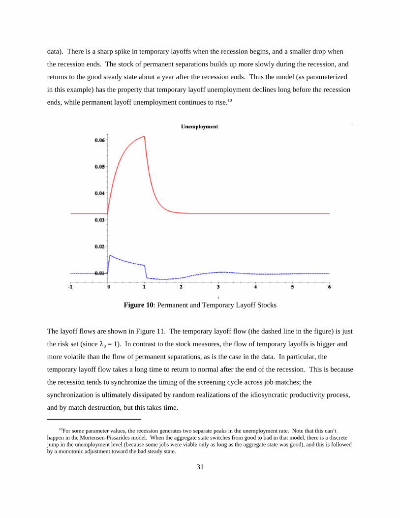
The unemployment stocks are shown in Figure 10. The temporary layoff stock (the lower series in

the figure) is basically proportional to the integral of the risk set over the interval (t-t0,t), but it is adjusted

for permanent separations that occur during a temporary layoff, and it excludes layoffs that occur at the

beginning of new matches (on the grounds that these would not be classified as temporary layoffs in the

10For some parameter values, the recession generates two separate peaks in the unemployment rate. Note that this can’thappen in the Mortensen-Pissarides model. When the aggregate state switches from good to bad in that model, there is a discretejump in the unemployment level (because some jobs were viable only as long as the aggregate state was good), and this is followedby a monotonic adjustment toward the bad steady state.

31

Figure 10: Permanent and Temporary Layoff Stocks

data). There is a sharp spike in temporary layoffs when the recession begins, and a smaller drop when

the recession ends. The stock of permanent separations builds up more slowly during the recession, and

returns to the good steady state about a year after the recession ends. Thus the model (as parameterized

in this example) has the property that temporary layoff unemployment declines long before the recession

ends, while permanent layoff unemployment continues to rise.10

The layoff flows are shown in Figure 11. The temporary layoff flow (the dashed line in the figure) is just

the risk set (since 80 = 1). In contrast to the stock measures, the flow of temporary layoffs is bigger and

more volatile than the flow of permanent separations, as is the case in the data. In particular, the

temporary layoff flow takes a long time to return to normal after the end of the recession. This is because

the recession tends to synchronize the timing of the screening cycle across job matches; the

synchronization is ultimately dissipated by random realizations of the idiosyncratic productivity process,

and by match destruction, but this takes time.

32

Figure 11: Permanent and Temporary Layoff Flows

Conclusion

The paper presents a new interpretation of temporary layoffs: they are caused by informational

friction between workers and employers. The model can generate worker flow data that look like what

happens in U.S. data during recessions. In the model, the spike in job destruction that occurs at the

beginning of a recession is generated to a large extent by temporary layoffs. This matches the data, and it

improves on the Mortensen-Pissarides model.

It is difficult to tell from the job flows data whether spikes in job destruction are caused by

temporary layoffs (one can ask whether establishments showing big employment losses at the onset of a

recession have offsetting employment gains in subsequent quarters, but given that there are only three

recessions in the basic data set, with large seasonal employment changes getting in the way, there is not

much hope of getting a reliable answer to this question). Meanwhile, as Katz and Meyer (1990) point

out, most workers who claim unemployment insurance indicate that they expect to be recalled by their

previous employer, so that the Mortensen-Pissarides model may be missing the point by treating all

11Of course there is a range of less extreme cases. When productivity is low, the firm could lay off a worker permanently, andthen search for a new worker if productivity recovers; alternatively, the worker can be laid off temporarily, and recalled ifproductivity recovers. Merz (1999) analyzes the socially efficient allocation in such an economy, assuming complete information,and asks whether such an allocation might exhibit employment fluctuations matching those seen in the data. The results in thispaper suggest that these fluctuations might instead be explained by private information.

33

unemployed workers as permanently separated from their jobs. This paper goes to the other extreme,

attributing job destruction bursts entirely to temporary layoffs.11

If workers can commit to leave this match and search for a new one whenever a wage demand is

rejected, there is no employment cycle at the micro level. On the other hand, this may lead to more

realistic unemployment dynamics in the aggregate. The most interesting case is when : lies in the

conditional screening region. Then when a new match is made, there is a screening offer if the aggregate

state is bad, and a pooling offer if the aggregate state is good. Following acceptance of a screening offer,

the worker is optimistic enough to screen again if the contract expires soon. But after some time the

belief reaches the unconditional screening region, and stays there. On the other hand, rejection of a

screening offer breaks up the match, so the worker’s belief is never more pessimistic than :. At the start

of the recession, all matches enter the risk set, so there is a jump in the separation rate. When the

recession ends, matches of age greater than K immediately leave the risk set (where age is redefined as

elapsed time since the last accepted screening offer). The main point of this version of the model is that

informational conflict continues to generate permanent separations for some time after the recession

ends, because some workers made successful screening demands during the recession, and they remain

optimistic enough to make aggressive demands for some time after the recession ends.

Appendices

See http://www.ssc.wisc.edu/~jkennan/research/index.htm.

34

References

Acemoglu, Daron, “Asymmetric Information, Bargaining, and Unemployment Fluctuations,”International Economic Review, November 1995, 36(4), 1003-1024.

Bleakley, Hoyt, Ann E. Ferris and Jeffrey C. Fuhrer, “New Data on Worker Flows During BusinessCycles,” New England Economic Review, July/August 1999, 49-76;http://www.bos.frb.org/economic/neer/neer1999/neer499c.htm

Cole, Harold L. and Richard Rogerson, “Can the Mortensen-Pissarides Matching Model Match theBusiness-Cycle Facts?” International Economic Review, 40(4), November 1999, 933-959.

Davis, Steven J., John C. Haltiwanger and Scott Schuh, Job Creation and Destruction. Cambridge: MITPress, 1996.

Hall, Robert E., “Wage Determination and Employment Fluctuations,” NBER Working Paper 9967,September 2003.

Katz, Lawrence F., and Bruce D. Meyer, “Unemployment Insurance, Recall Expectations, andUnemployment Outcomes,” Quarterly Journal of Economics, Vol. 105, No. 4. (Nov., 1990), pp.973-1002.

Kennan, John, “Repeated Bargaining with Persistent Private Information,” Review of Economic Studies,68, October 2001, 719-755.

Merz, Monika, “Heterogeneous Job-matches and the Cyclical Behavior of Labor Turnover,” Journal ofMonetary Economics 43, 1, February 1999, 91-124

Mortensen, Dale T., and Christopher A. Pissarides, “Job Creation and Job Destruction in the Theory ofUnemployment,” Review of Economic Studies, 61, July 1994, 397-415.

Shimer, Robert E., “The Cyclical Behavior of Equilibrium Unemployment and Vacancies: Evidence andTheory,” NBER Working Paper 9536, February 2003; http://home.uchicago.edu/~shimer/wp/.