Regulatory Fog: The Informational Origins of

Regulatory Persistence

Patrick Warren, Clemson University

Tom Wilkening, University of Melbourne

April 19, 2010

Regulation, even inefficient regulation, can be incredibly persistent. We propose a new

explanation for regulatory persistence based on “regulatory fog”, where regulation

obscures information about the effects of deregulation. This paper presents a dynamic

model of regulation, in which the environment is stochastic such that the imposition

of regulation can either be efficient or inefficient, and in which the regulator’s ability

to observe the underlying need for regulation is reduced when regulation is imposed.

As compared to a full-information benchmark, regulation is highly persistent, even

if there is a high probability of transition to a state in which regulation is inefficient.

This regulatory persistence decreases welfare and dramatically increases the proportion

of time the economy spends under regulation. The ability to perform deregulatory

experiments can improve outcomes, but only if they are sufficiently inexpensive and

effective, and regulation will still remain more persistent than in the full-information

benchmark.

JEL Classification:

Keywords: Information, Regulation, Experimentation

1

Better the devil you know than the devil you don’t. - R. Taverner, 1539

A bureaucratic organization is an organization that can not correct its behavior by learning

from its errors. - Crozier, 1964

1 Introduction

One common solution to market imperfections such as externalities and market power is

regulation, but regulation itself is costly. Administration and enforcement requires over-

head. Lobbying and avoidance dissipate rents. Centralized control distorts investment and

innovation.1

Furthermore, once applied, regulation tends to be very persistent, often outliving its use-

fulness. Deregulation of transportation, power, and communication networks often generate

large productivity gains both within the industry and in the broader economy. Preferential

trade policies for infant industries often persist well beyond the point in which dynamic

learning might be present and “temporary” assistance for disadvantaged groups often per-

sists long after its intended time limits. This persistence can magnify the costs of regulation

which might otherwise be optimal in the short run, since the gains today must we weighed

off against a potentially long tail of future inefficiencies.

Why does regulation end up being so persistent? We propose a new explanation for

regulatory persistence based on “regulatory fog,” where regulation obscures information

about the likely effects of deregulation. Our view is that regulatory persistence is a natural

byproduct of optimal static regulation — that regulation itself carries the seeds of its own

persistence by altering the dynamic information generated in the economy. In stochastic

environments, where the optimal policy varies over time, this regulatory fog can lead to

the persistence of policies which have become suboptimal. This dynamic inefficiency is an

important cost of regulation not often taken into account in the regulatory debate.

To illustrate the idea of regulatory fog, consider the regulation of a monopolistic market.

The producer and consumers adjust in response to regulation and market conditions. Some

of these adjustments are the very targets of the regulation: a monopolist increases quantity,

reduces pollution, or ceases the use of misleading marketing. But adjustments on other

dimensions will also occur. Consumers will adjust their consumption patterns both over

1For a broad overview of costs and benefits of regulation, see Guasch and Hahn (1999)

2

time and between substitutable/complementary goods. The monopolist will alter investment

rates and mix. Prices will be distorted in other markets. Entry and exit in the regulated

market or neighboring markets may occur. Because these adjustments are so far reaching

and subtle, and will certainly depend on the underlying state of the world, unpacking all the

consequences of deregulation may be extremely difficult.

Given this complexity, in stochastic environments where the optimal policy varies over

time, a perfectly public-interested regulator is likely to have a very difficult time determining

when to remove regulation. In cases where the consequences of a market failure are severe,

the regulator might be unwilling to take a risk since the benefits of deregulation are not

demonstrable while the historical potential cost of deregulation are salient. In these cases,

regulation could persist indefinitely despite its inefficiency.

In this paper, we build a dynamic model of regulation in which the underlying need for

regulation varies stochastically, and the presence of regulation affects the regulator’s ability

to observe the state of the world. Even in an environment where the regulator maximizes

public interest, regulation is more likely to persist indefinitely in this environment than in a

full-information benchmark. For most reasonable parameter values, regulatory fog increases

both the length of time an individual regulatory spell lasts and the proportion of time spent

under regulation. Regulatory fog also increases the probability that deregulation ends in

disaster, leading to a substantial negative effect on total welfare.

In additional to full-scale deregulation, policy makers often have available a range of

smaller scale policy experiments they could conduct. We next generalize the regulatory

environment to allow for small-scale experimentation, which may be less costly than full

deregulation but will provide a weaker signal about the counterfactual environment. We

characterize the regulator’s induced preferences over regulatory experiments, including his

optimal trade-off between costliness and effectiveness. Although these alternatives weakly

reduce regulatory persistence, the value of information is non-linear, so experimentation

is adopted only when the experiment is informative and the cost of experimentation is

reasonably low.

The difficulty in finding direct empirical evidence of regulation sustained by regulatory

fog is self-evident. However, the strong role that external information shocks have played

in historical deregulation suggests that a lack of information is a major deterrent to dereg-

ulation. The persistence of entry, price, and route regulation under the Civil Aeronautics

Board (CAB) provides a useful example of this phenomenon. Enacted in 1938, the CAB

3

managed nearly every aspect of the airline industry, including fare levels, number of flights

per route, entry into routes and the industry, and safety procedures.2 Leaving aside the

efficiency of the enactment, the longevity of these regulations is mysterious. These were

extremely inefficient regulations, as become apparent upon their removal in 1978.3 How did

such inefficient regulation persist, and why did it end when it did?

Critical to airline deregulation was the growth in intra-state flights, especially in Texas

and California, because they revealed information about the likely effects of deregulation.

These intra-state flights, and the local carriers who worked them, were not subject to regu-

lation under CAB, so they gave consumers a window into what might happen if regulation

was dropped more generally. A series of influential studies starting from Levine (1965) and

continued and expanded by William Jordan (1970), for example, demonstrated that fares

between San Francisco and Los Angeles were less than half those between Boston and Wash-

ington, D.C., despite the trips being comparable distances. Similar results obtained when

looking at flights within Texas. There was no discernable increase in riskiness, delay, or

evidence of so-called “excessive competition.”

The dissemination of these large-state market results proved to be a major catalyst for

deregulation.4 The proximate driver of deregulation was a series of hearings held in 1975

by the Subcommittee on Administrative Practice and Procedure of the Senate Committee

on the Judiciary (The so-called Kennedy hearings). An entire day of testimony at these

hearings was dedicated to exploring the comparison of intra-state and inter-state flights.

William Jordan testified extensively, explaining and defending the results of these studies.

The successful deregulation of airlines opeThe architect of the CAB deregulation, Alfred

Kahn, cited the importance of the “demonstration effect” provided by airline deregulation,

in understanding subsequent deregulation of trucking and railroads (Peltzman, Levine and

Noll (1989)). Likewise, the US experiment spurred airline deregulation overseas (Barrett

(2008)). Consistent with our model, a glimpse of the unregulated intra-state market spurred

a successful deregulation, which in turn prompted deregulation of related industries.

2For an extensive review of the CAB’s powers and practices, see “Oversight of Civil Aeronautics Boardpractices and procedures : hearings before the Subcommittee on Administrative Practice and Procedure ofthe Committee on the Judiciary”, United States Senate, Ninety-fourth Congress, first session (1975)

3For a nice overview and analysis of the economic effects of airline deregulation, see Morrison and Winston(1995)

4Derthick and Quirk (1985) lay out the politics and timing of the push for deregulation, and cite theseacademic studies as the primary ”ammunition” for those in favor of deregulation, as have others who haveinvestigated the issue ?

4

Our theory of regulatory fog should be contrasted with the political economy literature in

which rent seeking by entrenched groups is the primary driver of policy persistence. Coate

and Morris (1999) develop a model in which actors make investments in order to benefit

from a particular policy. In their model, once these investments are made, the entrenched

firms have an increased incentive to pressure the politician or regulator into maintaining the

current policy. Similar dynamics can be found in Brainard and Verdier (1994) which studies

political influence in an industry with declining infant industry protection.

While important contributions to the literature on policy persistence, these models have

no role for incomplete information, and so would have a hard time explaining the dynamics

of (de)regulation. For us, one of the key features that distinguishes regulation from other

policies is that it forces agents to take certain actions (or proscribes certain actions), and so

generates similar signals in different states of nature. This effect is the essence of regulatory

fog. As the political economy literature studies more generic policy, it ignores this important

effect of regulation.5

Asymmetric information has been interacted with rent seeking models by Fernandez and

Rodrik (1991). In their paper, uncertainty about the distribution of gains and losses of new

legislation leads to lukewarm support by potential beneficiaries. Since uncertainty alters

voting preferences in favor of the status quo, efficiency enhancing legislation rarely occurs.

In their model, it is the aggregation of uncertainty across many consumers which leads to

persistence. By contrast, we find persistence naturally arising even in situations where a

single regulator maximizes social welfare.

A second extant explanation for policy persistence is that investment by firms leads to

high or infinite transaction costs for changing policy. Pindyck (2000) calculates the optimal

timing of environmental regulation in the presence of uncertain future outcomes and two sorts

of irreversible action: sunk costs of environmental regulation and sunk benefits of avoided

environmental degradation. Just as in our model, there are information benefits from being

in a deregulated environment, and a social-welfare maximizing regulator takes these benefit

into account when designing his regulatory regime. Zhao and Kling (2003) extends this

model to allow for costly changes in regulatory policy. Transaction costs act to slow changes

in regulation, thereby creating a friction-based policy inertia. In our model, policy inertia is

generated endogenously by the information policies generate about the underlying state of

the world. We attribute inaction to policy-makers’ need to “wait for the fog to clear” which

5Contrast, for instance, the persistence of the CAB regulation to the huge variation in the tax code overthe same period Piketty and Saez (2007).

5

reduces the cost of experimentation and drives up the value of information.

In the next section, we lay out the basic model, and solve for the optimal regulatory

strategy under both the full-information benchmark and a simple incomplete information

environment. In section 3, we compare the results of these two models to illustrate the

effects of regulatory fog on persistence. In section 4, we extend the model to allow for small-

scale deregulatory experiments, and show that while it can improve outcomes, it comes with

its own set of problems that full deregulation avoids. Furthermore, the problem of regulatory

persistence remains. Finally, we conclude.

2 Model

Consider an economy which is home to a single producer who produces a single unit of

output each period which is required by the community. Producers have the option of

using one of two possible technologies which are ex-ante unobservable to the community

and the regulator: a low-pollution technology which delivers profit π0, and a high-pollution

technology which delivers a profit of πi.

There are two possible types of producers, Good (G) and Bad (B). Type-G sellers have

πi = πG < π0 and always produce using the low pollution technology. Type-B sellers have

πi = πB > π0 and thus have incentives to produce using the high pollution technology

barring intervention.

Net of the social value of the producer’s profits, the citizens’ suffer an externality cost

of −1 if the producer in their community uses the high-pollution technology. A welfare-

maximizing regulator recognizes this cost and can enforce low-pollution production by reg-

ulating the production facilities, (R ∈ {0, 1}) where regulation costs the regulator −d but

induces type-B sellers to use the low-pollution technology.6 Assume that 1 > d, so the regu-

lator prefers to pay the inspection cost rather than simply accept the pollution externality,

if he knows the producer is type-B. The regulator is risk and loss neutral and has a discount

6This reduced form could easily arise from a simple auditing regime. The inspector will reveal theproduction method employed with probability 1−p at cost c(p), and confiscate the producer’s profits if theyare caught using the high-pollution method. The type-B producers will produce using the high-pollutiontechnology unless the inspection level is high enough. Specifically, they will use low-pollution technology aslong as

π0 ≥ pπB .

Let p∗ represent the the probability which makes this hold with equality, and d = c(p∗).

6

rate of δ, and will regulate if indifferent.7

In each period, one of two states are possible which determine the producer’s type. In the

Bad state, the probability that a producer is of type-B is 1. In the Good state, the probability

that a producer is of type-G is 1. Both the good and the bad state are positively recurrent.

Transitions between the two states follow a Markov process with transition matrices:

(1) P =

(ρBB ρBG

ρGB ρGG

)

where Σjρij = 1 and ρi,j is the probability from changing from state i to j before the next

period. Both the good and the bad states are persistent with ρBB ∈ (.5, 1), ρGG ∈ (.5, 1)

and the transition probabilities are known to all parties.

The timing of the model is as follows. At the beginning of every period the regulator

chooses the policy environment R. Next, nature chooses the state, according to the transition

matrix above. The firm observes the policy environment and the state before choosing their

production technology. At the end of the period, the level of pollution is observed.

As the adoption of high pollution perfectly reveals the underlying state, type-B firms

never have an incentive to signal jam by mimicking good firms and delaying pollution. The

per-period value to the regulator for inspecting and not inspecting in each state is given by:

(2)

Good State Bad State

Regulation −d −dNo Regulation 0 −1

While the regulator would prefer to regulate in the good state and to not regulate in the

bad state, the current period’s regulation decision alters the information available to the

regulator for future decisions. Under regulation, the regulator gains no new information

about the underlying state, and simply updates according to the transition probabilities and

his prior. When he deregulates, he will learn the state for certain, since if the state is bad firms

will pollute. This difference in information generated by different policy implementations is

the information cost we explore throughout the paper.

7We assume here that the regulator is strictly publicly-interested. Allowing for some degree of interest-group oriented regulation in the spirit of Stigler (1971) or Grossman and Helpman (1994) does not substan-tively change the underlying persistence we are exploring. While the particulars of the regulator’s objectivefunction will affect the relative value of different states and the interpretation of actions, the impact ofregulatory fog on regulation and efficiency are quite similar.

7

2.1 Full Information Benchmark

Before developing the optimal policy for the regulator, it is useful to determine the optimal

policy when the the chosen policy does not influence future information. Consider, briefly,

a small change to the model above, in which the regulator observes the state every period,

regardless of the regulatory decision.

As the regulator knows the previous period’s state with certainty, the information en-

vironment is greatly simplified. If, in the previous period, the regulator was in the good

state, the probability that the state is bad is given by ρGB. Likewise, if the state was bad,

the probability that the state remains bad is ρBB. The regulator is not clairvoyant, as he

does not observe the state before he makes his regulatory decision for the period, but he

does learn what the state was at the end of the period, even if he chooses to regulate. The

following proposition characterizes the policy function of an optimal regulator:

Proposition 1 Assume the state is revealed each period, regardless of the regulation regime.

Then the regulator’s optimal strategy falls into one of the following cases:

1. If d ≤ ρGB, the regulator’s optimal choice is to regulate every period, regardless of the

state last period. Regulation is infinitely persistent.

2. If ρGB < d ≤ ρBB, the regulator’s optimal choice is to regulate after the bad state and

not regulate after the good state. Conditional on enactment, the length of a regulatory

spell follows a geometric distribution with expected length 1/ρBG. The proportion of

time spent under regulation is given by the steady state probability of the Markov Process

( ρGB

ρGB+ρBG).

3. If d > ρBB, the regulator’s optimal choice is to never regulate, even after a bad state.

Regulation never occurs.

Proof. All proofs in the appendix.

Proposition 1 identifies the key comparisons that drive the regulator’s decision, absent

differences in information generated by policy. d reflects the cost of regulation relative to the

cost incurred in the unregulated bad state. When this cost is small relative to the probability

of transitioning to the bad state, the regulator will regulate in every period regardless of the

state last period. This permanent regulation reflects the rather innocuous costs of regulation

relative to the potential catastrophe of being wrong.

8

Likewise, if the cost of regulation is very high relative to the cost of pollution, the regulator

prefers to take his chances and hope that the underlying state improves in the next period.

The regulatory cure is, on average, worse than the disease and leads to a Laissez-faire policy.

The interesting case for our model is the range of intermediate costs for which the regu-

lator finds it in his interest to adapt his policy to the information generated in the previous

period. In the full information case, the regulator applies the policy which is optimal rel-

ative to the state observed in the previous period. Except for the periods in which the

state actually transitions, the policy adopted by the regulator will be optimal. Even in this

full-information environment, there is some regulatory persistence. If the regulator regulates

this period, he is more likely to regulate next period, since the underlying state is persistent.

2.2 Optimal Regulation with Regulatory Fog

Return, now, to the base model, where the state is revealed only in the absence of regulation.

Regardless of the state, regulation will deliver a certain payoff of −d, since it will lead both

types of producer to use low-pollution technology. Deregulating may have a negative single

period expected value, but may reveal the state of nature and lead to less wasteful regulation

in the future.

As the state space has only two states, a sufficient statistic for the regulator is the

probability of being in the Bad state. Call that belief ε, and define a function P → [0, 1],

such that

(3) P (ε) = ερBB + (1− ε)ρGB.

This function represents the Bayesian updated belief that the state is Bad given the prior

belief ε and no new information. Let P k() represent k applications of this function. Then

for any starting ε ∈ [0, 1],

limk→∞Pk(ε) ≡ ε̃ =

ρGBρGB + ρBG

.

P (ε) is continuous and increasing in ε, P (ε) ≤ ε for ε ≥ ε̃, and P (ε) ≥ ε for ε ≤ ε̃.

Let R(ε) ∈ {0, 1} represent the regulator’s decision when he believes the state is bad

with probability ε, where R = 1 indicates regulation and R = 0 indicates deregulation. Let

V (R|ε) be the regulator’s value function playing inspection strategy R with beliefs ε. Define

9

V ∗(ε) as the value function of a regulator who chooses the maximizing inspection regime,

and let R∗(ε) be that maximizing strategy.

Given maximization in all subsequent periods, for any belief ε,

V (R = 1|ε) = −d+ δV ∗(P (ε)),(4)

V (R = 0|ε) = ε[−1 + δV ∗(P (1))] + (1− ε)[δV ∗(P (0))].(5)

For notational simplicity, let VB = V ∗(P (1)) and VG = V ∗(P (0)). VB represents the value

function after observing a bad state while VG represents the value function after observing

a good state.

V (R = 1|ε), V (R = 0|ε), and V ∗(ε) are all continuous and weakly decreasing in ε. Also

R∗(0) = 0 and R∗(1) = 1 since 1 > d. The Intermediate Value Theorem guarantees the

existence of a belief that makes the regulatory indifferent between regulating and not. In

fact, this belief is unique. The following Proposition formalizes this result.

Proposition 2 There exists a unique cutoff belief ε∗ ∈ [0, 1] such that the optimal policy for

the regulator is to regulate when ε > ε∗ and to not regulate when ε < ε∗

While the proof for Proposition 2 is included in the appendix, it is useful to develop its

intuition here. Define

(6) G(ε) = V (R = 1|ε)− V (R = 0|ε)

as the difference in value between regulation and deregulation given beliefs ε. Substitution

for (4) and (5) in equation (16) yields:

G(ε) = ε− d︸ ︷︷ ︸ExpectedCost ofSearch

− δ[εVB + (1− ε)VG − V ∗(P (ε))]︸ ︷︷ ︸Expected Value of Information

.

The first term represents the expected current period cost of deregulating, since the regulator

will suffer the bad state with probability ε , but saves the cost of enforcement (d). The second

term represents the value of information associated with learning the true state: instead of

having to work with a best guess of P (ε), the regulator will know that he is in the good state

for sure or that he is in the bad state for sure and can act accordingly.

10

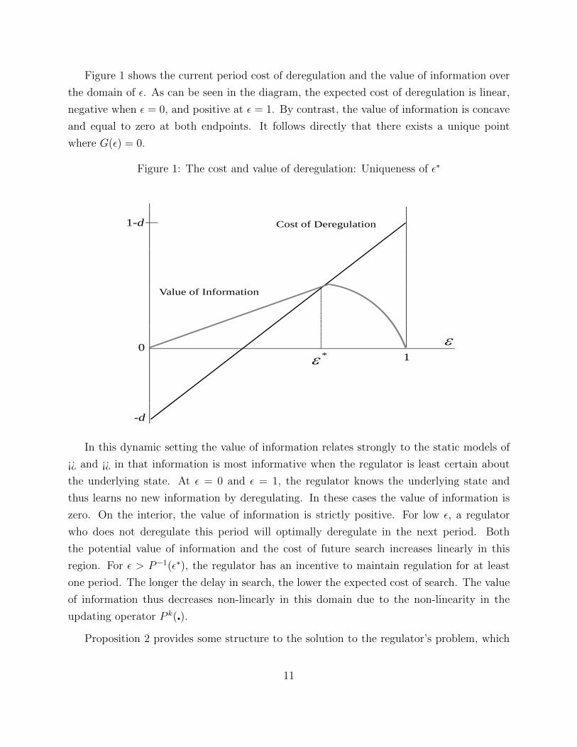
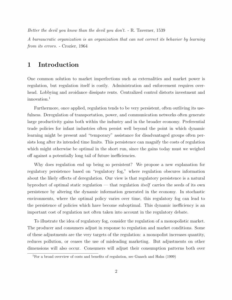
Figure 1 shows the current period cost of deregulation and the value of information over

the domain of ε. As can be seen in the diagram, the expected cost of deregulation is linear,

negative when ε = 0, and positive at ε = 1. By contrast, the value of information is concave

and equal to zero at both endpoints. It follows directly that there exists a unique point

where G(ε) = 0.

Figure 1: The cost and value of deregulation: Uniqueness of ε∗The Optimal Regulation Regime

Cost of Deregulation1-d

Value of Information

0*

1

-d

In this dynamic setting the value of information relates strongly to the static models of

¡¿ and ¡¿ in that information is most informative when the regulator is least certain about

the underlying state. At ε = 0 and ε = 1, the regulator knows the underlying state and

thus learns no new information by deregulating. In these cases the value of information is

zero. On the interior, the value of information is strictly positive. For low ε, a regulator

who does not deregulate this period will optimally deregulate in the next period. Both

the potential value of information and the cost of future search increases linearly in this

region. For ε > P−1(ε∗), the regulator has an incentive to maintain regulation for at least

one period. The longer the delay in search, the lower the expected cost of search. The value

of information thus decreases non-linearly in this domain due to the non-linearity in the

updating operator P k(�).

Proposition 2 provides some structure to the solution to the regulator’s problem, which

11

we now use to characterize the regulator’s equilibrium play. Although strategies are defined

for any belief ε, only countably many (and often finite) beliefs will arrive in equilibrium. Let

ε∗ be the regulator’s optimal cutoff as defined in Proposition 2, and define k∗ as the unique

k ∈ N∗ such that P k+1(1) ≤ ε∗ ≤ P k(1). If there does not exist a k which satisfies this

condition then k∗ =∞. This will be the case if and only if ε∗ ≤ ε̃.

We analyze two cases to characterize the optimal inspection regime. First, assume that

ε∗ < ρBG. Here, even after observing the good state, the regulator will want to regulate. Since

the regulator takes the same action in the good and the bad states, VG = VB = V ∗(P (ε))

and thus the value of information is zero. Thus, G(ε∗) = 0 when ε∗ = d, so this case will

obtain if d < ρGB, just like in the Full-Information benchmark.

Looking at the more interesting case, assume that ε∗ > ρBG so regulation will not be

imposed in the period immediately after the good state is observed. In this case, equilibrium

regulation has the following simple structure. After observing the bad state, the regulator

will regulate for k∗ periods (perhaps infinite) and deregulate in the k∗+1 period to see if the

state has changed. If, upon sampling, he observes the bad state, he updates his posterior to

P (1) at the start of the next period and begins the regulation phase again. If, on the other

hand, he finds himself in the good state, he does not inspect again until he experiences the

bad state.

For ε∗ > P (1) = ρBB this strategy means the regulator actually never imposes regulation,

which corresponds exactly with the full information case. As the value of information in this

case is zero, the no regulation criteria is the same as the full information model with full

regulation imposed when d > ρBB.

For ε∗ ∈ (ε̃, ρBB], a regulator who arrives in the bad state will impose regulation and

lift it every k∗ + 1 periods to see if the state has changed. This region is characterized

by potentially long periods of regulation punctuated by deregulation experiments at fixed

intervals. If ε∗ ≤ ε̃, the regulator’s beliefs will converge to the stationary state which is

above the cutoff belief necessary for experimentation. The regulator’s future value from

deregulating is not high enough to justify the potential risk of being in the bad state.

To differentiate between the permanent regulation and partial regulation cases, it suffices

to find the parameter values for which ε∗ converges to ε̃ from above. In the region of mixed

regulation, VG is related to VB by the potential transition from the good to the bad state.

12

Let κ denote the expected cost of the first bad state discounted one period into the future:

(7) κ =∞∑t=0

δt(1− ρGB)tδρGB =δρGB

1− δ + δρGB.

The expected value of the period following the good state is given by

(8) VG = V ∗(P (0)) = ρGB[−1 + δVB] + ρGGδVG = κ[−1/δ + VB],

where the first term is the cost of being caught in the bad state without inspection and the

second term is the future valuation of being in the bad state with certainty.

As ε∗ converges to ε̃ from above, k∗ →∞ and thus

(9) limk∗→∞

VB =−d

1− δ.

Finally, recall that ε∗ is defined as the point where G(ε∗) = 0 or equivalently where V (I =

1|ε∗) = V (I = 0|ε∗). Since ε∗ > ε̃, P (ε∗) < ε∗ and thus I∗(P (ε∗)) = 0. Replacing V ∗(P (ε∗))

in G(ε∗) yields the following indifference condition:

(10) d = (1− δ)[ε∗(δVG − δVB + 1)− δVG] + δ(δVG − δVB + 1)[ε∗ − P (ε∗)]

Since ε∗ − P (ε∗) converges to zero as ε∗ → ε̃, regulation is fully persistent if:

(11)d

1− δ≤ [ε̃+ (1− ε̃)κ]

[1 + δ

d

1− δ

]The left hand side of this equation represents the cost of permanent regulation. The right

hand side represents the expected cost of deregulating in the steady state and then perma-

nently regulating once the bad state occurs. Solving for d and bringing this result together

with the foregoing discussion leads to the following proposition, which summarizes the reg-

ulator’s optimal strategy:

Proposition 3 Assume the state is revealed at the end of each period if and only if the

regulator does not regulate. Then, there exists a unique pure strategy equilibrium for the

regulation game considered above. Good firms never pollute while bad firms pollute if and

13

only if unregulated. Let

(12) τ ≡

[δ + 1−δ

ρGB+ρBG

]1− δ[ε̃− ρGB]

> 1.

Once regulation is applied the first time, the regulator’s optimal policy falls into one of the

following cases:

1. If d ≤ ρGBτ , the regulator’s equilibrium policy is to regulate forever. Regulation is

infinitely persistent.

2. If d > ρBB, the regulator’s equilibrium policy is to never regulate, even after a bad

state. Regulation never occurs.

3. If ρGBτ < d ≤ ρBB, the regulator’s equilibrium policy is to regulate for k∗ > 0 periods

after the bad state is revealed and not regulate after the good state is revealed, where

k∗ is the first k such that P k+1(1) ≤ ε∗ ≤ P k(1) and ε∗ is the solution to the implicit

function:

(13) ε− d+ δ[εVB + (1− ε)VG − V ∗(P (ε))] = 0.

As with the full information benchmark, our goal is to relate the proportion of time spent

under regulation to the cost of regulation d. As the length of regulatory intervals (k∗) is a

weakly decreasing function of ε∗, it is useful to first determine how ε∗ changes with respect

to d.

Corollary 1 The threshold ε∗ is increasing in d.

The intuition for Corollary 1 can be seen in Figure 1. As d increases, the direct cost of

deregulation decreases. This leads the cost curve to shift downward which shifts ε∗ to the

right. At the same time an increase in d increases the cost of inspecting when the true state

of nature is good. This increases the value of information leading to an increase in the value

of information over all ε. As both of these effects makes G(ε) smaller, the overall effect is an

unambiguous increase in the inspection cutoff.

As k∗ is a weakly decreasing function of ε∗ it follows:

Corollary 2 k∗ is weakly decreasing in d.

14

Having characterized the regulator’s strategy under regulatory fog, the next section com-

pares the equilibrium outcomes to those in the full-information benchmark.

3 Comparison with Full Information

Regulatory fog has two fundamental consequences in our model, and each affects both the

time under regulation and overall social welfare. First, the regulator’s beliefs about the

underlying state evolves over time from a belief in which regulation is (almost) certainly

optimal to beliefs in which there is a greater likelihood that regulation is inefficient. For most

cases, this process naturally leads to regulatory inertia since delay (i) reduces the chance of

deregulatory disasters and (ii) increases the value of information from deregulating.

Second, while beliefs are evolving over time, beliefs under regulation always remain above

ε̃. This contrasts markedly with the full-information regulator, who will update to the

more optimistic ρGB after observing a good state, even while regulating. A decision maker

considering whether to deregulate is permanently faced with the potential of a deregulatory

disaster, where the removal of regulation in the bad state leads to losses. This potential

for disaster can lead to permanent persistence, particularly for environments in which the

decision maker is relatively myopic.

3.1 Permanently Persistent Regulation

We begin by studying the range of parameters for which regulation persists indefinitely. As

with the full-information benchmark, regulation is fully persistent if the normalized cost of

regulation is low relative to the probability of transition from the good to the bad state.

However, as there is now the potential for a deregulatory disaster, deregulation carries ad-

ditional risk which is represented by τ in Proposition 3. Since τ > 1, regulatory fog strictly

increases the set of parameters for which regulation persists permanently.

As τ is a decreasing function of δ, more myopic regulators are more affected by regulatory

fog. Purely myopic regulators ignore the value of information from deregulation and are

willing to deregulate only if the probability of being in the bad state falls below the cost of

regulation. Thus, as the regulator becomes more myopic, the range for which permanent

regulation is optimal becomes large. Institutions that induce short-sighted preferences by

regulators, such as having short terms in office, are expected to lead to more regulatory

15

persistence. Consistent with this prediction, Smith (1982) finds that states with legislators

having longer terms are more likely to deregulate the licensure of professions.8

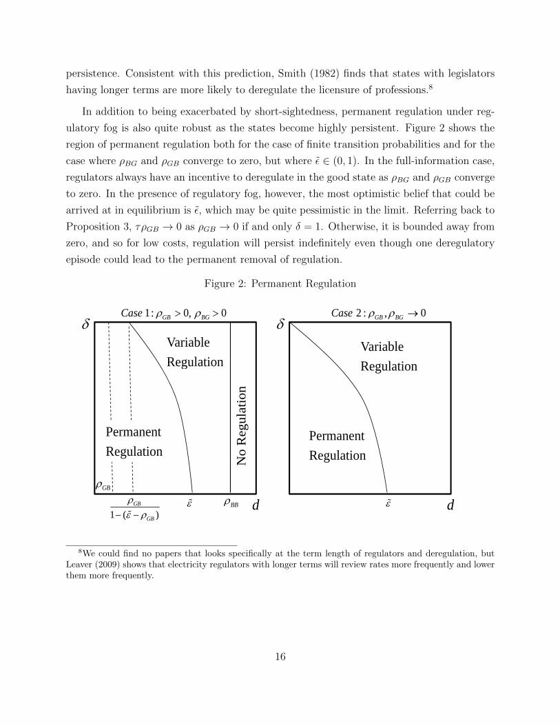
In addition to being exacerbated by short-sightedness, permanent regulation under reg-

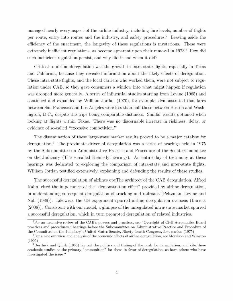
ulatory fog is also quite robust as the states become highly persistent. Figure 2 shows the

region of permanent regulation both for the case of finite transition probabilities and for the

case where ρBG and ρGB converge to zero, but where ε̃ ∈ (0, 1). In the full-information case,

regulators always have an incentive to deregulate in the good state as ρBG and ρGB converge

to zero. In the presence of regulatory fog, however, the most optimistic belief that could be

arrived at in equilibrium is ε̃, which may be quite pessimistic in the limit. Referring back to

Proposition 3, τρGB → 0 as ρGB → 0 if and only δ = 1. Otherwise, it is bounded away from

zero, and so for low costs, regulation will persist indefinitely even though one deregulatory

episode could lead to the permanent removal of regulation.

Figure 2: Permanent Regulation

The Optimal Regulation Regime

2 0C1 0 0C

Variable

2 : , 0GB BGCase

VariableRegulation

1: 0, 0GB BGCase

RegulationRegulation

atio

n

PermanentRegulationN

o R

egul

a

PermanentRegulation

ddGB

BB

N

1 ( )GB

1 ( )GB

8We could find no papers that looks specifically at the term length of regulators and deregulation, butLeaver (2009) shows that electricity regulators with longer terms will review rates more frequently and lowerthem more frequently.

16

3.2 Regulatory Cycles

Much of the most interesting dynamics from our model come from cases in which the cost

of regulation, d, is moderate. In this parameter region, regulatory policy is characterized

by periods of regulation and deregulation which are influenced by the underlying state. As

noted in Proposition 1, the transition from regulation and deregulation in the full information

benchmark is based on the arrival time of the first bad event. As arrival times follow a

geometric distribution, the expected length of a regulatory spell is 1ρBG

and the expected time

under regulation is equal to the steady state probability ε̃. Furthermore, for d ∈ (ρGB, ρBB),

there is no relation between the cost of regulation and its persistence.

Unlike the full information case, in which there is a direct relationship between persistence

and the stochastic nature of the environment, regulation under regulatory fog is characterized

by fixed periods of regulation followed by some period of deregulation. When the cost of

regulation is just above τρGB regulation will eventually be removed, but since the threshold

belief ε∗ is quite close to the steady state, the regulatory spell will be quite lengthy (k∗ is

large). As a result, a great proportion of the time will be spent under regulation. Likewise,

when the cost of regulation is ρBB, the regulator is just indifferent between regulation and

deregulation even after the bad state. In this case, k∗ = 1 and the regulator cycles rapidly

between regulation and deregulation. Thus, for large costs of regulation, regulation actually

ends up being less persistent under regulatory fog than in its absence.9

The overall effect of regulatory fog can best be seen by plotting the proportion of time

spent in regulation and deregulation as a function of d. As can be seen in Figure 3, regulatory

fog leads to more persistence for small and medium d and less persistence for large d. This

differential effect is driven by (i) the potential negative outcome from deregulating in the bad

state and (ii) the information learned about the underlying state which can benefit future

decisions.

When d is small, the relative cost of deregulating in the bad state is large leading to

delayed deregulation in order to reduce the chance for a deregulatory disaster. As d grows, the

value for being in the deregulatory good state grows while the additional cost to deregulation

9In economic environments, we view the region of parameters for which rapid cycles of deregulation andregulation should occur to be quite rare. It is our view that regulator myopia and moderate to low regulationcosts are typically the norm. In other fields such as medicine, however, there is suggestive evidence thatboth regions exist. Treatment for cancer, for instance, is characterized by cycles in treatment and carefulmonitoring. On the other hand, treatment for high blood pressure or depression are continuous with littlevariation in treatment over time.

17

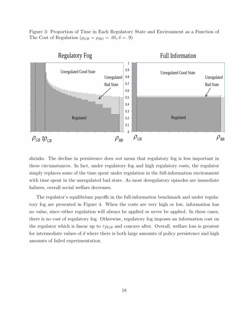
Figure 3: Proportion of Time in Each Regulatory State and Environment as a Function ofThe Cost of Regulation (ρGB = ρBG = .05, δ = .9)

0 9

1

0 9

1

Full InformationRegulatory Fog

0 5

0.6

0.7

0.8

0.9

0 5

0.6

0.7

0.8

0.9

UnregulatedBad State

Unregulated Good State Unregulated Good StateUnregulatedBad State

0 1

0.2

0.3

0.4

0.5

0 1

0.2

0.3

0.4

0.5

Regulated Regulated

0

0.1

0 0.1 0.2 0.3 0.4 0.5 0.6 0.7 0.8 0.9

0

0.1

0 0.1 0.2 0.3 0.4 0.5 0.6 0.7 0.8 0.9GB GB BB GB BB

Proportion of time in the regulatory state.05, .9GB BG

p g y

shrinks. The decline in persistence does not mean that regulatory fog is less important in

these circumstances. In fact, under regulatory fog and high regulatory costs, the regulator

simply replaces some of the time spent under regulation in the full-information environment

with time spent in the unregulated bad state. As most deregulatory episodes are immediate

failures, overall social welfare decreases.

The regulator’s equilibrium payoffs in the full-information benchmark and under regula-

tory fog are presented in Figure 4. When the costs are very high or low, information has

no value, since either regulation will always be applied or never be applied. In these cases,

there is no cost of regulatory fog. Otherwise, regulatory fog imposes an information cost on

the regulator which is linear up to τρGB and concave after. Overall, welfare loss is greatest

for intermediate values of d where there is both large amounts of policy persistence and high

amounts of failed experimentation.

18

Figure 4: The Cost of Regulatory Fog (ρGB = ρBG = .05, δ = .9)The Optimal Regulation Regime

GB BBGB

0

dGB BBGB

FIBVB

BVV1

1

BV

Expected Value of Regulator in Bad State4 Policy Experiments

Just how bad a problem is regulatory fog? In the preceding sections, we have left the regulator

with the stark choice between full regulation and full deregulation and shown that, in that

world, regulatory fog leads to very persistent regulation with significant losses in welfare.

We might wonder, however, just how bad the information problem is in an environment with

a broader policy space. After all, why can the regulator not simply make small alterations

to regulatory policy to generate new information without suffering the potentially disastrous

consequences of fully deregulating in the bad state? This section studies the regulator’s

optimal policy when he has access to experimentation, a broader set of policy options which

are less efficient than full regulation but which are potentially more informative.

Experiments vary from deregulation in two ways. First, experimentation can be con-

ducted while maintaining regulation, but these experiments have an additional cost which is

borne by society. These costs reflect both the direct overhead costs of measurement and the

indirect costs of implementing mechanisms which are more informative but deviate from the

optimal mechanism and are thus less efficient. Informative mechanisms will often be very dif-

ferent than the static mechanism, and thus the indirect costs of experimentation are unlikely

19

to be trivial. In our pollution example, for instance, simply reducing inspection leads to a

large change in the actions of the companies, and would be tantamount to deregulation. A

regulatory experiment which maintains regulation broadly must be more complicated than

simple cutting back on the degree of monitoring. In a broader context, dynamic mecha-

nisms will typically involve screening mechanisms which must distribute information rents

or encourage inefficiency in a subset of the population.

The second difference from full deregulation is the fact that small scale experiments will

lead to informative but imprecise information about the underlying state. This imprecision

comes from two sources. First, there are basic statistical problems associated with sampling

a small selection of firms or markets. Even a perfect, unbiased, experiment will have some

sampling variance. There is also always a risk that an improperly designed experiment

may lead to spurious results. Second, the very circumscribed nature of the experiment may

limit its usefulness. If firms expect the experiment to be temporary, for example, they may

react very differently than they would with a deregulation of indefinite length. The partial

equilibrium response of agents to a deregulatory experiment may be very different from the

general equilibrium response which would result from full deregulation.

To illustrate this idea, consider a regulator who wants to know the probable effects of a

general lowering of immigration restrictions, and experiments by relaxing the immigration

restriction by allowing easier immigration to certain regions. His experiment may give him

biased results for many reasons. If the demand for entry to the areas he chose was not repre-

sentative of the demand, overall, he may under- or over-estimate the demand for entry. Even

more importantly, the demand for entry to the selected regions may be directly affected by

the partial nature of the experiment. If it is known to be a temporary loosening, immigrants

may quicken their moves as compared to how they would react to indefinite deregulation, in

order to arrive within the window. Footloose immigrants with relatively weak preferences

across regions may demand entry into newly opened areas at a much higher level than they

would if the deregulation was more general. This effect, would, of course lead a naive regu-

lator to overestimate the consequences of deregulation. The true effect would depend of the

elasticities of substitution across regions, which may unknowable.10

10The immigration example is not merely a thought experiment. In 2004, the EU expanded to includethe so-called “A8” countries of Czech Republic, Estonia, Hungary, Latvia,Lithuania, Poland, Slovakia, andSlovenia. Accession nationals were formally granted the same rights of free immigration as nationals of extantmembers. As the accession approached, there was widespread worry in the more-developed EU15 countriesthat they would experience a huge spike of immigration from new member states, with new immigrantscompeting for jobs, depressing wages, and disrupting social cohesion. In response, the Treaty of Accession

20

The tradeoffs inherent in experimentation dictate its relative value in mitigating infor-

mation inefficiencies. When the cost of experimentation is close to zero, experimentation

will always be used and thus permanent regulation will arise only in cases where it is never

optimal to deregulate. However, as the costs of regulation rises or as its informativeness

declines, policy makers will eschew experimentation and opt for deregulation instead. In

these cases, the broader policy environment provides no relief from regulatory fog.

4.1 Augmenting the Base Model

Consider an augmentation of the base model presented in section 2 that expands the set of

actions available to the regulator in each period. In addition to regulating or deregulating,

the regulator may instead opt for a third option of performing a deregulatory experiment.

When performing the experiment, the regulator continues to perform his primary regulatory

function at cost d, and pays an additional cost of c > 0 to fund and monitor the experiment.

We consider the simplest signal structure from experimentation which captures the notion

of imprecise information. An experiment can either be a success or a failure which depends on

the underlying state and on chance. If the state is bad, the regulatory experiment will always

allowed EU15 members to impose “temporary” restrictions on worker immigration from the A8 countries forup to seven years after the accession. In the years immediately after accession, only the UK, Ireland, andSweden allowed open access to labor market, while the remaining A15 members maintained relatively strictwork permit systems. A similar pattern held when Bulgaria and Romania (the “A2” group) were admittedto the union in 2006.

Prior to the opening, an estimated 50,000 A8 and A2 nationals were residing in the UK, out of about850,000 in the EU15 at large Brcker, Alvarez-Plata and Siliverstovs (2003). Predictions of expected flows tothe UK from the A8 ranged from 5,000 to 17,000 annually Dustmann, Fabbri and Preston (2005). In reality,the immigrant flows were much larger than that. Even by the strictest definition, those who self-identifyupon arrival that they intend to stay for more than a year, A8 immigration was 52,000 in 2004, 76,000 in2005, and 92,000 in 2006 for National Statistics (2006). Using estimates based on the Eurostat Labour ForceSurvey, Gligorov (2009) finds that net flow of A8 worker immigrants between 2004 and 2007 was just under500,000.

One of the most cited explanations for the underestimate of immigration flows to the UK was not suffi-ciently accounting for the effects of the maintenance of immigration restrictions by the remaining 80-percentof the EU15 Gilpin, Henty, Lemos, Portes and Bullen (2006). The traditional destinations for migrant work-ers from Eastern Europe, Germany and Austria, were closed off be the temporary continuance of immigrationrestriction. Instead of waiting for these countries to open up, the migrants instead came to the UK (andIreland and Sweden, to a lesser degree). Not only is it hard for other Western European countries to learnmuch from the UK’s experiment, since they are not identically economically situated, but it’s even hard forthe UK to learn much about what completely free immigration across the EU would mean for itself. Theobserved patterns are likely an overestimate of the effect the UK should expect from open borders, but thedegree of overestimation will depend on how many of the migrants were crowded in by restriction elsewhereand how many legitimately preferred coming the the UK.

21

be a failure. If the state is good, the regulatory experiment will succeed with probability α

and will fail with probability (1− α).

A regulator observing a failed experiment can not determine whether this failure was due

to a randomly failed experiment or a bad state of the world. Denote the updated beliefs

from a failed experiment as ε̂, then :

(14) ε̂ =ε

ε+ (1− ε)(1− α).

Let E(ε) ∈ {0, 1} represent the regulator’s experimentation strategy when he believes the

state is bad with probability ε, where E = 1 indicates experimentation and E = 0 indicates

no experimentation. Let V (R,E|ε) be the regulator’s value function playing regulation

strategy R and experimentation strategy E with beliefs ε. Define V ∗∗(ε) as the value function

of a regulator who chooses the maximizing regulation and experimentation regime, and

let {R∗∗(ε), E∗∗(ε)} be that maximizing strategy. Since experimentation yields strictly less

information than regulation and has an additive cost, deregulating and experimenting in the

same period is never optimal.

Given maximization in all subsequent periods, for any belief ε, the value for regulation,

deregulation, and experimentation are respectively:

V (R = 1, E = 0|ε) = −d+ δV ∗∗(P (ε)),

V (R = 0, E = 0|ε) = ε[−1 + δV ∗∗(P (1))] + (1− ε)[δV ∗∗(P (0))],

V (R = 1, E = 1|ε) = −d− c+ [ε+ (1− α)(1− ε)][δV ∗∗(P (ε̂))] + (1− ε)α[δV ∗∗(P (0))].

As before, V (R = 1, E = 0|ε), V (R = 0, E = 0|ε), V (R = 1, E = 1|ε), and V ∗∗(ε) are all

continuous and weakly decreasing in ε. Further, since 1 > d > 0, and d+ c > d, deregulation

is optimal at ε = 0 and regulation is optimal at ε = 1.

Our solution strategy is similar to the base case in that we look for a cutoff belief ε∗∗

such that the regulator prefers experimentation to regulation when ε < ε∗∗. If this belief

exists and is greater than the cutoff point ε∗ for which deregulation is better than regulation,

optimal policy calls for experimentation each time the regulator’s belief falls below ε∗∗ and

deregulation if this experimentation is a success. As ε̂ < 1, a regulator who is unsuccessful

in experimentation will wait for a shorter amount of time before experimenting again. Thus

optimal policy will typically be characterized by a long initial regulation period followed by

22

cycles of experimentation and shorter regulatory spells.

If ε∗∗ < ε∗, the regulator’s optimal policy involves only deregulation. In this case, exper-

imentation will never be used and optimal policy is identical to that found in part 2.11

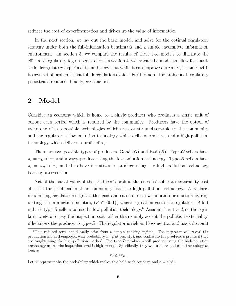
Figure 5 represents the value functions for each policy, as a function of the probability

of being in the bad state. In the first panel, experimentation is relatively effective (α ≈1) and inexpensive (small c) and so the equilibrium strategy of the regulator will follow

the experimental cycles outlined above. In the second panel, experiments are less effective

(α << 1), and so they are never utilized in equilibrium.

Note the shape of the three value functions. The values at each extreme ε (0 and 1)

are easy to pin down because there is no uncertainty about various policies and thus no

information consequences for various policies. The value of deregulating is linear in ε, since

it is a weighted average of the value of deregulating in good state and the value value of

deregulating in the bad state. The value of regulating is linear for low ε, since in amounts

to waiting one period and then deregulating, but it flattens out for higher ε, as the optimal

continuation includes waiting for more and more periods.

If it were not for the cost of running the experiment, the value of experimentation would

always be above that of regulation, since the regulator also receives an informational benefit.

Furthermore, if experiments are perfectly effective (α = 1), the value of experimentation is

also linear, since it is also a weighted average of the value of being in the good state and

the value of being in the bad state, but without the one-time consequences of being in a

deregulatory bad state. As experiments become less and less effective, the value function for

experimentation bows downward, become more and more convex. Once α = 0 it is simply a

downward shift of the regulation value function.

Given ε∗∗ and ε∗, we next check to see whether these beliefs fall below the steady state

belief ε̃. If they are both below this value, the regulator finds it optimal to regulate indefi-

nitely. If, on the other hand, one of the beliefs is above the cutoff value, optimal regulation

involves cycles.

11There is a third case which can occur if P (ε̂∗∗) < ε∗∗ and P (ε̂∗) ≤ ε∗. In this case a regulator may findit in his interest to experiment at ε∗∗ but eventually deregulate if his beliefs fall below ε∗. As this case onlyoccurs if α is extremely low and d is high we do not provide a formal analysis.

23

Figure 5: Value Functions of Deregulation, Regulation, and Experimentation

(a) α ≈ 1: Experimentation in Equilibrium

(b) α << 1: No Experimentation in Equilibrium

24

4.2 Optimal Policy with Experimentation

Just as in the base model, the added cost of experimentation results in a larger set of

parameters for which regulation is permanent. If ε∗∗ < ε̃, the regulator’s future value from

experimentation is never high enough to justify the additional costs of being in the bad

state. Letting ε∗∗ converge to ε̃ from above and assuming ε∗ < ε∗∗, regulation is permanent

if d ≤ ρGBτ′, where

(15) τ ′ ≡ 1 +

(c

α

)(1

κ(1− ε̃)

)> 1.

As evident in the last term on the right hand side, permanent regulation is mitigated if the

cost of experimentation is low relative to the value of information, which has a precision

bounded at α(1− ε̃) and value bounded at ρGB

κ. If experimentation does not have a positive

net present value at the steady state, it never will.

Figure 6 shows the relative importance of experimentation for different regulation costs,

d, and experimentation costs c. As can be seen, for low experimentation costs and low

regulation costs, there exists a region in which the policy decision is between permanent

regulation and experimentation. As d grows, the value of information increases leading to a

greater value for experimentation.

When d > ρGBτ , a regulator always deregulates eventually, and thus his decision is

between implementing a strict policy of regulation and deregulation cycles or a policy which

also includes experimentation. As d increases, the relative cost to deregulating declines and

thus deregulation becomes strictly more attractive.

While the cost of experimentation acts linearly on the value of experimentation, the

precision of information does not. As 1α

is multiplicative, experiments with low precision

have limited value to the policy maker. In these cases, the regulator finds it in his interest

to never use experimentation, or to use it in conjunction with periodic deregulation.

Figure 7 shows the value of experimentation to a policy which only uses deregulation in

{α, c} space. As one might expect, experimentation policies trace out indifference curves

which are increasing in α and decreasing in c. As the value of deregulation is a constant

in this space, there exists an indifference curve in which the value of experimentation is

the same as deregulation. If all potential experiments are above the indifference line, the

25

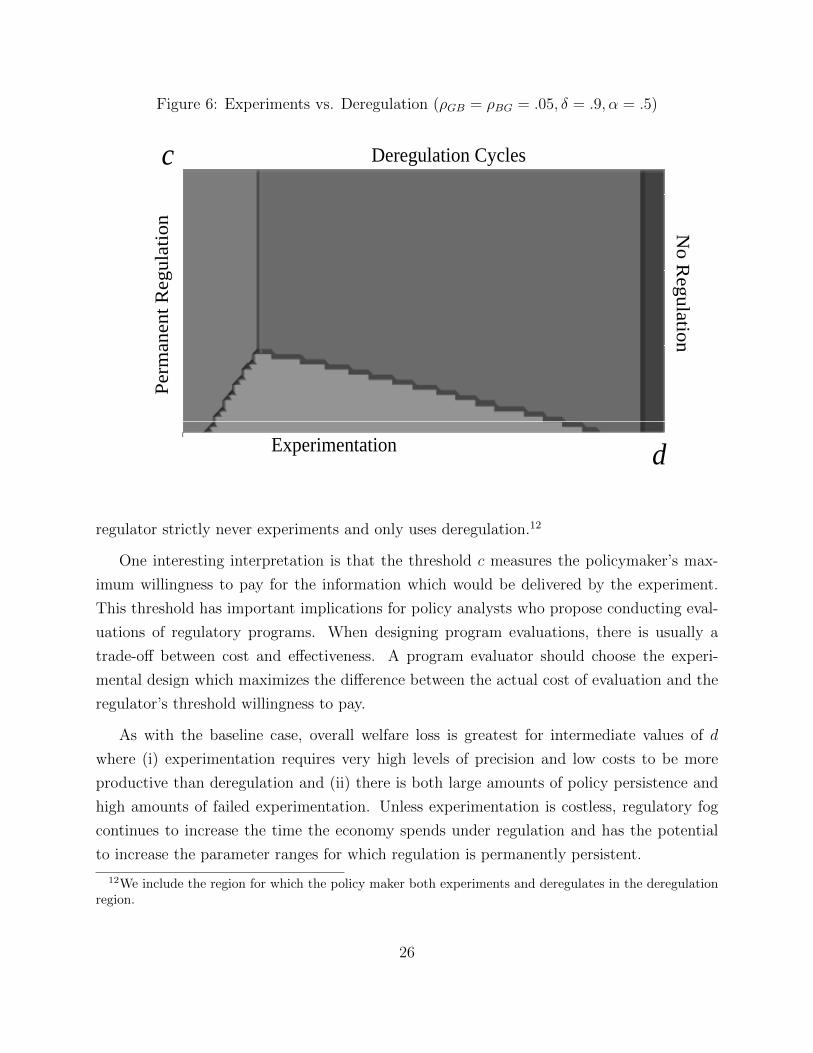
Figure 6: Experiments vs. Deregulation (ρGB = ρBG = .05, δ = .9, α = .5)

When are policy experiments optimal?p y p p

c Deregulation Cyclesul

atio

n No R

anen

t Reg

u Regulation

Perm

a n

dExperimentation

regulator strictly never experiments and only uses deregulation.12

One interesting interpretation is that the threshold c measures the policymaker’s max-

imum willingness to pay for the information which would be delivered by the experiment.

This threshold has important implications for policy analysts who propose conducting eval-

uations of regulatory programs. When designing program evaluations, there is usually a

trade-off between cost and effectiveness. A program evaluator should choose the experi-

mental design which maximizes the difference between the actual cost of evaluation and the

regulator’s threshold willingness to pay.

As with the baseline case, overall welfare loss is greatest for intermediate values of d

where (i) experimentation requires very high levels of precision and low costs to be more

productive than deregulation and (ii) there is both large amounts of policy persistence and

high amounts of failed experimentation. Unless experimentation is costless, regulatory fog

continues to increase the time the economy spends under regulation and has the potential

to increase the parameter ranges for which regulation is permanently persistent.

12We include the region for which the policy maker both experiments and deregulates in the deregulationregion.

26

Figure 7: Experiments vs. Deregulation (ρGB = ρBG = .05, δ = .9, d = .5)

When are policy experiments optimal?p y p p

0.5 c

DeregulationDeregulationOptimal

ExperimentationOptimal

0

0 0.5 1

Optimal

.05, .9, .5GB BG d

Optimal Policy: Deregulation vs. Experimentation5 Conclusions

Models of regulatory persistence are typically based on the role that agency and lobbying

play in influencing final policy. We argue that in many environments, regulation generates

the seeds of its own persistence by altering the dynamic information observable about the

environment - a phenomenon we refer to as regulatory fog. Under a stark policy environment

of regulation and deregulation and in a broader environment where experimentation is also

allowed, we find that the effects of regulatory fog can be quite severe. Regulatory fog can lead

to permanent regulation for a broad range of parameters, particularly by myopic regulators.

For most reasonable parameter values, fog delays deregulation — a phenomenon which leads

the economy to stay in the regulated state more often than the underlying environment

warrants alone. Finally, fog can lead to deregulatory disasters which can greatly diminish

overall social welfare.

Although we have chosen to explore regulatory fog in an environment with a perfectly

public-interested regulator, the information and political economy channels are quite com-

plementary. In an interest group model such as Coate and Morris (1999), information asym-

27

metries between regulated firms and consumers are likely to generate significant pressure

from regulated firms who are enjoying the protections of a regulated monopoly, but limited

pull by consumers who are uncertain as to the final outcome of deregulation. Likewise, in

an environment with politically charged regulation, partisan policy makers may be likely

to develop policies which deliberately eliminate information in order to limit the ability of

competing parties to overrule legislation in the future.

While we have framed the policy decision from the perspective of a centralized planner,

decentralization is of limited use when separated districts are symmetric and competitive.

As pointed out by Rose-Ackerman (1980) and generalized by Strumpf (2002), the potential

policy experiments in other districts provides incentives for policy makers to delay their own

deregulatory policies and can, in many cases, actually lead to more regulatory persistence.

Further, just like in the experimentation example, spill overs from one district to another are

likely to reduce the informativeness of experimentation and may ultimately make unilateral

policy decisions fail.

Finally, although this analysis has focused on regulation, we believe regulatory fog is a

general phenomenon which affects a wide variety of economic environments. Many economic

institutions such as monitoring, certification, intermediation, and organizational structures

are designed to alter the actions of heterogeneous agents which, in the process, affects the

dynamic information generated. These dynamic effects are likely to influence both the long-

term institutions which persist and the overall structure of markets and organizations.

6 Appendix

6.1 Proofs from Main Text

Proposition 1:

Proof. The information consequences and the continuation values of regulation and

deregulation are identical, so everything turns on the current period’s payoff. The payoff of

regulation is always −d, while the expected payoff of deregulation is −ε. This means the

optimal policy is to regulate if ε > d and otherwise deregulate. After observing the good

state, the regulator’s beliefs are ρGB and after observing the bad state, they are ρBB. So the

optimal strategy falls into the regions outlined in the proposition.

28

In the region of moderate costs, the probability of continuing regulation is exactly the

probability of staying the the bad state, ρBB. So the probability of having a spell of length

t is given by ρt−1BB(1 − ρBB). This is exactly the pdf of a random variable with a geometric

distribution with parameter ρBB, which has a mean length of 1/(1 − ρBB). Finally, since

the fraction of time spent under regulation has to be self-duplicating, it must be the steady

state of the Markov Process.

Proposition 2:

Proof. If the regulator is following the outlined strategy, the producer’s proposed strat-

egy is optimal since polluting in the unregulated state perfectly informs the regulator about

the state of nature. Assume that the regulator is playing some optimal strategy R∗(ε) which

induces a value function V ∗(ε). For any ε define

(16) G(ε) = V (R = 1|ε)− V (R = 0|ε).

V (R|ε) is continuous and thus G is continuous. Since G(0) < 0, G(1) > 1, and G is

continuous, there is some ε∗ for which G(ε∗) = 0. For the Proposition it would suffice would

show that this ε∗ is unique. In fact, we’ll show that G() is increasing, a stronger claim.

Replacing for (4) and (5) in equation (16),

G(ε) = −d+ δV ∗(P (ε))− ε[−1 + δVB]− (1− ε)δVG.

Replacing in turn for V ∗(P (ε)), this becomes

(17) max{ −d+ δ[(−d+ δV ∗(P 2(ε))]− ε[−1 + δVB]− (1− ε)δVG,−d+ δ[P (ε)[−1 + δVB] + (1− P (ε))δVG]− ε[−1 + δVB]− (1− ε)δVG

},

where the first constituent of the maximand is the difference in returns when choosing to

audit next period after auditing this period versus not auditing this period, and the second

constituent is the return to not auditing next period after auditing this period versus not

auditing this period. More generally, define Gk(ε) as the difference between the return for

auditing for k periods and then following optimal strategies from then on and simply not

auditing this period . I.e.,

Gk(ε) = −dk∑j=0

δj−1 + δk{P k(ε)[−1 + δVB] + (1− P k(ε))δVG} − ε[−1 + δVB]− (1− ε)δVG

29

Then for all k, Gk(ε) is differentiable and increasing. Furthermore

limk→∞

Gk(ε) = − d

1− δ− ε[−1 + δVB]− (1− ε)δVG,

which is also increasing in ε. Finally, note that G(ε) = maxkGk(ε), and since it is continuous

it must also be increasing. Therefore, there is a unique ε∗ where G(ε) R 0 if and only if

ε R ε∗, and that ε∗ will, therefore, satisfy the requirements of the Proposition.

Corollary 1: Proof. We’ll prove this using the implicit function theorem on G(ε). From

the proof of Proposition 2, G′(ε) > 0, and so it follows directly from the implicit function

theorem that

sgn(dε∗

dd) = sgn(−∂G(ε, d)

∂d)

From the text VG = κ[−1δ

+ VB], and so ∂VG∂d

= κ∂VB∂d.

The easier case occurs if ε∗ ≤ ε̃, then P (ε∗) ≥ ε∗, and so V (P (ε∗)) = VB = −d1−δ . In this

case,

G(ε, d) = −d− δ( d

1− δ)− ε(−1− δ d

1− δ)− (1− ε)δ[−κ

δ− κ(

d

1− δ)].

and so∂G(ε, d)

∂d) = −1 +

δ

1− δ[−1 + ε+ (1− ε)κ] < 0.

If ε∗ > ε̃, then P (ε∗) < ε∗, and so V (P (ε∗)) = P (ε∗)(−1+δVB)+(1−P (ε∗))δVG. Replacing

and simplifying,

∂G(ε∗, d)

∂d) = −1 + δ

∂VB∂d

[δ[P (ε) + (1− P (ε∗))κ]− [ε∗ + (1− ε∗)κ]

].

Since regulation cannot be used more than once per-period, ∂VB∂d

> − 11−δ . Furthermore,

since P (ε∗) < ε∗, P (ε∗) + (1− P (ε∗)κ < ε∗ + (1− ε∗)κ, and so

∂G(ε∗, d)

∂d) < −1 + δ(

−1

1− δ)(ε∗ + (1− ε∗)κ)(δ − 1) = −1 + δ(ε∗ + (1− ε∗)κ) < 0.

Corollary 2: Proof. Obvious from Corollary 1, since the P () function is unaffected by

d, and epsilon∗ increases.

Proposition 3: Proof. When d > ρBB regulation is never static optimal, even after the

30

most pessimistic beliefs that could arrive in equilibrium, so it will never be used. The

argument for the τρGB cutoff for permanent regulation is given in the text. We know beliefs

fall over time from ε = 1 to ε̃ via a the Markov process, so the characterization in Lemma 1

gives the result for the intermediary case.

References

Bailey, Elizabeth, “Deregulation and Regulatory Re- form: U.S. Domestic and Interna-

tional Air Transportation Policy During 1977- 79,,” in “Regulated Industries and Public

Enterprises: European and United States Perspective,” Lexington, 1980.

Barrett, Sean D., “Exporting Deregulation - Alfred Kahn and the Celtic Tiger,” Review

of Network Economics, 2008, 7, 573–602.

Brainard, S. Lael and Thierry Verdier, “Lobbying and Adjustment in Declining Indus-

tries,” European Economic Review, 1994, 38, 586–95.

Brcker, Herbert, Patricia Alvarez-Plata, and Boriss Siliverstovs, “Potential Migra-

tion from Central and Eastern Europe into the EU-15 An Update,” Technical Report,

European Commission, DG Employment and Social Affairs 2003.

Coate, Stephen and Stephen Morris, “Policy Persistence,” American Economic Review,

1999, 89, 1327.

Derthick, Martha and Paul J. Quirk, The Politics of Deregulation, The Brookings

Institute, 1985.

Dustmann, Christian, Frecesca Fabbri, and Ian Preston, “The Impact of Immigration

on the British Labour Market,” The Economic Journal, 2005, 115, F324–F341.

Fernandez, Raquel and Dani Rodrik, “Resistence to Reform: Status Quo Bias in the

Persistence of Individual-Specific Uncertainty,” American Economic Review, 1991, 81,

1146–55.

for National Statistics, Office, “International Migration: Migrants entering or leaving the

United Kingdom, England and Wales,” Technical Report, Office for National Statistics

2006.

31

Gilpin, Nicola, Matthew Henty, Sara Lemos, Jonathan Portes, and Chris Bullen,

“The Impact of Free Movement of Workers from Central and Eastern Europe on the

UK Labour Market,” 2006. Working Paper No. 29, Department of Work and Pensions,

UK.

Gligorov, Vladimir, “Mobility and Transition in Integrating Europe,” 2009. UNDP Hu-

man Development Research Paper 2009/15.

Grossman, Gene M. and Elhanan Helpman, “Protection for Sale,” American Economic

Review, 1994, 84, 833–50.

Guasch, J Luis and Robert W. Hahn, “The Costs and Benefits of Regulation: Im-

plications for Developing Countries,” The World Bank Research Observer, 1999, 14,

137–158.

Jordan, William, Air Regulation in America: Effects and Imperfections, The Johns Hop-

kins Press, 1970.

Leaver, Clare, “Bureaucratic Minimal Squawk Behavior: Theory and Evidence from Reg-

ulatory Agencies,” American Economic Review, 2009, 99, 572–607.

Levine, Michael E., “Is Regulation Necessary? California Air Transportation and National

Regulatory Policy,” Yale Law Journal, 1965, 74, 1416–47.

Morrison, Steven and Clifford Winston, The Evolution of the Airline Industry, The

Brookings Institute, 1995.

Peltzman, Sam, Michael Levine, and Roger Noll, “The Economic Theory of Regula-

tion after a Decade of Deregulation,” Brookings Papers on Economic Activity: Microe-

conomics, 1989, 1989, 1–59.

Piketty, Thomas and Emmanuel Saez, “How Progressive is the U.S. Federal tax system?

A Historical and International Perspective,” Journal of Economic Perspectives, 2007,

21, 3–24.

Pindyck, Robert, “Irreversibilities and the timing of environmental policy,” Resource and

Energy Economics, 2000, 22, 233–259.

Rose-Ackerman, Susan, “Risktaking and Reelection: Does Federalism Promote Innova-

tion,” Journal of Legal Studies, 1980, 9, 593–616.

32

Smith, Janet K., “Production of Licensing Legislation: An Economic Analysis of Interstate

Differences,” Journal of Legal Studies, 1982, 11, 117–138.

Stigler, George J., “The Theory of Economic Regulation,” Bell Journal of Economics,

1971, 2, 3–21.

Strumpf, Koleman, “Does Government Decentralization Increase Policy Innovation?,”

Journal of Public Economic Theory, 2002, 4, 207–241.

Zhao, Jinhua and Catherine L. Kling, “Policy persistence in environmental regulation,”

Resource and Energy Economics, 2003, 25, 255–268.

33