Behavior Research Methods, Instruments, & Computers2004, ?? (?), ???-???

Due to the advent of fast computers, the statistical esti-mation of parameters in mathematical models of cognitionis nowadays a feasible option (e.g., Ashby & Maddox,1992; Kruschke, 1992; Lamberts, 2000; Nosofsky &Palmeri, 1997). If one estimates the parameters of a model,it is of interest to know how informative each estimate isfor its corresponding parameter—in other words, how ac-curately each parameter has been estimated. In most ap-plications, the latter issue is overlooked. Obtaining an es-timate of this accuracy is the topic of the present article.

In the maximum likelihood framework, accuracy of aparameter estimate is usually assessed with a standarderror. A standard error is the standard deviation of the dis-tribution of parameter estimates over multiple samples,and hence, a small standard error implies high accuracy ofestimation. However, it turns out that the procedure forcalculating a standard error is also meaningful without thismultiple-sample interpretation. Specifically, a confidenceinterval is also the set of (parameter) points that have a cri-terion value on the optimized function (e.g., the likelihoodfunction or the least squares loss function) that deviatesfrom the optimal value by no more than a fixed value. Thisfact is useful, first, in a maximum likelihood context be-cause it allows evaluation of the precision of an estimate

if the usual assumptions that are needed for the multiple-sample interpretation of a standard error (e.g., the consis-tency of the maximum likelihood estimate; see Schervisch,1995) are not met or cannot be checked. Second, it allowsevaluation of the precision of a parameter estimate if onedoes not or even cannot perform maximum likelihoodestimation but has to resort to, for example, least squaresestimation. Each of the two settings (maximum likelihoodand least squares) will be illustrated with examples fromthe categorization literature.

An independent issue that, in principle, has to be ascer-tained before the parameters of a model are estimated isidentification of the model—that is, whether there is pre-cisely one set of parameters that optimizes the criterionfunction. If several different parameter values yield thesame optimal fit, parameter interpretation becomes awk-ward, because one’s conclusions may depend on the par-ticular set of parameters that was (arbitrarily) chosen (seeCrowther, Batchelder, & Hu, 1995, for a detailed discus-sion of this issue). Although it is, in general, difficult toprove that a model has been identified (i.e., has a single setof optimal parameters), standard errors often give a goodindication as to whether or not a model has been identi-fied. In particular, if standard errors are extremely large,the criterion (likelihood) function may be flat in one ormore directions in the parameter space, thus suggesting alack of identification. This issue will also be illustrated.

The remainder of this article is organized as follows. Wefirst will review briefly the usual methodology of standarderror calculation for model parameters. Second, we will

1 Copyright 2004 Psychonomic Society, Inc.

We thank Eef Ameel for her help with the ALCOVE estimation pro-grams and Francis Tuerlinckx for his useful comments on an earlier ver-sion of this paper. Correspondence concerning this article should be sentto T. Verguts, Department of Experimental Psychology, Ghent University,H. Dunantlaan 2, 9000 Ghent, Belgium (e-mail: tom.verguts@rug.ac.be).

Assessing the informational valueof parameter estimates in cognitive models

TOM VERGUTSGhent University, Ghent, Belgium

and

GERT STORMSUniversity of Leuven, Leuven, Belgium

Mathematical models of cognition often contain unknown parameters whose values are estimatedfrom the data. A question that generally receives little attention is how informative such estimates are.In a maximum likelihood framework, standard errors provide a measure of informativeness. Here, astandard error is interpreted as the standard deviation of the distribution of parameter estimates overmultiple samples. A drawback to this interpretation is that the assumptions that are required for themaximum likelihood framework are very difficult to test and are not always met. However, at least inthe cognitive science community, it appears to be not well known that standard error calculation alsoyields interpretable intervals outside the typical maximum likelihood framework. We describe and mo-tivate this procedure and, in combination with graphical methods, apply it to two recent models of cat-egorization: ALCOVE (Kruschke, 1992) and the exemplar-based random walk model (Nosofsky &Palmeri, 1997). The applications reveal aspects of these models that were not hitherto known and bringa mix of bad and good news concerning estimation of these models.

B260F BC JP

2 VERGUTS AND STORMS

show why this is also a useful procedure if the multiple-sample interpretation of a standard error cannot be as-sumed. Then, we will apply this method to two categoriza-tion models, ALCOVE and the exemplar-based randomwalk (EBRW) model, and will show that the method yieldsinsights in these models that have not been described before.

Precision of Parameter Estimates in theMaximum Likelihood Framework

Standard errors can be computed in the following way(see Mood, Graybill, & Boes, 1974, or Schervisch, 1995,for more details). Suppose one has a vector of parametersθ � (θ1, . . . , θN), which is estimated by the maximumlikelihood estimator θ̂. If the model is correct and if someregularity conditions hold, the estimator θ̂ has asymptoti-cally a (multivariate) normal distribution with a mean ofθ and a covariance matrix of C. The diagonal elements ofC contain the variances of the different estimates, or inother words, the squared standard errors. To obtain an es-timate of these standard errors, one needs to calculate theHessian matrix. This is the N � N matrix containing, atrow i and column j, the derivative of log L( θ̂ ) toward pa-rameters θi and θj, where log L( θ̂ ) is the logarithm of thelikelihood function (the log likelihood) evaluated in theestimate θ̂ . For example, if n independent samples xi aretaken from a normal distribution with a mean of µ and aknown standard deviation of σ, then

In this case, the second derivative toward parameter µ be-comes �n/σ2.

The importance of this Hessian matrix H resides in thefact that minus its inverse (i.e., �H�1) is approximatelythe covariance matrix C. Hence, in the example from theprevious paragraph, the second derivative of log L(µ)equals �n/σ2, and it follows that √(�HH�1) � σ/√n, theusual formula for the standard error of the (estimate ofthe) mean of a normal distribution. In this case, the ap-proximation is actually exactly the true standard error, butthis is not so in general. This procedure allows construc-tion of confidence intervals; for example, a 95% confi-dence interval for θi would be

(1)

where [(�H)�1]ii is the ith diagonal element of the esti-mated covariance matrix.

An alternative way to estimate standard errors is to per-form a bootstrap, a method that has been applied, for ex-ample, in psychophysics to generate confidence intervalsof estimated parameters (e.g., Wichmann & Hill, 2001).This procedure rests on fewer assumptions than the onedescribed above, but it also requires a distributional(multiple-sample) framework and can be very time con-suming for complex models. For this reason, bootstrapmethods will no longer be considered here.

The Confidence Interval ReconsideredThe procedure described in the previous section can be

extended to settings other than maximum likelihood by,essentially, a redefinition of the concept of a confidenceinterval. More specifically, a confidence interval can beconsidered as the set of points whose criterion functionvalue deviates from the optimal value by no more than afixed (appropriately chosen) constant. This redefinition isuseful because it allows interpretation of such intervalsoutside the context of maximum likelihood estimation.

We first will explain the reasoning in the one-dimensionalcase. Suppose we intend to maximize a (log) likelihoodfunction f(θ ), where θ is a (one-dimensional) parameter andθ0 is the optimal point (i.e., it maximizes f ). A second-orderTaylor approximation of this function yields

(2)

where f � denotes the derivative of f. Consider now thepoint θ that is m standard errors removed from θ0 (withm � 0), so θ � θ0 � m � SE, where SE denotes the stan-dard error. A conventional choice is m � 1.96, but othervalues are possible as well. Clearly, f �(θ0) � 0, and theprevious section suggests the Hessian approximation SE �{[�f �(θ0)]�1}1/2. Combining these, Equation 2 can berewritten as

(3)

Equation 3 shows that moving m standard errors awayfrom the optimal point amounts to decreasing the likeli-hood value by m2/2. Furthermore, to the extent that the ap-proximation in Equation 2 is valid, all points in between(e.g., between θ0 and θ0 � m � SE) have a likelihoodvalue that is in between f(θ0) and f(θ0) � m2/2. By usingthis, all the points from θ0 to θ0 � m � SE can be consid-ered acceptable points, in the sense that their likelihoodvalue differs from the optimal value f(θ0) by no more thanm2/ 2. In other words, a confidence interval is the set of pa-rameters that decreases the criterion value by no morethan m2/2 from the optimal value. Of course, different val-ues of m can be chosen depending on what decrease inlikelihood is still considered acceptable.

The advantage of the latter formulation is that it appliesto any continuous function that is optimized, as long asthe approximation in Equation 2 is valid. This assumptionis weaker than the usual assumptions needed for interpre-tation of a confidence interval (Schervisch, 1995). For ex-ample, it also applies to (least squares) error functions,whereas traditionally, confidence intervals are restrictedto a maximum likelihood context. Moreover, the assump-tion embodied in Equation 2 is easily checked graphically,as will be described below.

We now turn to the multidimensional case. Suppose wewant to maximize a continuous function f(θ ), where θ isan arbitrary point in an N-dimensional parameter space.Furthermore, θ0 is the point that maximizes f. In analogy

f f m( ) ( ) .θ θ= −0

2

2

f f f f( ) ( ) ( ) ( )( ) ,θ θ θ θ θ θ= + ′ + ′′ −0 0 0 021

2

ˆ . ( ) ,θiii

± −[ ]−1 96 1H

log ( ) log( ) ( ) .L xiiµσ

µ= − −∑constant 12 2

2

INFORMATION IN MODEL ESTIMATION 3

with the one-dimensional case, we consider all points θwith a fixed distance | f(θ ) � f(θ0) | � m2/2. To the extentthat the Taylor approximation of f is valid (the multivari-ate version of Equation 2; see, e.g., Schervisch, 1995), allsuch points lie on an ellipsoid (Press, Flannery, Teukol-sky, & Vetterling, 1989). All the points in this ellipsoidhave a distance | f(θ ) � f(θ0) | smaller than m2/2. Figure 1plots this situation for a two-dimensional optimizationproblem. As for the one-dimensional case, all points θ inthe ellipsoid can again be called acceptable points, in thesense that their function value f (θ ) is not too differentfrom that of f(θ0).

What we want now is the range of acceptable points foreach parameter separately. Indeed, plotting the appropri-ate ellipsoid is difficult for three parameters and impossi-ble for more than three parameters. Also, individual (one-dimensional) intervals are easier to interpret than a(multidimensional) ellipsoid. How are these individualranges for each parameter to be found? Projecting the el-lipsoid onto a single dimension of interest, one shouldconstruct a box, as in Figure 1, and for each dimension(parameter) look at the range of the box. For example, forthe first parameter (represented on the abscissa), the rangeextends from the arrow indexed as 1 to the arrow indexedas 2. The distance from θ0 to, for example, the right-handside of the box turns out to be m√[(�H)�1]ii for the ith di-mension (in the example, i � 1). Since, as was notedabove, the factor √[(�H)�1]ii is an approximation of thestandard error of the ith parameter estimate, it follows thata confidence interval (θ0 � m � SE, θ0 � m � SE) is a

projection of a confidence ellipsoid on a particular di-mension, where the confidence ellipsoid contains the setof points that deviate no more than m2/2 with regard to thecriterion (e.g., likelihood) function value.

The fact that the matrix H can be used to construct el-lipsoid contours of equal function value (and projectionsof these contours) is well known (e.g., Ashby & Maddox,1992). Press et al. (1989; see also Martin, 1971) appliedthis to chi-square minimization problems, but it may beusefully applied to any criterion function that is opti-mized, as long as the Taylor expansion (e.g., Equation 2 inthe one-dimensional case) is a good approximation of thefunction.

Following the procedure described above, it becomesmeaningful to apply confidence interval calculation out-side the maximum likelihood framework, as we will see inthe second application with Nosofsky and Palmeri’s(1997) EBRW model. This is useful, because it is ex-tremely difficult to estimate this model with maximumlikelihood but relatively simple with least squares. First,however, we will apply the methodology in a maximumlikelihood framework with the ALCOVE model (Kru-schke, 1992) of categorization.

Application 1: ALCOVEThe ALCOVE model is a network model of catego-

rization containing three layers of nodes. In the first, orinput, layer, one node is used per input dimension charac-terizing the stimulus. For example, the input dimensionsmay code for such features as the color or the size of the

2.5

2

1.5

1

0.5

0

–0.5

–1

–1.5

–2

–2.5–3 –2 –1 0 1 2 3

1

2

Parameter 2

Parameter 1

points with

Figure 1. Confidence ellipsoid and projection of this ellipsoid onto the abscissa (see thetext for an explanation).

4 VERGUTS AND STORMS

stimulus. The second layer is an exemplar layer, and eachnode in this layer codes for one exemplar (i.e., combina-tion of input values), which is why the model is called anexemplar model. Specifically, suppose each node in theexemplar layer corresponds to an exemplar hj � (hj1, . . . ,hjD) if D dimensions are used in the stimulus coding.Then, when stimulus x is presented in the input layer, nodej in the exemplar layer has an activation value as follows:

(4)

where the index d (d � 1, . . . , D) in Equation 4 is takenover input dimensions and xd is the d th component of x [sox � (x1, . . . , xD)]. Exemplar node j corresponds to exem-plar hj, in the sense that Aj

ex is maximally activated whenstimulus x � hj � (hj1, . . . , hjD ) is presented. The para-meters p and r determine the similarity decay function andthe metric, respectively; here, we will assume that p � 1(exponential decay function) and r � 1 (city block dis-tance metric). This is in line with standard assumptions(e.g., Kruschke, 1992; Nosofsky, Kruschke, & McKinley,1992). The parameter αd is the attention assigned to di-mension d. The parameter c is a sensitivity parameter, in-dicating how sensitive an exemplar node is to the distancefunction.

The third, or output, layer contains a node for each pos-sible category to which a stimulus can be assigned. Theoutput from the exemplar layer to the category K node(K � A or B, if there are two categories1) is a linear func-tion of activations Aj

ex as follows:

where it is assumed that there are J exemplars. The para-meter wjK is the connection between exemplar j and cate-gory K. Finally, the probability of choosing category A is

Pr(A) � (5)

There are four estimable parameters in this model.First, there is the parameter c (as in Equation 4). Second,there is a scaling parameter ϕ (Equation 5). Finally, thereis a parameter λα that determines the learning rate of the

attention values (αd) and a parameter λw that determinesthe learning rate of the weights wjK. All of these parame-ters are assumed to be positive valued. We will now de-scribe a simulation that was conducted to evaluate the in-formational value of ALCOVE’s parameters.

Model fitting procedure. We generated 100 stimulithat were randomly generated from a two-dimensionalnormal distribution with a mean of zero on both dimen-sions, a standard deviation of one half on both dimensions,and a zero correlation. The coordinates of these stimuliwill be denoted x1 and x2 for the first and the second di-mensions, respectively. If x1 � x2, a stimulus was assignedto category A; otherwise, it was assigned to category B.

Nine exemplars were placed in this two-dimensionalspace. The coordinates were approximately evenly spacedover the interval (�0.5, 0.5) for each parameter, whileavoiding that the two dimensional values should be equal(since x1 � x2 is the boundary separating categories A andB). Note that the term exemplars refers to the pointsplaced in the two-dimensional space (the points hj , men-tioned above) that are used for classification of the 100stimuli in the pseudo-experiment. Hence, the nine exem-plars are incorporated in the model prior to the pseudo-experiment and are used for purposes of classifying the100 stimuli. The true vector of parameters was (c, λw , λα ,ϕ) � (3, 0.1, 0.1, 4). Data were sampled for 100 pseudo-participants. The initial values αd were set at zero.

To estimate the parameters of the model, we started atthe true parameter point θ � (c, λw , λα , ϕ) � (3, 0.1, 0.1,4) and applied a steepest ascent algorithm to find the pointthat maximized the log likelihood function. Of course, anyother algorithm that finds the optimal point (grid search,Newton–Raphson, etc.) is acceptable for this purpose (butsee below). The optimal point was found to be θ0 �(3.000, 0.104, 0.101, 3.952).

Using the method described in the previous section, weconstructed confidence intervals containing 2 � 1.96standard errors (so m � 1.96). The intervals for the fourparameters are shown in the left-hand part of Table 1. Forλw and ϕ, these ranges are satisfactory. However, the pa-rameter range for c and λα is extremely large, given theirparameter values. For example, both intervals contain neg-ative values, which makes their interpretation impossible.

Contour plots. From the present analysis alone, it isnot possible to determine whether ALCOVE is not identi-fied or merely very weakly identified. To investigate this

exp

exp exp.

ϕ

ϕ ϕ

A

A A

Acat

Acat

Bcat

( )( ) + ( )

A A wj jj

J

Kcat ex

K( ) ( ) ,x x==

∑1

A c x hjex

d d jdr

d

D p r

( ) exp ,/

x = − −

=∑ α

1

Table 1Confidence Intervals

ALCOVE Normalized ALCOVE EBRW

Parameter Interval Parameter Interval Parameter Interval

c (�2.713, 8.715) c (2.852, 3.096) c (0.761, 1.201)λw (0.099, 0.109) λw (.090, .112) β (0.347, 1.982)λα (�0.284, 0.485) λγ (.078, .181) w1 (0.387, 0.585)ϕ (3.739, 4.165) ϕ (3.706, 4.418) Slope (1.030, 9.228)

Intercept (�1.940, 9.704)

Note—EBRW, exemplar-based random walk model.

INFORMATION IN MODEL ESTIMATION 5

issue in more detail, we made contour plots of equal loglikelihood for the six possible pairs of parameters. Otherparameters than those included in the pair were fixed attheir optimal values. Note that these plots are based on ac-tual log likelihood values and not on an approximationsuch as that in Equation 2.

The contour plot for the pair (λw , ϕ) is depicted in theupper panel of Figure 2. The curves of equal log likeli-hood in this case take the form of closed curves aroundthe point (0.104, 3.952). In this and in the following plots,adjacent contour lines have a difference in criterion valueof 1.92 ( � 1.962/2), and the most interior contour linecorresponds to a difference of 1.92 from the optimalvalue.2 The plot suggests that the log likelihood functionhas an isolated maximum in that point (if the function isrestricted to vary over these two dimensions only). Thesame, however, is not true for the parameters c and λα .These parameters were found to have extremely large con-fidence intervals. Figure 2 (lower panel) shows why:These parameters are in a tradeoff relation. In the neigh-borhood of the point (3, 0.101) (the optimal values forthese parameters; see above), contour lines take the formof nonclosed parallel curves. There is one such curvecrossing the “optimal” point (3, 0.101) itself, so that morethan one pair of parameter values (in fact, infinitely many)optimize the likelihood function. Contour plots for all

other pairs of parameters [e.g., (c, ϕ)] looked like those ofλw and ϕ. Hence, it seems that the problem is restricted tothe combination of c and λα.

Contour plots cannot be used to construct confidenceintervals, because they lack precision and condition onfixed values of all parameters not appearing in the partic-ular (two-dimensional) plot. However, in some cases,these contour plots provide useful information, as in thecase of the parameters c and λα, described above, wheredue to problems of numerical imprecision, it was not clearwhether the range of a parameter is infinitely large or justvery (finitely) large. We recommend using the two proce-dures together to exploit the strength of each technique.The method of using contour plots to check the precisionof estimates has been used before (Nobel & Shiffrin,2001). Nobel and Shiffrin constructed contour plots fortwo parameters by fixing the two parameters at differentvalues and optimizing a criterion function over the re-maining parameter(s). For each such pair of parameters, itwas evaluated whether the resulting criterion value wassignificantly worse than the optimal value. A confidenceinterval was then constructed by taking all those two-dimensional points at which the boundary between sig-nificance and nonsignificance was crossed. However, wethink the method discussed in the present article has extramerits: Because it is linked more tightly to standard pro-

–3182.0 –3183.9

–3180.1

4.2

4

3.8

3.6

0.11

0.1

0.09

0.08

0.096 0.098 0.1 0.102 0.104 0.106 0.108 0.11 0.112 0.114

2.8 2.85 2.9 2.95 3 3.05 3.1 3.15 �

Figure 2. Contour curves of equal log likelihood for parameters λw and ϕ (upper panel) and for para-meters c and λα (lower panel) in the (nonnormalized) ALCOVE model. Log likelihood values are indicatedfor some of the contour curves.

6 VERGUTS AND STORMS

cedures of confidence interval calculation, it does not re-quire the possibility of statistical testing, and it is moreeasily interpretable.

Local maxima. If there is more than one set of para-meters optimizing the likelihood function, why did wefind an estimate that was close to the true parameterpoint? The reason is that the optimization started from thetrue parameter point. Indeed, when we started the analy-sis from an arbitrary starting point, the algorithm did notconverge to the true parameter point. In fact, the algorithmdid not even converge to another parameter vector that op-timized the likelihood function, but to one of a few localmaxima (with much lower likelihood values than the op-timal value). Hence, it appears that the algorithm cannotfind one of the optimal values but is, instead, strongly at-tracted toward some suboptimal hills in the optimizationlandscape. This observation is in line with that of Nosof-sky, Gluck, Palmeri, McKinley, and Glauthier (1994), whocombined a hill-climbing method in combination withgrid search to avoid these local attractors. However, theseauthors applied such a combination algorithm only for therational model (Anderson, 1991), whereas they appliedhill climbing for the other models under investigation. Ourresults suggest that the combination (hill climbing andgrid search) is also useful for other, seemingly “well-behaved” models, such as ALCOVE.

Restriction of parameters. Calculation of the confi-dence intervals indicated that there is a problem with theparameters c and λα . The contour plots suggested that theproblem is one of identification. This in turn suggestedthat one should restrict one of the parameters c or λα be-fore model estimation. Indeed, even if the complete modelis identified, the (quasi-) tradeoff makes it impossible tointerpret the estimates of the two parameters. When wedid the analysis on the same data with λα restricted to itstrue value 0.1, intervals were (2.917, 3.101), (0.098,0.109), and (3.885, 4.019) for c, λw, and ϕ, respectively.Hence, the problem is solved by restricting λα to a fixedconstant. By setting the parameter λα to values other than0.1 (e.g., 0.3, 0.5, or 0.7), the same maximum likelihoodvalue was obtained as for λα � 0.1 with six-digit accu-racy. This again suggests that the unrestricted ALCOVEmodel is not identified.

The phenomenon described above is not an artifact ofone particular data set. Although only one data set is fo-cused on here for illustration purposes, many data setswere generated (with either the same or different parame-ter settings), and the same phenomenon was observed ineach. To further explore the generality of this finding, dif-ferent factors were varied to see whether the same con-clusion would hold. We tried setting the initial values of αdat 0.1 (instead of zero), a different number of persons(1,000 instead of 100), and different category structures,where attention should not be distributed evenly across di-mensions but, instead, more attention was needed for oneof the two dimensions. All these simulations yielded sim-ilar results. One small change in the original ALCOVEmodel, however, did have an important impact. This willbe described in the next section.

Normalized ALCOVE. Although it deviates from theoriginal procedure proposed by Kruschke (1992), manyauthors have normalized attention in ALCOVE in one wayor another (e.g., Johansen & Palmeri, 2002; Kruschke &Johansen, 1999; Nosofsky & Kruschke, 2002). The moststraightforward normalization, and the one we focus onhere, is to assume that all attention values are nonnegativeand sum to one.

Two procedures have been proposed to enforce such anormalization. The first (Johansen & Palmeri, 2002) is toleave the ALCOVE attention change equation (Kruschke,1992, p. 24, Equation 6) intact but to normalize attention be-fore plugging it into Equation 4 by dividing each attentionalvalue αd by the sum of the attention values. A second pro-cedure is that proposed by Kruschke and Johansen (1999) intheir RASHNL model. In this case, all attention values αdare written as a function of another parameter γd (Kruschke& Johansen, 1999, p. 1096, Equation 3), and error deriva-tives are computed for these parameters γd (rather than forαd ; see Kruschke & Johansen, 1999, for details). The firstprocedure seems unsatisfactory because the weight adapta-tion steps taken by ALCOVE can no longer be interpreted as(approximations of ) gradient descent steps. We thereforefollow the procedure outlined by Kruschke and Johansen.The same conclusion as that reported below holds, however,if the procedure followed by Johansen and Palmeri is used.

Data were generated using the normalized ALCOVEmodel for 100 persons and 100 items. The parametersused were c � 3, λw � 0.1, λγ � 0.1, and ϕ � 4. (Note thatthe learning rate parameter λα is now replaced with alearning rate parameter for the γ values, denoted λγ .)Stimuli were sampled from the same distribution as thatdiscussed before, and the same exemplars were used.

The results are given in the middle part of Table 1. Asis clear from this table, the problem that characterized thestandard, nonnormalized ALCOVE model is now solved.All the parameter estimates are very accurate: The confi-dence intervals contain the true values, and the intervalsare narrow. Moreover, starting from different initial pointsalways resulted in the same optimal value, suggesting thatthe model is also globally identified.

In Figure 3 we plot the contours of the likelihood func-tion for parameters c and λγ (comparable to c and λα , theparameters that caused problems in the standard AL-COVE; see the lower panel of Figure 2). This plot alsoclearly shows that the identification problem is solved bynormalizing the attention weights in ALCOVE. Plots forall other pairs of parameters were similar to the one shownin Figure 3. Note that the log likelihood values for the twoALCOVE versions cannot be meaningfully compared,since the normalized model is not a special case of thenonnormalized version (or vice versa).

The plot in Figure 3 suggests that the Taylor approxi-mation (the multivariate extension of Equation 2) is quiteaccurate: Indeed, this approximation implies isocentriccontour lines.3 Figure 3 suggests that this implication isquite reasonable. This illustrates our statement above, thatthe assumption needed to calculate such intervals is eas-ily checked graphically.

INFORMATION IN MODEL ESTIMATION 7

Theoretical implications. In our opinion, the analysisin the previous paragraph provides a rationale for per-forming attention weight normalization in the ALCOVEmodel. Indeed, interpretation of the model’s performanceis awkward if there is a tradeoff between two of the pa-rameters. For example, Dixon, Koehler, Schweizer, andGuylee (2000) presented data of a visual agnosia patientwho had problems learning two-dimensional XOR cate-gorization tasks, but not one-dimensional tasks. Normalcontrol participants had difficulties with neither catego-rization problem. The authors simulated (nonnormalized)ALCOVE performance on this task, with either a high ora low value of the specificity parameter c (all other para-meters constant). It was found that, with a high value, themodel had no difficulties with these tasks but that, with alower value (resulting in more overlap in perceptualspace), the model had difficulties with the XOR task (butnot the one-dimensional task). It was suggested that thepatient had a problem disambiguating stimuli in percep-tual space (low-specificity parameter c). However, due tothe tradeoff relation, it could just as well be argued thatthe patient had a slow attentional-learning parameter (λα).

Another example is from the original paper by Kr-uschke (1992): He simulated performance of ALCOVEon the classic Shepard, Hovland, and Jenkins (1961) dataand plotted ALCOVE simulations for “an intermediate attentional-learning rate” (Kruschke, 1992, p. 29). However,this statement makes little sense if the parameter c is notspecified at the same time. Exactly the same behavior canbe generated by the model with high or low attentional-learning rates if the parameter c is adjusted accordingly.

Yet another problem emerges when one wants to deter-mine the number of free parameters of the model. It is gen-erally stated that ALCOVE has four free parameters (e.g.,Kruschke, 1992, p. 25), although there are actually onlythree free parameters if the nonnormalized version of AL-COVE is used. This should be taken into account, for ex-ample, when calculating Akaike’s information criterion forgoodness of fit (Akaike, 1974), in which a model is penal-ized for having a large number of free parameters.

These problems disappear when the normalized versionof ALCOVE is used. Moreover, not only is the normalizedmodel identified, but also the confidence intervals of themodel are quite narrow (see Table 1). Hence, parameterinterpretation is well justified in the normalized version ofthe model. To sum up, our combination of analytical andgraphical methods showed precisely where the weaknesslies in estimation of the original ALCOVE model. It wasshown that normalization solved this problem. In the nextsection, another categorization model will be examined inthis respect.

Application 2: Exemplar-Based Random WalkModel

Like ALCOVE, EBRW model (Nosofsky & Palmeri,1997) is a model of categorization. However, unlike AL-COVE, it attempts to model response times (RTs) as wellas choice data. In this model, stimuli and exemplars arerepresented in a common multidimensional space (as inALCOVE). Each exemplar also has a corresponding cat-egory label (e.g., A or B, if there are two categories). Uponpresentation of a stimulus, all exemplars perform a race,

0.18

0.16

0.14

0.12

0.1

0.08

0.06

0.04

0.02

2.7 2.75 2.8 2.85 2.9 2.95 3 3.05 3.1 3.15

–3374.2

–3376.1

c

Figure 3. Contour curves of equal log likelihood for parameters λγ and c in the normalized ver-sion of ALCOVE. Log likelihood values are indicated for some of the contour curves.

8 VERGUTS AND STORMS

and the race time of each exemplar follows an exponentialdistribution in which the mean RT is a function of the dis-tance between the stimulus and the exemplar. If an exem-plar with a category A label wins the race, a random walkcounter is incremented by 1; if an exemplar of category Bwins, the counter is decremented by 1. This process con-tinues until the counter reaches an upper boundary (inwhich case, category A is chosen) or a lower boundary (inwhich case, category B is chosen).

The model explains RT speedup because it is assumedthat the memory strength of the exemplars increases overtime. In this way, the random walk process becomes moreconsistent, and each response step takes less time (Nosof-sky & Alfonso-Reese, 1999). For simplicity, we assume thateach time an exemplar is presented, its strength in memoryincreases by one (see Nosofsky & Palmeri, 1997, p. 237,Equation 3). Initial memory strengths start out with a valueof 1; this corresponds to the assumption that a first block ofstimuli was administered that is not used in fitting the data.

The parameters in this model are the following. First, incalculating the distance between the stimulus and the ex-emplar, each dimension d is assigned a dimension weightwd. These dimension weights add to one, so if there areonly two dimensions (as in the study reported here), thereis only one free attention weight w1 (and w2 � 1 � w1).

Second, to compute a race parameter (hazard rate of theexponentially distributed race time) for each exemplar, thedistance between stimulus i and exemplar j (dij) is trans-formed to a similarity measure as follows: ηij � exp(�c �dij). Thus, the specificity parameter c is the second para-meter of the model. Third, the time needed for the randomwalk counter to take a step is Tstep � β � t, where t is thetime needed to complete the exemplar race. The parame-ter β is interpreted as some extra (constant) time to per-form this step.

The times generated by the model are not scaled withthe actual RTs. Therefore, to put the two sets of RTs (ac-tual and simulated) on the same scale, a linear regressionis performed. This introduces two extra parameters, aslope and an intercept. In all, there are five parameters:w1, c, β, slope, and intercept. Following Nosofsky andPalmeri (1997), we used only the RTs in fitting the data(and not the choice data; but see below).

Model-fitting procedure. As before, we simulateddata to see how much information each particular para-meter estimate provides. Data were generated using upperand lower boundaries � 4 and �4, respectively. The realparameter values were c � 1, β � 5, w1 � 0.5, slope � 1,and intercept � 0. It was assumed that each exemplarstarts with a memory strength of 1.

8

6

4

2

0

8

6

4

2

0

4.6 4.8 5 5.2 5.4 5.6 5.8

–0.3 –0.25 –0.2 –0.15 –0.1

intercept

interceptslope

619.6

619.6

Figure 4. Contour curves of equal (least squares) error for the intercept and slope parameters (upperpanel) and the intercept and β* parameters (lower panel) in the exemplar-based random walk model. Leastsquares error values are indicated for some of the contour curves. In the lower panel, the plot is shown forthe untransformed β* parameter because the ellipsoid shape of the contour lines should be evaluated forthis (untransformed) parameter.

INFORMATION IN MODEL ESTIMATION 9

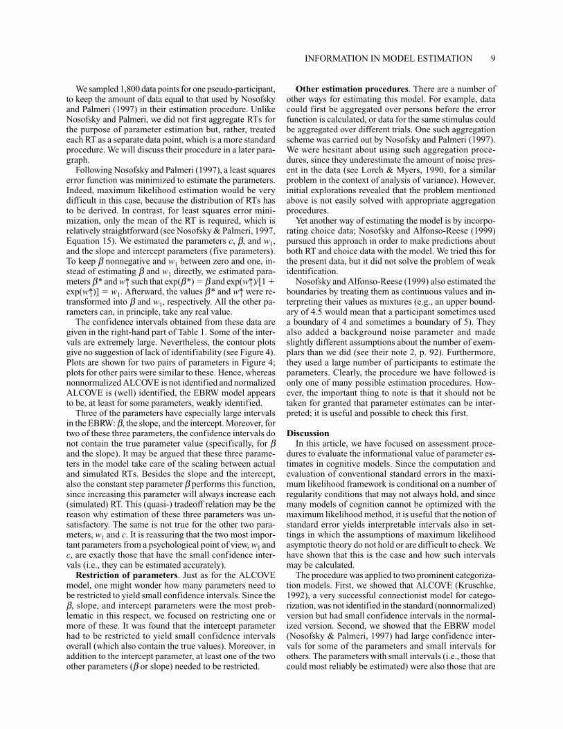
We sampled 1,800 data points for one pseudo-participant,to keep the amount of data equal to that used by Nosofskyand Palmeri (1997) in their estimation procedure. UnlikeNosofsky and Palmeri, we did not first aggregate RTs forthe purpose of parameter estimation but, rather, treatedeach RT as a separate data point, which is a more standardprocedure. We will discuss their procedure in a later para-graph.

Following Nosofsky and Palmeri (1997), a least squareserror function was minimized to estimate the parameters.Indeed, maximum likelihood estimation would be verydifficult in this case, because the distribution of RTs hasto be derived. In contrast, for least squares error mini-mization, only the mean of the RT is required, which isrelatively straightforward (see Nosofsky & Palmeri, 1997,Equation 15). We estimated the parameters c, β, and w1,and the slope and intercept parameters (five parameters).To keep β nonnegative and w1 between zero and one, in-stead of estimating β and w1 directly, we estimated para-meters β* and w1* such that exp(β*) � β and exp(w1*)/[1 �exp(w1*)] � w1. Afterward, the values β* and w1* were re-transformed into β and w1, respectively. All the other pa-rameters can, in principle, take any real value.

The confidence intervals obtained from these data aregiven in the right-hand part of Table 1. Some of the inter-vals are extremely large. Nevertheless, the contour plotsgive no suggestion of lack of identifiability (see Figure 4).Plots are shown for two pairs of parameters in Figure 4;plots for other pairs were similar to these. Hence, whereasnonnormalized ALCOVE is not identified and normalizedALCOVE is (well) identified, the EBRW model appearsto be, at least for some parameters, weakly identified.

Three of the parameters have especially large intervalsin the EBRW: β, the slope, and the intercept. Moreover, fortwo of these three parameters, the confidence intervals donot contain the true parameter value (specifically, for βand the slope). It may be argued that these three parame-ters in the model take care of the scaling between actualand simulated RTs. Besides the slope and the intercept,also the constant step parameter β performs this function,since increasing this parameter will always increase each(simulated) RT. This (quasi-) tradeoff relation may be thereason why estimation of these three parameters was un-satisfactory. The same is not true for the other two para-meters, w1 and c. It is reassuring that the two most impor-tant parameters from a psychological point of view, w1 andc, are exactly those that have the small confidence inter-vals (i.e., they can be estimated accurately).

Restriction of parameters. Just as for the ALCOVEmodel, one might wonder how many parameters need tobe restricted to yield small confidence intervals. Since theβ, slope, and intercept parameters were the most prob-lematic in this respect, we focused on restricting one ormore of these. It was found that the intercept parameterhad to be restricted to yield small confidence intervalsoverall (which also contain the true values). Moreover, inaddition to the intercept parameter, at least one of the twoother parameters (β or slope) needed to be restricted.

Other estimation procedures. There are a number ofother ways for estimating this model. For example, datacould first be aggregated over persons before the errorfunction is calculated, or data for the same stimulus couldbe aggregated over different trials. One such aggregationscheme was carried out by Nosofsky and Palmeri (1997).We were hesitant about using such aggregation proce-dures, since they underestimate the amount of noise pres-ent in the data (see Lorch & Myers, 1990, for a similarproblem in the context of analysis of variance). However,initial explorations revealed that the problem mentionedabove is not easily solved with appropriate aggregationprocedures.

Yet another way of estimating the model is by incorpo-rating choice data; Nosofsky and Alfonso-Reese (1999)pursued this approach in order to make predictions aboutboth RT and choice data with the model. We tried this forthe present data, but it did not solve the problem of weakidentification.

Nosofsky and Alfonso-Reese (1999) also estimated theboundaries by treating them as continuous values and in-terpreting their values as mixtures (e.g., an upper bound-ary of 4.5 would mean that a participant sometimes useda boundary of 4 and sometimes a boundary of 5). Theyalso added a background noise parameter and madeslightly different assumptions about the number of exem-plars than we did (see their note 2, p. 92). Furthermore,they used a large number of participants to estimate theparameters. Clearly, the procedure we have followed isonly one of many possible estimation procedures. How-ever, the important thing to note is that it should not betaken for granted that parameter estimates can be inter-preted; it is useful and possible to check this first.

DiscussionIn this article, we have focused on assessment proce-

dures to evaluate the informational value of parameter es-timates in cognitive models. Since the computation andevaluation of conventional standard errors in the maxi-mum likelihood framework is conditional on a number ofregularity conditions that may not always hold, and sincemany models of cognition cannot be optimized with themaximum likelihood method, it is useful that the notion ofstandard error yields interpretable intervals also in set-tings in which the assumptions of maximum likelihoodasymptotic theory do not hold or are difficult to check. Wehave shown that this is the case and how such intervalsmay be calculated.

The procedure was applied to two prominent categoriza-tion models. First, we showed that ALCOVE (Kruschke,1992), a very successful connectionist model for catego-rization, was not identified in the standard (nonnormalized)version but had small confidence intervals in the normal-ized version. Second, we showed that the EBRW model(Nosofsky & Palmeri, 1997) had large confidence inter-vals for some of the parameters and small intervals forothers. The parameters with small intervals (i.e., those thatcould most reliably be estimated) were also those that are

10 VERGUTS AND STORMS

most important for purposes of psychological interpreta-tion of the categorization data. The remaining parameterswere shown to be less accurately estimable, but these pa-rameters have less substantial representational or process-ing interpretations. In conclusion, we think that theseapplications show the usefulness of this procedure in de-termining just how much can be concluded from numeri-cal parameter values in formal models of cognition.

Although we have focused on the models of Kruschke(1992) and Nosofsky and Palmeri (1997), this articleshould not be interpreted as a critique directed specificallyat these models. On the contrary, we want to stress the ap-plicability of the procedure for evaluating parameter esti-mates in any formal model of cognition. The models weevaluated in this article were chosen because they havebeen proven to be both tractable and very successful in fit-ting empirical data in the area of categorization. It remainsto be seen how other models fare in this respect.

REFERENCES

Akaike, H. (1974). A new look at the statistical model identification.IEEE Transactions on Automatic Control, 19, 716-723.

Anderson, J. R. (1991). The adaptive nature of human categorization.Psychological Review, 98, 409-429.

Ashby, F. G., & Maddox, W. T. (1992). Complex decision rules in cat-egorization: Contrasting novice and experienced performance. Jour-nal of Experimental Psychology: Human Perception & Performance,18, 50-71.

Crowther, C. S., Batchelder, W. H., & Hu, X. (1995). A measurement-theoretic analysis of the fuzzy logic model of perception. PsychologicalReview, 102, 396-408.

Dixon, M. J., Koehler, D., Schweizer, T. A., & Guylee, M. J.(2000). Superior single dimension relative to “exclusive or” catego-rization performance by a patient with category-specific visual ag-nosia: Empirical data and an ALCOVE simulation. Brain & Cogni-tion, 43, 152-158.

Johansen, M. K., & Palmeri, T. J. (2002). Are there representationalshifts in category learning? Cognitive Psychology, 45, 482-553.

Kruschke, J. K. (1992). ALCOVE : An exemplar-based connectionistmodel of category learning. Psychological Review, 99, 22-44.

Kruschke, J. K., & Johansen, M. K. (1999). A model of probabilisticcategory learning. Journal of Experimental Psychology: Learning,Memory, & Cognition, 25, 1083-1119.

Lamberts, K. (2000). Information-accumulation theory of speededclassification. Psychological Review, 107, 227-260.

Lorch, R. F., Jr., & Myers, J. L. (1990). Regression analyses of re-peated measures data in cognitive research. Journal of ExperimentalPsychology: Learning, Memory, & Cognition, 16, 149-157.

Martin, B. R. (1971). Statistics for physicists. London: Academic Press.Mood, A. M., Graybill, F. A., & Boes, D. C. (1974). Introduction to

the theory of statistics. Singapore: McGraw-Hill.Nobel, P. A., & Shiffrin, R. M. (2001). Retrieval processes in recog-

nition and cued recall. Journal of Experimental Psychology: Learn-ing, Memory, & Cognition, 27, 384-413.

Nosofsky, R. M., & Alfonso-Reese, L. A. (1999). Effects of similar-ity and practice on speeded classification response times and accura-cies: Further tests of an exemplar-retrieval model. Memory & Cogni-tition, 27, 78-93.

Nosofsky, R. M., Gluck, M. A., Palmeri, T. J., McKinley, S. C., &Glauthier, P. (1994). Comparing models of rule-based classifica-tion learning: A replication and extension of Shepard, Hovland, andJenkins (1961). Memory & Cognition, 22, 352-369.

Nosofsky, R. M., & Kruschke, J. K. (2002). Single-system models andinterference in category learning: Commentary on Waldron andAshby (2001). Psychonomic Bulletin & Review, 9, 169-174.

Nosofsky, R. M., Kruschke, J. K., & McKinley, S. C. (1992). Com-bining exemplar-based category representations and connectionistlearning rules. Journal of Experimental Psychology: Learning, Mem-ory, & Cognition, 18, 211-233.

Nosofsky, R. M., & Palmeri, T. J. (1997). An exemplar-based randomwalk model of speeded classification. Psychological Review, 104,266-300.

Press, W. H., Flannery, B. P., Teukolsky, S. A., & Vetterling, W. T.(1989). Numerical recipes: The art of scientific computing. Cam-bridge: Cambridge University Press.

Schervisch, M. J. (1995). Theory of statistics. New York: Springer-Verlag.

Shepard, R. N., Hovland, C. I., & Jenkins, H. M. (1961). Learningand memorization of classifications. Psychological Monographs, 75(13, Whole No. 517).

Wichmann, F. A., & Hill, N. J. (2001). The psychometric function: II.Bootstrap-based confidence intervals and sampling. Perception &Psychophysics, 63, 1314-1329.

NOTES

1. In the following, we will assume that there are only two possible cat-egories, but both the models and our analysis thereof easily extend to thecase with more than two categories.

2. Note, however, that in principle the 95% confidence interval can bederived from a lower dimensional plot only if off-diagonal values of theHessian matrix are (approximately) zero.

3. Technically, this is true only if all the eigenvalues of the Hessian ma-trix are nonzero and of the same sign. Also, the converse is strictly speak-ing not true (isocentric contour lines do not automatically imply a sec-ond-order function as in Equation 2), but the validity of the approximationbecomes very plausible nevertheless.

(Manuscript received October 31, 2002;revision accepted for publication April 26, 2003.)