SPACECRAFT RADIO FREQUENCY FLUCTUATIONS IN THE ...

Draft version November 5, 2018Typeset using LATEX twocolumn style in AASTeX62

SPACECRAFT RADIO FREQUENCY FLUCTUATIONS IN THE SOLAR CORONA:A MESSENGER-HELIOS COMPOSITE STUDY

David B. Wexler,1, ⇤ Joseph V. Hollweg,2 Anatoli I. Efimov,3 Liudmila A. Lukanina,3 Anthea J. Coster,4

Juha Vierinen,5 and Elizabeth A. Jensen6

1University of Southern Queensland Center for Astrophysics, Toowoomba, AU2Department of Physics, University of New Hampshire, Durham, NH, USA

3Kotel’nikov Institute of Radio Engineering and Electronics, Russian Academy of Sciences, Moscow, RU4MIT Haystack Observatory, Westford, MA, USA

5Department of Physics and Technology, University of Tromsø, Tromsø, Norway6Planetary Science Institute, Tuscon, AZ, USA

(Received 9 Sep 2018; Revised 4 Nov 2018; Accepted xxx)

Submitted to ApJ

ABSTRACT

Fluctuations in plasma electron density may play a role in solar coronal energy transport and dissipa-tion of wave energy. Transcoronal spacecraft radio sounding observations reveal frequency fluctuations(FF) that encode the electron number density disturbances, allowing exploration of coronal compres-sive wave and advected inhomogeneity models. Primary FF observations from MESSENGER 2009and published FF residuals from HELIOS 1975-1976 superior conjunctions were combined to producea composite view of equatorial region FF near solar minimum over solar o↵set range 1.4-25R�. Meth-ods to estimate the electron number density fluctuation variance from the observed FF were developed.We created a simple stacked flux tube model that incorporated both propagating slow density wavesand advected spatial density variations to explain the observed FF. Slow density waves accounted formost of the FF at low solar o↵set, while spatial density inhomogeneities advected at solar wind speeddominated above the sonic point at 6R�. Corresponding spatial scales ranged 1-38 Mm, with scalesabove 10 Mm contributing most to FF variance. Flux-tube structuring of the model introduced radialelongation anistropy at lower solar o↵sets, but geometric conditions for isotropy were achieved as thethe flux tube widths increased further out in the corona. The model produced agreement with the FFobservations up to 12R�. FF analysis provides information on electron density fluctuations in the solarcorona, and should take into account the background compressive slow waves and solar wind-relatedadvection of quasi-static spatial density variations.

Keywords: solar corona — radio sounding — solar wind — frequency fluctuations — acoustic waves

1. INTRODUCTION

Coronal heating and acceleration mechanisms remaina challenging research focus in solar physics. Models forenergy transfer must account for both the propagationand dissipation of energy from the photospheric sourcesto the coronal expanse. Intense heating of solar plasma

Corresponding author: David B. Wexler

[email protected], [email protected]

⇤ Guest research student, MIT Haystack ObservatoryWestford, MA, USA

occurs in the transition region and the base of corona,while the plasma acceleration occurs at higher levels ofthe solar atmosphere, and out into the extended corona.Alfven wave propagation, initiated by transverse mo-tions of the emanating photospheric magnetic field, re-mains a favored mechanism for transfer of energy intothe extended corona. Alfven waves have been observedin the chromosphere (De Pontieu et al. 2007), transitionregion and base of corona (McIntosh et al. 2011; Tom-czyk et al. 2007). The corresponding Faraday rotationfluctuations observed in radio sounding studies at vari-ous coronal heights (Efimov et al. 2015a,b; Jensen et al.

2 Wexler et al.

2013; Hollweg et al. 1982; Andreev et al. 1997; Wexler etal. 2017) support the notion of Alfven waves continuingthis energy transport out into the corona and interplan-etary space.The search for mechanisms to explain transfer and

dissipation of the Alfven wave energy in the coronagarners continued interest. Dissipation of propagatingwaves and associated turbulence (Cranmer et al. 2015)constitute one important class of coronal-heating mod-els. Nanoflare-reconnection mechanisms also warrantconsideration (Sakurai 2017; Klimchuk 2015) in the in-vestigation of coronal magnetic energy release. Cran-mer et al. (2007) and Cranmer (2010) studied 1-D sim-ulations of MHD wave dissipation. They modeled anAlfven wave-based turbulent heating rate for which theexact kinetic mechanism for energy dissipation was notspecified. Suzuki & Inutsuka (2005) studied coronal en-ergy dissipation in a 1-D MHD simulation using non-linear Alfven wave generation of compressive waves andshocks. They found that the energy flux from the slowwaves increased with heliocentric radial distance (here-after solar o↵set, SO) in the corona, while that of theAlfven waves decreased. They concluded that slow lon-gitudinal compressive waves may be generated in thecorona as part of the energy transfer and dissipationprocess.When directed along magnetic field lines in low-beta

solar plasma1, longitudinal compressive waves may beconsidered acoustic or slow magnetoacoustic (magne-tosonic) waves. We shall apply the terms slow waves,acoustic waves and compressive waves all with same in-tent. Compressive waves have been directly observed asintensity fluctuations propagating from the photosphereto the chromosphere, and observed in the lower corona(Nakariakov & Verwichte 2005). Unlike the Alfvenwaves, however, the slow waves do not propagate farinto the corona. Damping of these waves indicates dissi-pation, suggesting their potential importance in coronalenergy transfer.Observational studies of density fluctuations beyond

the base of corona relies on radio sounding techniques.Transcoronal spacecraft radio transmissions will exhibitcenter frequency fluctuations (FF) at the receiving ra-dio telescope, caused by refractive index variations inthe coronal plasma associated with electron density dis-turbances. Presence of coronal FF is well-establishedand may present spectral characteristics consistent withturbulence regimes in varying degrees of energy cascade

1 plasma � is the ratio of thermal pressure to magnetic energydensity, � = nkBT

B2/2µ0

development (Yakovlev & Pisanko 2018; Efimov et al.2010). Coronal FF signify underlying plasma electronconcentration inhomogeneities that may include quasi-static bulk turbulence features convected with the solarwind, as well as compressive waves propagating withinthe wind (Efimov et al. 1993). We speculate that slowcompressive waves could be ubiquitous in the corona andcontributory to the observed FF power spectra particu-larly below the sonic point, where the solar wind speedis less than the speed of sound. Fast MHD waves couldalso produce FF, but may be evanescent in the corona(Hollweg 1978). It has been proposed that coronal mag-netoacoustic waves are generated locally via nonlinearinteractions of Alfven waves (Chashei et al. 2005; Efi-mov et al. 2012).Quasiperiodic component (QPC) FF spectral en-

hancements appear intermittently in coronal radiosounding observations (Efimov et al. 2012). Miyamotoet al. (2014) reported on the radial distribution of slowcompressive waves in the solar corona using Akatsukispacecraft radio occultation observations. They iden-tified peaks in FF wavelet analysis, then quantifiedspectral power of the presumed quasiperiodic densitywaves. They used these isolated QPC wavetrains to es-timate the fractional electron density fluctuation basedon the idea that the observed FF enhancements wereproduced wholly by QPC density fluctuations. Theirresults supported the presence of coronal compressivewaves with amplitudes su�cient for nonlinear e↵ects toappear in the region where solar wind initial acceler-ation occurs. However, estimates of wave energy fluxwere 1-2 magnitudes less than values obtained from thenumerical model of Suzuki & Inutsuka (2005).In the present study we evaluate FF using combined

data from the MESSENGER 2009 and HELIOS 1975-76coronal radio sounding observations near superior con-junction. These data give a composite picture of FF forthe near-equatorial regions close to solar activity min-imum, providing information for SO 1.4-25R�. There-fore we are exploring the coronal regions of slow solarwind formation and initial acceleration. We presentan approach to deduce the density fluctuation spec-trum from the power spectrum of observed FF, consid-ering the system as an ensemble of stacked magneticflux tubes containing uncorrelated density disturbances.Our model shows that compressive waves might con-tribute significantly to the observed FF at low solar o↵-set, while advected quasi-static spatial density variationsimpress the signature of solar wind acceleration into theFF observations at solar o↵set beyond the first few so-lar radii. In Section 2 we present the observational dataand methods to process FF. In Section 3, we present the

Coronal Radio Frequency Fluctuations 3

(a) (b)

(c) (d)

Figure 1. Magnetic field modeling from solar surface to 2.5R� from the Community Coordinated Modeling Center. (a) CR2090, MESSENGER egress data 2009, (b) CR 1642, corresponding to part of the HELIOS 2 data 1976. Potential field sourcesurface magnetic maps (2.5R�) for the Wilcox Solar Observatory: (c) MESSENGER CR 2090 (d) HELIOS CR 1642.

pertinent radio propagation theory and the method todetermine density fluctuation variance, and the relatedfractional fluctuation parameter. Section 4 develops atwo-component model of the frequency measure fluctu-ations, then provides the parameters used to implementthe model and gives results. In Section 5, a compar-ison is made between the solar wind speeds based onmass conservation in the flux tubes, and speed predic-tions from an established isotropic turbulence bulk flowmodel (Armand et al. 1987; Efimov et al. 2008), high-lighting di↵erences in the lower coronal region for whichquasi-static isotropic turbulence models may be inappli-cable. Our conclusions are summarized in Section 6.

2. OBSERVATIONS AND DATA REDUCTION

Our composite data set consists of primary radio tele-scope observations of MESSENGER spacecraft in su-perior conjunction near the solar minimum in 2009, andarchival results from HELIOS 1 and 2 over 1975-6, againwith solar activity near a minimum. Figure 1 illus-

trates coronal conditions with magnetic field line mod-els (Community Coordinated Modeling Center, CCMC)and source surface synoptic magnetic maps (Wilcox So-lar Observatory) for representative Carrington rotations2090 (MESSENGER) and 1642 (HELIOS 2). In bothcases the sun was in a fairly quiet dipole configuration,with equatorial region closed lines consistent with over-lying streamers.The MESSENGER spacecraft radio data (X-band,

8.4GHz) were recorded with the 100-m Green Bank Tele-scope with dual polarization feeds to allow determina-tion of polarization position angles needed to analyzeFaraday rotation. Technical details are found in Wexleret al. (2017) and Jensen et al. (2013). Here we are ex-ploring only the fluctuations in signal frequency. Ob-servations were recorded during ingress to superior con-junction on 8 Nov 2009, yielding 5000 seconds of us-able data over SO range 1.38-1.49R�. Egress recordingswere made on 10 Nov 2009, resulting in 14400 secondsof data covering SO range 1.63-1.89R�. Figure 2 shows

4 Wexler et al.

Figure 2. Approximate positioning of the LOS proximate points during the MESSENGER observations, shown on backgroundimages of STEREO B COR1 (green hues starting at inner occluding disk rim) and SOHO LASCO C2 (orange hues) for 10 Nov2009. The COR1 streamer configuration is only approximate because STEREO B was aligned obliquely to the MESSENGERLOS towards Earth. The central inset is an EIT 171A image from SOHO for the same date.

the approximate positioning of the points of closest ap-proach (proximate points) on the sounding line-of-sight(LOS) during the MESSENGER observations, shown ona background coronal images for 10 Nov 2009.The MESSENGER FF data were analyzed in a one-

second cadence from primary baseband data, which wererecorded at a 5 MHz sampling rate. For each one-seconddata frame, the radio peak baseband frequency was de-termined by a Guassian curve best-fit algorithm appliedto the power spectrum of the radio signal. A sample2000-second record of MESSENGER zero-centered ra-dio frequency data is shown in figure 3a. Clear fluctu-ations are evident in the frequency time series (upperpanel), along with a slow trend attributed to Doppler-shift from the spacecraft motion relative to Earth. Forsuch short data segments, the slow trend was removedwith a second-order polynomial fit (Song & Russell1999). The detrended data constitute the frequency fluc-tuation time series (lower panel). In the literature this

type data is variably referred to as Doppler residuals,Doppler noise or just (frequency) residuals.The power spectrum for the sample FF segment is

shown in figure 3b. Above ⇠30 mHz, the power-lawcurve drops into a flat spectral floor. The low-frequencypower is reduced by the detrend procedure, to revealthe spectrum believed to more accurately reflect the un-derlying plasma density fluctuations. The sample spec-trum shows enhanced spectral density over 5-7 mHz,consistent with a QPC. The variance of FF, �2

FF , wasobtained from numerical integration over a specified fre-quency band (see next section). The lower limit was setby the record length, and upper limit was set to a fre-quency below where the power spectrum drops into thenoise floor (the theoretical upper limit may be as highas the Nyquist frequency: 0.5 x sampling rate in s�1).Our practical range for frequency integration to obtain�

2FF was 1-28 mHz.In the MESSENGER data, considerable variability

was noted in the spectral index. Sporadic presentation


(a) (b)

Figure 3. Left: Time series of zero-centered frequency data. Upper panel shows the frequency fluctuation (FF) time series fora 2000-second analysis frame, at SO 1.675 R�. The dashed line is the second order polynomial used to remove the slow trendattributed to the Doppler shift of spacecraft motion. The lower panel shows the FF time series after the detrend procedure wasapplied. Right: Power spectral density (PSD) of the FF analysis segment. The detrend procedure a↵ects mostly low-frequencyspectral power, as shown with the dotted line. In this sample, enhancement of spectral power over 5-7 mHz relative to thebackground spectrum is noted.

of localized enhanced spectral power was noted. Indi-vidual data segments showed spectral indices below orabove the classic Kolmogorov 2/3 spectral index2 for FF.The spectral index determination is sensitive to methodof detrend, frequency range selected for the index linefit, noise reduction and smoothing, so it is best inter-preted cautiously in the present limited data set. Thespectral index was fitted over 1-10 mHz. Our methodfor power spectral processing included extraction of themean high-frequency noise floor and application of a 5-point smoothing algorithm with 1:2:3:2:1 weighting. Forthe MESSENGER data, we found the average spectralindex in ingress to be ↵ = 0.55 ± 0.08 and in egress,↵ = 0.58± 0.10.The HELIOS frequency fluctuation data (S-band, 2.3

GHz) were obtained already in integrated form fromJPL Deep Space Network Progress Reports (Berman &Rockwell 1975; Berman et al. 1976). The report pro-vided the best (i.e. smallest) noise estimates by av-eraging three selected groups of 10-20 averaged valuesjudged to provide the lowest noise values (as RMS) fora 60-second data sampling rate. These frequency datawere obtained from various DSN ground tracking sta-tions: 11, 12 and 14 in California, US, 42 and 43 inCanberra, AU and 61 and 62 in Madrid, Spain. The HE-

2 spectral index, ↵, is presented using positive index convention;the actual log-log spectral slope is negative

LIOS data were reported in two cycles of observationsfor superior conjunction in 1975, covering DOY 96-166,and DOY 227-251, and one cycle of observations fromHELIOS 2 in 1976, DOY 120-165. The HELIOS datacovered heliocentric o↵set range 2.22-25R�.The frequency fluctuations are sensitive to radio trans-

mission wavelength � (see Section 3). We combined theMESSENGER and HELIOS data sets by using the ra-dio wavelength-independent RMS frequency fluctuationmeasure �FM defined as

�FM =

p�

2FF

�

(1)

For the S-band observations, � = 0.1304 m and for X-band, � = 0.0357 m. The frequency-fluctuation mea-sure (FM) is analogous to the rotation measure used forFaraday rotation. A summary of the MESSENGER-HELIOS primary �FM composite data is given in figure4.To make the HELIOS frequency measure fluctuation

observations comparable to those from MESSENGER,two factors needed consideration. The first was cor-rection for the HELIOS two-way signal exposure toplasma inhomogeneities. In general, addition of vari-ances for time series x and y may combined as �

2x+y =

�

2x + �

2y + 2covariance(xy). In completely uncorrelated

x and y fluctuations, the covariance is zero so the addi-tion of x and y variances is simply the sum of individualvariances. However in the case of completely correlated

6 Wexler et al.

Figure 4. Composite of the frequency measure fluctuations,�FM . The MESSENGER data were obtained in a one-wayradio configuration. The 2-way HELIOS data shown herewere taken directly from JPL technical reports, normalizedto radio wavelength, but not yet corrected for correlated 2-way propagation inhomogeneities and the di↵erence in e↵ec-tive frequency band.

x and y signals, say x=y, the covariance(xy) = �

2x and

the total variance for the doubled path becomes 4�2x.

Two-way transmission enhancement in HELIOSsounding data was described by Efimov et al. (2004). Ina two-way regime, an outgoing terrestrial radio trans-mission crosses the corona en route to the spacecraft,then the spacecraft returns a phase-linked signal backthrough the corona to the receiving system on Earth.Spacecraft transmissions sent from the outer heliosphereshould have fluctuations uncorrelated to those of theoriginal inbound signal because the coronal plasma den-sity inhomogeneities should have moved and changedduring the interval required to reach the spacecraft andback. For such uncorrelated fluctuations, �2

FM arisingfrom a two-way path would be twice that of a one-wayobservation. However, the inner heliospheric position-ing of HELIOS during the 1975-6 sounding campaignresulted in largely correlated fluctuations on the returnpath, bringing the total variance to four times that of aone-way trip.An additional correction was required to compensate

for the di↵erence in e↵ective integration bands betweenHELIOS and MESSENGER data. HELIOS observa-tions, with one-minute frequency residual sampling overan average of 15 minutes, resulted in a frequency band1.11-8.33 mHz. Assuming spectrum of the Kolmogorovform, variance obtained from the 1.11-8.33 mHz bandwas about half the variance obtained over 1-28 mHz, towithin 5%. Combining the two separate e↵ects on HE-

LIOS variance, the Doppler residuals were multiplied bytwo for the bandwidth correction but divided by four tocorrect for the correlated two-way propagation. Takentogether the net correction was division of the reportedHELIOS variances by two (RMS by

p2), to approximate

equivalence with the one-way MESSENGER variance.

3. THE FREQUENCY FLUCTUATIONS MODEL

Radio propagation theory indicates that variations inthe signal frequency observed at the radio telescope,fobs, are related to the original transmitted frequency,f0, by fractional Doppler shift due to spacecraft veloc-ity Vrel relative to the radio LOS, and the time rate ofchange in electron density across the LOS (Efimov et al.2007; Jensen et al. 2016; Patzold et al. 2012); also seeHollweg & Harrington (1968); Vierinen et al. (2014):

fobs = f0 �Vrel

c

f0 +1

2⇡re�

d

dt

Z L

0ne(s, t)dS (2)

where � = cf0

is the radio transmitter wavelength, c isthe speed of light, ne is the electron number density, dSis the LOS integration path increment and the classicalelectron radius, re = 2.82⇥ 10�15 m, is

re =e

2

4⇡✏0mec2, (3)

S.I. units are used throughout unless otherwise noted.Here we develop a simplified coronal model consisting

of stacked slabs (Figure 5), intended to represent theseries of roughly parallel magnetic flux tubes throughwhich the sounding radio signal passes. In each fluxtube we treat the electron density as varying in time andspace along the solar radial axis, but vertically constantat a given moment over the integration element LLOS

equivalent to the flux tube width, i.e. the correlationlength along the LOS.When the Doppler shift is removed by a suitable de-

trend procedure (assumes the spacecraft motion is aslowly changing variable which can be well-representedby trajectory data or a mathematical function), then theequation for instantaneous frequency fluctuation of theradio signal frequency, �f(t) = fobs(t)� f0, for a singleslab simplifies to

�f(t) =1

2⇡re�LLOS

d

dt

ne(t). (4)

The electron number density includes a mean elec-tron number density ne(r) and a fluctuating componentof amplitude �ne. Only the fluctuating component willcontribute to the observed FF. For a density oscillationof form �ne(t) = �ne exp�i!t the time derivative has


Figure 5. The simplified scheme of oscillating densityfluctuations aligned parallel to the magnetic field, in a se-ries of stacked flux tubes. Each horizontal strip containsplasma density oscillations, illustrated by brightness vari-ations. LRAD is the horizontal length scale for convectedquasi-static density disturbances. The vertical scale LLOS

corresponds to width of a flux tube. The bulk plasma frameoutflow speed is VSW . Individual flux tube density fluctua-tions combine with random-walk statistics to yield the RMSfluctuation for the e↵ective LOS, Le.

magnitude !�ne. This relation is captured in the Fouriertransform:

F{�f(t)} =�i

2⇡re!�LLOSF{�ne(t)} (5)

Then using the FF power spectral density for a datasegment of temporal length T, notated |FF (!)|2 andgiven as 1

T F{�f(t)}F⇤{�f(t)}, we find

|FF (!)|2 =1

4⇡2r

2e�

2!

2L

2LOS |�ne(!)|2 (6)

where |�ne(!)|2 is the corresponding power spectral den-sity of electron concentration fluctuations.In terms of the oscillation frequency in Hz, ⌫ = !/2⇡,

and converting to radio-wavelength normalized fluctua-tion measure FM (equation 1), we obtain

|FM(⌫)|2 = r

2e⌫

2L

2LOS |�ne(⌫)|2 (7)

The electron concentrations along the LOS are gen-erally greatest near the proximate point. Heliocentricdistance, R, to the proximate point is the ”solar o↵set”(SO). This radial distance, when given in solar radiusunits (R�), will be notated r; R = rR�. For radiosounding studies, the LOS integration path lengths aretypically considered SO/2 in either direction from theproximate point for spherically symmetric coronal mod-els, giving an e↵ective integration length Le equal to R.The randomized density fluctuations of individual flux

tubes combine on the LOS as a sum of individual vari-ances. Using equation (7) for a single flux tube, multi-plication by the number of stacked flux tubes R/LLOS

gives the relation between the FM spectrum and theunderlying ne fluctuation spectrum as

|FM(⌫)|2 = r

2e⌫

2LLOSR|�ne(⌫)|2 (8)

Thus knowledge of the FM power spectrum from ob-servations can be used readily to determine the impliedelectron density fluctuation power spectrum (Figure 6).Note that this expression does not depend on whichphysical mechanism, e.g. propagating waves versus bulkoutflow of density inhomogeneities, produces the densityfluctuations on the sounding LOS. There is no assump-tion about the state of turbulence. We will clarify thosecontributions in section 4.

Figure 6. The electron density fluctuation power spectrum�n2

e (upper, blue curve) is calculated from the FM powerspectrum (lower, thick red curve) FM2 using equation (8)The variances �2

FM and �2ne

are integrated quantities shownas the hatched and light filled areas respectively, in the 0.001-0.028 Hz frequency band.

In a pure radial flux tube configuration, the LOS con-tributions would increase with azimuthal fan-out angle� as LLOS/ cos�. For a fan-out from the equator of nomore than ±30o, the maximum increase would be about15% at the wings, and most of the LOS path wouldhave an increase in LLOS of less than 10%. We chosethe simplified scheme of stacked horizontal elements torepresent the radial flux tubes (� = 0).Integrated measures are used to represent the spec-

tral density information in consolidated form to facili-tate comparisons. The HELIOS data were available onlyin the form of variances, not as primary spectral data,

8 Wexler et al.

and therefore required reworking of equation (8) into aformat based on integrated quantities. The goal is to ob-tain the number density fluctuation information basedon knowledge of the FF spectrum or even just the FFvariance.The fluctuation variances �2

FM and �

2ne

are defined forfrequency integration range [a,b] by

�

2FM ⌘

Z b

a

|FM(⌫)|2d⌫ (9)

�

2ne

⌘Z b

a

|�ne(⌫)|2d⌫ (10)

Equations (8) and (10) may be combined to give

�

2ne

=1

r

2eLLOSR

Z b

a

|FM(⌫)|2

⌫

2d⌫ (11)

These variances, represented as filled areas under thecurves in Figure 6, can be obtained by numerical inte-gration when the FM power spectrum is specified. Incontrast, the HELIOS frequency fluctuation data weregiven only as variances, so we treated the curves as ide-alized, single power-law spectra in order to estimate �ne

as follows.Assuming that the FM power spectrum follows a

power law of the form |FM(⌫)|2 = ⇣⌫

�↵, we may evalu-ate the integrals in equations (9) and (11) over frequencyrange [a,b] as

�

2FM =

⇣

1� ↵

⌫

(1�↵)|ba (12)

�

2ne

=�1

(↵+ 1)

⇣

r

2eLLOSR

⌫

�↵�1|ba (13)

For a known �

2FM and ↵, we can estimate ⇣ obser-

vationally, although it cancels out in the subsequentequation (14). We tested relation (10) with 2000-secondMESSENGER data segments and found that, when us-ing spectral index fitted over 1-10 mHz on the powerspectrum, the estimated variance matched the computa-tionally integrated value for range 0.001-0.028 Hz within10%.Equation (8) can be placed in the form of variances for

FM and �ne by integrating both sides using expressions(9), (10) and (11), then substituting in relations (12)and (13) to obtain

�

2FM = r

2e⌫

2cLLOSR�

2ne

(14)

provided a scaling frequency ⌫c is found from:

⌫

2c =

↵+ 1

↵� 1

⌫

1�↵|ba⌫

�↵�1|ba(15)

Therefore, �2ne

can be estimated from known �

2FM if

spectral index ↵ is known or well-approximated. Thisspecific electron number density variance is pertinentonly for the given frequency range, here 1-28 mHz. Sim-ilarly, the scaling frequency ⌫c is linked to the specificintegration frequency range (the ”observation window”)and the applicable spectral index for the data understudy.The fractional density fluctuation ✏ is defined as

✏ =�ne

ne(16)

where the mean local electron number density ne(r)may be estimated by a parameter model or calculatedfrom dual-frequency ranging data. Finally, equations(14) and (16) are consolidated to produce

✏ =�FM

re⌫cne

pLLOSR

(17)

This is the observational model for ✏ based on random-ized density fluctuations on the LOS in a stacked flux-tube coronal plasma. It is important to note that while✏ is a useful marker of electron density disturbances, thevalues must be interpreted in the context of the specificintegration frequency limits, accuracy of ⌫c (knowledgeand stability of the spectral index) and suitability of theelectron number density model. All factors which influ-ence �FM , such as of shifting frequencies on the sound-ing LOS from acceleration of the solar wind, may be im-pressed into the observational determination of ✏. In thenext section we implement equation (17) to present the✏ derived from the MESSENGER/HELIOS FF observa-tions, then develop a two-component density fluctuationmodel that incorporates the e↵ect of solar wind outflow.

4. IMPLEMENTATION AND RESULTS

A number of coronal electron number density mod-els exist. Several are reviewed by Bird & Edenhofer(1990). A standard model for electron number density isthe Allen-Baumbach formula derived from coronagrapheclipse observations of the K-corona:

ne(r) =

✓2.99

r

16+

1.55

r

6

◆⇥ 1014 (18)

in m�3. The first term on the right is important at closeSO, <⇡ 1.2R�, while the second term was intended tobe applicable out to 2-3 Rs. The model assumes spher-ical symmetry. To extend the range of number den-sity estimates into the extended corona, a third termwith a near inverse square power relationship is usu-ally added. The deviation from an exact 2 exponent inthe added term is attributed to acceleration of the solar


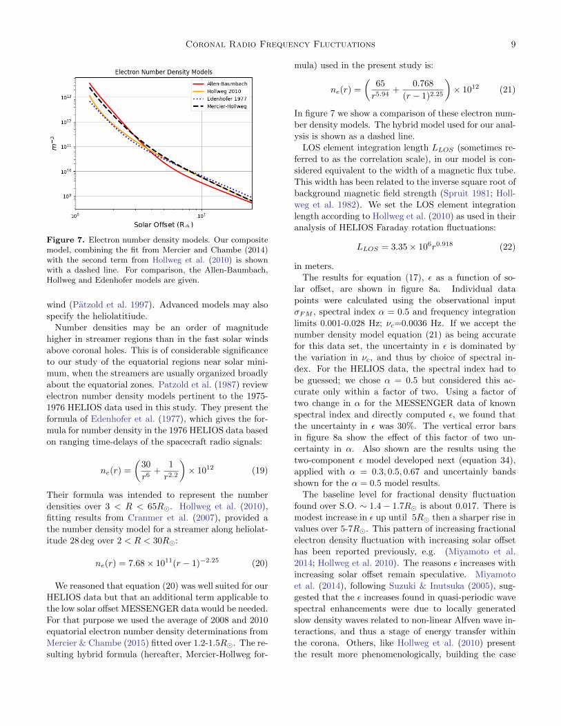
Figure 7. Electron number density models. Our compositemodel, combining the fit from Mercier and Chambe (2014)with the second term from Hollweg et al. (2010) is shownwith a dashed line. For comparison, the Allen-Baumbach,Hollweg and Edenhofer models are given.

wind (Patzold et al. 1997). Advanced models may alsospecify the heliolatitiude.Number densities may be an order of magnitude

higher in streamer regions than in the fast solar windsabove coronal holes. This is of considerable significanceto our study of the equatorial regions near solar mini-mum, when the streamers are usually organized broadlyabout the equatorial zones. Patzold et al. (1987) reviewelectron number density models pertinent to the 1975-1976 HELIOS data used in this study. They present theformula of Edenhofer et al. (1977), which gives the for-mula for number density in the 1976 HELIOS data basedon ranging time-delays of the spacecraft radio signals:

ne(r) =

✓30

r

6+

1

r

2.2

◆⇥ 1012 (19)

Their formula was intended to represent the numberdensities over 3 < R < 65R�. Hollweg et al. (2010),fitting results from Cranmer et al. (2007), provided athe number density model for a streamer along heliolat-itude 28 deg over 2 < R < 30R�:

ne(r) = 7.68⇥ 1011(r � 1)�2.25 (20)

We reasoned that equation (20) was well suited for ourHELIOS data but that an additional term applicable tothe low solar o↵set MESSENGER data would be needed.For that purpose we used the average of 2008 and 2010equatorial electron number density determinations fromMercier & Chambe (2015) fitted over 1.2-1.5R�. The re-sulting hybrid formula (hereafter, Mercier-Hollweg for-

mula) used in the present study is:

ne(r) =

✓65

r

5.94+

0.768

(r � 1)2.25

◆⇥ 1012 (21)

In figure 7 we show a comparison of these electron num-ber density models. The hybrid model used for our anal-ysis is shown as a dashed line.LOS element integration length LLOS (sometimes re-

ferred to as the correlation scale), in our model is con-sidered equivalent to the width of a magnetic flux tube.This width has been related to the inverse square root ofbackground magnetic field strength (Spruit 1981; Holl-weg et al. 1982). We set the LOS element integrationlength according to Hollweg et al. (2010) as used in theiranalysis of HELIOS Faraday rotation fluctuations:

LLOS = 3.35⇥ 106r0.918 (22)

in meters.The results for equation (17), ✏ as a function of so-

lar o↵set, are shown in figure 8a. Individual datapoints were calculated using the observational input�FM , spectral index ↵ = 0.5 and frequency integrationlimits 0.001-0.028 Hz; ⌫c=0.0036 Hz. If we accept thenumber density model equation (21) as being accuratefor this data set, the uncertainty in ✏ is dominated bythe variation in ⌫c, and thus by choice of spectral in-dex. For the HELIOS data, the spectral index had tobe guessed; we chose ↵ = 0.5 but considered this ac-curate only within a factor of two. Using a factor oftwo change in ↵ for the MESSENGER data of knownspectral index and directly computed ✏, we found thatthe uncertainty in ✏ was 30%. The vertical error barsin figure 8a show the e↵ect of this factor of two un-certainty in ↵. Also shown are the results using thetwo-component ✏ model developed next (equation 34),applied with ↵ = 0.3, 0.5, 0.67 and uncertainly bandsshown for the ↵ = 0.5 model results.The baseline level for fractional density fluctuation

found over S.O. ⇠ 1.4� 1.7R� is about 0.017. There ismodest increase in ✏ up until 5R� then a sharper rise invalues over 5-7R�. This pattern of increasing fractionalelectron density fluctuation with increasing solar o↵sethas been reported previously, e.g. (Miyamoto et al.2014; Hollweg et al. 2010). The reasons ✏ increases withincreasing solar o↵set remain speculative. Miyamotoet al. (2014), following Suzuki & Inutsuka (2005), sug-gested that the ✏ increases found in quasi-periodic wavespectral enhancements were due to locally generatedslow density waves related to non-linear Alfven wave in-teractions, and thus a stage of energy transfer withinthe corona. Others, like Hollweg et al. (2010) presentthe result more phenomenologically, building the case

10 Wexler et al.

(a) (b)

Figure 8. (a) Fractional electron density fluctuation ✏ (crosses), as calculated (equation 17) for the specified integrationfrequency band and with ↵ = 0.5; the wide error bars are due mostly to factor of 2 uncertainty in ↵. The solid line shows themodel for ✏ developed from combined acoustic wave and convected density variances (equation 35). The model itself has onlymodest sensitivity to choice of ↵ but the error bars are wide due primarily to uncertainly in ⌫c which is highly sensitive to ↵.(b) Modeled mass flux speed Vflux and sound speed Cs. The plasma speeds for mass conservation in the flux tubes were usedto represent solar wind speed VSW in implementation of the frequency fluctuation model.

that the fractional density fluctuations, whatever theirsource, were too small to account for the observed coro-nal Faraday rotation fluctuations.It is useful to compare the plot of ✏ (figure 8a) to esti-

mated solar wind speed, VSW , and the speed of sound,Cs (figure 8b). The speed of sound is found from

Cs =

s�kBT

mp(23)

with ratio of specific heats � = 5/3, proton mass mp,Boltzmann constant kB and coronal temperature T inKelvins. Coronal temperature was estimated by a fit todata presented by Newkirk (1967), in which it was con-sidered Ti = Te = T based on the available information.Specifically the coronal temperature was estimated as

log T = �0.54 log(r) + 6.30 (24)

such that the temperature dropped from 2.2 ⇥ 106K atthe solar surface to 0.4⇥ 106K at SO=20R�.The solar wind outflow speed, VSW , is modeled on

mass conservation in the flux tubes:

neL2LOSVflux = constant (25)

To enact the wind speed model we specify Vflux = 250km/s at r=20R�. This is a reasonable value for slowsolar wind speed at that solar o↵set, in accordance withstudies in optical (Sheeley et al. 1997), radio intensity

scintillation (Imamura et al. 2014) and dual-frequencyradio analysis (Muhleman & Anderson 1981). Modeledsolar wind speeds and sound speeds are shown in figure8b. The sonic point is at ⇠ 6R�, consistent with the5 � 7R� range mentioned by Efimov et al. (1993), andintermediate between lows of 2.5R� (Suzuki & Inutsuka2005) to 3.5R� in wave-heating simulations (Cranmeret al. 2007) and an upper range 12-14R� discussed byYakovlev & Pisanko (2018).It is interesting that the inflection in ✏, at r=6R�,

occurs in the region of the estimated sonic point. Theobservation suggests the possibility that the observedFF may be dominated by the advected ”frozen-in”,slowly changing density inhomogeneities near and abovethe sonic point. Propagating slow compressive waves(acoustic or slow magnetoacoustic) could then providethe main contribution below the sonic point.We now explore the basis for the observed increase in ✏

with increasing solar o↵set. The key observational inputis �FM . In our method, the ”observational window” isa fixed bandwidth [a,b] that is built into the scaling fre-quency ⌫c, such that an observed increase in �FM mustbe associated with a corresponding increase �ne

for agiven SO (see equation 14). We investigate whether theadvection of density disturbances across the soundingLOS by solar wind bulk outflow can explain the radialdependence of observational ✏ demonstrated in Figure8a.


A two-component model for ✏ and �

2FM is proposed,

based on two premises: 1) the quiet, equatorial coronamust have some basal spectrum of density inhomo-geneities from propagating slow density waves andquasi-static spatial density variations, and 2) the densityoscillations advected with the solar wind flow presentfrequency-shifted spectral information to the soundingLOS observational window. Given the negative powerlaw form of the density and FM fluctuation spectra, aright-shifted power spectrum will bring increased powerinto the fixed observational frequency window. It willbe shown that the propagating slow density waves willdominate the observational �FM and ✏ at low S.O. whilethe advected spatial spectrum of density variations willdominate as the solar wind speed prevails over the localspeed of sound.The two-component model developed below does re-

quire a number of assumptions and use of established pa-rameter formulae. Specifically, models for radial depen-dence of the speed of sound, solar wind outflow speed,coronal streamer background electron number densityand a choice of characteristic length scale for the quasi-static spatial density variations will be needed. We as-sume that a baseline level of fractional density fluctua-tion, ✏BL is present throughout the coronal region understudy when referenced to the comoving solar wind frameand the same frequency band (here, 1-28 mHz). Ourstarting point is ✏BL = 0.017 ± 0.002 as found from re-sults in Figure 8a, averaged over S.O. 1.4-1.7R� wherethere is relatively little e↵ect from solar wind. As wewish to provide the simplest explanation for the SO-dependence of ✏ with the fewest assumptions, we set ✏BL

to apply equally as the fractional RMS amplitude forboth the density waves and the spatial inhomogeneities.Also, we point out that the possibility of ✏BL chang-ing with time or position is not being considered in thismodel. The model we propose can be modified to in-corporate such refinements when new data allowing dis-crimination of density sources become available.In this model we predict the increase in observed ✏

(equation 17) relative to ✏BL will be the ratio of a shiftedscaling frequency ⌫shift that includes the e↵ect of ad-vection across the sounding LOS, to the native scalingfrequency ⌫c:

✏model ⌘ ✏BL⌫shift

⌫c(26)

Since ✏BL and ⌫c are known, the problem reduces tospecifying ⌫shift for acoustic waves and spatial densityvariations advected with the solar wind, as a function ofsolar o↵set.Acoustic waves introduced at the lower corona are ex-

pected to damp out quickly, but turbulent actions in the

corona could be expected to produce density waves lo-cally. Our modeled density wave component is thereforeconsidered to be a spectrum of locally generated slowwaves exhibiting a baseline level of density fluctuationall through the coronal region under study. Further-more, we consider that the slow waves may travel in ei-ther direction at the speed of sound, Cs. With advectionoutward at solar wind speed VSW , we will have a combi-nation of speeds VSW +Cs and VSW �Cs at the sound-ing LOS. When combined equally in quadrature, theRMS speed is Vacous =

pV

2SW + C

2s . The characteristic

source frequency of the acoustic wave is fwave and thelength scale for the acoustic waves is Lacous = Cs/fwave.In the context of equation (14), fwave = ⌫c, specificto the given observational frequency band. The shiftedacoustic wave frequency, ⌫shift,acous = Vacous/Lacous, is

⌫shift,acous = ⌫c

pV

2SW + C

2s

Cs(27)

With increasing SO, the e↵ect of solar wind speed can-not be ignored. For the acoustic waves, equation (14)may be adapted to

�

2FMacous

= r

2e⌫

2c ✏

2BL

V

2SW + C

2s

C

2s

n

2eLLOSR (28)

and the scaling for ✏ is then

✏model,acous = ✏BL

pV

2SW + C

2s

C

2s

(29)

At low SO, where VSW << Cs, ⌫shift ⇡ ⌫c, equations(28, 29) simplify and the results for baseline fluctuationsare demonstrated. Results for equation (28) are shownwith a dashed line in Figure 9. The acoustic waves can-not explain the �FM findings beyond about 3.0R�. Onechange to the model to keep the density waves perti-nent at higher SO could be increasing ✏BL, the under-lying amplitude of density wave fluctuations. This wasthe approach taken by Miyamoto et al. (2014). Thealternative is to introduce quasi-static spatial densityvariations that produce frequency fluctuations on thesounding LOS as the variations are advected by the solarwind bulk flow. There is considerable intuitive appealto bringing in this latter approach. In a general sense,the moving quasi-static density variations may roughlycorrespond to the ”Sheeley blobs” (Sheeley et al. 1997)and more recent optical demonstrations of outflowingintensity enhancements (DeForest et al. 2018). In addi-tion, the density variations will tend to be streamed radi-ally, potentially introducing an element of SO-dependentanisotropy (roughly defined LRAD/LLOS > 1) in theflux tubes. Exploring anisotropic features will help com-pare our model to work based on isotropic symmetriccorona models (see next section).

12 Wexler et al.

Quasi-static spatially distributed plasma density in-homogeneities advected past the sounding LOS result inFF. Let LRAD be the characteristic radial length scaleof the density inhomogeneities. Assuming the radial(⇠horizontal) orientation of the system, the frequencyof the density fluctuations ⌫shift on the observing LOSis found from the time derivative

d

dt

= Vrad ·r (30)

The solar wind speed VSW is assigned as Vrad and r ⇠1/LRAD.In analogy to the formulation for acoustic waves

(equation 28), the advected spatial variations contributeto the observed frequency measure fluctuation as

�

2FMspatial

= r

2e⌫

2c ✏

2BL

VSW

LRAD

1

⌫c

�2n

2eLLOSR (31)

and the scaling for ✏ is

✏model,spatial = ✏BLVSW

LRAD

1

⌫c(32)

in accordance with equation (26).The model is completed by combining the component

variances

�

2FMMODEL

= r

2e⌫

2c ✏

2modeln

2eLLOSR (33)

where ✏model is

✏model = ✏BL

sV

2SW + C

2s

C

2s

+

VSW

LRAD⌫c

�2(34)

We assign a value to LRAD from observational resultsat r=10R� using equations 33 and 34. Using the meanobserved �FM = 1.80 Hz/m, VSW = 160 km/s, Cs = 85km/s we find LRAD = 12000 km for ✏BL = 0.017 and⌫c = 0.0036 Hz (based on ↵ = 0.5, equation 15). Wehold LRAD constant for the SO range under study.Note that our approach uses a two point calibration:

✏BL is set from the low SO observations where acous-tic waves dominate the observed fluctuations, whereasLRAD is set at higher SO where the advected quasi-static density variations dominate the results. The cali-bration is specific to the frequency integration range and↵ used to obtain ⌫c and to the SW speed model used todetermine LRAD.Results of the two-component variances model are

shown in figure 9. The acoustic waves account for mostof the observed frequency measure fluctuations up toabout 3R�. The crossover between acoustic and spa-tial density variation dominance is apparent above 3R�,

and the components are distinctly separated by the es-timated sonic point of 6R�.For an estimate of uncertainty, we combined in

quadrature the fractional component uncertainties in ne,LLOS and ✏. Since our ne model was constructed specif-ically from results reported for epoch-relevant MES-SENGER and HELIOS observations, we estimate theuncertainty in ne to be no more than a factor of three.Uncertainty in LLOS is based on magnetic field strengthuncertainly, also guessed to be within a factor of three,but taken by its usage as the square root. Uncertaintyin ✏ was taken to be 30%, as above. The combineduncertainty in �FM is a factor of 3.7.Results of ✏model (equation 34) are plotted as lines over

the observationally determined individual values for ✏ infigure 8a, using representative ↵ assignments of 0.3, 0.5and 0.67. The error limits for the ↵ = 0.5 model infigure 8a (dotted lines), assuming the ne model to beaccurate, are derived from the combined uncertaintiesin ✏BL (10%), ⌫c (30%) and estimated SW speed (25%).

Figure 9. The composite MESSENGER-HELIOS fre-quency measure observations, shown with results of the fre-quency fluctuation model of combined component variances(equation 30). Acoustic wave contributions with ✏BL = 0.017are shown with the dashed line, while the convected spatialdensity variations with LRAD=12000 km are shown the dot-ted line. Uncertainty limits for the model are indicated withthe dot-dashed lines.

The MESSENGER and HELIOS composite data forma continuous curve, despite the 34-year separation in ob-servations, taken by di↵erent teams on di↵erent instru-ments. The combined variances model fits the observa-tions fairly well up to about 12R�. The scatter becomesgreater above SO 12R� where a distinct diminution of�FM beyond the uncertainty limits is apparent. This in-


dicates a breakdown in assumptions of the model, withstructural and dynamic changes in the corona. Suchchanges might readily a↵ect the power spectral index,electron density power law and turbulence spatial scales.Electron number density can vary up to an order of mag-nitude between the coronal holes and streamers (Patzoldet al. 1997), so we we raise the possibility that the out-lier HELIOS measurements beyond 12R� were obtainedwhile the sounding LOS was outside a dense streamerregion. Clarification of this matter will require analysisof other data sets.The close match between the model and observations

at low SO are particularly revealing because we expectcomplex, predominantly closed-field magnetic geometryin the equatorial regions out to at least the magneticfield ”source surface” at about 2.5R�. In this regime,we would expect little e↵ect from advected quasi-staticdensity variations because the solar wind is poorly devel-oped and flux tube orientations probably deviate fromthe radial flow scheme. The acoustic density waves, how-ever, could still contribute to FF fluctuations on theLOS, even with non-radial orientations. Until r=3R�,�FM trends with the acoustic wave component, as shownin figure 9. The findings are consistent with the presenceof compressive waves in the lower corona that contributeto observed frequency measure fluctuations even whenbulk plasma flow is slow and wave vectors are non-radial.Our two-component model (equations 33,34) repro-

duces the observations fairly well up r=12R� withoutintroducing any arbitrary changes to the parameters toobtain a fit. The model operates using three fixed pa-rameters, ✏BL, LRAD and ⌫c . The first two are foundby calibration to the data at SO 1.4-1.7R� and 10R�respectively, and the last is fixed by the frequency inte-gration limits and the spectral index of the FM powerspectrum. Aside from the constant re, the remainingvariables are dependent on solar o↵set r: ne(r), VSW (r),Cs(r), LLOS(r) and R = rR�. If we were to fit the find-ings with advected acoustic waves only, as with the workby Miyamoto et al. (2014) ✏BL would be forced to in-crease with increasing SO, with the mechanism for thatremaining speculative (Suzuki & Inutsuka 2005). Whilewe cannot be certain that the observed FF are not dueentirely to advected acoustic waves or entirely to advec-tion of the quasi-stationary disturbances, it is promisingthat no parameters had to be adjusted arbitrarily usingthe two-component model.Generally speaking, FF due solely to advected spatial

density variations would be expected to produce littleFF in the low SO region since Vsw is small. We couldcompensate by lowering LRAD at low SO. However, itwould be odd to shrink the spatial length scales at low

SO; if anything we should find length scales shorten-ing as the turbulent cascade evolves with increasing in-creasing SO. However, it is reasonable to consider thatLRAD as a fixed or slowly changing variable may applyonly over a limited SO range. Such adjustments to ourmodel will require further data in future work.There is also observational evidence to argue against

use of advected spatial density variations exclusively inthe model. We found no consistent di↵erences betweeningress and egress observations. If Cs was small or ab-sent and spacecraft projected motion was a significantfraction of VSW , we would expect �FM to be larger iningress than in egress due to a di↵erential in speed ofdensity disturbances moving across the LOS. This dif-ferential e↵ect would be most noticeable at low solar o↵-set, where VSW is comparable to the MESSENGER LOSspeed VMSR of about 13 km/s. In such a regime, thee↵ective speed of fluctuations across the sounding LOSduring ingress would be increased by VMSR, whereas inegress it would be decreased by this amount. Our modelexplains this lack of observed di↵erence between egressand ingress results by inclusion of compressive wavesmoving at the speed of sound, well above VMSR andmaking the di↵erence negligible.

5. ISOTROPIC QUASI-STATIC TURBULENCEMODEL

We now give consideration to an alternative, well-studied model based on bulk outflow of ”frozen-in” tur-bulence across the sounding LOS. A number of earlystudies on radio scattering laid the groundwork e.g.(Hollweg & Harrington 1968; Jokipii 1973; Woo 1978).Armand et al. (1987), Efimov et al. (2008) and Efi-mov et al. (2010) presented an isotropic turbulencemodel to evaluate coronal FF. The model assumes aquasi-static isotropic 3-D spatial electron density inho-mogeneity spectrum. This spatial density inhomogene-ity pattern moves with the solar wind across the sound-ing LOS to produce the observed FF, without contri-bution from propagating density waves. Spectral index↵, characterizes the frequency-dependence of the tur-bulence spectrum, and appears prominently the finalformula. In wavelength-normalized format, the Efimov-Armand isotropic turbulence model is:

�

2FM = r

2e

⇢↵

⇡(1� ↵)(⌫1�↵

up � ⌫

1�↵low )

�✏

2rune

2LeV

↵+1SW L

�↵0

(35)where ⌫up and ⌫low are the upper and lower integrationlimits used in the power-law portion of the FF powerspectrum, L0 is the outer scale of turbulence (Bird etal. 2002), ✏ru is the fractional density fluctuation asdetermined in this particular paradigm and the other

14 Wexler et al.

parameters are the same as described earlier. One maysolve equation (31) for VSW by applying the �FM ob-servations and the parameter estimates as above. It isnecessary to assign a value to the estimated fractionalfluctuation parameter, ✏ru. We note that the bracketedportion of (31) serves as the scaling factor on ✏ru basedon the frequency integration limits and spectral index↵. We roughly equate our baseline fractional fluctuationparameter ✏BL to ✏ru using the bracketed scaling factor.For the practical integration limits ⌫up = 0.028Hz and⌫low = 0.001Hz, and ↵ = 0.37 (see below), ✏ru = 0.129.The relatively large ✏ru value is related to the theoreticaldevelopment from the outer scale of turbulence, whichis associated with a low wave number and widened fre-quency limits in the definite integral for determinationof variance. In contrast, our formulation of ✏BL wasalready defined by more restricted frequency limits ofintegration, and therefore presented a smaller fractionalfluctuation value.For the outer scale of turbulence, we used

L0(r) = A0rµ (36)

with A0 = 0.23 ± 0.11R� and µ = 0.82 ± 0.13 as givenby Bird et al. (2002). The outer scale of turbulence hassignificant uncertainly, and is particularly poorly docu-mented for low solar o↵set.Spectral index ↵ measurements are known to exhibit

high variability, but is generally agreed to be less thanthe Kolmogorov value of 2/3 in the inner coronal regions,and gradually increasing to the Kolmogorov value by he-liocentric distance ⇡ 15R� (Yakovlev 2017; Efimov et al.2010). For illustration, we used ↵ = 0.37, a reasonableintermediate value between our MESSENGER finding of0.55-0.58 and the values around 0.2 shown in Yakovlev(2017). The number density model was kept the sameas used earlier (equation 21), and again Le ⇡ R.Figure 10 shows solar wind speed derived from the

isotropic turbulence model (equation 35), compared tothe speed curve Vflux from equation (25). Above 7R�the scatter is high but the trend does follow the speedspredicted by mass flux conservation. The considerablescatter reflects the dispersion in the �FM results seen infigure 5. Up until about 5R�, the spread in the data issmall and the corresponding outflow speeds are tightlygrouped. Over 2-7R� the isotropic turbulence modelunderestimates solar wind speed when compared to theexpected mass flux speeds. Larger wind speeds at lowsolar o↵set would have required smaller ✏ru or increasedL0. Similar estimates for solar wind outflow speed below7R� can be found in other radio sounding studies, suchas the work by Imamura et al. (2014). Their model forevaluation of intensity scintillations was also founded on

bulk flow of a quasi-static isotropic 3-dimensional spa-tial turbulence spectrum, with the Kolmogorov spectralindex assigned.

Figure 10. Solar wind velocity results using the isotropicturbulence equation (solid line - trend; dots - individual datapoints). For comparison, the Vflux (mass continuity) curveis shown as a dashed line. The illustrated error limits werebased only on the uncertainly in the outer scale of turbulence.

The lack of anisotropy in the classic models may helpexplain the low wind speed estimates at low solar o↵-set. Our model intrinsically introduced the possibilityof anisotropy in the sense of setting the characteristicradial length scale LRAD to the spatial density lengthalong the flux tube while separately setting the verticalintegration length LLOS to flux tube width. We con-sider anisotropy as LRAD/LLOS greater than one. Theobserved �

2FM resulted from the sum of element column

density variances, �2neL

2LOS , along the LOS integration

path. Over e↵ective LOS integration path, Le ⇡ R ,there are R/LLOS such element variances, so the totalLOS column density variance is �2

neLLOSR as contained

in equation (14). By the same reasoning, the isotropiccase roughly replaces LLOS with Liso, the length scalefor isotropic spatial turbulence set for the specific ob-servational frequency limits. Then the column densityfluctuation variance is �

2neLisoR. Since Liso is greater

than LLOS at low SO, the isotropic model produces alarger column density fluctuation and forces a lower cal-culated VSW for a given �

2FM than does the flux tube

model, until LLOS = Liso. This lowering of calculatedvelocity with the isotropic model is seen in Figure 10below ⇠ 7R�.Although LRAD=12000 km at the scaling frequency

⌫c=3.6 mHz, most of the spectral power resides in


the low frequencies e.g. 1-2 mHz, with correspond-ing length scales 19-38 Mm. The axial ratios asso-ciated with a radial length scale of say, 30 Mm, fallfrom 5 at r=2R� to about 1 at r=12R�. Armstronget al. (1990) demonstrated field-aligned density fluctu-ations with similar increases of axial ratio at low SO.Anisotropy was also demonstrated in coronal magneticfluctuations inferred from Faraday rotation observations(Andreev et al. 1997). In our model, shorter length scalecomponents reach equivalence to the flux tube widthat lower solar o↵sets than do the larger scale compo-nents. The anisotropy therefore fades to isotropy over arange of solar o↵sets for the range of length scales un-der study. If we take r=7R� as the transition to mostlyisotropic behavior in the stacked flux tube representa-tion, it is then of considerable interest that the Efimov-Armand isotropic turbulence model produces solar windspeeds similar to our mass conservation speeds startingat r=7R�, at least out to 12 R�.In the study of coronal slow compressive waves by

Miyamoto et al. (2014), the transverse integration lengthwas equated to radial wavelength, essentially forcing asort of 2-D isotropic behavior into the results at all so-lar o↵sets. Since the isotropic condition may result inlow wind speed estimates and/or low fractional densityfluctuation ✏ determination, low values ✏ < 0.01 at closesolar range found by Miyamoto et al. (2014) are notsurprising. The physical interpretation of such dimin-ished fractional density fluctuation estimates, however,is unclear. Our fractional fluctuation baseline of 0.017 issomewhat low compared to Hollweg’s value (Hollweg etal. 2010) of ⇠0.023-0.031, probably due our lack of thehigher amplitude, sub-mHz components missed by our1 mHz low frequency integration cut-o↵.An additional di↵erence between our study and that

of Miyamoto et al. (2014) is that they evaluated onlyselected segments showing the quasi-periodic compo-nent properties, presumably attributed to strong singu-lar density waves, while we considered the observed fluc-tuations as a statistical ensemble result of uncorrelateddensity variations in stacked flux tubes. Our model doesnot preclude the possibility of QPC results; a quasiperi-odic component may arise either from occasional ran-dom chance phase-alignments across flux-tubes, or moresignificantly, as the result of a large density-generatingevent that introduces phase-aligned disturbances into anumber of flux tubes simultaneously.Beyond about r=12R� the scatter in the pooled HE-

LIOS observations becomes large, likely due to combinede↵ects of less reliable Doppler noise estimates at smallamplitude, and structural di↵erences in the corona be-tween the 1975 and 1976 observing campaigns. We can-

not reliably extend the inferred velocity analysis out be-yond 12R� with these data, but look forward futurestudies utilizing contemporary, high-resolution FF data.

6. CONCLUSIONS

We presented a simplified model for coronal electrondensity fluctuations in a system of stacked magneticflux tubes to analyze radio frequency fluctuations (FF)obtained from spacecraft transcoronal sounding nearequatorial solar minimum. The observations includedMESSENGER 2009 occultation data probing the coronadown to 1.38R� and archival HELIOS Doppler noisemeasurements out to 25R�. The power spectrum ofFF originates from a corresponding power spectrum ofdensity fluctuations, from which �ne

is obtained com-putationally. The fractional density fluctuation param-eter, ✏, was found to exhibit a baseline of about 1.7percent at low solar o↵set for the specific fluctuationfrequency band we studied (1-28 mHz). The fractionaldensity fluctuation, as calculated from observed �FM ,increased above the baseline up to about 7.5 percentby r=10R�, with a curve not unlike that of the mod-eled solar wind outflow speed. We constructed a two-component model to predict frequency fluctuations thethe fluctuation fraction ✏ based on propagating den-sity waves and spatial density variations, both advectedwith the solar wind. The model predicted observationsfairly well up to about 12R�, suggesting that the ran-domized acoustic or slow magnetoacoustic waves explainmuch of the FF variance at low solar o↵set, while con-vected spatial variation density variations dominate theobservations as the solar wind accelerates. The modelwas successful at low SO despite more complex, non-radial magnetic structuring in closed field sub-streamerregions. Distinct anisotropy in density inhomogeneitylength scales was inherent to the model at low SO, butby about 7R� most of the component spatial lengthswere below flux tube width LLOS , allowing a roughapproximation to isotropic behavior. Interestingly, atand above 7R� the 3-D isotropic quasi-static turbulencemodel (Efimov et al. 2008) reproduced solar wind out-flow speeds expected from the literature and mass fluxconsiderations, at least to 12R�.Highlights of the present approach: 1. The method

brings stacked magnetic flux tube structuring of thecorona into the density inhomogeneity analysis. 2. Themodel produces anisotropic density structuring at lowsolar o↵set due to magnetic field strength control offlux tube widths. 3. The model invokes wave propa-gation close to the Sun to explain the lack of consis-tent di↵erence between egress and ingress FF observa-tions at low solar o↵set. 4. The model assumes mass-

16 Wexler et al.

conservation along flux tubes, and sets predicted solarwind speed based on VSW = 250km/s at SO r=20R�.5. The modeled sonic point is 6R�. 6. Close corre-spondence between the observations and our model pre-dictions suggests the presence of ubiquitous plasma den-sity fluctuations of temporal and spatial character in thecorona. These density fluctuations even at a relativelylow fractional amplitude seem to produce the observedFF. Whether the slow compressive waves play a directrole in coronal energy dissipation or perhaps represent amarker for energy transfer from Alfven waves needs ad-ditional study. A correlative study between co-measuredFaraday rotation fluctuations and frequency fluctuationscould be particularly useful in distinguishing compres-sive MHD waves from acoustic waves. 7. Our massflux derived speeds are generally consistent with resultsfrom the optical di↵erence-images study by Sheeley etal. (1997). 8. The two-component model for FM fluctu-ations reproduced the observations out to at least 12R�.This is a preliminary model however. More optical andradio sounding data, ideally concurrent observations, aredesirable to follow up on these impressions, refine the

model and clarify the expected FF at higher SO. Lastly,the long-awaited Parker Solar Probe (Kasper et al. 2016;Bale et al. 2016) mission should be uniquely poised too↵er contemporary coronal radio sounding opportuni-ties, with concurrent in-situ measurements, with whichto refine our understanding of the solar wind and vali-date space radio physics models.

We thank Paul Song, Igor Chashey, and Divya Oberoifor helpful discussions. Michael Bird provided technicalexpertise on the HELIOS data. Thanks to Ariel Wexlerfor computing consultation. Special appreciation to Pe-ter Macneice and the Community Coordinated Model-ing Center team for securing the solar magnetogramsand processing the global coronal magnetic field mod-els displayed in figure 1. We appreciate the reviewer’scomments, which greatly improved the final report. D.W. thanks Stephen Marsden for ongoing administrativesupervision. The University of Southern Queensland re-search o�ce kindly supported publication of this work.

REFERENCES

Andreev, V. E., M, Bird, K., et al. 1997, Astronomy

Letters, 23, 194

Andreev, V. E., Efimov, A. I., Samoznaev, L. N., Chashei,

I. V., & Bird, M. K. 1997, SoPh, 176, 387

Armand, N. A., Efimov, A. I., & Yakovlev, O. I. 1987,

A&A, 183, 135

Armand, N. A. and Efimov, A. I. and Samoznaev, L. N.

and Bird, M. K. and Edenhofer, P. and Plettemeier, D. &

Wohlmuth, R 2003, Journal of Communications

Technology and Electronics, 48, 970

Armstrong, J. W., Coles, W. A., Kojima, M., & Rickett,

B. J. 1990, ApJ, 358, 685

Bale, S. D., Goetz, K., Harvey, P. R., et al. 2016, SSRv,

204, 49

Berman, A. L., & Rockwell, S. T. 1975, Deep Space

Network Progress Report, 30,

Berman, A. L., Wackley, J. A., & Rockwell, S. T. 1976,

Deep Space Network Progress Report, 36,

Berman, A. L. 1977, The Deep Space Network,

Bird, M. K., & Edenhofer, P. 1990, Physics of the Inner

Heliosphere I, 13

Bird, M. K., Efimov A. I., Andreev V. E., Samoznaev

L. N., Chashei I. V., Edenhofer P., Plettemeier D., &

Wohlmuth R. 2002 Advances in Space Research, 30, 447

Chashei, I. V., Efimov, A. I., Samoznaev, L. N.,

Plettemeier, D., & Bird, M. K. 2005, Advances in Space

Research, 36, 1454

Cranmer, S. R., van Ballegooijen, A. A., & Edgar, R. J.

2007, ApJS, 171, 520

Cranmer, S. R. 2010, ApJ, 710, 676

Cranmer, S. R., Asgari-Targhi, M., Miralles, M. P., et al.

2015, Philosophical Transactions of the Royal Society of

London Series A, 373, 20140148

DeForest, C. E., Howard, R. A., Velli, M., Viall, N., &

Vourlidas, A. 2018, ApJ, 862, 1

De Pontieu, B., McIntosh, S. W., Carlsson, M., et al. 2007,

Science, 318, 1574

Edenhofer, P., Lueneburg, E., Esposito, P. B., et al. 1977,

Journal of Geophysics Zeitschrift Geophysik, 42, 673

Efimov, A. I., Yakovlev, O. I., Rudash, V. K., Chashei,

I. V., & Shishov, V. I. 1993, Astronomy Reports, 37, 542

Efimov, A. I., Bird, M. K., Chashei, I. V., & Samoznaev,

L. N. 2004, Advances in Space Research, 33, 701

Efimov, A. I., Samoznaev, L. N., Bird, M. K., Chashei,

I. V., & Plettemeier, D. 2008, Advances in Space

Research, 42, 117

Efimov, A. I., Samoznaev, L. N., Rudash, V. K., et al.

2007, Astronomy Reports, 51, 687


Efimov, A. I., Lukanina, L. A., Samoznaev, L. N., Chashei,

I. V. & Bird, M. K.” 2010 Journal of Communications

Technology and Electronics, 55, 1253

Efimov, A. I., Lukanina, L. A., Samoznaev, L. N., et al.


Efimov, A. I., Lukanina, L. A., Samoznaev, L. N., et al.

2012, Advances in Space Research, 49, 500

Efimov, A. I., Lukanina, L. A., Rogashkova, A. I., et al.


Efimov, A. I., Lukanina, L. A., Rogashkova, A. I., et al.

2015, SoPh, 290, 2397

Hollweg, J. V., & Harrington, J. V. 1968, J. Geophys. Res.,

73, 7221

Hollweg, J. V. 1978, Geophys. Res. Lett., 5, 731

Hollweg, J. V., Bird, M. K., Volland, H., et al. 1982,

J. Geophys. Res., 87, 1

Hollweg, J. V., Cranmer, S. R., & Chandran, B. D. G.

2010, ApJ, 722, 1495

Imamura, T., Tokumaru, M., Isobe, H., et al. 2014, ApJ,

788, 117

Jensen, E. A., Nolan, M., Bisi, M. M., Chashei, I., & Vilas,

F. 2013, SoPh, 285, 71

Jensen, E. A., Frazin, R., Heiles, C., et al. 2016, SoPh, 291,

465

Jokipii, J. R. 1973, ARA&A, 11, 1

Kasper, J. C., Abiad, R., Austin, G., et al. 2016, SSRv,

204, 131

Klein, K. G., Perez, J. C., Verscharen, D., Mallet, A., &

Chandran, B. D. G. 2015, ApJL, 801, L18

Klimchuk, J. A. 2015, Philosophical Transactions of the

Royal Society of London Series A, 373, 20140256

McIntosh, S. W., de Pontieu, B., Carlsson, M., et al. 2011,

Nature, 475, 477

Mercier, C., & Chambe, G. 2015, A&A, 583, A101

Miyamoto, M., Imamura, T., Tokumaru, M., et al. 2014,

ApJ, 797, 51

Muhleman, D. O., & Anderson, J. D. 1981, ApJ, 247, 1093

Nakariakov, V. M., & Verwichte, E. 2005, Living Reviews

in Solar Physics, 2, 3

Newkirk, G., Jr. 1967, ARA&A, 5, 213

Patzold, M., Bird, M. K., Volland, H., et al. 1987, SoPh,

109, 91

Patzold, M., Tsurutani, B. T., & Bird, M. K. 1997,

J. Geophys. Res., 102, 24151

Patzold, M., Hahn, M., Tellmann, S., et al. 2012, SoPh,

279, 127

Sakurai, T. 2017, Proceeding of the Japan Academy, Series

B, 93, 87

Sheeley, N. R., Wang, Y.-M., Hawley, S. H., et al. 1997,

ApJ, 484, 472

Song, P., & Russell, C. T. 1999, SSRv, 87, 387

Spruit, H. C. 1981, NASA Special Publication, 450,

Suzuki, T. K., & Inutsuka, S.-i. 2005, ApJL, 632, L49

Tomczyk, S., McIntosh, S. W., Keil, S. L., et al. 2007,

Science, 317, 1192

Vierinen, J., Norberg, J., Lehtinen, M. S., et al. 2014,

Radio Science, 49, 1141

Wexler, D. B., Jensen, E. A., Hollweg, J. V., et al. 2017,

Space Weather, 15, 310

Woo, R. 1978, ApJ, 219, 727

Woo, R., Armstrong, J. W., Bird, M. K., & Patzold, M.

1995, Geophys. Res. Lett., 22, 329

Yakovlev, O. I. 2017, Radiophysics and Quantum

Electronics, 60, 259

Yakovlev, O. I., & Pisanko, Y. V. 2018, Advances in Space

Research, 61, 552

SPACECRAFT RADIO FREQUENCY FLUCTUATIONS IN THE ...

Documents

Transcript of SPACECRAFT RADIO FREQUENCY FLUCTUATIONS IN THE ...