HAL Id: tel-02979507https://tel.archives-ouvertes.fr/tel-02979507v1

Submitted on 27 Oct 2020 (v1), last revised 5 Jan 2021 (v2)

HAL is a multi-disciplinary open accessarchive for the deposit and dissemination of sci-entific research documents, whether they are pub-lished or not. The documents may come fromteaching and research institutions in France orabroad, or from public or private research centers.

L’archive ouverte pluridisciplinaire HAL, estdestinée au dépôt et à la diffusion de documentsscientifiques de niveau recherche, publiés ou non,émanant des établissements d’enseignement et derecherche français ou étrangers, des laboratoirespublics ou privés.

Departure and arrival routes optimisation approachingbig airports

Jérémie Chevalier

To cite this version:Jérémie Chevalier. Departure and arrival routes optimisation approaching big airports. Optimizationand Control [math.OC]. Université Toulouse 3 Paul Sabatier, 2020. English. �tel-02979507v1�

THÈSEEn vue de l’obtention du

DOCTORAT DE L’UNIVERSITÉ DE TOULOUSE

Délivré par l'Université Toulouse 3 - Paul Sabatier

Présentée et soutenue par

Jérémie CHEVALIER

Le 28 septembre 2020

Optimisation des routes de départ et d'arrivée aux approches desgrands aéroports

Ecole doctorale : AA - Aéronautique, Astronautique

Spécialité : Mathématiques et Applications

Unité de recherche :

Thèse dirigée parPierre MARECHAL et Mohammed SBIHI

JuryM. Xavier PRATS, Rapporteur

M. Adnan YASSINE, RapporteurM. Daniel DELAHAYE, Examinateur

Mme Fulya AYBEK ÇETEK, ExaminatriceM. Valentin POLISHCHUK, Examinateur

M. Pierre MARECHAL, Directeur de thèse

Résumé

L'objectif de cette thèse est de proposer une méthodologie pour la conceptionoptimale des routes de départ et d'arrivée dans les espaces aériens entourantles grands aéroports, appelés Terminal Maneuvering Areas (TMA). Lesroutes que suivent les aéronefs pour décoller et atterrir sont respectivementappelées Standard Instrument Departures (SID) et Standard TerminalArrival Routes (STAR), et sont aujourd'hui créées à la main par desexperts métier. Cependant, l'augmentation prévue du tra�c aérien à l'échellemondiale va causer de plus en plus de problèmes de congestion dans lesannées à venir. Pour contrer ces problèmes, les di�érents acteurs du tra�caérien prennent des mesures, pour des améliorations à court et à long terme.L'une de ces mesures consiste à faire une meilleure utilisation de l'espaceaérien, à commencer par les TMA, qui sont les plus engorgées car ellesreprésentent un espace restreint contenant les points de départ et d'arrivéedu tra�c. Cette réorganisation de l'espace aérien, qui passe notamment parune meilleure construction des SIDs et STARs, ou de leur améliorationlorsqu'elles existent déjà, doit non seulement répondre de manière pertinenteà la situation de congestion croissante mais doit aussi prendre en comptediverses contraintes opérationnelles et enjeux environnementaux. Ainsi nousnous intéressons dans cette thèse au problème de conception optimale de cesroutes aériennes. Cette optimisation est e�ectuée en prenant en compte lescontraintes suivantes : navigablilité des routes (c'est à dire la facilité qu'unappareil donné aura à la suivre, l'inconfort occésionné pour les passagersetc.), évitement des obstacles, séparation des routes entre elles, séparationdes points de connexion des routes. Les points de connexion représententl'endroit où deux routes provenant de points d'entrée di�érents de la TMAse rejoignent pour n'en former qu'une, ou au contraire l'endroit où une routeest séparée en deux pour atteindre deux points de sortie di�érents de laTMA. Un meilleur placement de ces points de connexion permet de réduirela charge mentale des contrôleurs dans la gestion du tra�c. L'objectif quant àlui consiste à réduire la longueur des routes, l'espace total qu'elles occupent,ainsi que le bruit subi par les populations survolées par celles-ci.Nous commençons par formuler le problème comme un problèmed'optimisation mathématique. Dans ce modèle, les routes sont modéliséesen 3D et sont composées de deux parties. La première partie de laroute, représentant sa trace horizontale, est une succession de n÷uds dansun graphe discrétisant la base de la TMA. La seconde partie est uncône d'altitudes représentant pour chaque point de la partie horizontalel'intervalle d'altitudes dans lequel un aéronef peut se trouver à ce point de

2

la route. Les obstacles sont représentés par des cylindres à base polygonale,et les villes par des polygones en 2D auxquels sont associées des fonctionsindiquant la densité de population en chaque point de la surface polygonale.Les fonctions densité permettent de dé�nir le coût du bruit.Pour la résolution du problème, deux approches sont proposées. La premièreest une heuristique basée sur le principe de la programmation dynamique.Nous montrons d'abord que le sous-problème de la conception d'uneseule route (SID ou STAR) peut se ramener à un problème du pluscourt chemin contraint dans un graphe, réputé NP-di�cile. Pour des telsproblèmes, le principe de programmation dynamique peut être formulé, aveccomme variables d'état des étiquettes associées aux n÷uds du graphe, maiscontrairement au problème classique du plus court chemin il faut conserverun ensemble d'étiquettes à chaque n÷ud, ce qui mène à une complexité derésolution exponentielle. Pour y remédier, le principe est utilisé de façonheuristique : seul le plus court chemin jusqu'à un n÷ud donné est retenu,ce qui revient à se placer dans le cas d'une recherche sans contrainte. Cescontraintes son prises en compte par une phase de pré-traitement, qui associeà chaque n÷ud un intervalle d'altitudes autorisées. Lors de la recherche dechemin, un chemin peut passer par un n÷ud donné uniquement si l'altitudeatteinte à ce n÷ud se trouve à l'intérieur de l'intervalle calculé. Cetteheuristique est ensuite étendue à la conception de plusieurs routes. En plus dela sous-optimalité induite par l'utilisation heuristique de la programmationdynamique, cette heuristique suppose un ordre a priori pour la générationdes routes ce qui peut dégrader davantage la qualité de la solution obtenue.Nous proposons donc une deuxième approche.La seconde approche est basée sur l'utilisation d'une métaheuristique : lerecuit simulé (SA pour Simulated Annealing). Dans cette approche, unesolution est construite route par route puis optimisée pour le critère donné.Le fait de construire les routes dans un ordre donné n'est pas un problèmeici, car une composante aléatoire est introduite dans la recherche de route.La méthode repose sur deux étapes majeures : génération d'une solution,et production d'une solution voisine. Dans la génération d'une solution,chaque route est construite à l'aide d'une recherche de chemin dans le graphediscrétisant la base de la TMA. Le coût des arcs du graphe est préalablementdé�ni avec une méthode spéci�que, permettant de donner n'importe quelleforme aux routes en 2D. Par ailleurs, la partie verticale des routes estcalculée sur la base de pentes minimale et maximale, auxquelles peuvents'ajouter des vols en palier, pour répondre à des contraintes opérationnellesou pour franchir des obstacles. Certaines contraintes, telles que l'évitementdes obstacles, sont relâchées et intégrées à la fonction objectif. Les routessont générées par ordre décroissant d'importance des �ux. A�n de gérer leurspoints de fusion, le processus fonctionne comme suit : la première route estgénérée, de la piste jusqu'à son point d'arrivée. Ensuite, la deuxième route seconnecte sur la première en un point dé�ni par le SA. La troisième route seconnecte sur une des deux précédentes, en un autre point bien dé�ni et ainside suite. Une fois cette solution générée, une solution voisine est construiteen altérant la solution initiale, par exemple en modi�ant la forme d'uneroute, en ajoutant ou supprimant un vol en palier, ou en déplaçant un point

3

de connexion. L'une des deux solutions est ensuite choisie comme nouvellesolution initiale, et les étapes précédentes sont e�ectuées à nouveau, jusqu'àvéri�er une condition d'arrêt.Les deux approches ont d'abord été testées sur un cas test arti�ciel construitde façon ad hoc pour permettre de mesurer leurs forces et faiblesses ainsique leur sensibilité aux paramètres de modélisation et algorithmiques. Cestests sont réalisés de façon incrémentale : sans ou avec un, ou plusieursobstacles ; une ou plusieurs routes. Ces tests ont permis de mettre enlumière certaines limites de la première approche, basée sur le principe deprogrammation dynamique, que la méthode basée sur le recuit simulé neprésente pas, ou dans une forme très atténuée. De ce fait, seule cette dernièreapproche a été confrontée aux autres cas tests. Ces cas correspondent à desTMA réelles, tirées de la littérature : Stockholm, Paris Charles-de-Gaulleet Zurich. Chacun de ces tests a permis de mieux mesurer et comprendreles performances de notre algorithme. L'exemple de Stockholm montrel'importance du choix dans la manière de construire le graphe pour le résultat�nal. L'exemple de Charles-de-Gaulle nous a permis de tester les limitesde notre méthode dans un cas comportant un grand nombre de routes àconstruire, réparties sur quatre pistes. L'exemple de Zurich montre les limitesde l'algorithme dans un cas comportant un grand nombre d'obstacles. Endépit de ces limites, les tests e�ectués montrent que les performances denotre algorithme sont satisfaisantes, comparé à l'état de l'art ainsi qu'auxopérations en place actuellement, bien que des améliorations puissent êtreapportées. Notre méthode doit être prise comme un outil d'aide à la décisionpour les concepteurs de procédures, capable de fournir rapidement unepremière solution dans les cas de conception de routes complexes.

4

Abstract

This thesis aims at proposing a way to automatically design optimaldeparture and arrival routes in the airspace surrounding large airports,called Terminal Maneuvering Area (TMA). The routes that aircraft followto depart from and arrive to airports are respectively called StandardInstrument Departure (SID) and Standard Terminal Arrival Routes (STAR),and are currently designed by hand by experts. However, the predictedincrease in air tra�c worldwide is bound to cause more and more congestionissues in the years to come. In order to address that issue, variousmeasures are taken by the di�erent actors of air tra�c for short to longterm improvements. One of these measures is to make a more e�cient useof the airspace, beginning with TMAs, which are the most congested, asthey represent a narrow space containing the departure and arrival pointsfor the tra�c. This reorganization of the airspace, that involves a betterconstruction of the SIDs and STARs, or their improvement when theyalready exist, must not only provide an adequate solution to the situation ofincreasing congestion, but it must also take into account various operationalconstraints and environmental concerns. In this thesis, we address theproblem of the optimal design of these air routes. This optimization iscarried out by taking into account the following constraints: "�yablility" ofthe route (which measures how easy it is for a given aircraft to follow theroute, the discomfort for the passengers etc.), obstacle avoidance, pairwiseroute separation, separation of the merging points of the routes. Themerging points represent the location where two routes coming from di�erententry points of the TMA merge into one, or, conversely, where a route splitsinto two routes in order to attain two di�erent exit points of the TMA. Abetter placing of these merging points allows for a lower workload for thecontrollers in the air tra�c management. The objective consists in reducingthe length of the routes, the total space they occupy, as well as the noisedisturbance induced for the populations �own over.We begin by formulating the problem as a mathematical oprimizationproblem. In this model, the routes are considered in 3D and are representedin two parts. The �rst part of a route, which represents its horizontalcomponent, is a sequence of nodes in a graph structure obtained by samplingthe TMA. The second part is a cone of altitudes representing the range ofaltitudes for each point along the horizontal part of the route that an aircraftis able to attain at this point following the route. The obstacles are modeledas cylinders with polygonal bases, and the cities by 2D polygons associatedto a function indicating the population density on each point of the polygon.

5

The population density functions allow to de�ne the cost relative to noise.For the problem resolution, two approaches are proposed. The �rst one is aheuristic based on the dynamic programming principle. We �rst show thatthe subproblem of the design of one route (SID or STAR) can be assimilatedto the problem of �nding the shortest constrained path in a graph, which isNP-hard. For this problem, the principle of dynamic programming can beformulated, with the state variables set as labels associated to the verticesof the graph. However, as opposed to the usual, non-constrained shortestpath �nding case, several labels must be kept for each vertex, leading toan exponential resolution time. In order to solve this issue, the dynamicprogramming principle is considered heuristically: only the shortest path toeach vertex is kept as a label, and the other paths are discarded, as in thenon-constrained shortest path �nding problem. The constraints are takeninto account by means of a preprocessing phase which allocates an intervalof authorized altitudes for each vertex. During the path search phase, a pathcan pass through a given vertex only if the altitude attained at this vertex lieswithin the range of authorized altitudes. This heuristic is then broadenedto allow for the design of several routes. On top of the sub-optimality ofthe solution provided by this method, induced by the use of the dynamicprogramming principle by the means of a heuristic, this method requires ana priori order for the design of the routes, which can further deteriorate thequality of the obtained solution. Thus, we propose a second approach tosolve the problem.The second approach is based on the use of a metaheuristic: the SimulatedAnnealing (SA). In this approach, a solution is constructed one route at atime, then it is optimized for the given criterion. Here, designing the routesin a given order is not an issue, as randomness is introduced in the designof the routes. This method relies on two main steps: generating a solution,and producing a neighbor solution. In the solution generation, each routeis constructed by the means of a path search in the graph that discretizesthe base of the TMA. The costs of the edges in the graph are priory set tocarefully chosen values, allowing the possibility to give any desired shape tothe route in 2D. Additionally, the vertical part of the route is determinedby a minimum and a maximum slope, to which level �ights can be added inorder to comply with operational constraints or to avoid obstacles. Some ofthe constraints, such as the obstacle avoidance, are relaxed and integratedinto the objective function. The routes are generated by decreasing order oftra�c �ow. In order to manage their merging together, the process works asfollows: the �rst route is created, going from the runway to its ending point.Then, the second route connects to the �rst one on a point chosen by theSA. The third route connects on one of the previous two on another chosenpoint, and so on. Once the solution is generated, a neighboring solution iscreated, by altering the initial solution, for instance by modifying the shapeof a route, by adding or by removing a level �ight, or by moving a mergingpoint. One of the solutions is then chosen as the new initial solution, andthe previous steps are taken again, until a stopping criterion is met.The two approaches were �rst tested on an arti�cial case built in a way thatallows to measure their strengths and weaknesses, as well as their sensitivity

6

to the modeling and algorithmic parameters. These tests were performed inan incremental way: with or without one, or several obstacles; one or severalroutes. These tests allowed to shed some light on some of the limitationsof the �rst approach, based on the dynamic programming principle, thatdon't appear with the method based on the simulated annealing, or in amuch lighter form. Therefore, only the latter approach was tested againstthe subsequent test cases. These cases correspond to real-life TMAs, takenfrom the literature: Stockholm, Paris Charles-de-Gaulle and Zurich. Eachone of these tests helped in measuring and understanding the performancesof our algorithm. The Stockholm instance showed the importance of the wayto construct the graph in the �nal result. The Charles-de-Gaulle instanceallowed to test the limits of the method in a case where many routes, relatedto four di�erent runways, were to be designed. The Zurich instance showedthe limits of the algorithm in a case containing many obstacles. Despitethese limitations, these tests showed that our algorithm's performancesare satisfactory, relatively to both state-of-the-art methods and current airtra�c operations, although there is room for improvement. Our methodshould be viewed as a decision-helping tool for expert procedure designers,that is able to provide a quick �rst solution to a complex route designproblem.

7

Acknowledgments

I would like to thank all the people that helped me, directly or not, inachieving this work. These years have been the opportunity for me to workon a topic and in a context that I love, alongside great people. They allowedme to create an algorithm that I'm proud of, and to travel to countries thatI always dreamt of visiting. For that I am most grateful.Firstly, my thoughts go to my supervisors, Mohammed Sbihi, PierreMaréchal and Daniel Delahaye. These three great minds and kind humanbeings guided me through my thesis, with great advice on its scienti�c,methodological and algorithmic aspects. They have always been helpful andcaring, and it has been a genuine pleasure to share these years of my lifewith them. I look forward to our paths crossing again.I extend my warmest gratitude to the members of my jury: the reviewersXavier Prats and Adnan Yassine, and the examiners Valentin Polishchuk andFulya Aybek Çetek. They took the time to review my work, and expressedinterest in it which, coming from such experts in their domain, is a greathonor to me. They have been nothing but benevolent, and their insight onmy work helped me explore the topic in a broader way.I also want to thank CGX Aéro for giving me the opportunity to carry outthis project. It has been the occasion to meet wonderful and caring people,who are too numerous to be all named here but who will take the credit theyare entitled to. Nevertheless, I would like to stress my thanks to a few peoplein particular: Patrice Gonzalez, for always lending an ear to my requests,suggestions and feelings in the company; Pierre-Maël Mayne, even thoughhe left, for welcoming me and for getting me acquainted with the companyand with new algorithms in all his sassiness; and Antoine Charpentier forsharing his insights, and the o�ce with me.I would also like to thank the other PhD students, with whom I shared thissingular experience. It has been a pleasure exchanging points of view on ourwork, but also blowing o� some steam with them. They made this time waymore pleasant than it could have been, had I been on my own. My specialthanks to Romaric, Florian, Sana, Philippe, Gabriel and Jun, for their veryenjoyable company.My thanks also go to all of the Z building, full of people who are as nice asthey are competent. A special thanks to Serge Roux for his time and helpin all my connectivity endeavors, especially the day of my defense.I acknowledge the Région Occitanie, that partly funded my research, andallowed me to travel to present my work abroad.I thank my friends and family, who have always been supportive, and here

8

for me whenever I needed to. No one could dream of better company thantheirs.To my son, James, who arrived just in time to see his father become a doctor,and last on this page but �rst in my heart, to my wife, Nathalie, who stoodby me even in the darkest moments. Words will never be enough to expresshow much I love you. Thank you for being the extraordinary person thatI'm lucky enough to spend my life with.

9

Contents

1 Problem context: the framework of procedure design 20

1.1 The current and future state of air tra�c management . . . 201.2 Airspaces and �ight structure . . . . . . . . . . . . . . . . . 22

1.2.1 The di�erent airspaces and their purpose . . . . . . . 221.2.2 The di�erent steps of a �ight . . . . . . . . . . . . . 24

1.2.2.1 The climb . . . . . . . . . . . . . . . . . . . 241.2.2.2 The cruise . . . . . . . . . . . . . . . . . . . 261.2.2.3 The landing . . . . . . . . . . . . . . . . . . 261.2.2.4 The missed approach . . . . . . . . . . . . . 27

1.3 The purpose and design of SIDs and STARs . . . . . . . . . 281.3.1 The navigational aids and instruments . . . . . . . . 281.3.2 The di�erent types of procedures . . . . . . . . . . . 29

1.3.2.1 The conventional procedures . . . . . . . . . 301.3.2.2 The RNAV procedures . . . . . . . . . . . . 311.3.2.3 The RNP procedures . . . . . . . . . . . . . 311.3.2.4 A particular structure: the Point Merge . . 32

1.4 Operational context and objective of this thesis . . . . . . . 34

2 Literature review 36

2.1 Search space and route representation . . . . . . . . . . . . . 362.1.1 Triangulations . . . . . . . . . . . . . . . . . . . . . . 372.1.2 Natural graph structures . . . . . . . . . . . . . . . . 382.1.3 Cell decomposition . . . . . . . . . . . . . . . . . . . 39

2.2 Resolution methods for path and trajectory �nding problems 412.2.1 Exact methods . . . . . . . . . . . . . . . . . . . . . 42

2.2.1.1 Mathematical interpolations . . . . . . . . . 422.2.1.2 Exact path-�nding algorithms . . . . . . . . 45

2.2.2 Heuristics and meta-heuristics . . . . . . . . . . . . . 492.3 SID and STAR optimization . . . . . . . . . . . . . . . . . . 54

2.3.1 Automatic Design of Aircraft Arrival Routes withLimited Turning Angle . . . . . . . . . . . . . . . . . 54

2.3.2 Optimal Design of SIDs/STARs in TerminalManeuvering Area . . . . . . . . . . . . . . . . . . . 56

2.4 Conclusion . . . . . . . . . . . . . . . . . . . . . . . . . . . . 59

3 Problem modeling 61

3.1 Input data . . . . . . . . . . . . . . . . . . . . . . . . . . . . 613.2 Graph construction and route representation . . . . . . . . . 63

10

3.2.1 TMA representation and route network construction 633.2.2 The route representation . . . . . . . . . . . . . . . . 64

3.3 Optimization problem formulation . . . . . . . . . . . . . . . 693.3.1 Decision variables . . . . . . . . . . . . . . . . . . . . 693.3.2 Constraints . . . . . . . . . . . . . . . . . . . . . . . 70

3.3.2.1 Obstacle avoidance constraint . . . . . . . . 703.3.2.2 Limited turn constraint . . . . . . . . . . . 713.3.2.3 Route separation constraint . . . . . . . . . 713.3.2.4 Merge points constraint . . . . . . . . . . . 723.3.2.5 Flight levels constraint . . . . . . . . . . . . 73

3.3.3 Objective function . . . . . . . . . . . . . . . . . . . 733.3.3.1 The route length . . . . . . . . . . . . . . . 733.3.3.2 The graph weight . . . . . . . . . . . . . . . 733.3.3.3 The noise abatement . . . . . . . . . . . . . 743.3.3.4 The complete optimization problem . . . . . 75

4 Resolution approach 77

4.1 The dynamic programming principle . . . . . . . . . . . . . 774.1.1 Modeling of the optimal SID/STAR design problem

as an optimal shortest constrained path . . . . . . . . 784.1.2 Complexity analysis . . . . . . . . . . . . . . . . . . 81

4.1.2.1 Spatial complexity . . . . . . . . . . . . . . 814.1.2.2 Time complexity . . . . . . . . . . . . . . . 82

4.1.3 Dynamic programming based heuristic for designingone route . . . . . . . . . . . . . . . . . . . . . . . . 834.1.3.1 Without preprocessing . . . . . . . . . . . . 83

4.1.4 With preprocessing: imposing boundary values for theminimum and maximum altitude . . . . . . . . . . . 86

4.1.5 Heuristic for designing several routes . . . . . . . . . 914.1.6 Motivations for a metaheuristic based approach . . . 92

4.2 The Simulated Annealing algorithm for the SID/STAR designproblem . . . . . . . . . . . . . . . . . . . . . . . . . . . . . 95

4.3 Generating one route on the graph: the modi�ed Bellmanalgorithm . . . . . . . . . . . . . . . . . . . . . . . . . . . . 974.3.1 The adaptation of the Bellman-Ford algorithm to our

problem . . . . . . . . . . . . . . . . . . . . . . . . . 984.3.2 The management of the edges' weight . . . . . . . . . 103

4.4 The design of several routes with our algorithm . . . . . . . 1064.4.1 Choosing the merge layers . . . . . . . . . . . . . . . 1074.4.2 Generating a neighbor decision in the SA . . . . . . . 1104.4.3 Changing the level �ights . . . . . . . . . . . . . . . 1134.4.4 Changing the connection of a route . . . . . . . . . . 114

4.5 Solution evaluation . . . . . . . . . . . . . . . . . . . . . . . 119

5 Simulation results 124

5.1 Experimental setup . . . . . . . . . . . . . . . . . . . . . . . 1245.1.1 Introduction of the test cases . . . . . . . . . . . . . 124

5.1.1.1 The arti�cial instance . . . . . . . . . . . . 124

11

5.1.1.2 The Stockholm instance . . . . . . . . . . . 1255.1.1.3 The Paris Charles-de-Gaulle instance . . . . 1255.1.1.4 The Zurich instance . . . . . . . . . . . . . 125

5.1.2 Measuring the test results . . . . . . . . . . . . . . . 1255.1.3 The parameters used for the SA . . . . . . . . . . . . 126

5.2 The arti�cial instance . . . . . . . . . . . . . . . . . . . . . . 1265.2.1 The dynamic programming based approach . . . . . . 129

5.2.1.1 Designing one route . . . . . . . . . . . . . 1295.2.1.2 Designing several routes . . . . . . . . . . . 130

5.2.2 The Simulated Annealing based approach . . . . . . 1325.2.2.1 One runway . . . . . . . . . . . . . . . . . . 133

5.2.2.1.1 One route design and one obstacle 1335.2.2.1.2 Six routes design with all obstacles 137

5.2.2.2 The arti�cial instance with two runways . . 1415.2.2.2.1 The arti�cial case: two runways

with circular layers . . . . . . . . . 1415.2.2.2.2 The arti�cial case: two runways

with square layers . . . . . . . . . 1435.3 The Stockholm instance . . . . . . . . . . . . . . . . . . . . 145

5.3.1 Test case 1: only two cities taken into account . . . . 1485.3.2 Test case 2: all cities taken into account . . . . . . . 1485.3.3 Test case 3: circular layers . . . . . . . . . . . . . . . 150

5.4 The Paris Charles-de-Gaulle instance . . . . . . . . . . . . . 1515.4.1 The Paris CDG case: a comparison with the literature 156

5.4.1.1 The CDG instance: square layers . . . . . . 1575.4.1.2 The CDG instance: circular layers . . . . . 159

5.4.2 The Paris CDG case: adding a forbidden zone . . . . 1595.4.3 Comparative results for the CDG instance . . . . . . 165

5.5 The Zurich instance . . . . . . . . . . . . . . . . . . . . . . . 1665.5.1 The Zurich instance with square layers . . . . . . . . 1705.5.2 The Zurich instance with circular layers . . . . . . . 1725.5.3 Comparative results and discussion on the Zurich

instance . . . . . . . . . . . . . . . . . . . . . . . . . 1765.6 General discussion on the results . . . . . . . . . . . . . . . 177

6 Conclusions and perspectives 180

6.1 Review of the work . . . . . . . . . . . . . . . . . . . . . . . 1806.2 Discussion and perspectives . . . . . . . . . . . . . . . . . . 181

6.2.1 Technical perspectives . . . . . . . . . . . . . . . . . 1816.2.1.1 Carry out an extensive study on the choice

for the layers . . . . . . . . . . . . . . . . . 1826.2.1.2 Broaden the tests to the case of a metroplex 182

6.2.2 Methodological (conceptual) perspectives . . . . . . . 1836.2.2.1 Multiobjective approach . . . . . . . . . . . 1836.2.2.2 New route shape modeling . . . . . . . . . . 183

Bibliography 186

12

Nomenclature

• P 1, ...PNP the entry or exit points of the TMA

• F i the expected tra�c �ow on the entry/exit point P i

• Ri an air route connecting P i to the runway

• γih the projection of route Ri on the horizontal plan

• γiv the vertical pro�le of route Ri

• zi(s), zi(s) the minimal and maximal altitudes that an aircraft canattain at distance s from the starting point of route Ri

• C the center : the starting point of the SIDs or ending point of theSTARs for one graph structure

• L1, . . .LNLthe layers for a given graph structure

• N the number of vertices on one layer

• V the set of all vertices of a given graph

• Vi = {vi,j, j ∈ {1, . . . N}} the set of vertices on layer Li

• E the set of all edges of a given graph

• eij,k the edge that connects vi,j and vi+1,k

• e a random edge, and l(e) the length of e

• γh[i] the edge eij,k belonging to the horizontal pro�le γh

• γh[li, lj] the portion of the horizontal pro�le that starts at layer Li andends at layer Lj

• Lij = max{l ∈ {1, ..., NL }

∣∣ γih[1, l] = γjh[1, l]}

the merge layerbetween two routes i and j

• l(γh) :=1∫0

‖γ′h(s)‖ ds the total length of γh

• d(t) =t∫

0

‖γ′h(s)‖ ds the curvilinear abscissa at t ∈ [0, 1]

• 0 = τ1 < τ2 < ... < τNL= 1, such that γh([τm, τn]) = γh[m,n]

13

• ei−1j,k e

ik,l the angle formed by the edges ei−1

j,k and eik,l. It can also be

denoted vi−1j vikv

i+1l

• O the set of all obstacles

• o = (Bo, lo, uo) ∈ O an obstacle given by its base polygon Bo, lowerand higher altitudes (resp. lo and uo)

• T the set of all cities

• τ = (Bτ , ητ ) ∈ T a city given by its location in the plane as a polygonBτ , and the density function ητ : Bτ → R+ that gives the populationdensity at a given point in the city

• αmin and αmax the minimum and maximum climb slopes

• dh and dv respectively the minimum horizontal and vertical distancesto keep with an obstacle or another route

• dm the minimum distance to keep between two merge points

• θmin the minimum angle between two routes at a merge point

• θmax the maximum authorized turn angle

• nLFmax the maximum number of level �ights

• lLFmin, lLFmax the minimum and maximum length of a level �ight

14

Glossary

• ADS-B: Automatic Dependent Surveillance - Broadcast

• ANS: Air Navigation Services

• ATC: Air Tra�c Control

• ASM: AirSpace Management

• ATM: Air Tra�c Management

• AWY: AirWaY

• B&B: Branch & Bound

• CAT: CATegory

• CCO: Continuous Climb Operations

• CDG: Charles-de-Gaulle airport

• CDO: Continuous Descent Operations

• CFL: Cleared Flight Level

• CPDLC: Controller-Pilot Data Link Communications

• CTA: ConTrolled Airspace

• CTR: Controlled Tra�c Region

• DME: Distance Measuring Equipment

• FAF: Final Approach Fix

• FAP: Final Approach Point

• FIR: Flight Information Region

• FMM: Fast Marching Method

• FMS: Flight Management System

• GA: Genetic Algorithm

• GNSS: Global Navigation Satellite System

15

• GPS: Global Positioning System

• IAF: Initial Approach Fix

• ICAO: International Civil Aviation Organization

• ILS: Instrument Landing System

• IMU: Inertial Measurement Unit

• INS: Inertial Navigation System

• IP: Integer Programming

• LOC: LOCalizer

• MAPt: Missed Approach Point

• MILP: Mixed Integer Linear Programming

• NDB: Navigation DataBase or Non-Directional Beacon

• PANS: Procedures for Air Navigation Services

• PBN: Performance Based Navigation

• PRM: Probabilistic Roadmap Planner

• RNAV: aRea NAVigation

• RNP: Required Navigation Performance

• RNP-AR: RNP-Authorization Required

• RRT: Rapidly exploring Random Tree

• RVR: Runway Visual Range

• RWY: RunWaY

• SA: Simulated Annealing

• SESAR: Single European Sky ATM Research

• SID: Standard Instrument Departure

• STAR: Standard Terminal Arrival Route

• TACAN: TACtical Air Navigation system

• TCA: Terminal Control Area

• TLS: Transponder Landing System

• TMA: Terminal Maneuvering Area

• TOC: Top Of Climb

16

• TOD: Top Of Descent

• TSP: Traveling Salesman Problem

• UAV: Unmanned Air Vehicle

• VOR: VHF Omnidirectional Range

• UIR: Upper Information Region

17

Introduction

Air transportation is one of today's quickest ways to travel. The �rstcommercial �ight took place on January 1st, 1914 and paved the way forair travel as we know it today. The sector plays an important role in theglobal economy: in 2017, 4.1 billion passengers traveled by air on 45,091routes globally, generating $2.7 trillion (3.6% of the world's global economicactivity) and supporting over 65 million jobs worldwide [1]. The sector isgrowing every year, and forecasts see the number of �ights in Europe increaseby 53% between 2017 and 2040 [2]. Air transportation also plays a majorrole in the social landscape worldwide. As an example, in 2017, 57% ofinternational tourists traveled by air [1].The importance and size of global air tra�c are expected to grow in the next20 years according to EUROCONTROL's forecasts [3]. Over that period,tra�c would increase by an average of 1.9% per year, and according toBoeing's forecasts (in [4]), the major growth should take place in China andregions like South and Southeast Asia as these countries develop quickly andmore of their people begin to travel. Such an increase in demand is bound tobring new and complex challenges. Among them, the need to reduce carbonemissions, as there is more and more demand for greener transportation. In2017, 859 million tonnes of CO2 were emitted by airlines, 2% of the globalman-made emissions [1]. Companies and governments have already takenaction on the matter, and CO2 emissions per passenger per kilometer havebeen halved since 1990 [1].Another challenge to face is the already preoccupying congestion of majorairports, due to a demand in air or ground movements higher than whatthe network is able to absorb. London - Heathrow is a good example, as itoperates at 99% capacity, while other major European airports are around65/70% [3]. As global tra�c will very likely continue to grow, more and moreairports will have to deal with congestion. According to EUROCONTROL'sforecasts, 17 European countries could face a demand higher than theircapacity in 2040, in the most likely scenario [3]. This increase in demandwill lead to more delays, especially those related to Air Tra�c Flow andCapacity Management (ATFCM), which could be multiplied by 5 in averageover this period. In order to manage �ights in the best possible way toreduce delays, several elements are necessary, like e�cient infrastructuresand sectoring of the airspace. In order to face these challenges, new systemsare being developed, encompassing all aspects of air transportation. Thesesystems are developed under the name SESAR (Single European Sky ATMResearch) in Europe [5], and NextGen in the USA [6]

18

The airspace surrounding the airport is called Terminal Maneuvering Area(TMA). It is designed to handle the departing or arriving tra�c and playsa critical role in ATFCM. Thus, increasing the capacity of the TMA isan essential step towards a sustainable growth of air tra�c. In order toguide the aircraft from the airport to the en-route sector, or the other wayaround, the TMA contains pre-de�ned air routes: the procedures. Theyare respectively called Standard Instrument Departures (SID) and StandardTerminal Arrival Routes (STAR) and are created manually by experts asof today. This work requires to take many constraints into account, oftenmaking it impossible for humans to optimize any criterion in the design. Forinstance, creating short routes could help reduce the fuel consumption andCO2 emissions, making the topic a matter of interest, both economicallyand environmentally.In this work, the design of SIDs and STARs is addressed in an automatic andoptimal way in regard of the number of movements that can be undertakenin a given period of time. Several constraints are taken into account, suchas ground obstacles, route separation, controllers' workload, military zonesor cities. It features an adaptation of the Bellman-Ford algorithm to theproblem, used in combination with the Simulated Annealing metaheuristic.The method presented in this document allows to take a certain numberof operational constraints into account while providing an operationallye�cient way to manage the merging points between the routes, while keepinga relatively low computation time in regard of the context.This thesis is divided into �ve chapters. In chapter 1, the context of the studyis given. We introduce the structure of the airspace and the tools used toachieve a safe and e�cient air tra�c management; the procedures are alsointroduced. In chapter 2, we present a review of the literature, on generalmethods for paths and trajectory optimization, but also on more speci�cmethods used in the context of air transportation. We put an emphasison a speci�c work that serves as a basis of comparison later in the thesis.Chapter 3 presents the way that was chosen to model the problem as anoptimization problem. We give the way in which we model the search spaceas well as the constraints and the objective function. In chapter 4, theresolution approach that we developed is introduced in details. We explainthe way in which the constraints and objective were taken into account,as well as some algorithmic procedures and the limitations associated tothem. Finally, in chapter 5, the results obtained with our method arepresented. Four instances were chosen to conduct the tests, three of themtaken from the literature. A comparison with these results allow to estimatethe achievements and margin for progress of our work. The analysis of theresults of the tests allow to have a better understanding of the underlyingmechanisms of our method.

19

Chapter 1

Problem context: the framework

of procedure design

In this chapter we de�ne and explain the current state of Air Tra�cManagement (ATM): the stages that allow for an e�cient management of the�ights in due time, the various steps of a typical �ight, and the speci�citiesof each step, as well as the regulatory framework in air tra�c. We alsointroduce some of the tools used in air navigation and the ongoing changesmade to these equipments. Finally, we speci�cally present the object of thisthesis, the procedures: what they and their purpose are, and the criticalaspects of their design.

1.1 The current and future state of air tra�c

management

ATM is a large �eld that encompasses all systems (humans and equipment)that allow aircraft to take o� from an airport, travel to their destination andland safely. According to the Commission of the European Communities [7],it covers three main services:

• Air Tra�c Control (ATC): its purpose is to ensure su�cient separationbetween aircraft in the air and on the ground, and between aircraftand ground obstacles so as to avoid collisions. This has to be done ina way that keeps an orderly �ow of air tra�c.

• Air Tra�c Flow Management (ATFM): its purpose is to regulate the�ow of aircraft to avoid congestion in busy sectors. It aims at matchingin the best possible way the supply to the demand in terms of airspacecapacity by anticipating the needs in controllers.

• AirSpace Management (ASM): its purpose is to de�ne and allocate theairspace sectors as e�ciently as possible between the di�erent actors(civil and military).

These operations take place at di�erent moments in time. For instance, thedesign of the airspace sectors has to be done before the scheduled �ights

20

take place. To distinguish between these temporal milestones, three levelsof planning are in use in the aviation sector:

• The strategic level encompasses all operations that must be done asearly as up to one year before the actual �ights, and until a fewweeks before them. Such operations can be to build an estimate ofthe demand, congestion or other indicators, or to design the nominalroutes that aircraft will follow on a daily basis.

• The pre-tactical level encompasses all operations that take placebetween a few weeks and one day before the actual �ights. In thisphase, more precise data is collected, such as actual demand in airtra�c or weather, in order to adjust the work previously done at thestrategic level.

• The tactical level encompasses all operations that take place the dayof the �ights: tra�c control, possible re-routing, departure time slotsallocations and so on.

In order to manage the tra�c, especially at the tactical level, variousequipments and systems are used and regularly improved, such as:

• The Flight Management system (FMS). Embedded in (almost) allaircraft, its purpose is to allow the on-board sta� to pilot e�ciently.It gathers all the relevant information for the �ight, such as the �ightplan, the trajectory to follow and a way to transfer it to an automaticpilot, a Navigation DataBase (NDB), which usually contains:

� the airways;

� the waypoints, which will be detailed later in this document;

� the airports and runways;

� the departure and arrival routes (SIDs and STARs), which willbe explained later in this document.

• The surveillance system, which gathers all the technologies used tolocate aircraft and monitor tra�c. As of today, this is done with theuse of di�erent kinds of radars. The primary radar only detects thepresence of objects in its surrounding airspace, and works on its own.The secondary radar establishes a connection between the ground andthe aircraft, and allows the transfer of more information depending onthe used mode. The mode of the radar determines the nature of theexchanged information. The mode A transmits the aircraft's identi�er.The mode C, as the mode A, transmits the aircraft's identi�er, butalso its altitude. Finally, the mode S allows to transfer any kind ofinformation, such as the aircraft's identi�er, altitude, heading, speedetc. The information is then displayed to the controllers.

• The communication system between pilots and controllers. Currentlyalmost exclusively done by voice over radio, it could be improved byexchanging automatic messages with the ground. This solution, called

21

Controller-pilot data link communications (CPDLC), is already in usein several control centers.

These systems and technologies are bound to be improved, since they areinsu�cient to face the upcoming increase in tra�c demand. Therefore,new projects are emerging, such as the NextGen project in the USA orSESAR (Single European Sky ATM Research) in Europe. These projectsaim at improving the capabilities of ATM. For instance, instead of usingradars to locate and acquire data about �ights, the information could betransmitted directly by the aircraft with the ADS-B (Automatic DependentSurveillance - Broadcast) technology, which uses a GPS positioning and istherefore more accurate and reliable than the technology currently in use.Signi�cant improvements are also made in the �eld of air navigation withthe introduction of Performance Based Navigation (PBN), which will bedetailed later.

1.2 Airspaces and �ight structure

In order to distribute the tra�c in the most e�cient way, the airspacehas to be segregated into di�erent sectors. In this section, we are goingto review the di�erent types of sectors and their properties, as well as thestandard progress of a �ight.

1.2.1 The di�erent airspaces and their purpose

In order to achieve e�cient aircraft directing and separation, the airspace isgenerally divided into di�erent layers:

• The ground layer at an airport is a layer on its own. It is not usuallyreferred to as an airspace, but it still has dedicated controllers on alarge majority of airports. Its purpose is to allow controllers to handletra�c that go back and forth the gates and runways in a safe ande�cient way.

• The control zone, or Controlled Tra�c Region (CTR) is a controlledportion of airspace that extends from the ground to a speci�ed height.It is designed to protect the tra�c that take o� and land onto theairport.

• The control area (CTA) is a volume of controlled airspace that existsnear an airport, with speci�ed nonzero lower and upper limits. Usually,a CTA is located directly above one or several CTR (when, forexample, several airports are close to one another), but exceptionsexist. It is designed to provide a controlled portion of airspace thatmakes a link between the upper limit of a CTR and the airways.

• The Terminal Maneuvering Area (TMA), or Terminal Control Area(TCA) in the USA and Canada is a term designating a particular type

22

of CTA, which surrounds large airports (it often covers several airportsclose to each other). Usually, this part of airspace is divided intoseveral cylindrical layers of increasing radii, forming an "upside downwedding cake" above the CTRs (see �g 1.1). This type of airspace isdesigned to handle heavy tra�c between the upper limit of the CTRsand the airways.

• The airways, or air routes, are de�ned corridors that connect twogeographical points, identi�ed either by satellite coordinates or bynavaids (physical devices on the ground that aircraft can detect and�y to). They have a speci�ed altitude and width and allow aircraft totransit.

• The Flight Information Region (FIR) is a portion of airspace in which a�ight information service and an alerting service are provided. It is thelargest regular division of airspace, and can cover an entire country.Sometimes, a FIR is divided into two portions. In these cases, theupper portion is called Upper Information Region (UIR).

Figure 1.1 � The simpli�ed representation of a TMA.

These regions of airspace are often divided into categories, identi�ed withletters, according to the requirements an aircraft and its crew must meet tobe authorized to enter them. Some portions of airspace are not controlledat all. Finally, some portions of airspace can be temporarily or permanentlyrestricted. These are regions such as:

23

• Restricted areas, in which military activities can be conducted(missiles, artillery �ring...). These areas may be �own across whenthey are inactive, if a clearance has been issued by the controllers.They are identi�ed on the charts by the letter R.

• Warning areas, that are roughly the same as restricted areas. Theyexist in the USA and extend to 3NM outwards the coasts. They areidenti�ed by the letter W.

• Prohibited areas, in which all �ights are prohibited as a matter ofnational security. They are often located above major cities or sensitiveground areas. They are identi�ed with the letter P.

• National security areas, which are located above areas where securityand safety of ground facilities are necessary. It is required tovoluntarily avoid these areas. They are not identi�ed with a speci�cletter.

• Temporarily restricted areas, which may be used to clear the airspaceto allow important or urgent tra�c, such as rescue aircraft, to transitquickly.

The sectoring of the airspace is necessary to divide the workload betweencontrollers and thus achieve a safe and e�cient transit of all aircraft.

1.2.2 The di�erent steps of a �ight

A typical �ight is divided into three main steps: the climb, the cruise andthe descent. When a problem occurs in the landing phase, a fourth step isadded: the missed approach. Here, we explain in details how these stepsare performed and when. Figure 1.2 provides an illustration of the di�erentsteps of a �ight.

Figure 1.2 � The di�erent steps of a �ight (taken from [8]).

1.2.2.1 The climb

This phase is the �rst to take place. In order to take o�, a strict proceduremust be observed:

• The push back phase: when the plane is �nished boarding, the pilotasks the ground controller for a clearance to be pushed back from its

24

departure gate. A departure time slot is issued for this aircraft, andthe pilot completes the checklist before asking a clearance for taxi.

• The taxi phase: it is one of the most complex phases to handle for acontroller on large airports. It consists in "driving" the plane from astarting point to an ending point on the ground, by using the taxiways.In major airports, it is one of the main causes of congestion, sincemany aircraft need to transit, mostly between gates and runways, andthe taxiways network is not always able to absorb all the demand.Some research is conducted to improve the path �nding and reducecongestion on taxiways ([9] [10]).

• The take-o� phase: once an aircraft has taxied to its assigned holdingpoint, which is located next to the runway (note that a holding pointcan also be encountered at each road crossing) (see �g. 1.3), the pilotcan ask for a take-o� clearance. When it is granted, the pilot isauthorized to go onto the runway and take o�. During this phase,several moments are distinguished (see �g. 1.4).

Figure 1.3 � Two planes waiting at a holding point.

� The plane accelerates until it reaches a speed V1. Past this point,it is no longer safe to abort the take-o�.

� The plane keeps accelerating until it reaches a speed VR, therotation speed, at which the nose is lifted from the ground.

� The plane reaches the speed VLOF , the lift-o� speed, at which itno longer touches the ground.

25

� The plane reaches the speed V2, which is the minimum speed atwhich the plane can safely climb with one engine inoperative.

Figure 1.4 � The phases of take-o� (taken from [11]).

• The climb phase: once the aircraft has taken o�, it has to reach theen-route sector. It is almost always done by following pre-designedair routes called Standard Instrument Departures (SID) through theTMA. The structure and properties of a SID will be detailed in thenext section.

1.2.2.2 The cruise

In this phase, the aircraft has passed its Top Of Climb (TOC) point, at whichit stabilized its altitude, and travels towards its destination. The routesare straighter in average than in the previous phase, and the airspace lesscongested. However, with the increasing growth of air tra�c, this situationis bound to change. The main di�culty for controllers in this phase isto anticipate and resolve con�icts between crossing aircraft. The subjectis widely researched, and many works have already been published on thematter, with di�erent ways to avoid con�icts: change the heading of theaircraft [12] [13], its altitude [14] [15], its speed [16] or holding it on theground even before it takes o� [12] [17].

1.2.2.3 The landing

In this phase, the aircraft is close enough to its destination to initiate adescent. After obtaining a clearance from the controllers, the pilot leavesthe airway and enters the TMA of the destination airport. As of today,similarly to the climb phase, the descent is carried out in several phases.Usually, there are three of them. The �rst phase is the descent, in which theaircraft starts to lose altitude (this point is called the Top Of Descent (TOD)and reaches a �rst control point called the Initial Approach Fix (IAF). Thisphase may include holding paths when the airspace is congested. The secondphase is the approach. Here, the aircraft is ready to land and travels from theIAF to the last control point before the runway, denominated Final ApproachFix (FAF) or Final Approach Point (FAP). In this phase, a plane will haveits �aps out and will deploy the landing gear. The �nal step is the landing

26

on the runway and taxi to the arrival gate. Current works aim at reducingor even suppressing the need for holdings, level �ights, or radar vectoring(i.e. when a controller temporarily deviates an aircraft from its scheduledroute in order to avoid collisions). When arriving at large airports, aircraftusually follow pre-designed air routes through the TMA. Such routes arecalled Standard Terminal Arrival Routes (STAR). Note that, depending oncertain parameters (such as the weather and the aircraft capabilities), theTOD can be located well after the beginning of the STAR, which means thatan aircraft may engage in a STAR while still being in its cruise phase. Thecharacteristics and purpose of a STAR will be detailed in the next section.Once it has reached the end of the STAR and has been cleared to land,the aircraft may �nish its descent onto the runway and taxi to its assignedgate. In order to land safely, the pilot must ensure that all conditions aremet. When it is not the case, they must abort the landing. This is calleda missed approach, that will be detailed in the next paragraph. The lastpossible moment for a pilot to decide whether to land or not is directlyrelated to the decision height and the Runway Visual Range (RVR), whichis the distance over which a pilot is able to identify the center line of therunway. These values depend on three parameters:• The equipment available at the airport;

• The equipment of the aircraft;

• The training of the pilots.

Depending on them, the options for precision landing are classi�ed intocategories :• Category I: The decision height is 200ft (60m), with an RVR of 550m(1800ft);

• Category II: The decision heigth is 100ft (30m), with an RVR of 350m(1200ft);

• Category III A: The decision heigth is 100ft (30m), with an RVR of200m (700ft);

• Category III B: The decision heigth is 50ft (15m), with an RVR of50m (150ft);

• Category III C: There are no limits, the pilot can land without anyvisibility.

1.2.2.4 The missed approach

Under certain circumstances, an aircraft that was cleared to land may haveto abort the landing and re-take o�. This situation can be caused by variousfactors: debris or another aircraft on the runway, insu�cient visibility at thedecision height (which is the minimum height at which a pilot can decidewhether to land or not, and depends on the category of landing) or too much

27

wind too close to the ground... Depending on the cause, the aircraft eitherattempts to land another time, or is directed towards another airport (inthe case of persisting bad weather, for instance).

1.3 The purpose and design of SIDs and

STARs

To be able to handle safely heavy tra�c departing from and arriving tolarge airports, a speci�c type of air routes has been created: the procedures.They indicate the path that an aircraft should take in order to proceedfrom the runway to the en-route airspace (or the other way around). Thegeneral regulatory aspects for air tra�c and management are the topic ofone of the International Civil Aviation Organization (ICAO)'s Annexes.The procedures to follow for a given topic in aviation are gathered in theProcedures for Air Navigation Services (PANS) documents, such as [18]. Inthis section, we are going to describe how the procedures are made, and forwhich types of aircraft.

1.3.1 The navigational aids and instruments

In order to design a procedure, one must know beforehand the type of aircraftthat will use it, as well as the capabilities of the airport under considerationwith regard to its take-o� and landing equipment. Here, a non-exhaustivelist of equipments is presented, along with their purpose and performances.

• The Distance Measuring Equipment (DME) is an equipment thatmeasures the distance between an aircraft and a ground station byusing radio navigation technology. It works by timing propagationdelays of radio signals. In order to work, there must not be anyobstacle on the line of visibility from the station to the aircraft (soit cannot detect, for instance, aircraft below the horizon, or behind amountain). This equipment is often used with an azimuth guidancesystem, like a VOR or a TACAN.

• The VHF Omnidirectional Range (VOR) is a short-range radionavigation system that allows aircraft with an adequate receptor toknow their bearing (angle) relatively to the station. It works byemitting two signals: a "master" signal as reference, and another signalwhose phase di�ers from the master's by the value of the angle.

• The Tactical Air Navigation System (TACAN) is equivalent to thecombination of a VOR and a DME, with more accuracy. It is mostlyused by the military, but can also be used by civil aircraft.

• The Non-Directional Beacon (NDB) is a radio transmitter that has thesame purpose than a VOR, which is to provide an aircraft's bearing.It works by emitting a signal that is received by the aircraft, that inturn analyzes it to determine the direction in which it is the strongest.

28

This direction is that of the NDB. In opposition to the VOR, it followsthe curvature of the earth, so it can be perceived from a longer rangeat a lower altitude. It is however sensitive to atmospheric conditions,mountains or coast re�ection.

• The Localizer (LOC, or LLZ) is a part of the Instrument LandingSystem (ILS) equipment of an airport. Located beyond the runway, itprovides horizontal guidance to the aircraft and allows them to stayin its axis by giving the horizontal deviation from it.

• The Glide is also part of an airport's ILS. It is the vertical pendant ofthe Localizer, as it provides the optimal slope of descent to the runwayto the aircraft.

• The Transponder Landing System (TLS) is a precision landing systemthat can be implanted where a LOC/Glide equipment would beine�ective, for example in uneven terrains (mountains) or terrains withlarge obstacles nearby (buildings, for example). It works by usingthree antennas that interrogate the aircraft's transponder and usesthe information to perform a trilateration.

• The Inertial Navigation System (INS), sometimes referred to asInertial Measurement Unit (IMU), is an embedded system that allowsan aircraft to compute its position, speed and orientation without anyexterior equipment, by referring to the aircraft's last known parametersand by using a computer, accelerometers and gyroscopes.

• A Global Navigation Satellite System (GNSS), such as the GPS(from the USA), GLONASS (from Russia), Galileo (from Europe) orBeidou-2 (from China), is a satellite-based radio navigation systemthat uses trilateration to provide its position, speed and time to areceiver with a great accuracy. For the system to work, the receivermust be "visible" from at least four satellites.

As we established, these equipments have varying accuracies, and thuscannot be all used in the same way.

1.3.2 The di�erent types of procedures

In the air transportation domain, the procedure design is a highly regulatedtopic, that is subject to many changes and improvements. Due to thecomplexity of the task, designing the procedures is a task entirely handledby human experts by hand. In the following paragraphs, we will go overthe precise de�nition of SIDs and STARs, and the di�erent possibilities thatexist to design them.A Standard Instrument Departure (SID) is a procedure, a plan ofoperations that an aircraft equipped with IFR (Instrument Flight Rules,which means that the aircraft can be piloted by relying on the instruments)has to follow in order to depart from an airport. It begins right afterthe take-o� and leads to the en-route sector. The pilot must obtain a

29

clearance from the controllers to �y it. A Standard Terminal Arrival

Route (STAR) is the landing pendant of a SID. It usually connects theend of the en-route sector to the IAF, which marks the transition to theapproach control area, or sometimes all the way to the FAF, the last pointbefore the runway's threshold. A procedure usually contains informationand requirements about altitude at certain points. They usually includeone or several level �ights. However, a possible way to �y the proceduresis to perform Continuous Climb Operations (CCO) and Continuous

Descent Operations (CDO), which allow to climb and descend withoutthe need for an intermediary �ight at a constant altitude (see �g. 1.5). Thisimprovement allows to save fuel as well as to improve the noise abatementin the vicinity of airports. As these operations require additional margins,they tend to not be used in heavy tra�c conditions. It can be seen that the

Figure 1.5 � The illustration of Continuous Descent Operations.

SID and STAR design falls into the �eld of path planning, which is not tobe mistaken with trajectory planning. This di�erence will be explained inthe next chapter.

1.3.2.1 The conventional procedures

The conventional procedures rely solely on the ground-based equipment.They are often denominated by the equipment they use. Therefore, thetype of a STAR could be VOR/DME, or DME/DME for instance. Theseprocedures are constructed by using segments between the successive deviceson the ground. Their precision is relatively low compared to more recenttechnologies. Typically, a DME has a minimum error range of ± 400m,and increases with the distance to it. As a result, wide additional marginsmust be taken when designing a conventional procedure in order to ensurethe safety of the aircraft. The use of the airspace is then greatly limited.Another consequence is that the aircraft �ying conventional procedures arevery likely to be scattered around the nominal path, since their equipmentlacks accuracy. This often leads the controllers to give heading directions tomanage the tra�c, and creates congestion.

30

1.3.2.2 The RNAV procedures

The Area Navigation (RNAV) belongs to the wider category of thePerformance Based Navigation (PBN). As opposed to conventionalprocedures, which are de�ned by the equipment used, PBN is de�nedbased on its operational requirements. Therefore, as long as the requiredperformances are met, an aircraft �ying with PBN can rely on existingequipment, such as VOR or DME. The RNAV subcategory of PBN ischaracterized by the ability to �y any path, de�ned by waypoints, whichare geographic �xes such as ground navaids but also points given in lat/longcoordinates, for instance (see �g 1.6). Various denominations are in use

Figure 1.6 � The illustration of waypoints.

regarding RNAV, each corresponding to the degree of accuracy available.More speci�cally, it gives information about the lateral accuracy that thesystem is expected to achieve during at least 95% of the �ight. Thus, asystem quali�ed for "RNAV 1", for instance, will be able to remain within a2NM-wide path centered on the desired track (1NM on each side) for at least95% of the �ight. The usual systems are RNAV 10 for the en-route part ofthe �ight, and RNAV 5, 2 or 1 for the terminal area. The RNAV-quali�edaircraft must also comply with requirements of continuity (the service mustnot be interrupted during the �ight).

1.3.2.3 The RNP procedures

The Required Navigation Performance (RNP), like the RNAV, belongs tothe PBN category. It was �rst introduced by the ICAO in 1998 in thereference document 9613 [19]. As RNAV, it is referred to as "RNP X"where X is the acceptable lateral error. The major di�erence with RNAVis that RNP is required to provide integrity (the information provided bythe equipment must be reliable) by on-board performance monitoring andalerting. This component must be able to detect a failure that prevents theaircraft to remain within two times the RNP value, or if the probability ofthis happening exceeds 10−5.A speci�c type of RNP is de�ned, the RNP AR, for AuthorizationRequired [20]. This type of navigation is even more precise than standardRNP, with RNP values going from 0.3 to 0.1. They are used only for theapproach part of a �ight, and require a dedicated authorization given by thecorresponding safety authority. These enhanced capabilities allow a widerrange of maneuvers in the vicinity of the runway when landing. For instance,

31

with RNP AR, it is possible to go from the FAP to the decision altitude witha curve instead of a segment in the axis of the runway. Figure 1.7 providesan illustration of the comparison between conventional, RNAV and RNPcapabilities.In all cases, procedures must include su�cient margins on each side

Figure 1.7 � The comparison between conventional, RNAV and RNPprocedures (taken from [21]).

of the desired path, and between the path and the terrain or buildingsin altitude. Each type of procedure has its speci�cities, and each oneof them has been covered in a dedicated document from the ICAO.Since conventional procedures are quali�ed by the equipment they use(and not their performances), a manual is issued for each combination ofequipments: VOR/DME, DME/DME... (example in [22]). The way tobuild these protection areas will not be addressed in this thesis due tothe complexity and speci�city of the topic. The reader can refer to theo�cial documentation (Annexes and PANS documents) for further reading.An example of published procedure for Paris Charles-de-Gaulle airport isprovided in �g. 1.8.

1.3.2.4 A particular structure: the Point Merge

In order to decrease congestion, a new concept has emerged, �rst introducedby EUROCONTROL in 2006 [23]: the point merge. In the vicinity of largeairports, there are multiple STARs to merge together and controllers mustoften temporarily deviate the aircraft from their route to manage theirsequencing (this is called vectoring). They can also make them gain orreduce speed, although vectoring is preferred. To alleviate the workloadthat this situation generates for the controllers, the point merge works asfollows (see �g 1.9):

32

Figure 1.8 � An example of published procedure at CDG airport.

• A waypoint is set as the point merge. It is the point where the twoSTARs are supposed to merge initially.

• A cone is created, starting from the point merge and expandingtowards the beginning of the STARs.

• Layers are created inside the cone. They are portions of circles centeredon the point merge, set at di�erent distances from it. Each distancecorresponds to a level of congestion: the higher the congestion, thegreater the distance.

• When arriving to the speci�ed layer while �ying the STAR, theaircraft automatically set their route so as to remain on the layer untilinstructed otherwise.

• When the controller instructs it, the aircraft may reset its route to �ydirectly to the point merge.

33

This method allows for a naturally ordered sequencing, way easier to managethan a vectoring situation, and has already been implemented in 25 locationsaround the world. The design of departure and arrival procedures is a

Figure 1.9 � The illustration of the Point Merge concept [24].

very complex topic, due to the number and speci�city of the constraints,especially the design of protection areas around the paths. This speci�citycauses each case to be di�erent and generic approaches to be very likely tofail. The method presented in this work allows for exploring a large numberof possible designs. By doing so, it provides the possibility to introduceoptimization criteria, which is not easy when the design is done by hand.Our method is designed to remain as close as possible to the way in whichthe design is handled as of today.

1.4 Operational context and objective of this

thesis

This thesis is sponsored by CGX Aero (https://cgx-group.com/fr/index.htm) as one of their research projects. CGX is a company providingsolutions for airport and procedure design as part of their activities. In thiscontext, the aim of our work is to provide a tool that is capable of designingSIDs and STARs in an automatic way, including in complex situations (forinstance: with many routes to design, or in a complex terrain). The resultof our solution should be as close as possible to the design that an expertcould make. This would allow the expert procedure designers to be given a�rst solution to work on and improve if needed in a very short time.At CGX, a tool for checking the compliance of a given procedure withthe separation and route protection rules is available: GéoTITAN R©.This software allows to draw a procedure in a given terrain and test itscompliance with the constraints. An example is provided in �g. 1.10. As our

34

Figure 1.10 � The GéoTITAN R© software.

work aims at designing procedures, its output could be interfaced with theinput of GéoTITAN R© to proceed with a thorough evaluation of the solution.

The objective of this thesis is to provide a method to automatically designSIDs and STARs by optimizing various criteria while taking into accountthe operational constraints, with the aim of improving on the drawbacks ofexisting works. Indeed, although the topic of path and trajectory design hasalready been widely researched, few works in comparison were dedicated tothe speci�c topic of SID/STAR design. In the next chapter, we present somemethods and algorithms that can be applied to solve the general problemof path and trajectory �nding, but also some works that tackle the problemof automatic design of SIDs and STARs. Their speci�cities, advantages andlimitations are emphasized.

35

Chapter 2

Literature review

In this chapter we present the work that has already been done on the topicof automatic procedure design, and more generally the works on automaticpath or trajectory design. We de�ne paths and trajectories as follows:

• A path is a curve that connects a starting and an ending point whileavoiding static obstacles. The notions of time or speed are not takeninto account, as only static elements are taken under consideration.As an example, a path can be assimilated to a railway.

• A trajectory is the association of a path and the way to follow it. Ina trajectory �nding problem, dynamic obstacles and speed must betaken into account. For instance, �ying a plane in the presence ofhazardous weather falls into the trajectory �nding category.

In this thesis, the objective is to design paths, and although the speci�ctopic of automatic procedure design has not yet been extensively explored,the more general problem of path and trajectory �nding has been a subjectto interest for several decades, particularly in the domain of robotics. Inmost of the related works, the search space is taken to be of dimensiontwo. However, a certain number of works take the third dimension and theincrease in di�culty in processing into account. This chapter is dividedinto three parts. In the �rst part, we present the methods relative to therepresentation of the search space and of the routes or trajectories. In thesecond part, a review of methods for solving a path or trajectory �ndingproblem is given. In the last part, we focus on two speci�c SID and STARoptimization works that were taken as references for the tests in this thesis.

2.1 Search space and route representation

The �rst step in a path or trajectory planning problem is to identify theform to be given to a route, and therefore the way in which the search spaceis to be constructed. This section focuses on the methods used to representthese elements.

36

2.1.1 Triangulations

A standard way to discretize the space is to perform triangulation. It consistsin partitioning the search space with triangles. In this section, we considerthat the search space is given as the interior of a polygon, in 2D or 3Ddepending on the discussed case. Triangulation creates "tiles", thus makingthe path �nding problem discrete.The Delaunay triangulation [25] is probably the most frequently usedmethod for triangulation, since it veri�es in 2D a certain number ofmathematical properties [26]. Among them, the fact that the circumscribedcircle of each triangle contains only the points of this triangle. Thisrequirement allows to maximize the minimum angle in each triangle,which yields a result without any "degenerate" cell (for example �attenedcells). This type of discretization is achievable in a very reasonable time:O(n log n), where n is the number of points used to describe the searchspace [27]. Another advantage of this method is that it is easily translatableto 3D [26]. It is then referred to as tetrahedralization.The main drawback of this method is that in certain cases, the result is stillnot satisfactory: the shape of the search space makes it impossible to obtaina decent triangulation, as illustrated by �g. 2.1 where some triangles are toosmall, too thin and generally speaking very heterogeneous. This causes theneed for another category of triangulation: the Steiner triangulations. Theyconsist in adding new points on the border of the search space in order toobtain a more homogeneous triangulation (see �g. 2.1). The goal is thento choose the additional points, called Steiner points (as explained in [28]).The way to choose the points varies with the nature of the problem underconsideration: the Steiner points will not be in the same number and placewhether the aim is to obtain the most regular triangles, or to achieve a greatprecision in the discretization of the research space, for instance.The notion of triangulation is closely related to the structures of graphs

(a) The Delaunay triangulation. (b) A Steiner triangulation.

Figure 2.1 � Examples of the Delaunay triangulation and a Steinertriangulation in [28].

or trees: once the space is divided into cells, each one of these cells can beassimilated to a node. It is then possible to apply path �nding algorithmson this structure. The problem consisting in �nding the minimal Steinertree (i.e. a tree of minimal total length) is a NP-complete problem and isstill actively researched as of today [29] [30].

37

2.1.2 Natural graph structures

Apart from triangulation, there are other methods that allow to discretizea search space. The most intuitive approach is probably the creation of avisibility graph. This method can be used when the goal is to compute one orseveral shortest paths between points in a space where there are polygonalobstacles [31]. Intuitively enough, the shortest path between two points is astraight line when there are no obstacle, or a set of segments that connectthe starting and ending points by passing by the vertices of the obstacles(see �g. 2.2). Several works propose methods for �nding the shortest pathin a visibility graph, such as [31] [32] [33]. Note that this approach for ashortest path between two points is no longer acceptable in 3D, since theshortest path does not necessarily pass by the vertices of the obstacles. As anexample, we can consider the case in which the starting and ending pointsare separated by a rectangular parallelepiped (see �g. 2.3). More on thesubject can be found in [34]. The shortest path is likely to pass by one ofthe edges. Other works contribute to the extension of the visibility graphin 3D, such as [35] [36]. In some cases, the obstacles can be both polygons

Figure 2.2 � An example of visibility graph.

Figure 2.3 � The shortest path between the two points (in green) does notpass through a vertex of the parallelepiped. Therefore, connecting only thevertices is no longer su�cient to �nd the shortest path in 3D with a visibilitygraph, since the output would be the path in red.

and closed curves. In these cases, the equivalent to the visibility graph is

38

called the tangent graph, introduced by Liu and Arimoto in 1992 [37]. Inthis representation, a vertex of the graph is a point lying on the boundaryof an obstacle. An edge in this graph is then either a segment joining pointsbelonging to two di�erent obstacles or a curve between two nodes of thesame obstacle. This method can be used in cases where the obstacles to beavoided are circular, as in [38]. By using this method, the mobile passes asclose as possible to the obstacles. In some cases, it is instead required topass as far as possible from any obstacle. In order to achieve this goal, anintuitive behavior would be to follow paths that are at an equal distancefrom all obstacles, so as to remain "in the middle" of the unobstructed area.This notion of equal distance to objects is the principle of Voronoi diagrams.This technique relies on the concept of in�uence area of a particle, whichallows to determine all paths that are as far as possible from all obstacles(see �g 2.4). The speci�city of this diagram is that it is in fact the dual ofthe Delaunay triangulation. Thus, there exists a "natural" transition fromone to the other: every particle in the Voronoi diagram is a vertex in thecorresponding Delaunay triangulation. A bibliography on the subject canbe found in [39].

Figure 2.4 � An example of Voronoï diagram.

2.1.3 Cell decomposition

Another way to discretize space is to sample it by the means of a grid. Thereare several types of such structures. The constant step grids are probablythe simplest to implement: the only thing to do is to choose the length of theside of the cells, which will remain �xed and is the same for all grid cells. Thedrawback of this method is that it is very approximate in the cases whereobstacle detection is an issue, since the resolution is decided beforehand.Conversely, if a "good" resolution is chosen in order to accurately detectobstacles, this method is very likely to be too expensive in terms of datastorage, since it will also yield a good resolution on empty areas. On theother hand, transposing this method to 3D is immediate. In order to solvethe problem of constant resolution in constant step grids, one can use similardata structures, in a dynamical way: the quadtrees (see �g. 2.5). The idea

39

is to store only useful information, which means to require precision only inthe vicinity of obstacles or points of interest. This method allows to storeinformation on various levels: each square is divided in four, and so on untilthe required precision is attained on the interesting parts. This methodyields a "zoomable" structure, which is very useful in managing variouslevels of precision. The transition to 3D is once again quite easy: insteadof squares, the manipulated structures are cubes, and they are divided intoeight parts. They are then called octrees.Another way to subdivide the search space into cells can be, for instance,

Figure 2.5 � An example of quadtree ( [40]).

with parallel segments (see �g. 2.6). In this approach, each segment eitherpasses through or ends on a di�erent vertex of polygonal obstacles. Othertechniques of space subdivision can be found in [41] [42]. A connectivitygraph can then be established, by symbolizing each cell by a vertex and byconnecting two vertices whenever the corresponding cells are adjacent. Apath in such a structure can then be transposed from the graph to the cellsby taking each time the middle of the segment between two adjacent cellsas a passage point, for instance. Further detail on the applications of celldecomposition for path �nding can be found in [43] [44]. In order to gofurther on the topic of connectivity graphs, we can mention the abstractiongraphs. This structure is not a way to discretize space per se, but rather ameta-structure that allows to store additional information about the spacetopology. It allows, for instance, to know if a node is isolated, in a deadend, in a corridor or at a crossing [46] (see �g. 2.7). This technique allowsto discard useless research in the graph in a later path search, since allinformation about further connectivity is stored in the nodes, which can beparticularly useful in situations involving closed environments.

40

Figure 2.6 � A decomposition with parallel segments and the associatedconnectivity graph (from [45]).

Figure 2.7 � An example of abstract graph in [46].

2.2 Resolution methods for path and

trajectory �nding problems

The path and trajectory planning problem, as shown in the previous section,can take many shapes, depending on the provided data and the expectedresults. Depending on the form chosen for the route representation, di�erenttypes of optimization problems can be considered to tackle such problems.The corner stone in the path and trajectory planning is often to be able toe�ciently design one route, as many works in which several routes are tobe designed proceed sequentially. Another frequent concern in this topic isthe choice of the objective function. In some cases, and more particularly

41

in many air tra�c related works, there are multiple objectives to satisfyat the same time, which are often contradictory (in industry, this is oftentranslated in terms of safety/comfort vs savings/pro�t ; for another example,the reader can refer to [47]). In these situation, a solution is to introducethe Pareto Front of solutions. In order to de�ne the Pareto Front, we saythat a solution to a multi-objective optimization problem dominates anotherone when all criteria are better satis�ed in the �rst one. A Pareto front isthen de�ned by the set of solutions that are dominated by no other. Inthe rest of this document, whenever several criteria are to be optimized atthe same time, we will use the term "optimal" to qualify a solution thatis Pareto-optimal. In this section, we present some of the methods used tosolve the path and trajectory planning problem, gathered in two categories:exact methods, and heuristics or meta-heuristics.

2.2.1 Exact methods

2.2.1.1 Mathematical interpolations

Some methods consist in de�ning a path as a combination of known basisfunctions. Finding an optimal path then boils down to �nding the optimalcoe�cients for the combination. Some of these basis functions can befound in [48] and in [49]. In the following paragraphs, we assume thatthe path to be designed is constrained by a given sequence of points(x0, y0), (x1, y1), . . . , (xn, yn), through or by which the path must pass.The most intuitive way to interpolate a given sequence of points is byconnecting them with segments. This method is the piecewise a�neinterpolation. In this case each segment Si, 1 ≤ i ≤ n is de�ned as thefollowing function:

Si(x) = ai(x− xi) + bi, x ∈ [xi, xi+1] (2.1)

where ai =yi+1−yixi+1−xi and bi = yi. An example of piecewise a�ne interpolation

is given in �g. 2.8. The main drawback of this method is that the

Figure 2.8 � An example of piecewise linear interpolation (from [45]).

42

path provided is not smooth, its derivative is not continuous. In somecases, like in robotics, this can cause problems of maneuverability. Thepiecewise linear interpolation belongs to a larger family of interpolations,the piecewise polynomial interpolations. In the same fashion as piecewiselinear interpolation, this method allows to connect the given points, butthis time with polynomials of any order instead of segments. Such curvesare also called splines. The main advantage of this representation is that thecurvature of the result can be constrained, particularly at the control points,making the derivatives of the function continuous. The higher the order ofthe polynomials, the smoother the curve (see �g.2.9). The degree of thespline is the one of the polynomial of highest order. When all polynomialsare of the same order, the spline is uniform. The particular case of degree 3

(a) The interpolation of 4 points with aspline of degree 1.

(b) The interpolation of 4 points witha spline of degree 3.

Figure 2.9 � Illustration of spline interpolation.

splines is called the piecewise cubic Hermite interpolation.Another way to connect a given sequence of points is to create a uniquefunction instead of a piecewise function. The most famous interpolatingfunction in this domain is the Lagrange interpolating polynomial [50]. It isthe polynomial of minimal degree that passes through every given point. Itis de�ned as follows:

n∑i=0

yi∏

0≤j≤nj 6=i

x− xjxi − xj

(2.2)

This de�nition shows that for every xi, only one of the sub-products isnonzero. An example of Lagrange interpolation polynomial is given in�g. 2.10. In this �gure, every colored curve corresponds to one of the termsof the sum (one xi). They all evaluate to 0 on all but one xi. The resultingLagrange polynomial is represented by the dashed line. The main issue withLagrange's polynomial is the Runge phenomenon, where the interpolatingfunction's �tness to the real function can actually decrease when the numberof interpolation points increases, producing oscillations. Another issue, asfor the Bézier curves that will be introduced in the next paragraph, is itsdependency on all the points. In this particular case, this can cause a

43

Figure 2.10 � An example of interpolation with Lagrange's polynomial(from [45]).

heavy instability of the solution, depending on the points locations. Insome cases, passing through the given points is not required (we then usethe term approximation instead of interpolation), and passing by is su�cient(for instance, this is the case for the waypoints in the RNP procedures inaviation). In these cases, the Bézier curves [51] can be applied. By denotingthe points Pi = (xi, yi), 0 ≤ i ≤ n, the corresponding Bézier curve is de�nedby:

B(t) =n∑i=0

(n

i

)ti(1− t)n−i Pi, t ∈ [0, 1] (2.3)

The curve always starts on P0 and ends on Pn and usually only passes bythe other points, with some exceptions like in�exion points. An exampleof Bézier curve is given in �g. 2.11. The main drawback of this method,

Figure 2.11 � An example of Bézier curve (from [45]).

as for the Lagrange polynomial, is the dependency on all the points. Thisdependency results in a change of shape for the whole curve when only one

44

point is changed, but also in an increase in degree when a point is added,which can be di�cult to handle when too many points are considered. Away to cope with this problem is to use the equivalent of splines, adaptedto the Bézier curves: the B-splines (see �g. 2.12).

Figure 2.12 � An example of B-spline ( [52]).

2.2.1.2 Exact path-�nding algorithms

In a path planning problem, the objective to attain can take several forms.It could consist in simply �nding a collision-free path, or a path minimizingor maximizing a given criterion. This second objective falls into thecategory of path optimization, and the most common objective to attain isto �nd a path of minimum cost. The most famous of these algorithms, andone of the most used as of today, is the Dijkstra algorithm [53], that hasbeen widely studied since it came out. It consists in �nding the shortestpath between two points in a weighted graph that does not contain anyabsorbing circuit, which is a closed path in the graph that has a negativetotal weight. The basic idea is to iteratively expand the node with thelowest known cost from the start, denoted V0, by updating the cost of allits adjacent nodes V1, . . . , Vn. The new cost of a node Vi, 1 ≤ i ≤ n is theminimum between the current cost of Vi and the sum of the cost of V0 andthe cost to travel from V0 to Vi. When the node to expand V0 is the endingnode, the shortest path is found. The equivalent to the Dijkstra's algorithmfor the single-source multiple shortest paths problem is the Bellman-Fordalgorithm. First proposed by Alfonso Shimbel in 1955 [54], it was publishedby Lester Ford Jr. in 1956 [55] and by Richard Bellman in 1958 [56], towhom it owes its name. The main di�erence with Dijkstra's algorithm isthat the Bellman-Ford algorithm computes the shortest distances to allvertices in the graph where only the shortest path to one vertex was foundin Dijkstra's algorithm. In order to achieve this goal, the method consistsin expanding all vertices at each iteration instead of expanding only the onewith the lowest cost. This results in an increased time complexity, but alsoallows to detect absorbing circuits, which is not possible with Dijkstra'salgorithm. A more detailed presentation of the Bellman-Ford algorithm is

45

given in chapter 4.Another algorithm with a similar functioning is the A* algorithm [57].It works in a similar way to Dijkstra's algorithm by taking into accountan estimate of the "cost-to-go" on top of the current cost of a path(see �g. 2.13). This method has been equally, if not more, studied than

Figure 2.13 � An illustration of the principle of the A* algorithm.

Dijkstra's algorithm. Several variants were developed, so that the algorithmcan give a �rst solution quickly and improve it over time, or so that itcan take into account changes in its environment during the execution, forinstance [58]. The A* algorithm has been used in a variety of problems,including path and trajectory �nding in aeronautical contexts. For instance,in [59], the optimal routes in terminal areas are computed with this method,with considerations of minimum turn angle. Furthermore, it includes arepresentation of the possible altitudes of an aircraft �ying the routes withthe means of a cone de�ned along the 2D path. This idea will be explainedmore thoroughly later in this chapter. The A* algorithm was also usedin the context of trajectory planning under hazardous weather avoidanceconstraint, for example in [60] and [61]. The A* algorithm has becomequite popular in the path �nding domain because of its simplicity, and itsability to provide a good result in a short time, which makes it e�cient inreal-time applications.A domain in which the path �nding in a short time problem is particularlystudied is video games [46]. Various techniques are used in this �eld,most of which rely on triangulated environments. Among them, we willcite here the Funnel algorithm [62], designed to �nd the shortest pathin a corridor-like environment. It works by exploring the two sides ofthe corridor until the straight line connecting the starting point and thecurrent point intersects the boundaries, and then iterates with a newstarting point based on this intersection (see �g. 2.14). In video games,environments are modeled with polygons. However, there are applications

46

Figure 2.14 � An illustration of the funnel algorithm in [62].

in which the obstacles to avoid have di�erent shapes. In some of thesecases, the Dubins paths can be used. Their particularity compared to theother methods seen so far is that they consider circular obstacles, and sothey don't only rely on segments to construct a path, but on a successionof segments and arcs. It has been proved that Dubins paths are optimalwhen dealing with circular obstacles [63]. They are still studied as oftoday, particularly with the aim of integrating them to other path �ndingmethods or with meta-heuristics [64] [65], including in the �eld of aircraftmaneuvering [66][67].In the line of exact algorithms that tackle combinatorial problems, we willalso mention methods like Mixed Integer Linear Programming (used, forinstance, in trajectory planning: [68] [69]), where the objective functionand the constraint functions are linear and some of the variables can onlytake integer values. The main drawback of these exact methods is theircomputation time (which is often exponential with the size of the searchspace), which makes them unusable on large instances, at least when usedonly by themselves without hybridization with a heuristic-based approach.Some works take their inspiration in the processes found in nature, forinstance the light propagation phenomenon. In these approaches, in orderto simulate the propagation of light in the search space, the fast marchingmethod (FMM) can be applied. In principle, the fast marching algorithmin the case of shortest paths search works in a similar way than Dijkstra's

47

algorithm, and measures how fast a wavefront reaches a given point inspace when its starting point and speed function are given, with thepossibility that the front doesn't propagate uniformly in space, dependingon irregularities or obstacles (see �g. 2.15).The fast marching method is quite widely used in the domain of wave

Figure 2.15 � An illustration of wavefront propagation in complexenvironments in [70].

propagation [71] [72]. This method can be viewed as a particular caseof Optimal Control, which consists in �nding a command for a givendynamical system described by di�erential equations that is optimal withreference to a given objective function. For instance, it can be used to�nd the way to pilot an aircraft, given the equations of its dynamics, froma starting to an ending point, that minimizes its fuel consumption. Thistopic is addressed in [73] and [74], where the problem is modeled in a waythat takes into account many operational aspects of air tra�c control,such as the various speeds in use. In these works, the aim is to minimizethe fuel consumption of aircraft by computing an optimal trajectory whileavoiding possible intruders. Moreover, a focus on the use of this methodfor departure trajectories is provided, with the example of two aircraftdeparting from Barcelona airport. In previous works, a similar model basedon optimal control was used to design departure routes that minimize noiseover sensitive areas (see �g. 2.16) by using fuzzy logic, and lexicographicordering of the objectives and fairness criteria so as to design routes thatdon't penalize one area for the pro�t of the others [75] [76] [77]. In theseworks, the main goal is to minimize the noise disturbance over populatedareas. When the noise disturbance has reached a satisfactory level, theauthors optimize the design for fuel consumption as an economical criterion,while keeping the trajectory within the acceptable levels of noise. Thetopic of fuel consumption optimization by optimal control is also addressedin [78], with a less comprehensive model. Another criterion of optimizationcan be to resolve a maximum number of con�icts between several aircraft.

48

Figure 2.16 � The result of the optimization process in [77] with theirassociated noise disturbance. The optimal trajectories minimize themaximum noise over each area. The results are shown for two 10am �ights,an Airbus A340 (a) and an Airbus A321 (b).

This problem is addressed in [79], with the following works [80] and [81]integrating the managing of the route merging. In this case, it consistsin computing both the optimal trajectory for each aircraft and theirsequencing upon arrival at their destination. In [82], the authors use anoptimal control approach, solved by both direct and indirect methods, inorder to optimize the noise reduction around airports. A survey of optimalcontrol methods applied to trajectory planning can be found in [83].

2.2.2 Heuristics and meta-heuristics

The main problem with exact approaches is that they can take too muchtime to solve the given problem. Their complexity is often exponential withthe size of the search space. In order to obtain solutions in a more acceptabletime, one can turn towards the use of heuristics and meta-heuristics, thattry to estimate as accurately as possible the best possible solution. Somemethods mimic natural phenomena in order to compute the shortest path.One method to generate several routes is that of the �elds of potential. Thismethod was �rst introduced in 1980 in the domain of robotics [84], andrapidly improved to expand its possibilities, like the coordination of severalagents [85], or its application to the design of air routes [86]. The point isto attribute a "power of attraction" to the arrival point(s), and a "power ofrepulsion" to the obstacles. This generates a map of attraction �elds thatneeds to be traversed in the opposite direction of the attraction �eld fromthe arrival point(s) until the starting point(s) to �nd the optimal path(s)while avoiding the obstacles (see �g. 2.17: a path is constructed with �eldsof potentials, with the arrival point in green). This method has two maindrawbacks: �rst, it induces oscillations of the trajectory in the vicinity ofobstacles, while it should be as smooth as possible. The second drawbackof this method is, as other research works, that it remains theoretical inthe sense that it does not take into account the current and short-term

49

Figure 2.17 � An illustration of the method of the �elds of potentials in [86].

operational context of air tra�c. Thus, for instance, all paths created withthis method merge on the arrival point, which is not manageable from acontroller's point of view.Another method imitating behaviors found in nature that was investigatedis the wavefronts propagation. It aims at applying Fermat's principle, whichstates that light always follows the fastest possible path. In principle,the search space is assimilated to a propagation medium with a variablerefractive index, higher in areas covered by obstacles than in empty areas.This method has been used in numerous �elds, from path planning toboundary detection [87] [70], and also applied to the route �nding problemfor aircraft (but mainly in the en-route context) [88] (see �g. 2.18: a pathis designed with the lowest refractive index in blue and the highest in red),with roughly the same problems than with the �elds of potential. This work,in order to simulate the light propagation, makes use of a fast marchingmethod.The previous methods are mostly designed for a speci�c problem. In order tobe able to tackle several types of problem with the same approach, anotherfamily of algorithms has been developed, more generic: the meta-heuristics.Among them, the Particle Swarm Optimization [89] and its derivatives. Thismeta-heuristic is able to tackle problems of large dimension by �nding aglobal optimum without being dramatically a�ected by local minima, ascan be the case with other algorithms. It works by mimicking the behaviorof animal swarms in real life. Each individual moves with respect to threecriteria: its velocity, the best point stored in its history and the best pointknown to the entire swarm. This method allows an e�cient exploration ofthe search space. In an enhanced version, this algorithm allows to tacklemulti-criteria problems by using a cooperation/competition system [90].In this version, there are as many sub-swarms as there are criteria tobe optimized. Then, a system of duels allows to choose a representativesub-swarm for each criterion. The cooperation phase then aims at putting

50

Figure 2.18 � An illustration of the method of light propagation in [88].

together the information collected about the best solutions found by theswarm.In the family of meta-heuristics, another important type of algorithm isthe Genetic Algorithm (GA) [91]. It consists in mimicking the process ofevolution of living organisms: here again, it involves several individuals.They are iteratively put through a selection phase, where the less �tindividuals are removed from the group, and then the remaining individualsare paired with one another and produce o�springs. During this process,the o�spring inherits each of its characteristics from one parent or theother, and has a low probability of being subject to a mutation (usually0.1 to 1% chance). Note that one pair can generate several o�springs,usually depending on this pair's �tness. This process is designed to build apopulation that is as �t as possible for the problem under consideration. Thismethod has been applied to the problem of path and trajectory �nding in theaeronautical context, for instance in [92] and the following works [93] [94],where aircraft trajectories are designed between pairs of airports, withcon�ict resolution carried out with the use of Cleared Flight Levels (CFL),allowing for a separation of trajectories in altitude. An example of resultfound with this method is presented in �g. 2.19The Genetic Algorithm and its variants (such as the well-known Non-SortedGenetic Algorithm (NSGA-II) [95] for multi-objective problems) canbe seen as particular cases of Evolutionary Algorithms (EA). In therecent years, another type of EA has been proposed, the MultiobjectiveEvolutionary Algorithm based on Decomposition(MOEA/D) [96], that worksby decomposing a multi-objective problem into mono-objective subproblemsand solving each one of them independantly in order to �nd a solution tothe original problem. This method has been applied in the domain of SIDdesign in the works of Ho-Huu et al., initially to �nd SIDs that minimizenoise exposure for the inhabitants, as well as fuel consumption for theaircraft [97] [98], and then by integrating to these objectives a third one,

51

(a) Top view. (b) Side view.

Figure 2.19 � The result of the GA algorithm for 10 paths in [92].

consisting in allocating �ights to the routes [99] [100]. Figure 2.20 shows theresult obtained for the route design, along with the noise level (green curves)and number of people annoyed by the design. In complex optimization

Figure 2.20 � The result of the design of two SIDs along with their noiseimpact in [100].

problems, it is common to see a solution featuring a meta-heuristic thatuses exact methods to solve smaller sub-problems. This is the case,for example, in [101] where several routes are designed sequentially byusing a Fast Marching Method (FMM) [102]. In this representation, eachpreviously generated route is viewed as an obstacle for the others, whichpenalizes the last ones in terms of available space. Therefore, a SimulatedAnnealing meta-heuristic is added, that tests several possible orders for theroute generation. The Simulated Annealing has already been used andproven e�cient on problems relative to ATM [103] [104]. Sometimes, thesub-problem itself is solved with a meta-heuristic, resulting in the use oftwo (or more) meta-heuristics. This is the case, for instance, in [105], wherethe problem is that of designing a network for coal mining in a complexterrain. A �rst solution is computed by using an ant colony algorithm. This

52

meta-heuristic aims at mimicking the behavior of an ant colony to �nd anoptimal path. The problem in the scope of the work under consideration isthat this method yields a precocious result. In order to solve this problem,the authors integrate the ant colony algorithm into a SA. The possibilitiesfor hybridization are many, each meta-heuristic presenting its own strengthsand weaknesses.Finally, another family of algorithms, the Probabilistic RoadMap planners(PRM), allows to explore the state space with little risk to be caught in alocal minimum. It consists in picking random points in the state space (itcan take into account more than just a position, for instance an orientationor speed), and in trying to connect these states with one another by meansof an admissible path. An admissible path is such that it contains onlypoints in the state space. Therefore, for instance, it cannot pass through anobstacle. Quite many works have been conducted on the subject, althoughit is still studied as of today, particularly in robotics [106] [107]. In thecategory of the PRM, a type of algorithms is particularly adapted to thepath �nding problem in high dimensions: the Rapidly exploring RandomTrees (RRT) [108]. Their functioning is basically the same as the PRMin the way that it is based on picking random points in the search stateand trying to connect them with the previously generated points. Usually,the points are picked one by one and connected to the closest point of thecurrent solution, or the one generating the lowest cost to connect. Whenthe point cannot be connected with the existing solution, it is discardedand another one is drawn. By working this way, a tree structure is created,that eventually reaches the arrival point(s) (see �g. 2.21). Several works haveimproved this algorithm to be more time-e�cient [109] [110], or to allow it togo through more complex obstacles [111] [112] [113]. The strong advantage

Figure 2.21 � An example of Rapidly exploring Random Tree in [113].

of PRM and more particularly RRT is that they are but lightly a�ected bythe dimension of the state space, where other families of algorithms wouldsee their complexity heavily increased in high dimension search spaces.

53

2.3 SID and STAR optimization

In comparison with the route and trajectory design problems, the SID andSTAR design problem has been less extensively researched. The main reasonfor this is the large number of constraints that are to be taken into account,and the 3D nature of the problem, which make it di�cult to constructa simpli�ed model for the problem. Two of the works that tackle theSID/STAR optimization design are presented below. The �rst one aimsat constructing the STARs in the vicinity of Stockholm Arlanda's airportwith an Integer Programming (IP) based method [114]. The second onemakes use of the Simulated Annealing and the Branch-and-Bound (B&B)methods to optimize the SIDs and STARs on various scenarios [45]. Thisthesis relies on these two works from the literature for the tests undergone,in order to compare the method used to the state of the art. These twoworks focus on di�erent aspects in the design of SIDs and STARs, but bothaim at optimizing the procedures.

2.3.1 Automatic Design of Aircraft Arrival Routes withLimited Turning Angle

The �rst work to be presented is aimed at solving the optimal design ofSTARs problem in the vicinity of Stockholm Arlanda airport [114] and relieson Integer Programming (IP). It focuses on the operational usability of theoutput. In order to achieve this goal, the constraints taken into account are:• no more than two routes merging on the same point;

• two merging points must be far enough from each other;

• no sharp turns;

• obstacle avoidance;

• vertical separation between the SIDs and STARs, with their crossingonly authorized at a minimum distance from the runway.

The idea is then to model the surroundings of the runway with a grid, whichwill serve as an underlying graph for a path search. The grid's cells aredesigned so that the various routes can merge at a su�cient distance fromone another and create a solution that is acceptable for air controllers. Twoobjectives are taken into account: the individual length of each route, andthe weight of the solution, which measures the total space that it occupies.An example of solution found with this method is provided by �g. 2.22. Theperformed tests allowed to �nd a Pareto front for the solutions, displayedin �g. 2.23. One solution is represented by a set of edges of the grid. Inorder to further enhance the design, a post-processing technique is applied,which consists in removing any point that is not critical for the maximumturn angle constraint. This process is illustrated in �g. 2.24. The problemof route design with separated merging points is developed by some of thesame authors in another work [115], that takes into account the possibilities

54

Figure 2.22 � An example of solution in [114].

Figure 2.23 � The Pareto front found in [114].

Figure 2.24 � The post-processing technique used in [114].

of RNP, and more particularly the Radius-to-Fix possibility. Therefore, theroutes in this work are modeled as successions of segments and arcs of circles.

55

2.3.2 Optimal Design of SIDs/STARs in TerminalManeuvering Area

This thesis greatly relies and elaborates on the results found in [45].Therefore, in this paragraph, we present this work in more detail. As inour work, the aim of the thesis mentioned is to automatically design anoptimal set of departure and arrival routes in the vicinity of large airports,in 3D. A route is modeled in two parts:• the horizontal part, as a Dubins path (a succession of segments andarcs of circles);

• the vertical part, as a cone of altitudes representing all vertical pathsthat aircraft can take along the corresponding horizontal part.

In [45], obstacles are taken into account. They can be either ground obstacles(mountains, buildings...) or air obstacles (like forbidden zones), with anonzero minimum altitude. These obstacles are represented as cylinders,made up of:• a base, given as a circle, with its center and radius;

• a minimum altitude;

• a maximum altitude.

A representation of an obstacle is given in �g. 2.25. In her work, the

Figure 2.25 � The modeling of an obstacle in [45].

author considers that two obstacles whose projections on the horizontalplane completely overlap (one base circle is totally included in the other) areone and the same. This prevents from letting the possibility to pass betweenthe two obstacles. Conversely, there are obstacles, such as mountains, thatcannot be represented by only one cylinder, as the approximation wouldn'tmake any sense. In these cases, the obstacle is broken down into severalsub-obstacles that are more �tted for the problem (see �g. 2.26).

56

The chosen shape for the obstacles in [45] o�ers four possibilities to bypass

Figure 2.26 � Modeling of the obstacles in the Zurich airport region in [45].

them:• clockwise;

• counter-clockwise;

• by passing underneath;

• by passing above.

These possibilities are at the core of the method chosen to build the optimalpaths. The author solved the optimal path �nding subproblem for one routewith a Branch-and-Bound (B&B) algorithm. In this case, the branchingstrategies are the way to bypass obstacles. Therefore, all paths designedwith this method will automatically be collision-free. However, this alsoimplies that the time required to run the algorithm is directly linked to thenumber of obstacles to be taken into account. In order to reduce this number,a convex hull �lter is applied before launching the algorithm (see �g. 2.27).Applying the �lter allows to greatly reduce the number of obstacles to beaccounted for in some cases, allowing the algorithm to run faster. In thiswork, the author also takes into account the orientation of the runway. Thisis done by creating an arti�cial obstacle near the starting point of the route,and imposing the way to bypass it. By doing so, the initial orientation ofthe route is constrained (see �g. 2.28: the �ctitious obstacle is striped).The design of several routes is done in two ways. In the �rst one, the

author applies a 1 vs all strategy. This consists in designing the routes ina given arbitrary order. Each designed route serves as an obstacle for thenext ones. For each route, the design is �rstly done by considering only

57

(a) All starting obstacles.(b) The relevant obstacles afterapplying the convex hull �lter.

Figure 2.27 � The e�ect of the convex hull �lter in [45].

Figure 2.28 � The design of one route in [45].

the original obstacles. Then, if the newly designed route is in con�ict witha previously generated route, a new �ctitious obstacle is added, coveringthe area of con�ict, and the last route is designed again, by taking the newobstacle into account. This allows the routes to be separated in the verticalplane (see �g. 2.29: the route γ3 takes two detours to avoid γ1 by passingabove it and γ2 by passing below it). The con�ict detection is carried outby sampling the paths with a constant step and putting the resulting pointsinto a grid. Each cell of the grid is then analyzed: if it contains a point,all neighboring cells are checked for points from other paths. When another

58

Figure 2.29 � The con�ict resolution strategy in [45].

point is found, the vertical separation of the routes is evaluated. There isa con�ict whenever the separation is too small (this method is explained inmore details in chapter 3).This method of designing the routes imposes to choose beforehand an orderfor the design. Therefore, another way to design the routes was tested,using the Simulated Annealing meta-heuristic. In this method, all routesare generated regardless of the con�icts between routes. When all routeshave been generated, a neighboring solution is designed by adding �ctitiousobstacles for all routes on each area of con�ict and choosing an avoidancestrategy for these obstacles. The algorithm iterates by choosing variousavoidance strategies.Both methods were tested on a certain number of instances. Among them,the cases of Paris Charles-de-Gaulle and Zurich, which will be taken asreferences for the tests in this thesis. As stated before, the objective of thework from [45] is to produce the shortest possible routes. Incidentally, allroutes merge on the same point, which is the runway threshold. Such acon�guration is not manageable for a controller, as the workload induced bythe situation is too important. This constitutes the main drawback of themethod.

2.4 Conclusion

Although the topic of path and trajectory planning has been quiteextensively researched, the speci�c problem of SID/STAR design is still tobe solved e�ciently in the current state of air tra�c operations for largeairports. The main di�culty of such a design is the number and complexityof the constraints, which doesn't allow for the exclusive use of exact methods,that would take too long to yield a satisfactory result. The works that havealready been done on the subject present two major drawbacks:

59

• The method does not take into account the current state of air tra�coperations. As a result, the solutions found are often impossibleto use in real-life scenarios although they are compliant with themathematical objective that was assigned.

• The method is not suited for large instances. Some approaches work�ne on situations with few routes to design or with a narrow searchspace, but cannot give a satisfactory output on larger instances in anacceptable time.

The topic raises the problem of multiple optimal path �nding in a 3Denvironment, for which the literature does not yet provide fully satisfactorysolution. This work provides a method that allows to take into accountmany operational constraints (management of the merging points betweenthe routes, terrain avoidance, forbidden zones, limited turns...) and severalobjectives (noise reduction, distance �own...) at the same time, includingon large instances. The topic requires a speci�c mathematical model inorder to be addressed in a rigorous way. In the next chapter, we present themathematical modeling that was chosen for the SID/STAR optimizationproblem, including the variables, the constraints and the objective function.

60

Chapter 3

Problem modeling

This chapter depicts the problem of SID/STAR design as an optimizationproblem. We describe the mathematical modeling that was used to establishits formulation. This chapter is divided into three sections. First, we presentthe data that we consider known in advance, and provided as input forthe resolution method. In the second section, we explain how the TMAis represented, as well as the shape that was chosen for the routes to bedesigned. In the last section, we formulate the problem as an optimizationproblem. We express the constraints and the objective function.

3.1 Input data

In order to be able to design SIDs and STARs, some prior data is required.The �rst element to know is the departure and arrival points of each route tobe designed. Then, the highest points of the terrain in the area surroundingthe airport(s) are considered. They are the critical elements for route design,as they de�ne the lower boundary of the search space. The shape of theroutes depends on their height and positioning. Once these elements areidenti�ed, the designers can begin to create the routes, usually by startingwith the legs that are closest to the runway, and expanding towards theboundary of the TMA. Here, in order to compute the routes in the TMA,we assume that various parameters are known beforehand. We list them inthis section. They are separated into two categories: the elements relativeto the environment, and those relative to the aircraft and operations.The parameters relative to the environment are:

61

• the position and altitude of the starting point for the SIDs of everyrunway to take into account, as well as the position and altitude of theending point for the STARs (for instance the Initial Approach Fix) ofevery runway to take into account;

• the orientation used for each runway;

• the exit point of each SID to the en-route sector, associated to a rangeof admissible altitudes, as well as the entry point of each STAR intothe TMA, associated to a range of possible altitudes P 1, ...PNP whereNP is the total number of such points;

• the expected tra�c �ow on each route to be designed F i, i ∈{1, . . . NP};

• the elevation of the terrain beneath the TMA;

• the set of ground (such as mountains, buildings) or air (such as militaryzones) obstacles O. An obstacle o ∈ O is given as o = (Bo, lo, uo) whereBo is the base polygon, lo and uo are respectively the lower and higheraltitudes of the obstacle (see �g. 3.1);

• the set of cities T underneath the TMA. Each city τ ∈ T is given as2D polygons, as well as their population density: T = {τ = (Bτ , ητ )}where Bτ is a 2D polygon, and ητ : Bτ → R+ is the density functionthat gives the population density at a given point in the city.

The parameters relative to the operational context are:• the minimum and maximum climb and descent slopes αmin,climb,αmax,climb, αmin,descent, αmax,descent. To simplify the reading, we supposethat αmin,climb = αmin,descent = αmin and αmax,climb = αmax,descent = αmax

without loss of generality;

• the maximum admissible turn angle θmax;

• the maximum authorized number of level �ights nLFmax;

• the minimum and maximum authorized length of a level �ight lLFmin,lLFmax respectively;

• the minimum horizontal distance to keep with obstacles or other routesdh;

• the minimum vertical distance to keep with obstacles or other routesdv;

• the minimum horizontal distance between two merging points dm.

62

(a) The representation of an obstacle.

(b) Various obstacles.

Figure 3.1 � The modeling of the obstacles.

3.2 Graph construction and route

representation

In this section, we describe the construction of the support for the design ofthe routes and the way we chose to represent them. The approach consistsin discretizing the TMA into a suitable graph in which the routes will besearched. We �rst present the way in which the graph is built, then, in 3.2.2,the way in which the routes are represented based on this graph. The graphgives their horizontal shape to the routes. The vertical part is added oncethe horizontal path is designed.

3.2.1 TMA representation and route networkconstruction

We chose to turn towards a graph structure to design the routes (see �g. 3.2).More precisely, one graph structure is designed for each runway orientationthat is to be taken into account (see �g. 3.3). The vertices are constructedas follows :

• The starting point of the route (which is usually located near the

63

runway's threshold, in its alignment) is called the center, and isdenoted C. It represents the �rst waypoint at which an aircraft willbe authorized to maneuver.

• We construct concentric layers, centered on C. The layers can be theborders of any family of increasing convex sets (for instance: circles,or squares). They are denoted by the set L = {Li, i ∈ {1, . . . NL }}where NL is the total number of layers. We consider that C is itselfa layer. The layers are constructed so that LNL

passes through theexit point of the SID.

• Each layer is sampled to create a set of points. We denote Vi ={vi,j, j ∈ {1, . . . NLi

}} the set of all points yielded by the samplingof Li. In this notation, vi,j is the jth point on Li and NLi

is thenumber of points contained on Li. In order to simplify the reading,and without any loss of generality, we will consider in the rest of thedocument that: ∀i ∈ {2, . . . NL }, NLi

= N with N a constant.

This process provides a set V = ∪i∈{1,...NL }Vi of vertices. The next stepconsists in connecting these vertices together by edges in order to obtain agraph. This is done as follows (see Algorithm 1):

• We denote eij,k the segment that connects vi,j and vi+1,k.

• For a given vertex v2,j located on the second layer, we consider thesegment e1

1,j (lines 6-9 for the general case).

• The angle formed by the orientation of the runway and e11,j is evaluated

(lines 14-15). If it is not greater than θmax, e11,j is added to the set of

edges E (lines 16-17).

• This process is done for every point of L2.

• When all points of L2 have been considered, the layer L3 is processed.This is done by repeating the same process, but instead of checkingthe angle with the initial direction, we check the angle with everyedge between L1 and L2 (lines 11-13). We then do the same for allsubsequent layers.

This process provides an oriented graph G = (V,E), in which it is possible toperform path searches (see �g. 3.2). By construction, a graph is associatedto one runway threshold with its initial direction. Therefore, when severalthresholds are to be taken into account, one graph is created for eachthreshold. We obtain a con�guration illustrated in �g. 3.3.

3.2.2 The route representation

Based on the graph constructed in the previous paragraph, we are able tode�ne a route. It is composed of two parts. The horizontal pro�le is de�nedas a succession (e1

i1,i2, e2i2,i3

. . . eNL−1iNL−1,iNL

) of elements of E (see �g. 3.4). In

64

Algorithm 1 Construction of one search graph.

Require: center = (xc, yc), θmax the maximum turn angle, vertices adouble-entry array containing all vertices, such that vertices [i] [j] = vi,j,initialDirection = (xi, yi) a vector indicating the direction of the runway

1: Initialization: Let E := ∅, previousDirection := initialDirection,expectedDirection a null vector, currentPoint = center, nextPoint anull vertex, predecessors an empty double-entry array indexed by thevertices, such that predecessors [vi,j] contains the predecessors of vi,j asvertices

2: Set predecessors [center] =−−−−−−−−−−−−−−−−−→(initialDirection, center)

3: for i from 1 to NL − 1 do4: Set N ′ = 1 if i = 1, N otherwise5: for j from 1 to N ′ do6: currentPoint = vertices [i] [j]7: for k from 1 to N do

8: Set nextPoint = vertices [i+ 1] [k]

9: Set expectedDirection =−−−−−−−−−−−−−−−−−−→(currentPoint, nextPoint)

10: Set Np = predecessors [vi,j].length11: for l from 1 to Np do

12: previousPoint = predecessors [currentPoint] [l]

13: previousDirection =−−−−−−−−−−−−−−−−−−−−−→(previousPoint, currentPoint)

14: Set θ = angle(previousDirection, expectedDirection)15: if θ ≤ θmax then

16: E.add(expectedDirection)17: predecessors [nextPoint].add(currentPoint)18: end if

19: end for

20: end for

21: end for

22: end for

23: return E

the rest of the document, we will denote the horizontal path by severalpossible means, depending on the context:

As a function γh : [0, 1]→ R2, orAs a succession of edges (eij,k)1≤i≤NL−1 ∈ ENL−1

In the two cases, the horizontal pro�le is referred to as γh. In the secondnotation, an edge eij,k belonging to the horizontal pro�le can be referred toas γh[i]. Moreover, we denote:

65

Figure 3.2 � An example of discretization and graph construction (Fivelayers, one vertex every 5◦, θmax = 30◦).

Figure 3.3 � An illustration of graphs for three runway directions.

• l(γh) :=1∫0

‖γ′h(s)‖ ds the total length of γh;

• d(t) =t∫

0

‖γ′h(s)‖ ds the curvilinear abscissa at t of γh, which is the

distance �own along γh from the center to t with t ∈ [0, 1];

• γh[li, lj] the portion of the horizontal pro�le that starts at layer Li andends at layer Lj;

• The family 0 = τ1 < τ2 < ... < τNL= 1, such that γh([τm, τn]) =

γh[m,n]. This family allows us to describe a continuous portion of ahorizontal pro�le, by using the representation of γh as a function.

66

Figure 3.4 � An example of horizontal pro�le in the graph.

The second part of a route is the vertical pro�le. It is represented by afunction γv : [0, l(γh)]→ R+2

that gives, for a given curvilinear abscissa, theminimum and maximum altitudes at which an aircraft will be able to �y. Inthis work, we suppose that the vertical pro�le is composed of a continuousclimb, with possible level �ights, in a limited number. This choice has beenmade so as to take advantage of the CCO concept and its possibilities. Itwas also motivated by the observation of the take-o� and landing pro�les atParis Charles-de-Gaulle airport (see �g. 3.5). In this work a level �ight is

(a) Take-o� pro�les. (b) Landing pro�les.

Figure 3.5 � Take-o� and landing pro�les in Paris CDG airport [45].

considered as one or several consecutive edges of a horizontal pro�le on whichthe maximum (or minimum, in the case of a descent) altitude is constrained.Hence, given a minimum and a maximum climb slopes αmin and αmax, thevertical pro�le is entirely de�ned by the family (z1, ..., zNL−1) ∈ {0, 1}NL−1

where zi indicates the presence (1) or absence (0) of a level �ight betweenthe layers i and i + 1, i.e. on the arc γh[i]. It is then possible to buildthe function given previously, as explained by Algorithm 2. In essence, this

67

algorithm builds two functions:

z, z : [0, l(γh)] → Rs 7→ the minimum and maximum possible altitudes of an aircraft

at �own distance s from the center

The functions z, z are continuous piecewise linear and can be characterizedby their values at curvilinear abscissa of the intersection between the routeand the layers. By abuse of notation, the values corresponding to layer i are

Algorithm 2 Construction of z, z. They are computed layer by layer, byincreasing each time the altitude by the distance �own multiplied by theslope (lines 10-15), or by constraining the maximum altitude and updatingthe minimum altitude accordingly when there is a level �ight (lines 6-9).

Require: HorizontalPath = γh, VerticalPro�le = γv in the binaryrepresentation, an initial altitude Altinit, a minimum slope Slopemin, amaximum slope Slopemax

1: Initialization: Let z = (Altinit,0,...0) and z = (Altinit,0...,0) two arrays oflength NL , Altpreviousmax = Altinit, Alt

previousmin = Altinit

2: for i from 1 to NL − 1 do

3: Let (vij, vi+1k ) = HorizontalPath[i] and Alti = VerticalPro�le[i]

4: Let d = d2D(vij, v

i+1k )

5: Let Altmin = Altpreviousmin + Slopemind

100and Altmax = Altpreviousmax +

Slopemaxd

100

6: if Alti is true then

7: z[i+ 1]← min (Altpreviousmax , Altmin)

8: z[i+ 1]← Altpreviousmax

9: Altpreviousmin = min (Altpreviousmax , Altmin)

10: else

11: z[i+ 1]←Altmin

12: z[i+ 1]←Altmax

13: Altpreviousmax = Altmax

14: Altpreviousmin = Altmin

15: end if

16: end for

17: return (z, z)

denoted by z[i], z[i]. Figure 3.6 gives an example of the construction of thefunctions z, z, in which four layers are represented (two normal climbs andtwo level �ights in the picture on the right). In the rest of this document, γv

68

(a) A vertical pro�le with no level�ight.

(b) A vertical pro�le with two level�ights.

Figure 3.6 � Illustration of the vertical pro�le zγ.

will refer to either of the three formulations, depending on the context. Weadopt the same notations as with the horizontal pro�le: γv[i] and γv[l1, l2].A route is the association of a horizontal pro�le and a vertical pro�le.The aim of our work is to be able to design several routes for large airports.In order to do so, we denote by X i the element X for the ith route to bedesigned, with i ∈ [1, NP ]. For instance, we will denote γ3

h the horizontalpro�le of route 3.

3.3 Optimization problem formulation

In the previous section, we presented the underlying structure of the routesand the way to design them. Based on these representations, we areable to formulate the problem of the SID/STAR design as an optimizationproblem. In this section, we introduce the variables of the problem, then itsconstraints, and the objective function.

3.3.1 Decision variables

The problem consists in designing a set of routes in an optimal way.Therefore, the two variables at stake are:• the horizontal pro�les of the routes γih;

• the vertical pro�les of the routes γiv.

Since several routes are to be designed, we must also be able to de�nethe connection points between them, as we want these connections to beseparated from one another. Therefore, an aspect in the choice of thehorizontal pro�le must be emphasized: the merging points of the routes.We de�ne the merging layer of two routes i and j by

Lij = max{l ∈ {1, ..., NL }

∣∣ γih[1, l] = γjh[1, l]}

69

Note that, by construction, γiv[1, lij] = γjv[1, lij]. Also, lij always existswhenever routes i and j belong to the same graph and can be 1. In thiscase, the routes i and j only have the center in common. The merge pointis then introduced as the common node between γih and γ

jh located on layer

Lij. See �g. 3.7 for an illustration of a merge point.

Figure 3.7 � An illustration of merge point.

3.3.2 Constraints

In order for our work to yield relevant results, we must take some constraintsinto account. The problem of SID/STAR design is very complex due to thenumber, and sometimes the complexity, of these constraints. They arisefrom both the operational requirements of safety and operability, which arerelative to the shape of the routes, and the environment in which the routesare designed, that constrains the search space. We list these constraints inthe following paragraphs.

3.3.2.1 Obstacle avoidance constraint

Avoiding obstacles is the �rst, and sometimes the most di�cult aspect totake into account when designing SIDs and STARs. Here, we refer to groundobstacles, such as buildings, forests or terrain. For safety measures, it is notsu�cient to impose that the routes do not cross obstacles. We must providean additional margin around the route, both horizontally and vertically,to ensure that aircraft will be able to avoid the obstacles. The way tocreate this margin is quite complex, and depends on the type of procedure.In this work, we chose to take this constraint into account by adding a

70

constant margin horizontally and vertically to the route. The reader canrefer to [116][117][118] for more details on the construction of protectionareas. We denote o = (Bo, lo, uo) ∈ O an obstacle, given as a base polygonin 2D (Bo) and a lower and higher altitude (lo and uo). Thus the obstaclesare modeled as cylinders. The constraint is expressed as follows:

∀o ∈ O,∀i ∈ {1, ..., NP} ,∀t ∈ [0, 1] ,d(γih(t), Bo) ≥ dh or

max(zi(d(t)), lo)−min(zi(d(t)), uo) ≥ dv(3.1)

In this equation, d is the euclidean distance between two objects (i.e. theminimum distance between two points, one on the �rst object and the otheron the second) and dh and dv are respectively the minimum horizontal andvertical distances to keep with an obstacle.

3.3.2.2 Limited turn constraint

Since aircraft cannot maneuver in any direction instantly, the route designmust take a maximum turn angle into account:

∀n ∈ {1, ...NP},∀ei−1j,k = (vi−1

j , vik), eik,l = (vik, v

i+1l ) ∈ Rn, | vi−1

j vikvi+1l |≤ θmax

(3.2)This equation ensures that two consecutive arcs in the horizontal pro�le

form an angle lower than a maximum angle, with vi−1j vikv

i+1l being the angle

formed by the succession of vertices vi−1j , vik and v

i+1l . Figure 3.8 illustrates

this constraint: it shows a path that violates it by including too sharpturns. This �gure also illustrate the fact that even by taking into accountthe maximum turn angle in the graph's construction, some paths can stillviolate the constraint. This is due to the fact that the graph is essentiallybuilt by taking into account all possibilities of paths and putting all of themtogether. However, when designing a single path, the possibilities to go froma layer Li to a layer Li+1 are constrained by the choice that was made togo from the layer Li−1 to the layer Li.

3.3.2.3 Route separation constraint

As several routes are to be designed, we must ensure that they do notintersect each other. This constraint is similar to the obstacle avoidanceconstraint, except that we require an extra margin between the routes inorder to avoid airprox, the situation when two aircraft are too close to eachother, as much as possible. However, this condition cannot be met wheneverthe two routes at stake merge together. In this case, we impose that the anglebetween them at their merge point be greater than a minimum angle, so thatthe route are separated as soon as possible. The constraint is expressed asfollows:

∀i, j ∈ {1, ..., NP} , j 6= i, ∀t ∈[τ ilij , 1

],∀s ∈

[τ jlij , 1

],[

d(γih[lij + 1, N ](s)− γjh[lij + 1, N ](t)) ≥ dh, ormax(zi(d(s)), zj(d(t)))−min(zi(d(s)), zj(d(t))) ≥ dv

(3.3)

71

1 2 3 4 5

Figure 3.8 � A forbidden path with θmax = 30◦.

and

∀i, j ∈ {1, ..., NP} , j 6= i, eimejm ≥ θmin. (3.4)

In this last equation, eim and ejm denote the arcs that start on Lij for routesi and j respectively. Note that the second equation is not always applicable,since routes i and j can belong to two di�erent graphs. Therefore, in thiscase, lij is 0, and e

im and ejm are not de�ned.

3.3.2.4 Merge points constraint

As stated in the previous section, two merge points cannot be put too closeto one another when they belong to the same route. This is because itwould induce a requirement for increased attention from the controllerswhen monitoring the aircraft that use the routes, and an increased needof vectoring on these points (i.e. momentarily changing the aircraft's courseto avoid air con�icts). Such a situation would be similar to one where threeroutes merge together at the same time. This situation is not a problemwhen designing SIDs, since merging more than two SIDs in our work meansdividing the tra�c faster. Therefore, there is no need for increased attentionfrom the controllers, since the spacing between aircraft can only increasewhen a route is divided into several others. However, we chose to keep thisconstraint active for all routes in our work.

Two merge points that belong to the same routecannot be closer to each other than dm

(3.5)

72

3.3.2.5 Flight levels constraint

In order to favor the use of the CCO and CDO possibilities, we chose toimpose constraints on the level �ights. They are stated below:

The number of level �ights cannot exceed a given value nLFmax

The length of each level �ight cannot be less than a given distance lLFmin,for this wouldn't make sense in an operational context

The length of each level �ight cannot be greater than a given distance lLFmax,to allow the aircraft to climb

(3.6)

3.3.3 Objective function

This work aims at optimizing the design of air routes. In the previousparagraphs, we detailed the way in which these routes are represented, andthe constraints to take into account for the design. Now, we introducethe optimization function that will allow us to evaluate our design. In ourcase, the problem is multi-objective in nature. We identi�ed three distinctfunctions that can be optimized in the process. We detail them in thefollowing paragraphs.

3.3.3.1 The route length

The �rst and most intuitive criterion is the length of the routes, as shorterroutes are often the fastest ones. This may not always be the case, dependingon the speed of the aircraft. Indeed, when designing procedures, somevelocity constraints can be applied to the routes in order to reduce themargins that are to be taken with the obstacles. Therefore, if a shorterroute is velocity-constrained, it may be slower than a longer, unconstrainedroute. However, we make the assumption here that the speed is notroute-dependent, and that all routes are �own at the same speed. Therefore,creating shorter routes also allows airlines to save fuel and to emit less CO2.In this work, a part of the objective is to design a set of routes that havethe lowest cumulative length:

clength =

NP∑i=1

F i∑e∈γih

l(e) (3.7)

In this equation, clength is the cost associated to the route length criterion,F i is the expected tra�c �ow on route i and l(e) is the length of arc e. Thisobjective function will be referred to as the route length criterion in the restof this document.

3.3.3.2 The graph weight

Another objective that is considered is the graph weight, which representsthe total space occupied by the graphs. This objective is introduced as a wayto make the �nal solution usable in the current context of air tra�c control.

73

The aim is to orient the method towards merging together the routes thatare close to each other. This process allows to be left with as few routesas possible as soon as possible, which makes it easier for the controllers tohandle the various air �ows. It is equivalent to the problem of �nding anoptimal Steiner tree, which is an NP-complete problem. This objective thathas to be minimized is represented by equation 3.8:

cweight =∑e∈E

χ(e)l(e) (3.8)

In this equation, χ(e) = 1 if e belongs to at least one route, 0 otherwise.It can easily be seen that this part of the objective is di�erent, andsometimes contradictory with the route length criterion. An illustrationof this contradiction is provided by �g. 3.9.

Figure 3.9 � An illustration of the contradiction between best route length(in red) and best graph weight (in blue).

3.3.3.3 The noise abatement

As the air tra�c and the population grow, it is more and more di�cult toavoid �ying over cities. However, this is also more and more required whenthe routes are designed, as environmental concerns arise. Thus, this criterionhas been taken into account as follows in our work: the aircraft must avoid�ying over them, but if there is no choice, the impact has to be as small aspossible, so the routes must try to �y over the least populated areas.

cnoise =

NP∑i=1

Fi∑τ∈T

1∫0

zi(di(t))∫zi(di(t))

cτ (γih(t), z)dz

dt (3.9)

where cτ (γih(t), z) is the cost of an aircraft �ying at altitude z at γih(t)

regarding noise emissions. The noise intensity varies with the altitude of theaircraft, and its calculation can take into account many parameters [119]. As

74

a simpli�cation, in this document, we consider that the nominal noise (noiseintensity besides the aircraft) is decreased by 6dB every time the distanceto the aircraft is multiplied by 2. The nominal noise at 3 meters is set hereat 100dB [120]. The cost cτ (x, y, z) for τ being a city is expressed as:

cτ (x, y, z) = η(x, y) ·max

((100− 6

ln z3

ln 2

), 0

)(3.10)

A graphical representation of cτ is provided in �g. 3.10. In �g. 3.10, thefunction η(x, y) is represented on the ground on a 10×10 grid, and variesbetween 0 and 1. The brightest color corresponds to the highest populationdensity. Above, the cost function is represented, for a �ight at a constantaltitude of 10,000ft.

Figure 3.10 � An illustration of the cost function cτ (equation 3.9) at aconstant altitude of 10,000ft. The population density is displayed on thehorizontal plan (the brighter the color, the higher the density).

3.3.3.4 The complete optimization problem

As illustrated in the rest of this section, the problem is indeedmulti-objective. In order to simplify the optimization process, wechose to combine the three objectives into one, as a linear combination. Bytaking into account the constraints stated above, the overall optimizationproblem can be written as follows:

min αclength + βcweight + γcnoise

s.t. Obstacle avoidance constraint (3.1)Route separation constraint (3.3)(3.4)Limited turn constraint (3.2)Merge constraint (3.5)Level �ights constraint (3.6)

where α, β and γ are chosen by the user and express the relative importanceof these criteria.By choosing a single-objective function, all the criteria are combined into

75

one. As a result, the solutions may be optimal in neither of these criteria,as, for instance, the route length and the graph weight are contradictoryobjectives, most of the time: the route length objective tends to makethe routes go straight from the center to the exit point while the graphweight criterion will often push the merging points towards the exits. Inthis formulation, we add together two lengths and a measurement of noise.Therefore, it is not easy to compare the three criteria and to set values forα, β and γ. A solution can be to divide each criterion by an upper boundof this criterion, so as to manipulate percentages, which are comparable.However, �nding an upper bound for each criterion, that would preserve thescale of each value is not easy. Another solution would then be to take thenoise criterion out of the equation and to integrate it in the optimizationproblem as a constraint. This solution would allow to deal with a length asthe objective function, with two comparable parts (route length and graphweight). However, this solution is not explored in the context of this work.

In this chapter, we established the mathematical modeling for the optimalSID/STAR design problem. The TMA is sampled by the means of concentriclayers in the horizontal plan, which provide a graph structure in which amultiple path search can be performed. A route is made up of two parts: ahorizontal pro�le, represented by a path in the graph, and a vertical pro�le,which provides the range of possible altitudes that an aircraft can attainat each point along the horizontal pro�le. Numerous constraints, such asobstacle avoidance or the location of the merging points of the routes mustbe taken into account. The resulting optimization problem is complex, andas a simpli�cation, the three chosen optimization criteria are mixed togetherinto a single objective function. This choice allows to apply mono-objectiveresolution methods. In the next chapter, we present two resolution methods:a method based on the dynamic programming principle, and the other basedon the Simulated Annealing metaheuristic. The strengths and weaknessesof both methods are analyzed, and the details of the resolution process arepresented for each one of them.

76

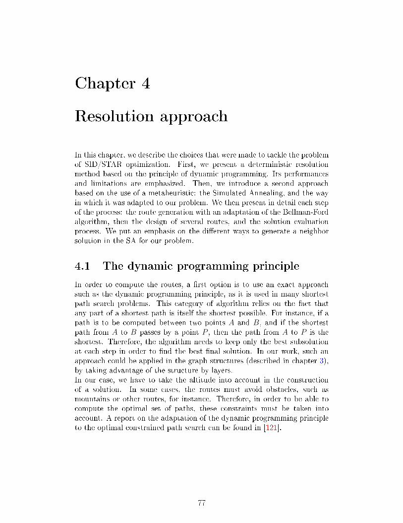
Chapter 4

Resolution approach

In this chapter, we describe the choices that were made to tackle the problemof SID/STAR optimization. First, we present a deterministic resolutionmethod based on the principle of dynamic programming. Its performancesand limitations are emphasized. Then, we introduce a second approachbased on the use of a metaheuristic: the Simulated Annealing, and the wayin which it was adapted to our problem. We then present in detail each stepof the process: the route generation with an adaptation of the Bellman-Fordalgorithm, then the design of several routes, and the solution evaluationprocess. We put an emphasis on the di�erent ways to generate a neighborsolution in the SA for our problem.

4.1 The dynamic programming principle

In order to compute the routes, a �rst option is to use an exact approachsuch as the dynamic programming principle, as it is used in many shortestpath search problems. This category of algorithm relies on the fact thatany part of a shortest path is itself the shortest possible. For instance, if apath is to be computed between two points A and B, and if the shortestpath from A to B passes by a point P , then the path from A to P is theshortest. Therefore, the algorithm needs to keep only the best subsolutionat each step in order to �nd the best �nal solution. In our work, such anapproach could be applied in the graph structures (described in chapter 3),by taking advantage of the structure by layers.In our case, we have to take the altitude into account in the constructionof a solution. In some cases, the routes must avoid obstacles, such asmountains or other routes, for instance. Therefore, in order to be able tocompute the optimal set of paths, these constraints must be taken intoaccount. A report on the adaptation of the dynamic programming principleto the optimal constrained path search can be found in [121].

77

4.1.1 Modeling of the optimal SID/STAR designproblem as an optimal shortest constrained path

Under certain hypotheses, that will be detailed later, the problem of optimalSID/STAR design can be described as a problem of shortest constrainedpath as presented in [121]. In [121], the problem of �nding the shortestconstrained path under constraints can be described by using the followingnotations:

• G = (V,A) an oriented graph, where V is the set of vertices, of size n,and A ⊂ V × V is the set of edges, of size m;

• R is the set of resources, of size R;

• To each arc (i, j) ∈ A is associated a cost cij and a non-negativeresource consumption vector (trij)r=1,...,R;

• The graph G cannot contain an absorbing circuit, i.e. it cannot containa subset B = {(i0, i1), (i1, i2) . . . (in, i0)} ⊂ A such thatn∑j=0

ciji(j+1)modn+1< 0;

• A path Px→y from vertex x to vertex y is a sequence of arcs: Px→y =∪pi=1{(ui, vi)} such that (ui, vi) ∈ A for all i, ui+1 = vi, u1 = x andvp = y;

• The length of the path Px→y presented above is p;

• The cost of the path Px→y presented above is de�ned as C(Px→y) =∑(u,v)∈Px→y

cuv.

The problem of shortest constrained path then consists in �nding the pathwith the minimum cost between two given vertices, that meet the resourceconstraints. These constraints can be expressed as follows: to each vertex iin V are associated R resource windows, denoted [ari , b

ri ] , r = 1, . . . , R. Each

window [ari , bri ] represents the amount of resource r that can be used before

reaching vertex i. Here, we examine the case where waiting is not permitted,which means that the amount of resource r consumed upon arrival at vertex icannot be less than ari . We denote Tx→y the vector of resource consumption:the rth component of Tx→y is associated to a path Px→y and represents thetotal amount of resource r consumed by taking this path. The resourceconsumption constraint can then be written as:

∀j ∈ Px→y,∀r ∈ 1, . . . , R, arj ≤ T r(Px→j) ≤ brj (4.1)

where j is a vertex through which Px→y passes, and T r(Px→j) is theconsumption of resource r upon arrival at vertex j when taking the pathPx→y:

∀r = 1, . . . , R, T r(Px→j) =∑

(u,v)∈Px→j

truv (4.2)

78

.We can apply this formalism, and the results obtained with it in [121], to theoptimal SID/STAR design problem, by making the following assumptionsfor the latter:

• We consider only one resource, which is the altitude. Therefore, withthe previous notations, R = 1;

• We assume that at each point, the range of authorized altitudes is aninterval (which in reality is not always the case: it can be a set ofintervals);

• In order to simplify the notations, we consider that αmin = αmax = α.Therefore, there is only one possible value for the altitude at a givenpoint on the path.

We construct the graph G = (V,A) described above by applying thefollowing steps:

• We consider the graph G = (V,E) built in section 3.2.1;

• We create a set E ′ of arcs, which is a duplicate of E;

• With l(e) the length of an arc e, we set the resource consumption (thealtitude) of each arc as follows:

• For all arcs e in E: t1e = αl(e). These arcs are those on which nolevel �ight is applied;

• For all arcs e′ in E ′: t1e′ = 0. These arcs are those on which alevel �ight is applied;

• We create the set A = E ∪ E ′;

• For each arc a ∈ A, we set its cost: ca = l(a);

• The results of [121] can be applied on the graph G′ = (V,A).

As mentioned in [121], �nding the shortest constrained path is a NP-hardproblem, even with a single resource to be taken into account.A way to tackle this problem is to use the principle of dynamic programmingdescribed above, that states that any subsequence of an optimal sequenceis itself optimal. In dynamic programming approaches, one method to solvethe problem is to create and update labels. A label is a vector representing apath, each coordinate of which represents either the cost associated to thispath or its consumption of the resources. For instance, in the case studiedhere, a label is a couple of values (c, z) where c is the cost of the path (itslength), and z is the altitude reached at the end of this path. Note that toeach possible path between two vertices in G = (V,A) corresponds a label.In particular, to each vertex can be associated a label, corresponding to thepath between the center of the graph (see section 3.2.1 for the de�nition ofthe center) and this vertex, as long as such a path exists.We de�ne the notion of dominance of a label over another in the followingway: a label (c, z) dominates a label (c′, z′) ((c, z) � (c′, z′)) if and only if:

79

• c ≤ c′, and

• z ≥ z′, and

• one of these inequalities is strict.

This criterion favors paths that allow for a quick climb. It allows to:

• reach the en-route sector at a su�cient altitude;

• avoid con�icts with ground obstacle as much as possible;

• reduce the number of level �ights, which is bene�cial in the context ofContinuous Climb Operations.

However, this criterion can also lead to poor results when consideringforbidden zones that must be �own under, since it favors quick climbs.Taking these into account would require a more complex model anddominance criterion. Therefore, we can temporarily discard forbidden zonesand their e�ects on the route design in order to keep this section more simple,as the results will not di�er in their interpretations.The set of all non-dominated labels (i.e. all labels that no other dominates)is called the Pareto front of the solution.In order to �nd the optimal solution in the SID/STAR design problem, onecan apply Algorithm 5 from [121], that presents a solution for acyclic graphs,which corresponds to the case of our study. This adaptation is described byAlgorithm 3.

80

Algorithm 3 The algorithm based on the dynamic programming principleto �nd the shortest constrained path between the center of the graph ofsection 3.2.1 and one arrival point. It works by computing all possible labelsfor each reachable vertex in the graph, and then by keeping only the Paretofront of labels for each.

Require: An acyclic graph G = (V,A) with a resource constraint of thetype [zmin, zmax] associated to each vertex in V ; a starting altitude zstart

at the center, an arrival vertex.1: We denote LAB(l, i) the set of all labels associated to the ith vertex of

the lth layer (see section 3.2.1 for the de�nition of layers). One suchlabel is of the form (c, z).

2: Initialization: Set LAB(1, 1)← (0, zstart).3: for l from 2 to NL do

4: for i from 1 to N the number of vertices per layer do5: LAB(l, i)← ∅6: for each arc (vl−1,j, vl,i) in A do

7: Denote cji the cost of this arc, zji its altitude variation.8: for each Lab ∈ LAB(l − 1, j) do9: if vl,i.zmin ≤ Lab.z + zji ≤ vl,i.zmax then

10: LAB(l, i)← LAB(l, i) ∪ {(Lab.c+ cji,Lab.z + zji)}11: end if

12: end for

13: end for

14: LAB(l, i)← the Pareto front of LAB(l, i)15: end for

16: end for

17: return the path corresponding to the label of minimum cost at thearrival vertex.

4.1.2 Complexity analysis

We can analyze the complexity of the resolution method provided byAlgorithm 3. The algorithm operates on the graph G′ = (V,A) constructedabove, in section 4.1.1. We denote N the number of vertices per layer, andNL the total number of layers.

4.1.2.1 Spatial complexity

We begin by determining the space that is required to carry out theprocedure. Any vertex in the graph has O(N) predecessors, except for the�rst and the second layers (the only vertex on the �rst layer, which is thecenter, has 0 predecessor, and any vertex on the second layer has at most 1predecessor: the center).Then, we compute the maximum number of labels held by any vertex inthe graph. This number is equal to the size of the Pareto front of solutionsfor the optimal path search problem between the center and this vertex. Inthe worst case, this Pareto front is the size of the number of possible pathsfrom the center to the vertex (which means that no path is dominated). By

81

recurrence:• a vertex on layer L2 holds two labels (one for the arc from the centerto this vertex without a level �ight, and one for the arc with the level�ight, see the de�nition of the set A of arcs in section 4.1.1);

• a vertex on layer L3 holds O(N) labels;

• a vertex on layer Li with i ≥ 2 holds O(N i−2) labels: two for eachlabel of each vertex on the previous layer.

In order to obtain the total spatial complexity, we sum over all vertices:

NL∑L=1

N ×NL−2 =

NL−1∑L=0

NL

=NNL − 1

N − 1

= O(NNL−1)

This result is intuitive enough: the space needed in the worst case is aboutthe total number of combinations of vertices, one vertex per layer. Thus,this complexity is exponential in the number of layers.

4.1.2.2 Time complexity

In order to compute the time complexity of the method, we analyze the path�nding process given by algorithm 3. It works by propagating to a vertexthe labels of all of its predecessors (lines 6-13), and then by �nding thePareto front of the resulting set (line 14). If we consider a vertex vi+1,j onlayer Li+1, i ≥ 2, then it has O(N) predecessors, each propagating O(N i−2)labels, based on the analysis of the previous paragraph. Therefore, thetime required to propagate all labels to vi+1,j from its O(N) predecessors isO(NN i−2) = O(N i−1).Then, we must compute the Pareto front for this vertex. By the dominancecriterion stated in section 4.1.1, we know that each label has to be comparedto every other label. There are O(N i−1) labels at vertex vi+1,j, so comparingone label to all others is done in O(N i−1) time. This operation has to becarried out for each label. The time complexity to compute the Pareto frontfor one vertex is then O(N i−1N i−1) = O(N2(i−1)).Finally, in order to �nd the optimal path between the center and a vertexlocated on layer LNL

, this operation must be done for each vertex on eachlayer:

NL∑L=1

N ×N2(L−1) =

NL∑L=1

N2L−1

=1

N× N2NL − 1

N2 − 1

= O(N2NL−3)

As for the space complexity, the time complexity is exponential with thenumber of layers. These results, although they are given for the worst case

82

scenario, should be close to the expected time and space complexity, giventwo reasons:

• Apart from the �rst layers, and depending on the way that the layersare sampled and the maximum authorized turn angle, it is very likelythat every vertex has an important number of predecessors, of theorder of N/3 for the test cases presented in this thesis;

• The dominance criterion given in 4.1.1 implies to keep a large numberof labels for each vertex, since the cost and altitude of a path areproportional to one another (with small variations depending on thelevel �ights).

Therefore, the expected time and space complexities should be close to theirworst case evaluation, which is exponential, and therefore not suitable forlarge instances, which are the subject of this thesis. In order to decreasethese complexities, a solution is to use heuristics.

4.1.3 Dynamic programming based heuristic fordesigning one route

4.1.3.1 Without preprocessing

A method to reduce the space and time complexity of the method canbe to consider only the cost of a path for the design, and to consider theminimum and maximum altitudes only when an obstacle is encountered.The corresponding method is described by Algorithm 4 and illustrated in�g. 4.1. This method di�ers from the one developed in [121] and adaptedin the previous section in that only one label is kept for each vertex,representing the cost of each path. By keeping only the cost for each path,we take this method back to a classic path search, only checking that theconstraints are met a each label's creation. By taking into account thestructure in layers, and since the edges are always oriented from a layer ito the layer i + 1, this algorithm has a time complexity in O(‖A‖), whichallows to tackle rather large instances.

83

Algorithm 4 The dynamic programming algorithm for the SID/STARdesign problem. In this algorithm, the cost of each edge is computed intwo con�gurations: with and without a level �ight (lines 11-13). The �nalcost of the edge is the minimum between the two, and the correspondingcon�guration is remembered (line 14). Each ending vertex of the edges hasthen its cost updated whenever its current cost is higher than the cost of aprevious vertex, to which is added the cost of the edge (lines 15-22). Thisprocess is done for all vertices, layer by layer (lines 9-10).

Require: A starting vertex s, a list of layers L composed of vertices,to which are attached edges, a minimum and a maximum slope ofclimb/descent, resp. αmin and αmax. The set of all vertices is denotedV , the set of all edges is denoted E.

1: Initialization: Create an array d of 'distances' the size of V such thatd [v] contains the distance from s to v. Create an array p of predecessorssuch that p [v] contains the predecessor vertex of v.

2: for each vertex v in V do

3: d [v] =∞4: p [v] = null5: end for

6: d [s] = 07: s.minimumAltitude = 08: s.maximumAltitude = 09: for i from 1 to L.size do

10: for each vertex u on Li do11: for (u, v) in E do

12: compute two surfaces S1 and S2. S1 is the 3D extension of(u, v) obtained applying αmin and αmax on the length of (u, v), startingrespectively at the minimum and maximum altitudes of u. S2 is obtainedwith the same method, by applying a level �ight on (u, v).

13: set c1 and c2 the costs of S1 and S2 respectively, according tothe constraints and objective function.

14: set c = min(c1, c2) and S the corresponding surface.15: if d [u] + c < d [v] then16: d [v] = d [u] + c17: p [v] = u18: if S is the version with a level �ight then19: set v.levelFlightLength = u.levelFlightLength +

distance2D(u,v)20: else

21: set v.levelFlightLength = u.levelFlightLength22: end if

23: end if

24: end for

25: end for

26: end for

27: return p, d

84

(a) The cost of each neighboring nodeis computed by taking all constraintsand the objective function intoaccount. Two costs are computed:one by considering a level �ight onthe arc, and the other without.

(b) The cost kept for the neighboris the minimum between the twocomputed previously. The costs ofall neighbors of the starting node arecomputed in the same way.

(c) Once all costs for the �rstneighboring layer have beencomputed, the same evaluationbegins for the second layer.

(d) The costs of the neighbors areupdated in the same fashion as inthe original Bellman-Ford algorithm.The process goes on layer by layeruntil all costs have been computed inthe graph.

Figure 4.1 � The �rst iteration for the dynamic programming algorithm. Allthe neighbors of the node are visited, but only a part of them is selected forthe next steps.

85

However, in three dimensions, applying this method without priorpreprocessing can lead to the impossibility to �nd a solution in someparticular cases. If we take for instance the situation illustrated in �g. 4.2a,in which an obstacle is to be �own over by making a detour so as to gainenough altitude to pass over it, this method is not able to �nd a feasiblesolution, as illustrated in �g. 4.2b. Indeed, by construction, this methodwill only retain for each node the least expensive way to attain it, basedon the information gathered by processing previous nodes. Therefore, itdoes not take into account the constraints yet to come, nor retains the otherpossibilities to attain the node. In the example given here, this translatesinto being unable to �nd a path that �ies over the obstacle when there mightbe one, because only the shortest path to each node is kept, and the attainedaltitude is too low to pass the obstacle.

(a) A situation where a detour isnecessary to be able to pass over theobstacle.

(b) The default behavior of themethod is to build the pathsprogressively, by keeping only thebest current solutions for each node.In this case, the path chosen to attainthe point P (solid line) is not longenough to allow for passing over theobstacle. The path that would allowit (in dashed line) was discarded, asit was not the best possible subpathto P .

Figure 4.2 � A situation where the naive heuristic leads to unfeasiblesolutions.

4.1.4 With preprocessing: imposing boundary valuesfor the minimum and maximum altitude

The issue raised in the previous section, regarding the possibility to end upin a dead end due to the lack of visibility on the constraints, can be partlyresolved by applying the principle of dynamic programming, in a reverseway (in our case: from the entry/exit point of the TMA towards the centerof the graph), so as to propagate the altitude constraints on all nodes on thegraph before applying the path search algorithm. This process is described

86

by Algorithm 5, and illustrated by �g. 4.3. This preprocessing phase allowsa later path search algorithm to �nd paths otherwise discarded by the �rstheuristic. However, it also creates a dependency on the entry/exit pointprocessed. Therefore, each route must be computed individually, whichdoubles the computing time of a solution in the case where one route isto be found, and multiplies the computing time of a solution by roughlytwo times the number of routes to compute in a general case (instead ofrunning the algorithm only once for the whole solution, it is run twice foreach route). This increase in computation time can be critical in instanceswhere numerous edges must be processed. In this preprocessing step, somevertices may be discarded for the subsequent path search (lines 25-29 inAlgorithm 5). This situation happens when the constraints on the minimumand maximum altitude lead to an unfeasible situation, where the minimumrequired altitude is higher than the maximum authorized altitude. Thisidea originates from Algorithm 1 in [121] and allows to overlook some of theinfeasible solutions during the path search.

87

Algorithm 5 The preprocessing method to take altitude constraints intoaccount. This algorithm provides each node of the graph with additionalconstraints. It begins by computing the requirements of altitude for thearrival point (lines 5-9). Then, these altitude constraints are propagatedtowards the center (lines 11-12). This is done by updating the minimumpossible altitude at the vertex (lines 13-19), and the maximum possiblealtitude at the vertex (lines 20-22).

Require: The starting vertex s of a route, its arrival vertex a, a list of layersL composed of vertices, to which are attached edges, a minimum slopeof climb/descent αmin, the altitude constraints imposed by the layout oneach vertex, respectively denoted zobstacles

min and zobstaclesmax . The set of all

vertices is denoted V , the set of all edges is denoted E.1: Initialization: Create two arrays zmin and zmax of minimum and

maximum altitudes both the size of V such that zmin [v] and zmax [v]contain resp. the minimum and maximum authorized altitudes uponarrival at v starting from s to attain a.

2: for each vertex v in V do

3: zmin [v] = +∞, zmax [v] = −∞4: end for

5: if a.zobstaclesmin or a.zobstacles

max is not a null value then6: zmin [a]← a.zobstacles

min and/or zmax [a]← a.zobstaclesmax

7: else

8: zmin [a]← +∞, zmax [a]← −∞9: end if

10: Set a as processed11: for i from L.size to 2 do12: for each edge (u,v) in E such that v is on Li and v is processed do13: if dmin [v] is �nite then14: Set d the length of the proj. of (u,v) on the horizontal plane15: zmin [u]← min (zmin [u] , zmin [v]− dαmin)16: end if

17: if u.zobstaclesmin is not a null value then

18: zmin [u] ← max(zmin [u] , u.z

obstaclesmin

)if zmin [u] is �nite,

u.zobstaclesmin otherwise

19: end if

20: zmax [u]← max (zmax [u] , zmax [v])21: if u.zobstacles

max is not a null value then22: zmax [u]← min

(u.zobstacles

max , zmax [u])if zmax is �nite, u.z

obstaclesmax

otherwise23: end if

24: end for

25: for all vertices u on layer i do26: if zmin [u] and zmax [u] are �nite and zmin [u] > zmax [u] then27: Discard vertex u and all the edges connected to it28: end if

29: end for

30: end for

31: return zmin, zmax

88

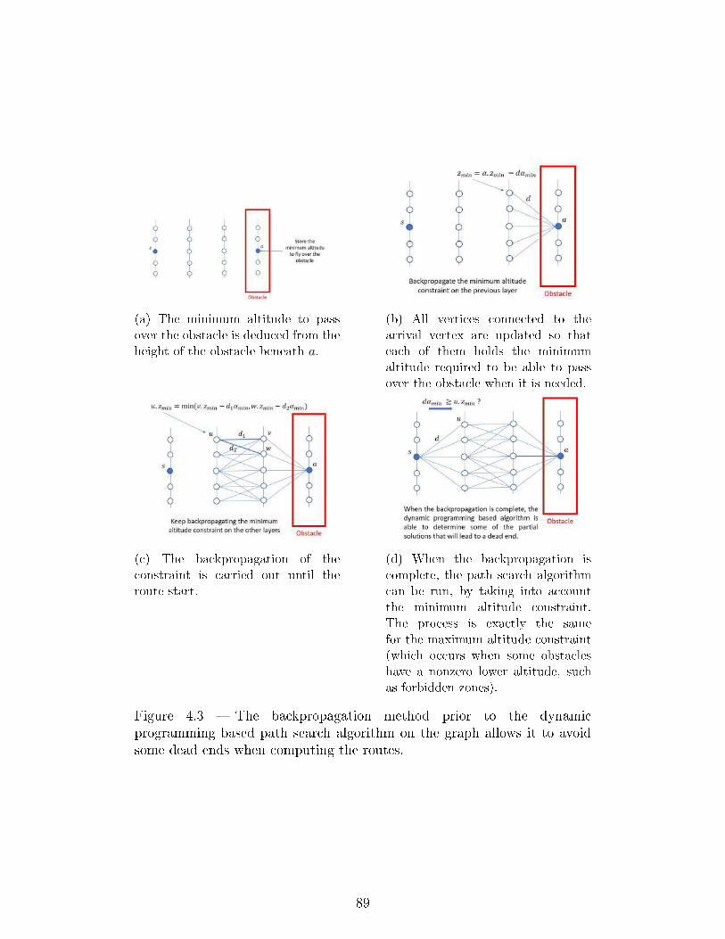
(a) The minimum altitude to passover the obstacle is deduced from theheight of the obstacle beneath a.

(b) All vertices connected to thearrival vertex are updated so thateach of them holds the minimumaltitude required to be able to passover the obstacle when it is needed.

(c) The backpropagation of theconstraint is carried out until theroute start.

(d) When the backpropagation iscomplete, the path search algorithmcan be run, by taking into accountthe minimum altitude constraint.The process is exactly the samefor the maximum altitude constraint(which occurs when some obstacleshave a nonzero lower altitude, suchas forbidden zones).

Figure 4.3 � The backpropagation method prior to the dynamicprogramming based path search algorithm on the graph allows it to avoidsome dead ends when computing the routes.

89

However, on top of the increase in computation time, applying Algorithm 5is not enough to guarantee the optimality of the solution. This is due tothe fact that this method stores only the most favorable constraint for thesubsequent path search. Therefore, it improves its capacity to �nd a solution,but �nding the optimal solution is subject to the same problem as statedbefore, in which a �rst part of a solution is computed, which is optimal forthe given criterion and for the subpath under consideration, but will lead toa suboptimal solution. This case is illustrated by �g. 4.4. In this example,two subpaths from the starting point s and a point P are illustrated, with thearrival point a behind an obstacle. The obstacle has two di�erent heights:low in blue and moderate in red. During the preprocessing phase, as it isdescribed in Algorithm 5, a minimum altitude is associated to the point P .This minimum altitude corresponds to the low obstacle. We assume thatthe altitude reached by the path in solid line is that same minimum altitude.Then, the best admissible path from P to a is over the low obstacle. Thispath will be chosen by the method, even though the path in dashed line is abetter solution to the problem. More importantly, this method still cannot

Figure 4.4 � A case where requiring a minimum altitude is not su�cient to�nd the optimal solution: the path in solid line is chosen over the one indashed line, even though the latter is shorter.

guarantee to �nd any solution when there might be one. An example isprovided by �g. 4.5. In this simpli�ed example, there are two possible routes:one that passes over a mountain, and one that passes beneath a forbiddenzone. With the method described above, and since only the most permissiveconstraints are backpropagated to each point, point P is not constrainedon the minimum altitude due to the backpropagation from the forbiddenzone, and P is not constrained in maximum altitude either, due to thebackpropagation from the mountain. If we consider that the shortest pathfrom the center to P is too long to allow to pass under the forbidden zone,but too short to allow to pass over the mountain, the algorithm cannot�nd any solution, even though there might be one (that passes over the

90

mountain), despite the preprocessing phase.

Figure 4.5 � A case where the preprocessing phase is not enough to allowthe algorithm to �nd a solution: the most permissive constraints only arebackpropagated from the forbidden zone and the mountain, and the resultingsituation leads to the same problem as the case where no preprocessing isapplied.

4.1.5 Heuristic for designing several routes

In the previous sections, we presented a method to design one route underaltitude constraints. In the next paragraphs, we extend this method to thedesign of several routes.A �rst idea can be to use repeatedly the method for one route until all routesare designed. This idea is illustrated by Algorithm 6. In this case, only one

Algorithm 6 Designing a set of routes sequentially by using the dynamicprogramming heuristic with preprocessing. All routes start at the center.

Require: The center of the graph c, all entry/exit points of the TMA asvertices P 1, . . . , PNP , a list of layers L composed of vertices, to whichare attached edges, a minimum slope of climb/descent αmin, the altitudeconstraints imposed by the layout on each vertex, respectively denotedzobstacles

min and zobstaclesmax . The set of all vertices is denoted V , the set of all

edges is denoted E.1: Initialization: Create an array r of routes.2: for each entry/exit point P i, i = 1, . . . , NP do

3: Apply the preprocessing technique of Algorithm 5 by consideringroutes 1, . . . , i− 1 as obstacles

4: Let ri be the result of Algorithm 4 applied between the center andP i

5: r[i]← ri

6: end for

7: return r

91

graph of the form G = (V,A) as described in section 4.1.1 is considered,which means that only one runway (and one orientation of this runway) istaken into account. The method, however, is the same when taking severalgraphs into account. The most important drawback of this method is thatit doesn't take into account the need to separate the merging points of theroutes. Indeed, Algorithm 6 shows that all routes depart from the origin. Asexplained in the previous chapters, such a design is not acceptable in real-lifeconditions. Therefore, some of the routes must be allocated a new startingpoint. In order to achieve this, one can proceed as explained in Algorithm 7.The routes are ordered by decreasing order of tra�c �ow. This will allowto favor a more direct design for the busiest routes. Then, for each route Rexcept the �rst one, we search for the point P with a maximum curvilinearabscissa such that P is too close to another route. We denote L the layercontaining P , and R′ the route that P is too close to. The new startingpoint for R is then the intersection of R′ with L. The process is illustratedby �g. 4.6.

(a) The initial solution for theconcurrent merging problem. RoutesR and R′ are too close, from thecenter to layer L.

(b) The new start for route R is theintersection of R′ with L.

Figure 4.6 � The heuristic for solving the concurrent merging problem. Theroutes start on the route closest to them, on the last layer on which theroutes were too close to each other.

4.1.6 Motivations for a metaheuristic based approach

As demonstrated in the last paragraphs, the heuristic constructed from thedynamic programming approach has several severe drawbacks in the scopeof this work. Firstly, the optimality of the solution is not automaticallyveri�ed. This problem could be overcome by keeping a Pareto front oflabels, but in our case, it would take too much time to �nd a solution,as demonstrated in section 4.1.2.2. Also, as for the routes in one graph,when several graphs are to be taken into account, these must be processedsequentially. Therefore, in order to �nd the optimal solution, one should alsotest all combinations for the order of generation of the graphs, and routes.

92

Even so, the optimality cannot be guaranteed. For instance, optimalitycannot be achieved in a case where two graphs are to be considered and theoptimal solution involves a level �ight in both, in order to avoid a route fromthe other (see an illustration of this case in �g. 4.7). Such a solution can onlybe found if both graphs are processed at the same time, or by introducingrandom behaviors. Finally, and most importantly, the method based on the

Figure 4.7 � A case where two graphs must be processed at the same timein order to �nd the optimal solution. Route R1 must have a level �ight inorder to pass below R3 and route R2 must have a level �ight to pass belowR1.

heuristic is not guaranteed to �nd a solution, even when one exists (evenwhen taking the preprocessing steps), as explained in section 4.1.4. Despitethese drawbacks, this method presents various advantages, listed below:• It is an e�cient way of designing a single route when only one obstacleis to be taken into account.

• It doesn't need any parameter setting, which makes it very easy touse. The user only has to provide the starting and ending point of theroute.

These features make the method fairly e�cient in cases where only one, orvery few routes are to be computed, with few to no obstacles to take intoaccount. However, with the risk of not being able to �nd any solution whenthere might exist one, by introducing a heuristic for the choice of the newstarting points for the routes, and with the need to process each separategraph in a sequence, this approach is not viable on its own for generalcases. This algorithm could be considered to make for a subroutine of ametaheuristc-based approach. In the next sections, we present the approachchosen to solve the optimal SID/STAR design problem, that is based on ameta-heuristic.

93

Algorithm 7 The heuristic for the design of several routes with the dynamicprogramming based approach. Lines 2 to 5 build a �rst solution, with allroutes starting on the center. Lines 6 to 15 determine for each route thelast route among the previous ones that is too close to the route underconsideration. Based on this information, lines 16 to 24 recompute theroutes with a new starting point so that the merging constraint as well asthe route separation constraint are met.

Require: The center c of the graph, the entry/exit points of the TMAP 1, . . . , PNP , a list of layers L composed of vertices, to which areattached edges, a minimum slope of climb/descent αmin, the altitudeconstraints imposed by the layout on each vertex, respectively denotedzobstacles

min and zobstaclesmax . The set of all vertices is denoted V , the set of all

edges is denoted E.1: Initialization: Create an empty set R of routes, a double-entry array A

of size NP × 2. This array will contain for each index i both the lastroute that is too close to Ri and the last layer for which the two routeswere too close to each other. All values of A are initialized to −1.

2: for i from 1 to NP do

3: Apply the preprocessing algorithm (Algorithm 5) between c and P i

4: Compute Ri between c and P i with Algorithm 45: end for

6: for i from 2 to NP do

7: for j from 1 to NL do

8: for k from 1 to i− 1 do9: if Ri and Rk violate the route separation constraint on layerj then

10: A[i][0]← k11: A[i][1]← j + 112: end if

13: end for

14: end for

15: end for

16: R← R1

17: for i from 2 to NP do

18: if A[i][1] = −1 or A[i][1] is greater than the number of the layerthat contains P i or A[i][1] is greater than the number of the layer thatcontains PA[i][0] then

19: Set the new starting point s = c20: else

21: Set the new starting point s = γA[i][0]h (τ

A[i][0]A[i][1] ), which is the

intersection of RA[i][0] with the layer LA[i][1]. If s is already a mergingpoint, increase the layer of connection until the intersection of RA[i][0]

with the layer is not already a merging point. If no such point exists,set s = c.

22: end if

23: Apply the preprocessing algorithm (Algorithm 5) between s and P i

24: Compute Ri between s and P i with Algorithm 425: R← Ri

26: end for

27: return R 94

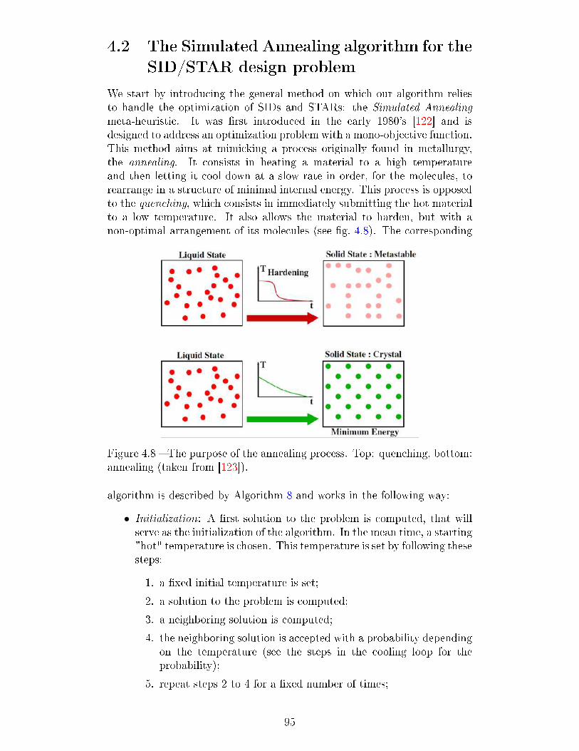
4.2 The Simulated Annealing algorithm for the

SID/STAR design problem

We start by introducing the general method on which our algorithm reliesto handle the optimization of SIDs and STARs: the Simulated Annealingmeta-heuristic. It was �rst introduced in the early 1980's [122] and isdesigned to address an optimization problem with a mono-objective function.This method aims at mimicking a process originally found in metallurgy,the annealing. It consists in heating a material to a high temperatureand then letting it cool down at a slow rate in order, for the molecules, torearrange in a structure of minimal internal energy. This process is opposedto the quenching, which consists in immediately submitting the hot materialto a low temperature. It also allows the material to harden, but with anon-optimal arrangement of its molecules (see �g. 4.8). The corresponding

Figure 4.8 � The purpose of the annealing process. Top: quenching, bottom:annealing (taken from [123]).

algorithm is described by Algorithm 8 and works in the following way:

• Initialization: A �rst solution to the problem is computed, that willserve as the initialization of the algorithm. In the mean time, a starting"hot" temperature is chosen. This temperature is set by following thesesteps:

1. a �xed initial temperature is set;

2. a solution to the problem is computed;

3. a neighboring solution is computed;

4. the neighboring solution is accepted with a probability dependingon the temperature (see the steps in the cooling loop for theprobability);

5. repeat steps 2 to 4 for a �xed number of times;

95

6. if the number of accepted neighbors is lower than a �xed value,increase temperature and repeat steps 2 to 6.

More detail on the choice of the initial temperature can be foundin [123], and the reader can refer to chapter 5 for the speci�c �xedvalues used in this work.

• Cooling loop:

� The result of the evaluation of the objective function for thecurrent solution xi is denoted yi, and the current temperatureof the algorithm is denoted by T .

� A neighbor xj of the current solution is randomly generated. Thisstep implies that it is possible to establish a notion of distancebetween two solutions in the algorithm.

� The objective function is evaluated for the neighbor solution xj.The result is denoted by yj.

� If yj is better than yi, then the neighbor is accepted as the newcurrent solution, and will serve as a starting point for the nextiteration of the loop.

� If yj is not better than yi, the neighbor is nonetheless accepted as

the new current solution, with a probability of eyi−yj

T (4.3). Thus,the probability of accepting a solution worse than the current onedecreases with the temperature.

� The temperature T is decreased.

• Stopping criterion: The algorithm stops when it has performed apre-de�ned number of iterations, or when the temperature reaches a�xed value. It can also stop earlier in the cases where the optimal valueof the objective function is known and the algorithm �nds a solutionfor which the objective function is evaluated to this value.

In our work, the general idea is to gather the data required to build aninstance of a problem, and then to apply a SA-based method to computea solution. The choice of using a meta-heuristic was made because of thelarge number and the complexity of the constraints to be taken into account,such as the route separation, which make the use of exact approaches moredi�cult to implement in terms of computation time. In the process usedhere, the routes are computed one by one in their decreasing order of tra�c�ow, then the resulting set is evaluated along the optimization function.This process is done iteratively until a stopping criterion is reached. Thealgorithm is designed to explore the solution space at the beginning, andthen focus more and more on the best solutions found towards the end.This exploration behavior, induced by the introduction of randomness in thepath search, which will be detailed later in this chapter, allows to generatethe routes sequentially, in any given order, without the drawback that thisinduces in deterministic approaches. In our case, the evaluation process iscarried out by putting the generated routes into a simulation containing the

96

Algorithm 8 The principle of functioning of the SA.

1: Build instance2: Set a starting temperature for the SA3: Compute an initial solution4: while stopping criterion isn't reached do5: for a �xed number of iterations do6: Compute a neighboring solution7: Evaluate the new solution8: Select one of the two solutions as reference for the next iteration9: end for

10: Decrease temperature11: end while

12: return best solution encountered

parameters relative to the terrain and the cities. This simulation computesthe cost of the given solution in order to estimate its performance in thescope of the problem (see �g. 4.9).

Figure 4.9 � The simpli�ed process for the SA adapted to our case. Thesolution computed by an iteration of the SA is evaluated by the means of asimulation and the result is used for the subsequent iterations of the SA.

4.3 Generating one route on the graph: the

modi�ed Bellman algorithm

In this section, we describe in details the way in which the SimulatedAnnealing and Bellman-Ford algorithms have been adapted to our problem.The Bellman-Ford algorithm is used to solve the single source shortest pathproblem in a directed graph [56]. In its original version, it works by updatingrepeatedly the minimum cost to each vertex in the graph with estimationsthat are more and more precise at each iteration. The original algorithmis described in Algorithm 9 and illustrated in �g. 4.10. This algorithmiteratively updates the cost of each vertex in the graph by comparing itscurrent cost with the cost of all of its neighbors added to the cost of travelingfrom the neighbor to the vertex (lines 8-13). This process is done as many

97

Algorithm 9 The original Bellman-Ford algorithm for the one-to-allshortest path problem in a graph.

Require: A starting vertex s, a list of vertices V , a list of edges E1: Initialization: Create an array d of distances the size of V such that d [v]

contains the distance from s to v. Create an array p of predecessors suchthat p [v] contains the predecessor vertex of v

2: for each vertex v in V do

3: d [v] =∞4: p [v] = null5: end for

6: d [s] = 07: for i from 1 to V .size-1 do8: for (u, v) with weight w in E do

9: if d [u] + w < d [v] then10: d [v] = d [u] + w11: p [v] = u12: end if

13: end for

14: end for

15: for (u, v) with weight w in E do

16: if d [u] + w < d [v] then17: Error: there is a negative cycle18: end if

19: end for

20: return p, d

times as there are vertices (minus one) so that all possible paths withinthe graph are checked (line 7). This algorithm has a time complexity inO(‖V ‖ ‖E‖).

4.3.1 The adaptation of the Bellman-Ford algorithm toour problem

In our version, we modify the Bellman-Ford algorithm to take advantage ofthe structure in layers. This adapted version is presented in Algorithm 10,which is illustrated by �g. 4.11. In �g. 4.11a, we consider the startingnode for a path, as well as its neighbors: V1.1 to V1.5, with their associatedcosts. At this point, the only marked node is s. The table below holds foreach vertex its minimal cost (distance) from s, d(v), the preceding vertexin the shortest path from s to this vertex, p(v), and a value true or falsethat indicates whether the arrival point a is reachable from the vertex underconsideration. In the second step (�g. 4.11b), the aim is to select a subset ofarcs with minimum cost among the arcs that allow to reach the arrival pointa. This subset is denoted Eu, u being the current expanded vertex (so, in�g. 4.11b, u = s). In step 3 (�g. 4.11c), the ending vertices of the selectededges are marked. The algorithm will then repeat the three steps with eachmarked vertex in the second layer, and proceed through all the layers in the

98

same way until the layer of a is considered. The shortest path from s to ais given by the sequence of predecessors starting at a, taken backwards.This version of the Bellman algorithm allows for a better computationtime, since we don't consider all edges at each iteration but only the edgesassociated to the vertices of a single layer. When a vertex is not marked,none of its edges is considered at all. The other noticeable feature of thismodi�ed version is the use of the list Eu containing only a portion of alledges coming out of a given vertex u. This choice was made in order tosave computation time by only considering the arcs with the lowest cost. Intheory, it puts the optimality of the solution in jeopardy by integrating agreedy behavior. However, when we consider the context of the work, twoarguments can be raised in favor of this approach:• The weights of the edges are their length, as they represent thedistance between two points. Therefore, there should be no signi�cantdi�erence between the weight of two edges starting on the same vertex,and so over the whole graph: the weights are uniform.

• This modi�ed version of the Bellman-Ford algorithm is used togenerate routes between two given points in the search space. In orderto allow for exploration of the search space, at each path search, theweight of the edges is changed, in a way that will be explained in thenext paragraph. Therefore, we do not, in fact, look for the shortestpath, but rather a short, reproducible path. Since the modi�edBellman-Ford algorithm is itself embedded in a Simulated Annealing,the latter is the one responsible for choosing the best weights for theedges. Since the algorithm is designed to explore the search space, it isvery likely that previously discarded edges will be taken into accountin a later iteration.

99

(a) The graph used for the example ofthe original Bellman-Ford algorithm.The starting node is colored in green.

(b) The initial state of the algorithm.The source node is A with cost 0, therest have an initial in�nite cost.

(c) Step 1: A �rst relaxation of allarcs is performed. The costs of allnodes are updated. There will be asmany relaxations as the number ofvertices except A. The nodes whosecost is updated are colored in blue.

(d) Step 2: A second relaxation ofall arcs is performed. The costs of allnodes are updated. Node B has itscost unchanged.

(e) Step 3: A third relaxation isperformed.

(f) Step 4: A fourth relaxation isperformed. Only node D has its costchanged.

Figure 4.10 � An example of run of the Bellman-Ford algorithm. The lettersare replaced by the cost for a better readability. The starting node is coloredin green ; the nodes whose cost is updated are colored in blue at eachiteration.

100

Algorithm 10 The Bellman-Ford algorithm in the SA method. The originalalgorithm is modi�ed to take the layer structure into account. The processis sped up by taking into account only the edges that allow to reach thedestination (line 11), by expanding only the nodes previously visited (lines8,10,17) and by visiting only a promising set of neighbors for each node (line11).

Require: A starting vertex s, an arrival vertex a, a list of layers L composedof vertices, to which are attached edges. s is located on the �rst layerand a on the last layer, an integer n giving the maximum number ofedges to take into account for each vertex expanded

1: Initialization: Create an array d of distances the size of V the set ofall vertices such that d [v] contains the distance from s to v. Create anarray p of predecessors such that p [v] contains the predecessor vertex ofv.

2: for each vertex v in V do

3: d [v] =∞4: p [v] = null5: Tag v as not marked6: end for

7: d [s] = 08: Tag s as marked9: for i from 1 to L.size-1 do

10: for each vertex u on L [i] tagged as marked do

11: create a list Eu containing the n edges (u, v) of E with the lowerweight and such that a is tagged as true for v. If there are fewer than nsuch edges, Eu contains all of them

12: for each (u, v) with weight w in Eu do13: if d [u] + w < d [v] then14: d [v] = d [u] + w15: p [v] = u16: end if

17: Tag v as marked18: end for

19: end for

20: end for

21: return p, d

101

(a) The initial state of the algorithm. Only s is marked.

(b) Expansion of the promising arcs. V1.5 is not expandedbecause a is unattainable.

(c) The state of the algorithm before the second iteration: theending vertices of the selected arcs are marked. Only markednodes on layer 2 will be expanded.

Figure 4.11 � The �rst iteration for the modi�ed Bellman-Ford algorithm.All the neighbors of the node are visited, but only a part of them is selectedfor the next steps.

102

4.3.2 The management of the edges' weight

Each individual path is computed with an adapted version of theBellman-Ford algorithm, with a carefully chosen cost for the arcs, as thealgorithm has to be able to explore various possible paths for two givenstarting and ending points. This last requirement implies that the cost ofthe edges can vary during the execution of the algorithm. Otherwise, fortwo given points, the result of the search would always be the same. Toachieve this, the algorithm biases the costs of the edges in the graph foreach path to be computed.This process is done by the SA. A number (thebias) between -1 and +1 is associated to each merging layer. A negativebias will increase the costs of the arcs 'on the right' of each node until thenext merge layer, while a positive bias will increase the costs 'on the left'(see Figure 4.12). The closer the bias is to -1 or +1, the sharper the turn

Figure 4.12 � Two paths to the same exit and the associated biais functions.The shape of the paths is similar to the associated shape of the bias functiong on [0 , 1].

will be, while a null bias will favor the straightforward paths. By resettingthe costs of the arcs at each path search, it is possible to have a completeexploration of the graph while keeping a way to recreate any path, givenits start and end points along with the biases. The way in which the biasesare applied to the edges of the graphs is described in Algorithm 11, andillustrated in �g. 4.13. In a nutshell, this piece of algorithm does, for eachnode and given biases, the following:

103

Algorithm 11 The arcs valuation algorithm.

Require: A starting vertex s, an exit vertex e, layers L1...Ln where sbelongs to L1 and e belongs to Ln, an array A of size n− 1 containing�oat values between −1 and +1.

1: Initialization: Set all arcs costs to their length. Tag s as marked. Choosean expansion coe�cient α.

2: for each L i do

3: for each marked vertex v on Li do

4: Let nv be the number of arcs starting on v5: Number all arcs (v, w) from 1 to nv from left to right and mark

each w6: Let m be b(1 + A[i])nv−1

2c+ 1

7: Arc number m has its cost unchanged8: Let G =Max(m,nP −m)9: for all arcs ek1 on the right of arc m do

10: Multiply the cost of ek1 by 1 + k1−mG

(α− 1)11: end for

12: for all arcs ek2 on the left of arc m do

13: Multiply the cost of ek2 by 1 + m−k2G

(α− 1)14: end for

15: end for

16: end for

• Find the middle node among its successors (Fig. 4.13a);

• Find the node corresponding to the assigned coe�cient. Thiscoe�cient is the same for all nodes between two given merging layers.The gap between the middle node and the node to �nd is proportionalto the assigned coe�cient (which is in [−1,+1]). The sign of thecoe�cient indicates the direction of the gap relatively to the middlenode (right or left). For instance (see �g. 4.13b), if there are 3 nodeson the right of the middle node, and the coe�cient is 1

3, then the node

to �nd is the �rst one on the right of the middle node. This new nodeis called the reference node;

• The reference node has its cost unchanged;

• The algorithm iteratively increases the costs of the nodes neighboringthe reference node. The farther the node from the reference node, themore its cost is increased (�g. 4.13c).

It is during this phase that the list Eu in Algorithm 10 is created. Once alledges starting on a given vertex have their new weight set, the n of themwith the lowest weight can be put into the list Eu. The coe�cients for thecost bias are chosen in a way that helps reducing the zigzag phenomenon.The aim is to generate a sequence of numbers that are coherent with theirpredecessors and successors. In order to achieve this, the generation isbased on the raised cosine function:

104

(a) Identi�cation of themiddle neighbor of anode.

(b) Identi�cation of thereference node.

(c) Valuation of thearcs. The cost to thered node is una�ected.The cost to the whiteone is heavily a�ected.

Figure 4.13 � The arcs valuation function. The cost of the arcs is increasedproportionally to the distance of their ending vertex to the reference node.

rcos(x, µ, s) =1

2s

[1 + cos

(x−µs

π

)]on [µ−s, µ+ s] (4.4)

The method works as follows, for a given starting vertex o (origin) and agiven ending vertex a (arrival):• A number α ∈ [0, 1] and two signs sgn1, sgn2 ∈ {−1,+1} are randomlychosen;

• Three amplitude values A1, A2, A3 in [0, 1] are set. These values canbe chosen randomly, but in this work, they are decreased down to zerowith the progress of the SA. This allows to explore the state spacewhen the temperature is high and focus on a narrower neighborhoodwhen it is low;

• Three raised cosine functions are generated (see Figure 4.14):

• rcos1(x) = sgn1 ·A1 · α2 · rcos(x,α2, α

2)

• rcos2(x) = − sgn1 ·A2 · 1−α2· rcos(x, α+ 1−α

2, 1−α

2)

• rcos3(x) = sgn2 ·A3 · 12· rcos(x, 1

2, 1

2)

• A function g is de�ned as g(x) = rcos1(x)+rcos2(x)+rcos3(x)2

on [0, 1], bysetting rcos1 = 0 on ]α, 1] and rcos2 = 0 on [0, α[;

• The coe�cients are chosen so that the route to �nd has the same shapethan g, scaled to the distance [o , a] (see �g. 4.12).

105

Figure 4.14 � The raised cosine functions to determine the biases in a generalcase. The function g is the weighted sum of the three others and its shapeis the one to give to the path under computation.

4.4 The design of several routes with our

algorithm

Once the �rst route is computed with the method above, a solution can befully generated by adding the remaining routes, creating a tree structure.The full process for the design of one solution is as follows:• One tree is constructed for each di�erent runway under consideration,with its layers, vertices and edges. For instance, in the case of anairport using two parallel runways, one for the departures and theother for the arrivals, two trees will be constructed;

• In each tree, the routes are built as follows:

� The �rst route (γ0h, γ

0v) is designed with the method explained

above;

� A subset of L is identi�ed as merge layers. They are the layerson which it will be possible for two routes to merge together.These layers cannot be chosen randomly, in order to avoid havingtwo merge points too close to one another. This aspect will bedetailed in the next paragraph;

� The intersection points between γ0h and the merge layers are

identi�ed as possible merge points;

� One of these points is chosen as the starting point for the nextroute search. Note that in the mathematical modeling, the wholeportion of route comprised between the center and the mergepoint is also counted as part of the new route. Bearing this inmind, all routes in a same tree start at the center of this tree;

� The second route is designed using the same method;

� The process continues until all routes have been computed;

• This process is performed for all trees under consideration.

Once a complete solution has been found, it can be optimized with the SAalgorithm as described at the beginning of this chapter.

106

4.4.1 Choosing the merge layers

As stated before, one of the main stakes in our approach is to choose whereto merge the routes. We chose to label some of the layers as merge layers,as explained in the previous paragraph. In this paragraph, we explain howthe merge layers are chosen. We consider here for simplicity purposes thatthere is only one graph, but in reality, the process is done for each graph.Firstly, the center is always a merge layer. This allows to ensure that eachroute can be designed, as long as there is at least one edge that ends on theirentry/exit vertex (i.e. that there exists an admissible path from the centerto this vertex). Indeed, the merge layers determine the starting points ofall routes. If the center were not considered as a merge layer, a signi�cantpart of the possible paths would be discarded, as it would be equivalent topreventing the routes to start on this point. If there is not a single pathleading from the center to a given ending point of a route, the graph has tobe constructed in an other way so that there exists at least one path for eachroute. The subsequent merge layers are chosen as follows (see �g. 4.15):• We de�ne the value r as the number of regular layers between twoconsecutive merge layers. Typically, in our tests, we chose r between1 and 9 depending on the size of the instance;

• We choose an o�set value between 1 and r;

• The second merge layer (the �rst being the center) is Loffset+2;

• Each subsequent merge layer is spaced with the previous one by a gapof r. For instance, the ith merge layer is Loffset+2+(i−2)·(r+1);

• The number m of merge layer is then

m = bNL − (o+ 2)

(r + 1)c︸ ︷︷ ︸

nb of regular merge layers

+

center and offset︷︸︸︷2 .

This method ensures that the merge layers are su�ciently far from eachother to abide by the merge constraint 3.5 as long as the space betweentwo consecutive layers is greater than a certain value. However, this processalone cannot guarantee that an entry or exit point isn't located on a mergelayer. This situation can be very problematic since it would allow aircraftto enter the TMA directly on another route, which in turn could generatecon�icts. In order to avoid such a situation, when an entry/exit point islocated on a merge layer, or on a layer that is too close, the merge layeris moved to the nearest layer that is farther than the minimum distanceto keep between two merge layers from the layer containing the entry/exitpoint, as long as it is not too close to another merge layer (see �g. 4.16). Ifthe minimum distances cannot be kept, the merge layer is simply deleted,and becomes a regular layer (see �g. 4.17). Typically, as the entry/exit pointthat is the farthest from the center is located on the last layer, the last mergelayer is often deleted.

107

Figure 4.15 � The positioning of the merge layers. In this case, the o�setis 2 and r is 3. Apart from the �rst and second ones, the merge layers arespaced by r regular layers.

(a) The exit point is located on a mergelayer, which is not acceptable.

(b) The merge layer is changed to beon a regular layer that is su�ciently farfrom both the exit point and the nearestmerge layer.

Figure 4.16 � The moving process of a merge layer when it is too close toan exit point.

108

(a) The exit point is located on a mergelayer, which is not acceptable.

(b) The merge layer cannot be movedto a regular layer that is su�cientlyfar from the closest merge layer. It istherefore deleted.

Figure 4.17 � The deleting process of a merge layer when it is too close toan exit point and it cannot be moved.

109

4.4.2 Generating a neighbor decision in the SA

When operating the SA, one of the most important processes is thegeneration of a neighbor for a given solution. A neighbor is a solution thatslightly di�ers from the original solution. In our work, and since the numberof iterations in the cooling process is known in advance, we de�ne the valuep ∈ [0, 1] as the progression of the algorithm. It is computed as p = T−Tend

Tinit−Tendwith T the current temperature. We also de�ne a random value R ∈ [0, 1]that is drawn at every neighbor generation. The possibilities to generate agiven type of neighbor are set as explained by Algorithm 12 and illustratedby the �owchart in �g. 4.18. In Algorithm 12, several operations are notdetailed, such as the management of the route connections or of the level�ights. These are addressed in the next paragraphs. Some of the operationslisted in Algorithm 12 change many features in the initial solution. Thesesteps aim at exploring the search space in the beginning of the algorithm. Itcan be seen that after 60% of progression of the algorithm, it is impossibleto fall in these cases. The algorithm then focuses on narrowing the bestsolutions' neighborhoods.

110

� ∈ [0, 1]� ∈ [0, 1]

Initial solution

Yes

No

?(1 − �). � > 0.4

0.5 < � ≤ 0.9

� > 0.9

� ≤ 0.5

Evaluate �

- Remove all level flights- Change all coefficients forthe Bellman-Ford algorithm

Change all coefficients forthe Bellman-Ford algorithm

- Change all merge layers- Remove all level flights- Change all route connections- Change all coefficients for theBellman-Ford algorithm

Yes No

Is there any conflict ? orIs there any level flight ? or

?� > 0.3

Set � ∈ {1, 2, 3} Set � ∈ {1, 2}

� = 1

� = 2

� = 3

Evaluate �

NoYes

?� > 0.5

Change the route ofconnection for a

random route (exceptthe first one)

Change the layer ofconnection for a

random route (exceptthe first one)

Change thecoefficients for the

Bellman-Fordalgorithm for arandom route

Create a level flightor

Change an existinglevel flight

Neighbor solution

Figure 4.18 � The illustration of Algorithm 12 for the neighbor generationin the SA. The major changes are colored in red, the medium changes inorange and the minor changes in blue. At the beginning of the SA, themajor changes are more likely to happen. Past a certain progression of thealgorithm, only minor changes can be performed.

111

Algorithm 12 The neighbor generation in the SA method. Major changescan happen at the beginning of the algorithm. Past a given progression ofthe algorithm, only minor changes can happen.

Require: the progression p, the random number R, an initial solution S tothe problem

1: Initialization: Create a new solution S ′ that is a copy of S2: if (1− p) ·R > 0.4 then3: if R > 0.9 then4: Change all merge layers5: Remove all existing level �ights6: Change all route connections7: Change all coe�cients for the Bellman-Ford algorithm8: else if R > 0.5 then9: Remove all existing level �ights

10: Change all route connections11: else

12: Change all coe�cients for the Bellman-Ford algorithm13: end if

14: else

15: Set a variable nbChoices = 3 if there are con�icts (between a routeand an obstacle, or between two routes) or if there are level �ights in S ′

or if R > 0.3, 2 otherwise16: Set a (the action) a random integer between 1 and nbChoices17: if a = 1 then18: if R > 0.5 then19: Change the route of connection for a randomly drawn route

except the �rst two20: else

21: Change the layer of connection for a randomly drawn routeexcept the �rst one

22: end if

23: else if a = 2 then24: Change the coe�cients for the Bellman-Ford algorithm for a

randomly drawn route25: else

26: Change the level �ights for a route on which there is a level �ight,or a route that is in con�ict with an obstacle or another route, or createa level �ight on a randomly drawn route

27: end if

28: end if

112

4.4.3 Changing the level �ights

In our work, we decided to include the management of level �ights in orderto be able to tackle complex scenarios where two routes can cross in thehorizontal plane. As stated in chapter 3, there are three constraints thatapply to the level �ights:• There is a limit to the number of level �ights that can appear in thesolution.

• A level �ight cannot be too short in terms of horizontal distance: itwouldn't make sense in a real operational context.

• A level �ight cannot be too long in terms of horizontal distance: theaircraft has to climb enough to reach the en-route sector.

In order to enforce these requirements, we decided to impose that a level�ight is always applied on the whole part of the horizontal pro�le of a routethat is comprised between two merge layers (see �g. 4.19). In doing so,the second point is always considered valid. The management of the �rstrequirement, concerning the number of level �ights, is achieved with theuse of a table shared between all sets of routes in a solution, whose sizeis the maximum authorized number of level �ights. It holds informationabout each level �ight by the means of the tree number, route number andlayer number to which it belongs (see �g. 4.19). At the beginning of the

Figure 4.19 � The illustration of the management of the level �ights in ourapproach. The table holds for each authorized level �ight the route and themerge layer on which it is applied.

algorithm, this table is empty. Once it contains at least one level �ight, thepossible actions concerning the level �ights in Algorithm 12 are as follows(see �g. 4.20):

113

• Changing an existing level �ight (i.e. changing the graph, route,and/or layer of an existing level �ight);

• Removing an existing level �ight;

• Creating a new level �ight. If the maximum number of level �ightsis already reached, the new one replaces an existing one, chosen atrandom.

If there is no existing level �ight, the only option is to create one.

Figure 4.20 � The possible choices for a change in the level �ights.

4.4.4 Changing the connection of a route

One of the main points addressed by our algorithm is the management ofthe route connections. The way two routes merge together has already beendescribed in chapter 3. In this paragraph, we give in detail the way inwhich the connections are created and modi�ed throughout the algorithm'sexecution. For a given tree, the connections are handled by the means of adedicated table whose size is the number of routes (see �g. 4.21). The indexi corresponds to the connection information of route i, which is given bythe number of the route on which route i is connected, and the number ofthe layer on which the connection takes place. When operating the SA, thetable is managed in the following way:

• The �rst route doesn't connect on anything, so we set the informationto a default value, like (-1,-1).

• All connections are decided before the �rst route is designed.

• When the route i is created or modi�ed, the algorithm checks the tablebetween indices i+1 and the table size. Each route that was connectedto route i is to be computed again, since their current connection maynot be acceptable anymore (it could induce a violation of the turnangle constraint, or the obstacle avoidance constraint, for instance)(see �g. 4.22). The other indices are not checked, since a route i canonly connect to a route between 1 and i− 1. Therefore, none of theseroutes are connected to route i.

114

Figure 4.21 � The illustration of the management of the route connectionsin our approach. The table holds for each route the route and merge layeron which the connection must be done.

• When creating or modifying a connection, the algorithm checkswhether the connection it tries to create already exists. If this is thecase, it proceeds as follows:

� It tries to establish a connection on a di�erent layer of the chosenroute;

� When no solution is found, it tries to connect on a random routewith an index lower than that of the route to connect;

� The last point is repeated until an acceptable connection is found,or a certain arbitrary count is reached. We set the count limit at100;

� If the count limit has been reached, the route connects at thecenter by default, even if another connection exists. This isthe only way to ensure that the route can be designed by thealgorithm. This kind of degraded cases can happen when thenumber of merge circles is too small, or if the �rst routes todesign are too short. In these cases, there are too few connectionpossibilities and they become saturated (see �g. 4.23). Thebest way to avoid this situation is to include more merge layerswhenever possible.

• It can happen that during the execution of the algorithm, a connectionleads to an infeasible design (see the example of �g. 4.24). In that case,the impossibility is detected by the modi�ed Bellman-Ford algorithm,as the arrival point is never marked, which means that there is nopath between the connection point and the arrival point. When thishappens, the algorithm changes the connection to the nearest merge

115

(a) Route 2 must be recomputed. (b) Route 2 is recomputed. Since route3 is connected to route 2, it must berecomputed as well.

(c) Route 3 is recomputed. Theother routes are not checked forrecomputation as they are not connectedto route 2.

Figure 4.22 � The illustration of the propagation of the change in one routein our method. The changes propagate to all subsequent routes that areconnected to the original route.

layer in the direction of the center, and repeats this process until afeasible route can be generated (see �g. 4.25). In some cases, thesituation is similar to the one described in the last point, and theroute connects on the center regardless of other existing connections.

116

Figure 4.23 � Route 3 cannot be computed, since it cannot be connectedanywhere: all possible connection points are taken (the merge layers aredisplayed in red, the regular layers in black). The only possible connectionpoint (route 1, layer 1) is already taken by route 2.

Figure 4.24 � An example of connection for which no solution can be found.There exists no path between the selected merging point and the route arrivalpoint.

117

(a) Route 2 must connect to route 1on layer 4, which is impossible.

(b) The connection layer for route2 is lowered to 3. There is still nopossible path for this connection.

(c) The connection layer for route 2is lowered to 2. A route can then befound for this connection.

Figure 4.25 � No route can be found in the graph for route 2 with the givenconnection. The merge layer is decreased until a route can be found. Onlythe merge layers are displayed.

118

4.5 Solution evaluation

In the simulated annealing meta-heuristic, it is necessary to be able toevaluate frequently a given solution (i.e. a set of routes). This evaluation iscarried out by the means of a grid with the following features:• The grid covers at least the area covered by the trees.

• Each cell of the grid is a square whose side length is not greater than theminimum horizontal separation (for example, their side is 1NM-longin this work).

• Each cell holds the following information:

� The height of the highest ground obstacle that can be found inthis cell (mountain, antenna, building...);

� The minimum and maximum altitudes of a forbidden �ight zonein this area (if any);

� The density of population on the ground (if any).

Thus, the obstacles are 'widened' due to the discretization. This allows totake additional margins, but could also lead to the loss of potential solutionsif the grid squares are too large. This is why it is important to keep themrather small.In order to simplify the path search process, some of the constraintspresented in 3 are relaxed. They are the following constraints:• maximum turn angle constraint;

• route separation constraint;

• obstacle avoidance constraint.

Instead of looking for routes that abide by these constraints in the pathsearch, we authorize the algorithm to design any set of routes. However,during the evaluation process, whenever a constraint is violated, theobjective function is heavily penalized, which forces the algorithm to discardsuch solutions. Note that in some complex cases, the algorithm mayterminate with its best solution still violating some constraints. In thiscase, one or several other tries are made. If the algorithm still cannot �ndan admissible solution, either the discretization or the limiting parameters(minimum/maximum slopes γ, maximum turn angle...) must be changed.To carry out the evaluation phase, each route is discretized with an arbitrarystep, for example dh (see �g. 4.26). Each of the created points belongs toone cell of the grid according to its coordinates in the plane, and is givena cost value, which is initialized at 0. The evaluation is done by processingsuccessively each cell of the grid containing at least one point. We alsode�ne the direct predecessors and direct successors of a point P with agiven curvilinear abscissa γ(P ) as all the points of the same route as Pwhose curvilinear abscissas are respectively within [γ(P )− 2dh, γ(P )] and[γ(P ), γ(P ) + 2dh] (see �g. 4.26). These values have been arbitrarily chosen,

119

so that a curved path is not penalized, but a zigzagging one should be.When a cell contains at least one point P , its evaluation is carried out as

Figure 4.26 � The discretization of one route for the evaluation process. Thedirect predecessors and direct successors are identi�ed.

follows:

• The cost of P is increased by the value of the discretization step, soas to take into account the route length objective;

• The cell containing P is checked for the presence of a city. When thereis one, the formula given in chapter 3 is applied, and the result is addedto the cost of P ;

• All cells in a dh radius around P are checked for obstacle intersections.For each cell checked, and each existing obstacle within them, ifthe obstacle separation constraint 3.1 is violated, the cost of P isdramatically increased;

• All cells in a dh radius around P are checked for other routes. Foreach cell checked, and each existing route point P ′ within them, thefollowing tests are carried out (see the illustration of each case in�g. 4.28). If P ′ is at a distance (in 2D) less than or equal to dh and:

� belongs to a route that is in another graph, or

� belongs to a route in the same graph that is not involved in aconnection with the route to which belongs P , or

� belongs to a route that is involved in a connection with the routeto which belongs P , but neither one of the direct predecessors of

120

P is a direct predecessor of P ′, nor one of the two points P andP ′ is a direct predecessor of the other, or

� belongs to the same route as P but is neither one of its directpredecessors or successors,

and the vertical distance between P and P ′ is less than dv, then thecost of P is dramatically increased. If one of the above conditions aremet, but the vertical distance between P and P ′ is more than or equalto dv, a slight increase in the objective function is applied, so that thealgorithm favors planar graphs. This choice has been made to keepthe cognitive load of the controllers at the lowest possible level, sincea crossing between two routes always draws attention, even when theyare separated in the vertical dimension.

On top of this cell-by-cell evaluation, the maximum turn constraint 3.2 isalso checked, by considering successively each individual route. Startingfrom the center and going towards each entry/exit point, the algorithmchecks each triplet of successive points. If the constraint is violated, thecost of the middle point is dramatically increased. See �g. 4.27 for theidenti�cation of the cells to check, and �g. 4.28 for an illustration of thepossible cases that can occur when another route point is found in theneighboring cells. Note that in our work and with our modeling, the case

Figure 4.27 � The evaluation process for one point of one route. One cell istested for all criteria. Neighboring cells in a given radius are tested for allcriteria but noise disturbance.

where P and P ′ are in con�ict while belonging to the same route is veryunlikely to happen, since an edge can only go from a layer i to a layer i+1.It may however still happen, with an adequate choice of layers and a widemaximum turn angle.

121

(a) P ′ is not checked for con�ict. (b) P ′ is a direct predecessor of P .

(c) P ′ is not a direct successor of P . (d) P ′ belongs to another route.

(e) P ′ and P have common directpredecessors.

(f) P ′ and P don't have any commondirect predecessor.

Figure 4.28 � The detection of con�icts between routes in our algorithm.Each possible case for the nature of P ′ is illustrated.

122

In this chapter, we presented two resolution approaches for the optimalSID/STAR design problem. The �rst one is inspired by the principle ofdynamic programming. However, resolving the problem as it is formulatedwith an exact algorithm is not feasible, as we established that both spaceand time complexities are exponential. Therefore, the method features aheuristic in order to reduce the risks of dead ends when a solution exists.Nevertheless, this �rst approach has major drawbacks, such as the necessityto impose an order for the route generation, or the fact that it cannot�nd any solution when there might be one in speci�c conditions. In orderto avoid these problems, a second method is introduced, based on theSimulated Annealing metaheuristic. This method allows to explore thevarious possibilities of solutions while being less prone to getting stuckin local minima. However, it also requires to tune a certain number ofparameters, often empirically. In the next chapter, we present the resultsthat were obtained for both approaches on an arti�cial test case. We alsomeasure the performances of the SA approach on three other instancesdepicting real-life scenarios, taken from the literature. A comparisonbetween the results of our approach and the ones from the literature isprovided.

123

Chapter 5

Simulation results

In this chapter, we present the results obtained with our methods. Thesetests were performed on various instances. First, we tested the approachbased on the principle of dynamic programming, on an arti�cial instance.This test allowed to highlight the strengths, but also the limitations of thisapproach. Then, we tested the SA approach on the same instance. Given thecomparative results on the performances for both methods, we then choseto continue the tests with only the SA approach. The subsequent testswere performed on three instances: Stockholm, Paris Charles-de-Gaulle andZurich. For each one of them, several con�gurations were tested (for instanceby varying the number and shape of the layers).

5.1 Experimental setup

We start here by laying out the experimental conditions in which the testswere performed. A short introduction of each test case is provided, thensome speci�cities about the way to measure the results are given. Finally,we give the numerical values used to parametrize the SA algorithm. All thetests were run on a 2.70 GHz Intel Core i7 processor with 16GB of RAM ona Windows operating system, with a code written in java.

5.1.1 Introduction of the test cases

5.1.1.1 The arti�cial instance

The �rst instance on which the algorithm was tested is an arti�cial instance,designed speci�cally for the method presented here. Two resolution methodsare tested on this instance: the dynamic programming based heuristic, andthe SA-based method. For the �rst approach, we successively consider aforbidden zone and a mountain. Then, we present a case with a mountain,a forbidden zone and a city together with six routes to design. These threeobstacles are then considered independently for the SA-based approach, thenall together again for the same six routes to be designed.

124

5.1.1.2 The Stockholm instance

The second test case for our algorithm is taken from the literature [114]and consists in designing �ve STARs in the vicinity of Sotckholm Arlanda'sairport. It is the �rst test case taken from a real-life scenario. In thiscase, the only obstacles to consider are the cities in the area. A comparisonbetween our results and those from [114] is provided.

5.1.1.3 The Paris Charles-de-Gaulle instance

The third scenario on which our method was tested is the ParisCharles-de-Gaulle case. For this design, we took the input data from [45] inorder to be able to compare our approach with a state-of-the-art method.The di�culty in this speci�c case is to be able to design a large number ofroutes.

5.1.1.4 The Zurich instance

The last test case for our method is also taken from [45]. It represents thevicinity of the Zurich airport with nine routes to be designed. The maindi�culty of this instance is to be able to take high mountains into accountin the design, in a TMA of a relatively small size. The results are alsocompared with those from [45].

5.1.2 Measuring the test results

The tests presented in this section were all run at least 30 times each forthe SA-based approach, in order to measure mean values for the variouscriteria. In the tests run for this work, some of them failed, in the way thatthe solution provided by the algorithm violated a con�ict constraint (i.e.at least one route passes through a ground obstacle, a forbidden zone oranother route). In this case, the algorithm is run again, and so until thesolution is feasible (i.e. it doesn't violate a con�ict constraint). The 30 to 50tests mentioned above represent only the number of successful tests. Whengiving the numerical results of our experiments, the computation time willbe mentioned. This computation time always takes into account the failedtests. Thus, when multiple solutions are rejected, the computation time islengthened. Another feature mentioned in the results will be the proportionof failed tests. These are always counted against the total number of tests,which is the sum of successful and failed tests. Therefore, the proportion offailed tests is always comprised between 0 and 100%. Therefore, for instance,a proportion of failed tests of 50% on a series of tests means that there wereas many failed tests as successful ones, since for each test, the algorithmstarts over every time the solution is not feasible.

125

5.1.3 The parameters used for the SA

The performed tests all make use of the Simulated Annealing, with the sameparameters. These parameters have been tuned, in preliminary tests, in sucha way that they �t the method. We set these parameters to the followingvalues:

• The initial temperature is chosen by iteratively generating a solutionand a neighbor (in our case, 100 times) and measuring the averageacceptation rate of the neighbor against the initial solution withequation 4.3. If this rate is lower than 80%, the temperatureis increased by 50% and the process starts over. The startingtemperature is set to 67.5;

• The stopping criterion is by default the temperature reaching theinitial temperature divided by 10,000;

• In the cooling phase, the temperature is decreased by 10% of its currentvalue each time it is decreased. This induces that the stopping criterionis equivalent to reaching a certain number of iterations (in our case,88);

• The number of neighbors kept for each vertex expansion (as describedin section 4.3.1 by �g. 4.11b) is 10;

• The coe�cients for the objective function are the same for all testcases: α = 2/29, β = 25/29 and γ = 2/29.

5.2 The arti�cial instance

For our �rst test scenario, we decided to create an arti�cial layout especiallydesigned to test all the possibilities of the algorithm: taking cities, groundobstacles and military zones into account. Firstly, we apply the dynamicprogramming algorithm on three separate cases. Two of them consist indesigning a single route, respectively with a forbidden zone to be �ownunder with a level �ight, and a mountain very close to the runway, to be�own over. The third test case for this method involves a forbidden zone, amountain and a city, with six routes to be designed. We then present theresults obtained for the SA-based approach. In these tests, we successivelymeasured the behavior of the algorithm on each of the three obstaclesused for the last test of the dynamic programming method individually.Then, the performances of the SA-based approach are measured on thesame case than before, with all obstacles and six routes to design at thesame time. Finally, we added a second runway in the scenario. In all testsconducted on the arti�cial instance, all routes are considered to be STARs.The layout for the obstacles is displayed in �g. 5.1, and the correspondingnumerical values are given in Table 5.1. In Table 5.1, each obstacle is givenin the form (((x1, y1); (x2, y2); . . . ; (xn, yn)) , lo, uo) and the city in the form(((x1, y1); (x2, y2); . . . ; (xn, yn)) , η(x, y)) where:

126

• (x1, y1); (x2, y2); . . . ; (xn, yn) are the coordinates of the base polygongiving the location of the city

• lo is the lower altitude of the obstacle (0 being on the ground)

• uo is the upper altitude of the obstacle

• η(x, y) is a function indicating the population on the ground at thepoint (x, y).

The data used for the routes is presented in Table 5.2.

Figure 5.1 � The layout used to test the algorithm in the SA-based approach.

Obstacle number Obstacle type (B, l, u) or (B, η)

1 Mountain(((300,-180);(300,178);(359,178);(359,-180)

), 0, 12

)2 City

(((-2,1);(-360,1);(-2,359)

), (x, y) 7→ 806− (y − x)

)3 Military Area

(((-120,-355);(-80,-355);(-80,100);(-80,-355)

), 15, 50

)4 Close mountain

(((50,-180);(50,178);(79,178);(79,-180)

), 0, 12

)

Table 5.1 � The obstacles and city for the arti�cial test case (see Figure 5.1).

127

Route number Tra�c �ow Graph center Entry point (polar coordinates)1 26.67%

(0,0,0)

(346NM, 0◦)2 24% (346NM, 10◦)3 21.33% (346NM ,350◦)4 13.33% (346NM ,90◦)5 12% (328.5NM, 135◦)6 2.67% (328.5NM, 230◦)

Table 5.2 � The data used for the routes in the arti�cial instance (1 runway).

Additionally, the data relative to the constraints in this case is the following:

• The runway is oriented by the vector (0, 1)

• The altitude range of the exit points is not relevant (so all ranges areaccepted in the solution)

• Maximum turn angle θmax = 30◦. It is the maximum authorized anglebetween two consecutive arcs in the horizontal pro�le.

• Minimum angle at merge points θmin = 15◦

• Minimum slope αmin: 3.24%

• Maximum slope αmax: 16.2% Note that the values for the slopes aretaken from the standards communicated by the ICAO.

• The maximum number of level �ights nLFmax = 4

• The minimum length of the level �ights was set to lLFmin = 10NM andthe maximum length lLFmax is not relevant here

• There is no orientation imposed on the entry points

For all tests conducted on the arti�cial instance, and for the ones presentedin the rest of this document, the layers have been arbitrarily chosen. Thelayers must provide a discretization both precise enough to represent theTMA, as if there are not enough, a signi�cant part of the possible solutionscan be missed, and sparse enough to keep the routes close to real ones,with a small enough number of possible turns, and a minimum distancebetween two potential decision-making points. It also keeps the instancewithin the computational capabilities of the algorithm, as the computationtime increases strongly with the number of points used to discretize theTMA.

128

5.2.1 The dynamic programming based approach

5.2.1.1 Designing one route

We �rst tested the dynamic programming approach with two situations.The �rst one is the design of one route (route 6 from Table 5.2) witha forbidden zone to avoid (obstacle 3 from Table 5.1). We chose to usecircular layers for all tests in this section, with 100 layers and 360 pointsequally distributed on each layer (it is the same discretization as the "heavydiscretization" used in the �rst test case of the SA approach, described inthe next section). The result is shown in �g. 5.2, with both the horizontaland the vertical pro�le of the route. It can be seen that the route avoids

(a) The horizontal pro�le of the routewith a forbidden zone to avoid.

(b) A more precise view of a portionof the route. The turns are madeas the discretization allows. Themaximum turn angle constraint ismet.

(c) The vertical pro�le of the route.

Figure 5.2 � The dynamic programming approach with one route to bedesigned with a forbidden zone to avoid.

the forbidden zone by making use of a level �ight, of minimum possiblelength. The route is as straightforward as possible between the center and

129

the exit point of the TMA.The second test that was conducted aims at designing a route that passesover a mountain that is located very close to the runway. Therefore, theroute needs to be longer before crossing the mountain, in order to gainaltitude. The results are shown in �g. 5.3. The results show that the

(a) The horizontal pro�le of the routewith a mountain to avoid.

(b) The vertical evolution of theroute.

Figure 5.3 � The dynamic programming approach with one route to designwith a mountain to avoid.

algorithm is able to choose the shortest route among only the feasible ones,thanks to the preprocessing phase indicating the minimum altitude requiredto pass the obstacles. Therefore, this approach is very e�cient to design asingle route with any kind of obstacle. In both cases presented above, themethod takes between 6 and 7 min to yield the result. The irregularitiesthat can be observed are due to the choice of the discretization. Theycould be removed, for instance, with a smoothing technique applied in apostprocessing phase, which is not the case here.

5.2.1.2 Designing several routes

In the next test case, we decided to design six routes (see Table 5.2) withthree types of obstacle: a city, a forbidden zone and a mountain (obstacles 1,2 and 3 from Table 5.1). For this test, the routes are designed sequentially,two times each (cf Algorithm 7). In the �rst design, each route is computedwith the preprocessing method (cf Algorithm 5), without taking the otherroutes into account. Therefore, the result is for each entry point the shortestroute from the center. When all routes have been computed in this fashion,the pairwise distance between them is measured. Then, for each route exceptfor the �rst one, a new starting point is chosen, as explained and illustratedin section 4.4, as the last point from another route that was too close to theroute under consideration. The results are shown in �g. 5.4.The results were obtained in approximately 43 min, which is a very

130

(a) The six routes at the endof the �rst computation, withoutconnection management (horizontalpro�les). All routes connect on thesame point: the center.

(b) The vertical pro�les at the end ofthe �rst computation.

(c) The six routes at the end ofthe second computation, with themerge separation constraint takeninto account (horizontal pro�les).Each route connects on a di�erentpoint so as to spread out the mergingpoints. Each route is connected onthe �rst available point.

(d) The Vertical pro�les at the endof the second computation.

Figure 5.4 � The result obtained with the dynamic programming approachfor six routes and three obstacles, with a management of the connectionpoints for the routes.

acceptable computation time considering the strategic context of the study,and show that the algorithm is capable of taking all constraints into account.However, the connection points for the routes have to be chosen eithermanually, or with a heuristic. The same limitation occurs when severalgraphs are to be taken into account, as the order for the design has to bechosen beforehand.As a comparison, we ran the same test with the dynamic programming-basedheuristic and with the Simulated Annealing approach, with routes 1, 2 and 3to design (see Table 5.2) with the mountain to avoid (obstacle 1, see �g. 5.1and Table 5.1). The numerical results for this test are provided in Table 5.3,and the shapes of the routes are illustrated in �g. 5.5. The results show thatthe dynamic programming-based approach is slower to �nd a solution thanthe SA. We can also note that the shape of the routes is more appropriatefor the SA approach, as the routes merge as soon as possible, far from thecenter. This allows for the controllers to have mainly one route to monitorinstead of three, which is valuable. As can be seen from these results, theSA approach is more likely to yield satisfactory results in the context of this

131

Measurement DP-based heuristic SA approachComputation time 20 min 34s 18 min 11s

Route length 1013.89 1280.79Graph weight 993.73 700.97

Table 5.3 � The mean results for the test of comparison between the dynamicprogramming-based approach and the SA approach

(a) The three routes designed bythe dynamic programming-basedheuristic. The merging points of theroutes are close to one another, andclose to the center.

(b) The three routes designed by theSA approach. The merging points ofthe routes are close to one another,but far from the center. The graphweight criterion is thus better thanfor the dynamic programming-basedheuristic.

Figure 5.5 � The comparative results for the design of three routes over amountain by the dynamic programming-based heuristic and the SimulatedAnnealing approach. The SA allows for a better "compactness" of thesolution, while the dynamic programming-based heuristic favors directroutes.

thesis. Therefore, we analyze this approach in more detail over the nextsection, before testing it against cases taken from the literature.In conclusion, the dynamic programming-based approach has manyadvantages for the design of a single route: the result is easily reproducible ;the method doesn't need parametrization and the input is very simple (onlythe starting and ending points are required, besides the operational features,such as the climb slopes). However, on its own, it lacks the explorationpower provided by metaheuristics, which is necessary to tackle situationswith more routes to handle, and with the introduction of a heuristic, it isnot guaranteed to �nd a solution, even when there might be one. In thenext section, we present the results obtained for the same instance, with theSA-based approach.

5.2.2 The Simulated Annealing based approach

For the SA-based approach, we �rst tested the case where only one runwayis taken into account, then we added a second runway.

132

5.2.2.1 One runway

In the case where only one runway is taken into account, we start bydesigning only one route at a time, in order to test the algorithm on each typeof obstacle. Then, several routes are computed together, with all obstaclesat the same time. In all this section, all tests were successful. Therefore,the proportion of failures is 0% for all cases with a single runway.

5.2.2.1.1 One route design and one obstacle

This test case successively considers the e�ects of a mountain, a city anda military zone on the design of one route. For each of these tests, thealgorithm was �rst run without any obstacle, so as to set a reference. Inall this section, the routes have been designed only once, as there was noreason to measure average values for the route length or the computationtime. The aim here is to observe the behavior of the algorithm when a routemust deviate from a straight line to avoid an obstacle. The type of layersused here is circular. The �rst obstacle that has been studied is a mountain,on the right-hand side of the map (see Figure 5.1), too high for the route to�y in a straight line from the center to its exit point. The results are shownin Figure 5.6. It can be seen from Figure 5.6 that the route is lengthenedfor the aircraft to gain altitude and to be able to �y over the obstacle.The second obstacle that has been studied is a city, as shown in Figure 5.1,with the highest population density at the center and decreasing towardsthe exterior. As before, the algorithm was �rst run without any constraintto set a reference. The results are shown in Figure 5.7. The turn towardsthe exit point is delayed so as to avoid �ying over the most populated areasof the city and cause noise disturbance. Finally, the e�ects of a militaryzone between the center and an exit point (see Figure 5.1) were tested. Theresults are shown in Figure 5.8. The algorithm does set level �ights on theroute for it to avoid the restricted area.Thus, taken one by one, all the constraints are well handled by the algorithm.In the next part,the e�ects of all obstacles at once with several routes to bedesigned are studied.

133

(a) The route without any obstacle.

(b) The route with a mountain toavoid. (c) The vertical pro�le of the route.

Figure 5.6 � The e�ects of a mountain on the route design.

134

(a) The route without anyobstacle. (b) The route with a city to avoid.

Figure 5.7 � The e�ects of a city on the route design. The route stays onthe side of the city until its minimum altitude is high enough to �y over thecity with a null cost with regard to the noise abatement criterion.

135

(a) The route without any obstacle.(b) The vertical pro�le with noobstacle.

(c) The route with a military zone toavoid.

(d) The Vertical pro�le in presence ofthe zone.

Figure 5.8 � The e�ects of a military zone on the route design.

136

5.2.2.1.2 Six routes design with all obstacles

The next test that we conducted is aimed at measuring how the algorithmbehaves when all the elements discussed in 5.2.2.1.1 are added. As for theother test cases, a �rst computation of all routes without any obstacle hasbeen performed to set a reference. The �rst test uses 50 circular layersregularly spaced by 7NM, and each layer is discretized into 72 vertices (oneevery 5◦). We also set a merge layer every 5 layers. The results are shownin Figure 5.9. It can be seen from Figure 5.9a that the routes have the

(a) The result of the algorithmwithout any obstacle seen from above.All constraints are met, including thelimited turn constraint.

(b) The result of the algorithm withall obstacles seen from above. Theroutes are modi�ed so as to meet allthe constraints, such as passing overthe mountain, or under the forbiddenzone.

(c) The vertical pro�le for one of theroutes above the mountain.

(d) The vertical pro�le for one of theroutes below the military zone.

Figure 5.9 � The result of the algorithm with all obstacles at once.

expected shape: they all go in a quite straightforward way to their assignedexit points. The merge points are located near the exits when several of them

137

are close to each other, while the route on the left merges with the othersquite close to the center, as no other exit is nearby. However, the routes areless straightforward than in the individual cases. This is due to the increasein the number of possible changes for a given iteration. In Figure 5.9b, bothroutes on the left have a signi�cant change in shape. All obstacles and otherroutes are still avoided, the merging constraint is met, and the routes remainquite straightforward, making the solution quite relevant.Then, the same test was run again, but with more circles (100, one every1NM, and a merge layer every 10 layers) and more points per circle (360, oneevery degree), so as to measure the performance of the algorithm in terms ofcomputation time on large instances. This also allows to see if it leads to asigni�cant change in the shape of the routes. The obtained results are shownin Figure 5.10. All the constraints are met: the routes on the right �y overthe mountain, and the route on the left doesn't pass through the militaryzone. However, the shape of some routes has been negatively a�ectedcompared to the previous case: both routes heading north are unnecessarilylonger, and their separation at the merge point is reduced. The solutionis, however, still acceptable. This test makes it explicit that a heavierdiscretization doesn't necessarily improve the solution. An explanation canbe that in the last case, the number of possible routes is strongly increasedwhile the algorithm runs the same number of iterations. This causes anunnecessary exploration of similar non-feasible solutions and allows for lessimprovements on the good ones. Table 5.4 gives some indicators on theperformed tests.We then tested the algorithm on the same instance, by changing the type of

(# oflayers, # ofpoints perlayer)

Computationtime

Obstacles(Table 5.1)

Routes length

without obstacles

Routes length

with obstacles

Graph weight

without obstacles

Graph weight

with obstacles

Single route(50,72) 9 min 20s 1

358.61417.36

358.61417.36

(50,72) 8 min 53s 2344.79

394.50344.79

394.50

(50,72) 9 min 0s 3378.83

376.17378.83

376.17

Six routes(50,72) 4 min 08s 1,2,3

2701.982970.13

1673.861874.41

(100,360) 19 min 38s 1,2,32568.06

2928.001601.70

2096.64

Table 5.4 � The numerical results of the experiments (circular layers, onerunway). The computation times are the same for both cases: with andwithout obstacles. The route length and graph weight criteria are worsenedby 25% in average in the worst case because of the obstacles.

layers to squares. The aim is to see to what extent a change in the shape ofthe layers can a�ect the solutions. In this test, the squares' sides are parallel

138

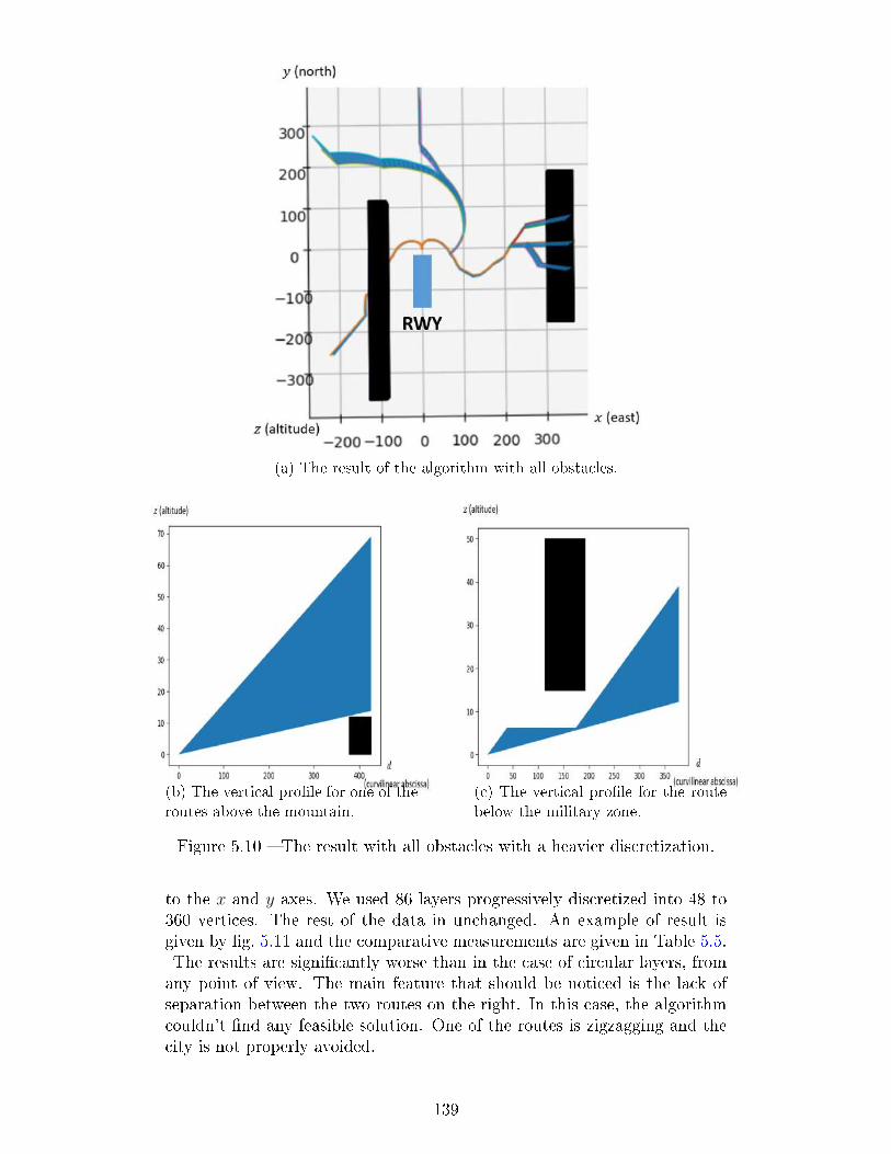
(a) The result of the algorithm with all obstacles.

(b) The vertical pro�le for one of theroutes above the mountain.

(c) The vertical pro�le for the routebelow the military zone.

Figure 5.10 � The result with all obstacles with a heavier discretization.

to the x and y axes. We used 86 layers progressively discretized into 48 to360 vertices. The rest of the data in unchanged. An example of result isgiven by �g. 5.11 and the comparative measurements are given in Table 5.5.The results are signi�cantly worse than in the case of circular layers, fromany point of view. The main feature that should be noticed is the lack ofseparation between the two routes on the right. In this case, the algorithmcouldn't �nd any feasible solution. One of the routes is zigzagging and thecity is not properly avoided.

139

Figure 5.11 � An example of result obtained on the arti�cial instance withsquares as layers.

Measurement Circular layers Square layersComputation time 4 min 08s 29 min 27s

Route length 2970.13 3276.15Graph weight 1874.41 2394.19

Table 5.5 � The mean results for the arti�cial instance with squares as layers(1 runway).

140

This test shows how discretization impacts the results. It is chosenarbitrarily, and to the best of our knowledge there is no way to knowbeforehand the type of discretization that will provide the better result.However, it has been observed in all the tests that were conducted, includingthe ones taken from the literature, that past a certain number of layers, thealgorithm becomes less performing. Therefore, the optimal solution shouldbe searched by changing the shape of the layers rather than their number.

5.2.2.2 The arti�cial instance with two runways

In order to complete the tests on the range of capabilities of the algorithm, weadded a second runway to the arti�cial instance. The corresponding datais gathered in Table 5.6, with the features of the �rst runway reminded.The tra�c �ows are relative to their associated runway. Therefore, the totaltra�c �ow for each runway is 100%. The entry points are given as polarcoordinates, relatively to their respective centers. This runway is orientedby the vector (0,-1), all other parameters are unchanged. The test has beenrun with the two discretizations: circular and square layers. The results arepresented in the next paragraphs.

5.2.2.2.1 The arti�cial case: two runways with circular layers

As for the con�guration with only one runway, we tested a "light" anda "heavy" discretization. The parameters of these discretizations arepresented in Table 5.7. We decided to keep the same discretization forthe two con�gurations on the second runway, as the aim was to measurethe performances of the algorithm under two di�erent workloads, andthe di�erence between the two discretizations for the �rst runway alreadyproviding a su�cient di�erence in workloads. Figure 5.12 provides examplesof the results that were obtained with this con�guration, and Table 5.8 themean numerical results of the tests. The �rst noticeable feature is thecloseness of the mean values for the route length and graph weight criteria.For the graph weight, the value is even lower for the light discretization.As for the case with one runway, it can be concluded that a heavier

Route number Tra�c �ow Graph center Entry point1 26.67%

(0,0,0)

(346NM, 0◦)2 24% (346NM, 10◦)3 21.33% (346NM ,350◦)4 13.33% (346NM ,90◦)5 12% (328.5NM, 135◦)6 2.67% (328.5NM, 230◦)7 54%

(150,300,0)

(547NM, 350◦)8 27% (547NM, 270◦)9 19% (547NM ,225◦)

Table 5.6 � The data used for the routes in the arti�cial instance (2 runways).

141

Parameter Light discretization Heavy discretization# of layers (1st runway) 50 100# of layers (2nd runway) 70 70

# of points per layer (1st runway) 72 360# of points per layer (2nd runway) 72 72

Table 5.7 � The data used for the arti�cial instance (circular layers, 2runways).

(a) An example of result that was obtained with the lightdiscretization.

(b) An example of result that was obtained with the heavydiscretization.

Figure 5.12 � Examples of results that were obtained with layers as circlesfor the arti�cial instance (2 runways).

142

Measurement Light discretization Heavy discretizationComputation time 35 min 22s 48 min 42s

Route length 6332.40 6330.77Graph weight 4283.12 4335.76

Table 5.8 � The mean results for the arti�cial instance with squares as layers(2 runways). The graph weight represents the sum of the lengths of each arcin the solution counted only once.

discretization does not necessarily give better results. It can also be noticedthat the shape of the layers does not impact the mean time necessary toobtain an admissible solution (i.e. a solution that does not violate theobstacle constraint): a solution for the light discretization scenario is foundin approximately 35 min whether the layers are circular or square, and asolution for the heavy discretization in roughly 50 min. The examples ofresults found by the algorithm also show that the solutions are quite similar.

5.2.2.2.2 The arti�cial case: two runways with square layers

Finally, we tested the algorithm with square layers for both runways inorder to compare the performances of the algorithm with the con�gurationwith circular layers. The characteristics of the layers used are gathered inTable 5.9. An example of result that could be obtained is presented in�g. 5.13. The numerical values for the optimization criteria are gathered inTable 5.10, with the values for the approach with circular layers remindedfor comparison. The results displayed in �g. 5.13 show that the algorithmbecomes unable to handle correctly the considered scenario. The maximumturn angle constraint is no longer met, and the routes are signi�cantly andunnecessarily longer, especially for the second runway. In these results,we included a "Number failed" line. It quanti�es the number of solutionsreturned by a complete run of the algorithm that violate the obstacleavoidance constraint (in this case: when a route passes through a mountainor a military zone). The proportion of failed runs is particularly high andshows that the algorithm reaches its limits in particularly complex cases.The complexity of an instance, as the comparison between the various testsshows, is not only determined by the layout and operational constraints(obstacles, position of the entry points, cities, maximum slopes and turn

Parameter Value# of layers (1st runway) 86# of layers (2nd runway) 110

# of points per layer (1st runway) from 48 to 360# of points per layer (2nd runway) from 48 to 360

Table 5.9 � The data used for the arti�cial instance (square layers, 2runways).

143

(a) The solution seen from above. The routes don't havea coherent shape, and one of them violates the maximumturn angle constraint.

(b) The vertical pro�les of thesolution. The ground obstacle andthe military zone are avoided. (c) The side view of the solution.

Figure 5.13 � A solution for the arti�cial case with two runways and squarelayers.

Measurement Circular layers Square layersComputation time 35 min 22s 55 min 13s

Route length 6332.40 6976.51Graph weight 4283.12 5470.63Number failed 0% 75%

Table 5.10 � The mean results for the arti�cial instance with squares aslayers (2 runways). The graph weight represents the sum of the lengths ofeach arc in the solution counted only once.

144

angles...), but also by the choice of the discretization to apply (shape andnumber of the layers, number and location of the vertices on the layers).The tests conducted on this arti�cial instance further demonstrated thesensitivity of the algorithm to the choice of the layers, as during our tests,two particular situations were encountered:• The algorithm couldn't �nd a single admissible solution over 50 runs.The tests were stopped under the assumption that no admissiblesolution would be found.

• The algorithm couldn't build a given route. This means that thechosen discretization didn't allow to �nd a single path that led tothe entry point. This case occurred more speci�cally when the �rstlayers were sampled into too few vertices and thus the maximum turnangle constraint was violated during the pre-processing part of thealgorithm. This case is illustrated in �g. 5.14.

In a nutshell, it can be concluded that the angular stone of the method lies in

(a) The exit point is not attainable. (b) The exit point is attainable.

Figure 5.14 � An illustration of the impact of the discretization.

the choice of the discretization: shape and number of the layers, number andpoints per layer. Although it has not been explicitly tested, it can also beinferred that the distribution of the points on the layers plays an importantrole. An idea would be to increase their number in the vicinity of obstaclesand allow fewer of them in open areas.

5.3 The Stockholm instance

The �rst instance of a real-life scenario on which the SA based algorithm wastested is taken from the literature [114]. It involves a single runway and fourSTARs to be designed for the Sotckholm Arlanda airport. In [114], the routesare designed only in 2D with an integer programming (IP)-based methodapplied on a grid (see �g. 5.15). In their work, the authors design severalsolutions for the presented problem in order to �nd the Pareto front withregard to the route length and graph weight criteria. The solution presentedin �g. 5.15 corresponds to the minimum graph weight. The drawback ofthis approach is its execution time: 9447 seconds (2h 37min 27s) to �nd theminimum weight spanning tree. The data that was used to conduct the test,with regard to the route parameters is presented in Table 5.11.

145

Figure 5.15 � The result from [114] and the layout used.

Route number Tra�c �ow Graph center Entry point1 25%

(7,11)

(14,13)2 25% (9,20)3 25% (0,10)4 25% (7,0)

Table 5.11 � The data used for the routes in the Stockholm instance.

146

Additionally, we used the following values for the parameters:

• Center = (7,12);

• The runway is oriented by the vector (0, 1);

• The altitude range of the exit points is not relevant (so all ranges areaccepted in the solution);

• Maximum turn angle θmax = 45◦. It is the maximum authorized anglebetween two consecutive arcs in the horizontal pro�le;

• Minimum angle at merge points θmin = 15◦;

• The minimum and maximum slopes αmin and αmax are not relevant;

• The number and minimum and maximum length of the level �ightsnLFmax, l

LFmin and lLFmax are not relevant;

• There is no orientation imposed on the entry/exit points.

In Table 5.12, we present the data that was used for the obstacles of theinstance. Although they are cities, we represented them as "hard" obstacles,in order to comply with the representation used in [114]. In Table 5.12, each

one of them is given in the form((

(x1, y1); (x2, y2); . . . ; (xn, yn)), lo, uo

)where:• (x1, y1); (x2, y2); . . . ; (xn, yn) are the coordinates of the base polygongiving the location of the city;

• lo is the lower altitude of the obstacle (0 being on the ground);

• uo is the upper altitude of the obstacle.

We conducted several series of tests on this same instance: one with onlytwo cities taken into account, and the other with all cities considered. Wepresent and explain the results obtained in the next paragraphs.

Obstacle (B, l, u)

Enköping(((1,10);(3,10);(3,12);(1,12)

), 0, +∞

)Stockholm

(((7,6);(9,6);(9,8);(7,8)

), 0, +∞

)Uppsala

(((5,13);(6,13);(6,15);(5,15)

), 0, +∞

)Sodertäle

(((5,4);(5,5);(6,5);(6,4)

), 0, +∞

)Table 5.12 � The obstacles for the Stockholm instance.

147

5.3.1 Test case 1: only two cities taken into account

In this �rst test, the aim is to compare the results of our approach to [114].Therefore, we considered only the cities of Stockholm and Enköping. Wechose to use 13 concentric square layers for this test so as to match thediscretization used in the literature. Square i has a 2(i − 1) NM-long side,with square 1 being the center at (7,12) as shown in �g. 5.16. There is avertex each 1NM on each square starting from a corner. This discretizationis the same as the one used in the literature. An example of result that wasobtained with our algorithm is presented in �g. 5.17, and the comparativeresults are presented in Table 5.13. The results presented here do not displaythe vertical pro�les, as they were not taken into account in [114], althoughthey were computed during the execution of the algorithm and taken intoaccount for the obstacle avoidance and route separation. Since cities areto be completely avoided and solutions can easily be made planar, anyslopes are acceptable. Both the route length and graph weight criteriaare better for the solution from the literature. This is explained by threeparticularities. The �rst one is that the MILP-based algorithm is an exactapproach, while the SA is not. The second reason is that in [114], thesolutions are post-processed to partially become independent from the grid:all vertices that can be removed without violating the turn angle constraintare deleted (see �g. 5.18). This allows for both shorter routes and lightergraphs. Finally, our algorithm does not allow for going from a layer Li toa layer Lj with j ≤ i. This causes the route coming from the south in theexample shown to be longer than IP route. These particularities are thereason why the solutions found with our method cannot attain the samecharacteristics as the ones from the literature with regard to route lengthand graph weight even if given more computational power.The last feature to notice in these results is the great di�erence incomputational time required by the solutions.

5.3.2 Test case 2: all cities taken into account

In this paragraph, we present the results obtained when including all cities ofTable 5.12. The results relative to the route length and graph weight criteriaare presented in Table 5.14, with a reminder of the previously presentedresults. As can be expected, both criteria are slightly degraded when allcities are taken into account. The shape and computing time of the averagesolution does not di�er from the previous case with only two cities taken intoaccount. The reason for that is that the two additional cities are already

Feature Solution from [114] Our solutionRoute length 45.74 48.11Graph weight 33.26 41.98

Computation time 9447s 4.54s

Table 5.13 � The comparative results for the Stockholm instance.

148

Figure 5.16 � The layers used for the �rst test with 7 of the 13 layers.

Feature Solutionfrom [114]

Our solution (2cities)

Our solution (allcities)

Route length 45.74 48.11 52.08Graph weight 33.26 41.98 43.56Computationtime

9447s 4.54s 3.46s

Table 5.14 � The comparative results for the Stockholm instance withsquares as layers.

149

(a) The solution found in theliterature [114].

(b) The solution found with ouralgorithm.

Figure 5.17 � Comparative results for the Stockholm instance.

Figure 5.18 � The post-processing technique used in [114].

avoided in the solutions from the previous test case.

5.3.3 Test case 3: circular layers

In this third test case, we decided to test another type of discretization.In this case, we tested circular layers regularly spaced by 0.5NM sampledinto 360 vertices each (one every degree). There are 25 layers in total inthis case. An example of result is shown in Figure 5.19. The comparative

Figure 5.19 � The result of the algorithm on the Stockholm instance by usingcircular layers.

results are given in Table 5.15. The results are way less satisfactory than in

150

Feature Our solution (squarelayers)

Our solution (circularlayers)

Route length 52.08 73.13Graph weight 43.56 52.4Computation time 4.54s 125.19s

Table 5.15 � The comparative results between square and circular layers forthe Stockholm instance with all cities.

the previous case, as the routes are signi�cantly longer and occupy a widersurface. The computation time is also dramatically increased, due to thestrong increase in layers and discretization points. Thus, the choice of thelayout, and more particularly the shape of the layers, has a great impact onthe quality of the solution given by the algorithm. The main improvementof our method over an exact approach is the reduced computation time.Although it is not critical in this particular case, since the routes are to bedesigned at a strategic level, which allows to take several hours, it will bean essential feature for larger instances.

5.4 The Paris Charles-de-Gaulle instance

The aim of this work is to be able to design routes for large airports, sincethese cases are very often more di�cult to tackle than cases involving asingle runway. In order to test our algorithm on a large size real-life scenario,we designed the layout of the Paris Charles-de-Gaulle airport (CDG). Thisinstance has already been studied in [45]. Therefore, in order to establisha comparison with this approach from the literature, we kept the samecon�guration.The SIDs and STARs currently in use at CDG airport are published andpublicly available from Jeppesen (see the example of �g. 5.20). In our work,the initial direction for the procedures is given by the orientation of therunway it depends on. This orientation is given by the heading that anaircraft follows when using the runway. Therefore, a runway always has twopossible orientations, di�ering by 180◦ from each other. This orientation isused to identify the runway, by rounding its heading to the nearest 10◦ andgiving the �rst two numbers. For instance, a runway oriented towards theheading 140 (140◦ clockwise relatively to the magnetic north pole) will beidenti�ed as 14. Since a runway has two opposite directions, the completeidenti�cation for this example is 14/32 (see �g. 5.21). When using a runwayfor departure or arrivals, only one number is given, that corresponds to theheading of the aircraft. Therefore, a plane landing on runway 32 meansthat its heading is 320 when landing. In large airports, it is common to seetwo or even three parallel runways next to each other. This con�gurationhelps absorb heavy tra�c �ows, as one runway can be used for take-o�sand the other one for landings. When this case occurs, the runways aredi�erentiated by letters: L for the left one, R for the right one and C for the

151

Figure 5.20 � An example of a published procedure at CDG airport.

152

Figure 5.21 � The identi�cation of a runway.

center one when applicable (see �g. 5.22). In the case studied here, thereare 4 runways, whose characteristics are gathered in Table 5.16 (this datais the same that is used in [45])(see �g. 5.23). Depending on the weather,the runways in use, the type of aircraft and other criteria, the operatingSIDs and STARs can change. In this work, as in [45], 15 routes have beenchosen. The corresponding o�cial waypoints, as well as the estimated tra�c�ow, are given in Table 5.17. The data is taken from [45]. The tra�c �owshave been measured by counting the relative number of aircraft taking theprocedures in a given time window. The graphical representation of theseroutes is given in �g. 5.24. The coordinates of the starting and endingpoints for the routes are gathered in Table 5.18.

Runway threshold Type of procedureGraph center

2D position Height (ft)27L SID (99.28, 122.95) 37026R SID (100.9, 121.5) 33827R STAR (111.12, 124.51) 339226L STAR (112.8, 122.66) 3316

Table 5.16 � The characteristics of the runway thresholds and starting pointsfor the tests.

153

Figure 5.22 � The identi�cation of parallel runways.

Figure 5.23 � The thresholds at CDG airport in [45].

Route Threshold Type of procedure Tra�c �ow Waypoints1 27R STAR 12.77% DINAN, XERAM, LORTA, BSN

2 27L SID 10.82% PG274, PG278, NAPIX, DIKOL

3 26R SID 10.72% PG266, PG289, DOPAP, OKASI

4 27R STAR 8.7% DPE, SOKMU, KOROM, MERUE, CREIL, PG525

5 26R SID 7.44% PG268, RBT, ADADA, AGOPA

6 26L STAR 7.33% BENAR, ROMLO, BALOD, DOMUS, PG515, PG516

7 26L STAR 7.16% RLP, TROY, OMAKO, PG512

8 27R STAR 6.97% MOPIL, XERAM, LORTA, BSN

9 27L SID 5.63% PG276, OPALE

10 26L STAR 5.61% DJL, TRO, OMAKO, PG512

11 27L SID 4.9% PG274, PG278, LAURA, LASIV

12 27L SID 4.76% PG276, NURMO

13 27L SID 3.38% PG280, PG284, EVREUX

14 26R SID 2.33% PG264, PG288

15 27R STAR 1.48% DVL, SOKMU, KOROM, MERUE, CREIL, PG525

Table 5.17 � The routes selected for the tests for Charles-de-Gaulle airport.

154

Figure 5.24 � The chosen published routes as shown in [45].

Route ThresholdGraph center

Entry/Exit point (2D)2D coordinates Height (ft)

2

27L (99.28, 122.95) 370

(159.87, 132.61)9 (73.18, 175.07)11 (167.34, 118.76)12 (107.11, 171.69)13 (48.26, 122.38)

326R (100.9, 121.5) 338

(111.77, 67.03)5 (80.87, 66.08)14 (31.89, 113.55)

1

27R (111.12, 124.51) 3392

(207.18, 177.27)4 (45.4, 176.02)8 (158.66, 193.36)15 (12.31, 138.75)

626L (112.8, 122.66) 3316

(29.88, 75.39)7 (211.86, 61.57)10 (208.23, 23.08)

Table 5.18 � The routes with their associated starting and ending points forthe Charles-de-Gaulle instance.

155

The additional characteristics of this instance are as follows:

• The altitude range of the exit points is not relevant (so all ranges areaccepted in the solution);

• Maximum turn angle θmax = 30◦;

• Minimum angle at merge points θmin = 15◦;

• Minimum slope (SID) αSIDmin : 7.0%;

• Maximum slope (SID) αSIDmax: 11%;

• Minimum slope (STAR) αSTARmin : 1.6%;

• Maximum slope (STAR) αSTARmax : 4.2%;

• The maximum number of level �ights nLFmax = 4 per runway threshold(so 16 in total);

• The minimum length of the level �ights was set to lLFmin = 10NM andthe maximum length lLFmax is not relevant here;

• There is no orientation imposed on the entry/exit points.

Finally, we set the city of Paris as an obstacle, in order to proceed on thesame base as the one that was used in [45]. It is represented as a cylinderwith the following characteristics:• The base is a circle centered on (92.43, 113.16) with a 5NM-radius;

• The lower altitude is 0;

• The higher altitude is 50,000 ft.

In the rest of this section, we provide the results that were obtained withboth circular and square layers, and we establish a comparison between orresults and those from the literature, in terms of route length and graphweight.

5.4.1 The Paris CDG case: a comparison with theliterature

In the approach tested in [45], the problem is solved by using aBranch-and-Bound algorithm to decide for each route the way to avoidobstacles when there are any (refer to Chapter 2 for the details of thisapproach). This approach allows to minimize the route length criterion ina search space where all obstacles are circular, in 2D. The results obtainedare shown in �g. 5.25. The main drawback of this approach is that it lacks amanagement of the merging points, and all routes merge on the equivalent ofthe center here, which makes it unusable in a real-life scenario. The resultsof our approach is shown below.

156

Figure 5.25 � The routes designed with the method from [45].

5.4.1.1 The CDG instance: square layers

We �rst tested the algorithm with square layers. These are set as shown inTable 5.19. In this case, the layers' sides are parallel to the x and y axes,and are discretized into 120 to 360 points (proportionally to their numberstarting at 2, so that, for instance, if there are 12 layers, L6 will be sampledinto 216 vertices). Another point to emphasize is that whenever two entryor exit points belonging to the same graph are too close to each other, theyare both put on the same layer, which is then located at mid-distance fromboth points. In this work, two points are considered too close to each otherwhenever the distance between them and the center di�ers by less than 1NM.The distance chosen depends on the type of layer:• If the layers are square, the distance is the L∞-norm, which is themaximum between the x and y values taken positively;

• For circular layers, which will be addressed later, the distance will bethe usual euclidean distance.

The layers are always spaced by a constant distance. For instance, if layerLi has a 2NM-long side and Li+2 has a 4NM-long side, then Li+1 hasa 3NM-long side. In Table 5.19, the "Layers interval and step" columngives a starting and an ending layer, along with the distance step betweentwo consecutive layers. With the same example as above, the column willindicate: Li → Li+2 : 0.5. The step given is the increase in the maximumx (or y) distance from the center, so half of the increase in side length (see�g. 5.26). The number given to the gates are the ones that correspondto their path (see Table 5.18). An example of result obtained with this

157

ThresholdTotal number

of layersLayers interval and step Gates involved

Layer ofthe gates

27L 17

1 → 11 : 4.874 12 1111 → 12 : 2.28 13 1212 → 13 : 1.1 9 1313 → 15 : 4.235 2 1515 → 17 : 3.735 11 17

26R 181 → 14 : 4.2265384

6 147 14

14 → 18 : 3.5162502 10 18

27R 21

1 → 14 : 5.055384615 4 1414 → 15 : 3.13 8 1515 → 20 : 5.442 1 2020 → 21 : 2.75 15 21

26L 251 → 21 : 4.146 3 21

21 → 25 : 4.15 2514 25

Table 5.19 � The structure of the square layers for the CDG instance. Thedistance step between two consecutive layers is given, as well as the layer onwhich each route starts or ends.

Figure 5.26 � The illustration of the functioning of Table 5.19 with a toyexample. Two di�erent spacings are used: 2 and 3NM, resp. from layer 1 to4 and from layer 4 to 7. Gate 2 is located on layer 4, gate 1 on layer 6 andgate 3 on layer 7.

158

discretization is shown in �g. 5.27.The results are quite satisfactory, since they present the followingcharacteristics:

• The city is avoided;

• There is no con�ict between the routes;

• The merging points are separated;

• The merging points are well located.

However, in this series of tests, it is to be noted that more than half of theresults were rejected and the test have been performed again because thesolution was not feasible. More precisely, 62% of the tests failed in that way.This means that although the city represents but a small portion of the area,the algorithm struggles to �nd routes that avoid it. This is mainly due tothe need to design many routes, and thus, in top of the city, all con�ictsbetween them are to be avoided, which reduces greatly the possibilities ofdesign.In order to test other possibilities, we then ran the same tests, with circularlayers.

5.4.1.2 The CDG instance: circular layers

The previous test cases showed that the shape of the layers play an importantrole in the outcome of the algorithm. Incidentally, we decided to run thetests in the same con�guration, but with circular layers. Their layout isgiven in Table 5.20. In this table, the mark "x" means that no gate isinvolved in the described layers. With all other parameters being equal tothose in the square layers test case, an example of result is shown in �g. 5.28.We observe that the routes are signi�cantly less direct, and the resulting setoccupy more space than in the square layers case. It can also be noted thatsome of the routes adopt a zigzagging behavior towards their end. This canbe due to the number of routes to design: the priority of the algorithm is toavoid the con�icts between the routes rather than designing them straight.This behavior can be smoothed with a post-processing of the result. In thisseries of tests, only 6% of the results were rejected due to con�icts. Thisis signi�cantly lower than in the case of square layers. This di�erence isdiscussed at the end of the chapter.

5.4.2 The Paris CDG case: adding a forbidden zone

In order to test further the capacities of the algorithm, we ran it again onthe same instance, with the same two sets of layers. The zone that wasadded has the following characteristics:

159

(a) 1st view.

(b) 2nd view.

Figure 5.27 � The results with square layers for the CDG instance (SIDs inblue/green, STARs in red/orange).

160

(a) 1st view.

(b) 2nd view.

Figure 5.28 � The results with circular layers for the CDG instance (SIDs inblue/green, STARs in red/orange).

161

ThresholdTotal number

of layersLayers interval and step Gates involved

Layer ofthe gates

27L 23

1 → 2 : 4.36493188 x x2 → 17 : 3 12 17

17 → 18 : 1.65825207 13 1818 → 20 : 3.633323535 9 2020 → 21 : 3.06539451 2 2121 → 23 : 3.41681383 11 23

26R 21

1 → 2 : 4.7756 x x

2 → 18 : 3.3884563 175 18

18 → 21 : 3.5126 14 21

27R 36

1 → 2 : 5.58456376 x x

2 → 28 : 34 288 28

28 → 33 : 3.249252328 15 3333 → 36 : 3.2515089 1 36

26L 46

1 → 2 : 5.44725926 x x2 → 32 : 3 6 32

32 → 39 : 2.9907397 7 3939 → 46 : 3.077382442 10 46

Table 5.20 � The disposition of the circular layers for the CDG instance.

• The base is a rectangle whose angles are at coordinates (130,60),(140,60), (140,127), (130,127);

• The lower altitude is 1.7NM;

• The higher altitude is 2NM.

The other parameters were left unchanged. An example of result is givenby �g. 5.29. In this �gure, some vertical pro�les are displayed, showing howthe forbidden zone is avoided by the routes. In comparison with the testcase without the forbidden zone, the shape of the routes is less satisfactory,especially in the positioning of the merging points. For instance, routes 7and 10 (the STARs that avoid the zone) could have merged much closer totheir respective gates, as these gates are close to each other. It would havebeen better to have only one route pass under the zone, that would split onlyafterward. This result can be explained by the need for the algorithm toavoid the forbidden zone, on top of the city and the con�icts between routes.By referring to the mathematical formulation of the problem, its priority isto �nd solutions that don't violate the constraints, and then comes theoptimization. In this series of tests, more than 78% failed. The main causefor failure remains the non-avoidance of the city (53% of the total numberof tests), the avoidance of the forbidden zone representing the other 25%.We then tested the algorithm in the same con�guration with circular layers.An example of result is given in �g. 5.30. The given vertical pro�les alsobelong to the routes avoiding the forbidden zone. As for the square layers

162

(a) The routes designed for the CDG instance with aforbidden zone and square layers.

(b) The vertical pro�le of route 7. (c) The vertical pro�le of route 10.

Figure 5.29 � The results with square layers for the CDG instance with aforbidden zone.

163

(a) The routes designed for the CDG instancewith a forbidden zone and circular layers (1st

view).

(b) The routes designed for the CDG instance with aforbidden zone and circular layers (2nd view) (SIDs inblue/green, STARs in red/orange).

(c) The vertical pro�le of route 7. (d) The vertical pro�le of route 6.

Figure 5.30 � The results with circular layers for the CDG instance with aforbidden zone.

164

case, we observe that the results are less satisfactory in terms of shape ofthe routes. The explanation is the same as before. In this series of tests,only 32% of the tests failed, with 23% due to the presence of the forbiddenzone and the remaining 9% to the non-avoidance of the city. Although itrepresents almost a third of the total number of tests run, this number isvery low compared to the previous case.

5.4.3 Comparative results for the CDG instance

Over all series of tests, measurements were taken in order to comparenumerically our results to the ones from the literature, and from the real-lifeimplantation of this case. The numerical results are gathered in Table 5.21.The measurements for the standard routes are taken from [45]. A �rst resultto consider is the di�erence in the route length criterion, which is higher inour work than in the published routes as well as the work from [45]. Thisdi�erence with the work from the literature is explained by the fact that thelatter is explicitly designed so as to minimize this criterion, by locating allmerging points on the runways' thresholds, and thus it does not take intoaccount the merging criterion. The di�erence with the published routes ismostly due to two elements:• Our algorithm is not able to connect a layer i to a layer j with j < i;

• We set a maximum turning angle smaller than the one observed onthe published procedures.

As a consequence, several routes are lengthened, mostly to avoid con�icts.This behavior can be observed for routes 4 and 15, route 6 and routes 2and 11. In a minor way, the routes from our solution are not as straightas in the published solution. The results on the graph weight criterion areexplained in a similar way. The last result to mention is the computationtime required to design the solutions. Within our own results, there is asigni�cant di�erence between the two choices of layers (circles or squares).This di�erence is due to the high proportion of failed results provided bythe square discretization, resulting in almost twice the number of iterationsnecessary to obtain the same number of admissible solutions in that case.

Measurement Published routes B&B approach ([45]) SA approach ([45])Route length 1358.26 1313.49 1295.51Graph weight NC 1313.49 1295.51

Computation time NC 9.8s 20 min

MeasurementSquare layers Circular layers

Without zone With zone Without zone With zoneRoute length 1910.38 1992.53 1972.12 1926.67Graph weight 1508.70 1558.42 1502.52 1470.16

Computation time 13 min 45s 20 min 02s 4 min 22s 6 min 17sNumber failed 72.22% 78.57% 0% 57.75%

Table 5.21 � The mean numerical results for the Charles-de-Gaulle instance.

165

The computation time in our worst-case scenario is however comparable tothe one from the literature using the same meta-heuristic (the SimulatedAnnealing). In this work, we consider that the acceptable time that can beused to �nd a satisfactory solution is of the order of 8 hours. Therefore ouralgorithm is compliant with this objective.The main element that was put forward with this test case is the greatsensitivity of the algorithm to the choice of the shape of the layers. In allcases, it managed to �nd solutions, but the number of trials necessary toachieve the same result varies strongly depending on this choice. Thus, itcan be seen that the case with the circular layers allowed the algorithm to�nd feasible solutions more easily. It has also been shown that increasingthe number of routes to be designed can a�ect negatively the shape of theroutes in order to comply with the given constraints, and in particular thecon�ict avoidance. It should also be noted that several discretizations weretested beside the ones presented in this document. For many of them, thealgorithm was unable to �nd a solution, either because it couldn't connectan entry/exit point to its runway threshold when constructing the graph,or because the discretization didn't allow it to �nd a feasible solution (allsolutions would include con�icts). This observation strengthens our previouscomment on the importance in the choice of the layers. The last point tomention is that we observed an important disparity in the observable qualityof the results given by the algorithm even in the same series of tests. Thisshows that in complex cases the algorithm cannot be considered constant inthe solution it provides, because of the numerous possibilities of design thatit encounters. Therefore, it appears necessary to perform several tests foreach given instance in order to obtain at least one fully coherent solution,i.e. a solution in which the shape of the routes is close to what a humancould intuitively design (without steep turns or unnecessary detours or level�ights, for instance). Empirically, we established that 20 successful testswere enough to attain this goal.In the next section, a di�erent layout is considered for measuring theperformance of the algorithm in a case where the main di�culty comesfrom the terrain.

5.5 The Zurich instance

In the Charles-de-Gaulle instance, the main di�culty is to design a largenumber of routes. In this case, the environment was relatively simple, asthe only obstacle was the city of Paris. Another situation that can be di�cultto handle for our algorithm is when the terrain is not �at, for instance inmountainous landscapes. Such a situation has been tackled in [45] with thecase of Zurich airport. In this instance, the main di�culty is to manage todesign the routes so that the aircraft �y over the mountains. Figure 5.31a(taken from [45]) presents the landscape in the considered area, and �g. 5.31bthe way that we modeled it. In this case, the grid we used was made upof 1NM×1NM squares. This instance features three runways: one for theSIDs (runway 10), and the STARs arrive on two di�erent runways, 32 and

166

(a) The terrain elevation in the Zurich instance as shownin [45].

(b) Our model for the terrain elevation in the Zurichinstance.

Figure 5.31 � The layout of the Zurich instance.

167

34. However, these runways share the same STARs, the separation occursjust before landing. Therefore, in the scope of this document, the algorithmworks as if there were only one runway, oriented at 330◦. The centers forthe Zurich instance are given in Table 5.22. In [45], for this instance, notra�c �ow is mentioned. Therefore, we chose to give the same importanceto all routes. Additionally, one of the SIDs to design (path number 4) issupposed to start from runway 32/34, but the author of [45] chose to changeits threshold to 10 on the grounds of keeping the design coherent. There are9 routes to design in total. The tra�c �ows and waypoints are gathered inTable 5.23. Figure 5.32 displays the published routes, that are currently inuse at this airport. The coordinates of the starting and ending points forthe routes are gathered in Table 5.24. The coordinates are the same as in[45].The additional features of this instance are as follows:

• The altitude range of the exit points is not relevant (so all ranges areaccepted in the solution);

• Maximum turn angle θmax = 30◦;

• Minimum angle at merge points θmin = 15◦;

• Minimum slope (SID) αSIDmin : 7.0%;

• Maximum slope (SID) αSIDmax: 11%;

• Minimum slope (STAR) αSTARmin : 2%;

• Maximum slope (STAR) αSTARmax : 5%;

• The maximum number of level �ights nLFmax = 4 per runway threshold(so 8 in total);

• The minimum length of the level �ights was set to lLFmin = 5NM andthe maximum length lLFmax is not relevant here;

• There is no orientation imposed on the entry/exit points.

With this data, the author from [45] presented two sets of results, one basedon a Branch-and-Bound approach (�g. 5.33a), the other on a SA approach(�g. 5.33b). In both �gures, the published routes are displayed in dashedlines, and the results obtained in solid lines. The green circles represent the

Runway threshold Type of procedureGraph center

2D position Height (ft)10 SID (348.60, 46.53) 1400

32/34 STAR (343.90, 50.66) 2615

Table 5.22 � The characteristics of the runway thresholds and graph centersfor the Zurich tests.

168

Route Threshold Type of procedure Tra�c �ow Waypoints1 10 SID 12% ZH502, ZH526, ARTAG, GERSA

2 10 SID 11% BREGO, VEBIT

3 10 SID 11% ZH502, KOLUL, DEGES

4 10 SID 11% SONGI

5 32/34 STAR 11% RILAX, LAMAX, AMIKI, ZUE, TRA

6 32/34 STAR 11% RAVED, NEGRA, MATIV, AMIKI, ZUE, TRA

7 32/34 STAR 11% KELIP, ZH625, KLO, GIPOL, TRAD10

8 32/34 STAR 11% BLM, GIPOL, TRAD10

9 32/34 STAR 11% DOPIL, ERMUS, GIPOL, TRAD10

Table 5.23 � The routes selected for the tests for Zurich airport.

Figure 5.32 � The chosen published routes for the Zurich instance in [45].

169

Route ThresholdGraph center

Entry/Exit point (2D)2D coordinates Height (ft)

1

10 (348.60, 46.53) 1400

(349.72, 21.42)2 (326.84, 32.85)3 (374.48, 46.86)4 (352.95, 66.5)

5

32/34 (343.9, 50.66) 2615

(343.07, 75.39)6 (391.14, 68.09)7 (359.69, 17.48)8 (304.10, 52.63)9 (328.47, 20.99)

Table 5.24 � The routes with their associated starting and ending points forthe Zurich instance.

obstacles that were chosen for the instance. As for the other cases, we testedboth square and circular layers. The results obtained with our approach arepresented in the next paragraphs.

5.5.1 The Zurich instance with square layers

As the results obtained on the Charles-de-Gaulle instance were moresatisfactory with the square layers, we decided to test those �rst. Theywere designed according to Table 5.25.In this case, we tested three di�erent discretizations of the layers:

• in the �rst one, there are 80 to 180 vertices per layer depending on thelayer's number (in the same way as for the CDG instance);

• in the second one, there are 80 to 360 vertices;

• in the third one, there are 120 to 480 vertices.

ThresholdTotal number

of layersLayers interval and step Gates involved

Layer ofthe gates

10 13

1 → 11 : 2 4 1111 → 12 : 1.76 2 12

12 → 13 : 3.7351 133 13

32/34 24

1 → 13 : 2.060833333 5 1313 → 15 : 2.47 9 1515 → 17 : 1.755 7 17

17 → 20 : 2.206666667 8 2020 → 24 : 1.86 6 24

Table 5.25 � The disposition of the square layers for the Zurich instance.

170

(a) The results from the literature (B&B algorithm).

(b) The results from the literature (SA algorithm).

Figure 5.33 � The results from the literature [45] on the Zurich instance.

171

The number and position of the layers don't change along tests, only thenumber of vertices per layer. This choice has been made in order for thealgorithm to be able to �nd solutions. This aspect will be discussed atthe end of this section on the Zurich instance, and more generally in theconclusion of this chapter and the discussion. The results are displayed in�g. 5.34. It appears that the results are very similar in their shapes. Themountains are avoided and no con�ict is observed between the routes. Theinteresting comparison to consider here is the proportion of failed iterationsof the algorithm (see Table 5.27). These values show that there are toofew discretization points in the �rst case, and the algorithm is unable toeasily �nd feasible routes, because only a small proportion of all possibilitiesactually leads to a feasible solution. In the third test case, the oppositeproblem is responsible for the number of failures: there are too manypossibilities, most of which are not feasible. Therefore, the algorithm is notable to easily �nd a feasible solution among all possibilities. These valuesput forward two important aspects:• The algorithm has reached its limits in terms of capacity to managethe terrain on this instance (a slightly more complex instance couldhave led to the impossibility to �nd any solution, at least with thistype of layers);

• The choice of the density of vertices is once again a critical criterionof the performance of the algorithm.

We can also mention that several other discretizations of the square layerswere attempted, which couldn't provide any feasible result. This puts anemphasis on the last point.

5.5.2 The Zurich instance with circular layers

As for the other test cases, we decided to implement the layers as circles.The layers that were used are as presented in Table 5.26.

ThresholdTotal number

of layersLayers interval and step Gates involved

Layer ofthe gates

10 27 1 → 27 : 1.0

4 211 262 273 27

32/34 51 1 → 51 : 1.0

5 269 347 388 416 51

Table 5.26 � The disposition of the circular layers for the Zurich instance.

172

(a) The results with the �rstdiscretization (1st view).

(b) The results with the �rstdiscretization (2nd view).

(c) The results with the seconddiscretization (1st view).

(d) The results with the seconddiscretization (2nd view).

(e) The results with the thirddiscretization (1st view).

(f) The results with the thirddiscretization (2nd view).

Figure 5.34 � The results on the Zurich instance with square layers.

173

As for the tests with square layers, and for the same reasons, the variationin discretization only applies to the number of vertices per layer:

• in the �rst case, there are 72 vertices per layer (one every 5◦, see�g. 5.35);

• in the second case, there are 360 vertices per layer (one every degree).

The results obtained are presented in �g. 5.36. As for the square layers, the

b

Center

bbbbbbbb

bbbb

bbbbbbbbbbbbbbbbbbbbb

bbbbbbbb b b b b b b b b b b b b b b b b b b

b bb bb bb bb bbbb

1NM 1NM

b

b

b

b

b

b

b

b

b

bb

bb

bb

bbbbbbbb

bb

bb

b

b

b

b

b

b

b

b

b

b

b

b

b

b

b

b

b

b

bb

bb

bb

b b b b b b bb

bb

bb

b

b

b

b

b

b

b

b

b

1NM

Figure 5.35 � An example of discretization for the Zurich instance in the �rsttest case for circular layers. They are separated by 1NM each, and sampledinto 72 vertices each. The same method for discretization applies for theother cases.

results are quite similar in shape. However, this time it can be observed thatthe solution from the "heavy" discretization yields a smoother result thanthe one with the lighter discretization, which presents irregularities. It canalso be noted that in this case, the solutions provided with circular layersare visually more coherent with real-life operations than with the squarelayers. Again, we can look at the proportion of failed tests in these twocases in Table 5.27. These numbers, as in the Charles-de-Gaulle instance,are much lower than their counterparts in the square layers case. This tendsto con�rm that circular layers are more suited when the instance is complexand an admissible solution can be hard to determine. In the next paragraph,we analyze the numerical results of the tests run on the Zurich instance.

174

(a) The results with the �rstdiscretization (1st view).

(b) The results with the �rstdiscretization (2nd view).

(c) The results with the seconddiscretization (1st view).

(d) The results with the seconddiscretization (2nd view).

Figure 5.36 � The results on the Zurich instance with circular layers.

175

5.5.3 Comparative results and discussion on the Zurichinstance

The results obtained for the tests on the Zurich instance are gathered inTable 5.27. The results show that it is possible for the algorithm to designa set of routes with a route length criterion approaching the one achievedby the procedures in use. The most remarkable feature in these resultslies in the big di�erence between the mean computation times for the caseswith circular layers. Two explanations can be brought. Firstly, it can beexplained by the fact that the number of vertices per layer was multiplied by5, which dramatically increased the time required to build the graphs as wellas the arcs valuation and path search processes. The second explanation,in a minor way, is that in the �rst case, the algorithm ended up with anon-feasible solution in a bigger proportion than for the �rst case.The last noticeable element from these results is the di�erence in values forthe two criteria (route length, but also graph weight) between our resultsand those from the literature. This is mainly due to the need to managethe location of the merging points. Although one could expect the graphweight criterion to be lower in our work, this is not automatically the case,especially in instances like Zurich, where the maneuverable area is small.In this case, forcing a separation of the merging points requires to occupymore space than if it wasn't necessary. Another explanation is that for eachof the two runways under consideration in this case, the entry/exit pointsare rather regularly spread around the centers. This implies that the routesshould share little to no common parts and rather immediately take di�erentdirections, which the merging points management prevents.The Zurich test case has shed some light on one of the most critical typesof scenarios for the design of procedures with our algorithm: the complexityof the layout of the search. We mentioned above that the number anddisposition of the layers weren't changed between the tests, only the numberof vertices per layer. This is due to the di�culty for the algorithm to �ndsolutions when the structure of the layers is not adapted. The followingcases were encountered:

Measurement Published routes B&B approach ([45]) SA approach ([45])Route length 439.52 380.44 387.69Graph weight NC 380.44 387.69

Computation time NC 2.7s 12 min 50s

MeasurementSquare layers Circular layers

1st discr. 2nd discr. 3rd discr. 1st discr. 2nd discr.Route length 483.95 520.30 540.28 520.94 506.68Graph weight 413.45 436.59 464.38 392.84 407.27

Computation time 1 min 44s 1 min 35s 6 min 53s 35s 4 min 57sFailed proportion 82% 51% 86% 20% 33%

Table 5.27 � The mean numerical results for the Zurich instance.

176

• If the layers are too close to one another, it is more di�cult forthe algorithm to design turns (as explained in the section about thearti�cial case). In this con�guration, the algorithm was not able toconnect one of the gates to its runway in the graph construction. Asolution to this problem would be to increase the number of verticesper layer. However, if the number of vertices per layer increases toomuch, the computation time is severely worsened, and most of thesolutions are very negatively a�ected in terms of coherence.

• If the layers are too far from one another, then there aren't enoughpossibilities to create paths. This often resulted in the algorithm notbeing able to �nd any admissible solution (all solutions had con�ictswith the terrain).

Many con�gurations that were tested led to a failure to �nd any admissiblesolution. The di�culty in this test case lies in the rather short maneuverabledistance between the runway thresholds and the mountains around them.This situation, as the situation of Charles-de-Gaulle airport did for thenumber of routes, allowed to de�ne the limits of the algorithm in termsof terrain elevation for a real-life scenario. It also brought to our attentionthe e�ects of scattered entry or exit points around the centers, which, dueto the management of the merging points, takes a toll on both the routelength and graph weight criteria.

5.6 General discussion on the results

The main and most important feature of the algorithm, as put into light bythe series of tests detailed above, is the choice of the layers.

177

The following elements were observed:

• The Stockholm instance showed the importance in the choice of theshape of the layers, even on "small" instances. The results can varystrongly depending on this choice.

• The tests on the arti�cial instance proved that the density of verticesalso played an important role in �nding a solution, even withoutchanging the shape of the layers. It appeared that increasing thenumber of vertices doesn't automatically lead to better solutions, andthere is no easy way to know beforehand what the best suited numberof vertices is.

• The Charles-de-Gaulle instance gave an example of the limits of thealgorithm in terms of capacity to produce a good solution whenthe number of routes to design increases strongly. There again, theimportance in the choice of the shape of the layers was emphasized,the square layers giving more coherent results than the circular ones,but also leading to many more failed runs of the algorithm thantheir circular counterparts. It was noted that better results could beobtained by allowing wider turn angles and by being able to go backto a previous layer.

• The Zurich instance showed the limits of the algorithm in termsof terrain management, with once again more di�culties to �ndadmissible solutions with square layers. The main di�culty for thisinstance was to be able to �nd the right number of layers and number ofvertices per layer to implement. This was due to the relative smallnessof the available search space compared to other large airports, andeven by putting the layers close to each other, their number could becritically low for the way the algorithm was designed. In this case, thecircular layers yielded better results than their square counterparts.

In all cases, the algorithm is very sensitive to the choice of the layers,both in the chosen shape and in the number of discretization points perlayer. It is di�cult to know in advance what type of layers will providethe most satisfactory results. However, we observed from the results ofour tests that the routes have a tendency to be shaped in the form ofthe underlying layers: the square layers provide routes that are ratherstraightforward, with sharper turn angles, while the circular layers giveroutes that are rounder. Based on that observation, it would appear that thesquare layers or similar (rectangles, diamonds, trapezoids, parallelograms,regular polygon...) should be more suited for instances where the routesare expected to be straightforward (for example when there are few tono obstacles, and/or when many routes are to be designed), and that thecircular layers or similar (ellipses) are more �tted for instances where it isnecessary to circumvent obstacles. These assumptions are backed by theresults on the tests performed for this work, but they should be investigatedmore thoroughly and more speci�cally with series of tests designed especially

178

to con�rm or in�rm them. Finally, it should be mentioned that circularlayers have a better tendency to provide admissible results than their squarecounterparts, sometimes at the detriment of the coherence of the solution(as shown with the Charles-de-Gaulle instance), which goes in the samedirection than the previous assumptions: this type of layers looks moresuited for maneuverability and square ones for straightforwardness.

179

Chapter 6

Conclusions and perspectives

6.1 Review of the work

In this thesis, we presented a solution to automatically design StandardInstrument Departures (SIDs) and Standard Terminal Arrival Routes(STARs) at a strategic level. The method relies on the possibilities o�eredby the Required Navigation Performance (RNP) procedures that are beingdeveloped throughout the world to improve the way to use the airspace. Thesolution proposed takes many criteria into account, among which the routelength, the avoidance of certain areas or the management of merging pointsbetween the routes. It was designed in order to be the closest possible tothe shape of the procedures currently in use in real-life scenarios, with theminimization of the controllers' workload as a primary objective.In our model, a route is represented by two elements. The �rst element isthe horizontal pro�le, which consists of a sequence of geographical points in2D (the waypoints) by which the aircraft are expected to �y. These pointsare constructed by sampling the Terminal Maneuvering Area (TMA) aroundthe runway by the means of concentric layers, which are themselves sampledinto vertices to form a graph. The horizontal pro�le is a sequence of pointsof increasing layers in that graph. The second part of the route model is thevertical pro�le, represented as a cone of altitudes associated to the horizontalpro�le. These altitudes encompass all the paths that aircraft following theroutes could �y in the vertical plane. The vertical pro�le is constructed byapplying a minimum and maximum slope along the horizontal pro�le, whiletaking into account possible level �ights.The obstacles are modeled as cylinders with a polygonal base, and aminimum and maximum altitudes. The cities are designed as 2D polygonsassociated to a population density function. They represent areas thatshould be avoided if possible, but that can be �own over if there is no otherchoice. The design of the routes is modeled as an optimization problem thatwe tackled with the use of an algorithm based on the Simulated Annealing(SA) meta-heuristic. For one runway, a �rst route is designed, and then theother routes can connect either to the runway or to a previously createdroute, by taking care not to connect with two routes at the same time. Eachroute is designed by attributing carefully chosen costs to the arcs in thegraph and then by applying a shortest path search in this graph between the

180

desired starting and ending points. The routes are designed by decreasingorder of tra�c �ow so as to favor the busiest ones. The same process is donefor all runways, then the SA optimizes the solution. The obstacle and citiesavoidance, as well as the avoidance of con�icts between routes are carriedout during the evaluation process of the SA, by increasing dramatically thecost of solutions that violate one or several constraints.This method was tested on several instances, both arti�cial and from real-lifescenarios. These tests provided satisfactory results in the current state of AirTra�c Management, but also showed the limits of the algorithm in terms ofcomplexity management, in terms of number of routes and terrain structure.The main element to handle is the shape of the layers used to discretize thesearch space. It appeared that circular layers had a better chance to giveadmissible results and was better tailored to instances in which avoidingobstacles is a major concern, while square layers proved to be more e�cientwhen the main objective is to design straightforward routes, especially inan environment with few to no obstacles. In all test cases, the algorithmran in a time span that is very acceptable in the context it is designed for.A comparison of our results with those from the literature showed that ourmethod could be improved, in terms of route length and space occupied bythe solutions. The main contribution of this thesis lies in the managementof the merging points between the routes, and the variety of constraints thatis taken into account, making it very close to the way actual procedures arecurrently designed.

6.2 Discussion and perspectives

The results showed that there is still room for improvement for the algorithm,including in terms of coherence of the routes on complex instances. Indeed,some of the routes display a zigzag behavior, are unnecessarily lengthenedor connect to other routes in a non-optimal way. However, compared to thecurrent way of designing procedures, by hand, the algorithm runs way faster.These observations make it very suited for decision-helping in the proceduredesign process. A �rst solution can be quickly provided by the algorithm,even on complex instances, and then improved by hand by experts. A �rstelement could be to add the design of the missed approach routes to thealgorithm, in order to add to the compatibility of the algorithm with thecurrent state of air operations. Other perspectives can also be considered,and are presented in the next paragraphs.

6.2.1 Technical perspectives

Various possibilities can be considered in order to improve, or explore furtherthe solution presented in this thesis, such as trying other meta-heuristics(genetic algorithms, ants colony algorithms, particle swarm optimization...)for instance. In this section, we present two technical perspectives that canbe looked into.

181

6.2.1.1 Carry out an extensive study on the choice for the layers

We established that the shape and sampling of the layers used to discretizethe search space play a critical role in the �nal solution provided by thealgorithm. We were able to make assumptions on the role played by theshape of the layers, and the following ideas could help enhance the algorithmon this aspect:• Con�rm or in�rm that circular or elliptic layers, and also regularpolygons with a high enough number of vertices are more suited toinstances in which the primary goal is to avoid obstacles;

• Con�rm or in�rm that square, rectangle, trapezoidal, diamond,parallelogram shapes or convex polygons that are non-regular orcontain few vertices are more suited to instances where there are fewto no obstacles, or where many routes are to be designed;

• Test the in�uence of "hybrid" shapes of layers (such as half-circles, forinstance, when all entry/exit points are located in the same half plane.The half-circles can be closed by a diameter, that would pass on thecenter) on instances containing both situations mentioned above;

• Improve the algorithm so that it becomes able to design routes thatpass several times on a given layer, allowing to make U-turns easierand thus improve the performances.

6.2.1.2 Broaden the tests to the case of a metroplex

The aim of this work is to be able to design routes for large airports.Therefore, the logical continuation is to test it on even larger instances thanCharles-de-Gaulle, like the New-York TMA (see �g. 6.1). An intermediarystep could be to add the airports of Paris-Orly and Paris-Le Bourget to theCharles-de-Gaulle instance. As the limits of the algorithm were seeminglyclose to be attained on the CDG instance, it should be expected thatrunning the algorithm on a more complex case would yield poor results,to no result at all (impossibility for the algorithm to build one or severalroutes). Implementing one of the solutions mentioned in 6.2.2 would thenbe necessary in order to tackle larger instances.

182

Figure 6.1 � The New-York metroplex (taken from [45]).

6.2.2 Methodological (conceptual) perspectives

6.2.2.1 Multiobjective approach

We stated in chapter 3 that the problem of SID and STAR design ismulti-objective in nature. An interesting perspective could then be tomodify the algorithm in a way that allows to explore the Pareto front of thesolutions, rather than outputting a single solution. This would also allowfor a better coverage of the various possibilities for the route design. Thiscoverage could also help in reducing the probabilities for the �nal outputto be an incoherent solution with regard to the current state of air tra�cmanagement.Another way to modify the objective function could be to take the costrelative to the noise out of it, in order to be left with two criteria with thesame unit (so only route length and graph weight). The part of the objectiverelative to the noise could then be integrated to the problem as a constraint.This constraint could be, for instance, to forbid to �y at a lower altitudethan a value set for each point of the grid. This constraint would then beindistinguishable from the obstacle constraint.

6.2.2.2 New route shape modeling

In our work, we decided to design one route by relying on a graph structurewith carefully chosen costs for the arcs and a shortest path search on thisgraph. It could be interesting to employ other means to design a route andcompare them to the work presented in this thesis. Two main possibilitiesshould be particularly interesting to consider.The �rst possibility is to replace the shortest path search by a constructionbased on splines. Splines are mathematical objects that can be used todesign smooth paths by interpolating them using �xed points. A splineis a sequence of polynomials of arbitrary degree, each polynomial beingde�ned between two consecutive �xed points. A useful property of splinesis that depending on their degree, regularity conditions can be imposed on

183

the connection points, which allows to create smooth paths. Using splinesinstead of arcs should take the solutions provided by the algorithm fartherfrom current designs and closer to a mathematical modeling of paths than theones presented in this work, but should help in implementing more e�cientlythe limited turn constraint.The second possibility to design the routes in another way is to use theoptimal control theory. This method takes in entry the state equations,describing the movement of an aircraft, functions describing the constraints,and an optimization function. Several methods can be used to solve theassociated optimization problem, and the solution provided gives the optimalway to �y the aircraft under the optimization function provided (for examplethe route shortness, or the fuel consumption...). Although all routes couldbe designed with this method, it could also be interesting to apply it toeach route, inside a Simulated Annealing-based algorithm. This would allowto modify the optimization function during the process, or for each route,allowing to explore the search space more thoroughly.

184

Publications

This thesis lead to two publications

• In AIAA's journal Aerospace: Departure and Arrival RoutesOptimization Near Large Airports, 6(7), 80, published on July, 12th,2019; https://doi.org/10.3390/aerospace6070080.

• For the EIWAC2019 conference in Tokyo, Japan: SID and STARroutes optimization near large airports, published in HAL archive:https://hal-enac.archives-ouvertes.fr/hal-02352437,February, 8th, 2020, HAL id: hal-02352437, version 1.

185

Bibliography

[1] �Global facts sheet.� https://aviationbenefits.org/media/

166713/abbb18_factsheet_global.pdf, 2018.

[2] �European aviation in 2040 - challenges of growth- annex 4: Network congestion.� https://www.

eurocontrol.int/sites/default/files/2019-05/

challenges-of-growth-2018-network-congestion-21122018.

pdf, 2018.

[3] �European aviation in 2040 - challenges of growth.� https://www.

eurocontrol.int/sites/default/files/content/documents/

official-documents/reports/challenges-of-growth-2018.pdf,2018.

[4] �Commercial market outlook 2019 - 2038.� https://

www.boeing.com/resources/boeingdotcom/commercial/

market/commercial-market-outlook/assets/downloads/

cmo-sept-2019-report-final.pdf, 2018.

[5] S. J. Undertaking, �European atm master plan - executive view,� tech.rep., 2020.

[6] F. A. A. (FAA), �Nextgen implementation plan,� tech. rep., 2018.

[7] E. Commission, �Air tra�c management - freeing europe's airspace,�tech. rep., Commission of the European Communities, 1996.

[8] C. Letondal, C. Hurter, R. Lesbordes, J.-L. Vinot, and S. Conversy,�Flights in my hands: Coherence concerns in designing strip'tic, atangible space for air tra�c controllers,� tech. rep., 04 2013.

[9] S. Rathinam, J. Montoya, and Y. Jung, �An optimization model forreducing aircraft taxi times at the dallas fort worth internationalairport,� MDPI, vol. 1, pp. 3470�3483, 2008.

[10] M. Zhang, Q. Huang, S. Liu, and H. Li, �Multi-objective optimizationof aircraft taxiing on the airport surface with consideration to taxiingcon�icts and the airport environment,� MDPI - Sustainability, vol. 11,p. 6728, 2019.

[11] T. Degaspare, P. Paglione, and C. Marinho, �Development of asimulation environment for ground control laws design,� 12 2015.

186

[12] S. Chaimatanan, D. Delahaye, and M. Mongeau, �A hybridmetaheuristic optimization algorithm for strategic planning of 4daircraft trajectories at the continental scale,� IEEE ComputationalIntelligence Magazine, vol. 9, pp. 46�61, 2014.

[13] O. Rodionova, M. Sbihi, D. Delahaye, and M. Mongeau, �Northatlantic aircraft trajectory optimization,� IEEE Transactions onIntelligent Transportation Systems, vol. 15, pp. 2202�2212, 2014.

[14] C. Allignol, N. Barnier, and A. Gondran, �Optimized verticalseparation in europe,� in 31st IEEE/AIAA Digital Avionics SystemsConference (DASC2012), pp. 4B3�1�4B3�10, 2012.

[15] N. Durand and J.-B. Gotteland, �Genetic algorithms applied to airtra�c management,� Metaheuristics for Hard Optimization Methodsand Case Studies, pp. 277�306, 2006.

[16] S. Ca�eri and N. Durand, �Aircraft decon�iction with speed regulation:New models from mixed-integer optimization,� Journal of GlobalOptimization, vol. 58, no. 4, pp. 613�629, 2014.

[17] N. Barnier and C. Allignol, �4d-trajectory decon�iction throughdeparture time adjustment,� in 8th USA/Europe Air Tra�cManagement Research and Development Seminar (ATM 2009), 2009.

[18] ICAO, PANS OPS vol II - Construction of Visual and InstrumentFlight Procedures, 2006.

[19] ICAO, Performance-based Navigation (PBN) Manual, 2008.

[20] ICAO, Required Navigation Performance Authorization Required(RNP AR) Procedure Design Manual, 2009.

[21] �Compatibility in clearances issued,� in International Federation of AirTra�c Controllers' Associations (IFACTA) 58th annual conference,2019.

[22] Eurocontrol, Guidance Material for the Design of Terminal Proceduresfor DME/DME and GNSS Area Navigation, 1999.

[23] Eurocontrol, Point Merge Integration of Arrival Flows EnablingExtensive RNAV Application and Continuous Descent - OperationalServices and Environment De�nition, 2010.

[24] �Point merge.� https://www.eurocontrol.int/concept/

point-merge.

[25] B. Delaunay, �Sur la sphère vide,� Izv. Akad. Nauk SSSR, OtdelenieMatematicheskii i Estestvennyka Nauk, vol. 7, pp. 793�800, 1934.

[26] P. Maur, �Delaunay triangulation in 3d,� 2002. State of the Art andConcept of Doctoral Thesis - University of West Bohemia in Pilsen,Czech Republic.

187

[27] G. Leach, �Improving worst-case optimal delaunay triangulationalgorithms,� in 4th Canadian Conference on Computational Geometry,1992.

[28] M. Brevilliers, �Triangulations de steiner,� 2006. LMIA Seminary.

[29] Y. Thoma, Tissu Numérique Cellulaire a Routage et Con�gurationDynamiques. PhD thesis, Ecole Polytechnique Fédérale de Lausanne,2005.

[30] D. Watel, Approximation de l'Arborescence de Steiner. PhD thesis,Université de Versailles Saint-Quentin-en-Yvelines, 2014.

[31] T. Lozano-Pérez and M. A. Wesley, �An algorithm for planningcollision-free paths among polyhedral obstacles,� Communications ofthe ACM, vol. 22, no. 10, pp. 560�570, 1979.

[32] H. Rohnert, �Shortest paths in the plane with convex polygonalobstacles,� Information Processing Letters, vol. 23, no. 2, pp. 71�76,1986.

[33] J. Storer and J. Reif, �Shortest paths in the plane with polygonalobstacles,� Journal of the ACM, vol. 41, pp. 982�1012, 1994.

[34] M. N. Bygi and M. Ghodsi, �3d visibility graph,� ComputationalScience and its Applications, 2007.

[35] M. Sharir and A. Schorr, �On shortest paths in polyhedral spaces,�pp. 144�153, 1984.

[36] K. Jiang, L. Seneviratne, and S. Earles, �Finding the 3d shortestpath with visibility graph and minimum potential energy,� vol. 1,pp. 679�684, 1993.

[37] Y.-H. Liu and S. Arimoto, �Path planning using a tangent graph formobile robots among polygonal and curved obstacles,� InternationalJournal of Robotic Research, vol. 11, no. 4, pp. 376�382, 1992.

[38] M. Pocchiola and G. Vegter, �Minimal tangent visibility graphs,�Computational Geometry, vol. 6, no. 5, pp. 303�314, 1996.

[39] F. Aurenhammer, �Voronoi diagrams - a survey of a fundamentalgeometric data structure,� ACM Computing Surveys, vol. 23,pp. 345�405, 1991.

[40] �Quadtree.� https://github.com/domoench/Quadtree.

[41] H. Choset, Sensor Based Motion Planning: The HierarchicalGeneralized Voronoi Graph. PhD thesis, California Institute ofTechnology, 1996.

188

[42] B. Chazelle and L. Guibas, �Visibility and intersection problems inplane geometry,� Discrete & Computational Geometry, vol. 4, no. 6,pp. 551�581, 1989.

[43] N. Sleumer and N. Tschichold-Gürman, �Exact cell decomposition ofarrangements used for path planning in robotics,� tech. rep., Instituteof Theoretical Computer Science Zurich, 1999.

[44] F. Lingelbach, �Path planning using probabilistic cell decomposition,�in Proceedings of 2004 IEEE International Conference on Robotics andAutomation, vol. 1, pp. 467�472, 2004.

[45] J. Zhou, Optimal Design of SIDs/STARs in Terminal ManeuveringArea. PhD thesis, Université Toulouse 3 Paul Sabatier, 2017.

[46] D. Demyen, �E�cient triangulation-based path�nding,� Master'sthesis, University of Alberta, 2007.

[47] A. Ait El Cadi, Plani�cation de Trajectoires pour une Flotte d'UAVs.PhD thesis, Université de Montreal, 2010.

[48] P. Gallina and A. Gasparetto, �A technique to analytically formulateand to solve the 2-dimensional constrained trajectory planningproblem for a mobile robot,� Journal of Intelligent and RoboticSystems, vol. 27, no. 3, pp. 237�262, 2000.

[49] D. Delahaye, S. Puechmorel, P. Tsiotras, and E. Feron, �Mathematicalmodels for aircraft trajectory design: A survey,� Air Tra�cManagement and Systems: Selected Papers of the 3rd ENRIInternational Workshop on ATM/CNS (EIWAC2013), pp. 205�247,2013.

[50] H. Je�reys and B. Je�reys, �Methods of mathematical physics.�Cambridge University Press, 1988.

[51] G. Farin and D. Hansford, The Essentials of CAGD. Natick, MA,USA: A. K. Peters, Ltd., 2000.

[52] W. Mula, �B-spline with control points/control polygon, and markedcomponent curves.� https://fr.wikipedia.org/wiki/B-spline#

/media/Fichier:B-spline_curve.svg.

[53] E. W. Dijkstra, �A note on two problems in connexion with graphs,�Numerische Mathematik, vol. 1, no. 1, pp. 269�271, 1959.

[54] A. Shimbel, �Structure in communication nets,� in Proceedings of theSymposium on Information Networks, pp. 199�203, Polytechnic Pressof the Polytechnic Institute of Brooklyn, 1955.

[55] L. Ford, Network Flow Theory. RAND Corporation, 1956.

[56] R. Bellman, �On a routing problem,� Quaterly of Applied Mathematics,vol. 16, no. 1, pp. 87�90, 1958.

189

[57] P. Hart, N. Nilsson, and B. Raphael, �A formal basis for the heuristicdetermination of minimum cost paths,� IEEE Transactions on SystemsScience and Cybernetics, vol. 4, no. 2, pp. 100�107, 1968.

[58] D. Ferguson, M. Likhachev, and A. Stentz, �A guide to heuristicbased path planning,� Proceedings of the Workshop on Planning underUncertainty for Autonomous Systems at The International Conferenceon Automated Planning and Scheduling (ICAPS), 2005.

[59] D. M. Pfeil, Optimization of Airport Terminal-Area Air Tra�cOperations under Uncertain Weather Conditions. PhD thesis,Massachusetts Inst. of Technology, Cambridge, MA, 2011.

[60] J. Chen, A. Youse�, S. Krishna, B. Sliney, and P. Smith, �Weatheravoidance optimal routing for extended terminal airspace in support ofdynamic airspace con�guration,� in 31st IEEE/AIAA Digital AvionicsSystems Conference (DASC2012), pp. 3A1�1�3A1�16, 2012.

[61] J. Chen, A. Youse�, S. Krishna, D. Wesely, B. Sliney, and P. Smith,�Integrated arrival and departure weather avoidance routing withinextended terminal airspace,� in 32nd IEEE/AIAA Digital AvionicsSystems Conference (DASC2013), pp. 1A4�1�1A4�17, 2013.

[62] M. Shakour, �Conception et implementation d'un algorithmede plani�cation de chemin dans un jeu vidéo comportant unenvironnement triangularisé,� Master's thesis, Université du Québecà Montréal, 2012.

[63] L. Dubins, �On curves of minimal length with a constraint onaverage curvature, and with prescribed initial and terminal positionsand tangents,� American Journal of Mathematics, vol. 79, no 3,pp. 497�516, 1957.

[64] T. Li, J. Jiang, Z. Zhen, and C. Gao, �Mission planning for multipleuavs based on ant colony optimization and improved dubins path,� inIEEE Chinese Guidance, Navigation and Control Conference, 2016.

[65] R. Garroppo, S. Giordano, and L. Tavanti, �A survey onmulti-constrained optimal path computation: Exact and approximatealgorithms,� Elsevier, 2010.

[66] C. H. and S. M. LaValle, �Time-optimal paths for a dubins airplane,�in 46th IEEE Conference on Decision and Control, pp. 2379�2384,2007.

[67] I. Lugo-Cárdenas, G. Flores, S. Salazar, and R. Lozano, �Dubinspath generation for a �xed wing uav,� in International Conferenceon Unmanned Aircraft Systems (ICUAS 2014), pp. 339�346, 2014.

[68] A. Richards, �Trajectory optimization using mixed-integer linearprogramming,� Master's thesis, Massachusetts Institute of Technology,2002.

190

[69] J. Bellingham, M. Tillerson, A. Richards, and J. How, Multi-TaskAllocation and Path Planning for Cooperating UAVs, pp. 23�41.Springer, 2003.

[70] G. Elghoumari, K. Hila, E. Delechelle, and E. Petit, �Analysequalitative des images par propagation de front d'ondes,� 2001.GRETSI, Groupe d'Etudes du Traitement du Signal et des Images.

[71] J. Sethian, �A fast marching level set method for monotonicallyadvancing fronts,� Proceedings of the National Academy of Sciencesof the United States of America, vol 33, pp. 1591�1595, 1996.

[72] J. Sethian and A. Vladimirsky, �Ordered upwind methods for statichamilton-jacobi equations,� Proceedings of the National Academy ofSciences of the United States of America, vol 98, pp. 11069�11074,2001.

[73] S. Vilardaga and X. Prats, �Con�ict free trajectory optimisation forcomplex departure procedures,� in 6th International Conference onResearch in Air Transportation (ICRAT2014), 2014.

[74] S. Vilardaga and X. Prats, �Mass estimation for an adaptivetrajectory predictor using optimal control,� in Proceedings of the 5thInternational Conference on Application and Theory of Automation inCommand and Control Systems (ATACCS15), pp. 75�84, 2015.

[75] X. Prats, V. Puig, J. Quevedo, and F. Nejjari, �Multi-objectiveoptimisation for aircraft departure trajectories minimising noiseannoyance,� Transportation Research Part C: Emerging Technologies,vol. 18, no. 6, pp. 975 � 989, 2010. Special issue on TransportationSimulation Advances in Air Transportation Research.

[76] X. Prats, V. Puig, and J. Quevedo, �Equitable aircraft noise-abatementdeparture procedures,� Journal of Guidance, Control, and Dynamics,vol. 34, pp. 192�203, 2011.

[77] X. Prats, V. Puig, and J. Quevedo, �A multi-objective optimizationstrategy for designing aircraft noise abatement procedures. case studyat girona airport,� Transportation Research Part D: Transport andEnvironment, vol. 16, pp. 31�41, 2011.

[78] M. Soler, A. Olivares, and E. Sta�etti, �Hybrid optimal controlapproach to commercial aircraft trajectory planning,� Journal ofGuidance, Control, and Dynamics, vol. 33, no. 3, pp. 985�990, 2010.

[79] D. Toratani and S. Ueno, �A study on trajectory optimization for theterminal area,� in 6th International Conference on Research in AirTransportation (ICRAT2014), 2014.

[80] D. Toratani, S. Ueno, and T. Higuchi, �Simultaneous optimizationmethod for trajectory and sequence for receding horizon guidance in

191

terminal area,� SICE Journal of Control, Measurement, and SystemIntegration, vol. 8, no. 2, pp. 144�153, 2015.

[81] D. Toratani, D. Delahaye, S. Ueno, and T. Higuchi, �Mergingoptimization method with multiple entry points for extendedterminal maneuvering area,� in 4th ENRI International Workshop onATM/CNS (EIWAC2015), 2015.

[82] S. Khardi and L. Abdallah, �Optimization approaches of aircraft�ight path reducing noise: Comparison of modeling methods,� AppliedAcoustics, vol. 73, no. 4, pp. 291�301, 2012.

[83] J. Betts, �Survey of numerical methods for trajectory optimization,�Journal of Guidance, Control, and Dynamics, vol. 21, no. 2,pp. 193�207, 1998.

[84] O. Khatib and J.-F. Le Maitre, �Dynamic control of manipulatorsoperating in a complex envrionment,� in 3rd Symposium on Theoryand Practice of Robots and Manipulators, pp. 267�282, 1980.

[85] D. Kim, H. Wang, G. Ye, and S. Shin, �Decentralized controlof autonomous swarm systems using arti�cial potential functions:Analytical design guidelines,� in 43rd IEEE Conference on Decisionand Control (CDC), 2004.

[86] L. Guys, Plani�cation de Trajectoires d'Avions sans Con�it :Fonctions Biharmoniques et Fonction de Navigation Harmonique.PhD thesis, Universite Toulouse 3 Paul Sabatier, 2014.

[87] F. Rejiba, Modélisation de la Propagation des OndesElectromagnétiques en Milieux hétérogenes - Application au RadarSol. PhD thesis, Université Pierre et Marie Curie - PARIS VI, 2002.

[88] N. E. Dougui, Plani�cation de Trajectoires Avion : Approche parAnalogie Lumineuse. PhD thesis, Universite Toulouse 3 Paul Sabatier,2011.

[89] J. Kennedy and R. Eberhart, �Particle swarm optimization,� in IEEEInternational Conference on Neural Networks, 1995.

[90] C. Goh, K. Tan, D. Liu, and S. Chiam, �A competitive andcooperative co-evolutionary approach to multi-objective particleswarm optimization algorithm design,� European Journal ofOperational Research 202, pp. 42�54, 2010.

[91] J. Holland, Adaptation in Natural and Arti�cial Systems. Universityof Michigan Press, 1975. second edition, 1992.

[92] D. Gianazza, N. Durand, and N. Archambault, �Allocating3d-trajectories to air tra�c �ows using a* and genetic algorithms,� inCIMCA 2004, international conference on Computational Intelligencefor Modelling, Control and Automation, 2004.

192

[93] D. Gianazza and N. Durand, �Separating air tra�c �ows by allocating3d-trajectories,� in 23rd Digital Avionics Systems Conference(DASC2004), vol. 1, pp. 2.D.4�21�13, 2004.

[94] D. Gianazza and N. Durand, �Assessment of the 3d-separation of airtra�c �ows,� in 6th USA/ Europe Air Tra�c Management Researchand Development Seminar (ATM2005), 2005.

[95] K. Deb, A. Pratap, S. Agarwal, and T. Meyarivan, �A fast and elitistmultiobjective genetic algorithm: Nsga-ii,� IEEE Transactions onEvolutionary Computation, vol. 6, no. 2, pp. 182�197, 2002.

[96] Q. Zhang and H. Li, �Moea/d: A multiobjective evolutionaryalgorithm based on decomposition,� IEEE Transactions onEvolutionary Computation, vol. 11, no. 6, pp. 712�731, 2007.

[97] V. Ho-Huu, S. Hartjes, H. Visser, and R. Curran, �An e�cientapplication of the moea/d algorithm for designing noise abatementdeparture trajectories,� Aerospace, vol. 4, p. 54, 2017.

[98] V. Ho-Huu, S. Hartjes, L. Geijselaers, H. Visser, and R. Curran,�Optimization of noise abatement aircraft terminal routes usinga multi-objective evolutionary algorithm based on decomposition,�Transportation Research Procedia, vol. 29, pp. 157 � 168, 2017.Aerospace Europe CEAS 2017 Conference.

[99] V. Ho-Huu, S. Hartjes, H. Visser, and R. Curran, �Integrated designand allocation of optimal aircraft departure routes,� TransportationResearch Part D: Transport and Environment, vol. 63, pp. 689 � 705,2018.

[100] V. Ho-Huu, S. Hartjes, H. Visser, and R. Curran, �An optimizationframework for route design and allocation of aircraft to multipledeparture routes,� Transportation Research Part D: Transport andEnvironment, vol. 76, pp. 273 � 288, 2019.

[101] J. Zhou, S. Ca�eri, D. Delahaye, and M. Sbihi, �Optimization of arrivaland departure routes in terminal maneuvering area,� 6th InternationalConference on Research in Air Transportation (ICRAT 2014), 2014.

[102] J. Sethian, �Fast marching methods,� SIAM Review, vol. 41,pp. 199�235, 1998.

[103] Y. Huo, D. Delahaye, J. Ma, and M. Sbihi, �Integrated Tra�c FlowBased Optimization of Airport and Terminal Area,� in SID 2019, 9thSESAR Innovation Days, 2019.

[104] M. Liang, Aircraft Route Network Optimization in TerminalManeuvering Area. PhD thesis, Université Toulouse 3 Paul Sabatier,2018.

193

[105] K. Liu and M. Zhang, �Path planning based on simulated annealingant colony algorithm,� 9th International Symposium on ComputationalIntelligence and Design, 2016.

[106] M. Kobilarov and G. Sukhatme, �Near time-optimal constrainedtrajectory planning on outdoor terrain,� in IEEE InternationalConference on Robotics and Automation, IEEE.

[107] R. Geraerts and M. Overmars, �A comparative study of probabilisticroadmap planners,� Algorithmic Foundations of Robotics V, SpringerTracts in Advanced Robotics vol 7, pp. 43�57, 2004.

[108] S. LaValle, �Rapidly-exploring random trees: A new tool for pathplanning,� tech. rep., Computer Science Department, Iowa StateUniversity, 1998.

[109] S. Karaman and E. Frazzoli, �Incremental sampling-based algorithmsfor optimal motion planning,� Robotics Science and Systems VI, 2010.

[110] J. Gammell, S. Srinivasa, and T. Barfoot, �Informed rrt*: Optimalsampling-based path planning focused via direct sampling ofan admissible ellipsoidal heuristic,� 2014 IEEE/RSJ InternationalConference on Intelligent Robots and Systems (IROS 2014),pp. 2997�3004, 2014.

[111] J. Gammell, S. Srinivasa, and T. Barfoot, �Bit*: Batch informed treesfor optimal sampling-based planning via dynamic programming onimplicit random geometric graphs.� 2014.

[112] J. Gammell, S. Srinivasa, and T. Barfoot, �Batch informed trees (bit*):Sampling-based optimal planning via the heuristically guided searchof implicit random geometric graphs,� IEEE International Conferenceon Robotics and Automation (ICRA 2015), pp. 3067�3074, 2015.

[113] J. Gammell, S. Srinivasa, T. Barfoot, S. Choudhury, and S. Scherer,�Regionally accelerated batch informed trees (rabit*): A framework tointegrate local information into optimal path planning,� 2016 IEEEInternational Conference on Robotics and Automation (ICRA 2016),pp. 4207�4214, 2016.

[114] T. A. Granberg, T. Polishchuk, V. Polishchuk, and C. Schmidt,�Automatic design of aircraft arrival routes with limited turningangle,� 16th Workshop on Algorithmic Approaches for TransportationModelling, Optimization, and Systems (ATMOS16)., 2016.

[115] V. Polishchuk, �Generating arrival routes with radius-to-�xfunctionalities,� 7th International Conference on Research in AirTransportation (ICRAT 2016), 2016.

[116] Eurocontrol, Guidance Material for the Design of Terminal Proceduresfor DME/DME and GNSS Area Navigation, 1999.

194

[117] Eurocontrol, Guidance Material for the Design of Terminal Proceduresfor Area Navigation (DME/DME, B-GNSS, Baro-VNAV andRNP-RNAV), 2003.

[118] ICAO, Required Navigation Performance Authorization Required(RNP AR) Procedure Design Manual, 2009.

[119] B. Schä�er, C. Zellmann, S. Pluess, K. Eggenschwiler, R. Bütikofer,and J. Wunderli, �Sound source data for aircraft noise calculations -state of the art and future challenges,� in EURONOISE 2012, 2012.

[120] �Aircraft noise levels.� https://www.faa.gov/about/office_org/

headquarters_offices/apl/noise_emissions/aircraft_noise_

levels/.

[121] O. Laval, S. Toulouse, and A. Nagih, �Rapport de recherche sur leproblème du plus court chemin contraint,� tech. rep., 2006.

[122] S. Kirkpatrick, C. D. Gelatt, and M. P. Vecchi, �Optimization bysimulated annealing,� Science, vol. 220, pp. 671�680, 1983.

[123] D. Delahaye, S. Chaimatanan, and M. Mongeau, Simulated Annealing: From Basics to Applications. Springer, 2018.

195