Prediction of Airport Arrival Rates Using Data Mining Methods

Dissertations and Theses

8-2018

Prediction of Airport Arrival Rates Using Data Mining Methods Prediction of Airport Arrival Rates Using Data Mining Methods

Robert William Maxson

Follow this and additional works at: https://commons.erau.edu/edt

Part of the Aviation Commons

Scholarly Commons Citation Scholarly Commons Citation Maxson, Robert William, "Prediction of Airport Arrival Rates Using Data Mining Methods" (2018). Dissertations and Theses. 419. https://commons.erau.edu/edt/419

This Dissertation - Open Access is brought to you for free and open access by Scholarly Commons. It has been accepted for inclusion in Dissertations and Theses by an authorized administrator of Scholarly Commons. For more information, please contact [email protected].

http://commons.erau.edu/

http://commons.erau.edu/

https://commons.erau.edu/edt

https://commons.erau.edu/edt?utm_source=commons.erau.edu%2Fedt%2F419&utm_medium=PDF&utm_campaign=PDFCoverPages

http://network.bepress.com/hgg/discipline/1297?utm_source=commons.erau.edu%2Fedt%2F419&utm_medium=PDF&utm_campaign=PDFCoverPages

https://commons.erau.edu/edt/419?utm_source=commons.erau.edu%2Fedt%2F419&utm_medium=PDF&utm_campaign=PDFCoverPages

mailto:[email protected]

PREDICTION OF AIRPORT ARRIVAL RATES USING DATA MINING

METHODS

By

Robert William Maxson

A Dissertation Submitted to the College of Aviation

in Partial Fulfillment of the Requirements for the Degree of

Doctor of Philosophy in Aviation

Embry-Riddle Aeronautical University

Daytona Beach, Florida

August 2018

ii

© 2018 Robert William Maxson

All Rights Reserved.

iv

ABSTRACT

Researcher: Robert William Maxson

Title: PREDICTION OF AIRPORT ARRIVAL RATES USING DATA

MINING METHODS

Institution: Embry-Riddle Aeronautical University

Degree: Doctor of Philosophy in Aviation

Year: 2018

This research sought to establish and utilize relationships between environmental variable

inputs and airport efficiency estimates by data mining archived weather and airport

performance data at ten geographically and climatologically different airports. Several

meaningful relationships were discovered using various statistical modeling methods

within an overarching data mining protocol

and the developed models were tested using historical data. Additionally, a selected

model was deployed using real-time predictive weather information to estimate airport

efficiency as a demonstration of potential operational usefulness.

This work employed SAS®

Enterprise MinerTM

data mining and modeling

software to train and validate decision tree, neural network, and linear regression models

to estimate the importance of weather input variables in predicting Airport Arrival Rates

(AAR) using the FAA’s Aviation System Performance Metric (ASPM) database. The

ASPM database contains airport performance statistics and limited weather variables

archived at 15-minute and hourly intervals, and these data formed the foundation of this

study. In order to add more weather parameters into the data mining environment,

National Oceanic and Atmospheric Administration (NOAA) National Centers for

Environmental Information (NCEI) meteorological hourly station data were merged with

v

the ASPM data to increase the number of environmental variables (e.g., precipitation type

and amount) into the analyses.

Using the SAS® Enterprise Miner

TM, three different types of models were created,

compared, and scored at the following ten airports: a) Hartsfield-Jackson Atlanta

International Airport (ATL), b) Los Angeles International Airport (LAX), c) O’Hare

International Airport (ORD), d) Dallas/Fort Worth International Airport (DFW), e) John

F. Kennedy International Airport (JFK), f) Denver International Airport (DEN), g) San

Francisco International Airport (SFO), h) Charlotte-Douglas International Airport (CLT),

i) LaGuardia Airport (LGA), and j) Newark Liberty International Airport (EWR). At each

location, weather inputs were used to estimate AARs as a metric of efficiency easily

interpreted by FAA airspace managers.

To estimate Airport Arrival Rates, three data sets were used: a) 15-minute and b)

hourly ASPM data, along with c) a merged ASPM and meteorological hourly station data

set. For all three data sets, the models were trained and validated using data from 2014

and 2015, and then tested using 2016 data. Additionally, a selected airport model was

deployed using National Weather Service (NWS) Localized Aviation MOS (Model

Output Statistics) Program (LAMP) weather guidance as the input variables over a 24-

hour period as a test. The resulting AAR output predictions were then compared with the

real-world AARs observed.

Based on model scoring using 2016 data, LAX, ATL, and EWR demonstrated

useful predictive performance that potentially could be applied to estimate real-world

AARs. Marginal, but perhaps useful AAR prediction might be gleaned operationally at

LGA, SFO, and DFW, as the number of successfully scored cases fall loosely within one

vi

standard deviation of acceptable model performance arbitrarily set at ten percent of the

airport’s maximum AAR. The remaining models studied, DEN, CLT, ORD, and JFK

appeared to have little useful operational application based on the 2016 model scoring

results.

vii

DEDICATION

For Dad, Major General William Burdette Maxson, United States Air Force - who

we lost early in this mission but has steadfastly remained on my wing ever since. I could

never have done this without him.

viii

ACKNOWLEDGEMENTS

I’ve had tremendous support working through this graduate program! I’d like to

start by thanking my classwork professors: Dr. Mary Jo Smith (Quantitative Research

Methods in Aviation), Dr. Dothang Truong (Research Methods, Operations Research &

Decision Making, Quantitative & Qualitative Data Analysis, Advanced Quantitative Data

Analysis, and Special Topics in Aviation), Dr. Haydee Cuevas (Human Factors in

Aviation, User-Centered Design, and also serving as my advisor), Dr. Bruce Conway

(Management of Systems Engineering), Dr. Alan Stolzer (Aviation Safety Management

Systems), Dr. John Sable (The Legal Environment of Aviation), and Dr. Mark Friend

(Topics in Aviation Safety Management Systems).

I had a superb dissertation committee: Dr. Dothang Truong served as my mentor

and committee chair and was assisted by the rest of my committee: Dr. David Esser, Dr.

Bruce Conway, and Dr. David Bright. You were all wonderful. I’d also like to thank the

mentors who recommended me for this program: Dr. Louis Uccellini, Dr. Tom Bogdan,

and Dr. Phil Durkee. Your encouragement along the way meant a great deal to me.

Thanks to the NWS Chief Learning Officer, John Ogren, for proctoring several class final

examinations. Finally, Drew Hill and Marty McLoughlin, Directors of Military and

Veteran Student Services at ERAU made all of this possible by translating my Post-911

Montgomery GI Bill benefits into funds that paid for nearly all my class and dissertation

work. It was a phone call from Drew over six years ago that got this started. The service

you provide to our veterans deserves the highest praise! Thank you.

ix

Life-long friends have emerged from this journey, and I hold this honor to be far

more precious than the degree we collectively pursued. Dr. John Maris is a forever-dear

friend, a real Renaissance man, and flight test pilot without peer. I would never have met

him without being in this ERAU program, and could not have succeeded without his sage

advice. Similarly, candidate Rich Cole and Dr. Kristy Kiernan kept the keel level as my

shipmates. There’s terrific history in your past work as former USAF F-15 and USCG

Falcon 20 pilots, respectively. I’ll simply say how much I admire the two of you for your

courage and service to our country.

Finally, to my family – who supported me: my wife Mary Ellen let me spend too

many hours in our basement or allowed me to be “drifty” while on our too-few vacations.

You were precious – thank you for six years of encouragement! Mom, (Nancy H.

Maxson): many thanks for being my strongest and most vocal fan! Our children (Leigh

and Katelyn) and their husbands (Matt and Evan), grandson William, and my sister -

Suzie - and her blessed sons and family: Eric (and Monica and Alma Suzanne), Ryan,

Kyle (and Sue Ellen), and Drew - have all led me to the wonderful place we find

ourselves today. Thank you.

x

TABLE OF CONTENTS

Page

Signature Page .................................................................................................................. iii

Abstract ............................................................................................................................. iv

Dedication ......................................................................................................................... ix

Acknowledgements ........................................................................................................... ix

List of Tables .................................................................................................................. xiv

List of Figures ................................................................................................................ xvii

Chapter I Introduction ................................................................................................ 1

Statement of the Problem ............................................................... 9

Purpose Statement ........................................................................ 10

Research Questions ...................................................................... 11

Significance of the Study ............................................................. 11

Delimitations ................................................................................ 13

Limitations and Assumptions ...................................................... 15

Definitions of Terms .................................................................... 17

List of Acronyms ......................................................................... 18

Chapter II Review of the Relevant Literature ........................................................... 23

Introduction .................................................................................. 23

Weather and the United States National Airspace System .......... 23

Airport Capacity........................................................................... 28

Review of Literature .................................................................... 32

Previous Work ................................................................. 35

xi

Data Mining, Decision Trees, Neural Networks, and Regression 58

Data Mining ..................................................................... 58

Sample, Explore, Modify, Model, Assess (SEMMA) ................. 70

Summary and Research Gaps ...................................................... 72

Chapter III Methodology ............................................................................................ 77

Research Approach ...................................................................... 78

Design and Procedures ..................................................... 80

Analytical Tools and Resources....................................... 83

Population/Sample ....................................................................... 84

Sources of the Data ...................................................................... 85

Data Collection Device ................................................................ 88

Treatment of the Data .................................................................. 89

Decision Trees ................................................................. 91

Regression ........................................................................ 91

Neural Networks .............................................................. 92

Model Comparison........................................................... 92

Scoring ............................................................................. 92

Descriptive Statistics ........................................................ 93

Reliability Testing ............................................................ 93

Validity Assessment..................................................................... 94

Summary ...................................................................................... 96

Chapter IV Results ...................................................................................................... 98

Demographics .............................................................................. 99

xii

Hartsfield-Jackson Atlanta International Airport........... 100

Charlotte Douglas International Airport ........................ 100

Denver International Airport.......................................... 101

Dallas/Fort Worth International Airport ........................ 101

Newark Liberty International Airport ............................ 102

New York-John F. Kennedy Airport ............................. 102

Los Angeles International Airport ................................. 102

New-York LaGuardia Airport ........................................ 103

Chicago O’Hare International Airport ........................... 103

San Francisco International Airport ............................... 103

Summary ........................................................................ 104

Descriptive Statistics .................................................................. 106

Model Comparison..................................................................... 118

Variable Importance................................................................... 123

Decision Trees ............................................................... 123

Regression ...................................................................... 138

Model Reliability and Validity .................................................. 139

Scoring ....................................................................................... 142

Numerical Weather Model Prediction of AAR ......................... 159

Chapter V Discussion, Conclusions, and Recommendations .................................. 162

Discussion .................................................................................. 162

Hartsfield-Jackson Atlanta International Airport........... 164

Charlotte Douglas International Airport ........................ 166

xiii

Denver International Airport.......................................... 168

Dallas/Fort Worth International Airport ........................ 170

Newark Liberty International Airport ............................ 171

New York-John F. Kennedy Airport ............................. 172

Los Angeles International Airport ................................. 174

New-York LaGuardia Airport ........................................ 175

Chicago O’Hare International Airport ........................... 176

San Francisco International Airport ............................... 177

Summary ........................................................................ 178

Conclusions ................................................................................ 181

Theoretical Importance .................................................. 186

Practical Importance ...................................................... 187

Recommendations ...................................................................... 188

Future Research Direction ............................................. 189

References ...................................................................................................................... 194

Appendices ..................................................................................................................... 199

A Tables ..................................................................................................... 199

B Diagrams ................................................................................................ 208

xiv

LIST OF TABLES

Table ......................................................................................................................... Page

1 Maximum Airport Capacity ................................................................................... 6

2 Literature Review Summary ................................................................................ 36

3 Airport Demographics Summary ....................................................................... 100

4 ATL Merged Two-year Descriptive Statistics ................................................... 109

5 CLT Merged Two-year Descriptive Statistics .................................................... 110

6 DEN Merged Two-year Descriptive Statistics ................................................... 111

7 DFW Merged Two-year Descriptive Statistics .................................................. 112

8 EWR Merged Two-year Descriptive Statistics .................................................. 113

9 JFK Merged Two-year Descriptive Statistics .................................................... 114

10 LAX Merged Two-year Descriptive Statistics .................................................. 115

11 LGA Merged Two-year Descriptive Statistics .................................................. 116

12 ORD Merged Two-year Descriptive Statistics .................................................. 117

13 SFO Merged Two-year Descriptive Statistics ................................................... 118

14 AAR Average Squared Error Using Three Different 2014-2015 Data Sets ..... 121

15 Comparison of Square Root of Validated 2014/2015 Model ASE ................... 122

16 15 Minute Data Decision Tree Variable Importance ........................................ 124

17 Hourly Data Decision Tree Variable Importance .............................................. 124

18 Hourly Merged Data Decision Tree Variable Importance ................................ 127

19 ATL Decision Tree Variable Importance for Three Data Sets ......................... 128

20 CLT Decision Tree Variable Importance for Three Data Sets .......................... 129

21 DEN Decision Tree Variable Importance for Three Data Sets ......................... 130

xv

22 DFW Decision Tree Variable Importance for Three Data Sets ........................ 131

23 EWR Decision Tree Variable Importance for Three Data Sets ........................ 132

24 JFK Decision Tree Variable Importance for Three Data Sets ........................... 133

25 LAX Decision Tree Variable Importance for Three Data Sets ......................... 134

26 LGA Decision Tree Variable Importance for Three Data Sets ......................... 135

27 ORD Decision Tree Variable Importance for Three Data Sets ......................... 136

28 SFO Decision Tree Variable Importance for Three Data Sets .......................... 137

29 ATL Observed Versus Predicted AAR in Scored 2016 Data ........................... 144

30 CLT Observed Versus Predicted AAR in Scored 2016 Data ............................ 145

31 DEN Observed Versus Predicted AAR in Scored 2016 Data ........................... 147

32 DFW Observed Versus Predicted AAR in Scored 2016 Data .......................... 148

33 EWR Observed Versus Predicted AAR in Scored 2016 Data .......................... 150

34 JFK Observed Versus Predicted AAR in Scored 2016 Data ............................. 151

35 LAX Observed Versus Predicted AAR in Scored 2016 Data ........................... 153

36 LGA Observed Versus Predicted AAR in Scored 2016 Data ........................... 154

37 ORD Observed Versus Predicted AAR in Scored 2016 Data ........................... 156

38 SFO Observed Versus Predicted AAR in Scored 2016 Data ............................ 157

39 LGA Observed Versus Predicted AAR in Scored 20171116 Data ................... 160

40 Model Performance Summary and Rankings .................................................... 180

A1 Descriptive Statistics for DFW Class Variables ............................................... 200

A2 Descriptive Statistics for DFW Interval Variables ........................................... 201

A3 Partial Hourly Surface Meteorological Archive Example ................................ 203

A4 Eight-Hour Lamp Model Output Example ....................................................... 205

xvi

A5 FAA ASPM Variable Definitions .................................................................... 206

A6 NCEI Meteorological Station DataVariable Definitions .................................. 207

xvii

LIST OF FIGURES

Figure Page

1 Projected Total Delay in Minutes Through 2019 ................................................... 3

2 Causes of Air Traffic Delay in the National Airspace System ............................. 24

3 Types of Weather Delays at New York Airports in 2013 .................................... 25

4 Airports with the Most Weather-related Delays in 2013 ..................................... 26

5 Airport Capacity Loss due to Inclement Weather ................................................ 35

6 Neural Network Schematic .................................................................................. 65

7 SEMMA Schematic .............................................................................................. 70

8 Four Airport Data Mining Schematic Example ................................................... 82

9 FAA ASPM Data Selection Interface .................................................................. 89

10 Data Analysis Schematic ..................................................................................... 97

11 Difference between ATL Actual and Predicted AAR in Scored 2016 Data ..... 144

12 Observed ATL arrival rates versus predicted AAR residuals ........................... 145

13 Difference Between CLT Actual and Predicted AAR in Scored 2016 Data ..... 146

14 Observed CLT Arrival Rates Versus Predicted AAR Residuals ...................... 146

15 Difference Between DEN Actual and Predicted AAR in Scored 2016 Data .... 147

16 Observed DEN Arrival Rates Versus Predicted AAR Residuals ...................... 148

17 Difference Between DFW Actual and Predicted AAR in Scored 2016 Data ... 149

18 Observed DFW Arrival Rates Versus Predicted AAR Residuals ..................... 149

19 Difference Between EWR Actual and Predicted AAR in Scored 2016 Data ... 150

20 Observed EWR Arrival Rates Versus Predicted AAR Residuals ..................... 151

21 Difference Between JFK Actual and Predicted AAR in Scored 2016 Data ..... 152

xviii

22 Observed JFK Arrival Rates Versus Predicted AAR Residuals ....................... 152

23 Difference Between LAX Actual and Predicted AAR in Scored 2016 Data .... 153

24 Observed LAX Arrival Rates Versus Predicted AAR Residuals ...................... 154

25 Difference Between LGA Actual and Predicted AAR in Scored 2016 Data .... 155

26 Observed LGA Arrival Rates Versus Predicted AAR Residuals ...................... 155

27 Difference Between ORD Actual and Predicted AAR in Scored 2016 Data .... 156

28 Observed ORD arrival rates versus predicted AAR residuals .......................... 157

29 Difference Between SFO Actual and Predicted AAR in Sored 2016 Data ....... 158

30 Observed SFO Arrival Rates Versus Predicted AAR Residuals ....................... 158

31 LGA Difference in Observed Versus Predicted AAR 20171116 Data ............. 161

32 ATL Actual and Predicted Difference versus Actual AAR .............................. 165

33 ATL Actual and Predicted Difference Versus Actual AAR (replot) ................ 166

34 15 Minute CLT Actual and Predicted Difference Versus Actual AAR ............ 167

35 DEN Actual and Predicted Difference Versus Actual AAR ............................. 169

36 DFW Actual and Predicted Difference Versus Actual AAR ............................ 171

37 EWR Actual and Predicted Difference Versus Actual AAR ............................ 172

38 JFK Actual and Predicted Difference Versus Actual AAR .............................. 173

39 LAX Actual and Predicted Difference Versus Actual AAR ............................. 174

40 LGA Actual and Predicted Difference Versus Actual AAR ............................. 176

41 ORD Actual and Predicted Difference Versus Actual AAR ............................. 177

42 SFO Actual and Predicted Difference Versus Actual AAR .............................. 178

B1 Hartsfield-Jackson Atlanta International Airport Diagram .............................. 209

B2 Charlotte Douglas International Airport Diagram ............................................ 210

xix

B3 Denver International Airport Diagram ............................................................. 211

B4 Dallas Fort Worth International Airport Diagram ............................................ 212

B5 Newark Liberty International Airport Diagram ................................................ 213

B6 John F. Kennedy International Airport Diagram .............................................. 214

B7 LaGuardia Airport Diagram ............................................................................. 215

B8 Los Angeles International Airport Diagram ..................................................... 216

B9 Chicago O’Hare International Airport Diagram ............................................... 217

B10 San Francisco International Airport Diagram ................................................... 218

B11 ATL DT Diagram (left) .................................................................................... 219

B12 ATL DT Diagram (right) .................................................................................. 220

1

CHAPTER I

INTRODUCTION

The Federal Aviation Administration (FAA) lists a number of accomplishments

on its Air Traffic by the Numbers web page (Federal Aviation Administration, 2016a).

The statistics for 2015 included a yearly total of 8,727,691 commercial flights flown with

an average of 23,911 flights that moved 2,246,004 passengers each day. The United

States operated 7,523 commercial and 199,927 general aviation aircraft and managed

5,000,000 and 26,000,000 miles of continental and oceanic airspace, respectively. To

accomplish this, the FAA maintained 21 Air Route Traffic Control Centers, 197 Terminal

Radar Approach Control Facilities, and 19,299 airports controlled by 14,000 air traffic

controllers that were supported by 6,000 airway transportation systems specialists. In

2015, there were no fatalities resulting from a United States commercial carrier accident.

As impressive as the accomplishments listed above were, the FAA and industry

continuously examined existing planning and operating procedures to improve the overall

efficiency and safety of the National Airspace System (NAS). Motivation to improve

NAS efficiencies may be traced to 2007, when more than one-quarter of all flights were

delayed or canceled, and some airports saw one-third of all flights delayed or canceled

(United States Government Accountability Office, 2010). The NAS was recognized to be

operating beyond its capacity, and passenger complaints generated congressional interest

in this problem. Subsequently, the number of delayed and canceled flights declined in

2008 and 2009, but the Government Accountability Office (GAO) noted the decrease in

flight delays should be attributed more to a recession in the U.S. economy that resulted in

a lack of passenger demand (and therefore fewer flights) than improved efficiencies in

2

overall NAS operations. Moreover, based on FAA estimates, the GAO reported even

when planned physical runway improvements and the implementation of advanced air

traffic control technologies resulting from NextGen improvements are made, annual total

flight delays (in millions of minutes) were projected to continue to increase and will

easily exceed those recorded in 2009 (GAO, 2010, p. 35). Figure 1 shows estimates of

total yearly flight delays (in millions of minutes) per year out to 2019 and compares the

2009 baseline delay estimate with those that anticipate new runway capacity and

improvements due to NextGen technology upgrades (that also includes runway capacity

improvements).

As part of its performance efficiency monitoring system effort, the FAA (Federal

Aviation Administration, 2013) tracked five different types of delay within its Aviation

System Metrics (ASPM) and Operations Network (OPSNET) programs at fifteen-minute

intervals each day. The specific delays tracked were: a) carrier delays, b) late arrival

delays, c) NAS delays, d) security delays, and e) weather delays. Carrier delays result

from internal conditions or decisions made by an airline resulting in an aircraft being late

for passenger dispatch. Reasons include aircraft cleaning or maintenance, inspections,

fueling, catering, crew-duty limit scheduling, and even removing an unruly passenger.

Late arrival delays are caused by the delayed arrival of a flight at a previous airport that

cascades delay to subsequent flights of the same aircraft throughout the day. NAS delays

fall within control of FAA airspace managers and result from airspace management

decisions to reduce traffic flows due to non-extreme weather (e.g., ceilings), airport

operations, traffic volumes, and air traffic control constraints. Security delays result from

a terminal or concourse evacuation due to security concerns, improperly functioning

3

security screening equipment, or when passengers experience security-screening lines

taking longer than 29 minutes to clear. Weather delays result from extreme or hazardous

weather and may occur at any location in the National Airspace System.

Figure 1. Projected total delay in minutes through 2019. Adapted from U.S. Government

Accountability Office, 2010.

Regardless of previously noted delay causes that may be opaque to traveling

passengers, flight delays also generate enormous costs to both the flying public and the

airlines. In a National Center of Excellence for Aviation Operations Research (NEXTOR)

report, Ball et al. (2010) estimated the total cost of flight delays was $32.9 billion in

2007. This estimate combined the direct costs borne by airlines and passengers as well as

the more subtle indirect costs that ripple through the U.S. economy resulting from flight

0

50

100

150

200

250

2009 2010 2011 2012 2013 2014 2015 2016 2017 2018 2019

Annual Total Delay Minutes (in millions)

Baseline Runways Case NextGen Case

4

delays. Flight delay costs for 2014 were estimated by AviationFigure (2015) to be $25

billion for U.S. air carriers.

With greater granularity, Klein, Kavoussi, and Lee (2009), and more recently

Klein, Kavoussi, Lee, and Craun (2011) further categorized operational flight delays

described by Ball et al. as avoidable or unavoidable in nature. Unavoidable flight delays

cannot be prevented or mitigated. Examples of unavoidable delays are those resulting

from severe weather that cannot be penetrated, those related to mechanical or system

failures, or those attributed to physical airport and airport terminal area designs limiting

aircraft arrival and departure rates based on established air traffic control procedures. In

contrast, avoidable delays are associated with inaccurate weather forecasts forcing

airspace managers to belatedly react to unanticipated weather conditions or when

airspace managers fail to apply optimal airspace loadings when presented with adequate

weather forecasts. An under-forecast results in unanticipated weather impact that

unexpectedly constrains traffic flows, while an over-forecast leads to added and

unnecessary restrictions to previously planned or normally scheduled airline activities.

While both cases result in significant loss of revenue, the former may unintentionally

place passenger aircraft into unexpected weather that can adversely affect flight safety. In

their follow-on study, Klein et al. (2011) focused only on the avoidable delay costs

associated with convective weather and estimated that 60 to 70 percent of these delays

were avoidable. Further, if avoidable delays caused by convection could be mitigated

through better weather prediction along with better reaction to changing weather

conditions by airspace managers, the annual benefit was “estimated to be in the hundreds

of millions of dollars” (p. 2).

5

Foundational components necessary to enhance airspace efficiencies are accurate

weather prediction and then correctly converting these anticipated environmental

conditions into expected impacts on scheduled traffic flows. A key driver in translating

weather conditions into impacts affecting air traffic flows at each major terminal is the

aircraft arrival rate (AAR). Per the FAA (2016c), the AAR is “a dynamic parameter

specifying the number of arrival aircraft that an airport, in conjunction with terminal

airspace, can accept under specific conditions throughout a consecutive sixty (60) minute

period” (sec. 10-7-3). FAA tactical operations managers along with terminal facility

managers establish primary airport runway configurations and associated AARs on at

least a yearly basis for each facility, or as required (e.g., as a result of airport construction

or terminal airspace redesign).

The AAR establishes maximum airport capacity as a function of aircraft

separation (miles-in-trail) on approach to the runway as determined by aircraft approach

speeds. Based on a simple equation, average aircraft approach speeds (in knots) are

divided by the desired miles-in-trail aircraft separation distance (with fractional

remainders from this division conservatively rounded-down to the nearest whole

number). Table 1 illustrates the simple relationship between aircraft ground speed,

desired aircraft approach distance expressed in miles-in-trail (MIT), separation (miles

between aircraft), and maximum AAR values.

6

Table 1

Maximum Airport Capacity

Miles in Trail and Airspeed vs. Airport Arrival

Rate (AAR) Miles between

Aircraft 2.5 3 3.5 4 4.5 5 6 7 8 9 10

AAR at 130

knot Threshold

Speed

52 43 37 32 28 26 21 18 16 14 13

AAR at 140

knot Threshold

Speed

56 46 40 35 31 28 23 20 17 15 14

Note. Adapted from FAA Operational Planning, 2016c.

Airport conditions must then be applied to potentially (and most likely) reduce the

maximum AAR to the optimal AAR for each airport runway configuration in order to

account for:

Intersecting arrival/departure runways,

Distance between arrival runways,

Dual purpose runways (shared arrivals and departures),

Land and hold short utilization,

Availability of high speed taxiways,

Airspace limitations/constraints,

Procedural limitations (missed approach protection, noise abatement, etc.),

and

Taxiway layouts (FAA, 2016c, sec. 10-7-5).

Additionally, FAA operational managers seek to identify optimal AAR for each runway

configuration. Optimal AARs are further adjusted by the current and forecast terminal

7

ceiling and visibilities:

Visual meteorological conditions (VMC) − Weather allows vectoring for a

visual approach,

Marginal VMC − Weather does not allow vectoring for a visual approach, but

visual separation on final is possible,

Instrument meteorological conditions (IMC) − Visual approaches and visual

separation on final are not possible, and

Low IMC − Weather dictates Category II or III operations, or 2.5 miles in trail

(MIT) on final is not available (FAA, 2016c, sec. 10-7-5).

In the first case, VMC, reducing the maximum AAR is not required. However, as ceilings

and visibilities decrease (to marginal VMC, then IMC, and then low IMC), the AARs

need to be reduced accordingly. This is due to the need to increase the miles in trail

between aircraft to ensure safe aircraft separation and manageable controller workloads

during reduced/restricted visibility flight operations. Further, AARs must be constantly

monitored and changed in response to real-time factors, such as:

Aircraft type/fleet mix,

Runway conditions,

Runway/taxiway construction,

Equipment outages, and

Terminal radar approach control constraints (FAA, 2016c, sec. 10-7-5).

AARs are based on principle runway configurations established at each airport.

Once baseline AARs are determined for each major runway configuration, optimal AARs

are derived in real-time and consider the factors previously listed above, and dynamic

8

real-time AAR adjustments are subject to the approval of the Director of System

Operations, Air Traffic Control System Command Center, ATCSCC (FAA, 2016c).

Determining optimal AARs involves considering multiple factors that include weather.

Given the number of potential inputs used to determine an optimal AAR, predictively

translating weather conditions into airport efficiency impacts, a priori, suggests using

multiple input variables with different levels of importance and non-linear variable

relationships.

Fortunately, both the FAA and the National Oceanic and Atmospheric

Administration (NOAA) have maintained meticulous historical databases that can be

applied to better understand how these variable relationships may contribute to AAR

values. Most notably, the FAA has assembled a comprehensive set of NAS performance

and weather data over the last decade. For the most part, this information has been used

in hindsight to assess previous day, week, month, and year airspace performance statistics

to reactively improve airspace efficiency problems. Hughes (2016) reports,

As NextGen implementation continues to move forward, the agency is

disseminating digital flight, aeronautical and weather data, and collaborating with

industry on ways to make use of the vast amounts of available information. The

agency is also conducting research on new applications made possible by

technological advances that increase the accessibility of FAA data…

Currently, the data are examined at some point after operations are completed…

Moreover, the data being archived today can be used to identify operational trends

and patterns that may be exploited to enhance airspace efficiencies. (per Maniloth

as cited in Hughes, 2016, para. 1-5)

9

This research examines National Airspace System performance data and NOAA

National Centers for Environmental Information (NCEI, formerly the National Climate

Data Center, or NCDC) data archives using data mining techniques to better understand

how external constraints, such as weather, alter airport and terminal operational

efficiencies. Explored in this study was the potential use these data have in understanding

how the airspace system responds to flow constraints, and if correctly interpreted, how

this knowledge can be used to predict future NAS reaction and performance by applying

numerical predictive weather guidance. This effort moved beyond the reactive use of

information described by Hughes and data mines large data sets to discover relational

patterns between various input variables (largely composed of weather elements) and

airport arrival rates by combining the FAA ASPM data with time-matched NOAA

meteorological station records. Most important, as both Hughes and Manikoth noted, is

the recognition that historical data might be used as a benchmark in predicting future

NAS capacities.

Statement of the Problem

Weather is responsible for approximately 70 percent of flight delays in the

National Airspace System (Sheth et al., 2015). As previously stated, total flight delay

costs are estimated to be roughly $30 billion or more per year, and delays resulting from

convective weather alone costs the airlines and passengers millions of dollars each year

due to delays that can potentially be avoided. Accordingly, a great deal of effort has been

spent trying to predict and estimate the effects of weather on the National Airspace

System. This research has been encouraging, but the results have been difficult to apply

operationally. Further, the actual impact of weather on operations is often complicated by

10

traffic metering inconsistencies, the accuracy of forecasts issued by the NWS, and

scheduled airspace loadings.

A well-assembled database of historical airport performance and weather data has

been archived for major airport terminals by the FAA and National Weather Service

(NWS), respectively, and continues to be recorded today. These data are used primarily

to derive post hoc reports of NAS performance efficiencies. While this information is

useful, what is needed are predictive tools that can assess the impacts of weather-based

NAS constraints before they occur.

Previous research has set the stage to create these tools. A great deal of this effort

has been spent establishing the relationships between various input variables and airport

arrival rates or runway configurations using evolving modeling approaches and statistical

tools, e.g., support vector machines (Smith, 2008), bagging decision trees (Wang 2011),

Bayesian networks (Laskey, et al., 2012), and logistic regression (Dahl, et al., 2013).

However, this work will take advantage of newer data mining statistical tools that can

assimilate an increased number of input variables and will also introduce additional

weather variables not found in the ASPM database. Additionally, the best models used to

estimate a given airport AAR either singularly or in combination as an ensemble, coupled

with objectively derived numerical weather element guidance to be used predictively,

have been left for further discovery.

Purpose Statement

This research examined the prediction of airport arrival rates based on weather

factors and other available a priori input variables using data mining methods.

Foundational to this study was the establishment of a baseline understanding on how

11

airports and airport terminal areas react to changing conditions. With an airport’s

response to various weather conditions better understood, arrival rates could then be

objectively estimated with greater skill (perhaps out to several days) using predictive

numerical weather guidance. The ability of national operations managers (NOM) at the

FAA National Command Center to estimate realistic airport arrival rates during the

planning phases of NAS operation has tactical and strategic real-world implications that

can improve National Airspace System efficiencies and lower airline operational costs.

Research Questions

This study asked two fundamental questions:

First, can data mining methods be used to discover significant

relationships between various meteorological variable inputs and airport

efficiencies recorded in the FAA and NCEI databases?

Second, what factors can then be used as inputs to estimate AARs?

The outcomes resulting from the first question fed directly into the second question. Any

consistencies in modeling results were noted across the 10 airports selected.

Significance of the Study

This research sought to translate predictive weather guidance into National

Airspace System performance impact. Foundational to this study was the use of data

mining techniques to detect patterns in the behavior of the airspace system through its

terminals as they react to changing weather conditions and traffic demands. With an

airport’s response to various weather conditions as well as other constraints better

understood, arrival rates could potentially be estimated with greater skill (perhaps out to

several days) using predictive numerical weather guidance. The ability of national

12

airspace managers to set realistic airport arrival rates during the early planning phases of

NAS operations is expected to enhance airport efficiencies, lower operational costs, and

improve flight safety. Accurately set AARs with ample lead times can prevent an

excessive number of flights from launching into airports with reduced capacities that

cannot support arrival demands, preventing airborne holding near the destination airport

or even more costly diversions to alternate airports. It also ensures air traffic controllers

can safely manage arrival demands, particularly during inclement weather events that

may include hazardous weather.

Theoretically, this study sought to build on the work of others by using data

mining techniques to discover relationships between meteorological input data and

airport performance. Different statistical approaches have been used in past studies, and

each has suggested there are meaningful relationships between various input variables

found in the ASPM data and the airport arrival rate. Further development was needed to

advance the predictive aspects of what has been discovered previously. That is, once the

linkage between the input variables and airport arrival rates were known, numerical

weather model guidance could potentially be used to take advantage of the patterns

revealed by data mining to predict future airport arrival rates. The efficacy of an objective

predictive airport arrival rate system was examined.

More practically, this research sought to understand the impact various weather

elements have on airport performance. In other words, it translated meteorological events

into measurable airport efficiency. Additionally, it compared model performance between

airports of differing capacities and geographical locations to estimate the usefulness of

this research for application by FAA air traffic managers as a planning tool.

13

Delimitations

Only a sample of the Aviation System Performance Metric (ASPM) tracked

airports was used in this research. However, as described below, the airports selected

were chosen for their geographic and climatological diversity. Additionally, while ASPM

data are available for the past decade, only the last three-year’s worth of data were used,

largely to keep the input variable file sizes to a manageable level, as these data were

recorded at 15-minute intervals.

All the models were constructed utilizing the SAS®

Enterprise MinerTM

. It is a

data mining software package that can be easily managed through its graphical interface

with little outstanding specific programming knowledge. As Tufféry (2011) reports, there

are a number of points to consider when selecting a statistical or data mining software

system. The factors that need to be considered are: a) the types of data mining and data

preparation processes available in a given software package, b) other tools the user may

already have available in resident software that may fill software gaps in the system being

considered, c) selecting software that is capable of “logistic regression, Fisher

discriminant analysis, decision trees, cluster analysis” (p. 114), and other more

commonly used modeling techniques and advanced statistical functionalities, d) the

quality of the algorithms contained in the software system, e) the computing power

required to drive the software, and finally, f) the software cost. Tufféry also notes the

advantages of having all the data formatting and analyses tools in the same software

package to avoid problematic data transfers and incompatible data formats that may result

in moving from one statistical or data mining software system to another. Tufféry

compares, at length, the features found in SAS, R, and SPSS (pp. 137-161) and notes that

14

SAS is “unequalled in its processing speed for large volumes, … is the most stable of the

three systems,”…“and now boasts a completely graphical user interface” (p. 162).

This study focuses largely on weather elements as principle input variables, and

as a result, all the meteorological variables contained in the ASPM data as well as the

Hourly Surface Meteorological Station datasets were used. Of the remaining variables in

the ASPM data, care was taken to remove variables that would not be available to an

airspace manager in the planning phases of their operations. For example, expected

periodic departure rates based on the time of day (as derived from historical data) is an

acceptable input; however, the actual departure rate included in the ASPM data is not a

variable that can be considered as input data for a predictive system.

Airports studied were selected based on passenger volume and weather diversity.

The eight busiest airports based on passenger volumes in 2015 were: a) Hartsfield-

Jackson Atlanta International Airport (ATL), b) Los Angeles International Airport

(LAX), c) O’Hare International Airport (ORD), d) Dallas/Fort Worth International

Airport (DFW), e) John F. Kennedy International Airport (JFK), f) Denver International

Airport (DEN), g) San Francisco International Airport (SFO), and h) Charlotte Douglas

International Airport (CLT). Within these eight airports, excellent weather/geographic

diversity is noted, from the wintery patterns seen in Chicago and New York, to the

summer-time convective weather regimes noted in Atlanta, Charlotte, and Dallas, to the

wind-sensitive mountainous domain represented by Denver, and finally, the maritime

stratus environment found at Los Angeles and San Francisco. LaGuardia and Newark

Liberty International Airports were added to complete the New York airport market triad

and to add the ramp and taxiway space-challenged LaGuardia Airport into this study.

15

Additionally, there are a number of numerical weather models that could have

been selected for the predictive segment of this research. These models vary in areal and

temporal resolution as well as forecast range, from several hours out to two weeks. For

the purpose of this research, the NWS Localized Aviation MOS (Model Output Statistics)

Program, or LAMP modeling system, was selected because of outputs specifically

tailored to airport locations, and the model’s readily available post-forecast verification

statistics (Ghirardelli & Glahn, 2010). Other models can replace the LAMP within the

research framework constructed here; however, this work is outside the scope of this

study and is left for further research.

Limitations and Assumptions

This study was limited by the available data. In particular, the FAA Aviation

System Performance Metric data are only collected for 77 selected airports, and without

these data this study would be extraordinarily difficult to accomplish. The ASPM data are

recorded at 15-minute and hourly intervals. Hourly global station weather data were

found for each airport location and were collected from the NOAA National Centers for

Environmental Information. Although limited weather information is already contained

within the ASPM data sets, the number of meteorological input variables were

significantly increased by combining the ASPM data with selected NCEI station data. In

general, these selected stations were in the immediate vicinity of a selected airport and

are also assumed to be representative of weather conditions at the airport at the time the

observations were recorded. This assumption was supported by cross checking the

common weather variables found in both data sets through the period of records used.

Additionally, the physical configuration at each airport selected for this study is

16

considered to be static. For example, while a new fifth runway was added at Atlanta’s

Hartsfield-Jackson International Airport in May 2006, this research only used data

collected from 2014 and later. Similarly, each airport used was checked for configuration

changes that may have occurred during the periods of data collection and analysis.

No assumptions were made regarding climate change that may or may not have

affected the seasonal severity of weather over the two-year period selected for the

training and validation data and the following year’s data used for model testing. Nor was

any effort made to normalize the varying weather conditions between–years during the

three-year period studied. Additionally, while traffic flow and passenger volumes were

compared at each airport for the three years studied, no formal estimate was made to

determine if the volume changes noted were significant. Finally, while the modeling

outcomes at the ten airports were briefly compared, it was assumed that a model’s

predictive performance at one airport may not be generalized to another airport. The

rationale behind this assumption is easy to visualize: two inches of snow at Chicago’s

O’Hare will not affect arrival rates in the same manner as Atlanta’s Hartfield-Jackson or

Dallas/Ft Worth International Airports because of O’Hare’s superior capability to

mitigate snow events. Other dimensions beyond weather factors, such as physical airport

design, may further compound the problem of generalizing the results found at one

airport to another. Nonetheless, a useful modeling design for a single airport that predicts

the effect selected input variables have on its arrival rate over an extended forecast period

would be a valuable tool, even without extensibility.

17

Definitions of Terms

Data Mining Data mining is the set of methods and techniques for

exploring and analysing [sic] data sets (which are often

large), in an automatic or semi-automatic way, in order to

find among these data certain unknown or hidden rules,

associations or tendencies; special systems output the

essentials of the useful information while reducing the

quantity of data (Tufféry, 2011, p. 4).

Decision Tree A decision tree represents a hierarchical segmentation of

the data … [and] is composed of a set of rules that can be

applied to partition the data into disjoint groups (Sarma,

2013, p. 170).

Multiple Linear Regression Multiple linear regression is a regression model with two or

more independent variables (Hair, 2010, p. 158).

Neural Networks A neural network has architecture based on that of the

brain, organized in neurons and synapses, and takes the

form of interconnected units (or formal neurons), with each

continuous input variable corresponding to a unit at a first

level, called the input layer, and each category of a

qualitative variable also corresponding to a unit of the input

layer (Tufféry, 2011, p. 217).

SAS® Enterprise Miner

TM SAS

® Enterprise Miner

TM is a suite of statistical, data

mining, and machine-learning algorithms that streamlines

18

the data mining process and creates highly accurate

predictive and descriptive models that are based on analysis

of vast amounts of data from across the enterprise

(Department of Veteran Affairs, 2016, sec 508).

List of Acronyms

AAR Airport Arrival Rate

ADR Airport Departure Rate

ADS−A Automatic Dependent Surveillance−Addressable

ADS−B Automatic Dependent Surveillance−Broadcast

AFP Airspace Flow Program

AIM Aeronautical Information Manual

ALS Approach light system

ARINC Aeronautical Radio, Inc.

ARSR Air route surveillance radar

ARTCC Air route traffic control center

ASOS Automated Surface Observing System

ASP Arrival sequencing program

ASPM Aviation System Performance Metrics

AT Air Traffic

ATC Air traffic control

ATCS Air traffic control specialist

ATCSCC David J. Hurley Air Traffic Control System Command

Center

19

ATCT Airport traffic control tower

ATM Air Traffic Manager

ATO Air Traffic Organization

ATREP Air Traffic representative

AWC Aviation Weather Center

AWIS Automated weather information service

AWOS Automated Weather Observing System

CCFP Collaborative Convective Forecast Product

CDM Collaborative decision making

CONUS Continental/Contiguous/Conterminous United States

CWA Center weather advisory

CWSU ARTCC Weather Service Unit

DCCWU ATCSCC Weather Unit

DVRSN Diversion

FAA Federal Aviation Administration

FCA Flow Constrained Area

FSS Flight service station

GA General aviation

GC Ground control

GDP Ground delay program(s)

GS Ground stop(s)

ICAO International Civil Aviation Organization

IFR Instrument flight rules

20

IFSS International flight service station

ILS Instrument landing system

IMC Instrument meteorological conditions

LAA Local airport advisory

LADP Local Airport Deicing Plan

LAHSO Land and hold short operations

LAWRS Limited aviation weather reporting station

LLWAS Low level wind shear alert system

LLWS Low Level Wind Shear

LOA Letter of agreement

METAR Aviation Routine Weather Report

MIT Miles−in−trail

MSL Mean sea level

NAS National Airspace System

NASA National Aeronautics and Space Administration

NM Nautical mile

NOAA National Oceanic and Atmospheric Administration

NOM National Operations Manager

NOS National Ocean Service

NOTAM Notice to Airmen

NTML National Traffic Management Log

NTMO National Traffic Management Officer

NTSB National Transportation Safety Board

21

NWS National Weather Service

NWSOP National winter storm operations plan

OAG Official Airline Guide

OM Operations Manager

PIREPS Pilot reports

POTA Percent On Time Arrivals

RVR Runway visual range

RVV Runway visibility value

SAER System Airport Efficiency Rate

SID Standard Instrument Departure

SIGMET Significant meteorological information

SOP Standard operating procedure

SPECI Non-routine (Special) Aviation Weather Report

SUA Special use airspace

SVFR Special visual flight rules

SWAP Severe weather avoidance plan

TDWR Terminal Doppler weather radar

TELCON Telephone Conference

TFMS Traffic Flow Management System

TM Traffic management

TMC Traffic management coordinator

TMI Traffic management initiatives

TMU Traffic management unit

22

TRACON Terminal radar approach control

USAF United States Air Force

UTC Coordinated universal time

VFR Visual flight rules

VMC Visual meteorological conditions

VOR Omnidirectional VHF navigational aid

WFO Weather Forecast Office

WSO Weather Service Office

23

CHAPTER II

REVIEW OF THE RELEVANT LITERATURE

Introduction

This chapter is broken into three parts: a) a brief discussion of how adverse

weather acts as a constraint that limits air traffic volume capacities of the United States

NAS, b) a summary literature review of relevant research recognized for its meaningful

role foundational to this research or that provides equally important guidance in

suggesting future research efforts yet to be addressed, and c) a cursory introduction into

the data mining, decision trees, neural networks, and regression techniques to be applied

in this research.

Weather and the United States National Airspace System

The FAA (2015) outlines the major causes of delays in the NAS. These sources of

delay (by percentage of total delay) are attributed to weather (69 percent), traffic volume

(19 percent), equipment failures (e.g. navigation, communications, surveillance

equipment, (one percent)), runway unavailability (six percent), and other miscellaneous

causes (five percent). As documented by a review of NAS performance data collected

over six years (from 2008 to 2013), adverse weather is the single largest cause of NAS

delays, accounting for almost 70 percent of all delays, and is depicted in Figure 2.

24

Figure 2. Causes of air traffic delay in the National Airspace System. Adapted from

FAA, 2015.

Further, based on performance metrics data, the FAA reports the specific causes

of air traffic delays vary by airport location and time of year. Using the New York

Metroplex as an example (Newark, Kennedy, and LaGuardia Airports taken in

aggregate), the 2013 statistics for the New York terminals show that low ceilings and

visibility, along with surface winds, caused most of the delays during the winter. In

contrast, during the summer months, the reasons for delays were attributed to convective

weather (thunderstorms) and surface winds. Figure 3 shows the delays caused by

different types of weather for the major commercial airline New York terminals in 2013.

To demonstrate the role geographic diversity plays in the effects of adverse

weather, the FAA describes the airports with the most weather delays. An example is

provided for 2013. The airports heavily impacted by delay were the New York terminals

(most delays), followed by Chicago, Philadelphia, San Francisco, and Atlanta. Airports

that operate near maximum capacity for extended periods each day are the most sensitive

69%

19%

1% 6% 5%

Airspace Delay Causes

Weather

Volume

Equipment

Runway

Other

25

to adverse weather in any form. Also of note, northern tier airports were more affected by

winter weather than Atlanta, while San Francisco (in this comparison) was uniquely

affected by marine status and associated lowered ceilings and visibilities. Figure 4 shows

the number of weather delays at the most-delayed airports in 2013.

Figure 3. Types of weather delays at New York airports in 2013. Adapted from FAA,

2015.

Thunderstorms, while largely a summertime phenomenon, are worthy of further

discussion because of the relatively large impact they have on the NAS traffic flow

efficiencies. The FAA recognizes that thunderstorms fall into two broad categories: those

storms that reach altitudes high enough to block planned en route flight operations and

storms not necessarily as intimidating in height but still can disrupt arrivals and

departures in the Terminal Radar Approach Controls (TRACONs) for aircraft near the

terminals. Both en route and terminal located thunderstorms can have a major impact on

airspace operations.

26

Figure 4. Airports with the most weather-related delays in 2013. Adapted from FAA,

2015.

If a single thunderstorm cell or line of larger thunderstorms cannot be safely

overflown because of their height, flights must deviate around storms along their

preplanned flight path. Almost immediately, and depending on en route traffic volume,

these deviations affect the anticipated arrivals scheduled at the destination airport. This

includes all the aircraft in-trail behind the deviated aircraft as well as those flights on

different flight plans to the same destination airport scheduled to land in the same arrival

bank.

The FAA (2015) notes when airline and high-level general aviation aircraft

cannot fly over thunderstorms, airborne (in-flight) aircraft will request re-routes around

the obstructive convective weather. In the case of traffic flows constrained by weather, en

route air traffic control centers can become overwhelmed by the amount of unanticipated

traffic flying through a particular air traffic control sector. In such cases, the FAA calls

on personnel at the Air Traffic Control System Command Center (ATCSCC) to estimate

0 10 20 30 40 50 60

New York Metro

Chicago Metro

Philadelphia

San Francisco

Atlanta

Thousands of Weather Delays

27

the best options available for rerouting aircraft into other sectors that may lie between

two or more Air Route Traffic Control Centers (ARTCC) in order to balance aircraft

flows and controllers’ workloads. Depending on the location of thunderstorm

development and en route air traffic volumes (e.g., the northeast United States), and

based on past FAA controller and national airspace manager experience, pre-defined

Severe Weather Avoidance Plans (SWAPs) may be put in place as part of the FAA

ATC’s pre-planned contingency tool-kit used to mitigate high-traffic volume delays in

the presence of adverse weather.

The National Business Aviation Association (2016) provides a brief overview of

the National Airspace System (NAS), Traffic Flow Management (TFM), and

Collaborative Decision Making (CDM) so operators can gain insight into how the overall

system functions. Their NAS description describes an integrated hierarchically organized

command and control airspace system aimed at seamless air traffic flows across the

nation. It is important to examine the Air Traffic Organization’s structure and how

adverse weather affects its efficiencies.

The United States Air Traffic Control system is broken up into 21 Air Route

Traffic Control Centers. Within these regional umbrellas are downstream TRACONs and

their associated airport Tower controllers who land and depart aircraft operating from

controlled airfields. Direct aircraft control starts at the airport tower level, is handed off to

departure control (TRACON), and thence from ARTCC to ARTCC as a flight continues

en route across the United States. The aircraft is then passed back to a TRACON for

approach and ultimately to the destination tower control during arrival. Supporting the

operational controllers located at each airport tower, TRACON, and ARTCC are

28

underlying planning activities that are active each day examining known en route airline

volumes against estimates of NAS capacities based on weather and known traffic

constraints. A fundamental estimate of airport and NAS capacities is based on airport

arrival rates.

Airport Capacity

The airport arrival rate (AAR) is an empirically derived and operationally defined

estimate of an airport’s incoming flight acceptance capacity based on multiple input

parameters. Per DeLaura et al. (2014), these inputs include various inclement weather

conditions (e.g., low ceilings, compression wind direction and speeds, convective storms,

runway conditions), the physical runway and taxiway configurations, departure demands,

and outages of equipment that support air traffic control (ATC). Other than the physical

airport configuration that are generally assumed to be constant unless under construction

and the en route airways and arrival navigational fixes (which are subject to only

occasional episodic change), the majority of independent variables that may be used to

estimate an airport’s AAR are dynamic. These variables (e.g., weather conditions,

equipment outages) are constantly monitored by national airspace managers in order to

assess the impacts of these changing parameters to regulate the relative impacts these

factors will have on overall traffic flows throughout the National Airspace System. When

it becomes apparent an airport demand exceeds anticipated arrival rates (and can be

exacerbated by airport departure demands), airspace managers electively employ traffic

management initiatives (TMIs) to retard the airborne en route system in order to

accommodate the resultant lowered AAR. As DeLaura et al. indicate, setting an airport

AAR is often discussed in collaboration with the respective airport tower, terminal area

29

controls, en route air traffic control centers, and FAA National Command Center

personnel. Additionally, National Weather Service personnel are embedded with FAA

airspace management specialists in the 21 en route air traffic control centers as well as

the FAA National Command Center. Formal collaborative discussions regarding national

scale strategic airspace planning are conducted every two hours (between the hours of 12

Z and 22 Z) and are led by the FAA National Command Center in collaboration with

NWS meteorologists each day.

Typically, regional areas of impact are discussed locally at the en route or

terminal level and then elevated nationally during scheduled FAA command center

strategic planning telephone conferences and webinars that occur every two hours. Tools

available to slow the en route traffic flows include extending en route miles in trail (MIT)

between arriving flights, en route holding to further slow down arrival flights already

airborne, ground delay programs (GDP) where aircraft departures destined for the

affected arrival airport with constrained AARs are delayed from taking off, and ground

stop programs (GS) that halt all inbound flights into the affected airport from designated

departure airports until local conditions improve. Other airspace management available to

air traffic managers are airspace flow programs (AFP) that identify en route weather or

traffic volume constraints and adjust aircraft flows feeding into the constrained

geographic area, severe weather avoidance plans (SWAP) where playbooks are designed

a priori for en route and terminal routings that are highly impacted in the presence of

convective weather, and special traffic management programs (STMP) where

extraordinarily high-volume traffic is anticipated due to events unrelated to adverse

30

weather (e.g., national and international sporting events, political conventions, and

cultural expositions).

Using Newark International Airport (KEWR) as an example, DeLaura et al. (pp.

2-3) note the salient weather conditions that can constrain the AAR. Surface winds

broken down into headwind and crosswind components, determine the most favorable

(and safest) airport runway arrival configurations, and nearly as a direct result, the

estimated AAR. In the absence of surface winds (calm conditions), airports typically have

preferred runway configurations that maximize overall airport capacity as measured by

flight arrivals and departures. As much as feasible, airport managers maintain the optimal

airport configuration until weather (or other) constraints force them to change runways to

less optimal airport arrival and departure runway combinations.

Airport ceiling and visibility similarly impact airport AARs. Arrival aircraft must

be spaced further apart during instrument flight conditions (IFR) than in visual flight

conditions (VFR) because landing aircraft must strictly follow designed instrument

approach procedures and routings, and larger flight separation distances are required for

landing aircraft to safely taxi off arrival runways. An airport may be forced to operate

under less than optimal runway configurations and efficiencies during IFR weather

conditions.

Arrival compression, caused by winds aloft that significantly push arriving

aircraft toward the airport but are also accompanied by high near-surface arrival runway

headwinds, can lead airport managers to lower the AAR. DeLaura et al. (2014) note:

Compression arises when headwinds increase significantly along the arrival

trajectory, causing the lead aircraft ground speed to decrease more rapidly than

31

the ground speed of the following aircraft. The greater than anticipated difference

in ground speed between lead and following aircraft results in a reduction in

aircraft spacing that can make it difficult for controllers to maintain required

aircraft separation. High winds aloft may also result in abnormally high or low

aircraft ground speeds, which may make it difficult to speed up or slow down

efficiently to the desired ground speed on final approach. (p. 2)

Compression occurs as the aircraft descends rapidly toward the airport but then

must turn on base leg during approach at a 90-degree offset to the airport and then

ultimately must execute another 90-degree turn toward the landing runway on final

approach. Essentially, a compression wind scenario loads aircraft on a runway final

approach with separation intervals that are unsafe for landing spacing and clearing the

active runway.

Runway surface conditions can also limit the AAR. Most notably, snow, slush,

sleet, ice, and rain limit the braking action of arriving aircraft, increase landing distances,

lengthen the amount of time arriving aircraft remain on the runway after touchdown, and

result in the need to increase arrival aircraft separation on final approach. Additionally,

frozen precipitation in any form is likely to force the airport to de-ice all departing

aircraft, a necessary safety precaution that further encumbers the airport’s overall

efficiency and capacity.

DeLaura et al. (2014) discuss more nuanced constraints that limit AARs. The fleet

mix during arrival demands can make approach and landing speeds uneven due to aircraft

types and associated landing weights. Also, major airports typically carry high travel

volumes (arrival and departure banks) at predictable and cyclic periods of the day. Any

32

perturbation to normal arrival flows (environmentally derived or otherwise) during these

high-volume periods can immediately have impact on the airport’s arrival capacity.

Additionally, in metropolitan regions with multiple airports (e.g., Chicago or New York),

a single airport or set of airports needs are considered dominant and drive the optimum

arrival configuration for the dominant airport onto the other airports in the metroplex.

Finally, any equipment failure associated with an airport’s arrival capability (e.g., a

runway glide slope out of service), will likely lead to reduced airport arrival capacities.

Review of Literature

The Transportation Research Board of the National Academies Airport

Cooperative Research Program (ARCP) Report 104, “Defining and Measuring Aircraft

Delay and Airport Capacity” (2014) seeks to gain greater understanding of airport delays,

capacities, metrics, and the measurement tools used to define these parameters. This

report describes how delays are estimated, identifies sources of data, and determines

airport capacity, all from the perspective of the stakeholders. It also examines how these

data should best be interpreted and applied in subsequent research. The report lays out a

common ground understanding of basic airport performance data, and therefore is a

benchmark reference to interpret the airport efficiency performance metrics and databases

that will be used in this study.

The FAA tracks instrument flight rules (IFR) flights that are delayed more than

15-minutes from the flight plan filed by its carrier or operator. Controlled delays are

implemented by the FAA Air Traffic Organization (ATO) to regulate the National

Airspace System (NAS) by holding a departing aircraft at the gate or on the airport

surface through in-flight holding or extending the flight routing by assigning vectors. The

33

FAA’s goal is to achieve an 88 percent on-time flight metric (less than 15-minutes

delayed) for all IFR flights arriving at designated “core 30” airports (29 major hubs and

Memphis) “excluding minutes of delay attributed to weather, carrier action, security

delay, and prorated minutes for late arriving flights at the departure airport” (ARCP,

2014, p. 5). While the FAA estimates “that 70 percent of all aviation delays are caused by

weather events” (p. 5), weather delays are excluded from the on-time metric calculations.

In other words, the FAA tracks on-time performance metrics by monitoring input factors

it can directly control.

In Chapter Two, Report 104 describes seven major sources of archived National

Airspace System (NAS) airport performance data that capture historical airport delay

data. These are: a) the Traffic Flow Management System Counts (TFMSC), b) the

Performance Data Analysis and Reporting System (PDARS), c) the Air Traffic

Operations Network (OPSNET), d) the Airline Service Quality Performance (ASQP), e)

the Aviation System Performance Metrics (ASPM), the Bureau of Transportation

Statistics (BTS), and f) those reported by local airport systems. These databases are

frequently combined; the “Taxi-in Time” of ASPM may be joined with the aircraft flight

number and runway assignment derived from PDARS as well as other information

provided by ASQP to develop a more comprehensive picture of gate delays for a given

time interval at a particular airport. Of these, the ASPM data are relevant to this study.

OPSNET is the “official FAA aircraft delay reporting system” (National Research

Council (U.S.) Transportation Research Board et al., 2014). Instead of using scheduled

airline departure and arrival times, OPSNET reports delays based on actual flight-plan

times submitted by airline dispatch to air traffic control. Also reported in OPSNET are

34

delays attributed to weather, volume, equipment, runway, and other causes. While airport

weather is an OPSNET factor in determining airport efficiency, weather effects are

aggregated and scored as a derived input variable.

ASPM data are captured by the FAA at 77 designated airports and for 22 air

carriers. As such, the database does not include every flight-plan filed flight in the United

States. The ASPM database notes the out-off-on-in (OOOI) times taken directly from

ARINC and compares taxi times with empirically derived unimpeded taxi times for a

given runway configuration at each ASPM airport to calculate delays. The actual gate-to-

gate times are measured against the scheduled block times taken from those published in

the Official Airline Guide (OAG). Most importantly to this study, ASPM performance

data are enhanced with weather data.

As noted in Chapter Four, airports have different capacities in various weather

conditions. Known as good weather capacity and bad weather capacity, some airports

may be relatively unaffected as environmental conditions change, while other airports

might have twice the capacity during good weather conditions as compared to the

capacity realized in bad weather conditions. When an airport capacity is sharply reduced

during bad weather, it is said to have poor “service reliability” (p. 52), particularly if the

annual expectance of bad weather is fairly high. For example, per Figure 4.3 and

presented as Figure 5 here, Seattle encounters bad weather 30 percent of the time, with a

resulting loss of capacity of 32 percent, while Minneapolis experiences bad weather 24

percent of the time resulting in only a seven percent loss of capacity. Thus, the service

reliability at Minneapolis is noted to be quite good, particularly when compared to

Seattle, and its AARs are less sensitive to environmental impacts.

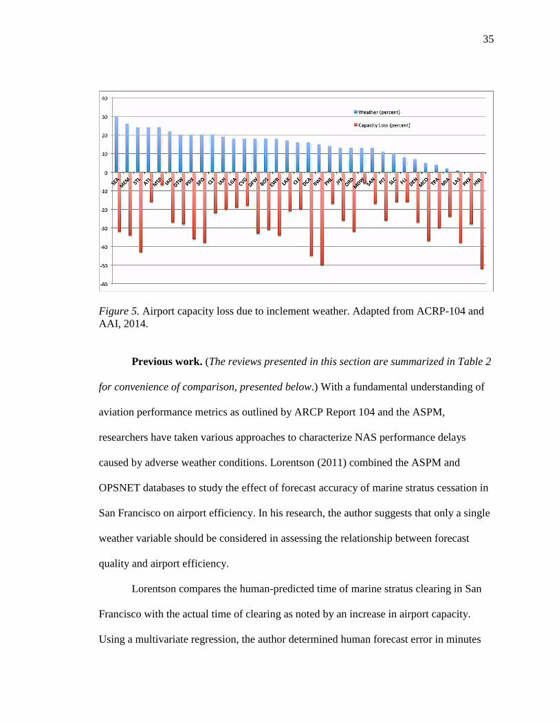
35

Figure 5. Airport capacity loss due to inclement weather. Adapted from ACRP-104 and

AAI, 2014.

Previous work. (The reviews presented in this section are summarized in Table 2

for convenience of comparison, presented below.) With a fundamental understanding of

aviation performance metrics as outlined by ARCP Report 104 and the ASPM,

researchers have taken various approaches to characterize NAS performance delays

caused by adverse weather conditions. Lorentson (2011) combined the ASPM and

OPSNET databases to study the effect of forecast accuracy of marine stratus cessation in

San Francisco on airport efficiency. In his research, the author suggests that only a single

weather variable should be considered in assessing the relationship between forecast

quality and airport efficiency.

Lorentson compares the human-predicted time of marine stratus clearing in San

Francisco with the actual time of clearing as noted by an increase in airport capacity.

Using a multivariate regression, the author determined human forecast error in minutes

36

can be predicted with some degree of confidence by the system airport efficiency rate

(SAER) and the percent on-time arrivals (POTA). While Lorentson’s results were

somewhat mixed, he makes good use of both the ASPM and OPSNET archival databases

through objective analysis.

Table 2

Literature Review Summary

Author(s) and

(Date)

Summary Statistical

Model(s), and

Data Sets Used

Findings Limitations

Lorentson

(2011)

Forecaster error

estimated by

system airport

efficiency rate

and percent on-

time arrivals

Multivariate

Linear

Regression

*****

ASPM,

OPSNET

Objective

relationship

between

SAER,

POTA, and

forecaster

accuracy

weakly

established

Reduced weather

to impact

categories in

order to isolate

correlations

between forecast

quality and traffic

flow impacts

Smith (2008)

& Smith,

Sherry, and

Donohue

(2008)

Estimated

AARs by

applying TAF

data after

weather

variables and

AAR

relationships

were

established

using SVT

Support Vector

Machine

(SVM)

*****

ASPM, BTS,

Terminal Area

Forecasts

(TAF)

SVM

technique

yielded strong

relationships

between

weather

variable

inputs and

estimated

AARs

A data mining

approach that also

includes non-

weather variables

that also impact

AARs is likely to

improve the

overall predictive

skill.

37

Table 2


Author(s) and

(Date)

Summary Statistical

Model(s), and

Data Sets Used


Parker,

Soloninka &

Littleton

(2010)

Used archived

VMC versus

IMC weather

conditions to

study arrival

and departure

performance at

ATL

Piece-wise

Linear

Regression

*****

ASPM

Positive

regression

slopes (one-

to-one)

indicate

airport

throughput

capacity

available,

while a slope

of zero

implies traffic

flow

saturation

Expand the data

analysis

techniques to

examine

enhanced airport

saturation

throughputs as a

result of

configuration

changes or new

NextGen

technologies

Laskey, Xu &

Chen (2012)

Examined flight

delays in flights

between ORD

and ATL by

breaking flights

up into eight

phases where

delays could

occur

Piece-wise

Linear

Regression,

Bayesian

Network

*****

ASPM,

National

Convective

Weather

Detection

(NCWD)

Departure

delays at hub

airports and

en route flight

and arrival

airport

weather

conditions

can affect

delay on all

flight phases

This study needs

to be extended to

different airport

pairs or during

different seasons,

e.g., winter versus

summer, to create

a tactical decision

planning tool for

airspace

managers.

38

Table 2


Author(s) and

(Date)

Summary Statistical

Model(s), and

Data Sets Used


Wang (2011) Introduced

ensemble

bagging

decision tree

modeling to

estimate

runway

configurations

(and hence

AARs) that

were then tested

using observed

and predicted

weather

Ensemble

decision

bagging tree,

support vector

machine

*****

ASPM,

METAR,

Weather

Impacted

Traffic Index

The ensemble

bagging

decision tree

modeling

consistently

outperformed

the SVM

models

introduced by

Smith (2008)

While ensemble

bagging trees

outperform the

single support

vector machine

models, both

modeling

techniques require

further fine-

tuning and other

impact variables

need to be

considered

beyond weather

inputs, e.g. noise

abatement

procedures.

Kulkarni,

Wang &

Sridhar (2013)

Further

compared

ensemble

bagging

decision trees,

support vector

machine, and

neural network

models using

10 weather

input variables

at eight airports

from 2006 to

2010

Ensemble

decision

bagging tree,

support vector

machine, neural

network

*****

ASPM,

National

Traffic

Management

Log

At eight

selected

airports,

ensemble

decision trees,

neural

networks, and

support vector

machine

modeling

consistently

rendered

similar

outcomes

Data mining and

decision support

works best in

decision spaces

regions of low or

moderate decision

difficulty, and

organizations

should focus on

these regions to

determine how

human decision

subjectivity plays

a role in setting

AARs, and value

needs to be added

in highly difficult

airspace metering

decisions.

39

Table 2


Author(s) and

(Date)

Summary Statistical

Model(s), and

Data Sets Used


Avery &

Balakrishman

(2015)

Used Discrete-

Choice

modeling to

predict runway

configurations

(out to three

hours) at LGA

and SFO

airports based

on historical

data

Area Forecast

Regression fed

Decision-

Choice Model

*****

ASPM,

Terminal Area

Forecasts

(TAF)

Introduced

decision-

maker derived

influence on

setting airport

runway

configuration

based on a

utility

function;

modeling also

derived

runway

crosswind

component

limits

objectively

Improvements

need to be made

in the runway

configuration

“inertia” term,

examine methods

to introduce

randomness by

decision makers

into the utility

function, seek to

reduce early

model bias that

amplifies out to

three-hours

Zhang &

Nayak (2010)

Developed

Macroscopic

Tool measuring

the delay at a

selected airport

and the effect

this delay has

on the NAS at

large

Two-Stage

Least Squares

Regression

*****

ASPM, NOAA

NCWD, and

BTS

Airspace

management

at single

airport has a

definite effect

on the NAS

as a whole;

IMC ratio has

a larger effect

than

convection on

airport and

NAS

performance,

winter months

effect NAS

more than

summer

months

Only two cases

(LGA and ORD)

studied directly

compared even

though ORD has

almost three times

the annual

passenger volume

when compared

to LGA.

40

Table 2


Author(s) and

(Date)

Summary Statistical

Model(s), and

Data Sets Used


Dhal, Roy,

Taylor, &

Wanke (2013)

Estimated

AARs

classified as

“low,”

“medium,” and

“high” at BOS

and DTW

airports using

weather

variable inputs

to construct a

generic

predictive

model for each

airport out to 24

hours

Multinomial

Logistic

Regression

*****

ASPM,

Terminal Areas

Forecast (TAF)

Introduced

Logistic

Regression as

a potential

modeling

technique that

also used

Synthetic

Minority

Oversampling

Technique

(SMOTE) to

mitigate

under-

represented

categories to

estimate AAR

bins

Model

deployment using

predictive

numerical

weather model

guidance

introduced

human-produced

errors associated

with Terminal

Area Forecasts

Smith (2008) and subsequently Smith, Sherry, and Donohue (2008) combined

multiple databases to create a decision support tool used to predict airport arrival rates

based on weather forecasts. In his work, the author(s) used the ASPM and BTS databases

to extract the airport arrival rates and the delay information, while adding National

Weather Service Terminal Aerodrome Forecasts (TAF) as the predictor variables once

the relationship between the combined AAR/Delay data and TAF data was understood.

Using a Support Vector Machine, which is a “method that performs classification tasks

by constructing hyper-planes in a multi-dimensional space that separates cases of

41

different class variables” (Smith, 2008, p. 4), Smith set the TAF information as

independent variables and then estimated the AAR as the dependent variable. Initial

results were favorable; tests on Philadelphia showed the SVM model was 81 percent

successful using the training data set and 83 percent successful with the testing data when

using a split-data sample. Smith further connected the predicted AAR to delay data from

the BTS to also estimate an overall flight delay (in minutes) associated with each AAR.

In spite of his success, Smith reported a disadvantage in using the SVM approach is that

it cannot distinguish if one variable has more influence than another in predicting AAR.

Also, he noted the SVM methodology is not capable of detecting a rare event. Smith

suggests future research examines other potential causal factors which might affect AARs

beyond weather, such as schedule congestion and airport construction. Smith’s final

conclusion was that data mining may be a more useful approach in examining this multi-

dimensional problem.

Parker et al. (2010) used the ASPM database to determine the drop off in AARs

observed during visual meteorological conditions (VMC) and instrument meteorological

conditions (IMC) as “the extent to which NAS performance is reduced during IMC

constitutes the performance gap between IMC and VMC” (p. 7). Using actual arrival

rates versus scheduled arrival rates, as well as instrument approach (IA) or visual

approach (VA) conditions extracted from the ASPM database, the authors used a

piecewise linear regression model using a least-squares technique to examine Atlanta’s

Hartsfield-Jackson Airport hourly throughput from 2005 to 2007. Part of their interest

revolved around Atlanta's installation of a new runway, which was expected to lessen the

weather VMC/IMC performance gap for both arriving and departing aircraft during IMC

42

operations. Parker et al. discovered that while the VMC versus IMC performance gap did

decrease slightly for arriving aircraft, it actually increased for departures, and the airport

continued to reach throughput saturation at a point of inflection where the piecewise

regression slope changed roughly from a positive one-to-one (airport throughput capacity

available) to a slope of zero (airport saturation).

Laskey et al. (2012) examined the ASPM database to better understand how

delays propagate in the National Airspace System, recognizing that delays are inherently

a “stochastic” phenomenon, and created a Bayesian Network model to examine the root

causes of aircraft delays. The authors considered a case study that focused on the delays

between Chicago O’Hare International Airport and Hartsfield-Jackson International

Airport in Atlanta and sought to identify how FAA systemic and FAA/NWS human

factors might result in arrival delays. In contrast to Lorentson (2011, August), Laskey et

al. suggested “different components of delay together is important because the

components interact in complex ways under the effects of airport conditions, weather

conditions, and system effects from NAS” (p. 1). Moreover, the authors asserted that a

“Bayesian network model not only provides predictions of future delays that incorporate

the interrelationships among causal factors, but also provides a means of assessing the

effects of causal factors and inferring the factors that contributed most to the final arrival

delay” (p. 2).

Laskey et al. took six deliberate steps to identify the components that cause delay

and how they interact in their case study that examines flights between Chicago O’Hare

and Atlanta Hartsfield-Jackson airports. These steps resulted in a regression model that

examines delay at each noted phase of flight (turn around delay, gate out delay, taxi out

43

delay, departure queue size, airborne delay, predicted time en route, taxi in delay, arrival

que size, and gate in delay):

(a) distinguish the most important explanatory factors for this phase using piece-

wise regression analysis and cross validation on the training sample; (b) create a

node in the BN to represent the delay phase; (c) set the factors selected from step

1. as the parent nodes of the given delay node in the Bayesian network; (e)

estimate initial local distributions for the given node by discretizing the regression

model. That is, the child node is modeled as a normal distribution with mean

equal to the regression mean and standard deviation equal to the regression

standard deviation. Most delay variables were discretized in 15-minute intervals,

but some were discretized more finely to improve accuracy; (f) use Dirichlet-

multinomial learning from the training data to update the distributions of all nodes

in the Bayesian network. We found this step to be necessary because the

regression model alone was not adequate to capture the complex relationships

between nodes and their parents. We gave a relative weight of 30:1 on observed

cases to the regression prior; and, (g) evaluate the model by comparing the model

predictions with observations on a holdout sample. (Laskey et al., p. 3)

Results from Laskey et al., confirmed that “departure delays at the busy hub

airport ORD are major contributors to the final gate arrival delay at the destination

airport,” and that “weather conditions en route and at the destination airport ATL have an

effect on delay in all flight phases” (p. 7). Ultimately, the authors expected to create a

planning tool that will provide insights into the ramifications of tactical decisions

regarding ground delay programs as well as flight cancelations, and how “flight

44

scheduling decisions by individual airlines contribute to the propagation of delay in the

system” (p. 7).

Wang (2011) compared the Support Vector Machine (SVM) approach employed

by Smith to a bagging decision tree (BDT) model used to predict weather-impacted

airport capacity. The author posits airport runway configuration is a critical element in

determining airport capacity and is dependent on noise abatement procedures, traffic

demand, surface congestion, operational considerations, surface congestion, navigational

system outages, and weather and concluded, “among these factors, the most important is

weather, wind direction and speed in particular” (p. 2). Wang used ASPM data as well as

weather observations and predictions to determine the relationships between weather,

runway configurations, and airport arrival rates at Newark, San Francisco, Chicago

O’Hare, and Atlanta.

As Wang reported, because of its robustness in classifying noisy or unstructured

data, an SVM is widely used in many applications “from protein function, and face

recognition, to text categorization” (p. 2). The SVM is constructed as previously

described by Smith and employs a Gaussian radial basis function (RBF) to extend the

classification technique from a linear to a non-linear decision function. Using this

technique, the SVM can be applied in a high-dimensional space non-linear mapping

problem.

In ensemble bagging decision trees, bagging uses random resampling of the data

to induce classification margins, or gaps, which bring essential diversity into the

ensemble process. The bagging process examines the average error for each subgroup

and then optimizes and assigns weights to the subspaces to construct the classifier. Per

45

Wang, “experimental results demonstrate that the method is robust for classification of

noisy data and often generates improved predictions than any single classifier” (p. 3).

Using cross-validation (N = 10), ten models were run using both the SVM and

ensemble BDT techniques and checked for accuracy against observations. Each time,

nine of the ten sub-groups of data were used for training, and the tenth subgroup was

saved for model testing. Ultimately, each of the ten subgroups was withheld from the

training data sets and used for testing purposes. This cross-validation technique

confirmed the Wang’s findings were not capricious.

The SVM and BDT results used to determine runway configuration were

compared using the overall accuracy rate, critical success index, and area under the

Receiver Operating Characteristic (ROC) curve, and these results were then compared at

four major airports. In all cases, the BDT outperformed the SVM approach. Moreover,

using the area under the curve statistic and based on airport weather, the BDT

impressively correctly classified the dissimilar runway configurations 92 to 83 percent of

the time at Newark, 92 to 77 percent of the time at San Francisco, 97 to 85 percent of the

time at Chicago O’Hare, and 95 to 88 percent of time in Atlanta. Performance dropped

somewhat when the BDT attempted to distinguish similar runway configurations, but the

ROC area under the curve still remained above 0.8 overall (p. 9).

Kulkarni, Wang, and Sridhar (2013) investigated data mining techniques to

enhance the decision-making of air traffic managers when implementing Ground Delay

Programs (GDP). As the authors suggest:

Data mining algorithms have the potential to develop associations between

weather patterns and the corresponding ground delay program responses. If

46

successful, they can be used to improve and standardize TFM decisions resulting

in better management of traffic flows on days with reliable weather forecasts. The

approach here seeks to develop a set of data mining and machine learning models

and apply them to historical archives of weather observations and TFM initiatives

to determine the extent to which the theory can predict and explain the observed

traffic flow behaviors. (pp. 1-2)

Kulkarni et al. noted the major reason to initiate a GDP is overwhelmingly due to

inclement weather conditions and studied the historic operational and weather statistics at

Newark, San Francisco, LaGuardia, Kennedy, Chicago O’Hare, Philadelphia, Boston,

and Atlanta airports from 2006 to 2010. GDP information was extracted from the

National Traffic Management Log (NTML) database and was then merged with ASPM

data. Hourly variables (wind speed, visibility, ceiling, instrument meteorological

conditions (IMC), scheduled arrivals, scheduled departures) were used as direct inputs

and also to derive a wind impacted traffic variable (the number of arriving or departing

aircraft with wind speeds greater than 15 knots) and an IMC impacted traffic variable (the

number of arriving or departing aircraft during IMC conditions). Initially, ten variables

were studied: wind speed, variation in wind speed, visibility, variation in visibility,

ceiling, variation in ceiling, instrument meteorological conditions (IMC), scheduled

arrivals, IMC-impacted traffic and wind-impacted traffic. Of these, the IMC-impacted

traffic and wind-impacted traffic variables were found to be most relevant.

The authors analyzed these data using three data mining techniques, ensemble

bagging decision trees (BDT), neural networks (NN), and support vector machine (SVM)

models. Kulkarni et al. noted that machine-learning performance depends on a consistent

47

decision-making process as well as the availability of training data to provide variable

input information at key points in the decision space analysis. However, because the

National Airspace System is operated by humans, it can respond to weather and traffic

conditions differently depending on the objectives, preferences, and training of the

operators who are responsible for the decision-making. Further, ambiguity in decision

outputs were noted in scenarios that had the same approximate decision inputs. As a

result, the authors looked toward a range of values or regions of decision consistency to

characterize the accuracy of the three modeling approaches.

The data were divided into regions of differing decision consistency. Comparison

was then made between the BDT, NN, and SVM data-mining methods within each region

of decision consistency. This was accomplished using a four by four (YY, YN, NY, NN)

confusion matrix which in turn allowed a Critical Success Index (CSI = YY/

(YY+NY+YN)) and False Alarm Ratio (FAR = YN/ (YY+NN)) to be calculated and

compared within each decision consistency region.

In regions of low decision consistency (0.58), the CSI and FAR for the NN was

0.64 and 0.27, for the BDT was 0.63 and 0.25, and for the SVM was 0.63 and 0.24,

respectively. In regions of medium decision consistency (0.77), the CSI and FAR for the

NN was 0.64 and 0.12, for the BDT was 0.61 and 0.12, and for the SVM was 0.65 and

0.18, respectively. In regions of high decision consistency (0.88), the CSI and FAR for

the NN was 0.82 and 0.24, for the BDT was 0.83 and 0.23, and for the SVM was 0.84

and 0.25, respectively.

Kulkarni et al. concluded there is probably little value in having a data-mining

decision support system in high decision consistency regions, e.g., days where the

48

weather is favorable to operations (no GDPs required) or days with significantly adverse

weather (multiple GDPs required). Instead, decision support should be focused in regions

of low to moderate decision consistency. Finally, the authors note the consistency

discovered between the three methods (NN, BDT, and SVM) provides confidence in

using a data mining approach for this particular problem.

Avery and Balakrishnan (2015) offered a probabilistic method to predict runway

configuration at forecast intervals of 15-minutes out to three hours. Using both ASPM

and Terminal Aerodrome Forecasts (TAFs), the authors employed a discrete-choice

modeling approach that they applied to LaGuardia and San Francisco airports. Unique to

this study were the thresholds for maximum tailwinds and crosswinds used to determine

the runway configurations and were derived from historical data. According to the

authors:

Discrete-choice models are behavioral models that describe the choice selection

of a decision maker, or the nominal decision selection among an exhaustive set of

possible alternative options, called the choice set. Each alternative in the choice

set is assigned a utility function based on defining attributes that are related to the

decision selection process. At any given time, the feasible alternative with the

maximum utility is assumed to be selected by the decision maker. (p. 2)

A utility function is used as a stochastic random variable with an observed

component that is deterministic as well as stochastic error component. The deterministic

observed component of the utility function is expressed as a linear function of weighted

attributes expressed in vector form. The random error portion of the utility function

contains the combined measurement errors with an assumed Gumbel distribution, a

49

location error of zero, and approximates a normal distribution to decrease computational

requirements. A Nested-Logit model was then employed to split the observable part of

the utility function into a component common to each possibility within the decision nest

and a component that varies between alternatives. As reported by Avery and

Balakrishnan, “the probability that a specific alternative is chosen is given by the

probability that its nest is chosen, multiplied by the probability that the specific

alternative is chosen from among the alternatives in that nest” (p. 3). Estimates of the

linear weighting attributes were estimated from the training data that maximized the

likelihood of the observation and were determined using a non-linear optimization

routine found in a software package named BIOGEME.

Using variables found in the ASPM database, the utility function in the model

estimated the importance of weather, wind speed, wind direction, arrival demand,

departure demand, as well as other factors to determine the most likely runway

configuration. The model starts with an initial runway configuration, and using the input

variables listed above, yields a probabilistic forecast for the next fifteen minutes, and so

on. Using these results as a training baseline, TAF data were used as inputs to obtain a

probabilistic runway configuration prediction out to three hours. With perfect a priori

(actual) information of weather conditions and traffic demands, the model was correct 81

percent of the time at San Francisco and 82 percent of the time at LaGuardia, in

hindsight. As a predictive tool, using scheduled demand and Terminal Aerodrome

Forecasts three hours in advance, the model was still impressive with an accuracy of 80

percent for San Francisco and 79 percent for LaGuardia airports.

50

Zhang and Nayak (2010) examine the factors that cause flight delays and the

impact delays at one airport have on the rest of the NAS. To do this at a selected airport,

different delay factors such as arrival queuing delays, differing demand management

scenarios, and adverse weather (both local constraints and en route convection) were

entered into a model composed of multivariate equations as independent variables. At the

national scale, the same variables were also considered in a model using similar

multivariate equations. The two models (of local and national scale) were then regressed

using a two-stage least squares technique.

Two airports were selected as case studies, New York’s LaGuardia Airport (LGA)

and Chicago’s O’Hare International Airport (ORD), based on the authors’ contention that

both airports are known for their “significant and persistent delays” (p. 88). Moreover,

Zhang and Nayak noted that the demand strategies for LGA and ORD were based on

similar slot control capacity schemes that were run in parallel by airspace managers

during the January 2000 through June 2004 period of their study. Fifteen-minute ASPM

data were analyzed, and by adding convective weather data from the National Oceanic

and Atmospheric Administration and passenger boarding data from BTS, the following

variables were constructed: a) daily arrival delay, b) deterministic queuing delay, c)

adverse weather including convective weather and IMC ratio, d) passenger load factor, e)

total flight operations, and e) seasonal and demand management dummy variables.

The two models, based on multivariate simultaneous equations supported by the

variables listed above, were regressed using a two-stage least squares technique that is an

extension of the least squares regression generally used when the models are

“nonrecursive with a bidirectional relationship between the causal factors and error

51

terms” and is particularly useful “when the dependent variable of one model could be one

of the independent variables of the other model” (p. 90). The results were significant,

with an R2

of 0.7741 and 0.8254 for LaGuardia and O’Hare Airports, respectively. The

principal weather driver causing delays at both airports was the IMC over the

thunderstorm ratio, and seasonally derived delays were dominant during the winter

months. Also noted to be significant were delays resulting from demand management

schemes, that is, how the airspace was regulated.

The results from the NAS models were equally impressive; the R2 for LGA

explained 94.35 percent of the of the average delay variation, while the R2 for ORD

accounted for 94.06 percent of the average delay variation. It was also discovered that a

one-minute delay at LaGuardia resulted in a 0.082 minute delay in the NAS, while a one-

minute delay at O’Hare resulted in a 0.052 minute delay in the NAS. Zhang and Nayak

noted how differing demands and management strategies of specific airports impacts the

system in its entirety. Another application of this study is the estimated improved

capacity at a single airport (e.g., additional runways) can be translated into an expected

improvement in overall NAS performance.

Zhang and Nayak conclude that the two-stage least squares regression

methodology could easily be extended to add more independent input variables. Also, the

single airport to NAS relationship could be generalized to the 22 Air Route Control

Centers (ARTCCs) and then applied to the NAS at-large. Finally, and again by extension,

the two-stage least squares regression could be replaced by a three-stage least squares

model to better refine the coefficients realized in the multivariate equations.

52

Dhal, Roy, Taylor, and Wanke (2013) estimated airport arrival rates (AAR) using

a multinomial logistic regression as a means to predict AARs over a 24-hour period. A

principle driver in their research was to derive a generic prediction algorithm for a given

airport, and their work examined the Boston Logan International and Detroit

Metropolitan Wayne County Airports as cases for the developmental design. While the

authors noted the importance of runway configuration as a factor in determining the AAR

(and as was later pursued directly by Avery and Balakrishnan), they chose to focus on

estimating AAR classifications (e.g., low, medium, and high) directly rather than airport

runway conditions.

Dhal et al. focused their study on building and refining the multinomial logistic

regression models for the two airports selected and then tested the models. In

constructing the model, the authors outlined a three-step process: a) identify factors, b)

gather historical data, and c) begin data mining, which iteratively includes data pre-

processing, running the regression model, and model evaluation. The three steps are

briefly described.

The first step led the authors to consider the major factors that control an airport’s

AAR. They noted that common environmental factors such as wind speed and direction,

ceiling, and visibility play a role in influencing the AAR. Moreover, these weather

elements can be predicted and therefore applied as regressors to practical AAR

forecasting tools. Beyond the common environmental elements, Dhal et al. identified

airport specific factors that also affect AARs. For example, LaGuardia Airport in New

York is physically constrained by the East River and has very limited ramp and taxi space

that slows down aircraft arrivals and departures during busy hours of the day. Similarly,

53

and depending on an airport’s physical layout, the authors conclude the airport departure

rate can also affect its arrival rate, although they did not consider this influence in their

2013 research. Additionally, since humans control the NAS, it was noted that variability

in AARs is also caused by the decision-making of airspace managers that “can mask and

overwhelm other dependencies in the data” (p. 3).

In the second step, Dhal et al. collected historical FAA performance data and

NWS weather archives. The FAA performance data were extracted from the ASPM

database, specifically hourly data between April 1st and September 30

th were assembled

for three years (2009 – 2011) as the training data set, and the test data were pulled from

the April 1st through September 30

th, 2012, archive. These data were time-matched with

National Weather Service Meteorological Terminal Aviation Routine Weather Report,

more commonly referred to as METARs.

As previously mentioned, the third step, data mining, is iterative in nature and

includes pre-processing, multinomial logistic regression model construction, and model

testing and refinement. The data pre-processing techniques used by Dhal et al. lend

insight into best practices when data-mining the FAA ASPM database. The authors

carefully identified each variable type (i.e., continuous or categorical) so that variables

were correctly entered into the regression. Also, the authors reclassified some of the data

such as “no ceiling” and “winds variable” into numerical data to match the otherwise

completely numerical data in these respective fields. As others have done previously (e.g.

Smith, 2008), the nighttime hours between midnight and 0700 local time were not

considered because of low traffic volumes, and therefore no loading on airport capacity.

Data associated with these local times were therefore removed from the regressions.

54

Another important pre-processing task reclassified the continuous variable AAR

into a categorical variable required for the multinomial logistic regression. This was an

important step as it binned the AARs into two or three categories based on observed

AARs, and in particular, should include categories that indicate low arrival rates

indicating constrained airport capacity. For Boston Logan International Airport, three

values were chosen: Low (AAR <= 45), Medium (45< AAR <= 60), and High (AAR >

60), while Detroit Metropolitan Wayne County Airport used only two levels: Low (AAR

<= 60) or High (AAR > 60).

The final pre-processing step conducted a sensitivity-specificity analysis of the

variables considered as regressors to determine their respective influence in predicting

the AAR. Variables with low influence as regressors on the dependent variable were

considered for removal from the regression. Per Dhal et al. (2013):

It is well-known that extraneous regressors tend to frustrate regression algorithms,

which in turn leads to poor performance of the obtained prediction models. The

sensitivity-specificity analysis can be used to identify unnecessary environmental

attributes, which can then be removed from the list of potential regressors for

AAR classification, if desired. (p. 4)

The multinomial logistic regression was then developed to estimate the AAR

based on the selected input variables. This particular statistical technique was chosen for

several reasons. With the AARs binned in to two or three categories, a multinomial (or

binary) logistic regression was used. Additionally, the input variables are both categorical

and continuous, and “the logistic regression immediately yields a stochastic model for

AAR categories given the regression parameters” (p. 4). The following regressors were

55

used: local hour, from 6 AM to 11 PM (18 total, categorical), presence/absence of

thunderstorms (categorical), ceiling (continuous), visibility (continuous), surface wind

angle (continuous), and surface wind speed (continuous). The aforementioned sensitivity-

specificity analysis confirmed each of these selected input variables were useful as

regressors. The use of local hour as a regressor is worthy of note as this input variable

added regularly scheduled airport traffic volume loadings that consistently occur on a

daily basis into the model.

With the multinomial (three category AAR categorical target variable) logistic

regression model constructed for Boston Logan International Airport using the multi-year

test data set, the model was evaluated by Dhal et al. using the six-month 2012 data. It

correctly classified 62 percent of the historical AAR categories by using a three by three

confusion matrix. The authors contend this is an acceptable performance:

This representation of the model’s performance is standard in the statistics and

data mining literature and is referred to as a confusion matrix. The confusion

matrix for this regressor indicates that the AAR levels are indeed being

distinguished by the regression, and in particular that the low AAR level can be

predicted well in this example. (p. 8)

With the basic multinomial logistic regression model constructed and tested, it

may be “iteratively refined by 1) changing the set of regressors used, 2) re-categorizing

the AAR and other logistic variables, and/or 3) modifying the regression algorithm itself”

(p. 5).

In contrast, the Detroit Metropolitan Wayne County Airport parallel case study

did not share the success of the Boston Logan International Airport using the same basic

56

modeling approach. The historical assessment of the AARs for this airport led to just two

levels (and hence a binary logistic regression) set at rate either above or below a 60 AAR.

Dhal et al. found well over 8,000 cases where the Detroit Airport accepted a 60 or better

AAR, but close to only 1,000 cases where the airport dipped below a 60 AAR. Little

explanation is given as to why a third, and more moderate category between a low and

high ARR was not selected as was applied with Boston Logan experimental design. One

might attribute these differences to the non-winter weather (April through September)

selected for this study that perhaps is indicative of an under-utilized airport that only

becomes over-burdened in the presence of thunderstorms during the spring through fall

months. In any case, to improve the regression in iteration, Dhal at al. suggest the

inequity in numbers of high and low AAR cases tends to force the regression to

artificially favor the higher classification. To combat this under-represented, rare-

occurrence problem statistically, the authors address the imbalance of high versus low

cases by interjecting synthetic “low” AARs into the model, a process identified as

Synthetic Minority Over-sampling Technique, or SMOTE. While there was some

improvement predicting the low AAR events, “this improvement came at a loss of

performance in predicting high ARR events” (p. 10).

With the models constructed and tested, Dhal et al. outline how they can be

deployed, although this was not performed in their 2013 research. For each forecast hour,

predicted weather values could be substituted for the historical regressor values used to

build the models e.g., surface wind speed and direction, ceiling, visibility, and the

presence of thunderstorms in order to calculate a Probability Mass Function to estimate

the probabilities of a specific AAR level. As posited by the authors, the simplest

57

approach is to choose the AAR level with the highest conditional Probability Mass

Function, and other possibilities were also lightly considered.

In conclusion, the authors examined both the methodology used in their research

as well as the data sets that could potentially be used for future AAR prediction. In the

first, Dhal et al. determined the multinomial logistic regression modeling technique

employed was effective in modeling low AARs but recognized the problems in selecting

the best model regressors and also the need to move past categorical AAR estimated

levels into continuous, or numerical predictions, and in actual model deployment,

selecting the best weather forecast tools to bring predictive weather elements into the

deployed model. In this, they recognized the various numerical weather models could

potentially be used as well as the complexities of their meaningful application.

Dhal et al. leave us with the idea that humans involved in the weather forecast

process, particularly for TAFs, (and for that matter, management of the NAS by human

specialists) leads to a variance of forecast success predictability that is very difficult to

model. The authors offer the possibility of directly interjecting both short-term, high-

resolution, probabilistic models as well as more classic deterministic-solutions of the

input variables across a 24-hour time frame. Either of these potential model inputs for

deployed models offer a consistent input bias that can be measured and corrected, but

then must be weighed against a lack of TAF fidelity and temporal forecasting resolution

that runs out to 30 hours. Dhal et al. suggest an automated but constantly advancing

forecast loop might well surpass the human-produced inputs if the numerical model

inputs can be directly entered into both the new algorithms and the deployed operational

AAR models. Noted in this approach are the complexities that must be overcome in

58

extracting sensible elements from the numerical weather models that can be directly

applied into the deployed logistic regression model with the correct time-steps and

correct physical scale. In other words, replace the variance found in high resolution but

human-produced TAFs with spatially downscaled weather elements extracted from

numerical weather models. Dhal et al. recognized the challenges of this approach and

acknowledge the principle problem will be in pulling the localized environmental

information from regional or global-scale numerical weather models. These efforts,

perhaps prescient, were left for further research.

Data Mining, Decision Trees, Neural Networks, and Regression

Data mining. There are numerous definitions that describe data mining. A simple

definition is data mining combines computer-aided statistical techniques and artificial

intelligence that allow the exploration of large data sets and databases to discover hidden

patterns in the data that may be subsequently exploited for predictive purposes. Dubey et

al. (2016) offer “unsophisticated” data (e.g. data from the Internet, that may be very large

in nature and highly unstructured) can be more usefully arranged by applying data mining

techniques (p. 5). In data mining, a descriptive model is created to approximate the

known or archived data available. These “patterns are then compared with this model to

find the deviation and is then analyzed or coded in the deviated form” (p. 8).

Gera and Goel (2015) suggest data mining is a subset of a larger “knowledge of

discovery in databases (KDD)” (p. 22). The idea that multiple databases can be

simultaneously queried is complimented by the concept that such databases may be static

or dynamic. Dynamic data sets can be very large, constantly flowing, and may make the

latencies associated with post hoc static data set analysis both impractical and of little

59

value. A dynamically supplied set of input data is particularly interesting in the

application of weather conditions toward the problem of predicting NAS efficiencies, as

these environmental parameters are constantly changing.

With data mining loosely defined, several commercially available software tools

are available for its application. Al Ghoson and Abdullah (2010) contrast the relative

strengths and weaknesses of the SAS® Enterprise Miner

TM, SPSS

® Clementine

TM, and the

IBM DB2® Intelligent Miner

TM when using decision tree and clustering analyses as might

be used for business decision making. Their evaluation was based on the following

criteria: a) performance, b) functionality, c) usability, and d) auxiliary task support. The

authors note decision trees and clustering are two of the most common classification

techniques used in business decision-making.

Compared to the other two data mining software packages, Al Ghoson and

Abdullah indicate SAS® Enterprise Miner

TM is a complete system that creates an

integrated environment which includes “predictive and descriptive modeling, text mining,

forecasting, optimization, simulation, and experimental design” (p. 62).

Decision trees. Per Tufféry (2011), decision trees recursively divide a population

into n predetermined segments through the use of chosen selection variables that provide

the best separation of the population into distinct classes (p. 313). The first split is called

the root or parent-node, and the sub-segments are called child-nodes, although if these

nodes are further divided, they may be called intermediate-nodes. The final segments that

cannot be further divided are called terminal-nodes, or leaves, and these nodes combined

with all their successors form a branch of the tree. Using a training data set, posterior

probabilities are calculated for each node and are based on the number of the sample

60

population that fall into a given node per the node rule established by the value set for the

selection variable. These values are called target levels, and the assignment of the

selection variable value at each node is called a decision. Each member of the population

is ultimately assigned to only one leaf. Decision trees are normally constructed to

minimize the overall classification error of the population, to maximize profit, or to guard

against loss (Sarma, 2013, p. 170). Tufféry (2011) notes decision trees fall into a space

that bridges descriptive and predictive modeling and therefore should be considered as a

“supervised divisive hierarchical” method (p. 313).

Using SAS® Enterprise Miner

TM as an example software package that supports

decision tree modeling, there are several methods used to assess decision tree worth.

These are: decision, average square error (ASE), misclassification, and lift. In decision,

the maximize function seeks the largest profit, while the minimize function seeks to

reduce costs. ASE is the average square of the difference between the predicted and

actual outcome and is used when the target is continuous. Misclassification seeks to

minimize the number of records that are misclassified, while lift compares the percentage

of correctly selected individuals with a desired set of traits from a given percentage of the

population as compared to those results found by a completely random model. Training,

validation, and test datasets are allocated by sample size. If the sample is large, the sets

can be of equal size, but if the sample is relatively small, it is common to use a 40/30/30

or 50/25/25 percent split for the training, validation, and test data subsets, respectively.

The validation dataset is sometimes called the pruning (model fine-tuning) dataset. A

larger training dataset generally results in more stable parameter estimates. The training

dataset performs three tasks: a) assigning rules used to make selections at each node, b)

61

estimating posterior probabilities at each node after the population selections are made,

and c) calculating the selection variable value, or decision, at each node. The validation

dataset is used to prune the tree, which usually is initially too large and is called the

whole tree or maximal tree. The optimal tree is one that yields a higher profit than any

other smaller tree but also yields an equal or higher profit than any other larger tree.


TM can do this automatically. To do this, the worth of the tree is

calculated by comparing the candidate splitting values used at each node and then

iteratively determining which combination of nodes and node decision values result in the

best tree. The method used for this comparison is selectable within SAS® Enterprise

MinerTM

. Finally, the test data set is used to assess the performance of the validated

model and is useful in comparing other models, such as neural networks or regression

models (Sarma, 2013, pp. 173-175).

During the validation phase, measuring the worth of the split depends on the type

of target variable being studied, e.g. for nominal variables SAS® Enterprise Miner

TM uses

the non-parametric test: ProbChisq (the p value of the Pearson Chi-Squared test), if

categorical but with ordered scales, it is ordinal and uses Entropy or Gini, and if interval

(parametric) it uses Variance or ProbF. In a binary split (categorical), the Chi-Squared

statistic is used to test the null hypothesis that the proportion of the responders with an

income less than X is not significantly different than those with an income greater than X.

The logworth of the p value is then calculated, and the larger this value, the lower the p-

value, and hence the split. Node impurity is determined using Gini and Entropy, with

pure being set to 0, and completely mixed being set to a value of 1. For more than a

binary target variable (e.g., three or greater number of categories), the Chi Squared

62

statistic is used in a r x b contingency table, where r in the number of target levels

(categories), and b is the number of child nodes being created on the basis of certain

input. When the target variable is continuous, the F-test is the selection criterion

employed to determine the effectiveness of the splitting decision. ANOVA is used first to

test the null hypothesis (as above, resulting in the F-test statistic) then the logworth of the

F-test (larger values imply lower p-values) that indicates a better split (Sarma, 2013, pp.

177-181).

Adjusting the p values using a Bonferroni or depth adjustment allows decision

splits to be compared from different inputs. The p-values can be modified using the

Bonferroni Adjustment, which minimizes type-I errors when multiple tests of

significance are carried out. Lowering the selected p value, e.g., less than 0.05, can

control decision tree growth. This increases the degree to which two child nodes must

differ in order that the considered split be significant. Thus, changing the threshold p

value controls tree growth. Tree size can also be controlled by setting the maximum

number of records: if set to 100, a leaf will not be created (the parent node will not be

split), if there are 99 records (or less) split into this node, or by limiting the depth of the

tree, which controls the number of downstream nodes from the parent node. Removing

binary sub-tree splits that do not contribute to model performance optimizes the final tree.


TM contains a graphical sub-tree assessment function that aids in

selecting the best model size (Sarma, 2013, pp. 183-185).

Tufféry (2011) offers decision tree advantages and disadvantages:

Advantages of decision trees.

Results are in terms of the original variables (as opposed to neural networks)

63

and do not need to be re-expressed;

DTs are non-parametric: The Independent Variables can be non-normal and

collinear;

The response of the dependent variable to the independent variables can be

non-linear or non-monotonic;

Relatively unaffected by outliers;

Can deal with missing data;

Can handle all types of data directly; and

Compute times are quite reasonable.

Disadvantages of decision trees.

A Decision tree detects local and not global optima (but this can overcome by

resampling);

Require a large enough sample to provide at least 30 to 50 samples per node;

Unlike neural networks, over-fitting is easily seen in decision trees;

Decision tree solutions may be rectangular representations of the variable

space that are less than optimal; and

Decision trees, while terrific classifiers, may be difficult to generalize as

predictive systems. (pp. 327-328)

Neural networks. Neural networks are multi-layered models that pass and

process information between layers and are sometimes referred to as artificial neural

networks or ANNs. They have been noted to approximate the human nervous system in

their architecture and learning abilities. Tufféry (2011) recognizes the nearly universal

64

application of neural networks; they can be used in clustering, classification, and

predictive modeling designs (p. 217). Charaniya and Dudul (2013) describe a forward-

feeding neural network as a series of source nodes that ultimately connect to an output

layer of neurons or computation nodes. There may be additional layers found between the

source nodes and output neurons that perform calculations on the data received from the

source nodes (or the previous layer, depending on model complexity) and then pass these

results to output layer (or the next layer, again depending on model complexity). If a

layer of nodes is not directly connected to the source or output nodes, it is called a hidden

layer, as it has no connectivity with external data input sources nor does it provide direct

output solutions. A neural network schematic is shown as Figure 6. As Sarma (2013)

notes, “A neural network model can be thought of as a complex nonlinear model where

the tasks of variable transformation, composite variable creation, and model estimation

(estimation of weights) are done simultaneously in such a way that a specified error

function is minimized” (p. 241).

65

Figure 6. Neural network schematic. (K. M. Fasuke, http://texample.net,

https://creativecommons.org/licenses/by/2.5/legalcode)

Within the hidden layers of a neural network model, the source data are

normalized, may then be transformed, and are processed by the model to achieve the best

results through iteration. Data normalization, foundational to neural networks, is non-

trivial and must be carefully considered based on the variable type. Normalization

treatment varies between continuous, discrete, and qualitative inputs (Tufféry, 2011, pp.

223-224).

Nielson (2015) develops a basic but most understandable treatment of neural

networks. Perhaps of greatest interest, neurons are noted to be the progeny of perceptrons

developed in the 1960s by Rosenblatt et al. Per Nielson (2015), a perceptron receives and

weights binary model inputs into a larger set of combined but similarly considered

distinct decision selection criteria. Once energized, perceptrons combine available input

data, and based on these informed and weighted inputs, make a fully mechanical but

http://texample.net/

66

enlightened decision. Perceptrons must be visualized and taken in aggregate, and as such

have been compared to the perceiving and responding parts of the human brain. Though

less complex, and hidden layers notwithstanding, the neural network is an approximation

in how humans solve problems based on our basic mental model.

Per Sarma (2013), SAS has a range of choices for these functions allowing for

combinations of hidden layer function, hidden layer activation function, target layer

combination function, and target layer activation function to be selected, and each

provides a different neural network model (p. 241). The multilayer perceptron networks

use linear combination functions and sigmoid (S-shaped) activation functions in the

hidden layers. Other neural networks use Radial Basis Function (RBF) and Multilayer

Perceptron (MLP) networks (p. 279). Within the SAS® Enterprise Miner

TM, the

AutoNeural node automatically configures a neural network (p. 307) by using a search

algorithm to select the best activation functions. Additionally, the Dmine Regression

node enables the computation of a forward stepwise, least squares regression model. In

each step, the independent variable that best contributes to the model R-Square value is

selected (p. 312). The tool can also automatically bin continuous terms. Finally, the

DMNeural node is used to fit a non-linear equation by selecting the best performing input

components based on an R-squared evaluation of the linear regression of the target

variable on the principle components (pp. 309-310).

Sarma (2013) concludes:

In summary, a neural network is essentially nothing more than a complex non-

linear function of the inputs. Dividing the network into different layers and

different units within each layer makes it very flexible. A large number of non-

67

linear functions can be generated and fitted to the data by means of different

architectural specifications. (p. 316)

Tufféry (2011) offers neural network advantages and disadvantages:

Advantages of neural networks.

Allow for non-linear relations and complex interactions between variables, if

the necessary investment is made in the hidden layers;

Are non-parametric, meaning independent variables are not assumed to follow

any particular probability distribution;

Some networks are insensitive to unstructured or defective data; and

Neural networks can handle a wide-range of problems.

Disadvantages of neural networks.

Convergence toward a globally-optimal solution is not always certain;

Considerable risk of over-fitting;

Impossible to handle a large number of variables;

Some applications cannot handle the non-explicit nature of the results;

Numerous parameters make the network hard to control; and

May be adversely affected by outliers. (pp. 499-500)

Regression. Tufféry (2011) notes there are two major reasons to include linear

regression into data mining at-large. First, “linear regression forms the basis of all linear

models and is universally acceptable” (p. 355). Second, linear regression must be

understood in order to better appreciate the complexities of the regression approach that

is likely to be applied in this research. As Tufféry suggests, modern regression techniques

(e.g. “ridge and lasso” regression) “are very useful” when the number of variables exceed

68

the number of observations or when collinearity is suspected between the predictor

variables (p. 355).

In simple linear regression, both the predictor variables and the target variable are

assumed to be continuous, and it is assumed the dependent variable “Y” is contrasted

with the independent variable(s) “X,” and these independent observations are controlled.

As Tufféry suggests, this basic model takes on a deterministic linear component and a

stochastic error component that models the errors associated with the imperfections found

in the “Y” solutions when fitted to the explicit “X” independent variable. Thus, errors are

assumed within the “Y” solutions based on the single best fit of multiple “X”

observations. The best fit of the single straight-line regression is generally the solution

that minimizes these collective errors when taken in aggregate. But assumptions are

made: a) the “variance of the errors is the same for all values of “X” (homoscedasticity)”,

b) the errors are linearly independent, and c) the errors are normally distributed (p. 356).

These collective errors are estimated by the residuals based on the coefficients

that approximate the slope and offset for the single line fit of the model. Tufféry notes

these coefficients are impossible to determine precisely as: “a) the linear model is often

only an approximation of reality; and b) we are working on samples, not the whole

population; and measurement errors occur” (p. 357). To reduce the levels of variance

within this regression technique, three approaches are offered: a) “increasing the size n of

the sample, b) increasing the range of the value of the observed values of “X,” or c) by

reducing the variance S2 of the errors in the sample” (p. 358).

Hair et al. (2010) succinctly identify the assumptions that need to be satisfied in

order to perform a linear regression. These assumptions can be difficult to satisfy and

69

need to be examined for each independent and dependent variable and then for the overall

relationship after model estimation. The necessary assumptions for each variable are

linearity, homoscedasticity, and normality (p. 208). For the overall variate, the

assumptions are linearity, homoscedasticity, independence of the residuals, and normality

(p. 220). Honoring all of these assumptions can be challenging.

Finally, Keith (2015) offers multiple linear regression (MR) advantages and

disadvantages:

Advantages of multiple regression (MR).

MR can use both categorical and continuous independent variables;

MR can easily incorporate multiple independent variables;

MR is appropriate for the analysis of experimental (active manipulation of the

independent variables) or nonexperimental research. (p. 18)

Disadvantages of multiple regression (MR).

The dependent variables must be a linear function of the independent

variables;

Each observation should be drawn independently from the population, and

associated error for each should be independent of the other observations;

The variance of errors should not be a function of the independent variables,

and dispersion of values along the regression line should be fairly constant for

all values of X (homoscedasticity).

The errors should be normally distributed. (pp. 187-188)

70

Sample, Explore, Modify, Model, Assess (SEMMA)

The SAS Institute recommends using a SEMMA modeling approach when using

the SAS®

Enterprise MinerTM

(Patel & Thompson, 2013) , and as an overarching guide, it

is the strategy used in this research. Specifically, the SEMMA acronym is broken down

as Sample, Explore, Modify, Model, and Assess. Note the SEMMA process should be

considered iterative in nature, as it is likely the researcher will return to the Sample or

Explore stages after model assessment to make changes and then retrace steps through

the Model, Modify, and Assess processes as variable relationships become better

understood and modeling strategies are improved. A SEMMA schematic is presented in

Figure 7.

Sample. Within this stage, the data are introduced into the data mining software

as input variables, and the target variable is selected, e.g. Airport Arrival Rate. In general,

the data are partitioned into model training and validation subsets during this step. The

SAS©

Enterprise MinerTM

accepts a large variety of data input formats.

Figure 7. SEMMA Schematic. Based on Patel and Thompson, 2013.

71

Explore. After the data are introduced into the Enterprise MinerTM

, the next step

examines the variables for outliers, skewed or peaked distributions, and missing values.

There are a number of tools provided within this stage, including “StatExplore,” as well

as variable association, clustering, graphical exploration, multi-plotting, path analysis,

and variable selection. In many ways, this step is critical to the subsequent modeling and

analysis because the data are foundationally discovered and interpreted within this

segment of the study. While the target and input variables are selected in the Sample

phase, it may be difficult to select the best input and target variables until the data are

inspected during this step.

Modify. With the variables thoroughly explored, the data needs to be prepped for

proper introduction into the selected models. Options in this stage include appending

additional data to the original data set, filtering the selected data, imputing missing

values, merging the data with other variables and data sets, or resampling the input data

into a smaller subset. Additionally, the data are further refined for the type of model

being considered. For example, in regression, skewed data may be transformed, dummy

variables can be put in place as proxies for categorical variables, and missing values can

either be imputed or list-wise removed from further consideration. Similarly, to prepare a

neural network, the AutoNeural function can be selected from the tools within the Model

tools grouping which tests and selects the best activation functions for the neural network

(Sarma, 2013).

Model. During the modeling phase, the prepared data are fed into different

models, such as decision trees, neural networks, and regression. Numerous models are

72

available in SAS®

Enterprise MinerTM

, and the parameters set for each model can be

further adjusted depending on the statistical approach that best suits the problem being

studied and the available data. Additionally, different models may be run in parallel so

their collective outputs can be directly compared.

Assess. Finally, the model results can be compared using the model comparison

function found under the Assess tools grouping. The model comparison function is

selected from the Assess tools and presents multiple performance scores to rank the

models such as the lowest average square error (ASE). Average square error is a

preferred model evaluation score because it provides common estimates of performance

for regression, neural networks, and decision trees. In the case of the scored models to be

deployed in this study, Tufféry (2011) recommends using ROC and lift curves and the

“measurements of area associated with them” to assess model performance (p. 541).

Therefore, different model evaluation statistics will be further explored.

Summary and Research Gaps

In summary, Lorentson (2011) objectively estimated forecast accuracy through

multivariate regression using System Airport Efficiency Rates (SAER) and Percent On-

Time Arrivals (POTA) extracted from the ASPM and OPSNET data sets. His work

discovered meaningful relationship between SAER, POTA, and forecaster accuracy.

Lorentson recommended that weather input variables be reduced into impact categories

to further isolate correlations between forecast quality and its impact on traffic flows.

Parker et al. (2010) examined VMC versus IMC conditions archived in the ASPM

database to study their effect on airport capacity. A piece-wise linear regression showed

that a positive regression slope indicated available airport traffic throughput capacity,

73

while a regression slope approaching zero suggested traffic flow saturation. Further study

using expanded analytic inputs was suggested.

Smith (2008) and subsequently Smith, Sherry, and Donohue (2008) employed a

Support Vector Machine (SVM) to successfully model airport arrival rates and airport

delay using the ASPM, BTS, and NWS Terminal Area Forecasts (TAF). With the

relationship of weather inputs on AAR established, the authors used human-produced

TAFs to estimate an airport’s AAR. In spite of their success, Smith et al. noted the

inability to detect a rare event and the inability to determine variable worth in the analysis

was a shortcoming of the SVM model and recommended the adoption of a data mining

approach that would integrate other casual factors of airport delay.

Wang (2011) built upon Smith’s work by introducing Ensemble Bagging decision

trees to analyze the ASPM database. In direct comparison, he found the Ensemble

Bagging decision trees outperformed the support vector machine models. Additionally,

Wang employed METAR and the Weather Impacted Traffic Index into the data analysis.

He also suggested that in order to predict the AAR, the airport runway configuration must

first be estimated. Like Smith, Wang also concluded that other variables, beyond weather

inputs, should be investigated for their contribution to airport performance degradation.

Subsequently, Kulkarni, Wang, and Sridhar (2013) used Ensemble Bagging

Decision trees, support vector machines, and neural networks to model multiple airports

using 10 weather input variables, some of which were derived to create predictive tools to

support air traffic flow decision making. They used the ASPM and National Traffic

Management Log to feed the three models at each airport. The authors noted that the

74

different modeling techniques produced similar outcomes, and the tool they developed

performed best in decision space regions of low to moderate difficulty.

Avery and Balakrishman (2015) developed a logistic regression fed Decision-

Choice Model to predict runway configurations out to three hours at the LaGuardia and

San Francisco Airports using the ASPM database and Terminal Area Forecasts. They

introduced a method to predict runway crosswind components objectively that then

informed the Decision-Choice Model. Avery and Balakrishman concluded the

“randomness” of human decision makers who control the runway configuration should be

further studied along with the problem associated with model bias in early forecasts that

amplifies during the three-hour analysis period.

Laskey, Xu, and Chen (2012) chose to study flight delays between the Chicago

and Atlanta city-pair with a piece-wise linear regression and Bayesian Network. Using

the ASPM combined with the National Convective Weather Detection databases, the

authors broke each flight studied into eight components and found that departure delays

at hub airports and en route and arrival weather can affect delay on all of the other

separated flight components. Left to further study are different city-pair combinations and

seasonal delay differences.

Zhang and Nayak (2010) developed a macroscopic tool that measures the delay at

a selected airport and the impact such a delay has on the National Airspace System at-

large. The authors used a two-stage least squares regression that pulled from the ASPM,

BTS, and National Convective Weather Detection databases. They conclude that airspace

management decisions made at one airport have a measurable effect on the National

75

Airspace System as a whole, that IMC conditions have more impact than convective

weather, and that winter months slow NAS efficiencies more than summer months.

Finally, Dhal, Roy, Taylor, and Wanke (2013) built a multinomial logistic

regression model improved with a Synthetic Minority Oversampling Technique using the

ASPM database and Terminal Area Forecasts. The authors successfully modeled low,

medium, and high AARs at the Detroit and Boston Airports, and suggested that TAFs

could then be used to predict the AARs in a deployed model. They also noted the

problems associated in using the human-produced TAFs to drive the deployed model due

to the random variance introduced by individual forecaster decisions during TAF

production. Dhal et al. suggested that input variables from objective numerical weather

model guidance would likely better serve the regression out to 24 hours. This effort was

left for further study.

From this cursory review, it is clear that significant and meaningful work has been

accomplished in using the historical ASPM database as a potential predictor of future

NAS performance. In overview, much of this effort has been placed in developing,

validating, and testing different modeling approaches. With the development of

sophisticated data mining and associated statistical software tools at-hand, largely

unavailable to many of the previous researchers whose work is described above, it is now

possible to push past model development and concentrate on model testing and

deployment as well. This will be central thrust of this confirmatory and exploratory

research.

Specifically, this study will employ and test the theories advanced by others:

76

Develop, validate, and test regression, decision tree, and neural network

modeling techniques (Smith et al., Wang et al., Dhal et al., and Kulkarni et

al.); and

Examine the efficacy of using data mining techniques to predict AAR (Smith

et al., Kulkarni et al., and Wang et al.).

Furthermore, significant effort will be made to refine, test, and deploy the models using

historical data as well as data derived from NWS numerical weather models to be used

predictively:

Examine the usefulness of merging the ASPM with hourly meteorological

station data;

Determine the differences in using hourly versus 15-minute interval ASPM

data;

Study the differences found in model performance in ten airports with

significantly different climatologic environments and traffic flow capacities;

and

Test the usefulness of introducing predictive numerical weather guidance into

the deployed models as a practical air traffic control tool.

77

CHAPTER III

METHODOLOGY

As discovered in the literature review, data mining is a relatively new and

effective approach to analyze the vast array of airport performance and efficiency

statistics assembled by the Federal Aviation Administration (and others) over multiple

years of observation. This NAS performance information is largely used in next-day and

weekly hindsight, to measure and then improve future National Airspace System

performance. However, yet to be discovered empirical relationships between the

variables captured in these large databases may also yield valuable insights into how the

NAS reacts to changing weather conditions and traffic demands that might be gainfully

applied in future operations.

This chapter describes the data sources, samples, data mining software, and

analytical techniques used in this study. The major thrust of this effort was to discover the

relationship different weather elements might have on airport efficiency with the idea that

if these relationships can be defined, weather forecast guidance can then be directly used

to estimate airport capacity a priori. Predictive data mining algorithms were used to

estimate the efficacy of this approach by testing newly-created models at multiple

airports, and these results were collectively compared to determine if there is consistent

behavior regarding weather input variables and airport performance between the sample

of selected airports.

78

Research Approach

This study was data driven and employed predictive data mining software and

techniques. According to Tufféry (2011):

Data mining is the set of methods and techniques for exploring and analyzing data

sets (which are often large), in an automatic or semi-automatic way, in order to

find among these data certain unknown or hidden rules, associations or

tendencies; special systems output the essentials of the useful information while

reducing the quantity of the data. Briefly, data mining is the art of extracting

information – that is, knowledge – from data. (p. 4)

Within this data mining paradigm, multiple models were created to compare

decision trees, neural networks, and linear regression performance to determine the

relationships between input variables and the selected target variable, AAR. The target

variable described a parameter of airport efficiency, while the input variables initially

ranged from weather variables, time of day, time of year, arrival demand, and departure

demands. Ultimately, airport arrival and departure demand statistics were removed from

the models as input variables.

Ten different and geographically dispersed airports were chosen for study to

determine if there is consistency between airports when comparing input variable worth

based on its predictive value toward the selected target variable as well as model

performance. Indirectly, this study examined how physically different airports are

impacted by weather, ranging from the relatively simple but runway and taxiway-

challenged LaGuardia Airport to the higher-capacity and less physically constrained

Atlanta, Dallas Fort Worth, and Denver airports. There are other reasons to vary the

79

airport selections for this study. The New York City market (LaGuardia, JFK, and

Newark airports) forms one corner of what the FAA has described as the “Golden

Triangle,” an airspace that most engages FAA national airspace managers each day: the

heavily traveled area geographically and demographically described by the New York,

Atlanta, and Chicago Metroplexes.

Beyond the obvious traffic demands placed on the Golden Triangle flight markets,

there are other factors that make the Dallas, Denver, and San Francisco airports

interesting. Specifically, Dallas operates in a weather and traffic-demand environment

similar to Atlanta and Charlotte. Denver predominately utilizes a north-south preferred

runway configuration that loses half of its traffic capacity during “all west” operations

and also sees constraints similar to Chicago and New York due to winter weather snow

events. San Francisco poses airport performance weather challenges unique to west-coast

airports in the United States: marine stratus layers (fog), predominantly found during the

summer months.

Significantly, the challenge was to identify if archived weather and performance

inputs offer reliable and objective predictors of past and future airport performance. Also,

how did airports with varying runway configurations, capacity demands, and

climatological conditions lend themselves to a data mining-based performance-based

estimation created from these historical data? Finally, with linkage between weather

inputs at the ten airports reliably established, could NWS predictive guidance be inserted

into a deployed model to predict airport future efficiencies? The potential to input very

large data sets and conduct analyses using a data mining approach offered new

perspectives on NAS behavior under stresses induced by weather, and at a minimum,

80

could objectively confirm the NAS does respond to various challenges in a manner that

can be better understood based on archived FAA performance and weather information.

Design and procedures. Using SEMMA guidance as previously described in

Chapter II, a brief outline of the data mining design and procedures used in this study is

presented below and are not airport specific. In fact, once the basic modeling applications

are established within the SAS® Enterprise Miner

TM environment for a single airport, it

was relatively easy to add new airports into the analytical process. In general, the design

and procedures were applied as described in detail by Sarma (2013), and a partial

diagram of the overall data mining schematic is presented in Figure 8. A broad overview

of the quantitative research design and procedures is provided here, and a more detailed

and repeatable description of this design and procedures may be found under the Data

Treatment segment of this chapter.

As described in Chapter II, three basic models were utilized for each of the ten

selected airports. These were decision trees, linear regression, and neural networks. Using

the SEMMA approach, the models were assessed, and their parameters adjusted in an

attempt to achieve best model performance.

The data were introduced to the models in three steps. The first step was to train

and validate the models using the entire two-year (2014/2015), 15-minute interval ASPM

data. The second step was to use the two-year FAA ASPM data set extracted at hourly

intervals, allowing comparison of the results at each airport using different sampling rates

with additional meteorological variables. The final data introduced was the merged FAA

ASPM and hourly NOAA NCEI surface meteorological data that add even more weather

information variables (beyond those found in the ASPM data) to the model analyses. In

81

all steps, the selection of input variables is further presented in Chapter Four. Throughout

this study, the airport arrival rate (AAR) was used as the target variable.

The performance of each model (decision tree, linear regression, and neural

network) was assessed for each airport. The ultimate goal was to create a predictive

system where estimated input variables could then forecast airport efficiency. 2014/2015,

15-minute and hourly ASPM data sets, as well as the ASPM and hourly merged surface

meteorological weather data sets were used to create and validate the models, and these

models were then scored using actual 2016 observed weather and airport AARs. These

results were then compared by model and for the three data sets used at each airport.

Finally, as a test, a model was deployed using predictive numerical weather

guidance. Weather inputs were extracted from NWS models as input variables to estimate

the target variable (Airport Arrival Rate). These estimates were then compared with the

actual AARs observed. This test used NWS LAMP model guidance that modeled future

AARs out to 24 hours.

82

Figure 8. Four airport data mining example.

Alternative designs. With the overall design and SEMMA previously described,

alternative schemes were modeled and compared with the basic results found as outlined

above. As previously mentioned, once the basic design was established in the SAS®

Enterprise MinerTM

, it was relatively easy to modify the data flows to evaluate changes in

the basic design, e.g. designate a new target variable, or adjust the number of branches or

leaf size in a decision tree. However, one caveat strictly observed was the need to

83

consistently apply any modeling changes to each airport data flow entered into the

experiment.

Using the techniques and tools previously described, additional statistical

comparisons were made in order to create contrast with the basic model outputs. These

were:

Model performance with selected input variables removed, particularly those

which would not be available a priori, such as arrival or departure scores; and

Comparison of the performance of each type of model used across the 10

airports selected for this study.

Examining these data using these differing modeling approaches and techniques

better isolated and ranked the input variables that determine impact on airport efficiency.

Analytical tools and resources. The FAA Aviation System Performance Metrics

data were extracted as a comma separated value file and then imported in Microsoft®

ExcelTM

2010 for initial inspection and reformatting. The IBM Statistical Package for the

Social Sciences (SPSS®

versions 23 through 25) and Microsoft® Excel

TM 2010 were also

used to conduct preliminary data analysis and exploration before the data are imported

into the SAS® Enterprise Miner

TM for modeling and also to merge the ASPM and NCEI

hourly surface meteorological data sets. This study then used the SAS® Enterprise

MinerTM

, version 14.1 for data mining, modeling, and scoring. The SAS® Enterprise

MinerTM

hosts a graphical interface and is relatively easy to use, even for those without

strong programming skills.

84

Population/Sample

In this study, ten airports were chosen. As previously reported, these airports are:

a) Hartsfield-Jackson Atlanta International Airport, b) Los Angeles International Airport,

c) O’Hare International Airport, d) Dallas/Fort Worth International Airport, e) John F.

Kennedy International Airport, f) Denver International Airport, g) San Francisco

International Airport, h) Charlotte Douglas International Airport, i) LaGuardia Airport,

and j) Newark Liberty International Airport. These airports, a subset of the larger 77

ASPM airport population performance-tracked by the FAA, were chosen for their varying

geographic and climatological diversity as well as runway configuration complexity.

Runway diagrams are provided in Appendix B.

For each of the ten airports, a two-year sample of 15-minute interval ASPM

performance metrics and weather observations was extracted from the FAA data base.

This created 70,080 observations (rows of data) with 83 variables within each

observation (or row) for each of the ten airports selected. A listing and description of the

variables, which are consistent for all ten airports, may be found in Appendix A. Note,

these data were also extracted at hourly-intervals resulting in 17,520 rows of data and

included data compiled over multiple years. A two-year sample (2014 and 2015) was

used to build and train the models, while a one-year sample (2016) was chosen to test the

models using the Score function in SAS®

Enterprise MinerTM

. The decision to use 2014

through 2016 data was based on using the most recent whole-year information available

to train, validate, and test the models, as the FAA reports airspace performance and

efficiencies annually by each calendar year. The fifteen-minute ASPM data set for each

85

airport studied represented the highest temporal resolution data available for all 83

variables contained in these data.

Additionally, the NCEI Global Surface Hourly Database was accessed to

download additional weather parameters such as precipitation and dew point to augment

the somewhat sparse meteorological information contained in the ASPM data sets. As

with the ASPM data, hourly information was extracted for 2014 and 2015 to build and

validate the models, while 2016 was withheld for modeling testing and scoring. The

Global Surface Hourly data were somewhat freeform temporally, with observations taken

near the top of each hour, and additional observations added between hours as

meteorological conditions change, for example, a passing thunderstorm. Time-matching

and merging the Global Surface Hourly data to the ASPM data was somewhat

challenging, and these data sets were manually merged. The merged ASPM and hourly

station meteorological data were of the same approximate sample size as the unmerged

hourly ASPM data.

Sources of the Data

This research used performance information extracted from the FAA ASPM

database, hourly station meteorological data pulled from the NOAA National Center for

Environmental Information, and LAMP model output data presented at the NWS

Meteorological Development Laboratory (MDL). Since the ASPM data are the principle

foundation of this research, discussion of how these data are assembled and quality

checked is offered here.

The FAA collects and archives performance metrics from ASPM designated

airports (of which there are currently 77) and flights by ASPM designated carriers (of

86

which there are currently 22). This includes all IFR traffic at these airports and by these

carriers, and some information regarding VFR flights is also collected. The ASPM

collection of data are broken into two major components, efficiency information and

metric information. Efficiency information collects air traffic data resulting from fights at

the ASPM 77 airports previously mentioned, while metric information traces individual

flights that are used to more accurately describe delay information.

According to the FAA (2016b), efficiency information may include missing data

records, while the metric data are either complete sets or the missing values are estimated

with some level of confidence. The reason to split these groups is based on the interest in

collecting as much efficiency data as possible at each ASPM 77 airport (even though

there may be sequences of missing values) and only relying on the more reliable metric

data to calculate delay statistics. Note that the efficiency data focus on airport

performance, while the metric data are based on individual flight delays.

Additionally, the FAA (2016b) reports meteorological data are added into the

ASPM data and include specific airport weather elements such as ceiling, visibility,

temperature, wind speed, wind angle, as well as airport arrival and departure rates.

Further,

This combination of flight and airport information provides a robust picture of air

traffic activity for these airports and air carriers. Preliminary next-day ASPM data

is used by the FAA for close monitoring of airport efficiency and other aspects of

system performance, and finalized ASPM data is invaluable for retrospective

trend analysis and targeted studies. (para. 3)

87

The ASPM database is an amalgamation of multiple data sets. These include the

Traffic Flow Management System (TFMS), a source of all flight level and departure and

arrival point data for aircraft which have filed flight plans; ARINC, which includes out-

off-on-in (OOOI) data for ACARS equipped airlines; CountOps, providing additional

OOOI information; Innovata, a private source of air carrier flight schedules; Airline

Service Quality Performance (ASQP), in which the airlines provide updated information

to OOOI inputs and final schedule data into the ASPM database; Unimpeded Taxi Times,

a database that estimates unconstrained taxi times from runway to gate and serves as a

baseline to estimate taxi delays; Operational Information System (OIS), which records

runway configuration and arrival and departure rates every 15-minutes; and the National

Weather Service, that provides hourly weather information through METARs

(Meteorological Aviation Routine Weather Report), ASOS (Automated Surface

Observing System), and QCLCD (Quality Controlled Local Climatological Data). Based

on levels of quality control, QCLCD is held as “best” information, followed by ASOS,

and then METARs. Data gaps in QCLCD data are filled by ASOS, and if unavailable,

subsequently by METARs in order to form as complete a representative record of

weather information as possible.

A key driver in the creation of the ASPM database is the need to have meaningful

metric information assembled into convenient and concise reports available for next-day

assessment by senior FAA management at 0700 Eastern time (IT Works, 2014). Given

the requirement to expeditiously present integrated information from multiple sources,

next-day data are considered to be preliminary in nature and undergo quality control for

final installation into the final database after 90 days. Because these data are used to

88

assess airport efficiency and performance that reflects directly on FAA, NWS, and airline

personnel and provides senior-level managers with critical business intelligence

necessary to make near real-time operational decisions, considerable efforts are made to

ensure the data are quality controlled. These data are considered to be final ninety days

after preliminary induction into the ASPM database.

The database ranges from January 2000 for 55 airports and data for 20 more

airports were added in October 2004. Arrival and departure rates and runway

configuration information has been collected since January 1, 2000. Next-day data are

posted by 0700 Eastern each week day (Federal Aviation Administration, 2015a).

Data Collection Device

The data were retrieved using the Aviation System Performance Metrics Internet

provided graphical user interface (https://aspm.faa.gov/) to select and download data sets

and time periods of interest. The header used for these data on the selection page is “FAA

Operations & Performance Data.” In the case of this study, special and nearly unlimited

access to these data (which are normally available to the public in generic formats) was

granted to the author by the FAA. A data selection display from the ASPM graphical user

interface is presented in Figure 9. In addition to the ASPM database, access to Airline

Service Quality Performance (ASQP), Flight Schedule Data System (FSDS), Operational

Network (OPSNET), Terminal Area Forecasts (TAF), Traffic Flow Management System

Counts (TFMSC), and legacy ASPM data are also provided.

Additional weather station data was also collected from the NOAA National

Centers for Environmental Information (NCEI, formerly the National Climatic Data

Center or NCDC) for each airport. These data include some weather parameters already

89

found in the ASPM data gathered by ASOS. Many additional weather parameters are also

included in the NCEI station data, including precipitation and precipitation type. The

additional weather parameters were merged with the ASPM data to examine the positive

or negative effect this additional information provides in the model development,

validation, and testing.

For the meteorological data, NCEI hourly station data was accessed at:

https://www7.ncdc.noaa.gov/CDO/cdopoemain.cmd?datasetabbv=DS3505&countryabbv

=&georegionabbv=&resolution=40. The NWS MDL LAMP model output data were

collected at: http://www.nws.noaa.gov/mdl/gfslamp/lavlamp.shtml.

Figure 9. FAA ASPM Selection Interface. From https://aspm.faa.gov/sys/main.asp

Treatment of the Data

The FAA ASPM data were collected for each airport as large comma separated

variable files and opened using Microsoft Excel©

2010. Within each airport file, the data

were sequentially ordered by year, date, and hour (or quarter hour). Each airport file was

then entered into SPSS©

to inspect for outliers, missing values, skewness, kurtosis, etc.

This step is worthwhile, as SAS®

Enterprise MinerTM

can represent larger data set

90

descriptive statistics by sampling, leading the researcher to believe there are fewer

missing values than actually contained in the data set being assimilated. It is worthwhile

to conduct data exploration using a familiar statistical analysis program and then to check

findings between different software packages for confirmation. As an overview, and for

each airport, the data were treated as follows:

• Download ASPM at 15-minute and hourly intervals for 2014 and 2015,

• Additionally, download ASPM 15-minute and hourly ASPM data for 2016,

• Similarly, download the meteorological hourly station data for 2014 and 2015 to

be combined with the ASPM, as well as for 2016.

• The ASPM 15-min and hourly data, recorded in separate columns by year, date,

hours, and minutes as “quarters,” were converted into minutes (e.g., 1-14, 15-29,

30-44, 45-59 minutes).

• Then, convert the ASPM data from local time to GMT in order to merge with the

meteorological hourly station data.

• Train and validate the decision tree, regression, and neural network models using

the three 2014-2015 data sets (ASPM 15 min and hourly unmerged data, the

hourly merged ASPM, and meteorological hourly station data).

• After building and comparing the models using both the 15-min and hourly

unmerged ASPM data, along with the merged near-hourly ASPM and

meteorological data sets – score the models using 2016 data that also was

similarly adjusted (as above, for the unmerged ASPM and merged ASPM and

meteorological hourly station data).

91

• Score the models using the “Score” and “Save” functions in SAS® EM

TM as well

as SAS® Studio

TM. The “Save” function allows recovery to the predicted AAR

target variable output in Microsoft Excel©

format.

• Additionally, one model was selected for trial deployment and additional data

manipulation was required to test the model real-time: LAMP guidance was

assimilated into a useful SAS® ingest data sets using manufactured variables (e.g.

IMC/VMC) to mimic those used to build and validate the model.

The modeling functions are discussed briefly below.

Decision trees. Decision trees tolerate missing values and are comfortable with

non-linear inputs, are easy to interpret, but are prone to instabilities with a tendency to

over-fit the solution and can struggle with simple linear or smoothly changing

relationships (Wielenga, 2007). As the default settings for decision trees in SAS®

Enterprise MinerTM

, a maximum branch size of two was tested, with a depth maximum of

six and a minimum categorical size of five. For an interval target rate (such as airport

arrival rates), a “ProbF” splitting rule criterion was selected. These selection criteria were

similarly used for each airport.

Regression. Regression modeling is widely accepted but has a tendency to chase

capricious trends in the data, is sensitive to input variable noisiness, and can be

computationally burdensome (Wielenga, 2007). With the missing values imputed, focus

was made on transforming the variables prior to regression. Using the “Transform”

function, interval input variables were transformed using the “best” subroutine, and for

class variables, “dummy indicators” were selected. For the regression itself, a stepwise

backward linear regression was chosen to fit the interval target value.

92

Neural networks. Neural networks can ably handle smooth, non-linear data, but

suffer from poor variable selection and are also prone to over-fitting. Therefore, it is

important to remove unnecessary variables prior to the analysis (Wielenga, 2007). To try

and alleviate this problem, the “AutoNeural” function was employed using a single layer

approach in a default mode with a maximum of eight iterations. These results were then

fed directly into the “Neural Network” function with default initialization seed of

“12345” and a model selection criterion of “average error.”

Model comparison. The Model Comparison function provides a quick reference

for initial results and is a tremendous tool to use to interpret potentially misapplied or

inconsistent settings across the multiple models being studied in the analysis. In this

study, under assessment reports, the number of bins was set to 20, a ROC chart selected,

and the selection statistic employed set to cumulative lift. The model output results for

each selected city (decision tree, neural network, and regression) were reported based on

ASE. ASE was the preferred model diagnostic because it provides common estimates of

performance for regression, neural networks, and decision trees.

For this study, the basic data mining outputs were:

Direct ASE, ROC, and Lift model scores for each airport; and

Relative variable worth (by airport) for each variable (including weather).

Scoring. The models were tested by scoring. SAS® scripts were created using the

Score assessment function, and a different data set was loaded to test the model

predictive capability by estimating the AARs using new input data. Fresh data were

introduced from a later range of dates, i.e., 2016 airport data were evaluated using the

models developed from 2014-2015 data sets and then the estimated 2016 AARs were

93

compared with the actual 2016 AARs observed. Additionally, predictive numerical

weather guidance was fed into a deployed model the estimated AAR was compared with

the actual airport arrival rates observed. NWS LAMP predictive numerical weather

guidance was used to test real-world model performance out to 24 hours.

Descriptive statistics. Representative descriptive statistics are presented in

Appendix A and are broken into class and interval variables. Note the class variables

contain some of the weather information used for this study. With the large number of

interval variables used, the ASPM descriptive statistics and meteorological hourly station

data are presented in multiple tables. The descriptive statistics were further explored and

are presented along with the data mining results in Chapter IV for each of the ten airports

studied.

Reliability testing. Within the data mining approach used in this research, the

reliability of this study foundationally rests on the quality of the quantitative input data

that are, for the most part, collected by automated systems. As was discussed in the

Sources of Data section, the FAA places a great deal of effort into reviewing data quality,

and these data are not considered to be “final” until 90 days after their initial entry in

order to undergo error checking before being placed in archive. Perhaps less well-

controlled, but also at the mercy of ambient environmental conditions that effect data

collection instrumentation, are the hourly station NCEI meteorological data that were

merged with the ASPM databases for each airport. The anomalies in these data are more

difficult to discern. However, efforts were made to cross-check the meteorological inputs

(e.g. wind speed, wind speed direction) between the ASPM meteorological data and the

hourly surface meteorological data sets.

94

As Field (2009) reports, reliability exists “when an instrument can be interpreted

consistently across different situations” (p. 11). Kulkarni et al. (2013) concisely bring

reliability to the fore when they ran the same airport data through different statistical

models and found largely the same the results. The authors noted:

Finally, we also found that there was not significant variation in the performance

of different data mining methods for this particular problem. The fact that

different mining methods show no significant variation also provide further

confidence in the results of data mining methods. (p. 13)

With the data sources considered as credible, reliability testing was therefore based on the

consistency of the results found in the different data mining models being utilized. The

consistency of findings using three different modeling approaches at each airport confirm

the results discovered by Kulkarni et al.

Validity Assessment

Hair et al. (2010) note that validity “is the degree to which a measure accurately

represents what it is supposed to” (p. 7). Within the overarching data mining paradigm

used in this research, validation techniques lie in segregating the data used into training,

validation, and testing sets. Fortunately, and as previously described, there are a large

amount of data within the FAA ASPM and NCEI databases being considered in this

study. Specifically, when using the ASPM 15-minute data, over 70,000 records

assembled from the entire 2014 and 2015 ASPM databases were used for each airport to

create and validate the models. Sixty percent of these data were used to create the initial

three-model suite for each location (decision trees, linear regression, and neural network

models), and 40 percent were used to validate these models. The validation data set,

95

recommended to be smaller than the training data set, was used to smooth potential over-

fitting in the models initially created with the training data sets.

Tufféry (2011) suggests the testing data set, employed to further validate model

performance, should ingest data from an “out-of-time” sample (p. 553). That is, the

model testing data should not be extracted/withheld from the same data set used to create

and validate the initial models. Creating and validating the models using the 2014

through 2015 data sets and then using 2016 data to score the models fully satisfies this

requirement. Moreover, he also recommends that the data segment sizes be “generally of

the same magnitude” (p. 34). Once again, with the training and validation data sets being

split in a 60/40 manner over a two-year time scale (2014 and 2015), and the testing data

set covering a single year (2016), this requirement was also honored.

Additionally, the 15-minute ASPM data were compared to the hourly ASPM data

as well as the merged hourly-ASPM and NCEI meteorological inputs and testing data

sets. Training, validation, and test model performance consistency was demonstrated

between the 15-minute and hourly ASPM data sets. By base-lining the model

performance observed in the 15-minute and hourly ASPM constructed models, models

created with the merged ASPM and NCEI data were relatively compared as improved or

degraded.

Finally, as noted by Tufféry (2011), to identify the best models in each class

(training, validation, and test), various statistical measures of model performance may be

used. Since the model constructs employed in this research are not of the “same kind”

(parametric and non-parametric), Tufféry indicates model error rates provide the best

objective measure of relative model performance (p. 35). As a result, average square error

96

(ASE) was the primary statistic used to compare training, validation, and test model

performance in this research.

Summary

A summary of the data analysis is shown in Figure 10. FAA ASPM were

collected for 10 selected airports at both 15-minute and hourly intervals for 2014 through

2016. Additionally, NCEI meteorological hourly station data was extracted for each

airport over the same time period. These data were merged with the ASPM data. Then,

using the SEMMA process and the 2014 – 2015 data, the unmerged 15-minute and

hourly ASPM data were modeled using decision trees, neural networks, and linear

regression, followed by the merged ASPM and meteorological data. From these three

data sets, model performance was compared at each airport. Then, the models were

scored using 2016 unmerged and merged data. Finally, a selected model was deployed

predictively to estimate airport arrival rates in real-time using NWS LAMP weather

guidance as the input variables in order to determine if weather factors can be used to

predict airport arrival rates.

97

Figure 10. Data analysis schematic.

Collect

Data for 10 Airports

•ASPM 15-min & Hourly (2014, 2015, and 2016)

•Meteorological Hourly Station Data (2014, 2105, and 2016)

•Hourly LAMP Data (current, out to 24 hours)

Preprocessing

•For unmerged ASPM no further work required, otherwise

•Merge ASPM and Meteorological Hourly Station Data in SPSS (convert ASPM from local time to GMT in Excel©and merge in SPSS©)

SAS Enterprise Miner

•SEMMA: Decision trees, neural networks, linear regression

•Construct & validate models using 2014-2015 data using ASPM (unmerged 15-min and hourly), and ASPM & Met data (merged, approximately hourly)

•Model performance comparison for each airport

Model Scoring

• Use 2016 ASPM 15-minute & Hourly data

• Use 2016 ASPM & Met Hourly Station Data (merged)

Real-world predictive deployment?

•Present day: score selected model usng LAMP Model Guidance (current 24-hour prediction of AARs)

98

CHAPTER IV

RESULTS

FAA ASPM data were collected for ten airports with differing physical

characteristics and geographic locations. This study used all available 2014 and 2015

ASPM records to train and validate each model created and 2016 ASPM records to then

score these models. Decision tree, linear regression, and neural network models were

created using combined 2014 and 2015 ASPM data sampled at both 15-minute and

hourly intervals. While the 15-minute data set offers three additional cases per hour when

compared to the hourly ASPM data, it contains fewer weather input variables than the

hourly data. In addition to the 15-minute and hourly ASPM data sets, a third data set was

created by merging the ASPM hourly data with NCEI meteorological station data that

adds a number of meteorological variables not found in either the 15-minute or hourly

ASPM data. Using these three different data sets and by running three different models

per data set; nine models were tested for each airport (90 models in total).

Additionally, three different input conditions were tested for the 90 models

created. The first input conditions used all of the weather variables available in each of

the three data sets used, but also added the airport performance variables “Arrival

Demand” and “Departure Demand” as inputs. While it is reasonable to estimate and use

these two variables in a predictive system based on historical traffic loadings and time of

day, it was desirable to estimate the arrival rates using only weather inputs, and these two

variables were removed in the second running of the 90 models. Finally, in the third set

of model runs, only weather variables were used as inputs, and additionally, cases

between midnight and 0600 were removed (per Dhal et al. 2013, and others) to discover

99

the impact of removing periods of light airport traffic demands in the model analyses.

These are the data used for reporting the results in this study, and they follow in later

tables.

The combined 2014 and 2015 data sets were partitioned 60 and 40 percent

respectively to train, validate, and compare the performance of all of the models. 2016

data were then used to score the models by using the Score node within the SAS®

EMTM

.

The 2016 scored data results yielded predicted arrival rates that were then compared with

the actual arrival rates observed that year. These results are presented as tables as well as

graphically. Finally, a present day case was run using NWS 24-hour predictive weather

guidance to predict AARs, and this estimate was then compared with the actual arrival

rate observed in hindsight.

Demographics

A table summarizing the airport demographics is provided in Table 3. The ten

airports studied are briefly described below. The information was obtained from the

FAA’s NextGen Web page that highlights the Core Thirty airports and its plans for

modernization (https://www.faa.gov/NextGen/snapshots/airport/). Additionally, the

AARs for each airport were reported from the FAA’s ATCSCC Operational Information

System (https://www.fly.faa.gov/ois/).

100

Table 3

Airport Demographics Summary

Airport

Number

of

Runways

Arrival/

Departure

Configs

Max

AAR

Min

AAR

Passenger

Enplanements

(millions)

Cargo Moved

(metric tons)

ATL 10 17 132 18 50.5 1,200,000

CLT 8 13 92 35 21.5 211,944

DEN 12 19 152 32 28.2 646,566

DFW 14 7 120 30 31.3 1,800,000

EWR 6 9 48 16 19.9 1,300,000

JFK 8 12 60 26 29.2 1,500.000

LAX 8 10 80 12 39.6 3,100,000

LGA 4 11 40 24 14.7 7,586

ORD 16 11 114 32 37.5 4,200,000

SFO 8 19 54 25 25.7 590,110

Note. 2016 data provided by FAA (2017).

Hartsfield-Jackson Atlanta International Airport. The FAA notes that the

Hartsfield-Jackson Airport is the busiest airport in the world, with 50.5 million passenger

enplanements in 2016. The airport supported the movement of over 1.2 million metric

tons of freight and mail in 2016 and is the primary hub for Delta Airlines. Airport Arrival

Rates range from 132 (VMC 3600/7) to 18 (low IMC) per hour using 17 different arrival

and departure runway combinations that are determined by traffic demands and local

weather. The airport supports 10 runways at a field elevation of 1,026 feet above sea

level. The airport diagram is presented in Appendix B as Figure B1.

Charlotte Douglas International Airport. The FAA reports that the Charlotte

Douglas International Airport is the second largest airport on the East Coast and was the

10th busiest in United States in 2016. The facility enplaned 21.5 million passengers and

moved 211,944 metric tons of cargo in 2016 and is the hub for the merged US

101

Airways/American Airline partnership. Airport arrival rates vary between 92 (VMC) to

35 (IMC) per hour using 13 different arrival and departure runway combinations set by

traffic demands, noise abatement, and local weather. The airport hosts eight runways at a

field elevation of 748 feet above sea level. The airport diagram is presented in Appendix

B as Figure B2.

Denver International Airport. The FAA reports that Denver International

Airport was the sixth busiest facility in North America in 2016 with 28.2 million

passenger enplanements and transported 646,566 metric tons of cargo. The airport

supports United Airlines, Southwest Airlines, and Frontier Airlines as its major domestic

carriers. Airport arrival rates range from 152 (optimal VFR) to 32 per hour when north-

south operations are not available due to high crosswinds. There are 19 different arrival

and departure runway combinations that utilize 12 runways. The airport elevation is

5,434 feet above sea level, and the airport diagram is presented in Appendix B as Figure

B3.

Dallas/Fort Worth International Airport. According to the FAA, Dallas/Fort

Worth Airport was the fourth busiest airport in North America with 31.3 million

passenger enplanements and hosted 1.8 million metric tons of cargo operations in 2016.

The airport serves as the major hub and headquarters for American Airlines. Airport

Arrival Rates vary between 120 (VMC) to 30 (IMC) per hour depending on weather

conditions. Its 14 runways support seven major arrival and departure configurations. The

airport elevation is 607 feet above sea level, and the airport diagram is presented in

Appendix B as Figure B4.

102

Newark Liberty International Airport. The FAA reports that Newark Liberty

International Airport was the 15th

busiest airport in 2016 with 19.9 million passengers

enplaned. Additionally, the airport serves as the small package operations center for the

New York and New Jersey area and processed 1.3 million metric tons of cargo in 2016.

The airport also is a secondary hub for United Airlines. Airport arrival rates range from

48 (VMC with favorable winds for runway 11) to 16 (low IMC with single runway

operations) per hour. Newark’s six runways support nine different arrival and departure

configurations. The airport elevation is 17 feet above sea level, and the airport diagram is

presented in Appendix B as Figure B5.

New York-John F. Kennedy Airport. The FAA reports the New York-John F.

Kennedy Airport was the fifth busiest with 29.2 million passenger enplanements, and

additionally 1.5 million metric tons of cargo was moved through the facility in 2016. It is

a major international terminal that supports more than 70 airlines. Airport Arrival Rates

range from 60 (VMC 2000/3) to 26 (low IMC) per hour. Its eight runways support 12

different arrival and departure combinations. The airport is 13 feet above sea level, and

an airport diagram is presented in Appendix B as Figure B6.

Los Angeles International Airport. According to the FAA, the Los Angeles

International Airport was the second busiest airport in North America in 2016 with 39.6

million passenger enplanements and 3.1 million metric tons of cargo and mail processed

through the terminal. The airport serves as a hub for American Airlines, United Airlines,

Alaska Airlines, and Virgin America. Airport arrival rates range from 80 (VMC 2000/3)

to 12 (IMC with noise abatement) per hour. Its eight runways support 10 different arrival

103

and departure configurations. The airport elevation is 128 feet above sea level, and an

airport diagram is presented in Appendix B as Figure B7.

New-York LaGuardia Airport. According to the FAA, the New York-

LaGuardia Airport is the 19th

busiest in North America in terms of passengers with 14.7

million passenger enplanements in 2016. Additionally, 7,586 metric tons of cargo was

processed through the terminal that year. The airport hosts a number of major carriers

including American Airlines, Delta Airlines, JetBlue Airlines, Southwest Airlines, and

United Airlines. Airport arrival rates range from 40 (VMC 3200/4) to 24 (low IMC) per

hour, and its four runways support 11 different arrival and departure configurations. The

airport is 21 feet above sea level, and an airport diagram is presented in Appendix B as

Figure B8.

Chicago O’Hare International Airport. The FAA notes Chicago O’Hare

International Airport is the third busiest airport in North America with 37.5 million

passenger enplanements in 2016 and 4.2 million metric tons of cargo processed. The

airport is a major hub for American Airlines and United Airlines. Airport arrival rates

range from 114 (VMC 2000/3) to 32 (low IMC) when north winds exceed allowable

East-West flow crosswind components. Sixteen runways support 11 different arrival and

departure combinations. The field elevation is 680 feet above sea level, and an airport

diagram is presented in Appendix B as Figure B9.

San Francisco International Airport. According to the FAA, San Francisco

International Airport had 25.7 million passenger enplanements and processed 590,110

metric tons of cargo in 2016. The airport is a major hub for United Airlines. Airport

arrival rates range from 54 (VMC) to 25 (low IMC) per hour. The use of Simultaneous

104

Offset Instrument Approaches (SOIA) for runways 28L/28R requires 1,600 foot ceilings

and four mile visibility and yields a 36 arrival rate per hour. Eight runways support 19

different arrival and departure configurations. The field elevation is 13 feet above sea

level, and an airport diagram is presented in Appendix B as Figure B10.

Summary. All ten airports selected for this study are part of the FAA’s “Core 30”

and are located in major metropolitan areas that see exceptionally high passenger and/or

air cargo demands. Some of the airports are capacity constrained by physical airport

layout or by geographical location and associated weather and climate conditions.

As an example, it is very difficult to improve upon the current efficiency of

LaGuardia Airport given its physical runway and taxiway layout, with very limited ramp

space due to airport parking on the south side of the runways and the East River/Long

Island Sound on its north side. As a result, it may be regarded as “half an airport” in

terms of its limited ramp and taxiway space compared to more modern airport designs.

Nonetheless, it runs 11 arrival and departure configurations for its four runways based on

traffic demands and weather conditions – all in an attempt to maximize its efficiency and

capacity. LGA moved 26.9 million passenger enplanements in 2016, not far behind

Newark (EWR) at 35.6 million enplanements. Although LaGuardia is used very sparingly

to transport air cargo, it operates at full capacity based on high passenger demands during

its daily routine unless its AARs are blunted by weather conditions or other NAS

problems.

Similarly, it is easy to envision that Newark (EWR) and Kennedy (JFK) are also

pushed to maximum capacity each day based on their respective passenger enplanements

along with cargo volumes that far exceed those found at LGA. In fact, based on Table 3,

105

the maximum AAR of LaGuardia, Newark, and Kennedy combined is 148, which falls

just short of Denver’s maximum capacity (152), but does exceed Atlanta (132), Dallas/Ft.

Worth (120) and Chicago (114). However, when passenger enplanement volume is

considered, the three New York/New Jersey airports combined (63.8 million

enplanements) exceed the numbers hosted by Atlanta (ATL), Los Angeles (LAX),

Chicago (ORD), or Dallas/Ft. Worth.

In addition to normal near-capacity daily traffic demands, the three New

York/New Jersey airports can be affected by adverse weather conditions in the summer

months (thunderstorms) and the winter months (winds and winter weather), along with

Chicago (ORD). Charlotte/Douglas (CLT), Atlanta (ATL), and Dallas/Ft. Worth (DFW)

undergo occasional winter weather but are largely constrained in capacity by

thunderstorms or ceilings. Denver (DEN) also can have occasional but significant winter

weather but is more largely constrained by wind direction and speeds. Finally, the two

West Coast airports, Los Angeles (LAX) and San Francisco (SFO), are predominately

affected by marine-layer stratus/fog predominately found in the summer months.

It should also be noted that several airports support large air cargo operations.

Chicago O’Hare and Los Angeles International airports reported 4.2 million and 3.1

million metric tons processed in 2016, respectively, followed by the Dallas/Ft. Worth (1.8

million metric tons), John F. Kennedy (1.5 million metric tons), Newark Liberty (1.3

million metric tons) and Atlanta Hartsfield (1.2 million metric tons) airports. In addition

to already large passenger volumes, the air cargo loading demands on these airports

suggest extended daily hours of operations.

106

While there are a number of variables that influence airport capacity, airports that

run consistently at maximum capacity (e.g. LGA, EWR) are potentially good targets for

estimating ARRs using predictive weather inputs. Many of the capacity constraining

input variables (e.g. NAS sector volumes and facility limitations) are daily system-based

constraints levied by constant traffic demands rather than episodic adverse weather

conditions. Against the backdrop of near-constant demand for maximum capacity, the

prediction of adverse weather events that further limit arrival rate capacity might allow

for meaningful AAR estimation using historically documented airport response to similar

weather conditions.

Descriptive Statistics

Descriptive statistics were assembled for the three data sets: 15-minute, Hourly,

and Hourly Merged. In the three sets listed, the number of available weather variables

increase from the 15-minute, to the Hourly, and then Hourly Merged data sets. The

Hourly Merged data set encompasses all the weather variables contained in the 15-minute

and Hourly data and adds weather variables beyond those two data sets. Therefore, the

non-categorical variables are presented as descriptive statistics for each airport using the

encompassing Merged Hourly data set.

The 15-minute (quarterly hour) data contain a simple set of weather data. These

are CEILING (measured in hundreds of feet), TEMP (or temperature, measured in

degrees Fahrenheit), VISIBLE (or visibility, measured in statue miles), WIND_ANGLE

(or wind angle, measure in degrees), and WND_SPED (or wind speed, measured in

knots). A categorical variable, MC (meteorological conditions) completes the weather

variables contained in the 15-minute data set and reports if the terminal weather

107

conditions were IFR (I) or VFR (V). While the weather variables are limited in the 15-

minute data sets, there are four times the number of cases than contained in the Hourly

and Hourly-Merged data sets. Additionally, most of these variables can be extracted

directly from the NWS LAMP airport predictive weather forecasts with relatively minor

derivation. This makes the 15-minute models attractive to deploy operationally.

The Hourly data adds four additional interval variables to the 15-minute data.

These are NEARBYTS (or nearby thunderstorms) that counts the number of

thunderstorms detected by nearby ASOS stations within 50 miles of the terminal,

N_CEILING (or nearby ceiling, measured in hundreds of feet) reporting the lowest

ceilings detected by ASOS stations within 50 miles, SEVERITY (or severity, measured

as an impact variable of 0, 1, 2, or 3), that assesses local weather impacts on airport

operations, and WIND (or wind), an impact variable designed to assess the combination

of wind speed and wind direction on airport operations. Additionally, the Hourly data

contains the categorical variable, WTHR_TYPE (or weather type) that describes weather

conditions impacting traffic flow, for example, VCTS –RA denotes thunderstorms in the

vicinity with light rain.

Close inspection of the WIND and N_CEILING variables revealed that instead of

containing weather impact assessment information they simply repeated the same

information as the WIND_SPED and CEILING variables already described in the 15-

minute data sets. Therefore in this study, the Hourly data introduces only three new

variables beyond those contained in the 15-minute data sets. These are NEARBYTS,

SEVERITY, and WTHR_TYPE. Perhaps the FAA will further develop the WIND and

N_CEILING as impact variables at a later date.

108

Finally, the Hourly-Merged data set joins the Hourly FAA ASPM data with the

near-hourly NCEI meteorological station data, adding both redundant and new weather

variables into the modeling analyses. As an example, CEILING is found in both the

ASPM and NCEI (as CLG, or ceiling) data sets, but unlimited ceilings are reported as the

numeric character 999 in the ASPM data, while unlimited ceilings in the NCEI data are

reported as 722, making the two data sets appear to be more different than they actually

are (surface hourly abbreviated data format and variable descriptors may be found at

https://www.ncdc.noaa.gov/cdohtml/3505doc.txt). In any case, the 722 or 999 unlimited

ceiling variables were found to occur often, and were left in the analysis unaltered to

represent a ceiling with no observed upper-level boundary.

The two data sets are not perfectly time matched, and the NCEI data times needed

to be advanced or retarded in time to synch the variables to the nearest hour, as well as to

adjust the GMT times to local time to match the FAA ASPM data formats. Therefore, a

great deal of time was spent merging the Hourly ASPM and near-hourly NCEI

meteorological data sets. Using IBM SPSS®, attempts were made to interleave the two

data sets that allowed all data from both sets to be preserved, but the interleaving based

on time left large gaps between time steps in both data sets, with far too many missing

variables left to impute. Ultimately, the smaller NCEI data were rounded to the nearest

hour and then appended to the ASPM hourly data using Microsoft® Excel

TM 2010. Of

particular interest in the NCEI data are variables not seen in the ASPM data and what

roles they assume when variable importance is examined. Variable descriptive statistics

are presented in Tables 4 through 13 below. Additionally, the variable definitions are

109

contained in Appendix A as Tables A5 for FAA ASPM data and A6 for NCEI

Meteorological Station data.

Table 4

ATL Merged Two-year Descriptive Statistics

Variable N Range Min Max Mean

Std.

Deviation

VISIBLE (st. miles) 17516 10.000 0.000 10.000 9.010 2.501

TEMP (F) 17516 89.000 6.000 95.000 62.958 16.021

WND_ANGL (deg) 17052 360.000 0.000 360.000 190.730 114.566

WND_SPED (kt) 17516 41.000 0.000 41.000 7.615 4.638

WIND (kt) 17516 41.000 0.000 41.000 7.615 4.638

N_CEILING (100s

ft within 50 miles)

17516 998.000 1.000 999.000 450.320 441.097

SEVERITY (0,1,2,3) 17516 3.000 0.000 3.000 0.284 0.736

NEARBYTS (TS

Within 50 miles

17516 13.000 0.000 13.000 0.299 1.146

SPD (MPH) 17515 33.000 0.000 33.000 7.560 4.593

CLG (100s ft) 17514 721.000 1.000 722.000 381.450 311.776

VSB (st. miles) 17515 10.000 0.000 10.000 9.159 2.309

TEMP (F) 17515 89.000 6.000 95.000 63.005 16.065

DEWP (F) 17515 88.000 -12.000 76.000 50.340 17.556

SLP (mb) 16828 36.900 1000.600 1037.500 1018.437 5.243

ALT (in) 17515 1.060 29.570 30.630 30.085 0.147

STP (mb) 17514 34.900 964.600 999.500 981.579 4.820

PCP01(lq water in) 16867 2.110 0.000 2.110 0.006 0.045

Valid N (listwise) 16383

110

Table 5

CLT Merged Two-year Descriptive Statistics


Std.

Deviation

CEILING (100s ft) 17516 998.000 1.000 999.000 457.254 443.657

VISIBLE (st. miles) 17516 10.000 0.000 10.000 9.178 2.236

TEMP (F) 17512 92.000 7.000 99.000 61.396 16.945

WND_ANGL (deg) 16707 360.000 0.000 360.000 150.602 121.808

WND_SPED (kt) 17513 36.000 0.000 36.000 6.027 4.175

WIND (kt) 17516 36.000 0.000 36.000 6.026 4.175

N_CEILING (100s

ft within 50 miles)

17516 998.000 1.000 999.000 457.254 443.657

SEVERITY (0,1,2,3) 17516 3.000 0.000 3.000 0.272 0.732

NEARBYTS (TS

within 50 miles)

17516 10.000 0.000 10.000 0.155 0.686

SPD (MPH) 17512 34.000 0.000 34.000 6.003 4.139

CLG (100s ft) 17513 721.000 1.000 722.000 382.635 312.625

VSB (st. miles) 17515 10.000 0.000 10.000 9.311 2.046

TEMP (F) 17515 92.000 7.000 99.000 61.463 16.996

DEWP (F) 17515 86.000 -12.000 74.000 47.283 18.290

SLP (mb) 16965 49.100 991.900 1041.000 1018.245 6.006

ALT (in) 17514 1.430 29.310 30.740 30.081 0.172

STP (mb) 17513 47.300 965.200 1012.500 990.721 5.696

PCP01(lq water in) 16961 1.320 0.000 1.320 0.005 0.035


111

Table 6

DEN Merged Two-year Descriptive Statistics


Std.

Deviation

CEILING (100s ft) 17514 998.000 1.000 999.000 506.047 439.972

VISIBLE (st. miles) 17514 10.000 0.000 10.000 9.195 2.331

TEMP (F) 17493 118.000 -18.000 100.000 50.969 20.114

WND_ANGL (deg) 16905 360.000 0.000 360.000 177.960 98.632

WND_SPED (kt) 17506 40.000 0.000 40.000 9.930 5.396

WIND (kt) 17514 40.000 0.000 40.000 9.926 5.399

N_CEILING (100s

ft within 50 miles)

17514 998.000 1.000 999.000 506.047 439.972

SEVERITY (0,1,2,3) 17514 3.000 0.000 3.000 0.312 0.857

NEARBYTS (TS

within 50 miles)

17514 6.000 0.000 6.000 0.095 0.450

DIR (10s of deg) 16736 980.000 10.000 990.000 220.161 185.327

SPD (MPH) 17503 51.000 0.000 51.000 9.857 5.317

CLG (100s ft) 17513 722.000 0.000 722.000 414.733 303.707

VSB (st. miles) 17512 10.000 0.000 10.000 9.310 2.151

TEMP (F) 17508 117.000 -17.000 100.000 51.045 20.218

DEWP (F) 17511 87.000 -23.000 64.000 31.503 15.444

SLP (mb) 16918 61.100 985.300 1046.400 1013.843 7.491

ALT (in) 17512 1.510 29.260 30.770 30.044 0.185

STP (mb) 17498 43.400 810.500 853.900 833.029 5.339

PCP01(lq water in) 16957 0.800 0.000 0.800 0.002 0.018


112

Table 7

DFW Merged Two-Year Descriptive Statistics


Std.

Deviation

CEILING (100s ft) 17515 998.000 1.000 999.000 500.802 445.071

VISIBLE (st. miles) 17515 30.000 0.000 30.000 9.388 2.064

TEMP (F) 17376 90.000 15.000 105.000 66.728 17.837

WND_ANGL (deg) 17159 360.000 0.000 360.000 167.588 98.661

WND_SPED (kt) 17485 40.000 0.000 40.000 10.652 5.626

WIND (kt) 17515 40.000 0.000 40.000 10.633 5.639

N_CEILING (100s

ft within 50 miles)

17515 998.000 1.000 999.000 500.802 445.071

SEVERITY

(0,1,2,3)

17515 3.000 0.000 3.000 0.215 0.670

NEARBYTS (TS

within 50 miles)

17515 18.000 0.000 18.000 0.386 1.654

DIR (10s of deg) 16725 980.000 10.000 990.000 193.740 153.842

SPD (MPH) 17510 36.000 0.000 36.000 10.692 5.637

CLG (100s ft) 17513 721.000 1.000 722.000 410.467 309.995

VSB (st. miles) 17515 10.000 0.000 10.000 9.461 1.747

TEMP (F) 17515 90.000 15.000 105.000 66.501 18.045

DEWP (F) 17515 79.000 -4.000 75.000 51.350 16.673

SLP (mb) 16955 51.700 994.100 1045.800 1016.215 6.507

ALT (in) 17514 1.480 29.390 30.870 30.027 0.185

STP (mb) 17512 49.200 973.900 1023.100 995.070 6.139

PCP01(lq water in) 16990 1.790 0.000 1.790 0.004 0.041


113

Table 8

EWR Merged Two-year Descriptive Statistics


Std.

Deviation

CEILING (100s ft) 17516 998.000 1.000 999.000 406.210 429.012

VISIBLE (st. miles) 17516 10.000 0.000 10.000 9.138 2.312

TEMP (F) 17503 96.000 1.000 97.000 55.265 19.536

WND_ANGL (deg) 17020 360.000 0.000 360.000 186.719 115.547

WND_SPED (kt) 17516 37.000 0.000 37.000 9.106 5.453

WIND (kt) 17516 37.000 0.000 37.000 9.106 5.453

N_CEILING (100s

ft within 50 miles)

17516 998.000 1.000 999.000 406.210 429.012

SEVERITY (0,1,2,3) 17516 3.000 0.000 3.000 0.312 0.796

NEARBYTS (TS

within 50 miles)

17516 16.000 0.000 16.000 0.121 0.775

SPD (MPH) 17516 36.000 0.000 36.000 9.057 5.419

CLG (100s ft) 17516 721.000 1.000 722.000 345.082 306.470

VSB (st. miles) 17516 10.000 0.000 10.000 9.247 2.150

TEMP (F) 17516 97.000 1.000 98.000 55.268 19.577

DEWP (F) 17516 94.000 -16.000 78.000 40.782 20.081

SLP (mb) 17515 61.200 982.700 1043.900 1017.311 7.626

ALT (in) 17515 1.810 29.020 30.830 30.044 0.226

STP (mb) 17508 61.200 981.700 1042.900 1016.334 7.633

PCP01(lq water in) 17512 1.260 0.000 1.260 0.005 0.032


114

Table 9

JFK Merged Two-year Descriptive Statistics


Std.

Deviation

CEILING (100s ft) 17516 998.000 1.000 999.000 414.491 429.637

VISIBLE (st. miles) 17516 10.000 0.000 10.000 9.147 2.363

TEMP (F) 17504 92.000 3.000 95.000 54.920 18.191

WND_ANGL (deg) 17377 360.000 0.000 360.000 195.278 108.785

WND_SPED (kt) 17515 37.000 0.000 37.000 11.058 6.007

WIND (kt) 17516 37.000 0.000 37.000 11.057 6.007

N_CEILING (100s

ft within 50 miles)

17516 998.000 1.000 999.000 414.491 429.637

SEVERITY (0,1,2,3) 17516 3.000 0.000 3.000 0.318 0.806

NEARBYTS (TS

within 50 miles)

17516 15.000 0.000 15.000 0.104 0.698

DIR (10s of deg) 16672 980.000 10.000 990.000 212.878 128.282

SPD (MPH) 17516 37.000 0.000 37.000 11.057 6.001

CLG (100s ft) 17515 721.000 1.000 722.000 353.698 306.605

VSB (st. miles) 17516 10.000 0.000 10.000 9.262 2.194

TEMP (F) 17516 92.000 3.000 95.000 54.919 18.225

DEWP (F) 17515 97.000 -22.000 75.000 41.151 20.149

SLP (mb) 17513 61.600 982.500 1044.100 1017.613 7.659

ALT (in) 17514 1.820 29.020 30.840 30.053 0.226

STP (mb) 17513 61.600 981.900 1043.500 1016.853 7.661

PCP01(lq water in) 17499 1.670 0.000 1.670 0.005 0.035


115

Table 10

LAX Merged Two-year Descriptive Statistics


Std.

Deviation

CEILING (100s ft) 17513 998.000 1.000 999.000 618.956 456.959

VISIBLE (st. miles) 17513 10.000 0.000 10.000 9.129 2.018

TEMP (F) 17510 61.000 37.000 98.000 65.078 7.569

WND_ANGL (deg) 16688 360.000 0.000 360.000 177.466 110.182

WND_SPED (kt) 17512 36.000 0.000 36.000 6.915 5.046

WIND (kt) 17513 36.000 0.000 36.000 6.915 5.046

N_CEILING (100s

ft within 50 miles)

17513 998.000 1.000 999.000 618.956 456.959

SEVERITY (0,1,2,3) 17513 3.000 0.000 3.000 0.208 0.616

NEARBYTS (TS

within 50 miles)

17513 8.000 0.000 8.000 0.015 0.209

SPD (MPH) 17511 36.000 0.000 36.000 6.899 5.045

CLG (100s ft) 17503 721.000 1.000 722.000 491.351 312.349

VSB (st. miles) 17512 10.000 0.000 10.000 9.243 1.888

TEMP (F) 17507 61.000 37.000 98.000 65.101 7.578

DEWP (F) 17496 69.000 3.000 72.000 52.473 11.272

SLP (mb) 16876 28.200 1000.800 1029.000 1014.767 3.572

ALT (in) 17509 0.830 29.560 30.390 29.971 0.104

STP (mb) 17504 27.800 989.300 1017.100 1003.090 3.502

PCP01(lq water in) 16882 0.620 0.000 0.620 0.001 0.011


116

Table 11

LGA Merged Two-year Descriptive Statistics


Std.

Deviation

CEILING (100s ft) 17516 998.000 1.000 999.000 421.943 434.629

VISIBLE (st. miles) 17516 10.000 0.000 10.000 9.150 2.313

TEMP (F) 17497 91.000 3.000 94.000 55.264 18.846

WND_ANGL (deg) 17218 360.000 0.000 360.000 189.905 113.515

WND_SPED (kt) 17515 33.000 0.000 33.000 10.281 5.474

WIND (kt) 17516 33.000 0.000 33.000 10.280 5.474

N_CEILING (100s

ft within 50 miles)

17516 998.000 1.000 999.000 421.943 434.629

SEVERITY (0,1,2,3) 17516 3.000 0.000 3.000 0.302 0.781

NEARBYTS (TS

within 50 miles)

17516 15.000 0.000 15.000 0.110 0.722

SPD (MPH) 17512 33.000 0.000 33.000 10.239 5.479

CLG (100s ft) 17510 721.000 1.000 722.000 359.352 309.295

VSB (st. miles) 17513 10.000 0.000 10.000 9.264 2.141

TEMP (F) 17513 91.000 3.000 94.000 55.272 18.874

DEWP (F) 17513 90.000 -16.000 74.000 40.088 19.600

SLP (mb) 17509 62.000 981.700 1043.700 1017.155 7.663

ALT (in) 17511 1.830 28.990 30.820 30.039 0.227

STP (mb) 17502 61.900 980.700 1042.600 1016.148 7.668

PCP01(lq water in) 17506 1.070 0.000 1.070 0.005 0.032


117

Table 12

ORD Merged Two-year Descriptive Statistics


Std.

Deviation

CEILING (100s ft) 17515 997.000 2.000 999.000 387.123 428.618

VISIBLE (st. miles) 17515 9.880 0.120 10.000 8.967 2.395

TEMP (F) 17495 108.000 -16.000 92.000 49.156 21.521

WND_ANGL (deg) 17334 360.000 0.000 360.000 186.382 106.568

WND_SPED (kt) 17514 34.000 0.000 34.000 9.968 5.455

WIND (kt) 17515 34.000 0.000 34.000 9.967 5.455

N_CEILING (100s

ft within 50 miles)

17515 997.000 2.000 999.000 387.123 428.618

SEVERITY (0,1,2,3) 17515 3.000 0.000 3.000 0.388 0.891

NEARBYTS (TS

within 50 miles)

17515 17.000 0.000 17.000 0.264 1.310

SPD (MPH) 17511 37.000 0.000 37.000 9.925 5.429

CLG (100s ft) 17509 720.000 2.000 722.000 333.732 309.289

VSB (st. miles) 17511 9.900 0.100 10.000 9.113 2.208

TEMP (F) 17511 108.000 -16.000 92.000 49.159 21.600

DEWP (F) 17511 104.000 -27.000 77.000 37.621 20.673

SLP (mb) 17481 59.500 984.300 1043.800 1016.862 7.819

ALT (in) 17509 1.710 29.060 30.770 30.022 0.223

STP (mb) 17494 56.700 960.300 1017.000 992.185 7.398

PCP01(lq water in)


118

Table 13

SFO Merged Two-year Descriptive Statistics


Std.

Deviation

CEILING (100s ft) 17513 998.000 1.000 999.000 573.885 459.553

VISIBLE (st. miles) 17513 10.000 0.000 10.000 9.625 1.332

TEMP (F) 17509 61.000 32.000 93.000 59.988 7.239

WND_ANGL (deg) 17381 360.000 0.000 360.000 202.654 112.895

WND_SPED (kt) 17511 40.000 0.000 40.000 9.502 6.855

WIND (kt) 17513 40.000 0.000 40.000 9.501 6.855

N_CEILING (100s

ft within 50 miles)

17513 998.000 1.000 999.000 573.885 459.553

SEVERITY (0,1,2,3) 17513 3.000 0.000 3.000 0.126 0.494

NEARBYTS (TS

within 50 miles)

17513 5.000 0.000 5.000 0.006 0.114

SPD (MPH) 17509 40.000 0.000 40.000 9.487 6.876

CLG (100s ft) 17507 721.000 1.000 722.000 457.487 317.029

VSB (st. miles) 17512 10.000 0.000 10.000 9.701 1.169

TEMP (F) 17506 58.000 35.000 93.000 59.998 7.252

DEWP (F) 17504 48.000 18.000 66.000 50.929 6.653

SLP (mb) 16855 36.800 994.800 1031.600 1016.375 4.595

ALT (in) 17511 1.080 29.380 30.460 30.015 0.136

STP (mb) 17501 36.600 994.300 1030.900 1015.836 4.597

PCP01(lq water in) 16852 0.710 0.000 0.710 0.001 0.015


Model Comparison

Ninety models were trained and validated. Three data sets were assembled for

each of the 10 selected airports: a) a 15-minute ASPM data set with a limited number of

meteorological variables, b) an Hourly data set, that essentially takes the information

contained from the 15-minute ASPM data set at the top of each hour and introduces

several more meteorological variables not contained in the 15-minute data, and c) a

119

merged data set containing the Hourly ASPM data and NCEI meteorological station data

that introduce even more weather variables (beyond the hourly ASPM) into the model

decision making process.

As previously stated, training and validating the 90 models was an iterative

process. Initially, two non- meteorological variables, Arrival Demand and Departure

Demand, were included into these analyses as input variables. It seemed reasonable to

include them as they can be estimated based on day of week and time of day, but it was

also desirable to isolate the effects of weather elements on airport capacity. Therefore, the

two non-meteorological variables were removed, and the models were re-trained and

validated with little change in the original Airport Arrival Rate ASEs.

Ultimately, the models were rerun again with the more quiescent nighttime hours

between midnight and 0600 (local time) data removed. For the most part, removing these

cases improved the overall ASE scores for each model. The training and validation

results for this set of model runs are presented in Table 14 below. The lowest validation

ASE scores are found in the models derived from the 15-minute data, but it should be

noted these errors were being captured in 15-minute periods vice one-hour intervals.

In an effort to directly compare the models, the square root of the validated model

ASEs were compared. In the cases of the 15-minute models, to account for a full hourly

error, the square root of the ASE was multiplied by four. Using this method, the lowest

value found amongst the nine validated models constructed for each airport determined

the best performing model. These results are presented in Table 15, and the bolded text

indicates the best single model selected for scoring using the fresh 2016 data for each

airport. The 2016 scored results are presented in the Scoring section.

120

Of the 10 best airport models selected, four used the Hourly data, four used the Hourly

Merged data, and two used the 15-minute data. Seven models were decision tree models,

while the remaining three were neural network models. While the linear regression

models performed comparatively well, none were selected for scoring using this process.

In general, all the validated model square root ASEs were very close in value for each

airport studied and are presented in Table 15.

121

Table 14

AAR Average Squared Error Using Three Different 2014-2015 Data Sets

Airport

Model

Type

Two-

Year 15

Min

Train

Two-

Year 15

Min

Validate

Two-

Year

Hourly

Train

Two-

Year

Hourly

Validate

Two-

Year

Merged

Train

Two-

Year

Merged

Validate

ATL DT 4.752 4.814 65.532 64.819 62.575 62.997

REG 5.337 5.299 72.811 69.978 54.796 68.683

NN 6.831 6.801 338.314 340.788 56.902 67.322

CLT DT 5.808 5.557 159.709 169.243 77.283 92.306

REG 6.079 5.773 154.710 167.217 68.300 96.175

NN 5.808 5.553 152.551 168.933 70.238 93.343

DEN DT 19.574 20.068 299.353 306.152 283.857 304.407

REG 20.447 20.436 292.867 304.474 245.504 307.783

NN 19.724 19.927 288.300 302.687 236.060 298.844

DFW DT 11.410 11.806 177.488 184.039 174.958 182.804

REG 11.964 12.206 174.161 185.924 154.132 203.038

NN 11.603 11.964 171.411 184.039 161.996 193.713

EWR DT 0.904 0.907 13.620 14.965 13.139 14.616

REG 1.010 0.977 14.112 14.914 11.936 84.826

NN 1.737 1.753 12.957 15.073 10.654 14.538

JFK DT 4.908 5.036 79.979 82.259 73.747 77.306

REG 5.113 5.122 77.608 82.152 69.547 82.021

NN 6.127 6.224 107.219 107.064 72.647 82.714

LAX DT 15.647 12.777 253.978 65.632 255.484 66.015

REG 16.586 13.617 253.790 66.111 235.103 73.110

NN 16.314 13.628 260.433 76.657 236.812 66.624

LGA DT 1.392 1.482 20.819 20.220 22.879 22.037

REG 1.507 1.535 22.175 21.899 20.099 23.459

NN 1.690 1.752 37.305 37.305 20.840 22.249

ORD DT 9.305 9.418 136.466 138.579 135.506 141.509

REG 9.957 9.740 135.395 142.009 97.411 179.135

NN 9.804 9.909 125.792 138.353 125.728 166.420

SFO DT 2.609 2.671 30.871 34.855 30.059 34.862

REG 2.820 2.857 35.411 38.019 31.543 38.611

NN 2.758 2.866 32.182 35.048 27.458 35.158

Note. Decision tree (DT), regression (REG), and neural network (NN). Bold indicates

best model selected from each data set based on ASE.

122

Table 15

Comparison of Square Root of Validated 2014/2015 Model ASE

Airport

Model

Type

Sq. Root of

15 Min

Data ASE

Sq. Root of

Hourly Data

ASE

Sq. Root of

Merged Data

ASE

ATL DT 8.776 8.051 7.937

REG 9.208 8.365 8.287

NN 10.431 18.460 8.205

CLT DT 9.429 13.009 9.608

REG 9.611 12.931 9.807

NN 9.426 12.997 9.661

DEN DT 17.919 17.497 17.447

REG 18.082 17.449 17.544

NN 17.856 17.398 17.287

DFW DT 13.744 13.566 13.521

REG 13.975 13.635 14.249

NN 13.836 13.566 13.918

EWR DT 3.810 3.868 3.823

REG 3.954 3.862 9.210

NN 5.296 3.882 3.813

JFK DT 8.977 9.070 8.792

REG 9.053 9.064 9.057

NN 9.979 10.347 9.095

LAX DT 14.298 8.101 8.125

REG 14.761 8.131 8.550

NN 14.766 8.755 8.162

LGA DT 4.870 4.497 4.694

REG 4.956 4.680 4.843

NN 5.295 6.108 4.717

ORD DT 12.276 11.772 11.896

REG 12.484 11.917 13.384

NN 12.592 11.762 12.900

SFO DT 6.537 5.904 5.904

REG 6.761 6.166 6.214

NN 6.771 5.920 5.929

Note. Decision tree (DT), regression (REG), and neural network (NN). Bold indicates

best model selected overall by airport based on the square root of ASE. Square root of

15-minute data ASE multiplied by four to account for a full hour of potential error.

123

Variable Importance

Variables were identified by their relative importance in the splitting decisions

made by the decision tree models. All the variables are weather inputs except for ALH,

which is Adjusted Local Hour. This hourly local time allowed the models to recognize

the airport demands are potentially time dependent and repeating. Year, month, date,

hour, and minutes were used as input variables for all 90 models created.

Decision trees. In order to gain a sense of how the variable importance ranked by

each airport, the top five variables are listed for the 15-minute, Hourly, and Hourly

Merged data sets in Tables 16, 17, and 18, respectively. Examining the 15-minute

variable importance (Table 16), there is little similarity of variable importance between

airports, although it might be argued that ceilings and temperatures are of more

importance than visibilities and wind speeds. Of more interest is how the variables are

added into the decision processes. Table 17 ranks the top five variables for each airport

using the Hourly data.

124

Table 16

15-minute Data Decision Tree Variable Importance

Airport 1st Var 2nd Var 3rd Var 4th Var 5th Var

ATL MC TEMP CEIL VIS ALH

CLT ALH MC CEIL VIS TEMP

DEN CEIL TEMP VIS ALH WND_S

DFW TEMP MC ALH VIS WND_A

EWR VIS TEMP ALH WND_S CEIL

JFK MC ALH TEMP WND_A CEIL

LAX ALH CEIL WND_A TEMP VIS

LGA WND_A TEMP CEIL VIS WND_S

ORD WND_A TEMP CEIL VIS WND_S

SFO ALH CEIL WND_A VIS WND_S

Note. ALH is adjusted local hour, CEIL is ceiling, MC is met condition, TEMP is

temperature, VIS is visibility, WND_A is wind angle, and WND_S is wind speed.

Importance compares within each airport for the three data sets, as more and different

Table 17

Hourly Data Decision Tree Variable Importance

Airport 1st Var 2nd Var 3rd VAR 4th VAR 5th VAR

ATL MC TEMP VIS NBTS CEIL

CLT MC CEIL SEV WND_A NBTS

DEN CEIL TEMP VIS NBTS WIND

DFW MC TEMP ALH NBTS SEV

EWR CEIL TEMP ALH WIND VIS

JFK MC CEIL WND_A VIS TEMP

LAX ALH CEIL WIND VIS SEV

LGA WND_A SEV CEIL TEMP WX_TYP

ORD WND_A SEV CEIL TEMP WX_TYP

SFO ALH CEIL WND_A SEV VIS

Note. ALH is adjusted local hour, CEIL is ceiling, MC is met condition, NBTS is nearby

thunderstorms, SEV is severity, TEMP is temperature, VIS is visibility, WND_A is wind

angle, WIND is wind speed, WND_S is wind speed, and WX_TYP is weather type.

Several changes or replacements of variable importance between the 15-minute

and Hourly data sets are noteworthy within each airport. The first is that the weather

125

impact variable SEV, or severity, has displaced other variables found in the 15-minute

data as a top five variable in five out of the ten airports (it actually occurs as a top-eight

or better variable in all ten airports). NBTS, or nearby thunderstorms, also moves into the

top five most important variables for ATL, CLT, DEN, and DFW and becomes the sixth

most important variable (not shown) for LGA and ORD. Curiously, out of nine total

weather variables examined in the Hourly data, NBTS was not selected at any level of

importance for EWR, JFK, or LGA. Nor was NBTS of interest for LAX or SFO, but this

is understandable given the west coast maritime climate patterns prevalent at these

airports inhibit the growth of thunderstorms. WX_TYP, or weather type, a descriptor of

various types of weather, creeps into the top five as the fifth most important variable for

LGA and ORD. It also is used by DEN (7th), CLT (8th

), DFW (8th

), JFK (8th

), and SFO

(10th

). Finally, WIND has replaced WND_S (or wind speed) at EWR (4th

) and LAX (3rd

)

as top five variables of importance. Recall the WIND variable appears to have been

created to account for wind speed and direction as a combined impact variable, but for

each airport studied it simply mimics the wind speed variable (shown in the descriptive

statistics as WND_SPED). Therefore, these two variables are considered to be

indistinguishable in this study.

Examining the Hourly Merged data as shown in Table 19, the combination of the

FAA ASPM data with the NCEI meteorological data is evident as several meteorological

data not found in the ASPM 15-minute or Hourly data have become variables that fall

within the top five of importance. Most notable among these is DEWP, or dew point, is

listed for ATL, DEN, and DFW. Also added as new variables are AW, or auto-observed

present weather, and GUS, or gusts. Several of the NCEI meteorological variables have

126

replaced essentially the same meteorological variables already found in the FAA ASPM

data, and these are TEMP_1 (that mimics TEMP), and VSB (that mimics VIS). However,

it should be noted these sister variables may not contain exactly the same values due to

the rounding of the NCEI data to the nearest hour used to merge these data. That is, the

merge between the ASPM and NCEI data sets may not be precisely time-synchronized.

In any case, if there are differences, the values for these variables are very close and

follow the same trends within the data time series. Several other new variables of lower

importance can be found in the 14 variables contained in the Hourly Merged data. These

are ALT (altimeter), CLG (mimics CEIL, or ceiling), DIR (mimics WND_A, or wind

angle), PCP01 (amount of last hourly precipitation as liquid water in inches), PCP06

(amount of last six hour of precipitation as a liquid water in inches), and SKC, or sky

conditions. Based on decision trees, the variable importance rankings are presented in

Tables 18 through 28. Additionally, a decision tree output schematic for ATL Hourly

Merged data set is presented in Appendix B as Figures B11 and B12 (the image is split

into two parts for viewing clarity).

127

Table 18

Hourly Merged Data Decision Tree Variable Importance

Airport 1st Var 2nd Var 3rd VAR 4th VAR 5th VAR

ATL MC DEWP VIS NBTS CEIL

CLT ALH MC CEIL SEV NBTS

DEN CEIL DEWP ALH VSB AW

DFW MC DEWP ALH TEMP_1 AW

EWR CEIL TEMP_1 ALH SPD VSB

JFK MC ALH CEIL WND_A TEMP_1

LAX ALH CEIL VSB WIND VIS

LGA DIR AW CEIL WIND WND_A

ORD DIR AW CEIL WIND WND_A

SFO ALH CEIL SEV GUS VIS

Note. ALH is adjusted local hour, AW is auto-observed weather, CEIL is ceiling, DEWP

is dew point, DIR is wind direction, GUS is gust, MC is met condition, NBTS is nearby

thunderstorms, SEV is severity, TEMP_1 is temperature, VIS and VSB are visibility,

WND_A is wind angle, WIND is wind speed, and WND_S is wind speed.

128

Table 19

ATL Decision Tree Variable Importance for Three Data Sets

Ratio of

Data Set/ Number of

Validation

Variable Splitting

Validation to Training

Name Rules Importance Importance Importance

15 MIN

MC 1 1.000 1.000 1.000

TEMP 13 0.448 0.424 0.946

CEILING 11 0.365 0.324 0.889

VISIBLE 11 0.333 0.331 0.994

ALH 7 0.274 0.246 0.898

WND_ANGL 7 0.156 0.105 0.671

WND_SPED 4 0.079 0.086 1.084

HOURLY

MC 1 1.000 1.000 1.000

TEMP 9 0.423 0.403 0.954

VISIBLE 7 0.305 0.288 0.944

NEARBYTS 4 0.305 0.282 0.925

CEILING 7 0.282 0.254 0.901

ALH 4 0.243 0.237 0.978

WIND 1 0.072 0.048 0.666

SEVERITY 1 0.038 0.052 1.359

HOURLY MERGED

MC 1 1.000 1.000 1.000

DEWP 2 0.472 0.451 0.955

VISIBLE 2 0.280 0.262 0.935

NEARBYTS 6 0.263 0.226 0.861

CEILING 4 0.237 0.184 0.778

ALH 3 0.227 0.233 1.027

SKC 3 0.194 0.201 1.038

TEMP 2 0.127 0.117 0.920

TEMP_1 1 0.103 0.073 0.712

CLG 1 0.100 0.075 0.750

AW 1 0.098 0.081 0.836

WIND 2 0.080 0.050 0.618

PCP01 1 0.051 0.066 1.296

129

Table 20

CLT Decision Tree Variable Importance for Three Data Sets

Ratio of

Data Set/ Number of

Validation

Variable Splitting



15 MIN

ALH 5 1.000 1.000 1.000

MC 1 0.618 0.615 0.996

CEILING 6 0.272 0.278 1.023

VISIBLE 7 0.210 0.214 1.020

TEMP 6 0.199 0.164 0.824

WND_ANGL 3 0.168 0.088 0.526

WND_SPED 1 0.066 0.062 0.944

HOURLY

MC 1 1.000 1.000 1.000

CEILING 6 0.475 0.468 0.986

SEVERITY 3 0.411 0.440 1.071

WND_ANGL 1 0.227 0.000 0.000

NEARBYTS 1 0.191 0.188 0.986

VISIBLE 1 0.146 0.000 0.000

WIND 2 0.121 0.121 0.999

WTHR_TYPE 1 0.104 0.103 0.988

HOURLY MERGED

ALH 5 1.000 1.000 1.000

MC 1 0.628 0.627 0.999

CEILING 3 0.248 0.250 1.007

SEVERITY 2 0.237 0.235 0.991

NEARBYTS 1 0.133 0.107 0.804

WND_ANGL 2 0.133 0.098 0.735

CLG 2 0.107 0.059 0.549

SKC 1 0.090 0.089 0.989

AW 1 0.089 0.070 0.794

WIND 2 0.071 0.059 0.828

PCP01 1 0.064 0.061 0.951

130

Table 21

DEN Decision Tree Variable Importance for Three Data Sets

Ratio of

Data Set/ Number of

Validation

Variable Splitting



15 MIN

CEILING 11 1.000 1.000 1.000

TEMP 13 0.562 0.526 0.935

VISIBLE 13 0.449 0.436 0.971

ALH 8 0.333 0.340 1.022

WND_SPED 5 0.200 0.170 0.851

WND_ANGL 4 0.150 0.090 0.598

HOURLY

CEILING 6 1.000 1.000 1.000

TEMP 3 0.464 0.364 0.784

VISIBLE 6 0.378 0.395 1.045

NEARBYTS 1 0.173 0.183 1.058

WIND 1 0.114 0.163 1.436

SEVERITY 1 0.076 0.062 0.822

WTHR_TYPE 1 0.056 0.026 0.463

HOURLY MERGED

CEILING 6 1.0000 1.0000 1.0000

DEWP 1 0.4876 0.4490 0.9208

ALH 4 0.3304 0.3003 0.9089

VSB 4 0.3185 0.3060 0.9607

AW 1 0.2723 0.2482 0.9117

TEMP 1 0.2417 0.1534 0.6348

PCP06 1 0.1587 0.0735 0.4631

VISIBLE 3 0.1416 0.1375 0.9707

WIND 1 0.0955 0.1079 1.1298

NEARBYTS 1 0.0891 0.0703 0.7893

GUS 1 0.0787 0.0116 0.1478

PCP01 1 0.0693 0.0219 0.3155

131

Table 22

DFW Decision Tree Variable Importance for Three Data Sets

Ratio of

Data Set/ Number of

Validation

Variable Splitting



15 MIN

TEMP 15.000 1.000 0.952 0.952

MC 1.000 0.938 1.000 1.066

ALH 5.000 0.551 0.579 1.052

VISIBLE 9.000 0.499 0.512 1.026

WND_ANGL 7.000 0.415 0.362 0.873

CEILING 11.000 0.400 0.387 0.965

WND_SPED 1.000 0.088 0.098 1.112

HOURLY

MC 1.000 1.000 1.000 1.000

TEMP 3.000 0.789 0.635 0.805

ALH 4.000 0.605 0.521 0.862

NEARBYTS 5.000 0.470 0.357 0.760

SEVERITY 2.000 0.457 0.408 0.893

CEILING 4.000 0.415 0.361 0.869

WIND 1.000 0.192 0.108 0.564

WTHR_TYPE 1.000 0.126 0.110 0.871

HOURLY MERGED

MC 1.000 1.000 1.000 1.000

DEWP 4.000 0.786 0.737 0.938

ALH 3.000 0.509 0.431 0.846

TEMP_1 5.000 0.498 0.505 1.015

AW 1.000 0.484 0.398 0.822

NEARBYTS 3.000 0.392 0.235 0.600

CEILING 4.000 0.376 0.357 0.950

ALT 4.000 0.260 0.257 0.987

WTHR_TYPE 1.000 0.158 0.074 0.470

VISIBLE 1.000 0.144 0.119 0.824

132

Table 23

EWR Decision Tree Variable Importance for Three Data Sets

Ratio of

Data Set/ Number of

Validation

Variable Splitting



15 MIN

VISIBLE 5 1.000 1.000 1.000

TEMP 11 0.621 0.587 0.946

ALH 5 0.441 0.409 0.927

WND_SPED 6 0.398 0.410 1.029

CEILING 12 0.385 0.379 0.985

WND_ANGL 10 0.357 0.339 0.951

HOURLY

CEILING 2 1.000 1.000 1.000

TEMP 1 0.497 0.352 0.708

ALH 3 0.468 0.455 0.971

WIND 8 0.455 0.463 1.019

VISIBLE 5 0.392 0.391 0.999

SEVERITY 2 0.302 0.313 1.038

WND_ANGL 2 0.258 0.038 0.149

HOURLY MERGED

CEILING 4 1.000 1.000 1.000

TEMP_1 2 0.535 0.453 0.846

ALH 3 0.463 0.457 0.986

SPD 1 0.351 0.320 0.911

VSB 2 0.349 0.283 0.813

AW 2 0.291 0.270 0.927

WIND 5 0.272 0.248 0.910

VISIBLE 1 0.238 0.244 1.025

DEWP 2 0.153 0.090 0.590

GUS 1 0.141 0.003 0.022

PCP06 1 0.119 0.065 0.541

ALT 1 0.096 0.076 0.791

WTHR_TYPE 1 0.093 0.077 0.828

SKC 1 0.089 0.055 0.618

133

Table 24

JFK Decision Tree Variable Importance for Three Data Sets

Ratio of

Data Set/ Number of

Validation

Variable Splitting



15 MIN

MC 1.000 1.000 1.000 1.000

ALH 8.000 0.783 0.789 1.008

TEMP 11.000 0.594 0.468 0.787

WND_ANGL 10.000 0.536 0.428 0.800

CEILING 10.000 0.511 0.519 1.016

VISIBLE 7.000 0.270 0.231 0.856

WND_SPED 4.000 0.196 0.102 0.522

HOURLY

MC 1.000 1.000 1.000 1.000

CEILING 5.000 0.523 0.404 0.772

WND_ANGL 1.000 0.418 0.240 0.575

VISIBLE 3.000 0.264 0.216 0.816

TEMP 1.000 0.142 0.071 0.501

WIND 1.000 0.133 0.075 0.566

SEVERITY 1.000 0.072 0.038 0.528

WTHR_TYPE 1.000 0.064 0.050 0.783

HOURLY MERGED

MC 1.000 1.000 1.000 1.000

ALH 4.000 0.754 0.707 0.938

CEILING 4.000 0.516 0.396 0.767

WND_ANGL 3.000 0.475 0.330 0.693

TEMP_1 2.000 0.276 0.159 0.576

WIND 3.000 0.174 0.165 0.946

VSB 2.000 0.141 0.062 0.436

STP 1.000 0.129 0.083 0.647

SPD 1.000 0.114 0.119 1.042

VISIBLE 1.000 0.102 0.000 0.000

ALT 1.000 0.098 0.084 0.854

WTHR_TYPE 1.000 0.097 0.029 0.298

134

Table 25

LAX Decision Tree Variable Importance for Three Data Sets

Ratio of

Data Set/ Number of

Validation

Variable Splitting



15 MIN

ALH 5 1.0000 1.0000 1.0000

CEILING 11 0.219 0.221 1.011

WND_ANGL 6 0.217 0.186 0.859

TEMP 10 0.182 0.154 0.843

VISIBLE 6 0.130 0.140 1.077

WND_SPED 3 0.116 0.113 0.975

MC 1 0.009 0.000 0.000

HOURLY ALH 1 1.000 1.000 1.000

CEILING 5 0.851 0.741 0.871

WIND 4 0.302 0.173 0.572

VISIBLE 3 0.168 0.148 0.882

SEVERITY 1 0.137 0.130 0.953

MC 1 0.046 0.016 0.340

HOURLY MERGED

ALH 1 1.000 1.000 1.000

CEILING 3 0.837 0.730 0.872

VSB 1 0.169 0.000 0.000

WIND 2 0.150 0.170 1.132

VISIBLE 1 0.089 0.058 0.658

SEVERITY 1 0.061 0.075 1.225

135

Table 26

LGA Decision Tree Variable Importance for Three Data Sets

Ratio of

Data Set/ Number of

Validation

Variable Splitting



15 MIN

WND_ANGL 8 1.000 1.000 1.000

TEMP 14.000 0.710 0.534 0.752

CEILING 11.000 0.574 0.613 1.070

VISIBLE 5.000 0.565 0.543 0.963

WND_SPED 6.000 0.371 0.280 0.755

ALH 2.000 0.156 0.097 0.619

HOURLY

WND_ANGL 4.000 1.000 1.000 1.000

SEVERITY 1.000 0.608 0.715 1.175

CEILING 4.000 0.591 0.529 0.896

TEMP 1.000 0.352 0.000 0.000

WTHR_TYPE 2.000 0.299 0.194 0.650

NEARBYTS 1.000 0.225 0.221 0.984

WIND 2.000 0.223 0.119 0.535

HOURLY MERGED

DIR 2.000 1.000 1.000 1.000

AW 1.000 0.645 0.790 1.226

CEILING 5.000 0.638 0.538 0.844

WIND 4.000 0.362 0.290 0.801

WND_ANGL 1.000 0.234 0.152 0.651

NEARBYTS 1.000 0.195 0.198 1.016

136

Table 27

ORD Decision Tree Variable Importance for Three Data Sets

Ratio of

Data Set/ Number of

Validation

Variable Splitting



15 MIN

WND_ANGL 8 1.000 1.000 1.000

TEMP 14 0.710 0.534 0.752

CEILING 11 0.574 0.613 1.070

VISIBLE 5 0.565 0.543 0.963

WND_SPED 6 0.371 0.280 0.755

ALH 2 0.156 0.097 0.619

HOURLY

WND_ANGL 4 1.000 1.000 1.000

SEVERITY 1 0.608 0.715 1.175

CEILING 4 0.591 0.529 0.896

TEMP 1 0.352 0.000 0.000

WTHR_TYPE 2 0.299 0.194 0.650

NEARBYTS 1 0.225 0.221 0.984

WIND 2 0.223 0.119 0.535

HOURLY MERGED

DIR 2 1.000 1.000 1.000

AW 1 0.645 0.790 1.226

CEILING 5 0.638 0.538 0.844

WIND 4 0.362 0.290 0.801

WND_ANGL 1 0.234 0.152 0.651

NEARBYTS 1 0.195 0.198 1.016

137

Table 28

SFO Decision Tree Variable Importance for Three Data Sets

Ratio of

Data Set/ Number of

Validation

Variable Splitting



15 MIN

ALH 11 1.000 1.000 1.000

CEILING 7 0.936 0.977 1.045

WND_ANGL 5 0.237 0.228 0.964

VISIBLE 7 0.223 0.210 0.943

WND_SPED 6 0.159 0.152 0.957

TEMP 2 0.057 0.061 1.072

MC 1 0.019 0.020 1.059

HOURLY

ALH 7 1.000 1.000 1.000

CEILING 2 0.938 0.962 1.026

WND_ANGL 4 0.225 0.184 0.820

SEVERITY 2 0.205 0.166 0.809

VISIBLE 3 0.163 0.096 0.591

WIND 3 0.151 0.135 0.898

MC 2 0.108 0.086 0.796

WND_SPED 1 0.031 0.019 0.602

WTHR_TYPE 2 0.030 0.032 1.076

HOURLY MERGED

ALH 8 1.000 1.000 1.000

CEILING 1 0.932 0.959 1.028

SEVERITY 2 0.204 0.166 0.812

GUS 1 0.163 0.179 1.098

VISIBLE 3 0.163 0.093 0.573

CLG 1 0.149 0.100 0.675

DEWP 1 0.135 0.090 0.663

DIR 2 0.117 0.071 0.611

WND_ANGL 1 0.081 0.062 0.766

WIND 2 0.078 0.045 0.585

PCP01 1 0.067 0.054 0.819

MC 1 0.056 0.000 0.000

WND_SPED 2 0.056 0.020 0.359

VSB 1 0.040 0.039 0.967

138

Regression. While regression models were not selected as a single “best” overall

model for any of the 10 airports included in this study, both EWR and JFK had regression

models as the best validated models within class for the hourly data sets (see Table 15).

Recall a stepwise backward linear regression was run for all the data sets at each airport.

It is worthwhile to examine these results more closely to gain an understanding of the

variables that best contributed to the variance models by the regression.

At EWR, the variables initially entered into the regression were adjusted local

hour, ceiling, temperature, meteorological conditions, nearby thunderstorms, nearby

ceilings, severity, visibility, wind, wind angle, and wind speed. After several iterations,

the meteorological conditions and nearby thunderstorm variables were removed from the

regression due to lack of significance. At the final iteration of the backwards regression,

the ceiling variable was not considered to be significant (Pr > |t| at 0.0138) leaving

adjusted local hour, temperature, nearby ceilings, severity, visibility, wind, wind angle,

and wind speed as the top eight variables of influence on the regression. Using the largest

absolute values from the Analysis of Maximum Likelihood Estimates for each variable,

the top five variables of most importance based on estimate were: visibility (-3.8430),

wind angle (-1.9857), temperature (1.7292), nearby ceilings (-1.6277), and adjusted local

hour (1.2897). Note that visibility, wind angle, and nearby ceilings were negatively

correlated.

At JFK, the same input variables were entered into the stepwise backwards

regression. These were adjusted local hour, ceiling, temperature, meteorological

conditions, nearby thunderstorms, nearby ceilings, severity, visibility, wind, wind angle,

and wind speed. Within the first several iterations, the variables wind and severity were

139

removed due to lack of significance. Of these variables, ceiling, nearby ceilings, nearby

thunderstorms, temperature, visibility, wind angle, and wind speed were found to be

significant. Using the largest absolute values from the Analysis of Maximum Likelihood

Estimates for each variable, the top five variables of most importance based on estimate

were wind angle (5.3805), temperature (4.3010), visibility (-3.9264), nearby ceilings

(-3.0898), and nearby thunderstorms (1.6552). Note that visibility and nearby ceilings

were negatively correlated.

Model Reliability and Validity

Model reliability discussion begins with the data collected to build the models,

followed by the construction of the models themselves, and the quality of data

subsequently collected to evaluate the models. In this study, the foundational data are the

FAA ASPM performance metrics that have been collected to evaluate airport/terminal

performance by the FAA since 2000 for 55 selected airports, with an additional 20

airports added in 2004.

As already noted, these ASPM data have also been merged with NCEI

meteorological station data containing additional weather variables collected at the same

ASOS location and overlap the meteorological data found in the ASPM database. In

general, the ASPM data were found to be of very high quality with nearly no missing

values. Problems were discovered with outliers; for example, the 2016 15-minute DEN

data reported AARs of 800 for 47 cases (out of 26,352 cases scored when the nighttime

cases were removed), clearly not possible with a published AAR maximum of 152 per

FAA OIS. Therefore, these 47 cases were list-wise removed, and the model was scored

again.

140

The NCEI meteorological station data also undergo a great deal of scrutiny but

may suffer from missing or misleading variable values due to ASOS sensor error or

station data recording capabilities. However, the additional NCEI information was simply

appended to the hourly FAA ASPM data in order to expand the potential reach of the

weather variables contained in the NCEI database to those already included in the FAA

ASPM Hourly data sets in the model analyses. In addition to adding fresh weather

variables to each analysis, these data mergers for each airport created redundant

variables, e.g., Wind_ANGL (wind angle, FAA ASPM data) and DIR (wind direction,

NCEI meteorological station data) that were found in both data sets. In building the

Hourly-Merged data models, all the weather variables from both the ASPM and NCEI

were used. The time-match merging of the FAA ASPM and NCEI data offered the

opportunity to compare common variables contained in both data sets, such as ceiling,

wind speed, and visibility. For the most part, even if the rounded hourly time-merger of

the ASPM and NCEI data was not perfect, across the 10 airports considered (except for

CLT, where the Hourly Merged validated model results were greatly improved over the

Hourly data models), the output results were extremely close when comparing the Hourly

and Hourly Merged model validation ASE results (please see Table 14). This indicates

the added meteorological variables contained in the NCEI data did not degrade the results

found in the less meteorologically comprehensive models constructed with the Hourly

ASPM data.

Additionally, while the input data were not without minor problems, the data sets

are quite large. The 2014/2015 ASPM two-year data contain roughly 70,080 cases for the

15-minute data, and 17,520 cases for the Hourly data. The Merged (Hourly ASPM and

141

near-Hourly NCEI) data also contained roughly 17,520 cases for the 2014/2015

combined data. Similarly, the 2016 data withheld and used in scoring contain the same

variables contained in both the FAA and NCEI data sets, support a similar 15-minute and

Hourly ratio of cases, and are roughly half of the case numbers reported for the two-year

data sets.

The models were consistently created using identical parameters from airport to

airport. This was achieved by copying the 15-minute, Hourly, and Hourly Merged model

templates and pasting them separately to a new page within SAS® EM

TM for each studied

airport. This ensured the same input variables were used or withheld, and also confirmed

the variable imputation and transformation protocols used for the regression and neural

network models was the same for all ten airports. The only changes made between each

airport was the loading of the 2014/2015 input data to train and validate the models, as

well as correctly imputing the 2016 data used to score the best model selected for each

airport.

As Kulkarni et al. (2013) noted, that three different modeling methods yield such

similar outcomes lends credence to the reliability of this data mining approach. Three

distinctly different models: decision trees, neural networks, and linear regression were

tested with strikingly similar validated average squared errors regardless of the model

used. These results confirm Kulkarni’s et al. observations.

Per Tufféry (2011), model validity should be established through the use of an

“out of date” testing data set. This was accomplished by using fresh 2016 data to score

the selected best model for each airport. It is also of note that the 2016 data sets used to

score the models were of roughly the same size as the 2014/2015 training and validation

142

sets that pulled from 60 and 40 percent of the two-year population, respectively. These

scoring results are presented in the following section.

Scoring

Selected models were scored using a full year’s worth of 2016 ASPM or

combined ASPM and NCEI merged data. As was described before, the 2016 data

variables needed to take on the same form as those used to train and validate the 2014-

2015 models. Specifically, this means the 2014-2015 data had the 2400 through 0600

(local time) cases removed, and additionally, the hourly ASPM data needed to be merged

with the near-hourly NCEI meteorological station data, (again with the 2400 through

0600 cases removed). The models with the lowest ASE in each data set were scored for

each airport. Within each data set, models noted in Table 14 as bolded selections are

those with the lowest ASE. Again, the 15-minute data sets only estimate an error for a

quarter of an hour, while the hourly data estimate model error for 60 minutes. Selection

of the best model was an automated process in using the Model Compare node in SAS®

EMTM

. In estimating the best model based on ASE, it is apparent that SAS® EM

TM was

swayed simply by selecting the lowest ASEs, rather than considering the nuances

involved in comparing the merits of a 15-minute model with an hourly model. Therefore,

effort was made to directly compare the 15-minute models with hourly models by

comparing the square root of the model ASE. As previously stated, the square root of the

15-minute model ASEs were multiplied by four (assuming a worst case 15-minute

additive hourly error) and compared with the hourly models, and the model with the

lowest square root ASE was selected for scoring. This allowed the best model (out of

nine) to be selected for each airport, as shown in Table 15.

143

SAS® EM

TM provides a scoring node that was used to predict the 2016 AARs

using the weather inputs from the three data sets. Using the best model of the nine created

for each airport as described in Table 15, the models were scored using 2016 data with

2400 to 0600 cases removed. These results are presented in Tables 29 through 38. In each

table, within the header, the model chosen to score is labeled (DT, NN, REG) and reflects

the results noted in Table 14 (above) between actual AAR observed in 2016 and the

predicted AAR estimated by the model. To give a sense of model fit graphically,

histograms depicting the difference between the actual airport AAR observed and the

values estimated by SAS® EM

TM are presented, as well as error residuals, separately, are

presented as Figures 11 through 30.

For the histograms, a perfect score would place the actual and predicted AAR

differences at zero for all cases considered. Thus, the larger the actual and model estimate

AAR differences are, the larger the spread by cases become and tend to flatten the

histograms as shown for each airport studied below. In addition, large horizontal

displacements from the origin on the X-axis indicated the likely presence of outliers in

the scored data inputs. Subsequent model and data input reevaluation was warranted if

the difference spread tended to exceed the maximum AAR as presented in Table 3 titled

Airport Demographics Summary.

144

Table 29

ATL Observed Versus Predicted AAR in Scored 2016 Data

ATL DT

15 MIN

ATL DT

HOURLY

ATL DT

MERGED

Mean 0.981 3.692 3.067

Standard Error 0.012 0.083 0.083

Median 1.033 4.126 3.178

Mode 2.663 4.126 3.178

Standard Deviation 1.942 6.702 6.717

Sample Variance 3.773 44.916 45.121

Kurtosis 11.569 9.072 8.933

Skewness -2.116 -1.592 -1.463

Range 35.802 131.191 131.191

Minimum -26.585 -84.980 -84.980

Maximum 9.217 46.211 46.211

Sum 25842.290 24319.620 20189.520

Count 26352 6588 6584

Note. Hourly merged DT model selected from the nine-model suite for scoring with 2016

data.

Figure 11. Difference between ATL actual and predicted AAR in scored 2016 data.

145

Figure 12. Observed ATL arrival rates versus predicted AAR residuals.

Table 30

CLT Observed Versus Predicted AAR in Scored 2016 Data

CLT NN

15 MIN

CLT REG

HOURLY

CLT DT

MERGED

Mean -0.614 -2.608 -3.630


Median -0.353 0.613 -0.155

Mode 2.647 1.039 2.093


Sample Variance 9.882 182.640 147.787

Kurtosis 4.643 4.344 5.831

Skewness -0.862 -1.985 -0.855

Range 25.256 79.032 105.686

Minimum -14.404 -56.489 -61.883

Maximum 10.852 22.543 43.804

Sum -16173.000 -17179.000 -23900.000

Count 26352 6588 6584

Note. 15-minute NN model selected from the nine-model suite selected for scoring with

2016 data.

146

Figure 13. Difference between CLT actual and predicted AAR in scored 2016 data.

Figure 14. Observed CLT arrival rates versus predicted AAR residuals.

147

Table 31

DEN Observed Versus Predicted AAR in Scored 2016 Data

DEN NN

15 MIN

DEN NN

HOURLY

DEN NN

MERGED

Mean 2.441 10.338 9.120


Median 2.593 10.889 10.861

Mode -20.862 -83.449 27.184


Sample Variance 67.965 1009.467 220.953

Kurtosis 329.162 354.792 5.877

Skewness 15.663 16.389 -1.596

Range 204.688 819.771 152.443

Minimum -22.917 -92.840 -92.840

Maximum 181.771 726.931 59.603

Sum 64311.070 68108.600 59952.870

Count 26352 6588 6574

Note. Hourly merged NN model selected from the nine-model suite for scoring with 2016

data.

Figure 15. Difference between DEN actual and predicted AAR in scored 2016 data.

148

Figure 16. Observed DEN arrival rates versus predicted AAR residuals.

Table 32

DFW Observed Versus Predicted AAR in Scored 2016 Data

DFW DT

15 MIN

DFW NN

HOURLY

DFW DT

MERGED

Mean 0.761 3.572 3.472


Median 1.187 5.151 5.172

Mode 2.638 17.151 6.674


Sample Variance 10.010 150.902 140.178

Kurtosis 3.742 2.188 2.100

Skewness -1.049 -0.859 -0.813

Range 39.195 151.598 134.910

Minimum -26.362 -96.849 -80.860

Maximum 12.833 54.748 54.050

Sum 20061.420 23531.650 21583.590

Count 26352 6588 6217

Note. Hourly merged NN model selected from the nine-model suite for scoring with 2016

data.

149

Figure 17. Difference between DFW actual and predicted AAR in scored 2016 data.

Figure 18. Observed DFW arrival rates versus predicted AAR residuals.

150

Table 33

EWR Observed Versus Predicted AAR in Scored 2016 Data

EWR DT

15 MIN

EWR REG

HOURLY

EWR NN

MERGED

Mean 0.112 0.281 0.039


Median 0.146 0.476 0.372

Mode 0.146 0.604 0.605



Kurtosis 24.853 25.935 26.877

Skewness -2.336 -2.578 -2.759

Range 16.231 55.676 55.691

Minimum -10.850 -41.944 -43.265

Maximum 5.381 13.732 12.426

Sum 2961.300 1848.910 239.540

Count 26352 6588 6218

Note. 15-minute DT model selected from the nine-model suite for scoring with 2016 data.

Figure 19. Difference between EWR actual and predicted AAR in scored 2016 data.

151

Figure 20. Observed EWR arrival rates versus predicted AAR residuals.

Table 34

JFK Observed Versus Predicted AAR in Scored 2016 Data

JFK DT

15 MIN

JFK REG

HOURLY

JFK DT

MERGED

Mean 0.123 0.325 0.394


Median 0.281 1.003 0.726

Mode 1.835 9.351 1.780



Kurtosis 1.473 1.064 1.207

Skewness -0.735 -0.748 -0.688

Range 18.510 69.865 73.138

Minimum -13.266 -50.576 -49.738

Maximum 5.244 19.289 23.400

Sum 3250.260 2137.990 2591.280

Count 26352 6588 6584

Note. Hourly merged DT model selected from the nine-model suite for scoring with 2016

data.

152

Figure 21. Difference between JFK actual and predicted AAR in scored 2016 data.

Figure 22. Observed JFK arrival rates versus predicted AAR residuals.

153

Table 35

LAX Observed Versus Predicted AAR in Scored 2016 Data

LAX DT

15 MIN

LAX DT

HOURLY

LAX DT

MERGED

Mean -0.284 -2.038 -1.856


Median -0.198 -0.084 -0.452

Mode -0.198 -0.084 -0.452



Kurtosis 141.651 17.943 16.610

Skewness -7.643 -3.765 -3.477

Range 61.788 72.744 68.434

Minimum -56.200 -57.858 -56.452

Maximum 5.588 14.886 11.983

Sum -7484.900 -13425.110 -12214.920

Count 26352 6588 6581

Note. Hourly DT model selected from the nine-model suite for scoring with 2016 data.

Figure 23. Difference between LAX actual and predicted AAR in scored 2016 data.

154

Figure 24. Observed LAX arrival rates versus predicted AAR residuals.

Table 36

LGA Observed Versus Predicted AAR in Scored 2016 Data

LGA DT 15 MIN

LGA DT

HOURLY

LGA DT

MERGED

Mean 0.119 0.489 0.505


Median 0.349 1.553 2.154

Mode 0.349 -5.899 2.154



Kurtosis 12.497 14.613 13.454

Skewness -2.141 -2.484 -2.411

Range 15.242 52.900 49.081

Minimum -9.651 -38.520 -37.846

Maximum 5.591 14.380 11.235

Sum 30921.000 3223.330 3321.950

Count 25986 6588 6584


155

Figure 25. Difference between LGA actual and predicted AAR in scored 2016 data.

Figure 26. Observed LGA arrival rates versus predicted AAR residuals.

156

Table 37

ORD Observed Versus Predicted AAR in Scored 2016 Data

ORD DT

15 MIN

ORD NN

HOURLY

ORD DT

MERGED

Mean 2.009 8.278 7.960


Median 2.179 10.335 6.340

Mode 2.174 12.210 6.340


Sample Variance 10.121 140.013 137.947

Kurtosis 6.908 7.377 7.606

Skewness -1.829 -1.876 -1.696

Range 37.641 144.466 141.964

Minimum -18.821 -66.494 -65.298

Maximum 18.820 77.972 76.667

Sum 52948.800 54533.670 52398.270

Count 26352 6588 6583

Note. Hourly NN model selected from the nine-model suite for scoring with 2016 data.

Figure 27. Difference between ORD actual and predicted AAR in scored 2016 data.

157

Figure 28. Observed ORD arrival rates versus predicted AAR residuals.

Table 38

SFO Observed Versus Predicted AAR in Scored 2016 Data

SFO DT

15 MIN

SFO DT

HOURLY

SFO DT

MERGED

Mean -0.048 -0.075 -0.201


Median 0.211 2.930 2.246

Mode 1.211 2.930 2.246



Kurtosis 1.411 2.039 2.263

Skewness -0.601 -0.740 -0.866

Range 18.926 46.269 47.604

Minimum -12.317 -24.070 -24.754

Maximum 6.610 22.198 22.850

Sum -1256.800 -496.660 -1321.900

Count 26352 6588 6581


158

Figure 29. Difference between SFO actual and predicted AAR in scored 2016 data.

Figure 30. Observed SFO arrival rates versus predicted AAR residuals.

159

Numerical Weather Model Prediction of AAR

With the basic models and modeling strategies established, it was desirable to test

the efficacy of using basic weather variables to estimate the AARs a priori. For this

effort, NWS numerical weather data estimates were fit into the FAA 15-minute ASPM

data formats so that the models created could be used in a true predictive sense to test if a

24-hour forecast of weather parameters from NWS can yield useful estimates of FAA

airport arrival rates as established by FAA air-traffic managers.

As an example, NWS LAMP output data were obtained and reformatted to be

accepted into the SAS® EM

TM frameworks established within the 15-minute modeling

format. The 15-minute ASPM data contain the fewest number of weather variables of the

three variable sets used in this study but generally had favorable ASEs in the train and

validation model output results and also did well when scored. As a result, these data are

ideal for a simple scoring test in assessing airport AARs using LAMP weather guidance.

Variables that needed to be reformatted or created from the LAMP data into ASPM

format include WIND_ANGLE, WIND_SPED, CEILING, VISIBILTY, ALH,

GMT_YMDHM, and MC. With the LAMP model output limited to 24 hours, a data set

was collected on November 15, 2017, with a valid forecast period beginning at 1700

GMT on November 16th

and running through 1700 GMT on November 17th

. These data

were then re-formatted to represent ASPM variables, scored within the SAS® EM

TM, and

were subsequently compared to the actual AARs observed and recorded in the FAA

ASPM database on November 18th

. Compared to the data sets used to train and validate

the models, the NWS 24-hour data sets are very small. Nonetheless, the initial test results

were encouraging. Actual airport arrival rates minus the predicted airport arrival rates for

160

a 15-minute decision tree model at LaGuardia are presented in Table 39. A histogram

showing the differences between the actual and predicted AARs (by frequency of cases)

is presented as Figure 31.

Table 39

LGA Observed Versus Predicted AAR in Scored 20171116 Data

Statistic LGA LAMP 24 HR

Mean 0.856

Standard Error 0.096

Median 0.583

Mode 0.583

Standard Deviation 0.789

Sample Variance 0.623

Kurtosis 0.282

Skewness 0.092

Range 3.623

Minimum -1.417

Maximum 2.206

Sum 57.340

Count 67.000

161

Figure 31. LGA difference in observed versus predicted AAR 20171116 data.

Model usefulness for estimating AARs will be discussed in Chapter Five; the

relevance of this demonstration is NWS predictive weather model guidance can

potentially be applied a priori to estimate airport arrival rates in a 24-hour cycle. The date

chosen for the collection of these data was happenstance and represents a typical day in

the NAS with changing weather conditions impacting the New York airspace. A positive

observed versus predicted AAR represents an underestimated arrival capacity at

LaGuardia, while the opposite (negative) difference marks an over-estimation of airport

capacity based on weather input variables and local time.

162

CHAPTER V

DISCUSSION, CONCLUSIONS, AND RECOMMENDATIONS

The intent of this research was to objectively examine the usefulness of applying

weather information predictively to estimate airport arrival rates (AAR). Set by National

Airspace Managers and not completely determined by environmental conditions, AARs

are the result of a human decision making process with multiple inputs that may be

confounding in post analysis. Nonetheless, airport arrival rates are certainly influenced by

prevailing and forecast weather conditions and are therefore influenced by environmental

factors that can be at least partially explained and potentially modeled using weather

variables as inputs. Ten major airports with differing physical characteristics,

geographically and climatologically dispersed, were studied to determine how predictive

weather information might be used to estimate future airport AARs as an operational

first-guess decision support tool for airspace managers.

Discussion

George Box’s pragmatic quote, “all models are wrong, but some are useful”

(1979, p. 202) provides excellent guidance in exploring the meaningfulness of the results

discovered in Chapter Four. Nine models were developed and tested for each of 10

airports by using three different types of models and three data sets, and from the nine

models developed for each airport, the best performing model was identified based on

model validation from withheld 2014/2015 data. To identify the best model performance

at each airport, recall that the square roots of the ASEs were compared, with the square

root of the 15-minute model’s ASEs multiplied by four to estimate an hourly error. This

163

allowed the 15-minute, Hourly, and Hourly Merged model validation results to be

directly compared for each airport (please refer to Table 15, p. 122.

When placed in an operational context by scoring the 2016 data, were any of

these models useful? That is, did they provide meaningful AAR prediction when applied

practically? To answer this question, closer examination of model performance at each

airport is required. Tables 29 through 38 in Chapter Four provide descriptive statistics of

the residual differences found between the observed versus predicted AARs by scoring a

full year of 2016 data and are depicted for each airport, but more insight is needed

regarding how the models behaved under changing weather conditions and to identify

model strengths and weaknesses. To accomplish this inspection, an arbitrary threshold of

10 percent (or less) of the maximum AAR for each airport was selected as an acceptable

error for a useful AAR estimate.

Recalling the maximum arrival rates for each airport are contained in Table 3 (p.

100), this implies that the maximum acceptable error (absolute value of observed minus

predicted AAR) for an AAR prediction at DEN would be 15.2 (or 15), while at LGA the

threshold for acceptable model performance would be an AAR predictive error of four.

Additionally, simple line plots of the observed AAR minus predicted AAR versus actual

AAR are presented for each airport, so a visual depiction and interpretation of model

performance can be more easily understood. A model with little difference between

observed versus predicted AARs would have a residual error near zero for all cases,

creating a line that hugs the origin along the X-axis for the entire range of AARs

observed; however, even as an idealized case, such a model would likely be over fit and

164

therefore of little operational value. What follows is a brief discussion of the scoring

results for the single model selected for each airport using the 2016 data sets.

Hartsfield-Jackson Atlanta International Airport. The Hartsfield-Jackson

Atlanta International Airport has a maximum arrival rate of 132, so an acceptable error

based on 10 percent of the maximum AAR is an absolute value of the observed minus

predicted AAR of 13. These results were derived from the decision tree model using the

merged hourly ASPM and meteorological station data. This model and data set

combination was selected as the best model based on model validation using data

withheld from the 2014/2015 data. Figure 32 shows the line graph of the difference

between the actual and predicted AAR plotted against the actual AAR. The highlighted

area of the graph is of interest and depicts the residuals (difference between the actual

and predicted AAR) when the AAR is roughly above 80. Note there are multiple

predicted values for each actual AAR scored, hence a vertical “stair step” or “saw tooth”

pattern is observed in the residuals for all the airport plots presented. Examining the

variable importance for Atlanta using this data set, the top five variables ranked by order

of importance in supporting the model decision making were: 1) meteorological

conditions (IMC versus VMC), 2) dew point, 3) visibility, 4) nearby thunderstorms, and

5) ceiling.

At first glance, the model performed poorly when actual AARs were low, likely

due to presence of adverse weather or when other capacity limiting factors were

encountered, such as a closed runway. This can be seen as an over-forecast of airport

capacity where the difference between the actual and predicted AARs are negative and

the over-forecasts are observed at the lower left-hand section of the figure. However,

165

further scrutiny of the data revealed that of the 6,584 cases scored using the 2016 hourly

merged data, there were only five cases where the actual AAR fell below 80. Recall an

AAR represents the number of aircraft an airport can accept in 60 minutes based on its

physical runway configuration, weather conditions, and other factors and is measured in

whole numbers.

Therefore, the output was replotted for ATL with the five cases where the AARs

fell below 80 are not shown by limiting the range of the X axis and are presented in

Figure 33. This is simply an expansion of the highlighted portion of Figure 32, although

the curve has been interpolated across the multiple residuals plotted for each actual AAR

using a cubic spline for clarity. If the useable error limit (again, arbitrarily set) is a

positive or negative AAR difference of 13, acceptable model performance may be seen at

actual AARs of roughly 105 or higher. An actual AAR of 105 or higher accounts for all

but 296 cases scored using the 2016 data: 6,288 of the 6,584 cases, or 95.5 percent of the

total cases analyzed.

Figure 32. ATL actual and predicted difference versus actual AAR.

166

In fact, 91.6 percent of all the 2016 cases studied had an absolute observed minus

predicted AAR error of less than 13, and over half the cases had an AAR error less than

four. However, even in the replotted graph presented in Figure 33, the decision tree

model struggles with the 296 cases with AARs below 105. Again, over-forecast of airport

capacity is seen at lower AARs, and a slight under-forecast of airport capacity is noted as

the actual AAR climbs to its 132 maximum.

Figure 33. ATL actual and predicted difference versus actual AAR (replot).

Charlotte Douglas International Airport. The Charlotte Douglas International

Airport has a maximum arrival rate of 92, so an acceptable error based on 10 percent of

the maximum AAR is an absolute value of the observed minus predicted AAR of nine.

Figure 34 shows the line graph of the difference between the actual and predicted AARs

plotted against the actual AAR. These results were derived from the neural network

model using the 15-minute ASPM data. This model and data set combination was

167

selected as the best model based on model validation using data withheld from the

2014/2015 data. Recall the 15-minute data have four times the number of cases contained

in the hourly data. Also, that the 15-minute observed versus predicted AAR acceptable

difference is one quarter of the hourly data previously set at nine based on the hourly

AAR maximum, with the 15-minute errors roughly set at two or less. Examining the

variable importance for Charlotte using the 15-minute decision tree data set, the top five

variables ranked by order of importance in supporting the model decision making were:

1) adjusted local hour, 2) meteorological conditions (IMC versus VMC), 3) ceiling, 4)

temperature, and 5) wind angle.

Figure 34. 15-minute CLT actual and predicted difference versus actual AAR.

Looking at the graph, the neural network model performance begins to stair step

into acceptable model performance near an AAR of 12 (for the 15-minute model), with

amplitude of nearly 10, which makes meaningful AAR prediction difficult. This

168

characteristic appears to result from the model cycling around a centered value. It is

interesting to note that vertical sections of the saw tooth line match themselves with

observed whole AAR numbers, and it is easy to visualize a fairly good model fit by

following the mean of the AAR differences between AARs of 15 and 21 per quarter hour.

If acceptable performance of the Charlotte 15-minute neural network model is

based on an AAR observed versus predicted error of two (or less), only 59.3 percent of

the 26,352 cases derived from the scored 2016 data meet this threshold. Again, the model

tends to overestimate airport capacity at lowered AARs while clearly underestimates

capacity with higher AARs. In a relative sense, the Charlotte model does not perform as

well as that demonstrated for Atlanta.

Denver International Airport. The Denver International Airport has a maximum

arrival rate of 152, so an acceptable error based on 10 percent of the maximum AAR is an

absolute value of the observed minus predicted AAR of 15. Figure 35 shows the line

graph of the difference between the actual and predicted AAR plotted against the actual

AAR. These results were derived from the neural network model using the Merged

Hourly ASPM and meteorological station data. This model and data set combination was


2014/2015 data. Examining the variable importance for Denver using the 15-minute

decision tree data set, the top five variables ranked by order of importance in supporting

the model decision making were: 1) ceiling, 2) temperature, 3) visibility, 4) adjusted local

hour, and 5) wind speed.

169

Figure 35. DEN actual and predicted difference versus actual AAR.

The Denver neural network model that employs the Merged Hourly data set

performs better at lower AAR rates than at higher rates. This is a different modeling

response when compared with both Atlanta and Charlotte. Using the acceptable model

performance with an ARR observed versus predicted error of 15, the lower AAR of 75 up

to roughly 125 falls within the maximum AAR ten percent error threshold. Conversely,

above the actual AAR of 125, this neural network model tends to under-forecast actual

arrival rates observed within the 2016 scored data.

Within the lower rate AAR cases observed, and outside the acceptable threshold

of a negative 15 AAR, the number of cases used to develop these predictions is low. Out

of 8,760 cases studied in 2016 for Denver, 605 have an observed versus predicted AAR

error that is lower than negative 15. On the other end of the predictive spectrum, 2,822 of

the 2016 cases exceed (under-forecast) the positive 15 AAR observed versus predicted

difference threshold which again favors the assessment that this neural network model

170

better supports conditions when airport arrival rates are lowered due to weather than

during conditions when favorable weather supports arrival rates above 120. Similar to

Charlotte, only 60.6 percent of the cases analyzed fall within the 10 percent error

threshold of the plus or minus observed versus predicted AAR absolute differential of 15.

While the Denver model is only marginally useful overall, it shows some degree of

promise when weather conditions constrain, or lower, AARs.

Dallas/Fort Worth International Airport. The Dallas/Fort Worth International


the maximum AAR is an absolute value of the observed minus predicted AAR of 12.

Figure 36 shows the line graph of the difference between the actual and predicted AARs

plotted against the actual AAR. These results were derived from the decision tree model

using the merged hourly ASPM and meteorological station data. This model and data set

combination was selected as the best model based on model validation using data

withheld from the 2014/2015 data. Examining the variable importance for Dallas/Fort

Worth using this data set, the top five variables ranked by order of importance in

supporting the model decision making were: 1) meteorological conditions (IMC versus

VMC), 2) dew point, 3) adjusted local hour, 4) auto-observed present weather (AW), and

5) nearby thunderstorms.

In general, the results for DFW are unstable, with the model over-forecasting

airport capacity at lowered AARs and under-forecasting at the higher AARs. While the

mean of the amplitudes look fairly good in actual AARs of approximately 78 through

110, there are a number of positive and negative spikes where the AAR differential easily

exceeds the plus or minus 12 thresholds. Of the 6,217 cases derived from the 2016 scored

171

data, only 65.3 percent satisfy a less than the 12 absolute differential of observed minus

predicted AARs.

Figure 36. DFW actual and predicted difference versus actual AAR.

Newark Liberty International Airport. The Newark Liberty International


the maximum AAR is an absolute value of the observed minus predicted AAR of 4.8, or

five. Figure 37 shows the line graph of the difference between the actual and predicted

AAR plotted against the actual AAR. These results were derived from the decision tree

model using the 15-minute ASPM data. This model and data set combination was


2014/2015 data. Again, the 15-minute data have four times the number of cases contained

in the hourly data. Also, the 15-minute observed versus predicted AAR acceptable

difference is one quarter that of the hourly data previously set at five based on the hourly

172

AAR maximum and is roughly set at 1.25. Examining the variable importance for

Newark using this data set, the top five variables ranked by order of importance in

supporting the model decision making were: 1) visibility, 2) temperature, 3) adjusted

local hour, 4) wind speed, and 5) ceiling.

Figure 37. EWR actual and predicted difference versus actual AAR.

In examining the 15-minute data for Newark, 87.2 percent of the 26,352 cases fall

within the 1.25 AAR observed minus predicted threshold. Similarly, the Hourly Merged

2016 scored decision tree model that had very similar square root of average squared

error as the 15-minute decision tree model was also checked for performance. The results

were nearly identical; 86.8 percent of the 6,218 cases fell within the plus or minus five

AAR hourly data error threshold.

New York-John F. Kennedy Airport. The New York-John Kennedy Airport has

a maximum arrival rate of 60, so an acceptable error based on 10 percent of the

173

maximum AAR is a value of the absolute values of the observed minus predicted AAR of

six. Figure 38 shows the line graph of the difference between the actual and predicted

AAR plotted against the actual AAR. These results were derived from the decision tree

model using the merged hourly ASPM and meteorological station data. This model and

data set combination was selected as the best model based on model validation using data

withheld from the 2014/2015 data. Examining the variable importance for Kennedy using

this data set, the top five variables ranked by order of importance in supporting the model

decision making were: 1) meteorological conditions (IMC versus VMC), 2) adjusted

local hour, 3) ceiling, 4) temperature, and 5) wind speed.

Figure 38. JFK actual and predicted difference versus actual AAR.

As with some of the other models, difficulty with over-forecasting airport

capacity occurred at the lower spectrum of AARs. Looking at the graph and associated

data, there are 236 cases out of 8,780 where the observed AAR was less than a negative

35, and the model struggles to correctly map these outlying events. Further, only 44.4

174

percent of the 2016 cases scored fell within the plus or minus six AAR error thresholds

for this decision tree. The steepness of the line’s curve suggests that this decision tree

model only performs well between AARs of 38 through 57.

Los Angeles International Airport. The Los Angeles International Airport has a

maximum arrival rate of 80, so an acceptable error based on 10 percent of the maximum

AAR is an absolute value of the observed minus predicted AAR of eight. Figure 39

shows the line graph of the difference between the actual and predicted AARs plotted

against the actual AAR. These results were derived from the decision tree model using

the Hourly ASPM data. This model and data set combination was selected as the best

model based on model validation using data withheld from the 2014/2015 data.

Examining the variable importance for Los Angeles using this data set, the top five

variables ranked by order of importance in supporting the model decision making were:

1) adjusted local hour, 2) ceiling, 3) wind speed, 4) visibility, and 5) severity.

Figure 39. LAX actual and predicted difference versus actual AAR.

175

The steepness of the curve is similar to that seen in the JFK plot, but the

frequency of scored cases falling within the plus or minus eight AAR observed minus

predicted AAR differential suggest that the performance of this decision tree model is

good. Of the 2016 scored cases examined, 91.7 percent fall within the plus or minus eight

AAR differential error thresholds. This suggests the cases that fall outside of this

threshold range are limited in number. Checking the data set, 620 cases fall below the

negative eight AAR differential error threshold, while only 16 cases exceed the positive

eight AAR differential error threshold. This further supports that the bulk of the cases do

fall within the arbitrary AAR differential error thresholds and suggests the LAX Hourly

decision tree owns far better predictive performance than what is graphically depicted in

Figure 40.

New-York LaGuardia Airport. The New York LaGuardia Airport has a

maximum arrival rate of 40, so an acceptable error based on 10 percent of the maximum

AAR is an absolute value of the observed minus predicted AAR of four. Figure 40 shows

the line graph of the difference between the actual and predicted AAR plotted against the

actual AAR. These results were derived from the decision tree model using the 2016

scored Hourly ASPM data. This model and data set combination was selected as the best

model based on model validation using data withheld from the 2014/2015 data.

Examining the variable importance for New York LaGuardia using this data set, the top

five variables ranked by order of importance in supporting the model decision making

were: 1) wind angle, 2) severity, 3) ceiling, 4) temperature, and 5) weather type.

176

Further inspection revealed 68.3 percent of the 8,784 cases derived from the 2016 scored

cases fall within the plus or minus four AAR observed minus predicted AAR error

differential of four. With this decision tree model, there were 2,333 cases with an error

lower than the minus four differential error, and 467 cases with an AAR differential error

greater than positive four. Overall, this model’s performance can be regarded as

marginal.

Figure 40. LGA actual and predicted difference versus actual AAR.

Chicago O’Hare International Airport. The Chicago O’Hare International


the maximum AAR is an absolute value of the observed minus predicted AAR of 11.

Figure 41 shows the line graph of the difference between the actual and predicted AAR

plotted against the actual AAR. These results were derived from the neural network

model using the Hourly ASPM data set. This model and data set combination was

177


2014/2015 data. Examining the variable importance for Chicago using the hourly

decision tree data set, the top five variables ranked by order of importance in supporting

the model decision making were: 1) wind angle, 2) severity, 3) ceiling, 4) temperature,

and 5) weather type.

While good model performance is noted between AARs of 90 to 110, the neural

network model is ineffective at the lower spectrum of AARs (unlike CLT and DEN) as

well as at the highest AARs. Only 45.1 percent of the 6,588 scored 2016 cases satisfy the

plus or minus 11 AAR differential errors previously established. Without post-run

correction, it is difficult to imagine this model has useful real-world application.

Figure 41. ORD actual and predicted difference versus actual AAR.

San Francisco International Airport. The San Francisco International Airport

has a maximum arrival rate of 54, so an acceptable error based on 10 percent of the

maximum AAR is an absolute value of the observed minus predicted AAR of five. Figure

178

42 shows the line graph of the difference between the actual and predicted AAR plotted

against the actual AAR. These results were derived from the decision tree model using

the Hourly ASPM data. This model and data set combination was selected as the best

model based on model validation using data withheld from the 2014/2015 data. Sixty-

eight percent of the 6,588 cases derived from the 2016 scored data satisfied the AAR plus

or minus error differential of five. In its present form, the SFO appears to have marginal

real-world application. Examining the variable importance for San Francisco using this

data set, the top five variables ranked by order of importance in supporting the model

decision making were: 1) adjusted local hour, 2) ceiling, 3) wind angle, 4) severity, and

5) visibility.

Figure 42. SFO actual and predicted difference versus actual AAR.

Summary. Of the 90 models created for 10 different airports, the best 10 for each

airport (using the square root of average squared error from the 2014-15 validated data)

were directly compared by scoring the models using fresh 2016 data. These results are

179

summarized in Table 40 and are based on the percent of cases that fall within the

arbitrarily set acceptable threshold of plus or minus 10 percent of the airport’s maximum

AAR. The model selected as “best” for a given airport was based on ASE criteria

established after model validation. Recall to directly compare the models, the square root

of the validated model ASE was used, and in the cases of the 15-minute models, the

square root of the ASE was multiplied by four to account for a full hour of potential error.

Using this method, the lowest value found amongst the nine validated models constructed

for each airport determined the best model (as presented in Table 15). Further, based on

this procedure, the models were ranked overall from one to 10 (best to worst) by

comparing the 2014/2015 model validation results, and these rankings are depicted in

Table 40. Also, the type of model considered to be the best performer for each airport is

included in the table (decision tree or neural network). Finally, the “best” model selected

was supported by one of three data sets, and the data set used to create each of these

models is presented for the ten airports studied.

180

Table 40

Model Performance Summary and Rankings

Airport Percent of

Cases within

10 Percent of

Maximum

AAR*

Validated

Model Ranking

based on

Squared Root

of ASE**

Model Type Data Set Used

LAX 91.7 5 Decision Tree Hourly

ATL 91.6 4 Decision Tree Hourly Merged

EWR 87.2 1 Decision Tree 15-minute

LGA 68.3 2 Decision Tree Hourly

SFO 68.0 3 Decision Tree Hourly

DFW 65.3 9 Decision Tree Hourly Merged

DEN 60.6 10 Neural Network Hourly Merged

CLT 59.3 7 Neural Network 15-minute

ORD 45.1 8 Neural Network Hourly

JFK 44.4 6 Decision Tree Hourly Merged

Note. *Based on scoring results using 2016 data. **Based on model validation using

withheld 2014/2015 data.

Reviewing these results, several features are salient. The first, the question if any

of these models are useful appears to have been answered. Based on the actual scoring of

large 2016 data files, LAX, ATL, and EWR demonstrate meaningful performance that

could potentially be applied operationally. Marginal, but perhaps useful model

performance might be gleaned from LGA, SFO, and DFW, as their overall successful

results fall within ten percent of each airport’s maximum AAR and are loosely within one

standard deviation of acceptable model performance based on all cases scored for one

year. The other four models studied, DEN, CLT, ORD, and JFK, appear to have little

useful operational application based on the 2016 model scoring results, although the DEN

model with poor overall performance might be of value in predicting lowered AARs

when environmental conditions deteriorate. Also of interest, model performance when

181

scoring the 2016 data was different from the model validation results noted when

withheld 2014/2015 data were used to validate the 90 models.

Conclusions

This study sought to examine detailed historical National Airspace System airport

performance archives as well as environmental data to see if there are meaningful signals

in these data that could gainfully apply databased machine learning predictively. Decision

tree, neural network, and linear regression models were created and validated for 10

geographically dispersed airports with different arrival capacities using comprehensive

FAA ASPM airport performance and NOAA NCEI 2014/2015 environmental data sets.

The “best” models, based on the squared root of the validated model ASE, were scored

using a full year’s worth of data 2016 with the same formats as those used to previously

create and validate the models. While many variables were available to apply to the

prediction of airport arrival rates in these data sets, ultimately it was decided to only use

weather variables in estimating airport arrival rates, as the ultimate goal of this research

was to determine if National Weather Service predictive weather model guidance could

potentially be fed into the models created to estimate key airport AARs. It was hoped this

effort could ultimately support FAA National Airspace Managers to estimate NAS

capacity a priori in order to more efficiently regulate air traffic flows in weather-

constrained airspace.

Using only weather variables to create, validate, and score the models, the results

were mixed but positive. Based on this approach, three airports: ATL, EWR, and LAX all

exhibited superior 2014/2015 validated model performance as well as when scored using

the 2016 data. All three of these “best” airport models placed within the top five of the

182

ten airport models created and validated, and all were decision tree models. Interestingly,

while the top three models after scoring were all decision tree models, each employed a

different type of data: LAX using Hourly, ATL using Hourly Merged, and EWR using

15-minute data sets.

Seven of the 10 airport models gravitated toward decision trees, while the

remaining three airport models settled on neural network models, with linear regression

models failing to be selected for any airport as a “best” model overall – regardless of data

set selected. This is likely due to the non-linear relationships between the predictors and

target variable; nonetheless, the regressions performed surprisingly well and perhaps

reflect the power of using this modeling approach with a very large number of cases

(over 15,000 to build and verify and over 6,000 cases to score the models). The large

number of cases used appears to overpower the need to meet the basic parametric linear

regression constraints required to assure the selected sample is an unbiased representation

of the population being estimated. In this study, all of the available cases were applied,

and a linear regression was selected specifically to estimate a continuous AAR variable.

While linear regression was not selected as a “best” model for any of the ten airports,

Table 15 (p. 122) shows how favorably the linear regression modeling technique behaved

(for the most part) against the non-linear decision tree and neural network models

ultimately selected as the “best” models.

Model performance was, for the most part, remarkably consistent across each of

the three model types created (decision tree, neural network, or linear regression models),

and all model types used three different training and validation data sets. Based on the

2016 scored data, at least three airport model and data set combinations, ATL (DT,

183

Hourly Merged), EWR (DT, 15-minute), and LAX (DT, Hourly) demonstrate a

predictive capability that could potentially be deployed operationally. LGA and SFO,

with validated model rankings (based on the squared root of the ASE) of two and three,

respectively, were somewhat disappointing when the 2016 scored model results were

reviewed. However, the top five models, based on the model validation squared root of

ASE, were also within the top five models based on the scored 2016 data – but the

ranking orders were shuffled (Table 40).

Based on the performance parameters used in this study, why does the EWR

model rise to the top of the three New York airports while LGA and JFK have less

successful results, given these three airport locations experience nearly the same weather

conditions? Considering the models tested and scored, the simple answer is the weather-

based variables affect each airport model differently as meaningful predictors in

capturing AAR variability, and this performance is relative to other non-weather inputs

that also play roles in determining the AAR. The three airport models ranked the

importance of weather variable inputs differently, and only EWR included visibility

within its top five input variables – as its highest ranked variable of importance. Also,

EWR has a known weather constraint based on its Runway 11 crosswind component that

significantly lowers its AAR when this runway becomes unavailable. Better results were

expected at SFO due to the marine stratus conditions that have such a large impact on its

AARs, but the results when evaluating the 2016 scored data were marginal (68.0 percent

of all cases falling within 10 percent of maximum AAR). More research is needed here.

A great deal of effort went into assembling three different data sets used to create,

validate, and score the models for each airport. Recall when moving from the 15-minute

184

to the Hourly, and finally the Hourly Merged data sets, the number of weather input

variables increased. The 15-minute data sets, with the fewest number of variables, offer

the advantage of four times the number of cases contained in either the Hourly or Hourly

Merged data sets and can be easily applied to create and score the models without

modification of the native weather variables provided by the FAA. Similarly, once

downloaded and uncompressed, the Hourly ASPM data are also in a format easily

ingested into SAS® EM

TM and offer several additional weather variables not found in the

15-minute ASPM data sets. Merging the FAA ASPM airport performance data with the

NOAA NCEI meteorological station data was tedious, as the NCEI data are not

necessarily collected at the top of the hour and are updated throughout each hourly cycle

in changing weather conditions, creating an uneven number of records between the two

different data sets that must be reconciled when the files are merged.

Based on the 2016 scored model results, the 15-minute data only supported two

“best” case models (EWR and CLT), while the Hourly data supported four such models

(LAX, LGA, ORD, SFO), and the Hourly Merged data supported the remaining four

“best” models (ATL, DEN, DFW, and JFK). Again, the top three “best” models (ATL,

EWR, and LAX) used the Hourly Merged, 15-minute, and Hourly data sets, respectively.

Within the 10 airports studied, the Hourly and Hourly Merged data sets outperformed the

15-minute data (even with four times the number of cases contained in the 15-minute

data), indicating the additional weather variables contained in the Hourly and Hourly

Merged data improved model performance overall. However, if a model is to be deployed

to predict an airport’s AAR tomorrow, the level of effort needed to extract the variables

used to support the selected predictive AAR model algorithms from NWS weather data

185

inputs needs to be considered. The LGA 24-hour model deployment example (pp. 159-

161) only used relatively simple-to-derive weather inputs found in the NWS LAMP 24-

hour model. But note the LAMP model provides hourly-time step outputs, so to feed a

15-minute based model, the hourly data needs to be replicated into four 15-minute time

steps for each hour, and fidelity is lost in artificially repeating input information that

could better support the 15-minute time-based algorithms if the data were supplied to the

predictive AAR model using a weather model with a native 15-minute temporal

resolution. In other words, a numerical weather model with 15-minute (or shorter) time

steps would best support one of the 15-minute predictive AAR models created in this

study. Alternatively, if an hourly model is being used, the additional weather variables

added to the hourly data beyond those found in the relatively simple 15-minute ASPM

data (e.g. Nearby Thunderstorms) must be extracted or approximated from the NWS

models used to predict future weather conditions. The greater the complexity of the

observed weather variables used to create the predictive AAR models, the greater the

level of effort needed to approximate these same variables from the feeding NWS

numerical weather models, raising the level of difficulty in deploying models constructed

with more weather variables. Also, the number of forecast hours contained in the NWS

weather models depends on the model selected. Some models run out to 80 hours and

beyond, while higher temporal resolution models with shorter time steps (e.g. 15-

minutes) cover a relatively shorter overall period of time (e.g. 24 hours). So, in designing

a deployable predictive system, the underlying weather model used as input to the AAR-

estimating model should match the weather model’s native time steps, areal resolution,

186

and extractable parameters. A weather-based predictive AAR model that cannot be easily

supported by an underlying environmental model is not useful.

Theoretical importance. This research built on the work of others in the

development and limited testing of models that use environmental variables to estimate

AARs, most notably, Smith (2008) and Kulkarni, Wang, & Sridhar (2013). Much of the

results from these previous efforts have been confirmed here. This study should be noted

for its extension in practical model application. Specifically, with models constructed and

validated, efforts were made to seek the best of the three models created for each airport

by testing the models with three different data sets. Then, using the predictive software

developed in SAS® EM

TM, the selected model for each airport was tested using a full

year’s worth of 2016 data leading to a fair approximation in how estimating AARs based

on weather parameters and date and time inputs might perform if deployed operationally.

Three different types of models were tested: decision trees, linear regression, and

neural networks. In the end, linear regression did not emerge as a “best” model (based on

ASE) for any of the 10 airports examined, but was surprisingly competitive when

compared with the decision tree and neural network results. Eight of the 10 “best” models

were decision trees, and the other two were neural network models. A notable difference

in the decision tree and neural network models was seen in the processing time needed to

train and validate the two model types. The decision tree models were trained and

validated in seconds using SAS® EM

TM, but the neural network models could sometimes

take over 10 minutes to complete their training and validation runs. It should be further

noted that this issue was of little consequence when the models were scored, as the code

generated from the validated models ran very quickly during scoring regardless of model

187

type. The key point is the decision trees were both computationally efficient and achieved

good overall performance based on the results of this study.

The value in using weather parameters (and time of day) to estimate AARs was

analyzed. As applied here, while the final results were mixed, useful relationships were

established using these inputs at ATL, EWR, and LAX. Then, as demonstrated at LGA, a

model was deployed for 24-hours using NWS LAMP station forecast data. With little

modification of the LAMP data as the weather parameter inputs, AARs were generated

predictively, and this effort offered insight toward building an objective and potentially

automated airport capacity estimation system based on numerical weather guidance

inputs.

Practical importance. The potential ability to translate changing weather

conditions into impacts affecting airport capacities and subsequently the en route NAS

overall is of major importance to the FAA, NWS, and the airline industry. The ability to

estimate AARs predictively at major airports offers the opportunity for National Airspace

Managers at en route air traffic control centers and at the FAA National Command Center

to more efficiently support NAS operations. Estimating the weather impacts on Core 30

airport capacities is critical to managing the entire NAS as a whole, and would support

efficient aircraft sequencing by enabling well-placed ground holds and ground stops that

result in lowering the number of total minutes spent in airborne holding and fewer flight

diversions as aircraft approach en route fuel minimums.

Credible weather information with associated traffic flow impacts, perhaps out to

several days, would be regarded as high-value intelligence by NAS managers and the

airlines. Such forecasts would provide advanced information on potential airspace

188

loadings, FAA controller and airport operations staffing requirements, and airline

industry needs as the NAS responds to changing weather conditions. An approaching

winter storm associated with an offshore coastal low pressure system moving up the

northeastern seaboard from Charlotte, NC, through Boston, MA, is an excellent scenario

that illustrates the value of a priori weather information. Which airports will receive rain

and which airports will be shut down due heavy snowfall? What will be the timing of

these events? How many additional staff should the FAA and airports call out to keep the

approach instrumentation systems and facilities clear of snow? Where do the airlines

want their aircraft parked during this storm, and how quickly can they reconstitute a

normal operational cadence?

Recommendations

Based on the findings of this research, estimating airport arrival rates (AARs)

based solely on weather inputs is challenging. Nonetheless, three out of the 10 airports

studied appear to demonstrate meaningful and useful results based on scoring full-year

2016 data sets. Using two years’ worth of FAA ASPM and combined NCEI

meteorological station data to train and validate the models, and subsequently scoring the

models with single year 2016 FAA ASPM and merged NOAA NCEI environmental data,

the ATL, EWR, and LAX models performed well in estimating AARs using

meteorological input variables alone. Additionally, a simple test in deploying an LGA

decision tree model moved beyond scoring the 2016 data and subsequently input NWS

LAMP predictive weather guidance to estimate 24 hours of future (and unknown) AARs

using the 2014/2015 model created in this study with favorable results (pp. 160-162).

This research sought to establish the practicality of data mining weather variables

189

contained within archived airport performance records as a potential unlock in predicting

future AARs and concentrated on the comparison of three different model types (decision

trees, neural networks, and linear regression) using three different data sets at 10 selected

airports. However, the overarching aim was to estimate how a predictive system, running

in real-time and using improved NWS weather model guidance might estimate future

airport arrival rates throughout the NAS. Based on the preliminary results found here,

thoughts on potential next-steps in building an objective predictive AAR system are

presented below as future research directions.

Future research direction. Given the lessons learned from this study,

recommendations are made in three categories: data, models, and creating a predictive

system. There are number of improvements that can be made within these three

categories. It is hoped some of these recommendations might be easily and usefully

applied to further research.

Data. Data are foundational to any data modeling or statistical system. The FAA

ASPM data provide a wealth of reliable information that has been meticulously archived

over a relatively long period of time. It is difficult to envision building an AAR

estimating system without these data. The 15-minute ASPM data provide a limited

number of weather variables that are fairly easy to extract from existing NWS predictive

weather models, e.g. IMC or VMC, wind speed and direction, etc. More weather

variables can be found in the Hourly ASPM data, although several variables are

redundant to those already contained in the 15-minute data, and similarly even more

weather information was contained in the Hourly Merged data sets constructed by

combining the FAA hourly and NCEI near-hourly data sets. With respect to collecting

190

airport weather information for this study, none of these data sets alone are ideal, and

they must be cobbled together forensically in hindsight. In particular, the FAA ASPM

data were assembled to monitor and measure specific airport performance metrics, and

the NCEI station data are principally designed to collect and archive weather and climate

information supporting environmental interests. The weather information in the ASPM

data is added to help explain airport performance, while the NCEI station data is designed

to capture changing weather conditions for the environmental sciences. Time-matching

these two data feeds that frustratingly are derived from the same instrumentation located

at each airport is difficult. It would be well worth the effort of future researchers to better

understand if the weather information contained within the FAA ASPM archives actually

contains more weather variables than the few that are presented in the 15-minute or

Hourly data outputs, and if so, if this larger set of weather information can be accessed

for research purposes. Regardless of the weather information contained in the archive, it

would be beneficial to collect meteorological information in real-time while a predictive

AAR system is deployed so that data can be tracked and constantly monitored for quality

and accuracy.

Models. Of the three models studied in this research (decision trees, neural

networks, and linear regression) the non-linear models performed best. Most notably,

decision trees were superior based on the 10 airports and three data sets examined. While

not examined in this study, Smith (2008) found good results using a support vector

machine (SVM) model. Other non-linear models could also be explored. Most notably,

SAS® EM

TM offers a high performance decision tree and SVM models that operate

191

parallel in-memory algorithms in a much higher performance environment than the one

used in this study.

Regardless of model or operating environment used, the overall modeling strategy

can also be revisited. For example, except for two neural network models (CLT, DEN),

most of the models tended to struggle when conditions forced the AARs toward lower

values. This is likely due to two reasons. First, the number of cases where low AARs

were observed was relatively small in number, and second, in tending to search for “best

fit” overall, the models tended to treat these few cases as outliers. Yet, cases where

environmental (or other) conditions force lower AARs are of great interest to National

Airspace Managers and are of far greater impact than those where the airport is operating

near optimum efficiency. One method to overcome this problem might be to break the

modeling domain into pieces in order to reduce the total range of possible AARs.

Another possibility is to correct the model outputs during conditions resulting in lowered

AARs through post-processing - if a consistent and repeatable bias can be discovered

over time.

Other model improvements should look toward introducing key non-weather

variables as model inputs. This was briefly examined in this research by considering

airport departure and arrival demands as input variables. The difficulty with this approach

is that any input variable used to create the model must also be somehow derived through

other modeling techniques or by real-time observation - if the model is to be deployed

operationally. Box’s quote: “all models are wrong, but some are useful,” (1979, p. 202) is

haunting; by adding more and more variables in a data mining environment, we can

192

construct an excellent model based on its training data but is over-fit, and as such would

likely be of little operational value as a predictive tool.

Predictive system. It is recommended that, one, or all three of the “best” models

created here be experimentally deployed for continuous observation. While not the

highest-ranked model per the evaluation criteria used in this study, EWR, as a 15-minute

model, employs relatively simple weather variable inputs that could be estimated and

autonomously produced from NWS LAMP numerical weather model guidance. Using the

computer code generated in this study by the SAS® EM

TM decision tree model, constant

output of AARs fed by automated NWS meteorological weather input data could be

monitored for accuracy in real-time for a lengthy period of time. The inspection of a

prototype EWR predictive system would thoroughly examine the operational efficacy of

this modeling approach and would also identify the strengths and weaknesses inherent

with this system. Long-term observation and evaluation of such a system would shed a

great deal of light on the positive and negative aspects of this modeling approach.

More broadly, based on the findings of this recommended research, a grander but

perhaps achievable vision could emerge. It is a continuously updating near-real time

predictive AAR system that monitors a number of inputs, calculates expected outcomes,

reconciles the differences between the expected versus observed outcomes, and then self-

adjusts to lower these differences for its next system run. In estimating AARs, it is

anticipated that a large number of the input variables would be derived from numerical

weather model guidance.

The basic models and algorithms (likely non-linear) deployed would be created

from research such as this. These models could consider many more inputs than were

193

used in this study and also could ingest local airport conditions that are often difficult to

predict, such as a closed runway. High-resolution weather models would provide

foundational input into the decisional model being deployed, while inputs that are

difficult to reliably predict could be fed into the system as real-time observations. More

than one decisional model may be operating simultaneously, and the model outputs could

be compared and weighted as an ensemble system. Model uncertainty would be

estimated, with higher ranges of uncertainty resulting in conservatively lowering the

AAR at each airport being monitored. The overall system would monitor the United

States “core thirty” airports and be fast enough to account for rapidly changing weather

and traffic conditions needed to cover daily operations. Using impact-based thresholds

established by National Airspace Managers, such a system could also offer AAR

planning estimates out to several days, and as a result, would become a critical planning

tool for improved NAS operational efficiencies in the future. These efficiencies would

result in an improved passenger flight experience by reducing diversions, flight holding

minutes, and in-aircraft ramp holds, and could significantly reduce the estimated $30B

costs resulting from weather-generated flight delays.

194

References

Al Ghoson, A. M. (2010). Decision tree induction & clustering techniques in SAS

enterprise miner, SPSS clementine, and IBM intelligent miner - A comparative

analysis. International Journal of Management and Information Systems, 14(3), 57-

70. Retrieved from

http://search.proquest.com.ezproxy.libproxy.db.erau.edu/docview/744239037?accou

ntid=27203

Avery, J., & Balakrishnan, H. (2015). Predicting airport runway configuration: A

discrete-choice modeling approach. Thirteenth USA/Europe Air Traffic Management

Research and Development Seminar (ATM2015), Lisbon, Spain.

AviationFigure. (2015). Worldwide flight delays cost airlines US$25B in 2014. Retrieved

from http://www.aviationfigure.com/worldwide-flight-delays-cost-airlines-us25b-in-

2014/

Ball, M., Barnhart, C., Dresner, M., Hansen, M., Neels, K., Odoni, A., . . . Zou, B.

(2010). Total delay impact study: A comprehensive assessment of the costs and

impacts of flight delay in the United States. Technical report, The National Center of

Excellence for Aviation Operations Research (NEXTOR). Retrieved from:

https://www.isr.umd.edu/NEXTOR/pubs/TDI_Report_Final_10_18_10_V3.pdf

Box, G.E. (1979) Robustness in the strategy of scientific model building. In Robustness

in statistics, Eds R Launer, G Wilkinson. New York, NY: Academic Press.

Charaniya, N. A., & Dudul, S. V. (2013). Design of neural network models for daily

rainfall prediction. International Journal of Computer Applications, 61(14), 23-27.

doi:10.5120/9997-4858

DeLaura, R. A., Ferris, R. F., Robasky, F. M., Troxel, S. W., & Underhill, N. K. (2014).

Initial assessment of wind forecasts for airport acceptance rate (AAR) and ground

delay program (GDP) planning (Tech. Rep. ATC-414). Lexington, MA: Lincoln

Lab.

Department of Veteran Affairs. (2016). SAS enterprise miner. Retrieved from

http://www.va.gov/TRM/ToolPage.asp?tid=9324

Dhal, R., Roy, S., Taylor, C. P., & Wanke, C. R. (2013). Forecasting weather-impacted

airport capacities for flow contingency management: Advanced methods and

integration. AIAA Aviation Technology, Integration, and Operations Conference,

Los Angeles, CA. doi:10.2514/6.2013-4356

Dubey, A., Kamath, S., & Kanakia, D. (2016). Learning data mining techniques.

International Journal of Computer Applications, 136(11), 5-8.

doi:10.5120/ijca2016908201

195

Federal Aviation Administration. (2013). Types of delay. Retrieved from

http://aspmhelp.faa.gov/index.php/Types_of_Delay

Federal Aviation Administration. (2015). FAQ: Weather delay. Retrieved from

https://www.faa.gov/nextgen/programs/weather/faq/

Federal Aviation Administration. (2016a). Air traffic by the numbers. Retrieved from

https://www.faa.gov/air_traffic/by_the_numbers/

Federal Aviation Administration. (2016b). ASPM overview. Retrieved from

http://aspmhelp.faa.gov/index.php/ASPM_System_Overview

Federal Aviation Administration. (2016c). Facility operation and administration (Change

1 ed.). Retrieved from

https://www.faa.gov/documentLibrary/media/Order/7210.3Z_-_Change_1.pdf

Field, A. P. (2009). Discovering statistics using SPSS: (And sex, drugs and rock 'n' roll)

(3rd ed.). Los Angeles: SAGE Publications.

Gera, M., & Goel, S. (2015). Data mining - techniques, methods and algorithms: A

review on tools and their validity. International Journal of Computer Applications,

113(18). doi:http://dx.doi.org.ezproxy.libproxy.db.erau.edu/10.5120/19926-2042

Ghirardelli, J. E., & Glahn, B. (2010). The meteorological development laboratory’s

aviation weather prediction system. Weather and Forecasting, 25(4), 1027-1051.

doi:10.1175/2010WAF2222312.1

Hair, J. F. (2010). Multivariate data analysis (7th ed.). Upper Saddle River, NJ; London:

Prentice Hall.

Hughes, D. (2016). The FAA eyes big data possibilities. Retrieved from

http://www.atca.org/Big-Data

IT Works. (2014). Aviation system performance metrics (FAA). Retrieved from

http://www.itworksdc.com/process/study/5/aviation-system-performance-metrics-

FAA

Keith, T. Z. (2015). Multiple regression and beyond: An introduction to multiple

regression and structural equation modeling (2nd ed.). New York, NY: Taylor &

Francis: Book review (2nd ed.). New York, NY: Routledge.

doi:10.1111/jedm.12108

Klein, A., Kavoussi, S., & Lee, R. S. (2009). Weather forecast accuracy: Study of impact

on airport capacity and estimation of avoidable costs. Paper presented at the

Proceedings of the 8th USA/Europe Air Traffic Management Research and

Development Seminar, ATM 2009, 12-21.

196

Klein, A., Kavoussi, S., Lee, R. S., & Craun, C. (2011). Estimating avoidable costs due to

convective weather forecast inaccuracy. Paper presented at the 11th AIAA Aviation

Technology, Integration, and Operations (ATIO) Conference, Including the AIAA

Balloon Systems Conference and 19th AIAA Lighter-than-Air Technology

Conference. doi:10.2514/6.2011-6811

Kulkarni, D., Wang, Y., & Sridhar, B. (2013). Data mining for understanding and

improving decision-making affecting ground delay programs. Paper presented at the

Digital Avionics Systems Conference (DASC), 2013 IEEE/AIAA 32nd, 5B1-1-5B1-8.

Retrieved from

https://www.google.com/search?q=predicting+airport+arrival+rates&ie=utf-

8&oe=utf-8

Laskey, K. B., Xu, N., & Chen, C. (2012). Propagation of delays in the national airspace

system. Retrieved from

http://erau.summon.serialssolutions.com/2.0.0/link/0/eLvHCXMwY2AwNtIz0EUrE

wxMQT0HU5MU8xRj42TQGV5GwKY06I7ZxERgHWuGeoI-A-

yGv8SiiswyyGnBScX6hkYGZnpmFqaWzAzMJsbgnb3-

EcBGJVgVUq3gJsjAD23OKThCwl-

IgSk1T5hBAHZVggI054gwmAYUAXun6eBgUMhPU3BJzUmsLFbIzFMANsAUo

IdTA83JBHYzE5NTFSAHiYsy6Li5hjh76ILtji-

AnAwRDzmrOQIoAnRzPMi98SD3GosxsAA786kSDApJwOo4LdHYPM0kzdjEIN

UgKSXRMtkwBdhwTzOxNE8yl2RQJcpIKSLVSTNwAat4I9DiJiNzGQaWkqLSV

FnQ0u7EUgAS_3qY

Lorentson, M. (2011, August). The use of aviation system performance metrics in

qualitative forecast evaluation. American Meteorological Society, 15th Conference

on Aviation, Range, and Aerospace Meteorology. Session 6, General Topics in

Aviation, Range, and Aerospace Meteorology, Part 1. Los Angeles, CA.

National Business Aviation Association. (2016). Traffic flow management (TFM).

Retrieved from https://www.nbaa.org/

National Research Council (U.S.). Transportation Research Board, TransSolutions, L.,

United States. Federal Aviation Administration, & Airport Cooperative Research

Program. (2014). Defining and measuring aircraft delay and airport capacity

thresholds. Washington, D.C.: Transportation Research Board. Retrieved from

http://erau.summon.serialssolutions.com/2.0.0/link/0/eLvHCXMwbZ09T8MwEIZPt

CwwQQHRUiRP3Vqljo3xwASpGBnYo4s_JAZSKQ0D_547p6lalNGO8uGL4zvde

34CkMtVtvy3JkiNMoYqw-

C0emKIWIhS6cqvY8yziKcEfehLV3tyoq9WjKFMqTdDXmtIoOlmBms0C1oreEd3

m5imwX1sGb3QvNBcXXQyDotJRo1gZHQiw-ZFEnIzS872ObN7MM-

hnWqh8efI8WyuYMybEa7hLNQTuDyCB95A8RZi-

ruDwNqL75TrS62vxjUYW8H8x990kLo4zBaOPKOjsFu09AZ3PK7dLcw2xefr-

5JvXe6TOWX35PIOxvW2Dvcg0CuL1hrvybIs4jlErdbWopJRRjOFycAFpjA_6e0t

WUouhZGzwZMe4ILCBdUlIOZwHukDCY-dbf4AgGmPxA

197

Nielson, M. (2015). Neural networks and deep learning. Determination Press. Retrieved

from http://neuralnetworksanddeeplearning.com/index.html

Parker, E. C., Soloninka, F., & Littleton, J. (2010). A new approach to measuring the

effect of weather on NAS performance. Journal of Air Traffic Control, 52(3), 7-12.

Patel, T., & Thompson, W. (2013). Data mining from A to Z, better insights, new

opportunities. (SAS White Paper).

Sarma, K. S. (2013). Predictive modeling with SAS enterprise miner: Practical solutions

for business applications (2nd ed.). Cary, NC: SAS Institute.

Sheth, K., McNally, D., Morando, A., Clymer, A., Somersall, P., & Shih, F. (2015).

Assessment of a national airspace system airborne rerouting tool. Eleventh

USA/Europe Air Traffic Management Research and Development Seminar

(ATM2015). Lisbon, Spain. Retrieved from

http://www.aviationsystemsdivision.arc.nasa.gov/publications/2015/ATM2015_Shet

h.pdf

Smith, D. A., Sherry, L., & Donohue, G. (2008). Decision support tool for predicting

aircraft arrival rates, ground delay programs and airport delays from weather

forecasts. Proceedings International Conference on Research in Air Transportation

(ICRAT-2008). Fairfax, VA.

Smith, D. A. (2008). Decision support tool for predicting aircraft arrival rates from

weather forecasts Retrieved from

http://erau.summon.serialssolutions.com/2.0.0/link/0/eLvHCXMwnV3JasMwEB3a9

FJ6SPcd9ANObUmW5VOhS-i55NBb0EoDIU5th_5-R45c0pReejLC2KCFp_

c0ozcAjI7SZAsTDLcpY0Yybo3NC8q98cKltNQU9YUWPx30oXeFiLPdg2SH3LY

y4dD8DtV3RgvK8vvlRxKqSIVoayypsQt7WTD2xvVdvD1sq_e-nXXqQ7DuCisvca

9PhYymPH2b_cLobuMZD6GPHvUJJ98lFaweBc_MjYzsDWvH__boEA6eNgL0R7

DjFscwjFSVRCBoTuD1KdbmIc1qGSg8aatqTpABk2UdYj8hm5qoWW1q5Vui6nq

GS5oEX4qGhCst5HPNPcMnzqimbU5hMn6ePL4ksTxD8s5zFJ6eFbnR1HMnvSu9t

Ug-bG7y1PhUl8JyrhxTknKNsqfIqCm5Ed4zz7TyWrEzGCyqhbsAIpUwnnOrUE

_ho8CfUZRp1unc81KqSzjvB2xq5_Mp0j5RIK-T2dWfb65hf53aEU5LbmDQ1it3

G3La1eoLgCTHCw

Tufféry, S. (2011). Data mining and statistics for decision making [Data Mining et

Statistique Decisionnelle]. Wiltshire, U.K.: John Wiley & Sons, Ltd.

United States Government Accountability Office. (2010). National airspace system.

Setting on-time performance targets at congested airports could help focus FAA's

actions. (Report to the Committee on Commerce, Science, and Transportation, U.S.

Senate No. GAO-10-542). Washington, D.C.: United States Government

Accountability Office.

198

Wang, Y. X. (2011). Prediction of weather impacted airport capacity using ensemble

learning. IEEE/AIAA 30th

Digital Avionics Systems Conference. Seattle, WA.

Retrieved from: http://erau.summon.serialssolutions.com/2.0.0/link/0/eLv

HCXMwlVxLawIxEB6KJ28tWvqE-QFV3E3a7h6LaOtNSkE8SR4zIrQRdtf_

30xc1PYm5JKQx5BA5kvmmw9A5cPR4N-dUCrnIxJXnrXl51xKSRFpvxrlNL

nsr4L-IXc9NFU9DKY2iWLZnr1ICX7K355OACKJgYrgpERql7N4tcqAEycxv YT-

MX0O5wfHcAUXFHrwPq8kJiL7gFvGxR564SxlKZLHt41ICjc4jt7LRWiM

wkhf4yTU9GO_CVsh1HUf1HTyNf4YyPorMX0l2s3O1Jt9LbWLgPOJ7eo62rsNdA

PorC6ULZnjo0uT54JN5r3RReaMZ7a38HTOzHfndb-Hbt7S27KXB-g01Y4ehQ

Nudr9umoui

Wielenga, D. (2007). Identifying and overcoming common data mining mistakes. 2007

SAS Global Forum. Orlando, FL.

Zhang, Y., & Nayak, N. (2010). Macroscopic tool for measuring delay performance in

national airspace system. Transportation Research Record: Journal of the

Transportation Research Board, 2177, 88-97. doi:10.3141/2177-11

199

APPENDIX A

Tables

A1 Descriptive Statistics for DFW Class Variables ............................................... 200

A2 Descriptive Statistics for DFW Interval Variables ........................................... 201

A3 Partial Hourly Surface Meteorological Archive Example ................................ 203

A4 Eight-Hour Lamp Model Output Example ....................................................... 205

A5 FAA ASPM Variable Definitions .................................................................... 206

A6 NCEI Meteorological Station DataVariable Definitions .................................. 207

200

Table A1

Descriptive Statistics for DFW Class Variables

201

Table A2

Descriptive Statistics for DFW Interval Variables

202

Table A2

Descriptive Statistics for DFW Interval Variables (con’t.)

203

Table A3

Partial Hourly Surface Meteorological Archive Example

USAF WBAN YR--MODAHRMN DIR SPD GUS CLG SKC L M H VSB MW MW MW MW AW AW AW AW W

725300 94846 201601010000 260 15 *** *** SCT * * * 10 ** ** ** ** ** ** ** ** *

725300 94846 201601010051 250 14 *** 722 SCT * * * 10 ** ** ** ** ** ** ** ** *

725300 94846 201601010151 250 14 21 722 SCT * * * 10 ** ** ** ** ** ** ** ** *

725300 94846 201601010251 250 13 *** 722 SCT * * * 10 ** ** ** ** ** ** ** ** *

725300 94846 201601010351 250 10 *** 47 *** * * * 10 ** ** ** ** ** ** ** ** *

725300 94846 201601010451 250 11 *** 42 *** * * * 10 ** ** ** ** ** ** ** ** *

725300 94846 201601010551 250 17 *** 28 *** * * * 10 ** ** ** ** ** ** ** ** *

725300 94846 201601010559 *** *** *** *** *** * * * **** ** ** ** ** ** ** ** ** *

725300 94846 201601010600 250 17 *** *** BKN * * * 10 ** ** ** ** ** ** ** ** *

725300 94846 201601010651 250 13 *** 722 *** * * * 10 ** ** ** ** ** ** ** ** *

725300 94846 201601010751 260 14 23 722 SCT * * * 10 ** ** ** ** ** ** ** ** *

725300 94846 201601010851 270 15 22 722 SCT * * * 10 ** ** ** ** ** ** ** ** *

725300 94846 201601010951 270 17 25 19 *** * * * 10 ** ** ** ** ** ** ** ** *

725300 94846 201601011051 280 14 22 17 *** * * * 9.1 ** ** ** ** ** ** ** ** *

725300 94846 201601011151 270 11 *** 18 *** * * * 9.1 ** ** ** ** 71 ** ** ** *

725300 94846 201601011200 270 11 *** *** OVC * * * 8.8 71 ** ** ** ** ** ** ** *

725300 94846 201601011251 270 13 *** 19 *** * * * 9.1 ** ** ** ** 71 ** ** ** *

725300 94846 201601011351 270 14 *** 20 *** * * * 10 ** ** ** ** ** ** ** ** *

725300 94846 201601011451 280 10 *** 20 *** * * * 10 ** ** ** ** ** ** ** ** *

725300 94846 201601011551 260 14 24 19 *** * * * 10 ** ** ** ** ** ** ** ** *

204

Table A3 (Continued)

USAF WBAN YR--MODAHRMN TEMP DEWP SLP ALT STP MAX MIN PCP01 PCP06 PCP24 PCPXX SD

725300 94846 201601010000 24 17 1025.6 ***** 1000.7 28 24 ***** ***** ***** ***** 2

725300 94846 201601010051 23 16 1025.8 30.26 1000.1 *** *** 0.00 ***** ***** ***** **

725300 94846 201601010151 23 16 1025.7 30.26 1000.1 *** *** 0.00 ***** ***** ***** **

725300 94846 201601010251 22 15 1025.6 30.26 1000.1 *** *** 0.00 ***** ***** ***** **

725300 94846 201601010351 23 15 1025.2 30.25 999.8 *** *** 0.00 ***** ***** ***** **

725300 94846 201601010451 24 16 1024.5 30.22 998.8 *** *** 0.00 ***** ***** ***** **

725300 94846 201601010551 24 16 1024.2 30.22 998.8 24 22 0.00 ***** ***** ***** 2

725300 94846 201601010559 **** **** ****** ***** ****** 28 *** ***** ***** 0 T***** 1

725300 94846 201601010600 24 16 1024.2 ***** 999.3 27 22 ***** ***** ***** ***** 2

725300 94846 201601010651 22 15 1023.5 30.2 998.1 *** *** 0.00 ***** ***** ***** **

725300 94846 201601010751 20 13 1023.3 30.19 997.8 *** *** 0.00 ***** ***** ***** **

725300 94846 201601010851 19 12 1023.3 30.19 997.8 *** *** 0.00 ***** ***** ***** **

725300 94846 201601010951 19 12 1022.8 30.18 997.4 *** *** 0.00 ***** ***** ***** **

725300 94846 201601011051 19 13 1022.9 30.18 997.4 *** *** 0.00T***** ***** ***** **

725300 94846 201601011151 20 14 1022.9 30.18 997.4 24 19 0.00T 0.00 T 0.02 ***** 2

725300 94846 201601011200 20 14 1022.9 ***** 998 28 19 ***** 0.00 T 0.02 ***** 2

725300 94846 201601011251 22 15 1022.8 30.17 997.1 *** *** 0.00T***** ***** ***** **

725300 94846 201601011351 23 16 1022.4 30.16 996.8 *** *** 0.00T***** ***** ***** **

725300 94846 201601011451 24 17 1023.1 30.18 997.4 *** *** 0.00 ***** ***** 0.06 **

725300 94846 201601011551 24 18 1023.4 30.19 997.8 *** *** 0.00 ***** ***** ***** **

205

Table A4

Eight-Hour Lamp Model Output Example

LaGuardia 24-Hour Lamp Forecast Data

UTC 1 2 3 4 5 6 7 8

TMP 57 57 57 56 56 56 56 55

DPT 53 54 54 53 53 53 53 52

WDR 9 10 11 12 12 11 12 11

WSP 7 7 7 7 6 6 6 5

WGS NG NG NG NG NG NG NG NG

PPO 0 0 1 0 0 0 0 1

PCO N N N N N N N N

P06 3 5 16 16

LP2 0 0 0 0 0 0 0 0

LC2 N N N N N N N N

CP2 0 0 0 0 0 0 1 1

CC2 N N N N N N N N

POZ 0 0 0 0 0 0 0 0

POS 0 0 0 0 0 0 0 0

TYP R R R R R R R R

CLD OV OV OV OV OV OV OV OV

CIG 4 4 3 3 2 2 2 2

CCG 4 4 3 3 3 3 3 3

VIS 7 7 7 7 7 7 7 6

CVS 7 7 7 7 7 7 7 6

OBV N N N N N N N BR

206

Table A5

FAA ASPM Variable Definitions

Name Level Definition

ARR_RATE Interval Airport Supplied Arrival Rate for Capacity

CEILING Interval Ceiling Measure in hundreds of feet

MC Nominal Meteorological Conditions (IFR or VFR)

NEARBYTS Interval Number of nearby TS within 50 miles per ASOS

N_CEILING Interval Nearby Ceilings within 50 miles per ASOS

SEVERITY Interval Assessed Weather Impact by Category

TEMP Nominal Temperature (F)

VISIBLE Interval Visibility in Nautical Miles

WIND Interval Wind Impact Categories (Airport Specific)

WND_ANGL Nominal Wind Direction (degrees from magnetic North)

WND_SPED Nominal Wind Speed (KT)

WTHR_TYPE Nominal Predominant Weather Categorized by Type

Note. Bolded variables are contained in the Hourly ASPM, but not in the 15-minute Data

set.

207

Table A6

NCEI Meteorological Station Data Variable Definitions

Name Level Definition

ALT Nominal Altimeter Setting

AW Nominal Auto-observed Present Weather

CLG Nominal Ceiling (hundreds of feet)

DEWP Nominal Dew point (F)

DIR Nominal Wind Direction in 36 Compass Degrees 990 is Variable

GUS Nominal Wind Gust, MPH

H Nominal High Cloud Type

L Nominal Low Cloud Type

M Nominal Middle Cloud Type

MAX Nominal Maximum Temp (F)

MIN Nominal Minimum Temp (F)

MW Nominal Manually-observed Present Weather

PCP01 Nominal One-Hour Liquid Precip (inches to nearest 100th)

PCP06 Nominal Six-Hour Liquid Precip (inches to nearest 100th)

PCP24 Nominal 24-Hour Liquid Precip (inches to nearest 100th)

PCPXX Nominal 3 or 24-Hour Liquid Precip (inches to nearest 100th)

SD Nominal Snow Depth (inches)

SKC Nominal Sky Cover (by octal)

SLP Nominal Sea Level Pressure (millibars to nearest tenth)

SPD Nominal Wind Speed, (MPH)

STP Nominal Station Pressure (millibars to nearest tenth)

TEMP Nominal Temperature (F)

VSB Nominal Visibility (statute miles to nearest tenth)

W Nominal Past Weather Indicator

208

APPENDIX B

Diagrams

B1 Hartsfield-Jackson Atlanta International Airport Diagram .............................. 209

B2 Charlotte Douglas International Airport Diagram ............................................ 210

B3 Denver International Airport Diagram ............................................................. 211

B4 Dallas Fort Worth International Airport Diagram ............................................ 212

B5 Newark Liberty International Airport Diagram ................................................ 213

B6 John F. Kennedy International Airport Diagram .............................................. 214

B7 LaGuardia Airport Diagram ............................................................................. 215

B8 Los Angeles International Airport Diagram ..................................................... 216

B9 Chicago O’Hare International Airport Diagram ............................................... 217

B10 San Francisco International Airport Diagram ................................................... 218

B11 ATL DT Diagram (left) .................................................................................... 219

B12 ATL DT Diagram (right) .................................................................................. 220

209

Figure B1. Hartsfield-Jackson Atlanta International Airport Diagram.

SE

-4, 0

9 N

OV

20

17 to

07

DE

C 2

017

SE

-4,

09

NO

V 2

01

7

to

07

DE

C 2

017

210

Figure B2. Charlotte Douglas International Airport Diagram.

SE

-2, 0

9 N

OV

20

17 to

07

DE

C 2

017

SE

-2,

09

NO

V 2

01

7

to

07

DE

C 2

017

211

Figure B3. Denver International Airport Diagram.

SW

-1, 0

9 N

OV

20

17

to 0

7 D

EC

20

17

SW

-1,

09

NO

V 2

017

to

0

7 D

EC

20

17

212

Figure B4. Dallas Forth Worth International Airport Diagram.

SC

-2, 0

9 N

OV

20

17

to 0

7 D

EC

20

17

SC

-2,

09

NO

V 2

01

7

to

07 D

EC

20

17

213

Figure B5. Newark Liberty International Airport Diagram.

NE

-2, 0

9 N

OV

20

17

to 0

7 D

EC

20

17

NE

-2,

09

NO

V 2

01

7

to

07 D

EC

20

17

214

.

Figure B6. John F. Kennedy International Airport Diagram.

NE

-2, 0

9 N

OV

20

17

to 0

7 D

EC

20

17

NE

-2,

09

NO

V 2

01

7

to

07 D

EC

20

17

215

Figure B7. LaGuardia Airport Diagram.

216

Figure B8. Los Angeles International Airport Diagram.

SW

-3, 0

9 N

OV

20

17

to 0

7 D

EC

20

17

SW

-3,

09

NO

V 2

017

to

0

7 D

EC

20

17

217

Figure B9. Chicago O’Hare International Airport Diagram.

EC

-3, 0

9 N

OV

20

17

to 0

7 D

EC

20

17

EC

-3,

09

NO

V 2

01

7

to

07 D

EC

20

17

218

Figure B10. San Francisco International Airport Diagram.

SW

-2, 0

9 N

OV

20

17

to 0

7 D

EC

20

17

SW

-2,

09

NO

V 2

017

to

0

7 D

EC

20

17

219

Figure B11. ATL DT Diagram (Left-hand side of image).

220

Figure B12. ATL DT Diagram (Right-hand side of image).

Prediction of Airport Arrival Rates Using Data Mining Methods

Documents

Transcript of Prediction of Airport Arrival Rates Using Data Mining Methods