IN IMMISCIBLE CAPILLARY FLOW - MSpace
201
MACROSCOPIC AND MICROSCOPIC APPROACHtrS TO THE trXCESS RESISTANCtr FORCtr IN IMMISCIBLE CAPILLARY FLOW Chonghui Shen A thesis presented to the Univelsity of lvlanitoba in partial fulfilment of the thesis requirement for the degree of Docior of Philosophy in Mechanical Engineering Winnipeg, lvlanitoba, Canada @Chonghui Shen 1994 by
-
Upload
khangminh22 -
Category
Documents
-
view
1 -
download
0
Transcript of IN IMMISCIBLE CAPILLARY FLOW - MSpace
MACROSCOPIC AND MICROSCOPIC
APPROACHtrS TO THE trXCESS
RESISTANCtr FORCtr
IN IMMISCIBLE CAPILLARY FLOW
Chonghui Shen
A thesis
presented to the Univelsity of lvlanitoba
in partial fulfilment of the
thesis requirement for the degree of
Docior of Philosophy
in
Mechanical Engineering
Winnipeg, lvlanitoba, Canada
@Chonghui Shen 1994
by

F*g National Library
Acquisit¡ons andBiblìographic Services Branch
395 Wellinolon SlreerOnawa, OñtarioK1A ON4
Bibliothèque nalionaledu Canada
Direction des acqu¡sitions etdes services bibl¡ographiques
395, rue WellingtonOnawa (Onlario)K1A ON4
Yar l¡l€ Votrc éléteicê
()ú hte Nottêtétètence
THE AUTHOR I{AS GRANTED ANIRREVOCABLE NON-EXCLUSIVELICENCE ALLOWING THE NATIONALLIBRARY OF CANADATOREPRODUCE, LOAN, DISTREUTE ORSELL COPIES OF HISÆIER TFIESIS BYANYMEANS AND IN ANYFORM ORFORMAT, MAKING THIS THESISAVAILABLE TO INTERESTEDPERSONS-
TI{E AUTHOR RETAINS OWNERSHIPOF TIIE COPYRIGHT IN HIS/FIERTI{ESIS. NEITHER THE TIIESIS NORSUBSTANTIAL EXTRACTS FROM ITMAY BE PRINTED OR OTHERWISEREPRODUCED WITHOUT HISÆ{ERPERMISSION.
L'AUTEUR A ACCORDE UNE LICENCEIRREVOCABLE ET NON EXCLUSWEPERMETTANT A LA BIBLIOT}IEQUENATIONALE DU CANADADEREPRODI'IRE, PRETER DISTRIBI.]EROU VENDRE DES COPIES DE SATI{ESE DE QUELQI.JE MANIERE ETSOUS QUELQUE FORME QUE CE SOITPOUR METTRE DES E)GMPLAIRES DECETTE THESE A LA DISPOSITION DESPERSONNE INTERESSEES,
L'AUTEUR CONSERVE LA PROPRIETEDU DROIT D'AUTEUR QUI PROTEGESA TI'IESE. NI LA T}IESE NI DESEXTRAITS SIJBSTANTIELS DE CELLE-CI NE DOIVENT ETRE IMPRIMES OUAUTREMENT REPRODUITS SANS SONAUTORISATION.
ISBN 0-315-98981-5
Canadi{

Dissedalion Abslrocls lnlernølionqlis orronged by h¿þod, generol subiecl colegories. Pleose selecl lhe one sub¡ect which mostneorly describes the content of your disserlolion. Enler lhe corresponding four-digit code in the spoces provided.
rel-.5T4]_g.l u.M'ISUBIECT CODE
Ancienr...............................0579Medievo1 ............................0581Modern ..............................0582slock .............................0328Africon...............................0331Alio. Auslrolio ond Oceonio 0332Conåd;on..... ..... o33¿EùrôóÐñ 0335Lorin'Americon.................... 033óMiddle Eosre.n ....................03 3 3Unired Slores....................... 0337
Hrilorv ôt 5. en.e O5l!5Low I 0398Poliricolscience
ceñero| ...... .. ........ ...........0ó15lnrernorionol Low ond
Re|orions........... .. ...........0ótóPublic Admìnistrorion ........... 0ól 7
Recrêorion................................081¿Sociolwork ............ . .... .........0452
uenero1..... ................-.... ..uólÔC¡iminoloov ond Penoloov 0ó27Demooro,ì]i" :1 0e38Erhñl."on¿JCociolstudies oó31l¡dividuolond Fomilv
srùdies . . . . . . . . . . : . . . . . . oó28lndust¡iolond Lobor
Re|o|ions..........................0ó29Public ond Sotiol welfore....0ó30Sociol Srructure ond
Develoome¡r.... . ......... . 0700Thæru ohd t¡erhods 03¿¿
l¡.ñsÕÒrlõhôn lr/l)9UrhoÅ ond Reoionol Plonnlno 0999W¡m¡n'c St '.1í¡r " 0153
IÂNGUAGI, IINRAÍURI AIIDGUTS (S
GenÉ¡ôl .. .. .06/9Anciên1...............................0289tinôu;slics . .. . .. . .... .... .. .0290M¿iäe,n 0291
cenero1..............................0401Clos¡ico|.............................029dComDd¡drivè .. . .. .... .-.... ..0295Medie'ol 0297Modern ....... ......................0298Africon...............................031óAme¡icon............................0591Asion .................................0305conodiôn lEnol;!h1..............0352conodion lF,e;chi ... .... .....03ssFn¡lich 0593Germonrc ...-.......................UJ I I
Lorin Americon....................031 2Middle EÕtern ....................031 5Romonce ........... .... .... ......031 3Slovic ond Eosr Europeon .....0314
PH¡I.OSOPHI RIIIGIOII AND
THEOIOGYPhi|osophy.......... .. ......... ..... ..0422
ë¿ñsôl o3l8Biblicol Siudi€s............. ......032ìCle¡ov O3l9Hi<rilv on 0320Philosâoh' of . .. . 0322
Theolosy.l...:............................0¿ó9
s00At s(l t(tsAmerìcõn Shrdies...................... 0323
Ar¿hÒ;fôôv o32aculru¡ol ..::... .......... . .. .....032óPhvsico1..............................0327
Bu!iñèi< Ädmini(rrôl ônGenero1..............................0310A.côùnri.o 0272BÕnlinõ 1 077AMonoô"emenl OA5AMo,LeÏi"o 0338
Conodion S¡Ties . .... .. ...........0385Economics
cene¡o| ....... ............... .. ...0s0ìAsf kul'ufof ........................ qlqqCommerce.ts!rness .. . ..-....UJU5Finonce ..............................0508Hisiorv................................0509Lohoi. ....... .. . ......... .0510Theo* 05ì l
Folklô¡e.:..................... .... .. . ..o3s8cæo¡oohv 03óóþeron1o1o9y.............................uJJ I
Hi5rory

}TACROSCOPIC ÁND ¡IICROSCOPIC APPROACEES TO TEE
EXCESS RESISTANCB FORCE IN IHUISCIBI,E CÁ?II,I,ÁRY ELOTJ
BY
CONGEI]I SEEN
A Thesis submitted to the Faculty of G¡aduate Studies of the University of Manitoba in partial
fuUiU.urent of the requi.rements for the degree of
DOCTOR OF PEILOSOPEY
o 1994
Pe¡mission has been granted to the LIBRARY OF TI{E UNTVB.SITY OF MANTTOBA to lend or
sell copies of this thesís, to the NATIONAL LIBR.ARY OF CANADA to nic¡ofilm this thesis a¡d
to lend o¡ sell copies of the film, a¡d UNTVERSITY MICROFILMS to publish ã¡ abstsact of this
thesis.
The author ¡esenres other publications righb, and neithe¡ the thesis no¡ e.xtensive exbacts from itmay be printed or othe¡wise reproduced without the auiho/s permission

Abstract
Trvo phase immiscible flow in capillaries is stuclied using both theoretical ancl
experimental approaches. The study consists of the follorving parts:
1. A general capillary flow equatiol for evaluating an excess resistance force is
clelived from a multipltase momentllm conselv¿tion equation. I¡r the clelivatiorr
a ch¿rlactelistic pârameter Ã' is ploposecl; 1l lepresents the magnitncle of excess
resistance folce rvith lespect to the fluid/fluicl interfacial tension and can be
measnled rvith experiments;
2. The firite element method is employed to numelically simulate immiscible florv
in capillaries. The simulations shorv that by choosing either constant or vali¿ble
microscopic clynamic coltact, the evaluated values of -I( factor ¿i'e vely close to
the ones for the lVashburn dynamic capillaly pressure, AcosO¿. The cleviation
between them is less than 3 per cent for Ca < 10-2;
3. An apparent viscosity moclel is proposed to resolve the singularity in contact
flow ploblems. It is found that the apparent viscosity model is ecluivalent to
the stress slip model in solving the contact flow problem around a solid cylincler
rolling over a planar snlface;
4. A grating shearing interference experimental technique is developed which has
the ability to measure simultaneously dynamic contact angles and meniscus
profiles close to the contact line. lVith the technique, tìre measulable range
of the profile is 5 - 150 p,m ftom the contact line, which is well within the
intermediate region. The accuracy of the measured angle can be within *0.5";
5. A Helle-Sharv cell type experimental app¿râtus is devised and a series of exper-
iments are car¡ied out to measure both the contact angles and the profiles of

intet'f¿ces uncler eithel static or dynamic conditions witliin planar cells of 0.020,
0.040 or 0.070 zn slot sizes;
Experimental profile lesults are conrpared with both theoletical ancl nnmeri-
cally simulated solutions. The cornparisons show that the equivalent bounclary
condition ploposerl by Dussan V. et al. [1991] is measur-al¡le in expeliments.
Therefole, a capillary florv ploblem in the outel region can be solvecl rvith this
l;or.urclaly conclition iustead of the one in the ilnel regiorr.

Acknowledgments
I would like to express my gratitucle to the members of my disseltation committee.
Special appreciation and gratitude are expressecl to Plofessol Douglas W. Rutll for.
his instructions and suggestions rvhich have made a great contribution to the progless
ofthe current lesearch. His charming personality and continuous guidance have macle
the research possible.
Tha;rlis are offelecl to NIr. Dave Schalclemose fol his help in piovicling expelirnental
clevices, Ivlr. Terry Pohjoisrinne fo:: his assistance in the laboratory ancl the Depart-
ment of Electlical aud Computer Engineeling fol lencling a lasel fol the expeliments.
I would also like to thank Dr. Elizabeth B. Dussan V. for her valuable discussions
and suggestions m¿de for the present lesearch.
The financí¿l supports of the University of ìvlanitoba (Glacluate Fellowship), Nat-
ural Sciences and Engineering Resealch Council of Canacla (Research Grant), ancl
Petro-Canada Resources Limited (Gr-aduate Research Arvard) made the current re-
sealch possible ancl are gratefully acknowledged.
Loving appreciation is expressed to my family for theil love, sacrifice ancl encour-
agements which have made the stucly possible.
Iu

Contents
Äbstract
Acknowledgments
List of Tables
List of Figures
Nomenclatule
ll¡
Introduction
1.1 Two Phase Immiscible Florv in Capillaries
L.2 Objectives
1.3 Telminology . . . .
1.4 Outline of the Disseriation
Review of the Literature 11
2.1 Development of the Washburn Equation .. .. .. 12
2.2 Flow near the Meniscus ...... 14
2.2.I Singulality and Slip fulodels
2.2.2 Viscous Resistance Force
The Contact Angle ancl the Shape
2.3.1 Definitions of Apparent Co
2.3.2 Ðxpelimental Approaches
2.3.3 Aualytical Apploacltes
of tlte ìlleniscns
ntact Angles
14
¿.ð
t7
19
19
20
27
2.4
2.5
3.2
The Applopriate Bor.urclary Conclition at a lvloviug Coutact Liue .
Sumuraly
Derivation of Capillary Flow Equation
3.1 Evaluation of Excess Resistance Force .
3.1.1 Separation of Excess Force Term
3.1.2 Evaluation of k for Steady Capillaly Flow in a Cilcular Tube .
The Contact Angle under Dynamic Conditions
Summary
Finite Element Analysis 49
4.1 Numerical Problem and lvleniscus lteration Scheme 49
4.2 Finite Ðlement Fo¡'mulation ...... 54
4.3 Adaptive Grid Generation Scheme 57
4.4 Numerical Results 58
29
34
34
39
44
48

The Apparent Viscosity Approach
5.1 Breakdorvn of the Classic Continuum Nforlel
5.2 Localization of lvlacroscopic Ploperties
5.3 Solutio¡ls in the Contact Line Region
5.3.i Formul¿tion of the P::oblem
5.3.2 Solutiorrs autl Discussious
5..1 Renrallis
A Grating Shearing Interference Method
6.1 Laser Beam Deflection and Shealing Interference .
6.1.1 Calculation of Deflection Using Ray Optics
6.L2 The Shearing Interference with a Grating
6.1.3 Iterative Reconstruction of a Meniscus
Numerical Tests .
Summary
71,
72
81
81
90
6.2
o.J
91
o,
crt
97
100
104
109
Expelimentation L10
7.1 Ðxperimental Setup . 110
7 .2 Experimental Proceclures 116
7.3 The Location of the Light Deflected fi'om the Contact Line 119
7.4 E¡ror Analysis L22
7.5 Results of Static Experiments L23
7.6 Results of lvleasured Dynamic Contact Angles ....... 126
vl

Comparison of Results 130
8.1 Dussan's Solution of an Immiscible Florv in a Planar Cell ....... 131
8.2 Compalison ivith Experimental Results 132
8.3 Finite Element Simulations of the Experiments . 138
Conclusions and l\ture Works 148
9.1 -Conclusions
148
9.2 Recornmenclations for Future lVolli 15i
References
A Derivation of the Finite Element Equations
B Newton-Raphson lteration Scheme
C The Outer Region Solution under Gravity
D Evaluation of Apparent Contact Angle
L52
168
772
t74
178
vu

List of Tables
4.1 Tlie simulatecl lesults of an inuliscible capillar:y flow in a palallel cell.
Simulation parameters: O - 25',45", 70" ancl 6 = 10-5. .
6.1 Palameters of the material system simulated. ....... 107
69
7.1 The locations of tlìe first
pattern of a straight edge.
six maxim¿ and ninirna of the diffi'action
127
8.1
8.2
8.3
8.4
The evaluated contact angles fi'om the expelimental results in the cell
of slot size I.016 mm (Ã - 10 ¡tm, B :10-'). . 133
The evaluated contact angles from the experimental results in the cell
of slot size 7.778 mtn (Ã - 10 p.m, ß = 10-'). . 136
The evaluated excess resistance forces for the cell of slot size L0I6 mnt.I47
The evaluated excess resistance forces for the cell of slot size 7,778 mm.l47
vlll

List of Figures
1.1 Nolnerclature fol' the lVashbuln equation.
2.1 Hoffman's cou'elatio¡r curve (solicl line). Expelimental clata ale clenot-
ed by different symbols.
3.1 Nolnencl¿tule of the multi-phase contlol volnme.
3.2 The control volume nsed to analyze the capillaly flow in ¿ iube,
3.3 The control volume usecl to delive the dynamic contact angle condition.
The numerical probiem conside¡'ed for the steacly movement of a fluid
meniscus displacing its vapour in a parallel cell.
A typical glici mesh aclaptively generated in the finite element simulation.
Velocity vector field.
Variation of wall shear stress for O - 25" and 6 = 10-5. Dimensional
quantity: \2 . (p.U I a).
Variation of w¿ll sheal stress fol O - 45" and B -- 10-5. Dimensional
quantity: \2 . (pU la).
Variation of wall shear stress for O - 70" and B = 10-5. Dimensional
quantity: Tz. }L.U la).
23
39
46
4.i
4.4
50
59
60
62
61
4.5
4_b
tx
63

4.7 Variation of slope angle of a meniscus, O - 25" andB= 10-5. . . 65
4.8 Variation of slope angle of a meniscus, O = 45" ancl 6= 10-5. .. 66
4.9 Variation of slope angle of a meniscus, O - 70' a.nd B = 10-5. 67
4.10 Lrterfaces under different displacement velocities, O - 45" ...... 68
4,11 The comparison of the excess dynamic pressure ÂcosO¡ ancl the 1l
factol fol a range of capillaly numbels. ...... 70
5.1 The valiation of the apparent viscosity with the gap size.
5.2 The fitted results of l(oplik's apparent viscosity data.
5.3 The fitted results of Bhattacharya's apparent viscosity data.
5.4 A schematic diagram of a cylintiel rolling over a plane.
5.5 The distributions of veiocity u on the flat surface and in the middle of
the gap for the appalent viscosity and the stress slip models.
77
78
70
81
84
5.6 The distribution of the she¿r str-ess on the flat sulface for the apparent
viscosity model and the stress slip models. 86
5.7 The distribution of the normal stress on the flat surface for the stress
slip model. 87
6.i A schematic diagram of the deflection of a ray through a cell.
6.2 The notations of the ray tracing formula
6.3 A computer simulated deflection pattern through a test cell.
6.4 A schematic diagram of the deflection of a ray through a cell.
6.5 The numerical reconstruction ofst¿tic menisci with a contact angle of
20".. . .
93
94
96
103
105

6.6 The numerical reconstluction ofstatic menisci with a contact angle of
40".. . . 106
6.7 The errol leduction of the reconstruction for a meniscus of O" - 20". 107
6.8 The error reduction of the reconstruction fol a meniscus of O, = {Q". 108
7.1 The layout of the expelimental setup. 111
7.2 A schematic diaglam of the cell aÌrange¡neD.t ancl the four specific rays
passing thlough the cell. 1I2
7.3 A typical pictule taken in experiments. The corlesponcling positions
of the four specific rays ale shown. i13
7.4 A sectional vierv of the cell ¿nd photographic film holders. 115
7.5 Overviervs of the cell holdel and the film holder. 117
7.6 A schematic diagram of the diffraction pattern fi'om a straight edge. . 120
7.7 The comparison between the analytical and reconstructed menisci (2a =l.016mm). .......124
7.8 The comparison between the analytical and reconstructed menisci (2a =1.778rnm). .......125
7.9 The apparent contact angles and the deflectecl contact angles measured
in experiments (cell slot size of 1.016 mïn). . . 128
7.10 The apparent contact angles and the deflected contact angles measured
in experiments (cell slot size of L.778 mm). . . I29
8.1 The variation of the fitted parameter ,4 with the capillaly number Co
in the cell of slot size 1.016 mtn. 134
xl

8.2 The variation of the fitted paranreter ,C with the capillaly numl¡er Cr¿
in the cell of slot size 1.778 rnnt. 135
8.3 Variation of the fitting parameter', ^C, with the capillary number, Ca,
obtained by ìvIarsh, Garoff & Dussan V. [1993]. . lJT
8.4 Tlre slope angles of the cell of slot size 7.016 m.m. The symbols reple-
sent the expelimental lesults and tl¡e solicl lines ¿le the fitted results. 139
8.5 The slope arrgles of the cell of slot size 1.778 n¿rn. TIle s¡'rnbols re¡>lc-
sent the expelimental lesults and the solicl lines are the fitiecl ¡esults. 140
8.6 Distortions of rnenisci unclel dynamic conclitions. 141
8.7 Finite element simulated slope angles of the immiscible florv, in cell of
slot size 7.016 mm. ...... 143
8.8 Finite element sirnulated slope angles of the imruiscible flolv, in cell of
slot size 1.778 mm. 744
8.9 Finite element simulated slope angles for clifferent v¿lues of the slip
coefficient (cell slot size 1.016 mrn). . . 1.15
C,l The gravity effects on the oute¡ region solution of a meniscns. 177
D.1 Nomenclature of refraction efect of light through a cell rvith an incli-
nation angle. 179
xll

Nornenclature
Latin Letters
D
P
deflection transform (Ecluation 6.8)
projection tensor (Ecluation 3.9) or projection
tlausfonn (Equatiou 6.10)
residne
shearing tralsform
stress tensor
body force vector
enelgy erLor estimator' (Equation 4.42)
unit base vector along axis c
unit base vector along axis g
excess force vector
unit tangeutial vector on Ð
unit outwal'd normal vector
deviatoric stress tensor
unit tangential vector
velocity vector
velocity vector
R
s
T
b
e
ijk
m
n
S
tu
XIII

A finite element matrix (Chapter 4) or amplitude (Chapter 6)
B slip coefficient, Ls f 2¡.t., ot finite element matrix (Chapter 4)
B dimensionless slip coeficient, .Le/2o
Bd the Boncl numbet, a2 pg f o
C contact line or finite element matlix (Chapter 4)
C a the capillary ntmber, p,U f o
D finite element matlix (Chapter 4)
F clrag folce or finite element natrix (Chapter 4)
G finite element matrix (Chapter 4)
H mean culvature or shift function (Equation 2.20)
f incident angle or light intensity (Chapter'6)
I{ excess resistance force factor (Equation 3.16)
Iin the l(nuclson number'
.L length of fluid column
L lengih parameter (Equation 2.35)
Ls slip length
lvI number of interface
P pressure
R specifrc distance from a contact line or residual cornponent
Re the Reynolcls \vmbet, pa(J f l.¿
,S closed surface bounding a control volume
St the Stokes number, pgo2lpU
T stress component
U displacement velocity
V mean velocity
Wb the lVeber number, (p¡ - p2) U2az loø length scale of the oute¡ region (e.g. radius or capillary length)
xlv

tl glating constant (pitch of grating)
/ function defined by Equation (2.16)
g function clefined by Equation (2.32)
Ç gravity
å height
¡ viltual unit number
/ diulensionless length of fluid colu¡n¡r
ú function rvhich de¡:encls ou a slip nroclel
1n older of light component
n refractive inclex
p dimensionless pressure, Pa/o
r clistance variable from the contact line
s tlre capillary lengtlt, (p¡ I QÈ
f time
u velocity component
t¡ velocity component
Greek Letters
I optical path length diffelence
^ deflection function (Chapter 6)
A cos O¡ dynamic capillary pressure (Equation 4.45)
O contact angle
E dividing surface
Õ interpolation function of velocity
ù interpoiation function of pressure

O domain of a control volume
o the slope angle of a meniscus to the holizontal a-ris
7 directional cosine
ô deviation function (Ecluation 6.19)
¿ climensionless slip length
e relative error
( p"tralty parameter'
d slope angle
À rvavelength
¡z viscosity
{ dinensio¡r of interface effect region
p clensity
o interfacial tensiol
I reorientation time (Chapter 2) or deviation function (Chapter 6)
X the capillary number modification factor
Subscripts
A upstream point
B downstream point
D deflected
H apparent angle related to I/L2 -t2-no[m
R quantiiy at the iocation of .R
a apparent or advancing
c critical

e
h
,i
t^
n
o
t'
.9
0
LU
ITI
1
2
e
p
o
Superscripts
ec¡uilibrium or estimatecl (Chapter 6)
apparent angle related to å
inner region or ith axis
the ftth interface
nolmal component
outer region or original (Chapter 6)
lelative ol lececliug
slteal corrtponent ol static
component along c
appalent angle lelatecl to the lVashbtrn ecluation
model I or intermediate region
moclel II
phase 1
phase 2
dimensionless
viscous
interfacial
ITI
model I
model iIinterfacial
NVll

Chapter 1
fntroduction
The immiscible clisplacement of one fluid by another in a porous meclium can be en-
counteled in many disciplines of engineering, such as, the process of injecting rvatel
into oil reservoirs to displace the oil as studied in petroleum engineering and the
drying processes of grain and wood as studied in agricultural engineering and forest
engineering, to name just tivo. Immiscible florvs aLe also dealt with in the areas whe¡e
the dynamics of liquid spreading over a solicl surface are of interest. Applications can
be found in film coating, ink printing, painting and bonding. In a porous medium,
there exist a large number of void spaces which may interconnect. These intercon-
nected void spaces construct channels rvhich permit fluicls to penetrâte through the
porous medium. Although the flow of fluids through the polous medium are governed
by the general conservative equations, the complexiiy of the geometry of tlie channels
and the solid-fluid interface makes it almost impossible fol us to perform a rigorous
mathematical analysis of the flow in each of the channels.
To simplify the analysis and to explore the basic behaviours behind real immiscible
flow in porous media, one of the approaches is to idealize the porous structure as a
netrvork in which spheles and tubes are interconnected to simulate the flolv channels

1.1 Two Phase Immiscible Flow in CapiJlaries
[Fatt 1956]. These "network models" have been found to be realistic r.epresentations
of the pore structure. By generating an applopriate net¡vork model, one can analyze
and calculate the florv in the model to obtain some macroscopic quantities wliich are
equivalent to the real medium. These quantities could be the floiv r.ate through the
medium, the pressnre diffelence across the sample, the por.osity and the per:meability
of the sample. The successful application of netrvolk models largely depencls on
a funclamental knorvledge of florv in a single capillar.y. With a linorvleclge of the
florv in e¿rch of the iclealizecl capillaly channels, one can sununar,ize ol avelage thr;
flow quantities to obtain the information of the porons media on a macroscopic scale
[l(oplik & Lasseter 1985; Dias & Payatakes 1986]. In the present research, the ploblern
is lestrictecl to the stucly of the immiscible flow behavior in a capillary florv channel
(a tube or a slot).
1.L Two Phase fmmiscible Flow in Capillaries
From the engineering point of view, it is of interest to knorv the pr-essure diference
betrvee¡: upstleam ancl dorvnstream locations on either side of the fluid/fluid interface
(i.e. meniscus), that is, the resistance to the flow. One of the character.istics of
multiphase immiscible florv is the effect of surface tension at the meniscus. The
existence of surface tension will result in a pressule difference (i.e. capillary pressule)
between the two immecliate sides of the meniscus. Therefore, in an immiscible flow,
the pressure difference in the flow consists basically of two components: one is the
viscoits drag at the solid/fluid interface, and the other is the capillary pressure across
the meniscus. One description for capillary flow rvas presented by Washburn in 1921;
it can be expressed in the following dimensionless form (see Figure 1.1 for the notation;
the variables in the figure are rvith dimension):
pA-pB -BCa(p,,,Jt+ tt',,2/2) -2coso¡, (1.i)

1.7 Two Phase Immiscible Flow in Capillaúes
Figule 1.1: Nomenclatule fol the Washbulu ecluatiol.
where p is the pressure, Ca(- pUlop) is the capillary number, ¡r. is the viscosity
ratio,i (: L/a) is tbe length of the fluid column, O¿ is the apparent contact angle ancl
the subsclipts 1 and 2 clenote the quantities of fluid 1 ancl fluid 2, respectively. The
dimensional quantities used to make Ecluation (1.1) dimensionless are: U, the velocity
ofthe meniscus movement; a, the radius ofthe tube; 7-21, the viscosity ofthe advancing
fluid ancl opf a, the stress oÌ pressule (ø12 is the inierfacial tension of the fluid/fluid
interface). Equation (1.1) is generally referred to as the lVashburn equation. There
are trvo assumptions involved in the delivation of the trVashburn equation: (i) the
fluids undergo a Poiseuille flow up to the interface; (ii) the inter{ace Lemains as a
sector of a sphele with an intersection angle between the sphere and the tube wall of
O¡ so that the capillary pressure can be evalu¿ted as in the static case. In essence, the
lVaslrburn equation is a,n ad åoc equation. Many researchers have found that the trvo
assumptions on which it is based are not physically correct. Both experiments ancl
theories have proven this. The florv pattern close to the meniscus is quite different
f¡om the Poiseuille case; there exists a radial flow near the meniscus due to its presence
[Dussan Y. 1977; Huh & Mason 1977; I(iss, Pintér & Wolfram 1985]. Furthermore,

1.1 Two Pltase Immiscible Flow in Capillaries
the shape of a meniscus under dynamic conditions is not circular, especially in the
vicinity of the contact line where the profile is severely disto¡ted due to the strong
viscous circulation of florv in that region [Hansen & Toong 1971; Lotvndes 1g80].
(lvlore detailed rese¿rch results on this topic will be revierved in the next chapter'.)
Although the above-mentioned Washburn ecluation is based on the ttvo prirnitive
assumptions, experiments [Fisher & Lalk 1979; Legait & Soulieau 1985] shorved that
it wolhs very rvell. Therefole, thele are two cluestions that neecl to l¡e ansp'eled.
First, ltow to eua,ltn"te tl¡,e ercess resistance force resttltin g frorn the Ttresctrce of tlte
n¿en'iscus? Second,, wlnt i,s the relationship between tlte encess resistance force antl
tlrc altparent contøct angle?
iVforeover, thele exists one mole challenging ploblem in immiscible flow. This
problern results from the involvement of the contact line at the solid/fluicl/fluicl in-
terface iu an illmiscible florv. It has been founcl that the clynarnics of florv in a rathel
small i'egion surlounding the contact lines (referred to as the inner region) cannot
be fully analyzed using the assumptions commonly associated rvith incompressible,
immiscible, Nervtonia¡r fluids. This has been signalecl by the appealance of a force
singularily at the rnoving contact line [Huh & Scliven 1971]. lVhen surface tensiol
plays a signifrcant lole as in immiscible flow, the fluicl interface neecls a boundary
condition at the contact line. The natulal bounclary condition is the specification
of the contact angle; the angle formecl between the local tangent planes of the solid
surface and the fluid interface. While there is no controversy concerning the use ofthe
contact angle as a boundary conclition in the absence of fluid motion, it is impossible
to use it as a bounclary condition in clynamic situations owing to the presence of the
singularity.
The appearance of the singulality at the moving contact line clearly shows that
the tlaclitional fluid dynamics models need to be changed and ne¡v models able to
¡emove the singularity near the moving contact line must be developed. However, up

7.1 Tvo Phase Immiscible Flo,çv in Capillaries
to now, veÌy little has been known about the physical mechanism of flow clynamics at
the contact line. Under this situation, some od åoc approaches have been employecl.
One popular apploach has been to alter the classic hydrodynamic moclel by replacing
the no-slip wiih a slip boundary condition. Various slip conditions have been triecl,
the most popular being the one iclentiûed by Navier in i823 [Goldstein 1938] befor.e
the no-slip boundaly condition ivas tvidely accepted. The price paicl for using a slip
boundary conclitiou is the introcluctiot of an extla palameter. associatecl ivith the
slip moclel, snclt ¿rs a slip length ol a sli¡r coefficieut, rvhich neecls to ì¡e cletclmiuerl
from experiments, Due to clifficulties in experinrents to measure the flow field ancl
the shape of the meniscus in the innel legion, the ¿d /¿oc moclels cautìot be validatecl
directly by experiments.
Theoretical anal.yses have shown that the introduction of a cliverse set of physical
models rvill have the same effect on the ovelall dynanrics of the entir.e fluid bocly
(the outer region) and the differences of flow appears only in the inner region [Dus-
san V. 1976; Ngan & Dussan V. 1989]. Dussan V. and her co-woLkers have argued
that the physics of the inner region (say, choice of slip bounclary conclition, size of
slip length, ancl clynamic behavior of the 'actual' contact angle, O), at small capillaly
number ancl negligible Reynolds number, affects tlÌe dynamics of the fluicls in the
outeÌ region only through one parameter O¿ clefined as follorvs:
(1.2)
Here, -R reptesents a specified distance from the contact line, locate<l within the
regiorr where the inner atrd the outer regions over'lap, O¿ denotes the slope of the
fluicl interf¿ce relative to thai of the solid sudace at the clistance .R, .L9 denotes the
slip length and l(O) ¡epresents a functioû which depends on the form of the slip
bounclary condition. F\rrthermore, O¿ is inclependent of the geometry of the oute¡
regiotr; that is, it represents a material property of the system. The significance of
o¿ : o *"" {" _#H,* [r*. r] + ao)]

7.7 Two Phase Immiscible Flow in Capillaries
this palarneter lies in the implication that one may possibly by-pass ihe difficulties
in determining the dynamics of fluids in the inner region. I(nowing the dynarnic
behavior of O¿ from experiments on the macroscopic length scale, one may be able
to completely detelmine the movement of fluids in the outer region, rvith no explicit
model of the clynamics of the fluids in the inner region neecled. Then, in the domain
common to the inner and outer regions, the fluid intelface obeys tlie relationship
a - si fs@¡¡)+ C, h;] (1.3)
Functiou 9(d) will be defined later by Equation (2.32). HeLe, the shape of the fluicl
interface is given in terms of the clependence of its local slope, d, relative to that of
the solid sulface, on the clistance, r, fi'om the moving contact line. By measuring g at
numerous values of r and compaling repeatedly ovel.. a range of contact line speeds,
the depenclence of O¿ on C¿ shoulcl be experimentally cletelminable. Then the usual
assumptions in fluid mechanics, with the contact angle boundaly condition replaced
by Equation (1.3), would represent a well-posed problem, independent of whether or
not fluid actually slips on solicl surfaces. However, the valiclity of this argument still
needs to be tested by experiments.
Based on the above discussion, it can be seen that: (i) the lVashbuln eqnation
can only be used to approximately estimate the resistance folce to an immiscible
flow in a capillary channel; (ii) a fundamental capillary flow equation, which can
more precisely prescribe a real flow, is still lacking; and (iii) a preferred flow equation
should be associated only ivith quantities which are experimentally measur¿bÌe.
Due to the difficulties in determining the ¡eal dynamics of fluicl flow in the in-
ner region, some theoretical and experimental approaches have been pursued to fintl
equivalent boundary conditions to replace the troublesome contact angle boundary
condition needed to define the flow in the outer region. The validity of this kind of
equivalent boundary condition has to be tested by experiments. However, to the best

1.2 Objectives
of the author's knorvledge, the ferv experimental r.esults available can only allo¡v an
indirect performance of such tests and no one is able to conduct a direct test. Hence,
to develop an experimental technique able to measure O¿ is crucial in this approach.
These ale the motivations for the plesent research. The objectives of this lesearch
are plesented belorv.
t.2 Objectives
1. To derive an equation for the variation of capillary pressut'e ot tlte ercess force
(the definition will be given in the foliowing section) in capillary flow, basecl
on the general momentum conservation equations, with the restliction that the
quantities ol palameters in the equation be expelimentally measurable;
2. To perform numerical simulations of immiscible florv with the finite element
method. Through the simulations, macroscopic quantities, snch as pLessure
clifference ancl apparent contact angle, can be obtained basecl on the details of
fluid florv;
3. To prrrsue an apparent viscosity moclel and to check the effectiveness of the
model in relieving the contact singula::ity problem;
4. To develop an experimental technique which is capable of measuling the dy-
namic contact angles and the shapes of menisci close to the moving contact line
and to conduct preliminary dynamic experiments. The experimental results will
cover the range in which the parameter O¿ is located;
5. To compa^re the experiment¿l results with the available theory and the finite
element simulations. Thus the validity of the equivalent boundary condition

1.3 Teuninology
given by Equation (1.2) ancl the general capillary flow equation cleriverl can
tested.
1.3 Terminology
The follorving terminology rvill be usecl in this clissertation.
Capillaly pressure: The excess pr:essrlLe rvhich lesults fiom the presence ofa menis-
cus in an imrniscil¡le svstem.
Meniscus: The intelface which separates the two bulk fluicl phases.
Excess force: The excess resistance folce rvhich is exeltecl on tlie fluicls orving to the
plesence of menisci.
Macroscopic level: The level on which the length scale is the same as the charac-
teristic length of the system, such as the diameter of a capillary tube or. the
slot size of a capillary plane cell. On tliis level, such macloscopic quantities as
the pressure difference between any two points in the flow, tLre apex height of a
meniscus ancl the height of capillary rise can be evaluated.
Microscopic level: This is the level with a length scale much smaller than that
of the system. On this level, such microscopic quantities as the profile of a
meniscus, the flow field ¿nd the wall shear stress distribuiion in the vicinity of
a contact line may be determined.
Inner region (or contact line region): The region with a length scale of the slip
length as introduced in slip models. In this region, the dynamics of fluicls is not
well lcnown and the flows of fluids in it are direcily âffected by the choice of slip
model.
be

1.4 Outline of tlte Dissettatioa
Outer region: The region with a lengih scale of the diameter of a capillar.y tube.
Intermediate region: The region rvhich connects the inner and outer regions or
rvhele the inner and outer regions overlap.
Contact angle: A general angle formed between the tangent plane of a meniscns
an<l th¿t of the solicl surface.
Microscopic contact angle: An actual contact angle folmed betrveen a meuiscus
ancl a solicl sulface.
Static contact angle: A microscopic contact angle formecl under stationary concli-
iions.
Dynamic contact angle: A microscopic contact angle formecl unrler. clynanric con-
clitions.
Apparent contâct angle: A macroscopic contact angle detelmined empilically un-
der dynamic conclitions using experimentally measurable quantities in the outer
region.
L.4 Outline of the Dissertation
This dissertation consists of nine chapiers. An extensive review of literature on the
topics relevant to the present research is presented in Chapter 2. The mathematical
apploaches are plesented in Chapters 3 and 4. The derivation of a genelal capillaly
flow ecluation based on the funclamental momentum equations is given in Chapter 3.
Ii is pointed out that the nerv quantities ideniified in the equation are experimentally
measurable. Also given in this chapter is a derivation of the microscopic contact
angle neecled in numerical simulations as a bounclary condition, Based on commonly

1.4 Outline of tlte Dissertation
usecl assumptions, snch as constant surface tensions ancì. no force singularity at the
contact line, the contact angle will be the same as the static angle. The proceclures
of nume'ical simulation using the finite elemeni meihod are desclibed in chapter. 4.
An aclaptive mesh generation scheme is also pr.esented in that chapter.
The approach of an appalent viscosity moclel in relieving the singular.ity of contact
florv ploblerns is described in Chapter 5. The results shorv that the appar.ent viscosity
moclel is eqnivalent to the stress slip model i¡r solving a contact florv pr-oblem of :r
c¡'lirrtlcl rolling ovcl a plane.
Chapters 6 ancl 7 coltain cletails about tlie experiurental apploach. Iu Cliapte:: 6,
a laser cleflection and glating shearing interfelence method, rvhich is able to nreasure
contact angles ancl shapes of menisci, is developed. The perfolmance of this method
is tested by using numerically genelated experimental data. Chapter 7 descril¡es the
cletails of the clyuamic experimental approach. Erlors associated rvith the expeliuteuts
a¡e rlocumented.
Comparisons of experimental t'esults with available theories ancl finite element
simulations are presentecl in Chapter' 8. Conclusions of the plesent resealch ancl
recommenclations for possible future work are presented in Chapter g.
10

Chapter 2
Review of the Literature
As mentionecl in the previous chapter, immiscible flows ale stucliecl in many ûelcls
of engineering. The literature of the stucly of irnmiscil¡le florv ancl the clynamics
of the spreading of liquids on solid sulfaces are scattelecl through many journals,
proceedings and books. General reviervs of the topic of wetting dynamics have been
given by Dussan V. [1979] ancì de Gennes [1985]. To present ¿ clear pictule of the
bacligrouncl of the present resealch and the latest developments of the plesent topic,
an extensive review of the literature will be plesented in this chapter..
This revierv will cover several topics related to capillary florv. These inclucle the
development of the lVashbuln equation, fl.orv near the meniscus, the shape of the
meniscus, the contact angle from both experimental and theoretical aspects, and the
identification of the applopriate boundary conditions at a moving contact line. The
volume of tlie lelevant literature is large; here only a small part of the literatu¡'e will
be cite<l to highlight the achievements of resealch in the field.

2.1 Development of the Waslburn Ecpatiott
2,L Development of the Washburn Equation
lVhen a capilla::y is brought into contact with a wetiing liquid, the liquicl will spou-
taneously wet the interior surface of the capillaly ¿nd lise into it uutil an ecluilibriunr
state is reachecl. The chiving force for this phenomenon in a vertical capillar.y is the
diffelence betrveen capillary and hydrostatic p::essules; that is,
Lp :2ot' coso¡, - p!L,u
whel'e AP is the pressure clrop resulting frorn fluicl motion betrveen the upstleanr ancl
clorvnstleam points, o is the laclius of the capillary, p is the clensity of the liqLricl, p is
the accelelation of glavity, and .L is the height of the liquicl column in the capillary.
Accorcling to the fir'st primitive assumption (Poiseuille's flow), the florv r.ate will be
^¿L(t\ ra4
""'-# BøxP,
where I is the time and p is the viscosity of the liquid. Substituting Equatiou (2.1)
into Equation (2.2) gives
8u , dL 2otc cos9to,t a
(2.3)
Assuming a constant contact angle, lVashburn [1921] derived a relation between the
length of the liquid column, -L, and the time, ú, in a capillary rise system:
(2.1)
(2.2)
(2.4)
wlrele .L" (= 2otzcosjnlap!) is lhe equilibrium height.
Although Equation (2.4) is usually referrecl as the lVashburn ecluation, sirnilal ap-
proaches can be found in the earlier wo¡l<s of lVest [1911] and Lucas [1918], and later,
Rideal [1922j independently derived a similar equation. The validity of the lVash-
burn equation has been tested extensively [Washburn 1921; Pickeit 1944; LeGrand
'=(#)l'''"¿^-4'

2.1 Development of tlrc Washbttrn Eqttation
& Rense 1945; Ligenza & Bernstein 1951; Templeton 1954; Oliva & Joye 19Zb; Good
& Lin 1976; Fisher & Lark 1979; Legait & Souriean 1985]. Generally speaking,
in the case of complete rvetting, O¡ = 0, the Washburn ecluation given by Equa-
tiou (2.4) desclibes experiments very rvell for. liquid retr.eat [Washburn 1921; Legait
& Sourieau 19B5 ] but it fails under liquid advancing conditions [Blake, Evar.ett &
Haynes 1967; Blake & Haynes 1969; Legait & Sourieau 19851. This is because the
advancirg appalent contact angle clepencls on the velocity of the clisplzrcement [Hoff-
rtttrrr 197õ]. Joos, Retnoot tele & Bt'¿rclie [1990] lrtive stuclierl the effects of r'¿r¡i¿ì¡le
advancing contact angle on the capillary-rise histoly i¡r ver.tic¿l capillar.ies. The cle-
vi¿tior betrveen the lesults with and without the clynamic contact angle effects is
pÌonouncecl.
The Washbuln ecluation (2.3), applicable to a quasi-static process, is not valid
for the initial stage of the capillary peletration. As the penetr.atecl length goes to
zero, the râte of rise goes to infinity. Szekely et al. [L97I] cleveloped the following
differential equation, applicable also to the initial unsteacly-state capillary rise:
e(L +1,,)ff *r.rrrr(#)' . oø +þr.{ -2op?sØ'¡', (25)
and solved it numerically, using the initial conditions -L = 0 at ú = 0 and dLldt - 0 at
ú - 0. The calculated results shorvn that after a felv seconcls the Washburn equation
becomes applicable in its usual form. The limitations applied to both approaches are
parallel flow, constant contact angle and negligible convection effects. The convection
effect rvill become signiûcant as the W eber nutnber (Wb : [p1- p2]U'o'lot ) inc¡eas-
es, such as in the cases of lalge density difference, high speed and lolv viscosity florv.
The convection effect rvill be consiclered in the subsequent derivation of the general
equation for capillary flow (Chapter 3).

2.2 FIow near tlte À,fe¡iscus
2.2 Flow near the Meniscus
It is noted that the presence of the meniscus imposes a coudition of plug florv at the
front of the liquicl column, whereas use of the Poiseuille equation implies a par.abolic
velocity distribution. This clifference is reconcilecl by a fountain-type motion of the
fluirls on both sides of the interface [Dussan Y. 1977; Huh & Scriven 1g71]. The
cleviation of the florv patteln frorn a parabolic one rvill result in a clifferent stress
clisttil¡ution i¡r the al'ea ¡reat the meniscus, es¡recially irr the legion close to the col-
tact line. The florv near the meniscus has beet exa,ninecl by a nurnber of authors
[e.g. Bliattacharji & Savic 1965; Bataille 1966; Huh & Scriven 1971; Huh & r\,la-
son 1977; Lorvndes 19801. Numelical results [Lowndes 1980] have shorvn that the w¿ll
shear stress rvill inclease rapidly as the contact line is approachecl. As mentioned in
Chapter 1, one of the clifficulties encountered in the analysis of capillary flow is the
singulality of the viscous clissipation on the solicl ryall rvhen classic continuum noclels
are usecl.
2.2.L Singularity and Slip Models
The no-slip condition bet¡veen the fluid and the solid sulface has been long acceptecl as
the propel boundary condition for viscous fl.ows. But in the problem of immiscible florv
over a solid sulface, if the fluids obey the no-slip bounclary condition at the surface
of the solid, then a nonequilibrium condition originating at the contact line could
not cause the contact line to move. After exarnining the mutual displacement of two
viscous fluicls along a flat solid sulface, Huh & Scriven [1971] found that the velocity at
the contact line is multi-valued and the dlag force on the solid surface is not integrable
uudel conditions of no-slip, when the fluids are Newtonian and incompressible (herein
referred to as the classic fluid model). After a careful examination of the flow near the
moving contact line, Dussan V. & Davis [t97+] arguecl that the multivalued velocity
74

2.2.1 SinguLaúty and Slip t\[odels
is kinetically compatible in the conventional coutinuum nrodels. It is the singularity of
force that arises at the moving contact line that causes the problem. The singularity
at the contact line is inhelent under the above-mentionecl assumptions. The multi-
valued velocity will give rise to ¿n infinite force for Nervtonian and incompressible
fluicls [Dussan V. & Davis 1974].
To remove tlie singularity, the classic fluicl model must be altered. There are
many possibilities, snch as a slip effect betrveen lic¡ricl ancl solid, a non-continuurn
effect, a non-Nervtouian fluid effect, and elasticity of the solid, th¿rt h¿ve the effcct
of removing ilie singulality. Thus fat' these effects are directe(l torvarcl relieving the
no-slip bountlaly conclition. Basically, thele are thlee categor.ies of slip moclels Lrsecl
in the litelature:
1. Classical (Navier) slippage model [Golclstein 1938]: a slip velocity Au.tproportional to the sheal stress exertecl on the solicl surface is allorved:
l5
t .(r.n) = fr".r, (2.6)
rvhere T is the st::ess tensor', B is the slip coefficient, (such that B:0 r'epre-
sents the conventional no-slip condiiion), and n and t are the irnit normal and
tangential vectols on the solid surface. The characteristic length, .L5 =.2p8,where ¡l is the liquicl viscosity, plovides an indication of the size of the region
near the contact line where slip is important.
2. Prescribed slippage model [Dussan V. 1976; Huh & fulason 1971: the fluicl
velocity u(Z) within the slip region is assumed to satisfy the follorving prescribed
function:
a=u(Z)t. (2.7)

2.2.1 SinguJaúty and Slip lv[odels
The slip function has the ploperties of
16
(2.8)
rvlrere U is the displacement velociiy and, Z is the distance fi'orn the contact
line along the wal1. One of the special cases of this moclel is the step slippage
moclel used by Huh & N'Iason [1977]. The fluicl ivithin the slip distance .Le slips
fieely ovel the solicl ancl thele is no slip in the legion outside of th¿rt clistancc
f o z-ou(z) - IlU Z--æ,
t.(T.n) = 0 for 0<Z<Ls,u - Ut fot Z>Ls,
(2 e)
(2.10)
where .L5 : Ur (r is a leolientation time, Hansen & ìvfiotto 1957). The sheal
stress is not contiuuous in this model- there is a suclden change at the distance
tr5 fiorn the co¡ttact line.
3. Yield stress slippage model [DuLbin 1988]r there is no slip if the wall shear
stress is below a critical level; once a critícal level is reached, the lic¡ricl begins
to slip. The stless satulates at this level, with furthel increase being pleemptecl
by slipping of the licluid along the surface.
[t . (T . n)][Àu. t] - ?:[Au. tl, (t .(T .n) I 4) (2.11)
where ?" is the critical or yield stress. The shear stress and slip velocity are
continuous, ancl no singularity arises.
The slippage mechanism may be very complicated. Slippage phenomena have
been observed in the molecular dynamics simulations of irnmiscible capillaly florvs
performed by Koplik, Banavar & lVillemsen [1989]. The molecules of fluid have a
tendency to stick to the solid surface, but under a high magnitude ofshear stress in the
vicinity of the co¡tact line, the molecules have to "compromise" to slip. Rucltenstein

2.2.2 Viscotts Resistance Force
& Dunn [1977] and Ruckenstein & Rajor.a [iOSe] have argued that a slip velocity at
the contact line of a liquid drop on a solid surface originates because of the force
induced by the gladient of the chemical potential in the liquid alolg the solid-liquicl
interface. The slippage may also be attributed to the roughness of the solicl surface
[Hocliing 1976; Schwaltz & Tejada 1972]
Although all the slippage moclels mentionecl above will effectively remove the
singulality, they rvill result in a consequence that the fluicl on the contact line will
nevel nro\¡e awa]' flotn it, rvhich is iu contraclictiou rvith I\e t olling-type ntotious
observed in experiments [Yarnold 1938; Schrvat'tz, Rader'& Hury 1964; Dussan V. &
Davis 1974].
The limitation of the application of the above-mentioned models lies in the cliffi-
culties in determining the parametels introcluced in them. These parametêrs (such as
the slip length or slip coefficient and the yielcl stless) are vely clificult to determine
directly througlt experiments.
2.2.2 Viscous Resistance Force
Bhattacharji & Savic [1965] and Bataille [1966] obtained solutions for florv nea¡ a
liquid/gas interface that remains planal at a contact angle of 90o. However ihey did
not mention the anomaly of the infinite folce due to the nonslip flo.rv conclition at
the contact line. Huh & Mason [i977] and Hocking I1SZZ] have examined the steady
motion of a licluid meniscus in a capillary tube in which slippage of the liquid on the
solid is permittecl at the contact line. These authors only consiclered contact angles
equal to or close úo 90'. The shear stress, fl, on the solid wall deriverl by Huh &
Mason lt9z7l is:
::- = -z [* c(tùÊr*)'ilfrry ¿t - 4 l"iy"ioy- ris"o.y - 1l , e.t2)ttultt Jo k rel " " yl'
T7

2.2.2 Viscotts Resisf¿¡ce Fo¡ce
rvhere 1,, is a modified Bessel function of orcler n, ci and si are the cosine and sine
integrals respectively [Abrarnowitz & Stegun 1965, p, 231]), and
c&) = ?V?&)- /o(fr)r,(ÅJl. (2.13)
Levine eú al. [1980] have examined the capillary rise of a liquid in a vertical cylin-
clrical tube ancl in a par:allel plate channel unclel conrlitions of slorv quasi-steady flow,
a circular menisctts witl¿ a contact angle of O¡, ancl the classic Naviet'stress slip tlod-
el in the i¡nmediate legion of the coltact lirre. They clelivecl the viscous clrag, F",
between the fluicl ancl the wall (for a tube) as:
r" - atr r!!!)¡L(t) + h(a) + a el, (2.14)
rvhere e (a function of contact angle O¡ ancl the dimensionless slip length e (: Ir/¿) )
rvas tabulated in their paper, I(l) is the height of the liquicl column ancl lr(a) is the
height of the meniscus apex.
The shear folce on the solid surface derivecl by Cox [fSA0], using the asymptotic
expansion methocl uncler the conditions of slip in the contact line region ancl the
dynamic contact angle being ihe sâme as the static one, is (at the order of Ca-r):
sino+2 f- 0"9:crò oOJo llþ,p)(2.15)
where O is the dynamic microscopic contact angle, p. is the viscosity ratio of the
receding phase, O- is the apparent contact angle, C" and Ct are functions of O-
which rvere given in Equation (2.15) of the original paper, and
¡tn ..\ _ 2sir-ll¡,Qp2 -sin2á) +2¡1.,{0(tr -d) +sin2á}+{("-á)2-sin2d}lJ \v¡tu) =
(2.16)
All of the detailed analyses of the florv near the meniscus revealed that the wall
shear siress i¡rcreases rapidly as the co¡rtact line is approached, instead of keeping
18

2.3 Tlte Contact Angle and the Shape of fåe À/e¡isc¿¡s
constant up to the contact line. The limitations of the above mentionecl results are
that the capillary number is small and a slip model has to be chosen. The introcluction
of a slip model in the analysis is, howeveL, based on the motivaiion of alleviating the
singulality. The slip models are o¿l åoc models, though thele is eviclence that slip cloes
occur in some florv problems [l(oplik, Banavar' & lVillemsen 1g8g]. Using clifferent
slip models rvill result in diferent stress distlibutions on the solicl wall, ancl thereby to
diffeleut viscous cl::ag folces [Huh & ìvlason 1977]. The slip length is a free pataInetet
rvhich has to be determinecl from experirnents. The r.estlictiolt of sm¿rll capillar.S'
number on the analytic resnlts plevents thenr fi.om pr:ecìictiug the clrag folce for high
capillary numbeL florv ploblems [see Cox 1986].
2.3 The Contact Angle and the Shape of the
Meniscus
Ii can be seen, from the above section, that either a dynamic contact angle or an
apparent contact angle appears in the analytic ¡esults. Both theoretical ancl exper-
imental approaches have been conducted to explore the behaviours of the contact
angles and the shape of the meniscus.
2.3.'l- Definitions of Apparent Contact Angles
Apparent contact angle can be defined in several different ways [see l(afl<a & Dus-
san V. 1979]. Usually, apparent contact angles are definecl by some experimentally
measurable quantities. Listed below are some of the definitions of apparent contact
angle found in the literatu¡e.
1(ì

2. 3. 2 Experiment al Appro aches 20
1. O, is defilecl by:
cosO, = 4Ca(P,,1lt * lL,,zlz) -f,b,, - nu),
where (p¡ - p¡) is the pressure dtop measured in experiments;
(2.17)
2. O¡, is defined by assuming that the macroscopic shape of the meniscus is circular
[Hansen & Toong 1971a]; that is,
2(h/a\(2.18)LUò\,'rr _ I+(h7;p,
3. O¡¡ was introclucecl by Huh & lvlason [1979], defined by the relationship
cosO¡¡ = ¿ff, (2.1e)
where È1 is the mean curvature of the fluicl/fluid interface evaluatecl at its apex;
a¡tcl
4. O¿ is the angle of inclination of the fluicl/fluid inielface at a clistance .R fi.om
the contact line as clefined by Equation (1.2) [Kafka & Dirssan V. 1979].
2.3.2 Experimental Approaches
Experiments ai-e usually pelformed in a simple flow geometry tvith gravitational and
inertial effects eliminated in o¡der to simplify the explanation of the restlts [de
Gennes 1985]. To remove the effect of gravity on the meniscns, the linear dimen-
sions of the meniscus (or of the drop) studied should be small ¡vhen compared to
the capillary length, s - (pglo)i. With common viscous fluicls, a slorv florv should
be maintained to eliminate the inertial and convective effects. Three aLrangements,
which satisfy the above requirements, have been used in detailed experiments (see
Dussan V. 1979, for a detailed review): (i) forced flow in a capillary; (ii) spontaneous
rise in a capillary and (iii) self-spreading of a drop on a horizontal soli<l surface.

2.3.2 Expe mental Approaches
Contact angles can be ne¿rsuled on l:oth macroscopi,c and microscopic levels. On a
macroscopic level, some macloscopic quantity, such as the apex height of a meniscns,
the radius of a spreading drop or the height of capillary tise, may be measured to
evaluate ân apparent contact angle. On a microscopic level, the profile of a meniscus
in the vicinity of a contact line is determined to clerive the contact angle. To measure
the coutact angle, it is clesilable to eliminate hysteresisl in the contact angle. ln
ordet to clo this, a smooth solicl surf¿ce shoulcl be chosel, the solid surface shoulcl be
c¿ìr'efull)r cle¿uecl aucl any contânìinànt in the fluicls shoukl l¡e removecl.
,A,pparent Contact Angle
Forced displacement floIvs ale usually performed in a circular capillary IChittenden &
Spinney 1966; Hansen & Toong 1971b; Blahe & Haynes 1972; Hofman 1975; Fermigiel
& Jenffer 1991] ol in a planar cell [Ngan & Dnssan V. 1982, 1989], but have ¿lso been
conrlucted for radial flow [Elliot & Riddifolcl 1967] ancl for a tape or a rod moving
through the interface of a quiescent pool fGutoff & I(end¡ick 1982; Ström eú oi. 1990;
Dussan V., Ramé & Garoff 1991]. The expeliment performed by Hoffman [1975] is
a typical investigation of the dynarnic contact angle with this method: an interface
bet¡veen liquid (advancing) and air (receding) is pushed at a constant velocity [/ in a
capillary tube. The contact angle O¡, measured in the advancing fluicl, increases with
the velocity U as a result of viscous stresses arising in the liquid phase. Through his
systematic experiments, with viscosity varying over ûve decades, capillary number
ranging from 10-a to 10 and apparent contact angle covering the range 0" - 180',
Hoffman [1975] found a universal relation between the dynamic contact angle and the
lHysteresis in tl¡e contact augle is another topic of research in rvetting dynamics. It may result
from su¡face roughness, chemical contamination or inhomogeneities in the solid surface, and solutes
in the liquid [de Gennes 1985]. Hysteresis is not considered in the present study.
21

2. 3. 2 Exper ime ntal Apptoaches
capillaly number:
¡l(O¡) - H(O")=Q6,
v/here ¡1 is a shift function with .H(0) - 0. The ¡elation between capillary number,
Ca., ancl the appareni contact angle, O¿, fi.om Hoffman [ig75] is shown in Figure 2.1.
The culve fits remarl<ably rvell to numerous experimental results.
Basecl on the clata from Hoffman's experiments, Jiang, Oh & Slattery [1SZS] pro-
posed an ec¡ration fol Hoffrnan's collelation,
22
(2.20)
(2.2r)
Eqnation (2.21), horvever, is not valicl as O¡ -' 180o, becanse in that case, Ca -- æ.
Equation (2.20) was developed for negligible viscosity of the rececling fluid (i.e.
¡¿. - 0). To investigate the inflnence of the viscosity ratio on the behavioLu of the
apparent contact angle, Foister [1990] conductecl a selies of liquicl/licluicl displacement
experiments using the drop spreading methocl. The viscosity ratio covered the range
from 5.90 x 10⁻³ to 3180 and the static contact angle the range from 70" to g0".
It was found that the correlation betrveen O¡ and Ca retainecl the general shape of
Hofman's correlation. Therefore, Foister proposed that it may be suitable to include
the viscosity latio effect in Hoffman's correlation by introducing a modified capillary
number dol:
cos O. - cos O"_.:-:n _ rauhf4.96 Cao.1o2l.I+cosO,
Ça' - y(¡r,)Ca.
The dependence of X on /¿€ was found to be of the form:
(2.22)
(2.23)x?t,)=a(t+p,)b,
where ¿ = 2.1 and å = 1.0 best fit the data.
By recording the height histoly of the capillary rise, differentiating it with respect
to time to obtain the corresponcling velocity of the meniscus movement and using

2. 3.2 ExpeLinental Apptoacltes
Figule 2.1: Hoffrnan's col'relation ctlve (solicl liIre). Expei'imental data are clenoted
by cliffelent symbols.
q()ho(.)
o
to't 1o-I
Ca+ H(o")
2. 3.2 Experi ment al Approaclrcs
Equation 2.17, the apparent contact angle, O,, veLsns velocity, [/ (or Ca), can be
evaluated [lvlumley, Raclke & Williams 1986; Braclie, Veoght & Joos 1989; Buclziali
& Neumann 19901. Stdcily speaking, the appa.r'ent contact angle, O,, derivecl with
this method may be clifferent from Ot clefinecl by Equation (2.18). The contact angle,
O,, defined by the lVashburn equation results f¡om the pressule diffelence, rvhile the
contact ângle O¡ results from the measuÌement of the apex height of the meniscus.
Tlie spreacling of a dlop under capillary action is a non-steacly process, rvith the
instant¿neous velocity of the contact line decreasing as ¿r, fuuction of ti¡le. TIle
expandiug taclius r¿(ú) is usually measurecl from photogr.aphs. Assuming that the
macloscopic shape of the clroplet is a sphelical cap, the apparent contact angle, the
radius ø(l) and the height of the drop apex ä(f) are relâ.ted by Equation (2.18).
lVlost of the results frorn drop spr:eading experirrents follow Hofman's correlation
þnner' 1979; Joarury & Andelman 1987; Chen 198B; Foister i990]. But there are
some exceptional cases in which the variation of the apparent contact angle does not
follow Hoffman's correlation [Schonhorn, Frisch & I(wei 1966; Btake & Haynes 1969].
As statecl in the above palaglaphs, appârent contact angles can be measulecl
in different geometries. Tliis raises a question whether the apparent contact angles
measuled in diferent geometties at the same capillary number C¿ are identical. Basecl
on their steady florv experiments in parallel cells ivith different slot sizes, Ngan &
Dussan V. [1982] have ptesented results which shown cliferences. The results shown
that the angle measured in a large size slot cell is lar.ger than that in a small size
slot cell. But Chen [i980] claimed that in his experimental ¡esults the apparent
contact angle did not depend on the volume of dlops. Cox [1986], based on his
asymptotic analysis, pointed out that the apparent contact angle will depend on the
capillary diameter (or the scale of the outer region), if the slip length is constant for
â given material system. I(oplik, Banavar & Willemsen [1989], from their numerical
simulations of molecular dynamics, found that there exists a slippage at the fluid/solid
24

2.3.2 Expe mentaL Approaches
interface in the vicinity of the contact line and that the slip leugth is constant.
Riddiforcl and his co-¡vorkels have observed a very differeni behaviour. of the ap-
parent contact angle versus the velocity [Elliott & Ricldiford 1g64, 1967; Loive &
Riddiford 1970a,b; Phillips & Ricldiford 1972]. They found th¿t at very low velocitl,,
O¡ rernainecl er¡,ral to O,. But as the interfacial velocity is increased above a clitic¿l
value, the apparent contact angle changes with velocity until at highel speeds the rate
of change clinrinishes ancl a limiting value, genelally less than 180", is r.eachecl. Ri(ld;
fot'd el ¿1. asclil¡ecl this l¡ehavior.tt to the molecnl¿rt rel¿ìxation ¡rhenornenon occuì'r'ing
at the aclvancing contact line. The reason fol the cliscrepancy betrveen Hoffntan's
Ìelation ¿ncl Ridclifolcl's one is still not cleâr. But this cliscrepancy shorvs, fiorn one
aspect, the compleúty of the capillary flow problem or the dynamic wetting pr.ocess
of lic¡rid spreading over solicl. A full underst¿ncling of the wetting process clepencls
lalgely on the development of physicochemistry. Hoffman's lelatiol has been shorvn,
from both continuum [Cox 1986] and molecular clynamic [Hoffuran 1983] apploaches,
to be one of the best predictions of the dynamic behaviour of the apparent contact
angle.
The chemical treatment of the solid surface will have a great infi.uence on the
wetting behaviour. Zisman [1964] found that depositing a mono-molecular layer on
the solid surface woulcl completely change its characteristics. In the fuIumley, Raclke
& Williams [1986] experiments, the capillaries rvere pr.etreated in three different ways
to produce surfâces that were dry, prervet, or prervet-dried. Their results clid shorv
diffelences in rvetting behaviour for the different pretreated sutfaces. The rise is much
faster in the prervet tubes than in the dry and the prewet-dried tubes, The results are
nearly independent of the upper nonlvetting (receding) fluid viscosity but are sensitive
to the lower wetting (advancing) fluid viscosity.

2.3.2 Experiment Approaches
Profile of The Meniscus
Different methocls have been use<1 to measure the plofile of a meniscus or the coutact
angle in the vicinity of the contact line. These methods include optical meniscus
projection [Dussan V., Ramé & Garoff 1991; Ivlarsh, Garoff & Dussan V. 1993],
optical intelferometry [Bascom, Cottington & Singleterry 1g64; Callaghan, Evereti &
Fleicher'1983; Chen & Wad¿ 1992], X-ray reflectivity [Léger. ef al. 1988], ellipsometly
[Bascorn, Cottingto' & Siuglerte.rS' 1964; Bezrglehole, Heslot et at. Igg0], scanniug
electlorr rnicloscopy (SEìvl) [PatLich & Br.orvu 1971; Radigan ct at. 797-c; Oliver &
lvlason 1977j and electrical lesistance [Ghiraclella, Racligan & Frisch 1975].
It has been found that the structute of the interface close to the contact line is vely
complicated, especially in the inner region where the inter-molecular forces play an
important mle [De Gennes 1985]. As early as 1919, Hardy clenonstratecl that a dlop of
cettain liquids rvhen placed on a solid will emit a very thin invisible film (prirnary frLm)
along tlre surface of the solicl. It is believed lhat su,rface di,ffusion contr.ibutes to the
folmation of the primary film. Equippecl rvith an ellipsometer ancl an interferometer,
Bascom et al. [1964] detected the existence of very thin plimary films aheacl of the
secondary film, for all the completely wetting liquids they stuclied, at the late stages
of spreading. The thickness of the primary ûim, for sclualane on stainless steel, is
approximately 20 Å, with the leading edge moving at speeds ranging from 0.03 to 1.0
Lûn sec-L. Oliver & fuIa^son [1977] also detected a precursor in front of a primary film
using SEùI. Hoçvever in the experiments of polymer melting on planar surfaces, there
lvas no preculsor film detectecl [Schonholn, Frisch & I(rvei 1966]. Fulther, Vfalsh,
Garoff & Dussan V. [1993] did not cletect a thin film in front of the bulk meniscus.
26

2. 3. 3 Analy t ic aJ Approaches
2.3.3 Analytical Approaches
Dynamics of Wetting
A lot of worli has been doue o' the dynamics of rvetting to find out the relation
betrveen the apparent contact angle O¡ ancl the capillar-y number C¿. Approaches
to build up models in these studies include dimensional analysis [Perry 1g67; Bur-ley
& Blacly 1973: trVilliinson 1975; Bulley & I(ennecly 1976], models basecl on contin-
uum corcepts [Lutlviksson & Lightfoot 1968; Hansen ,L Toolg 1g71: Iiennecly &
Brrrley 1977], moclels basecl on molecular co¡tcepts [Cher.r.y & Hohnes 1969; Blake &
Haynes 1969; Hoffman 1983] and one notal¡le effort to wecl the latter trvo apploaches
[ìvliller & Ruchenstein L974; López, fuIiller & Ruchenstein 1976]. Another. area of
interest is the precliction of flow fields in the region of the aclvancing interface [Huh
& Scriveu 1971; Hansen & Tooug 1971; N,Iiller'& Ruclienstein 1974: López, trIiller. &
Ruchenstein 1976; Bhattacharji & Savic 1965; Bataille 1966; Dussan V. 1976; Hock-
ing 1976, 1977; Huh & lvlason 1977; I(aflta & Dussan V. 1979; Hocking & Rivers 1982;
Cox 1986; Durbin 1988; Ngan & Dussan V. 1989].
Fol the case of two immiscible viscous fluids moving through a capillaly rvith an
almost flat fluicl/fluicl interface, I(afka & Dussan [1979] found:
o ^
= o ^ - I {( t t, + t¿2)lt.zz r rrr (l) *, *) * ff*[r. + zr rn (l) *, t ]], tt.rnl
where O¿ is the intermediate angle at a distance.R from the contact line. Assuming
a step slip model, they derived,
27
o¿ = o +I{0,, + t,)+F - # _1" * + h;Il. tttp2 64 r. , R tì* pt + *"f"' - 4)l + In (LsJs,YEJl' (2.25)
where O is the actual dynamic contact angle, and "ts, and .Ls, are the slip lengths
associated with the two flr¡ids.

2.3.3 Analytical Approaches 28
Based on Eyring's theory of altsolute reaction rates [Glasstone, Laidler.&
Eyring 1941], Hoffman [1983] derived an equation:
- 2(¡c/,() sinhlli(cos O, - cos O)] for O¿ ( 90", (2.26)
- [ 1 + (u,, /r.,") cot(180' - O)] 2(/r/fr) sinh[fr(cos O, - cos O)]
for O > 90', (2.27)
rvhele O" ancl O ¿re the static contact angle ancl the clynamic colìtact angle, respec-
tively. The othel c¡rzrutities ale definecl by the folloiviug cornpliczr,te<l lel¿tious:
k : o¡,NfnRT,
Ca
Ca
K
Uzi
ac
: (62N I n(L.v) exp(-AGÍ,a/Ã"),
_ o", [exp(-acf,,¡nr¡1 .ion Ql¿ecf NN /16RT zi|)
a.lexp(- LGf,,"l.R")l siuh{(cos O, - cos o)o¡,N/nÃ?}fol O ) 90".
s(0,p,)- l,'#ã,
(2.28)
(2.2e)
(2.30)
The meanings of the other notations 1v-er.e given in the original paper'. It is rvorth
noting that in Equation (2.27) a factor (u,, fu.) cot(180" - O) has been includecl to
account fo¡: a "t¿nk-tleacl motion effect" when the contact angle is lar.ger than g0..
This ecluation agrees well with experimental results. However, to use this equation,
one has to know all the quantities and constants of the phases.
By means of a singular perturbation method using thlee r.egions of expansion,
Cox [i986] delived an equation (to the lowest order Ca0):
e(Oi,) - e(O,) : C atn(Il e),
svhere e is the dimensionless slip length,
(2.31)
(2.32)
and f (8, ¡t,) is given in Equation (2.16). This equation agrees well with Hoffman's
experimental results [1975] if the dimensionless slip length e is chosen to be i0-4,
2.4 The Approptiate Boundary Condition at a Nloving Contact Line 29
except in the region rvhere the appãrent contact angle O¡ is close to 180.. Comparing
with Hoffman's lesults [1975], cox found ihat the function g is identical to Hofrnan's
shift function /y' for a vanishing viscosity ratio (i.e. p, - 0). Foister [1g90] conclucterl
a series of expeliments for non-vanishing viscosity ratio and found that the general
trencl of his results agrees with the cox equation (2.31) but noticeable deviation
bet¡veen exper'ímental and theoretical results rvas present.
Distortion of the Meniscus
Hanse¡r & Toong [1971] rvere the first to point out thai the viscons forces can play
an inrpot'tant role in cletermirring the shape of the meniscus in the immecliate vicinity
of the contact line, even at small capillary number' (e.g. - 10-3). Consequenily,
the contact angles measurecl ivith loiv-magniflcation optical methods can only be the
appalent contact angle, not the tme dynamic contact angle. Furthei. analytical ancl
nnmerical results [Huh & lvlason 1977; Loivndes 1980; Dussan V., Ramé & Garof
1991] confirmed the distortion of the meniscus at the contact line. Consequently,
the second assumption (i.e. sphei'ical meniscus) usecl i¡r the Washburn theory has no
expelimental basis.
2.4 ldentification of the Appropriate Boundary
Condition at a Moving Contact Line
As mentionecl in Chapter 1, in the analyses of immiscible florvs, one neerls a boundary
condition at the contact line. The natutal boundary condition is the specification of
the contact øzgle. Physically, a true contact angle should be determined by the forces
acting very near the contact line between the molecules of the two liquid phases and
of the solicl phase [Cox 1986]. However, to date, little is known about the physical

2.4 The Appropriate Bounda.ry Conrlition at a Nloving Contact Liae 30
processes of fluid florv in the inne¡'region. It still remains an open question whether
the dynamic contact angle depends on the movement of the contact line [Cherry& Holmes 1969; Bl¿ke & Haynes 19691. The lack of any insight into physical flow
meclìanism in the innel legion is a nrajor restriction to the analytical studies of rvetting
clynamics. To avoicl the difficulties in defining a bounclary condition in the vicinity
of a contact line, several apploaches have been used by varions researchers.
Iu early stuclies of rvetting dynamics, it was assumecl that iu fiont of a bulli pr.imary
flui<l pltase thete exists a vely thin lic¡rid fihn of unifolm thiclnress (in the or.rler. of
several moleculal cliarnetels) [Luclvikssol & Lightfoot 1968; Hansen & Tooug 1gZ1].
The folrnatior¡ of this film may be attributecl to snrface cliffusion effects [Ludviks-
son & Lightfoot 1968]. This algument rvas supportecl by experimental observations
[Delyagiu & Obulçhov 1935; Bascom et at. Ig64; Zakhavaeva et at. 1966; Oliver &
ilIasol 1977]. It has been fonncl that the larvs gover.ning the shape of a fluicl-fluicl
interface ale affected by the proximity to anoiher interface (such as a solid wall)
[Deryagin & Obukhov 1935]. Therefore, the classic concepts of flow ancl interface
belraviour are valid only at clistances greatel than 10-6 - 10-5 cm from the appai.ent
intersection of the interf¿ce rvith the solid rvall. By defining an angle betrveen the
solicl wall ancl a line tangeüt to the intei.face at the distance .[s (the dimension of
the inner region) from the contact line, Hansen & Toong [1971] performed hych.ocly-
namic analyses to reveal the behaviour of apparent contact angles and found that
the shapes of fluid-fluid interf¿ces near the contact line mighi be greatly distorted by
hydlodynamic forces. This approach has trvo unsolved problems: (i) the mechanism
of spreading in the thin film preceding the primary fluid phase; and (ii) the value of
.Lg where the contact angle is evaluated.
Li & Slattery [1991] analyzed the moving apparent contact line and dynamic
contact angle formed by a draining film. They assumed that a microscopic contact
line does not move. As viewed orì â macr-oscale, it appears to move as a succession

2.4 The Appropriate Boundaty Condition at a Nloving Contact Line 31
of stationary co¡rtact lines which are formed on a microscale, driven by a negative
disjoining pressure in the receding film. The amount of receding phase left str¿nded
by the formation of this succession of contact lines is too small to be easily detecterl.
In this approach, the micloscale contact line does not need to move with the bulli
phase and the movement ofthe apparent contact line and the valiation ofthe apparent
contact angle can be obtained. Horvever', this approach is restricted to the special
case of zelo contact angle and a florv ploblem in the inner.r.egion has to be solvccl.
Upon exaurining the as;'mptotic zrnaìyses of Hocliing [1977], Huh & ìvlâson [1977],
Dussan V. [tOZ0] ancl Greenspan [1978], K¿fl{a & Dussan V. [1979] founcl two fe¿tures
il common: (i) The velocity fielcls ale 'prematchecl'; that is, to lorvest olcler'.Lg/a
there ale no non-zero constânts to be determined by matching the inner and outer
velocity fielcls. In this sense, one can say that the velocity field in the outer region
is not clirectly affected by rvhat happens neal the moving contact line; (ii) The slope
of the fluicl-fluicl interface in the outer region can be completely cletermined except
for a constant of integration. i(nowleclge of this constant is equivalent to knowing
the angle of inclination of the interface, On, at a specific distance from the contact
line, å, located rvithin the region rvhere the inner and the outer regions overlap.
Furthermore, theoretical analyses have shown that the introduction of a cliver.se set
of physical models rvill have the same effect on the overall clynamics of the entire fluid
bocly (the outer region) and the difere¡rces of flow appeats only in the inner region
[Dussan Y. 1976; Ngan & Dussan V. 1989]. Dussan V. and her co-workers have
argued that the physics of the inner region (say, choice of slip boundary condition,
size of slip length, and dynamic behaviol of the 'actual' contact angle, O), at small
capillary number and negligible Reynolds number, affects the dynamics of the fluirls
in the outer region only through one parameter', O¿, defined as follorvs:
on = o * c" {" _#H,,o l'.*. r] + <ot}

2.4 Tlte Approptiate Boundary Condition at a Nloving Contact Line J2
Here, -ts clenotes the slip length and i(O) repi.esents a fiuction which depencls on the
fo¡m of ihe slip boundaly conditions. O¡ is independent of the geometry of the outer.
region; ihâ,t is, it represeuts a m¿terial property of the system. The significance of
this palamete:: lies in the implication that one may possibly by-pass the clifficulties
in determining the clynamics of fluicls in the inner region. Knorving the dynamic
behavior of O¿ from experiments on the macloscopic length scale, we may be âble
to completell' detelnrine the rnovement of fluicls in the outel'regiorr, with no explicit
luoclcl of the clyutrmics of tl¡e fluids in the iunel legiol ueedecl. Then, in the tlonrain
commorì to the innel'ancl onter l'egion6, the fluid interface obeys the r.elationshilr
d = e-r [e(o') + c" ln;] (2.34)
Here, the shape of the fluicl interface is given in terms of the clependence of itslocal slope, á, relative to that of the solid sur.face, on the clistance, r, fi'onr the
moving contact line. The â,ppearance of both -R and Oa in Equation (2.34) does
not mean one must cletermine trvo independent pâ,r'amete¡s. These trvo parameters
are interlelated and can be grouped into the unic¡re parameter below [lvlalsli, Gor.aff
& Dussan V. 1993]:
(2.35)
By measuring á at mrmer-ous values of r ancl comparing repeateclly over a range of con-
tact line speeds, the dependence of L on Ca shoulcl be experimentally determinable.
Then ihe usual assumptions in fluid mechanics, with the contact angle boundat'y
condition replaced by Equation (2.34), woukl represent a rveli-posecl problem, incle-
penclent of whether or not fluid actually slips on solicl sutfaces.
The validiiy of the above-mentionecl equivelent boundary conditiotr has been
tested through experimentations [Ngan & Dussan V. 1989; Dussan V., Ramé &
Garoff 1991; ìvlarsh, Goraf & Ðussan V. 1993]. The experimental results obtained by
Dussan V., Ramé & Garotr [i991] and ìVlarsh, Goraff & Dussan V. [1993] have shorvn
L=Rexpl-sP]

2.5 Summaly
good agreement with theories. Holever, theil experirnents have bee¡r limited to the
measuLement of fluid/fluicl interfaces at distances r ) 20 pm frorn the contact line.
This is actually outside of the intermediate region. This restriction of their. expeli-
ments prevented them fi'om comparing the calculated values of O¿ (at -R - I0 pm)
clirectly with the experimental results.
2.5 Summary
Although a large amount of rvorh has been done to solve capillary florv and dynamic
rvetting plocess problerns, the trvo questions askecl in the introcluction ale still not
completely answerecl. Both expelimental ancl theoretical studies have shown thai the
trvo plimary assumptions adoptecl in the Washburn equation are not correct. In tlie
theoretical stuclies of rvetting dynarnics, slip bounclary conclitions have been rviclell.
employed to relieve the contact line singularity. Although, other. possibilities have
been speculated upon, none have been ex¿mined in detail to date. To avoid the
difficulty of clefining a microscopic contact angle bounclary conclition at the contact
line, an equivalent bounclary condition defined in the intelmediate region has been
proposed ancl tested with the limited available experimental results. Accurate and
reliable experimental lesults are still lequired for making direct comparisons. Ther.e-
fore, it is the purpose of the plesent research to re-examine the lVashbur.n equation
accorcling to fundamental physical larvs ancl to find oui the measurable quantities
needecl to solve capillary florv ploblems.
.1.1

Chapter 3
The Derivation of A General
Capillary Flow Equation
This chaptel will give mathentatical formulatious for the evaluation of excess Lesis-
tance folce in a capillary florv and for the determination of the dynamic contact angle
as an essential l¡onndary concìition in the numelical simulation un<[er: some commonly
used assumptions.
3.1 Evaluation of Excess Resistance Force
As mentioned in the introduction, the trvo primitive assumptions acloptecl in the
lVashburn theory have proved to be inadequate. To mole precisely evaluate the
resistance folce exerted on the fluids in an immiscible flow, a fundamental equation,
which is applicable on the macroscopic level, will be derived.
J4

3.1.1 SepaLation of Excess Force Tenn
\C
\
C
Figure 3.1: Nomenclature of the multi-phase control volume.
3.1.L Separation of Excess Force Term
One of the characteristics of multiphase flow is the existence of interfaces and inter-
facial tensions. Because of the presence of the interfaces, the flow patterns in each of
the phases rvill be clifferent from that of a single phase florv. Conseqrrently, the stress
distributions in the fluids of a multiphase flow will not be the same as in a single phase
flow. The deviation of the stresses betrveen a rnultiphase folv ancl a single phase flow
is defined as exlcns stress (excess force results from integlated excess stless).
A contlol volume is shown in Figule 3.1. O denotes the region occupied by the
body of fluids, ,9 is the closed surface bounding the body, E is the dividing surfaces
enclosed by S, C are the lines formed by the intersections of Ð with ^9
and C("1) is tlie
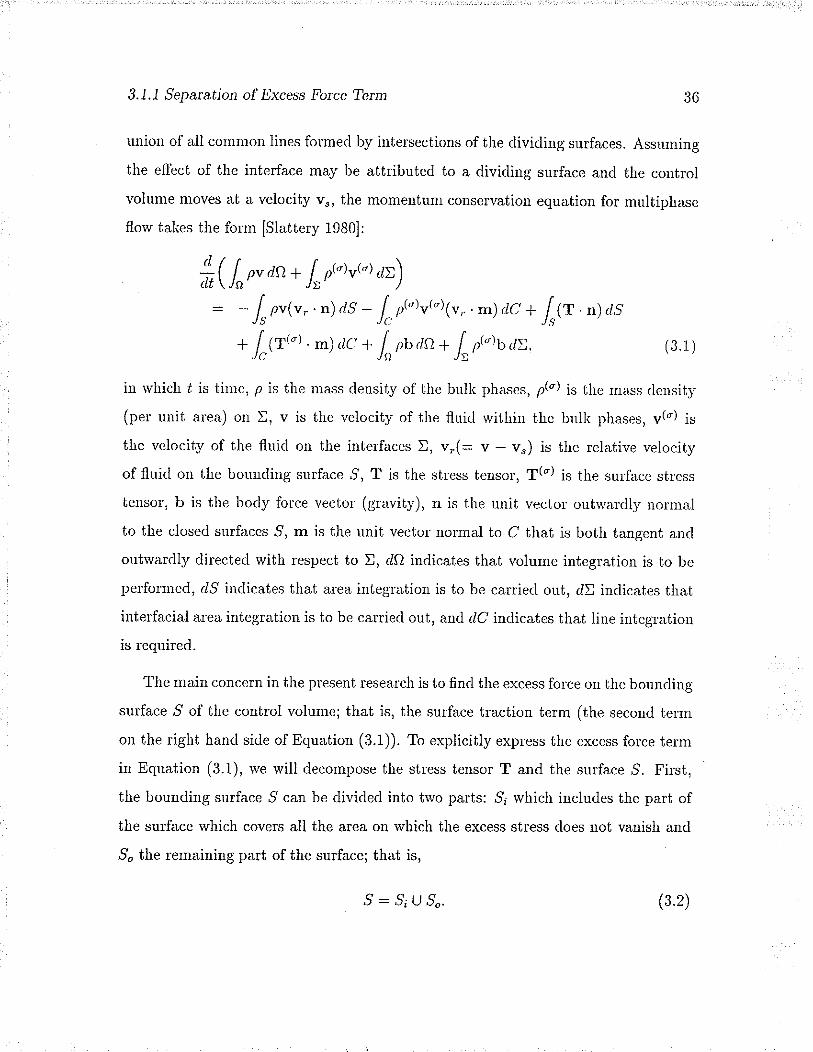
3.J.1 Separation of Excess Force Term
union of all common liues for.mecl by inter.sections of the dividing surfaces. Assunring
the effect of the interface may be attributed to a dividing surface ancl the control
voÌume moves at a velocity v,, the momentum conservation eqr.ration for muliiphase
flow talies the form [Slattery 1980]:
!l-( [,u¿aa I or"tuøt ¿y\dt\JnY'"" ' Jx' *")r .n)r1^9- lrøtut"t¡u,..m\rlC+ /ff .rrl¿S= - Jqpv\v, Jc ' Js.
+ [ gt"t. m)rlc+ [ ¡',ln+ [ pî)b,tÐ. (3 t)Jc' ' Jn' Jx''
in ivhich ú is time, p is the mass clensity of the bulli phases, p(") is the mass clensity
(pel unit alea) on I, v is the velocity of the fluirl within the bulk phases, v(") is
the velocity of the fluid on the intelfaces D, v,(- v - v") is the relative velocity
of fluid on the bounding surface ,9, T is the stress tensoL, T(") is the surface str.ess
tensor', tr is the body folce vector' (gravity), n is the unit vectol outtvardly normal
to the closed surfaces,9, m is the unit vectol normal to C that is both tangent ancl
outivarclly directed with respect to Ð, dO indicates that volume integration is to be
peúormed, d^9 indicates that alea integlation is to be carried out, dD inclicates that
interfacial area integration is to be carried out, and ¿lC inclicates that line integr.ation
is required.
The main concern in the present research is to find the excess force on the bounding
surface ,9 of the control volume; that is, the surface traction teÌm (the second ter.m
on the righi hand side of Equation (3.t)). To explicitly expless the excess force term
in Equation (3.1), we will clecompose the stress tensor T and the surface ,9. First,
the bounding surface ,9 can be divided into trvo palts: ,9¡ which includes the part of
the surface which covers all the area on which the excess stress does not vauish and
5o the remaining part of the surface; that is,
óo
^9=,9,U5,. (3.2)

3.7.1 Separatio¡ of Excess Force Te:'.m
Second, the stress tensor T can also be decomposed into two components:
T=Tp*T", (3.3)
rvhere Tu is the stless tensor which woulcl result from a single phase florv of the
corresponding fluicl phase in the flow channel as if the other phase of fluicl does not
eúsi (e.g. Poiseuille stress in pipe flow) (herein referr.ecl to as assumecl single phase
florv), ancl To is the excess stless tensor t'esulting from the plesence of the merriscus
irì the rnultiplìâse florv. The excess stLess tensot cal lte folmall¡' ex¡rLessecl as:
To=T-T¡. (3 4)
Then the snlface traction telm of Equation (3.1) can be clecomposecl into:
/rr "¡ as - l,Fu. n)r/s + lr,G"
. n)d.e + lr.{r .n) as. (3.5)
Substituting Equation (3.5) into Equation (3.1) ancl denoting the excess force term
by k; that is,
r< - / 1r" . n) as, (3.6)
the excess force term has to be balanced by the summation as shown below:
u = #( lrpv d,Q * lroþ\u@
,tt) + lrnv(v,.n) tts
* [ oøtut"t&,.m)dc_ / rr."l ¿s_ [ft,,.n)¿sJc' ' Js) Js,'-' -' ---
- [e,,.m)d.c- [pran- [p@u¿>. (3.2)Jc' ' Ja' Jy'
In older to study the influence of the interfaces on the resistance folce in multi-
phase florv, one can choose a simple flow geometry to eliminate the unsteacly (time
derivative) effect and the gravitational efect (which are often important in practice,
but are not fundamental) [de Gennes 1985]. Under these conclitions, in such a simple

3.1.7 Separation of Excess Force Tetm
geonretry, the unsteacly ancl body force telms can be neglected ancl Equation (3.7) is
leduced to:
u - l, nv(v,. n)r/^e - /.tr "l ds - ls:t. n) rts - l"ea) .rn) ac, (s.s)
where it is also assnurecl that the intelfacial convective force tenn is negligible. Each
telm on the light hand sicle of the above equation has a clear physical meaning.
The filst teLm accourÌts fol the co¡rvective effect, the second telm fol t[e tr¿rction
ou tlte sltrface fat arvay from the meniscus (rvhele the influcuccs of thc pr.escucc of
a meuiscns vanishes; that is, To - 0), the thilcl term for tÌaction resulting fi'om an
assumecl single phase florv or the surface close to the meniscns ¿ncl the fou¡th ter.m fol'
the interfacial tension force. The sum of the seco¡rcl ancl the thircl telms is the surface
traction that rvould result fi'om the assumed single phase florv in the entile control
volnure. The significance of Equation (3.8) is that although the excess r.esistance folce
of an immiscible flow is very clifficult to measure clirectly in experiments, it can be
evaluated through other quantiiies associated with this equation.
Evaluation of the excess fo¡:ce with Equation (3.8) rvill have the follorving aclvan-
tages: (i) All the quantities neeclecl to calc'late the integr.al teLms are in the outer
region; that is, no quantities, such as the stresses and sur{ace tensions, in the inner
region are involved; (ii) The quantities in the outer.region are easier to clefine ol toevaluate, for instance, the plessure difference; (iii) If the selected control volume is
lalge enough to cover the area where there is an interface efect, the value of k isinclepenclent of the selection of the control volume.
To illustr¿te the application of Ec¡ration (3.8) and to compare with the lVashburn
equation, we will evaluate k fo¡ a steady capillary flow it a cilcular tube in the
following section.
3B

3.7.2 Evaluatiott of k for Steady Capillar.y Flov in a Circular Tube
Conhol volume
s,
CèSo* Fluid 1 Fluid 2
ao
U
Figu::e 3.2: The contlol volume usecl to analyze the capillary florv i¡r a tnbe.
3.L.2 Evaluation of k for Steady Capillary Flow in a Circu-
lar Tube
Iu the capillary florv systen shotvn in Figure 3.2, Fluicl 1 displaces Fluicl 2 iu a
circular tube (the solid tube wall is Phase 3) of radius ¿ rvith a constant speed U.
The intelfacial tensions of the inteúaces of the three phases are ont o2J ancl a13. Itis of intelest to knorv the resistance force on the tube tvall. A cir.cular' fluicl colurnn,
as shown in Figure 3.2, was chosen to be a control volnme. The outer raclius of
the control volume is infinitesimally larger than the radius of the capillary a. Hence
the fluid/solicl interfaces are inclucled in the control volume. The control vohrme
is stationary with respect to the contact 1ine. The inlet and exit planes locatecl
at clistances of .L1 ancl L2 ftom the meniscus ( { < min{I1,I2}, € = max{(1, (2},
{1 and {2 ¿r'e the climensions of the interface effect regions of Fluid 1 ancl Fluicl 2
respectively).
If the viscous portion of the sur{ace stress tensor is neglected, the surface stress
tensor is ¡elated to an interfacial tension by the follorving expression [Slattery 1980]:
T@) = oP, (3.e)

3.1.2 Et aluation ofk for Steady Capillary FIow in a Circular Tube
¡vhere P is the projection tensor that transfolms vectors on Ð i¡rto their tangeutial
components. Under the conclitions of stead¡ fully developed florv, and negligible
gravity force, the excess force of the florv in a tube can be detelminecl from Eclua-
tion (3.8). In this specific ploblern, the horizontal comporent of k (k,) is of intelest.
Because of the axisymmetry, the impermeability of the tube wall and the steadiness
of the florv, the convective term can be easily evaluatecl as:
l"nu{r,., n) .irl.9 - -!nn'1p, - pz)(r2, (3.10)
whel'e i is the unit base vector along the ø axis. ,9o is chosen to consist of the inlet
¿ntl exit ¡tlanes. Becartse of tlie fully developecl florv condition, the only contlil¡ution
comes fLom plessuÌe folce on the inlet ancl exit planes. Therefore, the surface tlaction
on ,9o isI/ (T . n) . idS - raz(P; - Pa)./c
(3.1i )
,9¡ is the intelface betrveen the fluids and the wall of the contr.ol volunre. The shear
stresses of single phase flow on ,9; can be evaluated fi.om Poiseuille's law with the
¡esult:
[ $, .n) .idS - -2na (Y\ furt, + 11212), (3.12)Js;' t' \a/"'-'where ¡r1 and p2 are the viscosities of Fluid 1 and Fluid 2, respectively. C consists
of ihe interseciions of the fluid/solid intelfaces to the inlet and exit planes. Tlie
situation at the contact line needs some explanation. The three intelfacial tensions
among the three phases can be viewed as three strings rvhich are tied together at
the contact line. The string representing the fluid/fluicl interfacial tension, d12, encls
at the contact line. Because the radius of the control volume is larger than ø, o12
does not expose itself to the outside of the control volume. Therefole, the interfacial
tension of the meniscus is an inner force of the control volume selected and has no
contribution to the force component along the bulk flow direction. So the remaining
40

3.1.2 Evaluation ofk for Steady Capillary Flotv in a Circula¡ Tube 4i
contlibution of the inier{acial tensions are from the fluid/solicl inter{aces:
[|Jr, . m) .idC = 2¡ra(ozt - on), (3.13)Jc'
wher-e Equation (3.9) has been usecl.
Substituting Eqr.rations (3.10) - (3.13) into Equation (3.8) and dividing through
rvith (øo2), the holizontal component of the k integral is
l(,. 1. 8U , 2
n¿ : - r(ttt - p¿)U' - (P.r - Pe) + ](¡t:Ly + tttL¿) - :(ott - ot¿). (3.I+)
Ec¡ration (3.14) can be macle climensionless with the follorving chalacteristic qlran-
tities: ¿ for length, U for- velocity, ¡r1 for viscosity ancJ, (opf a) fol stress (pressule).
The dimeusionless form of Equation (3.1a) is
-li, 1' 1;:= - ,Þ't - ne) + iwa - Cal4(tt,rtt + !,.2tùl * ry, (3.15)a1t u o12 ¿
wlrere ?luü (- lp¡ - p2lU2 a2 f o12) is the Wel¡er number ancl tlie subsclipt e ancl the use
of lorver case Latin letters denote the climensionless c¡rantities.
A dimensionless excess folce parametel 1l can be clefined as:
_1,t( = _:_ (3.16)'- - 2r aop'
which is the ratio of the excess resistance force per.unit circumferential length to the
surface tension ø¡2. Then Equation (3.15) can be rervritten as:
'I Ix -'r@^- pù+ iwt- c.¡+1p,,Jt + u,,2t2)f*ry (3.17)
According to Equation (3.I7), I( should be a function of Ca and l,lzö; that is,
t{ = F(,Y6,go¡. (3.18)
Equation (3.18) implies ihat /l might be a properiy of the capillary florv system.

3.1.2 Evaluation of k for Steady Capillaty Flow in a Circulat Tube
Equation (3.i7) can be rervritten as:
pA - p B - c u[B(p,,yt¡ + p,,ztz)] - 2 ( oz:t - o ts - ¡r) - 1 lrr¿.\øtz/3
Ec¡ration (3.19) is vely sirnilar in form to the Washbur.n equation (2.17). Comparing
Equation (3.19) rvith the Waslibuln equation (2.17) under conditions of slow flow
(lyb << 1), ¿ relation between 1( ancl the apparent contact angle O,, will be
,. o2B - ûttlI =
-
- cosU,uot2
lVith ¿n assuurption lhat o¡2, d23 âncl ol3 ale properties of statel - iDdepenclent of
the plesence of florv, it follorvs that they can be clelivecl fi'ora Young's ecluatiou:
42
(3.1e)
(3.20)
(3.21)ú2J - ol\ : cos (Jj.
o12
It must be emphasizecl that this definitiol is not basecl on the assumption that the
dynamic contact angle is equal to O"2, whele O" is the static contact angle measur-ecl
through Fluid 1. It simply provides a means of calculating the ratio of interfacial
tensions. Therefore, Equation (3.20) can be rewritten as:
If = cos O, - cos O,. (3.22)
Equation (3.22) implies that 1l is equivalent to the excess dynamic pressuLe
A cos O¿ (: cos O, - cos O¡.) evaluatecl using the Washbum equation (i.e. the differ.-
ence ofthe static capillary pressure and the dynamic capillary pressure). Consequent-
ly, from the engineering point of view, in older to correctly evaluate the resistance
rln general, the energies associated rvith the solid/fluid interfaces, r13 eîd r23, can be thermo-
dynamically predicted, but can¡rot be experimentally measured.2In practíce, real material systems do not, have unique static contact angle O,. Under static
conditions, oûe measuÍes a sLatic adaøncing angle, Oo, and a static reced,ing angle, O", where all
angles, O, satisfying O, < O < Oo are static contact angles. To account for the static contact angle
hysteresis effect, ole may choose any proper value of Or, i,e,, O" < O, < O..

3.1.2 Evaluation of k for Steady Capillaty Flow in a Circular Tube 43
force in the capillâr'y flow, the apparent contact augle, O,, in the trVashburn equation
should be defined th.o.gh Equation (3.22); that is, base<l on the excess force. Asuch defined apparent contact angle may differ frorn that given by Equation (2.1g).
Whethel O¡ is a physical proper.ty of the flow systern (i.e. indepenrlent of tbe georn_
etry), is still questionable [Ngan & Dnss¿n V. 1982; Cheu 1984]. Tlie.efo'e, whethe'
O,, or 1l is inclepenclent of the geometry remains to be clarifiecl in future stuclies.
By analogl,, fol planal channel pr.oblern, a set of erluations sinlilar. to Equations
(3.15) - (3.17) and (3.t9) can be clerivecl:
#: r,^ - pB) +!w" - cn¡sçr,rtt * p,,2t2)l -r coso,,
whele b is the rvidth of the planal cell;
,, _k,b on'
1
1f = (p.r - pB) + VWI: - Ca [3(¡¿.,rlL + ¡r.,212)] + cosO"
1
p,t - pB - Cal3(p,rh + p,.212)l - (cos O, - K) - ;I'Vb
and
(3.23)
(3.24)
(3.25)
(3.26)
An altelnative apploach to derive a genelal capillary tube florv ec¡ration is to
choose the radius of control volume to be slightly iess than ¿. Then (i) the contr.ol
volume intersects the fluid/fluid interface (the contact liue norv lying outside the
cortrol volume), thus a term of the fotm i2n a op cos O must be incluclecl, ancl (ii)
there are no contributions fi'om an integral over C evaluated at the two ends of the
control volume (no contlibution similal to Ecluation (3.13) ). For this choice of the
control volume, Equation (3.20) becomes,
I( -- cos O - cos O-. (3.27)
where O denotes the actual dynamic contact angle. Although the above expression
for 1( has the aclvantage of containing no questionable assumptions, O is not experi-
mentallv measurable.

3.2 The Contact Angle under Dynantic Conditions
There are two advantages in measnring 1f baserl on Equations (3.12) anct (8.21)
over rneasuting the apparent contact angle in a capillaly tube. Filst, 1l is a real
excess resistance force ratio, but À cos O¡ is not; second, to determi¡re .IL, a pressur.e
clifference betrveen the inlet and the outlet of the capillary is all ihat needs to be
measuLed - this quantity can be obtainecl rvith high accuracy. On the contrar¡ to
measure the apparent contact angle with high accuracy in a capillary tube, undel
clytraruic contlitions, is still a clifficult taslç. Iu the uext chapter', it tvill be shorvn that
the v¿rlnes of O,, antl O/¡ al'e very close, consequerìtly O/r calt be eral¡¿rtecl l;-t, malii¡g
a vely sirnple pLessute measuLement.
3.2 The Contact Angle under Dynamic Condi-
tions
The dynamic contact angle, as an essential boundaly condition usecl in nnmerical
simnlatiou, has to be cletermined a priori.. Due to the complexity of the florv mecha-
nisms in the inner region, the conditiou of the dynamic contact angle is not clear.for
the general case [Dussan V. 1979]. The dynamic contact angle in previous analyses
was usually assumed to be the same as for the staiic case, and reasonable resr¡lts have
been obtained [Loivndes 1980; Cox 1986].
A true contact angle is detelmined by the forces acting very neal the contact line
betrveen the molecules of the trvo liquid phases ancl of the solicl phase [Cox 1g86].
From the thermodynamic point of view, the surface tension is the srrr.face enelgy
per unit area. Although recent studies [Chlistenson 1985; Christenson, lsraelachvili
& Pashley 1987] have shown some experimental evidence that the surface tension is
constant down to molecular diameters, it still rem¿ins an open question wheiher the
value ofthe surface energy on each interface is constant all the way to the contact line

3.2 The Contact Angle uncler Dynamic Contlitions
[Dussan V. 1979]. A further question is rvhether the surface enelgy is depelclent on the
tlynarnics of the interface, or in other word, does the microscopic contact angle depend
on tlìe movement of the interface [Cherry & Holmes 1969; Blake & Haynes 1g6g]? Due
to the lack of this cletailed information, rve ale restr-ictecl to examining the contact
angle undel dynamic conclitions rvith the commonly usecl assumptions.
To determine the bounclary conclition of the contact angle in the ptesent sttdy,
tlre folloiving assurnptions ale l¡acle: (i) The iutelface is a two-tl,itnensi.onal (i.e. Ibe
thicllless of the ilterf¿icial lr4el is infinitesiru¿rì compaling to the l¡ulli climensiol) cli-
vicling surface rvhich sepalates trvo homogeneous phases and oli rvhich all of its excess
energy is concentr'â.tecl; (ii) Surface enelgy is constant all the rvay to the coniact line;
(iii) The solicl surface is rigicl, rvhich is a valicl assrunption because fol orcliuary solicls
the cleformation neal the contact line is very srnall an(l ltence negligible [Lester. 1g6i];
(iv) The stress terÌsors in the dom¿in inclucling the bounclary are integrable. A non-
integrable stless tensoL means a failure of a physical model.
Under these conclitions, Equation (3.1) can be recluced to:
R(n) : -#Urpvtre-r l,or.u@ az) - lrov(v,.n)as+ /tr n) d^e + I"Gr,
. m) ttc + lnor an + l,o@a at
- [ ,t"tu@1v, . m) d,C : o, (8.28)Jc'
where R(O) clenotes the resiclue of the equation.
lVe choose a control volume as shorvn in Figur.e 3.3 rvhich inclucles a semi-circular
span in the fluid phases rvith its origin at the contact point and a radius of r. Therefole
the boundaries of the alea are the circumference of the semi-circle ancl the intelfaces
between the fluid phases and tlie solid phase. As mentioned in the previous section,
the inte¡facial tension of the meniscns at the contact line is an inner fo¡ce to the
45

3.2 Tl¡e Contact Angle under Dynamic Conditiots
Figure 3.3: The control volurne used to clerive the clynamic contact angle co¡ìdition.
control volume. ?he inietfacial tension tetm can be explessed by:
l"G'' ' m) dC - onmn * oztmzs *ør3 mr3.
Then, the resiclue of the momentum equation, R(O), will be
R(O) - (onmtz * o2s rn1a * ør¡ mrs)
-# (1,* on + l,nt")v{ò a>) - f, ou(u, . o) as
+/tr. n) rr^e + lnnr an + l,o@r, az
- l"o@u@{u,'rr')dc : o.
4t)
(3.2e)
(3.30)
Letting the semi-cilculal region shrink to the contact point (i.e. r --r 0 as rvell
as O -+ 0) ancl applying the assumptions made above, the surface traction term
becomes:
/{r'")as=1"" (3.31)
ancl other integral terms in Equation (3.30) vanish. Here /" is a concentrated force
which may exist only if the third phase is solicl. Furthermore, /" is a reaction force of
Phose 3

3.2 The Contact Angle under Dynamic Conditions
solicl on fluicls at the contact point to b¿lance the component of the surface tensiou
on the fluid/fluid inter{ace normal to the solid surface3. Therefor.e, the force balance
equation valid for the coniact point is
åt:àn(nl := ot2mt2 I o2sllr...¿* d13 m13 * /" n - O. (3.32)
Equation (3.32) can be applied to some special cases. Ifthe thilcl phase is another
immiscible fluicl insteacl of a solid, it is impossible fol a concentlated folce to exist
(except fol the intelfacial tension) so that the concent::¿l,tecl r.e¿rction folce /. ri,ill
vanish. In sLrch a case, Equation (3.32) recluces to Neumann's eqnation:
onmtz * ozs mzt * d13 m13 = Q (3.33)
If the solicl sudace is planar', then the force balance in the tangential direction of the
solicl sulf¿ce lvill recluce to Yonng's eqnation:
OZg - Ott = drz cos O. (3.34)
Because of the assumption (ii), the clynamic microscopic contact angle must be the
same one as in the static case; that is,
o-o,. (3.35)
The lesult given by Equation (3.35) has also been tested by numerical simulations
[Shen & Ruth 1991]. In the numerical simulations, we assumed different microscopic
contact angles (i0" - 170"). The results show that the asymptotic contact angle to
the wall always approaches to the static contact angle whatever microscopic contact
angle is assumed.
sThat the reaction force of the solid su¡face rvill only have a ve¡tical compotretrt had been ques-
tioned by Dussan V. [1979]. If the tangentia.l component of the ¡eactio¡r fo¡ce does not varish,
horvever, Young's equation (3.21) rvould ¡ot be valid.
47

3.3 Sttm¡narv
The above delivatio¡r is not intended to show rvhat the r.eal clynarnic contact
angle is, but to find out what the clynamic contact angle should be uuder the given
assumptions. Pismen & Nir [1982] clainied that an ignorable singularity can arise
rvhen the advancing contact angle is eclual to 180". But Ngan & Dussan V. [1984]
have shown that there is an elrol in their derivation. The present derivation can ¿lso
be usecl to explain the improperness of the approach pursued by Pismen & NiL [1982].
Any attempt to use a mict'oscopic contact angle cliffelent fi'om the static one rvithout
sollle pLopet moclific¿r.tious of the above-¡]1entioued assuÌrptioDs rvill not lte successlul.
3.3 Summary
The clerivation of a general capillary florv equation shotvs that the excess resistance
folce can be evaluatecl thlough other expelimentally measurable quantities associatecl
with the momentum equation (3.8). Fol the capillaly tube flow, a.Il factor can be
defined as the ratio of the excess resistance folce per unit circumferential length to
the fluid-fluicl interf¿cial tension. lVhether the If factol is a parameter of a material
system remains to be clarified in future studies. Under the commonly accepted as-
sumptions, it has been found that the micloscopic dynamic contact angle has to be
the same as the static contact angle. This implies ihat any different values of the
microscopic dynamic contact angle may only be possible if one or more of the usnal
assumptions is abandoned.
48

Chapter 4
Finite Element Analysis
To nrunerically examine the validity of the capillar.y flow equation de¡ivecl in the
previous chapter and to evaluate the differences of the genelal capillaly flow eclnation
from the lVashburn equation, a finite element simulation of immiscible capillary floiv
rvas perfolmed. The results are presented in this chapter.
In Section 4.1 the numerical problem and a meniscus iteraiive scheme are cle-
scribed. Section 4.2 gives the finite element formulation and Section 4.3 contains
the adaptive grid generation sche¡ne used to discr.etize the geometric domain of the
pr-oblem. Presented in Section 4.4 are the numerical results of 1l factor and dynamic
capillary pÌessure.
4.L Numerical Problem and Meniscus Iteration
Scheme
The numerical ploblem considered is the steady movement of a fluid meniscus dis-
placing its vapour in a parallel cell (Figure 4.1). The frame of reference is chosen so

4.7 Numerical Problem and Meniscus ltemtion Scheme
7"" = 2H lCaTnt =0Un =0
ut =0Ttz =o Tr2 =-(L+uÐlB
ut=0u2=(.1'3x)lt2(1+38)J
Figure 4.1: The numelical ¡rroblenr conside¡ed for the steady nroven:.ent of a fluid
nreniscus displacing its I'apoul in a palallel cell.

4.1 Numeúcal Problem ancl fuIeniscus lteration Scåeme
that the fluid/vapour i¡rterface is stationary. The origin is placecl at the micìrlle of the
iuterface. The sepalation of the two parallel srnooth plates is 2¿ and the width of the
plate is large enough to ensure that the florv is two dimensional. The gap of the cell
is sufficiently small that the effect of glaviiy is negligible, assuming that the systen
is horizontal. Foi' an incomp.essible Newtonian fluid and slow florv, the florv fielcl
behind the intelface can be detelmined by solving the dimensionless stokes equation
ancl the cotrtiuuity ec¡ration rvhich ale
Tt,t=0 (1.1)
(4.2)
?t=0, ¿l=1. (4.3)
For the tangential component of velocity, to remove the force singulality [Huh
& Scriven 1971; Dussan V. & Davis 19741, the classic Navier slip moclel is used.
rr, - -|P, + r), ø, = 1. (4.4)
Here 6 (: Ls l2a) is the dimensionless slip coefficieni.
2. At the inlet, fully developed flow is assumed. The velocity pr.ofile is
ur = 0, xz: -h, (4.5)1, - 3t:?az =
-
-'- -|¿1. (4.6)2(1+38)' e2 -
where 11 is the climensionless length of the flow region to be analyzed in the
direction of flow,
ancl
ùi,i : 0,
with the following bounclaly conclitions:
1. At the solicl wall, the normai component of velocity vauishes:

4.1 Numeúcal Problem ¿nd .Lle¡iscr¡s Iteration Schene
3. Along the centelline of the cell, flow is symmetlic. It follorvs that:
K.)
Al
Tn -0,
øt =0,
ct=0.
¿z = /¿,
xz=h,
(4.7)
(1.8)
(4.e)
(4.10)
(4.11)
4. At the intelface, there is a balauce betrveen the normal stress difference, 1.,,,across the interface ancl the capillaly pl'essuÌ.e,
-2HL(L
l¡r = U'
and no penetration of fluicl through the intelface,
u"=0,
zero sheal stLess
xz= h.
Here 1l is the mean cuÌvatuÌe of the interface.
5. At the contact line, the interface obeys the contact angle bounclar.y condition:
0 -4, .01 - 1. (4.r2)
The shape of the interface is not known a priorí and must be cletermined as
part of the solution. An iteration scheme can be used to upclate the shape. There
were several options employed in previous stu<lies [Sillirnan & Sct'iven 1g80]. The
shape of the interface can be updated by normal str.ess iteration [Orr & Scriven 1gZ8;
Silliman & Scriven 19B0]: this is inefficient in systematic large scale computations.
Some resealchers favol' Newton's method because of its quadratic rate of convergence
aûd the availability of the Jacobian matrix for path-following strategies and stability
analyses [Brown, Scriven & Silliman 1980; Saito & Scriven 1981]. Georgiou, Schultz &
Olson [1990j used full Newton iteration to solve the die-swell problem with a'spider-
web' grid around the static contact line. Recently, cost-efficient variants of Nervton's

4.1 Nttmeúcal Prcblem and Nleniscus Iteration Scheme
method ancl continuation schemes that exploit l(rylov iter.ative methocls have been
p'oposed [Brorvn & saad 1990; Huitfeldt & Ruhe igg0]. Because the present stucly
does not focus on developing a new and cost-efficient sinrulation package, a relatively
simple itelative scheme - a nolmal stress iteration scheme - rvas employecl, which
works in the region of low capillaly mrmber (say Ca < 70-2) and is easy to prograrn.
The implernentation of the meniscus moclification iterative techniclue appliecl here
is sirrilal to those of Lowncles [1980] âncl Tilton [1988]. For. the plaua.r plol:leur. the
plofile of the neniscus can be expressecl as IHrrnsen & Toong 1gZ1; Lorvndes 1980]:
dlt.
ttrt = cot u
and the me¿n curvature of the intelface is
u =|fr*"e.Hele d is the angle betrveen the tangent line to the interface at c1 and a line palallel
to the planar wall and is a function of o1. Eqtation (4.9) ca¡ be rvritten as:
T* = !! "o"oOa(Æ\
(4.13)
(4.14)
orr rz = h. (4.15)
Integrating Equation (a.13) with respect to n1 and using the bounclary conditions
cosd = 0 and å = 0 at ø¡ = 0, the equation for.the meniscus profile is obtained:
h(c) - lo" "otl,1r.(4.16)
In Equation (a.16), the slope angle of the interface, d, is determined by integr.ating
Equation (a.15) with respect to c1:
cosg - ca Io"
T^^ rh:. (4.17)
The normal-stress iterative scheme used to determine the meniscus profile is as
follows:

4.2 Finite Element Formulatton
1. Guess an initial neniscus plofile. In the present rvork this was a flat meniscus
proû1e.
2. solve the stokes ancl continuity equations for the velocity and pressur.e in the
fluicl, imposing ouly the boundary conclitions (4.3) - (4.8), (a.10) ancl (a.11).
3. Calculate the values of tolmal stless of tlie fluid on the meniscus ?,,, at cliscrete
values of c1. Note that the ptessut'e, ancl as a conseqtlence ?,,,,, is cletc::mirrecl
onl¡' rqr to a constant l:eca,use it cloes not zr,p1>ezrl iu nny of the zrppliecl boundar.y
conclitions. HorveveL, usirrg the bounclaly conclitio¡r 0 - O at ¿r = 1, Eclu¿-
tion (4.17) gives:
5+
(4.18)
ancl this integlal constraint sets the level of ?}" and hence the pressule, in the
florv fielcl.
4. Use the values of fl"" to integrate (a.16) ancl (4.17) numer.ically, and thereby
obtain a new meniscus plofile.
5. Repeat Steps (2) to (4) until the change in meniscus profile is belorv a specifiecl
tolerance.
4.2 Finite Element Formulation
Although in Section 4.1 the problem has been confined to that of Stokes flow, the finiie
element program has been developecl to accommodate the complete, incompr.essible,
Naviei'-Stokes equations. The finite element equations are derived belorv.
The dimensionless Navier-Stokes equation and continuity equation are
cos o = cn lot
T,,, rtr',
Reù¡ I Rea;,¡a¡ - Stbi - T¡¡¡ = 0 (4.1e)

55
(4.20)
(4.2r)
Rel- (pau I p1)l is the Reynoltls Nurnber, St [- (pgaz) l0r1U)] is the Stokes Number,
ö; is tlre bocly folce component and ¡r. [= UlUr] is the viscosity ratio. The char.acter-
istic climensional c¡rantities used are the lelgth a, the velocity LI, the tirue afLf, t\e
viscosity /¿r, the stless (or plessure) ¡tyU fa, a:nd, the body for.ce I (glavit1,).
Applying the Galelkin methoci [Chung 1978], the rveali for-ms of Ðquations (4.19)
and (4.20) areI
Jn(Reû* Reu¿,¡u¡ - Stbí- \j,j)ÕN¿f¿ - 0 (4.22)
au.cl
[ ,r.rúydQ - 0,JQ
whele O is the domain for finite element analysis. Let
?r; : Õ¡ u¡¡, P=ÚNpN,
where O and t! are interpolation functions of velocity and pressule on each element
respectively, and u;y; and pN âre norlal values of velocity ancl pressure respective-
ly. Substituting Equation (4.24) into Ecluations (4.22) and, (4.23) an<l making some
manipulations (see Appendix A fol details), the finite element equations are
4.2 Finite Elenent Formulation
and
where
AN*r i¿ ¡t¡ +
I
u¡,¡ = 0,
T¡¡ = -p 6¡¡ * I-¿' (u¡,¡ * u¡,;),
(4.23)
(4.24)
BNjununjuu¡ * DNv;jr¡r¡ *lG(fr).¡i¡¡ + G\]'l¡,* + G\(,l,rlaott
cN¡¡tp¡t * F¡t¡¡vp*t = øÍl] + rÍi] + rffi) @.25)
and
Ct¡¡¡¡¡ u¡¡¡ = 0, (4.26)
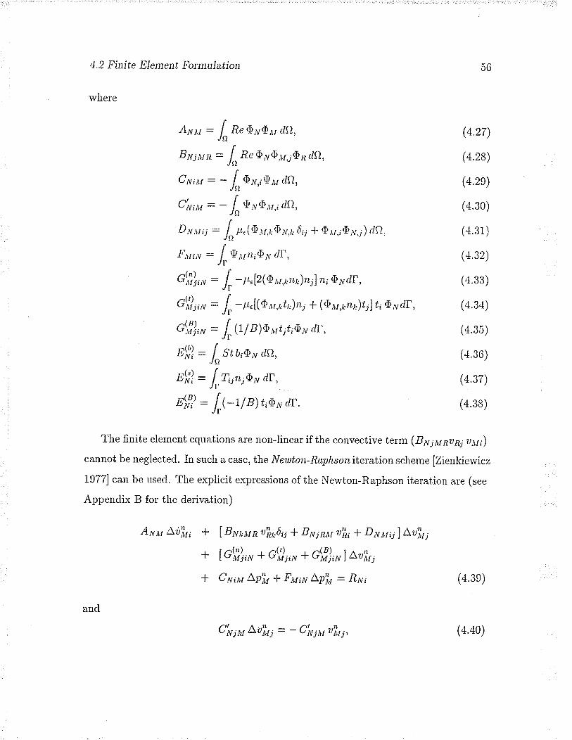
4.2 Finite Element Formulation
where
ü, = In-Re Õ¡Õ¡¡ dQ,
B ¡u j ¡r a = lnï" e rø r,re o rle,
cN¡,yr=-lnø*,,vnan,
C'N;*t=-/ vronr,,acl,
Dt¡¡t¡j = / l.(,Þrr,uÕr,u ô;r -l- iÞ.v,iÕ¡.;) dQ,
F,u;,v:/ú,yn¡Õ¡rtl,
CÍ?Ì," = f, - u,l2(Õ n,,u,r¡,)nil ø¡ Õ¡rtt,
cÍ?¡u" = / -1.[(Õ,u,rti") n¡ * (Q¡¡,¡n¡)t¡J ¿, o¡rdt,
Glrl'],* = I(1lB)øilrtlraN ff,n$l: lnstt,ø*aa,ø(fi) - lrrr¡n¡øN tr,ol) : l,t-r¡a) rio' ¿r.
A¡¡¡¡ Liti¡¡ * lB¡¡¡¡¡¡uþ¡6;j * B¡tjnuuþr+ Dy¡¡¡¡lLui¡'
+ lcî|)¡,r + Gf?,," + c1fl,,*l r"7,,
* C¡¡¿¡rt Apit * Fu¡¡t Lp'il = RNi
C'¡¡¡e¡ A,ui,,, = - C'¡o jvrftt¡,
(4.27)
(4.28)
(4.2e)
(4.30)
(4.31)
(4.32)
(4.33)
(4.34)
(4.35)
(4.36)
(4.37)
(4.38)
The finiie element equations are non-linea¡ if the convective letm (B ¡¡¡¡7 su p¡ u¡¡;)
cannot be neglecteci. In such a case, the Newton-Raph,son iteration scheme [Zienkiewicz
19771 can be used. The explicit explessions ofthe Newton-Raphson iteration are (see
Appendix B for the derivation)
(4.3e)
(4.40)
ancl

4.3 Adaptive Gúd Generation Scheme
wlÌere
á{, - (¿'fl)" + (¿$l)" + (ø[,{r¡"
-{rl"rr ùiri + B N j ì,r nukj af;¡¿ I D ¡ ¡¡ ¡¡ ul¡ ¡
+tcÍiln" + Gt)¡;n + cff),*7r¡, + cu¡u pît i Ftt;N p,i.tj. (4.41)
4.3 Adaptive Grid Generation Scheme
In capillary fl.otv ploblerns, the velocity ancl st::ess var.y clrarnatically neal the co¡tact
line. In order to obtain ¿ r'eliable ancl leasonable numerical result, an aclaptive gr.icl
generation scheme is usecl in the present rvork.
The adaptive glicl generation scheme, which was based on Zienkiervicz & Zhu,s
proceclr.rre [t087], was usecl to clivicle the clomain into six-nocle triangulal elements.
The basis of aclaptive scheme is that an er¡ol estimation is macle on the level of the
elements in the original mesh and then a nerv mesh is generatecl in orcler. to achieve
an even dist¡ibution of the error between elements. The elror estimator used in the
present aclaptive scheme is the enelgy elror. estimator for mixed elements [Zienkiewicz,
Liu & Huang 1989]:
llull, - Il" - "rll +llp - pnllr,
= ff. - sÀ¡î12¡i¡-11s - r/'),/e + ln{n - nY G)-1 (p - ph) da, e.42)
where s, sÀ, p and pÀ are the exact ancl finite element deviatoric stress tensors (i.e.
viscous stress tensors in the present problem) and pressure respectively and ( is the
penalty parameter. Because ihe deviatoric energy norm error llv - våll converges
at the same rate as the pressure error in .L2-norm llp - pollt, [Zienkiewicz, Liu &
Huang 1989], the relative error of the energy norm e can be defined as:
-- llu - "nllè - llvll-' (4.43)

4,4 Numeucal Res¿¡lts
where
llvll2 - lnsr (z¡e)-ls dQ
A converged resuli will guarantee that the relative error defined in Equation (4.48)
in each element is within a given couvergence criterion. Figure 4.2 shows an aclaptive
glid mesh genelated in the finite element simulatio¡r.
4,4 Numerical Results
Basecl on the finite element fo¡:mulation clerivecl above fol capillary flow, a compnter
plogram has been written. The numelical r.esults obtainecl will be presentecl belorv.
In the calculations, it was assumecl that the dimensionless slip coefficient 6 equals to
10-5.
Figure 4.3 shorvs a typical velocity vector clistlibution in a capillary florv. The
deviation of florv from the Poiseuille form is obvious in the legion close to the interface
- a raclial flow component is present in orcler to obey the impermeable bounclary
condition on the interface. Orving to the non-Poiseuille flow pattern close to the
inter{ace, the shear stless distribttion on the wall is quite diffelent from the one
predictecl by Poiseuille flow. As sho.çvn in Figures 4.4, 4.5 and 4.6, the ¡vall shear
stress increases dlamatically as the contact line is approached. The fluctuation
of pressure close to the contact line results fi'onr too tiny elements (of size 10-?). Itshould be noted that the dependence of the log of the wall shear stress on ln( å(1)-ø, )
is almost line¿r' in trvo regions - for 0 < [å(1) - r2] < L0-5 - B, the wall shear.
stress is nearly constant; and for lh(l) - r2l > 10-4, with a negative unit slope. This
may indicate the scales of two regions - the inner region with a length scale of the
slip length and the lower limit of the outer region with a length scale of one o¡der
higher than the slip length. The region connecting the inner region and the oute¡
region woulcl be an iutermediate region.
5B
(4.44)
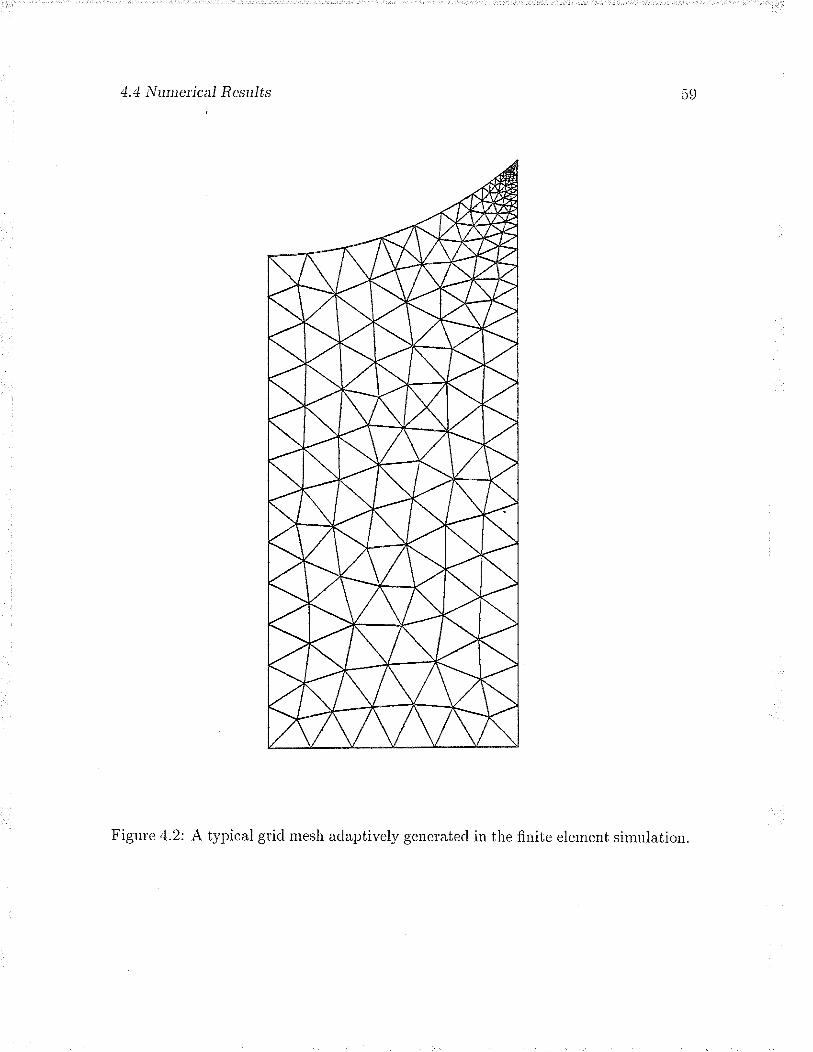
4.4 N¿rme¡icaj Res¿¡Jts
Figure 4.2: A typical gricl mesh aclaptively generatecl in the finite element simulation
59

4.4 N¡¡me¡ical Res¡rJfs 60
Figule 4.3: Velocity vector fielcl.

4.4 Numerical Results
106
105
104
T,, 1og
102
101
100I 0-8 1O-7 10-6 1O-5 1O-4 1O-3 10-2 1O-1 100
h(1) - x,
Figure 4.4: Valiation of wall shear stress fol O = 25' ancl 6 = 10-5. Dimensional
qnantity: Tn. fu.U la).
b-L

4.4 Numetical Results
106
10-
104
Í r, 103
102
10f
100
62
10
-2Co = l0
10-8 1O-7 10-6 l0-5 1o-4 1o-5 1o-2 I o-t 100
h(l) - x,
Figure 4.5: Variation of wall shear stress for O - 45' and 6 = 10-5. Dimensional
quantity: T72 ' fuU I a).

4.4 Numeücal Results
106
10"
104
T,,, 1 05
102
1or
lo01O-8 1O-7 10-6 10-5 1O-4 1O-3 1O-2 1O-1 100
h(l) - x,
Figure 4.6: Variation of wall shear stress for O - 70" and 6 = 10-5. Dimensional
quantity: \r.(pU/a).
OJ
10
-20Co=1

4.4 Numeúcal Results
As p'edicted by Lorvndes [i980], a severe deformation of the inte'face close to the
contact line c¿n be seen in numerical simulations, as shorvn in Figures 4.7,4.8 and
4.9. The deformation of an interface close to the contact line is a consequence offluicl acceleration in that region. A va.i¿tion of the appar.ent contact angle, O¿, is
an indication of the magniturle of the deformation. The profiles of interfaces uncler
diffelent displacement velocities are shown in Figure 4.10. As the velocity increases,
the appalent contact angle, O¡,, increases, rvhile the micloscopic contact angles, O,
rvet e iclentic¿ll.
The /f factor was ev¿luatecl using Equations (2.17) and (3.27). The excess cly-
namic pLessule A cos O¡, was evalnatecl rvith the follorving ec¡ration:
AcosO¡ = cosO - cosO¡ (4.45)
Essentially, this is the excess dynamic plessule evaluatecl thlough the \vashbuln
equation (1.1). The comparison of the results is listecì in Table 4.1 ancl Ap clenotes
the pressure difference (p¡-p¡). The variations of 1l and AcosO¡withCaar.eshown
in Figure 4.11. The deviations between I( (the hollow symbol lines) and ÂcosO¿
(the solid symbols) show that the apparent contact angle O, evaluatecl using the'Washburn
equation (2.17) would not be the same as O,¡, especially for high capillary
number'. But the difference between them is very small. For Ca - g.g1 the lelative
deviation between 1( and A cos O¿ is less than *3%. This implies that A cos 06 is
a good inclicaiion of the magnitude of excess force 1( and answers the question why
the primitive lVashburn equation (1.1) works so well.
b4

4.4 Numerical Results
90
80
70
60
50
40
30
20I O-E 1O-7 10-6 l0-5 1O-4 10-5 1O-2 10-f 100
1 - *,
Figule 4.7; Variation of slope angle of a meniscus, O - 25" and 6 = 10-5.
65
ooLo,oro
e
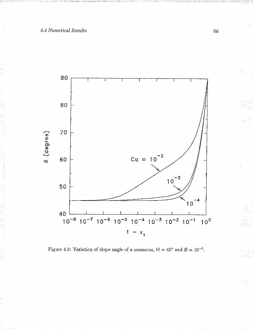
4.4 Numerica,l Results
40
66
90
BO
70
60
ooLq,c,E
o Co = 10
-z10
10
50
1O-8 1O-7 I 0-6 1O-5 1O-4 l0-5 10-2 l0-t 100
1 - "'
Figure 4.8: Variation of slope angle of a meniscus, g = 45o and 6 = 10-5.

4.4 Numerical Results
90
88
86
84
82
80
78
76
74
72
70
68I O-8 1O-7 10-6 l0-5 1o-4 1o-5 10-2 1o-1 100
1 - *,
Figure 4.9: Variation of slope angle of a meniscus, O - 70' and 6 - 10-5
67
ooLg,o!
a-2Co -- 10

'x
¡-¡U'Joañ
(u
otu
ofL
0.5
0.4
0.3
o.2
0.'l
0.0
4.4 Nr¡me.¡'rca1 Res¿lJfs
0.0 0.1 o.2 0.3 0.+ 0.5 0.ô o.7 0.8 0.9 1.0
Distonce frorn Centerline I x,]
Figule 4.10: Interfaces undel diferent displacernent velocities, O = 45"

4.4 Nttmerical Results
T¿rl¡le 4.1 : The siuulated I'esnlts of an iurmiscible capillar'¡' flol, in a par.allc.l
Simulation palametels: O - 25', 45', 70" and 6 = 10-5.
Ca o(") Ap å(1) o¡(") o.,(.) À cos O¡ T(
0.0001 -0.90125 0.6310 25.50 25.57 0.00372 0.00427
0.001 -0.85900 0.5805 29.73 29.92 0.03790 0.03957
0.01 -0.53725 0.3356 52.90 52.60 0.30310 0.29899
0.0001 45 -0.70361 0.4121 45.20 45.22 0.00247 0.00277
0.001 45 -0.67267 0.3921 47.18 47.t7 0.02741 0.02733
0.01 45 -0.39708 0.2419 62.80 62.33 0.25000 0.24277
0.0001 70 -0.33938 0.t752 70.12 70.12 0.00197 0.00198
0.001 70 -0.31584 0.i651 71.25 71.20 0.02058 0.01968
0.01 70 -0.09807 0.0759 81.32 80.77 0.19110 0.18168

4.4 Nttmerical Results 70
0.50
0.25
.c
e 0.20o(,
Lov o.io
0.05
-5B=10O=25o
70
Legend:oKe [cos@¡
0.000.000 0.002 0.004 0.006 0.008 0.010 0.o12
Co
Figule 4.11: The comparison of the excess dynamic pressute AcosO¡ and the 1(
factor for a lange of capillary numbers. Hollorv circle: .If; Solicl circle: A cos O¿.

Chapter 5
The Apparent Viscosity Approach
As reviervecl in Chapter 2, iniroclucing slippage models can effectively relieve the
singularity at a contact line. Horvever, such a practice rvill result in a consequence that
the fluicl on a contact line will never nrove alvay from it, rvhich is in contr.acliction with
the "rolling-type" ntotions observed in experiments [Yarnolct 1938; Schwa::tz, Racler
& Huly 1964; Dussan V. & Davis 1974]. Insteacl of relieving the no-slip boundary
concìition, the appalent viscosity approach, rvhich rvill be presented in this chapter,
can be applied to remove ihe singularity at the contact iine as well as to describe the
"rolling-type" motion.
The motion of fluid alound a solid cylinder which rolls over a planat solid surface
without slippage is analogous to the "rolling-type" motion of fluids ovel a solicl sulface
in the viciniiy of a contact line. In the rolling cylinder problem, the cylincler surface is
analogotts to the meniscus of a zero contact angle as in ¿n immiscil¡le capillary floiv.
One of the advantages in solving the rolling cylincler problem is that the cylinder
surface is pledefined, instead of needing to be solved for as in the capillary flow.
Therefore, solving the lolling cylincler problem, one is able to evaluate the effectiveness
of a nerv fluicl moclel in relieving singrrlzu'ity and/or describing the "rolling-type"
7I

5.1 Breakclotvn of the Classic Continttum Iodel
motion.
In section 5.1, evidence of the breakdown of the classic continuum fluid model was
reviewed. Based on available viscosity data in very small fluid systems, an apparent
viscosity model is presented in section 5.2. Then, a rolling cylinrler pr.oblem is solvecl
using both the apparent viscosity morlel ancl the classic stless slip model (sectiou b.3).
lVith the intlocluction of the apparent viscosity model, fluicl unclergoes ,,rolling-type"
motion as obselverl in expelimeuts (Section 5.4).
S.L Breakdown of the Classic Continuum Model
The classic continuum flow moclel may not be valicl in the region very close to the con-
tact line. It is knorvn that the size of the region surrounding the interface (intelfaciai
region) that contributes to the surface properties (energy, mass-clensity cliscontinuity
eúc.) extends many molecular cliameters into the bulk fChapela et aL lgTT; Saville
1977; Shukla & Robert 1992]. The phenomenon of mass-density fluctuation near.sol-
id walls (i.e. dynamic layering) has been founcl in both experimental [Israelachvili& Àclams 1978; Islaelachvili 1985] ¿ncl molecular dynamics studies of fluicls confined
by either artificial or molecular boundaries [Abr.aham 1978; Toxvarerd 1981; fuIagcla,
Tirrell & Davis 1985; Broughton & Gilme¡ 1986; Tallon 1986; I(oplik, Banavar &
lVillemsen 1989]. Outside of the "dynamic layering r.egion" (about three or.so molec-
ular diameters from the w¿ll [Alder & Wainwright 1970]) the average beliavionr.is the
same as the bulk. The decrease of tlte fluid density in the dynamic layering region
can lead to a clecrease in its shear viscosity [Chulaev, Sobolev & Somov 1984]. These
layering effects are not accounted for in the classic continuum moclels. The thickness
of the interfacial region is very small if it is compared with any typical length scale
(e.g. the radius of a capillary) and can be vietved as "zero thickness" with respect to
the typical length scale. However, in the case of a contact flow problem, the effects
72
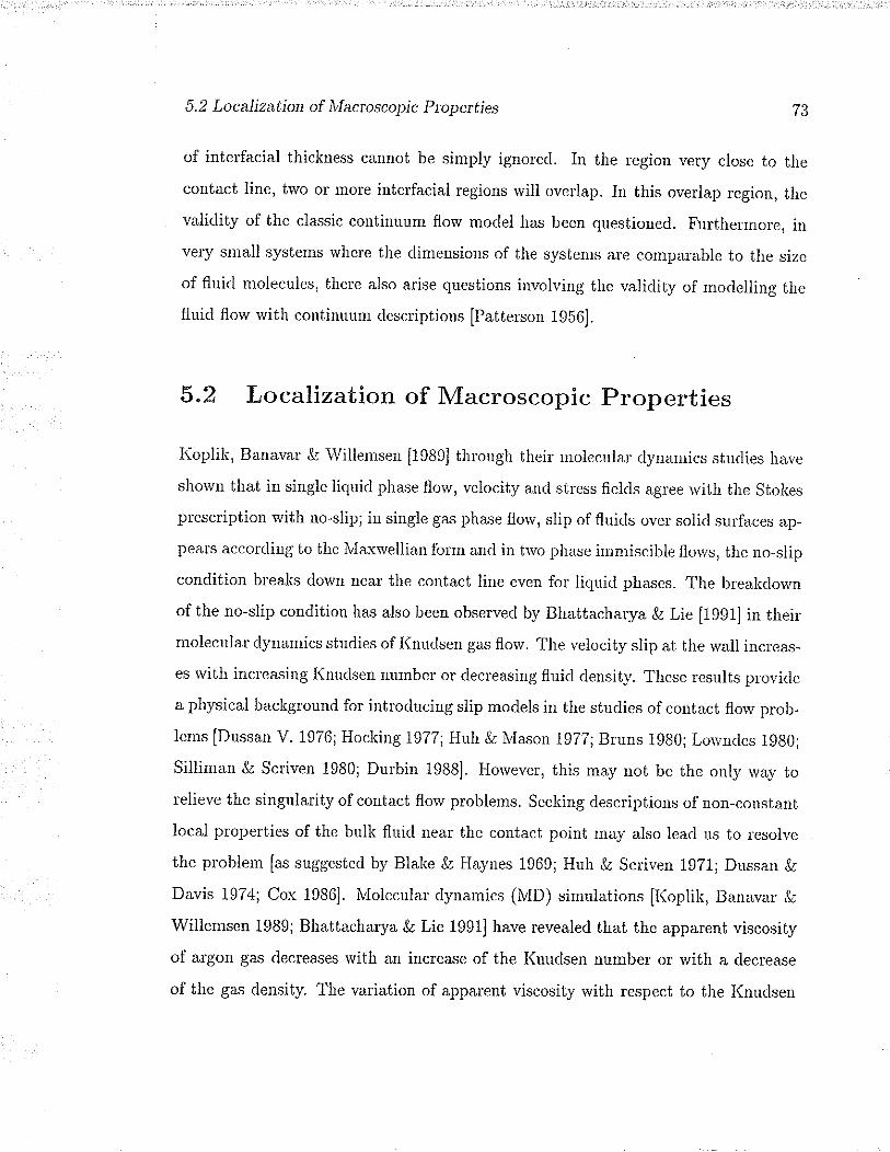
5.2 Localization of N[acroscopic Propeúies
of intelfacial thickness cannot be simply ignolecl. In the region very close to the
contact line, two or moLe intelfacial regions will overlap. In this ovellap regiol, the
validity of the classic continuum flow model has been questioned. Furthermore, in
very small systems whe¡'e the dimensions of the systems ale comparable to the size
of fluid molecules, there also arise questions involving the valiclity of moclelling the
fluicl florv with continuunr descr.iptions [Patterson 1956].
5.2 Localization of Macroscopic Properties
Iioplih, Banavar & lvillemsen [1989] through theil molecrrlar dynamics stlclies have
shown that in single liquid phase flow, velocity and stless fields agree rvith the stohes
prescription with no-slip; in single gas phase florv, slip of fluids over solicl sulfaces ap-
pears accorcling to the ,fax¡vellian form ancl in trvo phase irnmiscible florvs, the ¡o-slip
condition breaks dorvn near tlie contact line even for liquicl phases. The breakclown
of the no-slip condition has also been observecl by Bhattacharya & Lie [1991] in theil
moleculal dynamics studies of l(nudsen gas florv. The velocity slip at the ivall increas-
es with incleasing I(nuclsen mrmber or decreasing fluicl densit-r.'. These results provide
a physical background for intloducing slip moclels in the studies of contact flow plob-
lems [Dussa. V. 1976; Hocking 1977; Huli & ìviason 19ZZ; Bruns 1gB0; Lorvncles 1gg0;
Silliman & Scriven 1980; Durbin 19881. Horvever, this may not be the only rvay to
¡elieve the singularity of contact flow problems, seeking descriptions of non-constant
local properties of the bulk fluicl near the contact point may also leacì us to resolve
the problem [as suggested by Blake & Haynes 1969; Huh & Scriven 1971; Dussan &
Davis 1974; Cox 1986]. fuIolecular dynamics (ìvID) simulations [l(oplik, Bauavar &
Willemsen 1989; Bhattacharya & Lie 1991] have revealed that the appareût viscosity
of argon gas decreases ivith an increase of the l(nuclsen number or with a decrease
of tlie gas clensity. The variation of apparent viscosiiy with respect to the I(nuclse¡r
tó
5.2 Localization of Nlactoscopic Ploperties 74
number obtained by Bhattacharya & Lie [1991] in a micloscopic flow channel of rvall
separation5.64x10-6¿magteesiviihthatexperimentallymeasul.edinamacroscop.
ic florv system of wall sepalation 0'13 crn [Tegan & Springer' 1968]' The l(nudsen
number is the raiio of the mean f::ee path of the gas particle to the charactelistic
length of the flov system The l(nnclsen number can be large if the chalacteristic
Iength of the flow system is sufficiently small' for instance' in the contact line region
of a cylinde:: r:olling over a plane' Tliese results sltow some evicletlce that fluids ltave
localizetl perfolntances of the rnacloscol>ic pr-operties' at least fol tlte gas zr'r:gon ald
presutnablY for all gases'
Tlresitrrationofalicluiclflolvisnroreconrplicatecltlrantlratofagasflorv.Surface-
for.ceapparatuseshavebeenemployecìtomeaslrïetlremicroviscosityoflicluiclsirt
narrorv channels. Askwith eú al [1966] reporled a constant viscosity for hexadecane in
sc¡reeze films clorvn to 9 pnz tliiclilless' hl a stucly of polydimethysiloxanes' Derjaguin
et at. ll975l found no variation from the bulli viscosities in films with tliichness down
lo20n'm'Chan&HoLn[1985]havereachedtheconclusiontlrattheiiquidviscosity
cloes not cleviate measurably from its bulk value in films c{orvn to 50 ¿m thickness'
¿nc1 observecl a small but stearly enhancement of the liqui<l viscosity in tllinner films
of 5 - 50 nm. theenhancement of oii viscosity was also observed by Christenson &
Israelachvili [1987] Horvever, another stucly of viscosity [Christenson' Israelaclivili &
Pashley 19B7] has shorvn that for both hydrocarbon ancl water even in very thin films'
down to the last morecular layer, the fluicl has the bulk viscosity value. contrary to
the above results, experiments on liquid florving in very fine capillaries have shown
trrat the flow cloes uot obey poiseu re's formura [churaev, sobolev & somov 1983]
A11 these res'lts shorv that the beha,vioul of licgirl microviscosities is vely complicatecl
ancl may vary depending on configuration and fluici' It shoul<l be noted tliat in the
measurements of microviscosities with a surface-force apparatus' one measures the
total force on a sphere' exertecl by the liquicls ovel a wicle range of separations' It

5.2 Localization of Nlacroscopic Properties
woulcl be difficult to determined exactly how the effective viscosity deviates from
its bulk value as the sm¿llest region is apploached [Alsten, Glanick & Islaelachvili
1988]. Because the microviscosity of liquids shorvs different per.formance from those
of gases, we will lestlict the present analysis io gâses. However, there is nothing in
the mathematics of the present study which precludes extension to liquids.
Expetiments [l(linlienberg 1941; Schnell 1956; Chulaev, Sobolev & Somov 1983]
have shorvu that the flolv of fluids in very fine tubes (smallel than 1 ¡an in laclius)
is often greaie:: thau that pt'eclictecl by Poiseuille's formula. This can l¡e telnrecl ¿1.
"no¡r-Poiseuille" effect. One of the explanations fol this effect is the slip florv ilteoly,
in rvhich it is assumed that the viscosity of the fluicl is inclepenclent of the cliarnetel
of the tube and the fluid is allorved a finite slippage over the rvall of the tube. Basecl
on the Maxwellian form of slippage [see Jackson 1977]:
75
zru = ¿r?u,on
.,, _r''. AP /, , 4¿s\ 12.LP' - ït,L \'-;/ - 8p"L '
(5.1)
where Az is the slip velocity of a fluid at the wall, u is the velocity vector, n is the
unit outward not'nral of the wall and .Ls is the slip length, the Poiseuille ecluation
rvith the slip collection acquires the follorving form:
(5.2)
whele 1/ is the mean velocity of the fluid flowing through a capillar:y having length
.L and radius r, ¡r is the viscosity of the bulk fluid, AP is the pressure drop and ¡r.
is tlre mean apparent viscosity. Churaev eú ¿1. [i983] found that Ls x 30 nm lor
rvater flowing in hydrophobized quartz capillaries. The non-Poiseuille effect can also
be interpretecl with an apparent viscosity model in rvhich fluid does not slip over a
solid surface. The significance of Equation (refe:ttt) is ihat it gives us a clue as to the
connection between the slippage behaviour and the apparent viscosity perfolmance,
and to the form of the apparent viscosity. That is, the apparent viscosity of a gas

5.2 Localization of lvlacroscopic Ptoperties
can be explessecl as:
p
1+ 4t'-!1'
,, 62. ^P
/. 6¿s\ 62.^p12¡rI\-'6) 12p"L
The valiclity of the apparent viscosity model lies in that it is as porvelful as tlìe slip
moclel in pr-edicting flow behavionl as observecl in expeliments. This will be shorvn
belorv. In the case of florv between parallel plates, the mean velocity and the apparent
viscosity are lelatecl by the follorving ec¡rations:
It)
(5.3)
(51)
(5.5)
ancl
LT
. (J¿.ç
ò
where á is the gap between the two plates. The valiation of the apparent viscosity
given by Ec¡ration (5.5) is shorvn in Figur.e 5.1. The appatent viscosity clecreases
steadily fi onr its bulk value to zero ¿t the contact line rvhere Lsf6 -- oo. In gen-
eral, when the size of the flow channel clecreases to the scale of molecule diameters,
molecules undergo free molecular movement ancl these florvs cannot be studiecl in
the framervork of continuum hydrodynamics. Experinrents have shorvn that in a free
molecule florv, rvhen ihe size of a flow channel diminishes, the viscosity of fluid rvill
diminish also [Chapman & Coivling 1957]. Therefore, rve assume that Equations (5.3)
and (5.5) can be used to the extent that gap size diminishes. The properness of the
apparent viscosity form given by Equation (5.5) was examined by fitting the avail-
able viscosity data given by l(oplik, Banavar'& lVillemsen [1989j and Bhatiacharya
& Lie [1991]. The fitted results ¿re shown in Figules 5.2 and 5.3. The comparisons
a¡e based on the fact that the slip length is proportional to the mean-free path of
the gas molecules and the mean-free path is inversely proportional to the gas density.
The results do show that the variation of apparent viscosity obeys the form given by
Equation (5.5) at least in the region of the available data. The variation of viscosity

5.2 Localization of lv[acroscopic Properties
0 510 15 20
Le6
Figule 5.1: Tìre variation of the apparent viscosity rvith the gap size.
t,

5.2 Localization of fuIacroscopic Pt'operties
o MD sím u loiîon_ Fttt€ d
7B
2.5
2.0
1.5
u.o
1.0
0.5
0.014't210
L/p
Figure 5.2: The fitted ¡esults of l(oplik's apparent viscosity data.
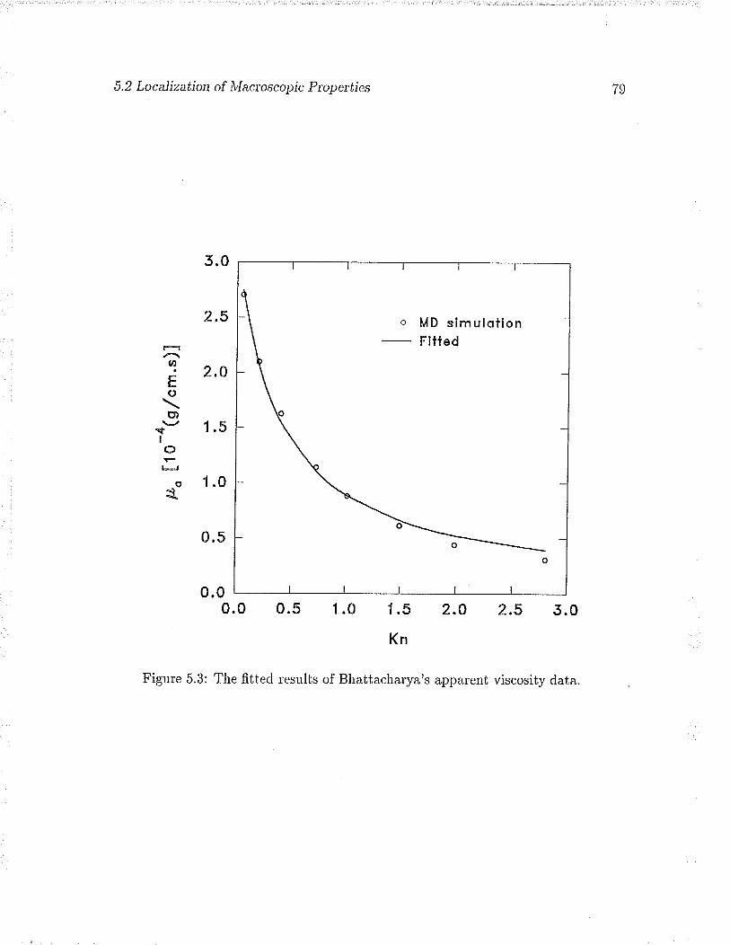
5.2 Localization of lv[acroscopic Ptoperties
5.0
2.5
2.0
1.s
1.0
0,5
0.00.0 0.5 l.s 2.o 2.5 5.0
Kn
Figure 5.3: The fitted results of Bhattacharya's apparent viscosity data.
qEo
u,I
I ot-¡
o-t
1.0

5.2 Localization of Iv[acroscopic Ptopetties
is an indication that the classical contimrum model is breaking down. By consicle::ing
that the viscosity valies, ther-e is no mathematical leason why the continuum moclel
may not be appliecl even rvhen the meau free path goes to i'finity. As fo'the stress
slip moclel, the appalent viscosiiy model may be viervecl as a mathematical technique
used to extencl the applicability of the continuum model to problems where the basic
assumption of a continuum moclel (that the mean free path is much smaller than the
physical clintensiols of the system) does not apply.
It seeurs th¿t uo det¿iled stucly h¿rs l¡een done o¡r the loc¿l ptoperty approtrch.
Therefore, the objective of the plesent study tvas to investigate the possibility of
lesolving the contact florv singulality problem by Lrsing an a,pparelìt viscosity moclel.
The contact floiv problem of a cylincler rolling ovel a plane was solved rvith trvo
continutm models - an appalent viscosity model ancl a stless slip model as clesclibecl
belorv.
The tivo models consicleled in the present studies ar.e
1. Apparent viscosity model (ùIoclel I): The appar.ent viscosity is clepenclent
on the characteristic size of the florv channel as describecl by Equation (b.5).
There is no slip between the fluid and the solid surfaces.
2, Stress slip model (ivfoclel II): The slippage of the fluid over the solid sulfaces
is proportionai to the wall sheal stress as described by Equation (5.1). It is
fu¡ther assumed that in this model the viscosity of the fluid is constant all the
way to the contact line ancl that its value is the same as the bullç viscosity.
80

5.3 Soltttions in the Contact Line Region
Figule 5.4: A schematic diaglam of a cylinder lolling over a plane.
5.3 Solutions in the Contact Line Region
5.3.1- Formulation of the Problem
Let a cylinclel roll at a constant velocity, U, over ¿ hor.izontal plane within a stationary,
infinite fluid. The gravitational folce is assumed to be small and lvill be ignored. The
cylincler and the plane are assumecl to be rigid. The fluid is incompr.essible, and the
rolling velocity of the cylinder is low enough that convection effects can be neglected
(Stokes floiv). Rectangular coordinates are attached to the system in such a rvay that
theil origins are alrvays located at the contact point and the c axis lies on the surface
of the plane as shorvn in Figule 5.4. In this coordinate system, the cylincler surface
has a constant circulatíon speed [/, and the plane and the fluid at inûnity move in
the ¿ direction at the same speed as the circumference of the cylinder.
In the contact line region, 0 S s < ,. (Ls << co 11 a), the gap between the plate
BI

ö.3.2 Soltttions ¿¡rJ Dlscussioris g2
and the cylinder', ó(ø), is very small so that the florv is governed by the followilg
dimensiouless lubrication equation:
ô2u dn
ctu. d,x)
The chalacteristic quantities used to make the above equations dimensionless are:
¿ for tlre length, U for the velocity, p fol the viscosity ancl pUf a for the stress or.
plessttl:e. Tlte collespottcling boundaly conclitiorrs fol each of tlie moclels ale listecl
l¡eloiv:
(5.6)
The gap size can be expr-essed as:
t
ölx) - -.The appalent viscosities of the trvo models are:
lul I lvlodeli] [ ìvlodeliI]dìr
A=rJ z=l e;-=u-1quou
U=ò\x) u-l ,T,=,-,,
, ólrr')t"' - 5ç4¡ç'..II
- t
1.
2.
(5.7)
(5.8)
(5.e)
(5.10)
(5.11)
wlrere e = Ls fa. Tbe supelscripts (or subscripts) I and II clenote lvfodel I ancl jvlodel
II respectively.
5,3.2 Solutions and Discussions
The general solution of Equation (5.6) is
,"" =t #a2 + A(r)y + B(r). (5.12)

5.3.2 Solutions ancl Discussio¡¡s
where A(ø) a'd B(ø) are unknolvn firnctions to be dete::mined fi'om the bouncla'y
conditions. ,A,pplying the boundary conditions given by Equations (5.7) ancl (b.g) to
Equation (5.12), the functions A(c) and B(o) for each of the moclels can be deter.-
minecl and ¿r'e listecl l¡elow:
Tlre pressr.rle graclient, dpf dx, can be cletelminecl by the nean velocity conclition
at any position of c:
v -| 1.0,1.,s¡as -o (5.15)
This is because the florv channel is closecl at the contact line ancl therefore ¡lo fluicl
penetlates through it. The evaluated pressure gradients ar.e:
dpt dpl 72 48
dx tlx ô(ó + 6€) Ì2(Ì2 + t2€)'
Substituting Ec¡rations (5.13), (5.14) and (5.16) into Ecluarion (5.12), one obtains
the velocity distributions:
IFunction] [Uoclel I ] [lvloctel ]I l.,ltz) - -!þln -t-'lptt ,2h- 2 tl:t -
B(.u) = pt" t,'.'-i'\t
w = 7-riþ-i), o<s<6
1L¡¡ : t-åû[#('-Ð-;], o<y<á
(5.13)
(5.14)
(5.16)
(5.17)
(5.18)
Therefore, at any r location, the profile of tlte z component of the velocity is par.abolic
for both models. The distributions of the velocity component z on the ff.at surface
(y = 0) alr¿ in the middle of the gap (A - 612) are shown in Figure 5.5. The velocity
u on the cylinder surface is identical to that on the flat surface. It can be seen that
in lvlodel I the velocity u has a value of one on the flat surface and minus a half in
ihe middle of the gap even at the contact line. Therefore, in lvlodel I, the velocity

5.3.2 Solutions a¡d Disc¿¡ssio¡s 84
1.5
1.0
0.5
0.0
-u.b
- 1.00.000 0.000
1)
Figui'e 5.5: The distlibutions of velocity z on the flat sulface and in the miclclle of
the gap for the appar-ent viscosity and the stress slip moclels.
0.010

5.3.2 Solutions a¡ci Discussions
is multiple-valued and the velocity gradient is singulal at the contact line. It rvill be
shown later that this singularity of velocity gradient will not give rise to a singular
stress in the result for the apparent viscosity model. In ìVloclel Ii, the velocities ,¿¿
o¡r the flat sulface and in the nliddle of the gap meet at the contact, therefore, the
velocity at the contact line is unique.
Frour Ðqr.rations (5.17) ancl (5.18) the shear st¡esses ?l(c) on the flat surface can
be evalrratecl as:
85
.rrt,.\ - ,,rattrl - 12rs \'!./ - f" Aulo=o- - r\lk
r!'@) : ,'"'ff|,=,= -"T*(5. re)
(5.20)
For the two models, the wall shear-stress distlibutions are identical aucl the stresses
are boundecl wiih the maximnm value of (-1le) locatecl at the contact line. The wali
shear stress clistribution is shorvn in Figure 5.6 for e = 10-8. Tlie viscous nolmal
stress, 7,., on the plate can be calculated as:
(5.21)
rilp¡ - ztttolttl --2,/t4l!l - 48¿
ay lr=o - 'zt+'-0r lc=o - -ê (Ì2 + tky (5'22)
Therefore, the wall normal stresses of the tivo moclels rliffer fi'om each other'. In
lvlodel I, the normal stress is identically zero; but in 4ode1 II it is not (see Figule 5.2).
Fortunately, the normal stress of lvloclel II is of the or.der e which is much smaller than
that of the shear stress. The m¿ximum normal stless is locatecl at ¿ = 2 eå with ¿
value -$e-å and the maximu¡n shear stless is locatecl at ¿ : 0 with a value -e-1.The ratio of the m¿l,ximum shear stress to the maximum normal stress is of the ol'cler
eå. For example, if e = 10-s, the maximum normal and shear stresses are about 10a
and 108, respectively, and the stress ratio is thelefore 10-a.
Frorn Equation (5.16), one can note that the pressure evaluated for both models
r!@) - zu,"afil,=,= -2p,"#1,_,= o

5.3.2 Solutiotts and Discussions
0
-0.1
-0.2
-0.3
-0.4
7l (xi08) -0.5
-0.6
-0.7
-0.8
-0.9
-1
e : 10-8
B6
0.008
Figure 5.6: The distribution of the shear stress on the flat surface for tlie apparent
viscosity model âncl the stress slip models.
0.01
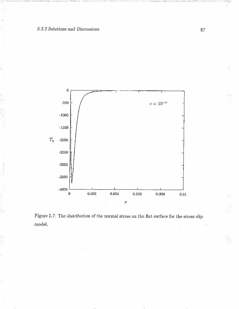
5. 3. 2 S olu tions a¡rcl Disc¿rssions
¿ = 10-s
0 0.002 0.004 0.006 0.008 0.01
Figure 5.7: The distribution of the normal stress on the flat surface for the str.ess slip
model.
0
-500
-1000
-1500
T" -2000
-2500
-3000
-3500
-4000

5.3.2 Solutions a¡¡d Discussiors
is singular at the contact point; that is,
p(r) - O(t:-t) as ø -r Q, (5.23)
ivhich is not integlable. If Equation (5.23) is integrate<ì with respect to ¿ to obtaiu
the vertical folce distribution, then the folce is still logarithamically singular at the
contact point. However', this does not pose a problem from the pliysical point of
vierv. First of all, because it has been assumecl that both the solicls (the cylindel
ancl the plane) ale rigicl, the solids cau sustaiu the singrrlal pressure. Fulthcl¡ror-e,
to cletelmine the movement of the cylinder, it is the r-esultaut force and the moment
that ale neecled; thzrt is, the lesultant fo::ces in both horizontal ancl veltical clilections
ancl the resultant moment rvith respect to the contact point.
If the plessr.rre is integraiecl on the symmetlic parts of the cylinrlel surface in the
contact lire legion definecl lry { * < l0l < 0o i, (o is an arbitrar.ily' chosen positive
small quaniity, d is clefinecl as the angle from the contact point as shown in Figure 5.4
and d6 is withi¡r the contact line region), then the horizontal for.ce F¿(d¡;a), the
vertical force F,(?s; a) ancl the moment ù1(d6;a) rvill be
F¡(ts;a) = l'"ln{e)"inllaffi+ l-}tr{e)"t el.oo
- lu" lr{Ð"inglattl - lt" lo{-.r)"rnrlour,
F,(ls; a) - l^ b{Ð "o"0lart| + I_}lnr/l "."e1.ae
- l^ lr{e) "o"rlarlt + lt" ln{-Ð "o"el n,te
(5.24)
(5.25)
ancl
l" @ "io 0)l nQ) cos 0 I artr + l-
" @ sin 0)lp(0) cos 0 I adr
t0' @ "tn 0)l n@) cos 0 I attg - l% {o "io
o)ln( -9) cos d I actt. (5.26)
lvI(0n;a) -

5.3.2 Soltttions and Discussions
Because the pressr.r::e clistlibution p(d) is antisymmetr.ic about á, the for.ces arrcl
moment acting on the defined cylincler sulface will be
F6(o¡; a) = z l^0" ln{e) "io
el oae,
F"(06 a) : A
ancl
Ã,1 (06; a) - Z [0" k "r¡ 0)[ p(0) cos 0 ] att\.' J^ '
Takirrg a limitiug plocess to inclucle the conttrct poiut, rve carr ol¡taiu
89
the
ancl
Fn(00) : lnX Fr,(do;a) - O(1),
¡,(áo)=!g3r,(áo;")-o
tul(0s) : lrlr¿,v¡(Bo'
CI) = o(1).
(5.27)
(5.28)
(5.2e)
(5.30)
(5.31)
(5.32)
Because the viscous normal and shear stresses are non-singular on the cylincler sur.-
face, their lesuitant fo¡ces and mornent are ûnite. Consequently, the total resultant
forces ancl moment acting on the cylinder are well clefined. Therefore, in spite of the
non-integlable plessule distribution, the solutions fol the present problem are stillphysically acceptable.
The comparison of the results shorvs the following points:
i. With Nlodel I (the apparent viscosity model) the velocity solution describes the
"rolling-type" motion offluid alound the contact line as observecl in experiments
fDussan V. & Davis 1974], but rvith ùIoclel II (the stless slip model) the velocity
of fluicl at the contact line is zelo so that the fluid particles initially on the
contact line will never move arvay from it;
2. ïViih the two models, identical solutions are obtained for the shear stress and
the pressure clistlibutions;

5.4 Remults g0
3. lvhile a zero normal stress is preclicied with lvlodel I, the one rvith fuIodel II is
nolzeÌo. Horvever, the order. of the normal stress is much lowe¡ than that of
the shear stress so that ii can be neglected;
4. Although the solution of pressure is singular, it is still physically acceptable
Hence, rve can conclucle that the stless slip and the appalent viscosity approaches ale
equivalent in solving the contact florv ploblera of a cylincler lolling ovel a fla,t plane.
5.4 Remarks
The equivalence of the str-ess slip model ancl the appatent model has a profouncl practi-
cal application. Although mosi of the computational fluid dynamics (CFD) softrvales
cannot handle slip bounclaly conclitions as encou¡rtelecl in contact floiv problerns (par-
ticularly commercially available simulators), they usually have the ability to <leal rvith
variable physical properties (such as densiiy, viscosity etc.). Ther.efore, by exploiting
the equivalence conclition, existing Ct'D ploglams may be utilized to solve contact
flow problems. A shift of the plesent finite element simulation pÌogram described in
Chapter 4 fi'om the stress slip model to the apparent viscosity model can be easily
irnplemented.
Chapter 6
A Grating Skrearing Interference
Method
The expelimental technique plesentecl in this chaptel is able io mahe direct measur:e-
ments of the contact angìe and the profile of a meniscus in a planar. capillar.y cell.
Deflection of light at the eclge of a liquid wedge is used to measure a contact angle
and shearing interfe¡ence of light through a gratilg is used to reconstnrct the profile
of the meniscus.
In Section 6.1, the theory of the experimental method is plesentecl. fulore specif-
ically, formulae of lay optics for calculating deflection ancl path length of liglit are
described in Section 6.1.1. Equations of the shealing interference are clerived in Sec-
tion 6.1.2. Basecl on the equations derived in Sections 6.1.1 and 6.1.2, iterative algo-
rithms, rvhich calculate the contact angle ancl Leconstruct the profile of the meniscns,
ale presented in Section 6.1.3. Then the convergence behavioul.of the algorithms is
tested numerically (Section 6.2) ancl experimentally (Section 6.3). In Section 6.4, a
summary about the experimental technique is presented.

6.1 Laser Beam Deflection and SJrearing Intefference
6.1 Laser Beam Deflection and Shearing fnterfer-
ence
lvhen a ray of light passes fiom one medium to another, the'e is a change of phase as
rvell as a change in direction (i.e. deflection) clue to the variation of refi.active indcx
at the intelface. In the measulernent of apparent contact angles b¡, the capillaly
tube urethocl, tlie effect of cleflection is ploblematic. Some colrections, eithel. iuclex
ulatching ol theoletical ruoclificzrtion, h¿ve to be rnacle to obtaiu r:reaningful r.esrrlts
[Hoffman, i975]. ln the palallel cell expeliments perfolurecl by Ngan ¿n<l Dussan V.
[1982, 1989], the effect of cleflection ilid not shoiv up because nolmal illu¡rin¿tio¡ rvas
used. In the plesent study, the same expelimental configurations as used by Ngan ancl
Dussan v. was employed but with a clifference in introclrrcing an oblicßre illumination
to the cells. It rvill be shorvn in the next section that the cleflection of light czrn be
pulposely used to measure contact angles and shapes of menisci.
6.L.L Calculation of Deflection Using Ray Optics
Figure 6.1 is a schematic diagram showing the deflection of a ray of light traveling
through a capillary cell. A slot is folmed by trvo glass slicles sepalated by a clistance
2a. 'Ihe slot is filled rvith two immiscible fluids. A meniscus (fluid/fluicl ilterface) is
formed between the two fluicls. As shown in this diagram, we assume that the wetting
phase is ¿t the bottom ancl the non-rvetting phase on the top. A coorciinate system
is shown in the ûgure. The origin of the coorclinate system is located on the contact
line. The vertical coordinate is clenoted by y at an input plane and Y at an ontpnt
plane, respectively. A ray of light goes into the cell at the point A, passes through the
points B, C,, D a.td comes out of the cell at the point E, then continues its journey
and finally reaches the point F on the observation plane located at o = rp. The
92

6.1.1 Ca.lculation of Deflection Using Ray Optics ôa
G¡ating
\I
plane Y
--rL(Y)
FlContact
Figule 6.1: A schematic diaglam of tlie cleflection of a ray thr.ough a cell.
dashed lines (A- B - Dt - E' - F') shorv the imaginaly path of the ray through the
cell that woulcl lesult if the meniscus were not there. The differ.ence of the cleflection
with ancl without the meniscus, A (we will refel to this variable as the deflection
function hereafter), is a function of the profile of the meniscus. By recording ancl
analyzing A, we may reconstruct the contact angle and the profile of the meniscus.
The trajectory of the ray can be traced by the formulae of ray optics:
. /dh\û _ ran_,
fd¿J ,
lT \tan? = - tan (7 - a,) ,
I*=Ur-0,, - nL-t
sllÌ -/; = sln l^- '
Iine
(6.1)
(6.2)
(6.3)
(6.4)

6.1.1 Calculation of Defrection Using Ray Optics
Figure 6.2: The notations of the lay tracing folmula.
94
ancl
Ui=Uu+IL-Ik
U*+t = UL
(6.5)
(6.6)
lvhele n¡ is the refractive indices of the nreclia, ir,(ø) is the function of the meniscus
profile, f is the incident angle to the interface, U is the angle of the light relaiive
to the horizontal axis, d is the angle between the meniscus and the solid surface,
a is the slope angle of the meniscus to the horizontal axis, subscript fr denotes the
quantities at the ,kth interface and the unprimed ancl the primed quantities represent
those before and after the interface, respectively. Some of these notations ale shorvn
in Figule 6.2. The sign conventions fol the angles used in the present ivork are similar
to those used in most moclern ray-trace texts (see O'Shea, 1985):
1. The angle of a ray with respect to a normal to a surface is positi,ue il a clocl;wise
rotation of the ray brings it parallel to the normal; it is negative if it takes a
counterclockwise rotation to do the same thing.

6.1,1 Calculation of Deflection Using Ray Optics
2. The same is true for the slope angle which is tlie angle betrveen a ray ancl the
optic (horizontal) axis. A clockwise rotation of a ray thlough an angle to bring
it parallel to the optic axis is posiiive; a counterclockwise lotation of a lay
thlough the slope angle is negative.
The cleflection function A(Y) can be expressecl as:
TT_I
A(Y) : Ð (,.u*, - r¡)tanUi - (1i - y),
'rvhele .¿1,1 is the numl¡er of intelfaces ou the path of tlie light, c¡ is the coolclin¿te
of the Àth inte::face, y is the coorclinate of tlie inciclent light (point B) aucl ),i¡ is
the cooldinate of the imagina::y point .t'l. The cleflection of liglrt thlough the cell
is a nonlinear transform of å(c) defined by Equation (6.2). ft is referred to as the
"deflection transfolm" and cienoted bv D:
A(Y)- D[rz(c)]. (6.8)
Similarly, a function of optical path length difference, l(Y), can be definecl as:
ltÍ -tf(Y) : t nr (¿*+r - x¡)l coslJ'¡ - P¡, (6.e)
rvhele P¡ is the optical path length of a ray traveling from the point .A to the point
.F'/. Ecluation (6.9) is referrecl to as the "path length transform,' of the meniscus ancl
denoted by P:
r(r) - P[å(z)]. (6.10)
Figure 6.3 shows a computer simulated deflection patter.n through a test cell. This
simulation Leveals sorne major features utilized in the plesent approach. Firsi, the
introduction of an oblique illumination results in a deflection at the first contact line.
The magnitude of the deflection is proportional to the contact angle. From this fi¡st
cleflection, tìre contact angle can be evaluated. A similar cleflection takes place at the
95
(6.7)

966.1.1 C
alculation of Defrection U
sing Ray O
ptics
-,'ìC)
boo
'oې.oq)
oõ(,)
áp.
o4(oouho

6.1.2 Tlte Sltearing Intetference with a Grating
seconcl contact line. Seconcl, the exit angles of the rays fi'om the cell span a quite
large range. Consequently, it is necessaly to recold the deflection pattern at a plane
very close to the exit plane of the cell. Last, as mentioned above, a ray which goes
into the cell at a cliffelent position is subject to a cliffele¡rt magnitude of cleflection
ancl the magnitude of deflection is directly lelated to the shape of a meniscus. Thus,
knowing whele the rays go in and come out of the cell, we can reconstruct the shape
of the neniscus. This can be ¿rchieved by placing a Ronchi r.uling, which cousists of
periodiczrl, equal rviclth, tlarrspzrLeut aud o1;zrque lines, in I'r.ont of the cell to e¡co{e
tlie light. As an apploxirnatiou, the fi.inge patter.n founecl at an oltselvation plane
can be vielecl as the geometrical plojection of the Ronchi r.uling cleformecl by the
meniscns. trVe rvill r'efel to this p¿tteÈn, her.eafter', as the "projection". Physically,
the glating put in the path of light plays the role of a beam splitter (or a shearing
dcvice) [Yoliozelii & Suzulti, 1971]. An interfer.ence intelpletation rvill pr.ovicle a mor.e
accuLate result as will be shorvn belorv,
6.1.2 The Shearing fnterference with a Grating
As a collintatecl lasel' beam illuminates a transparent grating, it is clecomposed into
several diffracted rvaves (or components). The propagation directions of the cornpo-
nents satisfy the following grating diffr'action equation [Longhurst, 1967]:
d(sinu'@)-sint/) -m), (6.11)
wlrere rl is the grating constant (i.e. pitch of the grating), IJ and IJ' are the inciclent
ancl exit angles of light with respect to the nolmal of grating, nz is the order. of light
componeuts ¿nd À is the rvavelength. These waves are coherent and it is possible
to ploduce the fourier image (or replica) of the grating as the result of interfelence
betrveen them at the distance nû f À f.rom the grating, where n is an integer. When
a phase object is placed betwee¡r the grating and its fourier image, the shape of the
s7

6.1.2 TIte Shearing Interfet'ence with a Grating
diffi'acted rvave will be changecl and thelefore the fourier image will be clistolte<I. This
distortion can be recolded ancl analyzed to reveal information about the phase object.
The optical alrangement and the olthogonal coordinate system were shorv¡r in
Figule 6.1. By assuming that the z axis is taken in the direction of the slit of the
g'ating, the problem can be expressed rvith trvo-dimensional notation. The ¡u ¿xis is
taken as that ofihe optical axis. Becanse the infolmation abont the object is obtainecl
as the clistottio¡r of the forttiet image, tltete is no neecl to obselve the fine st¡rctur.e
of the foLuiel initrge. In orcler to explzrin the pliucil>le of this nrethoct, it is clough to
use only the zetotli ald the positive first orclel cliffraction tvaves.
Tlie cor.uplex arnplitude clescliption of a plane wave fielcl pr.opagating in a z-y
plane can be explessed as [Goodman, 1968]:
tr,(x,y):;r uxpþ{ Ø¡ + t,u)1, (6.t2)
where A is the aurplitucle of the wave fiout, j is the virtual unit number. ancl .y, ancl
?s ale the clilectional cosines of the propagation vector. with respect to the ø and y
a-xes, respectively. If the distortion of the mth cliffr.action orcler rvave on the observing
plane P(z = øp) is given by 1",(Y) (Equation 6.9), the optical disturbance r(Y) on
the plane P may be expressed as:
u(Y) - ,,to "*p{jf l¡,6xo*1usY+r6(y)l}
+Ar exp{j! f¡,øo i 11Y+ rr(Y) I },
¡vhele the subscripts 0 and 1 denote quantities of the zeloth o¡cler ancl the fir'st order',
respectively. Accorcling to the grating diffraction equation (6.t1) and assuming that
the diff¡action angle is small, we can obtain the follorving relationships between the
directional cosines of the zeroth orcler and the first o¡der:
9B
À1ut='lso*¿
( 6.13)
(6.14)

6.1.2 The Slrear.irig lntefference wi t a Gtating
and
^ / À\
'Y¿t="t¡:o- a\tto+-1.The intensity distribution 1(Y) on the plane P is
99
(6.15)
(6.16)
I(Y) - u(Y)u.(Y)
- A3 + A1 + 2AoA,*. {i[å y +11(y) - ro(y)
-å (".*) '"1ÌTlte astel'isli ou ¿ cleuotes its coujugate fturction. As Y valies along its nxis, the
intensity of the optical fielcl varies peliodically ancl lesults in a series of maxima
ancl minima (i.e. fi'inges). The fir'st ancl last telms in the v¿r.iable of the cosine
function replesent the undistorted structure of the gr.ating ancl they ale not lelatecl
to any information of the meniscus. The difference of the tivo path length firnctions,
lr()') - l6(Y), replesents the distortion of the fi.inge patteln rvith respect to the
original one. Thelefore, a fringe distortion function Ã1f¡ on the plane P can l¡e
defined as:
Ã(v)-lt.,l"l-ro(y)¡. (6.17)
This is refellecl to as the "shealing transform" of the meniscus ancl clenotecl by S:
^(Y)- s[å(r')]. (6.18)
Generally speaking, the deflection function is clifferent from the fringe clistor.tiorr
function. The difference betrveen them can be expressed as:
ó(y)-^(y)-^(y) (6.1e)
If the distortion of the fringe pattern is sufficiently small, the fringe distortion function
Ã1f; *itt essentially approach to the cìeflection function A(Y) (i.e. ó(y) --+ 0).
Therefore, A(Y) is an approximate function of Â(y). Because both Â(}/) ana Ã1V¡
are nonlinear transforms of å(e), iterative schemes for approximate inversion of the
tlansforms D and S are requirecl.

6.1.3 Iterative Reconstrttction of a fuIenisctts
6.1.3 lterative Reconstruction of a Meniscus
Inversion of S [lz(e)]
The iterative scheme presentecl beloiv is sirnilar to the one r¡sed by cha & vest [1gg1],
but some moclifications have been macle to accommodate the present ploblern. The
ain of the itelative scheme is to fincì the function ó()') basecl on successive estimation
of the <levi¿rtion function defi¡lecl bv
(6.r0)
rvhele the subsclipts e ancl o replesent "estinatecl" ancl "oliginal", r.espectively.
The iterative algorithm is as follorvs:
IVIalie an initial estim¿te of tlle function á¡(Y), rvhere I - 0.
Calculate the colresponcling estimate of the deflection transform
^,(v)- Ã,_,(y) - ó;_r(Y) (6.21)
3. Approximately reconstruct the meniscus by using the itelative inverse cleflection
transformation (as clescribed belorv):
år(z) : O-t¡¿¡-11'¡1, (6.22)
4. Using the computational ray tracing folmulae given in Section 2,1, calculate the
optical path length functions:
f-(l') - Plht(y);u't"')1, m=0,7.
5. Calcul¿te a new estimate of the shearing tlansformation:
(6.23)
100
i.
2.
Ã,1r¡ - s[å;(ø)] - | t.,l"l - ro(v)1. (6.24)

6.1.3 IteLative Reconstrttction of ¿ À.fe¡lscus
6. Calculate an estimate of the deviation function:
r;(Y)=Ã'(Y)-Ã,(Y)
7. C¿lculate a nerv estimate of the funciion á()/):
101
(6.25)
(6.26)órff) - á'-r(Y) 4- r¡(Y).
8. Retnln to step (2) ¿ncl coltimte the itelation plocerlule Lrntil the magnitucle of
r¡()") is mininizerl ol smallel than some plecleterlrinccl value.
Inversion of D [å(ø)]
To develop a¡r iterative algorithrn for the inverse deflection tlatsfo::m lequirecl in
Step (3) of the invelsion algorithm of S [/r.(ø)], some assnmptions ar.e r.eqnir.ecl. It is
assunrecl that the shape of the r¡reniscus close to the contact li¡re valies monotouicall¡,
with the clistance to the contact line. Therefore an incident ray rvill intersect the left
half of the meniscus only once. Furthermore, it is assumed that the meniscus ancl the
solicl surface close to the contact line form a liquicl rveclge with the contact angle as
the rvedge angle. Some lesearcheLs have fornd that there exists a very thin precur.sor.
film ( < 50Å) ahead of the expedmentally measurable contact line for some material
systens [Bascom, Cottington & Singleterry 1964]. Horvevet in expeliments of polynter.
melting on planar surfaces, there was no precursoL film detected [Schonhorn, Flisch
& I(rvei 1966]. Fultlier', lvlarsh, Garoff & Dussan V. [1993] did not detect a thin film
in front of the bulk meniscus. Because the scale of the profile of the meniscus to be
measurecl is of an olclel much higher than that of the precursor if it should eúst, the
intlocluction of the seconcl assumption is not expected to result in noticeable erlols
in the lesults.
Based on the above-mentioned two assumptions, the iterative procedure is as
folìows:
6,1.3 Iterative Reconsttuction of a lvlenisctts 102
1. Calcnlate the range of angle (.-,n ( a 1 a^.,) in which the slope angle of the
meniscus can be found. The lower limii is zero contact angle (i.e. o_i" = -ä)and the upper lirnit is t'estlicted by the total reflection condition of rays on a
rnettiscus:
","". = -i+ þio-' (#'r *) *.''-' (o) ] , g.2T)
where the snbscripts g, o ancl ¿ denote the quantities fo:: glass, oil ancl air,
lespectively.
For point j (-l - 1 fol the point on the contact line), assunre a tr.ial slope augle
aj and calculate the intersection point of the ray of light witlì the meniscus
(r¡,y;) by the follorving ec¡rations:
@¡-t - ¡:¡q tand¡) - (n - t tanU'r)lau ui - tan aj
4 -l tanUt, (", - €),
(6.28)
(6.2e)
(6.30)
wlrere õ¡ - (a¡-r + a¡)12, tan U{ is the slope of the light ray inter.secting the
intelface and ({, a) is the location of the light on the ûrst solid/fluid interface
(see Figure 6.4 for the notation).
Trace the path of light to the recording plane and calculate the cleflection of the
light, A(Y¡), using Equation (6.7).
Calculate the following relative deviation:
a(yr) - a,(v,)'= ---^Jyi) -,
rvhere A;(Y) is given by Equation (6.21).
5, If the relative deviation is minimized or smaller than a predetermined value,
proceed to the next point. Otherwise, returtr to Step (2).

6,1.3 lterative Reconstruction of a Àfeirisc¿ls
Figure 6.4: A schematic diagram of the deflection of a ray through a cell.
,/ '/
,/ (f, n)
(x¡,r¡)
(x¡- 1 , r¡-r)
tI
Foa
Meniscus
SoLid surface

6.2 Numetical Tests
The contact angle OD can be completely cleterminecl
transfoi-m as given above; that is,
104
in the invetse cleflectiou
op - (f,+ a). (6.31)
Hence, if the contact angle only is of interest, one can recorcl a cleflection pattei.n
with no glating and then apply the above mentionecl inverse deflection transfolm to
calculate the corrtact arrgle.
6.2 Numerical Tests
A computer plog¡:am basecl on the algorithm presentecl in the above subsection was
rvritten. The behaviour of the algorithm rvas stuclied by applying it to clata generatecl
by numerictrl sirnulation of shealing experiments. Discrete values of the shearing
tlansfor¡n wele generatecl by computational ray tlacing through test cells lvith the
menisci expressecl in analytical forms. The trvo menisci usecl were circular profiles
with contact angles of 20" and 40". The parametels of the material system simulatecl
are listed ir Table 6.1.
Figures 6.5 and 6.6 show the results of reconstructing the slope angles of static
menisci with contact angles 20' and 40' respeciively. The deviation between the
results of projection (from the first itelation of the inversion of D [å(ø)]) ancl those of
shearing intelference is appreciable. Therefore, to achieve an accur¿te measurement
of the meniscus, the shearing interfelence approach must be usecl. But the apploach
of projection can still be well used to obtain approxìmate results. Figures 6.7 and 6.8
show the reduction of m¿ximum ancl average errors by the itelative procedure.
This technique was further tested experimentally by reconstructing static menisci.
The results will be presented in the next chapter.

6.2 Numeúcal Tests
0.00 o.02 0.04 0.060.6o.4(È o.2
-0.2-o,4
58
56
34
321R50!
o28
26
24
22
200.00 o.o2 0.04 0.0 6 0.08
x (mm)
Figure 6.5: The numerical reconstruction of static menisci with a contact angle of
20'.
0.08
l;";å;;;ii:"i" i
Seeei:!:3¡i;; iit
r::!!îoî-îvv.''vYY g Ë ; q- -i- -'e o tr.Þ..d..E..o..tr..É...9...''"...:..i...................1........ .
::i!

6.2 Numerical Tests
0.00 a,o2 0.04 0.06 0.08 0.10 0.12 0.14t.o1.2
9 0.80.40.0
-0,4
56
54
52
Ëô 50o)ga4E
46
44
42
400.00 0.02 0.04 0.06 0.08 0.1 0 0.12 0.14
x (mm)
Figure 6.6: The nume¡ical reconstruction of static menisci with a contact angle of
40..
i i:*;i;;;i-i"":i:"eti'...'-i-.=^o.ooie.g9.:.::. ...i .f .. .. i..seegiiii;ri;; ÍÍ: Í ; ; :; Í ÍJ J Í;;"," * o i

6.2 Numerical Tests
Table 6.1: Parameters of the mate¡ial system simulatecl
0 2 4 6 I lO 12 14 16
NUMBERS OF ITERATIONS
Figure 6.7: The e¡ror reduction of the reconstruction for a meniscus of O, = 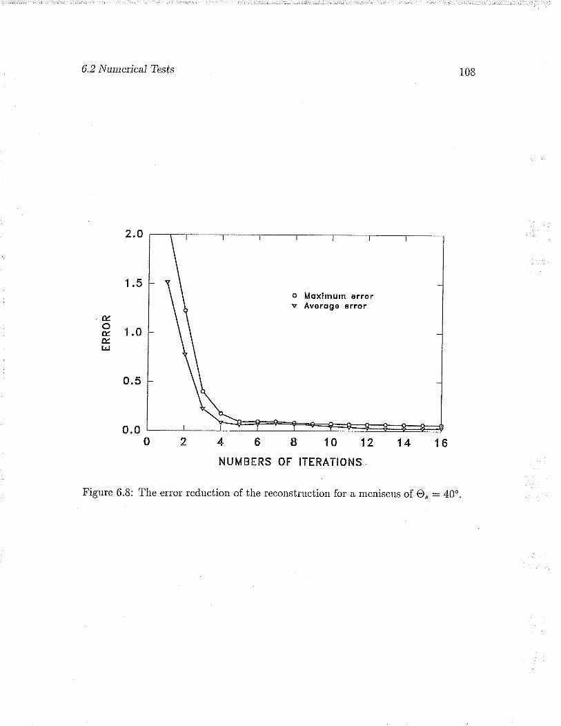
6.2 Numeúcal Tests
2.O
1.5
e.
P r.oÉ.t¡J
0.5
0.0o 2 4 6 I lO 12 14 16
NUMBERS OF ITERATIONS
Figure 6.8: The error reduction of the reconstruction fo¡ a meniscus of O, - 40..
108
6.3 Summaty
6.3 Summary
This chapter shows that the grating shearing ilterference rnethod presentecì is able to
make an accurate measurement of contact angle as rvell as the plofile of a meniscus.
The numerical tests shorv that the iteraiive schemes usecl in the inverse transfonns of
the deflection function and the shearing function ar.e very effective. trVith this exper-
imental method, the contact angle can be measulecl clilectly. The irnplementatio¡l of
ex¡relimeuts rvill be plesented in the next chaptel.
109

Chapter 7
Experimentation
Basecl on the grating shearing intelference methocl presented in the plevious chapter,
the implementation of experiments to make measuLements of clynamic contact angles
and the plofiles of menisci is clesclibecl in detail in this chaptet.
7.L Experimental Setup
The layout of the experimental setup is shorvn schematically in Figure 7.1, It com-
prises th.ee major palts: (i) a lase. aud light alignme't system to provide high quality
monochromatic ancl parallel liglit illumination to a test cell; (ii) a test cell holclel to
secure and seal the test cell in place and a photographic film holcler to position a film
at a fixed distance from the cell; ancl (iii) a sylinge pump to inject fluid into the cell.
An argon laser (Spectra-Physics ìvlodel 165), tuned to output light at a rvavelength
of 488.0 nrn, is used. The thin laser beam is expanded and collimated to a beam of
40 mm diameter and then directed to the capillary cell by two front-su¡face reflection
flat mirrors. The incident angle of the light to the test cell can be acljusted by rotating
the inclinecl angles ofthe mirrors. In ¿ll the experiments clescribed helein, the incident
110

Reflection Mirro¡
PhotograpiricFilm llolder
Figure 7.1: The layout of the experimentâl setup.
Argon Laser
Stepping Motor
It5€oIo
SD
aâ(D
Pulse Counterand Timer
Stepping MotorController

7.1 Expetimental Setup
RecordingPlane
GratinB... I
\lI
First contact line I
Inciden tLight Rays
Figure 7.2: A schematic diagram of the cell arl.angement and the foul specific rays
passing through ihe cell.
angle lvas 32.19". The parallelness of the light rvas checked, by using an optical flat
(ùfelles Griot, Cat.No. 02FQD007, flatness 1/20,\, diameter 40 mm,), to be within
| ftinge f 40mrn.
Figure 7.2(a) is a schematic diagram of the test cell. Four. specific lays (,L1,
L2, Ls and tra) ale shorvn in the figure. The path of Ray 1 is through the cell just
above the ûrst contact line; Ray 2 passes just below the meniscus; Ray 3 passes just
over the edge of the knife and Ray 4 passes throngh the contact line. The position
of the knife edge was specially arranged to ensure that Ray 3 is above Ray 4 on the
recording plane. A tr¿nsmission grating was placed just in front of the cell. The
density ofthe grating (Ronchi ruling) was 5000 lines per inch. The significance ofthe
rays are that (i) the clistance betrveen Lt atd Lz c¿n be used to calculate Hansen's
11.2
GlassSlid e
L2
L3
La
t:f.nife edgeljght block
.//

7.1 Experintental Setnp
ffi..{#Ê:fç,
Figure 7.3: A typical picture taken in experiments. The corresponcling positions of
the four specific rays are shown,
L7
L2
Lj

7.1 Expeñtnental Setup
apperent contact angle defined by Ec¡uation (2.18) (a worliing formula is clerivecl in
Appendix D); and (ii) the one between L1 and La is dir.ectly related to the deflection
contact angle which is measured in this study. Ther.efore, in a single experiment,
both Hansen's contact angle and the deflection contact angle can be meas,¡'ecl and itensrues exåct experimental conditions for the comparison of these tivo angles.
A photoglaphic film was sandrviched betrveen two glass slides ancl then placed in
the fil¡n liolder. The film hold lvas mounted on a tl¿nslation stage ivhich rvas ch'iven
l;y a nticlometel', This stnrctule cnal¡les one to êccutately ardjust the <listance of the
film f::om the cell (r'efel to Figule 7.4).
Cells rvere constructecl of trvo glass slicles (J. lvlelvin Fleecl Blancl, Cat. No. 301ìVI,
plairr) separatecl by one steel spacer (gauge stock of 0.02, 0.04 ot 0.07 in nominal
thickness). The method of pretreating the slides was simila:: to the one which was usecl
by Ngan & Dussan V. [1982]. ìVlany sets of slicles rvere tr.eatecl together so that the
entire set would be exposed to the same conditions. The slides rvere treatecl througli
the following procedures. Ðighteen slides were placed into a nylon slide staining rack.
The rack was then immersed in 1000 ml of deionizecl water () I1s lvIlf cm). Tbe
watel was heatecl to boiling for 10 minutes. The slides rvere submerged into five
additional b¿ths of boiling distilled water, and then dried in an oven at 60 .C. In
the process, any matelial on the surface of the glass rvill partition iiself betrveen the
surface phase ancl the bulk tvater, or in the case of surface active contaminant, be
removed by the rising bubbles ¿nd carried to the surface of the ivater. The steel
spacers were cleaned using the same procedules as for the slides.
Itr the construction of a cell, trvo slides were randomly selectecl fi'om the driecl
slides. Nine cells can be made from a batch of slides cleauecl as described previously.
The cells wele assembled first with an assembly template and sealed on two sides
with silicon sealant. The usage ofthe silicon sealani was to keep the glass slides and
the spacers in place. It macle it easier to put the cell assembly into the cell holder.
114

Cell holderMeiol spocer
Groiing
Fronl slideReor slide
lnterfo ce
N eed le
PTFE lcpe
Rubber sheel
Verticol seol screw
Horizonlol seol plote
Film tighf en screw
Figure 7.4: A sectional view of the cell ancl photographic film holclers.
Phologrophic film
)rt¡j€o
lL)
(,)
\l

7.2 Experinental P rccedutes
The sealing of the sides of the cell ¡vas realized by tightening the cell press plate.
The bottom eclge of the cell was sealed with PTFE tape. Tlien, the cell was placerì
onto a rubber base in the cell holder. The cletailed str.uctur.e of the cell holder is
shorvn in Figure 7.4. The sclerv shorvn on the top of the holcier is used to press the
cell clorvn to seal the bottom edge, ancl the sicle pr.ess plate is used to pless the glass
slides against the holder to seal the sicles of the cell and keep the cell at a separation
eclrral to the thiclçness of the spacer'. The aclvancing fluicl was int::oclucecl to the cell
thloLrgh a svliuge ueeclle ivhich peuetlates the ltbl¡el sheet ancl the PTFE tape zrt
the bottom of the cell. The neeclle was connected to the syringe pump rvith a Teflon
tube (0.032 ini.cl. ancl 0.064en o.d.). Overviervs ofthe cell holcler ancl the fil¡n hoftler.
are shown in Figure 7.5
The syringe pnmp rvas custom-macle. It consists of a syringe (Hamilton 1000
gastight selies, capacity 1.0 .rzl) and a stepping motor ch.iver.. The speecl of the
stepping motor rvas controlled by a stepping motor contlol device ancl rvas measured
by a pulse counter and timing device. The operation of the syringe pump is very
smootlr; the fluctuation of florv rate at a given value is rvithin 0.2%. "lbe florv range
of the pump is 0.1 - 12.0 pllmin. By replacing the 1.0 .ml syringe with 0.I ml or
10.0 rnl ones, the flow range can be extended to 0.01 - 120.0 pllmin.
A palaffin oil f¡om Fisher Scientific (white, light, Lot. No. 744044) rvas usecl. to
clisplace air in the test cell. The expeliments rvere perfot'med at ¡oom tempelatule
(20.0 + 0.2 "C). The densiiy, viscosity and surface tension of the paraffin oil are
respectively 866 kg/m3,0.054 Pa. s and 0.030 iV/rn.
7.2 Experimental Procedures
To ¡ecord a steady meniscus, the oil was injected into the cell at a preset flow rate for
about 5 pl, then while still injecting, an interferogram was recorcled on a photograpliic
116

Figure 7.5: Overviews of the cell holder and the film holcler
S e ction A-A
).¡ñt5x
ìJo
soIÞ
"uciCD

7, 2 Exp e r imental P tocedutes
film, After that, the syringe pump was stoppecl ancl tlie exposed film was r.emovecl
fi'orn the fil¡n holdel fol development. IVIany (up to 30) neasul.ements can be make
in a silgle cell by successively injecting oil into the cell at differeut florv rates. The
movement of the interface was alivays upwalcl. This ensures that ihe contact angles
ancl the menisci measulecl are the advancing ones, and the contact line moves over. a
clean sulface of the cell. In the expe::iments, nine different injection florv rates were
usecl. The::efore, in a single cell, thlee luns (each run consisting of measulernents ¿t
lline diflþlent florv lzttes) rvere ntacle. This ensrrles that the same sruface corrclitions
were pLesent ancl that a compat'ison of the resnlts of the thr.ee runs conlcl be ntacle.
In ::ecorcling a static meniscus) after' 5 ¡rl of oil rvas injected into the cell, the
syringe pump was stopped ancl the cell was left undisturbed for about l0 mán, to
allorv the static meniscus to form, befol'e an intelferograrn was lecor-clecl.
The cleflection pattem (interfeloglam) fi.om a moving interface rvas recolclecl di-
rectly onto high lesolution photograplìic film (I(oclak Technical Pan Film 241b), which
rvas placecl at a distance of 75 mrn from the cell. No lens oL camera was nsecl to take
the picture of the patteln. The exposule time rvas set at 1/1000 second. The film
rvas developerl in an extra fine glain ancl high contrast film developer (I(odali D1g)
for four minutes. The picture was enlalged about 10 times and then read unrlel a
traveliug micloscope. A typical fringe pattern is shown in Figule 7.2(b). The posi-
tions of the four specific rays (.L1 - Z¿) ale shown on the picture. The band betrveen
L1 ard L2 is darh, because the rays that rvould be present in this band rvere deflected
by the meniscus to the legion below -La. The band betrveen L2 aw), L3 is bright. This
is the region that receives the light rvhich passed beneath the meniscus. The bancl
between L3 ancl La is also darlc. In this region the light coming beneath the meniscus
was blocked by the light blocker and the light deflected by the firsi contact line was
still below it. The legion below Ia receives the light deflected by the meniscus anci
contains the most important information about the meniscus.
118

7.3 The Location of the Light Deflected from the Contact Line
7.3 The Location of the Light Deflected from the
Contact Line
To measure the contact angle and the p'ofile of the meniscus, one neecls to locate
L1 and La as well as fi'inges on an inter.ferograrn. Due to the diffraction of light by
the gratitrg, several components of light rvill leach the recor:cling plane and over.lap
one attother- to folm ¿r cotnplicated intelfelence pzrtter"n (see left half of the r.ierv i¡FiguLe 7.2(b)). Lt such a c¿ìse, oììe czrn har-clly locate tr1 and 2.1 on the pictule. To
ovelcone this difficulty, a paltitionecl masliing glating rvas usecl. It was macle by
duplicating the Ronchi luling onto one half of a high resolution photographic plate
(a holographic plate rvas used in the present wor.k) ancl then cutting the plate to the
size required. Using such a masking grating, we can obtain the partitionecl viervs of
the iutelferogram as shorvn in Figure 7.2(b). The left half of tlte vierv rvas Lecorclecl
with a Ronchi mling and can be used to locate the fi'inges; the right half without a
Ronchi ruling can be used to locate L1 and La. This enables us to accurately locate
L1 and La as well as the fringes on a single pictule.
From the light half of the interferoglam shown in Figur.e 7.2(b), it can be seen that
the intensity of the light at the location of the cleflectecÌ contact line at the observation
plane changes gladually instead of as an abrupt variation as predictecl by geometrical
optics. This is because a monoch¡omatic coherent light (laser) rvas used. The geo-
metric location of the cleflecied light from a contact line at the observation plane can
be determined by Flesnel's difraction theoly [see Longhurst, 1967]. Assunring that
the contact line can be viewed as a straight edge, it is known from diffraction theoly
that the diffraction pattern from a straight edge has a cohelent structule of minil¡a
and ma.xima (see Figure 7.6 ). \,Vith a collimated illumination, the locations of the
maxima and minima of the diffraction pattern of a straight edge can be calculated
[Longhurst, 1967]. The locations of the ûrst six ma"dma ancl minima are listecl in
119

7.3 The Location of the Ligltt Deflected ftom the Contact Line
1.50
1.25
'1 .00
o.75
0.50
0.25
0.00-4 -2
Figure 7.6: A schematic diagrarn of the diffraction pattern fi.om a straight edge.
r20
utc(¡)
c
Eo)N
=coz.

7.3 The Location of the Light Deflected hom the Contact Line
Table 7.1: The locations of the first six maxima ancl minima of the diffraction pattelu
of a stlaiglrt edge (.9 is the char'¿cteristic coorclinate from the geometr.ical location ofan edge).
p c c
1 1.2i8 1.873
2 z -,74í) 2.740
3 3.080 3.390
4 3.675 3.940
5 4.183 4.416
t) +.oJ I 4.848
Table 7.1 .
The spacing of minima or maxirna can be used to exti'apolate the geometrical
location of the eclge on the interfelogram. Fol example, it can be calculated that the
ratio of the distance fi'om the geometrical edge to the fir'st rninimum, to the spacing
between the first and the second minima is
121
s,u _ . _ ô 1ê- Sz-St (7.r)
Therefore, one can first measure the spacing between the first and second minima (say
AS12), then extrapolate a distance B4,912 - 2.164,912 from the fir.st minimum towald
the direction of the geometrical location of the eclge. The positiou so determinecl is
the geornetrical location of the ray cleflectecl f¡om the contact line.

7.4 Enor A.nalysis
7.4 Error Analysis
t22
There a'e varior¡s sources of elrors associated with the experiments. These error.s
oliginate in the measurements of the geometlical and physical quantities of the mate-
rial system, in locating the deflectecl lays and the fringes, as rvell as in the numerical
leconstruction of the shape of the meniscus.
It has been foLrncl that the rnajol sources of er.r.or.s in the calculation of contact
angle lesult fiom tlte nìeasulenìent of the lvidth of the fir'st cleflection at the co¡t¿rct
line (i.e. Lq - Lt) and the rneasulernent of the refractive inclex of the oil. An uncer'-
tainty of f5 pnz in the neasurement of La- tr1 carr result in an eLLoL of *0.2" in the
calculation of the contact angle. The value of the lefractive inclex of the glass slicle
(ns - 1.5151) was provided by the supplier. The refi'active inclex of the par.affin oil
was measurecl with a hollow prism methocl to an accnracy of t0.005. An uncertaiuty
of t0.005 in the refractive inclex of oil no may give rise to a contact angle ellor. of
10.12'. The accutacy of the measur-ement of the inciclent angle of light to the cell
is rvithin *0.25'lvhich may result in a possible contact angle error of 40.08". The
geometrical quantities such as the thickness of the glass slicle I,Iz, ancl the locatio¡t of
the recording plane øo were measurecl using a micrometer with an accuracy of. *.íp,m.
The errors associated with them are negligible. Therefore, it can be expected that
the overall acculacy i¡r the measurements of the contact angle is within t0.4..
The standard deviation associated rvith the reconstructed slope angle ofthe menis-
cus coulcl be 0.15o fol the convergence criteria 7 - 0.10. The errors proclucecl by the
uncertainties in the i¡rcident angle and the refractive index of the oil ale propoltional
to the distance from the contact line. The *0.25" uncertainty in the incident angle
of light to the cell may result in a possible error of å0.16" at r = I50p,m. The un-
certainty of the refractive index of oil (+0.005) may produce an error of t0.30'at
r = 750pm. The errors associated with the geometlical cFrantities are negligible. The

7.5 Results of Static Expetiments
parallelness of the light is within 11 fLinge/40 n¿n¿. Thelefore, the error resulting
from it is also negligible. No optical disto'tion was detected in the expe::iment by
recording the projection of the grating in the optical arrangement ancl then enlarging
the picture. conseclueutly, it can be expectecl that the overall accur.acy in the mea-
surement of tlie p'ofile of a meniscus is rviihin *0.2' at 5pm ancl *0.5" at 1bO¡znl
from the contact line.
7.5 Results of Static Experiments
The plofile of a static meniscus in a parnllel cell undet glavity is rvell clefilecl ancl can
be explessecl irr an asymptotic fotm, valicl as Bd - 0 (the derivation of the solution
is given in Appendix C):
cosd = (1 - c) cos o, + ls¿ {ltan o" + (r - r"n " ]
z \L X¡-O') sec'O'l
-(1 -c)þec2o"-(1 - r)'ll -t""'O.a¡csinf(l -ø)cosO,]i, (z.z)
rvhere Oo is the apparent contact angle ofthe outet region solution. In Equation (2.2),
BtI(- azrg¡orr) is the Bond numbe¡. Measuling the static menisci ¿ncl comparing
them with the analytical ones given by Equation (7,2), the present experimental
methocl can be tested and the smallest measurable distance fronr the contact line can
be found.
Static menisci in two cells, with slot size 2a = 7.076 mrn (0.0a0 zn ) arrd LTTB rnn¿
(0.070 in) respectively, ryere measurecl and leconstructed. The geometrical quanti-
ties ancl the physical properties of the material system were ali.eacly given in Table
6.1. Compalison betrveen the analytical and reconstructecl menisci are shorvn in Fig-
ures 7.7 and 7.8. The static contact angles measured for the two cells are 13.7o and
25.1', respectively.l Then, the measurecl values of the contact angles were used in
123
rTlre measured static contact angles of the trvo cells (2a = 1.076 mrn and,7.778 mm) are not
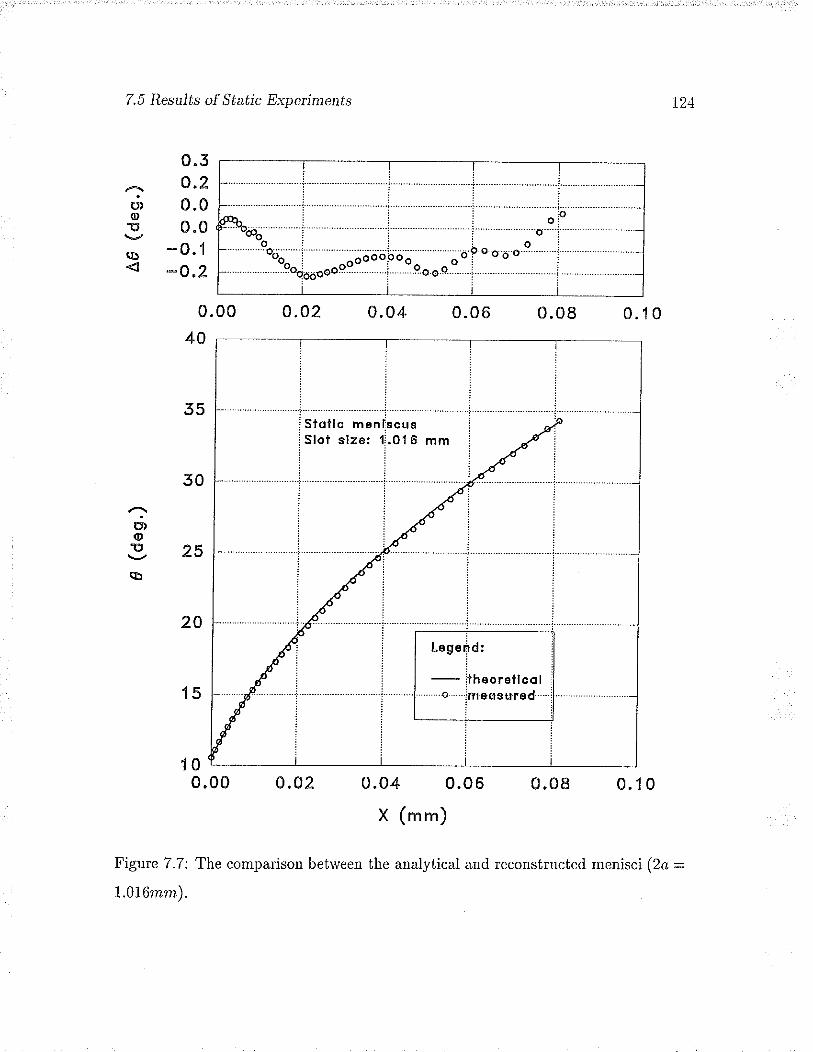
7.5 Results of Static Experiments 124
o)oE
o
0.5o.20.00.0
-0.1-o.2
0.00 o.o2 0.04 0.06 0.0840
35
50
25
20
15
100.00 o.o2 0.04 0.06 0.08 0.1
X (mm)
Figure 7.7: The compalison between the analytical anci reconstructed menisci (2o =
I.0l6mrn).
0.1 0
.lû,(D
î,(ò
,ôl,ól
:
Legeåd:i
- ithêo 16llco I
''''o- imeosured -i

Z5 ResuJts of Static Experiments
1g)o!
o
o.2
0.1
0.0
-0.1
-0.2
40
58
56
34
32
50
28
26
24
jiiii- -i - - I : :
^^^^^ i ' i "-í- " - i" "ooooooo,i-iiii''''''''''''''jn"oou6o;¡aooo;öäü^ - -i
i
i i i.--'-:gss:.îll.l-o--o-9ese-o
0.00 0.02 0.04 0.06 0.08 0.10 0.12
o)o!
o
t)tø
i Lagend: i
i- th eq retfco I
I o matisurad''i'" """""-i __"_
0.00 0.02 0.04 0.06 0.08 0.10 0.12
X (mm)
Figure 7.8: The comparison betrveen the analytical and reconstructed menisci (2o =L.778mtn).

7.6 Results of lv[easured Dynamic Contact Angles
the calculation of the analytical menisci by Equation (7.2). The Bond nurnbers for
the trvo cells are 0.073 ancl 0.224, respectively. The lesults show that the smallest
distance fiom the contact line measurable in experiments is less than 5prn. They also
shorv that the deviations between tlìe reconstructecl menisci and the analytical ones
are within 0.25". This inclicates that the plesent experimental technique can provicle
very acculate measurement tesults.
7.6 Results of Measured Dynamic Contact
Angles
Experiments rvele performed in cells with slot sizes of 1.016 and I.778 nrn. Both the
deflection contact angles O¡ and the apparent contact angles O¿ lvere measured in
the experiments. Figures 7.9 and 7.10 show the measur.ed contact angles in a set of
cells. Solicl symbols inclicate the value of the cleflectecl contact angle (O¡) and hollotv
symbols indicate the values of the apparent contact angle (O¡,). Different symbols
represent the results for cliffe¡ent experimental runs in either the same cell or differ.ent
cells. Thougli the deviations between different r.uns are noticeable, within each ofthe
runs the variation of the deflectecl contact angle, O¿, with the capillary mrmber
are very consistent. The ¡esults show that the cleflectecl angle clepencls stlongly on
the displacing velocity. Even for C¿ as lorv as 10-4, the increase of O¡ is about
identical. This may result because the surface conditions of the glass slides are difierent o¡ a real
static contact angle may not have been achieved for the time interval of 10 minutes waited in the
experiments. It is tvell knorv¡r tltat the advancing static contact angle may difer from the ¡eal static
co[tact artgle owing to contact angle hysteresis, Ilence, the static angles measu¡ed are true but
differ because of the hysteresis effect. IVfeasurements of O, performed il diffe¡ent cells of 1.016 and
7,778 mm slot sizes confirmed the above mentioned diference in O". The ¡esults vere presented in
Figures 7.9 and 7.10 as dø = 0.
r26

7.6 Rest ts of lvleasured Dynamic Contact AngÌes
50%. Laryet flnctuations of o¡ than o¿ can be seen in the resr¡lts shorvn. Because
the present expe'ime'tal apparatus is not specialÌy rlesigned for measur.ing o¡, the
accuLacy of o¿ is much lower tha' that of o¿. An uncertainty of *b ¡lrn in the
measurement of L2- L1 can result in an ei:r'ol of Ì5' in the calculation of the appar.ent
contact angle, O¡, (cf. 0.2" in O¿). Lorv accutacy in measuring Oi¡ was also shown
in Ngan & Dussan's experiments [1982, 1g8g]. According to the fitted curves of the
contact angles, the appalerrt coutact angle o¡, is lalgel thal that for.the collesponcling
clcflecte<l contir.ct angle O¿ in both the cell slot sizes.
Aclditioual expeliments perfolmecl in cells of 0.508 nun (0.020 riz) slot size shorvecl
unstal¡le rnovemeuts of the contact line. This rvas inclicatecl by the appealance of a
non-straight contact line. This lesults in clifficulties in the evaluation of dynamic
contact angles ancl profiles of menisci. Therefore, experimental ::esults for 0.508 mm
slot size cannot be pi'esentecl. The origin of tbe instability lias not been iclentifiecl in
the plesent stucly ancl may be studied in future.
The ¡esults of the measured profiles of clynamic menisci will be presented in the
next chapter'.
t27
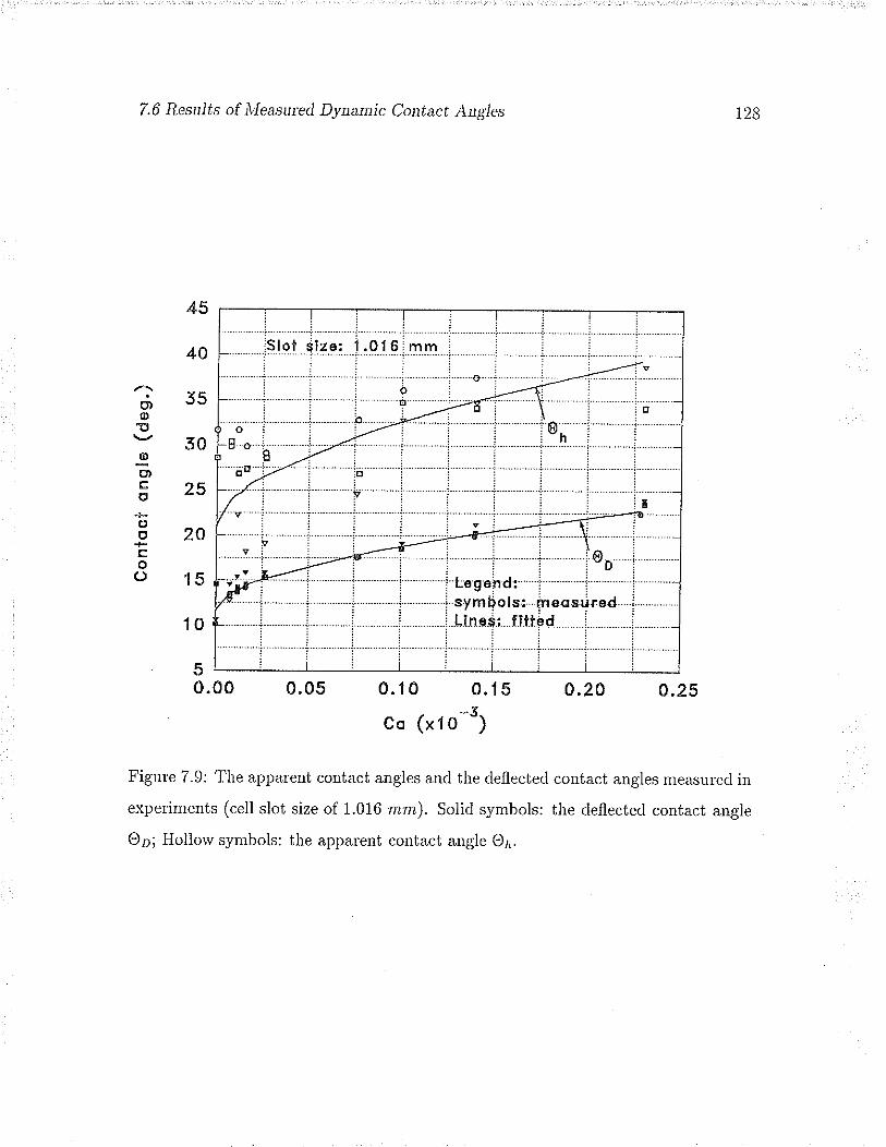
7.6 Resttlts of Ìvleasured Dyaamic Contact Angles
50.00 0.05 0.10 0.l s 0.20 0.25
-zco (xlO -)
Figure 7.9: The apparent contact angles and the deflectecl contact augles measuled in
experiments (cell slot size of 1.016 mrn). Solid symbols: the deflectecl contact angle
O¿; Hollow symbols: the apparent contact angle O¡.
t28
45
40
55
50
25
20
15
10
o)o!
Io)trIt
(,oco(J

7.6 Results of lvleaswed Dynamic Contact Angles
55
50
45
40
35
50
2s
200. 00 0.04 0.08 0.12
co (xt o-5)
r29
65
60
,/ìo)o!
gotco
oo
..1-tro()
0.1 6 0.20
Figure 7.10: The apparent contact angles and the deflected contact angles measurecl
in experiments (cell slot size of 1.778 rnrn). Solid symbols: the deflected contact algle
O¿; Hollorv symbols: the appalent contact angle O¿.
ililrlili:9tgl ri¡gi iJ:z-Z-e, qln i i i ei I-l i-- i -¡ ; i- | ---1 --: r-'1 -- -i : i i r itr- , I:;:t:ii::ti:,io.:ji
o..........:...............i......... i i o ¡ ll 1 .i ;- -,ri "i" io ;-- - i l-1" i "' i i"i" - i-- tt t ---'--"- öi i- ! -.o.-r.i..... -- r--o......i..9......2i.:-..j...........ir- ........ j....^ i i...r..ii. : n)::'-l ^-i- i@, i ," i i.4.....ò:;,4: "ll :; i**_L i ifi,';tÊ i'i
iþl*""i .;.*'--:-: .i . i...: .j. ¡. j
-v lt-...' i 1 i iLeoind: i i iWi --i--^"i ---i- "i stilËöi;; ilä;;ü;ä¿ i
-*-' I :- ---i- "i Stmi;öi;; ilä;;ü;ä¿ j
¡d'-i- "i i i-"itiñäiiritilää i ---i
i ì i i i:".--i i' i itiriiiiil

Chapter I
Cornparisons of Experimental withAnalytical and Numerical Results
In this chapter', the expelimental lesults fol dynamic me¡risci are compar.ecl rvith both
the analytical (asymptotic) solution presented by Dussan V., Ramé & GaLoff [1991]
(Dussan's solution) ¿ncl the numerical simulations using the finite eìement methocl
presented in chapter 4. The focusof the compalison will be on the valiclity of Dussan's
solution.
It is found that the experimental results can be well fitted rvith Dnssan's solution,
therefore, providing evidence that the ontel region solution can be well clefinecl by an
experimentally measurable parameter.

8.1 D¿rssan's Solution of an Immiscible Flotv in a Plana¡' Cell
8"1 Dussan's Solution of an Immiscible Flow in aPlanar Cell
The asymptotic folm of the intermediate region solution der.ived þ Dussan V., Ramé
& Garoff [1991] is given belorv:
13i
0t = (r-t Io(o,) + c,, tr!], (8 1)
rvhete the snbscti¡rt 1on á inclicates a c¡tantity defiled in the ilteunecli¿rte legion
only. The combinecl inter¡nerliate-outer region solution is
o = u-' fso) + cn '"ll + e. (i;",) - ",,
(8.2)
rvhere d,(r/a; O,) is the outer region solution clerived in Appendix C, Oo is the ap-
parent contåct angle of the outet region solution and
s@= l,PL-Y!:::!do (8.3)
if the receding phase viscosity is negligible (i.". p,,, = 0). In orcler to establish the
validity of Equation (8.1), a direct comparison rvith experiments is highly clesirable.
Horvever, to date, experimental compatisons have been macle with Equation (8.2)
alone.
Evaluating Equation (8.1) at any value of r, in the intermediate r.egion, clenote<l
by -R, one can obtain
o¡: o¡(R) = s-'ls@.) + c. nll (8.4)
s(oJ=s(op)-Ca (8.5)
Substituting the above into Ecluation (8.2) gives
e - s4fsr.R)+cah;f +e"(i;",) -r-'Io(o.) - ,"^:], (8.6)
,Rln-a

8.2 Comparison with Expeúmental Res¿¡Jfs
OI
0=9 -' lc " ni]+ e, (r; o") - s-' lc "
n il ,
1aD
(8.7)
(8.8)
(8 e)
where
L= Rexol_4gdl't co )Equation (8.5) can also be leclucerl to
e(o.): cahl.D.rssan \i., Raulé & Gtrioff [1991] h¿ve clenronstrated that oa cloes not deperrcl ou
the paramete' a. The.efore, ,C is ¿lso inclepenclent of o. This palaneter. was fir.st
introclucecl by ìvlalsli, Galoff & Dnssan v. [t991]. Norv it can be seen cleally tliat the
intermecliate region solution depencls on only one parameter L, ancl L is independent
of the outel region length scale ø.
Because the contril¡'tion of the oute. r'egio' solution in Equation (8.2) cloes not
vanish as long as,R > 0, the slope angle evaluatecl at .R using Equation (8.2), denotecl
by õ¿, will not be identical to O¿; that is
õ¿ - o¿ _ 0"(Rla;o") - o" > 0. (8.10)
An "actual" or "microscopic" dynamic contact angle can be eval.atecl ivith the fol-
lowing ecluation [Dussan V., Ramé & Garof 1gg1]:
/ ^ Ic \o - e ' lca tn7 ), (8.i r)
where -ts is the length scale of the inner region (such as a slippage length).
8.2 Comparison with Experimental Results
To compare Dussan's solution given by Equation (8.7) with the present experimental
results, the only unknown parameter, E, can be found by means of a least-scluared
minimization. The minimization procedule is as follows:

8,2 Compa'ison with Experimental lìesuJfs
Table 8.1: The evaluatecl contact angles from the experirneutal results in the cell of
slot size L.076 mm (Ã - 10 ¡.mt, B - l0-2).
U (pnz/ s) Ca O¿(") o,(") 6n(') o n(') o(") o¡(') L(mm)
4.68 8.42 x 10⁻⁶ 13.70 13.76 74.76 13.67 -L J. D4 1.51 x 10-80
7 .30 t.31 x 10-5 i4.06 14.18 15.14 14.05 14.01 8.43 x L0-57
10.18 i.83 x 10-5 14.56 14.68 15.59 14 51 i4.46 2.36 x 10-'r5
16.81 3.03 x 10-¡ Li). / o 15.9 3 16.7 4 15.67 15.61 2.76 x 10-rì5
4õ. t) / 8.75 x 10⁻⁵ 17.89 18.33 18,79 L7 .75 17.62 l./.ft) 4.88 x 10⁻¹⁹
63.72 i.15 x 10-a 1a o.' 19.65 20.0i 18.99 18.85 19.01 5.46 x 10- l8
88.62 1.60 x 10-a 20.24 21.12 20.31 20.15 20.37 3.73 x 10- 16
145.01 2.61 x 10-a tt,7, 23.91 22.85 22.64 22.97 2.I7x I0-La
1. Choose an initial value of .C;
2. Calculate Oo using Equation (8.9) then evaluate 0"(rla;Q.);
3. Estimate the deviation betrveen Equation (8.7) ancl the expetimental results fol
slope angles;
4. If the cleviation is minimizecl, terminate the plocess. Othelrvise, make a nerv
choice of ,C ancl go back to 2.
The appalent contact angles Op ancl O-¿, and the microscopic contact angle O can
now be calculated using Ecluations (8.8), (8.10) and (8.11). The results are presentecl
in Tables 8.1 ancl 8.2.
The variations of .4 with da are also shown in Figures 8.1 and 8.2. It can be
seen that the frtted parameter 4 is a function of Cø and increases with the capillary
number. The magnitude of .C depencls strongly on the static contact angle. The
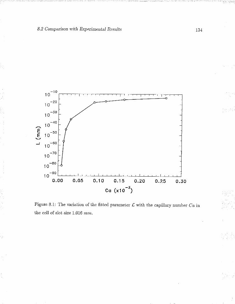
8.2 Compaúson with Experimental Results 134
EE
J
-lo10
10
-3010
-4010
-5010
-6010
-7010
-80t0-90
100.00 0.05 0.10 0.15 0.20 0.2s o.5o
co (xto-5)
Figure 8.1: The variation of the ûtted parameter. ,C ivith the capillar.y numl¡el d¿ in
the cell of slot size 1.016 mm.

8.2 Comparison wi t Experimenfal ResuJts l.óð
10 --
'I 0
-14010
-t 60l0
-18010
0.00 0.05 0.10 0.15-?Co (x10 -)
Figule 8.2: The variation of the fitted parameteÌ ,4 with the capillary number Ca in
the cell of slot size 1.778 mm.
EE
J

8.2 Compaûson vith Expetimenú¿J ResuJús
Table 8.2: The evaluated contact angles from the experimental results in the cell of
slot size I.778 mnt, (J? - 10 ¡.tnt,, ß - 70-2).
U (ptn/ s) Ca o¿(") o"(") 6¿(") o¿(') o(") o¡(") L(mnt)
2.62 4.71 x 10-c 25.84 25.81 26.44 25.79 25.79 25.74 < 10_1s5
4.08 7.35 x 10⁻⁶ 2ß.46 26.58 27.20 26.56 26.5 6 26.52 < 10-1s5
5.70 1.03 x 10⁻⁵ 26.76 26.82 26.79 ¿D.tó < 10_le5
9.41 1.69 x 10⁻⁵ 29.04 29.r4 29.72 29.09 29.09 29.06 4 19- ie5
27 .31 4.92 x 10⁻⁵ 1.13 x 10_ re4
35.90 6.46 x 10⁻⁵ 3 5.38 35.49 35.93 35.36 .J Ð. Jð 5.84 x 10-l
50.11 9.02 x 10⁻⁵ 36.93 37.11 37.50 36.94 36.93 36.97 5.g4 x 10_ r45
87.63 1.58 x 10-a 39.72 39.91 40.19 39.6 5 39.64 39.73 3.45 x 10_103
magnitude of ,C is inversely propottional to the static contact angìe. The values of
I calculatecl in the present work are much smaller then those presented by lvlar.sli,
Garoff & Dussan V. [1993] (lvIGD) (refer to Figule 8.3). In the present study, Itwas obtained that ,C - 10-200 - 10-14 mm fot Ca:10-6 - 10-a. Horvever, fuIGD
obt¿ined that L :10-6 - 10-3 rntn f.or Ca - 70-a - 10-2. The trend of L on Ca
in the present study is uprvarcl, while it is downwalcl in lvIGD. This may result from
the fact that the trvo expeliments are different. One of ihe differ.ences betrveen the
two experiments is the matelial systems used: palaffin oil/air/glass in the present
experiments and silicon oil/air'/glass in NIGD. The values of ,C were merely evaluated
through the least-sclualed fitting process previously describecl. Why the magnitude
of .C is small for the present tesults is not known at the present time1.
tln private comnrunication, Dussan V. [1994] suggested that the reason fo¡ such small values
of I may originate from the fact thai CahL/L approaches 9(O.), rvhere Oo denotes the static
advanciug coutact angle, a, nonzero quantity in the present experiments, as the contact line speecl
approaches zero, rvhich is not the case of ùfGD. Therefore, she suggested an ,improved, definition
r36

8.2 Conparisol with Experime¡úai Res¿¡iis
10-3
10-4
-E ro-u
;
10'6
70-7
10-4 10-3 10-2 10-1
U (crn/s)
Figure 8.3: Valiation of the fitting paremeter, ,4, with the capillary number, Ca,
obtained by lvlarsh, Galof & Dussan V. [1993]. o is the dipping angle ofa tube with
respect to fluid level.
O c=60oA q=70oo q,= B0oo c=90or q=100or c, = 1100
r[ Fftrw'"

8.3 Finite Element Sjmr¡Jaújo¡s of the Experiments
Because the st¿tic contact angles presently measnrecl in the same material systen
but diffe.ent slot sizes ale not identical, it is unable to make a similar comparisou
as puÌsuecl by i\lGD, in oÌclet' to examine the clependence of ,C on the outer r.egion
length scale a.
Fittecl Dussan's solutions of meniscus slopes are plotterl with the expelimental
restlts in Figures 8.4 and 8.õ. The root-mean-squarecl cleviation between them is
ivithin *0.06' fol all tlie menisci shorvn. The slope angles preclictecl b1' Dussan's
solntion, tltclefole, agrec ver')' ¡vell rvith the expeliureltal lesults. Fulthelmote. t[e
pleclictecl values of the contact angle O¡ ate very close to the ones rneasnrecl. Hence,
the plesent expelimental results plovide sonre clilect eviclence that the a.syruptotic
shape of a meniscus preclictecl analytically is measurable.
Figule 8.6 shorvs the viscous clistoltions of menisci uucler dynamic conclitions. ltcan be seett that as tlte capillaly numbel incleases, the clisto¡:tion of meniscus inct'eases
too, aborrt 2 al Ca = 10-4.
8.3 Finite Element Simulations of the
Experiments
The finite element analysis scheme presented in Chapter 4 rvas usecl to simulate the
expeliments. The microscopic contact angles used in the simulation rvere evaluatecl
using Equation (8.11) from the fitte<l values of I as listecl in Tables 8.1 ancl 8.2.
According to Equation (8.11) the microscopic contact angle O depends on the slip
coefficient B. An appropriate value of B coukl be found by fitting the meniscus plo-
files of simulation with those of the experiments as given belov¡. The simulated slope
angles with B = 10-2 ale plotted along with the experimental results in Figures 8.7
138
of I as .E exp[ (g(O ") - g(Op))/Cø], rvhel Oo is greater than zero.

8.3 Finite Element Simulations of the Experiments
0.00 0.04 0.08 0.12 0.1 6 0.20
i39
1o)o-o
o
0.2
0.1
0.0
-0.1-0.2
,ìg)o!(D
58
36
34
32
50
28
26
24
22
20
18
16
14
120.00 0.04 0.08 0,12 0.16 0.20
r (mm)
Figure 8.4: The slope angles of the cell of slot size 1,016 mm. ilhe symbols represent
the experimental results and the solid lines are the fitted results.
,såeg,irrFË!!isigüqE
Ill.:¡;qsf;o!ffi1:a.gg:å;¡llråiii|:fi;a,''::*
Ca
v' OOOô
EV

8.3 Finite Elentent Simulations of the Experinents
0.00 0.04 0,08 0.12 0.1 6 0,20
1o)o1t
(D
o,2
0.1
0.0
-0.1
-o.2
,ìo)o!
(b
46
44
42
40
58
36
34
32
50
28
26
240.00 0.04 0.0E 0.12 0.1 6 0.20
r (mm)
Figure 8.5: The slope angies of the cell of slot size 1.778 mm. 'lhe symbols represent
the experimental results and the solid lines are the ûttecl ¡esults.

8.3 Finite Elenent Simulations of tlte Experiments
Slot slze: l.0f 6 mm
Co =0.842x I O-5
0.00 0.04
r41
¡t)o!
È
g)o!
a
3432
30
28
26
2422
20
l816
14
120.08 0.12
r (mm)
Slol slze: 1.016 mm
Co=0.505x10-a
0.00 0.04 0.06 0.12
r (mm)
0.1 6 o.20
56
343250
28
26
2422
20
18
l614
0.1 6 o.20
Figure 8.6: Distortions of meniscí under dynamic conditions. Symbols: the measurecl
results; Solid lire: the combined solution d; Dashed line: the outer region solution do;
and Dash-dotted line: the intermediate region solution á¡. (continued)

8.3 Fiúte Element Sjmulations of tlte Experiments
Slol size: L0l 6
Cq=0.'1 15x10-3
0.00 0.04
o)o!
G
40
38
36
3432
50
28
26
2422
20
18
-ct)olJ
o
40
38
56
34
32
50
28
26
24
22
0.08 0.12
r (mm)
Slot slze: 1,016 mm
...f Co =0,2 6l xl0-5
..ø
0.00 0.04 0.08 0.12
r (mm)
0. 1 6 0.20
0.1 6 0.20
Figure 8.6: Distortions of menisci under dynamic conditions.

8.3 Finite Element ,Sim¿rJaújo¡s of the Expeúments
40
3E
36
34
32
30
28
26
24
22
20
l8160.00 o.o2 0.04 0.06
x (mm)
1.13
o,o!
o
0,08 0.10
Figure 8.7: Finite element simulated slope angles of the immiscible florv, in cell of
slot size 7.076 mm.
and 8.8. The sensitivity of the finite ele¡nent solution to the slip coefficient was
examined by choosing different values of the slip coefficient. The lesults are shorvn in
Figure 8.9. The results show that the selection of B - I0-2 gives the best fit betlveen
the experimental and the simulation results (refer to Figule 8.7). For this value of
6, the simulated profiles fit the measureci results very well with a loot-mean-squarecl
deviation of less than 0.5'. As the slip coefficient decreases, the microscopic angle
becomes smaller and the deviation between the experiments and the simulations in-
creases. The micloscopic contact angles evaluated with B - l0-2 are also listecl in
Slol slze: L016 mm
Legend:Symbols: meosu red"
o Co=0.876r I O
. Co=O.t f Sxl O-lo Co=0.160x10_,v Co=0.261x l0
Lines: FEM (e=to-2)

8.3 Finite Element Simulations of the Experiments
48
46
44
42
40
38
36
34
320.00 0,02 0.04 0.06 0.08 0.10 0.12 0.14
x (mm)
Figure 8.8: Finite element simulatecl slope angles of the immiscible floiv, in cell of
slot size L.778 ¡nm.
glo!
o
Slol sizer 1,778 mm
L€gènd:Symbols: meosurs4
o Co=0.492x1Or Co=0.646x10-ao Co=0.902x10-a
' Co=0.158x10⁻⁵Lines: FEM (s= I O-')

8.3 Finite Element Simulations of the Experiments
40
58
36
34
32
30
28
26
24
22
20
18
l60.00 0.02 0.04 0.06 0.08 0.10
x (mm)
Figure 8.9: Finite elernent simirlated slope angles for difelent values of the slip coef-
ficient (cell slot size I.016 mrn).
145
1o)(D
!
(Þ
S lot size: l.0l6 mm
Legend:Symbols: meosured.
o Co=0,676x10_,. Co=O.1 15x10_iv Co=0.160x10 -
' Co=O.ZS1x'1 O-5Llnes: FEM
-a_ B= l0-a----. B=1O

8.3 F jnite Element Sjnr¿rÌ¿tjo¡s of the Experiments
Tables 8.1 and 8.2. lt can be seen in these tables that the evaluated micr.oscopic angle
O depends on the capillaly number.
The pleclicted value of the slip length, .Ls, is about 70-3 cm for ¿ = 1 - 2 nun.,
¡vhiclr is lat'ger than that pledicted pleviously (trs = iO-a - 70-7 cnt) [Ngan &
Duss¿n V. 19891. The slip length plesently evaluated rvas basecl on the assumption
that the microscopic contact angle calì be calculatecl using Equation (S.11). It shoulcl
be noted tltat this ec¡rzrtion rvas clelivecl ânalytically [Dussan V., Ramé & Gar.off 1gg1]
¿ltd lt¿rs uot y'et been testecl expe::iurentally. The choice of aly clifi'elent nriciosco¡ric
contact angle in the sinrulation may result in a cliffetent value of the slip length to
best fit the measnrecl lesnlts.
Frorn the values listed in Tables 8.1 ancl 8.2 the O¡, evaluated is alnrost the same
as the deflection angle O¿ measurecl, while the diffelence betrveen them fi.om the
experiments is vely lalge. One of the possible oligins of the deviation is a systematic
error in measuLing L1- L2 in expetiments. The locations of tr1 and ¿2 are âlso subject
to the straight edge difraction effect. The influence of this efect was not quantified in
experiments. A possible systematic errol of 5 pm in L1- L2 ma! Ìesult in 5o of elr-or
in calculating O¿. Horvever, it must be emphasized that the expeliments rvere not
designed to optimize the measurement of O¿. Tables 8.3 and 8.4 shorv the evaluatecl
excess lesistance folces (If factor' ¿nd A cos O¡,) using the finite element method. ln
the tables, Ap denotes the pressure difference pA - pB. As predicted in Chapter.
4, the difference between fl factor and A cos O¿ is very small in the capillary range
calculated (Ca < 10-a). It should be notecl that the simulation results presented in
this chaptel rvele obtainecl by choosing valiable microscopic contact angles, instead
of choosing constant angles as in Chapter 4.
146

8.3 Finite Elenent SjmuJ¿fjo¡s of tlte Experirnents
Table 8.3: Tlre evaluated excess resistance forces for the cell of slot size 7.076 mtn.
U(pnt.ls) Ca Ap A cos O¡ K
48.67 8.75 x 10⁻⁵ -0.950 0.0192 0.0208
63.72 1.15 x 10-a -0.944 0.0261 0.0266
88.62 1.60 x 10- r -0.936 0.0311 0.0313
145.01 2.61x 10-a -0.918 0.0508 0.0515
Table 8.4: The evaluated excess resistance forces for the cell of slot size L778 mtn.
U(pmls) Ca Ap À cos O¡, K
2.62 4.71 x 10-G -0.901 0.0048 0.0045
4.08 7.35 x 10⁻⁶ -0.894 0.0108 0.0115
5.70 1.03 x 10⁻⁵ -0.892 0.0125 0.0135
9.41 1.69 x 10⁻⁵ -0.874 0.0315 0.0314
27.31 4.92 x 10⁻⁵ -0.835 0.0700 0.0702
35.90 6.46 x 10⁻⁵ -0.815 0.0902 0.0901
50.11 9.02 x 10⁻⁵ -0.798 0.1066 0.1069
¿l / _b.1 1.58 x 10-a -0.768 0.1365 0.1364

Chapter 9
Conclusions and F uture -Works
This chapter presents the conclusions of the pi.esent study on immiscible capillaly
florv. Recommenclations for futrrle rvorh are also given.
9.L Conclusions
The follorving conclusions can l¡e leached from the preselt stucly:
1. À general capillary florv ecluation for evaluating the excess lesistance force has
been derivecl from the multiphase momentum conservation ec¡ration. A char.-
acteristic parameter, If factor, was ploposed; /f replesents the ratio of the
viscous rvall drag on unit ci¡cumferential length to the interfacial tension o12.
The quantities associatecl with the genelal capillary flow equation ar.e all the
outer legion parameters and should be measurable in experiments.
2. Numerical simulations using the finite element method have shown that by
choosing either constant or variable microscopic dynamic contact, the evaluated
values of 1l factor are very close to the ones of the lVashl¡urn dynarnic capillary
148

9.1 Conclusions 149
plessule, A cos O¡,. Therefore, A cos O¿ is a goocl inclication of the magnitucle
of -Il. TIte devi¿tion betrveen them is less than 3To f.or Ca < 10-2 in the
simulations.
3. Although the Washbuln ecluation is based on two pr.imitive asstmptious, it is
still a good apploximate equation in evaluating tlte excess resistance for.ce, if a
suitable valiable dynamic contact angle lelationsìrip ivith the capilla::y nnmbeL
is utilized ancl uuclel the corrrlition that the capillar'¡' numl¡er. is small, such as
Ca < 70-2 .
4. A grating shealing interference expelirnental technic¡re has been clevelopecl. Ithas ihe ability to simultaneously measule clynamic contact angles ancl meniscus
profiles close to the contact line. It rvas validatecì both numerically ancl experi-
nentally. lVith the technic¡re, the measurable range of the pr.ofile is 5 - 750 l¿m
fronr the contact contact line, which is rvell lvithin the internediate region. The
accuracy of the measnled deflection engle can be rvithin *0.5".
5, A Helle-Shaw cell type experimental appatatus has been clevisecl for easy con-
struction ancl sealing of test cells. A partitionecl masliing glating techniclue lvas
developecl to locate the deflected liglit rays and interference pattern on a single
pictut'e.
6. The expelimental technique has been implemented to measure both the static
and the dynamic contact angles and the profiles of menisci. A set of preliminary
experiments was carried out in cells of slot sizes: 0.508, 1.016 anð,7.778 rnm.
The deflection and appalent contact angles rvere evaluated from experimental
¡esults. The cleflection contact angle, O¿, depends strongly on the displacement
velocity. Even when Ca is as low as 10-4, O¿ can be double its static value.

9.1 Conclusions
7. Good agreements have been leachecl i¡r compaling the expelimental results rvith
both Dussan's theo'eiical solution ¿ncl the finite element simulation results.
The experimental results can be rvell ûtted with the theoreiical solution by
choosing only one geometrically inclependent paralììeteL ,c. This shorvs that tl¡e
equivalent boruidary condition proposed by Dussan Y. et at. is measnrable in
experiments. Thelefole, a capillary florv ploblem in the outer.region can be rvell
cleflne<l rvith that bounclaly co¡tclition inste¿cl of the one in the inlel tegion.
8. Au appalent viscosity lnodel has )reen ploposecl and applicd to lesoh.e the
singularity in the contact florv problem. It has been founcl that the apparent
viscosity rnoclel is ec¡rivalent to the stress slip moclel in solving the contact
florv problem atound a cylincle:: rolling ovel a planar.surface - with iclentical
shear stress and pressure clistributions and a negligible diffelence in the viscous
normal stress clistribttion. The solutions with the apparent viscosity rnodel
can describe the "rolling-type" motion of the interface that has been observecl
in experiments, rvhile the one with the classic siress slip moclel cannot. This
provides a means to utilize some CFD programs, which ìrave no options to cleal
lvith slip bounclary conditions, to solve contact flow problems by utilizing the
usually available options of valiable fluid properties.
9. Uncler the commonly acceptecl assumptions mentioned in Section 3.2, the mi-
croscopic dynamic contact angle has to be the same as the static contact angle.
This implies that any different values of the micloscopic dynamic contact angle
may only be possible if one or more of the usual assumptions is al¡ando¡red.
150

9.2 Recommenclations for F¿¡úu¡e lVol Jç
9.2 Recommendations for Future'Work
The plesent wolk can be used as a starting poitit fol further studies leading to a
bettet' unclerstanding of the dynamics of two-phase inr¡¡iscible clisplacement florv iu
a capillaly ancl furthel in porous meclia. In particular, the follorving stuclies coulcl be
concluctecl:
1. The ptesent stucly plovicles ¿l l'elial¡le experimental technic¡re fol the investig¿r-
tion of inuniscible capillaly florv. The experiments can l¡e extendecl to urorc cell
slot sizes in olclel to examine rvhethel the palarneter.s ,C and 1( are r.elatecl to
the outer legion length scale a ancl rvhat that relationship shoulcl be.
2. The purpose of the general capillary florv equation (3.17) is to utilize measur'-
able pressnre chop across the meniscus to evalnatc the excess tesistance folce
in a capillary florv. In olcler to clo this, a similar experimental technique as was
utilized by Legait & Sourieau [1985] coulcl be employed to measule the displace-
ment velocity with a knorv pÌessure clrop or vice versa. This kind of study may
also lead to a clalification of rvhether' 1l is a ploperty of the mater.ial system,
inclepenclent of the outer region length scale o.
3. The dynamic contact angle ancl the excess resistance behaviouls could be in-
corpolated into netrvork simulations in order to explor.e macroscopic valiables
of trvo-phase flow immiscible displacemeni, such as dynamic wettability and
dynamic capillary presslrre culves, on the core scale,
151

Bibliography
[1] Ablahan, F.F. 1978. The iutelfaci¿rl clerrsity ¡;rofile of a Lenna,r,cl-Jotes fluicl
in contact rvith a (100) Lernat'cl-Jones rvall ancl its lelationship to iclealized
flrricl/rvall systems: a trlonte C¿::lo simulation. J. Clrem. Phys.68: 3713-3716.
[2] Ablamorvitz, NI. & Stegun, I. 1964. fJ¿¡dbo ol< of lv[athematical Fttnctions tvit]t
Fornrrlas, Graphs ancl lvlatltentatical ?abJes. NBS Appl. lvlaths. Ser.ies No. 55,
(US Govelnment Printing Office, Washington DC).
[3] Aicler', B.J. & lV¿iuvright, T.E. 1970. Decay of the velocity autocouelation
function. Phys. Reu. A L: L8-2L
[4] Alsten, V.J., Granick, S. & Islaelachvili, J.N. 1988. Concerning the measure-
ment of fluid viscosity betrveen culved surfaces. J. Colloi,d Interface Sci. -125:
739-740.
[5] Askwitli, T.C., Camelon, A. & Crouch, R.F. 1966. Chain length of acklitives in
relation to lubricants in thin film and boundary lubrication. Proc. R. Soc. Lon-
tlon Ser. ,4 291: 500.
[6] Bangham, D.H. & Saweries, Z. 1938. The behaviour of liquid dlops ancl aclsorbecl
films at cleavage surfaces. TYans. Faraday Soc.34: 554-570.

BIBLIOGRAPHY 153
[7] Bascom, lV.D., Cottington, R.L. & Singleter.ry, C.R. 1964. Dynamics surface
phenomena in the spontaneous spreacling of oil on solicls. ln Aclv. Chem.:
Amer. Chem. Soc. 43: 389.
[8] Bataille, J. 1966. C. R. Acad. Sci. Po.ris 262: 843.
[9] Beaglehole, D., Heslot, F,, Cabazat, A.lvI. & Levinson, P. 1990. in Hydrctly-
ri¿n¡ics of Dispersed ù/edia. (Erls: Hullin, J.P., Cabazat, A.il,I., Gugou, E. &
CaLuroun, F.), a5, (NoLth-Hollzrrrd, Amstc'rclarn).
[10] Benney, D.J. & Timson, \,V.J. 1982. Rolling motion of ¿ viscous fluicl on ancl off
a rigicl surface. Sttul. A74tl. Math. 63: 93.
[1i] Bhattacharji, S. & Savic, P. 1965. Real and appalent non-Newtonian behaviol
in viscous pipe flow of suspensions driven by fluicl piston. Proc. Heat Tfansfer
Fltútl, Meclt Inst.: 248.
[12] Bhattachalya, D. I(. & Lie, G.C. 1991. Nonequilibrium gas florv in the transitiou
legion; a molecr.rlar-dynamics study. Ph,ys. Reu. A 43: 76I-767.
[13] Blake, T.D., Evar:ett, & Haynes, J.lvl. 1967. in Wetting, SCI ùIonograph 25.
Society of Chemical Inclustry. Lonclon, 164-173. J. Colloitl Interface Sc.i. 'J.0:
180.
[14] Blake, T.D. & Haynes, J.ùI. 1969. I(inetics of liquicl/liquicl displacement. ,I.
Colloid, Interface Sci,. 3O: 421-423.
[15] Blake, T.D. & Haynes, J.ù1. 1972. Prog. Surf. Metnbr. Sci,.6: 125.
[16] Bi'acke, IvL, De Voeght & Joos, P. 1989. Prog. CoUoid Polym. Sci,.79: 142.
BIBLTOGRAPHY
[17] Bloughton, J.Q. & Gilmer', G.H. 1986. ivloleculal clynarnics investigation of the
clystal-fluid interface: VI. Excess sulface free energies of crystal liquicl systerns.
J. Chem. Phys.84: 5759-5768.
[18] Blown, R.4., Scliven, L.Ð., & Silliman, \,V.J. 1980. Computer-aiclecl analysis of
nonlineaÌ problems in transpoi't phenomena. In l{ew, Approacåes úo lfo¡Jjne¿¡
Problems in Dynamics. Philaclelphia: Soc. Ind. Appl. ivlath.: 289-307.
[i9] Blorvl, P.N. & Saacl, Y. 1990. H¡.blirl lir'1'lov rnethocls for nouliuc'¿rl sl'stems of
ec¡rations. SIAIUI J. Sci. Stat. Cotnprtt. L1: 450-481.
[20] Bluns, F,!V. 1980. A moving solicl-fluicl-solid contact line: tlie lemoval of the
force ancl presslue singularity by a slip ancl filtration fr,o.r. J. Colloid Interface
Sci.74: 347-348.
[21] Burlziah, C.J. & Neumann, A.W. 1990. Äutomation pf the capillar.y rise tech-
nique fol measuring contact angles. Colloids €! Su,rfaces 43: 279-2g3.
[ZZ] Builey, R. & Bracly, P.R. 1973. Displacernent of an air/liquicl interface by amov-
ing web of fibers. J. Colloitl InterJace Sci. 42 13I-136.
[23] Burley, R. & I(ennecly, B.S. 1976. An experimental stucly of ail entlainment ¿t
a solid/liquicl/gas interfåce. Chem. Eng. ,9c2. 31: 901.
[24] Callaghan, LC., Everett, D.H. & Fletcher, A.J.P. 1983. Liquid/liquicl/solicl con-
tact angles measured by intelfelence microscopy. J. Chem. Soc., Faratlay Trans.
79: 2723-2728.
[25] Cha, S. & Vest, C.ìVI. 1981. Tomographic reconstrnction of str.ongly refi.acting
fields ancl its application to interferometric measulement of boundary layers.
Applied, Opti,cs 20: 2787-2794.
15.1

BIBLIOGRAPHY
[26] Chan, D.Y.C. & Holn, R. G. 1985. The clrainage of thin lic¡ricl films betrveen
solid surfaces. J. Clrcm. Pltgs.83: 5311-5324.
[ZZ] Ctrang, W.V., Chang, Y.lvI., lVang, L.J. & trVang, Z.G.1982. Organic Coati.nss
antl Applied Polgmer Science Proceetlings (Anrerican Chemical Society, lliash-
ington, D.C.), 47.
[28] Chapela, G.4., Sti.ville, G., Thompson, S.NI. & Rorvliuson, J.S. 1977. Cornpnter.
sirnrtl¿rtion of a gas-lic¡ricl surface. ,./. Cl¿etn. Soc. Frurulay Ttr¿t¿s. II 73: 1133
1111.
[29] Clrapnran, S. & Corvling, T.G. 1970. Tlrc lv[at]tenatica] Theory of Non-(Jnifonn
Gases, 3rcl Ecliiion, (Cambridge University Pless, Camblidge).
[30] Chen, J.D. 1988. Expeliments on a spreacling drop ancl its contact angle on a
solicl. J. Colloid InterJace Sci. 122: 60-72.
[31] Chen, J.D., Wada, N. 1992. Edge profiles an<l clynamic contact angle of a spreacl-
ing chop. J. Collo'id InterJace Sci,. 148: 207-222.
[32] CheLLy, B.W. & Holmes, C.ìvI. 1969. I(inetics of wetting of surfaces by polymers.
J. Colloid Interface Sci.29: 174-176.
[33] Chittenclen, D.H. & Spinney, D.U. 1966. Expelimental stucly of sur.face compo-
sition effect on two-phase flow in glass capillaÌy tube. J. Colloid, Interface Sc'i.
22: 250-256.
[34] Christenson, H.lt. 1985. Capillary condensation in systems of immiscible liquicls.
J. Colloitl InterJace Sci. 1O4 234-249.
[35] Chlisteuson, H.I(. & Israelachvili, J.N. 1987. Direct measurements of inter.ac-
tions and viscosity of crude oils in thin films bet¡veen model clay surfaces. ,L
Colloi.tL Interface Sci, ll9: 194*202.
155

BIBLIOGRAPHY 156
[36] Christenson, H.i(., Islaelachvili, J.N. & Pashley, R.ÌVI. 1987. Ploperties of cap-
illaly fluids at the microscopic level. SPE Reserooir Eng.2: 75'o-165.
[37] Chnng, T.J. 1978. Finite Element Analysis in Fluid Dynamics, (fuIcGrarv-Hill,
Nerv Yorli).
[38] Chulaev, N.V., Sobolev, V.D. & Sornov, A.N, 1984. Slippage of Iiquicls over
lyoplrobic solicl snlf¿rces. J. Colloid Interfacc Sci. 97: 57 4-587.
[39.] Cox, R.G. 1986. The rll,uanrics of the splezrding of lit¡ritls on a soli<l surfacc.
Part 1. Viscous fr,ol. J. Flu,itl Mech. 168: 169-194.
[40] Derjaguin,8.V., I(arasev, V.V., Lavygin, I.4., Sliorokliodov, LI. & I(hromova,
E.N. 1975. in Researcl¡ in Sttfface Folces, Ecls: B.\¡. Deryagin, (Consultants
Bureau, Neiv Yolk) 1: 79.
[41] Deryagin, B.V. & Obulchov, E.V. 1935. Colloitl J. USSR (Enstásh TYansI.) 1:
385.
[42] Dias, lVI.lVI. & Payatahes, A.C. 1986. Netrvolh moclels fo:: tivo-phase flot' inporous media. J. Fluid Mech. 164: 305-358.
[43] Ducla, J.L. & Vrentas, J.S. 1971. Steacly flow in the r.egion of closecl stleamlines
in a cylinclrical cãvity. J. Fh¿id lulech.45: 247-260.
[44] Durbin, P.A. 1988. Considerations on the moving contact-line singularity, with
application to frictional drag on a slencler dr.op. J. Flui,d, Mech- Lg7: 157-169.
[45] Dussan V., Ð.8. & Davis, S.H. 1974. On the motion of a fluicl-fluid interface
along a solid surface. ,./. Flui,tl, Mech. 65: 71-95.
[46] Dussan V., E.B. 1976. Tlie moving contact line: the slip boundar.y condition.
J. Flt¿itl Mech.77: 665-684.
BIBLTOGRAPHY
[47] Dussan V., E.B, 1977. lmmiscible liquicl clisplacement in a capillary tirbe: the
moving contact lite. AICI¿Ð.¡. 23: 131-133.
[48] Dussan V., E.B. 1979. On the spr-eacling of liquids on solicl sur.faces: static ancl
dynamic contact lines. Ann. Reu. FluitL Mecl¿. L1: 371-400.
[49] Dussan V., 8.8., Ramé, E. & Galoff, S. 1991. On iclentifying the appropr.iate
bouncla,::¡' conclitions at a, movirrg cont¿rct liue: an expelirlental illvestigatiorr.
J. FhàtL tuIecl¿.230: 97-116.
[50] Elliott, G.E.P. ,þ Riclclifolct, A.C. 1962. D¡.narnic contact angles ancl rates of
aclsolption. Nahtre (London) 195: 795-796.
[51] Elliott, G.E.P. & Riddiforcl, A.C. 1964. Contact angles. in Recenú Plogless
i¡ Sr¡¡face Science. (Eds: Danietli, J.F., Pankhulst, Ii.G. & Riclcliford, A.C.)
(Acaclemic, Nerv York) 2: 111-128.
[52j Elliott, G.E.P. & Riddiford, A.C. 1967. Dynamic contact angle. I. The effect of
impressed motion. ,./. Colloi,d, Interface Sci. 23: 389-398.
[53] Fatt, I. 1956a. The netrvolh model of polons media: I. Capillary pressur.e char-
acteristics. Tbans., AIME 2O7: 744-759.
[5a] Fatt, I. 1956b. The netwolk model of polous media: lI. Dynamic propelties of
a single size tube network. Trans., AIME 207: 160-163.
[55] Fatt, I. 1956c. The network nodel of porous meclia: III. Dynamic properties
with tube r-aclius distributiott. Tlans., AIfutE 2O7: 163 181.
[56] Fermigier, M. & Jenffer, P. 1991. An experimental investigation of the clynamic
contact angle in a liquicl-liquid systems. J. Colloi.d InterJace Sci.. L46: 226-24L
157

BIBLIOGR,APHY 158
[57] Fisher', L.R. & Lalk, P.D. 1979. Àn experirnental study of the lVashburn eclua-
tion for liquid florv in very fine capillalies. J. Colloitl Interface Sci,.69: 486-492.
[58] Foister', R.T, 1990. The liinetics of clisplacernent rvetting in liquicl/lic¡ricl/solid
systems. J. Colloitl Interface Sci. -J.36: 266-282.
[59] Gennes, P.G. de 1985. trVetting: statics and clynamics. Reu. Motl. Pltys 17:
827-863.
[60] Geolgiou, C.G., Schultz, W.\\¡. & Olsol, L.Ci. 1990. Singulzrl fìuire eleurerrts fol
tlre srrclclen-expansion an<[ the die-srvell ploblems. Int. J. Ntm¿er. ]uÍetl¿. Flt¿itls
LO: 357-372.
[61] Ghiradella, H., Racligan, W. & Frisch, H.L. 1975. Electlical resistivity clianges
in spreacling liquid fihns. J. Colloitl Interface Sci. 6L: 522-526.
[62] Glasstone, S., Laidler, i(.J. & Eyling, H. 1941. Theoty of Ral'e Processes, Chap-
ter 9. (lvlcGraiv-Hill, New York).
[63] Goklstein, S. 1938. fuIodern Developments in Fluicl Dynamics, (Oxfolcl Univer.-
sity Press), pp. 676-80.
[6a] Good, R.J. & Lin, N.-J. 1976. Rate of penetratiol of a fluicl into a por.ous bocly:
II. Verification of ihe genetalization of the lVashburn equaiion for organic liquids
in glass capillaries. J. Colloi,d, InterJace Sci.54: 52-58.
[65] Goodman, J.I.V. 1968. Intrcduction to Fouúet Opú.ics, (lvlcGraw-Hill, Nerv Y-
ork).
[66] Greenspan, D. 1988. Ivlecllanics of capillarity via supelcompute¡ simulation.
Comput. Math. Appl. 16: 331-340.

BIBLIOGRAPHY
[67] Greenspan, H.P. 1978. On the motion of a sm¿ll viscous clroplet that wets a
surface. J. Flu'itl Mech. 84: 125.
[68] Grrtotr, E.B. & I(enclrick, C.E. 1982. Dynamic contact angles. AICLE J.28:459.
[69] Hansen, R.S. & ìvfiotto, iVI. 1957. Relaxation phenomena and contact angle
hystelesis. J. A¡n. Cl¿en¿. Soc.79: 176ó-1765.
[70] Hansen, R.J. & Toong, T.Y. 1971¿. Iutelface beha,vior as ole fluid coÌ)ìpletel)¡
clisplaces auothel from a small-cliar¡eter tube. J. Colloid Interfuce Sc,i. 36:
410-413.
[71] Hansen, R.J. & Toong, T.Y. 1971b. Dynamic contact angle ancl its relationship
to folces of hydlodynatric origin. J. Colloi.tl InterJace Sci. 37: 196-207.
[72] Hocking, L.ivi. 1976. A moving fluic1 intelface on a rorigh surface. J. Ftt¿i.tl Mecl¿.
76: 801-817.
[73] Hocking, L.ìVi. 1977. A moving fluid interface. Part 2. The lemovaÌ of the for.ce
singularity by a slip flotv. J. Flu:id Mech. 79 209-229.
[74] Hocking, L.ù1. & Rivels, A.D. 1982. The spleacling of a clrop by capillary action.
J. Flui.d Mech. l2l: 425-442.
[75] Hoffman, 1975. A study of the advancing interface. I. Interface shape in liquíd-
gas systems. J. Colloid Interface Sci.60: 228-247.
[76] Hotrman, 1983. A study of the advancing interface. IL Theoretical pr.ediction of
the dynamic contact angle in liquid-gas systems. J. Colloid InterJace Sc,i. 94:
470-486.
I <O

BIBLIOGRAPHY
[77] Huh, C. & ùIason, S.G. 1977. The sieacly movement of a liqLricl meniscus in a
capillary tube. "I. Fh¿id Mech.8L: 401-419.
[78] Huh, C & Scliven, L.E. 197f . Hyclrodynamic moclel of steady movement of a
solid/liquid/fluid coniact line. J. Colloirl, Interface Scz. 35: 85-101.
[79] Huitfeklt, J. Ruhe, A. 1990. À neiv alglithm fol numerical path follorving appliecl
toan exarnple ftom hychorlynamic¿rl florv. SIAM J. Sci. Stat. Cont1ntt.11: 1181-
1192.
[80] Islaelaclrvili, J. N. 1985. Intermolecuab ancl Surface Fotces (Academic, Lonclou).
[81] Israelachvili, J.N. & Adams, G.E. 1978. ivleasurenent of folces betrveen trvo
mica surfaces in aqueous electrolyte solutions in the tange 0 - 100 nm. "I.
Chem. Soc. Faratlay Trans. 174:975-1001.
[82] Jackson, R. L977. Transport jn Po¡o¡¡s CataJysts (Elsevier', Amsterdam).
[83] Jiang, T.S., Oh, S.G. & Slattery, J.C. 1979. Colrelation fol dynarnic contact
angle. J. Colloitl Interface Sci.69: 74-77.
[84] Joanny, J.F. & Andelman D. 1987. Steady-state motions of a liquicl/liquicl/solicl
contact line. J. Colloirl, Interface Sci.719: 451-458.
[85] Joos, P., Remoortere, P.V. & Bracke, NI. 1990. The kinetics of rvetting in a
capilla::y. J. Colloid Interface.9cz'. 136: i89-197.
[86] i(afha, F.Y. & Dussan V., E.B. 1979. On the interpletation of dynamic contact
angles in capillalies. J. Flui,tl Mech.96: 539-565.
[87] I(ennedy, B.S. & Burle¡ R. 1977. Dynamic fluid interface displacement and
prediction of air entrainment. J. Colloitl InterJace Sci. 62 48-62.
160
BIBLIOGRAPHY
[88] I(iss, E, Pintér', J. & Wolfram, E. 1985. Florv patterns of irnmiscible liquicl/licluicl
displacement in a capillaly túte. Prog. Colloid, ü Polgmer ^9c2.
70: 113-118.
[89] I(linhenbelg, L.J. 1941. Tlie permeability of porous media to liquicls ancl ga.ses.
Drilling antl Proth¿ction Practi,ce 30: 200.
[90] I(oplih, J., Banavar, J.R. & Willensen, J.F. 198g. lvlolecular dynamics of fluicl
florv ¿t solicl sulf¿ces. Plr,ys. Fhtitls,4 1: 781 794.
[9i] I(oplih, J. & La.ssetcr', T.J. 1985. Trvo-phzrse florv il lan<torn netrvolli nroclcls of
pororrs nreclia. SPE J.25: 89-100.
[92] Legait, B. & Sourieau, P. 1985. Effect of geometry on aclvalcing contact angles
in fine capillalies. J. Colloitl Interface Sci,. 107: 14-20.
[93] Léger, L., Ennan, lvl., GLrinet-Piccard, A.ìvI., Ansseré, D., Stlaziella, C., Be-
nattau, J.J., Rieutorcl, F., Daillant, J. & Bosio, L. 1988. Reu. Phys. Appl- 23:
1047.
[94] LeGrancl, E.J. & Rense, W.A. 1945. Dataon late of capillary :rìse. J. Aqtpl. Pttys.
16: 843-846.
[95] Lester', G.R. 1961. Contact angles of liquicls at cleformable solid surface. J.
CoLloitl Interface Sci,. 16: 315-326.
[96] Letelier S., IVI.F., Leutheusser, H.J. & Rosas 2., C.7979. Refined mathematical
analysis of the capillary penetration ptoblem. J. Colloi,tl, lnterface Sci,.72 465-
470.
[97] Levine, S., Lowndes, J., lVatson, E.J. & Neale, G. 1980. A theory of capillary
rise of a liquicl in a vertical cylindrical tube and in a parallel-plate channel. /.Colloid, Interface Sci. 73: 136-151.

BIBLIOGRAPHY
[98] Li, D.IVL & Slattery, J.C. 1991, Analysis of the moving âppal.ent common line
and dynamic contact angle folmecl by a draining frlm. J. Colloi,tl, Interface Sci,.
143: 382-396.
[99] Ligenza, J.r. & Belnstein, R.B. 1951. The late of rise of liquicls in fine vertical
capillalies. J. Amer. Cl¿em. Soc. 73: 4636-4638.
[100] Longhulst, R.S. 1967. Geot¡tetúcal and P)tysical Optics, (Longmaus), p. 285.
[101] López, J. ì\,liller', C.A. & Ruclceustein, E. 1976. Sp::eacliug liinetics of lic¡rid
dlops. J. Colloid Interface Sci,.56: 460 468.
[r0Z] l,owe, A.C. & Riddifolcl, A.C. 1970a. J. Cl¿em. Sco. D.,: 387.
[103] Loive, A.C. & Ridclifolcl, A.C. I970b. Can. J. Chem.48: 86b.
[104] Lowncles, J. 1980. The numerical simulation of the steacly movenent of ¿ fluitl
nteniscus in a capillary tube. "I. Flt¿itl Mech. 101: 631-646.
[t05] Lncas, R. i9i8. Kolloitln. Zk.23: 75.
[106] Ludvihsson, V. & Lightfoot, E.N. i968. Deformation of advancing me¡risci.
AIC\E J. t4: 674-677.
[107] ]vlagcla, J.J. Tirlell, fuI. & Davis, H.T. 1985. fuIolecul¿r clynamics of naLlow,
liquid-filled pores. ./. Cltem. Ph.ys.83: 18BB-1901.
[108] trIaÌsh, J.4., Garoff, S. & Dussan V., E.B. 1993. Dynamic contact angles and
hydrodynamics near a moving contact line. Pltys. Reu. Lett.7O: 2778-2781.
[109] iWiller, C.A. & Ruchenstein, E. 1974. The origin of florv during wetting of solids,
J. Colloi,tl Interface ^9ci,48: 368-373.
LD¿

BIBLIOGRAPHY
[110] ìvlumley, T.E., Radlie, C.J. & Williams, NI.C. 1986a. I(inetics of liquicl/lic¡ricl
capillaly::ise: I. Experimental obselvations. J. Colloid Interface ^9c¿.
1.09: 398-
412.
[111] lvlumley, T.8., Radke, C.J. & Williarns, ìvI.C. 1986b. l(inetics of liquicl/liquicl
capillaly lise: II. Expelimental obsen'ations. J. Colloi,tl Interfa¿e.9ci. 109: 398-
412.
[112] Ngaù, C.G. & Dussan \i., E.B. 1982. On the n¿rtule of the cll,lauric contact
angle: an expeliureutal stucly. ./. Fhri,d, lvlecl¿. L18: 27-40.
[tfa] Ngan, C.G. & Dussan V., E.B. 1984. The moving corrtact line rvith a 180"
advarrcing contact angle. Phys. Flui,tls 27: 2785-2787,
[tf+] Ngan, C.G. & DLrssan V., E.B. 1989. On the dynamics of liquicl spreacling on
solicl snlfaces. J. Fhtitl Mecl¿.2O9: 79L
[t tS] Oliver, J.F. & Joye, D.D. 1975. Detelmination of viscosity of Nervtonian licluicls
in a capillaly florv betrveen horizontal, palallel flat plates. "I. Colloid InterJace
Sci.5l: 509-515.
[tt0] Oliver, J.F. & lvlason, S.G. 1977. Vlicrospreading studies on rough surfaces by
scanning electlon microscopy. J. Colloitl Interface ^Sci. 60: 480-487.
[if 7] Orr, F.ìvI. & Scriven, L.E. 1978. Rimming florv: numelical solution of steacly
viscous free-surface flow with surf¿ce tension. J. Fluirl Mech.84: 145-165.
[118] O'Shea, D.C. 1985. Elements of Nloclern Optical Design, (John & Wiley, New
York).
[119] Patrick, R.L. & Brown, J.A. 1971. Contaci angles by scanning electron mi-
croscopy. Silicon oil on polished aluminum. J. Colloid Interface Sci.. 35: 362-
364.

BIBLIOGRAPHY
[120] Patterson, G.N. 1956. ù[olecu]ar Flotv of Gases (!Viley, Nerv Yor.k).
[tZt] PeLry, R.T. 1967. Ph.D. Thesis, University of ìvlinnesota.
[122] Pickett, G. 1944. Rate of rise of rvater in capillaly trrbes. J. A74tt. Phys. 75:
623.
[123] Philips, i\I.C. & Riddiforcl, A.C. 1972. Dynamic coutact angles: II. Velocity ancl
lelax¿tion effects fol valious licluicls. J. Colloi.d Interface Sci.4t: 77 85.
[12+] Pisnren, L.N,I. & Nir', A. 1982. ìVlotiou of a cont¿rct line. P/rys. Ftt¿itls 25: 3-7.
[tZS] Racligan, W., Ghiladella, H., Fliscli, H.L., Schonlioln, H. & i(rvei, T.I(. 1924.
I(inetics of spreading of glass on Fernico metal. J. Colloid Interface Sci. 49:
241 248.
[126] Reruooltere, P.V. & Joos, P. 1991. The kinetics of rvetting: the motion of a
tlrree phase contact line in a capillaly. J. Colloi,rl, Interface Sci. 141-: 348-359.
[127] Ricleâl, 8.K., 1922. Ph.,ilos. Mag. 44: 1152.
[128] Ruchenstein, E. & Dunn, C.S. 1977. Slip velocity dur.ing rvetting of solicls. J.
Colloid, InterJace Sci,. 59: 135-138.
[129] Ruckenstein, E. & Rajola, P. 1983. On the no-slip boundary condition of hy-
drodynamics. J. Colloitl Interface Sci. 96: 488-491.
[130] Saito, H., Scriven, L.E. 1981. Study of coating florv by the finite element method.
J. Comput. Phys.42: 53-76.
[131] Savile, G. 1577. Computer simulation of liquicl-solicl-vapor. contact angle. "/.
Chem. Soc. Farad,ay T\ans, II 73: 1722-7132.
161

BIBLTOGRAPHY
[132] Schnell, Ð. 1956. Slippage of rvater ovel nonwettable surfaces. J. Ap1l. Pltys.
27: 1749.
[133] Schonhorn, H. Frisch, H.L. & Iirvei, T.I(. 1966. I(inetics of wetting of snrfaces
by polymel melts. "i. Ap1tl. Phgs. 37: 4967-4973.
[134] Schwartz, A.fuI., Rader', C.A. & Hury E. 1964. Resistance to florv in capillary
syste s of positive coutàct ¿ngle. See Bascoln et al.: 250.
[135] Sclnvaltz, A.ñI. & Tajacla, S.B. 1972. Studies of dynamic contact augles on
solids. J. Colloid Interface Sci.38: 359-375.
[136] Shen, C.H. & Ruth, D.\,V. 1991. A lerv apploach to the oligit of meliscus
formation and dynamic contact angle. Proc. of tl¿e 13th Canatlian Congress oJ
Appl'ietl Mechanzcs, lVinnipeg, Canada, June 2-6: 478-479.
[137] Shukla, i(.P. & Robeli, ÌVI. 1992 Computel simulations of i¡rterfaces betrveen
two-dimensional fluid phases. FIuirI Pl¿ase Equilibria 79: 139.
[138] Silliman, !V.J. & Scliven, L.E. 1980. Separating florv near.a static contact line:
slip at a wall and shape of a free surface. J. Comput. Phys.34: 287-313.
[tSO] Slatter¡ J.C. 1980. Intelfacial transport phenomena. Chem. Eng. Commun.4:
149.
[140j Ström, G., Fredriksson, M., Stenius, P. & Radoev, B. 1990. I{inetics of steaciy-
state wetting. J. Colloid Interface Sci. L34: 107-116.
[141] Szekely, J., Neumann, A.\,V., & Clurang, Y.I(. 1971. The rate of capillary pen-
etration and the applicability of the Washburn equation. J. Colloi.tl, InterJace
Sci. 35: 273-278.
i65

BTBLIOGRAPHY
[t42] Tallon, J. 1986. Laye'wise structure in the fcc {l1t} solicl-liquicl inter.face.
Phys. Reu. Lett.57: 1328-1331.
[143] Tanner', L.H. 1979. Spreading of silicon oil drops on horizontal surface. /.Phys. D. Aptpl. Phys. 12: 7473-t484.
[t++] Tegan, \ /.P. & Springer, G.S. i968. Heat transfer and density clistribution
r¡easulements betrveen pa::allel plates in the transition leginre. Pltys. Fhtirls
1L: 479.
[145] Ternpleton, C.C. 1954. Study of clisplacements in micloscopic capillar.ies. .I.
Petro. Tecl¿nol. 6: 37-43.
[146] Tilton, J.N. 1988. The steady motion of an interface betrveen trvo viscous liquids
in a capillaly l¡be. Chem. Eng. Sci,.43: 1371-1384.
[147] Toxvareld, S. 1981. The structure ancl thermoclynamics of a solicl-fluicl interface.
J. Cl¿em, Phys.74: 1998-2005.
[148] trVashburn, E.lV. 1921a. The dynamics of capillary flow. Phgs. Reu. L7: 2TS-
283.
[149] lVashburn, E.\ /. 1921b. The clynamics of capillary flov. Phys. Reu. L7: JT 4-
[150] West, G.D. 1911. On resistance to ihe motion of a thread of mercury in a glass
Itbe. Proc. Roy. Soc., London Ser.,4 86: 20.
[t5t] trVilkinson, \,V.L. 1975. Ðntrainment of air-by a solicl surface entering a liquid/ail
interface, Chem. Eng, Sci.3O: 1227-1230.
[152] Yarnold, G.D. 1938. The motion of a mercury index in a capillary tube.
Phys. Soc. Lonrlon lO: 540.
IOt)

BIBLIOGRAPHY
[153] Yohozeki, S. & Suzuki, T. 1971. Shealing i¡rterfer.ornete¡ using the grating as
tlre bearn splitter. Apptied Optics L0: 1575-1580.
[tf+] Young, T. f805. An essay on the cohesion offluids. Phölos. T\ans. R. Soc. Lon-
don96:65.
[155] Zakhavaeva, N.N. et at. !966. Research in SttrfaceForces, (Ed: Der.yagin, B.V.)
(Consultants Bureau, Nerv Yorl<), 2: 156.
[156] Zienliiervicz, O.C. 7977. Tlte Finite Elenent lvlethod,3rcl Edition, (ì\,IcGrarv-
Hill, Neiv Yolh), pp. 787.
[15f Zienliielicz, O.C., Liu, Y.C. & Huang, G.C. 1989. Elror estimates and conveL-
gence rates for valious incompressible elemelts. Int. J. Numer. Methotls Eng.
28: 21.9t-2202.
[158] Zienldewicz, O.C. k Zbv, J.Z. 1987. A simple er.rol estimator ancl aclaptive
plocedure for practical engineering analysis. Int. J. Numer. Methotls Eng.24:
óJ /-J,l1.
[159] Zisman, I/V.A. 1964. Relation of equilibrium contact angle to liquid and solid
constitution. See Bascom et aI.: 1.
ltli

Appendix A
Derivation of the Finite Element
Equations
Applying the Galerkin metliocl [Chung 1978], the rveali folms of Equations (4.19)
and (4.20) ale
l-ßrt,,+ Rea¡,¡u¡ - Stl)i -o¡¡,¡)Õ¡do = 0 (4.1)Ja'
and
/ u¡,; ù¡ rlQ - 0, (,A'.2)
rvhere O is the clom¿in for' finite element analysis. Let
u¡ = Õ¡¿ u¡;, p = ú ¡ç pt¡, (A 3)
where <Þ ¿ncl {r ale the intelpolation functions ofvelocity and plessure on each element
respectively, ancl u¡; ancl p¡ ale the noclal values of velocity and plessure lespectively.
Substituting Equation (À.3) into Equations (4.1) ancl (A'.2), each term is clerivecl:
I R" i,,Qr da : /*Re(,u,r¡;
Õ,rr)Õ,v ¿QJa r
- ¡ty¡ JaI?e
Q.y Q¡ lQ, (Ä.1)
168

APPE¡VDIX A. DERTVATION OF THE FIvITE ELEI,IENT EQUATIONS 169
fno;¡'¡ ø N da
lnR" r,., u; Õ.v rlf)
ln n" 1, 0,,Õv.¡X.rn¡ .ÞÂ) .Þ,v ¿f¿
uti uni Jn
Re <Þ.1¡.; Õa <Þ¡ 1O.
f (lr ú.r)Õr,;1o
ar, lnv .u Õ¡,¡ dQ,
lro,, n,,ÞN ¿l - lnoi¡ ó N.¡ tl}
Iro,,rr,Õñ ¿l - ln[-0/,,, * rt,(u¡.¡ + u;,r)] Õ,v.;r/o, (4.6)
ln t, Õ .u ,, ,l(t-
(A.5)
(A.i)
(A.e)
lnu,@t; * u;,;)Õ,v; do : fn tr,(u n,, Q ¡¡.¡ t u¡1¡'Þ.rr,i)'Þ,v,j¿Q
- ,n ¡ ln¡r.(Õ,¡¡,¡(Þ¡,¡ ó¡¡ * Õ¡¡,¡Õ¡.;)dO, (A.s)
lnai,;úNdQ:0,
ln orclel to apply the stress slip ol zelo shear stress bounclary conclition on palt
of the bounclary, the sruface force telm (1st ter:m on tlie light hancl sicle of Equa-
tion (4.6)) coulcl be clecomposed into pressure, normal viscous stl'ess ancl tangential
viscous stress telms:
l, o,r,r,ÕN ¿l : lrl-ru,, * ¡r,(u¡,¡ * o;,;)l ni Õ,vdt
= lrGn)r,a * at + l, u,@li * t;,i)lni .Þlrll
= / (-l')n,o" ar + l, u,[Qil" -t u¡.¡)n¡n¡]n¿ Õ¡rttr,
+ Jrt+l(ui.t * u¡.;)n;l¡l t¡ Õñ¿1, (À.10)
where n ancl t are the unit normal vector ancl unit tangential vector of the bonnclary,
respectively.

APPEi\DL\ A. DERMTION OF THE FINITE ELEÌ'4ENT EQUA"IOTYS 770
SLrbstituting Ec¡ration (À.3) into Ecluatiou (4.i0), the collesponcling teÌrìÌs czìn
be clerived rvith the lesults
l,{-r),,,o* ar
(À.11)
: - lr$vt'u)¿;Õ,vrll: -P¡¡ lrv untø N ar ,
lrt,,[(u:.u t u¡.;)n;n¡] rr¡Õ¡,dl:11.{t(,Þr,r.r.y;) *(Õ,1¡.¡u1¡¡)]n;rr¡}rr.¡<Þ¡dl
- -¿'.r/j f -1,.[(tÞ.,r.u,,u)ir; -l- (<Þ.17,¡n¡)ó;¡rr¡] rr¡ ÕNr1l
- -LtMj lr-tt,l2(Qv,*,r¡,)ni] n; Õ¡dl, (4.12)
lr u,[@i,u * u¡.;)n¡ú¡] r¡ Õ¡dl - 1 1. {[(ov,tr,v;) * (Õ,1¡.;urr¡)]¿j¿a] r' oN¿l
- -t)¡r j / -r,.[(Õr*ro)n; * (iÞ,1¡,¡n¡)ó¡rtÀ] fi O,v¿t
- -t)Ir j / -r,.[(onr,*tu)n¡ * ((Þ,y,¡z¡)ú;] ¿i ,ÞNr¿1. (4.13)
Applying the stress slip boundary conclition
p,f(u¡¡ + u¡,¡)n¡f¡l - -|çr,t, + t), (4.14)
to Ec¡ratiou (4.13), the stress slip telm rvill be
t'u''"iu:W#J;ffi (A1b,
Combining Ðquations (4.4) - (A..9), (A..i1) - (4.13) and (4.15), the finite element
formula for Equations (4.19) ancl (4.20) are
A ¡t ¡t it u ¡ + B N j M nu Rj u ¡,t ; I D N u ¡j u, ¡ + | GÎì¡, * + Gf'J¡," + C\rB),r I u ¡¡ ¡
* Cx¡¡tp¡,tl-F¡t;Nprt=¿Ífl+¿,\;l+¿,Ç,S) (4.16)

APPEÀDI-ï A. DERIVATIOÀI OF ?IJE FIÀII?E .пE,VENT BQLI.-ITIOTYS 171
ancl
whele
CfY¡'¡¡ u'1¡¡ - o'
fuu = lnne Õ¡Õ,v¡ d0,
B Nj y a =/ R. o,uo^r.roo ao,
C,v¡.r¡ = -/ Õ.u.,ù,, lo,
clv;.r¡ : - rl v,uo,,,, ao,
Dxy¡j = r[ 1,.(Õrr,trÞr,o ó;; * (Þ¡¡,;<Þ¡.¡)r1Q,
rr,, = lrv,\r¿..oN ¿1,
cÍî]," = lr-r,,12(ótr,r,n¡,)n;l n; Õ¡rll,
GÍl¡,* : / -1.[(Õ.r,otu)rz¡ * (Õ¡¡,¡rz¡)ti] t' oN¿1,
Glu],, = I.GIB)ø¡rtjt$N (t,
nllt, = lnstr,;øN aa,
Efil - lrot1n¡o N ttt ,
ø\f,) - l,ç-t ¡ a) ú¡ Õ,v ¿lr.
(A.17)
(A.18)
(A.te)
(A.20)
(4.21)
(A.22)
(À.23)
(A.24)
(A.25)
(A.26)
(^.27)
(A.28)
(A.2e)

Appendix B
lTewton-Raphson ltera.tion
Scheme
TIle cliscretized non-li¡real systern can genelally be lvlitterr as a set of algebr-aic equa-
tions i¡r the follorving form [Zienkiervicz 1977]:
R(v) : P1u¡ +f =K(v) .v+f - 0, (B 1)
where v is the unhnolvn vectol to be detelmined.
If an approximate solution v : v" is assurnecl fol the above ecluation, an irnpr.oved
solutio¡r can be wlitten using a curtailecl Taylor explession as:
R(.,,"*') : R(v') + (ff)"1"" = o
rvith
vn+l-v"+Àv".
The Taylor explession can be lewritten as:
l9) ¡'": -R(v').\ v/
(B 2)
(8.3)
(8.4)
172

The ex¡;licit explessions of the clelivatives of the nonlineal ter.rn (B¡;¡¡¿u¿¡ u,1¡¡)
cau be (lerived rvith the results
AJ!y¡L uä;uli¡;) .,..,, _ln ..,¡
aþ'h) -'- auä, = (BN;ira uit') Àuft' (8 5)
and0(BN¡::,!f.uþ¡u'.il¡)aui,,,,= (B*¡n,nuþr)Àtrlio,. (8.6)
0(uv¡t
Consc.rluc'utl5', the Nervton-R¿rpltson itelntion foluntla fbl Ecluations (A.16) aurì
(À.17) auc
A¡¡¡ Arlj¡¡ f IBrorrn u]ìró¡; * BNjnv u'à¡ * D¡,17¡¡]Àujiry
+ IclÌ],, + cÍ?¡," + cfl]ur1l,i,,
I CN¡¡t Àpjr + .F',y;¡ Àpli¡ = Il¡i (8.7)
APP.ÐTVDIX B. TYEIVTON-RAPHSON .I?ERATION S CHE¡,IE t¡.t
C'¡¡ ¡¡¡ Luft1, = - C'N j ¡t uit j, (B 8)
Ã1v¡ - (E,fJ)" + (E$l)'+ (¿'Lq))"
-{A"r iti,, + B ¡ ¡ ¡¡ puft, ai¡¡ I D ¡ç ¡¡;¡ u!¡ ¡
+tcfiÌ," + Gl'?¡," + Gf],,"1 ufu; * cy¡¡1p\1+ F,viNpiì. (8.9)
ancl
where
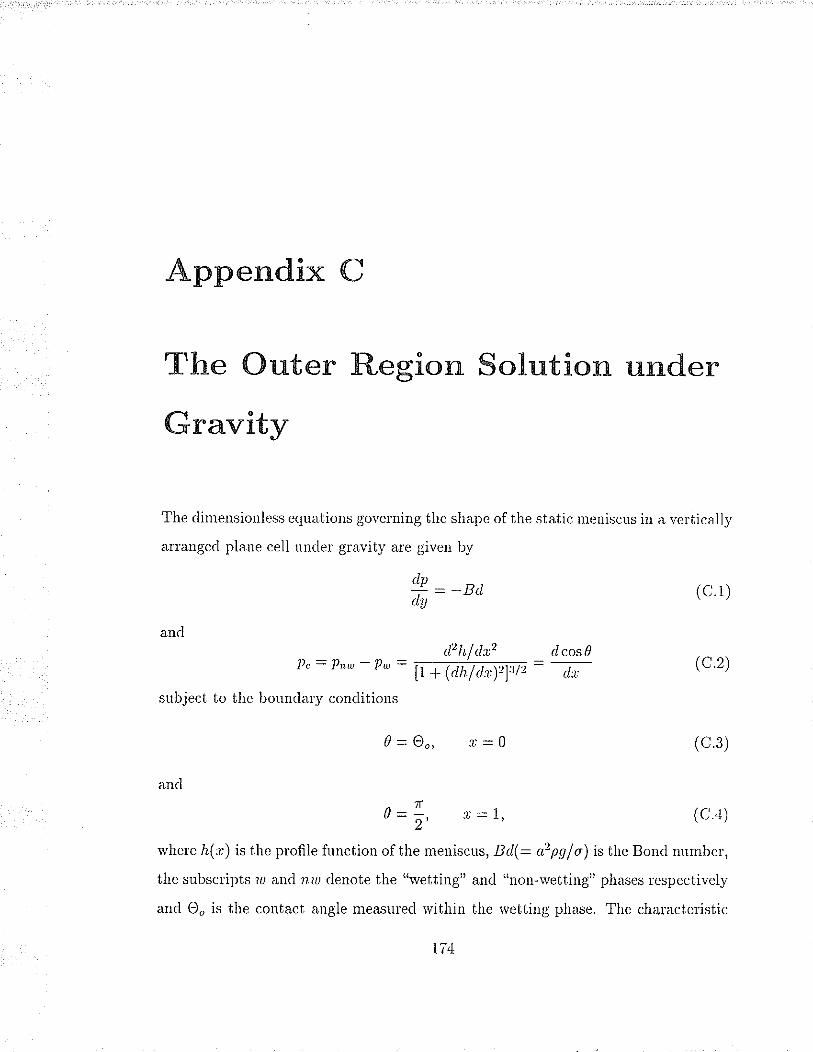
Appendix C
The Outer Region Solution under
Gravity
The ilimeusionless ecluations govelning the shape of the static ¡neniscns in a veltically
alrangecl plane cell unclel gravity ale given by
9--unda
¿2hl¿r2 tlcos 0_" _---------------_t'c - vtltu r* - lL-t(dhldtlzlttz - ,r.,
su):ject to the bounclaly conclitions
0 -- o,, ¿=0
(c.1)
(c.2)
(c.3)
(c 4)
ancl
rvlrele å(:r) is the plofile function of the meniscus, B d(: azrO¡o¡ is the Boncl number,
the subscripts'¿u ancl r¿'¿u denote the "wetting" ancl "non-rvetting" phases lespectively
ancl O, is the contact angle measulecl rvithin the rvetting phase. The chalacteristic
t71

APPENDIX C. THE OUTER REGION SOLUTION Ui\?ER GRAVITY 17i
length is ¿. The chalactelistic plessnle is of a. It oul ploblenr, the uon-rvetting phase
is air'. The pressLrre glaclient in the ail'is so small tltat it can be neglectecl. Tllerefole
p,,,, is constant anrl can be set to zeto. Tlìen Equtrtion (C.2) cau ì-:e r.educed to
tl cos 0lrt
1:t:(c.5)
rvhele the suìrsclipt 'ru on p has been clrop rvith ¡ro confusion.
Undcr the conclitiou of surall Bolcl nulnber' (B¿ << I). the fuuctious 7r aucl cos á
carr be ex¡>an<lcd as:
p=po*BrLp¡!...
ancl
cosá : cosdo I Btl cos?y ¡...
The lorvest-olcler pressrlre fielcl ancl interface shape satisf¡
d1t6
ancltlcos06
n = - po,
subject to the bounclaly conditions
cosd6 = ç95Qo, ¿=0,
(c 6)
(c 7)
(c.8)
(c.e)
(c,10)
(c.11)
(c.12)
(c,13)
ancl
cos d6 = [,
The solution for ps ancl cos9o aÌe
z=1
Po = -cosOo
cos de = (1 - r) cos O,.
ancl

APPETYDL\ C. THE OUTER REGION SOLU?ION UTVDER GR,\\,'ITY l/t)
He¡rce the lorvest-orcìel pressule fielcl is constant ¿nrl the lorvest-oldel intelface shape
is the alc of a citcle.
The fir'st-olcler pr:essllre fielcl ancl interface shape satisfy
ancldcos9r _
tl:tt
subject to the bouudaly cotì(litious
tLn '-_:_i - _1
tlv -
-Pt, at Y: lìo(rÌ),
(c.14)
(c.1õ)
(c.16)
(c.i7)
L3), lr¡(r) cau
cosd¡: g, c=0
aucl
cosÉ1 = g, ¿: 1.
Florn the lorvest-olcter- irtelf¿rce shape solution givel b¡' Ec¡raltiou (C
be clerivecl as
å6(ø) - tan Oo - [sec2 Oo - (1 - ¿-)'z]; (c.18)
The sohrtions ale
e, : -;tan o, * [sec2 o, - (1 - ¿)r]+ - iri -o,)sec2 oo (c.1e)
ancl
2 cos01 = ltano,+(f, -o,¡...,o,] {t -") -(r -")[sec2o,- (r -r)rjå- sec2 Oo arcsin[(I - c) cos O,]. (C.20)
Thelefole, the pelturbation solution of the shape of the static meniscus, valid as
Bd -+ 0, is
cosá - (1 -ø) coso, +f,aa{ltano,+(f, - o,).."'o,] {t -')-(1 - ,) [sec2 oo - (1 - r)'?]å - sec2 Oo alcsin[(l - c) cos O'] [.C.zt)

APPETVD.LY C. THE OUTER REGION SOLUTION UTYDER GRÅVITY 1.77
1.6
1.4
l.¿
1.0
0.8
0.6
o.4
0.2
0.00.0 0.2
-lu)@!
oo
o,4 0.6
x/o
1.0
Figule C.1: The gravity effects on the outer region solution of a meniscus.
As in the special case Bd - 0, the solution clegenelates into a no glavity solution (z.e
a cilcular meniscus):
cosd = (1 - c) cosO, (c.22)
The gravity effect on the shape of the meniscns is shorvn in Figule C.1. Fol the
testing cell with 1.77B 'n¿m slot size (Brl:0.224), the clevi¿tion in the slope angle of
the meniscus resulting from the gravity effect is appleciable (about 1.0'in the profile
range measurecl).
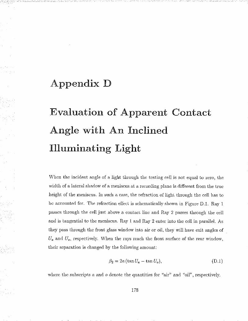
Appendix D
Evaluation of Apparent Contact
Angle with An Inclined
Illuminating Light
lVhen the incicleut angle of a light thloLrgh the testing cell is not ec¡ral to zero, the
wiclth of a latelal shaclorv of a meniscus at a recorcling plane is cliffelent fi.o¡n the tr.ue
height of the meniscus. In such a case, the lefi.action of light tlirough the cell has to
be accountecl for'. The refi'action effect is schematically shorvn in Figule D.1. Ray 1
passes through the cell just above a contact line and Ray 2 passes thr.ough the cell
ancl is tangential to the meniscus. Ray 1 and Ray 2 enter into ilie cell in parallel. As
they pass through the front glass winclorv into ¿ir or oil, they tvill h¿ve exit angles of
U" and Uo, respectively. lVhen the i'ays reach the front sulface of the rear rvinclotv,
their sepalation is changecl by the follorving amoltnt:
þz = 2a(tanU" - tan U,), (D.1)
rvhele the subscripts ¿ ancl o denote the c¡uantities for' "air" ancl "oil", respectively
178

APPEiYDI.X D, EVALUATION OF APPARENT CONTACT ANG¿E 179
(D 3)
Because Ray 1 and Ray 2 do not pass thlotgh the meniscns and the cell sLrrfaces aLe
all palallel to each other', rvhen the Iays pass through the cell, they will still be palallel
Figule D.1: Nomeltclatute oflefraction effect oflight throLrgh a cell lvith an inclination
angle.
The sepalation of Ray 1 and Ray 2 ¿t the fiont windoiv can be ev¿luated as
follorvs:
h = DF-DE+EF-EE-BD+EFa=
"*il*¿ - a(tanu" - tanuo)* ø(tantl" - tano¡)
a= ^ ,, - a (tan O¡ - tanU"). (D.2)
CoS (rÀ COS Uo
The sepalation of the rays at the front of the rear winclorv, B, is the sum of B1 ân(l
B2; that is,
þ = At +8, = " [æ**r, *2 tanUo - tan[J"- tanOr,]

APPÐNDI-X D. E\ALUATION OF APPARENT CONTACT ANGLE 180
as they exit it. As they conti¡me to travel to the leco::cling plarre, their. separ.ation
rvill not be changecl. Therefore, the recordecl height of the me¡riscus shadoiv is ec¡ral
to B and is relatecì io the appalent contact angle O¡.