1

ON THE CAPILLARY PRESSURE FUNCTION IN POROUS MEDIA BASED ON RELATIVE 1

PERMEABILITYIES OF TWO IMMISCIBLE FLUIDS 2

3

A.J. Babchin1 and B. Faybishenko2* 4 1) Alberta Research Council, Edmonton, Canada, and Tel Aviv University, Israel 5

, 2) Lawrence Berkeley National Laboratory, Berkeley, California, USA. 6 *) Corresponding Author; tel: 510-486-4852, fax: 510-486-5686, e-mail: bafaybishenko@lbl.gov 7

8

9

Abstract 10

The authors proposed a new analytical approach and derived an explicit formula to the 11

determination of a capillary pressure (Pc) curve in porous media, by combining the first 12

principles of surface science with classical concept of the phase relative permeability. The 13

developed formulae for Pc and a modified Leverett Jm-function are based on the relative 14

permeability functions for the wetting and nonwetting phases, an apparent specific surface area, 15

and an apparent (calculated) contact angle . The application of the proposed approach was 16

tested using several sets of data from existing publications. The developed Jm-function can be 17

described using the Weibull distribution model for the drainage and imbibition conditions. The 18

new approach can generally be used for any type of the relative permeability functions and 19

different types of a nonwetting phase. 20

21

Key Words: Immiscible fluids, capillary pressure, relative permeability, specific surface area, 22

porous media, Leverett J-function. 23

24

25

1. Introduction 26

Knowledge of reliable capillary pressure vs. saturation and relative permeability relationships is 27

an important aspect in the field of numerical simulations of transport of non-aqueous phase 28

Manuscript submitted to "Colloids and Surfaces A: Physicochemical and Engineering Aspects," June 16, 2014

2

liquids (NAPLs), including hydrocarbon liquids (oils), Dense NAPLs (DNAPLs), and Light NAPLs 29

(LNAPs), in the subsurface. In their recent review of theoretical and experimental studies on the 30

topic of spontaneous imbibition into porous and fractured media, Mason and Morrow [1] noted 31

that there are fundamental problems with the application of differential equations for modeling 32

approach, because of the nature and choice of appropriate relationships for the two (wetting 33

and nonwetting) relative permeabilities and capillary pressure as functions of saturation. This 34

issue has never been addressed in detail, and it is not clear how these functions should be 35

measured [1,2]. Several studies showed that the use of a single effective average contact angle, 36

i.e, cos(), is not a physically correct approach for systems where there is a distribution of 37

contact angles, especially in the event of the fractional wettability, nonwetting phase 38

entrapment, and redistribution of nonwetting phase between different types of pores [3-9]. 39

Direct measurement of two-fluid interfacial areas is difficult [8, 10]. 40

41

In this paper, the authors propose to determine first an apparent specific surface area, using an 42

explicit combination of the relative permeability functions for the wetting and nonwetting 43

phases, which then will be used to assess the capillary pressure-saturation function. The results 44

of calculations using a new approach for the drainage and imbibition capillary pressure curves is 45

demonstrated using the data from [11-13]. 46

47

2. Theoretical Background of a Proposed Approach 48

Numerical simulations of transport phenomena of two immiscible fluids, such as NAPL and 49

water, in porous media are usually based on using the Darcy law, in which relative permeabilities 50

for both the wetting and nonwetting phases are expressed as dimensionless functions: 51

52

3

where K is the porous media absolute permeability, Krn and Krw are relative permeability of 53

nonwetting and wetting phases, correspondingly, n and w are viscosity of nonwetting and 54

wetting phases, correspondingly, and Pn and Pw are pressures of nonwetting and wetting phases, 55

and capillary pressure is given by Pc = Pn – Pw. 56

57

For the purpose of simulation of flow of two immiscible fluids, Pc is often expressed by means of 58

the Leverett-J function [14]. Purcell [15] introduced the relation between the permeability and 59

capillary pressure. In his comments to the Purcell’s paper, Rose [16] presented an expression for 60

permeability, using the fractional wetting phase saturation and Leverett’s capillary pressure 61

function. Burdine [17] introduced a tortuosity factor in the model describing the relationship 62

between the relative permeability and capillary function, which for the case of two-phase flow is 63

given by 64

65

(1) 66

67

where w and n are the tortuosity factors, and symbols w and n are related to the wetting and 68

nonwetting phases. However, the tortuosity factors are not explicitly defined and cannot be 69

measure, thus, being just fitting parameters. 70

71

Rapoport and Leas [18] were probably the first who suggested that the capillary pressure (Pc) 72

and permeability functions are dependent on interfacial areas (although they have been typically 73

modeled as functions of fluid saturation). In the past about 20-25 years, various numerical 74

4

models and modeling techniques have been developed to simulate subsurface multiphase flow, 75

such as pore network models and Lattice-Boltzmann models [19-22]. An application of a 76

thermodynamically constrained macroscale description of flow in porous media, explicitly taking 77

into account the presence of interfaces, was proposed in [23-24]. Despite the wide interest in 78

measuring and calculating specific interfacial area and capillary pressure, there are surprisingly 79

very few works on this subject [25]. 80

81

Contrary to one-phase flow, when the specific surface area averaged over total volume of core 82

sample, is a constant value, in the case of two-phase flow of immiscible fluids, the total specific 83

surface area is a function of the phases distribution, and the total specific surface area is the sum 84

of phase specific surfaces. The wetting phase tends to reside in smaller pores, while nonwetting 85

fluid resides in larger pores. At residual wetting and nonwetting saturations the specific surface 86

values asymptotically approach infinity. Indeed, the residual phase is located in smallest 87

capillaries, as tiny ganglia, or as pendulum drops, bridging the solid grains. All this configurations 88

have very small radii, and, thus, high capillary pressure, exhibiting high capillary resistance to 89

flow, which the pressure gradient, imposed by displacement fluid flow is incapable to 90

overcome. Complete immobilization of the residual fluid is either equivalent to apparent radii 91

approaching zero value, or to specific surface approaching infinity. In other words, capillarity 92

effects should be taken into account in the evaluation of the specific surface area for a two-93

phase flow system in porous media, as these effects induce additional resistance to flow. Even 94

in simplified droplet train model capillary forces are capable to induce additional resistance to 95

flow [26]. 96

97

Babchin and Nasr [27] derived a simplified analytical expression for the capillary pressure 98

gradient in homogeneous porous two-fluid media, containing three bulk phases (solid phase, 99

wetting and nonwetting fluids), with three possible interfaces (solid-wetting, solid-nonwetting, 100

and nonwetting-wetting). They assumed a finite value of the three-phase contact angle 101

between two fluids and a solid phase of porous rock, and that the contact surface area between 102

two continuous fluid phases is small in comparison with contact surface areas between each 103

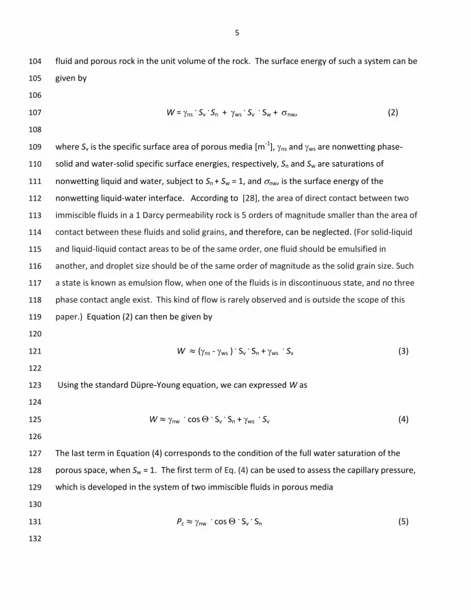
5

fluid and porous rock in the unit volume of the rock. The surface energy of such a system can be 104

given by 105

106

W = ns . Sv

. Sn + ws . Sv

. Sw + nw, (2) 107

108

where Sv is the specific surface area of porous media [m-1], ns and ws are nonwetting phase-109

solid and water-solid specific surface energies, respectively, Sn and Sw are saturations of 110

nonwetting liquid and water, subject to Sn + Sw = 1, and nw, is the surface energy of the 111

nonwetting liquid-water interface. According to [28], the area of direct contact between two 112

immiscible fluids in a 1 Darcy permeability rock is 5 orders of magnitude smaller than the area of 113

contact between these fluids and solid grains, and therefore, can be neglected. (For solid-liquid 114

and liquid-liquid contact areas to be of the same order, one fluid should be emulsified in 115

another, and droplet size should be of the same order of magnitude as the solid grain size. Such 116

a state is known as emulsion flow, when one of the fluids is in discontinuous state, and no three 117

phase contact angle exist. This kind of flow is rarely observed and is outside the scope of this 118

paper.) Equation (2) can then be given by 119

120

W (ns - ws ) . Sv

. Sn + ws . Sv (3) 121

122

Using the standard Düpre-Young equation, we can expressed W as 123

124

W nw . cos . Sv . Sn + ws

. Sv (4) 125

126

The last term in Equation (4) corresponds to the condition of the full water saturation of the 127

porous space, when Sw = 1. The first term of Eq. (4) can be used to assess the capillary pressure, 128

which is developed in the system of two immiscible fluids in porous media 129

130

Pc nw . cos . Sv . Sn (5) 131

132

6

The value of Sv in Eq. (5) can be expressed as an averaged value for a volume V of porous media 133

in the following integral form: 134

Sv =

(6) 135

The value in Eq.6 can be presented as a sum of two components—one for nonwetting, the 136

other for wetting phases, both being saturation dependent. For a general case of a single fluid 137

residing in porous media, the averaged pore size can be expressed in term of the equivalent 138

pore radius, re, using either (a) the apparent specific surface , or (b) porous media 139

permeability, K, and porosity, , given by 140

re = 1/Sv (7a) 141

re = (K/)1/2 (7b) 142

By equating Eqs. (7a) and (7b), the relationship for the averaged Sv is given by 143

Sv= (/K)1/2 (8) 144

In the case of transport of two immiscible fluids in porous media, the permeabilities of 145

nonwetting and wetting phases, subject to Snw + Sw = 1, can be expressed in terms of their 146

relative permeabilities, which are functions of phase saturations, given by 147

Knw = K Knr (Snw) 148

Kw = K Kwr (Sw) (9) 149

7

Using Eqs. (8) and (9), and assuming a constant porosity, , we can define the equations to 150

describe the relationships between the apparent specific surface area and permeability of each 151

phase: 152

n = [/ (K Knr) ]

1/2 (10a) 153

w = [ / (K Kwr) ]

1/2 (10b) 154

The total apparent specific surface, averaged within the volume V, and which is a function of the 155

liquid phases saturation, can be expresses as the sum of Eqs. (10a) and (10b) given by: 156

Sv = n +

w = 1/2 [ ( 1/ K Krnw )1/2 + ( 1 / K Krw)1/2 ] 157

or 158

Sv = (/K)1/2 (Krnw1/2 + Krw

1/2)/ (Krnw * Krw)1/2 (11) 159

At the residual saturation points Srnw and Srw, for nonwetting and wetting phases, respectfully, 160

the solution of Eq. (11) will result to singularities (i.e, function that is not differentiable), which 161

corresponds to well-known phenomena of an infinite suction pressure at the irreducible 162

saturation [28]. The physical explanation of these phenomena is as follows: at the residual 163

saturation points, the fluid phase resides in tiny pores or in the form of bridges matching the 164

grains or tiny ganglia, all of them having very small radius, rendering very high capillary pressure, 165

resisting either displacement or imbibition process beyond residual saturation points. For 166

example, the residual oil saturation is defined, generally, as the oil content that remains in an oil 167

reservoir at depletion, when oil ceases to recover [29]. The residual oil saturation in the 168

reservoir can range from 2% to 50%, with an approximate average from 15% to 20% [30]. Note 169

8

that the results of laboratory and field tests are often inconsistent and lead to the uncertainty in 170

the values of the oil residual saturation [31]. 171

To remove infinite values upon calculations, we can employ the system of reduced (normalized) 172

saturations Snn and Swn for nonwetting and wetting phases, respectively given by [11]: 173

Snn = (Sn – Snr ) / (1 – Snr – Swr) (12a) 174

Swn = (Sw – Swr ) / (1 – Sor – Swr) (12b) 175

Expressing nonwetting phase saturation in the reduced (normalized) form, we finally come to 176

the following expression for the nonwetting phase–water–solids capillary pressure: 177

Pc = nw cos . Sv . Snn + A (13) 178

where Sv is given by Eq. (11), Snn is given by Eq. (12), A is a constant that corresponds to initial 179

displacement pressure, when wetting phase is displaced by nonwetting phase, and A=0 for 180

imbibition [11]. Thus, based on Eq. (13), intrinsic hysteresis of Pc for drainage (water is displaced 181

by nonwetting phase) and imbibition (nonwetting phase is displaced by water) conditions is 182

determined within the constant. 183

184

3. Application of the Proposed Approach and Results of Calculations 185

The proposed approach was tested using a comparison of the results of calculations of Pc with 186

published data given by Collins [11], Das et al. [12], Beckner et al. [13, 32]. The input parameters 187

for calculations of relative permeability and Pc curves, which were taken from these publications, 188

9

are summarized in Table 1. (The graphs plotted in the referenced publications were digitized 189

using the Plot Digitizer, Version 2.6.4, a Java program written by J.A. Huwaldt 190

http://plotdigitizer.sourceforge.net ) 191

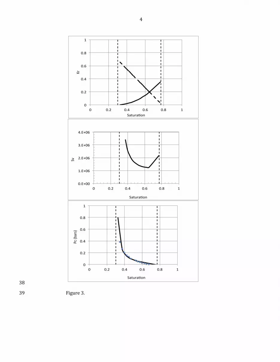
Figures 1 through 4 depict the relative permeability curves (upper figures), apparent specific 192

areas vs. saturation (middle figures) calculated from Eq. (11), and the resulting relationships Pc 193

vs. Sw (lower figures), calculated from Eq. 13. In calculations of the drainage curves, we used 194

constant values of A that equal to the capillary pressure at the residual saturation point Sor, and 195

for the imbibition curves, A=0. The match between the calculated and experimental Pc curves 196

was achieved using the contact angles given in Table 1. Note that in all cases, the contact angle 197

0 << 90o, indicative of water-wet conditions. The fact that the calculated contact angle > 0 198

could be explained by the fractional wettability of porous media [3, 33]. Based on the results of 199

calculations of cos given in Table 1, fractional wettability varies from 0.05 to 0.31. The 200

correlation analysis showed no correlation of the calculated apparent contact angle with the 201

absolute permeability, porosity, and specific surface area. 202

The results of Pc calculations from Eq. (13) were then used to evaluate a modified Leverett Jm-203

function given by 204

(14) 205

where cos is determined using the contact angle given in Table 1, Pc is taken in Bars, 206

absolute permeability K is in m2, and is in N/m, and the values of normalized wetting phase 207

saturation Swn are determined from Eq. (12b). 208

10

Combining Eqs. (13) and (14), we obtain a new form of the modified Leverett function given by 209

(15) 210

For the imbibition curve, when A = 0, Eq. (15) can be simplified to 211

(16) 212

Figure 5 of the modified Leverett function (Jm) vs. the normalized wetting saturation (Swn) shows 213

that despite of a significant difference in absolute and relative permeabilities and capillary 214

pressure curves shown in Figures 1 though 4, the scattering of points around the modified 215

Leverett Jm(Swn) function is minimal. 216

Statistical analysis of the calculated Pc values of shown in Figures 1 through 4, shows that the 217

modified Leverett Jm(Swn) function can be described using a 4-parameter Weibull distribution 218

model given by 219

(17) 220

with the following coefficients: a = 0.000589, b = 0.000582, c = 0.02208, and 221

d = -0.80742213. The value of A = 1.98E-5 in Eq. (15) for drainage, and A = 0 for imbibition. (The 222

coefficient of correlation of fitting of Eq. (15) to the experimental data shown in Figure 5 is 0.98.) 223

Note that the Weibull distribution model is one of the most widely used statistical distribution 224

models in reliability engineering and statistical data analysis due to its versatility. 225

226

4. Conclusions 227

11

Based on the notion of the specific surface area, the authors presented an analytical approach to 228

the determination of the capillary pressure curve and a modified Leverett Jm- function of two 229

immiscible fluids in porous media, using a combination of the relative permeability functions for 230

the wetting and nonwetting phases along with an equation for an apparent specific surface area 231

and an apparent contact angle. Based on the Leverett Jm-function for Pc in terms of relative 232

permeability, a solution for unstable fingering front of heavy oil displacement by water, 233

considered [34], can be resolved analytically. 234

235

In this paper, the results of calculations of Pc were used to assess the values of the contact angle 236

, which was then applied to assess the modified Leverett Jm-function versus the normalized 237

wetting phase saturation. The Jm-function is described using the Weibull distribution model for 238

both the drainage and imbibition conditions. 239

240

Acknowledgement: The work of the 2nd author was partially supported by the Sustainable 241

Systems Scientific Focus Area (SFA) program at LBNL, supported by the U.S. Department of 242

Energy, Office of Science, Office of Biological and Environmental Research, Subsurface 243

Biogeochemical Research Program, through Contract No. DE-AC02-05CH11231 between 244

Lawrence Berkeley National Laboratory and the U. S. Department of Energy. 245

246

247

References 248

249

[1] Mason J., and N. Morrow, Developments in spontaneous imbibition and possibilities for 250

future work, Journal of Petroleum Science and Engineering. 110 (2013) 268–293, 2013 251

[2] Larson, R.G., and N.R. Morrow, Effects of Sample Size on Capillary Pressures in Porous Media, 252

Powder Technology. 30 (1981) 123-138. 253

[3] Bradford, S.A., and F.J. Leij, Fractional wettability effects on two-and three-fluid capillary 254

pressure-saturation relations, Journal of Contaminant Hydrology 20 (1995) 89-109. 255

[4] van Dijke, M.I.J.. K.S. Sorbie, S.R. McDougall, Saturation-dependencies of three-phase 256

relative permeabilities in mixed-wet and fractionally wet systems, Adv in Water Resources 24 257

(2001) 365-384. 258

[6] Behbahani, H.Sh., Blunt, M.J., Analysis of imbibition in mixed wet rocks using pore-scale 259

modelling. SPE 90132, Annual Technical Conference and Exhibition, Houston, Texas, USA. 260

(2004). 261

12

[7] Behbahani, H. Sh., G.Di Donato, M.J. Blunt, Simulation of counter-current imbibition in water-262

wet fractured reservoirs, Journal of Petroleum Science and Engineering 50 (2006) 21– 39. 263

[8] Schramm, L.L, Surfactants: Fundamentals and Applications in the Petroleum Industry, 264

Cambridge University Press, 2010. 265

[9] Raeesi, B., N.R. Morrow, G. Mason, Effect of surface roughness on wettability and 266

displacement curvature in tubes of uniform cross-section, Colloids and Surfaces A: 267

Physicochemical and Engineering Aspects, Colloids and Surfaces A: Physicochem. Eng. Aspects 268

436 (2013) 392– 401. 269

[10] O’Carroll, D.M., L.M. Abriola,T, Catherine A. Polityka, S.A. Bradford, A.H. Demond, 270

Prediction of two-phase capillary pressure–saturation relationships in fractional wettability 271

systems, Journal of Contaminant Hydrology 77 (2005) 247– 270 272

[11] Collins, R.E., Flow of Fluids through Porous Materials, Reinhold Publishing Corporation, New 273

York. 1961. 274

[12] Das, D. B., S. M. Hassanizadeh, B.E. Rotter and B.Ataie-Ashtiani, A Numerical Study of Micro-275

heterogeneity Effects on Upscaled Properties of Two-phase Flow in Porous Media, Transport 276

in Porous Media 56 (2004) 329–350. 277

[13] Beckner, B. L., A. Firoozabadi, K. Aziz, Modeling transverse imbibition in double-porosity 278

simulators, paper presented at SPE California Regional Meeting, Long Beach, Calif., 23–25 279

March. 1988. 280

[14] Bear, J., Dynamics of Fluids in Porous Media, Dover Publications, 1972. 281

[15] Purcell, W. R., Capillary pressures—Their measurement using mercury and the calculation of 282

permeability, Trans. AIME, 186 (1949) 39-46. 283

[16] Rose, W. Comments to the paper by Purcel, Trans. AIME, 186 (1949) 46-48. 284

[17] Burdine, N. T., Relative permeability calculations from pore size distribution data, Trans. 285

AIME, 198 (1953) 71. 286

[18] Rapoport, L.A., Leas, W.J., 1951. Relative permeability to liquid in liquid-gas systems. Trans. 287

Am. Inst. Mineral. Metall. Petrol. Eng. 192, 83-95. 288

[19] Reeves P. and M. Celia. A functional relationship between capillary pressure, saturation, and 289

interfacial area as revealed by a pore-scale network model. Water Resources Research, 32 290

(1996), 2345–2358,. 291

[20] Held P. and M. Celia. Modeling support of functional relationships between capillary 292

pressure, saturation, interfacial area and common lines. Advances in Water Resources, 24 293

(2001) 325–343. 294

[21] Culligan, K.A., D.Wildenschild, B.S. Christensen, W.G. Gray, M.L. Rivers, and A.F.B.Tompson, 295

Interfacial area measurements for unsaturated flow through a porous medium, Water Resour. 296

Res., 40 (2004), W12413. 297

[22] Niessner J. and S.M. Hassanizadeh. A Model for Two-Phase Flow in Porous Media Including 298

Fluid–Fluid Interfacial Area. Water Resour. Res., 44 (2008) W08439. 299

[23] Gray, W. G., and S. M. Hassanizadeh (1989), Averaging theorems and averaged equations 300

for transport of interface properties in multiphase systems, Int. J. Multiphase Flow, 15, 81– 301

95. 302

[24] Gray, W. G., A. F. B. Tompson, and W. E. Soll, Closure conditions for two-fluid flow in porous 303

media, Transp. Porous Media, 47 (2002) 29–65. 304

[25] Joekar-Niasar, V., S. M. Hassanizadeh, and A. Leijnse. Insights into the relationship among 305

13

capillary pressure, saturation, interfacial area and relative permeability using pore-scale 306

network modeling. Transport in Porous Media, 74 (2008) 201–219. 307

[26] Babchin and J.-Y Yuang, On the Capillary Coupling between Two Phases in a Droplet Train 308

Model, Transport in Porous Media, 26 (1997) 225-228. 309

[27] Babchin, A.J., T.N. Nasr, Analytical Model of the Capillary Pressure Gradient in Oil-Water-Rock 310

System, Transport in Porous Media, 65 (2006) 359-362. 311

[28] Brooks, R.H., and Corey, A.T., Hydraulic Properties of Porous Media, Hydrol. Pap.3. Colorado 312

St ate University, Fort Collins (1964). 313

[29] Bradley, H.B., Petroleum Engineering Handbook, 1st edition, Society of Petroleum Engineers, 314

1987. ISBN 1-55563-010-3. 315

[30] Morrow, N.R., A Review of the Effects of Initial Saturation, Pore Structure and Wettability 316

on Oil Recovery by Waterflooding, In Proc. North Sea Oil and Gas Reservoirs Seminar, 317

Trondheim (December 2-4, 1985), Graham and Trotman, Ltd., London (1987) 179 -191. 318

[31] Donaldson, E.C., G.V. Chilingarian, T.F. Yen, Enhanced Oil Recovery, II: Processes and 319

Operations, Elsevier, 1989. 320

[32] Li K. and R.N. Horne, Comparison of methods to calculate relative permeability from 321

capillary pressure in consolidated water-wet porous media, Water Resour. Res., 42 (2005) 322

W06405. 323

[33] Boinovich, L. and A.M. Emelyanenko, The Analysis of the Parameters of Three-phase 324

Coexistence in the Course of Long-term Contact between a Superhydrophobic Surface and an 325

Aqueous Medium, Chem. Lett. 41 (2012). 326

[34] Babchin, A., I.Brailovsky, P.Gordon, and G.Sivashinsky, On Fingering Instability in Immiscible 327

Displacement, Physical Review E, 03 (2008) 77. 328

329

330

331

332

333

Table 1. Parameters used for calculations of Pc.

Parameters Das et al. (2004)

Beckner et al. (1988)

(cited in Li and

Horne, 2006, Fig.9)

Collins (1961,

Fig. 6-7)

Collins (1961,

Fig. 6-13)

Porosity, 0.4 0.225 0.225 0.32

Permeability, K (m2) 5.00E-12 2.90E-12 2.90E-12 1.97E-13

(N/m) 0.02 0.048 0.03 0.048

Srn 0.92 0.75 0.75 0.85

Swr 0.098 0.346 0.3 0.092

A (bars) 0.0135 0.04 0 0.1

Calculated apparent

contact angle

(deg) 87 80 72 84

Nonwetting fluid PCE oil oil oil

Table(s)

1

A. Babchin, B.Faybishenko, ON THE CAPILLARY PRESSURE FUNCTION IN POROUS MEDIA 1

BASED ON RELATIVE PERMEABILITYIES OF TWO IMMISCIBLE FLUIDS 2

3

Figure Captions 4

Figure 1. Comparison of calculated Pc curves with data from the paper by Das et al. [12]: upper 5

figure—relative permeability curves (solid curve—wetting phase, dashed curve—nonwetting 6

phase), middle figure—calculated specific surface area, and lower figure—calculated Pc curves: 7

symbols are from [12], and a solid line is a calculated Pc curve). Left vertical dashed line –residual 8

wetting phase saturation, and right vertical dashed line—nonwetting phase residual saturation. 9

Figure 2. Comparison of calculated Pc curves with data from [13] (as given in [32]: upper figure—10

relative permeability curves (solid curve—wetting phase, dashed curve—nonwetting phase), middle 11

figure—calculated specific surface area, and lower figure—calculated Pc curves: symbols are from Das 12

et al., 2004, and a solid line is a calculated Pc curve). 13

Figure 3. Comparison of calculated Pc curves with data from Figure 6-7 of the book by Collins [11]: 14

upper figure—relative permeability curves (solid curve—wetting phase, dashed curve—nonwetting 15

phase), middle figure—calculated specific surface area, and lower figure—calculated Pc curves: 16

symbols are from [11], and a solid line is a calculated Pc curve). 17

Figure 4. Comparison of calculated Pc curves with data from Figure 6-13 of the book by Collins [11]: 18

upper figure—relative permeability curves (solid curve—wetting phase, dashed curve—nonwetting 19

phase), middle figure—calculated specific surface area, and lower figure—calculated Pc curves: 20

symbols are from Collins [11], and a solid line is a calculated Pc curve). 21

Figure 5. Modified Leveret Jm-function calculated using the Pc from Eq.(13), with K, and 22

given in Table 1 vs. normalized saturation calculated from Eq. (12b), and fitting curves for the 23

drainage and imbibition described by the Weibull formula Eq. (14). 24

25

26

27

28

29

30

31

32

Figure(s)

2

33

34

Figure 1. 35

1.E+05

1.E+06

1.E+07

1.E+08

0 0.2 0.4 0.6 0.8 1

Sv

Satura on

0

0.2

0.4

0.6

0.8

1

0 0.2 0.4 0.6 0.8 1

Kr

Satura on

0

0.02

0.04

0.06

0.08

0.1

0.12

0 0.2 0.4 0.6 0.8 1

Pc

(bar

s)

Saturation

3

36

Figure 2. 37

0

0.1

0.2

0.3

0.4

0.5

0.0 0.2 0.4 0.6 0.8

Ps

(bar

s)

saturation

0

0.2

0.4

0.6

0.8

1

0 0.2 0.4 0.6 0.8

Kr

Saturation

1.E+06

2.E+06

3.E+06

4.E+06

0 0.2 0.4 0.6 0.8

Sv

Satura on

4

38

Figure 3. 39

0

0.2

0.4

0.6

0.8

1

0 0.2 0.4 0.6 0.8 1

Pc(b

ars)

Satura on

0

0.2

0.4

0.6

0.8

1

0 0.2 0.4 0.6 0.8 1

Kr

Satura on

0.E+00

1.E+06

2.E+06

3.E+06

4.E+06

0 0.2 0.4 0.6 0.8 1

Sv

Satura on

5

40

Figure 4. 41

0

0.2

0.4

0.6

0.8

1

0 0.2 0.4 0.6 0.8 1

Kr

Satura on

1.E+05

1.E+06

1.E+07

1.E+08

1.E+09

0 0.2 0.4 0.6 0.8 1

Sv

Satura on

Svvs.Sw

0.0

0.2

0.4

0.6

0.8

1.0

1.2

1.4

1.6

0 0.2 0.4 0.6 0.8 1

Pc(b

ars)

Satura on

drainage

imbibi on

6

42

Figure 5. 43

44