European Journal of Mechanics B/Fluids ( ) –

Contents lists available at SciVerse ScienceDirect

European Journal of Mechanics B/Fluids

journal homepage: www.elsevier.com/locate/ejmflu

Vertical excitation of axisymmetric liquid bridgesJ.-B. Valsamis a,∗, M. Mastrangeli b, P. Lambert aa BEAMS Department CP 165/56, Université Libre de Bruxelles, Avenue F. D. Roosevelt 50, B-1050 Bruxelles, Belgiumb Ecole Polytechnique Fédérale de Lausanne (EPFL), CH-1015 Lausanne, Switzerland

a r t i c l e i n f o

Article history:Received 29 May 2012Accepted 28 September 2012Available online xxxx

Keywords:MicrofluidicsMechanical modelFree interfaceKelvin–Voigt systemVertical oscillation

a b s t r a c t

This study presents an analytical model of the dynamics of an axisymmetric liquid bridge confinedbetween two circular pads and subjected to small vertical periodic perturbations. Such system findsimportant applications in microassembly and microjoint design, where force and damping need tobe precisely controlled. The liquid bridge is modelled by an equivalent spring/dashpot/mass systemcharacterised by the spring constant k, the damping coefficient b and the equivalent massm, respectively.An abacus for k as well as analytical approximations for k, b and m based on simplifications of theNavier–Stokes equation are provided. The study is validated by experiments and numerical simulationsof the system. We describe the experimental setup we designed to investigate vertical forces arising onthe bottom pad from small periodic perturbations of the top pad confining the liquid meniscus. The setupallowed the accurate control of all physical and geometrical parameters relevant for the experiments. Theparameters we investigated are both physical (viscosity and surface tension of the fluid) and geometrical(the edge angle between the meniscus and the pad, the height of the meniscus). The good agreementbetween model predictions and results let us conclude that k, b andm involve only one physical propertyof the liquid, namely the surface tension, the viscosity and the density, respectively.

© 2012 Elsevier Masson SAS. All rights reserved.

1. Introduction

Liquid bridges are liquid volumes confined between two solidsurfaces and surrounded by another fluid (most commonly, air).Mechanically, liquid bridges can be considered as joints betweentwo solids (e.g. a substrate and a component). Upon perturbation,they generate capillary forces that can be repulsive or attractivedepending on several properties of the fluid and the boundingsolids. These properties are both geometrical and physical [1–3].

Forces generated by liquid bridges are ubiquitous, and techno-logically relevant for e.g. flip-chip electronic assembly [4–6] andcapillary self-assembly of micro- and nanosystems [7,8]. Analyti-cal models and quasi-static numerical simulations – typically per-formed through Surface Evolver [9] – for such applications arewidely reported [3,10]. Different degrees of freedom are therebystrained, and the restoring forces or torques are computed. Al-though fully three-dimensional, these numerical models do notcontemplate dynamics.

Dynamical studies were introduced by van Veen [11] andMeurisse and Querry [12]. They proposed analytical models for

∗ Corresponding author.E-mail address: jvalsami@ulb.ac.be (J.-B. Valsamis).

dynamical parameters and restoring forces, and for the pressure ofthe liquid bridge as a function of the inverse of its gap, respectively.Cheneler et al. proposed an analysis of a liquid bridge to develop amicro-rheometer [13]. The liquid ismodelled as a dashpot in serieswith a calibrated spring/mass system. By measuring the phaseshift between the position of the mass and the force exerted, thefriction can be deduced. However, inertial effects are not includedin the model, and the study is not supported with experimentaldata.

Engmann et al. [14] presented a comprehensive review ofmain analytical expressions of viscous force corresponding toseveral squeeze film configurations, e.g. through slipping, non-slipping, viscoelastic, viscoplastic. In particular, the expressions ofthe viscous term developed by Pitois et al. [15] can thereby berecovered.

Concerning numerical simulations, Boufercha et al. [16] es-timated the time response and the position error of a self-positioning process of a chip on a substrate. The simulationincludes the motion of a liquid drop crushing a substrate madeof hydrophobic and hydrophilic regions, and the squeezing of thedrop by the chip. Lu and Bailey [17] devised a model to determinethe timescale of a chip self-alignment process. Their approach con-sists in coupling the motion of the solder driven by the chip, and ofthe chip itself. The coupling is justified by the identical timescalesof themotion of both elements. They concluded that the usual, un-coupled model underestimates the impact of viscosity.

0997-7546/$ – see front matter© 2012 Elsevier Masson SAS. All rights reserved.doi:10.1016/j.euromechflu.2012.09.008

2 J.-B. Valsamis et al. / European Journal of Mechanics B/Fluids ( ) –

Fig. 1. Degrees of freedom for a liquid bridge between a couple of solid interfaces.The substrates refer to generic solid surfaces. They can belong to a couple madeof e.g. a gripper (top) and a component (bottom), or of a component (top) and asubstrate (bottom).

Other problems involving the free liquid surface were ad-dressed in a rather different way by Montanero [18,19]. He stud-ied the possible oscillations of an air/liquid interface. In this case,the deformation is due to the inertia of the fluid, and fluids of lowviscosity are required. Beyond the theoretical consideration of in-ertial effect, the vibration of the interface loses interest in the prob-lem addressed in the presentwork. As itwill be shown, the effect ofthe capillary force is completely negligible at frequencies forwhichthe shape of the free interface presents wavelets. Finally, dynam-ical studies of lateral forces of liquid bridges were conducted byLambert et al. [20], including the effect of viscosity as well as freesurface forces.

In this paper,we consider an axisymmetric liquid bridge period-ically excited along its vertical axis. The dynamic behaviour of theliquid bridge is modelled by an equivalent spring/dashpot/masssystem characterised by the spring constant k, the damping coef-ficient b and the mass m. The study provides an abacus and ana-lytical approximations (bymeans of both a parabolic and a circularmodel) for k, as well as analytical laws for b and m. The analyticalpredictions are compared with experiments and numerical simu-lations. The good agreement obtained allows us to confirm the as-sumptions of the model, described in the following section.

2. Liquid bridge model

When the substrate (bottom solid) is fixed, the component(top solid) standing on top of the liquid bridge has six degrees offreedom with reference to the substrate: three translational andthree rotational (Fig. 1). For small periodic perturbations alongthe degrees of freedom, the dynamic response of these degreesof freedom may be decoupled into six frequential responses. Theresponses can be described in several ways, depending on how thesystem is excited (the input) on one hand, and on how the effect ofthe excitation (the output) is passed on, on the other.

This study focuses on the translational degree of freedom alongz (defined in Fig. 1). The liquid bridge is pinned by two circularand parallel interfaces providing an axially-symmetric geometryaround the z axis. All liquid bridge dimensions are smaller thanthe liquid capillary length.

2.1. Edge angle

As described later, the bounding plates of our experimentalsetup present sharp edges to ensure the pinning of the liquid.

Fig. 2. Pinning of the triple contact line. When the liquid is pinned on a sharp edge,the edge angle can be higher than the advancing contact angle.

Fig. 3. The Kelvin–Voigt model. Forces fk(t) and fb(t) represent the force of thespring and of the dashpot, respectively, while f (t) represents the total force exertedby liquid bridge on the system. Origin is assumed at the free length position. Thedirection of forces are represented for a stretched spring x(t) > 0, upwards velocityx(t) > 0 and upwards acceleration x(t) > 0.

Liquid pinning avoids the motion of the triple contact line, and af-fords the advantage of a less constrained edge angle. Indeed, con-sidering a planar surface, it is known that the liquid will recedeif its contact angle is smaller than the receding angle θr and willadvance if higher than the advancing angle θa. The plates are de-scribed by two surfaces – one horizontal in contactwith the bridge,the other nearly vertical defining the edge – onwhich receding andadvancing angles are considered (as shown in Fig. 2 for the bottomplate). In this case, the liquid will recede if the contact angle withthe horizontal surface is smaller than θr , and will advance only ifthe contact angle on the edge surface is higher than θa. Consideringthe horizontal plane as reference, the liquid will remain as long asthe contact is between θr and θm Fig. 2. Moreover, liquid pinningsimplifies the problem because, by avoiding the triple contact linemotion, the no slip condition applies.

2.2. Model

The mechanical model of the axial degree of freedom ispresented in Fig. 3: a Kelvin–Voigt system made up of a spring (ofstiffness k), a damper dashpot (of damping coefficient b) and anequivalent inertial force (of mass m) connected in parallel. Such asystem can be described by its frequential response and is entirelydefined when the coefficients k, b and m are known.

Typical input/output pairs are the position of an interface, its ve-locity, its acceleration and its force. The system can be completely

J.-B. Valsamis et al. / European Journal of Mechanics B/Fluids ( ) – 3

described by the frequential response of a single input/output pair.Here, we will characterise the vertical translation considering asinput the displacement of the top interface x(t), and as output theforce exerted on the bottom interface F(t).

The mass appears through inertial effects, which includeacceleration. As a consequence, from a sufficiently-high excitationfrequency onward, inertial effects cannot be neglected.

The gravitational effects can conversely be ignored because thedimensions involved (750 µm for the radius, around 200 µm forthe gap) are below the capillary length (Lc =

γ

ρg ≈ 1.4 mm forthe liquids used, see Section 4).

The expression of the forces is:

fk(t) = −kx(t)1x (1)fb(t) = −bx(t)1x (2)fm(t) = −mx(t)1x. (3)

The force exerted by the meniscus on the lower interface isthus:

F(t) = −fk(t) − fb(t) − fm(t). (4)

With periodic input of pulse ω, the system can be rewritten withphasors giving a transfer function of gain G and phase φ:

G(ω) =

k − ω2m

2+ ω2b2 (5)

φ(ω) = arctanωb

k − ω2m. (6)

3. Analytical estimation of coefficients

We present an analytical development to approximate thecoefficients of the Kelvin–Voigtmodel describing the liquid bridge.The aim is to decouple the liquid properties, namely the surfacetension, the viscosity and the density, into the stiffness k, thedamping b and the inertial massm, respectively.

Briefly, the spring force considers the fluid at rest, the dampingforce considers only the viscous force driving the fluid, andthe inertial force considers the force due to fluid acceleration.The Navier–Stokes equation is simplified consequently. The forceapplied by the fluid on the bottom interface is then computed, andthe corresponding coefficients are derived. Gravitational effects areignored, while inertial ones are contemplated where required.

3.1. Stiffness k

The force generated by a spring is independent of the speed atwhich its extremity moves. Therefore, to calculate the stiffness, itis appropriate to consider the liquid at rest. The pressure outsidethe liquid bridge p0 is assumed to be zero.

The geometry and the parameters are presented in Fig. 4. Inaddition to the axial symmetry, the geometry presents a symmetrywith respect to the r axis, which further reduces the parametersin the study. The input parameters are the radius of the plate rb,the gap (or meniscus height) h, and the edge angle θ . By fixingthese three parameters, the meniscus volume is automaticallydetermined.

The stiffness k can be deduced from the derivative of thespring force fk. Without damping nor inertial effect and using(1) and (4):

k = −dfkdh

=dFdh

. (7)

Fig. 4. Geometry and parameters for the analytical model.

Since the liquid is at rest, the inner pressure is due to the curvatureof the free interface1:

p = 2Hγ . (8)

The force of the liquid is thus the sumof the Laplace and the surfacetension forces:

F = 2πγ rb sin θ − 2πγ r2bH. (9)

And the stiffness is:

k =dFdh

= 2πγ rb cos θdθdh

− πγ r2bd(2H)

dh. (10)

The derivatives are done assuming the volume is constant. Withthe same convention1, the local curvature of an analytical axisym-metric shape r(z) is:

2H(z) = −r ′′(z)

[1 + r ′2(z)]32

+1

r(z)1 + r ′2(z)

. (11)

Unfortunately, there is no analytical solution r(z). Hence, we adoptthe following three strategies:

1. Calculating numerically the shape.2. Considering a parabolic shape and.3. Assuming a circular shape.

The first method is the numerical integration of (11) that matcheswith boundary conditions.2 The derivative of the curvature and theedge angle is computed by the finite difference method.

The parabolic and circular models provide analytical relations.Yet, they do not have a constant curvature on the whole interfacesince they are not the solution of (11). The curvature and itsderivative are taken at the neck of the meniscus (z = 0). Theserelations are summarised in Table 1.

3.2. Damping coefficient b

The evaluation of the damping coefficient highlights the effectof the viscosity of the fluid. This state is characterised by alow Reynolds number. We assume the surface tension to havea negligible impact compared to the viscous force; in particular,the variation of pressure due to the surface tension is negligiblecompared to the variation of pressure due to viscous forces. Theacceleration term is also neglected, so that the Navier–Stokesequation contains only pressure and viscous terms.

1 The sign of the curvature depends on the direction of the normal vector. Theconvention hereby adopted has the normal pointing outside of the liquid, giving apositive curvature for a sphere.2 We used bvp4c inMatlab

R⃝

.

4 J.-B. Valsamis et al. / European Journal of Mechanics B/Fluids ( ) –

Table 1Analytical expressions from the parabolic model and the circular model.

Parabolic model

dθdh = − sin θ

30r2b sin2 θ−20rbh sin θ cos θ+3h2 cos2 θ

10rbh2 sin θ−2h3 cos θ

d2Hdh = 2 cot θ

1h2

+2

(4rb−h cot θ)2

+

2hsin2 θ

1h2

−2

(4rb−h cot θ)2

dθdh

Circular model

dθdh = −

4r2b cos4 θ+4rbh sin θ cos3 θ+3h2 cos2 θ−h2 cos4 θ

3h3 sin θ cos θ+4rbh2 cos2 θ+( π2 −θ)(2h3 cos2 θ−3h3−2rbh sin 2θ)

−

−( π2 −θ)(3h2 sin θ+4rbh cos θ)

3h3 sin θ cos θ+4rbh2 cos2 θ+( π2 −θ)(2h3 cos2 θ−3h3−2rbh sin 2θ)

d2Hdh =

2 cos θ

h2+

2 sin θh

dθdh +

1−sin θ

(2rb cos θ−h(1−sin θ))2

2 cos θ − 2h dθ

dh

The damping coefficient b can be deduced from the derivativeof the damper force fb. Without spring nor inertial effect and using(2) and (4):

b = −dfbdh

=dFdh

. (12)

The considered geometry is cylindrical. The parameters areidentical to the approximation of the stiffness (Fig. 4), except forthe edge angle which is θ = 90°. Although a velocity field appearsin the meniscus, the deformation induced is small enough to beignored, so that the geometry can be considered constant.

The force applied by the liquid on the bottom plate is definedby the sum of all the constrains on the plate:

F1z =

Γb

(−p¯I + ¯τ) · dS

· 1z (13)

=

Γb

−p + 2µ

∂uz

∂z

dS

1z (14)

In the complete review of Engmann et al. [14], the authorspropose some assumptions on the velocity profile of a film of liquidsqueezed by two parallel plates at constant velocity. The verticalvelocity field (i.e. the z component) is assumed to be independenton r . Then, the starting assumption reads:

u = ur(t, r, z)1r + uz(t, z)1z . (15)

On the fluid/solid interface, the fluid cannot slip. The bottominterface is fixed and the top interfacemoves at a velocity h(t). Theboundary conditions of the fluid are:

uz

t, −

h2

= 0 (16)

uz

t,

h2

= h(t) (17)

ur

t, r, ±

h2

= 0. (18)

The cylindrical axisymmetric form of the mass conservationequation and the Navier–Stokes equation gives the followingsolution inside the meniscus:

u(t, r, z) = h(t)r3z2

h3−

34h

1r

+ h(t)

−2z3

h3+

32zh

+12

1z (19)

p(t, r, z) = 3µh(t)r2

h3− 6µh(t)

z2

h3+ K(t). (20)

Since it is an approximation, the stress is not balanced at theinterface. We define the constant K(t) of the pressure field byassuming a zero average stress at the interface:

Γi

−p + ( ¯τ · 1r) · 1r dS = 0. (21)

The force computed on the bottom interface using (14) leads to thedamper coefficient:

b =3π2

µr4bh3

+ 2πµr2bh

. (22)

When the gap is very small compared to the radius (rb ≫ h), thezero average stress is similar to a zero pointwise pressure at thetriple line, as used by Engmann. The second term of (22) can thenbe neglected, and the relation in [14] is recovered.

3.3. Equivalent mass m

The equivalent mass m can be deduced from the derivative ofthe inertial force fm. Without spring nor damping effect and using(3) and (4):

m = −dfmdh

=dFdh

. (23)

The assumption on the geometry is identical to the dampingcoefficient case (Fig. 4 with θ = 90°).

We assume that the only property governing the fluid is thedensity. The 2D axisymmetric Navier–Stokes equation will onlycontain the partial time derivative and the pressure term. Forsinusoidal excitation (h(t) = H sin 2π ft), only the inertial termcontains the squared frequency. The convective term is smallcompared to the acceleration term because the amplitude H of theexcitation appears squared (i.e. H2

≪ H).With increasing inertial effect, the laminar flow changes into a

boundary layer. Outside of the layer, the fluid velocity is uniform.Asymptotically the layer thickness tends towards zero andwemayassume that the fluid slips on the solid interface. The assumptionon the fluid is still (15). With the kinematic of the fluid/solidinterfaces, the solution of the simplified axisymmetric equationsgives:

u(t, r, z) = −h(t)r2h

1r + h(t)zh

+12

1z (24)

p(t, r, z) = ρh(t)

r2

4h−

z2

2h−

z2

+ K(t). (25)

The expression of the velocity shows that the radial velocity isconstant on a cylinder defined by r = C and the axial velocityis constant on a plane z = C . The constant K(t) is defined byassuming a zero average stress at the interface, as expressed in(21) and neglecting the viscous stresses. The force exerted onthe bottom interface, (14) without the viscous term, gives anequivalent mass:

m = πρr2b h

r2b8h2

−16

. (26)

4. Experimental setup

4.1. Devices

The experimental setup is shown in figure Fig. 5(a). A liquidbridge was pinned between two small circular plates (diameter:1.5 mm, height: 170 µm). The bridge was excited by the motion ofthe upper plate with a piezoelectric actuator (P-842.40 Physik

J.-B. Valsamis et al. / European Journal of Mechanics B/Fluids ( ) – 5

(a) Experimental setup. (b) Connection diagram with actuator and sensors.

Fig. 5. Experimental setup used to excite the liquid bridge.

Table 2Relevant characteristics of silicon oils. DFxxx means DC200FLUIDxxx.

Ref Liquid Dens. kg/m3 Dyn. visc. Pa s Surf. tens. N/m

OIL1 R47V500 970 0.485 21.1 10−3

OIL2 R47V5000 973 4.865 21.1 10−3

OIL6 DF100 960 0.096 20.9 10−3

OIL7 DF1000 971 0.971 21.2 10−3

Instrumente). To accurately measure the displacement of theupper plate, we used a CCD laser displacement sensor (LK-G10Keyence, controller LK-G3001PV), whose laser beam targeted thetop side of the upper plate. A small beam (aluminium alloy, 40 ×

14 × 6.3 mm3) was used as mechanical interface to offset theupper plate. The dimension of the beam (especially its height)ensured its first natural frequency (2875 Hz, [21]) to be very farfrom the excitation frequency of the meniscus, so that the beamcould be considered rigid. The force exerted by the liquid bridgeon the bottom plate was measured thanks to a highly accuratemicro force sensor (FT-S270 Femto Tools). The maximummeasurable force was 2000 µN with an accuracy of about 5 µN(the accuracy was actually dependent on the sampling rate ofmeasurement).

The liquid bridge was filmed by two cameras. Their optical axesmade an angle of 70° (orthogonality was physically not possibleon our setup) in order to control the alignment of the two circularplates and the shape of the interface. To ensure the alignment ofthe plate, the sensorwasmounted on a two-directional linear stage(DS40-XY Newport). Thewhole setupwasmounted on a vibrationisolating workstation (VH 3030 W-OPT Newport).

Signals generated by both sensors were acquired with a controland measurement platform (NI PXI 1042 with a NI PXI 6723for analog outputs and a NI PXI 6224 for digital inputs). Theanalog output was used to drive a home-made amplifier [22] thatsupplied the piezoelectric actuator. The logical diagram of devicesinterconnection is shown in Fig. 5(b).

The liquids used in our experiments were silicon oils whosecharacteristics are given in Table 2 (Rhodia (Rhodorsil Oil) andDow Corning (DC Fluids)). They had a wide range of viscositieswhile density and surface tension were almost constant. All theexperiments were performed in a laboratory environment: room

temperature varied between 24 and 26 °C and monitored relativeair humidity was about 35%.

4.2. Measurement protocol

Thanks to the data acquisition system, measurements werealmost fully automated. For each experiment, the following stepswere adopted:

1. The circular plates were cleaned with acetone and ethanol.2. A small amount of liquid (around 1 µL) was dropped on the

lower plate.3. The upper plate was lowered until the contact with the liquid

bridge.4. The lower plate was accurately positioned and aligned thanks

to the two cameras.5. The gap was fixed. If the volume needed to be adjusted, the

process restarted from step 2.6. Two pictures were taken in order to compute the volume.7. Dynamic parameters (frequency range, delays, amplitude of

actuator) were defined.8. A systematic acquisition program in Labviewwas used:

(a) An output was generated from the output analog signal ofthe piezoelectric driver.

(b) According to the oil viscosity and the actuation frequency, adelay was inserted to avoid any effect of transient response.

(c) Data were acquired and recorded.9. Two pictures were taken to control the final state of the

meniscus.

The protocol was restarted from step 8 to successively performmultiple experiments on the same system, from step 7 to get theeffect of the amplitude of the actuator, from step 5 to change thegap and from step 1 to change the liquid.

5. Results and discussion

The methodology adopted to validate the results consists oftwo steps (see Fig. 6): (i) a comparison between the analyticalapproximations of the mechanical parameters derived from theNavier–Stokes problem and numerical simulations, and (ii) acomparison between experimental and numerical data. That is,the numerical simulations act like a buffer between analyticalexpressions and experiments. The first comparison supports the

6 J.-B. Valsamis et al. / European Journal of Mechanics B/Fluids ( ) –

Fig. 6. Link between analytical, numerical and experimental results.

Fig. 7. Map of reduced stiffness k = k/γ according to the edge angle θ and thereduced height h = h/r . See zoom in app. Appendix.

simplifications made with the Navier–Stokes equation to obtainthe analytical expressions of k, b andm. For the second comparison,we directly used experimental data in numerical simulations:due to experimental errors, the symmetry around the planecontaining the neck (z = 0)was not exactly verified. The numericalsimulations were performed with Comsol Multiphysics 3.5a.

5.1. Analytical stiffness

The relation r(z) (11) was integrated considering the geomet-rical parameters (radius, height and edge angle). The height wasincreased by 0.1%, keeping the volume and the radius constant,giving a new curvature and a new edge angle. Then the numeri-cal derivative was performed.

We present these results as k-maps. These maps represent thereduced stiffness k = k/γ , according to the edge angle and thereduced height (i.e. form factor) h = h/r . The construction on the

k-maps is built on a mesh of uniformly spaced points (600 pointsfor θ and 2000 points for h). Some extra points were added at smallgaps (uniformly logarithmically spaced). Fig. 7 shows the reducedstiffness computed by numerical integration. Amore readablemapis given in app. Appendix.

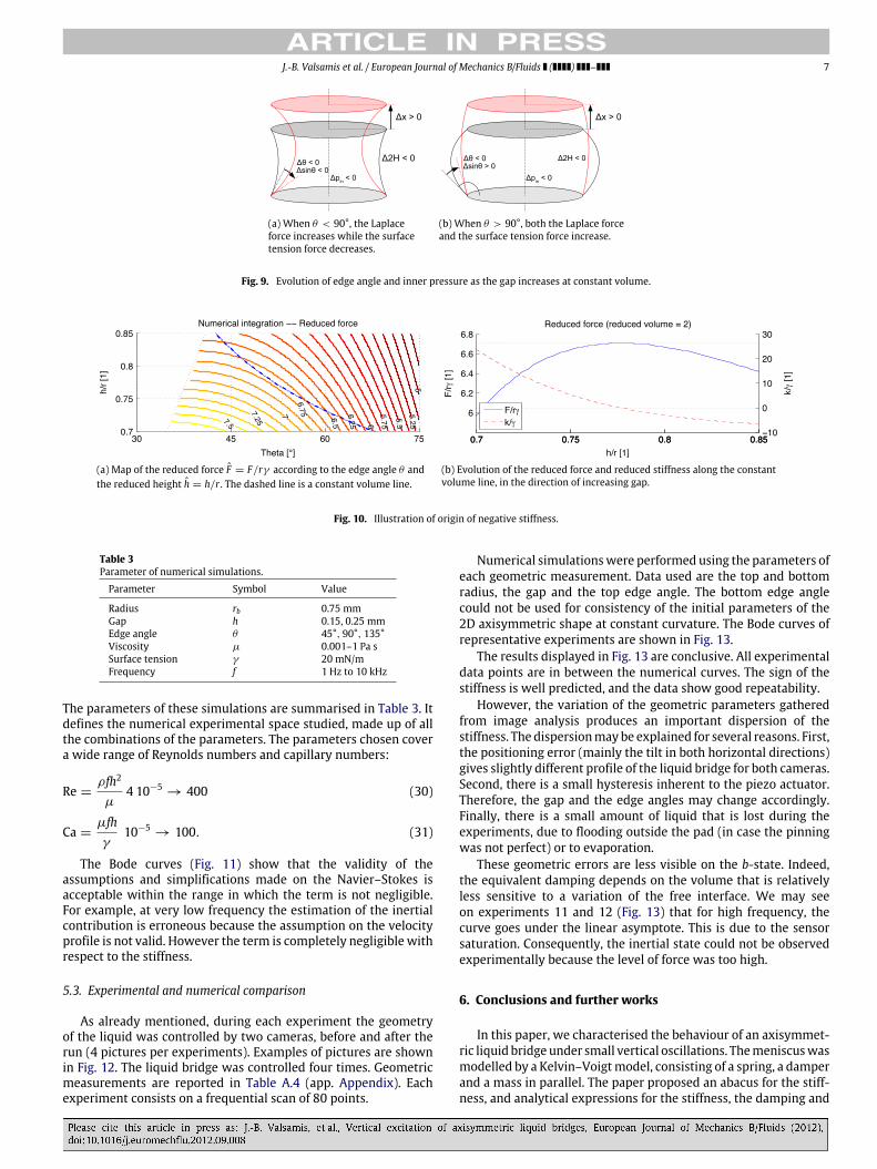
The relative errors on the parabolic and circular models areshown in Fig. 8(a) and (b) (computed with (10) and equationsfrom Table 1), and prove that the circular approximation is moreaccurate. Special caremust be used in the evaluation of the relativeerror near the region where the stiffness is zero: by definition,any small difference of value produces an error tending to infinity.The error tends to zero when the shape approaches a cylinder.The circular model gives an error below 30% for form factorh < 0.1.

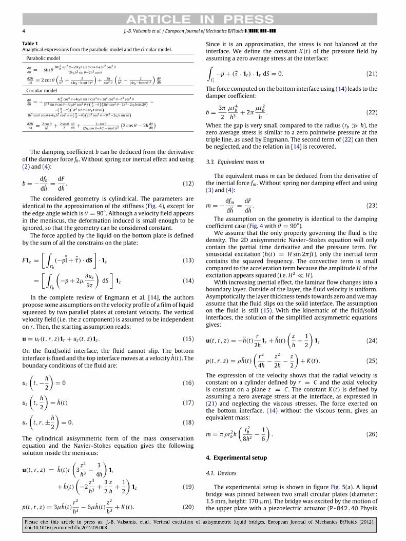
The stiffness coefficient k is not always positive. As illustrated inFig. 9, when the gap increases, the meniscus curvature decreases,reducing the inner pressure. The second term of the derivative ofthe force (10) is always positive. On the contrary, the sign of thecontribution of the surface tension force, expressed in the firstterm of (10), is changing: the edge angle always decreases as thegap increases. For angles below 90° the stiffness is negative, whilebigger angles give a positive stiffness.

Fig. 10(a) represents a part of the map of the reduced forceF = F/rγ according to the edge angle θ and the reduced heighth. The bold line is the evolution of the θ when the gap increasesat constant volume. The evolution of the force along this curve isrepresented in Fig. 10(b) (plain line). As the gap increases, the forcereaches amaximumand begins to decrease. The derivative (i.e., thestiffness) is therefore negative (dashed line).

Consequently, for certain configurations the meniscus can beconsidered as an anti-spring. Anti-springs are unstable becausethe force tends to deviate from the equilibrium state. However, ifthe anti-spring is mechanically constrained – as in the case of ameniscus – it is not unstable: the gap is fixed externally, whateverthe force.

5.2. Analytical and numerical comparison

The first set of experiments considers a fully-symmetric case:axisymmetry and top-down symmetry. For each model, wecompared the gain curves. We plot the asymptotes for each statesas:

logGk(ω) = log k (27)logGb(ω) = logω + log b (28)logGm(ω) = 2 logω + logm. (29)

(a) Relative error on the reduced stiffness computed fromparabolic model (kpm − k)/k according to the edge angle θ

and the reduced height h = h/r .

(b) Relative error on the reduced stiffness computed fromcircular model (kcm − k)/k according to the edge angle θ

and the reduced height h = h/r .

Fig. 8. Relative error for analytical models in logarithmic scale.

J.-B. Valsamis et al. / European Journal of Mechanics B/Fluids ( ) – 7

(a) When θ < 90°, the Laplaceforce increases while the surfacetension force decreases.

(b) When θ > 90°, both the Laplace forceand the surface tension force increase.

Fig. 9. Evolution of edge angle and inner pressure as the gap increases at constant volume.

(a) Map of the reduced force F = F/rγ according to the edge angle θ andthe reduced height h = h/r . The dashed line is a constant volume line.

(b) Evolution of the reduced force and reduced stiffness along the constantvolume line, in the direction of increasing gap.

Fig. 10. Illustration of origin of negative stiffness.

Table 3Parameter of numerical simulations.

Parameter Symbol Value

Radius rb 0.75 mmGap h 0.15, 0.25 mmEdge angle θ 45°, 90°, 135°Viscosity µ 0.001–1 Pa sSurface tension γ 20 mN/mFrequency f 1 Hz to 10 kHz

The parameters of these simulations are summarised in Table 3. Itdefines the numerical experimental space studied, made up of allthe combinations of the parameters. The parameters chosen covera wide range of Reynolds numbers and capillary numbers:

Re =ρfh2

µ4 10−5

→ 400 (30)

Ca =µfhγ

10−5→ 100. (31)

The Bode curves (Fig. 11) show that the validity of theassumptions and simplifications made on the Navier–Stokes isacceptable within the range in which the term is not negligible.For example, at very low frequency the estimation of the inertialcontribution is erroneous because the assumption on the velocityprofile is not valid. However the term is completely negligible withrespect to the stiffness.

5.3. Experimental and numerical comparison

As already mentioned, during each experiment the geometryof the liquid was controlled by two cameras, before and after therun (4 pictures per experiments). Examples of pictures are shownin Fig. 12. The liquid bridge was controlled four times. Geometricmeasurements are reported in Table A.4 (app. Appendix). Eachexperiment consists on a frequential scan of 80 points.

Numerical simulationswere performed using the parameters ofeach geometric measurement. Data used are the top and bottomradius, the gap and the top edge angle. The bottom edge anglecould not be used for consistency of the initial parameters of the2D axisymmetric shape at constant curvature. The Bode curves ofrepresentative experiments are shown in Fig. 13.

The results displayed in Fig. 13 are conclusive. All experimentaldata points are in between the numerical curves. The sign of thestiffness is well predicted, and the data show good repeatability.

However, the variation of the geometric parameters gatheredfrom image analysis produces an important dispersion of thestiffness. The dispersionmaybe explained for several reasons. First,the positioning error (mainly the tilt in both horizontal directions)gives slightly different profile of the liquid bridge for both cameras.Second, there is a small hysteresis inherent to the piezo actuator.Therefore, the gap and the edge angles may change accordingly.Finally, there is a small amount of liquid that is lost during theexperiments, due to flooding outside the pad (in case the pinningwas not perfect) or to evaporation.

These geometric errors are less visible on the b-state. Indeed,the equivalent damping depends on the volume that is relativelyless sensitive to a variation of the free interface. We may seeon experiments 11 and 12 (Fig. 13) that for high frequency, thecurve goes under the linear asymptote. This is due to the sensorsaturation. Consequently, the inertial state could not be observedexperimentally because the level of force was too high.

6. Conclusions and further works

In this paper, we characterised the behaviour of an axisymmet-ric liquid bridgeunder small vertical oscillations. Themeniscuswasmodelled by a Kelvin–Voigtmodel, consisting of a spring, a damperand a mass in parallel. The paper proposed an abacus for the stiff-ness, and analytical expressions for the stiffness, the damping and

8 J.-B. Valsamis et al. / European Journal of Mechanics B/Fluids ( ) –

Fig. 11. Gain curves.

(a) Picture from camera 1. (b) Picture from camera 2.

Fig. 12. Picture from cameras. The diameter of the pad is 1.5 mm.

the inertial coefficients. The validation was provided through nu-merical simulations and experimental data. The numerical simula-tions acted as a buffer for results validation: they were comparedfirst with analytical approximations (with amirror symmetry withrespect to the plane containing the neck of the meniscus) and thenwith experiments.

We showed that it is possible to characterise the meniscus bygeometrical andphysical parameters of liquids, andwithout down-scaling the system to microscopic dimension. The proposed ana-lytical laws were based on simplifications of the 2D axisymmetricNavier–Stokes equation. They can be used to quickly estimate theorder ofmagnitude of the different parameters k, b,m. The first oneinvolves the knowledge of the free liquid surface while the latterare based on the liquid volume. Consequently, the parameter k ismore difficult to evaluate: although it is a good approximation, theexperimental values of the edge angle and of the curvature of thefree surface may be rather difficult to estimate.

The results showed excellent agreement between analyticaland numerical models, validating the assumptions on the state ofthe fluid (static flow for spring state, viscous flow for the dampingstate and inertial flow for the inertial state). In this case, thecharacterisation of the inertial effects differs from the Reynoldsnumber since it is usually the convective term (ρu2/L) that isconsidered. In the vibration of the meniscus, the inertial termis related to the acceleration term (ρu). Hence an alternativeReynolds number might be defined by the ratio of the inertialforces and the viscous forces:

Reinertial =ρV uµuL

=ρVω

µL. (32)

The results showed good agreement between experimentaldata and numerical simulation, although measurements weredifficult to achieve. The present experimental bench did not allowus to inspect the inertial state experimentally since the needed

J.-B. Valsamis et al. / European Journal of Mechanics B/Fluids ( ) – 9

Fig. 13. Gain and phase curves for experiments. The circle represents experimental data, the square the individual parameters and the triangle the mean value of thegeometric parameters. Experimental parameters are given in Table A.4.

input frequencies are very high and forces generated are too largefor the sensor hereby adopted.

Finally, to complete the dynamic description of the liquid bridgeinvestigations of the response along the other degrees of freedomare required. In this respect, we earlier reported the study of thelateral oscillations of the liquidmeniscus in [20]. Still, further workis needed.

Acknowledgements

This work is funded by a grant of the F.R.I.A.—Fonds pourla Formation à la Recherche dans l’Industrie et l’Agriculture.J.-B Valsamis would also like to thank the Laboratory of Molecular

and Biomolecular Engineering3 (Prof. K. Bartik) for all the subsidiarychemical products, Mr. Zoltan Nagy and Dr. Felix Beyeler fromFemtoTool4 for their technical support about the force sensor andMrs Bruno Tartini, Jean-Salvatore Mele and Thierry Delvaux fortheir technical contribution.

Appendix

See Fig. 14.

3 http://dev.ulb.ac.be/polytech/chimorg/.4 http://www.femtotools.com/.

10 J.-B. Valsamis et al. / European Journal of Mechanics B/Fluids ( ) –

Fig. 14. Big size abacus (Zoom of Fig. 7).

J.-B. Valsamis et al. / European Journal of Mechanics B/Fluids ( ) – 11

Table A.4Experimental results fromboth cameras. Pictures 1 and 2have been recorded beforethe experiment and pictures 3 and 4 have been recorded after.

Experiment Picture Bottomradius[mm]

Topradius[mm]

Bottomangle[°]

Topangle[mm]

Gap[mm]

Volume[mm3

]

1 1 0.717 0.696 15.9 23.6 0.284 0.3541 2 0.735 0.721 15.3 20.1 0.298 0.3861 3 0.713 0.703 18.6 22.6 0.262 0.3351 4 0.738 0.732 13.9 16.2 0.281 0.3741 Mean 0.726 0.713 15.9 20.6 0.282 0.362

2 1 0.747 0.747 43.2 43.2 0.218 0.3452 2 0.77 0.746 36 46.7 0.242 0.3912 3 0.736 0.722 18.6 24.7 0.231 0.3252 4 0.747 0.729 20.2 28.1 0.235 0.3422 Mean 0.75 0.736 29.5 35.7 0.231 0.351

3 1 0.756 0.746 28.8 32 0.323 0.4733 2 0.745 0.748 34.7 33.6 0.317 0.4633 3 0.755 0.738 21.8 27.3 0.319 0.4493 4 0.767 0.755 21.4 25.2 0.322 0.4683 Mean 0.756 0.747 26.7 29.5 0.32 0.463

4 1 0.749 0.751 45.8 45.2 0.284 0.4464 2 0.755 0.752 46 47.4 0.28 0.4494 3 0.755 0.746 24.5 27.9 0.28 0.4124 4 0.758 0.735 22.4 31.1 0.273 0.44 Mean 0.754 0.746 34.7 37.9 0.279 0.427

5 1 0.75 0.751 50.7 50.1 0.255 0.4125 2 0.76 0.752 46.5 50 0.246 0.4045 3 0.751 0.75 41.6 42 0.251 0.3965 4 0.766 0.751 36.8 43.3 0.243 0.3935 Mean 0.757 0.751 43.9 46.3 0.249 0.401

7 1 0.743 0.747 27.4 24.9 0.158 0.2437 2 0.752 0.748 24.2 27.1 0.16 0.2557 3 0.744 0.744 40.8 40.8 0.155 0.257 4 0.758 0.752 43 47.2 0.163 0.2717 Mean 0.749 0.747 33.9 35 0.159 0.255

8 1 0.747 0.741 41 42 0.554 0.7438 2 0.754 0.751 40.1 40.6 0.562 0.7648 3 0.747 0.747 40 40 0.569 0.7568 4 0.754 0.746 39.1 40.5 0.575 0.7688 Mean 0.75 0.746 40.1 40.8 0.565 0.758

9 1 0.748 0.744 65.5 66.3 0.479 0.7589 2 0.765 0.754 65.5 67.8 0.485 0.89 3 0.745 0.744 52.1 52.3 0.482 0.7149 4 0.752 0.754 50.7 50.3 0.485 0.7279 Mean 0.752 0.749 58.5 59.2 0.483 0.75

10 1 0.743 0.75 25.4 22.4 0.26 0.38110 2 0.766 0.76 22.9 25.3 0.27 0.41210 3 0.748 0.745 29.8 30.8 0.266 0.39610 4 0.748 0.754 31.6 29.5 0.269 0.40610 Mean 0.751 0.752 27.4 27 0.266 0.399

11 1 0.734 0.751 30.5 24.6 0.293 0.42211 2 0.746 0.747 27.2 27.1 0.297 0.4311 3 0.739 0.752 32.9 28.1 0.295 0.43211 4 0.755 0.75 27 28.5 0.3 0.44311 Mean 0.743 0.75 29.4 27.1 0.296 0.432

12 1 0.753 0.757 11 9.83 0.334 0.43512 2 0.746 0.759 16 12.4 0.343 0.451

Table A.4 (continued)

Experiment Picture Bottomradius[mm]

Topradius[mm]

Bottomangle[°]

Topangle[mm]

Gap[mm]

Volume[mm3

]

12 3 0.746 0.761 15.9 11.7 0.335 0.44512 4 0.744 0.764 17.7 12.2 0.345 0.45812 Mean 0.747 0.76 15.2 11.5 0.339 0.447

References

[1] P.-G. de Gennes, F. Brochart-Wyard, D. Quéré, Gouttes, bulles, perles et ondes,Belin, 2002.

[2] P. Lambert, Capillary Forces in Microassembly: Modeling, Simulation,Experiments, and Case Study, Microtechnology and MEMS, Springer, 2007.

[3] M. Mastrangeli, J.-B. Valsamis, C.V. Hoof, J.-P. Celis, P. Lambert, Lateralcapillary forces of cylindrical fluid menisci: a comprehensive quasi-staticstudy, J. Micromech. Microeng. 20 (7) (2010) http://dx.doi.org/10.1088/0960-1317/20/7/075041. 075041 (13 p).

[4] W. Lin, S.K. Patra, Y.C. Lee, Design of solder joints for self-alignedoptoelectronic assemblies, IEEE Trans. Adv. Packaging 18 (3) (1995) 543–551.

[5] S.K. Patra, Y.C. Lee, Quasi-static modeling of the self-alignment mechanism inflip-chip soldering—part i: single solder joint, J. Electron. Packaging 113 (4)(1991) 337–342.

[6] S.K. Patra, Y.C. Lee, Modeling of self-alignment mechanism in flip-chipsoldering—part ii: multichip solder joints, in: Electronic Components andTechnology Conference, 1991, Proceedings., 41st, 1991.

[7] M. Mastrangeli, W. Ruythooren, C.V. Hoof, J.-P. Celis, Conformal dip-coating ofpatterned surfaces for capillary die-to-substrate self-assembly, J. Micromech.Microeng. 19 (4) (2009) 12.

[8] M. Mastrangeli, S. Abbasi, C. Varel, C.V. Hoof, J.-P. Celis, K. Bohringer,Self-assembly from milli- to nanoscales: methods and applications,J MicromechMicroeng 19 (8) (2009) 083001. http://dx.doi.org/10.1088/0960-1317/19/8/083001.

[9] K. Brakke, The surface evolver, Exp. Math. 1 (2) (1992) 141–165.[10] J. Berthier, K. Brakke, F. Grossi, L. Sanchez, L.D. Cioccio, Self-alignment of silicon

chips on wafers: a capillary approach, J. Appl. Phys. 108 (2010) 054905.[11] N. van Veen, Analytical derivation of the self-alignment motion of flip chip

soldered components, J. Electron. Packaging 121 (1999) 116–121.[12] M.-H. Meurisse, M. Querry, Squeeze effects in a flat liquid bridge between

parallel solid surfaces, J. Tribology 128 (3) (2006) 575–584.[13] D. Cheneler, M.C. Ward, M.J. Adams, Z. Zhang, Measurement of dynamic

properties of small volumes of fluid using mems, Sens. Actuators, B 130 (2)(2008) 701–706.

[14] J. Engmann, C. Servais, A.S. Burbidge, Squeeze flow theory and applications torheometry: a review, J. Non-Newtonian Fluid Mech. 132 (1–3) (2005) 1–27.

[15] O. Pitois, P. Moucheront, X. Chateau, Liquid bridge between two movingspheres: an experimental study of viscosity effects, J. Colloid Interface Sci. 231(1) (2000) 26–31.

[16] N. Boufercha, J. Sägebarth, M. Burgard, N. Othman, D. Schlenker, W. Schäfer, H.Sandmaier, Micro-assembly with fluids, MST/NEWS 2/08, 2008, pp. 29–30.

[17] H. Lu, C. Bailey, Dynamic analysis of flip-chip self alignment, IEEE Trans. Adv.Packaging 28 (3) (2005) 475–480.

[18] J.M. Montanero, Linear dynamics of axisymmetric liquid bridges, Eur. J. Mech.B 22 (2003) 167–178.

[19] J. Montanero, Theoretical analysis of the vibration of axisymmetric liquidbridges of arbitrary shape, Theoret. Comput. Fluid Dynamics 16 (2003)171–186.

[20] P. Lambert, M. Mastrangeli, J.-B. Valsamis, G. Degrez, Spectral analysis andexperimental study of lateral capillary dynamics (for flip-chip applications),Microfluid Nanofluid. 9 (4–5) (2010) 797–807.

[21] F. Dionnet, Télé-micro-manipulation par adhésion, Ph.D. Thesis, UniversitéPierre et Marie Curie, Paris, 2005.

[22] V. Vandaele, Contactless handling for micro-assembly: acoustic levitation,Ph.D. Thesis, Université libre de Bruxelles, Brussels, Belgium, 2008.