4. Axial Load - Chapter 1
52
2005 Pearson Education South Asia Pte Ltd 4. Axial Load 1 CHAPTER OBJECTIVES • Determine deformation of axially loaded members • Develop a method to find support reactions when it cannot be determined from equilibrium equations (statically indeterminated problem) • Analyze the effects of thermal stress and stress concentrations.
-
Upload
khangminh22 -
Category
Documents
-
view
0 -
download
0
Transcript of 4. Axial Load - Chapter 1

2005 Pearson Education South Asia Pte Ltd
4. Axial Load
1
CHAPTER OBJECTIVES
• Determine deformation of
axially loaded members
• Develop a method to find
support reactions when it
cannot be determined from
equilibrium equations (statically
indeterminated problem)
• Analyze the effects of thermal
stress and stress concentrations.

2005 Pearson Education South Asia Pte Ltd
4. Axial Load
2
CHAPTER OUTLINE
1. Saint-Venant’s Principle
2. Elastic Deformation of an Axially Loaded Member
3. Principle of Superposition
4. Statically Indeterminate Axially Loaded Member
5. Force Method of Analysis for Axially Loaded Member
6. Thermal Stress
7. Stress Concentrations

2005 Pearson Education South Asia Pte Ltd
4. Axial Load
3
• Localized deformation occurs at
each end, and the deformations
decrease as measurements are
taken further away from the ends
4.1 SAINT-VENANT’S PRINCIPLE
• c-c is sufficiently far enough away
from P so that localized deformation
“vanishes”, i.e., minimum distance
• At section c-c, stress reaches
almost uniform value as compared
to a-a, b-b

2005 Pearson Education South Asia Pte Ltd
4. Axial Load
4
4.1 SAINT-VENANT’S PRINCIPLE
Section a-a Section b-bSection c-c
savgP
Asavg
P
A savg=P
A
Section a-a Section b-bSection c-c
savgP
Asavg
P
A savg=P
A
Section a-a Section b-bSection c-c
savgP
Asavg
P
A savg=P
A
Load distorts linelocated near load
Lines located awayfrom the local andsupport remain straight
Load distorts linelocated near support
Load distorts linelocated near load
Lines located awayfrom the local andsupport remain straight
Load distorts linelocated near support
savg=P
A
The pink area is the area of the uniform average
normal stress, or savg = P/A

2005 Pearson Education South Asia Pte Ltd
4. Axial Load
5
4.1 SAINT-VENANT’S PRINCIPLE
d
L
A long bar/rod, L >> d, is
subjected to a tensile force
acting at its centroidal axisd
d
P
P
Non-uniform normal stress
Non-uniform normal stress
Uniform normal stress
savg= P/A
This behavior discovered by
Barré de Saint-Venant in
1855, this the name of the
principle
Saint-Venant Principle states
that localized effectscaused by any load acting
on the body, will
dissipate/smooth out within
regions that are sufficiently removed from location of
load

2005 Pearson Education South Asia Pte Ltd
4. Axial Load
6
• Relative displacement (δ) of one end of bar with respect
to other end caused by this loading
• Applying Saint-Venant’s Principle, ignore localized
deformations at points of concentrated loading and
where cross-section suddenly changes
4.2 ELASTIC DEFORMATION OF AN AXIALLY LOADED MEMBER

2005 Pearson Education South Asia Pte Ltd
4. Axial Load
7
Use method of sections,
and draw free-body diagram
4.2 ELASTIC DEFORMATION OF AN AXIALLY LOADED MEMBER
σ =P(x)
A(x) =
dδ
dx
σ = E
• Assume proportional limit not exceeded,
thus apply Hooke’s Law
P(x)
A(x)= E
dδ
dx( ) dδ =
P(x) dx
A(x) E

2005 Pearson Education South Asia Pte Ltd
4. Axial Load
8
4.2 ELASTIC DEFORMATION OF AN AXIALLY LOADED MEMBER
δ = ∫0
P(x) dx
A(x) E
L
δ = displacement of one point relative to another point
L = distance between the two points
P(x) = internal axial force at the section, located a distance x
from one end
A(x) = cross-sectional area of the bar, expressed as a function
of x
E = modulus of elasticity for material
2005 Pearson Education South Asia Pte Ltd
4. Axial Load
9
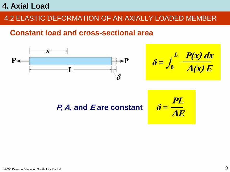
4.2 ELASTIC DEFORMATION OF AN AXIALLY LOADED MEMBER
Constant load and cross-sectional area
δ = ∫0
P(x) dx
A(x) E
L
P, A, and E are constant δ =PL
AE
P P
x
Ld

2005 Pearson Education South Asia Pte Ltd
4. Axial Load
10
4.2 ELASTIC DEFORMATION OF AN AXIALLY LOADED MEMBER
P1 P2 P3 P4
A1,E1A2,E2 A3,E3
L1 L2 L3
A B C D
Internal force in segment BC: P1 P2A B
PBC
Internal force in segment AB: P1PAB
A
P4D
PCDInternal force in segment CD:

2005 Pearson Education South Asia Pte Ltd
4. Axial Load
11
4.2 ELASTIC DEFORMATION OF AN AXIALLY LOADED MEMBER
P1 P2 P3 P4
A1,E1A2,E2 A3,E3
L1 L2 L3
A B C D
Displacement in segment AB: δAB = δ1 =PAB L1
A1 E1
Displacement in segment BC: δBC = δ2 =PBC L2
A2 E2
Displacement in segment CD: δCD = δ3 =PCD L3
A3 E3
The displacement of one end of the
bar with respect to the other isδ =
PL
AE = δ1 + δ2 + δ3

2005 Pearson Education South Asia Pte Ltd
4. Axial Load
12
4.2 ELASTIC DEFORMATION OF AN AXIALLY LOADED MEMBER
Sign convention
Sign Forces Displacement
Positive (+) Tension Elongation
Negative (−) Compression Contraction

2005 Pearson Education South Asia Pte Ltd
4. Axial Load
13
EXAMPLE 4-1
Composite A-36 steel bar shown made
from two segments AB and BD.
Area AAB = 600 mm2 and ABD = 1200
mm2.
Determine the vertical displacement of
end A and displacement of B relative to C.

2005 Pearson Education South Asia Pte Ltd
4. Axial Load
14
EXAMPLE 4-1
Internal force
Due to external loadings, internal axial forces
in segments AB, BC and CD are different.
Apply method of
sections and equation
of vertical force
equilibrium as shown.
Variation is also
plotted.
PAB
PBCPBC=35 kN
PAB=75 kN
PBC=35 kN
PCD
PBC=35 kN
PAB=75 kN
PCD=45 kN
2005 Pearson Education South Asia Pte Ltd
4. Axial Load
15
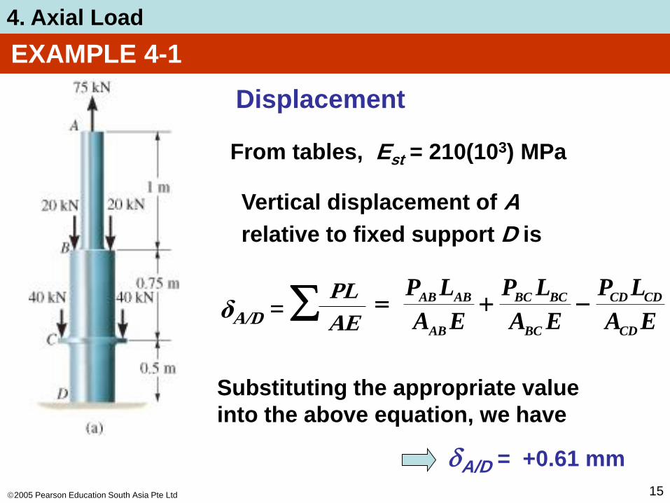
EXAMPLE 4-1
Displacement
From tables, Est = 210(103) MPa
Vertical displacement of A
relative to fixed support D is
δA/D =PL
AE
EA
LP
EA
LP
EA
LP
CD
CDCD
BC
BCBC
AB
ABAB
Substituting the appropriate value
into the above equation, we have
dA/D = +0.61 mm

2005 Pearson Education South Asia Pte Ltd
4. Axial Load
16
EXAMPLE 4-1
Since the result is positive, the bar elongates and, therefore, the displacement at A is upward
Displacement between B and C,
δB/C =PBC LBC
ABC E
= +0.104 mm
[+35 kN](0.75 m)(106)
[1200 mm2 (210)(103) kN/m2]=
Here, B moves away from C, since
segment elongates

2005 Pearson Education South Asia Pte Ltd
4. Axial Load
17
• After subdividing the load into components, the principle of superposition states that the resultant stress or
displacement at the point can be determined by first finding
the stress or displacement caused by each component load
acting separately on the member.
• Resultant stress/displacement determined algebraically by
adding the contributions of each component
4.3 PRINCIPLE OF SUPERPOSITION

2005 Pearson Education South Asia Pte Ltd
4. Axial Load
18
Conditions
1. The loading must be linearly related to the stress or displacement that is to be determined.
2. The loading must not significantly change the original geometry or configuration of the member
When to ignore deformations?
• Most loaded members will produce deformations so small that change in position and direction of loading will be insignificant and can be neglected
• Exception to this rule is a column carrying axial load, discussed in Chapter 13
4.3 PRINCIPLE OF SUPERPOSITION
2005 Pearson Education South Asia Pte Ltd
4. Axial Load
19
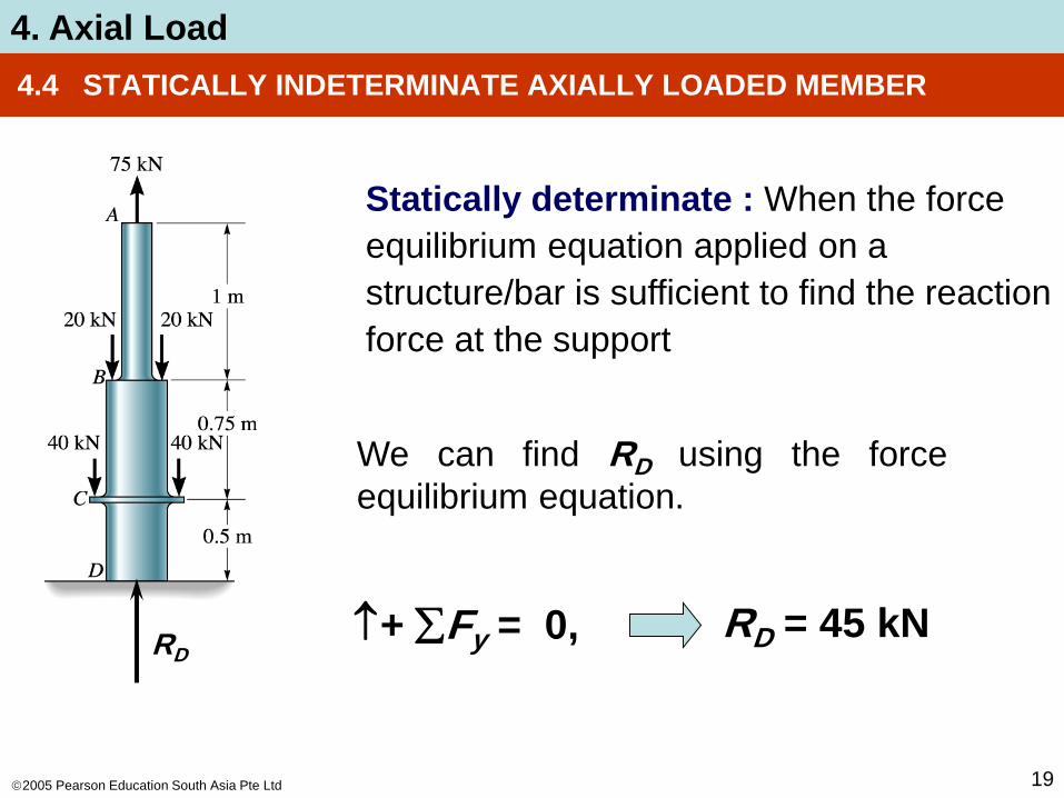
4.4 STATICALLY INDETERMINATE AXIALLY LOADED MEMBER
RD
We can find RD using the force
equilibrium equation.
+ Fy = 0,
Statically determinate : When the force
equilibrium equation applied on a
structure/bar is sufficient to find the reaction
force at the support
RD = 45 kN

2005 Pearson Education South Asia Pte Ltd
4. Axial Load
20
If bar is fixed at both ends,
then two unknown axial
reactions occur, and the
bar is
statically indeterminate
4.4 STATICALLY INDETERMINATE AXIALLY LOADED MEMBER
+↑ F = 0;
FB + FA − P = 0 (a)
We cannot find the value of FA and FB.
Free body diagram
FB
FA
P

2005 Pearson Education South Asia Pte Ltd
4. Axial Load
21
• To establish addition equation, consider geometry of
deformation. Such an equation is referred to as a
compatibility or kinematic condition
• Since the end supports fixed are fixed, the
compatibility condition is
4.4 STATICALLY INDETERMINATE AXIALLY LOADED MEMBER
δA/B = 0
• This equation can be expressed in terms of applied
loads using a load-displacement relationship, which
depends on the material behavior
δA/B =PL
AE = 0

2005 Pearson Education South Asia Pte Ltd
4. Axial Load
22
For linear elastic behavior,
compatibility equation can be
written as
4.4 STATICALLY INDETERMINATE AXIALLY LOADED MEMBER
FB
FA
P
FB
FA
P
FB
FA
Assume AE is constant, solve
Eqs.(a) & (b) simultaneously,
LCB
LFA = P ( )
LAC
LFB = P( )
FB
FA
P
FB
FA
FB
FA
FB
FA
P
FB
FA
FB
FA
FB + FA − P = 0 (a)
= 0FA LAC
AE
FB LCB
AE− (b)
δAC − δCB = 0
2005 Pearson Education South Asia Pte Ltd
4. Axial Load
23
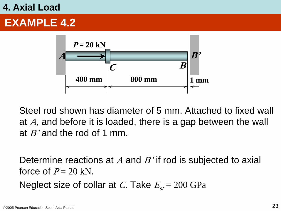
EXAMPLE 4.2
Steel rod shown has diameter of 5 mm. Attached to fixed wall
at A, and before it is loaded, there is a gap between the wall
at B’ and the rod of 1 mm.
Determine reactions at A and B’ if rod is subjected to axial
force of P = 20 kN.
Neglect size of collar at C. Take Est = 200 GPa
400 mm 800 mm
P = 20 kN
1 mm
A
C BB’

2005 Pearson Education South Asia Pte Ltd
4. Axial Load
24
EXAMPLE 4.2
400 mm 800 mm
P = 20 kN
1 mm
A
C BB’
P = 20 kNA
C B20 kN
P = 20 kNA
C
B’
FAFB
400 + dAC800 (1 + dCB)
Compatibility
equation:
δB/A = 0.001 = δAC + δCB

2005 Pearson Education South Asia Pte Ltd
4. Axial Load
25
EXAMPLE 4.2 (SOLN)
Equilibrium
Assume force P large
enough to cause rod’s end B
to contact wall at B’.
Equilibrium requires
− FA − FB + 20(103) N = 0 (a)
P = 20 kNA
C
B’
FAFB
Compatibility
Compatibility equation:
δB/A = δAC + δCB
0.001 m =FA LAC
AE
FB LCB
AE(b)
FAFA
FBFB
Solving Eq.(a) & (b) yields, FA = 16.6 kN FB = 3.39 kN

2005 Pearson Education South Asia Pte Ltd
4. Axial Load
26
• Used to also solve statically indeterminate problems by using
superposition of the forces acting on the free-body diagram
• First, choose any one of the two supports as “redundant” and
remove its effect on the bar
• Thus, the bar becomes statically determinate
• Apply principle of superposition and solve the equations
simultaneously
4.5 FORCE METHOD OF ANALYSIS FOR AXIALLY LOADED MEMBERS

2005 Pearson Education South Asia Pte Ltd
4. Axial Load
27
dB
FB
dB is displacement at
B only when redundant
force at B is applied
4.5 FORCE METHOD OF ANALYSIS FOR AXIALLY LOADED MEMBERS
dP is displacement at B
when redundant force
at B is removed
dP
P +=
PLAC
AEdP = FB L
AEdB =
dP – dB = 0

2005 Pearson Education South Asia Pte Ltd
4. Axial Load
28
EXAMPLE 4-3
A-36 steel rod shown has diameter of 5 mm. It’s attached to
fixed wall at A, and before it is loaded, there’s a gap between
wall at B’ and rod of 1 mm.
Determine reactions at A and B’.
400 mm 800 mm
P = 20 kN
1 mm
A
C BB’

2005 Pearson Education South Asia Pte Ltd
4. Axial Load
29
P = 20 kN
A
C BB’
Initial
position
1 mm
Compatibility
Consider support at B’ as redundant.
Use principle of superposition,
( + ) dP = positive
dB = negative
Compatibility equation: 0.001 m = δP −δB Eq. 1
EXAMPLE 4-3
A
C B’
dB
FB
Final
position
P = 20 kN
A
C B
dP

2005 Pearson Education South Asia Pte Ltd
4. Axial Load
30
P = 20 kN
A
C BB’
Initial
position
1 mm
EXAMPLE 4-3
Compatibility equation:
0.001 m = δP −δB Eq. 1
Displacement due to P, or dP
PLAC
AEdP = = …= 0.002037 m
FB LAB
AEdB = = …
= 0.3056(10-6)FB
Subst dP & dB yields: FB = 3.40 kN
Displacement due to FB, or dB
400 mm 800 mm
A
C B’
dB
FB
P = 20 kN
A
C B
dP
Final
position

2005 Pearson Education South Asia Pte Ltd
4. Axial Load
31
EXAMPLE 4-3
Equilibrium
From free-body diagram
− FA + 20 kN − 3.40 kN = 0+ Fx = 0;
FA = 16.6 kN
P = 20 kN
A C B
FB = 3.4 kNFA

2005 Pearson Education South Asia Pte Ltd
4. Axial Load
32
4.6 THERMAL STRESS
• Expansion or contraction of material is linearly related to
temperature increase or decrease that occurs (for homogenous
and isotropic material)
• From experiment, deformation of a member having length L is
δT = α ∆T L
α = liner coefficient of thermal expansion. Unit measure
strain per degree of temperature: 1/oC (Celsius) or 1/
oK
(Kelvin)∆T = algebraic change in temperature of member
δT = algebraic change in length of member

2005 Pearson Education South Asia Pte Ltd
4. Axial Load
33
4.6 THERMAL STRESS
• For a statically indeterminate member,
the thermal displacements can be
constrained by the supports, producing
thermal stresses that must be considered
in design.

2005 Pearson Education South Asia Pte Ltd
4. Axial Load
34
4.6 THERMAL STRESS
L T1 L T2 > T1
dT
A bar has initial length L and
temperature T1.
When the temperature is
increased to T2, the change in
length of the beam is
dT = a DTL = a(T2 – T1)L
No thermal stress produces in the
bar because thermal stress will
occur when the expansion of the
bar is constrained

2005 Pearson Education South Asia Pte Ltd
4. Axial Load
35
4.6 THERMAL STRESS
L T1 L DT(x)
dTIf the change in temperature varies
throughout the length of the bar,
i.e., DT = DT(x), or it varies along the
length, then the change in length is
L
T Tdx
0
Dad

2005 Pearson Education South Asia Pte Ltd
4. Axial Load
36
EXAMPLE 4-3
A-36 steel bar shown is constrained to just fit between two fixed supports when T1 = 30
oC.
If temperature is raised to T2 = 60oC, determine
the average normal thermal stress developed in the bar.

2005 Pearson Education South Asia Pte Ltd
4. Axial Load
37
EXAMPLE 4-3
Free expansion
dT
Free expansion,
dT = a(T2 – T1)L
Constrained,F L
AEdF =
Compatibility condition,
dA/B = 0 = dT – dF
LDT
A
B
Substituting the appropriate relation,
0 = a(T2 – T1)L –F L
AE
L
dF
F
F
Constrained

2005 Pearson Education South Asia Pte Ltd
4. Axial Load
38
EXAMPLE 4-3
Free expansion
dT
L
dFF
F
Constrained
From compatibility condition,
LDT
A
B
0 = a(T2 – T1)L –F L
AE
Solving the above equation
for force F,F = a(T2 – T1)AE
Data from inside back cover,
asteel = 12(10-6) oC-1
Substituting all values into the eq., we get F = 7.2 kN
The average thermal stress is then, s =F
A= … = 72 MPa

2005 Pearson Education South Asia Pte Ltd
4. Axial Load
39
4.7 STRESS CONCENTRATIONS
• Force equilibrium requires magnitude of resultant force
developed by the stress distribution to be equal to P. In
other words,
• This integral represents graphically the volume under
each of the stress-distribution diagrams shown.
P = ∫A σ dA
Undistorted
Distorted
P P
P P
a
Actual stress distribution
Average stress distribution
P
P
smax
savg

2005 Pearson Education South Asia Pte Ltd
4. Axial Load
40
4.7 STRESS CONCENTRATIONS
• In engineering practice, actual stress distribution not needed,
only maximum stress at these sections must be known.
Member is designed to resist this stress when axial load P is
applied.
• K is defined as a ratio of the maximum stress to the average
stress acting at the smallest cross section:
K =σmax
σavg

2005 Pearson Education South Asia Pte Ltd
4. Axial Load
41
4.7 STRESS CONCENTRATIONS
K
r
h
w
h= 4.0

2005 Pearson Education South Asia Pte Ltd
4. Axial Load
42
4.7 STRESS CONCENTRATIONS
K
r
w

2005 Pearson Education South Asia Pte Ltd
4. Axial Load
43
4.7 STRESS CONCENTRATIONS
• K is independent of the bar’s geometry and the type of
discontinuity, only on the bar’s geometry and the type of
discontinuity.
• As size r of the discontinuity is decreased, stress
concentration is increased.
• It is important to use stress-concentration factors in design
when using brittle materials, but not necessary for ductile
materials
• Stress concentrations also cause failure structural
members or mechanical elements subjected to fatigue loadings

2005 Pearson Education South Asia Pte Ltd
4. Axial Load
44
EXAMPLE 4-4
Steel bar shown below has allowable
stress, σallow = 115 MPa.
Determine largest axial force P that
the bar can carry.

2005 Pearson Education South Asia Pte Ltd
4. Axial Load
45
EXAMPLE 4-4
Because there is a shoulder fillet, stress-concentrating
factor determined using the graph shown
K
r
h

2005 Pearson Education South Asia Pte Ltd
4. Axial Load
46
K
r
h
EXAMPLE 4-4
Geometric parameters:
r
h=
10 mm
20 mm= 0.50
w
h
40 mm
20 mm= 2=
From the graph, K = 1.4

2005 Pearson Education South Asia Pte Ltd
4. Axial Load
47
EXAMPLE 4-4
Average normal stress at smallest cross-section,
P
(20 mm)(10 mm)σavg = = 0.005P N/mm2
which σallow = σmax yields
115 N/mm2 = 1.4(0.005P)
P = 16.43(103) N = 16.43 kN
σallow = K σavg
K =σmax
σavgApplying Eqn

2005 Pearson Education South Asia Pte Ltd
4. Axial Load
48
CHAPTER REVIEW
• When load applied on a body, a stress distribution is created
within the body that becomes more uniformly distributed at
regions farther from point of application. This is the Saint-
Venant’s principle.
• Relative displacement at end of axially loaded member
relative to other end is determined from
δ = ∫0
P(x)
dx
A(x) E
L

2005 Pearson Education South Asia Pte Ltd
4. Axial Load
49
CHAPTER REVIEW
• Make sure to use sign convention for internal load P
and that material does not yield, but remains linear
elastic
• Superposition of load & displacement is possible
provided material remains linear elastic and no
changes in geometry occur
• If series of constant external forces are applied and AE is
constant, then
δ =PL
AE

2005 Pearson Education South Asia Pte Ltd
4. Axial Load
50
CHAPTER REVIEW
• Reactions on statically indeterminate bar determined using
equilibrium and compatibility conditions that specify
displacement at the supports. Use the load-displacement
relationship, d = PL/AE
• Change in temperature can cause member made from
homogenous isotropic material to change its length by
d = aDTL . If member is confined, expansion will produce
thermal stress in the member

2005 Pearson Education South Asia Pte Ltd
4. Axial Load
51
CHAPTER REVIEW
• Holes and sharp transitions at cross-section create stress
concentrations. For design, obtain stress concentration
factor K from graph, which is determined empirically. The
K value is multiplied by average stress to obtain
maximum stress at cross-section, smax = Ksavg
• If loading in bar causes material to yield, then stress
distribution that’s produced can be determined from the
strain distribution and stress-strain diagram

2005 Pearson Education South Asia Pte Ltd
4. Axial Load
52
CHAPTER REVIEW
• For perfectly plastic material, yielding causes stress
distribution at cross-section of hole or transition to
even out and become uniform
• If member is constrained and external loading causes
yielding, then when load is released, it will cause
residual stress in the material