Available online at www.sciencedirect.com

www.elsevier.com/locate/advengsoft

Advances in Engineering Software 39 (2008) 923–936

Ultimate strength analysis of composite sections underbiaxial bending and axial load

A.E. Charalampakis, V.K. Koumousis *

Institute of Structural Analysis & Aseismic Research, National Technical University of Athens, Zografou Campus, Athens GR-15773, Greece

Received 4 April 2007; accepted 18 January 2008Available online 18 March 2008

Abstract

A new generic fiber model algorithm is presented that allows for the efficient analysis of arbitrary composite sections under biaxialbending and axial load. The geometry of the cross section is described by multi-nested curvilinear polygons i.e. closed polygons withedges that are straight lines or circular arcs. The polygons may be convex or concave and may contain openings. The stress–strain dia-grams of materials consist of any number and any combination of consecutive polynomials, which allows for consideration of variouseffects such as concrete confinement and tensile strength, strain hardening of the reinforcement etc. The integration of the stress field isperformed analytically. The algorithm focuses on the construction of moment–curvature diagrams, interaction curves and failure sur-faces. It can also be used for calculating the deformed state of a cross section under given external loads. Several examples are presentedto demonstrate the versatility and the advantages of the proposed algorithm in comparison to existing methods.� 2008 Elsevier Ltd. All rights reserved.

Keywords: Biaxial bending; Fiber model; Failure surface; Composite structure

1. Introduction

The analysis of arbitrary composite sections under biax-ial bending and axial load has received extensive attentionin the literature, as many of the widely used types of crosssections do not fall into the regular/symmetric category.The most common examples include L-shaped columns,symmetric sections with asymmetrically placed openings,structural steel and/or reinforcement, repaired sectionsand various composite sections.

With the advent of powerful desktop computer systems,the efficient analysis of such cross sections has been madepossible using the ‘‘fiber” approach. The results of suchanalyses agree closely with experimental data for flexuraltype of failure and monotonic loading and are widely usedin design. Moment–curvature diagrams and failure surfacescan also be obtained. The former can be used as back-bone

0965-9978/$ - see front matter � 2008 Elsevier Ltd. All rights reserved.doi:10.1016/j.advengsoft.2008.01.007

* Corresponding author.E-mail address: vkoum@central.ntua.gr (V.K. Koumousis).

curves in non-linear analyses under cyclic loading. Further-more, they can be extended to include stiffness degradation,strength deterioration and pinching effects in various phe-nomenological hysteretic models, such as the Bouc–Wenmodel [1]. The failure surface is widely used in damageanalysis, where a damage index can be derived from thedistance of the current load state to the failure surface. Itis also used in ‘‘bounding surface” plasticity theory, devel-oped by Dafalias and Popov [2] for metals and laterextended for soils [3] and reinforced concrete (R/C) sec-tions [4]. However, the formulation employed in this studydoes not address phenomena that are related to stress–crack opening displacement behavior, which is based onfracture mechanics concepts [5,6].

Although the notion of the fiber model is simple, as itrequires the equilibrium of internal and external forces,the computational task becomes tedious mainly due to thegeometrical irregularities and the non-linear stress–strainlaws. Therefore, the algorithmic implementation becomesimportant and there is a need for an efficient and stablealgorithm.

Z

Y

Fig. 1. Arbitrary cross section.

924 A.E. Charalampakis, V.K. Koumousis / Advances in Engineering Software 39 (2008) 923–936

In the literature, various techniques have been devel-oped to resolve the problem. Brondum-Nielsen [7] andYen [8] adopted the quasi-Newton method to determinethe exact location of the neutral axis. However, this itera-tive approach does not always converge when it is appliedto irregular cross sections with strongly eccentric arrange-ment of structural steel and reinforcement. Chen et al. [9]used the same technique and proposed the use of the plasticcentroid as the origin of the reference loading axes to over-come the aforementioned convergence problem. Rodriguezand Aristizabal-Ochoa [10] provided closed form expres-sions for the ultimate strength stress resultants usingGauss’ integral method for equilibrium. Rotter [11] andlater Fafitis [12] used Green’s theorem for the integrationof the stress field of polygonal cross sections. Sfakianakis[13] used computer graphics as an indirect computationaltool to identify various materials in the cross section bytheir color. Bonet et al. [14] proposed an integrationscheme based on the decomposition of the cross sectioninto thick layers and compared its performance with theintegration scheme of Fafitis [12]. Zupan and Saje [15]investigated the comparative performance when employinganalytical as opposed to numerical methods for the integra-tion of the stress field. Sousa and Muniz [16] also presenteda procedure that employs Green’s theorem. Their imple-mentation is applied to polygonal cross sections and uti-lizes piecewise polynomials as stress–strain material laws.Bonet et al. [17] compared the efficiency of analytical andnumerical methods for computing the interaction surfacesof rectangular and circular cross sections. There also exista number of other studies that implement or combine ideasfound mainly in the aforementioned references.

In an overall assessment, existing algorithms have cer-tain shortcomings which can be summarized as follows:

� Almost all algorithms use a strict form of stress–strainlaw for materials.� Almost all algorithms are applicable to polygonal cross

sections with straight edges. Few algorithms providedirect treatment of circles [9,17].� Some algorithms use Green’s theorem to transform sur-

face integrals to boundary integrals [11,12,15,16].Although the method is fast, the various subregionse.g. uncracked concrete zone, need to be determined atevery step. Thus, integration is performed over a contin-uously changing boundary.� Some algorithms use numerical integration schemes

which need some attention regarding the achievedlevel of accuracy. Studies indicate that, in certaincases, sufficiently accurate numerical methods may bethree times more expensive than analytical methods,while low order numerical integration may yield unac-ceptably large errors [15]. Most importantly, the suffi-cient order of numerical integration is not known apriori.� In most cases, the reinforcement bars are treated as

dimensionless individual fibers and the area occupied

by the bars is taken into account as of concrete. Thesame problem holds for encased structural steel sections.� Some algorithms are sensitive to the origin of the load-

ing axes and may not converge, especially under largeaxial forces [7,8].

In this work, a new algorithm is proposed whichaddresses the above issues in a unified manner. It uses exactrepresentation and direct handling of arbitrary curvedshapes and analytical integration of the stress field. More-over, the algorithm is implemented within a user-friendlygraphical interface in a computationally efficient and reli-able way.

2. Problem description

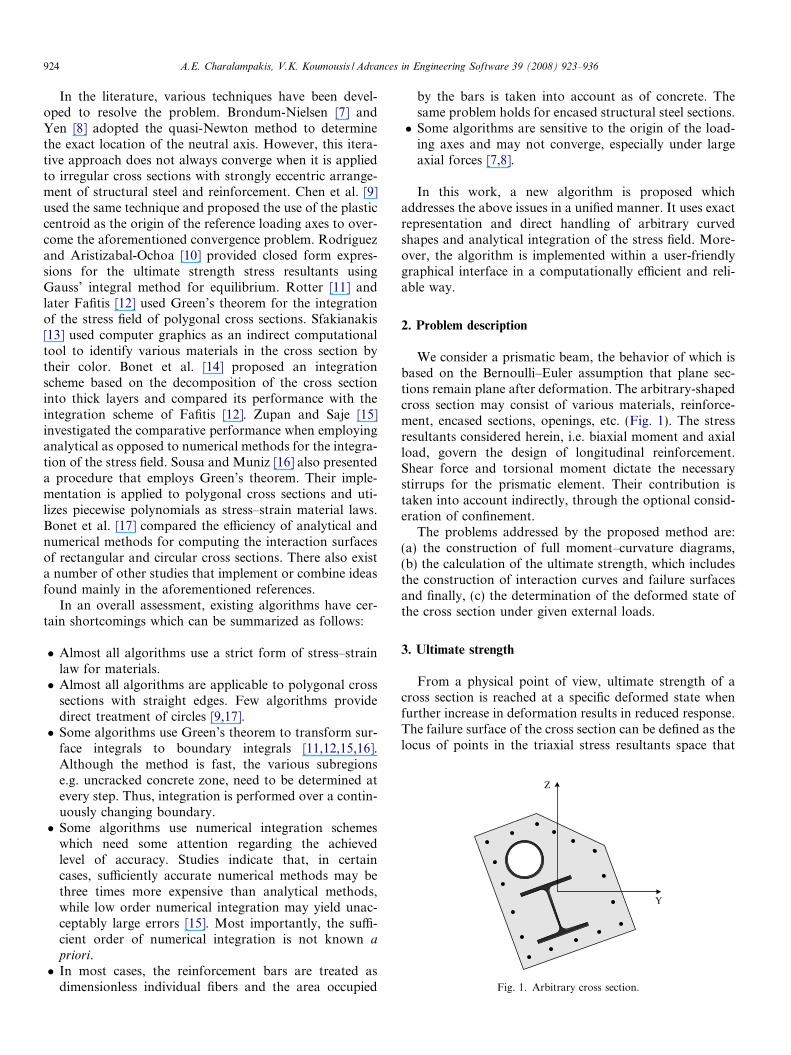
We consider a prismatic beam, the behavior of which isbased on the Bernoulli–Euler assumption that plane sec-tions remain plane after deformation. The arbitrary-shapedcross section may consist of various materials, reinforce-ment, encased sections, openings, etc. (Fig. 1). The stressresultants considered herein, i.e. biaxial moment and axialload, govern the design of longitudinal reinforcement.Shear force and torsional moment dictate the necessarystirrups for the prismatic element. Their contribution istaken into account indirectly, through the optional consid-eration of confinement.

The problems addressed by the proposed method are:(a) the construction of full moment–curvature diagrams,(b) the calculation of the ultimate strength, which includesthe construction of interaction curves and failure surfacesand finally, (c) the determination of the deformed state ofthe cross section under given external loads.

3. Ultimate strength

From a physical point of view, ultimate strength of across section is reached at a specific deformed state whenfurther increase in deformation results in reduced response.The failure surface of the cross section can be defined as thelocus of points in the triaxial stress resultants space that

A.E. Charalampakis, V.K. Koumousis / Advances in Engineering Software 39 (2008) 923–936 925

correspond to ultimate strength [13]. This locus is a closedsurface that depends on the geometry of the cross sectionand the stress–strain laws of the materials [18]. Thus, itcannot be described by analytical expressions and it mustbe constructed point-by-point.

In addition, a conventional or nominal failure surfacecan be defined. In general, this surface is almost similarin shape, but smaller in size as compared to the actual fail-ure surface [13]. Moreover, it is constructed directly, i.e.without calculating ultimate strength states, by points thatcorrespond to nominal failure which occurs when a prede-fined maximum compressive or tensile strain of a materialis reached.

The two aforementioned surfaces are often used indis-criminately and most algorithms are based on nominal fail-ure. In some cases, the additional assumption that failure isdue to concrete reaching a predefined nominal strain ecu ismade a priori [9,13]. Notably, it is possible that maximumresponse occurs prior to conventional failure. This mayhappen when one considers strongly softening branchesin stress–strain diagrams, such as in the case of unconfinedconcrete or reinforcement bars that are susceptible to buck-ling. In general, however, conventional failure occurs priorto maximum response when considering the usual materiallaws specified by the Codes e.g. Eurocode 2 [19] or ACI[20]. The proposed method calculates ultimate points byconstructing the full moment–curvature diagram for vary-ing axial loads and neutral axis orientations. Thus, bothmaximum response and conventional failure are consid-ered, while special treatment minimizes the computationaloverhead.

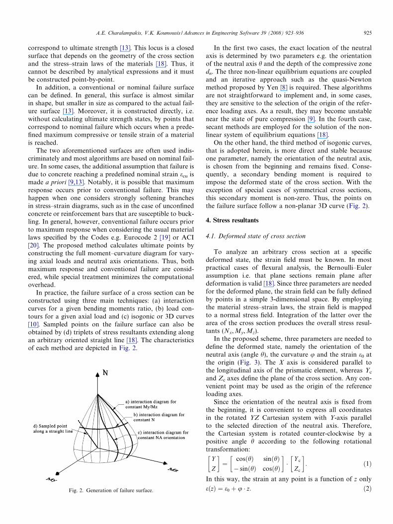
In practice, the failure surface of a cross section can beconstructed using three main techniques: (a) interactioncurves for a given bending moments ratio, (b) load con-tours for a given axial load and (c) isogonic or 3D curves[10]. Sampled points on the failure surface can also beobtained by (d) triplets of stress resultants extending alongan arbitrary oriented straight line [18]. The characteristicsof each method are depicted in Fig. 2.

Fig. 2. Generation of failure surface.

In the first two cases, the exact location of the neutralaxis is determined by two parameters e.g. the orientationof the neutral axis h and the depth of the compressive zonedn. The three non-linear equilibrium equations are coupledand an iterative approach such as the quasi-Newtonmethod proposed by Yen [8] is required. These algorithmsare not straightforward to implement and, in some cases,they are sensitive to the selection of the origin of the refer-ence loading axes. As a result, they may become unstablenear the state of pure compression [9]. In the fourth case,secant methods are employed for the solution of the non-linear system of equilibrium equations [18].

On the other hand, the third method of isogonic curves,that is adopted herein, is more direct and stable becauseone parameter, namely the orientation of the neutral axis,is chosen from the beginning and remains fixed. Conse-quently, a secondary bending moment is required toimpose the deformed state of the cross section. With theexception of special cases of symmetrical cross sections,this secondary moment is non-zero. Thus, the points onthe failure surface follow a non-planar 3D curve (Fig. 2).

4. Stress resultants

4.1. Deformed state of cross section

To analyze an arbitrary cross section at a specificdeformed state, the strain field must be known. In mostpractical cases of flexural analysis, the Bernoulli–Eulerassumption i.e. that plane sections remain plane afterdeformation is valid [18]. Since three parameters are neededfor the deformed plane, the strain field can be fully definedby points in a simple 3-dimensional space. By employingthe material stress–strain laws, the strain field is mappedto a normal stress field. Integration of the latter over thearea of the cross section produces the overall stress resul-tants (Nx,My,Mz).

In the proposed scheme, three parameters are needed todefine the deformed state, namely the orientation of theneutral axis (angle h), the curvature u and the strain e0 atthe origin (Fig. 3). The X axis is considered parallel tothe longitudinal axis of the prismatic element, whereas Yc

and Zc axes define the plane of the cross section. Any con-venient point may be used as the origin of the referenceloading axes.

Since the orientation of the neutral axis is fixed fromthe beginning, it is convenient to express all coordinatesin the rotated YZ Cartesian system with Y-axis parallelto the selected direction of the neutral axis. Therefore,the Cartesian system is rotated counter-clockwise by apositive angle h according to the following rotationaltransformation:

Y

Z

� �¼

cosðhÞ sinðhÞ� sinðhÞ cosðhÞ

� ��

Y c

Zc

� �: ð1Þ

In this way, the strain at any point is a function of z only

eðzÞ ¼ e0 þ u � z: ð2Þ

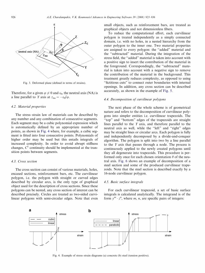
Fig. 3. Deformed plane (defined in terms of strains).

926 A.E. Charalampakis, V.K. Koumousis / Advances in Engineering Software 39 (2008) 923–936

Therefore, for a given u 6¼ 0 and e0, the neutral axis (NA) isa line parallel to Y axis at zna = �e0/u.

4.2. Material properties

The stress–strain law of materials can be described byany number and any combination of consecutive segments.Each segment may be a cubic polynomial expression whichis automatically defined by an appropriate number ofpoints, as shown in Fig. 4 where, for example, a cubic seg-ment is fitted into four consecutive points. Polynomials ofhigher order may be used but this entails integrals ofincreased complexity. In order to avoid abrupt stiffnesschanges, C1 continuity should be implemented at the tran-sition points between segments.

4.3. Cross section

The cross section can consist of various materials, holes,encased sections, reinforcement bars, etc. The curvilinearpolygon, i.e. the polygon with straight or curved edgesdescribed by circular arcs, is the only type of graphicalobject used for the description of cross sections. Since thesepolygons can be nested, any cross section of interest can bedescribed precisely. Circles are treated as two-sided curvi-linear polygons with semi-circular edges. Note that even

stress

strain

cubiclinear

a b

Fig. 4. Example of stress–strain diagrams

small objects, such as reinforcement bars, are treated asgraphical objects and not dimensionless fibers.

To reduce the computational effort, each curvilinearpolygon is treated independently as a simply connecteddomain, i.e. with no holes, in a nested hierarchy from theouter polygon to the inner one. Two material propertiesare assigned to every polygon: the ‘‘added” material andthe ‘‘subtracted” material. During the integration of thestress field, the ‘‘added” material is taken into account witha positive sign to insert the contribution of the material inthe foreground. Correspondingly, the ‘‘subtracted” mate-rial is taken into account with a negative sign to removethe contribution of the material in the background. Thistreatment greatly reduces complexity, as opposed to using‘‘fictitious cuts” to connect outer boundaries with internalopenings. In addition, any cross section can be describedaccurately, as shown in the example of Fig. 5.

4.4. Decomposition of curvilinear polygons

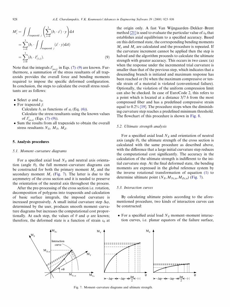
The next phase of the whole scheme is of geometricalnature and refers to the decomposition of curvilinear poly-gons into simpler entities i.e. curvilinear trapezoids. The‘‘top” and ‘‘bottom” edges of the trapezoids are straightlines parallel to the Y axis, and therefore parallel to theneutral axis as well, while the ‘‘left” and ‘‘right” edgesmay be straight lines or circular arcs. Each polygon is fullyand independently decomposed by a divide-and-conqueralgorithm. The polygon is split into two by a line parallelto the Y axis that passes through a node. The process iscontinuously applied to the newly created polygons untilthey all degenerate into trapezoids. This procedure is per-formed only once for each chosen orientation h of the neu-tral axis. Fig. 6 shows an example of decomposition of asteel section and some of the produced curvilinear trape-zoids. Note that the steel section is described exactly by a16-node curvilinear polygon.

4.5. Basic surface integrals

For each curvilinear trapezoid, a set of basic surfaceintegrals is calculated analytically. The integrand is of theform ym � zn, where m, n, are specific pairs of integers:

stress

strain

linearparabolic

(a) concrete (b) steel (tension positive).

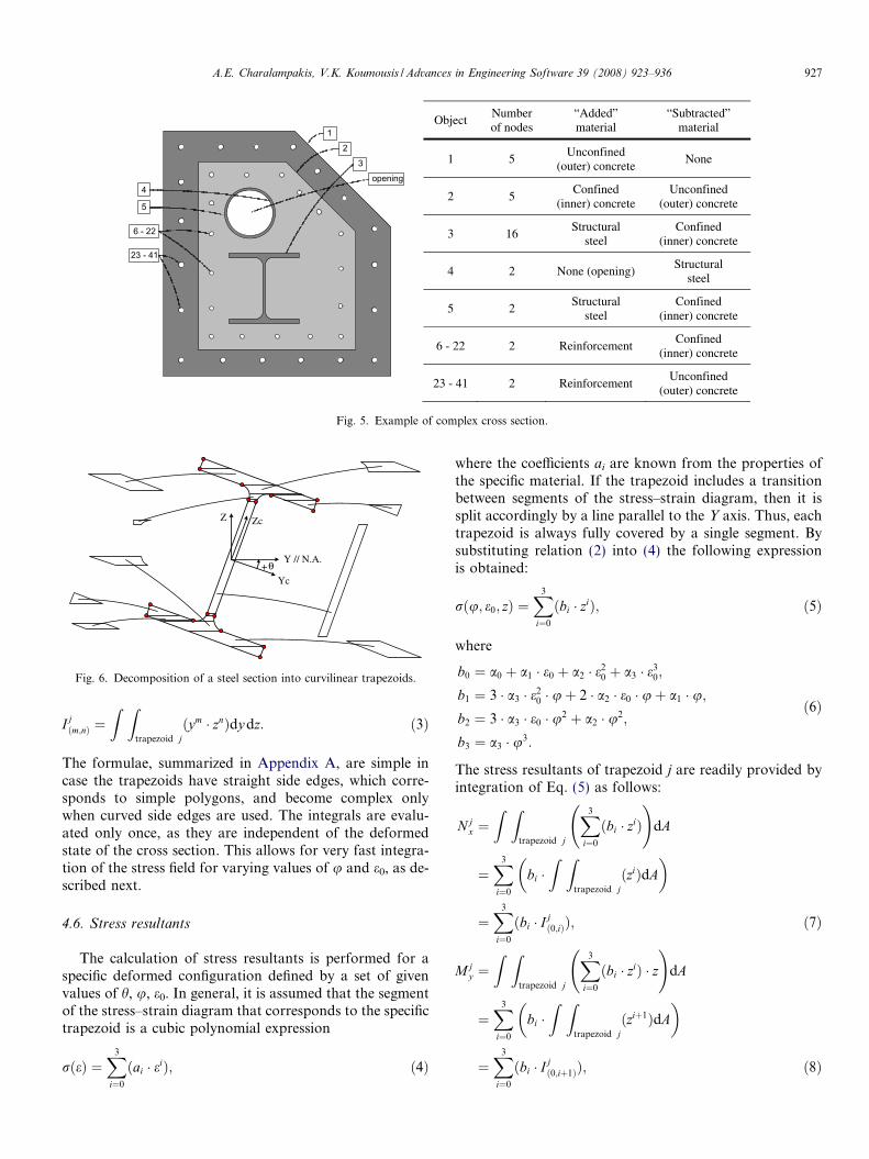
1

2

3

4

5

6 - 22

23 - 41

opening

ObjectNumberof nodes

“Added”material

“Subtracted”material

1 5 Unconfined

(outer) concrete None

2 5 Confined

(inner) concrete Unconfined

(outer) concrete

3 16 Structural

steelConfined

(inner) concrete

4 2 None (opening) Structural

steel

5 2 Structural

steelConfined

(inner) concrete

6 - 22 2 Reinforcement Confined

(inner) concrete

23 - 41 2 Reinforcement Unconfined

(outer) concrete

Fig. 5. Example of complex cross section.

Yc

θ

Zc

Y // N.A.

Z

+

Fig. 6. Decomposition of a steel section into curvilinear trapezoids.

A.E. Charalampakis, V.K. Koumousis / Advances in Engineering Software 39 (2008) 923–936 927

Ijðm;nÞ ¼

Z Ztrapezoid j

ðym � znÞdy dz: ð3Þ

The formulae, summarized in Appendix A, are simple incase the trapezoids have straight side edges, which corre-sponds to simple polygons, and become complex onlywhen curved side edges are used. The integrals are evalu-ated only once, as they are independent of the deformedstate of the cross section. This allows for very fast integra-tion of the stress field for varying values of u and e0, as de-scribed next.

4.6. Stress resultants

The calculation of stress resultants is performed for aspecific deformed configuration defined by a set of givenvalues of h, u, e0. In general, it is assumed that the segmentof the stress–strain diagram that corresponds to the specifictrapezoid is a cubic polynomial expression

rðeÞ ¼X3

i¼0

ðai � eiÞ; ð4Þ

where the coefficients ai are known from the properties ofthe specific material. If the trapezoid includes a transitionbetween segments of the stress–strain diagram, then it issplit accordingly by a line parallel to the Y axis. Thus, eachtrapezoid is always fully covered by a single segment. Bysubstituting relation (2) into (4) the following expressionis obtained:

rðu; e0; zÞ ¼X3

i¼0

ðbi � ziÞ; ð5Þ

where

b0 ¼ a0 þ a1 � e0 þ a2 � e20 þ a3 � e3

0;

b1 ¼ 3 � a3 � e20 � uþ 2 � a2 � e0 � uþ a1 � u;

b2 ¼ 3 � a3 � e0 � u2 þ a2 � u2;

b3 ¼ a3 � u3:

ð6Þ

The stress resultants of trapezoid j are readily provided byintegration of Eq. (5) as follows:

N jx ¼

Z Ztrapezoid j

X3

i¼0

ðbi � ziÞ !

dA

¼X3

i¼0

bi �Z Z

trapezoid jðziÞdA

� �

¼X3

i¼0

ðbi � I jð0;iÞÞ; ð7Þ

Mjy ¼

Z Ztrapezoid j

X3

i¼0

ðbi � ziÞ � z !

dA

¼X3

i¼0

bi �Z Z

trapezoid jðziþ1ÞdA

� �

¼X3

i¼0

ðbi � I jð0;iþ1ÞÞ; ð8Þ

928 A.E. Charalampakis, V.K. Koumousis / Advances in Engineering Software 39 (2008) 923–936

Mjz ¼

Z Ztrapezoid j

X3

i¼0

ðbi � ziÞ � y !

dA

¼X3

i¼0

ðbi �Z Z

trapezoid jðzi � yÞdAÞ

¼X3

i¼0

ðbi � Ijð1;iÞÞ: ð9Þ

Note that the integrals Ijðm;nÞ in Eqs. (7)–(9) are known. Fur-

thermore, a summation of the stress resultants of all trap-ezoids provides the overall force and bending momentsrequired to impose the specific deformed configuration.In conclusion, the steps to calculate the overall stress resul-tants are as follows:

� Select u and e0.� For trapezoid j:

Calculate bi as functions of ai (Eq. (6)).Calculate the stress resultants using the known valuesof Ij

ðm;nÞ (Eqs. (7)–(9)).� Sum the results from all trapezoids to obtain the overall

stress resultants NX, MY, MZ.

5. Analysis procedures

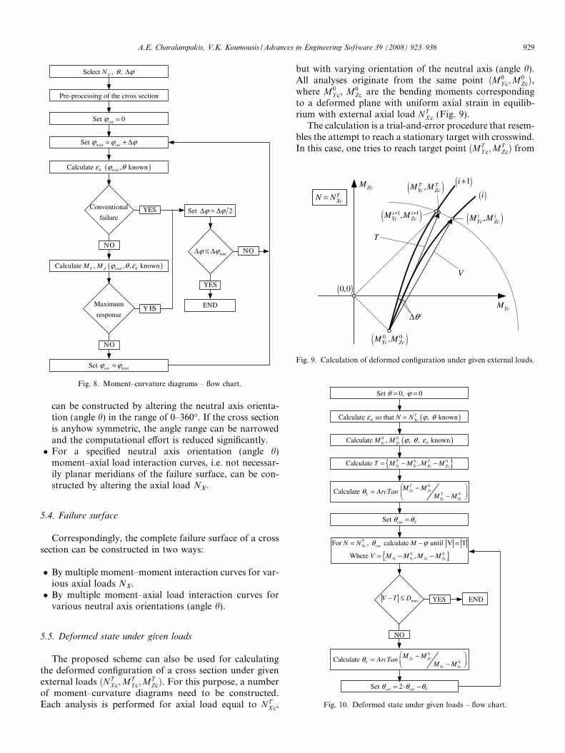
5.1. Moment–curvature diagrams

For a specified axial load NX and neutral axis orienta-tion (angle h), the full moment–curvature diagrams canbe constructed for both the primary moment My and thesecondary moment Mz (Fig. 7). The latter is due to theasymmetry of the cross section and it is needed to preservethe orientation of the neutral axis throughout the process.

After the pre-processing of the cross section i.e. rotation,decomposition of polygons into trapezoids and calculationof basic surface integrals, the imposed curvature isincreased progressively. A small initial curvature step Du,determined by the user, produces smooth moment–curva-ture diagrams but increases the computational cost propor-tionally. At each step, the values of h and u are known;therefore, the deformed state is a function of strain e0 at

+θ

Interaction curve

Δϕ

MZc,u

MYc,u

MZc

MYc

MY

MZ

MY

Fig. 7. Moment–curvature diag

the origin only. A fast Van Wijngaarden–Dekker–Brentmethod [21] is used to evaluate the particular value of e0 thatestablishes axial equilibrium to a specified accuracy. Basedon this deformed state, the corresponding bending momentsMy and Mz are calculated and the procedure is repeated. Ifthe curvature increment cannot be applied then the step ishalved and the algorithm proceeds to calculate the ultimatestrength with greater accuracy. This occurs in two cases: (a)when the response under the incremented trial curvature issmaller than that of the previous step, which indicates that adescending branch is initiated and maximum response hasbeen reached or (b) when the maximum compressive or ten-sile strain of a material is violated (conventional failure).Optionally, the violation of the uniform compression limitcan also be checked. In case of EuroCode 2, this refers toa point which is located at a distance 3/7 h from the mostcompressed fiber and has a predefined compressive strainequal to 0.2% [19]. The procedure stops when the diminish-ing curvature step reaches a predefined minimum threshold.The flowchart of this procedure is shown in Fig. 8.

5.2. Ultimate strength analysis

For a specified axial load NX and orientation of neutralaxis (angle h), the ultimate strength of the cross section iscalculated with the same procedure as described above,with the difference that a large initial curvature step reducesthe computational cost significantly. The accuracy in thecalculation of the ultimate strength is indifferent to the ini-tial curvature step. At the final deformed state, the bendingmoments are expressed in the global reference system bythe inverse rotational transformation of equation (1) todetermine ultimate point (NX,MYc,u,MZc,u) (Fig. 7).

5.3. Interaction curves

By calculating ultimate points according to the afore-mentioned procedure, two kinds of interaction curves canbe constructed:

� For a specified axial load NX moment–moment interac-tion curves, i.e. planar equators of the failure surface,

ϕ ϕΔϕ Δϕ

2Δϕ Δϕ Δϕ

2

MZ

rams and ultimate strength.

Select , , XN θ ϕΔ

Pre-processing of the cross section

curSet 0ϕ =

Set trial curϕ ϕ ϕ= + Δ

( )0Calculate , knowntrialε ϕ θ

Conventional

failure

( )0Calculate , , , knownY Z trialM M ϕ θ ε

Set 2ϕ ϕΔ = Δ

minϕ ϕΔ ≤ Δ

Maximum

responseEND

YES

NO

NO

Set cur trialϕ ϕ=

NO

YES

Y ES

Fig. 8. Moment–curvature diagrams – flow chart.Set 0, 0θ ϕ= =

( )0Calculate so that , knownTXcN Nε ϕ θ=

( )0 00Calculate , , , knownYc ZcM M ϕ θ ε

{ }0 0Calculate ,T TYc Yc Zc ZcT M M M M= − −

0

Calculate TZc ZcM MArcTanθ −=

YcM

ZcM

( )0,0

( )1i +

( )1 1,i iYc ZcM M+ +

iθΔ

TXcN N=

T

( ),i iYc ZcM M

( ),T TYc ZcM M

( )0 0,Yc ZcM M

( )i

V

Fig. 9. Calculation of deformed configuration under given external loads.

A.E. Charalampakis, V.K. Koumousis / Advances in Engineering Software 39 (2008) 923–936 929

can be constructed by altering the neutral axis orienta-tion (angle h) in the range of 0–360�. If the cross sectionis anyhow symmetric, the angle range can be narrowedand the computational effort is reduced significantly.� For a specified neutral axis orientation (angle h)

moment–axial load interaction curves, i.e. not necessar-ily planar meridians of the failure surface, can be con-structed by altering the axial load NX.

0TTYc YcM M−

maxV T D− ≤

Set cur Tθ θ=

{ }0 0

For , calculate until V T

Where ,

TXc cur

Yc Yc Zc Zc

N N M

V M M M M

θ ϕ= − =

= − −

YES END

5.4. Failure surface

Correspondingly, the complete failure surface of a crosssection can be constructed in two ways:

� By multiple moment–moment interaction curves for var-ious axial loads NX.� By multiple moment–axial load interaction curves for

various neutral axis orientations (angle h).

Set 2cur cur Vθ θ θ= ⋅ −

0

0Calculate Zc ZcV

Yc Yc

M MArcTanM M

θ −= −

NO

Fig. 10. Deformed state under given loads – flow chart.

5.5. Deformed state under given loads

The proposed scheme can also be used for calculatingthe deformed configuration of a cross section under givenexternal loads ðNT

X c;MTY c;M

TZcÞ. For this purpose, a number

of moment–curvature diagrams need to be constructed.Each analysis is performed for axial load equal to NT

X c,

but with varying orientation of the neutral axis (angle h).All analyses originate from the same point ðM0

Y c;M0ZcÞ,

where M0Y c, M0

Zc are the bending moments correspondingto a deformed plane with uniform axial strain in equilib-rium with external axial load NT

X c (Fig. 9).The calculation is a trial-and-error procedure that resem-

bles the attempt to reach a stationary target with crosswind.In this case, one tries to reach target point ðMT

Y c;MTZcÞ from

930 A.E. Charalampakis, V.K. Koumousis / Advances in Engineering Software 39 (2008) 923–936

fixed point ðM0Y c;M

0ZcÞ with crosswind, i.e. deviation of the

analysis paths due to the secondary moment MZ.As first attempt, the direction of the neutral axis is set

equal to the direction of the target vector T, connecting pointðM0

Y c;M0ZcÞ to ðMT

Y c;MTZcÞ. As the curvature is increased, the

path of the analysis deviates due to the secondary momentMZ. When the norm of the trial vector V reaches that ofthe target vector, the analysis stops, but the resulting Mi

Y c

and MiZc may differ from the target values MT

Y c and MTZc.

The direction of the neutral axis is then corrected by theangle difference Dhi between the target vector and the trialvector and the procedure is repeated. In the next attempt,the resulting Miþ1

Y c and Miþ1Zc are closer to the target values.

The procedure stops when a specified accuracy with respectto the given external loads is achieved. At this point, the val-ues of h, u, e0 define the deformed state of the cross section.The flowchart of this procedure is presented in Fig. 10.

6. Numerical validation – examples

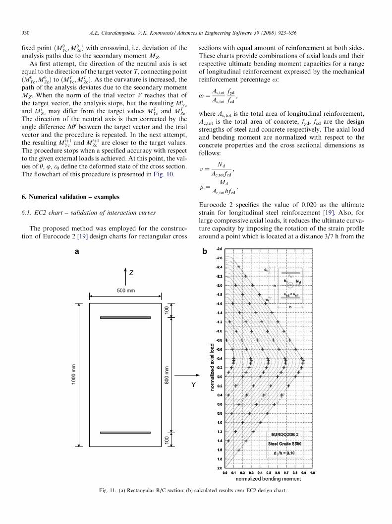
6.1. EC2 chart – validation of interaction curves

The proposed method was employed for the construc-tion of Eurocode 2 [19] design charts for rectangular cross

500 mm

1000

mm

800

mm

100

100

Y

Z

a

Fig. 11. (a) Rectangular R/C section; (b) ca

sections with equal amount of reinforcement at both sides.These charts provide combinations of axial loads and theirrespective ultimate bending moment capacities for a rangeof longitudinal reinforcement expressed by the mechanicalreinforcement percentage x:

x ¼ As;tot

Ac;tot

fyd

fcd

;

where As,tot is the total area of longitudinal reinforcement,Ac,tot is the total area of concrete, fyd, fcd are the designstrengths of steel and concrete respectively. The axial loadand bending moment are normalized with respect to theconcrete properties and the cross sectional dimensions asfollows:

v ¼ Nd

Ac;totfcd

;

l ¼ Md

Ac;tothfcd

:

Eurocode 2 specifies the value of 0.020 as the ultimatestrain for longitudinal steel reinforcement [19]. Also, forlarge compressive axial loads, it reduces the ultimate curva-ture capacity by imposing the rotation of the strain profilearound a point which is located at a distance 3/7 h from the

b

lculated results over EC2 design chart.

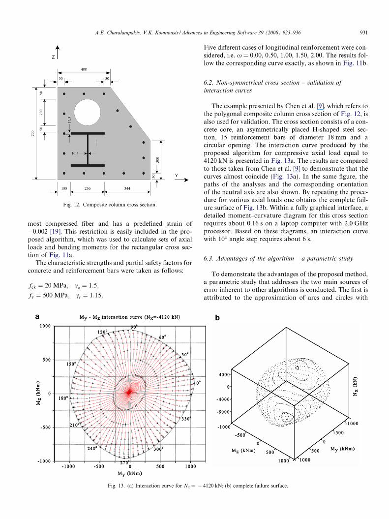
Fig. 12. Composite column cross section.

A.E. Charalampakis, V.K. Koumousis / Advances in Engineering Software 39 (2008) 923–936 931

most compressed fiber and has a predefined strain of�0.002 [19]. This restriction is easily included in the pro-posed algorithm, which was used to calculate sets of axialloads and bending moments for the rectangular cross sec-tion of Fig. 11a.

The characteristic strengths and partial safety factors forconcrete and reinforcement bars were taken as follows:

fck ¼ 20 MPa; cc ¼ 1:5;

fy ¼ 500 MPa; cr ¼ 1:15;

Fig. 13. (a) Interaction curve for Nx = �

Five different cases of longitudinal reinforcement were con-sidered, i.e. x = 0.00, 0.50, 1.00, 1.50, 2.00. The results fol-low the corresponding curve exactly, as shown in Fig. 11b.

6.2. Non-symmetrical cross section – validation of

interaction curves

The example presented by Chen et al. [9], which refers tothe polygonal composite column cross section of Fig. 12, isalso used for validation. The cross section consists of a con-crete core, an asymmetrically placed H-shaped steel sec-tion, 15 reinforcement bars of diameter 18 mm and acircular opening. The interaction curve produced by theproposed algorithm for compressive axial load equal to4120 kN is presented in Fig. 13a. The results are comparedto those taken from Chen et al. [9] to demonstrate that thecurves almost coincide (Fig. 13a). In the same figure, thepaths of the analyses and the corresponding orientationof the neutral axis are also shown. By repeating the proce-dure for various axial loads one obtains the complete fail-ure surface of Fig. 13b. Within a fully graphical interface, adetailed moment–curvature diagram for this cross sectionrequires about 0.16 s on a laptop computer with 2.0 GHzprocessor. Based on these diagrams, an interaction curvewith 10� angle step requires about 6 s.

6.3. Advantages of the algorithm – a parametric study

To demonstrate the advantages of the proposed method,a parametric study that addresses the two main sources oferror inherent to other algorithms is conducted. The first isattributed to the approximation of arcs and circles with

4120 kN; (b) complete failure surface.

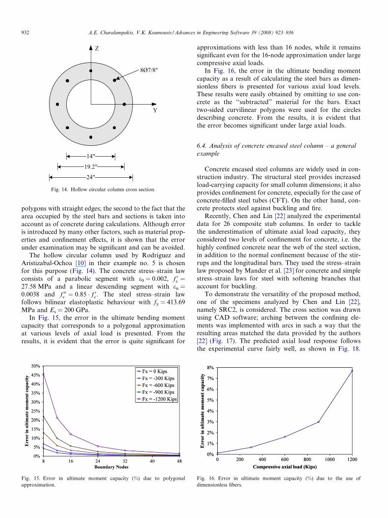
Fig. 14. Hollow circular column cross section.

932 A.E. Charalampakis, V.K. Koumousis / Advances in Engineering Software 39 (2008) 923–936

polygons with straight edges; the second to the fact that thearea occupied by the steel bars and sections is taken intoaccount as of concrete during calculations. Although erroris introduced by many other factors, such as material prop-erties and confinement effects, it is shown that the errorunder examination may be significant and can be avoided.

The hollow circular column used by Rodriguez andAristizabal-Ochoa [10] in their example no. 5 is chosenfor this purpose (Fig. 14). The concrete stress–strain lawconsists of a parabolic segment with e0 = 0.002, f 0c ¼27:58 MPa and a linear descending segment with eu =0.0038 and f 00c ¼ 0:85 � f 0c . The steel stress–strain lawfollows bilinear elastoplastic behaviour with fy = 413.69MPa and Es = 200 GPa.

In Fig. 15, the error in the ultimate bending momentcapacity that corresponds to a polygonal approximationat various levels of axial load is presented. From theresults, it is evident that the error is quite significant for

Fig. 15. Error in ultimate moment capacity (%) due to polygonalapproximation.

approximations with less than 16 nodes, while it remainssignificant even for the 16-node approximation under largecompressive axial loads.

In Fig. 16, the error in the ultimate bending momentcapacity as a result of calculating the steel bars as dimen-sionless fibers is presented for various axial load levels.These results were easily obtained by omitting to use con-crete as the ‘‘subtracted” material for the bars. Exacttwo-sided curvilinear polygons were used for the circlesdescribing concrete. From the results, it is evident thatthe error becomes significant under large axial loads.

6.4. Analysis of concrete encased steel column – a general

example

Concrete encased steel columns are widely used in con-struction industry. The structural steel provides increasedload-carrying capacity for small column dimensions; it alsoprovides confinement for concrete, especially for the case ofconcrete-filled steel tubes (CFT). On the other hand, con-crete protects steel against buckling and fire.

Recently, Chen and Lin [22] analyzed the experimentaldata for 26 composite stub columns. In order to tacklethe underestimation of ultimate axial load capacity, theyconsidered two levels of confinement for concrete, i.e. thehighly confined concrete near the web of the steel section,in addition to the normal confinement because of the stir-rups and the longitudinal bars. They used the stress–strainlaw proposed by Mander et al. [23] for concrete and simplestress–strain laws for steel with softening branches thataccount for buckling.

To demonstrate the versatility of the proposed method,one of the specimens analyzed by Chen and Lin [22],namely SRC2, is considered. The cross section was drawnusing CAD software; arching between the confining ele-ments was implemented with arcs in such a way that theresulting areas matched the data provided by the authors[22] (Fig. 17). The predicted axial load response followsthe experimental curve fairly well, as shown in Fig. 18.

Fig. 16. Error in ultimate moment capacity (%) due to the use ofdimensionless fibers.

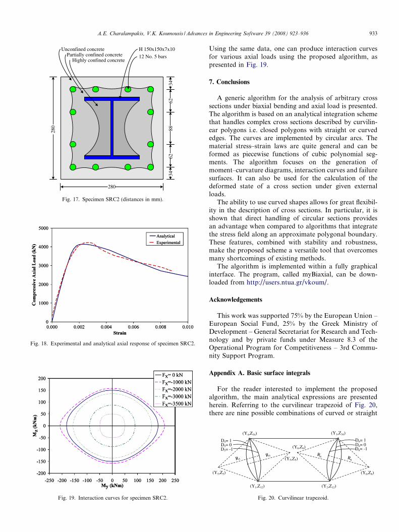
Fig. 18. Experimental and analytical axial response of specimen SRC2.

Fig. 19. Interaction curves for specimen SRC2.

280

Unconfined concretePartially confined concrete

Highly confined concrete12 No. 5 bars

H 150x150x7x10 28

0

6288

6234

34

Fig. 17. Specimen SRC2 (distances in mm).

A.E. Charalampakis, V.K. Koumousis / Advances in Engineering Software 39 (2008) 923–936 933

Using the same data, one can produce interaction curvesfor various axial loads using the proposed algorithm, aspresented in Fig. 19.

7. Conclusions

A generic algorithm for the analysis of arbitrary crosssections under biaxial bending and axial load is presented.The algorithm is based on an analytical integration schemethat handles complex cross sections described by curvilin-ear polygons i.e. closed polygons with straight or curvededges. The curves are implemented by circular arcs. Thematerial stress–strain laws are quite general and can beformed as piecewise functions of cubic polynomial seg-ments. The algorithm focuses on the generation ofmoment–curvature diagrams, interaction curves and failuresurfaces. It can also be used for the calculation of thedeformed state of a cross section under given externalloads.

The ability to use curved shapes allows for great flexibil-ity in the description of cross sections. In particular, it isshown that direct handling of circular sections providesan advantage when compared to algorithms that integratethe stress field along an approximate polygonal boundary.These features, combined with stability and robustness,make the proposed scheme a versatile tool that overcomesmany shortcomings of existing methods.

The algorithm is implemented within a fully graphicalinterface. The program, called myBiaxial, can be down-loaded from http://users.ntua.gr/vkoum/.

Acknowledgements

This work was supported 75% by the European Union –European Social Fund, 25% by the Greek Ministry ofDevelopment – General Secretariat for Research and Tech-nology and by private funds under Measure 8.3 of theOperational Program for Competitiveness – 3rd Commu-nity Support Program.

Appendix A. Basic surface integrals

For the reader interested to implement the proposedalgorithm, the main analytical expressions are presentedherein. Referring to the curvilinear trapezoid of Fig. 20,there are nine possible combinations of curved or straight

R5R5 R

6 R6

(Y2,Z12)(Y1,Z12)

(Y3,Z34)(Y4,Z34)

(Y5,Z5)

(Y5,Z5)

(Y6,Z6)

(Y6,Z6)

D5= 1

D5= -1D5= 0

D6= -1

D6= 1D6= 0

Fig. 20. Curvilinear trapezoid.

934 A.E. Charalampakis, V.K. Koumousis / Advances in Engineering Software 39 (2008) 923–936

edges. The parameters identifying the type of edge are D5,D6, as shown in the figure.

Three integrals are defined: the ‘‘middle” integral, whichrefers to the trapezoid with straight edges, the ‘‘left” inte-gral and the ‘‘right” integral, which refer to the correspond-ing circular segment, if any. Assuming that L14 = (y4 � y1)/(z34 � z12), L23 = (y3 � y2)/(z34 � z12) with z34 > z12, themiddle integral is calculated as follows:

Ij;midðm;nÞ ¼

Z z34

z12

Z y2þL23�ðz�z12Þ

y1þL14�ðz�z12Þðym � znÞdy

!dz:

Therefore

Ij;midð0;nÞ ¼

1

nþ 2� ðL23 � L14Þ � ðznþ2

34 � znþ212 Þ

þ 1

nþ 1� ðy2 � L23 � z12 � y1 þ L14

� z12Þ � ðznþ134 � znþ1

12 Þ;

A ¼ 1

2� ðL2

23 � L214Þ;

B ¼ ðy2 � L23 � z12Þ � L23 � ðy1 � L14 � z12Þ � L14;

C ¼ 1

2� ððy2 � L23 � z12Þ2 � ðy1 � L14 � z12Þ2Þ;

Ij;midð1;nÞ ¼

1

nþ 3� A � ðznþ3

34 � znþ312 Þ

þ 1

nþ 2� B � ðznþ2

34 � znþ212 Þ

þ 1

nþ 1� C � ðznþ1

34 � znþ112 Þ:

The ‘‘left” and ‘‘right” integrals are equal to zero if the cor-responding side is a straight line. If not, they can be calcu-lated for specific values of m, n following symbolicalprogramming:

Ij;leftðm;nÞ ¼

Z z34

z12

Z y1þL14�ðz�z12Þ

y5�D5

ffiffiffiffiffiffiffiffiffiffiffiffiffiffiffiffiR2

5�ðz�z5Þ2

p ðym � znÞdy

!dz;

Ij;rightðm;nÞ ¼

Z z34

z12

Z y6þD6

ffiffiffiffiffiffiffiffiffiffiffiffiffiffiffiffiR2

6�ðz�z6Þ2

py2þL23�ðz�z12Þ

ðym � znÞdy

0@

1Adz:

The final result is the sum of all three integrals:

Ijðm;nÞ ¼ Ij;left

ðm;nÞ þ I j;midðm;nÞ þ I j;right

ðm;nÞ :

For example, for D5 = 1, the ‘‘left” integrals are as follows:

A12 ¼ arcsinz5 � z12

R5

� �;

A34 ¼ arcsinz5 � z34

R5

� �;

S12 ¼ffiffiffiffiffiffiffiffiffiffiffiffiffiffiffiffiffiffiffiffiffiffiffiffiffiffiffiffiffiffiffiffiffiffiffiffiffiffiffiffiffiffiffiffiffiffiffiffiffiffiffiffiffiðR2

5 þ 2 � z5 � z12 � z25 � z2

12Þq

;

S34 ¼ffiffiffiffiffiffiffiffiffiffiffiffiffiffiffiffiffiffiffiffiffiffiffiffiffiffiffiffiffiffiffiffiffiffiffiffiffiffiffiffiffiffiffiffiffiffiffiffiffiffiffiffiffiðR2

5 þ 2 � z5 � z34 � z25 � z2

34Þq

;

Ij;leftð0;0Þ ¼ �y1 � z12 þ

1

2� L14 � z2

12 þ y5 � z12 �1

2� S12 � z12

þ 1

2� S12 � z5 þ

1

2� R2

5 � A12 þ y1 � z34

þ 1

2� L14 � z2

34 � L14 � z34 � z12 � y5 � z34

þ 1

2� S34 � z34 �

1

2� S34 � z5 �

1

2� R2

5 � A34;

Ij;leftð0;1Þ ¼

1

3� S3

12 �1

2� y1 � z2

12 �1

2� S12 � z5 � z12 þ

1

2� y5 � z2

12

þ 1

2� S12 � z2

5 þ1

2� z5 � R2

5 � A12

þ 1

6� L14 � z3

12 �1

3� S3

34 þ1

2� z5 � S34 � z34

� 1

2� S34 � z2

5 �1

2� z5 � R2

5 � A34 þ1

3� L14 � z3

34

þ 1

2� z2

34 � y1 �1

2� z2

34 � L14 � z12 �1

2� z2

34 � y5;

Ij;leftð0;2Þ ¼

1

8� R2

5 � S12 � z5 �1

2� S12 � z2

5 � z12 �1

8� R2

5 � S12 � z12

þ 1

8� R4

5 � A12 �1

8� R4

5 � A34

þ 1

3� z3

34 � y1 �1

3� z3

34 � y5 þ1

4� L14 � z4

34 �1

4� z34 � S3

34

� 5

12� z5 � S3

34 �1

2� S34 � z3

5

þ 1

12� L14 � z4

12 �1

3� y1 � z3

12 þ1

2� z2

5 � R25 � A12

þ 1

2� S12 � z3

5 þ1

4� S3

12 � z12 þ5

12� z5 � S3

12

� 1

2� z2

5 � R25 � A34 þ

1

8� R2

5 � S34 � z34 �1

8� R2

5 � S34 � z5

� 1

3� z3

34 � L14 � z12 þ1

2� z2

5 � S34 � z34 þ1

3� y5 � z3

12;

Ij;leftð0;3Þ ¼ �

1

2� z3

5 � R25 � A34 �

3

8� z5 � R4

5 � A34 �1

2� S12 � z3

5 � z12

þ 3

8� R2

5 � S12 � z25 þ

1

2� z3

5 � S34 � z34

� 3

8� R2

5 � S34 � z25 þ

7

20� z5 � S3

12 � z12 �1

4� z4

34 � y5

þ 3

8� z5 � R4

5 � A12 þ1

2� z3

5 � R25 � A12 þ

1

20� L14 � z5

12

� 1

4� y1 � z4

12 þ1

4� y5 � z4

12 þ1

5� S3

12 � z212 þ

2

15� R2

5 � S312

þ 9

20� z2

5 � S312 �

2

15� R2

5 � S334 �

1

5� z2

34 � S334

� 9

20� z2

5 � S334 �

3

8� R2

5 � S12 � z5 � z12 �7

20� z5 � z34 � S3

34

þ 1

2� S12 � z4

5 �1

2� S34 � z4

5 �1

4� z4

34 � L14 � z12

þ 1

4� z4

34 � y1 þ1

5� L14 � z5

34 þ3

8� z5 � R2

5 � S34 � z34;

Ij;leftð0;4Þ ¼ �

3

4� z2

5 � R45 � A34 �

1

2� z4

5 � R25 � A34 þ

1

16� R4

5 � S34 � z34

� 3

4� R2

5 � S34 � z35 þ

1

2� z4

5 � S34 � z34

A.E. Charalampakis, V.K. Koumousis / Advances in Engineering Software 39 (2008) 923–936 935

� 1

16� R4

5 � S12 � z12 þ1

16� R4

5 � S12 � z5

� 1

2� S12 � z4

5 � z12 þ3

4� R2

5 � S12 � z35 þ

3

4� z2

5 � R45 � A12

þ 1

2� z4

5 � R25 � A12 �

1

8� R2

5 � z34 � S334

� 49

120� z5 � R2

5 � S334 �

3

10� z5 � z2

34 � S334

� 2

5� z2

5 � z34 � S334 þ

3

10� z5 � S3

12 � z212

þ 49

120� z5 � R2

5 � S312 þ

1

8� R2

5 � S312 � z12

þ 2

5� z2

5 � S312 � z12 �

1

16� R4

5 � S34 � z5

� 3

4� R2

5 � S12 � z25 � z12 þ

3

4� z2

5 � R25 � S34 � z34

� 1

16� R6

5 � A34 �1

6� z3

34 � S334 �

7

15� z3

5 � S334

þ 1

5� z5

34 � y1 �1

5� z5

34 � y5 þ1

6� S3

12 � z312 þ

7

15� z3

5 � S312

� 1

2� S34 � z5

5 �1

5� z5

34 � L14 � z12

þ 1

6� L14 � z6

34 þ1

2� S12 � z5

5 þ1

16� R6

5 � A12

þ 1

30� L14 � z6

12 �1

5� y1 � z5

12 þ1

5� y5 � z5

12;

Ij;leftð1;0Þ ¼ �

1

2� y5 � R2

5 � A34 þ1

2� y5 � R2

5 � A12 �1

2� y5 � S34 � z5

þ 1

2� y5 � S34 � z34 þ

1

2� y5 � S12 � z5

� 1

2� y5 � S12 � z12 þ

1

6� L2

14 � z334 �

1

2� y2

1 � z12

þ 1

2� y2

1 � z34 �1

2� L2

14 � z234 � z12 þ

1

2� L2

14 � z34 � z212

þ 1

2� y1 � L14 � z2

34 �1

6� L2

14 � z312

� 1

2� z12 � z2

5 þ1

2� y2

5 � z12 þ1

2� z5 � z2

12 þ1

2� z12 � R2

5

þ 1

6� z3

34 �1

6� z3

12 þ1

2� L14 � y1 � z2

12 � y1 � L14 � z34 � z12

� 1

2� R2

5 � z34 �1

2� z2

34 � z5 þ1

2� z2

5 � z34 �1

2� y2

5 � z34;

Ij;leftð1;1Þ ¼

1

3� y5 � S3

12 þ1

4� z2

34 � L214 � z2

12 þ1

3� L14 � z3

34 � y1

� 1

3� L2

14 � z334 � z12 �

1

2� y5 � z5 � R2

5 � A34

þ 1

3� z5 � z3

12 þ1

4� R2

5 � z212 �

1

4� z2

5 � z212

� 1

24� L2

14 � z412 �

1

4� y2

1 � z212 þ

1

4� y2

5 � z212 �

1

3� z3

34 � z5

� 1

8� z4

12 �1

3� y5 � S3

34 þ1

8� z4

34 þ1

4� z2

34 � y21

� 1

4� z2

34 � y25 �

1

4� z2

34 � R25 þ

1

4� z2

34 � z25

þ 1

2� y5 � z5 � S34 � z34 �

1

2� y5 � S12 � z5 � z12

� 1

2� z2

34 � y1 � L14 � z12 þ1

2� y5 � S12 � z2

5

þ 1

6� L14 � y1 � z3

12 þ1

2� y5 � z5 � R2

5 � A12

þ 1

8� L2

14 � z434 �

1

2� y5 � S34 � z2

5;

Ij;leftð1;2Þ ¼

1

6� z3

34 � L214 � z2

12 �1

2� y5 � z2

5 � R25 � A34

þ 1

2� y5 � z2

5 � R25 � A12 �

1

8� y5 � R4

5 � A34

þ 1

8� y5 � R4

5 � A12 �1

8� y5 � R2

5 � S12 � z12

þ 1

2� y5 � S12 � z3

5 �1

2� y5 � S34 � z3

5

þ 1

8� y5 � R2

5 � S12 � z5 �1

10� z5

12 �1

2� y5 � S12 � z2

5 � z12

� 1

8� y5 � R2

5 � S34 � z5 þ1

8� y5 � R2

5 � S34 � z34

þ 5

12� y5 � z5 � S3

12 þ1

4� y5 � S3

12 � z12 �1

4� y5 � z34 � S3

34

� 1

6� z3

34 � R25 þ

1

6� z3

34 � z25 þ

1

6� z3

34 � y21

� 1

6� z3

34 � y25 �

5

12� y5 � z5 � S3

34 þ1

2� y5 � z2

5 � S34 � z34

� 1

60� L2

14 � z512 þ

1

10� z5

34 þ1

12� L14 � y1 � z4

12

þ 1

10� L2

14 � z534 �

1

6� y2

1 � z312 þ

1

6� y2

5 � z312

� 1

3� z3

34 � y1 � L14 � z12 �1

4� z4

34 � z5

� 1

4� L2

14 � z434 � z12 þ

1

4� L14 � z4

34 � y1

þ 1

4� z5 � z4

12 þ1

6� R2

5 � z312 �

1

6� z2

5 � z312;

Ij;leftð1;3Þ ¼

1

2� y5 � S12 � z4

5 �1

2� y5 � S34 � z4

5 þ1

5� y5 � S3

12 � z212

þ 2

15� y5 � R2

5 � S312 �

3

8� y5 � z5 � R4

5 � A34

þ 9

20� y5 � z2

5 � S312 �

1

2� y5 � z3

5 � R25 � A34

� 1

4� z4

34 � y1 � L14 � z12 �1

12� z6

12 �1

5� y5 � z2

34 � S334

� 2

15� y5 � R2

5 � S334 �

9

20� y5 � z2

5 � S334

þ 1

2� y5 � R2

5 � z35 � A12 þ

3

8� y5 � z5 � R4

5 � A12

þ 1

8� z4

34 � L214 � z2

12 �1

5� L2

14 � z534 � z12

þ 1

5� L14 � z5

34 � y1 þ1

12� z6

34 þ3

8� y5 � R2

5 � S12 � z25

� 1

2� y5 � S12 � z3

5 � z12 �1

5� z5

34 � z5

þ 1

12� L2

14 � z634 þ

3

8� y5 � z5 � R2

5 � S34 � z34

936 A.E. Charalampakis, V.K. Koumousis / Advances in Engineering Software 39 (2008) 923–936

� 3

8� y5 � R2

5 � S12 � z5 � z12 þ1

8� R2

5 � z412

� 1

8� z2

5 � z412 þ

1

5� z5 � z5

12 �1

8� z4

34 � R25 þ

1

8� z4

34 � z25

þ 1

8� z4

34 � y21 �

1

8� z4

34 � y25 þ

1

2� y5 � z3

5 � S34 � z34

� 3

8� y5 � R2

5 � S34 � z25 þ

7

20� y5 � z5 � S3

12 � z12

� 7

20� y5 � z5 � z34 � S3

34 �1

120� L2

14 � z612

þ 1

20� L14 � y1 � z5

12 �1

8� y2

1 � z412 þ

1

8� y2

5 � z412:

References

[1] Wen YK. Method of random vibration of hysteretic systems. J EngMech Div 1976;102(EM2):249–63.

[2] Dafalias YF, Popov EP. A model of nonlinearly hardening materialsfor complex loading. Acta Mech 1975;21:173–92.

[3] Dafalias YF. A model of soil behaviour under monotonic and cyclicloading conditions. In: Transactions of fifth international conferenceon structural mechanics and reactor technology. K1/8, Berlin; 1979.

[4] El-Tawil S, Deierlein GG. Nonlinear analysis of mixed steel–concreteframes. I: element formulation. ASCE J Struct Eng 2001;127(6):647–55.

[5] Chen DL, Wang Z. Derivation of applied stress–crack openingdisplacement relationships for the evaluation of effective stressintensity factor range. Int J Fract 2004;125:371–86.

[6] Sousa JLAO, Gettu R. Determining the tensile stress–crack openingcurve of concrete by inverse analysis. ASCE J Eng Mech 2006;132(2):141–8.

[7] Brondum-Nielsen T. Ultimate flexural capacity of cracked polygonalconcrete sections under biaxial bending. ACI Struct J 1985;82(6):863–70.

[8] Yen JYR. Quasi-Newton method for reinforced concrete columnanalysis and design. ASCE J Struct Eng 1991;117(3):657–66.

[9] Chen SF, Teng G, Chan SL. Design of biaxially loaded shortcomposite columns of arbitrary cross section. ASCE J Struct Eng2001;127(6):678–85.

[10] Rodriguez JA, Aristizabal-Ochoa JD. Biaxial interaction diagramsfor short RC columns of any cross section. ASCE J Struct Eng1999;125(6):672–83.

[11] Rotter JM. Rapid exact inelastic biaxial bending analysis. ASCE JStruct Eng 1985;111(12):2659–74.

[12] Fafitis A. Interaction surfaces of reinforced-concrete sections inbiaxial bending. ASCE J Struct Eng 2001;127(7):840–6.

[13] Sfakianakis MG. Biaxial bending with axial force of reinforced,composite and repaired concrete sections of arbitrary shape by fibermodel and computer graphics. Adv Eng Software 2002;33:227–42.

[14] Bonet JL, Romero ML, Miguel PF, Fernandez MA. A fast stressintegration algorithm for reinforced concrete sections with axial loadsand biaxial bending. Comput Struct 2004;82:213–25.

[15] Zupan D, Saje M. Analytical integration of stress field and tangentmaterial moduli over concrete cross-sections. Comput Struct2005;83:2368–80.

[16] Sousa JBM, Muniz CFDG. Analytical integration of cross sectionproperties for numerical analysis of reinforced concrete, steel andcomposite frames. Eng Struct 2007;29:618–25.

[17] Bonet JL, Barros MHFM, Romero ML. Comparative study ofanalytical and numerical algorithms for designing reinforced concretesections under biaxial bending. Comput Struct 2006;84:2184–93.

[18] De Vivo L, Rosati L. Ultimate strength analysis of reinforcedconcrete sections subject to axial force and biaxial bending. ComputMethods Appl Mech Eng 1998;166:261–87.

[19] Concrete structures. Euro-design handbook. Ernst and Sohn; 1995.[20] Nawy EG. Reinforced concrete. ACI 2005 update edition. Prentice

Hall; 2004.[21] Press WH, Teukolsky SA, Vetterling WT, Flannery BP. Numerical

recipes in C++: the art of scientific computing. Cambridge UniversityPress; 2002.

[22] Chen C-C, Lin N-J. Analytical model for predicting axial capacityand behaviour of concrete encased steel composite stub columns. JConst Steel Res 2006;62:424–33.

[23] Mander JB, Priestley MJN, Park R. Theoretical stress–strain modelfor confined concrete. J Struct Eng 1988;114(8):1804–26.