Do thermotropic biaxial nematics exist? A Monte Carlo study of biaxial Gay-Berne particles
27
Do thermotropic biaxial nematics exist? A Monte Carlo study of biaxial Gay–Berne particles. R. Berardi and C. Zannoni, Dipartimento di Chimica Fisica e Inorganica, Universit` a, Viale Risorgimento 4, 40136 Bologna, Italy. April 11, 2000 Abstract We have investigated with extensive Monte Carlo simulations in the isothermal isobaric ensemble a system of N = 8192 elongated attractive–repulsive biaxial Gay–Berne (GB) particles. We have found a uniaxial and biaxial nematic and a biaxial orthogonal smectic phase in this thermotropic model system. 1
Transcript of Do thermotropic biaxial nematics exist? A Monte Carlo study of biaxial Gay-Berne particles

Do thermotropic biaxial nematics exist?
A Monte Carlo study of biaxial Gay–Berne
particles.
R. Berardi and C. Zannoni,
Dipartimento di Chimica Fisica e Inorganica,
Universita, Viale Risorgimento 4,
40136 Bologna, Italy.
April 11, 2000
Abstract
We have investigated with extensive Monte Carlo simulations inthe isothermal isobaric ensemble a system of N = 8192 elongatedattractive–repulsive biaxial Gay–Berne (GB) particles. We have founda uniaxial and biaxial nematic and a biaxial orthogonal smectic phasein this thermotropic model system.
1
Claudio Zannoni
Claudio Zannoni
published in J. Chem. Phys., 113, 5971-5979 (2000)

1 Introduction
Biaxial nematic phases have been a subject of great interest for some time
and this interest is increasing as the chase for undisputed thermotropic bi-
axial nematics continues [1]. Part of this focused attention comes from the
possibility of technological applications in the fast display area [2], but much
of the fascination of the subject certainly originates from the basic research
arena and from the hiatus between theoretical [3] and experimental predic-
tions [4, 5]. Biaxial nematics are not theoretically forbidden and indeed have
been predicted to exist, and thus to be the most stable phase in a certain
range of thermodynamic conditions, by various approximate theories, mainly
on the basis of considerations of orientational order and of orientational free
energy [3, 6, 7, 8, 9, 10].
Monte Carlo simulations of systems of interacting biaxial centers placed on
a lattice [11, 12] have essentially confirmed these predictions and the phase
diagram obtained [12] has shown a biaxial region where the biaxial phase is
stable compared to both the uniaxial nematic and isotropic ones. However,
as we have already mentioned, none of the low molecular mass thermotropic
biaxial nematics put forward [13] appears to have been universally accepted
as such. Indeed various of the compounds classified as biaxial nematics on
the basis of their optical behavior have shown no detectable biaxiality when
examined with deuterium NMR [4, 5]. Such a searching test appears not to
have been yet performed on the polymer nematic liquid crystals classified as
biaxial [14].
Surprisingly enough the only generally recognized biaxial nematic is the first
one to be discovered: the lyotropic system introduced by Yu and Saupe in
1980 [15] although a recent report raises some doubts even on the stability
of the phase biaxiality of this mixture [16]. It should also be noticed that
lyotropic micellar systems add another complication as they have more than
one component and are anyway different in that the shape of the constituent
micelles can vary in different regions of the phase diagram [17].
The reason for the failure to date to observe thermotropic biaxial nematics
may be connected with the competition between this candidate mesophase
and other potential molecular organizations. Thus, if we return to the phase
2

diagram predicted by purely orientational interactions [12] it seems that only
a small region of molecular biaxiality around the maximum stands a chance
of being observed before a transition to smectic or crystal steps in [18], very
often arising at temperatures some 10% lower that the clearing tempera-
ture. To test this type of competition hypothesis theoretical models with
full translational freedom rather than lattice models should be employed.
As theoretical predictions of phase transitions for off–lattice models are not
easily available, the use of computer simulations (see, e.g. [19]) to test the
physical implications of a chosen model of molecular interactions becomes
particularly important. A pioneering work from this point of view has been
that of Allen [20, 21] who examined, using Molecular Dynamics, a system
of hard biaxial ellipsoids going from flat–like to rod–like shapes and showed
the existence of a biaxial nematic phase [20]. Systems of purely repulsive
particles formed of strings of oblate ellipsoids with a repulsive core similar to
that of Gay-Berne particles [22] have been studied by Sarman [23] and were
also found to give a biaxial nematic.
Hard particle systems are of course not temperature driven and it might be
significant that they bear more similarity to colloidal suspensions [24] or to
the lyotropic systems where the biaxial nematic was found. The question
of the existence of a biaxial nematic in a thermotropic system, especially in
competition with the formation of smectics, is thus quite an open one that
we wish to address here.
We have considered for this purpose a system of biaxial particles, using a
generalized attractive–repulsive Gay–Berne pair potential that we have pre-
viously developed [25]. We consider the effect of changing the interaction
biaxiality and examine a few cases where shape and interaction biaxiality
have the same or opposite sign. We then perform a fairly large scale isobaric–
isothermal (NPT) computer simulation for a system of biaxial particles with a
selected parameterization and show that it forms biaxial nematic and smectic
phases. We characterize the observed biaxial phases in terms of orientational
order parameters and a suitable set of averaged Stone [26, 27] rotational
invariants.
Our conclusion is that thermotropic biaxial nematics and smectics can exist
also for off lattice attractive–repulsive systems in competition with crystalline
3

phases.
2 Model
We consider a system formed by a set of N identical ellipsoidal biaxial par-
ticles interacting with the generalized attractive–repulsive Gay–Berne (GB)
interaction [25]
U(ω1, ω2, r12) = 4ε0ε(ω1, ω2, r12)
×[(
σc
r12 − σ(ω1, ω2, r12) + σc
)12
−(
σc
r12 − σ(ω1, ω2, r12) + σc
)6]. (1)
The biaxial ellipsoids have axes σx, σy, σz, orientation ωi and their center–
center intermolecular vector is r12 = r12 r12 with length r12 and orientation
r12, where we use the cap to indicate a unit vector. The potential contains
a shape (i.e. anisotropic contact distance) σ(ω1, ω2, r12) and an interaction
term ε(ω1, ω2, r12), namely
σ(ω1, ω2, r12) = (2 rT12A
−1(ω1, ω2)r12)−1/2. (2)
The symmetric overlap matrix A is defined as
A(ω1, ω2) = MT (ω1)S2M(ω1) +MT (ω2)S
2M(ω2), (3)
where S is the shape matrix with elements Sab = δa,bσa and M(ωi) are
rotation matrices from laboratory to molecular frame i. The interaction
term is ε(ω1, ω2, r12) = εν(ω1, ω2)ε′µ(ω1, ω2, r12), with µ and ν empirical ex-
ponents [22] and
ε(ω1, ω2) = (σxσy + σ2z)
[2σxσy
det[A]
]1/2
, (4)
ε′(ω1, ω2, r12) = 2 rT12B
−1(ω1, ω2)r12. (5)
The symmetric interaction matrix B is in turn
B(ω1, ω2) = MT (ω1)EM(ω1) +MT (ω2)EM(ω2), (6)
4

where the matrix E with elements Eab = δa,b(ε0/εab)1/µ contains the pa-
rameters εx, εy and εz proportional to the well depths for the side–to–side,
face–to–face and end–to–end interactions of the molecules. We employ units
of distance, σ0, and energy, ε0, and well width parameter σc.
Biaxial mesogens are often characterized by a biaxiality parameter repre-
senting deviation from cylindrical symmetry. While this is an all important
concept also for the molecular design of new mesogens [28], it is also a loosely
defined one. In particular, it should be pointed out that if different molecular
interactions contribute significantly to the pair potential then each of them
can have a different biaxiality parameter. In our case the deviation from
uniaxiality of repulsive and attractive interactions can be concisely described
in terms of two parameters:
Shape biaxiality
λσ =√
3/2σx − σy
2σz − σx − σy
, (7)
Interaction biaxiality
λε =√
3/2ε−1/µx − ε−1/µ
y
2ε−1/µz − ε
−1/µx − ε
−1/µy
. (8)
It is important to notice that these parameters are quite independent and
can even have opposite sign. If we consider the interaction potential as two
molecules approach with a certain orientation (say with two axes parallel)
the position of the energy minimum is clearly linked to the closest approach
distance and then on the σi and the chosen shape biaxiality. On the other
hand the interaction biaxiality λε defines the order of the strongest potential
wells. In Figures 1 and 2 we see examples of λσ and λε parameterizations
corresponding to different energy profiles. We see that varying the two types
of biaxiality, for instance by suitable chemical substitution, can provide an
important handle to tuning the intermolecular potential.
2.1 Biaxial Order Parameters
Since we are after the generation of biaxial phases it seems appropriate to
briefly discuss the orientational order in such phases, if only to have a way
5

of monitoring the occurrence or not of phase biaxiality. The description of
the static orientational properties can be realized in terms of the first few
expansion coefficients of the single particle orientational distribution [29] in
a basis of symmetrized Wigner rotation matrices [12, 30] (both phase and
molecules have an effective D2h symmetry)
RLm,n =
1
4δL,evenδm,evenδn,even[DL ∗
m,n +DL ∗−m,n +DL ∗
m,−n +DL ∗−m,−n]. (9)
These second rank order parameters can be explicitly written as
〈R200〉 =
⟨3
2cos2 β − 1
2
⟩, (10)
〈R220〉 =
⟨√3
8sin2 β cos 2α
⟩, (11)
〈R202〉 =
⟨√3
8sin2 β cos 2γ
⟩, (12)
〈R222〉 =
⟨1
4
(1 + cos2 β
)cos 2α cos 2γ − 1
2cos β sin 2α sin 2γ
⟩, (13)
where α, β and γ are Euler angles [30] giving the orientation of the molecule
in the director frame with axes X, Y and Z. The order parameters are
computed from the eigenvalues of the three ordering matrices relative to the
x, y and z molecular axes [12].
We recall that 〈R200〉 is the standard 〈P2〉 order parameter of uniaxial phases
while 〈R222〉, which is different from zero only for biaxial molecules in biaxial
phases, is the largest and thus most useful biaxial parameter. We shall
typically monitor 〈R222〉 as an indicator for phase biaxiality.
3 Monte Carlo Simulations
3.1 Exploring the effect of biaxialities
As we have just discussed, model particles with various combinations of shape
and interaction biaxiality can be chosen. This of course means that it would
be extremely demanding to perform a systematic study with the aim of ex-
ploring all possibilities. We have then chosen to perform a preliminary study
6

as a guide towards choosing a promising system to investigate with a large
scale simulation. The preliminary work has explored the effect of interaction
anisotropy on a system with fixed shape biaxiality λσ. Thus, we have as-
sumed σx = 1.4, σy = 0.714 and σz = 3 (all in σ0 units) giving λσ = 0.216.
The model exponents have been fixed to µ = 1, ν = 3 [31] and also σc = σy.
Several interaction biaxialities have then been explored: (i) λε = 0 (εx = 1,
εy = 1 and εz = 0.2, all in ε0 units); (ii) λε = 0.025 (εx = 1, εy = 1.2
and εz = 0.2); (iii) λε = 0.042 (εx = 1, εy = 1.4 and εz = 0.2); and (iv)
λε = −0.042 (εx = 1.4, εy = 1 and εz = 0.2). A uniaxial sample λσ = 0,
λε = 0 (σx = σy = 1, σz = 3, εx = εy = 1 and εz = 0.2) has also been
simulated.
Systems with N = 1024 particles under isobaric–isothermal (NPT) condi-
tions [32] have been simulated at various temperatures in a cooling–down
sequence of Monte Carlo runs started from well equilibrated configurations
in the isotropic phase. We have employed a rectangular box with periodic
boundary conditions and director axes parallel to the laboratory frame and
set the dimensionless pressure P ∗ ≡ σ30P/ε0 = 8 allowing the box shape to
change with a linear sampling of the volume V ∗ ≡ V/σ30. We have adopted
a pair potential cutoff radius rc = 4 σ0, a Verlet neighbor list [33] of ra-
dius rl = 5 σ0, and the acceptance ratio for MC moves has been set to
0.4. Molecular orientations have been stored as quaternions [34, 35]. We
have performed the computation of thermodynamic observables sampling
one configuration every 20 cycles, one cycle being a random sequence of N
attempted MC moves. In Figures 3–a, b we plot the average energy per par-
ticle 〈U∗〉 = 〈U〉/ε0 and number density 〈ρ∗〉 = Nσ30〈1/V 〉 as a function of
temperature T ∗ = kBT/ε0 for the four systems (i)–(iv) together with results
for the uniaxial case. We notice that the effect of all biaxial perturbations
is a shift of the observed values to lower temperatures. The curves for the
(i)–(iv) systems also appear more continuous than the uniaxial (e), which
presents well identifiable jumps at the isotropic–nematic and even nematic–
smectic transformations. To see the nature of the phases obtained we show in
Figures 3–c, d a plot of the two main [12] uniaxial and biaxial order param-
eters 〈R200〉 and 〈R2
22〉. We see from Figures 3 that all systems produce one
or more orientationally ordered phases. Figure 3–d shows that all systems
7

(except of course the uniaxial) yield some type of biaxial phase at sufficiently
low temperatures. The largest effect and clearest biaxial cases appears to be
that of pure shape biaxiality (i) and that of shape and interaction biaxiali-
ties with opposing sign (iv). We notice, however, that the biaxial phase for
the λε = 0 case (i) occurs at a much lower temperature than the isotropic–
nematic transition hinting, as we have verified from our investigation of the
structure, that the transformation is from the uniaxial nematic directly to
the biaxial smectic phase. Such a low temperature indicates a potential dif-
ficulty in realizing a real biaxial nematic purely based on shape anisotropy.
This is to some extent true also when allowing for non steric interactions at
least for the positive λε parameterizations (i) and (iii) but not for the neg-
ative interaction biaxiality case (iv). The main finding of our preliminary
study is then that parameterizations (i)–(iii) strongly favor face–to–face ar-
rangements leading to the formation of biaxial smectic phases in preference
to biaxial nematics which were in fact not observed for λε ≥ 0.
3.2 Simulation of a system with opposite shape and
interaction biaxialities
To enhance our chances of observing a biaxial nematic we have thus chosen
to investigate a system with an even larger negative λε than that used in the
preliminary study. We recall that physically this corresponds to enhancing
lateral attractive interactions between molecules. We have then chosen for
our model mesogen particles biaxial GB parameters σx = 1.4, σy = 0.714,
σz = 3 for the axes (all in σ0 units) and εx = 1.7, εy = 1.2 and εz = 0.2
for the interaction strengths (all in ε0 units). Thus, we have shape biaxiality
λσ = 0.216 and interaction biaxiality λε = −0.06. We use model exponents
µ = 1, ν = 3 and minimum contact distance σc = σy = 0.714σ0.
We have performed isobaric–isothermal ensemble Monte Carlo simulations
of N = 1024 and also N = 8192 biaxial Gay–Berne particles, using the
same conditions adopted for our exploratory runs. In Table 1 we report the
temperature T ∗, average enthalpy 〈H∗〉 = (〈U〉+P 〈V 〉)/ε0, energy 〈U∗〉 and
number density 〈ρ∗〉 for the N = 8192 system. The changes occurring in
the thermodynamic quantities upon varying the temperature are essentially
8

continuous for both system sizes, as we can see from Figures 4–a, b for the
energy, number density and estimated transition temperatures. We have
then determined orientational order parameters, radial correlation function
and related anisotropies, rotational invariants, structural properties that we
shall now describe in detail. The full set of order parameters 〈R200〉, 〈R2
02〉,〈R2
20〉 and 〈R222〉 are reported in Table 2 for the N = 8192 system and plotted,
also for the N = 1024 sample, in Figures 5–a, d. The usual second rank
order parameter 〈R200〉 shows the onset of the nematic phase at T ∗ = 3.2
but then increases quite regularly all through over the temperature range. In
contrast 〈R222〉 shows clearly the occurrence of a uniaxial–biaxial transition at
T ∗ = 2.9 (see Figure 5–d). To assess if the phases we are studying are fluid or
frozen in some glassy or, at least at the lowest temperatures, crystalline state,
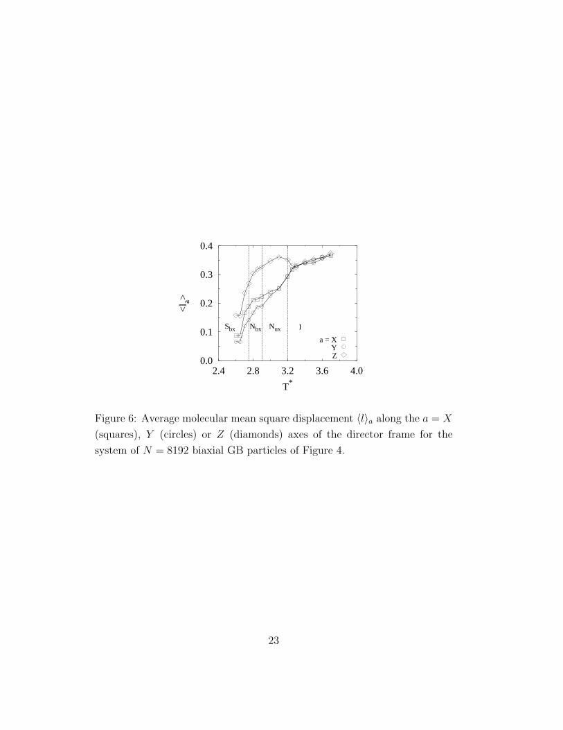
we have calculated the mean square displacements 〈l〉a = {∑Ni
∑Mn [r
(n)i,a −
r(0)i,a ]2}1/2/(NM) where a = X, Y or Z refers to one of the three director frame
axes and r(n)i = {ri,x, ri,y, ri,z}(n) the i th particle position with respect to the
director frame after n of M MC cycles starting from an arbitrary point r(0)i .
These are plotted in Figure 6 and show that at the uniaxial–biaxial nematic
transition the system is still quite fluid according to the classical Lindemann
type criterion [36] of comparing 〈l〉a with molecular dimensions, although
of course, the system becomes more and more rigid as the temperature is
lowered, until at T ∗ = 2.75 we observe the first instance of smectic layering.
We notice that in every case the mean square mobility is greater along the
principal director axis for this system.
Since we have performed a full simulation study of the system for two sample
sizes N = 1024 and N = 8192, we have plotted both sets of results in Figure 4
and we can see that size effects are quite negligible on energy and density, in
agreement with a near or full second–order character of the transformations
taking place. This is apparent also from the order parameter plots of Fig-
ure 5 where we mainly observe differences in the higher temperature regions
due to a better approximation to zero of the order parameter values for the
larger system. We notice also that the order parameter 〈R220〉 is very noisy
and, since its values are similar to the expected error threshold O(1/√N),
we observe that it is, differently from 〈R222〉, substantially unreliable as an
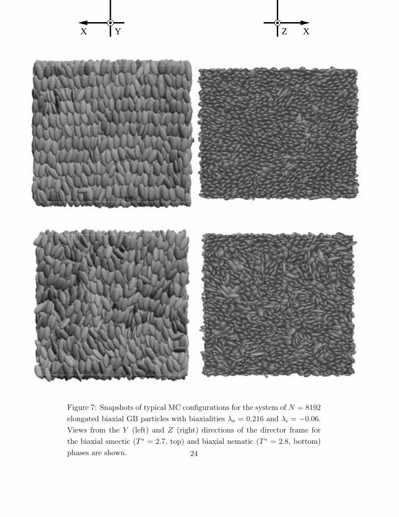
indicator of phase biaxiality. In Figure 7 we show snapshots of two typi-
9

cal configurations for the system in the biaxial nematic and biaxial smectic
phases. We show lateral and top views of the configurations that give an
immediate appreciation of the phase biaxiality, even in the absence of any
apparent layering of the nematic system, shown in Figure 7–bottom.
3.3 Structural Properties
Although the orientational order indicates phase biaxiality and the snapshot
in Figure 7 are quite suggestive of a biaxial nematic phase we have to check
that this assignment is consistent with average (and not just instantaneous)
structural properties. Thus, here we turn to a more detailed study of the
system structure and to a more reliable classification of the phases obtained.
We start calculating the radial correlation function
g0(r) =1
4πr2ρ〈δ(r − r12)〉12, (14)
where r is the radius of a spherical sampling region and 〈. . .〉12 indicates a
pair average. In Figure 8 we show g0(r) and notice, at T ∗ = 2.6, two close and
sharp peaks at r ≈ σy and 2σy indicating biaxial packing of nearest neighbor
molecules. This pair of peaks is not present at the two other temperatures
even at a closer examination (see inset). Notice also that in the nematic
phases g0(r) for the parameterization chosen is somehow intermediate in
shape between those typical of an elongated [31] or discotic [37] mesophase.
When the system enters a layered structure it is particularly useful to deter-
mine the density correlation along the director
g(z) =1
πR2ρ〈δ(z − z12)〉12, (15)
where R is the radius of a cylindrical sampling region and z12 = r12 cos θr is
measured with respect to the principal Z axis of the director frame, i.e. θr
is the angle formed by the intermolecular vector r12 and the phase principal
director Z [31]. The plot of g(z) shown in Figure 9 indicates clearly the
smectic nature of the system at T ∗ = 2.6. This is then a biaxial orthogonal
smectic. On the contrary the flat g(z) at temperature T ∗ = 2.8 and 3 are
consistent with the homogeneous mass distribution of a nematic structure.
10

Since the distribution of centers of mass in a liquid crystal is not expected to
be isotropic we also compute the anisotropic positional correlation functions
g+n (r) =
1
4πr2ρ〈δ(r − r12)Pn(cos θr)〉12. (16)
These g+n (r) provide a set of anisotropy coefficients for the distribution of
intermolecular vectors with respect to the principal director Z analogous to
the orientational order parameters for the distribution of molecular axes with
respect to the director frame.
In Figure 10 we report the second rank correlation g+2 (r). We see once more
a peculiarity in the lowest temperature curve where the value, similar to the
lowest possible value of −1/2, indicates nearly perfect biaxial stacking in the
smectic for the first few neighbors, with a structuredness propagating across
our sample size. The first positive peak originates from molecules in the
nearest layer. The curves at the two other temperatures are essentially iden-
tical and only show first neighbor stacking, indicating that the intermolecular
vector distribution in the uniaxial and biaxial nematic does not seem to vary.
3.4 Rotational Invariants
A convenient description of the positional–orientational correlations for a
system with overall spherical symmetry, as in the case of a system with no
external symmetry breaking field applied, can be effected in terms of the
expansion coefficients of the pair correlation function
g(2)(ω1, ω2, r12) =1
ρ
P (2)(ω1, ω2, r12)
P (1)(ω1)P (1)(ω2), (17)
in an orthogonal basis of rotational invariant functions SL1L2L3n1n2
(ω1, ω2, r12) as
introduced first by Blum and Torruella [26] and later by Stone [27]. Notable
examples of the expansion coefficients for biaxial systems are (real parts are
shown)
S22000 (r) =
1
2√
5
⟨δ(r − r12) (−1 + 3 (z1 · z2)
2)⟩
12, (18)
S22020 (r) =
√3
2 ×√10
⟨δ(r − r12) ( (x1 · z2)
2 − (y1 · z2)2)
⟩12, (19)
11

S22022 (r) =
1
4 ×√5〈δ(r − r12) ( (x1 · x2)
2 − (x1 · y2)2
− (y1 · x2)2 + (y1 · y2)
2
− 2 (x1 · y2) (y1 · x2)
− 2 (x1 · x2) (y1 · y2) )〉12 , (20)
where xi, yi, zi are unit vectors defining the orientations of molecular axes
and r is the radius of a spherical sampling region. The average invariants can
be written for large separations (compared to molecular dimensions) r � σc
in terms of single particle order parameters
S22000 (r) =
1√5
(〈R2
00〉2 + 2〈R220〉2
), (r � σc) (21)
S22020 (r) =
1√5
(〈R2
00〉〈R202〉 + 2〈R2
20〉〈R222〉
), (r � σc) (22)
S22022 (r) =
1√5
(〈R2
02〉2 + 2〈R222〉2
). (r � σc) (23)
This asymptotic behavior provides a useful route to check the single particle
order parameters obtained earlier on, even if these equations do not depend
on the sign of each order parameter. We have calculated these average Stone
invariants and in Figures 11, 12 and 13 we report results for S22000 (r), S220
20 (r)
and S22022 (r) at three temperatures. We see that the Stone invariants also
confirm the biaxiality of the two lower temperature phases. The order pa-
rameters obtained analyzing the large separation plateau are consistent with
those obtained by simultaneous diagonalization of the three order matrices
(see Table 2). The curves are not very structured and the limit plateau of
the correlations, when present, is reached after 5–6 σ0 units.
4 Conclusions
We have presented a computer simulation study of an anisotropic system of
elongated particles with both shape and attractive interaction biaxiality and
showed that it produces biaxial phases. We have found that while positive
biaxialities in both shape and interaction favor biaxial stacking, they also
favor too much the formation of smectic layering. On the other hand, we
12

have found that a negative interaction biaxiality λε yields a stable and fairly
wide biaxial nematic, that we have confirmed with a variety of observables.
At lower temperature an upright biaxial smectic phase is obtained, that to
our knowledge, has also still to be experimentally found [1]. In practice, a
negative attraction biaxiality could be obtained by lateral groups (e.g. weak
hydrogen bonding sites) that favor side–to–side attraction, thus competing
with face–to–face stacking. The present findings should hopefully be of help
in the current effort towards designing mesogenic molecules that can yield a
thermotropic biaxial nematic phase.
Acknowledgments
We thank MURST PRIN Cristalli Liquidi, CNR PF MSTA–II, University
of Bologna, EU TMR contract FMRX–CT97–0121 and NEDO (Japan) for
financial support.
References
[1] see, e.g. Oxford Workshop on Biaxial Nematics, ed. D. Bruce, G.R.
Luckhurst and D. Photinos, Mol. Cryst. Liq. Cryst. 323, 153 (1998).
[2] see, e.g., (a) Liquid Crystals for Advanced Technologies (Proc. Materials
Research Society Symposia), edited by T.J. Bunning, 425, (1996); (b)
Liquid Crystal Materials, Devices and Displays (Proc. SPIE), edited by
R. Shashidhar, (1995).
[3] M.J. Freiser, Phys. Rev. Lett. 24, 1041 (1970).
[4] S.M. Fan, I.D. Fletcher, B. Gundogan, N.J. Heaton, G. Kothe, G.R.
Luckhurst and K. Praefcke, Chem. Phys. Lett. 204, 517 (1993).
[5] J.R. Hughes, G. Kothe, G.R. Luckhurst, J. Malthete, M.E. Neubert, I.
Shenouda, B.A. Timimi and M. Tittelbach, J. Chem. Phys. 107, 9252
(1997).
[6] J.P. Straley, Phys. Rev. A 10, 1881 (1974).
13

[7] R.G. Priest, Solid State Comm. 17, 519 (1975).
[8] G.R. Luckhurst, C. Zannoni, P.L. Nordio and U. Segre, Mol. Phys., 30,
1345 (1975).
[9] D.K. Remler and A.D.J Haymet, J. Phys. Chem. 90, 5426 (1986).
[10] B. Bergensen, P. Palffy–Muhoray and D. Dunmur, Liq. Cryst. 3, 347
(1988).
[11] G.R. Luckhurst and S. Romano, Mol. Phys. 40, 129 (1980).
[12] F. Biscarini, C. Chiccoli, F. Semeria, P. Pasini and C. Zannoni, Phys.
Rev. Lett. 75, 1803 (1995).
[13] (a) S. Chandrasekhar, Contemp. Phys. 29, 527 (1988); (b) J. Malthete,
L. Liebert, A.M. Levelut and Y. Galerne, C. R. Acad. Sc. Paris 303,
1073 (1986); (c) K. Praefcke, B. Kohne, B. Gundogan, D. Singer, D.
Demus, S. Diele, G. Pelzl and U. Bakow, Mol. Cryst. Liq. Cryst. 198,
393 (1991); (d) J-F. Li, V. Percec, C. Rosenblatt and O.D. Lavrentovich,
Europhys. Lett. 25, 199 (1994).
[14] F. Hessel and H. Finkelmann, Polymer Bulletin 15, 349 (1986).
[15] L.J. Yu and A. Saupe, Phys. Rev. Lett. 45, 1000 (1980).
[16] V. Berejnov, V. Cabuil, R. Perzynski and Yu. Raikher, J. Phys. Chem.
B 102, 7132 (1998).
[17] V.L. Lorman, E.A. Oliveira and B. Mettout, Physica B 262, 55 (1999).
[18] A. Ferrarini, P.L. Nordio, E. Spolaore and G.R. Luckhurst, J. Chem.
Soc. Faraday Trans. 91, 3177 (1995).
[19] Advances in the Computer Simulations of Liquid Crystals, edited by P.
Pasini and C. Zannoni, (Kluwer Academic Publishers, Dordrecht, 1999).
[20] M.P. Allen, Mol. Phys. 52, 717 (1984); ibid., Liq. Cryst. 8, 499 (1990).
[21] P.J. Camp and M.P. Allen, J. Chem. Phys. 106, 6681 (1997).
14
[22] J.G. Gay and B.J. Berne, J. Chem. Phys. 74, 3316 (1981).
[23] S. Sarman, J. Chem. Phys. 104, 342 (1996); ibid J. Chem. Phys. 107,
3144 (1997).
[24] W.M. Gelbart and A. Ben–Shaul, J. Phys. Chem. 100, 13169 (1996).
[25] R. Berardi, C. Fava and C. Zannoni, Chem. Phys. Lett. 236, 462, (1995);
ibid., Chem. Phys. Lett. 297, 8 (1998).
[26] L. Blum and A.J. Torruella, J. Chem. Phys. 56, 303 (1972).
[27] A.J. Stone, Molec. Phys. 36, 241 (1978).
[28] K. Praefcke, D. Blunk, D. Singer, J.W. Goodby, K.J. Toyne, M. Hird, P.
Styring and W.D.J.A. Norbert, Mol. Cryst. Liq. Cryst. 323, 231 (1998).
[29] C. Zannoni, in The Molecular Physics of Liquid Crystals, chap. 3, edited
by G.R. Luckhurst and G.W. Gray (Academic Press, London, 1979).
[30] M.E. Rose, Elementary Theory of Angular Momentum, (Wiley, New
York, 1957).
[31] R. Berardi, A.P.J. Emerson, and C. Zannoni, J. Chem. Soc. Faraday
Trans. 89, 4069 (1993).
[32] D. Frenkel and B. Smit, Understanding Molecular Simulation: from Al-
gorithms to Applications, (Academic Press, San Diego, 1996).
[33] M.P. Allen and D.J. Tildesley, Computer Simulation of Liquids, (Claren-
don Press, Oxford, 1987).
[34] C. Zannoni and M. Guerra, Mol. Phys. 44, 849 (1981).
[35] S.L. Altmann, Rotations, Quaternions, and Double Groups, (Clarendon
Press, Oxford, 1986).
[36] F.H. Stillinger, Science 267, 1935 (1995).
[37] M. Bates and G.R. Luckhurst, J. Chem. Phys. 104, 6696 (1996).
15

T ∗ Ne Np 〈H∗〉 〈U∗〉 〈ρ∗〉2.60 60 120 6.824 ± 0.090 -16.293 ± 0.073 0.346 ± 0.001
2.65 600 360 6.790 ± 0.095 -16.333 ± 0.065 0.346 ± 0.002
2.70 150 540 14.725 ± 0.181 -10.470 ± 0.139 0.318 ± 0.002
2.75 380 440 16.510 ± 0.214 -9.198 ± 0.152 0.311 ± 0.002
2.80 20 420 19.674 ± 0.165 -6.987 ± 0.100 0.300 ± 0.001
2.85 20 240 20.843 ± 0.138 -6.265 ± 0.089 0.295 ± 0.001
2.90 223 350 21.655 ± 0.123 -5.793 ± 0.084 0.291 ± 0.001
3.00 20 133 23.034 ± 0.104 -5.030 ± 0.072 0.285 ± 0.001
3.10 24 266 24.430 ± 0.120 -4.281 ± 0.066 0.279 ± 0.001
3.20 100 440 26.059 ± 0.143 -3.435 ± 0.082 0.271 ± 0.001
3.25 20 80 26.990 ± 0.112 -2.958 ± 0.045 0.267 ± 0.001
3.30 80 300 27.251 ± 0.104 -2.860 ± 0.049 0.266 ± 0.001
3.40 40 140 27.829 ± 0.083 -2.639 ± 0.047 0.263 ± 0.001
3.50 20 60 28.322 ± 0.056 -2.468 ± 0.037 0.260 ± 0.001
3.60 20 80 28.737 ± 0.093 -2.338 ± 0.045 0.257 ± 0.001
3.70 20 40 29.163 ± 0.077 -2.206 ± 0.037 0.255 ± 0.001
Table 1: The temperature T ∗, average enthalpy 〈H∗〉 and energy 〈U∗〉 per
particle and number density 〈ρ∗〉 for the system of N = 8192 biaxial GB
particles with biaxialities λσ = 0.216 and λε = −0.06. All averages were
computed sampling one configuration each 20 MC cycles over NPT produc-
tion runs (of length Np k–cycles) at pressure P ∗ = 8. The equilibration runs
length Ne and the root mean square errors are also reported.
16

T ∗ 〈R200〉 〈R2
20〉 〈R202〉 〈R2
22〉2.60 0.964 ± 0.001 0.006 ± 0.001 0.006 ± 0.001 0.466 ± 0.001
2.65 0.965 ± 0.003 0.006 ± 0.001 0.006 ± 0.001 0.469 ± 0.001
2.70 0.899 ± 0.004 0.017 ± 0.001 0.019 ± 0.001 0.354 ± 0.005
2.75 0.871 ± 0.005 0.020 ± 0.001 0.024 ± 0.001 0.314 ± 0.008
2.80 0.783 ± 0.005 0.029 ± 0.003 0.039 ± 0.002 0.218 ± 0.014
2.85 0.748 ± 0.008 0.022 ± 0.002 0.042 ± 0.002 0.131 ± 0.008
2.90 0.717 ± 0.010 0.020 ± 0.005 0.045 ± 0.002 0.098 ± 0.020
3.00 0.653 ± 0.011 0.006 ± 0.003 0.050 ± 0.002 0.017 ± 0.008
3.10 0.535 ± 0.012 0.011 ± 0.006 0.058 ± 0.002 0.017 ± 0.007
3.20 0.329 ± 0.032 0.009 ± 0.008 0.057 ± 0.004 0.009 ± 0.006
3.25 0.062 ± 0.020 0.009 ± 0.012 0.021 ± 0.006 0.005 ± 0.004
3.30 0.078 ± 0.033 0.015 ± 0.014 0.021 ± 0.009 0.008 ± 0.005
3.40 0.033 ± 0.018 0.010 ± 0.011 0.011 ± 0.008 0.005 ± 0.003
3.50 0.026 ± 0.014 0.011 ± 0.008 0.010 ± 0.008 0.006 ± 0.003
3.60 0.021 ± 0.009 0.008 ± 0.008 0.005 ± 0.005 0.005 ± 0.003
3.70 0.021 ± 0.011 0.009 ± 0.008 0.007 ± 0.006 0.006 ± 0.004
Table 2: The average biaxial second rank orientational order parameters
〈R200〉, 〈R2
20〉, 〈R202〉 and 〈R2
22〉 for the system of N = 8192 biaxial GB particles
with biaxialities λσ = 0.216 and λε = −0.06 (see Table 1 for computational
details).
17

(a) (b)
-9
-6
-3
0
3
0 1 2 3 4 5
U*
r*
λσ = 0.216, λε = 0-9
-6
-3
0
3
0 1 2 3 4 5
U*
r*
λσ = 0.216, λε = 0.042
(c) (d)
-9
-6
-3
0
3
0 1 2 3 4 5
U*
r*
λσ = 0.216, λε = -0.042-9
-6
-3
0
3
0 1 2 3 4 5
U*
r*
λσ = 0, λε = 0
Figure 1: Distance dependence of the U∗ = U/ε0 energy for a pair of biax-
ial Gay–Berne molecules with fixed face–to–face, side–by-side and end–to–
end relative configurations using the parameterizations described in the text
which corresponding to shape biaxiality λσ = 0.216 and interaction biaxial-
ity (a) λε = 0, (b) λε = 0.042, and (c) λε = −0.042. The uniaxial profile
with λσ = 0 and λε = 0 is also shown (d). The potential cutoff radius
r∗c = rc/σ0 = 4 is also shown as a vertical dashed segment.
18

-9
-6
-3
0
3
0 1 2 3 4 5
U*
r*
λσ = 0.216, λε = -0.06
Figure 2: Distance dependence of the biaxial Gay–Berne U∗ energy for the
parameterization described in the text corresponding to shape biaxiality λσ =
0.216 and interaction biaxiality λε = −0.06. (see Figure 1 for additional
details).
19

(a) (b)
-16.0
-12.0
-8.0
-4.0
0.0
1.5 2.0 2.5 3.0 3.5 4.0
<U
* >
T*
λε x 103
02542
-42ux 0.24
0.28
0.32
0.36
1.5 2.0 2.5 3.0 3.5 4.0
<ρ* >
T*
λε x 103
02542
-42ux
(c) (d)
0.0
0.2
0.4
0.6
0.8
1.0
1.5 2.0 2.5 3.0 3.5 4.0
<R
2 00>
T*
λε x 103
02542
-42ux
0.0
0.1
0.2
0.3
0.4
0.5
1.5 2.0 2.5 3.0 3.5 4.0
<R
2 22>
T*
λε x 103
02542
-42ux
Figure 3: Average energy per particle 〈U∗〉 (a), number density 〈ρ∗〉 (b),
orientational order parameters 〈R200〉 (c) and 〈R2
22〉 (d) for systems of N =
1024 elongated GB particles with shape biaxiality λσ = 0.216 and interaction
biaxialities λε = 0 (circles), 0.025 (triangles), 0.042 (diamonds) and −0.042
(squares) (see Figure 1). Results for a uniaxial system λσ = λε = 0 (dots) are
also shown. All MC simulations were run in the NPT ensemble at P ∗ = 8.
20

-20
-15
-10
-5
0
2.4 2.8 3.2 3.6 4.0
<U
* >
T*
Sbx Nbx Nux I
N81921024
0.20
0.25
0.30
0.35
0.40
2.4 2.8 3.2 3.6 4.0
<ρ* >
T*
Sbx Nbx Nux I
N81921024
Figure 4: Average energy per particle 〈U∗〉 (top) and density 〈ρ∗〉 (bot-
tom) for systems of N = 1024 (circles) and N = 8192 (squares) biaxial GB
particles with biaxialities λσ = 0.216 and λε = −0.06 simulated in the MC–
NPT ensemble at P ∗ = 8. The estimated transition temperatures between
the isotropic (I), uniaxial nematic (Nux), biaxial nematic (Nbx) and biaxial
smectic (Sbx) phases are shown as dashed vertical lines.
21

(a) (b)
0.00
0.20
0.40
0.60
0.80
1.00
2.4 2.8 3.2 3.6 4.0
<R
2 00>
T*
Sbx Nbx Nux I
N81921024
0.00
0.02
0.04
0.06
0.08
0.10
2.4 2.8 3.2 3.6 4.0
<R
2 02>
T*
Sbx Nbx Nux I
N81921024
(c) (d)
0.00
0.02
0.04
0.06
0.08
0.10
2.4 2.8 3.2 3.6 4.0
<R
2 20>
T*
Sbx Nbx Nux I
N81921024
0.00
0.10
0.20
0.30
0.40
0.50
2.4 2.8 3.2 3.6 4.0
<R
2 22>
T*
Sbx Nbx Nux I
N81921024
Figure 5: Average orientational order parameters 〈R200〉 (a), 〈R2
02〉 (b), 〈R220〉
(c) and 〈R222〉 (d) for the systems of N = 1024 (circles) and N = 8192
(squares) biaxial GB particles of Figure 4.
22
0.0
0.1
0.2
0.3
0.4
2.4 2.8 3.2 3.6 4.0
<l a
>
T*
Sbx Nbx Nux I
a = XYZ
Figure 6: Average molecular mean square displacement 〈l〉a along the a = X
(squares), Y (circles) or Z (diamonds) axes of the director frame for the
system of N = 8192 biaxial GB particles of Figure 4.
23
YX Z X
Figure 7: Snapshots of typical MC configurations for the system of N = 8192
elongated biaxial GB particles with biaxialities λσ = 0.216 and λε = −0.06.
Views from the Y (left) and Z (right) directions of the director frame for
the biaxial smectic (T ∗ = 2.7, top) and biaxial nematic (T ∗ = 2.8, bottom)
phases are shown. 24

0.0
1.0
2.0
3.0
4.0
0 2 4 6 8 10 12
g 0 (r
* )
r*
T* 2.62.83.0
0
1
0 2 4
Figure 8: Radial correlation function g0(r) for the system of N = 8192
biaxial GB particles with biaxialities λσ = 0.216 and λε = −0.06 from MC–
NPT simulations at P ∗ = 8 and T ∗ = 2.6 (biaxial smectic), 2.8 (biaxial
nematic) and 3.0 (uniaxial nematic).
0.0
2.0
4.0
6.0
0 2 4 6 8 10 12
g (z* )
z*
T* 2.62.83.0
Figure 9: Density correlation along the director g(z) for the system of N =
8192 biaxial GB particles of Figure 8.
25

-0.5
0.0
0.5
1.0
0 2 4 6 8 10 12
g+ 2 (r
* )
r*
T* 2.62.83.0
Figure 10: Second rank anisotropic positional correlation g+2 (r) for the system
of N = 8192 biaxial GB particles of Figure 8.
0.00
0.10
0.20
0.30
0.40
0.50
0 2 4 6 8 10 12
S220
00 (
r* )
r*
T* 2.62.83.0
Figure 11: Average orientational correlation S22000 (r) for the system of N =
8192 biaxial GB particles of Figure 8. The asymptotic values computed from
the second rank order parameters are shown as thick horizontal segments.
26

0.00
0.02
0.04
0.06
0.08
0 2 4 6 8 10 12
S220
20 (
r* )
r*
T* 2.62.83.0
Figure 12: Average orientational correlation S22020 (r) for the system of N =
8192 biaxial GB particles of Figure 8. The asymptotic values computed from
the second rank order parameters are shown as thick horizontal segments.
0.00
0.05
0.10
0.15
0.20
0.25
0 2 4 6 8 10 12
S220
22 (
r* )
r*
T* 2.62.83.0
Figure 13: Average orientational correlation S22022 (r) for the system of N =
8192 biaxial GB particles of Figure 8. The asymptotic values computed from
the second rank order parameters are shown as thick horizontal segments.
27