Plane-Wave Analysis and Comparison of Split-Field, Biaxial, and Uniaxial PML Methods as ABCs for...

JOURNAL OF COMPUTATIONAL PHYSICS146,747–774 (1998)ARTICLE NO. CP986082

Plane-Wave Analysis and Comparison ofSplit-Field, Biaxial, and Uniaxial PMLMethods as ABCs for PseudospectralElectromagnetic Wave Simulations

in Curvilinear Coordinates

Baolin Yang∗,1 and Peter G. Petropoulos†∗Cadence Design Systems, Inc., 555 River Oaks Parkway, MS 3B1, San Jose, California 95134;†Department

of Mathematics, New Jersey Institute of Technology, Newark, New Jersey 07102E-mail: [email protected], [email protected]

Received February 24, 1998; revised August 10, 1998

In this paper, we discuss and compare split-field, biaxial, and uniaxial perfectlymatched layer (PML) methods for absorbing outgoing vector waves in cylindricaland spherical coordinates. We first extend Berenger’s split-field formulation intospherical and cylindrical coordinates in such a way that it maintains all the desir-able properties it exhibits in rectangular coordinates. Then we discuss the biaxialand the uniaxial medium PML methods in Cartesian coordinates and extend themto spherical and cylindrical coordinates. Properties of plane-wave solutions of thePML methods are analyzed. In particular, the decay and boundness properties of thesolutions are considered in order to provide further insight into the different formula-tions presented herein. Moreover, we propose a set of symmetric hyperbolic equa-tions for both the biaxial and the uniaxial PML methods in the time-domain, whichis fine-tuned in numerical experiments and very suitable for time-domain problems.All three types of spherical and cylindrical PML methods are applied in simulationsof plane wave scattering as well as radiating dipole problems. We use a multidomainpseudospectral (Chebyshev) numerical scheme, and the effectiveness of the PMLmethods is demonstrated through the accurate numerical results obtained. The orderof outer-boundary reflection is as low as 0.1% of the exact solution.c© 1998 Academic Press

Key Words:perfectly matched layer; pseudospectral method; multidomain method.

1. INTRODUCTION

In [1] Berenger proposed the perfectly matched layer (PML) method to truncate compu-tational domains, used in the numerical solution of Maxwell’s equations, without causingany reflection. The method was developed in Cartesian coordinates and the absorbing layer

747

0021-9991/98 $25.00Copyright c© 1998 by Academic Press

All rights of reproduction in any form reserved.

748 YANG AND PETROPOULOS

was shown to be nonreflecting at the rectangular vacuum-layer interface. It was extendedinto 3D in [2]. Recently, efforts have been seen to extend the rectangular PML methods intopolar (2D), as well as spherical and cylindrical (3D) coordinate systems.

Unfortunately, some direct extensions of the split-field rectangular PML to cylindricaland spherical coordinates are not sufficiently justified, either theoretically or numerically[5, 14]. They are not reflectionless. As the split-field methods are still being used, we thinkthat it is necessary to give extensions that are both theoretically and numerically justified.The split-field methods we propose and numerically tested attain this objective. Our methodsare different from those recently proposed by Teixeira and Chew in [15]. The hyperbolicformulation of their methods also required a Berenger-like field splitting that is differentfrom ours and were presented with no proof of the reflectionless property.

Also, the so-called uniaxial anisotropic medium (unsplit) rectangular PML methods[6–8] are extended to the coordinate systems considered herein. Extensions of these methodsinto other coordinate systems have also been attempted by many researchers. Kuzuogluand Mittra presented [9] nonplanar absorbers for finite-element mesh truncation. Theyderived the reflection coefficients of their methods for spherical and cylindrical waves andshowed that, in contrast to the rectangular true-PML method, the coefficients were nolonger identically zero. The existence of ideally nonreflecting PML methods in sphericalor cylindrical coordinate system remained unknown. In fact, the numerical results in [15]exhibit reflection up to 3%. In [16], the same authors obtained some different spherical andcylindrical PML methods, but no numerical results or comparison with the previous oneswere given and, again, they did not prove their approach constituted a true PML.

Earlier [3], Yanget al.had already proposed a split-field PML method in polar coordinates(2D) which they applied to simulations of scattering by circular cylinders. That method wasan extension of Berenger’s rectangular PML. It was proven to be perfectly matched at thecircular vacuum-layer interface while the superior accuracy of the method was demonstratedin numerical experiments. Further, [3] also discussed an alternative splitting, similar to thatrecently proposed in [15] and showed that its numerical results were substantially worsethan the results of the proposed splitting. In the present paper, we continue with extensionsof Berenger’s rectangular PML into more 3D coordinate systems. We shall show that, likein [3], these extensions still retain the perfectly matched property of Berenger’s rectangularPML method and we shall also present supporting numerical simulations. Indeed, goingfrom methods in 2D polar coordinates [3] to methods in 3D cylindrical coordinates in thepresent paper is direct.

A nonsplit and well-posed ideally nonreflecting formulation of the PML method in polarcoordinates was given in [4]. The efficacy of the method was demonstrated with numericalexperiments. The present paper shall show that ideally nonreflecting unsplit PML meth-ods can also be obtained in 3D spherical and cylindrical coordinate systems through thesame approach for vector electromagnetic waves. A plane-wave analysis of the unsplit PMLmethods is given to demonstrate the point. More importantly, the proposed time-domainequations of the unsplit PML methods are symmetric hyperbolic. Although these PMLmethods are still extensions of the anisotropic medium rectangular PML [6–8] into othercoordinate systems, the approach used to derive these extensions is different from that pro-posed in [16]. Due to the symmetry, well-posedness naturally follows from our formulation,which is not true for other formulations in general. We have also fine-tuned our formula-tion in numerical experiments and the proposed one in this paper is found to have the bestaccuracy and robustness.

ANALYSIS AND COMPARISON OF PML’S 749

Since our split and unsplit PML methods in cylindrical coordinates are straightforwardextensions of our corresponding polar PML methods in 2D, our emphasis will be on thediscussion of PML methods in spherical coordinates, where the split-field spherical PML,the biaxial spherical PML, and the uniaxial spherical PML will be analyzed and fullytested. We shall mainly discuss the plane-wave solutions of these PML methods and showthe perfectly matched property and the decay of fields propagating in an arbitrary directionusing plane waves.

For 3D spherical and cylindrical PML methods, the desired vacuum–layer interfaces arethe surface of a sphere and the surface of a cylinder, respectively. The methods we developadmit plane-wave solutions that match perfectly at the vacuum–layer interface, i.e., anyplane wave can pass through the interface without reflection. This is true for plane wavesof any frequency and any incident angle. Decay properties are discussed for the split-fieldPML methods only. The split-field spherical PML method has the unique merit that planewave of any incident angle decays in its propagation direction, which is true in the wholelayer region. Split-field PML methods in other coordinate systems do not have this propertyand they usually depend on the corner regions for the complete absorption of waves. Forthe proposed unsplit PML methods (biaxial or uniaxial), since the additional scaling factorsin the plane-wave solutions are only rational functions and the exponential decaying factordominates the magnitude of the solutions, influence of the additional scaling factors on thedecay properties of the solutions is limited. Here we want to emphasize that we have takenthe propagation direction of plane waves into account in our analysis of the decay property.Reflection and field decay analysis (using cylindrical and spherical waves), and the proofthat the uniaxial PML in cylindrical and spherical coordinates is a true PML can be foundin [17]. The analysis approach herein is related to the analysis approach of [17] through theplane wave expansion of cylindrical and spherical waves and the addition theorem.

Numerical simulations of plane-wave scattering by a metal sphere and a radiating dipoleare done to test the spherical PML methods. We also show a comparison of the split-field anduniaxial PML for a radiating dipole whose time variation is a step function that turns on andstays on for the duration of the simulation. Numerical simulations of scattering by a metalcylinder of finite length are also done to test the cylindrical PML methods. The numericalscheme we use is a multidomain pseudospectral (Chebyshev) scheme. The scheme is veryaccurate and as such it is a good choice in order to fully manifest the effects of PML methodsin numerical experiments. For example, our numerical results suggest that the reflection ofthe spherical PML methods is as low as 0.1% of the exact solution.

The remainder of our paper is organized as follows. In Section 2, we give the non-dimensionalized 3D Maxwell’s equations and its plane-wave solutions. In Section 3, wegive the extensions of Berenger’s PML methods into spherical and cylindrical coordinates.Section 4 discusses the biaxial and the uniaxial PML methods, first in rectangular, andthen in spherical and cylindrical coordinates. In Section 5, numerical results validating themethods are presented, and concluding remarks are given in Section 6.

2. THE NONDIMENSIONALIZED MAXWELL’S EQUATIONS

We consider Maxwell’s curl equations in free space:

∂ H

∂t= − 1

µ0∇ × E, (1)


∂ E

∂t= 1

ε0∇ × H . (2)

Hereε0 andµ0 are the free space permittivity and permeability, with the speed of light infree space beingc= (ε0µ0)

−1/2. To facilitate our analysis of PML methods, we scale theindependent variables to nondimensionalize the above equations,

x= x/L , y= y/L , t = ct/L ,

whereL represents a length scale. Subsequently, the fields are normalized,

H = H , E =√ε0

µ0E = Z−1

0 E,

where Z0 represents the free-space impedance, and the nondimensionalized Maxwell’sequations are obtained:

∂H

∂t= −∇ × E, (3)

∂E

∂t= ∇ × H. (4)

We can write out the vector components of the curl operators in (3)–(4) and obtain asystem of six coupled scalar equations. In three-dimensional spherical coordinates(r, θ, φ),we have

∂Er

∂t= 1

r sinθ

∂

∂θ(sinθHφ)− 1

r sinθ

∂Hθ

∂φ, (5)

∂Eθ∂t= 1

r sinθ

∂Hr

∂φ− 1

r

∂

∂r(r Hφ), (6)

∂Eφ∂t= 1

r

∂

∂r(r Hθ )− 1

r

∂Hr

∂θ, (7)

∂Hr

∂t= − 1

r sinθ

∂

∂θ(sinθEφ)+ 1

r sinθ

∂Eθ∂φ

, (8)

∂Hθ

∂t= − 1

r sinθ

∂Er

∂φ+ 1

r

∂

∂r(r Eφ), (9)

∂Hφ

∂t= −1

r

∂

∂r(r Eθ )+ 1

r

∂Er

∂θ. (10)

In three-dimensional cylindrical coordinates (ρ, φ, z), we have

∂Eρ∂t= 1

ρ

∂Hz

∂φ− ∂Hφ

∂z, (11)

∂Eφ∂t= ∂Hρ

∂z− ∂Hz

∂ρ, (12)

∂Ez

∂t= 1

ρ

∂ρHφ

∂ρ− 1

ρ

∂Hρ

∂φ. (13)

To avoid repetition, we skip the governing equations for components of the magnetic fields.This rule is followed hereafter when appropriate.


Maxwell’s equations admit the plane-wave solutions

E = (l1x +m1 y+ n1z) eiω(t−lx−my−nz), (14)

H = (l2x +m2 y+ n2z) eiω(t−lx−my−nz), (15)

where

l1x+m1 y+ n1z = (l2x+m2y+ n2z)× (l x+my+ nz), (16)

l2x+m2 y+ n2z = (l x+my+ nz)× (l1x+m1 y+ n1z). (17)

For a plane wave incident in the directionθ0, φ0, we have

eiω(t−lx−my−nz)= eiω(t − r (cosθ0 cosθ+ sinθ0 sinθ cos(φ−φ0))). (18)

in the spherical coordinate system and

eiω(t−lx−my−nz)= eiω(t −√1− n2ρ cos(φ−φ0)− nz) (19)

in the cylindrical coordinate system.The plane-wave field components in spherical coordinates are given as

Er = (cosφ sinθ l1+ sinφ sinθm1+ cosθn1) eiω(t − r (cosθ0 cosθ+ sinθ0 sinθ cos(φ−φ0))), (20)

Eθ = (cosφ cosθ l1+ sinφ cosθm1− sinθn1) eiω(t − r (cosθ0 cosθ+ sinθ0 sinθ cos(φ−φ0))), (21)

Eφ = (−sinφl1+ cosφm1) eiω(t − r (cosθ0 cosθ+ sinθ0 sinθ cos(φ−φ0))), (22)

and the plane-wave field components in cylindrical coordinates as

Eρ = (cosφl1+ sinφm1) eiω(t −√1−n2ρ cos(φ−φ0)− nz), (23)

Eφ = (−sinφl1+ cosφm1) eiω(t −√1−n2ρ cos(φ−φ0)− nz), (24)

Ez = n1 eiω(t −√1−n2ρ cos(φ−φ0)− nz). (25)

These plane-wave solutions are to be perfectly matched to decaying plane-wave solutionsin the absorbing layer.

3. EXTENSIONS OF BERENGER’S PML METHODS

In this section, we present the extensions of Berenger’s PML methods to spherical andcylindrical coordinates. The plane-wave solutions of these PML methods are simpler thanthose of the unsplit methods which will be given in Section 4. We shall also prove thatplane-wave solutions in the spherical PML decay in all directions of propagation.

In the following, we first explain Berenger’s PML method with a varying conductivityparameter and analyze its plane-wave solutions. Then we present our spherical and cylin-drical PML methods and analyze their decay property in the direction of wave propagation.We have found in our work that this property is important for the success of PML methods.In any numerical computation, there are numerical reflections at the outer boundaries of the


PML due to the inexact boundary conditions applied there and one wants those reflectedwaves, although of very small magnitude, to be further absorbed as they propagate backtowards the interior region.

3.1. Berenger’s Perfectly Matched Layer

In [1] Berenger gave the perfectly matched layer method suitable for rectangular gridtruncation and wave absorption. Here we give a simplified plane-wave analysis of themethod, where we consider a layer of continuously varying absorption strength.

Our approach is to obtain the equations that admit plane-wave solutions with a frequency-independent decay factor of the following form:

D(x, y, z) = e−lσx(x)−mσy(y)−nσz(z). (26)

We then have the split-field PML system in Cartesian coordinates,

∂Exy

∂t= ∂(Hzx+ Hzy)

∂y− σ ′y(y)Exy, (27)

∂Exz

∂t= −∂(Hyx + Hyz)

∂z− σ ′z(z)Exz, (28)

∂Eyz

∂t= ∂(Hxy+ Hxz)

∂z− σ ′z(z)Eyz, (29)

∂Eyx

∂t= −∂(Hzx+ Hzy)

∂x− σ ′x(x)Eyx, (30)

∂Ezx

∂t= ∂(Hyx + Hyz)

∂x− σ ′x(x)Ezx, (31)

∂Ezy

∂t= −∂(Hxy+ Hxz)

∂y− σ ′y(y)Ezy, (32)

that admits the following decaying plane-wave solutions:

Exy = −n2m eiω(t−xl−ym−nz)D(x, y, z), (33)

Exz = m2n eiω(t−xl−ym−nz)D(x, y, z), (34)

Eyz = −l2n eiω(t−xl−ym−nz)D(x, y, z), (35)

Eyx = n2l eiω(t−xl−ym−nz)D(x, y, z), (36)

Ezx = −m2l eiω(t−xl−ym−nz)D(x, y, z), (37)

Ezy = l2m eiω(t−xl−ym−nz)D(x, y, z). (38)

According to the relations (16)–(17) that couple (l ,m, n), (l1,m1, n1), and (l2,m2, n2), wehaveExy+Exz = Ex D(x, y, z), Eyz+Eyx= Ey D(x, y, z), andEzx+Ezy= EzD(x, y, z),whereEx, Ey, andEz are the plane-wave solutions in Eq. (14). So the decaying plane-wavesolutions in the layer region match perfectly with the plane-wave solutions in a vacuum ifwe letσx(x), σy(y), andσz(z) approach zero smoothly enough when (x, y, z) approachesthe vacuum–layer interface from the layer side.


3.2. Spherical Perfectly Matched Layer

In this section we propose a split-field spherical PML method. We use the method toterminate spherical computational domains and the vacuum–layer interface is a sphere. Weprove that plane waves of any incident direction and any frequency pass the vacuum–layerinterface without causing any reflection and decay in all directions of propagation in thelayer region independently of the frequency. The absorption in the layer only varies withthe radiusr , and it approaches zero smoothly towards the interface.

In designing such a perfectly matched layer, we split the original equations and add low-order absorbing terms (see undifferentiated terms below). Our approach is an extension ofthe idea of Berenger’s PML method to spherical coordinates, rather than a direct translationof Berenger’s PML equations to spherical coordinates (whichdoes notresult in a true PML).We have found that it is not necessary to split ther component of the fields as theEr andHr components are never tangential to a PML region. This is in contrast to the situation incylindrical coordinates (see Section 3.3).

In deriving the spherical PML method, our objective is to obtain differential equationsthat admit plane-wave solutions with a decaying factor of the form

D(r, θ, φ) = e−σr (r )(cosθ0 cosθ + sinθ0 sinθ cos(φ−φ0)). (39)

We obtain the following split-field formulation of Maxwell’s equations in the layer:

∂Er

∂t= 1

r sinθ

∂

∂θ(sinθ(Hφr + Hφθ ))− 1

r sinθ

∂(Hθφ + Hθr )

∂φ− σr (r )

rEr , (40)

∂Eθφ∂t= 1

r sinθ

∂Hr

∂φ− 1

r(Hφr + Hφθ )− σr (r )

rEθφ, (41)

∂Eθr∂t= −∂(Hφr + Hφθ )

∂r− σ ′r (r )Eθr , (42)

∂Eφr

∂t= ∂(Hθφ + Hθr )

∂r− σ ′r (r )Eφr , (43)

∂Eφθ∂t= −1

r

∂Hr

∂θ+ 1

r(Hθφ + Hθr )− σr (r )

rEφθ . (44)

We note that one only needs to solve 10 equations, of which we just give five in the above,compared with 12 equations one needs to solve for the split-field rectangular PML method.We also note that in [15], six additional field components are needed inside the PML. In[15], the reflection of the spherical PML is 0.8% of the maximum amplitude of the simulatedpulse. The methods are similar in nature in the frequency domain, and the approaches [15]require a splitting of the fields to give a PML for transient waves. However, no split-fieldtime-domain formulation was given in [15] and we had shown in [3] that having the rightsplit-field formulation is important.

Let the vacuum-layer interface be atr = r0. We require thatσr (r )= 0 for r ≤ r0 for thedecaying plane waves in the PML to match incident plane waves perfectly. The functionσr (r ) must satisfy the requirements

σr (r0) = 0 (45)


and

σr (r ) > 0 for r > r0, (46)

so that the plane-wave solutions decay forr > r0. We also require that

σ ′r (r ) > 0 for r > r0. (47)

An example of a valid choice forσr (r ) is

σr (r ) = C(r − r0)n, n = 1, 2, . . . ; r ≥ r0, (48)

where C is a positive constant. This family of functions satisfies the requirements in(45)–(47).

The split-field PML equations admit the following set of plane-wave solutions with thedesired decaying factor:

Er = (cosφ sinθ l1+ sinφ sinθm1+ cosθn1)eiω(t−r (cosθ0 cosθ+ sinθ0 sinθ cos(φ−φ0)))D(r, θ, φ),

(49)

Eθφ = (cosφ sinθ l2+ sinφ sinθm2+ cosθn2) sinθ0 sin(φ − φ0)

× eiω(t − r (cosθ0 cosθ+ sinθ0 sinθ cos(φ−φ0)))D(r, θ, φ), (50)

Eθr = (−sinφl2+ cosφm2)(cosθ0 cosθ + sinθ0 sinθ cos(φ−φ0))


Eφr = −(cosφ cosθ l2+ sinφ cosθm2− sinθn2)(cosθ0 cosθ + sinθ0 sinθ cos(φ−φ0))


Eφθ = −(cosφ sinθ l2+ sinφ sinθm2+ cosθn2)(cosθ0 sinθ − sinθ0 cosθ cos(φ−φ0))


where (l2,m2, n2), (l1,m1, n1), and (l ,m, n) satisfy (16)–(17). Note that now we havel = cosφ0 sinθ0,m= sinφ0 sinθ0, andn = cosθ0. One can verify that

Eθφ + Eθr =[(cosφ sinθ l2+ sinφ sinθm2+ cosθn2) sinθ0 sin(φ − φ0)

+ (−sinφl2+ cosφm2)(cosθ0 cosθ + sinθ0 sinθ cos(φ − φ0))

× eiω(t − r (cosθ0 cosθ+ sinθ0 sinθ cos(φ−φ0)))D(r, θ, φ)

= (cosφ cosθ l1+ sinφ cosθm1− sinθn1)]

× eiω(t − r (cosθ0 cosθ+ sinθ0 sinθ cos(φ−φ0)))D(r, θ, φ)

= Eθ D(r, θ, φ), (54)

and, similarly, one can also verify that

Eφr + Eφθ = EφD(r, θ, φ), (55)

by applying the relations (16)–(17) that couple (l ,m, n), (l1,m1, n1), and (l2,m2, n2), whereEφ , Eθ are the plane-wave solutions in Eqs. (20)–(22). Hence, at the vacuum–layer interface,


whereσr (r )= 0, the decaying plane wavesEr , Eθφ+ Eθr , andEφr + Eφθ match the plane-wave solutionsEr , Eθ , andEφ in free-space perfectly. Note that this is true for plane wavesof any frequency and any incident angle.

It is not straightforward to understand the decay property of the plane-wave solutions inthe layer by looking at the decay factore−σr (r )(cosθ0 cosθ+ sinθ0 sinθ cosφ−φ0)). In order to geta clear picture of the rate of change of the magnitude of the wave, one must analyze thedirectional derivative of the decay factor.

LEMMA 3.1. Let l= (cosφ0 sinθ0, sinφ0 sinθ0, cosθ0) be the normalized wave vectorand assume thatσr (r ) satisfies the conditions(46)–(47). Then all plane waves decay in thedirection of propagation as

∂D(r, θ, φ)

∂ l= ∂e−σr (r )(cosθ0 cosθ+ sinθ0 sinθ cos(φ−φ0))

∂ l< 0, (56)

when r> r0 for anyφ0 andθ0.

Proof.

∂D(r, θ, φ)

∂ l

= cosφ0 sinθ0∂D(r, θ, φ)

∂x+ sinφ0 sinθ0

∂D(r, θ, φ)

∂y+ cosθ0

∂D(r, θ, φ)

∂z

= cosφ0 sinθ0 cosφ sinθ∂D(r, θ, φ)

∂r− cosφ0 sinθ0

sinφ

r sinθ

∂D(r, θ, φ)

∂φ

+ cosφ0 sinθ0cosφ cosθ

r

∂D(r, θ, φ)

∂θ

+ sinφ0 sinθ0 sinφ sinθ∂D(r, θ, φ)

∂r+ sinφ0 sinθ0

cosφ

r sinθ

∂D(r, θ, φ)

∂φ

+ sinφ0 sinθ0sinφ cosθ

r

∂D(r, θ, φ)

∂θ

+ cosθ0 cosθ∂D(r, θ, φ)

∂r− cosθ0

sinθ

r

∂D(r, θ, φ)

∂θ

= (sinθ0 sinθ cos(φ − φ0)+ cosθ0 cosθ)∂D(r, θ, φ)

∂r

− sinθ0 sin(φ − φ0)1

r sinθ

∂D(r, θ, φ)

∂φ

+ (sinθ0 cosθ cos(φ − φ0)− cosθ0 sinθ)1

r

∂D(r, θ, φ)

∂θ

= −[(sinθ0 sinθ cos(φ − φ0)+ cosθ0 cosθ)2σ ′r (r )+ (sinθ0 sin(φ − φ0))

2σr (r )

r

+ (sinθ0 cosθ cos(φ − φ0)− cosθ0 sinθ)2σr (r )

r

]D(r, θ, φ).

Hence we have

∂D(r, θ, φ)

∂ l= ∂e−σr (r )(cosθ0 cosθ+ sinθ0 sinθ cos(φ−φ0))

∂ l< 0

for anyφ0 andθ0. j


The lemma shows that all plane waves entering the PML decay exponentially along anydirection of propagation inside the layer. In an actual computation, the PML does not extendto infinity and there will be reflections from the outer boundary of the PML region. In thiscase, the decay relation (56) still holds for the reflected waves. Thus, the reflected wavesget further attenuated along the way back towards the computational domain. Note thatreflected waves, even numerical reflections, can be expanded in plane waves locally. Thisis the reason for the success of the PML methods. Since

(sinθ0 sinθ cos(φ − φ0)+ cosθ0 cosθ)2σ ′r (r )+ (sinθ0 sin(φ − φ0))2σr (r )

r

+ (sinθ0 cosθ cos(φ − φ0)− cosθ0 sinθ)2σr (r )

r≥ min

(σ ′r (r ),

σr (r )

r

)> 0 (57)

for r > r0, we have a lower bound for the rate of decay regardless of the direction of wavepropagationφ0 andθ0 in the layer region away from the interface. We emphasize that wecannot find such a lower bound for the PML in Cartesian coordinates.

3.3. Cylindrical Perfectly Matched Layer

It is also desirable to have a perfectly matched layer method in cylindrical coordi-nates. Here the vacuum–layer interface is required to be atρ= ρ0 and |z| = z0, whereρ0 andz0 are constants. For this purpose, we can apply the polar perfectly matched layer[3] in the ρ−φ plane and apply rectangular perfectly matched layer method in thez-direction.

Our objective is to obtain the equations that admit plane-wave solutions with the decayfactor:

D(ρ, φ, z) = e−σρ(ρ)√

1− n2 cos(φ−φ0)− σz(z)nz. (58)

With the split-field approach, we need to solve the following equations:

∂Eρz

∂t= −∂(Hφz+ Hφρ)

∂z− σ ′z(z)Eρz, (59)

∂Eρφ∂t= 1

ρ

∂(Hzρ + Hzφ)

∂φ− σρ(ρ)

ρEρφ, (60)

∂Eφz

∂t= ∂(Hρz+ Hρφ)

∂z− σ ′z(z)Eφz, (61)

∂Eφρ∂t= −∂(Hzρ + Hzφ)

∂ρ− σ ′ρ(ρ)Eφρ, (62)

∂Ezρ

∂t= ∂(Hφz+ Hφρ)

∂ρ− σ ′ρ(ρ)Ezρ, (63)

∂Ezφ

∂t= − 1

ρ

∂(Hρz+ Hρφ)

∂φ+ Hφz+ Hφρ

ρ− σρ(ρ)

ρEzφ. (64)

We note that in [15], although it was tested in 3D, the equations for the cylindrical PMLwas actually given in 2D and the method was similar to Navarro’s method [14] already


discussed in [3]. Unfortunately, Navarro’s method was shown to have a poorer performancethan our method [3], which might be the reason for the substantial 3% reflection seen in[15]. The important thing to notice is that the term(Hφz+ Hφρ)/ρ is in Eq. (64) rather thanin Eq. (63).

Let the vacuum-layer interface be atρ = ρ0 and|z| = z0. We should require thatσρ(ρ)= 0for ρ <ρ0 andσz(z)= 0 for |z|< z0 in order for the decaying plane waves in the PMLto match incident plane waves perfectly. Following the considerations of the absorbingand reflectionless properties of the polar PML method,σρ(ρ) andσz(z) must satisfy therequirements:

σρ(ρ0) = 0, σz(z)||z|=z0 = 0, (65)

and

σρ(ρ) > 0 for ρ > ρ0, σz(z) > 0 for |z| > z0, (66)

so that the plane-wave solutions decay forρ >ρ0 or |z|> z0. We also require that

σ ′ρ(ρ) > 0 for ρ > ρ0, σ ′z(z) > 0 for |z| > z0. (67)

An example of a valid choice ofσρ(r ) andσz(z) is

σρ(ρ) = C(ρ − ρ0)n, n = 1, 2, . . . ; ρ ≥ ρ0, (68)

σz(z) = C(|z| − z0)n, n = 1, 2, . . . ; |z| ≥ z0, (69)

where C is a positive constant. This family of functions satisfies the requirements in(65)–(67).

For the cylindrical perfectly matched layer method, it can be verified that we have thefollowing decaying plane-wave solutions:

Eρz = (−sinφl2+ cosφm2)n eiω(t − ρ√1−n2 cos(φ−φ0)− zn)D(ρ, φ, z), (70)

Eρφ = n2 sin(φ − φ0)√

1− n2 eiω(t − ρ√1−n2 cos(φ−φ0)− zn)D(ρ, φ, z), (71)

Eφz = −(cosφl2+ sinφm2)n eiω(t − ρ√1−n2 cos(φ−φ0)− zn)D(ρ, φ, z), (72)

Eφρ = n2 cos(φ − φ0)√

1− n2 eiω(t − ρ√1−n2 cos(φ−φ0)− zn)D(ρ, φ, z), (73)

Ezρ =−(−sinφl2+ cosφm2) cos(φ−φ0)√

1−n2 eiω(t−ρ√1−n2 cos(φ−φ0)−zn)D(ρ, φ, z),

(74)

Ezφ =−(cosφl2+ sinφm2) sin(φ−φ0)√

1−n2 eiω(t−ρ√1−n2 cos(φ−φ0)−zn)D(ρ, φ, z),

(75)

where (l2,m2, n2), (l1,m1, n1), and (l ,m, n) satisfy relations (16)–(17). Note that now we


havel =√1− n2 cosφ0,m=√

1− n2 sinφ0, andn= n. One can verify that

Ezρ + Ezφ = −((−sinφl2+ cosφm2) cos(φ − φ0)+ (cosφl2+ sinφm2)

× sin(φ − φ0))√

1− n2 eiω(t − ρ cos(φ−φ0)− zn)D(ρ, φ, z)

= −(−sinφ0l2+ cosφ0m2)√

1− n2 eiω(t − ρ cos(φ−φ0)− zn)D(ρ, φ, z)

= n1 eiω(t − ρ√1−n2 cos(φ−φ0)− zn)D(ρ, φ, z)

= EzD(ρ, φ, z), (76)

and, similarly, one can also verify that

Eρz+ Eρφ = EρD(ρ, φ, z), (77)

Eφz+ Eφρ = EφD(ρ, φ, z), (78)

by applying the relations (16)–(17) that couple (l ,m, n), (l1,m1, n1), and (l2,m2, n2), whereEρ , Eφ , and Ez are plane-wave solutions in Eqs. (23)–(25). Hence, at the vacuum-layerinterface, whereσρ(ρ)= σz(z)= 0, the decaying plane wavesEρz+ Eρφ, Eφz+ Eφρ , andEzρ + Ezφ match the plane-wave solutionsEρ , Eφ , andEz in free-space perfectly. Note thatthis is true for plane waves of any frequency and any incident angle.

We can also analyze the directional derivative of the decaying factor to get a clear pictureof the rate of change of the magnitude of the plane waves. The analysis is a straightforwardextension of the 2D polar PML analysis given in [3]. Here we only give the result.

LEMMA 3.2. Let l= (√1− n2 cosφ0,√

1− n2 sinφ0, n)be the normalized wave vectorand assume thatσρ(ρ) andσz(z) satisfies the conditions(46)–(47). Then plane waves donot increase in all directions of propagation as

∂D(ρ, φ, z)

∂ l= ∂e−σρ(ρ) cos(φ−φ0)− σz(z)z

∂ l≤ 0, (79)

whenρ >ρ0 or |z|> z0 for anyφ0 and n.

The decay property of the cylindrical PML is shared by both the rectangular and polarPML methods [3]. It is only in two special cases that plane-wave solutions do not decayin the PML, i.e., when plane waves propagate in thez-direction and in the regionρ >ρ0

and |z| ≤ z0, or when plane waves propagate in the direction orthogonal toz and in theregionρ ≤ ρ0 and |z|> z0. The corner regions,ρ >ρ0 and |z|> z0, are important for allplane waves to be absorbed. However, the situation here is much less severe than that forthe rectangular PML method.

4. THE BIAXIAL AND THE UNIAXIAL PML METHODS

Since Berenger first presented the split-field PML method, efforts have been made tomodify the method and obtain unsplit PML methods. Besides from the latter methods’ beingcomputationally more efficient, the efforts are worthwhile since the split-field rectangularPML equations are only weakly well-posed and may suffer from instability problems, asshown in [11].


The unsplit PML methods we present in this section modify Maxwell’s equations byadding low-order (undifferentiated) source terms that satisfy ordinary differential equations.Hence the governing equations are symmetric hyperbolic and strongly well-posed just likethe original Maxwell’s equations. The plane-wave solutions now have additional scalingfactors which depend on the frequency,ω. This additional degree of freedom makes itpossible to design the unsplit-field PML methods.

4.1. The Perfectly Matched Anisotropic Medium

In [6] a PML method using an anisotropic lossy uniaxial medium was presented and wasapplied to frequency-domain-based finite-element methods. The works [7, 8] implementedthe uniaxial medium as a PML for the FD-TD algorithm. The constitutive parameters ofthis anisotropic medium are given in terms of the complex permittivity and permeabilitytensorsε = ε0[3] and ¯µ = µ0[3], where [3] is the diagonal matrix,

[3]=

1+ σ ′z (z)

iω 0 0

0 1+ σ ′z (z)iω 0

0 0 1

1+ σ ′z (z)iω

, (80)

that represents a uniaxial medium in thez-direction. In the uniaxial medium, the nondi-mensionalized Ampere’s law can be expressed in matrix form as

∂Hz

∂y − ∂Hy

∂z

∂Hx

∂z − ∂Hz

∂x

∂Hy

∂x − ∂Hx

∂y

= iω[3]

Ex

Ey

Ez

. (81)

It was shown in the original papers that the above equations admit the plane-wave solutions

E =(

l1x +m1y + n1

(1+ σ

′z(z)

iω

)z

)eiω(t−lx−my−nz)e−σz(z)n, (82)

H =(

l2x +m2y + n2

(1+ σ

′z(z)

iω

)z

)eiω(t−lx−my−nz)e−σz(z)n, (83)

where (l ,m, n), (l1,m1, n1), and (l2,m2, n2) are coupled by the relations (16)–(17). Theabove solutions are unbounded asω→ 0, which is certainly unphysical.

However, we can design a layer that has the plane-wave solutions

E =(

l1iω

σ ′z(z)+ iωx +m1

iω

σ ′z(z)+ iωy + n1z

)eiω(t−lx−my−nz) e−σz(z)n, (84)

H =(

l2iω

σ ′z(z)+ iωx +m2

iω

σ ′z(z)+ iωy + n2z

)eiω(t−lx−my−nz) e−σz(z)n, (85)

where (l ,m, n), (l1,m1, n1), and (l2,m2, n2) are coupled by the relations (16)–(17). Themagnitude of this set of plane-wave solutions are uniformly bounded. It can be verified that


they are the solutions of the following equations:∂Hz

∂y − ∂Hy

∂z

∂Hx

∂z − ∂Hz

∂x

∂Hy

∂x − ∂Hx

∂y

+

σ ′′z (z)σ ′z (z)+ iω Hy

− σ ′′z (z)σ ′z (z)+ iω Hx

0

= iω[3]

Ex

Ey

Ez

. (86)

Note that Eq. (86) implies the biaxial constitutive lawD = [3] · E+ [M ] · H , whereM isthe matrix

[M ]=

0 − σ ′′z (z)/ iω

σ ′z (z)+ iω 0

σ ′′z (z)/ iωσ ′z (z)+ iω 0 0

0 0 0

. (87)

Moreover, whenσ ′′z (z)= 0, Eq. (86) is the same as Eq. (81). In that case only, system(86) admits both the unbounded solutions in Eqs. (82)–(83) and the bounded solutions inEq. (84)–(85), asω→ 0. Clearly, the physical solutions are the bounded ones. Thus, weshow that if the strength of the uniaxial absorbing medium is constant, it admits decayingplane waves that are uniformly bounded, while in previous papers, there was always anunbounded scaling factor associated with the solution in the uniaxial medium.

In a numerical implementation an on/off switch can be used to drop the lower-order termsin the left-hand side of (86), i.e., zero theM matrix, thus allowing us to compare the biaxialand uniaxial approaches on a given problem with a given conductivity profile in the layer.Also, a varying-profile uniaxial PML can also be viewed as a series of constant-profile uni-axial PML’s. This, together with its simpler formulation, suggests that the uniaxial PML mayhave a better performance in numerical experiments. We note here that [10] gives a uniaxialPML in rectangular coordinates whose plane-wave solutions are uniformly bounded for avariable conductivity uniaxial PML, but the damping properties of that layer depend onωandone no longer obtains frequency-independent damping of propagating waves. Also, the time-domain form of [10] is computationally more expensive than the standard unsplit PML whichthey erroneously prove to be noncausal. We desire to maintain the frequency-independentdamping for the bounded solutions and therefore we develop the biaxial unsplit PML.

A direct application of the uniaxial medium idea in spherical and cylindrical coordinatesystems was presented in [9], where analysis of the reflection and absorption of cylindricaland spherical waves in the medium was given. Some restrictions and problems with thisdirect application of Sacks’ anisotropic medium idea in those coordinate systems wereobserved. Kuzuoglu and Mittra obtained the spherical and cylindrical wave solutions in themedium and their reflection coefficients at vacuum–layer interface. These authors observedthat the medium was not ideally nonreflecting anymore and showed that it could effectivelyabsorb waves without reflection only under the condition that the radius of the vacuum–layerinterface is electrically large.

In the following, we discuss the biaxial and the uniaxial medium PML methods which areideally nonreflecting at the vacuum–layer interface in spherical and cylindrical coordinates.These extensions are different from those proposed in [9], of course. The relation betweenthe biaxial and the uniaxial medium PML methods in spherical or cylindrical coordinatesis the same as that in Cartesian coordinates. The biaxial PML method admits plane-wave


solutions that are uniformly bounded and can be reduced to the uniaxial PML method bychoosing the spatial variation of the damping or by dropping the extra source terms asdescribed above. For conciseness, we will not give the equations or the solutions for theuniaxial PML methods separately.

4.2. Anisotropic Spherical PML Methods

In this section we give the equations and solutions of the anisotropic spherical PMLmethods. The methods, by construction, are symmetric hyperbolic and strongly well-posed.For this well-posed spherical PML method, the following plane-wave solution is what wedesired in the layer,

H r = Hr D(r, θ, φ), (88)

H θ =σr (r )

r + iω

σ ′r (r )+ iωHθ D(r, θ, φ), (89)

Hφ =σr (r )

r + iω

σ ′r (r )+ iωHφD(r, θ, φ), (90)

whereHr , Hφ , andHθ are plane-wave solutions of the original Maxwell’s equations and

D(r, θ, φ) = e−σr (r )(cosθ0 cosθ+ sinθ0 sinθ cos(φ−φ0)) (91)

is the decaying factor.Er , Eφ , andEθ are defined similarly. Let the vacuum–layer interfacebe atr = r0. We require thatσr (r )= 0 for r ≤ r0 for the decaying plane waves in the PMLto match incident plane waves perfectly. Following the considerations of the absorbing andreflectionless properties of the polar PML method,σr (r ) must satisfy the same conditionsas those in Eqs. (45)–(47). Thus the decaying plane-wave solutions are perfectly matchedwith the free-space plane-wave solutions. For the type of functionσr (r ) we use, one notesthat

σr (r )

r< σ ′r (r ) (92)

holds for allr > r0. Hence, the above plane-wave solutions are uniformly bounded.

LEMMA 4.1.

1

r sinθ

∂ H r

∂φ− ∂ Hφ

∂r− Hφ

r− σ ′′r (r )

Hφ

σ ′r (r )+ iω=

σr (r )r + iω

iωD(r, θ, φ)

∂Eφ∂t

. (93)

Proof. We have

1

r sinθ

∂ H r

∂φ− ∂ Hφ

∂r− Hφ

r− σ ′′r (r )

Hφ

σ ′r (r )+ iω

=σr (r )

r + iω

iω

(1

r sinθD∂Hr

∂φ− 1

rDHφ

)−

σr (r )r + iω

iω

(D∂Hφ

∂r

)

+ 1

rDHφ −

σr (r )r + iω

σ ′r (r )+ iω

1

rDHφ − σ ′′r (r )

Hφ

σ ′r (r )+ iω−(

σr (r )r + iω

σ ′r (r )+ iω

)′DHφ


=σr (r )

r + iω

iω

(1

r sinθD∂Hr

∂φ− 1

rDHφ − D

∂Hφ

∂φ

)+ σ

′r − σr

r

σ ′r + iω

1

rDHφ −

(σrr

)′σ ′r + iω

DHφ + σ ′′rσ ′r + iω

Hφ − σ ′′r (r )Hφ

σ ′r (r )+ iω

=σr (r )

r + iω

iωD(r, θ, φ)

(1

r sinθ

∂Hr

∂φ− ∂Hφ

∂r− Hφ

r

).

Hence Eq. (93) holds.j

Remark 4.1. Similarly, we can prove other relations that are needed to obtain the equa-tions that admit the desired set of solutions, e.g.,

∂ H θ

∂r− 1

r

∂ H r

∂θ+ H θ

r+ σ ′′r (r )

Hφ

σ ′r (r )+ iω=

σr (r )r + iω

iωD(r, θ, φ)

∂Eθ∂t

. (94)

The guiding principle of the construction is to maintain the principal part of Maxwell’sequations unchanged.

In obtaining the set of equations that admit the desired solutions, we add complementarysource terms to the original Maxwell’s equations. Let us denote

Bir = σ ′′r (r ). (95)

We first give the equations in the frequency-domain:

(σr (r )

r + iω)2

σ ′r (r )+ iωEr = 1

r sinθ

∂

∂θ(sinθ(Hφ))− 1

r sinθ

∂ H θ

∂φ, (96)

(iω + σ ′r (r ))Eθ = 1

r sinθ

∂ H r

∂φ− ∂ Hφ

∂r− Hφ

r− QH , (97)

(iω + σ ′r (r ))Eφ = ∂ H θ

∂r− 1

r

∂ H r

∂θ+ H θ

r+ RH . (98)

The supplementary fields have the solutions:

QH = Birσ ′r (r )+ iω

Hφ, (99)

RH = Birσ ′r (r )+ iω

H θ . (100)

To verify Eq. (96), one needs to notice that

1

r sinθ

∂


r sinθ

∂ H θ

∂φ=

σr (r )r + iω

σ ′r (r )+ iω

∂ Er

∂t. (101)

To verify Eq. (97) and Eq. (96), one needs to apply Eq. (93) and Eq. (94), respectively.Evolution equations forHr , Hθ , andHφ can be similarly obtained.


To obtain the time-domain equations, we let

Er =σr (r )

r + iω

σ ′r (r )+ iωEr , (102)

H r =σr (r )

r + iω

σ ′r (r )+ iωH r , (103)

and denote

DE = Er − Er , DH = H r − H r . (104)

We obtain the set of equations that is symmetric hyperbolic, from which the well-posednessfollows,

∂ Er

∂t+(

2σr (r )

r− σ ′r (r )

)Er

= 1

r sinθ

∂


r sinθ

∂ H θ

∂φ+(σr (r )

r− σ ′r (r )

)DE, (105)

∂ Eθ

∂t+ σ ′r (r )Eθ = 1

r sinθ

∂ H r

∂φ− ∂ Hφ

∂r− Hφ

r− QH , (106)

∂ Eφ

∂t+ σ ′r (r )Eφ = ∂ H θ

∂r− 1

r

∂ H r

∂θ+ H θ

r+ RH , (107)

and the supplementary ordinary differential equations are given in the following:

∂DE

∂t=(σ ′r (r )−

σr

r

)Er − σ ′r (r )DE, (108)

∂QH

∂t= Bir Hφ − σ ′r (r )QH , (109)

∂RH

∂t= Bir Hφ − σ ′r (r )RH . (110)

As in the Cartesian case, one can reduce the biaxial PML to the uniaxial PML methodeither by dropping the extra source terms, i.e., settingBir to zero with a switch, or bychoosing a linear loss profile in the layer. Then,QH andRH become zero and the governingODEs are not needed. A set of uniaxial plane-wave solutions for a varying uniaxial PML, i.e.σ ′′r (r ) not identically zero, can be obtained by multiplying the biaxial plane-wave solutionsby (σ ′r (r )+ iω)/ iω. The whole scenario is very similar to that in the Cartesian case.

In the frequency domain, the uniaxial PML equations obtained from Eqs. (96)–(98) areessentially the same as the ones proposed by Teixeira and Chew in [16], and the onesproposed by Petropoulos in [17]. However, the time-domain equations in [16] are differentand there are no numerical experiments presented.

The above supplementary fields exhibit some properties that have been found useful innumerical computation. One notes thatEr − DE = Er , H r − DE = H r , and the fieldsEr ,Eθ ,andEφ have the same scaling factor,σr (r )/r+iω/σ ′r (r )+iω. One also notes that all thesupplementary fields are zero at the vacuum–layer interface. In fact, the above formulationof the spherical PML method is obtained by fine-tuning the formulation of the auxiliary


fields and auxiliary equations. The final formulation is found to have the best accuracyand robustness in numerical experiments, besides having the property of being symmetrichyperbolic.

In our multidomain computational scheme simulating the spherical PML, we apply a lo-cally rotated coordinate system in subdomains near north and south poles to avoid the 1/sinθsingularity. Hence we want to transform forward and backward between (Ex, Ey, Ez) and(Er , Eθ , Eφ) to patch the fields. Note that this needs to be done at the subdomain interfacesof the rotated subdomains only. In our scheme, we make use of the fact that the supplemen-tary fields are zero at the vacuum–layer interface. The details of the implementation will begiven elsewhere.

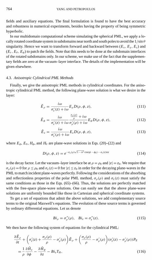
4.3. Anisotropic Cylindrical PML Methods

Finally, we give the anisotropic PML methods in cylindrical coordinates. For the aniso-tropic cylindrical PML method, the following plane-wave solution is what we desire in thelayer:

Eρ = iω

σ ′z(z)+ iωEρD(ρ, φ, z), (111)

Eφ = iω

σ ′z(z)+ iω

σρ(ρ)

ρ+ iω

σ ′ρ(ρ)+ iωEφD(ρ, φ, z), (112)

Ez = iω

σ ′z(ρ)+ iωEzD(ρ, φ, z), (113)

whereEφ , Eθ , Hφ , andHθ are plane-wave solutions in Eqs. (20)–(22) and

D(ρ, φ, z) = e−σρ(ρ)√

1− n2 cos(φ−φ0)− σz(z)nz (114)

is the decay factor. Let the vacuum–layer interface be atρ= ρ0 and|z| = z0. We require thatσρ(ρ)= 0 forρ ≤ ρ0 andσz(z)= 0 for |z| ≤ z0 in order for the decaying plane-waves in thePML to match incident plane-waves perfectly. Following the considerations of the absorbingand reflectionless properties of the polar PML method,σρ(ρ) andσz(z) must satisfy thesame conditions as those in the Eqs. (65)–(66). Thus, the solutions are perfectly matchedwith the free-space plane-wave solutions. One can easily see that the above plane-wavesolutions are uniformly bounded like those in Cartesian and spherical coordinate systems.

To get a set of equations that admit the above solutions, we add complementary sourceterms to the original Maxwell’s equations. The evolution of these source terms is governedby ordinary differential equations. Let us denote

Biρ = σ ′′ρ (ρ), Biz = σ ′′z (z). (115)

We then have the following system of equations for the cylindrical PML:

∂ Eρ

∂t+(σ ′z(z)+

σρ(ρ)

ρ− σ ′ρ(ρ)

)Eρ +

(σρ(ρ)

ρ− σ ′ρ(ρ)

)(σ ′z(z)− σ ′ρ(ρ))PE

= 1

ρ

∂ H z

∂φ− ∂ Hφ

∂z− BizTH , (116)


∂ Eφ

∂t+(σ ′z(z)+ σ ′ρ(ρ)−

σρ(ρ)

ρ

)Eρ +

(σ ′ρ(ρ)−

σρ(ρ)

ρ

)(σ ′z(z)−

σρ(ρ)

ρ

)QE

= ∂ Hρ

∂z− ∂ H z

∂ρ+ BizUH − BiρVH , (117)

∂ Ez

∂t+(σρ(ρ)

ρ+ σ ′ρ(ρ)− σ ′z(z)

)Ez+ (σ ′ρ(ρ)− σ ′z(z))

(σρ(ρ)

ρ− σ ′z(z)

)RE

= ∂ Hφ

∂ρ− 1

ρ

∂ Hρ

∂φ+ Hφ

ρ+ BiρWH , (118)

and the supplementary ordinary differential equations are given as

∂PE

∂t= Eρ − σ ′ρ(ρ)PE, (119)

∂QE

∂t= Eφ − σρ(ρ)

ρQE, (120)

∂RE

∂t= Ez− σz(z)RE, (121)

∂TH

∂t= Hφ − σ ′z(z)TH , (122)

∂UH

∂t= Hρ − σ ′z(z)UH , (123)

∂VH

∂t= H z− σ ′ρ(ρ)VH , (124)

∂WH

∂t= Hφ − σ ′ρ(ρ)WH . (125)

Note that the system of equations is symmetric hyperbolic and, hence, strongly well-posed.The supplementary fields are similar to those in the spherical case in formulation and can beobtained without much difficulty. As in the Cartesian case, we can reduce the biaxial PMLto the uniaxial PML by settingBiρ andBiz to be zero or by choosing a linear loss profilein the layer. ThenTH , UH , VH , andWH are not needed in the PDE. Hence, in that case, wedo not need to solve Eqs. (122)–(125), and that makes the uniaxial PML computationallyless expensive.

5. NUMERICAL EXPERIMENTS

The numerical method we use is a multidomain Chebyshev pseudospectral scheme. Asa pseudospectral scheme is infinite-order accurate for smooth solutions, we expect it tobe the best underlying scheme for the testing of PMLs. In testing the PMLs we want thenumerical reflection due to the PMLs, which is very small, to be fully manifested in theerror of numerical solutions.

The computational domain is decomposed into two layers of subdomains. The PMLsbeing considered are set up in the outer layer to terminate the computational domains.Detailed description of the 3D multidomain spectral scheme does not fit in here and wehope to report on it in the near future.


5.1. Simulations with the Spherical PML Methods

To test the spherical PML methods, we first apply them in the simulation of a modelproblem for which the exact solution is known. The problem is the same as that in [19],where an off-centered radiating electric dipole located atS= (0, 0, z0), z0> 0, is considered.Its time dependence is a Gaussian pulse centered att = t0 [19].

Unlike [19], we simulate the problem in 3D to test the spherical PML methods, althoughthe computational region can be reduced to a 2D region due to inherent symmetry. We de-compose the computational domain into 48 subdomains, where the computational mesh weuse in each subdomain is 12× 12× 12. Half of the subdomains are in the outer layer, i.e., inthe PML. The inner boundary of the computational domain is atr = 0.5[m], while the PMLlayers start atr = 1.0[m]. We setz0= 0.4[m] in our simulations. We shall compare the nu-merical solutions with the exact solutions at three different locations well inside the compu-tational domain:P1(θ = 45◦, φ= 0◦, r = 0.75[m]), P2(θ = 90◦, φ= 0◦, r = 0.75[m]), andP3(θ = 180◦, φ= 0◦, r = 0.75[m]).

In Fig. 1, we plot theφ-component of the magnetic field versus time at the locationsP1 and P2, computed with the split-field spherical PML method, on top of the exact so-lutions. The numerical errors at the two locations are very small. After the pulse passes,the maximum residual amplitude is only 0.1% of the exact solutions approximately. Note

FIG. 1. The numerical solution ofH φ at P1 and P2 (dashed lines), computed using the split-field sphericalPML method, is compared with the exact solution (solid line).


FIG. 2. The numerical solution ofH φ at P3 (dashed line), computed using the split-field spherical PMLmethod, is compared with the exact solution (solid line).

that when the pulse passes the location, there is no reflection coming from the boundarysince the wave has not yet reached the PML region. The error at that stage is solely dueto the discretization error of the sharp pulse. In Fig. 2, we plot theφ-component of themagnetic field at pointP3, computed with the same method, on top of the exact solu-tion which is zero atP3. One notes that the error is as low as 5.0E− 15, which stronglysuggests that reflections are absorbed locally and do not contaminate the solution else-where.

In Fig. 3, we plot theφ-component of the magnetic field versus time at the locationsP1

and P2, computed with the uniaxial spherical PML method, on top of the exact solutions.One notes that the reflection of the PML is also very small, less than 0.1% of the exactsolution. Theφ-component of the magnetic field at pointP3, computed with the samemethod, is also extremely small like in Fig. 2, which strongly suggests that the numericalerror is absorbed locally and does not contaminate the solution elsewhere.

In Fig. 4, we plot theφ-component of the magnetic field versus time at the locationsP1

and P2, computed with the biaxial spherical PML method, on top of the exact solutions.One notes that the reflection from the PML is again very small, less than 0.1% of theexact solution. Theφ-component of the magnetic field at pointP3, computed with the samemethod, is also extremely small like in Fig. 2, which strongly suggests that the numericalerror is absorbed locally and does not contaminate the solution elsewhere.


FIG. 3. The numerical solution ofH φ at P1 and P2 (dashed lines), computed using the uniaxial sphericalPML method, is compared with the exact solution (solid line).

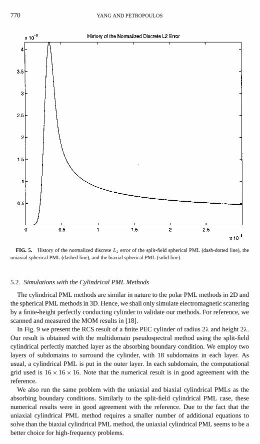
In Fig. 5, we compare the error history of different spherical PML methods. The discreteL2 error is computed on all the grid points in the inner subdomain and plotted versus timewith the field normalized. Numerical results show that the accuracy of the three types ofPML methods are very close.

Finally, in Fig. 6 we compare the split-field and the uniaxial PMLs for a dipole whoseamplitude as a function of time is a smoothed step function, i.e., for a source with significantω = 0 frequency content. As expected, both methods fail for this case; however, the overallerror history of the uniaxial PML is much better than that of the split-field PML. Thelatter is better at an early stage but diverges eventually. It appears that the underlyingproblem with the two methods is different. The result of the biaxial PML, which is closeto, but not as good as, that of the uniaxial PML, is omitted here. One unsolved problemwith biaxial PML in time domain is that whenω= 0, supplementary fields such asQH

and RH are unbounded at the vacuum–layer interfacer = r0. However, the biaxial PMLdoes not have this problem in frequency domain and the situation should be different infrequency domain. In the constant profile case, the time-domain uniaxial PML method wepropose only needs supplementary fieldsDH andDE that are uniformly bounded. Indeed,all fields are bounded in this case. These issues are currently under investigation. Note thatthe simulation time in this test is an order of magnitude larger than that of the previoustests.


FIG. 4. The numerical solution ofH φ at P1 andP2 (dashed lines), computed using the biaxial spherical PMLmethod, is compared with the exact solution (solid line).

We have also simulated scattering by a PEC sphere. In this simulation, we used 12subdomains, and in each subdomain a 16× 16× 16 grid is used. The split-field PML, thebiaxial PML, and the uniaxial PML methods were all used to truncate the simulation, andthe Mie-series result was taken as the RCS reference. To determine the size of the reflectionof the perfectly matched layers, we also compare the computed fields to those computedusing a larger computational domain.

In Fig. 7 we present the RCS result of scattering by a PEC sphere of electrical sizeka= 5.3, with the Mie-series RCS result as the reference. Here we use the multidomainpseudospectral method with the split-field, uniaxial, and biaxial spherical PMLs. All threeapproaches give very accurate results, within 0.01–0.02 db of the exact one. The resultsfrom all the methods are again very close.

In Fig. 8 we plot, versus time, theEx field λ/2 from the scatterer surface in the backscatter region, and the difference between the field and the one obtained in the refer-ence computation using a larger computational domain. It is shown in the figure that thedifference between the two fields is within 1× 10−3 after the initial noise, which is theresult of the initial nonsmoothness of the type of excitation used. Due to resource re-strictions, we could not run this test for a longer time. However, our 2D tests in [3, 4]suggest that the reflection of PML methods remain this low even after a much longertime.


FIG. 5. History of the normalized discreteL2 error of the split-field spherical PML (dash-dotted line), theuniaxial spherical PML (dashed line), and the biaxial spherical PML (solid line).

5.2. Simulations with the Cylindrical PML Methods

The cylindrical PML methods are similar in nature to the polar PML methods in 2D andthe spherical PML methods in 3D. Hence, we shall only simulate electromagnetic scatteringby a finite-height perfectly conducting cylinder to validate our methods. For reference, wescanned and measured the MOM results in [18].

In Fig. 9 we present the RCS result of a finite PEC cylinder of radius 2λ and height 2λ.Our result is obtained with the multidomain pseudospectral method using the split-fieldcylindrical perfectly matched layer as the absorbing boundary condition. We employ twolayers of subdomains to surround the cylinder, with 18 subdomains in each layer. Asusual, a cylindrical PML is put in the outer layer. In each subdomain, the computationalgrid used is 16× 16× 16. Note that the numerical result is in good agreement with thereference.

We also run the same problem with the uniaxial and biaxial cylindrical PMLs as theabsorbing boundary conditions. Similarly to the split-field cylindrical PML case, thesenumerical results were in good agreement with the reference. Due to the fact that theuniaxial cylindrical PML method requires a smaller number of additional equations tosolve than the biaxial cylindrical PML method, the uniaxial cylindrical PML seems to be abetter choice for high-frequency problems.


FIG. 6. The numerical solution ofEr at P1 computed using the split-field (dash) and uniaxial (dot) sphericalPML methods, is compared with the exact solution (solid line), and the normalized discreteL2 error of the split-fieldspherical PML (dash) is compared with that of the uniaxial spherical PML (dot).

6. CONCLUDING REMARKS

In this paper, three types of PML methods are discussed and compared, i.e. the split-field,the biaxial, and the uniaxial PML methods.

The proposed split-field spherical PML has the property of admitting plane-wave solu-tions that decay in all directions of propagation. The biaxial PML we propose differs fromother anisotropic PMLs in that it is shown to admit plane-wave solutions that are uniformlybounded while the fields in the layer decay exponentially independently of the frequency.However, we also show that the uniaxial PML admits uniformly bounded plane-wave solu-tions when the PML is constant, and the uniaxial PML needs less supplementary equationsthan the biaxial PML does. For both the biaxial and the uniaxial PML methods, we presenthere the time-domain equations that have the important property of being symmetric hy-perbolic, from which well-posedness follows. The reduction from the biaxial PML into theuniaxial PML can actually be controlled by a switch.

All the PML methods are demonstrated to be effective in numerical experiments andthey give very similar numerical results. Reflection from the PMLs is as low as 0.1% ofthe amplitude of the wave. A detailed presentation of the 3D multidomain spectral methodwe use and the implementation details of the PML methods, which have a big influence on


FIG. 7. Plots of RCS’s obtained from the pseudospectral method with the split-field spherical PML (dashedline), the uniaxial spherical PML (dash-dotted line), and the biaxial spherical PML (dotted line) on top of theMie-series RCS (solid line), for a PEC sphere of electrical sizeka= 5.3.

FIG. 8. Comparison of field obtained from spectral method with split-field spherical PML, dashed line, andreference, solid line, for a PEC sphere with electrical sizeka= 5.3.


FIG. 9. Comparison of RCS’s obtained from spectral method with cylindrical PML, solid line, and refer-ence, marked by “+,” for a PEC cylinder of radius 2λ and height 2λ, horizontal polarization(Einc= θ · Eθ ,

θ inc=π/4, φ inc=π/2, φobs=π/3).

the results, have to be omitted herein for conciseness, and we hope to report on them in thenear future.

Due to the fact that the uniaxial medium PML’s time-domain equations is symmetrichyperbolic and has the smallest number of equations, it is the most efficient one to use.What remains to be studied is the boundness of the plane-wave solutions when the PML isnot constant.

ACKNOWLEDGMENTS AND DISCLAIMER

The first author would like to thank Professor Marcus J. Grote for his help in setting up the radiating dipole testand Professor Jan Hesthaven for helpful discussions. Both authors are grateful to David Gottlieb for his constantencouragement. The first author was supported by DARPA/AFOSR Grant F49620-96-1-0426. The second authorwas supported in part by AFOSR Grant F49620-98-1-0001. The U.S. Government is authorized to reproduceand distribute reprints for governmental purposes notwithstanding any copyright notation thereon. The views andconclusions contained herein are those of the author and should not be interpreted as necessarily representing theofficial policies or endorsements, either expressed or implied, of the Defense Advanced Research Projects Agency,the Air Force Office of Scientific Research, or the U.S. Government.

REFERENCES

1. J.-P. Berenger, A perfectly matched layer for the absorption of electromagnetic waves,J. Comput. Phys.114,185 (1994).

2. J.-P. Berenger, Three-dimensional perfectly matched layer for the absorption of electromagnetic waves,J. Comput. Phys.127, 363 (1996).


3. B. Yang, D. Gottlieb, and J. S. Hesthaven, Spectral simulations of electromagnetic wave scattering,J. Comput.Phys.134, 216 (1997).

4. B. Yang, D. Gottlieb, and J. S. Hesthaven, On the use of PML ABC’s in spectral time—domain simulationsof electromagnetic scattering, inProc. 13th Annual Review of Progress in Applied Computational Electro-magnetics, 1997.

5. Q. Qi and T. L. Geers, Evaluation of the perfectly matched layer for computational acoustics,J. Comput.Phys.139(1), 166 (1998).

6. Z. S. Sacks, D. M. Kingsland, R. Lee, and J.-F. Lee, A perfectly matched anisotropic absorber for use as anabsorbing boundary condition,IEEE Trans. Antennas Propag.43, 1460 (1995).

7. S. D. Gedney, An anisotropic perfectly matched layer-absorbing medium for the truncation of FDTD lattices,IEEE Trans. Antennas Propag.44, 1630 (1996).

8. L. Zhao and A. C. Cangellaris, GT-PML: Generalized theory of perfectly matched layers and its applicationto the reflectionless truncation of finite-difference time-domain grids,IEEE Trans. Microwave Theory Tech.44, 2555 (1996).

9. M. Kuzuoglu and R. Mittra, Investigation of nonplanar perfectly matched absorbers for finite-element meshtruncation,IEEE Trans. Antennas Propag.45, 474 (1997).

10. M. Kuzuoglu and R. Mittra, Frequency dependence of the constitutive parameters of causal perfectly matchedanisotropic absorbers,IEEE Microwave Guided Wave Lett.6, 447 (1996).

11. S. Abarbanel and D. Gottlieb, A mathematical analysis of the PML method,J. Comput. Phys.134, 357 (1997).

12. S. Abarbanel and D. Gottlieb, On the construction and analysis of absorbing layers in C.E.M., inProc. 13thAnnual Review of Progress in Applied Computational Electromagnetics, 1997.

13. C. M. Rappaport, Perfectly matched absorbing boundary conditions based on anisotropic lossy mapping ofspace,IEEE Microwave Guided Wave Lett.5(3), 94 (1995).

14. E. A. Navarro, C. Wu, P. Y. Chung, and J. Litva, Application of PML superabsorbing boundary condition inthe non-orthogonal FD-TD method, IEE Electronics Letters Online No: 19941139 (1994).

15. F. L. Teixeira and W. C. Chew, PML-FDTD in cylindrical and spherical grids,IEEE Microwave Guided WaveLett.7(9) (1997).

16. F. L. Teixeira and W. C. Chew, Systematic derivation of anisotropic PML absorbing media in cylindrical andspherical coordinates,IEEE Microwave Guided Wave Lett.7(11) (1997).

17. P. G. Petropoulos, Reflectionless sponge layers as absorbing boundary conditions for the numerical solutionof Maxwell’s equations in rectangular, cylindrical, and spherical coordinates,SIAM J. Appl. Math., submitted.

18. S. D. Gedney and R. Mittra, The use of the FFT for the efficient solution of the problem of electromagneticscattering by a body of revolution,IEEE Trans. Antennas Propagat.38, 313 (1990).

19. M. J. Grote and J. B. Keller, Nonreflecting boundary conditions for Maxwell’s equations,J. Comput. Phys.139, 327 (1998).

Plane-Wave Analysis and Comparison of Split-Field, Biaxial, and Uniaxial PML Methods as ABCs for...

Documents

Transcript of Plane-Wave Analysis and Comparison of Split-Field, Biaxial, and Uniaxial PML Methods as ABCs for...