Reducing index, and pseudospectralmethods for differential-algebraic equations

E. Babolian a, M.M. Hosseini b,*

a Institute of Mathematics, University for Teacher Education, Tehran 15614, Iranb Department of Mathematics, Yazd University, Yazd, Iran

Abstract

In this paper, numerical solution of linear differential-algebraic equations is con-

sidered by pseudospectral method. Also, an index reduction technique for them is

suggested.

For Hessenberg index-2 system, the index reduction technique is defined and its use

is demonstrated. We give a condition under which the general linear form problem can

be easily transformed to the index reduced form by a simple formulation. Furthermore,

with providing some examples, the aforementioned cases are dealt with numerically.

� 2002 Elsevier Science Inc. All rights reserved.

Keywords: Differential-algebraic equations; Index reduction techniques; Spectral methods

1. Introduction

Many physical problems are most easily initially modeled as a system of

differential-algebraic equations (DAEs) [8]. Some numerical methods have

been developed, using both BDF [1,8,13] and implicit Runge–Kutta methods

[4,8]. These methods are only directly suitable for low index problems andoften require that the problem to have special structure. Although many im-

portant applications can be solved by these methods there is a need for more

*Corresponding author.

E-mail addresses: babolian@saba.tmu.ac.ir (E. Babolian), hosse_m@yazduni.ac.ir (M.M.

Hosseini).

0096-3003/02/$ - see front matter � 2002 Elsevier Science Inc. All rights reserved.

PII: S0096 -3003 (02 )00200-X

Applied Mathematics and Computation 140 (2003) 77–90

www.elsevier.com/locate/amc

general approaches. Some more general approaches were proposed in [2,3,9–

11].In this paper, we consider a linear (or linearized) model problem,

X ðmÞ ¼Xmj¼1

AjX ðj�1Þ þ By þ q; ð1aÞ

0 ¼ CX þ r; ð1bÞ

where Aj, B and C are smooth functions of t, 06 t6 tf , AjðtÞ 2 Rn�n,j ¼ 1; . . . ;m, BðtÞ 2 Rn, CðtÞ 2 R1�n, nP 2, and CB is nonsingular for each t

(hence the DAE has index mþ 1). The inhomogeneities are qðtÞ 2 R and

rðtÞ 2 R. The DAE (1a) and (1b) will be transformed into an implicit DAEform by representing a simple formulation. For this reason, we put

y ¼ ðCBÞ�1C X ðmÞ

"�Xmj¼1

AjX ðj�1Þ � q

#ð2Þ

and by substituting (2) in (1a), we obtain an implicit DAE which has index m,

as follows,

Xmj¼0

EjX ðjÞ ¼ q̂q; ð3Þ

where EjðtÞ 2 Rn�n, j ¼ 0; 1; . . . ;m, and except E0ðtÞ, others are singular ma-

trices. Note that system (3) has one equation less than system (1a) and (1b).Here, for numerical solution of DAE problems, we will use pseudospectral

method. It is known that the eigenfunctions of certain singular Sturm–Liouville

problems allow the approximation of functions in C1½a; b where truncation

error approaches zero faster than any negative power of the number of basic

functions used in the approximation, as that number (order of truncation N)

tends to infinity [12]. This phenomenon is usually referred to as ‘‘spectral ac-

curacy’’ [14]. The accuracy of derivatives obtained by direct, term-by-term

differentiation of such truncated expansion naturally deteriorates [12], but forlow-order derivatives and sufficiently high-order truncations this deterioration

is negligible, compared to the restrictions in accuracy introduced by typical

difference approximations (for more details, refer to [12,14]).

Throughout, we are using first kind orthogonal Chebyshev polynomials

fTkgþ1k¼0 which are eigenfunctions of singular Sturm–Liouville problem:

ffiffiffiffiffiffiffiffiffiffiffiffiffi1� x2

pT 0ðxÞ

� �0þ k2ffiffiffiffiffiffiffiffiffiffiffiffiffi

1� x2p TkðxÞ ¼ 0:

78 E. Babolian, M.M. Hosseini / Appl. Math. Comput. 140 (2003) 77–90

2. A simple formulation for index reduction

First, consider problem (1a) and (1b) with m ¼ 1, this problem is called the

Hessenberg index-2 system.

X 0 ¼ AX þ By þ q; ð4aÞ0 ¼ CX þ r; ð4bÞ

where, A ¼ ðaijÞn�n, B ¼ ðbiÞn�1, C ¼ ðciÞ1�n, q ¼ ðqiÞn�1, nP 2, and CBðtÞ 6¼ 0

for all t in ½0; tf , i.e.,

CBðtÞ ¼Xni¼1

ðcibiÞðtÞ 6¼ 0; 8t 2 ½0; tf : ð5Þ

By (4a) and (5), we have,

y ¼ ðCBÞ�1C½X 0 � AX � q; ð6Þ

and substituting (6) into (4a) implies,

X 0 ¼ AX þ BðCBÞ�1C½X 0 � AX � q þ q:

So, problem (4a) and (4b) transforms to the system:

ðI � BðCBÞ�1CÞ½X 0 � AX � q ¼ 0; ð7aÞCX þ r ¼ 0: ð7bÞ

Here, the overdetermined system (7a) and (7b) will transform to a fullrank

DAE system with n equations and n unknowns which has index 1.

Theorem 1. The index-2 DAE system (4a) and (4b), with n ¼ 2, is equivalent toindex-1 DAE system (8),

E1X 0 þ E0X ¼ q̂q; ð8Þ

such that,

E0 ¼b1a21 � b2a11 b1a22 � b2a12

c1 c2

� �; E1 ¼

b2 �b10 0

� �;

q̂q ¼b2q1 � b1q2

�r

� �and y ¼ ðCBÞ�1C½X 0 � AX � q:

Proof. As it is seen, the DAE system (4a) and (4b) is transformed to overde-

termined system (7a) and (7b) by using (6). Now by considering n ¼ 2,

ðI � BðCBÞ�1CÞ ¼ 1

c1b1 þ c2b2

c2b2 �c2b1�b2c1 c1b1

� �;

E. Babolian, M.M. Hosseini / Appl. Math. Comput. 140 (2003) 77–90 79

thus, (7a) has a form as below,

ðI � BðCBÞ�1CÞ½X 0 � AX � q

¼

c2½ðb1a21 � b2a11Þx1 þ b2x01 þ ðb1a22 � b2a12Þx2�b1x02 � b2q1 þ b1q2 ¼ 0;

�c1½ðb1a21 � b2a11Þx1 þ b2x01 þ ðb1a22 � b2a12Þx2�b1x02 � b2q1 þ b1q2 ¼ 0:

8>>><>>>: ð9Þ

Relation (5) implies that,

c1ðtÞ 6¼ 0; or c2ðtÞ 6¼ 0; 8t 2 ½0; tf :

So, we can arbitrarily eliminate one of the equations of the system (9) and the

overdetermined system (7a) and (7b) can transform to the following fullrankDAE system:

ðb1a21 � b2a11Þx1 þ b2x01 þ ðb1a22 � b2a12Þx2 � b1x02 ¼ b2q1 � b1q2;c1x1 þ c2x2 ¼ r0;

which has the form of system (8). In addition, we have,

detðE1ðtÞÞ ¼ 0; and detb2 �b1c1 c2

� �� �6¼ 0; 8t 2 ½0; tf ; ð10Þ

which by considering algorithm (4a), represented in [13], we conclude that the

DAE problem (8) has index 1.

In the case n > 2, for transforming the overdetermined system (7a) and (7b)to a fullrank system with index m, there is a need for one additional condition

on the problem (4a) and (4b). To proceed further, we define matrix, Mn�n, as

below:

M ¼Xni¼1

cibiðI � BðCBÞ�1CÞ;

and the lth-row and ðl; sÞth-element of matrix M denote by M ½l and M ½l; s,respectively, where 16 l, s6 n. �

Theorem 2. Consider problem (4a) and (4b), when n > 2, if

9k; 16 k6 n; ckðtÞ 6¼ 0; 8t 2 ½0; tf ð11Þ

then the kth-row of matrix ðI � BðCBÞ�1CÞ is linearly dependent with respect toother rows.

80 E. Babolian, M.M. Hosseini / Appl. Math. Comput. 140 (2003) 77–90

Proof. For problem (4a) and (4b), we have,

ðI � BðCBÞ�1CÞ ¼ 1Pni¼1 cibi

M ;

such that,

M ¼

Pni¼2

cibi �c2b1 � � � �ckb1 � � � �cnb1

�c1b2Pni¼1i6¼2

cibi � � � �ckb2 . . . �cnb2

..

. ... ..

. ...

�c1bk �c2bk . . .Pni¼1i6¼2

cibi . . . �cnbk

..

. ... ..

. ...

�c1bn �c2bn . . . �ckbn . . .Pni¼2

cibi

26666666666666666664

37777777777777777775

: ð12Þ

Suppose that t� be an arbitrary point in ½0; tf , we define,

J1 ¼ fj : 16 j6 n & cjðt�Þ ¼ 0g; ð13Þ

for all j 2 J1, by considering (12), M ½j; s ¼ 0, s ¼ 1; 2; . . . ; j� 1; jþ 1; . . . ; n,and M ½j; j 6¼ 0 (by (5)). Hence for all j 2 J1, the jth-row of M is linearly in-

dependent with respect to other rows of M (note that k 62 J1). Now put,

J2 ¼ fj : 16 j6 n & j 62 J1 & j 6¼ kg: ð14Þ

We will show that the M ½k is linearly dependent with respect to M ½j, j 2 J2.To do this, we show that,

ðckM ½kÞðt�Þ ¼Xl2J2

ðclM ½lÞðt�Þ: ð15Þ

To prove (15), it is sufficient to show that all corresponding components of two

sides of (15) are equal. By considering (12)–(14),

M ½l; s ¼�blcs; l 6¼ s;Pj2J2bjcj þ bkck l ¼ s:

(

So, for 16 s6 n, we have:

(i) if s 6¼ k,

ckM ½k; s ¼ �ckbkcs; ð16aÞ

E. Babolian, M.M. Hosseini / Appl. Math. Comput. 140 (2003) 77–90 81

�Xl2J2

clM ½l; s ¼Xl2J2l6¼s

�clð�blcsÞ � csXj2J2j 6¼s

bjcj

0BBBB@ þ bkck

1CCCCA

¼ �csbkck: ð16bÞ(ii) if s ¼ k,

ckM ½k; k ¼ ckXj2J2

bjcj

!; ð17aÞ

�Xl2J2

clM ½l; k ¼Xl2J2

�clð�blckÞ: ð17bÞ

By equality of (16a) and (17a) with (16b) and (17b), respectively, we get,

ðCkM ½k; sÞðt�Þ ¼ �Xl2J2

ðclM ½l; sÞðt�Þ; for all s; 16 s6 n;

and t� 2 ½0; tf ;

i.e., relation (15) is established and the kth-row of the matrix M is linearly

dependent with respect to other rows.Now, if M ðn�1Þ�n is obtained by eliminating kth-row of M (k is defined in

(11)), then the overdetermined system (7a) and (7b) can be transformed to the

following DAE system with n equation and n unknowns:

M ½X 0 � AX � q ¼ 0;CX þ r ¼ 0:

ð18Þ

Here, we must show that system (18) is fullrank and has index 1. �

Theorem 3. In relation (13), if F ¼ MC

� �n�n

and k is denoted as in (11) then,

j detðF ðtÞÞj ¼ jckðtÞjXni¼1

ðcibiÞðtÞ

n�1

; 8t 2 ½0; tf :

Proof. For simplicity, suppose that k ¼ 1, we have,

M ¼

�b2c1Pni¼1i6¼2

cibi � � � �b2cn

..

. ... ..

.

�bnc1 �bnc2 � � �Pn�1

i¼1

bici

266666664

377777775:

82 E. Babolian, M.M. Hosseini / Appl. Math. Comput. 140 (2003) 77–90

Since CBðtÞ ¼Pn

i¼1ðcibiÞðtÞ 6¼ 0, for all t 2 ½0; tf , so,

detðF Þ ¼ c1ðCBÞn�1det

� b2CB

1� b2c2CB

� � � �b2cnCB

..

. ... ..

.

� bnCB

� bnc2CB

� � � 1� bncnCB

1 c2 � � � cn

266666664

377777775

0BBBBBBB@

1CCCCCCCA

¼ c1ðCBÞn�1det

�b2CB

1 � � � �b2cnCB

�b3CB

0 � � � �b3cnCB

..

. ... ..

.

�bnCB

0 � � � 1� bncnCB

1 0 � � � cn

2666666666664

3777777777775

|fflfflfflfflfflfflfflfflfflfflfflfflfflfflfflfflfflfflfflfflfflfflfflffl{zfflfflfflfflfflfflfflfflfflfflfflfflfflfflfflfflfflfflfflfflfflfflfflffl}T

0BBBBBBBBBBBBBBBB@

1CCCCCCCCCCCCCCCCA

8>>>>>>>>>>>>>>>><>>>>>>>>>>>>>>>>:

þ c2 det

�b2CB

�b2CB

� � � �b2cnCB

..

. ... ..

.

�bnCB

�bnCB

� � � 1� bncnCB

1 1 � � � cn

26666666664

37777777775

|fflfflfflfflfflfflfflfflfflfflfflfflfflfflfflfflfflfflfflfflfflfflfflfflfflfflffl{zfflfflfflfflfflfflfflfflfflfflfflfflfflfflfflfflfflfflfflfflfflfflfflfflfflfflffl}z

0BBBBBBBBBBBBBB@

1CCCCCCCCCCCCCCA

9>>>>>>>>>>>>>>=>>>>>>>>>>>>>>;

:

Equality of first and second columns of matrix Z, implies, detðZÞ ¼ 0. By

continuing this process for 3rd, 4th, . . ., nth, columns of T, we get,

detðF Þ ¼ c1ðCBÞn�1det

�b2CB

1

0

..

. . ..

0�bnCB

� � � 1

1 � � � 0

26666666664

37777777775

0BBBBBBBBB@

1CCCCCCCCCA

) j detðF ðtÞÞj

¼ jc1ðtÞjjCBðtÞjn�1:

Now, since detðF ðtÞÞ 6¼ 0, for all t in [0; tf ], the following corollaries will ob-

tain. �

E. Babolian, M.M. Hosseini / Appl. Math. Comput. 140 (2003) 77–90 83

Corollary 1. RankðMÞ ¼ n� 1.

Corollary 2. The DAE system (18) is fullrank.

Corollary 3. The DAE system (18) has index 1.

Proof. We can rewrite (18) as bellow:

M0

� �X 0 þ �MA

C

� �X ¼ Mq

�r

� �;

sinceM0

� �is singular and

MC

� �is nonsingular, so, by considering algorithm

(4.1) mentioned in [13], the above system has index 1. Up to now, by repre-

senting a simple formulation, the Hessenberg index-2 system (4a) and (4b) is

transformed to the implicit DAE system with index 1 (with reducing one

equation). In continuation, for general form (1a) and (1b), this topic is dis-

cussed. According to presented process, by using (2), the problem (1a) and (1b)

transforms to the following overdetermined system:

ðI � BðCBÞ�1CÞ X ðmÞ

"�Xmj¼1

AjX ðj�1Þ � q

#¼ 0; ð19aÞ

CX þ r ¼ 0: ð19bÞ

Now, having Theorems 2 and 3, the above system can be transformed to the

following fullrank DAE system, with n equations and n unknowns,

M ½X ðmÞ �Pm

j¼1 AjXðj�1Þ � q ¼ 0;

CX þ r ¼ 0;

i.e.,

M0

� �X ðmÞ þ �MAm

0

� �X ðm�1Þ þ � � � þ �MA2

0

� �X 0 þ �MA1

C

� �X ¼ Mq

�r

� �;

or

EmX ðmÞ þ Em�1X ðm�1Þ þ � � � þ E1X 0 þ E0X ¼ q̂q: ð20Þ

Index of (20) is equal to m, to prove this, we define,

U0 ¼ X ;U1 ¼ X 0;Um�1 ¼ X ðm�1Þ

8<:

so, the system (20) can be written as:

84 E. Babolian, M.M. Hosseini / Appl. Math. Comput. 140 (2003) 77–90

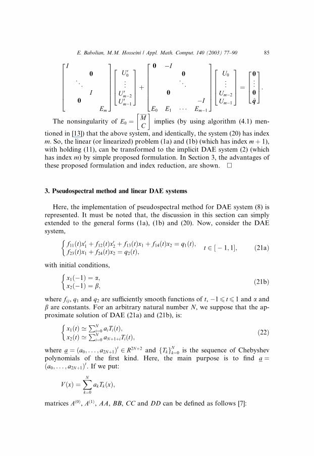
I0

. ..

I0

Em

26666664

37777775

U 00

..

.

U 0m�2

U 0m�1

26664

37775þ

0 �I0

. ..

0

�IE0 E1 � � � Em�1

26666664

37777775

U0

..

.

Um�2

Um�1

26664

37775 ¼

0

..

.

0

q̂q

26643775:

The nonsingularity of E0 ¼ MC

� �implies (by using algorithm (4.1) men-

tioned in [13]) that the above system, and identically, the system (20) has index

m. So, the linear (or linearized) problem (1a) and (1b) (which has index mþ 1),

with holding (11), can be transformed to the implicit DAE system (2) (whichhas index m) by simple proposed formulation. In Section 3, the advantages of

these proposed formulation and index reduction, are shown. �

3. Pseudospectral method and linear DAE systems

Here, the implementation of pseudospectral method for DAE system (8) is

represented. It must be noted that, the discussion in this section can simply

extended to the general forms (1a), (1b) and (20). Now, consider the DAE

system,

f11ðtÞx01 þ f12ðtÞx02 þ f13ðtÞx1 þ f14ðtÞx2 ¼ q1ðtÞ;f23ðtÞx1 þ f24ðtÞx2 ¼ q2ðtÞ;

t 2 ½

� 1; 1; ð21aÞ

with initial conditions,

x1ð�1Þ ¼ a;x2ð�1Þ ¼ b;

ð21bÞ

where fij, q1 and q2 are sufficiently smooth functions of t, �16 t6 1 and a and

b are constants. For an arbitrary natural number N, we suppose that the ap-

proximate solution of DAE (21a) and (21b), is:

x1ðtÞ ’PN

i¼0 aiTiðtÞ;x2ðtÞ ’

PNi¼0 aNþ1þiTiðtÞ;

ð22Þ

where a ¼ ða0; . . . ; a2Nþ1Þt 2 R2Nþ2 and fTkgNk¼0 is the sequence of Chebyshev

polynomials of the first kind. Here, the main purpose is to find a ¼ða0; . . . ; a2Nþ1Þt. If we put:

V ðxÞ ¼XNk¼0

akTkðxÞ;

matrices Að0Þ, Að1Þ, AA, BB, CC and DD can be defined as follows [7]:

E. Babolian, M.M. Hosseini / Appl. Math. Comput. 140 (2003) 77–90 85

V () Að0Þ; Að0Þij ¼ 1; i ¼ j;

0; i 6¼ j;

V 0 () Að1Þ; Að1Þij ¼ ð1=ciÞ2j; iþ j odd; j > 1;

0; otherwise;

with 06 i, j6N , and cj ¼2; i ¼ 0

1; i > 0

and

AA ¼ f11ðtÞAð1Þ þ f13ðtÞAð0Þ;BB ¼ f12ðtÞAð1Þ þ f14ðtÞAð0Þ;CC ¼ f23ðtÞAð0Þ;DD ¼ f24ðtÞAð0Þ;

8>><>>: ð23Þ

such that (21a) converts to:P2Nþ1

i¼0 ai/iðtÞ ’ q1ðtÞ;P2Nþ1

i¼0 aiwiðtÞ ’ q2ðtÞ;

ð24aÞ

in which,

/iðtÞ ¼Pi

k¼0ðAAÞkiTkðtÞ; 06 i6N ;Pik¼0ðBBÞkiTkðtÞ; N þ 16 i6 2N þ 1;

ð25aÞ

wiðtÞ ¼Pi

k¼0ðCCÞkiTkðtÞ; 06 i6N ;Pik¼0ðDDÞkiTkðtÞ; N þ 16 i6 2N þ 1;

ð25bÞ

and (21b) converts to:PNi¼0 Tið�1Þ ¼

PNi¼0 aið�1Þi ¼ a;PN

i¼0 aNþ1þiTið�1Þ ¼PN

i¼0 aNþ1þið�1Þi ¼ b:

ð24bÞ

Relation (24b) forms a system with two equations and 2N þ 2 unknowns, to

construct the remaining 2N equations we substitute Chebyshev–Guass–Raudo

points, i.e.,

tj ¼ cos2pj

ð2N � 1Þ

� �; j ¼ 0; . . . ;N � 1; ð26Þ

in (24a) and put:P2Nþ1

i¼0 ai/iðtjÞ ¼ q1ðtjÞ;P2Nþ1

i¼0 aiwiðtjÞ ¼ q2ðtjÞ;j

¼ 0; 1 . . . ;N � 1;

to obtain 2N equations. In addition, according to initial conditions (21b), the

Chebyshev–Guass or Chebyshev–Guass–Lobatto points can be chosen in (26).

86 E. Babolian, M.M. Hosseini / Appl. Math. Comput. 140 (2003) 77–90

4. Numerical examples

This section deals with some numerical tests on simple, but interesting,

problems. In all the examples, we use ‘‘ex’’ to denote the maximum over all

components of the error in X and ‘‘ey ’’ denotes the maximum of the error in y.These values are approximately obtained through their graphs. All the exam-

ples are solved, directly, using (4a) and (4b), and reduced index, using (8), by

pseudospectral method. Results show the advantages of index reduction

technique, mentioned in Section 2. In this section mP 1 is a parameter. The

presented algorithms in this article, are performed using Maple V with 20 digitsprecision.

Example 1. Consider for 06 t6 1,

x01 ¼ m � 12�t

) *x1 þ ð2� tÞmy þ q1ðtÞ;

x02 ¼m � 1

2� tx1 � x2 þ ðm � 1Þy þ q2ðtÞ;

0 ¼ ðt þ 2Þx1 þ ðt2 � 4Þx2 þ rðtÞ;

8><>: ð27Þ

with x1ð0Þ ¼ 1. This example has been analyzed in [4–6]. The inhomogeneities qand r are chosen to be

q ¼3� t2� t

� �et

2et

0@

1A; rðtÞ ¼ �ðt2 þ t � 2Þet;

so that the exact solution is x1 ¼ et, x2 ¼ et, y ¼ �et=2� t. Ascher in [6] men-tioned the following topics:

(i) The stability constant for unprojected collocation is exponentially large in

m, while that for projected collocation (and for the problem itself) grows

only linearly in m.(ii) Even the projected collocation scheme exhibits a behaviour common to

nonstiff integration methods, requiring a small step-size h when mh� 1.

By Theorem 2, the problem (27) can be converted to the system,

ðm � 1Þ mðt � 2Þ0 0

� �x01x02

� �þ

m � 1

2� tmðt � 2Þ

t þ 2 t2 � 4

24

35 x1

x2

� �

¼2t2 þ ð9� mÞt þ 3m � 11

2� tet

ðt2 þ t � 2Þet

24

35; ð28Þ

E. Babolian, M.M. Hosseini / Appl. Math. Comput. 140 (2003) 77–90 87

y ¼ ðCBÞ�1C½X 0 � AX � q

¼ t � 1

ð2� tÞ2x1 þ

x012� t

� x2 � x02 þ2t2 � 7t þ 5

ð2� tÞ2et: ð29Þ

In Table 1, we record results of running pseudospectral method with, i.e.

(28), and without, i.e. (27), index reduction, when m ¼ 100.

The advantage of using index reduction method (proposed in Section 2) isclearly demonstrated for this example.

Example 2

X 0 ¼ �X þ By þ q;0 ¼ CX þ r;

06 t6 1; ð30Þ

with CðtÞ ¼ ðsinðmtÞ, cosðmtÞÞ, B ¼ Ct, x1ð0Þ ¼ 1, and q and r are chosen to be

q ¼2et þ sinðmtÞet

2� t

2et þ cosðmtÞet2� t

0B@

1CA; r ¼ �ðsinðmtÞ þ cosðmtÞÞet;

such that the exact solution is X t ¼ et1

1

� �, y ¼ �et=ð2� tÞ. By Theorem 2,

problem (30) is equivalent to,

cosðmtÞx01 � sinðmtÞx02 þ cosðmtÞx1 � sinðmtÞx2 ¼ 2etðcosðmtÞ � sinðmtÞÞ;sinðmtÞx1 þ cosðmtÞx2 ¼ ðsinðmtÞ þ cosðmtÞÞet;

ð31aÞ

and

y ¼ ðCBÞ�1C½X 0 � AX � q

¼ sinðmtÞðx01 þ x1 � 2etÞ þ cosðmtÞðx02 þ x2 � 2etÞ � et

2� t: ð31bÞ

Here, the problems (30), (31a) and (31b) are solved using pseudospectral

method with m ¼ 1000, Table 2.

Table 1

Maximum norm error for Example 1, m ¼ 100

N Without index reduction With index reduction

ex ey ex ey

6 5.6 ()3) 3.1 ()3) 5.0 ()7) 5.3 ()7)10 3.8 ()5) 2.4 ()5) 2.4 ()13) 4.0 ()13)12 2.4 ()6) 1.3 ()6) 1.7 ()16) 2.2 ()16)16 7.4 ()9) 4.4 ()9) 6.8 ()18) 2.0 ()17)

88 E. Babolian, M.M. Hosseini / Appl. Math. Comput. 140 (2003) 77–90

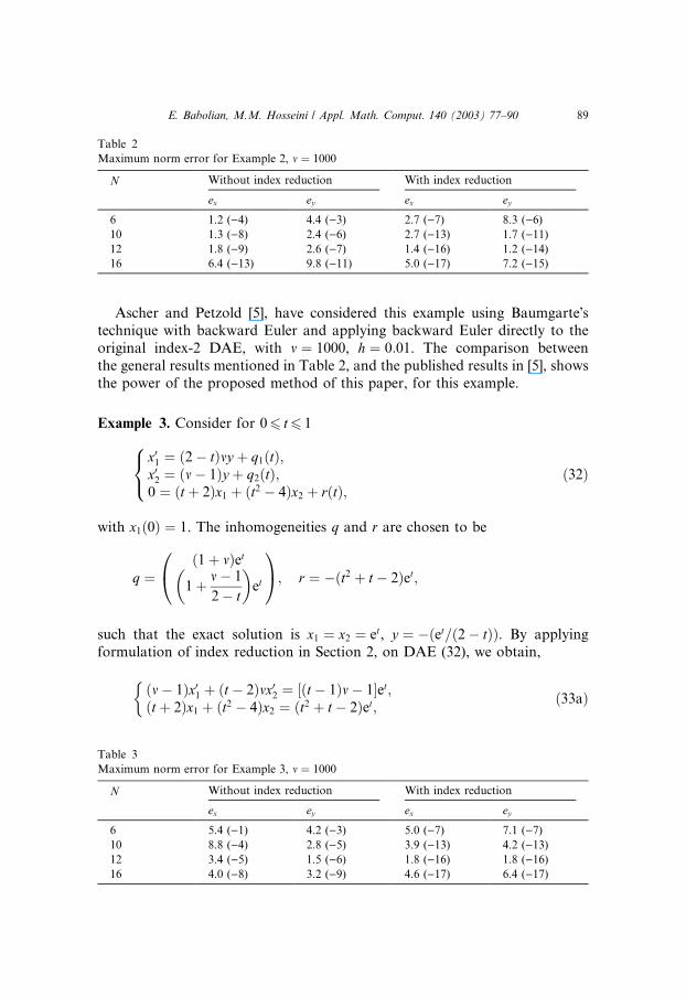
Ascher and Petzold [5], have considered this example using Baumgarte�stechnique with backward Euler and applying backward Euler directly to the

original index-2 DAE, with m ¼ 1000, h ¼ 0:01. The comparison between

the general results mentioned in Table 2, and the published results in [5], shows

the power of the proposed method of this paper, for this example.

Example 3. Consider for 06 t6 1

x01 ¼ ð2� tÞmy þ q1ðtÞ;x02 ¼ ðm � 1Þy þ q2ðtÞ;0 ¼ ðt þ 2Þx1 þ ðt2 � 4Þx2 þ rðtÞ;

8<: ð32Þ

with x1ð0Þ ¼ 1. The inhomogeneities q and r are chosen to be

q ¼ð1þ mÞet

1þ m � 1

2� t

� �et

0@

1A; r ¼ �ðt2 þ t � 2Þet;

such that the exact solution is x1 ¼ x2 ¼ et, y ¼ � et=ð2� tÞð Þ. By applying

formulation of index reduction in Section 2, on DAE (32), we obtain,

ðm � 1Þx01 þ ðt � 2Þmx02 ¼ ½ðt � 1Þm � 1et;ðt þ 2Þx1 þ ðt2 � 4Þx2 ¼ ðt2 þ t � 2Þet;

ð33aÞ

Table 2

Maximum norm error for Example 2, m ¼ 1000

N Without index reduction With index reduction

ex ey ex ey

6 1.2 ()4) 4.4 ()3) 2.7 ()7) 8.3 ()6)10 1.3 ()8) 2.4 ()6) 2.7 ()13) 1.7 ()11)12 1.8 ()9) 2.6 ()7) 1.4 ()16) 1.2 ()14)16 6.4 ()13) 9.8 ()11) 5.0 ()17) 7.2 ()15)

Table 3

Maximum norm error for Example 3, m ¼ 1000

N Without index reduction With index reduction

ex ey ex ey

6 5.4 ()1) 4.2 ()3) 5.0 ()7) 7.1 ()7)10 8.8 ()4) 2.8 ()5) 3.9 ()13) 4.2 ()13)12 3.4 ()5) 1.5 ()6) 1.8 ()16) 1.8 ()16)16 4.0 ()8) 3.2 ()9) 4.6 ()17) 6.4 ()17)

E. Babolian, M.M. Hosseini / Appl. Math. Comput. 140 (2003) 77–90 89

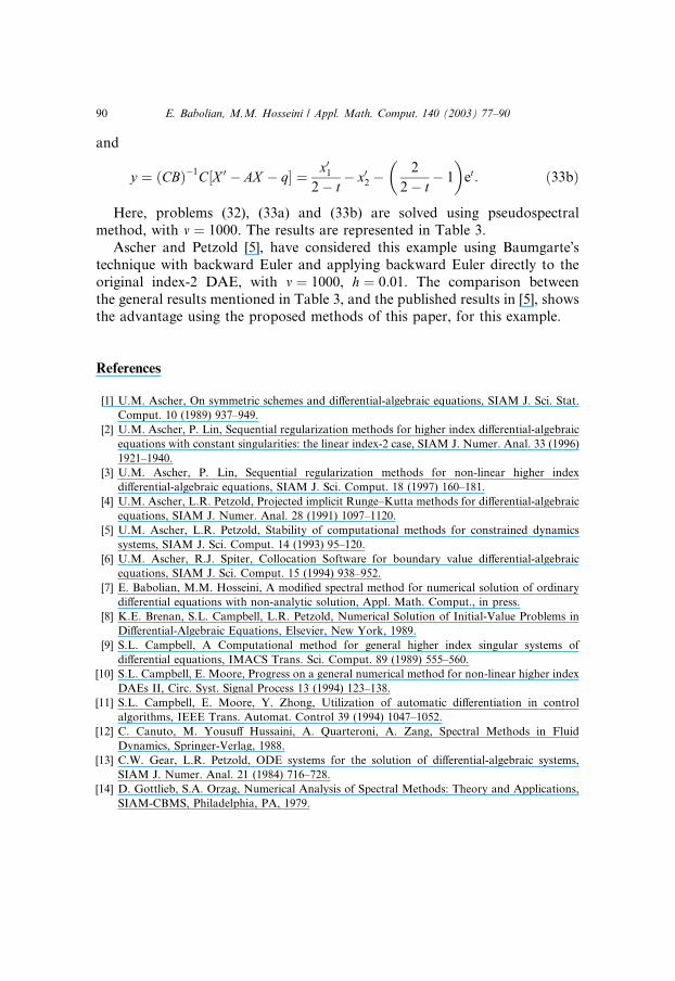
and

y ¼ ðCBÞ�1C½X 0 � AX � q ¼ x012� t

� x02 �2

2� t

�� 1

�et: ð33bÞ

Here, problems (32), (33a) and (33b) are solved using pseudospectral

method, with m ¼ 1000. The results are represented in Table 3.

Ascher and Petzold [5], have considered this example using Baumgarte�stechnique with backward Euler and applying backward Euler directly to the

original index-2 DAE, with m ¼ 1000, h ¼ 0:01. The comparison between

the general results mentioned in Table 3, and the published results in [5], showsthe advantage using the proposed methods of this paper, for this example.

References

[1] U.M. Ascher, On symmetric schemes and differential-algebraic equations, SIAM J. Sci. Stat.

Comput. 10 (1989) 937–949.

[2] U.M. Ascher, P. Lin, Sequential regularization methods for higher index differential-algebraic

equations with constant singularities: the linear index-2 case, SIAM J. Numer. Anal. 33 (1996)

1921–1940.

[3] U.M. Ascher, P. Lin, Sequential regularization methods for non-linear higher index

differential-algebraic equations, SIAM J. Sci. Comput. 18 (1997) 160–181.

[4] U.M. Ascher, L.R. Petzold, Projected implicit Runge–Kutta methods for differential-algebraic

equations, SIAM J. Numer. Anal. 28 (1991) 1097–1120.

[5] U.M. Ascher, L.R. Petzold, Stability of computational methods for constrained dynamics

systems, SIAM J. Sci. Comput. 14 (1993) 95–120.

[6] U.M. Ascher, R.J. Spiter, Collocation Software for boundary value differential-algebraic

equations, SIAM J. Sci. Comput. 15 (1994) 938–952.

[7] E. Babolian, M.M. Hosseini, A modified spectral method for numerical solution of ordinary

differential equations with non-analytic solution, Appl. Math. Comput., in press.

[8] K.E. Brenan, S.L. Campbell, L.R. Petzold, Numerical Solution of Initial-Value Problems in

Differential-Algebraic Equations, Elsevier, New York, 1989.

[9] S.L. Campbell, A Computational method for general higher index singular systems of

differential equations, IMACS Trans. Sci. Comput. 89 (1989) 555–560.

[10] S.L. Campbell, E. Moore, Progress on a general numerical method for non-linear higher index

DAEs II, Circ. Syst. Signal Process 13 (1994) 123–138.

[11] S.L. Campbell, E. Moore, Y. Zhong, Utilization of automatic differentiation in control

algorithms, IEEE Trans. Automat. Control 39 (1994) 1047–1052.

[12] C. Canuto, M. Yousuff Hussaini, A. Quarteroni, A. Zang, Spectral Methods in Fluid

Dynamics, Springer-Verlag, 1988.

[13] C.W. Gear, L.R. Petzold, ODE systems for the solution of differential-algebraic systems,

SIAM J. Numer. Anal. 21 (1984) 716–728.

[14] D. Gottlieb, S.A. Orzag, Numerical Analysis of Spectral Methods: Theory and Applications,

SIAM-CBMS, Philadelphia, PA, 1979.

90 E. Babolian, M.M. Hosseini / Appl. Math. Comput. 140 (2003) 77–90