Numerical Algebraic Geometry Boot Camp
107
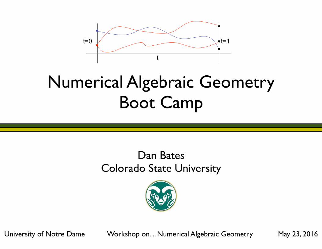
Numerical Algebraic Geometry Boot Camp Dan Bates Colorado State University University of Notre Dame Workshop on…Numerical Algebraic Geometry May 23, 2016 t t=0 t=1
-
Upload
khangminh22 -
Category
Documents
-
view
1 -
download
0
Transcript of Numerical Algebraic Geometry Boot Camp
Numerical Algebraic Geometry Boot Camp
!Dan Bates
Colorado State University !!!!
University of Notre Dame Workshop on…Numerical Algebraic Geometry May 23, 2016
t
t=0 t=1
• Introduce many of the basic
- structures,
- methods, and
- assumptions
of numerical algebraic geometry (and not the nitty-gritty theory underlying it)
!
• Show some Bertini Classic I/O
!
• Give us a common language for the next 2.5 days
!
Goals for this boot camp
1. Polynomial systems and their solution sets
2. Finding isolated solutions (homotopy continuation)
3. Advanced topics for isolated solutions
4. Finding positive-dimensional solution sets (briefly)
Game plan
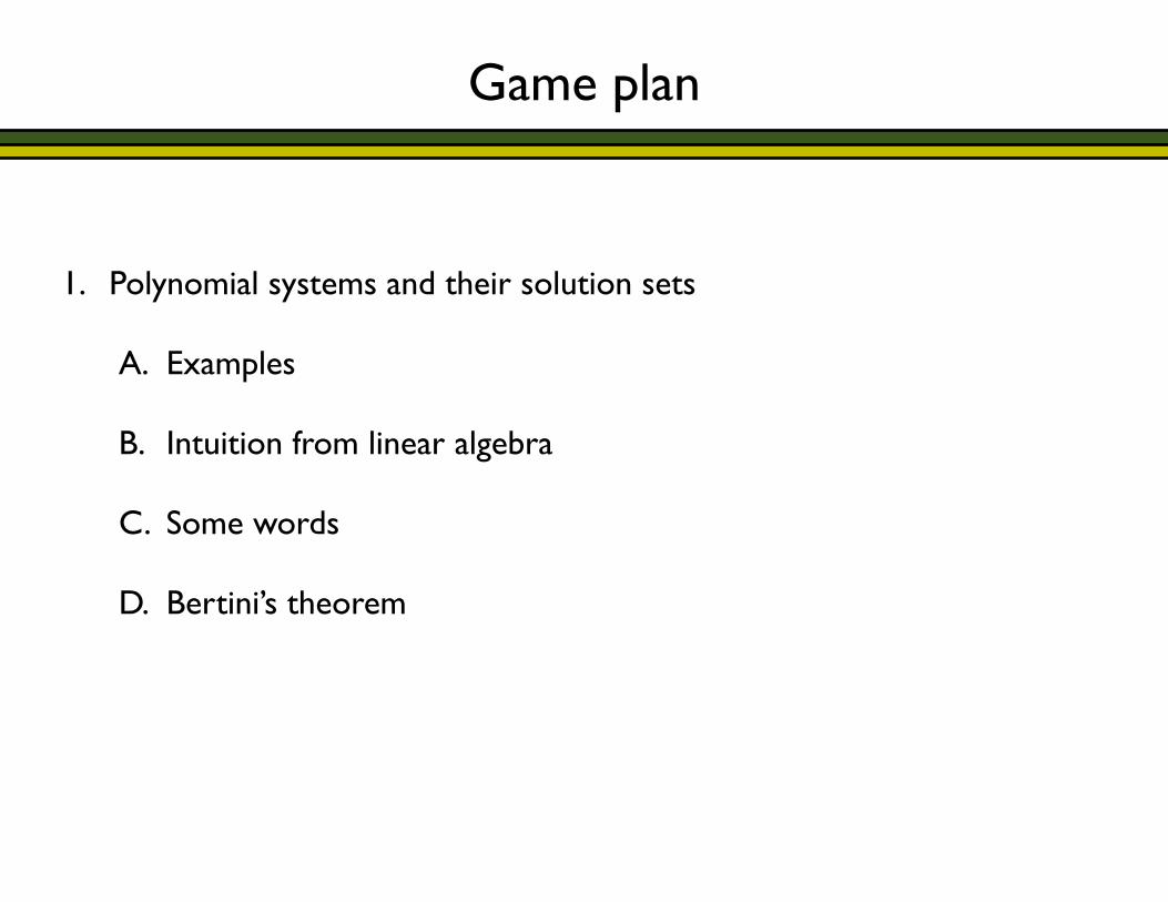
1. Polynomial systems and their solution sets
A. Examples
B. Intuition from linear algebra
C. Some words
D. Bertini’s theorem
Game plan
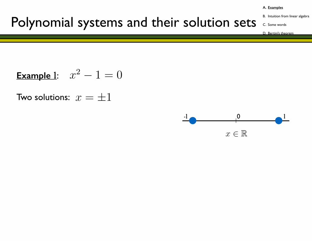
Example 1: !Two solutions: !!! !!!
x2 � 1 = 0
5
x2 � 1 = 0
x = ±1
5
Polynomial systems and their solution sets
1-1 0
x4 � 1 = 0
x = ±i
x 2 R
5
A. Examples
B. Intuition from linear algebra
C. Some words
D. Bertini’s theorem
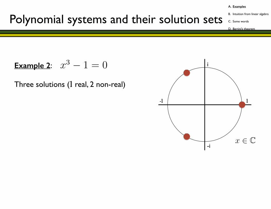
Example 2: !Three solutions (1 real, 2 non-real) !
x3 � 1 = 0
x = ±i
5
1-1
i
-i
x4 � 1 = 0
x = ±i
x 2 C
5
Polynomial systems and their solution setsA. Examples
B. Intuition from linear algebra
C. Some words
D. Bertini’s theorem
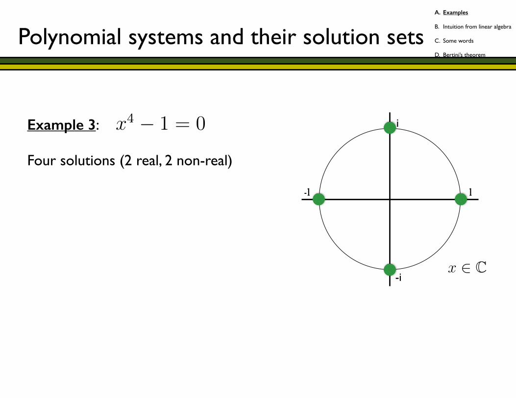
Example 3: !Four solutions (2 real, 2 non-real) !
x4 � 1 = 0
x = ±i
5
1-1
i
-i
x4 � 1 = 0
x = ±i
x 2 C
5
Polynomial systems and their solution setsA. Examples
B. Intuition from linear algebra
C. Some words
D. Bertini’s theorem
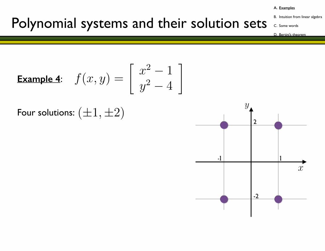
Example 4: !!Four solutions: !
x4 � 1 = 0
x = ±i
x 2 C
f(x, y) =
x2 � 1y2 � 4
�
5
1-1
2
-2
x4 � 1 = 0
x = ±i
x 2 C
f(x, y) =
x2 � 1y2 � 4
�
5
x4 � 1 = 0
x = ±i
y 2 C
f(x, y) =
x2 � 1y2 � 4
�
5
x4 � 1 = 0
x = ±i
y 2 C
f(x, y) =
x2 � 1y2 � 4
�
(±1,±2)
5
Polynomial systems and their solution setsA. Examples
B. Intuition from linear algebra
C. Some words
D. Bertini’s theorem
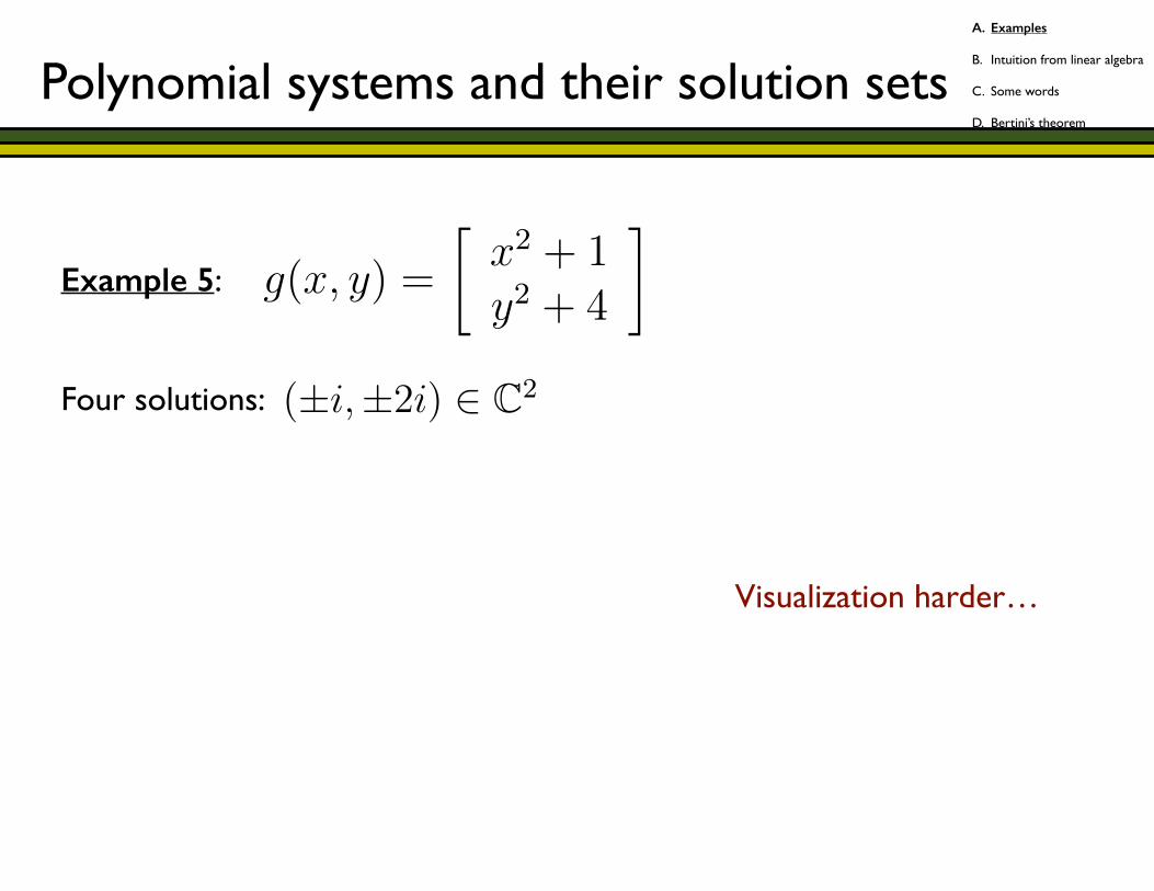
Example 5: !!Four solutions: !!! Visualization harder…
x4 � 1 = 0
x = ±i
y 2 C
g(x, y) =
x2 + 1y2 + 4
�
(±1,±2)
5
(1, 1), (�1,�1), (2,�1), (�2, 1)
f(x, y) =
f1 + f2 + f3f1 + 2f2 + f3
�
J =
2
64
@f1
@x1. . . @f1
@x
N
.
.
.
.
.
.
.
.
.
@f
N
@x1. . . @f
N
@x
N
3
75
(±i,±2i) 2 C2
6
Polynomial systems and their solution setsA. Examples
B. Intuition from linear algebra
C. Some words
D. Bertini’s theorem
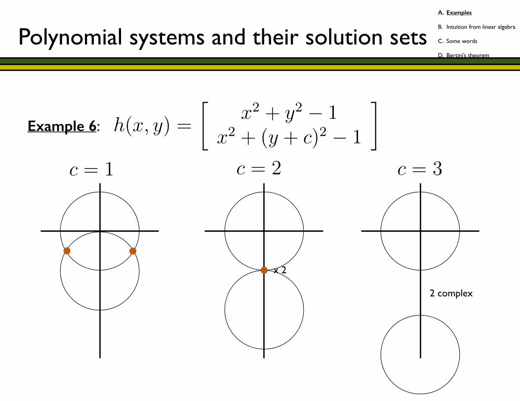
Example 6:
x4 � 1 = 0
x = ±i
y 2 C
h(x, y) =
x2 + y2 � 1
x2 + (y + c)2 � 1
�
c = 1
c = 2
c = 3
5
x4 � 1 = 0
x = ±i
y 2 C
h(x, y) =
x2 + y2 � 1
x2 + (y + c)2 � 1
�
c = 1
c = 2
c = 3
5
x4 � 1 = 0
x = ±i
y 2 C
h(x, y) =
x2 + y2 � 1
x2 + (y + c)2 � 1
�
c = 1
c = 2
c = 3
5
x4 � 1 = 0
x = ±i
y 2 C
h(x, y) =
x2 + y2 � 1
x2 + (y + c)2 � 1
�
c = 1
c = 2
c = 3
5
x 2
2 complex
Polynomial systems and their solution setsA. Examples
B. Intuition from linear algebra
C. Some words
D. Bertini’s theorem
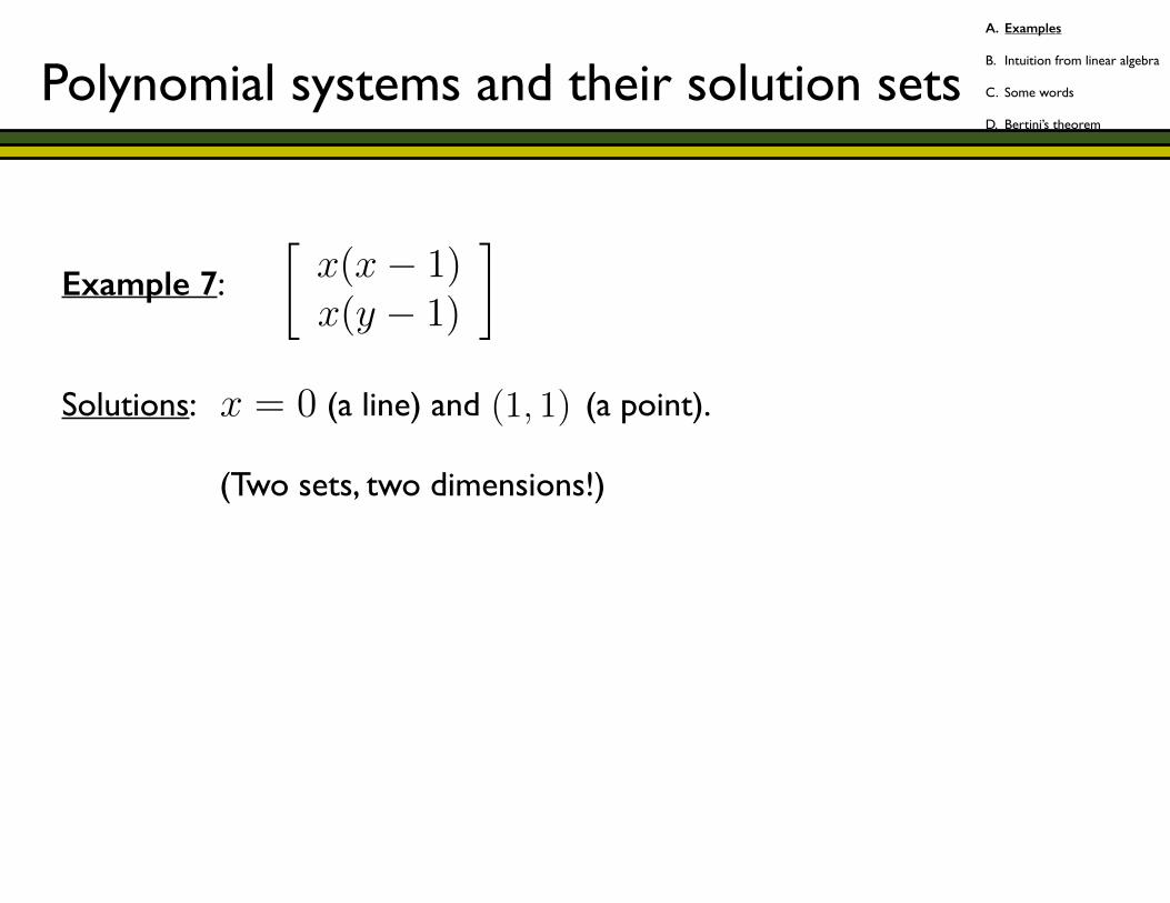
Example 7: !!Solutions: (a line) and (a point). ! (Two sets, two dimensions!) !
f =
x(x� 1)x(y � 1)
�
2
f =
x(x� 1)x(y � 1)
�
x = 0
x = y = 1
2
x4 � 1 = 0
x = ±i
y 2 C
g(x, y) =
x2 + 1y2 + 4
�
(1, 1)
5
Polynomial systems and their solution setsA. Examples
B. Intuition from linear algebra
C. Some words
D. Bertini’s theorem
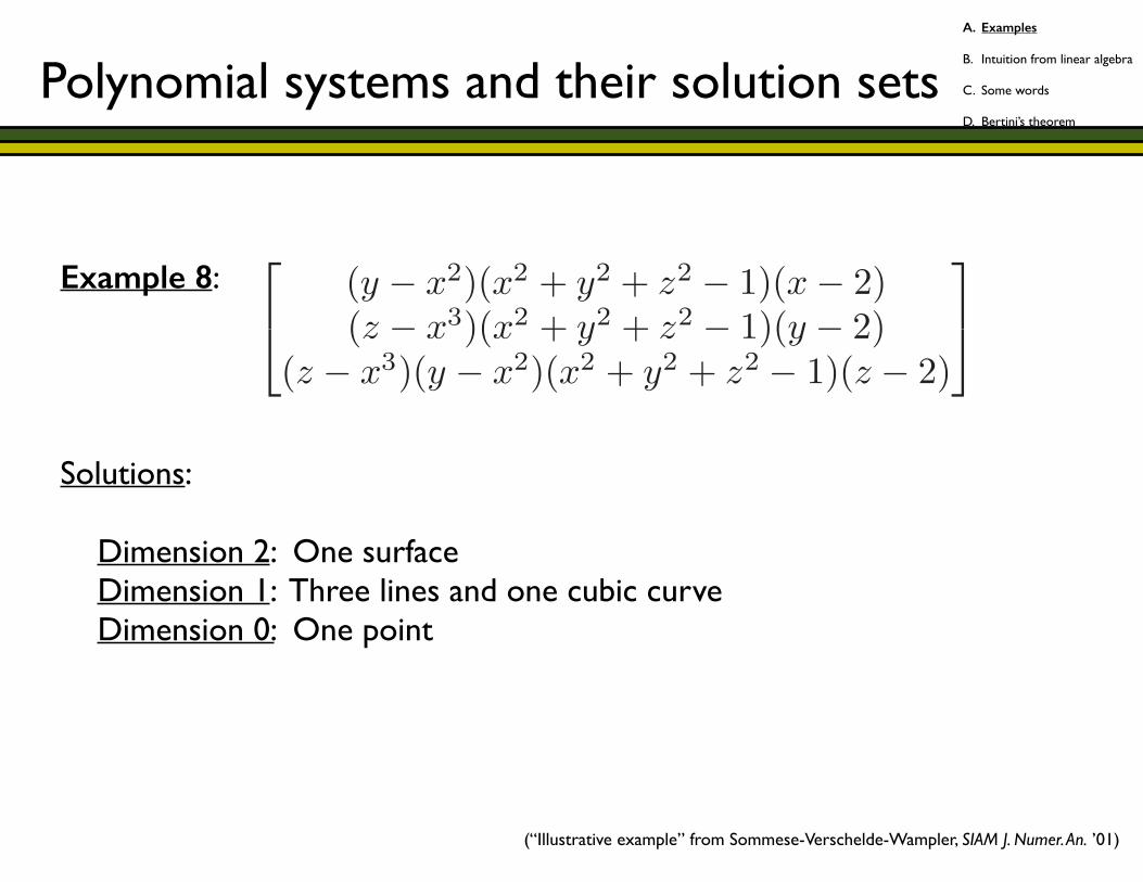
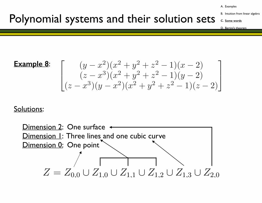
Example 8: !!!!Solutions: ! Dimension 2: One surface Dimension 1: Three lines and one cubic curve Dimension 0: One point
“main”2013/3/17page 159
✐
✐
✐
✐
✐
✐
✐
✐
DRAFT
Chapter 8
Positive-DimensionalComponents
In Part II of the book, we return to the fundamental problem of “solving” a poly-nomial system,
f(z) :=
⎡
⎢⎣f1(z1, . . . , zN)
...fn(z1, . . . , zN)
⎤
⎥⎦ = 0. (8.1)
As opposed to the case of systems of linear equations, where a nonempty so-lution set will consist of exactly one linear space, the solution set of a polynomialsystem can have several separate components and these may have different dimen-sions23 (points, curves, surfaces, etc). Thus, the problem of “solving” a polynomialsystem includes the detection of all such components no matter what dimensioneach has. Solution components of dimension greater than zero (everything exceptisolated points) are said to be “positive-dimensional.”
For example, consider the following system of three polynomials in the vari-ables x, y, z:
f =
⎡
⎣(y − x2)(x2 + y2 + z2 − 1)(x− 2)(z − x3)(x2 + y2 + z2 − 1)(y − 2)
(z − x3)(y − x2)(x2 + y2 + z2 − 1)(z − 2)
⎤
⎦ . (8.2)
The solution set of three linear equations in three variables must be one point, oneline, or one plane. The complex solution set of (8.2) consists of a surface, fourcurves, and a point. If we were to apply one of the homotopies presented in Part Ito solve this system, we would be assured to find the isolated solution, (2, 2, 2), butthere would be no guarantee of finding any points on the other components.
In brief, Part II presents how numerical algebraic geometry treats full solutionsets, including their positive-dimensional components. This chapter introduces thebasic concepts and shows results obtained with Bertini on some simple examples.The next two chapters, Chapter 9 and Chapter 10, which go into details of the
23We gave a definition of the dimension of a component in §1.2.2.
159
(“Illustrative example” from Sommese-Verschelde-Wampler, SIAM J. Numer. An. ’01)
Polynomial systems and their solution setsA. Examples
B. Intuition from linear algebra
C. Some words
D. Bertini’s theorem

Linear systems vs. polynomial systems
Linear Polynomial
# solutions 0 or 1 0 or more
# dimensions 1 1 or more
solution components
point, line, plane, etc.
points, curves, surfaces, etc.
vanishing set for each equation
hyperplane hypersurface
Polynomial systems and their solution setsA. Examples
B. Intuition from linear algebra
C. Some words
D. Bertini’s theorem
Some words
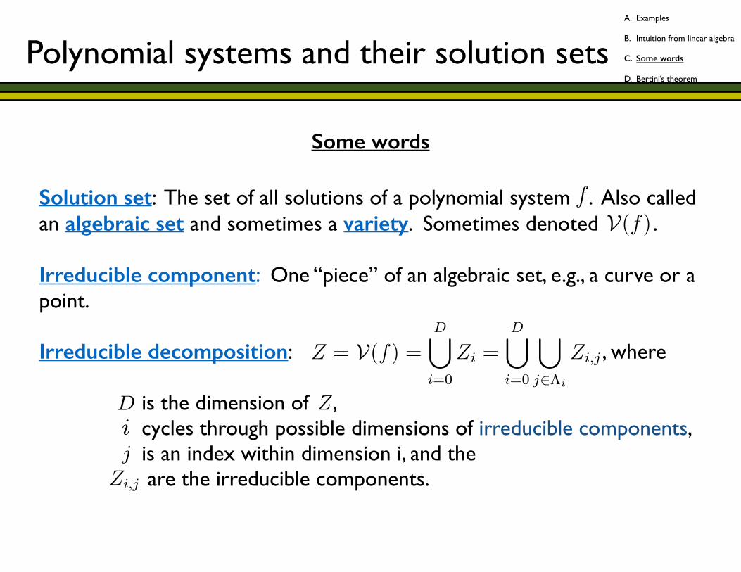
Solution set: The set of all solutions of a polynomial system . Also called an algebraic set and sometimes a variety. Sometimes denoted . !Irreducible component: One “piece” of an algebraic set, e.g., a curve or a point. !Irreducible decomposition: , where ! is the dimension of , cycles through possible dimensions of irreducible components, is an index within dimension i, and the are the irreducible components.
f : CN ! CN
f1, . . . , fn 2 C[z1, . . . , zN ]
bz 2 CN
fi(bz) = 0 8i
f = (f1, . . . , fn)
R
N = n
N 6= n
⇡
Z = V(f) =D[
i=0
Zi =D[
i=0
[
j2⇤i
Zi,j
1
f : CN ! CN
f1, . . . , fn 2 C[z1, . . . , zN ]
bz 2 CN
fi(bz) = 0 8i
f = (f1, . . . , fn)
R
N = n
N 6= n
⇡
Z = V(f) =D[
i=0
Zi =D[
i=0
[
j2⇤i
Zi,j
1
f : CN ! CN
f1, . . . , fn 2 C[z1, . . . , zN ]
bz 2 CN
fi(bz) = 0 8i
f = (f1, . . . , fn)
R
N = n
N 6= n
⇡
Z = V(f) =D[
i=0
Zi =D[
i=0
[
j2⇤i
Zi,j
1
f : CN ! CN
f1, . . . , fn 2 C[z1, . . . , zN ]
bz 2 CN
fi(bz) = 0 8i
f = (f1, . . . , fn)
R
N = n
N 6= n
⇡
Z = V(f) =D[
i=0
Zi =D[
i=0
[
j2⇤i
Zi,j
1
f : CN ! CN
f1, . . . , fn 2 C[z1, . . . , zN ]
bz 2 CN
fi(bz) = 0 8i
f = (f1, . . . , fn)
R
N = n
N 6= n
⇡
Z = V(f) =D[
i=0
Zi =D[
i=0
[
j2⇤i
Zi,j
1
f : CN ! CN
f1, . . . , fn 2 C[z1, . . . , zN ]
bz 2 CN
fi(bz) = 0 8i
f = (f1, . . . , fn)
R
N = n
N 6= n
⇡
Z = V(f) =D[
i=0
Zi =D[
i=0
[
j2⇤i
Zi,j
1
x4 � 1 = 0
x = ±i
y 2 C
h(x, y) =
x2 + y2 � 1
x2 + (y + c)2 � 1
�
c = 1
c = 2
c = 3
V(f)
5
x4 � 1 = 0
x = ±i
y 2 C
h(x, y) =
x2 + y2 � 1
x2 + (y + c)2 � 1
�
c = 1
c = 2
c = 3
f
5
Polynomial systems and their solution setsA. Examples
B. Intuition from linear algebra
C. Some words
D. Bertini’s theorem
Example 8: !!!!Solutions: ! Dimension 2: One surface Dimension 1: Three lines and one cubic curve Dimension 0: One point
“main”2013/3/17page 159
✐
✐
✐
✐
✐
✐
✐
✐
DRAFT
Chapter 8
Positive-DimensionalComponents
In Part II of the book, we return to the fundamental problem of “solving” a poly-nomial system,
f(z) :=
⎡
⎢⎣f1(z1, . . . , zN)
...fn(z1, . . . , zN)
⎤
⎥⎦ = 0. (8.1)
As opposed to the case of systems of linear equations, where a nonempty so-lution set will consist of exactly one linear space, the solution set of a polynomialsystem can have several separate components and these may have different dimen-sions23 (points, curves, surfaces, etc). Thus, the problem of “solving” a polynomialsystem includes the detection of all such components no matter what dimensioneach has. Solution components of dimension greater than zero (everything exceptisolated points) are said to be “positive-dimensional.”
For example, consider the following system of three polynomials in the vari-ables x, y, z:
f =
⎡
⎣(y − x2)(x2 + y2 + z2 − 1)(x− 2)(z − x3)(x2 + y2 + z2 − 1)(y − 2)
(z − x3)(y − x2)(x2 + y2 + z2 − 1)(z − 2)
⎤
⎦ . (8.2)
The solution set of three linear equations in three variables must be one point, oneline, or one plane. The complex solution set of (8.2) consists of a surface, fourcurves, and a point. If we were to apply one of the homotopies presented in Part Ito solve this system, we would be assured to find the isolated solution, (2, 2, 2), butthere would be no guarantee of finding any points on the other components.
In brief, Part II presents how numerical algebraic geometry treats full solutionsets, including their positive-dimensional components. This chapter introduces thebasic concepts and shows results obtained with Bertini on some simple examples.The next two chapters, Chapter 9 and Chapter 10, which go into details of the
23We gave a definition of the dimension of a component in §1.2.2.
159
x4 � 1 = 0
x = ±i
y 2 C
h(x, y) =
x2 + y2 � 1
x2 + (y + c)2 � 1
�
c = 1
c = 2
c = 3
f
Z = Z0,0 [ Z1,0 [ Z1,1 [ Z1,2 [ Z1,3 [ Z2,0
5
Polynomial systems and their solution setsA. Examples
B. Intuition from linear algebra
C. Some words
D. Bertini’s theorem
Some more words
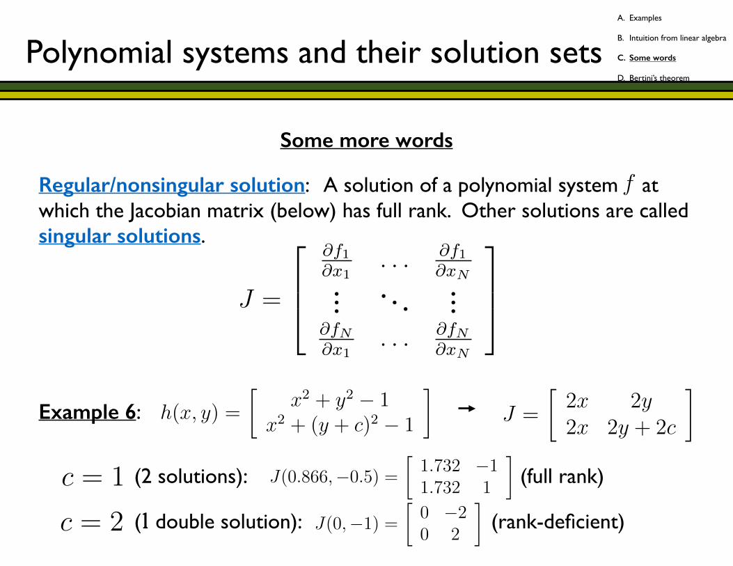
Regular/nonsingular solution: A solution of a polynomial system at which the Jacobian matrix (below) has full rank. Other solutions are called singular solutions. !!
x4 � 1 = 0
x = ±i
y 2 C
h(x, y) =
x2 + y2 � 1
x2 + (y + c)2 � 1
�
c = 1
c = 2
c = 3
f
5
(1, 1), (�1,�1), (2,�1), (�2, 1)
f(x, y) =
f1 + f2 + f3f1 + 2f2 + f3
�
J =
2
64
@f1
@x1. . . @f1
@x
N
.
.
.
.
.
.
.
.
.
@f
N
@x1. . . @f
N
@x
N
3
75
6
Example 6: !! (2 solutions): (full rank) ! (1 double solution): (rank-deficient)
x4 � 1 = 0
x = ±i
y 2 C
h(x, y) =
x2 + y2 � 1
x2 + (y + c)2 � 1
�
c = 1
c = 2
c = 3
5
f
Z = Z0,0 [ Z1,0 [ Z1,1 [ Z1,2 [ Z1,3 [ Z2,0
(1, 1), (�1,�1), (2,�1), (�2, 1)
f(x, y) =
f1 + f2 + f3f1 + 2f2 + f3
�
J =
2
64
@f1
@x1. . . @f1
@x
N
.
.
.
.
.
.
.
.
.
@f
N
@x1. . . @f
N
@x
N
3
75
(±i,±2i) 2 C2
i
L
J =
2x 2y2x 2y + 2c
�
6
x4 � 1 = 0
x = ±i
y 2 C
h(x, y) =
x2 + y2 � 1
x2 + (y + c)2 � 1
�
c = 1
c = 2
c = 3
5
x4 � 1 = 0
x = ±i
y 2 C
h(x, y) =
x2 + y2 � 1
x2 + (y + c)2 � 1
�
c = 1
c = 2
c = 3
5
f
Z = Z0,0 [ Z1,0 [ Z1,1 [ Z1,2 [ Z1,3 [ Z2,0
(1, 1), (�1,�1), (2,�1), (�2, 1)
f(x, y) =
f1 + f2 + f3f1 + 2f2 + f3
�
J =
2
64
@f1
@x1. . . @f1
@x
N
.
.
.
.
.
.
.
.
.
@f
N
@x1. . . @f
N
@x
N
3
75
(±i,±2i) 2 C2
i
L
J =
2x 2y2x 2y + 2c
�
J(0.866,�0.5) =
1.732 �11.732 1
�
6
f
Z = Z0,0 [ Z1,0 [ Z1,1 [ Z1,2 [ Z1,3 [ Z2,0
(1, 1), (�1,�1), (2,�1), (�2, 1)
f(x, y) =
f1 + f2 + f3f1 + 2f2 + f3
�
J =
2
64
@f1
@x1. . . @f1
@x
N
.
.
.
.
.
.
.
.
.
@f
N
@x1. . . @f
N
@x
N
3
75
(±i,±2i) 2 C2
i
L
J =
2x 2y2x 2y + 2c
�
J(0,�1) =
0 �20 2
�
6
Polynomial systems and their solution setsA. Examples
B. Intuition from linear algebra
C. Some words
D. Bertini’s theorem
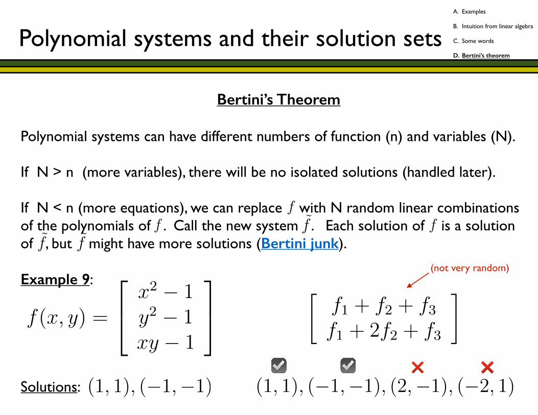
Bertini’s Theorem
Polynomial systems can have different numbers of function (n) and variables (N). !If N > n (more variables), there will be no isolated solutions (handled later). !If N < n (more equations), we can replace with N random linear combinations of the polynomials of . Call the new system . Each solution of is a solution of , but might have more solutions (Bertini junk). !Example 9: !!!!!Solutions:
N = n
N 6= n
⇡
Z = V(f) =D[
i=0
Zi =D[
i=0
[
j2⇤i
Zi,j
f =
x(x� 1)x(y � 1)
�
x = 0
x = y = 1
z
||z � bz|| < FinalTol
N > n
2
N = n
N 6= n
⇡
Z = V(f) =D[
i=0
Zi =D[
i=0
[
j2⇤i
Zi,j
f =
x(x� 1)x(y � 1)
�
x = 0
x = y = 1
z
||z � bz|| < FinalTol
N > n
2
x4 � 1 = 0
x = ±i
y 2 C
h(x, y) =
x2 + y2 � 1
x2 + (y + c)2 � 1
�
c = 1
c = 2
c = 3
f
Z = Z0,0 [ Z1,0 [ Z1,1 [ Z1,2 [ Z1,3 [ Z2,0
5
N = n
N 6= n
⇡
Z = V(f) =D[
i=0
Zi =D[
i=0
[
j2⇤i
Zi,j
f =
x(x� 1)x(y � 1)
�
x = 0
x = y = 1
z
||z � bz|| < FinalTol
N > n
2
x4 � 1 = 0
x = ±i
y 2 C
h(x, y) =
x2 + y2 � 1
x2 + (y + c)2 � 1
�
c = 1
c = 2
c = 3
f
Z = Z0,0 [ Z1,0 [ Z1,1 [ Z1,2 [ Z1,3 [ Z2,0
5
x4 � 1 = 0
x = ±i
y 2 C
h(x, y) =
x2 + y2 � 1
x2 + (y + c)2 � 1
�
c = 1
c = 2
c = 3
f
Z = Z0,0 [ Z1,0 [ Z1,1 [ Z1,2 [ Z1,3 [ Z2,0
5
x4 � 1 = 0
x = ±i
y 2 C
h(x, y) =
x2 + y2 � 1
x2 + (y + c)2 � 1
�
f(x, y) =
2
4x2 � 1y2 � 1xy � 1
3
5
c = 1
c = 2
c = 3
f
Z = Z0,0 [ Z1,0 [ Z1,1 [ Z1,2 [ Z1,3 [ Z2,0
5
(1, 1), (�1,�1)
6
(1, 1), (�1,�1)
f(x, y) =
f1 + f2 + f3f1 + 2f2 + f3
�
6
(1, 1), (�1,�1), (2,�1), (�2, 1)
f(x, y) =
f1 + f2 + f3f1 + 2f2 + f3
�
6
❌ ❌☑ ☑
(not very random)
Polynomial systems and their solution setsA. Examples
B. Intuition from linear algebra
C. Some words
D. Bertini’s theorem
1. Polynomial systems and their solution sets
2. Finding isolated solutions (homotopy continuation)
3. Advanced topics for isolated solutions
4. Finding positive-dimensional solution sets (briefly)
Game plan
!
2. Finding isolated solutions (homotopy continuation)
A. Homotopy continuation in a nutshell
B. Start systems
C. Bells & whistles
D. Endgames
E. Bertini Classic (1.x)
!
Game plan
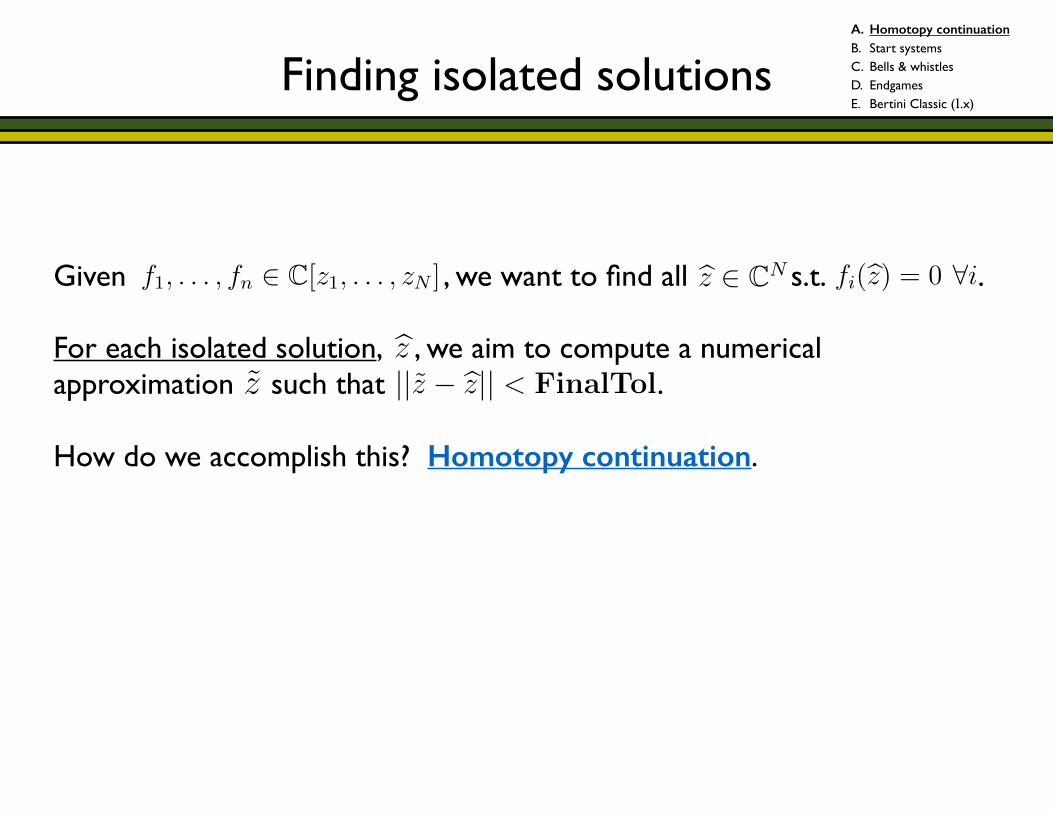
Finding isolated solutions
!!Given , we want to find all s.t. . !For each isolated solution, , we aim to compute a numerical approximation such that . !How do we accomplish this? Homotopy continuation.
f : CN ! CN
f1, . . . , fn 2 C[z1, . . . , zN ]
1
f : CN ! CN
f1, . . . , fn 2 C[z1, . . . , zN ]
bz 2 CN
fi(bz) = 0 8i
1
f : CN ! CN
f1, . . . , fn 2 C[z1, . . . , zN ]
bz 2 CN
fi(bz) = 0 8i
1
f : CN ! CN
f1, . . . , fn 2 C[z1, . . . , zN ]
bz 2 CN
fi(bz) = 0 8i
f = (f1, . . . , fn)
R
N = n
N 6= n
⇡
Z = V(f) =D[
i=0
Zi =D[
i=0
[
j2⇤i
Zi,j
1
f =
x(x� 1)x(y � 1)
�
x = 0
x = y = 1
z
2
f =
x(x� 1)x(y � 1)
�
x = 0
x = y = 1
z
||z � bz|| < FinalTol
2
A. Homotopy continuation B. Start systems C. Bells & whistles D. Endgames E. Bertini Classic (1.x)
Finding isolated solutions
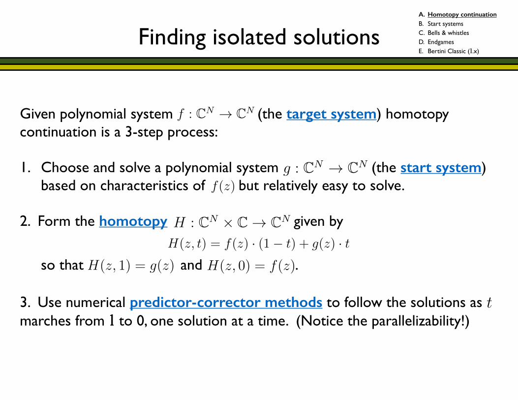
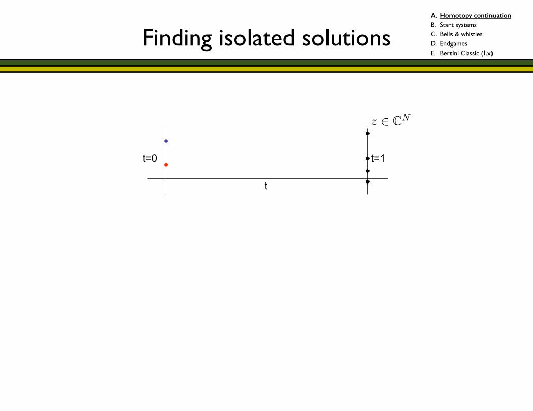
Given polynomial system (the target system) homotopy continuation is a 3-step process: !1. Choose and solve a polynomial system (the start system)
based on characteristics of but relatively easy to solve. !2. Form the homotopy given by !! so that and . !3. Use numerical predictor-corrector methods to follow the solutions as marches from 1 to 0, one solution at a time. (Notice the parallelizability!) !!
f : CN ! CN
1
f : CN ! CN
g : CN ! CN
f1, . . . , fn 2 C[z1, . . . , zN ]
bz 2 CN
fi(bz) = 0 8i
f = (f1, . . . , fn)
R
N = n
N 6= n
⇡
1
f : CN ! CN
g : CN ! CN
H : CN ⇥ C ! CN
f1, . . . , fn 2 C[z1, . . . , zN ]
bz 2 CN
fi(bz) = 0 8i
f = (f1, . . . , fn)
R
N = n
N 6= n
⇡
1
f : CN ! CN
g : CN ! CN
H : CN ⇥ C ! CN
H(z, t) = f(z) · (1� t) + g(z) · t
H(z, 1) = g(z)
H(z, 0) = f(z)
f1, . . . , fn 2 C[z1, . . . , zN ]
bz 2 CN
fi(bz) = 0 8i
f = (f1, . . . , fn)
R
1
f : CN ! CN
g : CN ! CN
H : CN ⇥ C ! CN
H(z, t) = f(z) · (1� t) + g(z) · t
H(z, 1) = g(z)
H(z, 0) = f(z)
f1, . . . , fn 2 C[z1, . . . , zN ]
bz 2 CN
fi(bz) = 0 8i
f = (f1, . . . , fn)
R
1
f : CN ! CN
g : CN ! CN
H : CN ⇥ C ! CN
H(z, t) = f(z) · (1� t) + g(z) · t
H(z, 1) = g(z)
H(z, 0) = f(z)
f1, . . . , fn 2 C[z1, . . . , zN ]
bz 2 CN
fi(bz) = 0 8i
f = (f1, . . . , fn)
R
1
f : CN ! CN
g : CN ! CN
H : CN ⇥ C ! CN
H(z, t) = f(z) · (1� t) + g(z) · t
H(z, 1) = g(z)
H(z, 0) = f(z)
f1, . . . , fn 2 C[z1, . . . , zN ]
bz 2 CN
fi(bz) = 0 8i
f = (f1, . . . , fn)
R
1
f : CN ! CN
g : CN ! CN
H : CN ⇥ C ! CN
H(z, t) = f(z) · (1� t) + g(z) · t
H(z, 1) = g(z)
H(z, 0) = f(z)
f1, . . . , fn 2 C[z1, . . . , zN ]
bz 2 CN
fi(bz) = 0 8i
f = (f1, . . . , fn)
R
1
A. Homotopy continuation B. Start systems C. Bells & whistles D. Endgames E. Bertini Classic (1.x)
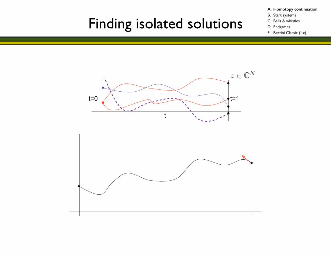
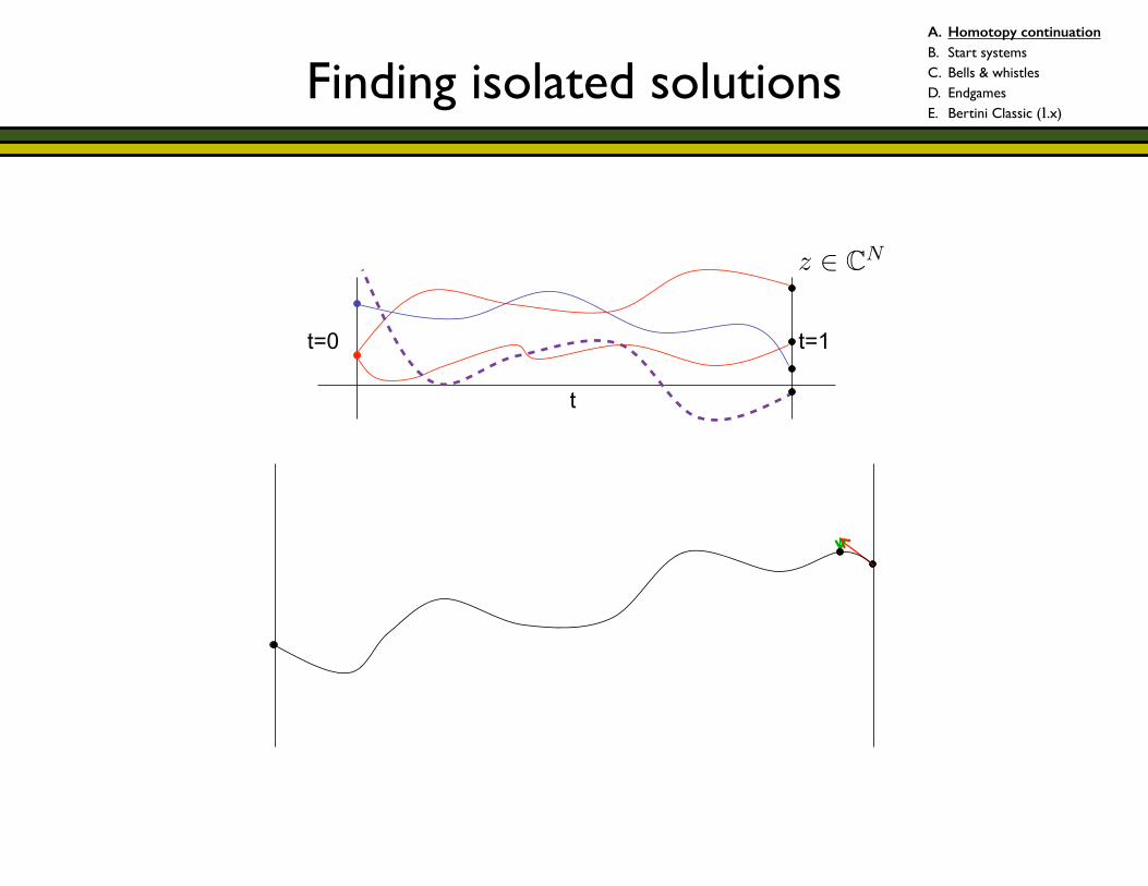
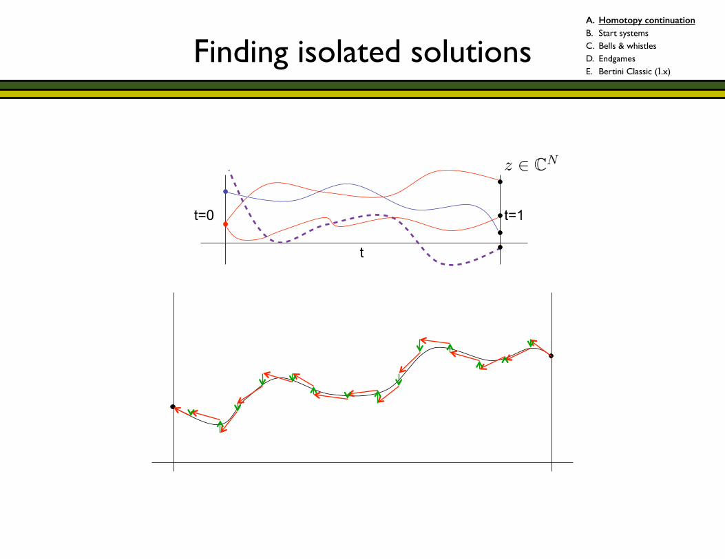
Finding isolated solutions
t
t=0 t=1
t 2 C
z 2 CN
1
A. Homotopy continuation B. Start systems C. Bells & whistles D. Endgames E. Bertini Classic (1.x)
Finding isolated solutions
t
t=0 t=1
t 2 C
z 2 CN
1
A. Homotopy continuation B. Start systems C. Bells & whistles D. Endgames E. Bertini Classic (1.x)
t=1
t=0.75
t=0.5
t=0.25t=0
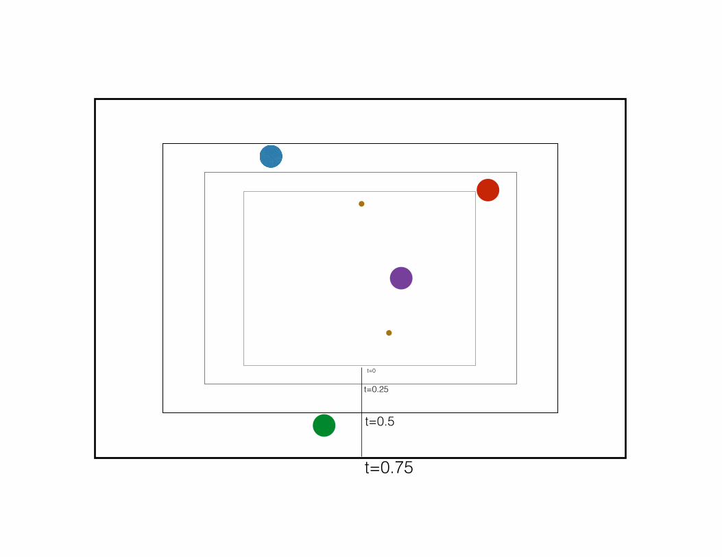
t=0.75
t=0.5
t=0.25
t=0
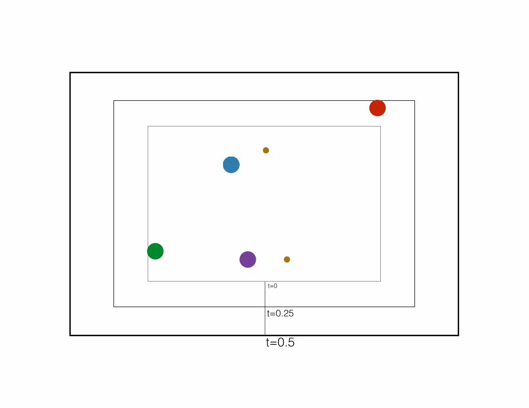
t=0.5
t=0.25
t=0
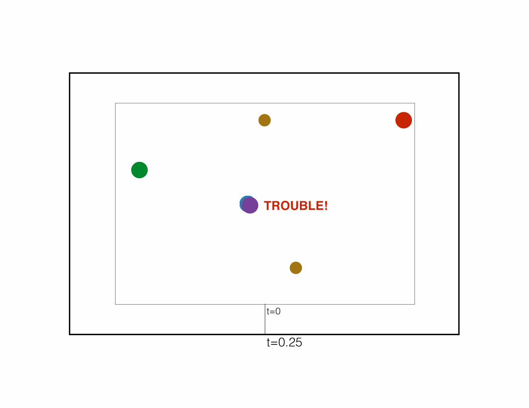
t=0.25
t=0
TROUBLE!
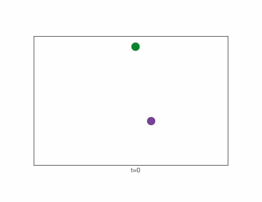
t=0
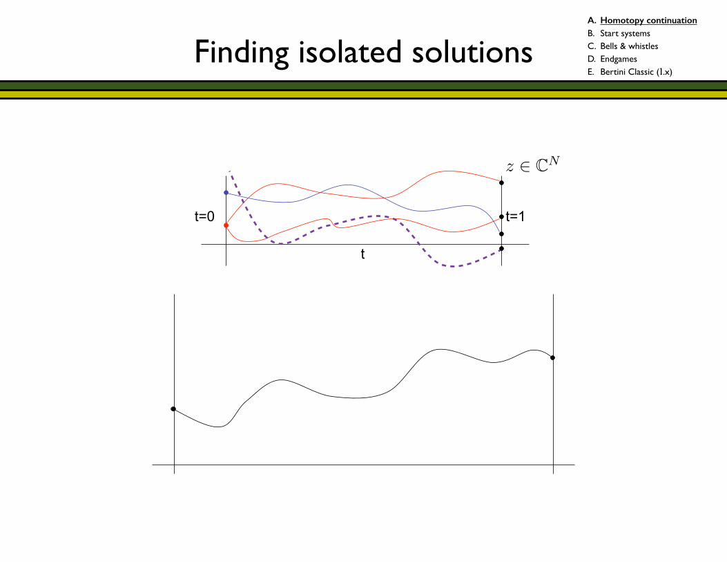
Finding isolated solutions
t
t=0 t=1
t 2 C
z 2 CN
1
A. Homotopy continuation B. Start systems C. Bells & whistles D. Endgames E. Bertini Classic (1.x)
Finding isolated solutions
t
t=0 t=1
t 2 C
z 2 CN
1
A. Homotopy continuation B. Start systems C. Bells & whistles D. Endgames E. Bertini Classic (1.x)
Finding isolated solutions
t
t=0 t=1
t 2 C
z 2 CN
1
A. Homotopy continuation B. Start systems C. Bells & whistles D. Endgames E. Bertini Classic (1.x)
Finding isolated solutions
t
t=0 t=1
t 2 C
z 2 CN
1
A. Homotopy continuation B. Start systems C. Bells & whistles D. Endgames E. Bertini Classic (1.x)
Finding isolated solutions
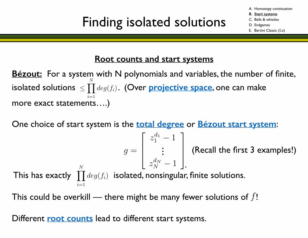
Bézout: For a system with N polynomials and variables, the number of finite, !isolated solutions . (Over projective space, one can make !more exact statements….) !One choice of start system is the total degree or Bézout start system:
! (Recall the first 3 examples!) ! . This has exactly isolated, nonsingular, finite solutions. !This could be overkill — there might be many fewer solutions of ! !Different root counts lead to different start systems.
N > n
N < n
PN
SecurityMaxNorm
⇧Ni=1 deg(fi)
di = deg(fi)
g =
2
64zd11 � 1
.
.
.
zdNN � 1
3
75
3
Root counts and start systems
NY
i=1
deg(fi
)
di
= deg(fi
)
g =
2
64zd11 � 1
.
.
.
zdNN
� 1
3
75
f(x, y) =
xy � 1x2 � 1
�
A 2 CN⇥N
A = U⌃V ⇤
(A) = s
max
s
min
Ax = b
ACC ⇡ PREC� log10((A))
K : CN ! Cd
4
NY
i=1
deg(fi
)
di
= deg(fi
)
g =
2
64zd11 � 1
.
.
.
zdNN
� 1
3
75
f(x, y) =
xy � 1x2 � 1
�
A 2 CN⇥N
A = U⌃V ⇤
(A) = s
max
s
min
Ax = b
ACC ⇡ PREC� log10((A))
K : CN ! Cd
4
f : CN ! CN
g : CN ! CN
H : CN ⇥ C ! CN
H(z, t) = f(z) · (1� t) + �g(z) · t
� 2 C
H(z, 1) = g(z)
H(z, 0) = f(z)
f1, . . . , fN 2 C[z1, . . . , zN ]
q1, . . . qM 2 Ck
M >> 0
z 2 CN
1
A. Homotopy continuation B. Start systems C. Bells & whistles D. Endgames E. Bertini Classic (1.x)
Finding isolated solutions
Root counts and start systems
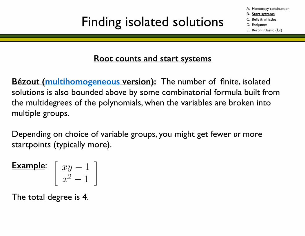
Bézout (multihomogeneous version): The number of finite, isolated solutions is also bounded above by some combinatorial formula built from the multidegrees of the polynomials, when the variables are broken into multiple groups. !Depending on choice of variable groups, you might get fewer or more startpoints (typically more). !Example: !!The total degree is 4.
N > n
N < n
PN
SecurityMaxNorm
⇧Ni=1 deg(fi)
di = deg(fi)
g =
2
64zd11 � 1
.
.
.
zdNN � 1
3
75
g =
xy � 1x2 � 1
�
3
A. Homotopy continuation B. Start systems C. Bells & whistles D. Endgames E. Bertini Classic (1.x)
Finding isolated solutions
Root counts and start systems
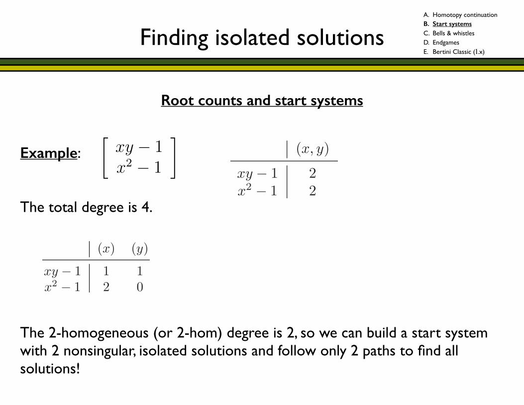
Example: !!The total degree is 4. !!!!!!The 2-homogeneous (or 2-hom) degree is 2, so we can build a start system with 2 nonsingular, isolated solutions and follow only 2 paths to find all solutions!
N > n
N < n
PN
SecurityMaxNorm
⇧Ni=1 deg(fi)
di = deg(fi)
g =
2
64zd11 � 1
.
.
.
zdNN � 1
3
75
g =
xy � 1x2 � 1
�
3
“main”2013/3/17page 81
✐
✐
✐
✐
✐
✐
✐
✐
DRAFT
5.1. Multihomogeneous homotopy 81
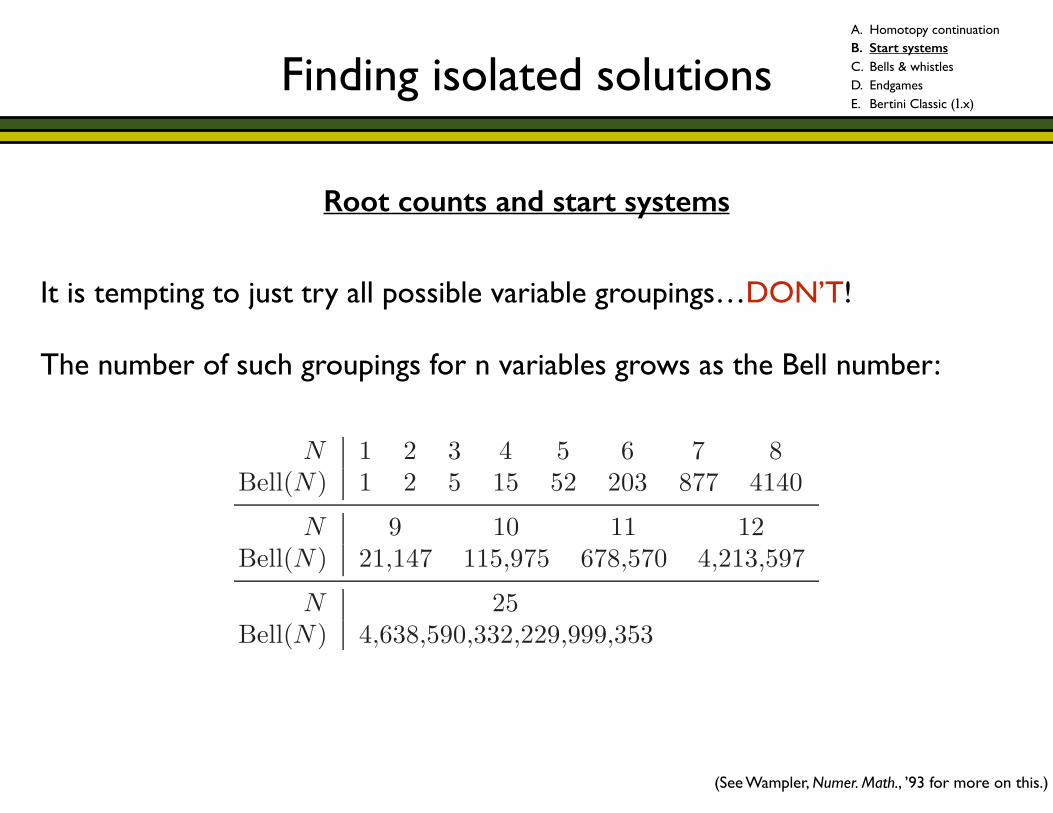
N 1 2 3 4 5 6 7 8Bell(N) 1 2 5 15 52 203 877 4140
N 9 10 11 12Bell(N) 21,147 115,975 678,570 4,213,597
N 25Bell(N) 4,638,590,332,229,999,353
Table 5.1. Illustration of the growth of Bell(N) as N grows.
example, the cubic x2z+xyz+1 is quadratic in (x, y) and linear in z, so a partitionof the variables as {(x, y), (z)} could be advantageous. If all three polynomials ina system of three polynomials in C[x, y, z] had this same degree structure, then itwould certainly be an advantage to partition the variables in this manner. Thesituation becomes more complicated when a subdivision reduces degrees in somepolynomials of the system but increases them in others.
5.1.1 Multihomogeneous Bezout number
The number of paths in a multihomogeneous homotopy, also called the multiho-mogeneous Bezout number17 of the system, is closely tied to multihomogeneousprojective spaces already mentioned in §4.5. To decide which grouping of the vari-ables to use, one may easily compute the multihomogeneous Bezout number of eachgrouping under consideration, and pick the smallest one. As already mentioned, thetotal number of possible groupings grows quickly with the number of variables, soBertini does not automate an exhaustive search. But with a little practice, a usercan identify and check the most promising candidates.
Instead of introducing a detailed notation for expressing the multihomoge-neous Bezout number, let us demonstrate the idea through examples. Let’s startwith the system
xy − 1 = 0, x2 − 1 = 0. (5.1)
There are two possible groupings, {(x, y)} and {(x), (y)}, each with its own Bezoutnumber. For each grouping, we make a multidegree table with one column pergroup and one row per equation, as follows. For the grouping {(x, y)}, the table is:
(x, y)
xy − 1 2x2 − 1 2
17For brevity, we may sometimes call this variously the ‘Bezout number’, the ‘Bezout count’, oreven simply the ‘root count’.
“main”2013/3/17page 82
✐
✐
✐
✐
✐
✐
✐
✐
DRAFT
82 Chapter 5. Types of Homotopies
since both equations have degree 2, while for {(x), (y)}, we have:
(x) (y)
xy − 1 1 1x2 − 1 2 0
indicating the degrees of the polynomials with respect to each variable group. Inthe latter case, we may say the polynomial xy − 1 has multidegree (1, 1), or moresimply, the polynomial is type (1, 1), while x2 − 1 is type (2, 0).
The rules for computing the Bezout number for a given degree table are asfollows. As a preparatory step, replace the variable groups with the dimension ofthe subspace they live in. That is, (x, y) ∈ C2, so the first table becomes
2
xy − 1 2x2 − 1 2
while since x ∈ C and y ∈ C, the second one becomes
1 1
xy − 1 1 1x2 − 1 2 0
Before evaluating the multihomogeneous Bezout count for these and otherexamples, let us describe the general methodology. First, lay out the multidegreetable for an m-homogeneous system as:
k1 · · · km
f1 d1,1 · · · d1,m...
......
fN dN,1 · · · dN,m
So kj is the dimension of the jth group of variables (Ckj or Pkj , as appropriate), anddi,j is the degree of the ith polynomial, fi, with respect to the jth variable group.With this notation, the rules for evaluating the m-homogeneous Bezout count are:
1. find all ways of choosing N of the di,j such that there is one chosen in eachrow and kj chosen in each column j;
2. for each such choice, multiply the chosen degrees; and
3. sum these products over all the choices.
Let us return to the example above. In the 1-homogeneous case of {(x, y)},there is only one combination of the multidegrees that is possible, so the Bezout
A. Homotopy continuation B. Start systems C. Bells & whistles D. Endgames E. Bertini Classic (1.x)
Finding isolated solutions
Root counts and start systems
It is tempting to just try all possible variable groupings…DON’T! !The number of such groupings for n variables grows as the Bell number: !
“main”2013/3/17page 81
✐
✐
✐
✐
✐
✐
✐
✐
DRAFT
5.1. Multihomogeneous homotopy 81
N 1 2 3 4 5 6 7 8Bell(N) 1 2 5 15 52 203 877 4140
N 9 10 11 12Bell(N) 21,147 115,975 678,570 4,213,597
N 25Bell(N) 4,638,590,332,229,999,353
Table 5.1. Illustration of the growth of Bell(N) as N grows.
example, the cubic x2z+xyz+1 is quadratic in (x, y) and linear in z, so a partitionof the variables as {(x, y), (z)} could be advantageous. If all three polynomials ina system of three polynomials in C[x, y, z] had this same degree structure, then itwould certainly be an advantage to partition the variables in this manner. Thesituation becomes more complicated when a subdivision reduces degrees in somepolynomials of the system but increases them in others.
5.1.1 Multihomogeneous Bezout number
The number of paths in a multihomogeneous homotopy, also called the multiho-mogeneous Bezout number17 of the system, is closely tied to multihomogeneousprojective spaces already mentioned in §4.5. To decide which grouping of the vari-ables to use, one may easily compute the multihomogeneous Bezout number of eachgrouping under consideration, and pick the smallest one. As already mentioned, thetotal number of possible groupings grows quickly with the number of variables, soBertini does not automate an exhaustive search. But with a little practice, a usercan identify and check the most promising candidates.
Instead of introducing a detailed notation for expressing the multihomoge-neous Bezout number, let us demonstrate the idea through examples. Let’s startwith the system
xy − 1 = 0, x2 − 1 = 0. (5.1)
There are two possible groupings, {(x, y)} and {(x), (y)}, each with its own Bezoutnumber. For each grouping, we make a multidegree table with one column pergroup and one row per equation, as follows. For the grouping {(x, y)}, the table is:
(x, y)
xy − 1 2x2 − 1 2
17For brevity, we may sometimes call this variously the ‘Bezout number’, the ‘Bezout count’, oreven simply the ‘root count’.
(See Wampler, Numer. Math., ’93 for more on this.)
A. Homotopy continuation B. Start systems C. Bells & whistles D. Endgames E. Bertini Classic (1.x)
Finding isolated solutions
Root counts and start systems
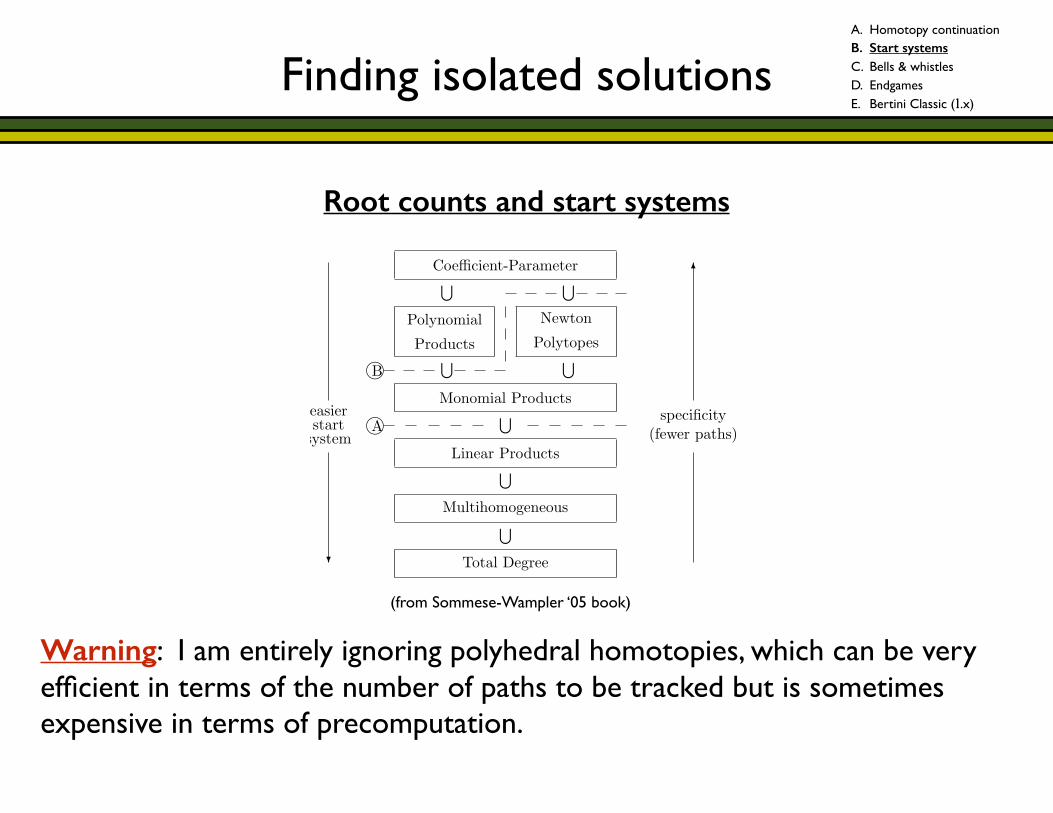
Warning: I am entirely ignoring polyhedral homotopies, which can be very efficient in terms of the number of paths to be tracked but is sometimes expensive in terms of precomputation.
December 29, 2004 11:35 WSPC/Book Trim Size for 9.75in x 6.5in main975x65
118 Numerical Solution of Systems of Polynomials Arising in Engineering and Science
8.1 A Hierarchy of Structures
Coefficient-Parameter
Polynomial
Products
Newton
Polytopes
Monomial Products
Linear Products
Multihomogeneous
Total Degree
!
!
!
!
!
!
!
easierstartsystem
❄
specificity(fewer paths)
✻
❥A❥B
Fig. 8.1 Classes of Product Structures. Below line A, start systems can be solved using onlyroutines for solving linear systems of equations. Above line B, special methods must be designedcase-by-case.
Figure 8.1 shows a hierarchy of classes of special structures that are useful inconstructing homotopies. Each structure in the diagram is a member of the classabove it; for example, a total degree structure is a particular kind of multihomo-geneous structure. (In particular, as we will shortly see, it is a one-homogeneousstructure.) As we ascend the hierarchy, each class of structures presents more andmore possibilities for matching a particular target system that we wish to solve. Asindicated on the right of the diagram, this means that we can select a more specialstructure, usually with the aim of reducing the number of solution paths to trackin the homotopy. The trade-off we face in this ascent is indicated by the downwardpointing arrow on the left of the diagram: the lower structures allow us to selectstart systems that are easier to solve. For some problems, the ascent up the dia-gram pays handsomely in path reduction and may turn an intractable problem intoa solvable one. On the other hand, it can happen that solving a start system for ahigher structure can consume more computer time than is saved in path reduction.Unfortunately, even just counting the number of roots of the start system can beexpensive, so it is a matter of experience to decide the most advantageous spot inthis hierarchy to solve a particular problem.
Two dashed lines appear in Figure 8.1 to demarcate significant differences in thestart systems of homotopies respecting the various special structures. Below Line A,
(from Sommese-Wampler ‘05 book)
A. Homotopy continuation B. Start systems C. Bells & whistles D. Endgames E. Bertini Classic (1.x)
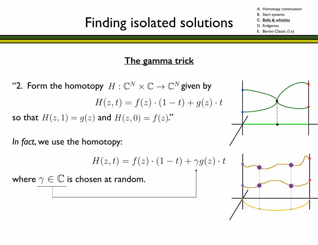
Finding isolated solutions!!
!!!!“2. Form the homotopy given by !!!so that and .” !!!!!
f : CN ! CN
g : CN ! CN
H : CN ⇥ C ! CN
f1, . . . , fn 2 C[z1, . . . , zN ]
bz 2 CN
fi(bz) = 0 8i
f = (f1, . . . , fn)
R
N = n
N 6= n
⇡
1
f : CN ! CN
g : CN ! CN
H : CN ⇥ C ! CN
H(z, t) = f(z) · (1� t) + g(z) · t
H(z, 1) = g(z)
H(z, 0) = f(z)
f1, . . . , fn 2 C[z1, . . . , zN ]
bz 2 CN
fi(bz) = 0 8i
f = (f1, . . . , fn)
R
1
f : CN ! CN
g : CN ! CN
H : CN ⇥ C ! CN
H(z, t) = f(z) · (1� t) + g(z) · t
H(z, 1) = g(z)
H(z, 0) = f(z)
f1, . . . , fn 2 C[z1, . . . , zN ]
bz 2 CN
fi(bz) = 0 8i
f = (f1, . . . , fn)
R
1
f : CN ! CN
g : CN ! CN
H : CN ⇥ C ! CN
H(z, t) = f(z) · (1� t) + g(z) · t
H(z, 1) = g(z)
H(z, 0) = f(z)
f1, . . . , fn 2 C[z1, . . . , zN ]
bz 2 CN
fi(bz) = 0 8i
f = (f1, . . . , fn)
R
1
!In fact, we use the homotopy: !!!where is chosen at random. !!!
f : CN ! CN
g : CN ! CN
H : CN ⇥ C ! CN
H(z, t) = f(z) · (1� t) + �g(z) · t
� 2 C
H(z, 1) = g(z)
H(z, 0) = f(z)
f1, . . . , fn 2 C[z1, . . . , zN ]
bz 2 CN
fi(bz) = 0 8i
f = (f1, . . . , fn)
1
f : CN ! CN
g : CN ! CN
H : CN ⇥ C ! CN
H(z, t) = f(z) · (1� t) + �g(z) · t
� 2 C
H(z, 1) = g(z)
H(z, 0) = f(z)
f1, . . . , fn 2 C[z1, . . . , zN ]
bz 2 CN
fi(bz) = 0 8i
f = (f1, . . . , fn)
1
The gamma trick
A. Homotopy continuation B. Start systems C. Bells & whistles D. Endgames E. Bertini Classic (1.x)
Finding isolated solutions
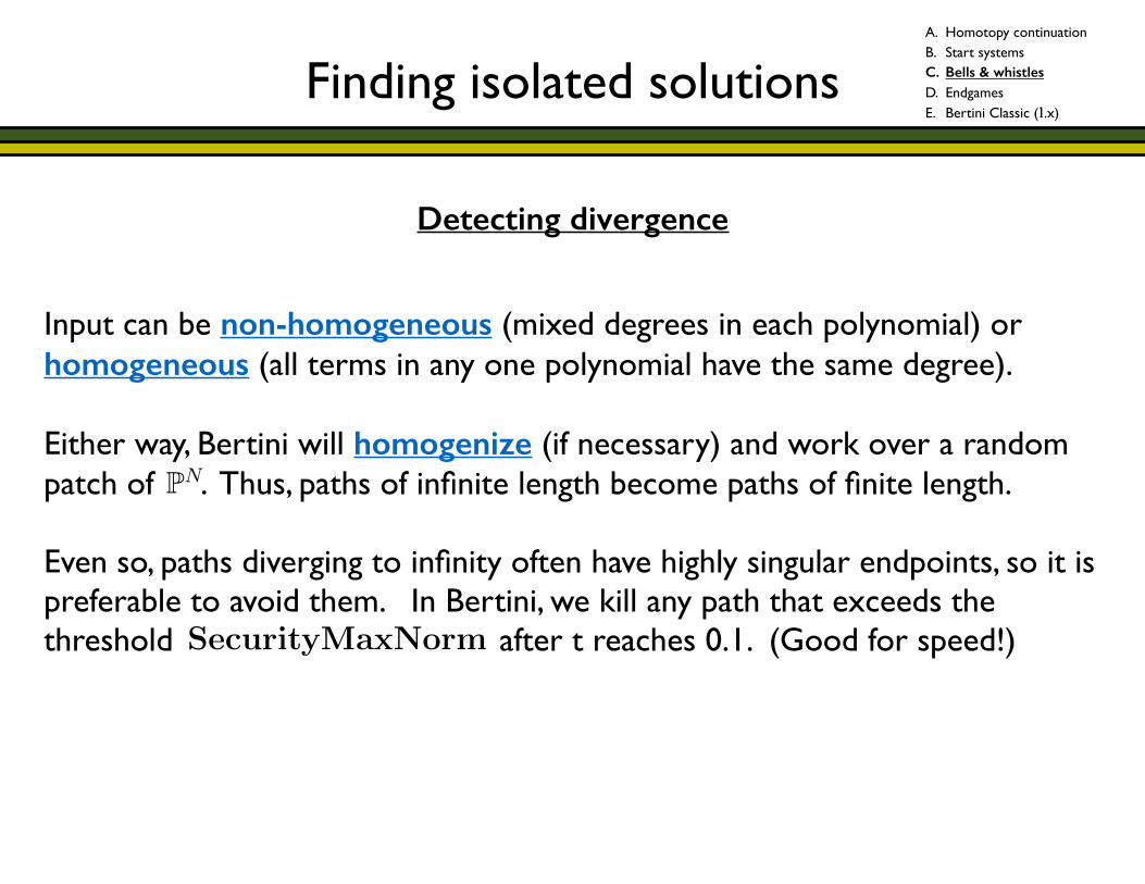
Detecting divergence!!Input can be non-homogeneous (mixed degrees in each polynomial) or homogeneous (all terms in any one polynomial have the same degree). !Either way, Bertini will homogenize (if necessary) and work over a random patch of . Thus, paths of infinite length become paths of finite length. !Even so, paths diverging to infinity often have highly singular endpoints, so it is preferable to avoid them. In Bertini, we kill any path that exceeds the threshold after t reaches 0.1. (Good for speed!)
N > n
N < n
PN
3
N > n
N < n
PN
SecurityMaxNorm
3
A. Homotopy continuation B. Start systems C. Bells & whistles D. Endgames E. Bertini Classic (1.x)
Finding isolated solutions
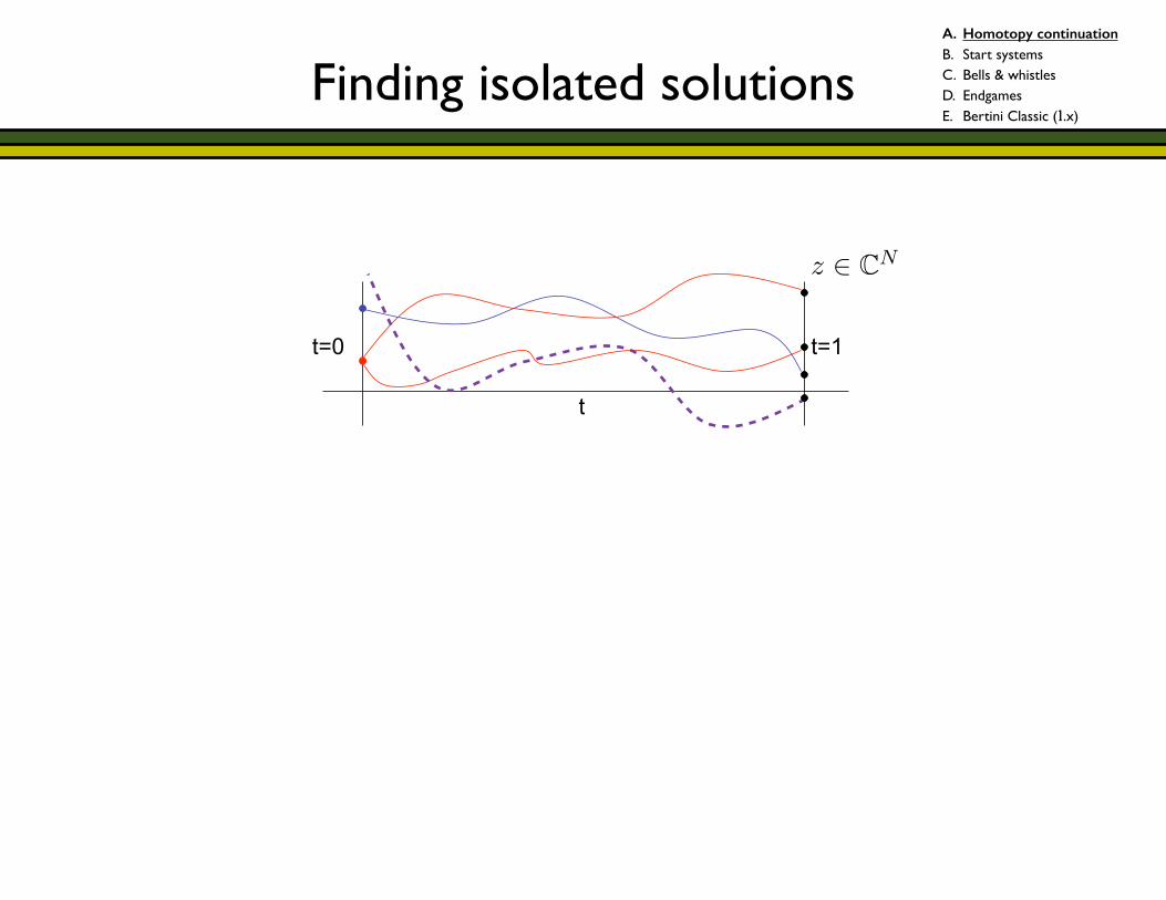
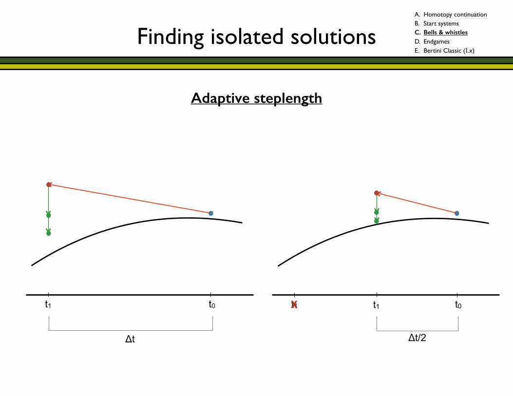
Adaptive steplength
t0t1 t0t1 t1X
Δt Δt/2
A. Homotopy continuation B. Start systems C. Bells & whistles D. Endgames E. Bertini Classic (1.x)
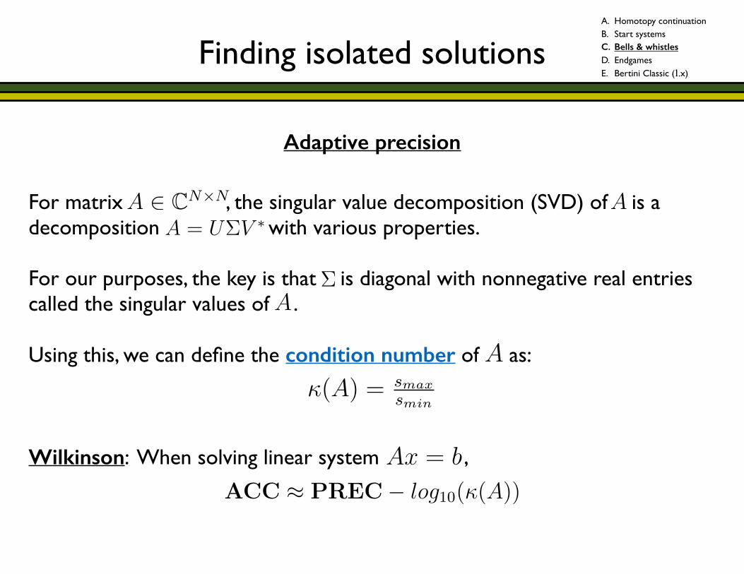
For matrix , the singular value decomposition (SVD) of is a decomposition with various properties. !For our purposes, the key is that is diagonal with nonnegative real entries called the singular values of . !Using this, we can define the condition number of as: !!!Wilkinson: When solving linear system ,
N > n
N < n
PN
SecurityMaxNorm
⇧Ni=1 deg(fi)
di = deg(fi)
g =
2
64zd11 � 1
.
.
.
zdNN � 1
3
75
g =
xy � 1x2 � 1
�
A 2 CN⇥N
3
N > n
N < n
PN
SecurityMaxNorm
⇧Ni=1 deg(fi)
di = deg(fi)
g =
2
64zd11 � 1
.
.
.
zdNN � 1
3
75
g =
xy � 1x2 � 1
�
A 2 CN⇥N
A = U⌃V ⇤
3
N > n
N < n
PN
SecurityMaxNorm
⇧Ni=1 deg(fi)
di = deg(fi)
g =
2
64zd11 � 1
.
.
.
zdNN � 1
3
75
g =
xy � 1x2 � 1
�
A 2 CN⇥N
A = U⌃V ⇤
3
N > n
N < n
PN
SecurityMaxNorm
⇧Ni=1 deg(fi)
di = deg(fi)
g =
2
64zd11 � 1
.
.
.
zdNN � 1
3
75
g =
xy � 1x2 � 1
�
A 2 CN⇥N
3
(A) = smax
smin
4
N > n
N < n
PN
SecurityMaxNorm
⇧Ni=1 deg(fi)
di = deg(fi)
g =
2
64zd11 � 1
.
.
.
zdNN � 1
3
75
g =
xy � 1x2 � 1
�
A 2 CN⇥N
3
(A) = smax
smin
Ax = b
4
(A) = smax
smin
Ax = b
ACC ⇡ PREC� log10((A))
4
Finding isolated solutions
Adaptive precision
N > n
N < n
PN
SecurityMaxNorm
⇧Ni=1 deg(fi)
di = deg(fi)
g =
2
64zd11 � 1
.
.
.
zdNN � 1
3
75
g =
xy � 1x2 � 1
�
A 2 CN⇥N
3
A. Homotopy continuation B. Start systems C. Bells & whistles D. Endgames E. Bertini Classic (1.x)
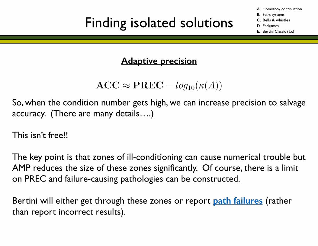
!!So, when the condition number gets high, we can increase precision to salvage accuracy. (There are many details….) !This isn’t free!! !The key point is that zones of ill-conditioning can cause numerical trouble but AMP reduces the size of these zones significantly. Of course, there is a limit on PREC and failure-causing pathologies can be constructed. !Bertini will either get through these zones or report path failures (rather than report incorrect results).
(A) = smax
smin
Ax = b
ACC ⇡ PREC� log10((A))
4
Finding isolated solutions
Adaptive precision
A. Homotopy continuation B. Start systems C. Bells & whistles D. Endgames E. Bertini Classic (1.x)
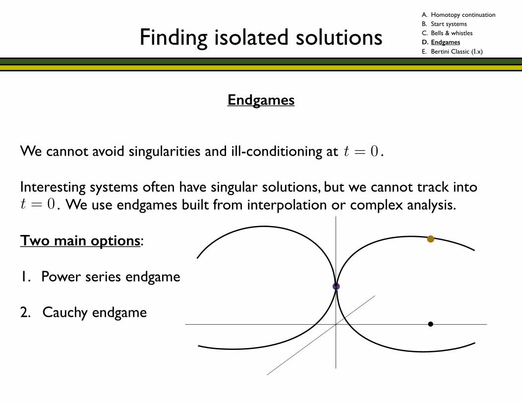
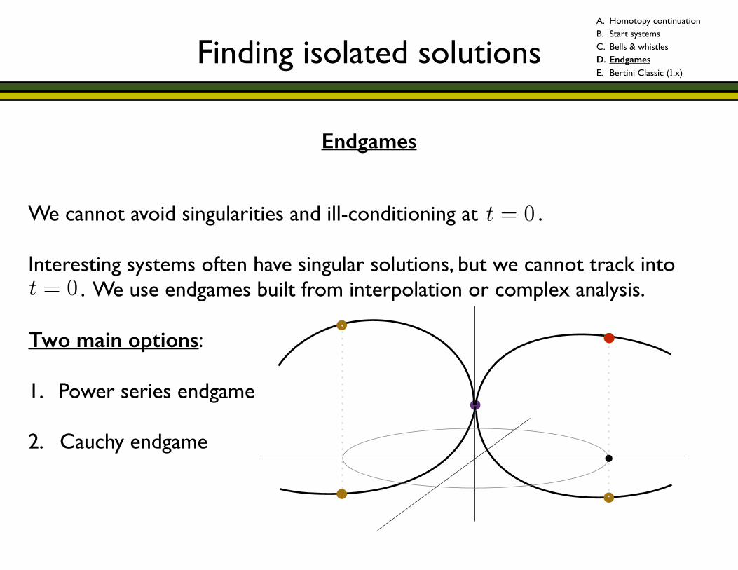
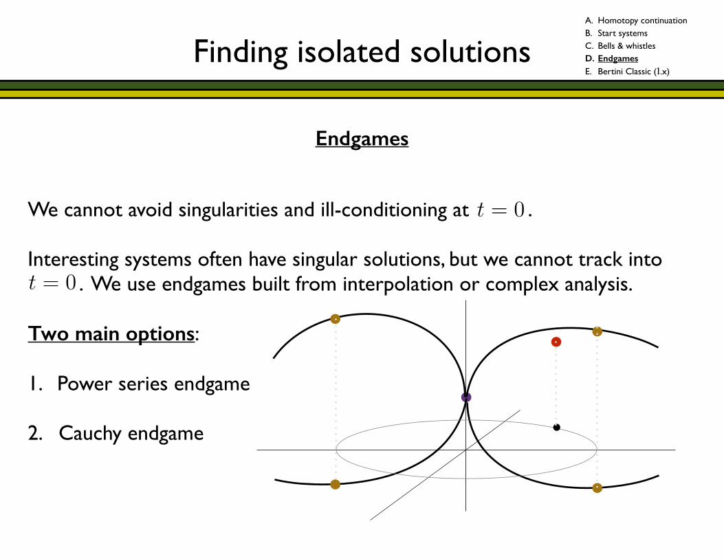
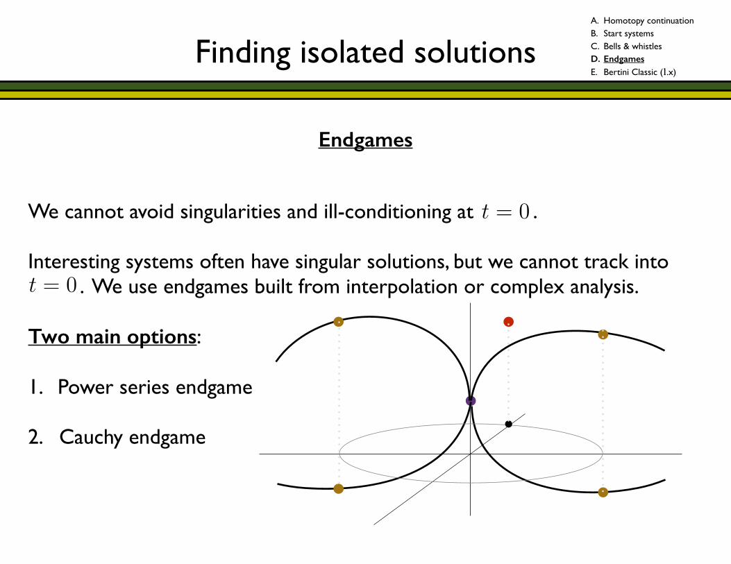
Finding isolated solutions
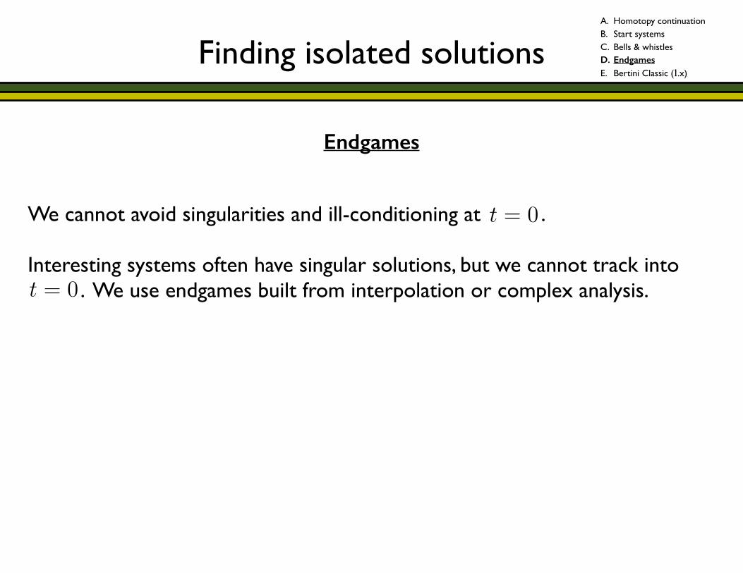
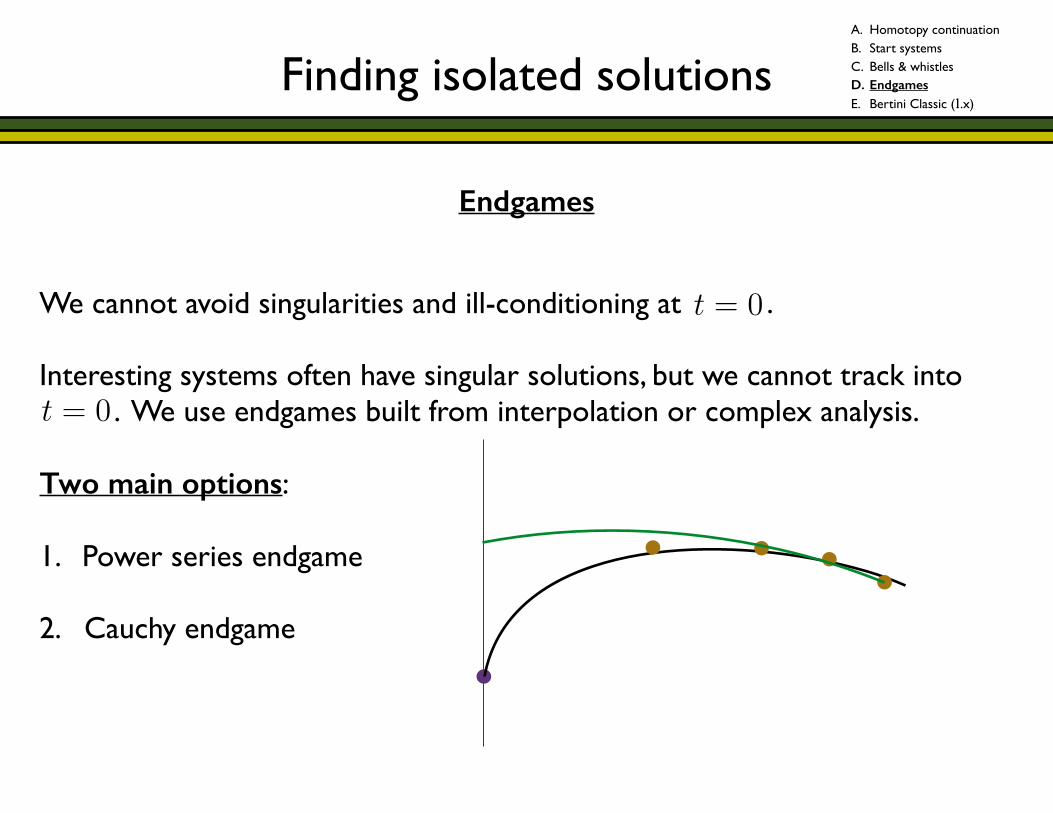
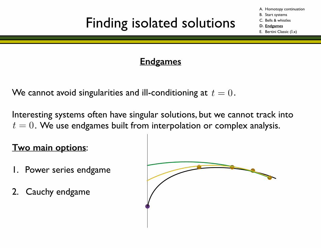
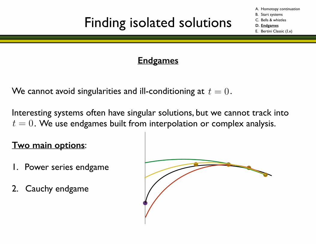
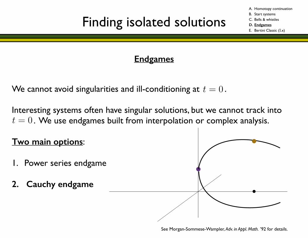
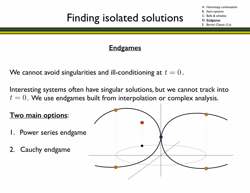
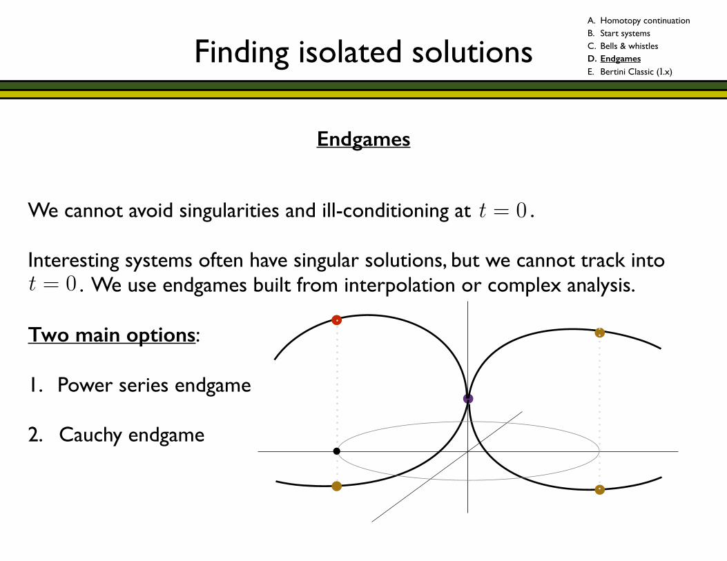
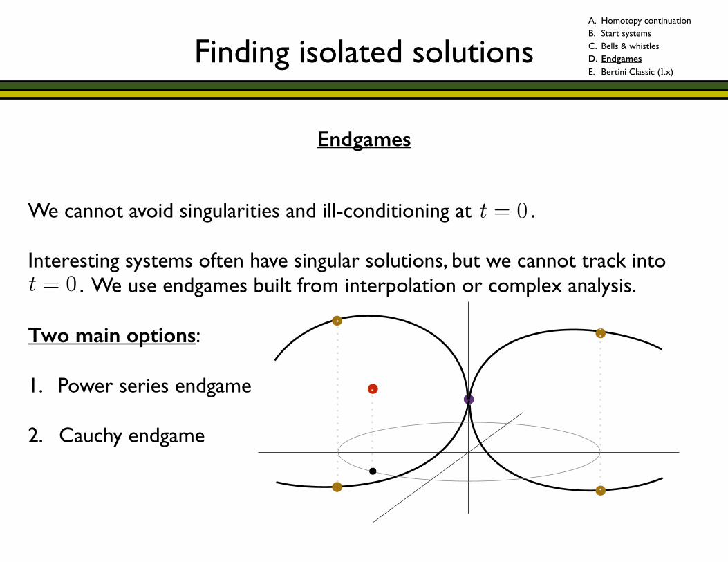
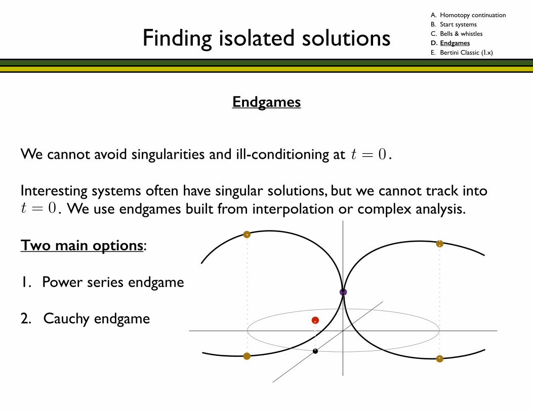
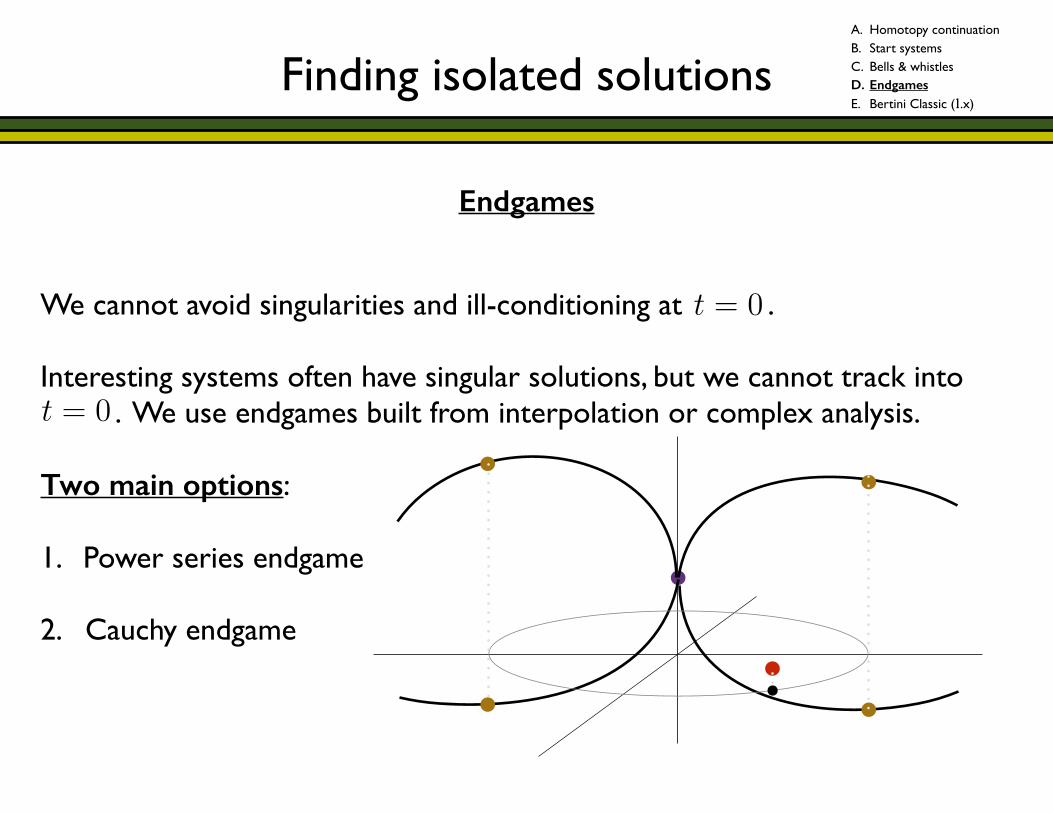
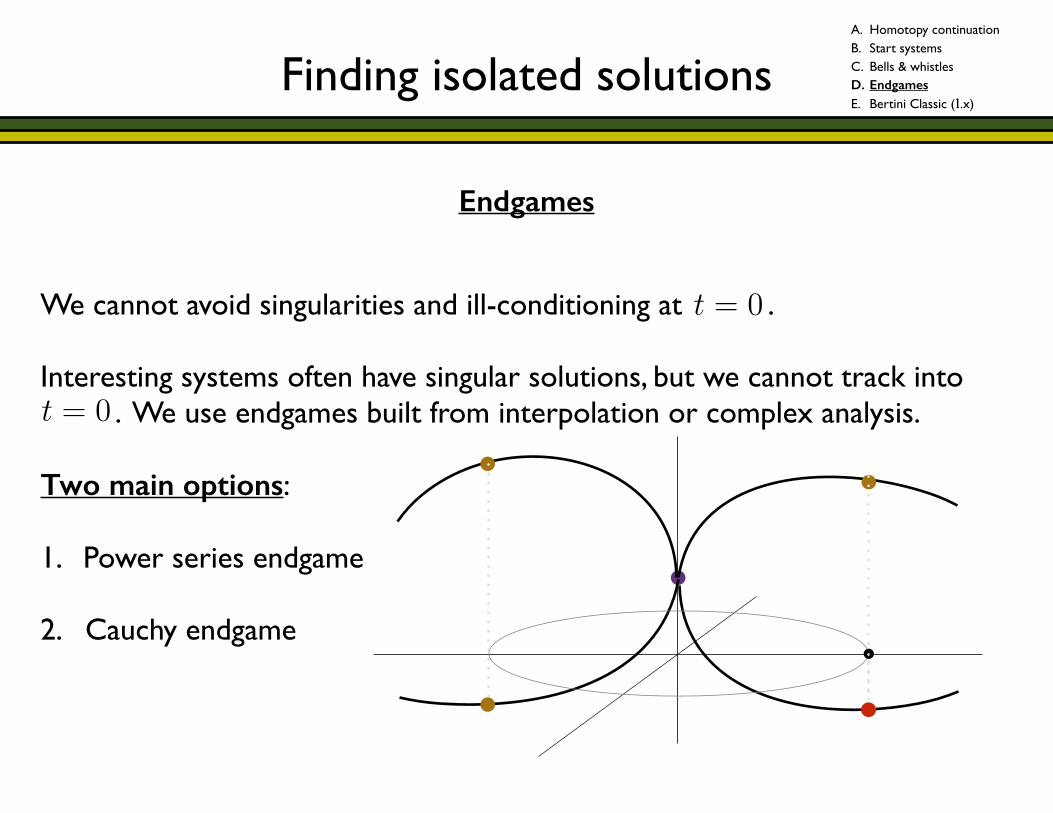
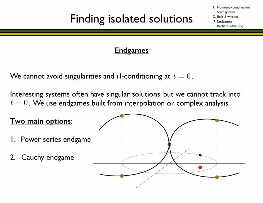
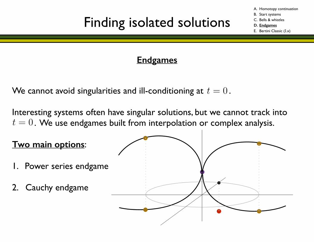
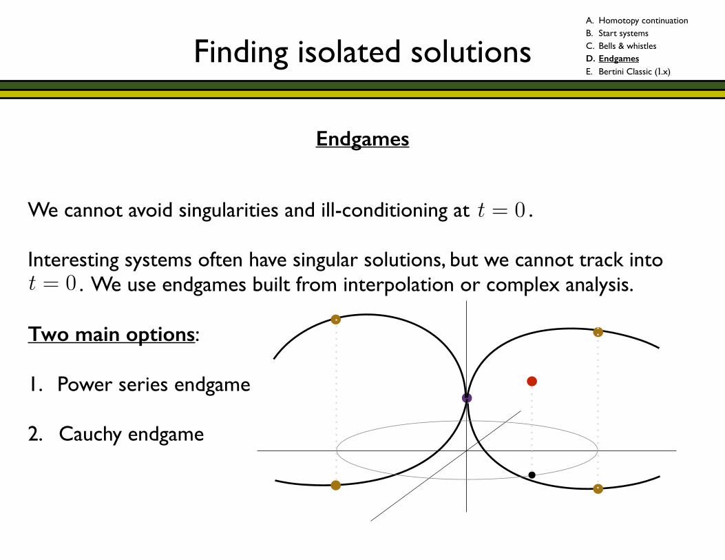
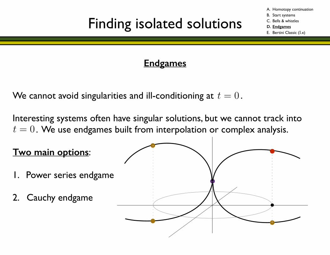
Endgames
We cannot avoid singularities and ill-conditioning at . !Interesting systems often have singular solutions, but we cannot track into . We use endgames built from interpolation or complex analysis. !!!!!!
t = 0
7
t = 0
7
A. Homotopy continuation B. Start systems C. Bells & whistles D. Endgames E. Bertini Classic (1.x)
Finding isolated solutions
Endgames
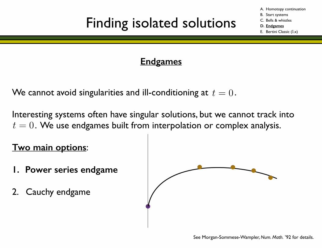
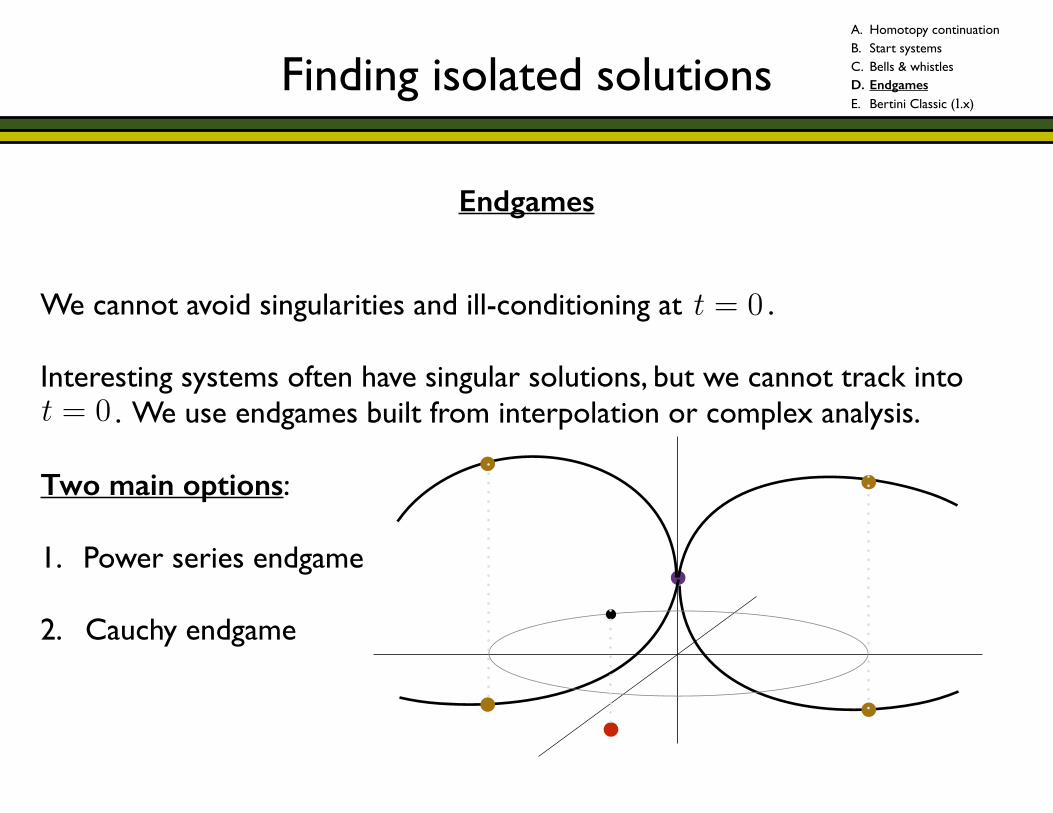
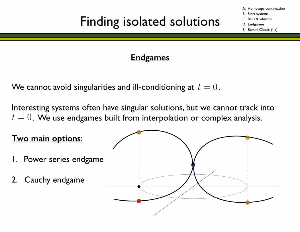
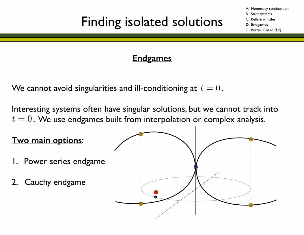
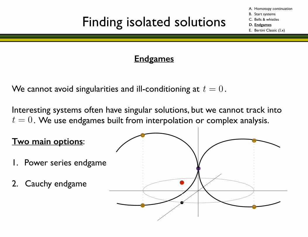
We cannot avoid singularities and ill-conditioning at . !Interesting systems often have singular solutions, but we cannot track into . We use endgames built from interpolation or complex analysis. !Two main options: !1. Power series endgame !2. Cauchy endgame
t = 0
7
t = 0
7
A. Homotopy continuation B. Start systems C. Bells & whistles D. Endgames E. Bertini Classic (1.x)
See Morgan-Sommese-Wampler, Num. Math. ’92 for details.
Finding isolated solutions
Endgames
We cannot avoid singularities and ill-conditioning at . !Interesting systems often have singular solutions, but we cannot track into . We use endgames built from interpolation or complex analysis. !Two main options: !1. Power series endgame !2. Cauchy endgame
t = 0
7
t = 0
7
A. Homotopy continuation B. Start systems C. Bells & whistles D. Endgames E. Bertini Classic (1.x)
See Morgan-Sommese-Wampler, Adv. in Appl. Math. ’92 for details.
Finding isolated solutions
Endgames
We cannot avoid singularities and ill-conditioning at . !Interesting systems often have singular solutions, but we cannot track into . We use endgames built from interpolation or complex analysis. !Two main options: !1. Power series endgame !2. Cauchy endgame
t = 0
7
t = 0
7
A. Homotopy continuation B. Start systems C. Bells & whistles D. Endgames E. Bertini Classic (1.x)
Finding isolated solutions
Endgames
t = 0
7
t = 0
7
A. Homotopy continuation B. Start systems C. Bells & whistles D. Endgames E. Bertini Classic (1.x)
We cannot avoid singularities and ill-conditioning at . !Interesting systems often have singular solutions, but we cannot track into . We use endgames built from interpolation or complex analysis. !Two main options: !1. Power series endgame !2. Cauchy endgame
Finding isolated solutions
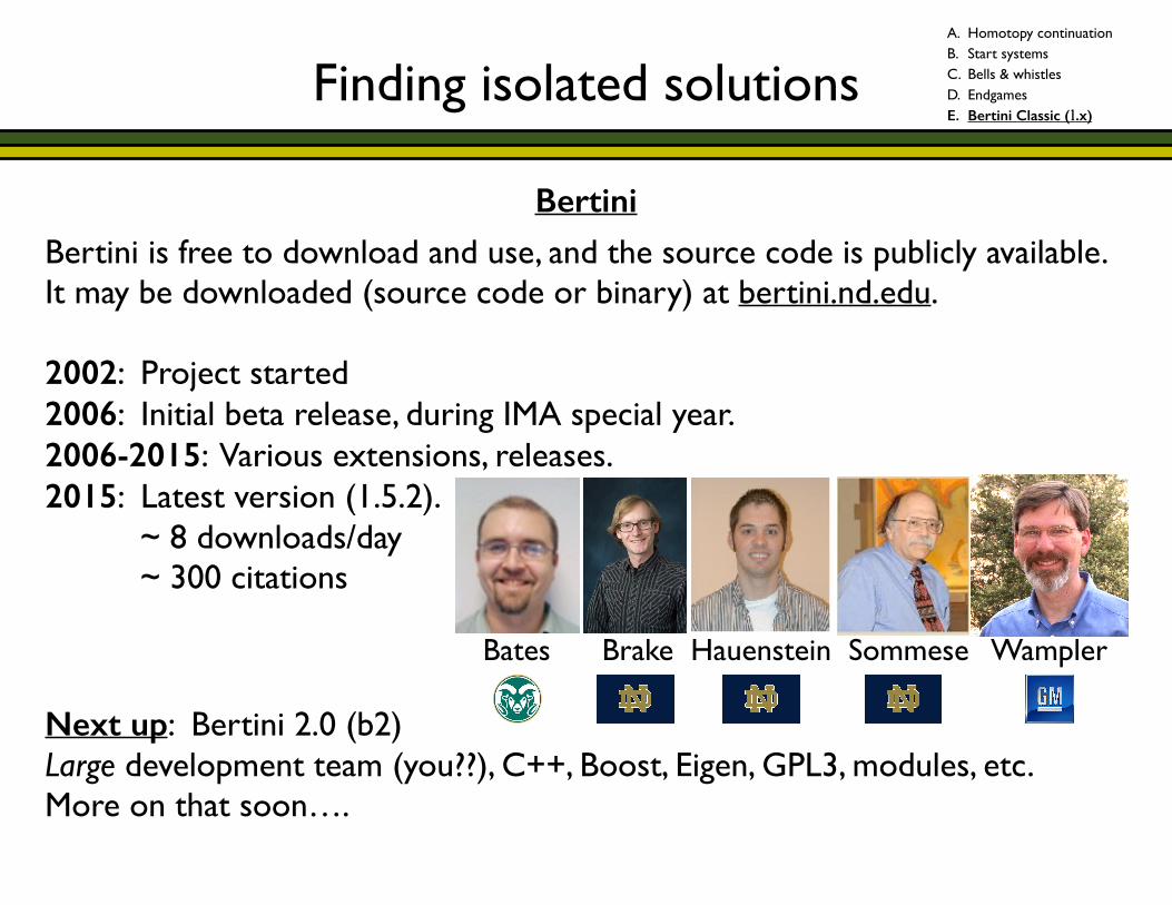
BertiniBertini is free to download and use, and the source code is publicly available. It may be downloaded (source code or binary) at bertini.nd.edu. !2002: Project started 2006: Initial beta release, during IMA special year. 2006-2015: Various extensions, releases. 2015: Latest version (1.5.2). ~ 8 downloads/day ~ 300 citations ! Bates Brake Hauenstein Sommese Wampler Next up: Bertini 2.0 (b2) Large development team (you??), C++, Boost, Eigen, GPL3, modules, etc. More on that soon….
A. Homotopy continuation B. Start systems C. Bells & whistles D. Endgames E. Bertini Classic (1.x)
Finding isolated solutions
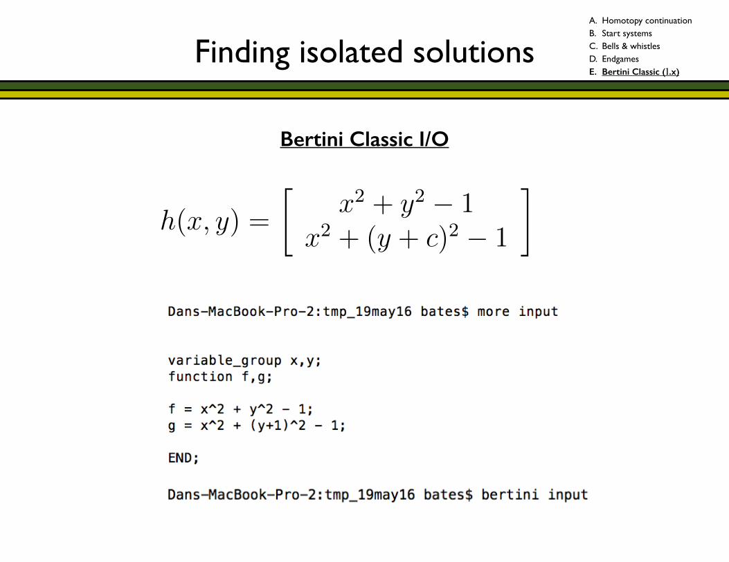
Bertini Classic I/O
x4 � 1 = 0
x = ±i
y 2 C
h(x, y) =
x2 + y2 � 1
x2 + (y + c)2 � 1
�
c = 1
c = 2
c = 3
5
A. Homotopy continuation B. Start systems C. Bells & whistles D. Endgames E. Bertini Classic (1.x)
Finding isolated solutions
Bertini I/O
A. Homotopy continuation B. Start systems C. Bells & whistles D. Endgames E. Bertini Classic (1.x)
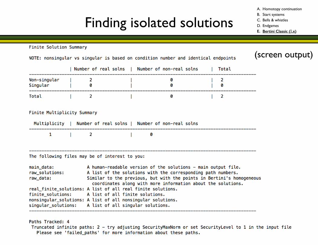
(screen output)
Finding isolated solutions
Bertini I/O
A. Homotopy continuation B. Start systems C. Bells & whistles D. Endgames E. Bertini Classic (1.x)
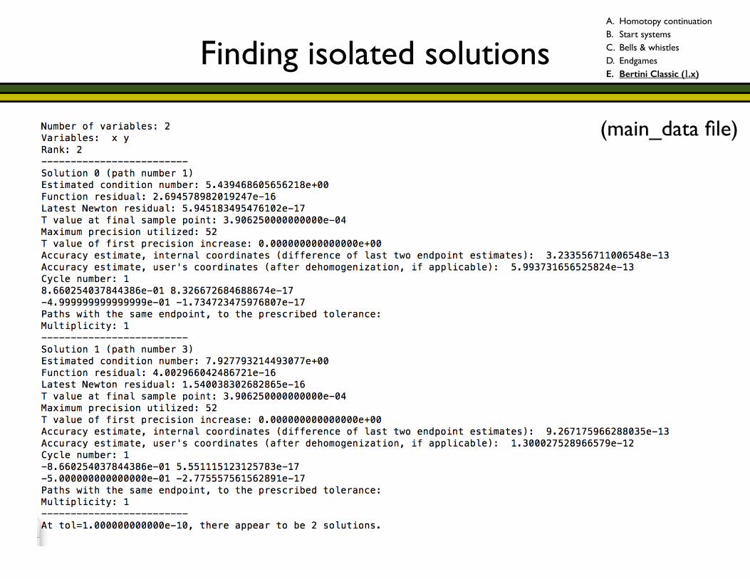
(main_data file)
1. Polynomial systems and their solution sets
2. Finding isolated solutions (homotopy continuation)
3. Advanced topics for isolated solutions
4. Finding positive-dimensional solution sets (briefly)
Game plan

!
!
3. Advanced topics for isolated solutions
A. Parameter homotopies
B. Certification
C. Regeneration
Game plan
Advanced topics for isolated solutions
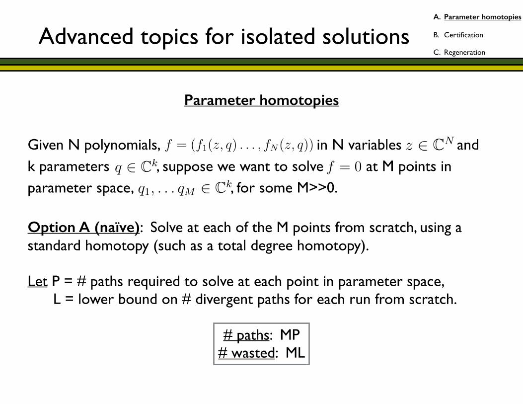
Given N polynomials, in N variables and k parameters , suppose we want to solve at M points in parameter space, , for some M>>0. !Option A (naïve): Solve at each of the M points from scratch, using a standard homotopy (such as a total degree homotopy). !Let P = # paths required to solve at each point in parameter space, L = lower bound on # divergent paths for each run from scratch. !
# paths: MP# wasted: ML
f : CN ! CN
g : CN ! CN
H : CN ⇥ C ! CN
H(z, t) = f(z) · (1� t) + �g(z) · t
� 2 C
H(z, 1) = g(z)
H(z, 0) = f(z)
f1, . . . , fN 2 C[z1, . . . , zN ]
bz 2 CN
fi(bz) = 0 8i
f = (f1(z, q) . . . , fN(z, q))
1
f : CN ! CN
g : CN ! CN
H : CN ⇥ C ! CN
H(z, t) = f(z) · (1� t) + �g(z) · t
� 2 C
H(z, 1) = g(z)
H(z, 0) = f(z)
f1, . . . , fN 2 C[z1, . . . , zN ]
z 2 CN
fi(bz) = 0 8i
f = (f1(z, q) . . . , fN(z, q))
1
f : CN ! CN
g : CN ! CN
H : CN ⇥ C ! CN
H(z, t) = f(z) · (1� t) + �g(z) · t
� 2 C
H(z, 1) = g(z)
H(z, 0) = f(z)
f1, . . . , fN 2 C[z1, . . . , zN ]
z 2 CN
q 2 Ck
fi(bz) = 0 8i
1
f : CN ! CN
g : CN ! CN
H : CN ⇥ C ! CN
H(z, t) = f(z) · (1� t) + �g(z) · t
� 2 C
H(z, 1) = g(z)
H(z, 0) = f(z)
f1, . . . , fN 2 C[z1, . . . , zN ]
z 2 CN
f = 0
q 2 Ck
1
f : CN ! CN
g : CN ! CN
H : CN ⇥ C ! CN
H(z, t) = f(z) · (1� t) + �g(z) · t
� 2 C
H(z, 1) = g(z)
H(z, 0) = f(z)
f1, . . . , fN 2 C[z1, . . . , zN ]
q1, . . . qM 2 Ck
M >> 0
z 2 CN
1
Parameter homotopies
A. Parameter homotopies
B. Certification
C. Regeneration
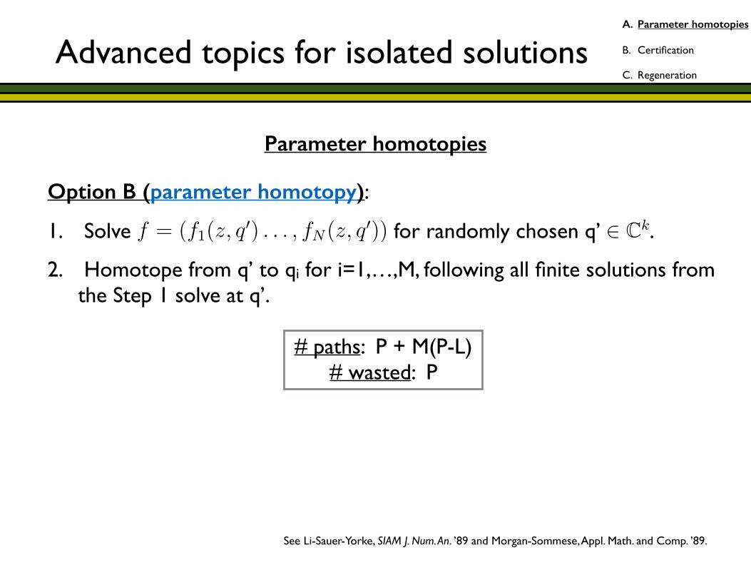
Option B (parameter homotopy):
1. Solve for randomly chosen q’ .
2. Homotope from q’ to qi for i=1,…,M, following all finite solutions from the Step 1 solve at q’.
!# paths: P + M(P-L)
# wasted: P !
!!!!!! See Li-Sauer-Yorke, SIAM J. Num. An. ’89 and Morgan-Sommese, Appl. Math. and Comp. ’89.
f = 0
q0 2 Ck
fi(bz) = 0 8i
f = (f1(z, q0) . . . , fN(z, q0))
R
N = n
N 6= n
⇡
Z = V(f) =D[
i=0
Zi =D[
i=0
[
j2⇤i
Zi,j
f =
x(x� 1)x(y � 1)
�
2
f = 0
q0 2 Ck
fi(bz) = 0 8i
f = (f1(z, q0) . . . , fN(z, q0))
R
N = n
N 6= n
⇡
Z = V(f) =D[
i=0
Zi =D[
i=0
[
j2⇤i
Zi,j
f =
x(x� 1)x(y � 1)
�
2
Parameter homotopies
Advanced topics for isolated solutionsA. Parameter homotopies
B. Certification
C. Regeneration
!!!
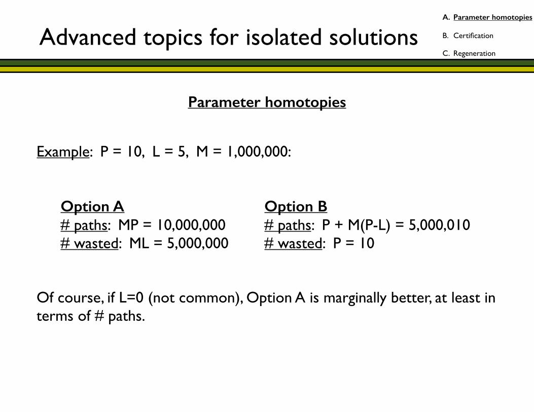
Example: P = 10, L = 5, M = 1,000,000: !!!!!!!Of course, if L=0 (not common), Option A is marginally better, at least in terms of # paths.
Option A # paths: MP = 10,000,000 # wasted: ML = 5,000,000
Option B # paths: P + M(P-L) = 5,000,010 # wasted: P = 10
Parameter homotopies
Advanced topics for isolated solutionsA. Parameter homotopies
B. Certification
C. Regeneration
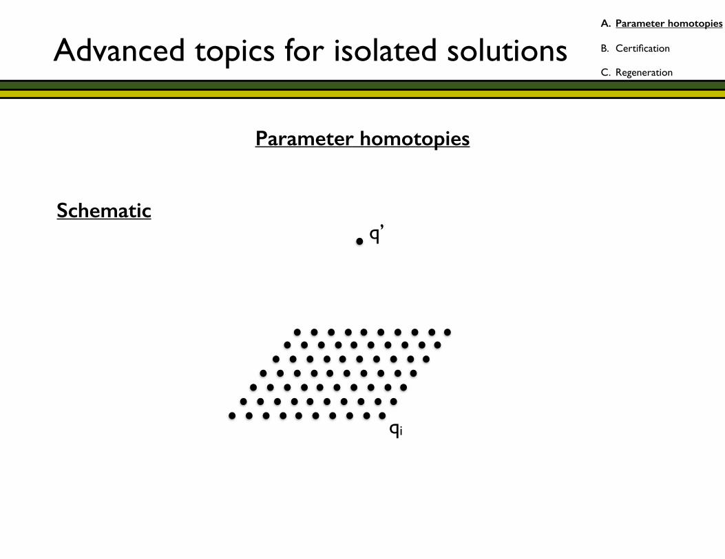
Schematic !
qi !
q’ !
Parameter homotopies
Advanced topics for isolated solutionsA. Parameter homotopies
B. Certification
C. Regeneration

Schematic: Step 1 !
qi !
q’ !
Parameter homotopies
Advanced topics for isolated solutionsA. Parameter homotopies
B. Certification
C. Regeneration
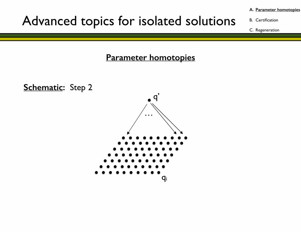
Schematic: Step 2 !
qi !
q’ !
… !
Parameter homotopies
Advanced topics for isolated solutionsA. Parameter homotopies
B. Certification
C. Regeneration

Problem: Standard NAG software options include parameter homotopy capabilities, but: * parallelization is within the run (not between runs), * failure mitigation is not automated (a headache), and * each run includes startup costs, e.g., parsing. !Solution: Paramotopy D. Bates, D. Brake (Notre Dame), and M. Niemerg (IBM/Oak Ridge) www.paramotopy.com ! Free to use, source code publicly available C++, Boost Uses Bertini as a library To be incorporated into Bertini 2.x in some form.
Parameter homotopies
Advanced topics for isolated solutionsA. Parameter homotopies
B. Certification
C. Regeneration

Certification
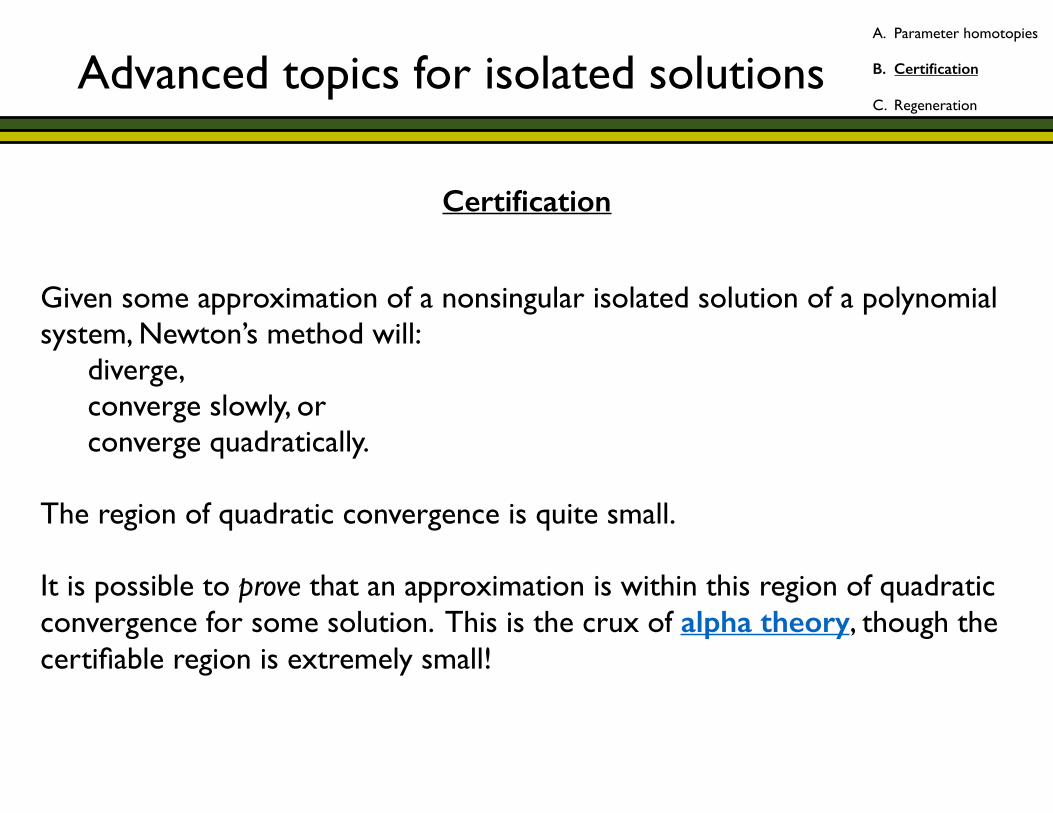
!Given some approximation of a nonsingular isolated solution of a polynomial system, Newton’s method will: diverge, converge slowly, or converge quadratically. !!!!!
Basins of attraction for z5 + 1 = 0 from MIT Open Courseware (Intro to Matlab Programming)
Advanced topics for isolated solutionsA. Parameter homotopies
B. Certification
C. Regeneration
Certification
!Given some approximation of a nonsingular isolated solution of a polynomial system, Newton’s method will: diverge, converge slowly, or converge quadratically. !The region of quadratic convergence is quite small. !It is possible to prove that an approximation is within this region of quadratic convergence for some solution. This is the crux of alpha theory, though the certifiable region is extremely small!
Advanced topics for isolated solutionsA. Parameter homotopies
B. Certification
C. Regeneration

Certification
Two basic options (more introduced recently): ! 1. Certify as you go through a homotopy (Beltran-Leykin, NAG4M2) or 2. Post-certify (Hauenstein-Sottile, alphaCertified). !See the upcoming talk of Nick Hein & Alan Liddell.
Advanced topics for isolated solutionsA. Parameter homotopies
B. Certification
C. Regeneration
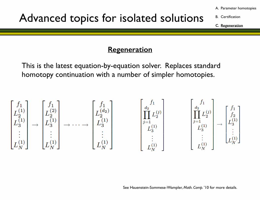
Regeneration
This is the latest equation-by-equation solver. Replaces standard homotopy continuation with a number of simpler homotopies. !!!!!!!!!!!! See Hauenstein-Sommese-Wampler, Math. Comp. ’10 for more details.
Advanced topics for isolated solutionsA. Parameter homotopies
B. Certification
C. Regeneration
1. Polynomial systems and their solution sets
2. Finding isolated solutions (homotopy continuation)
3. Advanced topics for isolated solutions
4. Finding positive-dimensional solution sets (briefly)
Game plan
!
!
!
4. Finding positive-dimensional solution sets (briefly)
A. Slicing and the numerical irreducible decomposition
B. Bertini Classic I/O
C. Sampling
D. Real solutions
Game plan
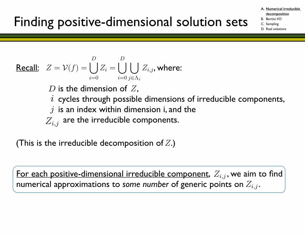
Finding positive-dimensional solution sets!!!!!!Recall: , where: ! is the dimension of , cycles through possible dimensions of irreducible components, is an index within dimension i, and the are the irreducible components.
f : CN ! CN
f1, . . . , fn 2 C[z1, . . . , zN ]
bz 2 CN
fi(bz) = 0 8i
f = (f1, . . . , fn)
R
N = n
N 6= n
⇡
Z = V(f) =D[
i=0
Zi =D[
i=0
[
j2⇤i
Zi,j
1
f : CN ! CN
f1, . . . , fn 2 C[z1, . . . , zN ]
bz 2 CN
fi(bz) = 0 8i
f = (f1, . . . , fn)
R
N = n
N 6= n
⇡
Z = V(f) =D[
i=0
Zi =D[
i=0
[
j2⇤i
Zi,j
1
f : CN ! CN
f1, . . . , fn 2 C[z1, . . . , zN ]
bz 2 CN
fi(bz) = 0 8i
f = (f1, . . . , fn)
R
N = n
N 6= n
⇡
Z = V(f) =D[
i=0
Zi =D[
i=0
[
j2⇤i
Zi,j
1
f : CN ! CN
f1, . . . , fn 2 C[z1, . . . , zN ]
bz 2 CN
fi(bz) = 0 8i
f = (f1, . . . , fn)
R
N = n
N 6= n
⇡
Z = V(f) =D[
i=0
Zi =D[
i=0
[
j2⇤i
Zi,j
1
f : CN ! CN
f1, . . . , fn 2 C[z1, . . . , zN ]
bz 2 CN
fi(bz) = 0 8i
f = (f1, . . . , fn)
R
N = n
N 6= n
⇡
Z = V(f) =D[
i=0
Zi =D[
i=0
[
j2⇤i
Zi,j
1
f : CN ! CN
f1, . . . , fn 2 C[z1, . . . , zN ]
bz 2 CN
fi(bz) = 0 8i
f = (f1, . . . , fn)
R
N = n
N 6= n
⇡
Z = V(f) =D[
i=0
Zi =D[
i=0
[
j2⇤i
Zi,j
1
!!!!!!(This is the irreducible decomposition of .) !!
R
N = n
N 6= n
⇡
Z = V(f) =D[
i=0
Zi =D[
i=0
[
j2⇤i
Zi,j
f =
x(x� 1)x(y � 1)
�
x = 0
x = y = 1
z
||z � bz|| < FinalTol
2
!For each positive-dimensional irreducible component, , we aim to find numerical approximations to some number of generic points on .
f : CN ! CN
f1, . . . , fn 2 C[z1, . . . , zN ]
bz 2 CN
fi(bz) = 0 8i
f = (f1, . . . , fn)
R
N = n
N 6= n
⇡
Z = V(f) =D[
i=0
Zi =D[
i=0
[
j2⇤i
Zi,j
1
f : CN ! CN
f1, . . . , fn 2 C[z1, . . . , zN ]
bz 2 CN
fi(bz) = 0 8i
f = (f1, . . . , fn)
R
N = n
N 6= n
⇡
Z = V(f) =D[
i=0
Zi =D[
i=0
[
j2⇤i
Zi,j
1
A. Numerical irreducible decomposition
B. Bertini I/O C. Sampling D. Real solutions
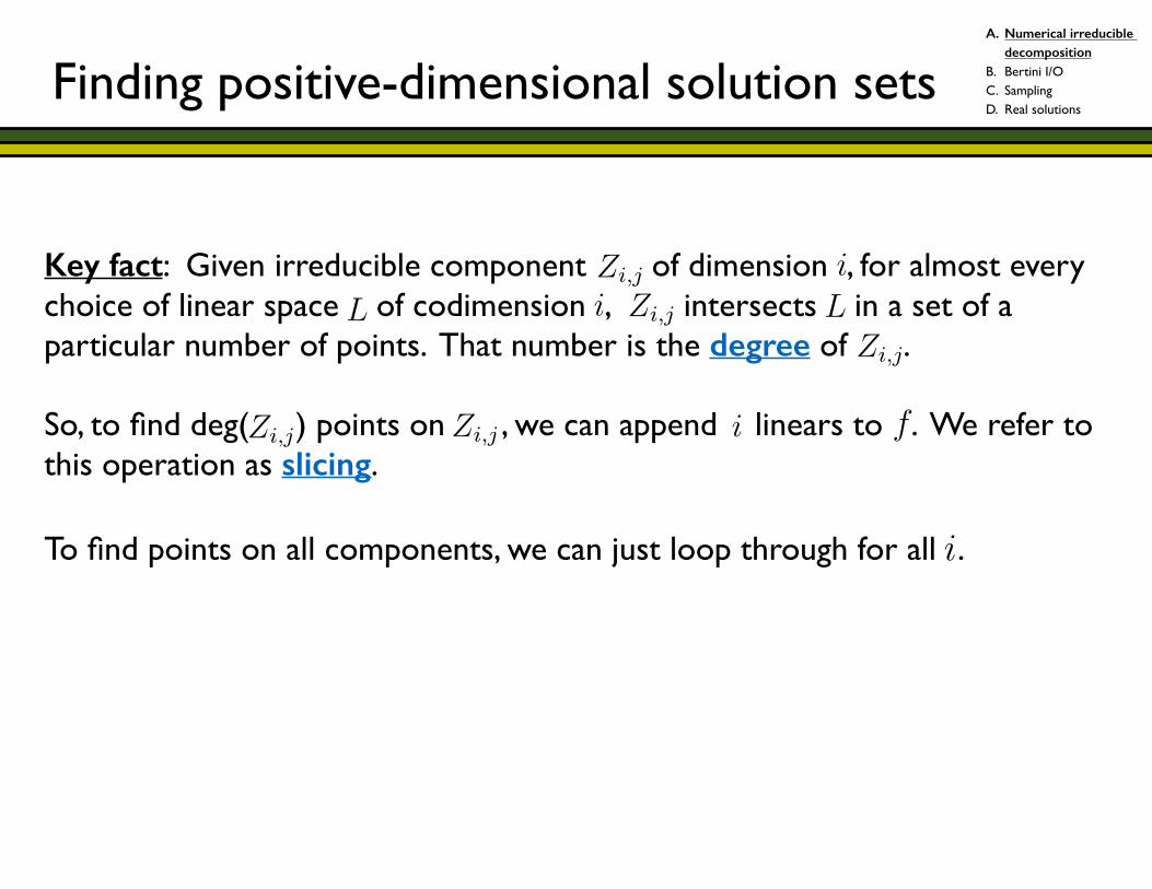
Key fact: Given irreducible component of dimension , for almost every choice of linear space of codimension , intersects in a set of a particular number of points. That number is the degree of . !So, to find deg( ) points on , we can append linears to . We refer to this operation as slicing. !To find points on all components, we can just loop through for all . !!
f : CN ! CN
f1, . . . , fn 2 C[z1, . . . , zN ]
bz 2 CN
fi(bz) = 0 8i
f = (f1, . . . , fn)
R
N = n
N 6= n
⇡
Z = V(f) =D[
i=0
Zi =D[
i=0
[
j2⇤i
Zi,j
1
f : CN ! CN
f1, . . . , fn 2 C[z1, . . . , zN ]
bz 2 CN
fi(bz) = 0 8i
f = (f1, . . . , fn)
R
N = n
N 6= n
⇡
Z = V(f) =D[
i=0
Zi =D[
i=0
[
j2⇤i
Zi,j
1
f : CN ! CN
f1, . . . , fn 2 C[z1, . . . , zN ]
bz 2 CN
fi(bz) = 0 8i
f = (f1, . . . , fn)
R
N = n
N 6= n
⇡
Z = V(f) =D[
i=0
Zi =D[
i=0
[
j2⇤i
Zi,j
1
f : CN ! CN
f1, . . . , fn 2 C[z1, . . . , zN ]
bz 2 CN
fi(bz) = 0 8i
f = (f1, . . . , fn)
R
N = n
N 6= n
⇡
Z = V(f) =D[
i=0
Zi =D[
i=0
[
j2⇤i
Zi,j
1
R
N = n
N 6= n
⇡
Z = V(f) =D[
i=0
Zi =D[
i=0
[
j2⇤i
Zi,j
f =
x(x� 1)x(y � 1)
�
x = 0
x = y = 1
z
||z � bz|| < FinalTol
2
f : CN ! CN
f1, . . . , fn 2 C[z1, . . . , zN ]
bz 2 CN
fi(bz) = 0 8i
f = (f1, . . . , fn)
R
N = n
N 6= n
⇡
Z = V(f) =D[
i=0
Zi =D[
i=0
[
j2⇤i
Zi,j
1
(1, 1), (�1,�1), (2,�1), (�2, 1)
f(x, y) =
f1 + f2 + f3f1 + 2f2 + f3
�
J =
2
64
@f1
@x1. . . @f1
@x
N
.
.
.
.
.
.
.
.
.
@f
N
@x1. . . @f
N
@x
N
3
75
(±i,±2i) 2 C2
i
L
6
(1, 1), (�1,�1), (2,�1), (�2, 1)
f(x, y) =
f1 + f2 + f3f1 + 2f2 + f3
�
J =
2
64
@f1
@x1. . . @f1
@x
N
.
.
.
.
.
.
.
.
.
@f
N
@x1. . . @f
N
@x
N
3
75
(±i,±2i) 2 C2
i
L
6
(1, 1), (�1,�1), (2,�1), (�2, 1)
f(x, y) =
f1 + f2 + f3f1 + 2f2 + f3
�
J =
2
64
@f1
@x1. . . @f1
@x
N
.
.
.
.
.
.
.
.
.
@f
N
@x1. . . @f
N
@x
N
3
75
(±i,±2i) 2 C2
i
L
6
(1, 1), (�1,�1), (2,�1), (�2, 1)
f(x, y) =
f1 + f2 + f3f1 + 2f2 + f3
�
J =
2
64
@f1
@x1. . . @f1
@x
N
.
.
.
.
.
.
.
.
.
@f
N
@x1. . . @f
N
@x
N
3
75
(±i,±2i) 2 C2
i
L
6
(1, 1), (�1,�1), (2,�1), (�2, 1)
f(x, y) =
f1 + f2 + f3f1 + 2f2 + f3
�
J =
2
64
@f1
@x1. . . @f1
@x
N
.
.
.
.
.
.
.
.
.
@f
N
@x1. . . @f
N
@x
N
3
75
(±i,±2i) 2 C2
i
L
6
Finding positive-dimensional solution setsA. Numerical irreducible
decomposition B. Bertini I/O C. Sampling D. Real solutions
(1, 1), (�1,�1), (2,�1), (�2, 1)
f(x, y) =
f1 + f2 + f3f1 + 2f2 + f3
�
J =
2
64
@f1
@x1. . . @f1
@x
N
.
.
.
.
.
.
.
.
.
@f
N
@x1. . . @f
N
@x
N
3
75
(±i,±2i) 2 C2
i
L
6

Problem 1: We could pick up points on higher-dimensional components. Problem 2: We could find points on multiple i-dimensional components. !!!!!
Example: Suppose there are two curves and a surface. When we slice for the curves, we will find points on both curves and also on the surface. !Solution 1: Start at the top dimension and work your way down. Use a membership test on points in lower dimensions to see if they sit on the higher-dimensional components already found. !Solution 2: Carry out an equidimensional decomposition, using monodromy and the trace test. !!!
Finding positive-dimensional solution setsA. Numerical irreducible
decomposition B. Bertini I/O C. Sampling D. Real solutions
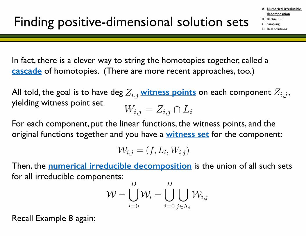
In fact, there is a clever way to string the homotopies together, called a cascade of homotopies. (There are more recent approaches, too.) !All told, the goal is to have deg witness points on each component , yielding witness point set !For each component, put the linear functions, the witness points, and the original functions together and you have a witness set for the component: !!Then, the numerical irreducible decomposition is the union of all such sets for all irreducible components: !!!Recall Example 8 again:
f : CN ! CN
f1, . . . , fn 2 C[z1, . . . , zN ]
bz 2 CN
fi(bz) = 0 8i
f = (f1, . . . , fn)
R
N = n
N 6= n
⇡
Z = V(f) =D[
i=0
Zi =D[
i=0
[
j2⇤i
Zi,j
1
f = 0
q0 2 Ck
fi
(bz) = 0 8i
f = (f1(z, q0) . . . , fN(z, q0))
R
N = n
N 6= n
⇡
W =D[
i=0
Wi
=D[
i=0
[
j2⇤i
Wi,j
Wi,j
= (f, Li,j
,Wi,j
)
2
Wi,j
= Zi,j
\ Li
f =
x(x� 1)x(y � 1)
�
x = 0
x = y = 1
z
||z � bz|| < FinalTol
N > n
N < n
PN
SecurityMaxNorm
3
f : CN ! CN
f1, . . . , fn 2 C[z1, . . . , zN ]
bz 2 CN
fi(bz) = 0 8i
f = (f1, . . . , fn)
R
N = n
N 6= n
⇡
Z = V(f) =D[
i=0
Zi =D[
i=0
[
j2⇤i
Zi,j
1
Finding positive-dimensional solution setsA. Numerical irreducible
decomposition B. Bertini I/O C. Sampling D. Real solutions
f = 0
q0 2 Ck
fi
(bz) = 0 8i
f = (f1(z, q0) . . . , fN(z, q0))
R
N = n
N 6= n
⇡
W =D[
i=0
Wi
=D[
i=0
[
j2⇤i
Wi,j
Wi,j
= (f, Li
,Wi,j
)
2
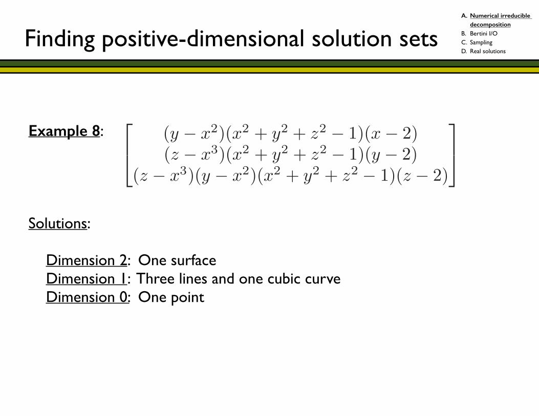
Example 8: !!!!Solutions: ! Dimension 2: One surface Dimension 1: Three lines and one cubic curve Dimension 0: One point
“main”2013/3/17page 159
✐
✐
✐
✐
✐
✐
✐
✐
DRAFT
Chapter 8
Positive-DimensionalComponents
In Part II of the book, we return to the fundamental problem of “solving” a poly-nomial system,
f(z) :=
⎡
⎢⎣f1(z1, . . . , zN)
...fn(z1, . . . , zN)
⎤
⎥⎦ = 0. (8.1)
As opposed to the case of systems of linear equations, where a nonempty so-lution set will consist of exactly one linear space, the solution set of a polynomialsystem can have several separate components and these may have different dimen-sions23 (points, curves, surfaces, etc). Thus, the problem of “solving” a polynomialsystem includes the detection of all such components no matter what dimensioneach has. Solution components of dimension greater than zero (everything exceptisolated points) are said to be “positive-dimensional.”
For example, consider the following system of three polynomials in the vari-ables x, y, z:
f =
⎡
⎣(y − x2)(x2 + y2 + z2 − 1)(x− 2)(z − x3)(x2 + y2 + z2 − 1)(y − 2)
(z − x3)(y − x2)(x2 + y2 + z2 − 1)(z − 2)
⎤
⎦ . (8.2)
The solution set of three linear equations in three variables must be one point, oneline, or one plane. The complex solution set of (8.2) consists of a surface, fourcurves, and a point. If we were to apply one of the homotopies presented in Part Ito solve this system, we would be assured to find the isolated solution, (2, 2, 2), butthere would be no guarantee of finding any points on the other components.
In brief, Part II presents how numerical algebraic geometry treats full solutionsets, including their positive-dimensional components. This chapter introduces thebasic concepts and shows results obtained with Bertini on some simple examples.The next two chapters, Chapter 9 and Chapter 10, which go into details of the
23We gave a definition of the dimension of a component in §1.2.2.
159
Finding positive-dimensional solution setsA. Numerical irreducible
decomposition B. Bertini I/O C. Sampling D. Real solutions
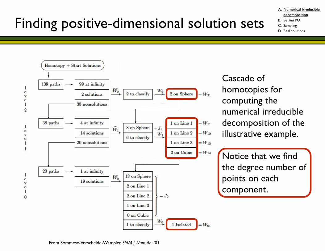
From Sommese-Verschelde-Wampler, SIAM J. Num. An. ’01.
Cascade of homotopies for computing the numerical irreducible decomposition of the illustrative example. !Notice that we find the degree number of points on each component.
Finding positive-dimensional solution setsA. Numerical irreducible
decomposition B. Bertini I/O C. Sampling D. Real solutions
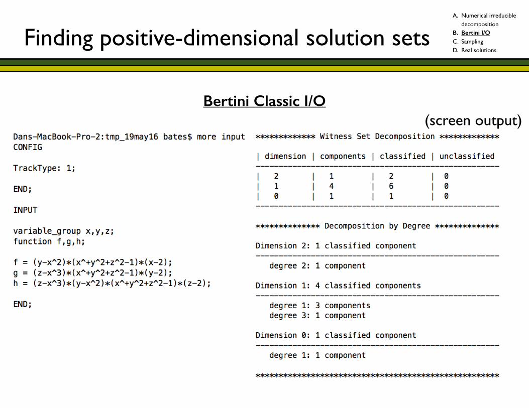
Bertini Classic I/O
Finding positive-dimensional solution setsA. Numerical irreducible
decomposition B. Bertini I/O C. Sampling D. Real solutions
(screen output)
By following the solutions as we move the linears from a witness set, we pick up more points on the same irreducible component. This is called component sampling. !In this way, you can find many points on a curve (or other irreducible component) quite rapidly.
Sampling
Finding positive-dimensional solution setsA. Numerical irreducible
decomposition B. Bertini I/O C. Sampling D. Real solutions
For real applications, people typically want real solutions! !This is very difficult. There are several recent, limited techniques using homotopy methods: ! * Khovanskii-Rolle continuation for fewnomials (Bates-Sottile, KhRo) ! * Seidenberg-like methods (Hauenstein) ! * Real cellular decompositions (Lu-Bates-Sommese-Wampler, Besana-Di Rocco-Hauenstein-Sommese-Wampler, Bates-Brake-Hao-Hauenstein-Sommese-Wampler, BertiniReal) !There are non-homotopy numerical methods, too (cellular exclusion, cylindrical decomposition, etc.). !This is still a major open problem!
Real solutions
Finding positive-dimensional solution setsA. Numerical irreducible
decomposition B. Bertini I/O C. Sampling D. Real solutions
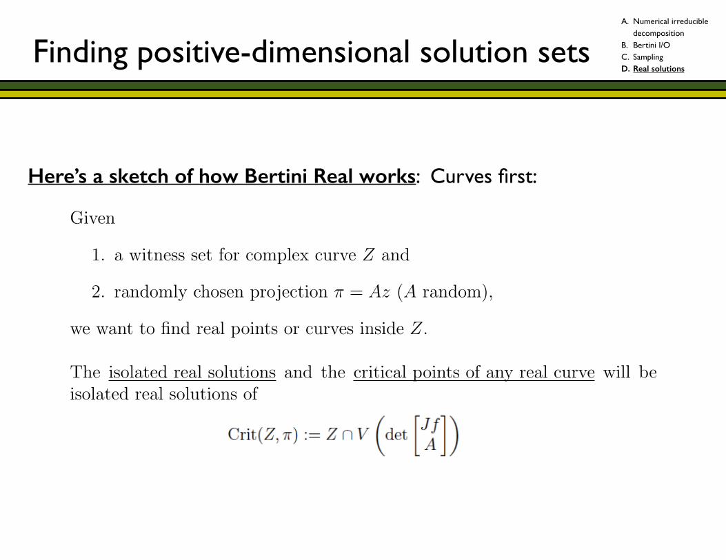
Here’s a sketch of how Bertini Real works: Curves first: !!!
Given
1. a witness set for complex curve Z and
2. randomly chosen projection � = Az (A random),
we want to find real points or curves inside Z.
The isolated real solutions and the critical points of any real curve will beisolated real solutions of
6
Finding positive-dimensional solution setsA. Numerical irreducible
decomposition B. Bertini I/O C. Sampling D. Real solutions
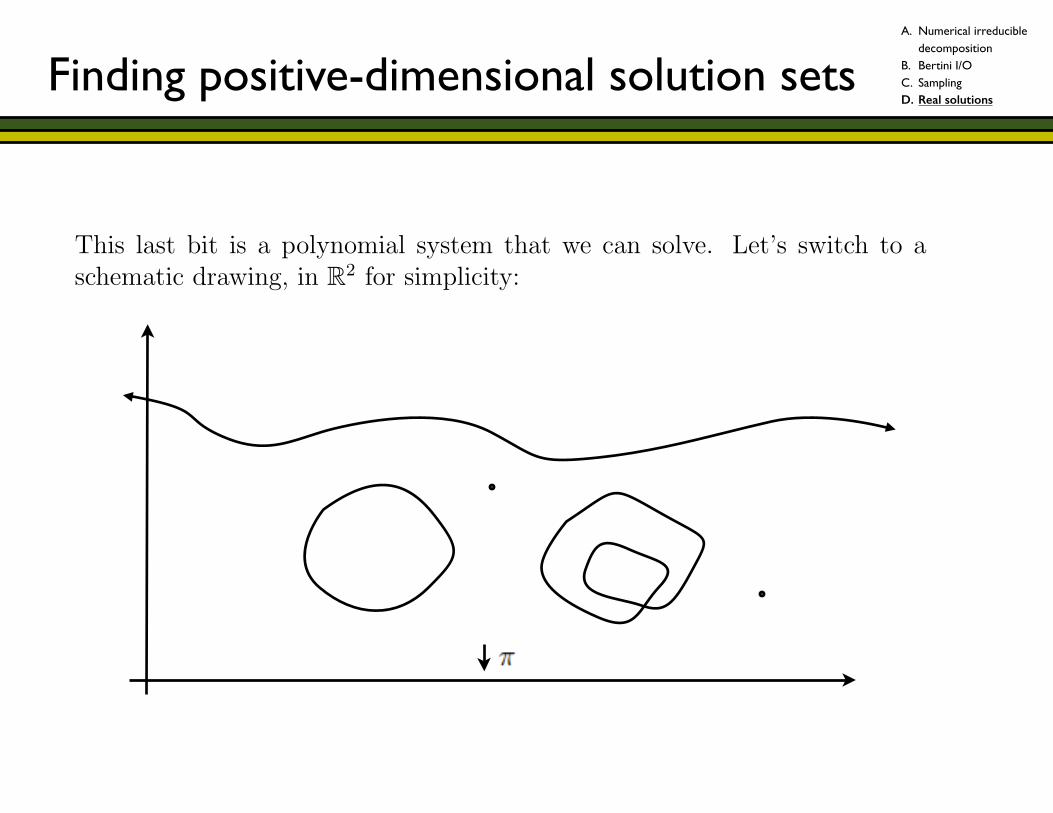
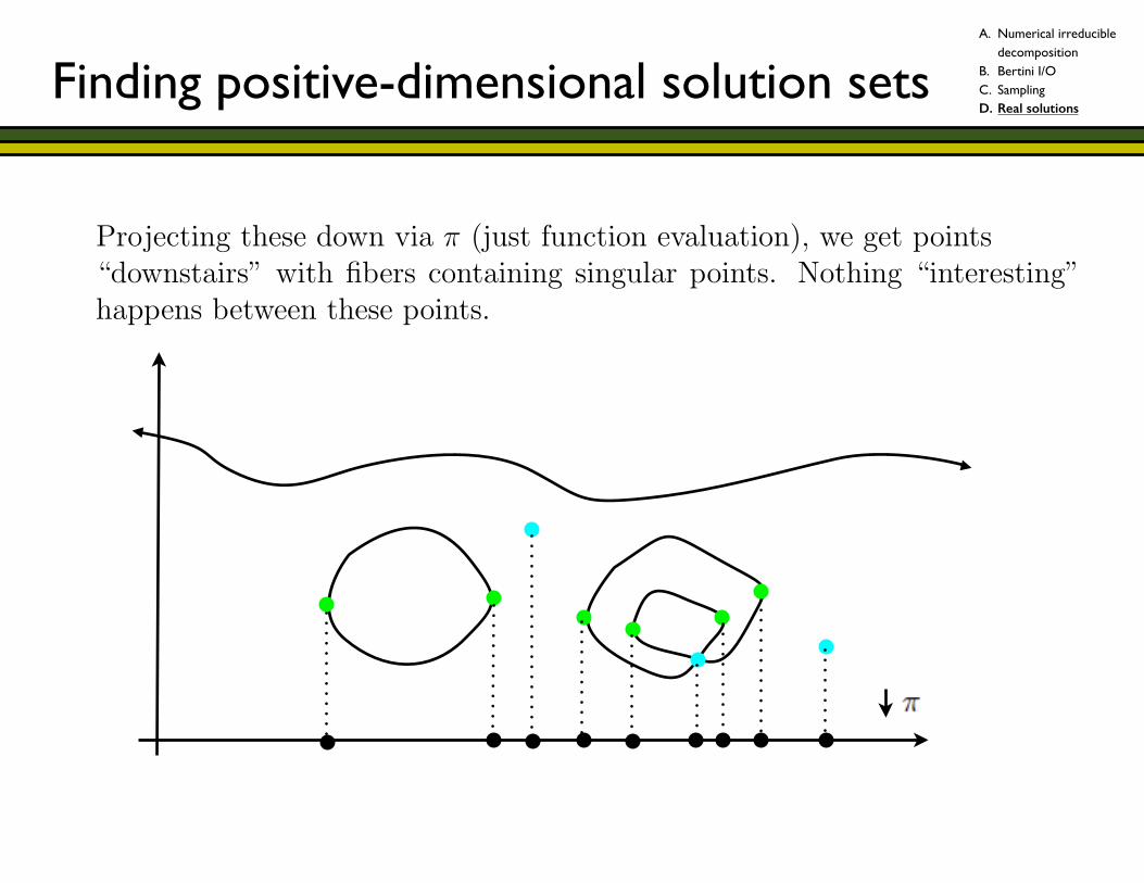
This last bit is a polynomial system that we can solve. Let’s switch to aschematic drawing, in R2 for simplicity:Notice that there are three real curves (two compact) and two points thatwe want to find.The polynomial system two slides back will find all inherent singular pointsand singular points of the projection (where topology changes occur).Projecting these down via �, we get points “downstairs” with fibers contain-ing singular points. Nothing “interesting” happens between these points.Choosing midpoints between these points “downstairs,” we may find allpoints in the fiber by moving the slices of the witness set for Z to the appro-priate linears.Moving these fiber points back and forth (moving the midpoints downstairsto the left and right to the black points), we get a schematic representation ofthe curve. This is impossible if the real curve is singular, without deflation.
7
Finding positive-dimensional solution setsA. Numerical irreducible
decomposition B. Bertini I/O C. Sampling D. Real solutions
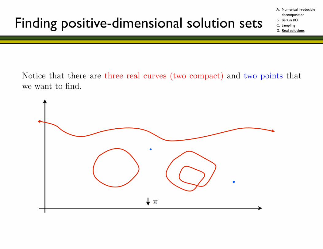
This last bit is a polynomial system that can easily solve. Let’s switch to aschematic drawing, in R2 for simplicity:Notice that there are three real curves (two compact) and two points thatwe want to find.The polynomial system two slides back will find all inherent singular pointsand singular points of the projection (where topology changes occur).Projecting these down via �, we get points “downstairs” with fibers contain-ing singular points. Nothing “interesting” happens between these points.Choosing midpoints between these points “downstairs,” we may find allpoints in the fiber by moving the slices of the witness set for Z to the appro-priate linears.
6
Finding positive-dimensional solution setsA. Numerical irreducible
decomposition B. Bertini I/O C. Sampling D. Real solutions
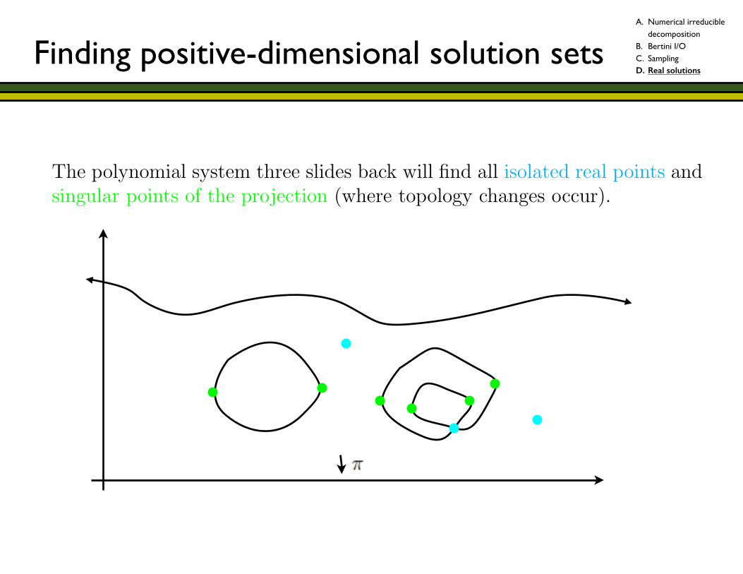
This last bit is a polynomial system that we can solve. Let’s switch to aschematic drawing, in R2 for simplicity:Notice that there are three real curves (two compact) and two points thatwe want to find.The polynomial system three slides back will find all isolated real points andsingular points of the projection (where topology changes occur).Projecting these down via � (just function evaluation), we get points“downstairs” with fibers containing singular points. Nothing “interesting”happens between these points.Choosing midpoints between these points “downstairs,” we may find allpoints in the fiber by moving the slices of the witness set for Z to the appro-priate linears. There is a special (parameter) homotopy for this move.Moving these fiber points back and forth (moving the midpoints downstairsto the left and right to the black points), we play connect-the-dots and get aschematic representation of the curve. If the real curve is singular deflationis necessary.
9
Finding positive-dimensional solution setsA. Numerical irreducible
decomposition B. Bertini I/O C. Sampling D. Real solutions
This last bit is a polynomial system that we can solve. Let’s switch to aschematic drawing, in R2 for simplicity:Notice that there are three real curves (two compact) and two points thatwe want to find.The polynomial system two slides back will find all inherent singular pointsand singular points of the projection (where topology changes occur).Projecting these down via � (just function evaluation), we get points“downstairs” with fibers containing singular points. Nothing “interesting”happens between these points.Choosing midpoints between these points “downstairs,” we may find allpoints in the fiber by moving the slices of the witness set for Z to the appro-priate linears.Moving these fiber points back and forth (moving the midpoints downstairsto the left and right to the black points), we get a schematic representation ofthe curve. This is impossible if the real curve is singular, without deflation.
7
Finding positive-dimensional solution setsA. Numerical irreducible
decomposition B. Bertini I/O C. Sampling D. Real solutions
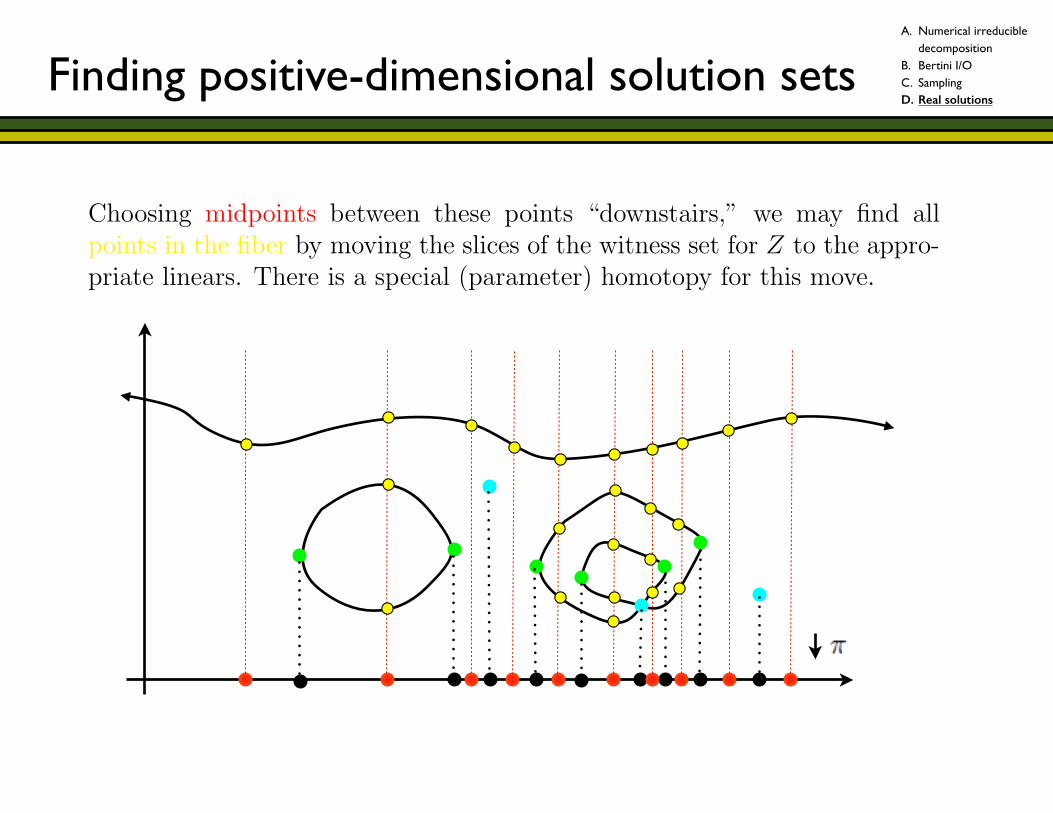
This last bit is a polynomial system that we can solve. Let’s switch to aschematic drawing, in R2 for simplicity:Notice that there are three real curves (two compact) and two points thatwe want to find.The polynomial system two slides back will find all inherent singular pointsand singular points of the projection (where topology changes occur).Projecting these down via � (just function evaluation), we get points“downstairs” with fibers containing singular points. Nothing “interesting”happens between these points.Choosing midpoints between these points “downstairs,” we may find allpoints in the fiber by moving the slices of the witness set for Z to the appro-priate linears. There is a special (parameter) homotopy for this move.Moving these fiber points back and forth (moving the midpoints downstairsto the left and right to the black points), we get a schematic representation ofthe curve. This is impossible if the real curve is singular, without deflation.
7
Finding positive-dimensional solution setsA. Numerical irreducible
decomposition B. Bertini I/O C. Sampling D. Real solutions
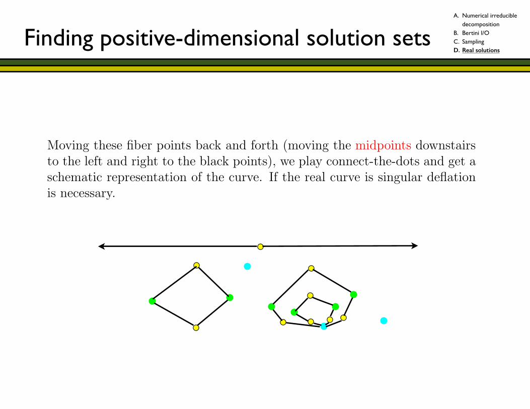
This last bit is a polynomial system that we can solve. Let’s switch to aschematic drawing, in R2 for simplicity:Notice that there are three real curves (two compact) and two points thatwe want to find.The polynomial system two slides back will find all inherent singular pointsand singular points of the projection (where topology changes occur).Projecting these down via � (just function evaluation), we get points“downstairs” with fibers containing singular points. Nothing “interesting”happens between these points.Choosing midpoints between these points “downstairs,” we may find allpoints in the fiber by moving the slices of the witness set for Z to the appro-priate linears. There is a special (parameter) homotopy for this move.Moving these fiber points back and forth (moving the midpoints downstairsto the left and right to the black points), we play connect-the-dots and get aschematic representation of the curve. If the real curve is singular deflationis necessary.
7
Finding positive-dimensional solution setsA. Numerical irreducible
decomposition B. Bertini I/O C. Sampling D. Real solutions
The surface case relies heavily on the curve case.
In the curve case, we find projections of critical points, then connect thedots in the fiber.
In the surface case, we find projections of critical points, constructcritical lines (giving critical curves), then connect the 2-D patches to thecritical curves.
Here’s a picture:
9
Now for the surface case: !!!
Finding positive-dimensional solution setsA. Numerical irreducible
decomposition B. Bertini I/O C. Sampling D. Real solutions
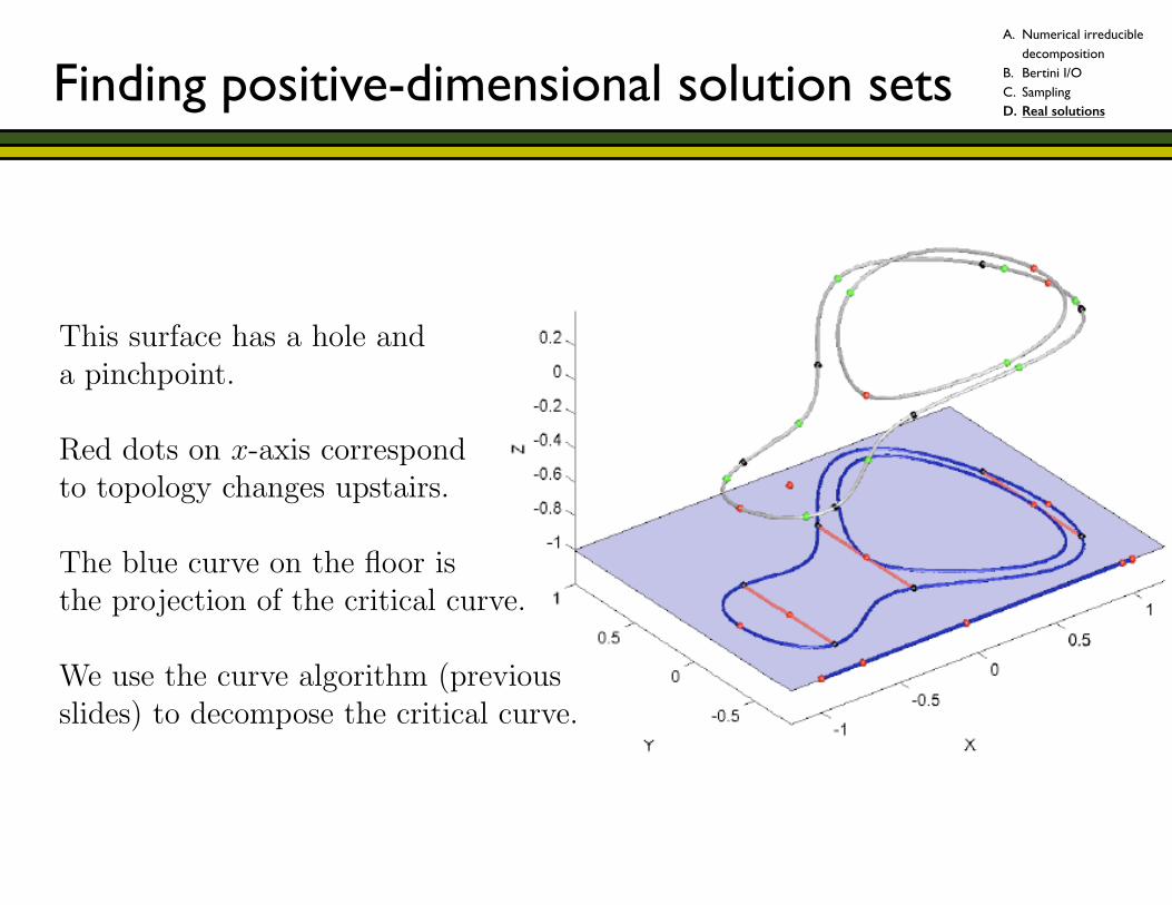
This surface has a hole anda pinchpoint.
Red dots on x-axis correspondto topology changes upstairs.
The blue curve on the floor isthe projection of the critical curve.
We use the curve algorithm (previousslides) to decompose the critical curve.
9
Finding positive-dimensional solution setsA. Numerical irreducible
decomposition B. Bertini I/O C. Sampling D. Real solutions
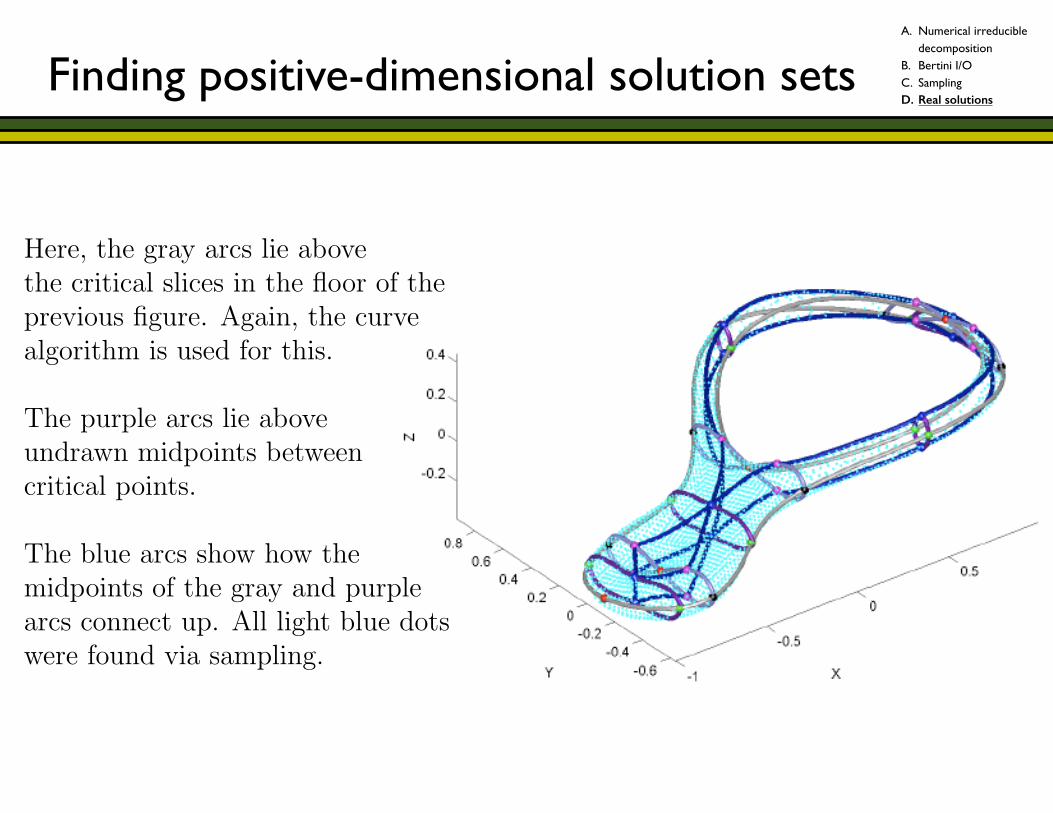
Here, the gray arcs lie abovethe critical slices in the floor of theprevious figure. Again, the curvealgorithm is used for this.
The purple arcs lie aboveundrawn midpoints betweencritical points.
The blue arcs show how themidpoints of the gray and purplearcs connect up. All light blue dotswere found via sampling.
10
Finding positive-dimensional solution setsA. Numerical irreducible
decomposition B. Bertini I/O C. Sampling D. Real solutions
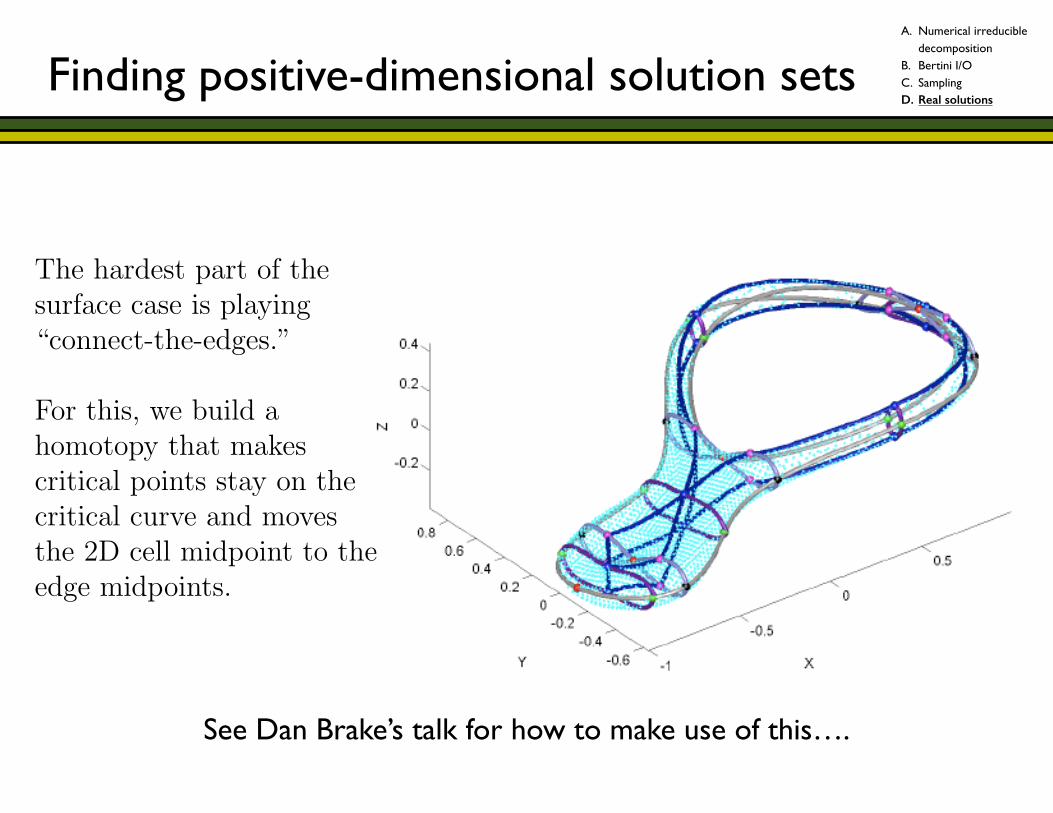
The hardest part of thesurface case is playing“connect-the-edges.”
For this, we build ahomotopy that makescritical points stay on thecritical curve and movesthe 2D cell midpoint to theedge midpoints.
12
See Dan Brake’s talk for how to make use of this….
Finding positive-dimensional solution setsA. Numerical irreducible
decomposition B. Bertini I/O C. Sampling D. Real solutions
General references for numerical algebraic geometry ! Sommese-Wampler, Numerical solution of polynomial systems arising in science and engineering, World Scientific, 2005. !Bates-Hauenstein-Sommese-Wampler, Numerically solving polynomial systems with Bertini, SIAM, 2013. !More specific references: !Path-tracking: Allgower-Georg, SIAM, 2004. Polyhedral methods: Li, Acta Numerica, 2003. Algebraic kinematics: Sommese-Wampler, Acta Numerica, 2013. Many more — just ask!
Finding positive-dimensional solution sets

THANKS!!! (These slides are already posted on my website.)
!!!!!!!!!!!!!!!!
Partially supported by NSF ACI-1440467, FA8650-13-1-7317, and the IMA.