Symbolic Solutions of First-Order Algebraic Differential ...
154
UNIVERSIT ¨ AT LINZ JOHANNES KEPLER JKU Technisch-Naturwissenschaftliche Fakult¨ at Symbolic Solutions of First-Order Algebraic Differential Equations DISSERTATION zur Erlangung des akademischen Grades Doktor der Technischen Wissenschaften im Doktoratsstudium der Technischen Wissenschaften Eingereicht von: Dipl.-Ing. Georg Grasegger Angefertigt am: Institut f¨ ur Symbolisches Rechnen, Doktoratskolleg Computational Mathematics (W1214) Beurteilung: Univ.-Prof. Dipl.-Ing. Dr. Franz Winkler (Betreuung) Prof. Dr. J. Rafael Sendra Linz, Juni 2015
-
Upload
khangminh22 -
Category
Documents
-
view
1 -
download
0
Transcript of Symbolic Solutions of First-Order Algebraic Differential ...

UNIVERSITAT LINZJOHANNES KEPLER JKU
Technisch-NaturwissenschaftlicheFakultat
Symbolic Solutions of First-Order AlgebraicDifferential Equations
DISSERTATION
zur Erlangung des akademischen Grades
Doktor der Technischen Wissenschaften
im Doktoratsstudium der
Technischen Wissenschaften
Eingereicht von:
Dipl.-Ing. Georg Grasegger
Angefertigt am:
Institut fur Symbolisches Rechnen,Doktoratskolleg Computational Mathematics (W1214)
Beurteilung:
Univ.-Prof. Dipl.-Ing. Dr. Franz Winkler (Betreuung)Prof. Dr. J. Rafael Sendra
Linz, Juni 2015


Eidesstattliche Erklarung
Ich erklare an Eides statt, dass ich die vorliegende Dissertation selbststandig und ohne
fremde Hilfe verfasst, andere als die angegebenen Quellen und Hilfsmittel nicht benutzt
bzw. die wortlich oder sinngemaß entnommenen Stellen als solche kenntlich gemacht
habe. Die vorliegende Dissertation ist mit dem elektronisch ubermittelten Textdoku-
ment identisch.
Linz, Juni 2015
Georg Grasegger
iii


Kurzfassung
Differentialgleichungen werden seit langer Zeit intensiv studiert. Diverse Methoden fur
spezielle Falle wurden entwickelt. Dennoch gibt es bisher keinen allgemeinen Algorith-
mus zur Berechnung expliziter exakter Losungen. Das wichtigste Ziel dieser Dissertation
ist die Entwicklung und Untersuchung neuer Methoden zur Berechnung exakter expli-
ziter Losungen von algebraischen Differentialgleichungen. Hierfur wird das differentielle
Problem in ein algebraisch geometrisches umgewandelt, indem die Differentialgleichung
als algebraische Gleichung betrachtet wird. Eine solche Gleichung beschreibt eine alge-
braische Varietat und somit konnen Werkzeuge der algebraischen Geometrie angewendet
werden. Im Speziellen spielen Parametrisierungen von algebraischen Varietaten eine we-
sentliche Rolle bei der Losung des Problems und beim Nachweis von Eigenschaften der
erhaltenen Losungen. Eine allgemeine Idee zum Losen autonomer algebraischer Diffe-
rentialgleichungen erster Ordnung wird prasentiert.
Das Hauptresultat der Dissertation ist die konkrete Anwendung der allgemeinen Idee auf
gewohnliche und partielle Differentialgleichungen. Die Idee wird fur autonome algebrai-
sche gewohnliche Differentialgleichungen erster Ordnung vorgestellt. Die prasentierte
Methode ist eine Verallgemeinerung von bereits existierenden Algorithmen zur Berech-
nung rationaler Losungen. Sie ermoglicht die Erweiterung zur Berechnung radikaler
Losungen. Außerdem erlaubt sie eine weitere Verallgemeinerung auf algebraische ge-
wohnliche Differentialgleichungen hoherer Ordnung. Ein zweiter Fokus liegt in der An-
wendung der allgemeinen Idee auf partielle Differentialgleichungen in beliebig vielen
Variablen. Die prasentierte Methode reduziert das Problem auf ein anderes, fur welches
Losungsmethoden existieren. Diverse bekannte Differentialgleichungen lassen sich mit
dieser Methode losen. Außerdem werden Klassen von Differentialgleichungen mit ratio-
nalen, radikalen oder algebraischen Losungen prasentiert. Mit Hilfe linearer Transforma-
tionen wird eine Methode fur gewisse nicht autonome Differentialgleichungen erreicht.
Die Methoden sind so konstruiert, dass die dadurch erhaltenen Losungen bestimmte
Kriterien erfullen. Es wird gezeigt, dass algebraische Losungen von gewohnlichen Diffe-
rentialgleichungen allgemeine Losungen sind. Rationale Losungen von partiellen Diffe-
rentialgleichungen sind bewiesenermaßen echt und vollstandig.
v


Abstract
Differential equations have been intensively studied for a long time. Various exact so-
lution methods have been proposed for specific cases. Nevertheless, there is no general
algorithm for finding explicit exact solutions. The main aim of this thesis is to develop
and investigate new methods for computing explicit exact solutions of algebraic differen-
tial equations. For this purpose, the differential problem is transformed into an algebraic
geometric one by considering the differential equation to be an algebraic equation. Such
an equation defines an algebraic variety and hence, tools from algebraic geometry can
be applied. In particular, parametrizations of algebraic varieties are intrinsically used
to solve the problem and prove properties of the obtained solutions. A general idea for
solving first-order autonomous algebraic differential equations is presented.
The main results of the thesis are applications of this general idea to ordinary and
partial differential equations. The idea is introduced for first-order autonomous algebraic
ordinary differential equations. The presented method is a generalization of an existing
algorithm for computing rational solutions. It admits an extension to the computation of
radical solutions. Moreover, it allows a further generalization to higher-order algebraic
ordinary differential equations.
A second focus lies on the application of the general idea to partial differential equations
in arbitrary many variables. The presented method reduces the problem to another one
for which solution methods exist. Various well-known differential equations are solved
by this method. Furthermore, classes of differential equations with rational, radical or
algebraic solutions are presented. With the help of linear transformations a solution
method for certain non-autonomous differential equations is achieved.
The procedures are constructed in such a way that the obtained solutions thereof sat-
isfy certain requirements. It is shown that algebraic solutions of ordinary differential
equations are general solutions. Rational solutions of partial differential equations are
proven to be proper and complete.
vii


Acknowledgments
First of all I want to thank my supervisor Franz Winkler for the chance to work in his
research group. His valuable and motivating advices have been an important factor of
my research. I appreciate a lot the chance to work on my own ideas and I also enjoyed
his lectures and the joint discussions.
I also want to express my gratitude to J. Rafael Sendra for his hospitality during my
research visit in Alcala. I learned a lot from him in the many fruitful mathematical
discussions. In this respect I also want to thank Alberto Lastra. Both of them made
my visit a most valuable one.
I want to thank James H. Davenport for hosting me at the university of Bath and for
discussions with him and Matthew England on the topic of my research. Similarly, I
thank Moulay A. Barkatou for the chance to visit him at the university of Limoges.
Furthermore, I thank the colleagues and secretaries at the doctoral program “Compu-
tational Mathematics” and at RISC for their help and the friendly atmosphere at the
institutes. The interesting research discussions at RISC have been a motivation for
many new ideas.
My special thanks go to my family who helped me a lot to achieve this goal. It was
due to their continuous support throughout the years, that I was able to focus on my
studies and research.
This thesis is based on research supported by the Austrian Science Fund (FWF) in
the frame of the doctoral program “Computational Mathematics”, grant W1214-N15,
project DK11.
ix


Contents
1. Introduction 1
1.1. Historical Background . . . . . . . . . . . . . . . . . . . . . . . . . . . . 2
1.2. Differential Algebra . . . . . . . . . . . . . . . . . . . . . . . . . . . . . . 3
1.2.1. Solutions of AODEs . . . . . . . . . . . . . . . . . . . . . . . . . 4
1.2.2. Solutions of APDEs . . . . . . . . . . . . . . . . . . . . . . . . . . 6
1.3. Algebraic Geometry . . . . . . . . . . . . . . . . . . . . . . . . . . . . . . 6
1.4. Differential Equations and Algebraic Hypersurfaces . . . . . . . . . . . . 8
2. Solution Method for AODEs 13
2.1. Rational Solutions . . . . . . . . . . . . . . . . . . . . . . . . . . . . . . 14
2.1.1. Autonomous First-Order AODEs . . . . . . . . . . . . . . . . . . 14
2.1.2. Non-autonomous First-Order AODEs . . . . . . . . . . . . . . . . 15
2.2. Non-rational Solutions . . . . . . . . . . . . . . . . . . . . . . . . . . . . 17
2.2.1. Radical Solutions . . . . . . . . . . . . . . . . . . . . . . . . . . . 21
2.2.2. Other Solutions . . . . . . . . . . . . . . . . . . . . . . . . . . . . 27
2.2.3. Investigation of the Procedure . . . . . . . . . . . . . . . . . . . . 28
2.3. Extension to Higher-Order AODEs . . . . . . . . . . . . . . . . . . . . . 30
3. Solution Method for APDEs 35
3.1. Two Variables . . . . . . . . . . . . . . . . . . . . . . . . . . . . . . . . . 36
3.1.1. Rational Solutions . . . . . . . . . . . . . . . . . . . . . . . . . . 41
3.1.2. Algebraic Solutions . . . . . . . . . . . . . . . . . . . . . . . . . . 47
3.1.3. Other Solutions . . . . . . . . . . . . . . . . . . . . . . . . . . . . 48
3.2. Three Variables . . . . . . . . . . . . . . . . . . . . . . . . . . . . . . . . 50
3.3. The General Case . . . . . . . . . . . . . . . . . . . . . . . . . . . . . . . 51
3.3.1. Rational Solutions . . . . . . . . . . . . . . . . . . . . . . . . . . 61
3.3.2. Other Solutions . . . . . . . . . . . . . . . . . . . . . . . . . . . . 64
3.4. Further approaches . . . . . . . . . . . . . . . . . . . . . . . . . . . . . . 67
xi

Contents
4. Linear Transformations 81
4.1. Linear Transformations of First-Order APDEs . . . . . . . . . . . . . . . 82
4.1.1. Properties Preserved by Linear Transformations . . . . . . . . . . 85
4.1.2. Linear Transformations of Special Equations . . . . . . . . . . . . 89
4.2. Linear Transformations of Higher-Order APDEs . . . . . . . . . . . . . . 92
5. Conclusion 95
A. More Differential Algebra 97
B. Parametrizations 101
B.1. Rational Parametrization . . . . . . . . . . . . . . . . . . . . . . . . . . . 101
B.1.1. Rational Parametrization of Curves . . . . . . . . . . . . . . . . . 102
B.1.2. Rational Parametrization of Surfaces . . . . . . . . . . . . . . . . 103
B.1.3. Rational Parametrization of Hypersurfaces . . . . . . . . . . . . . 109
B.2. Radical Parametrization . . . . . . . . . . . . . . . . . . . . . . . . . . . 110
B.2.1. Radical Parametrization of Curves . . . . . . . . . . . . . . . . . 110
B.2.2. Radical Parametrization of Surfaces . . . . . . . . . . . . . . . . . 111
B.2.3. Radical Parametrization of Hypersurfaces . . . . . . . . . . . . . 112
B.3. Other Parametrizations . . . . . . . . . . . . . . . . . . . . . . . . . . . . 113
C. List of Differential Equations 115
C.1. First-Order AODEs . . . . . . . . . . . . . . . . . . . . . . . . . . . . . . 115
C.2. Higher-Order AODEs . . . . . . . . . . . . . . . . . . . . . . . . . . . . . 116
C.3. First-Order APDEs . . . . . . . . . . . . . . . . . . . . . . . . . . . . . . 117
D. Method of Characteristics 125
Index 127
Bibliography 131
Curriculum Vitae 139
xii

1. Introduction
In the literature one can choose among several exact methods in order to solve ordinary
and partial differential equations (see for instance [73, Section II.B]). The main aim of
the present work is to provide an alternative novel exact method for solving first-order
algebraic differential equations. Our method provides a tool for systematically solving
various well-known equations.
In this chapter we introduce the topic and we describe some of the ideas which the
method is based on. In Section 1.1 we give an overview of similar and more specific
methods and their historical background. Later we briefly describe the important no-
tions of differential algebra (Section 1.2) and algebraic geometry (Section 1.3). Basic
key facts of both areas are summarized. In the last part of the introduction we investi-
gate the relation between solutions of differential equations and algebraic hypersurfaces.
This relation figures the general idea of our method (Section 1.4).
In Chapter 2 we show how this idea can be applied to find radical solutions of first-order
autonomous algebraic ordinary differential equations. This generalizes some previously
known methods which are therefore briefly presented as well. We also give an idea of
further generalization to finding non-algebraic solutions. At the end of the chapter we
elaborate some advantages of the method.
Next we present a generalization of the new method to partial differential equations in
Chapter 3. We first bring up the idea for the case of two variables. All important aspects
of the procedure can be found there. The method is illustrated by examples and classes
of partial differential equations with rational solutions are given. As an intermediate
step we show the case of three variable separately before we extend the method to an
arbitrary number of variables.
Finally, in Chapter 4 we introduce linear transformations and their application for solv-
ing some non-autonomous differential equations. These transformations have been used
for solving and classifying algebraic ordinary differential equations. We show how the
ideas can be used for partial differential equations.
1

1. Introduction
Additional information on differential algebra and algebraic geometry as well as an
extensive list of well-known ordinary and partial differential equations with computed
solutions can be found in the appendix.
The content of the thesis is based on the papers (co)authored by Grasegger [23, 21,
22]. Moreover, this thesis also contains further ideas and investigations. The main
contributions of the author are novel procedures for explicitly solving various classes of
algebraic differential equations. These include but are not restricted to
• autonomous algebraic ordinary differential equations of any order and rational
respectively radical solutions thereof,
• first-order autonomous algebraic partial differential equations (for arbitrary many
variables).
1.1. Historical Background
Recently algebraic-geometric solution methods for first-order algebraic ordinary differ-
ential equations (AODEs) have been investigated. A first result on computing solutions
of AODEs was presented in [30]. In this paper Hubert introduces a method for finding
implicit general and singular solutions of AODEs by computing Grobner bases. Later
in Eremenko [15] a degree bound for rational solutions of a given AODE is computed.
Such a bound enables to find solutions by solving algebraic equations.
The starting point for algebraic-geometric methods, such as the one described in this
thesis, was an algorithm by Feng and Gao [17, 19]. This algorithm decides whether or
not an autonomous first-order AODE, F (y, y′) = 0, has a rational solution and in the
affirmative case computes it. This is done by transformation properties between different
proper curve parametrizations and by a degree bound on such parametrizations [62]
which leads to a degree bound on the solutions. Hence, existence of a rational solution
can be decided. From a rational solution a rational general solution can be deduced.
Efficiency of the algorithm is obtained by Laurent series and Pade approximants. The
basic idea of the algorithm is presented in Section 2.1.1.
Using the ideas of Feng and Gao several generalizations have been investigated since
then. Aroca, Cano, Feng and Gao [5] presented an algorithm for finding algebraic
solutions of first-order autonomous AODEs. Ngo and Winkler [44, 45, 46] introduced
2

1.2. Differential Algebra
a method for finding rational solutions of non-autonomous AODEs, F (x, y, y′) = 0.
Here, parametrizations of surfaces play an important role. On the basis of a proper
parametrization, the algorithm builds a so called associated system of first-order linear
ODEs for which solution methods exist. Based on invariant algebraic curves a solution
of the associated system leads to a rational general solution of the differential equation.
A short introduction to this method is given in Section 2.1.2.
First results on higher-order AODEs can be found in [27, 28, 29]. Given a proper rational
hypersurface parametrization the solutions of the AODE correspond to solutions of an
associated system.
As shown in [37] also one-dimensional systems of first-order AODEs can be treated in a
similar way.
For partial differential equations much less is known. Of course several solution methods
do exist and can be found in standard textbooks but the knowledge on explicit symbolic
solutions is worth further investigation. For linear and quasilinear equations solution
methods can be found in textbooks (see for instance [73]). The method of characteristics
for instance can be applied to quasilinear equations. However, it might not always give
an explicit solution. Using this method it is possible to transform a partial differen-
tial equation to a system of ordinary ones. The method of characteristic plays a role
in our procedure for partial differential equations. A generalization of the method of
characteristics to arbitrary first-order partial differential equations was investigated by
Lagrange and Charpit (compare [66]). However, we show that our method is essentially
different.
1.2. Differential Algebra
All necessary notions of differential algebra which are needed in this thesis can found in
standard textbooks such as Ritt [55] or Kolchin [33]. We recall some important aspects
here and refer to Appendix A for a little more information.
We consider the field of rational functions K(x1, . . . , xn) for some algebraically closed
field K of characteristic 0; in practice, one may think of K as the field C of complex
numbers. By ∂∂xi
we denote the usual derivative by xi. Sometimes we might use the
abbreviations uxi = ∂u∂xi
. In case n = 1 we also write x for x1 and ′ or ddx
for ∂∂xi
. For
3

1. Introduction
higher-order derivatives we use u(1) = u′ and recursively u(k) = (u(k−1))′. In case n = 2
we also write x for x1 and y for x2. Then K(x1, . . . , xn) together with the derivations
is a (partial) differential field , i. e. the derivations are linear with respect to addition
and fulfill the Leibniz rule and moreover ∂∂xi
(∂u∂xj
)= ∂
∂xj
(∂u∂xi
). Hence, we might use
shorthand notation
∂2
∂x2j
=∂
∂xj
(∂
∂xj
),
∂k
∂xkj=
∂
∂xj
(∂k−1
∂xk−1j
),
∂k1+...+kn
∂xk11 . . . ∂xknn=
∂
∂xk11
(. . .
(∂
∂xkn−1
n−1
(∂
∂xknn
))).
As short hand notation we might also use u(k1,...,kn) = ∂k1+...+knu
∂xk11 ...∂xknn
.
The ring of differential polynomials is denoted by K(x1, . . . , xn){u}. It consists of all
polynomials in u and its derivatives, i. e.
K(x1, . . . , xn){u} = K(x1, . . . , xn)[u, ux1 , . . . , uxn , ux1x1 , . . . , uxnxn , . . .] .
An algebraic differential equation (ADE) is defined by a differential polynomial F ∈K(x1, . . . , xn){u} which is also a polynomial in x1, . . . , xn. We write
F (x1, . . . , xn, u, ux1 , . . . , uxn , ux1x1 , ux1x2 , . . . , ux1xn , . . . , uxnxn , . . .) = 0
for the considered differential equation. In case n = 1 this is an algebraic ordinary
differential equation (AODE). In case n > 1 it is an algebraic partial differential equation
(APDE). An ADE is called autonomous iff F ∈ K{u}, i. e. if the coefficients of F do not
depend on the variables of differentiation x1, . . . , xn. We call an ADE non-autonomous
if it is not necessarily autonomous.
1.2.1. Solutions of AODEs
Usually we want to describe solutions of ADEs by an expression which is as general as
possible, i. e. an expression which declares almost all solutions. Such an expression shall
be called a general solution. In the following we give a precise definition for the case of
AODEs. Let Σ be a prime differential ideal in K(x){u}. Then we call η a generic zero
4

1.2. Differential Algebra
of Σ iff for any differential polynomial P ∈ K(x){u} we have P (η) = 0 ⇐⇒ P ∈ Σ.
Such an η exists in a suitable extension field since Σ is prime.
Let F be an irreducible differential polynomial of order n. Then {F}, the radical
differential ideal generated by F , can be decomposed essential prime differential ideals
Σ1, . . . ,Σk (c. f. [55, Chapter II]).
{F} = Σ1 ∩ . . . ∩ Σk .
A prime divisor of an ideal is called essential if it does not contain any other prime
divisor. There is one component where the separant S := ∂F∂u(n)
does not vanish. It is a
prime differential ideal
Σ1 = {F} : 〈S〉 = {P ∈ K(x){u} |SA ∈ {F}} .
This Σ1 represents the general component.
The other part {F, S} represents the singular component . It can be further decomposed
in Σ2 ∩ . . . ∩ Σk.
A zero of {F} is called a solution of F . A solution is called non-singular if it does
not annul the separant. Otherwise it is called singular . The non-singular zeros are all
contained in the general component.
A generic zero of Σ1 is called a general solution of F = 0. A general solution depends
on some transcendental constant. Every non-singular solutions can be expressed by a
certain evaluation of the constants in the general solution. No choice of evaluating the
constant yields a singular solution.
Example 1.1.
Let us consider the AODE, F (u, u′) = u′2 + u′ − 2u− x = 0. Then 12(c + (c + x)2) is a
general solution. The separant of F is S = 2u′+ 1 which has solutions −x2
+ k for some
constant k. We choose k = −18
such that the solution of the separant is also a solution
of F . Then −x2− 1
8is a singular solution. It is easy to see that no choice of c in the
general solution would yield the singular one.
We say a general solution is rational if it is of the form u = akxk+...+a1x+a0
bmxm+...+b1x+b0, where the
ai and bi are constants in some field extension of K. An algebraic general solution is
a general solution v(x) which satisfies an algebraic equation g(x, u) = 0 (c. f. [5]). In
Section 2.2 we define the subclass of radical solutions.
5

1. Introduction
1.2.2. Solutions of APDEs
Similarly to the case of AODEs we want to describe solutions of partial differential
equations in a preferably general way. Again the ideal {F}, the radical differential ideal
generated by F , can be decomposed into prime differential ideals Σ1, . . . ,Σk (c. f. [55,
Chapter IX]),
{F} = Σ1 ∩ . . . ∩ Σk .
Furthermore, we can assume that all these prime differential ideals are essential. In
partial differential algebra the separant is defined with respect to an ordering of the
derivatives (for further details see Appendix A). Let v be the leader of F according
to this ordering. Then the separant of F is defined as ∂F∂v
. Let Σ1 be the part where
the separant does not vanish (such a component exists). In fact, Σ1 does not contain
any separant, whereas the other Σk contain all separants. Hence, Σ1 is the general
component, and the other Σk form the singular components. A zero of some Σk is called
a solution. A solution is called non-singular if it does not annul any of the separants.
Otherwise it is called singular . Then a general solution of F is the manifold of Σ1, i. e.
the set of all zeros of Σ1. Since Σ1 is a prime differential ideal, it has a generic zero.
Sometimes this generic zero is also called a general solution.
A solution u of an APDE is called rational if it is of the form u = a(x1,...,xn)b(x1,...,xn)
where a
and b 6= 0 are polynomials in K[x1, . . . , xn]. For APDEs, in difference to AODEs, there
is also an intermediate level of generally describing solutions. Such solutions are called
complete. This and other important properties of solutions of APDEs are described
later in Section 1.4.
1.3. Algebraic Geometry
An algebraic hypersurface S is an algebraic variety of codimension 1, i. e. a zero set of a
squarefree non-constant polynomial f ∈ K[x1, . . . , xn],
S = {(a1, . . . , an) ∈ An | f(a1, . . . , an) = 0} ,
where An is the n-dimensional affine space over K. In case n = 2 we call S an algebraic
curve. In case n = 3 we call S an algebraic surface. The polynomial f is identified
6
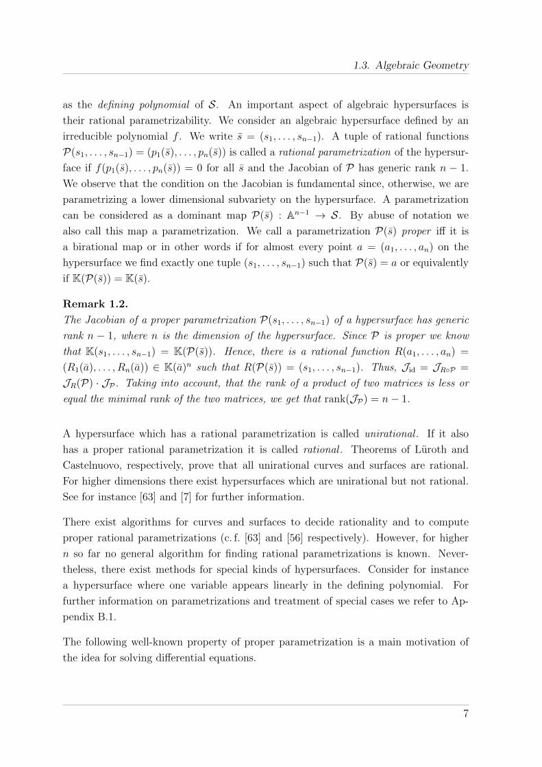
1.3. Algebraic Geometry
as the defining polynomial of S. An important aspect of algebraic hypersurfaces is
their rational parametrizability. We consider an algebraic hypersurface defined by an
irreducible polynomial f . We write s = (s1, . . . , sn−1). A tuple of rational functions
P(s1, . . . , sn−1) = (p1(s), . . . , pn(s)) is called a rational parametrization of the hypersur-
face if f(p1(s), . . . , pn(s)) = 0 for all s and the Jacobian of P has generic rank n − 1.
We observe that the condition on the Jacobian is fundamental since, otherwise, we are
parametrizing a lower dimensional subvariety on the hypersurface. A parametrization
can be considered as a dominant map P(s) : An−1 → S. By abuse of notation we
also call this map a parametrization. We call a parametrization P(s) proper iff it is
a birational map or in other words if for almost every point a = (a1, . . . , an) on the
hypersurface we find exactly one tuple (s1, . . . , sn−1) such that P(s) = a or equivalently
if K(P(s)) = K(s).
Remark 1.2.
The Jacobian of a proper parametrization P(s1, . . . , sn−1) of a hypersurface has generic
rank n − 1, where n is the dimension of the hypersurface. Since P is proper we know
that K(s1, . . . , sn−1) = K(P(s)). Hence, there is a rational function R(a1, . . . , an) =
(R1(a), . . . , Rn(a)) ∈ K(a)n such that R(P(s)) = (s1, . . . , sn−1). Thus, Jid = JR◦P =
JR(P) · JP . Taking into account, that the rank of a product of two matrices is less or
equal the minimal rank of the two matrices, we get that rank(JP) = n− 1.
A hypersurface which has a rational parametrization is called unirational . If it also
has a proper rational parametrization it is called rational . Theorems of Luroth and
Castelnuovo, respectively, prove that all unirational curves and surfaces are rational.
For higher dimensions there exist hypersurfaces which are unirational but not rational.
See for instance [63] and [7] for further information.
There exist algorithms for curves and surfaces to decide rationality and to compute
proper rational parametrizations (c. f. [63] and [56] respectively). However, for higher
n so far no general algorithm for finding rational parametrizations is known. Never-
theless, there exist methods for special kinds of hypersurfaces. Consider for instance
a hypersurface where one variable appears linearly in the defining polynomial. For
further information on parametrizations and treatment of special cases we refer to Ap-
pendix B.1.
The following well-known property of proper parametrization is a main motivation of
the idea for solving differential equations.
7

1. Introduction
Lemma 1.3.
Let P(s), Q(s) be two proper parametrizations of some algebraic hypersurface S ⊆ An.
Then there exists a rational function R(s) ∈ K(s) such that Q(s) = P(R(s)).
• In case n = 2, R(s) is a Mobius transformation, i. e. a linear rational function
R(s1) = a0+a1s1b0+b1s1
with a0b1 − a1b0 6= 0.
• In case n = 3, R(s) is a Cremona transformation (i. e. a birational map of the
plane to itself), and hence by the theorem of Castelnuovo-Noether a finite compo-
sition of quadratic transformations (s1, s2) 7→ (a0+a1s1+a2s2b0+b1s1+b2s2
, c0+c1s1+c2s2d0+d1s1+d2s2
) and pro-
jective linear transformations (c. f. [8, 64]).
• In general R(s) = P(Q−1(s)).
1.4. Differential Equations and Algebraic Hypersurfaces
Let F (u, ux1 , . . . , uxn) = 0 be an autonomous APDE. We consider the corresponding
algebraic hypersurface developed by replacing the derivatives by independent transcen-
dental variables, F (z, p1, . . . , pn) = 0. Whenever we talk about the differential equation
and its solutions we use the variables x1, . . . , xn. To distinguish the parametrization
problem we use the variables s1, . . . , sn there.
Given any non-constant differentiable function u(x1, . . . , xn) which satisfies the APDE,
F (u, ux1 , . . . , uxn) = 0, the tuple (u(s1, . . . , sn), ux1(s1, . . . , sn), . . . , uxn(s1, . . . , sn)) is a
parametrization. We call this parametrization the corresponding parametrization of the
solution and denote it usually by L. We observe that the corresponding parametrization
of a solution is not necessarily a parametrization of the associated hypersurface, since the
condition on the rank of the Jacobian may fail. For instance, let us consider the APDE,
ux = 0, with n = 2. A solution would be of the form u(x, y) = g(y), with g differentiable.
However, this solution generates (g(s2), 0, g′(s2)) that is a curve in the surface; namely
the plane p = 0. Now, consider the APDE, ux = λ, with λ a nonzero constant. Hence,
the solutions are of the form u(x, y) = λx+ g(y). Then, u(x, y) = λx+ y generates the
line (λs1+s2, λ, 1) while u(x, y) = λx+y2 generates the parametrization (λs1+s22, λ, 2s2)
of the associated plane p = λ. These examples motivate the following definition. Clearly,
a solution of an APDE is a function u(x1, . . . , xn) such that F (u, ux1 , . . . , uxn) = 0.
8

1.4. Differential Equations and Algebraic Hypersurfaces
Definition 1.4.
A solution of an APDE is rational iff u(x1, . . . , xn) is a rational function over K.
A rational solution of an APDE is proper iff the corresponding parametrization is proper.
In the case of autonomous ordinary differential equations, every non-constant solution
induces a proper parametrization of the associated curve (see [17]). However, this is not
true in general for autonomous APDEs. For instance, the solution x + y3 of ux = 1,
induces the parametrization (s1 + s32, 1, 3s
22) which is, although its Jacobian has rank 2,
not proper.
In addition, we observe that it can happen that none of the rational solutions of an
APDE is proper. This is the case for instance, of ux = 0, since all rational solutions are
of the form u = R(y), for some rational function R and K(R(s1), 0, R′(s1)) ( K(s1, s2).
Furthermore, we see that none of the solutions of this APDE generates a parametrization
of the associated hypersurface, since the Jacobian has rank 1.
Every solution of the problem under consideration in this work can be attained by the
knowledge of a set of complete solutions. We will see details later. For this reason,
we focus on finding families of complete solutions. This notion of a complete solution
is due to Lagrange (compare [14]). He calls a solution u(x, y) of a first-order PDE
complete, if it depends on two arbitrary constants, i. e. u(x, y) = u(x, y, c1, c2), such
that the elimination of the constants in the equations z−u, p−ux, q−uy gives back the
differential equation. Such a property for rational functions can be proven by Grobner
bases.
For the following we use a definition of completeness which is easier to check. This
definition can be found for instance in [31, 50].
Definition 1.5.
Let F (u, ux1 , . . . , uxn) = 0 be an autonomous APDE. Let u be a rational solution depend-
ing on n arbitrary constants c1, . . . , cn. Let L = (v0, v1, . . . , vn) be the parametrization
induced by the solution, i. e. v0 = u and vi = uxi for i ≥ 1. We call the solution complete
if the Jacobian J c1,...,cnL of L with respect to c1, . . . , cn has generic rank n.
We call the solution complete of suitable dimension if it is complete and the Jacobian
J s1,...,snL of L with respect to s1, . . . , sn has generic rank n.
Intuitively speaking, the notion of a complete solution is requiring that the correspond-
ing parametrization of the solution parametrizes an algebraic set on the hypersurface,
9

1. Introduction
independently of the constants c1, . . . , cn. On the other hand, the notion of suitable
dimension ensures that the corresponding parametrization really parametrizes the asso-
ciated hypersurface and not a lower dimensional subvariety.
The following example illustrates proper, complete and non-complete solutions for some
simple APDEs.
Example 1.6.
We consider the APDE, F (u, ux, uy) = ux = 0, with the solution u(x, y) = y + c1 + c2.
The corresponding parametrization is L = (s2 + c1 + c2, 0, 1). Then
J c1,c2L =
1 1
0 0
0 0
,
and hence u(x, y) is not complete. However, if we take u(x, y) = c1y + c2, the Jacobian
with respect to c1, c2 has generic rank 2, and u is complete but not of suitable dimension,
since the Jacobian of L with respect to s1, s2 has rank 1.
Now, we take the APDE, ux = 1. In Table 1.1 we see solutions and their properties.
Note, that the solution x+c1 +y2 +c2 is not complete and hence, not complete of suitable
dimension. However, the other requirement of suitable dimension is fulfilled.
solution complete suitable dim proper rank(J s1,s2L )
x+ c1 F F F 1
x+ y + c1 + c2 F F F 1
x+ c1 + c2y T F F 1
x+ c1 + y2 + c2 F F* T 2
x+ c1 + c2y2 T T T 2
x+ c1 + (y + c2)2 T T T 2
x+ c1 + (y + c2)3 T T F 2
x+ c1 + y3 + c2 F F* F 2
Table 1.1.: Properties of some solutions of ux = 1, where T means true, F false and F*
false since not complete but condition on Jacobian is true
Note, that in this example all possible combinations of properties are found. Indeed, by
Remark 1.2 the Jacobian of a proper solution has generic rank n and hence there is no
rational solution which is proper and complete but not of suitable dimension.
10

1.4. Differential Equations and Algebraic Hypersurfaces
In the case of AODEs, i. e. n = 1, the notion of complete and general solution is equiv-
alent. This is not the case for APDEs. Nevertheless, as shown by Lagrange (c. f. [14])
from a complete solution one can compute singular and general solutions by envelopes.
An envelope of a one-parameter family of surfaces, given implicitly by g(x, y, z, a) = 0
for parameters a, is the surface which touches each point on any of the surfaces in the
family. It is defined by the solution of the system
g(x, y, z, a) = 0 , ga(x, y, z, a) = 0 .
An envelope of a two-parameter family of surfaces, defined by g(x, y, z, a1, a2) = 0 for
parameters a1 and a2, is the surface which touches each point on any of the surfaces in
the family. It is defined by the solution of the system
g(x, y, z, a1, a2) = 0 , ga1(x, y, z, a1, a2) = 0 , ga2(x, y, z, a1, a2) = 0 .
Let us consider a complete rational solution u(x, y, c1, c2) of some APDE. Hence, the
equation of the family of surfaces is z − u(x, y, c1, c2) = 0.
Assume now c2 = ϕ(c1) for some function ϕ. Then, we consider the envelope of the
family of surfaces u(x, y, c1, ϕ(c1)), i. e. we solve 0 = ∂u(x,y,c1,ϕ(c1))∂c1
= uc1 + uc2ϕ′(c1)
for c1. Let c1 = ψ(x, y) be the solution. Then u(x, y, ψ(x, y), ϕ(ψ(x, y))) is a general
solution of the APDE, where ϕ is an arbitrary function.
On the other hand we might compute the envelope with respect to c1 and c2, i. e. solve
the equations ∂u∂c1
= ∂u∂c2
= 0 for c1 and c2. Let c1 = ϕ(x, y) and c2 = ψ(x, y). Then
u(x, y, ϕ(x, y), ψ(x, y)) is a singular solution of the APDE.
These computations can be done as well for implicitly given solutions (as actually shown
in [14]) and for APDEs in more variables.
General idea for solving AODEs and APDEs
We now want to present the general idea of the main procedure presented in this thesis.
Here only the introductory part, which does not depend on a specific number of variables,
is described. Details for AODEs can be found in Section 2.2. The procedure for APDEs
is presented in Section 3.1 and 3.3 for 2 and n variables respectively.
11

1. Introduction
Let F (u, ux1 , . . . , uxn) = 0 be an algebraic (partial) differential equation, where F is an
irreducible non-constant polynomial. We consider the hypersurface F (z, p1, . . . , pn) = 0
and assume it admits a proper (rational) hypersurface parametrization
Q(s1, . . . , sn) = (q0(s1, . . . , sn), q1(s1, . . . , sn), . . . , qn(s1, . . . , sn)) .
A summary of results for the problem of hypersurface parametrization is given in Ap-
pendix B.1.
Assume that L(s1, . . . , sn) = (v0, . . . , vn) corresponds to a solution of the APDE. Fur-
thermore we assume that the parametrization Q can be expressed as
Q(s1, . . . , sn) = L(g(s1, . . . , sn)) (1.1)
for some invertible function g(s1, . . . , sn) = (g1(s1, . . . , sn), . . . , gn(s1, . . . , sn)). This as-
sumption is motivated by the fact that in case of rational algebraic curves every non-
constant rational solution of an AODE yields a proper rational parametrization of the
associated algebraic curve (c. f. [17]) and each proper rational parametrization can be
obtained from any other proper one by a rational transformation (c. f. Lemma 1.3). In
the case of APDEs, however, not all rational solutions provide a proper parametrization,
as mentioned in the remark after Definition 1.4. What we still know is that any proper
rational hypersurface parametrization can be obtained from any other proper one by a
rational transformation. Assuming that g exists, it would be enough to find g−1 in order
to get the solution q0(g−1(x1, . . . , xn)). Looking at the Jacobian of the parametrizations,
equation (1.1) implies the following equation:
JQ(s1, . . . , sn) = JL(g(s1, . . . , sn)) · Jg(s1, . . . , sn) .
In particular we consider the first row,
∂q0
∂s1
=n∑i=1
∂v0
∂si(g)
∂gi∂s1
=n∑i=1
qi(s1, . . . , sn)∂gi∂s1
,
...
∂q0
∂sn=
n∑i=1
∂v0
∂si(g)
∂gi∂sn
=n∑i=1
qi(s1, . . . , sn)∂gi∂sn
.
(1.2)
This is a system of quasilinear equations in the unknown functions g1 to gn. In case of
n = 1 the system reduces to a single ordinary differential equation. Details on that case
are presented in Chapter 2. Further investigation of the APDE case can be found in
Chapter 3.
12

2. Solution Method for AODEs
As mentioned in the introduction there exist several algorithms for solving first-order
AODEs of some special kind. Especially linear AODEs are well-studied objects. In
this chapter we briefly describe some existing algorithms for finding explicit rational
solutions of (non-linear) first-order AODEs (Section 2.1).
We mainly focus on an algorithm by Feng and Gao for autonomous first-order AODEs
(Section 2.1.1) which can be considered to be the basis of subsequent algebraic-geometric
methods; among others the generalization of Ngo and Winkler for non-autonomous first-
order AODEs (Section 2.1.2). Likewise based on these algorithms we present an extended
method for finding radical solutions of first-order autonomous AODEs (Section 2.2).
This new procedure generalizes existing algorithms and follows the framework presented
in Section 1.4.
Using the general idea of finding a suitable transformation of a given parametrization,
for n = 1 the system (1.2) reduces to a single ODE which is easily solvable by existing
algorithms. Deduced from special properties of the components of a given proper rational
or radical parametrization, several classes of AODEs with radical solutions are presented.
Later we illustrate that this new method is not restricted to the computation of algebraic
solutions (Section 2.2.2).
In Section 2.3 we present ideas for a generalization to higher-order AODEs. We start
with an approach for special second-order AODEs and show difficulties arising in respect
of further generalization. Later we use ideas from partial differential equations for solving
general second-order and higher-order AODEs.
Examples are provided throughout the sections whenever suitable. For a more extensive
list of (well-known) examples from literature which can be solved by the method we
refer to Appendix C.1.
13

2. Solution Method for AODEs
2.1. Rational Solutions
Recently two algorithms for solving first-order AODEs have been presented. Both of
them intrinsically use rational parametrizations of curves respectively surfaces. In Sec-
tion 2.1.1 we recall an algorithm for finding rational solutions of autonomous first-order
AODEs. It is based on the computation of a proper rational parametrization and the
fact that a solution of the AODE yields such a parametrization.
Several improvements and generalizations of this algorithm have been published. Some
of these are presented in the following and references are given for others. First we recall
an algorithm for finding rational solutions of non-autonomous AODEs (Section 2.1.2).
Later, in Section 2.2 we present a new generalized method for finding non-rational
solutions of autonomous AODEs.
2.1.1. Autonomous First-Order AODEs
In this section we briefly describe the algorithm of Feng and Gao [17] for finding rational
solutions of autonomous first-order AODEs. As a key fact they show that any rational
solution v of an autonomous AODE corresponds to a proper rational parametrization
L = (v, v′). Furthermore, it is known, that from any proper rational parametrization Qany other proper parametrization P can be obtained by a transformation with a linear
rational function, i. e. P(s) = Q(a0+a1sb0+b1s
), (see Lemma 1.3).
Theorem 2.1. (Feng and Gao [17])
Let F (u, u′) = 0 be an autonomous first-order AODE. It has a rational general solution
if and only if there is a proper parametrization Q(s) = (q0(s), q1(s)) over Q of the
corresponding curve F (z, p) = 0 and for any such parametrization the indicator A :=q1(s)q′0(s)
is either in Q or equal to a(s− b)2, where a, b ∈ Q.
For both cases in Theorem 2.1 a constructive algorithm for computing an explicit rational
general solution can be given. The general idea of the algorithm for deciding rational
solvability and, in the affirmative case, for computing a solution of a given autonomous
first-order AODE is the following.
Algorithm 1. (Feng and Gao [17])
Input: An autonomous AODE, F (u, u′) = 0, where F is irreducible and non-constant.
Output: A rational general solution or a statement that it does not exist.
14

2.1. Rational Solutions
1. Compute a proper rational parametrization Q(s) = (q0, q1) of the corresponding
curve F (z, p) = 0. Let K be the ground field of Q.
If such a parametrization does not exist there is no rational solution. Otherwise
continue.
2. Compute A = q1q′0
.
• If A ∈ K return q0(A(x− c)).
• If A = a(s− b)2 with a, b ∈ K return q0(ab(x+c)−1a(x+c)
).
• Otherwise there is no rational solution.
The original algorithm in [17] is enhanced by the incorporation of an a priori test of
degree bounds. Using Laurent series solutions and Pade approximations this algorithm
was further improved to a polynomial time algorithm [19]. An algorithm for the special
case of polynomial solution can be found in [18] and a generalization of the algorithm
to algebraic solutions is described in [5]. We do not go into detail here. Instead we look
at an example for Algorithm 1.
Example 2.2.
Let us consider the simple AODE, F (u, u′) = u3 + u′2 = 0. The corresponding curve
has a rational parametrization Q(s) = (s2, s3). Then, A = 12s2. Hence,
(−1
12
(x+c)
)2
is a
rational general solution.
2.1.2. Non-autonomous First-Order AODEs
In this section we briefly describe the algorithm of Ngo and Winkler [44, 45, 46] for solv-
ing first-order AODEs which are not necessarily autonomous. An AODE, F (x, u, u′) = 0,
can be viewed as an algebraic surface, F (x, z, p) = 0, and the algorithm is based on a
given proper rational parametrization of this corresponding surface. A solution of a non-
autonomous AODE represents a curve on the surface. The aim is to find this specific
curve. The key idea is to construct an associated system of ODEs which depends on
the input parametrization. Given a parametrization Q(s, t) = (q0, q1, q2), the associated
system is defined as
s′1 =
∂q1∂s2− q2
∂q0∂s2
det(J(q0,q1)), s′2 =
∂q0∂s1q2 − ∂q1
∂s1
det(J(q0,q1)). (2.1)
15

2. Solution Method for AODEs
It is proven that there is a one to one correspondence between rational general solutions
of the AODE and rational general solutions of the associated system. Furthermore, the
associated system is of order 1 and degree 1 in the derivative. Hence, existing algorithms
can be used to solve the system; for instance by computing invariant algebraic curves
and their parametrizations P(t) = (p0(t), p1(t)). The system has a rational solution if
and only if one of the ODEs
T ′ =1
p′0(T )s′1(p0(T ), p1(T )) , T ′ =
1
p′1(T )s′1(p0(T ), p1(T )) , (2.2)
where s′i is as in (2.1), has a rational solution (see [45, Theorem 2.2]).
The idea of the algorithm in the generic case is described in Algorithm 2. A proper
rational parametrization of the corresponding surface has to be given. For details we
refer to [45].
Algorithm 2. (Ngo and Winkler [45])
Input: A first-order AODE, F (x, u, u′) = 0, where F is an irreducible non-constant
polynomial, and a proper rational parametrization Q(s1, s2) = (q0, q1, q2) of the corre-
sponding surface.
Output: A rational general solution of the AODE, if it exists.
1. Create the associated system as in (2.1).
2. Compute the irreducible invariant algebraic curves of the system, if possible.
3. Chose a general rational invariant curve and compute a parametrization P(t) =
(p0, p1), if possible.
4. Solve the ODEs in (2.2) if possible. Then P(T (x)) is a solution of the associated
system.
5. Compute c = q0(P(T (x)))− x.
6. Return q1(P(x− c)).
Example 2.3.
Consider the non-autonomous first-order AODE, from Example 1.1,
F (x, u, u′) = u′2 + 3u′ − 2u− x = 0 .
16

2.2. Non-rational Solutions
We briefly comment on the intermediate steps of Algorithm 2. The solution surface
p2 + 3p− 2z − 3x = 0 has the proper rational parametrization
Q(s1, s2) =
(s1,
s22 − s1 + s2
2, s2
).
The associated system is
s′ = 1 , t′ = 1 .
There is a 1-1 correspondence between the rational solutions of the original AODE and
the rational solutions of the associated system.
Now we consider the irreducible invariant algebraic curves of the associated system:
G(s1, s2) = s1 − s2 + c0 , G(s1, s2) = s21 − 2s1s2 + s1c1 + s2
2 − s2c1 + c0 .
These invariant algebraic curves are candidates for generating rational solutions of the
associated system. The first curve can be parametrized easily by P(t) = (t, t + c0). We
compute a solution of the ODE, T ′ = 1, i. e. T (x) = x. Then we solve c = q0(P(T (x)))−x = x− x = 0. Finally,
q1(x− c, x− c+ c0) =1
2((x+ c0)2 − x+ (x+ c0)) =
1
2(c0 + (x+ c0)2)
is exactly the general solution mentioned in Example 1.1.
2.2. Non-rational Solutions
In this section we present a method for finding radical solutions of first-order autonomous
AODEs based on the content of the author’s papers [21, 23]. However, additional infor-
mation and improvements are incorporated.
Let F (u, u′) = 0 be an autonomous AODE. For readability we ignore the index 1 in
x1, s1, p1, g1 and h1 and write x, s, p, g and h respectively instead. We consider
the corresponding algebraic curve F (z, p) = 0. As we know, for a non-trivial, i. e.
non-constant solution u of the AODE, L(s) = (u(s), u′(s)) is a parametrization of F
(not necessarily rational or radical). Assume we are given an arbitrary parametrization
17

2. Solution Method for AODEs
Q(s) = (q0(s), q1(s)). Following the general idea of Chapter 1 for n = 1 the system (1.2)
reduces to a single ordinary differential equation
dq0
ds= q1(s)
dg
ds. (2.3)
We define A = AQ = q1(s)q′0(s)
as in [17] (see Section 2.1.1). Then A acts as an indicator for
information on the solvability in a certain class of functions. In case A = 1 a solution
is already found. In case q0 ∈ K(s) and A ∈ K or A = a(b + t)2 there exists a rational
solution (see in Section 2.1.1). Further investigation on properties of A are done later.
For now we reason from (2.3) that
g′(s) =1
AQ(s).
Using symbolic integration and algebraic computation of h, such that g(h(x)) = x for
all x, the procedure continues as follows.
g(s) =
∫g′(s) ds =
∫1
AQ(s)ds ,
u(x) = q0(h(x)) .
Kamke [32] already mentions such a procedure where he restricts to continuously dif-
ferentiable functions q0 and q1 which satisfy F (q0(s), q1(s)) = 0. However, he does not
mention where to get these functions from.
In general g is not a bijective function. Hence, when we talk about an inverse function
we actually mean one branch of a multivalued inverse. Each branch inverse gives us a
solution to the differential equation.
We might add any constant c to the solution of the indefinite integral. Assume g(s) is
a solution of the integral and h its inverse. Then also g(s) = g(s) + c is a solution and
h(t) = h(s− c). We know that if u(x) is a solution of the AODE, so is u(x+ c). Hence,
we may postpone the introduction of c to the end of the procedure.
We summarize the procedure for the case of radical parametrizations and solutions (see
Section 2.2.1).
Procedure 3.
Input: An autonomous AODE defined by F (u, u′) = 0, where F is an irreducible non-
constant polynomial, and a radical parametrization Q(s) = (q0(s), q1(s)) of the corre-
sponding curve.
Output: A general solution u of F or “fail”.
18

2.2. Non-rational Solutions
1. Compute AQ(s) = q1(s)q′0(s)
.
2. Compute g(s) =∫
1AQ(s)
ds.
3. Compute h such that g(h(s)) = s.
4. If h is not radical return “fail”, else return q0(h(x+ c)).
The procedure finds a solution if we can compute the integral and the inverse function.
On the other hand it does not give us any clue on the existence of a solution in case
either part does not work. Neither do we know whether we found all solutions.
Step 2 of Procedure 3 is an instance of the problem of integration in finite terms. Liou-
ville’s investigation of the problem ([39, 40, 41], c. f. also [9, 54]) led to his well-known
theorem which proves that an elementary function integral of an algebraic function
is (if it exists) of the form∫u dx = w0(x) +
∑mi=1 ci log(wi(x)), where wi are algebraic
functions and ci are constants. Elementary functions are those obtained by finite compo-
sitions of algebraic functions, logarithms and exponential functions. Hence, an integral
of an algebraic function is not necessarily algebraic again. Furthermore, an elementary
integral of an algebraic function might not exist. In contrast, the integral of a rational
function can always be expressed by elementary functions. Based on a procedure of
Risch [51, 52] the theoretical theorem of Liouville led to algorithms deciding the exis-
tence of an elementary integral and computation thereof in the affirmative case. The
case which is of interest in our procedure was solved by Trager [67, 68]. Improvements of
this algorithm have been investigated and several generalizations of Liouville’s theorem
and algorithms resulting thereof have been found. Be refrain from listing them but refer
to Bronstein [9] for details and a general treatment of symbolic integration.
For computing h in Step 3 there is no general algorithm for deciding whether h is
rational, radical or algebraic. However, Ritt [53] investigated the special case when g is
a polynomial. For details see Theorem 2.12 in Section 2.2.1. In any case it would be
possible to either return an implicit solution or to solve the algebraic equation in Step 3
by approximation with truncated Puiseux series. Nevertheless, we restrict to finding
exact solutions here.
So far Procedure 3 fails if it does not find a radical solution. In Section 2.2.2 we see how
this case can be further investigated. Now, we focus on the case when the procedure
computes a result and show that it is indeed a general solution.
19

2. Solution Method for AODEs
Lemma 2.4. (Aroca, Cano, Feng, Gao [5, 17])
Let F (u, u′) be a first-order autonomous AODE and let u(x) be an algebraic solution of
F = 0. Then u(x+ c), with an arbitrary constant c, is an algebraic general solution. If
u(x) is rational, then u(x+ c) is a rational general solution.
Corollary 2.5.
Let F (u, u′) be a first-order autonomous AODE and let u(x) = q0(h(x + c)) be an
algebraic function computed by Procedure 3. Then u is an algebraic general solution of
F = 0.
Proof. Let u(x) = q0(h(x+ c)). We need to show that u′(x) = q1(h(x+ c)):
u′(x) = h′(x+ c)q′0(h(x+ c)) = h′(x+ c)q1(h(x+ c))
AQ(h(x+ c))
= h′(x+ c)g′(h(x+ c))q1(h(x+ c)) =dg(h(x+ c))
dxq1(h(x+ c))
= q1(h(x+ c))
Hence, u is a solution of F = 0. Lemma 2.4 implies that it is a general algebraic
solution.
We show now that Algorithm 1 accords with Procedure 3. Assume we are given
an AODE with a proper parametrization Q(s) = (q0(s), q1(s)). Assume further that
AQ(s) = a ∈ K or AQ(s) = a(s− b)2. Then we get from Procedure 3
AQ(s) = a , AQ(s) = a(s− b)2 ,
g′(s) =1
a, g′(s) =
1
a(s− b)2,
g(s) =s
a+ c , g(t) = − 1
a(s− b)+ c ,
h(s) = a(s− c) , h(s) =−1 + ab(s− c)
a(s− c).
We see that q0(h(s)) is exactly what Feng and Gao found aside from the sign of c. Feng
and Gao [17] already proved that there is a rational general solution if and only if A is
of the special form mentioned above and all rational general solutions can be found by
the algorithm.
However, as mentioned above, in case the indicator A is not of such a special type,
Procedure 3 does not answer the question whether the AODE has a rational solution.
It might, however, find non rational solutions for some AODEs.
20

2.2. Non-rational Solutions
2.2.1. Radical Solutions
The research area of radical parametrizations is rather new. Sendra and Sevilla [60]
recently published a paper on parametrizations of curves using radical expressions. In
this paper Sendra and Sevilla define the notion of radical parametrization and they
provide algorithms to find such parametrizations in certain cases which include but
are not restricted to curves of genus less or equal 4. Every rational parametrization
is a radical one but obviously not the other way round. Further considerations of
radical parametrizations can be found in Schicho and Sevilla [59], Harrison [24] and
Schicho, Schreyer and Weimann [58]. First approaches for the computation of radical
parametrization of surfaces can be found in [61]. Nevertheless, for the beginning we
restrict to the case of first-order autonomous equations and hence to algebraic curves.
We summarize important definitions here and refer to Appendix B.2 for further details
on radical parametrizations.
Definition 2.6.
Let K be an algebraically closed field of characteristic zero. A field extension K ⊆ Lis called a radical field extension iff L is the splitting field of a polynomial of the form
xk−a ∈ K[x], where k is a positive integer and a 6= 0. A tower of radical field extensions
of K is a finite sequence of fields
K = K0 ⊆ K1 ⊆ K2 ⊆ . . . ⊆ Km
such that for all i ∈ {1, . . . ,m}, the extension Ki−1 ⊆ Ki is radical.
A field E is a radical extension field of K iff there is a tower of radical field extensions
of K with E as its last element.
A polynomial h(x) ∈ K[x] is solvable by radicals over K iff there is a radical extension
field of K containing the splitting field of h.
Let now C be an affine plane curve over K defined by an irreducible polynomial f(x, y).
According to [60], C is parametrizable by radicals iff there is a radical extension field Eof K(s) and a pair (p1(s), p2(s)) ∈ E2 \K2 such that f(p1(s), p2(s)) = 0. Then the pair
(p1(s), p2(s)) is called a radical parametrization of the curve C.
We call a function f(x) over K a radical function iff there is a radical extension field
of K(x) containing f(x). Hence, a radical solution of an AODE is a solution that is a
radical function. A radical general solution is a general solution which is radical.
21

2. Solution Method for AODEs
Computing radical parametrizations as in [60] goes back to solving algebraic equations
of degree less or equal four. Depending on the degree we might therefore get more than
one solution to such an equation. Each solution yields one branch of a parametrization.
Therefore, we use the notation a1n for any n-th root of a.
In fact we do not need to restrict to rational or radical parametrizations. More generally
a parametrization of f is a generic zero of the prime ideal generated by f in the sense
of van der Waerden [69].
Now we extend our set of possible parametrizations and also the set, in which we are
looking for solutions, to functions including radical expressions. In the following we
investigate special cases for which the procedure yields solvability information.
Theorem 2.7.
Let Q(t) = (q0(s), q1(s)) be a radical parametrization of the curve F (z, p) = 0. Assume
AQ(s) = a(b+ s)n for some n ∈ Q \ {1}, a 6= 0.
Then q0(h(x)), with h(x) = −b+ (−(n− 1)a(x+ c))1
1−n , is a radical general solution of
the AODE F (u, u′) = 0.
Proof. From the procedure we get
g′(s) =1
AQ(s)=
1
a(b+ s)n,
g(s) =
∫g′(s) ds =
(b+ s)1−n
a(1− n),
h(s) = −b+ (−(n− 1)as)1
1−n .
Then u(x) = q0(h(x)) is a solution of F and q0(h(x+ c)), for some arbitrary constant c,
is a general solution of F .
The result of the algorithm of Feng and Gao is therefore a special case of Theorem 2.7
with n = 0 or n = 2 using rational parametrizations. In exactly these two cases h is a
rational function. Feng and Gao [17] used rational parametrizations for finding rational
solutions. The existence of a rational parametrization is of course a necessary condition
for rational solvability. However, in Procedure 3 we might use a radical parametrization
of the same curve which is not rational and we might still find a rational solution.
If AQ = a(b + 1), i. e. the exceptional case n = 1 of Theorem 2.7, then g contains a
logarithmic part and hence its inverse contains an exponential term.
22
2.2. Non-rational Solutions
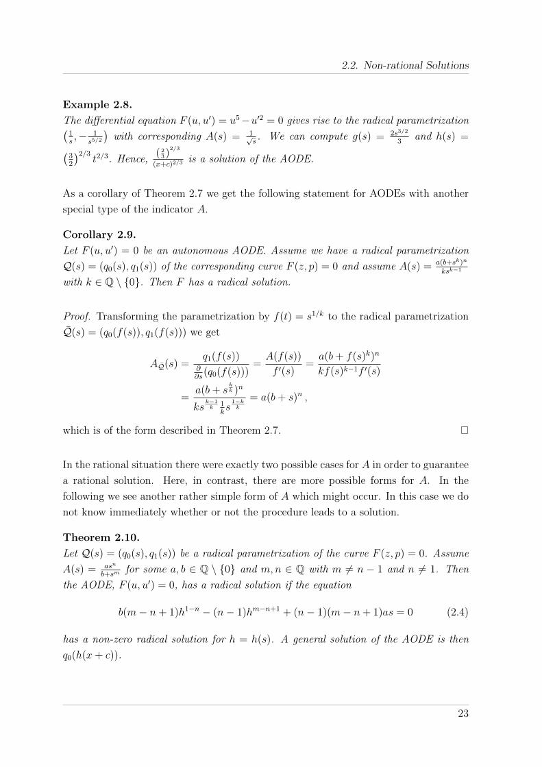
Example 2.8.
The differential equation F (u, u′) = u5−u′2 = 0 gives rise to the radical parametrization(1s,− 1
s5/2
)with corresponding A(s) = 1√
s. We can compute g(s) = 2s3/2
3and h(s) =(
32
)2/3t2/3. Hence,
( 23)
2/3
(x+c)2/3is a solution of the AODE.
As a corollary of Theorem 2.7 we get the following statement for AODEs with another
special type of the indicator A.
Corollary 2.9.
Let F (u, u′) = 0 be an autonomous AODE. Assume we have a radical parametrization
Q(s) = (q0(s), q1(s)) of the corresponding curve F (z, p) = 0 and assume A(s) = a(b+sk)n
ksk−1
with k ∈ Q \ {0}. Then F has a radical solution.
Proof. Transforming the parametrization by f(t) = s1/k to the radical parametrization
Q(s) = (q0(f(s)), q1(f(s))) we get
AQ(s) =q1(f(s))
∂∂s
(q0(f(s)))=A(f(s))
f ′(s)=a(b+ f(s)k)n
kf(s)k−1f ′(s)
=a(b+ s
kk )n
ksk−1k
1ks
1−kk
= a(b+ s)n ,
which is of the form described in Theorem 2.7.
In the rational situation there were exactly two possible cases for A in order to guarantee
a rational solution. Here, in contrast, there are more possible forms for A. In the
following we see another rather simple form of A which might occur. In this case we do
not know immediately whether or not the procedure leads to a solution.
Theorem 2.10.
Let Q(s) = (q0(s), q1(s)) be a radical parametrization of the curve F (z, p) = 0. Assume
A(s) = asn
b+smfor some a, b ∈ Q \ {0} and m,n ∈ Q with m 6= n − 1 and n 6= 1. Then
the AODE, F (u, u′) = 0, has a radical solution if the equation
b(m− n+ 1)h1−n − (n− 1)hm−n+1 + (n− 1)(m− n+ 1)as = 0 (2.4)
has a non-zero radical solution for h = h(s). A general solution of the AODE is then
q0(h(x+ c)).
23

2. Solution Method for AODEs
Proof. The procedure yields
g′(s) =1
AQ(s)=b+ sm
asn,
g(s) =
∫g′(s) ds =
1
as1−n
(b
1− n+
sm
1 +m− n
).
The inverse of g can be found by solving the equation
1
ah(s)1−n
(b
1− n+
h(s)m
1 +m− n
)= s
for h(s). By a reformulation and the assumptions for m and n this is equivalent to
(2.4).
In the excluded cases n = 1 or m = n − 1 the integral in Step 2 of Procedure 3 is not
radical.
Example 2.11.
For the AODE, F (u, u′) = −u5− u′ + u8u′ = 0, we compute the radical parametrization
Q(s) =(
1s, s3
1−s8
)with corresponding A(s) = s5
−1+s8. Then equation (2.4) has a solution,
e. g. −(2s−
√−1 + 4s2
)1/4. Hence, we get the solution of the AODE
u(x) = −(
2(x+ c)−√
4(x+ c)2 − 1)−1/4
.
It remains to show when (2.4) is solvable by radicals (i. e. when g(t) in the proof of
Theorem 2.10 has an inverse which is expressible by radicals). The following theorem
due to Ritt [53] helps us to do so.
Theorem 2.12.
A polynomial g has an inverse expressible by radicals if and only if it can be decomposed
into
• linear polynomials,
• power polynomials xn for n ∈ N,
• Chebyshev polynomials and
• degree 4 polynomials.
24

2.2. Non-rational Solutions
Certainly also polynomials of degree 2 and 3 are invertible by radicals but it can be
shown, that Theorem 2.12 applies to them. We prove now that a certain polynomial is
not decomposable into non-linear factors.
Theorem 2.13.
Let g(t) = C1tα +C2t
β ∈ K[t] where K is a field of characteristic zero, C1, C2 ∈ K \ {0},α, β ∈ N, gcd(α, β) = 1, β > α > 0 and β > 4. Assume g = f ◦ h for some polynomials
f and h. Then deg f = 1 or deg h = 1.
Proof. Assume g(t) = f(h(t)) with f =∑n
i=0 aixi and h =
∑mk=0 bkx
k, where an 6= 0,
bm 6= 0, m,n > 1. In case b0 6= 0 it follows that g(t) = f(h(t)) where f(t) = f(b0 + t)
and h(t) = h(t)− b0. Hence, without loss of generality we can assume that b0 = 0 and
therefore also a0 = 0.
We denote the coefficient of order k in a polynomial g by coefk(g). Let now τ ∈{1, . . . ,m} such that bτ 6= 0 and bl = 0 for all l ∈ {1, . . . , τ − 1}. Similarly let π ∈{1, . . . , n} such that aπ 6= 0 and al = 0 for all l ∈ {1, . . . , π − 1}. This implies that
coef l(g) = 0 for all l ∈ {1, . . . , τπ − 1} and coefτπ(g) = aπbπτ 6= 0. Hence, α = τπ.
Assume now that π < n. Then α = τπ < m(n− 1) + l and therefore
0 = coefm(n−1)+l(g)
= coefm(n−1)+l
(an
(m∑j=τ
bjxj
)n)
= nanbn−1m bl +
∑ε∈E
(n
εl+1, . . . , εm
)an
m∏j=l+1
bεjj
for all l ∈ {τ, . . . ,m− 1} where ε = (εl+1, . . . , εm) and
E =
{ε |
m∑k=l+1
εk = n,m∑
k=l+1
kεk = m(n− 1) + l
}.
This yields, that 0 = coefmn−1(g) = nanbn−1m bm−1, hence, bm−1 = 0. By induction it
follows that bl = 0 for all l ∈ {τ, . . . ,m− 1} which contradicts bτ 6= 0.
Therefore, τ = m or π = n. But then we have m | α and m | β or n | α and n | β which
contradicts gcd(α, β) = 1 since m,n 6= 1.
25

2. Solution Method for AODEs
Let us now consider the function
g(t) =1
at1−n
(b
1− n+
tm
1 +m− n
)from the proof of Theorem 2.10. In general g is not a polynomial. Our aim is to find
a radical function h with a radical inverse such that g = g(h) is a polynomial. Then g
has a radical inverse if and only if g has a radical inverse.
Let z1, z2 ∈ Z, d1, d2 ∈ N such that 1 − n = z1d1
, m − n + 1 = z2d2
and gcd(z1, d1) =
gcd(z2, d2) = 1. Then g(t) = g(h(t)) where h(t) = td
d1d2 and
g(t) =1
atn(
b
1− n+
tm−n
1 +m− n
), (2.5)
with exponents n = (1−n)d1d2d
, m = (m−n+1)d1d2d
and d = gcd(z1d2, z2d1). Hence, m, n are
integers with gcd(m, n) = 1. The function h has an inverse expressible by radicals. If
m− n+ 1, 1− n are positive integers, then also m, n are positive. On the other hand if
n−m− 1, n− 1 ∈ N we get a polynomial by a further composition with f(t) = t−1.
If not both n and m are positive and not both are negative but |m|+ |n| ≤ 4, computing
the inverse function of g is the same as solving an equation of degree less or equal 4,
which can be done by radicals.
We summarize this discussion using Theorem 2.12 and 2.13 as follows.
Corollary 2.14.
The function g from the proof of Theorem 2.10,
g(t) =1
at1−n
(b
1− n+
tm
1 +m− n
),
has an inverse expressible by radicals in the following cases (where we use the notation
from above):
• b = 0,
• m, n ∈ N and max(|m|, |n|) ≤ 4,
• −m,−n ∈ N and max(|m|, |n|) ≤ 4 ,
• −m, n ∈ N and |m|+ |n| ≤ 4,
• m,−n ∈ N and |m|+ |n| ≤ 4.
26

2.2. Non-rational Solutions
It has no inverse expressible by radicals in the cases
• m, n ∈ N and max(m, n) > 4,
• −m,−n ∈ N and max(|m|, |n|) > 4.
Proof. In the cases where m and n have the same sign and |m|+ |n| > 4 the function g
as discussed above fulfills the requirements of Theorem 2.13. Hence, if g = f1 ◦ f2 either
f1 or f2 is of degree one. It is not difficult to show, that the other one can neither be a
power polynomial nor a Chebyshev polynomial. Hence, by the Theorem of Ritt g has
no radical inverse.
The case b = 0 is obvious. In all the other cases mentioned in the theorem and not
discussed so far we end up in solving an algebraic equation of degree less or equal four
and hence, there is a radical inverse.
Hence, in some cases we are able to decide the solvability of an AODE with properties as
in Theorem 2.10. Nevertheless, the procedure is not complete, since even Corollary 2.14
does not cover all possible cases for m and n.
2.2.2. Other Solutions
So far we were looking for rational and radical solutions of AODEs. However, the proce-
dure is not restricted to these cases but might also solve some AODEs with non-radical
solutions as we can see in the following examples where trigonometric and exponential
solutions are found. This is the case when Step 2 (integration) or 3 (solving algebraic
equation) cannot be computed in the field of rational functions but in some field exten-
sion. For the integration problem the existing algorithms provide information on the
necessary field extensions. Further investigation of non-algebraic results of the procedure
are subject to further research.
Example 2.15. (c. f. Example 1.371 of [32])
Consider the equation F (u, u′) = ±u3 + u2 + u′2 = 0. The corresponding curve has
the parametrization Q(s) = ∓(1 + s2, s(1 + s2)). We get A(s) = 12(1 + s2) and hence,
g(s) = 2 arctan(s). The inverse function is h(s) = tan( s2) and thus, u(x) = ∓(1 +
tan(x+c2
)2) = ∓ sec(x+c2
)2 is a solution.
27

2. Solution Method for AODEs
Example 2.16.
Consider the AODE, F (u, u′) = u2 + u′2 + 2uu′ + u = 0. We get the rational parame-
trization(− 1
(1+s)2,− s
(1+s)2
). With A(s) = −1
2s(1 + s) we compute g(s) = −2 log(s) +
2 log(1+s) and hence h(s) = 1−1+es/2
, which leads to the solution −e−(x+c)(−1+e(x+c)/2)2.
These examples show that we can find non-radical solutions even with rational param-
etrizations.
2.2.3. Investigation of the Procedure
In many books on differential equations we can find a method for transforming an
autonomous ODE of any order F (u, u′, . . . , u(n)) = 0 to an equation of lower order by
substituting v(u) = u′ (see for instance [32, 73]). For the case of first-order ODEs this
method yields a solution. It turns out that this method is somehow related to our
procedure. The method does the following:
• Substitute v(u) = u′.
• Solve F (u, v(u)) = 0 for v(u).
• Solve∫
1v(u)
du = x for u.
These computations are a special case of our general procedure where a specific form of
parametrization is used, i. e. Q(s) = (s, q1(s)).
We now give some arguments concerning the possibilities and benefits of the general
procedure. Since in the procedure any radical parametrization can be used we might
take advantage of picking a good one as we see in the following example.
Example 2.17.
We consider the AODE, F (u, u′) = u′6 + 49uu′2 − 7 = 0, and find a parametrization of
the form (s, q1(s)): s,√(
756 + 84√
28812s3 + 81)2/3 − 588s
√6(756 + 84
√28812s3 + 81
)1/6
.
28

2.2. Non-rational Solutions
Computing the corresponding integral is not very efficient and might not be done in some
computer algebra systems. Nevertheless, we can input another parametrization to our
procedure. An obvious one to try next is
(q0(s), q1(s)) =
(−−7 + s6
49s2, s
).
It turns out that here we get g(s) = 221s3− 4s3
147. Its inverse can be computed h(s) =
12
(−147s−
√7√
32 + 3087s2)1/3
. Applying h(x+ c) to q0(t) we get the solution
u(x) =7− 1
64
(−147(x+ c)−
√7√
32 + 3087(x+ c)2)2
494
(−147(x+ c)−
√7√
32 + 3087(x+ c)2)2/3
.
The procedure might find a radical solution of an AODE by using a rational param-
etrization as we have seen in Example 2.11 and 2.17. As long as we are looking for
rational solutions only, the corresponding curve has to have genus zero. Now we can
also solve some examples where the genus of the corresponding curve is greater than
zero and hence no rational parametrization exists. The AODE in Example 2.18 below
corresponds to a curve with genus 1.
Example 2.18.
Consider the AODE, F (u, u′) = −u3− 4u5 + 4u7− 2u′− 8u2u′+ 8u4u′+ 8uu′2 = 0. We
compute a parametrization and get(1
s,
−4 + 4s2 + s4
s(4s2 − 4s4 − s6 −
√−16s4 + 16s8 + 8s10 + s12
))
as one of the branches. The procedure yields
A(s) = − s (−4 + 4s2 + s4)
4s2 − 4s4 − s6 −√−16s4 + 16s8 + 8s10 + s12
,
g(s) =2s4 + s6 +
√s4 (2 + s2)2 (−4 + 4s2 + s4)
4s2 + 2s4,
h(s) = −√
1 + s2
√1 + s
,
u(x) = −√
1 + c+ x√1 + (c+ x)2
.
29

2. Solution Method for AODEs
2.3. Extension to Higher-Order AODEs
Higher-order AODEs have already been studied in [29]. We present how the key idea
corresponds to these investigations. Before doing so, we show some simple methods for
special kinds of higher-order AODEs.
In Section 2.2 we presented a procedure for solving AODEs of the form F (u, u′) =
0. Obviously we can use this procedure just as well for solving differential equations
F (u(n−1), u(n)) = 0 for any n ≥ 1. We do so by first solving F (v, v′) = 0 and then
computing u from u(n−1) = v by integration (compare [32, Example 7.18, p. 604]).
Second-Order AODEs of the form F (u, u′′) = 0
In the following we show an attempt to extend the procedure to second-order AODEs
of the form F (u, u′′) = 0. Note, that the content of this section is mainly a collection
of ideas. A more elaborate investigation is subject to further research. Already Kamke
gave a special case of the method in [32, Section 23.1 and Example 7.19, p. 605]. He
restricts to ODEs which are solvable for the highest derivative u(n). Later we show
difficulties arising in the general setting for higher n.
Assume we are given a differential equation F (u, u′′) = 0 and a rational or radical
parametrization Q = (q0, q1) of the corresponding curve. The method will, as we see
later, in general yield a radical solution. We assume (as usual) that Q = L(g) for some
function g(s), where L is the parametrization corresponding to the solution. Then the
following equations have to be fulfilled
q0 = u(g) , q1 = u′′(g) .
We take derivatives of the first equation and get
q′0 = g′u′(g) ,
q′′0 = g′2u′′(g) + g′′u′(g) = g′2q1 + g′′q′0g′. (2.6)
This yields an ODE of order 2 in g which can be reduced to an ODE in g of order 1 by
setting g = g′. This quasilinear ODE can be solved:
g =q′0√
c1 − 2∫−q1q′0 ds
,
g = c2 +
∫g ds .
30

2.3. Extension to Higher-Order AODEs
Using this method we can solve differential equations of the form F (u(n−2), u(n)) = 0
with n ≥ 2 by first solving F (v, v′′) = 0 and then u(n−2) = v.
Example 2.19. (Example 2.6 of Kamke [32])
We consider the AODE, F (u, u′′) = u′′ − u. It is easy to see that Q = (s, s) is a
parametrization of the associated curve. Equation (2.6) simplifies to sg′3 + g′′ = 0 which
can be reduced to sg3 + g′ = 0. Thus, we get g = − 1√s2−2c1
and hence g = log(s +√s2 − 2c1) + c2. Computing the inverse h of g we get the solution h = 1
2e−s+c2 + es−c2c1,
since q0 = s.
Now we would like to generalize this idea to AODEs of the form F (u, u(n)) = 0. The
Formula of Faa di Bruno describes the higher-order derivatives of a function composi-
tion:
q(η)0 =
∂ηu(g)
∂sη=
∑(κ1,...,κη)∈Rη
(η
κ1, . . . , κη
)∂κ1+...+κηu
∂sκ1+...+κη(g)
η∏m=1
(∂mg∂sm
m!
)km
, (2.7)
where Rη = {(κ1, . . . , κη) ∈ Nη |∑η
i=1 iκi = η}. Using Bell polynomials this can be
denoted in a different way
∂ηu(g)
∂sη=
η∑k=1
∂ku
∂sk(g)Bη,k(g
′(s), . . . , g(η−k+1)(s)) ,
where
Bη,k(x1, . . . xη−k+1) =∑
j1,...,jη−k+1∑ji=k∑iji=η
(η
j1, . . . , jη−k+1
) η−k+1∏i=1
(xii!
)ji.
Equation (2.7) yields a system of algebraic equations in the indeterminates u(k)(g).
Indeed, it is possible to eliminate u(k)(g) for all k ∈ {1, . . . , n − 1}. In the resulting
equation we replace the remaining u(n)(g) by q1. Hence, we get a differential equation
in g of order n. It is easy to see that g itself does not appear in the equation. Therefore,
we can transform to a differential equation of order n − 1. However, this ODE is in
general not linear and not quasilinear either. For n = 3 for instance we get
G(g, g′, g′′) = 3gg′q′′0 + q′0(gg′′ − 3g′2
)− g2q
(3)0 + g5q1 = 0 .
31

2. Solution Method for AODEs
These considerations lead over to the investigation of general second-order autonomous
AODEs, F (u, u′, u′′) = 0.
General second-order autonomous AODEs
Using our general idea, we need a parametrization of the corresponding surface. How-
ever, the solution only yields a parametrization of some curve on the surface. We can
avoid these circumstances and consider the AODE to be in fact an APDE of the form,
F (u, ux, uxx) = 0. Given a solution v(x, y) of the APDE, we can compute a solution
v(x, c) of the AODE for some constant c. Of course this feels like cracking a nut with a
sledgehammer but nevertheless it could work as we see on the next example. A method
for solving the related APDE is presented in 3.4.
Example 2.20. (Example 6.107 of Kamke [32])
We consider the AODE, F (u, u′, u′′) = uu′′ + u′2 = 0. For simplicity we chose the
constant of the original Example in Kamke to be zero. In Example 3.28 we solve the
APDE, F (u, ux, uxx) = uuxx + u2x = 0, and get u(x, y) =
√2t3/2√s−t −
√2s√t√
s−t as a solution.
Hence, v(x) = u(x+ c1, c2) is a solution of the AODE.
This idea can be easily generalized to higher-order AODEs.
General higher-order AODEs
First we consider a general autonomous AODE, F (u, u′, . . . , u(n)) = 0. We assume the
equation to be in fact an APDE, F (u, u(1,0,...,0), . . . , u(n,0,...,0)) = 0, in n independent
variables. Such APDEs can be solved with Procedure 6. Let u(x1, . . . , xn) be a solution
of the APDE. Then u(x1−c1, c2, . . . , cn), with arbitrary constants c1, . . . , cn, is a solution
of the AODE.
Note, that if u is rational, the arbitrary constants c1, . . . , cn are indeed independent since
by Lemma 3.30 a rational solution computed by Procedure 6 is proper.
Example 2.21. (Example 3.3.13 of [49])
We consider the AODE, F (u, u′, u′′) = uu′′′ − u′u′′ = 0. This coincides with Exam-
ple 3.3.13 of [49] for a = 1. In Example 3.29 we solve the APDE, F (u, ux, uxx) =
uuxxx − uxuxx = 0, and get u(x1, x2, x3) =ex1√x2(e−2x1
√x2−2x2x3)
2x2as a solution. Hence,
u(x+ c1, c2, c3) is a solution of the AODE.
32

2.3. Extension to Higher-Order AODEs
The same can be done for non-autonomous AODEs, F (x, u, u′, . . . , u(n)) = 0, by applying
Procedure 7 to the APDE, F (x1, u, u(1,0,...,0), . . . , u(n,0,...,0)) = 0, in n + 1 independent
variables. Let u(x1, . . . , xn+1) be a solution of the APDE. Then u(x1, c1, c2, . . . , cn) is a
solution of the AODE with arbitrary constants c1, . . . , cn.
Remark 2.22.
In Procedure 7 the method of characteristics yields a system of ODEs. In case n = 1,
this system coincides with the associated system from [44], which is described in (2.1) in
Section 2.1.2. For higher order, the system coincides with the associated system defined
in [29]. Hence, the algorithms in [29, 44] are special cases of the Procedure for computing
rational solutions. To this effect those algorithms (respectively the corresponding papers)
also provide more information on solvability.
33


3. Solution Method for APDEs
In this chapter we investigate the general idea of Section 1.4 for the case of two and
more variables and present a method for solving first-order autonomous APDEs. The
procedure is a generalization of Procedure 3.
For APDEs (n ≥ 2), the system (1.2) definitely consists of more than one equation. We
first (Section 3.1) present the case of two variables and show how the system can be
transformed to a single quasilinear equation in one component which we know how to
solve.
The separate presentation of the three variable case (Section 3.2) shall depict the es-
sentially new steps needed for the generalization to an arbitrary number of variables.
The difference is now that we transform system (1.2) to a set of independent quasilin-
ear equations, i. e. PDEs which are linear in the derivatives but possibly non-linear in
the dependent function and the variables (see Appendix D for further information). We
show in detail how to find these equations but omit further elaboration in this section.
Finally, we show the general case for an arbitrary number of variables in Section 3.3
including all details and restrictions. Furthermore, we prove properties of the computed
solutions. As in the case of AODEs we provide evidence that the method is not restricted
to finding rational solutions.
Several examples illustrate the procedure and its capabilities. Further examples con-
taining well-known equations from literature can be found in Appendix C.3.
At the end of this chapter, in Section 3.4 we present further approaches for solving
APDEs. These techniques are related to the previously investigated procedures. They
include a glimpse of an idea of a generalization to higher order and a systematic way
of computing solutions that are not proper. Furthermore, a procedure for degenerate
APDEs, where only derivatives by one variable appear, is presented. This procedure
can be used for solving higher-order AODEs.
35

3. Solution Method for APDEs
3.1. Two Variables
In this section we present the generalization of Procedure 3 to APDEs in two variables.
The general approach is the same. However, new ideas are needed to solve system (1.2)
which now really is a system of PDEs in the unknowns g1 and g2. It turns out that
this system can be transformed to a quasilinear equation in one of the components of g.
Such equations can be solved by a well-known method. We present all important details
in this section and join them to a procedure similar to the AODE case.
The content of this section is in a large part based on results in [22]. Nevertheless,
additional information is incorporated.
We recall the idea of Section 1.4 for the specific setting of n = 2. Let F (u, ux, uy) = 0
be an algebraic partial differential equation.
We consider the surface F (z, p, q) = 0 and assume it admits a proper (rational) surface
parametrization
Q(s, t) = (q0(s, t), q1(s, t), q2(s, t)) .
An algorithm for computing a proper rational parametrization of a surface can be found
for instance in [56]. For further information on rational parametrization of surfaces we
refer to Appendix B.1.2. Here, we stick to rational parametrizations, but the proce-
dure which we present works as well with other kinds of parametrizations, for instance
radical ones. First results on radical parametrizations of surfaces can be found in [61].
Assume that L(s, t) = (v0(s, t), v1(s, t), v2(s, t)) is the corresponding parametrization of
a solution of the APDE. Furthermore we assume that the parametrization Q can be
expressed as
Q(s, t) = L(g(s, t))
for some invertible function g(s, t) = (g1(s, t), g2(s, t)). This assumption is motivated
by the fact that in case of rational algebraic curves every non-constant rational solution
of an AODE yields a proper rational parametrization of the associated algebraic curve
and each proper rational parametrization can be obtained from any other proper one by
a linear rational transformation. However, in the case of APDEs, not all rational solu-
tions provide a proper parametrization, as mentioned in the remark after Definition 1.4.
Nevertheless, we will see later that it does still make sense to stick to the assumption.
Now, using the assumption, if we can compute g−1 we have a solution Q(g−1(s, t)).
36

3.1. Two Variables
Let J be the Jacobian matrix. Then we have
JQ(s, t) = JL(g(s, t)) · Jg(s, t) .
Taking a look at the first row we get the specific case of system (1.2)
∂q0
∂s=∂v0
∂s(g)
∂g1
∂s+∂v0
∂t(g)
∂g2
∂s= q1(s, t)
∂g1
∂s+ q2(s, t)
∂g2
∂s,
∂q0
∂t=∂v0
∂s(g)
∂g1
∂t+∂v0
∂t(g)
∂g2
∂t= q1(s, t)
∂g1
∂t+ q2(s, t)
∂g2
∂t.
(3.1)
This is a system of quasilinear equations in the unknown functions g1 and g2. In case
q1 or q2 is zero the problem reduces to ordinary differential equations. Hence, from now
on we assume that q1 6= 0 and q2 6= 0. First we divide by q1 and simplify notation:
a1 =∂g1
∂s+ b
∂g2
∂s,
a2 =∂g1
∂t+ b
∂g2
∂t
(3.2)
with
a1 =∂q0∂s
q1
, a2 =∂q0∂t
q1
, b =q2
q1
. (3.3)
By taking derivatives we get
∂a1
∂t=∂2g1
∂s∂t+∂b
∂t
∂g2
∂s+ b
∂2g2
∂s∂t,
∂a2
∂s=∂2g1
∂t∂s+∂b
∂s
∂g2
∂t+ b
∂2g2
∂t∂s.
(3.4)
Subtraction of the two equations yields
∂b
∂t
∂g2
∂s− ∂b
∂s
∂g2
∂t=∂a1
∂t− ∂a2
∂s. (3.5)
This is a single quasilinear differential equation which can be solved by the method
of characteristics (see for instance [73] and Appendix D). In case ∂b∂t
= 0 or ∂b∂s
= 0
equation (3.5) reduces to a simple ordinary differential equation.
Remark 3.1.
If both derivatives of b are zero then b is a constant. Hence, the left hand side of (3.5)
is zero. In case the right hand side is non-zero we get a contradiction, and therefore, no
37

3. Solution Method for APDEs
proper solution exists. In case the right hand side is zero as well we get from (3.5) that
0 =∂a1
∂t− ∂a2
∂s=
∂
∂t
(∂q0∂s
q1
)− ∂
∂s
(∂q0∂t
q1
)
=∂2q0∂t∂s
q1 − ∂q0∂s
∂q1∂t
q21
−∂2q0∂s∂t
q1 − ∂q0∂t
∂q1∂s
q21
= −∂q0∂s
∂q1∂t− ∂q0
∂t∂q1∂s
q21
,
hence,
0 =∂q0
∂s
∂q1
∂t− ∂q0
∂t
∂q1
∂s.
Moreover, since b is constant, q1 = kq2 for some constant k. But this means that the
rank of the Jacobian of Q is 1, a contradiction to Q being proper.
Therefore, we assume from now on, that the derivatives of b are non-zero. According
to the method of characteristics, we need to solve the following system of first-order
ordinary differential equations
ds(t)
dt= −
∂b∂t
(s(t), t)∂b∂s
(s(t), t),
dv(t)
dt=
∂a1∂t
(s(t), t)− ∂a2∂s
(s(t), t)
− ∂b∂s
(s(t), t).
The second equation is linear and separable but depends on the solution of the first.
The first ODE can be solved independently. Its solution s(t) = η(t, k) depends on
an arbitrary constant k. Hence, also the solution of the second ODE depends on k.
Finally, the function g2 we are looking for is g2(s, t) = v(t, µ(s, t))+ν(µ(s, t)) where µ is
computed such that s = η(t, µ(s, t)) and ν is an arbitrary function. In case we are only
looking for rational solutions we can use the algorithm of Ngo and Winkler [44, 45, 46]
for solving these ODEs.
Knowing g2 we can compute g1 by using (3.1) which now reduces to a separable ODE
in g1. The remaining task is to compute h1 and h2 such that g(h1(s, t), h2(s, t)) = (s, t).
Then q0(h1, h2) is a solution of the original PDE.
Finally the method reads as
38

3.1. Two Variables
Procedure 4.
Input: An autonomous APDE, F (u, ux, uy) = 0, where F is irreducible and F (z, p, q) = 0
is a rational surface with a proper rational parametrization Q = (q0, q1, q2).
Output: A solution of the APDE or “fail”.
1. Compute the coefficients b and ai as in (3.3).
2. If ∂b∂s
= 0 and ∂b∂t6= 0 compute g2 =
∫ ∂a1∂t− ∂a2
∂s∂b∂t
ds+ κ(t) and go to step 6 otherwise
continue.
If ∂b∂s
= ∂b∂t
= 0 return “No proper solution”.
3. Solve the ODE, ds(t)dt
= −∂b∂t
(s(t),t)∂b∂s
(s(t),t), for s(t) = η(t, k) with arbitrary constant k.
4. Solve the linear ODE, dv(t)dt
=∂a1∂t
(η(t,k),t)− ∂a2∂s
(η(t,k),t)
− ∂b∂s
(η(t,k),t), by computing the integral
v(t) = v(t, k) =∫ ∂a1
∂t(η(t,k),t)− ∂a2
∂s(η(t,k),t)
− ∂b∂s
(η(t,k),t)dt+ ν(k).
5. Compute µ such that s = η(t, µ(s, t)) and then g2(s, t) = v(t, µ(s, t)).
6. Use the second equation of (3.2) to compute g1(s, t) = m(s) +∫a2 − b∂g2∂t dt.
7. Determine m(s) by using the first equation of (3.2).
8. Compute h1, h2 such that g(h1(s, t), h2(s, t)) = (s, t).
9. Return the solution q0(h1(x, y), h2(x, y)).
Observe that the proper rational parametrization Q can be computed applying Schicho’s
algorithm (see [56]). In addition, we also observe that the procedure can be extended
to the non-rational algebraic case, if one has an injective parametrization, in that case
non-rational, of the surface defined by F (z, p, q) = 0.
In general ν depends on a constant c2 and m on a constant c1. As a special case of
the procedure we fix ν = c2. This choice is done for simplicity reasons but we may
sometimes refer to cases with other choices which are a subject of further research.
Furthermore, the procedure can be considered symmetrically in Step 2 for the case
that ∂b∂t
= 0 and ∂b∂s6= 0. In such a case the rest of the procedure has to be changed
symmetrically as well. We do not go into further details.
39

3. Solution Method for APDEs
Theorem 3.2.
Let F (u, ux, uy) = 0 be an autonomous APDE. If Procedure 4 returns a function v(x, y)
for input F , then v is a solution of F .
Proof. By the procedure we know that v(x, y) = q0(h1(x, y), h2(x, y)) with hi such that
g(h1(s, t), h2(s, t)) = (s, t). Since g is a solution of system (3.1) it fulfills the assumption
that u(g1, g2) = q1 for some solution u of the APDE. Hence, v is a solution. We have
seen a more detailed description at the beginning of this section.
Remark 3.3.
In Step 3 and 4 ODEs have to be solved. Depending on the class of functions to which
the requested solution should belong, these ODEs do not necessarily have a solution.
Furthermore, an explicit inverse (Step 8) does not necessarily exist.
It will be a subject of further research, to investigate conditions on cases for which the
procedure does definitely not fail.
Now, we show that the result of Procedure 4 does not change if we postpone the intro-
duction of c1 and c2 to the end of the procedure. It is easy to show that if u(x, y) is
a solution of an autonomous APDE then so is u(x + c, y + d) for any constants c and
d. From the procedure we see that in the computation of g1 we use the derivative of g2
only (and hence c2 disappears). We can write
g2 = g2 + c2 , g1 = g1 + c1
for some functions g1 and g2 which do not depend on c1 and c2. Let g = (g1, g2) and
g = (g1, g2). In Step 8 we are looking for a function h such that g ◦ h = id. Now
g ◦ h = g ◦ h + (c1, c2). Take h such that g ◦ h = id. Then g ◦ h(s − c1, t − c2) = id.
Hence, we can introduce the constants at the end.
In case the original APDE is in fact an AODE, the ODE in Step 4 turns out to be
trivial and the integral in Step 7 is exactly the one which appears in the Procedure 3
for AODEs. Of course then g is univariate and so is its inverse. In this sense, this new
procedure generalizes Procedure 3. We do not specify Procedure 4 to handle this case
separately.
In the following we show some examples which can be solved by Procedure 4. Note,
that the examples have more solutions than those computed below. In Example 3.4
for instance, other solutions can be found by choosing different ν, e. g. ν(x) = c2 + x2.
40
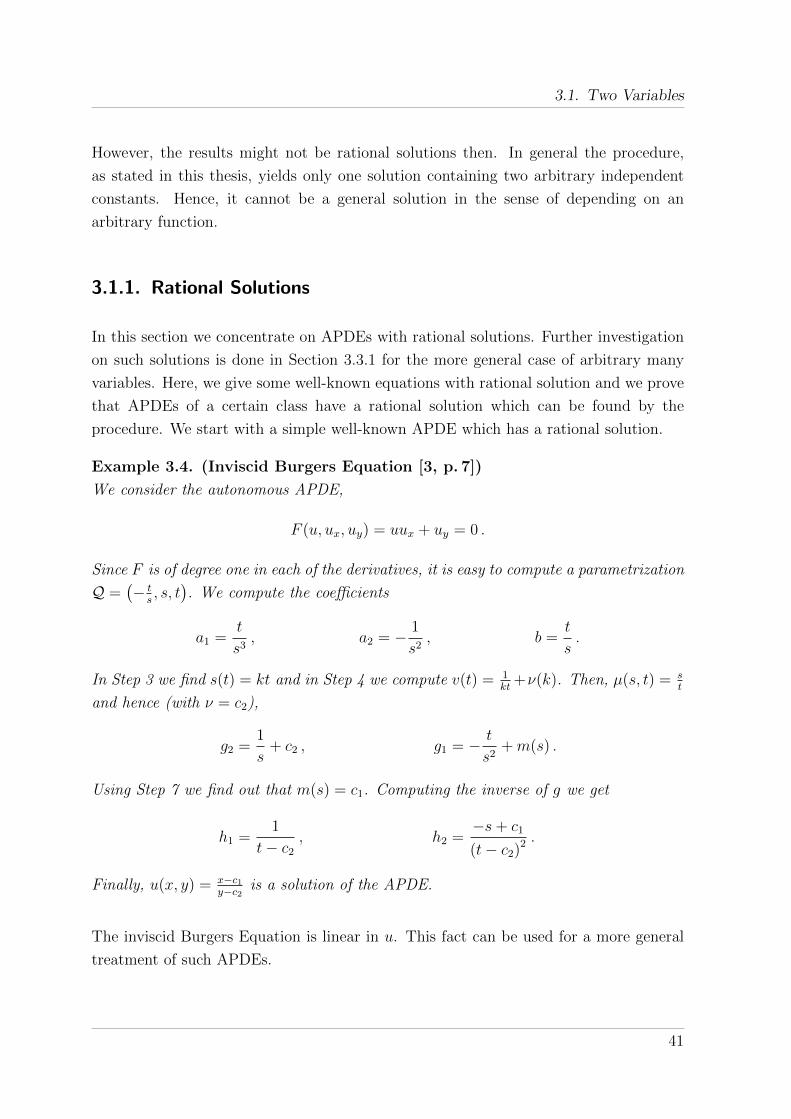
3.1. Two Variables
However, the results might not be rational solutions then. In general the procedure,
as stated in this thesis, yields only one solution containing two arbitrary independent
constants. Hence, it cannot be a general solution in the sense of depending on an
arbitrary function.
3.1.1. Rational Solutions
In this section we concentrate on APDEs with rational solutions. Further investigation
on such solutions is done in Section 3.3.1 for the more general case of arbitrary many
variables. Here, we give some well-known equations with rational solution and we prove
that APDEs of a certain class have a rational solution which can be found by the
procedure. We start with a simple well-known APDE which has a rational solution.
Example 3.4. (Inviscid Burgers Equation [3, p. 7])
We consider the autonomous APDE,
F (u, ux, uy) = uux + uy = 0 .
Since F is of degree one in each of the derivatives, it is easy to compute a parametrization
Q =(− ts, s, t
). We compute the coefficients
a1 =t
s3, a2 = − 1
s2, b =
t
s.
In Step 3 we find s(t) = kt and in Step 4 we compute v(t) = 1kt
+ν(k). Then, µ(s, t) = st
and hence (with ν = c2),
g2 =1
s+ c2 , g1 = − t
s2+m(s) .
Using Step 7 we find out that m(s) = c1. Computing the inverse of g we get
h1 =1
t− c2
, h2 =−s+ c1
(t− c2)2 .
Finally, u(x, y) = x−c1y−c2 is a solution of the APDE.
The inviscid Burgers Equation is linear in u. This fact can be used for a more general
treatment of such APDEs.
41

3. Solution Method for APDEs
Lemma 3.5.
Let F (u, ux, uy) = B(ux, uy)u + A(ux, uy) = 0 be an APDE with coprime polynomials
A,B ∈ C[p, q], B 6= 0. Let γ(s, t) = A(s,t)B(s,t)
and assume that γ(s, t) = γ( ts) for some
function γ. Then γ(t,−s) is a rational solution.
Proof. Due to the assumptions on A and B, we know that F is irreducible and Q =
(−γ(s, t), s, t) is a proper parametrization of the surface F (z, p, q) = 0. We show that
P(s, t) = Q(−ta2(−t, s), ta1(−t, s)) yields a solution, where ai are defined as in (3.3).
Indeed we have
P(s, t) =
(−γ(
ta1(−t, s)−ta2(−t, s)
),−ta2(−t, s), ta1(−t, s))
=
(−γ(−s
t),
1
tγ′(−s
t),− s
t2γ(−s
t)
).
Now it is easy to prove that this yields a solution
∂(−γ(− s
t))
∂s=
1
tγ′(−s
t) ,
∂(−γ(− s
t))
∂t= − s
t2γ′(−s
t) .
Procedure 4 can also handle more complicated APDEs.
Example 3.6.
We consider the APDE,
0 = F (u, ux, uy) = uu4x + u3
xuy − uu3xuy − u2
xu2y + uu2
xu2y + uxu
3y − uuxu3
y + uu4y .
A proper parametrization of the corresponding algebraic surface is for instance
Q =
(− t (1− t+ t2)
1− t+ t2 − t3 + t4, tγ(s, t), γ(s, t)
),
with γ(s, t) =t(−10+7t)(−9+t2)(−1+2t−3t2+3t4−2t5+t6)
2s(45−63t+5t2)(1−t+t2−t3+t4)2. This parametrization is not easy to
find. It is computed by first using parametrization by lines and then applying a linear
transformation in s. Alternatively one could use the parametrization by lines directly.
42

3.1. Two Variables
In that case Procedure 4 would find the same solution, but the intermediate steps would
need more writing space. Using the procedure with the parametrization Q we get
g1 = s
(7
10− 7t− 1
t+
2t
−9 + t2
), g2 =
2s (45− 63t+ 5t2)
(−10 + 7t) (−9 + t2),
h1 = −t (−90s3 − 63s2t+ 10st2 + 7t3)
2s (45s2 + 63st+ 5t2), h2 =
−ts,
and finally the solution u(x, y) =xy(x2+xy+y2)
x4+x3y+x2y2+xy3+y4. As mentioned before, u(x+c1, y+c2)
with constants c1 and c2 is also a solution.
Parametrization by lines (see Appendix B.1.2 and B.1.3) can be used if there is a (d−1)-
fold point, where d is the degree of the APDE. In such cases the resulting parametrization
is of the form (sD(s, t), tD(s, t), D(s, t)), assuming the singular point to be in the origin.
The following Lemma describes solvability assuming that such a parametrization by lines
fulfills further conditions.
Lemma 3.7.
Assume we have an APDE, F (u, ux, uy) = 0, with a parametrization of the form Q =
(sn+1B(t), tsnB(t), snB(t)) where B(t) = N(t)D(t)6∈ K with N(t), D(t) ∈ K[t], gcd(N,D) =
1 and n ∈ Z. Then F has an algebraic solution.
Proof. Assume we have Q = (sn+1B(t), tsnB(t), snB(t)) with B(t) 6∈ K (the constant
case is shifted to Lemma 3.8). Then we can use the procedure to get the following:
b =1
t, a1 =
n+ 1
t, a2 =
s
t
B′
B,
and hence, ∂b∂s
= 0 but ∂b∂t6= 0. Therefore
g2 =
∫ ∂a1∂t− ∂a2
∂s∂b∂t
ds =
∫ −n+1t2− 1
tB′
B
− 1t2
ds =
∫(n+ 1) + t
B′
Bds
= s(n+ 1 + tB′
B) ,
g1 =
∫a2 − b
∂g2
∂tdt+m(s) =
∫sB′
tB− s
t
(tB′′ +B′)B −B′B′
B2dt+m(s)
=
∫s
t
B′B − tB′′B −B′B +B′B′
B2dt+m(s)
=
∫s
t
t(−B′′B +B′B′)
B2dt+m(s) =
∫−s(B′
B
)′dt+m(s)
= −sB′
B+m(s) .
43

3. Solution Method for APDEs
Now we need to find m(s). We do so by using the equation as in the procedure
∂q1
∂s= q2
∂g1
∂s+ q3
∂g2
∂s
(n+ 1)snB = sntB
(−B
′
B+m′(s)
)+ snB
(n+ 1 + t
B′
B
)(n+ 1)snB = −sntB′ + sntBm′ + sn(n+ 1)B + sntB′
0 = sntBm′
0 = m′ .
Hence, m is a constant and we choose m = 0. Finally we need to find h1, h2 fulfilling
g1(h1, h2) = s , g2(h1, h2) = t ,
−h1B′(h2)
B(h2)= s , h1
(n+ 1 + h2
B′(h2)
B(h2)
)= t .
Since B is non-constant we can eliminate h1 and get
−s B(h2)
B′(h2)= t
(n+ 1 + h2
B′(h2)
B(h2)
)−1
−sB(h2)
(n+ 1 + h2
B′(h2)
B(h2)
)= tB′(h2)
B(h2)s(n+ 1) +B′(h2)(sh2 + t) = 0 .
Hence, we have an algebraic equation for h2 and therefore also for h1 (since the equations
are linear in h1). Thus, we get an algebraic solution.
In Lemma 3.7 the case of B(t) ∈ K was excluded. It is shifted to the next Lemma.
Lemma 3.8.
Assume we have an APDE, F (u, ux, uy) = 0, with a parametrization of the form Q =
(sn+1β, tsnβ, snβ) where β ∈ K. Then F has a rational solution.
Proof. Assume we have Q = (sn+1β, tsnβ, snβ) with B(t) = β ∈ K. According to the
procedure we get g2 = (n+ 1)s+ κ(t). We choose κ(t) = t2. Then g1 =∫a2− b∂g2∂t dt+
m(s) = −∫ κ′(t)
tdt = −2t + m(s). As before we get that m is constant and we choose
m = 0. Finally we need to find h1, h2 fulfilling
s = g1(h1, h2) = −2h2 , t = g2(h1, h2) = h1(n+ 1) + h22 .
44

3.1. Two Variables
Then h2 = − s2
and hence h1 =t−h22n+1
. Thus, q0(h1(x, y), h2(x, y)) = h1(x, y)n+1β =
β
(y−x
2
4
n+1
)n+1
is a rational solution.
Note, that we might get algebraic solutions with other choices of κ.
Using the results of Lemma 3.7 we can prove that certain APDEs have rational solu-
tions.
Lemma 3.9.
Assume we have an autonomous APDE, F (u, ux, uy) = 0, with a parametrization Q =
(sn+1B(t), tsnB(t), snB(t)). Let B(t) = kN(t)D(t)
, where N(t), D(t) ∈ K[t] are monic, k ∈ Kand gcd(N,D) = 1. The APDE has a rational solution if one of the following holds.
1. n = −1
2. deg(N) = deg(D) = 0
3. deg(N) = 0, deg(D) > 0 and
(a) D(t) = (t− β1)δ(t− β2)n+1−δ with β1 6= β2, δ ≥ 1 and n ≥ 1, or
(b) D(t) = (t− β1)δ with δ 6= n+ 1 and δ ≥ 1
4. deg(D) = 0, deg(N) > 0 and
(a) N(t) = (t− α1)ε(t− α2)−n−1−ε, with α1 6= α2, ε ≥ 1 and n ≤ −3, or
(b) N(t) = (t− α1)ε with −ε 6= n+ 1 and ε > 1
5. N = (t− α1)ε and D = (t− β1)n+1+ε with ε ≥ 1 and n+ ε ≥ 0
Proof. In the proof of Lemma 3.7 we concluded that an APDE of the type under con-
sideration has an implicitly given solution. The algebraic equation we found was
B(h2)s(n+ 1) +B′(h2)(sh2 + t) = 0 . (3.6)
Since the equations in the proof of Lemma 3.7 are linear in h1 it suffices to show that in
all the cases of this lemma, the algebraic equation (3.6) has a rational solution. In the
following we will write N = N(ζ) and D = D(ζ). We need to show that the equation
E(ζ) := s ((n+ 1)DN + ζ(N ′D −ND′)) + t(N ′D −ND′) = 0
has a rational solution for ζ.
45

3. Solution Method for APDEs
1. n = −1: E(ζ) has the factor sζ + t.
2. This was shown in Lemma 3.8.
3. deg(N) = 0, deg(D) > 0: In this case E(ζ) = N (s ((n+ 1)D − ζD′)− tD′).
(a) D(ζ) = (ζ − β1)δ(ζ − β2)n+1−δ with β1 6= β2, δ > 1 and n > 1: Then
D′ = δ(ζ − β1)δ−1(ζ − β2)n+1−δ + (n+ 1− δ)(ζ − β1)δ(ζ − β2)n−δ and
E(ζ) = N(ζ − β1)δ−1(ζ − β2)n−δ · E(ζ) ,
E(ζ) : = (n+ 1)(β1 − ζ)(β2s+ t)− δ(β1 − β2)(sζ + t) .
Thus, E is linear in ζ.
(b) D(ζ) = (ζ − β1)δ with δ 6= n+ 1 and δ > 1: Then
E(ζ) = N(ζ − β1)δ−1((n+ 1)s(ζ − β1)− δ(sζ + t))
has a linear factor that depends on s and t.
4. deg(D) = 0, deg(N) > 0: In this case E(ζ) = D(s ((n+ 1)N + ζN ′) + tN ′).
(a) N(ζ) = (ζ − α1)ε(ζ − α2)−n−1−ε, with α1 6= α2, ε > 1 and n < −3: Then
E(ζ) = D(ζ − α1)ε−1(ζ − α2)−n−2−εE(ζ) ,
E(ζ) : = ε(α1 − α2)(sζ + t) + (n+ 1)(α1 − ζ)(sα2 + t) .
Thus, E(ζ) is linear in ζ.
(b) N(ζ) = (ζ − α1)ε with −ε 6= n+ 1 and ε > 1: Then
E(ζ) = D(ζ − α1)ε−1 (s(n+ 1)(ζ − α1) + ε(ζs+ t))
has a linear factor that depends also on s and t.
5. N = (ζ − α1)ε and D = (ζ − β1)n+1+ε with ε ≥ 1 and n+ ε ≥ 0: Then
E(ζ) = (ζ − α1)ε−1(ζ − β1)n+εE(ζ) ,
E(ζ) : = ε(α1 − β1)(sζ + t) + (n+ 1)(α1 − ζ)(sβ1 + t) .
Thus, E(ζ) is linear in ζ.
46

3.1. Two Variables
Example 3.10.
We give examples for all cases of Lemma 3.9.
1. F = −u4x − 2uu2
xu2y + uxu
3y − u4
y with Q =(−1+t−t4
2t2, −1+t−t4
2st, −1+t−t4
2st2
)2. F = 2u− u2
y with Q = (2s2, 2st, 2s)
3. (a) F = 4u− u2x − 2uxuy − 2u2
y with Q =(− 4s2
−2−2t−t2 ,−4st
−2−2t−t2 ,−4s
−2−2t−t2
)F = −u5
x + 8u4xuy − 25u3
xu2y + 38u2
xu3y − 28uxu
4y + 8u5
y + 3u4 with Q =(3s5
(−2+t)3(−1+t)2, 3s4t
(−2+t)3(−1+t)2, 3s4
(−2+t)3(−1+t)2
)(b) F = −10u3ux − 2u3
y with Q =(− 1
5s2t,− 1
5s3,− 1
5s3t
)F = −u6
x + 7u2u3y with Q =
(7s3
t6, 7s2
t5, 7s2
t6
)4. (a) F = −u3 + u2
x − 10uxuy − u2y with Q =
(−1−10t+t2
s2,t(−1−10t+t2)
s3, −1−10t+t2
s3
)F = 6u4 + 5u3
x + 5u2xuy with Q =
(−5t2+5t3
6s3,− t(5t2+5t3)
6s4,−5t2+5t3
6s4
)(b) F = 4ux − 4uy + u2
y with Q = (−s(−4 + 4t),−t(−4 + 4t), 4− 4t)
F = −7u2u2x + 6u5
y with Q =(
7s3t2
6, 7s2t3
6, 7s2t2
6
)5. F = −u4ux + 4u6
x + u4uy with Q =
(− s(s4−s4t)
4t6,− s4−s4t
4t5,− s4−s4t
4t6
)
3.1.2. Algebraic Solutions
We have seen in Lemma 3.7 that solutions computed by the procedure might be consid-
ered implicitly. Hence, Procedure 4 is not restricted to rational solutions nor to rational
parametrizations as we see in the following examples. In certain steps of the procedure
we might do computations in a radical field extension. For instance Step 8 might be
an algebraic equation without rational solution. In this case h is an algebraic function.
The following example illustrates such a case.
Example 3.11. (Eikonal Equation [4, p. 2])
We consider the APDE,
F (u, ux, uy) = u2x + u2
y − 1 = 0 .
47

3. Solution Method for APDEs
From the rational parametrization of a circle it is easy to see that
Q =
(s,
1− t2
1 + t2,
2t
1 + t2
)is a parametrization of the corresponding surface. Using the procedure we get some
rational g1 and g2 which yield
h2 =−s+ c1 ±
√s2 + t2 − 2sc1 + c2
1 − 2tc2 + c22
t− c2
,
h1 = ±√s2 + t2 − 2sc1 + c2
1 − 2tc2 + c22 .
Finally, we get the radical solution
u(x, y) = ±√
(x− c1)2 + (y − c2)2 .
We can use Lemma 3.7 to show that a certain class of APDEs has algebraic solutions,
i. e. we show that a suitable parametrization exists to apply Lemma 3.7.
Corollary 3.12.
Let the APDE be of the form F (u, ux, uy) = λum + γm−1(ux, uy) = 0 , where m ∈ N, λ ∈C \ {0} and γm−1(p, q) be a form of degree m− 1. Then F has an algebraic solution.
Proof. Observe that F (z, p, q) is irreducible, and can be parametrized as
Q(s, t) =
(−sγm−1(t, 1)
λsm,−tγm−1(t, 1)
λsm,−γm−1(t, 1)
λsm
),
which corresponds to the parametrization form in Lemma 3.7 with n = −m and B(t) =
−γm−1(t, 1)/λ. Hence, there is an algebraic solution.
3.1.3. Other Solutions
As in the AODE case we might do certain steps in the procedure by doing computations
in some extension field. Investigation of such computation will be subject to future
research. Nevertheless, we want to give a brief glimpse of what might be possible. In a
further example we compute an exponential solution of an APDE.
48

3.1. Two Variables
Example 3.13. (Convection-Reaction Equation [3, p. 7])
We consider the APDE,
F (u, ux, uy) = ux + cuy − du = 0 ,
where d 6= 0 and c 6= 0. We compute a parametrization Q =(s+ctd, s, t
)and the coeffi-
cients
a1 =1
ds, a2 =
c
ds, b =
t
s.
Solving the ODEs of Step 3–6 we get
g2 =c log(t)
d+ c2 , g1 = c1 +
log(s)
d.
Computing the inverse of g we find
h1 = eds−dc1 , h2 = edtc− dc2
c .
Finally, we get the solution u(x, y) = ed(x−c1)+ced(y−c2)
c
d.
Table 3.1 presents a list of some well-known equations in two variables and the solutions
found by the procedure. For the sake of readability we neglect the arbitrary constants
and present only specific solutions.
Name APDE Parametrization Solution
Burgers (inviscid) [73] uux + uy(− ts, s, t
)xy
Traffic [10] uy − ux(
2uvmrm− vm
) (rm(t+svm)
2svm, s, t
)rm(−x+yvm)
2vmy
Eikonal [4] u2x + u2
y − 1(s, 1−t2
1+t2, 2t
1+t2
)±√x2 + y2
Convection-Reaction
[3]
ux + cuy − du(s+ctd, s, t
)edx+ce
dyc
d
Generalized Burgers
(special case) [73]
uy + uux + αu+ βu2 (sB, tB,B)e−xβ(1−exβ)α
(1+eαy)β
B = − (1+sα)st+s2β
Table 3.1.: Well-known APDEs and their solutions found by Procedure 4.
49

3. Solution Method for APDEs
3.2. Three Variables
In this section we consider the system (1.2) for n = 3. This case is discussed separately
since it is still suitable to show step by step details but it is also general enough to
intuitively lead to the overall picture presented in Section 3.3. Without loss of generality
we assume that q1 6= 0. Hence, we might divide by q1 and get
a1 =∂g1
∂s1
+ b1∂g1
∂s1
+ b2∂g2
∂s1
,
a2 =∂g1
∂s2
+ b1∂g1
∂s2
+ b2∂g2
∂s2
,
a3 =∂g1
∂s3
+ b1∂g1
∂s3
+ b2∂g2
∂s3
,
(3.7)
with ai =∂q0∂si
q1and bi = qi
q1. Now we take derivatives of these equations
∂a1
∂s2
=∂2g1
∂s2∂s1
+∂b1
∂s2
∂g1
∂s1
+ b1∂2g1
∂s2∂s1
+∂b2
∂s2
∂g2
∂s1
+ b2∂2g2
∂s2∂s1
,
∂a1
∂s3
=∂2g1
∂s3∂s1
+∂b1
∂s3
∂g1
∂s1
+ b1∂2g1
∂s3∂s1
+∂b2
∂s3
∂g2
∂s1
+ b2∂2g2
∂s3∂s1
,
∂a2
∂s1
=∂2g1
∂s1∂s2
+∂b1
∂s1
∂g1
∂s2
+ b1∂2g1
∂s1∂s2
+∂b2
∂s1
∂g2
∂s2
+ b2∂2g2
∂s1∂s2
,
∂a2
∂s3
=∂2g1
∂s3∂s2
+∂b1
∂s3
∂g1
∂s2
+ b1∂2g1
∂s3∂s2
+∂b2
∂s3
∂g2
∂s2
+ b2∂2g2
∂s3∂s2
,
∂a3
∂s1
=∂2g1
∂s1∂s3
+∂b1
∂s1
∂g1
∂s3
+ b1∂2g1
∂s1∂s3
+∂b2
∂s1
∂g2
∂s3
+ b2∂2g2
∂s1∂s3
,
∂a3
∂s2
=∂2g1
∂s2∂s3
+∂b1
∂s2
∂g1
∂s3
+ b1∂2g1
∂s2∂s3
+∂b2
∂s2
∂g2
∂s3
+ b2∂2g2
∂s2∂s3
.
Choosing aj,k =∂aj∂sk− ∂ak
∂sjand bi,k = ∂bi
∂skand subtracting suitable equations we get
a1,2 = b2,2∂g2
∂s1
− b2,1∂g2
∂s2
+ b3,2∂g3
∂s1
− b3,1∂g3
∂s2
,
a1,3 = b2,3∂g2
∂s1
− b2,1∂g2
∂s3
+ b3,3∂g3
∂s1
− b3,1∂g3
∂s3
,
a2,3 = b2,3∂g2
∂s2
− b2,2∂g2
∂s3
+ b3,3∂g3
∂s2
− b3,2∂g3
∂s3
.
(3.8)
By a linear combination we get
b2,3a1,2 + b2,1a2,3 − b2,2a1,3
= (b2,3b3,2 − b2,2b3,3)∂g3
∂s1
+ (b2,1b3,3 − b2,3b3,1)∂g3
∂s2
+ (b2,2b3,1 − b2,1b3,2)∂g3
∂s3
.
50

3.3. The General Case
This is a quasilinear PDE in g3. Hence, it can be solved by the well-known method of
characteristics. Once we have g3 we get a quasilinear PDE in g2 adding the two first
equations of (3.8):
a1,2 + a1,3 −(
(b3,2 + b3,3)∂g3
∂s1
− b3,1∂g3
∂s2
− b3,1∂g3
∂s3
)= (b2,2 + b2,3)
∂g2
∂s1
− b2,1∂g2
∂s2
− b2,1∂g2
∂s3
.
Again, this can be solved by the method of characteristics. Finding g1 is finally com-
puting an integral from (3.7).
Note, here we have shown a recursive way. However, some computations can also be
done in parallel, since there is no reason for the particular choice of the roles of the gi.
Indeed, we may as well consider another quasilinear PDE in g2 which is similar to the
one for g3:
b3,3a1,2 + b3,1a2,3 − b3,2a1,3
= (b2,2b3,3 − b2,3b3,2)∂g2
∂s1
+ (b2,3b3,1 − b2,1b3,3)∂g2
∂s2
+ (b2,1b3,2 − b2,2b3,1)∂g2
∂s3
.
In fact, the two quasilinear PDEs can be expressed as
1
q21
det
∂q0∂s1
∂q0∂s2
∂q0∂s3
∂q1∂s1
∂q1∂s2
∂q1∂s3
b2,1 b2,2 b2,3
= det
∂g3∂s1
∂g3∂s2
∂g3∂s3
b2,1 b2,2 b2,3
b3,1 b3,2 b3,3
− 1
q21
det
∂q0∂s1
∂q0∂s2
∂q0∂s3
∂q1∂s1
∂q1∂s2
∂q1∂s3
b3,1 b3,2 b3,3
= det
∂g2∂s1
∂g2∂s2
∂g2∂s3
b2,1 b2,2 b2,3
b3,1 b3,2 b3,3
3.3. The General Case
Based on the ideas of Section 3.1 and 3.2 we can finally derive the generalization to
arbitrary many variables. Furthermore, in this section we elaborate details which we
omitted in the previous ones. These include but are not restricted to exceptional cases
and properties of the computed solutions.
Note that, when we talk about the differential equation and its solution we use the vari-
ables x1, . . . , xn, whereas in the parametrization problem we use the variables s1, . . . , sn.
51

3. Solution Method for APDEs
We recall system (1.2) from the introduction.
∂q0
∂s1
=n∑i=1
∂v0
∂si(g)
∂gi∂s1
=n∑i=1
qi(s1, . . . , sn)∂gi∂s1
,
...
∂q0
∂sn=
n∑i=1
∂v0
∂si(g)
∂gi∂sn
=n∑i=1
qi(s1, . . . , sn)∂gi∂sn
.
(3.9)
This is a system of quasilinear equations in the unknown functions g1 to gn. In case qi is
zero for some i the problem reduces to lower order. Since Q is a proper parametrization
of a hypersurface, at most one of its components can be zero. So, we can ensure that
there exists a non-zero qi with i > 0. Let us assume that q1 6= 0. If this is not the case,
we can always change the role of x1 and xi with i > 1. We proceed as in the case for
three variables. First we divide by q1:
a1 =∂g1
∂s1
+n∑i=2
bi∂gi∂s1
,
...
an =∂g1
∂sn+
n∑i=2
bi∂gi∂sn
.
(3.10)
with ai =∂q0∂si
q1and bi = qi
q1. For each j ∈ {1, . . . , n} we take derivatives of the j-th
equation in (3.10) with respect to the variables sk for j 6= k. This yields a new system
of PDEs, which are henceforth of second order.
∂aj∂sk
=∂2g1
∂sk∂sj+
n∑i=2
∂bi∂sk
∂gi∂sj
+ bi∂2gi∂sk∂sj
for j 6= k . (3.11)
Obviously, we would like to get rid of the second-order terms. Thus, we take pairwise
differences of equations in (3.11) and get the following equations where the second
derivatives vanish.
aj,k =n∑i=2
bi,k∂gi∂sj− bi,j
∂gi∂sk
, for j < k , (3.12)
with aj,k =∂aj∂sk− ∂ak
∂sjand bi,k = ∂bi
∂sk.
The aim now is to take suitable linear combinations of the equations from (3.12) such
that all derivatives of gi vanish except for i = n, i. e. we are left with a quasilinear PDE
52

3.3. The General Case
in gn. In Section 3.1 this was shown for n = 2 and in Section 3.2 we did so for n = 3.
Now we prove the general case.
Theorem 3.14.
Let n ≥ 2 be the number of independent variables. Let M = (bk,`)2≤k≤n,1≤`≤n, where bi,j
are as in (3.12). Then system (3.10) yields a quasilinear PDE in gn of the following
form
∑i,j∈{1,...,n}
i<j
ai,j(−1)i+j+n det(M{n},{i,j}) =n∑i=1
∂gn∂si
(−1)i det(M∅,{i}) , (3.13)
where MR,S denotes the matrix which is obtained from M by deleting all rows with index
in R and all columns with index in S.
Proof. We proceed by rearranging the left hand side of equation (3.13) as long as equality
to the right hand side is shown. Laplace expansion plays an important role in the proof.
We use equation (3.12) for replacing the ai,j and we rearrange the sums. Then, the left
hand side of (3.13) reads as
∑i,j∈{1,...,n}
i<j
(n∑k=2
bk,j∂gk∂si− bk,i
∂gk∂sj
)(−1)i+j+n det(M{n},{i,j})
=n∑k=2
n∑i=1
n∑j=i+1
(bk,j
∂gk∂si− bk,i
∂gk∂sj
)(−1)i+j+n det(M{n},{i,j})
=n∑k=2
(n∑i=1
n∑j=i+1
bk,j∂gk∂si
(−1)i+j+n det(M{n},{i,j})
−n∑i=1
n∑j=i+1
bk,i∂gk∂sj
(−1)i+j+n det(M{n},{i,j})
)
=n∑k=2
(n∑i=1
n∑j=i+1
bk,j∂gk∂si
(−1)i+j+n det(M{n},{i,j})
−n∑i=2
i−1∑j=1
bk,j∂gk∂si
(−1)i+j+n det(M{n},{i,j})
)
53
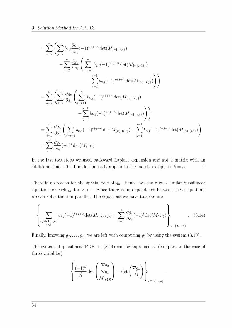
3. Solution Method for APDEs
=n∑k=2
(n∑j=2
bk,j∂gk∂s1
(−1)1+j+n det(M{n},{i,j})
+n∑i=2
∂gk∂si
(n∑
j=i+1
bk,j(−1)i+j+n det(M{n},{i,j})
−i−1∑j=1
bk,j(−1)i+j+n det(M{n},{i,j})
))
=n∑k=2
(n∑i=1
∂gk∂si
(n∑
j=i+1
bk,j(−1)i+j+n det(M{n},{i,j})
−i−1∑j=1
bk,j(−1)i+j+n det(M{n},{i,j})
))
=n∑i=1
∂gn∂si
(n∑
j=i+1
bn,j(−1)i+j+n det(M{n},{i,j})−i−1∑j=1
bn,j(−1)i+j+n det(M{n},{i,j})
)
=n∑i=1
∂gn∂si
(−1)i det(M∅,{i}) .
In the last two steps we used backward Laplace expansion and got a matrix with an
additional line. This line does already appear in the matrix except for k = n.
There is no reason for the special role of gn. Hence, we can give a similar quasilinear
equation for each gν for ν > 1. Since there is no dependence between these equations
we can solve them in parallel. The equations we have to solve are∑
i,j∈{1,...,n}i<j
ai,j(−1)i+j+ν det(M{ν},{i,j}) =n∑i=1
∂gν∂si
(−1)i det(M∅,{i})
ν∈{2,...,n}
. (3.14)
Finally, knowing g2, . . . , gn, we are left with computing g1 by using the system (3.10).
The system of quasilinear PDEs in (3.14) can be expressed as (compare to the case of
three variables) (−1)ν
q21
det
∇q0
∇q1
M{ν},∅
= det
(∇gνM
)ν∈{2,...,n}
.
54

3.3. The General Case
This is a consequence of using backward Laplace expansion by the first row, of the right
hand side determinant, and generalized Laplace expansion by the first two rows of the
left hand side determinant.
Note, that the determinants on the right hand side of (3.14) do not depend on ν. In the
following we see some cases where the determinants on the right hand side have special
properties. Mainly, we are asking some or all of them to be zero.
Remark 3.15.
If det(M∅,{i}) = 0 for all but one index i ∈ {1, . . . , n} \ {`}, and det(M∅,{`}) 6= 0, then
the equations (3.14) reduce to n− 1 ODEs with solution
gν =
∫ ∑i,j∈{1...n}
i<j
ai,j(−1)i+j+ν det(M{ν},{i,j})
(−1)` det(M∅,{`})ds` +K(s1, ..., s`−1, s`+1, ..., sn) .
In the following remark and theorem we see what happens if the right hand side of (3.14)
is zero. Two possible cases might occur: Either the left hand side is zero as well, or it
is not.
Remark 3.16.
If det(M∅,{i}) = 0 for every i ∈ {1, . . . , n} and∑i,j∈{1,...,n}
i<j
ai,j(−1)i+j+ν det(M{ν},{i,j}) 6= 0
for some ν ∈ {1, . . . , n}, then we get a contradiction, and hence, the assumption Q =
L(g) was wrong. This, however, means that there is no proper rational solution (compare
Lemma 1.3). Nevertheless, there might be a non-proper rational solution, which we
cannot find with the procedure presented here.
From this we conclude for instance that the linear transport equation cannot have a
proper rational solution.
Example 3.17. (Linear Transport Equation [3])
We consider the transport equation F (u, ux, uy) = ux + duy = 0. We choose the proper
parametrization Q = (s1,−ds2, s2). Then det(M∅,{i}) = 0 but the left hand side of (3.14)
is∑
i,j∈{1,...,n}i<j
ai,j(−1)i+j+ν det(M{ν},{i,j}) = − 1ds22
.
Indeed, the general solution of the linear transport equation is u(x, y) = ϕ(y − dx) for
some arbitrary function ϕ, (see for instance [3]). The Jacobian of the corresponding
parametrization has rank 1 and hence, this solution cannot be proper.
55

3. Solution Method for APDEs
We show now that the left hand side cannot be zero according to our assumptions. Note,
that the proof can also be applied in the case when Q is not rational.
Theorem 3.18.
If det(M∅,{i}) = 0 for every i ∈ {1, . . . , n}, and∑i,j∈{1,...,n}
i<j
ai,j(−1)i+j+ν det(M{ν},{i,j}) = 0
for every ν ∈ {1, . . . , n}, then Q turns out to be a parametrization of a variety of
dimension strictly less than n.
Proof. In order to prove this statement, we take the matrix M = (bk,`)2≤k≤n1≤`≤n
. From the
fact that det(M∅,{i}) = 0 for every i ∈ {1, . . . , n}, the rank of M is, at most, n− 2. By
definition of the bk,` we know
bk,` =∂bk∂s`
=∂
∂s`
(qkq1
)= q−2
1
(∂qk∂s`
q1 −∂q1
∂s`qk
)for every k ∈ {2, . . . , n} and ` ∈ {1, . . . , n}. Let M? = (∂qk
∂s`)2≤k≤n
1≤`≤n. Then each row in M
is obtained from a linear combination of the corresponding row in M? and the vector
(∂q1∂s`
)1≤`≤n. More precisely, the ν-th row in M is given by
∇(qν+1)1
q1
−∇(q1)qν+1
q21
for every ν ∈ {1, . . . , n− 1}, and where ∇(qj) = (∂qj∂s1, ...,
∂qj∂sn
). So the rank of
(∇q1
M?
)is
upper bounded by n−1. It remains to prove that this rank is preserved when the vectors
(∂q0∂sj
)1≤j≤n and (∂q1∂sj
)1≤j≤n are incorporated to M? as new rows. If this occurs, then the
matrix (∂qj∂sk
)0≤j≤n1≤`≤n
would have rank strictly smaller than n, and the parametrization does
not correspond to a variety of dimension n.
From their definition,
ai,j =∂ai∂sj− ∂aj∂si
=∂
∂sj
(∂q0∂si
q1
)− ∂
∂si
(∂q0∂sj
q1
)=
1
q21
(∂q0
∂sj
∂q1
∂si− ∂q0
∂si
∂q1
∂sj
).
56

3.3. The General Case
By the assumption of the theorem the left hand side of equation (3.14) vanishes for
every ν ∈ {2, . . . , n}, hence,
∑i,j∈{1,...,n}
i<j
(∂q0
∂sj
∂q1
∂si− ∂q0
∂si
∂q1
∂sj
)(−1)i+j det(M{ν},{i,j}) = 0 (3.15)
for ν ∈ {2, . . . , n}. Regarding the generalized Laplace expansion (see for instance [16]),
the left hand side of (3.15) is the determinant of a single n× n-matrix and we get
det
∇q0
∇q1
M{ν},∅
= 0 .
Hence, all such n × n matrices have rank n − 1. We still need to show, that the
rank of
(∇q0
M?
)is at most n − 1. Assume to the contrary, that the rank is n. Then
(∇q2, . . . ,∇qn) are linearly independent. Since the rank of
(∇q1
M?
)is at most n − 1,
we know that (∇q1, . . . ,∇qn) are linearly dependent. Hence, ∇q1 can be written as a
linear combination of ∇q1 =∑n
j=2 λj∇qj. We take k such that λk 6= 0. Then ∇qk =
1λk
(∇q1 −
∑nj=2j 6=k
λj∇qj)
. Hence, the rank of
(∇q0
M?
)equals the rank of
∇q0
∇q1
M{k},∅
which we have shown to be at most n− 1 so we have a contradiction.
From this we conclude that the rank of (∂qj∂sk
)0≤j≤n1≤k≤n
is, at most, n − 1, and the parame-
trization does not correspond to a variety of dimension n.
For the rest of the thesis we assume that the quasilinear equations (3.14) are non-trivial,
i. e. we are not in one of the special cases described above.
Method of characteristics
The quasilinear equations (3.14) can be solved by using the method of characteristics
(see for instance [73] and Appendix D). Doing so we need to solve the following system
57
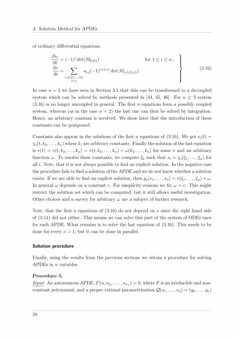
3. Solution Method for APDEs
of ordinary differential equations.
∂si∂t
= (−1)i det(M∅,{i}) for 1 ≤ i ≤ n ,
dv
dt=
∑i,j∈{1,...,n}
i<j
ai,j(−1)i+j+ν det(M{ν},{i,j}) .
(3.16)
In case n = 2 we have seen in Section 3.1 that this can be transformed to a decoupled
system which can be solved by methods presented in [44, 45, 46]. For n ≥ 3 system
(3.16) is no longer uncoupled in general. The first n equations form a possibly coupled
system, whereas (as in the case n = 2) the last one can then be solved by integration.
Hence, an arbitrary constant is involved. We show later that the introduction of these
constants can be postponed.
Constants also appear in the solutions of the first n equations of (3.16). We get si(t) =
χi(t, k2, . . . , kn) where ki are arbitrary constants. Finally the solution of the last equation
is v(t) = v(t, k2, . . . , kn) = v(t, k2, . . . , kn) + ω(k2, . . . , kn) for some v and an arbitrary
function ω. To resolve these constants, we compute ξk such that si = χi(ξ1, . . . , ξn) for
all i. Note, that it is not always possible to find an explicit solution. In the negative case
the procedure fails to find a solution of the APDE and we do not know whether a solution
exists. If we are able to find an explicit solution, then gν(s1, . . . , sn) = v(ξ1, . . . , ξn) +ω.
In general ω depends on a constant c. For simplicity reasons we fix ω = c. This might
restrict the solution set which can be computed, but it still allows useful investigation.
Other choices and a survey for arbitrary ω are a subject of further research.
Note, that the first n equations of (3.16) do not depend on ν since the right hand side
of (3.14) did not either. This means we can solve this part of the system of ODEs once
for each APDE. What remains is to solve the last equation of (3.16). This needs to be
done for every ν > 1, but it can be done in parallel.
Solution procedure
Finally, using the results from the previous sections we obtain a procedure for solving
APDEs in n variables.
Procedure 5.
Input: An autonomous APDE, F (u, ux1 , . . . , uxn) = 0, where F is an irreducible and non-
constant polynomial, and a proper rational parametrization Q(s1, . . . , sn) = (q0, . . . , qn)
58

3.3. The General Case
of the corresponding hypersurface defined by F .
Output: A solution of the APDE or “fail”.
1. Compute the coefficients ai =∂q0∂si
q1, and bi = qi
q1. Compute further aj,k =
∂aj∂sk− ∂ak
∂sj
and bi,` = ∂bi∂s`
.
2. Compute det(M∅,{i}) for all i. If only one of them is non-zero, solve the ODEs by
integration as described in Remark 3.15 and continue with Step 4.
If all determinants are zero, compute∑
i,j∈{1,...,n}i<j
ai,j(−1)i+j+ν det(M{ν},{i,j}). If
this is non-zero, there is no proper rational solution. The procedure stops. If this
is zero, then Q does not fulfill the requirements.
3. Solve (in parallel) the quasilinear PDEs (3.14) for gν , n ≥ ν > 1, respectively.
Using the method of characteristics proceed as follows.
a) Solve the system of ODEs, ∂si∂t
= (−1)i det(M∅,{i}), for all 1 ≤ i ≤ n and get
solutions si(t) = χi(t, k2, . . . , kn).
b) Solve the ODE, dvdt
=∑
i,j∈{1,...,n}i<j
ai,j(−1)i+j+ν det(M{ν},{i,j}), by integration.
c) Compute ξk such that si = χi(ξ1, . . . , ξn) for all i.
d) Compute gν(s1, . . . , sn) = v(ξ1, . . . , ξn) + cν .
4. Use (3.10) to compute g1.
5. Compute h1, . . . , hn such that g(h1(s1, . . . , sn), . . . , hn(s1, . . . , sn)) = (s1, . . . , sn).
6. Compute the solution q0(h1(x1, . . . , xn), . . . , hn(x1, . . . , xn)).
We want to prove now that Procedure 5 actually computes solutions of APDEs. Prop-
erties of the output solutions are presented later on.
Theorem 3.19.
Let F (u, ux1 , . . . , uxn) = 0 be an autonomous APDE. If Procedure 5 returns a function
v(x1, . . . , xn) for input F , then v is a solution of F = 0.
59

3. Solution Method for APDEs
Proof. By the last step of the procedure we know that
v(x1, . . . , xn) = q0(h1(x1, . . . , xn), . . . , hn(x1, . . . , xn)) .
with hi such that g(h1(s1, . . . , sn), . . . , hn(s1, . . . , sn)) = (s1, . . . , sn). Since g is a solution
of the system (3.12), it fulfills the assumption that u(g1, . . . , gn) = q0 for some solution
u of the APDE. Hence, v is a solution. We have seen a more detailed description at the
beginning of this section.
Now, we show that the result does not change if we postpone the introduction of the
constants c1, . . . , cn to the end of the procedure. It is easy to see that if u(x1, . . . , xn) is
a solution of an autonomous APDE then so is u(x1 + c1, . . . , xn + cn) for any constants
ci, 1 ≤ i ≤ n. From the procedure we get for i ≥ 2 that gi = gi + ci with gi not
depending on cj for all j. Furthermore, we see that in the computation of g1 we use the
derivatives of gi only (and hence the ci disappear). Therefore, we have that g1 = g1 + c1.
Let g = (g1, . . . , gn) and g = (g1, . . . , gn). In Step 5 we are looking for a function h such
that g ◦ h = id. Now g ◦ h = g ◦ h + (c1, . . . , cn). Take h such that g ◦ h = id. Then
g ◦ h(s1 − c1, . . . , sn − cn)) = id. Hence, we can introduce the constants at the end.
In case the original APDE is in fact an AODE, the ODE in (3.16) turns out to be trivial
and the integral in Step 4 is exactly the one which appears in Procedure 3. Of course
then g is univariate and so is its inverse. We do not specify Procedure 5 to handle this
case. Furthermore, if n = 2 this procedure specifies to Procedure 4. In this sense, this
new procedure generalizes Procedure 3 and 4.
Remark 3.20.
Procedure 5 might fail in several steps. First of all, we avoided to talk about parametriz-
ability by assuming there is a parametrization of the corresponding hypersurface. In case
such a parametrization does not exist in a certain class there cannot exist a solution in
this class either. Further we use the method of characteristics which might not give an
explicit solution (compare [73]).
Later we compute g1 by integration where a solution might only be found in a field
extension, i. e. we might get out of the class of functions we are looking for. Nevertheless,
if we find an integral in a field extension and the subsequent steps are successful as well,
we might still get a solution. See for instance the examples in Section 3.3.2.
60

3.3. The General Case
Finally, in Step 5 it might happen that there is no explicit solution for hi. In all of these
cases, we say that the procedure fails and then we do not know anything about solvability
of the input APDE. In the latter case, however, we might state the solution implicitly.
3.3.1. Rational Solutions
For first-order autonomous AODEs the algorithm of Feng and Gao [17] gives an answer
on whether or not a rational solution exists. As Procedure 5 is a generalization of
Procedure 3 for AODEs, it also generalizes this algorithm. As in Procedure 4, any
final result of the procedure is a solution of the differential equation, but however, the
procedure might fail and then it does not tell us whether a solution might exist. In the
following we collect properties of rational solutions and compute some examples.
Properties of Rational Solutions
Now we discuss the properties of rational solutions computed by Procedure 5. In par-
ticular we show that these solutions are proper and complete of suitable dimension.
Lemma 3.21.
If Procedure 5 yields a rational solution, then the solution is proper.
Proof. Let L be the corresponding parametrization of the output solution. In the pro-
cedure we start with a proper parametrization Q of the associated surface. When the
procedure is successful we know that L(g) = Q and the inverse h of g exists. Hence,
L = Q(h) is proper as well.
Recall Remark 1.2 which proves that the Jacobian of the corresponding parametrization
of a proper solution computed by the procedure has generic rank n.
Theorem 3.22.
Assume Procedure 5 yields a rational solution u(x1, . . . , xn). Then the solution u is
complete of suitable dimension.
61

3. Solution Method for APDEs
Proof. From the investigation below Theorem 3.19 we know that u(x1, . . . , xn) = u∗(x1+
c1, . . . , xn + cn) for some u∗. As usual, let L be the corresponding parametrization of u.
For the case of two variables we see that
J c1,c2L =
ux(x+ c1, y + c2) uy(x+ c1, y + c2)
uxx(x+ c1, y + c2) uxy(x+ c1, y + c2)
uyx(x+ c1, y + c2) uyy(x+ c1, y + c2)
= J x,yL = JL .
The equation J c1,...,cnL = J x1,...,xn
L also holds in general. From Lemma 3.21 we know that
L is proper and from Remark 1.2 we know that a proper solution has a Jacobian of rank
n.
APDEs with Rational Solutions
We start with a full computation of an example. Examples and classes of APDEs in
two variables with rational solutions can be found in Section 3.1.1 and Appendix C.3.
Therefore, we focus on an example with more than two variables.
Example 3.23. (Example 7.11 of Kamke [31])
We consider the APDE, F (u, ux1 , ux2 , ux3) = d1u2x1
+ d2u2x2
+ d3u2x3− u = 0, where d1,
d2 and d3 are non-zero constants. A possible parametrization is
Q =
s1, s2,−√−d2d3s1 + d1
√−d2d3s2
2 +√−d2d3d3s
23
2d2s3
,s1 − d1s
22 + d3s
23
2d3s3
.
The coefficients as computed in the procedure are
a1 =1
s2
, a2 = 0, a3 = 0 ,
b2 =−√−d2d3s1 + d1
√−d2d3s2
2 +√−d2d3d3s
23
2d2s2s3
, b3 =s1 − d1s
22 + d3s
23
2d3s2s3
.
Then we have to solve the following quasilinear equations
−s1 + d1s22 + d3s
23
2d3s32s
23
= −
√−d2d3
(s3
∂g2∂s3
+ s2∂g2∂s2
+ 2s1∂g2∂s1
)2d2s3
2s3
,
−
√−d2d3
(s1 − d1s22 + d3s
23)
2d2s32s
23
= −
√−d2d3
(s3
∂g3∂s3
+ s2∂g3∂s2
+ 2s1∂g3∂s1
)2d2s3
2s3
.
62

3.3. The General Case
Simplifying these equations and using the ideas of the method of characteristics, we have
to solve the following system of ODEs.
s′1 =2s1s3√−d2d3d3
,
s′2 = −
√−d2d3s2s3
d2
,
s′3 = −
√−d2d3s2
3
d2
,
v′ =d1s
22 + d3s
23 − s1
d3
, resp. v = −
√−d2d3
(−d1s22 + d3s
23 + s1)
d2
.
The first three equations are independent from the last one. They yield solutions
s1 =c2(
c1
√−d2d3d3 + t
)2 , s2 =c3
c1d2 −√−d2d3t, s3 = − d2
c1d2 −√−d2d3t,
for some arbitrary constants c1, c2, c3. Resolving t and the constants results in
t = −
√−d2d3d3
s3
, c2 = −d2d3s1
s23
, c3 = −d2s2
s3
. (3.17)
Solving the last equation of the system of ODEs by integration yields
v =
c23d1d2
+ c2d3
+ d2d3
t, resp. v =
√−d2d3
(c23d1d3 + c2d2 − d2
2d23)
d22t
Using (3.17) we get the solutions
g2 =
√−d2d3
(−s1 + d1s22 + d3s
23)
s3
, g3 =s1 − d1s
22 + d3s
23
s3
.
Now, we need to compute g1. We do so be taking the first equation of (3.10). Thus,
g1 = m1(s2, s3) ,
where m1 is an arbitrary function. Using the second equation of (3.10) we compute m1
and get
m1 = 2d1s2 +m2(s3) .
63

3. Solution Method for APDEs
Finally, we compute m2 = c1 using the last equation in (3.10). We choose c1 to be 0.
Hence,
g1 = 2d1s2 .
Solving the system gi(h) = si, we get
h1 =1
4
(s2
1
d1
+s2
2
d2
+s2
3
d3
), h2 =
s1
2d1
, h3 =
s2√− d2d3
+ s3
2d3
.
Hence,
q0(h(x1, x2, x3)) = h1(x1, x2, x3) =1
4
(x2
1
d1
+x2
2
d2
+x2
3
d3
)is a solution of the APDE and q0(h(x1 + c1, x2 + c2, x3 + c3)) is a complete one.
3.3.2. Other Solutions
So far we concentrated on rational solutions. For the case of n = 2 we additionally saw
on examples that non-rational solutions might be computed by the procedure. In the
general case we can as well try to do computations in some field extension and as before
this will be subject to further investigation. Though, before we show some examples for
the general case, we also prove some properties of any result of the procedure regardless
of the class of functions. Similarly to Lemma 3.21 we get the following.
Lemma 3.24.
If Procedure 5 yields a solution, then the corresponding parametrization is injective al-
most everywhere.
Proof. Let L be the corresponding parametrization of the output solution. In the pro-
cedure we start with a proper parametrization Q of the associated surface. When the
procedure is successful we know that L(g) = Q and the inverse h of g exists. Hence,
L = Q(h) is injective almost everywhere.
A parametrization which is injective almost everywhere is also called almost injective.
Note, that the Jacobian of an almost injective parametrization P(s1, . . . , sn) has generic
rank n. Indeed, since P is almost injective, there exists a map R such that id = R ◦ P
64

3.3. The General Case
generically. Thus Jid = JR◦P = JR(P) · JP . Taking into account, that the rank of a
product of two matrices is less than or equal to the minimal rank of the two matrices,
we get that rank(JP) = n.
Theorem 3.25.
Assume Procedure 5 yields a solution u(x1, . . . , xn). Then the solution u is complete of
suitable dimension.
Proof. As usual, let L be the corresponding parametrization of u. Then the equation
J c1,...,cnL = J x1,...,xn
L holds in general. From Lemma 3.24 we know that L is almost
injective and the notes above show that an almost injective solution has a Jacobian of
expected rank.
The following examples show that the method is not restricted to finding rational solu-
tions. It might happen that the steps in Procedure 5 can be done by doing computations
in some extension field. In this case we can of course continue in the procedure and might
get a non-rational solution.
Example 3.26. (Eikonal Equation with 5 variables)
We consider the APDE, F (u, ux1 , . . . , ux5) =(∑5
i=1 u2xi
)− 1 = 0. A possible rational
parametrization of the corresponding hypersurface is
Q =
(s1,
s22 + s2
3 + s24 + s2
5 − 1
D,2s2
D,2s3
D,2s4
D,2s5
D
),
where D = s22 + s2
3 + s24 + s2
5 + 1. The parametrization is proper. Indeed, the inverse is
given by
s1 = z , s2 = − p2
p1 − 1, s3 =
p3(p1 + 1)
p22 + p2
3 + p24 + p2
5
,
s4 =p4(p1 + 1)
p22 + p2
3 + p24 + p2
5
, s5 =p5(p1 + 1)
p22 + p2
3 + p24 + p2
5
.
The coefficients appearing in the procedure are
a1 =s2
2 + s23 + s2
4 + s25 + 1
s22 + s2
3 + s24 + s2
5 − 1, ai = 0 , for i ≥ 2 ,
bi =2si
s22 + s2
3 + s24 + s2
5 − 1.
65

3. Solution Method for APDEs
Then we get the following quasilinear equations for 2 ≤ i ≤ 5.
32si
(s22 + s2
3 + s24 + s2
5 − 1)5 =
16 (s22 + s2
3 + s24 + s2
5 + 1) ∂gi∂s1
(s22 + s2
3 + s24 + s2
5 − 1)5 .
Here we are in the case of Remark 3.15 and hence, by integration we get
gi =2s1siD
, for i ≥ 2 .
Note, that for simplicity we chose the arbitrary functions which occur in the solutions
of the ODEs to be 0. Now we need to compute g1. We do so by taking the first equation
of (3.10). As a solution we get g1 =s1(s22+s23+s24+s25−1)
D+ m1(s2, s3, s4, s5), where m1
is an arbitrary function. Step by step we compute m1 by using the other equations of
(3.10). Using the second equation we have an ODE in m1. We get m1 = m2(s3, s4, s5).
Continuing like this we finally get m1 = c1 for an arbitrary constant. Since, we can deal
with constants at the end of the procedure, we choose c1 to be zero for the moment. Now
we have to solve the system gi(h) = si. A solution of this system is
h1 =
√s2
2 (s21 + s2
2 + s23 + s2
4 + s25)
s2
,
hi =s1s2si − si
√s2
2 (s21 + s2
2 + s23 + s2
4 + s25)
s2 (s22 + s2
3 + s24 + s2
5), for i ≥ 2 .
Hence we conclude that
q0(h(x)) = h1(x) =√x2
1 + x22 + x2
3 + x24 + x2
5
is a solution of the APDE.
Example 3.27.
We consider the APDE, F (u, ux1 , ux2 , ux3) = (ux1 +d1)ux2 − (u+d2)ux3 = 0. A possible
proper parametrization is Q = (s1, s2, s3,(s2+d1)s3s1+d2
). The coefficients are
a1 =1
s2
, a2 = 0 , a3 = 0 ,
b2 =s3
s2
, b3 =(s2 + d1)s3
(s1 + d2)s2
.
Then we have to solve the following quasilinear equations
d1 + s2
(d2 + s1)s32
=1
(d2 + s1)2s32
s3
((d1 + s2)s3
∂g2
∂s3
+ s2
((d1 + s2)
∂g2
∂s2
+ (d2 + s1)∂g2
∂s1
)),
− 1
s32
=1
(d2 + s1)2s32
s3
((d1 + s2)s3
∂g3
∂s3
+ s2
((d1 + s2)
∂g3
∂s2
+ (d2 + s1)∂g3
∂s1
)).
66

3.4. Further approaches
Omitting the details and intermediate steps we get the solutions
g2 = −(d2 + s1)(d1 − log(s2)s2)
(d1 + s2)s3
, g3 =(d2 + s1)2(d1 − log(s2)s2)
(d1 + s2)2s3
.
Now, we need to compute g1. We do so be taking the first equation of (3.10). This
results in
g1 =(1 + log(−s2))s1
d1 + s2
+m1(s2, s3) ,
where m1 is an arbitrary function. Using the second equation of (3.10) we compute
m1 =d2(1 + log(−s2))
d1 + s2
+m2(s3)
Finally, we compute m3 = c1 using the last equation in (3.10). We choose c1 to be 0.
Hence,
g1 =(1 + log(−s2))(d2 + s1)
d1 + s2
.
Solving the system gi(h) = si, we get
h1 = −d2s2 + d1s3 − e−1− s1s2
s3 s3
s2
,
h2 = −e−1− s1s2
s3 ,
h3 =e−1− s1s2
s3
(−s1s2 +
(−1 + d1e
1+s1s2s3
)s3
)s2
2
.
Hence,
q0(h(x)) = h1(x1, x2, x3) = −d2x2 + d1x3 − e−1−x1x2
x3 x3
x2
is a solution of the APDE.
3.4. Further approaches
In this section we present some approaches which might be used for extending the class
of APDEs for which we can compute solutions. The approaches under consideration
connect methods described in Chapter 2 respectively 3 and other known methods. The
67

3. Solution Method for APDEs
first approach helps to find solutions of AODEs, whereas the second idea, which is based
on a known method, computes non-proper solutions of APDEs. The ideas are briefly
discussed but more elaborate treatment is subject to further research.
Solving AODEs via ideas from APDEs
In Section 2.3 we introduced some ideas for higher-order AODEs referring to a similar
idea for APDEs which we present here. Let us consider an autonomous second-order
APDE, F (u, ux, uxx) = 0. Assume we have a proper rational parametrization Q =
(q0, q1, q2) of the surface F (z, p1, p2) = 0. As usual, we assume that Q = L(g) for some
function g, where L is the parametrization corresponding to a solution. Then, similar
to system (1.2) for the first-order case we now get the following equations.
q0(s, t) = u(g1(s, t), g2(s, t)) ,
q1(s, t) = ux(g1(s, t), g2(s, t)) ,
q2(s, t) = uxx(g1(s, t), g2(s, t)) ,
which yield by taking first derivatives
∂q0
∂s=∂g2
∂suy(g1, g2) +
∂g1
∂sux(g1, g2) =
∂g2
∂suy(g1, g2) +
∂g1
∂sq1 ,
∂q0
∂t=∂g2
∂tuy(g1, g2) +
∂g1
∂tux(g1, g2) =
∂g2
∂tuy(g1, g2) +
∂g1
∂tq1 ,
∂q1
∂s=∂g2
∂suxy(g1, g2) +
∂g1
∂suxx(g1, g2) =
∂g2
∂suxy(g1, g2) +
∂g1
∂sq2 ,
∂q1
∂t=∂g2
∂tuxy(g1, g2) +
∂g1
∂tuxx(g1, g2) =
∂g2
∂tuxy(g1, g2) +
∂g1
∂tq2 .
Elimination of uy(g1, g2) from the first two equations and uxy(g1, g2) from the last two
equations yields
∂g2
∂s
∂q0
∂t− ∂g2
∂t
∂q0
∂s=
(∂g2
∂s
∂g1
∂t− ∂g2
∂t
∂g1
∂s
)q1 , (3.18)
∂g2
∂s
∂q1
∂t− ∂g2
∂t
∂q1
∂s=
(∂g2
∂s
∂g1
∂t− ∂g2
∂t
∂g1
∂s
)q2 . (3.19)
Combining these two equations we get a quasilinear PDE in g2.
q1
(∂q1
∂t
∂g2
∂s− ∂g2
∂t
∂q1
∂s
)= q2
(∂q0
∂t
∂g2
∂s− ∂g2
∂t
∂q0
∂s
). (3.20)
We can solve the quasilinear equation by the method of characteristics to get g2. Equa-
tion (3.18) is a quasilinear equation in g1, when g2 is given. Once knowing g1 and g2
68

3.4. Further approaches
we compute, as usual, h1 and h2 such that (g1(h1, h2), g2(h1, h2)) = (s, t). The following
example illustrates the procedure.
Example 3.28.
The usability of this example is shown in Example 2.20 where the solution of this APDE
is needed to solve a second-order AODE. We consider the APDE, F (u, ux, uxx) =
uuxx + u2x = 0. It is easy to see that Q =
(s, t,− t2
s
)is a proper parametrization of
the corresponding surface. In this case equation (3.20) is
t∂g2
∂s− t2
s
∂g2
∂t= 0 .
Using the method of characteristics we need to solve the ODEs
ds(t)
dt= −s(t)
t,
dv(t)
dt= 0 .
The solution of the first equation is s(t) = kt, which yields k = st. The solution of the
second equation is v(t) = ν2(k) for some function ν2. Then g2(s, t) = ν2(st). Now we
take equation (3.18) to compute g1:
−q1∂g2
∂t
∂g1
∂s+ q1
∂g2
∂s
∂g1
∂t=∂g2
∂s
∂q0
∂t− ∂g2
∂t
∂q0
∂s
−stν ′2(st)∂g2
∂s+ t2ν ′2(st)
∂g1
∂t= −sν ′2(st)
Using again the method of characteristics we have to solve the ODEs
ds(t)
dt= −s(t)
t,
dv(t)
dt= −s(t)
t2.
The first equation yields s(t) = kt, i. e. k = st. Solving the second equation by integration
we get v(t) =∫
kt3
dt = − k2t2
+ ν1(k) for some function ν1. Then g1(s, t) = − s2t
+ ν1(st).
We choose ν1 = ν2 = id. Then we can compute h1 and h2:
h1 =
√2t3/2√s− t
−√
2s√t√
s− t, h2 = −
√t√
2s− 2t.
Since q0 = s we know that h1(x, y) is a solution of the APDE and so is h1(x+c1, y+c2).
69

3. Solution Method for APDEs
This idea can be generalized to higher order. Let F (u, u(1,0,...,0), . . . , u(n,0,...,0)) = 0, where
u(k1,...,kn) = ∂k1
∂xk11
(. . .(∂knu
∂xk1n
)). Let Q(s1, . . . , sn) = (q0, . . . , qn) be a proper rational
parametrization of the corresponding hypersurface. As usual, we assume that Q = L(g),
where g is an invertible function and L is the parametrization induced by a solution.
Then the following equations have to be fulfilled.
qk = u(k,0,...,0)(g) , for k ∈ {0, . . . , n} , (3.21a)(∂qk∂si
)i∈{1,...,n}
= G ·(∂u(k,0,...,0)
∂xi(g)
)i∈{1,...,n}
, for k ∈ {0, . . . , n− 1} , (3.21b)
where G = ( ∂gi∂sj
)i,j∈{1,...,n}. Since g is an invertible function, the matrix G has an inverse.
We pick the first row in each equation of (3.21b) and use (3.21a) to get
(qi)i∈{1,...,n} = M · ((G−1)1)T ,
where M =(∂qi∂sj
)i∈{0,...,n−1}j∈{1,...,n}
and (G−1)1 is the first row of the inverse of G. By Cramer’s
rule we know that
(G−1)1,k =det(Mk)
det(M),
where Mk is constructed from M by replacing the i-th column by (q1, . . . , qn)T . Using
the definition of an inverse we conclude that
n∑i=1
∂g1
∂sidet(Mi) = det(M) , (3.22a)
n∑i=1
∂gk∂si
det(Mi) = 0 , for k > 1 . (3.22b)
These are quasilinear PDEs and can be solved by the method of characteristics. Finally,
we summarize the procedure.
Procedure 6.
Input: An autonomous APDE, F (u, u(1,0,...,0), . . . , u(n,0,...,0)) = 0, with an irreducible
and non-constant polynomial F , and a proper rational parametrization Q(s1, . . . , sn) =
(q0, . . . , qn) of the corresponding hypersurface defined by F .
Output: A solution u(x1, . . . , xn) of the APDE or “fail”.
• Solve the quasilinear PDE from (3.22b) with the method of characteristics and
take n− 1 independent solutions to get g2, . . . , gn.
70

3.4. Further approaches
• Solve the quasilinear PDE (3.22a) with the method of characteristics to get g1.
• Compute h such that g(h) = id.
• Return q0(h(x1, . . . , xn)).
Note, that for n = 2 this procedure indeed specializes to the idea from above.
Example 3.29.
The solution of this example is used in Example 2.21. We consider the APDE,
F (u, ux, uxx, uxxx) = uuxxx − uxuxx = 0 .
It is easy to see that Q =(s1, s2, s3,
s2s3s1
)is a proper parametrization of the correspond-
ing hypersurface. In this case M = In and hence, (3.22) yields
∂g1
∂s1
s2 +∂g1
∂s2
s3 +∂g1
∂s3
s2s3
s1
= 1 ,
∂g2
∂s1
s2 +∂g2
∂s2
s3 +∂g2
∂s3
s2s3
s1
= 0 ,
∂g3
∂s1
s2 +∂g3
∂s2
s3 +∂g3
∂s3
s2s3
s1
= 0 .
Using the method of characteristics we need to solve the system of ODEs
ds2(t)
dt=s3(t)
s2(t),
ds3(t)
dt=s3(t)
t.
We get s2 = −√t2k1 + 2k2 and s3 = tk1. Since the right hand side of the quasilinear
equations for g2 and g3 is zero we conclude that g2 = ν2(k1, k2) and g3 = ν3(k1, k2) for
some arbitrary functions ν2, ν3. We choose g2 = k1 and g3 = k2. It remains to compute
g1. For this we integrate 1s2(t)
and get −log(√
k1√k1t2+2k2+k1t
)√k1
. We resolve k1 and k2 which
yields k1 = s3t
and k2 = 12(s2
2 − ts3). Hence,
g1 = −log(s3 +
√s3s1
√s2
2
)√
s3s1
, g2 =s3
s1
, g3 =1
2
(s2
2 − s1s3
).
71

3. Solution Method for APDEs
Finally, we compute h such that g(h) = id and get
h1 =es1√s2(e−2s1
√s2 − 2s2s3
)2s2
,
h2 =es1√s2(2s2s3 + e−2s1
√s2)
2√s2
,
h3 =1
2es1√s2(e−2s1
√s2 − 2s2s3
).
Therefore, q0(h1(x1, x2, x3), h2(x1, x2, x3), h3(x1, x2, x3)) = h1(x1, x2, x3) is a solution of
the APDE.
The idea can be further generalized to non-autonomous APDEs. Let F be such an
APDE, i. e. F (x1, u, u(1,0,...,0), . . . , u(n,0,...,0)) = 0, in n+1 variables. Let Q(s1, . . . , sn+1) =
(q−1, q0, . . . , qn) be a proper rational parametrization of the corresponding hypersurface.
As usual, we assume that Q = L(g). Then the following equations have to be fulfilled.
qk = u(k,0,...,0)(g) , for k ∈ {0, . . . , n} , (3.23a)(∂q−1
∂si
)i∈{1,...,n+1}
= G · (1, 0, . . . , 0)T , (3.23b)(∂qk∂si
)i∈{1,...,n+1}
= G ·(∂u(k,0,...,0)
∂xi(g)
)i∈{1,...,n+1}
, for k ∈ {0, . . . , n− 1} , (3.23c)
where G = (∂gj∂si
)i,j∈{0,...,n}. Since g is an invertible function, the matrix G has an inverse.
We pick the first row of each equation in (3.23c) and the first row of (3.23b). Using
(3.23a) we get
(1, q1, . . . , qn)T = M · ((G−1)1)T ,
where M =(∂qi∂sj
)i∈{−1,...,n−1}j∈{1,...,n}
and (G−1)1 is the first row of the inverse of G. By Cramer’s
rule we conclude that
n∑i=1
∂gk∂si
det(Mi) = 0 , for k ≥ 1 , (3.24)
where Mk is constructed from M by replacing the i-th column by (1, q1, . . . , qn)T . These
are quasilinear PDEs and can be solved by the method of characteristics. Finally, we
summarize the procedure.
72
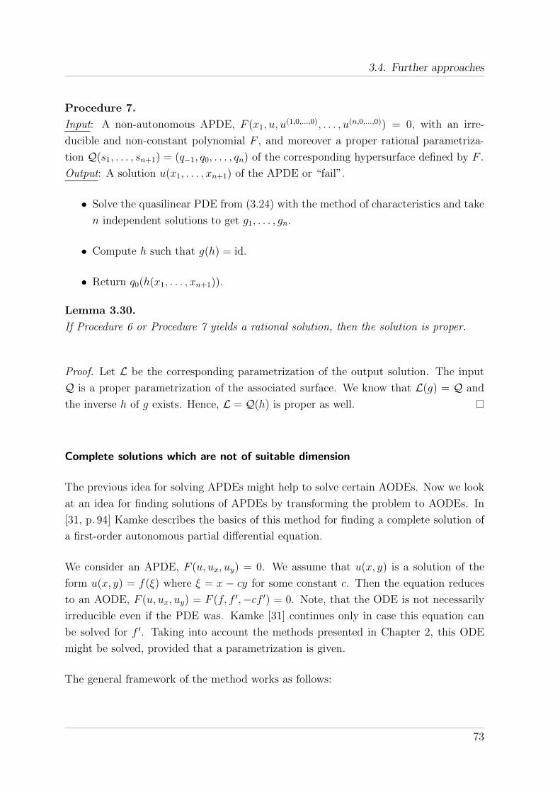
3.4. Further approaches
Procedure 7.
Input: A non-autonomous APDE, F (x1, u, u(1,0,...,0), . . . , u(n,0,...,0)) = 0, with an irre-
ducible and non-constant polynomial F , and moreover a proper rational parametriza-
tion Q(s1, . . . , sn+1) = (q−1, q0, . . . , qn) of the corresponding hypersurface defined by F .
Output: A solution u(x1, . . . , xn+1) of the APDE or “fail”.
• Solve the quasilinear PDE from (3.24) with the method of characteristics and take
n independent solutions to get g1, . . . , gn.
• Compute h such that g(h) = id.
• Return q0(h(x1, . . . , xn+1)).
Lemma 3.30.
If Procedure 6 or Procedure 7 yields a rational solution, then the solution is proper.
Proof. Let L be the corresponding parametrization of the output solution. The input
Q is a proper parametrization of the associated surface. We know that L(g) = Q and
the inverse h of g exists. Hence, L = Q(h) is proper as well.
Complete solutions which are not of suitable dimension
The previous idea for solving APDEs might help to solve certain AODEs. Now we look
at an idea for finding solutions of APDEs by transforming the problem to AODEs. In
[31, p. 94] Kamke describes the basics of this method for finding a complete solution of
a first-order autonomous partial differential equation.
We consider an APDE, F (u, ux, uy) = 0. We assume that u(x, y) is a solution of the
form u(x, y) = f(ξ) where ξ = x − cy for some constant c. Then the equation reduces
to an AODE, F (u, ux, uy) = F (f, f ′,−cf ′) = 0. Note, that the ODE is not necessarily
irreducible even if the PDE was. Kamke [31] continues only in case this equation can
be solved for f ′. Taking into account the methods presented in Chapter 2, this ODE
might be solved, provided that a parametrization is given.
The general framework of the method works as follows:
73

3. Solution Method for APDEs
Procedure 8.
Input: An autonomous APDE, F (u, ux, uy) = 0, where F is irreducible and non-
constant.
Output: A set of solutions (ui(x, y))i∈{1,...,η} of the APDE, where each element is of the
form f(x− cy), or “fail”.
• Compute G(f, f ′) = F (f, f ′,−c2f′).
• Take all irreducible factors of G, say G1, . . . , Gη.
• Compute parametrizations of Gi(y, z) = 0, if possible.
• Use methods from Chapter 2 for computing solutions fi of Gi(f, f′) = 0.
Return “fail” if the computation fails.
• Compute u = (ui(x, y))i∈{1,...,η} = (fi(x− c2y))i∈{1,...,η}.
From the above discussion it is easy to show that the result is indeed a solution.
Theorem 3.31.
Let v be the result of Procedure 8 for a given input F . Then vi is a solution of F = 0
for each i.
An autonomous APDE, F (u, ux, uy) = 0, has a rational solution of the form f(x− cy) if
and only if there is an i such that Gi(f, f′) has a rational solution. By Theorem 2.1 this
is the case if and only if for any proper rational parametrization P(t) = (r1(t), r2(t)) of
Gi the quotient r2r′1
is either in the ground field of P or a quadratic polynomial a(t−b)2.
As usual, we are interested in the properties of solutions computed by Procedure 8.
Lemma 3.32.
If Procedure 8 computes a list of non-constant rational solutions u, then each component
v is non-proper.
Proof. If v is a solution of an APDE computed by Procedure 8, then v(x, y) = f(x−c2y)
for some rational function f . Let L = (v, vx, vy) be the corresponding parametrization
of v. Then the Jacobian of L is
J x,yL =
f ′(x− c2y) −c2f′(x− c2y)
f ′′(x− c2y) −c2f′′(x− c2y)
−c2f′′(x− c2y) c2
2f′′(x− c2y)
.
74

3.4. Further approaches
It is easy to prove that rank(J x,yL ) ≤ 1. Due to Remark 1.2, L is not proper and so
neither is v.
Note, that rationality of the solution is only required in the definition of proper. The
fact that the rank of the Jacobian equals 1 is also valid for non-rational solutions.
Lemma 3.33.
Let u be the output of Procedure 8. Let v = ui(x + c1, y) for some i. Assume v is
non-constant and rational. Then v is a complete solution.
Proof. If u is computed by Procedure 8, then v(x, y) = f(x+ c1− c2y) for some rational
function f . Since ui is a solution we know by Theorem 3.31, and the fact that the APDE
is autonomous, that v is a solution as well. Let L = (v, vx, vy) be the corresponding
parametrization of v. Then the Jacobian of L with respect to c1 and c2 is
J c1,c2L =
f ′(x+ c1 − c2y) −yf ′(x+ c1 − c2y)
f ′′(x+ c1 − c2y) −yf ′′(x+ c1 − c2y)
−c2f′′(x+ c1 − c2y) −f ′(x+ c1 − c2y) + c2yf
′′(x+ c1 − c2y)
.
Since, v is non-constant and rational, it is easy to verify that rank(J c1,c2L ) = 2.
Note, if v is not rational, then the statement is not necessarily true. Assume for instance,
that f(ξ) = eξ. Then
J c1,c2L =
ec1+x−c2y −c2ec1+x−c2y
ec1+x−c2y −c2ec1+x−c2y
−c2ec1+x−c2y c22ec1+x−c2y
,
which has only rank 1.
Corollary 3.34.
A solution computed by Procedure 8 is not complete of suitable dimension.
Proof. In the proof of Lemma 3.32 we have shown that the Jacobian has rank ≤ 1.
We show on some examples how the procedure works and describe the connection and
differences to the methods in Chapter 2 and 3.
75

3. Solution Method for APDEs
Example 3.35.
We consider the APDE, F (u, ux, uy) = 6u4 + 5u3x + 5u2
xuy = 0. Using Procedure 4 we
find the solution 103(x+c1−y−c2)2(y+c2)
which is complete of suitable dimension.
Now we use Procedure 8 to get G(f, f ′) = 6f 4 + 5f ′3(1 − c2). We find a proper ratio-
nal parametrization P = (56t3(c2 − 1), 5
6t4(c2 − 1)). Hence, A = 1
3t2. This fulfills the
requirements for a rational solution of the AODE (c. f. Theorem 2.1). A solution of the
AODE is f(x) = 52
9(1−c2)(x+c1)3
. Hence, we get a solution u(x, y) = 52
9(1−c2)(x−c2y+c1)3
of F = 0.
This solution is complete, but not of suitable dimension.
In the following example G contains f ′ as a factor which always leads to a constant
solution. Furthermore there is a factor not depending on f and f ′ at all, but only on c.
Such factors give solutions with arbitrary functions f .
Example 3.36.
Consider the APDE, F (u, ux, uy) = ux−uy = 0. By the transformation we get f ′(1+c) =
0. Now either f ′ = 0 and hence f is constant, or c = −1. In the latter case we get that
u(x, y) = f(x+ y) is a solution for any f .
The following lemma shows some cases in which Procedure 8 finds a rational solution.
Lemma 3.37.
Let F (u, ux, uy) = 0 be an APDE such that the origin is a (d−1)-fold point of F (z, p, q) =
0, where d is the total degree of F . Furthermore, we assume that there is a parame-
trization of F of the form Q = (sn+1B(t), tsnB(t), snB(t)) where n ∈ Z \ {−1} and
B(t) ∈ K(t). Then Procedure 8 yields a rational solution.
Proof. Procedure 8 defined G to be G(a, b) = F (a, b,−c2b). Let P(s) = (p1(s), p2(s)) =
(sn+1B(− 1c2
),−sn 1c2B(− 1
c2)). Then
G(p1, p2) = F (p1, p2,−c2p2) = F (Q(s,− 1
c2
)) = 0 .
Hence, P is a parametrization of Gi for some i. We compute A = p2p′1
= −1c2(n+1)
.
By Theorem 2.1 there is a rational solution f(ξ) = (− ξ+c1c2(n+1)
)n+1B(− 1c2
). Hence,
(−x−c2y+c1c2(n+1)
)n+1B(− 1c2
) is a rational solution of the APDE.
76

3.4. Further approaches
Note, that by Lemma 3.7 Procedure 4 yields an algebraic (but not necessarily rational)
solution for an APDE which fulfills the requirements of the above lemma. Recall, that
Lemma 3.9 describes cases in which the solution is indeed rational. By Lemma 3.37 we
can now find rational (but non-proper) solutions even if none of the cases of Lemma 3.9
is fulfilled.
Using Procedure 3 instead of Algorithm 1 for solving the ODEs in Procedure 8 might
result in non-algebraic solutions.
Example 3.38.
We consider the APDE, F (u, ux, uy) = u2 + uxuy = 0. Procedure 8 computes G =
f 2 +cf ′2 = (f+√c2f′)(f−√c2f
′). Hence, we get P = (±√c2s, s) with A = s±√c2 . Then
g(s) =∫
1A
ds = ±√c2 log(s) and its inverse h(s) = e± s√
c2 . Thus, f(ξ) = ±√c2e± ξ√
c2 is
a solution of G and hence, ±√c2e± c1+x−c2y√
c2 is a solution of F .
The ideas of Procedure 8 are easily generalized to an arbitrary number of independent
variables. In this case we have two choices. Either we reduce to an AODE directly, or
we just reduce to an APDE with less variables.
Reduction of the number of variables
We consider an APDE, F (u, ux1 , . . . , uxn) = 0 and assume that u(x1, . . . , xn) is a solution
of the form u(x1, . . . , xn) = f(ξ, x3, . . . , xn), where ξ = x1 − c2x2 for some constant
c2. Then the APDE reduces to another APDE of lower order, F (u, ux1 , . . . , uxn) =
F (f, fξ,−c2fξ, fx3 , . . . , fxn) = 0. Now, in fact, this PDE (or to be precise, its factors)
might be solved by Procedure 5. Note, that we could solve F directly by Procedure 5.
However, we would get other solutions.
Procedure 9.
Input: An autonomous APDE, F (u, ux1 , . . . , uxn) = 0, where F is irreducible and non-
constant.
Output: A set of solutions (ui(x1, . . . , xn))i∈{1,...,η} of the APDE, where each element is
of the form f(x1 + c1 − c2x2, x3, . . . , xn), or “fail”.
• Compute G = F (f, fξ,−c2fξ, fx3 , . . . , fxn).
• Take all irreducible factors of G, say G1, . . . , Gη.
• Compute parametrizations of Gi, if possible.
77

3. Solution Method for APDEs
• Use Procedure 5 for computing solutions fi of Gi = 0.
Return “fail” if the computation fails.
• Compute u = (ui(x1, . . . , xn))i∈{1,...,η} = (fi(x1 + c1 − c2x2, x3, . . . , xn))i∈{1,...,η}.
Theorem 3.39.
Let v be the result of Procedure 9 for a given input F . Then vi is a solution of F = 0
for each i.
Of course we can take any number of linear combinations xi− ci,jxj for reduction. Fur-
thermore, we could take linear combinations involving more than two variables. A special
case using relations for all variables reduces to an ODE as we see in the following.
Reduction to ODE
We consider an APDE, F (u, ux1 , . . . , uxn) = 0. The following idea has been already
mentioned in [31, 13.2]. However, we can now incorporate the methods from Chapter 2.
We assume that u(x1, . . . , xn) is a solution of the form u(x1, . . . , xn) = f(ξ) where
ξ = x1 −∑n
i=2 cixi for some constants ci. Then the equation reduces to an ODE
F (u, ux1 , . . . , uxn) = F (f, f ′,−c2f′, . . . ,−cnf ′) = 0. Now, in fact, this ODE (or to be
precise, its factors) might be solved by Algorithm 1 or by Procedure 3.
Procedure 10.
Input: An autonomous APDE, F (u, ux1 , . . . , uxn) = 0, where F is irreducible and non-
constant.
Output: A set of solutions (ui(x1, . . . , xn))i∈{1,...,η} of the APDE, where each element is
of the form f(x1 + c1 −∑n
i=2 cixi)), or “fail”.
• Compute G(f, f ′) = F (f, f ′,−c2f′, . . . ,−cnf ′).
• Take all irreducible factors of G, say G1, . . . , Gη.
• Compute parametrizations of Gi, if possible.
• Use methods from Chapter 2 for computing solutions fi of Gi(f, f′) = 0.
Return “fail” if the computation fails.
• Compute u = (ui(x1, . . . , xn))i∈{1,...,η} = (fi(x1 + c1 −∑n
i=2 cixi))i∈{1,...,η}.
78

3.4. Further approaches
Theorem 3.40.
Let v be the result of Procedure 10 for a given input F = 0. Then vi is a solution of F
for each i.
The ideas from above can be easily extended to higher-order autonomous APDEs. We
briefly discuss the case for two variables.
Higher-Order APDEs
We consider an APDE, F (u, ux, uy, . . . ,∂νu∂xν
, ∂νu∂xν−1∂y
, . . . , ∂νu∂yν
) = 0. We assume that
u(x, y) is a solution of the form u(x, y) = f(ξ) where ξ = x − cy for some constant
c. Then our equation reduces to an ODE
F (u, ux, uy, . . . ,∂νu
∂yν) = F (f, f ′,−cf ′, . . . , f (ν),−cf (ν), . . . , (−c)νf (ν)) = 0 .
We can use the method described in Section 2.3 for solving the ODE. Note, that it is
of course also possible to combine higher order and arbitrary many variables, but in
the general case notation will be rather long and hence, we refrain from explicitly doing
so.
Example 3.41. (Laplace Equation)
We consider the Laplace equation F (u, ux, uy, uxx, uxy, uyy) = uxx + uyy = 0. Then we
get the ODE, F (f, f ′,−cf ′, f ′′,−cf ′′, c2f ′′) = f ′′ + c2f ′′ = f ′′(1 + c2) = 0. This ODE
has the solution f(ξ) = c1 + c2ξ. Hence, u(x, y) = f(x− cy) = c1 + c2(x− cy) which is
definitely a solution of F = 0.
Note, that we did not define the notions of complete and suitable dimension for higher
order.
79


4. Linear Transformations
Transformations are widely used in different sense for solving differential equations (see
for instance [73, Chapter I.B] for transformations of both ODEs and PDEs). The main
aim is usually to transform a differential equation to another one which is easier to
solve. After solving the new equation, the solution can be transformed back to obtain a
solution of the original equation.
The kind of transformations we are investigating here are linear ones which transform
implicit differential equations and likewise the parametrizations of their corresponding
hypersurfaces. Linear transformations have been used in [42] for classifying AODEs.
Using this classification it can be decided whether a given AODE can be transformed to
an autonomous one, i. e. whether the class under consideration contains an autonomous
AODE. It was shown in [42] that the associated system (see Section 2.1.2) remains
invariant under linear transformations.
Here, we want to use the same idea for transforming non-autonomous APDEs to au-
tonomous ones. This approach helps to solve some non-autonomous APDEs. Though,
we do not have the associated system as an invariant, but there are still certain properties
which are preserved by the transformation.
The idea of linear transformations can be generalized to transformations by birational
maps (see [43] for AODEs). However, investigation of using this idea for APDEs is not
topic of the current work.
In Section 4.1 we consider first-order APDEs in several variables. Specifying the number
of variables to n = 1 yields the known transformations for AODEs. Many conclusions
from the ODE case can be adopted rather easily. However, we will see that some nice
results are not true for APDEs in general. A main question under consideration is
whether some given APDE can be linearly transformed to an autonomous one. Later
in Section 4.2 we show how the approach can be extended to higher order whereat for
notational reasons we focus on the case of second order.
81

4. Linear Transformations
4.1. Linear Transformations of First-Order APDEs
In this section we introduce linear transformations for partial differential equations. For
now we focus on first-order APDEs. The definitions work quite analogously to the case
of AODEs in [42]. Let F (x1, . . . , xn, u, ux1 , . . . , uxn) = 0 be a first-order APDE. Let L
be a linear map defined by
L : K(x1, . . . , xn)2n+1 −→ K(x1, . . . , xn)2n+1 ,
w 7−→ Aw +B ,
where A is an invertible ((2n+ 1)× (2n+ 1))-matrix and B a column vector. We are in-
terested in such L which map any tuple (x1, . . . , xn, u, ux1 , . . . , uxn) ∈ K(x1, . . . , xn)2n+1
to a similar one, say (x1, . . . , xn, v, vx1 , . . . , vxn).
Obviously not every matrix is suitable. Using some simple examples for the function u,
we find out that the matrix A and the vector B have to be of the form
A =
1 0 · · · 0 0 0 · · · 0
0 1. . .
... 0 0. . .
......
. . . . . . 0...
. . . . . . 0
0 · · · 0 1 0 · · · 0 0
β1 β2 · · · βn α 0 · · · 0
0 0 · · · 0 0 α. . .
......
. . . . . . 0...
. . . . . . 0
0 · · · 0 0 0 · · · 0 α
, B =
0
0...
0
δ
β1
...
βn
,
with α, δ, βi ∈ K, α 6= 0. In short notation we write
A =
In 0
β
0αIn+1
, B =
0
δ
βT
, (4.1)
where β is a row vector. Let x = (x1, . . . , xn)T . Then we get that
L(x1, . . . , xn, u, ux1 , . . . , uxn) = A ·
x
u
∇u
+B =
x
β · x+ αu+ δ
α∇u+ βT
.
We need to show that ∂∂xj
(β · x+ αu+ δ) = (α∇u+ βT )j. But this is easy to see.
82

4.1. Linear Transformations of First-Order APDEs
Now we define the set G as the set of pairs [A,B] with A and B of the form (4.1).
Let L1 = [A1, B1] and L2 = [A2, B2] be elements of G. We define the operation ◦ as
follows.
L1 ◦ L2 = [A1 · A2, A1 ·B2 +B1] =
In 0
β1 + α1β2
0α1α2In+1
,
0
α1δ2 + δ1
α1βT1 + βT2
,
which is again in G. There is a neutral element N = [I2n+1, 0] with respect to ◦. It is
easy to see that In 0
− 1α1β1
01α1In+1
,
0
− δ1α1
− 1α1βT1
is the inverse of L1. Hence, (G, ◦) is a group. We call it the group of linear transforma-
tions . Note, that this is a direct generalization of the ODE case which was investigated
in [42]. For n = 1 the group G exactly accords with the group described in that paper.
Lemma 4.1.
The group (G, ◦) forms a group action on the set of algebraic partial differential equa-
tions, APDE.
� : G ×APDE −→ APDE ,(L, F ) 7−→ L � F = (F ◦ L−1) .
Proof. Obviously, N � F = F ◦N = F . Furthermore
(L1 ◦ L2) � F = F ◦ (L1 ◦ L2)−1 = F ◦ (L−12 ◦ L−1
1 ) = (F ◦ L−12 ) ◦ L−1
1 = L1 � (L2 � F ) .
From this we see that linear transformations keep the degrees of u and its derivatives
uxi invariant. However, the degrees of the independent variables xi might change.
Lemma 4.2.
The group action (G, ◦) as defined in Lemma 4.1 can be extended to the set of parametriz-
able APDEs. Indeed if P is a proper parametrization of the corresponding hypersurface,
F (x1, . . . , xn, z, p1, . . . , pn) = 0, then L ◦ P is a proper parametrization of the hypersur-
face L � F (x1, . . . , xn, z, p1, . . . , pn) = 0.
83

4. Linear Transformations
Proof. The proof works the same way as in the ODE case [42]. Let F ∈ APDE and
let P be a proper parametrization of the hypersurface F (x1, . . . , xn, z, p1, . . . , pn) = 0.
Then
(L � F )(L ◦ P) = (F ◦ L−1)(L ◦ P) = F (P) = 0
and hence, L ◦ P is a proper parametrization, since L is invertible.
Remark 4.3.
Note, that the solution u of an APDE, F (x1, . . . , xn, u, ux1 , . . . , uxn) = 0, induces a
parametrization
P = (x1, . . . , xn, u(x1, . . . , xn), ux1(x1, . . . , xn), . . . , uxn(x1, . . . , xn))
of a lower dimensional hypersurface on the hypersurface, e. g. if n = 2 it parametrizes
a surface on the hypersurface. In this sense the parametrization P cannot be proper.
Nevertheless, we can consider properness according to the surface defined by the param-
etrization (u(x, y), ux(x, y), uy(x, y)).
We show by an example how linear transformations might be applied to solve non-
autonomous APDEs.
Example 4.4.
Consider the APDE, F (x, y, u, ux, uy) = −6 +u+ 4ux−u2x + 2uy +u2
y− 2x+ y = 0. We
are interested in whether this can be linearly transformed to an autonomous APDE. Let
L ∈ G be an arbitrary linear transformation. Then
L � F = F (x, y,−β1
αx− β2
αy +
1
αu− δ
α,ux − β1
α,uy − β2
α)
= −3− δ
α+u
α−(−2− β1
α+uxα
)2
+
(1− β2
α+uyα
)2
− 2x− β1x
α+ y − β2y
α,
which is autonomous for −2− β1α
= 0 and 1− β2α
= 0. For instance take α = 1, β1 = −2,
β2 = 1. Then we get
L � F = −3− δ + u− u2x + u2
y .
This APDE can be solved by the procedure from Chapter 3. The solution is u = 3 + δ +14
(x− c1)2 − 14
(y − c2)2. Hence, (x, y, u, ux, uy) = L−1(x, y, u, ux, uy) yields a solution
84

4.1. Linear Transformations of First-Order APDEs
of F = 0. We get the following complete solution
u = −β1
αx− β2
αy +
1
αu− δ
α
= 2x− y + u− δ
= 2x− y + 3 +1
4(x− c1)2 − 1
4(y − c2)2 .
Note, that the solution is not complete of suitable dimension. Note further, that here we
cannot, as in the autonomous case, add arbitrary constants to x and y respectively but
of course c1 and c2 can still be chosen arbitrarily.
This is, however, not always possible. Some APDEs cannot be transformed to a non-
autonomous one. Consider for instance the APDE, F (u, ux, uy) = u+ ux + uy + x2 = 0.
Applying a general linear transformation yields u−β1x−β2y−δ+ux−β1+uy−β2+αx2 =
0, which is not autonomous for any choice of α, β1, β2 and δ. The reason is the relation
of degrees which is described in Section 4.1.2.
The question whether a given APDE can be linearly transformed to an autonomous one,
is decidable. We can always apply a general linear transformation and solve a system of
equations to check the existence of a suitable choice of the parameters α, βi, δ. In some
cases we can even decide linear transformability in advance as we see in Section 4.1.2.
4.1.1. Properties Preserved by Linear Transformations
In this section we investigate whether properties of solutions are preserved under linear
transformations. Since, some of these properties were so far just defined for autonomous
APDEs we first have to generalize them. For proving properties of a solution u(x, y) we
sometimes need the tuple (u, ux, uy).
Definition 4.5.
Let u(x1, . . . , xn) be a solution of some APDE. Then u yields a parametrization L =
(x1, . . . , xn, u, ux1 , . . . , uxn) of the hypersurface defined by F = 0. We define L∗ =
(u, ux1 , . . . , uxn) and call it the corresponding parametrization. We call a solution
proper iff the corresponding parametrization is proper. Similarly we define solutions
to be complete or complete of suitable dimension as for APDEs using the corresponding
parametrization L∗.
85

4. Linear Transformations
The fist result on preservation of properties is disillusioning.
Remark 4.6.
It is easy to see, that properness is not necessarily preserved. Consider for instance
F (x, y, u, ux, uy) = u2x − 4u+ 3 + 4y = 0 .
Then obviously v(x, y) = x2 +x+1+y is a solution. The corresponding parametrization
is L∗(s, t) = (s2 + s+ t+ 1, 2s+ 1, 1) which is proper.
Now we take the linear transformation with α = 1, β2 = −1 and β1 = δ = 0. We get
the new equation L � F = u2x − 4u+ 3 = 0 and the corresponding solution is x2 + x+ 1
which is definitely not proper.
The example shows that properness is not preserved in general. However, there are
certain cases, in which properness can be proven to be preserved. The proofs are rather
simple and are based on the following. Let u be a proper rational solution of some
APDE, F = 0 and let v be the transformed solution. We assume that the rank of
the Jacobian of the parametrization induced by v is less than or equal to 1, i. e. that
determinants of all (2× 2)-submatrices are 0.
0 = vxvxy − vyvxx = (β1 + αux)uxy − (β2 + αuy)uxx , (4.2a)
0 = vxvyy − vyvxy = (β1 + αux)uyy − (β2 + αuy)uxy , (4.2b)
0 = vxxvyy − v2xy = uxxuyy − u2
xy . (4.2c)
From this we conclude the following lemmata.
Lemma 4.7.
Let u be a proper rational solution of an APDE, F = 0, and let v be the trans-
formed solution of the transformed APDE. Let (p0, p1, p2) be the proper parametriza-
tion corresponding to u. Assume there is a rational function ϕ such that ϕ(p1, p2) =
(ϕ1(p1, p2), ϕ2(p1, p2)) = (x, y). Then v is proper.
Proof. Since, u is proper there is a rational function R such that R(p0, p1, p2) = (x, y).
Let (q0, q1, q2) be the parametrization corresponding to v. We define a rational function
T using R and ϕ:
T (ω0, υ1, υ2) := R
(ω0 − β1ϕ1(υ1, υ2)− β2ϕ2(υ1, υ2)− δ
α, υ1, υ2
),
T (ω0, ω1, ω2) := T (ω0,ω1 − β1
α,ω2 − β2
α) .
86

4.1. Linear Transformations of First-Order APDEs
Then T proves the properness of v since
T (q0, q1, q2) = R(p0, p1, p2) = (x, y) .
Lemma 4.8.
Let u be a proper rational solution of an APDE, F = 0, and let v be the transformed
solution of the transformed APDE. Let ux 6= −β1α
, uy 6= −β2α
. Let further uxy = 0 or
uxx = 0 or uyy = 0. Then the Jacobian of the parametrization corresponding to v has
rank 2.
Proof. If uxx = 0 we conclude from (4.2c) that uxy = 0. If uyy = 0 we conclude from
(4.2c) that uxy = 0. Since, uxy = 0 and ux 6= −β1α
, uy 6= −β2α
we conclude from (4.2)
that uxx = uyy = 0 which is a contradiction to u being proper. Hence, the Jacobian of
the parametrization corresponding to v has rank 2.
Lemma 4.9.
Let u be a proper rational solution of an APDE, F = 0 and let v be the transformed
solution of the transformed APDE. Assume that ux = −β1α∈ K or uy = −β2
α∈ K. Then
v is not proper.
Proof. Let ux = −β1α∈ K. Then, obviously, uxx = uxy = 0. The equations in (4.2) are
satisfied, hence, v is not proper. The same holds for the other case.
This can be easily generalized to the following Lemma.
Lemma 4.10.
Let u(x, y) = (λβ2 − β1)x + G(y + λx) or u(x, y) = (λβ1 − β2)y + G(x + λy), for some
λ ∈ K and some rational function G, be a proper rational solution of an APDE, F = 0,
and let v be the transformed solution of the transformed APDE. Then v is not proper.
Proof. Let u(x, y) = (λβ2 − β1)x + G(y + λx). From the definition of u we get that
λuy = ux − (λβ2 − β1). Hence, the Jacobian of the corresponding parametrization of v
is α(ux + β1) αλ(ux + β1)
λαuxy αuxy
αuxyαλuxy
,
87

4. Linear Transformations
which has rank less than or equal to 1. Hence, v is not proper. The other case works
analogously.
After this short consideration of properness we continue with other possible properties
of solutions. Though, properness is not preserved, we are more lucky with completeness
of solutions.
Lemma 4.11.
If L∗ is a parametrization corresponding to a complete solution of some APDE, F = 0,
then (L ◦ L)∗ is a parametrization corresponding to a complete solution of L � F .
Proof. Let u(x1, . . . , xn, c1, . . . , cn) be a complete solution of the APDE, F = 0, and let
L = (x1, . . . , xn, u, ux1 , . . . , uxn). Then L ◦ L = A · L + B = (x1, . . . , xn, v, vx1 , . . . , vxn),
where [A,B] ∈ G. Since u is complete, the Jacobian of L∗ = (ux1 , . . . , uxn) with respect
to c1, . . . , cn has rank n. Hence, J c1,...,cn(L◦L)∗ = αJ c1,...,cn
L∗ . Therefore, we have shown that v
is a complete solution.
Unfortunately, this proof does not extend to completeness of suitable dimension. The
next remark shows why.
Remark 4.12.
It is easy to see, that completeness of suitable dimension is not necessarily preserved.
Consider for instance
F (x, y, u, ux, uy) = u2x − 4u+ 3 + 4y = 0 .
Then obviously v(x, y) = (x − c1 − c2y)2 + 34
+ y is a solution. The Jacobians of L∗ =
(v, vx, vy) with respect to c1, c2 and x, y respectively are
J c1,c2L∗ =
−2(x− c1 − c2y) −2y(x− c1 − c2y)
−2 −2y
2c2 −2(x− c1 − 2c2y)
,
J x,yL∗ =
2(x− c1 − c2y) −2c2(x− c1 − c2y) + 1
2 −2c2
−2c2 2c22
,
which have rank 2 and hence, v is complete of suitable dimension. Now we take the
linear transformation with α = 1, β2 = −1 and β1 = δ = 0. We get the new equation
88

4.1. Linear Transformations of First-Order APDEs
L � F = u2x − 4u + 3 = 0 and the corresponding solution is (x − c1 − c2y)2 + 3
4. This
solution yields Jacobians of the corresponding parametrization with respect to c1, c2 and
x, y respectively
J c1,c2(L◦L)∗ =
−2(x− c1 − c2y) −2y(x− c1 − c2y)
−2 −2y
2c2 −2(x− c1 − 2c2y)
,
J x,y(L◦L)∗ =
2(x− c1 − c2y) −2c2(x− c1 − c2y)
2 −2c2
−2c2 2c22
,
which have rank 2 and 1 and hence, the solution is complete but not of suitable dimension.
4.1.2. Linear Transformations of Special Equations
In this section we investigate how some classes of APDEs behave under linear trans-
formation. For instance, we consider APDEs which are solvable for some variables and
examine whether the transformed APDE is again solvable for the same variable. Fur-
thermore, we check whether degrees are preserved and how this is related to the question
whether certain APDEs can be linearly transformed to an autonomous one.
Generalizing Example 4.4 we get the following result for APDEs which are linear in u
and the independent variables.
Corollary 4.13.
Let F (x1, . . . , xn, u, ux1 , . . . , uxn) = G(ux1 , . . . , uxn) +u+ c+∑n
i=0 aixi = 0 where G is a
polynomial which does not depend on x1, . . . , xn, u. Then there is a linear transformation
from F to an autonomous APDE, F = 0, with F (0, . . . , 0) = 0.
Proof. This is done by the choice α = 1, βi = ai for all i ∈ {1, . . . , n}, and δ =
c+G(−β1, . . . ,−βn).
This corollary can be easily generalized.
Corollary 4.14.
Let F (x1, . . . , xn, u, ux1 , . . . , uxn) =∑m
k=0 (u+ c+∑n
i=0 aixi)kGk(ux1 , . . . , uxn) = 0 with
polynomials Gk which do not depend on x1, . . . , xn, u. Then there is a linear transfor-
mation from F to an autonomous APDE.
89

4. Linear Transformations
Proof. This is done by the choice α = 1, βi = ai for all i ∈ {1, . . . , n}, and arbitrary
δ.
As mentioned before, the degrees in some variables are invariant whereas other degrees
change under linear transformations. Starting from an autonomous APDE, we examine
how the degrees might change under linear transformation.
Corollary 4.15.
Let F (x1, . . . , xn, u, ux1 , . . . , uxn) = F (u, ux1 , . . . , uxn) = 0 be an autonomous APDE and
let G = L � F . Then
degxi(G) =
degu(F ) if βi 6= 0 ,
0 if βi = 0 ,
degu(G) = degu(F ) ,
deguxi (G) = deguxi (F ) .
The converse statement of this corollary can be used in some cases for deciding whether
an APDE can be linearly transformed to an autonomous one.
Corollary 4.16.
Let F (x1, . . . , xn, u, ux1 , . . . , uxn) = 0 be an arbitrary APDE. Then F can not be linearly
transformed to an autonomous APDE if one of the following holds.
• 0 6= degxi(F ) 6= degu(F ) for some i ∈ {1, . . . , n}.
• 0 6= degxi(F ) 6= degxj(F ) 6= 0 for some pair (i, j) ∈ {1, . . . , n}2.
Given some condition on the monomial with highest degree in u we can go further.
Corollary 4.17.
Let F (x1, . . . , xn, u, ux1 , . . . , uxn) =∑m
i=0 uiGi(x1, . . . , xn, ux1 , . . . , uxn) for some poly-
nomials Gi ∈ K[x1, . . . , xn, ux1 , . . . , uxn ]. If Gm 6∈ K[ux1 , . . . , uxn ], then F cannot be
linearly transformed to an autonomous APDE.
Proof. We see that
L � F = um1
αm(L �Gm) +
m−1∑k=0
ukm∑i=k
(i
k
)1
αi
(−δ −
n∑j=0
βjxj
)i−k
(L �Gi) .
90

4.1. Linear Transformations of First-Order APDEs
Since L � Gm ∈ K[x1, . . . , xn, ux1 , . . . , uxn ] \ K[ux1 , . . . , uxn ], Corollary 4.16 implies that
L � F is not autonomous.
The next paragraphs show results on APDEs which are solvable for some elements. Here,
by solvable we mean rationally solvable, i. e. the APDE is linear in some variable.
Equations solvable for uxi
We consider an APDE whose defining polynomial is linear in some first derivative
(w. l. o. g. say ux1), i. e.
0 = F (x1, . . . , xn, u, ux1 , . . . , uxn) = ux1 −G(x1, . . . , xn, u, ux2 , . . . , uxn)
for some rational function G. Then the transformed equation
L � F =ux1 − β1
α−G(x1, . . . , xn,
1
α(u− δ −
n∑k=0
βkxk),ux2 − β2
α, . . . ,
uxn − βnα
)
is again solvable for ux.
Equations solvable for u
We consider an APDE whose defining polynomial is linear in u, i. e.
0 = F (x1, . . . , xn, u, ux1 , . . . , uxn) = u−G(x1, . . . , xn, ux1 , . . . , uxn)
for some rational function G. Then the transformed equation
L � F =1
α
(u− δ −
n∑k=0
βkxk
)−G(x1, . . . , xn,
ux1 − β1
α, . . . ,
uxn − βnα
)
is again solvable for u.
Equations solvable for xi
We consider an APDE whose defining polynomial is linear in some independent variable
(w. l. o. g. say x1), i. e.
0 = F (x1, . . . , xn, u, ux1 , . . . , uxn) = x1 −G(x2, . . . , xn, u, ux1 , . . . , uxn)
for some rational function G. In this case the transformed equation
L � F = x1 −G(x2, . . . , xn,1
α(u− δ −
n∑k=0
βkxk),ux1 − β1
α, . . . ,
uxn − βnα
)
is not necessarily solvable for x1, since the degree of x1 in L � F depends on the degree
of u in G.
91

4. Linear Transformations
4.2. Linear Transformations of Higher-Order APDEs
The group G from Section 4.1 can be easily generalized to higher-order PDEs. For
notational reasons we restrict to second order. For the case of n variables and order 2
we have n+(n2
)= n(n+1)
2different second derivatives uxixj with i ≤ j. By ∇2 we denote
the vector of these derivatives ordered lexicographically by the pair (i, j).
A =
In 0
β
0αIn(n+3)/2
, B =
0
δ
βT
0
,
where β is a row vector of dimension n. Similarly, let x = (x1, . . . , xn)T . Then we get
that
L(x1, . . . , xn, u, ux1 , . . . , uxn , ux1x1 , . . . , uxnxn) = A ·
x
u
∇u∇2u
+B =
x
β · x+ αu+ δ
α∇u+ βT
α∇2u
.
We need to show that ∂∂xj
(β · x + αu + δ) = (α∇u + βT )j and ∂∂xj
(α∇u + βT )i =
(α∇2u)(i−1)(2n−i)/2+j. But this is easy to see.
Again we let G be the group consisting of pairs [A,B] with A and B of the form above.
The proof, that G is indeed a group, works similarly to the first-order case. Also the
proofs for the group action are the same.
Applying the group action in the case of two variables yields
L � F = F ◦ L−1 = F (x, y,u− β1x− β2y − δ
α,ux − β1
α,uy − β2
α,uxxα,uxyα,uyyα
) .
This implies that the exponents of the second derivatives remain invariant under linear
transformations, i. e.
L �
(∑i,j,k
uixxujxyu
kyyGi,j,k(x, y, u, ux, uy)
)=∑i,j,k
uixxujxyu
kyy
αi+j+k(L �Gi,j,k)(x, y, u, ux, uy) .
Hence, the degree of second derivatives is preserved. Likewise the property of F being
solvable for some second derivatives remains invariant. Similarly to the case of first
order we can conclude, that the degrees of u and its derivatives are invariant under linear
transformations. Furthermore, invariance of solvability for some variable is inherited:
92

4.2. Linear Transformations of Higher-Order APDEs
• Solvability for xi is not invariant as we have seen for the first-order case.
• Solvability for u is invariant, since second derivatives do not interfere in the degrees.
• Solvability for uxi is invariant, since second derivatives do not interfere in the
degrees.
• Solvability for uxi,xj is invariant, since second derivatives are transformed to con-
stant factors of itself.
The following example illustrates the usage of linear transformations for higher-order
APDEs.
Example 4.18.
We consider the non-autonomous APDE,
F (x, y, u, ux, uy, uxx, uxy, uyy) = −2− u+ uux + uy + x− uxx+ 2y − 2uxy − uxxµ = 0 .
By a general linear transformation we get
L � F = −2− u
α+uuxα2
+uyα
+ x− uxx
α+ 2y − 2uxy
α− uβ1
α2+
2xβ1
α− uxxβ1
α2
+2yβ1
α+xβ2
1
α2− β2
α+yβ2
α− uxyβ2
α2+yβ1β2
α2+δ
α− uxδ
α2+β1δ
α2− uxxµ
α.
With the choice α = 1, β1 = −1, β2 = −2, δ = 0 we get
L � F = uux + uy + µuxx ,
which is the viscid Burgers equation.
Elliptic, parabolic and hyperbolic APDEs
For second-order PDEs there is a classification by using the discriminant. There are
three different types: elliptic, parabolic and hyperbolic. We recall this classification.
Given an APDE, F = 0, by
a(x, y)uxx + b(x, y)uxy + c(x, y)uyy + d(x, y)ux + e(x, y)uy + f(x, y)u− g(x, y) = 0 .
Let D = D(F ) = a(x, y)c(x, y)− b(x,y)2
2. D is called the discriminant. Then the equation
is called
93
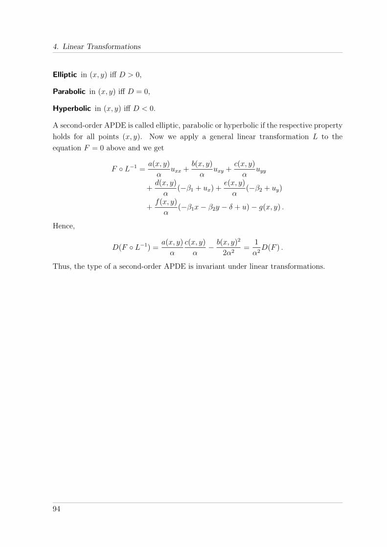
4. Linear Transformations
Elliptic in (x, y) iff D > 0,
Parabolic in (x, y) iff D = 0,
Hyperbolic in (x, y) iff D < 0.
A second-order APDE is called elliptic, parabolic or hyperbolic if the respective property
holds for all points (x, y). Now we apply a general linear transformation L to the
equation F = 0 above and we get
F ◦ L−1 =a(x, y)
αuxx +
b(x, y)
αuxy +
c(x, y)
αuyy
+d(x, y)
α(−β1 + ux) +
e(x, y)
α(−β2 + uy)
+f(x, y)
α(−β1x− β2y − δ + u)− g(x, y) .
Hence,
D(F ◦ L−1) =a(x, y)
α
c(x, y)
α− b(x, y)2
2α2=
1
α2D(F ) .
Thus, the type of a second-order APDE is invariant under linear transformations.
94

5. Conclusion
Several exact procedures are presented in the preceding chapters. They are all based
on the same idea but work for different kinds of differential equations. As mentioned
throughout the text the procedures generalize several existing methods. Summarizing
the new achievements; there are methods for autonomous algebraic ordinary differential
equations of any order (Procedure 3 and 6) and there is a procedure for autonomous first-
order algebraic partial differential equations with an arbitrary number of independent
variables (Procedure 5). Furthermore, previously known methods induce a procedure
for higher-order autonomous APDEs (see Section 3.4) and linear transformations allow
to solve some non-autonomous AODEs and APDEs (see Chapter 4).
All these methods have in common, that they assume the existence of a transformation
from an arbitrary given parametrization of a hypersurface to a parametrization induced
by a solution. This assumption is well reasoned but not always valid. Hence, the
methods might fail to find a solution. This, however, does not mean that no solution
exists. If the problem is computationally too expensive, a different input parametrization
might lead to success. Furthermore, some intermediate steps of the procedures do not
necessarily yield explicit symbolic solutions. But even if the methods fail to yield an
explicit solution, they still very often lead to an implicit description.
It is desirable to extend the procedures to decision algorithms, i. e. algorithms which
compute a solution in a certain class of functions or show that such a solution cannot
exist. However, this remains to be an open problem.
Nevertheless, the procedures represent a useful tool to tackle differential equations. As
shown in Appendix C the procedures work for a wide range of well-known differential
equations from literature. The main procedures for AODEs and APDEs (Procedure 3
and 5 respectively) compute proper and complete solutions of suitable dimension. All
other procedures for first-order ADEs yield at least complete solutions.
More detailed investigation of the idea for higher-order AODEs is currently under de-
velopment. Further generalizations of the method might be worth considering:
95

5. Conclusion
• higher-order APDEs
• (1-dimensional) systems of AODEs
• non-autonomous APDEs
The latter is currently work in progress.
96
A. More Differential Algebra
In this chapter we recall further definitions of differential algebra which are not essential
for the main part of the thesis but useful for a more comprehensive understanding of the
basics. Most of these notions can be found in standard textbooks on differential algebra
such as [33, 55].
We start with the main definition of a differential field.
Definition A.1. (c. f. Ritt [55])
Let K be an algebraically closed field of characteristic zero. Let δ : K −→ K be an
operation on that field with the following properties
δ(x+ y) = δ(x) + δ(y) , linearity,
δ(x · y) = δ(a) · b+ a · δ(b) , Leibniz rule.(A.1)
Then we call (K, δ) a differential field.
Let δ1, . . . , δm be operations on the field K each of them fulfilling (A.1). Assume also
that
δi(δj(z)) = δj(δi(z)) ,
for all z ∈ K. Then we call (K, δ) a partial differential field.
Similarly to commutative ring theory we can think about ideals which should now also
be closed under derivation.
Definition A.2. (c. f. Ritt [55])
Let K(x){u} be the ring of differential polynomials and let I ⊆ K(x){u}. Then, I is a
differential ideal iff the following conditions hold.
• For all p1, . . . , pk ∈ I and c1, . . . , ck ∈ K(x){u} the linear combination c1p1 + . . .+
ckpk is also in I.
• For all p ∈ I the derivative δ(p) is in I.
97

A. More Differential Algebra
Let K(x1, . . . , xn){u} be the ring of partial differential polynomials and let I be a subset
of K(x1, . . . , xn){u}. Then, I is a partial differential ideal iff the following conditions
hold.
• For all p1, . . . , pk ∈ I and c1, . . . , ck ∈ K(x1, . . . , xn){u} the linear combination
c1p1 + . . .+ ckpk is also in I.
• For all p ∈ I the derivatives δj(p) are in I for all j ∈ {1, . . . , n}.
Standard notions from commutative algebra transfer to differential algebra.
Definition A.3. (c. f. Ritt [55])
Let I, J be (partial) differential ideals.
• I is called prime iff ∀p, q ∈ K(x1, . . . , xn){u} : pq ∈ I ⇒ (p ∈ I ∨ q ∈ I).
• Let J ⊆ J be an ideal. Then J is called a divisor of J .
If J is prime, then J is called a prime divisor.
• Let J be a prime divisor of J . Then J is called essential iff J is not a divisor of
any other prime divisor of J .
• The (partial) differential ideal√I = {p ∈ K(x1, . . . , xn){u} |∃n ∈ N : pn ∈ I} is
called the radical differential ideal of I.
• A differential ideal I is called perfect iff I =√I.
Let P be a set of (partial) differential polynomials P ⊆ K(x1, . . . , xn){u}. Let [P ] be
the set of all linear combinations of elements of P . Then [P ] is a (partial) differential
ideal. We say [P ] is generated by P . In fact, [P ] is the smallest (partial) differential
polynomial containing P .
We write {P} for the smallest perfect ideal containing P . We call {P} the radical
differential ideal generated by P or the perfect differential ideal generated by P .
Let ν be an element of some extension field of K(x1, . . . , xn). We call ν a zero of P iff
for all p ∈ P we have p(ν) = 0.
The following definition of an ordering on the derivatives is needed for the notion of
separants in partial differential algebra.
98

Definition A.4. (Ritt [55])
Let K(x1, . . . , xn){u} be the ring of partial differential polynomials. We define an order-
ing on the derivatives as follows. For each xi we fix positive integers αi,1, . . . , αi,ν for
some ν. Let v1 and v2 be compositions of derivations:
v1 =∂i1+...+in
∂xi11 . . . ∂xinn
,
v2 =∂j1+...+jn
∂xj11 . . . ∂xjnn
.
We define the marks of v1 as βj =∑ν
k=1 αk,jik for each j. Let γj be the marks of v2.
We say that v1 is of higher rank than v2 iff there is an index ι such that βι > γι and
βj = γj for all j < ι.
Let F be a partial differential polynomial. We call a derivative v = ∂i1+...+in
∂xi11 ...∂x
inn
the leader
of F iff it is the derivative with highest rank occurring in F .
99


B. Parametrizations
In this chapter we present some more details on the problem of parametrization of hyper-
surfaces. We mainly focus on special classes of curves, surfaces and general hypersurfaces
which can be parametrized easily. We further give references of general algorithms if
they exist and remarks on available implementations. Sometimes it might be interesting
to use a known parametrization for finding another one which is in some sense simpler
or better. This approach is called reparametrization. We also give references to such
algorithms.
In the methods presented in Chapter 2 and Chapter 3 we assume a parametrization as
input. Therefore, information on how to actually compute parametrizations is in large
part omitted. We make up for this topic here. In Section B.1 we present rational pa-
rametrizations, whereas in Section B.2 we give further ideas of radical parametrizations.
Finally, Section B.3 contains ideas on other kinds of parametrizations.
B.1. Rational Parametrization
In this section we summarize different algorithms from literature for computing rational
parametrizations of algebraic curves, surfaces and hypersurfaces. The problem for curves
and surfaces can be considered to be solved in general, whereas for hypersurfaces there
is still no general algorithm.
All important definitions of rational parametrizations and their properties can be found
in Chapter 1.
In the following sections we present algorithms, ideas and references for special kinds of
curves, surfaces and hypersurfaces respectively. For the sake of the readers who might
be interested in parametrization of varieties of a certain dimension, some of the methods
are presented in each of the subsections even if they are just specialized versions of more
general methods.
101

B. Parametrizations
B.1.1. Rational Parametrization of Curves
The problem of rational parametrizability of curves is fully solved. An algebraic curve
has a rational parametrization if and only if it has genus1 zero. There is a general
algorithm for computing proper rational parametrizations of curves (see for instance
[63]). An implementation of such an algorithm can be found for instance in the computer
algebra systems Maple2 (package algcurves, available since Version V R5, based on an
algorithm described in [70]) and Magma3 (since version V2.8 [11]). For certain classes
of curves, special algorithms exist.
Linear Occurrence of a Variable
Let f(x, y) be the defining polynomial of an algebraic curve. We assume that f(x, y) =
g0(x) + yg1(x) for some polynomials g0 and g1. Then obviously Q(s) =(s,−g0(s)
g1(s)
)is a
rational parametrization of the curve. It is easy to see that the parametrization is also
proper. This works analogously if x appears linearly.
Parametrization by Lines
Let f(x, y) be the defining polynomial of an algebraic curve. Let d be the degree of
f . We assume that f(x, y) = fd(x, y) + fd−1(x, y), where fk is a non-zero form of
degree k, i. e. a homogeneous polynomial of degree k, i. e. a polynomial of the form∑ki=0 cix
iyk−i. This means the curve has a (d−1)-fold point in the origin. Then Q(s) =(−fd−1(1,s)
fd(1,s),− sfd−1(1,s)
fd(1,s)
)is a proper parametrization of the curve. This parametrization
is achieved by considering a pencil of lines through the origin. The idea can be easily
generalized to curves with any (d − 1)-fold point. See for instance [63] for further
details.
Figure B.1 illustrates parametrization by lines for the ellipse defined by.
f(x, y) = (x+ 4)2 + 4y2 − 16 = x2 + 4y2 + 8x = 0 .
This curve is of degree d = 2 and hence, any point of the curve can be used for the
parametrization. In the figure the origin is chosen.
1For a definition see for instance [63].2Waterloo Maple Inc., Maple, Waterloo, Canada3Magma is distributed by the Computational Algebra Group at the University of Sydney.
102
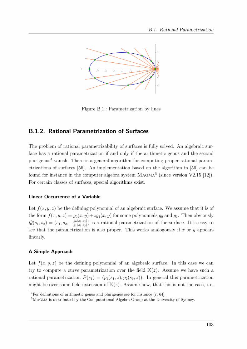
B.1. Rational Parametrization
-8 -7 -6 -5 -4 -3 -2 -1
-2
-1
1
2
Figure B.1.: Parametrization by lines
B.1.2. Rational Parametrization of Surfaces
The problem of rational parametrizability of surfaces is fully solved. An algebraic sur-
face has a rational parametrization if and only if the arithmetic genus and the second
plurigenus4 vanish. There is a general algorithm for computing proper rational param-
etrizations of surfaces [56]. An implementation based on the algorithm in [56] can be
found for instance in the computer algebra system Magma5 (since version V2.15 [12]).
For certain classes of surfaces, special algorithms exist.
Linear Occurrence of a Variable
Let f(x, y, z) be the defining polynomial of an algebraic surface. We assume that it is of
the form f(x, y, z) = g0(x, y)+zg1(x, y) for some polynomials g0 and g1. Then obviously
Q(s1, s2) = (s1, s2,−g0(s1,s2)g1(s1,s2)
) is a rational parametrization of the surface. It is easy to
see that the parametrization is also proper. This works analogously if x or y appears
linearly.
A Simple Approach
Let f(x, y, z) be the defining polynomial of an algebraic surface. In this case we can
try to compute a curve parametrization over the field K(z). Assume we have such a
rational parametrization P(s1) = (p1(s1, z), p2(s1, z)). In general this parametrization
might be over some field extension of K(z). Assume now, that this is not the case, i. e.
4For definitions of arithmetic genus and plurigenus see for instance [7, 64].5Magma is distributed by the Computational Algebra Group at the University of Sydney.
103

B. Parametrizations
P is also rational in z. Then, Q(s1, s2) = (p1(s1, s2), p2(s1, s2), s2) is a rational surface
parametrization. There is no reason for the special choice of z.
Parametrization by Lines
Let f(x, y, z) be the defining polynomial of an algebraic surface. Let d be the degree of
f . We assume that f(x, y, z) = fd(x, y, z) + fd−1(x, y, z), where fk is a non-zero form of
degree k. This means the surface has a (d− 1)-fold point in the origin. Then
Q(s1, s2) =
(−fd−1(1, s1, s2)
fd(1, s1, s2),−s1
fd−1(1, s1, s2)
fd(1, s1, s2),−s2
fd−1(1, s1, s2)
fd(1, s1, s2)
)is a proper parametrization of the surface. This can be easily generalized to surfaces
with any (d− 1)-fold point by using linear point transformations. See Section B.1.3 and
for instance [47] for further details. Obviously, this method always works for quadrics,
i. e. surfaces with defining polynomial of degree 2. Figure B.2 was created with Math-
ematica6.
Figure B.2.: Parametrization by lines
Cubic Surfaces
Cubic surfaces are those with defining polynomial of degree 3. Non-singular cubic sur-
faces are rational (c. f. [64, p. 256]). In [6] non-singular cubic surfaces are divided in
6Wolfram Research, Inc., Mathematica, Version 10.0, Champaign, IL (2014)
104

B.1. Rational Parametrization
five families, for four of which a rational parametrization is computed, whereas the fifth
involves square roots in the parametrization and hence is a radical one. For radical
parametrizations see also Section B.2.
Revolution Surfaces
Revolution surfaces are constructed by a rotation of a so called profile curve around
some axis. Obviously, if the profile curve is rational, the surface is rational as well, since
the circle is rational. Let P = (p1(s1), p2(s1)) be the rational parametrization of the
profile curve in the yz-plane. We consider rotation around the z-axis. Then(p1(s1)
1− s22
1 + s22
, p1(s1)2s2
1 + s2
, p2(s1)
)is a rational parametrization of the surface. However, not all rational revolution surfaces
can be constructed like this (compare for instance [1, Example 2.3]).
According to [1] the problem of deciding whether an implicitly given surface is a revo-
lution surface, seems to be unsolved.
Figure B.3 shows a revolution surface constructed by rotating the semicubical parabola,
i. e. P = (s21, s
31). The implicit equation of the surface is y6−z4 +3y4x2 +3y2x4 +x6 = 0.
Figure B.3 was created with Surfer7.
Figure B.3.: Revolution surface
7Surfer is a program by the Mathematisches Forschungsinstitut Oberwolfach (MFO) in collaboration
with the Martin Luther University Halle-Wittenberg.
105

B. Parametrizations
Swung Surfaces
By definition these are surfaces which can be parametrized by
Q(s1, s2) = (p1(s1)q1(s2), p1(s1)q2(s2), p2(s1)) .
This kind of surfaces is a generalization of revolution surfaces. A swung surface can
be constructed by two space curves [1]: a profile curve in the yz-plane and a trajectory
curve in the xy-plane. We consider the swinging of the profile curve around the z-axis
along the trajectory curve. The resulting surface is the one in question.
The parametrization of the profile curve is then (0, p1(s1), p2(s1)) and the trajectory
curve is parametrized by (q1(s2), q2(s2), 0).
Reparametrization of swung surfaces is considered in [1].
Figure B.4 shows a swung surface constructed with the semicubical parabola as profile
curve and the astroid as trajectory curve i. e.
q1(s, t) =8t3(1 + 6t+ 12t2 + 8t3)
1 + 12t+ 63t2 + 184t3 + 315t4 + 300t5 + 125t6,
q2(s, t) =(1 + 2t+ t2)(1 + 10t+ 36t2 + 54t3 + 27t4)
1 + 12t+ 63t2 + 184t3 + 315t4 + 300t5 + 125t6.
The implicit equation of the surface is
0 =x18 + 9x16y2 + 36x14y4 + 84x12y6 + 126x10y8 + 126x8y10 + 84x6y12 + 36x4y14
+ 9x2y16 + y18 − 3x12z4 + 468x10y2z4 − 4662x8y4z4 + 9417x6y6z4 − 4662x4y8z4
+ 468x2y10z4 − 3y12z4 + 3x6z8 + 252x4y2z8 + 252x2y4z8 + 3y6z8 − z12 .
Figure B.4 was created with Surfer8.
8Surfer is a program by the Mathematisches Forschungsinstitut Oberwolfach (MFO) in collaboration
with the Martin Luther University Halle-Wittenberg.
106

B.1. Rational Parametrization
Figure B.4.: Swung surface
Canal Surfaces
Canal surfaces are defined as the envelope of spheres centered around a space curve (the
spine curve). The spheres thereby might have a rationally changing radius. If the radius
is constant the surface is also called a pipe surface. It is known that if the spine curve
is rational then the canal surface is unirational (see [34, 48]).
Algorithms for computing rational parametrization of canal and pipe surfaces can be
found in [35, 36, 48].
Ruled Surfaces
A main property of rational ruled surfaces is that they admit a parametrization of the
form
Q = (p1(s1) + s2q1(s1), p2(s1) + s2q2(s1), p3(s1) + s2q3(s1)) .
We omit a precise definition here and refer to [7, 64, 65] for more details. An algorithm for
deciding whether an implicitly given algebraic surface is a rational ruled surface can be
found in [65]. In the affirmative case, this algorithm also computes a parametrization.
Algorithms for the purpose of reparametrization in the case of ruled surfaces can be
found for instance in [2, 38].
107

B. Parametrizations
Figure B.5 shows the one-sheeted hyperboloid which is a ruled surface, in fact it is even
doubly ruled. Its parametrization is Q(s1, s2) =(
1−s21s21+1− 2s1
s21+1s2,
2s1s21+1
+1−s21s21+1
s2, s2
)and
the implicit equation is x2 + y2 − z2 = 1. Note, the hyperboloid is also a revolution
surface, rotating a hyperbola. Figure B.5 was created with Mathematica9.
Figure B.5.: Ruled surface
Del Pezzo Surfaces
Del Pezzo surfaces play a role in the general parametrization algorithm in [56]. For in-
stance smooth cubic surfaces are a subset of Del Pezzo surfaces (c. f. [7, Theorem IV.13]).
We omit a definition here. A general approach is given in [56]. Further contributions to
the parametrization of such surfaces can be found in [13, 20, 25]. The computer algebra
system Magma10 (c. f. [12]) contains particular functions for parametrizing Del Pezzo
surfaces.
Tubular Surfaces
A tubular surface is defined by a polynomial of the form f(x, y, z) = a(z)x2+b(z)y2+c(z).
A parametrization algorithm can be found in [57].
9Wolfram Research, Inc., Mathematica, Version 10.0, Champaign, IL (2014)10Magma is distributed by the Computational Algebra Group at the University of Sydney.
108

B.1. Rational Parametrization
B.1.3. Rational Parametrization of Hypersurfaces
So far there is no general algorithm for parametrizing algebraic hypersurfaces. Even
parametrization of special kinds of hypersurfaces is not very much investigated. Nev-
ertheless, for simple kinds of hypersurfaces some of the following approaches might be
worth trying.
Linear Occurrence of a Variable
Let f(x1, . . . , xn) be the defining polynomial of an algebraic hypersurface. We assume
that
f(x1, . . . , xn) = g0(x1, . . . , xn−1) + xng1(x1, . . . , xn−1)
for some polynomials g0 and g1. Then obviously
Q(s1, . . . , sn−1) =
(s1, . . . , sn−1,−
g0(s1, . . . , sn−1)
g1(s1, . . . , sn−1)
)is a rational parametrization of the hypersurface. It is easy to see that the parametriza-
tion is also proper. This works analogously for any other variable appearing linearly.
A Simple Approach
Let f(x1, . . . , xn) be the defining polynomial of an algebraic surface. In this case we can
try to compute a curve parametrization over the field K(xκ, . . . , xn) for some 2 ≤ κ ≤ n.
Assume we have such a rational parametrization of a hypersurface of lower dimension,
P(s1, . . . , sκ−2) = (p1(s1, . . . , sκ−2, xκ, . . . , xn), . . . , pκ−1(s1, . . . , sκ−2, xκ, . . . , xn)) .
In general such a parametrization might be found (if it exists) over some field extension
of K(xκ, . . . , xn). Assume now, that this is not the case, i. e. P is also rational in
xκ, . . . , xn. Then,
Q(s1, . . . , sn−1) = (p1(s1, . . . , sn), . . . , pκ−1(s1, . . . , sn), sκ−1, . . . , sn−1)
is a rational hypersurface parametrization.
Parametrization by Lines
Let f(x1, . . . , xn) be the defining polynomial of an algebraic hypersurface. Let d be the
degree of f . We assume that f(x1, . . . , xn) = fd(x1, . . . , xn) + fd−1(x1, . . . , xn), where fk
109

B. Parametrizations
is a non-zero form of degree k. This means the surface has a (d − 1)-fold point in the
origin. Let R(s1, . . . , sn−1) = −fd−1(1,s1,...,sn−1)
fd(1,s1,...,sn−1). Then
Q(s1, . . . , sn−1) = (R(s1, . . . , sn−1), s1R(s1, . . . , sn−1), . . . , sn−1R(s1, . . . , sn−1))
is a parametrization of the hypersurface. This can be easily generalized to hypersurfaces
with any (d−1)-fold point by using linear point transformations. Let us briefly consider
how the above parametrization is derived. We take a pencil of lines through the origin
xk = sn−1x1 for k > 1. Note, that there is no reason for the special role of x1, any
other xi could be chosen as well. Each of these lines intersects the hypersurface in an
additional point. We obtain
0 = f(x1, s1x1 . . . , sn−1x1) = xd1fd(1, s1 . . . , sn−1) + xd−11 fd−1(1, s1 . . . , sn−1) .
This has two factors. One yields the origin, the other the new intersection point.
B.2. Radical Parametrization
The definition of radical parametrizations can be found in Section 2.2.1. Since this
definition accords to intuitive ideas on radicality, it is easy to come up with certain
radical parametrizations of some specific hypersurfaces, e. g. those where all variables
have degree less than or equal to four. Regardless of these ideas, detailed investigation
of radical parametrization started rather recently. Here we give a brief overview on
existing algorithms and other knowledge on computing such parametrizations for curves
and surfaces. So far there seems to be no general treatment of radical parametrizations
of hypersurfaces. Nevertheless, simple approaches might help.
B.2.1. Radical Parametrization of Curves
The curves of genus zero are exactly those that can be parametrized rationally. For
curves of higher genus we want to find radical parametrizations if they exist. In [60]
algorithms for computing radical parametrizations for curves of genus up to four are
presented. For curves of genus five and six algorithms can be found in [24]. Zariski
[71, 72] already proved that for the general curve of genus seven, there is no radical
110

B.2. Radical Parametrization
parametrization. Algorithms using gonality (i. e. the smallest possible degree d such that
there is a d : 1-map from the curve to the projective line) can be found in [58, 59].
As for the rational case there are some classes of curves which allow a simple computation
of radical parametrizations.
Variable with degree less than or equal to 4
Let f(x, y) be the defining polynomial of an algebraic curve. We assume that f(x, y) =∑4i=0 y
igi(x) for some polynomials gi. Since the equation has degree less than or equal
to 4, there is a solution for y in terms of radicals. This works analogously if x appears
with degree less than or equal to 4.
Parametrization by Lines
Let f(x, y) be the defining polynomial of an algebraic curve. Let d be the degree of
f . We assume that f(x, y) =∑r
i=0 fd−i(x, y) with r ≤ 4, where fk is a non-zero form
of degree k, i. e. a polynomial of the form∑k
i=0 cixiyk−i. This means the curve has a
(d − r)-fold point in the origin. Intersecting a pencil of lines y = sx with the curve
yields
0 = f(x, sx) =r∑i=0
xd−ifd−i(1, s) = xd−rr∑i=0
xr−ifd−i(1, s) ,
which has a factor of degree r ≤ 4 and hence is solvable by radicals for x. This can be
easily generalized to curves with any (d− r)-fold point. See for instance [60] for further
details.
B.2.2. Radical Parametrization of Surfaces
So far not very much investigation was done in this field. In [61] first algorithms for
radical parametrization of surfaces are presented. For instance parametrization by lines
is introduced and used for radically parametrizing irreducible curves of degree 5 and
singular curves of degree 6. Furthermore, an algorithm for computing radical parame-
trizations of surfaces with a pencil of curves that has low genus is described. Again we
can consider some special classes of surfaces which can be parametrized easily.
111
B. Parametrizations
Variable with degree less than or equal to 4
Let f(x, y, z) be the defining polynomial of an algebraic surface. We assume that
f(x, y, z) =∑4
i=0 zigi(x, y) for some polynomials gi. Since the equation has degree
less than or equal to 4, there is a solution for z in terms of radicals. This works analo-
gously if x or y appears with degree less than or equal to 4. Obviously, cubic surfaces
can be parametrized like this.
Parametrization by Lines
Let f(x, y, z) be the defining polynomial of an algebraic surface. Let d be the degree of
f . We assume that f(x, y, z) =∑r
i=0 fd−i(x, y, z) with r ≤ 4, where fk is a non-zero form
of degree k. This means the surface has a (d− r)-fold point in the origin. Intersecting
a pencil of lines y = s1x, z = s2x with the surface yields
0 = f(x, s1x, s2x) =r∑i=0
xd−ifd−i(1, s1, s2) = xd−rr∑i=0
xr−ifd−i(1, s1, s2) ,
which has a factor of degree r ≤ 4 and hence is solvable by radicals for x. This can be
easily generalized to curves with any (d− r)-fold point. See for instance [61] for further
details.
B.2.3. Radical Parametrization of Hypersurfaces
So far no general methods for radical parametrization of hypersurfaces are known. Nev-
ertheless, the two standard classes of hypersurfaces can be easily parametrized.
Variable with degree less than or equal to 4
Let f(x1, . . . , xn) be the defining polynomial of an algebraic hypersurface. We assume
that f(x1, . . . , xn) =∑4
i=0 xingi(x1, . . . , xn−1) for some polynomials gi. Since the equa-
tion has degree less than or equal to 4, there is a solution for xn in terms of radicals.
This works analogously if any other xi appears with degree less than or equal to 4.
Parametrization by Lines
Let f(x1, . . . , xn) be the defining polynomial of an algebraic hypersurface. Let d be the
degree of f . We assume that f(x1, . . . , xn) =∑r
i=0 fd−i(x1, . . . , xn) with r ≤ 4, where
112

B.3. Other Parametrizations
fk is a non-zero form of degree k. This means the hypersurface has a (d− r)-fold point
in the origin. Intersecting a pencil of lines xk = sn−1x1, k > 1, with the hypersurface
yields
0 = f(x1, s1x1 . . . , sn−1x1) =r∑i=0
xd−i1 fd−i(1, s1, . . . , sn−1)
= xd−r1
r∑i=0
xr−i1 fd−i(1, s1, . . . , sn−1) .
which has a factor of degree r ≤ 4 and hence is solvable by radicals for x1. This can be
easily generalized to curves with any (d− r)-fold point.
B.3. Other Parametrizations
In [26] trigonometric parametrizations of curves are defined to be of the form(m∑k=0
a1,k sin(kφ) + a2,k cos(kφ),n∑k=0
b1,k sin(kφ) + b2,k cos(kφ)
).
A curve is called trigonometric if it admits such a parametrization. It is shown in [26]
that the trigonometric curves are a subset of rational curves.
113


C. List of Differential Equations
This chapter contains a collection of examples together with the parametrizations in use
and the solutions found by the procedures presented in Chapter 2 and 3. For reference
we use the same numbering as in the literature. We prepend a letter to distinguish the
referenced books.
K Kamke [32] and [31] for ODEs and PDEs respectively
PS Polyanin and Sajzew [49]
PZ Polyanin and Zaitsev [50]
In Section C.1 first-order AODEs are collected. Right afterward some examples of
higher-order AODEs are solved. First-order APDEs can be found in Section C.3.
Intermediate steps of the procedures are skipped. Due to readability also the arbi-
trary constants are sometimes omitted. However, they can be easily introduced for
autonomous first-order equations.
Note, that these lists are by no means complete. They are just a selection of examples
which can be solved using the presented methods. Other equations also listed in the
above mentioned collections might be solved as well. Furthermore, the methods do solve
plenty of differential equations which are not listed in the collections.
C.1. First-Order AODEs
In this section we present a list of autonomous first-order AODEs which can be solved
by Procedure 3. Table C.1 shows a selection of such examples from [32].
Note, that for K.1.209 the original ODE in [32] is not an algebraic one, but solutions of
the AODE here imply solutions of the original ODE.
115

C. List of Differential Equations
Source AODE Parametrization Solution
K.1.12 u2 + u′ − 1 (s, 1− s2) e2x−1e2x+1
K.1.23 u′ + au2 − b (s, b− as2)√b tanh(
√a√bx)√
a
K.1.209 u′2u2 − au2 − b(s,√as2+bs
) √a2x2−b√
a
K.1.369 u2 + u′2 − a2(a1−s2s2+1
, 2ass2+1
)a cos(x)
K.1.371 u2 − u3 + u′2 (1 + s2, s(1 + s2)) sec2(x2
)K.1.389 (1 + 4u)(u− u′) + u′2
(− s(s−5)
(2s−5)2, 5s
(2s−5)2
)ex (ex + 1)
K.1.462 uu′2 − 1(
1s2, s)
− 3√−1(
32
)2/3x2/3
K.1.486 u2 + u2u′2 − a2(s,−
√a2−s2s
)±√a2 − x2
Table C.1.: Well-known AODEs and their solutions found by Procedure 3.
C.2. Higher-Order AODEs
In this section we present examples of second-order autonomous AODEs which can be
solved by the methods presented in Section 2.3. Table C.2 lists some AODEs where
the first derivative does not appear and hence, equation (2.6) can be used for finding
solutions. In Table C.3 a pool of examples can be found for which the approach from
Section 3.4 using APDEs yields a solution of the AODE. Here erf is the non-elementary
error function and sn the Jacobi elliptic function. The solutions of the examples in
Table C.2 were computed by the method from Section 2.3 for AODEs of the form
F (u, u′′) = 0. In Table C.3 the general method for higher-order AODEs (Procedure 6)
is applied.
The solutions shown in Table C.3 are just an arbitrary choice. Other solutions might be
found as well with the same procedure by choosing different intermediate solutions in
the ODEs of the method of characteristics. Note, that K.6.71 can as well be solved using
Procedure 3 for 8v′ + v4 and integration. Example K.7.16 was solved by first solving
3uu′′ − 5u′2.
116

C.3. First-Order APDEs
Source AODE Parametrization Solution
K.2.2 u′′ + u (s,−s) √c1 sin(x− c2)
K.2.6 u′′ − u (s, s) 12e−x+c2 + ex−c2c1
K.2.9 u′′ + au (s,−s) −√c1 sin(
√a(c2−x))a
K.6.7 u′′ − au3 (s, as3) −4√−2c1 sn( 1
2(−2)3/4 4√ac1(x−c2)|−1)
4√a
K.6.104 uu′′ − a(s, a
s
)c1e− erf−1
(−i√
2aπ
1c1
(x−c2))2
K.6.209 u′′u3 − a(s, a
s3
)−√a+c21(c2−x)2√c1
Table C.2.: Well-known second-order AODEs with solutions found by the procedure
from Section 2.3.
C.3. First-Order APDEs
In this section examples of first-order autonomous APDEs which are solvable by Pro-
cedure 5 are given. Table C.4 shows rational solutions, Table C.5 radical solutions
and Table C.6 non-algebraic solutions of first-order APDEs in two variables. Table C.7
collects solutions of APDEs with more than two variables. In Table C.8 a list of non-
autonomous APDEs is solved with the aid of linear transformations.
Note, that in Table C.6 W is the Lambert W function. Note, that in Table C.7 we used
ui for u(i). The polynomials G,H ∈ K[u1, u2, u3] are used for abbreviation. They are
defined as G(u1, u2, u3) = Ga1,a2,a3(u1, u2, u3) = a1u21 + a2u
22 + a3u32 and H(u1, u2, u3) =
Hb1,b2,b3(u1, u2, u3) = b1u1u2 + b2u1u3 + b3u2u3. The rational function S in the solution
of Example PZ.4.1.4.4 is defined as
S =− d
c+
(x23 (4a1a2 − b2
1) + x22 (4a1a3 − b2
2) + x21 (4a2a3 − b2
3))c
4 (4a1a2a3 − a1b23 − a2b2
2 − a3b21 + b1b2b3)
+(x3x2(b1b2 − 2a1b3) + x1x3(b1b3 − 2a2b2) + x1x2(b2b3 − 2a3b1))c
2 (4a1a2a3 − a1b23 − a2b2
2 − a3b21 + b1b2b3)
.
Using linear transformation we can also solve some non-autonomous APDEs. The trans-
formations in Table C.8 are given in the form α, β, δ. In Example K.6.33 Kamke [31]
already describes the linear transformation.
117

C. List of Differential Equations
Source AODE Parametrization Solution
K.2.1 u′′ (s, t, 0) (x− c1)c2
K.6.71 8u′′ + 9u′4(s, t,−9
8t4)
x−c13√x−c1
+ c2
K.6.107 uu′′ + u′2 − a(s, t, a−t
2
s
) √x−c1+a2(x−c1−c2)2
√a
K.6.110 u′′u− u′2 + 1(s, t, t
2−1s
)12c2e−x−c1
c2
(e
2(x−c1)c2 − 1
)K.6.111 u′′u− u′2 − 1
(s, t, t
2+1s
)c2
√sinh2
(x−c1c2
)+ 1
K.6.125 u′′u− au′2(s, t, at
2
s
)−c2((a− 1)(x− c1))
11−a
K.6.138 2u′′u− u′2 + a(s, t, t
2−a2s
)−4ac22+(x−c1)2
4c2
K.6.150 2u′′u− 3u′2(s, t, 3t2
2s
)4c32
(c2−x+c1)2
K.6.151 −4u2 − 3u′2 + 2uu′′(s, t, 4s2+3t2
2s
)4(tan2(x−c1)+1) cot2(x−c1)
c2
K.6.157 3u′′u− 5u′2(s, t, 5t2
3s
)3√
32c5/22
2√
(c2−x+c1)3
K.6.158 4u− 3u′2 + 4uu′′(s, t, 3t2−4s
4s
)((x−c1)2c22−64)
2
25622
K.6.164 nu′′u− (n− 1)u′2(s, t, (n−1)t2
ns
) ((x−c1)c2
n
)nK.6.168 (au+ b)u′′ + cu′2
(s, t,− ct2
as+b
)− ba− c2
((a+c)(x−c1)
a
) aa+c
K.6.191 (1 + u2)u′′ + (1− 2u)u′2(s, t, (2s−1)t2
s2+1
)tan(log((x− c1)c2))
K.6.192 (u2 + 1)u′′ − 3uu′2(s, t, 3st2
s2+1
)− (x−c1)c2√
1−(x−c1)2c22
K.6.209 u′′u3 − a(s, t, a
s3
)−√−4ac22(x−c1−c2)2−1
√2√c2
K.6.210 (u3 + u)u′′ − (3u2 − 1)u′2(s, t,
(3s2−1)t2s(s2+1)
)−√−2(x−c1)c2−1√
2√x−c1
√c2
K.7.10 2u′u′′′ − 3u′′2(s1, s2, s3,
3s232s2
)− (x−c1)c2c3+4
(x−c1)c22
K.7.11 (u′2 + 1)u′′′ − 3u′u′′2(s1, s2, s3,
3s2s23s22+1
) √1−(x−c1)2c22
c2− c3
c2
K.7.16 3u′′u′′′′ − 5u′′′2(s1, s2,
5s223s1
) √x−c1c2
+ c3(x− c1) + c4
PS.3.3.13 uu′′′ − u′u′′(s1, s2, s3,
s2,s3s1
)e(x−c1)c2(e−2(x−c1)c2−2c3)
2c22
Table C.3.: Well-known higher-order AODEs with solutions found by Procedure 6.
118

C.3. First-Order APDEs
Sourc
eA
PD
EP
ara
metr
izati
on
Solu
tion
PZ
.1.1
.1.1
8ux
+auuy
( −s at,s,t)
y ax
K.2
.45
uux
+uy−a
(s,t,a−st
)x y
+ay 2
PZ
.1.1
.1.1
9ux
+auuy−b
( b−s at,s,t)
bx 2+
y ax
K.2
.47
−uux
+ux
+uuy
+uy
( s,t,
(s−
1)t
s+1
)y−x
x+y
PZ
.1.1
.1.2
8u
(uy−ux)
+a(u
x+uy)
( a(s+t)
s−t,s,t)
a(y−x
)x
+y
PZ
.1.1
.1.2
9(a
1−a
2u
)ux
+(b
1+b 2u
)uy−c( a 1s+
b 1t−c
a2s−b 2t,s,t)
c(b 2x
+a2y)
2(a
2b 1
+a1b 2
)+
(a1y−b 1y)
(b2x
+a2y)
K.2
.68,
PZ
.1.1
.1.4
7,k
=1
ux
+(b
+au
)uy−c
( c−s−bt
at,s,t)
cx 2+
y−bx
ax
K.6
.23,
PZ
.2.1
.1.8
,k
=3
uxuy−bu
3( s,
bs3 t,t)
1bxy
K.6
.66,
PZ
.2.1
.6.1
4a
2u
2 x+b2u
2 y−c2u
( a2 s2+b2t2
c2,s,t)
1 4c2( x2 a
2+
y2
b2
)P
Z.2
.1.6
.17,k
=1
u2 x
+u
2 y−au
( s2 +t2
a,s,t)
1 4a
(x2
+y
2)
PZ
.2.1
.6.1
7,k
=3
u2 x
+u
2 y−au
3( s,√
as3−t2,t)
4a(x
2+y2)
PZ
.2.1
.7.3
bu+ux(u
x+auy)
( −s(s+at)
b,s,t)
by(y−ax
)a2
PZ
.2.1
.7.2
2ux(uux
+auy)
+b
( −b+ast
s2,s,t)
ax y−
by2
3a2
K.6
.1u
2 x−auy−b
( s,t,t2−b
a
)−ax2
4y−
by a
K.6
.115
u3 x−uuy
( s,t,t3 s
)−
x3
27y
K.6
.117
u3 x−u
2 y(s,t
2,t
3)
4x3
27y2
Table C.4.: Well-known APDEs with rational solutions found by Procedure 5.
119

C. List of Differential Equations
Sourc
eA
PD
EP
ara
metr
izati
on
Solu
tion
K.6
.21,
PZ
.2.1
.1.1
uxuy−a
( s,t,a t
)2i√a√−x√y
K.6
.26,
PZ
.2.1
.3.1
(ux−b)uy−aux
( s(b+at)
t,b
+at,a
+b t
)bx
+2i√b√−ax√y
+ay
PZ
.2.1
.4.4
4ux−au
4u
2 y(s,as4t2,t
)5√−
5y2/5
22/5
5√ax
K.6
.55
−c2
+u
2 x+u
2 y
( s,c−ct
2
t2+
1,
2ct
t2+
1
)−c√ x
2+y
2
K.6
.56,
PZ
.2.1
.6.1
−c2
+a
2u
2 x+b2u
2 y
( s,c−ct
2
at2
+a,
2ct
bt2+b
)−c√
b2x2+a2y2
ab
K.6
.68,
PZ
.2.1
.6.1
5
−b2−au
2+u
2 x+u
2 y
( s,√b2
+as2
(1−t2
)t2
+1
,2t√b2
+as2
t2+
1
)e−√a√x2+y2−ab2e√
a√x2+y2
2a
PZ
.2.1
.6.1
6u
2( u2 x+
u2 y
+1) −
a2
( s,
√ a2 s2−
1(1−t2
)t2
+1
,2√ a2 s
2−
1t
t2+
1
)−√ a2
−x
2−y
2
PZ
.2.1
.7.2
3b
+uux(u
x+auy)
( −b
s2+ats,s,t)
3√−
132/3by
((y−ax
)2)2/3
(ax−y)(−aby
)2/3
PZ
.2.1
.8.4
(ux
+auy
+b)ux
+cu
y+d( s,
t,−d+t(b+t)
c+at
)2cy−a(cx
+by
)−2√
(da2+c2−abc
)y(y−ax
)
a2
K.6
.120
(u2 x
+a)uy−
(c+bu
)ux
( s,t,
(c+bs
)tt2
+a
)1 2
( −2c b+bxy−x√ b2 y
2+
4a)
Table C.5.: Well-known APDEs with radical solutions found by Procedure 5.
120

C.3. First-Order APDEs
Sourc
eA
PD
EP
ara
metr
izati
on
Solu
tion
PZ
.1.1
.1.2
2−bu
+auyu
+ux
( s b−at,s,t)
bebxy
ebxa+
1
K.6
.25,
PZ
.2.1
.2.1
ux(a
+uy)−bu
( s(a+t)
b,s,t)
y(−
log(by)a
+a
+bx
)
PZ
.2.1
.8.1
0uyu
(bu
+aux)
+u
2 x
( −t2 bs+at,−t3
bs2+ats,−t2
bs2+ats
)−
4by
a2W
( −2ebx a−2
a
)( W
( −2ebx a−2
a
) +2
)
K.2
.20
−au
+ux
+uy
(s,t,as−t)
eay(ax−
log(eay))
a
K.2
.35,
n=
1
aux
+bu
y−u−c
( s,t,c+s−at
b
)−c
+ey/bx−aey/blo
g( ey/b
)K
.6.3
0,
PZ
.2.1
.3.1
4
(a+ux)(bu
+uy)−c( s,t,
−abs−bst+c
a+t
)e−by(a
(abx
+ceby)−
clo
g(aeby+
1))
a2b
Table C.6.: Well-known APDEs with non-algebraic solutions found by Procedure 5.
121

C. List of Differential Equations
Sourc
eA
PD
EP
ara
metr
izati
on
Solu
tion
K.7
.8u−
(u1
+u
2)2
+2u
3((s 1
+s 2
)2−
2s3,s
1,s
2,s
3)
x2 2 4−
e−x3 2x
2+
e−x3 2x
1
K.7
.9,
PZ
.4.1
.2.1
G(u
1,u
2,u
3)−
1
( s 1,s
2,i√ a
2a3R
a2,−Ra3
) ,−√a1a2x2 3+a1a3x2 2+a2a3x2 1
√a1√a2√a3
R=
a1s2 2
+a3s2 3−
1
2s 3
K.7
.10,
PZ
.4.1
.3.7
H(u
1,u
2,u
3)−d
( s 1,s
2,s
3,d−b 1s 2s 3
b 3s 3
+b 2s 2
)√d√
(b3x1+b 2x2−b 1x3)2−
4b 3b 2x1x2
i√b 1√b 2√b 3
K.7
.11
G(u
1,u
2,u
3)−u
( s 1,s
2,i√ a
2a3R
a2,−Ra3
) ,1 4
( x2 1
a1
+x2 2
a2
+x2 3
a3
)R
=a1s2 2
+a3s2 3−s 1
2s 3
K.7
.29
3 ∑ i=1
aiui ui−
1( s 1
,−a2s2 1s2 2−a3s3 1s3 3
+1
a1s 1
,s2,s
3
)√ a
1x2 2
2a2x1
+4√a1x3/2
3
3√
3√a3√x1
+2x1
a1
K.7
.31,
n6=
1
un 1
+un 2
+un 3−
1( s 1
,s2,s
3,(−sn 2−sn 3
+1)
1/n)
( xnn−1
1+x
nn−1
2+x
nn−1
3
)n−1 nP
Z.4
.1.1
.12
u1
+3 ∑ i=
2
aiu
2 i+b iui
( s 1,−
3 ∑ i=2
(ais
2 i+b is i
),s 2,s
3
)a2(b
3x1−x3)2
+a3(b
2x1−x2)2
4a2a3x1
PZ
.4.1
.2.3
,
k6=
2
G(u
1,u
2,u
3)−uk
( s 1,s
2,s
3,√ −a
1s2 2−a2s2 3
+sk 1
a3
)( (k−
2)2
4
( x2 1
a1
+x2 2
a2
+x2 3
a3
))1 2−k
PZ
.4.1
.3.8
u1u
2+a
2u
1u
3+a
3u
2u
3−cu
( a 2s 1s 3
+a3s 3s 2
+s 1s 2
c,s
1,s
2,s
3
)−c (
(−a2x2+a3x1−x3)2−
4a2x2x3)
4a2a3
PZ
.4.1
.4.4
(G+H
)(u
1,u
2,u
3)−cu−d
( (G+H
)(s 1,s
2,s
3)−d
c,s
1,s
2,s
3
)S
(x1,x
2,x
3)
Table C.7.: Well-known APDEs in three variables with solutions found by Procedure 5.
122
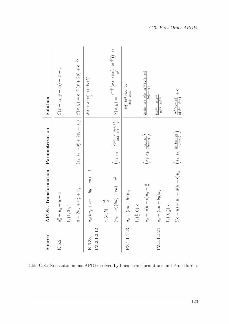
C.3. First-Order APDEs
Sourc
eA
PD
E,
Tra
nsf
orm
ati
on
Para
metr
izati
on
Solu
tion
K.6
.2u
2 x+uy
+u
+x
S(x−c 1,y−c 2
)−x−
1
1,(1,0
),1
u−
2ux
+u
2 x+uy
(s1,s
2,−s2 2
+2s
2−s 1
)S
(x,y
)=
e−y
(x+
2y)
+e−
2y
K.6
.33,
PZ
.2.1
.2.1
2
ux(kuy
+ax
+by
+cu
)−
1S
(x−c 1,y−c 2
)−ax−by
+bk c
c
c,(a,b
),−bk c
(ux−a)(kuy
+cu
)−c2
( s 1,s
2,−
c(as 1
+c−s 1s 2
)k(a−s 2
)
) S(x,y
)=
e−cy k
( a2x−c
log( 1−aecy k
)) −ac
a2
PZ
.1.1
.1.2
3ux
+(au
+bx
)uy
−−bc
2 1+bx
2+
2c 2−
2y
2ax−
2ac 1
1,(b a,0
),c
ux
+a(u−c)uy−
b a
( s 1,s
2,
as 2−b
a2(c−s 1
)
)2ac(x−c 1
)+b(x−c 1
)2+
2(y−c 2
)2a(x−c 1
)
PZ
.1.1
.1.2
4ux
+(au
+by
)uy
byebc1−bc
2ebx
aebx−aebc1
1,(0,b a),c
b(c−u
)+ux
+a(u−c)uy
( s 1,s
2,bc−bs
1+s 2
a(c−s 1
)
)bebx(y−c 2
)
a(ebx−
ebc1)
+c
Table C.8.: Non-autonomous APDEs solved by linear transformations and Procedure 5.
123


D. Method of Characteristics
Here we briefly describe the idea of the method of characteristics for solving quasilinear
APDEs. For more details we refer to literature, for instance [73]. A generalization of
the method of characteristics to arbitrary first-order partial differential equations was
investigated by Lagrange and Charpit (compare [66]). Nevertheless, we describe it just
for the quasilinear case. A first-order APDE is quasilinear iff it is linear in the derivatives
(and possibly non-linear in the dependent function u). Let F define a quasilinear APDE,
i. e.
F (x1, . . . , xn, u, ux1 , . . . , uxn) = −b(x1, . . . , xn, u) +n∑i=0
ai(x1, . . . , xn, u)uxi = 0 .
A characteristic curve (x1(t), . . . , xn(t), v(t)) is defined by the following characteristic
equations.
dxidt
= ai(x1, . . . , xn, v) , for i ∈ {1, . . . , n} ,
dv
dt= b(x1, . . . , xn, v) .
Let us consider some initial data
u = g(x1, . . . , xn) = 0 on h(x1, . . . , xn) = 0 .
These can be written parametrically with parameters k2, . . . , kn as xi = σi(k2, . . . , kn)
and u = υ(k2, . . . , kn). These parametric expressions can be used as initial data (for
t = 0) in solving the system of characteristic equations. Finally, a solution u of the above
ODE still depends on k2, . . . , kn. Let χi(t, k2, . . . , kn) be solutions of the characteristic
equations. Then we solve the system xi = χi(t, k2, . . . , kn) for k2, . . . , kn. Note, that this
might not always be possible. In case it is possible we get ki = ξi(x1, . . . , xn). Then,
u(x1, . . . , xn) = v(x1, ξ2(x1, . . . , xn), . . . , ξn(x1, . . . , xn)) is a solution of the quasilinear
APDE.
Note, that the method of characteristics does not necessarily result in a complete solution
of suitable dimension. Compare for instance [66, Problem 3.12], where a complete
125

D. Method of Characteristics
solution of the eikonal equation is found by the method of characteristic. This solution
is not of suitable dimension and envelope computations are needed to get the same
solution of suitable dimension as in Example 3.11.
Example D.1. ([66, Problem 3.12])
Applying the generalized method of characteristics yields u(x, y) = c2x+√a− c2
2y+c1 as
a solution of the eikonal equation u2x+u2
y−1. Then the Jacobians of the parametrization
L induced by the solution with respect to x, y and c1, c2 respectively, are
J x,yL =
c2
√1− c2
2
0 0
0 0
, J c1,c2L =
1 x− c2y√
1−c22
0 1
0 − c2y√1−c22
.
Hence, the solution is complete, but not of suitable dimension (and not proper). The so-
lution√x2 + y2 which was found by Procedure 4 in Example 3.11 is complete of suitable
dimension. It can be obtained from the one considered here by envelope computations
(as shown in [66]).
126

Index
ADE, 4
algebraic
curve, 6
hypersurface, 6
solution, 5
surface, 6
almost injective, 64
AODE, 4
APDE, 4
associated system, 15
autonomous, 4
Burgers equation
inviscid, 41, 49
viscid, 93
canal surface, 107
characteristic
curve, 125
equation, 125
method of, 57, 125
convection-reaction equation, 49
corresponding
curve, 8
hypersurface, 8
parametrization, 8, 85
surface, 8
Cremona transformation, 8
cubic surface, 104
curve, see hypersurface
trigonometric, 113
defining polynomial, 7
Del Pezzo surface, 108
differential
field, 4, 97
partial, 4, 97
ideal, 97
generated by, 98
partial, 98
perfect, 98
prime, 5
radical, 98
polynomial, 4
discriminant, 93
divisor, 98
essential, 98
prime, 98
eikonal equation, 47, 49, 65, 126
elementary function, 19
elliptic, 94
envelope, 11
essential, 5
form, 102, 104, 110
general
component, 5, 6
solution, 5, 11
generic zero, 4
hyperbolic, 94
hypersurface
127

INDEX
algebraic, 6
rational, 7
unirational, 7
Laplace equation, 79
leader, 99
Leibniz rule, 4, 97
linear transformation, 83
Mobius transformation, 8
manifold, 6
mark, 99
method of characteristics, 57, 125
non-autonomous, 4
parabolic, 94
parametrizable by radicals, 21
parametrization, 22
by lines, 102, 104, 109, 111, 112
corresponding, 8, 85
proper, 7
radical, 21, 110
rational, 7, 101
trigonometric, 113
pipe surface, 107
polynomial
defining, 7
homogeneous, 102
profile curve, 105, 106
proper, 7
parametrization, 7
solution, 9, 85
quadratic transformation, 8
quadric surface, 104
quasilinear, 125
radical
extension field, 21
field extension, 21
tower of, 21
function, 21
parametrization, 21
solution, 21
rank, 99
rational
hypersurface, 7
parametrization, 7
solution, 5, 9
revolution surface, 105
ruled surface, 107
separant, 5
singular
component, 5, 6
solution, 5, 6, 11
solution
algebraic, 5
complete, 9, 85
of suitable dimension, 9, 85
general, 5
non-singular, 5, 6
proper, 9, 85
radical, 21
rational, 5, 9
singular, 5, 6
solvable by radicals, 21
spine curve, 107
surface, see hypersurface
swung surface, 106
traffic equation, 49
trajectory curve, 106
transformation
Cremona, 8
128

INDEX
linear, 83
Mobius, 8
quadratic, 8
transport equation
linear, 55
tubular surface, 108
zero, 98
generic, 4
129

Bibliography
[1] C. Andradas, T. Recio, J. R. Sendra, L.-F. Tabera, and C. Villarino. Reparametriz-
ing swung surfaces over the reals. Applicable Algebra in Engineering, Communica-
tion and Computing, 25(1–2):39–65, 2014.
[2] C. Andradas, T. Recio, L. F. Tabera, J. R. Sendra, and C. Villarino. Proper real
reparametrization of rational ruled surfaces. Computer Aided Geometric Design,
28(2):102–113, 2011.
[3] W. Arendt and K. Urban. Partielle Differenzialgleichungen. Eine Einfuhrung in
analytische und numerische Methoden. Spektrum Akademischer Verlag, Heidelberg,
2010.
[4] V. I. Arnold. Lectures on Partial Differential Equations. Springer-Verlag, Berlin
Heidelberg, 2004.
[5] J. M. Aroca, J. Cano, R. Feng, and X.-S. Gao. Algebraic General Solutions of
Algebraic Ordinary Differential Equations. In M. Kauers, editor, Proceedings of
the 2005 International Symposium on Symbolic and Algebraic Computation, ISSAC
’05, pages 29–36, New York, 2005. ACM.
[6] C. L. Bajaj, R. L. Holt, and A. N. Netravali. Rational Parametrizations of Nonsin-
gular Real Cubic Surfaces. ACM Transactions on Graphics, 17(1):1–31, 1998.
[7] A. Beauville. Complex algebraic surfaces, volume 34 of London Mathematical Soci-
ety Student Texts. Cambridge University Press, Cambridge, 2nd edition, 1996.
[8] M. C. Beltrametti, E. Carletti, D. Gallarati, and G. Monti Bragadin. Lectures on
curves, surfaces and projective varieties, A classical view of algebraic geometry.
European Mathematical Society (EMS), Zurich, 2009.
[9] M. Bronstein. Symbolic integration I: Transcendental functions. Springer, Berlin,
2nd edition, 2005.
131

BIBLIOGRAPHY
[10] H.-J. Bungartz, S. Zimmer, M. Buchholz, and D. Pfluger. Modellbildung und Sim-
ulation. Springer-Verlag, Berlin Heidelberg, 2013.
[11] J. Cannon and Bosma W. (editors). Handbook of Magma functions. Sydney, 2.8
edition, 2001.
[12] J. Cannon and Bosma W. (editors). Handbook of Magma functions. Sydney, 2.15
edition, 2008.
[13] W. A. de Graaf, J. Pılnikova, and J. Schicho. Parametrizing Del Pezzo surfaces of
degree 8 using Lie algebras. Journal of Symbolic Computation, 44(1):1–14, 2009.
[14] S. B. Engelsman. Lagrange’s early contributions to the theory of first-order partial
differential equations. Historia Mathematica, 7:7–23, 1980.
[15] A. Eremenko. Rational solutions of first-order differential equations. Annales
Academiae Scientiarum Fennicae. Mathematica, 23(1):181–190, 1998.
[16] H. Eves. Elementary matrix theory. Dover Publications, Inc., New York, 1980.
[17] R. Feng and X.-S. Gao. Rational General Solutions of Algebraic Ordinary Dif-
ferential Equations. In J. Gutierrez, editor, Proceedings of the 2004 International
Symposium on Symbolic and Algebraic Computation, ISSAC ’04, pages 155–162,
New York, 2004. ACM.
[18] R. Feng and X.-S. Gao. Polynomial General Solutions for First Order Autonomous
ODEs. In H. Li et al., editor, Computer Algebra and Geometric Algebra with Ap-
plications, volume 3519 of Lecture Notes in Computer Science, pages 5–7, Berlin
Heidelberg, 2005. Springer.
[19] R. Feng and X.-S. Gao. A polynomial time algorithm for finding rational gen-
eral solutions of first order autonomous ODEs. Journal of Symbolic Computation,
41(7):739–762, 2006.
[20] J. Gonzalez-Sanchez, M. Harrison, I. Polo-Blanco, and J. Schicho. Algorithms for
Del Pezzo surfaces of degree 5 (construction, parametrization). Journal of Symbolic
Computation, 47(3):342–353, 2012.
[21] G. Grasegger. Radical Solutions of Algebraic Ordinary Differential Equations. In
K. Nabeshima, editor, Proceedings of the 39th International Symposium on Symbolic
and Algebraic Computation, ISSAC ’14, pages 217–223, New York, 2014. ACM.
132

BIBLIOGRAPHY
[22] G. Grasegger, A. Lastra, J. R. Sendra, and F. Winkler. On Symbolic Solutions of
Algebraic Partial Differential Equations. In V.P. Gerdt et al., editor, Computer Al-
gebra in Scientific Computing, volume 8660 of Lecture Notes in Computer Science,
pages 111–120. Springer International Publishing, 2014.
[23] G. Grasegger and F. Winkler. Symbolic solutions of first-order algebraic ODEs.
In Computer Algebra and Polynomials, volume 8942 of Lecture Notes in Computer
Science, pages 94–104. Springer International Publishing, 2015.
[24] M. Harrison. Explicit solution by radicals, gonal maps and plane models of algebraic
curves of genus 5 or 6. Journal of Symbolic Computation, 51:3–21, 2013.
[25] M. Harrison and J. Schicho. Rational Parametrisation for Degree 6 Del Pezzo
Surfaces Using Lie Algebras. In Proceedings of the 2006 International Symposium
on Symbolic and Algebraic Computation, pages 132–137, New York, 2006. ACM.
[26] H. Hong and J. Schicho. Journal of Symbolic Computation, 26(3):279–300, 1998.
[27] Y. Huang, L. X. C. Ngo, and F. Winkler. Rational General Solutions of Trivariate
Rational Systems of Autonomous ODEs. In Proceedings of the Fourth Interna-
tional Conference on Mathematical Aspects of Computer and Information Sciences,
MACIS 2011, pages 93–100, 2011.
[28] Y. Huang, L. X. C. Ngo, and F. Winkler. Rational General Solutions of Trivariate
Rational Differential Systems. Mathematics in Computer Science, 6(4):361–374,
2012.
[29] Y. Huang, L. X. C. Ngo, and F. Winkler. Rational General Solutions of Higher Order
Algebraic ODEs. Journal of Systems Science and Complexity, 26(2):261–280, 2013.
[30] E. Hubert. The General Solution of an Ordinary Differential Equation. In Y. N.
Lakshman, editor, Proceedings of the 1996 International Symposium on Symbolic
and Algebraic Computation, ISSAC ’96, pages 189–195, New York, 1996. ACM.
[31] E. Kamke. Differentialgleichungen: Losungsmethoden und Losungen II. Akademi-
sche Verlagsgesellschaft Geest & Portig K.-G., Leipzig, 1965.
[32] E. Kamke. Differentialgleichungen: Losungsmethoden und Losungen. B. G. Teub-
ner, Stuttgart, 1997.
133
BIBLIOGRAPHY
[33] E. R. Kolchin. Differential algebra and algebraic groups, volume 54 of Pure and
Applied Mathematics. Academic Press, New York-London, 1973.
[34] W. Lu and H. Pottmann. Pipe surfaces with rational spine curve are rational.
Computer Aided Geometric Design, 13(7):621–628, 1996.
[35] G. Landsmann, J. Schicho, and F. Winkler. The parametrization of canal sur-
faces and the decomposition of polynomials into a sum of two squares. Journal of
Symbolic Computation, 32(1–2):119–132, 2001.
[36] G. Landsmann, J. Schicho, F. Winkler, and E. Hillgarter. Symbolic Parametrization
of Pipe and Canal Surfaces. In Proceedings of the 2000 International Symposium on
Symbolic and Algebraic Computation, ISSAC ’00, pages 202–208, New York, 2000.
ACM.
[37] A. Lastra, L. X. C. Ngo, J. R. Sendra, and F. Winkler. Rational General Solutions
of Systems of Autonomous Ordinary Differential Equations of Algebro-Geometric
Dimension One. Publicationes Mathematicae Debrecen, 86(1–2):49–69, 2015.
[38] J. Li, L.-Y. Shen, and X.-S. Gao. Proper Reparametrization of Rational Ruled
Surface. Journal of Computer Science and Technology, 23(2):290–297, 2008.
[39] J. Liouville. Premier Memoire Sur la determination des Integrales dont la valeur
est algebrique. Journal de l’Ecole polytechnique, 14:124–148, 1833.
[40] J. Liouville. Second Memoire Sur la determination des Integrales dont la valeur est
algebrique. Journal de l’Ecole polytechnique, 14:149–193, 1833.
[41] J. Liouville. Memoire sur l’integration d’une classe des fonctions transcendantes.
Journal fur die Reine und Angewandte Mathematik, 13:93–118, 1835.
[42] L. X. C. Ngo, J. R. Sendra, and F. Winkler. Classification of algebraic ODEs with
respect to rational solvability. In Computational Algebraic and Analytic Geometry,
volume 572 of Contemporary Mathematics, pages 193–210. American Mathematical
Society, Providence, RI, 2012.
[43] L. X. C. Ngo, J. R. Sendra, and F. Winkler. Birational transformations preserving
rational solutions of algebraic ordinary differential equations. Journal of Computa-
tional and Applied Mathematics, 286:114–127, 2015.
134

BIBLIOGRAPHY
[44] L. X. C. Ngo and F. Winkler. Rational general solutions of first order non-
autonomous parametrizable ODEs. Journal of Symbolic Computation, 45(12):1426–
1441, 2010.
[45] L. X. C. Ngo and F. Winkler. Rational general solutions of parametrizable AODEs.
Publicationes Mathematicae Debrecen, 79(3–4):573–587, 2011.
[46] L. X. C. Ngo and F. Winkler. Rational general solutions of planar rational systems
of autonomous ODEs. Journal of Symbolic Computation, 46(10):1173–1186, 2011.
[47] S. Perez-Dıaz, J. Sendra, and J. R. Sendra. Parametrization of approximate alge-
braic surfaces by lines. Computer Aided Geometric Design, 22(2):147–181, 2005.
[48] M. Peternell and H. Pottmann. Computing rational parametrizations of canal
surfaces. Journal of Symbolic Computation, 23(2–3):255–266, 1997.
[49] A. D. Polyanin and V. F. Sajzew. Sammlung gewohnlicher Differentialgleichungen.
Verlag Harri Deutsch, Thun und Frankfurt am Main, 1996.
[50] A. D. Polyanin and V. F. Zaitsev. Handbook of nonlinear partial differential equa-
tions. CRC Press, Boca Raton, FL, 2nd edition, 2011.
[51] R. H. Risch. The problem of integration in finite terms. Transactions of the Amer-
ican Mathematical Society, 139:167–189, 1969.
[52] R. H. Risch. The solution of the problem of integration in finite terms. Bulletin of
the American Mathematical Society, 76:605–608, 1970.
[53] J. F. Ritt. On algebraic functions, which can be expressed in terms of radicals.
Transactions of the American Mathematical Society, 24:21–30, 1924.
[54] J. F. Ritt. Integration in Finite Terms. Columbia University Press, New York,
1948.
[55] J. F. Ritt. Differential algebra, volume 33 of Colloquium Publications. American
Mathematical Society, New York, 1950.
[56] J. Schicho. Rational Parametrization of Surfaces. Journal of Symbolic Computation,
26(1):1–29, 1998.
[57] J. Schicho. Proper Parametrization of Real Tubular Surfaces. Journal of Symbolic
Computation, 30(5):583–593, 2000.
135
BIBLIOGRAPHY
[58] J. Schicho, F.-O. Schreyer, and M. Weimann. Computational aspects of gonal
maps and radical parametrization of curves. Applicable Algebra in Engineering,
Communication and Computing, 24(5):313–341, 2013.
[59] J. Schicho and D. Sevilla. Effective radical parametrization of trigonal curves.
In Computational Algebraic and Analytic Geometry, volume 572 of Contempo-
rary Mathematics, pages 221–231. American Mathematical Society, Providence, RI,
2012.
[60] J. R. Sendra and D. Sevilla. Radical parametrizations of algebraic curves by adjoint
curves. Journal of Symbolic Computation, 46(9):1030–1038, 2011.
[61] J. R. Sendra and D. Sevilla. First steps towards radical parametrization of algebraic
surfaces. Computer Aided Geometric Design, 30(4):374–388, 2013.
[62] J. R. Sendra and F. Winkler. Tracing index of rational curve parametrizations.
Computer Aided Geometric Design, 18(8):771–795, 2001.
[63] J. R. Sendra, F. Winkler, and S. Perez-Dıaz. Rational Algebraic Curves, A Com-
puter Algebra Approach, volume 22 of Algorithms and Computation in Mathematics.
Springer-Verlag, Berlin Heidelberg, 2008.
[64] I. R. Shafarevich. Basic Algebraic Geometry 1, Varieties in Projective Space.
Springer-Verlag, Berlin Heidelberg, third edition, 2013.
[65] L.-Y. Shen and S. Perez-Dıaz. Characterization of rational ruled surfaces. Journal
of Symbolic Computation, 63:21–45, 2014.
[66] I. Shingareva and C. Lizarraga-Celaya. Solving nonlinear partial differential equa-
tions with Maple and Mathematica. Springer-Verlag, Wien, 2011.
[67] B. M. Trager. Integration of simple radical extensions. In E. W. Ng, editor, Sym-
bolic and algebraic computation, EUROSAM ’79, volume 72 of Lecture Notes in
Computer Science, pages 408–414, Berlin Heidelberg, 1979. Springer.
[68] B. M. Trager. On the integration of algebraic functions. PhD thesis, Massachusetts
Institute of Technology, 1984.
[69] B. L. van der Waerden. Algebra, volume II. Springer-Verlag, New York, 1991.
[70] M. van Hoeij. Rational Parametrizations of Algebraic Curves using a Canonical
Divisor. Journal of Symbolic Computation, 23(2–3):209–227, 1997.
136
BIBLIOGRAPHY
[71] O. Zariski. Sull’ impossibilita di risolvere parametricamente per radicali
un’equazione algebrica f(x, y) = 0 di genere p > 6 a moduli generali. Atti della
Accademia Nazionale dei Lincei, Rendiconti, VI. Serie, 3:660–666, 1926.
[72] O. Zariski. Collected papers, volume III: Topology of curves and surfaces, and
special topics in the theory of algebraic varieties. The MIT Press, Cambridge,
Massachusetts, London, 1978.
[73] D. Zwillinger. Handbook of Differential Equations. Academic Press, San Diego, CA,
third edition, 1998.
137


Curriculum Vitae
Personal Data
Full Name: Georg Grasegger
Year of Birth: 1985
Place of Birth: Linz
Nationality: Austria
Education
2004 High School Diploma (Matura), with distinction
2005–2010 Bachelor Studies in Technical Mathematics at Johannes Ke-
pler University Linz, Austria, Bakk.techn. 2010 (with distinc-
tion)
2008–2009 Exchange Student at the Norwegian University of Science and
Technology, Trondheim, Norway
2010–2011 Master Studies in Computer Mathematics at Johannes Kepler
University Linz, Austria, Dipl.-Ing. 2011 (with distinction)
2013 – 2014 Research Visit at University of Alcala, Alcala de Henares,
Spain
2011–now PhD Studies in Technical Sciences at Johannes Kepler Uni-
versity Linz, Austria
139

Curriculum Vitae
Career
2010 – 2011 Student assistant, Institute for Algebra, Johannes Kepler Uni-
versity Linz, Austria
2011 Research assistant, Research Institute for Symbolic Compu-
tation, Johannes Kepler University Linz, Austria
Feb. 2013, 2014,
2015
Course instructor, Projektwoche Angewandte Mathematik,
Stiftung Talente
2011 – now Research assistant, Doctoral Program Computational Math-
ematics, Johannes Kepler University Linz, Austria
2012 – now Lecturer, Johannes Kepler University Linz, Austria
Publications
Refereed publications:
• G. Grasegger, G. Horvath, and K. A. Kearnes. Polynomial Equivalence of Finite
Rings. Journal of the Australian Mathematical Society, 96(2):244–257, 2014
• G. Grasegger. Radical Solutions of Algebraic Ordinary Differential Equations.
In K. Nabeshima, editor, Proceedings of the 39th International Symposium on
Symbolic and Algebraic Computation, pages 217–223, New York, 2014. ACM.
• G. Grasegger, A. Lastra, J. R. Sendra, and F. Winkler. On Symbolic Solutions of
Algebraic Partial Differential Equations. In V. P. Gerdt et al., editor, Computer
Algebra in Scientific Computing, volume 8660 of Lecture Notes in Computer Sci-
ence, pages 111–120. Springer International Publishing, 2014.
• G. Grasegger and F. Winkler. Symbolic solutions of first-order algebraic ODEs. In
Computer Algebra and Polynomials, volume 8942 of Lecture Notes in Computer
Science, pages 94–104. Springer International Publishing, 2015.
Technical reports:
• G. Grasegger. A procedure for solving autonomous AODEs. Technical Report:
2013-05, DK Computational Mathematics, Johannes Kepler University Linz, 2013.
2013-03, RISC, Johannes Kepler University Linz, 2013.
140

• G. Grasegger, A. Lastra, J. R. Sendra, and F. Winkler. A solution method for
autonomous first-order algebraic partial differential equations. Technical Report:
2014-07, DK Computational Mathematics, Johannes Kepler University Linz, 2014.
2014-03, RISC, Johannes Kepler University Linz, 2014.
• G. Grasegger, A. Lastra, J. R. Sendra, and F. Winkler. A solution method for
autonomous first-order algebraic partial differential equations in several variables.
Technical Report:
2015-02, DK Computational Mathematics, Johannes Kepler University Linz, 2015.
2015-02, RISC, Johannes Kepler University Linz, 2015.
Talks
At other universities:
• November 4, 2013: Seminario de fısica y matematicas, Universidad de Alcala
Talk: Radical solutions of algebraic ordinary differential equations
• June 26, 2014: Seminaire Calcul Formel, Universite de Limoges
Talk: A solution method for algebraic partial differential equations
• September 2, 2014: University of Bath
Talk: Solving first-order algebraic differential equations
At conferences:
• AAA84, 84th Workshop on General Algebra, June 8–10, 2012, Dresden, Germany
Talk: An explicit polynomial equivalence of the rings Z2p and Zp[t]/(t2)
• Conference on commutative rings, integer-valued polynomials and polynomial func-
tions, December 19–22, 2012, Graz, Austria
Talk: Polynomial equivalence of finite rings
• Workshop on Approximation Theory, CAGD, Numerical Analysis, and Symbolic
Computation, August 25–30, 2013, Sozopol, Bulgaria
Talk: Using parametrizations for solving algebraic ordinary differential equations
• AICA 2013, Aplicaciones Industriales del Algebra Computacional, November 7–8,
2013, Universidad Complutense, Madrid, Spain
Poster: Symbolic solutions of algebraic ordinary differential equations
141

Curriculum Vitae
• Computer algebra and polynomials (Workshop 3 of Special Semester on Appli-
cations of Algebra and Number Theory), November 25–29, 2013, RICAM, Linz,
Austria
Talk: Radical solutions of algebraic ordinary differential equations
• III Seminario sobre “Algoritmos y Aplicaciones en Geometrıa Algebraica”, De-
cember 16–17, 2013, CIEM (Centro Internacional de Encuentros Matematicos),
Castro Urdiales, Spain
Talk: Radical solutions of algebraic ordinary differential equations
• AAA87&CYA28, 87th Workshop on General Algebra and 28th Conference of
Young Algebraists, February 7–9, 2014, Linz, Austria
Talk: Rational and radical solutions of algebraic differential equations
• ISSAC 2014, 39th International Symposium on Symbolic and Algebraic Compu-
tation, July 23–25, Kobe, Japan
Talk: Radical solutions of algebraic ordinary differential equations
• CASC 2014, 16th International Workshop on Computer Algebra in Scientific Com-
puting, September 8–12, Warsaw, Poland
Talk: On symbolic solutions of algebraic partial differential equations
142