Algebraic operator method for the construction of solitary solutions to nonlinear differential...

Algebraic operator method for the construction of solitary solutions to

nonlinear differential equations

Zenonas Navickas a,1, Liepa Bikulciene a,2, Maido Rahula b, Minvydas Ragulskis c,⇑

aDepartment of Applied Mathematics, Kaunas University of Technology, Studentu 50-325, LT-51368 Kaunas, Lithuaniab Institute of Pure Mathematics, Tartu University, J. Liivi 2-427, Tartu EE-50409, EstoniacResearch Group for Mathematical and Numerical Analysis of Dynamical Systems, Kaunas University of Technology, Studentu 50-222, Kaunas LT-51368, Lithuania

a r t i c l e i n f o

Article history:

Received 12 July 2012

Received in revised form 27 September 2012

Accepted 7 October 2012

Available online 14 November 2012

Keywords:

KdV equation

Generalized operator of differentiation

Solitary solution

Condition of existence

a b s t r a c t

Solutions of the KdV equation are derived by the algebraic operator method based on

generalized operators of differentiation. The algebraic operator method based on the

generalized operator of differentiation is exploited for the derivation of analytic solutions

to the KdV equation. The structure of solitary solutions and explicit conditions of existence

of these solutions in the subspace of initial conditions are derived. It is shown that special

solitary solutions exist only on a line in the parameter plane of initial and boundary

conditions. This new theoretical result may lead to important findings in a variety of

practical applications.

� 2012 Elsevier B.V. All rights reserved.

1. Introduction

The Korteweg-de Vries equation takes the form

@w

@s� 6w

@w

@zþ @3w

@z3¼ 0: ð1Þ

The KdV Eq. (1) was discovered in 1895 by Korteweg and de Vries [10]. This equation is a paradigmatic partial differential

equation in nonlinear physics. It models one-dimensional shallow water waves with small but finite amplitudes. It has also

been used to describe a number of important physical phenomena such as solitons, magnetohydrodynamics waves in warm

plasma, acoustic waves in anharmonic crystals, ion-acoustic waves [33,36,1,17,3,24].

Eq. (1) is integrable and the Cauchy problem for this equation can be solved [7,14,9]. This equation has soliton, rational

and elliptic solutions [2,27].

A suitable modification of the inverse scattering transform helps to shown that under the KdV flow an initial profile sup-

ported on ð�1;0Þ instantaneously evolves into a meromorphic function with no poles on the real line [28].

Inverse scattering transform method is exploited for explicit computation of the shapes and the speeds of the asymptotic

solitons for the KdV equation for several types of linearizable boundary conditions in [6].

1007-5704/$ - see front matter � 2012 Elsevier B.V. All rights reserved.

http://dx.doi.org/10.1016/j.cnsns.2012.10.009

⇑ Corresponding author. Tel.: +370 69822456; fax: +370 37330446.

E-mail addresses: [email protected] (Z. Navickas), [email protected] (L. Bikulciene), [email protected] (M. Rahula), minvydas.ragulskis@

ktu.lt (M. Ragulskis).

URL: http://www.personalas.ktu.lt/~mragul (M. Ragulskis).1 Tel.: +370 68223789; fax: +370 37456472.2 Tel.: +370 68217227.

Commun Nonlinear Sci Numer Simulat 18 (2013) 1374–1389

Contents lists available at SciVerse ScienceDirect

Commun Nonlinear Sci Numer Simulat

journal homepage: www.elsevier .com/locate /cnsns


mailto:[email protected]





http://www.personalas.ktu.lt/~mragul


http://www.sciencedirect.com/science/journal/10075704

http://www.elsevier.com/locate/cnsns

Many different methods for the construction of exact solutions of nonlinear evolution equations have been established

and developed. The inverse scattering transform [1], the Hirota’s bilinear operators [9], the Jacobi elliptic function expansion

[16], the Darboux transformation [19], the Backlund transformation method [34] are successfully used to construct analyt-

ical solutions of nonlinear evolutions. A number of methods based on the extensive use of symbolic computations have been

developed during the last decades. Homogeneous balance method [32], the Exp-function method [8,4], the tanh method

[18,25] and its various extensions [5,15,31], the (G0/G) expansion method [38], the auxiliary (or subsidiary) ordinary differ-

ential equation method [35,30,37] are successfully used to solve high-dimensional nonlinear evolutions in mathematical

physics with the help of symbolic computation. The key idea of most of these methods is that the traveling wave solution

of a complicated nonlinear evolution equation can be guessed (supposed) as a polynomial (or a ratio of polynomials) of stan-

dard functions whose argument is a traveling wave term. The degree of the polynomial can be determined by considering

homogeneous balance between the highest derivatives and nonlinear terms in the nonlinear evolution equation considered.

Nevertheless, it can be noted that a straightforward application of these methods has attracted a considerable amount of

criticism [12,23,11,22,13,26].

1.1. The purpose of the paper

The main objective of this paper is to show that well-known solitary solutions to KdV equation do not hold for all initial

conditions. Formal operator techniques based on the generalized differential operator are used for the KdV equation to

derive solutions expressed in a ratio of finite sums of standard functions [21]. We use an analytical criterion based on the

concept of H-ranks and determine if a solution of the KdV equation can be expressed in an analytical form comprising

standard functions. The employment of this criterion does not only give an answer to the above-stated question but gives

the structure of the solution so that one does not have to guess what the form of the solution is. The load of symbolic

calculations is brought before the structure of the solution is identified. This is in contrary to the methods described in

[32,8,4,18,25,5,15,31,38,35,30,37] where the structure of the solution is first proposed, and then symbolic calculations are

exploited for the identification of parameters.

We perform well-known transformations [29] before commencing the analysis of Eq. (1). The change of variables based

on the existence of a propagating wave w z; sð Þ ¼ x z� rsð Þ (where r is the constant wave speed) yields an ordinary differen-

tial equation:

� r þ 6xð Þx0x þx000

xxx ¼ 0; ð2Þ

where the prime mark stands for a derivative ofxwith respect to the variable of the propagating wave x ¼ z� rt. Integration

of Eq. (2) with respect to x yields:

� r þ 3xð Þxþx00xx ¼ 3C; C ¼ const: ð3Þ

Eq. (3) which can be rewritten in the following form:

x00xx ¼ c2 x�x1ð Þ x�x2ð Þ; x1;x2; c 2 C; ð4Þ

where x1;2 ¼ � r6�

ffiffiffiffiffiffiffiffiffiffiffiffiffir2

36� C

q; c2 ¼ 3. We will seek structural solutions of Eq. (4) using algebraic operator techniques.

Elliptic function solutions (doubly periodic solutions) play an important role in studying exact solutions of nonlinear

wave equations. Particularly, the Weierstrass elliptic function expansion method is used to seek doubly periodic solutions

of the KdV equation, the Generalized KdV equation and the modified KdV equation in [39–42].

Note that Eq. (4) is the simple reduction of the KdV equation in the traveling waves. Eq. (4) can be integrated once more,

and the resulting differential equation can be solved in terms of Weierstrass elliptic functions. Such a straightforward

integration produces the solitary solution but does not produce conditions of its existence in the space of initial conditions

[39–42]. The main goal of this paper is to demonstrate that algebraic operator techniques can simultaneously produce sol-

itary solutions and conditions of their existence. And even though the KdV equation is one of the most studied nonlinear

differential equations, we argue that conditions of existence of solitary solutions to the KdV equation cannot be produced

by the Weierstrass elliptic function expansion method; formal application of algebraic operator techniques is necessary

for that purpose.

1.2. Outline

The paper is organized as follows. Initial definitions and concepts used in the search of structural solutions are given in

Section 2; the special solutions of KdV type ordinary differential equation are derived in Section 3; results of computational

experiments are discussed in Section 4 and concluding remarks are given in Section 5.

2. Preliminaries

Several definitions and statements which will be exploited in the process of the search of special solutions of the KdV

equation are concisely presented in this section.

Z. Navickas et al. / Commun Nonlinear Sci Numer Simulat 18 (2013) 1374–1389 1375

2.1. Functions and their extensions

Functions of two types are used in this paper. Functions of the first type pj ¼ pj c; s0; . . . ; sn�1ð Þ describe the mapping

pj : Ij � Is0 � � � � � Isn�1! R; where Ij; Is0 ; . . . ; Isn�1

� R are variation intervals (or unions of intervals) of variables

c; s0; . . . ; sn�1 2 R. These functions are differentiable any number times in respect of every variable. It can be noted that

the identification of variation intervals (or unions of intervals) is a straightforward task whenever the expression of

pj c; s0; . . . ; sn�1ð Þ is given explicitly. For example, the function

p c; s0ð Þ ¼ 1

c 1þffiffiffiffiffiffiffiffiffiffiffiffiffiffiffiffi1� 4s0

p� � ð5Þ

is defined and differentiable any number of times in respect of j and s0 when c 2 �1;0ð ÞS 0;þ1ð Þ and s0 2 �1; 14

� �(the

principal square root is considered in (5)). The analysis of functions of the first type is not the objective of this paper, but

we will consider only such functions pj ¼ pj c; s0; . . . ; sn�1ð Þ that intervals Ij; Is0 ; . . . ; Isn�1exist and are not empty sets. The

set of functions of the first type is denoted as Uj;s0 ;s1 ;...;sn�1.

Functions of the second type are constructed from functions of the first type using the following algorithm.

(i) Construct the power series:

f0 x; c; s0; . . . ; sn�1ð Þ ¼Xþ1

j¼0

xj

j!pj c; s0; . . . ; sn�1ð Þ; ð6Þ

such that its domain of convergence xj j < R 6 þ1 is nonempty and the convergence radius R depends on the properties of

functions of the first type {pj ¼ pj c; s0; . . . ; sn�1ð Þ; j ¼ 0;1;2; . . .}.

(ii) Extend the function f0 x; c; s0; . . . ; sn�1ð Þ to a wider domain (if it is possible) using classical extension techniques. The

extended function f x; c; s0; . . . ; sn�1ð Þ is denoted as the second type function.

For example, the series

f0 x; c; s0ð Þ ¼Xþ1

j¼0

xj

j!j!

1


p� � !j

0@

1A ¼

Xþ1

j¼0

x


p� � !j

can be extended to a function

f x;j; s0ð Þ ¼ c 1þffiffiffiffiffiffiffiffiffiffiffiffiffiffiffiffi1� 4s0

p� �


p� �� x

for s0 2 �1;0ð Þ and c 1þffiffiffiffiffiffiffiffiffiffiffiffiffiffiffiffi1� 4s0

p� �– x. From now on we will use the equality

Xþ1

j¼0

xj

j!j!

1


p� � !j

0@

1A ¼ c 1þ

ffiffiffiffiffiffiffiffiffiffiffiffiffiffiffiffi1� 4s0

p� �


p� �� x

assuming that the transformation into the extended function does not cause any misunderstandings and will not specify do-

mains for x; c and s0.

Other forms of the second type functions can be used. Typical cases (structures of f0) are listed below:

f0 x; c; s0; . . . ; sn�1ð Þ ¼Xþ1

j¼0

x� cð Þjj!

pj c; s0; . . . ; sn�1ð Þ;

f0 c; s0; . . . ; sn�1ð Þ ¼Xþ1

j¼0

cj

j!pj c; s0; . . . ; sn�1ð Þ:

It can be noted that it is not necessary to introduce the function norm (neither for the first type functions nor for the sec-

ond type functions) in the process of the construction of analytic solutions of nonlinear ordinary differential equations.

The set of extended functions is denoted as Ux;c;s0 ;...;sn�1(Uc;s0 ;...;sn�1

� Ux;c;s0 ;...;sn�1).

We will use several standard functions for the construction of generalized solutions of differential equations:

y1 xð Þ ¼Xþ1

j¼0

xj

j!; y1 xð Þ ¼ exp xð Þ; x 2 R; y1 xð Þð ÞðnÞx ¼ exp xð Þ: ð7Þ

y2 xð Þ ¼Xþ1

j¼0

xj; xj j < 1; y2 xð Þ ¼ 1

1� x; x– 1; y2 xð Þð ÞðnÞx ¼ n!

1� xð Þ1þn: ð8Þ

1376 Z. Navickas et al. / Commun Nonlinear Sci Numer Simulat 18 (2013) 1374–1389

2.2. The H-rank of the sequence and the characteristic Hankel equation

Let pj; j 2 Z0

� �is a sequence of numbers or functions. Then the corresponding sequence of Hankel matrixes H1;H2; . . .ð Þ

reads:

H1 :¼ p0½ �; H2 :¼ p0 p1

p1 p2

� �; H3 :¼

p0 p1 p2

p1 p2 p3

p2 p3 p4

264

375; . . . ð9Þ

and the sequence of determinants of these matrixes is denoted as dk; k 2 Nð Þ; where dk :¼ detHk.

Definition 1. A sequence pj; j 2 Z0

� �has an H-rank equal tom if dm – 0 but dmþn ¼ 0 for all n 2 N. The following notion will

be used throughout the manuscript:

Hr pj; j 2 Z0

� �¼ m: ð10Þ

Let Eq. (10) holds for a sequence pj; j 2 Z0

� �. Then it is possible to construct a characteristic H-equation [20]:

det

p0 p1 � � � pm

p1 p2 � � � pmþ1

� � �pm�1 pm � � � p2m�1

1 q � � � qm

26666664

37777775¼ 0: ð11Þ

Definition 2. Roots q1;q2; . . . ;qm of the characteristic H-Eq. (11) are H-eigenvalues of the sequence pj; j 2 Z0

� �.

Theorem 1. Let the characteristic H-Eq. (11) has n different H-eigenvalues q1;q2; . . . ;qn; n 6 mð Þ; the recurrence indexes of qk

are mk; mk 2 Nð Þ; m1 þm2 þ � � � þmn ¼ m. Then,

pj ¼Xn

r¼1

Xmr�1

k¼0

lrk

j

k

qj�k

r ; j ¼ 0;1;2; . . . ; ð12Þ

where lrk are appropriate coefficients;jk

:¼

j!r! j�kð Þ! when jP k;

0 when j < k;

�here it is assumed that 00

:¼ 1; 0 � �1ð Þ :¼ 0.

The proof of Theorem 1 is given in [20]. It can be noted that coefficients lrk can be determined solving a system of linear

algebraic equations which consists from m different equalities of Eq. (12) (H-eigenvalues q1;q2; . . . ;qn and their recurrence

indexes m1;m2; . . . ;mn must be determined beforehand). The simplest system is produced when the first m equalities of Eq.

(12) are selected (for j ¼ 0;1; . . . ;m� 1). But the same results can be produced for j ¼ j1; j2; . . . ; jm where

0 6 j1 < j2 < � � � < jm < þ1. Moreover, this system of linear algebraic equations has a unique solution.

Definition 3. A sequence pj; j 2 Z0

� �whose elements pj; j ¼ 0;1;2; . . . can be expressed in the form (12) is called an

algebraic progression.

2.3. Structures of analytical solutions

Let two polynomials are defined as follows:

P1 c; sð Þ ¼X

k;l2Z0

aklcksl; P2 c; s; tð Þ ¼

X

k;l;r2Z0

bklrcksltr; ð13Þ

where akl and bklr are fixed real (or complex) numbers; c; s and t are real (or complex) variables. Then it is possible to con-

struct two ordinary differential equations with initial conditions:

y0x ¼ P1ðx; yÞ; ð14Þ

where y ¼ yðx; c; sÞ; yðc; c; sÞ ¼ s; and

x00xx ¼ P2 x;x;x0

x

� �; ð15Þ

where x ¼ x x; c; s; tð Þ; x c; c; s; tð Þ ¼ s; x0x x; c; s; tð Þ

��x¼c

¼ t.

Usual differentiation operations in respect of variables x; c; s and t are denoted by symbols Dx;Dc;Ds and Dt . Then it is pos-

sible to construct generalized differential operators Dy and Dx in respect of variablesy and x [22]:


Dy :¼ Dc þ P1 c; sð ÞDs; ð16Þ

Dx :¼ Dc þ tDs þ P2 c; s; tð ÞDt : ð17Þ

Definition 4. Dy is the generalized differential operator of the differential equation (14) and Dx is the generalized

differential operator of the differential equation (15).

Generalized differential operators Dy and Dx can be exploited to construct analytical solutions y x; c; sð Þ and x x; c; s; tð Þ ofdifferential equations (14) and (15) [22]:

y ¼Xþ1

j¼0

x� cð Þjj!

Djys; ð18Þ

x ¼Xþ1

j¼0

x� cð Þjj!

Djxs; ð19Þ

which converge in some nonempty surrounding x� cj j < e in the complex plane. Furthermore, functions y ¼ y x; c; sð Þ and

x ¼ x x; c; s; tð Þ can be extended into the whole complex plane with the exception of possible singular points.

Definition 5. Terms Djys and Dj

xs are denoted as coefficients of solutions of differential equations (14) and (15).

2.4. Structures of analytical algebraic solutions

It is important for many engineering applications to obtain analytical – algebraic representations of solutions of ordinary

differential equations in the following form:

y ¼Xm

r¼1

lrfr x� cð Þqrð Þ; ð20Þ

where m is a finite constant; m 2 N; lr ; fr and qr are ordinary functions. We will use the H-rank and associated H-eigen-

values for the construction of special analytical – algebraic solutions.

Given the differential equation (14), let us denote:

Djys :¼ pj; j ¼ 0;1;2; . . . ð21Þ

Then the following theorem holds true.

Theorem 2. The following three following statements are equivalent:

(i) pj ¼ j!Pm

r¼1

Pmr�1k¼0 lrk

jk

qj�k

r ; j ¼ 0;1;2; . . .where qk; lrk 2 Fc;s; m;mr ¼ 1;2; . . .; moreover lr; mr�1ð Þ – 0.

(ii) Hrpjj!; j 2 Z0

� �¼Pn

r¼1mr and the recurrence indexes of roots qr 2 Fcs of the characteristic H-equation are mr ; r ¼ 1;2; . . . ;n.

(iii) There exist functions lrk 2 Fcs; qr 2 Fcs; r ¼ 1;2; . . . ;m; k ¼ 0;1;2; . . . ;mr � 1; m;mr 2 N which satisfy following

conditions:

(a) lr mr�1ð Þ – 0; r ¼ 1;2; . . . ;m; moreoverPm

r¼1lr0 ¼ s;

(b) Dyqr ¼ q2r ;

(c) Dylrk ¼ rkmr� 2k� 1ð Þqrlrk þ rðkþ1Þmr

� klr kþ1ð Þ,

where rkl :¼1; when k 6 l;

0; when k > l;

�k; l 2 Z0:

The rigorous proof of the Theorem 2 is given in [21]. It can be noted that analogous theorems hold for the differential

equation (15) and differential equations of the same type.

Corollary 1. Let the statement (i) of the Theorem 2 holds. Then the solution (18) of the differential equation (14) can be expressed

in the following form:

y ¼Xþ1

j¼0

x� cð Þjj!

j!Xm

r¼1

Xmr�1

k¼0

lrk

j

k

qj�k

r ¼Xm

r¼1

Xmr�1

k¼0

lrk

x� cð Þkk!

Xþ1

j¼0

jþ kð Þ!j!

qr x� cð Þð Þj ¼Xm

r¼1

Xmr�1

k¼0

lrk x� cð Þk

1� qr x� cð Þð Þkþ1; ð22Þ

because 1� zð Þ� kþ1ð Þ ¼Pþ1j¼0

jþ kj

zj when zj j < 1.


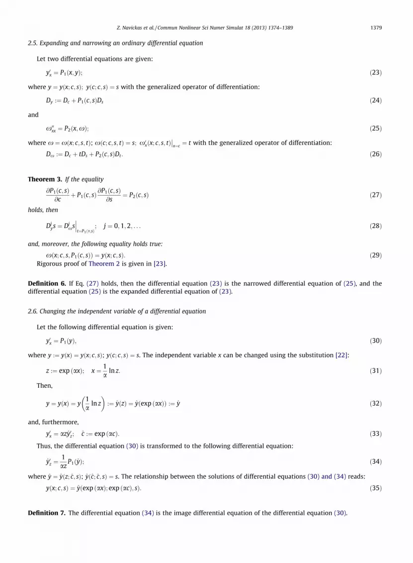
2.5. Expanding and narrowing an ordinary differential equation

Let two differential equations are given:

y0x ¼ P1 x; yð Þ; ð23Þ

where y ¼ y x; c; sð Þ; y c; c; sð Þ ¼ s with the generalized operator of differentiation:

Dy :¼ Dc þ P1 c; sð ÞDs ð24Þ

and

x00xx ¼ P2 x;xð Þ; ð25Þ

where x ¼ x x; c; s; tð Þ; x c; c; s; tð Þ ¼ s; x0x x; c; s; tð Þ

��x¼c

¼ t with the generalized operator of differentiation:

Dx :¼ Dc þ tDs þ P2 c; sð ÞDt: ð26Þ

Theorem 3. If the equality

@P1 c; sð Þ@c

þ P1 c; sð Þ @P1 c; sð Þ@s

¼ P2 c; sð Þ ð27Þ

holds, then

Djys ¼ Dj

xs��t¼P1 m;sð Þ

; j ¼ 0;1;2; . . . ð28Þ

and, moreover, the following equality holds true:

x x; c; s; P1 c; sð Þð Þ ¼ y x; c; sð Þ: ð29ÞRigorous proof of Theorem 2 is given in [23].

Definition 6. If Eq. (27) holds, then the differential equation (23) is the narrowed differential equation of (25), and the

differential equation (25) is the expanded differential equation of (23).

2.6. Changing the independent variable of a differential equation

Let the following differential equation is given:

y0x ¼ P1 yð Þ; ð30Þ

where y :¼ y xð Þ ¼ y x; c; sð Þ; y c; c; sð Þ ¼ s. The independent variable x can be changed using the substitution [22]:

z :¼ exp axð Þ; x ¼ 1

aln z: ð31Þ

Then,

y ¼ y xð Þ ¼ y1

aln z

:¼ y zð Þ ¼ y exp axð Þð Þ :¼ y ð32Þ

and, furthermore,

y0x ¼ azy0z; c :¼ exp acð Þ: ð33Þ

Thus, the differential equation (30) is transformed to the following differential equation:

y0z ¼1

azP1 yð Þ; ð34Þ

where y ¼ y z; c; sð Þ; y c; c; sð Þ ¼ s. The relationship between the solutions of differential equations (30) and (34) reads:

y x; c; sð Þ ¼ y exp axð Þ; exp acð Þ; sð Þ: ð35Þ

Definition 7. The differential equation (34) is the image differential equation of the differential equation (30).


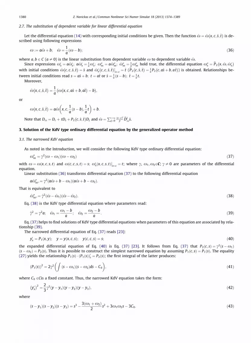
2.7. The substitution of dependent variable for linear differential equation

Let the differential equation (14) with corresponding initial conditions be given. Then the function x ¼ x x; c; s; t� �

is de-

scribed using following expressions

x :¼ axþ b; x ¼ 1

ax� bð Þ; ð36Þ

where a; b 2 C (a– 0) is the linear substitution from dependent variable x to dependent variable x.

Since expressions x0x ¼ ax0

x; ax0x ¼ 1

ax0

x; x00xx ¼ ax00

xx; x00xx ¼ 1

ax00

xx hold true, the differential equation x00x ¼ bP2 x; x; x0

x

� �

with initial conditions x c; c; s; t� �

¼ s and x0x c; c; s; t� ��

x¼c¼ t (bP2 c; s; t

� �¼ 1

aP2 c; asþ b; a t� �

) is obtained. Relationships be-

tween initial conditions read s ¼ asþ b; t ¼ at or s ¼ 1as� bð Þ; t ¼ 1

at.

Moreover,

x x; c; s; t� �

¼ 1

ax x; c; asþ b; at� �

� b� �

;

or

x x; c; s; t� �

¼ ax x; c;1

as� bð Þ;1

at

þ b:

Note that Dx ¼ Dc þ tDs þ P2 c; s; t� �

Dt and x ¼Pþ1j¼0

x�cð Þjj!bDj

x s.

3. Solution of the KdV type ordinary differential equation by the generalized operator method

3.1. The narrowed KdV equation

As noted in the Introduction, we will consider the following KdV type ordinary differential equation:

x00xx ¼ c2 x�x1ð Þ x�x2ð Þ ð37Þ

with x ¼ x x; c; s; tð Þ and x c; c; s; tð Þ ¼ s; x0x x; c; s; tð Þ

��x¼c

¼ t; where c, x1;x22C; c – 0 are parameters of the differential

equation.

Linear substitution (36) transforms differential equation (37) to the following differential equation

ax00xx;¼ c2 axþ b�x1ð Þ axþ b�x2ð Þ:

That is equivalent to

x00xx;¼ c2 x� x1ð Þ x� x2ð Þ: ð38Þ

Eq. (38) is the KdV type differential equation where parameters read:

c2 ¼ c2a; x1 ¼ x1 � b

a; x2 ¼ x2 � b

a: ð39Þ

Eq. (37) helps to find solutions of KdV type differential equations when parameters of this equation are associated by rela-

tionship (39).

The narrowed differential equation of Eq. (37) reads [23]:

y0x ¼ P1 x; yð Þ; y ¼ y x; c; sð Þ; y c; c; sð Þ ¼ s; ð40Þ

the expanded differential equation of Eq. (40) is Eq. (37) [23]. It follows from Eq. (37) that P2 c; sð Þ ¼ c2 s�x1ð Þs�x2ð Þ ¼ P2 sð Þ. Thus it is possible to construct the simplest narrowed equation by assuming P1 c; sð Þ ¼ P1 sð Þ. The equality

(27) yields the relationship P1 sð Þ � P1 sð Þð Þ0s ¼ P2 sð Þ; the first integral of the latter produces:

P1 sð Þð Þ2 ¼ 2c2Z

s�x1ð Þ s�x2ð Þds� C0

; ð41Þ

where C0 2Cis a fixed constant. Thus, the narrowed KdV equation takes the form:

y0x� �2 ¼ 2

3c2 y� y1ð Þ y� y2ð Þ y� y3ð Þ; ð42Þ

where

s� y1ð Þ s� y2ð Þ s� y3ð Þ ¼ s3 � 3 x1 þx2ð Þ2

s2 þ 3x1x2s� 3C0: ð43Þ


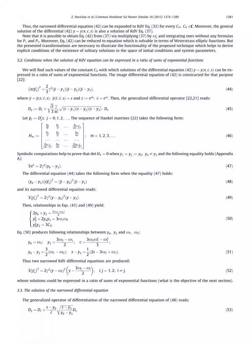
Thus, the narrowed differential equation (42) can be expanded to KdV Eq. (32) for every C0; C0 2C. Moreover, the general

solution of the differential (42) y ¼ y x; c; sð Þ is also a solution of KdV Eq. (37).

Note that it is possible to obtain Eq. (42) from (37) via multiplying (37) by x0x and integrating ones without any formulas

for P1 and P2. Moreover, Eq. (42) can be reduced to equation which is solvable in terms of Weierstrass elliptic functions. But

the presented transformations are necessary to illustrate the functionality of the proposed technique which helps to derive

explicit conditions of the existence of solitary solutions in the space of initial conditions and system parameters.

3.2. Conditions when the solution of KdV equation can be expressed in a ratio of sums of exponential functions

We will find such values of the constant C0 with which solutions of the differential equation (42) y ¼ y x; c; sð Þ can be ex-

pressed in a ratio of sums of exponential functions. The image differential equation of (42) is constructed for that purpose

[22]:

azy0z� �2 ¼ 2

3c2 y� y1ð Þ y� y2ð Þ y� y3ð Þ; ð44Þ

where y ¼ y z; c; sð Þ; y c; c; sð Þ ¼ s and z :¼ eax; c ¼ eac . Then, the generalized differential operator [22,21] reads:

Dy :¼ Dc þffiffiffi2

3

rcac

ffiffiffiffiffiffiffiffiffiffiffiffiffiffiffiffiffiffiffiffiffiffiffiffiffiffiffiffiffiffiffiffiffiffiffiffiffiffiffiffiffiffiffiffiffiffiffiffiffis� y1ð Þ s� y2ð Þ s� y3ð Þ

p� Ds: ð45Þ

Let pj :¼ Djys; j ¼ 0;1;2; . . .. The sequence of Hankel matrixes [22] takes the following form:

Hm :¼

p00!

p11!

. . . pm�1

m�1ð Þ!p11!

p22!

. . . pmm!

. . . . . . . . . . . .pm�1

m�1ð Þ!pmm!

. . .p2m�2

2m�2ð Þ!

2666664

3777775; m ¼ 1;2;3; . . . ð46Þ

Symbolic computations help to prove that detH4 ¼ 0 when y1 ¼ y2 :¼ y0; y0 – y3 and the following equality holds (Appendix

A):

3a2 ¼ 2c2 y0 � y3ð Þ: ð47Þ

The differential equation (44) takes the following form when the equality (47) holds:

y0 � y3ð Þ zy0z� �2 ¼ y� y0ð Þ2 y� y3ð Þ ð48Þ

and its narrowed differential equation reads:

3 y0x� �2 ¼ 2c2 y� y0ð Þ2 y� y3ð Þ: ð49Þ

Then, relationships in Eqs. (43) and (49) yield:

2y0 þ y3 ¼ 3 x1þx2ð Þ2

y20 þ 2y0y3 ¼ 3x1x2

y20y3 ¼ 3C0:

8><>:

ð50Þ

Eq. (50) produces following relationships between y0; y3 and x1; x2:

y0 ¼ x1; y3 ¼ 3x2 �x1

2; c ¼ 3x2x2

1 �x31

3;

y0 � y3 ¼ 3

2x1 �x2ð Þ; s� y3 ¼ 1

22s� 3x2 þx1ð Þ: ð51Þ

Thus two narrowed KdV differential equations are produced:

3 y0x� �2 ¼ 2c2 y�xið Þ2 y� 3xj �xi

2

; i; j ¼ 1;2; i– j; ð52Þ

whose solutions could be expressed in a ratio of sums of exponential functions (what is the objective of the next section).

3.3. The solution of the narrowed differential equation

The generalized operator of differentiation of the narrowed differential equation of (48) reads:

Dy ¼ Dc þs� y0

c

ffiffiffiffiffiffiffiffiffiffiffiffiffiffiffiffis� y3y0 � y3

rDs: ð53Þ


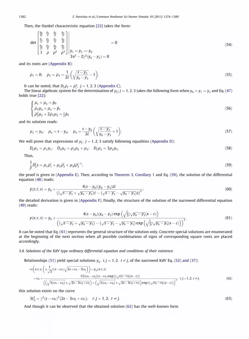
Then, the Hankel characteristic equation [22] takes the form:

det

p00!

p11!

p22!

p33!

p11!

p22!

p33!

p44!

p22!

p33!

p44!

p55!

1 q q2 q3

266664

377775

�� y1 ¼ y2 :¼ y0

3a2 � 2c2 y0 � y3ð Þ ¼ 0

¼ 0 ð54Þ

and its roots are (Appendix B):

q1 ¼ 0; q2 ¼ q3 ¼ 1

2c


r� 1

: ð55Þ

It can be noted, that Dyqj ¼ q2j ; j ¼ 1;2;3 (Appendix C).

The linear algebraic system for the determination of lj; j ¼ 1;2;3 takes the following form when y0 ¼ y1 ¼ y2 and Eq. (47)

holds true [22]:

l1 þ l2 ¼ p0

q2l2 þ l3 ¼ p1

q22l2 þ 2q2l3 ¼ 1

2p2

8><>:

ð56Þ

and its solution reads:

l1 ¼ y0; l2 ¼ s� y0; l3 ¼ s� y02c


rþ 1

: ð57Þ

We will prove that expressions of lj; j ¼ 1;2;3 satisfy following equalities (Appendix D):

Dyl1 ¼ q1l1; Dyl2 ¼ q2l2 þ l3; Dyl3 ¼ 3q2l3: ð58Þ

Thus,

1

j!Dj

ys ¼ l1q

j1 þ l2q

j2 þ l3jq

j�12 ; ð59Þ

the proof is given in (Appendix E). Then, according to Theorem 3, Corollary 1 and Eq. (59), the solution of the differential

equation (48) reads:

y z; c; sð Þ ¼ y0 þ4 s� y0ð Þ y0 � y3ð Þzc

ffiffiffiffiffiffiffiffiffiffiffiffiffis� y3

p þ ffiffiffiffiffiffiffiffiffiffiffiffiffiffiffiffiy0 � y3

p� �c � ffiffiffiffiffiffiffiffiffiffiffiffiffi

s� y3p � ffiffiffiffiffiffiffiffiffiffiffiffiffiffiffiffi

y0 � y3p� �

z� �2 ; ð60Þ

the detailed derivation is given in (Appendix F). Finally, the structure of the solution of the narrowed differential equation

(49) reads:

y x; c; sð Þ ¼ y0 þ4 s� y0ð Þ y0 � y3ð Þ exp

ffiffi23

qcffiffiffiffiffiffiffiffiffiffiffiffiffiffiffiffiy0 � y3

px� cð Þ

� �



p� �� ffiffiffiffiffiffiffiffiffiffiffiffiffi


y0 � y3p� �

expffiffi23

qcffiffiffiffiffiffiffiffiffiffiffiffiffiffiffiffiy0 � y3

px� cð Þ

� �� 2 : ð61Þ

It can be noted that Eq. (61) represents the general structure of the solution only. Concrete special solutions are enumerated

at the beginning of the next section when all possible combinations of signs of corresponding square roots are placed

accordingly.

3.4. Solutions of the KdV type ordinary differential equation and conditions of their existence

Relationships (51) yield special solutions yij; i; j ¼ 1;2; i– j, of the narrowed KdV Eq. (52) and (37):

x x;c;s; � 1ffiffiffi3

p c s�xrð Þffiffiffiffiffiffiffiffiffiffiffiffiffiffiffiffiffiffiffiffiffiffiffiffiffiffiffiffiffi2sþxr�3xj

q ¼yrj x;c;sð Þ

¼xrþ12 xr�xj

� �s�xrð Þexp c

ffiffiffiffiffiffiffiffiffiffiffiffiffiffiffiffixr�xj

px�cð Þ

� �ffiffiffiffiffiffiffiffiffiffiffiffiffiffiffiffiffiffiffiffiffiffiffiffi3 xr�xj

� �q�

ffiffiffiffiffiffiffiffiffiffiffiffiffiffiffiffiffiffiffiffiffiffiffiffiffiffiffiffiffi2s�3xjþxr

p� �þ

ffiffiffiffiffiffiffiffiffiffiffiffiffiffiffiffiffiffiffiffiffiffiffiffi3 xr�xj

� �q�

ffiffiffiffiffiffiffiffiffiffiffiffiffiffiffiffiffiffiffiffiffiffiffiffiffiffiffiffiffi2s�3xjþxr

p� �exp c

ffiffiffiffiffiffiffiffiffiffiffiffiffiffiffiffixr�xj

px�cð Þ

� �� 2 ; r;j¼1;2; r– j; ð62Þ

this solution exists on the curve

3t2rj ¼ c2 s�xrð Þ2 2s� 3xj þxr

� �; r; j ¼ 1;2; r – j: ð63Þ

And though it can be observed that the obtained solution (62) has the well-known form


1= c1 sinh axþ c2 cosh axð Þ2 þ c3;

the explicit expression of the curve (63) is a new and important finding describing the existence of solitary solutions in the

space of initial conditions and system parameters.

As mentioned in the Introduction, explicit expressions of analytic solutions of KdV equation can be found using different

methods and techniques based on the proposition that the structure of the solution takes certain form and then using sym-

bolic computations to identify the necessary values [32,8,4,18,25,5,15,31,38,35,30,37]. But we argue that conditions of the

existence of these special solutions in the space of the system’s parameters can not be derived using those methods.

Note that another differential equations of KdV type can be obtained using substitutions (35) and relationships (39) for

parameters c; x1; x2 and c; x1; x2.

3.5. Several comments on special solutions of the KdV type ordinary differential equation

Special solutions of the KdV Eq. (62) exist and have sense not only when parameters c; x1 and x2 are complex numbers,

but when the parameter of the initial condition s is a complex number also. Thus, in general, solutions (Eq. 62) are complex

functions of the real variable x:

yk ¼ uk x; c; sð Þ þ ivk x; c; sð Þ; ð64Þ

where k ¼ 1;2; i2 ¼ �1. Then Eq. (37) yields a system of KdV differential equations whose special solutions are functions

uk ¼ uk x; c; sð Þ and vk ¼ vk x; c; sð Þ; k ¼ 1;2. But a more deep analysis of solutions uk and vk is out of scope of interests in this

paper. In general, the independent variable x can be a complex variable then; complex variable functions theory methods

could be exploited for the analysis of special complex solutions.

In this paper we will introduce the limitation that c;x1; x2 and s are real numbers. It can be noted that functions yk in Eq.

(64) are complex functions even if the aforementioned limitation is in force; special solutions satisfy the following system of

KdV differential equations:

ukð Þ00xx ¼ c2 uk �x1ð Þ uk �x2ð Þ � v2k

� �;

vkð Þ00xx ¼ c2 2uk � x1 þx2ð Þð Þvk;

(ð65Þ

where k ¼ 1;2 and functions uk; vk satisfy initial conditions:

uk m; m; sð Þ ¼ s; vk m; m; sð Þ ¼ 0: ð66Þ

Functions uk and vk are structural solutions of the system of differential equation (65). Therefore, their first derivatives must

fulfill the following equalities defined by Eq. (63):

d uk x; m; sð Þð Þdx

��x¼c

¼ ak;d vk x; m; sð Þð Þ

dx

��x¼c

¼ bk; ð67Þ

where tk ¼ ak þ ibk; k ¼ 1;2; ak and bk are real numbers computed from the equations of curves defined by Eq. (63).

4. Classical KdV solitary solutions and numerical experiments

Let us assume that x1 ¼ 0 and x2 ¼ 23s. Then, Eq. (62) yields:

y11 x; c; sð Þ ¼ 4s exp cffiffiffiffiffiffiffiffiffiffi�x2

px� cð Þð Þ

1þ exp cffiffiffiffiffiffiffiffiffiffi�x2

px� cð Þð Þð Þ2

¼ s � sech2 c2

ffiffiffiffiffiffiffiffiffiffi�x2

px� cð Þ

� �: ð68Þ

But if x1 ¼ 0 the second root must be equal to x2 ¼ � r3(Eq. (4)); also c2 ¼ 3. Then,

y11 ¼ � r

2� sech2

ffiffiffir

p

2x� cð Þ

¼ � r

2� sech2

ffiffiffir

p

2z� rs� cð Þ

; ð69Þ

what is a solution of the KdV equation describing solitary waves observed by Rassel in 1834.

It is important to note, that solutions for other values on x1 andx2 may not exist in the whole plane of parameters s and

t. We argue that these conditions of existence can not be determined using methods based on the principle when the struc-

ture of the solution is initially supposed and then symbolic computations are used for the determination of appropriate coef-

ficients. We have shortly discussed the limitations of these methods in the Introduction. We will now demonstrate that

solutions for the other set of parameters x1 and x2 are limited by their conditions of existence.

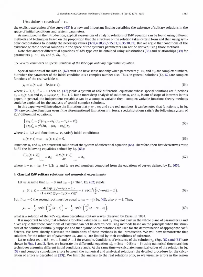
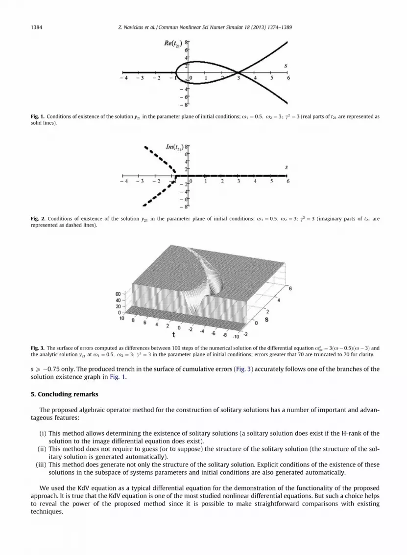
Let us select x1 ¼ 0:5; x2 ¼ 3 and c2 ¼ 3 for example. Conditions of existence of the solution y21 (Eqs. (62) and (63)) are

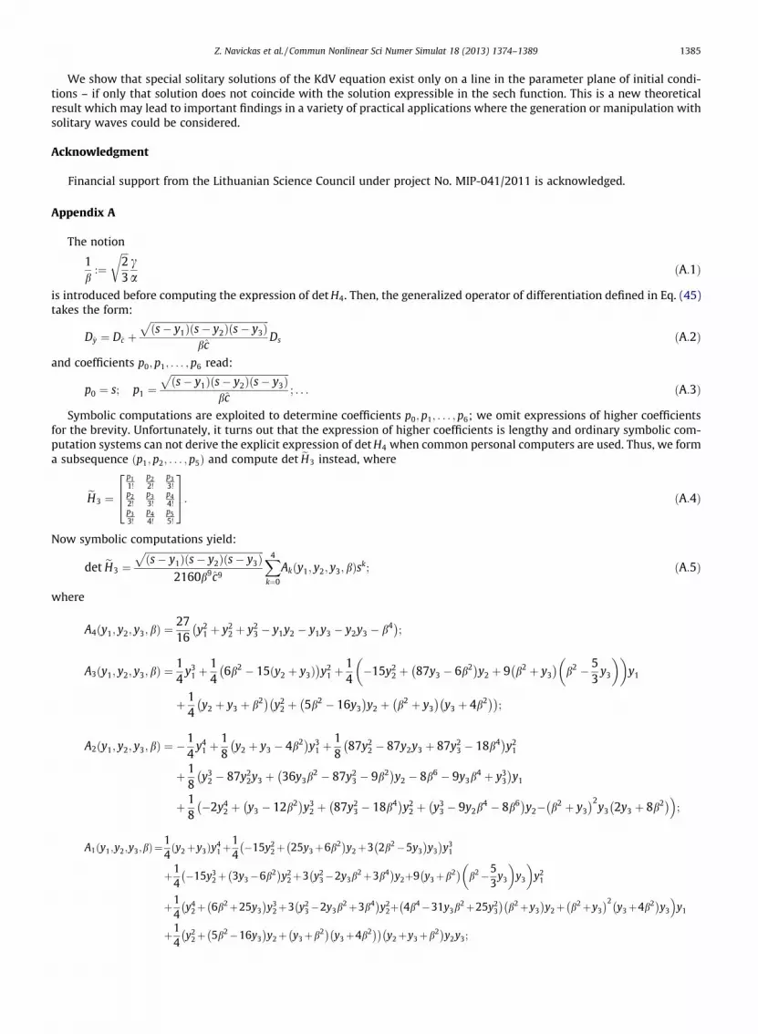
shown in Figs. 1 and 2. Next, we integrate the differential equation x00xx ¼ 3 x� 0:5ð Þ x� 3ð Þ using numerical time marching

techniques assuming different initial conditions s and t. At the same time we calculate numerical values of the solution in Eq.

(62) and compute cumulative errors between the numerical and analytical solutions (the detailed procedure for the calcu-

lation of errors is described in [23]). We limit the analysis to the real solutions only, so we visualize errors in the region


sP �0:75 only. The produced trench in the surface of cumulative errors (Fig. 3) accurately follows one of the branches of the

solution existence graph in Fig. 1.

5. Concluding remarks

The proposed algebraic operator method for the construction of solitary solutions has a number of important and advan-

tageous features:

(i) This method allows determining the existence of solitary solutions (a solitary solution does exist if the H-rank of the

solution to the image differential equation does exist).

(ii) This method does not require to guess (or to suppose) the structure of the solitary solution (the structure of the sol-

itary solution is generated automatically).

(iii) This method does generate not only the structure of the solitary solution. Explicit conditions of the existence of these

solutions in the subspace of systems parameters and initial conditions are also generated automatically.

We used the KdV equation as a typical differential equation for the demonstration of the functionality of the proposed

approach. It is true that the KdV equation is one of the most studied nonlinear differential equations. But such a choice helps

to reveal the power of the proposed method since it is possible to make straightforward comparisons with existing

techniques.

Fig. 1. Conditions of existence of the solution y21 in the parameter plane of initial conditions; x1 ¼ 0:5; x2 ¼ 3; c2 ¼ 3 (real parts of t21 are represented as

solid lines).

Fig. 2. Conditions of existence of the solution y21 in the parameter plane of initial conditions; x1 ¼ 0:5; x2 ¼ 3; c2 ¼ 3 (imaginary parts of t21 are

represented as dashed lines).

Fig. 3. The surface of errors computed as differences between 100 steps of the numerical solution of the differential equation x00xx ¼ 3 x� 0:5ð Þ x� 3ð Þ and

the analytic solution y21 at x1 ¼ 0:5; x2 ¼ 3; c2 ¼ 3 in the parameter plane of initial conditions; errors greater that 70 are truncated to 70 for clarity.


We show that special solitary solutions of the KdV equation exist only on a line in the parameter plane of initial condi-

tions – if only that solution does not coincide with the solution expressible in the sech function. This is a new theoretical

result which may lead to important findings in a variety of practical applications where the generation or manipulation with

solitary waves could be considered.

Acknowledgment

Financial support from the Lithuanian Science Council under project No. MIP-041/2011 is acknowledged.

Appendix A

The notion

1

b:¼

ffiffiffi2

3

rca

ðA:1Þ

is introduced before computing the expression of detH4. Then, the generalized operator of differentiation defined in Eq. (45)

takes the form:

Dy ¼ Dc þffiffiffiffiffiffiffiffiffiffiffiffiffiffiffiffiffiffiffiffiffiffiffiffiffiffiffiffiffiffiffiffiffiffiffiffiffiffiffiffiffiffiffiffiffiffiffiffiffis� y1ð Þ s� y2ð Þ s� y3ð Þ

p

bcDs ðA:2Þ

and coefficients p0; p1; . . . ; p6 read:

p0 ¼ s; p1 ¼ffiffiffiffiffiffiffiffiffiffiffiffiffiffiffiffiffiffiffiffiffiffiffiffiffiffiffiffiffiffiffiffiffiffiffiffiffiffiffiffiffiffiffiffiffiffiffiffiffis� y1ð Þ s� y2ð Þ s� y3ð Þ

p

bc; . . . ðA:3Þ

Symbolic computations are exploited to determine coefficients p0; p1; . . . ; p6; we omit expressions of higher coefficients

for the brevity. Unfortunately, it turns out that the expression of higher coefficients is lengthy and ordinary symbolic com-

putation systems can not derive the explicit expression of detH4 when common personal computers are used. Thus, we form

a subsequence p1; p2; . . . ; p5ð Þ and compute det eH3 instead, where

eH3 ¼

p11!

p22!

p33!

p22!

p33!

p44!

p33!

p44!

p55!

264

375: ðA:4Þ

Now symbolic computations yield:

det eH3 ¼ffiffiffiffiffiffiffiffiffiffiffiffiffiffiffiffiffiffiffiffiffiffiffiffiffiffiffiffiffiffiffiffiffiffiffiffiffiffiffiffiffiffiffiffiffiffiffiffiffis� y1ð Þ s� y2ð Þ s� y3ð Þ

p

2160b9c9

X4

k¼0

Ak y1; y2; y3;bð Þsk; ðA:5Þ

where

A4 y1; y2; y3;bð Þ ¼ 27

16y21 þ y22 þ y23 � y1y2 � y1y3 � y2y3 � b4� �

;

A3 y1; y2; y3;bð Þ ¼ 1

4y31 þ

1

46b2 � 15 y2 þ y3ð Þ� �

y21 þ1

4�15y22 þ 87y3 � 6b2

� �y2 þ 9 b2 þ y3

� �b2 � 5

3y3

y1

þ 1

4y2 þ y3 þ b2� �

y22 þ 5b2 � 16y3� �

y2 þ b2 þ y3� �

y3 þ 4b2� ��

;

A2 y1; y2; y3;bð Þ ¼ �1

4y41 þ

1

8y2 þ y3 � 4b2� �

y31 þ1

887y22 � 87y2y3 þ 87y23 � 18b4� �

y21

þ 1

8y32 � 87y22y3 þ 36y3b

2 � 87y23 � 9b2� �

y2 � 8b6 � 9y3b4 þ y33

� �y1

þ 1

8�2y42 þ y3 � 12b2

� �y32 þ 87y23 � 18b4

� �y22 þ y33 � 9y2b

4 � 8b6� �

y2�

� b2 þ y3� �2

y3 2y3 þ 8b2� ��

;

A1 y1;y2;y3;bð Þ¼1

4y2þy3ð Þy41þ

1

4�15y22þ 25y3þ6b2

� �y2þ3 2b2�5y3

� �y3

� �y31

þ1

4�15y32þ 3y3�6b2

� �y22þ3 y23�2y3b

2þ3b4� �

y2�

þ9 y3þb2� �

b2�5

3y3

y3

y21

þ1

4y42þ 6b2þ25y3

� �y32þ3 y23�2y3b

2þ3b4� �

y22�

þ 4b4�31y3b2þ25y23

� �b2þy3� �

y2þ b2þy3� �2

y3þ4b2� �

y3

�y1

þ1

4y22þ 5b2�16y3

� �y2þ y3þb2

� �y3þ4b2� ��

y2þy3þb2� �

y2y3;


A0 y1; y2; y3; bð Þ ¼ 1

1627y23 þ 27y22 � 58y2y3� �

y41 �1

1627y32 � 33y22y3 þ 3y2y3 8b2 � 11y3

� �þ 27y33

� �y31

þ 1

1627y42 þ 33y32y3 þ 24y3b

2 � 27b4 � 105y23� �

y22�

þ 24b2y23 þ 33y33 þ 18y3b4

� �y2 þ 27y43 � 27b4y23

�y21

� 1

829y32 þ 12b2 � 33

2y3

y22 � 12y3b

2 þ 33y23 þ 9b4� �

y2

þ b2 þ y3� �

8b4 � 17y3b2 þ 29y23

� ��y1y2y3

� 27

16y2y3 � y22 � y23 þ b4� �

y22y23:

The necessary and sufficient conditions for det eH3 ¼ 0 are equalities

Ak y1; y2; y3; bð Þ ¼ 0; k ¼ 0;1;2;3;4: ðA:6Þ

The equality

A4 y1; y2; y3; bð Þ ¼ 0; ðA:7Þ

yields the following relationship:

b4 ¼ y21 þ y22 þ y23 � y1y2 � y1y3 � y2y3: ðA:8Þ

Next, the equality (A.8) is incorporated into the expression of A3 y1; y2; y3; bð Þ:

A3 y1; y2; y3;ffiffiffiffiffiffiffiffiffiffiffiffiffiffiffiffiffiffiffiffiffiffiffiffiffiffiffiffiffiffiffiffiffiffiffiffiffiffiffiffiffiffiffiffiffiffiffiffiffiffiffiffiffiffiffiffiffiffiffiffiffiffiffiffiffiffiffiffiffiffiffiy21 þ y22 þ y23 � y1y2 � y1y3 � y2y3

4

q ¼ 0: ðA:9Þ

Elementary transformations in Eq. (A.9) yield necessary and sufficient conditions for Eq. (A.8) (b– 0) to hold. These condi-

tions require that two of the three parameters y1; y2; y3 must coincide, for example, y1 ¼ y2 :¼ y0 and y0 – y3 (then

b ¼ ffiffiffiffiffiffiffiffiffiffiffiffiffiffiffiffiy0 � y3

p). Now, the expressions of y0 and b can be introduced into Ak y1; y2; y3; bð Þ; k ¼ 0;1;2. Elementary transforma-

tions help to prove that equalities in (A.6) hold true for all k.

Thus, det eH3 ¼ 0 when y1 ¼ y2 :¼ y0, (A.1) and the equality b ¼ ffiffiffiffiffiffiffiffiffiffiffiffiffiffiffiffiy0 � y3

pyield:

3a2 ¼ 2c2 y0 � y3ð Þ: ðA:10Þ

Now, straightforward symbolic computations help to prove that detH4 ¼ 0, but detH3 – 0.

Appendix B

Coefficients of the equality (54) read:

p0 ¼ s;

p1 ¼ s� y0c


r;

p2 ¼ 3

2

s� y0c2 y0 � y3ð Þ


r�3

2y0 þ

2

3y3

� 1

3y0 �

2

3y3 þ s

;

p3 ¼ 3s� y0

c3 y0 � y3ð Þ


rs� y3ð Þ þ 1

2y0 �

3

2sþ y3 � 3s

;

p4 ¼ 15

2

s� y0

c4 y0 � y3ð Þ2ffiffiffiffiffiffiffiffiffiffiffiffiffiffiffiffis� y3y0 � y3

r�12

5�1

3y0 �

2

3y3 þ s

y0 � y3ð Þ

�3

5y20 �

16

5y3sþ

8

5y23 þ

6

5y0sþ s2

;

p5 ¼ 45

2

s� y0


r�5

3y20 þ

10

3y0sþ s2 þ 8

3y23 �

16

3y3s

þy3

20

3s� 4

3y0

þ 2

3y20 �

10

3s2;

p6 ¼ 315

4

s� y0


r�30

7�16

15y23 þ y3

8

15y0 �

8

3s

�3

5y20 þ

2

3y0sþ s2

y0 � y3ð Þ

þ 97

7y23s�

32

7y33

þ y330

7y20 �

60

7y0s�

66

7s2

� 5

7y30 �

15

7y20sþ

45

7y0s

2 þ s3


Eq. (54) then reads:

1

64

y0q s� y0ð Þ4

c8 y0 � y3ð Þ4�2 qc þ 1ð Þ y0 � y3ð Þ


ry0

1

2þ qc

� y3 � qcy3 þ

1

2s

þ1

4s2 þ y20

1

2þ qc

2

þy0 s q2c2 þ 3qc þ 3

2

� 2y3 � 5qcy3 � 3q2c2y3

�s 3qcy3 þ 3q2c2y3 þ 2y3� �

þ 2y23 qc þ 1ð Þ2�¼ 0:

Eq. (54) is solved using symbolic computation techniques; three roots read:

q1 ¼ 0; q2 ¼ q3 ¼ � 1

2c

�y0 þ 3y0

ffiffiffiffiffiffiffiffiffiffis�y3y0�y3

qþ 4y3 � 4y3


q� 3sþ s


q

�y0 þ 2y0


qþ 2y3 � 2y3


q� s

¼ 1

2c


r� 1

:

Appendix C

The equality Dyq1 ¼ q21 is trivial because q1 ¼ 0.

q2 ¼ q3 ¼ 12c


q� 1

� �, therefore:

Dyq2 ¼ Dm þs� y0

c


rDs

1

2c


r� 1

¼ � 1

2c2


r� 1

þ s� y0

2c2


r1

2ffiffiffiffiffiffiffiffiffiffiffiffiffiffiffiffiffiffiffiffiffiffiffiffiffiffiffiffiffiffiffiffiffiffiffiy0 � y3ð Þ s� y3ð Þ

p

¼ 1

4c22þ s� y0

y0 � y3� 2


r ¼ 1

4c2s� y3y0 � y3

� 2


rþ 1

¼ 1

2c


r� 1

2

¼ q22:

Appendix D

We will prove that Dyl1 ¼ q1l1; Dyl2 ¼ q2l1 þ l3; Dyl3 ¼ 3q2l3.

The first equality is trivial because Dyl1 ¼ 0 and q1 ¼ 0.

Next, Dyl2 ¼ Dc þ s�y0c


qDs

� �s� y0ð Þ ¼ s�y0

c


q. But

q2l1 þ l3 ¼ 1

2c


r� 1

s� y0ð Þ þ s� y0

2c


rþ 1

¼ s� y0

c


r:

Finally,

Dyl3 ¼ Dc þs� y0

c


rDs

s� y02c


rþ 1

¼ � s� y02c2


rþ 1

þ s� y0

2c2


r ffiffiffiffiffiffiffiffiffiffiffiffiffiffiffiffis� y3y0 � y3

rþ 1þ s� y0

2ffiffiffiffiffiffiffiffiffiffiffiffiffiffiffiffiffiffiffiffiffiffiffiffiffiffiffiffiffiffiffiffiffiffiffiy0 � y3ð Þ s� y3ð Þ

p !

¼ � s� y02c2


rþ 1

þ s� y0

2c2s� y3y0 � y3

þffiffiffiffiffiffiffiffiffiffiffiffiffiffiffiffis� y3y0 � y3

rþ s� y02 y0 � y3ð Þ

¼ s� y0

2c2s� y3y0 � y3

� 1þ s� y02 y0 � y3ð Þ

¼ s� y02c2

� �2y0 þ 2y3 þ 2s� 2y3 þ s� y02 y0 � y3ð Þ ¼ 3 s� y0ð Þ2

4c2 y0 � y3ð Þ :

But, on the other hand,

3q2l3 ¼ 31

2c


r� 1

s� y02c


rþ 1

¼ 3 s� y0ð Þ

4c2s� y3y0 � y3

� 1

¼ 3 s� y0ð Þ2

4c2 y0 � y3ð Þ ;

what concludes the proof.

Appendix E

Proof of the equality in (59).

p0 ¼ s, therefore:

1

1!Dys ¼ Dy l1 þ l2

� �¼ 0þ l2q2 þ l3 ¼ l10þ l2q2 þ l3

1

1

q0

2 ¼ 1

1!p1:


Let the following equality hold true:

1

j!Dj

ys ¼ l2q

j2 þ l3

j

1

qj�1

2 ¼ 1

j!pj:

Then,

1

jþ 1ð Þ!Djþ1y

s ¼ 1

jþ 1Dy l2q

j2 þ l3

j

1

qj�1

2

¼ 1

jþ 1l2q2 þ l3

� �qj

2 þ l2jqj�12 q2

2 þ 3jq2qj�12 þ jl3 j� 1ð Þqj�2

2 q22

� �

¼ 1

jþ 1l2 jþ 1ð Þqjþ1

2 þ 1þ 3jþ j j� 1ð Þð Þl3qj2

� �¼ l2q

jþ12 þ l3

jþ 1

1

qj

2 ¼ 1

jþ 1ð Þ! pjþ1

what concludes the proof.

Appendix F

y z; c; sð Þ ¼Xþ1

j¼0

z� cð Þj

j!Dj

ys

¼Xþ1

j¼0

z� cð Þj y0cj þ s� y0ð Þ 1

2c


rþ 1

j

þ s� y02c


rþ 1

j

1

2c


r� 1

j�1!

¼ y0 þ s� y0ð Þ 1

1� 12c


q� 1

� �z� cð Þ

þ s� y02c


rþ 1

z� cð Þ

1� 12c


q� 1

� �z� cð Þ

� �2

¼ y0 þ s� y0ð Þ1� 1

2c


q� 1

� �z� cð Þ þ z� cð Þ 1

2c


qþ 1

� ��

1� 12c


q� 1

� �z� cð Þ

� �2

¼ y0 þ s� y0ð Þ c þ z� cð Þ4c y0 � y3ð Þ2c

ffiffiffiffiffiffiffiffiffiffiffiffiffiffiffiffiy0 � y3

p � ffiffiffiffiffiffiffiffiffiffiffiffiffis� y3

p � ffiffiffiffiffiffiffiffiffiffiffiffiffiffiffiffiy0 � y3

p� �z� cð Þ

� �2

¼ y0 þ4 s� y0ð Þ y0 � y3ð Þzc



p� �c � ffiffiffiffiffiffiffiffiffiffiffiffiffi


y0 � y3p� �

z� �2 :

References

[1] Ablowitzand MJ, Clarkson PA. Solitons, nonlinear evolution equations and inverse scattering. Cambridge University Press; 1991.[2] Airault H, McKean HP, Moser J. Rational and elliptic solutions of the KdV equation and related many-body problems. Commun Pure Appl Math

1977;30:95–148.[3] Debath L. Nonlinear water partial differential equations for scientists and engineers. Berlin: Birkhauser; 1998.[4] Ebaid A. Exact solitary wave solutions for some nonlinear evolution equations via Exp-function method. Phys Lett A 2007;365:213–9.[5] Fan EG. Extended tanh-function method and its applications to nonlinear equations. Phys Lett A 2000;277:212–8.[6] Fokas AS, Lenells J. Explicit soliton asymptotics for the Kortewed-de Vries equation on the half-time. Nonlinearity 2010;23:937–76.[7] Gardner CS, Green JM, Kruskal MD, Miura RM. Method for solving the Korteweg-de Vries equations. Phys Rev Lett 1967;19:1095–7.[8] He JH, Wu XH. Exp-function method for nonlinear wave equations. Chaos Solitons Fract 2006;30:700–8.[9] Hirota R. Exact solution of Korteweg-de Vries equation for multiple collisions of solitons. Phys Rev Lett 1971;27:1192–4.[10] Korteweg DJ, de Vries G. On the change of the form of long waves advancing in rectangular canal, and on a new type of stationary waves. Philosoph

Magaz 1895;39:422–43.[11] Kudryashov NA. On new travelling wave solutions of the KdV and the KdV–Burgers equation. Commun Nonlinear Sci Numer Simul 2009;14:1891–900.[12] Kudryashov NA, Loguinova NB. Be careful with Exp-function method. Commun Nonlinear Sci Numer Simul 2009;14:1881–90.[13] Kudryashov NA. Seven common errors in finding exact solutions of nonlinear differential equations. Commun Nonlinear Sci Numer Simul

2009;14:3507–29.[14] Lax PD. Integrals of nonlinear equations of evolution and solitary waves. Commun Pure Appl Math 1968;21:467–90.[15] Li B, Chen Y, Zhang HQ. Explicit exact solutions for compound KdV-type and compound KdV–Burgers-type equations with nonlinear terms of any

order. Chaos Solitons Fract 2003;15:647–54.[16] Liu SK, Fu ZT, Liu SD. Jacobi elliptic function expansion method and periodic wave solutions of nonlinear wave equations. Phys Lett A 2001;289:69–74.[17] Liu XQ, Jiang S, Fan WB, Liu WM. Soliton solutions in linear magnetic field and time-dependent laser field. Commun Nonlinear Sci Numer Simul

2004;9:361–5.[18] Malfeit W. Solitary wave solutions of nonlinear wave equations. Am J Phys 1992;60:650–4.[19] Matveev VB, Salle MA. Darboux transformations and solitons. Berlin, Heidelberg: Springer-Verlag; 1991.[20] Navickas Z, Bikulciene L. Expressions of solutions of ordinary differential equations by standard functions. Math Model Anal 2006;11:399–412.[21] Navickas Z, Bikulciene L, Ragulskis M. Generalization of Exp-function and other standard function based methods. Appl Math Comput

2010;216:2380–93.[22] Navickas Z, Ragulskis M. How far one can go with the Exp-function method? Appl Math Comput 2009;211:522–30.[23] Navickas Z, Ragulskis M, Bikulciene L. Be careful with the Exp-function method – additional remarks. Commun Nonlinear Sci Numer Simul

2010;15:3874–86.


[24] Ozer MN, Tascan F, Koparan M. Derivation of Korteweg-de Vries flow equations from modified nonlinear Schrodinger equation. Nonlinear Anal RealWorld Appl 2010;11:2619–23.

[25] Parkes EJ, Duffy BR. An automated tanh-function method for finding solitary wave solutions to non-linear evolution equations. Comput Phys Commun1996;98:288–300.

[26] Popovych RO, Vaneeva OO. More common errors in finding exact solutions of nonlinear differential equations: Part I. Commun Nonlinear Sci NumerSimul 2010;15:3887–99.

[27] Rosales RR. The similarity solution for Korteweg-de Vries equation and related Painleve transcendent. Proc Roy Soc Lond A 1978;361:265–75.[28] Rybkin A. Meromorphic solution to the KdV equation with non-decaying initial data supported on a left half line. Nonlinearity 2010;23:1143–67.[29] Scott A. Nonlinear science: emergence and dynamics of coherent structures. Oxford: Oxford University Press; 2003.[30] Sirendaoreji, Jiong S. Auxiliary equation method for solving nonlinear partial differential equations. Phys Lett A 2000;309:387–96.[31] Wazwaz AM. Analytic study for fifth-order KdV-type equations with arbitrary power nonlinearities. Commun Nonlinear Sci Numer Simul

2007;12:904–9.[32] Wang ML. Exact solutions for a compound KdV–Burgers equation. Phys Lett A 1996;213:279–87.[33] Washimi H, Taniuti T. Propagation of ion-acoustic solitary waves of small amplitude. Phys Rev Lett 1966;17:996–8.[34] Yan Z, Zhang H. Backlund transformation and exact solutions for (2+1)-dimensional Kolmogoroff–Petrovesky–Piscounov equation. Commun Nonlinear

Sci Numer Simul 1999;4:146–51.[35] Yomba E. The extended Fan’s sub-equation method and its application to KdV–MKdV, BKK and variant Boussinesq equations. Phys Lett A

2000;336:463–76.[36] Zabuski NJ, Kruskal MD. Interaction of solitons in a collisionless plasma and the recurrence of initial states. Phys Rev Lett 1965;15:240–2.[37] Zhang H. A note on some sub-equation methods and new types of exact travelling wave solutions for two nonlinear partial differential equations. Acta

Appl Math 2009;106:241–9.[38] Zhang H. Application of the (G0/G)-expansion method for the complex KdV equation. Commun Nonlinear Sci Numer Simul 2010;15:1700–4.[39] Chen Yong, Yan Zhenya. The Weierstrass elliptic function expansion method and its applications in nonlinear wave equations. MM Research Preprints

2003;29:382–401.[40] Porubov AV. Periodic solution to the nonlinear dissipative equation for surface waves in a convecting liquid layer. Phys Lett A 1996;221:391–4.[41] Korostil AM. On finite-gap elliptic solutions of the KdV equation. Nonlinear Math Phys 1997;4:175–9.[42] Zhen-Ya Yan. NewWeierstrass semi-rational expansion method to doubly periodic solutions of soliton equations. Commun Theor Phys 2005;43:391–6

(Beijing, China).


Algebraic operator method for the construction of solitary solutions to nonlinear differential...

Documents

Transcript of Algebraic operator method for the construction of solitary solutions to nonlinear differential...