Mesh adaptation for pseudospectral ultrasound simulations
183
Mesh adaptation for pseudospectral ultrasound simulations Elliott Steven Wise A dissertation submitted in partial fulfillment of the requirements for the degree of Doctor of Philosophy of University College London. Department of Medical Physics and Biomedical Engineering University College London November 21, 2018
-
Upload
khangminh22 -
Category
Documents
-
view
1 -
download
0
Transcript of Mesh adaptation for pseudospectral ultrasound simulations

Mesh adaptation for pseudospectralultrasound simulations
Elliott Steven Wise
A dissertation submitted in partial fulfillment
of the requirements for the degree of
Doctor of Philosophy
of
University College London.
Department of Medical Physics and Biomedical Engineering
University College London
November 21, 2018

2

3
I, Elliott Steven Wise, confirm that the work presented in this thesis is my own.
Where information has been derived from other sources, I confirm that this has been
indicated in the work.


Abstract
High-intensity focussed ultrasound (HIFU) is an emerging cancer therapy that holds
great promise, as it is minimially invasive, requires no ionising radiation, and can
treat small volumes precisely. However, currently therapies are hindered by an inad-
equate capacity for treatment planning, as the interactions between the sound waves
and tissue are complex and difficult to simulate. The Fourier pseudospectral method
is one way of efficiently performing these simulations, as it can provide high accura-
cies with low computational costs. However, it is typically used with uniform com-
putational meshes, wasting resolution in regions of the simulation where only low
frequencies are present, and typically under-resolving the acoustic field in the focal
region. This thesis addresses this problem in two ways: First, a bandwidth-based
measure of the spatial resolution requirements for a model solution is developed
and integrated into a moving mesh method. This allows spatially and temporally-
varying resolution requirements to be met. Bandwidth-based meshes are shown to
perform very well when compared with current mesh adaptation approaches. Sec-
ond, a technique is presented for discretising arbitrary acoustic source distributions
that does not rely on the source’s region of support coinciding with the mesh. This
not only allows sources to be represented with adaptive meshes, but greatly im-
proves the accuracy of source discretisations for uniform meshes as well. These
two contributions are of vital importance in the context of HIFU simulation, and
can easily be applied to the many other problems for which the Fourier pseudospec-
tral method is used.


Impact Statement
This thesis describes algorithms for enhancing the Fourier pseudospectral method, a
numerical technique that is used to solve partial differential equations. Specifically,
algorithms are developed for generating adaptive computational meshes, and per-
forming high-accuracy discretisations of source terms. These algorithms have been
motivated by treatment planning for high-intensity focussed ultrasound, a promis-
ing therapy for destroying cancerous tissue. They could thus generate impact within
the research community (where novel therapies are investigated), industry (where
simulations are used to develop equipment), and clinical applications (through indi-
vidualised treatment plans). Beyond ultrasound, the Fourier pseudospectral method
has a wide range of applications, and so researchers from many other fields will
be able to make use of the enhancements described here. To facilitate this, the
work contained in this thesis has all either been published, or is in the process of
publication. In addition, the algorithms are in the process of being included in the
open-source k-Wave MATLAB toolbox. This toolbox aims to facilitate ultrasound
research, and an interface is currently being developed for treatment planning within
medical clinics. It is distributed under the terms of the GNU Lesser General Pub-
lic License, allowing both commercial and non-commercial use. Through these
channels, the contributions in this thesis can easily be put into practice by other
researchers, and adapted for other purposes. This will ensure ongoing impact.


Acknowledgements
This research would not have been possible without the support of many people.
First and foremost, I would like to thank my supervisors Bradley Treeby and Ben
Cox for their generosity and guidance. I am particularly grateful for the trust they’ve
shown in encouraging me to set my own research directions, and for introducing me
to the elegance of spectral methods. More broadly, the members of the Biomedical
Ultrasound Group have provided me with a fantastic working environment and my
PhD would not have been nearly so pleasant without you all.
To my family, thank you for always being there, even though I’m on the other
side of the world. To the many housemates I’ve had since moving to London, thank
you for building such a wonderful home with me. Life here would not have been
the same without you all. To the many people I’ve shared a dance with, thank you
for bringing me into your community. You’ve shown me a side of Europe that I
never imagined I would experience.
Finally, to my partner Liv, thank you for the truly countless ways that you’ve
supported me. I wouldn’t be here without you.


Contents
1 Introduction 21
1.1 High-intensity focussed ultrasound (HIFU) . . . . . . . . . . . . . 21
1.1.1 Overview . . . . . . . . . . . . . . . . . . . . . . . . . . . 21
1.1.2 Physical mechanisms . . . . . . . . . . . . . . . . . . . . . 22
1.1.3 Treatment planning . . . . . . . . . . . . . . . . . . . . . . 24
1.2 Acoustic models for HIFU . . . . . . . . . . . . . . . . . . . . . . 25
1.2.1 Treeby–Cox space-fractional wave equation . . . . . . . . . 25
1.2.2 Westervelt wave equation . . . . . . . . . . . . . . . . . . . 27
1.2.3 Khokhlov–Zabolotskaya–Kuznetsov (KZK) equation . . . . 27
1.2.4 Burgers’ equation . . . . . . . . . . . . . . . . . . . . . . . 28
1.3 Numerical methods . . . . . . . . . . . . . . . . . . . . . . . . . . 29
1.3.1 Problem scales . . . . . . . . . . . . . . . . . . . . . . . . 29
1.3.2 Fourier pseudospectral methods . . . . . . . . . . . . . . . 30
1.3.3 Convergence theorems . . . . . . . . . . . . . . . . . . . . 33
1.3.4 Sampling theorems . . . . . . . . . . . . . . . . . . . . . 35
1.3.5 Opportunities in HIFU modelling . . . . . . . . . . . . . . 36
1.4 Goals of the thesis . . . . . . . . . . . . . . . . . . . . . . . . . . . 37
1.5 List of publications . . . . . . . . . . . . . . . . . . . . . . . . . . 38
2 Spectral Moving Mesh Methods 41
2.1 Calculus on transformed meshes . . . . . . . . . . . . . . . . . . . 42
2.1.1 Mapped Fourier pseudospectral methods . . . . . . . . . . 42
2.1.2 The rational trigonometric pseudospectral method . . . . . . 43

12 Contents
2.2 Spectral methods with static mesh transformations . . . . . . . . . . 44
2.3 The moving mesh method framework . . . . . . . . . . . . . . . . 45
2.3.1 Monitor functions, equidistribution, and alignment . . . . . 46
2.3.2 Moving Mesh PDEs . . . . . . . . . . . . . . . . . . . . . 48
2.3.3 Mesh/model coupling and solution procedure . . . . . . . . 50
2.4 Derivative-based mesh adaptation . . . . . . . . . . . . . . . . . . 52
2.5 Smoothness-based mesh adaptation . . . . . . . . . . . . . . . . . 53
2.5.1 Analyticity-based mesh adaptation . . . . . . . . . . . . . . 53
2.5.2 Frequency-based mesh adaptation . . . . . . . . . . . . . . 55
2.6 Conclusion . . . . . . . . . . . . . . . . . . . . . . . . . . . . . . 56
3 Analyticity-based mesh adaptation in one dimension 57
3.1 Derivation of mesh density function . . . . . . . . . . . . . . . . . 58
3.1.1 Singularity localisation . . . . . . . . . . . . . . . . . . . . 58
3.1.2 A mesh density function based on a Schwarz–Christoffel
mapping . . . . . . . . . . . . . . . . . . . . . . . . . . . 63
3.2 Numerical methods . . . . . . . . . . . . . . . . . . . . . . . . . . 66
3.3 Numerical experiments . . . . . . . . . . . . . . . . . . . . . . . . 67
3.3.1 Burgers’ equation . . . . . . . . . . . . . . . . . . . . . . . 67
3.3.2 The Treeby–Cox space-fractional wave equation . . . . . . 76
3.4 Remaining issues . . . . . . . . . . . . . . . . . . . . . . . . . . . 80
3.5 Conclusion . . . . . . . . . . . . . . . . . . . . . . . . . . . . . . 84
4 Bandwidth-based mesh adaptation in one dimension 87
4.1 Derivation of mesh density function . . . . . . . . . . . . . . . . . 88
4.1.1 Local measures of bandwidth . . . . . . . . . . . . . . . . 88
4.1.2 A periodic Hilbert transform for nonuniform samples . . . . 92
4.1.3 Examples for static functions using Chebyshev approximants 94
4.2 Numerical methods . . . . . . . . . . . . . . . . . . . . . . . . . . 99
4.2.1 Spatial calculus and time-stepping . . . . . . . . . . . . . . 99
4.2.2 Smoothing the mesh density function . . . . . . . . . . . . 100

Contents 13
4.2.3 Mesh density function updates . . . . . . . . . . . . . . . . 100
4.3 Numerical experiments . . . . . . . . . . . . . . . . . . . . . . . . 101
4.3.1 Example problems . . . . . . . . . . . . . . . . . . . . . . 101
4.3.2 Convergence rates . . . . . . . . . . . . . . . . . . . . . . 107
4.3.3 Effect of the smoothing parameter . . . . . . . . . . . . . . 112
4.4 Conclusion . . . . . . . . . . . . . . . . . . . . . . . . . . . . . . 113
5 Bandwidth-based mesh adaptation in multiple dimensions 115
5.1 Derivation of mesh density function . . . . . . . . . . . . . . . . . 116
5.1.1 Multidimensional local bandwidth . . . . . . . . . . . . . . 116
5.1.2 The bandwidth mesh density function . . . . . . . . . . . . 117
5.2 Numerical methods . . . . . . . . . . . . . . . . . . . . . . . . . . 119
5.2.1 Spatial calculus and time-stepping . . . . . . . . . . . . . . 119
5.2.2 Computing the bandwidth mesh density vector . . . . . . . 119
5.2.3 Mesh smoothing . . . . . . . . . . . . . . . . . . . . . . . 120
5.2.4 Constraining boundary nodes . . . . . . . . . . . . . . . . 121
5.3 Numerical experiments . . . . . . . . . . . . . . . . . . . . . . . . 121
5.3.1 Model equations . . . . . . . . . . . . . . . . . . . . . . . 121
5.3.2 Results for Burgers’ equation . . . . . . . . . . . . . . . . 122
5.3.3 Results for heterogeneous advection . . . . . . . . . . . . . 127
5.3.4 Discussion . . . . . . . . . . . . . . . . . . . . . . . . . . 128
5.4 Conclusion . . . . . . . . . . . . . . . . . . . . . . . . . . . . . . 130
6 Representing arbitrary acoustic source distributions 133
6.1 Band-limiting source distributions . . . . . . . . . . . . . . . . . . 134
6.1.1 Background . . . . . . . . . . . . . . . . . . . . . . . . . . 134
6.1.2 Band-limiting via convolution . . . . . . . . . . . . . . . . 135
6.1.3 The band-limited delta function . . . . . . . . . . . . . . . 136
6.1.4 Discretisation of the band-limiting convolution . . . . . . . 140
6.1.5 Truncation of source grid weights . . . . . . . . . . . . . . 141
6.2 Numerical experiments . . . . . . . . . . . . . . . . . . . . . . . . 143

14 Contents
6.2.1 Terminology and simulation codes . . . . . . . . . . . . . . 143
6.2.2 Example source discretisations . . . . . . . . . . . . . . . . 144
6.2.3 Illustration and correction of staircasing errors . . . . . . . 145
6.2.4 Convergence for a circular piston . . . . . . . . . . . . . . 147
6.2.5 Convergence for a focussed bowl source . . . . . . . . . . . 148
6.3 Discussion . . . . . . . . . . . . . . . . . . . . . . . . . . . . . . . 153
6.3.1 Acoustic interpretation of integration points . . . . . . . . . 153
6.3.2 Integration scheme . . . . . . . . . . . . . . . . . . . . . . 153
6.3.3 Memory requirements for source grid weights . . . . . . . . 153
6.4 Extension to other problems . . . . . . . . . . . . . . . . . . . . . 154
6.4.1 Application to moving sources . . . . . . . . . . . . . . . . 154
6.4.2 Application to distributed sensors . . . . . . . . . . . . . . 155
6.4.3 Enforcing boundary conditions . . . . . . . . . . . . . . . . 157
6.5 Implementation with transformed meshes . . . . . . . . . . . . . . 160
6.6 Conclusion . . . . . . . . . . . . . . . . . . . . . . . . . . . . . . 163
7 General conclusions 167
Bibliography 170

List of Figures
1.1 Sonic Concepts H151 spherically focussed ultrasound transducer. . . 22
1.2 Simulated HIFU treatment of the kidney. . . . . . . . . . . . . . . . 23
1.3 Illustration of numerical dispersion for finite-difference and Fourier
pseudospectral methods. . . . . . . . . . . . . . . . . . . . . . . . 33
1.4 Illustration of algebraic and geometric convergence rates. . . . . . . 35
2.1 A Gaussian function and the corresponding arclength and curvature
mesh density functions. . . . . . . . . . . . . . . . . . . . . . . . . 48
3.1 Illustration of the Schwarz–Christoffel mapping process. . . . . . . 64
3.2 Analytic continuation of Burgers’ equation, with and without trans-
formed coordinates. . . . . . . . . . . . . . . . . . . . . . . . . . . 65
3.3 Convergence rates for Burgers’ equation with a weak shock front. . 70
3.4 Mesh node trajectories for Burgers’ equation with a weak shock front. 71
3.5 Convergence rates for Burgers’ equation with a weak shock front
based on the singularities in the model’s derivative. . . . . . . . . . 72
3.6 Error when solving Burgers’ equation using different mesh speed
parameters. . . . . . . . . . . . . . . . . . . . . . . . . . . . . . . 73
3.7 Convergence rates for Burgers’ equation with a steep shock front. . 75
3.8 Solution to Burgers’ equation with multiple shock fronts, using the
analyticity-based moving mesh method. . . . . . . . . . . . . . . . 77
3.9 Pole and mesh trajectories for Burgers’ equation with multiple
shock fronts, using the analyticity-based moving mesh method. . . . 78

16 List of Figures
3.10 Model solution, and pole and mesh trajectories for Burgers’ equa-
tion with multiple shock fronts, using the ARS method. . . . . . . . 79
3.11 Solution and analytic continuation for the Treeby–Cox wave equa-
tion with a time-varying sinusoidal pressure source. . . . . . . . . . 81
3.12 Pole trajectories for the Treeby–Cox wave equation with a time-
varying sinusoidal pressure source. . . . . . . . . . . . . . . . . . . 82
4.1 Convergence of Chebyshev approximations to a Gaussian function
under bandwidth-based mesh transformations. . . . . . . . . . . . . 96
4.2 Convergence of Chebyshev approximations to a Runge-type func-
tion under bandwidth-based mesh transformations. . . . . . . . . . 98
4.3 Solution and mesh trajectories for the heterogeneous advection
equation, exhibiting a sharp crest. . . . . . . . . . . . . . . . . . . 103
4.4 Solution and mesh trajectories for Burgers’ equation with a single
shock front. . . . . . . . . . . . . . . . . . . . . . . . . . . . . . . 104
4.5 Solution and mesh trajectories for Burgers’ equation with multiple,
merging shock fronts. . . . . . . . . . . . . . . . . . . . . . . . . . 106
4.6 Solution and mesh trajectories for the Korteweg-de Vries equation,
exhibiting multiple solitons. . . . . . . . . . . . . . . . . . . . . . 108
4.7 Convergence rates for the heterogeneous advection equation. . . . . 109
4.8 Convergence rates for Burgers’ equation with a single shock front. . 110
4.9 Convergence rates using finite-difference methods for the heteroge-
neous advection equation. . . . . . . . . . . . . . . . . . . . . . . . 112
4.10 Convergence rates using finite-difference methods for Burgers’
equation with a single shock front. . . . . . . . . . . . . . . . . . . 113
4.11 Error and number of timesteps for the heterogeneous advection
equation with a varying smoothing parameter. . . . . . . . . . . . . 114
5.1 Illustrative solution and mesh for a two-dimensional Burgers’ equa-
tion. . . . . . . . . . . . . . . . . . . . . . . . . . . . . . . . . . . 123

List of Figures 17
5.2 Illustrative solutions and meshes for one- and two-dimensional
Burgers’ equations. . . . . . . . . . . . . . . . . . . . . . . . . . . 124
5.3 Convergence rates for one- and two-dimensional Burgers’ equations. 126
5.4 Time-step sizes for one- and two-dimensional Burgers’ equations. . 127
5.5 Illustrative solutions/meshes and convergence rates for a two-
dimensional, heterogeneous advection equation. . . . . . . . . . . . 129
6.1 An arbitrary source distribution, showing the region of support for
the source, and potential discretisation points. . . . . . . . . . . . . 136
6.2 Illustration of the band-limited delta functions. . . . . . . . . . . . 140
6.3 Error in approximating the band-limited delta functions with a sinc
function. . . . . . . . . . . . . . . . . . . . . . . . . . . . . . . . . 142
6.4 Truncation thresholds for a two-dimensional sinc approximation to
the band-limited delta functions. . . . . . . . . . . . . . . . . . . . 143
6.5 Illustrative examples of on- and off-grid source discretisations. . . . 145
6.6 Steady-state acoustic pressure field for on- and off-grid discretisa-
tions of a line source in two-dimensions. . . . . . . . . . . . . . . . 146
6.7 Waveforms recorded from on- and off-grid discretisations of a ro-
tating line source. . . . . . . . . . . . . . . . . . . . . . . . . . . . 147
6.8 Steady-state acoustic pressure field (central plane) and convergence
rate (with varying integration point density) for a circular piston. . . 148
6.9 Steady-state acoustic pressure field (central plane) and convergence
rate (with PPW) for a focussed bowl source. . . . . . . . . . . . . . 150
6.10 On-axis acoustic pressure amplitude and error for a focussed bowl
source. . . . . . . . . . . . . . . . . . . . . . . . . . . . . . . . . . 151
6.11 Convergence rates (with PPW) for a focussed bowl source discre-
tised using sinc approximations to the off-grid delta functions. . . . 152
6.12 Illustration of the Doppler effect for a moving point source in one
dimension. . . . . . . . . . . . . . . . . . . . . . . . . . . . . . . . 155
6.13 Directivity of on- and off-grid line sensors in two-dimensions. . . . 157

18 List of Figures
6.14 Time-harmonic modes for the wave equation on a disc-shaped do-
main with a sound-soft boundary condition. . . . . . . . . . . . . . 159
6.15 Error in simulated harmonic modes after one period on a disc-
shaped domain with varying spatial and temporal resolution. . . . . 161
6.16 Difference between initial and final acoustic pressure fields for a
harmonic mode on a disc-shaped domain. . . . . . . . . . . . . . . 162
6.17 A pair of homophonic drums. . . . . . . . . . . . . . . . . . . . . . 163
6.18 Spectra for the two homophonic drums. . . . . . . . . . . . . . . . 164
6.19 Source grid weights for an offgrid rectangle generated with uniform
and nonuniform meshes. . . . . . . . . . . . . . . . . . . . . . . . 165

List of Tables
1.1 Realistic domain sizes for HIFU therapy simulations. . . . . . . . . 29


Chapter 1
Introduction
1.1 High-intensity focussed ultrasound (HIFU)
1.1.1 Overview
Ultrasound is widely used in medical practice, for both imaging and therapy. High-
intensity focussed ultrasound (HIFU) is one such class of therapies. It works by
focussing acoustic waves down to a very small volume using either a spherically
curved ultrasound transducer (see Fig. 1.1), an acoustic lens, or by applying time-
delayed signals to a collection of ultrasound transducers. By focussing the wave-
field, extremely high acoustic pressures are generated, causing heating, vaporisa-
tion, and exerting mechanical forces. Some of the therapeutic applications of HIFU
include the mechanical destruction of tissue (histotripsy), fragmentation of kidney
stones (lithotripsy), and thermal ablation of cancerous tumours. Within this last cat-
egory, devices for treating bone metastases, prostate, breast, kidney, liver, pancre-
atic, and soft-tissue cancers have all been approved in Europe [38]. HIFU therapies
have many benefits over other techniques, including a lack of ionising radiation, no
incisions, and comparatively low equipment costs. However, overall, HIFU ther-
apy remains little-used when compared with conventional cancer treatments. Even
when it is used, the vast majority of treatments are for uterine fibroids and prostate
tumours [39]. These diseases are relatively straightforward to access with the HIFU
beam, making treatment planning easy. Unfortunately, many tumours are in more
difficult to reach locations in the body. The application of HIFU to these tumours is

22 Chapter 1. Introduction
Figure 1.1: Sonic Concepts H151 spherically focussed ultrasound transducer.
hindered by difficulties in predicting the interactions between the ultrasound waves
and insonified tissue within clinical settings.
1.1.2 Physical mechanisms
HIFU therapies rely on high amplitude acoustic waves being focused so that large
amounts of acoustic energy are deposited at a specified target [3]. There are many
physical mechanisms that affect the way in which such wavefields develop in human
tissue. These are described below. For further reading: Naugolnykh and Ostrovsky
[71] provide a good reference for nonlinear acoustic effects and absorption mech-
anisms, Hamilton and Blackstock [46] gives similar information on nonlinearity
as well as sections on propagation in inhomogeneous media and HIFU fields in
medicine (their focus is more on acoustic models), and Duck [33] provides a more
general reference for the acoustic properties of human tissue.
Ultrasound propagation in the body can largely be understood to behave sim-
ilarly to pressure waves travelling through a fluid. That is, the primary mechanism
of propagation is through compressional waves. This approximation is accurate for

1.1. High-intensity focussed ultrasound (HIFU) 23
Figure 1.2: Simulated HIFU treatment of the kidney. The focus is distorted by the bodywall and a layer of fat. Images are adapted with permission from [59].
many purposes because soft tissues in the body do not readily support shear waves.
If bones are present in the acoustic field, then shear wave modes become impor-
tant as well, but many HIFU applications attempt to avoid insonifying bones (they
absorb and reflect sound strongly, which is not usually desirable). Within soft tis-
sues, waves will encounter changes in sound-speeds and material densities. This
causes their path to distort in a number of ways, including reflecting from tissue
boundaries, refracting (changing direction) as they pass from tissue to tissue, and
diffracting around objects in the wave’s path. As human tissue is highly heteroge-
neous, these path distortions have a strong effect on the resultant ultrasound fields.
In the context of HIFU, they can disrupt focussing by creating shifts in the focal
region and reducing overall pressure gains (see Fig. 1.2). This can limit the effec-
tiveness of treatments and even cause unwanted damage to tissues surrounding the
desired treatment region.
An important characteristic of HIFU fields is that they include a focal region
in which the waveform reaches very high acoustic pressures. When such waves
propagate, harmonics (integer multiples) of the source frequency quickly form. This

24 Chapter 1. Introduction
effect is known as nonlinear wave propagation, and it arises from two sources. The
first is convection, in which particles move either with or against the bulk wave
motion. The second is a nonlinear pressure density relation for the tissue itself.
Here, tissues become harder to compress as pressures increase, and as they stiffen
the sound speed increases. These both have the effect of steepening waveforms (i.e.
producing shock fronts), though this is often mitigated by acoustic absorption.
Absorption is the dissipation of acoustic energy into heat. This arises from
many mechanisms in complex tissues, but a general power-law dependence of the
form α0 f γ is typically an appropriate model for a given tissue type [33]. Here, f
is the waveform’s frequency, and α0 and γ are the power-law prefactor and expo-
nent. The rate of absorption increases with frequency, meaning a balance typically
arises between harmonic formation due to nonlinear wave propagation and loss of
harmonics due to absorption. As harmonics are strongest within the small, high-
amplitude focal region of the acoustic field, absorption (and hence heating) is highly
localised.
1.1.3 Treatment planning
Presently, little effort is made in clinical settings to predict the propagation of HIFU
waves in tissue. Treatments are instead planned using simplistic models of geo-
metric focussing, which only account for the properties of the acoustic source and
ignore the effect of the acoustic medium. This is to its detriment, as complex tissue
structures can cause the focal region to shift, widen, split, or fail to appear at all
[64]. To mitigate the risks arising from inaccurate plans, treatments must be care-
fully monitored using magnetic resonance (MR) thermometry [57] or ultrasound
imaging [106], and manually corrected when the acoustic waves fail to focus as
intended. These monitoring techniques are not ideal. MR thermometry is insensi-
tive to fatty tissues [80], limiting the kinds of tumours it can be applied to, and it
requires MR-compatible HIFU equipment. Ultrasonic image monitoring provides
no quantitative temperature information (it relies on structural changes that alter
the sound-speed), and suffers from interference between the imaging detectors and
HIFU waves [106].
1.2. Acoustic models for HIFU 25
In other cancer therapies, for instance radiotherapy, treatment plans are devel-
oped ‘off-line’. This involves taking an x-ray computed tomography (CT) scan of
the patient prior to surgery, and then simulating potential treatments. In a similar
vein, off-line plans could be developed for HIFU therapy. Acoustic wave models
can account for all previously discussed acoustic effects, and they can be coupled
with heat deposition models to estimate thermal doses [58, 101, 89]. Thus, the clin-
ician can be provided with more accurate acoustic and temperature field estimates
during the planning stage to reduce their reliance on monitoring. Such off-line plans
are not yet used because of the complexity of the physical interactions between tis-
sue and ultrasound waves, and the computational scales involved in modelling these
interactions. This thesis is concerned with the latter.
1.2 Acoustic models for HIFU
In this section a number of partial differential equations (PDEs) are provided that
describe nonlinear acoustic wave propagation and are particularly relevant to sim-
ulating HIFU fields. These are based upon conservation equations for mass and
momentum (reflecting the fact that human tissue is compressible and has inertia),
along with an equation of state relating the acoustic pressure and density. Note that
of these models, the Treeby–Cox, Khokhlov–Zabolotskaya–Kuznetsov, and Burg-
ers’ models are used in this thesis. In later chapters, advection and Korteweg-de
Vries wave models will also be introduced and used to illustrate the generality of
the numerical methods in this thesis, but these are not especially relevant to HIFU.
1.2.1 Treeby–Cox space-fractional wave equation
To perform clinically relevant HIFU simulations, a model with few simplifying as-
sumptions is required. This is known as a full-wave model. Starting with the acous-
tic conservation equations and equation of state, the Treeby–Cox model [100] is

26 Chapter 1. Introduction
defined by
∂u∂ t
=− 1ρ0
∇p, (momentum conservation)
∂ρ
∂ t=−(2ρ +ρ0)∇ ·u−u ·∇ρ0, (mass conservation)
p = c20
(ρ +d ·∇ρ0 +
B2A
ρ2
ρ0−Lρ
). (equation of state)
(1.1)
Here, four acoustic variables have been introduced. These are the acoustic pressure
p, acoustic particle velocity u, density ρ , and particle displacement d. The acoustic
medium is described by an ambient density ρ0, a sound speed c0, a material nonlin-
earity parameter B/A, and a loss operator L. The material nonlinearity coefficients
A and B arise from representing the nonlinear pressure-density relationship using
the first two terms of a Taylor series. The loss operator L is defined using fractional
Laplacians as
L = τ∂
∂ t
(−∇
2) γ
2−1+η
(−∇
2) γ+12 −1
,
where the absorption and dispersion proportionality coefficients are given by
τ =−2α0cγ−10 , η = 2α0cγ
0 tan(πγ/2).
This loss operator allows general power-law absorption and dispersion to be ac-
counted for, with the power-law prefactor being given by α0 and the power-law
exponent being γ . Note that the exponent is limited to the range 0 < γ < 3, γ 6= 1.
Within the Treeby–Cox model most material parameters can be spatially het-
erogeneous (c0,ρ0,α0,B/A), harmonics can form anywhere in the spatial domain
and at any time, and tissue-realistic absorption mechanisms are included. These
features provide great flexibility in the problems it can be applied to, but they also
pose a computational challenge. This challenge is discussed later in this chapter,
along with ways that it can be addressed.

1.2. Acoustic models for HIFU 27
1.2.2 Westervelt wave equation
Another well-known full-wave model is the Westervelt wave equation [46, p. 55].
This can be derived from the Treeby–Cox model by assuming thermoviscous ab-
sorption (γ = 2), and combining the resulting system of equations:
(∇
2− 1c2
0
∂ 2
∂ t2 +δ
c40
∂ 3
∂ t3
)p =− β
ρ0c40
∂ 2 p2
∂ t2 . (1.2)
Here, β is a nonlinearity coefficient defined by
β = 1+B2A
.
The absorption term now includes a coefficient δ which is the sound diffusivity.
All of the material parameters of the Westervelt equation can be spatially varying if
the acoustic medium is heterogeneous. If the density ρ0 is heterogeneous, then an
additional 1ρ0
∇ρ0 ·∇p term should be added to the right of (1.2) [100].
1.2.3 Khokhlov–Zabolotskaya–Kuznetsov (KZK) equation
A simpler model which is often used in nonlinear acoustics is the Khokhlov–
Zabolotskaya–Kuznetsov (KZK) equation [116, 62]:
∂ 2 p∂ z∂τ
=c0
2∇
2⊥p+
δ
2c30
∂ 3 p∂τ3 +
β
2ρ0c30
∂ 2 p2
∂τ2 , ∇2⊥ =
∂ 2
∂x2 +∂ 2
∂y2 .
This can be derived from the homogeneous Westervelt equation by introducing a
retarded time frame τ = t − z/c0 that tracks the wave-front (assuming one-way
propagation along the coordinate z) [46, p. 60–61]. The three terms in the KZK
equation correspond to diffraction (note that ∇⊥ is the Laplacian in the transverse
plane), absorption, and nonlinearity, respectively. An augmented form of the KZK
equation is widely used in nonlinear acoustics research as it can be solved efficiently
and because a fast simulation code is available in the KZK Texas simulation pack-
age [63].1 Recently, Yuldashev and Khokhlova [115] demonstrated a method that
1Available from http://people.bu.edu/robinc/kzk/.
28 Chapter 1. Introduction
solves a similar one-way formulation of the Westervelt wave equation2 which has
produced very high accuracy results for HIFU simulations.
One of the key advantages of the KZK equation is that it can produce highly
efficient discretisations. This is because the solution tracks the wave-front (which
is often either a compact pulse or one cycle of a continuous wave), meaning only
a small portion of the space-time domain needs to be modelled. This makes it
extremely useful for modelling very large numbers of harmonics. However, the
one-way propagation assumption limits its relevance largely to transducer charac-
terisation, rather than simulating clinical HIFU treatments. Here, heterogeneous
tissue structures lead to significant reflections, invalidating the one-way propaga-
tion assumption.
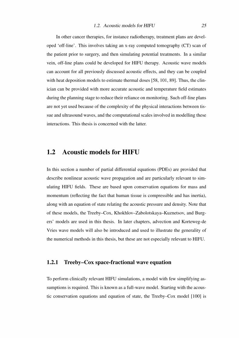
1.2.4 Burgers’ equation
Lastly, Burgers’ equation can be derived from the homogeneous, one-dimensional
Westervelt equation in the same way as the KZK equation, with the additional re-
striction that the solutions be plane-waves propagating along the z-axis [46, pp. 56–
57]. The result of this process is
∂ p∂ z− δ
2c30
∂ 2 p∂τ2 =
β pρ0c3
0
∂ p∂τ
.
Burgers’ equation is the simplest model of wave propagation which includes non-
linear effects and acoustic absorption. Its simplicity makes it useful as a model
problem for testing numerical methods, but limits its applications. For test prob-
lems, a non-dimensional form of this equation is usually used. Letting
t =zc0, x =
ρ0c20
βτ, ε =−ρ0c0
2β 2 δ , u = p,
yields∂u∂ t
= ε∂ 2u∂x2 +u
∂u∂x
.
2The only difference between this and the KZK equation is the use of a full Laplacian, whichis usually simplified by assuming slow variation in pressure along the main propagation axis z, i.e.∂ 2 p∂ z2 ∂ 2 p
∂x2 ,∂ 2 p∂y2 . This slow variation is due to the retarded time-frame.

1.3. Numerical methods 29
Table 1.1: Realistic domain sizes for HIFU therapy simulations (partially replicated from[59]).
Domain size (cm3) Maximum frequency (MHz) Domain size (wavelengths)10×10×10 5 6673
10 13333
20 26673
50 66673
20×20×20 5 13333
10 26673
20 53333
50 133333
Here, ε is a viscosity parameter that controls the width of the wave-front when it is
maximally shocked.
1.3 Numerical methods
1.3.1 Problem scales
A key difficulty with computationally solving nonlinear ultrasound models is the
relative length scales involved. Typical HIFU transducers produce frequencies in
the range of 0.5–4 MHz, which gives a wavelength of around 0.375–3 mm in water
(and a similar wavelength in soft tissues). However, even low levels of acoustic non-
linearity requires models that capture around 10 harmonics [114] and high levels of
nonlinearity requires models to capture around 600 harmonics [60]. The resultant
wavelengths are very small when compared with anatomical structures, leading to
domain sizes on the order of hundreds to thousands of wavelengths for the highest
frequency components (see Table 1.1). In addition, the large propagation distances
require commensurately lengthy simulation times. This presents a tremendous com-
putational burden, typically requiring the use of supercomputing resources [59] and
sometimes making problems intractable.
To minimise computational expense, careful consideration must be given to
the acoustic model that is solved, and to the numerical method that is applied. For
example, a common task is to characterise the acoustic field emitted by a HIFU
transducer in a homogeneous medium. In particular, the focal amplitude and fre-

30 Chapter 1. Introduction
quency spectrum are of interest. The KZK equation is well-suited to this task as the
characterisation conditions match the assumptions of the model, namely that the
propagation be one-way and that accuracy in the near field is not required. It is also
highly computationally efficient, as only two spatial dimensions need to be discre-
tised, along with a small time window surrounding the temporal waveform. Some
examples from the literature include [2, 29, 61, 115], which modelled fields emitted
by electrohydraulic lithotripters, spherical bowl arrays, and ring-arrays of trans-
ducers in homogeneous tissue and water. These solved the model equations using
Runge–Kutta, finite-difference, and angular spectrum methods. As an example of
the scale of simulations that are possible with this method, Yuldashev and Khoklova
modelled 10,000×10,000 grid points in the spatial dimensions and 500 harmonics
in time [115]. Of course, clinically realistic HIFU simulations are also desirable,
and to this end numerous three-dimensional simulations have been conducted using
full-wave models. Some examples from the literature include [78, 73, 79], which all
modelled trans-cranial HIFU therapy, and solved the model equations using finite-
difference methods. These included simulations with 600–1400 grid points per spa-
tial dimension, and required around 100 computing cores and many compute-hours.
As seen from the above examples, finite-difference methods have been a com-
mon choice for HIFU simulations. While their computational properties and subse-
quent performance for a given grid size is impressive, a key limitation they pose is
that they require very dense grids to limit the accumulation of dispersive errors over
long simulations. This limits the number of harmonics such methods can model,
given available computational resources. A largely dispersion-free alternative to
these approaches is found in spectral methods. In the next section, the Fourier pseu-
dospectral method will be presented as an efficient tool for simulating HIFU fields,
and a comparison is made with finite-difference methods.
1.3.2 Fourier pseudospectral methods
There is an extensive literature on the subject of pseudospectral methods: for refer-
ence, the reader is referred to [15]. In this thesis, the focus will be on the Fourier
pseudospectral method, as it is especially effective for ultrasound simulations (ex-

1.3. Numerical methods 31
amples include [90, 94, 100]). In this introduction, attention will be restricted to
those aspects of the method which are necessary for understanding the contribu-
tions made in this thesis.
The Fourier pseudospectral method is based on representing acoustic field vari-
ables as discrete Fourier series in the spatial coordinate, or sets of sinusoidal basis
functions. Let x be a one-dimensional spatial coordinate, uniformly sampled with
with spacing ∆x at N nodes over a periodic domain. For a function f (x), the corre-
sponding Fourier series is
f (x) =1N ∑
ka(k)eikx, eikx = cos(kx)+ isin(kx).
Here, k are a finite set of spatial wavenumbers arising from the use of discrete
Fourier transforms
k j =2π
N∆xj,
where j =
−n,−n+1, . . . ,n if N is odd,
−n,−n+1, . . . ,n−1 if N is even,
and n =
N−1
2 if N is odd,
N2 if N is even.
(1.3)
The coefficients a(k) are basis function weights, and can be computed using a fast
Fourier transform (FFT). Spatial calculus operations can then be constructed by
operating on each basis function explicitly. For instance, the first derivative is given
byd fdx
= ∑k
ika(k)eikx,
with the sum being quickly evaluated on the sampled coordinates using an inverse
FFT. In multiple dimensions, a tensor product of these series is used
f (x1,x2) = ∑k1,k2
a(k1,k2)eik1xeik2y,

32 Chapter 1. Introduction
and multidimensional calculus operators follow in the same manner.
An important consequence of using a Fourier basis for discretising the spatial
part of the solution to wave problems is that dispersion errors are eliminated. These
arise from the sound speed becoming artifically frequency-dependent as a result of
the numerical discretisation, and become increasingly severe over long simulation
times. The reason Fourier discretisations of differential operators are dispersion-
free is because they have eigenvalues which match those of the corresponding con-
tinuous operator. For instance, the eigenvalues of the derivative operator d/dx are
ik where k are the corresponding wavenumbers. The eigenvalues of a Fourier dis-
cretisation can be found by considering a matrix-vector product which is equivalent
to the summation expressions above. The eigenvalues of this matrix are ik j.
Having discretised spatial operators with a Fourier basis, all that remains to
solve the acoustic wave models previously described is an approach for approximat-
ing time-derivatives. This is typically achieved with the method of lines, which con-
siders the spatially discretised model to be a system of ordinary differential equa-
tions in the time variable. Temporal derivatives are then solved using time-stepping
formulae, which are typically derived from finite-differences. This is sometimes
referred to as time-integration. To improve the accuracy of this approach, Fourier
pseudospectral methods can be combined with k-space corrected finite-difference
time-stepping schemes [102].
To highlight the effectiveness of the Fourier pseudospectral method in solv-
ing wave problems, Fornberg [40] provides a good analysis of the difference in the
number of mesh nodes required by finite difference methods and the Fourier pseu-
dospectral method for typical levels of accuracy. There, it is shown that the memory
savings can be enormous, with a fourth-order finite-difference method requiring
four-times as many points in each spatial dimension as a Fourier pseudospectral
method, and a second-order finite-difference method requiring 16× as many. These
factors are 16× and 4096× in three-dimensions.
A significant cause of the discrepancy between Fourier and finite-difference
methods is the aforementioned dispersion error. To illustrate this, Fig. 1.3 has been

1.3. Numerical methods 33
- / x 0 / xWavenumber
- / x
0
/ x
Mul
tiplic
atio
n fa
ctor
2nd order4th order6th order20th order80th orderExact (Fourier PS)
Figure 1.3: Multiplication factor for each wave mode under differentiation based on finite-difference methods and the Fourier pseudospectral method. The imaginary uniti has been omitted from these factors.
replicated from [40]. It depicts the effect of a finite-difference discretisation of
the derivative operator on each wave mode (up to the maximum wavenumber sup-
ported by the grid). In the exact case, each mode should be multiplied by a fac-
tor that is equal to its corresponding wavenumber times the imaginary unit i. For
finite-difference methods, the multiplication factor is close to that of the true factor
for small wavenumbers, but not large ones. This error remains large even as the
accuracy of the method increases to very high orders. In contrast, the Fourier pseu-
dospectral method is dispersion-free, with the multiplication factor matching that of
the true operator exactly.
1.3.3 Convergence theorems
Aside from dispersion, the main reason Fourier pseudospectral methods produce
such efficient spatial discretisations is because of their convergence properties. Tre-
fethen [103, p. 33] summarises a number of theorems on these, which are simplified
in the following paragraphs for convenience. Let u be the true solution to the acous-
tic model equations, and v be a Fourier interpolant defined by v j = u(x j), with x j
being grid nodes separated by a distance h and k being the corresponding wavenum-
bers. The variables u(k) and v(k) are then Fourier-space representations of these
34 Chapter 1. Introduction
functions. The rate at which v converges on u depends on the differentiability and
analyticity (colloquially smoothness) properties of u.
If u is (p− 1)-times continuously differentiable, and has a p-th derivative of
bounded variation, then the error in v(k) is O(hp+1) as h→ 0. This means that model
solutions obtained using the Fourier pseudospectral method will exhibit algebraic
convergence rates as the number of grid nodes increases, with this rate depending
on the differentiability of the true model solution. If u has an infinite number of
continuous derivatives, then the error in v(k) is O(hm) as h→ 0 for every m ≥ 0.
This means that the convergence rate of a Fourier pseudospectral method will be
super-algebraic, that is, faster than any algebraic rate.
To measure smoothness beyond infinite derivatives, the concept of analytic
continuation is important. In the context of this thesis, this is where a function
that is defined on the domain x ∈ R has its definition continued into the complex
plane z ∈C. If the continued function is then complex-differentiable at a point, it is
said to be analytic at that point. The region in which a function can be analytically
continued is limited by the presence of singularities in the function, such as poles
and branch points. While all of this may seem abstract when considering a real-
valued quantity such as the spatial coordinate, such singularities are known to occur
in the vicinity of difficult-to-resolve portions of many model solutions. In Burgers’
equation, for example, branch points appear near shock fronts, with their proximity
to the real axis increasing with the severity of the shock [11, 108]. This highlights
the relevance of analytic continuation to the shock fronts that feature in HIFU fields.
Returning to convergence properties, if u is analytic and bounded within a
complex strip of finite extent η along the imaginary axis, then the error in v(k) is
O(e−π(η−ε)/h) as h→ 0 for every ε > 0. This means that the convergence rate of a
Fourier pseudospectral method will be geometric, which is faster than any algebraic
rate. Lastly, if the u can be analytically continued throughout the whole complex-
plane (meaning it is entire), and has its growth bounded such that |u(z)| = o(eaz)
for some a > 0 as |z| → ∞, then v = u provided h ≤ π/a. This means that many
entire functions can be exactly represented by Fourier interpolants, given a sufficient
1.3. Numerical methods 35
101 102
Number of mesh nodes
10-15
10-10
10-5
100
App
roxi
mat
ion
erro
r
0 20 40 60 80 100Number of mesh nodes
10-15
10-10
10-5
100
App
roxi
mat
ion
erro
r
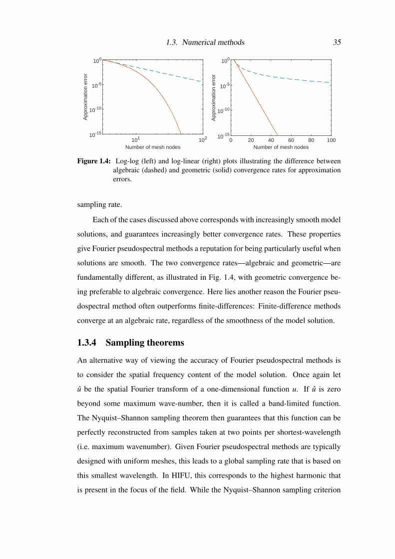
Figure 1.4: Log-log (left) and log-linear (right) plots illustrating the difference betweenalgebraic (dashed) and geometric (solid) convergence rates for approximationerrors.
sampling rate.
Each of the cases discussed above corresponds with increasingly smooth model
solutions, and guarantees increasingly better convergence rates. These properties
give Fourier pseudospectral methods a reputation for being particularly useful when
solutions are smooth. The two convergence rates—algebraic and geometric—are
fundamentally different, as illustrated in Fig. 1.4, with geometric convergence be-
ing preferable to algebraic convergence. Here lies another reason the Fourier pseu-
dospectral method often outperforms finite-differences: Finite-difference methods
converge at an algebraic rate, regardless of the smoothness of the model solution.
1.3.4 Sampling theorems
An alternative way of viewing the accuracy of Fourier pseudospectral methods is
to consider the spatial frequency content of the model solution. Once again let
u be the spatial Fourier transform of a one-dimensional function u. If u is zero
beyond some maximum wave-number, then it is called a band-limited function.
The Nyquist–Shannon sampling theorem then guarantees that this function can be
perfectly reconstructed from samples taken at two points per shortest-wavelength
(i.e. maximum wavenumber). Given Fourier pseudospectral methods are typically
designed with uniform meshes, this leads to a global sampling rate that is based on
this smallest wavelength. In HIFU, this corresponds to the highest harmonic that
is present in the focus of the field. While the Nyquist–Shannon sampling criterion

36 Chapter 1. Introduction
is typically used with uniform sampling, this is not strictly required. For many
problems of interest, spatial resolution requirements are not uniform throughout
the simulated domain. Band-limited functions with a spatially varying frequency
content can be perfectly reconstructed using non-uniform samples taken at a rate
equal to twice the local bandwidth [25].
If a function contains frequencies beyond the highest wavenumber that is sup-
ported by the spatial sampling rate, aliasing occurs. Such functions are no longer
uniquely determined by their samples, and so high-frequencies wrap back into the
supported wavenumber range [15]. This scenario is common, and might arise be-
cause a sufficiently dense sampling is computationally intractable, or because the
function is not band-limited. In such cases, aliasing is unfortunate but inevitable,
and sampling aims to ensure that the errors due to aliasing are below some accept-
able tolerance level.
1.3.5 Opportunities in HIFU modelling
The focussed nature of HIFU fields means that high-levels of nonlinearity appear
in waveforms, but it also means that these form within a very small region of the
computational domain. As Fourier pseudospectral methods typically use uniform
meshes, this means that considerable computational expense is wasted in areas
where high simulation resolutions are not required. Thus, there is an strong mo-
tivation to develop methods that include nonuniform computational meshes. In
particular, meshes which adapt to evolving solutions are of interest, since the fo-
cal location and shock severity are a-priori unknown in clinical HIFU applications
due to complex acoustic effects.
To give an example of the computational savings that are possible with nonuni-
form sampling, consider the simulations recently conducted in [89]. Here, a realistic
HIFU treatment in the kidney was simulated using a Fourier pseudospectral method.
The computational domain was uniformly discretised such that just over four har-
monics were represented. In this study, the focal volume made up just 0.0001% of
the total simulated volume. If a nonuniform grid were used that supported the same
number of harmonics in the focal region, but only the source frequency elsewhere,

1.4. Goals of the thesis 37
the number of grid nodes would reduce by 76.2%. This improvement increases as
the desired number of modelled harmonics goes up. For instance, if twice as many
harmonics are needed in the focal region (as will often be the case), then this sav-
ing rises to 88.1%. This rough estimate doesn’t even account for the fact that the
highest harmonics are only present over part of the waveform (the steep front), with
much of the waveform being much smoother. Thus, adaptive meshes which can
track these fronts can offer even greater improvements.
1.4 Goals of the thesisHIFU is a promising cancer therapy, but it is currently hindered by inadequate treat-
ment plans. To improve these, the complex interactions between HIFU wave-fields
and human tissue structures must be accounted for. This requires accurate acous-
tic modelling, but the relative difference in scale between ultrasound waves and
anatomic structures poses a computationally challenging task. The Fourier pseu-
dospectral method can overcome this challenge to some degree, but there is con-
siderable scope for further improvement. In particular, the highly localised nonlin-
earity in HIFU means there are potentially tremendous computational savings to be
had if adaptive, nonuniform meshes are used.
This thesis aims to develop the numerical methods required to perform mesh
adaptation within the Fourier pseudospectral method. The specific goals of the
thesis are thus to:
1. Develop a nonuniform mesh specification that accounts for spatially-varying
frequency content and enhances the performance of the Fourier pseudospec-
tral method.
2. Integrate this specification into a mesh adaptation algorithm and use this to
solve a range of wave models.
3. Devise a technique for accurately incorporating HIFU sources into simula-
tions in a way which does not rely on an uniform computational mesh.

38 Chapter 1. Introduction
4. Demonstrate the performance of the aforementioned algorithms through com-
parisons with widely used alternatives.
This thesis is structured as follows. In Chapter 2, background is given on
moving mesh methods which can accommodate temporally- and spatially-varying
resolution requirements. These augment the model equation with a moving mesh
PDE, which adjusts the location of mesh nodes in response to the requirements of
the model solution. In Chapter 3, this is put into practice with a one-dimensional
mesh adaptation approach based on the analyticity of the underling model solution.
This leverages one of the convergence theorems discussed in §1.3.3 which relates
the accuracy of Fourier interpolants to the locations of singularities in the analytic
continuation of the model solution. In Chapter 4, the spatial bandwidth is presented
as a more robust and more widely applicable approach to mesh adaptation. This
leverages the sampling theorems discussed in §1.3.4 which relate the accuracy of
Fourier interpolants to the range of spatial frequencies that are locally present in
the model solution. Chapter 5 then extends bandwidth-based mesh adaptation into
multiple dimensions. Finally, Chapter 6 considers the consequences of mesh adap-
tation on acoustic source representations, and counters them with a technique for
implementing source terms whose region of support does not align with the mesh.
1.5 List of publicationsThe work contained in this thesis has previously been presented in the following
publications:
• E. S. Wise, B. T. Cox, and B. E. Treeby. A monitor function for spectral
moving mesh methods applied to nonlinear acoustics. In International Sym-
posium on Nonlinear Acoustics (ISNA), 2015. Permission to reproduce this
material has been granted by AIP Conference Proceedings.
• E. S. Wise, B. T. Cox, and B. E. Treeby. Mesh density functions based on
local bandwidth applied to moving mesh methods. Communications in Com-
putational Physics, 22(5):1286–1308, 2017.

1.5. List of publications 39
• E. S. Wise, J. L. B. Robertson, B. T. Cox, and B. E. Treeby. Staircase-free
acoustic sources for grid-based models of wave propagation. In IEEE In-
ternational Ultrasonics Symposium (IUS), pages 1–4, 2017. Permission to
reproduce this material has been granted by the IEEE, © 2017 IEEE.
• E. S. Wise, B. T. Cox, and B. E. Treeby. Bandwidth-based mesh adapta-
tion in multiple dimensions. Journal of Computational Physics, 371:651–
662, 2018. Permission to reproduce this material has been granted by Else-
vier under the terms of the Creative Commons Attribution License (CC BY),
https://creativecommons.org/licenses/by/4.0/.
In addition, the following publications contain work that was conducted during the
author’s studies, but which is not included in this thesis:
• B. E. Treeby, E. S. Wise, and B. T. Cox. Nonstandard Fourier pseudospectral
time domain (PSTD) schemes for partial differential equations. Communica-
tions in Computational Physics, 24(3):623–634, 2018.
• B. E. Treeby, J. Budisky, E. S. Wise, J. Jaros, and B. T. Cox. Rapid calculation
of acoustic fields from arbitrary continuous-wave sources. The Journal of the
Acoustical Society of America, 143(1):529–537, 2018.


Chapter 2
Spectral Moving Mesh Methods
In the previous chapter, HIFU was presented as an emerging cancer therapy that
holds great promise. It is already approved for treating numerous tumours [38, 39],
but poor systems for treatment planning are a roadblock to further uptake. To ad-
dress this, full-wave ultrasound models can be used. These account for the many
important physical interactions between HIFU waves and tissue, thus providing
much-needed predictions of the efficacy of a given treatment plan. To solve these
models, high-performance numerical methods are needed to accurately model the
large number of wave harmonics that can be generated in the ultrasound field’s focal
region. The Fourier pseudospectral method holds particular promise for this, but is
held back by spatial meshes which do not account for the highly localised nature of
these harmonics.
This chapter discusses an approach for generating adaptive, nonuniform spa-
tial meshes. It begins with a guide to forming Fourier pseudospectral methods
on nonuniform meshes, before providing a literature review of methods which use
static (temporally-fixed) nonuniform meshes. Moving mesh methods are then pre-
sented as a framework which allows for temporally-varying spatial mesh adaptation.
Two adaptive spectral methods are identified from the literature that hold particular
promise, as they address the convergence and sampling theorems from the previ-
ous chapter. This chapter concludes with a discussion of some of the limitations
of these methods. Note that the numerical techniques described in this chapter are
used throughout this thesis.

42 Chapter 2. Spectral Moving Mesh Methods
2.1 Calculus on transformed meshes
2.1.1 Mapped Fourier pseudospectral methods
In this subsection, calculus operators are formulated for physical meshes x which
are defined using a transformation from a computational mesh s. This is achieved
using the chain rule for differentiation. These calculus operators are expressed as-
suming a Fourier pseudospectral method will be used, but they are easily reformu-
lated for other numerical methods.
Let the physical and computational coordinates have the same domain of pe-
riodicity, and let the computational coordinate be uniformly sampled. For a scalar-
field u, spatial gradients can then be computed in two steps. First, a gradient is taken
with respect to the computational mesh, computed using the FFT via
∂u∂ s
= F−1ikFu.
Here, k is a vector-field of wavenumbers corresponding to the computational coor-
dinate s, and the Fourier differentiation property has been used. Next, derivatives
are converted into the physical domain using the chain rule. The d-dimensional
mesh Jacobian matrix is defined as
J =∂ s∂x
=
∂ s1∂x1
· · · ∂ s1∂xd
... . . . ...∂ sd∂x1
· · · ∂ sd∂xd
,
and physical gradients are then given by
∇ =∂
∂x= JT ∂
∂ s.
For example, in two-dimensions this becomes
∇ =
∂ s1∂x1
∂ s2∂x1
∂ s1∂x2
∂ s2∂x2
∂
∂ s1
∂
∂ s2
=
∂ s1∂x1
∂
∂ s1+ ∂ s2
∂x1
∂
∂ s2∂ s1∂x2
∂
∂ s1+ ∂ s2
∂x2
∂
∂ s2
=
∂
∂x1
∂
∂x2

2.1. Calculus on transformed meshes 43
More complex differential operators are similarly computed. For instance, the diver-
gence of a vector-field v is given by the Frobenius product (sum of the element-wise
products)
∇ ·v = JT :∂v∂ s
=
∂ s1∂x1
· · · ∂ sd∂x1
... . . . ...∂ s1∂xd
· · · ∂ sd∂xd
:
∂v1∂ s1
· · · ∂v1∂ sd
... . . . ...∂vd∂ s1
· · · ∂vd∂ sd
.
To compute the mesh Jacobian matrix using a Fourier pseudospectral method, the
following expression is used:
∂x∂ s
=∂
∂ s(x− s)+ I.
Here, I is the identity matrix. This approach transforms the smooth, monotonic
mesh transformation x(s) into a periodic function x− s for which Fourier pseu-
dospectral differentiation is suitable. The mesh Jacobian matrix is then computed
as the inverse
J =
(∂x∂ s
)−1
.
Strictly speaking, this approach may not guarantee monotonicity in the implied con-
tinuous mesh mapping, but in practice a well-sampled mesh transformation ensures
that this is the case. Finally, integral terms may also be expressed in the computa-
tional domain using the chain rule:
∫Ω
udx =∫
ΩC
udet(J−1)ds.
As the computational coordinate s is uniformly sampled and periodic, trapezoidal
quadrature is then appropriate.
2.1.2 The rational trigonometric pseudospectral method
In one-dimension, the rational trigonometric interpolant of [4] can be used to form
a pseudospectral method on a nonuniform mesh without applying the chain rule.
This interpolant can be defined for arbitrary sampling points, but sampling points

44 Chapter 2. Spectral Moving Mesh Methods
x j = x(s j) which are generated by a conformal map from uniform points s j are of
particular interest, as the convergence properties of standard Fourier interpolants
hold for these. Let u j be a scalar field sampled at N such nonuniform mesh nodes
x j. The rational trigonometric interpolant through u j can then be written as
r(x) =
N−1
∑j=0
(−1) j cst(
x− x j
2
)u j
N−1
∑j=0
(−1) j cst(
x− x j
2
) , cstx :=
cscx, if N is odd,
cotx, if N is even.
A differentiation matrix D(n) of order n can be applied to this interpolant as
∂ nr∂xn
∣∣∣∣xi
=N−1
∑j=0
D(n)i j u j, i = 0,1, . . . ,N−1,
with
D(1)i j =
12(−1) j−i cst
(xi− x j
2
)if i 6= j,
−N−1
∑k=0,k 6=i
D(1)ik if i = j,
D(n) =(
D(1))n
.
Alternatively, a formula for computing D(n) directly is available [4]. Note that this
approach is O(N2) as it involves matrix-vector products, whereas the chain rule
technique described previously is O(N logN) as it uses FFTs.
2.2 Spectral methods with static mesh transforma-
tionsEarly examples of one-dimensional spectral mesh adaptation typically used
parametrised functions as static mesh transformations. For instance, in [6, 43, 5, 7],
various authors used functional mesh transformations in conjunction with Cheby-
shev pseudospectral methods to solve problems in combustion, and [1] solves
simple wave problems with Chebyshev and Fourier pseudospectral methods. The
parameters in these transformations were chosen using optimisation procedures

2.3. The moving mesh method framework 45
to minimise interpolation error functionals based on the model solution and its
derivatives. In [14], a similar mapping was used with the Fourier pseudospec-
tral method and applied to shocks, fronts, and internal boundary layers, but with
parameter choices based on prior estimates of the desired resolution change (and
some trial and error). More recently, Treeby [96] used functional mesh transforma-
tions in nonlinear acoustics, with parameter choices based on the local frequency
content of a reference solution on a uniform mesh, and on the magnitude of the
solution’s derivative. All of these methods have the advantage of having robustly
defined meshes, but the use of parametrised mesh transformation functions leads to
inflexibility in their capacity to deal with complex wave-fields.
In multiple dimensions, static nonuniform meshes have mostly considered ge-
ometric issues. For example, in [41, 72] nonuniform mesh transformations are used
to provide faithful representation of boundaries in material properties, and in [34]
a nonuniform mesh was generated to represent a surface topography. These exam-
ples used Fourier and hybrid Fourier–Chebyshev pseudospectral methods to solve
elastic wave models. While material boundaries are also important in HIFU simula-
tions, nonlinearity is of much greater concern, and static meshes have little capacity
to address this as the location, extent, and severity of this nonlinearity is not known
a-priori, and may change over the course of the simulation.
2.3 The moving mesh method framework
To accommodate both spatially and temporally varying resolution requirements, the
moving mesh method framework can be used. Good reviews of these methods can
be found in [19, 56]. Moving mesh methods dynamically adapt mesh node positions
throughout a simulation in a solution-dependent manner. This is sometimes called
r-refinement, with ‘r’ referring to the node positions. Mesh node trajectories (i.e.,
the movement of mesh node positions over time) are controlled using a moving
mesh PDE. This is coupled to the model PDE and the resulting system is solved
numerically. Monitor functions are used to link the model solution to the mesh,
and hence guide mesh adaptation. These components are broadly described in the

46 Chapter 2. Spectral Moving Mesh Methods
following sections, and more detail follows in the remaining chapters of this thesis
as it is required.
2.3.1 Monitor functions, equidistribution, and alignment
A monitor function monitors the model solution to determine where mesh nodes
should be placed. In one-dimension, it is a positive-valued scalar-field usually de-
noted by ρ that specifies the local density of mesh nodes, and is thus often re-
ferred to as a mesh density function. In multiple dimensions, monitor functions are
positive-definite matrix-valued fields denoted by M which specify the density and
orientation of the mesh. This can be understood by considering their eigendecom-
position: If λ is an eigenvalue of M and v is the corresponding eigenvector, then
the specified mesh will be compressed in the direction v when λ first increases then
decreases in this direction, and expanded when the change is reversed [23].
Given a monitor function M, a mesh is considered to be M-uniform when
equidistribution and alignment conditions are satisfied. Recalling that J is the mesh
Jacobian, these are [51, 53]
det(J)−1 det(M)12 =
σ
|ΩC|, (equidistribution)
1d
tr(JM−1JT ) = det(JM−1JT )1d , (alignment)
for all x ∈Ω where
σ =∫
Ω
det(M)12 dx.
Here, Ω is the physical domain, |ΩC| is the volume of the computational domain
ΩC, and d is the number of dimensions. The equidistribution condition states that
the product of the eigenvalues of the mesh Jacobian should be equal in the metric
M and uniform over the domain. In multiple dimensions, this ensures that mesh
element volumes are equal in this metric. In one dimension, this ensures that the
mesh nodes are uniformly spaced in this metric. The alignment condition states
that the arithmetic (sum) mean of the eigenvalues of the mesh Jacobian should be
equal to the geometric (product) mean in the metric M. In multiple dimensions, this
ensures that mesh elements are equilateral in this metric. It has no meaning in one

2.3. The moving mesh method framework 47
dimension. Together, the equidistribution and alignment conditions fully specify
the mesh transformation.
Moving mesh methods have largely evolved in the context of finite-difference
and finite-element methods. These typically use local, low-order polynomials as
basis functions, hence local error metrics can be defined using error bounds for
low-order polynomial interpolants. Mesh density functions and monitor functions
have reflected this. For instance, Huang and Russell [56, §2.4, §5.2] derive mesh
density functions and monitor functions based on polynomial interpolation error
bounds. These are shown to be optimal for particular orders of interpolant, and
under particular norms. However, in practice they appear to be little used, and
are generally simplified into two more common forms. For one-dimensional mesh
density functions, these are the based on the arclength and curvature of the model
solution
ρ =
√1+∣∣∣∣∂u∂x
∣∣∣∣2, ρ =
(1+∣∣∣∣∂ 2u∂x2
∣∣∣∣)14
. (2.1)
In higher dimensions, similar monitor functions are given by
M = I+∇u(∇u)T , M = I+ |H|,
where |H| is the absolute value of the Hessian of the model solution u. By
comparing these with their respective optimal forms in [56], it can be seen that
gradient-based mesh adaptation can be motivated by numerical methods which
use piecewise-constant interpolants, and curvature-based mesh adaptation by those
that use piecewise-linear interpolants. As an example, Fig. 2.1 depicts the ar-
clength and curvature mesh density functions that correspond to a Gaussian function
u = exp(−x2). Peaks in the arclength mesh density function occur where ∂u/∂x is
highest, and peaks in the curvature mesh density function occur where ∂ 2u/∂x2 is
highest. Note that arclength- and curvature-based meshes will be used throughout
this thesis as benchmarks.

48 Chapter 2. Spectral Moving Mesh Methods
-4 -3 -2 -1 0 1 2 3 4Position
0
0.2
0.4
0.6
0.8
1O
rigin
al fu
nctio
n
1
1.05
1.1
1.15
1.2
1.25
1.3
1.35
1.4
Mes
h de
nsity
func
tion
GaussianArclengthCurvature
Figure 2.1: A Gaussian function and the corresponding arclength and curvature mesh den-sity functions (2.1).
2.3.2 Moving Mesh PDEs
In practice, it is difficult to find a mesh which perfectly satisfies the equidistribution
and alignment conditions for a given monitor function. It is instead typical for
meshes to be generated such that they minimise a functional I that consists of some
combination of equidistribution and alignment. For instance [50, 53] propose
I[s] =∫
Ω
√det(M)
(tr(JM−1JT)) d p
2 dx
+(1−2θ)dd p2
∫Ω
√det(M)
(det(J)√det(M)
)p
dx,
where θ ∈ (0,1) controls the balance between equidistribution and alignment, and
p > 0 is a parameter that can help ensure the functional has a well-behaved mini-
mum.
To find the minima of a mesh functional, a Moving Mesh PDE (MMPDE) can
be used. For a functional of the form
I[s] =∫
Ω
G(J,det(J),M,x)dx,

2.3. The moving mesh method framework 49
a MMPDE can be derived [52] by taking the functional derivative (Euler–Lagrange
equation)δ Iδ s
=−∇ ·(
∂G∂J
+∂G
∂ det(J)det(J)J−1
),
and then forming a gradient flow equation
x =Pτ
J−1 δ Iδ s
.
Here, an overset dot indicates a time-derivative in the computational coordinate’s
frame of reference, P is a ‘balancing’ function which acts to regularise the mesh
and τ is a relaxation time that controls the rate of mesh movement (this should
match the time-scale over which the model’s features evolve). While effective in
practice, this approach is clearly quite complex.
An alternative MMPDE is the parabolic Monge–Ampere (PMA) equation [21],
which has previously been applied to mesh generation for meteorological applica-
tions [18, 17, 109].1 It is given by
x =1τ
∂
∂ s
(det(M)det(J−1)
θ
)1/d
, θ =∫
Ω
det(M)dx. (2.2)
The PMA equation converges on a mesh that meets the equidistribution condition
exactly, while minimising a functional I[x] measuring the overall amount of adap-
tation
I[x] =∫
ΩC
‖x(s)− s‖2 ds.
This functional arises in optimal transport problems and, in attempting to minimise
the net amount of adaptation, produces a fast-converging MMPDE. It is notable that
the PMA equation ignores directional information in the monitor function, since it
takes the monitor function’s determinant. This might lead one to think that it would
produce isotropic meshes only. However, it has been shown that this is not the case,
1The PMA equation is usually expressed in terms of a potential function whose gradient gives themesh transformation. In the present work, it is expressed in terms of the mesh coordinate directlyfor consistency with the standard MMPDE form. Additionally, the Laplacian smoothing operatorthat is usually included in the PMA equation has been discarded in favour of alternative smoothingtechniques that are discussed in later chapters of this thesis.

50 Chapter 2. Spectral Moving Mesh Methods
and that the mesh anisotropy produced by the PMA equation aligns with that of
features in the model solution to which it’s applied [20]. This is because changes in
the specified mesh node density align with features in the model solution. Indeed, it
is likely that the alignment specified by a well-chosen monitor function will match
the alignment of solution features, making this information somewhat redundant.
In one-dimension, the PMA equation reduces to the widely used MMPDE5 of
[55]
x = τ−1 ∂
∂ s
(ρ
∂x∂ s
),
where ρ is a mesh density function. Note that the scaling factor θ has been dropped
in this formulation, but that this has no effect on generated meshes, whose density
is proportional to that specified (the mesh speed parameter may need adjustment in
response).
2.3.3 Mesh/model coupling and solution procedure
The model and mesh equations can be coupled using two approaches. The first is
rezoning. After each time-step that is taken with the model equations, the monitor
function is computed and the MMPDE is integrated until it converges on a minima
of the meshing functional. The model is then interpolated onto this new mesh and
another time-step is taken. Thus, the mesh appears to be static from the perspective
of the model between time-steps.
The second option is the quasi-Lagrange approach, in which the mesh moves
continuously in time. The model and mesh equations are then solved simultane-
ously by expressing the model’s temporal derivative in the computational coordi-
nate’s frame of reference using the following relationship [56, p. 142]:
∂u∂ t
= u−∇u · x. (2.3)
This can be rearranged to yield u, and solved simultaneously with the mesh equation
for x given by the MMPDE. The quasi-Lagrange approach has the disadvantage of
coupling the two PDE’s time-stepping stability criteria together. This means that
unnecessarily small time steps may be required for solving the model PDE, since the

2.3. The moving mesh method framework 51
MMPDE’s stability tends to be more restrictive. However, it has the advantage of
avoiding computationally expensive interpolation steps (though increased stiffness
may outweigh this), is simple to implement, and limits the lag between changes in
the model solution and the resulting mesh movement, helping with accuracy.
To perform time-stepping of the model and mesh equations, explicit Runge–
Kutta methods can be used. They solve problems of the form
y = f (t,y), y(t0) = y0.
For the method of lines, y will be a vector of solution samples, y is the corresponding
temporal derivative, and f will capture the already-discretised spatial portion of
the problem’s equations. Thus, the model/mesh problem is posed as a system of
dependent ODEs, one for each solution sample. Runge–Kutta methods compute
the value of y(tn+1) at the next time step by summing the present value y(tn) and
a weighted average of a number of increments towards the next time, where each
increment is a product of the size of the time step and an estimated slope of the
function at the increment’s time. As a formula, this is expressed as
y(tn+1)≈ y(tn)+∆ts
∑i=1
biki, (2.4a)
ki = f
(tn + ci∆t,yn +∆t
i−1
∑j=1
ai jk j
). (2.4b)
Here, s is the number of stages in the method, which plays a role in determining the
order of accuracy of the method, and a,b,c are coefficients which vary depending on
the precise method used. The error involved in taking a time step can be controlled
using an adaptive formulation of this method. Here, two Runge–Kutta formulae are
used, one with order of accuracy O(∆t p) and one with order of accuracy O(∆t p−1).
The error between y(tn+1) computed by each of these methods is found, and the
time step reduced until a given error threshold is reached. This is extremely useful
for moving mesh methods, where the movement of mesh nodes alters the size of the
time step which can be taken for a given level of accuracy.

52 Chapter 2. Spectral Moving Mesh Methods
Another way of increasing the size of time-steps is to adjust the stability region
of the method. The number of stages in the method has some effect on this, but
the difference between an explicit and implicit method is far more significant. An
implicit method is formed by changing (2.4b) to
ki = f
(tn + ci∆t,yn +∆t
s
∑j=1
ai jk j
)(2.4c)
In (2.4c), the sum for ki goes from j = 1 to s, rather than stopping at i− 1 as it
does for the explicit formulation (2.4b). This means that each increment ki can
be computed from previously computed increments alone with an explicit method,
whereas an implicit method requires the increments to be computed together as a
system of algebraic equations. This increases computational costs significantly. The
benefit that is gained from implicit formulations is that stability criteria are relaxed,
allowing for larger time steps to be taken.
2.4 Derivative-based mesh adaptationThe use of moving mesh methods has largely been in the context of finite-difference
and finite-element methods. However, there have been a number of multidimen-
sional spectral moving mesh methods developed. Examples of Chebyshev-type
methods include [68], which solved boundary-value problems, and [91], which
solved boundary value problems described by a multi-phase or multi-component
fluid model.2 Note that [68] deviated from the approach laid out in §2.3 by gen-
erating a rough initial solution and corresponding mesh using a finite-difference
moving mesh method, and then re-solving the problem with the same mesh but a
pseudospectral method. They found that errors improved by around four orders of
magnitude relative to a finite-difference moving mesh method at the same resolu-
tion. Tapia and Lopez [91] do not make an explicit comparison with other numer-
ical methods, but find qualitatively good performance for very narrow transition
regions in their model solution. An example of a Fourier-type method is found
2These used the moving mesh method framework as a way of iteratively improving the mesh, asthe model equation was not time-dependent.

2.5. Smoothness-based mesh adaptation 53
in [37, 36], which solved material microstructure evolution problems described by
the Allen–Cahn and Cahn–Hilliard equations. The authors found that, for a similar
level of accuracy, mesh adaptation reduced compute times by a factor of 18–20.
They also estimated that the number of grid nodes needed to decrease by a factor
of 3–4 in each dimension for overall compute times to reduce, as mesh adaptation
brings significantly increased computational costs for a given number of grid nodes.
Lastly, a Chebyshev–Legendre Galerkin-type method is presented in [85], and ap-
plied to two-phase flow problems modelled by the Navier–Stokes equations. They
also found that mesh adaptation allowed the number of grid nodes to be reduced by
a factor of around 3–4 in each dimension for a given level of accuracy.
All of the spectral moving mesh methods described in the previous paragraph
chose to adapt meshes such that nodes clustered around regions of the solution ex-
hibiting steep gradients. As the problems they solved all featured rapid transitions
in solution values over short spatial lengths, it is unsurprising that gradient-based
mesh adaptation was effective. However, many problems include features for which
gradient-based adaptation is not an obvious choice. Also, as discussed previously,
derivative-based monitor functions like these arise from error bounds for low-order
polynomial interpolants, and thus are not theoretically justified in the context of
spectral methods. It is likely then that more optimal monitor functions can be de-
rived through explicit consideration of the properties of spectral methods. In the
next section, a review is given of two adaptive mesh methods which are especially
tailored to pseudospectral methods. These address the convergence and sampling
theorems that were previously discussed in §1.3.3 and §1.3.4 for the Fourier pseu-
dospectral method.
2.5 Smoothness-based mesh adaptation
2.5.1 Analyticity-based mesh adaptation
In §1.3.3, the convergence rate of Fourier pseudospectral interpolants was related to
the analyticity of the approximated function’s continuation into the complex plane.
This idea has been exploited by Tee et al. [93, 92, 45, 44] in one-dimensional adap-

54 Chapter 2. Spectral Moving Mesh Methods
tive Fourier and Chebyshev pseudospectral methods, with the former focussed on
in this thesis. Their approach will be referred to as the Adaptive Rational Spectral
(ARS) method in this thesis, and it is described briefly here and in greater detail in
Chapter 3. First, Pade (or sometimes Fourier-Pade) approximants are constructed
based on the simulated model solution, in order to perform an analytic continuation.
These approximants contain poles, whose location gives an accurate estimate of the
true locations of singularities in the analytic continuation of the model solution.
Second, a Schwarz–Christoffel conformal map g−1 is constructed that moves these
poles around the complex plane. This mapping is symmetric about the real-axis,
and aims to move the poles onto the edges of a strip running parallel to the real axis.
In doing so, far-out singularities move towards the real-axis and nearby singularities
move outwards. As convergence depends on the distance to the nearest singularity,
the overall effect of the conformal mapping is to improve the rate of convergence.
This conformal mapping is then applied to an equisampled s coordinate to gener-
ate nonuniform coordinates x = g(s). Third, the solution is interpolated onto this
mesh at each time-step, making this a rezoning-style adaptive mesh method (though
without the use of a MMPDE). Note that this method uses the rational trigonometric
interpolant described in §2.1.2, but the techniques on which it is based are valid for
the mapped methods based on traditional Fourier interpolants described in §2.1.1.
Tee et al. apply the ARS method to a variety of problems encompassing numer-
ous model equations, demonstrating its effectiveness over a wide range of solution
features [93, 92, 45, 44]. It is also shown to produce extremely fast convergence
rates when compared with standard static spectral methods, with an adaptive finite
difference method [69], and with an adaptive Chebyshev spectral method [8]. How-
ever, while addressing the error properties of Fourier interpolants in a remarkably
elegant way, the ARS method also has a number of shortcomings. A number are
specific to Tee et al.’s implementation. For instance, they fix the number of sin-
gularities they search for after the first time-step, meaning the appearance of new
singularities is not accounted for, nor is their disappearance [92]. They also only use
first-order poles in the analytic continuation, meaning other singularities are inac-

2.5. Smoothness-based mesh adaptation 55
curately located [92]. Finally, the method fails when multiple wave-fronts interact
[92, 44] because the Schwarz–Christoffel mesh mapping isn’t defined when the real
part of each wave-front’s associated singularities coincide. More general shortcom-
ings include the fact that the ARS method relies on model solutions being analyt-
ically continuable and having singularities (or at least near-singular behaviour) in
that continuation, and that it doesn’t readily extend into multiple dimensions, as
the Pade approximants and Schwarz–Christoffel mappings on which it relies are
inherently one-dimensional.
2.5.2 Frequency-based mesh adaptation
In §1.3.4, the sampling rates for Fourier interpolants were related to the local fre-
quency content of the model solution. A mesh adaptation approach that addresses
this has been presented by Subich [88] and applied with success to one-dimensional
problems. It was based on the Chebyshev pseudospectral method, and used a high-
pass filter to find regions with large high-frequency solution components. An en-
velope of these components was then used as a mesh density function, and mesh
adaptation was performed with a MMPDE and quasi-Lagrange coupling.
Subich’s method has a number of advantages over the analyticity-based ARS
method. First, it is more widely applicable in the sense that it does not rely on
the solution being analytically continuable. Second, it is more robust in that solu-
tion features are free to appear, merge, and disappear as the simulation progresses.
Third, it extends easily into multiple dimensions, as frequency-filters and envelop-
ing are both applicable beyond one-dimension. However, there are a number of
issues with this method as well. First is a missing link between computing an enve-
lope of high-frequency solution components and generating a mesh whose density
is proportional to this. Second is that the method makes use of the properties of
the model equation when choosing a frequency threshold for the high-pass filter,
limiting its general applicability. Third, by using a threshold at all, this method in-
herently categorises the solution into low- and high-frequency parts, meaning some
low-frequency parts will still be oversampled. Nonetheless, using the local fre-
quency content of a model solution to form a mesh density function is an intuitive

56 Chapter 2. Spectral Moving Mesh Methods
and general approach that has remained largely unexplored.
2.6 ConclusionIn this chapter, moving mesh methods have been proposed as an elegant way of
implementing spatial mesh adaptation in Fourier pseudospectral methods. A review
of past spectral moving mesh methods was given, and it was concluded that they all
used monitor functions in their mesh specifications borrowed from finite-difference
and finite-element moving mesh methods. It is thus likely that more optimal monitor
functions can be derived by explicitly considering the properties of spectral meth-
ods. Two such alternatives were then discussed. The first based adaptive meshes on
the analyticity of the underlying model solution. The second based them on the lo-
cal frequency content of that solution. In both cases, the error properties of Fourier
pseudospectral methods were explicitly addressed. However, both methods also
have a number of significant shortcomings, largely based around their inability to
efficiently and robustly solve problems with complex, evolving, interacting features,
such as the nonlinear waveforms that propagate through heterogeneous tissue struc-
tures during HIFU treatments. These shortcomings are addressed in the remainder
of this thesis, with the next chapter dedicated to investigating and improving the
robustness of the analyticity-based ARS method for mesh adaptation.

Chapter 3
Analyticity-based mesh adaptation in
one dimension
In the last chapter, two strategies were identified for specifying adaptive, nonuni-
form meshes for use with the Fourier pseudospectral method. One of these was
analyticity-based adaptation. This addressed one of the convergence theorems in
§1.3.3, which showed that the error in Fourier pseudospectral methods can be re-
lated to the presence of singularities in the analytic continuation of the model solu-
tion (for certain classes of solution). Specifically, the rate of convergence depends
on the distance from the real-axis to the nearest singularity in the analytic contin-
uation, that is, its widest analytic strip. Tee et al.’s analyticity-based ARS method
addressed this by finding singularities in the analytic continuation of the model so-
lution, and then forming a conformal map which brings them all equidistant to the
real axis. The distance from the real axis to these singularities will be greater than
that of the original function, thus the ‘mapped’ function’s convergence rate will be
faster than that of the ‘unmapped’ function. The conformal map can finally be used
to generate an equivalent nonuniform mesh on which the model can be discretised.
There are many limitations to analyticity-based mesh adaptation, as imple-
mented in the ARS method. These include its capacity to represent and accurately
locate singularities which aren’t simple poles and to adaptively adjust the number
of poles throughout a simulation. In this chapter, an analyticity-based moving mesh
method is presented that remedies these limitations. It is shown to perform well

58 Chapter 3. Analyticity-based mesh adaptation in one dimension
when compared with alternative mesh specifications, and across a number of wave
problems. Its application to the Treeby–Cox wave equation is also examined, to
demonstrate its potential for full-wave HIFU simulations.
This chapter is structured as follows. First, methods for analytic continuation
are discussed, and the singularity-mapping process is reformulated so as to be com-
patible with a traditional moving mesh method framework. These developments
ensure that the method can be more reliably applied across different problem types,
and facilitate the method’s future extension into multiple dimensions. Following
this, the method is applied to shock front problems described by the Burgers’ and
Treeby–Cox wave equations. Finally, some opportunities are identified for solving
those limitations in the method which remain.
3.1 Derivation of mesh density function
To incorporate the ARS method’s analyticity-based approach into a moving mesh
method, a mesh density function must be derived. This derivation has two parts.
First, techniques for analytic continuation are discussed and the ARS method is
updated to account for more recent work in this field. This allows the approximate
localisation of singularities in the model solution. Second, the Schwarz–Christoffel
mapping is described and updated to permit more flexible singularity structures.
This is then formed into an equivalent mesh density function.
3.1.1 Singularity localisation
3.1.1.1 Pade and Fourier–Pade approximants
Consider a Fourier pseudospectral approximation to a model solution u. To analyt-
ically continue the model solution from the real line to the complex plane, it is not
sufficient to simply replace a real-valued coordinate x with a complex coordinate z,
as the accuracy of Fourier interpolants rapidly degrades beyond the nearest singu-
larity as z→±i∞. Pade approximants provide a way of addressing this since, with
some caveats, they converge on the analytic continuation throughout a wide region
3.1. Derivation of mesh density function 59
of complex plane.1 Let n,m ∈Z. To find a Pade approximant for a function u that is
accurate around the origin (translations follow trivially), first define a power series
approximant u
u(z) =n+m
∑j=0
c jz j = u(z)+O(zm+n+1), c j =1j!
∂ ju∂x j
∣∣∣∣x=0
.
A classical (linear) type (m,n) Pade approximant is then formed from two new
power series, p and q of order m and n, respectively
p(z) =m
∑j=0
a jz j, q(z) =n
∑j=0
b jz j.
These are chosen to form a linear system with u, such that
q(z)u(z)− p(z) = 0.
The coefficients of p and q can be found by matching the various powers of z in this
expression, as outlined in [92]. Finally, the Pade approximant is defined as
r(z) =p(z)q(z)
,
and it can be seen that r(z) is equal to the power series u(z). Singularities in the
underlying function are represented by poles in the Pade approximant, and can be
located by computing the roots of q(z).
Pade approximants provide a useful way of finding poles which are near the
point about which they are defined, but global mesh adaptation requires a way of
finding poles which arise throughout the entire complex domain. One way of doing
so is to use a Fourier–Pade approximant. Consider a Fourier series approximation
to a function u defined on the periodic domain x ∈ [−π,π). Unlike a Taylor series,
this approximant aims to provide accuracy over the whole real line, rather than
just around a single point. Denoting Fourier coefficients by ck and c−k and letting k
1See [104, pp. 204–205] for a summary of theorems regarding the convergence of Pade approxi-mants.

60 Chapter 3. Analyticity-based mesh adaptation in one dimension
denote wavenumbers (these are integer-valued for the given domain size), this series
can be expressed in a split, exponential form as
u(x) =m+n
∑′
k=0ckeikx +
m+n
∑′
k=0c−ke−ikx,
with the prime indicating the k = 0 terms should be halved (so the DC component
is spread over both series). This is a Laurent series (or two power series) about the
origin under the coordinate transformations z± = e±ix, yielding
u(z±) =m+n
∑′
k=0ckzk
++m+n
∑′
k=0c−kzk
−.
These transformations map the real line onto the unit circle. A type (m,n) Fourier–
Pade approximant is then defined as a sum of type (m,n) Pade approximants to each
of these power series
r(x) =p1(z+)q1(z+)
+p2(z−)q2(z−)
.
The inverse coordinate transformation x =∓i lnz± can be used to convert the poles
of each Pade approximant (zeroes of q1 and q2) into the poles of the Fourier–Pade
approximant.
In practice, the ARS method uses Pade and Fourier–Pade approximants as fol-
lows. Before mesh adaptation begins, a Fourier–Pade approximant is used to find
poles over the whole computational domain. The mesh can then be adapted to these
poles. After this, finding Fourier coefficients becomes problematic because samples
are no longer uniform. Hence, Fourier–Pade approximants cannot be formed, and
so regular Pade approximants are used instead. A collection of these are defined
about each point on the real-axis where a pole was last found, thus locally tracking
them. Each local Pade approximant is of order (3,2), reflecting two things. First,
the denominator order is chosen because the model solutions the original authors
were interested in typically contain conjugate pairs of singularities. This denom-
inator order thus ensures that the ARS method seeks only to track a single pair
of previously found poles, and not find new ones. Second, the numerator order is

3.1. Derivation of mesh density function 61
likely chosen to be low because of difficulties that arise when computing high-order
power series coefficients (rounding errors limit the number of derivatives that can
be accurately computed [13]).
A key restriction of the ARS method is that the order (and hence number of
poles) of the Fourier–Pade approximant is fixed, and no extra poles are subsequently
sought with the collections of regular Pade approximants. This limits applicability
to problems where the number of singularities the solution possesses is known a-
priori.
3.1.1.2 Robust Fourier–Pade approximants
More recent work on Pade approximants has provided a way of adaptively choosing
the number of poles. In [105], Trefethen et al. describe an algorithm that adaptively
chooses the order of the numerator and denominator polynomials based on an es-
timated relative error in the power series coefficients to which they are fit. The
algorithm’s inputs are a starting order for the Pade approximant and a set of power
series coefficients for the function that is being approximated. The algorithm works
as follows. First, a linear system of equations for the Pade approximant coeffi-
cients is formed. The singular values of this system are computed and compared
with the estimated relative error in the function’s power series coefficients. If any
are below this, the order of the Pade approximant is reduced appropriately and the
problem is reformed and solved. The overall effect of this algorithm is to remove
spurious poles, which are poles whose effect on the approximant is cancelled out by
nearby zeroes. These poles do not exist in the approximated function’s true continu-
ation, and they have previously plagued Pade approximants [87]. An adaptive-order
Fourier–Pade approximation can be produced similarly from a set of Fourier coeffi-
cients, using the usual transformation from the real line to the complex unit circle.
3.1.1.3 Robust Fourier-rational interpolants
To avoid computing Fourier coefficients, rational interpolants can be used in place
of Pade approximants. Like Pade approximants, rational interpolants are also
formed as a ratio of two power series of specified orders, only this time these are
chosen so that q(zk)u(zk)+ p(zk) = 0 where zk are a set of sampling points. Many

62 Chapter 3. Analyticity-based mesh adaptation in one dimension
of the theorems regarding the large regions of the complex plane in which Pade
approximants converge have analogues for rational interpolants [104, p. 205]. Like
the Pade case, rational interpolant coefficients can be computed by solving a linear
system of equations. One slight difference is that, if the number of function sam-
ples exceeds the order of accuracy of the rational interpolant, then the linear system
is solved as a least squares minimisation. A Fourier rational interpolant can also
be formed in the same way as a Fourier–Pade approximant, by transforming the
domain from the real line to the complex unit circle.
While adaptivity removes the need to specify the desired number of poles in
advance, it still fixes the number of poles for the rest of the simulation, as low-order
ordinary Pade approximants must be used once mesh adaptation begins. One way
of avoiding this is to use the adaptive Fourier-rational interpolation algorithm of
[75] which allows for nonuniform meshes. However, attempts at using this proved
unstable. A more recent implementation of this algorithm is found in [42], but
this is defined for equispaced samples, and so solutions must be interpolated onto a
dense set of equispaced points, requiring considerable computational expense. This
version of the algorithm was used to generate the results in this chapter, and it is
acknowledged that this is a significant weakness of the presented method. However,
since this work was completed in 2015, a number of advances have been made that
allow the use of arbitrary sampling points. These are discussed in §3.4.
3.1.1.4 Considerations for branch points
The analytic continuation algorithms described above all represent singularities as
poles of varying orders. Many models exhibit such poles in their analytic continu-
ations, but it is also common for them to exhibit branch points. For these, adaptive
Pade and rational interpolation algorithms will produce strings of poles which con-
verge on the corresponding branch cuts as the order of the approximant increases
[86]. However, none of these poles are guaranteed to land on the branch points
themselves, and this representation necessarily monopolises many of the degrees of
freedom in the Pade approximant.
If branch points are logarithmic, a better way of locating them is to analytically
3.1. Derivation of mesh density function 63
continue the function’s derivative, rather than the function itself. This converts a
logarithmic branch point into a pole which is more easily located. If the logarithmic
branch point is not in the function itself but instead in its n-th derivative, then the
function will need to be differentiated n+1 times to perform this conversion. This
technique has been demonstrated by Driscoll and Fornberg [31] for use in reducing
the Gibbs phenomenon which arises from logarithmic branch points.
3.1.2 A mesh density function based on a Schwarz–Christoffel
mapping
3.1.2.1 The Schwarz–Christoffel mapping
Having found singularities in the analytic continuation of the model solution, a con-
formal map must be formed to move these to better locations in the complex plane.
This is computed using the Schwarz–Christoffel mappings described in [92, 45, 44].
To understand the Schwarz–Christoffel mapping process, it is not necessary to un-
derstand the derivation of the relevant map, but it is helpful to understand its action.
Figure 3.1 shows a diagram illustrating the effect of an example mapping. Starting
with the diagram on the right, a pair of slits is placed starting at each approximated
pole in the analytic continuation and extending to ±i∞. A conformal mapping g is
then defined that transforms the edges of an infinite strip (left diagram) onto these
slits. This squeezes the analytic region that is beyond the closest singularity (and
between the slits) into a single strip. The result is that the distance from the real
line to the nearest singularity is widened, i.e. η > ε2. Thus, any computations per-
formed in the computational domain (left diagram) will converge faster than those
performed in the physical domain (right diagram). Finally, a nonuniform mesh is
defined by equi-sampling the real line in the computational domain (left diagram),
and transforming these points via the mapping into the physical domain (right dia-
gram).
Figure 3.2 illustrates the improvement that the Schwarz–Christoffel mapping
process gives in terms of the smoothness of the model solution. The left plots show
a solution to Burgers’ equation, depicted in the physical coordinate x. The top part

64 Chapter 3. Analyticity-based mesh adaptation in one dimension
f, x
−π π
ε1
ε2
ε3
−ε1
−ε2
−ε3
f g, s
η
−η
−π π
x = g(s)
Figure 3.1: Illustration of the Schwarz–Christoffel mapping process (after [44, Fig. 4.5]).A map g is formed from an infinite strip of width η to a series of slits extend-ing from the poles of the model’s solution (whose imaginary components are±ε1,±ε2,±ε3) to ±i∞. A set of equispaced nodes in the s domain can thenbe used to find non-uniform nodes in the x domain. This process squeezes theanalyticity of f that would otherwise be lost in forming a spectral method (any-thing beyond the strip formed by ε2 in this case) into the widest analytic stripof f g.
shows the solution on the real-axis, and the bottom part shows an approximated
analytic continuation. A series of poles is evident and marked with a single red line
indicating a slit out to ±i∞. The strip of analyticity is indicated with a dashed line.
The right plot shows the same solution in the computational coordinate. The poles
in the approximated analytic continuation have been mapped onto the edges of a
strip whose width is much greater than the strip in the physical coordinate. As a
result, the model solution (top part) is smoother in this coordinate.
3.1.2.2 Pole-filtering
The robust analytic continuation algorithms described above will often represent
each singularity with multiple poles. This causes a problem when defining the mesh
transformation, as the Schwarz–Christoffel mappings described in [92, 45, 44] are
only defined for collections of poles with unique real-parts. This is easily dealt with
using a filtering approach. Poles are grouped if the real parts of their locations are
within a specified distance of one another, and only the pole nearest the real axis
in each group is kept. In this thesis, the distance is 10−3 times the simulated do-
main size, a choice which was empirically found to ensure the Schwarz–Christoffel

3.1. Derivation of mesh density function 65
Figure 3.2: (Left) A solution u to Burgers’ equation for a sinusoidal initial condition anda numerical analytic continuation of this solution beyond the real line. A stringof poles can be seen at the shock front along the branch cut, indicated by thesolid line. The widest analytic strip of u is the region between the dashedlines. (Right) The composition of u with a conformal map g generated fromthe approximate poles of u, along with its analytic continuation beyond the realline. The poles of ug now appear on the edges of a single strip, indicated witha solid line, whose width has increased by a factor of approximately 4.02×.
mapping could be numerically computed.
3.1.2.3 Conversion to a mesh density function
To incorporate the Schwarz–Christoffel mapping described above into a one-
dimensional moving mesh method, an equivalent mesh density function must be
defined. Up to a scaling factor, this is given by the reciprocal of the mesh mapping
function’s derivative
ρ =1
g′(s),
where g is the mesh transformation discussed above. By construction, the Schwarz–
Christoffel mapping’s derivative is strictly positive on the real line, ensuring that
the mesh density function will also be strictly positive. This is a requirement for a
one-dimensional mesh density function because it ensures that there exists a unique
equidistributing mesh [56, p. 28]. In the remainder of this chapter, this mesh density
function will be referred to as the spectral mesh density function. Later chapters will
refer to it as the analyticity mesh density function, as they present alternative mesh

66 Chapter 3. Analyticity-based mesh adaptation in one dimension
density functions for spectral methods.
3.2 Numerical methodsTo summarise the discussion in the previous section, computing the spectral mesh
density function requires a number of steps:
1. Upsample the model solution onto a uniform mesh, whose sampling is equal
to that of the densest portion of the nonuniform mesh.
2. Fit a Fourier-rational interpolant to the upsampled model solution using the
robust algorithm in [42].
3. Locate the poles (in the complex plane) of this interpolant, and keep a subset
whose real parts are distinct (to a tolerance of 10−3), keeping those whose
imaginary component is smallest.
4. Generate a Schwarz–Christoffel mapping based on the pole locations using
the maps defined in [92, 45, 44].
5. Take the reciprocal of the mapping’s derivative, and sample it on the nonuni-
form mesh to give the mesh density function.
This process is computationally expensive relative to the remainder of the moving
mesh method, and so simulations were sped up by only updating the mesh density
function 100 times throughout the simulation. This seems to be sufficient to rep-
resent the speed at which the model solutions change in the problems addressed in
this chapter, and corresponds to the length of time it takes the mesh to converge,
given the chosen mesh speed parameter.
Following the ARS method, the rational trigonometric interpolant described in
§2.1.2 was used to solve all of the spatial calculus operations in the model and mesh
equations. For time-stepping, MATLAB’s ODE solver ode23tb was used. This
ODE solver uses an adaptive Runge–Kutta method with an explicit trapezoidal rule
and an implicit backward differentiation formula [48].

3.3. Numerical experiments 67
3.3 Numerical experimentsThis section examines the performance of the spectral mesh density function. This
examination is in six parts. First, a comparison is made with alternative mesh den-
sity functions in solving Burgers’ equation with a weak shock. Second, the spectral
mesh density function results are repeated, but locating singularities via the solu-
tion’s derivative. Third, the effect of the mesh speed parameter is examined. Fourth,
a comparison is made with the ARS method in solving Burgers’ equation with a
much stronger shock. Fifth, the method is applied to Burgers’ equation with multi-
ple shocks and compared with the ARS method. Sixth, a solution to the Treeby–Cox
space-fractional wave equation is analytically continued to investigate its singular-
ity structure.
3.3.1 Burgers’ equation
Burgers’ equation is a common test problem for adaptive mesh methods. It is par-
ticularly useful for the method presented in this chapter, because some features of
the continuation of its solution into the complex plane are known. For example:
• In [108], the author showed that for the inviscid (non-absorbing) Burgers’
equation with an initial condition that results in blow-up, the continuation of
the solution contains a logarithmic branch point in the negative half-plane
with a cut extending to −i∞. This branch point moves towards the real axis,
reaching it when the solution becomes singular.
• In [11], the authors showed that for the inviscid Burgers’ equation with an
initial condition that results in a shock front, the continuation of the solution
contains a pair of order two algebraic branch points placed symmetrically
about the real axis. These also move towards one another, coinciding when
the shock forms. Branch cuts are made extending from these to ±i∞.
• In [82], the authors note that the solution for the viscous Burgers’ equation
(again with a shock front) contains a string of simple poles rather than a
branch point. These lie along the branch cuts which would be made in the
68 Chapter 3. Analyticity-based mesh adaptation in one dimension
inviscid case, with the distance between poles and the proximity of the near-
est pole to the real axis depending on the viscosity coefficient.
In medical ultrasound, absorption plays a significant role, and so the viscous
form of Burgers’ equation is of interest. For clarity, the model and mesh PDEs
from §1.2 and §2.3.2 are repeated here (written in the computational coordinate’s
reference frame):
u = ε∂ 2u∂x2 +u
∂u∂x
+∂u∂x
x, u(x,0) = u0, t ∈ [0, t f ], (3.1a)
x =1τ
∂
∂ s
(ρ
∂x∂ s
), x(s,0) = s, x,s ∈ [−π,π). (3.1b)
Recall that ε is a viscosity coefficient and τ controls the mesh speed. The variable
u0 is an initial condition, which will vary throughout the subsections below.
3.3.1.1 Comparison of mesh density functions for a weak shock
To examine the performance of the spectral mesh density function, Cole’s solution
to Burgers’ equation (3.1) (with a sinusoidal initial condition) was used as a refer-
ence [28]. The number of mesh nodes was varied and four mesh density functions
were used. These are the uniform (no mesh movement), arclength, curvature, and
spectral mesh density functions. The viscosity parameter ε = 0.1 was chosen be-
cause Cole’s solution is numerically difficult to compute for smaller ε values. The
termination time was chosen to be t f = 1.618839, approximately when the slope at
the shock front is maximised for this problem. A mesh speed of τ = 0.01 was cho-
sen as suggested in [56, p. 7]. The adaptive time-stepping algorithm was provided
with relative and absolute error tolerances of 10−9 and 10−10, to ensure that errors
in the spatial numerical method dominate. Poles were found using a relative error
estimate of 10−2, chosen to be well above the likely level of error introduced by the
spatial and temporal components of the numerical method.
Figure 3.3 shows the final waveform, for which the results of each mesh density
function were compared, along with their convergence rates for a varying number
of mesh nodes. It appears that the derivative-based mesh density functions provide
a limited improvement in performance. Indeed, the curvature mesh density func-

3.3. Numerical experiments 69
tion exhibits an algebraic convergence rate. In contrast, the spectral mesh density
function gives geometric convergence at a rate which is significantly faster. Using
this mesh density function, the exponent in the convergence rate has improved by a
factor of approximately 3.4 over the uniform method. This means that for a given
accuracy, one might expect to use 3.4 times fewer mesh nodes than for a static spec-
tral method. Note that the repeating pattern in the error curves corresponds to even
and odd numbers of mesh nodes.
Figure 3.4 shows the mesh node trajectories for the three non-static mesh den-
sity functions. The spectral and arclength mesh density functions can be seen to
cluster nodes about the shock front itself, while the curvature mesh density function
clusters nodes around the peaks and troughs of the waveform. The spectral mesh
density function also produces a greater spread of mesh nodes than the arclength
mesh density function, which is much more localised in its clustering. In all cases,
sudden changes in the mesh node trajectories are evident. For the arclength and
curvature mesh density functions, these correspond to the first time at which the
mesh density function was updated. This reflects the fact that these mesh density
functions are not constant for the sinusoidal initial condition. This is in contrast to
the spectral mesh density function, which shows no sudden change here. Instead,
a jump occurs at around t = 0.35. This corresponds to a sudden change in the ap-
proximated location of the singularity corresponding to the shock front. This is
indicative of an inaccurate representation of the singularity structure of the shock
front.
To more accurately represent the singularity structure of the model solution, the
same results were gathered using a spectral mesh density function based on poles
computed using the model solution’s derivative ∂u/∂x. As mentioned previously,
this approach is useful when logarithmic branch points are present because differen-
tiation transforms branch points into poles. Although the viscous Burgers’ equation
actually contains a string of poles rather than a branch cut, the approximated poles
from previous simulations were observed to not be lying on these. The true poles are
spaced by a constant distance of O(ε), but the approximated poles’ proximity to one

70 Chapter 3. Analyticity-based mesh adaptation in one dimension
Real axis, x-π 0 π
Field
variable,u
-1
-0.5
0
0.5
1
Number of mesh nodes, N0 20 40 60 80 100 120
L∞
errorin
solution
10-8
10-6
10-4
10-2
100
O(e−0.17N )
O(e−0.58N )
UniformArclengthCurvatureSpectral
Figure 3.3: (Top) Numerical solution to Burgers’ equation (3.1) using the spectral movingmesh method presented in this chapter with N = 64. (Bottom) Convergencerates in solving (3.1) with a spectral moving mesh method and various meshdensity functions.

3.3. Numerical experiments 71
Real axis
-π 0 π
Tim
e
0
0.2
0.4
0.6
0.8
1
1.2
1.4
1.6
Real axis
-π 0 π
Tim
e
0
0.2
0.4
0.6
0.8
1
1.2
1.4
1.6
Figure 3.4: Mesh node trajectories for the spectral, arclength, and curvature mesh den-sity functions (top–bottom) when solving Burgers’ equation (3.1). Each linecorresponds to the location in the physical domain of one of the mesh nodes.

72 Chapter 3. Analyticity-based mesh adaptation in one dimension
Number of mesh nodes, N0 10 20 30 40 50 60 70
L∞
errorin
solution
10-8
10-6
10-4
10-2
100
O(e−0.58N )
O(e−0.64N )
Spectral valuesSpectral derivative
Figure 3.5: Comparison of the performance of the spectral mesh density function whenlocating singularities based on the values or derivative values of the model so-lution for Burgers’ equation (3.1).
another varied and depended on the number of poles that the rational interpolant in-
cluded (this non-uniform spacing is evident in Fig. 3.2). Due to the similarity of the
singularity structure in the viscous and inviscid cases, it seemed likely that finding
poles of the viscous model solution’s derivative may provide a similar improvement.
The results of this are shown in Fig. 3.5. This method improves the convergence
rate by around 10%, bringing the improvement over the static spectral method up
to approximately 3.8 times. Based on these results, the model solution’s derivative
is used for computing the spectral mesh density function for the remainder of the
results presented in this chapter.
3.3.1.2 The effect of varying the mesh speed
The only significantly tuneable parameter in the spectral moving mesh method pre-
sented in this chapter is the mesh speed τ . This approximately sets the time it will
take for the mesh to converge and equidistribute the mesh density function. To ex-
amine this, the spectral mesh density function results of the previous subsection
were repeated for various mesh speeds, and for a subset of node numbers. These
are shown in Fig. 3.6. There are three key features evident in these results. The first
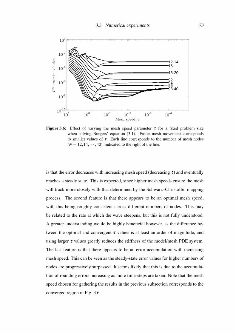
3.3. Numerical experiments 73
Mesh speed, τ10-410-310-210-1100101
L∞
errorin
solution
10-10
10-8
10-6
10-4
10-2
100
12-1416
18-20
22242628-40
Figure 3.6: Effect of varying the mesh speed parameter τ for a fixed problem sizewhen solving Burgers’ equation (3.1). Faster mesh movement correspondsto smaller values of τ . Each line corresponds to the number of mesh nodes(N = 12,14, · · · ,40), indicated to the right of the line.
is that the error decreases with increasing mesh speed (decreasing τ) and eventually
reaches a steady state. This is expected, since higher mesh speeds ensure the mesh
will track more closely with that determined by the Schwarz–Christoffel mapping
process. The second feature is that there appears to be an optimal mesh speed,
with this being roughly consistent across different numbers of nodes. This may
be related to the rate at which the wave steepens, but this is not fully understood.
A greater understanding would be highly beneficial however, as the difference be-
tween the optimal and convergent τ values is at least an order of magnitude, and
using larger τ values greatly reduces the stiffness of the model/mesh PDE system.
The last feature is that there appears to be an error accumulation with increasing
mesh speed. This can be seen as the steady-state error values for higher numbers of
nodes are progressively surpassed. It seems likely that this is due to the accumula-
tion of rounding errors increasing as more time-steps are taken. Note that the mesh
speed chosen for gathering the results in the previous subsection corresponds to the
converged region in Fig. 3.6.

74 Chapter 3. Analyticity-based mesh adaptation in one dimension
3.3.1.3 Comparison with the ARS method in resolving a steep shock
front
To confirm that the spectral moving mesh method maintains the performance of the
ARS method, an explicit comparison was made. To this end, Burgers’ equation (3.1)
was solved with ε = 10−2 and t f = 1.6037 using the ARS method and the present
method. Code that implements the ARS method for this problem can be found in
[92, Appendix D]. The viscosity parameter ε was chosen because it represents a
much steeper shock than the previous problem, and because the maximum slope is
known (as well as the time at which this occurs) [92, p. 76]. The spectral moving
mesh method was applied using two mesh speeds to illustrate the effect on the
convergence rate. These were a convergent (fast) mesh speed and the optimal mesh
speed, chosen using the same procedure that produced the results in Fig. 3.6. The
final waveform and the comparison results are shown in Fig. 3.7.
It is evident that all three results exhibit roughly similar rates of convergence.
All methods reproduce the maximum slope to five decimal places with very few
mesh nodes. The difference in floor values in the two spectral moving mesh method
results is due to the use of optimal (τ = 0.2) and convergent (τ = 0.01) mesh speeds.
3.3.1.4 Multiple shock fronts
To conclude with Burgers’ equation, a demonstration of the ability of the updated
pole-finding algorithm to deal with an unspecified, varying number of singularities
is provided. This is done by solving (3.1) with
u0 = 0.5(cos(x)− sin(3x)) , (3.2a)
ε = 0.025, N = 64, τ = 0.01. (3.2b)
The ODE solver’s error tolerances were also significantly relaxed for fast compu-
tation, with relative errors kept below 10−2 and absolute errors below 10−3. Snap-
shots from this simulation are shown in Fig. 3.8 and the trajectories of the mesh
nodes and poles are shown in Fig. 3.9. The poles can be seen to move towards the

3.3. Numerical experiments 75
Real axis, x-π 0 π
Field
variable,u
-1
-0.5
0
0.5
1
Number of mesh nodes, N0 20 40 60 80 100
Absolute
errorin
maxim
um
slope
10-8
10-6
10-4
10-2
100
102
Tee et al.
SMMM, τ = 0.01
SMMM, τ = 0.2
Figure 3.7: (Top) A solution to Burgers’ equation (3.1) computed using the ARS methodwith viscosity ε = 10−2 and N = 63 mesh nodes. (Bottom) Comparison be-tween the ARS method (Tee et al.) and the moving mesh method with spectralmesh density function (SMMM) in computing the maximum slope of the modelsolution. Two mesh speed parameters τ = 0.01,0.2 were used. All methodscorrectly reproduce the maximum slope to all five decimal places, with roughlysimilar rates of convergence.
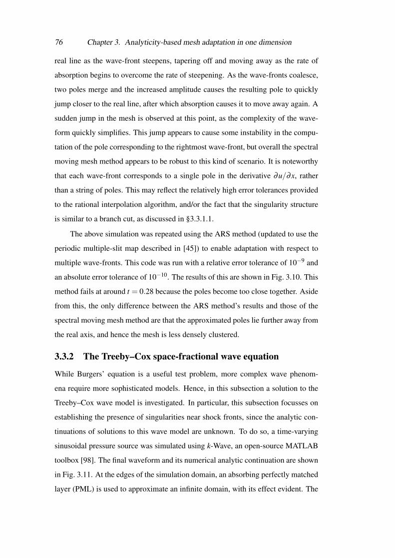
76 Chapter 3. Analyticity-based mesh adaptation in one dimension
real line as the wave-front steepens, tapering off and moving away as the rate of
absorption begins to overcome the rate of steepening. As the wave-fronts coalesce,
two poles merge and the increased amplitude causes the resulting pole to quickly
jump closer to the real line, after which absorption causes it to move away again. A
sudden jump in the mesh is observed at this point, as the complexity of the wave-
form quickly simplifies. This jump appears to cause some instability in the compu-
tation of the pole corresponding to the rightmost wave-front, but overall the spectral
moving mesh method appears to be robust to this kind of scenario. It is noteworthy
that each wave-front corresponds to a single pole in the derivative ∂u/∂x, rather
than a string of poles. This may reflect the relatively high error tolerances provided
to the rational interpolation algorithm, and/or the fact that the singularity structure
is similar to a branch cut, as discussed in §3.3.1.1.
The above simulation was repeated using the ARS method (updated to use the
periodic multiple-slit map described in [45]) to enable adaptation with respect to
multiple wave-fronts. This code was run with a relative error tolerance of 10−9 and
an absolute error tolerance of 10−10. The results of this are shown in Fig. 3.10. This
method fails at around t = 0.28 because the poles become too close together. Aside
from this, the only difference between the ARS method’s results and those of the
spectral moving mesh method are that the approximated poles lie further away from
the real axis, and hence the mesh is less densely clustered.
3.3.2 The Treeby–Cox space-fractional wave equation
While Burgers’ equation is a useful test problem, more complex wave phenom-
ena require more sophisticated models. Hence, in this subsection a solution to the
Treeby–Cox wave model is investigated. In particular, this subsection focusses on
establishing the presence of singularities near shock fronts, since the analytic con-
tinuations of solutions to this wave model are unknown. To do so, a time-varying
sinusoidal pressure source was simulated using k-Wave, an open-source MATLAB
toolbox [98]. The final waveform and its numerical analytic continuation are shown
in Fig. 3.11. At the edges of the simulation domain, an absorbing perfectly matched
layer (PML) is used to approximate an infinite domain, with its effect evident. The

3.3. Numerical experiments 77
Real axis, x-π 0 π
Field
variable,u
-1
-0.5
0
0.5
1
Real axis, x-π 0 π
Field
variable,u
-1
-0.5
0
0.5
1
Real axis, x-π 0 π
Field
variable,u
-1
-0.5
0
0.5
1
Figure 3.8: Solution to Burgers’ equation (3.1) using the spectral moving mesh methodwith parameters given by (3.2). (Top–bottom) Snapshots from t = 0,1.5,6.The leftmost wave-front travels right and the other two travel left. (Bottom)After the left two wave-fronts coalesce they travel rightwards.

78 Chapter 3. Analyticity-based mesh adaptation in one dimension
Real axis
-π 0 π
Tim
e
0
1
2
3
4
5
6
Figure 3.9: (Top) Mesh node trajectories and (bottom) pole trajectories for the solutionto Burgers’ equation (3.1) with parameters given by (3.2). (Top) Snapshotsshown in Fig. 3.8 are indicated by horizontal lines. (Bottom) Colouring is fromthe start of the simulation (dark) to the end (light).

3.3. Numerical experiments 79
Real axis, x-π 0 π
Field
variable,u
-1
-0.5
0
0.5
1
Real axis
-π 0 π
Tim
e
0
1
2
3
4
5
6
Real axis-π 0 π
Imaginary
axis
-1
-0.5
0
0.5
1
Figure 3.10: Solution to Burgers’ equation (3.1) using the ARS method with parametersgiven by (3.2). (Top) Snapshot at t = 1.5. (Middle) Mesh trajectory and(bottom) pole trajectories throughout the simulation. The snapshot in the topplot is indicated by a horizontal line. (Bottom) Colouring is from the start ofthe simulation (dark) to the end (light).

80 Chapter 3. Analyticity-based mesh adaptation in one dimension
trajectories of the poles of this continuation at each time step through one cycle of
the pressure source are shown in Fig. 3.12. Conjugate strings of poles are visible
at each wave-front, with their proximity to the real axis increasing as the shock
forms. There also appears to be a number of pole trajectories which are unrelated
to the propagation of the wave. These occur near the acoustic source and near the
edge of the absorbing boundary layer. The poles near the source may be caused by
Gibbs’ oscillations around the source point, since the derivative of the pressure field
is almost always discontinuous here. Those near the perfectly matched layer arise
because the PML parameters are not analytic at the PML boundary.
3.4 Remaining issues
Despite the successes described above in updating and extending the ARS method,
there are a number of substantive issues that remain. The first is a lack of jus-
tification for the numerator and denominator orders that the rational interpola-
tion algorithm is initialised with. At present, the starting order is specified as
m = n = bN/4c−1, where N is the number of function samples. The choice m = n
was made because diagonal Pade approximants are known to converge nicely as
m,n→ ∞ [104, p. 205]. The choice m+ n N was made to prevent the rational
interpolant from over-fitting the model solution. However, the adaptive nature of
these algorithms means that the orders are changed such that the approximant may
not remain diagonal, and the choice m+ n N may limit the accuracy of pole-
finding. An alternative is to choose m n with m+ n+ 1 = N. This choice is
known to converge nicely as m→∞ if the approximated function contains exactly n
poles [104, p. 205], which a robust continuation algorithm will ensure by adjusting
n
The second issue that remains is the use of an analytic continuation algorithm
that requires equispaced samples (and hence interpolation and upsampling from
a nonuniform mesh). Two new algorithms for analytic continuation stand out as
useful in this regard since the work presented in this chapter was completed in
2015. The first is RKFIT, found in the Rational Krylov Toolbox for MATLAB [9,

3.4. Remaining issues 81
Normalised real axis, x-π 0 π
Norm
alisedfield
variable,p
-1
-0.5
0
0.5
1
Figure 3.11: (Top) Snapshot of the pressure field p for a solution to the Treeby–Cox waveequation (1.1) with a time-varying sinusoidal pressure source. (Bottom) Realpart of the analytic continuation of this solution using a rational interpolant.Each wave-front corresponds to a number of poles, indicated with circularmarkers.

82 Chapter 3. Analyticity-based mesh adaptation in one dimension
Figure 3.12: Trajectories of poles shown in Fig. 3.11 for a solution to the Treeby–Cox waveequation (1.1) over one cycle of a time-varying sinusoidal pressure source.Pairs of poles can be seen to track along with each wave-front. Colouring isfrom the start of the source cycle (dark) to the end (light).
10], which is a Krylov-based approach for solving nonlinear rational least squares
problems. The second is the adaptive Antoulas–Anderson (AAA) algorithm [70]. It
produces a rational approximant that is based on function samples at an adaptively-
chosen subset of arbitrary input points. Both of these algorithms are applicable to
arbitrary meshes, and the latter doesn’t require an initial estimate for the number of
poles.
The third issue identified in the numerical experiments above has been diffi-
culty in representing singularity structures which are similar to branch points. Pade
approximants place poles along branch cuts, but often the branch cut closest to the
real axis will monopolise the poles, leaving few available to represent the remain-
ing branch points. As noted in [108], quadratic Pade approximants may provide one
means of representing branch points better. These approximants contain both poles
and branch points. Like in the linear case, they can be written as
pu2 +qu+ r = 0 −→ u =−q±
√q2−4pr
2p, (3.3)

3.4. Remaining issues 83
where u is a power series approximation to u. If an equivalent rational interpolant
is sought, then u can be replaced with u, and the expression can be rewritten using a
set of sampling points. However, quadratic Pade approximants have proven difficult
to work with. In preliminary investigations, the two solutions corresponding to the
± in (3.3) seemed to share equally in approximating the function, and blew up to
±∞ in regions where the opposing solution was accurate. Additionally, branch cuts
did not lie where expected and even poles were inaccurately placed.
The fourth issue is the computational complexity of the algorithm. It was men-
tioned in the results above that the spectral mesh density function is not computed at
every time step, and instead updated at regular intervals. This was done because the
analytic continuation algorithms are considerably more computationally expensive
than the remainder of the method as they are iterative in nature (adjusting the order
of the approximant). This could be alleviated by changing the input orders based
on previous time-steps, acknowledging the fact that the approximant is likely to be
similar from one time-step to the next.
Of course, the biggest issue that remains is extending the method into multiple
dimensions. To do so, multidimensional analogues must be found for singularity
localisation and the associated Schwarz–Christoffel mappings. For the former, it
would be natural to consider multi-dimensional Pade approximants. Unfortunately,
these are not as well understood as one-dimensional Pade approximants. For the
latter, there is no obvious approach. An alternative that may work for both singular-
ity localisation and the Schwarz–Christoffel mapping is to apply these techniques
along each mesh line independently, as if in one dimension. The resulting mesh
density functions can then be combined and smoothed to form a monitor function.
Unfortunately, preliminary attempts at doing so struggled with inconsistencies be-
tween both parallel and intersecting mesh lines that were too great for a sensible
amount of smoothing to overcome. This last issue stands in the way of ongoing
development of this technique.

84 Chapter 3. Analyticity-based mesh adaptation in one dimension
3.5 Conclusion
In this chapter, a mesh adaptation technique has been described that addresses the
analyticity of the model solution. This is based on the ARS method, which uses
a combination of numerical analytic continuation and Schwarz–Christoffel map-
pings to find a mesh transformation that improved the analyticity of the model so-
lution. This method has a number of shortcomings, most notably that it is unable
to deal with a-priori unknown numbers of singularities in the analytic continuation
of the model solution, nor with changes to the number of singularities throughout
a simulation. These have been alleviated in this chapter by using more recent ana-
lytic continuation algorithms, and through modifications to the Schwarz–Christoffel
mapping process. A moving mesh method was then formed and applied to Burgers’
equation, and the Treeby–Cox wave equation’s analytic continuation was investi-
gated.
It was found that analyticity-based mesh adaptation outperformed the more
commonly used gradient-based adaptation techniques by a substantial margin, and
that the method faithfully reproduced the performance of the ARS method. The
modifications to the ARS method were also tested through application to Burgers’
equation with multiple, interacting shock fronts, and it was shown that the method
was robust to this scenario. Lastly, the analytic continuation of a solution to the
one-dimensional Treeby–Cox wave model was found to feature a similar singularity
structure to Burgers’ equation, indicating the potential for these ideas to be applied
to more complex acoustic problems.
Unfortunately, despite the excellent convergence rate improvements described
in this chapter, a number of issues remain with analyticity-based mesh adaptation,
and it was ultimately concluded that an alternative pathway forwards should be
sought. One way of doing so, explored in the next two chapters, is to consider the
local frequency content of the model solution. While this method is independently
justified by the discussion of sampling criteria in §1.3.4, it can also be related to
analyticity. This can be seen by considering the analytic continuation of sinusoidal
basis functions. These blow up to infinity as the spatial coordinate departs the real

3.5. Conclusion 85
line, with the rate at which this blow-up occurs increasing with frequency. A model
solution which contains spatially localised high-frequency components can thus be
considered to exhibit localised, near-singular behaviour.


Chapter 4
Bandwidth-based mesh adaptation in
one dimension
In the previous chapter, the analyticity of the model solution was used to generate
adaptive meshes. This addressed fundamental error properties for pseudospectral
methods and resulted in excellent improvements in error convergence rates when
applied to developing and propagating shock fronts. However, the complexity of
the method limited its ability to deal with complicated problems, and there was no
obvious pathway from one spatial dimension to multiple dimensions. An alternative
approach is to address the frequency-based considerations discussed in §1.3.4. A
past work of particular relevance is that of Subich [88], who recently demonstrated
a mesh density function that is given by the envelope of the high-frequency com-
ponents of the model solution. However, Subich provided no direct justification for
why an envelope should correspond to a beneficial mesh density. Moreover, the
threshold beyond which frequencies are considered to be high was chosen based
on model-specific and interpolant-specific considerations. Nonetheless, using the
local frequency content of a model solution to form a mesh density function is an
intuitive and general approach that has remained largely unexplored.
In this chapter, a family of one-dimensional mesh density functions are derived
which are based on a spatially localised measure of the bandwidth of the approxi-
mated model solution. As discussed in §1.3.4, this addresses a nonuniform analogue
of the Nyquist–Shannon sampling theorem, thus these mesh density functions are

88 Chapter 4. Bandwidth-based mesh adaptation in one dimension
not strictly tied to the error properties of any particular spatial interpolant, nor do
they consider any problem-specific factors. This makes the bandwidth mesh density
functions applicable to both spectral and non-spectral methods, as well as a wide
range of problem types. Their capabilities are illustrated in two ways: first, through
application to function approximation using Chebyshev polynomials, and second,
through application to a variety of acoustics problems modelled by an advection
equation with a heterogeneous sound-speed, a viscous Burgers’ equation, and the
Korteweg-de Vries equation. These acoustics problems are primarily solved using a
periodic spectral moving mesh method, with some additional validation for periodic
finite-difference moving mesh methods.
4.1 Derivation of mesh density function
4.1.1 Local measures of bandwidth
In this section, mesh density functions are derived from the local spatial frequency
content of the solution to a one-dimensional model PDE. For notational purposes,
it is useful to consider such a solution as a signal u that is a function of a spatial
coordinate x with corresponding wavenumbers k. In §1.3.4, the sampling criteria
for such signals were discussed and it was noted that a band-limited signal could be
perfectly reconstructed given samples taken at twice the signal’s local bandwidth,
i.e. bandwidth at a particular value of x. Of course, not all signals possess a hard
cut-off in their frequency content, and it was also pointed out that such sampling
criteria aim to minimise aliasing errors in these cases. The latter scenario is more
likely for many PDEs, particularly those which are nonlinear. Hence it is useful to
consider statistical measures of bandwidth.
Now let the signal u be real-valued, 2π-periodic, and normalised such that
∫π
−π
|u|2 dx =∫
∞
−∞
|u|2 dk = 1,
where u is the Fourier transform of u. The local amplitude A, phase ϕ , and spatial
frequency ∂ϕ/∂x of this signal are inherently coupled when the signal is directly

4.1. Derivation of mesh density function 89
analysed. The analytic signal provides a way of decoupling them. It does this by
attaching an imaginary counterpart to the original signal. This is typically done via
the Hilbert transformH, yielding
v = u+ iHu= Aeiϕ .
To define a local, statistical measure of bandwidth, the analytic signal is consid-
ered to have a joint position–wavenumber power density P(k,x) which satisfies the
marginals
P(x) =∫
∞
−∞
P(k,x)dk = |v|2, P(k) =∫
π
−π
P(k,x)dx = |v|2,
where v is the Fourier transform of v. Position–wavenumber power densities can
be computed using a variety of transformations, including the short-time Fourier
transform and the wavelet transform, but it suffices to consider the concept alone
here. A useful family of statistical bandwidth measures are the even-order spectral
moments
〈k2m〉=∫
∞
−∞
k2mP(k)dk. (4.1)
The order of the spectral moments can be chosen based on the desired weighting
given to the power density’s tail. Since the m = 1 moment corresponds to the vari-
ance (assuming symmetry in P(k) about k = 0), and the square root of the variance
is commonly used as a measure of bandwidth, the second spectral moment is used
for the derivation that follows. Similar derivations are easily made for other choices
of m. From the global spectral moment, a local equivalent may be derived using the
conditional power density
P(k|x) = P(k,x)P(x)

90 Chapter 4. Bandwidth-based mesh adaptation in one dimension
as
〈k2〉=∫
∞
−∞
k2P(k)dk
=∫
∞
−∞
k2(∫
π
−π
P(k,x)dx)
dk
=∫
∞
−∞
k2(∫
π
−π
P(k|x)P(x)dx)
dk
=∫
π
−π
(∫∞
−∞
k2P(k|x)dk)
P(x)dx
=∫
π
−π
〈k2〉|xP(x)dx (4.2)
Here, the local second spectral moment has been defined by [30]
〈k2〉|x =∫
∞
−∞
k2P(k|x)dk. (4.3)
This choice of definition is intuitive when P(k|x) is considered as a local frequency
distribution, and when (4.1) is compared with (4.3). While (4.3) could be used to
compute the local bandwidth of a signal, it is convenient to avoid explicitly com-
puting a joint power density.
An alternative way of computing local spectral statistics is to consider the op-
erator
K =
1i
ddx in the position representation
k in the wavenumber representation.(4.4)
For the wavenumber representation, this operator can be used to compute the global
second spectral moment as
〈k2〉= 〈v|K2|v〉
= 〈Kv,Kv〉
=∫
∞
−∞
k2|v|2 dk,
as expected. Similarly, for the position representation the global second spectral

4.1. Derivation of mesh density function 91
moment is given by [30]
〈k2〉= 〈v|K2|v〉
= 〈Kv,Kv〉
=∫
π
−π
∣∣∣∣∂v∂x
∣∣∣∣2 dx
=∫
π
−π
∣∣∣∣∂v/∂xv
∣∣∣∣2 |v|2 dx. (4.5)
Making a comparison with (4.2), the left term of the integrand in (4.5) is considered
to be the local second spectral moment [26, 30]:
〈k2〉|x =∣∣∣∣∂v/∂x
v
∣∣∣∣2 . (4.6)
In [27], this interpretation of similar operators is justified by showing that it leads
to established results for a number of quantum mechanical statistics. Taking the
square root of (4.6) then gives a definition of the local bandwidth, which is used
to define the first of two proposed mesh density functions: the ordinary bandwidth
mesh density function
ρ =
∣∣∣∣∂v/∂xv
∣∣∣∣ . (4.7)
A complication arises when this mesh density function is computed from an ana-
lytic signal v whose amplitude drops to zero, since computing the local bandwidth
becomes ill-posed in these regions. One approach to regularisation is to include an
amplitude-weighting. This leads to the amplitude-weighted bandwidth mesh density
function, defined as
ρ =
∣∣∣∣∂v∂x
∣∣∣∣ . (4.8)
The difference in effect between the ordinary and amplitude-weighted bandwidth
mesh density functions is as follows: The ordinary bandwidth mesh density func-
tion was derived with equal consideration given to every point on the function.
Hence, the resultant sampling minimises local errors. The introduction of ampli-
tude weighting will increase the sampling in regions with large amplitudes, and

92 Chapter 4. Bandwidth-based mesh adaptation in one dimension
thereby reduce the overall absolute error.
The bandwidth mesh density functions presented in this section are not the
only ones that could be derived from consideration of the local spatial frequency
content of a solution. Possible alternative choices that could be made include:
• Using a different order of spectral moment, or using a different spectral statis-
tic altogether.
• Decoupling the amplitude and phase of signals using an approach that doesn’t
involve the analytic signal [65].
• Computing the local statistics using an explicit position–wavenumber power
density.
• Regularising the ordinary bandwidth mesh density function by adding a small
constant to the denominator, or by introducing amplitude-weighting for small
amplitudes only.
4.1.2 A periodic Hilbert transform for nonuniform samples
The bandwidth mesh density functions require a complex-valued analytic signal to
be defined from the real-valued solution to a model PDE. In one dimension, this is
done using the Hilbert transform, which can be defined in the frequency domain by
Hu= F−1 −isign(k)Fu .
For equispaced samples, this is easily approximated using fast Fourier transforms.
For nonuniform samples, computing a Fourier transform is not so straightforward.
An alternative is to use the Hilbert transform’s definition as a convolution
Hu(x) = 12π
p.v.∫
π
−π
u(ξ )h(ξ − x)dξ , h(x) = cot(x
2
), (4.9)
where p.v. indicates the Cauchy principal value, and h is the circular Hilbert kernel.
When computing the integrand in (4.9), special consideration needs to be given
to the singularity at ξ = x. As described in [24], this singularity can be made re-

4.1. Derivation of mesh density function 93
movable by rewriting (4.9) as
Hu(x) = 12π
∫π
−π
(u(ξ )−u(x))h(ξ − x)dξ +u(x)2π
p.v.∫
π
−π
h(ξ − x)dξ . (4.10)
The singularity is now present only in the second integral; the first integral is instead
of indeterminate form at ξ = x. The singularity is easily dealt with by noting that
the circular Hilbert kernel is antisymmetric and 2π periodic, meaning the Cauchy
principal value of the second integral is equal to zero.
The indeterminate point in the first integral in (4.10) is evaluated by computing
the limit of the integrand as ξ → x. To do so, note that the Hilbert kernel can be
obtained by making the Cauchy kernel, defined as 1/x, 2π-periodic:
cot(x
2
)= 2
[1x+
∞
∑n=1
(1
x−2πn+
1x+2πn
)].
Now let t = ξ − x and f (t) = u(ξ )−u(x). From the first integrand in (4.10), write
f (t)h(t) = 2 f (t)
[1t+
∞
∑n=1
(1
t−2πn+
1t +2πn
)].
As t→ 0, each of the terms in the sum will cancel one another. Thus,
limt→0
f (t)h(t) = limt→0
2 f (t)t
.
Because f (0) = 0, this fraction is indeterminate, but it can be solved using
L’Hospital’s rule. Let f ′(t) = ∂ f/∂ t, then
limt→0
f (t)h(t) = 2 f ′(0).
Returning to the original variables, this is written as
limξ→x
[(u(ξ )−u(x))h(ξ − x)] = 2u′(ξ ),
which can be substituted into the left integrand in (4.10) when it is solved.

94 Chapter 4. Bandwidth-based mesh adaptation in one dimension
Finally, to compute the Hilbert transform, a change of variables is made from
x to s. Letting u =Hu, this gives
u(x) =1
2π
∫π
−π
F(x,ξ )∂ξ
∂ sds, F =
(u(ξ )−u(x))h(ξ − x) ξ 6= x
2u′(ξ ) ξ = x.
This is solved using the trapezoid rule, discretised at a set of equispaced, discrete s
nodes. Letting subscripts denote the index of a variable, ξ is discretised equal to x,
and the resultant expression is
ui =1
2π∑
jFi, j
(∂x∂ s
)∣∣∣∣x j
∆s, Fi, j =
(u j−ui)h(x j− xi) i 6= j
2u′(x j) i = j.
4.1.3 Examples for static functions using Chebyshev approxi-
mants
As a first examination of mesh transformations resulting from the bandwidth mesh
density functions, a Gaussian function and a Runge-type function are considered.
These both have known Hilbert transforms, and so the ordinary and amplitude-
weighted bandwidth mesh density functions can be explicitly computed. They also
represent two important classes of function: The Gaussian is an entire function,
and the Runge-type function is analytic in a neighbourhood of the real axis. Since
neither are band-limited, they are both well-suited to the statistical bandwidth defi-
nitions given in § 4.1.1, and are smooth enough to provide geometric convergence
rates when a spectral method is applied to their approximation. The Runge-type
function also provides an excellent opportunity to compare bandwidth-based sam-
pling with analyticity-based sampling from Chapter 3.
For the first example, consider the following Gaussian function and its Hilbert
transform
u = exp(−x2), Hu= 2F(x)√π
.
Here, F is the Dawson integral. The derivative of the corresponding analytic signal

4.1. Derivation of mesh density function 95
v = u+ iHu is∂v∂x
=−2xexp(−x2)+ i2−4xF(x)√
π.
From this, the ordinary and amplitude-weighted bandwidth mesh density functions
were computed via formulae (4.7) and (4.8). Mesh transformations were then gen-
erated using Chebfun [32] (a software package for working with Chebyshev approx-
imants) by numerically computing (and scaling/translating) the indefinite integrals
of the reciprocal of the mesh density functions on the domain x ∈ [−15,15]. The
original function u was then composed with each mapping, and the Chebyshev co-
efficients corresponding to the original function and its transformed counterparts
were computed. These were used as a proxy for the approximation error, and com-
pared to examine the effect of the transformations on the convergence rate of each
Chebyshev interpolant. Figure 4.1 depicts the original and transformed functions,
along with their Chebyshev coefficients.
Two convergence regimes are evident in Fig. 4.1. The untransformed Gaussian
function exhibits a convergence rate that is faster than geometric (consistent with
it being entire), while the transformed Gaussian functions both exhibit geometric
convergence, initially at a faster rate than the untransformed Gaussian. Thus, the
transformed meshes provide benefit for low-frequency spectral components, but not
for higher-frequency ones, and so their effectiveness depends on the desired accu-
racy of the spectral approximation. In this case, they provide a benefit up until
approximately 5 digits of accuracy, after which they are detrimental.
A similar investigation was carried out for the arclength and curvature mesh
density functions. Their effectiveness was assessed by the number of Chebyshev
coefficients that were needed to represent the original Gaussian to machine preci-
sion under mesh transformations resulting from their use, computed as described
above. For the original Gaussian function, this number was 183. For the arclength-
and curvature-based transformations, they were 1,021 and 1,513 respectively. This
drastic increase is likely to be the result of a lack of smoothness in the arclength
and curvature mesh density functions themselves, and can be alleviated with a sec-
ondary smoothing step (as is often done in moving mesh methods), as discussed

96 Chapter 4. Bandwidth-based mesh adaptation in one dimension
-15 -10 -5 0 5 10 15
Untransformed spatial coordinate
-0.2
0
0.2
0.4
0.6
0.8
1
Function m
agnitude
Original
Ord. Bandwidth
A.W. Bandwidth
50 100 150 200 250 300Coefficient index
10-15
10-10
10-5
100
Coe
ffici
ent m
agni
tude
OriginalOrd. BandwidthA.W. Bandwidth
Figure 4.1: Chebyshev interpolation of a Gaussian function under mesh transformationscorresponding to the ordinary (Ord.) and amplitude-weighted (A.W.) band-width mesh density functions. (Top) Function values plotted against an un-transformed spatial coordinate. The widening that results from composing theGaussian with each mesh transformation corresponds to an increased functionsampling density. (Bottom) Chebyshev coefficients corresponding to the func-tions depicted in top subfigure. The convergence rate for the original function isfaster than geometric, while the transformed functions exhibit geometric con-vergence. For this Gaussian function, the transformations provide benefit forlow accuracy Chebyshev interpolants, and are detrimental at higher accuracies.

4.1. Derivation of mesh density function 97
in §4.2, below. Nonetheless, these results illustrate the limitation of applying the
arclength and curvature mesh density functions to spectral methods, particularly
when there are no large, localised variations in the approximated function’s first or
second derivatives.
For the second example, consider the following Runge-type function and its
Hilbert transform
u =1
1+25x2 , Hu= 5x1+25x2 .
The corresponding analytic signal and derivative are
v =i
5x+ i,
∂v∂x
=− 5i
(5x+ i)2 .
As above, the decay rate of Chebyshev coefficients was used to assess the effec-
tiveness of the bandwidth mesh density functions in producing mesh transforma-
tions, this time on the interval x ∈ [−1,1]. In addition, a mesh was generated us-
ing the analyticity-based approach discussed in Chapter 3, but with the Schwarz–
Christoffel maps using the function’s known singularities at ±0.2i, rather than ap-
proximating them via numerical analytic continuation. Figure 4.2 depicts the origi-
nal and transformed functions, along with their Chebyshev coefficients.
Unlike for the Gaussian function, all three mesh transformations provide an
improvement in the convergence rate of the Runge-type function’s Chebyshev co-
efficients at all frequency scales. There is also a significant difference between
the convergence rates under each mesh transformation. In order of effectiveness,
these are the analyticity-based mesh transformation, followed by the transforma-
tions resulting from the amplitude-weighted and ordinary bandwidth mesh density
functions. The performance gap between the analyticity-based technique and the
bandwidth mesh density functions is significant. However, for many approximated
functions, such as those generated numerically as solutions to PDEs, exact singu-
larity locations are unknown, and must be approximated as described in Chapter 3.
This reduces the performance gap significantly, as will be shown in later sections of
this chapter.

98 Chapter 4. Bandwidth-based mesh adaptation in one dimension
-1 -0.5 0 0.5 1
Untransformed spatial coordinate
0
0.2
0.4
0.6
0.8
1
Function m
agnitude
Original
Ord. Bandwidth
A.W. Bandwidth
Singularity
Figure 4.2: Chebyshev interpolation of a Runge-type function under mesh transforma-tions corresponding to the ordinary (Ord.) and amplitude-weighted (A.W.)bandwidth mesh density functions, and the analyticity-based mesh mappingof [45, 44]. (Top) Function values plotted against an untransformed spatial co-ordinate. The widening that results from composing the Runge-type functionwith each mesh transformation corresponds to an increased function samplingdensity. (Bottom) Chebyshev coefficients corresponding to the functions de-picted in top subfigure. All exhibit geometric convergence rates, and the meshtransformations are beneficial in all cases.

4.2. Numerical methods 99
Finally, the arclength and curvature mesh density functions were again exam-
ined based on the number of Chebyshev coefficients that were required to repre-
sent the Runge-type function under transformations resulting from their use. For
the original Runge-type function, this number was 189. For the arclength- and
curvature-based transformations, they were 1,329 and 7,415 respectively. As be-
fore, this illustrates the limitation of applying such mesh density functions to spec-
tral methods, especially since the Runge-type function also exhibits no obvious
localised, derivative-based features.
4.2 Numerical methods
4.2.1 Spatial calculus and time-stepping
To examine the application of the bandwidth mesh density functions to PDEs, two
moving mesh methods are used. These are outlined below, but it is important to note
that the bandwidth mesh density functions are agnostic to the algorithmic choices
that have been made. The two moving mesh methods are distinguished by the nu-
merical method they use for computing spatial gradients in the model/mesh PDEs.
Both assume periodic model solutions, but one uses spectral interpolants and the
other uses centred finite-differences. For the spectral interpolants, gradients are
computed using either a standard Fourier interpolant (when taken with respect to
the computational coordinate) or a rational trigonometric interpolant (when taken
with respect to the physical coordinate). For the finite-difference method, gradients
are computed using centred finite-differences of various accuracy-orders taken with
respect to the computational coordinate, and physical gradients are then computed
using the chain rule.
Time-stepping is performed using Matlab’s ode15i function [83]. This algo-
rithm solves ODEs of the form f (t,y, y) = 0 using adaptive-order backward differ-
entiation formulae, with an adaptive timestep size. Here, y is a vector of model solu-
tion values and mesh node positions, and y is the corresponding temporal derivative
in the computational coordinate’s reference frame.
100 Chapter 4. Bandwidth-based mesh adaptation in one dimension
4.2.2 Smoothing the mesh density function
A mesh density function is usually spatially smoothed before being applied to a
MMPDE. This is done for a number of reasons. First, it ensures that the mesh
density function is well-sampled by the mesh, and hence that the MMPDE can be
efficiently solved. Second, it ensures smooth mesh transformations, which in turn
produce fast convergence rates when the model is solved. Third, it lessens the inher-
ent increase in stiffness that comes with mesh adaptivity, improving the efficiency of
time-stepping algorithms [54]. Let ρ and ρ be the smoothed and unsmoothed mesh
density functions respectively. In this chapter, these are related by the equation
ρ−β−2 ∂ 2ρ
∂ s2 = ρ, (4.11)
where the parameter β controls the degree of smoothing [54, 56]. With homoge-
neous Neumann boundary conditions, (4.11) constrains the relative rate of change
in the smoothed mesh density by |∂ ρ/∂ s|/ρ ≤ β , and similar behaviour is observed
for periodic boundary conditions. Equation (4.11) is solved using a Fourier inter-
polant via
ρ = F−1 Fρ
1+β−2k2
,
where k are wavenumbers corresponding to s. The smoothing parameter can be
chosen to be discretisation-dependent, so that it has a similar effect to nearest-
neighbour smoothing. This choice aims to ensure that the mesh density function
is well-sampled, since, for example, a well-sampled peak will be smoothed (and re-
duced) less than a poorly sampled one. Unless otherwise stated, here β = (∆s√
2)−1
[54], where ∆s is the discretisation size in the computational coordinate. A numer-
ical experiment is described in §4.3.3, which analyses this choice for one of the
model problems presented below.
4.2.3 Mesh density function updates
Lastly, a final difference between the methods used in this chapter and those of
Chapter 3 is that the mesh density function is recalculated every time the model and
mesh update. In Chapter 3 the mesh density functions were instead calculated at

4.3. Numerical experiments 101
regular intervals throughout the simulation, as the analyticity mesh density function
was expensive to compute relative to the other variables. This is not the case for the
bandwidth mesh density functions. Recalculating the mesh density function more
frequently allows it to better track the model solution throughout a simulation, and
produces less jerky mesh movement.
4.3 Numerical experiments
4.3.1 Example problems
The bandwidth mesh density functions are demonstrated through application to four
problems and three acoustic models. The problems each exhibit different feature
types. The first problem is based on a heterogeneous advection equation, and ex-
hibits the formation and propagation of a sharp crest. The second problem is based
on the viscous Burgers’ equation, and exhibits the formation of a stationary shock
front. These problems are used to demonstrate the performance of spectral and finite
difference moving mesh methods in §3.3 and §3.4, respectively. The third problem
is also based on the viscous Burgers’ equation, and exhibits the formation, propa-
gation, and merging of multiple shock fronts. The fourth problem is based on the
Korteweg-de Vries equation, and exhibits the formation of multiple solitons, and
their subsequent interactions. All use dimensionless units and a periodic domain
x ∈ [−π,π). The adaptive time-stepping algorithm was provided with relative and
absolute error tolerances of 10−9 and 10−10, to ensure that errors in the spatial nu-
merical method dominate. The mesh speed parameter was τ = 10−2. For the illus-
trations presented in Figs. 4.3–4.6 below, the amplitude-weighted bandwidth mesh
density function was used in conjunction with the spectral moving mesh method
described in §4.2.
4.3.1.1 A heterogeneous advection equation
The first model presented in this section is an advection equation with a heteroge-
neous sound speed:
∂u∂ t
= c(x)∂u∂x
, c(x) = [1+0.9cos(x)]−1 .

102 Chapter 4. Bandwidth-based mesh adaptation in one dimension
Note that the time-derivative in the model equation should be adjusted via (2.3)
before discretisation, so that it is expressed in the computational coordinate’s ref-
erence frame. This model describes linear wave propagation, with a propagation
speed that is slower in the middle of the domain than the edges. It is solved using a
sinusoidal initial condition
u(x,0) = cos(x−π),
and the resulting wave is propagated until t = 2π , when it has travelled the full
length of the spatial domain and periodic wrapping has occurred. For this problem,
the initial and final waveforms are equal, and can be compared to measure the accu-
racy of a given simulation. The heterogeneous sound speed causes the peak in the
wave to sharpen as it propagates through the centre of the domain, making an adap-
tive mesh beneficial. A solution to this problem is depicted in Fig. 4.3, computed
using N = 64 mesh nodes. The snapshots in the upper subplot show the formation
of the sharp wave crest, and the lower subplot shows the trajectories of the mesh
nodes, which cluster densely around this crest.
4.3.1.2 The viscous Burgers’ equation
The second model presented in this section is the viscous Burgers’ equation (3.1).
The first of two problems that use this equation exhibits a single, stationary shock
front and is the same as the problem posed in §3.3.1.3. It is given by the following
initial condition and viscosity coefficient:
u(x,0) = sin(x), ε = 10−2.
The simulation is terminated at t = 1.6037, which is approximately when the shock
front is steepest. A solution to this problem is depicted in Fig. 4.4, computed using
N = 64 mesh nodes. The snapshots in the upper subplot show the formation of the
shock front, and the mesh node trajectories in the lower subplot smoothly converge
around this shock front.
The second problem that uses Burgers’ equation is similar to that in §3.3.1.4,

4.3. Numerical experiments 103
Snapshots
-π 0 π
Space
t = 0
t = π/8
t = π/4
Figure 4.3: A solution to the heterogeneous advection equation. (Top) Snapshots showingthe formation of a sharp wave crest. The solution and its computed Hilberttransform are represented by solid and dashed lines respectively. Dots indicatemesh nodes. (Bottom) A combined solution/mesh plot. Colours indicate themodel solution (yellow high, blue low), and the trajectories of mesh nodes areshown as black lines. The mesh has been downsampled to N = 32 nodes forclarity.

104 Chapter 4. Bandwidth-based mesh adaptation in one dimension
Snapshots
-π 0 π
Space
t = 0
t = 0.8018
t = 1.6037
Figure 4.4: A solution to the viscous Burgers’ equation. (Top) Snapshots showing the for-mation of a steep, stationary shock front. The solution and its computed Hilberttransform are represented by solid and dashed lines respectively. Dots indicatemesh nodes. (Bottom) A combined solution/mesh plot. Colours indicate themodel solution (yellow high, blue low), and the trajectories of mesh nodes areshown as black lines. The mesh has been downsampled to N = 32 nodes forclarity.

4.3. Numerical experiments 105
but this time it exhibits seven propagating shock fronts that merge over time, rather
than three. It is given by the following initial condition and viscosity coefficient:
u(x,0) = 2sin(x)+ cos(7x), ε = 10−2.
This simulation is terminated at t = 1, when most of the shock fronts have merged,
and the remainder have diffused significantly. A solution to this problem is depicted
in Fig. 4.5, computed using N = 128 mesh nodes. The mesh nodes follow each
wavefront smoothly, and become denser as the shock fronts coalesce and increase
in severity.
4.3.1.3 The Korteweg-de Vries equation
The third model presented in this section is the Korteweg-de Vries equation, which
combines nonlinear wave propagation with dispersion. It is given by
∂u∂ t
= αu∂u∂x
+β∂ 3u∂x3 .
The Korteweg-de Vries model admits solitons in its solutions. These are waveforms
whose size, shape, and velocity are constant provided they remain well separated.
Their speed is amplitude-dependent, and when two solitons interact the faster soli-
ton is shifted forwards and the slower soliton is shifted back. After interacting,
solitons regain their original shape. It is not obvious that solitons are difficult to re-
solve since they appear visually smooth, but their analytic continuations are known
to include singularities that limit convergence rates [92]. The initial condition and
parameters
u(x,0) = cos(x), α =−π, β =−(0.022)2π
3,
were chosen to match the problem presented in [117], modified to suit a domain of
length 2π . The initial condition first steepens, before dispersion causes a number of
solitons to form and propagate. Soliton formation begins at approximately tB = 1/π ,
and completes at around tF = 3.6tB. After this, the solitons propagate until the

106 Chapter 4. Bandwidth-based mesh adaptation in one dimension
- 0
t=0
t=0.33
t=0.67
t=1
Figure 4.5: A solution to the viscous Burgers’ equation. (Top) Snapshots showing the for-mation, propagation, and merging of numerous steep shock fronts. The solutionis represented by a solid line, dots indicate mesh nodes. (Bottom) A combinedsolution/mesh plot. Colours indicate the model solution (yellow high, bluelow), and the trajectories of mesh nodes are shown as black lines. The meshhas been downsampled to N = 32 nodes for clarity. The mesh nodes track eachshock front.

4.3. Numerical experiments 107
periodic boundary conditions cause them to interact. The simulation was terminated
at t = 8tB. A solution to this problem is depicted in Fig. 4.6, computed using N =
128 mesh nodes. The mesh nodes compress around each soliton, and continue to
track them as they interact.
4.3.2 Convergence rates
4.3.2.1 Fourier pseudospectral
This section provides a performance evaluation for the bandwidth mesh density
functions when used with the Fourier pseudospectral method described in §4.2.
Performance is judged by the rates at which approximated solutions to the problems
in §4.3.1 converge as the number of mesh nodes increases, measured using the
maximum absolute error in the final simulated solution. This illustrates the ability
of meshes resulting from the bandwidth mesh density functions to reduce the trade-
off between memory usage and accuracy.
First, the advection problem from §4.3.1 was solved with a varying number
of mesh nodes. Three different mesh specifications were used: one uniform spec-
ification, and two based on the ordinary and amplitude-weighted bandwidth mesh
density functions. To evaluate their performance, the initial and final waveforms
were interpolated onto 10,001 uniformly distributed mesh nodes and compared,
since they should be equal to one another. Figure 4.7 depicts these results. Both
adaptive meshes produced error convergence rates which are more than five times
faster than those produced by the uniform mesh. It also seems that there is a slight
advantage to using the amplitude-weighted bandwidth mesh density function over
the ordinary one. The arclength and curvature mesh density functions were also
applied to the advection problem, but produced unstable time-stepping due to their
lack of smoothness.
A similar evaluation was performed for the first Burgers’ equation problem
(which exhibits one shock front) in §4.3.1. A set of uniform mesh results were
first generated for varying N, computed to near machine precision using Chebfun’s
spin algorithm, which uses exponential integrators for time-stepping and a stan-
dard Fourier pseudospectral method in space [32, 67]. Results were then computed

108 Chapter 4. Bandwidth-based mesh adaptation in one dimension
- 0
t=0
t=tF
t=2.5
Figure 4.6: A solution to the Korteweg-de Vries equation. (Top) Snapshots showing theformation and propagation of numerous solitons. The solution is representedby a solid line, dots indicate mesh nodes. (Bottom) A combined solution/meshplot. Colours indicate the model solution (yellow high, blue low), and thetrajectories of mesh nodes are shown as black lines. The mesh has been down-sampled to N = 32 nodes for clarity. The mesh nodes compress around eachsoliton, and smoothly track them as they interact.

4.3. Numerical experiments 109
18 100 500Number of mesh nodes
10-6
10-4
10-2
100
Abs
olut
e er
ror
UniformOrd. BandwidthA.W. Bandwidth
Figure 4.7: The error in the final waveform for the advection simulation depicted in Fig. 4.3computed using a spectral moving mesh method. The solutions computed usingthe bandwidth mesh density functions exhibit much faster convergence ratesthan those that used a uniform mesh.
for four adaptive methods. The first was the analyticity-based ARS method. This
was applied with odd numbers of nodes in the range N = 15 to N = 99 (odd N
ensures a node at x = 0 for their implementation). The remaining results were com-
puted using the Fourier pseudospectral moving mesh method described in §4.2, in
conjunction with the arclength, ordinary bandwidth, and amplitude-weighted band-
width mesh density functions. These used even node numbers in the range N = 16
to N = 100. All approximated solutions were interpolated onto 10,001 uniformly
distributed mesh nodes and compared to the results computed using the spin algo-
rithm when the uniform mesh was at its densest. Figure 4.8 depicts this comparison.
The uniform mesh produces very slow convergence for this problem. The arclength
mesh density function provides a significant improvement, but nonetheless con-
verges far more slowly than the remaining methods. The analyticity-based method
and the two bandwidth mesh density specifications clearly perform best. These all
produced error convergence rates that were more than an order of magnitude faster
than those produced by a uniform mesh, and two to three times faster than those
using the arclength mesh density function. Once again, the amplitude-weighted

110 Chapter 4. Bandwidth-based mesh adaptation in one dimension
15 100 1000Number of mesh nodes
10-6
10-4
10-2
100A
bsol
ute
erro
r
UniformArclengthSingularityOrd. BandwidthA.W. Bandwidth
Figure 4.8: Convergence rates for solutions to the viscous Burgers’ equation simulationdepicted in Fig. 4.4 using a spectral moving mesh method. The bandwidthmesh density functions clearly produce faster convergence rates than a uniformmesh specification or the arclength mesh density function, and converge at asimilar rate to the analyticity-based method of Tee et al. [93, 92, 45, 44].
bandwidth mesh density function outperforms its ordinary counterpart, this time by
a larger margin. It also outperforms the analyticity-based approach, though by a
smaller margin. As with the advection problem, the curvature mesh density func-
tion was also applied to the Burgers’ equation problem, but was again non-smooth,
causing instability in the simulation.1
In addition to the results presented in Fig. 4.8, results were gathered using
the amplitude of the solution’s analytic signal as a mesh density function. It was
found that this produced a small benefit over a uniform mesh. This is likely be-
cause the feature of interest is a steep gradient, which produces an analytic signal
with an infinite amplitude in the limit as the gradient’s magnitude increases to infin-
ity. This may help to explain why the amplitude-weighted bandwidth mesh density
function outperforms the ordinary bandwidth mesh density function for this prob-
lem. In contrast, when the amplitude was used as a mesh density function for the
advection problem, no benefit was found because the amplitude of the solution’s
1In Chapter 3, no difficulties were encountered when applying the curvature mesh density func-tion to Burgers’ equation. This was because a weaker shock was simulated.

4.3. Numerical experiments 111
analytic signal is approximately constant. This illustrates the problem specificity of
amplitude-weighting, and may motivate alternative mesh density functions for other
applications, for instance one which includes an amplitude weighting for small am-
plitudes only.
4.3.2.2 Finite-difference
This section provides a performance evaluation for the bandwidth mesh density
functions when applied to the periodic finite-difference moving mesh method de-
scribed in §4.2. This highlights the fact that the frequency considerations on which
the bandwidth mesh density functions are based are relevant for piecewise polyno-
mial interpolants as well as spectral ones.
First, the performance evaluation for the advection equation was repeated.
Three sets of results were computed using the amplitude-weighted bandwidth mesh
density function, with each corresponding to a different accuracy-order for the finite
differences. Figure 4.9 depicts these results. The spectral convergence rates have
been replaced with algebraic ones, as expected, and as the accuracy-order of the
finite-difference method increases, the accuracy improves. Figure 4.9 also depicts
the previous spectral results for a uniform mesh. It is clear that the introduction of
mesh adaptation can improve the performance of finite-difference methods to such
an extent that they exceed that of the uniform spectral method.
Second, the performance evaluation for Burgers’ equation was repeated using
the finite-difference moving mesh method. In contrast to the results gathered using
the Fourier pseudospectral method in the previous section, only the arclength and
amplitude-weighted bandwidth mesh density functions were examined this time.
Figure 4.10 depicts these results. The spectral convergence rates have been replaced
with algebraic ones, as expected, and as the accuracy-order of the finite-difference
method increases, the accuracy improves noticeably in almost all cases. Comparing
each finite-difference method, it is clear that the amplitude-weighted bandwidth
mesh density function improves upon the results obtained using the arclength mesh
density function significantly. Figure 4.10 also depicts the previous spectral results
for a uniform mesh, and it is clear that the adaptive meshes drastically outperform

112 Chapter 4. Bandwidth-based mesh adaptation in one dimension
18 100 500
Number of mesh nodes
10-4
10-2
100
Absolu
te e
rror
A.W. Band. 2nd ord.
A.W. Band. 4th ord.
A.W. Band. 6th ord.
Uniform (Spect.)
Figure 4.9: The error in the final waveform for the advection simulation depicted in Fig. 4.3computed using centred, periodic finite-difference moving mesh methods. Thenumbers in the legend indicate the accuracy-order of the finite-differencemethod that was used. Adaptive meshes computed using the amplitude-weighted bandwidth mesh density function improve the performance of thesefinite difference methods to the point where they’re comparable with a spectralmethod on a uniform mesh.
a uniform mesh in this case.
4.3.3 Effect of the smoothing parameter
One free parameter in many moving mesh methods is the degree of smoothing that
is applied to a computed mesh density function prior to its application within a
MMPDE. For the advection problem outlined in §4.3.1.1 (and examined in §4.3.2),
the mesh smoothing parameter’s effect was investigated by varying it from β = 1
to β = 20. Figure 4.11 depicts the error in the resulting solution, as well as the
number of timesteps that were taken. As the mesh density function is increasingly
smoothed, both the number of timesteps required and the error slowly decrease,
before turning and increasing at a faster rate. This reflects the fact that the mesh
density function has been smoothed to a point where it no longer produces a bene-
ficial mesh [68]. The turning point in the error is close to the smoothing parameter
choice mentioned in §4.2, which is β = (∆s√
2)−1 ≈ 7.2 for this example.

4.4. Conclusion 113
20 40 60 80 100
Number of mesh nodes
10-6
10-4
10-2
100
Absolu
te e
rror
Arc. 2nd ord.
Arc. 4th ord.
Arc. 6th ord.
Band. 2nd ord.
Band. 4th ord.
Band. 6th ord.
Uniform (Spect.)
Figure 4.10: Convergence plots for solutions to the viscous Burgers’ equation simulationdepicted in Fig. 4.4 using centred, periodic finite-difference moving meshmethods. The numbers in the legend indicate the accuracy-order of the finite-difference method that was used. The amplitude-weighted bandwidth meshdensity function clearly produces faster convergence rates than the arclengthmesh density function.
4.4 ConclusionIn this chapter, a family of bandwidth-based mesh density functions have been
derived using even-order spectral moments, thus measuring the local frequency-
content of the model solution. Two were examined in detail, with both based on the
second-order spectral moment and one including an amplitude-weighting factor for
regularisation. These mesh density functions were applied to both static function
approximation, and to a number of time-varying model problems in acoustics.
The performance of bandwidth-based mesh adaptation is favourable when
compared with other approaches. When applied to Chebyshev interpolation,
bandwidth-based mesh adaptation was shown to generally improve the decay rates
of Chebyshev coefficients, while arclength- and curvature-based meshes performed
very poorly. When applied to a Fourier pseudospectral method, bandwidth-based
meshes outperformed arclength-based ones, and matched the performance of the
analyticity-based approach described in Chapter 3. With regard to the latter,
bandwidth-based mesh adaptation was also able to handle more complex waveforms

114 Chapter 4. Bandwidth-based mesh adaptation in one dimension
5101520Mesh smoothing parameter
0
0.5
1
1.5
2
2.5N
umbe
r of
tim
e-st
eps
×104
10-5
10-1
Absolute error
Figure 4.11: Error and number of timesteps for the advection simulation depicted inFig. 4.3 with a varying smoothing parameter. Smoothing increases from leftto right. Both the number of timesteps required (solid line) and the error(dashed line) decrease slightly as the mesh density function is increasinglysmoothed, before turning around and increasing at a faster rate. Beyond theturning point, the mesh density function may become so smooth that the re-sulting mesh is no longer beneficial. Note that the minimum error is achievedfor a smoothing parameter that is very close to the discretisation-dependentchoice β = (∆s
√2)−1 which equals 7.2 for this example.
(seven shock fronts in this chapter, compared with three in Chapter 3). Lastly, the
performance of the bandwidth mesh density functions was shown to extend beyond
pseudospectral methods through the demonstration of a finite-difference moving
mesh method. Overall, the numerical methods and problems described in this chap-
ter demonstrate the strong performance and wide applicability of bandwidth-based
sampling and mesh adaptation.
In multiple dimensions, the Riesz transforms can be used to extend the Hilbert
transform, replacing the analytic signal with the monogenic signal, and allowing
bandwidth-based mesh adaptation to be applied. The next chapter does this and
provides further numerical experiments demonstrating the efficacy of bandwidth-
based mesh adaptation in the context of wave modelling.

Chapter 5
Bandwidth-based mesh adaptation in
multiple dimensions
In Chapter 4, the (spatially) local bandwidth was presented as a robust approach
to frequency-based mesh adaptation, and applied to a variety of one-dimensional
acoustics problems. When compared with other mesh adaptation techniques, the
bandwidth-based approach considerably improved the convergence rates of Cheby-
shev, Fourier, and even finite-difference methods. However, the algorithm presented
in that chapter is limited to one-dimensional problems, as it uses the analytic signal
to decouple the spatial phase and amplitude of the model variable.
This chapter introduces a multidimensional bandwidth-based mesh adaptation
method. It works by first decoupling the spatial phase and amplitude of the model
solution using the monogenic signal [35, 16]. From this, the local bandwidth of the
solution is computed in a similar manner to that described in Chapter 4 and used as
a specification for mesh adaptation. This specification is integrated into a Fourier
spectral moving mesh method, and assessed against arclength- and curvature-based
mesh adaptation. To do so, a multidimensional viscous Burgers’ equation and a
heterogeneous advection equation are used to simulate the formation and propaga-
tion of a shock front and a sharp peak. The performance of bandwidth-based mesh
adaptation is compared with arclength- and curvature-based adaptation, and against
a static mesh.

116 Chapter 5. Bandwidth-based mesh adaptation in multiple dimensions
5.1 Derivation of mesh density function
5.1.1 Multidimensional local bandwidth
To perform local, multidimensional spatial frequency analysis, it is useful to con-
sider the monogenic signal [35]. This is a multidimensional generalisation of the
analytic signal, and similarly augments the original signal to decouple the local
amplitude and phase. This makes local frequency analysis more straightforward.
Given a scalar field u defined over d spatial dimensions, the monogenic signal can
be written as a vector field v with d+1 components consisting of the original scalar
field and its Riesz-transformed counterparts
v =(
u R1u · · · Rdu)T
.
Here, the Riesz transformR j is defined in Fourier-space by
R ju= F−1− ik j
‖k‖Fu, (5.1)
where k is a vector-field of wavenumbers corresponding to x, and j indicates the
coordinate axis.
From here, the derivation of the local bandwidth proceeds along the same lines
as in Chapter 4, but it is repeated here for clarity. Let v(k) be the Fourier transform
of v(x), and assume without loss of generality that
∫Rd‖v‖dk = 1.
Then, the square of the global spatial bandwidth B j aligned with coordinate axis j
is defined as the expected value of k2j . That is,
B2j = 〈v|k2
j |v〉=∫Rd
k2j ‖v‖dk.
To localise the spatial bandwidth, the definition of K in (4.4) is applied to each
5.1. Derivation of mesh density function 117
dimension j as
K j =
1i
ddx j
in the position representation
k j in the wavenumber representation.
Then, the expected value can be written in either the position or wavenumber do-
mains since
B2j = 〈v|K2
j |v〉= 〈v|K2j |v〉.
This can in turn be rearranged to give
B2j = 〈v|K2
j |v〉
= 〈K jv,K jv〉
=∫Rd
∥∥∥∥ ∂v∂x j
∥∥∥∥2
dx
=∫Rd
∥∥∥∥∂v/∂x j
v
∥∥∥∥2
‖v‖2 dx
The local spatial bandwidth b j is then defined as the square root of the left term in
this integrand, that is
b j =
∥∥∥∥∂v/∂x j
v
∥∥∥∥ ,so that
B2j =
∫Rd
b2j ‖v‖2 dx.
5.1.2 The bandwidth mesh density function
As was done in Chapter 4, the local spatial bandwidth b j can be amplitude-weighted
when used as a mesh specification, so that resolution is not spent on regions in which
the model solution has little power. This gives
ρ j =
∥∥∥∥ ∂v∂x j
∥∥∥∥ .

118 Chapter 5. Bandwidth-based mesh adaptation in multiple dimensions
For example, ρ1 is computed in two dimensions as
ρ1 =
[(∂u∂x1
)2
+
(∂ (R1u)
∂x1
)2
+
(∂ (R2u)
∂x1
)2] 1
2
.
These ρ j can finally be combined to form the bandwidth mesh density vector
ρρρ =(
ρ1 · · · ρd
)T.
Each component of the bandwidth mesh density vector specifies desired mesh
node densities along the coordinate axes (which are by definition orthogonal), and
so a diagonal matrix of its elements could serve as a monitor function M. However,
in this chapter the PMA equation (2.2) will control mesh adaptation, and it only
makes use of the monitor function’s determinant. Thus, det(M) can be replaced
with a scalar-valued mesh density function ρ . This could simply be ρ = det(M),
where M is the aforementioned diagonal matrix with elements given by ρρρ , but this
choice can result in no mesh nodes being placed at a location if any component of
ρρρ is zero. An alternative is to use a measure of the bandwidth mesh density vector’s
length. This ensures that ρ = 0 only when all ρ j are zero and the model solution
is constant locally (an expected behaviour since a constant function requires one
sample over an infinite domain). This thesis considers the root-mean-square
ρ = d−12 ‖ρρρ‖ . (5.2)
As an example, in two dimensions this is given by
ρ =1√2
[(∂u∂x1
)2
+
(∂u∂x2
)2
+
(∂ (R1u)
∂x1
)2
+
(∂ (R1u)
∂x2
)2
+
(∂ (R2u)
∂x1
)2
+
(∂ (R2u)
∂x2
)2] 1
2
.
Equation (5.2) incorporates information from every component of ρρρ and scales ap-
propriately with dimensionality. The L2 norm was chosen to ensure ρ is smooth

5.2. Numerical methods 119
when each component of ρρρ is smooth. This makes it appropriate for use with spec-
tral methods.
5.2 Numerical methods
5.2.1 Spatial calculus and time-stepping
To compute spatial calculus terms in the model and mesh equation, standard Fourier
interpolants were used when derivatives were taken with respect to the computa-
tional coordinate, and the chain rule was used when derivatives were taken with
respect to the physical coordinate. This process is described in detail in §2.1.1.
To integrate the mesh and model time-derivatives, two of Matlab’s ODE
solvers were used [84]. For the convergence analysis presented in §5.3.2.2,
ode113 was chosen. This is an Adams–Bashforth–Moulton predictor–corrector
method with an adaptive order between 1 and 12. It is recommended for use when
very small error tolerances are required. For the stiffness analysis presented in
§5.3.2.3, ode23 was chosen. It uses the Bogacki–Shampine (2,3) Runge–Kutta
pair. This solver provides a more smoothly varying time-step size than ode113,
and hence makes it easier to compare the relative stiffness of the systems of equa-
tions resulting from different mesh specifications.
5.2.2 Computing the bandwidth mesh density vector
To compute each component of the bandwidth mesh density vector, the Fourier
multiplier for the Riesz transform in (5.1) is combined with the gradient’s Fourier
multiplier ik j. This yields
F
∂v∂ s j
=(
ik jk jk1‖k‖ · · ·
k jkd‖k‖
)TFu.
From here, each component is transformed back out of the Fourier domain and
combined into a mesh density vector ρρρC in the computational domain. This is finally
transformed into the physical domain
ρρρ = JTρρρC,

120 Chapter 5. Bandwidth-based mesh adaptation in multiple dimensions
and the bandwidth mesh density function is computed using (5.2).
In one dimension, this approach yields a similar (but not identical) mesh den-
sity function to the physical-domain expression given in Chapter 4. The difference
between the two arises from the fact that the Riesz transforms (or, equivalently, the
Hilbert transform in one dimension) are computed in the computational domain in
the present chapter, and in the physical domain in the previous chapter. The reason
for this difference lies in the fact that the Hilbert and Riesz transforms are singular
integrals. In Chapter 4, a technique was used to subtract out the Hilbert transform’s
singularity, allowing its integral definition to be easily computed. The technique that
was used to do so does not readily extend to the higher-order singularity present in
the multi-dimensional Riesz transforms. The Fourier-domain expressions avoid the
Riesz transforms’ singularities, but discrete forms require equispaced samples or a
nonuniform Fourier transform (the latter has not been considered in this thesis).
5.2.3 Mesh smoothing
In the previous chapter, smoothing was presented as a way of alleviating the in-
creased stiffness that arises from mesh adaptation. Another way of doing so is to
discretise the mesh at a lower resolution than the model (and upsample it when
needed for gradient calculations). This is known as a two-level moving mesh
method [49, 56]. It exploits the observation that a highly accurate model solution
doesn’t require an equally accurate mesh equation solution. Here, spatial smooth-
ing is extended for the same purpose. To do so, a smoothing kernel is defined in
the computational spatial frequency domain as a tensor product of one-dimensional
Blackman windows. These windows are constructed to decay to zero by a particular
cut-off wavenumber. They are then applied to both the mesh density function ρ , and
to the mesh velocity x. The cut-off wavenumber ensures that the mesh coordinate
will always be oversampled, since any frequency components past this wavenum-
ber will be zeroed when the window is applied. Compared with a conventional
two-level method, this approach gives a similar reduction in stiffness, but avoids
the computational expense of upsampling the mesh and is algorithmically simpler
to implement.

5.3. Numerical experiments 121
5.2.4 Constraining boundary nodes
As a Fourier collocation method is used to solve the model and mesh equations,
periodic boundary conditions are implied. However, while the mesh transformation
is periodic, the mesh nodes themselves are free to translate beyond the boundaries
of the simulation. This is problematic for visualisation, so it is useful to keep the
solution within a fixed domain. To fix boundary nodes in space, the normal compo-
nent of the boundary nodes’ velocity is subtracted from every node’s velocity. This
modification does not affect the overall density of nodes, but does slow the conver-
gence of the PMA equation slightly and can produce a small amount of skewness
(evident in Fig. 5.1).
5.3 Numerical experiments
5.3.1 Model equations
5.3.1.1 A multidimensional viscous Burgers’ equation
To evaluate multidimensional bandwidth-based mesh adaptation, two model equa-
tions are used. The first is a viscous Burgers’ equation. This equation generates
shock fronts for which dense, anisotropic meshes are beneficial. In one dimension,
it takes the standard form in (3.1) with ε = 10−2. In two-dimensions, an extension
of this equation propagates the solution parallel to a specified unit vector w
∂u∂ t
= ε∆u−u(∇u ·w), ε = 10−2.
In both dimensionalities, the viscosity parameter ε is chosen to generate a steep
shock front. Illustrative examples are provided in §5.3.2.1, and some numerical
results are presented in §5.3.2.2 and §5.3.2.3. Note that these results are not signif-
icantly affected by the choice of propagation vector w.
5.3.1.2 A heterogeneous advection equation
The second model is an advection equation, similar to that used in Chapter 4:
∂u∂ t
=−c(x)∂u∂x1
, c(x) = [1+0.9cos(x1)]−1 .

122 Chapter 5. Bandwidth-based mesh adaptation in multiple dimensions
This model describes linear advection along the x1 coordinate axis, with a propaga-
tion speed that is slower in the middle of the domain than the edges. This causes the
propagating wave to anisotropically compress and expand as it propagates, making
the use of an adaptive mesh beneficial.
5.3.2 Results for Burgers’ equation
5.3.2.1 Illustrative examples
Illustrative simulations for Burgers’ equation conducted with two initial conditions
are shown in Figs. 5.1 and 5.2. Both use the bandwidth mesh density function for
mesh adaptation. The first simulation is two-dimensional, and uses a smoothed line
as an initial condition, and a propagation vector w = (1,0)T that is parallel to the
x1 coordinate axis. A shock front can be seen to form, and a close-up view of the
mesh shows anisotropic adaptation aligned with the shock front. The second initial
condition is a variation on the von Mises distribution
u(x,0) = exp
[d
∑j=1
cos(x j)+d
∏j=1
cos(x j)− (d +1)
], w =
(12
√3
2
),
where d is the number of dimensions (d = 1,2). This initial condition is 2π-periodic
in all dimensions, and w produces off-axis propagation through the domain. The
initial condition was chosen for two reasons. First, it is smoothly periodic, and so
Gibbs oscillations will not appear when a Fourier pseudospectral method is applied
to it. Second, it is approximately rotationally symmetric in two dimensions, so
that results can be easily compared with one-dimensional simulations. As before, a
single shock front forms as time progresses. The slope of this shock is maximised at
approximately t = 2.5, at which point the simulation concludes. Again, a close-up
view of the mesh shows anisotropic adaptation aligned with the shock front. This
example is used in the remaining numerical experiments presented below.
5.3.2.2 Convergence
A number of simulations based on the second example in §5.3.2.1 were conducted
to examine the performance of the bandwidth mesh density function. Comparisons

5.3. Numerical experiments 123
Figure 5.1: Burgers’ equation solutions from simulations conducted using the bandwidthmesh density function (5.2). The model and mesh resolution were Nu =Nx = 32in each dimension. (Top-left) Initial condition and (top-right) final solution fora two-dimensional simulation. (Bottom) Close view of the two-dimensionalmesh surrounding the shock front region indicated in the top-right subplot.Patches are centred on mesh nodes, and colour intensity indicates the deter-minant of the mesh Jacobian matrix (i.e. the overall mesh density at that node).Colours alternate between blue and yellow for clarity. The slight vertical distor-tion in the mesh arises from using fixed (but still periodic) boundary conditionsin the mesh equation.

124 Chapter 5. Bandwidth-based mesh adaptation in multiple dimensions
- 0
Spatial coordinate
0
1
Mod
el v
aria
ble
mag
nitu
de
Figure 5.2: Burgers’ equation solutions from simulations conducted using the bandwidthmesh density function (5.2). The model and mesh resolution were Nu =Nx = 32in each dimension. (Top-left) Initial condition (solid, blue) and final solution(dashed, orange) for a one-dimensional simulation. (Top-right) Initial conditionand (bottom-left) final solution for a two-dimensional simulation. (Bottom-right) Close view of the two-dimensional mesh surrounding the shock front re-gion indicated in the bottom-left subplot. Patches are centered on mesh nodes,and colour intensity indicates the determinant of the mesh Jacobian matrix (i.e.the overall mesh density at that node). Colours alternate between blue andyellow for clarity.
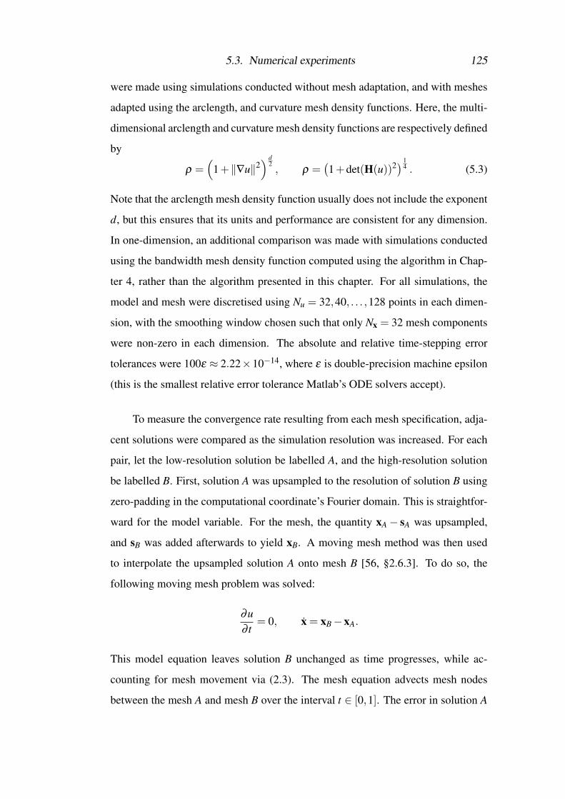
5.3. Numerical experiments 125
were made using simulations conducted without mesh adaptation, and with meshes
adapted using the arclength, and curvature mesh density functions. Here, the multi-
dimensional arclength and curvature mesh density functions are respectively defined
by
ρ =(
1+‖∇u‖2) d
2, ρ =
(1+det(H(u))2) 1
4 . (5.3)
Note that the arclength mesh density function usually does not include the exponent
d, but this ensures that its units and performance are consistent for any dimension.
In one-dimension, an additional comparison was made with simulations conducted
using the bandwidth mesh density function computed using the algorithm in Chap-
ter 4, rather than the algorithm presented in this chapter. For all simulations, the
model and mesh were discretised using Nu = 32,40, . . . ,128 points in each dimen-
sion, with the smoothing window chosen such that only Nx = 32 mesh components
were non-zero in each dimension. The absolute and relative time-stepping error
tolerances were 100ε ≈ 2.22×10⁻¹⁴, where ε is double-precision machine epsilon
(this is the smallest relative error tolerance Matlab’s ODE solvers accept).
To measure the convergence rate resulting from each mesh specification, adja-
cent solutions were compared as the simulation resolution was increased. For each
pair, let the low-resolution solution be labelled A, and the high-resolution solution
be labelled B. First, solution A was upsampled to the resolution of solution B using
zero-padding in the computational coordinate’s Fourier domain. This is straightfor-
ward for the model variable. For the mesh, the quantity xA− sA was upsampled,
and sB was added afterwards to yield xB. A moving mesh method was then used
to interpolate the upsampled solution A onto mesh B [56, §2.6.3]. To do so, the
following moving mesh problem was solved:
∂u∂ t
= 0, x = xB−xA.
This model equation leaves solution B unchanged as time progresses, while ac-
counting for mesh movement via (2.3). The mesh equation advects mesh nodes
between the mesh A and mesh B over the interval t ∈ [0,1]. The error in solution A
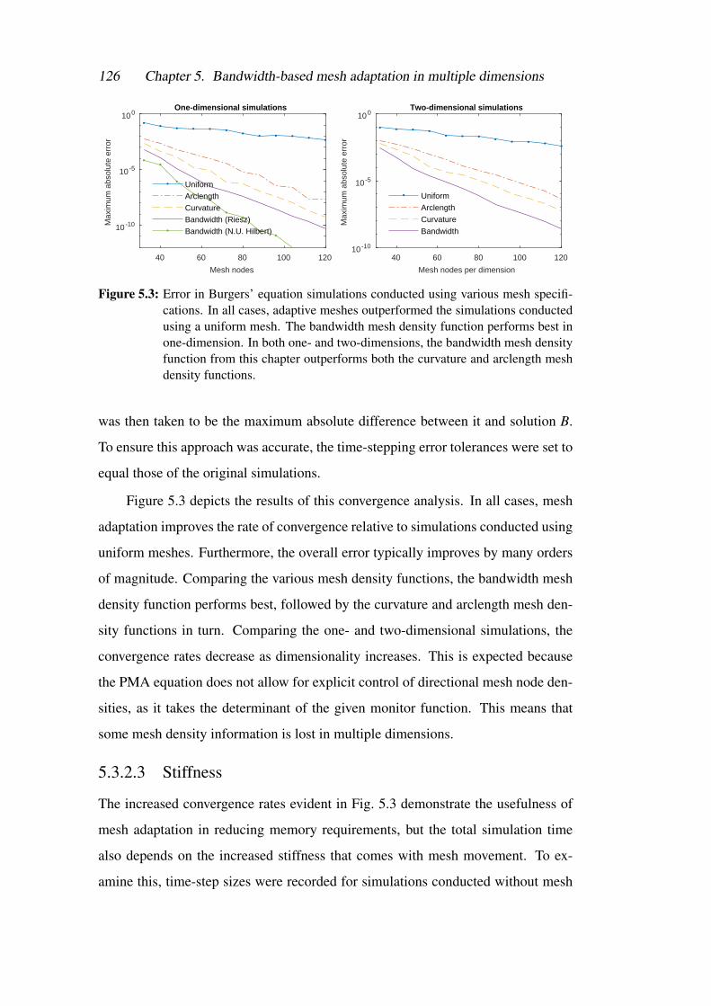
126 Chapter 5. Bandwidth-based mesh adaptation in multiple dimensions
40 60 80 100 120
Mesh nodes
10 -10
10 -5
100M
axim
um a
bsol
ute
erro
rOne-dimensional simulations
Uniform
Arclength
Curvature
Bandwidth (Riesz)
Bandwidth (N.U. Hilbert)
40 60 80 100 120
Mesh nodes per dimension
10 -10
10 -5
100
Max
imum
abs
olut
e er
ror
Two-dimensional simulations
Uniform
Arclength
Curvature
Bandwidth
Figure 5.3: Error in Burgers’ equation simulations conducted using various mesh specifi-cations. In all cases, adaptive meshes outperformed the simulations conductedusing a uniform mesh. The bandwidth mesh density function performs best inone-dimension. In both one- and two-dimensions, the bandwidth mesh densityfunction from this chapter outperforms both the curvature and arclength meshdensity functions.
was then taken to be the maximum absolute difference between it and solution B.
To ensure this approach was accurate, the time-stepping error tolerances were set to
equal those of the original simulations.
Figure 5.3 depicts the results of this convergence analysis. In all cases, mesh
adaptation improves the rate of convergence relative to simulations conducted using
uniform meshes. Furthermore, the overall error typically improves by many orders
of magnitude. Comparing the various mesh density functions, the bandwidth mesh
density function performs best, followed by the curvature and arclength mesh den-
sity functions in turn. Comparing the one- and two-dimensional simulations, the
convergence rates decrease as dimensionality increases. This is expected because
the PMA equation does not allow for explicit control of directional mesh node den-
sities, as it takes the determinant of the given monitor function. This means that
some mesh density information is lost in multiple dimensions.
5.3.2.3 Stiffness
The increased convergence rates evident in Fig. 5.3 demonstrate the usefulness of
mesh adaptation in reducing memory requirements, but the total simulation time
also depends on the increased stiffness that comes with mesh movement. To ex-
amine this, time-step sizes were recorded for simulations conducted without mesh

5.3. Numerical experiments 127
0 0.5 1 1.5 2 2.5
Time
10 -3
10 -2
Tim
e-st
ep s
ize
One-dimensional simulations
Uniform
Arclength
Curvature
Bandwidth (Riesz)
Bandwidth (N.U. Hilbert)
0 0.5 1 1.5 2 2.5
Time
10 -4
10 -3
10 -2
10 -1
Tim
e-st
ep s
ize
Two-dimensional simulations
Uniform
Arclength
Curvature
Bandwidth
Figure 5.4: Time-step sizes for Burgers’ equation simulations conducted using variousmesh specifications. All simulations can be seen to stiffen as the shock frontdevelops.
adaptation, and using the arclength, curvature, and bandwidth mesh density func-
tions. The number of solution components and non-zero mesh components were
Nu = 64 and Nx = 32 in each dimension. The absolute and relative time-stepping er-
ror tolerances were 10−6 in one-dimension, and 10−4 in two-dimensions, with both
chosen to ensure smoothly varying time-step sizes. Figure 5.4 depicts the results
of these simulations. All adaptive meshes stiffen the system of equations beyond
that of the uniform mesh. In the one-dimensional simulations, the bandwidth-based
simulation is stiffest, followed in turn by the curvature- and arclength-based sim-
ulations. In the two-dimensional simulations, the arclength- and bandwidth-based
simulations are not consistently stiffer than one another, but both are stiffer than the
curvature-based simulation.
5.3.3 Results for heterogeneous advection
To illustrate the generality of multidimensional bandwidth-based mesh adaptation,
a two-dimensional simulation for the advection equation is shown in Fig. 5.5. The
initial condition is a shifted version of the von Mises distribution
u(x,0) = exp [cos(x1−π)+ cos(x2)+ cos(x1−π)cos(x2)−3] ,
and the bandwidth mesh density function is used for mesh adaptation. The initial
condition can be seen to compress as it propagates rightwards, forming a sharp

128 Chapter 5. Bandwidth-based mesh adaptation in multiple dimensions
peak. As with Burgers’ equation, a close-up view of the mesh shows anisotropic
adaptation aligned with the sharp peak.
To assess the performance of the multidimensional bandwidth mesh density
function, a convergence analysis like that in §5.3.2.2 was performed. All parameters
were kept the same, only the model equation was changed. The results of this
analysis are presented in Fig. 5.5. Once again, mesh adaptation improved the rate
of convergence relative to simulations conducted using uniform meshes. Comparing
the various mesh density functions, the bandwidth mesh density function performs
best, followed by the arclength and curvature mesh density functions in turn.
5.3.4 Discussion
The convergence and stiffness results in §5.3.2 and §5.3.3 illustrate two aspects of
moving mesh methods. These are that they aim to reduce the trade-off between
accuracy and the number of mesh nodes, but tend to increase the stiffness of the
resulting system of equations. The effect of moving mesh methods on the memory
requirements and computation time of a simulation is more complex, and depends
on problem-specific factors and the hardware that is available for computations.
However, some general statements on the matter can be made. For a given number
of mesh nodes, the memory usage and number of computations per time-step will be
higher for a moving mesh method than a static method. This is because both a model
and mesh equation need to be discretised. Reductions in overall memory usage for
a given level of accuracy must therefore come from an improvement in the rate of
convergence that outweighs this. Improved convergence rates can similarly reduce
the number of computations that are performed per time-step. However, a reduction
in the overall computation time for a simulation then requires this to outweigh any
increase in the number of time-steps that are taken, since moving mesh methods are
typically stiffer than static methods. Note that this discussion is not uniquely appli-
cable to bandwidth-based mesh adaptation. For the Fourier spectral moving mesh
method, the computational complexity of the bandwidth mesh density function is
comparable to that of the arclength and curvature mesh density functions, and so no
additional computational penalty is incurred for its use.

5.3. Numerical experiments 129
40 60 80 100 120Mesh nodes per dimension
10-6
10-4
10-2
100
Max
imum
abs
olut
e er
ror
Two-dimensional simulations
UniformArclengthCurvatureBandwidth
Figure 5.5: (Top-left to bottom-left) Advection equation solutions from simulations con-ducted using the bandwidth mesh density function (5.2). The model and meshresolution were Nu = Nx = 32 in each dimension. (Top-left) Initial conditionand (top-right) final solution for a two-dimensional simulation. (Bottom-left)Close view of the two-dimensional mesh surrounding the shock front region in-dicated in the top-right subplot. Patches are centred on mesh nodes, and colourintensity indicates the determinant of the mesh Jacobian matrix (i.e. the over-all mesh density at that node). Colours alternate between blue and yellow forclarity. The slight vertical distortion in the mesh arises from using fixed (butstill periodic) boundary conditions in the mesh equation. (Bottom-right) Errorin the advection equation simulations conducted using various mesh specifica-tions. In all cases, adaptive meshes outperformed the simulations conductedusing a uniform mesh. The bandwidth mesh density function from this chapteroutperforms both the curvature and arclength mesh density functions. The cur-vature mesh density function failed to produce stable time-stepping for smallvalues of Nu.

130 Chapter 5. Bandwidth-based mesh adaptation in multiple dimensions
To give a sense of what this means in practice, the two-dimensional simulations
from §5.3.2.2 are considered. To achieve an absolute error of approximately 10−3,
the curvature-, arclength-, and bandwidth-based approaches required approximately
7, 10, and 16-times fewer nodes respectively than the static approach. This implies
substantial reductions in memory were achieved, even accounting for the extra sys-
tem of equations that was solved. However, the wall-clock times for the curvature-,
arclength-, and bandwidth-based simulations were 5.3, 1.3, and 1.2-times longer
that of the uniform simulation. This is largely explained by two factors. The first is
the increasing stiffness that comes with mesh adaptation. The number of timesteps
the curvature-, arclength-, and bandwidth-based simulations took were respectively
9.8, 2.9, and 3.0-times those of the static simulation. The second factor is the differ-
ing number of computations that were performed, since an extra system of equations
is solved when the mesh is adaptive.
5.4 Conclusion
In this chapter, bandwidth-based mesh adaptation has been extended to multiple
spatial dimensions. This was achieved by using the Riesz transforms to compute
a monogenic signal from the model solution. This decouples the local amplitude
and phase, after which the bandwidth can be computed using a Fourier-domain
operator. When applied to a viscous Burgers’ equation and a heterogeneous advec-
tion equation, multidimensional bandwidth-based mesh adaptation produced con-
vergence rates which exceeded those arising from arclength- and curvature-based
adaptation by a large margin.
Together, the last two chapters have demonstrated the ability of bandwidth-
based mesh adaptation to improve the performance of the Fourier pseudospectral
method in a range of contexts. However, up until this point only initial value prob-
lems have been solved. In the context of HIFU, acoustic sources must also be
included. This can be problematic when uniform meshes are used, as sources are
often non-planar and do not conform to orthogonal grids. When meshes are mobile,
an extra challenge arises as the source discretisation must change over time. The

5.4. Conclusion 131
next chapter solves this problem. It presents a method for accurately representing
arbitrary acoustic source distributions in Fourier pseudospectral methods, for both
uniform and nonuniform meshes.


Chapter 6
Representing arbitrary acoustic
source distributions
In the preceding three chapters, techniques for mesh adaptation have been discussed
and demonstrated. These demonstrations have only considered initial value prob-
lems, but many problems require the introduction of source terms as well. For nu-
merical methods which use unstructured meshes, such as the finite element method,
mesh nodes can be chosen such that they align with the source geometry. This gives
such methods a significant advantage over methods with structured meshes, such as
the Fourier pseudospectral method. Here, mesh nodes close to the required source
surface are typically defined as source points, but this can result in ‘staircasing’ and
serious errors in the acoustic field [81].
In the context of mesh adaptation, source terms are even more problematic.
Here, constraints would need to be placed on the mesh node trajectories to ensure
that source points remain fixed on the source geometry. An alternative approach is
to discretise source terms in a way that does not rely on grid nodes coinciding with
the source. Considering the case of a singular point source (i.e. a delta function) at
an arbitrary location, there are a number of examples in the literature. Walden [107]
approximated one-dimensional delta functions within finite-difference and finite-
element methods using compactly supported functions that satisfied some number
of moment conditions. Similarly, Tornberg and Engquist [95] did this for the finite-
difference method in the multidimensional case. Petersson et al. [76] note that

134 Chapter 6. Representing arbitrary acoustic source distributions
source discretisations that only satisfy moment conditions will introduce spurious
oscillations, and so add a number of smoothness conditions to their delta function
approximations.
In a similar manner, this chapter describes a method for representing arbitrary
source distributions within Fourier pseudospectral methods. This representation is
based on a convolution between the source distribution and the band-limited delta
function. The resulting source discretisations are examined using a range of ex-
amples relevant to problems in ultrasound. Much of this chapter is dedicated to
describing and validating the source discretisation algorithm in the context of uni-
form meshes (hence the term ‘grids’ will be used throughout), but these techniques
are equally applicable with nonuniform meshes as well. This is explained at the end
of this chapter, in §6.5.
6.1 Band-limiting source distributions
6.1.1 Background
Consider the homogeneous, linear wave equation
(1c2
0
∂ 2
∂ t2 −∇2)
p(x, t) = S(x, t). (6.1)
Here, the source term S(x, t) can, in many cases, be separated into a spatial distri-
bution and a temporal waveform
S(x, t) = g(x) f (t).
When solved with a Fourier pseudospectral method, the approximate solution to
(6.1) has a clear physical interpretation: the spatial part of it must be in the set Bof functions that are supported by the discrete set of wavenumbers (1.3), which are
determined by the computational grid spacing. This leads to the question: How
can a source be incorporated if it is not band-limited, i.e. g(x) /∈ B? For example,
consider a source distribution corresponding to the surface of a physical ultrasound
transducer, which may be a bowl or a planar disc. In this case, the support of

6.1. Band-limiting source distributions 135
the source supp(g)—the region in which g(x) is non-zero—is a two-dimensional
surface embedded in R3 and is therefore not band-limited. Furthermore, it is likely
that few, if any, grid points coincide exactly with this surface. This highlights a
related problem: As the source in a collocation method can only be defined by
assigning values at the grid points x j, which of the grid points should be used as
source points, and what should the source grid weights g j be to best approximate
the source distribution g(x)? Progress can be made by realising that the closest
approximation to a source that can be made within a Fourier pseudospectral method
is the projection of the source distribution onto the set of band-limited functions B.
Thus, a band-limited source distribution can be defined, and the source grid weights
can be generated by sampling this distribution at the grid points.
6.1.2 Band-limiting via convolution
Any source can be written as a convolution of the source distribution function with
a point source. Let δ (x;ξξξ ) denote a delta function centred on a point ξξξ . Then the
spatial distribution of the source is, trivially
g(x) =∫
supp(g)δ (x;ξξξ )g(ξξξ )dξξξ .
To band-limit this source, the delta function δ /∈B should be replaced with its band-
limited version b ∈ B, which is the projection of δ onto B. This gives
g(x) =∫
supp(g)b(x;ξξξ )g(ξξξ )dξξξ ,
where g(x) is the band-limited source distribution. In the general case this convo-
lution cannot be solved exactly, and so it must be numerically approximated. This
can be done by replacing the integral with a discrete sum
g j =M
∑i=1
Cib(x j;ξξξ i)g(ξξξ i), (6.2)
where i are a set of M indices, Ci are quadrature weights, and ξξξ i are integration
points. Computing this discrete convolution involves two main tasks. First, an an-

136 Chapter 6. Representing arbitrary acoustic source distributions
Figure 6.1: An arbitrary source distribution. The region of support supp(g) is indicated inblue, and potential integration points ξξξ i for (6.2) are indicated with black dots.The background grid represents the discretised domain, with grid points x j atthe intersection of grid lines.
alytical expression is required for the band-limited approximant b(x;ξξξ ) to a Dirac
delta function centred at an arbitrary point ξξξ . Second, a strategy is needed for
effectively and efficiently discretising the convolution. This involves choosing dis-
crete integration points ξξξ i covering supp(g), and selecting corresponding quadrature
weights Ci.
6.1.3 The band-limited delta function
6.1.3.1 The delta function in Fourier-space
The one-dimensional delta function (positioned at the origin) has a Fourier trans-
form which is equal to one for all wavenumbers. However, recall that in Fourier
pseudospectral methods the wavenumbers are restricted to a finite set, given by
(1.3). It follows then that the band-limited approximation to a delta function is the
function whose Fourier transform is equal to one for all supported wavenumbers,
and equal to zero for all others. To translate the band-limited delta function to an
arbitrary position, a Fourier-space shifting operator can be applied. The following

6.1. Band-limiting source distributions 137
subsections do so for both odd and even N.
6.1.3.2 Odd number of grid nodes
To begin with, consider a one-dimensional grid in which the number of grid points
N is odd. In Fourier-space, the band-limited delta function is then simply given by
the shift operator
b(k j;ξ ) = e−ik jξ .
To get an expression for b(x;ξ ), the Fourier series is evaluated:
b(x;ξ ) =1N
n
∑j=−n
eik j(x−ξ ).
The imaginary components in this sum cancel because of conjugate symmetry about
j = 0
b(x;ξ ) =1N
(1+2
n
∑j=1
cos(k j(x−ξ ))
),
and the series simplifies to yield
b(x;ξ ) =sin(
π(x−ξ )∆x
)N sin
(π(x−ξ )
N∆x
) . (6.3)
A scaled version of this function is often referred to as the Dirichlet kernel, appear-
ing in many texts including [47, p. 156].
6.1.3.3 Even number of grid nodes
If the number of grid points N is even, further steps are required. As a real-valued
point source should have a real-valued representation on the grid, the Fourier co-
efficients of the band-limited delta function must be conjugate symmetric. For the
odd case, this was not an issue because the wavenumber set defined in (1.3) is sym-
metric. For the even case, it contains a negative Nyquist term with no positive
counterpart. This gives the Fourier series
b(x;ξ ) =1N
n−1
∑j=−n
eik j(x−ξ ),

138 Chapter 6. Representing arbitrary acoustic source distributions
which is not conjugate symmetric about j = 0. Now, let b′(x;ξ ) be the band-limited
delta function that would be derived from the shift operator without conjugate sym-
metry. In Fourier-space, this is given by
b′(k j;ξ ) = e−ik jξ ,
for which the Fourier series sums to [99]
b′(x;ξ ) =1N
sin(−k−n(x−ξ ))
tan(−k−n(x−ξ )
N
) + isin(−k−n(x−ξ ))
.
To ensure conjugate symmetry, an additional term f (x;ξ ) is required so that
b(k;ξ ) =
cos(k jξ ) if j =−n,
e−ik jξ otherwise,
where b = b′+ f . Comparing the Nyquist terms for b′ and b, the additional term
can be seen to be
f (k;ξ ) =
isin(k jξ ) if j =−n,
0 otherwise,
for which
f (x;ξ ) =1N
isin(k−nξ )eik−nx
=1N
isin(k−nξ )(cos(k−nx)+ isin(k−nx))
=1N
sin(k−nξ )(icos(k−nx)− sin(k−nx))
Starting with the real components, adding f to b′ yields
Reb= Reb′+Re f
=1N
sin(−k−n(x−ξ ))
tan(−k−n(x−ξ )
N
) − sin(k−nξ )sin(k−nx)

6.1. Band-limiting source distributions 139
Now, the imaginary component of b′ is
Imb′= 1N
sin(−k−n(x−ξ )),
which can be expanded using the trigonometric product-to-sum identities
Imb′= 1N(sin(−k−nx)cos(k−nξ )− cos(−k−nx)sin(k−nξ )) ,
and rearranged to yield
Imb′= 1N(cos(k−nξ )sin(−k−nx)− sin(k−nξ )cos(−k−nx)) .
Noting that cos(−k−nx) = cos(k−nx), the second term in this expression can be seen
to be negated by the imaginary component of f
Im f= 1N
sin(k−nξ )cos(k−nx),
and hence it is clear that
Imb= 1N
cos(k−nξ )sin(−k−nx).
Finally, combining the real and imaginary components and substituting the
wavenumbers in (1.3) yields
b(x;ξ ) =1N
sin(
π(x−ξ )∆x
)tan(
π(x−ξ )N∆x
) − sin(
πξ
∆x
)sin(
πx∆x
)+ icos
(πξ
∆x
)sin(
πx∆x
) .
(6.4)
The last two terms in this expression are zero at all grid points regardless of the
shift ξ . For a shift that is a multiple of the grid node spacing ∆x, they are also
zero between the grid points. In this case, the expression matches that derived
by Trefethen [103, p. 20] using a modified Fourier series that treats wavenumbers
symmetrically. Note that b(x;ξ ) 6= b(x− ξ ) in the even case, except when ξ is a

140 Chapter 6. Representing arbitrary acoustic source distributions
Figure 6.2: Illustration of the band-limited delta functions (6.3) and (6.4) derived in §6.1.3.Band-limited delta function with an odd number of samples (top), and an evennumber of samples (middle). (Bottom) Band-limited delta functions with aneven number of samples, shifted in space.
multiple of ∆x.
6.1.3.4 Remarks
Figure 6.2 depicts the odd and even (real component only) band-limited delta
functions (6.3) and (6.4). The odd band-limited delta function is shift-invariant,
and so has only been depicted once. The even band-limited delta function is not
shift-invariant, and can be seen to have an extra Nyquist sinusoid whose ampli-
tude depends on the shift distance. Note that the band-limited delta functions can
be extended into higher dimensions via a tensor product. For example, in three-
dimensions it is given by
b(x;ξξξ ) = b(x1;ξ1)⊗b(x2;ξ2)⊗b(x3;ξ3),
where the subscript indicates the dimensional component.
6.1.4 Discretisation of the band-limiting convolution
Discretisation of the band-limiting convolution in (6.2) requires a number of steps.
First is the selection of a finite number of integration points ξξξ i. In general, these

6.1. Band-limiting source distributions 141
should be placed according to a given quadrature rule. In this chapter, a uniform
sampling strategy is used, with the spacing between integration points being ap-
proximately equal, and the outermost integration points offset from the source’s
boundary. To avoid staircasing effects, integration points are placed such that they
also conform to the source’s boundary, rather than to the computational grid.
Second, the quadrature weights Ci must be chosen. These account for any
difference in the spacing of the integration points relative to the grid spacing, and are
all equal with a uniform sampling strategy. As an example, for a two-dimensional
source embedded in a three-dimensional domain, the quadrature weights are given
by
Ci =Mon
Moff, Mon =
A(∆x)2 ,
where A is the area of supp(g), Mon is the (generally non-integer) number of grid
squares that cover the source, and Moff is the number of integration points that has
been used. Note that the number of integration points will be measured relative
to the grid in this chapter. The phrase ‘integration point density’ will refer to the
ratio Moff/Mon, and a source will be referred to as upsampled if Moff/Mon > 1 and
undersampled if Moff/Mon < 1.
6.1.5 Truncation of source grid weights
A set of grid points x j must be chosen over which the band-limited source is evalu-
ated to give source grid weights g j = g(x j). In principle, every grid point should be
used because band-limiting means that supp(g) =Rd where d is the number of spa-
tial dimensions (a function with compact support in the spatial frequency domain
will have infinite support in the spatial domain, and vice versa). However, it can
be computationally beneficial to restrict the discretised source to grid points which
lie near supp(g) as this limits the number of band-limited delta function evaluations
and subsequent memory requirements for source grid weights. To see why the num-
ber of grid points used can be considerably reduced without introducing substantial
errors, note that for a large domain size the band-limited delta functions (6.3) and

142 Chapter 6. Representing arbitrary acoustic source distributions
101 102 103
Domain size N
10-4
10-3
10-2
10-1
100
Err
or (
L-n
orm
)
OddEven
Figure 6.3: Maximum error in approximating the band-limited delta functions with a sincfunction (based on a shift distance of ξ = ∆x/2). The sinc approximation con-verges algebraically with the domain size, and reaches 1% error when the gridsize reaches approximately 100 grid points.
(6.4) can be approximated by a sinc function
b(x;ξ )≈ sinc(
π(x−ξ )
∆x
). (6.5)
Figure 6.3 illustrates the accuracy of this approximation as N increases for a shift
distance of ξ = ∆x/2. It can be seen that the error drops below 1% when the grid
size reaches approximately 100 grid points.
The envelope of the sinc approximation decays at a rate of approximately
∆x/π|x− ξ |, thus a magnitude threshold can be defined beyond which contribu-
tions from a given integration point can be ignored. Denoting this threshold ε , a
given band-limited delta function thus only needs to be evaluated to
m =
⌈1
πε
⌉
grid points on either side of the integration point’s centre ξi. For example, with
ε = 10% each band-limited delta function needs to be evaluated to a distance of
only m = 4 grid points, and for ε = 1% this becomes m = 32 grid points. Note that
in multiple dimensions the benefit of truncation compounds, as diagonal decay rates
are higher than those along the grid axes. The benefit of truncation also increases

6.2. Numerical experiments 143
10%
1%
0.1%
-30 -20 -10 0 10 20 30y-index [nodes]
-30
-20
-10
0
10
20
30
x-in
dex
[nod
es]
Figure 6.4: The truncation distance for a two-dimensional domain beyond which the mag-nitude of sinc approximations to band-limited delta functions decay below var-ious tolerances.
with domain size, as the truncation distance m is independent of this. To illustrate
the reduction in extent that this provides, Fig. 6.4 depicts the distance at which these
thresholds lie in two dimensions.
Without truncating the source grid weights, the source discretisation is equal to
the bandlimited source g(x). However, when fewer source grid weights are used, it
is no longer true that the resulting off-grid source is the optimal choice, and an alter-
native choice for the source grid weights might be closer to g(x) in some sense (such
as in a least-squares sense). However, to be of practical use it would be necessary
to devise a computationally efficient method to find such source grid weights.
6.2 Numerical experiments
6.2.1 Terminology and simulation codes
If the integration points are restricted to the grid points, the resulting approxima-
tion will be called an on-grid source. When the integration points are allowed to
lie anywhere, the resulting approximation will be called an off-grid source. On-

144 Chapter 6. Representing arbitrary acoustic source distributions
grid sources will often be subject to staircasing effects, and the errors that result
from this. In the following subsections, both on- and off-grid sources are compared
numerically through application to problems in ultrasound.
To solve these problems, two Fourier pseudospectral methods are used. The
first is the Acoustic Field Propagator (AFP) [97], which can solve time-harmonic
wave problems in the form of (6.1). The second is k-Wave [98], which is not re-
stricted to time-harmonic problems and uses a dispersion-corrected finite-difference
scheme for time-stepping. The AFP and k-Wave give solutions that match to a high
degree of accuracy.
6.2.2 Example source discretisations
To illustrate the source discretisation procedure, Fig. 6.5 depicts distributions of
integration points for three different sources:
1. (Top-left) An on-grid approximation to an arc source is shown to illustrate the
effects of staircasing. Here, the integration points have been restricted to the
grid points, and are thus misaligned with the true source.
2. (Top-right) A staircase-free, off-grid arc source. The integration points are
spread equally over an arc, with the end-points offset from the ends of the
source by half the inter-point spacing. The integration point spacing is ap-
proximately half that of the grid spacing.
3. (Bottom-left) A disc source. The integration points have been chosen as con-
centric circles whose number increases algebraically with radius. This en-
sures all points are approximately equidistant from their neighbours. Once
again the outermost points are offset from the edge of the source to ensure
uniform sampling, and the integration point spacing is approximately half
that of the grid spacing.
4. (Bottom-right) A square source that is not aligned with the grid. Here the
integration points form a regular grid, but one which is aligned with the
source boundaries rather than the computational grid. Once again the out-

6.2. Numerical experiments 145
Figure 6.5: Examples of on- and off-grid integration point distributions in two-dimensions.(Top-left) A staircased arc. (Top-right to bottom-right) An evenly sampled cir-cular arc, disc, and square. Black dots indicate integration points, red linesindicate each source’s region of support. The background grid represents thediscretised domain. The off-grid integration points can be seen to uniformlycover and conform to the regions of support for their respective sources.
ermost points are offset from the edge of the source, and the integration point
spacing is approximately half that of the grid spacing.
6.2.3 Illustration and correction of staircasing errors
To demonstrate the elimination of staircasing errors using off-grid sources, a line
source was simulated in two dimensions using the AFP. This source was placed
a fixed distance from a sensor position, and emitted a continuous sinusoidal pres-
sure waveform. The source was rotated around the sensor and the acoustic field
was computed for each rotation angle. Both on- and off-grid sources were used.
For the off-grid approach, source grid weights were calculated using an integration
point spacing that was half that of the grid spacing, and were based on the exact,
untruncated band-limited delta functions.
Figure 6.6 depicts the steady-state amplitude of the pressure field generated
by the line source at an angle of 30. The on-grid source produces considerable

146 Chapter 6. Representing arbitrary acoustic source distributions
-2 0 2y-position [m]
-3
-2
-1
0
1
2
3
x-po
sitio
n [m
]
-2 0 2y-position [m]
-3
-2
-1
0
1
2
3
x-po
sitio
n [m
]
Figure 6.6: Steady-state acoustic pressure amplitude generated by a line source in twodimensions. The integration points are indicated with red dots, and the locationof a sensor is indicated with a red circle. Phase errors are evident in the near-field generated by an on-grid source (top). These errors are not present in thefield generated by an off-grid source (bottom).
staircasing errors. Of particular note is the irregular interference pattern in the near-
field, caused by phase errors resulting from shifting integration points to nearby grid
points. In contrast, the field generated with an off-grid source shows no evidence of
staircasing errors.
Figure 6.7 depicts time-domain data recorded at the sensor for each angle.
Phase errors are evident in the shifted waveforms produced by the on-grid source,
and an angular dependence is seen in their amplitude due to the larger spacing be-
tween on-grid integration points as the source becomes diagonal to the grid. In
contrast, the off-grid source produces consistent waveforms regardless of the orien-

6.2. Numerical experiments 147
0 0.05 0.1 0.15 0.2 0.25Time [s]
0
10
20
30
40O
rient
atio
n [d
eg]
0 0.05 0.1 0.15 0.2 0.25Time [s]
0
10
20
30
40
Orie
ntat
ion
[deg
]
Figure 6.7: Waveforms recorded at the sensor for the rotating line source simulation de-picted in Fig. 6.6. Phase errors are again evident with an on-grid source (top),and eliminated with an off-grid source (bottom). Amplitude errors are also evi-dent for the on-grid source, with the amplitude reducing as the source becomesdiagonal to the grid due to the larger spacing between integration points.
tation of the source relative to the grid.
6.2.4 Convergence for a circular piston
As mentioned in §6.1.4, the integration points that are used to discretise the band-
limiting convolution need not be chosen with the same spacing as the grid points.
To investigate the spacing requirements, a circular piston was simulated. The piston
diameter was 20 mm, and the driving waveform was a 1 MHz sinusoid. The sound
speed was 1500 ms−1. The wavefield was computed using the AFP to a distance of
50 mm, at spatial resolutions of 3, 5, and 7 points per wavelength (PPW). The source
grid weights were computed using exact, untruncated band-limited delta functions
centred on points like those of the disc source in Fig. 6.5. The source was positioned
such that it aligned with the grid along the axial direction. An analytical reference
solution given by Pierce [77, p. 232] was used for the axial pressure.

148 Chapter 6. Representing arbitrary acoustic source distributions
-20 -15 -10 -5 0 5 10 15 20x-position [mm]
-10
-5
0
5
10
y-po
sitio
n [m
m]
10-1 100 101
Integration point density relative to grid spacing
10-3
10-2
10-1
100
101
Rel
ativ
e am
plitu
de e
rror
(on
-axi
s)
3 PPW5 PPW7 PPW
Figure 6.8: (Top) Steady-state acoustic pressure amplitude (central plane) generated bya circular piston. (Bottom) Convergence of the on-axis pressure generated byoff-grid sources with a varying integration point spacing (relative to the gridspacing), and varying spatial grid resolutions (PPW). The errors converge al-gebraically, with less than 2% error achieved for all three PPWs when the inte-gration point density is approximately 4× that of the grid points.
Figure 6.8 depicts the relative L∞ error in the maximum axial pressure with a
varying integration point spacing for the off-grid sources. The error can be seen to
converge algebraically with an increasing integration point sampling rate, with less
than 2% error achieved for all three PPWs at an upsampling rate of approximately
Moff/Mon = 4. This corresponds to an integration point spacing that is half that of
the grid spacing, since the source is a two-dimensional surface.
6.2.5 Convergence for a focussed bowl source
To demonstrate the convergence of the band-limited source distribution on the true
source distribution as the grid resolution increases, a focussed bowl source was
simulated. This source geometry is especially prone to staircasing errors, as it is

6.2. Numerical experiments 149
impossible to align any portion of it with an orthogonal grid [66]. The bowl had
an aperture diameter of 20 mm, a radius of curvature of 20 mm, and was driven
by a 1 MHz sinusoid. The sound speed was set to 1500 ms−1. The wavefield was
computed with the AFP to a distance of 47 mm, using a varying number of PPW for
the grid spacing. The off-grid sources used integration points that were generated
with a spiral phyllotaxis pattern (this can produce uniform samples covering any
surface of revolution). A reference solution was given by O’Neil [74] for the axial
pressure (ignoring the first two wavelengths, as these fall behind the bowl’s aperture
plane where the reference solution is inaccurate). This reference is valid when the
transducer diameter is large compared to both the transducer height and the acoustic
wavelength, as is the case here.
Figure 6.9 depicts the convergence of the relative L∞ error in the maximum ax-
ial pressure with an increasing number of PPW, for three different source discretisa-
tions. The on-grid source converges slowly and produces considerably higher errors
than either off-grid source. Indeed, it is known that this error will not converge to
zero, because diagonally-aligned portions of the source will be undersampled and
hence produce lower amplitudes than they should [66]. The off-grid sources used
exact, untruncated band-limited delta functions. They differed in their density of
integration points relative to the grid points, with one being undersampled (0.25×)
and one being upsampled (4×). The errors resulting from an undersampled off-
grid source are considerably worse than those produced by an upsampled off-grid
source, but are nonetheless much better than those resulting from an on-grid source.
The errors resulting from both off-grid sources will also converge to zero as the
PPW increases, unlike those resulting from an on-grid source. The upsampled off-
grid source converges much more quickly than the others, dropping below 0.3%
relative error with only 3 PPW.
To clarify the character of the errors in the field, Fig. 6.10 is provided. It de-
picts the maximum axial pressure from solutions obtained using the various sources
at 3 PPW. The top subplot shows the reference solution and the solution obtained
using an on-grid source. The amplitude is substantially underestimated at the focus

150 Chapter 6. Representing arbitrary acoustic source distributions
-20 -10 0 10 20x-position [mm]
-10
-5
0
5
10
y-po
sitio
n [m
m]
2 3 4 5 6 7Grid spacing (PPW)
10-4
10-3
10-2
10-1
100
101
Rel
ativ
e am
plitu
de e
rror
(on
-axi
s)
On-gridOff-grid (exact, 0.25 )Off-grid (exact, 4 )
Figure 6.9: (Top) Steady-state acoustic pressure amplitude (central plane) generated by afocussed bowl source. (Bottom) Convergence of the on-axis pressure generatedby on- and off-grid (under- and upsampled) sources with a varying spatial gridresolution (PPW). The error resulting from an on-grid source is high, and doesnot converge to zero. The errors resulting from off-grid sources are much lower,with the error from the upsampled off-grid source dropping below 0.3% withonly 3 PPW.
due to the undersampling of portions of the source which are diagonally-aligned
with the grid. In the near-field some pressures are also overestimated, likely due
to phase errors, and there is a misalignment of the null points. In contrast, the un-
dersampled off-grid source produces pressures which are visually indistiguishable
from the reference solution in the far-field, and produces very small errors in the
near-field. To show this in more detail, the bottom subplot depicts the relative error
for undersampled and upsampled off-grid sources. It can be seen that the errors for
both off-grid sources are greatest in the near-field, and that the pressure resulting
from the upsampled off-grid source oscillates about the reference solution. The er-
ror arising from the undersampled off-grid source also oscillates but with an offset

6.2. Numerical experiments 151
0 10 20 30 40x-position [mm] (relative to bowl)
0
2
4
6
8
10
12
Am
plitu
de [M
Pa]
ReferenceOn-gridOff-grid (exact, 0.25 )
0 10 20 30 40x-position [mm] (relative to bowl)
-0.015
-0.01
-0.005
0
0.005
0.01
0.015
Rel
ativ
e am
plitu
de e
rror
(on
-axi
s)
Off-grid (exact, 0.25 )Off-grid (exact, 4 )
Figure 6.10: (Top) On-axis pressure generated by an on-grid discretisation of a focussedbowl source, compared with an analytical reference solution. A large ampli-tude error is evident, with the far-field underestimated and the near-field partlyoverestimated. There is also a misalignment of the null points in the near-field.The undersampled off-grid source shows only a small amount of error in thenear-field, and is visually indistiguishable from the reference solution in thefar-field. (Bottom) Error in the on-axis pressure generated by off-grid sources.These errors are very low when compared with the on-grid source (top), withboth under- and upsampled off-grid sources having greater errors in the nearfield than the far-field.
from zero, indicating a misalignment of the two solutions.
Finally, to examine the use of the sinc approximation (6.5) to the band-limited
delta functions, and in particular to determine an appropriate truncation threshold
ε , the focussed bowl simulations above were repeated using a number of sinc-based
off-grid sources. The results of this comparison are shown in Fig. 6.11. The ex-
act band-limited delta functions and untruncated sinc approximation can be seen

152 Chapter 6. Representing arbitrary acoustic source distributions
2 3 4 5 6 7Grid spacing (PPW)
10-4
10-3
10-2
10-1
Rel
ativ
e am
plitu
de e
rror
(on
-axi
s)
Off-grid (exact, 4 )Off-grid (sinc, 4 )Off-grid (sinc, 4 , =10%)Off-grid (sinc, 4 , =1%)
Figure 6.11: Effect of using a truncated sinc approximation to the band-limited delta func-tion on the error in the on-axis pressure amplitude generated by an off-gridfocussed bowl source. The domain size is evidently large enough that thesinc function is an accurate approximation, and a truncation threshold of 1%ensures the error drops below 1% by 3 PPW and reaches 0.2% by 7 PPW.
to produce nearly identical levels of error. This is expected, as the domain size
is large enough that the sinc approximation is accurate (all dimensions had more
than 100 grid points). With a truncation threshold, the error resulting from sinc
approximations is considerably higher than produced by exact band-limited delta
functions. However, at ε = 1% the error drops below 1% by 3 PPW and reaches
0.2% by 7 PPW. To give a sense of the difference in compute times between these
source discretisations, the time taken to compute source grid weights was recorded.1
At 2 PPW, it took approximately the same time to generate a source using an un-
truncated sinc approximation as it did using the exact band-limited delta function.
However, with ε = 1% this computation was around 9× faster, and with ε = 10%
it was around 130× faster. At 7 PPW these advantages become 326× and 4760×respectively, demonstrating that the computational benefit improves with domain
size, as expected.
1This experiment was performed on a desktop computer without significant optimisations in thesource discretisation algorithms.

6.3. Discussion 153
6.3 Discussion
6.3.1 Acoustic interpretation of integration points
An alternative viewpoint on the source discretisation procedure described in this
chapter can be had by reinterpreting the discrete source convolution (6.2) in terms of
Huygens–Fresnel principle. Instead of considering each point ξξξ i to be an integration
point, it can be considered as the location of a point source emitting the desired
waveform. The task of source discretisation is then to define a weighted collection
of off-grid point sources that cover the true source. This interpretation also gives
some insight into the required number of integration points since, as the number of
point sources increases, the Huygens-Fresnel principle becomes better satisfied. It
may also explain why errors are greatest in the near field: When a finite number
of integration points are used, it will take some distance before spherical spreading
causes the individual point source wavefronts to merge.
6.3.2 Integration scheme
Turning to the results in §6.2, one analysis that was not included in this chapter was
an investigation into the convergence rate of the source grid weights as the density
of integration points increased. Instead, the convergence of the resulting acoustic
field was examined. This choice reflects the fact that it is the acoustic field that is
ultimately of consequence when discretising a source term. Through this analysis,
it was seen that an integration point density that is 4× that of the grid points appears
to work well in practice, but there may be circumstances in which this rule of thumb
is inappropriate. It may then be beneficial to use nonuniform or adaptive sampling
schemes to ensure that the band-limiting source convolution is solved to a specified
level of accuracy prior to the generation of source grid weights.
6.3.3 Memory requirements for source grid weights
One aspect of the proposed source discretisation method that warrants further dis-
cussion is its computational expense. Specifically, off-grid source discretisations
have a wider region of support than on-grid discretisations, meaning memory re-
quirements may become problematic. While it has already been said that the use

154 Chapter 6. Representing arbitrary acoustic source distributions
of a truncated sinc approximations to band-limited delta functions provides sub-
stantial computational savings by reducing both the number of evaluation points
and the subsequent number of source grid weights, there are implementations that
may complement this in certain circumstances. The most obvious is that source
grid weights need not be computed in advance, and instead can be added to the
pressure field on-the-fly (and in parallel if the computer hardware supports this).
In addition, a middle-ground between on-the-fly computation and full precomputa-
tion is possible: Because each band-limited delta function can be decomposed into
a separable product across the spatial dimensions, the corresponding source grid
weights can be stored as a set of vectors, one for each dimension. For Np integra-
tion points in a three-dimensional simulation, the overall memory required is then
O(Np(Nx +Ny +Nz)), which will typically be less than the O(NxNyNz) required for
a fully precomputed set of source grid weights. To reconstruct the full set of source
grid weights from the set of vectors, a tensor product must be performed for each in-
tegration point, followed by a sum over all of the integration points. This approach
also allows one-off, precomputation of expensive trigonometric operations (to com-
pute each integration point’s vector set), and subsequent element-wise elementary
arithmetic at each time-step to reassemble the full set of source grid weights.
6.4 Extension to other problems
6.4.1 Application to moving sources
This chapter has considered acoustic sources which are fixed in space, and which
can be separated into a product S(x, t) = g(x) f (t). However, moving sources also
prove problematic when discretised using on-grid integration points, as the source
is not guaranteed to align with the grid at arbitrary times. To accommodate such
sources within a time-stepping scheme, they can be thought of as a series of station-
ary sources separately defined for each time-step. This allows the off-grid source
discretisation procedure to be applied. To demonstrate such a scenario, a moving
point source was simulated in one dimension using k-Wave. The source was dis-
cretised using a series of off-grid points corresponding to the location of the source

6.4. Extension to other problems 155
0 0.5 1 1.5 2Frequency [MHz]
0
0.2
0.4
0.6
0.8
1
1.2
Am
plitu
de [P
a]
Figure 6.12: Illustration of the Doppler effect for a moving point source in one dimension.(Top) The simulation setup. The start- and end-points of the source trajectoryare indicated with circles, and the red cross indicates the location of the sen-sor. (Bottom) Spectra computed from the recorded signal as the point sourceapproached (red) and retreated (blue) from the sensor. The simulated spectra(solid lines) match the expected Doppler-shifted frequencies (dashed lines).
at each time-step. The domain size was 200 mm, and the sound-speed was set to
1500 ms−1. The point source moved from one side of the domain to the other at
400 ms−1, emitting a 1 MHz sinusoid as it travelled. The simulation was resolved
at 10 PPW relative to the source frequency, and the time-stepping algorithm used a
Courant–Friedrichs–Lewy number of 0.1. This resulted in the point source moving
by 4 µm per time-step, or ∆x/37.5. The resulting waveform was recorded at a sen-
sor half-way along the source’s trajectory, and the frequency spectra on its approach
and retreat were computed. Figure 6.12 depicts these spectra. A sharp peak appears
in each at the expected Doppler-shifted frequencies, along with a corresponding
amplitude change.
6.4.2 Application to distributed sensors
Another application this work can be extended to is the modelling of acoustic sen-
sors. To do so, the source (now sensor) grid weights g j should be used as quadrature
weights. For example, if the sensor is a two-dimensional surface with area A, then

156 Chapter 6. Representing arbitrary acoustic source distributions
the average pressure over the sensor is given by
psensor =∆x2
A ∑j
p jg j,
where p j are the pressure values on the grid. Medical ultrasound has many examples
where this application is important, as the same transducers are often used as both
sources and sensors. Note that the sensor distribution g(x) encodes the sensitivity
of the sensor, and can be used to model spatially varying sensitivities, or to convert
between units such as pressure and voltage. If a simple average of the field variable
is desired, then g(x) should be made equal to one over its region of support.
To illustrate the elimination of staircasing errors using off-grid sensors, a line
sensor was simulated in two dimensions using the AFP. This sensor was placed
in the path of a continuous plane wave, and the average pressure over the sensor
was computed for a number of orientation angles. This experiment measures the
sensor’s directivity, or directional sensitivity. Both on- and off-grid sensors were
used. For the off-grid sensor, grid weights were calculated using an integration
point spacing that was half that of the grid spacing, and were based on the exact,
untruncated band-limited delta functions. Note that the centre of the sensor lay
on a grid point, so that the on-grid sensor was aligned with the grid whenever the
orientation angle was a multiple of π/2. Additionally, the length of the sensor was
a multiple of the grid spacing.
Figure 6.13 depicts the normalised pressure recorded at multiple orientation
angles. The directivity of the on-grid sensor exhibits considerable staircasing er-
rors, as multiple orientations produce the same sensor grid weights. Pressures were
overestimated, even when the on-grid sensor was aligned with the grid. This occurs
because both end-points are included in the sensor’s discretisation, meaning its ef-
fective length is greater than it should be. In contrast, the directivity of the off-grid
sensor shows no evidence of staircasing errors, and matches the reference solution
given by Blackstock [12, pp. 504–505].

6.4. Extension to other problems 157
-80 -60 -40 -20 0 20 40 60 80Orientation [deg]
-0.4
-0.2
0
0.2
0.4
0.6
0.8
1
1.2
Nor
mal
ised
ave
rage
pre
ssur
e
ReferenceOn-gridOff-grid
Figure 6.13: Directivity of a line sensor in two-dimensions. Staircasing errors are evidentwith on-grid sensor, whereas an off-grid sensor matches the reference solu-tion.
6.4.3 Enforcing boundary conditions
In addition to sources, boundary conditions are a significant area of inflexibility for
Fourier pseudospectral methods. Typically, only periodic boundary conditions are
used, and often absorbing layers are added at the edges of the computational domain
to approximate free-field conditions. Reflective boundaries are also possible at the
edge of the domain if discrete Fourier transforms are replaced with discrete sine or
cosine transforms. However, interior reflective boundaries are also desirable, for
instance when modelling bones or air in medical ultrasound. One way of imple-
menting these is to define a solution-adaptive source term that adjusts the acoustic
field such that the boundary condition is enforced. For example, a sound-soft, re-
flective boundary condition can be implemented by using a source term that negates
the acoustic pressure at each time-step. The following subsections describe how
this can be done, and provide two illustrative examples.
6.4.3.1 Discretisation and enforcement procedure
To perform an off-grid discretisation of a sound-soft boundary condition, a set of
off-grid points ΞΞΞ = ξξξ 1, . . . ,ξξξ M are placed on the boundary. The pressure field is
then interpolated onto these points using the band-limited delta functions as inter-

158 Chapter 6. Representing arbitrary acoustic source distributions
polation weights
p(ξξξ i) = ∑j
p jb(x j;ξξξ i).
To find a source that negates the pressure field at these points, a matrix problem is
then solved. Let
A = b(ΞΞΞ;ΞΞΞT ) =
b(ξξξ 1;ξξξ 1) · · · b(ξξξ 1;ξξξ M)
... . . . ...
b(ξξξ M;ξξξ 1) · · · b(ξξξ M;ξξξ M)
,
be a matrix that encodes the values that each band-limited delta function takes at
the locations of all of the other boundary points. The source weights are then given
by
g(ΞΞΞ) =−A−1 p(ΞΞΞ).
This ensures that the interaction between source points is accounted for (since a
source at some off-grid boundary point will typically have a non-zero effect at the
other boundary points), and hence that the negation will be exact at all boundary
points ΞΞΞ. It also accounts for any deviations in the spacing between boundary points.
Finally, this source can be added to the acoustic pressure field to yield the desired
boundary condition
p(x j)→ p(x j)+∑i
g(ξξξ i)b(x j;ξξξ i).
A few notes must be made regarding the implementation of this procedure.
First, when computing the matrix A, it is important to include the real-valued
Nyquist sinusoid that appears in the even band-limited delta function. For source
terms, this is evaluated on grid nodes where this term is zero, whereas for A it is
evaluated at off-grid points x ∈ΞΞΞ where it is typically non-zero. Second, the matrix
A becomes poorly conditioned if the boundary is discretised using points which are
spaced much closer than the grid spacing.2 Third, to ensure numerical stability the
2Note that while integration point interactions can also be accounted for when discretising off-grid sources, the integration point spacing limitation means that such sources cannot be upsampled
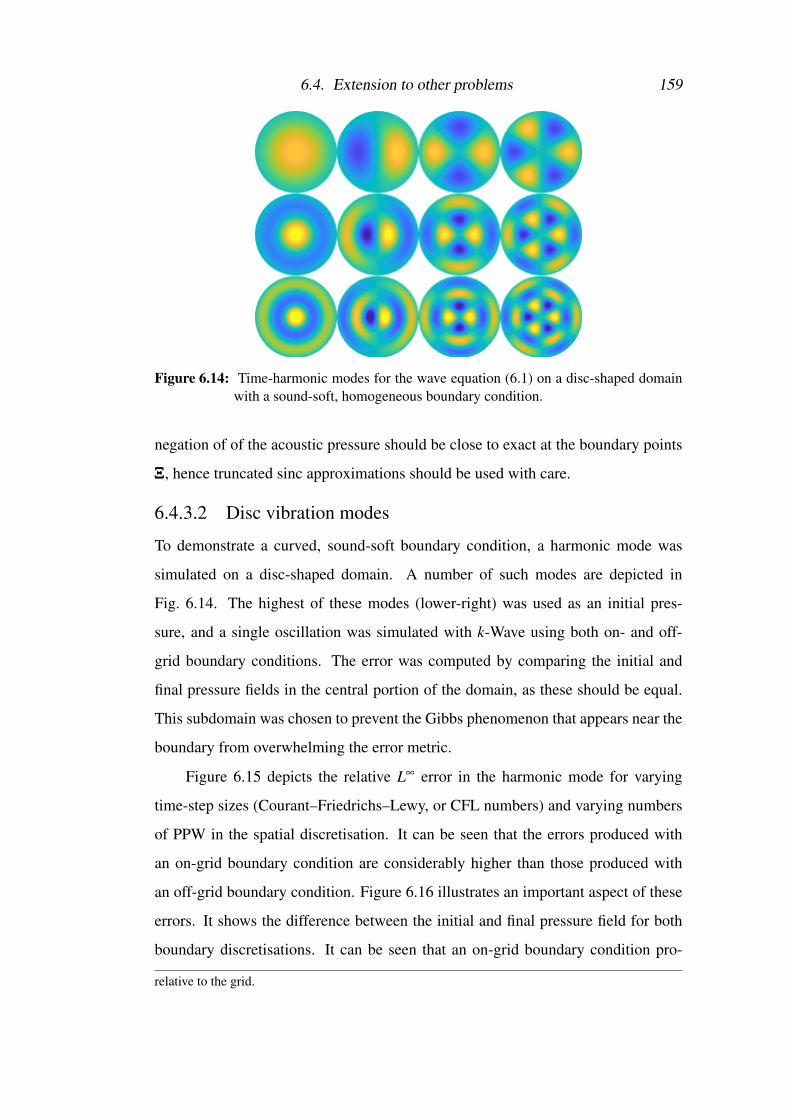
6.4. Extension to other problems 159
Figure 6.14: Time-harmonic modes for the wave equation (6.1) on a disc-shaped domainwith a sound-soft, homogeneous boundary condition.
negation of of the acoustic pressure should be close to exact at the boundary points
ΞΞΞ, hence truncated sinc approximations should be used with care.
6.4.3.2 Disc vibration modes
To demonstrate a curved, sound-soft boundary condition, a harmonic mode was
simulated on a disc-shaped domain. A number of such modes are depicted in
Fig. 6.14. The highest of these modes (lower-right) was used as an initial pres-
sure, and a single oscillation was simulated with k-Wave using both on- and off-
grid boundary conditions. The error was computed by comparing the initial and
final pressure fields in the central portion of the domain, as these should be equal.
This subdomain was chosen to prevent the Gibbs phenomenon that appears near the
boundary from overwhelming the error metric.
Figure 6.15 depicts the relative L∞ error in the harmonic mode for varying
time-step sizes (Courant–Friedrichs–Lewy, or CFL numbers) and varying numbers
of PPW in the spatial discretisation. It can be seen that the errors produced with
an on-grid boundary condition are considerably higher than those produced with
an off-grid boundary condition. Figure 6.16 illustrates an important aspect of these
errors. It shows the difference between the initial and final pressure field for both
boundary discretisations. It can be seen that an on-grid boundary condition pro-
relative to the grid.

160 Chapter 6. Representing arbitrary acoustic source distributions
duces much higher errors within the disc. These errors are the result of instability
in the harmonic modes due to the staircasing. The errors produced with an off-grid
boundary condition are much lower within the disc, and equal in magnitude on both
sides of the boundary. These reflect the non-locality of the solution-negating source
approach to boundary condition enforcement that results from the spatial spread of
band-limited delta functions.
6.4.3.3 Homophonic drums
As a second example of the enforcement of boundary conditions, a pair of homo-
phonic drums were simulated [22]. These are boundary shapes that produce the
same spectrum when excited at a particular point within the domain. Figure 6.17
depicts the off-grid boundary discretisation that was used, along with the point at
which the drums should be excited.
To generate spectra, each drum was initialised with a narrow Gaussian pressure
distribution centred on the appropriate excitation location. The acoustic waves were
then allowed to propagate freely, and the resulting pressure trace was recorded at
the initial excitation location. From this a spectrum for each drum was computed.
These spectra are depicted in Fig. 6.18. They can be seen to be very similar, with
peaks occuring at the same modal frequencies.
6.5 Implementation with transformed meshesWhile all of the discussion in this chapter has assumed uniform computational
meshes, it is relatively straightforward to extend the method to nonuniform meshes.
To do so, the source distribution must be written in terms of the computational co-
ordinate, i.e. s(x)→ s(s), after which the process described above can be applied as
presented. One difficulty which may be encountered is in uniformly placing inte-
gration points over the source’s region of support in the computational coordinate,
since the coordinate transformation s(x) is not typically explicitly known. An alter-
native is to generate uniform integration points in the physical coordinate system,
then interpolate these to the corresponding computational coordinates. To account
for the subsequent change in integration point spacing, the quadrature weights Ci

6.5. Implementation with transformed meshes 161
Figure 6.15: Error in the acoustic pressure field for a harmonic mode on a disc-shapeddomain after one period with varying spatial and temporal resolution. (Top)On-grid boundary condition. (Middle) Off-grid boundary condition. (Bot-tom) Comparison of on- and off-grid boundary conditions, with a Courant–Friedrichs–Lewy (CFL) number of 0.1.

162 Chapter 6. Representing arbitrary acoustic source distributions
-1 -0.5 0 0.5 1y-position [m]
-1
-0.5
0
0.5
1
x-po
sitio
n [m
]
-1 -0.5 0 0.5 1y-position [m]
-1
-0.5
0
0.5
1
x-po
sitio
n [m
]
Figure 6.16: Difference between initial and final acoustic pressure fields for a harmonicmode on a disc-shaped domain (note that colour scales are equal in both sub-plots). (Top) On-grid boundary condition. (Bottom) Off-grid boundary con-dition.
should then be multiplied by the mesh density det(J) at the corresponding integra-
tion point. A second complicating factor is that the source grid weights must be
regenerated whenever the physical mesh changes, but this is unavoidable.
As an illustrative example of this process, source grid weights were generated
for an off-grid square using a uniform mesh and a nonuniform, tensor product mesh.
These are depicted in Fig. 6.19. The source grid weights can be seen to be uniform
across the source in both cases (though with the discretised source’s band-limited
nature evident in the deviation of the grid weights from unity).
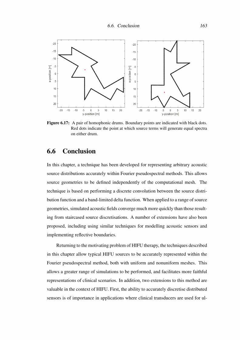
6.6. Conclusion 163
Figure 6.17: A pair of homophonic drums. Boundary points are indicated with black dots.Red dots indicate the point at which source terms will generate equal spectraon either drum.
6.6 Conclusion
In this chapter, a technique has been developed for representing arbitrary acoustic
source distributions accurately within Fourier pseudospectral methods. This allows
source geometries to be defined independently of the computational mesh. The
technique is based on performing a discrete convolution between the source distri-
bution function and a band-limited delta function. When applied to a range of source
geometries, simulated acoustic fields converge much more quickly than those result-
ing from staircased source discretisations. A number of extensions have also been
proposed, including using similar techniques for modelling acoustic sensors and
implementing reflective boundaries.
Returning to the motivating problem of HIFU therapy, the techniques described
in this chapter allow typical HIFU sources to be accurately represented within the
Fourier pseudospectral method, both with uniform and nonuniform meshes. This
allows a greater range of simulations to be performed, and facilitates more faithful
representations of clinical scenarios. In addition, two extensions to this method are
valuable in the context of HIFU. First, the ability to accurately discretise distributed
sensors is of importance in applications where clinical transducers are used for ul-

164 Chapter 6. Representing arbitrary acoustic source distributions
Figu
re6.
18:
Spec
tra
com
pute
dfo
rea
chof
the
hom
opho
nic
drum
sin
Fig.
6.17
usin
ga
narr
owG
auss
ian
initi
alco
nditi
on.
The
seca
nbe
seen
tobe
appr
oxim
atel
yeq
ual,
show
ing
peak
sat
the
sam
em
odal
freq
uenc
ies.

6.6. Conclusion 165
-1.5 -1 -0.5 0 0.5 1 1.5y-position [au]
-1.5
-1
-0.5
0
0.5
1
1.5
x-po
sitio
n [a
u]
-1.5 -1 -0.5 0 0.5 1 1.5y-position [au]
-1.5
-1
-0.5
0
0.5
1
1.5
x-po
sitio
n [a
u]
Figure 6.19: (Top-left) Source grid weights for an offgrid rectangle generated with a uni-form mesh and (top-right) with a nonuniform mesh. (Bottom) The nonuni-form, tensor product mesh that was used.
trasound detection, for instance when simulating ultrasound-guidance within HIFU
therapy. Second, the implementation of perfectly reflecting boundary conditions
allows for certain sharply discontinuous medium properties to be effectively repre-
sented, for instance air or bone. More broadly, these techniques allow the user of a
simulation code to consider only the physical geometry of the sources, sensors, and
boundaries they wish to simulate, after which discretisation can be automated.


Chapter 7
General conclusions
The aim of this thesis was to develop and demonstrate a nonuniform mesh specifi-
cation that enhances the performance of the Fourier pseudospectral method. This
goal was motivated by the need for accurate HIFU therapy planning, which is cur-
rently hindered by extreme computational expense. Two directions were identified
for doing so: one based on the analyticity of the model solution (acoustic field),
and the other based on its local frequency content. In addition, the incorporation of
HIFU sources on nonuniform meshes was identified as a key challenge that would
need to be addressed.
The first mesh specification, investigated in Chapter 3, was based on the an-
alyticity of the model solution. Specifically, mesh adaptation was performed by
analytically continuing the model solution into the complex plane, locating singu-
larities, and generating a Schwarz–Christoffel mapping from these singularity lo-
cations, from which a mesh specification was derived. When applied to Burgers’
equation with a single shock front, it was found that this approach produced signif-
icant convergence rate improvements when compared with commonly used mesh
adaptation techniques. When a solution to the Westervelt wave equation (with
multiple shock fronts) was analytically continued, a similar singularity structure
was observed, indicating the methods potential for full-wave problems. However,
analyticity-based mesh adaptation did not prove sufficiently robust for application
to complex acoustic problems, and there was no obvious path from one-dimensional
simulations to multiple dimensions.

168 Chapter 7. General conclusions
The second mesh specification, investigated in chapters 4 and 5, was based
on a measure of the local spatial bandwidth of the model solution. This is the
range of spatial frequency components that are present in the solution at a particular
point in space. The local bandwidth was computed using Hilbert transform in one
dimension, and the Riesz transforms in two dimensions, along with a wavenumber-
domain operator for the second-order spectral moment. When applied to a hetero-
geneous advection equation and to Burgers’ equation in one-dimension, substantial
convergence rate improvements were again seen, and an illustrative example with
the Korteweg-de Vries equation was also provided. In multiple dimensions, similar
performance was observed with heterogeneous advection and Burgers’ equations.
In all of the mesh adaptation examples in this thesis, initial value problems
were solved. However, problems with source terms are ubiquitous, for example pre-
dicting the acoustic field emitted from a HIFU transducer. In the context of mesh
adaptation, source terms are problematic as they must be discretised in a manner
which does not rely on mesh nodes coinciding with the source’s region of support.
This problem was addressed in Chapter 6. Indeed, this chapter addressed the more
general problem of staircasing for the Fourier pseudospectral method, which arises
when source geometries do not align with the (typically regular, orthogonal) spa-
tial mesh. To do so, arbitrary, continuous source distributions were band-limited
through a convolution with the band-limited delta function. Such source discreti-
sations are referred to as off-grid sources. When compared with staircased source
discretisations, off-grid sources performed extremely well, providing faithful source
representations at very low resolutions.
While the techniques described in this thesis have proven highly effective, a
number of challenges remain before these can be applied to large-scale, full-wave
HIFU simulations. For mesh adaptation, two issues stand out as having been con-
sistently difficult to address. The first is time-stepping. A number of time-stepping
routines have been tested, and all have proven sufficient for the test problems used
in this thesis, but larger-scale simulations will require much more efficiency. To
this end, it may be useful to explicitly compute Jacobian matrices for the discre-
169
tised systems, thus improving the effectiveness of stiff ODE integrators. Attempts
were made to do this, but the task proved difficult due to the coupling between the
mesh coordinates and spatial calculus operators. Additionally, it may prove useful
to use an implicit-explicit (IMEX) ODE solver to separately address the stiff and
non-stiff portions of the model/mesh equations. The second is stability. A number
of mesh smoothing strategies were tested, both to reduce stiffness and to ensure
that the scheme would not get bogged down if oscillations in the solution appeared.
The two-level, frequency-filtering approach described in Chapter 5 proved most ef-
fective in this regard, but more complex problems will require greater investigation
into this process.
Turning to source representations, two areas stand out as candidates for fu-
ture work. The first is improving the computational efficiency of the discretisation
process. In particular, the truncated source discretisations presented in Chapter 6
are likely not optimal (relative to the untruncated discretisations, in a least-squares
sense). Hence, alternative discretisations might retain the compactness of the trun-
cated source while improving its accuracy. The second candidate for future re-
search is improving the boundary condition discretisation process. This process is
currently slow and memory intensive, as it requires accurate interpolation of the
acoustic field onto every boundary point at each time-step, an inverse problem to be
solved, and separate source/sensor grid weights to be computed and stored for every
boundary point. If this process could be improved, then the Fourier pseudospectral
method could be applied to a much wider range of problems than is currently pos-
sible.
Overall, this thesis contributes two significant new enhancements to the Fourier
pseudospectral method: bandwidth-based mesh adaptation and off-grid source dis-
cretisation. While these techniques have not been combined within a full-wave
simulation of HIFU therapy, they constitute a substantial step towards this goal,
and thus towards translation into the clinic. Beyond this, they will contribute to the
many other problems for which the Fourier pseudospectral method is used, and may
inspire similar techniques for other numerical methods.


Bibliography
[1] J. M. Augenbaum. An adaptive pseudospectral method for discontinuous
problems. Applied Numerical Mathematics, 5(6):459–480, 1989.
[2] M. A. Averkiou and R. O. Cleveland. Modeling of an electrohydraulic
lithotripter with the KZK equation. The Journal of the Acoustical Society
of America, 106(1):102–112, 1999.
[3] M. R. Bailey, V. A. Khokhlova, O. A. Sapozhnikov, S. G. Kargl, and L. A.
Crum. Physical mechanisms of the therapeutic effect of ultrasound (a re-
view). Acoustical Physics, 49(4):369–388, 2003.
[4] R. Baltensperger. Some results on linear rational trigonometric interpolation.
Computers and Mathematics with Applications, 43(6-7):737–746, 2002.
[5] A. Bayliss, D. Gottlieb, B. J. Matkowsky, and M. Minkoff. An adaptive
pseudo-spectral method for reaction diffusion problems. Journal of Compu-
tational Physics, 81(2):421–443, 1989.
[6] A. Bayliss and B. J. Matkowsky. Fronts, relaxation oscillations, and pe-
riod doubling in solid fuel combustion. Journal of Computational Physics,
71(1):147–168, 1987.
[7] A. Bayliss and B. J. Matkowsky. Nonlinear dynamics of cellular flames.
SIAM Journal on Applied Mathematics, 52(2):396–415, 1992.
[8] A. Bayliss and E. Turkel. Mappings and accuracy for Chebyshev pseudo-
spectral approximations. Journal of Computational Physics, 101(2):349–
359, 1992.

172 BIBLIOGRAPHY
[9] M. Berljafa and S. Guttel. Generalized rational Krylov decompositions with
an application to rational approximation. SIAM Journal on Matrix Analysis
and Applications, 36(2):894–916, 2015.
[10] M. Berljafa and S. Guttel. The RKFIT algorithm for nonlinear rational ap-
proximation. SIAM Journal on Scientific Computing, 39(5):A2049–A2071,
2017.
[11] D. Bessis and J. D. Fournier. Pole condensation and the Riemann surface
associated with a shock in Burgers’ equation. Journal de Physique Lettres,
45(17):L:833–L:841, 1984.
[12] D. T. Blackstock. Fundamentals of physical acoustics. John Wiley & Sons,
Inc., 2000.
[13] F. Bornemann. Accuracy and stability of computing high-order derivatives
of analytic functions by Cauchy integrals. The Journal of the Society for the
Foundations of Computational Mathematics, 11(1):1–63, 2011.
[14] J. P. Boyd. The arctan/tan and Kepler–Burgers mappings for periodic solu-
tions with a shock, front, or internal boundary layer. Journal of Computa-
tional Physics, 98(2):181–193, 1992.
[15] J. P. Boyd. Chebyshev and Fourier Spectral Methods. Dover Publications
Inc., 31 East 2nd Street, Mineola, New York, NY 11501, USA, 2000.
[16] C. P. Bridge. Introduction to the monogenic signal. arXiv, 2017.
1703.09199v1.
[17] P. A. Browne, C. J. Budd, C. Piccolo, and M. Cullen. Fast three dimensional
r-adaptive mesh redistribution. Journal of Computational Physics, 275:174–
196, 2014.
[18] C. J. Budd, M. J. P. Cullen, and E. J. Walsh. Monge–Ampere based mov-
ing mesh methods for numerical weather prediction, with applications to the
Eady problem. Journal of Computational Physics, 236:247–270, 2013.

BIBLIOGRAPHY 173
[19] C. J. Budd, W. Huang, and R. D. Russell. Adaptivity with moving grids. Acta
Numerica, 18:111–241, 2009.
[20] C. J. Budd, R. D. Russell, and E. Walsh. The alignment properties of Monge–
Ampere based mesh redistribution methods: I linear features. arXiv, 2014.
1402.5453v1.
[21] C. J. Budd and J. F. Williams. Moving mesh generation using the
parabolic Monge–Ampere equation. SIAM Journal on Scientific Computa-
tion, 31(5):3438–3465, 2009.
[22] P. Buser, J. Conway, P. Doyle, and K.-D. Semmler. Some planar isospectral
domains. International Mathematics Research Notices, 1994(9):391–400,
1994.
[23] W. Cao, W. Huang, and R. D. Russell. A study of monitor functions for two-
dimensional adaptive mesh generation. SIAM Journal on Scientific Comput-
ing, 20(6):1978–1994, 1999.
[24] Z. Chen and Y. Zhou. An efficient algorithm for solving Hilbert type singu-
lar integral equations of the second kind. Computers & Mathematics with
Applications, 58(4):632–640, 2009.
[25] J. J. Clark, M. R. Palmer, and P. D. Lawrence. A transformation method
for the reconstruction of functions from nonuniformly spaced samples.
IEEE Transactions on Acoustics, Speech, and Signal Processing, ASSP-
33(5):1151–1165, 1985.
[26] L. Cohen. Instantaneous ‘anything’. In Proceedings of the IEEE Interna-
tional Conference on Acoustics, Speech, and Signal Processing, volume 4,
pages 105–108, Washington, DC, USA, 1993. IEEE Computer Society.
[27] L. Cohen. Local values in quantum mechanics. Physics Letters A,
212(6):315–319, 1996.

174 BIBLIOGRAPHY
[28] J. D. Cole. On a quasi-linear parabolic equation occurring in aerodynamics.
Quarterly of Applied Mathematics, 9(3):225–236, 1951.
[29] F. P. Curra, P. D. Mourad, V. A. Khokhlova, R. O. Cleveland, and L. A. Crum.
Numerical simulations of heating patterns and tissue temperature response
due to high-intensity focused ultrasound. IEEE Transactions on Ultrasonics,
Ferroelectrics, and Frequency Control, 47(4):1077–1089, 2000.
[30] K. L. Davidson and P. J. Loughlin. Instantaneous spectral moments. Journal
of the Franklin Institute, 337(4):421–436, 2000.
[31] T. A. Driscoll and B. Fornberg. Pade-based interpretation and correction of
the Gibbs phenomenon. In A. J. Jerri, editor, Advances in the Gibbs Phe-
nomenon, chapter 5. Sigma Sampling Publishing, 2007.
[32] T. A. Driscoll, N. Hale, and L. N. Trefethen. Chebfun Guide. Pafnuty Publi-
cations, 2014.
[33] F. A. Duck. Physical Properties of Tissue: A Comprehensive Reference Book.
Academic Press, 1990.
[34] T. Ekkehart, K. Dan, and B. Alfred. Elastic wave propagation simulation
in the presence of surface topography. Geophysical Journal International,
108(2):621–632, 1992.
[35] M. Felsberg and G. Sommer. The monogenic signal. IEEE Transactions on
Signal Processing, 49(12):3136–3144, 2001.
[36] W. M. Feng, P. Yu, S. Y. Hu, and Z. K. Liu. A Fourier spectral moving mesh
method for the Cahn-–Hilliard equation with elasticity. Communications in
Computational Physics, 5(2-4):582–599, 2009.
[37] W. M. Feng, P. Yu, S. Y. Hu, Z. K. Liu, Q. Du, and L. Q. Chen. Spectral im-
plementation of an adaptive moving mesh method for phase-field equations.
Journal of Computational Physics, 220(1):498–510, 2006.

BIBLIOGRAPHY 175
[38] Focused Ultrasound Foundation. Focused ultrasound: State of the field.
Technical report, Focused Ultrasound Foundation, 2017.
[39] Focused Ultrasound Foundation. Focused ultrasound: State of the field.
Technical report, Focused Ultrasound Foundation, 2018.
[40] B. Fornberg. The pseudospectral method: Comparisons with finite differ-
ences for the elastic wave equation. Geophysics, 52(4):483–501, 1987.
[41] B. Fornberg. The pseudospectral method: Accurate representation of inter-
faces in elastic wave calculations. Geophysics, 53(5):625–637, 1988.
[42] P. Gonnet, R. Pachon, and L. N. Trefethen. Robust rational interpolation and
least-squares. Electronic Transactions on Numerical Analysis, 38:146–167,
2011.
[43] H. Guillard and R. Peyret. On the use of spectral methods for the numerical-
solution of stiff problems. Computer Methods in Applied Mechanics and
Engineering, 66(1):17–43, 1988.
[44] N. Hale. On The Use Of Conformal Maps To Speed Up Numerical Compu-
tations. PhD thesis, University of Oxford, 2009.
[45] N. Hale and T. W. Tee. Conformal maps to multiply slit domains and appli-
cations. SIAM Journal on Scientific Computing, 31(4):3195–3215, 2009.
[46] M. F. Hamilton and D. T. Blackstock, editors. Nonlinear Acoustics. Acous-
tical Society of America, 2008.
[47] J. S. Hesthaven, S. Gottlieb, and D. Gottlieb. Spectral Methods for Time-
Dependent Problems. Cambridge Monographs on Applied and Computa-
tional Mathematics. Cambridge University Press, 2007.
[48] M. E. Hosea and L. F. Shampine. Analysis and implementation of TR-BDF2.
Applied Numerical Mathematics, 20(1–2):21–37, 1996.

176 BIBLIOGRAPHY
[49] W. Huang. Practical aspects of formulation and solution of moving mesh par-
tial differential equations. Journal of Computational Physics, 171(2):753–
775, 2001.
[50] W. Huang. Variational mesh adaptation: Isotropy and equidistribution. Jour-
nal of Computational Physics, 174(2):903–924, 2001.
[51] W. Huang. Mathematical principles of anisotropic mesh adaptation. Com-
munications in Computational Physics, 1:276–310, 2006.
[52] W. Huang and L. Kamenski. A geometric discretization and a simple imple-
mentation for variational mesh generation and adaptation. Journal of Com-
putational Physics, 301:322–337, 2015.
[53] W. Huang, L. Kamenski, and R. D. Russell. A comparative numerical study
of meshing functionals for variational mesh adaptation. Journal of Mathe-
matical Study, 48(2):168–186, 2015.
[54] W. Huang and R. D. Russell. Analysis of moving mesh partial differential
equations with spatial smoothing. SIAM Journal on Numerical Analysis,
34(3):1106–1126, 1997.
[55] W. Huang and R. D. Russell. Adaptive mesh movement — the MMPDE
approach and its applications. Journal of Computational and Applied Math-
ematics, 128:383–398, 2001.
[56] W. Huang and R. D. Russell. Adaptive moving mesh methods, volume 174
of Applied Mathematical Sciences. Springer Science+Business Media, 223
Spring Street, New York, NY 10013, USA, 2011.
[57] M. Huisman, R. M. Staruch, M. Ladouceur-Wodzak, M. A. van den Bosch,
D. K. Burns, A. Chhabra, and R. Chopra. Non-invasive targeted peripheral
nerve ablation using 3D MR neurography and MRI-guided high-intensity
focused ultrasound (MR-HIFU): Pilot study in a swine model. PLOS ONE,
10(12):1–18, 2015.

BIBLIOGRAPHY 177
[58] S. A. Ilyin, S. M. Bobkova, V. A. Khokhlova, and L. R. Gavrilov. Simulation
of thermal lesions in biological tissues irradiated by high-intensity focused
ultrasound through the rib cage. Physics of Wave Phenomena, 19(1):62–67,
2011.
[59] J. Jaros, A. P. Rendell, and B. E. Treeby. Full-wave nonlinear ultrasound
simulation on distributed clusters with applications in high-intensity focused
ultrasound. International Journal of High Performance Computing Applica-
tions, 30(2):137–155, 2016.
[60] V. A. Khokhlova, O. V. Bessonova, J. E. Soneson, M. S. Canney, M. R.
Bailey, and L. A. Crum. Bandwidth limitations in characterization of high
intensity focused ultrasound fields in the presence of shocks. AIP Conference
Proceedings, 1215:363–366, 2010.
[61] V. A. Khokhlova, R. Souchon, J. Tavakkoli, O. A. Sapozhnikov, and
D. Cathignol. Numerical modeling of finite-amplitude sound beams: Shock
formation in the near field of a cw plane piston source. The Journal of the
Acoustical Society of America, 110(1):95–108, 2001.
[62] V. P. Kuznetsov. Equations of nonlinear acoustics. Soviet Physics Acoustics,
16(4):467, 1971.
[63] Y.-S. Lee. Numerical solution of the KZK equation for pulsed finite amplitude
sound beams in thermoviscous fluids. PhD thesis, The University of Texas at
Austin, 1993.
[64] H.-L. Liu, N. McDannold, and K. Hynynen. Focal beam distortion and treat-
ment planning in abdominal focused ultrasound surgery. Medical Physics,
32(5):1270–1280, 2005.
[65] P. J. Loughlin and B. Tacer. On the amplitude- and frequency-modulation
decomposition of signals. The Journal of the Acoustical Society of America,
100(3):1594–1601, 1996.

178 BIBLIOGRAPHY
[66] E. Martin, Y. T. Ling, and B. E. Treeby. Simulating focused ultrasound trans-
ducers using discrete sources on regular Cartesian grids. IEEE Transactions
on Ultrasonics, Ferroelectrics, and Frequency Control, 63(10):1535–1542,
2016.
[67] H. Montanelli and N. Bootland. Solving periodic semilinear stiff PDEs in
1D, 2D and 3D with exponential integrators. arXiv, 2017. 1604.08900v4.
[68] L. S. Mulholland, W. Z. Huang, and D. M. Sloan. Pseudospectral solution of
near-singular problems using numerical coordinate transformations based on
adaptivity. SIAM Journal on Scientific Computing, 19(4):1261–1289, 1998.
[69] L. S. Mulholland, Y. Qiu, and D. M. Sloan. Solution of evolutionary partial
differential equations using adaptive finite differences with pseudospectral
post-processing. Journal of Computational Physics, 131(2):280–298, 1997.
[70] Y. Nakatsukasa, O. Sete, and L. N. Trefethen. The AAA algorithm for ratio-
nal approximation. arXiv, 2017. 1612.00337v2.
[71] K. Naugolnykh and L. Ostrovsky. Nonlinear Wave Processes in Acoustics.
Cambridge University Press, 1998.
[72] P. Nielsen, F. If, P. Berg, and O. Skovgaard. Using the pseudospectral method
on curved grids for 2D elastic forward modelling. Geophysical Prospecting,
43(3):369–395, 1995.
[73] K. Okita, K. Ono, S. Takagi, and Y. Matsumoto. Development of high inten-
sity focused ultrasound simulator for large-scale computing. International
Journal for Numerical Methods in Fluids, 65(1-3):43–66, 2011.
[74] H. T. O’Neil. Theory of focusing radiators. The Journal of the Acoustical
Society of America, 21:516–526, 1949.
[75] R. Pachon, P. Gonnet, and J. van Deun. Fast and stable rational interpola-
tion in roots of unity and Chebyshev points. SIAM Journal on Numerical
Analysis, 50(3):1713–1734, 2012.

BIBLIOGRAPHY 179
[76] N. A. Petersson, O. O’Reilly, B. Sjogreen, and S. Bydlon. Discretizing sin-
gular point sources in hyperbolic wave propagation problems. Journal of
Computational Physics, 321:532–555, 2016.
[77] A. D. Pierce. Acoustics: An introduction to its physical principles and ap-
plications. The Acoustical Society of America, 500 Sunnyside Boulevard,
Woodbury, New York 11797, USA, 1991.
[78] G. Pinton, J.-F. Aubry, M. Fink, and M. Tanter. Effects of nonlinear ul-
trasound propagation on high intensity brain therapy. Medical Physics,
38(3):1207–1216, 2011.
[79] A. Pulkkinen, B. Werner, E. Martin, and K. Hynynen. Numerical simulations
of clinical focused ultrasound functional neurosurgery. Physics in Medicine
& Biology, 59(7):1679–1700, 2014.
[80] V. Rieke and K. B. Pauly. MR thermometry. Journal of Magnetic Resonance
Imaging, 27(2):376–390, 2008.
[81] J. L. B. Robertson, B. T. Cox, J. Jaros, and B. E. Treeby. Accurate simulation
of transcranial ultrasound propagation for ultrasonic neuromodulation and
stimulation. The Journal of the Acoustical Society of America, 141(3):1726–
1738, 2017.
[82] D. Senouf, R. Caflisch, and N. Ercolani. Pole dynamics and oscillations for
the complex Burgers equation in the small-dispersion limit. Nonlinearity,
9(6):1671–1702, 1996.
[83] L. F. Shampine. Solving 0=F(t,y(t),y’(t)) in Matlab. Journal of Numerical
Mathematics, 10(4):291–310, 2002.
[84] L. F. Shampine and M. W. Reichelt. The MATLAB ODE suite. SIAM Journal
on Scientific Computing, 18(1):1–22, 1997.

180 BIBLIOGRAPHY
[85] J. Shen and X. Yang. An efficient moving mesh spectral method for the
phase-field model of two-phase flows. Journal of Computational Physics,
228(8):2978–2992, 2009.
[86] H. Stahl. The convergence of Pade approximants to functions with branch
points. Journal of Approximation Theory, 91(2):139–204, 1997.
[87] H. Stahl. Spurious poles in Pade approximation. Journal of Computational
and Applied Mathematics, 99:511–527, 1998.
[88] C. J. Subich. A robust moving mesh method for spectral collocation solutions
of time-dependent partial differential equations. Journal of Computational
Physics, 294:297–311, 2015.
[89] V. Suomi, J. Jaros, B. Treeby, and R. O. Cleveland. Full modeling of high-
intensity focused ultrasound and thermal heating in the kidney using realistic
patient models. IEEE Transactions on Biomedical Engineering, 65(5):969–
979, 2018.
[90] M. Tabei, T. D. Mast, and R. C. Waag. A k-space method for coupled first-
order acoustic propagation equations. The Journal of the Acoustical Society
of America, 111(1):53–63, 2002.
[91] J. J. Tapia and P. Gilberto Lopez. Adaptive pseudospectral solution of a
diffuse interface model. Journal of Computational and Applied Mathematics,
224(1):101–117, 2009.
[92] T. W. Tee. An Adaptive Rational Spectral Method for Differential Equations
with Rapidly Varying Solutions. PhD thesis, University of Oxford, 2006.
[93] T. W. Tee and L. N. Trefethen. A rational spectral collocation method with
adaptively transformed Chebyshev grid points. SIAM Journal on Scientific
Computing, 28(5):1798–1811, 2006.

BIBLIOGRAPHY 181
[94] J. C. Tillett, M. I. Daoud, J. C. Lacefield, and R. C. Waag. A k-space method
for acoustic propagation using coupled first-order equations in three dimen-
sions. The Journal of the Acoustical Society of America, 126(3):1231–1244,
2009.
[95] A.-K. Tornberg and B. Engquist. Numerical approximations of singular
source terms in differential equations. Journal of Computational Physics,
200(2):462–488, 2004.
[96] B. E. Treeby. Modeling nonlinear wave propagation on nonuniform grids
using a mapped k-space pseudospectral method. IEEE Transactions on Ul-
trasonics, Ferroelectrics, and Frequency Control, 60(10):2208–2213, 2013.
[97] B. E. Treeby, J. Budisky, E. S. Wise, J. Jaros, and B. T. Cox. Rapid calcula-
tion of acoustic fields from arbitrary continuous-wave sources. The Journal
of the Acoustical Society of America, 143(1):529–537, 2018.
[98] B. E. Treeby and B. T. Cox. k-Wave: MATLAB toolbox for the simula-
tion and reconstruction of photoacoustic wave fields. Journal of Biomedical
Optics, 15(2):021314–1–12, 2010.
[99] B. E. Treeby and B. T. Cox. A k-space Green’s function solution for acoustic
initial value problems in homogeneous media with power law absorption.
The Journal of the Acoustical Society of America, 129(6):3652–3660, 2011.
[100] B. E. Treeby, J. Jaros, A. P. Rendell, and B. T. Cox. Modeling nonlinear
ultrasound propagation in heterogeneous media with power law absorption
using a k-space pseudospectral method. The Journal of the Acoustical Society
of America, 131(6):4324–4336, 2012.
[101] B. E. Treeby and T. Saratoon. The contribution of shear wave absorption to
ultrasound heating in bones: Coupled elastic and thermal modeling. In IEEE
International Ultrasonics Symposium (IUS), 2015.

182 BIBLIOGRAPHY
[102] B. E. Treeby, E. S. Wise, and B. T. Cox. Nonstandard Fourier pseudospectral
time domain (PSTD) schemes for partial differential equations. Communica-
tions in Computational Physics, 24(3):623–634, 2018.
[103] L. N. Trefethen. Spectral Methods in MATLAB. Society for Industrial and
Applied Mathematics, 2000.
[104] L. N. Trefethen. Approximation Theory and Approximation Practice. SIAM,
2013.
[105] L. N. Trefethen, P. Gonnet, and S. Guttel. Robust Pade approximation via
SVD. SIAM Review, 55(1):101–117, 2013.
[106] S. Vaezy, X. Shi, R. W. Martin, E. Chi, P. I. Nelson, M. R. Bailey, and L. A.
Crum. Real-time visualization of high-intensity focused ultrasound treatment
using ultrasound imaging. Ultrasound in Medicine & Biology, 27(1):33–42,
2001.
[107] J. Walden. On the approximation of singular source terms in differential
equations. Numerical Methods for Partial Differential Equations, 15:503–
520, 1998.
[108] J. A. C. Weideman. Computing the dynamics of complex singularities of
nonlinear PDEs. SIAM Journal on Applied Dynamical Systems, 2(2):171–
186, 2003.
[109] H. Weller, P. Browne, C. Budd, and M. Cullen. Mesh adaptation on the sphere
using optimal transport and the numerical solution of a Monge–Ampere type
equation. Journal of Computational Physics, 308:102–123, 2016.
[110] E. S. Wise, B. T. Cox, and B. E. Treeby. A monitor function for spectral
moving mesh methods applied to nonlinear acoustics. In International Sym-
posium on Nonlinear Acoustics (ISNA), 2015.

BIBLIOGRAPHY 183
[111] E. S. Wise, B. T. Cox, and B. E. Treeby. Mesh density functions based
on local bandwidth applied to moving mesh methods. Communications in
Computational Physics, 22(5):1286–1308, 2017.
[112] E. S. Wise, B. T. Cox, and B. E. Treeby. Bandwidth-based mesh adaptation
in multiple dimensions. Journal of Computational Physics, 371:651–662,
2018.
[113] E. S. Wise, J. L. B. Robertson, B. T. Cox, and B. E. Treeby. Staircase-
free acoustic sources for grid-based models of wave propagation. In IEEE
International Ultrasonics Symposium (IUS), pages 1–4, 2017.
[114] G. Wojcik, J. Mould, N. Abboud, M. Ostromogilsky, and D. Vaughan. Non-
linear modeling of therapeutic ultrasound. In IEEE Ultrasonics Symposium,
volume 2, pages 1617–1622, 1995.
[115] P. V. Yuldashev and V. A. Khokhlova. Simulation of three-dimensional non-
linear fields of ultrasound therapeutic arrays. Acoustical Physics, 57(3):334–
343, 2011.
[116] E. A. Zabolotskaya and R. V. Khokhlov. Quasi-plane waves in the nonlinear
acoustics of confined beams. Soviet Physics Acoustics, 15(1):35–40, 1969.
[117] N. J. Zabusky and M. D. Kruskal. Interaction of “solitons” in a collision-
less plasma and the recurrence of initial states. Physical Review Letters,
15(6):240–243, 1965.