Wave Optics

• In part 1 we saw how waves can appear to move in straight lines and so can explain the world of geometrical optics

• In part 2 we explore phenomena where the wave nature is obvious not hidden

• Key words are interference and diffraction

Wave motion (1)

• See the waves lecture course for details!

• Basic form of a one-dimensional wave is cos(kx−ωt−φ) where k=2π/λ is the wave

number, ω=2πν is the angular frequency, and φ is the phase

• Various other conventions in use

Cylindrical wave

A plane wave impinging on a

infinitesimal slit in a plate.

Acts as a point source and

produces a cylindrical wave

which spreads out in all

directions.

Finite sized slits will be treated

later.

Remainder of this course will use slits unless specifically stated

Two slits

A plane wave impinging on a

pair of slits in a plate will

produce two circular waves

Where these overlap the

waves will interfere with one

another, either reinforcing or

cancelling one another

Intensity observed goes as

square of the total amplitude

Interference

Constructive:

intensity=4

+

=

Destructive:

intensity=0

+

=

Two slit interference

Two slit interference

Peaks in light

intensity in

certain directions

(reinforcement)

Minima in light

intensity in other

directions

(cancellation)

Can we calculate these directions directly

without all this tedious drawing?

Two slit interference (2)

• These lines are the sets of positions at which the waves from the two slits are in phase with one another

• This means that the optical path lengthsfrom the two slits to points on the line must differ by an integer number of wavelengths

• The amplitude at a given point will oscillate with time (not interesting so ignore it!)

Two slit interference (3)

Central line is locus of points at same

distance from the two slits

Two path lengths

are the same

Two slit interference (4)

Next line is locus of points where distance

from the two slits differs by one wavelength

Path lengths

related by

xleft=xright+λ

xleft xright

Two slit interference (5)

Next line is locus of points where distance

from the two slits differs by one wavelength

Path lengths

related by

xleft=xright+λ

xleft xright

d

Two slit interference (6)

d

D

Interference pattern observed on a distant screen

yθ

As y<<D the three blue lines are effectively parallel

and all make an angle θ≈y/D to the normal. The

bottom line is slightly longer than the top.

Two slit interference (7)

dθ

Close up

Green line is normal to the blue lines, and forms

a right angled triangle with smallest angle θ. Its

shortest side is the extra path length, and is of size d×sin(θ)≈dy/D

Two slit interference (8)

View at the screen

Bright fringes seen when the extra path length is

an integer number of wavelengths, so y=nλD/d

Dark fringes seen when y=(n+½)λD/d

λD/d

Central fringe midway between slits

Taking λ=500nm, d=1mm, D=1m, gives a fringe

separation of 0.5mm

Practicalities: colours (1)

• The above all assumes a monochromaticlight source

• Light of different colours does not interfere and so each colour creates its own fringes

• Fringe separation is proportional to wavelength and so red fringes are bigger than blue fringes

• Central fringe coincides in all cases

Practicalities: colours (2)

Observe bright central fringe (white with coloured

edges) surrounded by a complex pattern of colours.

Makes central fringe easy to identify!

Interference (1)

• It is easy to calculate the positions of maxima and minima, but what happens between them?

• Explicitly sum the amplitudes of the waves A=cos(kx1−ωt−φ)+cos(kx2−ωt−φ)

• Write x1=x−δ/2, x2=x+δ/2 and use cos(P+Q)+cos(P-Q)=2cos(P)cos(Q)

• Simplifies to A=2cos(kx−ωt−φ)×cos(kδ/2)

Interference (2)

• Amplitude is A=2cos(kx−ωt−φ)×cos(kδ/2)

• Intensity goes as square of amplitude so I=4cos2(kx−ωt−φ)×cos2(kδ/2)

• First term is a rapid oscillation at the frequency of the light; all the interest is in the second term

• I=cos2(kδ/2)=[1+cos(kδ)]/2

Interference (3)

• Intensity is I=cos2(kδ/2)=[1+cos(kδ)]/2

• Intensity oscillates with maxima at kδ=2nπand minima at kδ=(2n+1)π

• Path length difference is δ=dy/D

• Maxima at y=Dδ/d with δ=2nπ/k and k=2π/λgiving y=nλD/d

Exponential waves (1)

• Whenever you see a cosine you should consider converting it to an exponential! exp(ix)=cos(x)+ i sin(x)

• Basic wave in exponential form is

cos(kx−ωt−φ)=Re{exp[i(kx−ωt−φ)]}

• Do the calculations in exponential form and convert back to trig functions at the very end

Exponential waves (2)

• Repeat the interference calculation

• Explicitly sum the amplitudes of the wavesA=Re{exp[i(kx−kδ/2−ωt−φ)]+exp[i(kx+kδ/2−ωt−φ)]} =Re{exp[i(kx−ωt−φ)]×(exp[−ikδ/2]+exp[+ikδ/2])}

=Re{exp[i(kx−ωt−φ)]×2cos[kδ/2]}

=2cos(kx−ωt−φ)×cos[kδ/2]}

• Same result as before (of course!) but can be a

bit simpler to calculate

• Will use complex waves where convenient from

now on

Exponential waves (4)

• Use a complex amplitude to represent the wave

A=exp[i(kx−ωt−φ+kδ/2)]×2cos[kδ/2]

• The intensity of the light is then given by the

square modulus of the amplitude: I=A*A=4cos2[kδ/2]

• This approach loses the rapid time oscillations,

but we have previously ignored these anyway!

Result is the peak intensity which is twice the

average intensity.

Diffraction gratings (1)

• A diffraction grating is an extension of a double

slit experiment to a very large number of slits

• Gratings can work in transmission or reflection

but we will only consider transmission gratings

• The basic properties are easily understood from

simple sketches, and most of the advanced properties are (in principle!) off-syllabus

Diffraction gratings (7)

Points on a wavefront must be in phase, so the extra

distances travelled must be multiples of a wavelength

λ2λ3λ

4λ5λ

6λ

Diffraction gratings (8)

From trigonometry we see that sin(θ)=6λ/6d where θ is the angle between the ray direction and the normal

θ

6λ

6d

Basic diffraction equation: λ=d sin(θ)

θ

Diffraction gratings (9)

Can also get diffraction in the same direction if the

wavelength is halved!

2λ4λ6λ

8λ10λ

12λ

General diffraction equation: n λ=d sin(θ)

θ

Dispersion (1)

• n λ=d sin(θ)

• Different colours have

different wavelengths

and so diffract at

different angles

• Take red (λ=650nm),

green (λ=550nm), and

blue (λ=450nm) light

and d=1.5µm

n=0n=1

n=2

Dispersion (2)

• Angular dispersion of a grating is D=dθ/dλ=n/d cos(θ)

=n/�(d2−n2λ2)

• Increases with order

of the spectrum and when d≈nλ

• Note that high order

spectra can overlap!

n=0n=1

n=2

Between the peaks (1)

We also need to work out what happens in other

directions. Between n=0 and n=1 there is a direction

where the light from adjacent sources exactly cancel

each other out – just as for two slits!

λ/23λ/25λ/2 2λ3λ λ

Between the peaks (2)

Closer to n=0 there is a direction where light from

groups of three adjacent sources exactly cancels out

With an infinite number of sources will get cancellation

in every direction except for the main peaks!

λ2λ

phasors

Between the peaks (3)

With an finite number of sources the last effective

cancellation will occur when the path length difference

between the first and last sources is about λ

phasors

≈λ

Single slit diffraction (1)

• Consider a single slit illuminated by a plane wave source

• If the slit is perfectly narrow this will create a cylindrical wave

• If the slit has significant width we must treat it as a continuous distribution of sources and integrate over them

Single slit diffraction (2)

bθ

Green line is normal to the blue lines, and forms

a right angled triangle with smallest angle θ. Its

shortest side is the extra path length, and is of size δ = xsin(θ)

x

Consider a slit of width b

and light coming from a

point at a distance x from

the centre

Light coming from x has an extra phase kδ

Single slit diffraction (3)

• Final amplitude is obtained by integrating over all points x in the slit and combining the phases, most simply in complex form

• A = �exp(ikδ) dx = �exp(ikx sin(θ)) dx

• Integral runs from x=−b/2 to x=b/2 and then normalise by dividing by b

Single slit diffraction (4)

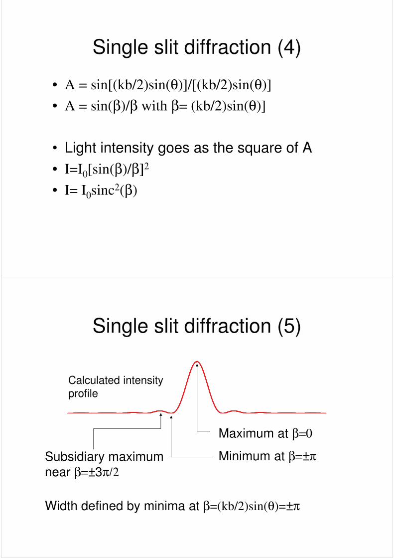
• A = sin[(kb/2)sin(θ)]/[(kb/2)sin(θ)]

• A = sin(β)/β with β= (kb/2)sin(θ)]

• Light intensity goes as the square of A

• I=I0[sin(β)/β]2

• I= I0sinc2(β)

Single slit diffraction (5)

Calculated intensity

profile

Maximum at β=0

Minimum at β=±πSubsidiary maximum

near β=±3π/2

Width defined by minima at β=(kb/2)sin(θ)=±π

Single slit diffraction (6)

Calculated intensity

profile

Width defined by minima at β=(kb/2)sin(θ)=±π

Solution is θ=arcsin(2π/bk)=arcsin(λ/b)≈λ/b

Get significant diffraction effects when the slit

is small compared to the wavelength of light!

Single slit diffraction (8)

� The Rayleigh Criterion says that two diffraction

limited images are well resolved when the

maximum of one coincides with the first minimum of the other, so θR=arcsin(λ/b)

� Alternative criteria can also be used

Resolving Power

• Basic ideas for the resolving power of a diffraction grating have been seen already, but now we can do the calculation properly

• Resolving power is defined as the reciprocal of the smallest change in wavelength which can be resolved as a fraction of the wavelength

Dispersion

• n λ=d sin(θ)

• Dispersion described by n dλ/dθ=d cos(θ)

• So the limiting

wavelength resolution

depends on the

limiting angular

resolution according to n δλ=d cos(θ) δθ

n=0n=1

n=2