Limit loads for centrally cracked square plates under biaxial ...
26
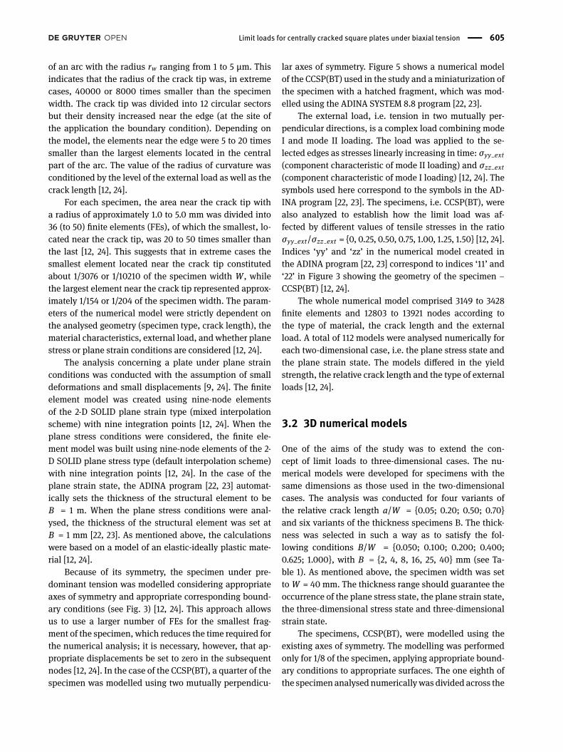
© 2016 Marcin Graba, published by De Gruyter Open. This work is licensed under the Creative Commons Attribution-NonCommercial-NoDerivs 3.0 License. Open Eng. 2016; 6:601–626 Research Article Open Access Marcin Graba* Limit loads for centrally cracked square plates under biaxial tension DOI 10.1515/eng-2016-0088 Received May 6, 2016; accepted October 3, 2016 Abstract: This paper is concerned with the determina- tion of limit loads for centrally cracked square plates sub- jected to biaxial tension. It briey discusses the concept of limit loads and some aspects of numerical modelling. It presents results of numerical calculations conducted for two-dimensional (plane strain state and plane stress state) and three-dimensional cases. It also considers the rela- tionship between the limit load and the crack length, the specimen thickness, the yield strength and the biaxial load factor, dened for the purpose of this work. The paper in- cludes approximation formulae to calculate the limit load. Keywords: limit load, centrally cracked plate, biaxial ten- sion, FEM, stationary crack, square plate Introduction The strength of strain-hardened elastic-plastic solids con- taining a crack should be analysed numerically [1–10]. Nu- merical calculations is the only rational solution as there exists no exact or perfect analytical solution [11]. A review of the literature reveals various approaches [1–9] but these only oer approximate solutions. Numerical calculations, however, are time-consuming and require specialised pro- grams and highly qualied engineering sta [9]. It is no longer sucient to be acquainted with a computer pro- gram or have the right skills to employ the nite element method (FEM). Engineers solving such problems need to be experienced to properly use their expertise [12]. The strength of ideally plastic solids can also be de- termined by applying the concept of limit loads [10]. This work, known as the EPRI procedures [10], oers a rela- tively simple tool to estimate the strength of plastic (and even elastic-plastic) solids. There are many formulae that *Corresponding Author: Marcin Graba: Kielce University of Tech- nology, Faculty of Mechatronics and Mechanical Engineering, De- partment of Manufacturing Engineering and Metrology, Kielce, Poland, E-mail: [email protected] can be used to calculate the limit load in structural el- ements but the solutions are conservative because real solids are generally strain hardened [11, 12]. Although the solutions of fracture mechanics are not suciently accu- rate, they are superior to the formulae of the classical strength of materials; they are less conservative but oer greater safety [11, 12]. The classical strength of materials rejects the analysis of solids (structural elements) contain- ing cracks. Fracture mechanics uses suitable tools to anal- yse a structural element containing a crack. Depending on the tools, it allows us to determine the distribution of stresses, the process of crack growth and even the time to failure of the structural element. In many a case, knowl- edge of the limit loads is not necessary [11, 12]. (a) (b) (c) Figure 1: Three modes of loading for structural elements in structure mechanics: (a) mode I loading – crack opening; (b) mode II loading – in-plane shear; (c) mode III loading – anti-plane shear (developed by the author based on [11, 12]). Limit loads were rst thoroughly discussed in 1981 by the authors of the Electric Power Research Institute (EPRI) procedures in a report entitled “Engineering Approach for Elastic-Plastic Fracture Analysis” [10]. The work provides formulae to calculate the force required for the plasticity of the uncracked portion of the specimen near the crack front in an elastic-plastic material. This indicates that the speci- men (a structural element) reaches the limit load if the un- cracked portion of the specimen is characterized by a state in which the stresses calculated according to the Huber- Mises-Hencky (HMH) hypothesis are equal to or greater than the yield strength [11, 12]. The formulae apply only to elements satisfying the plane strain or plane stress condi-
-
Upload
khangminh22 -
Category
Documents
-
view
0 -
download
0
Transcript of Limit loads for centrally cracked square plates under biaxial ...
© 2016 Marcin Graba, published by De Gruyter Open.This work is licensed under the Creative Commons Attribution-NonCommercial-NoDerivs 3.0 License.
Open Eng. 2016; 6:601–626
Research Article Open Access
Marcin Graba*
Limit loads for centrally cracked square platesunder biaxial tensionDOI 10.1515/eng-2016-0088Received May 6, 2016; accepted October 3, 2016
Abstract: This paper is concerned with the determina-tion of limit loads for centrally cracked square plates sub-jected to biaxial tension. It brie�y discusses the conceptof limit loads and some aspects of numerical modelling.It presents results of numerical calculations conducted fortwo-dimensional (plane strain state andplane stress state)and three-dimensional cases. It also considers the rela-tionship between the limit load and the crack length, thespecimen thickness, the yield strengthand thebiaxial loadfactor, de�ned for the purpose of this work. The paper in-cludes approximation formulae to calculate the limit load.
Keywords: limit load, centrally cracked plate, biaxial ten-sion, FEM, stationary crack, square plate
1 IntroductionThe strength of strain-hardened elastic-plastic solids con-taining a crack should be analysed numerically [1–10]. Nu-merical calculations is the only rational solution as thereexists no exact or perfect analytical solution [11]. A reviewof the literature reveals various approaches [1–9] but theseonly o�er approximate solutions. Numerical calculations,however, are time-consuming and require specialised pro-grams and highly quali�ed engineering sta� [9]. It is nolonger su�cient to be acquainted with a computer pro-gram or have the right skills to employ the �nite elementmethod (FEM). Engineers solving such problems need tobe experienced to properly use their expertise [12].
The strength of ideally plastic solids can also be de-termined by applying the concept of limit loads [10]. Thiswork, known as the EPRI procedures [10], o�ers a rela-tively simple tool to estimate the strength of plastic (andeven elastic-plastic) solids. There are many formulae that
*Corresponding Author: Marcin Graba: Kielce University of Tech-nology, Faculty of Mechatronics and Mechanical Engineering, De-partment of Manufacturing Engineering and Metrology, Kielce,Poland, E-mail: [email protected]
can be used to calculate the limit load in structural el-ements but the solutions are conservative because realsolids are generally strain hardened [11, 12]. Although thesolutions of fracture mechanics are not su�ciently accu-rate, they are superior to the formulae of the classicalstrength of materials; they are less conservative but o�ergreater safety [11, 12]. The classical strength of materialsrejects the analysis of solids (structural elements) contain-ing cracks. Fracture mechanics uses suitable tools to anal-yse a structural element containing a crack. Dependingon the tools, it allows us to determine the distribution ofstresses, the process of crack growth and even the time tofailure of the structural element. In many a case, knowl-edge of the limit loads is not necessary [11, 12].
(a) (b) (c)
Figure 1: Three modes of loading for structural elements in structuremechanics: (a) mode I loading – crack opening; (b) mode II loading– in-plane shear; (c) mode III loading – anti-plane shear (developedby the author based on [11, 12]).
Limit loads were �rst thoroughly discussed in 1981 bythe authors of the Electric Power Research Institute (EPRI)procedures in a report entitled “Engineering Approach forElastic-Plastic Fracture Analysis” [10]. The work providesformulae to calculate the force required for the plasticity ofthe uncracked portion of the specimennear the crack frontin an elastic-plastic material. This indicates that the speci-men (a structural element) reaches the limit load if the un-cracked portion of the specimen is characterized by a statein which the stresses calculated according to the Huber-Mises-Hencky (HMH) hypothesis are equal to or greaterthan the yield strength [11, 12]. The formulae apply only toelements satisfying the plane strain or plane stress condi-

602 | Marcin Graba
tion; determining the limit load requires knowing the yieldstrength and the dimensions of the structural element. Itshould be noted that the EPRI procedures [10] provide so-lutions to the limit load for structural elements subjectedto mode I loading – see Figure 1a [12].
It is worth noting that the formulae provided in theEPRI procedures [10] do not consider the specimen thick-ness. The original or modi�ed formulae can be found alsoin the SINTAP procedures [13], the FITNET procedures [14]and, the British standards R6 [15] and BS 7910 [16]. Thelarge number of formulae to determine the limit load ofstructural elements is desirable; however, they should bedivided systematically, according to the thickness of thestructural elements or predominant plane stress or planestrain conditions. The next sections will explain why theyare necessary at all [12].
Figure 2: Failure assessment diagram (developed by the author onthe basis of [11, 12]).
Knowing the limit load, an engineer is able to immedi-ately assess the condition of a structural element contain-ing a crack which may fail when subjected to an externalload [11]. The diagnosismay be performed using failure as-sessment diagrams (FADs) [11], proposed by Dowling andTownley [17] and Harrison et al. [18, 19]. The latter devel-oped a very simple procedure based on two completely dif-ferent criteria: the stress intensity factor (SIF) and the limitload [11]. This approach is now known as the two-criterionmethod [11]. If the assumptions of the Dugdale model aremet [11], the simplest failure assessment diagram can beobtained on the basis of the following formula:
Kr = Lr[8π2 ln
(sec(π2 Lr
))]− 12
(1)
where Kr is the standardized stress intensity factor (cal-culated as the ratio of the stress intensity factor (SIF) KIfor the actual load state, the specimen geometric condi-tions and the critical value of the stress intensity factorKIC: Kr = KI/KIC), and Lr is the standardized externalload calculated as the ratio of the actual load (frequentlydenoted by P) and the limit load (frequently denoted byP0):Lr = P/P0 [11].
Formula (1) is used to plot a failure curve, also calledthe Failure Assessment Diagram (FAD). As shown in Fig-ure 2, the diagram is then analysed following appropriaterules (not discussed in this paper) [11, 12].
The FAD, illustrated in Figure 2, is one of two ap-proachesused to assess the strength of a structure contain-ing a crack. The other method, which is based on the con-cept of the Crack Driving Force (CDF) [11], uses the valuesof the J-integral instead of the stress intensity factor. TheCDF-based approach requires that the standardized exter-nal load and the limit load be known [11, 12].
This is the reason why the author decided to recon-sider the limit loads, even though they have been dis-cussed many times in various publications. Limit loadshave been discussed thoroughly. When assessing thestrength of a structural element with a crack, engineersmay not have the knowledge and skills to perform an FEanalysis, or theymay not have time to develop a numericalmodel. It is thus essential to create catalogues of solutionsto determine the limit load so that the strength of struc-tural elements containing cracks will be easy to assess.
2 Description of the specimens, thematerial and the loading mode
The numerical analysis, which aimed at estimating thelimit loads, was performed for specimens with a relativelyatypical geometry – centrally cracked square plates underbiaxial tension – shown in Figure 3. For the purpose of thisand other studies conducted by the author, the geometrywill be referred to as a centrally cracked square plate underbiaxial tension – CCSP(BT) [12].
The lack of detailed research reports concerning thebehaviour of a centrally cracked plate under biaxial ten-sion as well as the lack of empirical formulae is the reasonwhy this problem is discussed here and the numerical re-sults are presented.
Table 1 shows the geometric dimensions of the spec-imens used to estimate the limit loads. As can be seen,plates with four di�erent crack lengths – very short,short, standard (a/W =0.50) and long cracks – were con-

Limit loads for centrally cracked square plates under biaxial tension | 603
sidered. The numerical analysis was performed for two-dimensional (planar stress and planar strain conditions)and three-dimensional problems.When 3D problemsweresolved, it was vital to properly select the thickness of theplates (specimens) so that the considerations were focuson predominant plane stress state (small plate thickness),cases with predominant plane strain state (large platethickness) and indirect cases (see Table 1) [12].
The choice of the specimen geometry is not accidentaland it has rarely beendiscussed in researchpapers [20, 21].This geometry is not considered in the EPRI [10], SIN-TAP [13] and FITNET procedures [14]. The work by Meekand Ainsworth [20] deals with limit loads for centrallycracked square plates under biaxial tension. It discussesthe e�ects of the plate size and the biaxial load, de�nedas σ11/σ22 (see Figure 3), on the level of the external load;the considerations are limited to the plane strain state andtwo crack lengths [12]. The authors used a basic formula toassess the limit load for this geometry:
(σ2)lbL = 2σ0√3·MIN
{1∣∣ σ11σ22∣∣ ;
(1 − a
W)∣∣1 − σ11
σ22(1 − a
W)∣∣}
(2)
where (σ2)lbL is the limit load, i.e. the normal stress ap-plied to a specimen resulting in the full plasticity of the un-cracked portion of the specimen, σ0 is the yield strength,a/W is the standard crack length, and the ratio σ11/σ22is the measure of biaxial load [20]. The index ‘lb’ of thelimit load refers to the least possible solution obtained inRef. [20]; according to the authors, it is the lower boundlimit load solution [20]. The formula is true for ‘long’plates, which suggests that the plate height must be equalto or greater than the length of the uncracked portion ofthe specimen calculated as the di�erence (W − a) [20].
Furthermore, reference [20] also provides other formu-lae that can be used to calculate the limit load for platessubjected to tension in two mutually perpendicular direc-tions. In that paper, the researchers analysed both longand short plates. In this study, the plate width was equalto its length and the uncracked portion of the specimenwas smaller than the plate length. Thus, as suggested bythe authors of Ref. [20], the plate considered here is a longplate. The following formula can be used to assess the up-per bound limit load solution [20]:
(σ2)ubL = 2σ0√3·[ (
1 − aW)∣∣1 − σ11
σ22(1 − a
W)∣∣]
H ≥ (w − a) (3)
where (σ2)ubL is the limit load, i.e. normal stress appliedto the specimen resulting in the full plasticity of the un-cracked portion of the specimen. The index ‘ub’ of thelimit load refers to the best possible solution obtained in
Ref. [20]; according to the authors, it is the upper boundlimit load solution [20]. It is worth noting that the formu-lae provided in [20] are suitable only for the plane strainstate.
The above formulae have beenmodi�ed inmanywaysto be suitable for plates with di�erent dimensions, i.e. dif-ferent ratio between the plate width and the plate length.In Ref. [20] only two relative crack lengths are considered(a/W = 0.20 and a/W = 0.60); other lengths are not dis-cussed [12].
Figure 3: CCSP(BT): 2a – crack length, 2W – specimen width, B– specimen thickness, σ22 – stress normal to the crack surface(external load component according to mode I loading), σ11 – stressshearing the crack surface (external load component according tomode II loading) [12, 24].
The limit load is determined for elastic-ideally plas-tic materials. A model of such a material was used in thisstudy to perform numerical calculations. The aim was todetermine the e�ects of the yield strength on the numeri-cally calculated limit load. The material was modelled as-suming a constant value of Young’s modulus E = 206 GPaand a constant value of Poisson’s ratio ν = 0.30. Four typesof elastic and ideally plastic materials were analysed; theydi�ered in the yield strength (see Table 2) [12].
The specimens – centrally cracked square plates un-der biaxial tension – were loaded by applying tensilestresses to the edges inmutually perpendicular directions:σ11 – tensile stresses acting on the plate in the direc-tion of the crack propagation and σ22 – tensile stressesacting on the plate in the direction perpendicular to thecrack surface – normal direction. Seven variants of exter-nal load, expressed as the ratio σ11/σ22 ={0, 0.25, 0.50,0.75, 1.00, 1.25, 1.50} to represent biaxial tensile stresses

604 | Marcin Graba
Table 1: Geometric dimensions (with con�gurations) of the specimens used in the numerical program to calculate the limit loads forCCSP(BT) [12].
specimen width, relative crack length, Specimen thickness, B, specimen thickness, B,W [mm] a/W for the 2D analysis [mm] for the 3D analysis [mm]
plane stress state plane strain state40 0.05 1 1000 2
0.20 40.50 80.70 16
2540
Table 2: Mechanical properties of the elastic-ideally plastic materials modelled numerically to determine the limit loads [12].
Young’s modulus, Poisson ratio, Yield strength, Strain corresponding toE [MPa] ν σ0 [MPa] the yield strength, ϵ0 = σ0/E
206000 0.30
315 0.00153500 0.002431000 0.004851500 0.00728
were analysed to obtain more accurate values of the limitload [12, 24].
3 Numerical models of CCSP(BT)The numerical models for determining the limit loads inCCSP(BT) were developed using the ADINA SYSTEM 8.8calculation package [22, 23]. The numerical calculations,which aimed at determining the limit loads, were per-formed using an elastic - perfectly plastic material assum-ing that Young’s modulus E and Poisson’s ratio ν are con-stant while the yield strength σ0 varies [12, 24]. Table 2shows the mechanical properties of the material modelsused in the numerical analysis. The models of the elastic-ideally plasticmaterials are represented graphically in Fig-ure 4. All the calculations were conducted from two pointsof view. The plate was modelled as a two-dimensionalcase (assuming the predominance of plane strain or planestress conditions) and as a three-dimensional element [12,24].
3.1 2D numerical models – plane stress orplane strain conditions [12, 24]
The analysis of the plate under plane stress or plane strainconditions required modelling the crack tip as a quarter
Figure 4: Graphical representation of the elastic-ideally plasticmaterial models used to calculate the limit loads [12].
Limit loads for centrally cracked square plates under biaxial tension | 605
of an arc with the radius rw ranging from 1 to 5 µm. Thisindicates that the radius of the crack tip was, in extremecases, 40000 or 8000 times smaller than the specimenwidth. The crack tip was divided into 12 circular sectorsbut their density increased near the edge (at the site ofthe application the boundary condition). Depending onthe model, the elements near the edge were 5 to 20 timessmaller than the largest elements located in the centralpart of the arc. The value of the radius of curvature wasconditioned by the level of the external load as well as thecrack length [12, 24].
For each specimen, the area near the crack tip witha radius of approximately 1.0 to 5.0 mm was divided into36 (to 50) �nite elements (FEs), of which the smallest, lo-cated near the crack tip, was 20 to 50 times smaller thanthe last [12, 24]. This suggests that in extreme cases thesmallest element located near the crack tip constitutedabout 1/3076 or 1/10210 of the specimen width W, whilethe largest element near the crack tip represented approx-imately 1/154 or 1/204 of the specimen width. The param-eters of the numerical model were strictly dependent onthe analysed geometry (specimen type, crack length), thematerial characteristics, external load, and whether planestress or plane strain conditions are considered [12, 24].
The analysis concerning a plate under plane strainconditions was conducted with the assumption of smalldeformations and small displacements [9, 24]. The �niteelement model was created using nine-node elementsof the 2-D SOLID plane strain type (mixed interpolationscheme) with nine integration points [12, 24]. When theplane stress conditions were considered, the �nite ele-ment model was built using nine-node elements of the 2-D SOLID plane stress type (default interpolation scheme)with nine integration points [12, 24]. In the case of theplane strain state, the ADINA program [22, 23] automat-ically sets the thickness of the structural element to beB = 1 m. When the plane stress conditions were anal-ysed, the thickness of the structural element was set atB = 1 mm [22, 23]. As mentioned above, the calculationswere based on a model of an elastic-ideally plastic mate-rial [12, 24].
Because of its symmetry, the specimen under pre-dominant tension was modelled considering appropriateaxes of symmetry and appropriate corresponding bound-ary conditions (see Fig. 3) [12, 24]. This approach allowsus to use a larger number of FEs for the smallest frag-ment of the specimen, which reduces the time required forthe numerical analysis; it is necessary, however, that ap-propriate displacements be set to zero in the subsequentnodes [12, 24]. In the case of the CCSP(BT), a quarter of thespecimen was modelled using two mutually perpendicu-
lar axes of symmetry. Figure 5 shows a numerical modelof the CCSP(BT) used in the study and aminiaturization ofthe specimen with a hatched fragment, which was mod-elled using the ADINA SYSTEM 8.8 program [22, 23].
The external load, i.e. tension in two mutually per-pendicular directions, is a complex load combining modeI and mode II loading. The load was applied to the se-lected edges as stresses linearly increasing in time: σyy ext(component characteristic of mode II loading) and σzz ext(component characteristic of mode I loading) [12, 24]. Thesymbols used here correspond to the symbols in the AD-INA program [22, 23]. The specimens, i.e. CCSP(BT), werealso analyzed to establish how the limit load was af-fected by di�erent values of tensile stresses in the ratioσyy ext/σzz ext = {0, 0.25, 0.50, 0.75, 1.00, 1.25, 1.50} [12, 24].Indices ‘yy’ and ‘zz’ in the numerical model created inthe ADINA program [22, 23] correspond to indices ‘11’ and‘22’ in Figure 3 showing the geometry of the specimen −CCSP(BT) [12, 24].
The whole numerical model comprised 3149 to 3428�nite elements and 12803 to 13921 nodes according tothe type of material, the crack length and the externalload. A total of 112 models were analysed numerically foreach two-dimensional case, i.e. the plane stress state andthe plane strain state. The models di�ered in the yieldstrength, the relative crack length and the type of externalloads [12, 24].
3.2 3D numerical models
One of the aims of the study was to extend the con-cept of limit loads to three-dimensional cases. The nu-merical models were developed for specimens with thesame dimensions as those used in the two-dimensionalcases. The analysis was conducted for four variants ofthe relative crack length a/W = {0.05; 0.20; 0.50; 0.70}and six variants of the thickness specimens B. The thick-ness was selected in such a way as to satisfy the fol-lowing conditions B/W = {0.050; 0.100; 0.200; 0.400;0.625; 1.000}, with B = {2, 4, 8, 16, 25, 40} mm (see Ta-ble 1). As mentioned above, the specimen width was setto W = 40 mm. The thickness range should guarantee theoccurrence of the plane stress state, the plane strain state,the three-dimensional stress state and three-dimensionalstrain state.
The specimens, CCSP(BT), were modelled using theexisting axes of symmetry. The modelling was performedonly for 1/8 of the specimen, applying appropriate bound-ary conditions to appropriate surfaces. The one eighth ofthe specimen analysed numericallywas divided across the

606 | Marcin Graba
Figure 5: Numerical model of the CCSP(BT) used to determine the limit loads for the plane stress or plane strain cases: a) fragment of thespecimen modelled in the ADINA program; b) general model; c) magni�ed fragment of the mesh near the crack tip; d) model of the cracktip [12, 24].
thickness into nine layers located in the normalized co-ordinates x/B = {0.000; 0.119; 0.222; 0.309; 0.379; 0.434;0.472; 0.483; 0.494; 0.500} or alternatively x/B ={0.000;0.124; 0.230; 0.319; 0.390; 0.444; 0.480; 0.496; 0.499;0.500}, with the thickness of the layers decreasing fromthe specimen axis (x/B= 0.000) from the specimen edge(x/B = 0.500). It should be noted that the layer locatedalong the specimen axis was (20 to 100) times greater thanthe layer at the edge of the specimen, which was due to alarge gradient of stresses in this area.
The area near the crack tip with a radius of about 2 to4 mm was divided into 18 to 50 �nite elements, of whichthe smallest located near the crack tip was 14 to 100 timessmaller than the last. That indicated that the element con-stituted 1/1376 to 1/25262 of the specimen width W, whilethe largest modelling area near the crack tip represented1/96 to 1/267 of the specimenwidth. The crack tipwasmod-elled as a quarter of the arcwith the radius rw = (1 to 5) µm.In extreme cases, it was found to be 40000 to 8000 timessmaller than the specimenwidth. The arc was divided into12 equal parts.
In the calculations performed for the three-dimensional cases, it was assumed that low strains and
small displacements [9], as well as the �nite elementmesh was generated using 3-D SOLID-type �nite elements(mixed interpolation scheme). The basic mesh selected forthe CCSP(BT) was a mesh with eight nodes (eight integra-tion points) because in the ADINA program [22, 23], it isrecommended that for structural elements where tensilestresses predominate, eight-node spatial meshes shouldbe used. In the analysis, only the number of nodes in thebasic mesh was changed (from 8 to 20, with 27 integra-tion points). The purpose was to check whether di�erentmeshes, i.e. meshes di�ering in the number of nodes, pro-vided similar results.
All the models used in the analysis were parameter-ized. Figure 6 presents a numerical model of the specimen− CCSP(BT) − used in the calculations and the specimenminiature with a hatched fragment that was modelled inthe ADINA SYSTEM 8.8 program [22, 23].
In the numerical analysis, the external load, i.e. ten-sion in twomutually perpendicular directions, was a com-plex load combiningmode I andmode II loading. The loadwas applied to the appropriate edges of the models as pre-de�ned stresses linearly increasing in time: σyy ext (com-

Limit loads for centrally cracked square plates under biaxial tension | 607
Figure 6: Numerical model of the CCSP(BT) used to calculate the limit loads for the 3D cases: a) specimen fragment modelled in the ADINAprogram; b) general model; c) view of the specimen with the edge; d) magni�ed fragment of the mesh near the crack tip; e) crack tip model.
ponent characteristic ofmode II loading) and σzz ext (com-ponent characteristic of mode I loading).
3D modelling of CCSP(BT) involved determining howthe limit load was a�ected by di�erent values of tensilestresses in the ratio σyy ext/σzz ext = σ11/σ22 {0, 0.25, 0.50,0.75, 1.00, 1.25, 1.50} [12, 24].
The whole numerical model consisted of 15552 to17988 �nite elements with 18018 to 20790 nodes, depend-ing on the type of material, the crack length, the specimenthickness and the external load. A total of 672models wereanalysednumerically as 3D cases; theydi�ered in the yieldstrength, the relative crack length, the specimen thicknessand the type of external loads.
4 Numerical resultsThe numerical results, which were used to determine thelimit load of the CCSP(BT), were based on the analysis ofthe plastic region near the crack tip. That involved observ-ing the growth of the plastic zone in the uncracked portionof the specimen and, in certain cases, interpreting the re-lationship between external loads and time.
The limit load for the centrally cracked square platesunder biaxial tension, CCSPs(BT), was assumed to beequal to the normal tensile stress σ22 applied to one edge,which was, relative to the tensile stress σ11 applied to an-other edge perpendicular to edge one, responsible for thefull plasticity of the uncracked portion of the specimen.The limit stress for CCSPs(BT) was denoted by (σ22)P0. Theresults of the analysis of the 224 cases where plane strainor plane stress conditions were predominant as well as the
608 | Marcin Graba
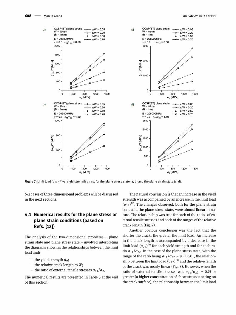
Figure 7: Limit load (σ22)P0 vs. yield strength σ0 vs. for the plane stress state (a, b) and the plane strain state (c, d).
672 cases of three-dimensional problemswill be discussedin the next sections.
4.1 Numerical results for the plane stress orplane strain conditions (based onRefs. [12])
The analysis of the two-dimensional problems – planestrain state and plane stress state – involved interpretingthe diagrams showing the relationships between the limitload and:
– the yield strength σ0;– the relative crack length a/W;– the ratio of external tensile stresses σ11/σ22.
The numerical results are presented in Table 3 at the endof this section.
The natural conclusion is that an increase in the yieldstrength was accompanied by an increase in the limit load(σ22)P0. The changes observed, both for the plane strainstate and the plane stress state, were almost linear in na-ture. The relationship was true for each of the ratios of ex-ternal tensile stresses and each of the ranges of the relativecrack length (Fig. 7).
Another obvious conclusion was the fact that theshorter the crack, the greater the limit load. An increasein the crack length is accompanied by a decrease in thelimit load (σ22)P0 for each yield strength and for each ra-tio σ11/σ22. In the case of the plane stress state, with therange of the ratio being σ11/σ22 = 〈0, 0.50〉, the relation-ship between the limit load (σ22)P0 and the relative lengthof the crack was nearly linear (Fig. 8). However, when theratio of external tensile stresses was σ11/σ22 = 0.75 orgreater (a higher concentration of shear stresses acting onthe crack surface), the relationship between the limit load

Limit loads for centrally cracked square plates under biaxial tension | 609
Figure 8: Limit load (σ22)P0vs. crack length for the plane stress state.
Figure 9: Limit load (σ22)P0vs. crack length for the plane strain state.
(σ22)P0 and the crack length was nonlinear. The greaterthe yield strength, the stronger the nonlinearity of the re-lationships between (σ22)P0 and a/W.
In the case of the plane strain state, the relationshipbetween the limit load (σ22)P0 and the relative crack lengtha/W was obvious: the shorter the crack, the greater thelimit load. However, changes in the (σ22)P0 = f (a/W)curves corresponded to the changes in the ratio of externaltensile stresses acting on the plate σ11/σ22 (Fig. 9). Whenσ11/σ22 = 0 (plate under uniaxial tension), the relation-shipbetween the limit loadand the crack lengthwas foundto be linear. An increase in the ratio σ11/σ22 ranging 〈0.25,0.50〉 caused that the relationship (σ22)P0 = f (a/W) wasnonlinear, resembling a hyperbola. A further increase in
the ratio σ11/σ22 ranging 〈0.75, 1.25〉 resulted in a changein the character of the relationship (σ22)P0 = f (a/W); thecurve resembled a diagram of a third order polynomialfunction. At σ11/σ22 = 1.50, the (σ22)P0 = f (a/W) curveshad a shape of an inverse parabola.
It is interesting to observe the in�uence of the ratio ofexternal tensile stresses σ11/σ22 on the limit load (σ22)P0
(Fig. 10). For the plane stress condition and a �xed yieldstrength, the relationship (σ22)P0 = f (σ11/σ22) was de-pendent on the relative crack length. For plates with verylong cracks (a/W = 0.70), the limit load was reportedto increase with increasing ratio σ11/σ22. The increasewas nearly linear reaching about 15–18% in relation to(σ22)P0 for the ratio σ11/σ22 = 0 (depending on the yield

610 | Marcin Graba
Figure 10: Limit load (σ22)P0vs. ratio σ11/σ22 for the plane stress state.
Figure 11: Limit load (σ22)P0vs. ratio σ11/σ22 for the plane strain state.
strength). For standard cracks (a/W =0.50) and the ra-tio σ11/σ22 = 〈0, 1〉, the increase in the limit load (σ22)P0
was almost linear, then the limit load decreased slightlywhen the ratio was σ11/σ22 = 〈1.25, 1.50〉. The decreaseof about 3% was small in relation to the value of (σ22)P0
for σ11/σ22 =1. When the cracks were short (a/W = 0.20),with the ratio being σ11/σ22 = 〈0; 0.75〉, the limit load in-creased by about 10–15% in relation to the value of ratioσ11/σ22 = 0, then it dropped. The decline of about 1%wassteadywhen σ11/σ22 = 〉0.75; 1.0〉. Then,when σ11/σ22 = 1,the limit load decreased considerably by about 20–30%.Similar conclusions can be drawn for the case of plateswith very short cracks (a/W = 0.05). It was found that the
shorter the crack, the more intensive the changes in the(σ22)P0 = f (σ11/σ22) curves.
The conclusions were not so obvious for the (σ22)P0 =f (σ11/σ22) curves when the relative crack length was�xed and the plane stress was predominant. For veryshort cracks,a/W = 0.05 and a/W = 0.20, the limitload increased until the ratio was σ11/σ22 = 0.50 andσ11/σ22 = 0.75 respectively; then, the value of the limitload decreased considerably and the decrease was non-linear. For the standard cracks (a/W =0.50), the limitload (σ22)P0 �rst increased by approximately 15–20% atσ11/σ22 = 〈0; 1〉, and then decreases by about 3–5%.
The analysis of the relationship (σ22)P0 = f (σ11/σ22)for predominant plane strain conditions (seeFig. 11) shows

Limit loads for centrally cracked square plates under biaxial tension | 611
Figure 12: Shape of the plastic zones in the CCSP(BT) with the same crack length and extreme values of the ratio of tensile stressesσ11/σ22: a) σ11/σ22 = 0, plane stress state; b) σ11/σ22 = 1.50, plane stress state; c) σ11/σ22 = 0, plane strain state [12]; d) σ11/σ22 = 1.50,plane strain state [12].
that the conclusions are similar to those drawn for theplane stress state. For very long cracks (a/W = 0.70) whenthe ratio σ11/σ22 increased in the range 〈0; 1.50〉, the limitload (σ22)P0 increased by about 73% for each value of theyield strength. For standard cracks (a/W = 0.50), with theratio in the range σ11/σ22 = 〈0; 1〉, the limit load rose non-linearly by approximately 78%, and then it droppedalmostlinearly by about 12.5%. For very short cracks (a/W = 0.05and a/W = 0.20), there was a strongly nonlinear increasein the limit load of about 125-0135%when the ratio rangedσ11/σ22 = 〈0; 1〉 followed by an almost linear decrease.It can be seen that under the plane strain conditions, thelevel of intensity of changes is higher than that observed
when the plane stress was predominant (compare Fig-ures 10 and 11).
Figures 12 and 13 show distributions of plastic re-gions in the model quarter of the plate (analysis based onRef. [12]). The diagrams were prepared for the moments atwhich full plasticity of the uncracked portion of the spec-imen was reached. As can be seen, the size and distribu-tion of the plastic zone is strongly dependent on the cracklength, the ratio of external tensile stresses and whetherthe plane stress conditions or plane strain conditions areconsidered.

612 | Marcin Graba
Figure 13: Shape of the plastic regions in the CCSP(BT) with: (a, d) a/W = 0.05, σ0 =315 MPa, σ11/σ22 =0.25; (b, e) a/W = 0.20,σ0 =500 MPa, σ11/σ22 =0.50; (c, f) a/W =0.70, σ0 =1500 MPa, σ11/σ22 =0.50 – ((a-c) – plane stress, (d-f) – plane strain [12]).
Limit loads for centrally cracked square plates under biaxial tension | 613
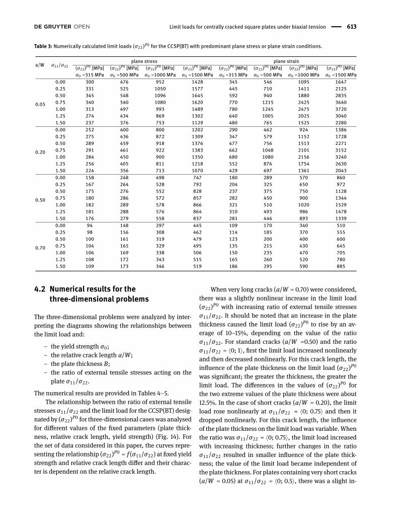
Table 3: Numerically calculated limit loads (σ22)P0 for the CCSP(BT) with predominant plane stress or plane strain conditions.
a/W σ11/σ22plane stress plane strain
(σ22)P0 [MPa] (σ22)P0 [MPa] (σ22)P0 [MPa] (σ22)P0 [MPa] (σ22)P0 [MPa] (σ22)P0 [MPa] (σ22)P0 [MPa] (σ22)P0 [MPa]σ0 =315 MPa σ0 =500 MPa σ0 =1000 MPa σ0 =1500 MPa σ0 =315 MPa σ0 =500 MPa σ0 =1000 MPa σ0 =1500 MPa
0.05
0.00 300 476 952 1428 345 546 1095 16470.25 331 525 1050 1577 445 710 1411 21250.50 345 548 1096 1645 592 940 1880 28350.75 340 540 1080 1620 770 1215 2425 36401.00 313 497 993 1489 780 1245 2475 37201.25 274 434 869 1302 640 1005 2025 30401.50 237 376 753 1129 480 765 1525 2280
0.20
0.00 252 400 800 1202 290 462 924 13860.25 275 436 872 1309 347 579 1152 17280.50 289 459 918 1376 477 756 1513 22710.75 291 461 922 1383 662 1048 2101 31521.00 284 450 900 1350 680 1080 2156 32401.25 256 405 811 1218 552 876 1754 26301.50 224 356 713 1070 429 697 1361 2043
0.50
0.00 158 248 498 747 180 289 570 8600.25 167 264 528 792 204 325 650 9720.50 175 276 552 828 237 375 750 11280.75 180 286 572 857 282 450 900 13441.00 182 289 578 866 321 510 1020 15291.25 181 288 576 864 310 493 986 14781.50 176 279 558 837 281 446 893 1339
0.70
0.00 94 148 297 445 109 170 340 5100.25 98 156 308 462 114 185 370 5550.50 100 161 319 479 123 200 400 6000.75 104 165 329 495 135 215 430 6451.00 106 169 338 506 150 235 470 7051.25 108 172 343 515 165 260 520 7801.50 109 173 346 519 186 295 590 885
4.2 Numerical results for thethree-dimensional problems
The three-dimensional problems were analyzed by inter-preting the diagrams showing the relationships betweenthe limit load and:
– the yield strength σ0;– the relative crack length a/W;– the plate thickness B;– the ratio of external tensile stresses acting on the
plate σ11/σ22.
The numerical results are provided in Tables 4–5.The relationship between the ratio of external tensile
stresses σ11/σ22 and the limit load for the CCSP(BT) desig-nated by (σ22)P0 for three-dimensional caseswas analysedfor di�erent values of the �xed parameters (plate thick-ness, relative crack length, yield strength) (Fig. 14). Forthe set of data considered in this paper, the curves repre-senting the relationship (σ22)P0 = f (σ11/σ22) at �xed yieldstrength and relative crack length di�er and their charac-ter is dependent on the relative crack length.
When very long cracks (a/W = 0.70) were considered,there was a slightly nonlinear increase in the limit load(σ22)P0 with increasing ratio of external tensile stressesσ11/σ22. It should be noted that an increase in the platethickness caused the limit load (σ22)P0 to rise by an av-erage of 10–15%, depending on the value of the ratioσ11/σ22. For standard cracks (a/W =0.50) and the ratioσ11/σ22 = 〈0; 1〉, �rst the limit load increased nonlinearlyand then decreased nonlinearly. For this crack length, thein�uence of the plate thickness on the limit load (σ22)P0
was signi�cant; the greater the thickness, the greater thelimit load. The di�erences in the values of (σ22)P0 forthe two extreme values of the plate thickness were about12.5%. In the case of short cracks (a/W = 0.20), the limitload rose nonlinearly at σ11/σ22 = 〈0; 0.75〉 and then itdropped nonlinearly. For this crack length, the in�uenceof the plate thickness on the limit loadwas variable.Whenthe ratio was σ11/σ22 = 〈0; 0.75〉, the limit load increasedwith increasing thickness; further changes in the ratioσ11/σ22 resulted in smaller in�uence of the plate thick-ness; the value of the limit load became independent ofthe plate thickness. For plates containing very short cracks(a/W = 0.05) at σ11/σ22 = 〈0; 0.5〉, there was a slight in-

614 | Marcin Graba
Figure 14: Limit load (σ22)P0 vs. ratio σ11/σ22 for three-dimensional cases at �xed yield strength and relative crack length.
crease in the limit load (an increase in the thickness wasaccompanied by a slight increase in the limit load); a fur-ther increase in the ratio σ11/σ22 resulted in a decreasein the limit load (σ22)P0; �rst the relationship was nonlin-ear and then linear. In the case of very short cracks, thelimit load (σ22)P0 was not dependent on the plate thick-ness when the ratio was σ11/σ22 = 〈0.75; 1.5〉. The con-clusions provided in this section are characteristic of eachvalue of the yield strength studied.
The analysis of the relationship (σ22)P0 = f (B) (seeFig. 15) was also interesting. As mentioned above, forvery short cracks (a/W = 0.05), no relationship was ob-served between the limit load (σ22)P0 and the plate thick-ness B. An increase in the crack length (to a/W = 0.20)caused the limit load (σ22)P0 to rise slightly with increas-ing plate thickness; the e�ect was very small, almost in-visible, in the presented diagrams. It should be noted thatthe (σ22)P0 = f (B) curves were almost linear in nature forboth cases. When the analysis concerned standard cracklengths (a/W = 0.50), the (σ22)P0 = f (B) curves showed
a slight and linear increase in the limit load with increas-ing plate thickness and the yield strength being σ0 = 〈315;1000〉 MPa. When the yield strength σ0 = 1500 MPa, thecurves (σ22)P0 = f (B) were slightly nonlinear; the in-crease in the plate thickness resulted in a slight increase inthe limit load. Similar conclusions can be drawn from theanalysis of the curves (σ22)P0 = f (B) obtained for platescontaining very long cracks (a/W = 0.70).
If, however, the results presented in this paper will berecalculated based on the value of the force - do not stress.Engineers need to con�rm the well-known fact that theload limit increases with the thickness of the plate. Thereis nothing new, but it is important to mention this.
The e�ects of the yield strength σ0 on the limit load(σ22)P0 are clear (Fig. 16). It can be concluded that thehigher the yield strength, the greater the limit load. Whenthe cracks were very short (a/W = 0.05), the (σ22)P0 =f (σ0) curves suggested that the limit loadwas almost unaf-fected by the plate thickness,whichwasmentioned above.

Limit loads for centrally cracked square plates under biaxial tension | 615
Table 4: Numerically calculated values of the limit load (σ22)P0 for CCSP(BT) (3D problems) at the relative crack lengths a/W = 0.05 anda/W = 0.20.
B [mm] σ11/σ22a/W = 0.05 a/W = 0.20
(σ22)P0 [MPa] (σ22)P0 [MPa] (σ22)P0 [MPa] (σ22)P0 [MPa] (σ22)P0 [MPa] (σ22)P0 [MPa] (σ22)P0 [MPa] (σ22)P0 [MPa]σ0 =315 MPa σ0 =500 MPa σ0 =1000 MPa σ0 =1500 MPa σ0 =315 MPa σ0 =500 MPa σ0 =1000 MPa σ0 =1500 MPa
2
0.00 304 480 963 1440 256 405 804 12150.25 335 531 1063 1593 279 440 885 13200.50 348 552 1105 1656 292 464 924 13890.75 343 545 1088 1634 293 465 930 13951.00 314 497 995 1494 286 453 906 13591.25 274 436 870 1306 257 408 816 12241.50 238 377 755 1132 226 358 717 1075
4
0.00 305 485 963 1454 256 405 816 12150.25 336 534 1068 1602 280 445 888 13350.50 355 556 1111 1667 294 465 933 13950.75 340 546 1088 1638 295 468 936 14041.00 314 498 997 1494 287 455 911 13651.25 274 436 871 1307 258 409 819 12301.50 238 377 755 1132 226 359 719 1079
8
0.00 308 486 975 1458 260 410 816 12300.25 340 540 1075 1620 284 450 900 13500.50 354 562 1123 1685 298 473 947 14190.75 344 546 1100 1638 299 474 948 14231.00 314 498 998 1494 290 460 916 13801.25 274 436 872 1308 260 412 824 12361.50 238 377 755 1133 228 361 723 1084
16
0.00 308 492 988 1476 264 415 828 12450.25 344 546 1088 1638 292 460 912 13800.50 359 570 1138 1710 304 485 971 14550.75 348 552 1100 1656 306 485 972 14551.00 315 499 998 1498 295 465 936 13951.25 275 436 872 1308 263 417 834 12501.50 238 377 755 1133 230 365 730 1095
25
0.00 308 492 988 1476 268 420 840 12600.25 344 546 1100 1638 296 470 936 14100.50 360 570 1138 1710 312 495 984 14850.75 348 552 1106 1656 314 495 996 14881.00 315 499 998 1498 300 473 948 14241.25 275 436 872 1308 266 421 842 12641.50 238 377 756 1134 232 368 735 1103
40
0.00 312 492 994 1476 275 429 860 12800.25 348 552 1100 1656 308 479 960 14400.50 360 575 1150 1726 324 512 1020 15200.75 348 552 1108 1656 326 512 1020 15361.00 315 500 998 1498 303 481 960 14401.25 275 436 872 1308 267 424 848 12721.50 238 377 756 1134 232 370 739 1108
It is evident that an increase in the crack length caused thelimit load to increase with increasing plate thickness.
For the three-dimensional cases, the e�ects of the rel-ative crack length a/W on the limit load (σ22)P0 are alsoobvious: the longer the crack, the smaller the limit load(σ22)P0. The (σ22)P0 = f (a/W) curves for di�erent valuesof the plate thickness B (Fig. 17) indicate that the higherthe ratio of external tensile stresses σ11/σ22, the morenonlinear the decrease in the limit load in relation to therelative crack length. The relationship between the limitload (σ22)P0 and the relative crack length a/W was almost
linear when the ratio of the external tensile stresses wasσ11/σ22 = 〈0; 0.5〉. For higher values of the ratio σ11/σ22,the decrease in the limit load with increasing crack lengthwas strongly nonlinear, especially for plates characterisedby a very large thickness B = {25; 40}.

616 | Marcin Graba
Figure 15: Limit load (σ22)P0 vs. thickness for 3D cases at �xed values of the yield strength and the relative crack length.
5 Comparison of the numericalresults with the existingsolutions
The numerical results concerning the limit load (σ22)P0 forthe CCSP(BT) under plane strain conditions can be com-pared with the data determined according to formulae (2)and (3), provided in Ref. [20].
The results concerning the limit load under the planestress conditions could not be analyzed as the authorsdo not mention them. As suggested in [20], formulae (2)and (3) were used to calculate the upper and lower limitloads, (σ2)lbL and (σ2)ubL , respectively, for four values ofthe yield strength, four values of the relative crack lengthand seven values of the ratio of external tensile stressesσ11/σ22. The results are shown in Table 6. Table 7, on theother hand, presents the percentage di�erence betweenthe set of results analyzed in this paper (σ22)P0 for predom-inant plane strain and the data obtained from formulae(2) and (3) proposed in Ref. [20], (σ22)P0−(σ2)lbL
(σ22)P0· 100% and
(σ22)P0−(σ2)ubL(σ22)P0
· 100%, respectively.As can be seen, formula (3) [20] is not suitable to cal-
culate the limit load (σ2)ubL for one con�guration of therelative crack length a/W and the ratio of external ten-sile stresses σ11/σ22, (see Table 6). From the analysis ofthe data shown in Table 7 it is clear that the di�erencesbetween the numerical results for the plane strain state(σ22)P0 and the values determined according to formulae(2) and (3) [20] are dependent on the con�guration result-
ing from the combination of the relative crack length a/Wand the ratio of external tensile stresses σ11/σ22.
The smallest di�erences between the numerical re-sults and the data obtained from formulae (2) and (3)were reported for plates containing very long cracks(a/W = 0.70). In such case, the numerical results (σ22)P0
were up to 7% smaller than those determined using formu-lae (2) and (3) − (σ2)lbL and (σ2)ubL , respectively. For stan-dard crack lengths (a/W =0.50), the di�erences betweenthe numerical solution (σ22)P0 and the values of (σ2)lbL(formula (2) [20]) reached up to 13–14% (the values calcu-lated using the FEM were lower than those calculated ac-cording to formula (2)); however, for ratios σ11/σ22 = {1.25;1.50}, the numerical values of the limit load were higher.The di�erences between the numerical value (σ22)P0 andthe values calculated from Eq. (3) (σ2)ubL [20] were thesmallest at σ11/σ22 = 〈0; 1〉. In the case of plateswith shortcracks (a/W = 0.20) or very short cracks (a/W = 0.05),the smallest di�erences between the numerical solution(σ22)P0 and the analytical solutions, (σ2)lbL and (σ2)ubL ,(formulae (2) and (3), respectively [20]) were observed forσ11/σ22 = 〈0; 0.5〉. A more detailed analysis can be per-formed by comparing the data presented in Tables 3 and 6with the di�erences given in Table 7.
Eqns. (2) and (3) in [20] are limited only for planestrain state. As we can see, the Eq.(3) proposed in [20]does not allow for one of the cases set a level of limit load(σ11/σ22, a/W = 0.20). Furthermore, with regard to the nu-merical results presented in this paper, equations (2) and(3) used to estimate the limit loads for plates with veryshort cracks(a/W= 0.05) generated signi�cant di�erences,

Limit loads for centrally cracked square plates under biaxial tension | 617
Figure 16: Limit load (σ22)P0 against yield strength for three-dimensional cases at �xed ratio and relative crack length.
Figure 17: Limit load (σ22)P0 against relative crack length for three-dimensional cases at �xed ratio and yield strength.

618 | Marcin Graba
Table 5: Numerically calculated values of the limit load (σ22)P0 for CCSP(BT) (3D problems) at the relative crack lengths a/W = 0.50 anda/W = 0.70.
B [mm] σ11/σ22a/W = 0.50 a/W = 0.70
(σ22)P0 [MPa] (σ22)P0 [MPa] (σ22)P0 [MPa] (σ22)P0 [MPa] (σ22)P0 [MPa] (σ22)P0 [MPa] (σ22)P0 [MPa] (σ22)P0 [MPa]σ0 =315 MPa σ0 =500 MPa σ0 =1000 MPa σ0 =1500 MPa σ0 =315 MPa σ0 =500 MPa σ0 =1000 MPa σ0 =1500 MPa
2
0.00 159 254 504 760 96 153 304 4590.25 168 270 539 800 100 159 316 4770.50 177 280 560 840 102 162 325 4860.75 182 290 580 870 106 168 335 5041.00 185 293 585 879 108 171 345 5131.25 184 292 584 875 110 174 350 5221.50 177 281 563 844 111 177 354 531
4
0.00 159 255 511 760 96 153 305 4590.25 171 270 539 810 100 159 320 4770.50 180 285 567 850 104 165 330 4950.75 185 293 587 880 108 171 340 5131.00 186 296 592 888 110 174 350 5221.25 186 294 588 884 112 177 355 5311.50 178 283 566 849 113 180 360 540
8
0.00 162 260 518 770 98 156 310 4680.25 174 275 546 820 102 162 325 4860.50 183 290 574 860 106 168 335 5040.75 189 300 595 899 110 174 350 5221.00 190 302 602 905 114 180 360 5401.25 189 300 601 899 116 183 365 5491.50 180 287 573 859 117 186 370 558
16
0.00 165 265 525 788 100 159 318 4770.25 177 280 560 849 106 168 336 5040.50 189 300 595 899 110 174 348 5220.75 195 310 616 929 114 183 366 5491.00 198 310 623 939 118 189 378 5671.25 195 310 616 930 122 192 384 5761.50 185 294 588 881 122 195 390 585
25
0.00 168 270 532 798 102 162 324 4860.25 183 290 574 869 106 168 336 5040.50 195 310 616 919 112 177 354 5310.75 201 320 637 950 116 186 372 5581.00 204 325 644 970 120 192 384 5761.25 201 320 637 959 124 198 396 5941.50 190 301 602 903 126 201 402 603
40
0.00 171 270 539 811 102 162 324 4860.25 186 295 588 878 108 171 342 5130.50 198 315 630 944 114 180 360 5400.75 210 330 658 989 120 189 378 5671.00 213 340 679 1011 124 198 396 5941.25 210 335 665 1000 130 204 408 6121.50 195 311 620 931 132 210 420 630
reaching up to almost 50 (in the case of formula (2)) andthe 200 and 800 percent (in the case of formula (3)) in re-lation to the results obtained numerically, for cases char-acterized by the ratio of external loads σ11/σ22 = 〈0.5;1.5〉. Also for the case of short cracks (characterized bya/W=0.20), the di�erence between the numerical solutionof the formulas (2) and (3) are almost 50% and 240% re-spectively, for cases characterized by the ratio of externalloads σ11/σ22 = 〈0.5; 1.5〉. Di�erences between the numer-ical solution and the formula (3) for plate with the norma-tive cracks (characterizedbya/W=0.50) for the rangeof the
ratio of external loads σ11/σ22 = 〈1.0; 1.5〉 range from 13%to 160%.
Comparative studies of the author of this paper sug-gest a limited applicability of the formulas (2) and (3). Inthe case of very short and short cracks, theseEqns. are con-sistent with the numerical results in a small range of theratio of external loads σ11/σ22 = 〈0.0; 0.5〉. In case of in-crease of the crack length, the applicability of equation (2)and (3) increases, whereas for very long cracks, it can bewrite that convergence between both solutions of numeri-cal results is quite correct.

Limit loads for centrally cracked square plates under biaxial tension | 619
Table 6: Values of the limit loads (σ2)lbL and (σ2)ubL for CCSP(BT) with predominant plane strain conditions calculated numerically from for-mulae (2) and (3) [20].
a/W σ11/σ22plane strain, formula (2) [20] plane strain, formula (3) [20]
(σ2)lbL [MPa] (σ2)lbL [MPa] (σ2)lbL [MPa] (σ2)lbL [MPa] (σ2)ubL [MPa] (σ2)ubL [MPa] (σ2)ubL [MPa] (σ2)ubL [MPa]σ0 =315 MPa σ0 =500 MPa σ0 =1000 MPa σ0 =1500 MPa σ0 =315 MPa σ0 =500 MPa σ0 =1000 MPa σ0 =1500 MPa
0.05
0.00 346 548 1097 1645 346 548 1097 16450.25 453 719 1439 2158 453 719 1439 21580.50 658 1045 2089 3134 658 1045 2089 31340.75 485 770 1540 2309 1202 1908 3816 57231.00 364 577 1155 1732 6911 10970 21939 329091.25 291 462 924 1386 1843 2925 5850 87761.50 242 385 770 1155 813 1291 2581 3872
0.20
0.00 291 462 924 1386 291 462 924 13860.25 364 577 1155 1732 364 577 1155 17320.50 485 770 1540 2309 485 770 1540 23090.75 485 770 1540 2309 727 1155 2309 34641.00 364 577 1155 1732 1455 2309 4619 69281.25 291 462 924 1386 —- —- —- —-1.50 242 385 770 1155 1455 2309 4619 6928
0.50
0.00 182 289 577 866 182 289 577 8660.25 208 330 660 990 208 330 660 9900.50 242 385 770 1155 242 385 770 11550.75 291 462 924 1386 291 462 924 13861.00 364 577 1155 1732 364 577 1155 17321.25 291 462 924 1386 485 770 1540 23091.50 242 385 770 1155 727 1155 2309 3464
0.70
0.00 109 173 346 520 109 173 346 5200.25 118 187 374 562 118 187 374 5620.50 128 204 408 611 128 204 408 6110.75 141 223 447 670 141 223 447 6701.00 156 247 495 742 156 247 495 7421.25 175 277 554 831 175 277 554 8311.50 198 315 630 945 198 315 630 945
Thenumerical values of the limit loads (σ22)P0 and thevalues determined according to formulae (2) and (3) [20]can be used to verify and assess the strength of a struc-ture – CCSP(BT) – using the Failure Assessment Diagrams(FADs) or the Crack Driving Force (CDF) diagrams [11, 13–16]. This approach is generally applied when the serviceconditions of the structure and the sizes of defects areknown. As the study focused on numerical analysis, sup-ported by theoretical analyses, this work discusses onlythe changes in the numerically calculated value of theJ-integral (frequently de�ned as the crack driving force)as a function of external loads normalized by the limitload [11, 13–16].
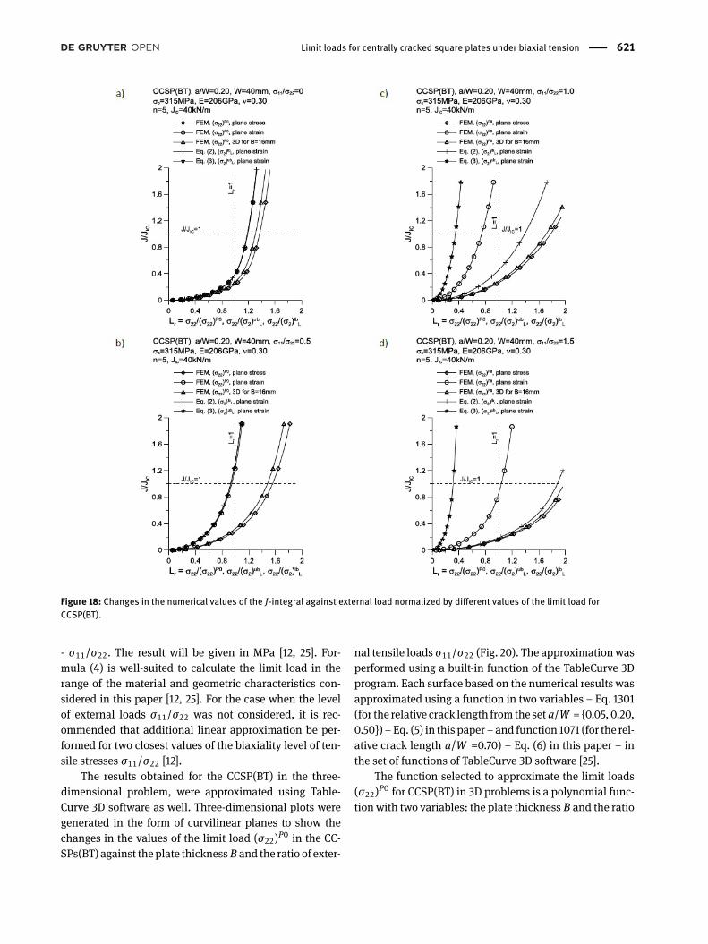
Thematerial considered in this paper is also one anal-ysed by Sumpter and Forbes [26] to assess fracture tough-ness. Thematerial [26] had the yield strength σ0 = 315MPa,Young’s modulus E = 206 GPa, Poisson’s ratio ν = 0.3 andthe strain hardening exponent n =5. When the materialwas subjected to plane strain conditions, Sumpter deter-mined the fracture toughness to be JIC = 40 kN/m. Thematerial is characterized by brittle fracture with extendedplastic zones. The material was also discussed in Ref. [30]
to verify the local crack criteria. A numerical analysis wasconducted for that material and CCSPs(BT) at the relativecrack length a/W = 0.20 and the ratio of tensile stressesσ11/σ22 = {0; 0.5; 1.0; 1.5}. The analysis involved using a �-nite element mesh to model an elastic-plastic material bycalculating the stress distribution near the crack tip andthe J-integral. The numerical models and integration con-tour necessary to calculate the J−integral and the methodto determine the stress distributions were generated ac-cording to the recommendations provided in Refs. [10, 27–29].
Figure 18 shows the relationship between the J-integral and the external load normalized by di�erent val-ues of the limit load – the values of (σ22)P0 presentedabove, which were determined numerically for the planestrain state, the plane stress state and 3D problems, andalso the values of the limit load (σ2)lbL and (σ2)ubL , deter-mined according to Eqs. (2) and (3) [20]. The diagrams arenot analyzed here. It is important to note that the mostconservative solution and approach to the problemof limitloads guarantee that engineering problems can be solvedusing the values determined for the plane stress state. If,

620 | Marcin Graba
Table 7: Percentage di�erences between the numerical values of the limit loads determined for the plane strain state (σ22)P0 and the valuescalculate from formulae (2) and (3) [20].
a/W σ11/σ22(σ22)P0−(σ2)lb
(σ22)P0 · 100%, plane strain (σ22)P0−(σ2)ub(σ22)P0 · 100%, plane strain
(σ2)lbL [MPa] (σ2)lbL [MPa] (σ2)lbL [MPa] (σ2)lbL [MPa] (σ2)ubL [MPa] (σ2)ubL [MPa] (σ2)ubL [MPa] (σ2)ubL [MPa]σ0 =315 MPa σ0 =500 MPa σ0 =1000 MPa σ0 =1500 MPa σ0 =315 MPa σ0 =500 MPa σ0 =1000 MPa σ0 =1500 MPa
0.05
0.00 0% 0% 0% 0% 0% 0% 0% 0%0.25 -2% -1% -2% -2% -2% -1% -2% -2%0.50 -11% -11% -11% -11% -11% -11% -11% -11%0.75 37% 37% 37% 37% -56% -57% -57% -57%1.00 53% 54% 53% 53% -786% -781% -786% -785%1.25 55% 54% 54% 54% -188% -191% -189% -189%1.50 49% 50% 50% 49% -69% -69% -69% -70%
0.20
0.00 0% 0% 0% 0% 0% 0% 0% 0%0.25 -5% 0% 0% 0% -5% 0% 0% 0%0.50 -2% -2% -2% -2% -2% -2% -2% -2%0.75 27% 27% 27% 27% -10% -10% -10% -10%1.00 47% 47% 46% 47% -114% -114% -114% -114%1.25 47% 47% 47% 47% —- —- —- —-1.50 43% 45% 43% 43% -239% -231% -239% -239%
0.50
0.00 -1% 0% -1% -1% -1% 0% -1% -1%0.25 -2% -2% -2% -2% -2% -2% -2% -2%0.50 -2% -3% -3% -2% -2% -3% -3% -2%0.75 -3% -3% -3% -3% -3% -3% -3% -3%1.00 -13% -13% -13% -13% -13% -13% -13% -13%1.25 6% 6% 6% 6% -56% -56% -56% -56%1.50 14% 14% 14% 14% -159% -159% -159% -159%
0.70
0.00 0% -2% -2% -2% 0% -2% -2% -2%0.25 -3% -1% -1% -1% -3% -1% -1% -1%0.50 -4% -2% -2% -2% -4% -2% -2% -2%0.75 -4% -4% -4% -4% -4% -4% -4% -4%1.00 -4% -5% -5% -5% -4% -5% -5% -5%1.25 -6% -7% -7% -7% -6% -7% -7% -7%1.50 -7% -7% -7% -7% -7% -7% -7% -7%
however, the solutions are to be less conservative, the re-sults obtained for three-dimensional cases should be usedto analyze the behaviour of the CCSP(BT). More details onthe elastic-plastic problems, particularly stress �elds nearthe crack tip, the J-integral and the parameters from theelastic-plastic fracturemechanics, will be presented in theauthor’s next paper.
6 Approximation of the numericalresults (based on Refs. [12])
The numerical results obtained in this study for a two-dimensional case (plane stress or plane strain conditions)and for a three-dimensional case were approximated. Theapproximation was conducted separately for the two-dimensional [12] and three-dimensional problems.
The two-dimensional cases – plane stress state andplane strain state – were approximated using TableCurve3D software [25], which produces three-dimensional plotsshowing, in the form of curvilinear planes, changes in the
values of the limit load (σ22)P0 for the CCSP(BT) as a func-tion of the yield strength σ0 and the relative crack lengtha/W [12]. Figure 19 shows plots obtained for the planestress state and the plane strain state [12]. The next step ofthe analysis involved using a built-in function of the Table-Curve 3D software and approximating each surface with apolynomial function in two variables [12] – Equation 1 inthe set of functions of the TableCurve 3D software [25].
The function selected to approximate the limit loads(σ22)P0 is a polynomial function with two variables: theyield strength σ0 and the relative crack lengtha/W [12]:
(σ22)P0 = A1 + A2 · σ0 + A3 ·( aW
)+ A2 · (σ0)2
+ A5 ·( aW
)2+ A6 · σ0 ·
( aW
)(4)
where the coe�cients A1, A2, A3, A4, A5, A6 are depen-dent on the ratio σ11/σ22 determining the level of biaxi-ality of the external load (external tensile loads) [12]. Thevalues of the coe�cients are provided in Table 8.
When formula (4) is used, it is necessary to know therelative crack length a/W, the yield strength σ0 given inMPa and the mutual ratio between external tensile loads
Limit loads for centrally cracked square plates under biaxial tension | 621
Figure 18: Changes in the numerical values of the J-integral against external load normalized by di�erent values of the limit load forCCSP(BT).
- σ11/σ22. The result will be given in MPa [12, 25]. For-mula (4) is well-suited to calculate the limit load in therange of the material and geometric characteristics con-sidered in this paper [12, 25]. For the case when the levelof external loads σ11/σ22 was not considered, it is rec-ommended that additional linear approximation be per-formed for two closest values of the biaxiality level of ten-sile stresses σ11/σ22 [12].
The results obtained for the CCSP(BT) in the three-dimensional problem, were approximated using Table-Curve 3D software as well. Three-dimensional plots weregenerated in the form of curvilinear planes to show thechanges in the values of the limit load (σ22)P0 in the CC-SPs(BT) against theplate thickness B and the ratio of exter-
nal tensile loads σ11/σ22 (Fig. 20). The approximationwasperformed using a built-in function of the TableCurve 3Dprogram. Each surface based on the numerical results wasapproximated using a function in two variables – Eq. 1301(for the relative crack length from the set a/W = {0.05, 0.20,0.50}) – Eq. (5) in this paper – and function 1071 (for the rel-ative crack length a/W =0.70) – Eq. (6) in this paper – inthe set of functions of TableCurve 3D software [25].
The function selected to approximate the limit loads(σ22)P0 for CCSP(BT) in 3D problems is a polynomial func-tion with two variables: the plate thickness B and the ratio

622 | Marcin Graba
Figure 19: Relationship (σ22)P0 = f (σ0, a/W) for the CCSP(BT) under conditions of a) predominant plane stress, σ11/σ22 =0.25; b) pre-dominant plane strain, σ11/σ22 =1.50; results presented for the �xed ratio σ11/σ22 – ratio of biaxial external tensile stresses in the plate –diagrams used in the approximation of the numerical results for two-dimensional problems [12].
of the external tensile stresses σ11/σ22:
(σ22)P0 =(A1 + A3 · B + A5 ·
(σ11σ22
)+ A7 · B2
+A9 ·(σ11σ22
)2+ A11 · B ·
(σ11σ22
))/(1 + A2 · B+
A4 ·(σ11σ22
)+ A6 · B2 + A8 ·
(σ11σ22
)2+ A10 · B ·
(σ11σ22
))for a/W = {0.05, 0.20, 0.50} (5)
(σ22)P0 =(A1 + A2 · B + A3 · B2 + A4 ·
(σ11σ22
)+A5 ·
(σ11σ22
)2+ A6 ·
(σ11σ22
)3)/(
1 + A7 · B + A8 · B2
+ A9 · B3 + A10 ·(σ11σ22
))for a/W = 0.70 (6)
where the coe�cients A1, A2, A3, A4, A5, A6, A7, A8, A9,A10, A11 are dependent on the yield strength σ0 and therelative crack length a/W. The set of approximation coef-�cients is given in Table 9.
When formulae (5) and (6) are used, it is necessary toknow the plate thickness B, the relative crack length a/W,the yield strength σ0 given in MPa and the mutual ratiobetween external tensile loads - σ11/σ22. The result willbe given in MPa. Formulae (5) and (6) are well-suited tocorrectly estimate the limit load in the range of the mate-rial and geometric characteristics considered here. For thecase when the level of external loads σ11/σ22 or geome-try (a/W, B) or material characteristics (σ0) were not con-sidered, it is recommended that additional linear approxi-mation be performed for two closest values of the level ofbiaxiality of tensile stresses σ11/σ22 and/or the materialcharacteristics (σ0) and the plate geometry (a/W, B).
7 ConclusionsThis paper has considered the determination of the limitloads (σ22)P0 for centrally cracked square plates under bi-axial tension – CCSPs(BT). The work has brie�y discussedthe concept of limit loads, some aspects of numericalmod-elling as it slightly di�erswhen two-dimensional problems– plane stress state and plane strain state – and three-dimensional problems are analysed. The paper has alsodescribed all the numerical results. In the study, it was es-sential to determine the in�uence of various parameterson the value of the limit load, with the parameters includ-ing the relative crack length a/W, the yield strength σ0,the plate thickness B and the ratio of biaxial external loadsσ11/σ22, being the ratio of external tensile stresses actingon the plate. Approximation formulae used for all the re-sults are presented.
The conclusions drawn during the study are natu-ral and obvious. The limit load increases with increas-ing yield strength and decreases with increasing cracklength. The numerical calculations conducted for thethree-dimensional cases indicate that for the analysed ge-ometry there is a slight increase in the limit load (σ22)P0
when the plate thickness increases – if the limit load isused in [MPa] units. If, however, the results presented inthis paper will be recalculated based on the value of theforce [kN] - donot stress, engineerneed to con�rm thewell-known fact, that the load limit increaseswith the thicknessof the plate. There is nothing new, but it is important tomention this. Of interest is the in�uence of the level of bi-axiality of external tensile stresses acting on the plate intwo directions σ11/σ22. In the case of very short and shortcracks (a/W = 0.05 and a/W = 0.20, respectively), this isa considerable increase in the limit load with increasing

Limit loads for centrally cracked square plates under biaxial tension | 623
Table 8: Approximation coe�cients for Eq. (4) required to estimate the limit load (σ22)P0 for CCSP(BT) under conditions of predominantplane stress and plane strain.
CCSP (BT) - plane stress stateσ11/σ22 A1 A2 A3 A4 A5 A6 R2
0.00 0.755351 1.000471 -2.48845 1.26E-06 4.212296 -1.00903 0.9999990.25 6.585902 1.101109 -56.3316 2.01E-06 79.63272 -1.14564 0.9999810.50 2.703452 1.155056 -23.5847 6.66E-07 33.21768 -1.20072 0.9999780.75 -9.29601 1.144691 94.69308 4.93E-07 -126.76 -1.15786 0.9999361.00 -35.2018 1.074304 344.7311 -5.92E-07 -460.49 -1.02438 0.9988561.25 -51.2732 0.943359 505.4566 2.18E-07 -674.699 -0.81063 0.9980621.50 -55.6479 0.815609 544.7044 -1.54E-07 -726.302 -0.61435 0.996762
CCSP (BT) – plane strain stateσ11/σ22 A1 A2 A3 A4 A5 A6 R2
0.00 -0.83579 1.151174 11.71494 3.76E-06 -8.1789 -1.1703 1.00000.25 17.50299 1.499167 -257.559 -6.78E-06 350.7361 -1.62151 0.99970.50 55.32455 1.971651 -539.714 6.92E-06 726.4338 -2.32906 0.99880.75 27.17162 2.633399 -241.897 4.99E-07 316.4248 -3.23179 0.99321.00 -10.0275 2.689586 131.8 4.72E-06 -175.276 -3.21873 0.99601.25 -25.6442 2.174414 247.2069 3.01E-06 -321.686 -2.36762 0.99911.50 -21.4071 1.625967 236.2928 -5.81E-06 -328.903 -1.45234 0.9993
Figure 20: Relationship (σ22)P0 = f (B, σ11/σ22) for CCSP(BT), 3D problems – results presented for the �xed relative crack length and yieldstrength: a) σ0 =315, a/W =0.05; b) σ0 = 500, a/W = 0.20; c) σ0 = 1000, a/W = 0.50; d) σ0 = 1500, a/W = 0.70.
ratio σ11/σ22; however, after the ratio of tensile stressesσ11/σ22 reaches a certain level, the limit loads decreasewith increasing ratio σ11/σ22. In the case of standard crack
lengths (a/W = 0.50), the (σ22)P0 = f (σ11/σ22) curves aresimilar. For long cracks (a/W = 0.70), there is an increasein the limit load (σ22)P0 with increasing ratio σ11/σ22, de-

624 | Marcin Graba
Table 9: Approximation coe�cients for Eqs. (5) and (6) required to calculate the limit load (σ22)P0 for CCSP(BT) – 3D problems.
a/W = 0.05 (Equation (5)) a/W = 0.20 (Equation (5))σ0 =315 MPa σ0 =500 MPa σ0 =1000 MPa σ0 =1500 MPa σ0 =315 MPa σ0 =500 MPa σ0 =1000 MPa σ0 =1500 MPa
A1 304.032 481.8922 962.9015 1446.111 255.5897102 404.1778941 807.1481105 1212.849411A2 -0.00792 -0.00794 -0.00678 -0.00802 -0.01002803 -0.01108645 -0.01084617 -0.01203512A3 -2.11139 -3.30179 -5.27882 -10.0401 -2.03732373 -3.76821956 -7.34143825 -12.4845912A4 -0.72379 -0.71595 -0.76513 -0.73102 -0.65899379 -0.60542718 -0.62610699 -0.58958701A5 -84.1022 -129.827 -316.315 -417.465 -81.7314521 -99.0596309 -214.911089 -279.874754A6 9.01E-05 7.84E-05 7.38E-05 7.20E-05 3.32236e-05 6.28611e-05 7.22904e-05 8.04511e-05A7 0.023694 0.030574 0.057222 0.082438 0.00339423 0.017532261 0.044733849 0.072235693A8 0.615457 0.603294 0.621659 0.607219 0.348429109 0.335429152 0.346131432 0.322662294A9 58.46168 87.59038 202.3852 274.0999 20.32888141 20.80668779 51.31295921 48.41197883A10 0.003349 0.003745 0.003374 0.004143 0.005543195 0.005164528 0.004846094 0.005279761A11 0.89567 1.604645 2.657629 5.391933 1.30452199 2.009179103 3.691308612 6.224973082R2 0.999188 0.999396 0.999437 0.999372 0.9973131908 0.9975972918 0.9977115782 0.9974149095
a/W = 0.50 (Equation (5)) a/W = 0.70 (Equation (6))σ0 =315 MPa σ0 =500 MPa σ0 =1000 MPa σ0 =1500 MPa σ0 =315 MPa σ0 =500 MPa σ0 =1000 MPa σ0 =1500 MPa
A1 157.503661 252.5863619 504.0432455 751.4867099 94.25404428 150.676942 300.0564977 452.024134A2 -0.01254617 -0.01153338 -0.01166579 -0.01069029 -0.92869231 -2.84764264 -4.17257963 -8.53889366A3 -1.45287539 -2.07061296 -4.46605773 -5.53115132 0.00778915 0.036823999 0.047053689 0.110358944A4 -0.21658444 -0.3380263 -0.36120058 -0.32871355 -1.3606413 4.643625755 2.657867287 14.00052627A5 11.67030473 -22.9200869 -57.8207353 -48.9408426 -2.87323616 -2.05560208 -6.20409817 -6.01464165A6 0.000101521 6.4666e-05 5.73314e-05 5.66167e-05 -1.18320898 -2.09000915 -4.54922868 -6.33139295A7 0.008377213 0.002728202 0.007395764 0.004529457 -0.01644531 -0.02457572 -0.01966601 -0.02457199A8 0.056388459 0.104205919 0.099020687 0.08068719 0.000336218 0.000482888 0.000371949 0.000482881A9 -15.1666275 -6.92516632 -16.7640822 -46.061543 -3.1226e-06 -3.1032e-06 -2.5663e-06 -3.1062e-06A10 -0.00252795 -0.00155999 0.000170094 -0.0007911 -0.1659777 -0.10399358 -0.13740333 -0.10371964A11 -0.60069484 -0.66231983 -0.30438633 -1.34743833 — — — —R2 0.9965096854 0.9947349475 0.9970068403 0.9962752165 0.9970358348 0.9972035715 0.9976895918 0.997217039
termining the level of biaxiality of external stresses actingon the plate in two directions.
The numerically calculated values of the limit loads(σ22)P0 for the CCSP(BT) were compared with the resultsavailable in the literature. They were veri�ed using the as-sumptions of elastic-plastic fracture mechanics. The con-clusions drawn from the comparison are also universal –the conservatism of the solution guarantees that in engi-neering problems the values of the limit loads (σ22)P0 de-termined for the plane stress state can be used. If the ap-proach is less conservative, the calculated values of thelimit loads (σ22)P0 can be used for real three-dimensionalcomponents.
The approximating formulae presented in this workare suitable to estimate the limit load for cases not consid-ered in the numerical program while solving engineeringproblems.
Acknowledgement: The research reported herein wassupported by a IUVENTUS PLUS grant from the Ministryof Science and Higher Education (No. IP2012 011872).
Nomenclature
CCSP(BT) Centre Cracked Plate in Biaxial TensionCDF Crack Driving ForceEPRI Electric Power Research Institute procedures,
report entitled “Engineering Approach forElastic-Plastic Fracture Analysis”
FAD Failure Assessment DiagramFEM Finite Element MethodFITNET FITNET Report - European Fitness-for-service
NetworkHMH Huber-Mises-HenckySIF Stress Intensity FactorSINTAP Structural Integrity Assessment Procedures
for European Industry2D two dimensional3D three dimensionala crack length, [m]A1,. . . ,A11 coe�cients of the approximationa/W standard crack lengthB specimen (plate) thickness, [m]E Young modulus, [MPa]J J – integralJIC critical value of the J-integralKI stress intensity factor for the actual load
state, [MPa·m0.5]

Limit loads for centrally cracked square plates under biaxial tension | 625
KIC critical value of the stress intensity factor,[MPa·m0.5]
Kr standardized stress intensity factorLr standardized external load calculatedn Strain hardening exponentP actual load, [N]P0 limit load, [N]rw crack tip radius [m]W specimen (plate) width, [m]σ0 yield strength, [MPa]σ11/σ22 measure of biaxial load(σ2)lbL limit load proposed by Meek and
Ainsworth, i.e. the normal stress ap-plied to a specimen resulting in the fullplasticity of the uncracked portion ofthe specimen; the index ‘lb’ of the limitload refers to the least possible solutionobtained in Ref. [20], [MPa]
(σ2)ubL limit load, i.e. normal stress applied tothe specimen resulting in the full plastic-ity of the uncracked portion of the speci-men; the index ‘ub’ of the limit load refersto the best possible solution obtained inRef. [20], [MPa]
(σ22)P0 limit stress (limit load) for CCCSP(BT),[MPa]
ν Poisson’s ratioσ0 strain corresponding to the yield
strength, σ0 = σ0/E
References[1] Hutchinson J.W., Singular Behavior at the End of a Tensile Crack
in a Hardening Material, Journal of the Mechanics and Physicsof Solids,1968, 16(1), 13-31.
[2] Rice J.R., Rosengren G.F., Plane Strain Deformation Near a CrackTip in aPower-LawHardeningMaterial, Journal of theMechanicsand Physics of Solids, 1968, 16 (1), 1-12.
[3] O’Dowd N.P., Shih C.F., Family of Crack-Tip Fields Characterizedby a Triaxiality Parameter – I. Structure of Fields, J. Mech. Phys.Solids,1991, 39 (8), 989-1015.
[4] O’Dowd N.P., Shih C.F., Family of Crack-Tip Fields Characterizedby a Triaxiality Parameter – II. Fracture Applications, J. Mech.Phys. Solids, 1992, 40(5), 939-963.
[5] Yang S., Chao Y.J., Sutton M.A., Higher Order Asymptotic CrackTip Fields in a Power-Law HardeningMaterial, Engineering Frac-ture Mechanics,1993, 19(1), 1-20.
[6] Wanlin G., Elastoplastic Three Dimensional Crack Border Field –I. Singular Structure of the Field, Engineering Fracture Mechan-ics, 1993, 46(1), 93-104.
[7] Wanlin G., Elastoplastic Three Dimensional Crack Border Field– II. Asymptotic Solution for the Field, Engineering Fracture Me-
chanics, 1993, 46(1), 105-113.[8] Wanlin G., Elastoplastic Three Dimensional Crack Border Field –
III. Fracture Parameters, Engineering Fracture Mechanics, 1995,51(1), 51-71.
[9] Graba M., Numerical analysis of the mechanical �elds near thecrack tip in the elastic-plastic materials. 3D problems., PhD dis-sertation, Kielce University of Technology - Faculty of Mecha-tronics and Machine Building , Kielce 2009 (in Polish).
[10] Kumar V., German M.D., Shih C.F., An engineering approach forelastic-plastic fracture analysis, Electric Power Research Insti-tute, Inc. Palo Alto CA, EPRI Report NP-1931, 1981.
[11] Neimitz A., Dzioba I., Graba M., OkrajniJ. , The assessment ofthe strength and safety of the operation high temperature com-ponents containing crack, Kielce University of Technology Pub-lishing House, Kielce, 2008.
[12] Graba M., O wyznaczaniu obciążeń granicznych płyt kwadra-towych z centralną szczeliną w dwuosiowym rozciąganiu, Com-puter Systems Aided Science Industry and Transport, Proceed-ings of 19-th International Conference TRANSCOMP 2015 (20November 2015 -3 December 2015, Zakopane, Poland) (in Pol-ish).
[13] SINTAP: Structural Integrity Assessment Procedures for Euro-pean Industry. Final Procedure, Brite-Euram Project No BE95-1426. – Rotherham: British Steel, 1999.
[14] FITNET Report, (European Fitness-for-service Network), Editedby M. Kocak, S. Webster, J.J. Janosch, R.A. Ainsworth, R. Koers,Contract No. G1RT-CT-2001-05071, 2006.
[15] R6 - Assessment of the integrity of structures containing de-fects, Nuclear Electric-R6 Manuals, Nuclear Electric Ltd, BarnettWay, Barnwood, Gloucester GL4 3RS, United Kingdom, 1997.
[16] BS 7910: Guide on Methods for Assessing the Acceptability ofFlaws in Metallic Structures, 2005.
[17] Dowling A.R., Townley C.H.A., The e�ects of defects on struc-tural failure: a two-criteria approach, International Journal ofPressure Vessels and Piping, 1975, 3, 77-137.
[18] Harrison R.P., Loosemore K., Milne I., Assessment of the in-tegrity of structures containing defects, CEGB Report R/H/R6,Central Electricity Generating Board, United Kingdom, 1976.
[19] Harrison R.P., Loosemore K., Milne I., Dowling A.R., Assess-ment of the integrity of structures containing defects, CEGB Re-port R/H/R6-Rev.2, Central Electricity Generating Board, UnitedKingdom, 1980.
[20] Meek C., Ainsworth RA. The e�ects of load biaxial-ity and plate length on the limit load of a centre-cracked plate, Engineering Fracture Mechanics (2015),http://dx.doi.org/10.1016/j.engfracmech.2015.03.034
[21] Eftis J., Jones D.L., Influence of load biaxiality on the fractureload of center cracked sheets, Int. Journ. of Fracture, 1982, 20,267-289.
[22] ADINA 8.8, ADINA: User Interface Command Reference Manual– Volume I: ADINA Solids & Structures Model De�nition, ReportARD 11-2, ADINA R&D, Inc., 2011.
[23] ADINA 8.8, ADINA: Theory and Modeling Guide – Volume I: AD-INASolids&Structures, Report ARD 11-8, ADINAR&D, Inc., 2011.
[24] Graba M., Charakterystka pól naprężeń przed wierzchołkiempęknięcia dla kwadratowej płyty poddanej dwuosiowemu roz-ciąganiu, Computer Systems Aided Science Industry and Trans-port, Proceedings of 19th International Conference TRANSCOMP2015 (20 November 2015 -3 December 2015, Zakopane, Poland)(in Polish) (in Polish)

626 | Marcin Graba
[25] TableCurve 3D version 4.0.0, 1993-2002[26] Sumpter J.G.D., Forbes A.T., Constraint based analysis of shal-
low cracks in mild steels, Proceedings of TWI/EWI/IS Int. Confon Shallow Crack Fracture Mechanics, Toughness Tests and Ap-plications, Paper 7, Cambridge U.K. 1992.
[27] Graba M., Gałkiewicz J., Influence of the Crack Tip Model on Re-sults of the Finite Element Method, Journal of Theoretical andApplied Mechanics, 2007, 45(2), 225-237.
[28] Brocks W., Cornec A., Scheider I., Computational Aspectsof Nonlinear Fracture Mechanics, Bruchmechanik, GKSS-Forschungszentrum, Geesthacht, Germany, Elsevier, 2003,127-209.
[29] Brocks W., Scheider I., Reliable J-Values. Numerical Aspectsof the Path-Dependence of the J-integral in Incremental Plas-ticity, Bruchmechanik, GKSS-Forschungszentrum, Geesthacht,Germany, Elsevier, 2003, 264-274.
[30] Neimitz A., Graba M., Gałkiewicz J., An Alternative Formulationof the Ritchie-Knott-Rice Local Fracture Criterion, EngineeringFracture Mechanics, 2007, 74, 1308-1322.