ENGINEERING ANALYSIS OF CRACKED BODIES USING J ...

1

ENGINEERING ANALYSIS OF CRACKED BODIES USING J-INTEGRAL METHODS

by

MUSTAFA DAGBASI B.Sc., M.Sc.

A thesis submitted for the degree of Doctor of Philosophy in the Faculty of Engineering, University of London, and the Diploma of

Imperial College.

Department of Mechanical Engineering, Imperial College of Science and Technology,

London SW7 2BX,United Kingdom.

February 1988

2

ABSTRACTThe overall intent is to improve the procedures for estimating and

using J-Integral methods for fracture safe design. Stress analysis

solutions to crack problems are reviewed under two headings;

elastic, elastic-plastic. Simple geom etrical models representing

cracked structural com ponents are studied using analytical,

numerical and experimental procedures to examine some particular

problem s. These are; quasi-2D states, evaluation of J from

load-deflection equations, combined bending and tension loadings,

regions of stress concentrations and tearing resistance curves.

A 2-D elastic-plastic FE code is modified to deal with problems

which are neither in plane stress nor in plane strain. The method

gives satisfactory results and offers considerable savings compared

to 3-D analysis, both in data preparation and computer effort.

Practical methods of estimating the degree of plane strain to be

incorporated are suggested.

Mathematical representation of elastic plastic load-deflection, Q-q,

relations for single edge notched, (SEN) geometries subjected to

tensile or bending loadings are studied. Two separate forms of

equation are considered to represent the FE solutions for

e las tic -rig id p lastic m ateria l p roperties . J -In te g ra l is then

estimated from the rate of change of work done due to crack

extension and compared with those from FE contour solutions. It is

found that very accurate representation of the Q-q relations is

necessary for reasonably accurate estimates of J-Integral.

SEN geometry with rigid plastic material properties, subjected to

tensile type of loading eccentric to the uncracked ligament, is

studied to examine the effect of geometry and eccentricity on the

plastic tj factor (which relates J to work done) and on the limit load.

3

Comparisons between analytical and FE solutions are favourable at

least for deep notch cases when bending stresses are dominant.

Difficulties in FE studies and definition of 'pure tension' loading are

discussed and a possible method suitable for shallow notch cases is

suggested.

Cracks in regions of stress concentration of various geometries with

elastic-work hardening plastic material properties are studied using

FE methods. Numerical results are presented and compared with

those from the LEFM solutions and the 'EnJ estimation method'. In

the LEFM regime the well known division into 'short' and 'long' crack

is used. In the EPFM regime the method is found to be useful for

either case provided the estimates for short cracks are carried out

with reference to local strain rather than local stress.

Tearing toughness of metals is generally studied using J-Integral

definitions, and recently attention has been focussed on behaviour of

non-standard test geometries. Reduction in the geometric dependence

of data, when scaled with original ligament, thickness or a material

factor has been reported in literature. Bending geometry using HY130

steel is experimentally studied with the emphasis being laid on the

effect of ligament on toughness. Large crack growth is considered

and toughness is related to various work terms. A useful form of

predicting the behaviour of one geometry from another is stated.

It is concluded that improved J-Integral estimations, some simple

some computed, can be made for a number factors; degree of plane

strain, combined bending and tension, effect of stress concentration

and tearing toughness, so that J-based design methods can be used

more confidently.

to my wife,

YONCA

5

ACKNOWLEDGEMENTS

I wish to express my sincere gratitude to Professor C.E. Turner for

his constant guidance, encourangement and supervision throughout

the course of this work.

I would also like to thank my colleagues; Dr. M.R. Etemad, Dr. S. John

and Dr. K. O leyede for their valuable discussions, to Mr. H.

MacGillivray for his assistance in the laboratory and to Dr. F. Nadiri

for her invaluable general advice. Thanks are also due to Mr. C. Noad

and Mr. P. Pathak for their help.

I am indebted to my family for their unrelenting moral support and

encouragement.

Finally, I am most grateful to Eastern Mediterranean University,

Turkish Republic of Northern Cyprus, and The British Council for

their financial support during the course of this work.

6

NOTATION

The definitions given below generally hold true throughout the text,unless otherwise stated for particular cases.

a, a , a Crack length, original, current

a« Total crack length including the feature of stress

concentration

{a} Flow vector

A Area

b, b0, bc,b{ Uncracked ligament, original, current, final

B Thickness

C Geometric constant

D measure of K or J dominat region, gauge length for tensile specimens

[D] elastic stiffness matrix

e, e’ strain, deviatoric strain

{e} strain vector

E, E' Young's Modulus of elasticity, effective

f yield function

G, Gy elastic energy release rate, evaluated at a stress level

equal to yield stress

Ga Crack separation energy

7

H' local slope of stress-plastic strain relations of a material

I Second moment of area, Elastic strain energy release rate for an EPE system

J J-Integral

Second stress invariant in terms of deviatoric stress

componenets.

k yield stress in shear

kt Elastic stress concentration factor based on remote

stress level

K stress intensity factor

KIC critical stress intensity factor for opening mode under

plane strain constraint

L constraint factor

m stress intensification factor

m , m l bending moment, limit bending moment

N work hardening exponent

q , q l Load, limit load

Q Plastic potential

q Load point displacement

R Resistance to crack extension. Size feature of a stress concentration

r Rotational factor

rp’ rpo’ rpe Plastic zone size, under plane stress conditions, under

plane strain conditions

Span in three point bending

Length of path in a contour. Size of shear lip

Tearing modulus. Temperature

Traction vector, component along x-axis.

Work or energy

displacement vector, componet along x-axis

Potential energy

Internal energy

Specimen width

LEFM shape factor, for short crack treatment, for long

crack treatment

Strain energy density

GREEK SYMBOLS

coefficient of thermal expansion, constant

constant

contour path around a carck tip

surface enfgy per unit thickness

crack opening displacement, at original crack tip, at

current crack tip

Kronecker delta( 8 =1 when i=j, 8- =0 when i*j)

9

e eccentricity of applied tensile load measured from the centre of uncracked ligament

Am crack mouth opening

*n numerical factor relating work done to J-Integral,

K work hardening parameter

X Lame's constant

<P> <P0 compliance of specimen, compliance of unnotched

specimen

P shear modulus of elasticity

X shear stress

c averaging factor between plane stress and plane strain conditions

<X> non dimensional COD

CO defined as (b/J)(dJ/da)

a, o', {a} stress, deviatoric stress, stress vector

V Poisson's ratio

SUFFIXES

av average

app applied

c critical

10

d

e (el)

ef

i,i+1

i

m

mat

o

P (PO

pe, pa

prR

r,0

re

s

TP

th

u

x,y,z

ys

deformation theory

elastic

effective

Ith, (i+1)th increment

Initial, initiation

mechanical, modified

material

flow, overall

plastic

plane strain, plane stress

previous

resistance

polar coordinates

residual

surface, system

test piece

thermal

work

directions of mutually perpendicular axes

yield stress

11

ABREVIATIONS

ASTM American Society for Testing and Material

ASTM STP ASTM's Special Technical Publication

BS British Standard

CCE Compliance correction equation

CCP Centre cracked panel

CG Clip gauge

COA Crack opening angle

CCD Crack opening displacement

CT Compact tension

CTO A Crack tip opening angle

CTOD Crack tip opening displacement

DECP Double edge cracked panel

ECP Edge cracked panel

EPE Elastic-plastic-elastic

EPFM Elastic-plastic fracture mechanics

FE Finite elements

FEM Finite elements method

FPB Four point bend

HCCTR High constraint crack tip region

HRR Hutchinson* Rice and Rosengren stres-strain field

12

J J-Integral

J-R J resistance

LEFM Linear elstic fracture mechanics

LVDT Linear voltage displacement transducer

NLE Non-linear elastic

OR Load ratio defined as Q/Q. used in curve fitting as the

range of data considered for determining curve fitting constants

SCF stress concentration factor

SEN Single edge notched

TPB Three point bend

TPT Three parameter technique

13

CONTENTS

ABSTRACT 2

ACKNOWLEDGEMENTS 4

NOTATION 6

GREEK SYMBOLS 9

SUFFIXES 10

ABBREVIATIONS 11

CONTENTS 13

LIST OF FIGURES 19

LIST OF TABLES 29

LIST OF PLATES 29

CHAPTER-1: INTRODUCTION 30

LITERATURE REVIEW

CHAPTER-2: LINEAR ELASTIC FRACTURE MECHANICS 35

2.1 INTRODUCTION 35

2.2 THE ENERGY BALANCE APPROACH 35

2.2.1 The Griffith Theory 35

2.2.2 Modifications To The Original Griffith Theory 37

2.2.3 Griffith Theory For General Boundary

Conditions 38

2.3 STRESS INTENSITY APPROACH 39

2.3.1 Irwin's Stress Intensity Factors 39

2.3.2 Stress Intensity Factors for Finite

Geometries 42

2.4 CRACK TIP PLASTIC ZONE: SIZE AND SHAPE 43

2.4.1 Introduction 43

2.4.2 Irwin's Plastic Zone Model 43

2.4.3 Dugdale's Plastic Zone Model 44

2.4.4 Plastic Zone According to Yield Criterion 45

14

2.4.5 Crack Tip Opening Displacement (COD) 46

2.5 PLANES OF PLASTIC DEFORMATION AT THE

CRACK TIP 47

2.6 EFFECT OF THICKNESS ON TOUGHNESS 48

2.7 THE K DOMINANT CRACK TIP FIELD 48

2.8 K,c TESTING 49

2.9 LEFM RESISTANCE CURVE 50

CHAPTER-3: ELASTIC-PLASTIC FRACTURE MECHANICS 60

3.1 INTRODUCTION 60

3.2 CRACK OPENING DISPLACEMENT, COD ( 5 ) 60


3.2.2 Determination of COD 61

3.2.3 Basis of COD Design Curve 62

3.3 J-INTEGRAL 63


3.3.2 HRR Stress and Strain Field Equations 66

3.3.3 The T\.Factor For J-Integral Estimation 68

3.3.4 The J-Dominant Crack Tip Field 70

3.3.5 J iq Testing 71

3.3.6 J Controlled Crack Growth 72

3.4 RESISTANCE CURVES 73


3.4.2 Methods of Experimental Crack Length

Predictions 74

3.4.3 COD From Crack Mouth Displacement

Measurements 75

3.4.4 J Formulations for Growing Cracks 76

3.5 DUCTILE TEARING INSTABILITY THEORIES 81

3.5.1 The T THEORY' 81

3.5.2 The ’I THEORY' 82

15

CHAPTER-4: FINITE ELEMENT METHODS IN THE STUDY OF

FRACTURE MECHANICS PROBLEMS 894.1 INTRODUCTION TO THE FINITE ELEMENT METHOD 89

4.2 APPLICATION OF FEM TO FRACTURE MECHANICS

PROBLEMS 92

4.3 DETERMINATION OF STRESS INTENSITY FACTORS 93

4.3.1 Direct Methods 93

4.3.2 Indirect Methods 95

4.4 STUDY OF POST YIELD FRACTURE MECHANICS

PROBLEMS 96


4.4.2 Evaluation of EPFM Parameters, J and COD 97

4.5 ANALYSIS OF STATIONARY CRACKS 99

4.6 ANALYSIS OF STABLE CRACK GROWTH 101


4.6.2 Methods for Crack Growth Modelling 102

4.6.3 Criterion for Crack Extension 103

RESULTS and CONCLUSIONS

CHAPTER-5: 2-D ELASTIC-PLASTIC ANALYSIS WITH CONTROLLEDOUT OF PLANE STRESSES 107

5.1 INTRODUCTION 107

5.2 MODIFIED 2-D ELASTICITY EQUATIONS FOR

ISOTROPIC MATERIALS 108

5.3 MODIFYING THE PLASTICITY EQUATIONS 111

5.4 INITIAL TEST OF THE NEW APPROACH 113

5.5 NUMERICAL STUDY OF COMPACT TENSION and

THREE POINT BEND GEOMETRIES 115

5.6 DISCUSSIONS 116

16

CHAPTER-6: ELASTIC-PLASTIC LOAD-DISPLACEMENT

EQUATIONS FOR ESTIMATING J. 126

6.1 INTRODUCTION 126

6.2 FORMULATION OF LOAD-LOAD POINT DISPLACEMENT

RELATION 127

6.3 EVALUATION OF J FROM LOAD-LOAD POINT

DISPLACEMENT EQUATION 128

6.4 NUMERICAL STUDY of SINGLE EDGE CRACKED

GEOMETRY 130

6.5 CURVE FITTING TO NUMERICAL

LOAD-DISPLACEMENT DATA 130

6.6 J ESTIMATES FROM CURVE FITTED

LOAD-DISPLACEMENT EQUATIONS 132

6.7 DISCUSSIONS 133

CHAPTER-7: J ESTIMATION FOR SINGLE EDGE CRACKGEOMETRIES SUBJECTED TO ECCENTRIC

TENSILE LOADING 1487.1 INTRODUCTION 148

7.2 FORMULATION OF GOVERNING EQUATIONS 150

7.3 EVALUATION OF J FOR A GIVEN LOADING SYSTEM 151

7.4 A SIMPLE CASE WITHOUT THE HCCTR 152

7.5 PURE BENDING CASE WITH HCCTR 153

7.6 COMBINED TENSION and BENDING WITH HCCTR 154

7.6.1 Assumptions for a possible solution 154

7.6.2 Solution of The Governing Equations 155

7.7 THE ANALYTICAL AND NUMERICAL STUDY OF DEEP

NOTCHES 157

7.7.1 Analytical Results 157

7.7.2 Numerical Results 157

7.8 DISCUSSIONS 159

7.9 A METHOD SUGGESTED FOR SHORT CRACKS 162

17

CHAPTER-8: SCALING OF TEARING RESISTANCE CURVES

FOR HY-130 STEEL 1818.1 INTRODUCTION 181

8.2 MATERIAL and TEST GEOMETRY DETAILS 182

8.3 THE COMPUTER INTERACTIVE UNLOADING

COMPLIANCE TEST METHOD 182


8.3.2 Essentials of The On-Line Interactive

Computation of Test Data 183

8.4 COMPLIANCE EQUATIONS FOR BENDING TEST

SPECIMENS 184

8.5 STUDY OF CRACK FRONT CURVATURE 185

8.6 SIZE EFFECTS ON CRACK LENGTH PREDICTIONS 186

8.6.1 Thickness Effects 186

8.6.2 Effects of Uncracked Initial Ligament Size 187

8.7 ROLLER INDENTATION 187

8.8 EFFECT OF LARGE DEFORMATIONS ON LOAD IN TPB

AND FPB CONFIGURATIONS 188

8.8.1 Kinematics of Three point and Four Point

Bendings 188

8.8.2 Force Analysis 191

8.8.3 Axial Stress in the Central Part of the Beam 191

8.8.4 Experimental Investigation Using Unnotched Beams 193

8.9 EFFECT OF DEFORMATION ON THE LIMIT LOAD OF

NOTCHED BEND SPECIMENS 193

8.10 RESULTS ON RESISTANCE CURVES 194

8.11 DISCUSSIONS 196

CHAPTER-9: CONCLUSIONS and RECOMMENDATIONS 234

18

APPENDICES

APPENDIX-1: EVALUATION OF 2-D CONTOUR INTEGRALS 222

APPENDIX-2: ELASTICITY EQUATIONS FOR ISOTROPIC

MATERIALS 222

APPENDIX-3: INTRODUCTION TO FLOW THEORY OF

PLASTICITY 224

APPENDIX-4: ESTIMATES OF THE J-INTEGRAL FOR

CRACKS AT REGIONS OF STRESS

CONCENTRATION 225

REFERENCES 264

52

52

53

53

54

55

56

56

56

57

57

58

58

LIST OF FIGURES

Crack in an infinite plate under biaxial loading

Elastic load-displacement diagram for a cracked body

Modes of fracture

Three dimensional crack tip coordinate system

Plastic zone size and notional crack increment

a) First estimate of plastic zone

b) lrwin's plane stress plastic zone

c) lrwin's plane strain plastic zone

Dugdale model of crack tip plastic zone

Plastic zone shape according to Von-Mises yield criteria

a) Two dimensional

b) Three dimensional

a) Displacement of crack flanks when loaded in opening mode

b) Definition of COD for the notional crack at the original crack

tip

Planes of maximum shear stress

a) Plane stress

b) Plane strain

a) Variation of Kc with thickness

b) Slant and flat fracture

The concept of 'K-Dominant Region'

R-Curve for plane strain behaviour

20

FIG.2.13.a Krafft's original rising R-Curve 59

FIG.2.13.b Use of the unique R-Curve to examine fracture conditions

for different initial crack lengths 59

FIG.3.1 Position from where assesment of COD is made 85

a) Somewhat arbitrarily defined position in infiltration studies

b) Relationship between the plastic components of COD, 8p

and the mouth opening, Am p with the assumed hinge rotation

at 'O', a fraction of the ligament away from the crack tip

FIG.3.2 a) Crack in a large plate with gauge points at 2D apart 86

b) Diagrammatic non-dimensional COD, (O) against

strain ratio for different crack to gauge length ratios

FIG.3.3 Contour path around crack tip for proving the path

independency of J-Integral 86

FIG.3.4 Load displacement diagram for a cracked body, and

associated changes due to crack extension 87

FIG.3.5 Schematic of crack tip conditions for J-controlled growth 87

FIG.3.6 Garwood's fictitious NLE curve matching the three

parameters: load, displacement and crack length 88

FIG.3.7 Energy interchange due to crack extension at constant

overall displacement for an elastic-plastic material with

linear elastic unloading (dotted lines indicate relative

position when crack extension occurs under constant load) 88

21

FIG.4.1 Isoparametric singularity elements 105

a) Quarter point quadrilateral with 1/Vr singularity at node-1

b) Quarter point triangular with 1/Vr singularity at node-1

c) Collapsed 8-noded quadrilateral with 1/r singularity at node-1

FIG.4.2 Some common methods of assessing COD in finite

element studies from deformed crack flanks 105

a) Elastic-plastic interface method

b) 90° intercept method

c) Extrapolation method

FIG.4.3 A definition of COD and related parameters in Finite

Element studies 106

FIG.4.4 Crack growth modelling by the Node Shifting Method 106

FIG.5.1 Comparison of elastic stress relations of the two methods

for the general 2-D problems as a function of £ 118

a) Out of-plane stress as a ratio of in-plane stresses

b,c) First and second elements of stiffness matrix (equ.5.4, 5.8)

FIG.5.2 Comparison of numerical and theoretical tensile

stress ratios for the tensile test specimen, when

non-work hardening elastic material is considered 119

a) At the beginning of plasticity

b) At extensive plasticity (Eeyy=3oys)

FIG.5.3 Stresses in the tensile test specimen for different

values of £ for an elastic-non linear plastic material 120

a) Tensile stress in the direction of loading

b) Out of plane tensile stress

121

FIG.5.4 Stress-plastic strain relation of the A533-B pressure

vessel steel

22

FIG.5.5 Load-load point displacement relations for standard

compact tension geometry (a/W=0.56) for different

values of the out of-plane constraint factor, 122

FIG.5.6 Load-load point displacement relations for standard three

point bend geometry (a/W=0.5, S/W=4) for different

values of the out of-plane constraint factor, 123

FIG.5.7 J-Integral - Load point displacement relations for

compact tension geometry (a/W=0.56) for different

values of the out of plane constraint factor, 124

FIG.5.8 J-Integral - Load point displacement relations for three

point bend geometry (a/W=0.5, S/W=4) for different

values of the out of plane constraint factor, 125

FIG.6.1 Edge crack geometry 136

a) Under tensile loading (SENT)

b) Under three point bending (TPB)

FIG.6.2 The constants A2 and A3 of selected load-displacement

equations as a function of crack length 137

a,b) For SENT geometry

c,d) For TPB geometry

FIG.6.3 Numerical and estimated (logarithmic) load-displacement

relations for SENT geometry 138

a) QR=0.85

b) QR=0.98

23

FIG.6.4 Numerical and estimated (trigonometric) load-displacement

relations for SENT geometry 139

a) QR=0.85

b) QR=0.975

FIG.6.5 Numerical and estimated (logarithmic) load-displacement

relations for TPB geometry 140

a) QR=0.85

b) QR=0.95

FIG.6.6 Numerical and estimated (trigonometric) load-displacement

relations for TPB geometry 141

a) QR=0.85

b) QR=0.95

FIG.6.7 Variation of constraint factor, as obtained from numerical

results, with crack length for SENT and TPB geometries 142

FIG.6.8 Comparison of J-Integral values estimated from

load- displacement equation (logarithmic, QR=0.98)

with numerical values from FE study for SENT geometry 143


load-displacement equation (trigonometric, QR=0.975)

with numerical values from FE study for SENT geometry 144


load-displacement equation (logarithmic, QR=0.90)

with numerical values from FE study for TPB geometry 145


load-displacement equation (trigonometric, QR=0.95)

with numerical values from FE study for TPB geometry 146

24

FIG.7.1 Edge cracked geometry subjected to tensile load

eccentrically applied to the uncracked ligament 163

FIG.7.2 Idealised stress distribution across the ligament 163

FIG.7.3 a) The applied system of forces 163

b) Equivalent system of forces 163

c) Idealised general displacements 163

FIG.7.4 Relations among load, load point eccentricity and moment

in the absence of the High Constraint Crack Tip Region 164

FIG.7.5 Variation of r|p| with eccentricity of the applied load in the

absence of the High Constraint Crack Tip Region 165

FIG.7.6 Eccentric tensile loading of SEN geometry resulting in a

central deflection v. 166

FIG.7.7 Analytical results for deep notch case when the High

Constraint Crack Tip Region is assume to vary linearly

from pure bending to pure tension 167

a) Load moment relation

b) r|pj as a function of applied load eccentricity

FIG.7.8 Analytical results for deep notches when ripI is taken as

unity for pure tension 168

a) Variation of applied load and moment with loadpoint

eccentricity

b) Variation of *np, as a function of applied load eccentricity

25

FIG.7.9 Analytical results for deep notches when t|p| is taken as


a) Load-moment relation

b) t|p| as a function of applied load eccentricity

FIG.7.10 Analytical results for deep notches when ripl is taken as


a) Load-moment relation

b) ripl as a function of applied load eccentricity

FIG.7.11 SEN geometry considered in the finite element study

showing the rigid end pieces attached to the main body 171

FIG.7.12 Numerical results for SEN geometry with a/W=0.3 172

FIG.7.13 Numerical results for SEN geometry with a/W=0.5 173

FIG.7.14.a Comparison of numerical and analytical results for deep

notch geometry ( ripl =0.0 assumed for pure tension) 174

FIG.7.14.b Comparison of numerical and analytical results for deep

notch geometry ( rip| =0.25 assumed for pure tension) 175

FIG.7.14.c Comparison of numerical and analytical results for deep

notch geometry ( r|p| =0.50 assumed for pure tension) 176

FIG.7.14.d Comparison of numerical and analytical results for deep

notch geometry ( rip| =0.75 assumed for pure tension) 177

26

FIG.7.15.a Variation of r|pl with eccentricity of applied load for SEN

geometry for small crack lengths (assuming = 1.0

for pure tension and m=(1 +rc/2) for pure bending) 178

FIG.7.15.b Variation of applied load with eccentricity for SEN

geometry for small crack lengths (assuming rip| =1.0

for pure tension and m=(1 +n/2) for pure bending) 179

FIG.7.15.C Variation of applied moment with eccentricity of applied

load for SEN geometry for small crack lengths (assuming

T|pl =1.0 for pure tension and m=(1 +n/2) for pure bending) 180

FIG.8.1 Stress strain relations for HY-130 steel 200

FIG.8.2 Plate dimensions and relative orientation of specimens 201

FIG.8.3 Four point bend test geometry 201

FIG.8.4 Schematic set-up of equipment for the unloading

compliance test technique 202

FIG.8.5 Flowchart outline of the computer program for unloading

compliance testing 203

FIG.8.6 Ratio of corrected compliance to measured compliance

as a function of total crack extension (estimated using the

measured compliance) to width ratio forTPB specimens

(B=20mm, W=50mm, S/W=4) 204

FIG.8.7 Comparison of measured and estimated crack extensions

to width ratios for TPB specimens

(B=20, W=50, S/W=4.0) 204

27

FIG.8.8 Variation of shear lip size with initial uncracked ligament size 205

FIG.8.9.a Kinematic analysis of a loaded TPB geometry by assuming

two symmetric rigid halves rotating about a hinge point 206

FIG.8.9.b Kinematic analysis of loaded FPB geometry by assuming two

symmetric rigid portions between upper and lower rollers 207

FIG.8.10 Applied system of forces in bend type loadings of beams 208

a) On the rollers supporting the beam

b) On the beam under FPB loading

c) On the beam under TPB loading

FIG.8.11 a) Slip line field solution for an indentation problem 209

b) Axial stress distribution in an unnotched beam with

rigid plastic material properties under FPB loading 209

c) Axial stress distribution in an unnotched beam with

rigid plastic material properties under TPB loading 209

FIG.8.12.a Load-load line displacement relations for the unnotched

TPB configuration 210

FIG.8.12.b Load-load line displacement relations for the unnotched

FPB configuration 211

FIG.8.13 Variation of constraint factor with load point displacement 212

FIG.8.14 Variation of constraint factor with crack extension 213

FIG.8.15.a Representation of resistance in terms of JQ 214

FIG.8.15.b Effect of normalised abscissa on J0 resistance curves 215

FIG.8.16.a Representation of resistance in terms of Jj+1 216216

FIG.8.16.b Effect of normalised abscissa on Jl+1 resistance curves 217

FIG.8.17.a Representation of resistance in terms of J jp j 218

FIG.8.17.b Effect of normalised abscissa on JTPT resistance curves 219

FIG.8.18.a Representation of resistance in terms of Jy 220

FIG.8.18.b Effect of normalised abscissa on Jy resistance curves 221

FIG.8.19 Total work and work rate as a function of crack extension 222

FIG.8.20.a Total plastic work (dissipated energy) as a function of crack

extension 223

FIG.8.20.b Dissipated energy rate as a function of crack extension 224

FIG.8.21 Variation of elastic energy (recoverable) with crack extension 225

FIG.8.22.a COD resistance curves 226

FIG.8.22.b COD resistance curves with normalised abscissa 227

FIG.8.23.a Variation of normalised load line displacement with crack

extension 228

FIG.8.23.b Variation of normalised load line displacement

rate with crack extension 229

FIG.A1.1 a) Contour for J-Integral evaluation 240

b) Contour defined by points for J-Integral evaluation in

FE studies 240

28

29

LIST OF TABLES

TABLE 6.1 Generalised constants for representing the load

displacement relations for the edge cracked geometry 147

TABLE 8.1 Geometrical and loading variations of specimens studied 230

TABLE 8.2 Crack length, crack extension and compliance data

of the six specimens (B=20, W=50, S/W=4) used

to study crack front curvature 231

LIST OF PLATES

PLATE 8.1 Crack surfaces of broken calibration specimens

showing different amount of crack extensions 232

PLATE 8.2 Crack surfaces of various broken specimens showing

different size of shear lips and crack extensions. 232





30

CHAPTER 1

INTRODUCTION

Structural components, however well built, will always have some

kind of m etallurgical or m anufacturing defect. Under service

conditions, eg. cyclic loading, a crack may originate from such

defects. Development of a crack in a structural component may also

be the result of various other factors, such as accidental

overloadings, environm ental conditions and regions of stress

concentrations.

Fracture mechanics is an extremely useful tool for assessing the

integrity of cracked components. For example, it may be used for

estimating the critical load or crack length of a component when

subjected to static loadings. For this type of analysis a material

related fracture mechanics parameter such as initiation toughness

is essential.

In this study static mechanical loadings of cracked components are

considered and fracture analysis is carried out assuming a

continuous and homogeneous material with isotropic properties.

Furthermore, the cracked geometry and applied loadings are generally

represented by simplified models.

The fracture of structural steels may be broadly classified into

brittle (c leavage) and ductile types. M icroscopically, cleavage

fracture occurs by direct separation along crystallographic planes

31

and is usually associated with negligible plastic deform ation,

although post-yield cleavage, i.e. crystal separation after general

plastic flow is also found. Ductile fracture, however, is by

micro-void coalescence, M VC, and is usually associated with

relatively large plastic deformations, although these might be so

localised that an overall elastic theory is still adequate. From the

continuum mechanics point of view, the behaviour of a cracked

component is either, essentially elastic or elastic-plastic. While an

elastic stress analysis technique may be applied effectively for the

analysis of the former type, the extent of yielding in the latter type

requires an elastic-plastic analysis.

In the Linear Elastic Fracture Mechanics (LEFM) regime cracked

geometries are characterised by the stress intensity factor 'K' (or

equivalently by the elastic energy release rate 'G'). In Elastic Plastic

Fracture Mechanics (EPFM) regime, the K concept ceases to be useful,

and this has led to the development of the two leading post yield

fracture m echanics param eters, J -In tegra l and C O D (5 ). The

m athem atically rigorous J-Integral is only strictly valid for 2-D

plane problem s (p lane stress/strain ) with non-linear elastic

material characteristics. However, it is widely used as a toughness

param eter for elastic-plastic materials in practical situations.

Finite element, FE, methods are readily applied to cracked geometries

for the evaluation of the crack tip severity. Often two-dimensional

analysis, corresponding to the plane stress and plane strain

extrem es, are applied to determine the bounds of the solution.

Alternatively, for 3-D FE studies modified versions of the J-Integral

can be applied.

32

Generally accepted standard methods for fracture toughness testing,

provide critical K values under plane strain conditions for the LEFM

regime and initiation values of J and COD in the EPFM regime.

Recently, characterisation of material's toughness properties in the

form of resistance to crack extension, R-curves, has proved to be

useful. It was generally anticipated that R-curve could be expressed

as a material characteristic independent of geom etry other than

thickness. This, however does not seem to be so particularly for the

EPFM ones. The scaling of J R-curves has been studied by

T u rn e r (1 9 8 6 ) , and s iz e -re la te d va ria tio n s in toughness

characteristics have been reduced significantly for some cases, by

various normalisation schemes.

The main aim of this thesis is to estimate the applied crack tip

severity for various models of components using J-Integral methods

taking account of several features not normally considered. In

particular the role of stress concentartion factors (SCF), degree of

plane strain, combined tension-bending loading, large ductile crack

growth, and estim ations from load displacem ent equations are

examined. Analytical, numerical and experimental methods utilising

various definitions of J-Integral have been used. The EnJ estimation

method, which essentially provides guidance for the prediction of

applied severity, has been applied to cracks in regions of stress

concentrations.

The organisation of this thesis is outlined below.

Directly relevant and related topics have been reviewed under two

separate headings; linear elastic fracture mechanics (Chapter 2), and

33

elastic plastic fracture mechanics (Chapter 3). This is followed by

the review of finite elem ent methods in fracture mechanics in

Chapter 4.

The modification of a 2-D finite element code, thus making it

suitable for semi-plane strain problems, is outlined in Chapter 5.

M ath em atica l deve lopm en ts for e lastic and e las tic -p las tic

conditions are followed by the application to standard test piece

geometries and discussion of results.

The estimation of J-Integral from load displacement equations of

cracked geometries are considered in Chapter-6 where two separate

forms have been considered to represent numerically obtained data.

Comparisons of J-Integral estim ates from these equations with

those from FE studies are provided. An extensive discussion of the

method and results is also given.

The relation between J-Integral and external work done is studied

analytically and num erically in C hapter 7 for edge cracked

geom etries. Specifically the effect of eccentricity of the applied

load on plastic r[ factor (which relates J to work done) is examined.

Comparison and discussion of analytical and numerical results for

deep notch cases is followed by a method suggested for shallow

notch cases.

In Chapter 8 , J resistance curves for H Y-130 steel are studied

experimentally using bend type specimens and the effects of the size

of the specimen's uncracked ligament on resistance curves are

investigated. An apparent rise in the limit load due to crack

34

extension, especially for specimens with small initial uncracked

ligament, has been found and explained. Results are presented using

J-Integral and work component definitions. A useful form to relate

size-dependent R-curves is provided and the applicability is

discussed.

The application of EnJ estimation method to cracks emanating from

regions of stress concentrations is given in Appendix-4 (also in

EC F6(1986)). Typical models of structural components, with various

geometrical discontinuities and crack sizes, subjected to bending or

tensile loadings have been considered. Comparison of numerical

results with those from the EnJ estimation method is provided. In

the LEFM regime, cracks are divided into the well known 'short crack'

and 'long crack' categories. A relationship is stated to establish the

category of a given crack geometry. The method has been extended

into the EPFM regime where the EnJ estimation method is also found

to be useful.

A better understanding of approximate treatm ents of all these

factors has emerged. In principle such improved or more rational

treatments could be inserted in any of the EPFM design methods, EnJ

as used here or the better known R-6 or COD methods. That step has

not been attempted and remains for the future.

3 5

CHAPTER 2

LINEAR ELASTIC FRACTURE MECHANICS

2.1 INTRODUCTION

Linear Elastic Fracture Mechanics (LEFM) evolved from early studies

of stress analysis around material discontinuities, namely cracks. In

recent years this has proved itself to be a useful tool in assessing

the integrity of structures containing crack like defects. The

applicability of LEFM is restricted to those structures which, either

remain or behave essentially elastically w here the plasticity is

confined to a small region around the crack tip.

LEFM is well established. With its simple formula supported by vast

am ount of inform ation provided in handbooks for various

configurations, it can be used to evaluate the applied crack tip

severity almost under any loading condition.

2.2 THE ENERGY BALANCE APPROACH

2.2.1 The Griffith Theory

Griffith(1924) used lnglis(1913) solution for the stresses around an

elliptical hole in an infinite plate in tension, to calculate the change

in the stored elastic energy in the plate due to the introduction of a

through thickness crack. For a thin, biaxially loaded plate (see

F ig .2 .1 ) having fixed boundary conditions (i.e . at constant

displacem ent) Griffith presented the following equation for the

evaluation of this change of elastic strain energy content.

3 6

(2.1)

w here wr = total released strain energy due to the introduction of the crack

c=uniform stress at infinity

a=half crack length

E=Young's modulus of elasticity

B= Thickness of plate

Griffith argued that this released elastic strain energy due the

introduction of the crack is expended to form the new crack surfaces.

Hence writing the surface energy of the crack as;

w h ere ye is surface energy per unit area, Griffith further argued that

instability would occur when the released elastic strain energy due

to an incremental crack extension, Aa, exceeds the energy required to

form that incremental crack surface. Therefore, for instability,

Since fixed displacement conditions are imposed, the amount of

strain energy released is equal to the decrease in the strain energy

content of the body. Instability condition is therefore expressed as

the decrease of strain energy rate (at constant displacement) being

bigger than the increase in surface energy rate (equ.2.4.a). The

critical values of stress and crack length at the Instant of instability

is then found from the equality of these energy rates (equ.2.4.b).

U = 4 B a vS *8 (2 .2 )

A w .> AU s (2 .3)

(2.4.a)

3 7

CTc (2.4.b)

Subscript (c) in Equ.2.4. refers to critical values of stress and crack

length and q refers to the displacement of load point.

The elastic strain energy release rate per unit thickness due to crack

extension at constant displacement is denoted by G after Griffith,

there fo re ,

The elastic loading lines of a body containing different crack lengths

are schematically shown in Fig.2.2. Referring to this figure and

equ.2.5 the area OAB may be identified as B.G.Aa.

2.2.2 Modifications To The Griffith Original Theory

Original Griffith's theory was based on materials exhibiting no

plasticity, and were suitable for plane stress conditions. For plane

strain cases it is appropriate to modify the Young's Modulus only to

an effective value as;

where v = Poisson's ratio.

For m etals the G riffith theory is m odified as suggested

independently by lrwin(1947) and Orowan(1949). This modified form

includes the plastic work done in the vicinity of the crack tip as an

additional energy term to surface energy term required for the

formation of new crack surfaces. Therefore, a more general,

modified Griffith relation is given as follows:-

G =1 / dw \ ic a2 a B ' da '3 ~ E1 / dw (2.5)

(2.6)

38

2 E* yn a.

w here E'=E for plane stress conditions

=E/(1-v>2)

(2-7)

Y = Y 9+Yp

yp represents work done due to plastic deformation in the crack tip

region.

Although Griffith's theory is based on unit thickness of the material,

lrw in(1947) argued that, crack extension under elastic conditions

would be expected when the elastic energy released due to an

incremental crack area exceeds the total energy required (surface

energy and work of plastic deformation around crack tip) for that

incremental crack surface area. Later Irwin and Kies(1952) restated

this argument by changing the incremental crack area to incremental

crack length and per unit thickness. This latter argument assumes

that the crack front shape remains constant during any crack

extension.

2.2.3 Griffith Theory for General Boundary Conditions

Griffith theory, based on unit thickness, was expressed for fixed

boundary conditions, where there is no external work input to the

body during any crack extension. Under these conditions, since the

extending crack causes the compliance of the body to increase, a drop

in the applied load is observed.

Under fixed load boundary conditions, the increase in the compliance

due to crack extension causes an increase in the displacement of the

load point, hence allowing energy input to the system (see Fig.2.2).

Referring to Fig.2.2, the strain en^gy terms before and after the

3 9

crack extension Aa, and the work input during crack extension Aa is

related as:-

w (a) + AU - w(a+Aa) + area(OACB) (2.8)

w here AU = Q.Aq (area ACEDB)

w (a) = strain energy of the body having a crack of length (a)

(area OABD)

From equ.2.8 it can be seen that the in internal energy of the body

increases during a small crack extension at constant load. This

increase is represented by the area (OACB) and since the area (ABC) %is a second order term,

OACB-OAB = B.G.Aa

Q

(2.9)

(2.10)

Under fixed load crack extension, the energy required for both,

creating new surfaces and increasing the strain energy content of

the body comes from the work increment (or loss of external

potential energy).

2.3 STRESS INTENSITY APPROACH

2.3.1 Irw in's Stress Intensity Factors

Irwin (1957) used the mathematical procedures of W estergaard

(1939) to develop a series of equations for the elastic crack tip

stress field. Irwin showed that the stress field at the tip of a crack

is characterised by a singularity of stress which decreases in

proportion to the inverse square root of the distance from the crack

tip. Irwin (1958) later generalised the crack tip stress field, which

is dominated by the singularity, as the sum of three distinct stress

patterns, taken in proportions, depending on load, dimensions and

shape factors. The three stress patterns which are generated by the

4 0

three "modes of fracture". These modes, shown in Fig.2.3, are:-

Mode I:- The opening mode: The crack surfaces are forced to move

away from each other in opposite directions normal to the

crack plane.

Mode II:- The sliding mode: The crack surfaces are forced to move,

in opposite directions, in the plane of the crack and normal

to the crack front line.

Mode III:- The tearing mode: The crack surfaces are forced to move,

in opposite directions, in the plane of the crack and

parallel to the crack front line.

Among these modes, the opening mode; Mode I, is considered to be the

most severe, hence received most attention by engineers and

scientists. In this thesis, unless otherwise stated, discussions will

be limited to the opening mode (M ode I). The stresses and

displacem ents equations in cartesian coordinate system , as

generated by Irwin, for the near crack tip region under Mode I

loading, are given below in tensor form (refer to Fig.2. 4. for

coordinate system).

w here K, = Stress intensity factor

(2.11.a)

(2.11 .b)

r,0= polar coordinates

|i=shear modulus

f(0), g(0) = functions of polar angle

41

The out of plane stress and displacement equations for plane stress

and plane strain cases should be added to those above for

completeness. The stress intensity param eter (K,) describes the

magnitude of the inverse square root stress singularity at the crack

tip. Expressions similar in form to those of Equ.2.11 were also

developed for Mode II and for Mode III loadings, incorporating K|(and

K,,, as stress intensity factors respectively. These stress intensity

factors can be expressed as a function of the geometry and loading as

fo llo w s;

o = remotely applied stress level for Mode I

= remotely applied shear stress (in plane for Mode II, and

out of plane for Mode III)

S ince stress intensity factor, K, provides a one param eter

description of the crack tip environment, the material resistance to

fracture can now be characterised as by a critical value of stress

intensity factor, Kc. Therefore the critical value of applied stress at

infinity for a given geometry and material can be expressed as;

K|| =C 2o J n a

K||| = C3 ° (2.12)

w here C= relevant geometric factor

Kca (2.13)

4 2

2 .3 .2 S tress In te n s ity F acto rs fo r F in ite G eo m etries

The solution for stress intensity factor in the previous section is

strictly valid for the infinite plate containing a small crack of

length 2a. For finite geometries the expression for stress intensity

factor needs further modifications as the finite size will influence

the crack tip stress field. A general form of the modified expression

where C 1 and /(a /w ) have to be determined by stress analysis. But

the complexity of the problem limited the closed form solutions to a

few special cases only. In general practice the stress intensity

factors are obtained by approximate methods, where equ.2.14 is

simplified as;

where Y is referred to as the shape factor of the geometry under the

given type of loading. The values of Y for a vast number of

geometries can be found in various handbooks, such as Rooke and

Cartwright(1976) and Tada et al (1973).

For an infinite plate containing a small through thickness crack the

shape factor Y is unity. Comparison of Equ.2.15 with Equ.2.5 indicates

a relationship between K, and G, for the infinite plate case under

plane stress condition. This can be generalised to cover both plane

stress and plane strain conditions.

is;

(2.14)

(2.15)

(2.16)

where E'= E for plane stress, = E/(1-d 2) for plane strain

4 3

The equivalence of energy release rate, G, and stress intensity

factor, K was shown above in a simplified form. A rigorous proof of

this equivalence is given by Garwood(1977 ).

2.4 CRACK TIP PLASTIC ZONE; SIZE AND SHAPE

2.4.1 Introduction

Irwin's crack tip stress equations result in infinite stresses at the

tip of a sharp crack. But, because structural m aterials deform

plastically when subjected to stress levels above some effective

yield stress value, a plastic zone instead of the stress singularity,

will exist at the crack tip region of a loaded crack (see Fig.2.5). The

shape of this plastic zone is complex and difficult to describe. For

this reason, models of this plastic zone attempt either to describe

the size by assuming a selected shape or describe the shape and

retain the size to a first order approxim ation. As a first

approximation to the the plastic zone size in plane stress, (r ), yield

stress value may be substituted in Equ.2.11 for the case of 0= 0 ,

giving,

= 1 ( K| )2 rpa 2n 'ey *

ys(2.17)

2.4.2 Irwin's Plastic Zone Model

lrw in(1960) considered an elastic-perfectly plastic material and

assumed that the plastic zone ahead of the real crack has a circular

shape of radius rpo, given by Equ.2.17 for plane stress cases (see

Fig.2.5). Further, Irwin argued that this plastic zone makes the real

44

crack behave as if it was longer than its physical size by rpo. This

notional crack is assumed to have the elastic stress field outside the

plastic zone.

For plane strain conditions, the triaxiality of the stresses causes the

stress level in the plastic zone to increase by a factor of three.

Substituting the yield stress in Equ.2.17 by this high value of stress

(3 a y) present in the plastic zone gives a plastic zone size for planeof

strain cases which is smaller than that for plane stress by a

factor of nine. Irwin argued that this factor of nine is too severe,

since the stress in the plastic zone is not uniform and plane stress

conditions prevail at open surfaces, and suggested the following

equation as more appropriate.

rpe=_L(Jiy

671 Vrr 'ys

(2.18)

The stress intensity factor for this notional crack is based on the

effective crack length which includes the contribution from plastic

zone size.

Kl = a Y >/ 7t(ae()' (2.19)

ae ( = a + rp (2.20)

2.4.3 Dugdale's Plastic Zone Model

Dugdale (1960) also considered an elastic-perfectly plastic material

and assumed that the plastic zone ahead of the real crack is in a

form of narrow strip along x-axis (see Fig.2.6). Dugdale, as in Irwin's

analysis also argued that a notional crack increment must be added

to the real crack size to account for plastic zone. However, Dugdale's

4 5

model assumes that this notional crack increment extends right

through the plastic zone, and carries a uniform stress. Although the

model is based on elastic-rigid plastic material behaviour under

plane stress conditions, the stress in the plastic zone may beof

assumed to be higher than the yield stressvmaterial . This extends

the applicability of the model to materials with work hardening

characteristics. Under plane stress conditions and referring to the

yield stress of the material, the plastic zone size in this model is

calculated by;

aa+r

pa

rpa when a « cr and r « ays pa

(2.21.a)

(2.21.b)

Although the size of the plastic zone for plane stress cases obtained

by Dugdale's model is comparable to that obtained from Irwin's model

(Dugdale's model predicting 23% bigger compared to Irwin's model),

the notional crack increment for Dugdale's model is bigger than that

of Irwin's by a factor of approximately 2.5.

2.4.4 Plastic Zone According to Yield Criterion

The two yield criteria, von-Mises and Tresca, can be employed to

find the shape and size of the plastic zone at the crack tip. Equations

2.22.a and 2.22.b, given below, are obtained by using Irwin's elastic

crack stress field equations and Von-Mises yield criteria for plane

stress and plane strain conditions. Similar equations may be obtained

by em ploying Tresca's yield criterion (see B ro ek (1982) for

mathematical details). The plastic zone defined by Equ.2.22 is shown

in Fig.2.7.a.

4 6

«2r (0) = — ( l + - S i n 20 + Cos0) p° 47taJ 2

(2.22.a)ys

r (0) = -— — ( Sin20 + (1 -2 d )2( 1+ CosG)) pe 4jca?_ 2

(2.22. b)

Plane strain conditions prevail at the interior parts of a relatively

thick material containing a through thickness crack. But the through

thickness stress, a 2Z gradually decreases from that of plane strain

value at mid-planes to zero at outer surfaces. As a consequence of

this decrease o fo zz the plastic zone size gradually increases to plane

stress values at outer surfaces (see Fig.2 .7 .b)

2.4.5 Crack Tip Opening Displacement (COD)

Irwin's elastic crack displacement equations may be modified, by

changing the reference coordinate system, see Fig.2 .8 .a, to give

displacements of crack flanks as given by Equ.2.23 . It is to be

emphasised here that this equation is derived from Irwin's elastic

crack field equations which are valid for the immediate vicinity of

the crack tip. Further, this equation has no significance for x>a and

x<-a.

4a / , 2 17Uy = -gTV (a - x ) (2.23)

Equ.2.23 predicts zero displacements at the very crack. If the

notional crack is considered, see Fig.2 .8 .b, the displacement of the

physical crack tip can be estimated by substituting (a+rp) and (a) for

(a) and (x) respectively in Equ.2.23. Hence,

4 7

8 =2 2

(a+rp) -a

5 =

w here 8= COD

(2.24)

m=1 for plane stress, 3 for plane strain

Similarly for the Dugdale Model, Burdekin and Stone(1966) derived an

expression for COD given by Equations 2.25 and 2.26. Although these

equations are given with reference to yield stress, sometimes a

weighted avarage between yield and flow stresses is used in

practice.

8 a8 =

ys%E a Ln S e c ( - ^ - )

2a ys(2.25)

when the applied remote stress is much smaller than the yield stress, equ.2.25

simplifies to that given by equ.2.26.

8 =JS

Ea.when « 1.

a.(2.26)

ys ~ys

The COD calculated from Dugdale's model is slightly less that that

calculated from Irwin’s analysis.

2.5 PLANES OF PLASTIC DEFORM ATION AT THE CRACK TIP

The state of stress in the vicinity of the crack tip will determine the

planes of maximum shear stress, along which deformation will occur.

Using Mohr's circle and Irwin's elastic crack stress field equations,

these planes are determ ined. For cracks under plane stress

conditions, the maximum shear stress planes are found to contain the

4 8

x-axis and be at 45° from y-axis (see Fig.2 .9 .a). For plane strain

conditions, and assuming constant volume plastic deformation, the

maximum shear stress planes are found to contain the z-axis and be

at 45° from y-axis (see Fig.2.9.b).

2.6 EFFECT OF THICKNESS ON FRACTURE TOUGHNESS

For fracture to occur, the applied crack stress intensity must be

equal to a value, Kc. It is found that this critical value of stress

intensity factor is highly affected by the thickness of the material.

The general shape of the Kc as a function of thickness (constant

width) is shown in Fig.2.10. For relatively thick plates the critical

value of toughness approaches to a constant, known as "plane strain

fracture toughness value, K|C", which is taken to be the material

property. Although various models have been proposed to explain the

thickness dependence of fracture toughness, (eg; Hartranft(1973) )

none of these are considered satisfactory. It is generally accepted

that planes of maximum shear stress, discussed in previous section,

have an effect on fracture, causing slant fracture under plane stress

and flat fracture under plane strain conditions. G enerally the

increase in fracture toughness is attributed to the increasing

proportion of the slant fracture (shear lips) to flat fracture.

2.7 THE K DOMINANT CRACK TIP FIELD

In LEFM the field solutions in a small region D, surrounding the crack

tip are determined by K. The presence of a plastic zone at the crack

tip, of which the size rp is also determined by K, disturbs the strict

4 9

K based field solutions. Whilst LEFM requires this plastic zone size

to be small compared to the crack length, it should also be small

compared to the K dominant region D, to have negligible influence on

the field solutions (Fig.2.11).

rp « D < a (2 .27)

Under these restrictions, the K dominant region D, determines the

stresses and strains at the plastic boundary and controls all

occurrences within it. This implies equal crack tip field state for

equal K irrespective of geometry and loading conditions.

2.8 K|C TESTING

This is aimed at determining the lower bound fracture toughness

which may be considered as a material property. Strict guidelines as

to the size requirements and testing procedure are given in ASTM

E-399(1981) and B.S.5447(1977). While the minimumm thickness of a

specimen for a plane strain dominant crack tip is related to the plane

strain plastic zone size ( B > 50 rpe), other size requirements are

specified to guarantee fracture condition which will be determined

by the K field ( as discussed in previous section). All the test piece

size requirements may be simply expressed as:-

B.b.a > 2.5 (K|C/a ys)2 (2 .28 )

Specimen types are recommended on the basis of achieving fracture

conditions at relatively lower loads. These include C-shaped, TPB and

CT specimens where in all of them the uncracked ligament is

primarily subjected to bending stresses.

50

2.9 THE LEFM RESISTANCE CURVE

G riffith 's(1924) energy balance criterion for crack extension, as

modified by lrw in(1947) and O row an(1949) requires the elastic

energy released (or change of potential energy) due to an incremental

crack extension to be equal to the energy required to form the

incremental crack. This energy required for an incremental crack

extension, when expressed as a rate is referred to as the material's

resistance to crack extension, R (Equ.2.29). The criterion for crack

extension in terms of resistance (Equ.2.30) is the equality of 'G' to

the materials resistance, R.

G = R

(2.29)

(2.30)

w here U p= crack tip plastic deformation work related to crack

extension.

Except for the cases of plane strain, the material resistance to crack

extension varies with crack extension. This variation of resistance

to fracture with crack extension is presented as a resistance curve

(R-curve). The constancy of R for a growing crack under plane strain

conditions, ( « B ), results in a constant critical value of value ofpe

G c, denoted by G |C (see Fig.2 .12). For those cracks which are not

under plane strain conditions ( rp is not small compared to B), the

varying resistance to fracture due to crack growth requires a varying

value of G for continued crack extension.

Krafft et all(1961) observed the variation of fracture toughness with

size of the specimen and proposed the rising R-curve with crack

growth. The rise of R with crack growth was attributed to the energy

absorbed by the increasing size of shear lips as crack growth

51

progresses. Krafft stated that instability will only occur when the

elastic energy release rate is elevated, by raising the applied load,

to a position of tangency with the rising R-curve (see Fig.2 .13 .a).

Therefore at the point of instability;

G c= R

0G _0R 3a “ 3a

(2.29.a)

(2.29.b)

Krafft also suggested that the R-curve is invariant, implying that the

fracture conditions for other cracks having different initial crack

lengths but same thickness, can be examined by this 'unique R-curve'

(Fig.2 .13 .b). The tangency condition for different initial crack lengths

will then dictate the corresponding critical value of G c and total

stable crack extension.

a♦ ♦♦ ♦

FIG. 2.1 Crack in an infinite plate under biaxial loading

FIG. 2.2 Elastic load-displacement diagram for a cracked body

53

*

Opening Mode Sliding Mode Tearing Mode

FIG. 2.3 . Modes of fracture

FIG. 2.4 Three dimensional crack tip coordinate system

54

(a)

(b)

(c)

FIG. 2.5 Plastic zone size and notional crack increment(a) First estimate of plastic zone(b) Irwin's plane stress plastic zone(c) Irwin's plane strain plastic zone

55

FIG 2.6 Dugdale Model of Crack Tip Plastic Zone

56

(b)

#*•

FIG. 2.7 Plastic zone shape according to Von-Mises yield criteria(a) Two dimensional(b) Three dimensional

FIG. 2.8 a) Displacement of Crack flanks when loaded in opening modeb) Definition of COD for the notional crack at the original crack tip.

57

(a)

FIG. 2.9 Planes of maximum shear stressa) Plane stressb) plane strain

Slant

(a) (b)

FIG. 2.10 a) Variation of Kc with thickness b) Slant and fiat fracture

58

FIG. 2.11 The concept of 'K-Dominated Region'

FIG.2.12 R-curve for plane strain behaviour

59

FIG. 2.13.a Krafft's original rising R-Curve.

a

FIG. 2.13.b. Use of the Unique R-curve to examine fracture conditions for different initial crack lengths..

6 0

CHAPTER 3

ELASTIC-PLASTIC FRACTURE MECHANICS

3.1 INTRODUCTION

W here LEFM param eters cease to apply as crack characterising

parameters because of the assumptions made are no longer valid,

some other parameters are to be used. Among those proposed COD(8)

and J-Integral have emerged as the two popular single parameter

methods to measure the severity of crack tip loadings beyond the

reach of LEFM. Both of these methods degenerate to LEFM parameters

when those conditions of LEFM are satisfied, hence they are referred

to as Elastic-Plastic Fracture Mechanics (EPFM ) parameters. As

discussed by Turner(1984), there is some doubt about the adequacy

of single parameter EPFM methods in some cases. For example

McClintock(1965) has pointed out the deficiency of these methods

for non-hardening materials. On the other hand expressions, based on

J-Integral, uniquely describing the stress and strain intensities at

the crack tip for power law hardening materials were derived by

Hutchinson(1968) and Rice and Rosengren(1968). Although some

restrictions are present, the use of these EPFM parameters, at least

for certain types of material behaviour and constraint have proved

worthwhile, both in testing and design.

3.2 CRACK OPENING DISPLACEM ENT, COD (5)

3.2.1 Introduction

This is a strain based EPFM crack characterisation parameter,

introduced by W ells(1961). The method is based on the assumption

that fracture process is controlled by the intense deformation rather

61

than the stress level at the crack tip region after significant

plasticity occurs. The method also assumes that COD (6) is a measure

of this intense deformation, and a critical value of COD, 8„ exists at

which crack extension begins.

W ells(1963) considered non-work hardening material and suggested

that the energy balance under plane stress conditions for an

incremental crack extension can be written as follows.

G = 8.ays (3.1)

This suggestion is in agreement with the results obtained by Stone

and Burdekin(1966) from Dugdale model of plastic zone. For plane

strain conditions Equ.3.1 can be modified by using a constrained yield

stress value. Therefore a more general equation relating COD to

elastic energy release rate is:-

G= m .ays. 8 (3.2)

where m is factor accounting for the constraint available. According

to LEFM the value of m is V3 for plane strain conditions, but can go

as high as * 2 .9 8 if the Prandtl type slip line field solutions are

considered for contained yielding. However, for most cases m cannot

remain at such high values throughout the yielded zone, especially if

net section yielding occurs, otherwise the stresses in the ligament

will require loads larger than the collapse load.

3.2.2 Determination of COD.

Analytical prediction of COD was introduced in the previous chapter,

where the predictions were kept simple and suitable for LEFM. Both

of the methods considered are based on the size of the plastic zone

62

ahead of the tip of a loaded crack. The equation for COD obtained

from Dugdale model of plastic zone is also suitable for cases beyond

LEFM.

Experim ental and com putational determ ination of COD poses

difficulties and uncertainties depending on the technique used

(F ig.3.1). Experimentally direct measurement of COD at the very

crack tip is impossible, hence various techniques/methods suggested

rely on m easurem ents made elsew here. For exam ple in the

in filtration studies, (eg. G ib so n (1986) ), apart from other

uncertainties in the method, the position of COD measurement is

somewhat arbitrarily selected. B .S .5762(1979) assumes a two

component definition of COD. W hile the elastic component is

determined from K as given by Equ.2.24, the plastic component is

extrapolated from crack mouth displacem ent m easurem ents by

assuming a hinge rotation somewhere beyond the crack tip (Fig.3.1).

COD determination from finite elements, FE, studies of cracked

geometries also presents difficulties in deciding the position from

where the assessment is to be made. Several methods, basically

describing how and from where, with respect to crack tip, the

assessment of COD is to be made have been proposed, a summary of

which is given by Turner(1984) (more details in section 4). There is

no agreed number for the value of (m) in equ.3.2. Subject to geometry,

loadings and method used to determine COD, values ranging from 1.0

to 2.14 have been reported in literature.

3.2.3 Basis of the COD Design Curve.

Using Dugdale's strip model of plasticity Burdekin and Stone(1966)

evaluated the overall strain over a gauge length D, for a centre

cracked geom etry in the axial direction (F ig .3 .2 .a) and plotted

63

non-dim ensional CO D values, O , against strain ratio, e /e forys

different crack to gauge length ratios (Fig.3 .2 .b). The intention was

to provide a family of curves suitable for design.

<x>=2n a e ys

eys =ysE

(3 .3 .a )

(3.3.b)

Experimental work by Burdekin and Stone(1966) carried out on wide

plates proved that the analytical estimates of the COD are too

conservative for strain ratios over 0.5. The COD design code

PD6493(1980) takes Equ.3.4 given below, which represents an upper

bound curve to the experimental data, as the basis for design

purposes.

® = ( — )e. 'ys

e

eys

for — < 0 .5 e

(3 .4 .a )ys

0 .25 for — > 0 .5 e ys

(3.4 .b )

w here

0>=2 % e ays

I = Yn

(3.4.C)

(3.4.d)

3.3 J-INTEGRAL

3.3.1 Introduction.

The J-Integral concept, introduced by R ice(1968) using one of

Eshelby's(1956) two dimensional path independent contour integrals,

is an energy balance approach. The form of J-Integral as proposed by

64

Rice(1968)is given below (Equ.3.5). The path independency of the

J-Integral can be proved by using the property of J which is equal to

zero for a closed path as shown in Fig.3.3. And the path independency

of J-Integral may be utilised for its evaluation, by using such

contours passing through areas of known stress/strain states away

from the crack tip zone.

J = j ( Zdy -T .|j± d s ) (3.5)r

w here Z= strain energy density

r = path surrounding crack tip, traversed in anticlockwise

direction

T=Traction vector, normal to the path in outward direction

u * displacement vector

ds= an elemental length of the path

R ice(1968) assumed non-linear elastic m aterial behaviour, and

showed that J-Integral is equivalent to the change of potential

energy for a virtual crack extension, da, that is:-

J4 <£>o-4 <£)B x 0a 'q

w here V= Potential energy

(3.6)

W hen this is reduced to linear-elastic cases this potential energy

change is identified as the elastic energy release rate, G. Therefore

for linear elastic cases:-

Jel = G (3.7)

65

Similar to linear elastic cases, the potential energy change due to

crack extension for a non-linear elastic material can be represented

graphically as shown in Fig.3.4. Therefore, referring to this figure, J

can be written as follows.

(3.8.a)

(3.8.b)

If J, analogues to G, is considered as an elastic-plastic energy

release rate, though strictly based on non-linear elastic (NLE)

m aterial behaviour, it will have a critical value, Jc to predict

fracture conditions.

Plasticity problems can be dealt with by treating the stress-strain

relations as non-linear elastic through the deformation theory of

plasticity. The restrictions imposed on J-Integral when applied to

problems with real elastic-plastic m aterial properties originates

from the NLE material assumption in the formulation. Although

non-linear elasticity satisfies path independency requirement of

J-Integral, it restricts any part of the m aterial from unloading

during any stage of loading, because the physical unloading path will

be different from that predicted by deformation theory of plasticity.

The latter implies that any crack extension is to prohibited for

J-Integral to be applicable as an energy release rate, as newly

created crack surfaces will indicate unloading there. Nevertheless,

the J-Integral has been proposed and used as a general EPFM

parameter for cases associated with appreciable plasticity and crack

growth.

6 6

J-Integral, similar to its elastic equivalent, G, is related to COD

through an equation similar to Equ.3.2. Depending on various

definitions used for the assessment of COD and in plane constraint,

the constant m in Equ.3.9 may have values in the range of 1.0-2.4.

J - m cys8 (3.9)

However, for contained yield problems, Dugdale model may be

utilised to estimate COD, hence J using equ.3.9 where the value of m

is then fixed.

3.3.2 HRR Stress and Strain Field Equations.

Hutchinson(1968) and Rice and Rosengren(1968) demonstrated that

J-Integral characterises the stress and strain singularity around the

crack tip. For their analysis, they considered a non-linear elastic

material obeying the stress-strain relation given by Equ.3.10. It is to

be noticed that the second term of this equation gives the plastic

component of strain while the first gives the elastic component.

— = - 2 - + a ( - 5 - ) N evg a ays ys ys

(3.10)

w here N = Hardening exponent, 1 for linear elastic, ©o for perfect

plastic material

a = constant

In the analysis, both Hutchinson, and Rice and Rosengren, considered

such remotely applied stress levels causing a crack tip plastic zone

size small compared to the size of the crack. Their results indicate

the power of the stress singularity as r'l1/(1+NM and that of strain as

6 7

r -[N /(N +i)] obviously for the linear elastic case, (N =1), powers of

singularities are identical to those of Irwin’s (E qu .2 .11). These

solutions, referred to as 'HRR stress and strain field solutions',

were later written in terms of J by McClintock(1971) in the form

given below.

JEcr r*,©) = oys

Ioccyys a

1N+1 1

( r )

1N+1

fij W (3 .1 1 .a)

e y (r,0) = a e ysJE

l a a ysa

NN+1

TT ^j(0)

( r )N+1

(3 .1 1.b)

u. (r,0) = a aJE

1<x°ys a

NN+1

Nf1/ r( - ) hj(e) (3 .1 1.c)

w h e r e 1= I ( n )

The HRR solutions give support to the use of J-Integral as a crack

characterising param eter for m aterials obeying the 'deformation

theory' of plasticity. On the other hand the path independency of

J-Integral was dem onstrated, in numerical studies, by various

workers. Hayes(1970) and Sumpter(1974) considered 'flow theory' of

plasticity with von-M ises criterion of yield and verified the path

independency subject to a numerical accuracy of about 5%. Further to

these, others, e.g. Shih et al (1979), obtained the J-Integral,

considering both flow and deformation theory, and reported identical

result, even with the presence of small crack growth.

6 8

3.3.3 The i \ Factor For J-Integral Estimation

The first experimental evaluation of J was carried out by Begley and

Landes (1972). They utilised the potential energy definition of J as

given by Equ.3.6. The procedure involved the use of a number of

specimens having different crack lengths but otherwise identical.

Plots of work input, U, against crack length at equal displacements,

q, provided (3U /3a)q, hence J from Equ.3.8. This method is lengthy and

considered expensive because of the number of specimens involved.

So, alternative method, specifically methods where J is related to

work rather than work rate were sought.

Expressions relating toughness to work were first used in LEFM in

the form given below.

Where Ue| - 0.5 Q.q

*ne|= Elastic factor

b = remaining ligament of the specimen

B ■ Thickness of the specimen

For LEFM, the elastic t\ factor, r|e|, which relates the energy release

rate, G, to total work done, can be expressed in terms of, either the

elastic compliance, <p, or the well known shape factor Y.

(3.12)

b dcp(3.13)

+■

r _^2<p0 EQ

2Bg20

Where <p0=compliance of uncracked specimen

c= remotely applied stress level

69

For yielding fracture mechanics, Rice et al (1973) related plastic

component of J, to plastic component of work done and Sumpter and

Turner(1976) proposed a two component evaluation of J using elastic

and plastic work components separately (Equ.3.14).

J = ^ Uel + T1plUplBb

(3.14)

Using limit load expressions, as given by Equ.3.15, and variables

separable arguments, Turner (1984) developed expressions for

plastic tj factors, for TPB and tension specimens (Equ.3.16).

q l =L B b a.ys

DN-1

M b d LT | = N - — — •p* L da

w here N *= 1 for tension, 2 for TPB

L = Plastic constraint factor

D - Span in TPB, gauge length in tension

(3.15)

(3.16)

The t| factor is extremely useful in experimental evaluation of J,

especially for cases where Tie| and rip| are equal. For TPB cases with

D/W =4 and 0.4<a/w<0.7, t|e|=*npl=2.0. Merkle and Corten (1974) studied

compact tension geometry and later Clarke and Landes (1979) showed

that for a/w >0.45 'nel=<np|=f(a/w). In these cases, where T|e|—ri p J is

evaluated using the total work done.

J =_ \ UTBb

(3.17)

This latter form of usage of x\ eliminates the need of separating work

into elastic and plastic components and related arguments.

7 0

3.3.4 The J-Dominant Crack Tip Field.

HRR solutions show that J, apart from being an energy term, also

characterises the crack tip stress and strain field. According to

Equ.3.11, equal J will indicate equal crack tip field for the same

material irrespective of crack length and geometry, and therefore

everything happening at the crack tip should be determined by

J-integral. A material property to indicate a critical value of J, J ,

for the onset of crack extension can then be expected.

However, as real materials do not follow deformation theory of

plasticity, some limitations as to the use of J as a crack field

characteris ing param eter exist. U nder small scale yielding

conditions M cM eeking(1977) showed that there exists a small,

extensively deformed region around a blunt crack tip in which

J-Integral is path dependent. In a larger region surrounding this

small region path, independency of J is maintained. McMeeking also

showed that this extensively deformed crack tip region is still

controlled by the path independent J-Integral so long as its size is

small compared to the surrounding region. This small region is

quantified by McMeeking as roughly a circle of radius equal to 5

times the crack opening displacement centered at the crack tip.

Similar work by McMeeking and Parks(1978) was carried on deeply

cracked specimens in fully plastic state. Their findings indicate

that, under fully plastic conditions the crack tip field is closely

similar to that under small scale yielding conditions subject to

absolute size restrictions expressed as:-

b >= a J /aQ (3 .18)

where a is taken as 25 for bend geometries and 200 for ieasion

geom etries.

71

3.3.5. JiC Testing

Standard test method of ASTM E 813-81 (1981) imposes strict

requirements as to the size and geometry of the test pieces to

guarantee J-Dom inant crack tip conditions under plane strain

constraint and confine plasticity to the uncracked ligament area.

Further, as the test will involve some crack extension, this must be

limited to be very small compared to any dimension of the specimen

(see also subsection 3.3.6).

In this respect deep notch specimens where the ligament is

subjected to primarily bending stresses are preferred, due to lower

absolute size restrictions, expressed as:-

b, B >=25 JjC/o 0

0 .5<a /w <0 .75

where a 0=flow stress

In the method J, evaluated from the work input, is obtained as a

function of apparent crack growth, Aa, and then extrapolated to zero

actual crack growth for J,c . The blunted shape of the deformed crack

tip, before any real crack extension occurs, is assumed to be a

semi-circle centred at the initial crack tip with a diameter equal to

COD. The radius of this semicircle, which is expressed as 6 /2

(= J /2 .a ys ) is then subtracted from the apparent crack extension for

the actual crack extension.

Although in strict LEFM J|c and K)C are equivalent, this test is not

aimed to obtain K,c , but obtain J jC for those materials with high

toughness which cannot be treated with LEFM in convenient sizes.

(3 .19 .a)

(3.19.b)

7 2

Logston and Begley(1977) demonstrated that J,c equivalent K|C may

be an underestimate of real the K|C value for materials having high

toughness values.

3.3.6 J Controlled Crack Growth.

Crack growth invariably involves some local elastic unloadings in

real materials, which is not modelled by the deformation theory

based J-Integral. The conditions of J-Controlled crack growth,

discussed here, are imposed to assure essentially identical results

from deformation and flow theories of plasticity.

Hutchinson and Paris(1979) considered crack extension under large

scale yielding conditions. They argued that a small crack extension,

Aa, in a large region D where J field is dominant, will have negligible

effect on the J dominancy of the field values (see Fig.3.5). Hence the

first restriction of J-Controlled crack grow is expressed as:-

Aa « D (3.20)

A second restriction, concerning the proportionality of the changes

within the region D, is also imposed. Hutchinson and Paris expressed

this restriction in a non dimensionalised form as:-

0) = ^ M > > 1. (3 .21 )J da

The magnitude of J-Controlled crack growth was quantified by Shih

et al (1979). Their numerical work on CT geom etry specimens

exam ines 'near field' and 'far field' values of J evaluated along

different contours surrounding the crack tip. The qualification of

J-Controlled crack growth was then based on the close agreement of

7 3

these J-Integral values. Their findings indicate that J-Controlled

crack growth occurs for a total extension of about 6% of the original

ligament. Beyond this range 'near field' J-Integral values are lower

than 'far field' values, with an increasing difference as crack growth

increases. Furthermore, experimentally obtained J values are shown

to be in agreement with the far field values for the range of crack

extension considered there. A numerical test using the deformation

theory was carried out, and this shows complete agreement between

'near field' and 'far field' J-Integral values for the entire range of

crack extension. In this study A533-B pressure vessel steel was

used which gives ©«40 for the J-Controlled crack growth.

3.4 RESISTANCE CURVES

3.4.1 Introduction

The variation of toughness, based on J or 8 , with crack extension is

called J or 8 resistance curve respectively. In recent years this

subject has received considerable attention, and several workers

have highlighted some properties. Krafft et al (1961) had concluded

that resistance of a material to crack extension should increase due

to the formation of shear lips. However, several authors challenged

this conclusion by producing resistance curves which cannot be

explained with the formation of shear lips. Etem ad(1983) reported

increase in toughness in terms of J even with adequately

side-grooved specimens where the formation of shear lips were

suppressed. On the other hand infiltration studies by Gibson(1986)

supported the earlier claim by Garwood(1977) that COD measured at

the advancing crack tip, CTOD, is constant with crack extension even

in the presence of shear lips. Although different J formulations and

7 4

CTOD interpretations have been proposed in the representation of

R-Curves, there are still uncertainties as to its meaning. Generally J

based R-Curves are considered to be a measure of the overall

resistance, whereas CTOD based R-Curves are considered as a

measure of the local resistance to fracture.

Experimental determination of R-curves requires toughness to be

evaluated as a function of crack growth. The assessed toughness

values, J or 8 , as well as determined crack lengths depend on the

techniques used. The absence of a standard R-curve test procedure is

an indication of the lack of complete understanding of the subject.

The experim ental techniques related to the determ ination of

R-curves has been recently reviewed by Etemad(1983), Gibson(1986)

and John(1986). In the following subsections some of these methods

to evaluate J and 8 in the presence of crack growth will be

introduced, while techniques related to the crack length predictions

will be named only.

3.4.2 Methods of Experimental Crack Length Predictions

The lengthy and expensive way of producing an R-curve involves the

use of the multi-specimen test technique. In this method a number of

identical test pieces are loaded to a d ifferent point on the

load-disp lacem ent curve to cause different am ount of crack

extensions. Crack extension is then measured by breaking open the

specimen after heat tinting to mark the end of stable tearing. Single

specimen R-curve determination rely on accurate prediction of crack

length at various points along the loading path, and only initial and

final crack length can be checked at the end of the test. Some of the

crack monitoring methods are;

7 5

i) Optical method

ii) Strain gauge method

iii) Electric potential method

iv) Unloading compliance method.

The unloading compliance method will be discussed in detail in

section 8 .

3.4.3 COD From Crack Mouth Displacement Measurements

This method simply relates crack mouth opening to COD by a simple

geom etric construction, and appears to be attractive as direct

involvement with the crack tip is not required. In the analysis 8 is

considered to have elastic and plastic components.

5 - 5e + 5p ( 3.22 )

The elastic component is obtained using its relation to the LEFM

parameters as proposed by W ELLS(1963), viz;

K

m ays E'(3.23)

The plastic component 8p is obtain* by linearly extrapolating the

plastic component of crack mouth opening displacement A m p to the

crack tip by assuming a hinge rotation beyond the crack tip. For bend

geometries this hinge point is within the boundaries of the specimen

(see Fig. 3.1) and 8rt is related to A_ n as:-p 'I IjP

5 = A -------- -----------p mp ( W - b ) + r.b

(3-24)

7 6

The BS 5762(1979) assumes values for m and r as 2.0 and 0.4

respectively. Although these numbers may be justifiable by

experim ental evidences , the use of double clip gauges will

eliminate the need of assuming the position of the hinge point.

3.4.4 J Formulations For Growing Cracks

In experimental work J is invariably evaluated from the area under

load-displacement record, U, through the use of t\ factors.

J = i r g ^ (3 .25)

Strictly speaking, this formulation is true for stationary cracks or

for the so called J-Controlled crack extension regime. Over the past

years numerous procedures evolved to evaluate J for growing cracks

where the effects of crack extension is somehow accounted for.

However, close agreement among J values obtained through these

various procedures is only evident for small crack extensions. For

large crack extensions J is dependent on both the procedure and the

interpretation of the term U.

Early studies of the J-resistance curves used,

t\ ( U +AU) R" Bb

w here U= total work done up to initiation

AU= total work done after initiation

(3 .26 )

Equation 3 .26 is justified for small crack extension and where the

variation of rj is negligible as can be seen from the differential of

equ. 3.25, given below.

7 7

(3.27)

This equation can be evaluated numerically by representing the

differentials dJ, da, dr| in terms of increments AJ, Aa, and A ti with

the variables J, b and r| taking values corresponding to a particular

point along that step. For larger crack extensions ( eg, outside the

J-controlled regime), Turner(1986) used a simple form for TPB

specimens, which is stated as:-

where bc is current ligament and Uj j+1 is work increment from step

(i) to (i+1).

Garwood et al (1975) introduced a modified method to evaluate J for

initiation. The technique implies a fictitious NLE curve matching the

load, displacement and crack length (F ig.3.6) at any stage after

initiation. Step by step evaluation corresponding to successive crack

lengths is carried out where current value of J is related to previous

one. The most general equation is given by equation 3 .29 .a, while

3.29.b is for TPB specimens where r|=2 for 0.4<a/w<0.7. The subscript

TPT stands for 'three parameter technique'.

(3.28)

growing cracks, hence overcorrP the objection to the use of J after

JtptW-Jjpi-O-1) ( 3.29.a)

7 8

’ W -a j * 2 Ui,M+ B ( W - aM ) ( 3.29.b)

AJ “ TPT ® " ^TPT^ )2 Ui,MB bi-1

#TP*r ( f - i ) (3.29.C)

Hutchinson and Paris(1979) assumed load to be separable functions

of displacement and crack length for deeply notched bend specimens.

Interpreting J as path independent, they used:-

_ f M f J“ 2 J B b d0c J b da

Where 0c=displacement due to presence of crack only

M = Applied bending moment

(3.30)

Equation 3 .30 can be numerically integrated which gives an

incremental form for deep notch bend specimens as given by equ.3.31.

The terms b and J may take any value corresponding to that step

while AU is the work increment during that step.

AJ =2 eAUBb

J—Aa b (3.31.a)

J — J. + £ AJ e i (3.31 .b)

The formulation by Ernst et al (1981), which is the accepted form by

the ASTM, E813(1981) J,c testing guide follows deformation theory

interpretation of J (path independent). Ernst et al also assumed load

to be separable function of crack length, a, and load line

displacem ent, q. Incremental evaluation of J after initiation is

7 9

carried out for small crack extension increments, where current

value is related to previous value by equation 3.32

where y = 1.0 for bend specimens

= 1.0 + 0.76 b/w for compact tension specimen

A second formulation by Ernst(1983) aims at satisfying the condition

that rate of change of J should not be a function of rate of crack

growth for non work hardening materials. The proposed form of this J

is

W here Jd is deformation theory based J. For deep notch TPB and CT

specimens with non work hardening material, this can be written in

incremental form as;

It is to be noted that in this formulation Jp| is defined as the

difference between J and G.

Turner(1984) suggested an adjusted J formulation, which is an

interpolation between LEFM and rigid plastic cases.

o

(3.33)

AJ = AJ. + 7-77- Aa m o ' d(3.34)

8 0

( 3.35.a)

( 3.35.b)

where subscript (o) and (f) refers to original and final values

respectively, N is work hardening exponent (equ. 3.30) and U is the

total work done. This adjusted J also satisfies the requirement of J

as was stated for Jm.

As can be seen from the difference equations of these various J

formulations, a negative increment of J, -AJ is possible. This is

associated with those formulations where the deformation theory

was invoked during the derivation. Etemad and Turner(1985,a)

reported drooping J based resistance curves for large crack

extensions. An analytical approach to identify the necessary

conditions for drooping was based on internal energy ( as defined by

3.36 but not necessarily recoverable ) interpretation of U in

equations 3.25 and 3.27, viz;

Aw = AU - B J Aa (3.36.a)

T\WBb ( 3.36.b)

(3.36.C)

Therefore, for drooping R-curves ( (dJ/da) < 0 )

(3.36.d)

81

3.5 DUCTILE TEARING IN S TA B ILITY THEO RIES

The two well known theories, T and T \ approach the subject from

different considerations. The 'tearing modulus', T, is a displacement

based theory while I theory is based on the balance of energy.

3.5.1 The T THEO RY'

This approach, proposed by Paris et al (1979) was limited to the

J-controlled growth regim e. The theory considers limit load

behaviour and utilises the elastic shortening and plastic lengthening

due to a small crack extension at constant overall displacement. The

instability condition is then identified with the former exceeding the

la tte r.

(dqel + dqp|) <0 ( 3.37)

For centre cracked tension geometries, Paris et al related the elastic

shortening to the drop in limit load while plastic lengthening was

visualised as an extension of COD. For the latter relation between

COD and J (Equ.3.9) was utilised, as J based R-curves are more

readily available then the COD based ones. The instability condition

for this geometry was found as:-

^ > - ^ = T W 0.2 da (3.38)

The RHS of Equ.3.38 is considered as a material property while LHS is

treated as the applied tearing modulus. The instability condition is

therefore expressed as;

( T >aPP > ( T >m.t (3.39)

The theory requires the evaluation of T for different geometries®rr

while T mat is calculated from a relevant R-curve.

8 2

Paris et al applied a similar principle to bend geometries, but now in

terms of limit moment, ML, and angle of bend 0. Contrary to tension

case the relation between J and work (equ. 3.17) was utilised and

central deflection was considered as the overall displacement. The

T „ was found to be:-app

2 b2S e E

app= W3 ‘ Oy( 3.40.a)

2Q.S

0 = - 3 g r <3-40-b)

w here S= span of the specimen

I = Second moment of area of uncracked body

In the above derivations rigid end conditions (fixed boundary) were

considered. This means that the overall displacement considered is

related to the specimen alone. In real life situations, where the

cracked body is part of a structure, the constant displacement

generally refers to points away from the cracked body. To account

for this point, Paris et al considered an effective length, Sef defined

as:-

9S ef = S ( 1 + ■— )

9,(3 .4 1 )

w here <pm=effective compliance of the cracked component and the

surrounding structure

<p0=compliance of the uncracked specimen

John(1986) took it <pm as the sum of machine and notched specimen

compliances in his instability analysis.

The formulation by Hutchinson and Paris(1979) for bend geometry is

considered more accurate as they used J defined by equ.3.30 which is

83

more suitable for growing cracks than equ.3.17. The applied tearing

modulus is given as:-

2 2L b Se, _JE_

W3 bc^s(3-42)

where L is the constraint factor for rigid plastic bending (as used in

equ.3.15)

Some other formulations for exists in the literature, but as theapp

main trend is the same, they will not be discussed here.

3.5.2 The T TH E O R Y1

Turner (1979) introduced this energy based theory w here the

instability is identified with the elastic energy release rate being in

excess of the energy absorption rate. The elastic energy release

rate, I, is derived considering elastic-plastic materials with linear

elastic unloading (Fig.3.7). Originally the total drop in load due to a

small crack extension was related to the drop in limit load. Clearly

this restricts the application of the theory to load levels which are

at or near limit load. This range was broadened by Turner(1984)

where t |pl in the original formulation was replaced with an overall

term, r j0 which degenerates to ti6, for LEFM and Tip) for rigid plastic

cases (see Equs 3.14, 3.17).

I= G ( 2^0

^el(3.43)

A further modification to Equ.3.43 was made to include the effects

of machine compliance (or compliance of the surrounding structure)

in r je| and t |0. To this effect a system related r |e| factor, r ie| s w as

8 4

obtained by adding machine compliance to specimen compliance in

equ.3.13. For a system related ti0 factor, r|os equs 3.14 and 3.17 were

used with elastic component of work term including the elastic

energy of the machine.

V s =V

l + <t>

0 =<jjTT_

%>

( i + f r ) n e|Ue|-Mip|UPi

( 1 + * ) U el + Up|

(3.44.a)

(3.44.b)

(3.44.C)

The energy balance for an EPE material is stated as the equality of

energy for fracture to the difference of work input and elastic

energy released (equ. 3 .45 .a) Turner then argued that this energy for

fracture should be identical to that used for obtaining a deformation

theory based J for growing cracks (eg: Equ. 3 .36 ). Hence, the

instability at constant displacement ( ie AU ■ 0 ) is related to the

resistance curve as given by Equ.3.44.b.

Aw = AU - B I Aa

j> J_ dw__jD dJ_ J / b dn B da da ^ da

(3.44.a)

(3.44. b)

Turner(1984) draws attention to the equality of the two methods for

those materials where J truely represents the energy release rate. A

recent comparison of the two methods was done by John(1986). His

findings indicate that I theory predicts instability with greater

certainty than the T theory.

85

(a)

Fig. 3.1 Positon from where assessment of COD is made.a) Somewhat arbitrarily defined position in infiltration

studiesb) Relationship between the plastic components of COD and

the mouth opening A ,„fp with the assumed hinge rotation at O, a fraction of the ligament away from the crack tip.

86

(a) (b)

Fig. 3.2 a) Crack in a large plate with gauge points at 2D apartb) Diagrammatic non-dimensional COD (o ) against strain

ratio for different crack length to gauge length ratios.

T

► x

Fig. 3.3 Contour paths around crack tip for proving path independency of the J-Integral.

87

Fig. 3.4 Diagrammatic Load displacement diagram for a cracked body, and associated changes due to crack extension

Fig. 3.5 Schematic of crack tip conditions for J-controlled crack growth.

8 8

Fig. 3.6 Garwood's fictitious NLE curve matching the three parameters: load, displacement and crack length.

i

FIG. 3.7 Energy interchange due to crack extension at constantoverall displacement for an elastic-plastic material with

linear elastic unloading (dotted lines indicate relative positions when crack extension occurs under constant load).

8 9

CHAPTER 4

FINITE ELEMENT METHODS IN THE STUDY OF

FRACTURE MECHANICS PROBLEMS

4.1 INTRODUCTION TO THE FINITE ELEMENT METHOD

In any continuum, the actual number of degrees of freedom is

infinite. For an exact analysis, a closed form solution is necessary

which, if exists usually involves some assumptions. For a numerical

solution, such as in the finite element method (FEM), the behaviour of

the continuum is represented by a finite number of freedoms.

For the FE analysis, the continuum is divided into small regions,

elem ents, and elements are connected with neighbouring ones

through nodal points. In each element the behaviour of basic field

variables are prescribed using an assumed function. The continuity of

variables over adjacent elements is applied through nodal points.

Any basic geometrical shape can be formulated to be a finite element

which gives great flexibility to the method in handling complex

shapes. Different types of elements, suitable for various geometries

including one, two and three dimensional types are available. These

elements are further classified according to the complexity of the

assumed field variations within it, usually by polynomials of various

orders. Different types of boundary conditions and loadings can be

readily incorporated.

The method is well developed and fully documented (eg;Zienkiewicz

(1977). Linear as well as non-linear problems can be handled with

the latter being more costly. Accuracy of solutions is directly

related to the modelling of the structure and the number and type of

90

elements used. Generally use of smaller elements improve accuracy

but at a higher computational cost. The higher the order of elements

used, the lower the number of elements required for a comparable

accuracy.

A typical FE mesh consists of a number of elements and nodal points,

each separately and sequentially numbered. The total number of

degrees of freedom for the system in a FE study is a multiple of

number of nodes. The data of the FE mesh representing the geometry

under study must be supplied to the computer. This includes data for

nodal point coordinates, elem ent definition by nodal numbers,

material properties and boundary conditions. Supplying all these may

be time consuming, but automatic data generation by the computer is

possible at least if simple elements are selected.

For stress analysis problems, the basic field variable within an

element may be selected to be force, displacement or both, defining

force method, displacement method or hybrid method respectively.

Below, the method for elastic and then for elastic-plastic problems

will be briefly introduced.

For each element, the assumed displacement variation together with

material properties and elasticity equations are utilised to relate

nodal displacem ents to nodal forces. These relations are then

assembled to yield an overall relation between applied loads and

nodal displacements, which is numerically solved. Stresses and

strains at any point may then be obtained from calculated nodal

displacements and forces.

The assumed displacem ent variation within the elem ent also

controls the stress and strain variation. It is therefore necessary to

use smaller elem ents in those areas where high stress/strain

variations are expected. This is absolutely necessary for constant

91

stress elements and to a lesser degree, for higher order elements.

For e lastic-p lastic analysis the basic elastic equations are

supplemented with extra equations which controls the stress-strain

behaviour in plasticity (see Appendix-3). The solution process is

iterative and requires non-linear stress strain data as well as

controlling parameters for step size, tolerances and convergence

criteria. For this type of problem basically two solution procedures

are available, initial stress and tangential stiffness. In the former,

the elastic stiffness matrix is maintained throughout the solution,

while in the latter, it is continuously updated with non-linear

effects. This updating requires more computing time, but generally

results in a quicker convergence.

FE methods are further classified as 'small geometry change' and

'large geometry change' formulations. For the former formulation, the

stiffness of an element, deformed or undeformed, is always referred

to the corresponding initial undeformed shape. For the 'large

geometry change' formulation however, the elem ent shapes are

continuously updated, hence the elem ent stiffnesses. For most

fracture mechanics problems 'small geometry change' formulations

are suitable and can be used up to limit load levels without

significant loss of accuracy.

For each applied load increment, displacem ent increments are

evaluated. From these, the strain increments are obtained and related

to stress increments through yield criteria and plasticity laws (see

Appendix-3). This process is repeated within each step until the so

called residual force vector is tolerably small.

92

4.2 APPLICATION OF FEM TO FRACTURE M ECHANICS PROBLEMS

Although analytical solutions to some fracture mechanics problems

do exist, these are generally limited to a few special cases. In most

cases the complexity of the structure coupled with the presence of a

crack makes an analytical solution impossible. The finite element

method, FEM, provides a general stress analysis technique, which is

also applicable to any structural body containing a crack. The

structure can be considered as being a three dimensional body, 3-D,

or where appropriate, can be idealised as a two dimensional, 2-D,

body in plane stress or plane strain. The reduction in the dimensional

consideration of the body reduces computational effort for a

solution, but usually at a cost of accuracy.

In the linear elastic range, FE techniques and associated numerical

procedures are well established and developed. A careful modelling

of the structure will give accurate and reliable results. For the

solution of e lastic-p lastic problems however, an increm ental

approach both to loading and to solutions is necessary, which may

result in large accumulated errors. Careful mesh design and smaller

loading steps may be employed to reduce those errors which

undoubtly result in higher computer costs. Element selection as well

as solution technique employed in solving the non-linear equations

influence results, especially when large plastic strains result.

Commonly used elem ents in the study of fracture mechanics

problems are constant strain elements (triangular or rectangular)

and the isoparam etric family of elem ents (quadrilaterals and

triangular), the latter type having the advantage of requiring

relatively coarse mesh design. Three dimensional FE studies are

generally done with brick or wedge shaped isoparametric elements.

Special elements incorporating a known form of stress and/or strain

93

singularity are also available both for two and three dimensional

studies, and these can be used to model the singular crack tip.

Generally, the use of such elements require specialist knowledge and

subroutines.

Recent developm ent in digital computers and readily available

general and special package FE programs resulted in large usage of FE

methods in various areas, including fracture mechanics problems. In

the remainder of this section a brief review of some of th a t work,

which highlight main areas of fracture mechanics in which the FEM

was used will given. Application in LEFM and EPFM regimes as well as

growing crack studies will be considered.

4.3 DETERMINATION OF STRESS INTENSITY FACTORS

Two different methods are employed to determine stress intensity

factor, K, by using FEM. These are classified as

i) direct methods

ii) indirect methods.

4.3.1 Direct Methods

These methods utilise the analytical solution to the near crack tip

area , either in term s of stress or displacem ent. Stress and

displacement solutions for a crack under Mode-I type of loading is

given by equ.2.11 (and repeated below). The field solutions for a

particular point near the crack tip can be used to calculate K, by

using either of those equations.

0i i= v ^ r v e> (4.1.a)

94

Ujj = c K, y? gsj (0) (4.1.b)

W atwood(1969) applied this principle to centre crack panels, CCP,

and edge crack panels, ECP, under tensile loading and determined K

from different stress components from various locations around the

crack tip. Results proved to be inconsistent and unreliable with no

apparent trend. Chan et al(1970) recognising the the poor accuracy of

field solution in the near crack tip field used a different approach.

They calculated apparent K along the crack face, which was then

plotted as a function of distance from the crack tip, and extrapolated

to the tip for the real K. Resulting K for an infinite plate with a

central crack differs from the analytical solution by about 5%.

This procedure was improved by the introduction of special crack tip

elements. Such an element was used by Byskov(1970) for modelling

crack tip in cracked plates and obtained K values with accuracies

sufficient for practical purposes. T racey(1971) introduced an

alternative type of singularity elem ent. He used quadrilateral

isoparametric elements which were made triangular at the crack tip

requiring two nodes to coincide. The K was calculated from

displacements and a maximum error of less than 4% was reported

even though relatively coarser meshes were used.

Henshell and Shaw (1975) modified ordinary 8-node isoparametric

elements to obtain the required singularity at the crack tip. Contrary

to other special crack tip elements this technique does not require

the addition of any special subroutine to the existing FE code. They

proved that by shifting the mid-side nodes on two adjacent edges to

quarter position from their common node (Fig. 4 .1 ), the required

singularity is achieved at that node. In application, all mid-side

nodes on those edges having the crack tip node as a corner node are

95

shifted to quarter position from the crack tip node. Henshell and

Shaw calculated apparent K from the displacements of the crack

faces and extrapolated to the crack tip for K. They noted, however,

that the local solutions in this modified element are still poor and

therefore should be excluded from the analysis to calculate K. The

results compares favorably with those obtained using other special

crack tip elements.

4.3.2 Indirect Methods

All indirect methods rely on the relationship between K and G (=Je()

and therefore utilise the identity given below.

2 2 K / 5w \ / 9w \ P 9<pE' " ^ " ' d a 'q " ' da ~ 2 da~

(4.2)

Mowbray(1970) applied the compliance technique to ECP subjected to

tensile loadings for a range of a/W ratios. W atwood(1969) used the

internal energy based definition of G to calculate K for CCP and ECP.

The internal energy of the cracked body can be calculated as a sum of

internal energy of individual elements or can be taken as the work

done by external loads. In these two indirect methods, a numerical

differentiation is necessary to obtain 9<p/3a or 3 U /9 a , therefore

requiring more than one computer run. Watwood noted that for

consistency of results the same FE mesh should be used for any two

computer runs required for numerical differentiation.

The drawback to these two indirect methods is the requirement of

numerical differentiation which necessitates two runs. The crack

closure energy method, introduced by Kfouri and M iller(1974)

eliminates this need and hence associated errors. In this method, the

reaction force at the crack tip node is balanced by an externally

96

added force. The constraint of that node is then relaxed which

simulates a crack extension, Aa, equal to the distance from the

relaxed node to the next constrained node along the crack plane. The

work done by this external force in moving the crack tip node to a

distance away from the crack line is taken as the change in potential

energy due to crack extension Aa. Kfouri and Miller applied this

technique to CCP geometries and reported K values to within less

than 2% of the accepted values.

The above methods rely on the changes in energy or compliance,

occurring due to crack extension modelling and therefore calculated

values are generally taken as for the average crack length. Further,

some degree of mesh refinement near the crack tip is required for

the crack closure energy method as well as for the other two,

following the comment of W atwood. On the other hand, use of

J-integral allows the calculation of energy release rate without the

need of neither m odelling crack extension nor numerical

differentiation. Furthermore, no special mesh refinem ent in the

crack tip area is required as the path independency of J-integral

allows the use of such contours away from the crack tip area. This

method was first suggested by Chan et al(1970).

4.4 STUDY OF POST YIELD FRACTURE MECHANICS PROBLEMS

4.4 .1 In tro d u c tio n

The numerical results from an elastic-plastic FE analysis depends, in

general, strongly on the theoretical basis of the computer code.

Subjective factors, like mesh design, loading increment steps,

convergence tolerance also play an important role. Generally for,

cracked geom etries the effect of the above factors are more

9 7

significant. For some simple cases the solution can be compared to

known analytical solutions to assess the accuracy of the FEM. For

this purpose, for example, if applicable limit load analysis can be

employed otherwise experimental verification is sought. It is to be

emphasised that such comparisons only indicate the accuracy of the

overall solution rather than the local solutions.

In FE studies of EPFM problems, a special crack tip element

incorporating a r' 1,0 singularity [ r('N/N+1) if NLE material behaviour ]

in strain is more appropriate than r'0 5 as the stresses at the crack

tip area are bounded. Such* a singularity element was introduced by

Barsum(1977), where an 8-node isoparametric quadrilateral element

is converted into an 8 -node triangular e lem ent with three

independent nodes at the crack tip (Fig.4.1).

For a particular geometry and loading the EPFM parameters can be

calculated using various methods. Numerically obtained data is

usually quoted as normalised to aid comparison and understanding.

The importance of normalisation is more pronounced in EPFM range,

due to the absence of a shape factor like term (which is independent

of load level in LEFM) and lack of a simple mathematical relation

between stress and strain in plastic range. For normalisation of data,

parameters related to material properties (eg; a ,E), to geometry

(eg; a ,W ,B ,S ,D ) or to LEFM (eg; Y ,G ,G y) are used in various

com binations. A detailed description of various normalisation

schemes are given by Turner(1984).

4.4.2 Evaluation of EPFM Parameters, J and COD

a) Methods to extract COD

Various methods to extract COD from a FE solution to an EPFM

problem were suggested. Each method listed below is suitable to one

9 8

or more geometries. It is not intended here to discuss relevant

merits of each method or to compare them, but merely to describe

them. Each method essentially defines two points on the crack faces

(since the COD at the current crack tip node is zero) , where the

distance between them is taken as COD at the corresponding

remotely applied load or displacement (see Fig.4.2)

i ) Elastic-plastic interface on the crack face.

ii) 90° intercept method

iii) At a specified node or distance from crack tip node

iv) Extrapolation of crack face displacement to the tip

Crack opening displacement definitons for growing cracks, at the

original and advancing crack tips, will be referred to as COD ( 80) and

crack tip opening displacement, CTOD ( 8a) respectively. Two other

closely related parameters, namely crack opening angle, COA, and

crack tip opening angle, CTOA, will be mentioned for completeness

(see Fig. 4.3).

b Methods to extract J-integral

Extraction of J-integral from FE studies is relatively simple as a

rigorous mathematical definition exists. Some commonly applied

methods for evaluation of J-Integral in FE studies include;

i) contour integral

ii) potential energy definition

iii) work done

iv) crack separation energy

v) virtual crack extension

The first two methods are based on the definition of the J-Integral

and its relation to potential energy changes while the third method

relates work input to the J-Integral (ch.3). Virtual crack extension

9 9

method (Parks, 1977) and crack separation energy methods (Kfouri

and Miller, 1974) require modelling of a small crack extension, hence

some degree of mesh refinement near the crack tip. Mesh refinement

near the crack tip area may also be applicable to the potential energy

difference method, to enable the use of the same FE mesh for the two

runs required.

As J-Integral can be evaluated from any contour surrounding the

crack tip, generally more than one J from different paths are

obtained. This may be used to check path independency. In FE studies

each path is defined as a series of convenient points, either nodal

points or gauss points, (see Appendix-1), where field solutions are

readily available.

4.5 ANALYSIS OF STATIONARY CRACKS

Collaborative bench work tests have been conducted testing various

FE techniques in EPFM. One such work was reported by Wilson and

O as is (1978). Comparison of various param eters from different

contributors shows that whilst results agrees in linear elastic

range, differences in the plastic range are large and increasing with

increase in plasticity. The problem for this study was selected to be

a TPB specimen geometry under plane strain constraint with a/W =0.5

and S/W =4. The large differences in results were attributed to one or

more of the followings:-

i) Theoretical basis of the FE code

ii) Modelling of concentrated loads

iii) Element types and mesh design.

iv) Use of crack tip elements.

v) Method of evaluation of the fracture mechanics

parameters.

1 0 0

DeLorenzi and Shih(1977) carried comparative FE tests on the

suitability of different elements for extensive plasticity cases. They

acknowledged the problems with constant strain elements and used

8-node isoparametric elements. Four point bend geometries, with and

without a crack w ere studied under plane strain constraint.

Assessment of element suitability was based on the comparison of

limit load and elastic crack face displacem ent with theoretical

values. They concluded that 8 -node isoparametric elements with

straight edges coupled with collapsed crack tip elements are best

suited for extensive plasticity analysis. They did not, however,

confirm their conclusions neither with other FE codes nor with other

geom etries.

Bleackley and Luxm oore(1983) reported comparison of numerical

results for load, displacement, and J-Integral (Q ,q,J), from various

contributors with experimental data. For compact tension geometry,

CT, generally numerical Q-q results agree with experimental result,

more closely at low applied load levels. At high load levels, some

discrepancy among numerical results were observed. For TPB

geometry, larger discrepancies among numerical results compare to

those for CT were reported. The poor correlation with experimental

data for the TPB study, even in the elastic range for some cases were

again attributed partly to the modelling of concentrated loads.

Bleackley and Luxmoore also provided a comparison of J obtained by

different methods described in subsection 4.3.2. For CT study, close

agreem ent among results and with experimental data was reported.

Report also highlights that J from one contour should not always be

considered as a reliable result, and in general mid-side nodes of

elements should not be used to represent crack tip.

Shiratori and Miyoshi(1980) reported a round robin analysis of CT

101

specim ens w here solutions from d ifferent contributors were

compared. Two sets of comparisons were made, one for a standard

mesh supplied by the organiser and the other for a mesh freely

designed by the individual contributor. The agreement among results

for the standard mesh case were excellent and expectedly better

than for the non standard mesh.

Lam ain(1981) carried out comparative studies on TPB geometry

where the emphasis of study were on virtual crack extension method

and special crack tip elements. He concluded that J from contour

integral and from virtual crack extension method are in close

agreement. Further, findings reveal that although use of crack tip

elements have negligible effects on J and overall behaviour of the

structure, the effect on CTOD is considerably larger.

4.6 ANALYSIS OF STABLE CRACK GROWTH

4.6.1 Introduction

Modelling crack growth in numerical studies requires a criteria to

decide, at each loading step, on the amount of crack extension and a

method to simulate this crack extension. The criteria is usually

based either on the crack characterising parameters or on physical

and micromechanical behaviour of the material, although sometimes

a numerical criteria such as a critical crack tip nodal force is used.

Among the proposed parameters only those which are directly related

to COD and J-integral, will be considered here. Specifically some

uses of J-Integral, crack separation energy, GA and COD and COD

related parameters ( CTO D, COA, CTOA (Fig.4.3)) will be briefly

reviewed.

Each crack growth param eter can be assessed on the basis of

1 0 2

satisfying those requirements, given by Shih et al(1979), which are

repeated below.

i) measure of crack tip stress-strain state

ii) Geometry independence

iii) preferably constant during crack growth

iv) Obtainable from local, (preferably global), measurements

v) Insensitivity to mesh design, loading step size

vi) Suitability in instability analysis

vll) Applicability to 3-D cracks geometries

vlll) Possibility of extension to mixed mode fracture.

4.6.2 Methods for Crack Growth Modelling

The first way to model a crack extension is to relax the crack tip

node when some criteri is achieved. The drawback to this is the

step increment of each crack extension, which is equal to the size of

the elem ent involved. For a smaller or smoother crack growth

simulation a high degree of mesh refinement in the crack tip region

is required.

Shih et all (1976) introduced a node shifting technique coupled by

node release method to model a continuous crack extension (Fig. 4.4).

In this method the current crack tip node is shifted as long as crack

growth criterion is satisfied. For crack growth longer than the size of

the current element, the nodes of this elem ent is released and

shifting is continued with the next element. Some degree of mesh

refinement along the path of crack extension is required.

Crack growth involves local unloading, hence the FE code used must

be able to handle nonreversible unloadings. Usually relaxation of

nodes in the plastic range are carried out in a number of steps, both

to avoid divergence and to obtain better accuracy.

1 0 3

4.6.3 Criterion for Crack Extension

Anderson(1973) used a two parameter approach to stable crack

growth problem where he considered the CTOA as the criterion for

growth. Anderson assum ed that critical CTOA is continuously

decreasing from an initiation value to a propagation value. He also

argued that most of the change in CTOA in decreasing to the

propagation value takes place at the beginning of growth, he

infiltration studies by Garwood(1976) on TPB steel specimens also

support the constancy of CTOA during crack extension. In the FE

representation he, therefore, considered a higher critical value for

the first crack extension, and a lower critical value for subsequent

extensions. It is suggested that initiation and propagation values of

critical CTOA should be determined from other crack parameters,

such as J.

DeKonning(1977) demonstrated the constancy of CTO A by using

experimentally obtained Load-crack growth, (Q-Aa) data, to control

crack extension in the numerical study of CCP specimens. However,

infiltration studies by Gibson(1986) indicates that the CTOA is notbe

well defined, hence its constancy may notvjustifiable. Experimental

and numerical studies of Luxmoore et al (1977) on CCP and DECP

specimens verified the constancy of CTOA during crack extension,

but with some mild geometry dependence.

The crack separation energy, GA, proposed by Kfouri and Miller (1974)

can also be employed in stable crack growth studies. Light et al

(1975, 1976) determined a critical value of this parameter, CG A, by

releasing the crack tip node corresponding to the experimentally

observed initiation load/displacement. At subsequent loading steps,

the crack separation energy corresponding to the next crack

extension is calculated. Crack extension was then allowed if the

1 0 4

criteria was satisfied . R easonably good correlation between

experimental and numerical Q-Aa curves support the use of GA as a

criterion for crack growth, at least for those cases considered.oat

Shih et al (1979) carried 'extensive comparative numerical analysis

on various crack growth criteria using CT and CCP geometries under

plane strain constraint. They considered J and COD based resistance

curves as well as CTOD, COA and CTOA as criteria for crack growth.

Good correlation between experimental data, obtained from side

grooved specimens, and numerical results were reported. The

findings relating to CTO A criteria supports the two param eter

method of Anderson (1973) , but this parameter was classified as

sensitive to elem ent and loading step sizes. Two param eter

characterisation of stable growth (an initiation followed by a

propagation value), in terms of J (Jj and dJ/da) and in terms of COD

(8 j and d8/da) were also examined. The findings indicate that while

the former can only be used within the so called J-controlled regime,

the latter can be used over the entire range of crack growth

considered in the study. However, the experim ental work of

G ibson(1986) shows that J is linear with crack extension for

considerably larger growths, which suggests that stable crack

growth can also be characterised by J outside the J-Controlled

regime.

1 0 5

Fig. 4.1 Isoparametric Singularity elements

a) Quarter point quadrilateral with singularity at node 1b) Quarter point triangular with jL singularity at node 1

c) Collapsed 8-noded quarilateral with -L singularity at node 1

Fig. 4.2 Some Common methods of assessing COD in Finite Element Studies from deformed crack flanks

a) Elastic-plastic interface methodb) 90° Intercept methodc) Extrapolation method

1 0 6

Fig. 4.3 A Definition of COD and Related Parameters in Finite Element studies

Fig. 4.4: Crack Growth Modelling by The Node Shifting Method

CHAPTER 5

2-D ELA STIC -PLA STIC , SEM I-PLANE

STRAIN ANALYSIS FOR J ESTIMATION

5.1 IN TR O D U C TIO N

Three dimensional FE programs are generally expensive to run, and

data preparation, unless automatic generation is available, is a very

tedious and time consuming process. A large number of degrees of

freedom is involved in modelling, which may affect the accuracy of

solution, especially for elastic-plastic cases.

Two dimensional idealisation as plane stress or plane strain

significantly reduces both data preparation and computing times. The

resulting numerical solution is relatively more accurate within the

assumptions made. Plane stress conditions are assumed for thin

sheets, and plane strain conditions are assumed for thick ones. Other

than this, there is no mathematical rule as to the decision on plane

stress or plane strain. Plane stress and plane strain solutions

represent lower and upper bound solutions respectively, at least for

plate-like structural problems.

Mathematical formulations for elastic behaviour of isotropic solids

under plane stress or plane strain conditions are similar and are

given in Appendix-2. Furthermore, the same formulation is used for

both plane stress and plane strain solutions, with modified material

properties for the latter. For e lastic plastic analysis, the

differences between plane stress and plane strain field solutions are

significantly larger than that for elastic analysis.

1 0 8

In the following sections, a new approach to 2 -D idealisation of 3-D

problems, with isotropic material properties will be introduced.

First elastic problems, including thermal effects will be considered

and extension to elastic-plastic problems will then be given. This

new approach may be considered as a weighted average of plane

stress and plane strain solutions and the degree of plane strain may

be specified by a user selected constant. The aim of this study may

be simply stated as obtaining more realistic solutions to physical

problems of plate-like nature. This may be achieved by varying the

degree of plane strain in the numerical analysis so that it matches

with the experimental data, eg. load-displacement relation.

5.2 MODIFIED 2-D ELASTICITY EQUATIONS FOR ISOTROPIC

MATERIALS

Plane stress/strain formulations assume zero values for the shear

stress component involving the thickness direction (o xz, oyz) and for

either direct stress (o zz) or direct strain (ezz) in the thickness

direction (A ppendix-2 ). The assum ptions regarding the shear

stresses are retained in this new analysis. The direct stress or

strain in thickness direction is redefined with plane stress or plane

strain conditions representing the two extreme ends.

Two basic methods, which are described below, have been employed

to define the magnitude of direct strain in thickness direction (ezz).

In the first method, ezz is defined in terms of in-plane direct

stresses, a YY and while in the second it is defined in terms of

in-plane direct strains, e YY and evu. It is to be noted that the firstxx yy

1 0 9

method is effectively the same as defining a zz in terms of cjxx> a yy.

For plane stress and plane strain conditions the stress and strain in

the thickness direction are given (Appendix-2) as;

azz(po)= 0 (5.1.3)

ezz(pa)= a AT-v ((oxx+ a yy)/E ) (5.1 .b)

ezz(pe)= 0 (5.2.3)

ozz(pe)=- a AT+v ((<?xx+ oyy)/E (5.2.b)

where (po) indicates plane stress conditions and (pe) indicates plane

strain conditions. For other conditions which are neither plane stress

nor plane strain, a thickness averaged value of ezz will be assumed to

exist. Furthermore as this strain will have a value somewhere

between that of plane stress and of plane strain, it may be taken as a

weighted average of these two extremes. Undoubtedly the weighting

factor will also be a function of thickness, but this will not be

considered here.

a) Method-1

For a general case, ezz is assumed to be defined as;

e zz= ( K ) ezz(P°) (5-3)

£ is the weighting factor, £ =0 represents plane stress and £ =1

represents plane strain conditions. No specific assumptions on

stress a zz is required.

Substitution of equations 5.3 and 5.1 into constitutive equations

(given in Appendix-2) results in:-

1 1 0

°xx ' D„ D12 0 ' eXX a AT

ayyE

P2I ^22 0 eyy

o"lLUI a AT

1+v V

Gxy 0 0 0.5 [ e*y] o

0zz = ^ V ( axx + <Iy y ) - E ? « AT

where,

D<< = D00 = 1-Ev:11 22 l-v -2ty 1

D =d =v n±£yj 12 21 l-v-2Cv2

(5.4)

(5.5)

As mentioned before, equ.5.5 also represent a weighted average of

plane stress and plane strain values. Equations 5.3-5 degenerate to

plane stress and plane strain solutions for £=0 and £ =1 respectively.

b) M ethod-2

In this case, the direct strain for plane stress conditions in

thickness direction is written in terms of in plane direct strains.

ezzM = [ a A T - - ^ ( e xx+eyy)] (5.6)

A weighted averaging technique, similar to 'M ethod-1', gives the

following relations for semi-plane strain cases.

zz = (C- i ) [ o A T - 1^ ( exx+ e y y ) ]V - t

(5.7)

axx Fn F12

ayyE

~ 1+vF21 F22

o 0 0xy

e rXX a AT

Feyy - E - l i a AT

Ve 0L *y.

(5.8)

111

C ( l - v ) v , E a A T C ( l - v )z z l - v - 2 v 2 ( 1 - 0 xx yy 1—v - 2 v 2 ( 1 - 0

(5.9)

w here,

P _ P l - 2 v + lv2 p _ p _ v ( l - 2 v + E v )11 22 " l - 3 v + 2 v 2 12 2 1 “ j _ 3 v + 2 v 2

The two methods give very similar results, and a comparison of

coefficients as a function of (£) is given in Fig.5.1. As can be seen,

'Method-1' yields a linearly varying coefficient for o22, and 'Method-2 '

yields linearly varying coefficients for a and c t . In the followingxx yy

subsections, only 'Method-1' will be considered.

5.3 M O DIFYING THE PLASTIC ITY EQUATIONS.

An introduction to the flow theory of plasticity is given in

Appendix-3, where stress and strain increments are related through

an elastic-plastic stiffness matrix, [D ep]. This stiffness matrix is

related to the elastic stiffness matrix, [D ], work hardening

parameter, H ' and flow vector, {a}. In two dimensional problems, [D]

is defined to have (3x3) elements while {a} has 4 elements. It is

therefore necessary, for the purpose of evaluating {dD}=[D]{a}, to use

an expanded form of the elastic stiffness matrix, [D s] having (4x4)

elements. The extra terms introduced into [D] should correspond to

out of plane stress and strain. The method of obtaining [D s] from [D]

is given below.

Suppose the plane stress-strain relation, including out of plane

stress and strain components is written as given by equ.5.10 where

D 14, D24, D41, D42 and D44 are unknown quantities.

1 1 2

aXX V 0 ^14 eXX

°yy LU

v 1 0 D24

(D 5

axy 1-V 2 o o o CD X

°zz ^41 ^42 3 ^44

CD H

To satisfy plane stress conditions, it is required that:-

(5.10)

D 14= D24 =0 D41- D42 (1 -v )D 42- v D44 (5.11)

Further, because ozz=0, a 'zz= -(o 'xx+ a 'yy), (a 'xx being the deviatoric

component of stress, as defined in Appendix-3) it is equally correct

to use D42=D41=0 and D44=1.

Ds(po)=E

1—v2

1 V 0 0

V 1 0 0

1 -v0 0

20

0 0 0 1

(5.12)

Similar arguments can be carried for plane strain and for the general

2-D cases. In fact, the existence of out of plane strain enables the

use of 4x4 elastic stiffness matrix for plane strain case (equ.5.13) .

And for the general 2-D case (Method-1) equ. 5.14 were used.

Ds(pe) E (1—v) ( l+ v )( l-2v)

1 $ 0 $

$ 1 0 $

0 0 1—2v 2( l-v )

0

$ $ 0 1

(5.13)

( 1-v )w here $ = v/.

1 1 3

D.K) -

l - £ v 2 v + ^ v 2 0 0

LLI

v + £ v 2 1 - £ v 2 0 0

( l + v ) ( l - v - 2 £ v2) 0 01—v —£v2

2 ( l - v )0

v + £ v 2 V + t v 2 0 1—V —£v2

(5 .1 4 )

It is to be noted here that the lower row in equation 5.14 may be

replaced by (0 0 0 1) since a '+ o '+ c ' =0x y z

The original elastic-plastic 2-D FE code, which is fully described by

Hinton and Owen (1979) and Owen and Hinton (1980) was modified to

be suitable for general 2 -D problems. The changes described above

were coded into all the relevant subroutines of the program

including those which are indirectly affected. Running of the program

requires the weighting factor, £, as the only extra input data.

Apart from these obvious changes the subroutine of the FE code used

dealing with residual forces in plastic state, "SUBROUTINE RESIDUE",

was also modified. This modification essentially imposes an upper

limit on the out of plane direct stress, c 2Z as:-

o < 0.5 L (a +a )zz b ' xx yy'

where 0.5 stands for plastic equivalent of Poisson's ratio.

(5.15)

5.4 IN ITIAL TEST OF THE NEW APPROACH

Uniaxial tension of a narrow rectangular strip with length to width

ratio, L/W , of 4 w as modelled with 8 square isoparametric

elements. Loading was introduced by parallel end displacement and

non-work hardening elastic-plastic m aterial with E =210kN /m m 2,

v=0.3 was used. The out of plane constraint has been varied from

1 1 4

plane stress to plane strain by supplying different values for the

weighting factor £.

For this simple case, materials yield stress may be related to the

applied axial stress after yielding through the definition of effective

stress, a ef (Appendix-3). Identifying y and z as the loading and the

thickness directions respectively,

2 2 2 o , = a +o - a aef yy zz yy zz

Using the relation between a zz and a yy

effective stress with yield stress,

(5.16)

(equ.5.5) and identifying the

°yS = ay y (1’ £V + £2v2) (5-17)

Equation 5.17 was used to check the accuracy of numerically

obtained values of oyy at the beginning of plasticity with v=0.3 and at

extensive plasticity with v=0.5 as shown in Fig.5.2 where extensive

plasticity refers to eyy * 3 o ys/ £

A second test on a similar geometry with L/W=2.5, but modelled with

40 isoparam etric e lem ents w ere carried out. In this case,

elastic-non linear plastic material, representative of a pressure

vessel steel, with v=0.3 a ys= 0 .57364 kN /m m 2 and E=210 kN/mm2

were used (nb: the material's stress-plastic strain relations used in

this part of the study may be identified from Fig.5.3, when £=0.). The

resulting in-plane and out-of plane stresses for different values of

the weighting factor, £ are shown in Fig.5 .3 .

1 1 5

5.5 NUM ERICAL STUDY OF COMPACT TENSION and THREE POINT

BEND GEOMETRIES

Standard compact tension, (CT) geometry with a/W =0.56 and three

point bend, (TPB) geometry with a/W =0.5, S/W =4 were modelled with

2 -D isoparam etric e lem ents. The m ateria l in the study is

represen ta tive of the pressure vessel steel A 53 3 -B , with

E = 21 4 .8 k N /m m 2, a ys= 0 .5 2 5 k N /m m 2 , and stress-plastic strain

relations are shown in Fig.5.4. Loading was introduced by successive

displacement increments of a node point representing the pin loading

of the geometry. Eight contours were used to calculate an average

value for J-Integral where appropriate and different values of the

weighting factor £ were used, ranging from plane stress (£=0 .0) to

plane strain (£=1 .0 ).

Load displacement relations for two selected geometries are shown

in Fig.5.5 and Fig.5 .6 for different values of £. It is to be noticed that

the non-linear effects of £ on in-plane stresses (F ig.5.3) is also

reflected on the load.

J-integral is not expected to be path independent for those cases

which are neither plane stress nor plane strain. This is due to the

original definition of J which is strictly true for 2 -D cases; plane

stress or plane strain. For those cases where £ *0 and £*1 the out of

plane stress, c zz, contributes to the total work done which upsets the

energy terms involved in J-integral. It is easy to show that this work

is proportional to ( £ - £ 2). Nevertheless path independency of

J-Integral was within an acceptable limit for the TPB geometry (max

=5% deviation from the average) but not for the CT geometry (up to

= 12% deviations from average).

1 1 6

Under such conditions, that is when the J-Integral is path dependent,

ri factor offers a method to determine J-Integral for the state of

load. For the chosen CT geometry, Clarke and Landes (1979) gives

rj =2 .234. From plane stress and plane strain solutions where path

independency of J exists, a slightly lower value of r| ( 2.12 for plane

strain, 2.04 for plane stress) was computed. For this geometry ti= 2 .0 8

were used to determine J-Integral from work considerations for only

those cases which are neither plane stress nor plane strain. As

expected £ also has non-linear effects on J-Integral (Fig 5.7-8).

A lthough various m odified J -In te g ra l de fin ition s for 3 -D

applications have been proposed by various workers, suitability of

these equations to this modified 2-D analysis has not been explored.

5.6 D ISC USSIO N

The method provides both load and J-Integral variations with respect

to the load point displacem ent (or any other variable) for any

selected value of the averaging factor between plane stress and

plane strain. The decision regarding the value of £ must be related to

the m aterial properties and geom etry of the specimen under

consideration. In this respect limited experim ental work may be

undertaken to find the effect of thickness on elastic compliance of a

particular geometry. Hence, £ may be determined as a function of

thickness for that particular geometry by matching experimental and

numerical compliances.

Another way of estimating £ is to proportionate shear lip size to the

total thickness of the specimen. In this respect, Irwin's plastic zone

size estimation method may be utilised by taking a particular value

1 1 7

of J, such as the initiation value, Jr

rpa

B- 2 r_____P2.

B

w here B=Thickness of specimen.

(5.18a)

(5.18b)

The accuracy of the method may be judged by comparing results

obtained from this method with those obtained from a 3-D FE work.

Although this point (3-D FE work) was not pursued here, favourable

limited comparison was possible. For example, Wellman et al (1985)

compare 2-D plane stress/plane strain FE solutions for TPB geometry

with 3-D FE and experimental work. Although their comparison is in

terms of load-clip gauge displacem ent, the 3-D FE solution is

approximately a weighted average between plane stress and plane

strain solutions.

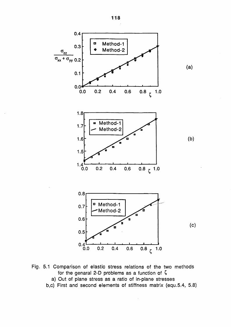
118

(b)

(c)

Fig. 5.1 Comparison of elastic stress relations of the two methods for the genaral 2-D problems as a function of £

a) Out of plane stress as a ratio of in-plane stresses b,c) First and second elements of stiffness matrix (equ.5.4, 5.8)

119

Fig. 5.2. Comparison of numerical and theoretical tensile stress ratios for the tensile test specimen, when non-work hardening elastic-plastic material Is considered,

a) At the beginning of plasticityb) at extensive plasticity (Ee « 3 o ys)

120

(a)®yy ( p la s t ic )

© yy (P,astlc)

(b )

Fig.5.3 Stresses in the tensile test specimen for different values of C for an elastic-non linear plastic material.

a) Tensile stress in the direction of loading.b) Out of plane tensile stress

121

% plastic strain

Fig.5.4 Stress-piastic strain relation of the A533-B pressure vessel steel.

1 2 2

Fig.5.5 Load-Load point displacement relations for standard compact tensiongeometry (a/W=0.56) for different values of the out-of plane constraintfactor,

123

0.12Q

BWi ys

0.10

0.08

0.06

0.04

0.02

0.00

$

♦ X* - +

X

+

♦ 5=1.0 plane strain

O £=0.75

x £=0.5

• £=0.25+ £=0.0 plane stress

0.0 2.0 4.0 6.0 8.0 10.0 12.0q E

W a ys

Fig.5.6 Load-Load point displacement relations for standard Three Point BendGeometry (a/W=0.5, S/W=4) for different values of the out-of planeconstraint factor,

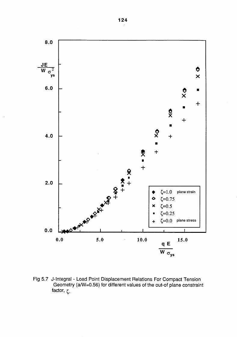
124

0 .0 5 .0 1 0 .0 1 5 .0q E

Fig 5.7 J-Integral - Load Point Displacement Relations For Compact TensionGeometry (a/W=0.56) for different values of the out-of plane constraint

factor, £

125

3.0

JEv T ^

ys

2.0

sx

$ +X

♦oX

+

♦o

X

+

1.0

0.0

f

$

*m+

£+

+

♦ £=1.0 plane straino £=0.75X £=0.51 £=0.25

+ £=0.0 Plane stress

8q E

W

10 12

ys

Fig. 5.8 J-Integral - Load Point Displacement Relations for Three Point Bend Geometry (a/W=0.5, S/W=4.0) for different values of the out-of plane constraint factor £•

126

CHAPTER 6

ELASTIC-PLASTIC LOAD-DISPLACEMENT

EQUATIONS FOR ESTIMATING J

6.1 INTRODUCTION

Representing an actual load-displacem ent, (Q -q), relation of a

cracked body by a mathematical equation is a complicated task,

especially if extensive plasticity is considered. Even for simple

geometries, an accurate yet simple equation can not be obtained

except for LEFM. Bucci et al(1972) presented a method to obtain the

com pliance of a geom etry using LEFM param eters where an

approximate procedure to account for the plastic zone size is also

provided.

For EPFM cases, an equation relating displacement to load, material

and geometry is bound to be complex. The absence of a shape factor

like term, and varying material properties with extent of plasticity

further complicates the task.

Load point displacem ent, q, of an elastic-plastic body can be

considered as a sum of elastic and plastic components. The elastic

component can be obtained from the elastic compliance of the body,

which is a function of geometry and elastic material properties,

Young's modulus of elasticity E, and Poisson's ratio v, and can be

easily determined using Bucci et al (1972) type analysis. The plastic

com ponent however, in addition to those influencing elastic

component, will also be a function of load level and material work

hardening characteristics. Although the precise form of relations

among these are not known, any selected form of equation is required

127

to give unbounded displacem ents at collapse load. This latter

statement raises the question of defining the collapse load for work

hardening materials.

In the following sub-sections, empirical equations to represent

displacem ent-load , (q -Q ), relations will be considered. Only

non-work hardening materials will be studied where the limit load is

taken as the collapse load.

As for the equations to represent (q-Q) relations, the elastic part

will always be related to the elastic compliance of the geometry,

while the plastic component will be approximated by either a

logarithmic or trigonometric function. Numerical solutions will be

used to determine and rationalise those constants involved in the

formulations. These equations will be integrated to evaluate the

complementary energy, C, or work input, U. J will then be calculated

from the change of this energy due to crack growth. In fact this J

estimation process is similar to the method originally used by

Begley and Landes (1972) in their experimental work.

6 .2 FO R M U LA TIO N O F LO A D -LO A D P O IN T D IS P L A C E M E N T

R ELA TIO N .

The load point displacement, q, of a cracked geometry is split into

elastic and plastic components, i.e.,

q=qei + qPi (6 -1)

The elastic component can always be obtained using LEFM concepts

and may be written as;

128

Qei- AtQ (6.2)

W here A1 is the elastic compliance of the cracked geometry

The plastic part of the displacement will be approximated by either a

logarithmic or trigonometric function which has been selected as;

qpl= A2Q tan2(,tQ /2 Q L) (6.3.a)

qp|=-A3Q Log( 1- Q /Q L) (6.3b)

W here Q L is the limit load of the geometry as defined by equ.3.15.

Both of these equations satisfies the requirement of unbounded

displacements at limit loads. A2 (and A3), is assumed to be a function

of geometry only, while the rest of the term; tan( ) or Log( ), includes

the effects of both geometry and load. In this study, single edge

notched geometry, (SEN), subjected to tensile loading, SENT, by

parallel end displacements or three point bending, (TPB), will be

considered. Furthermore, in each configuration only crack length will

be varied and A2 (and A3 ) will be assumed to be separable functions

of crack length and gauge length of that geometry.

6.3 EVALUATION OF J FROM LOAD-LOAD POINT DISPLACEMENT

EQUATIONS

Following the work of Begley and Landes (1972), J may be evaluated

as the change of either complementary energy or work done with

respect to crack length.r dC -I _ [ dll I1 3a JQ B l 3a Jq (6.4)

where, and

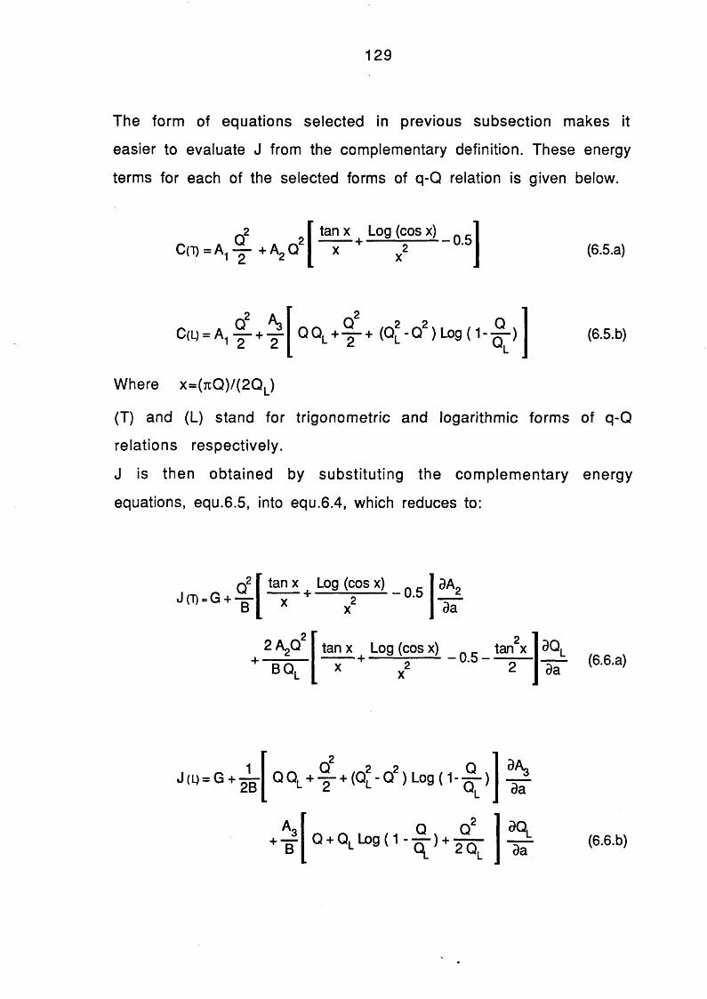
129

The form of equations selected in previous subsection makes it

easier to evaluate J from the complementary definition. These energy

terms for each of the selected forms of q-Q relation is given below.

Where x=(rcQ)/(2QL)

(T) and (L) stand for trigonometric and logarithmic forms of q-Q

relations respectively.

J is then obtained by substituting the com plem entary energy

equations, equ.6.5, into equ.6.4, which reduces to:

(6.5.a)

(6.5.b)

J (T) = G + —q2 tan x | Log (cos x) Q ^

- 0.5 9A2

2 AjQ tan x Log (cos x)

(6.6.b)

130

6.4 NUMERICAL STUDY OF THE SEN GEOMETRY

The SEN geometry (Fig.6.1) was numerically studied using a small

geometry change, elastic-plastic 2-D FE code. Due to symmetry, only

half of the geom etry has been m odelled with eight node

isoparam etric elem ents. Two different loading modes of the

geometry, namely TPB and parallel end tension, were considered. The

gauge length (span for the TPB) to width ratio was fixed at 4, while

crack length was varied as 0 .0 5 < a /W < 0 .3 . Non-work hardening

elastic-plastic material with plane strain constraint was assumed

and loading was implemented by successive displacement increments

of the loading points. For the TPB configuration, the central load was

distributed over a small region to avoid plastic instability at that

point. J integral for the cracked body has been evaluated as a contour

integral over 8 different paths, and average was taken as the

representative value.

6.5 CURVE FITTING TO NUM ERICAL LO AD-DISPLACEM ENT DATA

When fitting any of the selected curves to the numerical data, A1 of

equ.6.3, was always taken as the elastic compliance of the geometry

as determined from the numerical results. Least square curve fitting

techniques were then used to find best fit to the plastic component

of displacem ent hence determining A2 (or A3). In this latter case

those data points corresponding to load levels nearing or at the limit

load were excluded from the curve fitting analysis (excluded if (

Q/Ql )> QR).

A series of crack lengths was considered to enable the

determination of a functional relationship between A2 (or A3) and

131

crack length. Furthermore, as the derivative of limit load with

respect to crack length appears in J formulations, (Equ.6.6), a

functional relationship between constraint factor, L, and crack

length will also be determined.

The values of constants A2 and A3 are shown in Fig.6.2 as a function

of crack length for the two different loading configurations

considered. It is to be noticed that the range of load ratios

considered in the regression analysis (0 < Q /Q L<Q R) influences the

values of these constants, hence the accuracy of the q-Q equation in

representing the numerical data. Both constants, A2 and A3, suggest a

functional relation (except A3 for QR=95 for TPB) to crack length as;

<jB

(6.7)

where d,p=constant depending on QR

B=Thickness of plate

Table 6.1 presents the constants d and p for different values of QR

for both SENT and TPB loadings.

Typical comparison of m athem atically obtained load-load point

displacement relations with those from the FE method are given in

Fig.6.3-6. Both of the selected equation proves to be good in the near

linear region of the curve. The advantage of the trigonometric form

is evident at high load levels and for larger crack sizes. The value of

QR (as described above) is only important if more accurate

representation of q-Q relations for longer cracks or for short cracks

at higher load levels are required. However, with the selected forms

of equations this higher accuracy is achieved at the expense of

accuracy in the near linear range.

132

The constraint factor, L, as determined from numerical results, is

shown in Fig.6 .7 as a function of crack length, which can be

represented by the following equations for the loading modes

considered.

t a »0.3731^=1.0 + 0.1183 (.$> (6.8.a)

a \0-2686Lg = 1.0+ 0.6348 I (6.8.b)

where subscripts T and B stands for tension and bending cases

respectively.

6.6 J ESTIM ATES FROM LO AD-DISPLACEM ENT EQUATIONS

Once the constants related to q-Q equations, namely Ar A2 and A3,

and the constraint factor, L, has been determined as a function of

crack length, J for a given load level (Q /Q L) may be estimated.

Substitution of relevant form of L, Q L and A2 ( or A3 ) in equ.6.6

results;

£ (l) = 1 + ( ^ ) P 2 ( P [ 025 + ^ + 0.5 -1) log(1-z) ]

- T V )['0 5 + 7 + T ' ° 9 ( 1’2 )] } (6-9-a>z z2

OC T X

|2/aL’ N a u tan(x) | log[cos(x)] Q 5 tan (x)j 1 (6gb)

x 9X

133

w here N=1 for tension, 2 for TPB

Y= LEFM shape factor of the geometry

a = 1 for tension, (1.5 S/W) for TPB

z= Q/Q l and x=tcQ /2Q l

E'= E for plane stress, E/(1-v2) for plane strain

L'= 3L /a(a /W )

Comparison of numerical and estimated J values are given in

Fig .6.8-11. It is to be noted that, the J estimates from the q-Q

equations are based on load, and where reference is made to

displacement, it refers to those from the FE analysis.

6.7 D ISC U SSIO N S

Comparison of numerical and estimated q-Q relations for a given load

level, (Figs.6.3-6), indicates relatively large differences in the near

limit load range. Conversely from displacement point of view, the

differences in load between numerical and estimated values are

significantly smaller. However, displacement has been selected as

the dependent variable of q-Q equations, and such differences

mentioned above will reflect on J estimates.

Accurate estimates of J from such simple equations representing

q-Q relations should not be expected for the near limit load levels.

The deficiencies of the 'selected equations' are evident in Fig.6.3-6.

While low values of QR (range of loads considered for regression

analysis) provide good correlation only in the near linear range, high

values of QR provide better correlation in the near limit load range

but at the expense of accuracy in the near linear range. This is due to

the fixed form of the selected functions (trigonom etric or

134

logarithmic), which is being forced to correlate with a relatively

arbitrary curve. Generally speaking, the trigonometric function has

better ability in representing q-Q relations in the near limit load

range.

Differences between numerical and estimated q-Q relations resulted

in unacceptably high differences between numerical and estimated

values of J. Evaluation of J using the rate of change in energy at

constant displacement will reduce such high differences in the near

limit load range, but not in the near linear range. Due to the

complicated form of complementary energy equation (equ.6.5), this

point was not taken up.

The differences in J at low load levels must be related to the

selected functions, particularly to their deficiency in accurately

representing q-Q relations simultaneously in the near linear range

and in the near limit load range. The differences in J, between

numerical and estim ated values, in the near linear range may

therefore be reduced by restricting the q-Q equation to that range,

i.e. by using lower values of QR.

A different method of estimating J from q-Q equations, namely by

relating work done to J through the *n factor, may be sought. The

estimation of work done, U, from the q-Q equation will not pose any

difficulties, however large errors in U, hence in J, in the near limit

load levels may result as displacement is the dependent variable in

the q-Q equations. Nevertheless, better accuracy, especially at low

load levels may be expected if an accurate t| factor for the geometry

is known.

G enerally, the logarithmic form used overestim ates numerically

obtained J values in the near linear range and underestimates in the

135

near limit load levels. The trigonometric form, however, does the

opposite of the logarithmic form.

The general form of q-Q relations require some very complex

equations for accurate representation. For such complex forms

separation of variab les will be extrem ely d ifficult, if not

impossible. If simple forms, such as those used here, are selected,

they should be retained as representing the q-Q relations in a coarse

m anner. Further, any information obtained by processing such

equations should also be treated as coarse, and their use must be

properly justified.

1 3 6

.D ►

Q

T

L J J

(a)

Fig.6.1 Edge crack geometrya) Under tensile loading (SENT)b) Under three point bending (TPB)

137

(a)W

w(b )

( «* )

Fig.6.2 The constants a 2 and a 3 of selected load-displacement equations as a function of crack length. a,b) For SENT geometry c,d) For TPB geometry

138

BWa.

4 * ------------

• /

p

Ax * 's ' V K '

A > "x

< «|»<t .♦♦ - -

* .30 0.90

O COMPUTED (fl/W=0-05) A FITTED lfl/W=0.05 ) + COMPUTED Cfl/Hr0.14) X FITTED (fl/W=0.14) ❖ COMPUTED (fl/H=0 .25) A FITTED (R/H=0.25)

1 .50 2 .10 2-70 3.30 3.90 4 .50

qE5.10

(a)wcr

.>$-------------

Q

BWO„

AX>'*/ / -

Jk'j*

*A'*

yp

as ia a ------►“

________

,^.30

A

0.90 1 .50 2.10 2.70 3.30

(b)

O COMPUTED A FITTED + COMPUTED X FITTED 4> COMPUTED ♦ FITTED-------- 1--------------

3.90

fl/W=0.05) fl/W=0.05 ) R/H=0.14J R/H=0.14) A/W=0.25) fl/H=0.25)4.50 5.10

q e

w av

Fig.6.3 Numerical and Estimated (Logarithmic) load-displacement relationsfor SENT geometry a) QR=0.85 , b) QR=0.98

139

O--------- >--------- 1---------------------1--------- 1 ___________1 -----1_______________1_______________

oo✓

> ______ _A Xs ' Y

oCDS '

S ' * s’ 4.

o'

Q S sSs *

DO $ 0.6(

____

__1__

A 'S '

A'*'o

o"

oCVJwe*o / O COMPUTED (R/W=0.05)s A FITTED (A/W = 0 .05 )

+ COMPUTED (R/W=0.14J X FITTED (R/W=0.!4)

o O COMPUTED (R/W=0.25)o 4“ FITTED (fl/Wr0.25)|U-30 o'.90 l'.50 Z. 10 2‘.70 3‘.30 3'.90 4 '.50 5.

(a)

Q

B WO,

,6t K ? '

p>

- A- -Ok

------------*

r mM'' *K

A*A'«

O COMPUTED A FITTED + COMPUTED X FITTED $ COMPUTED ♦ FITTED

( A/W: ( R/W: (R/W: (fl/W: (fl/W: (fl/W:

=0.05 I :0.05) =0.14) = 0.14) =0.25) =0.25)

^b.30 0.90 l .50 2 .10 2-70 3.30 3-90 4 .50qEwa,

(b)

Fig.6.4 Numerical and Estimated (trigonometric) load-displacement relationsfor SENT geometry a) QR=0.85 , b) QR=0.975

140

Q

BWOy *

_ _____ o

X X

XX '

4 ✓ / /-x4 // /

4 */ /

/.X' /

*X A * ¥

X 'X A X ¥J¥

^•00 1 .50 3.00

O C0MPUTE0 (A/W=0.05) 4 FITTED (fl/W=0.05) + COMPUTED 1fl/W=0.15) X FITTED (R/H=0.15J O COMPUTED (fl/W=0.30) ♦ FITTED (fl/H=0.30J

4.50 6.00 7.50 9.00 10.50q E

12

(a)w o ,

A * ___ OA*

x _ X X x _ x _ _

Q

B W O y ® ' ✓ * / // a /- / A X / a//a/x +' ' >♦

t t t i - ’- ----- a-------------

/

/* rf* a'X a x ¥¥

O COMPUTED (fl/H=0•05) A FITTED (R/W=0.05)+ COMPUTED 1fl/W=0.15) X FITTED (A/W=0.15) <!> COMPUTED ( A/W=0 • 30 ) ♦ FITTED (fl/W=0.30 )

^ .00 l .50 3.00 4.50 6 .0 0 7.50 9.00

(b)

10.50

qEw av

12

Fig.6.5 Numerical and Estimated (logarithmic) load-displacement relationsfor TPB geometry a) QR=0.85 , b) QR=0.95

141

Q

BWOy 2

__ ____o

// x/ X'

/ ✓ d s

/ * d /

/ / ,>■4 / * '

• d // r

^.oo

/4 dd/ y** *4* d

d ' d *X d

/

1 .50

O COMPUTED (fl/W=0.05) A FITTED t fl/W=0 • 05 ) + COMPUTED (R/W=0.15) X FITTED IR/W=0.15) O COMPUTED (fl/W=0 • 30) + FITTED I fl/W=0.30 )

3.00 4.50 6 . 00 7.SO 9.00 10.50q e

wau

12

(a)

Q

BWO

' y UJ

^ — X__ _ _____

X/ y X '

' y d // *-d y ♦

/ 7 ^/ '

4 / t*■ d y

'd »y d/ ,Jd *4* d

d + ' d **ds

1 .00

O COMPUTED A FITTED + COMPUTED X FITTED O COMPUTED ♦ FITTED

(R/Hr0.05J (fi/W=0.05) [R/W=0.15) (R/W=0.15) (R/W=0.30 ) (R/W=0.30 )

1 .50 3.00 4 .50 6 .0 0 7.50 9.00

(b)

10.50qEw a

12

Fig.6.6 Numerical and Estimated (trigonometric) load-displacement relationsfor TPB geometry a) QR=0.85 , b) QR=0.95

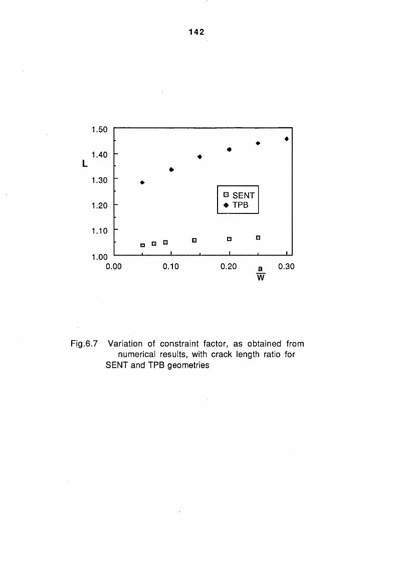
142

1.50

1.40L

1.30

1.20

1.10

1.000.00 0.10 0.20 a 0.30

B SENT ♦ TPB

□ □ n__________ I__________ i__________ L

w

Fig.6.7 Variation of constraint factor, as obtained from numerical results, with crack length ratio for

SENT and TPB geometries

.80

1-20

1.

60

2-00

2.

40

2-80

'• oo ; cm"5 CO

II.1

I

O COMPUTED (fl/H=.05) a ESTIMATED IA/W=.0S) + COMPUTED (R/W= .14) X ESTIMATED (A/Wr.14) <!> COMPUTED IA/W=.2S) * ESTIMATED (fi/W= .25)

%

♦ ^

^.00 Q1.20 0-40 0.60 0.80 1 .0 Q_Ql

oii <\jo cn-

I

o03

OO

OUD

Or\j

I

© C O M P U T E D (A/W=.05) A ESTIMATED (A/W=.05) + COMPUTED lA/W= . 14 ) X ESTIMATED (fl/W=.14) <!> COMPUTED ( A/W= .25 1 * ESTIMATED (A/W=.25)

1 I 1 I 'w

ai U A+ iif

A ll,tf

If

+ ¥ * t.- -

X 4.X ♦ * ♦

A ">/|X

X ^X ♦/'

X + V+ S fS

/ ' *v /

X♦

ooo(^ .00 i‘.oo 2'.00 3 .0 0 4*. 00 5.0^

qEway

Fig.6.8 Comparison of J-Integral values estimated from Load-displacement equation(logarithmic, QR=0.98) with Numerical values from FE study for SENT geometry.

143

.20

1.60

2

.00

2

.40

2

.80

3-20 <*>

Xl

I

4

O COMPUTED (A/M=.05) A ESTIMATED (A/W=.05) + COMPUTED (R/W= .14 1 X ESTIMATED (R/W=.14) O COMPUTED (A/W= .25) * ESTIMATED (A/W=.25)

{Ii

iIIHft//

* a

—. ■ .’15' A $♦-Mh-Xf-X i f * » *►

i o I CM

O i <n""3

oOO

CM

OOCM

O COMPUTED (R/W=.05) A ESTIMATED (A/W=.05) + COMPUTED (A/W= .14) X ESTIMATED (A/W=.14) O C0MPUTE0 (A/W= .25 ) * ESTIMATED (A/W=.25)

x

Ii II I ' /' / ' ' / '' / /

x(/f"/'/

-oD CD

Hn

nU

S 1

0

<*r O '• ♦ **

^.00 0.20 0.40 0.60 o'. 80

oCD

.00 i '.oo 2*.00 3'. 00 4f.00 5 .0qE

Q l w a y

Fig.6.9 Comparison of J-Integral values estimated from Load-displacement equation(trigonometric, QR=0.975) with Numerical values from FE study for SENT geometry.

14 4

.80

1 .20

1.60

2.

00

2.40

2.

00oCM

^ «“ ”3

IIIIIfl»I I* I I I I I fI i I 2

© C O M P U T E D (A/W=.05) A ESTIMATED (A/W=.05) + COMPUTED (A/W= .151 X ESTIMATED (A/W=.15) <!> COMPUTED (A/W=.25) * ESTIMATED (A/W= .25J

I aI I I

/k//

I I I* II I

/' * / I X

' /▲ / / ‘A ✓ / *A / /K x .JO x ' *

_’ * ♦

t !/ f x/ X

♦♦

oCM

O «"“O

o00CM

OCM

OOCM

OID

OCM

//

//

/' /

//

© C O M P U T E D (fl/W=.05) A ESTIMATED (A/W=.05) + COMPUTED (A/W= .15) X ESTIMATED IA/W= .15) ❖ C O M P U T E D (A/W=.25) ♦ ESTIMATED lA/W= .25)

/

P/

/ A

/7 /V/A / /7 // / , /

f / /

/

*

/ 4 /X

♦

/

X

♦

^.00 0-20 o'. 40 O'. 60 o'. 80 7.00QQ l

ooo^.00 2.00 4 .00 6.00 8.00

qEWGy

Fig.6.10 Comparison of J-Integral values estimated from Load-displacement equation(logarithmic, QR=0.90) with Numerical values from FE study for TPB geometry.

145

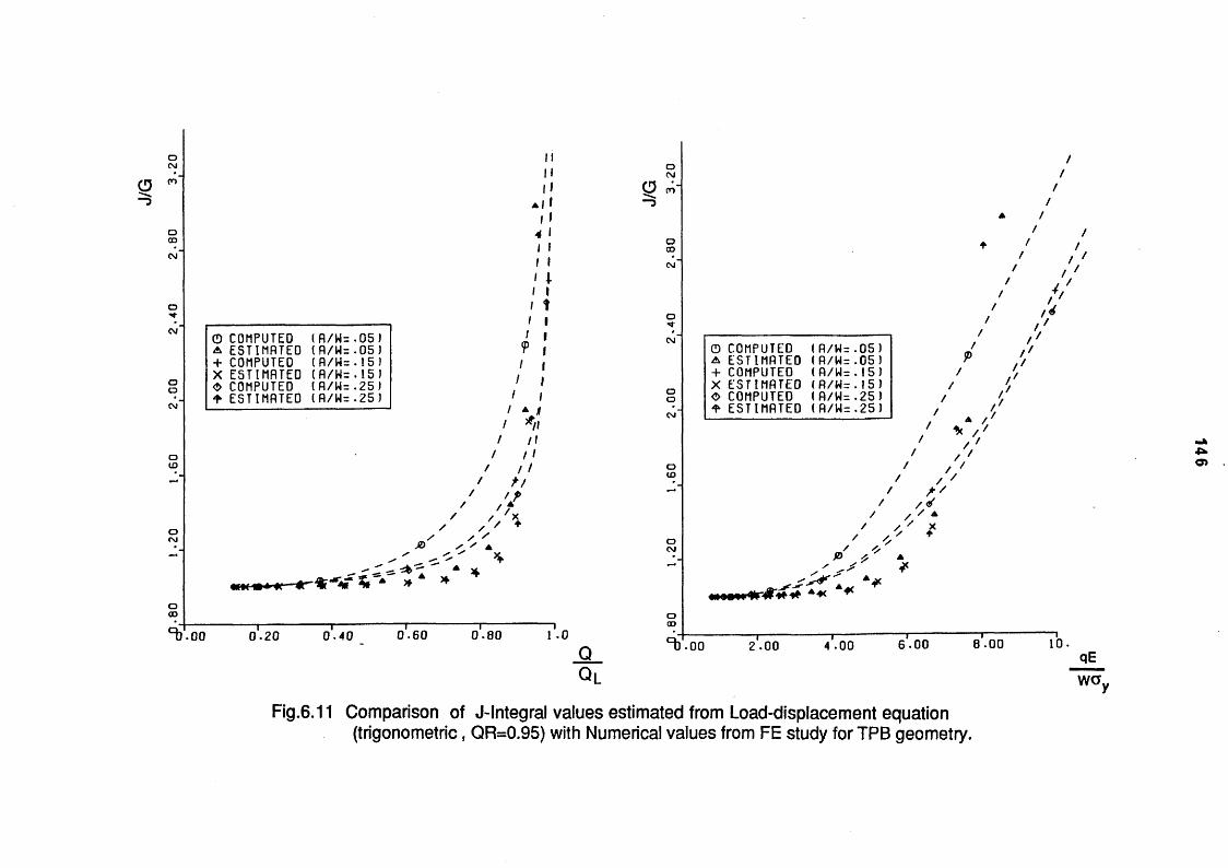
.80

1.20

1.

60

2.00

2.

40

2.80

oCsleg "

oCM

//

O COMPUTED (fl/W= .05 1 A ESTIMATED ( A/W= .05) + COMPUTED (A/W=.15) X ESTIMATED (fl/H=.15) 0 COMPUTED (A/W=.25) ♦ ESTIMATED (A/W= .25)

ll eg cn~

A | 1 . |—s

4 1 o1 1 CO

1 1 cm"

1 11 1/ tI I f IV ii Ii I

iit n

/ // / ‘

/ / '

JD/ / '

/ ' A•X’ *

"■ A

*4

f/1

/ / / /

t/

'x♦

//

A /

/♦

//

©COMPUTED (A/W= . 05 ) A ESTIMATED (A/W=.05) + COMPUTED (A/W= .15) X ESTIMATED (A/W=.l5) O COMPUTED (A/W= .25 ) * ESTIMATED (A/W= .25)

//

//

' */*

/ * v / / //

/

/ AxV ♦

//

^.00 T0.20 0*. 4 0 0*. 60 o '. 80

i1 .0Q_Q l

ooocb .00 2.00 4.00 6.00 8.00 10.

qEway

Fig.6.11 Comparison of J-Integral values estimated from Load-displacement equation(trigonometric, QR=0.95) with Numerical values from FE study for TPB geometry,

146

147

QR i 0.85 i 0.925 i 0.975. j ____ _____d ! 9.11e-4 ! 4.36e-6

. 1 1i«0.404e-6

p ! 2.0571 ! 1.966 1 j 1.373

TENSION ( T )

QR I 0.80 ! 0.90 | 0.95

d j 34.16e-4 j 18.85e-4 | 6.88e-4 BENDING(T)

p

ir—LOOI___I

0.4 | 0.27

QR , 0.85 , 0.90_i i_

' 0.98i

d ! 2.87e-3 ! 4.392e-3 i 3.559e-3i_4___________TENSION (L )

pT1 1.9 ■ 1.928 1 1.422

QR ii 0.80 i 0.90 '

L___ j

diii 18.45e-3 ! 14.03e-3 i

piii

0.643 1 0.2542 T

BENDING ( L)

(L) Logarithmic form (T) Trigonometric form

TABLE 6.1 Generalised constants for representing the load-displacement relations for the edge crack geometry.

148

CHAPTER 7

J ESTIMATION FOR SINGLE EDGE CRACK

GEOMETRIES SUBJECTED TO ECCENTRIC

TENSILE LOADING

7.1 IN TR O D U C TIO N .

Structural components with cracks are seldom subjected to pure

tension or bending types of loading. Estimates of the crack tip

severity for such components in the EPFM range are difficult.

N um erical studies may provide answ ers but require the

consideration of different ratios of tension to bending loads.

Use of r| factors to estimate J in experimental work has proved

successful for deep notch bend and compact tension (CT) type

specimens. Merkle and Corten(1974) have studied the CT specimen to

determine the plastic component of i\ factor. They simply considered

rigid plastic material and idealised stress distribution across the

ligament to obtain t |p| as a function of crack length to width ratio,

a /W . As will be shown later the validity of these results are

restricted to deep notch geometry cases subjected to primarily

bending loads. Clarke and Landes (1979) have demonstrated that for

the standard CT specimen, tigj and r ip| are identical, which is

extremely convenient in experimental work.

Ernst(1983) has studied single edge notched specimen with load

applied eccentrically to the centre of the ligament in tension, with

bending effects. His work covered the entire range, from pure bending

149

to tension. Estimates of Tip| were provided in a tabular form as a

function of eccentricity of applied load. It is to be stressed here that

the work by Ernst was also limited to deep notch geometries.

It is generally accepted that high stress levels in the vicinity of

crack tip region may result due to plastic deformation coupled with

plane strain constraint effects. Slip line field theory has been

employed to show that, stresses in a region near the crack tip may be

as high as ~3cr for deep notch bending cases. The same study for

single edge crack geometries subjected to 'pure tension' shows the

absence of such a high constraint region. It is to be noted here that

a rigorous definition for pure tension of single edge cracked

geometries does not exist, as it does for pure bending. This point

will be discussed later in subsection 7 .8 . In the following

subsections unless otherwise stated, the term 'pure tension' will be

used to indicate such loading types which produces uniform tensile

stress across the entire ligament for rigid plastic materials (e=0 in

Fig.7.1).

In this section, edged cracked geometries subjected to eccentric

tensile loading, hence producing bending effects, will be studied.

Rigid plastic m aterials will be considered and the effect of

eccentricity on the applied load will be investigated. Contrary to

previous workers, ie. Clarke and Landes(1979), where appropriate, a

high constraint crack tip region, (HCCTR), will be included in the

analysis. The study is aimed at obtaining loads and r |p| factor, for

determining J, as a function of eccentricity. Known solutions, namely

'pure tension' and 'pure bending' cases will be utilised for

comparative analysis. The analytical work here is formulated in

general so as to allow extension to shallow notch geometries.

150

7.2 FORM ULATION OF GOVERNING EQUATIONS

Consider a 2-D cracked body of unit thickness subjected to an axial

load (perpendicular to the ligament in the plane of the body) with an

eccentricity of (e) from the centre of the ligament (Fig,7.1). For a

rigid plastic material the stress distribution across the ligament

may be idealised as shown in Fig.7.2 . Note that the HCCTR is

represented by a uniform stress level of (m^>1) over a region of

y. Consideration of force and moment equilibrium leads to;

Q = [ ( m 1- 1 ) y + 2 x j (,c

M = Qe =

w here c 0= a ys

( — ( t y- y2 ) + ( ~ x 2 )

for Tresca yield criterion

4 \ 0-5c0 = c ( — ) for Von-Mises yield criterion7 u

(7.1)

(7.2)

b= remaining uncracked ligament.

For pure tension (e=0) and bending (e-»°°), the limiting values of load

and moment are;

QL= o 0 b (7.3)

m l = L 0 oT (74>

where L is the constraint factor for the cracked geometry when

subjected to bending loads and accounts for the HCCTR. It is to be

noted that while Q (and hence M) represents the load (and moment)

for a given eccentricity of applied load, limiting values under 'pure

tension' and 'pure bending' types of loading are represented,

151

respectively by Q L and by M L.

Equations 7.1-4 may be combined to give:-

M Q ML = a QL

(7.5)

Q , j i y 2x o [ = < mi - 1> b + T

(7.6)

2 2 , Q ^ / y y \ , 4 x

a L ^ - = 2 ( m i - 1 ) ( ^ - ^ ) + 1- —L D D

(7.7)

4ea " Lb

(7.8)

7.3 EVALUATION OF J FOR A GIVEN LOADING SYSTEM .

J integral for a cracked body may be evaluated from the work done by

the applied forces, either as the rate of change with respect to crack

length, or through the use of rj factors.

duda

r\ U bB (7.9)

The work done for the system shown in Fig.7.1 can also be calculated

from the equivalent system, shown in Fig.7.3. For a rigid plastic

material, the work, U, which is given by equ.7.10 is combined with

equ.7.9 to give rjpl (equ.7.11).

U = Q.q = Q.s +M.0 (7.10)

_ __b_ 3Q “ - Q da

q(7.11)

152

7.4 A SIM PLE CASE W ITHO UT THE HCCTR

When the HCCTR is neglected (eg; m ^ l and L=1) simple mathematical

equations emerge and this may be solved analytically. Using

equ.7.1-9, the following basic equations may be obtained.

Q__ 2e b

X = 8

(7.12)

(7.13)

(7.14)

The relationship between load and moment and their variation with

respect to eccentricity of the applied load are shown in Fig.7.4. The

ripl factor for this case can be evaluated by substituting equ.7.13 into

equ.7.11, and noting that both e and QL change with respect to crack

length (da=2 de).

Tv«=

b2e

7 f - i .

(7.15)

w here

As expected, equ.7.15 gives identical results to those given by Merkle

and Corten (1974) analysis, hence correct Tip| for deep notch

geometries with e=1.5(b) or larger (Fig.7.5). The effect of changing

(e) with respect to crack growth is also shown in Fig.7.5 where a

153

second T jpl factor has been plotted by treating e as a constant.

Although this consideration is unrealistic from the modelling point

of view, its plausibility for practical problems can be demonstrated.

W hen a cracked component is loaded eccentrically the effect of

bending moment (Q.e ) causes a central deflection v (« 0 .D), as shown

in Fig.7 .6 . An increase in crack length causes an increase in

eccentricity (de=0.5da) and hence the ratio of moment to load, which

in turn increases the central deflection, v. This increase in v

effectively reduces the eccentricity, e. Therefore, although the

increase in crack length increases the eccentricity, for practical

problems this increase is somewhat reduced by the increase in

central deflection due to the increased bending effects.

7.5 PURE BENDING CASE WITH HCCTR.

The 'Pure tension' case, which does not have a HCCTR, has already

been addressed in the previous subsection. For pure bending cases

an analytical solution is possible as values of (L ) and (m - j ) are

known, at least for deep notch cases. From equations 7.5 -8 the

following are deduced.

(7.17)

(7.16)

zb

or m+1(7.18)

154

where m and z are, respectively the corresponding values of m-j and

y for the pure bending case. Substitution of deep notch bend values of

m [= 1 + 0 .5 (ti)], and L [=1.261 (M ille r(1982))] gives numerical

estimates of the size of the HCCTR and the position of the neutral

axis (where stress reversal occurs). As it is generally accepted that

the neutral axis is about 0.4(b) from the crack tip (BS.5762, (1979)),

only the -ve sign in equ.7.18 is taken to be correct. This also gives

the size of HCCTR as *0 .1 (b).

E qu .7 .18 also provides a functional relationship between the

intensity of stress (m) within the HCCTR and its size (z) for shallow

notch cases. Although neither the size (z), nor the stress within the

HCCTR are known, either of these is sufficient when assumed, eg. to

be the same as that for deep notch cases, for a possible solution.

This point will be further explored in subsection 7.9.

7.6 COMBINED TENSION and BENDING WITH HCCTR.

7.6.1 Assumptions for a possible solution

Generally, for cases with HCCTR, solution of the governing equations

require an assumption to be made as there are 4 unknowns (Q, y, x,

for the three basic governing equations (equ .7 .5 -7 ). These

formulations make it easier to have assumptions for HCCTR, either

on its size, y, or on the magnitude of stress, mr within it. The

limiting values of both y and m1 are considered to be known (m ^ m ,

y=z for bending, and m ^ l or y=0 for ’pure tension'). Any assumption

made in this respect is therefore required to satisfy these limiting

conditions. A summary of different assumptions considered are listed

155

below;

a) m1 = my = z ( 1 ’ q [ )

(7.19.a)

b) m1 =my = Z ( “ - Q [ )

(7.19.b)

c) y = z (m, - 1 ) = ( m -1 ) ( 1 ~ ) (7.19.C)

d) y = z (7.19.d)

e ) m1 = m/ -na\p

y = z ( 1 - e ) (7.19.e)

f) y=z (m1- 1 ) = (m -1 ) (1 - e 'n“ )P (7.19.f)

These assumptions are formulated as to have variable power

coefficients, (n) for the first four and (n) and (p) for the last two and

these will be varied to satisfy certain requirements, eg. t |p|=1 for

'pure tension' cases.

7.6.2 Solution of The Governing Equations.

For a particular geometry, (a, W ), when subjected to pure bending,

the constraint factor, L, and the magnitude of stress within the

HCCTR are supposed to be known. Using one of the assumptions

listed in the previous subsection together with equations 7.5, 7.6 and

7.18, equ.7.7 can be reduced to;

X c , ( § - ) ' =00i=1 U L

(7.20)

w here C p CjfL.m .s.b^.n.p)

r,- r,(n,p)

156

Generally an analytical solution to equ.7.20 is not possible except

for some special values of n (or n, p). Therefore, a numerical

technique is employed to obtain a solution for Q /Q L corresponding to

a particular set of values of e, n, etc.

The evaluation of r ipl, from equ.7.11, requires the rate of change of

load w .r.t crack length. For this purpose, equ.7 .20 has been

differentiated algebraically, and then arranged in the following

general form:

where (») indicates derivative w.r.t (a/W).

Once a solution to (Q/QL) is obtained, a solution to equ.7.21 may

follow for (Q /Q l )» .

When expressed in terms of load ratios, equ.7.11 becomes:

A computer program has been written to solve equations 7.20 and

7.21 and also calculate *np). This program requires user supplied

values for a, W, m, L, L' (derivative w.r.t a/W ), desired value of rjp|

for 'pure tension' (i.e. e=0), and a selected value of power index p in

the case of assumptions e,f (equ.7.19). An iterative procedure is then

followed for e /b = (1 0 "6) to determine the power index, (n), until the

selected value of r|p, is achieved. Once (n) is fixed the calculations

s s r. -1(7.21)

q.(7.22)

for other values of e/b follow.

157

7.7 THE ANALYTICAL AND NUMERICAL STUDY OF DEEP

NOTCHES

The formulation of the problem has been carried out in general sense,

and it can be applied to any crack size, provided 'L' and 'm' for pure

bending are known. In general, though 'L' is known as a function of

a/W , eg. Miller(1982), the value of 'm' or 'z' are not known. For this

reason this part of the study is restricted to deep notches. Strictly

speaking, as long as the deep notch cases are adhered to (a/W >=0.296

according to M ille r(19 8 2 ) ,^ > = 0 .1 8 according to G reen andw

Hundy(1956)), for which 'L' is a constant, the actual value of a/W is

not important for the analytical model.

7.7.1 Analytical Results

Results of solution to equ.7.20 and calculated r|pI factor for various

assumptions considered (equ.7.19) are shown in Fig.7.7-10. In all

cases shown, except Fig.7.7, the power index n (Equ.7.19) has been

determined to give rip| =1 for 'pure tension' (e=0). The advantage of

assumptions e,f over the others (a,b,c,d) is the ability of altering

load and ripl for e/b«<2, hence having better chances of matching the

data obtained by other methods. For e /b >= 2 all assumptions give

practically identical results to the Merkle and Corten(1974) analysis

and tipi=2.0 for Pure bending.

7.7.2 Numerical Results

A single edge notched geometry with a/W =0.5 (or =0.3), and D/W=2

was modelled for a finite element study of the problem (Fig.7.11). A

small geometry change elastic-plastic 2-D FE code with 8 noded

158

isoparametric elements were used and plane strain conditions were

assumed. The material was considered to be elastic-rigid plastic

with E=210.KN/m m 2, v=0.3 and c ys=0.57364 KN/mm2 . The loading of

the geometry has been achieved by successive displacements of a

nodal point to simulate pin loading. To avoid plasticity at the loading

point, a different material, as welded to the ends of the actual

geometry, was also modelled. This added part was considered to have

considerably higher Young’s modulus of elasticity and yield stress ( 5

and 10 times higher, respectively ) compared to the main body.

J-Integral for the loaded geometry has been evaluated along 8

different contours, hence checking path independency, and average of

all was taken as the representative value. While G, the elastic energy

release rate, has been taken as the elastic part of J, the plastic

components of J and work done by the applied load have been used to

evaluate np, (equ.7.24).

J = G + JPiAJ

TV l - B b AUPi

Pi

(7.23)

(7.24)

where A Jp| and A U p| are corresponding changes, respectively in Jpl

and Up| for a finite change in overall the displacement. This equation

is assumed to be applicable in the extensive plasticity regime, that

is when plasticity spreads across the entire ligament. Numerical

results which are shown in F ig .7 .12 -13 , are com pared with

analytical results (assumption e and f of equ.7.19) in Fig.7.14.

159

7.8 D ISC USSIO N S

Numerical results indicate that for rip| to be unity, the applied load is

required to have an eccentricity, e /b «0 .07 . This means that the

ligament is subjected to a small amount of bending moment. For

smaller eccentricities, (e/b<0.07), though an elastic solution to the

problem does exist, in the extensive plasticity regime, the crack

flanks interfere each other, suggesting a -ve applied bending

moment. Furthermore, while for e/b=0 theoretical tensile limit load,

Q l , is numerically matched, for some small values of ( e/b) a load, Q,

higher than Q L was obtained. These indicate the presence of HCCTR

even when the geometry is subjected to such tensile loadings giving

V 1-0 -

For (e /b)>=0.4, good agreem ent between analytical and numerical

results for rip| is observed for (a/W )=0.5 case, but a rather poor one

for (a/W )=0.3. For (e/b)<0.4 the correlation between numerical and

analytical results is poor for all a/W values considered here. This

may suggest that for (e/b)<0.4, either the assumed variation of the

size of HCCTR ( or the stress within it ) is poor, or the numerical

results are effected, so far by unaccounted factors. Furthermore,

according to numerical results, the measure of eccentricity should

not be referred to the centre of the ligament but to a point away

from the centre, nearer to the crack tip.

The definition of 'pure tension', which in this work was taken as

load applied along the centre of the ligament and producing uniform

stress across the entire ligament, is suspicious. The other types of

tensile loadings of SEN geometries does not either offer an answer

to the meaning of 'pure tension' in practical applications. Other

160

commonly used tensile tensile type of loading of SEN geometries are

listed here.

a) Applied uniform tensile stress across the entire width

b) Applied uniform displacement across the entire width

c) Pin loading along the centre of the specimen width

In all cases, the point of applied loading is implied to be at distances

far from the the crack plane. Miller(1982) gives the assumed form of

tensile limit load, (equ.7.3), for SEN geometries loaded by uniform

displacement across the width (i.e. as case (b) above). For uniform

stress or pin type of loadings a rather lower limit load was given.

The former type of loading may be idealised as the pin loading type,

which has an applied load eccentricity of e=0.5a. While uniform end

displacement type of loading will result in a -ve applied bending

moment, the other two will result in a +ve rotation of the ends.

However, the numerical model used here in representing the pin type

of eccentric tensile loading, further imposes a different kind of

restriction to the ends of the specimen. This is due to the rather

stiff properties of the end piece , which restricts the contraction of

the ends. Nevertheless, different effects are to be expected from

each type of loading, especially with short gauge lengths.

The numerical results are also affected by the gauge length,

especially for loadings with small eccentricity. Part of the effect

may be attributed to the central deflection, as discussed in

subsection 7 .4 ., which may be reduced by choosing shorter gauge

lengths. On the other hand, short gauge lengths may interfere with

slip lines, which for the pure tension case extend from the crack tip,

at 45° to the loading line, to the back face of the specimen. For the

161

bending case, the maximum size of the plastic region in the direction

of loading is less than that of tension. Therefore, for the numerical

model, the gauge length was selected as D =2W to avoid this

interference. However, in the numerical study, plasticity was found

to spread beyond the bounds determined by slip lines, though more

pronounced for the a/W =0.3 case. For predominantly tensile loading

cases ( e/b<0.4), the plasticity was found to extend up to (near to for

a/W =0.5) the loading line. For the a/W =0.3, though deep notch case is

assumed, plasticity was even found to break back to the front face of

the specimen, indicating loss of crack tip constraint. This latter

point may account for the rather low value, (compared to the

analytical estimates), of r ipl factor.

This spread of plasticity introduces considerable errors in results,

especially on r iP| as the plastic work will include such terms which

are not accounted for in the analytical model, i.e. plastic work done

outside the slip line field pattern. Better agreem ent between

analytical and numerical results are observed when the plasticity is

confined to within and immediate vicinity of the area bounded by slip

lines ( eg; a/W =0.5 e/b>=0.4). A rather crude solution to this problem

of plasticity spread may be to disregard the plastic work outside the

bounds of slip lines, at least for r|p| calculations.

Limit loads of cases with combined tension and bending were given

by Miller(1982). The problem considered there was different; a single

edge notched geometry subjected to pin type of tensile load combined

with pure bending type of load. A direct comparison is, therefore

only possible for cases, what is called there as tension, which

corresponds to e=0.5a here. For both cases, a /W =0.5 and a/W =0.3,

162

relatively good agreem ent is observed, considering the range of

values due to different power indices (Fig.7.9-10).

7,9 A METHOD SUGGESTED FOR SHALLOW NOTCH CASES

The constraint factor, L, for shallow notch geometries, (a /W <=0 .3 ),

subjected to pure bending type of loadings w ere given by

M iller(1982). Although the magnitude of the constraint factor

indicates the presence of a H CCTR, neither its size nor the

magnitude of stresses within it are known. Therefore, to apply the

analytical model to shallow notch geometries, a further assumption

regarding the HCCTR is required. Given 'L' and assuming a typical

value for 'm' (or for 'z'), equ.7.17 may then be used to determine 'z'

(or 'm'). Similar to deep notch cases, the HCCTR may be varied from

pure bending to pure tension according to one of the forms given by

Equ.7.19.

Perhaps the most simple assumption is to take the size of HCCTR (or

the magnitude of stress within it) identical to the deep notch

bending case. One such result using m=(1+0.57c) and assuming the

variation of HCCTR to be according to equ.7.19.f is given in Fig.7.15,

where for 'pure tension ( e/b=0 ) ti ,«1.0 was assumed. As expected,

Tip| values for pure bending case converge to those which may be

calculated by equ.3.16.

163

Fig.7.1 Edge cracked geometry subjected Fig.7.2 Idealised stressto tensile load eccentrically distribution across

applied to the uncracked ligament the ligament.

(a) (b) (c)

Fig. 7.3 a) The applied system of forces b) Equivalent system of forces,

c) Idealised general displacements

164

b

(a)

Fig 7.4 Relations among Load, Load point eccentricity and Moment in the absence of the High Constraint Crack Tip Region

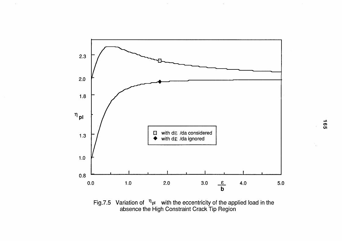
0.0 1.0 2.0 3.0 _e_ 4.0 5.0b

Fig.7.5 Variation of pi with the eccentricity of the applied load in the absence the High Constraint Crack Tip Region

165

166

Fig.7.6 Eccentric tensile loading of SEN geometry resulting in a central deflection v.

16 7

o

(a )

o

Fig.7.7 Analytical results for deep notch case when the High Constraint Crack Tip Region is assumed to vary linearly from pure bending to pure tensiona) Load-Moment relationb) rj as a function of applied load eccentricity.

.00

1.30

1.60

1.90

2.20

2.50

n.OO

0-20

0-40

0.60

0-80

m*-

S- %\xV

\x/

X

t V' i.\ /

V

i \*/

,/ \\xA

II

3.00 0.50 l'.OO

Cx-

t--- x- —

LOAD

0 m,- m / , Q v“MOMENT

O

A m,- rn / Q x 0.963y-z(®ojO *

+ y-z X

X y-z (mr1Hm-1)( a^-)° 6 Z

____-- *- —

r.so 2*. 00 2.50 3.00 3.50

(a)e/b

A> - ----- • - _ A

/ */a1 0 m,- m / . Q »“

111

A m,- m / Q \ 0.SS3

+ y-z (mt-1Wm-1)(l— ■)'

X y-z

"b.oo o'. 50 1 .00 1 .50 2 '. 00 2.50 3.00 3.50

(b)

7 .0 0

e/b

Fig.7.8 Analytical results for deep notches when i\p\ is taken as unity for pure tension

a) Variation of applied Load and Moment with load point eccentricityb) Variation of npj as a function of applied load eccentricity.

1 6 9

O

(a)

o

R9'7'9 fo T S e n T o !3 f° rdeeP n°,CheS Wh8n ^ p iis taken as unity a) Load-Moment relation ^)^pi ss a function of applied load eccentricity.

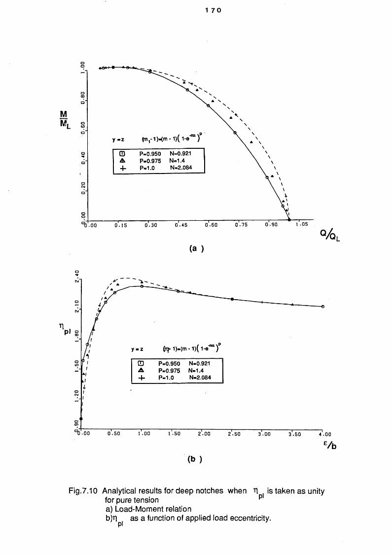
1 7 0

Fig.7.10 Analytical results for deep notches when is taken as unity for pure tension pa) Load-Moment relationb) ri as a function of applied load eccentricity.

171

i !

. . . . . ■ .

8 , b 1 2

D ^

Rigid added portion

" T

t D_10

D2

y i

12

y f

i

D_10

Fig.7.11 SEN geometry considered in the Finite Element study showing the rigid end pieces attached to the main body.

(pla

stic

)

172

FIG.7.12 Numerical results for SEN geometry (a/W=0.3)

M/M

L

(pla

stic

)

173

1.2

1.0 0.8

0.6

0.4

0.2

0.00.2 0.4 0.6 0.8 1.0 1.2

q/q l

FIG.7.13 Numerical results for SEN geometry (a/W=0.5)

174

Cj

O +

Fig.7.l4.a Comparison of Numerical and Analytical results for deep notchgeometry (n p| =0.0 assumed for pure tension )

OS-3 00*2

OS* I 00*1

0S*0 00* CT

00*'l 08*0

Og.'o

0*-'o Q2*'o

00*

1 75

(01,-1 )-(m-1)(l-e‘na)F

O N=2 .485 P=0 .975A N=4 .229 P=1 .010+ NUMERICAL A/W=0 • 3X NUMERICAL A/W=0.5

D .00 0-20 0-40 0.60 0.80 1 .00 l -20 1 .40 1 .60

e/ b

X XX

+X

+ X

Fig.7.14.b Comparison of Numerical and Analytical results for deep notchgeometry ( np( =0.25 assumed for pure tension )

176

^Pl

O

o N=2.121 P = 0 .975N=3 .631 P=1 .010

+ NUMERICAL A/W=0 *3X NUMERICAL A/W=0 .5

1 .60

e/b

1-40^ • 0 0 0.20 0.40 0.60 o'. 80 1 .00 1 .20

x x X

+X

+ X

Fig.7.14.c Comparison of Numerical and Analytical results for deep notchgeometry ( r \p] =0.50 assumed for pure tension )

177

“Hpi

OLO

^.00 0.20 0.40 0-60

y«z (m1-1)«(nvl)(i-e'nB)F

0 N=1 .760 P=0.975A N=3.031 P=1 .010+ NUMERICRL R/W=0.3X NUMERICAL R/W=0.5

0.80 1 .00 l'. 20 1 .40 1 .60

e/b

x x X

+X

+ X

Fig.7.14.d. Comparison of Numerical and Analytical results for deep notchgeometry ( np| =0.75 assumed for pure tension )

oLO

%

Fig.7.15.a Variation of ^pi with eccentricity of applied load for SEN geometry for smallcrack lengths ( assum ing r| , = 1 .0 for pure tension and m=(1+7c/2) for pure bending)

178

.00

0.2

0

0.4

0

0.6

0

0.8

0

1.00

' V .\x*n

A\NX \ x \\^\ x

\ \ 'Hv \ NM

N x

\ \ N \ \ v N

\ \

\ V\

N'N s N X ^ V. N \ \ N S

>0 ^ ^ ^ s

s n v. ">+

y=z (ml -l)= (m -1 )( i-e 'n“)

o fl /H = 0 .01 N = 2 9 .701A R/W = 0 • 05 N = 6 .889+ n/w=o.io N = 3 .889X f l / w = 0 . 15 N=2 • 866o fl/W = 0 .20 N = 2 i 373* n / W=0 . 25 N = 2 • 154

-*JCO

^ .0 0 0 . 2 5 0 . 5 0 0 . 7 5 1 .00 1 .25 1 .50 1 .75 2.00

E/b

Fig.7.15.b Variation of applied load with eccentricity for SEN geometry for smallcrack lengths ( assuming r ip) =1.0 for pure tension and m=(1 +tc/2) for pure bending)

• 00

0.2

0

0.4

0

0.6

0

0-80

1.

00

/ft*

-TV

y=z (m1-1)a(m -1) ( i - e ’no)

o fl/W=0.01 N = 29 -701A n/w=o.oi N = 6 .889+ R / W = 0 .10 N = 3 • 889X n / w = o . i s N = 2 .866<!> fl/W = 0 .20 N = 2 .373

fl/W = 0 .25 N = 2 .154

^ .0 0 0V25 0 .50 0*. 75 l'.OO r .25 1'. 50“i----1 .75 2.00

Fig.7.15.c Variation of Moment with eccentricity of applied load for SEN geometry for smallcrack lengths ( assuming ^ =1.0 for pure tension and m=(1 +k/2) for pure bending)

r

18

0

181

CHAPTER 8

SCALING OF TEARING RESISTANCE CURVES

FOR HY130 STEEL

8.1 INTR O D U C TIO N

Ductile tearing resistance of most engineering materials is studied

using resistance curves expressed as toughness versus crack

extension. The existing guidelines for testing aims at determining

the initiation value for plane strain conditions. For large amounts of

growth neither an agreed method of testing, nor a unique way of

representing data exists. Recently, normalisation of J-Resistance

curve have been examined by Etemad and Turner (1985a, 1985b,

1986), John(1986), Turner(1986) and Gibson and D ruce(1986).

Various factors have been suggested in so far as reducing variation

in data due to size effects are considered. Although the existence of

a unique resistance curve, independent of geometry, is questioned

some apparent success has been reported.

In this section, tearing resistance curve of HY130 steel, with large

amounts of crack extension, will be studied using bending specimens

and unloading compliance techniques. Basically the effect of initial

ligament size on tearing resistance will be examined using various

definitions of toughness including normalised work increment, ,

and dissipative work rate, Rms. Further to these, the representation of

resistance characterises in terms of load line displacement will be

explored.

1 8 2

8.2 MATERIAL and TEST GEOMETRY DETAILS

The HY130 is a high strength low work-hardening alloy steel. The

tensile test result in longitudinal direction is shown in fig.8.1 and

related material properties are given below.

0.2% yield stress (kN/mm2) ..................................................... 0 .93

ultimate tensile strength (kN/mm2) .................................... 1.00

Young’s modulus of elasticity (kN/mm2)............................ 200

All bending specimens have been prepared in the LT orientation from

one 300x600x50m m plate (see Fig.8.2). The specimens have been

fatigue precracked to a /W ~0.52 and tested under bending loadings

according to ASTM E813 (1981) guidelines using the unloading

compliance test method. The test geom etry sizes and loading

variations which were investigated are given in Table 8.1.

8.3 THE COMPUTER INTERACTIVE UNLOADING COMPLIANCE

TEST METHOD

8.3.1 Introduction

The unloading compliance method of producing resistance curves is a

major contender to multi-specimen and other methods. The technique

essentially utilises the compliance of the specimen, as obtained

from partial unloadings at any stage, to estimate the corresponding

crack length. The interactive computation of test data is an

attractive feature of the method.

The subject has recently been reviewed and compared with other test

methods by John(1986). The associated equipment, related computer

programs and test procedure, which are fully described there, is

adopted here with minor changes. A schematic set-up of equipment

used is given in Fig.8.4, and in the next subsection, essentials of the

computer program is outlined and the changes made are explained.

1 8 3

8.3.2 Essentials of the on-line interactive computation of

test data

The computer program developed by John(1986), required minor

modifications to deal with problems associated with large crack

extensions planned in this study. It must be emphasised that these

modifications which are described below (see also Fig.8 .5 ), are

related only to the equipment used.

i) Handling of large number of acquired and generated data.

The micro-computer used here for on-line data acquisition and

subsequent processing had a relatively small capacity for data

handling. A subroutine was introduced to the existing program, to

store data corresponding to each loading-unloading stage on disc. The

stored data also allows further analysis if and when required.

ii) Large movements of displacement transducers.

The combination of digitiser-am plifier-transducers used in the

set-up limits the voltage handling capacity to 2 volts (-1 to +1) for

the CG and to 14 volts (-7 to +7) for the LVDT. To keep the high

sensitivity of the displacement transducers a 'shifting' technique has

been devised which enables high amplifier gains to be used. At the

end of each unloading, this shifting technique allows the voltage

outputs from the displacement transducers to be reduced to or near

starting values. The shifting has been achieved through an 'off-set'

device for the CG output and through physical movement of the

transducer itself for the LVD T output. The reductions are

automatically recorded and added to subsequently acquired data.

Further to these, a subroutine to generate COD resistance curve has

been added to the main program.

1 8 4

8.4 COM PLIANCE EQUATIONS FOR BENDING TEST SPECIMENS

Compliance of test piece geometries as a function of crack length

ratio are given with reference to crack mouth opening or load line

displacem ent. The inverse of these equations may be used to

estim ate crack length from the compliance information. In this

study, compliance and inverse compliance equations given by Kapp et

al (1985) for TPB (equ.8.1) and FPB (Equ.8.2) geometries have been

used.

( w ) f PB= -° -9 8 **4 + 5 -15 ^ Z ' 4 -2 8 ( V 3 + 1 -1 1 C*4>4 (8 -1-a )

J ________1.975 S Q1 B E W A mm

(8.1.b)

(J ) ™ = - 1-03 (*8> + 6-°(V Z - 6'37( ^ )3 + 2-73('1J3)4 -

0.321 (4/3)5 (8.2.a)

¥ =

1 +

1

3.95 S Q 1 E’ B W Amm

(8.2.b)

E’ B W W 3.95 S a

(8.2.C)

where A m/Q is the mouth opening compliance of the specimen and

subscripts FPB ( and 4) and TPB (and 3) refers to four point and three

point bend loading configurations respectively.

1 8 5

8.5 STUDY OF CRACK FRONT CURVATURE

During stable tearing crack tunnelling occurs if specimens are

inadequately sidegrooved. Under such conditions an effective

com pliance is m easured and crack length predictions usually

underestimate the physical crack length measured in accordance

with A STM -E813(1981). The object of this part of the study is to

find an empirical equation to correct the measured compliance for

accurate crack length predictions.

Six identical TPB specimens, a /W =0.52, s/W =4, B=20mm, W=50mm,

has been deformed to different exten ts of crack extensions, heat

tinted and broken open in two halves. The measured crack length,

both initial and final, are then compared with those estimated

(uncorrected) from the unloading compliance method (Table 8.2 ). For

each specimen the compliance corresponding to the measured final

crack length have been calculated (Equ. 8.2.c) and normalised with

the corresponding measured ones (Fig. 8.6) . These data points are

then used, through curve fitting techniques, to generate the

emperical relationship given by equ.8.3.

<PC [ Aal r Aal2 [ A a l 3- £ • - 1 .0 + 1.3661 + 41.191 [ y ^ J - 115.058 [ "w J (8 3 >

w here cpc= corrected compliance

(pm= measured compliance

[Aa/W ]= predicted crack extension ratio based on measured

compliance.

The compliance correction equation, CCE, (Equ.8 .3 ) has a local

maximum at [A a /W ]= 0 .2 54 1 , therefore, for crack extension ratios

larger than this, the local maximum value of compliance ratio

1 8 6

((pcApm^2 -119) assumed. Fig.8.7 compares predicted crack

extensions with those measured in accordance with the '9 point

average method' for the six specimens used for the calibration.

The use of the CCE for other specimens having different initial

uncracked ligament sizes or thicknesses will be discussed in the

next subsection.

8.6 SIZE EFFECTS ON CRACK LENGTH PREDICTIONS

8.6 .1 T h ick n es s E ffec ts

The plane stress or plane strain behaviour of a specimen is largely

controlled by its thickness. Therefore, the use of Young's modulus of

elasticity (if necessary adjusted for plane strain) may not be

justified for all thicknesses. This is especially true in unloading

com pliance tests, since the accuracy of predictions are also

depending on correct values for E'. Gordon(1986) suggests the

determination of an effective Young's modulus, Eef ((EB)ef for side

grooved specim ens) for the geom etry using initial compliance

measurements on the cracked specimen itself. Here, the effective

Young's modulus was determined by using the principle suggested by

Gordon and trial-error methods.

Each R-Curve test was performed using an assumed value for the Eef

(= 2 0 0 K N /m m 2). At the end of each test, the initial crack length was

determined from the measurements on the broken specimen halves.

The data was then re-analysed and predicted initial crack length was

matched with the corresponding measured one by varying the value of

E ef. This value of Eef was then used throughout the analysis for that

specimen.

1 8 7

8.6.2 Effects of Uncracked Initial Ligament Size

The em pirical compliance correction equation, CCE (Equ.8.3), was

determ ined from those specim ens given in TABLE 8.2 , and

corresponding shear lip sizes as a function of crack extension can be

seen in PLATE 8.1. However, shear lip size is largely determined by

the size of the initial uncracked ligament (see PLATE 8.2-4, and

F IG .8.8). Therefore, use of Equ.8.3 for other geometries having

different initial uncracked ligament sizes will result in incorrect

crack length predictions. A correction procedure based on the

comparison of measured and predicted final crack lengths, which is

described below, was used to account for this factor.

The validity of CCE, as determined in subsection 8.5, was limited to

crack growths (uncorrected) to width ratios, A a/W , of less than

0.2541. For crack growth ratios larger than this, the value of CCE

corresponding to [A a/W ]=0.2541 was suggested. However, the

limiting value of [A a/W ], which is « 0 .2 for the calibration

specimens, will be different for other specimens having different

initial uncracked ligament sizes. This principle was used in the

re-analysis of data. Predicted and measured final crack lengths were

matched by varying the limiting value of [Aa/W], as described above.

8.7 ROLLER INDENTATION

Roller indentation tests were performed using broken specimen

halves. This is basically a TPB set up where the span is reduced to a

possible minimum using the same rollers as used in the actual

R-Curve test. The small span effectively eliminates any deflection

due to bending of the specimen, hence load-load point displacement

trace represents indentation as a function of load. The slope of the

1 8 8

linear portion of this trace may then be used in correcting for the

extraneous energy, Ur

U,= 0.5 q>j Q2 (8 .4)

where <Pj = Inverse slope (compliance) as obtained from the

indentation test.

An indentation test was performed using broken TA specimen (see

TABLE 8.2) and the indentation compliance, q>j , was determined to be

1 .6 *1 0 '3mm/KN. This value of <pj was used in all subsequent tests.

8.8 EFFECT OF LARGE DEFORMATIONS ON LOAD IN TPB AND

FPB CONFIGURATIONS

As will be discussed in subsection 8.9 the constraint factor, L, for

notched bending specimens was found to increase with crack

extension and deform ation. TPB and FPB tests of unnotched

rectangular bars were considred here to investigate the effect of

deform ation on limit load. The following analysis, therefore

considers the kinematics of TPB and FPB configurations and explains

the rise in limit load by the change in the effective moment arm,

friction forces at contacting surface and slip line field solutions.

8.8.1 Kinematics of Three Point and Four Point Bendings

Kinematics of TPB and FPB configurations are diagrammatically

explained, respectively in Fig.8 .9 .a and in F ig .8 .9 .b. For both

configurations, the motion of the beam is idealised and the rollers

are assumed to rotate without slipping. Furthermore, for simplicity

the deform ed configuration is assum ed to be the result of

consecutive motions.

1 8 9

a) TPB CONFIGURATION

The beam is assumed to rotate as two rigid halves about a hinge

point directly under the central roller, which is assumed to move in

vertical direction, ( y-direction) only. The deformed configuration

(Fig.8 .9 .a) is achieved by two separate motions of the specimen's

halve. First, it is translated in horizontal direction by an amount 'u'

which also causes the roller to rotate. This is then followed by a

rotation about the roller by an angle '0 ' while the roller is restrained

from any motion. The position of the hinge point, which is assumed to

travel in the vertical direction only, dictates a relationship between

'0 ', 'u' and dimensions of the configuration.

Basic dimensions of the deformed configuration may now be related

to the dimensions of the the undeformed configuration through

central deflection, q, and angle of bend, 0 .

/ D1 \q = ( — + h ) (1 - Cos©) + B3. Sin©

-■ Sef = B3. Cos© + h. Sin©

t^ =W . Cos© - B3. Sin©

D 1 D 1S - 0 — ( -t“ + h ) Sin©B 2 2 7

3 1 + Cos©

Similar results are also given by Steenkamp(1985)

b) FPB CONFIGURATION

In this case the analysis is focussed on to the outer portions of the

beam, which is assumed to be rigid, and the deformed configuration

is achieved by three separate motions. First the beam, together with

(8.5.a)

(8.5.b)

(8.5.c)

(8.5.d)

1 9 0

the upper roller and forcing bar, is rotated about the lower roller,

which is now restrained from any motion, by an angle 0 . The forcing

bar is then translated by 'u \ along the inclined plane, which also

causes the upper roller to rotate. Finally, the forcing bar is rotated

about the upper roller, which is now restrained from any motion,

back to horizontal position. The position of the forcing bar, which is

assum ed to travel in the vertical direction only, dictates a

relationship between 'u \ ' 0 ' and dimensions of the configuration.

It is to be noted that, in practice, the deformation of the beams is

expected to cause the lower rollers to move. This can be incorporated

into the above analysis by a translation of the beam in the horizontal

direction before the motions described above, while only the forcing

bar is kept stationary. It may easily be shown that this latter motion

does not influence the analysis concerned here.

Basic dimensions of the deformed configuration is related to those

of the undeformed configuration through the angle of bend, © , and

displacement, q, of the forcing bar.

q = q - B4. Sin© (8.6.a)

(8.6.b)

(8.6.c)

w here

(8.6.d)

(8.6.e)2 ( 1 + Cos©)

B4 = B5 (1+Cos6 ) (8.6. f)

8.8.2 Force Analysis

The free-body-diagram of a loaded roller and of the loaded beam are

shown in Fig.8.10. The static equilibrium of the roller requires:-

= Q Sine = Q 2 1 + Cos© " 2

(8.7)

It must be emphasised here that the magnitudes and directions of

friction forces under the upper roller(s) are specifically selected to

have the extensively deformed part of the beam free from axial

loads.

Maximum bending moment applied to the beam should include the

effectsvdeformation, ie. change in moment arm and friction forces.

Referring to Fig.8 .9 -10 the maximum applied bending moment is

expressed as:

8.8.3 Axial Stress in the central part of the beam

The stress-strain relation of the HY-130 steel (F ig .8.1) can be

approxim ated as an elastic, non work hardening plastic with

a ue=1 . O k N / m m 2. For large deformations it is also reasonable toys

assume rigid-plastic material behaviour. Hence, the bending stresses

in the centre part of the beam is taken as that shown in Fig.8-t\.b. The

moment required to produce this stress distribution is given as:-

of

(8.8.a)

(8.8.b)

1 9 2

(8.9)

w here2

ao = - 7 ^^ 3 ys

However, the above mentioned stress distribution is strictly valid

for pure bend cases (FPB). For the TPB cases, the presence of the

upper roller is very likely to influence this stress distribution. Slip

line field solution to an indentation problem, given by Hill(1950) (see

Fig.11 .a), has been utilised to modify the axial stress distribution

given in F ig .H .b to that given in F ig .U .c . This slip line field solution

is also used to determine the width, c, of indentation of the central

roller (Equ.8.10.a) and the size of the high constraint region, d,

(Equ.8.10.b).

2c = -------------------- (8.10.a)

0 - + f K B

d = c ^ 2 (8.10.b)

The neutral axis, where the stress reversal occurs, is determined by

assuming the net section to be free from any axial load.

w here m = 1 + %/2

The modified stress distribution for TPB requires an applied moment

as given by equ.8.12.

x = d ( m - 2)/2 (8 .11)

2

(8.12)

1 9 3

8.8.4 Experimental investigation using unnotched beams

Two rectangular cross section beams of HY-130 steel were tested

under TPB and FPB configurations and the resulting Load-Load point

displacem ent relations are shown, respectively in Fig.8 .1 2 .a and

Fig.12.b. As can be seen, the measured load continues to increase

beyond the theoretical limit load (based on the dimensions of the

undeformed configuration), with increasing deformation. For both

configurations at deformations levels of © ~ 1 1 ° ( 0 = 2 q /S for TPB,

and «4q /S for FPB) slipping of outer rollers were observed. At this

deform ation level ( 0 * 1 1 ° ) the effective coefficient of friction

(eq u .8 .7 ), ^ ef, is 0 .096, which is a reasonable number for such

contacting problems.

The measured applied loads corresponding to the beginning of roller

slipping, ( 0 * 1 1 ° ) , can now be estimated with an accuracy of about

2.0% by using equations 8.5-12 as appropriate.

8.9 EFFECT OF DEFORMATION ON THE LIMIT LOAD OF NOTCHED

BEND SPECIMENS

The constraint factor for deep notch bend geometries is given by

Alexander and Komoly(1962) and Green and Hundy(1956) as 1.261 for

pure bend cases and 1.32 for TPB (S/W =4) cases respectively. These

values are based on slip line field solutions, and the higher value for

TPB cases reflects the effect of back face loading.

Experimental findings here indicate that the constraint factor L,

which is based on initial dimensions of the configuration and current

uncracked ligament size, increases with both, deformation level and

crack extension (see Fig.8.13-14). For some cases this rise is as

high as 90%, and friction type forces and change in effective moment

1 9 4

arm due to deformation (see previous subsection) may only account

for about 5-7% of it. Such high values for L were also found by

Gordon(1988). Furthermore, reanalysis of the original data of Etemad

and Turner(1985,a) has resulted in an average constraint factor of

about 2.5.

Since the material considered here is effectively non-work hardening

the rise in L should be the result of extensive plastic deformation.

Plastic deformation causes material to flow from the tension side to

the compression side of the specimen, which causes a decrease and

an increase in thickness respectively.

The flow of the material also causes bulging on the back face along

the crack plane, especially for the FPB configuration. Presence of the

back face roller in the TPB case may prevent this, but provides

resistance to the flow of the material. The nature of the steel used

here coupled with the uncertainties of the testing method resulted in

high scatter, nevertheless, roughly linear rise of L with deformation

and crack extension is evident (F ig .8.13-14). For small specimens

crack extension begins at or near limit loads, while for large

specimens it begins at load levels below the limit load ( L < ~ *-3 ).

However, rise in L is still evident with crack extension.

8.10 RESULTS ON RESISTANCE CURVES

The unloading compliance method, as described in this section, was

used to generate resistance curves to crack extensions by using

those specimens given in TABLE 8.1. Practically same results were

obtained from the two specimens tested for each size, in spite of

different configurations for some cases. Therefore, throughout the

remainder of this section, usually discussions and comments will be

1 9 5

referred to one of the specimen in each size group.

All tests were carried at room temperature and loading rate was

kept constant at 0.5mm/min for all specimens. The resistance to

crack extension is presented using J, work and work rate , COD and

displacement and displacement rate definitions as the characterising

parameter. Normalisation of data, using initial uncracked ligamanet

size and thickness were considered.

A brief description of the param eters used to characterise

resistance to crack extension are given below,

a) J Resistance ,fcuLves

Four different definitions of J, namely J0 (Equ.3.26), Jy (Equ.3.28),

J TPT (Equ.3.29), and Jj+1 (Equ.3.32) were used and results are

presented in Fig.8.15.a through Fig.8.18.b.

b?Work and Work Rate Resistance Curves.

Total work and total work rate characterisation of resistance curves

are presented in Figs 8.19. Furthermore, the total work has been

separated into e lastic (recoverab le , E q u .8 .1 5 ) and plastic

(dissipated) terms by using the measured load line unloading

compliance and plastic work and plastic work rate have been also

used to represent resistance characteristics (Fig.8 .20). Variation of

elastic energy and elastic energy rate with crack extension are given

in Fig.8.21.

Ue . 4 ° \

U pl = U. - U e,

au piR<is = B 9a

(8.15.a)

(8.15.b)

(8.16)

1 9 6

It is to be noted here that equ.8.16, when defined in terms of 0 t

is equivalent to the 2yef.

c) COD Resistance Curves

Elastic and plastic components of COD were assessed according to

the method outlined in BS.5762(1979) ( given by Equ.3.23 and 3.24) at

each unloading stage. The plastic component of crack mouth opening

was separated from the total one by using the measured crack mouth

compliance. COD resistance curves are presented in Figs 8.22.a-b.

d) Displacement and Displacement Rate Resistance Curves

The deformation level of the test piece is identified with the

normalised load line deflection, 2q/S for TPB and 4q/S for FPB.

Resistance to crack extension is represented in F ig.8.23.a-b using

normalised load line displacement and displacement rates.

8.11 D IS C U S S IO N S

The tests w ere carried out for large crack extension, and no

particular attention was given, neither to the initiation value of

various parameters used to represent toughness nor to the so called

'J-Controlled regime'. Nevertheless, initiation value in terms of J, J.,

may be approximately taken as 0.2 KN/mm. Based on this assumed

value of Jj it is clear that all specimens satisfy the ASTM

E 813(1981) requirement for J jC testing. However, for K|c testing

(B S .5 4 4 7 (1 9 7 7 )), B ,bo >*100m m is required when based on the Jj

equivalent K {.

1 9 7

The degree of plane strain for a particular geom etry can be

estimated by comparing the thickness (B) with the plastic zone

d iam eter 2 rpa and the required thickness for K,c testing. The

maximum shear lip size measured from the broken specimen halves

was about 9mm (see Fig.8.8). This is about 2mm bigger than the plane

stress plastic zone size when based on the above assumed value of J|.

Clearly, all those specimens with B«20mm have very low degree of

plane strain if not in plane stress.

According to the dimensions of the initial uncracked ligament area

the specimens can be divided into three groups, as:

i) B>b0 ( specimens: 20B, 27B, 37B )

ii) B<b0 ( specimens: 64B, 95B )

iii) B=b0 ( specimens: 53A, 95AA )

Considering the nature of the material tested and the uncertainties

in the testing method, the J-R curves from all those specimens with

B«20m m can be assumed to be within a scatter band, hence not

requiring any normalisation (e.g. Fig.8 .15 .a). The higher degree of

plane strain in the thicker specimen is clearly reflected on J-R

curves, hence normalisation of data with thickness B, is appropriate

(e.g. Fig.8 .1 5 .b). However a somewhat minor influence of initial

ligament size within each of the groups mentioned above, has been

observed (e.g. Fig.15.b). For data normalised with B, non of the

various J definitions used here has any marked advantage over the

others when crack extensions Aa/B<0.4 are considered. However, J j

seems to have a disadvantage when large crack extensions (Aa/B>0.4)

are considered.

Data from John(1986) on titanium and from Etemad and Turner(1986)

on HY130 steel indicate that when higher degree of plane strain

1 9 8

conditions prevail, normalisation by b0 is appropriate for a given

thickness. The linearity of shear lip size with bQ and its use in

normalisations clearly indicates its effect on degree of plane strain

of a given specimen. On the other hand, when normalising with

thickness, specimens with thicknesses less than about 2rpa should be

excluded.

Characterisation of resistance using work and work rate are

considered in Fig.8.19-20. Work and work rate, be it total or plastic,

characterisations result in the rising and decreasing resistance

curves respectively. The scatter in the data, which is further

am plified by num erical d iffe ren tia tio n , prohib its any firm

conclusions on the work rate characterisation. However, a clear

trend for all data, which decreases to a near constant value for crack

extensions larger than 0.2bo is evident. This value of crack extension

(0 .2 b o) corresponding to the transition from the decreasing to the

near constant value of resistance is not surprising as it corresponds

to the measured shear lip size. Some further reduction in the scatter

is possible if the ordinate is also scaled with b0 (F ig.8 .2 0 .b).

COD resistance curves for the geometries considered are given in

Fig.8 .22 .a and scaling of the abscissa with specimen thickness is

considered in Fig.8.22.b.

Norm alised load line displacem ent and displacem ent rate is

considered for characterisation of resistance to crack extension

(F ig .8 .2 3 .a,b .). In the former, normalisation of the abscissa with

initial ligam ent size b0 results in different curves with similar

slopes. Normalised displacement rate as a function of normalised

crack extension, (Fig.8.23.b), can then be considered as a unique curveCO

for representing resistance to crack extension. Similar to work rate

see foo tno te on p a g e 199

1 9 9

representation, the sharp drop in resistance to a near constant value

for crack extensions larger than 0.2bo is evident which, in this case,

is followed by a rise for crack extensions larger than 0.6bQ.

Normalised load line displacement is a measure of the angle of bend,

hence the intensity of deformation at the ligament area. Further, the

crack opening angle, COA (the angle formed by the flanks of the

crack) can also be approximated by the angle of bend of the specimen.

The evidence then suggests that, although COA is a function of both

crack extension and specimen's dimensions, its rate of change is

constant at least for a range of crack extensions. After all, this may

be considered to be in line with the suggestion of Anderson(1973),

which states that, CTOA decreases from its initiation value to a

steady state propagation value soon after crack extension starts.

This is strictly valid for the main series of test pieces considered ( i.e. except 95AA and 95BB). A thickness dependence is suspected, therefore this should be interpreted as a "uniqiue curve for a given thickness

Str

ess

(kN

/mm

?)

FIG. 8.1 Stress-strain relations for HY130 steel

200

201

450mm▼

FIG.8.2 Plate dimension and relative orientation of specimen

FIG.8.3 Four point bend test geometry

202

FIG .8.4 Schematic set-up of equipment for The Unloading C om pliance Test techn ique

2 0 3

FIG. 8.5 Flowchart Outline of The Computer Program for interactive Unloading Compliance testing technique.

204

Estimated (uncorrected) crack extension ratio Aa/W

FIG. 8.6 Ratio of corrected compliance to measured compliance as a function of total crack extension (estimated using the measured compliance) to width ratio forTPB specimens (B=20mm, W=50mm, s/w=4).

measured A a /W

FIG. 8.7 Comparison of measured and estimated crack extensions to width ratios forTPB Specimens (B=20mm, W=50mm, S/W=4)

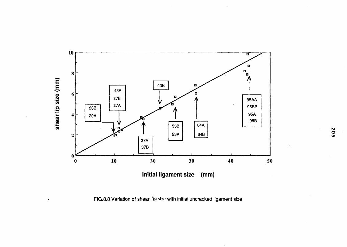
Initial ligament size (mm)

FIG.8.8 Variation of shear lip size with initial uncracked ligament size

20

5

206

assumed hinge point

FIG.8.9.a Kinematic analysis of a loaded TPB geometry by assuming two symmetric rigid halves rotating about a hinge point.

207

i

FIG.8.9.b Kinematic analysis of loaded FPB geometry by assuming twosymmetric rigid portions between upper and lower rollers

208

(a)

FIG.8.10 Applied system of forces in bend type loadings of beams a) On the roller supporting the beam

b) On the beam under FPB loading c) On the beam under TPB loading

2 0 9

W A

(- )

(+)

(b)

FIG .8.11 a) Slip line field solution for an indentation problemb) Axial stress distribution in an unnotched beam, with

rigid plastic material properties, under FPB loading c) Axial stress distribution in an unnotched beam,with

rigid plastic material properties, under TPB loading

ro| a

2 1 0

FIG.8.12.a Load-load point displacement relations for the unnotched TPB configuration.

Loa

d.Q

(kn

)

211

FIG.8.12.b Load-load point displacement relations for the unnotched FPB configuration.

Con

stra

int F

acto

r L

Con

stra

int F

acto

r L

2 1 2

Normalised load point displacement 2q/s

2.5 ■

2.0 ■

„ H □□ ■ □ Q c* O

I □1.5 A A % a A A A

* “ i ^ □ * 4u * ■ ■ r ■ 37A1.0 A A 1 □

aa □ 64A□ A 95A

AA ■ A 95AA

0.5 ■ H 43B

‘ A

0.0 >1------------------ ------------------- 1---------------— '------------------1--------------- *0 .00 0 .0 5 0 .1 0 0 .15

Noramlised load point displacement 2q/S (4q/S for FPB)

FIG.8.13 Variation of constraint factor with load point displacement

Con

stra

int F

acto

r L

213

Normalised crack extension Aa/bo

2.5 -

s 2.0o(0LL*-»S 1.5 co0)coO 1.0

■ 37A□ 64AA 95AA 95AA■ 43B

i □ A 4 A

■ Ds *

1 ■ A■ DAAA ^ A A

a A a A A

0.50.0 0.2 0.4 0.6 0.8Normalised crack extension Aa/b Ao

FIG.8.14 Variation of constraint factor with crack extension

(KN

/mm

)

2.0

1.0

0.0

“ AB

A AB A

A AB A

♦ A• A

B O A1 A

» i *♦ " A

■ A + 20B+X * > X 27B

+ A ■ 37B

■+ X ■ ► ♦ 5 3 A

+ ^ • B 64B

+ b * * A 9 5A•+ X®9 4 A 9 5A A

t A*

i A______________ ______________ 1---------------------- ■---------------------- 1---------------------- •------__________1_____________

0 10 20 30

Crack extension Aa (mm)

FIG.8.15.a Representation of resistance in terms of JQ

214

(KN

/mm

) J0

(K

N/m

m)

215

Normalised crack extension, Aa/B

2.0 -

+ 20BX 27B■ 37Bo 53AB 64BA 95AA 95 AA

1.0 -

■ A

kB&

0.0 0.00

x

4 oB A ° ^

* / * A _

+ X4X

A 4- ^ y

+ * *

0.20 0.40 0.60

Normalised crack extension, Aa/bQ

FIG.8.15.b Effect of normalised abscissa on JQ Resistance curves

(KN

/mm

)

"3

+ 1FIG.8.16.a Representation of resistance in terms of J.

216

(KN

/mm

)

217

EEz*

+"3

2.0

1.5

1.0

0.5

0.00 .0 0 .2 0 .4 0 .6 0 .8 1 .0

H n

•A

+ "X ^I + g A A-+ W O*

■ X

IPK

i ±

m 4

AS

■ * A ♦

■ A* "+ 20BX 27B■ 37B♦ 53A■ 64BA 95AA 95AA

Normalise crack extension, Aa/B

2.0 -

^ 1.0 -

Normalised crack extension Aa/b

FIG.8.16.b Effect of normalised abscisa on J. resistance curvesi+i

(KN

/mm

)

2.00

1.50

1.00

0.50

0.00

*

L I

HA

a a o «

■ • . A

A A O

++ 8

f+ x°"A .

" •* +

^ °

° X■ xv * x

A A

+ 20BX 27B■ 37B♦ 53A■ 64BA 95AA 95AA

0.0 10.0 20.0 30.0


FIG.8.17.a. Representation of resistance in terms of JJpT

218

(KN

/mm

) J

(KN

/mm

)

219

Normalised crack extension Aa/B

Normalised crack extension Aa/bQ

FIG.8.17.b Effect of normalised abscissa on JTPT

resistance curves

4

EE

• + 20BX 27B■ 37BA 53AHi 64B

■ A 95AA 95AA

2 -

HAHI A

* A ♦ A

0

+ x. x ■+X ■ 0

+ ■+ X*

A++ J A *

+ AA A■*A

________ .-----------o

A AA A

A A

10 20 30


FIG.18.a Representation of resistance in terms of Jy

220

221


EE

' BB■ + 20B B *

X 27B AB A

■ 37B A " a♦ 53A * B AB 64B ■

AB<

A 95A A O- A 95 AA A " » •A A A

■ " ■ X+- A A ° X

■ A ♦ . X +A - *X

AB A . + 4 X

■ B £A X

; A

0.00 0.20 0.40 0.60Normalised crack extension Aa/bo

FIG.8.18.b Effect of normalised abscissa on resistance curves

dU/B

da (

KN

/mm

) U

/B

(KN

)

2 2 2

50

40 h

30

20

10

■ Am *

ft■ A

J ■ "ft ■ \ ^ x

0

+ 20BX 27B■ 37Bo 53AH 64BA 95AA 95AA

0 10 20 30


+4

10

4Fk

+ 20BX 27B■ 37Bo 53AB 64BA 95AA 95AA

-fcB*♦

0

0.0

; Ax* V______ i_____

0.2

A 4k -X

XA

+♦*

0.4

i « * *♦« / /* , y .

0.6 0.8Normalised crack extension Aa/bQ

FIG.8.19 Total work and work rate as a function of crack extension

0 10 20 30


FI68*20.a Total plastic work (dissipated energy) as a function crack extension

223

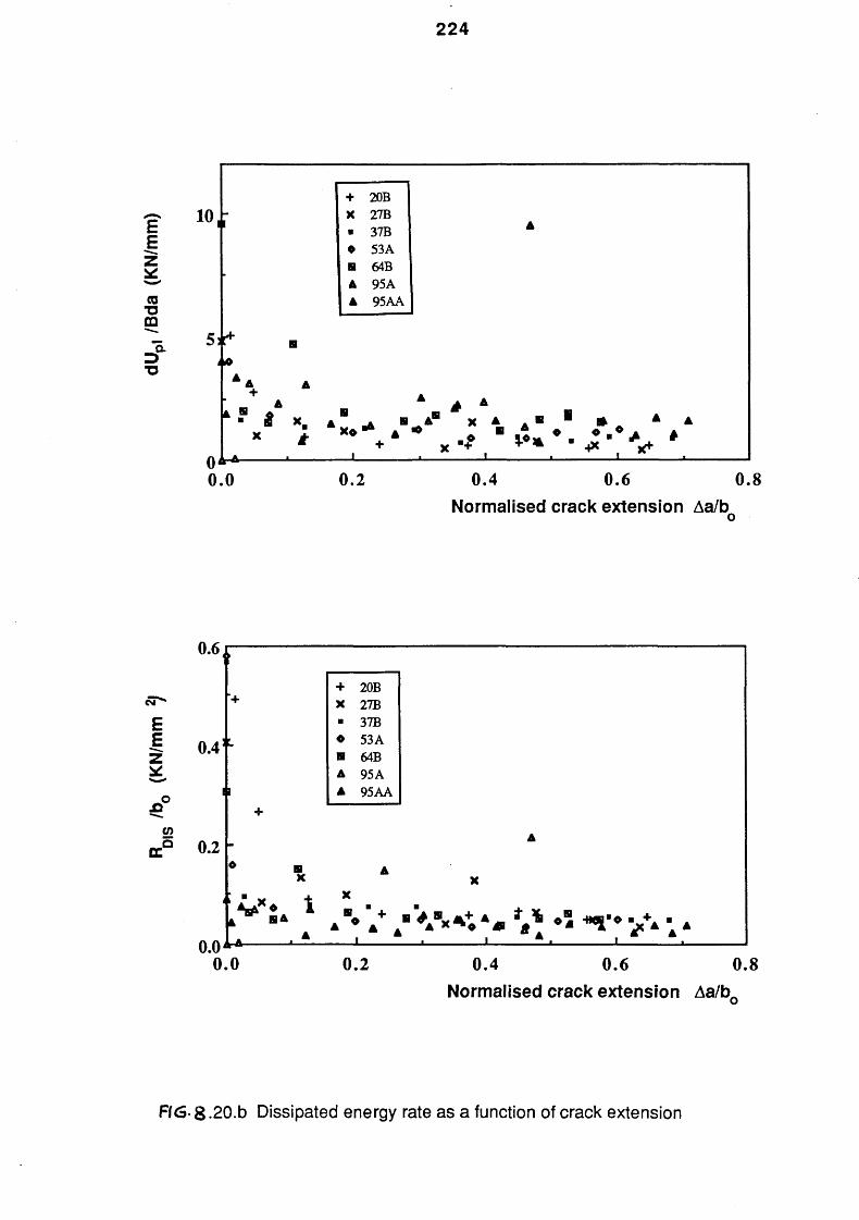
/b0

(KN

/mm

2j

dUp,

/B

da (

KN

/mm

)

224

10

5:&

+ 20BX 27B■ 37B0 53An 64BA 95AA 95 AA

A+

£ x. a " + ■ *B x A A rn ■ AX t + A „ **» ■ J * *

A A #

0

0.0

0.2 0 . 4 0.6 0.8Normalised crack extension Aa/b

0.6

0.4

tLa 0.2

0.00 . 0 0 . 2 0 . 4 0 . 6 0 . 8

Normalised crack extension Aa/bQ

+ 20BX 27B■ 37B♦ 53A■ 64BA 95AA 95AA

* a “ * a + * g \ • “ ■ / * ; A

Ff6g.20.b Dissipated energy rate as a function of crack extension

/Bb0

(K

N/m

m)

U0|

/B (

KN

)

225

6

5

4

3

2

1

00 10 20 30

Crack extension Aa(mm)

AA A

A A

■. A H

+ 20BX 27B■ 37BA 53AH 64BA 95AA 95 AA

» A

A "A ■

I- A ■■ A■ -X X w " . A

X * ■ . ♦ ♦+ + X w * • .

■» + * * _____ ,___ ■________

_a>

0.15 ■ + 20BA X 27B

■ 37BA * A 53A

0.101 ,* A * A H 64B* ♦ H A 95A

■ B * 4 AA _ .

A 95AA

0.05!x

<»+ +

0.000.00 0.20

• A■ x • r* m

X+

0.40

A

X+ ** V

0.60

X . * A

Normalised crack extension Aa/b0

FIG.8.21 Variation of elastic energy (recoverable) with crack extension

CO

D(to

t) (m

m)

226

20 30Crack extension Aa (mm)

EE

Q.aoo

1.2A

1.0 -f t A

AA A

AH A A

0.8 »■ a * *

■ ♦ ° A

0.6 ♦ . • ■ ♦ A

+ 20BX 27B■■ * 4_ ■ ■ ■ 37B

0.4 H _ ■+ t x a

♦ 53A

0.2

+J- *

* * * ■A

64B95A

*sr A A 95AAi 6*

0.0' ____ i__________1__________i__________1__________i. ______ 1___0 10 20 30


Fl6-&.22.a COD Resistance curves

CO

D(t

ot)

(mm

)

2 27

1.5

1.0

0.5

0.0

+ 20BX 27B A

. ■ 37B A A♦ 53A A A * A HH 64B 4 “ * ■ '■ A 95A A * B * B

■ A 95 AA A H *A A a ♦ °■ * A • ♦ °

A •

H A ° ■ ■ ■ ■ ■B

. * i + x X

' k VBl

X

ifSci ih—

i- I ------------- 1------------- 1________1________1________1________1________ 1_______

0.0 0.2 0.4 0.6 0.8 1.0Normalised crack extension Aa/B

1.2

1.0

EE 0.8

£ 0.6Oo

0.4

0.2

0.00.00 0.25 0.50 0.75 1.00


. A

AA A A B A

• A A A B

► ► B

A A H AA

" A ° °■ A ♦ a * + 20B

♦A B ■ "X 27B

■ _ B■ ■ 37B

+ + > * + * X A 53 AA:

<

*■ *

+JU. B 64B

+ “ A 9 5AA ' 95 A A

L-A----------- ,----------------- 1-----------------1._________ 1__________ 1__________ 1___ .

Fie.S.22.b COD resistance curves with normalised abscissa

Nor

mal

ised

dis

plac

emen

t 2q/

S

22 8

0.15

0.10

0.05

+ *

+ X

+ x

o• ■

• ■• ■

+ 20BX 27B■ 37Bo 53As 64BA 95AA 95 AA

l* * - • ■ ■x ■ 4 *

x ■ ■ * A

A * AA

0.00 x0 10 20 30


0.00 0.20 0.40 0.60Normalised crack extension Aa/bo

FIG.8.23.a Variation of normalised load line displacementwith crack extension.

(2bo

/s)(5

q/3a

)

229


1.0

0.8

0.6

0.4

0.2

0.0

- 0.20.00 0.20 0.40 0.60

Normalised crack extension Aa/bo

■+

+ 20BA X 27B A

O ■ 37B- O 53A

S 64B+ A 95A A

A 95 AA. A * A

hA X H B ■ A

A X m A + m A 4 * * "H A V ■ A _ ^ j . A * a * ™ " K * A T * ■ + ■ Aa

A A « a A * * a

___________________

FIG.8.23.b Variation of normalised load line displacement rate

with crack extension

230

Code Thickness B (mm)

W idth w (mm)

Crack ratio a/w

Loadingtype

20A20B

20.7 20 .8 0 .5160.520 TPB (S /W -4)

27A27B

20.7 27 .2 0 .5930.561 TPB (S/W=4)

37A37B

20.7 36.80 .5260.536

FPB (S/W =6.3) TPB (S/W=4)

53A53B *

20.7 53 .20.5340.517

TPB (S/W=4) FPB(S/W =4.36)

64A64B

20.9 64 .00 .5250.513

TPB (S/W=4) FPB (S/W=4)

95A95B

21.3 93.90 .5260.529 TPB (S /W -4)

95AA95BB

49.8 94 .2 0 .5320.539

TPB (S /W -4)

4 3 A * *4 3 B ** 21.3 42 .8

43 .90.740.503

TPB (S /W -6)

* The upper rollers were restraint from any kind of motion ** These were not considered in R-Curve studies.

TABLE.8.1 Geometrical and loading variations of specimens studied

231

Specimencode

Initial Crack Ratio

Total Crack Extension (mm)

Specimen Compliance

mm/kN ( x 1 0 '3 )

(a0/w)e ( V w)9 (Aa)e (A3)9 cpT m q>

TA 0.525 0 .528 0.660 0.53 10.449 10.280

TB 0.524 0.521 0.732 1.211 10.449 11 .075

TC 0.534 0.536 1.608 2.44 12 .406 13.78

TD 0.519 0.518 4.09 5.93 15 .453 19.823

TE 0.529 0.529 7.14 10.47 25 .447 43 .82 8

TF 0.515 0 .514 10.204 13.89 36.846 74 .10 4

NOTES ON SUBSCRIPTS:

e for estimated based on measured compliance 9 for measured according to ASTM E813 m for measured c for corrected

TABLE 8.2 Crack length, crack extension and compliance data of the six TPB specimens (B=20mm, W=50mm, S/W =4 ) used to study crack front curvature.

232

PLATE 8.1 Crack surfaces of broken calibration specimens showing different amount of crack extensions

PLATE 8.2 Crack surfaces of various broken specimens showing different size of shear lips and crack extensions

233

PLATE 8.3 Crack surfaces of various broken specimens showing different size of shear lips and crack extensions

PLATE 8.4 Crack surfaces of various broken different size of shear lips and crack

specimens showing extensions

234

CHAPTER 9

CONCLUSIONS and RECOMMENDATIONS

A 2-D finite element method was developed to deal with plane problems which

are neither in plane stress nor in plane strain conditions. This method, which has

the advantageous of the 2-D idealisations, has been used for EPFM analysis of

test piece geometries. For plane stress or plane strain conditions J has been

evaluated from the contour integral definition. The average value of r| factor as

determined from the latter analysis has then been used to evaluate J from work

input for the semi-plane strain conditions. A modified J integral definition, which

will account for the energy input due to the stresses and strains in the thickness

direction, may be sought as a better way of evaluating the applied crack tip

severity.

Two forms of equations to represent load-displacement, (Q-q), relations for edge

cracked geometries have been formulated and rationalised using numerical

solutions. The study, which had been limited to materials with non-work

hardening properties, utilises work rate at constant load to estimate J. Naturally,

the accuracy of estimates rely on the accuracy of the Q-q equations in

representing the numerical data. In the LEFM regime, good correlation between

the estimated and numerically evaluated J values has been achieved. In the

EPFM regime, especially at near limit load levels, the poor correlation between

estimated and numerically obtained Q-q relations has resulted in large

differences between the corresponding values of J. It is believed that use of work

rate at constant displacement to evaluate J in the EPFM regime, will reduce

differences between estimated and numerical values. Further, the method is

likely to give better results for materials with work hardening characteristics.

Other forms of equations, easier to handle mathematically and with improved

accuracy, may also be sought.

Single edge notched geometries subjected to the tensile type of pin loadings

have been studied, both analytically and numerically. Useful relations for limit

235

load and plastic component of ri factor, Tip|, as a function of applied load

eccentricity has been obtained. For cases where the net section area is primarily

subjected to bending stresses (large eccentricity), good correlation between

analytical and numerical results has been achieved.

For cases with small eccentricities (primarily tensile stresses in the net section

area) the analytical results depend on the the selected form of variation of

HCCTR, and the numerical results are appreciably affected by the model used

for the study. However, for large eccentricity cases the inclusion of the HCCTR in

the analytical studies hardly matters, hence the form of solutions for plane stress

or plane strain are practically identical.

The constraint factor, L, has been found to increase with both deformation level

and crack extension. Experiments on unnotched bend specimens have been

considered and the rise of load with deformation has been successfully

explained by the change in effective span, friction forces and slip line field

theory.

Normalisation of J based resistance curves with thickness has reduced the

variations in data due to different thicknesses of test pieces. For thinner

specimens, where the size is comparable to the plane stress plastic zone

diameter, 2rpo, no normalisation is required. When normalising data with

thickness, a minimum reference thickness, corresponding to about 2 ^ seems to

be necessary. However, when normalising with initial ligament size, if required,

no such limits are apparent.

The shear lip size is found to be linearly proportional to the initial uncracked

ligament size, at least for those geometries and sizes studied here. Although its

effect on out of plane constraint here is negligible, on thicker specimens, it may

explain the normalisation of data with initial ligament size for a given thickness.

When geometrically similar specimens are considered, normalising by thickness

or initial ligament size expectedly have equal effects.

Total and plastic component of work and their rate with crack extension has

been considered to characterise the resistance to crack extension. Especially

the work rate, be it total or plastic only, is found to decrease to a near constant

value after some crack extension. This could be a measure of the material's

236

basic resistance since scaling of the ordinate by initial ligament size has little

effect on the data.

The normalised displacement rate as a function of normalised crack extension

resulted in a unique curve, which has been proposed as a measure of

resistance to crack extension^

The EnJ method for estimating the applied crack tip severity has been applied to

short cracks emanating from regions of stress concentrations and compared with

2-D numerical results. The well known ’short crack' and 'long crack' division has

been applied and a relationship has been established to determine whether a

given crack is to be treated as 'long' or 'short'. This relationship is strictly based

on LEFM parameters and a size feature of the stress concentration, where for

'long' cracks, the latter is considered to be part of the real crack.

In the LEFM regime, the estimation process is based on the remote stress level

for the 'long' cracks and on the local stress level for 'short' cracks. In the EPFM

regime 'short' cracks require the EnJ estimation to be based on the local strain

rather then the local stress for better estimates. Local strain can be estimated

using the Neuber's rule.

The EnJ method is based on the upper bound representation of numerical data

for shallow cracks. Therefore, the estimations are expectedly better for shallower

cracks irrespective of the 'short' or 'long' crack treatment.

The range of work considered here, which is aimed at improving J estimation

methods for numerical, analytical and experimental studies of fracture

mechanics problems, has produced fairly useful results. Although some further

improvements may be required in some cases, the finding*can be incorporated

in design methods.

see foo tno te on p a g e 199

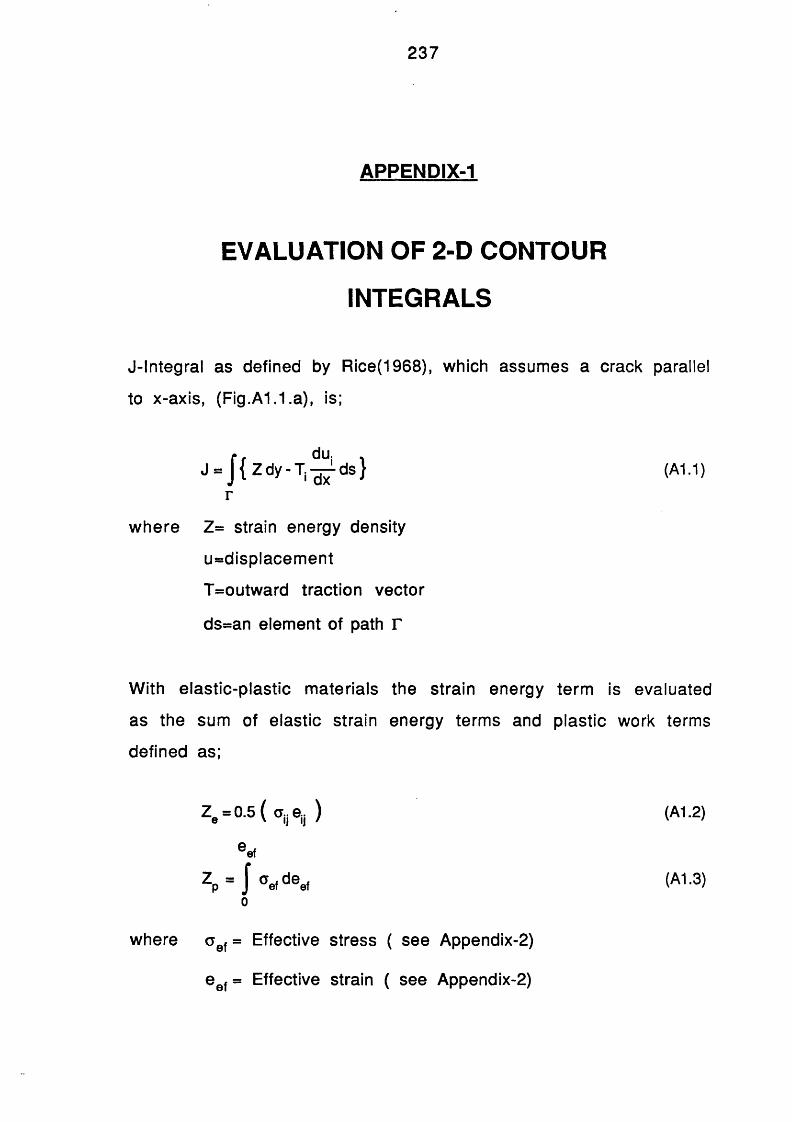
237

APPENDIX-1

EVALUATION OF 2-D CONTOUR

INTEGRALS

J-Integral as defined by Rice(1968), which assumes a crack parallel

to x-axis, (Fig.A1.1.a), is;

J = | { z d y - T . ^ d s } (A1.1)r

w here Z= strain energy density

u=displacem ent

T=outward traction vector

ds=an element of path r

With elastic-plastic materials the strain energy term is evaluated

as the sum of elastic strain energy terms and plastic work terms

defined as;

Ze = ° -5 ( V , j ) <A1-2>

e ef

Z p = J CTef d eef <A1-3 )0

where a e f= Effective stress ( see Appendix-2)

e e f= Effective strain ( see Appendix-2)

238

The relation of traction vector com ponents to local stress

components are;

where (a-90) is the angle between outward normal and +ve x-axis.

To evaluate J-Integral in a FE analysis, a subroutine to an existing

program may be added to process already evaluated stress and

strains. When defining a path to evaluate J, such points where

stresses and strains are readily available, e.g. node points (or gauss

points for isoparametric elements), are chosen. J is then evaluated

for each of these segments between two adjacent chosen points, and

then summed to give the J-integral for the path. For calculations

purpose it is easier to consider each term of J-Integral separately.

Furthermore, plastic work term for each segment at the end of a

loading step is recorded and utilised in the next loading step.

Considering two adjacent points defining a segm ent of a path,

Fig.A1.1.b, J-Integral is evaluated as:

Tx = °xxsina - % ° o s a

Ty = -Oyy cosa + 0xy sina (A1.4)

i+1

(A1.5)

H-1

(A1.6)

239

du. duXX dx + ° x y - d r ) a v sln«

du du,xy dx /av" (°yy 1 ? + axv"^r).- cosa } As (A1.7)

i=n-1

pathi«=1

(1) + j (2) + j (3) )ij+1 J i.H-1 + J i,i+1 / (A1.8)

w here As = Length of segment

8e0f * Plastic strain increment during current loading step.

n = total number of points defining the path.

Subscripts (av) and (pr) stands for average values between two

adjacent points and calculated value for the previous loading step

respectively.

*

References:

RICE, J.R. (1968). Journal of Applied Mechanics, 35, pp.379-386.

H E LLE N , T .K . (1984 ). H Post Yield Fracture Mechanics", Applied

Science Publishers, London, Ed. Latzko, D.G.H.

240

Fig.A I .1 a) Contour for J-Integral evaluation

b) Contour defined by points for J-Integral evaluation in FE. studies.

241

APPENDIX-2

ELASTICITY EQUATIONS FOR ISOTROPIC

MATERIALS

Strain-displacem ent relations are;f 3us 9u:

e:1 . 3u. 9u. v_ j _ / j _ _ i_ \

'•i “ 2 ' 3Xj + 3x. ' (A2.1)

strains may be caused by mechanical, thermal or residual effects.

e - e m + e th + e re ( A 2 -2 )

Constitutive equations relate mechanical stresses to mechanical

strains which may be given as;

a ij= x 5ijekk+ 2 ^ eij

(1 + v ) ( l - 2 v )

(A2.3.a)

(A2.3.b)

E= ----------

2 (1+v)

Where E is Young's modulus of elasticity, v is Poisson's

(A2.3.C)

ratio, and 8

is the cronecker delta ( 5^=1 if i=j and 5^=0 if i* j), and summation

over repeated indices are implied in Equ.A2.3.a.

For plane problems, the two shear stress components involving the

thickness direction (z direction for convenience) are assumed to have

zero values together with, either a zz=0 for plane stress or ezz=0 for

plane strain conditions.

Constitutive equations including thermal strains may be written in

matrix form and the same equations may be used for either case by

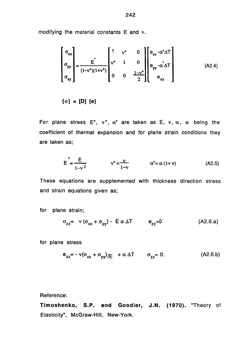
242

modifying the material constants E and v.

G _XX

a. Eyy

(l-v*)(l+v*)axy

0

0

i = £2

exx -a ‘ A T

eyy -a AT (A2.4)

M = [D] {e}

For plane stress E*, v * , a* are taken as E, v , a , a being the

coefficient of thermal expansion and for plane strain conditions they

are taken as;

* EE -------- v* = -^ — a*= a (1+ v) (A2.5)

l - v 2 1—v

These equations are supplemented with thickness direction stress

and strain equations given as;

for plane strain;

°zz= v K x + a y y )' E a AT ezz=0 (A2.6.a)

for plane stress

ezz= - v(oxx + oyy) /E + a AT azz= 0. (A2.6.b)

Reference:

T im o s h e n k o , S .P . and G o o d ie r , J .N . (1 9 7 0 ). "Theory of

Elasticity", McGraw-Hill, New-York.

243

APPENDIX-3

INTRODUCTION TO FLOW THEORY OF

PLASTICITY

The yield criterion determines the stress level in a material at

which plastic flow begins and can be stated in a general form as;

F= F(g ,k) = / (a ) - k(ic)=0 (A3.1)

where k(ic) is material property to be determined experimentally and

k is the hardening parameter.

Von-Mises criterion of yielding is well supported by experimental

evidence and states that the plastic flow will occur when the

equivalent stress, a ef, reaches a critical value. This may be

expressed as;

F = K x - °y y )2+ ( °y y - ^ z z ^ x x)2

+6( a xy2+ c yz2+ a zx2) -2 a ef2=0 (A3.2)

or in terms of deviatoric stress components

F= — o|. a,’, - of, = 02 >j y 3 ef

a!. = a . - — a ,. &. y ij kk ij

(A3. 3)

(A3. 4)

where 8y is kronecker delta and summation over repeated indices are

im plied.

For elastic conditions deviatoric strains (defined below) are related

directly to deviatoric stresses.

244

(e!.) « -JL v |J ye 2G

(e ij )e = (e jj)e * 3 (ekk)e ij

(A3. 5)

(A3. 6)

Plastic strains are assumed to occur at constant volume, hence;

(0 ii>P = ° <deii )P =0 (e ij)P= (e ?P (A 3*7 )

An effective plastic strain, (eef)pis defined, (similar to effective

stress), as a function of plastic strain components, (equ.A3.8), where

the constant 2/9 was introduced to satisfy uniaxial tension

conditions. A sim ilar definition also exist for plastic strain

increments, (equ.A3.9).

e ef = { J [ ( e r e2) 2+ (e2- e 3) 2+ ( e ^ ) 2 ] } °'5 A3.8

where e ^ e g ^ are principal strains

<d 0ef )p = ( | ( deij)p (d e ij>p ) ° 5 (A3-9 )

Strain and strain increments can be written as a sum of elastic and

plastic components.

®ij = (®ij)e + (®ij)p (A 3 ' 1° )

deij= (d 6 ij)e + (d^j)p (A3. 11)

For continued plastic flow, F=0 together with dF=0 is required as

dF<0 will indicate elastic unloading.

... 9F . 3F , . 2 ^ „dF------- do;, + -------daef = 0jj do, - - O j (de„)B =0ef

da.ij

daef

daef

<d e ef)|= H '

(A3.12)

(A3.13)

where H' is the local slope of stress-plastic strain curve.

245

The potential theory of plasticity assumes that the plastic strain

increments are proportional to the stress gradient of Q, which

term ed as the 'plastic potential'. Further, Q is assumed to be

identical with the yield function / of equ .A I.

(de )p = P ^ - (A3.14)J P d Cf . ..

The differential of equ.A3.1 can be written as;

{a}T{do} - Ap=0

w hereT j>F_ 3F_ dF_ _3F_ J F _ dF

V ^a2,^ aXy, t o * ' d° yz

A —p 3 k

{a} is termed as the flow vector.

(A3.15)

(A3.16)

(A3.17)

Using A3.14 and A2.4 the total strain increment (equ.A3.11) is now

written as;

{de}= [D]'1{dc} + p{a} (A3.18)

pre-multiplying equ.A3.18 with {a}T[D] and using equ.A3.15 gives p as;

P= (a}T [D]

A + {a}T [D] {a}{de} (A3.19)

Substitution of equ.A3.19 into equ.A3.18 and solving for stresses

gives.

{da}= [Dep] {de}

w here

[Dep] = [D ]-(dD } « U T

A + {cyT {a}

(A3.20)

(A3.21)

246

{dD} = [ D ] {a } (A3.22)

The constants A and p are determined by referring to uniaxial tensile

test data and postulating the degree of work hardening ( k ) to be a

function of total plastic work done. Therefore,

•<(«)- t f y ( * ) (A3.23)

K = W p = J a ij.(dejj)p (A3.24)

dK = a|j.(deij)p=p {a}T{a } (A3.25)

and the hardening param eter, k , is assumed to be equal to the

effective plastic strain, (e0f)p.

For uniaxial case, there Is only one applied stress component, which

can be identified with the yield stress a ys, and strain components are

defined by the effective value e0f (equ.A3.9). The flow vector has one

term, and p is obtained from equ.A3.23 by using Euler's theorem

applicable to homogeneous functions.

d /(c JdK = P ay = Pay = ay.(deef)p (A3.26)

P = (d e ef)p (A3.27)

The constant A is found by substituting equ.A3.27 and equ.A3.23 into

equ.A3.17 to give;

daA = Y = H' (A3.28)

<d e ef)p

This method is quite suitable for numerical work with the added

advantage of requiring no inversion of matrices. Using von-Mises

yield criterion, the function ( / ) is identified with the second stress

247

invariant in terms of deviatoric stress components.

/(o „ ) = ( 3 J '2)0-5

where J '2 = 0.5 (o'# ) (a'„)

and the flow vector {a} becomes

- { o ' }

(A3.29)

(A3.30)

references:

H i 11, R . (1 9 5 0 ) . 'M athem atica l Theory of P lastic ity ', Oxford

University Press.

O w en , D .J .R . and H in to n , E. (1 9 8 0 ). 'F inite Elem ents in

Plasticity; Theory and Practice', Pineridge press.

248

APPENDIX-4

ESTIMATES OF THE J-INTEGRAL FOR CRACKS AT REGIONS OF STRESS'omzwrmm— ~ — ---------------------------------------------------------------------------------------------------------------------------------------------------------------—

*ETEMAD, M .R., DAGBASI, M ., and TURNER, C .E .

Numerical results for cracks in regions of stress concentration of various geometries are presented and compared with estimates by several methods. In the LEFM regime the well known division into 'short' or 'long' crack is used. Short cracks are treated by the local stress, (kta) and a shape factor for a small crack size ratio such as Vrc, and large cracks are treated by the remote stress (c)and a shape factor, Y, related to the size of the crack plus concentration feature. A relationship is stated to establish whether a given crack should be treated as 'long' or 'short'. In the EPFM regime the EnJ estimation method is found useful for either case provided that for cracks that are short EnJ is entered according to the local strain at the stress concentration rather than the local stress.

INTRODUCTION

L in e ar e la s t ic f ra c tu re mechanics, LEFM, has prooved an in v a lu a b le to o l , in both design and assessment o f s tru c tu ra l in t e g r i t y . I t uses the crack s iz e , a , the nominal remote s t r e s s ,e r , and a geometr ic shape fu n c tio n , Y , to d e fin e the s tre s s in te n s ity fa c to r , K, which g ives the magnitude o f the crack t ip s e v e r ity .

K=Yav a (1)

To account fo r small sca le p la s t ic i t y , an es tim ate o f the p la s t ic zone developing ahead o f the crack t ip is made in con junction w ith Eqn.l to g iv e ,

r p= (l/$ 7 T )(K /a y ) 2 ( * )

where 3 is a numerical co n stan t; 2 fo r plane s tress (upper bound) and 6 fo r plane s tra in (lo w e r bound). K is then increased by

♦Research A s s is ta n t, Research Student and Professor o f M a te r ia ls • re s p e c tiv e ly ; Mechanical Engineering Peoartm ent, Im o eria l C o lleg e , London SW7, UK. '

92-1

249

FRACTURE CONTROL OF ENGINEERING STRUCTURES - ECF 6

re p la c in g the crack s iz e (a ) in Eqn.l by (a + r ) . Some users update Y c o rres o n d in g ly , w h ils t some do n o t. An ex ten sive d iscussion on

'va rio u s p la s t ic zone s iz e es tim a tio n and c o rre c tio n procedures can be found in R e f . l . For more ex ten s ive p la s t ic i t y , severa l e la s t ic - p la s t ic design methods have been proposed, C 0D (2 ), R -6 (3 ) , EPRI(4 ) and E n J (5 ). These methods have been described and compared fo r severa l case s tu d ies in R e f .5 .

Although most eng in eerin g s tru c tu re s are designed and operated w ith in t h e ir e la s t ic l i m i t , they may experience y ie ld le v e l stresses lo c a l ly a t geom etric d is c o n t in u it ie s . In LEFM i t s e l f , a crack a r is in g in a reg ion o f s tress co n centra tion is a llow ed fo r by the choice o f ap p ro p ria te Y fa c to r where known, eg. R e f .5 , where the Y fa c to r is not known an approxim ate express io n , sometimes used fo r sh o rt cracks is given by,

K=kt a/fra (3 )

Eqn.3 im p lies a small crack o f len g th (a ) in a rem otely ap p lied uniform s tress f i e ld o f magnitude k t a where k t i s the conventional e la s t ic s tress co n cen tra tio n fa c to r eva luated here using the gross cross s e c tio n a l a re a . In many in s ta n c e s , such a crack a t a s tress co n cen tra tio n is b e t te r m odelled as an edge crack in a wide p la te , g iv in g ,

K =1.12kt a^?a (4 )

In some o f the EFPM ( e la s t ic - p la s t ic f ra c tu re mechanics) methods the procedure fo r e s tim a tin g the a p p lie d crack t ip s e v e r ity is by using an e f fe c t iv e s tre s s le v e l , which a t le a s t in R e f .2 is taken as (Kt o).

For the LEFM regime th is paper presents and compares the s e v e r ity o f cracks in s tress co n cen tra tio n areas as published ( 6 ) , as estim ated by E qn .3 , Eqn.4 and by Smith and M i l le r (7 ) and as obta ined n u m e ric a lly . S p e c if ic a l ly cracks emanating from e l l i p t ic a l holes in wide p la te s subjected to te n s ile load ing w ith p a r a l le l ends are f i r s t s tu d ie d , see F ig . l and Table 1 . The geom etries modelled fo r the numerical s tu d ies gave r is e to nominal s tress co n cen tra tio n fa c to rs , SCF, o f 2 , 3 and 5 . The study is then expanded to o th e r geom etries where standard s o lu tio n s are not a v a i la b le , and the on ly comparison made is th e re fo re between estim ated and n u m e ric a lly obta ined v a lu e s . Analyses beyond LEFM regime is then d e ta ile d by comparing computed J - in te g r a l values w ith those p red ic ted by EnJ, fo r both sh o rt crack and long crack cases. The lo ca l p la s t ic s t ra in in the notch , as found by f i n i t e elem ent study o f the uncracked body, was a lso used in the EnJ es tim a tio n procedure.

92-2

250


T.ABLE 1 - D e ta ils o f Geometries S tu d ied .

(a ) E l l ip t i c a l cen tre notch ( F i g . l . a )

Case W . mm

D .mm

R. , mm

Hmm

SCFNominal True

M212 100 100 5 10 2 2 .04

M202 . 50 200 5 10 2 2.041

M203 50 200 10 10 3 3.153

M205 50 200 10 5 5 5.183

(b ) Edge notch ten s io n ( F i g . l .b )

CaseWmm

Dmm

Rmm

Hmm

Type o f Notch SCF

M202T 50 200 5 10 Semi-e T l ip t ic a l

2 .124

M205T 50 200 10 5 Semi - e l l i p t i c a l

5 .869

M99RT 10 40 1 .8 0 .5 u-notch 7 .8

(c ) Edge notch bending ( F i g . l . c )

Case W(mm) D(mm) R(mm) H(mm) Type o f Notch

SCF

M202B 50 200 5 10 Semi -e l l i p t i c a l

1.627

M205B 50 200 10 5 Semi - e l l i p t i c a l

4 .475

M99RA 10 40 1 .8 0 .5 u-notch 5 .5M99R 10 40 2 0 .5 u-notch 5 .8

92-3

251


(d ) The s tru c tu re ( F i g . l . d , l . e )

Case W(mm) D(mm) R (mm) H (mm) Loading SCF

Ml 21B 50 200 5 10 Bending 1 .4 6 5 (1 .1 8 7 )

M121T ii n it n Tension 1 .5 5 (1 .4 0 0 )*

*F ig u res in paren thes is are based on reduced sectio n a re a .

THE FINITE ELEMENT PROGRAM

A tw o -d im ension al, sm all geometry change FE code w ith 8 noded is o p aram etric elements was used to model various s tru c tu re s fo r nume r ic a l s tudy. The m a te r ia l m odelled was a pressure vessel s te e l w ith m ild work hardening w ith y ie ld s tress a =573.64 MN/m2 .Young's modulus E=210xl03MN/M2 , and Poisson's r a t io v = 0 .3 .

A ll goem etries s tud ied were constra ined to plane s t r a in , and the J - in te g r a l was evaluated along 10 d i f fe r e n t contours around the crack t i p , to prove path independence o f the method. W h ils t e la s t ic , these values were converted to K and Y using

K = /(J /E ')= Y av /a t

where E '= E / ( l - v 2,) and

a^=a+R

where R is th e notch s iz e (see F ig .1 ) .

STRESS CONCENTRATION CASES IN LEFM

(5)

(6a )

(6b)

In f in i t e Geometry Cases

Estim ates o f the s tress in te n s ity fa c to r K by Eqns 3 and 4 and those obta ined using the equations given by Smith and M i l le r ( 7 ) , are compared w ith FE re s u lts obta ined here and those presented in R e f.6 , fo r cracks a t e l l i p t i c a l holes in th ree cases o f nominal SCF, 2 , 3 and 5 , in F ig .2 . Note th a t the geom etries s tud ied by the FE method were o f f i n i t e s iz e , see F ig . la and Tab le l a , so th a t a c o rre c tio n to i n f i n i t e s ize was made using /sec(7rat /w due to Fedderson ( 8 ) . The FE re s u lts agree w ith those given in R e f . (6 ) being 2% h ig h e r, but p re d ic tio n s by Eqn.3 are always low er fo r low SCF cases. For h ig h er SCF cases p re d ic tio n s by Eqn.3 are lower fo r sm all cracks and h ig h er fo r lo nger cracks than those given by R e f.6 . On the o th e r hand Eqn.4 p re d ic ts exact o r h ig h er i< values fo r a l l those cases presented in F ig .2 . The amount o f over-estim ate by Eqn.4 depends upon both the crack s iz e (a ) and the SCF. For

93-4

252


sh o rt cracks the p re d ic tio n by Eqn.4 approaches to the exact so lu t io n . F ig .2 fu r th e r shows th a t the s tress in te n s ity fa c to r fo r these geom etries increases w ith the increase o f crack s iz e , approaching to the cen tre crack panel s o lu tio n a f t e r s l ig h t ly overshooting i t . T h e re fo re , the s tress in te n s ity fa c to r p re d ic te d by the long crack (a t ) approach, th a t is the cen tre crack panel w ith a crack s iz e ( 2 a . ) , using E qn .7 , which is e s s e n t ia lly Eqn.5 w ith Y = /tt, w h ile being reasonably accurate fo r long c rac k s , w i l l be p erhaps too con serva tive fo r short c racks.

K = a v/TTra^. = a / { 7 r ( a + R ) ( 7 )

Furtherm ore use o f Eqn.4 fo r sh o rt cracks proves to be a good or s l ig h t ly co nservative es tim ate o f the tru e s tress in te n s ity fa c to r . A sim ple c r i t e r io n to d is tin g u is h those cracks in a region o f s tress co n cen tra tio n where a sh o rt crack approach w i l l be b e tte r than the long crack approach and v ic e versa can be obtained by equating the two s o lu tio n s fo r K, i . e , Eqns.4 and 7 , fo r a p a r t ic u l a r crack length a ' .

K=k^.al. 12i/rra1 = a/rra^ = o/ir(a+R) (8 )

to g iv e ,

a '= R /| (1 .1 2 k t ) 2-- | | (9 )

i f a<a' a sh o rt crack trea tm e n t (Eqn .4) is p re fe rre d

a>a' a long crack trea tm en t (Eqn .7) is p re fe rre d .

F in ite geom etries

The idea o f a 'short crack' in an e le v a te d te n s ile s tre s s f i e l d (k .a ) o r lo n g c ra c k 'in the s tre s s f i e ld (cr) can be extended to cover edge notch cases in geom etries o f f i n i t e s iz e s , such as p a r a l le l end tens ion and bending. To apply to such cases, Eqns.4 and 7 are m odified fo r f i n i t e s iz e s , re s p e c t iv e ly , as fo llo w s .

K = k^aYgt^a

K = aYL/(a + R )

Equating th e s e , fo r a p a r t ic u la r crack le n g th , g iv e s ,

“ I V | j V s/YL) * - l ] (11)

(10a)

(10b)

where

Y = Y „(a ,V L ,D ) as is taken in tension s s ' n 7Y| = Y . (a f ,W,D) as is taken fo r the ac tu a l geometry (see

L L z F i g . l . a , b , c , d , e ) .

92-5

253


Use o f Eqn.11 enables a d ec is io n to be made on the 's h o rt crack ' o r Hong crack* trea tm en t o f a crack problem in a s tress co ncentra tion a re a . Again when a<a' the short crack trea tm en t is p re fe rre d and fo r a>a* the long crack trea tm en t is p re fe rre d .

A summary is given in Table 2 , comparing long o r sh o rt crack treatm ents fo r those geom etries s tu d ie d , see Table 1 and F i g . l , to support the c r i t e r i a s ta te d above. Where re le v a n t estim ates using the equations given by Smith and M i l le r (R e f .7) are a lso given

TABLE 2 - Comparison o f Estim ated and N um erica lly obta ined S tress In te n s ity Factors

(a ) Cases favo u rin g s h o rt crack approach

Case SCF a ' +(mm)

a(mm)

K/a+Computed Eqn.10a Eqn.10b

M202T 2 .1 2 1 .7 1 (1 .3 ) + 0 .5 2 .8 3 2 .9 3 (2 .7 5 ) 4 .9 9II n 1 .7 1 (1 .3 ) 1 .0 3 .8 4 .2 5 (3 .9 0 ) 5 .17ii it 1 .7 1 (1 .3 ) 1 .5 4 .47 5 .16 5 .43

M202B 1.63 2 .035 0 .5 2 .32 2 .2 8 4 .0 7

Ml 21T 1.55 4 .5 2 2 .5 4 .2 7 5 .0 4 5 .92Ml 21T ( * ) 1 .4 5.21 2 .5 3 .92 4.71 3 .36Ml 21T (* ) 1 .4 5.21 5 .0 5.41 6 .6 0 4 .7 2Ml 21B{ * ) 1 .19 4 .2 7 2 .5 3 .12 3 .86 2 .85

(b ) Cases favo u rin g long crack approach

Case SCF a '(mm)

a(mm)

K/o+

Computed Eqn.10a Eqn.10b

M205T 5 .87 0 .3 9 (0 .6 5 ) 0 .5 5 .98 8 .2 4 (5 .0 7 ) 7 .35M205B 4 .4 8 0 .4 0 .5 4 .5 8 6 .2 8 5 .65M99RA 5 .5 0 .0 5 0 .2 2 .44 3 .67 2 .45M99R 5 .8 0 .0 5 0.1 2 .33 3 .6 4 2 .53

ii ii it 0 .2 2 .58 5 .15 2 .6 0it ii ii 0 .2 5 2 .66 5 .76 2 .63

M99RT 7 .8 0 .0 4 0 .2 3.16 7 .42 3 .18

Ml 21T 1.55 4 .5 2 5 .0 6.01 7.31 7 .12Ml 21B 1.47 2 .4 3 2 .5 3.91 4 .76 4 .7 2Ml 21B ii ii 5 .0 5 .0 8 6 .9 7 5 .50Ml 21B (*) 1 .19 4 .2 7 5 .0 4.11 5 .65 3 .92

+ Figures in paren thes is are obta ined using^fcef.7 .* S tress is based on the reduced sec tio n area i e . R=0 in Eqn. 10b.

92-6

254


THE COMPUTED RESULTS AND EnJ

Given the m a te r ia l p ro p e r t ie s , a , E, and a l im i t in g value o f J , J=JC, estim ates o f J can be converted to e ith e r :

i ) an a llo w a b le s tress le v e l i f crack s iz e and shape fa c to rY are known, or

i i ) an a llo w a b le crack s iz e i f s tress le v e l and shape fa c to rY are known.

Here the data are examined according to EnJ, although remarks s im ila r in nature but d i f fe r in g cons id erab ly in d e ta i l could a lso be made in resp ect to C 0D (2 ), R -6 (3 ) and EPR1(4).

The EnJ equations (9 ) are

J/G = (e f /e y ) 2 [ l + 0 . 5 ( y y * l fo r ef /e y <=l .2 (12a)

0/G = 2 .5 [fe f /e y ) - 0 .2 ] fo r e f /e > 1 .2 (12b)

where ( e Je ) is the e f fe c t iv e s t ra in r a t io and G is the LEFM value o f G(=K2/E J w ith o=o . y

J'In the near LEFM regim e, w h ile y ie ld is s t i l l contained near

the crack t ip re g io n , the rem otely ap p lied s tress r a t io {a/a ) may be used in s tead o f e J e . This near LEFM regime is defined ¥n R e f .10 as: T y

Q/Qf <=0.8 0 3 )

where Q = A pplied load o r moment

Qf = B .b .a fo r tension 0 4 )

and = ( B . b z . O y ) / 4 fo r bending (1 5 )

Comparison o f Data w ith EnJ

J/G obta ined from Eqn.12, based on (a /a ) , w i l l depend upon the a p p lie d load o n ly . Th is is shown in F ig .'G w here i t is compared w ith data from num erical s tud ies using the c o rre c t shape fa c to r as obta ined from com putation. For load le v e ls Q/Qf < = 0 .8 ,EnJ p re d ic tio n s are e ith e r e x ac t or upper bound to n u m eriia l re s u lts fo r a l l geom etries s tud ied h ere . These correspond to a s tress le v e l o f o/a <=0.72 in tens ion and a/a < 1 .08 in bending in the present cases ywhere both a/w and at /w are s m a ll. As can be seen the EnJ p re d ic tio n s are a good es tim ate o f the tru e J/G fo r small cracks in a low s tress co n cen tra tio n re g io n , but a margin o f conservatism extends as e ith e r the crack s iz e o f SCF is in creased . Examining Table 1 to g e th e r w ith F ig .3 shows th a t the s m a lle r the (K/a) obta in e d from a small crack trea tm en t (E qn .4) as compared to th a t

92-7

255


obtained from a la rg e crack tre a tm e n t, E qn .7 , the c lo s e r the es tim ate by EnJ is to the num erical r e s u lt .

E stim ation by EnJ

In the EnJ es tim a tio n method, "the sh o rt crack" approach is implemented by e n te r in g Eqn.12 a t (k .o /a ) and using the ac tu a l crack s iz e (a ) to g e th e r w ith a shape Tacxor Y=Y (a ,w ) , see F i g . l . On the o th e r hand "th e long crack" approach is implemented by e n te r in g Eqn.12 a t remote s tre s s le v e ls (cr/cr ) , and using (a .=a+R ) fo r the crack s iz e to g e th e r w ith a shape fa c to r Y=Y, a p p ro p ria te fo r the geometry and ( a . /w ) . Note th a t fo r the geom etries s tud ied in the s h o rt crack trea tm e n t the shape fa c to r Y is approxim ated to 1 .1 2 / tn s ince a/w < = 0 .1 , and in the "long crack" tre a tm e n t, since a ./w < = 0 .2 8 , the shape fa c to r Y, is approxim ated to / it fo r cen te r tra c k and 1 .1 2 /ir fo r edge c rack .

In F ig .4 , the s h o rte s t cracks fo r a l l cases s tu d ied here are shown as tre a te d by the sh o rt crack approx im atio n , ir re s p e c t iv e o f 'lo n g ' o r 's h o rt c rack ' a n a ly s is req u ired according to E q n . l l . C le a r ly the EnJ e s tim a tio n f o r those cases re q u ir in g long crack a n a ly s is becomes too c o n s e rv a tiv e , e .g . M205 and M99R. In F ig .5 , the data is shown again tre a te d by the 'lo n ^ c rac k ' crack a n a ly s is . Here the EnJ es tim a tio n procedure fo r cases re q u ir in g sh o rt crack a n a ly s is becomes too c o n s e rv a tiv e , e .g . M202B. M oreover, i f a llo w ab le crack s izes ( in th is case a.=a+R) are to be eva lu a ted fo r a given ap p lied lo a d , i t is very T ik e ly th a t one w i l l end up w ith a crack s iz e a. which is a c tu a lly s h o rte r than the notch s ize R. I t is th e re fo re x o n c lu d e d th a t the d iv is io n between the long and sh o rt crack treatm ents in the LEFM regime must be c a rr ie d over in to conta ined y ie ld in g .

Contained Y ie ld in g and beyond

A b e t te r approach, a lso co n s is te n t w ith the EnJ d e r iv a t io n , is to use the e f fe c t iv e s t ra in r a t io (e f /e y ) . For sh o rt cracks the notch t ip s t r a in , NTS, r a t io (e ^ /e v ) Tir r the absence o f any c ra c k , may be used in EnJ eq u a tio n s . F o rr ig o ro u s LEFM (e -r/e )=k. (a /a ) , but w ith any degree o f y ie ld in g these terms d i f f e r . Estim ates y from EnJ by using the NTS r a t io (e-r/e ) ob ta ined by com putation, are compared w ith the num erical re iu lx s in F ig .6 . The agreement o f EnJ fo r s h o rt cracks ob ta ined in th is way appears to have improved fo r those cases s tro n g ly favo u rin g sh o rt crack tre a tm e n t. T h e re fo re , tru e notch t ip s t r a in r a t io en tered in to EnJ gives a good e s tim a te , both in LEFM and in contained y ie ld in g , fo r cracks in s tre s s co n cen tra tio n a re a , favo u rin g 's h o r t c rack ' tre a tm e n t. Hence fu tu re work in c ludes e s tim a tin g the NTS in a s tress concent r a t io n area in the absence o f any c rack . Neuber (11 ) type a n a ly s is as suggested by Begley e t a l (12 ) is favoured fo r th is study and exten sion to y e t more e x ten s ive y ie ld in g is envisaged.

92-8.

256


CONCLUSIONS

A sim ple fo rm u la tio n has been proposed d iv id in g a "sh o rt crack" from a "long crack" trea tm e n t fo r cracks a t regions o f s tre s s conc e n tra t io n . Comparison o f computed data a l l w ith SCF<=5 and w ith at /W <=0.28, w ith exact s o lu tio n support the a n a ly s is which is then c a rr ie d over in to o th e r c o n fig u ra tio n s fo r which exact so lu tio n s do no t e x is t . This same concept is ap p lied to cases w ith some degree o f y ie ld in g and good agreement found w ith e s tim a tio n by EnJ when en tered a t the lo c a l s t ra in e^ /e^ in the uncracked body.

REFERENCES

(1 ) T u rn e r, C .E ., Methods fo r post y ie ld f ra c tu re m echanics,"Post Y ie ld F ra c tu re M echanics", Ed. D .G .H .L a tzko , App.Science P ub ., 1979, C h.2.

(2 ) Guidance o f Some Methods fo r The D e riv a tio n o f Acceptance Levels o f Defects in Fusion Welded J o in ts , B r i t is h Standards In s t i t u t io n , PD6493, 1980.

(3 ) H a rr is o n , R .P ., Loosemore, K . , and M iln e , I . , Assessment o f the in t e g r i t y o f s tru c tu re s c o n ta in in g d e fe c ts , CEGB Report R /H /R 6, 1976 and supplements 1979, 1981.

(4 ) EPRI D u c tile F rac tu re Research Review Document, Ed. O .M .N orris e t a l . , LPRI, (P a lo A l t o ) , D ec .1980.

(5 ) T u rn e r, C .E ., ASTM STP 803 , V o l . I I , 1983, p p .8 0 -1 0 2 .

(6 ) Rooke, D .P ., and C a r tw r ig h t, D .J . , "Compendium o f S tress In te n s ity F a c to rs " , Her M a je s ty 's S ta tio n e ry O f f ic e , London, 1974.

(7 ) Sm ith , R .A ., M i l l e r , K .J . , In t .J .M e c h .S c i. , V o l.2 0 , y e a r ,p p .201-206 .

(8 ) Fedderson, C .E ., D iscussion , ASTM STP 410 , 1967, p p .7 7 -7 9 .

(9 ) T u rn e r, C .E ., The J-Based F rac tu re Assessment Method, EnJ, and A p p lic a tio n to Two S tru c tu ra l D e ta i ls , IC F6, V o l .2 , pp .1053 - 1061.

(10 ) T u rn e r, C .E ., A J-Based Engineering procedure (EnJ) fo r f r a c tu re s a fe ty assessment. Seminar sponsored by 'H .M . N uclear In s t a l la t io n In s p e c to ra te ', M .P.A . S tu t tg a r t , O c t .1982.

92-9

257


(11) Neuber, H . , Transactions o f ASME, 1961, p p .544-550.

(12) Begley, J . A . , Landes, J . D . , and W ilson, W .K ., ASTM STP 560, p p .155-169.

92-10

258


D/2 ,, , D/2

p-*- £ # "1L A ± _(b)

D/2 t | | D/2 , ,

1s r

(<o

pD/2 - D/2 * 1

£

<i Si __

— r f I^ ^ — r. * t

(«)(a ) Center notch tension(b ,c ) Edge notch tension and bending(d ,e ) S tru c tu re in tension and bending

Figure 1 , D e ta i ls o f geometries studied

92-11

92-12

F igure 2 , Comparison o f s tress in te n s i ty fa c to rs fo r i n f i n i t e p la tes

FRA

CTU

RE

CO

NTR

OL O

F EN

GIN

EE

RIN

G S

TRU

CTU

RE

S -

ECF 6

3 0-

2-5

2*0

>.

1-5-1

1-0

0-5-

+ Based on narrow end dimensions

M 2 0 2 T -------------------------p,MQODT _________ _____ 1 0M205T

i f B iM101T +M \C\ IM191T fs>\xI I j p j

'liW/

lYl \Cm 1 1

M205------------------- j|

1

mJ2JBM121B+

0 0 015 030 0-45 0-60 0-75 0.90 1.05 120 1-35 1-50070y

Figure 3, Comparison o f numerical re s u lts (using tne computed shape fa c to r ) w ith EnJ

260

roo>

Figure a , 'Sho r t Crack1, (a ) treatm ent o f numcerial data using Y = 1 .1 2 ^ 'a n d comoarison w ith End entered a t (k^.q/qy)

2 6 4

REFERENCES

ALEXANDER, J.M. and KOMOLY, T.J.(1962) Journal of The Mechanics

and Physics of Solids, 10, 265-75.

ANDERSSON, H. (1973) Journal of The Mechanics and Physics of Solids,

21,337-356.

ASTM E-399 (1981) "Standard Test Method for Plane Strain Fracture

Toughness of Metallic Materials"

ASTM E813 (1981) "Standard Test for JjC, A Measure of Fracture Toughness"

BARSOUM, R.S. (1977) International Journal of Numerical Methods In

Engineering, 11,85-98.

BEGLEY, J.A. and LANDES, J.D. (1972) ASTM STP 514, pp. 1-20.

BLEACKLEY, M.H. and LUXMOORE, A.R. (1983) International Journal of

Fracture, 22,15-39.

BROEK, D.(1982) "Elementary Fracture Mechanics", 3rd Ed., Martinus Nijhoff

Publishers.

BS 5447 (1977) "Methods of Test for Plane Strain Toughness (K|c) of

Metallic Materials".

BS 5762 (1979) "Methods for crack opening displacement (COD) testing,

British Standard Institution", London.

2 6 5

BUCCI, R.J., PARIS, P.C., LANDES, J.D. and RICE, J.R. (1972)

ASTM STP 514, PP. 40-69.

BURDEKIN, F.M. and STONE, D.E.W.(1966) Journal of Strain

Analysis.1,145.

BYSKOV, E. (1970) International Journal of Fracture Mechanics, 6,159-167.

CHAN, S.K., TUBA,I.S. and WILSON, W.K. (1970) Engineering Fracture

Mechanics, 2,1-17.

CLARKE, G.A. and LANDES, J.G. (1979) Journal of Testing and

Evaluation, Vol.7, No:5, 264-269.

DeKONNING, A.U. (1977) Fracture 1977, ICF-4, 3, 25-33.

DeLORENZI, H.G. and SHIH, C.F. (1977) International Journal of

Fracture, 13, 507-511.

DUGDALE, D.S.(1960) Journal of The Mech. and Physics of Solids, 8,100.

ERNST, H.A. (1983) ASTM STP 803, pp 191-213.

ERNST, H.A., PARIS, P.C. and LANDES, J.D. (1981) ASTM STP 743,

pp. 476-502.

ESHELBY, J.D. (1956) Solid State Physics, 3, p.79.

ETEMAD, M.R. (1983) "Ph.D Thesis", Imperial college of Science and

Technology, University of London.

ETEMAD, M.R. and TURNER, C.E. (1985,a) International Journal of

Pressure Vessels and Piping, 21, pp. 81-88.

2 6 6

ETEMAD, M.R. and TURNER, C.E. (1985,b) International Journal of

Pressure Vessels and Piping, 20, pp.1-5.

ETEMAD, M.R. and TURNER, C.E. (1985,c) Journal of Strain Analysis,

20,4, pp.201-208.

ETEMAD, M.R. and TURNER, C.E. (1986) International Journal of

Pressure Vessels and Piping, 26, pp.79-86.

GARWOOD, S.J.(1977) "Ph.D Thesis”, Imperial College of Science and


GARWOOD, S.J., ROBINSON, J.N. and TURNER, C.E. (1975)

International Journal of Fracture, 11, pp.528-530.

GIBSON, G.P.,(1986) "Ph.D Thesis" Imperial College of Science and


GIBSON, G.P. and DRUCE, S.G.(1986)"Size effects in Fracture", The

Institution of Mechanical Engineers.

GREEN, A.P. and HUNDY, B.B. (1956) Journal of Mechanics and Physics

of Solids, 4, pp. 128-144.

GRIFFITH, A.A.(1924) The theory of rupture, Proc. of first Int. Cong, for

Applied Mechanics, Delft.

GORDON, J.R.(1986) "An assessment of the accuracy of the unloading

compliance method for measuring crack growth resistance curves", Welding

Institute Research Report 325/1986.

GORDON, J.R. (1988) Private communication.

2 6 7

HARTRANFT, R.J.(1973) International Journal of Fracture, 9, pp.75-82.

HAYES, J.D. (1970) "Ph.D. Thesis", Imperial College of Science and


HENSHEL, R.D. AND SHAW, K.G. (1975) International Journal for

Numerical Methods in Engineering, 9, 495-507.

HILL, R. (1950) "The Mathematical Theory of Plasticity", Oxford University

Press.

HINTON, E. and OWEN, D.J.R. (1979) ’Finite Element Programing’, 2nd

Ed., Academic press.

HUTCHINSON, J.W. (1968) Journal of The Mechanics and Physics of

Solids, 16, pp. 13-31.

HUTCHINSON, J.W. and PARIS, P.C. (1979) ASTM STP 668, pp.37-64.

INGLIS, C.E. (1913) Trans. Inst. Naval Archit., LV 1,219.

IRWIN, G.R. (1947) Fracture Dynamics, ASM seminar on The Fracturing of

Metals, 29th National Metal Congress and Exposition, Chicago.

IRWIN, G.R. (1957) Journal of Applied Mechanics, 24, p.361.

IRWIN, G.R. (1958) Fracture; In Handbuch der Physik, Vol.6, p.551. Berlin,

Springe r-Verlag.

IRWIN, G.R. (1960) Plastic zone near a crack and fracture toughness. Proc.

7th Sagamore Ordinance Material Research Conf., Report Nfi M&TE 661-611/F.,

Syracuse University Research Institute.

<\AajK

S . ( i i u )

Teclvvxoiojtj

Ph-ft T W psvj", l^vvp^rV^I

U. </j I— »

m.V/7

2 6 8

IRWIN, G.R., and KIES, J.A. (1952) Fracturing and Fracture Dynamics,

Welding research supplement, 17, 95s.

KAPP, J.A, LEGER, G.S. and GROSS, B. (1985) ASTM STP 868,

pp.27-44

KFOURI, A.P. and MILLER, K.J. (1974) The Int. Journal of Pressure Vessel

and Piping, 2, pp.495-507.

KRAFFT, J.M., SULLIVAN, A.M. and BOYLE, R.W.(1961) Effects of

dimensions on fast fracture instability in notched sheets, "Symp. on Crack

Propagation", paper A1, Cranfield.

LAMAIN, L.G. (1981) Int. Conference on Structural Mechanics In Reactor

Technology, Paris-France, paper M1/6

LIGHT, M.F., LUXMOORE, A. and EVANS, W.T. (1975) International

Journal of Fracture, 11, pp.1045-46.

LIGHT, M.F., LUXMOORE, A. and EVANS, W.T. (1976) International


LOGSTON, W.A. and BEGLEY, J.A.(11977) Engineering Fracture

Mechanics, 9, pp.4611-70.

LUXMOORE, A., LIGHT, M.F. and EVANS, W.T.(1977) Int .Journal of

Fracture, 13, pp.257-258.

McCLINTOCK, F.A. (1965) "Effects of root radius, stress, crack growth and

rate on fracture instability". Proc.Royal Soc.(London), Ser.A, 285, pp.58-72.

McCLINTOCK, F.A. (1971) "Fracture, An Advanced Treatise",

Ed.Leibowitz.H., Vol.3, pp.47-225, Academic Press.

2 6 9

McMEEKING, R.M. (1977) Journal of The Mechanics and Physics of Solids,

1977, 25, pp.357-381.

McMEEKING, R.M. and PARKS, D.M. (1978) ASTM STP 668,

pp.175-194.

MERKLE, J.G. and CORTEN,H.T. (1974) "Journal of Pressure Vessel

Technology", Transaction of ASME Vol.96, pp.286-292.

MILLER, A.G.(1982) Review of Limit Loads of Structures Containing Defects,

CEGB report No:TPRD/B/0093/N82

MOWBRAY, D.F. (1970) Engineering Fracture Mechanics, 2,173-176.

OROWAN, E. (1949) Fracture and Strength of Solids, Reports of Progress in

Physics, Vol.12, p.185, Physical Society, London.

OWEN, D.J.R. and HINTON, E. (1980)' Finite Elements in Plasticity;

Theory and Practice', Pineridge press.

PARIS, P.C., TADA, H., ZAHOOR, A. and ERNST, H.A. (1979) ASTM

STP 668, pp.5-36.

PARKS, D.M. (1977) Computer Methods in Applied Mechanics and

Engineering, 12.

PD 6493 (1980) "Guidance on Some Methods for the Derivation of

Acceptance Levels for Defects in Fusion Welded Joints"

RICE, J.R. (1968) Journal of Applied Mechanics, 35, pp.379-386.

RICE, J.R., PARIS, P.C. and MERKLE, J.G. (1973) ASTM STP 536,

pp.231-245.

2 7 0

RICE, J.R. and ROSENGREN, G.F.(1968) Journal of The Mechanics and

Physics of Solids, 16, pp. 1 -12.

ROOKE, D.P. AND CARTWRIGHT, D.J. (1976) "Compendium of stress

intensity factors", H.M.S.O., London.

SHIH, C.F., deLORENZI,H.G. and ANDREWS, W.R. (1979) ASTM STP

668, pp.65-120.

SHIH, C.F., deLORENZI, H.G. and GERMAN, M.D. (1976) International


SHIRATORI, M. and MIYOSHI, T. (1980) Proc. Second Int. Conference

on Numerical Methods in Fracture Mechanics, Swansea-UK, 417-431.

SIH, G.C. (1973) "Handbook of stress intensity factors", Institute of Fracture

and Solids Mechanics, Lehigh University, Bethlehem, Pennsylvania.

STEENKAMP, P.A.J.M. (1985) "J R-Curve testing of three point bend

specimens by the unloading compliance method". Presented at 18th National

Symposium on Fracture Mechanics, Colorado, USA.

SUMPTER, J.D.G. (1974) "Ph.D. Thesis", Imperial College of Science and


SUMPTER, J.D.G. and TURNER, C.E. (1976) ASTM STP 601, pp. 3-18.

TAD A, H., PARIS, P. and IRWIN,G.R. (1973) "The stress analysis of

cracks handbook", Del Research Corporation, Hellertown, Pennsylvania.

TRACEY, D.M. (1971) Engineering Fracture Mechanics, 3, 255-265.

TURNER, C.E. (1979) ASTM STP 677, pp 614-628.

2 7 1

TURNER, C.E. (1984) "Post Yield Fracture Mechanics", Applied Science

Publishers, London, Ed.Latzko, D.G.H., pp.25-221.

TURNER, C.E. (1986) "Size effects in Fracture", The Institution of Mechanical

Engineers.

WATWOOD Jr., V.B. (1969) Nuclear Engineering and Design, 11,323-332.

WELLMAN, G.W., ROLFE, S.T. and DODDS, R.H. (1985) ASTM, STP

668, pp.214-237.

WELLS, A.A. (1961) "Unstable crack propagation in metals;cleavage and

fast fracture." Paper B4,Symp.Crack Propagation, Cranfield.

WELLS, A.A. (1963) "Application of fracture mechanics at and beyond

yielding", Brit.Weld.J., 10, pp.563-70.

WESTERGAARD, H.M. (1939) "Bearing pressures and cracks",

J.Appl.Mech., 60, A49.

WILSON, W.K. and OSIAS, J.R. (1978) International Journal of Fracture,

14, pp.R98-109.

ZEINKIEWICZ, O.C. (1977) "The Finite Element Method", McGraw-Hill Book

Co. Ltd, London.

ENGINEERING ANALYSIS OF CRACKED BODIES USING J ...

Documents

Transcript of ENGINEERING ANALYSIS OF CRACKED BODIES USING J ...