Enriched kinematic fields of cracked structures

Carole Henninger, Stephane Roux, Francois Hild

Laboratoire de Mecanique et Technologie (LMT-Cachan)ENS Cachan/CNRS-UMR 8535/Universite Paris 6/PRES UniverSud Paris

61 avenue du President WilsonF-94235 Cachan Cedex, France

Abstract

Far from the crack tip process zone where non-linear phenomena take place, the

mechanical behavior of a cracked medium can be analyzed within the framework of

elasticity. Apart from the classical singular stress field associated with the elastic

behavior, the effect of a confined process zone is decomposed over a set of (super-

singular) fields. Because these fields are indexed by the exponent of their decay

with distance from the crack tip, the dominant effect of non-linear mechanisms is

characterized by the amplitudes of the first super-singular fields (modes I and II).

This approach provides a macroscopic characterization of crack tip non-linearities

and describes accurately the displacement field. As an application, the cyclic loading

of a cracked elasto-plastic medium is discussed.

Keywords:

Williams’ series, displacement field, global approach to fracture

Email address: carole.henninger,stephane.roux,francois.hild@lmt.ens-cachan.fr

(Carole Henninger, Stephane Roux, Francois Hild)

Preprint submitted to International Journal of Solids and Structures September 27, 2010

hal-0

0535

952,

ver

sion

1 -

14 N

ov 2

010

Author manuscript, published in "International Journal of Solids and Structures 47 (2010) 3305-3316" DOI : 10.1016/j.ijsolstr.2010.08.012

1. Introduction

Linear elastic fracture mechanics has proven to capture the most salient features

of fracture, even though it is based on a seemingly elastic description of the solid.

The reason for this success is the fact that the elastic singular crack field relies on the

mechanical behavior outside the confined crack tip zone where non-linear processes

(e.g. damage in composites [1, 2] and concrete [3], plasticity in metals [4, 5, 6])

take place. As such, it allows the far-field (possibly complicated) elastic loading to

be linked with the local crack tip through few meaningful loading parameters, for

instance, stress intensity factors [7].

However, this reduction to (three-mode) characteristic loading may appear for

some applications to be too crude to allow for a meaningful analysis. This is the

case in fatigue for an elasto-plastic material, where at the level of the stress intensity

factors, no change is expected past the first loading cycle. These problems call for an

extended or enriched characterization, which is the motivation of the present work.

In the following analysis, more emphasis is put on the kinematics of the problem.

The reason for this is the development of measurement techniques yielding accurate

estimates of full-field displacements [8]. Among them, digital image correlation was

used to address different aspects related to the presence of cracks in a solid. For

instance, stress intensity factors [9, 10, 11], crack tip opening angles [12] or crack

opening displacements [13] and toughness [14] are measured with a low uncertainty

levels.

To address the question of enrichment, let us follow the basic philosophy underly-

ing linear elastic fracture mechanics, namely, outside the confined process zone where

dissipative mechanisms are active, the mechanical behavior of many solids remains

linear elastic. Moreover, it is through this elastic field that the crack tip interacts

2

hal-0

0535

952,

ver

sion

1 -

14 N

ov 2

010

with the external load applied to the solid. Thus the approach will be based on a

characterization of the elastic field radiating from the crack tip. In that sense, it

departs from the analysis recently proposed by Ma et al. [15], in which the process

zone is the main focus. Similarly, the Modified Boundary Layer (MBL) method [16],

which consists in matching the boundary conditions with the singular field dictated

by the stress intensity factor and the next non-singular field (T-stress), allows for the

study of non-linearities within the process zone. In contrast, the aim of the present

work is to propose an enrichment of such boundary conditions that can be seen as

a signature in the elastic domain of the confined non-linearities of the process zone.

Conversely, it is in the same spirit as that proposed by Pommier and Hamam [17]

even though the kinematic bases are different.

To solve the problem, one cuts out of the studied domain a zone D containing the

crack tip process zone, and one substitutes to it an equivalent boundary condition

on ∂D. The elastic field outside D is identical to the elasto-plastic solution of the

medium with its complete geometry. At this stage, the applied loading on ∂D is

unknown. Moreover, as in linear elastic fracture mechanics [18], it is assumed that

the medium is infinite, and devoid of any loading (this hypothesis will be revisited

in the sequel). At this level of generality, the elastic problem for an arbitrary loading

is solved. Such a task is easily performed within the framework of plane elasticity

by resorting to complex potentials [19, 20, 7].

All elastic fields that fulfill the crack face boundary conditions (i.e., the traction

on this boundary vanishes) are easily obtained [20]. Moreover, they are naturally

ranked. A basis for such space of elastic fields is constructed from functions that

have a power law dependence with the distance r to the crack tip, with an exponent

αn for the nth field. Sorting out these functions with respect to exponent αn allows

one to rank them according to their far-field influence. This structure is similar to

3

hal-0

0535

952,

ver

sion

1 -

14 N

ov 2

010

a multipole expansion encountered for instance in electrostatics [21]. Among those

fields, the usual mode I and mode II displacement fields [19, 7] are found. Looking

for an enriched description, it suffices to browse this library of functions and keep

only the lowest orders, at a level that will be judged satisfactory. This point will be

addressed later on.

The result of this analysis is that a description of the crack kinematics is com-

pleted from the usual stress intensity factors (SIF) description, by a few additional

parameters that are the dominant corrections in the elastic field due to the non-

linearity occurring in the process zone. In the case of cyclic loading where a small

amount of plastic flow at the crack tip is taking place at each cycle, it will be shown

that even for a periodic SIF evolution, those additional “enriched” parameters may

follow a non-periodic change, leading to fatigue. The paper is organized as follows.

First, the elastic solution is derived in plane elasticity, and the basis of functions

alluded to above is identified. A physical interpretation of those fields is given. The

ability of a reduced set of fields to offer an accurate description of the displacement

field is then illustrated on an elasto-plastic case solved by using a finite element

approach. The cyclic loading is characterized with the additional terms of the de-

scription and interpreted in the framework of perfect plasticity.

2. Elastic fields

2.1. Displacement eigenfunctions

Within the framework of plane elasticity, the solution to an elastic problem is

reduced to the identification of two analytic functions of the complex variable z =

x + iy, ϕ(z) and ψ(z), the so-called Kolossov-Muskhelishvili potentials [19]. From

4

hal-0

0535

952,

ver

sion

1 -

14 N

ov 2

010

the latter, the displacement field U = Ux + iUy reads

2µU ≡ κϕ(z)− zϕ′(z)− ψ(z) (1)

where µ is the shear modulus and κ a dimensionless (Kolossov) material constant

related to Poisson’s ratio, ν, through κ = (3−4ν) for plane strain or κ = (3−ν)/(1+ν)for plane stress conditions.

The crack tip is here assumed to be at the origin of the coordinate system (z = 0)

and the crack lies along the negative real axis (see Fig. 1a).

crack

x

yr

θ

z = x+ iy = reiθ

(a)

x

yx0

r1

assumedcorrected

crack tip position crack tip position

(b)

Figure 1: (a) Sketch of the crack and coordinate systems used in the theoretical development; (b)

Representation of crack tip offset r1. The origin of the coordinate system is shifted.

Thus the traction t = σyy + iσyx, along the crack faces is expressed as [19]

t = ϕ′(z) + ϕ′(z) + zϕ′′(z) + ψ′(z) , z = re±iπ (2)

No characteristic scale is involved in the considered formulation. Consequently,

ϕ and ψ are homogeneous functions of z, i.e., proportional to zα.

The crack face boundary condition, t = 0, implies that a non-trivial solution is

obtained for potentials of the form ϕ(z) = Azn/2 and ψ(z) = Bzn/2, where n is an

integer, and for the following relation between potential amplitudes

B = −(n/2)A− (−1)nA (3)

5

hal-0

0535

952,

ver

sion

1 -

14 N

ov 2

010

In order to define more precisely the various contributions, let us write the dis-

placement along the crack faces

2µU(r, θ = ±π) = rn/2e±iπn/2(κ + 1)A (4)

A first distinction arises from the consideration of displacement continuity across

the crack, namely, odd exponents (n = 1− 2m) involve a discontinuity whereas even

exponents n = −2m correspond to continuous displacement fields.

It can also be noticed that the displacement on each crack face is aligned with

the A direction, which allows one to associate two modes with each exponent n,

namely, ℜA and ℑA . In particular, for odd exponents, real values of A correspond to

displacements along the y direction, whereas purely imaginary values of A correspond

to displacements along the x direction.

Thus the displacement fields Ωn (resp. Υn) corresponding to any exponent n and

A = 1/√2π (resp. A = i/

√2π) read

Ωn =1

2µ√2πrn/2

[

κeinθ/2 − (n/2)ei(2−n/2)θ + ((−1)n + n/2)e−inθ/2]

(5)

Υn =i

2µ√2πrn/2

[

κeinθ/2 + (n/2)ei(2−n/2)θ + ((−1)n − n/2)e−inθ/2]

(6)

so that the most general field is written as

U =∑

n

[ωnΩn(z) + υnΥn(z)] (7)

where ωn and υn are real numbers, with dimension MPa.m1−n/2.

The factor√2π is introduced here to match the standard singular crack field

definition [7], obtained for n = 1. The stress intensity factors KI and KII thus

correspond precisely to the amplitudes ω1 and υ1 of Ω1, and Υ1 respectively. In pure

6

hal-0

0535

952,

ver

sion

1 -

14 N

ov 2

010

mode I, the crack opening discontinuity reads

[[U ]] ≡ i(U+y − U−

y )

= i∑

n

ωn

(

ℑ(Ωn)(r, θ = +π)− ℑ(Ωn)(r, θ = −π))

= iκ+ 1

µ√2π

∑

n odd

(−1)(1−n)/2ωnrn/2

(8)

and in pure mode II

[[U ]] ≡ (U+x − U−

x )

=∑

n

υn

(

ℜ(Υn)(r, θ = +π)− ℑ(Υn)(r, θ = −π))

= − κ + 1

µ√2π

∑

n odd

(−1)(1−n)/2υnrn/2

(9)

For n = 2 the classical T-stress contribution [20] and the rigid body rotation are

retrieved from Ωn and Υn respectively.

The fields that are more singular than the usual crack solution are referred to as

“supersingular” (i.e., n < 0), and those that are less, are termed “subsingular” (i.e.,

n > 1).

The subsingular fields have no impact on the crack tip kinematics. However,

since the corresponding stress fields increase with the distance to the crack tip, they

are useful to match the singular fields with the remote geometry and the boundary

conditions. This use will be exemplified in the sequel with a numerical example in

which the crack has a finite extent.

On the contrary, the stress fields associated with supersingular fields are dominant

at the process zone scale so that they carry the most important information in the

analysis of a fracture process, as will be argued in the sequel. Note that these

supersingular fields are usually ignored because their asymptotic behavior near the

crack tip leads to an unbounded energy density [18]. In the present linear elastic

7

hal-0

0535

952,

ver

sion

1 -

14 N

ov 2

010

analysis, the crack tip process zone is excluded because of its non-linear behavior

(see Section 3.1), thus there is no need to reject these solutions.

The first supersingular mode I field Ω−1 is seen as the superposition of two usual

mode I crack fields with crack tips located at −δ/2 and +δ/2, and with SIFs equal

to −K and +K respectively, in the limit where δ tends to 0, and K diverges, while

the product Kδ remains finite. This field is thus interpreted as a dipole of cracks.

Similarly the second odd supersingular mode I field, Ω−3, is a quadrupole, and gene-

rally the supersingular fields form a multipole hierarchy. Mode II fields obey the

same structure.

In the following section, this structure is exploited to yield characteristic features

of the crack tip process zone.

2.2. Interpretation of supersingular fields

Noting that consecutive order functions are related through

∂Ωn

∂x=n

2Ωn−2 and

∂Υn

∂x=n

2Υn−2 (10)

a simple recurrence thus provides

∂nΩ1

∂xn=

(−1)n+1

(2n− 1)22n(2n)!

n!Ω1−2n (11)

for n ≥ 1. The same expression also holds for the mode II functions.

To highlight the role of ω−1, the crack tip is now assumed to be located at

z = z0 = (x0, 0) (Fig. 1b). If one uses expansion (7) together with the derivation

8

hal-0

0535

952,

ver

sion

1 -

14 N

ov 2

010

property (11), one notes that

ω1Ω1(z − z0) + ω−1Ω−1(z − z0) = ω1

(

Ω1(z − z0) + 2ω−1

ω1

∂Ω1(z−z0)∂x

)

= ω1

(

Ω1(z − z0)− 2ω−1

ω1

∂Ω1(z−z0)∂x0

)

= ω1

(

Ω1(z − z0) + r1∂Ω1(z−z0)

∂x0

)

with r1 = −2ω−1

ω1

= ω1Ω1(z − (z0 + r1))

(12)

where ∂∂x0

= − ∂∂x

is the derivative with respect to the crack tip position on the

x-axis, x0.

This expression is a first order Taylor expansion of a usual crack field whose tip

would be located at position z0 + r1 (Fig. 1b), where

r1 = −2ω−1

ω1

(13)

Since the crack tip vicinity is affected by non-linear mechanisms (in the process

zone), the exact position of the tip is ambiguous, but it has to be defined to allow for

reliable measurements of crack advance, for instance. For the present analysis, the

most relevant choice is the one that allows for the best match with the far elastic field.

As shown in Equation (12), an offset in the crack tip position generates essentially

an ω−1 correction to the KI-field. The crack tip position is therefore defined such

that ω−1 = 0. Once this position is prescribed, the first non-trivial correction is a

quadrupolar term

ω1Ω1 + ω−3Ω−3 = ω1

[

Ω1 − 4ω−3

ω1

∂2Ω1

∂x2

]

(14)

that is independent of the crack tip location and hence intrinsic to the process zone.

Additional corrections decay more quickly to infinity with r than Ω−3. Hence it

is the dominant enrichment to linear elastic fracture mechanics. Dimensionally the

ratio 8ω−3/ω1 ≡ r22 is interpreted as proportional to the square of the extent of the

process zone, r2.

9

hal-0

0535

952,

ver

sion

1 -

14 N

ov 2

010

2.3. Summary of the approach

With the above results, the analysis of non-linear fracture kinematic fields is ad-

dressed. First, the core of the process zone has to be defined and omitted from any

subsequent analysis. The outside displacement field is then decomposed over the

basis of functions Ωn (mode I) and Υn (mode II). The effective crack tip position

is estimated from the relative importance of the ω−1 and ω1 (or υ−1 and υ1) ampli-

tudes. Moving the crack tip so that the n = −1 amplitude vanishes, allows for the

characterization of a process zone size from the n = −3 field amplitude.

3. Application to a test case

The studied material has an elastic-plastic behavior with Young’s modulus E =

200 GPa, Poisson’s ratio ν = 0.30, and an initial yield stress σy = 400 MPa. It

follows a J2-flow rule. A plastic behavior close to perfect plasticity is chosen in order

to interpret the results with a simple model (see Section 5). For this reason and

in order to avoid numerical problems, a very small hardening (yield stress 450 MPa

for 100% plastic strain) is prescribed. The hardening is chosen linear isotropic for

the sake of computation rapidity and it can be assumed that the results would be

identical if a kinematic hardening was chosen, since the loading is never compressive

(see below). Let us stress that in this example the process zone is identified with the

plastic region at the crack tip. However, the proposed formalism is equally applicable

to other types of non-linear behaviors.

The analyzed geometry is a square sample of edge length 2b = 2 m. A centered

crack is present, its length (2a = 20 mm) corresponds to 1% of the plate width

so that an infinite medium is a legitimate approximation. Geometrical and loading

symmetries allow for the modeling of only a quarter of the plate with the appropriate

10

hal-0

0535

952,

ver

sion

1 -

14 N

ov 2

010

boundary conditions Ux = 0 on the left-hand edge and Uy = 0 on the non-cracked

part of the bottom edge (Fig. 2). The crack edges and the right-hand edge are

traction-free.

1000 mm

1000 mm

Σ

Σ

k10 20 30

x

y

Figure 2: Dimensions, load and boundary conditions of the model (quarter of real sample). The

half-crack is located at the bottom left edge, along the x direction.

To investigate the ability of the description to account for a plastic behavior in the

process zone, a tensile load-unload-reload sequence is simulated, namely, the sample

is subjected to a variable uniaxial remote tension Σ applied in three phases. First a

loading part where the stress on the edge of the square is progressively increased to

200 MPa in ten steps. In a second stage, the stress is decreased down to 20 MPa,

again in ten steps. Last, in a third stage, the stress is increased up to 200 MPa in

11

hal-0

0535

952,

ver

sion

1 -

14 N

ov 2

010

ten steps. Thus 30 different steps have been carried out and the displacement field

of each of these states has been recorded.

The finite element computations are performed with ABAQUS [22] on a free

triangular mesh of 48421 CPE3 elements (plane strain assumption and linear inter-

polation) and 24545 nodes (Fig. 3). The mesh is refined in the crack tip vicinity so

that the edge of the first element near the crack tip is approximately 5 µm (Fig. 3c).

3.1. Displacement projection

The displacement field in the elastic domain is projected onto the previously

introduced basis. Because of the symmetry of the problem, only mode I fields are

considered. Supersingular fields are considered down to the order n = N0 = −3 (i.e.,

quadrupolar crack field). Subsingular functions are necessary to account for the fact

that the crack has a finite extent. A maximum order of N1 = 8 was selected. As

shown in Fig. 4, the stress intensity factor at maximum loading is quite stable within

the range [−5;−3] for N0, and for N1 ≥ 8, and the discrepancy with the theoretical

value of the SIF (see Equation (18)) remains below 2% for the chosen truncation

(N0 = −3 ; N1 = 8) (see also Fig. 11b).

Hence, the displacement reads

Ufit(x, y) =

8∑

n=−3

ωnΩn(z − z0) (15)

where z0 is the crack tip position. The projection is performed on a zone bounded

by Rin and Rout, which are chosen relatively to the dominance of the KI field and

the expected information given by supersingular modes. The outer radius Rout is

arbitrarily chosen to be 28 mm and complementary studies not discussed herein

show that outer radii taken in the range 15 − 50 mm do not affect the meaningful

amplitudes (SIF and supersingular amplitudes) by more than 5%. The cut-off radius

12

hal-0

0535

952,

ver

sion

1 -

14 N

ov 2

010

Rin is introduced because the displacement field cannot be described with the basis

of elastic fields at the crack tip where confined plasticity occurs. This radius takes

the value 0.2 mm. It is approximately the level of the plastic radius ρ in plane strain

(estimated with von Mises’ criterion) at maximum loading

ρ =K2

I

2πσ2y

(1− 2ν)2 (16)

At this distance from the crack tip, the KI field is the most dominant mode after

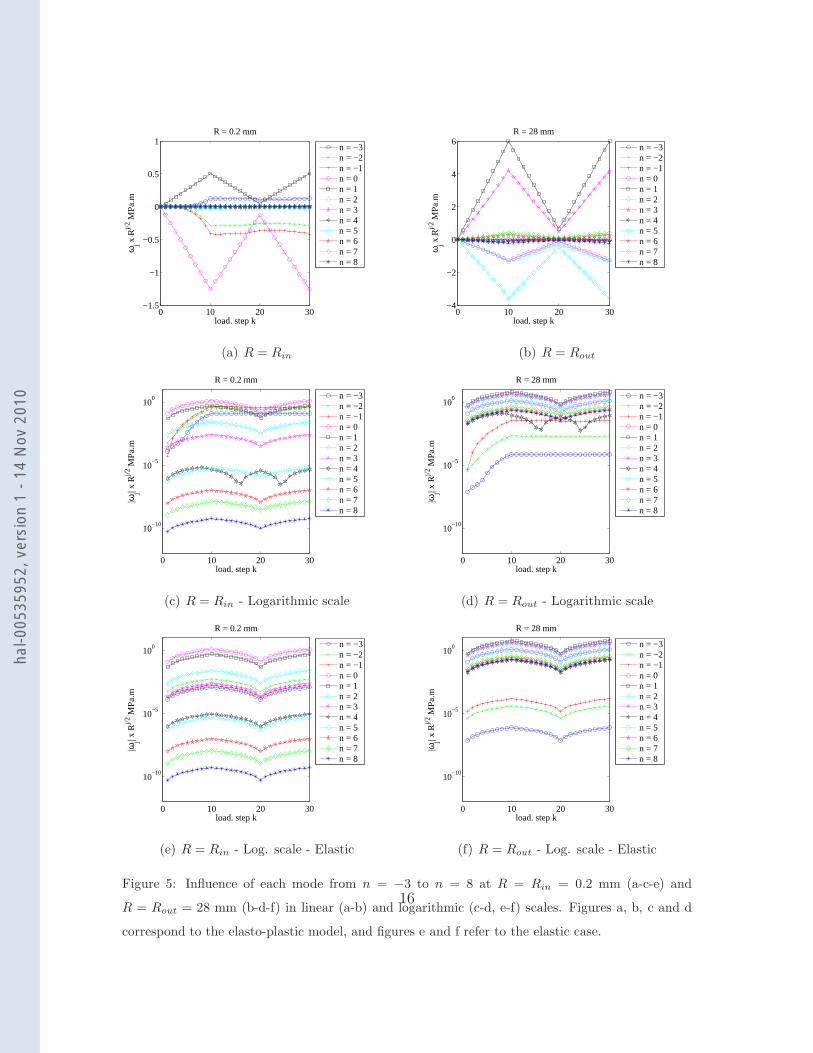
the translation (n = 0), as shown in Fig. 5a and c. The next most important contri-

butions are those from the supersingular fields, and as expected, such contributions

far from the crack tip (Fig. 5b and d) are very weak. Besides, their non-proportional

change along the loading history (Fig. 5c and d) proves that they are affected by

crack tip plasticity, as highlighted by the comparison with the elastic case (Fig. 5e

and f). This will be further commented in Section 4. On the contrary, all subsingular

amplitudes follow the loading history - the bump for mode n = 4 (Fig. 5c and d) is

an artifact of the logarithmic scale due to a sign reversal of ω4.

13

hal-0

0535

952,

ver

sion

1 -

14 N

ov 2

010

(a) Mesh of the whole model (1× 1 m2)

(b) View of a zone of size 40× 40 mm2

(c) Zoom on crack tip zone (radius 0.2 mm)

Figure 3: Mesh of the numerical case. One quarter is modeled (a). Detail of the mesh for the whole

crack (b) and zoom around the crack tip (c).

14

hal-0

0535

952,

ver

sion

1 -

14 N

ov 2

010

1 2 3 4 5 6 7 8 9 10 11 1228

29

30

31

32

33

34

35

36

37

N1

SIF

ω1 (

MP

a.m

0.5 )

at s

tep

k=10

N0 = −5

N0 = −4

N0 = −3

N0 = −2

N0 = −1

Figure 4: Stress intensity factor at maximum loading (k = 10) vs. maximum order N1 in Williams’

decomposition, for various minimum orders N0.

15

hal-0

0535

952,

ver

sion

1 -

14 N

ov 2

010

0 10 20 30−1.5

−1

−0.5

0

0.5

1

load. step k

ωj x

Rj/2

MP

a.m

R = 0.2 mm

n = −3n = −2n = −1n = 0n = 1n = 2n = 3n = 4n = 5n = 6n = 7n = 8

(a) R = Rin

0 10 20 30−4

−2

0

2

4

6

load. step k

ωj x

Rj/2

MP

a.m

R = 28 mm

n = −3n = −2n = −1n = 0n = 1n = 2n = 3n = 4n = 5n = 6n = 7n = 8

(b) R = Rout

0 10 20 30

10−10

10−5

100

load. step k

|ωj| x

Rj/2

MP

a.m

R = 0.2 mm

n = −3n = −2n = −1n = 0n = 1n = 2n = 3n = 4n = 5n = 6n = 7n = 8

(c) R = Rin - Logarithmic scale

0 10 20 30

10−10

10−5

100

load. step k

|ωj| x

Rj/2

MP

a.m

R = 28 mm

n = −3n = −2n = −1n = 0n = 1n = 2n = 3n = 4n = 5n = 6n = 7n = 8

(d) R = Rout - Logarithmic scale

0 10 20 30

10−10

10−5

100

load. step k

|ωj| x

Rj/2

MP

a.m

R = 0.2 mm

n = −3n = −2n = −1n = 0n = 1n = 2n = 3n = 4n = 5n = 6n = 7n = 8

(e) R = Rin - Log. scale - Elastic

0 10 20 30

10−10

10−5

100

load. step k

|ωj| x

Rj/2

MP

a.m

R = 28 mm

n = −3n = −2n = −1n = 0n = 1n = 2n = 3n = 4n = 5n = 6n = 7n = 8

(f) R = Rout - Log. scale - Elastic

Figure 5: Influence of each mode from n = −3 to n = 8 at R = Rin = 0.2 mm (a-c-e) and

R = Rout = 28 mm (b-d-f) in linear (a-b) and logarithmic (c-d, e-f) scales. Figures a, b, c and d

correspond to the elasto-plastic model, and figures e and f refer to the elastic case.

16

hal-0

0535

952,

ver

sion

1 -

14 N

ov 2

010

3.2. Validity of the description at various stages of loading

A quality estimate based on the displacement residual is defined as

ε =〈‖UFEM − Ufit‖〉

σ(UFEM)(17)

where UFEM denotes the computed displacement field (it may also be the measured

one when experimental data are used), Ufit corresponds to the mode I decomposi-

tion (15), and σ the root mean square value of UFEM. The denominator is chosen to

make the error estimator dimensionless. Let us also note that this quality estimate is

based on a uniform measure over all nodes of the finite element computation, and not

a weight proportional to the element area. Because of the mesh refinement close to

the crack tip, this quality measure is strongly weighted by the crack tip. Moreover,

other error measures could have been chosen. In particular, measures with a mecha-

nical content are an alternative (e.g., based on constitutive equation gap [23, 24, 25]).

They are not considered since the identification procedure developed herein aims at

using full field displacement measurements. The latter information is the raw data to

be processed. Fig. 6 shows that the residual error remains always less than 6 × 10−3

so that the global quality of the analysis is deemed satisfactory. The highest level of

error is reached at maximum unloading (k = 20), when the discrepancy between the

plastic displacement UFEM and the elasticity-based projection Ufit is maximum. For

the maximum load (k = 10 or k = 30), error ε ≤ 10−3 and hence, the process zone

influence is well captured by this approach.

From the finite element simulation, the field of cumulative plastic strain is deter-

mined. The latter is comparable for the maximum load levels (k = 10 or k = 30).

Fig. 7 shows the equivalent strain field for k = 30. The plastic strain is confined

to a rather small neighborhood of the crack tip. A disk of radius 0.5 mm cuts out

most of the plastic strain. In the present analysis, a smaller disk was chosen (i.e.,

17

hal-0

0535

952,

ver

sion

1 -

14 N

ov 2

010

0 5 10 15 20 25 300

1

2

3

4

5

6x 10

−3

load. step k

ε

Figure 6: Dimensionless residual error change for the entire loading history. The error peaks at

maximum unloading (k = 20), but still remains below 6 × 10−3.

Rin = 0.2 mm), which still leaves in the analyzed domain some significant plastic

deformation.

x (mm)

y (m

m)

Cumulative plastic strain at k= 30

−0.5 0 0.50

0.2

0.4

0.6

0.8

1

0.02

0.04

0.06

0.08

0.1

0.12

Figure 7: Map of equivalent cumulative plastic strain at the end of the reloading cycle (k = 30).

A detailed comparison of the displacement components Ux and Uy are shown in

18

hal-0

0535

952,

ver

sion

1 -

14 N

ov 2

010

Fig. 8 and 9, respectively. On the left, finite element results are shown, and on the

right the fit of the data with 12 fields. Moreover each figure presents a wide map

(20×20 mm2), and two close-up views in the vicinity of the crack tip (4×2 mm2 and

1 × 1 mm2). The difference between FEM and fitted displacement components in

the close neighborhood of the crack tip is plotted in Fig. 10. The maximum relative

errors for both components are located near the crack tip (where plastic deformation

takes place) and are approximately equal to 30%. Yet, purely elastic fields still fit

the displacement data very accurately.

The amplitude ω1 corresponds to the mode I stress intensity factor. Its change

along the loading history is shown in Fig. 11a and compared (Fig. 11b) to the tabu-

lated values KthI resulting from an LEFM assumption [26]

KthI = Σ

√πa(1.0 + 0.128a/b− 0.288(a/b)2 + 1.523(a/b)3) (18)

Fig. 11b also shows the relative error of the SIF estimated from the J-integral

KI =

√

EJ

1− ν2(19)

with respect to the tabulated values KthI . The J-integral is computed with ABAQUS

on a quadrangular mesh, on a domain containing the crack tip and spreading over a

distance of approximately 1.3 mm from it.

The amplitude ω1 follows strictly the change of the stress on the edge of the

sample and deviates very slightly from the reference value, as if the material were

purely elastic. The ratio of KI over the applied stress Σ is not constant, but varies

only slightly in the range [0.176, 0.200] along the entire loading history. Furthermore,

the tangent SIF, dKI/dΣ, remains almost constant, with a maximum deviation of

6.2% as compared with its first value (Fig. 12).

19

hal-0

0535

952,

ver

sion

1 -

14 N

ov 2

010

x (mm)

y (m

m)

Ux measured (mm)

−10 −5 0 5 100

2

4

6

8

10

−10

−8

−6

−4

−2

0x 10

−3

(a)

x (mm)

y (m

m)

Ux fitted (mm)

−10 −5 0 5 100

2

4

6

8

10

−10

−8

−6

−4

−2

0x 10

−3

(b)

x (mm)

y (m

m)

Ux measured (mm)

−2 −1 0 1 20

0.5

1

1.5

2

−10

−9

−8

−7

−6

−5

−4

−3

−2

−1

x 10−3

(c)

x (mm)

y (m

m)

Ux fitted (mm)

−2 −1 0 1 20

0.5

1

1.5

2

−10

−9

−8

−7

−6

−5

−4

−3

−2

−1

x 10−3

(d)

x (mm)

y (m

m)

Ux measured (mm)

−0.5 0 0.50

0.2

0.4

0.6

0.8

1

−10

−9

−8

−7

−6

−5

−4

−3

−2

−1

x 10−3

(e)

x (mm)

y (m

m)

Ux fitted (mm)

−0.5 0 0.50

0.2

0.4

0.6

0.8

1

−10

−9

−8

−7

−6

−5

−4

−3

−2

−1

x 10−3

(f)

Figure 8: Comparison between Ux obtained as FEM results (left figures a, c and e) or fitted (right

figures b, d and f), over a 20×20 mm2 square (top a and b), close-up views of a 4×2 mm2 rectangle

(middle c and d) and a 1× 1 mm2 square (bottom e and f) at the end of the entire loading history

k = 30.

20

hal-0

0535

952,

ver

sion

1 -

14 N

ov 2

010

x (mm)

y (m

m)

Uy measured (mm)

−10 −5 0 5 100

2

4

6

8

10

0

0.005

0.01

0.015

0.02

(a)

x (mm)

y (m

m)

Uy fitted (mm)

−10 −5 0 5 100

2

4

6

8

10

0

0.005

0.01

0.015

0.02

(b)

x (mm)

y (m

m)

Uy measured (mm)

−2 −1 0 1 20

0.5

1

1.5

2

0

2

4

6

8

10

12

14

x 10−3

(c)

x (mm)

y (m

m)

Uy fitted (mm)

−2 −1 0 1 20

0.5

1

1.5

2

0

2

4

6

8

10

12

14

x 10−3

(d)

x (mm)

y (m

m)

Uy measured (mm)

−0.5 0 0.50

0.2

0.4

0.6

0.8

1

0

2

4

6

8

10

x 10−3

(e)

x (mm)

y (m

m)

Uy fitted (mm)

−0.5 0 0.50

0.2

0.4

0.6

0.8

1

0

2

4

6

8

10

x 10−3

(f)

Figure 9: Comparison between Uy obtained as FEM results (left figures a, c and e) or fitted (right

figures b, d and f), over a 20×20 mm2 square (top a and b), close-up views of a 4×2 mm2 rectangle

(middle c and d) and a 1× 1 mm2 square (bottom e and f) at the end of the entire loading history

k = 30.

21

hal-0

0535

952,

ver

sion

1 -

14 N

ov 2

010

x (mm)

y (m

m)

|Ux measured − U

x fitted| (mm)

−0.5 0 0.50

0.2

0.4

0.6

0.8

1

0

0.5

1

1.5

2

x 10−3

(a)

x (mm)

y (m

m)

|Uy measured − U

y fitted| (mm)

−0.5 0 0.50

0.2

0.4

0.6

0.8

1

0

0.2

0.4

0.6

0.8

1

1.2

1.4

1.6

1.8

x 10−3

(b)

Figure 10: Difference between measured and fitted Ux (a) and Uy (b) over a 1×1 mm2 square at

the end of the entire loading history k = 30. The maximum relative errors with respect to the FE

computation are approximately 30% for both components.

0 5 10 15 20 25 300

5

10

15

20

25

30

35

40

load. step k

ω1 M

Pa.

m1/2

(a) SIF KI (=ω1)

0 5 10 15 20 25 30−5

0

5

10

15

20

load. step k

Rel

ativ

e er

ror

to th

eore

tical

SIF

(%

)

KI = ω

1

Computed from J−integral

(b) Relative error

Figure 11: Change of the SIF KI = ω1 as a function of loading step k (a) and error relative to the

tabulated value of KI (b). The relative error is compared to that of the SIF estimated from the

J-integral computed with ABAQUS.

22

hal-0

0535

952,

ver

sion

1 -

14 N

ov 2

010

0 5 10 15 20 25 30

1

1.02

1.04

1.06

1.08

1.1

load. step k

Adi

men

sion

ed

dω1/d

Σ

Figure 12: Tangent SIF (normalized by its value at k = 1) vs. loading step k.

23

hal-0

0535

952,

ver

sion

1 -

14 N

ov 2

010

4. Cyclic loading: Macroscopic characterization

The identification of the entire sequence of 30 loading steps is now commented.

As earlier mentioned, subsingular and supersingular fields have to be distinguished.

Subsingular fields essentially reflect the loading history. Since the associated stress

increases with the distance to the crack tip, the amplitude of these fields is mainly

dictated by the far-field boundary conditions, and hence they do follow the loading

history (Fig. 5).

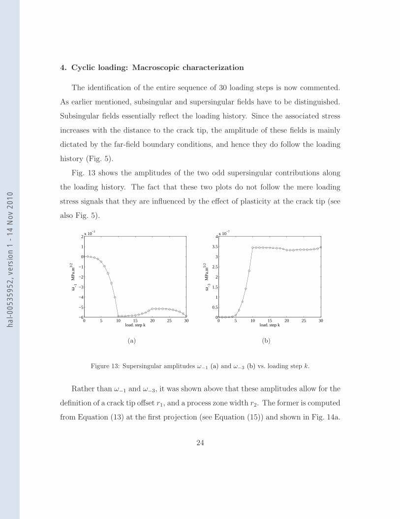
Fig. 13 shows the amplitudes of the two odd supersingular contributions along

the loading history. The fact that these two plots do not follow the mere loading

stress signals that they are influenced by the effect of plasticity at the crack tip (see

also Fig. 5).

0 5 10 15 20 25 30−6

−5

−4

−3

−2

−1

0

1

2x 10

−3

load. step k

ω−

1 M

Pa.

m3/2

(a)

0 5 10 15 20 25 300

0.5

1

1.5

2

2.5

3

3.5

4x 10

−7

load. step k

ω−

3 M

Pa.

m5/2

(b)

Figure 13: Supersingular amplitudes ω−1 (a) and ω

−3 (b) vs. loading step k.

Rather than ω−1 and ω−3, it was shown above that these amplitudes allow for the

definition of a crack tip offset r1, and a process zone width r2. The former is computed

from Equation (13) at the first projection (see Equation (15)) and shown in Fig. 14a.

24

hal-0

0535

952,

ver

sion

1 -

14 N

ov 2

010

The process zone width r2 is defined once the crack tip has been moved. Fig. 14b

shows several computations of r2 versus loading step, corresponding to successive

projections aiming at canceling out ω−1. At iteration (k + 1), the projection of

the displacement field (see Equation (15)) is achieved with the corrected crack tip

position z0 + r1, where r1 is computed with Equation (13) at iteration (k). The

process zone width change is close to that from the first identification, except for the

values around the maximum unloading k = 20.

0 5 10 15 20 25 30−1

−0.5

0

0.5

1

1.5

2

2.5

3

load. step k

r 1 (m

m)

(a)

0 5 10 15 20 25 300

0.2

0.4

0.6

0.8

1

load. step k

r 2 (m

m)

Ncorr

= 0

Ncorr

= 1

Ncorr

= 2

Ncorr

= 3

Ncorr

= 5

(b)

Figure 14: Change with loading step k of (a) the crack tip offset, (b) the process zone width at first

projection (Ncorr = 0) and after successive corrections of crack tip location (Ncorr > 0).

It is interesting to relate either the supersingular amplitudes or the correspond-

ing length scales as functions of the SIF ω1, as shown respectively in Fig. 15 and

16. In the former, the supersingular amplitudes ω−1 and ω−3 follow a dependence

with ω1 reminiscent of a quasi-ideal elasto-plastic behavior. The formation of the

plastic zone during the first loading stage is characterized by a strong increase in

the supersingular amplitudes. During unloading, these amplitudes remain almost

constant, and virtually reversible, so that the state reached for k = 30 is very close

25

hal-0

0535

952,

ver

sion

1 -

14 N

ov 2

010

to the end of the first loading period (k = 10).

0 10 20 30 400

1

2

3

4

5

6x 10

−3

ω1 MPa.m1/2

|ω−

1| M

Pa.

m3/2

(a)

0 10 20 30 400

0.5

1

1.5

2

2.5

3

3.5

4x 10

−7

ω1 MPa.m1/2

ω−

3 M

Pa.

m5/2

(b)

Figure 15: Supersingular amplitudes |ω−1| (a) and ω

−3 (b) vs. SIF ω1.

0 10 20 30 40−1

−0.5

0

0.5

1

1.5

2

2.5

3

ω1 MPa.m1/2

r 1 (m

m)

(a)

0 10 20 30 400

0.1

0.2

0.3

0.4

0.5

0.6

0.7

0.8

ω1 MPa.m1/2

r 2 (m

m)

(b)

Figure 16: Crack tip offset r1 (a) and process zone size r2 (b) (after correction of crack tip location)

vs. SIF ω1.

26

hal-0

0535

952,

ver

sion

1 -

14 N

ov 2

010

5. Cyclic loading: Interpretation

An interesting observation leading to a simplified picture of the mechanics at play

is to consider the tangent SIF, dKI/dΣ, where the finite difference between loading

steps is considered instead of the derivative. In Fig. 12, this quantity is further

normalized to its first value, where plasticity is essentially negligible. It is observed

that at load reversal the incremental behavior is essentially elastic. However as

loading or unloading proceed, a small but significant deviation from unity is observed.

Thus plasticity takes place upon unloading and the small hysteresis observed, e.g.,

in Fig. 15, during unloading and reloading is not an identification artifact.

In this section, a simple interpretation of the previous observations is proposed.

To proceed, the problem is simplified and an elastic-perfectly plastic behavior is

assumed (the absence of hardening is a simplification as compared to the chosen

constitutive law for the previous simulation, even though the hardening modulus

was very small as compared to the Young’s modulus).

5.1. Loading

Let us assume that the problem has been solved for a given stress level Σref .

Outside the plastic process zone, the elastic field is assumed to be characterized by

amplitudes ωrefn for fields Ωn. From the latter, it is easy to deduce the solution

to the problem for an arbitrary level Σ of a monotonic loading. The SIF, or ω1,

is proportional to the load level. However, what will dictate the extension of the

process zone is the yield stress. Since no other scale is specified, the plastic radius is

used to rescale all distances, and match the reference case. From this argument, the

plastic radius scales as

ρp ∼(ωref

1 )2

(Σref)2Σ2

σ2y

(20)

27

hal-0

0535

952,

ver

sion

1 -

14 N

ov 2

010

All amplitudes are further related

ωn ∝ σyρ1−n/2p ∝ σy

(

ω1

σy

)2−n

(21)

Thus amplitudes ωn are linked with ω1 through

ωn ∝ ω2−n1 (22)

The crack tip offset r1 = −2ω−1/ω1 is thus expected to scale as

r1 ∝ ω21 ∝ ρp (23)

The next supersingular amplitude, ω−3, scales as

ω−3 ∝ ω51 (24)

so that the size of the process zone r2 also scales as r1 or ρp. Fig. 17 probes the

proportionality of ω1/3−1 and ω

1/5−3 with ω1. A linear behavior is observed, especially

for the first supersingular amplitude.

5.2. Unloading

At the end of the loading stage, a developed plastic zone has been created where

von Mises’ stress has reached the yield stress. Upon unloading, it is expected that,

incrementally, the usual singular crack field is to be subtracted to the stress state.

However, this would produce a diverging stress at the crack tip that will induce re-

verse plastic flow. Thus the incremental displacement field is rather the one observed

during the loading stage, but since one started with a stress field that was the yield

limit, the effective yield stress that is seen is in fact twice as large [27]. The previous

results are used to relate the decrease of amplitude ∆ωn versus the decrease of stress

intensity factor

∆ωn ∝ 2σy

(

∆ω1

2σy

)2−n

(25)

28

hal-0

0535

952,

ver

sion

1 -

14 N

ov 2

010

0 10 20 30 400

0.05

0.1

0.15

0.2

ω1 MPa.m1/2

|ω−

1|1/3 (

MP

a.m

3/2 )1/

3

(a)

0 10 20 30 400

0.01

0.02

0.03

0.04

0.05

0.06

ω1 MPa.m1/2

ω−

31/

5 (M

Pa.

m5/

2 )1/5

(b)

Figure 17: Supersingular amplitudes |ω−1| (a) and ω

−3 (b) raised to the expected power (resp. 1/3

and 1/5) vs. SIF, for the first loading stage.

To avoid the dependence of the above quantity with the yield stress, let us introduce

the supersingular amplitudes at the maximum load, with a superscript ∗

∆ωn

ω∗n

= 2n−1

(

∆ω1

ω∗

1

)2−n

(26)

This result predicts a simple universal unloading characteristics, close to Masing’s

rule [28] in plasticity.

5.3. Reloading

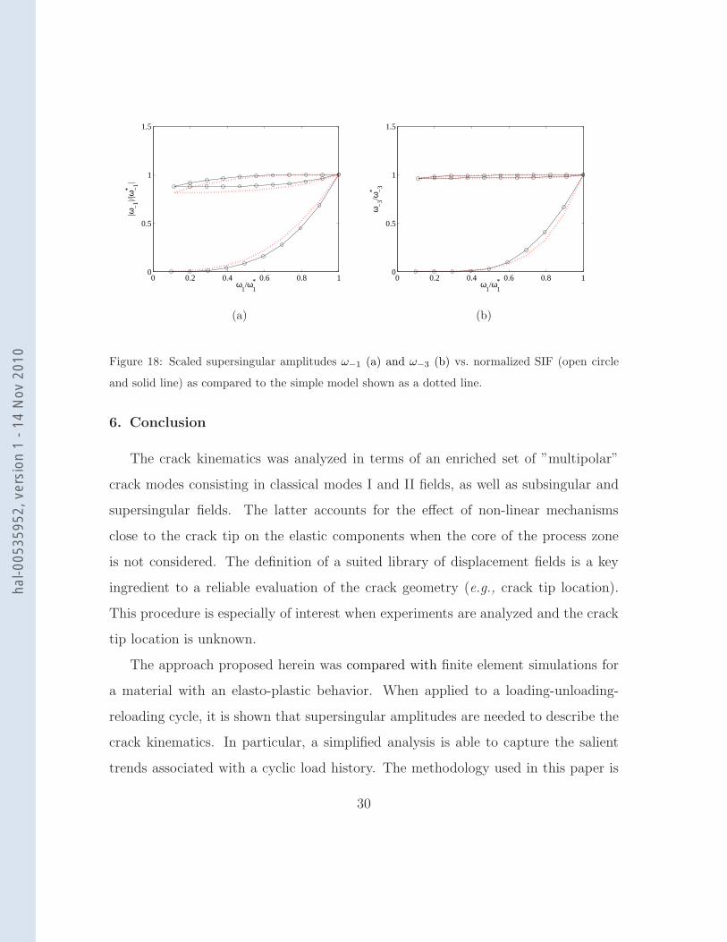
During the reloading stage, the same incremental law is used (provided no other

intermediate radius reaches the yield stress). Fig. 18 shows a comparison between

the observed normalized amplitudes ω−1 and ω−3 and the proposed model. Some

differences are observed, but still the main features are captured.

29

hal-0

0535

952,

ver

sion

1 -

14 N

ov 2

010

0 0.2 0.4 0.6 0.8 10

0.5

1

1.5

ω1/ω

1*

|ω−

1|/|ω

−1

*|

(a)

0 0.2 0.4 0.6 0.8 10

0.5

1

1.5

ω1/ω

1*

ω−

3/ω−

3*

(b)

Figure 18: Scaled supersingular amplitudes ω−1 (a) and ω

−3 (b) vs. normalized SIF (open circle

and solid line) as compared to the simple model shown as a dotted line.

6. Conclusion

The crack kinematics was analyzed in terms of an enriched set of ”multipolar”

crack modes consisting in classical modes I and II fields, as well as subsingular and

supersingular fields. The latter accounts for the effect of non-linear mechanisms

close to the crack tip on the elastic components when the core of the process zone

is not considered. The definition of a suited library of displacement fields is a key

ingredient to a reliable evaluation of the crack geometry (e.g., crack tip location).

This procedure is especially of interest when experiments are analyzed and the crack

tip location is unknown.

The approach proposed herein was compared with finite element simulations for

a material with an elasto-plastic behavior. When applied to a loading-unloading-

reloading cycle, it is shown that supersingular amplitudes are needed to describe the

crack kinematics. In particular, a simplified analysis is able to capture the salient

trends associated with a cyclic load history. The methodology used in this paper is

30

hal-0

0535

952,

ver

sion

1 -

14 N

ov 2

010

directly applicable to a broad class of different materials (brittle to ductile) and test

geometries for which the process zone is small as compared to the region of interest.

This type of analysis may also be used in experiments. Two routes can be fol-

lowed. First, an a posteriori analysis of the measured displacement field similar to

the one carried out herein, where the measured field is used instead of the computed

one. Another one, referred to as an integrated analysis [11], considers the library of

displacement fields Ωn and Υn and performing, for instance, digital image correla-

tion to identify directly the unknown components ωn and υn. It corresponds to yet

another way of using the concept of “diffuse stress gauging” [29, 30]. By using an

integrated approach, the support of the gauge is diffuse on the sample face. In that

sense, it is a “crack gauge” that measures, for instance, stress intensity factors, but

also crack tip location and a first characterization of confined non-linearity.

It is of interest to extend the present analysis to more complex loading conditions

to address, for instance, mixed mode crack loading, or the initial stage of fatigue

where plastic yielding is more developed. Investigating three dimensional fatigue

cracks using X-ray tomography constitutes also a very challenging direction for future

investigation [31, 32].

Acknowledgments

This work was funded by the French National Agency for Research (ANR) through

the project RUPXCUBE (ANR-09-BLAN-0009-01 grant): “ Three-dimensional iden-

tification of local crack propagation laws with X-ray tomography, full-field measure-

ments and extended finite element simulations.”

[1] S. M. Spearing and A. G. Evans, The role of fiber bridging in the delamination

resistance of fiber-reinforced composites, Acta Metall. Mater. 40 [9] (1992) 2191-

2199.

31

hal-0

0535

952,

ver

sion

1 -

14 N

ov 2

010

[2] B. Budiansky, J. W. Hutchinson and A. G. Evans, Matrix fracture in fiber-

reinforced ceramics, J. Mech. Phys. Solids 34 [2] (1986) 167-189.

[3] Z. P. Bazant, Size effect in blunt fracture: concrete, rock, metal, J. Engrg Mech.

ASCE 110 (1984) 518-535.

[4] J. W. Hutchinson, Singular behavior at the end of a tensile crack in a hardening

material, J. Mech. Phys. Solids 16 (1968) 18-31.

[5] J. W. Hutchinson, Plastic stress and strain fields at a crack tip, J. Mech. Phys.

Solids 16 (1968) 337-347.

[6] J. R. Rice and G. F. Rosengren, Plane strain deformation near a crack tip in a

power-law hardening material, J. Mech. Phys. Solids 16 (1968) 1-12.

[7] G. R. Irwin, Analysis of the stresses and strains near the end of a crack traversing

a plate, ASME J. Appl. Mech. 24 (1957) 361-364.

[8] P. K. Rastogi, edts., Photomechanics, (Springer, Berlin (Germany), 2000), 77.

[9] S. R. McNeill, W. H. Peters and M. A. Sutton, Estimation of stress intensity

factor by digital image correlation, Eng. Fract. Mech. 28 [1] (1987) 101-112.

[10] J. Rethore, A. Gravouil, F. Morestin and A. Combescure, Estimation of mixed-

mode stress intensity factors using digital image correlation and an interaction

integral, Int. J. Fract. 132 (2005) 65-79.

[11] F. Hild and S. Roux, Measuring stress intensity factors with a camera: Inte-

grated Digital Image Correlation (I-DIC), C.R. Mecanique 334 (2006) 8-12.

[12] D. S. Dawicke and M. S. Sutton, CTOA and crack-tunneling measurements in

thin sheet 2024-T3 aluminum alloy, Exp. Mech. 34 (1994) 357-368.

32

hal-0

0535

952,

ver

sion

1 -

14 N

ov 2

010

[13] M. A. Sutton, W. Zhao, S. R. McNeill, J. D. Helm, R. S. Piascik and W. T. Rid-

del, Local crack closure measurements: Development of a measurement system

using computer vision and a far-field microscope, in: Advances in fatigue crack

closure measurement and analysis: second volume, STP 1343 , R. C. McClung

and J. Newman, J.C., eds., (ASTM, 1999), 145-156.

[14] P. Forquin, L. Rota, Y. Charles and F. Hild, A method to determine the tough-

ness scatter of brittle materials, Int. J. Fract. 125 [1] (2004) 171-187.

[15] F. Ma, M. A. Sutton and X. Deng, Plane strain mixed mode crack-tip stress

fields characterized by a triaxial stress parameter and a plastic deformation

extent based characteristic length, J. Mech. Phys. Solids 49 (2001) 2921-2953.

[16] Z.-Z. Du and J. W. Hancock, The effect of non-singular stresses on crack-tip

constraint, J. Mech. Phys. Solids 39 [4] (1991) 555-567.

[17] S. Pommier and R. Hamam, Incremental model for fatigue crack growth based

on a displacement partitioning hypothesis of mode I elastic-plastic displacement

fields, Fat. Fract. Engrg. Mater. Struct. 30 [7] (2007) 582-598.

[18] M. F. Kanninen and C. H. Popelar, Advanced fracture mechanics , (Oxford Uni-

versity Press, 1985).

[19] N. I. Muskhelishvili, Some basic problems of the mathematical theory of elasti-

city , (P. Noordholl Ltd, Groningen (Holland), 1953).

[20] M. L. Williams, On the stress distribution at the base of a stationary crack,

ASME J. Appl. Mech. 24 (1957) 109-114.

33

hal-0

0535

952,

ver

sion

1 -

14 N

ov 2

010

[21] R. E. Raab and O. L. de Lange, Multipole theory in electromagnetism: classical,

quantum, and symmetry aspects, with applications, (Oxford University Press,

2004).

[22] http://www.simulia.com/products/abaqus standard.html

[23] P. Ladeveze, Comparaison de modeles de milieux continus , (these d’Etat, Uni-

versite Paris 6, 1975).

[24] R. V. Kohn and B. D. Lowe, A variational method for parameter identification,

Math. Mod. Num. Ana. 22 [1] (1988) 119-158.

[25] G. Geymonat, F. Hild and S. Pagano, Identification of elastic parameters by

displacement field measurement, C. R. Mecanique 330 (2002) 403-408.

[26] G. C. Sih, Handbook of stress-intensity factors: Stress-intensity factor solutions

and formulas for reference, Bethlehem, Pa (USA), Lehigh University (1973), 815

p.

[27] J. R. Rice, Mechanics of crack tip deformation and extension by fatigue, Procee-

dings Fatigue crack propagation, STP 415 , (ASTM, Philadelphia (USA), 1967),

247-309.

[28] G. Masing, Eigenspannungen und Vertfestigung beim Messing, Proceedings of

the Second International Congress of Applied Mechanics, Zurich, Switzerland

(1926) 332a5 [in German].

[29] S. Roux, F. Hild and S. Pagano, A stress scale in full-field identification proce-

dures: a diffuse stress gauge, Eur. J. Mech. A/Solids 24 (2005) 442-451.

34

hal-0

0535

952,

ver

sion

1 -

14 N

ov 2

010

[30] F. Hild and S. Roux, Digital image correlation: from measurement to identifi-

cation of elastic properties - A review, Strain 42 (2006) 69-80.

[31] N. Limodin, J. Rethore, J.-Y. Buffiere, A. Gravouil, F. Hild and S. Roux, Crack

closure and stress intensity factor measurements in nodular graphite cast iron

using three-dimensional correlation of laboratory X-ray microtomography ima-

ges, Acta Mater. 57 [14] (2009) 4090-4101.

[32] N. Limodin, J. Rethore, J.-Y. Buffiere, F. Hild, S. Roux, W. Ludwig, J. Rannou

and A. Gravouil, Influence of closure on the propagation of fatigue cracks in a

nodular cast iron investigated by X-ray tomography and 3D Volume Correlation,

Acta Mater. 58 [8] (2010) 2957-2967.

35

hal-0

0535

952,

ver

sion

1 -

14 N

ov 2

010