i B U L L E T I N of the International Association of ENGINEERING GEOLOGY Paris - No 49 - Avril 1 9 9 4 de i'Association Internationale de GI~OLOGIE DE L'INGENIEUR I

M O D E L L I N G DEBRIS FLOWS AS K I N E M A T I C W A V E S

M O D ~ 2 L E M A T H E M A T I Q U E D E L A D Y N A M I Q U E D E S L A V E S T O R R E N T I E L L E S , B A S E S U R L A T H t ~ O R I E D E L ' O N D E C I N I ~ M A T I Q U E

M. A R A T T A N O * , W.Z. S A V A G E * *

Abstract

We present a mathematical model f~)r movement of debris tlows, based on kinematic wave theory, and apply our model to published data from two debris flows that occurred in 198i on Mount St. Helens, Washington, U.S.A. The model, which is based on a relationship originally developed for water flow in open channels, shows good agreement with the field data.

Rdsumd

Un modble mathdmatique est prdsentd, qui concerne la dynamique des <, laves torrentielles ,,, base sur la thdorie de I'onde cindmatique. Le mod/zle est applique aux donndes publiEes se rapportant 5. deux phdnom,Snes de laves torrentielles qui ne sont produits en 1981 sur le Mont St. Helens, Etat de Washington, aux Etats-Unis. Le module, qui est base sur une dquation d,Svelopp~e ~ l'origine pour le flux d'eau en canal ouvert, laisse appara~tre une bonne correspondance avec los donndes expdrimentales.

Introduction

Debris f lows are highly concentra ted dispersions of poorly sorted sediment ( f rom clay- to boulder-s ized par- ticles) in water that c o m m o n l y move at very high speeds and have great dest ruct ive power (Pierson, 1986; Takahashi, t978). Debris f lows general ly appear as waves (surges) that have steep fronts consis t ing mostly of boulders that can be surprisingly large (Johnson, 1.970). Behind the bouldery front the number of boulders gradual ly decreases and the surge is charged with pebble-s ized f ragments and then more and more diluted until it appears as muddy water (Johnson, 1970; Costa and Wil l iams, 1984).

Debris f lows have been modeled using Bagnold ' s (1954) dilatant fluid concept (Takahashi. 1978, 1980) or as B ingham (1922) plastic fluids (Yano and Daido, 1965; Johnson, 1970; Rodine and Johnson, 1976). Chen (1987, 1988) as part of a review of Japanese concepts for mod- el ing debris f lows formula ted a genera l ized viscoplas t ic f luid model for debris flows.

Debris f lows have also been successful ly descr ibed by models or iginal ly deve loped to s imulate surface water f lows (Laenen and Hansen, 1988). Water f low models generate useful informat ion about the possible evolu t ion of debris f lows and al low compar ison between water- f low behavior and the flow behavior of debris.

Little is known about the details of init iation of debris flows. For example , debris f lows can be t r iggered by volcanic eruptions, by landsl ides, or by failure of natural dams (Pierson, 1986). In some cases it has been possible to reconstruct the condi t ions for debr is- f low initiation and to find a close analogy with dam-break phenomena (Gal lono and Pierson, 1984). This, of course, is partic- ularly true if a debris f low initiates during failure of a natural darn.

Dam-break phenomena have been analyzed using kine- matic wave theory (Hunt, 1982). Kinemat ic waves are a dis t inct ive type of wave mot ion arising in one-d imen- sional f low problems with wave properties that fo l low direct ly from the cont inui ty eqaution. Kinemat ic wave motion is dist inct f rom class ical wave motion. Classical wave motion depends on the comple te momen tum equa- tion (and is, therefore, ca l led dynamic) ; classical waves possess at least two wave veloci t ies at each point and can move in two direct ions from their source. Kinemat ic waves possess only one wave veloci ty and move only in one direct ion (Lighthi l l and Whitham, 1955).

The kinemat ic wave model is one of a number of ap- proximat ions of the dynamic wave model, and is suit- able, in particular, to descr ibe wave propagat ion phenomena in channels having steep slopes (Henderson, 1966; Malone , 1977; Mil ler , t984). This model which i n v o l v e s n e g l e c t o f all the d e r i v a t i v e t e rms in the m o m e n t u m equat ion is known in the l i t terature as the

* C.NR. I.R.P.I., Strada delle Caccc, 73; Todno. Italy. ** U.S. Geological Sarvey; Box 25046, M.S. 966, Denver, Co 80225, U.S.A.

kinematic wave approximation. We will show that debris flows, which usually occur in steep mountain torrents, can be amenable to a kinematic wave approximation.

An important advantage of the kinematic wave approxi- mation is that it makes the equations significantly easier to solve and, as shown by Hunt (1982), allows one to obtain a closed-form solution. A closed-form solution becomes particularly useful, compared to a numerical solution, because information concerning initial condi- tions, needed for the application of numerical solutions, are rarely known for debris flows.

We will show that, regardless of the cause of initiation, the subsequent behavior of debris flows can be de- scribed by a model similar to a model developed for the movement of floodwaves resulting from a dam break. The dam-break model of Hunt (1982), based on kinematic wave theory, applies at large distances downstream from a failed dam. We modify this model, originally developed for flow in wide rectangular chan- nels, for narrow rectangular channels and those channels that have a cross sectional form that can be approxi- mated by a rectangular form. This modification allows us to account for flow in the narrow channels in which debris flows generally occur.

We also discuss analogies between our model and Weir's (1982) model for lahars. Weir (1982) used kinematic wave theory, with discharge unstead of flow height as the dependent variabte in the continuity equation. Be- cause Weir's model can be used only if discharge is known, it cannot be applied to situations in which only flow height is known. Weir's (1982) model was used by Pierson and others (1990) to reconstruct the propa- gation of the catastrophic lahars triggered by the Nevado del Ruiz, Colombia, eruption of 13 November 1985.

We apply our model to data collected on 1 October 1981, from two gaging stations along a reach of a stream channel on Mount St. Helens (Pierson, 1986). The model shows very good agreement with some of the observed data.

T h e m a t h e m a t i c a l m o d e l

One-dimensional, unsteady flow in a rectangular chan- nel having a fixed slope is described by the momentum equation,

3u 3u 3h (I) u ~x + -Or +g ~x = g i - g i r

and the continuity equation (Abbott, t966),

Oh Oh 3-" = 0 (2) 0-7 + u + h a x

In these equations t is time, g is the gravitational ac- celeration constant, u is velocity, x is distance along the channel, i is channel slope, h is flow height, and if is the bed resistance term.

Equations (1) and (2) are derived for an infinitesimal element of fluid of unit width. The first two terms in equation (1) represent the acceleration over the element, and the third term represents the potential gradient over

4

the element. The first term in equation (2) represents the accumulation within an element and the last two terms the net inflow into the element. Dimensionless variables are introduced in the following in order to pat equation (1) into a form involving quantities that can be neglected. The dimensionless spatial variables are.

h (3a) h , = ....

H"

and x (3b) L'

I t (3c) /" ~ -LT'

where L is a typicaI length. H is a typical flow height, and i is the channel slope. The other dimensionless vari- ables introduced are

u (4a)

and Ut (4b)

l.. -- ~ - ,

where U is a typical velocity in the flow.

Using the dimensionless variables the momentum and continuity equations become

U:ru.~U. Ou.] t t 3h. . . (5)

7L Z : - - - ' - ' / dx,

and

Oh. 3u. Oh. (6) at. + h" G-2 + u" 0.-Z = ~

U2 From equation (3c) the term ~ can also be written as

iU 2- gH" The term ~ . which is the square of the Froude

number, Fr, is a measure of the relative importance of kinetic and potential energy in the flow.

In linematic wave theory it is assumed that the product of the Froude number and the acceleration terms and the product of the ratio H/L and the flow height gradient term (the pressure term) in equation (5) are negligible when compared to the slope term. This can occur in steeply sloping channels if the wave is flat and accel- erations are small. Then. provided that the Froude num- ber is not too large (Fr < 2), the derivative terms in the momentum equation can be neglected compared to the terms on the right hand side of equation (5). Thus equa- tion (5) simply becomes

if = i (7)

and the flow is described by equation (6). Since debris flow waves commonly move at nearly constant veloci- ties, have long flat profiles (Takahashi, 1991, Fig. 1.4) and usually occur in steep mountain torrents, they should be amenable to the kinematic wave approxima- tion.

We use the Manning equation in the following to ex- press the velocity, u, in equation (6) as a function of flow height, h. Expressing the velocity as a function of flow height is essential to the integration of equation (6). The Manning equation is an empirical relationship that relates mean flow velocity to channel roughness, hydraulic radius and channel slope (Chow, 1959): that is,

1 ~ -' ( 8 ) u = - R ~i :

n

where u is the mean velocity of the fluid, ,7 is the rough- ness coefficient, R is the hydraulic radius, and i is the channel slope.

Hydraulic radius R is the ratio of the cross sectional area of the flow to the wetted perimeter of the channel (Rouse, 1938). for an infinitely wide rectangular chan- nel R = h. For narrow rectangular channels we propose for R the following expression

R = ah ~' (9)

where a and kt are parameters depending on the width of the channel. Since R = h for an infinitely wide rec- tangular channel, we have from equation (9) that a = I and k~ = I. For rectangular channeIs of zero width a = 0 and kl = 0. Thus, for rectangular channels that have a width between 0 and ~, a and kj range between 0 and 1. Details for calculating a and kt for rectangular channels of intermediate widths are given in Arattano and Savage (1992). Because almost any cross sectional channel form that has no abrupt changes in shape can be approximated as a rectangle, the theory has general applicability.

Substituting equation (9) in equation (8) gives the Man- ning equation in terms of flow height as

-' (tO) u = Ch~i : ,

1 2 where C = a - and k = kl Equation (I0) in dimen-

n 3 " sionless terms is

u, = h< (1 la)

Differentiating equation (1 l a) with respect to x, we ob- tain

Ou Z = kh{_ t Oh. (1 ib) Ox, Ox,

When equation ( l i b ) is substituted into the second term

in equation (6), h.-a-~,' it becomes

Oh. (12a) C~.:,2. "

Expression (12a) can be simplified by substituting equa- tion ( l l a ) to give

Oh. Oh. 12b) khk* 3 Z = ku, Ox-?

When equation (12b) is substituted in the contmuity equation (equation 6) it becomes

Oh, Oh, (13) -js + (k + 1) , , ~-~-. = 0.

Equation (13) in dimensional form is

0h Oh O-r + (k + 1) u ~ = O.

(i4)

Equation (14), which is obtained by using the simple relationship between velocity and flow height given as equation (I0), is a single first-order, partial differential equation governing the propagatbn of perturbations in flow height. In the next section we will use equation (14) as the governing equation for modeling debris t'lows as kinematic waves.

K i n e m a t i c wave m o d e l fo r d e b r i s f lows

A possible condition /'or debris flow initiation is sketched in Fig, 1. The debris mass from which the de- bris flow develops is represented to be like a water mass behind a dam before collapse.

Because flow velocity depends directly on flow height, the portion of the initial mass having greatest height will tend to move towards the front resulting in a change of the wave form. Thus, far from the point of inception, information concerning the initial configuration are lost and hence the choice of initial conditions concerning the form of the original debris mass is somewhat arbi- trary.

We also show in Fig. I the meaning of the parameters H and L that are used in what follows. The maximum initial (undisturbed) height of debris in the channel is H. The parameter H is analogous to the water height immediately behind an unbreached dam. The initial un- disturbed length of the debris mass in the channel is L The parameter L is analogous to the reservoir length be- hind an unbreached dam. Kinematic wave theory re- quires the wave profile to change little with distance downslope so that the pressure term will be small. This is not the case initially if we model the beginning shape of the debris mass as a water mass behind a clam (Fig. 1). However, in his kinematic wave analysis of the dam-break problem, Hunt (1982) shows that, if G r 2, his solution applies after the floodwave front has traveled a distance of 5.2 times the length of the original dammed reservoir, in fact, after the wave has traveled that distance, it has spread to the point that the neglected terms in equation (5) are less than 10 percent of the channel slope term.

Since a constant channel slope is assumed, the H and L parameters are linked by the relation

H (15) i -

k '

which was given earlier as equation (3c).

Referring fo Fig. 1, we see that the flow height h(x , t ) in equation (14) ts subject to the initial conditions,

H (t6a) h ( x , 0 ) = ~ x for 0 < x < L

O E

.B ID

"13

c

:I:: O

o

o o O

I

I

-'e g

c~

A

c5 A

-h-

E O

o

i!

c5 II

e..- x

O

/ " ' -4

~'ig. 1 : Sketch of some possible initial condi t ions for debr i s - f low init iat ion and their m o d e l i n g with k i n e m a t i c wave theory.

and

h(x,O) = O ]'or oo < x <0 and L < x <+oo. (16b)

Equation (16a) gives the initial height of the undisturbed debris mass in the channel, which has a length L. For x less than zero and for x greater than L the debris height is initially zero (equation 16b).

The theory predicts that any kinematic wave profile ad- vances with the front face becoming continually steeper. With the continuous steepening of the wave front a kine- matic shock develops. This shock is a region in front of the flow in which terms neglected in the momentum equation become imporant and the governing equations break down (Lighthill and Whitham, 1955). We will defer further discussion of the nature of the shock front at this point and here simply require x.~(t), the location of the shock front region, to move with the speed of the fluid immediately behind the shock; that is,

dxs(0 (17) - u ( . v , ( 0 . t ) ,

dt

where

xs (0) = L (18)

Equation (18) is the initial condition for differential equation (17).

Equations (10) and (14) and conditions (16). (17), and (18) can be written in nondimensional form as

u , = h~/, (19)

Oh, h, ~ Oh. (20) at, + ( k + 1) ~.OC~r = 0 .

where

h,(x,,0) =x. for 0 < x. _< 1

h,(x,,O) = 0 for oo < x, < 0 and 1 < x. < +~,(21)

and

dx..~(t.) = h~(x.s(t.),t.), (22) dt,

where

X,~(0) = 1. (23)

Solving equation (20) by the method of characteristics (Abbott, 1966) we find that

dh. (24) - 0

dt.

along characteristic curves that have the slope given by

@- = (k+l)hi. (25) dt,

Equations (24) and (25) are both ordinary differential equations that are integrated to give

h, = C1 (26)

along the characteristic curves given by

x.-(k+ 1)hk/t. = Ca. (27)

Here C~ and C2 are constants of integration and k is constant along the channel. Note that k, which depends on the cross sectional form of the channel, is constant because no abrupt change in cross sectional form is as- sumed for the flow.

Using the initial condition (21). we can calculate the integration constant for any characteristic curve. In the ( x , , t . ) plane (Fig. 2) a charactersitic curve given by equation (27) intersects the x, axis at x, =x,0 (where 0 < x,0 < 1) when t, = 0.

Thus for t, = 0, equation (27) gives the integration con- stant

X - = -:r ----- C 2

and equation (27) becomes

x . - ( k+ 1)hk;r. = x.o. (28)

Recall from equation (21) that the dimensionless flow height tz,(x,.0) = x. for 0 _< x. -< 1;

that is,

h. =x,0. (29)

Eliminating the parameter x*0 from equations (28) and (29) we find the characteristic curve equation

x.-(k+ 1 )h~t. = h.. (30)

Equation (30) represents a straight line in the (x., t-) plane. The characteristic curves are thus straight lines, and along each curve the flow height, h*, has a constant value. These lines leave the x. axis along the interval 0 < x, < 1 as an expansion fan in the (.r~, tO plane (Fig. 2). Outside this interval, along the x, axis, the flow height is zero, as we can see from initial conditions (21), and the characteristic curves leaving the .r. axis are straight lines parallel to the t. axis.

The intersection of the two families of characteristic curves gives the position of the shock. The position of the shock can be found analytically by assuming that debris volume is conserved during the process (Hunt. 1982; Weir, 1982, 1983).

Defining A to be debris volume per unit cross sectional width we then have. in dimensional variables.

; i ~(~ h(x.t)dx = A, (3 1 )

for debris-volume conservation. Remembering the meaning of the H and L parameters (Fig. 1), we can write

A = I HL. (32)

Using equation (32) in equation (31) and writing equa- tion (31) in dimensionless we get"

1 (33) , / 0 h 4x:,,r.)dx. = 2'

As shown by Hunt (1982), equation (33) is easily inte- grated when equation (30) is used to change the inte- gration variable from x to h; that is,

dx, = ( l+k(k+ 1)hk, - It,)dh,. (34)

tU

L

2.40

1.80

1.20

0.60

0.00

II

i

*1 / I

�9 # . .

II

2 Z

c o

Ii

T .

0 0 0 0 0 0 0 0 0 m io m (,4 ul m ,-

o o 6 o ~ .- ~- d

Fig. 2 : Character is t ics and shock path in .r., t. plane.

s h o c k

0 0 0 ~t ~. 0

d m

x/k

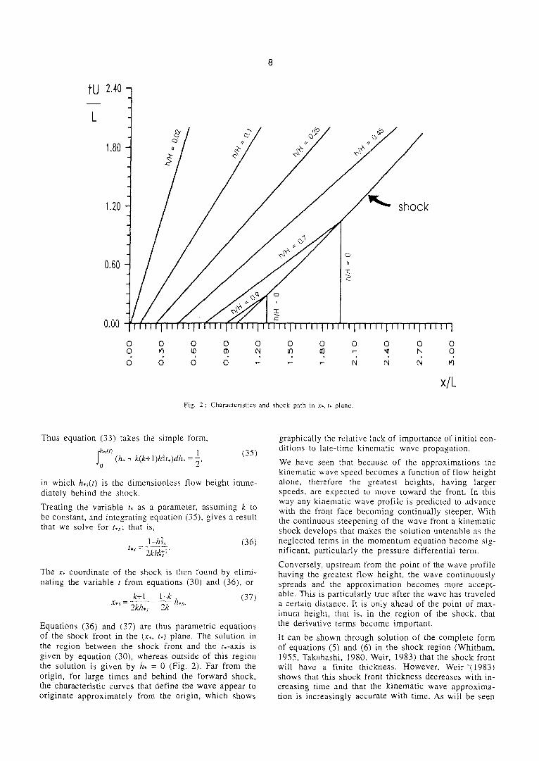
Thus equation (33) takes tile simple form,

�9 ,I,) (h , ~- k ( k + l ) h { t , ) d h , = 2 ' (35)

in which h.~(t) is the dimensionless flow height imme- diately behind the shock.

Treating the variable t. as a parameter, assuming k to be constant, and integrating equation (35), gives a result that we solve for t,.~.: that is,

1--4v;~ (36) l * s - - "~ ~- I "

, . k ~ ,

The x. coordinate of the shock is then found by elimi- nating the variable t from equations (30) and (36), or

k+l l -k h .... (37) .r.~. = 2k/z..~ 2k

Equations (36) and (37) are thus parametric equations of the shock front in the (x., t.) plane. The solution in the region between the shock front and the t .-axis is given by equation (30), whereas outside of this region the solution is given by h, = 0 (Fig. 2). Far from the origin, for large times and behind the forward shock, the characteristic curves that define the wave appear to originate approximately from the origin, which shows

graphically the relative lack of importance of initial con- ditions to late-time kinematic wave propagation.

We have seen that because of the approximations the kinematic wave speed becomes a function of flow height alone, therefore the greatest heights, having larger speeds, are expected to move toward the front. In this way any kinematic wave profile is predicted to advance with the front face becoming continually steeper. With the continuous steepening of the wave front a kinematic shock develops that makes the solution untenable as the neglected terms in the momentum equation become sig- nificant, particularly the pressure differential term.

Conversely, upstream from the point of the wave profile having the greatest flow height, the wave continuously spreads and the approximation becomes more accept- able. This is part icularly true after the wave has traveled a certain distance. It is only ahead of the point of max- imum height, that is, in the region of the shock, that the derivative terms become important.

It can be shown through solution of the complete form of equations (5) and (6) in the shock region (Whitham, t955, Takahashi, 1980, Weir, 1983) that the shock front will have a finite thickness. However, Weir "(1983) shows that this shock front thickness decreases witk in- creasing time and that the kinematic wave approxima- tion is increasingly accurate with time. As will be seen

in our applications of the theory to Mount St. Helens debris flows the kinematic wave approximation works welt on the descending limbs of the hydrographs and appears to remain valid up to the steep front, consider- ing the "steep front" to be the portion of the wave ahead of the point of maximum height of the wave.

Analogies with Weir's (1982) mathematical model

Equation (30) can be rewritten as

h. (k* l)h~t- 1 . . . . . . . . . . .

X* X*

(38)

h , . For large x, f lu id height, h-, is small, and thus - - is

X.

small ; therefore equation (30) can be approximated by

t (39)

) .

Equation (39) shows that at a fixed point, x,, water I

depth, h,, varies as t , - s

Weir (1982), using kinematic wave theory and an asymptotic solution valid for large times, showed that discharge of lahars to varies as a negative power of time. Weir (1982) arrived at the expression

(40)

,._ " j

where ~ is a constant parameter and f(x) is a compli- cated function of x. Thus at a fixed point, x. discharge

K varies as tTT-t.

C o m p a r i s o n w i t h d e b r i s - f l o w d a t a

When modeling lahars, eruption time can be determined from seismic records and the value of the time variable to be used in equation (39) is then also known. In fact, Weir (1982) used such information in his equation de- scribing the change of discharge with time for lahars.

For debris flows we normally do not know the time of flow initiation. This difficulty can be removed by in- stalling two gaging stations at a fixed distance along the channel. Knowing the distance l between the two stations and adopting the same value of k for both cross sections, we then write equation (37) in dimensional form for the two stations as the two equations

ffs_ k~+l_ (1-k)hs~ (41)

L 2k tl,~ 2kH H

and

x.~-H k+l ( l~:)h, , (42)

L 2k !!s,- 2kH H

in which h,L and h~ are the peak flows at the first and second stations, respectively and xs is the unknown dis- tance from the first =~,aoin~,= = station to the origin of the flow. We can express the parameter L in equations (41) and (42) as a function of channel slope, i, and initial height, H, by equation (3c). Equations (41) and (42) then give a system of equations for the unknowns H and x~. Solving this system we get the following ex- pressions for H and x=. as functions of k :

H = li+-k2@ (h.~l-hs2) (43 )

k - . l ( l 1 ]

and ~-_/7 @.e_ h~l

1 (" k - I l~t~ "~ -'fs ---- [ S F ; ; I ~ / ' 2 - 2 ~ _ h ~ 1 ~ (44)

) If the cross sectional shape and hence k is unknown we can choose a trial value for k (for example 0.66. valid for wide rectangular channels) to get approximate values for the unknown initial height H and x~ from equations (43) and (44). We then have h,s by using the flow height at the first station in equation (3a). Then

l-lz~ equation (36). t.~-2khan_ I, gives t.~, which is the time

for the shock to travel from the point of inception to the first gaging station. Here h-s, the shock height, is equal to the peak flow height.

To express t,, in dimensional form we use the definition of nondimensional time (equation 4b), which requires that U and L be known. The velocity U is given by

k I U = C H ~ (Equation 10, the Manning equation, with h

H = /4), and L is given by i = - ~ (equation 3c). Also, as

shown in Arattano and Savage (1992), C, which is re- lated to the Manning roughness coefficient (equation I0), can be obtained from the mean values of peak velocity and flow height at stations I and 2. Assuming C to be constant with flow height we then have U and hence dimensional t.~, which represents a value for the elapsed time between debris l low initiation and the ap- pearance of the peak height of the debris flow at the first gaging station.

If equation (39) is plotted with log h(t) as the ordinate and log t as the abscissa, then, for fixed x, a straight

1 line with slope -~ . results. If we find that a plot of the

logarithm of the hydrograph data collected at the first gaging station - that is, log h(t), against the logarithm of time, log t (starting from the time of appearance of debris-flow peak height at the first gaging station) - can be approximated as a straight line with negative slope, then we can estimate k. This value for k is then used in equations (43) and (44) to give improved values for H and xs, and we can repeat the calculations. The it- eration is rapidly convergent and gives consistent values for H, x~, t~ and k. Finally, having determined the par- ameters necessary to predict the hydrograph beyond the first gaging station, we can predict the form of the hy- drograph at the second ~,a~,in,, station using equation

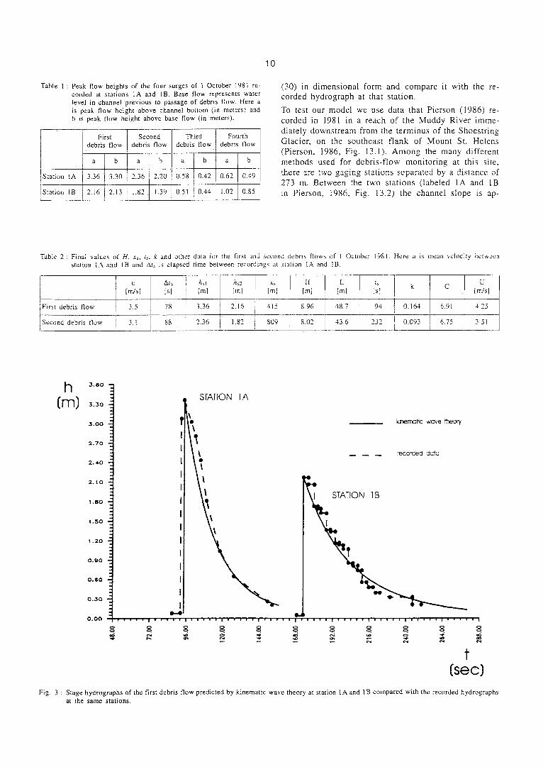
Table 1 : Peak flow heights of the four surges of I October 1981 re- corded at s tat ions 1A and lB. Base flow represents water level in channel previous to passage of debris flow. Here a is peak flow height above channel bottom (in meters) and b is peak flow height above base flow (in meters).

Station IA i

3ration IB

First Second Third debris f low debris f low debris flow

a b a i b a b J

3.36 3.30 2.36 2.20 0.58 0.42

2.16 2.13 1.82 1.59 0.51 0.44

Fourth debris f low

a b

0.62 0.49

1.02 0.85

10

(30) in dimensional form and compare it with the re- corded hydrograph at that station.

To test our model we use data that Pierson (1986) re- corded in 1981 in a reach of the Muddy River imme- diately downstream from the terminus of the Shoestring Glacier, on the southeast flank of Mount St. Helens (Pierson, 1986, Fig. 13.1). Among the many different methods used for debris-flow monitoring at this site, there are two gaging stations separated by a distance of 273 m. Between the two stations (labeled 1A and IB in Pierson, 1986, Fig. 13.2) the channel slope is ap-

Table 2 : Final values of H, xs, ts. k and other data for the first and second debris flows of 1 October 1981. Here u is mean ,,elocity between station IA and IB and Ats is elapsed time between recordings at station IA and lB.

u &Is i hd hs2 x, H k G [m/s] is] ] [ml [ml [mJ [m] [m] Is] k

3.36 2.16 415 8.96 48.7 94 J? 0 .164 I

=,rst debris flow 3.5 78 I

~econd debris flow 3.1 88 2.36 1.82 809 8.02 43.6 232 ; L ]0.093

U C [r~sl

6.91 4.25

6.75 3.51

h [m]

3 . 6 0

3 . 3 0

3 . 0 0

2 . 7 0

2 . . 4 0

2 . 1 0

1 . 8 0

t . 5 0

1 . 2 0

0 . 9 0

0 . 6 0

0 . , . 30

0.00

STATION 1A

knernatic wave theon/

recorded acta

' k STATION 1 B

I

�9 �9 ' �9 �9 I " " ' ' ' I ' ' ' ' ' I ' ' ' �9 �9 I " ' �9 ' . I ' ' ' ' ' I ' ' ' , �9 I �9 ' ' ' ' I ' ' ' ' ' I ' ' " �9 ' I

t [sec]

Fig. 3 : Stage hydrographs of the first debris flow predicted by kinemat ic wave theory at station IA and 1B compared with the recorded hydrographs at the same stations.

11

h [m]

2 . 4 0

2 . 1 0

1 . 8 0

1 . 5 0

1 . 2 0

0 . 9 0

0 . 6 0

0..30

0.00

o M

STATION 1A kJnematlc w a v e fheo,'y

Q, 1D

\

5, 5.

11,

rec~'decl da ta

1B

�9 . . i i | . | �9 . I I ' ' ' ' n I ' I I . . I ' ' ' ' ' I | �9 i . �9 I ' ' �9 i i I �9 ' �9 ' ' I ' ' ' i . I �9 | n | i I

N ~ ~ N ~ N 8 N N . , o . q . . . . . .

t [sec]

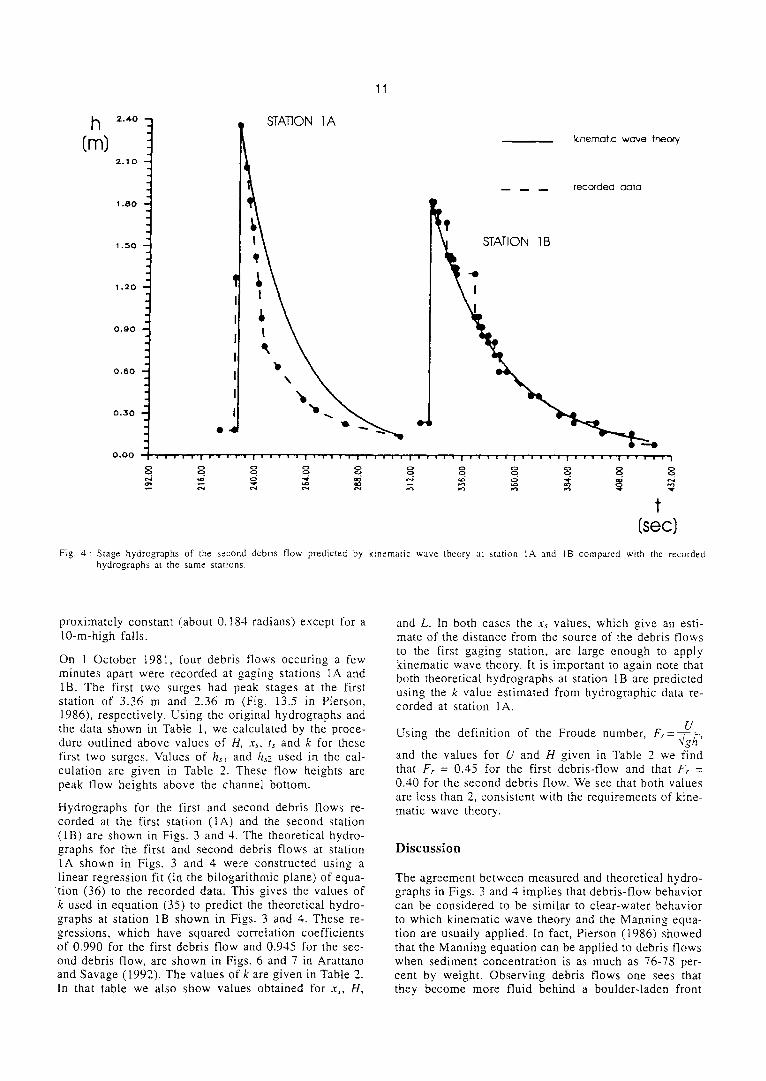
Fig. 4 : Stage bydrographs of the second debris flow predicted by kinematic wave theory at station IA and IB compared with the recorded hydrographs at the same stations.

proximately constant (about 0.184 radians) except for a 10-m-high falls.

On 1 October 1981, four debris flows occuring a few minutes apart were recorded at gaging stations IA and lB. The first two surges had peak stages at the first station of 3.36 m and 2.36 m (Fig. 13.5 in Pierson, 1986), respectively. Using the original hydrographs and the data shown in Table 1, we calculated by the proce- dure outlined above values of H, x~, t+. and k for these first two surges. Values of hst and h,2 used in the cal- culation are given in Table 2. These flow heights are peak flow heights above the channel bottom.

Hydrographs for the first and second debris flows re- corded at the first station (1A) and the second station (1B) are shown in Figs. 3 and 4. The theoretical hydro- graphs for the first and second debris flows at station IA shown in Figs. 3 and 4 were constructed using a linear regression fit (in the bilogarithmic plane) of equa-

t ion (36) to the recorded data. This gives the values of k used in equation (35) to predict the theoretical hydro- graphs at station 1B shown in Figs. 3 and 4. These re- gressions, which have squared correlation coefficients of 0.990 for the first debris flow and 0.945 for the sec- ond debris flow, are shown in Figs. 6 and 7 in Arattano and Savage (1992). The values of k are given in Table 2. In that table we also show values obtained for x+, H,

and L. In both cases the x, values, which give an esti- mate of the distance from the source of the debris flows to the first gaging station, are large enough to apply kinematic wave theory. It is important to again note that both theoretical hydrographs at station 1B are predicted using the k value estimated from hydrographic data re- corded at station 1A.

U Using the definition of the Froude number, F ,=~ ,~ - ,

and the values for U and H given in Table 2 we find that Fr = 0.45 for the first debris-flow and that Fr = 0.40 for the second debris flow. We see that both values are tess than 2, consistent with the requirements of kine- matic wave theory.

D i s c u s s i o n

The agreement between measured and theoretical hydro- graphs in Figs. 3 and 4 implies that debris-flow behavior can be considered to be similar to clear-water behavior to which kinematic wave theory and the Manning equa- tion are usually applied. In fact, Pierson (1986) showed that the Manning equation can be applied to debris flows when sediment concentration is as much as 76-78 per- cent by weight. Observing debris flows one sees that they become more fluid behind a boulder-laden front

12

and can develop features typical of water behavior such as the hydraulic jump shown by Costa and Williams (1984).

The assumption of a constant k value along the channel seems to be reasonable for flows 1 and 2. We see that at both stations predicted hydrographs with constant k values show good agreement with the actual debris flows; however, with no information about cross sectional shape, we have been unable to verify the k values obtained by the procedures outlined above. The k value for the second debris flow is smaller than the k value for the first debris flow. This difference could result if the flow cross section was narrowing by deposi- tion, by a reduction in flow height, or a combination of these effects.

The model allows a prediction of the distance that the debris flow has traveled from its point of inception to the first gaging station, xs. Values found for Xs using equation (44) show that the two debris flows should have started on the Shoestring Glacier at 415 m and 809 m from the first station, respectively. We note that Pierson (1986) postulated that one source of these flows could be glacier outburst floods.

Also recall that our model does not account for changing slopes. We note that the slope in the Muddy River in- creases above the monitored channel reach; this increase could affect estimated values for ts, I i , xs and, thus, k. Tile model could be improved by taking account of changing slope by using an expression for slope as a function of distance such as that used by Weir (1982).

More data are needed to show the validity of this model�9 It would be useful to predict the movement along a stream channel of a known mass of debris caused by a landslide or a previous debris flow. Knowing debris volume, the amount of water required for mobilization, and the mean width of the stream channel, we could calculate the parameter A in equation (31) by dividing the debris and water volume by the mean channel width. Knowing the channel slope, we could then calculate the parameters H and L in equation (32). Also, if we have values for k and for C along the stream channel, we could predict the propagation of the debris flow along the entire channel.

Our model does not take into account other features of debris flows. For example, debris flows do not show a vertical front but rather a continuous, rapid rise to peak discharge that may be imperceptible to recorders. The predicted vertical front is a consequence of the mathe- matical approximations made in kinematic wave theory�9 Because of these approximations we do not take account of what is happening inside the front region and we neg- lect the possible physical effects of the front on the por- tion of the wave behind it.

Physically, steep fronts observed in debris flows may be both a consequence of kinematic behavior and of the strength of the flowing material. Perhaps the steep front, rich in highly concentrated debris, could be modeled as a Bingham fluid. Johnson (1970), for example, has successfully modeled clay rich debris flows as Bingham fluids. The Bingham model predicts a critical depth

below which motion should stop. This behavior is not commonly observed in debris flows which show excess fluid height to decrease continually to near-zero or zero values with passage of the flow. In fact, behind the front, the concentration of debris rapidly decreases and we observe muddy, turbulent water that behaves as a Newtonian fluid which can be successfully described using a Manning-type equation. Perhaps this is why our Newtonian fluid-based model fits the descending limb of the hydrograph well (especially after the wave has traveled a greater distance, as at station B). It remains to be answered whether the front, which is probably af- fected by material strength, or the remaining part of the flow, which behaves as a Newtonian fluid, prevails in conditioning the overall behavior of debris flow waves.

As we have noted, Whitham (1955) and Takahashi (1980) derived theoretical expressions to account for tile lobate profile of the leading edge of a flow. Whitham's equation was derived to model the profile of the leading edge of a mass of water propagating along a stream channel after a dam failure, whereas Takahashi's equa- tion was derived for debris flows. We have not used such expressions here because of the steep front profile shown by the debris flows examined and our attention to modeling the descending limb of the hydrograph, that is, the portion of the wave behind the front.

Our model does not allow any prediction about how far debris flows can travel. Theoretically kinematic waves propagate indefinitely; however, shock height decreases downstream untiI, after a finite distance from the starting point, it reaches a practically nul[ value. In fact, because of its larger height, that portion of the flow close to the shock will move faster than portions behind the shock, causing the spread of the flow longitudinally. Because mass has to be conserved, this causes a decrease in flow height�9 Also, because of direct propor- tionality between flow height and velocity, longitudinal spreading causes a decrease in velocity.

The model could be improved by using for the term i, which accounts for bed resistance through the Manning equation (Arattano and Savage, 1992), a relationship that accounts also for a Bingham behavior (Johnson, 1970) of the debris flow front. This Bingham viscoplas- tic behavior would account for the apparent strength of the slurry, a strength that would keep the boulders in place at the front of the flow.

Finally, the model does not explain the effects of deposi- tion or erosion along the stream channel during flow because it is based on the hypothesis of constant volume. That hypothesis is made when we assume A to be a constant to find the parametric equation of the shock front in the (x,, ts) plane (equations 33 and 34). If, because of erosion of deposits along the channel, the peak flow value were to increase during the flow from the first to the second gaging station, the model could not be applied. A higher peak flow value at the second ~a~,lno~, ~,' ,, station could also be caused by an abrupt chan~e. in cross sectional form at that station. But, again, our model cannot account for such a circumstance, because

we h a v e a s s u m e d the c r o s s s e c t i o n a l f o r m to r e m a i n

c o n s t a n t a l o n g t he c h a n n e l . W e h o p e to a c c o u n t for

c h a n g i n g d e b r i s - f l o w v o l u m e a n d c h a n g i n g c h a n n e l

c r o s s s e c t i o n a l f o r m in f u t u r e m o d e l i n g e f f o r t s .

C o n c l u s i o n s

To m o d e l d e b r i s f l o w s , w e m o d i f i e d a m a t h e m a t i c a l ap- p r o a c h d e v e l o p e d f r o m o p e n - c h a n n e l h y d r a u l i c t heo ry . T h i s a p p r o a c h w a s o r i g i n a l l y u s e d to p r e d i c t the be- h a v i o r o f a m a s s o f w a t e r s u d d e n l y r e l e a s e d in a w i d e , r e c t a n g u l a r s t r e a m c h a n n e l a f t e r a d a m b r e a k . In add i - t ion to d e m o n s t r a t i n g a n a l o g i e s b e t w e e n d e b r i s - f l o w a n d d a m - b r e a k p h e n o m e n a , o u r m o d e l h a s b e e n m o d i f i e d to a p p l y to the n a r r o w c h a n n e l s t yp i ca l o f d e b r i s f l o w s .

O u r m o d e l a p p e a r s to s i m u l a t e the f o r m o f s t a g e h y - d r o g r a p h s f r o m two d e b r i s f l o w s tha t o c c u r r e d in the M u d d y R ive r , on M o u n t St. H e l e n s , on 1 O c t o b e r 1 9 8 l r e a s o n a b l y wel l . F r o m the h y d r o g r a p h s o f t h e s e d e b r i s f l o w s , r e c o r d e d by two g a g i n g s t a t i o n s 273 m a p a r t on the s t r e a m , we w e r e ab l e to u s e the h y d r o g r a p h r e c o r d e d at the f i rs t s t a t i o n and t he p e a k f low v a l u e o f the h y - d r o g r a p h r e c o r d e d at t h e s e c o n d s t a t i o n to c a l c u l a t e the m o d e l p a r a m e t e r s a n d t h e n f o r e c a s t the f o r m o f the h y - d r o g r a p h s r e c o r d e d at the s e c o n d s t a t i on . T h e s e fo re - c a s t s s h o w g o o d a g r e e m e n t w i t h ac t ua l d a t a a n d a b e h a v i o r o f the d e b r i s f l o w s e x a m i n e d tha t is v e r y s i m - i lar to tha t o f c l e a r wa te r . T h e m o d e l a l l o w s an e s t i m a - t ion o f the p o s i t i o n o f the s o u r c e s o f the d e b r i s f l o w s a n d the t i m e o f t r a v e l o f t h e s e f l o w s to the f i r s t s t a t i o n . A l s o k v a l u e s f o r the c h a n n e l , k b e i n g a p a r a m e t e r tha t a c c o u n t s for c h a n g e s o f h y d r a u l i c r a d i u s w i t h f l o w d e p t h , w a s e s t i m a t e d f r o m r e c o r d e d f l ow da ta .

M o r e r e s e a r c h is n e e d e d to v e r i f y the g e n e r a l a p p l i c a - b i l i ty a n d r e l i a b i l i t y o f th i s m o d e l . A t th i s t i m e the m o d e l c a n n o t i n c l u d e t he e f f e c t s o f c h a n g i n g c h a n n e l s lope , o r e r o s i o n or d e p o s i t i o n d u r i n g d e b r i s f l o w m o v e - m e n t , a n d it c a n n o t p r e d i c t t he d i s t a n c e tha t a d e b r i s f l ow c a n t r ave l . N e v e r t h e l e s s , the m o d e l p r o v i d e s a q u a n t i t a t i v e t h e o r y tha t c a n be u s e f u l for f u t u r e r e s e a r c h on d e b r i s - f l o w b e h a v i o r .

R e f e r e n c e s

ABBOTT M.B.. 1966: An introduction to the method of charac- teristics: New York, american Elsevier, 2-1.3 p.

ARATTANO M. and SAVAGE W.Z.. 1992: Kinematic wave theory for debris flows : U.S. Geological Survey Open-File Report, 92- 290, 39 p.

BAGNOLD R.A., 1954 : Experiments on a gravily-free dispersion of large solid spheres in a Newtonian fluid near shear : Proceedings. Royal Society of I.ondon, ser. A, v. 225, p. a9-63.

BINGHAM E.C., 1922 : Fluidity and plasticity : McGraw-Hill. New York, 440 p.

CHEN C.L., 1987: Comprehensive review of debris flow modeling concepts in Japan. in Costa J.E., and Wieczorek G.F., eds., Debris flow/avalanches - Process, recognition and mitigation : Geological

13

Society of America, Reviews in Engineering Geology, v. 7, p. 13- 29.

CHEN C.L., 1988: Generalized viscoplastic modeling of debris flows : American Society of Civil Engineers, Journal of Hydraulic Engineering, v. 114, no. 3, p. 237-258.

CHOW V.T., 1959 : Open-channel hydraulics : McGrav,'-Hi!l, New York, 680 p.

COSTA J.E. and WILLIAMS G.P.. 198d- : Debris-flow dynamics : U.S. Geological Survey Open-File Report 84-606, Video Tape, 23 rain.

GALLINO G.L. and PIERSON r .c . , 1984: The 1980 Polallie creek debris flow and subsequent dam-break flood, east Fork Hood river basin, Oregon : U.S. Geological Survey Open-File Report, 84-578, 39 p.

HENDERSON F.M.. 1966 : ()pen channel flow : MacMillan Publish- ing Co. Inc., New York, 522 p.

HUNT B., 1982 : Asymptotic solution for dam-break problem : Journal of the Hydraulics division, Proceedings of the American Society of Civil Engineers. v. 108, no. HYI, p. I15-126.

JOHNSON A.M., 1970 : Physical processes in geology : W.H. Freeman, San Francisco, 577 p.

LAENEN A. and HANSEN R.P., 1988 : Simulation of three lahars in the mount St. Helens area, Washington, using a one-dimensional, unsteady-state streamflow model : U.S. Geological Survey Water- Resources Investigation Report 88-4004, 20 p.

LIGHTHILL M.J. and WHITHAM G.B., 1955 : On kinematic waves I. Flood movement in Long rivers: Proceedings of the Royal Society of London, v. A 229, p. 28~-316.

MAIONE L., 1977 : Appunti di idrologia. Le piene tluviali : La Goli- ardica Pavese, Pavia, Italy, v. 3. 224 p.

MILLER J.E.. 1984 : Basic concepts of kinematic-wave models. U.S. Geological Survey Professional Paper 1302 : 32 p., Washington.

PIERSON T.C., 1986: Flow behavior of channelized debris flows. Mount St. Helens, Washington, in Abrahms A.D., ed., Hillslope Processes : Allen & Unwin, Boston, p. 269-296.

PIERSON T.C., JANDA R.J., THOURET J. and BORRERO C.A., 1990 : Perturbation and melting of snow and ice by the 13 Novem- ber 1985 eruption of Nevado del ruiz, Colombia, and consequent mobilization, flow and deposition of lahars: Journal of Vol- canology and Geothermal Research, v. 41, p. 17-66.

RODINE J.M. and JOHNSON A.M., 1976: The ability of debris. heaviIy freighted with coarse clastic materials, to f,~.~w on gentle slopes : SediTnentology, v. 23, p. 213-234.

ROUSE fT., 1938 : Fluid mechanics for hydraulic engineers : McGraw- Hill, New York, 422 p.

TAKAHASHt T., 1978: Mechanical characteristics of debris flow: Journal of the Hydraulics Division, Proceedings of the American Society of Civil Engineers, v. 104, no. HY8, p. 1153-1169.

TAKAHASHI T., 1980 : Debris flow on prismatic open channel : Jour- nal of the ttydraulics Division, Proceedings of the American Society of Civil Engineers, v. 106, no, HY3, p. 381-398.

TAKAHASHI T., t991 : Debris Flows : Rotterdam, AHR/A1RH mon- ograph, A.A. Balkema, 165 p.

WEIR G.J., 1982: Kinematic wave theory for Ruapehu lahars: New Zealand Journal of Science, v. 25, p. 197-203.

WEIR G.J., 1983 : ]'he asymptotic behavior of simple kinematic waves of finite volume: Proceedings of the Royal Society of London. vol. A 387, p. -,i.59-467.

WHITHAM G.B., 1955 : The effects of hydraulic resistance in the dam-break problem : Proceedings of the Royal Society of I,ondon. v, A 227, p. 399-407.

YANO K. and DAIDO A., 1965: Fundamental study on mud-flow: Kyoto, Japan, Kyoto University, Bulletin of the Disaster Prevention Research Institute, V. 14. p. 69-83.