Kinematic dynamo simulations of von Karman flows: application to the VKSexperiment

A. Pinter,∗ B. Dubrulle, and F. DaviaudService de Physique de l’Etat Condense, CEA, IRAMIS,

CNRS/URA 2464, CEA-Saclay, F-91911 Gif-sur-Yvette, France(Dated: Eur. Phys. J. B 74, 165-176 (2010))

The VKS experiment has evidenced dynamo action in a highly turbulent liquid sodium vonKarman flow [R. Monchaux et al., Phys. Rev. Lett. 98, 044502 (2007)]. However, the existence andthe onset of a dynamo happen to depend on the exact experimental configuration. By performingkinematic dynamo simulations on real flows, we study their influence on dynamo action, in particularthe sense of rotation and the presence of an annulus in the shear layer plane. The 3 components ofthe mean velocity fields are measured in a water prototype for different VKS configurations throughStereoscopic Particle Imaging Velocimetry. Experimental data are then processed in order to usethem in a periodic cylindrical kinematic code. Even if the kinematic predicted mode appears to bedifferent from the experimental saturated one, the results concerning the existence of a dynamo andthe thresholds are in qualitative agreement, showing the importance of the flow characteristics.

PACS numbers: 47.65.-d, 91.25.Cw

I. INTRODUCTION

Dynamo action is an instability by which mechanicalenergy is transformed into magnetic energy for Rm ≥ Rcmwhere Rm is the magnetic Reynolds number. Since Lar-mor’s prediction concerning the solar dynamo[1], a lotof work has been devoted to this field, including boththeories and numerical simulations. In the last decade,the interest for dynamo has been renewed by the posi-tive results obtained by the Riga [2] and Karlsruhe [3]fluid dynamo experiments. These experiments rely onanalytical predictions by Ponomarenko [4] and Robert[5] and have been designed accordingly. In particular,the generated turbulent sodium flows are organized sothat the instantaneous flow remains always close to themean flow, allowing the kinematic dynamo predictionsof the thresholds and of the neutral modes (respectivelyoscillatory and stationary) to be very accurate.

A new step was passed very recently in the von KarmanSodium (VKS) experiment. Different dynamos havebeen observed inside a flow of liquid sodium at largeReynolds number (Re ∼ 107) [6–9]. Depending on thethe control paramaters, statistically stationary dynamosor dynamical dynamo regimes including field reversalshave been reported. Under these conditions, the flow isfully turbulent, with many large and small scale fluctu-ations, and the instantaneous flow is very different fromthe mean flow [10, 11]. The dynamo instability takingplace in the VKS experiment is thus at variance withthe classical instabilities taking place in laminar flows orin turbulent flows remaining very close to their mean.Nevertheless, many kinematic dynamo simulations havebeen performed to optimize this flow, using the syntheticMND flow [12] or time-averaged flows measured in water-

∗Electronic address: kontakt@alexander-pinter.de

prototype experiments [13, 14, 20].

Different observations have been made that can helpelucidate the exact mechanism by which the dynamo in-stability develops in the VKS experiment: i) in the ex-actly counter-rotating case, dynamo action is observedabove a critical magnetic Reynolds number Rcm ≈ 32 andthe dominant saturated mode is an axisymmetric m=0mode in cylindrical coordinates [6]; ii) so far, dynamo hasonly been observed with iron propellers [9]; iii) in a givenexperimental set up with iron disks, dynamo has beenobserved when counter-rotating disks in (+) ’non scoop-ing’ direction (with respect to the propellers blades), butno dynamo has been observed when counter-rotating thedisks in the (-) ’scooping’ direction [9].

Observation i) shows that the dynamo mechanism isnot the simple linear response to the mean flow alone,since the latter is axisymmetric and produces a trans-verse m = 1 mode (m denotes the azimuthal wavenum-ber) above Rcm ' 43 as indicated by kinematic dynamosimulations [14]. It has been suggested in [15] that them=0 mode of the VKS experiment is in fact generated bynon-axisymmetric fluctuations through an alpha-omegamechanism taking place within the blades of the pro-pellers. This suggestion has been confirmed by recent nu-merical simulations [16] showing that the addition of an(empirical and large) alpha term in the induction equa-tion changes the dominant m=1 mode into a dominantm=0 mode with a dynamo threshold close to the observedexperimental critical value Rcm ≈ 32. Another interest-ing suggestion has been made by [17], namely that them=0 mode could arise from a secondary bifurcation ofthe m=1 mode, since the latter breaks the original ax-isymmetry of the velocity field.

Observation ii) shows that magnetic boundary condi-tions have a large impact on the dynamo instability. Highmagnetic permeability conditions are known to decreasethe dynamo threshold for the Roberts and Ponomarenkoflows [18] and more recently for von Karman type flows

arX

iv:1

106.

1717

v1 [

phys

ics.

flu-

dyn]

9 J

un 2

011

2

[19]. For iron disk, it is suggested that the dynamothreshold could be reduced by a factor as large as 2 withrespect to stainless disks. Since it has not been yet possi-ble to get beyond Rm = 50 in the VKS experiment, thiscould explain why dynamo has not been observed withstainless steel disks, while it is observed around Rm = 32with iron disks. Other kinematic simulations [20] haveshown that the sodium flow behind the disks can lead toan increase from 12% to 150%. Using iron disks can thusalso screen magnetic effects of the flow behind the disks.PARLER des DISQUES CAMEMBERTS?

Observation iii) shows that the dynamo is not pro-duced only by the rotation of magnetized iron disks ina conducting fluid but depends on the flow characteris-tics: it is a real fluid dynamo. However, not much hasbeen done so far to try and exploit this observation. Inparticular, no kinematic dynamo simulations have beenperformed so far with experimental flows including anannulus as in the VKS experiment or with propellerscounter-rotating in the (-) ’scooping’ direction.

In the present paper, we use Stereoscopic ParticleImaging Velocimetry (SPIV) measurements obtained invon Karman water (VKE) experiments modeling theVKS experiment to perform kinematic dynamo simula-tions. We investigate the role of the mean field structureon the dynamo threshold, with special attention to therotation sense. Because of the axisymmetry, the exhib-ited kinematic mode is, as expected, different from theexperimental saturated one. However, we show that thekinematic dynamo thresholds qualitatively vary like theobserved dynamo thresholds and discuss how these re-sults can be useful to understand the actual mechanismsat the origin of VKS dynamo.

Our paper is organized as follows: In Sec. II, afterthe problem formulation, we describe the experimentalmeasurements and the numerical method. In Sec. III,we focus on the processing procedure of the measuredvelocities and perform a comparison with previous esti-mates based on Laser Doppler Velocimetry (LDV) mea-surements. Results for dynamo action are presented inSec. IV and compared with the VKS experiments. Fi-nally, we discuss the consequences of these results for theVKS dynamo.

II. METHODS

A. Problem Formulation

In the present paper, we focus on the kinematic dy-namo problem: we consider a given velocity field u, e.g.as measured in a water experiment, and check its abilityto sustain dynamo action by solving the magnetic induc-tion equation

∂b

∂t= ∇× (u× b) +

1

µσ4b, (1)

where b denotes the magnetic field with ∇ · b = 0, µ andσ are respectively the magnetic permeability and the elec-trical conductivity of the considered medium, and ∆ isthe Laplacian operator. Since u is given, the equation islinear in b. There are two possible long-time behaviourfor the magnetic field: either it is decaying and there is nodynamo, or it is increasing, and there is dynamo. Growthor decay is in general exponential (although there can betransient algebraic growth, due to non-normality of theoperator, see [21]). To quantify the growth, we introducethe growth rate σ = ∂t ln

⟨B2⟩

that is based on the mag-

netic energy⟨B2⟩, where the average is taken over the

spatial domain.Since the equation is linear, no saturation is observed

in the kinematic approach. This technique is thereforeunable to detect subcritical or finite amplitude dynamos[22] or to study the saturation regime [25–27] as in nu-merical flows such as the Taylor-Green flow.CITER SIM-ULATIONS FOREST??. However, this approach givesan estimation for the dynamo threshold as a function ofthe mean velocity field.

B. Experimental measurements

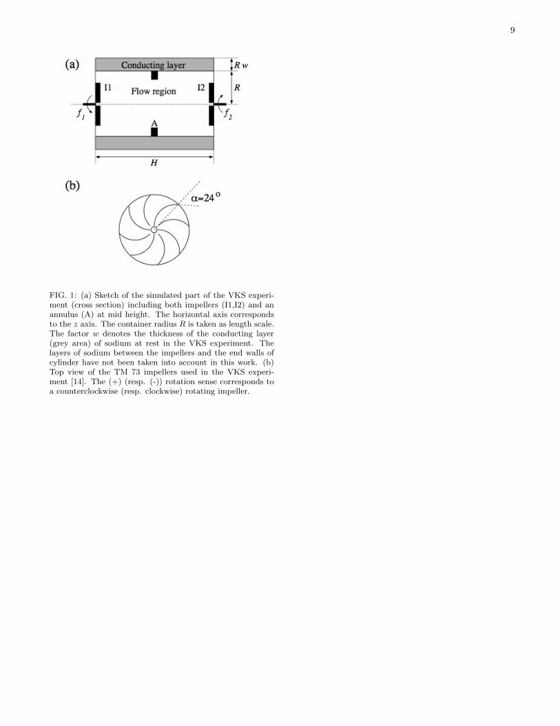
Geometry and experimental setup.— The setup corre-sponding to the VKS experiment is described in detailsin [6] and sketched in Figure 1(a). A cylindrical vesselwith a fixed aspect ratio of L = H/R = 1.8, where R(resp. H) denotes the radius (reps. the length) of thevessel which is filled with liquid sodium. We arrangethe coordinate system such, that the axial extension ofthe cylinder is situated in the interval z ∈ [−0.9, 0.9].The fluid is stirred by two independent rotating so calledTM73 impellors [14], at frequencies f1 and f2. The im-pellers are fitted with curved blades (see Fig. 1 (b)).Therefore, the flow properties depend on the sense of ro-tation, specifically on whether the blades are presentingtheir concave ((-) rotation) or convex ((+) rotation) sideto the flow during impeller rotation. In the special casewhere f1 = f2 > 0 (resp. f1 = f2 < 0) with the sign con-vention of Fig. 1, the impellers fullfill exact (+) (resp.(-)) counter-rotation. An optional concentric annulus canalso be inserted at mid height and has been used in thefirst dynamo runs. This annulus reduces large scale fluc-tuations [11] and can also have an impact on the meanflow, in particular on the toroidal to poloidal ratio Γ (seebelow). In the VKS experiment, an additional layer ofresting sodium is present in the outer part of the experi-ment.

The VKE experiment is the exact half-scale watermodel of the VKS experiment, except that the experi-ment is realized vertically (vertical z axis) whereas theVKS setup is horizontal. The cylinder radius and heightof the VKE vessel are R = 100 and 240 mm respectively.We have used TM73 impellers of diameter 150 mm fittedwith radial blades of height 20 mm and curvature radius92.5 mm. The inner faces of the disks are H = 180 mm

3

apart. We have worked with different vessel geometries,allowing the insertion of an annulus - thickness 5 mm, in-ner diameter 170 mm - in the equatorial plane. Note alsothat in the VKE experiment, the layer of resting fluid isabsent. The velocity field is therefore only measured inthe flow region, see Fig. 1 (a).

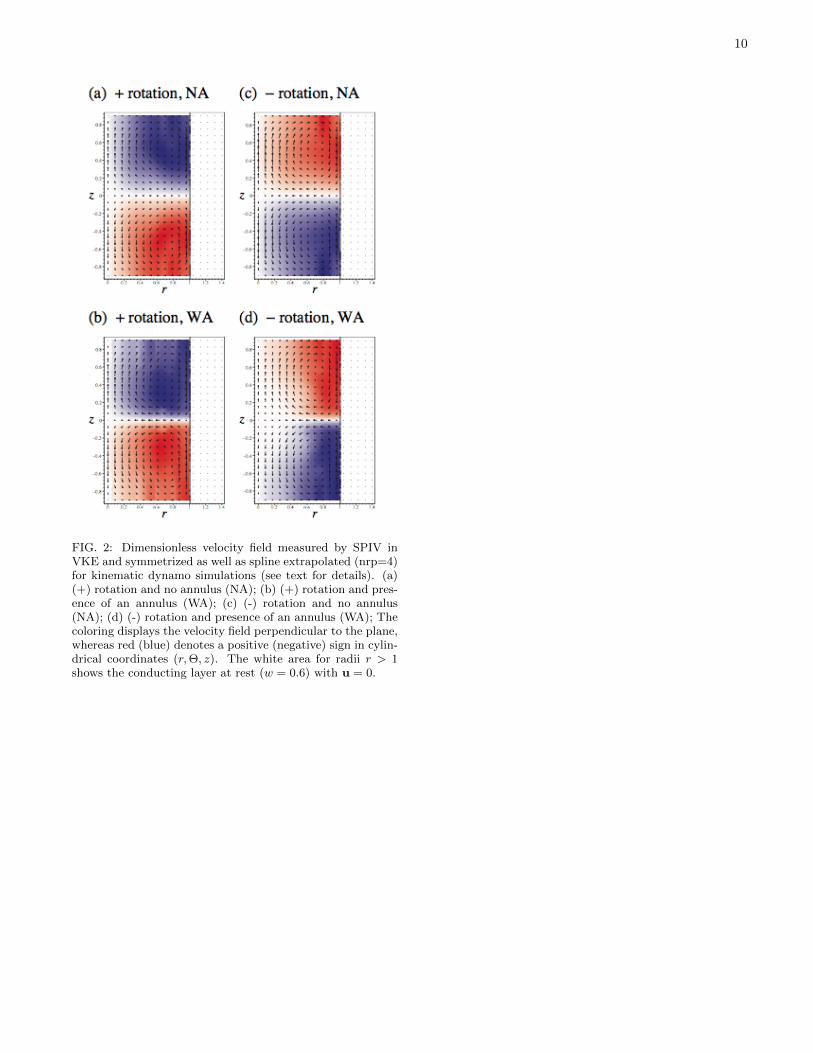
Velocity measurements are performed using a DAN-TEC SPIV system, providing the three components ofthe velocity field on a plane through a 95 × 66 pointsgrid [28]. In all that follows, the measurement plane is ameridian plane containing the rotation axis. The velocityfields are averaged over time series of 5000 regularly sam-pled values (sampling frequency between 1 and 15 Hz). Inthe exact counter-rotating regime, the system is axisym-metric and symmetric with respect to any rotation Rπof π around any radial axis in its equatorial plane. Themean flow is composed of two toroidal cells separated byan azimuthal shear layer and two poloidal recirculationcells. Figure 2 shows the velocity fields obtained in the 4studied configurations: (+) and (-) rotation sense in thepresence or the absence of an annulus in the equatorialplane. Note that in the exact counter-rotating regime, noturbulent bifurcation towards a one cell state is observedwith the TM73 impellers contrary to what is reportedfor impellers with higher curvarture blades in [29]. Thebifurcation is observed in the (+) sense for a rotationnumber θ = (f1 − f2)/(f1 + f2) = 0.1 without annulusand θ = 0.17 with annulus [11].

Control parameters.— Choosing the magnetic field dif-fusion time µσR2 as the time scale, and the maximumabsolute value of the flow velocity |u|max as velocity unit,the induction equation can be expressed in dimensionlessform:

∂b

∂t= Rm∇× (u× b) +4b, (2)

where Rm = µσR|u|max is the magnetic Reynolds num-ber. The critical magnetic Reynolds number Rcm for dy-namo onset is then defined such that σ(Rcm) = 0. An-other important parameter to characterize the velocityfield is the poloidal to toroidal ratio:

Γ =〈P 〉〈T 〉

, with (3a)

〈P 〉 =

∫ L/2

−L/2dz

∫ 1

0

√ur(r, z)2 + uz(r, z)2rdr, (3b)

〈T 〉 =

∫ L/2

−L/2dz

∫ 1

0

|uΘ(r, z)| rdr, (3c)

which is known to have a great impact on the dy-namo threshold [13, 14]. Here we denoted the compo-nents of the velocity field in cylindrical coordinates asu = (ur, uΘ, uz).

C. Numerical code

Because the system is axisymmetric, the time-averagedvelocity field is supposed to be axisymmetric. We inte-grate the induction equation using an axially periodickinematic dynamo code. We only provide here its briefdescription, details can be found in [30]. The codeis pseudospectral in the axial and azimuthal directionswhile the radial dependence is treated by a high-orderfinite difference scheme. The numerical resolution corre-sponds to a grid of 81 points for one wavelength in axialdirection, 4 points in azimuthal direction (correspondingto azimuthal wave numbers m = 0,±1) and 31 points inradial direction for the flow domain. The time scheme issecond-order Adams-Bashforth with a typical time stepof 10−5.

Electrical conductivity and magnetic permeability arehomogeneous and the external medium is insulating. Im-plementation of the magnetic boundary conditions for afinite cylinder is difficult, due to the nonlocal character ofthe continuity conditions at the boundary of the conduct-ing fluid [19]. In contrast, axially periodic boundary con-ditions are easily formulated, since the harmonic externalfield then has an analytical expression. Indeed, the nu-merical elementary box consists of two mirror-symmetricexperimental velocity fields in order to avoid strong ve-locity discontinuities along the z axis [14]. Note that wedo not take into account the effet of the flow behind thepropellers. This effect has been studied in details in otherkinematic simulations [20].

Finally, we can act on the electromagnetic boundaryconditions by adding a layer of stationary conductor ofdimensionless thickness w, corresponding to sodium atrest surrounding the flow exactly as in the VKS experi-ment in Cadarache [6]. This extension is made keepingthe radial resolution of the experimental measured ve-locity field constant (31 points in the flow region). Thevelocity field we use as input for the numerical simula-tions is thus simply fit in an homogeneous conductingcylinder of radius 1 + w:

u = uflow for 0 ≤ r ≤ 1, (4a)

u = 0 for 1 < r ≤ 1 + w. (4b)

Former investigations [14] showed a decrease of the criti-cal magnetic Reynolds number for increasing conductinglayer size, with a saturation above w = 0.4. Therefore,we fixed w = 0.4 (meaning altogehter 43 points in radialdirection) in order to save computing time. Some cal-culations with w = 0.6 (49 points) have also been done,when comparing with older computations based on LDVmeasurements.

Figure 3 gives an example of the total velocity fieldused in kinematic simulations, consisting of an experi-mentally measured velocity field uflow and a conductinglayer with w = 0.6.

4

III. DATA PREPARATION AND TESTS

A. Preparation of measured velocities

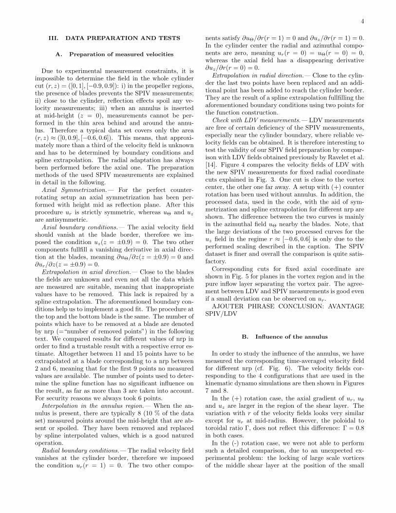
Due to experimental measurement constraints, it isimpossible to determine the field in the whole cylindercut (r, z) = ([0, 1], [−0.9, 0.9]): i) in the propeller regions,the presence of blades prevents the SPIV measurements;ii) close to the cylinder, reflection effects spoil any ve-locity measurements; iii) when an annulus is insertedat mid-height (z = 0), measurements cannot be per-formed in the thin area behind and around the annu-lus. Therefore a typical data set covers only the area(r, z) ≈ ([0, 0.9], [−0.6, 0.6]). This means, that approxi-mately more than a third of the velocity field is unknownand has to be determined by boundary conditions andspline extrapolation. The radial adaptation has alwaysbeen performed before the axial one. The preparationmethods of the used SPIV measurements are explainedin detail in the following.

Axial Symmetrization.— For the perfect counter-rotating setup an axial symmetrization has been per-formed with height mid as reflection plane. After thisprocedure ur is strictly symmetric, whereas uΘ and uzare antisymmetric.

Axial boundary conditions.— The axial velocity fieldshould vanish at the blade border, therefore we im-posed the condition uz(z = ±0.9) = 0. The two othercomponents fullfill a vanishing derivative in axial direc-tion at the blades, meaning ∂uΘ/∂z(z = ±0.9) = 0 and∂ur/∂z(z = ±0.9) = 0.

Extrapolation in axial direction.— Close to the bladesthe fields are unknown and even not all the data whichare measured are suitable, meaning that inappropriatevalues have to be removed. This lack is repaired by aspline extrapolation. The aforementioned boundary con-ditions help us to implement a good fit. The procedure atthe top and the bottom blade is the same. The number ofpoints which have to be removed at a blade are denotedby nrp (=“number of removed points”) in the followingtext. We compared results for different values of nrp inorder to find a trustable result with a respective error es-timate. Altogether between 11 and 15 points have to beextrapolated at a blade corresponding to a nrp between2 and 6, meaning that for the first 9 points no measuredvalues are available. The number of points used to deter-mine the spline function has no significant influence onthe result, as far as more than 3 are taken into account.For security reasons we always took 6 points.

Interpolation in the annulus region.— When the an-nulus is present, there are typically 8 (10 % of the dataset) measured points around the mid-height that are ab-sent or spoiled. They have been removed and replacedby spline interpolated values, which is a good naturedoperation.

Radial boundary conditions.— The radial velocity fieldvanishes at the cylinder border, therefore we imposedthe condition ur(r = 1) = 0. The two other compo-

nents satisfy ∂uΘ/∂r(r = 1) = 0 and ∂uz/∂r(r = 1) = 0.In the cylinder center the radial and azimuthal compo-nents are zero, meaning ur(r = 0) = uΘ(r = 0) = 0,whereas the axial field has a disappearing derivative∂uz/∂r(r = 0) = 0.

Extrapolation in radial direction.— Close to the cylin-der the last two points have been replaced and an addi-tional point has been added to reach the cylinder border.They are the result of a spline extrapolation fullfilling theaforementioned boundary conditions using two points forthe function construction.

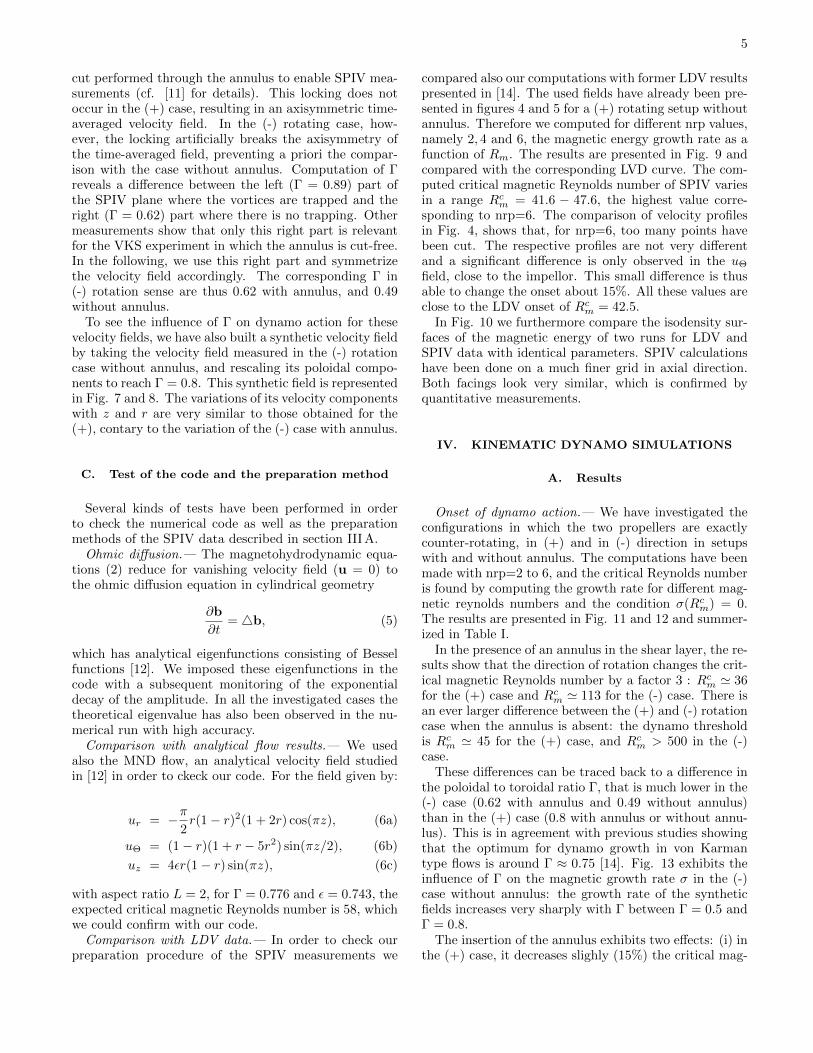
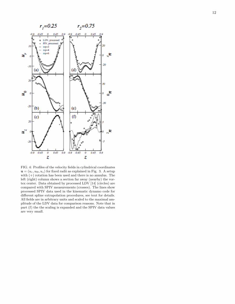
Check with LDV measurements.— LDV measurementsare free of certain deficiency of the SPIV measurements,especially near the cylinder boundary, where reliable ve-locity fields can be obtained. It is therefore interesting totest the validity of our SPIV field preparation by compar-ison with LDV fields obtained previously by Ravelet et al.[14]. Figure 4 compares the velocity fields of LDV withthe new SPIV measurements for fixed radial coordinatecuts explained in Fig. 3. One cut is close to the vortexcenter, the other one far away. A setup with (+) counterrotation has been used without annulus. In addition, theprocessed data, used in the code, with the aid of sym-metrization and spline extrapolation for different nrp areshown. The difference between the two curves is mainlyin the azimuthal field uΘ nearby the blades. Note, thatthe large deviations of the two processed curves for theuz field in the regime r ≈ [−0.6, 0.6] is only due to theperformed scaling described in the caption. The SPIVdataset is finer and overall the comparison is quite satis-factory.

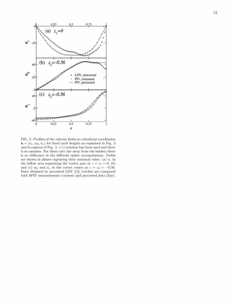
Corresponding cuts for fixed axial coordinate areshown in Fig. 5 for planes in the vortex region and in thepure inflow layer separating the vortex pair. The agree-ment between LDV and SPIV measurements is good evenif a small deviation can be observed on ur.

AJOUTER PHRASE CONCLUSION: AVANTAGESPIV/LDV

B. Influence of the annulus

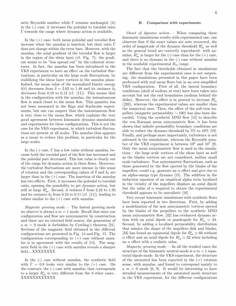
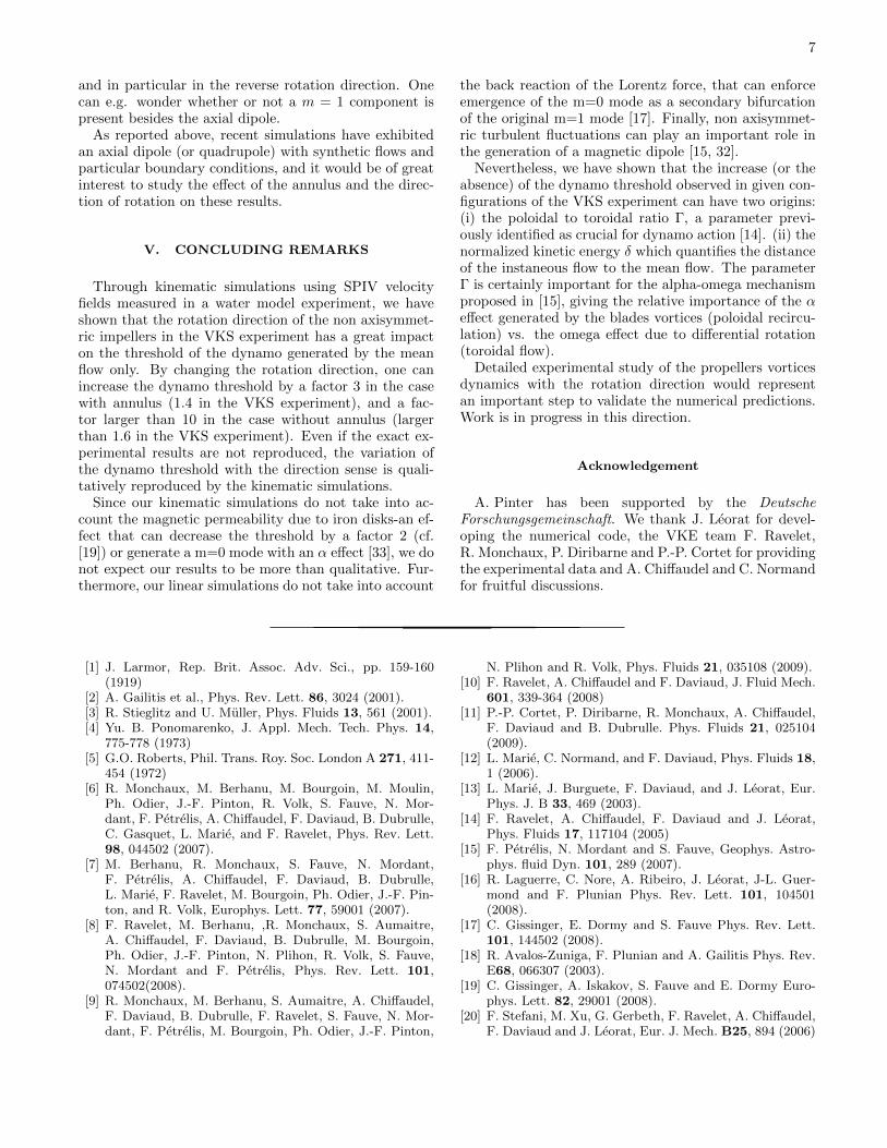
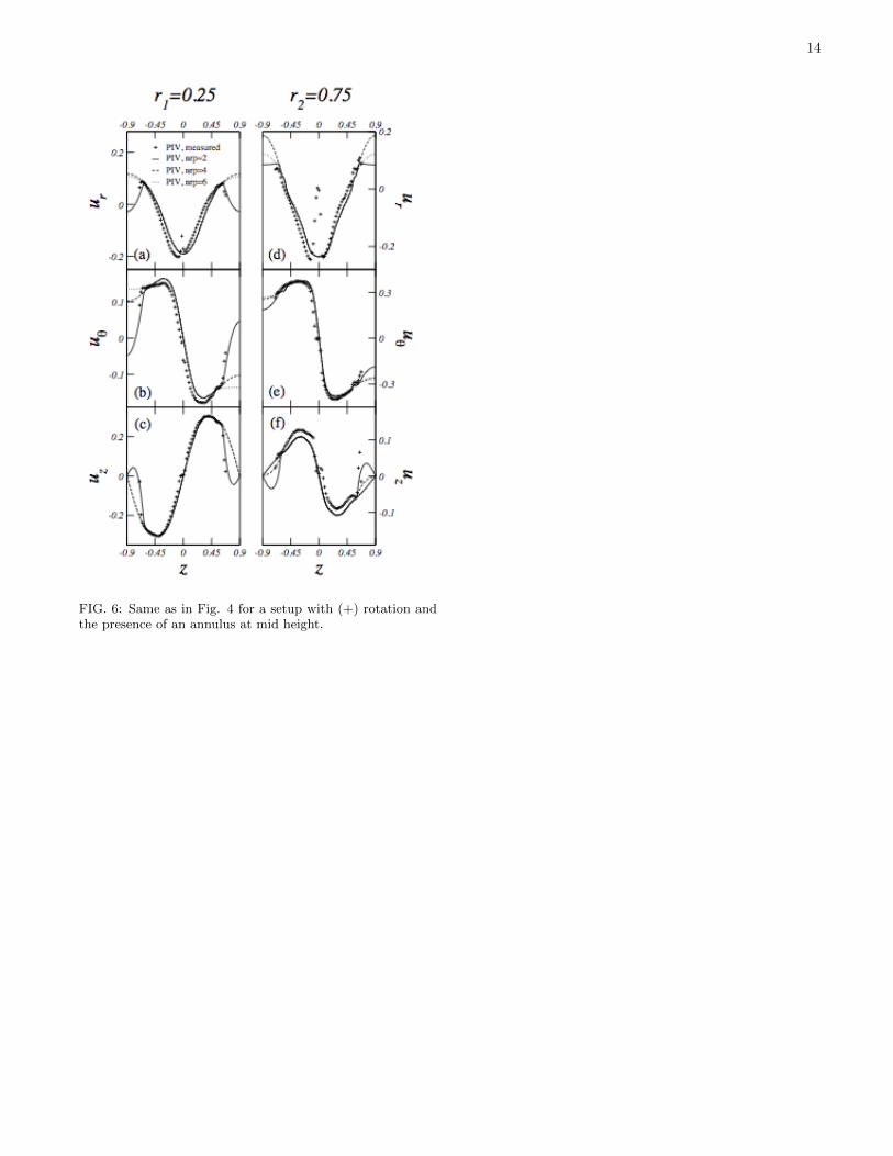
In order to study the influence of the annulus, we havemeasured the corresponding time-averaged velocity fieldfor different nrp (cf. Fig. 6). The velocity fields cor-responding to the 4 configurations that are used in thekinematic dynamo simulations are then shown in Figures7 and 8.

In the (+) rotation case, the axial gradient of ur, uθand uz are larger in the region of the shear layer. Thevariation with r of the velocity fields looks very similarexcept for ur at mid-radius. However, the poloidal totoroidal ratio Γ, does not reflect this difference: Γ = 0.8in both cases.

In the (-) rotation case, we were not able to performsuch a detailed comparison, due to an unexpected ex-perimental problem: the locking of large scale vorticesof the middle shear layer at the position of the small

5

cut performed through the annulus to enable SPIV mea-surements (cf. [11] for details). This locking does notoccur in the (+) case, resulting in an axisymmetric time-averaged velocity field. In the (-) rotating case, how-ever, the locking artificially breaks the axisymmetry ofthe time-averaged field, preventing a priori the compar-ison with the case without annulus. Computation of Γreveals a difference between the left (Γ = 0.89) part ofthe SPIV plane where the vortices are trapped and theright (Γ = 0.62) part where there is no trapping. Othermeasurements show that only this right part is relevantfor the VKS experiment in which the annulus is cut-free.In the following, we use this right part and symmetrizethe velocity field accordingly. The corresponding Γ in(-) rotation sense are thus 0.62 with annulus, and 0.49without annulus.

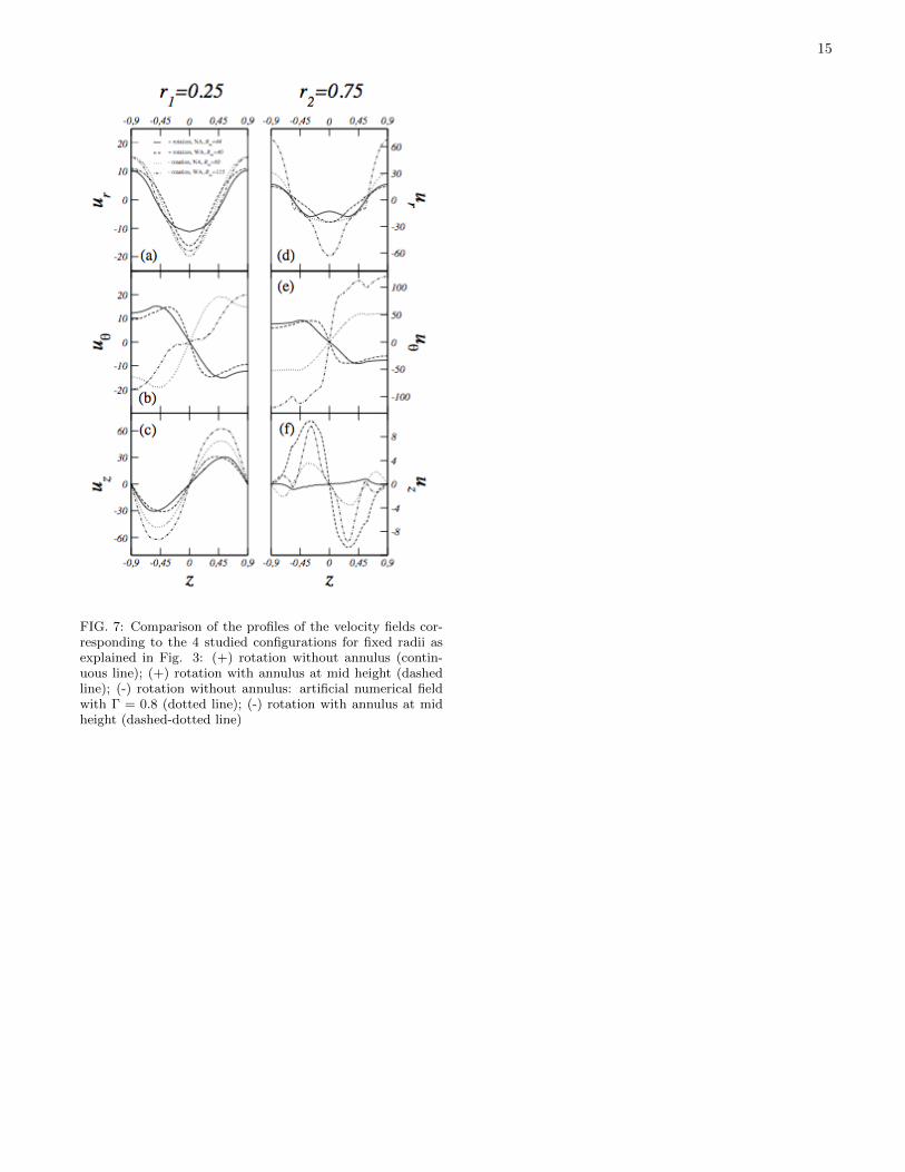
To see the influence of Γ on dynamo action for thesevelocity fields, we have also built a synthetic velocity fieldby taking the velocity field measured in the (-) rotationcase without annulus, and rescaling its poloidal compo-nents to reach Γ = 0.8. This synthetic field is representedin Fig. 7 and 8. The variations of its velocity componentswith z and r are very similar to those obtained for the(+), contary to the variation of the (-) case with annulus.

C. Test of the code and the preparation method

Several kinds of tests have been performed in orderto check the numerical code as well as the preparationmethods of the SPIV data described in section III A.

Ohmic diffusion.— The magnetohydrodynamic equa-tions (2) reduce for vanishing velocity field (u = 0) tothe ohmic diffusion equation in cylindrical geometry

∂b

∂t= 4b, (5)

which has analytical eigenfunctions consisting of Besselfunctions [12]. We imposed these eigenfunctions in thecode with a subsequent monitoring of the exponentialdecay of the amplitude. In all the investigated cases thetheoretical eigenvalue has also been observed in the nu-merical run with high accuracy.

Comparison with analytical flow results.— We usedalso the MND flow, an analytical velocity field studiedin [12] in order to ckeck our code. For the field given by:

ur = −π2r(1− r)2(1 + 2r) cos(πz), (6a)

uΘ = (1− r)(1 + r − 5r2) sin(πz/2), (6b)

uz = 4εr(1− r) sin(πz), (6c)

with aspect ratio L = 2, for Γ = 0.776 and ε = 0.743, theexpected critical magnetic Reynolds number is 58, whichwe could confirm with our code.

Comparison with LDV data.— In order to check ourpreparation procedure of the SPIV measurements we

compared also our computations with former LDV resultspresented in [14]. The used fields have already been pre-sented in figures 4 and 5 for a (+) rotating setup withoutannulus. Therefore we computed for different nrp values,namely 2, 4 and 6, the magnetic energy growth rate as afunction of Rm. The results are presented in Fig. 9 andcompared with the corresponding LVD curve. The com-puted critical magnetic Reynolds number of SPIV variesin a range Rcm = 41.6 − 47.6, the highest value corre-sponding to nrp=6. The comparison of velocity profilesin Fig. 4, shows that, for nrp=6, too many points havebeen cut. The respective profiles are not very differentand a significant difference is only observed in the uΘ

field, close to the impellor. This small difference is thusable to change the onset about 15%. All these values areclose to the LDV onset of Rcm = 42.5.

In Fig. 10 we furthermore compare the isodensity sur-faces of the magnetic energy of two runs for LDV andSPIV data with identical parameters. SPIV calculationshave been done on a much finer grid in axial direction.Both facings look very similar, which is confirmed byquantitative measurements.

IV. KINEMATIC DYNAMO SIMULATIONS

A. Results

Onset of dynamo action.— We have investigated theconfigurations in which the two propellers are exactlycounter-rotating, in (+) and in (-) direction in setupswith and without annulus. The computations have beenmade with nrp=2 to 6, and the critical Reynolds numberis found by computing the growth rate for different mag-netic reynolds numbers and the condition σ(Rcm) = 0.The results are presented in Fig. 11 and 12 and summer-ized in Table I.

In the presence of an annulus in the shear layer, the re-sults show that the direction of rotation changes the crit-ical magnetic Reynolds number by a factor 3 : Rcm ' 36for the (+) case and Rcm ' 113 for the (-) case. There isan ever larger difference between the (+) and (-) rotationcase when the annulus is absent: the dynamo thresholdis Rcm ' 45 for the (+) case, and Rcm > 500 in the (-)case.

These differences can be traced back to a difference inthe poloidal to toroidal ratio Γ, that is much lower in the(-) case (0.62 with annulus and 0.49 without annulus)than in the (+) case (0.8 with annulus or without annu-lus). This is in agreement with previous studies showingthat the optimum for dynamo growth in von Karmantype flows is around Γ ≈ 0.75 [14]. Fig. 13 exhibits theinfluence of Γ on the magnetic growth rate σ in the (-)case without annulus: the growth rate of the syntheticfields increases very sharply with Γ between Γ = 0.5 andΓ = 0.8.

The insertion of the annulus exhibits two effects: (i) inthe (+) case, it decreases slighly (15%) the critical mag-

6

netic Reynolds number while Γ remains unchanged; (ii)in the (-) case, it increases the poloidal to toroidal ratioΓ towards the range where dynamo action is available.

In the (+) case, both mean poloidal and toroidal flowincrease when the annulus is inserted, but their ratio Γdoes not change within the error bars. However, with theannulus, the axial gradient of the toroidal flow is largerin the region of the shear layer (cf. Fig. 7): the gradi-ent seems to be ”less spread out” by the coherent struc-tures. In fact, the annulus has been intruduced in theVKS experiment to have an effect on the turbulent fluc-tuations, in particular on the large scale fluctuations, bystabilizing the shear layer vortices in the annulus plane.Indeed, the mean value of the normalized kinetic energyδ(t) decreases from δ = 2.02 to 1.48 and its variance δ2decreases from 0.18 to 0.12 (cf. [11]). This means thatin the configuration with the annulus, the instantaneousflow is much closer to the mean flow. This quantity hasnot been measured in the Riga and Karlsruhe experi-ments, but one can suspect that the instantaneous flowis very close to the mean flow, which explains the verygood agreement between kinematic dynamo simulationsand experiments for these configurations. This is not thecase for the VKS experiment, in which turbulent fluctua-tions are present at all scales. The annulus thus appearsas a mean to reduce this problem, in particular for thelarge scales.

In the (-) case, Γ has a low value without annulus, be-cause both the toroidal part of the flow has increased andthe poloidal part decreased. This low value is clearly outof the range for dynamo action in these flows. Moreover,the turbulent fluctuations are more intense in this senseof rotation and the corresponding values of δ and δ2 arelarger than in the (+) case. The insertion of the annulushas two effects. First, it increases the poloidal to toroidalratio, opening the possibility to get dynamo action, butstill at large Rcm. Second, it reduces δ from 2.22 to 1.50and its variance δ2 from 0.24 to 0.11 (cf. [11]), leading tovalues similar to the (+) case with annulus.

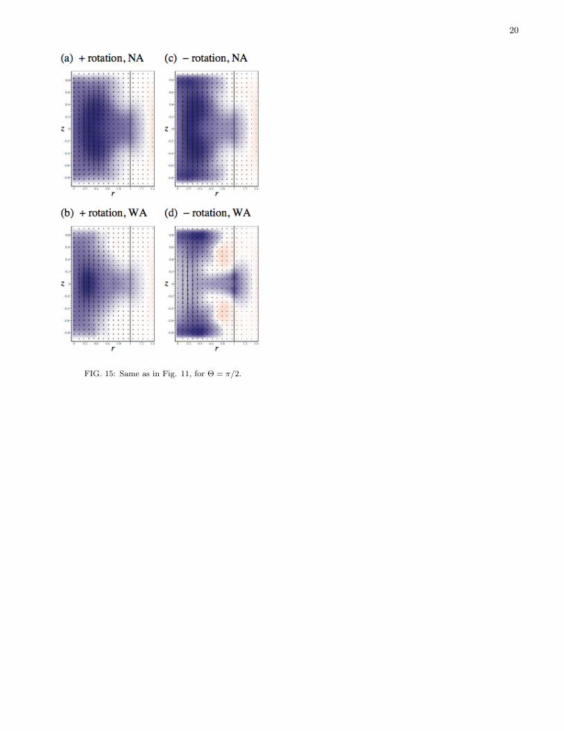
Magnetic growing mode.— The fastest growing modewe observe is always a m = 1 mode. Recall that since ourconfiguration and flow are axisymmetric by constructionand there are no external field source, the generation ofa m = 0 mode is forbidden by Cowling’s theorem [31].Sections of the magnetic field obtained in the differentconfigurations are presented in Fig. 14 and Fig. 15. Theconfiguration corresponding to (+) case without annu-lus is in agreement with the results of [14]. The mag-netic field in the (+) case with annulus reveals a sharperfield....XXXXXXXX

In the (-) case without annulus, the synthetic fieldwith Γ = 0.8 looks very similar to the (+) case. Onthe contrary, the (-) case with annulus, that correspondsto a larger Rcm is very different from the 3 other cases..XXXXXXXXXXXX

B. Comparison with experiments

Onset of dynamo action.— When comparing thesekinematic simulations results with experimental one, oneobserves that if the exact values are note recovered, theorder of magnitude of the dynamo threshold Rcm as wellas the general trend are correctly reproduced: with an-nulus, Rcm is larger for the (-) case than for the (+) case,and there is no dynamo in the (-) case without annulusin the available experimental Rm range.

The fact that the thresholds obtained in simulationsare different from the experimental ones is not surpris-ing: the simulations presented in this paper have beenperformed with real mean flows but in an over-simplifiedVKS configuration. First of all, the lateral boundaryconditions (shell of sodium at rest) have been taken intoaccount but not the end boundaries (sodium behind thedisks). However, the effect is in general to increase Rcm([20]), whereas the experimental values are smaller thanthe numerical ones. Then, the effect of the soft-iron im-pellers (magnetic permeability ∼ 100) has also been dis-carded. Using the synthetic MND flow [12] to describethe von Karman mean axisymmetric flow, it has beenshown that infinite permability boundary conditions areable to reduce the dynamo threshold by 5% to 10% [19].Finally, and perhaps more importantly, turbulence is notadressed in the simulations, whereas the Reynolds num-ber of the VKS experiment is between 106 and 107 [9].Only the mean axisymmetric flow is used in the simula-tions : the large scale vortices of the shear layer as wellas the blades vortices are not considered, neither smallscale turbulence. Non axisymmetric fluctuations, such asthose generated by the flow ejected by the blades of theimpellers, could e.g. generate an α effect and give rise toan alpha-omega type dynamo [15]. The addition in theinduction equation of an empirical alpha term localizedin the vicinity of the impellers displays an axial dipolebut the value of α required to obtain the experimentalthreshold appears to be unrealistic [16].

Very recent kinematic simulations with synthetic flowshave been reported in two directions. First, by addinga modelization of the non axisymmetric vortices ejectedby the blades of the propellers to the synthetic MNDmean axisymmetric flow, [32] has evidenced dynamo ac-tion with an axial dipole or quadrupole for Rcm ' 34.Second, by adding a localized permeability distributionthat mimics the shape of the impellers disk and blades,[33] has found an equatorial dipole for Rcm ' 60 withoutα effect and an axial dipole for Rcm ' 32 when includingan α effect with a realistic value.

Magnetic growing mode.— In all the studied cases thestructure of the kinematic neutral mode is a m = 1 equa-torial dipole mode. In the VKS experiment, the structureof the saturated has been reported in the (+) rotationsense, with annulus, and found to correspond mainly toa m = 0 mode [6, 9]. It would be interesting to havedetailed measurements of the saturated mode structurein the VKS experiment, for the different configurations

7

and in particular in the reverse rotation direction. Onecan e.g. wonder whether or not a m = 1 component ispresent besides the axial dipole.

As reported above, recent simulations have exhibitedan axial dipole (or quadrupole) with synthetic flows andparticular boundary conditions, and it would be of greatinterest to study the effect of the annulus and the direc-tion of rotation on these results.

V. CONCLUDING REMARKS

Through kinematic simulations using SPIV velocityfields measured in a water model experiment, we haveshown that the rotation direction of the non axisymmet-ric impellers in the VKS experiment has a great impacton the threshold of the dynamo generated by the meanflow only. By changing the rotation direction, one canincrease the dynamo threshold by a factor 3 in the casewith annulus (1.4 in the VKS experiment), and a fac-tor larger than 10 in the case without annulus (largerthan 1.6 in the VKS experiment). Even if the exact ex-perimental results are not reproduced, the variation ofthe dynamo threshold with the direction sense is quali-tatively reproduced by the kinematic simulations.

Since our kinematic simulations do not take into ac-count the magnetic permeability due to iron disks-an ef-fect that can decrease the threshold by a factor 2 (cf.[19]) or generate a m=0 mode with an α effect [33], we donot expect our results to be more than qualitative. Fur-thermore, our linear simulations do not take into account

the back reaction of the Lorentz force, that can enforceemergence of the m=0 mode as a secondary bifurcationof the original m=1 mode [17]. Finally, non axisymmet-ric turbulent fluctuations can play an important role inthe generation of a magnetic dipole [15, 32].

Nevertheless, we have shown that the increase (or theabsence) of the dynamo threshold observed in given con-figurations of the VKS experiment can have two origins:(i) the poloidal to toroidal ratio Γ, a parameter previ-ously identified as crucial for dynamo action [14]. (ii) thenormalized kinetic energy δ which quantifies the distanceof the instaneous flow to the mean flow. The parameterΓ is certainly important for the alpha-omega mechanismproposed in [15], giving the relative importance of the αeffect generated by the blades vortices (poloidal recircu-lation) vs. the omega effect due to differential rotation(toroidal flow).

Detailed experimental study of the propellers vorticesdynamics with the rotation direction would representan important step to validate the numerical predictions.Work is in progress in this direction.

Acknowledgement

A. Pinter has been supported by the DeutscheForschungsgemeinschaft. We thank J. Leorat for devel-oping the numerical code, the VKE team F. Ravelet,R. Monchaux, P. Diribarne and P.-P. Cortet for providingthe experimental data and A. Chiffaudel and C. Normandfor fruitful discussions.

[1] J. Larmor, Rep. Brit. Assoc. Adv. Sci., pp. 159-160(1919)

[2] A. Gailitis et al., Phys. Rev. Lett. 86, 3024 (2001).[3] R. Stieglitz and U. Muller, Phys. Fluids 13, 561 (2001).[4] Yu. B. Ponomarenko, J. Appl. Mech. Tech. Phys. 14,

775-778 (1973)[5] G.O. Roberts, Phil. Trans. Roy. Soc. London A 271, 411-

454 (1972)[6] R. Monchaux, M. Berhanu, M. Bourgoin, M. Moulin,

Ph. Odier, J.-F. Pinton, R. Volk, S. Fauve, N. Mor-dant, F. Petrelis, A. Chiffaudel, F. Daviaud, B. Dubrulle,C. Gasquet, L. Marie, and F. Ravelet, Phys. Rev. Lett.98, 044502 (2007).

[7] M. Berhanu, R. Monchaux, S. Fauve, N. Mordant,F. Petrelis, A. Chiffaudel, F. Daviaud, B. Dubrulle,L. Marie, F. Ravelet, M. Bourgoin, Ph. Odier, J.-F. Pin-ton, and R. Volk, Europhys. Lett. 77, 59001 (2007).

[8] F. Ravelet, M. Berhanu, ,R. Monchaux, S. Aumaitre,A. Chiffaudel, F. Daviaud, B. Dubrulle, M. Bourgoin,Ph. Odier, J.-F. Pinton, N. Plihon, R. Volk, S. Fauve,N. Mordant and F. Petrelis, Phys. Rev. Lett. 101,074502(2008).

[9] R. Monchaux, M. Berhanu, S. Aumaitre, A. Chiffaudel,F. Daviaud, B. Dubrulle, F. Ravelet, S. Fauve, N. Mor-dant, F. Petrelis, M. Bourgoin, Ph. Odier, J.-F. Pinton,

N. Plihon and R. Volk, Phys. Fluids 21, 035108 (2009).[10] F. Ravelet, A. Chiffaudel and F. Daviaud, J. Fluid Mech.

601, 339-364 (2008)[11] P.-P. Cortet, P. Diribarne, R. Monchaux, A. Chiffaudel,

F. Daviaud and B. Dubrulle. Phys. Fluids 21, 025104(2009).

[12] L. Marie, C. Normand, and F. Daviaud, Phys. Fluids 18,1 (2006).

[13] L. Marie, J. Burguete, F. Daviaud, and J. Leorat, Eur.Phys. J. B 33, 469 (2003).

[14] F. Ravelet, A. Chiffaudel, F. Daviaud and J. Leorat,Phys. Fluids 17, 117104 (2005)

[15] F. Petrelis, N. Mordant and S. Fauve, Geophys. Astro-phys. fluid Dyn. 101, 289 (2007).

[16] R. Laguerre, C. Nore, A. Ribeiro, J. Leorat, J-L. Guer-mond and F. Plunian Phys. Rev. Lett. 101, 104501(2008).

[17] C. Gissinger, E. Dormy and S. Fauve Phys. Rev. Lett.101, 144502 (2008).

[18] R. Avalos-Zuniga, F. Plunian and A. Gailitis Phys. Rev.E68, 066307 (2003).

[19] C. Gissinger, A. Iskakov, S. Fauve and E. Dormy Euro-phys. Lett. 82, 29001 (2008).

[20] F. Stefani, M. Xu, G. Gerbeth, F. Ravelet, A. Chiffaudel,F. Daviaud and J. Leorat, Eur. J. Mech. B25, 894 (2006)

8

[21] P. Livermore and A. Jackson, Proc. Roy. Soc. A 462,2457 (2006).

[22] Y. Ponty, J.-P. Laval, B. Dubrulle, F. Daviaud, and J.-F. Pinton, Phys. Rev. Lett. 99, 224501 (2007).

[23] Forest[24] Lathrop[25] Y. Ponty, P. D. Minnini, D. Montgomery, J.-F. Pinton,

H. Politano and A. Pouquet, Phys. Rev. Lett. 94, 164502(2005).

[26] J.-P. Laval, P. Blaineau, N. Leprovost, B. Dubrulle, andF. Daviaud, Phys. Rev. Lett. 96, 204503 (2006).

[27] B. Dubrulle, P. Blaineau, O. Mafra-Lopez, F. Daviaud,J.-P. Laval and R. Dolganov, New J. Phys. 9, 308 (2007).

[28] R. Monchaux, Mecanique statistique et effet dynamo dansun ecoulement de von Karman turbulent, PhD thesis,Universite de Paris 7 (2007).

[29] F. Ravelet, L. Marie, A. Chiffaudel, F. Daviaud, Phys.Rev. Lett. 93, 164501 (2004).

[30] J. Leorat, Numerical simulations of cylindrical dynamos:Scope and method, in Progress in Turbulence Research,Progress in Astronautics and Aeronautics, Vol. 162(AIAA, Washington,1994),p. 282.

[31] H.K. Moffatt, Magnetic field generation in electricallyconducting fluids, Cambridge University Press, Cam-bridge, 1978

[32] C. Gissinger, A numerical model of the VKS experiment,arXiv:0906.3792 (2009)

[33] A. Giesecke, F. stefani and G. Gerbeth, Role of soft-ironimpellers on the mode selection in the VKS dynamo ex-periment, preprint (2009)

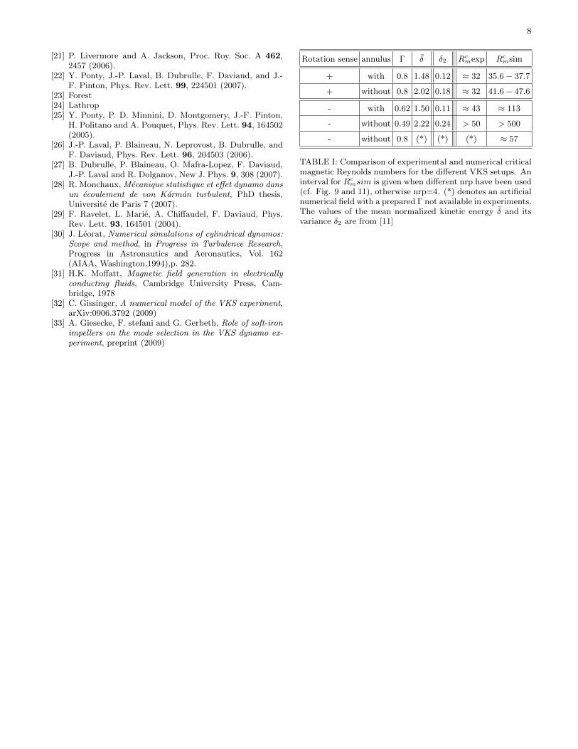
Rotation sense annulus Γ δ δ2 Rcmexp Rc

msim

+ with 0.8 1.48 0.12 ≈ 32 35.6 − 37.7

+ without 0.8 2.02 0.18 ≈ 32 41.6 − 47.6

- with 0.62 1.50 0.11 ≈ 43 ≈ 113

- without 0.49 2.22 0.24 > 50 > 500

- without 0.8 (*) (*) (*) ≈ 57

TABLE I: Comparison of experimental and numerical criticalmagnetic Reynolds numbers for the different VKS setups. Aninterval for Rc

msim is given when different nrp have been used(cf. Fig. 9 and 11), otherwise nrp=4. (*) denotes an artificialnumerical field with a prepared Γ not available in experiments.The values of the mean normalized kinetic energy δ and itsvariance δ2 are from [11]

9

FIG. 1: (a) Sketch of the simulated part of the VKS experi-ment (cross section) including both impellers (I1,I2) and anannulus (A) at mid height. The horizontal axis correspondsto the z axis. The container radius R is taken as length scale.The factor w denotes the thickness of the conducting layer(grey area) of sodium at rest in the VKS experiment. Thelayers of sodium between the impellers and the end walls ofcylinder have not been taken into account in this work. (b)Top view of the TM 73 impellers used in the VKS experi-ment [14]. The (+) (resp. (-)) rotation sense corresponds toa counterclockwise (resp. clockwise) rotating impeller.

10

FIG. 2: Dimensionless velocity field measured by SPIV inVKE and symmetrized as well as spline extrapolated (nrp=4)for kinematic dynamo simulations (see text for details). (a)(+) rotation and no annulus (NA); (b) (+) rotation and pres-ence of an annulus (WA); (c) (-) rotation and no annulus(NA); (d) (-) rotation and presence of an annulus (WA); Thecoloring displays the velocity field perpendicular to the plane,whereas red (blue) denotes a positive (negative) sign in cylin-drical coordinates (r,Θ, z). The white area for radii r > 1shows the conducting layer at rest (w = 0.6) with u = 0.

11

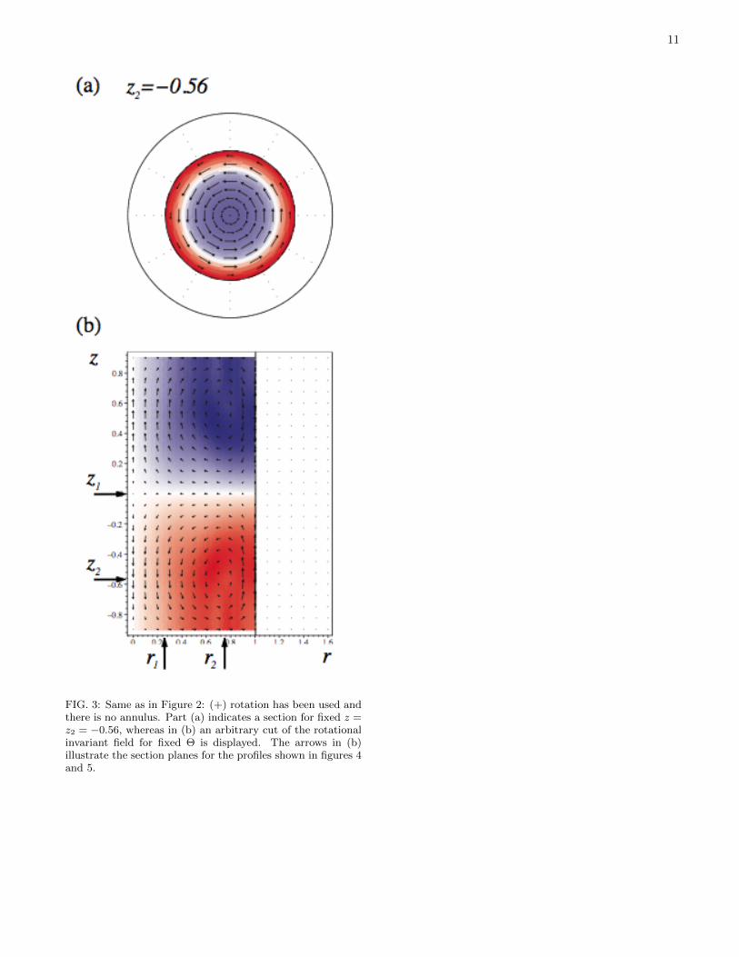
FIG. 3: Same as in Figure 2: (+) rotation has been used andthere is no annulus. Part (a) indicates a section for fixed z =z2 = −0.56, whereas in (b) an arbitrary cut of the rotationalinvariant field for fixed Θ is displayed. The arrows in (b)illustrate the section planes for the profiles shown in figures 4and 5.

12

FIG. 4: Profiles of the velocity fields in cylindrical coordinatesu = (ur, uΘ, uz) for fixed radii as explained in Fig. 3. A setupwith (+) rotation has been used and there is no annulus. Theleft (right) column shows a section far away (nearby) the vor-tex center. Data obtained by processed LDV [14] (circles) arecompared with SPIV measurements (crosses). The lines showprocessed SPIV data used in the kinematic dynamo code fordifferent spline extrapolation procedures, see text for details.All fields are in arbitrary units and scaled to the maximal am-plitude of the LDV data for comparison reasons. Note that inpart (f) the the scaling is expanded and the SPIV data valuesare very small.

13

FIG. 5: Profiles of the velocity fields in cylindrical coordinatesu = (ur, uΘ, uz) for fixed axial heights as explained in Fig. 3and in caption of Fig. 4. (+) rotation has been used and thereis no annulus. For these cuts (far away from the blades) thereis no difference in the different spline extrapolations. Fieldsare shown in planes capturing their maximal value: (a) ur inthe inflow area separating the vortex pair at z = z1 = 0; (b)and (c) uΘ and uz in the vortex center at z = z2 = −0.56.Data obtained by processed LDV [14] (circles) are comparedwith SPIV measurements (crosses) and processed data (line).

14

FIG. 6: Same as in Fig. 4 for a setup with (+) rotation andthe presence of an annulus at mid height.

15

FIG. 7: Comparison of the profiles of the velocity fields cor-responding to the 4 studied configurations for fixed radii asexplained in Fig. 3: (+) rotation without annulus (contin-uous line); (+) rotation with annulus at mid height (dashedline); (-) rotation without annulus: artificial numerical fieldwith Γ = 0.8 (dotted line); (-) rotation with annulus at midheight (dashed-dotted line)

16

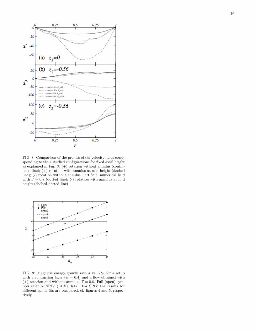
FIG. 8: Comparison of the profiles of the velocity fields corre-sponding to the 4 studied configurations for fixed axial heightas explained in Fig. 3: (+) rotation without annulus (contin-uous line); (+) rotation with annulus at mid height (dashedline); (-) rotation without annulus:: artificial numerical fieldwith Γ = 0.8 (dotted line); (-) rotation with annulus at midheight (dashed-dotted line)

FIG. 9: Magnetic energy growth rate σ vs. Rm for a setupwith a conducting layer (w = 0.4) and a flow obtained with(+) rotation and without annulus, Γ = 0.8. Full (open) sym-bols refer to SPIV (LDV) data. For SPIV the results fordifferent spline fits are compared, cf. figures 4 and 5, respec-tively.

17

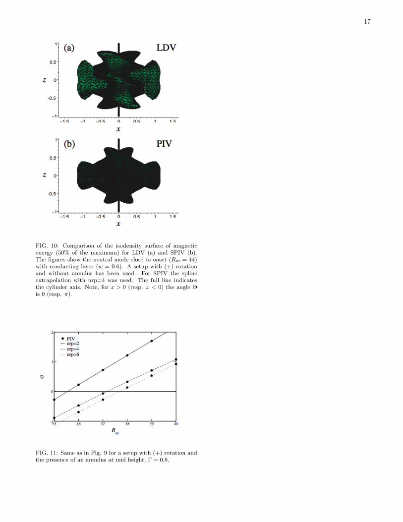
FIG. 10: Comparison of the isodensity surface of magneticenergy (50% of the maximum) for LDV (a) and SPIV (b).The figures show the neutral mode close to onset (Rm = 44)with conducting layer (w = 0.6). A setup with (+) rotationand without annulus has been used. For SPIV the splineextrapolation with nrp=4 was used. The full line indicatesthe cylinder axis. Note, for x > 0 (resp. x < 0) the angle Θis 0 (resp. π).

FIG. 11: Same as in Fig. 9 for a setup with (+) rotation andthe presence of an annulus at mid height, Γ = 0.8.

18

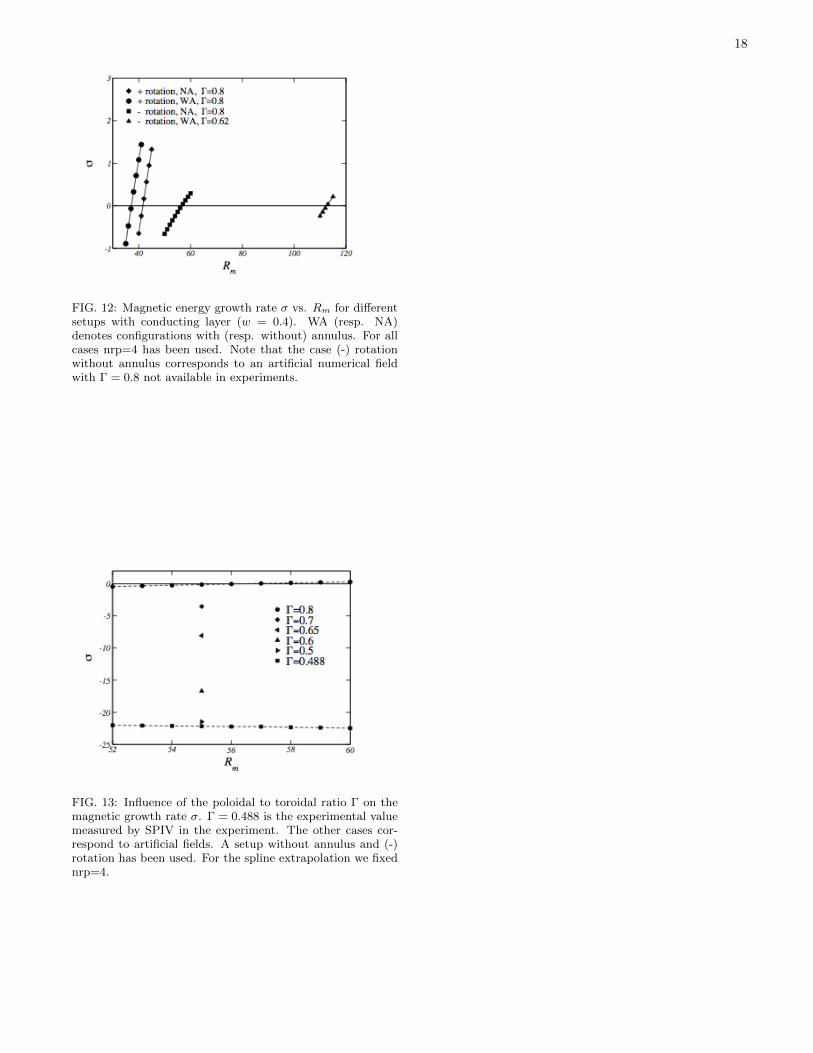
FIG. 12: Magnetic energy growth rate σ vs. Rm for differentsetups with conducting layer (w = 0.4). WA (resp. NA)denotes configurations with (resp. without) annulus. For allcases nrp=4 has been used. Note that the case (-) rotationwithout annulus corresponds to an artificial numerical fieldwith Γ = 0.8 not available in experiments.

FIG. 13: Influence of the poloidal to toroidal ratio Γ on themagnetic growth rate σ. Γ = 0.488 is the experimental valuemeasured by SPIV in the experiment. The other cases cor-respond to artificial fields. A setup without annulus and (-)rotation has been used. For the spline extrapolation we fixednrp=4.

19

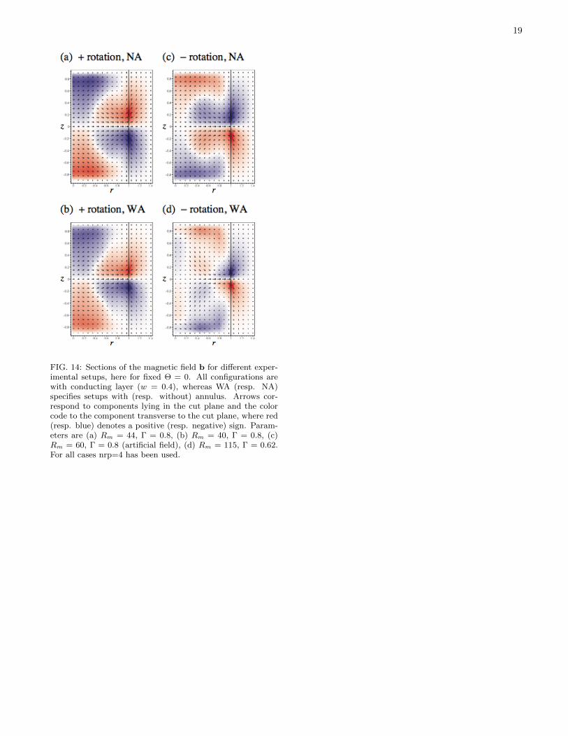
FIG. 14: Sections of the magnetic field b for different exper-imental setups, here for fixed Θ = 0. All configurations arewith conducting layer (w = 0.4), whereas WA (resp. NA)specifies setups with (resp. without) annulus. Arrows cor-respond to components lying in the cut plane and the colorcode to the component transverse to the cut plane, where red(resp. blue) denotes a positive (resp. negative) sign. Param-eters are (a) Rm = 44, Γ = 0.8, (b) Rm = 40, Γ = 0.8, (c)Rm = 60, Γ = 0.8 (artificial field), (d) Rm = 115, Γ = 0.62.For all cases nrp=4 has been used.

20

FIG. 15: Same as in Fig. 11, for Θ = π/2.