
An unconditionally convergent algorithm for the evaluation of the ultimate limit state of RC...
40
INTERNATIONAL JOURNAL FOR NUMERICAL METHODS IN ENGINEERING Int. J. Numer. Meth. Engng 2007; 72:924–963 Published online 9 May 2007 in Wiley InterScience (www.interscience.wiley.com). DOI: 10.1002/nme.2033 An unconditionally convergent algorithm for the evaluation of the ultimate limit state of RC sections subject to axial force and biaxial bending G. Alfano 1 , F. Marmo 2, ∗, † and L. Rosati 2 1 School of Engineering and Design, Brunel University, Uxbridge, Middlesex UB8 3PH, U.K. 2 Dipartimento di Ingegneria Strutturale, Universit` a degli Studi di Napoli Federico II, Italy SUMMARY We present a numerical procedure, based upon a tangent approach, for evaluating the ultimate limit state (ULS) of reinforced concrete (RC) sections subject to axial force and biaxial bending. The RC sections are assumed to be of arbitrary polygonal shape and degree of connection; furthermore, it is possible to keep fixed a given amount of the total load and to find the ULS associated only with the remaining part which can be increased by means of a load multiplier. The solution procedure adopts two nested iterative schemes which, in turn, update the current value of the tentative ultimate load and the associated strain parameters. In this second scheme an effective integration procedure is used for evaluating in closed form, as explicit functions of the position vectors of the vertices of the section, the domain integrals appearing in the definition of the tangent matrix and of the stress resultants. Under mild hypotheses, which are practically satisfied for all cases of engineering interest, the existence and uniqueness of the ULS load multiplier is ensured and the global convergence of the proposed solution algorithm to such value is proved. An extensive set of numerical tests, carried out for rectangular, L-shaped and multicell sections shows the effectiveness of the proposed solution procedure. Copyright 2007 John Wiley & Sons, Ltd. Received 12 May 2006; Revised 5 October 2006; Accepted 7 February 2007 KEY WORDS: reinforced concrete sections; ultimate limit state; Newton method 1. INTRODUCTION Non-linear solution procedures are becoming more and more popular in current engineering practice concerning the analysis and design of reinforced concrete (RC) structures. ∗ Correspondence to: F. Marmo, Dipartimento di Ingegneria Strutturale, Universit` a degli Studi di Napoli Federico II, Via Claudio 21, 80125 Napoli, Italy. † E-mail: [email protected] Contract/grant sponsor: Consorzio ReLuIS (Rete dei Laboratori Universitari di Ingegneria Sismica) Copyright 2007 John Wiley & Sons, Ltd.
Transcript of An unconditionally convergent algorithm for the evaluation of the ultimate limit state of RC...

INTERNATIONAL JOURNAL FOR NUMERICAL METHODS IN ENGINEERINGInt. J. Numer. Meth. Engng 2007; 72:924–963Published online 9 May 2007 in Wiley InterScience (www.interscience.wiley.com). DOI: 10.1002/nme.2033
An unconditionally convergent algorithm for the evaluationof the ultimate limit state of RC sections subject to
axial force and biaxial bending
G. Alfano1, F. Marmo2,∗,† and L. Rosati2
1School of Engineering and Design, Brunel University, Uxbridge, Middlesex UB8 3PH, U.K.2Dipartimento di Ingegneria Strutturale, Universita degli Studi di Napoli Federico II, Italy
SUMMARY
We present a numerical procedure, based upon a tangent approach, for evaluating the ultimate limit state(ULS) of reinforced concrete (RC) sections subject to axial force and biaxial bending. The RC sectionsare assumed to be of arbitrary polygonal shape and degree of connection; furthermore, it is possible tokeep fixed a given amount of the total load and to find the ULS associated only with the remaining partwhich can be increased by means of a load multiplier. The solution procedure adopts two nested iterativeschemes which, in turn, update the current value of the tentative ultimate load and the associated strainparameters. In this second scheme an effective integration procedure is used for evaluating in closed form,as explicit functions of the position vectors of the vertices of the section, the domain integrals appearingin the definition of the tangent matrix and of the stress resultants. Under mild hypotheses, which arepractically satisfied for all cases of engineering interest, the existence and uniqueness of the ULS loadmultiplier is ensured and the global convergence of the proposed solution algorithm to such value isproved. An extensive set of numerical tests, carried out for rectangular, L-shaped and multicell sectionsshows the effectiveness of the proposed solution procedure. Copyright q 2007 John Wiley & Sons, Ltd.
Received 12 May 2006; Revised 5 October 2006; Accepted 7 February 2007
KEY WORDS: reinforced concrete sections; ultimate limit state; Newton method
1. INTRODUCTION
Non-linear solution procedures are becoming more and more popular in current engineering practiceconcerning the analysis and design of reinforced concrete (RC) structures.
∗Correspondence to: F. Marmo, Dipartimento di Ingegneria Strutturale, Universita degli Studi di Napoli Federico II,Via Claudio 21, 80125 Napoli, Italy.
†E-mail: [email protected]
Contract/grant sponsor: Consorzio ReLuIS (Rete dei Laboratori Universitari di Ingegneria Sismica)
Copyright q 2007 John Wiley & Sons, Ltd.

LIMIT STATE ANALYSIS OF RC SECTIONS 925
This is mainly due to the fact that most of the modern building codes [1–4] adopt an ultimatelimit state (ULS) approach and to the need of employing non-linear finite element codes [5–9]in order to fulfil the strict requirements imposed by the performance-based methodology forthe design of new structures and the analysis of the existing ones subject to seismic or windforces.
Within this framework a prominent place is represented by RC sections of arbitrary shape, eithersingle- or multi-cell, subject to axial force and biaxial bending since their ULS analysis routinelyoccurs in a huge variety of practical cases, such as abutments, bridge piers, columns or core wallsystems.
Furthermore, the non-linear finite element analysis of RC structures, often based on a tangentapproach, requires the calculation of the stiffness matrix of the cross section and the evaluation ofthe internal forces obtained by integrating non-linear stress fields over the section.
Several contributions have appeared in the past on the two issues referred above. With specificreference to the ULS analysis of RC sections we mention, without any claim of completeness,the research by Brondum [10, 11] and Yen [12] who adopted a method based upon a rectangularstress block. More refined approaches have been proposed in [13–20].
Recently, Fafitis [21] developed a method for the computation of the interaction surface of RCsections subject to axial force and biaxial bending based upon the Green’s theorem. The method,which is based on special assumptions on the stress distribution in the cross section, has beensubsequently employed in [22].
A different approach for computing the stiffness matrix and the internal forces of the section hasbeen presented in [23, 24]. Particularly original is the approach presented in [23] since the authorsdeveloped a numerical algorithm based upon the decomposition of the section in quadrilateralsin order to generalize the classical cells (or fibres) and layers methods currently employed infibre-based finite-element non-linear analysis of RC frames [7–9].
Clearly, the technique which adopts the decomposition of the cross section in a dense grid ofcells is extremely expensive from the computational point of view due to the large amount ofinformation needed to characterize the non-linear behaviour of the section, through its tangentstiffness matrix, and to evaluate the internal forces.
Conversely, we illustrate a solution strategy of tangent type for evaluating the ULS of RCsections of arbitrary shape and degree of connection in which the above-mentioned drawbacks arecompletely ruled out.
The proposed strategy adopts two nested iterative schemes: the first one updates the currentvalue of the tentative ultimate load in the form fi = fe + (�i − 1)fl by searching for a positivescalar �i which amplifies the initial set fe of the applied forces along a specified load direction fl,fe typically being the values obtained at a given section by the analysis of the structural modelwhich the section belongs to.
Under the typically satisfied hypothesis that the admissible domain is convex and assumingfe internal to such domain, the existence and uniqueness of the load multiplier �∗ correspondingto the attainment of the ULS is easily verified. It is also proved that the proposed algorithm isglobally convergent to this unique solution.
The second iterative procedure represents the main computational burden of the proposed solu-tion strategy since it amounts to evaluating the parameters of the unknown strain field associatedwith fi . This task is accomplished by means of a modified Newton method, occasionally enhancedwith line searches, so that the evaluation of the tangent stiffness matrix of the cross section andof the internal forces associated with the non-linear stress field is required.
Copyright q 2007 John Wiley & Sons, Ltd. Int. J. Numer. Meth. Engng 2007; 72:924–963DOI: 10.1002/nme

926 G. ALFANO, F. MARMO AND L. ROSATI
Global convergence of the second iterative procedure is ensured by proving its equivalence to theminimization of a convex potential which is bounded below and adopting a suitable modificationof the exact Hessian of the potential. The rate of convergence of the procedure is quite satisfactorysince it has been found to be quadratic in most of the performed numerical tests.
It is worth noting that the second procedure of the proposed solution strategy involves two of thebasic ingredients of any non-linear finite element analysis of RC structures, that is the evaluationof the tangent stiffness matrix and of the internal forces of a given element to be later assembledat the structural level. Therefore, the proposed algorithm can also represent a useful contributionto the non-linear finite element analysis of RC structures.
Actually, adopting a fibre approach [7] any beam or column of the structural model has to besubdivided into several subdomains and, for each of them, the stiffness matrix and the internalforces of the cross section have to be computed. Considering also the fact that this operation isrepeated for each element of the structural model and each iteration performed both at the elementand at the structural level to ensure the fulfillment of equilibrium and compatibility, the importanceof evaluating the stiffness matrix and the internal forces of a cross section as efficiently as possibleis apparent.
Remarkably, this task is accomplished in the present paper since the domain integrals representingthe entries of the stiffness matrix of the internal force vector are evaluated in closed form solely asfunctions of the position vectors of the vertices of the section, assumed to be polygonal. Thus, whatare really needed in our approach are the constitutive parameters of the non-linear stress functionto be integrated and the vertices of the section, provided that it has, or it can be approximated by,a polygonal shape. As a consequence, no special assumption has to be made on the uniformityof the stress field along at least one direction as customary in other contributions on the samesubject [23].
Furthermore, the algorithm employed for evaluating the sectional stiffness matrix and the internalforces is organized in such a way as to be readily extended to concrete constitutive laws, see e.g.[25], more elaborate than the classical parabola–rectangle law adopted in the present paper tocomply with the prescriptions of the building codes [1, 2].
An additional nice feature of the proposed solution strategy, analogous to an early proposal onthe same subject [15], is to provide directly the ultimate load starting from an initial value fe.The ultimate load is obtained by increasing fe along a defined loading direction fl without theneed of knowing or constructing explicitly the whole interaction surface. Clearly, this representsa particularly useful property for efficiently post-processing the values of the internal forcesobtained from the analysis of the structural model since we directly estimate whether they are safeby checking that the ultimate load f ∗ = fe + (�∗ − 1)fl is associated with a value of �∗>1; thus �∗provides a sort of safety factor against the ultimate state.
Hundred of thousands of numerical experiments have been successfully carried out for severalRC sections in order to fully test the proposed algorithm in terms of robustness and computationalefficiency. The most significant results are reported in this paper for rectangular, L-shaped andmulticell sections.
2. ASSUMPTIONS AND MATERIAL PROPERTIES
The ULS analysis of RC sections subject to axial load and biaxial bending is carried out byadopting the assumptions specified in [1, 2]; for the reader’s ease, they are briefly recalled
Copyright q 2007 John Wiley & Sons, Ltd. Int. J. Numer. Meth. Engng 2007; 72:924–963DOI: 10.1002/nme

LIMIT STATE ANALYSIS OF RC SECTIONS 927
below:
(a) beam sections remain plane after deformation and perfect bond between steel bars andconcrete is assumed. Hence the strain in the concrete and in the steel rebars, in the directionof the beam axis, is provided by the same linear function which will be denoted by �;
(b) the stress state is uniaxial in the direction of the beam axis. Hence, the stress and straincomponents in this direction will be simply referred to as stress and strain;
(c) the tensile strength of concrete is neglected;(d) the constitutive law of concrete is provided by
�c(�) =
⎧⎪⎪⎨⎪⎪⎩0 if 0<�
�� + ��2 if �cp<��0
�cu if �cu<���cp
(1)
where �c denotes the stress in the concrete, � = −1000�cu, � = 250�, the ultimate stress�cu =−0.85fck/1.6 is expressed as a function of the characteristic compression strength fckof the concrete while �cp = −0.002 and �cu =−0.0035. The constitutive law (1) is reporteddiagramatically in Figure 1(a);
(e) the following elastic–perfectly plastic constitutive law is assumed for the reinforcing bars,see e.g. Figure 1(b)
�s(�) =
⎧⎪⎪⎨⎪⎪⎩
−�sy if − �su<�� − �sy
Es� if − �sy<���sy
�sy if �sy<���su
(2)
where �s denotes the steel stress, Es the Young modulus, �sy and �sy = �sy/Es representin turn the yield stress and the yield strain and �su is the ultimate strain. It is assumed that�su = 0.01 while, denoting by fyk the characteristic yield stress, �sy = fyk/1.15.
(a) (b)
Figure 1. Constitutive laws of materials: (a) concrete and (b) steel.
Copyright q 2007 John Wiley & Sons, Ltd. Int. J. Numer. Meth. Engng 2007; 72:924–963DOI: 10.1002/nme
928 G. ALFANO, F. MARMO AND L. ROSATI
The ULS of the section is established to be attained when the maximum compressive strain inthe concrete is equal to �cu and/or the maximum steel tensile strain is equal to �su.
Furthermore, in the case of a fully compressed section and denoting by h the section depthalong the direction orthogonal to the neutral axis, it is assumed that, for the concrete fibres lying ata distance equal to 3
7h from the most compressed vertex, strain attains values which do not exceedthe value �cp. In this circumstance we shall denote the strain at the most compressed vertex as�−c so that the minimum strain attainable in the concrete is equal to �cl where �cl = �−c for a fullycompressed section or �cl = �cu otherwise.
3. FORMULATION OF THE PROBLEM
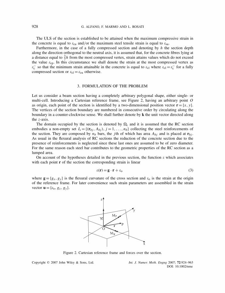
Let us consider a beam section having a completely arbitrary polygonal shape, either single- ormulti-cell. Introducing a Cartesian reference frame, see Figure 2, having an arbitrary point Oas origin, each point of the section is identified by a two-dimensional position vector r= {x, y}.The vertices of the section boundary are numbered in consecutive order by circulating along theboundary in a counter-clockwise sense. We shall further denote by k the unit vector directed alongthe z-axis.
The domain occupied by the section is denoted by �c and it is assumed that the RC sectionembodies a non-empty set Is ={(rbj , Abj ), j = 1, . . . , nb} collecting the steel reinforcements ofthe section. They are composed by nb bars, the j th of which has area Abj and is placed at rbj .As usual in the flexural analysis of RC sections the reduction of the concrete section due to thepresence of reinforcements is neglected since these last ones are assumed to be of zero diameter.For the same reason each steel bar contributes to the geometric properties of the RC section as alumped area.
On account of the hypotheses detailed in the previous section, the function � which associateswith each point r of the section the corresponding strain is linear
�(r)= g · r + �o (3)
where g= {gx , gy} is the flexural curvature of the cross section and �o is the strain at the originof the reference frame. For later convenience such strain parameters are assembled in the strainvector u= {�o, gx , gy}.
Figure 2. Cartesian reference frame and forces over the section.
Copyright q 2007 John Wiley & Sons, Ltd. Int. J. Numer. Meth. Engng 2007; 72:924–963DOI: 10.1002/nme

LIMIT STATE ANALYSIS OF RC SECTIONS 929
Defining the three-dimensional vector q={r, 0}, the stress resultants are
Nr =∫
�c
�c[�(r)] d� +nb∑j=1
�s[�(rbj )]Abj (4)
Mr =∫
�c
q× {�c[�(r)]k} d� +nb∑j=1q× {�s[�(rbj )]k}Abj (5)
where Nr is the internal axial force and the vector MTr = {(Mr)x , (Mr)y, 0} is the internal bending
moment.For the ensuing developments it is more convenient to express the previous relation in a simpler
form by introducing the two-dimensional vector ([Mr]⊥)T = {−(Mr)y, (Mr)x } obtained by pickingthe two non-zero entries of the vector k×Mr
[Mr]⊥ =∫
�c
�c[�(r)]r d� +nb∑j=1
�s[�(rbj )]Abjrbj (6)
In the sequel the stress resultants will be collectively referred to as fTr = {Nr, −(Mr)y, (Mr)x }.Clearly, on the basis of the hypothesis made on the concrete behaviour in tension and of thenon-linear behaviour of materials, the vector fr is a non-linear function of u.
The set of values of fr associated with a strain field �c��cl in the concrete and �s��su for thesteel bars defines the admissible domain. Its boundary represents the interaction surface.
We shall also indicate by fe an external force vector, i.e. the vector fTe = {Ne, −(Me)y, (Me)x }collecting the known values of axial force and biaxial bending moments which have to be checkedagainst the ULS, typically the values resulting from the analysis of the structural model which thegiven section belongs to.
Similar to [15] we do not explicitly evaluate the interaction surface in order to check whetherthe external forces collected in the vector fe lie inside the admissible domain since this task is notonly expensive to achieve but also completely unnecessary. Rather, we verify that the strain field�(r) induced by fe fulfils the above-defined limitations.
Furthermore, we suppose that the external force vector fe can be decomposed as follows:
fe = fd + fl (7)
where fd is associated with the dead load and fl embodies the external forces induced in thesection by the live load acting on the structure which the section belongs to. Thus, introducingthe vector
f(�) = fd + �fl = fe + (� − 1)fl (8)
the value �∗>0, for which f(�∗) belongs to the interaction surface, gives us a measure of howmuch the external force vector fe is distant from the interaction surface along the direction of fl.Actually, a value �>1 implies that the external force vector fe can be further increased, along thedirection defined by fl, till the ULS of the section is achieved.
On account of the above specifications we formulate the ULS problem of RC sections as follows.
Copyright q 2007 John Wiley & Sons, Ltd. Int. J. Numer. Meth. Engng 2007; 72:924–963DOI: 10.1002/nme
930 G. ALFANO, F. MARMO AND L. ROSATI
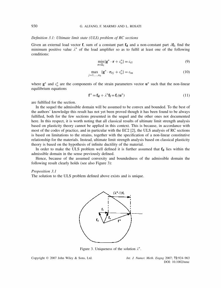
Definition 3.1: Ultimate limit state (ULS) problem of RC sections
Given an external load vector f, sum of a constant part fd and a non-constant part �fl, find theminimum positive value �∗ of the load amplifier so as to fulfil at least one of the followingconditions:
minr∈�c
{g∗ · r + �∗o} = �cl (9)
maxj=1,...,nb
{g∗ · rbj + �∗o} = �su (10)
where g∗ and �∗o are the components of the strain parameters vector u∗ such that the non-linearequilibrium equations
f ∗ = fd + �∗fl = fr(u∗) (11)
are fulfilled for the section.In the sequel the admissible domain will be assumed to be convex and bounded. To the best of
the authors’ knowledge this result has not yet been proved though it has been found to be alwaysfulfilled, both for the few sections presented in the sequel and the other ones not documentedhere. In this respect, it is worth noting that all classical results of ultimate limit strength analysisbased on plasticity theory cannot be applied in this context. This is because, in accordance withmost of the codes of practice, and in particular with the EC2 [2], the ULS analysis of RC sectionsis based on limitations to the strains, together with the specification of a non-linear constitutiverelationship for the materials. Instead, ultimate limit strength analysis based on classical plasticitytheory is based on the hypothesis of infinite ductility of the material.
In order to make the ULS problem well defined it is further assumed that fd lies within theadmissible domain in the sense previously defined.
Hence, because of the assumed convexity and boundedness of the admissible domain thefollowing result clearly holds (see also Figure 3):
Proposition 3.1The solution to the ULS problem defined above exists and is unique.
Figure 3. Uniqueness of the solution �∗.
Copyright q 2007 John Wiley & Sons, Ltd. Int. J. Numer. Meth. Engng 2007; 72:924–963DOI: 10.1002/nme

LIMIT STATE ANALYSIS OF RC SECTIONS 931
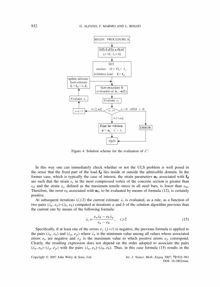
4. SOLUTION ALGORITHM
The peculiar form of system (11) naturally suggests two alternative solution strategies: the first one,exploited in [15], iteratively looks for a strain vector ui fulfilling at least one of the constraints(9)–(10) and generating a stress field over the section such that the resultant can actually bedecomposed as the sum of the fixed vector fd and of the variable one �i fl, where �i is evaluatedas a function of ui .
The second solution strategy, which is the one we are going to illustrate in the subsequentsections, first evaluates a tentative value of the variable load amplifier �i and only subsequentlyprovides the strain vector ui associated with the updated value of the ultimate load fi = fd + �i fl.
Thus, at each iteration of this last solution strategy, two nested iterative schemes have to becarried out: the first one, which is indicated as procedure A and is by far simpler, amounts toestimating the current value �i as a function of the quantities evaluated at the previous iterations.
The second iterative scheme, which will be referred to as procedure B, represents the maincomputational burden of the whole algorithm since it evaluates the strain parameters ui associatedwith fi by means of a modified Newton method enhanced with line searches.
Thus, at the i th iteration of the solution algorithm, we first estimate a tentative value �i of theload amplifier �∗ and then the strain parameters ui associated with the load fi = fd + �i fl. Theproblem of evaluating the strain vector u corresponding to a load f will be often invoked in thesequel and denoted as the non-linear problem u(f ).
The whole solution algorithm is synthetically described in Figures 4 and 5.
4.1. Solution scheme for the evaluation of �∗: Procedure A
The rationale of this phase of the solution algorithm is to associate with each estimate �i of thevariable load amplifier an error ei which measures the amount by which the current value ui ofthe strain parameters is far from the attainment of the ULS.
The error ei is defined as follows:
ei = min
{ �cl − �ci,min
�cl; �su − �si,max
�su
}(12)
where
�ci,min = minr∈�c
{�(i)o + g(i) · r}, �si,max = maxj=1,...,nb
{�(i)o + g(i) · rbj } (13)
and �(i)o and g(i) are the entries of the vector ui . Accordingly, the error ei can be considered as acomposite function of ui and �i .
Clearly, a null value of ei is indicative of the attainment of an ultimate state for the sectionwhile a positive (negative) value of ei is associated with a current estimate of the ultimate loadfi = fd + �i fl which lies inside (outside) the admissible domain. Convergence is attained if
|ei |<tole (14)
where, in our calculations, it has been assumed that tole = 10−5.The solution algorithm starts (i = 0) by setting �0 = 0 so that only the fixed part fd of the load
is initially supposed to act on the section.
Copyright q 2007 John Wiley & Sons, Ltd. Int. J. Numer. Meth. Engng 2007; 72:924–963DOI: 10.1002/nme
932 G. ALFANO, F. MARMO AND L. ROSATI
Figure 4. Solution scheme for the evaluation of �∗.
In this way one can immediately check whether or not the ULS problem is well posed inthe sense that the fixed part of the load fd lies inside or outside the admissible domain. In theformer case, which is typically the case of interest, the strain parameters u0 associated with fdare such that the strain �c in the most compressed vertex of the concrete section is greater than�cl and the strain �s, defined as the maximum tensile stress in all steel bars, is lower than �su.Therefore, the error e0 associated with u0, to be evaluated by means of formula (12), is certainlypositive.
At subsequent iterations (i�2) the current estimate �i is evaluated, as a rule, as a function oftwo pairs (�a, ea)–(�b, eb) computed at iterations a and b of the solution algorithm previous thanthe current one by means of the following formula:
�i = ea�b − eb�aea − eb
, i�2 (15)
Specifically, if at least one of the errors e j ( j<i) is negative, the previous formula is applied tothe pairs (�n, en) and (�p, ep) where �n is the minimum value among all values whose associatederrors en are negative and �p is the maximum value to which positive errors ep correspond.Clearly, the resulting expression does not depend on the order adopted to associate the pairs(�n, en)–(�p, ep) with the pairs (�a, ea)–(�b, eb). Thus, in this case formula (15) results in the
Copyright q 2007 John Wiley & Sons, Ltd. Int. J. Numer. Meth. Engng 2007; 72:924–963DOI: 10.1002/nme

LIMIT STATE ANALYSIS OF RC SECTIONS 933
Figure 5. Solution scheme for the evaluation of u(fi ).
following linear interpolation:
�i = ep�n − en�p
ep − en, i�2 (16)
�n and �p being positive by definition, the previous formula always provides positive values for �i .The same circumstance occurs if the errors e j , evaluated at the iterations j previous than
the current one, are positive but the last two pairs of errors (�i−2, ei−2)–(�i−1, ei−1) define adecreasing linear function in the plane (�, e). In this case formula (15) results in the followinglinear extrapolation:
�i = ei−2�i−1 − ei−1�i−2
ei−2 − ei−1, i�2 (17)
which supplies a positive value for �i since, by hypothesis, ei−2>ei−1 and �i−2<�i−1.Finally, when the errors e j are positive but the pairs (�i−2, ei−2)–(�i−1, ei−1) define a non-
decreasing linear function, we update �i in the form
�i = 2(�i−1 − �i−2) + �i−1, i�2 (18)
that is by adding to the last value �i−1 twice the interval between the last two estimates of �.In fact, because of the existence and uniqueness of the solution to the ULS problem and the
fact that e0 = e(0)>0, we are sure that, for a sufficiently large value of �i , e will become negative.Notice that, there is no theoretical reason for adopting 2 as amplification of the interval �i−1–�i−2if not the objective of achieving as soon as possible values of �i which make ei negative. In this
Copyright q 2007 John Wiley & Sons, Ltd. Int. J. Numer. Meth. Engng 2007; 72:924–963DOI: 10.1002/nme

934 G. ALFANO, F. MARMO AND L. ROSATI
fd
e=0fl
e<0
e>0
Figure 6. Typical case when formula (18) is used; the dashed lines are the level sets of e(�).
way we can more rapidly individuate the value �∗ which makes the error e vanish and hencecharacterize the ULS of the section.
It is worth noticing that the use of formula (18) is typically invoked at the very beginning ofthe solution algorithm whenever we are, depending on the adopted values of fd and fl, particularlyfar from the solution.
In fact, suppose that fd has been chosen very close to the (unknown) interaction surface, hencethe error e0 is very small, and that we are moving along a direction fl which makes the ultimateload f ∗ be attained for a value of �∗ by far greater than the one associated with −fl. In this casethe numerical experiments have shown that the function e(�) corresponding to the adopted choiceof fl is increasing in the vicinity of �0 = 0 so that formula (18) must be necessarily resorted to(see Figure 6).
Let us now detail how the numerical algorithm for the evaluation of �∗ proceeds after the pair(0, e0) has been determined. Actually, it is apparent that, in order to employ formulas (16)–(18),at least two values of the pair (�, e) are needed.
The second pair (�1, e1), to be used at the beginning of the algorithm is estimated as follows.Let us linearize the function u=u(f ) at f= fd
u(fd + �fl) � u(fd) +(
�u�fr
)fd
�fl =u0 +(
�fr�u
)−1
u0
�fl (19)
where (�fr/�u)u0 is the tangent operator evaluated at solution of the iterative scheme, to be detailedin the next subsection, which provides the strain vector u0 associated with fd.
Since u0 is not a limit state, the strain limits �cl and �su are not attained at any point of thesection; accordingly, we evaluate the positive scalar �1 by scaling the fixed quantity (�fr/�u)−1
u0 fladded to u0 so as to make the strain limits be attained at least at one point of the section.
The strain at the generic vertex of the concrete section or at the generic steel bar is given by
� j =u ·
⎛⎜⎜⎝
1
x j
y j
⎞⎟⎟⎠= u0 ·
⎛⎜⎜⎝
1
x j
y j
⎞⎟⎟⎠+ �
(�fr�u
)−1
u0
fl ·
⎛⎜⎜⎝
1
x j
y j
⎞⎟⎟⎠= a j + �b j (20)
Copyright q 2007 John Wiley & Sons, Ltd. Int. J. Numer. Meth. Engng 2007; 72:924–963DOI: 10.1002/nme

LIMIT STATE ANALYSIS OF RC SECTIONS 935
and is a linear function of �. Thus it is an easy matter to compute the value �cj necessary to enforcethe ultimate strain �cl at the j th vertex of the concrete section
�cj =�cl − a j
b j(21)
or, analogously, the value
�sk = �su − akbk
(22)
associated with the attainment of �su at the kth bar.Accordingly, the required value of �1 is given by
�1 = min�>0
{�cj , �sk}, j ∈ V�c, k ∈ {1, . . . , nb} (23)
where V�c denotes the set collecting the vertices of the concrete section.Starting from the value �1 we can solve the non-linear problem u(fd + �1fl) that provides the
actual strain parameters u1 associated with the load fd + �1fl, and evaluate the relevant error e1by means of (12).
We now dispose of two pairs (0, e0) and (�1, e1) which allow us to get the load amplifier at thesecond iteration of the solution algorithm; namely, if e1<e0 we get from (16) or (17)
�2 = e0�1e0 − e1
(24)
while, in the opposite case, the value
�2 = 3�1 (25)
is obtained from formula (18).For the reader’s convenience the essential steps of the algorithm are summarized in Figure 4.
4.2. Solution scheme of the non-linear problem u(f ): Procedure B
As repeatedly pointed out in the previous subsection the proposed solution algorithm requires theevaluation of the strain parameters u associated with a given value f= fd + �fl of the axial forceand bending moments acting on the section.
In this respect we remark that, in this phase of the solution algorithm, we are not looking fora limit state of the section but simply evaluating the strain field in the section corresponding toa given load value. Actually, the load fi = fd + �i fl associated with the i th estimate of � maylie outside the admissible domain so that stress on the section relative to u(fi ) may attain valuesbeyond the ultimate values reported in (1) and (2).
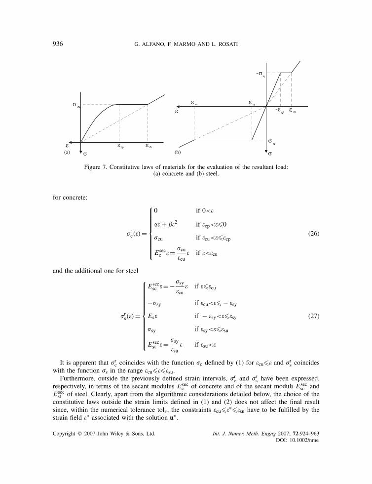
Therefore, in order to compute the resultant vector fr associated with such a stress field, weneed to define the constitutive laws (1) and (2) for strain values external to the intervals consideredtherein. For this reason the non-linear constitutive laws of the materials have been extended beyondthe ultimate values, as illustrated in Figures 7(a) and (b), by means of the following relationship
Copyright q 2007 John Wiley & Sons, Ltd. Int. J. Numer. Meth. Engng 2007; 72:924–963DOI: 10.1002/nme
936 G. ALFANO, F. MARMO AND L. ROSATI
(a) (b)
Figure 7. Constitutive laws of materials for the evaluation of the resultant load:(a) concrete and (b) steel.
for concrete:
�rc(�) =
⎧⎪⎪⎪⎪⎪⎪⎪⎨⎪⎪⎪⎪⎪⎪⎪⎩
0 if 0<�
�� + ��2 if �cp<��0
�cu if �cu<���cp
E secc � = �cu
�cu� if �<�cu
(26)
and the additional one for steel
�rs(�) =
⎧⎪⎪⎪⎪⎪⎪⎪⎪⎪⎪⎪⎨⎪⎪⎪⎪⎪⎪⎪⎪⎪⎪⎪⎩
E secsc �= −�sy
�cu� if ���cu
−�sy if �cu<�� − �sy
Es� if − �sy<���sy
�sy if �sy<���su
E secst �= �sy
�su� if �su<�
(27)
It is apparent that �rc coincides with the function �c defined by (1) for �cu�� and �rs coincideswith the function �s in the range �cu����su.
Furthermore, outside the previously defined strain intervals, �rc and �rs have been expressed,respectively, in terms of the secant modulus E sec
c of concrete and of the secant moduli E secsc and
E secst of steel. Clearly, apart from the algorithmic considerations detailed below, the choice of the
constitutive laws outside the strain limits defined in (1) and (2) does not affect the final resultsince, within the numerical tolerance tole, the constraints �cu��∗��su have to be fulfilled by thestrain field �∗ associated with the solution u∗.
Copyright q 2007 John Wiley & Sons, Ltd. Int. J. Numer. Meth. Engng 2007; 72:924–963DOI: 10.1002/nme

LIMIT STATE ANALYSIS OF RC SECTIONS 937
To avoid prolification of symbolism the stress resultants associated with the fields �rc and �rswill be collected in the vector fr, thus extending the original definition introduced after formulas(4) and (5).
Notice that any increasing function is adequate to extend �rc below �cu and �rs outside the range[�cu, �su] since, otherwise, the resultant vector fr would not be able to equilibrate an arbitrary valueof the applied load f; thus, the most natural choice for extending the definition of the constitutivelaws, which amounts to keeping constant the stresses for values of strain exceeding �cu and �su,would not meet our purposes.
Let us now illustrate the details of the modified Newton algorithm enhanced with line searcheswhich has been adopted to solve the non-linear problem u(fi ).
Suppose that a given load fTi = fTd + �i fTl = {Ni , −(Mi )y, (Mi )x } is assigned at the i th iteration
of the solution algorithm and denote by u(k)i the estimate of the relevant strain parameters ui at
the kth iteration of the modified Newton algorithm described in the sequel.To avoid cumbersome symbolism the quantity u(k)
i will be simplified to u(k) while the vector
f (k)r ={N (k)
r , −(M(k)r )y, (M
(k)r )x } will denote the resultant of the stress field generated by u(k).
Analogously we shall set f= fi . In other words, from now on, we shall describe in detail theprocedure in Figure 5 by assuming tacitly that it is started at the i th iteration of procedure Aillustrated in Figure 4 and discussed in the previous section.
According to the Newton method we introduce the residual vector
R(k) =R(u(k)) = f (k)r − f=
⎡⎣ N (k)
r − N
[M(k)r ]⊥ − [M]⊥
⎤⎦ (28)
and its derivative with respect to the strain vector evaluated at u(k)
dR(k) =(
�R�u
)u(k)
= �fr�u
∣∣∣∣u(k)
=
⎡⎢⎢⎢⎢⎣
�Nr
��o
∣∣∣∣u(k)
[�Nr
�g
]Tu(k)
�[Mr]⊥��o
∣∣∣∣u(k)
�[Mr]⊥�g
∣∣∣∣u(k)
⎤⎥⎥⎥⎥⎦ (29)
The strain vector u(k) is updated in the form
u(k+1) =u(k) − �(k)[H(k)]−1R(k) = u(k) + �(k)d(k) (30)
where d(k) = − [H(k)]−1R(k) and �(k) is a positive line search parameter.The matrix H(k) represents a positive-definite matrix which is obtained by suitably modifying
dR(k), as detailed in Section 6, in such a way that the algorithm is globally convergent and, inmost of the cases, still possesses quadratic rate of convergence.
Actually, the very special form of the constitutive laws (26) and (27) can lead to ill conditioningor even singularity of the tangent matrix dR(k). This may happen, for instance, when large positivevalues of the axial force, near the ultimate load in pure traction, are applied to the section. In thiscase the compressed portion of the concrete section is void and all of the steel bars are yielded.
A similar circumstance occurs when the concrete section is uniformly compressed and the strainvalue ranges between �cu and �cp.
Copyright q 2007 John Wiley & Sons, Ltd. Int. J. Numer. Meth. Engng 2007; 72:924–963DOI: 10.1002/nme

938 G. ALFANO, F. MARMO AND L. ROSATI
Thus, as suggested in [26], it is necessary to modify the tangent matrix dR(k) in order toguarantee convergence of the Newton method. As shown in Section 6 such a modification isnaturally suggested by physical considerations and represents a viable alternative to additionaltechniques such as the Levenberg–Marquardt approach.
Convergence of the Newton method is attained if
‖R(k)‖‖f‖ <tolR (31)
specifically, in the numerical examples reported in the sequel, it has been assumed tolR = 10−5.
4.2.1. Finding u(f ) by solving a minimization problem. In order to prove the global convergence ofthe proposed algorithm the following result, whose proof is reported in Appendix A, is important:
Proposition 4.1The function fr is integrable and admits the following convex, C1 potential
�(u) =∫
�c
∫ �(r,u)
0�rc(�) d� +
nb∑j=1
Abj
∫ �(rbj ,u)
0�rs(�) d� (32)
The closed form expression of � as a function of the co-ordinates of the vertices and of thebars is given in Appendix E.
Hence, the problem of evaluating the strain parameters u corresponding to a given applied loadf is equivalent to that of minimizing a convex function �, which is defined as follows:
�(u) = �(u) − f · u (33)
Clearly, it results R(k) =∇�(u(k)), so that the updating formula (30) can be rewritten as follows:
u(k+1) =u(k) − �(k) H(k) ∇�(u(k)) (34)
Hence, since H(k) is positive definite the updating formula provides a descent algorithm.From the expression of �, provided in Appendix E, it is easy to verify that for any section which
has at least one steel bar in its interior, i.e. always in practice, some quadratic or cubic terms inthe potential prevail and � grows indefinitely when u= (�o, g) and → +∞. This also meansthat lim→+∞ �(u) = + ∞ for any u, so that the recession cone of � is the null vector. Then,by applying Theorem 1(ii) of [27], or equivalently Theorem 27.1 of [28], the following existenceresult is obtained:
Proposition 4.2A solution u∗ to the problem u(f ) always exists, with �(u) attaining a finite global minimumat u∗. Convexity of the function � also ensures the existence of the solution to the line searchproblem.
The solution is not necessarily unique in terms of the strain-parameter vector u. In fact, thereexist possible states of deformation for the section whereby, in each point of the concrete part andin each steel bar, stress and strain define a point within a flat part of the corresponding stress–straincurves. For example this is the case when the whole section is in tension, with a zero stress in the
Copyright q 2007 John Wiley & Sons, Ltd. Int. J. Numer. Meth. Engng 2007; 72:924–963DOI: 10.1002/nme
LIMIT STATE ANALYSIS OF RC SECTIONS 939
concrete and all the steel bars yielded but with a strain below 0.01, or when the whole section isin compression, with a strain in the concrete �c verifying �cu<�c<�cp, and all the steel bars yieldedin compression. If one of these states, say u, corresponds to the solution of the problem u(f ) fora given applied load f, it is then clear that a small enough variation u of u will not change theinternal force vector fr, so that u + u will also be a solution. On the contrary, the solution isobviously unique in terms of internal force fr.
Furthermore, by making use of Corollary 8.7.1 of [28], we can also state the following result,which will be used in the next section.
Proposition 4.3Given ∈R the level set {u : �(u)�}, if not empty, is always compact.
4.2.2. Line searches. The line search parameter �(k) is estimated as the final value of the iterativeestimates �(k)
l evaluated in such a way that the residual [29]
r (k)l = r (k)(�(k)
l ) = R(u(k) + �(k)l d(k)) · d(k)
R(u(k)) · d(k)(35)
fulfils the stopping criterion
r (k)(�(k))�0.9 (36)
Further, in order to ensure that the function � actually decreases, another requirement on �(k)
is [30]�(u(k)) − �(u(k) + �(k)d(k))
�(k)R(u(k)) · d(k)� − 0.1 (37)
LemmaThe scalar function r (k) defined by (35) is a non-increasing function of �(k)
l .
ProofBeing the resultant force fr a non-decreasing function of the strain vector u
[fr(u2) − fr(u1)] · (u2 − u1)�0 ∀u1,u2 (38)
since fr is the gradient of �, see e.g. [28].The same property is fulfilled by R= fr − f. In particular, at the kth iteration of procedure B
reported in Figure 5 and for any �(k)a and �(k)
b
[R(u(k) + �(k)a d(k)) − R(u(k) + �(k)
b d(k))] · (u(k) + �(k)a d(k) − u(k) − �(k)
b d(k))�0 (39)
from which one infers
[R(u(k) + �(k)a d(k)) · d(k) − R(u(k) + �(k)
b d(k)) · d(k)](�(k)a − �(k)
b )�0 (40)
Thus, R(u(k) + �(k)d(k)) · d(k) is a non-decreasing function of �(k).On the other hand, the definition of d(k) yields
R(u(k)) · d(k) =−R(u(k)) · {[H(k)]−1R(u(k))}<0 (41)
Copyright q 2007 John Wiley & Sons, Ltd. Int. J. Numer. Meth. Engng 2007; 72:924–963DOI: 10.1002/nme

940 G. ALFANO, F. MARMO AND L. ROSATI
Hence, due to the positive-definiteness of H(k) and to the fact that the residual R(u(k)) is alwaysdifferent from zero when u(k) is not a solution vector, the scalar function r (k) defined by formula(35) is a non-increasing function of �(k) and the lemma is proved. �
The line search parameter �(k) is estimated as a function of two pairs (�(k)a , r (k)
a ) and (�(k)b , r (k)
b )
computed at iterations a and b previous than the current one l, by the linear interpolation formula
�(k)l = r (k)
a �(k)b − r (k)
b �(k)a
r (k)a − r (k)
b
, l�2 (42)
which is identical to the one adopted in the previous section for updating �i .Specifically, if at least one of the residual r (k)
j ( j<l) is negative, the previous formula is applied to
the pairs (�(k)n , r (k)
n )–(�(k)p , r (k)
p ), irrespective of the order of association, where �(k)n is the minimum
among all values whose associated residuals r (k)n are negative and �(k)
p is the maximum value which
positive residuals r (k)p correspond to. We thus write
�(k)l = r (k)
p �(k)n − r (k)
n �(k)p
r (k)p − r (k)
n
, l�2 (43)
In order to handle the situations in which the iterations previous than the current one arecharacterized only by positive residuals we specialize formula (42) as follows:
�(k)l = r (k)
l−2�(k)l−1 − r (k)
l−1�(k)l−2
r (k)l−2 − r (k)
l−1
, l�2 (44)
It certainly provides positive values for �(k)l when r (k)
l−2 = r (k)l−1 since the function r (k) is non-
increasing. Finally, whenever should it be∣∣∣∣∣r(k)l−2 − r (k)
l−1
r (k)l−2
∣∣∣∣∣<10−5 (45)
the following formula is adopted:
�(k)l = 2(�(k)
l−1 − �(k)l−2) + �(k)
l−1, l�2 (46)
Similar to the updating formulas for �i , the numerical procedure detailed above can be initiatedonly if two pairs (�(k)
l , r (k)l ) are available. They are simply provided by the values (0, 1) and
(1, r (k)(1)) so that formula (43) or (44) supplies
�(k)2 = 1
1 − r (k)(1)(47)
if r (k)(1)<1 while formula (44) specializes to
�(k)2 = 3�(k)
1 (48)
if |1 − r (k)(1)|<10−5.
Copyright q 2007 John Wiley & Sons, Ltd. Int. J. Numer. Meth. Engng 2007; 72:924–963DOI: 10.1002/nme
LIMIT STATE ANALYSIS OF RC SECTIONS 941
4.3. Global convergence of the solution algorithm
In order to prove the global convergence of the entire solution algorithm, we first prove thatprocedure B always converges. To this end we invoke the global convergence theorem (2.4.1)proved in [30] when formula (2.4.7) replaces (2.4.3). Actually, the theorem still holds in this caseas proved on page 22 of Reference [30].
This theorem is specialized here to the present context for the reader’s convenience:
Proposition 4.4For a descent method with partial line search, in which criteria (36) and (37) are used and thefollowing ‘angle condition’
− ∇�(k) · d(k)
‖∇�(k)‖‖d(k)‖�>0 (49)
is satisfied for some fixed , and if ∇� exists and is uniformly continuous on the level set{u : �(u)<�(u(1))}, then either ∇�(k) = 0 for some k, or �(k) → − ∞, or ∇�(k) → 0.
The angle criterion is certainly satisfied when the condition number ofH(k), i.e. the ratio betweenthe maximum and the minimum eigenvalue ofH(k), is bounded above (see [30, p. 23]) as is detailedin Appendix D, which describes how H(k) is obtained modifying the exact Hessian matrix. In ourcase H(k) is assembled as a sum of two terms. One, which is contributed by the concrete part,is positive semidefinite and has a maximum eigenvalue bounded above by the eigenvalue of thematrix obtained using the initial stiffness of the concrete stress–strain curve. The second term,which is contributed by the steel bars, is also positive definite. Its minimum eigenvalue is boundedboth below, by the eigenvalue of the matrix obtained using the minimum stiffness used when thebar is yielded, and above, by the eigenvalue of the matrix obtained using always the elastic stiffnessfor all the bars. Hence, the condition number of the sum of the two terms is certainly boundedabove and the angle criterion is then satisfied.
Furthermore, because of Proposition 4.3, the level set {u : �(u)�} is compact. Hence, by theHeine–Cantor theorem ∇� is uniformly continuous on it, so that it is also uniformly continuouson {u : �(u)<�(u(1))}. Furthermore, because of Proposition 4.2, we can rule out the case that�(k) → −∞, so that only the two remaining cases are possible, both of them implying convergenceof procedure B.
On the other hand, we have seen that procedure A starts with a positive value of the error e, andthat for the assumed case of a convex admissible domain there is only one value �∗ of the loadmultiplier, corresponding to the ULS sought, that makes the error e vanish. For greater values of� the error is always negative. The extrapolation/interpolation procedure used for procedure A isthen convergent to the solution �∗. Also in terms of ULS the solution is not unique in terms ofthe strain parameters vector u.
In conclusion, the following global convergence result can be stated:
Proposition 4.5If the admissible domain is convex and bounded, the solution �∗ to the ULS problem exists andis unique, and the algorithm described in Sections 4.1 and 4.2 converges to it for any assignedvalues of fd and fl , provided that fd is internal to the admissible domain.
Copyright q 2007 John Wiley & Sons, Ltd. Int. J. Numer. Meth. Engng 2007; 72:924–963DOI: 10.1002/nme
942 G. ALFANO, F. MARMO AND L. ROSATI
5. EVALUATION OF THE RESULTANT FORCE VECTOR
The main computational burden of the modified Newton algorithm described in the previous sectionfor the evaluation of the strain vector associated with a given load fi is represented by the evaluationof the residual R(k) and the matrix H(k). Postponing to the next section a detailed account of thelatter issue we here address the computation of the residual R(k), see formula (28).
In particular, fi being fixed, we actually need to compute only (f (k)r )T={N (k)
r , −(M(k)r )y, (M
(k)r )x }
that is the axial force and the biaxial moments in equilibrium with the stress field �(k) associatedwith the strain field �(k), resulting from u(k), via the constitutive laws (26) and (27).
According to (4) and (6) the internal resultants of the stress field on the section can be written as
N (k)r =
∫�c
�rc[�(k)(r)] d� +nb∑j=1
�rs[�(k)(rbj )]Abj (50)
[M(k)r ]⊥ =
∫�c
�rc[�(k)(r)]r d� +nb∑j=1
�rs[�(k)(rbj )]Abjrbj (51)
where �(k)(r)= �(k)o + g(k) · r is the strain at the generic point associated with the parameters ofthe strain vector (u(k))T ={�(k)o , g(k)
x , g(k)y }.
The integrals in the previous formulas are evaluated by subdividing the domain of integrationinto several subdomains depending on the strain ranges appearing in the definition of the function�rc and �rs, see e.g. (26) and (27). Thus, the domain �c of the cross section is assumed to be theunion of four subdomains (e.g. see Figure 8)
�c =
⎧⎪⎪⎪⎪⎪⎪⎪⎨⎪⎪⎪⎪⎪⎪⎪⎩
�(k)c0 : {r∈ �c : 0��(k)(r)}
�(k)c1 : {r∈ �c : �cp��(k)(r)�0}
�(k)c2 : {r∈ �c : �cu��(k)(r)��cp}
�(k)c3 : {r∈ �c : �(k)(r)��cu}
(52)
Similarly the set of bars Is is subdivided into five non-overlapping subsets
Is =
⎧⎪⎪⎪⎪⎪⎪⎪⎪⎪⎪⎨⎪⎪⎪⎪⎪⎪⎪⎪⎪⎪⎩
I (k)s1 : {(rbj , Abj ) ∈ Is : �(k)(rbj )<�cu}I (k)s2 : {(rbj , Abj ) ∈ Is : �cu��(k)(rbj )< − �sy}I (k)s3 : {(rbj , Abj ) ∈ Is : −�sy��(k)(rbj )<�sy}I (k)s4 : {(rbj , Abj ) ∈ Is : �sy��(k)(rbj )<�su}I (k)s5 : {(rbj , Abj ) ∈ Is : �su��(k)(rbj )}
(53)
where the apex (·)(k) emphasizes that the subdomains iteratively change during the solution of thenon-linear problem u(f ).
We further remark that �(k)c0 , although inessential in our calculations, has been explicitly consid-
ered in (52) in order to easily extend our treatment to the cases in which concrete tensile resistance
Copyright q 2007 John Wiley & Sons, Ltd. Int. J. Numer. Meth. Engng 2007; 72:924–963DOI: 10.1002/nme
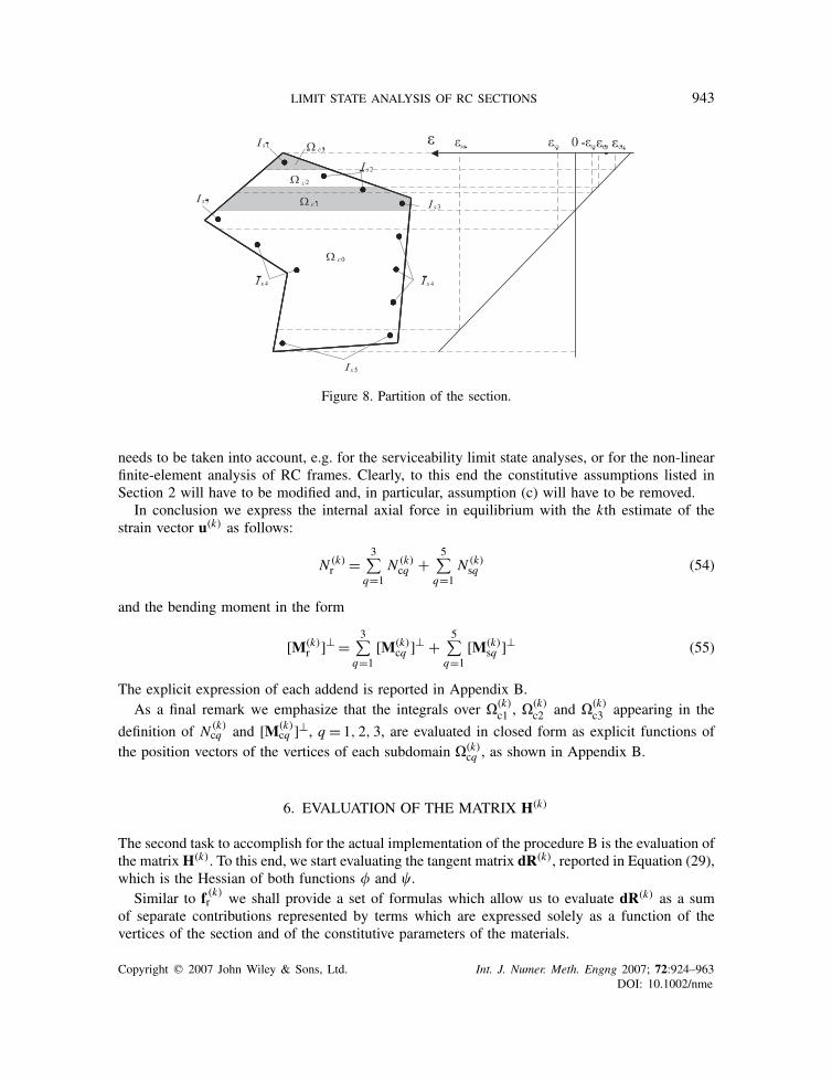
LIMIT STATE ANALYSIS OF RC SECTIONS 943
Figure 8. Partition of the section.
needs to be taken into account, e.g. for the serviceability limit state analyses, or for the non-linearfinite-element analysis of RC frames. Clearly, to this end the constitutive assumptions listed inSection 2 will have to be modified and, in particular, assumption (c) will have to be removed.
In conclusion we express the internal axial force in equilibrium with the kth estimate of thestrain vector u(k) as follows:
N (k)r =
3∑q=1
N (k)cq +
5∑q=1
N (k)sq (54)
and the bending moment in the form
[M(k)r ]⊥ =
3∑q=1
[M(k)cq ]⊥ +
5∑q=1
[M(k)sq ]⊥ (55)
The explicit expression of each addend is reported in Appendix B.As a final remark we emphasize that the integrals over �(k)
c1 , �(k)c2 and �(k)
c3 appearing in the
definition of N (k)cq and [M(k)
cq ]⊥, q = 1, 2, 3, are evaluated in closed form as explicit functions ofthe position vectors of the vertices of each subdomain �(k)
cq , as shown in Appendix B.
6. EVALUATION OF THE MATRIX H(k)
The second task to accomplish for the actual implementation of the procedure B is the evaluation ofthe matrixH(k). To this end, we start evaluating the tangent matrix dR(k), reported in Equation (29),which is the Hessian of both functions � and �.
Similar to f (k)r we shall provide a set of formulas which allow us to evaluate dR(k) as a sum
of separate contributions represented by terms which are expressed solely as a function of thevertices of the section and of the constitutive parameters of the materials.
Copyright q 2007 John Wiley & Sons, Ltd. Int. J. Numer. Meth. Engng 2007; 72:924–963DOI: 10.1002/nme

944 G. ALFANO, F. MARMO AND L. ROSATI
Adopting the same procedure illustrated for f (k)r we subdivide the concrete cross section into
four subdomains �(k)cq for computing the integrals associated with concrete and five subsets I (k)
sqfor steel.
The entries of matrix (29) have been evaluated as follows:
�Nr
��o
∣∣∣∣u(k)
=3∑
q=1
�Ncq
��o
∣∣∣∣u(k)
+5∑
q=1
�Nsq
��o
∣∣∣∣u(k)
(56)
�Nr
�g
∣∣∣∣u(k)
=3∑
q=1
�Ncq
�g
∣∣∣∣u(k)
+5∑
q=1
�Nsq
�g
∣∣∣∣u(k)
(57)
for what concerns the derivatives of the axial force Nr and
�[Mr]⊥��o
∣∣∣∣u(k)
=3∑
q=1
�[Mcq ]⊥��o
∣∣∣∣∣u(k)
+5∑
q=1
�[Msq ]⊥��o
∣∣∣∣∣u(k)
(58)
�[Mr]⊥�g
∣∣∣∣u(k)
=3∑
q=1
�[Mcq ]⊥�g
∣∣∣∣∣u(k)
+5∑
q=1
�[Msq ]⊥�g
∣∣∣∣∣u(k)
(59)
for the derivatives of [Mr]⊥. The explicit expression of each addend in the sums above is reportedin Appendix C.
However, it has been emphasized in Section 4 that the tangent matrix dR(k) may be ill conditionedor singular in special situations which can occur during the iterations of the Newton method whenlarge compressive or tensile axial forces are near the ultimate values corresponding to pure axialstrain applied to the section.
For this reason the matrixH(k) used in the update formula (30) is obtained by suitably modifyingdR(k), in order to get positive definiteness and good conditioning. To this end, the entries of H(k)
are evaluated as in the formulas (56)–(59) above except for the derivatives of the quantities Ns2,Ns4, [Ms2]⊥ and [Ms4]⊥ associated in turn with the horizontal plateau of the steel constitutive law.Accordingly, a fictitious hardening constitutive law (see Figure 9), whose constant slope has been
numerically evaluated in order to improve the convergence rate of procedure B, has been assigned
Figure 9. Steel constitutive law for the evaluation of H(k).
Copyright q 2007 John Wiley & Sons, Ltd. Int. J. Numer. Meth. Engng 2007; 72:924–963DOI: 10.1002/nme

LIMIT STATE ANALYSIS OF RC SECTIONS 945
to the steel bars belonging to the sets I (k)s2 and I (k)
s4 . Obviously, in order to correctly evaluate the
resultant vector f(k)r , the stress pertaining to each bar in the sets I (k)s2 and I (k)
s4 has been left constantand equal to −�sy and �sy, respectively. For the details the reader is referred to Appendix D.
7. NUMERICAL RESULTS
We present a comprehensive set of numerical examples which have been carried out with the aimof testing the proposed algorithm quite intensively.
Actually, although the algorithm has been conceived with the objective of finding the ultimateload associated with a fixed given load fd and a given load direction fl, it has been decided toconstruct the whole failure surface for several RC sections.
In particular, see Figure 10, each surface has been constructed in the space N , Mx , My bymaking the load fd move along the segment defined by end points fNmax − fNmin and assuming that,for each fd, the unit vector fl ={0, cos �, sin �} uniformly spans the subspace Mx − My .
The vectors fNmax and fNmin are the resultant of the stress field corresponding to a uniform strainfield �o over the section associated, respectively, with the values �o = �sy and �o = �cp.
All interaction surfaces have been constructed by considering 100 values of fd and, for each ofthem, 100 vectors fl so that the total number of analyses carried out for each surface has an orderof magnitude equal to 104.
Several typologies of RC sections have been analysed with the aim of considering a representativeset of the most typical shapes encountered in buildings, precast sheds and bridge piers. In thispaper we present numerical results obtained for a rectangular, L-shaped and a multicell section.
Geometric data and reinforcement pattern for each of them are reported in Figures 11–14 whereinRck is the characteristic compressive cubical strength of concrete. The value Rck = 25N/mm2 hasbeen used in all examples. In accordance with [1, 2], the corresponding value of fck is 20.75N/mm2.
Figure 10. Assumption of the fixed load vector.
Copyright q 2007 John Wiley & Sons, Ltd. Int. J. Numer. Meth. Engng 2007; 72:924–963DOI: 10.1002/nme

946 G. ALFANO, F. MARMO AND L. ROSATI
Figure 11. Rectangular section.
Figure 12. Failure surface (100× 100) of the rectangular section.
The numerical performances of the solution algorithm are also supplied in Table I which reportsthe minimum, maximum and average number of iterations necessary to achieve convergence ineach of the separate iterative procedures namely
• the iterative procedure used to evaluate �∗;• the iterative procedure used to evaluate u(f );• the line-search (L-S) procedure.
In this respect we remind that the second iterative procedure is invoked at each single iteration ofthe first one and that, if necessary, the third iterative procedure is adopted within a single iteration
Copyright q 2007 John Wiley & Sons, Ltd. Int. J. Numer. Meth. Engng 2007; 72:924–963DOI: 10.1002/nme

LIMIT STATE ANALYSIS OF RC SECTIONS 947
Concrete:Rck = 25 N/mm2
fck = 20.75 N/mm2
Steel: FeB38Kfyk = 375 N/mm2
� 16 at the corners� 16 on the faces
Figure 13. L-shaped section.
Figure 14. Multicell section.
Table I. Number of iterations for the construction of the failure surfaces (100× 100) of the rectangular,L-shaped and multicell sections of Figures 11, 13 and 14.
Rectangular L-shaped Multicell
Average Min. Max. Average Min. Max. Average Min. Max.
�∗ 13.2 5 30 12.7 5 30 12.4 6 30u(fi ) 6.72 2 26 6.65 2 392 6.94 1 57L–S 0.121 0 59 0.138 0 26 0.105 0 27
of the second one. In particular the average number of L-S iterations, reported in the figures thatillustrate the interaction surfaces, is by far less than 1; this confirms that the L-S procedure isactually resorted to only occasionally.
Copyright q 2007 John Wiley & Sons, Ltd. Int. J. Numer. Meth. Engng 2007; 72:924–963DOI: 10.1002/nme

948 G. ALFANO, F. MARMO AND L. ROSATI
Table II. Failure surface points (6× 6) of the rectangular section of Figure 11.
N (MN) Mx (MNm) My (MNm) N (MN) Mx (MNm) My (MNm) N (MN) Mx (MNm) My (MNm)
0.0148 0.0328 −0.0311 −0.3218 0.0710 −0.0471 −0.6585 0.0940 −0.05430.0148 0.0328 0.0311 −0.3218 0.0710 0.0471 −0.6585 0.0940 0.05430.0148 −0.0211 0.0410 −0.3218 −0.0105 0.0705 −0.6585 0.0000 0.08510.0148 −0.0835 0.0360 −0.3218 −0.0975 0.0502 −0.6585 −0.0953 0.05500.0148 −0.0835 −0.0360 −0.3218 −0.0975 −0.0502 −0.6585 −0.0953 −0.05500.0148 −0.0211 −0.0410 −0.3218 −0.0105 −0.0705 −0.6585 0.0000 −0.0851
−0.9951 0.1058 −0.0550 −1.3317 0.0995 −0.0453 −1.6683 0.0782 −0.0269−0.9951 0.1058 0.0550 −1.3317 0.0995 0.0453 −1.6683 0.0782 0.0269−0.9951 0.0105 0.0807 −1.3317 0.0211 0.0641 −1.6683 0.0316 0.0356−0.9951 −0.0791 0.0518 −1.3317 −0.0528 0.0427 −1.6683 −0.0154 0.0271−0.9951 −0.0791 −0.0518 −1.3317 −0.0528 −0.0427 −1.6683 −0.0154 −0.0271−0.9951 0.0105 −0.0807 −1.3317 0.0211 −0.0641 −1.6683 0.0316 −0.0356
Note: {N , Mx , My}max = {0.3514,−0.0316, 0.0000} and {N , Mx , My}min = {−2.0049, 0.0316, 0.0000}.
Table III. Failure surface points (6× 6) of the L-shaped section of Figure 13.
N (MN) Mx (MNm) My (MNm) N (MN) Mx (MNm) My (MNm) N (MN) Mx (MNm) My (MNm)
0.0904 0.0975 −0.0639 −0.4749 0.1573 −0.0946 −1.0402 0.1792 −0.10340.0904 0.1083 0.0640 −0.4749 0.2036 0.1183 −1.0402 0.2663 0.15370.0904 −0.0079 0.1347 −0.4749 −0.0039 0.2096 −1.0402 0.0000 0.23070.0904 −0.1065 0.0539 −0.4749 −0.1586 0.0878 −1.0402 −0.1803 0.10410.0904 −0.1537 −0.0872 −0.4749 −0.2339 −0.1343 −1.0402 −0.2725 −0.15730.0904 −0.0079 −0.1126 −0.4749 −0.0039 −0.2025 −1.0402 0.0000 −0.2329
−1.6054 0.1723 −0.0957 −2.1707 0.1406 −0.0736 −2.7360 0.0881 −0.0395−1.6054 0.2716 0.1561 −2.1707 0.2143 0.1222 −2.7360 0.1279 0.0716−1.6054 0.0039 0.2103 −2.1707 0.0079 0.1647 −2.7360 0.0118 0.0925−1.6054 −0.1728 0.1036 −2.1707 −0.1368 0.0866 −2.7360 −0.0756 0.0550−1.6054 −0.2411 −0.1400 −2.1707 −0.1759 −0.1030 −2.7360 −0.0855 −0.0516−1.6054 0.0039 −0.2304 −2.1707 0.0079 −0.1839 −2.7360 0.0118 −0.1045
Note: {N , Mx , My}max = {0.6556,−0.0118,−0.0046} and {N , Mx , My}min = {−3.3013, 0.0118, 0.0046}.
Furthermore, Tables II–IV report, for each section, the points of the relevant failure surfacedetermined assuming six values of fd and, for each of them, six vectors fl.
To provide further insights into the proposed numerical algorithm we report the sequence ofload amplifiers �i and relevant errors ei generated for two different sections. In the first case fd = 0,while in the second case both fd and fl are non-null. We further specify that, in the following,axial forces are expressed in Mega-Newton and bending moments in MNm.
The first case refers to the rectangular section of Figure 11 in which the vector fTe = {−0.65,−0.051,−0.082}. Since fl = fe, we are looking for the load amplifier �>0 which proportionallyincreases fe till reaching the ULS for the section. The ultimate load is (f ∗)T = {−0.7178,−0.0563,−0.0906} and the load amplifier is �∗ = 1.104340; the value of �∗ slightly greater than 1 meansthat the external load vector fe lies very close to the interaction surface and within the admissibledomain. The relevant results are reported in Table V.
Copyright q 2007 John Wiley & Sons, Ltd. Int. J. Numer. Meth. Engng 2007; 72:924–963DOI: 10.1002/nme

LIMIT STATE ANALYSIS OF RC SECTIONS 949
Table IV. Failure surface points (6× 6) of the multicell section of Figure 14.
N (MN) Mx (MNm) My (MNm) N (MN) Mx (MNm) My (MNm) N (MN) Mx (MNm) My (MNm)
6.2449 4.5641 −2.6351 −1.1475 7.9960 −4.6165 −8.5398 9.5820 −5.53226.2449 4.5641 2.6351 −1.1475 7.9960 4.6165 −8.5398 9.5820 5.53226.2449 0.0000 8.2561 −1.1475 0.0000 14.6726 −8.5398 0.0000 16.81526.2449 −4.5641 2.6351 −1.1475 −7.9960 4.6165 −8.5398 −9.5820 5.53226.2449 −4.5641 −2.6351 −1.1475 −7.9960 −4.6165 −8.5398 −9.5820 −5.53226.2449 0.0000 −8.2561 −1.1475 0.0000 −14.6726 −8.5398 0.0000 −16.8152
−15.9322 9.1302 −5.2713 −23.3246 7.1404 −4.1225 −30.7169 3.9657 −2.2896−15.9322 9.1302 5.2713 −23.3246 7.1404 4.1225 −30.7169 3.9657 2.2896−15.9322 0.0000 16.2803 −23.3246 0.0000 12.9491 −30.7169 0.0000 7.2800−15.9322 −9.1302 5.2713 −23.3246 −7.1404 4.1225 −30.7169 −3.9657 2.2896−15.9322 −9.1302 −5.2713 −23.3246 −7.1404 −4.1225 −30.7169 −3.9657 −2.2896−15.9322 0.0000 −16.2803 −23.3246 0.0000 −12.9491 −30.7169 0.0000 −7.2800
Note: {N , Mx , My}max = {13.6372, 0.0000, 0.0000} and {N , Mx , My}min = {−38.1093, 0.0000, 0.0000}.
Table V. Iterations of Procedure B for the rectangular sectionsubject to fd ={0, 0, 0} and fl = {−0.65,−0.051,−0.082}.
�i ei
0.000000 +1.00E+002.479895 −2.97E+000.624736 +6.47E−010.956791 +3.38E−011.112499 −3.37E−021.098371 +2.36E−021.104184 +6.29E−041.104336 +1.54E−051.104340 +3.75E−07
Table VI. Iterations of procedure B for the multicell section subject tofd = {−1.50, 1.90,−3.60} and fl = {−6.00, 3.40, 5.30}.
�i ei
0.000000 +7.98E−011.659495 +4.79E−014.146055 −2.88E+002.013478 +1.75E−012.135631 −8.39E−022.096068 +2.12E−022.104048 +6.94E−042.104307 +1.03E−052.104311 +1.50E−07
Let us now consider the multi-cell section of Figure 14 and suppose that the external forcesassociated with dead load, e.g. self-weight and permanent loads, are kept fixed and equal tofTd ={−1.50, 1.90,−3.60}.
Copyright q 2007 John Wiley & Sons, Ltd. Int. J. Numer. Meth. Engng 2007; 72:924–963DOI: 10.1002/nme

950 G. ALFANO, F. MARMO AND L. ROSATI
Assuming that the external forces due to live load are equal to fTl = {−6.00, 3.40, 5.30} wewant to know the degree of safety of the load fe = fd + fl when only the live load is increased,i.e. when we increase fe along fl. We obtain in this case the results reported in Table VI, with�∗ = 2.104311.
8. CONCLUSIONS
An unconditionally convergent algorithm for evaluating the ULS analysis of arbitrarily shaped RCsections subject to axial force and biaxial bending has been presented.
The ultimate load acting on the section is defined as the sum of a vector of internal forces whichis kept fixed and an additional one which is amplified through a load multiplier till the ULS ofthe section is attained.
Under the usual assumption of a convex and bounded interaction surface the numerical procedurewhich provides the ultimate load multiplier unconditionally converges to a unique solution.
A further iterative procedure is nested within the solution scheme delivering the ultimate loadmultiplier: it provides the strain parameters associated with a given load acting on the section. Thisfurther procedure is based upon a modified Newton method enhanced with line searches and isproved to be unconditionally convergent due to its connection with the minimization of a convexpotential.
Integrals of the stress field necessary to evaluate the residual and the entries of the modifiedHessian matrix have been evaluated in closed form as a function of the position vectors ofthe vertices of the polygonal sections. Thus, the proposed formulas for the evaluation of theintegrals can also represent a useful contribution to the non-linear finite-element analysis of RCstructures.
Further lines of research will concern the extension of the methodology proposed in the paperto stress–strain constitutive laws with softening.
APPENDIX A: PROOF OF PROPOSITION 4.1
Let �(uo,u) be a generic regular curve in �3 which connects the two points uo and u, having aparametric description in terms of an arc length s given by u= u(s), with u(so) =uo and u(s)=u.In the absence of steel bars, the work Lc
� performed by fr(u) along � is given by
Lc� =
∫ s
so
{∫�c
[�rc[�(r, u(s))]�rc[�(r, u(s))]r
]· u′(s) d�
}ds =
∫ s
so
[∫�c
F(r, s) d�]ds (A1)
F being a compound function of continuous functions, it is continuous, too. Furthermore, since�× [so, s] is a compact set of �3, the last integral exists and is finite, thus Fubini’s theorem allowsus to change the order of integration and obtain
Lc� =
∫�c
[∫�(uo,u)
�rc[�(r, u)] (d�o + dg · r)]d� (A2)
Copyright q 2007 John Wiley & Sons, Ltd. Int. J. Numer. Meth. Engng 2007; 72:924–963DOI: 10.1002/nme

LIMIT STATE ANALYSIS OF RC SECTIONS 951
Since �(r, u) = �o + g · r, we can write d�(r, u) = d�o + dg · r and then, changing variable ofintegration we obtain
Lc� =
∫�c
[∫ �(r,u)
�(r,uo)�rc(�) d�
]d� (A3)
in which the dependance on the curve � has disappeared.Analogous developments for the steel bars allow us to conclude that, for a given initial point
uo, L� is a function only of u, that is the potential � of the function fr. Assuming uo = 0 it results
�(u) =∫
�c
[∫ �(r,u)
0�rc(�) d�
]d� +
nb∑j=1
Abj
∫ �(rbj ,u)
0�rs(�) d� (A4)
To prove that the � is convex, it is equivalent to demonstrate that its derivative, that is fr, ismonotonically increasing. This follows from:
[fr(u2) − fr(u1)] · (u2 − u1) =[
Nr(�o2, g2) − Nr(�o1, g1)
[Mr]⊥(�o2, g2) − [Mr]⊥(�o1, g1)
]·[
�o2 − �o1
g2 − g1
]
=∫
�c
{�rc[�(r,u2)] − �rc[�(r,u1)]}[�(r,u2) − �(r,u1)] d�
+nb∑j=1
{{�rs[�(rbj ,u2)] − �rs[�(rbj ,u1)]}Abj [�(rbj ,u2)
− �(rbj ,u1)]}�0 (A5)
Since the stress–strain laws are monotonically increasing both for concrete and for steel, the lastinequality holds because the two terms on its left-hand side are integral or sums of non-negativeterms.
APPENDIX B: INTEGRATION FORMULAS FOR THE EVALUATION OF f (k)r
Recalling definitions (52) and (53) and that �(k)o and g(k) are the components of u(k), the explicitexpression of the terms which contribute to the sums in (54) and (55) are
N (k)c1 =
∫�(k)c1
�rc d�= (��(k)o + �(�(k)o )2)A(k)c1 + (� + 2��(k)o )s(k)c1 · g(k) + �J(k)
c1 g(k) · g(k)
N (k)c2 =
∫�(k)c2
�rc d�= A(k)c2 �cu
N (k)c3 =
∫�(k)c3
�rc d�= E secc A(k)
c3 �(k)o + E secc s(k)c3 · g(k)
(B1)
where A(k)cq , s
(k)cq and J(k)
cq denote the first three area moments of each concrete subdomain �(k)cq .
Copyright q 2007 John Wiley & Sons, Ltd. Int. J. Numer. Meth. Engng 2007; 72:924–963DOI: 10.1002/nme
952 G. ALFANO, F. MARMO AND L. ROSATI
Since each subdomain is polygonal, the three moments above can be evaluated as functions ofthe position vectors of the relevant vertices r (k)
q j by means of the general formula reported in [15].Furthermore, the contributions to the expression of N (k)
r in (54) due to steel are provided by
N (k)s1 = ∑
j∈I (k)s1
�rs(�(rbj ))Abj = E secsc A(k)
s1 �(k)o + E secsc s(k)s1 · g(k)
N (k)s2 = ∑
j∈I (k)s2
�rs(�(rbj ))Abj = −�sy A(k)s2
N (k)s3 = ∑
j∈I (k)s3
�rs(�(rbj ))Abj = EsA(k)s3 �(k)o + Es s
(k)s3 · g(k)
N (k)s4 = ∑
j∈I (k)s4
�rs(�(rbj ))Abja = �sy A(k)s4
N (k)s5 = ∑
j∈I (k)s5
�rs(�(rbj ))Abj = E secst A(k)
s5 �(k)o + E secst s(k)s5 · g(k)
(B2)
where A(k)sq denotes the total area of bars included in the qth steel subset I (k)
sq of the reinforcements
set Is and s(k)sq the relevant first moment of inertia.Accordingly
A(k)sq = ∑
j∈I (k)sq
Abj , s(k)sq = ∑j∈I (k)
sq
Abjrbj (B3)
For what concerns the bending moment the sums in (55) associated with the concrete subdomainsare given by
[M(k)c1 ]⊥ =
∫�(k)c1
�rcr d�=[��(k)o + �(�(k)o )2]s(k)c1 + (� + 2��(k)o )J(k)c1 g
(k)
+ �J(k)c1 (g(k) ⊗ g(k))
[M(k)c2 ]⊥ =
∫�(k)c2
�rcr d�= �cus(k)c2
[M(k)c3 ]⊥ =
∫�(k)c3
�rcr d�= E secc �(k)o s(k)c3 + E sec
c J(k)c3 g
(k)
(B4)
while those associated with steel are
[M(k)s1 ]⊥ = ∑
j∈I (k)s1
�rs(�(rbj ))Abjrbj = E secsc �(k)o s(k)s1 + E sec
sc J(k)s1 g
(k)
[M(k)s2 ]⊥ = ∑
j∈I (k)s2
�rs(�(rbj ))Abjrbj =−�sys(k)s2
[M(k)s3 ]⊥ = ∑
j∈I (k)s3
�rs(�(rbj ))Abjrbj = Es�(k)o s(k)s3 + EsJ
(k)s3 g
(k) (B5)
Copyright q 2007 John Wiley & Sons, Ltd. Int. J. Numer. Meth. Engng 2007; 72:924–963DOI: 10.1002/nme
LIMIT STATE ANALYSIS OF RC SECTIONS 953
[M(k)s4 ]⊥ = ∑
j∈I (k)s4
�rs(�(rbj ))Abjrbj = �sys(k)s4
[M(k)s5 ]⊥ = ∑
j∈I (k)s5
�rs(�(rbj ))Abjrbj = E secst �(k)o s(k)s5 + E sec
st J(k)s5 g
(k)
The third-order tensor J(k)cq appearing in (B4) is evaluated by means of the same general formula
reported in [15]
J(k)cq =
∫�(k)cq
(r ⊗ r⊗ r) d�= 1
20
n(k)cq∑j=1
c(k)q j [r(k)
q j ⊗ r(k)q j ⊗ r(k)
q j
+ 1
3(r(k)
q( j+1) ⊗ r(k)q j ⊗ r(k)
q j + r(k)q( j+1) ⊗ r(k)
q( j+1) ⊗ r(k)q j + r(k)
q( j+1) ⊗ r(k)q j ⊗ r(k)
q( j+1)
+ r(k)q j ⊗ r(k)
q( j+1) ⊗ r(k)q j + r(k)
q j ⊗ r(k)q( j+1) ⊗ r(k)
q( j+1) + r(k)q j ⊗ r(k)
q j ⊗ r(k)q( j+1))
+ r(k)q( j+1) ⊗ r(k)
q( j+1) ⊗ r(k)q( j+1)] (B6)
where n(k)cq is the number of vertices of �(k)
cq and
c(k)q j = r(k)
q j · [r(k)q( j+1)]⊥ =
⎛⎜⎝x (k)
q j
y(k)q j
⎞⎟⎠ ·
⎛⎜⎝ y(k)
q( j+1)
−x (k)q( j+1)
⎞⎟⎠ (B7)
provided that the vertices of the boundary of each subdomain �(k)cq have been numbered in
consecutive order by circulating in counter-clockwise sense.Composition of J(k)
cq with the second-order tensor g(k) ⊗ g(k), see e.g. (B4)1, is performed asfollows:
[J(k)cq (g(k) ⊗ g(k))]i =[J(k)
cq ]i jk[g(k) ⊗ g(k)] jk (B8)
Finally, the second area moment of the qth steel subdomain is
J(k)sq = ∑
j∈I (k)sq
Abjrbj ⊗ rbj (B9)
where the significance of the adopted symbols is analogous to that employed in (B3).
APPENDIX C: INTEGRATION FORMULAS FOR THE EVALUATIONOF THE TANGENT MATRIX dR(k)
The aim of this appendix is to detail the computation of the derivatives appearing in expressions(56)–(59) for each one of the subdomains defined in (52)–(53). In this respect we remark that the
Copyright q 2007 John Wiley & Sons, Ltd. Int. J. Numer. Meth. Engng 2007; 72:924–963DOI: 10.1002/nme
954 G. ALFANO, F. MARMO AND L. ROSATI
sets I (k)sq are collections of lumped areas, so that the area moments of the steel bars belonging to
the generic set I (k)sq are discontinuously dependent on �(k)o and g(k), i.e. they are piecewise constant.
Accordingly, the derivatives of the area moments of the steel bars are zero and will be omitted inthe sequel.
The addends of the sums in (56) are given by
�Nc1
��o
∣∣∣∣u(k)
= (� + 2��(k)o )A(k)c1 + [��(k)o + �(�(k)o )2] �Ac1
��o
∣∣∣∣u(k)
+ 2�s(k)c1 · g(k)
+ (� + 2��(k)o )�sc1��o
∣∣∣∣u(k)
· g(k) + ��Jc1��o
∣∣∣∣u(k)
g(k) · g(k)
�Nc2
��o
∣∣∣∣u(k)
= �Ac2
��o
∣∣∣∣u(k)
�cu
�Nc3
��o
∣∣∣∣u(k)
= E secc A(k)
c3 + E secc �(k)o
�Ac3
��o
∣∣∣∣u(k)
+ E secc
�sc3��o
∣∣∣∣u(k)
g(k)
(C1)
for concrete and
�Ns1
��o
∣∣∣∣u(k)
= E secsc A(k)
s1 ,�Ns2
��o
∣∣∣∣u(k)
= 0
�Ns3
��o
∣∣∣∣u(k)
= EsA(k)s3 ,
�Ns4
��o
∣∣∣∣u(k)
= 0
�Ns5
��o
∣∣∣∣u(k)
= E secst A(k)
s5
(C2)
for steel bars.Similarly, the derivatives in (57) of the axial force with respect to g evaluated at u(k) are given by
�Nc1
�g
∣∣∣∣u(k)
= (��(k)o + �(�(k)o )2)�Ac1
�g
∣∣∣∣u(k)
+ (� + 2��(k)o )s(k)c1
+ (� + 2��(k)o )
[�sc1�g
]Tu(k)
g(k) + 2�J(k)c1 g
(k) + ��Jc1�g
∣∣∣∣u(k)
(g(k) ⊗ g(k))
�Nc2
�g
∣∣∣∣u(k)
= �Ac2
�g
∣∣∣∣u(k)
�cu
�Nc3
�g
∣∣∣∣u(k)
= E secc �(k)o
�Ac3
�g
∣∣∣∣u(k)
+ E secc s(k)c3 + E sec
c
[�sc3�g
]Tu(k)
g(k)
(C3)
Copyright q 2007 John Wiley & Sons, Ltd. Int. J. Numer. Meth. Engng 2007; 72:924–963DOI: 10.1002/nme

LIMIT STATE ANALYSIS OF RC SECTIONS 955
for concrete and
�Ns1
�g
∣∣∣∣u(k)
= E secsc s(k)s1 ,
�Ns2
�g
∣∣∣∣u(k)
= 0
�Ns3
�g
∣∣∣∣u(k)
= Ess(k)s3 ,
�Ns4
�g
∣∣∣∣u(k)
= 0
�Ns5
�g
∣∣∣∣u(k)
= E secst s(k)s5
(C4)
for steel bars. Notice that the composition of the third-order tensor [�Jc1/�g]u(k) with (g(k) ⊗ g(k))
is performed as in (B8)
[�Jc1�g
∣∣∣∣u(k)
(g(k) ⊗ g(k))
]i
=[
�Jc1�g
∣∣∣∣u(k)
]jli
[g(k)] j [g(k)]l = �[Jc1] jl�gi
∣∣∣∣u(k)
[g(k)] j [g(k)]l (C5)
The derivatives at u(k) of the three area moments Acq , scq and Jcq of the generic concretesubdomain �(k)
cq with respect to the strain parameters �o and g can be evaluated by invoking thegeneral formula reported in [15] and recalling that each subdomain is polygonal. Actually, eachsubdomain �(k)
cq changes with the strain parameters and the same happens for the area moments.Derivatives of area:
�Acq
��o
∣∣∣∣u(k)
= 1
2
n(k)cq∑j=1
(�rq j��o
∣∣∣∣u(k)
· [r(k)q( j+1)]⊥ + r(k)
q j · �[rq( j+1)]⊥��o
∣∣∣∣∣u(k)
)= 1
2
n(k)cq∑j=1
p(k)q j
�Acq
�g
∣∣∣∣u(k)
= 1
2
n(k)cq∑j=1
⎛⎝[�rq j
�g
]Tu(k)
[r(k)q( j+1)]⊥ +
[�[rq( j+1)]⊥
�g
]Tu(k)
r(k)q j
⎞⎠ = 1
2
n(k)cq∑j=1
q(k)q j
(C6)
Derivatives of first area moment:
�scq��o
∣∣∣∣u(k)
= 1
6
n(k)cq∑j=1
[p(k)q j (r(k)
q j + r(k)q( j+1)) + c(k)
q j
(�rq j��o
∣∣∣∣u(k)
+ �rq( j+1)
��o
∣∣∣∣u(k)
)]
�scq�g
∣∣∣∣u(k)
= 1
6
n(k)cq∑j=1
[(r(k)
q j + r(k)q( j+1)) ⊗ q(k)
q j + c(k)q j
(�rq j�g
∣∣∣∣u(k)
+ �rq( j+1)
�g
∣∣∣∣u(k)
)] (C7)
Copyright q 2007 John Wiley & Sons, Ltd. Int. J. Numer. Meth. Engng 2007; 72:924–963DOI: 10.1002/nme

956 G. ALFANO, F. MARMO AND L. ROSATI
Derivatives of second area moment:
�Jcq��o
∣∣∣∣u(k)
= 1
12
n(k)cq∑j=1
{p(k)q j [r(k)
q j ⊗ r(k)q j + sym(r(k)
q( j+1) ⊗ r(k)q j ) + r(k)
q( j+1) ⊗ r(k)q( j+1)]
+ c(k)q j
[�rq j��o
∣∣∣∣u(k)
⊗ r(k)q j + sym
(�rq( j+1)
��o
∣∣∣∣u(k)
⊗ r(k)q j
)
+ �rq( j+1)
��o
∣∣∣∣u(k)
⊗ r(k)q( j+1) + r(k)
q j ⊗ �rq j��o
∣∣∣∣u(k)
+ sym
(r(k)q( j+1) ⊗ �rq j
��o
∣∣∣∣u(k)
)+ r(k)
q( j+1) ⊗ �rq( j+1)
��o
∣∣∣∣u(k)
]}
�Jcq�g
∣∣∣∣u(k)
= 1
12
n(k)cq∑j=1
{[r(k)
q j ⊗ r(k)q j + sym(r(k)
q( j+1) ⊗ r(k)q j ) + r(k)
q( j+1) ⊗ r(k)q( j+1)] ⊗ q(k)
q j
+ c(k)q j
[�rq j�g
∣∣∣∣u(k)
⊗ r(k)q j + sym
(�rq( j+1)
�g
∣∣∣∣u(k)
⊗ r(k)q j
)
+ �rq( j+1)
�g
∣∣∣∣u(k)
⊗ r(k)q( j+1) + r(k)
q j ⊗ �rq j�g
∣∣∣∣u(k)
+ sym
(r(k)q( j+1) ⊗ �rq j
�g
∣∣∣∣u(k)
)+ rq( j+1) ⊗ �rq( j+1)
�g
∣∣∣∣u(k)
]}
(C8)
The previous formulas emphasize that the required derivatives of the area moments depend uponthe change, with respect to �o and g, of the position vectors which define each subdomain �(k)
cq .Such vectors can be grouped in two mutually disjoint subsets. The first one contains the positionvectors which define the boundary of �c; accordingly their co-ordinates are fixed and the relevantderivatives with respect to �o and g are trivially zero.
Therefore, we shall concentrate on the second set, denoted in the sequel by �(k)cq , which collects
the position vectors r(k)q j belonging to the generic edge of the boundary of �c with the exception of
the relevant end points. In other words, the position vectors included in �(k)cq are those which define
vertices belonging to two adjacent subdomains �(k)c, j and �(k)
c, j+1 but different from the verticesdefining the boundary of �c.
The derivative at u(k) of each rq j ∈ �(k)cq with respect to �o and g can be derived as follows.
Let ra and rb be the end vertices of the edge of the section boundary which r(k)q j belongs to (see
Figure A1). Thus, r(k)q j can be expressed in parametric form as
r(k)q j = ra + ϑ
(k)q j (rb − ra) (C9)
Since r(k)q j ∈ �(k)
cq we can set �(r(k)q j ) = �∗ where �∗ = 0 if r(k)
q j belongs to the neutral axis
i.e. r(k)q j ∈ �(k)
c0 ∩ �(k)c1 , �∗ = �cp if r(k)
q j ∈ �(k)c1 ∩ �(k)
c2 , and �∗ = �cu if r(k)q j ∈ �(k)
c2 ∩�(k)c3 . Thus, the
Copyright q 2007 John Wiley & Sons, Ltd. Int. J. Numer. Meth. Engng 2007; 72:924–963DOI: 10.1002/nme

LIMIT STATE ANALYSIS OF RC SECTIONS 957
Figure A1. Evaluation of the position vector r(k)q j .
parameter ϑ(k)q j in (C9) can be evaluated explicitly as
ϑ(k)q j = �∗ − �(k)a
�(k)b − �(k)a
(C10)
where
�(k)a = �(k)o + g(k) · ra, �(k)b = �(k)o + g(k) · rb (C11)
Notice that the case �(k)a = �(k)b can be excluded since, otherwise, the edge defined by the endvertices ra and rb would be parallel to or belong to a generic axis of constant strain subdividingtwo adjacent subdomains �c, j and �c, j+1; in both cases no point of the edge belongs to �(k)
cq .In conclusion, on the basis of the previous three formulas we can write
�rq j��o
∣∣∣∣u(k)
= �ϑq j
��o
∣∣∣∣u(k)
(rb − ra),�rq j�g
∣∣∣∣u(k)
= (rb − ra) ⊗ �ϑq j
�g
∣∣∣∣u(k)
(C12)
where
�ϑq j
��o
∣∣∣∣u(k)
= − 1
�(k)b − �(k)a
,�ϑq j
�g
∣∣∣∣u(k)
= ra(�∗ − �(k)b ) − rb(�∗ − �(k)a )
(�(k)b − �(k)a )2(C13)
Let us now consider the derivatives appearing in (58). Invoking (B4) and (B5) one gets
�[Mc1]⊥��o
∣∣∣∣u(k)
= (� + 2��(k)o )s(k)c1 + (��o + �(�(k)o )2)�sc1��o
∣∣∣∣u(k)
+ 2�J(k)c1 g
(k)
+ (� + 2��(k)o )�Jc1��o
∣∣∣∣u(k)
g(k) + ��Jc1��o
∣∣∣∣u(k)
(g(k) ⊗ g(k))
�[Mc2]⊥��o
∣∣∣∣u(k)
= �cu�sc2��o
∣∣∣∣u(k)
�[Mc3]⊥��o
∣∣∣∣u(k)
= E secc s(k)c3 + E sec
c �(k)o�sc3��o
∣∣∣∣u(k)
+ E secc
�Jc3��o
∣∣∣∣u(k)
g(k)
(C14)
Copyright q 2007 John Wiley & Sons, Ltd. Int. J. Numer. Meth. Engng 2007; 72:924–963DOI: 10.1002/nme
958 G. ALFANO, F. MARMO AND L. ROSATI
for concrete and
�[Ms1]⊥��o
∣∣∣∣u(k)
= E secsc s(k)s1 ,
�[Ms2]⊥��o
∣∣∣∣u(k)
= 0
�[Ms3]⊥��o
∣∣∣∣u(k)
= Ess(k)s3 ,
�[Ms4]⊥��o
∣∣∣∣u(k)
= 0
�[Ms5]⊥��o
∣∣∣∣u(k)
= E secst s(k)s5
(C15)
for steel bars.Finally, the derivatives in (59) at u(k) of [Mcq ]⊥ and [Msq ]⊥ with respect to g are given by
�[Mc1]⊥�g
∣∣∣∣u(k)
= (��(k)o + �(�(k)o )2)�sc1�g
∣∣∣∣u(k)
+ (� + 2��(k)o )J(k)c1
+ (� + 2��(k)o )�Jc1�g
∣∣∣∣u(k)
g(k) + 2�J(k)c1 g
(k)
+ ��Jc1�g
∣∣∣∣u(k)
(g(k) ⊗ g(k))
�[Mc2]⊥�g
∣∣∣∣u(k)
= �cu�sc2�g
∣∣∣∣u(k)
�[Mc3]⊥�g
∣∣∣∣u(k)
= E secc �(k)o
�sc3�g
∣∣∣∣u(k)
+ E secc J(k)
c3 + E secc
�Jc3�g
∣∣∣∣u(k)
g(k)
(C16)
for concrete and
�[Ms1]⊥�g
∣∣∣∣u(k)
= E secsc J(k)
s1 ,�[Ms2]⊥
�g
∣∣∣∣u(k)
= 0
�[Ms3]⊥�g
∣∣∣∣u(k)
= EsJ(k)s3 ,
�[Ms4]⊥�g
∣∣∣∣u(k)
= 0
�[Ms5]⊥�g
∣∣∣∣u(k)
= E secst J(k)
s1
(C17)
for steel bars.With reference to (C16) we remark that[
�Jcq�g
∣∣∣∣u(k)
g(k)]i j
=[
�Jcq�g
∣∣∣∣u(k)
]il j
[g(k)]l = �[Jcq ]il�g j
∣∣∣∣u(k)
[g(k)]l (C18)
[�Jcq�g
∣∣∣∣∣u(k)
g(k) ⊗ g(k)
]i j
=[
�Jcq�g
∣∣∣∣∣u(k)
]ilm j
[g]l [g]m = �[Jcq ]ilm�g j
∣∣∣∣∣u(k)
[g]l [g]m (C19)
Copyright q 2007 John Wiley & Sons, Ltd. Int. J. Numer. Meth. Engng 2007; 72:924–963DOI: 10.1002/nme
LIMIT STATE ANALYSIS OF RC SECTIONS 959
The third- and fourth-order tensor reported above can be computed as follows:
�Jcq��o
∣∣∣∣∣u(k)
= 1
20
n(k)cq∑j=1
{p(k)q j
[r(k)q j ⊗ r(k)
q j ⊗ r(k)q j + 1
3(r(k)
q( j+1) ⊗ r(k)q j ⊗ r(k)
q j
+ r(k)q( j+1) ⊗ r(k)
q( j+1) ⊗ r(k)q j + r(k)
q( j+1) ⊗ r(k)q j ⊗ r(k)
q( j+1)
+ r(k)q j ⊗ r(k)
q( j+1) ⊗ r(k)q j + r(k)
q j ⊗ r(k)q( j+1) ⊗ r(k)
q( j+1)
+ r(k)q j ⊗ r(k)
q j ⊗ r(k)q( j+1)) + r(k)
q( j+1) ⊗ r(k)q( j+1) ⊗ r(k)
q( j+1)
]
+ c(k)q j
���o
[rq j ⊗ rq j ⊗ rq j + 1
3(rq( j+1) ⊗ rq j ⊗ rq j
+ rq( j+1) ⊗ rq( j+1) ⊗ rq j + rq( j+1) ⊗ rq j ⊗ rq( j+1)
+ rq j ⊗ rq( j+1) ⊗ rq j + rq j ⊗ rq( j+1) ⊗ rq( j+1)
+ rq j ⊗ rq j ⊗ rq( j+1)) + rq( j+1) ⊗ rq( j+1) ⊗ rq( j+1)
]u(k)
}(C20)
where �/��o(a ⊗ b ⊗ c) = �a/��o ⊗b⊗ c + a⊗ �b/��o ⊗ c + a⊗ b⊗ �c/��o.Finally
�Jcq�g
∣∣∣∣∣u(k)
= 1
20
n(k)cq∑j=1
{[r(k)q j ⊗ r(k)
q j ⊗ r(k)q j + 1
3(r(k)
q( j+1) ⊗ r(k)q j ⊗ r(k)
q j
+ r(k)q( j+1) ⊗ r(k)
q( j+1) ⊗ r(k)q j + r(k)
q( j+1) ⊗ r(k)q j ⊗ r(k)
q( j+1)
+ r(k)q j ⊗ r(k)
q( j+1) ⊗ r(k)q j + r(k)
q j ⊗ r(k)q( j+1) ⊗ r(k)
q( j+1)
+ r(k)q j ⊗ r(k)
q j ⊗ r(k)q( j+1)) + r(k)
q( j+1) ⊗ r(k)q( j+1) ⊗ r(k)
q( j+1)
]⊗ q(k)
q j
+ c(k)q j
��g
[rq j ⊗ rq j ⊗ rq j + 1
3(rq( j+1) ⊗ rq j ⊗ rq j
+ rq( j+1) ⊗ rq( j+1) ⊗ rq j + rq( j+1) ⊗ rq j ⊗ rq( j+1)
+ rq j ⊗ rq( j+1) ⊗ rq j + rq j ⊗ rq( j+1) ⊗ rq( j+1)
+ rq j ⊗ rq j ⊗ rq( j+1)) + rq( j+1) ⊗ rq( j+1) ⊗ rq( j+1)
]u(k)
}(C21)
where �/�g(a ⊗ b ⊗ c) = �a/�g⊗ b⊗ c + a⊗ �b/�g⊗ c + a⊗ b⊗ �c/�g.
Copyright q 2007 John Wiley & Sons, Ltd. Int. J. Numer. Meth. Engng 2007; 72:924–963DOI: 10.1002/nme

960 G. ALFANO, F. MARMO AND L. ROSATI
As a final remark, we draw the reader’s attention to the fact that the derivatives of Ns2 and Ns4,see e.g. formulas (C2) and (C4), as well as the derivatives of [Ms2]⊥ and [Ms4]⊥, formulas (C15)and (C17), with respect to �o and g are zero.
Further, if the strain is �cu����cp over the entire concrete section then �(k)c1 , �(k)
c3 and �(k)cq ,
q = 1, 2, 3, are empty being �(k)c2 ≡ �c, thus the derivatives of the area moments of �(k)
cq as wellas the derivatives of Ncq and [Mcq ]⊥, q = 1, 2, 3, with respect to �o and g are zero.
This motivates the necessity of modifying the tangent matrix in order to avoid singularity.
APPENDIX D: EVALUATION OF THE MATRIX H(k)
The aim of this appendix is to define a proper modification for the tangent matrix in order to avoidits singularity. To this end, it is enough to replace the derivatives of the axial force and of thebending moment associated with the steel bars pertaining to the sets I (k)
s2 and I (k)s4 with suitably
defined values which result in a positive definite matrix H(k). In this respect we define for eachbar belonging to I (k)
s2 and I (k)s4 a modified constitutive law �rmbj having constant slope
��rmbj (�)
��= b, �sy����su (D1)
where the parameter b is defined by
b= ��sy − �sy�su − �sy
(D2)
Numerical experiments, carried out by making � range in the interval [1.0001; 1.1], have shownthat the better performances are obtained by setting � = 1.01.
Integration of Equation (D1) leads to:
�rmbj (�) = abj + b�, �sy����su (D3)
If we wanted to evaluate R(k) using Equation (D3), we would need to evaluate the integrationconstant abj by using the condition �rmbj [�(k)(rbj )] = �sy. This would ensure that the resultant f(k)r ,
and hence the residual R(k) in (28), is not affected by the modified constitutive law (D3) whoseonly purpose is to ensure a positive-definite matrix H(k) in the modified Newton method. However,the residual R(k) is always evaluated using the constitutive laws (26) and (27) and it is worth notingthat the values of the integration constant abj are inessential in the evaluation of H(k).
To show this property we evaluate the stress resultants pertaining to the j th bar belonging toI (k)s2 and I (k)
s4 . On account of (D3) the relevant expressions are provided by
N (k)bj = �rmbj Abj = (abj + �(k)o b)Abj + bAbjrbj · g(k) (D4)
[M(k)bj ]⊥ = �rmbj Abjrbj = (abj + �(k)o b)Abjrbj + bAbj (rbj ⊗ rbj )g(k) (D5)
Copyright q 2007 John Wiley & Sons, Ltd. Int. J. Numer. Meth. Engng 2007; 72:924–963DOI: 10.1002/nme

LIMIT STATE ANALYSIS OF RC SECTIONS 961
Thus, the relevant derivatives with respect to the strain parameters become
�Nbj
��o
∣∣∣∣∣u(k)
= bAbj ,�Nbj
�g
∣∣∣∣∣u(k)
= bAbjrbj
�[Mbj ]⊥��o
∣∣∣∣∣u(k)
= bAbjrbj ,�[Mbj ]⊥
�g
∣∣∣∣∣u(k)
= bAbjrbj ⊗ rbj
(D6)
Summing up the previous contributions for all bars we finally obtain
�Ns2
��o
∣∣∣∣u(k)
= bA(k)s2 ,
�Ns2
�g
∣∣∣∣u(k)
= bs(k)s2
�[Ms2]⊥��o
∣∣∣∣u(k)
= bs(k)s2 ,�[Ms2]⊥
�g
∣∣∣∣u(k)
= bJ(k)s2
(D7)
for the index set I (k)s2 and
�Ns4
��o
∣∣∣∣u(k)
= bA(k)s4 ,
�Ns4
�g
∣∣∣∣u(k)
= bs(k)s4
�[Ms4]⊥��o
∣∣∣∣u(k)
= bs(k)s4 ,�[Ms4]⊥
�g
∣∣∣∣u(k)
= bJ(k)s4
(D8)
for the bars belonging to I (k)s4 .
The above derivatives replace the analogous quantities appearing in formulas (56)–(59) so thatthe so obtained matrix H(k) is always positive definite as well as symmetric.
APPENDIX E: INTEGRATION FORMULAS FOR THE EVALUATION OF �
The expression of � as a closed form function of the co-ordinates of the vertices of the subdomainsdefined in (52) and of the bars pertaining to the subsets in (53) is as follows:
�(u(k)) =3∑
q=1�cq(u
(k)) +5∑
q=1�sq(u
(k)) (E1)
where
�c1(u(k)) =
(�
2(�(k)o )2 + �
3(�(k)o )3
)A(k)c1 + (� �(k)o + � (�(k)o )2) s(k)c1 · g(k)
+(
�
2+ � (�(k)o )
)J(k)c1 g(k) · g(k) + �
3J(k)c1 g(k) g(k) · g(k)
Copyright q 2007 John Wiley & Sons, Ltd. Int. J. Numer. Meth. Engng 2007; 72:924–963DOI: 10.1002/nme

962 G. ALFANO, F. MARMO AND L. ROSATI
�c2(u(k)) =
(�
2�2cp + �
3�3cp
)A(k)c2 + �co (�(k)o − �cp)A
(k)c2 + �co s
(k)c2 · g(k) (E2)
�c3(u(k)) =
(�
2�2cp + �
3�3cp
)A(k)c3 + �co (�cu − �cp)A
(k)c3 + E sec
c
2((�(k)o )2 − �2cu)A
(k)c3
+ E secc �(k)o s(k)c3 · g(k) + E sec
c
2J(k)c3 g
(k) · g(k)
for concrete, and
�s1(u(k)) = A(k)
s1
[Es
2�2sy − �sy(�cu + �sy) + E sec
sc
2((�(k)o )2 − �2cu)
]
+ E secsc �(k)o s(k)s1 · g(k) + E sec
sc
2J(k)s1 g
(k) · g(k)
�s2(u(k)) = A(k)
s2
[Es
2�2sy − �sy (�(k)o + �sy)
]− �sys
(k)s2 · g(k)
�s3(u(k)) = A(k)
s3Es
2(�(k)o )2 + Es�
(k)o s(k)s3 · g(k) + Es
2J(k)s3 g
(k) · g(k)
�s4(u(k)) = A(k)
s4
[Es
2�2sy + �sy(�
(k)o − �sy)
]+ �sy s
(k)s4 · g(k)
�s5(u(k)) = A(k)
s5
[Es
2�2sy + �sy(�su − �sy) + E sec
st
2((�(k)o )2 − �2su)
]
+ E secst �(k)o s(k)s5 · g(k) + E sec
st
2J(k)s5 g
(k) · g(k)
(E3)
for the steel bars.
ACKNOWLEDGEMENTS
The financial support of the Consorzio ReLuIS (Rete dei Laboratori Universitari di Ingegneria Sismica)is gratefully acknowledged.
REFERENCES
1. Decreto Ministeriale del Ministero dei Lavori Pubblici del 01.09.1996, Norme tecniche per il calcolo, l’esecuzioneed il collaudo delle strutture in cemento armato, normale e precompresso e delle strutture metalliche.
2. Eurocode 2: Design of Concrete Structures, European Prestandard ENV 1992-1-1: 199, Brussels, 1991.3. Ministero delle Infrastrutture e dei Trasporti, Testo Unico, Norme Tecniche per le Costruzioni.4. Ordinanza della Presidenza del Consiglio dei Ministri n. 3431 del 03.05.2005, Primi elementi in materia di criteri
generali per la classificazione sismica del territorio nazionale e di normative tecniche per le costruzioni in zonesismiche.
5. Izzudin BA, Lloyd Smith D. Efficient nonlinear analysis of elasto-plastic 3D R/C frames using adaptive techniques.Computers and Structures 2000; 78:549–573.
Copyright q 2007 John Wiley & Sons, Ltd. Int. J. Numer. Meth. Engng 2007; 72:924–963DOI: 10.1002/nme
LIMIT STATE ANALYSIS OF RC SECTIONS 963
6. Izzudin BA, Siyam AAFM, Lloyd Smith D. An efficient beam-column formulation for 3D reinforced concreteframes. Computers and Structures 2002; 80:659–676.
7. Spacone E, Ciampi V, Filippou FC. Mixed formulation of nonlinear beam finite element. Computers and Structures1996; 58:71–83.
8. Spacone E, Filippou FC, Taucer FF. Fibre beam-column model for non-linear analysis of R/C frames: part I.Formulation. Earthquake Engineering and Structural Dynamics 1996; 25:711–725.
9. Spacone E, Filippou FC, Taucer FF. Fibre beam-column model for non-linear analysis of R/C frames: part II.Applications. Earthquake Engineering and Structural Dynamics 1996; 25:727–742.
10. Brondum T. Ultimate limit states of cracked arbitrary cross sections under axial loads and biaxial bending. ACIConcrete International 1982; 4(11):51–55.
11. Brondum T. Ultimate flexural capacity of cracked polygonal concrete sections with circular holes under biaxialbending. ACI Concrete International 1987; 84(3):212–215.
12. Yen JR. Quasi-Newton method for reinforced concrete column analysis and design. Journal of StructuralEngineering (ASCE) 1991; 117(3):657–666.
13. Chen SF, Teng JG, Chan SL. Design of biaxially loaded short composite columns of arbitrary section. Journalof Structural Engineering (ASCE) 2001; 127(6):678–685.
14. Contaldo M, Faella G. Un Procedimento per il calcolo automatico per la verifica allo stato limite ultimo pertensioni normali di sezioni in c.a. Giornale del Genio Civile 1987; 10:23–37.
15. De Vivo L, Rosati L. Ultimate strength analysis of reinforced concrete sections subject to axial force and biaxialbending. Computer Methods in Applied Mechanics and Engineering 1998; 166:261–287.
16. Kawakami MT, Kagayau M, Hirata M. Limit states of cracking and ultimates strength of arbitrary cross sectionsunder biaxial loading. ACI Journal 1985; 82(1):203–212.
17. Kwan KH, Liaw CT. Computerized ultimate strength analysis of reinforced concrete sections subjected to axialcompression and biaxial bending. Computers and Structures 1985; 21(6):1119–1127.
18. Malena M, Petrolo AS, Casciaro R. Caratterizzazione di domini di interazione e suo uso nell’analisi non linearedi telai 3D in C.A. Report No. 9, Lab. Mec., Universita della Calabria, 2003.
19. Rodriguez-Gutierrez JA, Dario Aristizabal-Ochoa J. Biaxial interaction diagrams for short RC columns of anycross section. Journal of Structural Engineering (ASCE) 1999; 125(6):672–683.
20. Sfakianakis MG. Biaxial bending with axial force of reinforced, composite and repaired concrete sections ofarbitrary shape by fiber model and computer graphics. Advances in Engineering Software 2002; 33:227–242.
21. Fafitis A. Interaction surfaces of reinforced-concrete sections in biaxial bending. Journal of Structural Engineering(ASCE) 2001; 127(7):840–846.
22. Chiorean CG. A fast incremental-iterative procedure for inelastic analysis of RC sections of arbitrary shape. ActaTechnica Napocensis 2005; 47:85–98.
23. Bonet JL, Romero ML, Miguel PF, Fernandez MA. A fast stress section integration algorithm for reinforcedconcrete sections with axial loads and biaxial bending. Computers and Structures 2004; 82:213–225.
24. Thanoon WA, Hamed AMM, Noorzaei J, Jaafar MS, Al-Silayvani BJ. Inelastic analysis of composite sections.Computers and Structures 2004; 82:1649–1656.
25. Comite Euro-internacional du beton. New developments in non-linear analysis methods. CEB Bull No. 229, Paris,France, 1995.
26. Luenberger DG. Linear and Nonlinear Programming (2nd edn). Addison-Wesley: Reading, MA, 1989.27. Kaufmann H. On existence and uniqueness of a vector minimizing a convex function. ZOR—Methods and Models
of Operations Research 1988; 32:357–373.28. Rockafellar RT. Convex Analysis. Princeton University Press: Princeton, NJ, 1970.29. Crisfield MA. Non-linear Finite Element Analysis of Solids and Structures. Wiley: New York, 1991.30. Fletcher R. Practical Methods of Optimization. Wiley: Chichester, 1980.
Copyright q 2007 John Wiley & Sons, Ltd. Int. J. Numer. Meth. Engng 2007; 72:924–963DOI: 10.1002/nme


![05-03ChapGere[1] | Bending | Beam (Structure) - xdocs.net](https://static.fdokumen.com/doc/165x107/6323c1d9be5419ea700ebf89/05-03chapgere1-bending-beam-structure-xdocsnet.jpg)


