A Cooperative Dispatching Approach for Scheduling in Flexible

b1anufacturing Cells

Ahmed W. El-Bouri

A t hesis

presented to the Faculty of Graduate Studies

in partial fulfillnient of the requirernents for the degree of

Doctor of Philosophy

in

Mechanical and Industrial Engineering

Department of Mechanical and Industrial Engineering

University of Manitoba

Winnipeg, klanitoba, Canada

QAhmed W. El-Bouri 2000

National Library Bibliothèque nationale du Canada

Acquisitions and Acquisitions et Bibliographic Services services bibliographiques

395 Wellington Street 395, nie Wellington OttawaON KtAON4 Ottawa ON K1A ON4 Canada Canada

The author has granted a non- exclusive licence allowing the National Library of Canada to reproduce, loan, distribute or sel1 copies of this thesis in microforni, paper or electronic formats.

The author retains ownership of the copyright in this thesis. Neither the thesis nor substantid extracts f bm it may be printed or otheMrise reproduced without the author's permission.

L'auteur a accordé une licence non exclusive permettant à la Bibliothèque nationale du Canada de reproduire, prêter, distribuer ou vendre des copies de cette thèse sous la forme de microfiche/^, de reproduction sur papier ou sur format électronique.

L'auteur conserve la propriété du droit d'auteur qui protège cette thèse. Ni la thèse ni des extraits substantiels de celle-ci ne doivent être imprimés ou autrement reproduits sans son autorisation.

THE UNIVERSITY OF MANITOBA

FACULTY OF GRADUATE STUDIES **+**

COPYRIGHT PERMISSION PAGE

A Cooperative Dispatching Approach for Scheduling in Flexible Manufacturing Celis

Ahmed W. El-Bouri

A Thesis/Precticum submitted to the Faeulty of Graduate Studies of The University

of Manitoba in partial fullillment of the requirements of the degree

of

Doctor of Philosophy

AHMED W. EL-BOURI O 2000

Permission has been granted to the Library of The University of Manitoba to Iend or sell copies of this thesidpracticum, to the National Library of Canada to microfilm this thesis/practicnm and to lend or sell copies of the film, and to Dissertations Abstracts International to publish an abstract of this thesislpracticum.

The author reserves other pabiication rights, and neither this thesis/practicum nor extensive extracts from it may be printed or otherwise reproduced without the author's written permission,

1 hereby declare that I am the sole author of this thesis.

1 authorize the University of Manitoba to lend this thesis to other institutions

or individuals for the purpose of scholarly research.

1 further authorize the Cniversity of Manitoba to reproduce this thesis by ptio-

tocopying or by other means, in total or in part. at the request of other institutions

or iiidividuals for the purpose of scholarly research.

The Cniversity of Manitoba requires the signatures of al1 persons using or pho-

tocopying this thesis. Please sign below, and give address and date.

iii

This fhesis is dedzcated to mg parents, Wahbi El-Boun' and Obaidu Kanaun. and

tu m y iovely urife Hana. and our two children May and Wahbi.

Abstract

.A cooperative dispatching approach is proposed for scheduling a flexible man-

ufacturing ce11 (FMC) that is modeled as a rn-machine Bowshop. hlany of the

current flowshop scheduling heurist ics and algorithms are eit her inflexible or based

cm s u m p t i u n s that are üver1y ïestriçiiv~ h r the highly autûrnated FLICS. Priurity

dispatching rules. on the other hand, are more flexible but their reliance on local

data can frequently result in mediocre schedules. païticularly in the case of Elow-

shops. Cooperative dispatching combines heuristic qualities and the Rexibility of

dispatching rules in a distributed scheduling procedure t hat eniploys inore global

and real-time data to support dispatching decisions at the machines. -1 dispatching

selection at any machine is reached collectively after consultation. through agents

operating over a local area network, with the otlier machines in the cell. The con-

sultation is initiated every time a machine needs to make a loading decision. and

it takes the form of a poll that seeks a consensus regarding di ich of the candidate

jobs should be selected. taking into consideration the performance cri terion. Seu-

r d networks are amilable to assist the machines in formulating their replies a h e n

polled. The cooperative dispatching approach \vas tested in cornputer simulations

and compared to traditional dispatching rules. for cases of both static and dynamic

job arriwls. It perfurmed consistently better than Ieading dispatching rules for three

difFerent criteria and in three routing configurations. Cooperative dispatching \vas

also observed to be less sensitive than other dispatching rules to the amount of part

overtaking permitted in the intermediate bufIers. an issue that is relevant to FNCs

which may have particular in-process buffer selection constraints stemming from

automation hardware restrictions.

Acknowledgements

1 mi very grateful to rny supervisor, Prof. Subramaniam Balakrishnan, without

whose advice. guidance and support this work would not have been possible. The

time and energv devoted by Prof. Balakrishnan to this project, and his practical

iiisigha, aw prulvuiidy apyrrsiatrll. IL w;ij a h my brturic tû hiive the ben& of

the valuable advice of Prof. Neil Popplewell. Prof. Popplewell's knowledge and

experience. as well a s his highly motivating encouragement. were instruniental to

this thesis. In addition. 1 would like to thank Mr. Ken Tarte for his indispensable

assistance in setting up and mnning the equipnient that \vas used in the esperimental

part of this work. Finally. I wish to acknowledge the financial support of the Natural

Sciences and Engineering Research Coulicil of Canada (NSERC).

Contents

LIST OF FIGURES xii

LIST OF TABLES xiv

1 . Introduction

. . . . . . . . . . . . . . . . . . . . . . . . . . . . . . . . 1.1 Background 1

. . . . . . . . . . . . . . . . . . . . . . . 1.1.1 Scheduling Flelcibility 5

. . . . . . . . . . . . . . . . . . . . . 1.1 . 2 Jobshops ancl Flowshops 6

- . . . . . . . . . . . . . . . . . . . . . . . . . 1.1.3 Dispatching Rules r

. . . . . . . . . . . . . . . . . . . . . . . . 1.1.4 Scheduling Criteria 8

. . . . . . . . . . . . . . . . . . . . . . . . . . . 1.2 Research Motivation 10

. . . . . . . . . . . . . . . . . . . . . . . . . . . . 1.3 Problem Statement 12

. . . . . . . . . . . . . . . . . . . . . . . . . . . . 1.4 Solution Approach 14

. . . . . . . . . . . . . . . . . . . . . . . . . . . . . . . . . . 1.5 Overview 15

2 . Literature Review 17

. . . . . . . . . . . . . . . . . . . . . . . . . . . . . . . . 2.1 Introduction 17

. . . . . . . . . . . . . . . . . 2.2 Hierarchical and Heterarchical Control 18

. . . . . . . . . . . . . . . 2.2.1 State Dependent Dispatching Rules 21

. . . . . . . . . . . . . . . . . . . . . . . . . . . . . . . 2.3 The Flowshop 33

. . . . . . . . . . . . . . . . . . 2.4 Single Machine Sequencuig Problems 40

. . . . . . . . . . . . . . . . . . . . . . . . . . . . . . . . 2.5 Conclusions -12

vii

3 . Cooperative Dispatching 44

. . . . . . . . . . . . . . . . . . . . . . . . . . . . . . . . 3.1 Introduction 44

. . . . . . . . . . . . . . . . . . . . . . . . . . . 3.2 SIathematical Model 49

. . . . . . . . . . . . . . . . . . . . . . . . . . . . 3.2.1 Background 49

. . . . . . . . . . . . . . . . . . . 3.2.2 Constructing the SC SIatrix 52

3.2.2.1 Calculation of machine ready time ( Rk) . . . . . . . $6

. . . . . . . . . . . . . . . . . . . 3.2.2.2 Calcuiation of A+. 62

3.2.2.3 Determining the Core Sequence for Machine k . . . 67

. . . . . . . . . 3.2.2.4 Dynamic Programming Forniulation 69

. . . . . . . . . . . . . . . . . . . 3.2.2.5 Calculating SCk, 70

. . . . . . . . . . . . . . . . . 3.2.3 Selection of Job for Dispatching 74

-* . . . . . . . . . . . . . . . . . 3.2.3.1 Identifying Candidates , a

. . . . . . . . . . . . . 3.2.3.2 Deterniining the ÇVinning Job 78

. . . . . . . . . . . . . . . 3.2.4 Cooperative Dispatching Algorit hm 79

. . . . . . . . . . . . . . . . . . . . . . . . . . . 3.3 Numerical Example QY

. . . . . . . . . . . . . . . . . . . . . . . . . 3.4 Performance Evaluation 90

. . . . . . . . . . . . . . . . . . . . . . . . . . . 3.4.1 Test Problems 90

. . . . . . . . . . . . . . . . . 3.4.2 SIinimizing the !dean Flowtime 92

. . . . . . . . . . . . . . . . . 3.4.3 Minimizing the Mean Tardiness 95

. . . . . . . . . . . . . 3.4.4 3finimizing the Xurnber of Tardy Jobs 97

. . . . . . . . . . . . . . . . . . . . . . . . . 3.4.3 Non-FIFO Buffers 99

. . . . . . . . . . . . . . . . . . . . . . . . . 3.4.6 Effect of Routing 101

. . . . . . . . . . . . . . . . . . . 3.5 Optimizationin the Core Sequence 102

. . . . . . . . . . . . . . . . . . . . . . . . . . . . . . . . 3.6 Conclusions 105

4 . Single Machine Sequencing with Neural Networks 108

. . . . . . . . . . . . . . . . . . . . . . . . . . . . . . . . 4.1 Introduction 108

4.3 Art ificial Yeural Networks . . . . . . . . . . . . . . . . . . . . . . . . 109

. . . . . . . . . . . 4.3 -1 Neural Yetwork for Single Machine Sequencing 111

. . . . . . . . . . . . . . . . . . . . . . 4.3.1 Training 'rfethodology 114

. . . . . . . . . . . . . . . . 4.3.2 Evaluation of Learning Capability 118

. . . . . . . . . . . . . . . . . . . . . . . 4.3.3 Illustrative Problem 1'23

4 4 Performance for Different Criteria . . . . . . . . . . . . . . . . . . . . 125

. . . . . . . . . . . . . 44.1 Minimiziiig the SLauirnurn Job Lateness 126

4.42 SIinirnizing Flowtime Criteria . . . . . . . . . . . . . . . . . . 126

. . . . . . . . . . . . . . . . . 4.4.3 Slinimizing the Lfean Tirdiness 1'18

4 . 5 Neural .Job Classification and Sequencing Network . . . . . . . . . . . 130

. . . . . . . . . . . . . . . . . . . . . . . . . . 4.3.1 Post-processing 13.5

4 . 2 NJCASS for Mnimizing the 'vlean Tardiness . . . . . . . . . . 136

4 . 3 -4 Limited Exponential Cost Function . . . . . . . . . . . . . . 142

. . . . . . . . . . . . . . . . . . . . . . . . . . . . . . . . 4.6 Conchsions 145

5 . Dynamic Scheduling with Cooperative Dispatching 148

. . . . . . . . . . . . . . . . . . . . . . . . . . . . . . . . 5.1 Introduction 1-18

. . . . . . . . . . . . . . . 5.2 CD Scheduling rvith Dynamic Job Arrivais 149

. . . . . . . . . . . . . . . . . . . . . . . . . . . . . . . . . 5.3 Simulation 150

5.3.1 Generation of Test Data . . . . . . . . . . . . . . . . . . . . . 151

. . . . . . . . . . . . . . . . . 3.3.2 Minimizing the Mean Flowtime 152

. . . . . . . . . . . . . . . . . 5.3.3 Minimizing the Mean Tardiness 159

. . . . . . . . . 5.3.3.1 Cells with FIFO Intemiediate Buffers 160

5.3.3.2 Cells with non-FIFO Intermediate Buffers . . . . . . 166

. . . . . . . . . . . . . . . . . . . . . . . . . . . . . . . . . 5.4 Conclusion 171

6 . Implementation of CD in an Existing FMC 173

. . . . . . . . . . . . . . . . . . . . . . . . . . . . . . . . 6.1 Introduction 173

6 A CD-based Scheduling and Control System . . . . . . . . . . . . . . 173

. . . . . . . . . . . . . . . . . . . . . . . . . 6.2.1 Informative Agents 17'4

6 . 2 2 The Main Prograrn . . . . . . . . . . . . . . . . . . . . . . . . 175

. . . . . . . . . . . . . . . . . . . . . . . . . . . . 6.3 Experirneutal Trials 176

6.3.1 Procedure . . . . . . . . . . . . . . . . . . . . . . . . . . . . . 178

. . . . . . . . . . . . . . . . . . . . . . . . 6.3.2 Esperiniental Data 179

6.4 Conclusions . . . . . . . . . . . . . . . . . . . . . . . . . . . . . . . . 182

7 . Conclusions and Recommendations 184

7.1 Recornmendations . . . . . . . . . . . . . . . . . . . . . . . . . . . . . 186

7.1.1 Artificial Neural Xetworks . . . . . . . . . . . . . . . . . . . . 187

7.1.2 Cooperative Dispatching . . . . . . . . . . . . . . . . . . . . . 157

APPENDICES 198

A . Neural Network Data 199

. . . . . . . . . . . . . . . . . . . . . . . . . . . . . . . A.1 MLATENET 200

. . . . . . . . . . . . . . . . . . . . . . . . . . . . . . . . A.2 FLONET . 2 OZ

. . . . . . . . . . . . . . . . . . . . . . . . . . . . . . . A.3 MTARXET - 2 0 4

. . . . . . . . . . . . . . . . . . . . . . . . . . . . . . . . A.4 MTCLASS . 2 06

. . . . . . . . . A.5 Seural Sequencers for Mniniizing the Mean Tardiness 207

B . Test data for FMC experimental trials

List of Figures

. . . . . . . . . . . . . . . . . 1.1 Cont rol architectures in manufacturing 3

. . . . . . . . . . . . . . . . . 1.2 Category scale for control architectures 4

- . . . . . . . . . . . . . . . . . . . . . . 1.3 1 general . m-machine flowshop

. . . . . . . . 1.4 Schematic of F'VIC at University of Manitoba's CISI Lab 13

. . . . . . . . . . . . . . . . 3.1 Three different job routing configurations 48

. . . . . . . . . . . . . . . . . . 3.2 Gantt charts showing partial schedules 34

. - . . . . . . . . . . . . . . . . . . . . . . . . . . . . . . 3.3 Computing XlVk J I

. . . . . . . . . . . . . . . . . . . . . . . . . . . . . . 3.4 X r . k ~ h e n k E j , 64

. . . . . . . . . . . . . . . . . . . . . . . . . . . . . . 3.3 XrSk when k $! 3, 63

. . . . . . 3.6 Gantt chart showing final schedule for the example problem 59

. . . . . . . . . . 3.7 hIini1nizing the mean flowtirne with CD ancl LWKR 93

. . . . . . . . . . . . 3.8 Mnimizing the mean flowtime in large problems 94

. . . . . . . . . . . 3.9 Minimizing the mean tardiness with CD and SIDD 96

. . . . . . . . . . . . . . . . . . . 3.10 SIinimizing the number of tardy jobs 98

. . . . . . . . . 3.11 SIinimizing the number of tardy jobs in large problems 99

3.12 CD performance for mean flowtinie and non-FIFO buffers . . . . . . . 100

3.13 CD performance for number of tardy jobs and non-FIFO buffers . . . . 101

. . . . . . . . . 3.14 Performance of CD with non-optimal core sequencing 104

3.15 Effect of different core sequences on CD's performance . . . . . . . . 105

. . . . . . . . . . . 4.1 .A t hree-layered, feedfonvard neural network (BPS) 110

. . . . . . . . . . . . . . . . . . . . . . . . . . 4.2 Training of 11-5-1 BPN 120

-6

. . . . . . . . . . 4.3 TSS during training with different hidden layer sizes 121

4.4 Behaviour of e, with training . . . . . . . . . . . . . . . . . . . . . . . 1'71

4.5 Total Displacement (TD) during network training . . . . . . . . . . . . 123

4.6 Schematic of XJCASS procedure . . . . . . . . . . . . . . . . . . . . . 132

4.7 A 10-category classifier . . . . . . . . . . . . . . . . . . . . . . . . . . 134

4.8 lIinimizing the mean tardiness for 12-job problems with NJC.US . . . 137

4.9 SJCASS Performance with increasing job size . ri . . . . . . . . . . . . 138

4.10 Performance of ?;.JChSs for limited exponential function . . . . . . . . 145

5.1 Minimizing the mean flowtinie with FIFO intermediate buffers . . . . . 154

5.2 Slinimizing the mean flowtinie with non-FiFO intermediate buffers . . 133

Mnimizing the mean flowtime in a Type I configuration with 6 nia-

chines . . . . . . . . . . . . . . . . . . . . . . . . . . . . . . . . . . . . 128

. . . . . . . Mean tardiness for Type 1 configuration with FIFO buffers 162

. . . . . . Mean tardiness for Type II configuration with FIFO buffers 163

. . . . . . Mean tardiness for Type III configuration with FlFO buffers 164

. . . . Mean tardiness for Type 1 configuration with non-FIFO buffers 168

. . . . SIean tardiness for Type II configuration with non-FIFO buffers 169

. . . Mean tardiness for Type III configuration with non-FIFO buffers 170

Schematic of the control system for the F'IIC . . . . . . . . . . . . . . 177

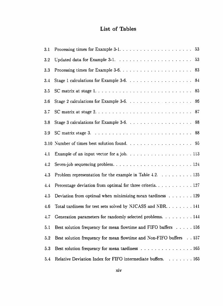
List of Tables

3.1 Processing times for Esample 3.1 . . . . . . . . . . . . . . . . . . . . . 53

3.2 C'pdated data for Example 3.1 . . . . . . . . . . . . . . . . . . . . . . 53

3.3 Processing times for Example 3.6 . . . . . . . . . . . . . . . . . . . . . 83

3.4 Stage 1 calculations for Example 3.6 . . . . . . . . . . . . . . . . . . . 84

. . . . . . . . . . . . . . . . . . . . . . . . . . . . 3.5 SC rnatrix at stage 1 85

3.6 Stage 2 calculations for Example 3.6 . . . . . . . . . . . . . . . . . . 86

. . . . . . . . . . . . . . . . . . . . . . . . . . . . 3.7 SC rnatrix at stage 2 87

3.5 Stage 3 calculations for Exaniple 3.6 . . . . . . . . . . . . . . . . . . . 88

. . . . . . . . . . . . . . . . . . . . . . . . . . . . . 3.9 SC niatrk stage 3 58

3.10 Xumber of tirries best solution found . . . . . . . . . . . . . . . . . . . 93

4.1 Esaniple of an input vector for a j o b . . . . . . . . . . . . . . . . . . . 113

4 . 2 Seven-job sequencing probleni . . . . . . . . . . . . . . . . . . . . . . . 124

4.3 Problem representation for the exarnple in Table 4.2. . . . . . . . . . 125

4.4 Percentage deviation from optimal for three criteria . . . . . . . . . . . 127

4.5 Deviation from optimal when minimizing mean tardiness . . . . . . . 129

4.6 Total tardiness for test sets solved by XJCASS and XBR . . . . . . . . 141

4.7 Generation parameters for randomly selected problems . . . . . . . . . 144

1 Best solution frequency for mean flowtime and FIFO buffers . . . . . 136

5.2 Best solution frequency for mean flowtime and Non-FIFO buffers . . 157

5.3 Best solution frequency for mean tardiness . . . . . . . . . . . . . . . 163

5.4 Relative Del-iation Index for FIFO intemediate buffers . . . . . . . . 165

xiv

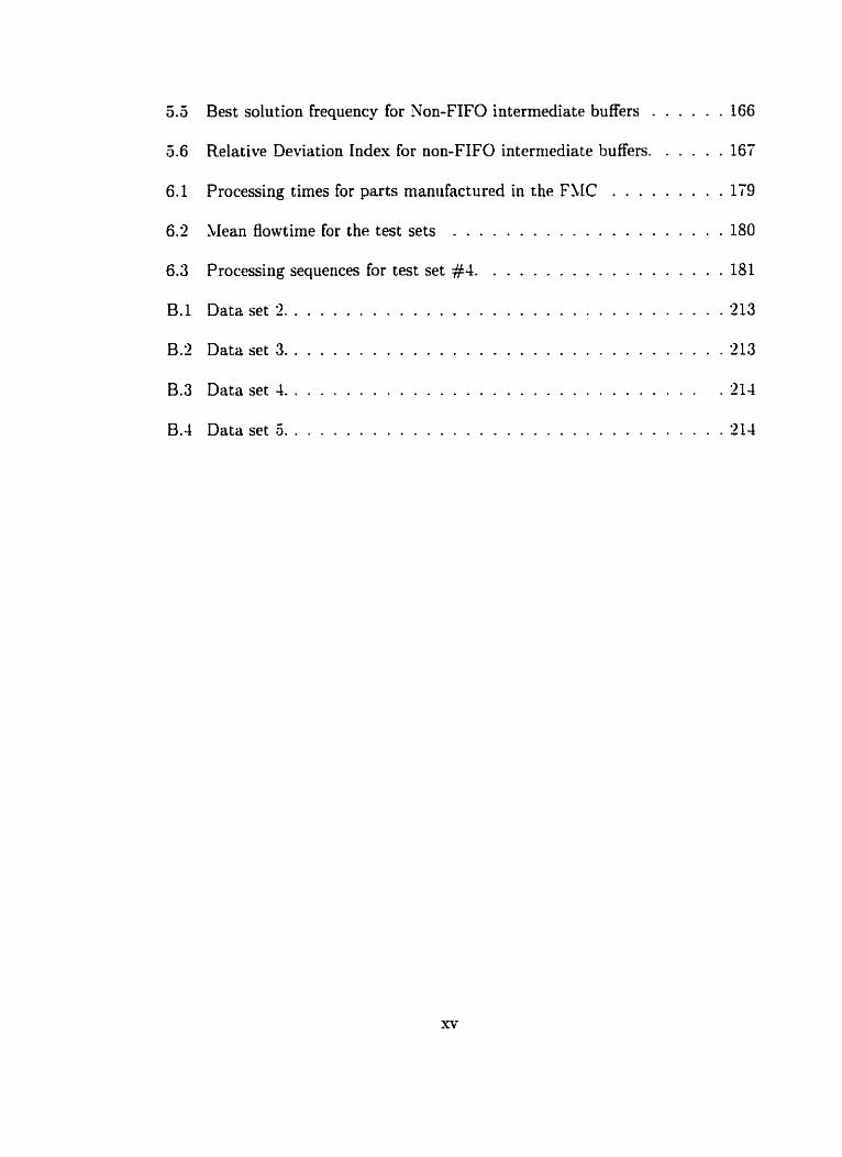
Best solution frequency for Xon-FIFO intermediate buffers . 166

Relative Deviation Index for non-FIFO interrriediate buffers . . . . . . 167

Processing times for parts manufactured in the FLIC . . . . . . . . . 179

. . . . . . . . . . . . . . . . . . . . . blean flowtime for the test sets 180

. . . . . . . . . . . . . . . . . . . Processing sequences for test set #4 181

. . . . . . . . . . . . . . . . . . . . . . . . . . . . . . . . . Data set '2 -213

. . . . . . . . . . . . . . . . . . . . . . . . . . . . . . . . . . Data set 3 213

. . . . . . . . . . . . . . . . . . . . . . . . . . . . . . . . Data set 4 -21-4

. . . . . . . . . . . . . . . . . . . . . . . . . . . . . . . . . . Data set 5 214

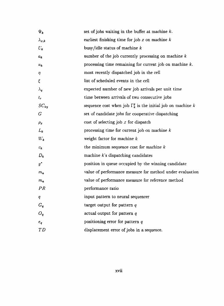
Nomenclature

number of jobs to be scheduled

total number of machines in the ce11

xachinc numbcr

processing time for job i on macliine k

holding costfunit for job i

tardiness cost/unit time for job i

due date for job i

operation due date for job i on machine Il

completion time for job i

a schedule of n jobs

an optimal schedule (S' E S)

nurnber of machine where job dispatching is considered.

indes number of position in the buffer queue.

set of jobs wvaiting a t machine k's buffer

set of jobs available for dispatching

number of jobs waiting in the buffer at machine s

index number of job in sequence at machine k's buffer

index number of job considered for dispatching (r = Tf)

set of machines remaining on job x's route

the i l h machine in job r's route starting from machine s

number of machines that job x still has to visit.

the position of machine k in the route for job x (d,)

set of jobs that have yet to visit machine k

set of machines visited by the jobs in Rç

ready time for machine k

Pr

Lk

cr,

set of jobs waiting in the buffer at niachine k.

earliest finishing time for job x on machine k

busy/idle status of machine k

oumber of the job currently processing on machine k

processing time reniaining for current job on machine k.

most recently dispatched job in the ceIl

list of scheduled events in the ce11

expected number of new job arrivals per unit tinie

time between arrivals of two consecutive jobs

sequence cost when job TY, is the initial job on niachine k

set of candidate jobs For cooperat ive dispatching

cost of selecting job r for dispatch

processing time for ciment job on machine k

iveight factor for machine k

the minimum sequence cost for machine k

machine k's dispatching candidates

position in queue occupied by the winning candidate

value of performance measure for method under evaluation

value of performance nieasure for reference method

performance ratio

input pattern to neural sequencer

target output for pattern q

actual output for pattern q

positioning error for pattern q

displacement enor of jobs in a sequeoce.

Chapter 1

Introduction

1.1 Background

Modern manufacturing operates in highly corn petit ive environnients t hat de-

mand reduced costs and low lead times. Approximately 60 to 80% of the manufac-

turiiig of discrete parts involves mid-varietu, mid-quantitu products. The emergence

of groiip technology (GT). coupled with advances in reducing set-up times. has al-

lowed lower leatl time and reduced levels of in-process iiiventory for this production

category. GT emphasizes the production of like products in dedicated rnanufactur-

ing cells. Flexible manufacturing celIs (FSICs) irnplement this GT concept in a n

environment that is characterized by high automation. A FlIC is a collection of

machines that are capable of producing families of parts bearing sirnilar production

charaçteristics. Very short set-up times are made possible for the products by the

high lerel of automation and tool-change capabilit. Part movements in the ce11 are

performed by using automated material handling, such as an Automated Guided

Vehicle (AGV) or robots. A Flexible Manufacturing System (FhIS) is a collection

of FSICs supported by an inter-cellular handling system.

Due to its fast product changeover. a FMC allows the simultaneous processing

of different parts in smdl lot sizes. This simultaneous processing has the admntage

of decreasing the work-in-process (WP) compared to a h e n the parts are processed

in larger lots. In addition to the reduced WIP? simultaneous processing accounts

for increased machine utilization, a lower flowtime, and reduced storage capacity

requirements (Duffie and Piper [l]) . The disadvantage of simultaneous processing

is the greater complexity of scheduling.

A FMC is controlled by one or more cornputers that normally operate under

hierarchical control. In fullp centralized control, a computer acts as the cell's su-

pen-isor to communicate directly with each of the cell's components. as illustrated

in Figure 1 .l(a). These coniponents are the machines. the material tandling sys-

tem. sensors and other control devices. The supervisor obtains information froni

the units. and sends appropriate comrnands to the individual devices in order to

control the activities in the cell. The supervisor is also responsible for tracking and

controlling al1 the part movements in the cell. dispatching part programs to the

machines. and responding to faults that may occur in the cell's operations. The

tasks and responsibilities for the supervisor in a centralized control system increase

in complexity as the size of the ce11 and the number of parts it processes grows.

Centralized control systems favor fked schedules that are stored in the system

and implemented directly by the hardware. When a schedule needs to be modified

or updated. the supervisor must collect al1 the pertinent information from the ce11

and generate a new and efficient schedule in a very short period (usually a matter of

seconds). In such situations, hierarchical systems are at a disadmntage because of

the great amount of information that needs to be collected. analyzed and processed

quickiy. De-centralized control enables faster rescheduling and better flexibility to

accommodate variable scheduling demands.

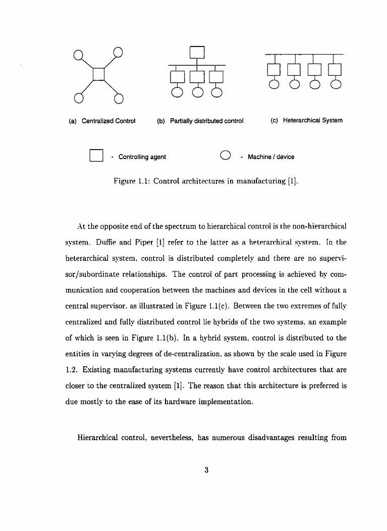
(a) Centralized Control (b) Partially distributed control (c) Heterarchicai System

- Controliing agent O - Machins / davica

Figure 1.1: Cont rol architectures in rnanufacturing (11.

At the opposite end of the spectrum to hierarchical control is the non-hierarchical

system. Diiffie and Piper [1] refer to the latter as a het~rarchical system. In the

heterarchical system, control is distributed completely and there are no supervi-

sor/subordinate relationships. The control of part processing is achieved by corn-

munication and cooperation between the machines and devices in the ce11 without a

central supervisor. as illustrated in Figure l . l(c). Between the two ertremes of full?

centralized and fully distributed control lie hybrids of the two systems. an esample

of which is seen in Figure l.l(b). In a hybrid system. control is distributed to the

entities in varying degrees of de-centralization. as s h o m by the scale used in Figure

1.2. Existing manufact uring systems currently have cont rol architectures t hat are

closer to the centralized system (11. The reason that this architecture is preferred is

due mostIp to the ease of its hardware implementation.

Hierarchical control: nevertheless, has numerous disadvantages resulting from

Centralized cdntrol

Commercial hierarchical control

Hierarchical control wiîh dynamic scheduling

Heterarchical control

Fully Distributed Entities

Figure 1.2: Category scaie for control architectures [l].

the non-modularity of its architecture. A lack of modularity means that changes.

or even minor modifications in the cell. require significant effort to niodify the cell's

control system. In addition. the software to run hierarchical systems is extensive.

comples and costly to develop and maintain. Therefore. a manufacturing ce11 that

is controlled hierarchically is not a very flexible one in changing environments. As

an example. if the machine configuration in a ce11 is to be modified. then large

amounts of software may have to be rewritten to incorporate the modification. On

the other hand. in a non-hierarchical system. the localized nature of the control

requires software that is less cornplex. In addition: the software is duplicated in the

modules. making it more convenient to perform any updates or modifications. -4s

fax as scheduling in a FMC is concerned, the locaiization of information provided by

modularization leads to reduced problem complexity This. in tum. pemits more

efficient d p a m i c scheduling in the cell.

1.1.1 Scheduling Flexibiüty

Scheduling flexibility describes the ability to implement the best schedule pos-

sible for the current jobs and hardware setup (in the FMC) without the need for

selecting, rnodifying or re-writing software to accommodate particular configurations

and job roiitings. There are several issues that contribute to scheduling flesibility

Two have particular interest. The first concerns the adaptability to changing ob-

ject ives and priorities. Scheduling and job priorit ization are controlled by software

in a FSIC. If the scheduling's objectives are changed. then the software should be

capable of meeting the new objectives without having to be rnodified. Aiso. disrup-

tion in ce11 operations. such as rush orders. reworks. machine failure etc.. mean that.

in reality. the ce11 operations are dynamic in nature. Schedules have to be updated

frequent ly or reworkecl completely to remain valid under dynamic conditions.

The second matter of interest is that raised by the high levels of automation

found in FJICs. This automation may impose constraints on a cell's activities that

would not be bund in a non-automated system. or in one with low automation.

The main constraint of interest here is the type of buffers that hold the KIP for

each of the machines in the cell. Specifically the use of robotic handling requires

that parts be located at fixed locations and orientations. This rneans that the buffer

must not only hold the parts but it has the task of delivering them to the robot's

gripper at the desired pick-up point and in the correct orientation. The least costly

and simpiest buffers employ gravity-feed. Such buffers, however. norrnally restrict

the order in which the parts can be processed on the machine to a first-in. first-out

(FIFO) order. On the other hand, if an arbitrary selection from the parts aaiting

in the buffer is to be allowed, then a more compIex buffer, such as a carousel- needs

to be used. In addition to being costlier. these latter buffers also require more space

and software. 'ievertheless. buffers that allow part selection are more desirable from

the viewpoint of scheduling because they improve machine utilization and lower the

WP. It is conceivable that economic and technical constraints may result in a F4LC

having some buffers constrained to FIFO queues. dong with others that permit a

selection from the queue. Therefore. a flexible scheduling system should be effective

for F M 3 ranging from those that have strictly FIFO buffers to those that have al1

their buffers perniitting a selection. To use terminology from scheduling t h e o p the

sensitivity of the scheduling system to the amount of perrnissible 'part overtaking*

should be minimal.

1.1.2 Jobshops and Flowshops

A FMC is actually a highly automated jobshop. In a jobshop. rach part vis-

its the machines according to a job 'route' that defines the sequence of operations

necessary to cornplete the part. Workpieces may start and end their routes at an?

one of the machines. There are no restrictions on which machine a job can iisit

next after completing an operation on one of the other machines in the shop. On

the other hand. a flowshop is a jobshop having a uni-directional flow restriction.

A job m. enter the flowshop at any machine, but the machines it can visit next

are limited to only those dovvnstream of the direction of the part Bow. Specificall-

if there are m machines that are numbered from 1 to rn? then a job cannot move

from one machine to another machine which has a lower number. Figure 1.3 de-

picts the general Bowshop. When it is required that each part visits every one of the

rn machines in a (m-machine) flowshop, then that flowshop is called a pure flowshop.

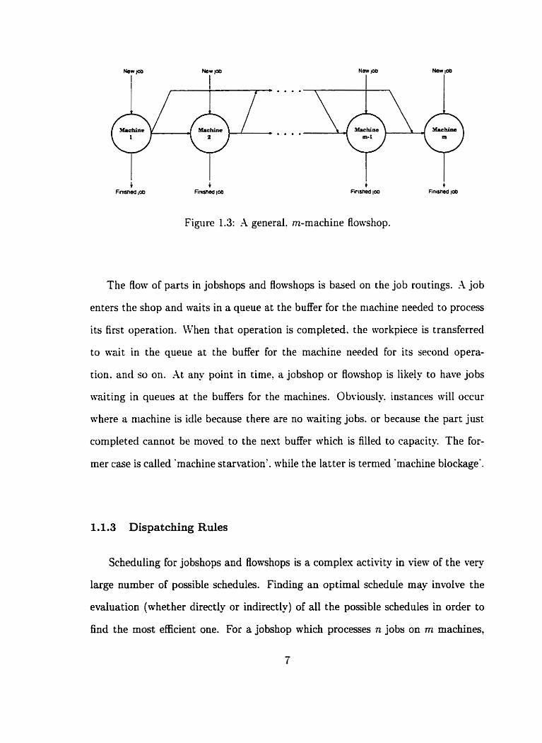
Figure 1.3: A general. m-machine Bowshop.

The Row of parts in jobshops and flowshops is based on the job routings. h job

enters the shop and waits in a queue at the buffer for the machine needed to process

its first operation. W hen t hat operation is completed. the workpiece is transferrecl

to m i t in the queue at the buffer for the machine needed for its second opera-

cion. and so on. At any point in time. a jobshop or Aowshop is likelp to have jobs

waiting in queues at the buffers for the machines. Obviously. instances will occur

where a niachine is idle because there are no waiting jobs. or because the part just

completed cannot be moved to the oext buffer which is filled to capacity. The for-

mer case is called 'machine starvation'. while the latter is termed 'machine blockage'.

1.1.3 Dispatching Rules

Scheduling for jobshops and flowshops is a cornplex activity in tiew of the very

large number of possible schedules. Finding an optimal schedule may involve the

evaluation (whether directly or indirectly) of al1 the possible schedules in order to

find the most efficient one. For a jobshop which processes n jobs on m machines,

the number of schedules that c m be constructed is theoretically as high as ( n ! ) m . In

practice. the nuniber of feasible schedules is Lower but it is still a significant propor-

tion of (n!)". Even in the most restrictive case. namely a pure flowshop with no part

overtaking, a total of n! different schedules is possible. Mathematical techniques

are available that implicitly enumerate al1 the possible schedules to find the optimal

one. However. they are compucacionaily expensive when n is more chan i5 EU 20

jobs (given current cornputer technoiogy).

The cornbinatorial nature of the scheduling problem makes dispatching rules a

favored approach for a jobshop and many types of flowshop. A dispatching rule

specifies which job? from those available in a queue. has the highest priority to t>e

selectetl as the next one on a machine that has just become available. The job hav-

ing the highest priority is the one that is dispatched for processing on the machine.

Thus. a schedule is coiistructed on an 'as-needed' basis. and not a priori. Conse-

quently. dispatching rules are well-suited for dynamic scheduling.

1.1.4 Scheduling Criteria

The scheduling problem is that of arranging the sequences for the processing

of jobs in the shop in a manner that allows desired objectives to be met. as much

as possible. Each job passing through the shop has several operations and each

operation requires a certain 'processing time' on one of the machines in the shop.

In addition, the job is to be completed by a predefined tirne, called the due date.

In the event that the due date is not met. the job is said to be tard. and a penalty

is incurred that is usually a function of the tardiness.

The most comrnonly occurring scheduling objectives attempt to optiniize one or

more of the following criteria.

- Minimum makespan. where it is required to complete al1 the available jobs in

the iiiiiiiiiiuiii puaailde tiiitr apéii. This cri trriuii is relevarit tu stat ic shüps.

where the number of jobs to be scheduled is known at the s ta i .~ uf production

and no new job arriva1 is allowed in the rneantinie.

- hfinimum mean tardiness. where the emphasis is to reduce the total aniourit

of tardiness.

- Minimum mean Bowtime. which seeks to minimize the average time spent by

a job in the systern. This criterion helps to reduce the W P leveis.

- Minimum number of tardy jobs. where the goal is a schedule that minimizes

the total nimber of jobs that are completed beyond their due dates.

In addition to the above criteria. many less comrnonly occurring ones esist. and

others r n q also be formulated that are application specific.

More often than not, scheduling criteria are conflicting ones. For example. a

schedule that minimizes the mean flowtime can be poor with respect to minimizing

the mean tardiness. and vice-versa. In modern manufacturing, a W P reduction and

on-t ime delivery are normally CO-O bject ives. Thus, the scheduling objective is. in re-

ality. a combination of several cnteria. There are two major approaches to deal ni th

multiple performance criteria. The first approach is to rank the criteria in terrns of

importance as prirnary, secondary, tertiary. etc. h schedule satis&ing the primary

criterion is devised. Then this schedule is adjusted as much as possible to meet the

seconda- criterion, wi t hout diminishing the degree of satisfaction obtained for the

primary objective. and so on. The second approach is a cost-based one. -1 unified

equivalent cost is selected to quanti& the performance with respect to the different

criteria. Then a single cost-based criterion is developed to represent the multiple

criteria.

1.2 Research motivation

The priniary motivation for this research is based on implementing an automated

scheduling systern for a FLIC located in the Computer Integrated Slanufacturing

Laboratory a t the Faculty of Engineering, University of Slanitoba. Although this

FLIC serves educational purposes. it represents real-world srstems in the high degree

of automation it employs. Furt hermore. as a collection of autonomous sub-systems.

it provides the opportunity to implement a non-hierarchical control systern. The

type of products niade in this ce11 belong to a family of parts which have primary.

seconda. and tertiary operations that are applied sequentially. The first two ma-

chines in the ceIl are for the primary operations. the third machine performs the

secondary operations. while the teniary operations are perforrned ou the last ma-

chine. The sequential manufacturïng stages involved with these products give this

F'VIC the characteristics of a flowshop.

A direct implementation of theoretical models to a highly automated celi that

operates in a continuously changing environment is not simple. The difficulties are

best described by Dudek. Panwalker and Smith [2] for the case of the flowshop.

The- contend that there are very few real-world situations that have the charac-

teristics of the classical flowshop assumed theoreticall. The main reasons cited in

[2] for the lack of industrial application of previous Bowshop research are 1) overly

restrictive assumptions: 2) inflexibility of the algorithms: and 3) failure to focus on

the fact that real tlowshops are more often dynamic (rather than static) and subject

to multiple performance criteria. Although these observations relate to the pure

flowshop. they are also true. to a significant degree. of other types of Row and job

shops.

The seconcl source motivating this research is automation. A FUC is not as

highly autoniated with respect to scheduling control in cornparison to the hard-

ware, When there is a cieviation from the schedule. off-line human intervention is

nornially needed to revise or update the schedule. One source of deviation to a

current schedule is a change in the scheduling objectives. The scheduling flexibility

in F'vICs may be enhanced. through automation. to allow the system to quickly pro-

vide good schedules for changed objectives. multiple scheduling criteria or criteria

that are unique to particular situations. The 'inflexibility' of many of the theoret-

ical scheduling algorithms poses an obstacle to achieving a high Rexibility for the

scheduling component in a FLIC. The flexibility that is desired for the FIyICs has

the following characteristics:

1. It permits adaptation to hardware reconfiguration without the need for major

modifications to the scheduling software.

2. On-Iine adaptation is allowed whenever the scheduling criteria change.

3. A consistent performance level is provided, regardless of the types and sizes

of the in-process buffers, or the predominant part routings.

4. It efficiently meets the scheduling criteria regardless of the number of different

part types that are produced simultaneously in the cell.

1.3 Problem Statement

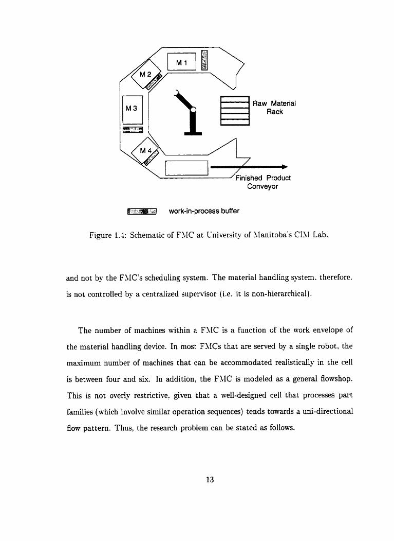
The type of FNC under consideration is illustrated in Figure 1.1. The ce11

contains several machines. as well as a material handling system consisting of an

'ASEX robotic arm. The robot loads and unloüds the machines. and it transports

the workpieces between the machines. The activities of the robotic arm and its

interaction with the machines is coordinated by means of a system of sensors. pro-

grammable logic controllers (PLCs). and the robot's controller. The PLCs monitor

the signals from the sensors on the machines as well as the buffers. Th- send

appropriate outputs to the robot's controller. which then initiates the programs cor-

responding to the robot's desired actions. Requests For service from the robot arm

are received and dispatched by the robot's controller in an order that is generally

unpredictable. The controller monitors incoming requests by means of a looping

program. When a request is detected and acknowledged, the monitoring program

is interrupted and the routines (programs) for servicing the acknowledged request

are executed by the robot. When the requests have been sewiced. the monitoring

program resumes from the point at which it was interrupted. New requests arriving

during the interruption rnay be serviced ahead or after previously waiting requests.

depending where the interruption occuned in the monitoring program. Scheduling

for the robot's movements is performed by an outside agent (the robot's controller)

Raw Material Rack

Finished Product Conveyor

work-in-process buffer

Figure 1.4: Schematic of FSIC at University of SIanitobats CI11 Lab.

and not by the FlIC's scheduling system. The material handling system. therefore.

is not controlled by a centralized supervisor (i.e. it is non-hierarchical).

The number of machines within a FSIC is a fuiiction of the work envelope of

the material handling device. In most FSICs that are served by a single robot. the

maximum number of machines that can be accommodated realistically in the ce11

is between four and six. In addition. the F41C is modeled as a general fiowshop.

This is not overly restrictive, given that a well-designed ce11 that processes part

families ( w hich involve similar operat ion sequences) tends t owards a uni-direct ional

Born pattern. Thus. the resemch problem can be stated as follows.

Given a FLIC similar to the one depicted in Figure 1.4 (which has the charac-

teristics of a general flowshop), it is required to sequence the flow of jobs through

the machines (or stations) in the ce11 such that a cost function. 2. is minimized.

The cost function of interest, Z = f ( h i 7 t i ) , depends upon the holding C O S ~ S (hi)

and the tardiness costs (ti) for each one. i. of the jobs. h detailed statenient of the

scheduling problem and the assumptions used is given in Chapter 3.

The objective of this research is to develop a scheduling control system for this

FlllC that is :

1) flexible with respect to performance for different scheduling criteria:

2 ) consistently efficient for difFerent routing configurations. and for different ar-

rangements of FIFO-constrained and non-constrained intermediate buffers:

and

3) implementable in an automated fashion and in a dynamic environment.

1.4 Solut ion Approach

The approach adopted is one that emphasizes a high degree of heterarchy in the

scheduling control. This approach is facilitated by the use of a networked control

-tem. Each station: comprising a machine and its buffer. is treated as an inde-

pendent entity. The entities communicate over the network mith each other and

'cooperate' in making decisions deding with dispatching priorities for the current

jobs. This auti-hierarchicd approach, which promot es individuality and Local deci-

sion making, makes single-machine scheduling theory an attractive tool. When al1

jobs have equal release times (Le. they are al1 available at a given instant in time

and ready to be scheduled) , t hen single machine scheduling is basically a sequencing

problem that is generally sinipler to solve than multiple machine scheduling prob-

lems. The approach taken here is called 'Cooperative Dispatching'. Cooperative

Dispatching uses single machine scheduling theory. with the simpiiiying assumprion

of equal release times, as the basis of the interaction between the individual enti-

ties in the cell. The results of these interactions is a series of on-line dispatching

decisions that ultimately produce a final schedule. To expand the applicability to

uncommon or unique scheduling criteria. a neural network is proposed for solving

the single machine sequencing problems that are used in Cooperative Dispatching.

This thesis is organized as follorvs. Chapter 2 reriews the literature relevant to

heterarchical systems and dispatching niles. wit h emphasis on state-dependent dis-

patching rules. as well as scheduling in Rowshops and single machines. Cooperative

Dispatching is presented next in Chapter 3. and results are given for its performance

in static problems. These results are compared with those from other rnethods that

may be used for the test problems. In Chapter 4. a novel approach is presented

for sequencing jobs on a single machine by using artificial neural networks. The

use of neural networks promotes flexibility by allowving performance criteria that

are new or unique. and for which no aigorithm are readily available. The perfor-

mance of Cooperative Dispatching in djmamic flowshops is evaluated. in Chapter J1

by cornparison to the more traditional dispatching rules used in similar cases. The

application of Cooperative Dispatching in the FMC at the University of Manitoba is

described in Chapter 6. and results from a number of experimentsl trials are given.

Finally. Chapter 7 provides the conclusions. and sorne recommendations for the di-

rection of future research.

Chapter 2

Literature Review

2.1 Introduction

A Flexible hlanufacturing System (FMS) normally has manufacturing cells linked

together by material handling and information systems. Research in the area of FAIS

scheduling may be classified according to the level of the scheduling. This can be

a t the system level (the FSIS as a whole). or at the ce11 level (individual FhlCs).

The scheduling problem a t the system level includes tool allocation and the loading

problem. which is basicaily the açsignrnent of the jobs to each of the available cells

(task assignment). At the ce11 level. the scheduling problem is confined to organiz-

ing the sequence of activities in the ce11 to optimally meet the desired performance

criteria. In this respect. the problern at the ce11 level often resembles scheduling

problems for jobshops and fiowshops.

The focus of this surveg is on the literature for scheduling a t the ce11 level.

However, under hierarchical control systems. the problem at the ce11 level is often

influenced by decisions taken a t higher levels. The literature on hierarchical schedul-

ing in FMS is too large to be covered adequateiy in this surve. Only two examples

are selected to illustrate approaches that attempt to address the performance of

the individual celIs under hierarchically controlled scheduling. The advantages of

heterarchical, as opposed to hierarchical, sgst ems is t hen discussed. With the modu-

larization provided by heterarchical control, the focus shifts to scheduling at the ce11

level. The two major approaches considered are dispatching rules and heuristics. For

dispatching rules, the review concentrates on research dealing with state-dependent.

dispatch rule selection. The heuristics that are discussed are those that treat the

FMC as a flowshop. Finally. research on the sequencing of jobs or tasks on a single

machine is reviewed briefly. This relates to the single machine sequencing optimiza-

tion that is required for the algorithmic approach proposed in t his t hesis.

2.2 Hierarchical and Heterarchicd Control

Scheduling in FMS has traditionally been part of an integrated hierarchical a p

proach for managing a system. Problems are usually defined at ari aggregated levei

of detail. and the information flows downward with increasingly detailed decisions

taken at the lower levels. An example of such an approach is found in Stecke [3].

who focuses on higher planning levels. The FSIS is modeled as a closed queuing

network that gives average performance levels for the aggregate input data. This in-

formation is passed to the next planning levels. where the machine groups (or pools)

are identified. and jobs are assigned (loaded) for each grouping by using mised in-

teger programming models. The logic behind this procedure is that decisions taken

at these stages enhance efficiency at the lower levels of decision. where on-line and

dynamic control can be applied. The disadvantage of this approach. which is corn-

mon to many hierarchically controlled systems. is that the need to finalize certain

decisions before start-up ümits performance under d p a m i c conditions.

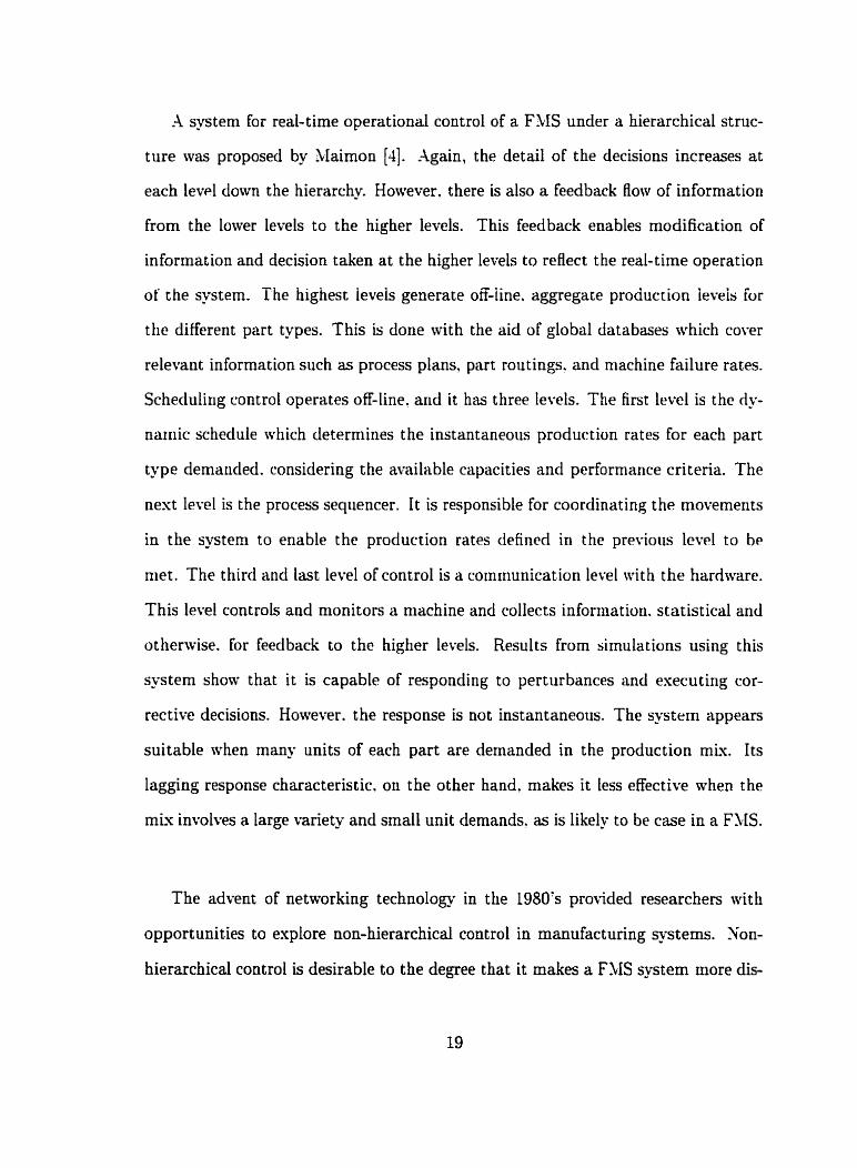
A system for real-time operational control of a F M under a hierarchical struc-

ture was proposed by Maimon [4]. Again, the detail of the decisions increases at

each lev4 d o m the hierarchy However. there is also a feedback flow of information

from the lower levels to the higher levels. This feedback enables modification of

information and decision taken at the higher levels to reflect the real-time operation

of the system. The highest ieveis generate on-iine. aggregate production ieveis fur

the different part types. This is done with the aid of global databases which cover

relevant information such as process plans. part routings. and machine failure rates.

Scheciuling control operates off-line. and it has three levels. The first level is the du-

naiiiic schedule which determines the instantaneoiis production rates for each part

type demauded. considering the amilable capacities and perforniance criteria. The

nest level is the process seqiiencer. It is responsible for coordinating the rnovements

in the system to enable the production rates definetl in the prwiocis levd to b~

met. The third and last level oE control is a communication level wit h the hardware.

This level controls and monitors a machine and collects information. statistical and

othenvise. for feedback to the higher levels. Results from simulations using this

system show that it is capable of responding to perturbances and executing cor-

rective decisions. However. the response is not instantaneous. The system appears

suitable when many units of each part are demanded in the production mix. Its

lagging response characteristic. on the other hand. makes it less effective when the

mis involves a large variety and small unit demands. as is likely to be case in a F M .

The advent of networking technologi in the 1980's pro~-ided researchers with

opportunities to explore non-hierarchical control in manufact unng systems. Non-

hierarchical control is desirable to the degree that it makes a F'VIS system more dis-

tributed and dynamic, resulting in less cornplexity and more modularit- as well as

lower development. operation and maintenance costs. Piper and Dufie [1] used the

term 'heterarchical' synonymously with 'non-hierarchicai' to describe a distributed

control system. They identified several of the critical questions that need to be

addressed in non-hierarchical systems. Furthermore. they outiined a plan of how a

distributed controi system wouid operate without centraiizeci supervision. Piper and

Duffie's concept called for each part entering the machining ce11 to initiate a pro-

gram under a multitasked operating systern. The part then communicates. through

its program. with the machines it ueeds to visit and the rnaterial handling system

in order to negotiate its way through the ce11 to its completion stage. The technique

is highly dynamic, resulting in on-line machine assignnient ancl self-configuration.

These characteristics also a!!ow an on-line re-configuration in the event of machine

failure. A more detailed description of this cooperative schedtiling approach is givm

in Duffie and Prabhu [SI.

Shaw [6] described a method. based on the concept of cooperative problem solv-

ing, for dynamic scheduling in a non-hierarchical Cornputer Integrated hlanufac-

turing (CI-VI) environment. The CIM had cells that cooperated by means of a

network-wide. bidding scheme to schedule the jobs. The scheduling method is a two

level method. In the first level. jobs are assigned to the cells. At the second level

(the ce11 level)? the jobs are scheduled within the cell. The fint level scheduling

is finalized through the bidding scheme and network communication. Ctlen a job

has completed its current operation in a cell. that ce11 announces the availability

of the job for its next operation. The cells in the -teni: including the one that

makes the announcement. make bids for the job. The value of a cell's bid is the

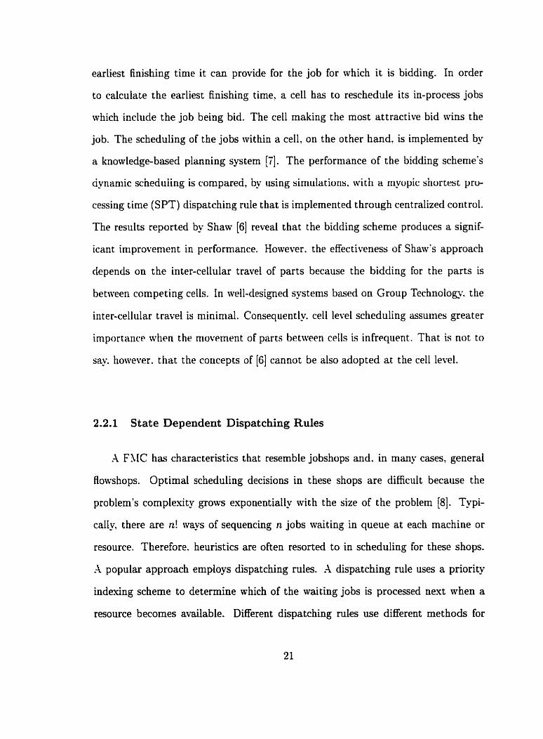
earliest finishing time it can provide for the job for which it is bidding. In order

to calculate the earliest finishing tirne! a ce11 has to reschedule its in-process jobs

which include the job being bid. The ce11 rnaking the most attractive bid wins the

job. The scheduling of the jobs within a cell. on the other hand, is implemented by

a knowledge-based planning system [7]. The performance of the bidding schenie's

àynamic sciieàuiirig is compareci, Oy using siniulatioiis. wirii a riiypic siiorwst pro-

cessing time (SPT) dispatching rule that is implemented through centralized control.

The results reported by Shaw (61 reveal that the bidding scheme produces a signif-

icant iniprovement in performance. However. the effectiveness of Shaw's approach

depends on the inter-cellular travel of parts because the bidding for the parts is

between competing cells. In dl-designed systems based on Group Technolog;. the

inter-cellular t rave1 is minimal. Consequencly ce11 level scheduling assumes greater

importance when the mowment of parts between c ~ l l s is infrequent. That is not ta

s a . however. that the coricepts of [6] cannot be also adopted at the ce11 level.

2.2.1 State Dependent Dispatching Rules

A FMC has characteristics that resemble jobshops and. in many cases. general

flowshops. Optimal scheduling decisions in these shops are difficult because the

problem's complexity grows exponentially with the size of the problem (81. Typi-

cal- there are n! ways of sequencing n jobs waiting in queue at each machine or

resource. Therefore. heuristics are often resorted to in scheduling for these shops.

A popular approach employs dispatching mies. h dispatching rule uses a priority

indexing scheme to determine mhich of the rvaiting jobs is processed next when a

resource becomes available. Different dispatching mies use different methods for

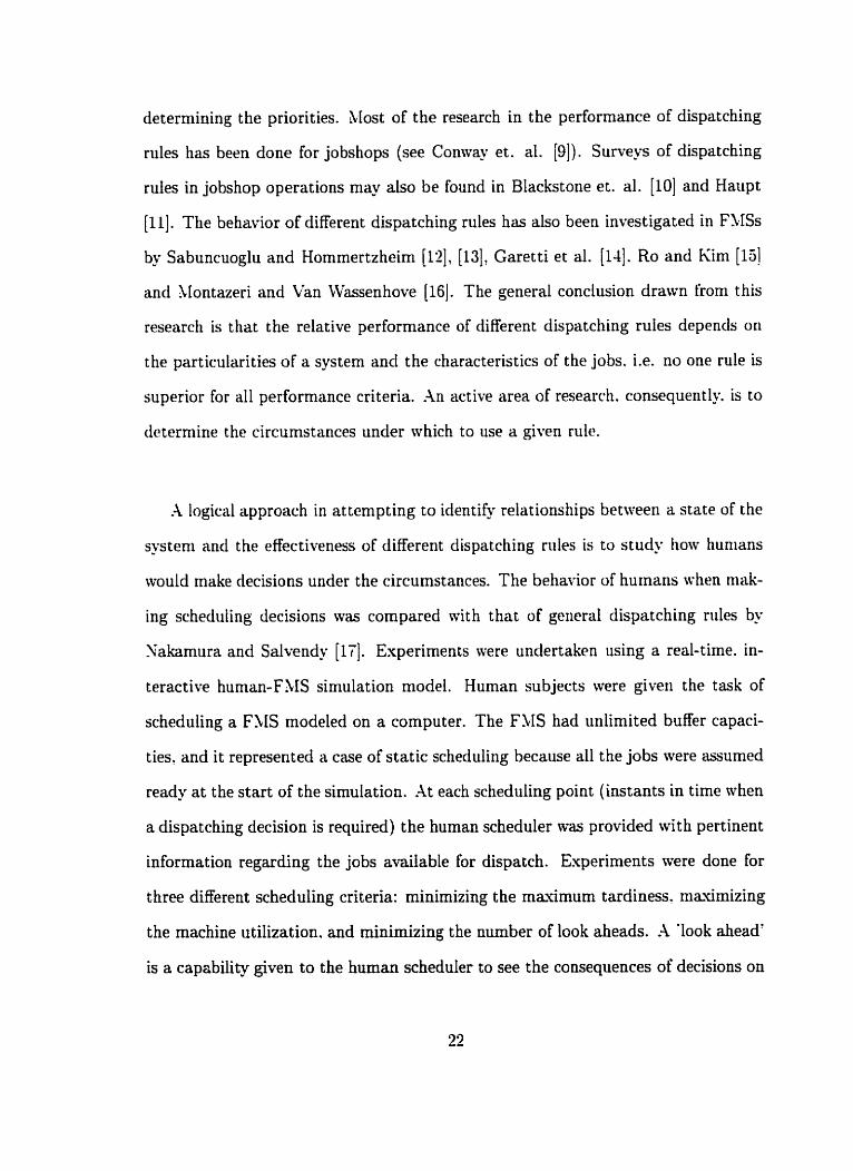
determining the priorities. Most of the research in the performance of dispatching

rules has been done for jobshops (see Conivay et. al. [9]). Surveys of dispatching

rules in jobshop operations may also be found in Blackstone et. al. [IO] and Haupt

[IL]. The behavior of different dispatching rules has also been investigated in FSISs

by Sabuncuoglu and Hommertzheim [Hl, [13]. Garetti et al. [14]. Ro and Kim [lj]

and Llontazeri and Van CVassenhove 1161. The general conclusion drawn froni thh

research is that the relative performance of different dispatching ruies depends on

the particularities of a systern and the characteristics of the jobs. i.e. no one rule is

superior for al1 performance criteria. An active area of research. consequently. is to

determine the circurnstances under which to use a given rule.

A logical approach in attcmpting to identify relationships between a state of the

systeni and the effectiveness of different dispatching rules is to study how tiunians

would rnake decisions under the circumstances. The behavior of humâns when mak-

ing scheduling decisions was compared with that of ge~ierül dispatching riiles by

Sakamura and Salvendy [KI. Experirnents wece undertaken using a real-tirne. in-

teractive human-FSIS simulation model. Human subjects were given the task of

scheduling a FSIS modeled on a cornputer. The FMS had unlimited buffer capaci-

ties. and it represented a case of static scheduling because al1 the jobs were assumed

ready at the start of the simulation. At each scheduling point (instants in time when

a dispatching decision is required) the human scheduler was provided wi th pertinent

information regarding the jobs avdable for dispatch. Experiments were done for

hree different scheduling criteria: minimizing the maûmum t ardiness. maximizing

the machine utilization. and minimizing the number of look aheads. h 'look ahead'

is a capability given to the human scheduler to see the consequences of decisions on

the final schedule prior to making those decisions. It aids the scheduler in dispatch-

ing. The 'look ahead' capability was included in the experiments in order to help

determine its effect on performance. The results showed that, in al1 the test prob-

lems. the best human schedulen achieved results better than or equal to the best

of eight typical dispatching rules. The effect of the 'look ahead' capability was seen

to have an impact if used sparingiy and oniy at che initiai stages of the sclieduiirig.

The results from Nakamura and Salvendy [l'il underlined the ability of hurnans

to weigh current system attributes in reaching dispatching decisions. This ability is

lacking when a single dispatching rule is applied automatically at scheduling points.

.A number of researchers approached this issue with niethods that sought to allow

the selection of different dispatching rules djmamically. i.e. as situations evolved in

the rnanufactiiring system.

There are two elements involved in the dynamic selection of an appropriate dis-

patching rule. First. the state of the system must be represented in some fashion

t hrough identifiable attributes. Second. for any given state. knowledge must be

available as to what is the most favorable dispatching rule. This problem has at-

tracted the interest of Artificial Intelligence researchers. particularly in the areas of

knowledge-based systems and neural networks.

Intelligent scheduling methods which employ knowledge-based systems generally

utilize If-Then rules to reach decisions. Knowledge for the mie base is commonly

gained from discrete event simulations of different states of the systern. W u and

Wysk [18]' Kusiak and Chen [19], and Kathamala and Allen [?O], for esample, con-

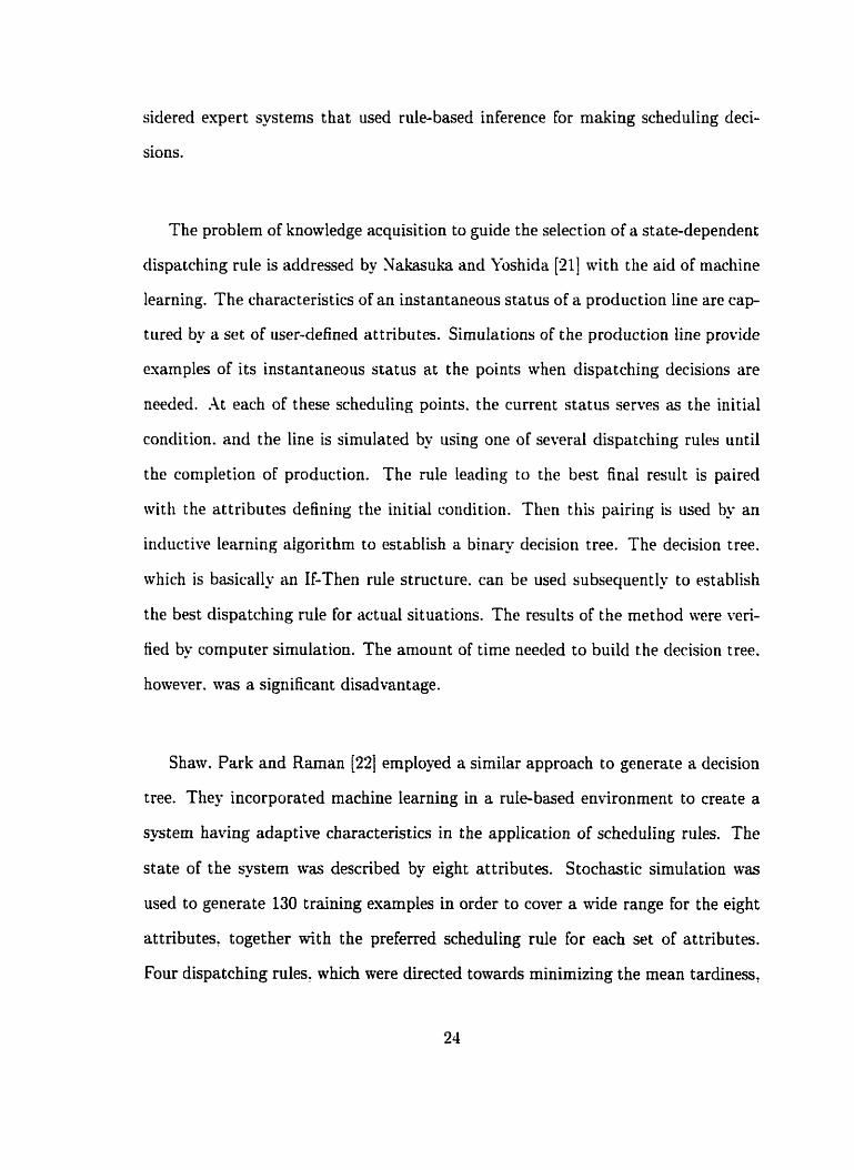
sidered expert -stems that used rule-based inference for making scheduling deci-

sions.

The problem of knowledge acquisition to guide the selection of a state-dependent

dispatching rule is addressed by Xakasuka and b s h i d a [21] 116th the aid of machine

learning. The characteristics of an instantaneous status of a production line are c a p

tured by a set of user-defined at tribu tes. Simulations of the production line provide

examples of its instantaneous status at the points rvhen dispatching decisions are

needed. At each of these scheduling points. the current status serves as the initial

condition. and the line is simulated by using one of several dispatching rules until

the completion of production. The rule leading to the best final result is paired

with the attributes defining the initial coridition. Then tliis pairing is used by an

inductive learning algorithm to establish a b i n a - decision tree. The decision tree.

which is basically an If-Then rule structure. can be used subsequently to lvtablish

the best dispatching mle for actual situations. The results of the method were yen-

fiecl by compiiter simulation. The amount of time needed to build the decision tree.

however. was a significant disadvantage.

Shaw. Park and Raman [22] employed a similar approach to generate a decision

tree. They incorporated machine learning in a mle-based environment to create a

s y t e m having adaptive characteristics in the application of scheduling rules. The

state of the -stem was described by eight attributes. Stochastic simulation rvas

used to generate 130 training examples in order to cover a wide range for the eight

attributes. together with the preferred scheduling d e for each set of attributes.

Four dispatching rulest which were directed towards minirnizing the mean tardiness,

were used in the learning. E-xperimentation showed that the scheduling directed by

the decision tree performs better. as expected, than the use of a single dispatching

rule.

Chiu and Yih [73] also ernployed induced knowledge. in this case to aid the se-

lection of a dispatching rule at each machine every time it becomes available. The'

selected eight vital attributes. including the number of jobs in the system and the

number of reniaining operations. to describe the state of the system. -4 discrete

event sirnulator was used to generate training esamples in the forrn of pairings be-

tween different dynaniic states and the corresponding preferred dispatching rule for

each state. A total of four rides was considered and a multi-criterion performance

mesure was eniployed to encompass the niakespan. number of tardy jobs and the

mit,~inium lateness. Chiu and Yih noted that a schedule coiilci be described in

terms of a series of dispatching decisions niade a t the scheduling points. A genetic

algorit hm t a s used to find good schedules from strings representing t tie training

examples. This method reduced the time required to find solutions for the problenis

that provided the training examples. An incremental learning algorithm. similar to

that used by Nakasuka and ioshida [XI. ivas then employed to extract knowledge

from the solutions in the form of a bina- decision tree. This tree tvas used to

determine the dispatching rules most appropriate for the dynamic states identified

during actual scheduling operations. The system also employed a performance eval-

uator. If the performance was deemed unsatisfactory. then the l e m i n g algorithm

could modi. the decision tree accordingly. Results showed that the method per-

formed better than a static scheduling procedure based upon a single dispatching

rule. The system appeared better suited to problems that have stable product m~ues.

An alternative method for learning relationships between instantaneous system

states and the corresponding dispatching niles makes use of neural networks. The

concept is simple. Neural networks are trained to respond to an input stimulus by

producing a corresponding output. When the input stimuli represent system states

and the outputs correspond to dispatching rules. a trained neural network should

be able to retrieve an appropriate dispatching rule when presented with an input

pattern representing the system's current state.

A neural network is often used in conjunction with other techniques as part of

a scheduling system. For example. Cho and Wysk ['>-LI utilized a neural network to

generate several part dispatching strategies which are subsequently evaluated in a

multi-pas simulation (251. The neural network accepted an input pattern of seven

elements which defined the status of the workstation: viz. the routing complexity

performance criterion. ratio of material handling time to processing time. system

congestion. machine utilization. job lateness factor and a queue status factor. The

output pattern had nine elements (units). each one representing a particular dis-

patching strategy (or nile). The training data was accumulated from the results

of cornputer simulations of the production system. When presented with an input

pattern. the neural network responds with an output pattern that indicates the acti-

vation in each of the nine units. Each output level reflects how well the dispatching

strategy is sui ted for the :vorkstation stat us represented in the corresponding input

pattern. The two most favorable dispatching strategies are selected based on the

output pattern. They are then processed by a multi-pas simulator over a user-

defined window of time. The strategy that better satisfies the performmce criterion

is selected. FinaIl- the duration of the time rvindow is important because it con-

trols the interval between calls to the neural network. The longer is the window,

the fewer are the opportunities to switch dispatching stratedes. The authors found

that the simulation window's ideal duration depended on the performance criterion

under consideration.

-4 similar implementation of neural networks is described by Rabelo et al. [26].

who organized the networks in a modular system. Neural networks are trairied.

one for each of seven performance measures. by using backpropagation to select dis-

patching rules for an input pattern representing the state of the system. The output

of each one of these seven 'expert' networks is a ranking in order of the effectiveness

of thirteen different dispatching rules. The rankings from the expert netrvorks are

directed. together with the systern's state and the desired performance rrieasure. to

a gating network. The gating network releases a set of suggested dispatching d e s

(selected from the thirteen rules available). The gating network. which is trained

by using the cascade correlation paradigm (271. gives a higher weight to the expert

networks that are better able to meet the performance criteria. The authors re-

portedly achieved quick training and good generalization abilities in their modular

neural networks system.

The met hods t hat adop t s t at e-de pendent policies for selecting dispatching rules

are subject to system 'nervousness'. Nervousness is characterized by the changing

of a dispatch rule before it c m have its desired effect on the system's performance.

Frequent mjtching between different rules arises in response to vigorously changing

attributes in the state of the system. Shaw et al. [22] incorporated a smooth-

ing constant which ensured adequate time for a nenr dispatching rule to have its

desired scheduling effect. Other researchers. however. adopted more sophisticated

ap proaches.

Ishii and Talavage [28]. for example. proposed that the duration a dispatching

rule is maintained should extend from the start of a transient state in the system

to the beginning of the next transient state. This approach implies that a method

of detecting transient states is needed. The authors proposed a function. called

I'iDEX. for measuring a system's state at time t. The value of INDES at time ( t ) is

a function of the number of parts in the system. part processing times. the waiting

and transportation times. and the due dates. The scheduling interval is determined

by simulating the curreiit system using FIFO over a future interval. INDEX is cal-

culated at points within this interval. .-\ transient state is detected by arialyzirig the

time series data from 1'iDE.Y. The scheduling interval is defined from the current

instant to the instant when the value of INDEX increases (which is taken to indicate

a transierice). Once the scheduling interval is determined. four different dispatching

mles are simulated over this interval and the rule that perforrns best is adopted.

The scheduling algorithm was tested by using a simulation mode1 of a F M hav-

ing four work centers. two loading and unloading stations. and three AGVs. Tests

compared the performance of the transient-based scheduling interval and a multi-

pass simulation method that used a constant scheduling interval against a method

that ernployed a single dispatching rule throughout the entire manufacturing period

(i.e. a single-pas algorit hm). An average 5% improvement of the transient-based

resufts were reported over the data from the single-pass algorithm which, in turn.

performed better on average than the multi-pas met hod. Moreover, the multi-pass

method with constant scheduling intervals was less stable and it produced a more

widely varying performance between problems than the transient-based scheduliiig

interval method. It is noteworthy that. contrary to other results published in the

literature for the multi-pass simulation method [Xi], Ishii and Talavage found this

rnethod to be sornewhat inferior to algoritlims based on a single dispatching rule.

rhis ditference may indicate a sensitivity of multi-pass methods to particular prob-

lem data and facili ty configurations.

Jeong and Kini [99] also favored simulation in a FM3 as a tool for determining

which dispatching rule to select and the duration it should be used. They pro-

posed a real-time scheduling mechanism composed of three modules: a controller. a

sirnulator. and a scheduler. The controller nioriitos the systeni's performance and

iipdates the databases of the system's status. The controller sends a signal to the

scheduler when it senses that a significant discrepancy exists between the actual and

estimated performances or when a disturbance. such as a machine breakdown or a

rush order. is detected. The scheduler's function is to decide which dispatching rule

is to be used and when it should be used. It makes this decision after consulting

with the simulator. The simulator runs each of sixteen different dispatching rules

from the current time to the end of the planning horizon. and it returns the results

to the scheduler. Based on the results of the simulations. the scheduler selects the

best dispatching rule and relays this information to the controller for the rule's im-

plementation. Experimentation -9th this scheduling system led to the conclusions.

which are basically similar to those reached by earlirr researchers. that a sgstem's

performance is improved by the d ~ a m i c switching of dispatching d e s . 'rloreover.

the performance is also sensitive to the method for deciding when rule switches

should be considered.

41in et al. [30] considered a competitive neural network that suggested decision

rules in a niulti-objective F M S. At pre-defined production intervals (for example.

each d o ) . the neural network is presented rvith a n input vector containing the de-

sired changes in the performance criteria for the following interval. The magnitude

of the desired changes are determined by the operator in order to meet the multiple

performance criteria. The input vector. therefore. contains relative data between

the current values for the performance measures and the values targeted for the fol-

lorving production interval. The output of the neural network is a class in which the

aggregate input vector is most similar to the one presented at the input. The FSIS

considered employs four scheduling variables. These are 1) a part's selectioii of a

machine to move to: 2) a part's selection of a storage rack: 3) the select ion of a part

by a free machine: and 4) the selection of a part by the material handling system (a

crane in this instance). Each decision variable uses one of between three and four

different operational policies. For example. one of the policies used by the crane is

to serve the closest part first. and so on. A long duration simulation is performed to

generate training data for the neural network. The simulation is divided into many

intervals and, in each interval, a random selection of policies for the decision vari-

ables is applied. The system's states and the performance measures are recorded for

each in tend. The two sets of decision rules and the differences that they produce in

the performance measures between e v e l two consecutive intervals are collected as

input vectors for the neural network. The neural network is trained by the Kohonen

[31] learning nile. Shen, the trained network is used on-line to identify the class for

the input vector representing the curent states at the end of the perïod. .A search

algorithm is used to find the closest match from the vectors in that class. Once

the match is completed. the policies for the four decision variables are selected for

the succeeding interval. The method was tested against a policy where the decision

variables are selected randomly in each period. The results showed that the neural

network is better able to respond to the operator's desired data for performance

critena related to different objectives. However. the met hod was rioL conipared wid i

static policies for the decision variables. Furthermore. it is not clear how sensitive is

the approach to the striugency of the operator's demands for desired values of the

performance criteria kom one period to the next.

The need to control the frequency of rule switches is a negative aspect in a p

plying state-dependent dispatching niettiods. A l o n switching frequency means less

system tienousness. but it also prodiices a more sluggish response to a system's

changes that ultimately marginalize any gains over dispatching nith a single rule.

An approach to deal with this problem is to use composite rules that are an amal-

gamat ion of contributions from several different dispatching d e s . As a system's

state changes. the relative contributions from the different rules change accordingly.

Thus. the character of the rule alters gradually and not in the discrete manner that

occurs in mle switching. An example of such an approach follows next.

Sim et al. [32] proposed a hybrid neural network - expert system that can be

applied dynamically to make dispatching decisions. An expert system evaluates the

prevailing shop conditions and determines which one of sixteen sub-networks is most

appropriate for making the required dispatching decision. Each of the sub-networks

is a neural network that is trained by backpropagation to make the dispatching de-

cisions under specific shop Boor conditions which are defined by a job arriva1 rate

and a scheduling criterion. The specialized neural networks are trained with data

acquired from the results of simulations for ten different dispatching rules run un-

der defined shop Boor conditions. Each job that is a candidate for dispatching is

represented by an input array of fourteen, O - 1 nodes. These nodes indicate the

preserice or absence of pmicuiar attributes. Furtherrriore. rhey eucode the curreiir.

shop conditions and scheduling criteria. The output of the neural network is a value.

which lies between O and 1. that mesures the level of priority determined by the

neural network for the job represented at the input lqer. After processing al1 jobs.

the one determined by the neural network to have the highest priority is selected

for dispatching. In this fashion. the dispatching rule is a composite rule defined by

the relative contributions from the ten rules considered in the training stages. In

cornparison to techniques that switch between dispatching rules. the methocl of Sim

et al. [32] effectively 'invents' a rule for the particular combination of job a t t r ibuts

and shop conditions at hand. The authors also presented results sliowing the su-

periority of the composite rule method over dispatching with any one single rule.

Whether composite rules are more effective than a dp-naniic selection between the

individual dispatching rules remains unanswered.

Although a very significant part of the research in jobshop scheduling has been

devoted to dispatching rules? most real worid manufacturing consists of a prod-

uct mis containing a demand of individual parts in multiple numbers. Identical

parts Nill generally possess identical attributes, resulting in a tendency for most

dispatching d e s to batch the production. This batching conflicts with the concepts

advocated in flexible rnanufacturhg, namely simultaneous production and a batch

size ideally equal to one unit. The need to produce in very low batch sizes assumes

greater importance in flexible assembly systems. where daerent parts are needed

sirnultaneously at the point of assembly. In such cases, the use of a dispatching

rule like SPT gives equd priority to d l the demanded quantities of a single part

because al1 these quantities will have the same value for the selection attribute.

namely the processing tirne. The result is that a batched production is observed

in many instances when the t raditional dispatching rules are emplqed. Analyt ical

and heuristic methods are alternative approaches in such cases. They are usually

developecl for the specific type of problem at hand. Consequently. their application

is usually less general t han dispatching rules.

2.3 The Flowshop

The review of heuristics for scheduling in FLICS that follows covers flowshops

only. This is because the F'VIC is modeled as a general flowshop in this thesis.

.-\ssuming that a FSIC should preferably produce parts belonging to a family in ac-

cordance with Group Technology concepts. it is not unreasonable to use a fiowshop

rnodel. This is because parts from a farnily are likely to have similar manufacturing

operation sequences and. therefore, sirnilar part routings. Thus. an FLIC'S layout

cm frequeutly resemble that of a general flowshop.

The most widely studied flowshop problem is a pure Bowshop in which the ob-

jective is to minimize the makespan. Johnson [33] provided an algorithm that finds

the optimal solution for the correspondhg two-machine problem, as well as for the

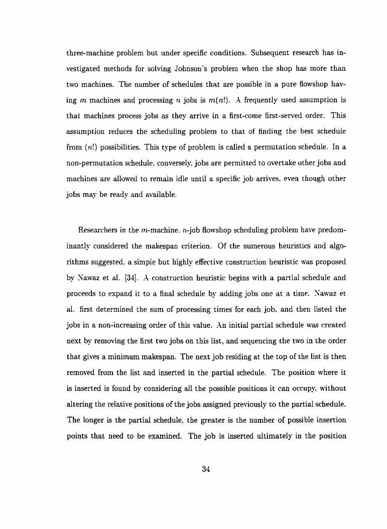
three-machine problem but under specific conditions. Subsequent research has in-

vestigated methods for solving Johnson's probIem when the shop has more than

two machines. The number of schedules that are possible in a pure floivshop hav-

ing rn machines and processing n jobs is m(n!). A frequently used assumption is

that machines process jobs as they arrive in a first-corne first-served order. This

assumption reduces the scheduling problem to that of tinding the best schedule

from (n!) possibilities. This type of problem is called a permutation schedule. In a

non-permutation schedule. conversely. jobs are permitted to overtake other jobs and

machines are allowed to rernain idle iintil a specific job arrives. even though other

jobs may be ready and available.

Researchers in the rn-machine. ri-job fiowshop scheduling probleni have predom-

inantly considered the makespan criterion. Of the numerous heuristics and algo-

rit hms suggested, a simple but highly effective constriict ion heuristic \vas proposed

by Yawaz et al. [34]. A construction heuristic begins witli a partial schedule and

proceeds to expand it to a final schedule by adding jobs one a t a tirno. Ya~vaz et

al. first determined the surn of processing times for each job. and then listed the

jobs in a non-increasing order of this value. An initial partial schedule was created

next by removing the first two jobs on this list, and sequencing the two in the order

that gives a minimum makespan. The next job residing at the top of the list is then

removed from the list and inserted in the partial schedule. The position where it

is inserted is found by considering al1 the possible positions it can occupy, without

altering the relative positions of the jobs assigned previously to the partial schedule.

The longer is the partial schedule, the greater is the number of possible insertion

points that need to be examiced. The job is inserted ultimatelp in the position

that gives the minimum makespan for the partial schedule. The jobs in the list are

scheduled in a like fashion until a final schedule is obtained. A study by Park [35]

concluded that the heuristic suggested by Nawaz et al. (which is cornrnonly labeled

the NEH algorithm) was the 'least biased and most effective' of siuteeri heuristics

tested in problems combining 15 to 30 jobs and 4 to '20 machines. The NEH al-

gorichrri's ruurirrie is siightiy iuuger tiiari cuiuparabie iieuribticb iii large il00 juLa

and more) problerns. However. modifications due to Taillard (361 have significantly

improved the computational time.

The NEH algorithrn was designed for permutation schedules. Recently. KouIa-

nias [37] cleveloped a construction heuristic (called HFC) that aims to minimize

the makespan through repeated use of Johnson's two-machine algorit hm [33] For

determining a priority index for each job. Nunierical experimerits showed that HFC

outperformed the XEH algorithm in problems where the optimal solution was a

non-permutation schedule. In problems where permutation schedules are optimal.

the HFC and NEH algorithms were reportedly comparable.

Initially. the main direction of flowshop research nas aimed at minimizing the

makespan. This was probably a consequence of the interest stirred by Johnson's

work [33]. Later researchers, however, began to invest igate ot her performance cri-

teria in Bowshops. Gupta [38], for example. described three algorithms for finding

permutation schedules that minimize the mean flowtirne in the n-job. m-machine

Bowshop. One algorithm? called XIINT, was reported to be the more effective of

the three algorithms in t e m s of near optimality. The MINIT algorithm is based

on a sequence-dominance check and an approximation based on minimizing the idle

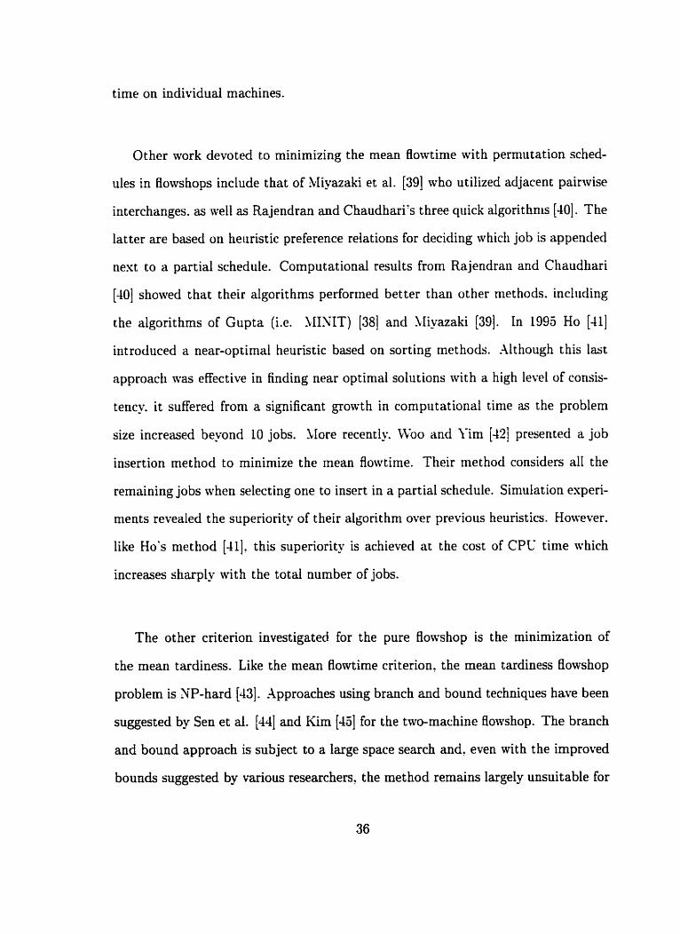
time on individuai machines.

O ther work devoted to minimizing the mean flowtime with permutation sched-

ules in flowshops include that of Miyazaki et al. [39] who utilized adjacent painvise

interchanges. as well as Rajendran and Chaudhari's t hree quick algorit hnis [-LOI. The

latter are based on heuristic preference relations for deciding which job is appended

nest to a partial schedule. Computational results from Rajendran and Chaudhari

[40] showed t hat t heir algorithms perforrned bet ter than other methods. incliiding

the algorithms of Gupta (i.e. 'YIINIT) [38] and Sliyazaki (391. In 1995 Ho [41]

introduced a near-optimal heuristic based on sorting methods. Although t his last

approacti \vas effective in finding near optimal solutions with a high level of consis-

tency. it suffered from a significant growth in cornpiitational time as the problem

size increased beyond 10 jobs. More recentlv. Woo and Yim [42] presented a job

insertion method to minimize the mean flowtime. Their rnethod considers al1 the

remaining jobs when selecting one to insert in a partial schedule. Simulation esperi-

ments revealed the superiority of t heir algorit hm over previous heuristics. Hoivever.

like Ho's method [Al] . this superiority is achieved a t the cost of CPC time which

increases sharply nrith the total oumber of jobs.

The other criterion investigated for the pure flowshop is the minimization of

the mean tardiness. Like the mean flowtime criteriont the mean tardiness flowshop

problem is XP-hard [43]. Approaches using branch and bound techniques have been

suggested by Sen et al. [44] and Kim [45] for the tm-machine flowshop. The branch

and bound approach is subject to a large space search and, even with the improved

bounds suggested by various researchers, the method remains largely unsuitable for

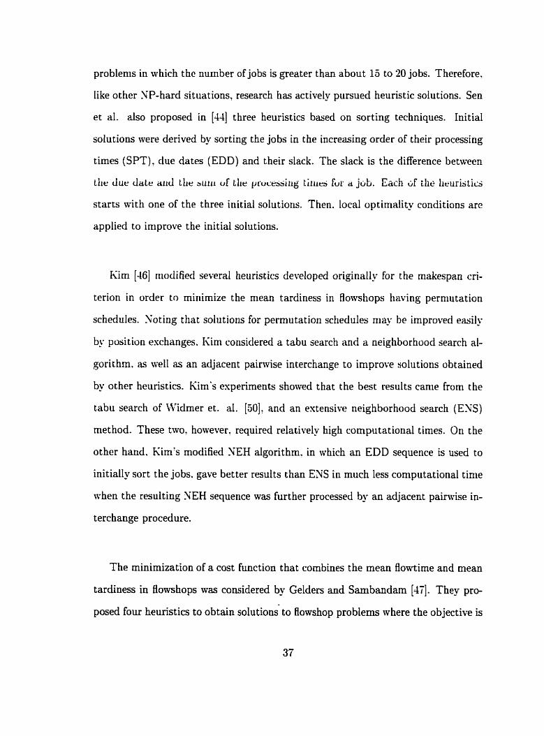
problenis in which the nu~nber of jobs is greater than about 15 to 20 jobs. Therefore.

like other NP-hard situations, research has actively pursued heuristic solutions. Sen

et al. dso proposed in [44] three heuristics based on sorting techniques. Initial

solutions were derived by sorting the jobs in the increasing order of their processing

times (SPT). due dates (EDD) and their slack. The slack is the difference between

tlic due date aiid the suiii uf tlir pructssiiig tiiiin Fui. a jub. Each ûf the Iiruristics

starts with one of the three initial solutions. Then. local optimality conditions are

applied to irnprove the initial solutions.

Kim [46] niodified several heuristics developed originally for the makespan cri-

terion in order to miriimize the niean tardiness in Howshops hüving permutation

schedules. Noting that solutions for permutation schedules niay be irnproved easily

by position eschanges. Kim considered a tabu search and a neighborhood search al-

gorithm. as te l l as an adjacent painvise interchange to improve solutions obtained

by other heuristics. Kim's experiments showed that the best results came h m the

tabu search of Widmer et. al. [SOI. and an extensive neighborhood search (ENS)

method. These twvo. however. required relatively high computational times. On the

other hand. Kim's modified NEH algorithm. in which an EDD sequence is used to

initially sort the jobs. gave better results than ENS in much less computational time

when the resulting NEH sequence was further processed by an adjacent painvise in-

terchange procedure.

The minimization of a cost function that combines the mean flowtime and mean

tardiness in flowshops tvas considered by Gelders and Sambandam [-li]. They pro-

posed four heuristics to obtain solutions to fiowshop problems where the objective is

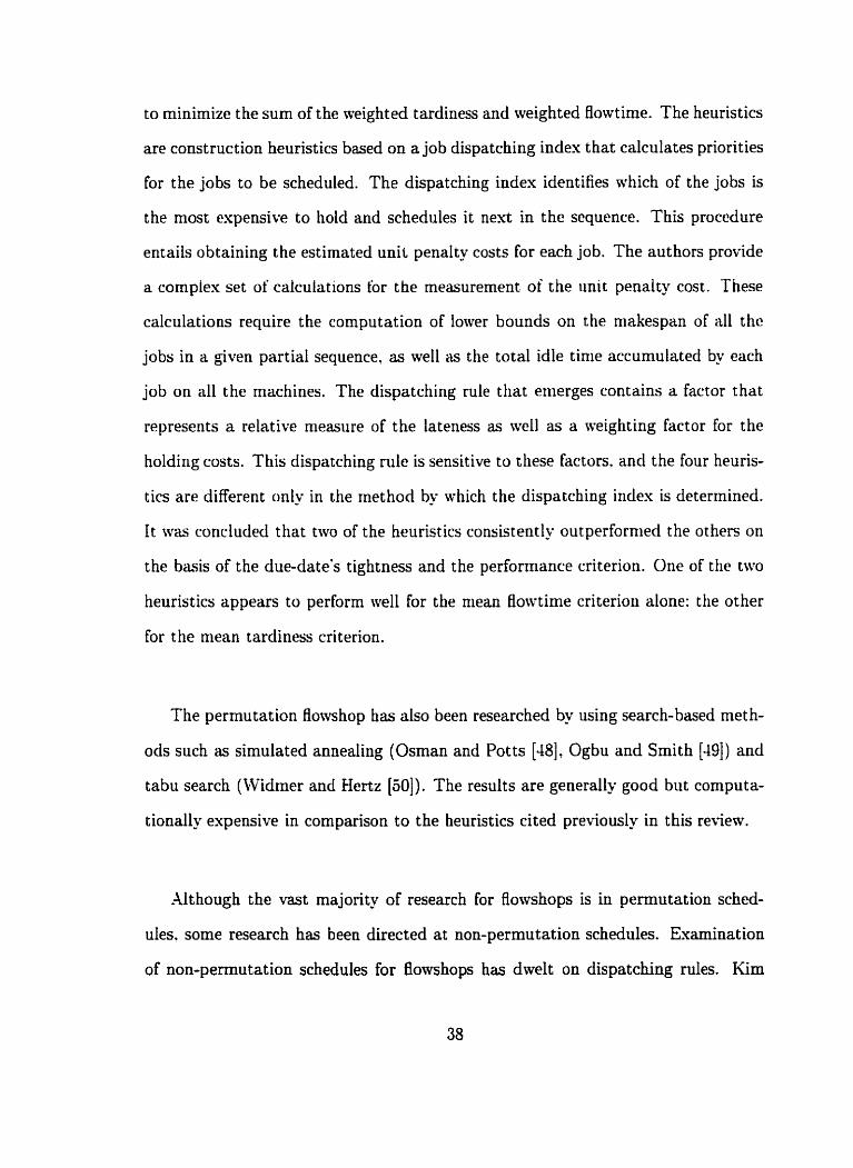
to minimize the surn of the weighted tardiness and weighted Elowtime. The heuristics

are construction heuristics based on a job dispatching index t hat calculates priorities

for the jobs to be scheduled. The dispatching index identifies which of the jobs is

the most expensive to hold and schedules it next in the sequence. This procedure

entails obtaining the estimated unit penalty costs for each job. The authors provide

a cornpiex set of calculations for the measurement of the unit penalty cost. These

calculations require the computation of iower bounds on the niakespan of al1 the

jobs in a given partial sequence. as well as the total idle tinie accumulatecl by each

job on al1 the machines. The dispatching rule that emerges contains a factor that

represents a relative measure of the lateness as well as a aeighting factor for the

holding costs. This dispatching rule is sensitive to these factors. and the four heuris-

tics are different only in the method by which the dispatching index is determined.

I t was concludecl that two of the heuristics consisteotly outperfornied the others on

the b a i s of the due-date's tightness and the performance criterion. One of the tttyo

heuristics appears to perform well for the mean flontime criterion alone: the other

for the mean t ardiness cri t erion.

The permutation flowshop has also been researched by using search-based meth-

ods such as simulated annealing (Osman and Potts [48]. Ogbu and Smith [49]) and

tabu search (Widmer and Hertz [SOI). The results are generally good but cornputa-

tionally expensive in cornparison to the heuristics cited previously in this review.

Although the v a t majority of research for fiowshops is in permutation sched-

ules. some research has been directed at non-permutation schedules. Examination

of non-permutation schedules for flowshops has dmelt on dispatching d e s . Kim

[46] investigated the performance of seven priority rules for dispatching, under the

critenon of niinimizing the mean tardiness. The rules were tested by using 1000

randomly generated problems. each having frorn 15 to JO jobs, and between Z and

25 machines in the flowshop. The due dates assigned to each job were determined

b an adaptation of the method of Potts and Van Wassenhove [jl] for a flowsliop.

The test problerns covereci a reasonabiy wiàe range of due date cightnesses. Kirri

concluded that the best performance was given by the Modified Due Date (LIDD)

rule. followed closely by the Apparent Tardiness Cost (.\TC) and the 'rlodified Op-

eration Due-date (!dOD) rules.

A comparative study of dispatching rules in Rowshops and jobshops \vas under-

takeu by Rajendran and Holthaus [SI. The objective was to evaluate the relative

performance of thirteen dispatching rules for the two shop types and dynamic job

arrivals. Three of these rules nere developed earlier by the same authors [S3]. The

study involved a number of performance criteria. including the mean flowtime. ma-

imum flowtime. mean tardiness and the proportion of jobs that are tardy. among

others. Extensive simulation experiments were conducted for a variety of machine

utilization levels and due-date tightness factors. Job arrivals in the simulations were

generated by using an exponential distribution for the inter-arriva1 tirnes. Values of

the performance rneasures were tabulated for each of the dispatching rules tested.

The main conclusion is that the performance of dispatching mles is influenced by

the job routings and shop floor configurations. Furthemore. dispatching rules that

contain additional information, such as the total work content of the jobs queuing

for the next operation, are more apt to simultaneonsly rninimize multiple perfor-

mance measures. The study did h d 7 however. that the COVERT (cost over time)

dispatching rule performed better in flowshops than in jobshops. This conclusion

contradicts earlier results [46] regarding the performance of COVERT in 0owshops.

The discrepancy may be attributed to how each of the investigators applied the

COVERT rule. because the rule requires user defined parameters to estimate the

lead times. Also? a noticeable omission from the dispatching rules tested by Rajen-

dran and Hoithaus is the 4IDD mie, a ruie that has been frequently cireci as being

a powerful one for rninimizing tardiness based criteria in flowshops.

Chan and Bedworth [54] considered the rninimization of the mean flowtinie in

florvshops. They derived formulae for computing temporap flowtimes between pairs

of jobs. Their algorithm was tested on specific configurations (nhere jobs can have

one of several fised routes) in what they called a niodified flowshop. The tests indi-

cated that the heuristic \vas preferable to using the l e s t work reniaining (LCVKR)

dispatching rule. In addit ion. the aut hors outlined the applicability of their heuris-

tic to dynarnic flowshops. where job arrivals at the shop are not simultaneous (Le.

unequal release times). Although the experimental results were satisfactory. they

were done for static flowshops only. and included problerns having only ten or fewer

jobs.

2.4 Single Machine Sequencing Problems

The static scheduling for a single machine is a permutation problem. The o p

timal solution is one of n! possible job sequences. For sorne performance criteria.

the optimal sequence can be obtained by sorting the jobs in a particular order (for

example, SPT in the case of minimizing the mean flowtime). For other perfor-

mance criteria, such as minimizing the mean tardiness, the problem is XP-hard [55].

When the scheduling criteria involve performance objectives that are YP-bard: many

heuristics attempt to capitdize on special dominance properties in order to curtail

the solution space. For exaniple. Russell and Holsenback [36] used the doniinance

properties described by Emmons i57j in t heir heurisric for ininimizing the mean car-

diness. O t her notable heiiristics for mean tardiness minimizat ion were presented by

Panwalker et al. [58]. Wilkerson and Invin [59] as well as Potts and Van Wassenhove

[3 11. Scheduling objectives involving two (bicriterion) and multiple criteria have also

been investigated. Then the niain approacli w a s to build particular heuristics for

the specific combinations of the performance objectives. Esamples of such instances

may be fotind in Van CFassenhove and Gelders [60]. Lin [61] and Chen and Bulfin [62].

lpproaches that are more generally applicable (i.e. that are valid for any perfor-

mance criteria) revolve around search-based techniques such as simulated annealing

(Potts and Van Wassenhove [XI). tabu seardi (Armentano and Roncini (631) and

genetic algorithms (Lee and Choi [64]). Scheduling fiexibility requires the ability to

develop good schedules for any given performance criterion. Search based methods

are flexible due to their generalized abilities. and the quality of their solutions im-

proves with more computational time. This cornputational demand severely lirnits

the effectiveness of these methods for on-line scheduling applications.

The scheduling approach proposed in this thesis is distributive in nature. It is

characterized by the developrnent of local schedules a t each machine. These localized

schedules! mhich are based on single machine sequencing, provide the frarnework for

the dispatching decisions that are made in order to determine which job is loaded on

the next available machine. The effectiveness of the approach. therefore. rests upon

the ability to find quick solutions of the single machine sequencing problem. Fast

search-based methods are needed if the system is to be applicable to cases involklng

new? uncornmon or multi-factor performance criteria. Chapter 4 in this thesis is

devoted to describing a neural aetwork that ran learn and generalize relationships

between jobs and the position each job should occupy in a sequence that satisfies

the given performance objectives optinially. A system of such networks may then

be used to quiîkly find nelu optimal sequences.

2.5 Conclusions

Two conclusioris rnay be drawn from the preceding review of the Literature on

scheduling and distributed scheduling in FSlSs. First . dispatching rules have a

natural appeal due to their low requirements for global data. and their suitability

to on-line scheduling. Secotidl- a state-dependent selection of dispatching rules

improves performance over the use of a single dispatching rule throughout the pro-

duction period.

The concept of switching dispatching mles in response to changes in a system's

attribut es poses a considerable operational difficulty. That difficulty is the decision

of when to mitch from an existing nile. and for how long the new rule is allowed to

operate before it too is reconsidered. The approach taken in this thesis employs a

dispatching mle that is based on a cornplex cost-based evaluation of the current state

of the system as a whole. The proposed dispatching met hod is. effectively. the result

of a cooperative decision between al1 the machines in a systern. The rule dynami-

cally alters priority levels for the jobs and irnplicitly achieves rule switching without

the problem of deciding when to switch. Furthermore, no knowledge relating system

states s i t h particular dispatching rules needs to be acquired. Finally. the proposed

cooperative dispatching approach avoids the 'bacchingt thar is common to most dis-

patching rules wheu jobs having identical processing and due-date data are involved.

Chapter 3

Cooperat ive Dispatching

Distributed control in a FMS utilizes data that is locally arailable to the enti-

tics in the system. The effectiveness of the scheduling system as a whole towards

meeting the performarice objectives depends on the quality OF the local data. The

availability of a computerized network linking the individual entities enhances che

local information by allowing the entities to exchangc data. without the need for

central supervision.

This chapter is devoted to describing and illustrating a rnethodology that is de-

signed to achieve consistently good scheduling in a FSIS under a distributed control

environment. The met hodolog.. called Cooperative Dispatching (CD). has been in-

troduced cursorily in the previous two chapters. CD behaves similar to dispatching.

but it focuses on boosting the quality of local data in a rnanner that enables overall

performance objectives to be met better.

3.1 Introduction

The principle of CD and an algorithm for its implementation are presented in this

chapter. A dispatching decision involves determining the priorities of the jobs wait-

ing in queue for a machine. This prioritization is based normally on the scheduling

objective. Traditional dispatching rules. such as SPT, EDD. MDD. etc. are quick

and simple methods that are comrnonly iised to decide dispatching priorities. It has

been s h o w [8] that. for given objectives and congestion levels? certain dispatching

rules outperform others. Most research dealing with dispatching rules has been per-

formed for jobshop environments, where the SPT rule was found empiically to be

better than a host of other ruies in minimizing the rnean Rowtinie i8i. For mini-

mizing the mean tardiness, however. a number of due-date based dispatching rules

were found to be equally competent but rather sensitive to shop congestion and

due-date tightness 191. Although flowshops are specific cases of jobshops. there are

indications t hat the conclusions wi t h regard to dispatching rules in jobshops clinnot

be generalized to Bowshops. For erample. Kim [46] reported that the COVERT

dispatching rule (81. generally acknowledged as a good one for jobshops. does not

perform satisfactorily in pure flowshops. Furthermore. a rule's performance can de-

pend on routing configurations. in addit ion to the congestion and due-date tightness.

Cooperative Dispatching is designed to overcome the preceding limitations by

providing a new dispatching procedure that is less sensitive to the previously men-

tioned factors. and more flexible for different performance measures. Cooperative

Dispatching is sirnilar to traditional dispatching rules in that its purpose is to se-

lect. from a number of candidates, a job to be processed next. It does differ from

t raditional dispatching rules in t hat the dispatching decision is taken collectively.

after the other machines in the ce11 are consulted in a unique manner. This ?con-

sultation' involves polling the other machines for their input regarding which of the

candidates available for dispatching is selected by the machine waiting to be loaded.

A procedure for resolving the competing claims of the candidate jobs is employed to

find the successful candidate, which is selected and then dispatched. The processes

of 'consultation' and conflict resolution which characterize t his approach lead to the

name 'Cooperative' Dispatching.

This chapter provides the details of Cooperative Dispatching and the algorithm

proposed for its implementation. The performance of the algorithm is evaluated by

using the t hree different routing configurations shown in Figure 3.1, wit h t hree differ-

ent performance rneasures: viz 1) minimizing the mean flowt ime. 2) minimizing the

mean tardineçs. and 3) minimizing the number of tard- jobs. The configurations in

Figure 3.1 are selected because they represent the more interesting routing patterns.

The Type 1 configuration represents the pure flon~shop. and Type II considers the

case where a machine can receive jobs frorn alternate machines (convergent routes).

Type III is a configuration that allows more than one possible destination for jobs

leaving a machine (divergent routes).

Given a flexible manufacturing system having rn machines and processing n jobs.

it is required to sequence the flow of jobs through the machines (or stations) in the

ce11 such that some cost function Z is rninimized.

Let

hi = holding cost for job i per unit time.

ti = tardiness cost for job i per unit time.

di = due date for job i.

n = total number of jobs available and ready for scheduling.

C, = time of completion of al1 processes for job i.

Bi = mau[ Ci - di ; O 1. Z = f (h i , ti).

The function Z that is of main interest is

The following assurnpt ions are made.

1. Jobs do not have alternate routings.

2. Set-up times are sequence independent. This nieans that set-up times can be

included in the processing time for a job on a given machine.

3. Pre-emption is not permitted. Once a job is started on a machine. it cannot

be intemipted in favor of another job. and then resumed aftenvards.

4. Inserted idle time is not allowed. .A machine ivill not rernain idle in order to

wait for a particular job to arrive if there are other jobs already a~ailable and

waiting to be processed.

5. Buffers have unlimited capacities.

6. Sorne or al1 of the buffers may be constrained to FIFO processing of the local

job queues.

7. Parts are arriving continuously to the cell, and they immediately enter the

system (Le. the jobs have unequd reIease times: and the Bowshop is dqriiamic).

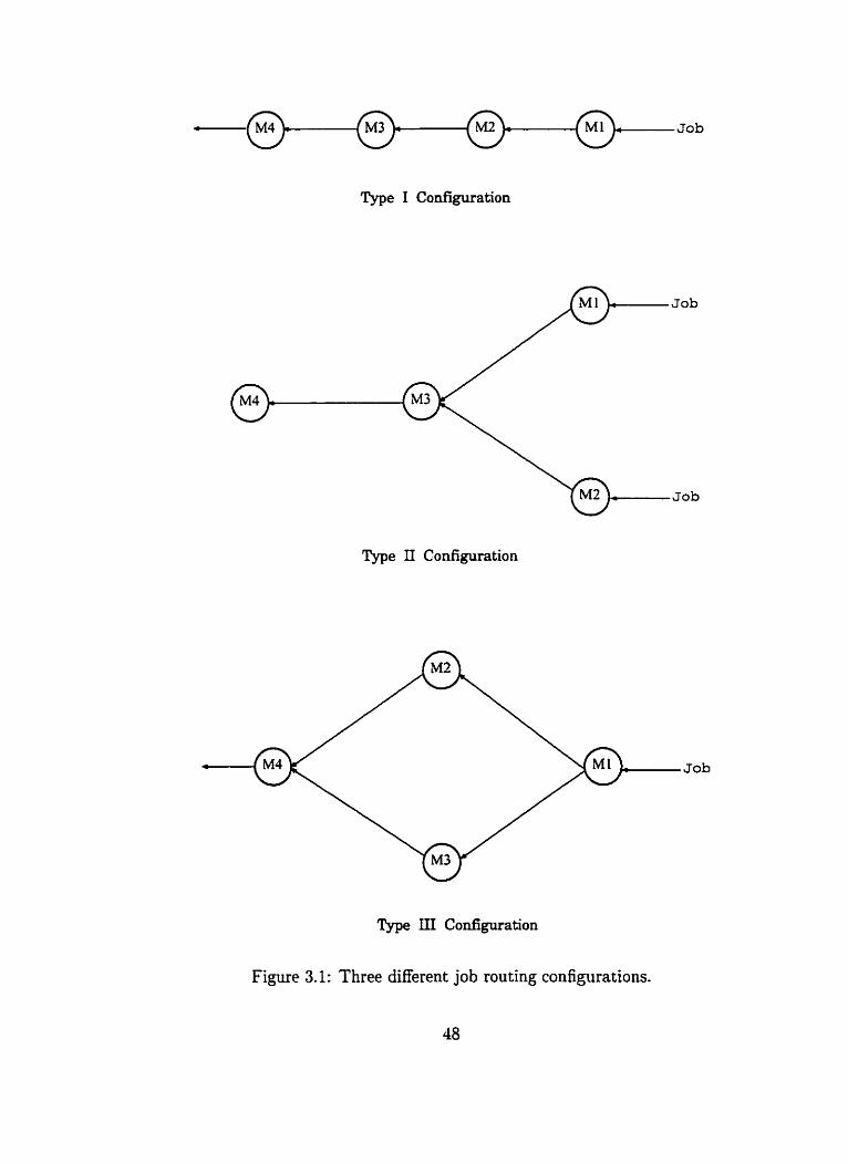
Job

Type 1 Configuration

Job

Job

Type II Configuration

Job

Type III Configuration

Figure 3.1 : Three different job routing configurations.

48

A static flowshop may be realized by setting the release times equal for al1 the

jobs. t hereby ensuring t heir simultaneous arrivais.

8. The holding cost for a job is uniform for al1 machines in the system.

3.2 Mathemat ical Mode1

3.2.1 Background

This section discusses the concepts behind the CD approach for sequencing the

Row of jobs through a m-machine ce11 that may be modeled as a pure or as a modified

Bowshop. The approach is best described as a heterarchical [1] one in which each

of the niachines in the ce11 acts independently in attempting to optimize the perfor-

mance measiire. In this environment. each machine specifies the sequence that mil!

enable it to minimize locally the perforniance measure under certain constraints and

assumptions. The constraints relate to the carliest possible starting tirnes (ready

times) for specific jobs on the machines. The assiimptions allow each individual

machine to behave as though it were operating as a single machine.

The consequences of this heterarchical approach. where each machine seeks to

optimize the performance measure locally and not globall- is usually a set of con-

Bicting demands regarding the setting of the dispatching priorities. These conflicts

are resolved through a cost-based methodology which aims to reconcile the local

optima in a manner that will promote the 'global' solution by selecting a candidate

job that is most acceptable to al1 the parties (machines) involved. It should be noted

that not al1 the machines have equd footing in determining the dispatched job. In

fact, each machine's 'say' in the decision is weighted by a factor that is commensu-

rate with its 'importance' at the global level. In this manner, the satisfaction of the

performance criterion locally is manipulated in the direction of sa t i skng the per-

formance criterion for the ce11 as a whole (Le. globally) . This relationship between

the local and global satisfaction of the performance criteria is explored further in

section 3.5.

The dispatching decision in the CD mode1 is centered around a matrk of real

nurnbers that is used as the ba i s for determining the priorities for the jobs ready

for dispatching on the next available niachine (machine s). This matriu. called the

sequence cost (SC) matriu. has dimensions of m x nr, The m is the number of

machines in the ce11 whilst nr, represents the number of jobs that are immediately

available for loading (i.e. the contents of the buffer a t machine s ) . The element

SCk, represents what is called the sequence cost to machine k in the event that the

job in the buffer is selected for dispatch.

The sequence cost to a machine is defined as the d u e of the performance

measure for a panicular scheduling of the jobs on that machine. Let. for simplic-

ity. the variable r represent the yth job in the biiffer at machine s (i.e. x = r:). Then. the schedule used in determining the sequence cost for machine k is that

which optimizes the performance mesure on machine k? given that job z is the

first in sequence. The remaining jobs that are to visit machine k are assumed to

be ready and available by the time the processing of job r is completed on machine

k. This assumption of equal release times is adopted solely for reducing the cal-

d a t i o n burden. Although this sirnplihng assumption may seem unrealistic, it is

not overly unreasonable considering that it still allows a cornparison of the sequence

costs for al1 of the machines to be made on the b a i s of lower bound estimates of

the performance measure. The optimal sequence of the set of jobs Rk on machine k,

excluding job is determined by treating this situation as a sub-problem involving

the solution of a single machine sequencing problem. Each entry in rnatrix SC.

therefore. entails solving a separate single machine sequencing problem.

Whencver the occasion calls for a dispatching decision at machine S . CD requires

that al1 the machines in the flowshop are polled to deterniine which job each machine

favors. -4 machine is allowed to nominate two candidates. the second candidate be-

ing essentially an alternate to mitigate the negative impact in the event that its first

choice is not selected. Each machine. therefore. selects its two most favored jobs.

namely those two that give the least sequence costs in the SC matris for the respec-

tive machines. Once the coniplete set of dispatching candidates is compiled. conflict

resolution is performed with the aid of the SC mat rk to determine the 'winning' job.

The main steps in the CD approach are summarized next.

1. CD dispatching is invoked whenever a machine s is available and more than

one job is ready and waiting to be processed on it.

2. Sequence costs are calculated at each machine and the corresponding SC ma-

t rix is constructed.

3. By using the SC matrk, the candidate jobs for dispatching are identified. (See

section 3.2.3.)

4. With the aid of the SC matriv again, one of the candidate jobs is selected for

dispatching.

The above cycle constitutes what is called a 'stage' in the CD procedure. A

stage is concluded after a job is selected and dispatched.

3.2.2 Constructing the SC Matrk

The cornerstone of the CD approach is the SC matrix. To explain the crucial

paranieters involved in constructing this matrix. the bllowing illiistrative example

is introduced.

An exaniple of a piire flowshop problem rvith five jobs on four machines is pre-

sented in Table 3.1. A11 the in-process buffers for this problern are seniced according

to the FIFO rule. Hence the schedule of the jobs on the niachines is a permutation

schedule. and dispatching occurs only at the initial machine (machine number 1).

For the purpose of explmation. it is assumed that the first three jobs (i.e. jobs 1.

2, and 3) have been dispatched already in the order of the job numbers. The result-

ing partial schedule is s h o m after the first three stages in Figure 3.2(a) in the f o m

of a Gantt chart. .A 'stage* in the construction of the schedule represents the series

of calculations culminating in a dispatching decision. The partial schedule shown

in Figure 3.2(a) indicates that 55 time units after the dispatch of job 1, machine 1

is available again. At this instant, the remaining possibilities are to dispatch either

job 4 or job 5. The partial schedule can be updated to reflect the current status by

setting the current tirne to zero and accordingly updating al1 the times. (Thus the

*5 2

Table 3.1: Processing times for Esaniple 3-1.

tiriie is advaricecl by t h e 55 units clapsed in the first ttiree stages.) The current-tiiiie

statiis is showii in Figiirc 3.2(b). where a decision is iioa to Le niade (at tinie zero)

on niachine 1. This decision involves the iipdattd tirrie data (i.e. the niodified dile

dates) for the trvo jobs rvaiting to be loaded at niachine 1. as siiowi in Table 3.9.

Note that as niachine 1 is the only niachine in Esample 3-1 wtiere dispatcliing takes

place. the variable a eqiials one.

Table 3.2: Cpdated data for Esaniple 3-1.

Esaniple 3-1 illustrated a typical setting in rvhich CD is invoked. Sanieh

a machine is aiailable for dispatching at an instant in tirne. and sequence costs for

.)

time

time (b)

Figure 3.2: Gant t charts showing partial schedules.

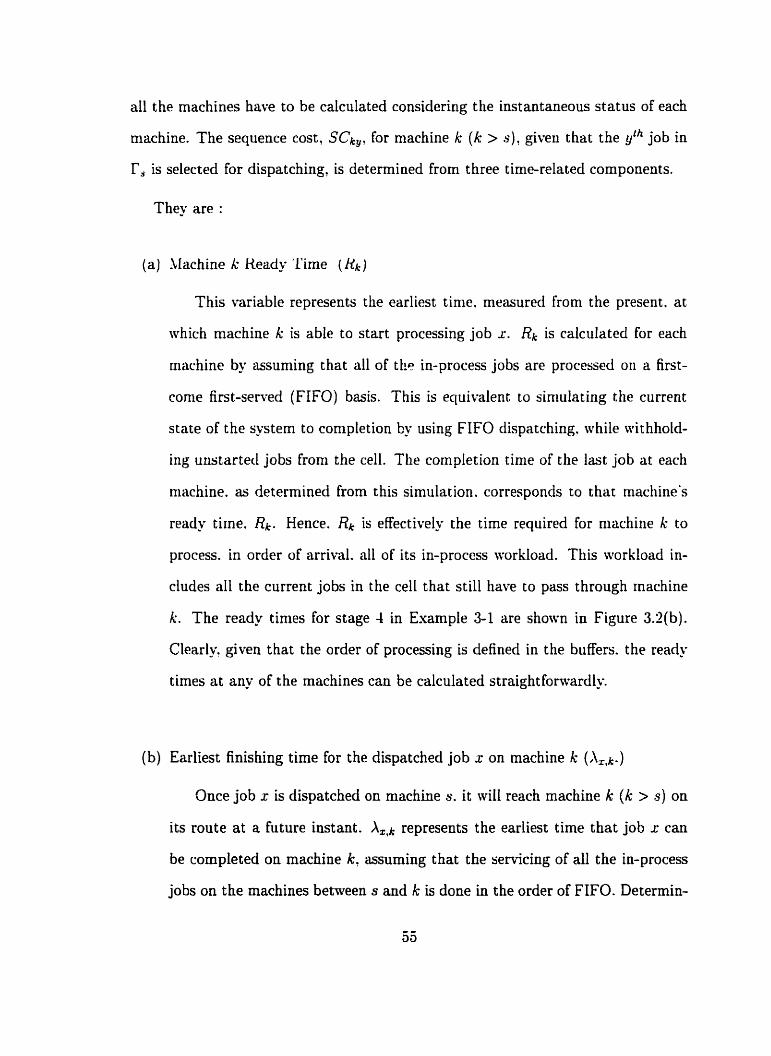
al1 the machines have to be calculated considering the instantaneous status of each

machine. The sequence cost. SCk,, for machine k (k > s )? giveu that the y'h job in

r, is selected for dispatching, is determined from three t ime-related components.

The- are :

(a) Machine A: Heady 'Lime ( H k )

This variable represents the earliest tinie. measured from the present. a t

which machine k is able to start processing job s. Rk is calculated for each

machine by assuming that al1 of the in-process jobs are processed on a first-

corne first-served (FIFO) basis. This is equivalent to siniulating the current

state of the system to completion ty using FIFO dispatching. while withhold-

ing unstartecl jobs from the cell. The completion time of the last job at each

machine. as determined from this simulation. corresponds to that machine's

reiidy tirne. Rk. Hence. Rk is effectively the time required for niachirie k to

process. in order of arrival. al1 of its in-process workload. This workload in-

cludes al1 the current jobs in the ce11 that still have to p a s through machine

k. The ready times for stage 4 in Example 3-1 are shown in Figure 3.2(b).

Clearl- given that the order of processing is defined in the buffers. the ready

times a t any of the machines can be calculated straightforwardly.

(b) Earliest finishing time for the dispatched job x on machine k ( A z v k - )

Once job x is dispatched on machine S. it wilI reach machine k (k > s) on

its route at a future instant. represents the earliest time that job x can

be completed on machine k? assuming t hat the senicing of dl the in-process

jobs on the machines between s and k is done in the order of FIFO. Determin-

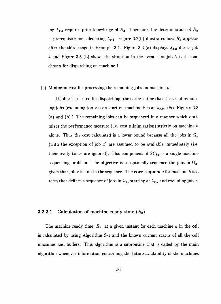
ing X r V k requires prior knowledge of Rk. Therefore? the determination of Rk

is prerequisite for calculating Xrak. Figure 3.2(b) illustrates how RI. appears

after the third stage in Erample 3-1. Figure 3.3 (a) displays if x is job

-4 and Figure 3.3 (b) shows the situation in the event that job 5 is the one

chosen for dispatching on machine 1.

4lininium cost for processing the rernaining jobs on niachine k.

If job 2 is seleçted for dispatching, the earliest time that the set of remain-

ing jobs (excluding job x) can start on machine k is a t /\r.k. (See Figures 3.3

(a) and (b).) The remaining jobs can be sequenced in a nianner which opti-

mizes the performance measure (Le. cost niinimization) strictly on machine k

alocie. Thus the cost calculated is a lower bound because al1 the jobs in RI.

(with the exception of job s) are assumed to be available immediately (i.e.

their ready times are ignored). This component of SCk, is a single machine

sequencing probleni. The objective is to optimally sequence the jobs in Rk.

given that job s is first in the sequence. The core sequence for machine k is a

term that defines a sequence of jobs in Rç, starting at and escluding job r.

3.2.2.1 Calcuiation of machine ready time (Rk)

The machine ready tirne? Rk, at a given instant for each machine k in the ce11

is calculated by using Algorithm S-1 and the known current status of a11 the ce11

machines and buffers. This algorithm is a subroiitine that is called by the main

algorithm whenever information concerning the future availability of the machines

*

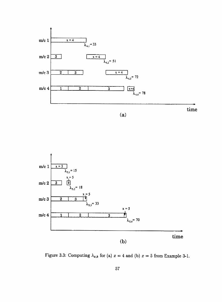
time (a)

Figure 3.3: Computing for (a) z = 4 and (b) x = 5 from Example 3-1.

is required. Algorithm S-1 merely simulates the evolution of the in-process flow in

the ce11 up to a point that allows the determination of when. a t the earliest. each

machine will be able to accommodate a newly dispatched part. This simulation

merely tracks the event instances leading to this point. An event occurs whenever

a machine completeç its current job and becomes available for the next. Algorithni

S-1 is described next.

Algorithm S-1

Let

= tirne.

= machine where dispatching is requircd.

= machine number k = 1.2 . m.

= set of jobs lined up at the buffer for machine k.

= job currently in-process a t machine k.

= time taken to complete current operation on machine k .

= most recently dispatched job in the cell.

= triplet (a.b.c) that describes an event. aherc

a = tirne of the event's occurrence.

b = job involved in the event.

c = machine where the event occurs.

= set of the active triplets having the form d.

Step 1. Initializat ion.

E = 0.

Rk = O Y k.

For al1 k. if ak # O. then q~ = (ua, 'aky k) is appended to E.

Step 2. Identification of Event.

If E = 0. then continue to Step 6.

Othenvise determine d E E which has the earliest event occurrence

amongst the triplets current in E. Let o* be the tinie of this occur-

rence. m' be the machine concerned. and j * be the job for this event.

Step 3. Job Transfer to Next Machine.

If m* is not the last machine in the route for job j'. rernove j * frorn

a,- and add it to Q k where k is the nest machirie in the route of j'.

If ak = O. then ap = j' and gk = II.

Step 4. Loading Curent Machine.

Remove 9 = (a*. j'. m*) from E.

If m* = q. then &- = t.

Step 5. Updating Event List.

If ik,- # O , then

a,- = next job waiting in line at the buffer for machine m*: and

u,_. = processing time for job am- on machine m*.

Add d = (O* + u,_. -a,-? m*) to E.

R e t m to Step 2.

Step 6. Termination.

Return values calculated for &. k = 1.2. . rn to the calling Algo-

rithm.

Stop.

Algorithm S-1 is iterative. An iteration starts with the completion of a job on

one of the machines jstep 2)' and covers the transfer of this job to its next destina-

tion (step 3). the loading of the now vacant niachine with the next part in its buffer

(step 4). and ends with the updating of the cellas status (step 5 ) .

To demonstrate the application of hlgori t hm S- 1. the machine ready t inies ( Rk)

are calculated a t the beginning of stage 4 for Esample 3-1. The instantaneous sit-

uation. with machine 1 waiting to be Ioaded. is illustrated in the Gantt chart of

Figure 3.2 (b). Step 1 initializes the variables to reflect the current status of the ce11

at instant t=O. At the start of stage 4. jobs 3. 2 and 1 are in-process on machines 2.

3 and 4 respectively, and machine 1 is available for loading. Thus. al = O: a? = 3:

a:, = 2: and a4 =l. The times remaining to complete the current jobs on machines

2' 3 and 4 are 10, 16 and 16 units, respectivele so that (LI = O. u2 = 10. us = 16

and (14 = 16. Ri t hrough & are initialized to zero' and 9 to Q4 are empty because

there are no jobs waiting in the intemediate buffers. The events list, E. at time

t=O is {(10,3.2),(16,2,3),(16,1~4)}. The job dispatched in the previous stage. q. is

job 3 (Le. q- = 3).

Iteration 1

Job 3 is completed on machine 2 a t time t=10. Then it. is unloaded and moved to

the buffer for machine 3. As job 3 is the job identified by 0' its completion signals

that the machine ready time for machine 2 is equal to t . Therefore R2 = 10. E is

now updated and appears as {(16,2.3).(16,1.4)}.

Iteration 2

E shows that job 2 on niachine 3 and job 1 on machine 4 are completed sirnulta-

neoiisly. This tie is settled arbitrari15 and job 2 is unloaded from machine 3 and

moved to the buffer for niachine 4. Job 3. waiting in the buffer. is loaded next on

machine 3. E now becomes { ( 16.1 A) $30.3.3) }.

Iteration 3

Job t is completed at time t=16 and it is unloaded from machine 4. Job 2 is loaded

next on machine 4. and E is now {(30.3.3).(33.2.4)}.

Iteration 4

Job 3 is completed on machine 3 at time t=30. It is unloaded and moved to the

buffer for machine -4. Rg equals 30 because the job just unloaded vas the job q. E

is now {(35.2,4)).

Iteration 5

Job 2 is completed and unloaded from machine 4 at tirne t =35. Job 3, waiting in

the buffer for machine 4: is then loaded. E is {(69:3.4)}.

Iteration 6

Job 3 is cornpleted and unloaded from machine 4 a t time t=69. Therefore. R4 is

equal to 69 ( q = 3). E = 0 now. and the .Ilgorithm S-1 terminates at this point.

Algorit hm S-1 returns the following machine ready times for Example 3- 1.

RI = O: R2 = 10: R3 = 30: and R.4 = 69.

These results can be verified with reference to Fig. U ( b ) .

3.2.2.2 Calculation of

The earliest time that the dispatch candidate (job c) can be completed on ma-

chine k. depends on whether or not machine k belongs to the set of remaining

machines that will be visited by job x (3,). If machine k is visited by job r ( k E 3,).

then XITk is influenced directlp by the earliest finishing times for job x on the preced-

ing machines on the route of job x. If job x does not visit machine k (k 4 3,). then

does not theoreticaily exist. Nevertheless. the processing of job r on machines

preceding k in the flowshop indirect ly influences the earliest complet ion t imes for

other jobs that share some machines with job x and that do visit machine k. Con-

sequently. an artificial job is created for use in determining a value for XZL in the

case where machine k is not visited by job 2.

Case 1 : job x visits machine k ( k E ,&)

An example of such a situation would occur in the Type III configuration de-

picted in Figure 3.1. Supposing that job xk route is ;I, = {1.2.4}, then X l Y k would

be calculated when k is 1. 2. or 4 under this case. Here. job r c m start on machine k

if and only if this machine is available. and the operation for job r on the preceding

machine in job 2 s route is completed. as illustrated in Figure 3.4.

With the exception of the pure flowshop (Type 1) configuration. a job need not

always go next to the machine having the imniediately following index number.

Therefore. the indes pk identifies the index number of machine k in the set 3,.

Thus machine k d l be the pih machine in the remainder of the route for job x.

To illustrate. if 3, = {1.2.4}. then Equation (3.2) gives pl=l: p2=2: and p4=3:

PJ does not exist (because 3 $ 3,).

Referring to Figure 3.4. it is seen that XrQk is equal to the maximum of the

earliest starting tirne on machine k (Rk) and the earliest finishing time for job x on

the machine preceding k on the route of job x (dg*-l). plus the processing tirne for

job x on machine k. Thus. AZt can be calculated by :

machine

t irne

Figure 3.4: when k E 3,.

Case II : job I. does not visit machine k ( k @ 3,)

Consider the same example as that used in Case 1. Here X E s 2 when k = 3. would

fa11 under a Case II situation because job x's route does not include machine 3.

Application of Equation (3.3) in this instance woiild leave equal to Rk. In

reality. hotvever. the selection of job r at machine s when k 6 & implies that other

dispatching candidates that do pass through machine k will be delayed in reaching

k. the more so as they share preceding machines Nith job x. Consequentlp. allowing

= Rk here would result in a substantial underestimation of the sequence cost

in machine k. This would cause machine k to gain an unwarranted weight in the

dispatching decisions. To find a doser estimate of an 'artificial' job is created

and used as a 'dummy' for job x. The processing time on machine k for this artificial

job iç taken simply as the average of the processing times of al1 the jobs in Rk that

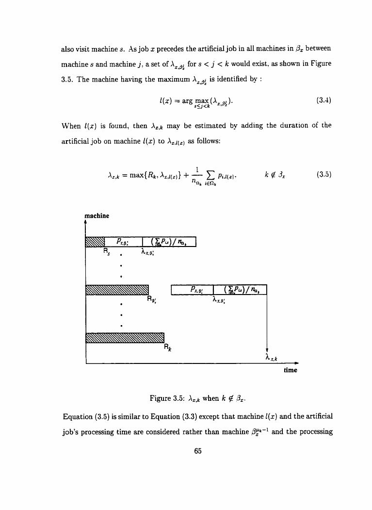
also visit machine S. As job x precedes the artificial job in al1 machines in between

machine s and machine j, a set of for s < j < k would exist. as shown in Figure

3.3. The machine having the maximum Ar,di is identified by :

When 1(x) is found? then AtIk may be estimated by adding the duration of the

artificial job on machine 1(x) to as follows:

machine 4

Figure 3.5: when k @ 8.

Equation (3.5) is similar to Equation (3.3) except t hat machine Z(x) and the artificial

job's processing t h e are considered rather than machine @k-' and the processing

time of job z respectivel. Equations (3.3) and (3.5) can be combined into one

general equation to detemine Xzqk as :

Equation (3.6) allows the computation of in general, for al1 the configurations

considered in Figure 3.1.

Example 3-3

The following example illustrates how is found frorn Equation (3.6) in stage

4 of the problem described in Example 3-1. Equation (3.6) indicates that

is calculated recursively. This means that. to find X4;2. values of A4+ and

must be available beforehand. Xote that the ready times for the four machines

(RI =O. R2=10. R3=30.&=69) have been calculated already in Exampie 3-2. and

that the route for job x = 4 is 34 = {1.2.3.4). Hence. by applying Equation (3.3).

we have XJIo = 0.

To find X4,1? Equation (3.2) is used to find pl :

Applying Equation (3.6), and noting t hat 3: =O;

&,1 = ma{&, X4.0} + P4J = 33.

Frum Equation (3.6), and noting that 3:=l:

1 .- - mâ~{&, .?;,:} + p4.1 = 51. - * t ,L

This result may be verified by using the Gantt chart presented in Figure 3.3 (a).

3.2.2.3 Determining the Core Sequence for Machine C

Once is known. the jobs remaining in machine k's workload (Rk) can be

sequenced as a single machine problem start ing at time . Thus A,,k is the instant

in time after which the assumption of single machine sequencing holds. The order

in which the jobs in Rn. are sequenced influences the performance nieasure when it is

applied to machine k alone. .A sequence's effectiveness in meeting the performance

nieasure may be expressed as a cost function in the form of :

f i f f > O where 6(1 ) =

O i f s 5 0

and k = 1:2,-,m: y = 1?2,---,nr,.

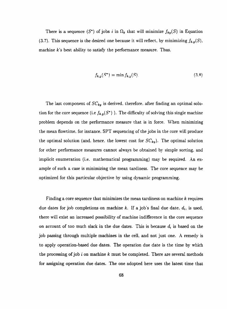
There is a sequence (S*) of jobs i in Rk that will minimize fky(S) in Equation

(3.7). This sequence is the desired one because it will reflect , by minimizing fkJS),

machine k's best ability to satisfy the performance measure. Thus.

The last component of SCk. is derived. therefore. after finding an optimal solu-

tion for the core sequence (i.e fk,&T) ). The difficulty of solving this single machine

problem depends on the performance measure that is in force. When minimizing

the mean Aowtirne. for instance. SPT sequencing of the jobs in the core will produce

the optimal solution (and. hence. the lowest cost for SCk,). The optimal solution

for other performance measures cannot always be obtained b - simple sorting. and

iniplicit enumeration (i.e. mathematical programming) may be required. An ex-

ample of such a case is minimizing the mean tardiness. The core sequence niay be

op t imized for t his part icular objective by using dynamic prograrnming.

Finding a core sequence that minimizes the mean tardiness on machine k requires

due dates for job completions on machine k. If a job's final due date. d*, is used.

there will exist an increased possibility of machine indifference in the core sequence

on account of too much slack in the due dates. This is because d, is based on the

job passing through multiple machines in the cell. and not just one. h remedy is

to apply operation-based due dates. The operation due date is the t h e by which

the processing of job i on machine k must be completed. There are sewral methods

for açsigning operation due dates. The one adopted here uses the iatest time that

the processing of job i can be completed on machine k without contributing to the

tardiness in completing job j. The operation due dates are calculated as :

3.2.2.4 Dynamic Programming Formulation

The performance measure described by Equation (3.7) is a function of the com-

pletion times of the jobs. .A sequence that minimizes function (3.7) may be found

by using dynamic programming (DP). The DP method used here is based on [65].

and it is described nest.

Let Qi = + Ci. Then function (3.7) can be rewritten as :

min Z = C g i ( ~ i )

where

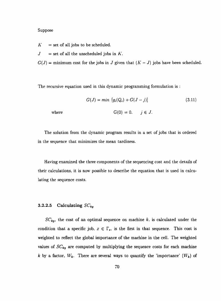
Suppose

Ii = set of a11 jobs to be scheduled.

J = set of al1 the unscheduled jobs in K.

G ( J ) = minimum cost for the jobs in J given that (li - J ) jobs have been scheduled.

The recursive equation used in this dynarnic programming formulation is :

G ( J ) = min [g i (Qi ) + G(J - j ) ] (3.11)

w here G(0) = O. j E J .

The solution from the dynamic program results in a set of jobs that is ordered

in the sequence t hat minimizes the mean tardiness.

Having examined the three components of the sequencing cost and the details of

their calculations: it is now possible to describe the equation that is used in calcu-

lating the sequence costs.

SCh, the cost of an optimal sequence on machine k: is cdculated under the

condition that a specific job. x E I',: is the first in that sequence. This cost is

weighted to reflect the global importance of the machine in the cell. The weighted

values of SCk, are computed by multiplying the sequence costs for each machine

k by a factor, LVk. There are several mays to quantify the 'importance' (Wk) of

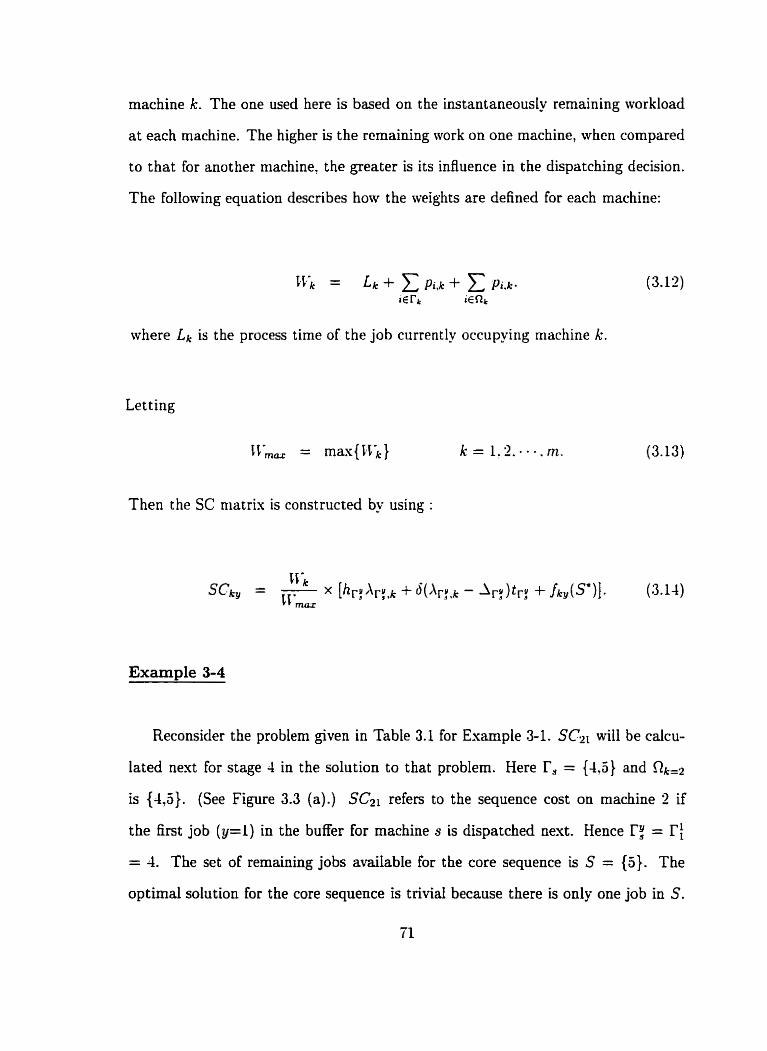
machine k. The one used here is based on the instantaneously remaining workload

a t each machine. The higher is the rernaining work on one machine, when compared

to that for another machine, the greater is its influence in the dispatching decision.

The following equation describes how the weights are defined for each machine:

where Lk is the process time of the job currently occupying machine k.

Let t ing

\ILu = rnax{DL}

Then the SC niatrix is constructed by using :

Reconsider the problem given in Table 3.1 for Example 3-1. SC2[ will be calcu-

lated next for stage 4 in the solution to that problem. Here T, = {4'5} and Rk=*

is (-43). (See Figure 3.3 (a).) SC2i refers to the sequence cost on machine 3 if

the first job (y=l) in the buffer for machine s is dispatched next. Hence ry = Tf

= 1. The set of remaining jobs available for the core sequence is S = {j}. The

optimal solution for the core sequence is tnvid because there is only one job in S.

71

Hence. S*={J). Had there been more than one job in S. then S* would have been

a sequence of those jobs that minimizes the mean tardiness.

Noting that ri = 4 and using Equation (3.14) gives:

From Equations (3.12) and (3.13):

IL; = 33 + 15 = 48:

I.Ci = 10 + 28 + 3 = 31:

Li, = 2 1 + 14 + 21 + 3 = 65;

CC:, = 27 + 19 + 34 + 6 + 1 = SI .

From Equation (3.9): the operational due date for job 5 on machine 2 is:

A value for fil(S*) is needed in calculating SCb. It is found by using Equations

(3.7) and (3.8) as follows :

Recalling from Example 3-2 that X4;2 = 51 for this situation:

Thus. by using Equation (3.14) to compute SC2l:

From Equation (3.9) :

A4;L = 40 - (21 + 6) = 13

so t hat .

SC21 = 0.36 x [O + S(5l - 13) + -IO] = 27.79 .

SimiIar calculations produce fil = 37: f12 =3: = 23: f31 = 38: f3* = '20:

fJl = 61: and f42 = 36.

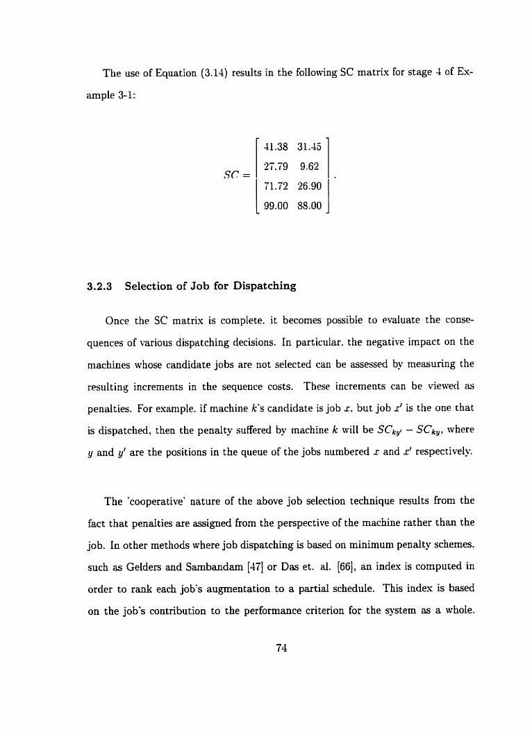
The use of Equation (3.14) results in the following SC matriv for stage 4 of Ex-

ample 3-1:

3.2.3 Selection of Job for Dispatching

Once the SC matrix is cornplete. it becomes possible to evaluate the conse-

quences of various dispatching decisions. In particular. the negative impact on the

machines whose candidate jobs are not selected can be assessed by measuring the

resulting increments in the sequence costs. These increments can be viewed as

penalties. For example. if machine k's candidate is job r. but job r' is the one that

is dispatched. then the penalty suffered by machine k will be SCkg( - SCk,, where

y and y' are the positions in the queue of the jobs numbered r and 2 respectively.

The 'cooperative' nature of the above job selection technique results from the

fact that penalties are assigned from the perspective of the machine rather than the

job. In other methods where job dispatching is based on minimum penalty schemes.

such as Gelders and Sambandam [ d i ] or Das et. al. [66], an index is computed in

order to rank each job's augmentation to a partial schedule. This index is based

on the job's contribution to the performance criterion for the system as a whole.

In cooperative dispatching, conversely, the main ent it ies are the machines. not the

jobs. and the penalties are a measure of the deviation from the optimal satisfaction

of the performance criterion locdly, with respect to each machine. The final job

dispatching decision reflects a resolution of these. usually conflicting, requirements

for local optimization. The conflicts are resolved through a process that involves

nvminatiûns sf pmferred jobs from cach of thc mxhincs, folloxcd bj- thc sclcction

of a winning candidate.

3.2.3.1 Identifying Candidates

The next step is to determine which of the jobs in T, are preferred by each

of the machines involved in the dispatching decisiori. Every machine. as explairieci

previously :nakes a first and a second choice. Di and DF respectivel. as follows:

DL = arg min Y

and

The set of jobs nominated for dispatch. labeled set G. is

G = D i u D 2 U - - - D k k = l . 2 , - - 7 m . (3.18)

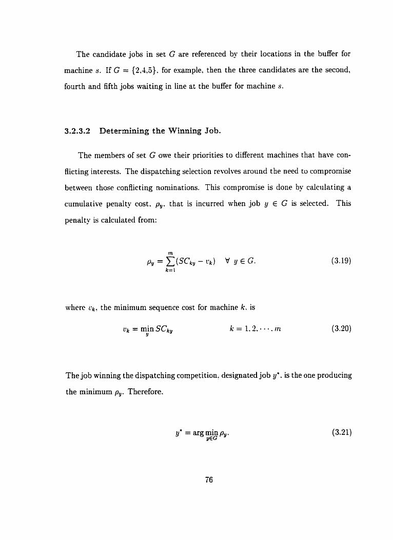
The candidate jobs in set G are referenced by their locations in the buffer for

machine S. If G = {2.4,5}. for example, then the three candidates are the secoiid?

fourth and fifth jobs waiting in line at the buffer for machine S.

3.2.3.2 Deterrnining the Winning Job.

The members of set G owe their priorities to different machines that have con-

fiicting interests. The dispatching selection revolves around the need to compromise

between t hose con flic t ing noniinat ions. This compromise is doue by calculat ing s

cumulative penalty cost. p,. that is incurred when job y E G is selected. This

pend ty is calciilated from:

where L T ~ , the minimum sequence cost for machine k. is

uk = min SCk, k = 1 . 2 . - - - . m Y

The job winning the dispatching cornpetition. designated job y'. is the one producing

the minimum p,. Therefore.

y* = arg minp,,. YEG

The job to be dispatched nest is, therefore, the job occupying the y*th position

in queue at the buffer For machine S. This job is identified by I'$. An example is

employed nert to illustrate the procedure of decidingo by means of the SC rnatrix.

which job. from a set of available jobs, is dispatched next.

Suppose that. at a certain stage. job nurnbers 6. 3. 1. 4 and 8 are queued in that

order in the buffer For machine S. .Assume the corresponding sequence cost rnatrix

is:

The set of available jobs being considered for dispatching is T, = {6.3.1.4.8}.

From Equat ion (3.30)

u, = 245.00: u* = 81.55; ug = 372.43: and u~ = 235.66.

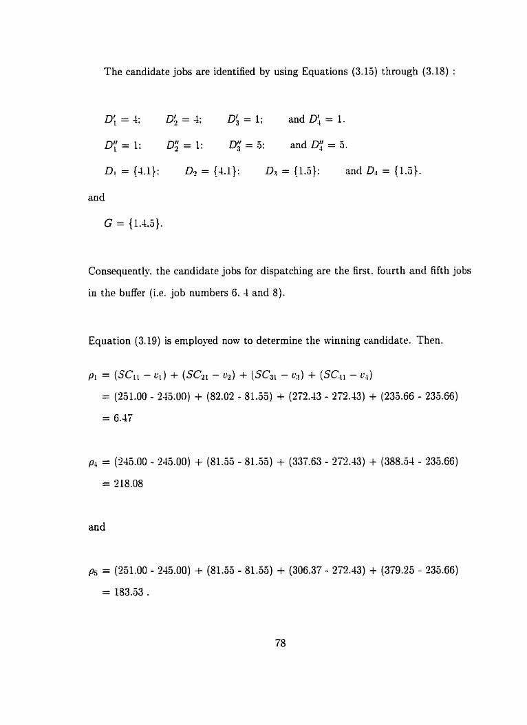
The candidate jobs are identified by using Equations (3.13) t hrough (3.18) :

Di = 4: D!, - = 4; 0; = 1; and DI, = 1.

Dy = 1: Dg = 1: 03 = 5: and Dy = 5.

D! = {4.1): = {-Li): DrI = {l .5}: and D., = (1.5).

and

G = (1.4.5).

Consequently. the candidate jobs for dispatching are the first. fourth and fifth jobs

in the buffer (i.e. job numbers 6. 4 and 8).

Equation (3.19) is employed now to determine the winning candidate. Then.

and

-4 cornparison of p l , p4 and p~ shows that pl hm the l e s t numerical value. Hence

the winning job is the first one in the buffer. which corresponds to job number 6

(because I'3 = 6). Therefore, CD dispatching results in job 6 being dispatched next

on machine S.

3.2.4 Cooperative Dispatching Algorithm

Steps in a construction algorithm to irnplement the cooperative dispatching

mode1 are outlined next.

S tep 1. Initializat ion.

1.1 :kc = I if tliere is a job route from rnacliin~ k to miwiiine c.

Othenvise. :k, = O for k = 1.2.. + * . rn and c = 1.2. -. . . m.

1.2 Determine the operation due dates. &. from Equation (3.9) for

al1 jobs.

1.3 Set CFk = O if machine k is constrained to FIFO dispatching

only. Othenvise CFk = 1.

1.4 = 0. Rk = O for k = 1.2.-. m.

1.5 If r'k exists. then append (O.O,k) to ( V k.

1.6 Set t = 0.

Step 2. Event Response.

2.1 If < is empty, proceed to Step 6 .

2.2 Find the 6 E < which has the earliest event time. Let s and a

be the machine and job for this event and t* be the time of its

occurrence.

2.3 If cu = 0, put x'= O and proceed to Step 5.

2.4 Set t = t'. Subtract t* from al1 lik and from al1 time elements.

o. in <.

2.5 The next machine on job a's route is .3:flL. where p, =

~ g , ~ , ~ , , ~ ( J i = k). Let kt = 3zs'l. If k' does not exist. then

r, = t' and proceed to Step 3.

2.6 If machine k' exists and it is free. then job a is loaded on this

machine and the corresponding event's triplet ( O ) is added to the

event list. Othenvise. job û is added at the end of the buffer for

machine kt . .1Iathematically. if LTL = O. then C i l = n and the

event triplet (p,,r).n.k' is appended to ,t. Othenvise. a is put at

the end of the set r p .

2.7 If CF, # 1. set r' = and proceed to Step 5.

Step 3. Construction of SC Matrix.

3.1 If ï: does not exist, set x' = rf and proceed to Step 5 .

3.2 SCxv = -1.00 for k = 1.2;-..rn: y = 1.2,-ob.nr,.

Determine a, and set x = 1.

3.3 If r: does not ~ ~ i r t , prîceeb to $tep 5 .

Determine 3,.

3.4 Calculate Rk V k E as by using sub-algorithm S-1.

3.5 Determine Rk b' k E a,.

3.6 Calculate SCk, V t E 9, by using Equation (3.14).

3.7 Increment r by 1 and return to step 3.3.

Step 4. Cooperative Dispatching Decision.

4.1 Derive set G according to Equations (3. l'i) and (3.18).

4.2 Find p, V y E G.

4.3 Let x* he the job having the minimum p,.

4.4 Select job I':' for dispatching.

Step 5. Updates.

1 Load job x* on machine s and rernove this job from r,.

5.2 Add the event triplet 2'. s ) to {.

5.3 Retum to Step 2.

Step 6. Termination

6.1 Calculate the performance measures by using the job complet ion

times in the set 7.

6.9 Stop.

3.3 Numerical Example

The CD algorithni is used now to find a solution for a problem exemplifying a

Type III configuration. The Type III configuration is selected simply to illustrate

the CD algorithm for a flowshop configuration other than the pure flowshop case.

Table 3.3 presents the processing tirnes and performance costs for a four-job.

four-machine sequencing problem. The performance criterion is the minimization of

the mean Bowtime. h zero processing time for a job on a given machine indicates

that the job's route does not include that particular machine. Dispatching occurs

for this problem only at machine 1. where the jobs are loaded into the cell. It is

also given that the jobs in the intermediate buffers for machines 2, 3. and 4 are

processed on a first-corne: first-served (FIFO) basis. Thus. al1 the machines except

machine 1 are constrained to a FIFO policy for servicing queues.

The solution found by CD for the problem of Table 3.3 is described next in a

stage by stage fashion. The number of stages is three because only three dispatching

Table 3.3: Processing times for Example 3-6.

/ MACHINE

decisions are required at machine 1 in this problem. After the third stage only one

job remains to be scheduled. and no selection decision is needed for that.

Init ializat ion

The initialization step for this problem first defines the configuration. For the

Type III configuration. zoi = 212 = ri3 = ;r4 = z3.! = 1. As machines 2. 3 and 4

are constrained to FIFO processing, then CF2 = CF:, = CF4 = 0. and CFI=l. Op-

erational due dates are not initialized because the due dates play no role when the

performance criterion is the minimization of the rnean flowtime. The starting status

in the ce11 is that jobs 1. 2? 3 and 4 are waiting, in a random order. for processing

on machine 1. The randornized order used here gives rI = {2,1.4,3}. The buffers

for the other machines are empty so that T2 = r3 = FI = 0. The initial event list

is E = ((0.0.1)) and the current time is t = 0.

Table 3.4: Stage 1 calculations for Exam~le 3-6.

Stage 1

Machine 1 is available and a job from T i = {?.1.1,3} is to be selected at time

t' = O. The set of machines visited by the jobs in TI is aI = {1,2,3,4). Table 3.4

summarizes the current status of the variables that are used in Equation (3.14) to

calculate the SC matrix shown in Table 3.5 for stage 1.

From the SC mat rk at stage 1, G is found from step 4.1 to be {4,1,2). Step 4.2

84

Table 3.2: SC matri.. a t stage 1.

gives py = { 24.44. 60.16. 166.86 }. and r' = 4 is determined in step 4.3. Thus. the

loiirth job waiting in the buffer for machine 1 (Th;) is selected. This is job number

3. Stage 1 ends. therefore. witli the dispatch of job number 3 on machine 1. Mter

that. ï l becornes {1.2.4} and the triplet (14.3.1) is added to (. ( is now {(14.3.t)}.

Stage 2

Job 3 is finished on machine 1 at time t' = 14. triggering stage 2. The triplet

(14.3J) is now removed from et and t is reset to zero. Al1 due dates and time data in

[ are reduced by 14 time units. The next machine on the route for job 3 is machine

3. Machine 3 is çurrently free, so job 3 is unloaded from machine 1 and loaded

directly on machine 3. Triplet (&3.3), which corresponds to the event rnarking the

scheduled completion of job 3 on machine 3. is added to 5. Machine 1 is to be

loaded next by a job from TI = {1.204). Table 3.6 shows the status at stage 2 for

the variables that are used in finding the SC matrix, bearing in rnind that QI is the

set {1,21314). The SC matnv for stage 2 is presented in Table 3.7.

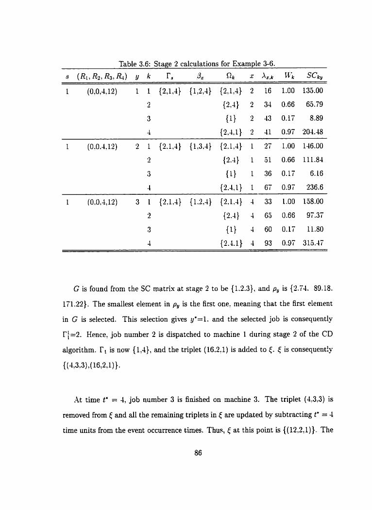
Table 3.6: Stage 2 calculations for Example 3-6.

s (Rl?R2?R3t&) Y k rs ,3x Qk x L . k w i Scn,

1 ( O , O , , l ) 1 1 ( 1 4 (1,2,4} ( l , } 2 16 1.00 135.00

9 - 4 2 34 0.66 65.79

3 (1} 2 43 0.17 8.89

4 { . l } 2 41 0.97 204.48

G is found from the SC matriv at stage 2 to be {1.2.3}. and p, is (2.74. 89.18.

li1.22}. The srnallest element in p, is the first one. meaaing that the first element

in G is selected. This selection gives y'=l. and the selected job is consequently

r:=2. Hence, job number 3 is dispatched to machine 1 during stage 2 of the CD

algorithm. rl is oow {l?-L}, and the triplet (16.2,l) is added to c. is consequent!~

{(4.3.3) ,(16,Z71)}.

At time t* = 4 job number 3 is finished on machine 3. The triplet (4.3.3) is

removed from 5 and all the rernaining triplets in ( are updated by subtracting t* = 4

time units from the event occurrence times. Thus, at this point is {(12,2,1)). The

Table 3.7: SC rnatrk at stage 2.

next machine on the route of job 3 is machine 4. Job 3 is unloaded off machine

3 and loaded directly on machine -4 (which is currently free). The triplet (8.3.4).

which represents tne completion time for job 3 on machine -4. is appended to <. so

that E is now {(8.3.4).(19.2.1)}.

.At time t* = 8. job 3 is completed on machine 4 and unloaded out of the cell.

The triplet for the job just completed is removed frorn <. and the remaining triplets

are updated by siibtracting t* = 8 units so that f is now {(4.9.1)}.

Stage 3

At time t g = 4, job number 2 is finished on machine 1. It is taken then from

machine 1 and loaded direct- on machine 2. which is the next machine on the route

of job 2. The corresponding triplet (18,202) is put in and it replaces the expired

triplet (-L,&l). Machine 1 is now available. and this event marks the start of stage

3, where a job from the t m remaining jobs (Ti = {14)) is selected. Current values

for the variables used in the computation of the SC rnatrkx for stage 3 are given in

Table 3.8, knowing that <Pl is {1,2,3,4). The SC matrix is shown in Table 3.9.

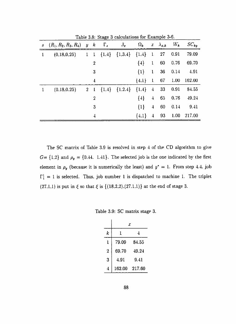
Table 3.8: Stage 3 calculations for Example 3-6.

s (Rl ,R2,R3>&) 4 k r s 3, R b x L . k bh Sck,

1 (018025) 1 i {1.4} { 3 {l.4} 1 27 0.91 79.09

3 - {A} L 60 0.76 69.70

3 {1} 1 36 0.1-4 4.91

-4 4 . 1 67 1.00 162.00

The SC matrix of Table 3.9 is resoked in step 4 of the CD algorithm to give

G= {1.2} and p, = IO.44. l.-41}. The selected job is the one indicated by the first

element in p, (becauso it is numerically the least) and y* = 1. From step 4.4. job

ri = 1 is selected. Thus. job number 1 is dispatched to machine 1. The triplet

(27.1.1) is put in i so that < is {(18.2.2).(27.1.1)} at the end of stage 3.

Table 3.9: SC matrix staq 3.

1 ; + v stage 1 stage 2 stage 3 tirne

Figure 3.6: Ga~i t t chart showing final schedule for the esample probleni.

CD dispatcliing has no further roie to play in the solution becaiise no niore

decisions are required. The algorithni continues by cycling between step 2 and step 5

as the reniaining jobs are processed in FIFO order throughoiit the cell. The prograni

terminates nhen al1 the jobs have exited the cell. The final solution provided by the

CD algorithm in this example is to dispatch jobs at machine 1 in the sequence of

jobs 3. 2. 1 and 4. The Gant t chart for this solution. whicli gives a niean flowtinie

of 82 units. is given in Figure 3.6.

3.4 Performance Evaluation

The perforniance of the CD algorithm is evaluated in this section in cornparison

with other procedures taken from the literature. The problenis tested are strictly

stat ic sequencing problems. ?i static problem implies t hat the initial conditions

correspond to. I ) no parts in-process in the cell: and 2 ) all the jobs are avaiiabie

and ready at the start of the scheduling period. Static cases provide the advan-

tage of enabling scheduling to be perfornied off-line. Off-line sçheduling alloas a

variety of methods to be used. including simulation. in order to search nunierous

sequeuces arid to choose the best one. Ritli oti-line schedulirig however. once a

part is dispatclied there is no chance to reverse that decision. The CD approach

is a dispatching niechanisni that is basically on-line oriented. It can also be used.

rievcrtheless. as a single-pus procedure for the off-line. static sequenci~ig of jobs.

3.4.1 Test Problems

The CD approach is evaluated by using sets of randoirily generated test prob-

l em. The test problenis are generated by usirig the sanie niethod as that described

in Kim [46]. Each set contains 110 problems. al1 having a coninion number of jobs.

A prograrn written in the C computer language [ i 5 ] and designed to sinlulate the

activities in a FhIC under the control of different dispatching rules is used in this

comparative ewiuation of CD. The simulation prograrn processes an input data set

according to the selected dispatching nile. and it calculates d u e s br the corre-

sponding performance measures. The abilities of CD and other dispatching rules to

sati* the given performance criteria are compared by using this program.

The cornputer simulations that are run in the evaluation of CD's perfomiance

cover cases involving the three routing configurations of Figure 3.1 and three different

pcrforniance criteria. The evaluation is performed by comparing CD's perfomiance

with t h of the dispatching rules that have been demonstrated in previous publi-

cations to be the most effective for the performance criterion under consideration.

The ie~ü!ts arc crcpresscd. ;i~hcocrcr con~cnicnt!:; possiblc. i:: tcrms of thc dc:.intion

from the optimal solutions. The optimal solution to each problem is found from an

exhaustive enurneration ol al1 the possible solutions.

Calculation of the optimal solutions, hoivever. beconies prohibitive in problenls

with a large riuriiber of jobs due to the cornbinatorial esplosion arising froni complete

enunieration. It is niore convenient. then. to evaluate the CD algorit hni relative to

O t lier dispatching proceclures. The cornparison is perfornied by t aking as a refercnce

a clispatcliirig riile that is known to give acceptable results for the perforniance cri-

terion under consideration. and then rneasiiring CD's results against this reference.

The rneawre that is adopted is called the performance ratio (PR). and it is defined

by :

u-here ma and m, are the results for the method under evaluation (Le. CD) and

the reference method respectively. .A larger PR value above 1.0 indicates that the

method being evaluated performs increasingly better than the reference method. -4

PR value near 1 .O signifies near-equivalent performance.

The tests are conducted for dl three confqprations shom in Figure 3.1. The

T-ype 1 configuration is limited to three machines only. This is to provide a uni-

forrnity in total workload with the other two configurations. mhere the part routes

pass strictly through three of the four machines that are amilable in each of those

configurations.

3.4.2 Minimizing the Mean Flowtime

The performance of CD in mininiizing the rnean fiowtinie is eviluiited by coiripar-

ing its results a i th those obtained frorn using the Least Aork Reriiairiing (LWKR)

dispatcliing rule. The LWKR rule is chosen for this purpose becaiise it has been

shown to be the better of several dispatching rules considered for flowsliop configu-

rat ions [-L61.

Figure 3.7 compares CD and LWKR in terms of percentage deviation from the

optima. The test data includes sis sets of problems. each set covering a probleni

size from 5 and upto 10 jobs. Figure 3.7 shows that the CD algorithni's results

rire aithin 5% of the optima. Furtherniore. CD's perforniance appears to be quite

consistent in al1 t h e configurations as the riumber of jobs grows to ten. On the

other hand. the LWKR rule gives results generally deviating upwards of 2% from

the optimal. Mso. the quality of the results from the LWKR shows a pronounced

deterioration wit h more jobs.

The performance of CD for problems having upto JO jobs is presented in Figure

3.8. Figure 3.8 uses a performance ratio (PR) with LWXR as the reference method.

The results indicate that, as the number of jobs grows beyond 15, the CD algorithm

outperforms the LWKR dispatching rule by about 5 to 10%. The CD improves

Nurnber of Jobs

Figure 3.7: IIinirniziiig the nieari flowtinie a i th CD aiid LKKR.

steadily witli an increasing number of jobs upto about 25. but lewls off with a

consistent ciifference froni the LWKR data as the nuniber of jobs increases further.

This obsewation hoids for al1 three configurations. although the CD dispatching still

appears at its best for Type 1 configuratioris. The results presentetl in Figures 3.7

and 3.8 generally dernonstrate the superiority of CD dispatching.

Another indication of how well a part icular method out performs other niet hods

c m be found in the number of times the given method produces the best result in

identical test situations. This information is presented in Table 3.10 using, as an

example, the case of a pure flowshop (T-ype 1 configuration). The CD algorithm is

cornpared in this table with the LWKR rule and a slightly modified YEH algorithm

[34]. The NEH algorithm was developed originally to minimize the makespan in

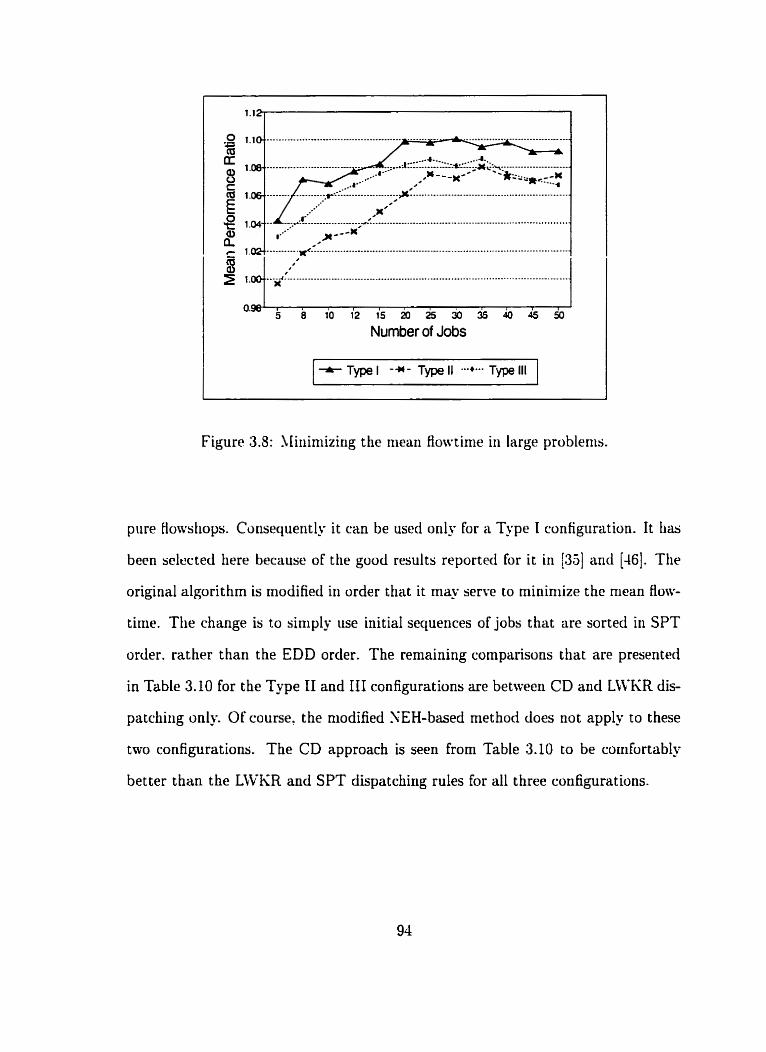
I

b 1'0 i 2 i 5 ia iS j0 j5 & 45 b Number of Jobs

Figure 3.5: SIininiiziug the mean fiowtirne in large problenis.

pure Howstiogs. Co~isequently it can be useci only for a Type I configuration. It lias

been selected here becuuse of the good results reported for it in [35] and [46]. The

original algorithm is modified iri order that it rn iq serve to mininiize the niean Bow-

tirne. The change is to simply use initial sequences of jobs that are sorted in SPT

order. ratlier than the EDD order. The remaining cornparisons that are presented

in Table 3.10 for the Type II and III configurations are between CD and LWKR dis-

patching only. Of course. the modified NEH-based methocl does not apply to these

two configurations. The CD approach is seen from Table 3.10 to be comfortably

better than the LWKR and SPT dispatching rules for dl three configurations.

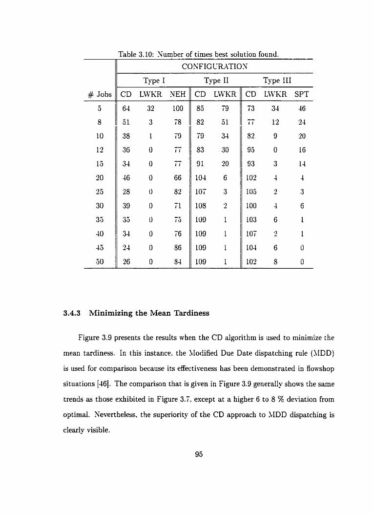
Table 3.10: h m b e r of times best solution found.

# Jobs

Type I

CD LWKR XEH

6-4 32 100

Z l 3 18

38 I 19

36 O -.-. I I

34 O -.-. I I

46 O 66

28 O 82

39 O il

35 O -- f a

3-4 0 16

24 O 86

26 O 84

Type II

CD LWKR

85 19

8'2 31

19 34

53 30

91 20

104 6

107 3

108 3 - 109 1

109 1

109 1

109 1

Type III

CD LWKR SPT

3.4.3 Nlinimizing the Mean Tardiness

Figure 3.9 presents the results when the CD algorithm is used to minimize the

niean tardiness. In this instance. the SIodified Due Date dispatching rule (ILDD)

is used for comparison because its effectiveness has been demonstrated in fiowshop

situations [46]. The comparison that is given in Figure 3.9 generall- shows the same

trends as those exhibited in Figure 3.7. except at a higher 6 to 8 % deviation from

optimal. Nevertheless. the superiority of the CD approach to SIDD dispatching is

clearly visible.

Number of Jobs

CD -*- MDD 1

Figure 3.9: Mininiizing the menn tardiness with CD and SIDD.

U'heii rriiriimizing the niean tardiriess. CD uses dynaniic progrüniniing to opt i-

mize the core sequences. This is acceptable when the nuniber of jobs is not niorr

than about 15 to 20. If a greater nuniber is involved. then the çoniputatio~ial re-

quirements of finding optimal core sequences beconie oveni-helniing. Obviously.

near-optimal solut ions that can be generated quickly For large problems can be sub-

stituted for optimized core sequences. The effect of noil-optimization in the cure

sequence is discussed later in this chapter. The performance of CD in minimizing

the mean tardiness in flowshops involving a large (up to 30) number of jobs will

be addressed in the next chapter. after a new method for finding near-optimal core

sequences is presented.

3.4.4 Minimizing the Number of Tardy Jobs

In order to further test CD's ffexibility of application for different criteria. its

performance in niinirnizing the number of tard- jobs in flowshops is evaluated. This

time. CD finds the optimal core sequences by employing Hodgson's form (see Baker

[8]) of the algorithm developed by Moore [6f] to mininiize the number of tardy jobs

in a single machine. The behavior of the more comnion dispatching rules in niini-

mizing the number of tardy jobs in flowsliops and jobshops is not well docunieiited.

Consequently a series of tests was undertaken to compare the EDD. SPT. SIDD

ancl LKKR rules wheri applied to flowsliops ha~ ing any of three configurations con-

sidered in this thesis. The tests revealed a slight advantage in favor of using the

SPT rule when the number of jobs is less than about twenty. Klieti the tiumber of

jobs is greatrr than that. the SIDD mle beconies attractive. Therefore. it is decided

to evaluate CD in coniparison to the SPT rule when coniparirig problems with sniall

job sizes. and to the l IDD rule for large sired problems.

Figure 3.10 shows the results obtained from using CD for niinimizing the nuniber

of tardy jobs. espressed as percentage deviation frorn the optima. The results that

are obtained bu using the SPT rule are also included in Figure 3.10 for cornparison.

The indications frorn Figure 3.10 are that. even though CD's performance is signifi-

cantly siib-optimal. it is nonetheless appears somewhat better than that of the SPT

rule.

CD dispatching becomes substantially superior as the nuniber of jobs increases.

This is evident from Figure 3.11, where CDk performance is compared ni th the

MDD rule in terms of PR. MDD is the reference method. It may be concluded.

Figure 3.10: Mnimizing the number of tardy jobs.

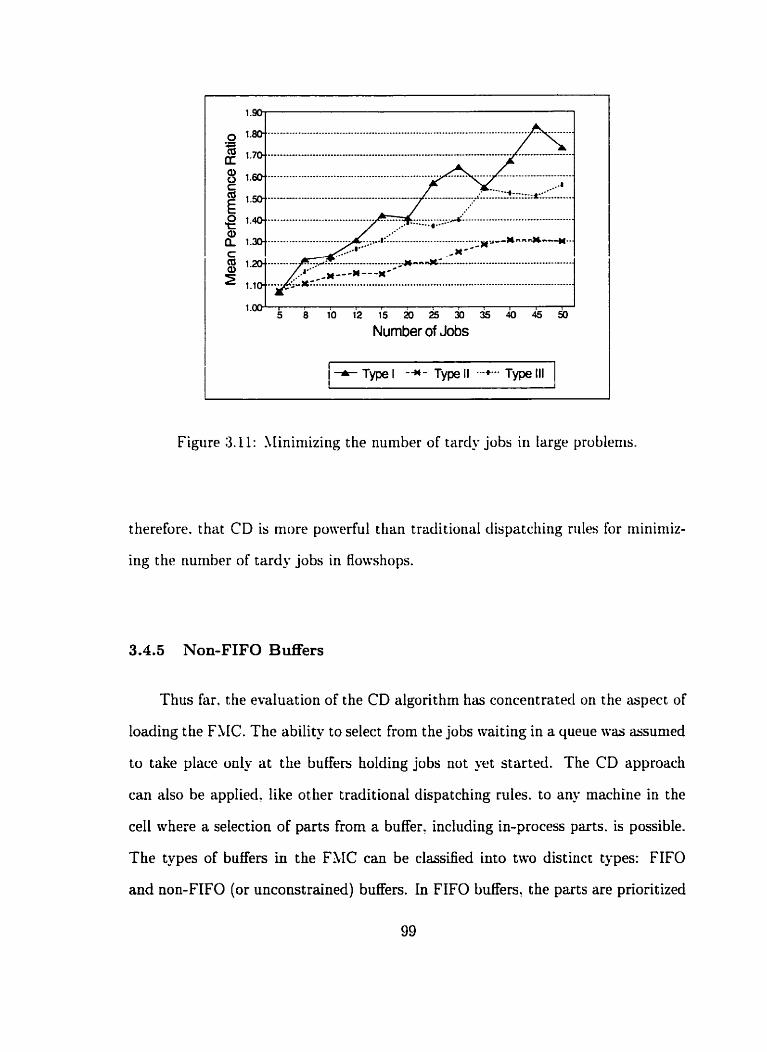
Number of Jobs

Figure 3.11: llininiizing the nurnber of tard' jobs in large problenis.

therefore. thüt CD is more powerful than traditional clispatcliing rtiles for mininiiz-

ing the nuniber of tard? jobs in Rowshops.

Thus far. the evaluation of the CD algorithm has concentrated on the aspect of

loading the FSIC. The ability to select from the jobs wait ing in a queue \vas assumed

to take place on- a t the buffers holding jobs not yet started. The CD approach

can also be applied, like other traditional dispatching rules. to any machine in the

cell where a selection of parts from a buffer, including in-process parts. is possible.

The types of buffers in the FLIC can be classifieci into two distinct types: FIFO

and non-FIFO (or unconstrained) bufEers. In FIFO buffers? the parts are prioritized

Number of Jobs

Figure 3.19: CD perforniarice for niean flowt ime and non-FIFO buffers.

on a first-corne. first-semrd b a i s only. In non-FIFO biiffers. on the other tiand.

there is a possibility to select any one of the parts currently residing ir i the buffer

for immediate processing. The CD algorithm is tested nest in cases rvhere al1 the

buffers in the ce11 are unconstrained. The cornparisons are perfornied. as previously.

against the L W i R and MDD dispatching rules.

Figure 3.12 displays the results of minimizing the mean flowtinie when all the

buffers are non-FIFO. The- are consistent with those found in Figure 3.8. albeit

with lower PR values. The results of Figures 3.8 and 3.12 demonstrate the Bexibil-

i t - of CD by shoaing that it performs consistentl- regardless of the part selection

const raints in the intermediate buffers.

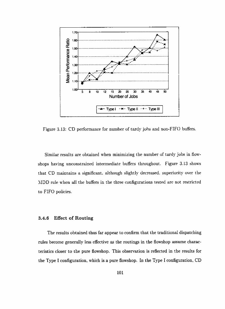
' " '5 L io i2 i s aO i5 j0 j5 jO 95 &J I

Number of Jobs

-- - -

+ Type 1 -*- Type Il ---+--- Type Ill

Figure 3.13: CD performance for nuniber of tardy jobs aiid riori-FIFO buHers.

Siniilar results are obtained when rninimiziiig the nuniber of tard- jobs in Aow-

shops havirig iiricoristrained intermediate buffers t hroughout. Figure 3.13 shows

that CD maintains a significaiit. although slightly decreased. siiperiority over the

MDD rule n-hen al1 the buffers in the three configurations tested are not restricted

to FIFO policies.

3.4.6 Effect of Routing

The results obtained thus far appear to confirm t hat the traditional dispatching

d e s becorne generally less effective as the routings in the flomvshop assume charac-

teristics closer to the pure Bowshop. This observation is reflected in the results for

the Type 1 configuration, which is a pure flowshop. In the Type 1 configuration, CD

outperforms the other dispatching rules by a margin that is geater than in the other

two configurations, which dlow two digerent job routes. The fact that CD's relative

performance is better in the pure flowshop is an indication of its ability to respond

to routing Limitations in the shop. This feature is an important one because the

status of a ce11 is changing constantly during processing and. at any instant. certain

rouriiigs tiiay predoiriiiiara. Fur naiilplr. cui&lrr lie Qpe III cuufiguratiuii iii t l i r

everit when an inordinate number of the jobs have rnerely one of the two possible

routes (SV route SI1 - 513 - 114). This situation reseinbles the pure flowshop closely.

even though the physical configuration is strictly not a pure flowshop. .-\II effective

scheduling systeni should be able to adjust to the nea conditioris. even though they

rriay be teiriporary. Based on the results shown in Figures 3.7 tlirough 3.11. CD

dispatching indeed appears to possess the atiaptabili ty needed for acconirriodating

such dy nariiic situations as t lieu rnay arise.

3.5 Optimization in the Core Sequence

The basic preniise used in constructing the SC niatris is that each niachine at-

tempts to have its candidates selected for dispatching by rriiriiniizing its sequence

costs (SCk,). This rninimization is achieved t hrough opt imally sequencing the jobs

in the core. To investigate the effect of non-optimal sequences in the cores. an es-

periment is performed that involves CD for minimizing the mean flowtinie. This

criterion is selected because the optima can be calculated s i m p - for large sized

problems. In this experiment. LPT and randomized sequencing are used in Equa-

tion (3.7) rather than the (optimal) SPT. LPT is used because it wvorks to mavimize

rather than minimize the mean flowtime. This will show the effect when dl machines

jointly perform sub-optirnally. The resulting performance of the CD algorit hm is

evaluated by using 1100 test problems generated randomly. again usirig the method

of (511. Figure 3.14 displays the results. which are expressed as a percentage devi-

ation from the results achieved with optirnized core sequencing. The results show

that. with randoniized sequencing in the core. the CD performs at about 8 to 10%

wurse tliaii witli tlir uptiiiiizt.4 cùres. Iniêrestiiigl:;. ivhen LPT is enipiûycd in thc

cores. the performarice of CD is within only 1% of the results froni CD with opti-

mized cores. Figure 3.14 show that the impact of a non-optiniized core is lcssenecl

if the sub-optimal triet hod is applied uniformly to al1 the core sequences. 1u ot lier

words. nith a 'level playing field' in whicli al1 the machines are subject to the sarrie

rule. the CD algorithni appears to be not very sensitive to the riilc useci in t h r core.

Nevert helcss. Figure 3.14 clemonst rates t hat opt iniized core sequencing provides a

solution tliat is generally bet ter thari t hc non-optirriizetl one. Altliough the differ-

erice is srnall. apprmirriately two out of three test problenis in the data sets had a

bet ter solut ion ahen the core sequence \vas opt imized.

A siniilar esperinient to determine the impact of optirriization in the core se-

quences is done by testing CD. with different core sequence generation methods. to

rninimize the number of tardy jobs. The test data that is used is the sanie data that

gave the results shown in Figure 3.11. The configuration that is used is Type 1. and

it is selected arbitrarily.

The esperiment involves running the CD algorithm for the test data three times.

each time using one of the EDD, SPT and SIDD priority rules in place of Hodgson's

algorithm to determine the core sequences. The resulting performance of CD in each

- 4 b IO i s b & k i 8 45 50

Number of Jobs

Figure 3.14: Performance of CD mi th nori-optimal cure sequericing

instance is shown in Figure 3.15. The results froni CD with Hodgson's algorithm

are also shown iri Figure 3.15 for cornparison.

Figure 3.15 clearly denionstrates tliat using other than the optimal sequence in

the core can significantly degrade CD's performance. Of the three priority rules

used in the esperiment. the l1DD rule was the better one. yet it resulted in about a

17% increase in the total number of tardy jobs. for the same data set. as compared

to r h e n Hodgson's rule is employed. Hence. it may be concluded that optimal se-

quencing in the core can be expected to have a positive impact on CD's perforn~ance.

The sipiticance of that impact may vaq. depending on the performance criterion.

Number of Jobs

Figure 3.13: Effect of different core sequences on CD's performance.

3.6 Conclusions

Cooperative Dispatching, CD. was introduced in this chapter as a new schedul-

ing procedure that is suitable for FMCs. It is designed to have a high flexibility in

its applications. and cornputer simulations were performed for the purpose of evalu-

ating this flexibility. The simulations involved a comparison of CD with a number of

other traditional dispatching niles. The cornparisons covered three flowshop configu-

rations, and t hree different performance crit eria: 1) rninimizing the mem flooatime:

2) minimizing the mean tardiness: and 3) rninimizing the number of tardy jobs.

The corn puter simulations, which involved randomly generated test problems. led

to three main conclusions regarding the performmce of CD.

First CD exhibited a performance that i.as consistently better t han the alterna-

tive dispatching rules it was conipared with in al1 the three flowshop configurations.

The results indicated a low sensitivity of CD to the differences between the three

configurations. This result reinforces CD's clairns of flexible application in flowshops

having different layout configurations (or job routings) .

Secotidly. CD was able to accommodate quite well Roashops nhere interniediate

buffers were not restricted to a FIFO policv in servicing the waitiiig jobs. This

\vas in contrast to the other dispatching rules. wliose pcrforniaricr stood to berle-

fit in proportion to the tiurribrr of intertuediate buffers that were not restricted to

FIFO queueing policies. This fact again denionstrates CD's flexibility under differ-

cnt tiardware cons t raints.

Thirdly. CD showed a good ability to nieet a iiumber of different perforniance

criteria. sirnply by using the appropriate single machine secluenciiig problem to help

the individual machines collectively reach dispatching decisioris. In al1 the corn-

puter simulations. and for al1 of the performance criteria that were consitlerecl. CD

enierged stronger than the best of the other dispatching rules to which it \vas coni-

pared. Together. these three conclusions are a strong indicat,ion of CD's overall

scheduling flexibility. This Rexibility means minimal disnipt ion. particularly the

need for rewriting of software. in the event of reconfiguration or other managerial

changes in the system.

The third conclusion implies that CD is likeiy to perform well for a given per-

formance criterion. provided that a fast method is available for deterrnining optimal

solutions in a single machine setting for that criterion. It was already pointed out

tliat. for some criteria such as rninimizing the mean tardiness. optimal solutions ni.

be difficult to obtain because of the extreme cornputational requirenients when the

number of jobs is large. In order to address such complications. a iiew metliod for

sequencing n jobs on a single machine is introduced in the following chapter. This

riew ma~iiud eiiipioys artiliciül iirural iietiwrk. It is design4 tu prviide fat and

near optimal solutions for generalized performance criceria. The rieural networks

work to support the calculations for gerierating the SC matrix rvheii the perfor-

niarice criteria are NP-harcl. like the niininiization of thc niean tardiness.

Chapter 4

Single Machine Sequencing with Neural Networks

4.1 Introduction

The core equat ion (Equation 3.7) descri bed in su bsect ion 3.2.2.3 of the preceding

ciiapter is a single machine seqiiençing problern. As notecl in Chapter 3 . this problerii

is NP-hard for sonie perforniance criteria. and niost of the good scarch heuristics

or op tiniizat ion algorit lirris ir i t hose cases corisunie excessive cornputat ional tinie.

The heuristics t h are Fast are generally designed for specific criteria and they are

not usually portable to other perforniance criteria. In t his ctiapter. an alteriiative

approach ttiat is based on artificial neural networks is presented. The choice of

neural networks is mot ivated by two Factors: speed and fiesibili ty. Computat ional

speed Facilitates the developnierit of algorithnis for other types of problenis where

a large number of sub-problerns having the Form of a single niachine sequencirig

problern need to be solved quickly. The CD approach described in the preceding

chapter is one such example. The second hctor is flexibility with respect to the

performance criteria. In reality, the perfomiance criterion ma! not be a standard

one but. rather. a complex cost function for which no quick and accurate heuristics

are known. In such situations. either a customized algorithm has to be developed

or 'quick and dirty' sorcing procedures may be employed (Potts and t'an Cl-assen-

hove [XI). Sorting in the order of non-decreasing due dates (the EDD rule) or

non-decreasing processhg times (SPT rule) are esamples of the latter. Hence. t here

is a need for an approach that quickly produces good sequences when the perfor-

mance criteria are uncomnion. but without having to develop a unique algorithm or

heuristic for every individual situation.

The method for solving single machine job sequencing problenis that is presented

here is based on artificial neural networks ( A 3 N ) . It is conceptually simple. An .\SN

is used to l e m a functional relationship betrveeli a set of exarnple. single machine

problenis and the correspondiiig sequences t hat opt imize the given performance cri-

terion. This 'trained' neural network is then able tu apply the learnt relatiouship to

nea problenis through its generalization property.

4.2 Artificial Neural Networks

An art ificial neural network is a collection of highly interconnecteci processing

iinits that has the ability to learn and store patterns. as well as to generalize when

presented rvith new patterns. The 'learnt' information is stored in the forni of nu-

merical values. called weights. that are assigned to the connections between the

processing units of the network. The type of neural network that is used here is

called a 'feedfonvard' network. [t organizes the processing units into multiple 1-rs.

one of which serves as an input layer, and another as the output layer. The rest

of the layers are called 'hidden' layers. They exist between the input and output

layers. Figure 4.1 illustrates a three-layer feedfomard neural network. The units

in the input Iayer serve as a terminal for receiving the input patterns. These units

are clamped to the values contained in the patterns introduced at the input Iayer.

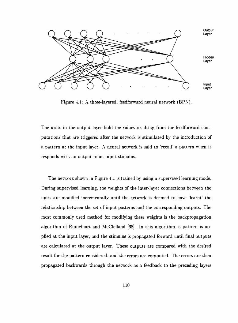
n n n - Output Layer

Hidden Layer

Input La y8 r

Fi y r e 4.1: -1 three-layered. feedfonvard neural network (BPN).

The uriits in the output Iqer hold the valiies resulting froni the feedfonvarcl coni-

putations t hat are triggered after the network is stiniulated by the introduction of

a pattern at the input Iqer. A neural network is said to 'recall' a pattern when it

responds with an output to an input stiniuliis.

The netivork shown in Figure 4.1 is trained by using a supervised learnirig mode.

During supervised learning. the wights of the inter-layer connections between the

units are rnodified incrementally until thc network is deemed to have 'learnt' the

relationship between the set of input patterns and the correspooding outputs. The

most cornrnonly used method for modifying these weights is the backpropagation

algorithm of Rumelhart and .CIcClelland [68]. In this algorithni. a pattern is a p

plied a t the input Iayer. and the stimulus is propagated fornard until final outputs

are calculated at the output layer. These outputs are compared a i t h the desired

result for the pattern considered. and the errors are cornputed. The errors are then

propagated backavards through the network as a feedback to the preceding layers

to determine the changes in the connection weights that will mininiize these errors.

A series of such input-output training examples is presented repeatedly to the net-

work during the backpropagation algorithm until the total sum of the squares of the

errors is reduced to an acceptable level. At this point. the network is considered

'trained'. Data presented at the input layer of a trained network will result in values

f ron thc output !-cr that arc consistcnt r i th thc rc!citionship !cx:it 5': the netvork

froni the training examples. A feedfonvard neural network that is trairied bu using

the backpropagation algorithm. is often termed a Backpropagation Setwork (BPN).

The backpropagation algorithm is implemecited witti the ilse of a siniulation pro-

gram writ ten in the DESIRE/YEC'NET mat rix lariguage [69]. The design. training

ancl testing of al1 the neural networks described in this chapter is clone nith the use

of this software package.

4.3 A Neural Network for Single Machine Sequencing

The neural network that is proposed for the single machine seqiiencing problern

lias the same architecture as that shown in Figure 4.1. It consists of an input layer of

eleven units. one hidden layer. and an output laver having a single unit. The number

of units in the input and output layers is dictated by the specific representation

adopted for the sequeocing problem. In the proposed representation. each of the n

jobs in the problem are described by an Il-tuple vector of continuous values. Each

vector. or pattern. holds information particular to the job it represents as well as to

its relation to the other jobs in the problem. Therefore. the input layer has eleven

input units to accommodate each one of the elements of the input vectors. This

particular choice for representing the problern? mhereby the jobs are processed by

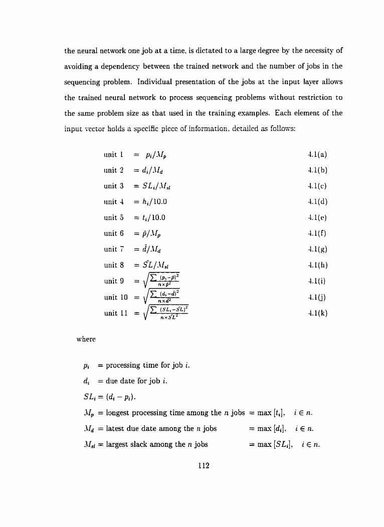
the neural network one job at a tirne, is dictated to a large degree by the necessity of

avoiding a dependency between the trained network and the number of jobs in the

sequencing problem. Individual presentation of the jobs at the input 1-r allows

the trained neural network to process sequencing problems without restriction to

the same problern size as that used in the training exaniples. Eaçh element of the

input rcctûr hdds a spccific piccc of information. dctailcd as fc!!o:vs:

unit 1

unit 2

unit 3

iiriit 4

unit 5

unit 6

unit 7

unit 8

unit 9

unit 10

unit 11

where

(SL, -s-L)'

4.1ja)

-4.l(b)

4.1 (c)

4.1 (d)

4.1 (c)

4.1 ( f )

4.1 (d 4 4 h )

-l.I(i)

44.j 1

pi = processing time for job i.

di = due date for job i.

S Li = (di - p i ) .

Jip = longest processing time among the n jobs = mau [tilt i E n.

-\id = latest due date among the n jobs = m w [ d i ] : i E n .

Alsi = largest siack among the n jobs =rnau[SLi], i ~ n .

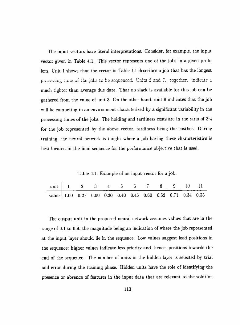
The input vectors have literal interpretations. Consider. for euaniple. the input

vector given in Table 4.1. This vector represents one of the jobs in a give~i prob-

lem. Gnit 1 shows that the vector in Table 4.1 describes a job that has the longest

prucessing time ûf the jobs to be sequcnced. Laits 2 and 7 . togcthcr. indicatc r

muçh tighter than average due date. That no slack is available for this job can be

gathered from the value of unit 3. On the other ha~id. unit 9 indicates ttiat the job

will be conipeting in an environnierit characterizecl by a significant variability in the

processing tirries of the jobs. The holding and tardiness costs arc in the ratio of 3:4

for the job rcprcserited by the above vector. tardiriess beirig the costlier. During

training. the neural network is taiight ivhere a job having t hese characteristics is

best Located in the final sequence for the perfor~riance objective that is iised.

Table 4.1: Eaample of an input vector for a job.

The output unit in tlie proposed neural network assumes values that are in the

range of 0.1 to 0.9, the magnitude being an indication of where the job represeiented

at the input laver should lie in the sequence. Low values suggest lead positions in

the sequence: higher values indicate less priority and. hence. positions totvards the

end of the sequence. The number of units in the hidden layer is selected by trial

and error during the training phase. Hidden units have the role of identibing the

presence or absence of features in the input data that are relevant to the solution

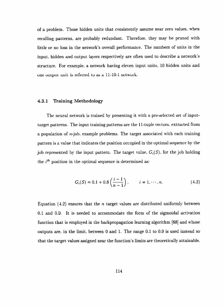
of a problem. Those hidden units that cnnsistently assume near zero values. when

recalling patterns. are probably redundant. Therefore, they may be prüned mith

little or no loss in the network's overall performance. The numbers of units in the

input. hidden and output layers respectively are often used to describe a network's

structure. For example. a network having eleven input units. 10 hidden units and

oiie uutyiii. iiiiil ib i~efrrrrci lu a a il-10-i iirtwurk.

4.3.1 Training Methodology

The neural network is trairied by presentiiig it with a pre-selected set of input-

target patterns. The input training patteriis are the 1 1-tuple vectors. extractcd froni

a population of n-job. esample problems. The target associated with each traiiiirig

pattern is a value tliat indicatcs the position occupied in the optimal sequence by the

job represented bu the input pattern. The t a r g ~ t value. G,(S). for the job holding

tlie ith position in the optirrial sequence is deterniiried as:

Equat ion (4.2) ensures t hat the n target values are distributed uniformly between

0.1 and 0.9. It is needed to accommodate the forni of the sigrnoidal activation

function that is employed in the backpropagation learning algorithm [68] and n-hose

outputs are. in the limit. between O and 1. The range 0.1 to 0.9 is used instead so

that tlie target d u e s assigned near the function's Lirnits are t heoretically attainable.

The number of jobs, n' in the example (training) problems has a bearing on

the target value that is ascribed to each input pattern. As the output space ranges

from 0.1 to 0.9, the n target values needed by the n jobs in the problem are spaced

equally in increments of (0.9 - O.l)/n within that range. Consequently. as n grows.

the target values for jobs in the sequence tend to migrate closer together. This

mea is t h a the targcts arc niore accurate in spccif-ying thc dcsircd position in :hc

sequence. The tighter tolerances may rnake training more difficult but. on the other

hand. the trained network is able to assign the job positions with better precision

in a sequence. Therefore. training patterns should preferably corne frotri esaniple

problenis having n as large as possible. This is not alrvays easy to accotnplisli be-

cause finding optinial solutions for NP-hard example probleins is increasingly more

cfenianding, iri terrris of coniputational storage and t inie requirernerits. as n increases.

Hence. a trade-off ne& to be made between the size of n for the esample problems

and the time and resources that can be afforded for the training phase. Where

optinial solutions are obtained means of complete enunierat ion. 8-jo b probieiiis

are chosen here as the source for the training patterns. This is because complete

enunieration for problenis involving more than 8 jobs recpires significaritly niore

computer time due to the iiuniber of individual problenis that need to be solved to

generate the training set. In instances where optinial solutioiis can be found by du-

narnic progranirning (Held and Karp [65]) , a procedure which is more efficient than

complete enurneration. the training patterns are extracted from 12-job rather than

%job example problems. Although dynarnic prograrnming couid have been used

to extract the patterns from problems having n as high as 20. the decision to use

12-job problerns is influenced by expediency, cornputer resources and development

time lirnitations~ as w l l as the ease of making comparisons.

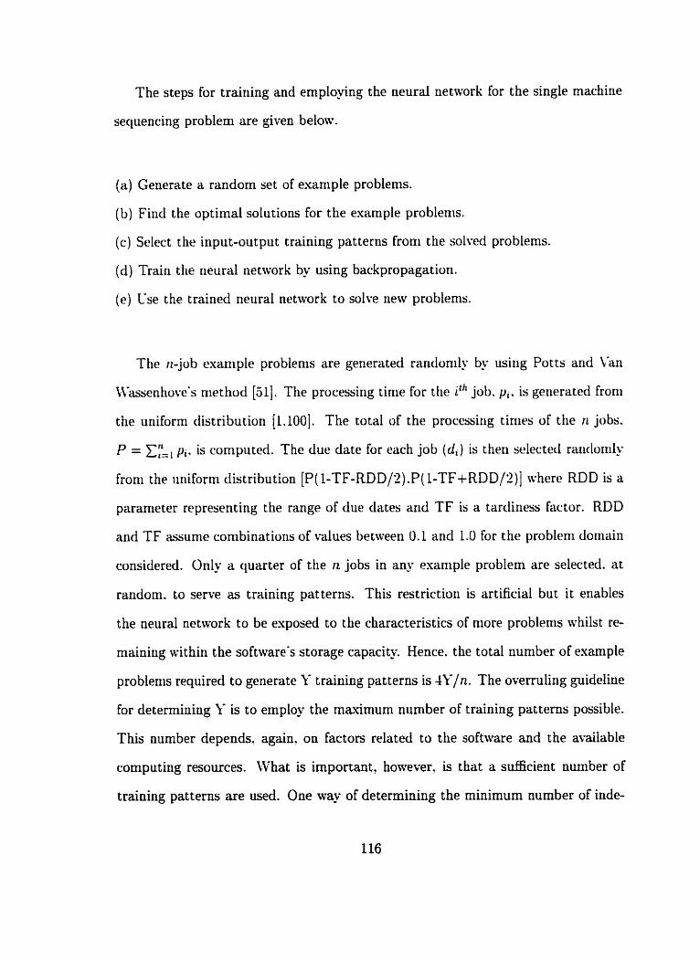
The steps for training and employing the neural network for the single machine

sequencing problem are given below.

(a) Generate a random set of example problems.

(b) Find the optimal solutioris for the example problenis.

(c) Select the input-output training patterns froni the solved problems.

(d) Train the neural network by using backpropagation.

(e) Use the trained neural network to solve riew problenis.

The 11-job exaniple problerns are generated randonily by usiiig Potts and Van

Clksscnhove's niethod [XI. The processirig tinie for the i th job. p,. is generated froni

the uniforni clistribution [1.100]. The total of the processing tinies of the n jobs.

P = Er., p, . is computed. The due date for each job (d,) is then selected rariclorrily

froni the uniform distribution [P(LTF-RDD/'I).P(LTF+RDD/'L)] where RDD is a

paranieter representing the range of due dates arid TF is a tarcliness factor. RDD

and TF assunie conibinations of d u e s between 0.1 and 1 .O for the problem domüin

considered. Only a quarter of the rt jobs in an. esaniple problem are selected. at

random. to serve as training patterns. This restriction is artificial but it enables

the neural network to be exposed to the characteristics of niore problems shilst re-

maining within the software's storage capacity Hence. the total number of example

proble~ris required t O generate Y training patterns is 4Y/n. The overruliiig guideline

for determining k' is to employ the maximum number of training patterns possible.

This number depends. again. on factors related to the software and the avaiIable

computing resources. What is important, however' is that a sufficient number of

training patterns are used. One way of determining the minimum number of inde-

pendent training patterns that are needed is to start with a limited number. and

then increase this number gradually in separate training trials. When it is observed

that the addition of further patterns does not significantly reduce the generalization

error. then it m q be accepted that the loaer bound for the required number of

patterns has been surpassed. This approach is impleniented in the training of the

ncural nctwrks dcscrihcd in this Chaptcr. In al1 instances. thc nunber of Pattciiis

used in training a neural network is well above the lower bound. as dcterniined by

trial and error, for the case under consideration.

Test problerns tliat are generated randonil- in a triaiiner sirtiilar to the training

set. but with a different seed. are used during the training phase to evaliiate the

'learning' of the neural network. This evaluation is based on monitoring the average

'positioning error'. The positioning error, e, . for pattern q is nicasured as :

where

0, = output resporise when pattern q is presented at the input layer: and

G, = target response for test pattern q.

Equiition (-4.3) indicates how closely the neural network is able to position the

job represented by pattern q to the position that the job should occupy in the o p

timal sequence. An e, that is larger than unity shows that the error is greater than

one full position in the sequence. Conversely. an average error for the test data

pat tems t hat is less t han unity suggests that the neural nehvork is able, on average.

to place the jobs in their correct sequentid positions.

During the traiuing stage, t railiing is interriipted intermit tent ly and the network

is tested by using tlie set of test patterns. The average positioning error is cotnpiled

and examineci at each interruption. This process is euded when the error just be-

gins to increase with further training. This is because the network then starts to

'rriemorize' the training set which leads to a loss in its generalization abilities.

4.3.2 Evaluation of Learning Capability

The effectiveness of the proposed neural rietwork niet hodolog? for job sequenc-

ing is evaluated nest by testirig with a performance rriterion for which a simple

solution is knonn to esist. This criterion is the rnininiization of the iiiasiniuni job

Iateness. It is optiniized by merely sorting the jobs in the order of non-decreasing

due-dates [SI. Heiice. the target values. G,(S). are coniputed for a sequcnce S sorted

in EDD hion on. The objective in this e~aliiation is to deterniine how effective tlie

neural iietwork is in deducing, based soiely on its esposure to the training problenis

and their solutious. that the EDD sorting rule optirnizes the criterion.

The 4320 training patterns are der i~ed from 1600. 1'2-job esample problems gen-

erated randomly for combinations of TF and RDD that range. in increnients of 0.1-

between 0.2 and 1.0 for TF. and between 0.1 and 1.0 for RUD. 12-job problenis are

used to find how a neural network, which is trained more conveniently from exam-

ple problerns having a relatively small n (i.e. n = 12). performs when dealing n-ith

redistic problems having a much higher value of n. This is not an issue for the per-

formance crit erion current ly under considerat ion because optimal solut ions to large

sized problems can be obtained very conveniently. However, there are other criteria

for which finding the optimal solutions for the training data does pose difficulty as

the probleni size increases. For those cases, the use of training problems having a

12-job size ni- provide a satisfactory balance between size and cornputational h i e

recpirenients.

Initially. a L 1-5- 1 network is used. To cleterniine how closely t lie seqiiences gerier-

ated by the neural network for the test set match the correct sequerices. a 'distarice'

rrieasurr. TD. is used in addition to the average positioriirig error. e,. TD sirnpiy

sunis the job displacenients. A dispiacerrient for a job is thr niirriber of positions by

which it is out of sequence. For example. if a job is out of its optimal location by two

positions. theri its displacement is two units. The lower is t lie total displacement.

the closer are the jobs to tlieir optimal positioris in the scqucrice.

Figure -4.2 shows the behaviour e-xhibited during the training of the 11-54 net-

wvork. -4s the training progresses. TSS (the total suni of the squares of the errors)

decreases as the network learns the set of the training patterns. hfter every 1000

cycles. training is interrupted and the test patterns are processed through the net-

work to calculate e, and TD. The test data contains 300 patterns representing 25.

12-job problems that are generated in a random nianner identical to that used for

the training set, but with a different seed.

Figure 4.2 shows that the training of the 11-54 network can be terminated aft.er

11.000 cycles, when e, is seen to be minimal. At that point TD is observed to be

zero, rneaning that the network has sequenced al1 of the jobs optimally.

t . , - . , . r x , .10.630 1 3 5 7 9 I l 13 15 17 19 21 23 25 27 29

Cycles (x 1 000)

Figure 4.2: Training of 11-5-1 BPS.

The entire training process just described for the 11-.j-1 network is repeated s e p

arately for networks having seven. nine and twelve units in the hidden lqer. Figure

4.3 compares the learriirig abilities of each of these networks. In the cotifiguratioris

with feaer hidden units. the TSS is observeci to converge to higher values. This

indicates that the networks with mure units in the hidden layer are better able to

learn the training data. Generall- the final nuniber of units required in the hidden

layer is that number beyond which the addition of a funher unit results in only

negligible improvement in the network's ability to learn the training data. This

tr ial and error method is the technique that is chosen in this thesis for selecting the

number of hidden layer units in the neural net~vorks.

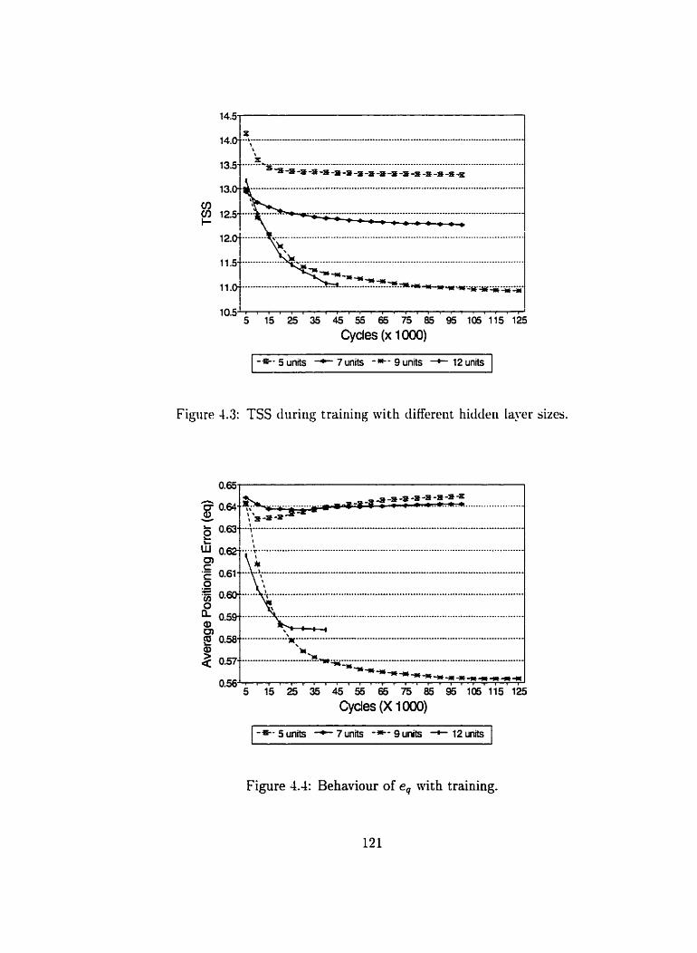
Figure 4.3: TSS during training with rlifferent hidderi layer sizes.

Figure 4.4: Behaviour of e, with training.

The rnanner in which this behaviour translates to a generalization capability is

illustrated in Figures 4.4 and 4.5. Figure 4.4 conipares the average e, in the four

network configurations. It is seen that e, is less in the 11-94 network in corriparison

with the 11-3-1 and 11-7-1 networks. 'vIoreover. there is no clear advantage in the

11-12-1 network. where e, is at a level comparable to that in the 11-94 network.

e- r igure 4.5 compares the four rirtwurka wich C L * J ~ ~ . C L LU TD. Tilr i 1-3- l. duCl the il-

7-1 networks are seen to lower the TD i ~ i the test data better than the other two

networks that have more units in the hidden layers. This nieans that. althoiigh

the 11-54 and 11-7-1 nctworks have higher positioning errors as seen in Figure 4.4.

the? arc able to generalize their learning and find correct sequerices in new problems

better thari the ottier networks that are trairied to a lotver positioiiing error. This

anonialy is esplaincd bu the fact that as a network learris 'bthtter' by riieaus of niin-

iniizing t l i ~ positioning errors. it begins to also learn 'additiorial' data iri its efforts

to find niore accurate relationships between the input and output data. In the case

of niiniinizing tlie maximum lateness. this additional data is niost probably the job

processirig tinies. which is inelevant in finding optinial solutions. Consequeritly. an

emphasis on minimizing positioning error can lead to overtrairiing and niemoriza-

tion of the training data a t the expense of the desired generalization capabilities.

The perioclic testing to determine TD during training helps to deterniine when the

network can be accepted as satisfactorily t rained.

Although Figure 4.5 shows the 11-5-1 and 11-74 networks to be almost equiv-

dent in rninimizing TD. the 11-5-1 network is selected after 15.000 training cycles.

This selection is based on the fewer number of hidden uliits. as well as on the fact

that the 11-3-1 network actually demonstrates a zero TD. Fewer nurnber of units

Cydes (X 1000)

Figure 4.5: Total Displacenierit (TD) during network training.

in the hidden layer is ge~erierally preferable because it results in qiiicker processing

(feedforward propagation) across the network. This 11-Z-1 neural network. trained

for rninirnizing the maximum job lateriess. is designated 'ILLATESET. .\Il tmined

networks that assign jobs a position iri a sequeilce. such as SILATENET. will be

called neural sequencers. The details of the training of IILATENET and its final

weights are given in section -4.1 of Appendk A.

4.3.3 Illustrative Problem

An esample is presented now to demonstrate hon- a neural sequencer generates

sequences to satisfj- the performance criterion. Table 4.2 shows a Q o b problem

that serves as an example. This problem is generated randornb for an arbitrarily

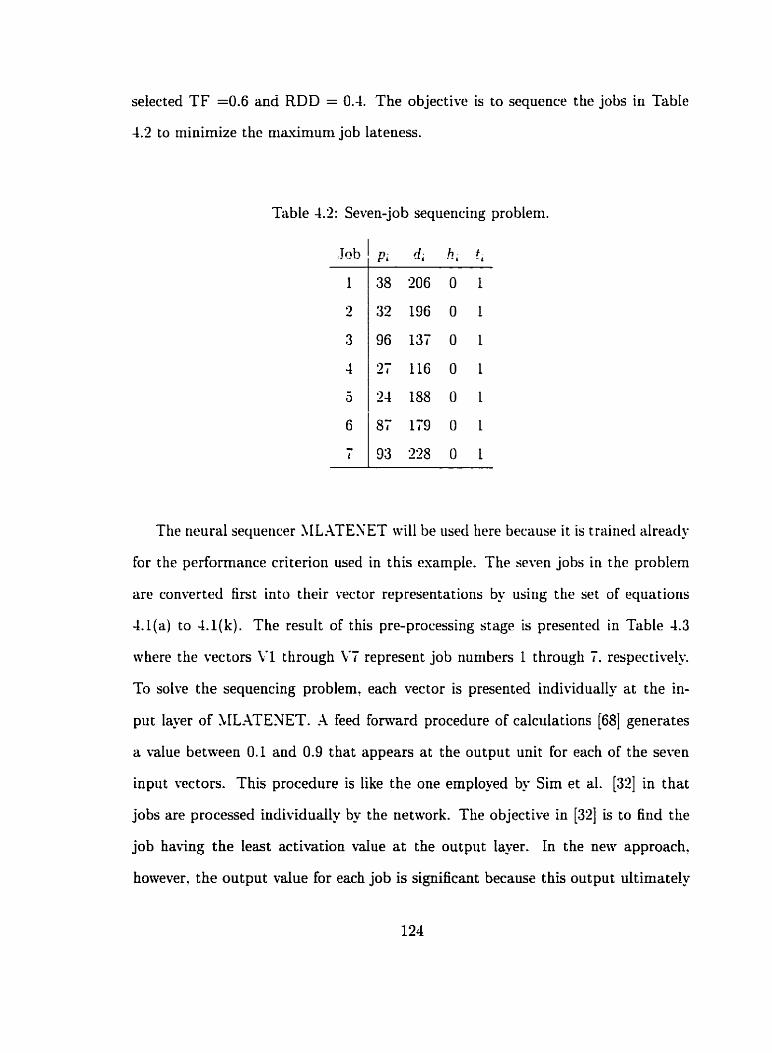
selected TF =0.6 and RDD = 0.4. The objective is to sequence the jobs in Table

4.2 to minimize the niauimum job lateness.

Table 4.2: Seven-job sequencing problem.

: h b pi di h ; t;

The neural sequeiicer ML-UESET will be used here because it is trainetl already

for the performance criterion used in t his esample. The sewn jobs in the problem

are converted first into their vector representations by usiiig the set of equatioris

( a ) O l ( ) The result of this pre-processing stage is preserited in Table 4.3

where the vectors Y1 through VT represent job numbers 1 through 7. respective-

To solve the sequencing problem, each vector is presented i~idividually at the in-

put Iayer of MLATEXET. -4 feed fonvard procedure of calculations [68] generates

a value between 0.1 and 0.9 that appears at the output unit for each of the seven

input vectors. This procedure is like the one employed by Sim et al. [32] in that

jobs are proçessed individually by the network. The objective in [32] is to find the

job having the least activation d u e at the output 1-r. In the new approach.

however, the output value for each job is signifiant because this output ultimately

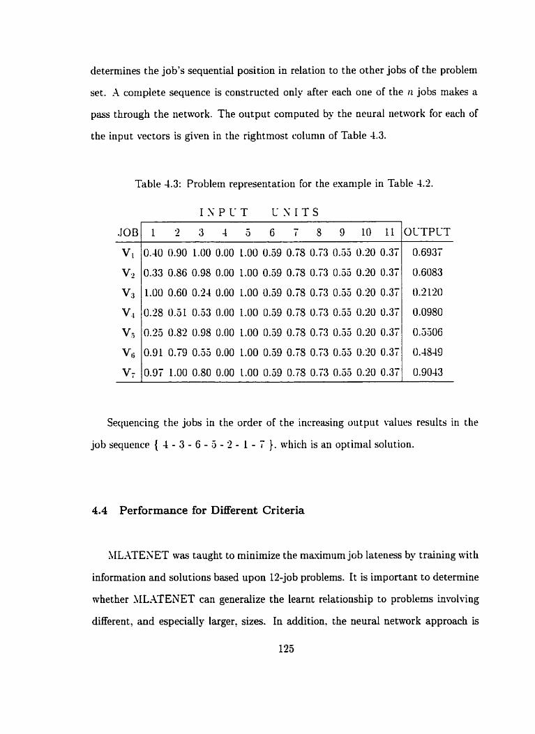
determines the job's sequential position in relation to the other jobs of the problern

set. -1 coniplete sequence is constructed only after each one of the n jobs makes a

pass through the network. The output computed by the neural network for each of

the input vectors is given in the rightmost colurnn of Table 4.3.

Table 4.3: Problem representation for the exaniple in Table 4.2.

Sequencing the jobs in the order of the incrcasirig output values results in the

job sequence { 4 - 3 - 6 - 5 - 2 - 1 - 7 }. which is an optimal solution.

4.4 Performance for Different Criteria

.LILATENET was taught to minimize the maximum job lateness by training with

information and solutions based upon 12-job problems. It is important to determine

whether SILATENET can generalize the learnt relationship to problerns invoiving

different , and especially larger, sizes. In addit ion. the neural network approach is

evaluated for other commonly used performance criteria to better uiiderstand its

scope of application.

4.4.1 Minimizing the Maximum Job Lateness

SILATESET is tested by usirig problerris involring upto 100 jobs. Each test

consists of 200 replications for eüch value of n. The test problenis are generated rari-

tlotiily l~ usitig Potts and L i n Wasserihove's niet hod with RF={O.Z.O.4.0.6.0.S.l .O}

aricl TF={O.'I.O.-L.O.G.O.$.l.O}. A11 h, are zero aritl al1 t , arc eclual to 1.0 in the test

problerns. The results are sliown in colunin 1 of Table 4.4. Thcy are espressed in

ternis of the percentage deviation froni the optimal solution. It is seeri frotri the

tests that MLATENET hos learnt quite well to secpence the jobs in an order that

enables rrii~iiniization of the nia,~i~riuni latcness.

1.4.2 Minimizing Flowtime Criteria

The neural network approach is evaluated riext for mininiizirig either the mean

Bowtinie or a variant. the weighted mean fiowtime. These two objectives are satisfied

optinially by sorting the jobs in the order of non-decreasing processing time divided

by the weight for each of the jobs (i.e. the WSPT rule)[S]. Optimal solutions. t here-

fore' are easily found for any job s i x n. Sloreover. one neural rietwork. which is

trained to rninimize the weighted flowtime. suffices because the mean Ron-time is a

special case of the weighted fiotvtime in which al1 the weights are equal.

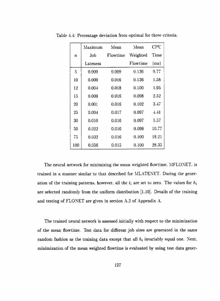
Table 4.4: Percentage deviation froni optimal for three criteria.

'1Ia.simum bIean Mean CPC

Job Flowtinie Weighted Tirrie

Lateness Flowtime (ms)

The neural network for niinimizirig the niean wiglited flowtinie. NFLONET. is

trained in a manner similar to that described for .\ILATENET. During the gener-

ation of the training patterns. honever. al1 the t , are set to zero. The mlues for h,

are selected randomly frorn the uniform distribution [1.10]. Details of the training

and testing of FLONET are given in section A.2 of Appendix A.

The trained neural network is assessed initially wit h respect to the minimization

of the mean Aowtime. Test data for different job sizes are generated in the same

random fashion as the training data except that dl hi invariably equd one. Xext.

rninimization of the mean weighted flowtime is e d u a t e d by using test data gener-

ated identically but with the hi randomly taking vaiues between 1 and 10. The test

data consists of 10 sets. Each set contains 200 problems having size n. The values

for n that are tested are identical to those selected for the test ing of MLATENET

in the previous section.

The results froni FLONET are also presented in Table -4.4. The t hird and Fourth

colunins derrioristrate that FLOXET has learnt. quite well. tlie reiationship that

leads to a niinimization of either the mean Aowtime or the mean weighted flowtinie.

This relatioristiip is etiibodied in sorting the jobs iri tilt. order of non-decreasirig

weighted processing t inies.

Table 4.4 siiggests that. if there is a well structurrd rule that Ica& to the optirilal

job secluence. siich as KSPT or EDD sorting. tlien t tic rieiiral networks are able to

dedoce it. Furt herniore. even t hough the training is perforrned on information froni

only l'-job problems. tlie neural networks are still able to apply the learned rela-

tionship to problenis having n niuch higher tlian twelve. Table 4.4 also shows that

the CPC tinie is only rnilliseconds per problern. when using an IBSI compatible.

Pentiuni 130 '\[Hz rriicrocomputer having 16 SIB of RAII.

4.4.3 Minimizing the Mean Tardiness

A performance criterion that is studied widely is the minimization of the mean

job tardiness (or total tardines)! a problem which is XP-hard [55]. Job due dates

are the main influence on the mean tardiness of a given job sequence. The capabilit-

of neural networks in sequencing jobs to minirnize the mean tardiness is investigated

solution to this bottleneck is to break the problem domain into 'categories'. each

category containing problems having similar defining characteristics. Such a scheme

is described in the aest section. Neural solutions can also be improved based upon

the implications of Equation (4.3). which relays the positioning error in the trained

network. The average positioning error in the network trained to niininiize the mean

tardines. h r e:iample. is fûund to Sc around 1.4. This particülar raluc iiîdicatcs

that any job's current position in the sequence is. on average. tiearly one and a half

positions away froni the preferred position in the optimal sequence. Therefore. the

job sequerices produced by the neural network appear well groonicd. as a result of

rnininiizing the positioriing error. for Further iniprovenierit b ~ . nieans of a simple.

adjacent pairwise interchange strate=.

4.5 Neural Job Classification and Sequencing Network

The breakdom of the problem cioniain into inclividual categories aims primarily

to group elenients ha~irig similarities. This categoriaation (or classitication) can be

perfornied ideally by cornpetitive neural networks. Cornpetitive networks consist of

two layers: an input laver and an output layer. A pattern presented at the input

laver stimulates the activation of one and only one output unit. By having as many

output units as the number of categories desired. such networks can be trained to

ciassify input patterns into groupings based on similar characteristics.

Baker [S] indicates that the tightness and range for due dates are attributes that

determine how 'difficult' or 'easy' it is to generate job sequences to minirnize the

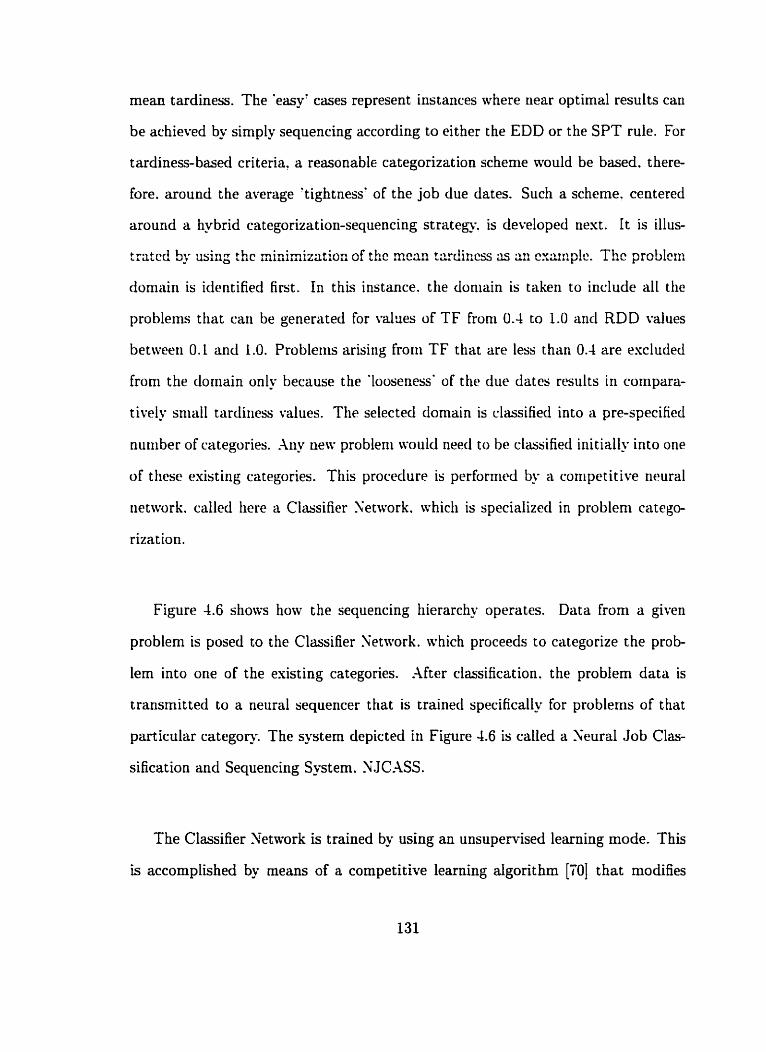
mean tardiness. The 'easy' cases represent instances where oear optimal results can

be achieved by simply sequencing according to either the EDD or the SPT rule. For

tardiness-based criteria. a reasonable categorization schenie would be based. there-

fore. around the average 'tightness' of the job due dates. Such a scheme. centered

around a hybrid categorization-sequencing strategu. is developed next. It is illus-

tratcd by using i hc minimiztitior, of the mmn tirdincss ÿs an cxÿrnplc. Thc problcrn

domairi is identified first. In this instance. the doniain is takeri to include al1 the

problems that can be generated for vdiies of TF froni 0.4 to 1.0 and RDD values

between 0.1 and 1.0. Problenis arising fror~i TF that are less than 0.4 are excludeci

from the dornain only because the 'looüeness' of the due dates results in compara-

t ively sniall tarcliness values. The selected domain is classified into a pre-specified

nuniber of categories. Any new probleni nould need to be classified initially into one

of tliese existing categories. This proceclure is perfornicd by a conipetitive neural

tietwork. called here a Classifier Network. whicli is specialized in problern catego-

riza t ion.

Figure 4.6 shows how the sequencing hierarchy operates. Data from a given

problem is posed to the Classifier Network. which proceeds to categorize the prob-

lem into one of the esisting categories. After classification. the problem data is

transmitted to a neural sequencer that is trained specifically for problems of that

particular c a t e g o . The systern depicted in Figure 4.6 is called a Xeural Job Clas-

sification and Sequencing System. NJCASS.

The Classifier Network is trained by using an unsupervised learning mode. This

is accomplished by means of a cornpetitive leaming algonthm [ ï O ] that modifies

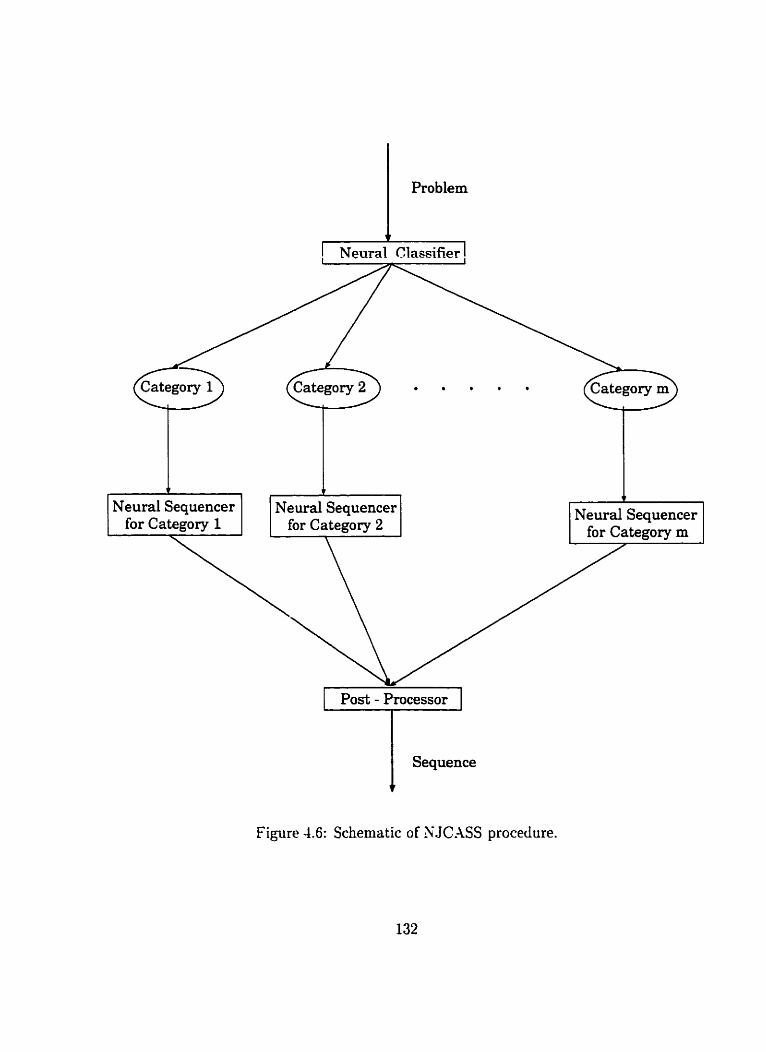
Pro blem

! Neural Classifier!

1 Neural Sequencer 1 1 Neural Sequemer 1 I N~air=l ~ O R I ~ P I I F P P A 16 iCI CII U G y Y b u b b A

for Category m

1 ~ o s t - Processor

I Sequence

Figure -4.6: Schematic of NJCASS procedure.

the weights so that only one of the output units responds to the input. Whenever

a pattern is presented at the input layer. the output unit whose weiglit vector is

closest to the pattern 'wins' the conipetition. The weight connections leading to

the winning unit are updated to reinforce the relation betneen the input pattern

and that unit at the expense of the other units. Inhibitory connections exist be-

rweeri the unics in the outpur i q e r tu eusure thac oriiy tiie 'wiiiriing' uriit accivates.

The resiilt is thüt the input data is organized automatically into a nuniber of clus-

ters. each cluster corresponding to siniilar inputs and represented by one of the

output units. The Classifier Network for niininiizing ttie nieaii tarcliness is calleci

1ITCLASS. It is trained by using 10.000 problems. with sizes selected in the range

froni n=i to n=65. These problerns are gerierated randornly (again by using Potts

and Van LVassenhove's niethod [XI) to produce a uriiforni sarnple of patterns across

the problem clornain. The patterns arc to hc çlassifi~d siirti that trn catrgoriw are

described. The riutriber ten is chosen arbitrarilu. The greater is this nuniber. the

more specialized are the sequencing networks wliich. intuitively rnay Iead to a better

overall perforniance. The tradeoff. of course. is that niore training timc is neetled

and a larger system has to be rnanaged. SITCLASS has a 4-unit input 1-r that

accepts continuous~d~ued input data vectors. Each vector for a n-job problem is

described by :

Pl = minimum due date:

P2 = average due date:

P3 = mauinium due date: and

P-l = 100.00 (a reference value).

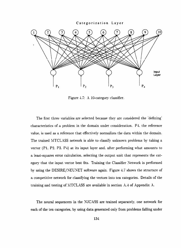
C a t e g o r i z a t i o n L a y e r

Figure 4.7: A 10-category classifier.

The First threc variables are selected because they are considercd the 'defining'

cliaracteristics of a problem in the domain iinder consideration. P-l. the refercnce

value. is tised as a rehrerice t hat effectively nornializes the data mithiti t tie tlomairi.

The trained hITCLASS network is able to classify iinknown problenis by taking a

vector (Pl . P2. P3. P4) at its input laver and. after performing what amounts to

a least-squares error calculation. selecting the output unit that represents the cat-

ego- that the input vector best fits. Training the Classifier Network is perfornied

by using the DESIRE/NEI;NET software again. Figure 4.7 shows the structure of

a cornpetitive network for classifying the vectors into ten categories. Details of the

training and testing of UTCWSS are available in section -1.4 of Appendk A.

The neural sequencers in the XJCLASS are trained separatels one network for

each of the ten categories, by using data generated only from problenis failing under

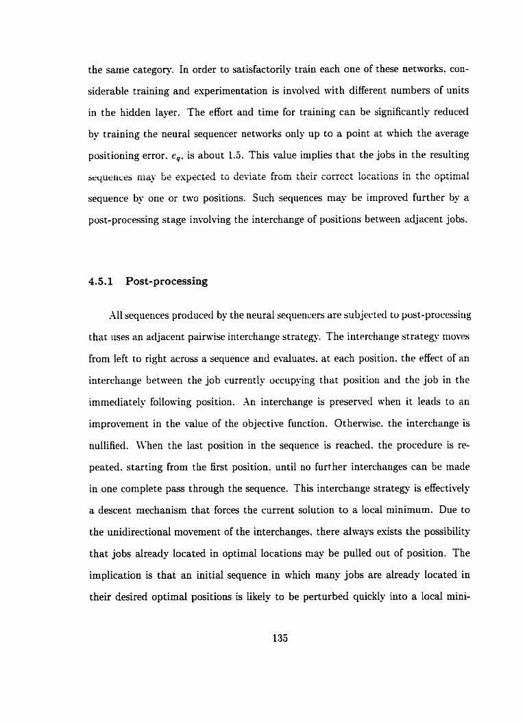
the same category. In order to satisfactorily train each one of these networks, con-

siderable training and experimentation is involved with different numbers of units

in the hidden layer. The effort and tinie for training can be significantly reduced

by training the neural sequencer networks only up to a point at which the average

positioning error. E,, is about 1.5. This value iniplies that the jobs in the resuiting

sequriices n lq - be çspect4 tu deviate frmi thcir concct locations in the optimal

sequence by one or two positions. Such sequences niay be iniproved further by a

post-processing stage involving the interchange of positions between adjacent jobs.

Al1 sequerices produced by the neural sequenccrs are subjected tu post-proccssirig

that uses an adjacent painvise interchange strateg.. The iriterctiange strategy rrioves

Froni left to right across a sequence and evaluates. a t each position. the effect of an

interchange between the job currently occiipying ttiat positiori and the job in the

immecliately folloaing position. An interchange is preserved ahen it leads to an

improvernent in the value of the objective function. Othenvise. the interchange is

nullified. When the 1st position in the sequence is reached. the procedure is re-

peated. starting from the first position. until no further interchanges can be made

in one complete pzss through the sequence. This interchange strategy is effectively

a descent mechanism that forces the current solution to a local minimum. Due to

the unidirectional movement of the interchanges. there a l n q s exists the possibility

that jobs dready located in optimal locations may be pulled out of position. The

implication is that an initial sequence in which many jobs are already located in

their desired optimal positions is likely to be perturbed quickly into a local rnini-

murn that is very close to the initial sequence. Therefore. the initial sequence in

this instance needs to have the maximuni number of jobs located in their optimal

positioris. On the otlier hanci' a starting solution where more jobs are near their

desirecl positions (Le. out of place by only one or two positions) appeals more to

the particular interchange strategy used in the post processing stage. With a larger

iiiiniber uf jvbs iûlerated vut of pcjition in the starting sequcncc. the need to m i n

the networks to a very lon error. e,. is reduced substantially. This reduction trans-

lates iiito less training tinie for these networks.

4.5.2 NJCASS for Minimizing the Mean Tardiness

Ten tieiiral sequencers are trained for the XJCASS to niininiize the trieail tar-

diriess. The training procedure for each category is siniilar to t h ernployed for the

previous networks. but wit h differeiices regarding when to accept the uetwork as

satisfk torily trained. The training sets are derived froni l%jo b esaniple problcnis

that are solved by dynarriic programming. For the neural sequencers specialized

for this NJCASS. the training is stopped after every 100 cycles and the network is

tested by erriploying a test data set. During this testing. the sequence generated

by the neural netivorks is post-processed by the interchange strategv. The training

is stopped when the test resuits appear to have 'bottomed out'. This occurs at

between 300 and 5000 training cycles. depending on the category. In three of the

ten categories. it is observed that the post processing interchange strategv results

in near optimal solutions when applied to initial sequences sorted in the order of

their non-decreasing due dates (EDD). It is decided. therefore. to train the neural

sequencers for these three particular categories to sequence the jobs in the order of

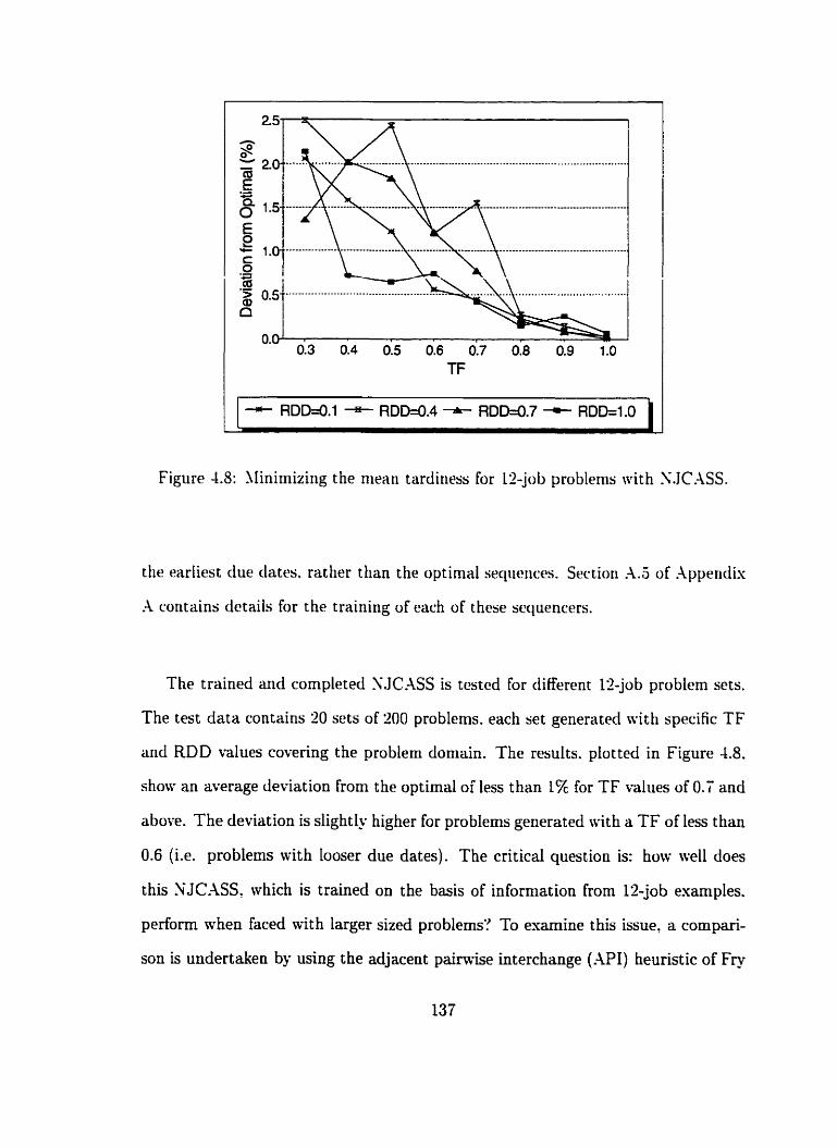
Figure 4.8: 'rlinirniziiig the mean tardiness for 12-job problenis \vit h SJCASS.

the earliest due dates. rather than the optimal sequerices. Sertiori A.5 of Appendis

A coritains details for the training of each of these sequencers.

The trained and completed XJCASS is tested for ciifferent 12-job problem sets.

The test data contains 20 sets of '100 problems. each set generated witli specific TF

and RDD values coverîng the problem domain. The results. plot ted in Figure 4.8.

show an average deviation from the optimal of less than 1% for TF values of 0.7 and

above. The deviation is slightly higher for problems generated with a TF of less than

0.6 (Le. problems with Looser due dates). The critical question is: how well does

this NJCASSI which is trained on the basis of information from 12-job examples.

perform when faced with larger sized problems? To examine this issue, a cornpari-

son is undertaken by using the adjacent paim-ise interchange (.\PI) heuristic of Fry

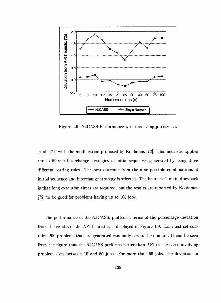
~5~ I 5 8 10 12 15 20 25 30 40 50 75 100

Number of jobs (n)

Figure 4.9: N.JC.-\SS Performance tvith increasing job size. r r .

et al. [Tl] with the niodification proposed by Koularnas [T?]. This heuristic applies

three different interchange strategies to initial sequerices generated b - using three

different sorting rules. The best outcome From the nine possible combinations of

initial sequence ancl interchange strategy is selected. The heuristic's main drawback

is that long esecution times are required. but the results are reported by Koulamas

[72] to be good for problerns having up to 100 jobs.

The performance of the NJCASS. plotted in terms of the percentage deviation

from the results of the API heuristic. is displayed in Figure 4.9. Each test set con-

tains 200 problems that are generated randomiy across the domain. It can be seen

from the figure that the NJCASS performs better than API in the cases involving

problem sizes between 10 and 50 jobs. For more than 50 jobs. the deviation in

performance between the two approaches is in favour of the ;\PI. The reason for the

gradua1 deterioration obscrved in the performance of NJCASS. starting froni about

n=%, is because it is trained based on target values which are derived from rnerely

1'2-job problems. This approach is apparently not sufficiently accurate for more than

50 jobs. The loss in accuracy. as n grows, is a result of the current positioning error

Lrcutiiiiig & . t i k el- ~.rakrr. 111 u~lirr wurda. a ps i~ iu i i iug m u r riicuiiipiwxa imre

positioris as r l grows bccause increasingly more jobs have to fit within the interval

between G, and G,+i. The result is that a job may be off-target. on average. by

several positions rather than one or two for a giveri positioning error of. s a y 1.5.

t h is büsed on 12-job training problems. Tlien siniple adjacent intercliariges have

greater difficulty in bringing an off-target job to the desirable sequeritial position.

The reiiicdy is to iniprove the target accuracy kq basing the training on data froni

problenis in ahich n is greater than ttvelve. where possible. The conclusion froiii

Figure 4.9. on the other hand. is that the N.IC.4SS can competc. for up to JO-job

problenis, tvith the API heuristic.

The ;\PI heuristic based on Fry et al. [ T l ] and modified by Kouiamas [ï2] is

chosen in this coniparison for two reasons. First. its solution is cornpetitive with

the better heuristics for mininiking the mean tardiness. as reported iri Table 1 of

ref. [Z]. Second. the API is a general purpose interchange heuristic. the applica-

tion of which need not be limited to one specific performance criterion. Figure 4.9

demonstrates that the result of an initial sequence produced by the neural network

and modified by a simple adjacent pairwise interchange is comparable, if not slight ly

better. than that generated by the nine different combinations of initial sequence

and interchange st rategies encompassed in the API heuris tic.

-1s a further evaluation of the solution quality of the NJCASS. a cornparison is

niade with one of the several leading heuristics that are specific to the mean tar-

diness criterion. For example. Russell and Holsenback [T3] demonstrated that the

PSK heuristic of Panwalker. Smith and Koulamas [58] and the Net Benefit of Relo-

cation (SBR) heuristic of Holsenback and Russell [56] are niore or less comparable.

The SBR is stronger in certain cases. while the PSK is better in other cases. For

convenience. the N.JCASS is conipared next wit h one of t hese heurist ics. nainely

the SBR algorithni taken froni ref. [XI. The latter uses a domiriance ride. basecl

on Eninions' coiiditions of opt iniality [XI. toget lier wit h calculat ions to deteririirie

the net benefit of job relocatioris in the sequetices. The cornparison is perfornied

by using a procedure identical to that eniployxl in ref. [56]. Twenty sets of test

data are iised: each set contairis teri problenis of rr jobs aliere n is 12. 25 or 30.

Individual sets are generated by utilizing the Potts and \ i n \Vassenliove nictliod

[el] for specific TF and RDD values. The 12-job problerns are testcd becausc that

is the problem size used in the training of tlie neural sequencer networks. The tests

for the 25 and S0 job problems are done to evaluate how relatively well the S.JCASS

performs for larger problems. Table 4.6 presents the results. The integers under tlie

columns tieaded 'Best' indicate the numbers of times XJCASS achieved a solution

better than or equal to NBR in each set.

Table 4.6 shows t hat N JCASS produces solutions nhich are generally compara-

ble to those given by NBR. The SJCASS is better in 26 out of the 60 sets tested.

XBR is better in 2 1 sets. and the two methods give equal total tardiness in the

remaining sets. On the other hand, NBR is slightly superior based on the total

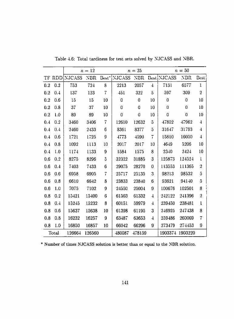
Table 4.6: Total tardiness for test sets solved by YJCASS and NBR.

TF RDD

0.2 0.2

0.2 0.4

0.2 0.6

0.2 0.8

0.2 1.0

0.4 0.2

0.4 0.4

0.4 0.6

0.4 0.8

0.4 1.0

0.6 0.2

0.6 0.4

0.6 0.6

0.6 0.8

0.6 1.0

0.8 0.1

0.8 0.4

0.8 0.6

0.8 0.8

0.8 1.0

Total

* Number of times NJCASS solution is bet ter than or equai to the NBR solution.

tardiness values summed over the 20 data sets for each problem size n. This result

is due mainly to a particular weakness of YJCXSS in tliose data sets having low

RDD. It is not surprising because the optimal sequences in such cases d i b i t no

strong patterns or rules that help the neural networks to learn the relationships

between the input data and the desired sequence. Yevertheless. NJCASS can be

ruiia1ict.d tiieii Lj iiici.ciwiug ~ l ic iiwiber uf wtegûries co'rt-ring this rcgion of thc

problem. The irnprovenient to be expected is reflected in the behaviour illustrated

in Figure 4.9. This figure shows what happens wheri nierely a single neural iietwork

is trained to cover the entire problem doniaiu rather than the 10 currently iised by

XJCASS. The overall trend froni the single neural sequericer is siniilar to that from

the NJCASS. except that it is about 2% less accurate. This deterioration reduces

the accuracy to a level that reriders the single network's perforniarice niargirial in

coniparison to t hat of heuristics sucli as those nientioned in re t [2].

4.5.3 A Limited Exponential Cost Function

A hypothetical situation involving penalty costs that eshibit a limited exponen-

tial behaviour is described now. The example is iised to illustrate how the SJCASS

can be irnplemented in situations where no heuristic is known beforehand for o p

tirnizing the given criterion. The mean tardiness mesure applies a penalty that

increases in linear proportion to the tardiness. In extreme cases. it is possible that

the penalty may actually exceed the value of the job. The cost function considered

next differs in that a substantial proportion of a total penalty is assessed a t the

instant of tardiness. As the tardiness increases, the penalty follows an exponentially

decreasing rate up to a maximum \due. This limited esponential cost function is

expressed in the following form:

Two variants of this function are analyzed and tested with a S.JCASS set up for the

piirpose.

Case (i)

The first scenario lias ri jobs due at different tinies. The tardiness penalty per tinie

unit is iiriiforrn for a11 jobs (i.e. t , = 1 V i). Lt is applicd in the Liniited esporieiitially

iricreasing faskiion of Equatiori (4.4).

Case ( i i )

The tardiness penalty is not uniform but differs froni job to job. The training and

test data for the N.JCASS has ti selectecl randomly &on1 t lie uniforrri distribution

[1.10].

The NJCASS for minimizing cost functiori (4.4) also has ten categories. the nuni-

ber of categories are selected arbitrarilu again for illustration purposes. It is trained

and constmcted in a manner identical to that discussed previously for minimizing

the mean tardiness. Presuming that no quick method is available for minimizing

cost function (4.1) in large sized problems. complete enurneration is used to deter-

mine the solutions needed for the training problems. Thus, the sequencer networks

are trained for each category by uçing 8-job example problems.

Table 4.7: Generation parameters for raudonily selected problenis.

The hypotheticül cost function of equation (4.4 is tested for cases ( i ) and (ii) by

using the NJCASS. Two randomly found data sets. each containing '200 problenis.

are gerierated from the combinations of TF and RDD givcn iii Table 4.7. Ttiese

TF

RDD

combinat ions are selected as representative of cases involving a riioderate tightness

and range of due dates. Finding a good heuristic for niiuiniizing Equation (4.4)

0.1 0.8

O . 0.8

may range froni using 'quick and dirty' mettiods to more involved techriiques. The

.\PI heuristic is chosen for cornparison because. not only docs it combine scvcral

of the proniinent 'quick and dirty' rules. but it furttier eriliaiices their results by

using three different interchange strategies. The API results. when taken in the

contest that they conie from ari approach that is based on a rule-of-thunib. c m be

considered reasonably good. even for a function like that usecl in Equation (-4.4).

The coniparison between the .\PI and NJCASS approaches is dispiayed in Figure

4.10.

The results in Figure 4.10 are presented in terms of the percentage deviation of

the NJCASS results from those of the .-\PI heuristic. A negative deviation means

that the .%PI heuristic is worse. Therefore. the generd superiority of the NJC.-\SS

over the API approach is demonstrated clearly in Figure 4.10 for the case (il and

case(ii) scenarios.

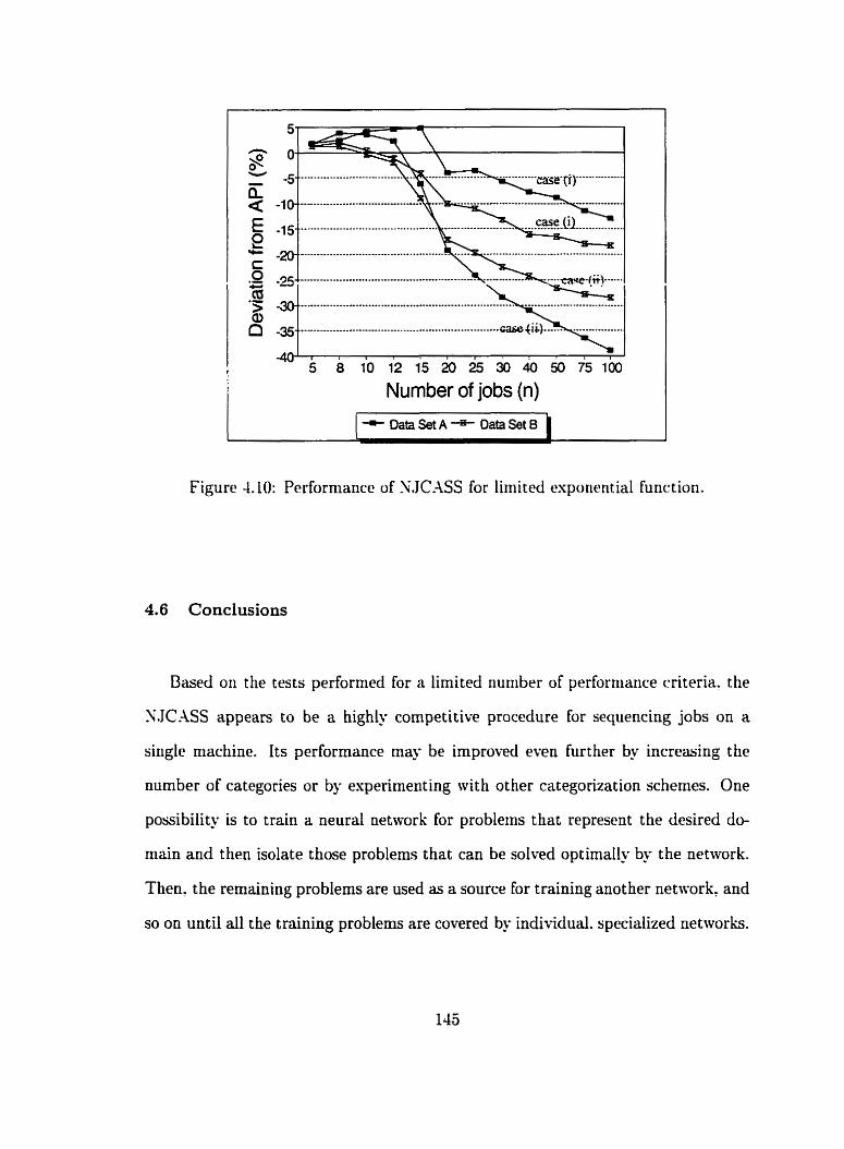
Figure 4.10: Performance of N.JC;\SS for lirriited exponential function.

4.6 Conclusions

Based on the tests performed for a limited nurnber of petforniance criteria. the

NJCASS appears to be a highly cornpetitive procedure for sequencing jobs on a

single niachine. Its performance may be improved even further by increasing the

number of categories or by esperirnenting with other categorization schemes. One

possibility is to train a neural network for problems that represent the desired do-

niain and then isolate those problems that can be solved optimally by the network.

Then. the rernaining problems are used as a source for training another network? and

so on until al1 the training problems are covered by individual. specialized networks.

The neural network approach highlighted by the XJCASS provides several ad-

vantages. but chiefiy the flexibility of application for different perforniance criteria.

Special purpose heuristics, developed for a specific criterion, may be unsuitable when

a different criterion is considered. Furthermore. a heuristic ni- perforin well. on

average. but still remain consistently weak for a certain class of problenis. The SJ-

C-ASS aiid ils ciiwificat iuii aclieiiir a h a wha: arc i R ~ t i ~ ~ l y C U G ~ U ~ ~ Z C ~ ' h e ü ~ i ~ i i ~ ~ '

for probleni classes having similar characteristics witliin a domain. The user needs to

identify only key characteristics and the clesireci nuniber of categories. Tiie iinsuper-

visecl Leariiing algorithm results in a Classifier Network that is capable of suggestirig

a suitable categorization based on informatiori frorii the vector data with ivtiich it

is trained. Thus. the procedure can be conceivably automated with the categories

self-gerierated through unsupervised learning. Ranclonily generated problerns can

be prodiiced to represent tliese categories and the problenis can also br ~ised subse-

querit ly to train t lie specialized sequericer rietaorks.

Any neural netivork approach possesses the disadvantages of neural netivorks

in general. narriely the tiine to train and test the networks as well as the esperi-

eiice required to achieve good results. Although the NJCASS's performance is quite

cornpetitive. it is unlikely to be noticeably better than a good heuristic dewloped

painstakingly for the purpose. k t . in the event that no such heuristic is available.

the N.IC.ASS appears to be a better alternative to makeshift rneasures based on

intuition or modification of existing mles or heurist ic procedures. Sloreover. the

development time for NJCASS is much shorter than that needed to evolve a full-

blown heuristic procedure. It should be noted, however. that neural sequencing

appears best suited to performance measures that are regular. -1 regular perfor-

mance nieasure is one where the value of the function can grow only if at least one

of the completion times in the schedule increases [8]. Initial results using neural

sequencing for a criterion involving an irregular performance nieasure, namely min-

imizing the completion time variance (Yerten and Muller [(-LI)' suggest that it is

not much niore effective t han simple sorting heuristics. Hoivever. fwt her researcli is

3 t il1 ~ t d e d .

Chapter 5

Dynamic Scheduling with Cooperative Dispatching

5.1 Introduction

Scheduling in manufacturirig cells is frequently dynaniic in nature. Tlie du-

namisni arises priniarily under tivo circumsraiices. Thc first is when jobs arrive

continuously at a ce11 and join other jobs aliich are already waiting in queue. This

differs Froni the static case. nhere a fixed nuniber of jobs is availablc at the start of

the sclieduling and the initial schedule remains valid until ail tlic jobs are conipieted.

The second circumstance anses when uiiespected or unpreciictable erents. such as

a rnacliine M u r e or a defective product. invalidate the current schedule.

Schecliilirig under dynarnic conditions iniplies the need to eontinually update

t lie schedule. The terms 'on-line sclieduling'. u teal-t irne scheduling' and 'dynaniic

scheduling' are often used interchangeably to describe situations requiring a con-

t inuous schedule modification. In fac t. t here is a fine distinction be tween real-t ime

and on-line scheduling. Real-t ime scliecluling may be performed cit her on-liae or

off-line. If it is performed off-line. then a "snapshot" of the cell's current status and

activities is captured and a new schedule is devised almost instantaneously. The

need to efficiently finalize this 're-scheduling' in a matter of seconds poses computa-

tional difficulties. part icularly if t here are many jobs m i t ing. If on-line scheduling

is employed, on the other hand, the scheduling is reduced to making dispatching

decisions whenever a resource becomes wailable. This reduction in the scope of

the scheduling problem to a series of 'as-needed' decisions makes on-line scheduling

attractive for real-time scheduling demands.

The CD approach described in Chapter 3 can be performed on-line. like other

dispatching rules. Cnlike most simple dispatching rules. tiowever. CD is more coni-

plex and recpires real-tinie inforniation regarding the current states of the jobs and

machines in a cell. Current coniputer networking and ce11 control techriologu. how-

ever. alloa t his inforniation to be collecteci aiitornatically JO t hat the CD approach

is impleniexitable for an FSIC. The remainder of this chapter describes the perfor-

mance of CD in dynamic scheduling. The el-aluatiori of CD is undertaken by usirig

a simulation approach for dynamic job arrivals.

5.2 CD Scheduling with Dynamic Job Arrivals

FSICs often have to process orders that arrive randomly. The unpredictability

of the tinie of arrival poses obvious problems because existing schedules. if any. be-

corne obsolete immediately. On-line scheduling treats a n e n arriva1 siniply as an

additional job joining a queue. The next time that a machine needs to be loaded.

the new arrivals are considered immediately. together with the previous jobs mit ing

to be dispatched. Therefore. with on-line scheduling based on dispatching rules. no

major scheduling disruption is experienced as a consequence of the new arrivals.

5.3 Simulation

The performance of CD is evaluated esperimentally for dynamic job arrivals.

The experiments are performed by means of a computer program written in the C

language [XI. They are designed to siniulate activities related to the movement of

parts through a PMC. The program nionitors each Job's starting and Bnishing times

on the machines. from which the desired performance data is collected. The pro-

gram allows simulations having a selected nurriber of dispatching rules. in addition

to CD.

The objective of the simulations is to study the comparative effectiveness of CD

br different job arriva1 rates. The jobs are assumed to bc arrivirig at the ce11 accord-

ing to a Poisson process. In t his process. the expected nuinber of arrivais occurring

in an intemal of tinie. t. has a Poisson distribution with a parameter X,t in wliich

A, is the expected number of arrivals per unit time. Assuming that the nurnber

of arrivais in each non-overlapping intemal are independent of one another. then

the t irne between successive arrivals is dist ri buted esponent ially ni t h paramet er A,.

The higher is A,, the greater is the frequency of arrivais and the more severe is the

likely congestion. The evaluation of CD takes the form of a cornparison with the

traditional dispatching rules that are expected to be the most effective for the given

scheduling criterion. The individual criteria t bat are considered and tested. under

different job arriva1 rates, are the minimum mean flowtime and the minimum rnean

tarciiness.

5.3.1 Generation of Test Data

The data for each simulated test problem relates to 500 jobs. Initiallx two

jobs are assurned to be already in the system and awaiting their first operations.

The arrival times for these two jobs correspond to time zero. Each riew mbsequent

job arrives at an instant that is generated randonil. Arrivds occur at intervals

that are distributed exponentiall. The length of the intemal betweeri arrivals. t,.

is deterniined randomly from:

where p is a real-valucd random number from the uniforrri distribution C[O.l]. The

arrival t inie of each new job is detenriined by iricreriientirig the previous job's arrival

time by t,. This proceclure is repeaccd until 500 job arrivals have been getierated.

Each test set contains 20 different problems that are created randonily in this fash-

ion for a specific arrival rate. A,. and a given performance criterion.

In order to study CD's performance in mininiizing the mean tardincss. the

method of Potts and L i n Wassenhove [XI. which was eniployed in the previous

chapter. is adapted for generating problems having dynamic arrivais to multiple-

machine cells. The main modification is in computing a d u e for P. which is the

main influence on the value of the generated due date (see section 4.3.1). In the

static case. P is sirnply the sum of the processing times for al1 the jobs in the prob-

lem set. Sow P is an estimate based on the expected flotvtime that a job would

have assurning FIFO processing, plus the surn of the processing times on the indi-

Mdual machines for that job. The value of P that is computed for the ith job is then

used in Potts and Van FVassenhove% method [ai] to generate a due date for that job.

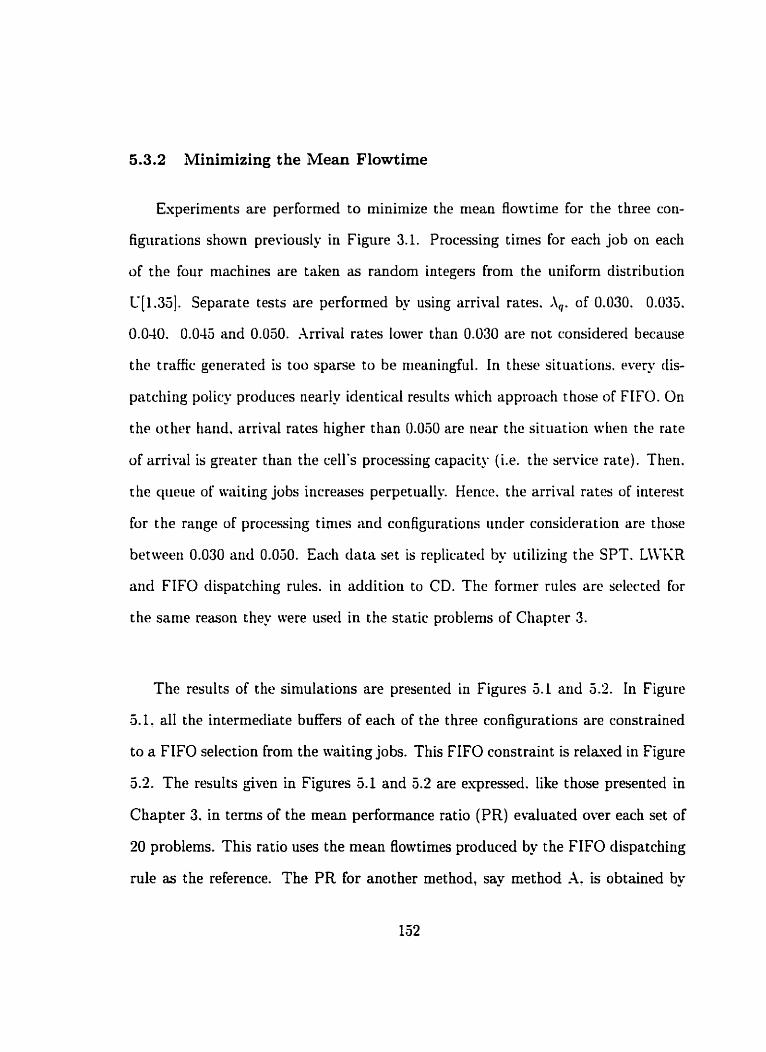
5.3.2 Minimizing the Mean Flowtime

Experiments are performed to minimize the niean Rowtime for the three con-

figurations shown previously in Figure 3.1. Processing times for each job on each

of the four machines are taken as random integes from the uniform distribution

C[1.35]. Separate tests are performed by using arrival rates. A,. of 0.030. 0.035.

0.040. 0.045 and 0.050. Arriva1 rates Iower than 0.030 are not considered because

the trafic gerierateci is too sparse to be nieaningful. In these situatioiis. every dis-

patching policy produces riearly identical results which approach those of FIFO. On

the other tiarid. arrival rates higher t han 0.050 are riear the situation wlien the rate

of arrivil is greater than the cell's processing capacity (i.e. the service rate). Then.

the queue of aaiting jobs increases perpetually. Hencc. the arrival rates of interest

for the range of processing times and configuratioris iinder consicleration are those

between 0.030 and 0.050. Each chta set is replicatecl by utilizing the SPT. LWKR

and FIFO dispatching rules. in addition to CD. The former rules are selected for

the same reason they tvere used in the static problems of Chapter 3.

The results of the simulations are presented in Figures 5.1 and 5.2. In Figure

.5.1. al1 the intermediate buffers of each of the three configurations are constrained

to a FIFO selection from the tvaiting jobs. This FIFO constraint is relwed in Figure

5.2. The results given in Figures 5.1 and 5.2 are espressed. like those presented in

Chapter 3. in terms of the mean performance ratio (PR) ewluated over each set of

20 problems. This ratio uses the mean flowtimes produced by the FIFO dispatching

rule as the reference. The PR for another method, say method A. is obtained by

dividing the mean result froni the reference method by tliat from method A. A PR

value that is greater than 1.0 is a nieasure of the percentage superiority of niethod

A's results over those obtained by the reference method.

It can be observed from Figure 5.1 that CD outperforms the SPT and LLVKR

rules by as much as 5% in the Type 1 arid Type III configurations. but only by about

1% in the Type II configuration. The general trend apparent in Figure 5.1 is that

CD perfornis increasingly better than t hese two rules as the arrival rate grotvs. This

beharior indicates that CD is niore effective in niinimizing the nieaii flowtinie under

conditions of high ce11 congestion. The trends witnesscd in Figure S.1 appear ro

hold also for the cases shown in Figure 5.2. Le. for non-FIFO interniediate buffers.

Again. CD iricreasingly out performs the ot her two dispatching rules as the arrival

rate grows. albeit at a magnitude not exceeding 2%.

The closeness in performance to FIFO that is observed in Figure 3.1 for al1 the

dispatching rules in the Type II configuration is because the job arrirals are shared

initially between two machines rather than only one machine. CVitii an arrival rate

of 0.05. the average queue lengths for the first two machines rarely exceed 2 or 3 jobs

in the Type II configuration. The average queue at the third machine. which receives

jobs from both the first two machines. is significantly higher. When the queue at the

buffer for the third machine, which is a strong bottleneck. is constrained to FIFO

processing, al1 the ot her dispatching rules are no t significant ly more effective t han

FIFO. This is evidenced in Figure 5.1. On the other hand. if the bottleneck is not

constrained to a FIFO selection, then the dispatching d e s show improved results

in cornparison to FIFO. See Figure 5.2.

Type I mfgurat(0n

Type II corifiguraüm

- - -

Type I I I configuration

I T - - -

T

0.03 0.04 O.&

Arriva1 Rate

( + CD + SPT -*- LWKR ]

Figure 5.1: Minirnizing the mean flowtirne +th FIFO intermediate buffers.

154

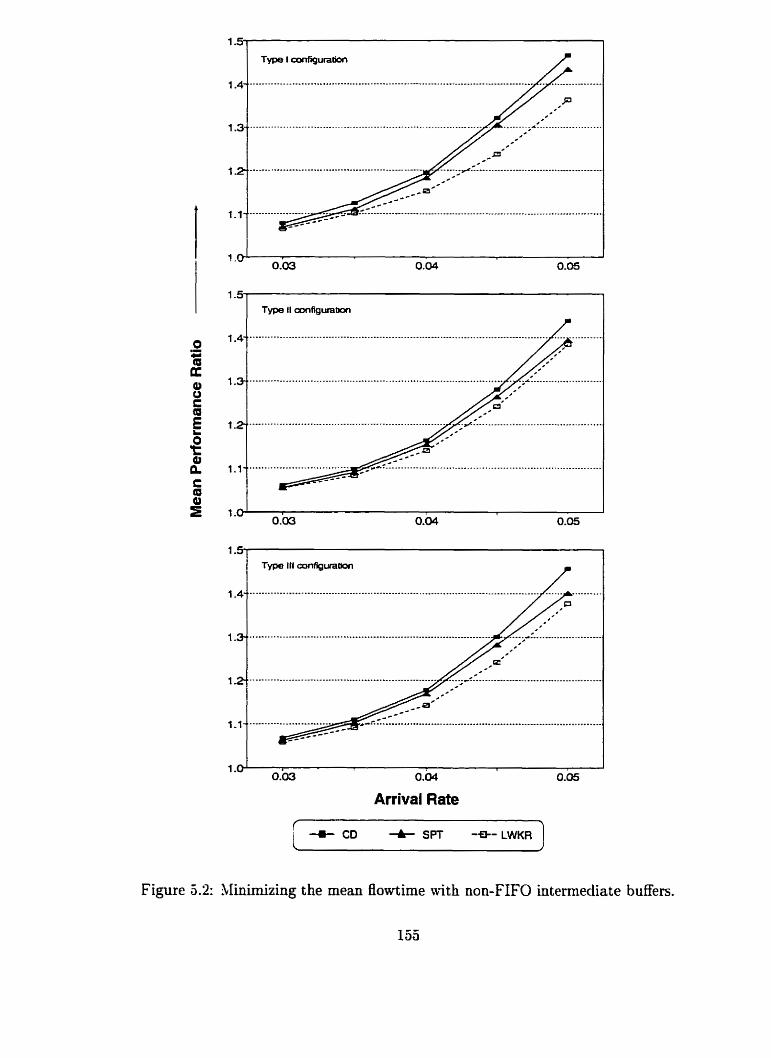
Type III configwatlon

/

0.03 5

0.04 0.05

Arriva1 Rate

( t CD SPT *- LWKR

Figure 5.2: Minimizing the mean flowtime ~ 4 t h non-FIFO intermediate buffers.

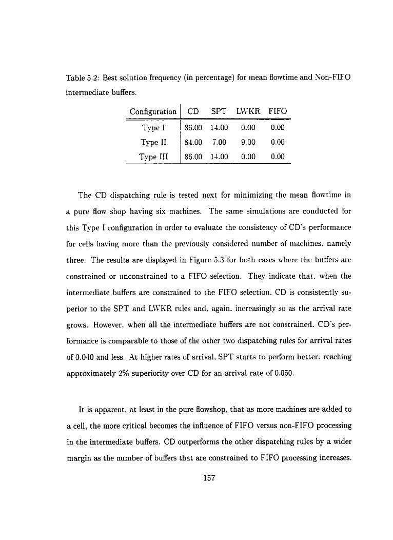
Table 5.2: Best solution frequency (in percentage) for inean flowtime and Non-FIFO

intermediate buffers.

Configuration

Type III 1 86.00 14.00 0.00 0.00

CD SPT LWKR FIFO

Type II

The CD dispatching rule is tested nest For rniriimizing t h niean fiowtirne in

a pure How shop having sis machines. The sarne siniulatioris are coriducted for

this Type I configuration in order to evaluate the coiisistency of CD's performance

for cells having more tiian the previously considercd nuniber of niachines. iianiely

three. The results are displaycd in Figure 5.3 fur both cases rvhere the buffers are

constraineti or unconstrained to a FIFO selection. They indicate that. when the

inter~iiediate buffers are constrained to the FIFO selectiori. CD is consistently su-

perior to the SPT and LWKR rules and. again. increasingly so as the arriva1 rate

grows. Honever. when al1 the intermediate buffers are not constrained. CD's per-

formance is comparable to those of the other two dispatching rules for arriva1 rates

of 0.040 and les . At higher rates of arrival. SPT starts to perform better. reaching

approxirnately 2% superiority over CD for an arrival rate of 0.050.

T q e 1 56.00 14.00 0.00 0.00 I

84.00 7.00 9.00 0.00

It is apparent. at least in the pure flowshop, that as niore machines are added to

a cell, the more critical becomes the influence of FIFO versus non-FIFO processing

in the intermediate buffers. CD outperforrns the other dispatching d e s by a wider

rnargin as the number of buffers that are constrained to FIFO processing increases.

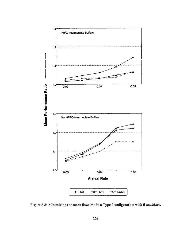
FlFO Intemediate Buffers

1.3 Non-nFO Intermediate Buffers

' 0.03 r

0.04 0.05

Arrival Rate

+ CD SPT -*- LWKR J

Figure 5.3: hlinimizing the mean Bowtime in a Type I configuration wïth 6 machines.

On the other hand, the other dispatching rules are at their best when the nu~nber

of constrained buffers. particularly in bottleneck machines. is minimum. ..A compar-

ison of the results presented in Figure 3.3 ivith those shown in Figures 3. l and 5.2

indicates that CD's power tends to diminish as the number of machines grows in a

cell. Despite this trend. CD remains cornpetitive in probleriis for which the other dis-

parciiirig ruies excei. sucii as: cases iiivulv iiig iiuri-FiFO LulFera a d I&li arriçal rd tea.

5.3.3 Nlinimizing the Mean Tardiness

The evaluation of CD for niinimizing the niean tardines is conducted nest by

eniployirig siniulation experirnents on data sets organized as follows.

1. Eadi data set coritaiiis 20 randonil- gerierated probleriis: each problem covers

500 job arrivais.

2 . Data sets are generated for the arriva1 rates of 0.030. 0.040 arid 0.050.

3. The due date for each job is specified by using the modified Potts and \an CVaçsenhove method with TF and RDD equel to 0.4 or 0.8. respectively.

T h . there are four possible combinations of these TF and RDD values:

TF=RDD=O.4: TF=O.4 & RDD=0.8: TF=O.S k RDD=O.4: and TF=RDD=O.S.

T'ne simulations are undertaken in a manner similar to that used for the mean flow-

time criterion. However. in this instance, the dispatching rules to which CD is corn-

pared are : 1) SPT: 2) EDD: 3) MDD: -1) minimum rernaining slack (.\ISLE;): and

5) FIFO. With the exception of FIFO and SPT. these dispatching rules are selected

because they are due date based d e s . Due date based d e s are a logical choice for

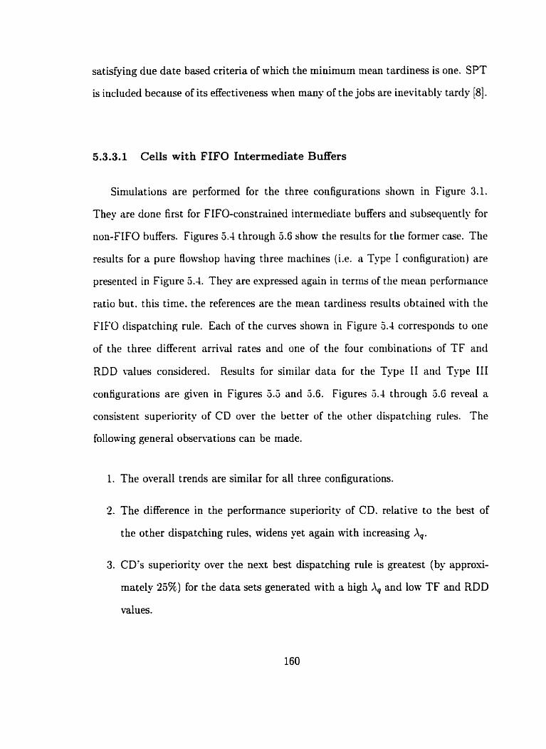
satisfying due date based criteria of which the minimum mean tardiness is one. SPT

is included because of its effectiveness when many of the jobs are inevit ably tardy [8].

5.3.3.1 Ceils with FIFO Intermediate Buffers

Siniulations are perforrned for the three configurations shown in Figure 3.1.

The- are done first for FIFO-constrüined intermediate buffers and subsequently for

non-FIFO buffers. Figures 5.4 through 5.6 show the results for the former case. The

results for a piire Bowstiop tiaving t h c e niachines (i.e. a Type 1 configuration) are

preseiited in Figure J.4. They arc expressecl agairi in terrns of the niean perforniarice

ratio but, this time. the references are the niean tardiness results obtained witii the

FIFO dispatching rule. Eacb of the curves stiown in Figure 3.4 corresponds to one

of the three different arriva1 rates and one of the four combinations of TF and

RDD values considereci. Results for similar data for the Type II and Type III

configuratioris are given in Figures 5.3 and 2.6. Figures 3.4 through 5.6 reveal a

consistent. superiority of CD over the better of the other dispatching rules. The

following general observations can be made.

1. The overall trends are similar for al1 three configurations.

2. The difference in the performance superiority of CD. relative to the best of

the other dispatching rules. Mdens yet again with increasing A,.

3. CD's superiority over the next best dispatching rule is greatest (by approxi-

mately 25%) for the data sets generated with a high A, and low TF and RDD

values.

-4. The use of non-FIFO buffers for severe bottleneck machines, as seen in the

Type II configuration. greatly improves the performance in the cell.

Table 5.3 compares the frequency. expressed as a percentage of the total number

of problems tested, with which each dispatching rule provides the best solution in

the test problems. The results are sorted according to the coufiguration and the due

date tardiness Factor. TF. Table 5.3 indicates that CD domiiiates in the Type I and

Type III configurations. It is also the better in more ttian two out of every three

problenis for the Type II configuration.

Figures 5.4 through 5.6 generally show a steady decline in the perforriiance ratio

as TF increases. This trend is attributable to tlie iricreasing total tardiness accorri-

patij-irig tiigh TFs. When the total tardiness nunibers are low. sniall differences

are niagnifid if the niimbers arc espressed as a percentage of one of the tardiness

values. The converse is truc for large tardiness nunibers. Hrnce. a furtlier arialpis

of tlie results is undertaken by identifying the riuniber of tiriics that cadi clispatch-

ing rule gives the best solution. It is performed by using the Relative Deviation

Indes (RDI) proposed by Kim [46]. The RD1 rneasures the deviation from the best

and worst restilts obtained by the methods being compared. The RD1 is defined as

(Ta - Tb)/(Tw - Tb). Ta is the result given by the rnethod under evaluation. Tb and

Tw are the results given by the best and worst solutions. respectively.

Table 5.4 combines the results for al1 tardiness factors in each configuration.

The. are expressed in terms of the mean RD1 and the corresponding standard de-

viation. .- mean RD1 that is nearer zero indicates a greater consistency in giving

the best solution. A mean RD1 around 1.0 implies that a particular method tends

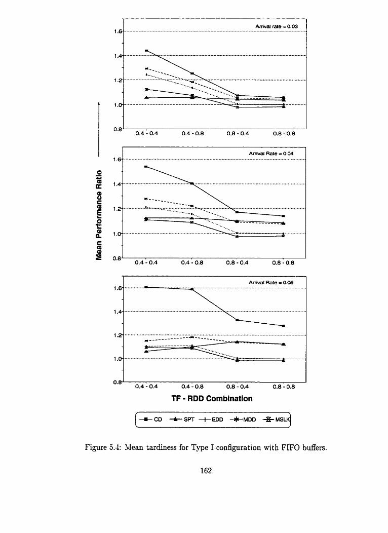
Amval Rate = 0.04 ...--*--.--*--*.-**.**-------------.----..---..-----~..--..-.-------.---.-.--..-.---..--.-------.-*---.---...----------

Amval Rate = 0.05 1 &,.-..*.*.-..* ..---***.-...--.---..----*-..--...---.------.--------.-.---.--------...---------.-*..

TF - RDD Combination

Figure 5.4: Mean tardiness for Type I configuration with FIFO buffers.

1 .O8 Amval rate = 0.03

o. 0.4 - 0.4 0.4 - 0.8 0.8 - 0.4 0.8 - 0.8

TF - RDD Combination

+ CD + SPT +€DO -*-MD0 MS

Figure 5.5: Mean tardiness for T-ype II configuration with FIFO buffers.

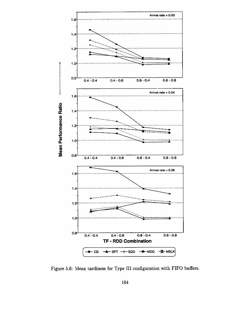
TF - RDD Combination

/ + CD + SPT -+ EDO -4-MDD MSW]

Figure 5.6: Mean tardiness for Tvpe III configuration Nith FIFO buffers.

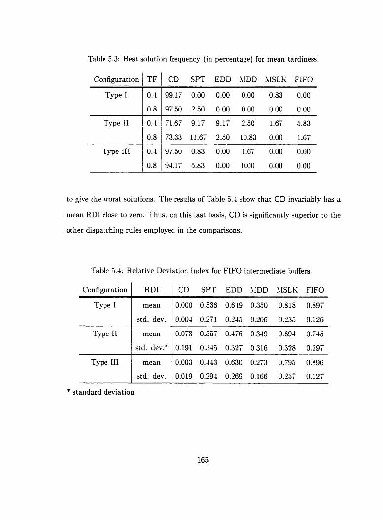
Table 5.3: Best solution frequency (in perceotage) for mean tardiness.

Configuration 1 TF

Type 1 l CD SPT EDD MDD MSLK FIFO

to givc the worst solutions. The results of Table 5.4 show t tiat CD invariablu has a

mean RDI close to zero. Thus. on this last basis. CD is significantly superior to the

otlier dispatching riiles employed in the comparisons.

Table 5.4: Relative Deviation Index for FIFO intermeciiate buffers.

Configuration RD1

Type I mean

std. dev.

Type II

/ std. der..

Type III mean

std. dev.

CD SPT EDD M I D NSLK FIFO

* standard deviation

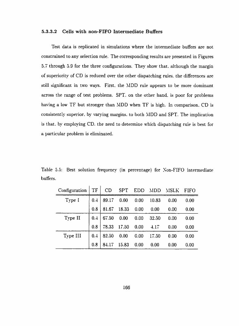
5.3.3.2 Cells wit h non-FIFO Intermediate Buffers

Test data is replicated in simulations where the intermediate buffers are not

const rained to any select ion rule. The correspotiding results are presented in Figures

5.7 through 5.9 for the three configurations. They show that, although the margin

oi superiority of CD is reduced over the other dispatching rules. the differences are

still significant in two ways. First. the hIDD rule appears to be niore dominant

across the range of test problems. SPT. on the other hand. is poor for problems

having a low TF but stronger than SIDD when TF is high. In cornparison. CD is

consistently superior. by varying niargins. to both h1DD and SPT. The implication

is that. by eniploying CD. the need to cletermine nhich dispatcliing rule is best for

a part icular problem is eliminatecl.

Table 5.5: Best solut ion frequency

buffers.

Configuration 1 TF 1 CD

(in percentage) for Non-FIFO interniediate

SPT EDD 1,lDD .ClSLK FIFO

Type 1

Type II

0.4

Type III

89.11 0.00 0.00 10.53 0.00 0.00

0.4

0.8

61.50 0.00 0.00 32.30 0.00 0.00

78.33 17.50 0.00 4.11 0.00 0.00

0.4

0.8

82.50 0.00 0.00 17.50 0.00 0.00

84.11 15.83 0.00 0.00 0.00 0.00

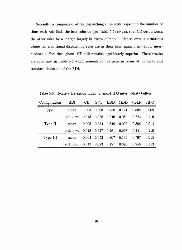
Secondly. a cornparison of the dispatching rules with respect to the number of

times each mle finds the best solution (see Table 5.5) reveals that CD outperfornis

the other rules by a rnargin Iargely in excess of 2 to 1. Hence. even in situations

where the traditional dispatching rules are at their best. narnely non-FIFO inter-

mediate buffers t hroughou t . CD st il1 rernains significantly superior. These results

hre cüiiSrmec! in Table 3.6 nhich prcsents coniparisûns in tcrins ~f the m a n and

standard cleviation of the RDI.

Table .5.6: Relative Deviation Indes for rion-FIFO intermediate buffers.

1 std. dev. i 0.013 0.328 02-46 0.080 0.223 0.116

CD SPT EDD !bIDD hISLK FIFO

0.003 0.360 C.638 0.141 0.808 0.909

Configuration

Type I

RD[

tiiean

Type II

Type III mean 1 std. dev.

mean

std. dev.

0.004 0.352 0.807 0.136 0.797 0.91s

0.013 0.323 0.127 0.090 0.256 0.113

0.005 0.354 0.649 0.091 0.806 0.9L4

0.013 0.327 0.161 0.068 0.244 0.110

Arrivai rate = 0.04

0.6 ' , F

0.4 - 0.4 0.4 - 0.8 0.8 - 0.4 0.8 - 0.8

TF - RDD Combination

Figure 5.7: Mean tardiness for Type 1 configuration with non-FIFO buffers.

Amvai rate = 0.03

Arrival rate = O 04

2.0 Arrivai rate = 0.05

0.8 l 5

0.4 - 0-4 0.4 - 0.8 0.8 - 0.4 0.8 - 0.8

TF - RDD Combination

+ CD + SPT 4 E D D -*-MD0 * MS

Figure 5.8: Mean tardiness for T-ype II configuration with non-FIFO buffers.

169

2 0 Arrivai rate = 0.03

0.4 - 0.4 0-4 - 0.8 0.8 - 0.4 0.8 - 0.8

TF - RDD Combination

Figure 5.9: SIean tardiness for Type III configuratioo with non-FIFO buffers.

5.4 Conclusion

The evaluation of CD under conditions of dynamic job a r r i d s has demonstrated

that CD has flexibility with respect to the following factors.

Satisfaction of different performance criteria.

CD perforrns better than the most obvious 'quick and dirty' rules that cm be used

for the performance criteria tested.

Adaptabi l i ty to different configurations.

In al1 three configurations. CD is generally superior for the different criteria inves-

tigated. The overall performance of CD is also observed to be less sensitive to the

configuration than the other dispatching rules testeci.

Buffer Constraints .

The two extremes of a cc11 having either al1 FIFO or al1 non-FIFO interniediate

buffers are investigated. CD excels in both estremes. It is therefore highly proba-

ble that CD is also superior in configurations shere only a selected number of the

intermediate buffers are const rained to FIFO select ions. This makes CD attractive

in cells whose hardware constraints necessitate the combining of buffers that allow

part overtaking with those that do not.

Finail- it may be conchded that the advantages of CD that were identified r h e n

it mas tested with static problems are also appxent in the dynamic shop scenarios.

Thus, CD provides a combination of the algorithmic power of static heuristics mith

the high flexibility that is observed in on-line dispatching rules.

Chapter 6

Implementation of CD in an Existing FMC

6.1 Introduction

.A scheduling and control systern that is based on CD. and its iniplenientation

on a real FSIC. is preserired in this chapter. Chapter 1 described a FLIC that is

located ici the Autoniation Laboratop at the Cniversity of Slanitoba. This FSIC is

the siibject of a physical implenicntation of CD. The niain purpose of this actual.

real-morld application of CD is to demonstrate its feasibility arid to identify prob-

lems. hardware or othenvise. that can be a major impedinient in its use in industrial

set tings.

6.2 A CD-based Scheduling and Control System

CD's requirement for real-time machine status information is met through the

employment of 'agents'. These agents are independent programs that have specific

functions. They can communicate with each other as ive11 as with the main con-

trol program residing in one of the persoual cornputers. Agents may be classified

as 'intelligent' or 'informative'. The agents utilized in the implementation of CD

are strict ly informative. serving to facilitate a heterarchical relationship between

machines. Their prirnary tasks are to monitor specific activities. and to respond

with the appropriate information when interrogated by the main program that is

controlling the CD process.

6.2.1 Informative Agents.

Informative agents are created at the start-up of the FlIC control prograni (Le.

the niain program). Each machine is provided with the followirig three agents.

1. Downloading agent.

2. Monitoring agent.

The functions of each agent are describeci next.

0 The Downloading Agent.

This agent receives jobs as they arrive at a machine and it retrieves the corre-

sponding CSC part progranis. It supervises the successful dotvnloading of the

part program. and informs the Monitoring agent once the machine is ready to

start operations. Cpon completion of the operations. the Downloading agent

consults the Buffer agent of the machine to which the completed part is to

be unioaded. Depending on the response. the Downloading agent authorbes

the unloading or it waits until a clearance is received from the next machine's

Buffer agent.

a The Monitoring Agent.

The Slonitoring agent's main task is to monitor the processing operations on

a job. It responds to queries regarding the anticipated time rernaining until

cornpletion of the current operation on the machine. and it notifies the down-

loading agent upon successful completion of the current job. The Monitoring

ageiiL albu cuiiiparn tlie actual aiid esprctetl prwsssiiig iiiiiaa fur jûb. If

niiiior deviations are observed. the agent updates its database to reflect the

actual processing tirne for that particular job. Thus. this agent is able to detect

trends in a machine's capabilities. Ntliough iiot considcred in this researcli.

such information may be iised. say. in a tool wear analusis.

O Ttie Buffer Agent.

The Buffer agent's function is purcly organizational. It tracks the jobs in the

buffer. biocks the reception of new jobs if the buffer is fillecl to capacity. and

it collects data for the calculation of instaritarieoiis and ot-erall WIP levels.

6.2.2 The Main Program

The main program mns the CD algorithm axid dispatches jobs. It conimuni-

cates witli al1 the different agents of the machines. The main program is nornially

in a 'wait' mode. awaiting requests. When a machine is free. its downloading agent

sends a message to the main prograni. requesting to be loaded with a new job. Cpon

receiving this message. the main program identifies al1 the jobs that are available

for selection and it initiates the CD algorithm. -111 the Monitoring agents are con-

tacted with requests for the remaining tirnes of the jobs currentlp being proressed.

The main program also obtains the number and Fpes of jobs waiting at each buffer

from the corresponding Buffer agent. Al1 this information is used subsequently to

determine the machines' ready times, which is needed by the CD algorithm. When

a job is selected by the CD. the main program replies to the machine that sent the

initial request. giving the identity of the job that will be processed next.

Figure 6.1 illustrates the Lines of communication between the different agents and

machines. as w l l as between the programmable logic controller (PLC) and material

haridling systern for the FSIC. The operating systern that is used is UNS 4.0 [76].

The QXS 4.0 operating systern provides an environment that is highly suitablc for

niulti-tasking and networked conimunications between progranis runnirig on cliffer-

erit cornputers and coritrolling different equipnient in the FSIC.

6.3 Experimental Trials

The awilability of an actual FSIC allows the testing of CD iinder 'real-world'

conditions. The robotic handling systern found in t his Fl IC is a shared resource so

that jobs often have to wait for service. Conseqcentl. a job's waiting time as well

as the travel times between the different machines are factors affecting the sched-

ule. The airn of the esperiments is to investigate how well CD performs in tliis

kind of situation. considering t hat the previous computer simulations had assumed

these travel times to be negligible. Actual travel time includes travel-empty and

travel-loaded times. as well as the pick-up and dropoff times. In the FLIC under

consideration. the total travel time expended in sen-icing a part t r a d e r averages

between 10 and 12 seconds, depending on the distance between the origin and des-

tination of the travel.

Figure 6.1: Schematic of the control system for the FMC.

6.3.1 Procedure

The FMC contains four machines. The first machine is a TERCO. two and one-

half axis mill. The second is âlso a mill, an EMCO two aiid one-hdf axis machine.

Part progranis are downioaded to these machines from a PC. The downloading time

depends on the cornplexity of the operatiolis on the part. but usuallp ranges between

25 and 30% of the part's processing time. This relatively higli downloading time is

due to the old technology used in these aged (1980's) but available niachines. The

retnairiing two triachines are locally constructed gadgets tliat arc designecl to siniu-

lace a paint booth and an inspection machine. They go through the motions of the

sirnulateci activities. bii t no processing act ually occurs. Ttie FLIC lias part buffers

to load the TERCO and the EhICO mills. Ttre absecicc of interr~iediate buffers to

liold the LVIP means that machine blockage and starvation is a major factor in the

performance of this FAIC.

Nine parts are manufactureci in the experinients. 111 the parts have the same

route. namely Machine 1 (TERCO) to !dachine 3 and then to Machine 4. Ttie

inclusion of al1 four machines in the experirnents \va5 not possible due to limitations

on the available input-output cards used in the PCs. The nine parts are listed

in Table 6.1 together with the processing tirnes (in seconds). A given processing

time includes only the duration that a machine is physically processing a part.

Downloading t imes are independent of the processing t imes.

Table 6.1: Processing tirnes (in seconds) for parts manufactured in the FLIC.

Part TERCO EMCO PAIXT ISSPECT

(411) (hl-) (413) (bI4)

6.3.2 Experimental Data

Each test set involves jobs t hat are selected ranclorrily h m the nine parts listed

in Table 6.1. Five different sets are created and processed in the FSIC. Test set

#1 contains one of each part for a total of nine jobs. In each of the remaining four

sets. four of the parts shown in Table 6.1. are selected randomly Three of these

parts. which are also picked randomly, have a demand of three units each. and the

remaining part has a demand of tmo units to give a total of eleven jobs in each set.

The part types and demanded quantities in each of the last four test sets are given

in section 1 of Appendk B.

The performance cnterion selected in these experirnents is the minimum mean

flowtime. The test sets are fed to the FMC in the form of bills-of-materials (B.O.M.)

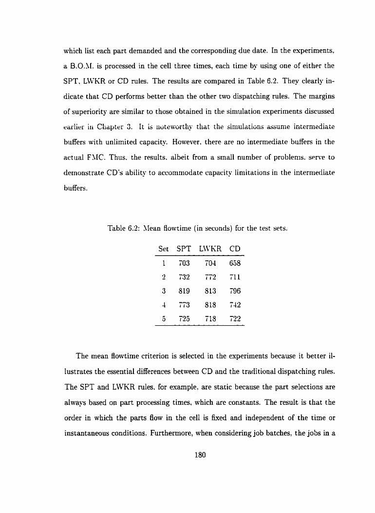
which Iist each part demanded and the corresponding due date. In the experiments.

a B.O.!d. is processed in the ce11 three times, each time by using one of either the

SPT, LWKR or CD rules. The results are compared in Table 6.2. They clearly in-

dicate that CD performs better than the other two dispatching rules. The margins

of superioritg are similar to those obtained in the siniulation experiments discussed

rarlirr ii i Cliaptcr 3. It is u i i i a w u r i ~ ihai the siniulaiiûnii a u n i e intermediate

buffers with unlimited capacity. However. there are no interniediate buffers in the

actual FSIC. Thus. the results. albeit from a srnall nuniber of problenis. wrve to

cleinorist rate CD's ability to acconiniodate capacity liniitat ions iu the interrriecliate

biiffers.

Table 6.2: Mean Rowtime (in seconcls) for the test sets.

Set SPT LWKR CD

2 132 772 Ill

The mean flowtime criterion is selected in the experiments becawe it bet ter il-

Iust rates the essent ial differences between CD and the t raditional dispatching rules.

The SPT and LWKR rules. for example. are static because the part selections are

always based on part processing times. which are constants. The result is that the

order in which the parts flow in the ce11 is fked and independent of the time or

instantaneous conditions. Furthermore, when considering job batches: the jobs in a

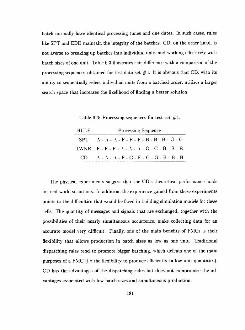
batch oormally have identical processing times aod due dates. In such cases. rules

like SPT and EDD maintain the integrity of the batches. CD. on the other hand. is

not averse to breaking up batcfies into individuai units and working effectively with

batch sizes of one unit. Table 6.3 illustrates this difference with a cornparison of the

processing sequences obtained for test data set #4. I t is obvious tiiat CD. with its

abiii- LU sequeiitiaiiy seiect i d i v i d u a i urii ts Iruiii a LatcLecl urcler. u ~ i 1 i ~ t . s a iargrr

search space that increases the likelihood of finding a better solution.

Table 6.3: Processing sequences for test set #4.

RCLE Processing Sequerice

SPT - 4 - . A - - 4 - F - F - F - 1 3 - B - B - G - G

LLVKR F - F - F - - 4 - - 4 - . A - G - G - B - B - B

CD . A - - 4 - - 4 - F - G - F - G - G - B - B - B

The physical experinients siiggest t hat the CD's t lieoret ical perforniance holds

for real-world situations. In addition. the erperience gained from t tiese experiments

points to the difficulties t hat would be faced in building simulation models for these

cells. The quantity of messages and signals that are esclianged. together with the

possibilities of their nearly simultaneous occurrence. make collecting data for an

accurate rnodel very difficuit. Finallq: one of the main benefits of FJiCs is their

flexibiiity that allows production in batch sizes as low as one unit. Traditional

dispatching rules tend to promote bigger batching, which defeats one of the main

purposes of a FMC (i.e the flexibility to produce efficiently in low unit quantities).

CD has the advantages of the dispatching d e s but does not compromise the a 6

vantages associated wit h low bat ch sizes and simultaneous production.

6.4 Conclusions

The implementation of CD in a real FLIC is realized by means of a computer-

ized network over which individual programs can comniunicate wirh eacii d e r anci

share information in order to collectively nieet the scheduling objectives.

A iiiiniber of experinients designed to test CD's perforrriance in real-norld situ-

ations were dotie. In tïiese esperinients. CD's calculations were based on real-time

job conipletion and in-process tirne data. The travel cimes between the niachines.

though real. were nonetheless assunied negligible in CD's calculatioris. Cnlike the

siniulations. iiowever. the effect of tliese rravel tinies is conveyed to the CD algorithni

indirectly through the actual cornpletion times. A more accurate irnplementation

nould use an estiniate of the anticipated travel time in CD's çalculation of the ma-

chine ready tinies (Rk). This modification is likely to boost the CD's performance.

The travel tinie est imates between different destinations can be obtainetl straight-

fomardly bu maintaining a record of actual travel times durhg the operations of

the FLIC.

A major advantage of the rnodular scheduling control architecture described in

this chapter is the ease with which system reconfiguration can be adopted. New

machines may be integrated into the scheduler simply by creating new agents and

opening the lines of communication between these and the existing agents. Like-

wise: a machine may be taken out of the .stem merel. by disengaging its agents.

Finally. the ease with which historicd data can be collected, processed and then

used to modify scheduling procedures gives the CD-based scheduling and control

system described in this chapter potential for further Rexibility and adaptability in

real-world applications.

Chapter 7

Conclusions and Recommendat ions

Orie impediment to realizing efficient and autornated scheduling in FLICS is the

inflexibility of scheduling algorithms ['JI. Scheduiing systerns are usually selected

bearing in mind the characteristics of the FhIC under consideration. -1 nioclifi-

cation or update of the initial schedules norniallp requires nianual intervention.

On-line scheduling utilizing dispatching rules permits greater flcsibility froiri niodu-

larization. but there still reniains the problem of deciding which rule to use at each

niachine.

CD is a hybrid algorithm-dispatching rule that is designed to permit a niore

generic approach to scheduling in FLICS. Its algorithniic nature allows the quick

compiitation of 'good' solutions by rcducirig the coniplexity of a probleni to a se-

ries of single machine problelns. When perforniarice criteria are unique so that no

method is known to be 'best' for the single machine probleni. a neural network can

be trained to leam a relationship to determine the job sequences. The dispatching

component. on the other hand. imparts flexibility to the algorithm through niodu-

larization and localization of the scheduling decisions. Therefore. CD is designed to

be generally effective for different scheduling criteria. as well as for different hard-

ware setups or configurations, and for operations under highly dynamic conditions

involving the need to constantly update schedules.

The CD approach was introduced in this thesis and its formulation was pre-

sented. Its performarice was evaluated by rneans of a series of simulations and tests

using randornly generated data. These tests covered three different perforr~iance

criteria; t hc minimum mean flowt ime, the minimum mean tardiness. and the min-

imum nurnber of tardy jobs. The performance of CD was also investigated under

cuiidiiiui~s aktrviiig fur part ui-ertiiliug {Le. ii~ii-FIFO prucrsaiiig iii tlie iiiteriiir

diate buffers). The evaluation of CD was niade througti coniparisoiis with existing

dispatching rules t h are identified in the literature to be the niost appropriate for

each of the scheduling criteria and configurations erarnined.

Several important conclusions were reaclied froni the particular test evduations

and froni observations about CD's general performance. CD is a scheduling systcin

t liat c m be iniplenierited in a non-hierarcliically controlled cell. .As sucli. i t iniproves

the possibility for greiiter scheduling fiexibility Although the sanie can be said for

t radit ional dispatching rules. CD possesses the following adrantages over t hese rules.

based oii the results from the problems tested.

First . CD generally performs bet ter t han tradi t ional dispatching rules in sat is-

fying the given performance criterion. Second, CD eliniinates the need to decide

which dispatching rule to use and ahen it is to be usecl. CD is a self-contained

rule t hat adapts to the exist ing scheduling criteria and instantaneous conditions.

Third. CD is the least sensitive of the scheduling rnethods and rules exarnined for

the different types of configurations considered. Fourth. CD is able to adjust well

to cells that have one or more intermediate buffers restricted to a FIFO policy for

processing the jobs waiting in a queue. In cornparison? traditional dispatching rules

are sensitive to the ability of intermediate buffers to select h m the queue. More-

over. their performance deteriorates rapidly as more of these buffen are restricted

to FIFO. Consequently? CD represents a step in the direction of a more 'generic'

dispatching rule, one that is less sensitive to hardware configurations and machine

setup or layout details. In addition, CD is observed to perform equally well in dy-

namic cw d l as ~t i i i ic ~ i i ü i l i i ~ i l ~ .

In conclusion. CD adequately addresses the issue of the in flexi bility of algorit linis

raised in [2] by conibining the power of algorit hniic solutions wit h the utility and

flesibility of the dispatching rule approach. T h e resiilt is a scheduling systern that

rneets the challenge of operating in a highly autornated environnierit ttiat is subject

to variations and uncertainties in the scheduling demands placed on it. Fiirtherriiore.

CD is wll-suited to application in a non-hierarchical framenork. the resulting ben-

efits of ahich are self-configuration. good adaptability to operatiorial variations and

hardware constraints. as well as simplified control software.

7.1 Recommendat ions

Experiences from the present work allow several recomniendations and sugges-

tions to be made concerning possible directions of future research. The reconinienda-

tions are categorized into those that involve artificial neural networks in scheduling

and tliose that pertain to CD and its concepts.

7.1.1 Artificial Neural Networks

The artificial neural network was used for single machine problenis. There are

two areas mhere further research could be useful,

The first recommendat ion is an application-oriented one. In many indust rial and

service applications. sequencing decisions are made by tiurnan operators on a rule-

of-thunib bais . The decision process is vague and not defiued clearly. The neural

networks proposecl in Chapter 4 miq be used to learn the decision making function.

The? can be trained on-lirie by collecting data and documenting the operator's de-

cisions. Once trained. it would be interesting to see hon w l l a neural network van

actually replace the operator.

The second reconiriiendation involves using a neural rietwork as a preprocessor to

derive starting solutions for further processing by means of siniulated arinealing. An

initial solution generated by a neural rietwork is subjected to siniulated annealirig.

the purpose of which is to arrive a t a sequence of jobs ttiat better satisfies the @en

performance criterion. The research's objective would be to cleterrriine how much

faster simulated annealing is able to find a solution within a given percentage of the

optimal when its starting sequence (the seed) is supplied by a neural network simi-

lar to that described in Chapter 4. rather than by other commonl- employed means.

7.1.2 Cooperative Dispatching

The results from CD are encouraging but further work is needed in its application

in red-morld situations. The foUowing recommendations are suggested a i t h this

187

objective in mind.

1. The açsumption of unlimited buffer sizes \vas maintained throughout this re-

search. This assumption is often unredistic because FLICS usually have a

finite buffer that has a very limited size. CD needs no modification to enable

i t in p r n v ~ s raws involving finite hiifFer 4 7 ~ s . In pr;l<*tir~. if ii hiiflw is f i i l l .

the preceding station would be 'machine-blocked' and it w u i d not be calling

the dispatching algorithm. There is no reasori to expect that CD would be

any less effective in cells having buffers of finite size. Therefore. it is sug-

gestecl to further test and evaluate. by means of simulation espeririients. the

performance of CD for finite buffer sizes.

2 . The assumption that a machine does not m i t for any job that is not already

in its buffer eliniinates niari- scheduliiig alterriat ives. CD cari be iiiodified to

run without this 'no inserted idlc tirne' constraint. This rclaation is one that

should be considered for further research.

3. The number of routing possibilities (configurations) considered is srnall. Fur-

tlier research with CD is needed in Rowshops having a greater nurnber of

routing patterns. A possibility is the investigatiori of CD in a FAIS that is

composed of individual cells of the t h e e types showri in Figure 3.1.

4. The extension of CD to job shops is ivorth considering. -4 drawback is the

fact that traditional dispatching rules excel as a shop's routing configurations

approach that of a job shop. Nevertheless. CD rnay yet exhibit strength in

this ares? particularly if there are restrictions on the sequence of processing

job queues at the intermediate buffers.

5 . Finally, there is still room to improve the quality of the CD solutions beyond

that achieved in this research. Specifically. studies ni- lead to improved meth-

ods for estimating the sequence costs, SCb: discussed in Chapter 3. Also, the

assignnient of the weight. 1.h. to each machine. k, in the cooperative selection

routine can be investigated further with a view to using neural networks to

learn whac weigiit to ÿssign to eacii rnaciiirie urider certain cutiditioiis.

Duffie. X. A. and Piper. R. S., 1986. Nonhierarchical control of manufacturing

systerns. Technical Note. Jovrnal of hlanujacturing Systerns. vol. 5 . no. 2. pp.

137-139.

Dudek. R. A.. Panwalkar, S. S. and Smith. 41. L.. 1991. The lessons of flowshop

scheduling research. Operations Research. vol. -40. no. 1. pp. 7-13.

Stecke. K. E.. 1986. A hierarchical approach to solre niachine grouping ancl

loading pro blems of flexible manufact uring systenis. Europeun JO u r n d o j Op-

erutiond Research. vol. 24. no. 3. pp. 369-378.

Maimon. O. 2.. 1986. Real-tinie operat ional control of flexible rnanufacturing

systerns. Journal of ihnufactcr~ng Systenis. vol. 6. no. 2. pp. 221-231.

Dufbe. 5. A. and Prabhu. \'. V.. 1994. Real-tinie distributed scheduling of het-

erarchical nianufac t uring systerns. Jolinial of Manujact uring Systerns. vol. 13.

no. 2. pp. 94-107.

Shaw. SI. J.. 1988. Dynamic sclieduling in cellular manufacturing systems: a

frarnework for networked decision making. Journal of iClonujucturing Systems.

vol. 7. no. 2. pp. 221-231.

Shaw. SI. J.. 1988. Knowledge-based scheduling in flexible manufacturing sys

tems: an integrat ion of pat tem-directed inference and heurist ic search. Inter-

national Journal of Production Research. vol. 26. no. 3. pp. 821-844.

Baker. K. R.? 1974. Introduction to Sequencing and Scheduling. J. Wiley Si

Sons, Kew kork.

[9] Conway. R. W.. 'rlaxwell, W. L. and Miller. L. W.. 1967. Theory of Scheduling.

Addison-Wesley, Reading, hl.-\.

[IO] Blackstone, J . H.. Phillips, D. T. and Hogg, G. L.! 1982. A state-of-the-art

survey of dispatching rules for manufacturing job shop operations. Intemutional

Journal of Production Research. vol. 20, no. 1. pp. 27-45.

[ I l ] Haupt. R.. 1989. -4 survey of priority ride-based scheduling. OR Spektnim.

vol. 11. no. 1. pp. 3-16.

[12] Sabiincuoglu. 1. and Hornmertzheim. D. L.. l!XX. Dyriamic dispatching al-

gorit hni for scheduling niactiine and automated guidect vehicles in a Aesi ble

niancifacturing systeni. International Journal of Production Resenrch. vol. 30.

rio. 3. pp. 1033-10'79.

[13] Sabuncuoglu. 1. and Homniertzhcini. D. L.. 1992. Esperiniental investigation of

FSIS niachine and AG\- scheduling rules against the rneaii Row- t ime crit erion.

fritemational Journal O/ Production Research. vol. 30. no. 7. pp. 16174635.

[l-t] Garetti. M.. Pozzetti. A. and Bareggi. .A.. 1990. On-line Ioading and dispatch-

ing in flexible manufact uring syteins. International Journal O/ Production

Research. vol. 28. no. 7, pp. 1971-1292.

[l5] Ro. 1. and Kim: J.. 1990. SIulti-criteria operational control rules in flexible

manufacturing systems (FhISs). International Journal of Production Research.

vol. 28. no. 1. pp. 47-63.

[16] Montazeri. M. and Van Wassenhove. L. 3.: 1990. Analysis of scheduling rules

for an F4IS. International Journal of Production Research. vol. 28. no. 4: pp.

785-802.

[17] Nakamura, N. and Salvendy G., 1988. An experimental study of human

decision-making in cornputer-based scheduling of f l e ~ b l e rnanufacturing sys-

tem. International Journal of Production Research. vol. 26, no. 4. pp. 567-583.

[18] Wu. S. D. and CVysk. R. A.. 1990. An inference structure for the control and

scheduling of nianufact uring systerns. Cornputers & Industrial Engineering.

vol. 18. no. 3. pp. 247-262.

[19] Iiusiak. A. and Chen, 41.. 1988. Expert systerns for planning and schedulirig

nianufacturing systerns. European Jouniul uf Operatiorra1 Reseurch. vol. 34.

no. 2 . pp. 113-130.

[-O] Kathmala. Y. and Allen. W.R.. 1993. Expert systenis and job shop scheduling.

Iriteniational Journul of Operations Cï Production LLIunagenient. vol. 13. no. 2 .

pp. 23-35.

[21] Sakasuka. S. and Yoshida. T.. 1992. Dynamic schecluling systern utilizing nia-

chine learriing as a knowledge acquisition tool. International .Journal of Pro-

duction Research, vol. 30? no. '2. pp. 411-431.

[22] Shaw 11. J.. Park. S. and Raman. 3.. 1992. Intelligent scheduling wit h machine

learning capabilities: the induction of scheduling knowledge. IIE Transactions.

vol. 24. no. 2 : pp. 136-168.

[23] Chiu. C. K. and Yih. Y.: 1995. A learning-based niethodology for dynamic

scheduling in distributed manufacturing systems. International Journal of Pro-

duction Research. vol. 33, no. 11. pp. 3217-3232.

1241 Cho. H. and Wysk. RA., 1993. A robust adaptive scheduler for an intelligent

workstation controller. International Journal of Production Research, vol. 31.

no. 4. pp. 771-789.

[25] Wu. S . D. and Wysk. R. A.. 1988. SIulti-pass espert control system - .A con-

t rol/scheduling architecture for flexible manufact iiring ceils. Journal of Bhrm-

fachring Systems, vol. T 1 no. 2 , pp. 107-1".

(261 Rabelo. L.. Yih, Y.. Jones: A. and Witzall. G.. 1993. Intelligent FUS scheduling

using modular neural networks. Proceedzngs of the 1993 in t en ia t iond confer-

rrrce on neuml netuiorks. vol I I I . San Francisco. California. pp. 12244229.

[Zf] Fahlman. S. and Lebiere. C.. 1990. The cascade-correlat ion learning arclii tec-

ture. Techical report CMC - CS - 90 - 100.

['28] Ishii. N. and Talavage. .J. J.. 1991. h transient-bsed real-tinie scheduling

algorit hm in F M . International .Journal of Production Reseurch. vol. 29. no. 12.

pp. 2501-2520.

(291 Jeong. K.-C. and Kim. Y.-D.. 1998. A real-tinie scheduling niechanisrn for a

flexible manufacturing system: using simulation and dispatching rules. Inter-

national Journal 01 Production Research. vol. 36. no. 9. pp. 2609-2626.

[30] Min. H.-S.. k'ih. Y. and Kim, C.-O.. 1998. A cornpetitive neural network a p

proach to mu1 ti-objective FUS scheduling. International Journal of Production

Research. vol. 36. no. 7, pp. 17-19-1765.

[31] Kohonen. S.. 1984. Self-Organization aod Associative hlernory. Springer-

Verlag, Berlin.

[32] Sim. S. K.? Yeo, K. T. and Lee, W. H., 1994. In expert neural network systeni

for dynamic job shop scheduling. Inten<atzona/ Journal of Production Research.

vol. 32, no. 8, pp. 1759-1'73.

[33] Johnson. S. M.. 1954. Optimal two- and three- stage production sctiedules with

set-up times included. ;Vaval Research Logistics Quarterly, no. 1. pp. 61-68.

[34 Nawaz. .LI.. Enscore. E. E. and Ham. 1.. 1983. -4 heuristic algorithm for the rn-

niachine, n-job Aow-shop scheduling problem. Orneyu. vol. 11. no. 1. pp. 9 1-95.

[35] Park. Y. B.. 1981. A simulation study and aiialysis for evaluatiori of

performance-effect iveness of Rowshop sequcncirig tieurist ics: a sta t ic and a dy-

namic Bowshop model. Master's t hesis. Pennsylvariia S tate Cniversi ty.

[36] Taillard. E.. 1990. Sonie efficient heuristic methods for the How shop sequencing

probleni. Europeun .Journal of Operational Reseurch. vol. 47. no. 1. pp. 63-74.

[ 3 i ] Koulamas. C.. 1996. .-\ new constructive heuristic for the flotvshop schedulirig

problem. European Journal of Operationul Research. vol. 105. no. 1. pp. 66-71.

[38] Gupta. J. S. D.. 1972. Heuristic algorit hms for niultistage flowshop scheduling

problem. AUE Transactions. vol. 4. no. I. pp. 11-15.

[39] Myazaki. S.: Nishiyarna. 9. and Hashimoto. F.. 1978. An adjacent painvise

approach to the mean Bowtime scheduling problern. Journal O/ Operations

Reseurch Society O/ Japan. vol. 21, pp. 287-299.

[do] Rajendrm. C. and Chaudhuri. D.. 1992. .in efficient heuristic approach to the

scheduling of jobs in a flowshop. European Journal of Operational Research.

vol. 61, no. 3. pp. 318-325.

[-II] Ho, J. C., 1995. Flowshop sequencing with mean flowtime objective. European

Journal of Operational Reseurch, vol. 81, no. 3, pp. 571-578.

[42] Woo. H. and Yim, D.' 1998. A heuristic algorithm for mean Aowtime objective

in flowshop scheduling. Computers and Operations Research. vol. 25. no. 3.

pp. 175182.

[431 Gare- LI. R.. Johnson. D. S. and Sethi. R.. 1976. The çomplexity of flowshop

and jobshop scheduling. Math. Opns. Res.. vol. 1. no. '2. pp. l l X % .

4 4 Sen. T.. Dileepan. P. and Gupta. J . 3. D.. 1989. The two-niachine flomstiop

schediiling pro blem wit h total tardiness. Computers und Operutioris Reseurch.

vol. 16. no. 4. pp. 333-340.

[45] Kim. Y. D.. 1993. A new branch and bound algorithni For minimizing mean tar-

diriess in tw-machine Aowshops. Concputers and Opemtioris Research. vol. 20.

no. 4. pp. 391-401.

[46] Iiirn. Y. D.. 1893. Heuristics for flonshop scheduling problems niinimizing meari

tardiness. J o v n a l of the Operational Research Society. vol. 44. no. 1. pp. 19-28.

[47] Gelders. L. F. and Sambandam. 3.. 1978. Four simple heuristics for scheduliiig a

flowshop. International Journal of Production Research. vol. 16. no. 3. pp. 221-

231.

[4S] Osman. I.H. and Potts. C.N.. 1989. Simulated annealing for permutation Ron--

shop scheduling. Ornega, vol. 17. no. 6. pp. 551-557.

[49] Ogbu. FA. and Smith, D.K.. 1990. The application o f the simulated annealing

algorithm to the solution of the n/m/C,, Bowshop problem. Cornputers and

Operations Research, vol. 17, no. 3, pp. 243-233.

[SOI Widmer, M. and Hertz, A.. 1989. A new heuristic For the flow shop sequencing

problem. Evropean Journal of Ope~ational Reseurch, vol. 41. no. 2. pp. 186-193.

[3l] Potts C. N. and Van LVassenhove' L. Y.. 1991. Single machine tardiness se-

quencilig heuristics. IIE Transactions. vol. 23. cio. 4, pp. 3-16-334.

[52! Rajmrlran. C. and Holt haus, O. , 1999. A c o r n p a r ~ t i v ~ ctiirly o f rlispatching

rules in dynamic flowshops and jobshops. Eurupean .lownal o/ Operutional

Reseclrch. vol. 116. no. 1. pp. 156-170.

(531 Holthaus. 0. and Rajendran. C.. 1997. Efficient dispatching rules for scheduling

in a job shop. Inteniationul Journal of Production Econornics. vol. 48. no. 1.

pp. 81-105.

(541 Chari. D. Y. and Bedwort h. D. D.. 1990. Design of a scheduling system for fl~s-

ible maniifacturing cells. Internutiorial .Journal of Production Research. vol. 28.

no. 1 1. pp. 2037-2049.

[55] Du. -1. and Leung, J.Y.T. 1990. Minirnizing total tardiness on one niachine is

SP-tiard. Math. Opns. Res. vol. 13. no. 3. pp. 483-495.

[56] Holseriback. J . E. and Russell. R. JI.. 1992. .A heuristic algorithm for sequencing

on one machine to mininiize total tardiness. Journal of the Operationul Research

Society. vol. 43, no. 1. pp. 53-62.

[si] Emmons. H.. 1969. One machine sequencing to rninirnize certain functions of

job tardiness. Operations Research. vol. 17. no. 4. pp. 701-715.

[58] Panwalker. S. S., Smith, SI. L. and Koulamas, C. P.? 1993. -1 heuristic for the

single machine tardiness problem. European Journal of Operational Research,

vol. 70, no. 3: pp. 304310.

[59] Wilkerson, L. J . and Invin, J. D., 1971. An improved algorithm for scheduling

independent tasks. A IIE Trunsactions, vol. 3. pp. 339-243.

[60] Yan LVassenhove, L. Y. and Gelders. L. F.. 1980. Solving a bicriterion scheduling

problem. European Journal of Operational Research, vol. JI no. 1: pp. 42-48.

b 1611 , Lin. K. S.. 1983. Hyhrid algorithm For s q i i ~ n r i n g with hirrit~ria. .loiirnnl

Optirniration Theory und Applicatioris. vol. 30. no. 1. pp. 103-124.

[62] Ctien. C-L. and Bulfin. R. L.. 1994. Scheduiing a single machine to niininiize

two criteria: mavimum tardiriess and number of tard- jobs. IIE Trarisactioris.

vol. 26. no. 5 . pp. 239-245.

[63] hrrrientano. C'. A. and Roncini. D. P.. 1999. Tabii search for total tarcliriess

minimization in Rowshop scheduling problems. Cornputers und Operations Re-

srurch. vol. 26. no. 3. pp. '219'235.

[64] Lee. C.Y. and Choi. .J. Y.. 1993. A genetic algorithni for job sequericirig prob-

lems with distinct due-dates and general early-tard. penalty weights. Coniput-

ers and Operatioris Research. vol. 2. no. 8. pp. 857-869.

[65] Held. 11. and Karp. R. M.. 1962. .A dynamic prograrnming approach to se-

quencing problerns. J. Soc. Indust. Appl. hlath.. vol. 10. no. l. pp. 196-210.

(661 Das. S. R.. Gupta. J . 3. D. and Khumawala. B. SI.. 1995. -1 savings indes

heurist ic algorit hm for flowshop scheduling wit h sequence dependent set-up

times. Journal of the Operational Research Society. vol. 46. no. 11. pp. 1365-

1373.

[67] Moore. J. M., 1968. -4 n-job, one machine sequencing aigorithm for minimizing

the number of late jobs. Ilfanagement Science, vol. 15. no. 1, pp. 102-109.

[68] Rumelhart? D. E., !vfcClelland, J. L. and the PDP Research Group: 1986. Par-

allel Distributed Processing: Exphrations in the lIicrostructure of Cognition.

vol. 1. MIT Press/Bradford Books. Cambridge. SIA.

[69] Granino. A. K., 1992. Neural Network Experirnents on Personal Cornputers

and Korkstations. The MIT Press, Cambridge, LIA..

[;O] Grossberg, S.. 1976. Adaptive pattern classification and universal recoding:

Part 1. parallel developnient and coding of neural feature detectors. Biological

Cybemetics. vol. 23. pp. 121-134.

[ i l ] Fry. T. D.. Cïckens. L.. 'iIaCleod. K. and Fernandez. S.. 1989. A heiiristic solu-

tion procedure to niinimize f on a single machine. .Jolr~rnal of the Operationul

Research Society. vol. 40. no. 3. pp. 293-297.

[Z] Koulamas. C.. 1994. The total tardiiiess probleni: review and esterisioris. Op-

erations Research. vol. 43. no. 6. pp. 1025-1041.

1731 Russell. R. SI. and Holsenback. J . E.. 1997. Evaluation of leading Iieoristics

for the single machine tardiness problem. European Joumol of Operationul

Research. vol. 96. no. 3. pp. 538-545.

[7J] SIerten. A. G. and Sfuller. .CI. E.. 1972. Variance mininiization in single machine

sequencing problem. Management Science. vol. 18. no. 9. pp. 518-328.

[Z] Turbo C++. 1990. Borland International Inc. Scotts Valley. Ch.

[ i 6 ] Q-iS 4 Operating System. QNX Softwue Systems Ltd. Kanata. Ontario.

Appendix A

Neural Network Data

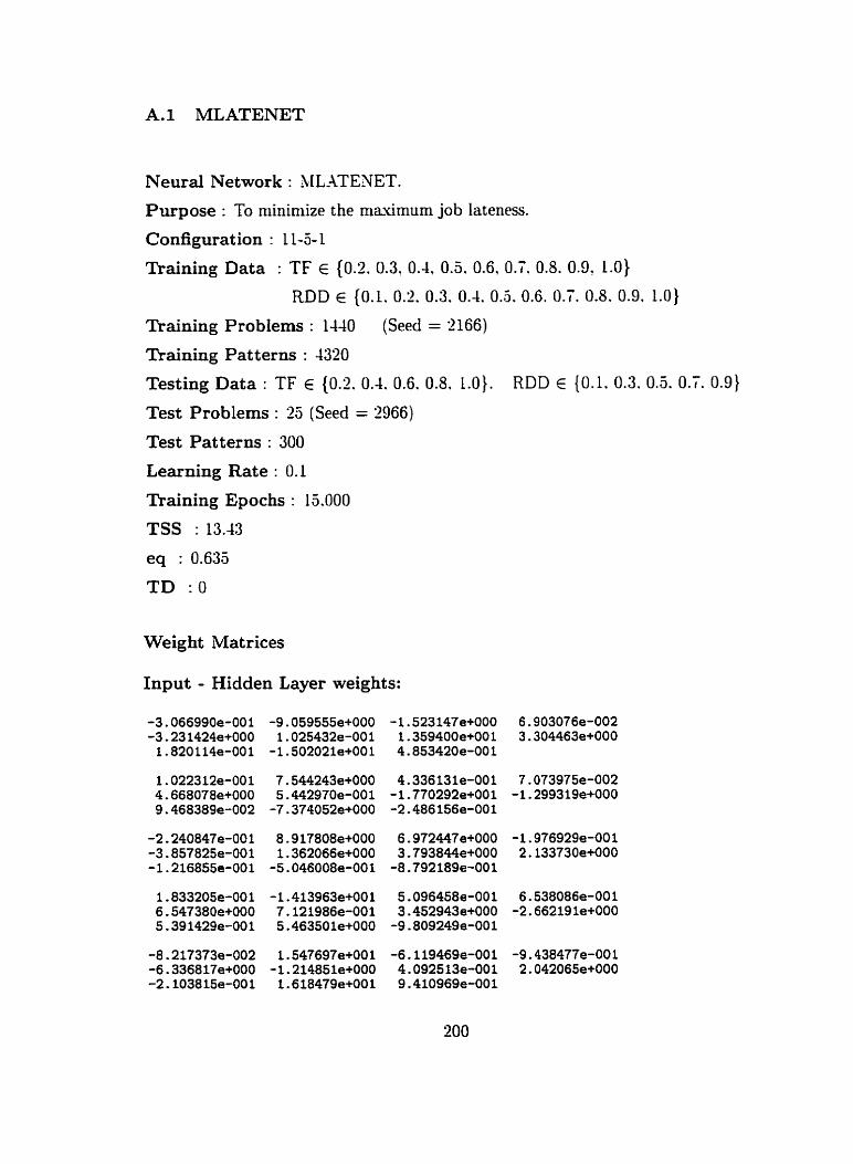
A.l MLATENET

Neural Network : MLATEXET.

Purpose : To niininiize the maximum job lateness.

Configuration : 1 1-5 1

Training Data : TF E (0.2. 0.3. 0.4. 0.3. 0.6. 0.7. 0.8. 0.9. 1.0)

RDD E I0.1. 0.2. 0.3. 0.4. 0.5. 0.6. 0.7. 0.8. 0.9. 1.0}

Training Problems : 1440 (Seed = 2166)

Training Patterns : 4320

Testing Data : TF E (0.2. 0.4. 0.6. 0.8. 1.0). RDD E (0.1. 0.3. 0.5. 0.7. 0.9)

Test Problems : '25 (Seed = 2966)

Test Patterns : 300

Learning Rate : 0.1

Tkaining Epochs : 15.000

TSS : 13.43

Weight Matrices

Input - Hidden Layer weights:

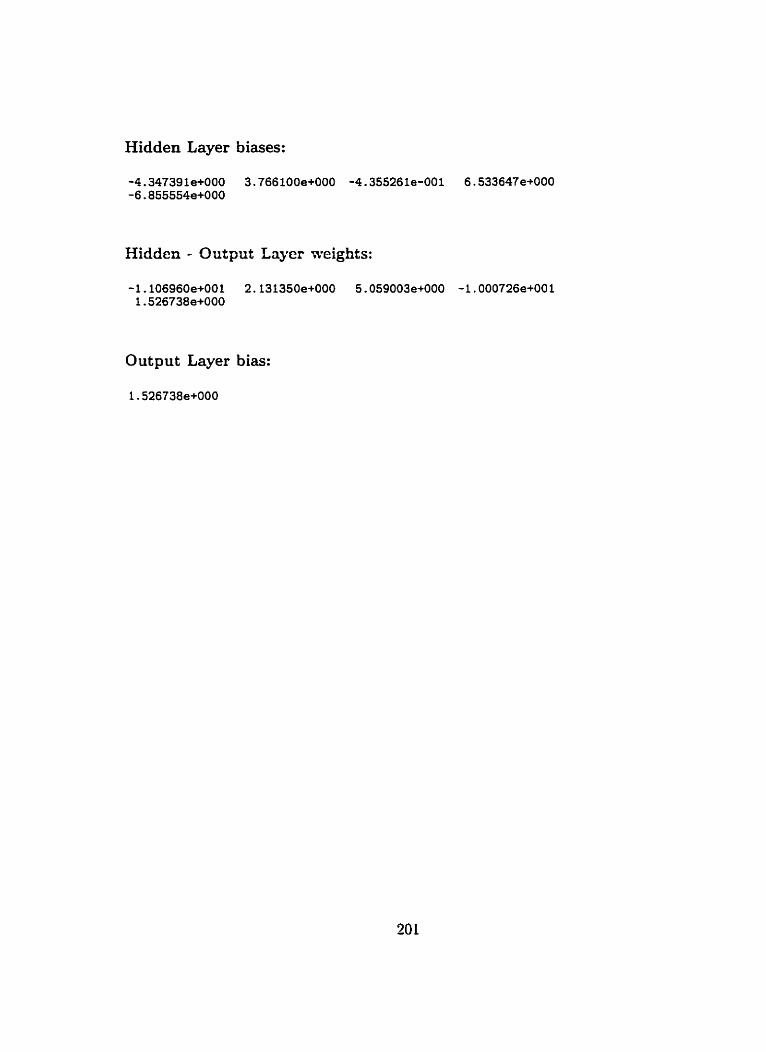
Hidden Layer biases:

Hidden - Output Layer neights:

Output Layer bias:

1.526738e+000

A.2 FLONET

Neural Network : FLONET.

Purpose : To minimize the mean weighted Rowtime

Configuration : 11-9-1

Training Data : TF E (0.2. 0.3. 0.4, 0.5. 0.6. 0.7. O.S. 0.9. 1.0}

RDD E (0.1. 0.2. 0.3, 0.4. 0.5. 0.6. 0.7. O.S. 0.9. 1.0}

Training Problems : 1440 (Seed = 2166)

Training Patterns : 4320

Testing Data : TF E (0.2. 0.4. 0.6. 0.8. 1.0}. RDD E (0.1. 0.3. 0.5. 0.7. 0.9}

Test Problems : 25 (Seed = 3966)

Test Patterns : 300

Learning Rate : 0.1

Training Epochs : 13.000

TSS : 26.29

eq : 0.859

TD 2 6

Weight Matrices

Input - Hidden Layer weights:

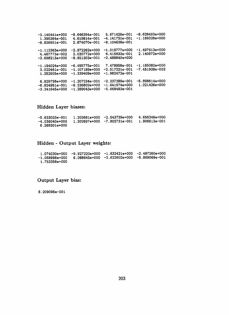
Hidden Layer biases:

Hidden - Output Layer weights:

Output Layer bias:

A.3 MTARNET

Neural Network : MTARNET.

Purpose : To minimize the mean tardiliess.

Configuration : 11-54

Training Data : TF E I0.2. 0.3. 0.4. 0.5. 0.6. 0.7. O.S. 0.9. 1.0}

RDD E {0.1. 0.2. 0.3. 0.4. 0.5: 0.6. 0.7. 0.8. 0.9. 1.0)

Training Problems : 14-40 (Seed = Y 166)

Training Patterns : 4320

Test Problems : 25 (Seed = 2966)

Test Patterns : 300

Learning Rate : 0.1

Training Epochs : 50.000

TSS : S4.35

Weight Matrices

Input - Hidden Layer weights:

Hidden Layer biases:

Hidden - Output Lapr weights:

Output Layer bias:

8.815259e-001

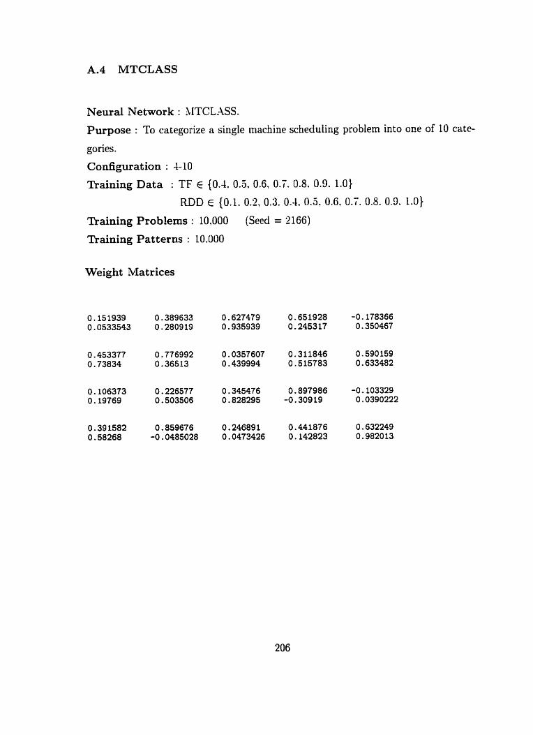
A.4 MTCLASS

Neural Network : MTCLASS.

Purpose : To categorize a single machine scheduling problem into one of 10 cate-

gones.

Configuration : 4-10

Training Data : TF E {0.1. 0.5. 0.6. 0.1. 0.8. 0.9. 1.0)

RDD E (0.1. 0.2, 0.3. 0.4. 0.3, 0.6, 0.7. 0.8. 0.9. 1.0)

Training Problems : 10.000 (Seed = Y 166)

Training Patterns : 10.000

Weight Matrices

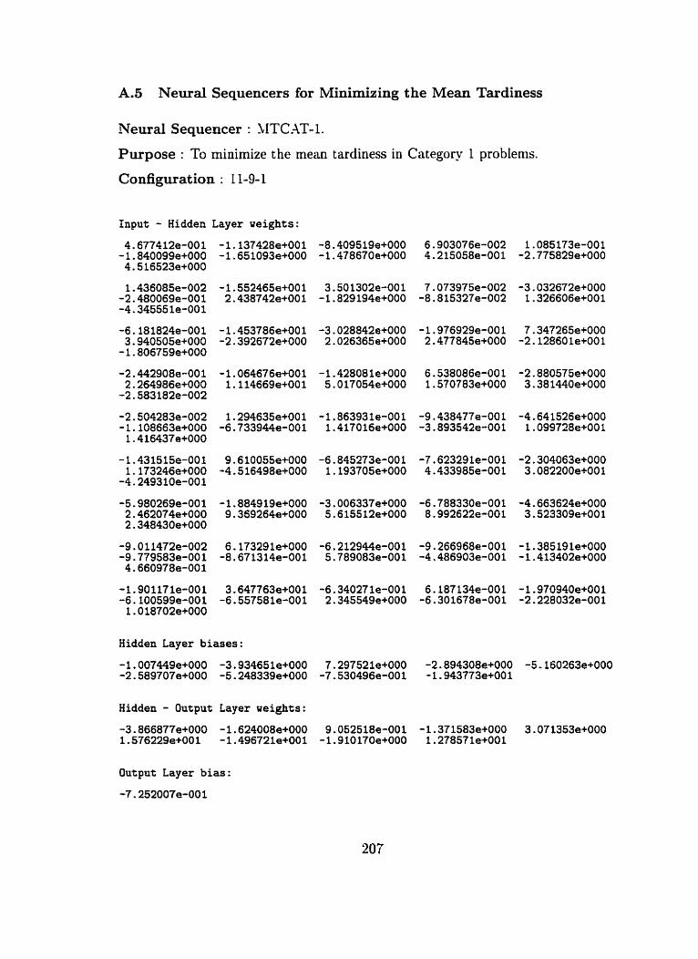
A.5 Neural Sequencers for Minimizing the Mean Tardiness

Neural Sequencer : .LLTCAT-1.

Purpose : To minimize the mean tardiness in Category 1 problems.

Configuration : 1 1-9-1

Input - Hidden Layer ueights:

Hidden Layer biases:

Hidden - Output Layer ueights:

Output Layer bias:

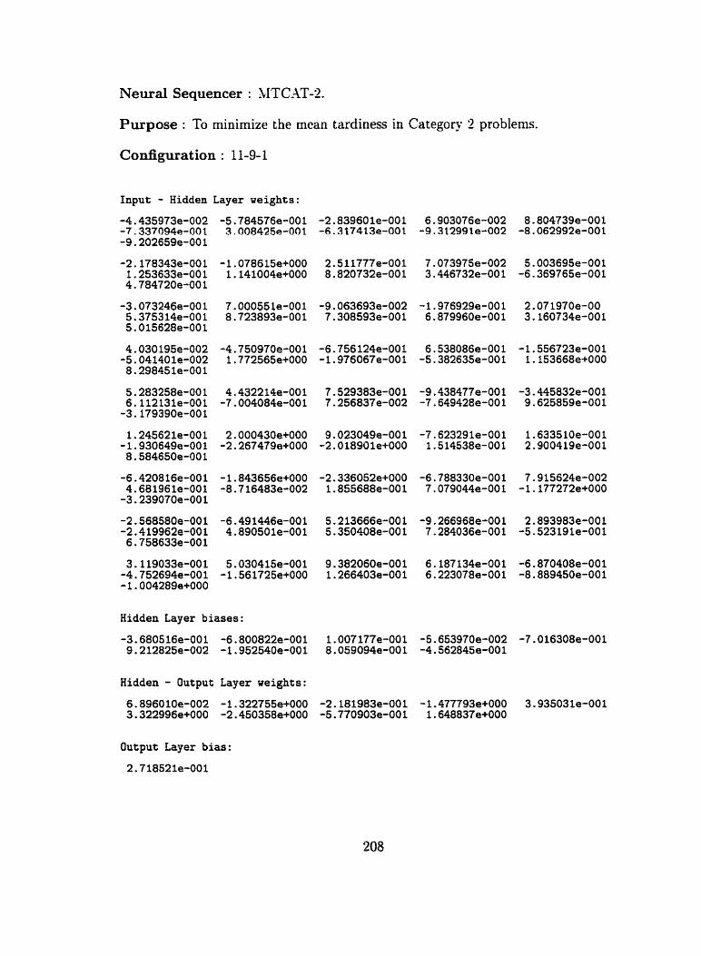
Neural Sequencer : MTCAT-2.

Purpose : To minimize the mean tardiness in Category 2 problems.

Configuration : 11-9-1

Input - Hidden Layer veights:

Hidden Layer biases:

Hidden - Output Layer ueights:

Output Layer bias:

Neural Sequencer : bLTCAT-3.

Purpose : To rninimize the mean tardiness in Category 3 problems.

Configuration : 1 1-9- 1

Input - Hidden Layer weights:

Hidden Layer biases:

Hidden - Output Layer weights:

Output Layer bias:

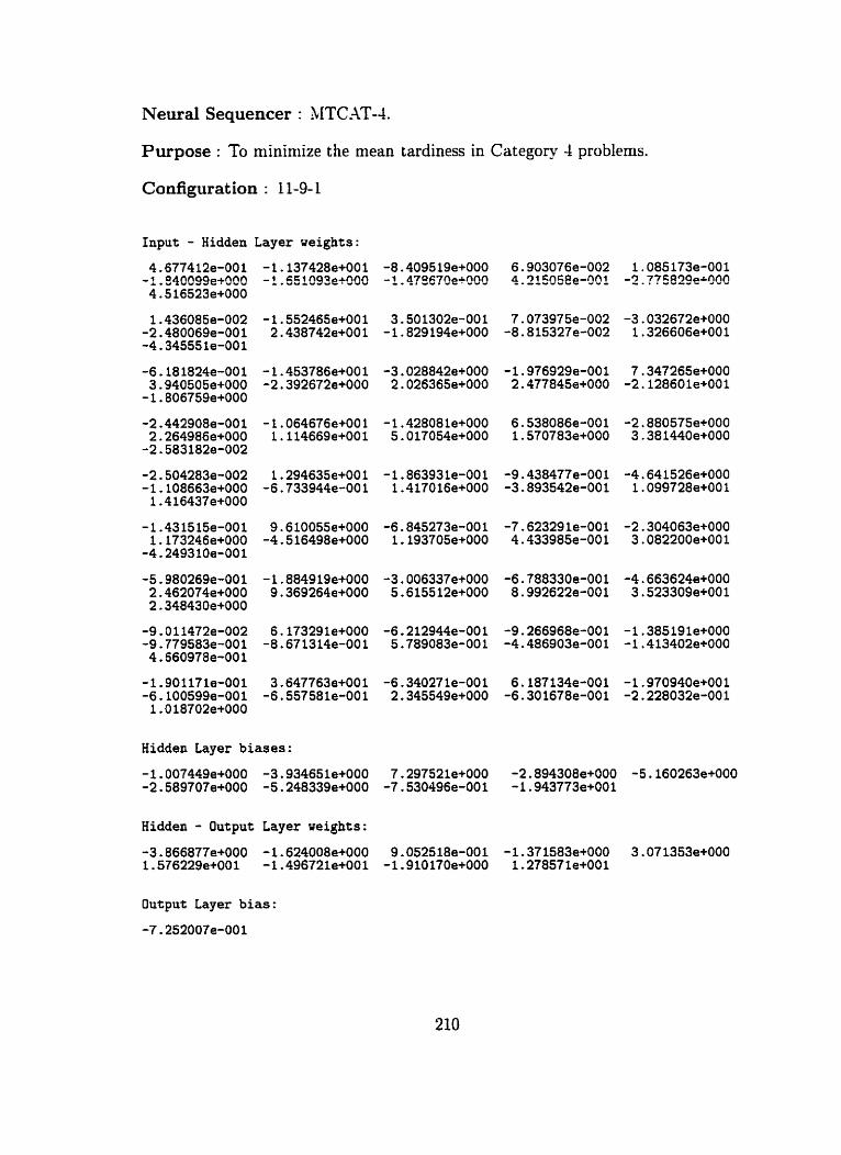
Neural Sequencer : MTCAT-4.

Purpose : To minimize the mean tardiness in Category 4 problems.

Codgurat ion : 1 1-9- 1

Input - Hidden Layer ueights:

Hidden Layer biases:

Hidden - Output Layer weights:

Output Layer bias:

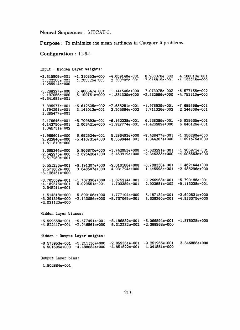
Neural Sequencer : SITCAT-5.

Purpose : To minimize the mean tardiness in Category 5 problems.

Configuration : 1 1-9-1

Input - Hidden Layer weights:

Hidden Layer biases:

Hidden - Output Layer weights:

Output Layer bias:

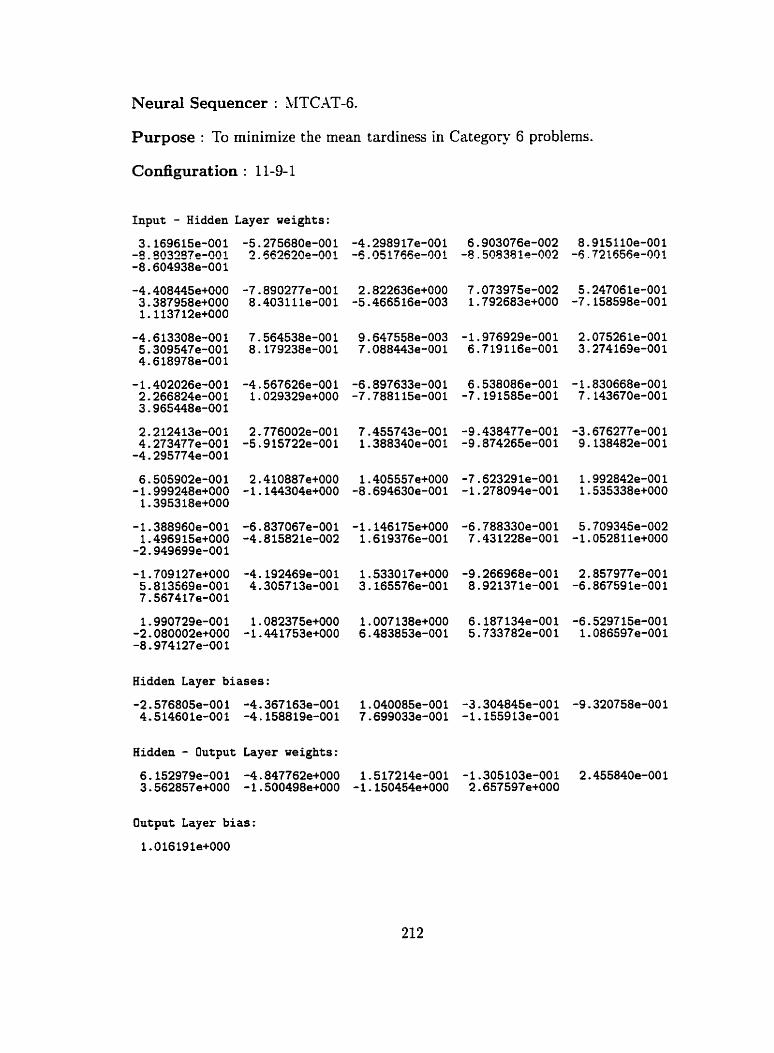
Neural Sequencer : MTCAT-6.

Purpose : To minimize the mean tardiness in Category 6 problems.

Configuration : 1 1-9- 1

Input - Hidden Layer weights:

Hidden Layer biases:

Hidden - Output Layer ueights:

Output Layer bias:

Neural Sequencer : NTCAT-7.

Purpose : To minimize the mean tardiness in Category 7 problems.

Coxdigurat ion : 1 1-9- 1

Input - Hidden Layer ueights:

Hidden Layer biases:

Hidden - Output Layer weights:

Output Layer bias:

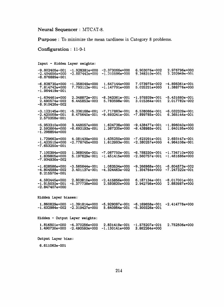
Neural Sequencer : SITCAT-8.

Purpose : To minimize the mean tardiness in Category 8 problems.

Configuration : t 1-9-1

Input - Hidden Layer ueights:

Hidden Layer biases:

Hidden - Output Layer ueights:

Output Layer bias:

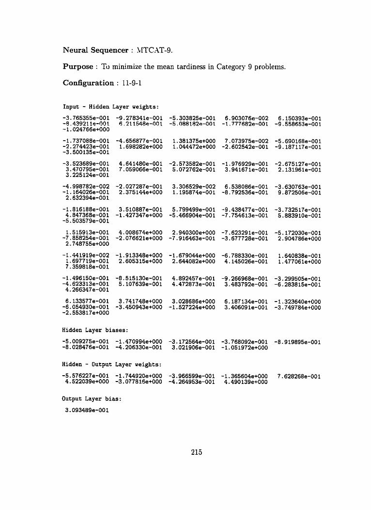
Neural Sequencer : LITCAT-9.

Purpose : To minimize the mean tardiness in Category 9 problems.

Configuration : 11-9-1

Input - Hidden Layer weights:

Hidden Layer biases:

Hidden - Output Layer weights:

Output Layer bias:

Neural Sequencer : MTCAT-10.

Purpose : To minimize the mean tardiriess in Category 10 problems.

Configuration : 1 1-9- 1

Input - Hidden Layer weights:

Hidden Layer biases:

Hidden - Output Layer weights:

Output Layer bias:

Appendix B

Test data for FMC experimental trials

Problem data for the experimental tests of CD on the FMC at the Gniversity of

Manitoba:

Table B.1: Data set '2.

Part 1 Quantity

Table B.2: Data set 3.

Part 1 Quantity

Table B.3: Data set 4.

Table BA: Data set 5.

Part

A

F

C

G

Part 1 Quantity

Quantity

3

3

3

*> -