
Instabilities in magnetized rotational flows: A comprehensive short-wavelength approach
37
arXiv:1401.8276v1 [physics.flu-dyn] 30 Jan 2014 Under consideration for publication in J. Fluid Mech. 1 Instabilities in magnetized rotational flows: A comprehensive short-wavelength approach O.N. KIRILLOV 1 †, F. STEFANI 1 AND Y. FUKUMOTO 2 1 Helmholtz-Zentrum Dresden-Rossendorf, P.O. Box 510119, D-01314 Dresden, Germany 2 Institute of Mathematics for Industry 744 Motooka, Nishi-ku, Fukuoka 819-0395, Japan (Received ?; revised ?; accepted ?. - To be entered by editorial office) We perform a local stability analysis of rotational flows in the presence of a constant vertical magnetic field and an azimuthal magnetic field with a general radial depen- dence characterized by an appropriate magnetic Rossby number. Employing the short- wavelength approximation we develop a unified framework for the investigation of the standard, the helical, and the azimuthal version of the magnetorotational instability, as well as of current-driven kink-type instabilities. Considering the viscous and resistive case, our main focus is on the case of small magnetic Prandtl numbers which applies, e.g., to liquid metal experiments but also to the colder parts of accretion disks. We show in particular that the inductionless versions of MRI that were previously thought to be restricted to comparably steep rotation profiles extend well to the Keplerian case if only the azimuthal field slightly deviates from its field-free profile. Key words: 1. Introduction The interaction of rotational flows and magnetic fields is of fundamental importance for many geo- and astrophysical problems (R¨ udiger, Hollerbach, Kitchatinov 2013). On one hand, rotating cosmic bodies, such as planets, stars, and galaxies are known to gen- erate magnetic fields by means of the hydromagnetic dynamo effect. Magnetic fields, in turn, can destabilize rotating flows that would be otherwise hydrodynamically sta- ble. This effect is particularly important for accretion disks around black holes and protostars, where it allows for the tremendous enhancement of outward directed an- gular momentum transport that is necessary to explain the typical mass flow rates onto the respective central objects. Although this magnetorotational instability (MRI), as we call it now, had been discovered already in 1959-60 by Velikhov (1959) and Chandrasekhar (1960), it was left to Balbus & Hawley (1991) to point out its relevance for astrophysical accretion processes. Their seminal paper has inspired many investiga- tions related to the action of MRI in active galactic nuclei (Krolik 1998), X-ray binaries (Done, Gierlinski & Kubota 2007), protoplanetary disks (Armitage 2011), and even plan- etary cores (Petitdemange, Dormy & Balbus 2008). An interesting question concerns the non-trivial interplay of the hydromagnetic dy- namo effect and magnetically triggered flow instabilities. For a long time, dynamo re- search had been focussed on how a pre-given flow can produce a magnetic field and, † Email address for correspondence: [email protected]
Transcript of Instabilities in magnetized rotational flows: A comprehensive short-wavelength approach

arX
iv:1
401.
8276
v1 [
phys
ics.
flu-
dyn]
30
Jan
2014
Under consideration for publication in J. Fluid Mech. 1
Instabilities in magnetized rotational flows:A comprehensive short-wavelength approach
O.N. K IRILLOV1†, F. STEFANI1
AND Y. FUKUMOTO2
1Helmholtz-Zentrum Dresden-Rossendorf, P.O. Box 510119, D-01314 Dresden, Germany2Institute of Mathematics for Industry 744 Motooka, Nishi-ku, Fukuoka 819-0395, Japan
(Received ?; revised ?; accepted ?. - To be entered by editorial office)
We perform a local stability analysis of rotational flows in the presence of a constantvertical magnetic field and an azimuthal magnetic field with a general radial depen-dence characterized by an appropriate magnetic Rossby number. Employing the short-wavelength approximation we develop a unified framework for the investigation of thestandard, the helical, and the azimuthal version of the magnetorotational instability, aswell as of current-driven kink-type instabilities. Considering the viscous and resistivecase, our main focus is on the case of small magnetic Prandtl numbers which applies,e.g., to liquid metal experiments but also to the colder parts of accretion disks. We showin particular that the inductionless versions of MRI that were previously thought to berestricted to comparably steep rotation profiles extend well to the Keplerian case if onlythe azimuthal field slightly deviates from its field-free profile.
Key words:
1. Introduction
The interaction of rotational flows and magnetic fields is of fundamental importancefor many geo- and astrophysical problems (Rudiger, Hollerbach, Kitchatinov 2013). Onone hand, rotating cosmic bodies, such as planets, stars, and galaxies are known to gen-erate magnetic fields by means of the hydromagnetic dynamo effect. Magnetic fields,in turn, can destabilize rotating flows that would be otherwise hydrodynamically sta-ble. This effect is particularly important for accretion disks around black holes andprotostars, where it allows for the tremendous enhancement of outward directed an-gular momentum transport that is necessary to explain the typical mass flow ratesonto the respective central objects. Although this magnetorotational instability (MRI),as we call it now, had been discovered already in 1959-60 by Velikhov (1959) andChandrasekhar (1960), it was left to Balbus & Hawley (1991) to point out its relevancefor astrophysical accretion processes. Their seminal paper has inspired many investiga-tions related to the action of MRI in active galactic nuclei (Krolik 1998), X-ray binaries(Done, Gierlinski & Kubota 2007), protoplanetary disks (Armitage 2011), and even plan-etary cores (Petitdemange, Dormy & Balbus 2008).An interesting question concerns the non-trivial interplay of the hydromagnetic dy-
namo effect and magnetically triggered flow instabilities. For a long time, dynamo re-search had been focussed on how a pre-given flow can produce a magnetic field and,
† Email address for correspondence: [email protected]
2 O. N. Kirillov, F. Stefani and Y. Fukumoto
to a lesser extent, on how the self-excitation process saturates when the magnetic fieldbecomes strong enough to act against the source of its own generation. Similarly, most ofthe early MRI studies have assumed some pre-given magnetic field, e.g. a purely axial ora purely azimuthal field, to assess its capability for triggering instabilities and turbulentangular momentum transport in the flow. Nowadays, however, we witness an increasinginterest in treating the dynamo effect and instabilities in magnetized flows in a moreself-consistent manner. Combining both processes one can ask for the existence of “self-creating dynamos” (Fuchs, Radler & Rheinhardt 1999), i.e. dynamos whose magneticfield triggers, at least partly, the flow structures that are responsible for its self-excitation.A paradigm of such an essentially non-linear dynamo problem is the case of an accretion
disk without any externally applied axial magnetic field. In this case the magnetic fieldcan only be produced in the disk itself, very likely by a periodic MRI dynamo process(Herault et al. 2011) or some sort of an α − Ω dynamo (Brandenburg et al. 1995), theα part of which relies on the turbulent flow structure arising due to the MRI. Sucha closed loop of magnetic field self-excitation and MRI has attracted much attentionin the past, though with many unsolved questions concerning numerical convergence(Fromang & Papaloizou 2007), the influence of disk stratification (Shi, Krolik & Hirose2010), and the role of boundary conditions for the magnetic field (Kapyla & Korpi 2011).In problems of that kind, a key role is played by the so-called magnetic Prandtl number
Pm = ν/η, i.e. the ratio of the viscosity ν of the fluid to its magnetic diffusivity η = 1/µσ(with µ denoting the magnetic permeability and σ the conductivity). While closed-loopMRI-dynamo processes can easily be shown to work for Pm ∝ 1, its functioning forsmall values of Pm, as it is typical for the outer parts of accretion disks around blackholes, and for protoplanetary disks, is far from being settled. While Lesur & Longaretti(2007) have argued for a power-law decline of the turbulent transport with decreasing Pm,other authors find indications for some critical Rm in the order of 103...104 beyond whichthe MRI-dynamo loop seems to work (Fleming, Stone & Hawley 2000; Oishi & Mac Low2011).Another paradigm of the interplay of self-excitation and magnetically triggered in-
stabilities is the so-called Tayler-Spruit dynamo as proposed by Spruit (2002). In thisparticular (and controversially discussed) model of stellar magnetic field generation, theΩ part of the dynamo process (to produce toroidal field from poloidal field) is played, asusual, by the differential rotation, while the α part (to produce poloidal from toroidalfield) is taken over by the flow structure arising from the kink-type Tayler instability(Tayler 1973) that sets in when the toroidal field acquires a critical strength to overcomestable stratification.At small values of Pm, both dynamo and MRI related problems are very hard to treat
numerically. This has to do with the fact that both effects rely on induction effects whichrequire some finite magnetic Reynolds number. This number is the ratio of magneticfield production by the velocity to magnetic field dissipation due to Joule heating. Fora fluid flow with typical size L and typical velocity V it can be expressed as Rm =µ0σLV . The numerical difficulty for small Pm problems arises then from the relationthat the hydrodynamic Reynolds number, i.e. Re = Pm−1Rm, becomes very large, sothat extremely fine structures have to be resolved. Furthermore, for MRI problems it isadditionally necessary that the magnetic Lundquist number, which is simply a magneticReynolds number based on the Alfven velocity vA, i.e. S = µ0σLvA, must also be in theorder of 1.A complementary way to study the interaction of rotating flows and magnetic field at
small Pm and comparably large Rm is by means of liquid metal experiments. As for thedynamo problem, quite a number of experiments have been carried out (Stefani, Gailitis, Gerbeth
Instabilities in magnetized rotational flows 3
2009). Up to present, magnetic field self-excitaion has been attained in the liquid sodiumexperiments in Riga (Gailitis et al. 2000), Karlsruhe (Muller & Stieglitz 2000), and Cadarache(Monchaux et al. 2007). Closely related to these dynamo experiments, some groups havealso attempted to explore the standard version of MRI (SMRI), which corresponds tothe case that a purely vertical magnetic field is being applied to the flow (Sisan et al.2004; Nornberg et al. 2010). Recently, the current-driven, kink-type Tayler instabilitywas identified in a liquid metal experiment (Seilmayer et al. 2012), the findings of whichwere numerically confirmed in the framework of an integro-differential equation approachby Weber et al. (2013).
With view on the peculiarities to do numerics, and experiments, on the standardversion of MRI at low Pm, it came as a big surprise when Hollerbach & Rudiger (2005)showed that the simultaneous application of an axial and an azimuthal magnetic fieldcan change completely the parameter scaling for the onset of MRI. For Bφ/Bz ∝ 1,the helical MRI (HMRI), as we call it now, was shown to work even in the inductionlesslimit (Priede 2011; Kirillov & Stefani 2011), Pm = 0, and to be governed by the Reynolds
number Re = RmPm−1 and the Hartmann number Ha = SPm−1/2, quite in contrast tostandard MRI (SMRI) that was known to be governed by Rm and S (Ji et al. 2001).
Very soon, however, the enthusiasm about this new inductionless version of MRI cooleddown when Liu et al. (2006) showed that HMRI would only work for comparably steeprotation profiles. Using a short-wavelength approximation, they were able to identify aminimum steepness of the rotation profile Ω(R), expressed by the Rossby number Ro :=R(2Ω)−1∂Ω/∂R < RoLLL = 2(1−
√2) ≈ −0.828. This limit, which we will call the lower
Liu limit (LLL) in the following, implies that the inductionless HMRI in the case whenBφ(R) ∝ 1/R does not extend to the Keplerian case, characterized by RoKep = −3/4.Interestingly, Liu et al. (2006) found also a second threshold of the Rossby number,which we call the upper Liu limit (ULL), at RoULL = 2(1+
√2) ≈ +4.828. This second
limit, which predicts a magnetic destabilization of extremely stable flows with stronglyincreasing angular frequency, has attained nearly no attention up to present, but willplay an important role in the present paper.
As for the general relation between HMRI and SMRI, two apparently contradicting ob-servations have to be mentioned. On one hand, the numerical results of Hollerbach & Rudiger(2005) had clearly demonstrated a continuous and monotonic transition between HMRIand SMRI. On the other hand, HMRI was identified by Liu et al. (2006) as a weaklydestabilized inertial oscillation, quite in contrast to the SMRI which represents a desta-bilized slow magneto-Coriolis wave. Only recently, this paradox was resolved by showingthat the transition involves a spectral exceptional point at which the inertial wave branchcoalesces with the branch of the slow magneto-Coriolis wave (Kirillov & Stefani 2010).
The significance of the LLL, together with a variety of further predicted parameterdependencies, was experimentally confirmed in the PROMISE facility, a Taylor-Couettecell working with a low Pm liquid metal (Stefani et al. 2006, 2007, 2009). Present exper-imental work at the same device (Seilmayer et al. 2013) aims at the characterization ofthe azimuthal MRI (AMRI), a non-axisymmetric “relative” of the axisymmetric HMRI,which is expected to dominate at large ratios of Bφ to Bz (Hollerbach et al. 2010). How-ever, AMRI as well as inductionless MRI modes with any other azimuthal wavenumber(which may be relevant at small values of Bφ/Bz), seem also to be constrained by theLLL as recently shown in a unified treatment of all inductionless versions of MRI byKirillov et al. (2012).
Actually, it is this apparent failure of HMRI, and AMRI, to apply to Keplerian profilesthat has prevented a wider acceptance of those inductionless forms of MRI in the astro-
4 O. N. Kirillov, F. Stefani and Y. Fukumoto
physical community. Given the close proximity of the LLL (≈ −0.83) and the KeplerianRossby number (−0.75), it is certainly worthwhile to ask whether any physically sensiblemodification would allow HMRI to extend to Keplerian flows?Quite early, the validity of the LLL forBφ(R) ∝ 1/R had been questioned by Rudiger & Hollerbach
(2007). For the convective instability, they found an extension of the LLL to the Keple-rian value in global simulations when at least one of the radial boundary conditions wasassumed electrically conducting. Later, though, by extending the study to the absoluteinstability for the travelling HMRI waves, the LLL was vindicated even for such mod-ified electrical boundary conditions by Priede (2011). Kirillov & Stefani (2011) made asecond attempt by investigating HMRI for non-zero, but low S. For Bφ(R) ∝ 1/R it wasfound that the essential HMRI mode extends from S = 0 only to a value S ≈ 0.618, andallows for a maximum Rossby number of Ro ≈ −0.802 which is indeed slightly abovethe LLL, yet below the Keplerian value. A third possibility may arise when consideringthat saturation of MRI could lead to modified flow structures with parts of steeper shear,sandwiched with parts of shallower shear (Umurhan 2010).A recent letter (Kirillov & Stefani 2013), has suggested another way of extending the
range of applicability of the inductionless versions of MRI to Keplerian profiles, andbeyond. Rather than relying on modified electrical boundary conditions, or on locallysteepened Ω(R) profiles, we have evaluated Bφ(R) profiles that are shallower than 1/R.The main physical idea behind this attempt is the following: assume that in some low-Pm regions, characterized by S << 1 so that standard MRI is reliably suppressed, Rmis still sufficiently large for inducing significant azimuthal magnetic fields, either from aprevalent axial field Bz or by means of a dynamo process without any pre-given Bz. Notethat Bφ ∝ 1/R would only appear in the extreme case of an isolated axial current, whilethe other extreme case, Bφ ∝ R, would correspond to the case of a homogeneous axialcurrent density in the fluid which is already prone to the kink-type Tayler instability(Seilmayer et al. 2012), even at Re = 0.Imagine now a real accretion disk with its complicated conductivity distributions in
radial and axial direction. For such real disks a large variety of intermediate Bφ(R) profilesbetween the extreme cases ∝ 1/R and ∝ R profiles is well conceivable. Instead of goinginto those details, one can ask whichBφ(R) profiles could make HMRI a viable mechanismfor destabilizing Keplerian rotation profiles. By defining an appropriate magnetic Rossby
number Rb we showed that the instability extends well beyond the LLL, even reachingRo = 0 when going to Rb = −0.5. It should be noted that in this extreme case ofuniform rotation the only available energy source of the instability is the magnetic field.Going then over into the region of positive Ro in the Ro−Rb plane, we found a naturalconnection with the ULL which was a somewhat mysterious conundrum up to present.The present paper represents a significant extension of the short letter (Kirillov & Stefani
2013). In the first instance, we will present a detailed derivation of the dispersion relationfor arbitrary azimuthal modes in viscous, resistive rotational flows under the influence ofa constant axial and a superposed azimuthal field of arbitrary radial dependence. For thispurpose, we employ the short-wavelength approximation in its rigorous form followingEckhoff (1987), Bayly (1988), Lifschitz & Hameiri (1991), Friedlander & Vishik (1995),Hattori & Fukumoto (2003), and Friedlander & Lipton-Lifschitz (2003).Second, we will discuss in much more detail the stability map in the Ro − Rb-plane
in the inductionless case of vanishing magnetic Prandtl number. For various limits wewill discuss a number of strict results concerning the stability threshold and the growthrates. Special focus will be laid on the role that is played by the line Ro = Rb, and bythe point Ro = Rb = −2/3 in particular.Third, we will elaborate the dependence of the instability on the azimuthal wavenumber

Instabilities in magnetized rotational flows 5
and on the ratio of the axial and radial wavenumbers and establish that the pattern ofinstability domains in the case of small, but finite Pm, is governed by a periodic bandstructure found in the inductionless limit.Next, we will establish connection between disipation-induced destabilization of Chan-
drasekhar’s equipartition solution and azimuthal MRI as well as study the links betweenthe Tayler instability and AMRI.Last, but not least, we will delineate some possible astrophysical and experimental
consequences of our findings, although a comprehensive discussions of the correspondingdetails must be left for future work.
2. Mathematical setting
2.1. Non-linear equations
The standard set of non-linear equations of dissipative incompressible magnetohydrody-namics consists of the Navier-Stokes equation for the fluid velocity u and of the inductionequation for the magnetic field B
∂u∂t + u · ∇u− 1
µ0ρB · ∇B + 1
ρ∇P − ν∇2u = 0,
∂B∂t + u · ∇B −B · ∇u− η∇2
B = 0, (2.1)
where P = p+ B2
2µ0is the total pressure, p is the hydrodynamic pressure, ρ = const the
density, ν = const the kinematic viscosity, η = (µ0σ)−1 the magnetic diffusivity, σ the
conductivity of the fluid, and µ0 the magnetic permeability of free space. Additionally,the mass continuity equation for incompressible flows and the solenoidal condition forthe magnetic induction yield
∇ · u = 0, ∇ ·B = 0. (2.2)
2.2. Steady state
We consider the rotational fluid flow in the gap between the radii R1 and R2 > R1, withan imposed magnetic field sustained by currents external to the fluid. Introducing thecylindrical coordinates (R, φ, z) we consider the stability of a steady-state backgroundliquid flow with the angular velocity profile Ω(R) in helical background magnetic field (amagnetized Taylor-Couette (TC) flow)
u0(R) = RΩ(R) eφ, p = p0(R), B0(R) = B0φ(R)eφ +B0
zez. (2.3)
Note that if the azimuthal component is produced by an axial current I, then
B0φ(R) =
µ0I
2πR, (2.4)
and, consequently,
∇×B0 =
00
R−1∂R(RB0φ)
= 0. (2.5)
The angular velocity profile of the background TC flow is
Ω(R) = a+b
R2, (2.6)
where
a =µΩ − η2
1− η2Ω1, b =
1− µΩ
1− η2R2
1Ω1, η =R1
R2, µΩ =
Ω2
Ω1. (2.7)
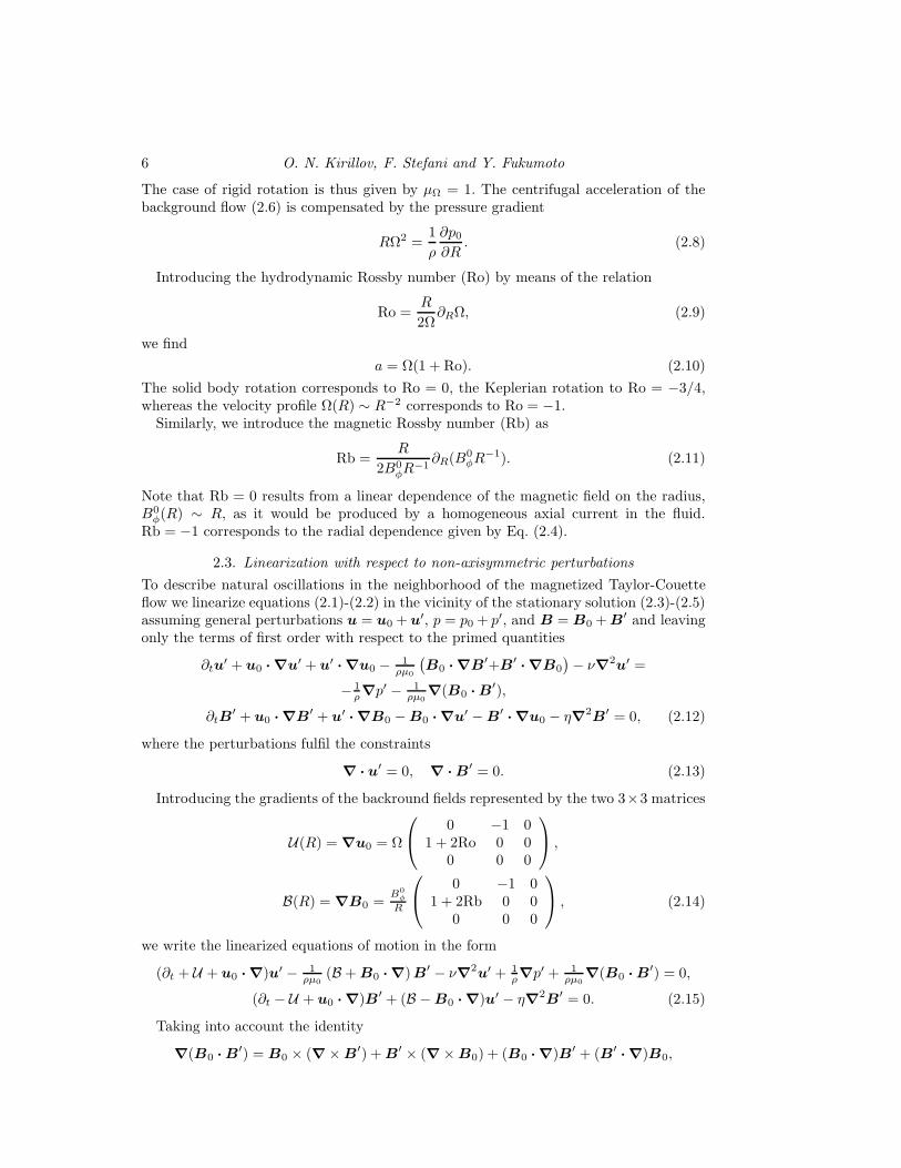
6 O. N. Kirillov, F. Stefani and Y. Fukumoto
The case of rigid rotation is thus given by µΩ = 1. The centrifugal acceleration of thebackground flow (2.6) is compensated by the pressure gradient
RΩ2 =1
ρ
∂p0∂R
. (2.8)
Introducing the hydrodynamic Rossby number (Ro) by means of the relation
Ro =R
2Ω∂RΩ, (2.9)
we find
a = Ω(1 + Ro). (2.10)
The solid body rotation corresponds to Ro = 0, the Keplerian rotation to Ro = −3/4,whereas the velocity profile Ω(R) ∼ R−2 corresponds to Ro = −1.Similarly, we introduce the magnetic Rossby number (Rb) as
Rb =R
2B0φR
−1∂R(B
0φR
−1). (2.11)
Note that Rb = 0 results from a linear dependence of the magnetic field on the radius,B0
φ(R) ∼ R, as it would be produced by a homogeneous axial current in the fluid.Rb = −1 corresponds to the radial dependence given by Eq. (2.4).
2.3. Linearization with respect to non-axisymmetric perturbations
To describe natural oscillations in the neighborhood of the magnetized Taylor-Couetteflow we linearize equations (2.1)-(2.2) in the vicinity of the stationary solution (2.3)-(2.5)assuming general perturbations u = u0 +u
′, p = p0 + p′, and B = B0 +B′ and leaving
only the terms of first order with respect to the primed quantities
∂tu′ + u0 · ∇u
′ + u′· ∇u0 − 1
ρµ0
(B0 · ∇B
′+B′· ∇B0
)− ν∇2
u′ =
− 1ρ∇p′ − 1
ρµ0∇(B0 ·B
′),
∂tB′ + u0 · ∇B
′ + u′· ∇B0 −B0 · ∇u
′ −B′· ∇u0 − η∇2
B′ = 0, (2.12)
where the perturbations fulfil the constraints
∇ · u′ = 0, ∇ ·B
′ = 0. (2.13)
Introducing the gradients of the backround fields represented by the two 3×3 matrices
U(R) = ∇u0 = Ω
0 −1 01 + 2Ro 0 0
0 0 0
,
B(R) = ∇B0 =B0
φ
R
0 −1 01 + 2Rb 0 0
0 0 0
, (2.14)
we write the linearized equations of motion in the form
(∂t + U + u0 · ∇)u′ − 1ρµ0
(B +B0 · ∇)B′ − ν∇2u′ + 1
ρ∇p′ + 1ρµ0
∇(B0 ·B′) = 0,
(∂t − U + u0 · ∇)B′ + (B −B0 · ∇)u′ − η∇2B
′ = 0. (2.15)
Taking into account the identity
∇(B0 ·B′) = B0 × (∇×B
′) +B′ × (∇×B0) + (B0 · ∇)B′ + (B′
· ∇)B0,

Instabilities in magnetized rotational flows 7
we transform equations (2.15) into
(∂t + U + u0 · ∇)u′ + 1ρ∇p′ + 1
ρµ0B0 × (∇×B
′) + 1ρµ0
B′ × (∇ ×B0) = ν∇2
u′,
(∂t − U + u0 · ∇)B′ + (B −B0 · ∇)u′ = η∇2B
′. (2.16)
Equations (2.16) are simplified for the profile (2.4) in view of the identity (2.5).
3. Geometrical optics equations
We seek for solutions of the linearized equations (2.16) in the form of the geometricaloptics approximation, see e.g. Lifschitz (1989) and Friedlander & Lipton-Lifschitz (2003):
u′(x, t, ǫ) = eiΦ(x,t)/ǫ
(u(0)(x, t) + ǫu(1)(x, t)
)+ ǫur(x, t),
B′(x, t, ǫ) = eiΦ(x,t)/ǫ
(B
(0)(x, t) + ǫB(1)(x, t))+ ǫBr(x, t),
p′(x, t, ǫ) = eiΦ(x,t)/ǫ(p(0)(x, t) + ǫp(1)(x, t)
)+ ǫpr(x, t), (3.1)
where x is a vector of coordinates, 0 < ǫ ≪ 1 is a small parameter, Φ is a real-valued scalarfunction that represents the phase of oscillations, and u
(j), B(j), and p(j), j = 0, 1, r arecomplex-valued amplitudes.Following Landman & Saffman (1987), Lifschitz (1991), Dobrokhotov & Shafarevich
(1992), and Eckhardt & Yao (1995) we assume further in the text that ν = ǫ2ν andη = ǫ2η and introduce the derivative along the fluid stream lines
D
Dt:= ∂t + u0 · ∇. (3.2)
Substituting expansions (3.1) into equations (2.16), taking into account the identities
(A · ∇)ΦB = (A · ∇Φ)B +Φ(A · ∇)B,
(∇× ΦB) = Φ(∇×B) + (∇Φ×B)
as well as the relation
∇2(u′) = eiΦ/ǫ
(∇
2 + i2
ǫ(∇Φ · ∇) + i
∇2Φ
ǫ− (∇Φ)2
ǫ2
)(u(0) + ǫu(1)), (3.3)
collecting terms at ǫ−1 and ǫ0, and expanding the cross products, we arrive at the systemof partial differential equations
DΦDt u
(0) + p(0)
ρ ∇Φ− 1ρµ0
B(0)(B0 · ∇Φ) + 1
ρµ0∇Φ(B0 ·B
(0)) = 0,
DΦDt B
(0) − (B0 · ∇Φ)u(0) = 0,(
DDt + ν(∇Φ)2 + U
)u(0) + 1
ρ∇p(0) + iDΦDt u
(1) + i p(1)
ρ ∇Φ (3.4)
+ 1ρµ0
B0 ×∇×B(0) − i 1
ρµ0B0 ×B
(1) ×∇Φ + 1ρµ0
B(0) ×∇×B0 = 0,
iDΦDt B
(1) +(
DDt + η(∇Φ)2 − U
)B
(0) + (B −B0 · ∇)u(0) − i(B0 · ∇Φ)u(1) = 0.
From the solenoidality conditions (2.13) it follows that
u(0)
· ∇Φ = 0, ∇ · u(0) + iu(1)
· ∇Φ = 0,
B(0)
· ∇Φ = 0, ∇ ·B(0) + iB(1)
· ∇Φ = 0. (3.5)
Taking the dot product of the first two of the equations (3.4) with ∇Φ, u(0), B(0), in
8 O. N. Kirillov, F. Stefani and Y. Fukumoto
view of the constraints (3.5) we arrive at the following system
(∇Φ)2(
p(0)
ρ + 1ρµ0
(B0 ·B(0)))= 0,
DΦDt B
(0)·B
(0) − (B0 · ∇Φ)u(0)·B
(0) = 0,
DΦDt B
(0)· u
(0) − (B0 · ∇Φ)u(0)· u
(0) = 0,
DΦDt u
(0)·B
(0) − 1ρµ0
B(0)
·B(0)(B0 · ∇Φ) = 0,
DΦDt u
(0)· u
(0) − 1ρµ0
B(0)
· u(0)(B0 · ∇Φ) = 0, (3.6)
that has for ∇Φ 6= 0, B(0) 6= 0, and u(0) 6= 0 a unique solution
p(0) = − 1
µ0(B0 ·B
(0)),DΦ
Dt= 0, B0 · ∇Φ = 0. (3.7)
With the use of the relations (3.7) we simplify the last two of the equations (3.4) as
(DDt + ν(∇Φ)2 + U
)u(0) − 1
ρµ0(B +B0 · ∇)B(0) = − i
ρ
(p(1) + 1
µ0(B0 ·B
(1)))∇Φ,
(DDt + η(∇Φ)2 − U
)B
(0) + (B −B0 · ∇)u(0) = 0. (3.8)
Eliminating pressure via multiplication of the first of Eqs. (3.8) by ∇Φ and taking intoaccount the constraints (3.5), we transform equations (3.8) into
(DDt + ν(∇Φ)2 + U
)u(0) − 1
ρµ0(B +B0 · ∇)B(0)
= ∇Φ|∇Φ|2 ·
[(DDt + U
)u(0) − 1
ρµ0(B +B0 · ∇)B(0)
]∇Φ,
(DDt + η(∇Φ)2 − U
)B
(0) + (B −B0 · ∇)u(0) = 0. (3.9)
Differentiating the first of the identities (3.5) yields
D
Dt(∇Φ · u
(0)) =D∇Φ
Dt· u
(0) +∇Φ ·Du
(0)
Dt= 0. (3.10)
Using the identity (3.10), we write(
DDt + ν(∇Φ)2 + U
)u(0) − 1
ρµ0(B +B0 · ∇)B(0)
= ∇Φ|∇Φ|2 ·
[Uu(0) − 1
ρµ0(B +B0 · ∇)B(0)
]∇Φ− ∇Φ
|∇Φ|2D∇ΦDt · u
(0), (3.11)(
DDt + η(∇Φ)2 − U
)B
(0) + (B −B0 · ∇)u(0) = 0.
Now we take the gradient of the identity DΦ/Dt = 0:
∇∂tΦ+∇(u0 · ∇)Φ
= ∂t∇Φ+ (u0 · ∇)∇Φ+ UT∇Φ
= DDt∇Φ+ UT
∇Φ = 0. (3.12)
Denoting k = ∇Φ, we deduce from the phase equation (3.12) that
Dk
Dt= −UT
k. (3.13)
Hence, the amplitude (or transport) equations (3.11) take the final form
Du(0)
Dt = −(I − 2kk
T
|k|2)Uu(0) − ν|k|2u(0) + 1
ρµ0
(I − kk
T
|k|2)(B +B0 · ∇)B(0),
DB(0)
Dt = UB(0) − η|k|2B(0) − (B −B0 · ∇)u(0), (3.14)

Instabilities in magnetized rotational flows 9
where I is a 3 × 3 identity matrix, cf. Friedlander & Vishik (1995). In the absence ofthe magnetic field these equations are reduced to that of Landman & Saffman (1987),Lifschitz (1991), Dobrokhotov & Shafarevich (1992), and Eckhardt & Yao (1995) and inthe inviscid case to that of Lifschitz & Hameiri (1991).
4. Dispersion relation of the amplitude equations
Let the orthogonal unit vectors eR(t), eφ(t), and ez(t) form a basis in a cylindricalcoordinate system moving along the fluid trajectory. With k(t) = kReR(t) + kφeφ(t) +kzez(t), u(t) = uReR(t) + uφeφ(t) + uzez(t), and with the matrix U from (2.14), we findthat
eR = Ω(R)eφ, eφ = −Ω(R)eR. (4.1)
Hence, the equation (3.13) in the coordinate form is
kR − Ωkφ = −Ωkφ −R∂RΩkφ, kφ +ΩkR = ΩkR, kz = 0.
Therefore,
kR = −R∂RΩkφ, kφ = 0, kz = 0. (4.2)
According to Eckhardt & Yao (1995) and Friedlander & Vishik (1995), in order tostudy physically relevant and potentially unstable modes we have to choose bounded andasymptotically non-decaying solutions of the system (4.2). These correspond to kφ ≡ 0and kR and kz time-independent. Denoting α = kz|k|−1, where |k|2 = k2R + k2z , we findthat kRk
−1z =
√1− α2α−1 and taking into account relations (A 1) we write the partial
differential equations (3.14) for the amplitudes in the coordinate representation
∂tu(0)R +Ω
(∂φu
(0)R − u
(0)φ
)+ ν|k|2u(0)
R +Ωu(0)φ − 2Ωu
(0)φ α2 +
B0φ
ρµ0R2α2B
(0)φ
−αB0
φ
R
α∂φB(0)R
−√1−α2∂φB
(0)z
ρµ0− αB0
zα∂zB
(0)R
−√1−α2∂zB
(0)z
ρµ0= 0,
∂tu(0)φ +Ω
(∂φu
(0)φ + u
(0)R
)+ (Ω + 2ΩRo)u
(0)R + ν|k|2u(0)
φ − 1ρµ0
B0φ
R ∂φB(0)φ − B0
z∂zB(0)φ
ρµ0
− 2ρµ0
B0φ
R (1 + Rb)B(0)R = 0,
∂tu(0)z +Ω∂φu
(0)z + 2
√1− α2αΩu
(0)φ + ν|k|2u(0)
z +B0
φ(α2−1)∂φB
(0)z
ρµ0R
+α√1−α2B0
φ(∂φB(0)R −2B
(0)φ
)
ρµ0R+B0
z
√1−α2α∂zB
(0)R
−(1−α2)∂zB(0)z
ρµ0= 0,
∂tB(0)R +Ω
(∂φB
(0)R −B
(0)φ
)+ΩB
(0)φ + η|k|2B(0)
R −B0z∂zu
(0)R − B0
φ
R ∂φu(0)R = 0,
∂tB(0)φ +Ω
(∂φB
(0)φ +B
(0)R
)− (Ω + 2ΩRo)B
(0)R + η|k|2B(0)
φ −B0z∂zu
(0)φ
+2RbB0
φ
R u(0)R − B0
φ
R ∂φu(0)φ = 0,
∂tB(0)z +Ω∂φB
(0)z + η|k|2B(0)
z −B0z∂zu
(0)z − B0
φ
R ∂φu(0)z = 0. (4.3)
10 O. N. Kirillov, F. Stefani and Y. Fukumoto
Assuming that the solution to Eqs. (4.3) has the modal form eγt+imφ+ikzz , we obtain
(γ + imΩ+ ν|k|2)u(0)R − 2α2Ωu
(0)φ + 2α2 B0
φ
ρµ0RB
(0)φ
−iα(m
B0φ
R + kzB0z
)αB
(0)R
−√1−α2B(0)
z
ρµ0= 0,
(γ + imΩ+ ν|k|2)u(0)φ + 2Ω(1 + Ro)u
(0)R − 2
ρµ0
B0φ
R (1 + Rb)B(0)R
− iB(0)φ
ρµ0
(m
B0φ
R + kzB0z
)= 0,
(γ + imΩ+ ν|k|2)u(0)z + 2
√1− α2αΩu
(0)φ +
B0φ(α
2−1)imB(0)z
ρµ0R
+α√1−α2B0
φ(imB(0)R
−2B(0)φ
)
ρµ0R+ ikzB
0z
√1−α2αB
(0)R −(1−α2)B(0)
z
ρµ0= 0,
(γ + imΩ+ η|k|2)B(0)R − iu
(0)R
(m
B0φ
R + kzB0z
)= 0,
(γ + imΩ+ η|k|2)B(0)φ − 2ΩRoB
(0)R + 2Rb
B0φ
R u(0)R − iu
(0)φ
(m
B0φ
R + kzB0z
)= 0,
(γ + imΩ+ η|k|2)B(0)z − iu
(0)z
(m
B0φ
R + kzB0z
)= 0, (4.4)
cf. e.g. Friedlander & Vishik (1995). Taking into account that B(0)R kR+B
(0)z kz = 0 in the
short-wavelength approximation, we single out the equations for the radial and azimuthalcomponents of the fluid velocity and magnetic field
(γ + imΩ+ ν|k|2)u(0)R − 2α2Ωu
(0)φ + 2α2 B0
φ
ρµ0RB
(0)φ − iB
(0)R
ρµ0
(m
B0φ
R + kzB0z
)= 0,
(γ + imΩ+ ν|k|2)u(0)φ + 2Ω(1 + Ro)u
(0)R − 2
ρµ0
B0φ
R (1 + Rb)B(0)R
− iB(0)φ
ρµ0
(m
B0φ
R + kzB0z
)= 0, (4.5)
(γ + imΩ+ η|k|2)B(0)R − iu
(0)R
(m
B0φ
R + kzB0z
)= 0,
(γ + imΩ+ η|k|2)B(0)φ − 2ΩRoB
(0)R + 2Rb
B0φ
R u(0)R − iu
(0)φ
(m
B0φ
R + kzB0z
)= 0.
Introducing the viscous, resistive, and Alfven frequencies corresponding to the axialand azimuthal components of the magnetic field:
ων = ν|k|2, ωη = η|k|2, ωA =kzB
0z√
ρµ0, ωAφ
=B0
φ
R√ρµ0
, (4.6)
so that Rb is simply
Rb =R
2ωAφ
∂RωAφ, (4.7)
we write the amplitude equations (4.5) as
(γ + imΩ+ ων)u(0)R − 2α2Ωu
(0)φ + 2α2 ωAφ√
ρµ0B
(0)φ − iB
(0)R√ρµ0
(mωAφ
+ ωA
)= 0,
(γ + imΩ+ ων)u(0)φ + 2Ω(1 + Ro)u
(0)R − 2ωAφ√
ρµ0(1 + Rb)B
(0)R − iB
(0)φ√ρµ0
(mωAφ
+ ωA
)= 0,
(γ + imΩ+ ωη)B(0)R − iu
(0)R
√ρµ0
(mωAφ
+ ωA
)= 0,
(γ + imΩ+ ωη)B(0)φ − 2ΩRoB
(0)R + 2RbωAφ
√ρµ0u
(0)R − iu
(0)φ
√ρµ0
(mωAφ
+ ωA
)= 0.
(4.8)

Instabilities in magnetized rotational flows 11
The solvability condition written for the above system of equations yields the dispersionrelation of the amplitude equations
p(γ) := det(H− γE) = 0, (4.9)
where E is the 4× 4 identity matrix and
H =
−imΩ− ων 2α2Ω imωAφ
+ωA√ρµ0
− 2ωAφα2
√ρµ0
−2Ω(1 + Ro) −imΩ− ων2ωAφ√ρµ0
(1 + Rb) imωAφ
+ωA√ρµ0
i(mωAφ+ ωA)
√ρµ0 0 −imΩ− ωη 0
−2ωAφRb
√ρµ0 i(mωAφ
+ ωA)√ρµ0 2ΩRo −imΩ− ωη
.
(4.10)The fourth-order polynomial (4.9)
p(γ) = (a0 + ib0)γ4 + (a1 + ib1)γ
3 + (a2 + ib2)γ2 + (a3 + ib3)γ + a4 + ib4, (4.11)
has complex coefficients, where
a0 = 1, b0 = 0, a1 = 2(ωη + ων), b1 = 4mΩ,
a2 = −4α2ω2Aφ
Rb + 4α2Ω2(1 + Ro) + (ων + ωη)2 − 2(3m2Ω2 − (mωAφ
+ ωA)2 − ωνωη),
b2 = 34a1b1,
a3 = 2(ων + ωη)(−2α2ω2Aφ
Rb− (3m2Ω2 − (mωAφ+ ωA)
2 − ωνωη)) + 8α2Ω2ωη(1 + Ro),
b3 = a2b12 +
b318 − 8Ωα2(ωA +mωAφ
)ωAφ,
a4 = ((4Ω2(ωA +mωAφ)2 − 4Ω4m2 + 4Ω2ω2
2)Ro + 8ωAφωAmΩ2 + 4Ω2ω2
η − 4Ω4m2)α2
−Ω2m2(ων + ωη)2 + (m2Ω2 − (ωA +mωAφ
)2 − ωνωη)2
+4(Rb + 1)ω2Aφ
α2(m2Ω2 − (ωA +mωAφ)2) + 4ω2
Aφα2(m2Ω2 − ωνωηRb),
b4 = −4mΩα2[(Ro + 1)(ωη − ων) + (Rb + 1)(ωη + ων)]ω2Aφ
−4ωAΩα2(Ro(ωη − ων) + 2ωη)ωAφ
+2mΩ(4α2Ω2ωη(Ro + 1) + (ων + ωη)(ωνωη −m2Ω2 + (ωA +mωAφ)2)). (4.12)
When Rb = −1, the dispersion relation is reduced to that derived by Kirillov et al.(2012). In the particular case when ων = 0, ωη = 0, and ωA = 0, the coefficients (4.12) ofthe dispersion relation exactly coincide with those derived by Friedlander & Vishik (1995)when the quantization constant introduced in that work vanishes and the azimuthalAlfven frequency A = A(R) and the angular velocity Ω = Ω(R) are functions of only theradial coordinate R. Hence, according to Eq. (4.7)
∂RA = ∂RωAφ=
2Rb
RωAφ
. (4.13)
With the relations (2.9) and (4.13), the dispersion relation derived by Friedlander & Vishik(1995) reduces to ours at ων = 0, ωη = 0, and ωA = 0.
Note also that in the absence of the magnetic fields, the dispersion relation determinedby the matrix H reduces to that derived already by Krueger et al. (1966) for the non-axisymmetric perturbations of the hydrodynamic TC flow. Explicitly, this connection isestablished in Appendix B. In the presence of the magnetic fields with Rb = −1 andm = 0, the dispersion relation reduces to that derived by Kirillov & Stefani (2010).
12 O. N. Kirillov, F. Stefani and Y. Fukumoto
5. Connection to the known stability and instability criteria
Let us compose a matrix filled in with the coefficients of the complex polynomial (4.11)
B =
a4 −b4 0 0 0 0 0 0b3 a3 a4 −b4 0 0 0 0
−a2 b2 b3 a3 a4 −b4 0 0−b1 −a1 −a2 b2 b3 a3 a4 −b4a0 −b0 −b1 −a1 −a2 b2 b3 a30 0 a0 −b0 −b1 −a1 −a2 b20 0 0 0 a0 −b0 −b1 −a10 0 0 0 0 0 a0 −b0
. (5.1)
The stability criterion by Bilharz (1944) requires positiveness of the determinants of thefour diagonal sub-matrices of even order of the matrix B (Kirillov 2013)
m1 = det
(a4 −b4b3 a3
)> 0, . . . , m4 = detB > 0 (5.2)
in order that all the roots of the complex polynomial (4.11) have negative real parts.In the ideal case the dispersion relation of SMRI by Balbus & Hawley (1992) reads as
p(γ) = (γ2 + ω2A)
2 + 4α2Ω2(1 + Ro)(γ2 + ω2A)− 4α2Ω2ω2
A
and follows from our result when settiung ωAφ= 0, ων = 0, and ωη = 0 in the form
p(γ) = γ4 + (4Ω2α2Ro + 4Ω2α2 + 2ω2A)γ
2 + 4ω2AΩ
2α2Ro + ω4A.
In the dissipative case, the threshold for the Standard MRI is given by the equationm4 = 0 with ωAφ
= 0. This yields the expression found in Kirillov & Stefani (2012)
Ro = −(ω2
A + ωνωη)2 + 4α2Ω2ω2
η
4α2Ω2(ω2A + ω2
η). (5.3)
When Ro = 0, Ω = 0, and m = 0 we get an instability condition that extends that ofChandrasekhar (1961) (see also Rudiger et al. (2010)) to the dissipative case
Rb >(ωνωη + ω2
A)2 − 4α2ω2
Aω2Aφ
4α2ω2Aφ
(ωνωη + ω2A)
. (5.4)
On the other hand, under the assumption that Ω = 0 and ωA = 0 the dispersionrelation is a real polynomial. Hence, by vanishing its constant term we determine thecondition for a static instability
Rb >(ωνωη +m2ω2
Aφ)2 − 4α2m2ω4
Aφ
4α2ω2Aφ
(ωνωη +m2ω2Aφ
). (5.5)
When Rb = 0 the criterion (5.5) yields the onset of the standard Tayler (1973) instabilityat
ωAφ>
√ωνωη
α2 − (m± α)2. (5.6)
Another particular case ωA = 0 and m = 0 yields the following extension of thestability condition by Michael (1954):
Ro > −1 + Rbω2Aφ
Ω2
ων
ωη− ω2
ν
4α2Ω2. (5.7)

Instabilities in magnetized rotational flows 13
Choosing, additionally, ωAφ= 0, we reproduce the result of Eckhardt & Yao (1995)
Ro > −1− ω2ν
4α2Ω2.
The ideal Michael criterion
d
dR(Ω2R4)− R4
ρµ0
d
dR
(B0
φ
R
)2
> 0 (5.8)
or
Ro > −1 + Rbω2Aφ
Ω2(5.9)
follows from Eq. (5.7) when ωη = ων and ων → 0 (see also Howard and Gupta (1962)).Finally, letting in the equation (4.10)
Rb = Ro, Ω = ωAφ(5.10)
and assuming ων = 0 and ωη = 0, we find that (4.9) has the following roots
γ1,2 = 0, γ3,4 = −2iωAφ(m± α),
indicating marginal stability. Indeed, for the inviscid fluid of infinite electrical conduc-tivity with P = const., conditions (5.10) define at Rb = Ro = −1 Chandrasekhar’s
equipartition solution, which is stable (Chandrasekhar 1956, 1961; Bogoyavlenskij 2004).
6. Dispersion relation in dimensionless parameters
The dispersion relation (4.9) of the system (4.8) has the same roots as the equation
det(HT− γET) = 0, (6.1)
where T = diag (1, 1, (ρµ0)−1/2, (ρµ0)
−1/2). Let us change in the equation (6.1) the spec-tral parameter as γ = γ
√ωνωη and in addition to the hydrodynamic (Ro) and magnetic
(Rb) Rossby numbers introduce the magnetic Prandtl number (Pm), the ratio of theAlfven frequencies (β), Reynolds (Re) and Hartmann (Ha) numbers as well as the mod-ified azimuthal wavenumber n as follows
Pm =ων
ωη, β = α
ωAφ
ωA, Re = α
Ω
ων, Ha =
ωA√ωνωη
, n =m
α. (6.2)
Then, the dispersion relation (6.1) transforms into
p(γ) = det
(H− γ√
PmE
)= 0, (6.3)
with
H =
−inRe− 1 2αRe iHa(1+nβ)√Pm
− 2αβHa√Pm
− 2Re(1+Ro)α −inRe− 1 2βHa(1+Rb)
α√Pm
iHa(1+nβ)√Pm
iHa(1+nβ)√Pm
0 −inRe− 1Pm 0
−2βHaRb
α√Pm
iHa(1+nβ)√Pm
2ReRoα −inRe− 1
Pm
. (6.4)
The coefficients of the polynomial (6.3) are explicitly given by Eq. (C 1) in Appendix C.Next, we divide the equation (6.3) by Re and introduce the eigenvalue parameter
λ =γ
Re√Pm
=γ√ωνωη
αΩ=
γ
αΩ. (6.5)

14 O. N. Kirillov, F. Stefani and Y. Fukumoto
This results in the dispersion relation
p(λ) = det(M− λE) = 0, (6.6)
where
M =
−in− 1Re 2α i(1+nβ)
√NRm −2αβ
√NRm
− 2(1+Ro)α −in− 1
Re2β(1+Rb)
α
√NRm i(1+nβ)
√NRm
i(1+nβ)√
NRm 0 −in− 1
Rm 0
−2βRbα
√NRm i(1+nβ)
√NRm
2Roα −in− 1
Rm
, (6.7)
Here, N = Ha2/Re is the Elsasser number (interaction parameter) and Rm = RePm isthe magnetic Reynolds number. Explicit coefficients of the dispersion relation (6.6) can befound in equation (C 2) of the Appendix C. In the following, we will use the dispersionrelations (4.9), (6.3), and (6.6) with different parameterizations in order to facilitatephysical interpretation and comparison with the results obtained in astrophysical, MHD,and hydrodynamical communities.
7. Inductionless approximation
In this section, we focus on the inductionless approximation by setting the magneticPrandtl number to zero (Hollerbach & Rudiger 2005; Priede 2011) which is a reasonableapproximation for liquid metal experiments as well as for some colder parts of accretiondisks.
7.1. The threshold of instability
We put Pm = 0 into the expressions for mi in equation (5.2). For the coefficient m4 =detB this leads to a great simplification and yields the instability threshold in a compactand closed form:
(1 + Ha2(nβ + 1)2)2 − 4Ha2β2(1 + Ha2(nβ + 1)2)Rb− 4Ha4β2(nβ + 1)2
Ha4β2(nβ + 1)2Ro2 −[[1 + Ha2((nβ + 1)2 − 2β2Rb)]2 − 4Ha4β2(nβ + 1)2
](Ro + 1)
=
(2Re
1 + Ha2((nβ + 1)2 − 2β2Rb)
)2
. (7.1)
Equation (7.1) can be resolved with respect to the hydrodynamic Rossby number,which yields the critical Ro as a function of all other parameters. Taking subsequentlythe limits Re → ∞ and Ha → ∞ we obtain the expressions for the two branches
Ro± = −2 +(nβ + 1)2 − 2β2Rb±
√((nβ + 1)2 − 2β2Rb)2 − 4β2(nβ + 1)2
2β2(nβ + 1)2((nβ + 1)2 − 2β2Rb)−1. (7.2)
At n = 0 and Rb = −1 the expressions (7.2) reduce to that derived in the earlier workby Kirillov & Stefani (2011)
Ro± =4β4 + 1± (2β2 + 1)
√4β4 + 1
2β2, (7.3)
which after resolution with respect to β coincide with the formulas by Priede (2011).
Instabilities in magnetized rotational flows 15
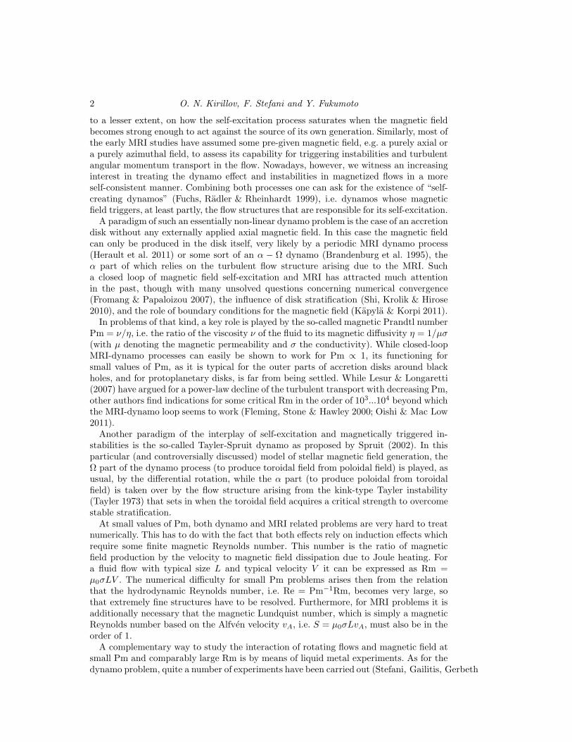
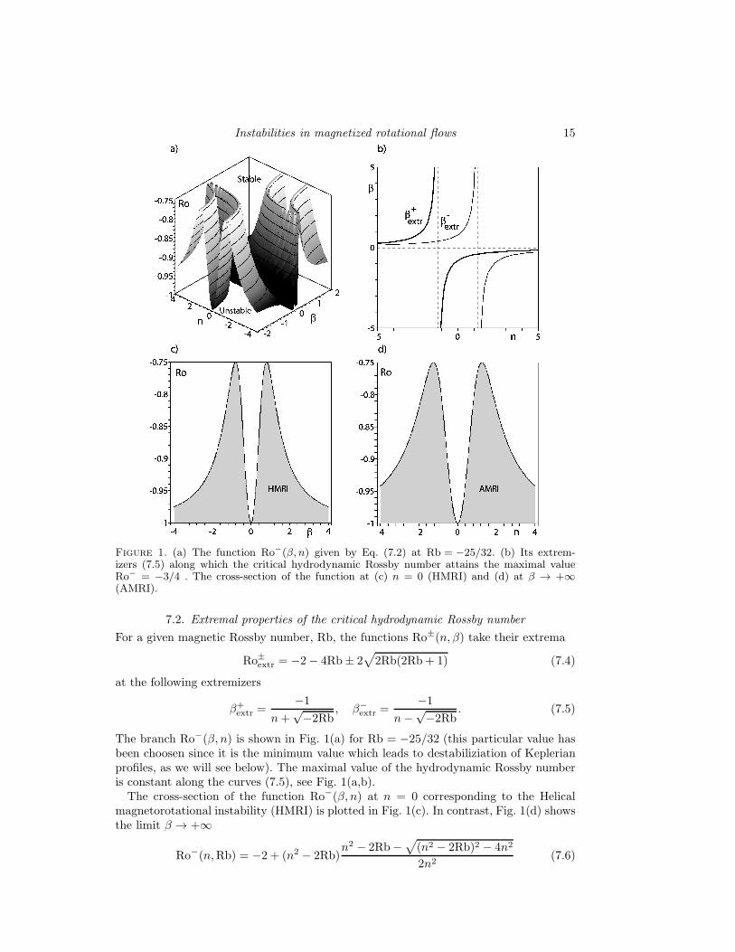
Figure 1. (a) The function Ro−(β, n) given by Eq. (7.2) at Rb = −25/32. (b) Its extrem-izers (7.5) along which the critical hydrodynamic Rossby number attains the maximal valueRo− = −3/4 . The cross-section of the function at (c) n = 0 (HMRI) and (d) at β → +∞(AMRI).
7.2. Extremal properties of the critical hydrodynamic Rossby number
For a given magnetic Rossby number, Rb, the functions Ro±(n, β) take their extrema
Ro±extr = −2− 4Rb± 2√2Rb(2Rb + 1) (7.4)
at the following extremizers
β+extr =
−1
n+√−2Rb
, β−extr =
−1
n−√−2Rb
. (7.5)
The branch Ro−(β, n) is shown in Fig. 1(a) for Rb = −25/32 (this particular value hasbeen choosen since it is the minimum value which leads to destabiliziation of Keplerianprofiles, as we will see below). The maximal value of the hydrodynamic Rossby numberis constant along the curves (7.5), see Fig. 1(a,b).The cross-section of the function Ro−(β, n) at n = 0 corresponding to the Helical
magnetorotational instability (HMRI) is plotted in Fig. 1(c). In contrast, Fig. 1(d) showsthe limit β → +∞
Ro−(n,Rb) = −2 + (n2 − 2Rb)n2 − 2Rb−
√(n2 − 2Rb)2 − 4n2
2n2(7.6)
16 O. N. Kirillov, F. Stefani and Y. Fukumoto
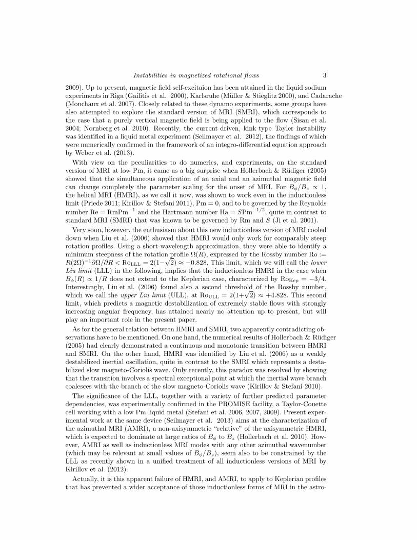
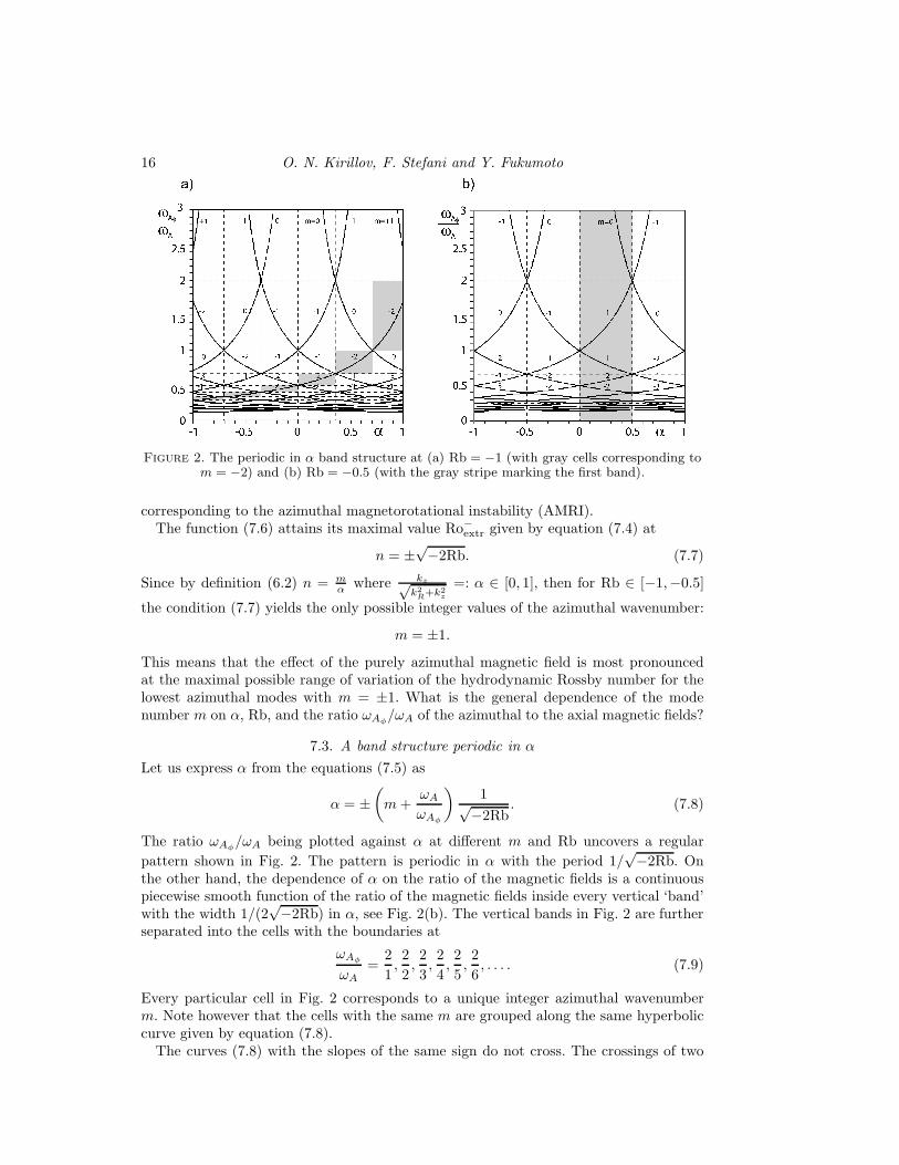
Figure 2. The periodic in α band structure at (a) Rb = −1 (with gray cells corresponding tom = −2) and (b) Rb = −0.5 (with the gray stripe marking the first band).
corresponding to the azimuthal magnetorotational instability (AMRI).The function (7.6) attains its maximal value Ro−extr given by equation (7.4) at
n = ±√−2Rb. (7.7)
Since by definition (6.2) n = mα where kz√
k2R+k2
z
=: α ∈ [0, 1], then for Rb ∈ [−1,−0.5]
the condition (7.7) yields the only possible integer values of the azimuthal wavenumber:
m = ±1.
This means that the effect of the purely azimuthal magnetic field is most pronouncedat the maximal possible range of variation of the hydrodynamic Rossby number for thelowest azimuthal modes with m = ±1. What is the general dependence of the modenumber m on α, Rb, and the ratio ωAφ
/ωA of the azimuthal to the axial magnetic fields?
7.3. A band structure periodic in α
Let us express α from the equations (7.5) as
α = ±(m+
ωA
ωAφ
)1√
−2Rb. (7.8)
The ratio ωAφ/ωA being plotted against α at different m and Rb uncovers a regular
pattern shown in Fig. 2. The pattern is periodic in α with the period 1/√−2Rb. On
the other hand, the dependence of α on the ratio of the magnetic fields is a continuouspiecewise smooth function of the ratio of the magnetic fields inside every vertical ‘band’with the width 1/(2
√−2Rb) in α, see Fig. 2(b). The vertical bands in Fig. 2 are further
separated into the cells with the boundaries at
ωAφ
ωA=
2
1,2
2,2
3,2
4,2
5,2
6, . . . . (7.9)
Every particular cell in Fig. 2 corresponds to a unique integer azimuthal wavenumberm. Note however that the cells with the same m are grouped along the same hyperboliccurve given by equation (7.8).The curves (7.8) with the slopes of the same sign do not cross. The crossings of two
Instabilities in magnetized rotational flows 17
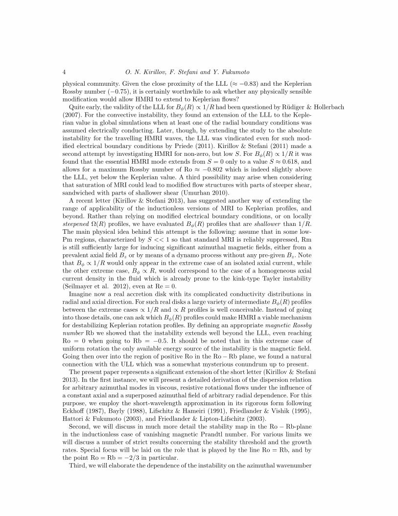
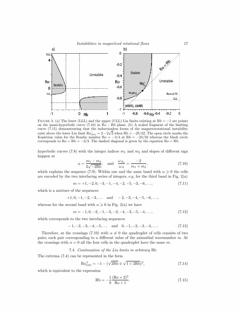
Figure 3. (a) The lower (LLL) and the upper (ULL) Liu limits existing at Rb = −1 are pointson the quasi-hyperbolic curve (7.16) in Ro − Rb plane. (b) A scaled fragment of the limitingcurve (7.15) demonstrating that the inductionless forms of the magnetorotational instability
exist above the lower Liu limit Ro−extr = 2−2√2 when Rb > −25/32. The open circle marks the
Keplerian value for the Rossby number Ro = −3/4 at Rb = −25/32 whereas the black circlecorresponds to Ro = Rb = −2/3. The dashed diagonal is given by the equation Ro = Rb.
hyperbolic curves (7.8) with the integer indices m1 and m2 and slopes of different signhappen at
α =m1 −m2
2√−2Rb
, andωAφ
ωA=
−2
m1 +m2, (7.10)
which explains the sequence (7.9). Within one and the same band with α > 0 the cellsare encoded by the two interlacing series of integers, e.g. for the third band in Fig. 2(a)
m = +1,−2, 0,−3,−1,−4,−2,−5,−3,−6, . . . , (7.11)
which is a mixture of the sequences
+1, 0,−1,−2,−3, . . . and − 2,−3,−4,−5,−6, . . . ,
whereas for the second band with α > 0 in Fig. 2(a) we have
m = −1, 0,−2,−1,−3,−2,−4,−3,−5,−4, . . . , (7.12)
which corresponds to the two interlacing sequences
− 1,−2,−3,−4,−5, . . . and 0,−1,−2,−3,−4, . . . . (7.13)
Therefore, at the crossings (7.10) with α 6= 0 the quadruplet of cells consists of twopairs; each pair corresponding to a different value of the azimuthal wavenumber m. Atthe crossings with α = 0 all the four cells in the quadruplet have the same m.
7.4. Continuation of the Liu limits to arbitrary Rb
The extrema (7.4) can be represented in the form
Ro±extr = −1− (√2Rb∓
√1 + 2Rb)2, (7.14)
which is equivalent to the expression
Rb = −1
8
(Ro + 2)2
Ro + 1. (7.15)

18 O. N. Kirillov, F. Stefani and Y. Fukumoto
A particular case of equation (7.15) at Rb = −1 yields the result of Liu et al. (2006),reproduced also by Kirillov & Stefani (2011) and Priede (2011). Solving (7.15) at Rb =−1, we find that the critical Rossby numbers Ro(Ha,Re, n, β) given by the equation (7.1)and thus the instability domains lie at Pm = 0 and Rb = −1 outside the stratum
2− 2√2 =: RoLLL < Ro(Ha,Re, n, β) < RoULL := 2 + 2
√2,
where RoLLL is the value of Ro−extr at the lower Liu limit (LLL) and RoULL is the valueof Ro+extr at the upper Liu limit (ULL) corresponding to the critical values of β given bythe equation (7.5).Fig. 3(a) shows how the LLL and ULL continue to the values of Rb 6= −1. In fact, the
LLL and the ULL are points at the quasi-hyperbolic curve
(Rb− Ro− 1)2 − (Rb + Ro + 1)2 =1
2(Ro + 2)2, (7.16)
which is another representation of equation (7.15). At Rb = −1/2 the branches Ro−extr(Rb)and Ro+extr(Rb) meet each other. Therefore, the inductionless magnetorotational insta-bility at negative Rb exists also at positive Ro when Ro > Ro+extr(Rb), Fig. 3(a). Noticealso the second stability domain at Rb > 0 and Ro < −1.We see that in the inductionless case Pm = 0 when the Reynolds and Hartmann
numbers subsequently tend to infinity and β and n are under the constraints (7.5), themaximal possible critical Rossby number Ro−extr increases with the increase of Rb. At
Rb > −25
32= −0.78125 (7.17)
Ro−extr(Rb) exceeds the critical value for the Keplerian flow: Ro−extr > −3/4.Therefore, the very possibility for Bφ(R) to depart from the profile Bφ(R) ∝ R−1
allows us to break the conventional lower Liu limit and extend the inductionless versionsof MRI to the velocity profiles Ω(R) as steep as the Keplerian one and even to the lesssteep profiles, including that of the solid body rotation at Rb = −1/2, Fig. 3(b).
7.5. Scaling law of the inductionless MRI
What asymptotic behavior of the Reynolds and Hartmann numbers at infinity leads tomaximization of negative (and simultaneously to minimization of positive) critical Rossbynumbers? To get an idea, we investigate extrema of Ro as a solution to equation (7.1)subject to the constraints (7.5). Taking, e.g., β = β−
extr in equation (7.1), differentiatingthe result with respect to Ha, equating it to zero and solving the equation with respectto Re, we find the following asymptotic relation between Ha and Re when Ha → ∞:
Re = 2Rb√3Rb + 2(
√1 + 2Rb +
√2Rb)β3Ha3 +O(Ha). (7.18)
For example, at Rb = −1 and n = 0 we have β = β−extr = 1/
√2. After taking this into
account in (7.18) we obtain the scaling law of HMRI found in Kirillov & Stefani (2010)
Re =2 +
√2
2Ha3 +O(Ha). (7.19)
Figure 4 shows the domains of the inductionless helical MRI at Rb = −0.74 when theHartmann and the Reynolds numbers are increasing in accordance with the scaling law(7.18). The instability thresholds easily penetrate the LLL and ULL as well as the Kep-lerian line and tend to the curves (7.2) that touch the new limits for the critical Rossbynumber: Ro−extr(−0.74) ≈ −0.726 and Ro+extr(−0.74) ≈ 2.646. Note that the curves (7.2)correspond also to the limit of vanishing Elsasser number N, because according to the

Instabilities in magnetized rotational flows 19
Figure 4. Domains of the inductionless HMRI for Pm = 0, n = 0, and Rb = −0.74 when theHartmann and Reynolds numbers follow the scaling law (7.18) with β satisfying the restraints(7.5): (a) Ha = 5 and Re ≈ 92; (b) Ha = 100 and Re ≈ 736158. With the increase in Ha andRe the HMRI domain easily penetrates the conventional Liu limits as well as the Kepler lineRo = −0.75 and its boundary tends to the curves (7.2) that touch the new limits for the criticalRossby number: Ro−extr(−0.74) ≈ −0.726 and Ro+extr(−0.74) ≈ 2.646.
scaling law (7.18) we have N ∝ 1/Ha as Ha → ∞. This observation makes the dispersionrelation (6.6) advantageous for investigation of the inductionless versions of MRI.
7.6. Growth rates of HMRI and AMRI and the critical Reynolds number
We will calculate the growth rates of the inductionless MRI with the use of the dispersionrelation (6.6). Assuming in (6.6) Rm := RePm = 0, we find the roots explicitly:
λ1,2 = −in+N(2β2Rb− (nβ + 1)2
)− 1
Re± 2
√X + iY , (7.20)
where
X = N2β2(β2Rb2 + (nβ + 1)2
)− Ro− 1, Y = Nβ(Ro + 2)(nβ + 1) (7.21)
Separating the real and imaginary parts of the roots, we find the growth rates of theinductionless MRI in the closed form:
(λ1,2)r = N(2β2Rb− (nβ + 1)2
)− 1
Re±√2X + 2
√X2 + Y 2. (7.22)

20 O. N. Kirillov, F. Stefani and Y. Fukumoto
Figure 5. Domain of the viscous inductionless MRI (7.25) of a Keplerian flow (Ro = −0.75) atRb = −0.75 when (a) n = 0 (axisymmetric HMRI) and (b) β → ∞ (nonaxisymmetric AMRI).Open circles mark the location of the minima of the critical hydrodynamic Reynolds number:(a) β ≈ 0.848, N ≈ 0.193, Re ≈ 198.5; (b) n ≈ 1.180, NA ≈ 0.139, Re ≈ 198.5.
Particularly, at n = 0 we obtain the growth rates of the axisymmetric helical magnetoro-tational instability in the inductionless case.
Introducing the Elsasser number of the azimuthal field as
NA := β2N (7.23)
and then taking the limit of β → ∞ we obtain from the equation (7.22) the growth ratesof the inductionless azimuthal MRI:
(λ1,2)r = NA(2Rb− n2)− 1Re ±
√2 (7.24)
×√N2
A(Rb2 + n2)− Ro− 1 +
√(N2
A(Rb2 + n2)− Ro− 1
)2+N2
A(Ro + 2)2n2.
In the inviscid limit Re → ∞ the term 1Re vanishes in the expressions (7.22) and (7.24).
On the other hand, in the viscous case the condition (λ1,2)r > 0 yields the criticalhydrodynamic Reynolds number beyond which inductionless MRI appears. For example,
Instabilities in magnetized rotational flows 21
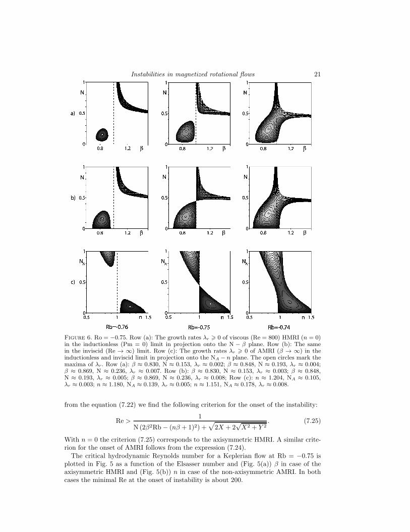
Figure 6. Ro = −0.75. Row (a): The growth rates λr > 0 of viscous (Re = 800) HMRI (n = 0)in the inductionless (Pm = 0) limit in projection onto the N − β plane. Row (b): The samein the inviscid (Re → ∞) limit. Row (c): The growth rates λr > 0 of AMRI (β → ∞) in theinductionless and inviscid limit in projection onto the NA − n plane. The open circles mark themaxima of λr. Row (a): β ≈ 0.830, N ≈ 0.153, λr ≈ 0.002; β ≈ 0.848, N ≈ 0.193, λr ≈ 0.004;β ≈ 0.869, N ≈ 0.236, λr ≈ 0.007. Row (b): β ≈ 0.830, N ≈ 0.153, λr ≈ 0.003; β ≈ 0.848,N ≈ 0.193, λr ≈ 0.005; β ≈ 0.869, N ≈ 0.236, λr ≈ 0.008; Row (c): n ≈ 1.204, NA ≈ 0.105,λr ≈ 0.003; n ≈ 1.180, NA ≈ 0.139, λr ≈ 0.005; n ≈ 1.151, NA ≈ 0.178, λr ≈ 0.008.
from the equation (7.22) we find the following criterion for the onset of the instability:
Re >1
N (2β2Rb− (nβ + 1)2) +√2X + 2
√X2 + Y 2
. (7.25)
With n = 0 the criterion (7.25) corresponds to the axisymmetric HMRI. A similar crite-rion for the onset of AMRI follows from the expression (7.24).The critical hydrodynamic Reynolds number for a Keplerian flow at Rb = −0.75 is
plotted in Fig. 5 as a function of the Elsasser number and (Fig. 5(a)) β in case of theaxisymmetric HMRI and (Fig. 5(b)) n in case of the non-axisymmetric AMRI. In bothcases the minimal Re at the onset of instability is about 200.
22 O. N. Kirillov, F. Stefani and Y. Fukumoto
7.7. HMRI and AMRI as magnetically destabilized inertial waves
Consider the Taylor expansion of the eigenvalues (7.20) with respect to the Elsassernumber N in the vicinity of N = 0
λ1,2 = −i(n∓ 2√Ro + 1)− 1
Re
+N(−(nβ + 1)2 + 2β2Rb± β (Ro+2)√
Ro+1(nβ + 1)
)+O(N2). (7.26)
Expressions (7.20) and (7.26) generalize the result of Priede (2011) to the case of arbitraryn, Re, and Rb and exactly coincide with it at n = 0, Re → ∞, and Rb = −1.In the absence of the magnetic field (N = 0) the eigenvalues λ1,2 correspond to damped
inertial waves. According to (7.25) at finite Re there exists a critical finite N > 0 that isnecessary to trigger destabilization of the inertial waves by the magnetic field, see Fig. 5and Fig. 6(a). However, as the expansion (7.26) demonstrates, in the limit Re → ∞ theinductionless magnetorotational instability occurs when the effect of the magnetic fieldis much weaker than that of the flow — even when the Elsasser number is infinitesimallysmall, Fig. 6(b,c).In the inviscid case the boundary of the domain of instability (7.25) takes the form
N = ±2
√β2(Ro + 2)2(nβ + 1)2 − ((nβ + 1)2 − 2β2Rb)2(Ro + 1)
((nβ + 1)2 − 4β2(Rb + 1))((nβ + 1)2 − 2β2Rb)2(nβ + 1)2. (7.27)
The lines (7.27) bound the domain of non-negative growth rates of HMRI in Fig. 6(b).When Ro = Rb, the stability boundary has a self-intersection at
n = − 1
β± 2
√Rb + 1, N =
±1
2β2
√−(3Rb + 2)
(Rb + 1)(Rb + 2). (7.28)
For example, when Rb = Ro = −0.75 and n = 0, the intersection happens at β = 1 andN =
√5/5, Fig. 6(b). If Rb = Ro = −0.75 and β → ∞, the intersection point is at n = 1
and NA =√5/5, Fig. 6(c). In general, the intersection exists at N 6= 0 for
Ro = Rb < −2
3. (7.29)
At Ro = Rb = − 23 the intersection occurs at N = 0.
In Fig. (6) we see that when Ro < − 23 and Ro > Rb, the instability domain consists
of two separate regions. In the case when Ro < − 23 and Ro < Rb, the two regions merge
into one. When the condition (7.29) is fulfilled, the two sub-domains touch each otherat the point (7.28). At Ro = Rb = − 2
3 the lower region shrinks to a single point whichsimultaneously is the intersection point (7.28) with N = 0.On the other hand, given Ro < −2/3 and decreasing Rb we find that the single
instability domain tends to split into two independent regions after crossing the lineRo = Rb. The further decrease in Rb yields diminishing the size of the lower instabilityregion, see Fig. 6. At which Rb does the lower instability region completely disappear?Clearly, the lower region disappears when the roots of the equation N(n) = 0 become
complex. From the expression (7.27) we derive
(nβ + 1)2 ± βRo + 2√Ro + 1
(nβ + 1)− 2β2Rb = 0. (7.30)
The equations (7.30) have the roots n complex if and only if their discriminant is negative:
(Ro + 2)2
Ro + 1+ 8Rb < 0, (7.31)
Instabilities in magnetized rotational flows 23
which is simply the domain with the boundary given by the curve of the Liu limits (7.15)that is shown in Fig. 3. Note that Rb = −2/3 and Ro = −2/3 satisfy the equation(7.15), which indicates that the line Ro = Rb is tangent to the curve (7.15) at the point(−2/3,−2/3) in the Ro-Rb plane, see Fig. 3(b).Finally, we notice that the left hand side of the equation (7.30) is precisely the coef-
ficient at N in the expansion (7.26). In the inviscid case it determines the limit of thestability boundary as N → 0, quite in accordance with the scaling law (7.18). Resolvingthe equation (7.30) with respect to Ro, we exactly reproduce the formula (7.2). At n = 0and Rb = −1 the equation (7.30) exactly coincides with that obtained by Priede (2011).
8. HMRI and AMRI at small, but finite Pm
An advantage of the inductionless limit discussed above is the considerable simplifica-tion of dispersion relations at Pm = 0 or Rm = 0 that yields expressions for growth ratesand stability criteria in explicit and closed form. Real physical situations are character-ized, however, by small but finite values of the magnetic Reynolds and Prandtl numbers.Below, we demonstrate numerically that HMRI and AMRI exist also when Pm 6= 0 orRm 6= 0. It turns out that, quite remarkably, the pattern of the stability domains keepsthe structure that we have found in the inductionless case. Moreover, the instability cri-teria of the inductionless limit serve as rather accurate guides in the physically morerealistic situation of finite Pm.
8.1. Islands of HMRI at various integer n and their reconnection
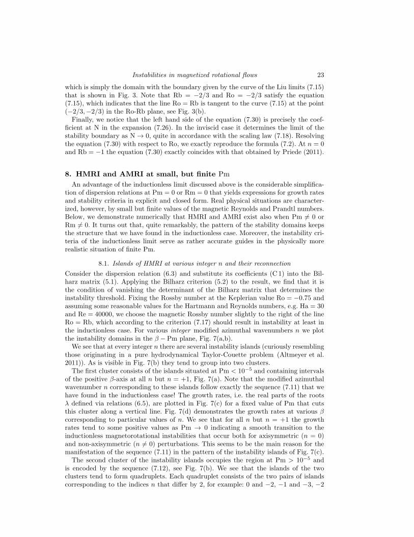
Consider the dispersion relation (6.3) and substitute its coefficients (C 1) into the Bil-harz matrix (5.1). Applying the Bilharz criterion (5.2) to the result, we find that it isthe condition of vanishing the determinant of the Bilharz matrix that determines theinstability threshold. Fixing the Rossby number at the Keplerian value Ro = −0.75 andassuming some reasonable values for the Hartmann and Reynolds numbers, e.g. Ha = 30and Re = 40000, we choose the magnetic Rossby number slightly to the right of the lineRo = Rb, which according to the criterion (7.17) should result in instability at least inthe inductionless case. For various integer modified azimuthal wavenumbers n we plotthe instability domains in the β − Pm plane, Fig. 7(a,b).We see that at every integer n there are several instability islands (curiously resembling
those originating in a pure hydrodynamical Taylor-Couette problem (Altmeyer et al.2011)). As is visible in Fig. 7(b) they tend to group into two clusters.The first cluster consists of the islands situated at Pm < 10−5 and containing intervals
of the positive β-axis at all n but n = +1, Fig. 7(a). Note that the modified azimuthalwavenumber n corresponding to these islands follow exactly the sequence (7.11) that wehave found in the inductionless case! The growth rates, i.e. the real parts of the rootsλ defined via relations (6.5), are plotted in Fig. 7(c) for a fixed value of Pm that cutsthis cluster along a vertical line. Fig. 7(d) demonstrates the growth rates at various βcorresponding to particular values of n. We see that for all n but n = +1 the growthrates tend to some positive values as Pm → 0 indicating a smooth transition to theinductionless magnetorotational instabilities that occur both for axisymmetric (n = 0)and non-axisymmetric (n 6= 0) perturbations. This seems to be the main reason for themanifestation of the sequence (7.11) in the pattern of the instability islands of Fig. 7(c).The second cluster of the instability islands occupies the region at Pm > 10−5 and
is encoded by the sequence (7.12), see Fig. 7(b). We see that the islands of the twoclusters tend to form quadruplets. Each quadruplet consists of the two pairs of islandscorresponding to the indices n that differ by 2, for example: 0 and −2, −1 and −3, −2
24 O. N. Kirillov, F. Stefani and Y. Fukumoto
Figure 7. Ha = 30, Ro = −0.75, Re = 40000, Rb = −0.755. (a,b) Islands of low Pm magnetoro-tational instability (HMRI for n = 0 and AMRI for n 6= 0) corresponding to different modifiedazimuthal wave numbers n. (c,d) The growth rates λr of the perturbation (c) as functions of βat Pm = 4 · 10−6 and different n and (d) as functions of Pm at different n and β.
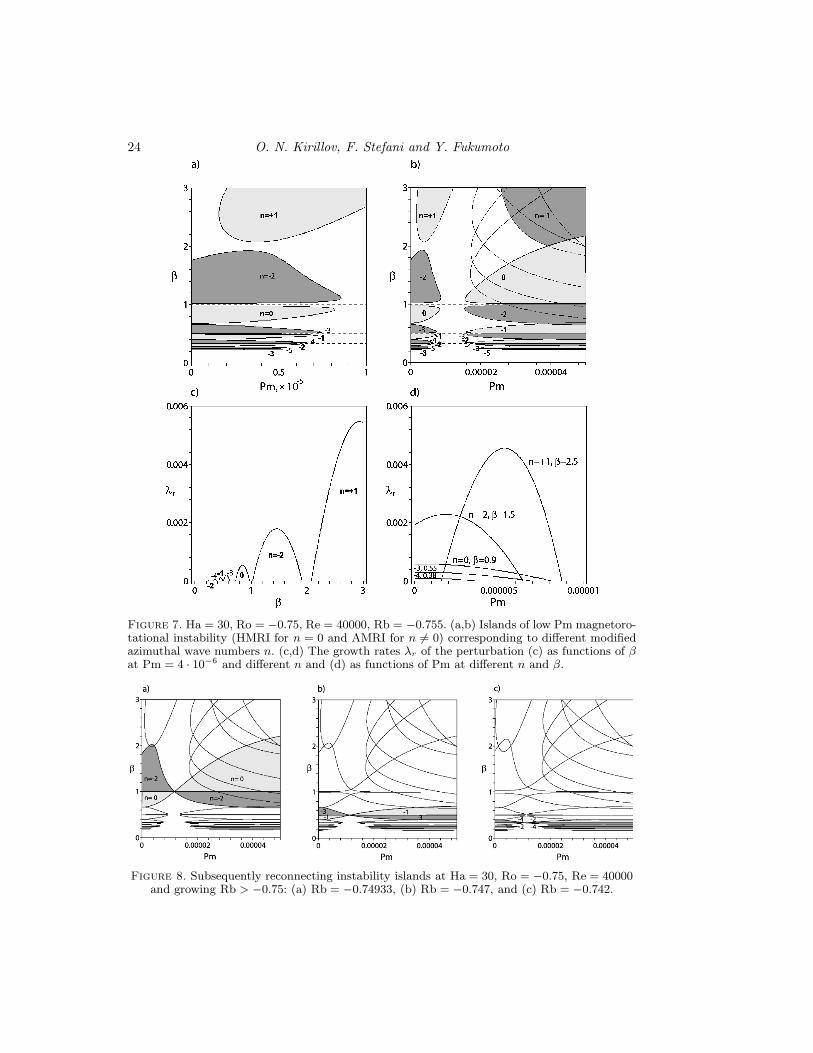
Figure 8. Subsequently reconnecting instability islands at Ha = 30, Ro = −0.75, Re = 40000and growing Rb > −0.75: (a) Rb = −0.74933, (b) Rb = −0.747, and (c) Rb = −0.742.
Instabilities in magnetized rotational flows 25
and −4 etc. Each quadruplet whose pairs are labeled with the indices ni, nj 6 0 tendsto be centered at β = βij , where
βij = − 2
ni + nj, (8.1)
which is exactly the second of the equations (7.10). Moreover, the whole pattern of theinstability islands in Fig. 7(b) repeats the pattern of cells in the second and third bandsshown in Fig. 2(a).It is natural to ask what are the conditions for reconnection of the islands in the pairs
that constitute every particular quadruplet. To get an idea we play with the two Rossbynumbers in Fig. 8. We fix Ro = −0.75 and slightly increase Rb. As a result, at Rb =−0.74933 the islands with the indices n = −2 and n = 0 reconnect at β−2,0 = 1, Fig. 8(a).At Rb = −0.747 these islands overlap whereas the islands in the next quadruplet withn = −3 and n = −1 reconnect at β−3,−1 = −1/2, Fig. 8(b). At Rb = −0.742 thereconnection happens in the third quadruplet at β−4,−2 = 1/3, and so on, Fig. 8(c).This sequence of the reconnections indicates the special role of the line Ro = Rb which
seems to be even more pronounced in the inviscid limit (Re → ∞). In the following wecheck these hypotheses when the magnetic field has only the azimuthal component whichcorresponds to the limit β → ∞.
8.2. AMRI as a dissipation-induced instability of Chandrasekhar’s equipartition solution
In the matrix (6.7) let us replace via the relation (7.23) the Elsasser number N of theaxial field with the Elsasser number of the azimuthal field NA and then let β → ∞. If,additionally
NA = Rm (8.2)
and
Ro = Rb, (8.3)
then in the ideal limit (Re → ∞, Rm → ∞) the roots of the dispersion relation (6.6) are
λ1,2 = 0, λ3,4 = −2i(n± 1). (8.4)
With the use of the relations (6.2) it is straightforward to verify that the condition (8.2)requires that Ω = ωAφ
. Thus, the conditions (8.2) and (8.3) are equivalent to (5.10), whichat Rb = Ro = −1 define the Chandrasekhar equipartition solution (Kirillov et al. 2014)belonging to a wide class of exact stationary solutions of MHD equations for the case ofideal incompressible infinitely conducting fluid with total constant pressure that includeseven knotted flows (Golovin & Krutikov 2012). It is well-known that the Chandrasekharequipartition solution is marginally stable (Chandrasekhar 1956, 1961; Bogoyavlenskij2004). According to equation (8.4) the marginal stability is preserved in the ideal casealso when Rb = Ro 6= −1. Will the roots (8.4) acquire only negative real parts with theaddition of electrical resistivity?In general, the answer is no. Indeed, under the constraints (8.2) and (8.3) in the limit
of vanishing viscosity (Re → ∞) the Bilharz criterion applied to the dispersion relation(6.6) gives the following threshold of instability
16(n2 − Rb2)(n2 − Rb− 2)2Rm4
+(n6 − 12n2Rb2 + 32n2(Rb + 1)− 16Rb2(Rb + 2))Rm2
−4Rb2 + 4n2(Rb + 1) = 0. (8.5)
In the (n,Rb,Rm) space the domain of instability is below the surface specified by
26 O. N. Kirillov, F. Stefani and Y. Fukumoto
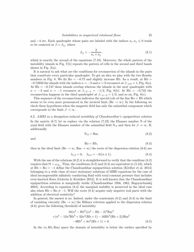
Figure 9. (a) The threshold of instability (8.5) at NA = Rm and Re → ∞ in the (n,Rb,Rm)space and (b) its projection onto Rb−n plane. The increase in Rm makes the instability domainmore narrow so that in the limit Rm → ∞ it degenerates into a ray (dashed) on the straight
line (8.6) that emerges from the point (open circle) with the coordinates n = 2√
3
3and Rb = − 2
3
and passes through the point with n = 1 and Rb = −1.
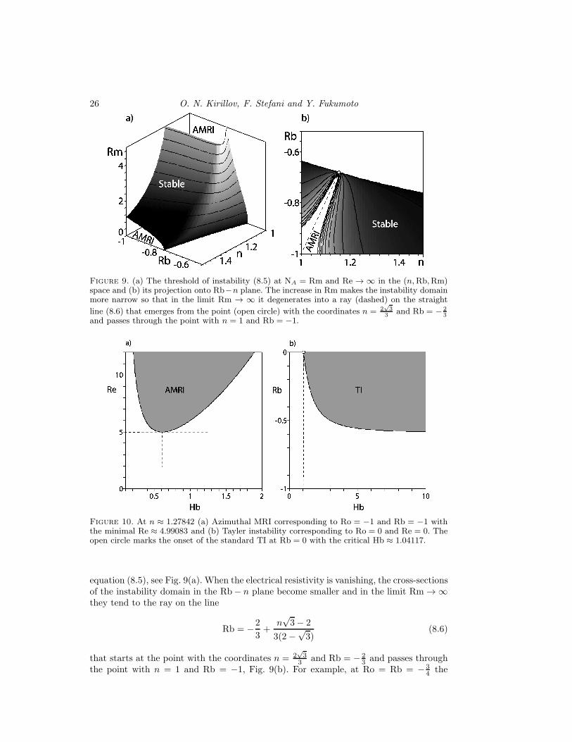
Figure 10. At n ≈ 1.27842 (a) Azimuthal MRI corresponding to Ro = −1 and Rb = −1 withthe minimal Re ≈ 4.99083 and (b) Tayler instability corresponding to Ro = 0 and Re = 0. Theopen circle marks the onset of the standard TI at Rb = 0 with the critical Hb ≈ 1.04117.
equation (8.5), see Fig. 9(a). When the electrical resistivity is vanishing, the cross-sectionsof the instability domain in the Rb− n plane become smaller and in the limit Rm → ∞they tend to the ray on the line
Rb = −2
3+
n√3− 2
3(2−√3)
(8.6)
that starts at the point with the coordinates n = 2√3
3 and Rb = − 23 and passes through
the point with n = 1 and Rb = −1, Fig. 9(b). For example, at Ro = Rb = − 34 the
Instabilities in magnetized rotational flows 27
equation (8.6) yields
n =1
4+
√3
2. (8.7)
On the contrary, when the magnetic Reynolds number Rm decreases, the instabilitydomain widens up and in the inductionless limit at Rm = 0 it is bounded by the curve
Rb =n(n−
√n2 + 4)
2. (8.8)
The wide part of the instability domain shown in Fig. 9(a) that exists at small Rmrepresents the azimuthal magnetorotational instability (AMRI). We see that this insta-bility quickly disappears with the increase of Rm or Rb. On the other hand, the idealsolution with the roots (8.4) that corresponds to the limit Rm → ∞ is destabilized bythe electrical resistivity. For n given by equation (8.7) we have, for example, an unstableroot λ ≈ 0.00026 − i0.00493 at Rm = 100. In general, if Rb and n satisfy (8.6), thenalready an infinitesimally weak electrical resistivity destabilizes the solution specifiedby the constraints (8.2) and (8.3) at vanishing kinematic viscosity that includes Chan-drasekhar’s equipartition solution as a special case. This dissipation-induced instability
(Kirillov 2009, 2013) further develops into the AMRI with Rm decreasing to zero.
9. Transition from AMRI to the Tayler instability
The Tayler instability (Tayler 1973; Rudiger & Schultz 2010) is a current-driven, kink-type instability that tapes into the magnetic field energy of the electrical current inthe fluid. Although its plasma-physics counterpart has been known for a long time, itsoccurrence in a liquid metal was observed only recently (Seilmayer et al. 2012). In thecontext of the on-going liquid-metal experiments in the frames of the DRESDYN project(Stefani et al. 2012) it is interesting to get an insight on the transition between theazimuthal magnetorotational instability and the Tayler instability.Consider the instability threshold (7.1) obtained in the inductionless approximation
(Pm = 0). Let us introduce the Hartmann number corresponding to the pure azimuthalmagnetic field as
Hb := βHa, (9.1)
so that NA = Hb2
Re . Substituting (9.1) into (7.1) and then letting β → ∞, we find
Re2 =((1 + Hb2n2)2 − 4Hb2Rb(1 + Hb2n2)− 4Hb4n2)(1 + Hb2(n2 − 2Rb))2
4(Hb4Ro2n2 − ((1 + Hb2(n2 − 2Rb))2 − 4Hb4n2)(Ro + 1)). (9.2)
Note that the expression (9.2) can also be derived from the equation (7.24).Consider the threshold of instability (9.2) in the two special cases corresponding to
the lower left and the upper right corners of the Ro − Rb diagram shown in Fig. 3(b).At Ro = −1 and Rb = −1 the function Re(n,Hb) that bounds the domain of AMRI hasa minimum Re ≈ 4.99083 at n ≈ 1.27842 and Hb ≈ 0.61185, see Fig. 10(a).Putting Re = 0 in (9.2), we find the threshold for the critical azimuthal magnetic field
Rb =(Hb2n2 + 1)2 − 4Hb4n2
4Hb2(1 + Hb2n2)(9.3)
that destabilizes electrically conducting fluid at rest (cf. criterion (5.5)). At Rb = 0 ex-pression (9.3) gives the value of the azimuthal magnetic field at the onset of the standard

28 O. N. Kirillov, F. Stefani and Y. Fukumoto
Figure 11. In the assumption that Ro(Rb) = −√−Rb2 − 2Rb and n ≈ 1.27842 (a) The domain
of the inductionless instability bounded by the surface (9.2) in the (Hb,Rb,Re) space and itscross-sections at (b) Re = 5.4, (c) Re = 5.734, and (d) Re = 6. The domains of TI and AMRIreconnect via a saddle point at Re = 5.734.
Tayler instability (cf. criterion (5.6))
Hb =1√
1− (1− |n|)2. (9.4)
For example, at n ≈ 1.27842
Hb ≈ 1.04117, (9.5)
see Fig. 10(b). In the following, we prefer to extend the notion of the Tayler instabilityto the whole domain bounded by the curve (9.3) and shown in gray in Fig. 10(b).How the domains of the Tayler instability and AMRI are related to each other? Is
there a connection between them in the parameter space?Let us look at the Ro − Rb diagram shown in Fig. 3(b). To connect the two opposite
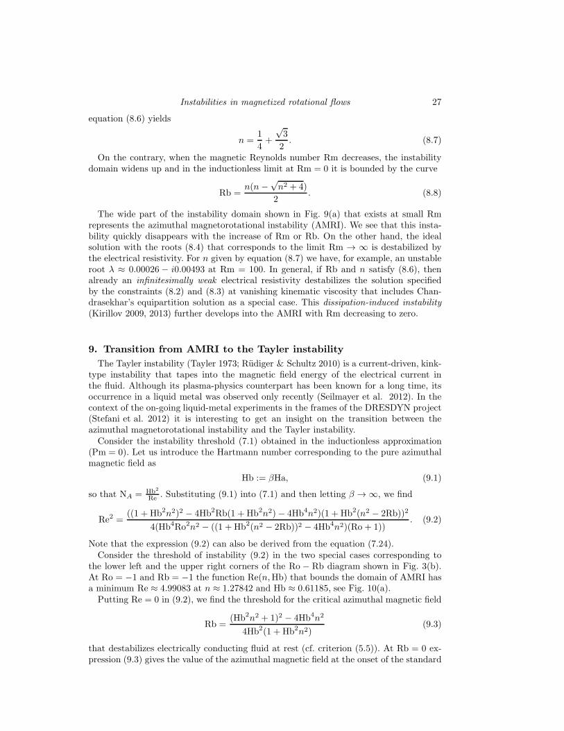
corners of it we obviously need to take a path that lies below the line Ro = Rb. Indeed,any path above this line penetrates the limiting curve (7.15) which creates an obstaclefor connecting the two regions shown in Fig. 10. On the contrary, any path below thediagonal in Fig. 3(b) lies within the instability domain which opens a possibility to
Instabilities in magnetized rotational flows 29
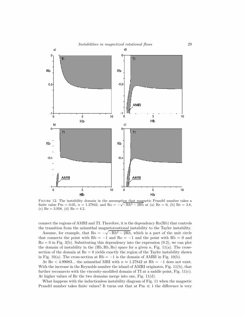
Figure 12. The instability domain in the assumption that magnetic Prandtl number takes afinite value Pm = 0.05, n = 1.27842, and Ro = −
√−Rb2 − 2Rb at (a) Re = 0, (b) Re = 3.8,
(c) Re = 3.958, (d) Re = 4.2.
connect the regions of AMRI and TI. Therefore, it is the dependency Ro(Rb) that controlsthe transition from the azimuthal magnetoroational instability to the Tayler instability.Assume, for example, that Ro = −
√−Rb2 − 2Rb, which is a part of the unit circle
that connects the point with Rb = −1 and Ro = −1 and the point with Rb = 0 andRo = 0 in Fig. 3(b). Substituting this dependency into the expression (9.2), we can plotthe domain of instability in the (Hb,Rb,Re) space for a given n, Fig. 11(a). The cross-section of the domain at Re = 0 yields exactly the region of the Tayler instability shownin Fig. 10(a). The cross-section at Rb = −1 is the domain of AMRI in Fig. 10(b).At Re < 4.99083... the azimuthal MRI with n ≈ 1.27842 at Rb = −1 does not exist.
With the increase in the Reynolds number the island of AMRI originates, Fig. 11(b), thatfurther reconnects with the viscosity-modified domain of TI at a saddle point, Fig. 11(c).At higher values of Re the two domains merge into one, Fig. 11(d).
What happens with the inductionless instability diagram of Fig. 11 when the magneticPrandtl number takes finite values? It turns out that at Pm ≪ 1 the difference is very
30 O. N. Kirillov, F. Stefani and Y. Fukumoto
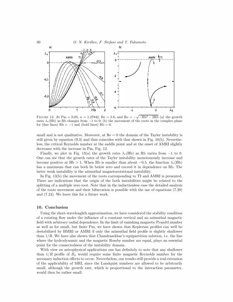
Figure 13. At Pm = 0.05, n = 1.27842, Re = 3.8, and Ro = −√−Rb2 − 2Rb (a) the growth
rates λr(Hb) as Rb changes from −1 to 0; (b) the movement of the roots in the complex planefor (fine lines) Rb = −1 and (bold lines) Rb = 0.
small and is not qualitative. Moreover, at Re = 0 the domain of the Tayler instability isstill given by equation (9.3) and thus coincides with that shown in Fig. 10(b). Neverthe-less, the critical Reynolds number at the saddle point and at the onset of AMRI slightlydecreases with the increase in Pm, Fig. 12.Finally, we plot in Fig. 13(a) the growth rates λr(Hb) as Rb varies from −1 to 0.
One can see that the growth rates of the Tayler instability monotonously increase andbecome positive at Hb > 1. When Rb is smaller than about −0.5, the function λr(Hb)has a maximum that can both lie below zero and exceed it in dependence on Rb. Thelatter weak instability is the azimuthal magnetorotational instability.In Fig. 13(b) the movement of the roots corresponding to TI and AMRI is presented.
There are indications that the origin of the both instabilities might be related to thesplitting of a multiple zero root. Note that in the inductionless case the detailed analysisof the roots movement and their bifurcation is possible with the use of equations (7.20)and (7.24). We leave this for a future work.
10. Conclusion
Using the short-wavelenghth approximation, we have considered the stability conditionof a rotating flow under the influence of a constant vertical and an azimuthal magneticfield with arbitrary radial dependence. In the limit of vanishing magnetic Prandtl numberas well as for small, but finite Pm, we have shown that Keplerian profiles can well bedestabilized by HMRI or AMRI if only the azimuthal field profile is slightly shallowerthan 1/R. We have also shown that Chandrasekhar’s equipartition solution, i.e. the linewhere the hydrodynamic and the magnetic Rossby number are equal, plays an essentialpoint for the connectedness of the instability domain.With view on astrophysical applications one has definitely to note that any shallower
than 1/R profile of Bφ would require some finite magnetic Reynolds number for thenecessary induction effects to occur. Nevertheless, our results still provide a real extensionof the applicability of MRI, since the Lundquist numbers are allowed to be arbitrarilysmall, although the growth rate, which is proportional to the interaction parameter,would then be rather small.
Instabilities in magnetized rotational flows 31
The consequences of our findings for those parts of accretion disks with small magneticPrandtl numbers are still to be elaborated. The action of MRI in the dead zones ofprotoplanetary disks is an example for which the extended parameter region might haveconsequences. Particular attention should also be given to the possibility of quasi-periodicoscillations which might easily result from the sensitive dependence of the action of HMRIon the radial profile of of Bφ and the ratio of the latter to Bz. We notice however thatpure hydrodynamical scenarios of transition to turbulence in the dead zones had alsobeen proposed (Marcus et al. 2013).As for liquid metal experiments, our results give strong impetus for a special set-up in
which the magnetic Rossby number can be adjusted by using two independent electricalcurrents, one through an central, insulated rod, the second one through the liquid metal.A liquid sodium experiment dedicated exactly to this problem is presently being designedin the framework of the DRESDYN project (Stefani et al. 2012). Apart from this, therecently observed, and numerically confirmed, strong sensitivity of AMRI on a slightsymmetry breaking of an external magnetic field (Seilmayer et al. 2013) may also berelated to our findings.
Acknowledgement
This work was supported by Helmholtz-Gemeinschaft Deutscher Forschungszentren(HGF) in frame of the Helmholtz Alliance LIMTECH, as well as by Deutsche Forschungs-gemeinschaft in frame of the SPP 1488 (PlanetMag). We acknowledge fruitful discussionswith Marcus Gellert, Rainer Hollerbach, and Gunther Rudiger.
Appendix A. Some technical details
For convenience, we provide here explicit expressions for the vectors (B0 · ∇)u(0),
(B0 · ∇)B(0), and (u0 · ∇)u(0) in cylindrical coordinates:
(B0 · ∇)u(0) =
B0φ
R ∂φu(0)R +B0
z∂zu(0)R − B0
φu(0)φ
RB0
φ
R ∂φu(0)φ +B0
z∂zu(0)φ +
B0φu
(0)R
RB0
φ
R ∂φu(0)z +B0
z∂zu(0)z
,
(B0 · ∇)B(0) =
B0φ
R ∂φB(0)R +B0
z∂zB(0)R − B0
φB(0)φ
RB0
φ
R ∂φB(0)φ +B0
z∂zB(0)φ +
B0φB
(0)R
RB0
φ
R ∂φB(0)z +B0
z∂zB(0)z
,
(u0 · ∇)u(0) =
u0R∂Ru
(0)R +
u0φ
R
(∂φu
(0)R − u
(0)φ
)+ u0
z∂zu(0)R
u0R∂Ru
(0)φ +
u0φ
R
(∂φu
(0)φ + u
(0)R
)+ u0
z∂zu(0)φ
u0R∂Ru
(0)z +
u0φ
R ∂φu(0)z + u0
z∂zu(0)z
. (A 1)
Appendix B. Connection to the work of Krueger et al. (1966)
The linearized equations derived in the small gap approximation by Krueger et al.(1966) have the form
L(D2 − (kzd)2)u′ = −(kzd)
2TΩl(x)v′, Lv′ = u′, (B 1)
32 O. N. Kirillov, F. Stefani and Y. Fukumoto
whereD = d/dx, d/dR = d−1d/dx, T = −4aΩ1d4/ν2, u′ = u2adδ/(νΩ1), v
′ = v/(R1Ω1),δ = d/R1,
L := D2 − (kzd)2 − i(σ + k
√T Ωl(x)), Ωl(x) = 1− (1 − µ)x, (B 2)
σ = ωd2/ν, and k = m√−Ω1
4a . The coefficient a is defined by Eq. (2.10). Then,
L = −d2
ν
(ν(k2R + k2z) + i(ω +mΩ1Ωl)
)
= −d2
ν
(ν|k|2 + i(ω +mΩ1Ωl)
)= −d2
ν(ων + i(ω +mΩ1Ωl)) . (B 3)
Consequently, the first equation in (B 1) becomes
− d2
ν(ων + i(ω +mΩ1Ωl)) (−d2|k|2)2adδ
νΩ1u = −k2zd
2(−4aΩ1d4/ν2)Ωlv/(R1Ω1).(B 4)
Simplifying this equation yields
(ων + i(ω +mΩ1Ωl)) |k|2u = vk2z2Ω1Ωld/(δR1), (B 5)
and, finally,
(ων + i(ω +mΩ1Ωl))u = 2α2Ω1Ωlv, (B 6)
where α = kz/|k|. The second equation in (B 1) takes the form
(ων + i(ω +mΩ1Ωl)) v = −2auδR1/d, (B 7)
and, finally,
(ων + i(ω +mΩ1Ωl)) v = −2Ω(1 + Ro)u. (B 8)
The equations (B 6) and (B8) constitute the following system
(ων + i(ω +mΩ1Ωl)) u = 2α2Ω1Ωlv,
(ων + i(ω +mΩ1Ωl)) v = −2Ω(1 + Ro)u. (B 9)
Since Ω ≈ Ω1Ωl, then
(ων + i(ω +mΩ))u = 2α2Ωv,
(ων + i(ω +mΩ)) v = −2Ω(1 + Ro)u. (B 10)
The system (B 10) can be written in the matrix form Aw = iωw with the vector w =(u, v)T and
A =
(−imΩ− ων 2α2Ω−2Ω(1 + Ro) −imΩ− ων
). (B 11)
The matrix A is nothing else but the submatrix of the matrix H defined by Eq. (4.10)situated at the corner corresponding to the first two rows and first two columns of H.Let A0 = A(ων = 0), then
A0 = −G−1AT
0 G, G = iJ, J =
(0 −11 0
), (B 12)
meaning that F = −iGA0 = FTis a Hermitian matrix:
F =
(2Ω(1 + Ro) imΩ
−imΩ 2α2Ω
). (B 13)

Instabilities in magnetized rotational flows 33
Then, the eigenvalue problem A0w = iωw acquires the Hamiltonian form
Fw = iωJw, F = FT. (B 14)
Appendix C. Coefficients of the dimensionless dispersion relations
The coefficients of the complex polynomial (6.3) are:
a0 = 1, b0 = 0, a1 = 2(√
Pm+ 1√Pm
), b1 = 4nRe
√Pm,
a2 = 2(β2Ha2 − 3Re2Pm)n2 + 4βHa2n
+2(1 + (1 − 2Rbβ2)Ha2) + 4Re2(1 + Ro)Pm+a21
4 , b2 = 6nRe(1 + Pm),
a3 = a1(β2Ha2 − 3Re2Pm)n2 + 2a1βHa
2n
+a1(1 + (1 − 2Rbβ2)Ha2) + 8Re2(1 + Ro)√Pm,
b3 = 4n3√PmRe(β2Ha2 − Re2Pm)
+2nRe(4Pm2Re2(1 + Ro) + (1 + Pm)2 + 2Pm(1 + Ha2))/√Pm
−8(1− n2 + βn(1 + Rb))βHa2Re√Pm,
a4 = ((β2Ha2 − Re2Pm)n2 + 2Ha2βn+Ha2 + 2PmRe2)2
+2(2Re2PmRo + 1)((Ha2β2 − Re2Pm)n2 + 2Ha2βn+Ha2)− (1 + Pm)2Re2n2
+4Re2(1 + Ro)− (Ha2 + 2PmRe2)2 +Ha4 + 1− 4Rbβ2Ha2
−4Ha2β2(Ha2(βn+ 1)2 − PmRe2n2)(1 + Rb),
b4 = 2Re(1 + Pm)(β2Ha2 − Re2Pm)n3 + 4ReHa2β(1 + Pm)n2
+2Re(2(1 + Ro)(2Re2Pm− β2Ha2(1−Pm))+(1+Pm)(1 + Ha2(1− 2β2(1 + Rb))))n
−4βHa2Re(2 + (1− Pm)Ro). (C 1)
The next equation gives the coefficients of the dispersion relation (6.6):
a0 = 1, b0 = 0, a1 = 2(
1Re +
1Rm
), b1 = 4n,
a2 = 2(
β2NRm − 3
)n2 + 4βN
Rm n
+ 2Rm
(1Re + (1− 2Rbβ2)N
)+ 4(1 + Ro) +
a21
4 , b2 = 34a1b1,
a3 = a1
(β2NRm − 3
)n2 + 2a1β
NRmn+ a1
Rm
(1Re + (1 − 2Rbβ2)N
)+ 8
Rm (1 + Ro),
b3 = 4(
β2NRm − 1
)n3 + 2n
(4(1 + Ro) +
a21
4 + 2Rm
(1Re +N
))
−8(1− n2 + βn(1 + Rb)) βNRm ,
a4 =(
β2NRm − 1
)2n4 + 4βN
Rm
(β2NRm − 1
)n3
+(
2Rm
(β2NRm − 1
) (N+ 1
Re−2(β2(1+Rb)N−(1+Ro)Rm))+ 4N2β2
Rm2 − a21
4
)n2
+ 4NβRm2
(N+ 1
Re − 2(β2(1 + Rb)N− (1 + Ro)Rm))n
+ 1Rm2
((N+ 1
Re
)2 − 4N(
β2RbRe − RoRm
)+ 4(1 + Ro)− 4N2β2(1 + Rb)
),
b4 = a1
(β2NRm − 1
)n3 + 2a1
βNRmn2 − 4βN
Rm
(2
Rm +(
1Rm − 1
Re
)Ro)
+(
a1
Rm
(1Re + (1 + 2β2(Ro− Rb))N
)− 8(1+Ro)
Rm
(β2NRm − 1
))n. (C 2)
34 O. N. Kirillov, F. Stefani and Y. Fukumoto
REFERENCES
Acheson, D. J. 1978 On the instability of toroidal magnetic fields and differential rotation instars. Phil. Trans. R. Soc. A 289(1363), 459–500.
Acheson, D. J. & Hide, R. 1973 Hydromagnetics of rotating fluids. Rep. Prog. Phys. 36,159–221.
Altmeyer, S., Hoffmann, C. & Lucke, M. 2011 Islands of instability for growth of spiralvortices in the Taylor-Couette system with and without axial through flow. Phys. Rev. E84, 046308.
Armitage, P. J. 2011 Protoplanetary disks and their evolution. Annu. Rev. Astron. Astrophys.49, 67–117.
Balbus, S. A. & Hawley, J. F. 1991 A powerful local shear instability in weakly magnetizeddisks. 1. Linear Analysis. Astrophys. J., 376, 214–222.
Balbus, S. A. & Hawley, J. F. 1992 A powerful local shear instability in weakly magnetizeddisks. 4. Nonaxisymmetric perturbations. Astrophys. J., 400, 610–621.
Bayly, B. J. 1988 Three-dimensional centrifugal-type instabilities in inviscid two-dimensionalflows. Phys. Fluids 31, 56–64.
Bilharz, H. 1944 Bemerkung zu einem Satze von Hurwitz. Zeitschrift fur Angewandte Mathe-matik und Mechanik 24, 77–82.
Bogoyavlenskij, O. I. 2004 Unsteady equipartition MHD solutions. Journal of MathematicalPhysics 45, 381–390.
Brandenburg, A., Nordlund, A., Stein, R.F. & Torkelsson, U. 1995 Dynamo-generatedturbulence and large-scale magnetic fields in a Keplerian shear flow. Astrophys. J. 446,741–754.
Chandrasekhar, S. 1956 On the stability of the simplest solution of the equations of hydro-magnetics. Proc. Natl. Acad. Sci. U.S.A. 42, 273–276.
Chandrasekhar, S. 1960 The stability of non-dissipative Couette flow in hydromagnetics.Proc. Natl. Acad. Sci. U.S.A. 46, 253–257.
Chandrasekhar, S. 1961 Hydrodynamic and hydromagnetic stability, Oxford University Press,Oxford, UK.
Dobrokhotov, S. & Shafarevich, A. 1992 Parametrix and the asymptotics of localizedsolutions of the Navier-Stokes equations in R3, linearized on a smooth flow. Math. Notes,51, 47–54.
Done, C., Gierlinski, M. & Kubota, A. 2007 Modelling the behaviour of accretion flows inX-ray binaries. Astron. Astrophys. Rev., 15, 1–66.
Eckhoff, K. S. 1987 Linear waves and stability in ideal magnetohydrodynamics. Phys. Fluids30, 3673–3685.
Eckhardt, B. & Yao, D. 1995 Local stability analysis along Lagrangian paths. Chaos, Solitons& Fractals, 5(11), 2073–2088.
Fleming, T. P., Stone, J. M., & Hawley, J. F. 2010 The effect of resistivity on the nonlinearstage of the magnetorotational instability in accretion disks. Astrophys. J. 530, 464–477.
Friedlander, S. & Vishik, M. M. 1995 On stability and instability criteria for magnetohy-drodynamics. Chaos 5, 416-423.
Friedlander, S. & Lipton-Lifschitz, A. 2003 Localized instabilities in fluids. In Handbookof Mathematical Fluid Dynamics, vol. II (ed. S. J. Friedlander & D. Serre), vol. 2, pp.289–353. Elsevier.
Fromang, S. & Papaloizou, J. 2007 MHD simulations of the magnetorotational instability ina shearing box with zero net flux. Astron. Astrophys. 476, 1113–1122.
Fuchs, H., Radler, K.-H. & Rheinhardt, M. 1999 On self-killing and self-creating dynamos.Astron. Nachr. 320, 127–131.
Gailitis, A., Lielausis, O., Dement’ev, S., Platacis, E., Cifersons, A., Gerbeth, G.,Gundrum, T., Stefani, F., Christen, M., Hanel, H., Will, G. 2000 Detection of aflow induced magnetic field eigenmode in the Riga dynamo facility. Phys. Rev. Lett. 84,4365–4368.
Goedbloed, H., Keppens, R. & Poedts, S. 2010 Advanced Magnetohydrodynamics, Cam-bridge University Press, Cambridge, UK.
Golovin, S.V. & Krutikov, M.K. 2012 Complete classification of stationary flows with con-
Instabilities in magnetized rotational flows 35
stant total pressure of ideal incompressible infinitely conducting fluid. J. Phys. A: Math.Theor. 45, 235501.
Hattori, Y. & Fukumoto, Y. 2003 Short-wavelength stability analysis of thin vortex rings.Phys. Fluids 15(10), 3151–3163.
Herault, J., Rincon, F., Cossu, C., Lesur, G., Ogilvie, G.I., & Longaretti, P.-Y.2011. Periodic magnetorotational dynamo action as a prototype of nonlinear magnetic-field generation in shear flows. Phys. Rev. E 84(10), 036321.
Hollerbach, R. & Rudiger, G. 2005 New Type of Magnetorotational Instability in Cylindri-cal Taylor-Couette Flow. Phys. Rev. Lett. 95(12), 124501.
Hollerbach, R., Teeluck, V. & Rudiger, G. 2010 Nonaxisymmetric magnetorotationalinstabilities in cylindrical Taylor-Couette flow. Phys. Rev. Lett. 104, 044502.
Howard, L. N. & Gupta, A. S. 1962 On the hydrodynamic and hydromagnetic stability ofswirling flows. J. Fluid Mech. 14, 463-476.
Ji, H., Goodman, J. & Kageyama, A. 2001 Magnetorotational instability in a rotating liquidmetal annulus. Mon. Not. R. Astron. Soc. 325(2), L1–L5.
Ji, H. & Balbus, S. 2013 Angular momentum transport in astrophysics and in the lab. PhysicsToday August 2013, 27–33.
Kapyla, P. J. & Korpi, M. J. 2011 Magnetorotational instability driven dynamos at lowmagnetic Prandtl numbers. Mon. Not. R. Astr. Soc., 413, 901-907.
Kirillov, O. N. 2009 Campbell diagrams of weakly anisotropic flexible rotors. Proc. of theRoyal Society A 465, 2703–2723.
Kirillov, O. N. & Stefani, F. 2010 On the relation of standard and helical magnetorotationalinstability. Astrophys. J., 712, 52–68.
Kirillov, O. N. & Stefani, F. 2011 Paradoxes of magnetorotational instability and theirgeometrical resolution. Phys. Rev. E 84(3), 036304.
Kirillov, O. N. & Stefani, F. 2012 Standard and helical magnetorotational instability: Howsingularities create paradoxal phenomena in MHD. Acta Appl. Math. 120, 177–198.
Kirillov, O. N., Stefani, F., & Fukumoto, Y. 2012 A unifying picture of helical and az-imuthal MRI, and the universal significance of the Liu limit. Astrophys. J., 756, 83 (6pp).
Kirillov, O. N. & Stefani, F. 2013 Extending the range of the inductionless magnetorota-tional instability. Phys. Rev. Lett., 111, 061103 (5pp).
Kirillov, O. N. 2013 Nonconservative stability problems of modern physics, De Gruyter Studiesin Mathematical Physics 14, De Gruyter, Berlin, Boston.
Kirillov, O. N., Stefani, F., & Fukumoto, Y. 2014 Instabilities of rotational flows in az-imuthal magnetic fields of arbitrary radial dependence. Fluid Dyn. Res., 46, in press.
Krolik, J. H. 1998 Active Galactic Nuclei, Princeton University Press, Princeton.Krueger, E. R., Gross, A., & Di Prima, R. C. 1966 On relative importance of Taylor-
vortex and non-axisymmetric modes in flow between rotating cylinders. J. Fluid Mech.,24(3), 521–538.
Landman, M. J. & Saffman P. G. 1987 The three-dimensional instability of strained vorticesin a viscous fluid. Phys. Fluids 30, 2339–2342.
Lesur, G. & Longaretti, P.-Y. 2007 Impact of dimensionless numbers on the efficiencyof magnetorotational instability induced turbulent transport. Mon. Not. R. Astron. Soc.378(8), 1471-1480.
Lifschitz, A. 1989 Magnetohydrodynamics and Spectral Theory, Kluwer Academic Publishers,Dordrecht.
Lifschitz, A. & Hameiri, E. 1991 Local stability conditions in fluid dynamics. Phys. FluidsA 3, 2644–2651.
Lifschitz, A. 1991 Short wavelength instabilities of incompressible three-dimensional flows andgeneration of vorticity. Phys. Lett. A 157, 481–486.
Liu, W., Goodman, J., Herron, I., & Ji, H. 2006 Helical magnetorotational instability inmagnetized Taylor-Couette flow. Phys. Rev. E 74(5), 056302.
Marcus, P. S., Pei, S., Jiang, C.-H., Hassanzadeh, P. 2013 Three-Dimensional VorticesGenerated by Self-Replication in Stably Stratified Rotating Shear Flows. Phys. Rev. Lett.,111(8), 084501.
Michael, D. H. 1954 The stability of an incompressible electrically conducting fluid rotatingabout an axis when current flows parallel to the axis. Mathematika, 1, 45–50.

36 O. N. Kirillov, F. Stefani and Y. Fukumoto
Monchaux, R., Berhanu, M., Bourgoin, M., Moulin, M., Odier, Ph., Pinton, J.-F.,Volk, R., Fauve, S., Mordant, N., Petrelis, F., Chiffaudel, A., Daviaud, F.,Dubrulle, B., Gasquet, C., Mari, L., Ravelet, F. 2007 Generation of a magneticfield by dynamo action in a turbulent flow of liquid sodium. Phys. Rev. Lett., 98, 044502.
Muller, U. & Stieglitz, R. 2000 Can the Earth’s magnetic field be simulated in the labora-tory? Naturwissenschaften, 87, 381–390.
Nornberg, M. D., Ji, H., Schartman, E, & Roach, A. 2010 Observation of magnetocoriolisWwves in a liquid metal Taylor-Couette experiment. Phys. Rev. Lett., 104, 074501.
Ogilvie, G. I. & Pringle, J. E. 1996 The non-axisymmetric instability of a cylindrical shearflow containing an azimuthal magnetic field. Mon. Not. R. Astron. Soc., 279, 152–164.
Oishi, J. S. & Mac Low, M.-M. 2011 Magnetorotational turbulence transports angular mo-mentum in stratified disks with low magnetic Prandtl number but magnetic Reynoldsnumber above a critical value. Astrophys. J., 740, 18.
Petitdemange, L., Dormy, E. & Balbus, S. A. 2008 Magnetostrophic MRI in the Earth’souter core. Geophys. Res. Lett., 35, L15305.
Priede, J. 2011 Inviscid helical magnetorotational instability in cylindrical Taylor-Couette flow.Phys. Rev. E , 84, 066314.
Rudiger, G. & Schultz, M. 2010 Tayler instability of toroidal magnetic fields in MHD Taylor-Couette flows. Astron. Nachr. 331, 121–129.
Rudiger, G. & Hollerbach, R. 2007 Comment on ”Helical magnetorotational instability inmagnetized Taylor-Couette flow”. Phys. Rev E 76, 068301.
Rudiger, G., Gellert, M., Schultz, M. & Hollerbach, R. 2010 Dissipative Taylor-Couetteflows under the influence of helical magnetic fields. Phys. Rev E 82, 016319.
Rudiger, G., Hollerbach, R. & Kitchatinov, L. 2013 Magnetic Processes in Astrophysics,Wiley-VCH, Berlin.
Seilmayer, M., Stefani, F., Gundrum, T., Weier, T., Gerbeth G., Gellert, M.,Rudiger, G. 2012 Experimental evidence for a transient Tayler instability in a cylindricalliquid metal column. Phys. Rev. Lett. 108, 244501.
Seilmayer, M., Galindo, V., Gerbeth, G., Gundrum, T., Stefani, F., Gellert, M.,Rudiger, G., Schultz, M., & Hollerbach, R. 2013 Experimental evidence for non-axisymmetric magnetorotational instability in an azimuthal magnetic field. Phys. Rev. Lett.submitted; arXiv:1311.7223.
Shi, J., Krolik, J.H., & Hirose, S. What is the numerically converged amplitude of magne-tohydrodynamics turbulence in stratified shearing boxes? Astrophys. J. 708, 1716.
Sisan, D.R., Mujica, N., Tillotson, W.A., Huang, Y.-M., Dorland, W., Hassam, A.B.,Antonsen, T.M., Lathrop, D.P. 2004 Experimental observation and characterization ofthe magnetorotational instability. Phys. Rev. Lett. 93, 114502.
Spruit, H. C. Dynamo action by differential rotation in a stably stratified stellar interior.Astron. & Astrophys. 381, 923–932.
Stefani, F., Gundrum, T., Gerbeth, G., Rudiger, G., Schultz, M., Szklarski, J., &Hollerbach,R. 2006 Experimental evidence for magnetorotational instability in a Taylor-Couette flow under the influence of a helical magnetic field. Phys. Rev. Lett. 97, 184502.
Stefani, F., Gundrum, T., Gerbeth, G., Rudiger, G., Szklarski, J., & Hollerbach, R.2006 Experiments on the magnetorotational instability in helical magnetic fields. New J.Phys. 9, 295.
Stefani, F., Gerbeth, G., Gundrum, T., Hollerbach, R., Priede, J., Rudiger, G., &Szklarski, J. 2009 Helical magnetorotational instability in a Taylor-Couette flow withstrongly reduced Ekman pumping. Phys. Rev. E. 80, 066303.
Stefani, F., Gailitis, A., & Gerbeth, G. 2008 Magnetohydrodynamic experiments on cosmicmagnetic fields. ZAMM 88, 930-954.
Stefani, F., Eckert, S., Gerbeth, G., Giesecke, A., Gundrum, T., Steglich, C., Weier,T., & Wustmann, B. 2012 DRESDYN - A new facility for MHD experiments with liquidsodium. Magnetohydrodynamics 48, 103-113.
Tayler, R. 1973 The adiabatic stability of stars containing magnetic fields. Mon. Not. R. Astr.Soc., 161, 365–380.
Umurhan, O. M. 2010 Low magnetic-Prandtl number flow configurations for cold astrophysicaldisk models: speculation and analysis. Astron. Astrophys., 513, A47.

Instabilities in magnetized rotational flows 37
Velikhov, E. P. 1959 Stability of an ideally conducting liquid flowing between cylinders rotat-ing in a magnetic field. Sov. Phys. JETP-USSR, 9, 995–998.
Weber, N., Galindo, V., Stefani, F., Weier, T., & Wondrak, T. 2013 Numerical simu-lation of the Tayler instability in liquid metals. New J. Phys., 15, 043034.