Mars without the equilibrium rotational figure, Tharsis,and the remnant rotational figure

I. Matsuyama1 and M. Manga1

Received 29 June 2010; revised 24 September 2010; accepted 13 October 2010; published 31 December 2010.

[1] We use a revised partitioning of the planet figure into equilibrium and nonequilibriumcontributions that takes into account the presence of an elastic lithosphere to study theMartian gravity field and shape. The equilibrium contribution is associated with thepresent rotational figure, and the nonequilibrium contribution is dominated by Tharsis anda remnant rotational figure supported by the elastic lithosphere that traces the paleopolelocation prior to the formation of Tharsis. We calculate the probability density functionsfor Tharsis’ size and location, the paleopole location, and the global average thickness ofthe elastic lithosphere at the time Tharsis was emplaced. Given the observed degree‐3spherical harmonic gravity coefficients, the expected Tharsis center location is 258.6 ± 4.2°E,9.8 ± 0.9°N, where the uncertainties represent the 90% confidence interval. Given thisTharsis center location and the observed degree‐2 spherical harmonic gravity coefficients,the expected paleopole location prior to the emplacement of Tharsis is 259.5 ± 49.5°E,71.1−14.4+17.5°N, and the expected elastic lithospheric thickness at the time of loading is58−32

+34 km. Our estimated paleopole colatitude implies 18.9−17.5+14.4° of true polar wander

(TPW) driven by the emplacement of Tharsis, in disagreement with previous studies thatinvoke large TPW. The remnant rotational figure is visible in both the nonequilibriumdegree‐2 geoid (areoid) without Tharsis and the nonequilibrium degree‐2 topographywithout Tharsis. The remnant rotational figure is also visible in the total nonequilibriumgeoid without Tharsis, but it is not visible in the total nonequilibrium topography withoutTharsis due to the strong signal of the north‐south dichotomy. Shorter wavelengthgeological features become significantly more visible in the geoid with the removal of thelong wavelength contributions of the equilibrium rotational figure, Tharsis, and theremnant rotational figure. Removal of the equilibrium rotational figure and Tharsis fromthe topography reveals a better defined north‐south dichotomy boundary.

Citation: Matsuyama, I., and M. Manga (2010), Mars without the equilibrium rotational figure, Tharsis, and the remnantrotational figure, J. Geophys. Res., 115, E12020, doi:10.1029/2010JE003686.

1. Introduction

[2] The gravitational figure of planetary bodies is com-monly partitioned into hydrostatic and nonhydrostatic con-tributions (hereafter nonhydrostatic theory). In this case,under the assumption that the planet has no long‐termrigidity, the hydrostatic contribution corresponds to therotational figure assuming hydrostatic equilibrium. The re-maining gravitational figure comprises the nonhydrostaticcontribution. However, the nonhydrostatic theory is gener-ally not suitable for planets with an elastic lithosphere likeMars. Bills and James [1999] noted that the present Martianrotational state is unstable in the framework of the non-hydrostatic theory. Daradich et al. [2008] showed that thepresent Martian rotation pole is stable, as expected, with a

revised partitioning into equilibrium and nonequilibriumcontributions (hereafter nonequilibrium theory). We extendtheir analysis in several ways. First, Daradich et al. [2008]focused on two degree‐2 spherical harmonic gravity coef-ficients (C20 and C22), while we consider all the degree‐2spherical harmonic coefficients. Second, Daradich et al.[2008] used the Tharsis center location estimated by Zuberand Smith [1997]. The latter study adopts the traditionalpartitioning of the gravitational figure, while we calculatethe location of the Tharsis center using a method that isindependent of the adopted partitioning. Third, in addition tofinding best fit solutions, we calculate probability densityfunctions for the thickness of the elastic lithosphere, Tharsis’size and location, and the paleopole location given theobserved spherical harmonic gravity coefficients. Finally,we consider the effect of the equilibrium and nonequilibriumcontributions on the Martian gravity field and shape.[3] Gravitational field observations have been used to

argue for large true polar wander (TPW), a change in theorientation of a planet relative to its rotation vector, driven

1Department of Earth and Planetary Science, University of California,Berkeley, California, USA.

Copyright 2010 by the American Geophysical Union.0148‐0227/10/2010JE003686

JOURNAL OF GEOPHYSICAL RESEARCH, VOL. 115, E12020, doi:10.1029/2010JE003686, 2010

E12020 1 of 14

by the mass distribution associated with the emplacement ofTharsis [Zuber and Smith, 1997; Sprenke et al., 2005].However, these studies adopt the traditional partitioning ofthe gravitational figure into hydrostatic and nonhydrostaticcontributions. Our probability density functions for thepaleopole longitude and latitude provide revised constraintson the possible TPW driven by the formation of Tharsis.

2. Traditional Partitioning of the GravitationalFigure

[4] We expand the gravity field at a point with sphericalcoordinates (r, �, �) in spherical surface harmonics as

F¼GM

rþGM

r

X∞‘¼1

X‘m¼0

R

r

� �‘

P‘m cos �ð Þ C‘m cosm�þS‘m sinm�½ �;

ð1Þ

where G is the gravitational constant, M is the planetmass, R is the mean planetary radius, P‘m is the associatedLegendre function, and C‘m and S‘m are spherical harmoniccoefficients. We adopt the sign convention of geodesy andastronomy in which the gravitational potential is positive,and the following definition for the associated Legendrefunctions [e.g., Arfken and Weber, 1995],

P‘m xð Þ ¼ 1� x2� �m=2 dm

dxmP‘ xð Þ; ð2Þ

whereP‘ is a Legendre polynomial.We use the Jet PropulsionLaboratory Mars gravity field MRO95A [Zuber, 2008]. Theunnormalized degree‐2 spherical harmonic coefficients arelisted in Table 1.[5] Given the unnormalized degree‐2 spherical harmonic

coefficients, the total inertia tensor can be written as [e.g.,Lambeck, 1980]

Iij ¼ I0�ij þMR2

13C20 � 2C22 �2S22 �C21

�2S22 13C20 þ 2C22 �S21

�C21 �S21 � 23C20

0@

1A; ð3Þ

where dij is the Kronecker delta and I0 is a sphericallysymmetric contribution that is not constrained by thespherical harmonic coefficients. Replacing the observedspherical harmonic coefficients (Table 1) in equation (3) anddiagonalizing the inertia tensor yields a maximum principalaxis that is nearly aligned with the present rotation axis (theoffset is <2 × 10−5 degrees), as expected.[6] Using the nonhydrostatic theory, Sprenke et al. [2005]

estimated the most stable rotation pole location prior to theemplacement of Tharsis by diagonalizing the nonhydrostatic

inertia tensor without contributions associated with Tharsis.They followed the numerical procedure of Zuber and Smith[1997] to remove Tharsis’ contribution to the nonhydrostaticgravity field and inertia tensor assuming a 6% nonhydro-static Tharsis contribution to the spherical harmonic coef-ficient C20. This is in the range estimated by Bills and James[1999], ∼5–7%, based on the observed precession rate andthe nonhydrostatic theory.[7] We revisit the analysis of Sprenke et al. [2005] to

illustrate the apparent instability of the present rotationalstate in the framework of the nonhydrostatic theory, and tovalidate an analytic method for removing Tharsis contribu-tions from the gravity field that will be used in the followingsections. Assuming that Tharsis is axisymmetric at longwavelengths, we can characterize the direct and deformationalTharsis contributions to the gravity field with the sphericalharmonic coefficients for the case when the symmetry axis isaligned with the z axis, C‘0

T,TD′. Note that C‘mT,TD′ = 0 for m ≠ 0

by symmetry in this case. We use the “T” and “TD” super-scripts to identify Tharsis and deformational effects ofTharsis, respectively. The spherical harmonic coefficients forthe case with the Tharsis center at an arbitrary location withspherical coordinates (�T, �T) are given by

CT ;TD‘m

ST ;TD‘m

" #¼ CT ;TD′

‘0 2� �m0ð Þ ‘� mð Þ!‘þ mð Þ!P‘m cos �Tð Þ cos m�Tð Þ

sin m�Tð Þ

� �;

ð4Þwhere we use the addition theorem for spherical harmonics(e.g., equation (12.171) [Arfken and Weber, 1995, p.746])and dm0 is the Kronecker delta. For each spherical harmonicdegree ‘, we can find the best fit C‘0

T,TD′ by finding theminimum of the misfit function,

f CT ′

‘0

� ¼X‘m¼0

CNH‘m � CT ;TD

‘m

� �2þ SNH‘m � ST ;TD‘m

� �2h i; ð5Þ

where C‘mNH and S‘m

NH are the nonhydrostatic spherical harmoniccoefficients. We minimize equation (5) with Mathematicaimplementations of the downhill simplex and simulatedannealing methods [e.g., Press et al., 1992, chapter 10].Following Sprenke et al. [2005], if we assume a 6% non-hydrostatic contribution to the observed C20 (the othercoefficients are 100% nonhydrostatic) and the Tharsis centerlocation estimated by Zuber and Smith [1997] (248.33°E,6.67°N) minimization of equation (5) yields C20

T ′ = 2.34857× 10−4. The corresponding degree‐2 spherical harmoniccoefficients for the Tharsis center at 248.33°E, 6.67°N canbe found using equation (4) and are listed in Table 1.[8] The nonhydrostatic spherical harmonic coefficients

after removing Tharsis’ contribution are also listed in Table 1.

Table 1. Unnormalized Degree‐2 Spherical Harmonic Gravity Coefficientsa

Observed Nonhydrostatic Tharsis Nonhydrostatic Without Tharsis

C20 −1.95661 × 10−3 −1.17397 × 10−4 −1.12676 × 10−4 −4.72074 × 10−6

C21 4.73087 × 10−10 4.73087 × 10−10 −1.00048 × 10−5 1.00053 × 10−5

S21 −9.40775 × 10−11 −9.40775 × 10−11 −2.51793 × 10−5 2.51792 × 10−5

C22 −5.46322 × 10−5 −5.46322 × 10−5 −4.21264 × 10−5 −1.25058 × 10−5

S22 3.15871 × 10−5 3.15871 × 10−5 3.97535 × 10−5 −8.16638 × 10−6

aWe use the Jet Propulsion Laboratory Mars gravity field MRO95A [Zuber, 2008]. The nonhydrostatic coefficients are calculated assuming a 6%nonhydrostatic contribution to C20. The Tharsis spherical harmonic coefficients are calculated using equation (4) with C20

T′ = 2.34857 × 10−4, �T = 90°–6.67°, and �T = 248.33°. The last column is calculated by removing the Tharsis coefficients from the nonhydrostatic coefficients.

MATSUYAMA AND MANGA: NONEQUILIBRIUM MARS WITHOUT THARSIS E12020E12020

2 of 14

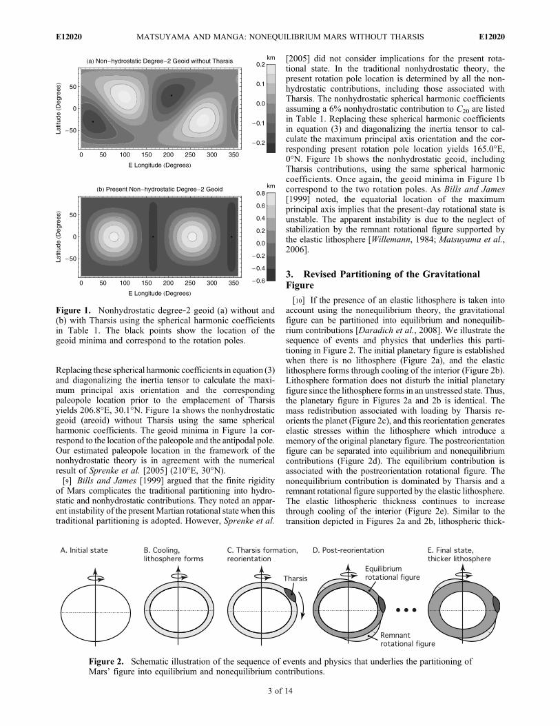
Replacing these spherical harmonic coefficients in equation (3)and diagonalizing the inertia tensor to calculate the maxi-mum principal axis orientation and the correspondingpaleopole location prior to the emplacement of Tharsisyields 206.8°E, 30.1°N. Figure 1a shows the nonhydrostaticgeoid (areoid) without Tharsis using the same sphericalharmonic coefficients. The geoid minima in Figure 1a cor-respond to the location of the paleopole and the antipodal pole.Our estimated paleopole location in the framework of thenonhydrostatic theory is in agreement with the numericalresult of Sprenke et al. [2005] (210°E, 30°N).[9] Bills and James [1999] argued that the finite rigidity

of Mars complicates the traditional partitioning into hydro-static and nonhydrostatic contributions. They noted an appar-ent instability of the present Martian rotational state when thistraditional partitioning is adopted. However, Sprenke et al.

[2005] did not consider implications for the present rota-tional state. In the traditional nonhydrostatic theory, thepresent rotation pole location is determined by all the non-hydrostatic contributions, including those associated withTharsis. The nonhydrostatic spherical harmonic coefficientsassuming a 6% nonhydrostatic contribution to C20 are listedin Table 1. Replacing these spherical harmonic coefficientsin equation (3) and diagonalizing the inertia tensor to cal-culate the maximum principal axis orientation and the cor-responding present rotation pole location yields 165.0°E,0°N. Figure 1b shows the nonhydrostatic geoid, includingTharsis contributions, using the same spherical harmoniccoefficients. Once again, the geoid minima in Figure 1bcorrespond to the two rotation poles. As Bills and James[1999] noted, the equatorial location of the maximumprincipal axis implies that the present‐day rotational state isunstable. The apparent instability is due to the neglect ofstabilization by the remnant rotational figure supported bythe elastic lithosphere [Willemann, 1984; Matsuyama et al.,2006].

3. Revised Partitioning of the GravitationalFigure

[10] If the presence of an elastic lithosphere is taken intoaccount using the nonequilibrium theory, the gravitationalfigure can be partitioned into equilibrium and nonequilib-rium contributions [Daradich et al., 2008]. We illustrate thesequence of events and physics that underlies this parti-tioning in Figure 2. The initial planetary figure is establishedwhen there is no lithosphere (Figure 2a), and the elasticlithosphere forms through cooling of the interior (Figure 2b).Lithosphere formation does not disturb the initial planetaryfigure since the lithosphere forms in an unstressed state. Thus,the planetary figure in Figures 2a and 2b is identical. Themass redistribution associated with loading by Tharsis re-orients the planet (Figure 2c), and this reorientation generateselastic stresses within the lithosphere which introduce amemory of the original planetary figure. The postreorientationfigure can be separated into equilibrium and nonequilibriumcontributions (Figure 2d). The equilibrium contribution isassociated with the postreorientation rotational figure. Thenonequilibrium contribution is dominated by Tharsis and aremnant rotational figure supported by the elastic lithosphere.The elastic lithospheric thickness continues to increasethrough cooling of the interior (Figure 2e). Similar to thetransition depicted in Figures 2a and 2b, lithospheric thick-

Figure 1. Nonhydrostatic degree‐2 geoid (a) without and(b) with Tharsis using the spherical harmonic coefficientsin Table 1. The black points show the location of thegeoid minima and correspond to the rotation poles.

Figure 2. Schematic illustration of the sequence of events and physics that underlies the partitioning ofMars’ figure into equilibrium and nonequilibrium contributions.

MATSUYAMA AND MANGA: NONEQUILIBRIUM MARS WITHOUT THARSIS E12020E12020

3 of 14

ening does not disturb the planetary figure since the newlithosphere forms in an unstressed state. Thus, the planetaryfigure in Figures 2d and 2e is identical, and the equilibriumand nonequilibrium contributions must be calculatedassuming the elastic lithospheric thickness at the time ofloading by Tharsis.[11] Daradich et al. [2008] showed that the present

Martian rotational state is stable when the partitioning intoequilibrium and nonequilibrium contributions is adopted,and we will not repeat this analysis here. For Mars, thenonequilibrium gravitational figure has contributions fromTharsis, a remnant rotational figure supported by the elasticlithosphere, and any excess contributions. Thus, the degree‐2spherical harmonic coefficients can be written as

C2m ¼ CEQ2m þ CRR

2m þ CT ;TD2m þ CEX

2m

S2m ¼ SEQ2m þ SRR2m þ ST ;TD2m þ SEX2m ;ð6Þ

where we use the superscripts “EQ,” “RR,” “T,TD,” and“EX” to identify equilibrium, remnant rotational figure,Tharsis, and excess contributions respectively. Once again,the Tharsis contributions include the deformation of theplanet in response to Tharsis, hence the superscript “T,TD.”[12] In a reference frame with the z axis aligned with the

present rotation axis, the only nonzero equilibrium degree‐2spherical harmonic coefficient is

CEQ20 ¼ � 1

3kT2

w2R3

GM; ð7Þ

where k2T is the secular degree‐2 tidal Love number and w is

the final rotation rate. Replacing this spherical harmoniccoefficient in equation (3) and setting the other coefficients tozero yields a diagonalized inertia tensor with the maximumprincipal axis aligned with the rotation axis (z axis), as ex-pected. The dimensionless tidal Love number describes theresponse to tidal forcings and depends on the planet’sinterior structure and rheology. We adopt a five‐layerinternal structure model similar to the one adopted by Billsand James [1999], as described in Table 2. We use themethod of Sabadini and Vermeersen [2004] to calculate thecorresponding Love numbers. Figure 3a shows k2

T for elasticlithospheric thicknesses in the range 0–200 km.[13] Remnant rotational figure contributions arise due to

changes in rotation rate and/or orientation of the rotationaxis. These contributions are associated with the mass dis-tribution that retains a memory for prior rotational states due

Table 2. Reference Mars Model Parameter Valuesa

Layer R (km) r (kg m−3) m (GPa)

1 1400 7200 02 2000 4300 1553 2400 4100 1204 3190 3600 805 3390 3000 45

aColumns correspond to layer number, outer radius, density, and shearmodulus.

Figure 3. Secular degree‐2 (a) tidal Love number, k2T; (b) load Love number, k2

L; (c) displacement tidalLove number, h2

T; and (d) displacement load Love number, h2L as a function of the elastic lithospheric

thickness. We adopt the five‐layer internal structure model described in Table 2.

MATSUYAMA AND MANGA: NONEQUILIBRIUM MARS WITHOUT THARSIS E12020E12020

4 of 14

to long‐term elastic strength. Thus, these contributions arealigned with the initial (prior to reorientation) rotation axis.The remnant rotational figure contributions can be written as[Matsuyama and Nimmo, 2009]

CRR20 ¼ 1

6kT*2 � kT2

� w2*R

3

GM1� 3 cos2 �R� �

CRR21 ¼ � 1

6kT*2 � kT2

� w2*R

3

GMsin 2�Rð Þ cos�R

SRR21 ¼ � 1

6kT*2 � kT2

� w2*R

3

GMsin 2�Rð Þ sin�R

CRR22 ¼ � 1

12kT*2 � kT2

� w2*R

3

GMsin2 �R cos 2�Rð Þ

SRR22 ¼ � 1

12kT*2 � kT2

� w2*R

3

GMsin2 �R sin 2�Rð Þ;

ð8Þ

where k2T* is the secular (or fluid limit) degree‐2 tidal Love

number for the case without an elastic lithosphere, w* isthe initial rotation rate, and �R and �R are the spherical co-ordinates for the initial rotation pole. The remnant rotationalfigure is established in response to loading by Tharsis. Thus,the degree‐2 tidal Love number for the case with an elasticlithosphere in equations (7) and (8), k2

T, must be calculatedassuming the elastic lithospheric thickness at the time ofloading by Tharsis. Replacing the spherical harmonic coef-ficients for the remnant rotational figure in equation (3) anddiagonalizing the inertia tensor yields a maximum principalaxis aligned with the initial rotation axis, as expected.[14] Given an interior structure model and the corre-

sponding Love numbers, there are two unknowns for thespherical harmonic coefficients of the remnant rotationalfigure (the initial rotation pole coordinates) and five unknowndegree‐2 spherical harmonic coefficients of Tharsis. Thus,even if we ignore any excess contributions, there are fiveconstraints (the observed degree‐2 spherical harmoniccoefficients) and seven unknowns, and the system is under-determined. Assuming that Tharsis is predominantly axi-symmetric at long wavelengths, the total degree‐2 sphericalharmonic coefficients, excluding excess contributions, canbe written as (ignoring terms associated with tidal defor-mation [Matsuyama and Nimmo, 2009])

C20 ¼ � 1

3kT2

w2R3

GM� 1

6kT*2 � kT2

� w2*R

3

GM� Q 1� 3 cos2 �T

� �� 1� 3 cos2 �R� � �

C21 ¼ 1

6kT*2 � kT2

� w2*R

3

GMQ sin 2�Tð Þ cos�T � sin 2�Rð Þ cos�R½ �

S21 ¼ 1

6kT*2 � kT2

� w2*R

3

GMQ sin 2�Tð Þ sin�T � sin 2�Rð Þ sin�R½ �

C22 ¼ 1

12kT*2 � kT2

� w2*R

3

GMQ sin2 �T cos 2�Tð Þ� sin2 �Rcos 2�Rð Þ �

S22 ¼ 1

12kT*2 � kT2

� w2*R

3

GMQ sin2 �T sin 2�Tð Þ� sin2 �R sin 2�Rð Þ �

;

ð9Þ

where �T and �T are the spherical coordinates of the Tharsiscenter. Tharsis’ size is given by the dimensionless load size

Q � �CT ;TD′20

CRR′20

¼ CT ′20

1þ kL2kT*2 � kT2

!3GM

w2*R

3; ð10Þ

whereC20T ′ is the (uncompensated) Tharsis spherical harmonic

coefficient for the case when the symmetry axis is alignedwith the z axis. Since we assume that Tharsis is axisymmetric,the excess contributions include nonaxisymmetric Tharsiscontributions. In equation (10), k2

L is the secular degree‐2 loadLove number for the case with an elastic lithosphere, and thefactor of 1 + k2

L, where k2L < 0, accounts for the deformation

due to Tharsis loading. Figure 3b shows k2L for elastic lith-

ospheric thicknesses in the range 0–200 km.

4. Tharsis Center Location and Size

[15] Zuber and Smith [1997] estimated the Tharsis centerlocation (248.33°E, 6.67°N) using the nonhydrostatic theoryand assuming a 5% contribution to the observed sphericalharmonic coefficient C20. Once again, in the nonhydrostatictheory, the partitioning of the gravitational figure intohydrostatic and nonhydrostatic contributions leads to anapparent instability of the present‐day rotational state. If wetake into account the presence of an elastic lithosphere usingthe nonequilibrium theory, we can calculate the nonequi-librium contribution to C20 by subtracting the equilibriumcontribution (equation (7)) from the observed value. Thisyields nonequilibrium contributions of 7%, 13%, and 19%for elastic lithospheric thickness of 0, 50, and 100 km,respectively. Our estimate for the case with no elastic lith-osphere, 7%, is consistent with the estimate of Bills andJames [1999], ∼5%–7%, using the nonhydrostatic theory,as expected since there is no remnant rotational figure in thiscase.[16] Although it is possible to find best fit solutions for the

paleopole location (�R and �R), Tharsis size (Q), and theTharsis center location (�T and �T) simultaneously usingthe method described in the following section, the problemis greatly simplified if the Tharsis center location and/or sizeare known a priori. The equilibrium and remnant rotationalfigure contributions to the gravity field are limited tospherical harmonic degree 2. Thus, the spherical harmoniccoefficients for higher degrees (‘ > 2) can be written as

C‘m ¼ CT ;TD‘m þ CEX

‘m

S‘m ¼ ST ;TD‘m þ SEX‘m ;ð11Þ

where we use the “T,” “TD,” and “EX” superscripts toidentify Tharsis, deformational effects of Tharsis, andexcess contributions respectively. Since there are no equi-librium and remnant rotational figure contributions, we canassume that Tharsis dominates the degree‐3 gravity field. Inthis case, assuming an axisymmetric Tharsis and using theaddition theorem for spherical harmonics (equation (4)),tan�T ∼ S31/C31, tan(2�T) ∼ S32/C32, and tan(3�T) ∼ S33/C33.Using the MRO95A spherical harmonic coefficients [Zuber,2008], this yields �T = 261°, 256°, and 252° for the order 1,2, and 3 spherical harmonic coefficients respectively. Thesesimple estimates are in good agreement with each other andwith the observed Tharsis center location, validating ourassumption that an axisymmetric Tharsis dominates thedegree‐3 gravity field.[17] The simplest assumption for the degree‐3 excess

contributions in equation (11), including nonaxisymmetricTharsis contributions, is that they represent random pertur-bations. In this case, we can find best fit solutions for the

MATSUYAMA AND MANGA: NONEQUILIBRIUM MARS WITHOUT THARSIS E12020E12020

5 of 14

Tharsis center location and size by minimizing the misfitfunction

�3 ¼X3m¼0

COBS3m � CT ;TD

3m

� �2þ SOBS3m � ST ;TD3m

� �2h i: ð12Þ

[18] In equation (12), C3mOBS and S3m

OBS are the observedspherical harmonic coefficients, and the predicted degree‐3Tharsis coefficients,C3m

T,TD and S3mT,TD, are given by equation (4).

The latter are functions of a single spherical harmonic coef-ficient (C30

T,TD′) and the Tharsis center location (�T and �T).Sincewe assume an axisymmetric Tharsis, the symmetry axesfor the degree‐2 and the degree‐3 gravity field associatedwithTharsis are the same. Minimization of equation (12) yields abest fit solution with C30

T,TD′ = 1.3055 × 10−4, �T = 80.2° and�T = 258.6°. This estimate of the Tharsis center longitudeagrees with the simple estimate above using the ratio betweenspherical harmonic coefficients.[19] We can extend equation (12) to consider higher

degree spherical harmonic coefficients. Assuming thatTharsis is predominantly axisymmetric up to degree 5, wecan find best fit solutions for the Tharsis center location andspherical harmonic coefficients by minimizing the misfitfunction

�3�5 ¼X5‘¼3

X‘m¼0

COBS‘m � CT ;TD

‘m

� �2þ SOBS‘m � ST ;TD‘m

� �2h i: ð13Þ

[20] Minimization of equation (13) yields �T = 80.5°, �T =257.3°, C30

T,TD′ = 1.31603 × 10−4, C40T,TD′ = 5.28363 × 10−5,

and C50T,TD′ = −2.13278 × 10−5. These best fit solutions are in

agreement with the solutions described above using thedegree‐3 spherical harmonic coefficients alone, validatingour assumption that Tharsis is predominantly axisymmetricat long wavelengths. Our results are not sensitive to theparticular spherical harmonic degree chosen for the trunca-tion in equation (13). For example, choosing degree 6 as thetruncation degree yields �T = 80.6°, �T = 257.2°, C30

T,TD′ =1.32316 × 10−4,C40

T,TD′ = 5.25002 × 10−5,C50T,TD′ = −2.15358 ×

10−5, and C60T,TD′ = −2.19211 × 10−5.

[21] Unless otherwise stated, we adopt the method forfinding the best fit Tharsis parameters based on the degree‐3spherical harmonic coefficients alone throughout the rest ofthe paper. The probability density function (PDF) for theobserved degree‐3 spherical harmonic coefficients giventhe Tharsis spherical harmonic coefficient (C30

T,TD′) and theTharsis center location (�T and �T) is proportional to c3

−N/2,

where N = 7 is the number of degree‐3 spherical harmoniccoefficients [Sivia and Skilling, 2006, section 8.2]:

PDF3 C3m; S3m j CT ;TD′

30 ; �T ; �T

� / �

�7=23 : ð14Þ

[22] Using Bayes’ theorem [Sivia and Skilling, 2006], thePDF for the unknown model parameters (C30

T,TD′, �T, and �T)given the observed spherical harmonic coefficients is alsoproportional to c3

−N/2 if we assume a uniform distribution forthe prior PDF(C30

T,TD′, �T, �T). Thus,

PDF3 CT ;TD′

30 ; �T ; �T j C3m; S3m�

/ ��7=23 : ð15Þ

[23] Note that this PDF is independent of the thickness ofthe elastic lithosphere since there are no equilibrium orremnant rotational figure contributions to the degree‐3gravity field. Using marginalization [Sivia and Skilling,2006], the PDFs for the Tharsis colatitude, longitude, andspherical harmonic coefficient given the observed degree‐3spherical harmonic coefficients are given by

PDF3 �T j C3m; S3mð Þ / R PDF CT ;TD′

30 ; �T ; �T j C3m; S3m�

dCT ;TD′

30 d�T

PDF3 �T j C3m; S3mð Þ / R PDF CT ;TD′

30 ; �T ; �T j C3m; S3m�

dCT ;TD′

30 d�T

PDF3 CT ;TD′

30 j C3m; S3m�

/ R PDF CT ;TD′

30 ; �T ; �T j C3m; S3m�

d�Td�T

;

ð16Þ

respectively. We assume 0 < �T < 180° and 0 < �T < 360°for the Tharsis center location integration domains, and afinite domain around the best fit C30

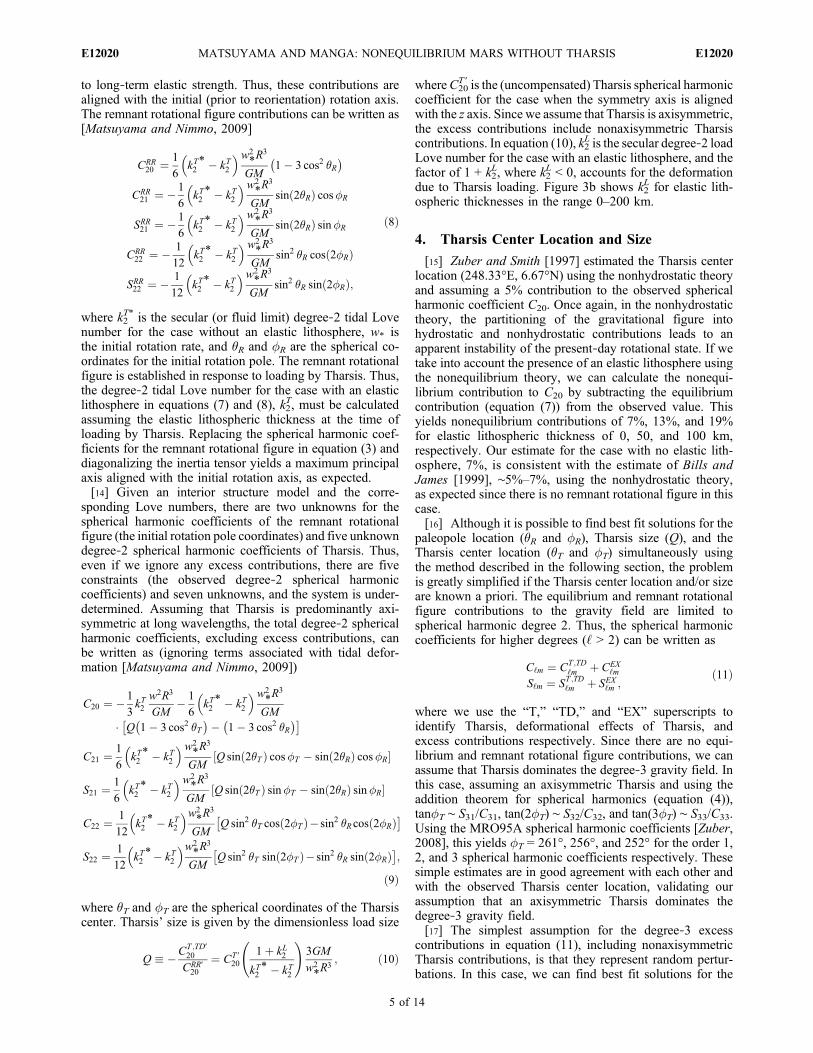
T,TD′ = 1.3055 × 10−4. ThePDFs in equation (16) are shown in Figure 4. The maximaof the PDFs represent the most likely values given theobserved degree‐3 spherical harmonic coefficients andcoincide with the parameters of the best fit solution C30

T,TD′ =1.3055 × 10−4, �T = 80.2° and �T = 258.6°. The area underthe PDF between two values is proportional to how much webelieve the parameter of interest is in that range. The shadedregions in Figure 4 enclose the smallest 90% confidenceinterval: 79.3° < �T < 81.2° and 254.4° < �T < 262.8°.

5. Paleopole Location and Thickness of the ElasticLithosphere

[24] The degree‐2 gravity field has equilibrium, rem-nant rotational figure, Tharsis, and excess contributions

Figure 4. Probability density function (PDF) for Tharsis’ (a) latitude, (b) longitude, and (c) size calcu-lated using equation (16). The shaded region encloses the smallest 90% confidence interval.

MATSUYAMA AND MANGA: NONEQUILIBRIUM MARS WITHOUT THARSIS E12020E12020

6 of 14

(equation (6)). Similar to the degree‐3 excess contributions,given our assumption of axisymmetry for Tharsis, theexcess contributions also include Tharsis perturbationsfrom axisymmetry. Once again, the simplest assumptionfor the excess contributions is that they represent randomperturbations. Under this assumption, we can find best fitsolutions by minimizing the misfit function

�2 �X2m¼0

COBS2m � C2m

� �2þX2m¼1

SOBS2m � S2m� �2

: ð17Þ

[25] In equation (17), C2mOBS and S2m

OBS are the observedspherical harmonic coefficients, and C2m and S2m are thepredicted spherical harmonic coefficients for the equilib-rium, remnant rotational figure, and Tharsis contributionsgiven by equation (9). The predicted spherical harmoniccoefficients are functions of the Tharsis size and location(Q, �T, and �T), the paleopole location (�R and �R), and thedegree‐2 Love numbers, which in turn depend on the elasticlithospheric thickness (Te). We ignore rotation rate varia-tions. Given the Tharsis center location inferred using thedegree‐3 gravity field (�T = 80.2° and �T = 258.6°), we findbest fit solutions for the degree‐2 gravity field by mini-mizing equation (17) with respect to Tharsis size (Q) and thepaleopole location (�R and �R).[26] The probability density function (PDF) for the

unconstrained model parameters (Te, Q, �R, and �R) giventhe observed degree‐2 spherical harmonic coefficients (C2m

and S2m) and the Tharsis center location (�T and �T) is pro-portional to c2

−N/2, where N = 5 is the number of degree‐2

spherical harmonic coefficients [Sivia and Skilling, 2006,section 8.2],

PDF2 Te;Q; �R; �R j C2m; S2m; �T ; �Tð Þ / ��5=22 : ð18Þ

[27] In equation (18), c2 is given by equation (17) and weuse Bayes’ theorem [Sivia and Skilling, 2006] under theassumption of a uniform distribution for the prior PDF(Te,Q, �R, �R) over a specified interval. Since the Love numbersin equation (9) are functions of the elastic lithosphericthickness (Te), we highlight this dependency in equation (18).[28] Using marginalization [Sivia and Skilling, 2006], the

PDFs for the elastic lithospheric thickness, Tharsis size, andthe paleopole colatitude and longitude are given by

PDF2 Te j C2m; S2m; �T ; �Tð Þ/Z

PDF2 Te;Q; �R; �R j C2m; S2m; �T ; �Tð ÞdQd�Rd�R

PDF2 Q j C2m; S2m; �T ; �Tð Þ/Z

PDF2 Te;Q; �R; �R j C2m; S2m; �T ; �Tð ÞdTed�Rd�R

PDF2 �R j C2m; S2m; �T ; �Tð Þ/Z

PDF2 Te;Q; �R; �R j C2m; S2m; �T ; �Tð ÞdTedQd�R

PDF2 �R j C2m; S2m; �T ; �Tð Þ/Z

PDF2 Te;Q; �R; �R j C2m; S2m; �T ; �Tð ÞdTedQd�R: ð19Þ

[29] We adopt the following integration domains for thepaleopole location: 0 ≤ �R < 90° and �T − 90° ≤ �R ≤ �T + 90°.[30] Turcotte et al. [2002] estimate a global average

elastic lithospheric thickness Te = 90 ± 10 km using corre-lations between gravity anomalies and topography. Thisestimate includes topography that formed at various timesand the thickness of the elastic lithosphere generally in-creases with time [Zuber et al., 2000;McKenzie et al., 2002;McGovern et al., 2004], as expected due to cooling. There-fore, we adopt 100 km as a conservative upper limit. As wewill show below, the PDF for the elastic lithospheric thick-ness approaches zero as Te approaches ∼15 km (Figure 5d).Thus, we adopt 15 km as a reasonable lower limit.[31] We estimate the Tharsis size integration domain

using the degree‐3 spherical harmonic coefficient associatedwith Tharsis, C30

T,TD′, and assuming a surface density distri-bution for Tharsis [Willemann, 1984],

� �ð Þ ¼�0

2cos �

�

y

� �þ 1

� �; � � y

0; � > y ;

8<: ð20Þ

where s0 is the surface density at the center (� = 0) and y isthe angular radius of Tharsis. The value of s0 is notimportant since it drops out of equation (22) below. Thedegree‐2 and degree‐3 spherical harmonic coefficientsassociated with Tharsis and the deformation of the planet inresponse to loading by Tharsis are given by

CT ;TD′

20 ¼ 1þ kL2� � 2�R2

M

Z y

0d� sin �P20 cos �ð Þ� �ð Þ

CT ;TD′

30 ¼ 1þ kL3� � 2�R2

M

Z y

0d� sin �P30 cos �ð Þ� �ð Þ;

ð21Þ

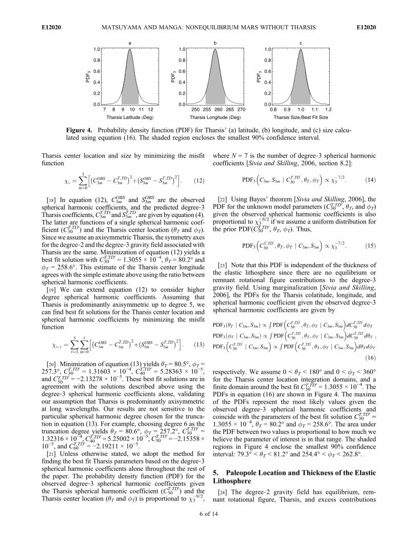
Figure 5. Probability density function for the paleopole (a)latitude and (b) longitude, (c) Tharsis size, and (d) the elasticlithospheric thickness. The shaded region encloses the smal-lest 90% confidence interval.

MATSUYAMA AND MANGA: NONEQUILIBRIUM MARS WITHOUT THARSIS E12020E12020

7 of 14

where k2L and k3

L are the secular degree‐2 and degree‐3 loadLove numbers. Thus, the normalized degree‐2 Tharsis size(equation (10)) can be written as

Q ¼ CT ;TD′

30

1þ kL21þ kL3

� �1

kT*2 � kT2

!3GM

w2*R

3

R y0 d� sin �P20 cos �ð Þ� �ð ÞR y0 d� sin �P30 cos �ð Þ� �ð Þ :

ð22Þ

[32] Assuming an angular radius y = 35° for Tharsisyields 0.7 < Q < 4.6 for elastic lithospheric thicknesses inthe range 15–100 km. This estimate requires assuming aparticular surface density distribution; however, our resultsare not sensitive to the adopted Tharsis size integrationdomain.[33] Figure 5 shows the PDF for the paleopole location,

Tharsis size, and thickness of the elastic lithosphere usingequation (19). The maximum of the PDF represents the mostlikely value: �R = 14.8°, �R = 259.5°,Q = 1.6, and Te = 40 km.The area under the PDF between two values is proportional tohow much we believe the parameter of interest is in thatrange. The shaded regions in Figure 5 enclose the smallest90% confidence interval: 1.4° < �R < 33.3°, 210.0° < �R <309.0°, 1.2 < Q < 4.0, and 26 km < Te < 92 km. Although themaximum of the PDF indicates the single most probablevalue for the parameter of interest X, the weighted average,

�X �RXPDF2dXRPDF2dX

; ð23Þ

or expected value, is more representative since it takes intoaccount the asymmetry of the PDF. The expected values are��R = 18.9°, ��R = 259.5°, �Q = 2.5, and �T e = 58 km. Note thatthe expected and most likely values for the paleopole longi-tude are identical since the PDF is symmetric about themaximum (Figure 5b). Similarly, the expected and mostlikely values for the PDFs of Tharsis’ location (Figure 4) areidentical.[34] Assuming an axisymmetric Tharsis and ignoring

excess contributions at spherical harmonic degree 2, rota-tional stability requires the paleopole longitude to be equalto the Tharsis center longitude [Matsuyama et al., 2007].The expected paleopole longitude, 259.5°, and Tharsiscenter longitude, 258.6°, nearly satisfy this; validating ourassumption of a predominantly axisymmetric Tharsis andsmall excess contributions to the gravitational figure. Sim-ilarly, under the same assumptions, rotational stability re-quires [Matsuyama et al., 2007],

�R ¼ 1

2sin�1 Q

�sin 2�Tð Þ

� �; ð24Þ

where

� � 1þ 32�

5Te

1þ

5þ

� �R3

GM2

� �hT

2

2

kT*2 � kT2

!ð25Þ

quantifies the stabilizing effect of the elastic energy in thelithosphere by reducing the effective Tharsis size. Inequation (25), m, n, and Te are the shear modulus, Poisson’sratio, and thickness of the elastic lithosphere respectively;and h2

T is the secular degree‐2 displacement tidal Love

number (Figure 3c). Assuming n = 0.25 and m = 45 GPa(Table 2) and replacing the expected values; �Q = 2.5, ��T =80.2°, and �T e = 58 km; in equations (24) and (25) yieldsb ∼ 1.5 and �R = 16.4°; which is slightly smaller than theexpected paleopole colatitude, 18.9°. The small discrepancycould be due to small excess contributions, including non-axisymmetric Tharsis contributions. There are two possiblesolutions for the paleopole colatitude in equation (24), 16.4°and 90°–16.4° = 73.6°, both of which are consistent withrotational stability given Tharsis’ size and colatitude. Ouranalysis provides an independent constraint that favors thesmall TPW solution.

6. Gravity Field

[35] Figure 6 shows the observed geoid and illustrates theeffect of removing the equilibrium rotational figure, Tharsis,and the remnant rotational figure. We use the Jet PropulsionLaboratory Mars gravity field MRO95A [Zuber, 2008]. It isuseful to consider the degree‐2 geoid alone since the equi-librium and remnant rotational figure only affect the degree‐2geoid. Figure 6a shows the observed degree‐2 geoid. For theexpected thickness of the elastic lithosphere, Te = 58 km,k2T = 1.10 (Figure 3a), and the only nonzero equilibriumdegree‐2 spherical harmonic coefficient is C20

EQ = −1.68468 ×10−3 (equation (7)). We calculate the Tharsis and remnantrotational figure spherical harmonic coefficients usingequation (9) with the expectedmodel parameters (�T e = 58 km,�Q = 2.5, ��T = 80.2°, ��T = 258.6°, ��R = 18.9, and ��R = 259.5°)and ignoring equilibrium contributions. Table 3 lists thedegree‐2 Tharsis and remnant rotational figure sphericalharmonic coefficients.[36] The equilibrium rotational figure dominates the observed

degree‐2 geoid (Figure 6a). The degree‐2 nonequilibriumgeoid (Figure 6b), calculated by removing the equilibriumrotational figure from the observed degree‐2 geoid, isdominated by Tharsis. The nonequilibrium geoid is not fullycentered around Tharsis due to the remnant rotational figureand excess contributions. The remnant rotational figurebecomes visible after removal of Tharsis from the non-equilibrium geoid (Figure 6c). Figure 6d shows the excessgeoid; that is, the nonequilibrium geoid without the Tharsisand remnant rotational figure contributions. The excesscontributions are smaller than the nonequilibrium contribu-tions, dominated by the Tharsis and remnant rotational fig-ure, by roughly an order of magnitude. The excess geoid isoffset with respect to the Tharsis geoid, as expected if itrepresents excess contributions that are not associated withan axisymmetric Tharsis. Once again, the excess geoid in-cludes nonaxisymmetric Tharsis contributions. There is noclear correlation between the degree‐2 excess geoid and theElyisum rise or the Utopia, Isidis, or Hellas basins.[37] Following the method of section 4, we find best fit

solutions for the Tharsis spherical harmonic coefficients atdegree ‘ by minimizing the misfit function,

�‘¼X‘m¼0

COBS‘m � CT ;TD

‘m

� �2þ SOBS‘m � ST ;TD‘m

� �2h i; ð26Þ

where C‘mOBS and S‘m

OBS are the observed coefficients and C‘mT,TD

and S‘mT,TD are the Tharsis coefficients given by equation (4).

Minimization of equation (26) given the expected (and most

MATSUYAMA AND MANGA: NONEQUILIBRIUM MARS WITHOUT THARSIS E12020E12020

8 of 14

likely) Tharsis center location (258.6°E, 9.8°N) yields thefollowing spherical harmonic coefficients for the case withTharsis at the pole (�T = 0): C30

T,TD′ = 1.3055 × 10−4, C40T,TD′ =

5.32303 × 10−5, and C50T,TD′ = −2.10345 × 10−5. The corre-

sponding coefficients for the case with the Tharsis center at

the expected location (258.6°E, 9.8°N) can be found usingequation (4) and are listed in Table 4. We characterizeTharsis with spherical harmonics up to degree 5 since higherdegree harmonics introduce features that are clearly notassociated with an axisymmetric Tharsis centered at 258.6°E,

Figure 6. (a) Observed degree‐2 geoid (areoid) and the same geoid (b) without the equilibrium rota-tional figure, (c) without the equilibrium rotational figure and Tharsis, and (d) without the equilibriumrotational figure, Tharsis, and the remnant rotational figure. (e) Observed geoid up to degree and order40 and the same geoid (f) without the equilibrium rotational figure, (g) without the equilibrium rotationalfigure and Tharsis, and (h) without the equilibrium rotational figure, Tharsis and the remnant rotationalfigure. We use the Jet Propulsion Laboratory Mars gravity field MRO95A [Zuber, 2008]. The centers forthe Tharsis and Elyisum rise and the Utopia, Isidis, and Hellas basins are indicated by the correspondingfirst letter. The paleopole location is indicated by the letter P.

MATSUYAMA AND MANGA: NONEQUILIBRIUM MARS WITHOUT THARSIS E12020E12020

9 of 14

9.8°N. Our results are not significantly changed if Tharsis ischaracterized with higher degree spherical harmonics sincethe misfit function (equation (26)) yields small sphericalharmonic coefficients in this case.[38] Figures 6e–6h show the observed geoid up to degree

and order 40 and illustrate the effect of removing theequilibrium rotational figure, Tharsis, and the remnant rota-tional figure. We remove axisymmetric Tharsis contributionsup to degree and order 5 using the spherical harmonic coef-ficients in Tables 3 and 4. Similar to the degree‐2 nonequi-librium geoid (Figure 6b), the total nonequilibrium geoid(Figure 6f) is not fully centered around Tharsis due tothe remnant rotational figure and excess contributions. Theremnant rotational figure becomes visible after removal ofTharsis from the nonequilibrium geoid (Figure 6g). Shorterwavelength geological features (e.g., the Elyisum rise and theUtopia, Isidis, and Hellas basins) become more visible withthe removal of the long wavelength geoid associated with theequilibrium, Tharsis, and the remnant rotational figure con-tributions (Figure 6h).

7. Shape

[39] The equilibrium rotational figure, Tharsis, and theremnant rotational figure also affect the shape of Mars. Weexpand the radius at a point with spherical coordinates (�, �)in spherical surface harmonics as

r �; �ð Þ ¼X∞‘¼0

P‘m cos �ð Þ c‘m cos m�ð Þ þ s‘m sin m�ð Þ½ �; ð27Þ

where c‘m and s‘m are spherical harmonic coefficients. Theonly nonzero spherical harmonic coefficient for the equi-librium rotational figure can be written as

cEQ20 ¼ �RhT2w2R3

3GM; ð28Þ

where h2T is the secular degree‐2 displacement tidal Love

number. For the expected thickness of the elastic litho-sphere, �T e = 58 km, h2

T = 2.00 (Figure 3c) and c20EQ =

−10422.9 m. Similarly, the spherical harmonic coefficientfor the remnant rotational figure for the case when the initialrotation axis is aligned with the z axis can be written as

cRR′

20 ¼ �R hT*2 � hT2

� w2*R

3

3GM; ð29Þ

where h2T* = 2.18 (Figure 3c) is the secular degree‐2 dis-

placement tidal Love number for the case without an elasticlithosphere and w* is the initial rotation rate. Ignoringrotation rate variations, c20

RR′ = −933.204 m for the expectedthickness of the elastic lithosphere, �T e = 58 km. Thespherical harmonic coefficients for the case with the initialrotation axis at the expected location; ��R = 18.9° and ��R =259.5°; are given by

cRR2msRR2m

� �¼ cRR

′

20 2� �m0ð Þ 2� mð Þ!2þ mð Þ!P2m cos ��R

� � cos m ��R

� �sin m ��R

� �� �; ð30Þ

where we use the addition theorem for spherical harmonics.These spherical harmonic coefficients are listed in Table 5.[40] Assuming an axisymmetric Tharsis aligned with the z

axis, the spherical harmonic coefficients for the planetdeformation in response to loading by Tharsis can be writtenas

cTD′

‘0 ¼ RhL‘CT ′

‘0 ; ð31Þ

where h‘L is the secular degree‐‘ displacement load Love

number (Figure 3d) and C‘0T ′ is the gravity spherical har-

monic coefficient for the direct contribution of Tharsis. The

Table 3. Degree‐2 Spherical Harmonic Coefficients for the Tharsis and the Remnant Rotational FigureContributions to the Gravity Field

Tharsis Remnant Rotational Figure

‘ m C‘m S‘m C‘m S‘m

2 0 −1.57321 × 10−4 −1.16144 × 10−4

2 1 −1.1424 × 10−5 −5.66568 × 10−5 7.69775 × 10−6 4.15333 × 10−5

2 2 −7.7116 × 10−5 3.24166 × 10−5 3.37541 × 10−6 −1.2957 × 10−6

Table 4. Spherical Harmonic Coefficients for the Tharsis Contri-bution to the Gravity Field and Shape to Degree and Order 5a

Gravity Shape

‘ m C‘m S‘m c‘m (m) s‘m (m)

3 0 −3.17219 × 10−5 −494.5943 1 5.43608 × 10−6 2.69599 × 10−5 84.7569 420.3473 2 −4.97279 × 10−6 2.09037 × 10−6 −77.5335 32.59213 3 2.9256 × 10−6 4.30489 × 10−6 45.6147 67.11994 0 1.43738 × 10−5 259.7944 1 1.23406 × 10−6 6.12024 × 10−6 22.3045 110.6184 2 1.58276 × 10−6 −6.65329 × 10−7 28.607 −12.02534 3 2.03039 × 10−7 2.98763 × 10−7 3.66977 5.39994 4 1.82899 × 10−7 −1.8677 × 10−7 3.30574 −3.375715 0 −5.82909 × 10−6 −118.2965 1 3.13432 × 10−7 1.55445 × 10−6 6.3608 31.54615 2 −3.65795 × 10−7 1.53766 × 10−7 −7.42345 3.120535 3 4.35589 × 10−8 6.4095 × 10−8 0.883986 1.300755 4 −1.23018 × 10−8 1.25622 × 10−8 −0.249653 0.2549385 5 8.53697 × 10−9 5.54397 × 10−9 0.17325 0.11251

aSee Tables 3 and 5 for the degree‐2 coefficients.

Table 5. Degree‐2 Spherical Harmonic Coefficients for the Tharsisand the Remnant Rotational Figure Contributions to the Shape

TharsisRemnant Rotational

Figure

‘ m c‘m (m) s‘m (m) c‘m (m) s‘m (m)

2 0 −1947.04 −786.3332 1 −141.386 −701.195 52.1164 281.1952 2 −954.402 401.194 22.8527 −8.77231

MATSUYAMA AND MANGA: NONEQUILIBRIUM MARS WITHOUT THARSIS E12020E12020

10 of 14

gravity and shape spherical harmonic coefficients for thedirect Tharsis contribution, C‘0

T′ and C‘0T′, are related by

CT ′

‘0 ¼ 4�R2

M 2‘þ 1ð Þ �cT ′

‘0; ð32Þ

where r is the density of the Tharsis load. Thus, thespherical harmonic coefficients for the total Tharsis contri-bution to the topography, including the planet deformationdue to loading and for the case when the symmetry axis isaligned with the z axis, can be written as

cT ;TD′

‘0 ¼ CT ;TD′

‘0

1þ kL‘

M 2‘þ 1ð Þ4�R2�

þ RhL‘

� �: ð33Þ

[41] In equation (33), C‘0T,TD′ = (1 + k‘

L)C‘0T′ are the spherical

harmonic coefficients for the gravity field associated withTharsis and the planet deformation in response to loadingby Tharsis. Assuming a Tharsis load density r = 3 g cm−3;the expected elastic lithospheric thickness, �T e = 58 km;and the gravity spherical harmonic coefficients found insection 6 in equation (33) yields c20

T,TD′ = 4264.74 m, c30T,TD′ =

2035.48 m, c40T,TD′ = 962.093 m, and c50

T,TD′ = −426.876 m. Thespherical harmonic coefficients for the case with the Tharsiscenter at the expected location; ��T = 80.2° and ��R = 258.6°;are given by

cT ;TD‘m

sT ;TD‘m

" #¼ cT ;TD

′

‘0 2� �m0ð Þ ð‘� mÞ!ð‘þ mÞ!P‘m cos ��T

� � cos m ��T

� �sin m ��T

� �" #

;

ð34Þ

where we use the addition theorem for spherical harmonics.These spherical harmonic coefficients are listed in Table 4.[42] Once again, it is useful to focus on the degree‐2

topography since the equilibrium and remnant rotationalfigure are limited to degree 2. Figure 7a shows the observeddegree‐2 topography and Figures 7b–7d illustrate the effectof removing the equilibrium rotational figure, Tharsis, andthe remnant rotational figure. The degree‐2 geoid andtopography for these contributions are correlated and showmany similarities. First, the equilibrium rotational figuredominates the observed degree‐2 topography (Figure 7a).Second, the nonequilibrium topography is dominated byTharsis, but it is not fully centered around Tharsis due to theremnant rotational figure and excess contributions (Figure 7b).Third, the remnant rotational figure becomes visible afterremoval of Tharsis from the nonequilibrium topography(Figure 7c). Fourth, the excess topography is offset withrespect to the Tharsis topography, as expected (Figure 7d).Finally, there is no clear correlation between the degree‐2excess topography and the Elyisum rise or the Utopia, Isidis,or Hellas basins. The most notable difference between thedegree‐2 geoid and the degree‐2 topography is an offset ofthe excess contributions (compared Figures 6d and 7d).[43] Figures 7e–7f show the observed topography up to

degree and order 40 and also illustrate the effect of removingthe equilibrium rotational figure, Tharsis, and the remnantrotational figure. We remove axisymmetric Tharsis con-tributions up to degree and order 5 using the spherical har-monic coefficients in Tables 4 and 5. Similar to the observedgeoid (Figure 6e), the equilibrium rotational figure dominates

the observed topography (Figure 7e). However, while thenonequilibrium geoid is dominated by Tharsis (Figure 6f),the nonequilibrium topography is dominated by bothTharsis and the north‐south dichotomy (Figure 7f). Simi-larly, while the remnant rotational figure is visible in thenonequilibrium geoid without Tharsis (Figure 6g), thenonequilibrium topography without Tharsis is dominatedby the north‐south dichotomy and the remnant rotationalfigure is not visible (Figure 7g). The absence of the north‐south dichotomy in the degree‐2 topography (Figures 7b–7d)is expected since it is approximately a degree‐1 feature. Thiscan be illustrated by considering a simple model. If weassume a height distribution,

h �ð Þ ¼ �h0; � � y0; � > y ;

�ð35Þ

where y is the angular radius of the northern lowlands, theonly nonzero degree‐2 shape coefficient is

c20 ¼ � 5

4h0 cosy sin2 y ; ð36Þ

which approaches zero as y approaches 90°.

8. Summary and Discussion

[44] We have used the Martian gravity field to calculateprobability density functions for Tharsis’ size and location,the paleopole location prior to the formation of Tharsis, andthe thickness of the elastic lithosphere at the time of loading.We adopt a revised theory in which the gravitational field ispartitioned into equilibrium and nonequilibrium contribu-tions [Daradich et al., 2008;Matsuyama and Nimmo, 2009].We illustrate the sequence of events and the physics thatunderlies this partitioning in Figure 2. Unlike the traditionalpartitioning into hydrostatic and nonhydrostatic contribu-tions, which is generally not appropriate for planets with anelastic lithosphere, the revised partitioning is consistent withpresent rotational stability.[45] Given the observed degree‐3 spherical harmonic

coefficients, the expected (and most likely) Tharsis centerlocation is 258.6 ± 4.2°E, 9.8 ± 0.9°N, where the un-certainties represent the smallest 90% confidence interval(Figure 4). This location is different from the location esti-mated by Zuber and Smith [1997] (248.33°E, 6.67°N).However, the latter estimate is based on the traditionalpartitioning of the planet figure into hydrostatic and non-hydrostatic contributions. The finite rigidity of Mars com-plicates this traditional partitioning and leads to an apparentinstability of the present rotational state [Bills and James,1999]. We estimate the Tharsis center location using thedegree‐3 gravity field and assuming that Tharsis is pre-dominantly axisymmetric at long wavelengths. Our methodis independent of the particular partitioning assumed sincethe degree‐3 gravity field does not contain contributionsassociated with the rotational figure.[46] Given the Tharsis center location and the observed

degree‐2 spherical harmonic coefficients, the expected elasticlithospheric thickness is 58−32

+34 km (Figure 5d). Turcotte et al.[2002] estimated 90 ± 10 km for the global average elasticlithospheric thickness using correlations between gravityanomalies and topography. We estimate the elastic litho-

MATSUYAMA AND MANGA: NONEQUILIBRIUM MARS WITHOUT THARSIS E12020E12020

11 of 14

spheric thickness at the time Tharsis was emplaced, whilethe estimate of Turcotte et al. [2002] includes topographythat formed after Tharsis. Since the thickness of the elasticlithosphere generally increases with time [Zuber et al., 2000;McKenzie et al., 2002; McGovern et al., 2004], as expected

due to cooling, our estimated thickness is expected to besmaller than the estimate of Turcotte et al. [2002]. Ourestimate is consistent with the estimate of Jellinek et al.[2008] for the elastic lithospheric thickness at the time ofTharsis uplift, ]40 km, on the basis of joint consideration of

Figure 7. (a) Observed degree‐2 topography and the same topography (b) without the equilibrium rota-tional figure, (c) without the equilibrium rotational figure and Tharsis, and (d) without the equilibriumrotational figure, Tharsis, and the remnant rotational figure. (e) Observed topography up to degree andorder 40 and the same topography (f) without the equilibrium rotational figure, (g) without the equilib-rium rotational figure and Tharsis, and (h) without the equilibrium rotational figure, Tharsis, and the rem-nant rotational figure. We use Mars Orbiting Laser Altimetry (MOLA) data. The centers for the Tharsisand Elyisum rise and the Utopia, Isidis, and Hellas basins are indicated by the corresponding first letter.The paleopole location is indicated by the letter P.

MATSUYAMA AND MANGA: NONEQUILIBRIUM MARS WITHOUT THARSIS E12020E12020

12 of 14

magnetic field anomalies and dynamic topography aroundTharsis.[47] Given the Tharsis center location and the observed

degree‐2 spherical harmonic gravity coefficients, the ex-pected paleopole location prior to the emplacement of Tharsisis 259.5 ± 49.5°E, 71.1−14.4

+17.5°N (Figures 5a–5b). This paleo-pole location lies within a degree of a great circle passingthrough the center of Tharsis and the present pole, as expectedfor any TPW driven by the emplacement of an axisymmetricTharsis. The expected amount of TPW, 18.9+17.5

−14.4°, also agreeswell with the amount of TPW estimated on the basis ofrotational stability, 16.4°, given the expected Tharsis size,�Q = 2.5 (Figure 5c), and Tharsis center colatitude, ��T =80.2° (Figure 4a).[48] The expected paleopole location (259.5 ± 49.5°E,

71.1−14.4+17.5°N) is significantly different from the estimate of

Sprenke et al. [2005] (210°E, 30°N) also inferred using thedegree‐2 gravity field. However, the latter study adopts thetraditional partitioning of the planet figure into hydrostaticand nonhydrostatic contributions. Once again, the finiterigidity of Mars complicates this traditional partitioning andleads to an apparent instability of the present rotational state[Bills and James, 1999]. As illustrated in Figure 2, we use arevised partitioning into equilibrium and nonequilibriumcontributions that takes into account finite rigidity [Daradichet al., 2008;Matsuyama and Nimmo, 2009]. This partitioningis consistent with a present Martian rotational state that isstable [Daradich et al., 2008].[49] Several observations have been used to infer that

large TPW occurred on Mars. These observations includethe distributions of large impact craters that may have tracedancient equatorial satellites [Schultz and Lutz‐Garihan,1982]; the resemblance between equatorial and polar sedi-ments [Schultz and Lutz, 1988]; and magnetic paleopolelocations estimated using crustal magnetic anomalies[Arkani‐Hamed and Boutin, 2004; Hood et al., 2005]. Ourestimate for the paleopole location implies 18.9° of expectedTPW, and <33.3° of TPW with 90% confidence, driven bythe formation of Tharsis. Since Tharsis is the dominant massanomaly capable of driving large TPW, our constraint on theamount of TPW is not consistent with the large TPW sug-gested by previous studies.[50] The expected paleopole location (259.5 ± 49.5°E,

71.1−14.4+17.5°N) agrees with the estimate of Mutch et al. [1976]

(250°E, 75°N), based on the global distribution of valleynetworks, assuming that they trace the paleoequator. How-ever, Phillips et al. [2001] concluded that the location andorientation of many of the valley networks was controlledby, and hence postdate, Tharsis. In this case, the valleynetworks are not expected to trace the paleoequator prior toTPW driven by the formation of Tharsis.[51] Recent studies suggest TPW subsequent to the for-

mation of Tharsis and our constraint for TPW driven by theemplacement of Tharsis has implications for these studies.Perron et al. [2007] show that the long wavelength defor-mation of putative shorelines [Clifford and Parker, 2001]can be explained by 30–60° of TPW. Similarly, Kite et al.[2009] illustrate that the 5–10° offset between paleopolardeposits and the present rotation axis can be explained byTPW. In both studies, the inferred TPW path is approxi-mately 90° from the center of Tharsis, as expected for apost‐Tharsis TPW if Tharsis remains the dominant mass

anomaly. Perron et al. [2007] and Kite et al. [2009] foundthat surface loads can explain the inferred TPW paths.However, the size of the loads necessary to drive the inferredTPW depends on the prior TPW driven by Tharsis and bothstudies required a large TPW driven by Tharsis. Our con-straint of a small TPW event driven by Tharsis precludes thepossibility that the surface loads considered by Perron et al.[2007] and Kite et al. [2009] were responsible for the post‐Tharsis TPW. Ancient internal or surface loads that no longerhave observable signatures are required to explain theinferred post‐Tharsis TPW. The present rotation pole, thepre‐Tharsis paleopole, and the center of Tharsis lie within adegree of the same great circle. This close alignment requiresthat other surface or internal loads no longer represent sig-nificant mass anomalies, otherwise the alignment would bebroken.[52] The total nonequilibrium geoid is dominated by

Tharsis (Figure 6f). Our estimated Tharsis center does notcoincide with the center of the nonequilibrium geoid (Figure6f) because the nonequilibrium geoid also contains remnantrotational figure and excess contributions. The remnantrotational figure becomes visible with the removal of Tharsis(Figure 6g). Removal of the long wavelength contributions ofthe equilibrium rotational figure, Tharsis, and the remnantrotational figure improves the visibility of shorter wavelengthgeological features (Figure 6h).[53] The nonequilibrium topography is dominated by

Tharsis and the north‐south dichotomy (Figure 7f). Unlikethe nonequilibrium geoid, the remnant rotational figure doesnot become visible with the removal of Tharsis due to thestrong signal associated with the north‐south dichotomy(Figure 7g). Instead, the nonequilibrium topography withoutTharsis reveals a better defined north‐south dichotomyboundary (Figure 7g) similar to the elliptical boundary seen inthe crustal thickness maps of Andrews‐Hanna et al. [2008].

[54] Acknowledgments. We acknowledge support from the MillerInstitute for Basic Research and NASA grant NNX09AN18G.

ReferencesAndrews‐Hanna, J. C., M. T. Zuber, and W. B. Banerdt (2008), The bor-ealis basin and the origin of the Martian crustal dichotomy, Nature,453, 1212–1215, doi:10.1038/nature07011.

Arfken, G., and H. Weber (1995), Mathematical Methods for Physicists,4th ed., 952 pp., Academic, Orlando, Fla.

Arkani‐Hamed, J., and D. Boutin (2004), Paleomagnetic poles of Mars:Revisited, J. Geophys. Res., 109, E03011, doi:10.1029/2003JE002229.

Bills, B. G., and T. S. James (1999), Moments of inertia and rotational stabil-ity of Mars: Lithospheric support of subhydrostatic rotational flattening,J. Geophys. Res., 104(E4), 9081–9096, doi:10.1029/1998JE900003.

Clifford, S. M., and T. J. Parker (2001), The evolution of the Martianhydrosphere: Implications for the fate of a primordial ocean and the currentstate of the northern plains, Icarus , 154 , 40–79, doi:10.1006/icar.2001.6671.

Daradich, A., J. X. Mitrovica, I. Matsuyama, J. T. Perron, M. Manga, andM. A. Richards (2008), Equilibrium rotational stability and figure ofMars, Icarus, 194, 463–475, doi:10.1016/j.icarus.2007.10.017.

Hood, L. L., C. N. Young, N. C. Richmond, and K. P. Harrison (2005),Modeling of major Martian magnetic anomalies: Further evidence forpolar reorientations during the noachian, Icarus, 177, 144–173,doi:10.1016/j.icarus.2005.02.008.

Jellinek, A. M., C. L. Johnson, and G. Schubert (2008), Constraints on theelastic thickness, heat flow, and melt production at early tharsis fromtopography and magnetic field observations, J. Geophys. Res., 113,E09004, doi:10.1029/2007JE003005.

Kite, E. S., I. Matsuyama, M. Manga, J. T. Perron, and J. X. Mitrovica(2009), True polar wander driven by late‐stage volcanism and the distri-

MATSUYAMA AND MANGA: NONEQUILIBRIUM MARS WITHOUT THARSIS E12020E12020

13 of 14

bution of paleopolar deposits on Mars, Earth Planet. Sci. Lett., 280,254–267, doi:10.1016/j.epsl.2009.01.040.

Lambeck, K. (1980), The Earth’s Variable Rotation: Geophysical Causesand Consequences, 449 pp., Cambridge Univ. Press, Cambridge.

Matsuyama, I., and F. Nimmo (2009), Gravity and tectonic patterns ofmercury: Effect of tidal deformation, spin‐orbit resonance, nonzero eccen-tricity, despinning, and reorientation, J. Geophys. Res., 114, E01010,doi:10.1029/2008JE003252.

Matsuyama, I., J. X. Mitrovica, M. Manga, J. T. Perron, and M. A. Richards(2006), Rotational stability of dynamic planets with elastic lithospheres,J. Geophys. Res., 111, E02003, doi:10.1029/2005JE002447.

Matsuyama, I., F. Nimmo, and J. X. Mitrovica (2007), Reorientation ofplanets with lithospheres: The effect of elastic energy, Icarus, 191,401–412, doi:10.1016/j.icarus.2007.05.006.

McGovern, P. J., S. C. Solomon, D. E. Smith,M. T. Zuber,M. Simons,M. A.Wieczorek, R. J. Phillips, G. A. Neumann, O. Aharonson, and J. W. Head(2004), Correction to “localized gravity/topography admittance and corre-lation spectra on Mars: Implications for regional and global evolution,”J. Geophys. Res., 109, E07007, doi:10.1029/2004JE002286.

McKenzie, D., D. N. Barnett, and D.‐N. Yuan (2002), The relationshipbetween Martian gravity and topography, Earth Planet. Sci. Lett.,195(1–2), 1–16, doi:10.1016/S0012-821X(01)00555-6.

Mutch, T., R. E. Arvidson, J. Head, K. L. Jones, and R. S. Saunders (1976),The Geology of Mars, Princeton Univ. Press, Princeton, N. J.

Perron, J. T., J. X. Mitrovica, M. Manga, I. Matsuyama, and M. A. Richards(2007), Evidence for an ancient Martian ocean in the topography ofdeformed shorelines, Nature, 447, 840–843, doi:10.1038/nature05873.

Phillips, R. J., et al. (2001), Ancient geodynamics and global scale hydrologyon Mars, Science, 291(5513), 2587–2591, doi:10.1126/science.1058701.

Press, W. H., S. A. Teukolsky, W. T. Vetterling, and B. P. Flannery (1992),Numerical Recipes in C. The Art of Scientific Computing, 2nd ed., 994pp., Cambridge Univ. Press, Cambridge.

Sabadini, R., and B. Vermeersen (2004), Global Dynamics of the Earth:Applications of Normal Mode Relaxation Theory to Solid‐Earth Geo-physics, Kluwer Acad., Dordrecht, Netherlands.

Schultz, P., and A. B. Lutz (1988), Polar wandering of Mars, Icarus, 73,91–141, doi:10.1016/0019-1035(88)90087-5.

Schultz, P. H., and A. B. Lutz‐Garihan (1982), Grazing impacts on Mars—A record of lost satellites, Proc. Lunar Planet. Sci. Conf., 13th, Part 1,J. Geophys. Res., 87, suppl., A84–A96.

Sivia, D. S., and J. Skilling (2006), Data Analysis: A Bayesian Tutorial,2nd ed., Oxford Univ. Press, New York.

Sprenke, K. F., L. L. Baker, and A. F. Williams (2005), Polar wanderon Mars: Evidence in the geoid, Icarus, 174, 486–489, doi:10.1016/j.icarus.2004.11.009.

Turcotte, D. L., R. Shcherbakov, B. D. Malamud, and A. B. Kucinskas(2002), Is the Martian crust also the Martian elastic lithosphere?, J. Geo-phys. Res., 107(E11), 5091, doi:10.1029/2001JE001594.

Willemann, R. J. (1984), Reorientation of planets with elastic lithospheres,Icarus, 60, 701–709, doi:10.1016/0019-1035(84)90174-X.

Zuber, M. T. (2008), Mars reconnaissance orbiter derived gravity data,MRO‐M‐RSS‐5‐SDP‐V1.0, NASA Planet. Data Syst., Greenbelt, Md.

Zuber, M. T., and D. E. Smith (1997), Mars without tharsis, J. Geophys.Res., 102(E12), 28,673–28,685, doi:10.1029/97JE02527.

Zuber, M. T., et al. (2000), Internal structure and early thermal evolution ofMars from Mars global surveyor topography and gravity, Science, 287,1788–1793, doi:10.1126/science.287.5459.1788.

M. Manga and I. Matsuyama, Department of Earth and PlanetaryScience, University of California, 307 McCone Hall, Berkeley, CA94720, USA. (manga@seismo.berkeley.edu; isa@berkeley.edu)

MATSUYAMA AND MANGA: NONEQUILIBRIUM MARS WITHOUT THARSIS E12020E12020

14 of 14