Anisotropy of photofragment recoil as a function of dissociation lifetime, excitation frequency,...

Anisotropy of photofragment recoil as a function of dissociation lifetime,excitation frequency, rotational level, and rotational constant

Hahkjoon Kim, Kristin S. Dooley, and Simon W. NorthDepartment of Chemistry, Texas A&M University, P.O. Box 30012, College Station, Texas 77842

Gregory E. HallChemistry Department, Brookhaven National Laboratory, Upton, New York 11973-5000

P. L. Houstona�

Department of Chemistry and Chemical Biology, Baker Laboratory, Cornell University, Ithaca,New York 14853

�Received 25 April 2006; accepted 25 May 2006; published online 4 October 2006�

Quantum mechanical calculations of photofragment angular distributions have been performed as afunction of the frequency of excitation, the lifetime of the dissociative state, the rotational level, andthe rotational constant. In the limit of high J values and white, incoherent excitation, the generalresults are found to agree exactly with both those of Mukamel and Jortner �J. Chem. Phys. 61, 5348�1974�� and those of Jonah �J. Chem. Phys. 55, 1915 �1971��. Example calculations describe howthe anisotropy is dependent on the degree of broadening, the rotational constant, the initial rotationallevel, and the frequency of excitation. Applications are also made to interpret experimental resultson the photodissociation of ClO via the 11-0, 10-0, and 6-0 bands of the A 2�3/2–X 2�3/2 transitionand on the photodissociation of O2 via the 0-0 band of the E 3�u

−–X 3�g− transition. © 2006

American Institute of Physics. �DOI: 10.1063/1.2216708�

I. INTRODUCTION

The use of photofragment angular distributions to pro-vide insight into excited state symmetry, lifetimes, and dy-namics is well documented.1–9 In diatomic molecules thephotofragment angular distributions arising from one-photondissociation using linearly polarized light can be expressedas10,11

I�� =1

4��1 + �P2�cos �� , �1�

where � is +2 for a purely parallel transition ��=0� and −1for a purely perpendicular transition ��= ±1�, P2�cos �� isthe second Legendre polynomial, and � is the angle betweenthe fragment recoil direction and the polarization direction.The normalization factor 1 /4� corresponds to unit probabil-ity for the integral of I�� over all solid angles. A value of �intermediate between the extremes of 2 and −1 can haveseveral origins: a mixed transition, depolarization due to anexcited state lifetime comparable to the rotational period, ora breakdown of the axial recoil approximation. In polyatomicmolecules, reduction in � from its limiting values will alsooccur when the recoil axis is neither parallel or perpendicularto the transition dipole moment. If the recoil direction is atan angle � with respect to the transition moment, then thelimiting form of � can be calculated as �=2P2�cos ��.

There is ample previous work on how and why the an-isotropy of photofragment recoil will be reduced from thelimiting values. The breakdown of the axial recoil approxi-mation has been considered recently by Demyanenko et al.12

and by Wrede et al.13 Here we concentrate on the reductiondue to the effect of the lifetime of the excited state prior todissociation. This topic has been addressed in a semiclassicalmodel by Jonah,14 who calculated for a parallel transitionthat

I�� =cos2�� + 1/� +

4 + 1/, �2�

where is the lifetime of the molecule and is its classicalangular frequency. Note that when →0, I�� is given by acos2�� distribution and � achieves its limiting value of 2,but as the lifetime gets long compared to the reciprocal of therotational frequency, � is reduced from this limiting value,ultimately by a factor of 4. As satisfyingly simple as are thisexpression and the corresponding one for a perpendiculartransition, they leave open several questions. How will �behave as a function of frequency; i.e., how does it varyacross the absorption band? How will it depend on the spe-cific value of J?

Several studies have addressed these questions for the→� limit, i.e., when the absorption lines are sharp anddissociation is slow relative to rotation. For example, Zaredemonstrated how to calculate the alignment of molecules byoptical absorption, which is directly related to the dis-sociation anisotropy for long-lived states.15 More recently,Cosofret et al. showed how to perform the calculation forboth one- and two-photon excitations using the example ofphotodissociation of NO.16 Dixon has recently tabulated �for a variety of multiphoton excitation schemes to dissocia-tive states that live long enough to have sharp lines.17 How-ever, while these papers do predict � at specified frequen-cies, they do not address how � changes when the lifetime ofa�Electronic mail: [email protected]

THE JOURNAL OF CHEMICAL PHYSICS 125, 133316 �2006�

0021-9606/2006/125�13�/133316/10/$23.00 © 2006 American Institute of Physics125, 133316-1

Downloaded 11 Oct 2006 to 128.253.219.80. Redistribution subject to AIP license or copyright, see http://jcp.aip.org/jcp/copyright.jsp

http://dx.doi.org/10.1063/1.2216708

http://dx.doi.org/10.1063/1.2216708

http://dx.doi.org/10.1063/1.2216708

the dissociation state becomes comparable to or shorter thanthe rotational period and, thus, they do not address frequen-cies nonresonant with individual rotation levels.

Mukamel and Jortner did address these questions in1974.18 We briefly outline their approach here to put our owninto context. The cross section for dissociation from a speci-fied starting state �g�JM ,k� is given by

JM��,E� =�2��2

�c�K,�ac�T�E��g�JM,k2� . �3�

Here, g is the lower electronic state; �, its vibrational level;J ,M is the rotational state; k is the photon wave vector, fromwhich linear polarization direction the angle � is measured;�K ,�ac� represents the dissociative state, described by anoutgoing plane wave following absorption of the photon;T�E� represents the Hamiltonian; and � corresponds to thedensity of states in the dissociative continuum. Under rea-sonable assumptions that the various levels decay indepen-dently, Mukamel and Jortner find that

�K,vac�T�E��g�JM,k�

= �J�M�

�Kvac�HV�s�J�M��s�J�M��Hint�g�JM,k�E − EJ� + i��J�/2�

, �4�

where HV is the part of the Hamiltonian that couples theexcited state to the dissociative continuum, Hint is the part ofthe Hamiltonian giving rise to the optical excitation, �J� isrelated to the lifetime of the upper level, �J�=1/ ��, andthe summation is over the various excitation branches, typi-cally P, Q, and R. Their paper then proceeds to evaluate thetwo matrix elements on the right-hand side �rhs� of �4� indetailed fashion. An intermediate result, of use to us later, isthat

JM��,E�

=�2��2

�c�2J + 1��

� �J�,J�=J,J±1

RJ�RJ�* AJ�AJ�DM�

J� ��,�,0�DM�J�*

��,�,0�

�E − EJ� + i��J�/2��E − EJ� − i��J�/2��.

�5�

Here, RJ involves integrals over the radial part of the wavefunction, and it is assumed that these do not vary stronglywith E over the excitation range. The functions A are theone-photon excitation functions, in this case for linear polar-ization, while D are rotation matrices. Note that the result in�5� must be summed over all initial JM states that throughtheir broadened lines contribute to excitation at the energy E.Of course, the initial J ,M states must be weighted by theirpopulations; for a thermal distribution the weight is simplyexp�−E�J ,M� /kT� /Qrot, where E�J ,M� gives the energy forthis initial state and Qrot is the rotational partition function.

The approach taken here and in Ref. 16 is, essentially, tojump directly to the equivalent of �5�. As have both Jonahand Mukamel and Jortner, we assume the axial recoil limit.We write the angular and frequency dependent dissociationprobability as

I��,�� = C�J,M

Pop�J,M��L��,J − 1�A�J,M,�i,� f,J − 1�

�N�J − 1�dM,�f

J−1 �� + L��,J�A�J,M,�i,� f,J�

�N�J�dM,�f

J �� + L��,J + 1�A�J,M,�i,� f,J + 1�

�N�J + 1�dM,�f

J+1 ��2. �6�

In this equation C is a constant; Pop�J ,M� is the populationof the initial state, given by exp�−E�J� /kT� /Qrot, indepen-dent of M for an isotropic thermal sample, although polar-ized or nonthermal distributions are easily represented byother forms of Pop�J ,M�; A�. . .� is a function giving theabsorption amplitude for a particular transition; N�J��= ��2J�+1� /2�1/2 is a normalization factor �see below�;dM�

J �� is a rotation matrix element; and L�� ,J�� is a Lorent-zian broadening amplitude given by

L��,J�� =��/2��1/2

� − �J,J� + i��/2�. �7�

Here, �J,J� is the center frequency for the particular P, Q, orR transition. The function L�� ,J�� must be complex �ratherthan, for example, the real square root of the Lorentzianprobability� in order to have the correct magnitudes andphases for the off-diagonal products in �6�.19

A justification for �6� and a route for application to morecomplicated cases is given as follows. Dissociation from aninitial J ,M state to produce products at an angle � is theanalog of an experiment where light passes through threeslits and strikes a screen. The P, Q, and R excitations corre-spond to the paths through the three slits and � correspondsto the final position on the screen. As in the classic interfer-ence experiment, the probability amplitudes for the threepaths must be added before determining the final probabilityby squaring �more correctly, by multiplying by the complexconjugate�. However, in the dissociation experiment, it is asif the slits have slightly different widths, since the probabilityamplitude depends not only on the P, Q, or R path throughthe slightly different values of the function A�. . .� but also onhow far the frequency � is from the resonance for each ofthese lines. For each path, the probability depends on thebroadening amplitude, on the optical excitation probabilityamplitude, and on a rotation matrix element.

The optical excitation probability amplitude A�. . .� issimply an M-state resolved version of the Hönl-London fac-tor; that is, the sum over M of squares of the function A�. . .�gives the Hönl-London factor. Values of A�. . .�, for both thelinear polarization used here and for circular polarization, aretabulated, for example, by Bray and Hochstrasser20 and eas-ily programed. The rotation matrix element can be inter-preted as follows, following the physical interpretation givenon p. 92 of Ref. 21: The rotation matrix element dM,�f

J �� isthe probability amplitude that a rotation vector making aprojection of M onto one axis will make a projection � f ontoanother axis rotated from the first by an angle �. Alterna-tively put, it is the probability amplitude that, if J makes aprojection M onto one axis and � f onto another axis, the twoaxes will be rotated from one another by an angle �. In the

133316-2 Kim et al. J. Chem. Phys. 125, 133316 �2006�


case at hand, for example, in the Q branch, the rotation ma-trix element gives the probability amplitude that if J makes aprojection M onto the Z axis �defined as the axis of linearpolarization� and a projection � f onto the internuclear axis,the internuclear axis will be at an angle of � relative to the Zaxis. In the axial recoil limit, where the products recoil alongthe internuclear axis, the distribution of � thus gives the dis-tribution of products. We conclude that for this description,which is Hund’s case �a� coupling �see, for example, the

diagram on p. 298 of Ref. 21�, the product dM,�f

J ��dM,�f

J*��

is simply the angular distribution for the products producedfrom excited states J, M, and � f in the axial recoil limit.

In summary, for each of the three paths there is an am-plitude given by the product of a broadening amplitude, anoptical excitation amplitude, and a probability amplitude fordissociation with the internuclear axis at an angle � withrespect to the Z axis. The probability amplitudes are thensummed, the sum is multiplied by its complex conjugate togive the probability, and the probabilities are summed overall relevant initial states weighted by their populations. Thefactor N�J��= ��2J�+1� /2�1/2 is a normalization constant for

the rotation matrix elements: �2J�+1� /2dM�,N�J� ��dM,N

J ��sin �d�=�J,J��M,M��N,N�, as described in Eq. 3.113 ofRef. 21.

The remainder of this paper is divided as follows. In Sec.II we show that the results of the Jonas formula, the Muka-mel and Jortner formulation, and our own are in agreementfor the high-J limit and for incoherent, white light excitation.We then apply Eqs. �6� and �7� to cases of isolated P, Q, andR triplets to develop intuition about how � varies as a func-tion of frequency, broadening parameter, and rotational level.In Sec. III we briefly describe experiments at Texas A&M onClO and at Cornell on O2. Section IV provides the results ofthese experiments and presents calculations that help to un-derstand the variation of � with excitation frequency. Theyalso provide a user guide as to how to perform such calcu-lations, both in the more straightforward case such as ClO,where Eqs. �6� and �7� are sufficient, and in the more com-plicated case such as O2, where these equations need to beextended to cover, for example, Fano line shapes, more ex-citation pathways, and behavior intermediate to Hund’s cases�a� and �b�. Section V provides directions for further exten-sion of this approach as well as concluding remarks. An Ap-pendix provides a formula for extending this approach tomore complicated systems.

II. CALCULATED EXAMPLES

We begin this section by showing that Eqs. �1�, �5�, and�6� all lead to the same prediction for the reduction in � fromits limiting values as the lifetime of the excited state in-creases. Mukamel and Jortner have shown �their Eqs. �4�–�10��, in the limit of broadband incoherent excitation �that is,integration over E� and for a 1�– 1� transition, that �5� leadsto18

I�� = C1cos2�� − 2J�J + 1��2J + 1�2

�J2

1 + �J2 P2�cos �� , �8�

where C1= ��2��2 /��2� /��RJ�2 and �=2B�2J+1� /�J withB as the rotational constant. To compare �2� and �8� requiresa consistent normalization, which can be obtained by replac-ing C1 in �8� by 3/ �4�� and by multiplying the rhs of �2� by3/ �4��. Normalizing �2� and �8� as described and then equat-ing each to �1� produces, in the first case,

� = 2�1 + ��2�

�1 + 4��2�, �9�

and in the second,

� = 2�1 − 3J�J + 1��2J + 1�2

�J2

1 + �J2 . �10�

Equating �9� and �10� leads to an equation whose solution, inthe high-J limit, gives the correspondence between Jonah’s and � /B, namely, �=2 or �2J+1� / �� /B�=.22 Notethat �� in �7� is identical to �J� in �4�.

With this correspondence it is now possible to comparethe results of the three approaches. Figure 1 shows that forJ=20, Eqs. �9� and �10� predict exactly the same curves �thedotted curve cannot be seen because it falls exactly on thesolid one�. The points calculated from Eq. �6� also lie onthese curves. Similar results are obtained for J=5 and J=10. However, for J=2, where the high-J limit is notachieved, the calculations of �6� and �10� are in agreementand are slightly different from those calculated from theJonah equation, �9�. All three approaches correctly predictthe decrease in � with increasing for white light excita-tion in the high-J limit. Note, however, that the implicit Jdependence of � for a particular predissociation lifetime inJonah’s classical result �2� does not give correct predictions

FIG. 1. Comparison of � vs log10�� for equations of Jonah �Ref. 14��solid line�, Mukamel and Jortner �Ref. 18� �dashed and dotted lines�, andthis work �individual points� for a variety of values of J.

133316-3 Anisotropy of photofragment recoil J. Chem. Phys. 125, 133316 �2006�


for individually selected rotational lines, but only for theuncommon case of broadband excitation from an isotropicsample of a single initial J state.

The exact agreement between the approach of �6� andthat of Mukamel and Jortner is not surprising, once one ex-amines the correspondence between �6� and �5�. In the latterequation, a normal approximation is to assume that the RJ

functions are not strongly dependent on J, so that they can bepulled out of the sum and incorporated into an overall con-stant. Multiplication of the D rotation matrices produces can-cellation of the factors involving the azimuthal variable to

give the reduction dM,∧J� ��dM∧

J�*��. Mukamel and Jortner con-

sidered only singlet states, where �=�. For parallel polar-ization M�=M, so summation over this factor is not needed.The factors AJ functions of �5� are identical to the A�. . .�functions of �6�. Finally, the summation in �5� over J� ,J�=J ,J±1 produces nine terms. These nine terms correspondto the nine terms produced in �6� when the three-term sum inthat equation is multiplied by its complex conjugate. Theonly differences involve equivalent ways of writing the nor-malization and broadening terms and the omission in �5� ofthe Boltzmann factor, which is included elsewhere in theMukamel and Jortner approach. Thus, under reasonable as-sumptions about RJ, the approaches represented by �5� and�6� are equivalent.

We now use Eq. �6� to develop some intuition about how� should vary with � for simple cases, since this variation isnot treated by Jonah. Figure 2 illustrates two extreme cases.In the bottom panel, a single frequency located �x from the Qline will produce nearly zero absorption unless �x is nearlyresonant with one of the lines; the broadening of the lines istoo small to provide much amplitude at other frequencies. Inthe top panel, the broadening is much larger, so all three linesare excited together with amplitudes that differ but are ofsimilar magnitude.

Figures 3–5 show how � and the absorption due to asingle P, Q, and R triplet vary with � for a parallel transitionand for differing values of �� /B. The spectrum is generatedfrom �6� simply by integrating the angular distribution oversin �d�. In each panel, the dashed line gives �, as read from

the right-hand ordinate, while the solid line gives the spec-trum, in arbitrary units, as read from the left-hand ordinate.The panels show the results for increasing J from bottom totop. In Fig. 3, the lines are very sharp compared to the spac-ing between them, so as the frequency is scanned each linemakes a nearly “separate” contribution. By “separate,” wemean that although all lines experience the radiation, theweighting factor in �6� for the one on resonance is so muchlarger than that for the other two that the other two makelittle contribution. Note that the contribution from the Q lineis small for this parallel transition ��=1 to ��=1�, but thatthe value of � at the wavelength corresponding to the Q lineis negative. Of course, since the intensity is small, measure-ment of � at this frequency would be difficult at high J.

The predictions for � at the frequencies in resonancewith the P, Q, and R lines are in agreement with the sharp-line calculations of Zare.15 For an �=0 to �=0 transition�not shown in the figures�, � at, for example, the R�2�, R�5�,and R�15� lines is 0.80, 0.64, and 0.55, respectively, whilefor the P�2�, P�5�, and P�15� lines it is 0.20, 0.36, and 0.45,respectively. These are equal to the values that are calculatedfrom Eqs. �9� and �10� of Ref. 15. In the limit of high J, thesevalues approach 0.5. Similar behavior at high J can be seenin Fig. 3.

In Fig. 4, the broadening is comparable to the spacingbetween lines at low J, and the curves for � as a function of� are not much changed. Again, there is significant intensity

FIG. 2. Excitation of a P, Q, and R triplet under cases where the broadeningis much larger than the spacing �top� or much smaller �bottom�.

FIG. 3. � and spectrum as a function of J for �� /B=0.01 and a paralleltransition.

FIG. 4. � and spectrum as a function of J for �� /B=1 and a paralleltransition.



only near the line centers, but over a somewhat broaderrange. Siebbeles and co-workers,23,24 in their experiments ontriplet hydrogen, scanned the excitation laser frequency overtwo resonances �Q�1� and R�1�� and observed all possiblevalues between −1 and 2 of the photofragment anisotropyparameter �. Their results and calculations show the samebehavior as depicted in the bottom trace of Fig. 4.

In Fig. 5, the broadening is much larger than the spacingbetween the individual lines, and the envelope of the absorp-tion shows a Lorentzian profile �the abscissa for this figurecovers considerably more spectral range than that for Figs. 3and 4�. The P, Q, and R contributions to the amplitude arenow similar at nearly all frequencies, and � is uniformlyequal to its limiting value of 2 across the spectrum. Note thatthis value is substantially larger than the value for any sepa-rate line when, as in Fig. 3, the lines are sharp. The limitingvalues of � are most readily achieved when the amplitudesof the P, Q, and R contributions in the sum of Eq. �6� arenearly equal. Indeed, it is the coherence of the excitation thatleads to the limiting value.

Similar calculations have been performed for a perpen-dicular transition, with similar results, except of course thatthe limiting value for � is −1.

Since � is so sensitive to the coherent nature of the ex-citation, one might wonder whether a spectral simulationwould need to be performed using �6� or whether it could beperformed in the usual way of treating the contribution fromeach line separately. Fortunately, it is easy to show that thelatter case is obtained. When the sum in �6� is multiplied byits complex conjugate, there will be diagonal terms involv-ing, for example, the term for the P line multiplied with itscomplex conjugate, and off-diagonal terms involving prod-ucts of, for example, the P term and the complex conjugateof the Q term. At a given angle �, these off-diagonal termsare important for determining scattering, and they thus affect�. On the other hand, when one integrates over sin �d�, thecross terms vanish due to the aforementioned orthogonality�Eq. 3.113 in Ref. 21� of the dM,�f

J �� matrix elements. Thus,if one were to want only the spectral simulation and not��, one could reasonably perform the simulation line by

line. However, if �� is desired, one must be careful toconsider together and coherently all paths from each initialstate to a final scattering angle �, as in �6�.

III. EXPERIMENT

A. Photodissociation of ClO

The Texas A&M University velocity-map ion-imagingapparatus used in the ClO experiments has been described indetail elsewhere.25,26 Briefly, a pulsed, collimated, ClO mo-lecular beam was intersected at 90° by two copropagatinglinearly polarized laser beams from the frequency doubledoutput of two Nd:YAG �yttrium aluminum garnet� pumpeddye lasers. Both fundamental wavelengths were calibratedusing a Ne-filled hollow cathode lamp. The photolysis beamwas provided by a Nd:YAG �Spectra Physics GCR-150-10�pumped dye laser �Spectra Physics PDL-1� after frequencydoubling. Four Pellin-Broca prisms were used to maintainoverlap of the photolysis and probe laser beams during thephotofragment excitation �PHOFEX� scans. Typical photoly-sis and probe pulse energies were 20 and 30 �J, respectively.The Cl�2P3/2� atoms were probed using 2+1 REMPI �reso-nantly enhanced multiphoton ionization� transition at235.336 nm �4p2D3/2←3p2P3/2� �Ref. 27� and the O�3P0�atoms were probed using the 2+1 REMPI transition near226 nm �3p3P2,1,0←2p3P2,1,0�.28 The resulting chlorine andoxygen cations were accelerated by velocity mapping ionoptics29 prior to entering a 50 cm long field-free flight tubealong the axis defined by the molecular beam. The ions wereprojected on a position-sensitive detector consisting of a dualmicrochannel plate-phosphor assembly. Images were ac-quired using a charge-coupled device �CCD� camera and aframe grabber controlled by a commercial software �CODA32�which involved centroiding and event counting.30 The finalO�3P0� images were obtained by repeatedly scanning Dop-pler profiles over the REMPI transitions to achieve homoge-neous detection efficiency. The three dimensional velocitydistributions were reconstructed from the two-dimensionalprojections using the basis set expansion �BASEX� algorithmdeveloped by Drinbinski et al.31 The ClO molecular beamwas generated using the flash pyrolysis of a Cl2O/He mix-ture as described previously.25 Simulations of the PHOFEXspectra �vide infra� indicates that the radicals are character-ized by Trot�100±20 K with negligible vibrational andelectronic excitations.

B. Photodissociation of O2

The experimental procedure and primary data have al-ready been presented in detail elsewhere,32 so they will besummarized only briefly here. A molecular beam of oxygenentered an ion imaging apparatus and was crossed at rightangles with copropagating light of 120.4 and 130.2 nm. Eachlaser wavelength was generated by four-wave difference fre-quency generation in krypton using the same 212.55 nmlight for the two-photon transition in krypton and using twovisible wavelengths, 729 and 578 nm, to obtain 120.4 and130.2 nm, respectively. The former wavelength excited O2

on the 0-0 band of the E 3�u−–X 3�g

− transition, while thelatter wavelength excited O�3P� products in the first step of a

FIG. 5. � and spectrum as a function of J for �� /B=1000 and a paralleltransition.



1+1� ionization scheme, where the second photon was re-sidual light from the 212.55 source. O�1D� was also probedby 2+1 REMPI using light at 203.7 nm. Photofragmentyield spectra were generated by scanning the wavelength ofthe source centered at 120.4 nm while recording the signalintensity of the probed O�1D2� or O�3P2�. Angular and speeddistributions were obtained for each of O�1D2�, O�3P2�, andO�3P0� at five specific dissociation wavelengths. The angulardistributions were analyzed and found to indicate significantalignment of the O�1D� and O�3P2� fragments, with produc-tion of mostly mJ=0. The values of � at the five wavelengthswere reasonably consistent across the pairs of recoiling frag-ments, although there was substantial error from the experi-ment and from the fitting procedure. As expected, the angulardistributions indicated a basically parallel transition, withvalues ranging between �=0.74 and 1.53. The results aresummarized in Table II of Ref. 32 and will be presentedgraphically in Sec. IV.

IV. RESULTS AND DISCUSSION

A. Photodissociation of ClO

The predissociation of the ClO A 2�� state represents anideal system to test the modeling of fragment spatial aniso-tropy. Excitation to the A 2�3/2 state involves a parallel��=0� corresponding to an intrinsic anisotropy parameterof �=2.0 in the limit of prompt recoil. There have beennumerous spectroscopic studies of the A 2�� state and thespectroscopic constants are well known.33–37 The A 2�3/2state, which correlates to O�1D�, is bound but is predissoci-ated by a number of repulsive states which correlate toO�3P�. The individual vibronic bands of the A 2�3/2 stateexhibit partially resolved rotational structure with the resolu-tion of each band dependent on the predissociation lifetimes,which vary from 0.5 to 10 ps. The lifetimes do not dependon J, suggesting that predissociation is due to spin-orbit cou-pling and not induced by molecular rotation. Our previousinvestigations of ClO produced beams with rotational tem-peratures near 100 K, a temperature which provides accessto a wide range of rotational states, J�20, with reasonablesignal-to-noise ratio. These factors permit coarse “tuning” ofthe number of overlapping transitions to explore the limits ofthe current model. In addition, since the O�3P0� fragment has

no angular momentum, the ion images are sensitive only tothe spatial anisotropy, avoiding complications involvingatomic alignment.

In this work we have measured spatial anisotropy param-eters for the O�3P0� fragments arising from the predissocia-tion of the ClO A 2�3/2 state throughout the 10-0 and 6-0vibronic bands and in sections of the 11-0 band. These bandswere selected primarily due to their different lifetimes, 2.5,1.0, and 0.5 ps for the 11-0, 10-0, and 6-0 bands, respec-tively. Figure 6 shows raw O�3P0� images �upper panel� aris-ing from ClO photodissociation at 279.50 and 280.20 nmcorresponding to excitation at the band head and in the tailregion on the 10-0 band, respectively. Photodissociation ofthe 6-0, 10-0, and 11-0 bands results in the production ofonly Cl�2P3/2� fragments in coincidence with O�3P0� frag-ments, and therefore the images consist of a single ring. Thedifference in the spatial anisotropy arising from photodisso-ciation at the two wavelengths is clear from inspection of theraw images. Anisotropy parameters derived from the imagesfor both vibronic bands are shown as the upper data points inFigs. 7 and 8.

In order to provide wavelength calibration and to deter-mine the rotational temperature, we collected PHOFEXspectra for each band investigated. PHOFEX spectra wereobtained through analysis of Cl�2P3/2� ion images acquiredacross each band rather than by collecting total ion signalassociated with either O�3P0� or Cl�2P3/2� products. Sincethe PHOFEX is a relative signal, a small feature in the ionimages due to Cl2 photodissociation was used as a constantintensity reference to which the strongly wavelength-dependent ClO feature was compared. Such analysis re-quired us to assume that the contribution from Cl2 photodis-sociation, due to a broad absorption spectrum in this region,was constant over each run �despite large run-to-run variabil-ity in the overall Cl2 signal�. Our experience suggested thatthis assumption was reasonable. A comparison of the relativeintensities of the Cl2 photodissociation and ClO photodisso-ciation contributions to the speed distributions also providedcorrection for beam overlap and probe power. We find thatthe PHOFEX experiments were highly reproducible.

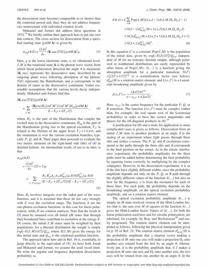
Figure 7 shows the photofragment excitation spectrumof ClO on the 10-0 band of the A 2�3/2–X 2�3/2 transition aswell as the experimental measurements of � at several wave-lengths. Equation �6� was used to calculate the spectral simu-lation and the variation of � with wavelength.38 The resultsare given as solid lines, calculated for ��=4.0 cm−1. Thespectral simulation parameters were B�=0.623 45 cm−1, B�=0.360 13 cm−1, �00=35 752.74 cm−1, and T=100 K. Rota-tional levels up to J=49 were included.

Figure 8 shows a similar photofragment excitation spec-trum for ClO on the 6-0 band of the A 2�3/2–X 2�3/2 transi-tion. The results are calculated for ��=10.0 cm−1. Thespectral simulation parameters were the same for the groundstate as in the 10-0 calculation: B�=0.389 cm−1, �00

=34268.43 cm−1, and T=80 K. Note that the broadening ishigher for the 6-0 band than for the 10-0 band, resultinggenerally in higher values of �, as might be expected fromcomparing Figs. 4 and 5.

Encouraged by these results, we attempted to see if one

FIG. 6. Raw O�3P0� ion images arising from ClO photodissociation in the10-0 band of the A 2�3/2 state.



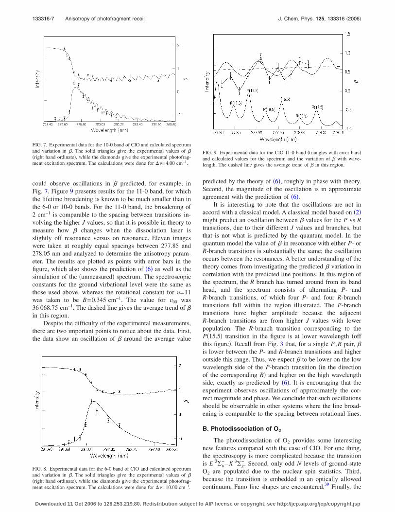
could observe oscillations in � predicted, for example, inFig. 7. Figure 9 presents results for the 11-0 band, for whichthe lifetime broadening is known to be much smaller than inthe 6-0 or 10-0 bands. For the 11-0 band, the broadening of2 cm−1 is comparable to the spacing between transitions in-volving the higher J values, so that it is possible in theory tomeasure how � changes when the dissociation laser isslightly off resonance versus on resonance. Eleven imageswere taken at roughly equal spacings between 277.85 and278.05 nm and analyzed to determine the anisotropy param-eter. The results are plotted as points with error bars in thefigure, which also shows the prediction of �6� as well as thesimulation of the �unmeasured� spectrum. The spectroscopicconstants for the ground virbational level were the same asthose used above, whereas the rotational constant for �=11was taken to be B=0.345 cm−1. The value for �00 was36 068.75 cm−1. The dashed line gives the average trend of �in this region.

Despite the difficulty of the experimental measurements,there are two important points to notice about the data. First,the data show an oscillation of � around the average value

predicted by the theory of �6�, roughly in phase with theory.Second, the magnitude of the oscillation is in approximateagreement with the prediction of �6�.

It is interesting to note that the oscillations are not inaccord with a classical model. A classical model based on �2�might predict an oscillation between � values for the P vs Rtransitions, due to their different J values and branches, butthat is not what is predicted by the quantum model. In thequantum model the value of � in resonance with either P- orR-branch transitions is substantially the same; the oscillationoccurs between the resonances. A better understanding of thetheory comes from investigating the predicted � variation incorrelation with the predicted line positions. In this region ofthe spectrum, the R branch has turned around from its bandhead, and the spectrum consists of alternating P- andR-branch transitions, of which four P- and four R-branchtransitions fall within the region illustrated. The P-branchtransitions have higher amplitude because the adjacentR-branch transitions are from higher J values with lowerpopulation. The R-branch transition corresponding to theP�15.5� transition in the figure is at lower wavelength �offthis figure�. Recall from Fig. 3 that, for a single P ,R pair, �is lower between the P- and R-branch transitions and higheroutside this range. Thus, we expect � to be lower on the lowwavelength side of the P-branch transition �in the directionof the corresponding R� and higher on the high wavelengthside, exactly as predicted by �6�. It is encouraging that theexperiment observes oscillations of approximately the cor-rect magnitude and phase. We conclude that such oscillationsshould be observable in other systems where the line broad-ening is comparable to the spacing between rotational lines.

B. Photodissociation of O2

The photodissociation of O2 provides some interestingnew features compared with the case of ClO. For one thing,the spectroscopy is more complicated because the transitionis E 3�u

−–X 3�g−. Second, only odd N levels of ground-state

O2 are populated due to the nuclear spin statistics. Third,because the transition is embedded in an optically allowedcontinuum, Fano line shapes are encountered.39 Finally, the

FIG. 7. Experimental data for the 10-0 band of ClO and calculated spectrumand variation in �. The solid triangles give the experimental values of ��right hand ordinate�, while the diamonds give the experimental photofrag-ment excitation spectrum. The calculations were done for ��=4.00 cm−1.

FIG. 8. Experimental data for the 6-0 band of ClO and calculated spectrumand variation in �. The solid triangles give the experimental values of ��right hand ordinate�, while the diamonds give the experimental photofrag-ment excitation spectrum. The calculations were done for ��=10.00 cm−1.

FIG. 9. Experimental data for the ClO 11-0 band �triangles with error bars�and calculated values for the spectrum and the variation of � with wave-length. The dashed line gives the average trend of � in this region.



transition is an intermediate case between Hund’s cases �a�and �b�, so the wave function and transition amplitudes mustbe modified.40

The incorporation of Fano line shapes is reasonablystraightforward. The factor L�� ,J�� given in �7� should bereplaced by F�� ,J��=g�q+ ��−�C� /g�� / ��−�C+ ig�, whereg is the broadening parameter and q measures the strength ofthe continuum coupling. In the case of O2, q=q0+qN�J��J�+1��2 and g=g0+gN�J��J�+1��, with qN=2.8�10−5 and gN

=0.18.41 We have treated q0 and g0 as adjustable parameters.3� electronic states intermediate between cases �a� and

�b� have been considered by Tatum and Watson.40 Briefly, theenergy levels are given by

F1�J� = BJ�J + 1� + �2� − �� − �� − B +1

2�

− �� − B +1

2� 2

+ 4J�J + 1��B −1

2� 2�1/2

,

F2�J� = BJ�J + 1� + �2� − �� , �11�

F3�J� = BJ�J + 1� + �2� − �� − �� − B +1

2�

+ �� − B +1

2� 2

+ 4J�J + 1��B −1

2� 2�1/2

.

The common term �2�−�� is normally included in the elec-tronic energy. For the 0-0 band of the E 3�u

−–X 3�g− transition

in O2, B�=1.437 77, ��=1.984, and ��=0.008 37, all incm−1, while B�=1.4701, ��=−3.3725, and ��=0.045. Notethat each rotational state N will be split into three spin-rotation states J=N+1, N, and N−1 corresponding to the F1,F2, and F3 states, respectively.

The wave functions for the three states are given by

�F1�J�� = cJ�3�0,JM� + 21/2sJ��

3�1,JM� + �3�−1,JM�� ,

�F2�J�� = 21/2��3�1,JM� − �3�−1,JM�� , �12�

�F1�J�� = sJ�3�0,JM� − 21/2cJ��

3�1,JM� + �3�−1,JM�� ,

where

cJ = F2�J� − F1�J�F3�J� − F1�J��1/2

,

�13�

sJ = F3�J� − F2�J�F3�J� − F1�J��1/2

.

Note that for every value of N, there will be, in general�except for N=1�, 14 branches,40 of which five will haveidentical values of J�=N−1 and F�=3, five will have J�=N+1 and F�=1, and four will have have J�=N and F�=2.These several branches starting from a single initial statethen replace the P, Q, and R branch terms in �6�—instead ofa three slit analog, we have a four or five slit analog. For atransition from F� to F�, the functions that replace A�. . .� in�6� have modified amplitudes. These can be calculated by

evaluating �F��J��Hint�F��J�� using �12� and the normal defi-nitions for A�. . .�. The matrix element for the transition fromF�=1 to F�=3, for example, is

cJ�sJ�A�J�,M,�� = 0,�� = 0,J��

− � cJ�sJ�

2 �A�J�,M,�� = 1,�� = 1,J��

+ A�J�,M,�� = − 1,�� = − 1,J�� . �14�

When the squares of these and the other similar terms aresummed over M, they provide the modified Hönl-Londonfactors listed for the 14 branches in Table 2 of Tatum andWatson. From the point of view of the Mukamel-Jortnertreatment, these modified Hönl-London factors are thesquares, summed over M, of the matrix elements�s�J�M��Hint�g�JM ,k� given in �4�. The equivalent of therotational part of the matrix element �K�HV�s�J�M�� in �4� issimply proportional to a function of the form of �12� inwhich dM,�f

J �� replaces �3��f,JM�. Thus each of the terms

in �6� that substitute for the P, Q, and R terms will be of theform of a broadening amplitude, given by F�� ,J��, multi-plied with a factor of the form of �14�, replacing A�. . .�, mul-tiplied with a factor of the form of �12� with the substitutionof the rotation matrix element, as just described. The Appen-dix provides a concise summary.

Calculations were performed using the spectroscopicconstants given above with �00=80 382.8 cm−1. The resultsare compared to the measured values of � and the photofrag-ment excitation spectrum in Fig. 10. The parameters that bestfit the data are q0=−12.0, g0=5.0 cm−1, and T=20 K.

V. CONCLUSION

The good agreement between experimental and calcu-lated values of the yield spectra and the variation of � with �show that the approach of �6� or, equivalently, of �5� can beuseful in interpreting spectroscopic and anisotropy results.An advantage of this approach is that it can be modifiedrelatively easily to cover new situations as they arise.

FIG. 10. Experimental results and calculations for the spectrum and varia-tion of � for the 0-0 band of the E 3�u

−–X 3�g− band in O2. The open symbols

correspond to measurements of O�3P�, while closed ones correspond tomeasurements of O�1D�. The solid lines are the results of the calculation.



For example, for two-photon excitation only minormodifications are needed. The principle is the same, in thatthe sum in �6� must coherently combine all the possibleroutes from initial states to products at a particular angle.Generally, this will involve the product of A�. . .� functionsgoing through states of the �virtual� intermediate. This ap-proach has been taken, for example, in a study of the two-photon photodissociation of NO through Rydberg levels inthe 265–278 nm region.16

If results are desired for different Hund’s cases, the wavefunctions can be modified as done above for O2, where bothelectronic states were of mixed character, or as done in theNO study,16 where different Hund’s cases describe the upperand lower electronic states. See also the Appendix.

Extension to polyatomic molecules, either symmetric orasymmetric tops, should be possible by treating the initialstate as �JKM� and replacing A�. . .� with the appropriate lin-ear excitation amplitudes. When the projection of the elec-tronic angular momentum onto the top axis is zero or muchsmaller than K, the situation is particularly simple. In thecase of symmetric tops, the A�. . .� functions42 are the same asthose listed in Bray and Hochstrasser20 with K replacing �.

The rotation matrix element dM�,K�J� �� then gives the prob-

ability amplitude that the figure axis, where J� makes projec-tion K�, will be at an angle � with respect to Z, where J�makes projection M�. With these substitutions, �6� predictsthe angular distribution for the figure axis. If this axis is alsothe recoil axis, then the distribution gives �; if the recoil axisis rotated from the figure axis by an amount �, then � will bereduced from the value for the figure axis by a factorP2�cos ��, as can be calculated using the spherical harmonicaddition theorem.

Use of circular rather than linear polarization is alsostraightforward, since Bray and Hochstrasser have given theone-photon versions that correspond to A�. . .�.20

Finally, it will be interesting to extend the current ap-proach to excitation by coherent light, whose bandwidth isbroad compared to the spectrum.

In summary, we have investigated how � changes as afunction of � and the broadening parameter�s� for situationsintermediate between short and long upper state lifetimesrelative to the rotational period of the dissociating molecule.A practical method is provided for calculating ��, whichhas the side benefit of additionally generating a simulatedspectrum by simply integrating the angular distribution ateach wave number over sin �d�. Despite the long history andimportance of the anisotropy parameter, it is surprising thatcalculations of �� are not routinely performed. The methodfor doing so was described in 1974,18 but was somewhatcumbersome. Perhaps the more descriptive treatment givenabove, in the Appendix, and in the available computerprogram43 will encourage better use of this tool.

ACKNOWLEDGMENTS

The work at Texas A&M was supported by the Robert A.Welch Foundation �Grant No. A-1402�. The work atBrookhaven National Laboratory was performed under Con-tract No. DE-AC02-98CH10886 with the U.S. Department

of Energy and supported by its Division of Chemical Sci-ences, Office of Basic Energy. The work at Cornell was sup-ported by the National Science Foundation under Grant No.CHE-0548867. One of the authors �S.W.N.� would like toacknowledge Mike White at Brookhaven National Labora-tory for the PDL used in these experiments.

APPENDIX: THE GENERAL CASE

Although Eq. �6� contains the essential physics, indi-vidual spectroscopic cases can be more complicated both be-cause of parity considerations and because coupling casesintermediate to cases �a� and �b� are often encountered. Zarehas outlined21 how parity and intermediate behavior can beconsidered by expressing the wave functions of the initialand dissociative states as linear combinations of case �a�wave functions. Indeed, this is the approach that has beentaken by Tatum and Watson.40 The wave functions for theinitial �double prime� and dissociative �single prime� statesare expanded as

��J�,M�,P�,F�� = ��=−��

��

�� J�,M�,�� ,

�A1�

��J�;M�,P�,F�� = ��=−��

��

�� J�,M�,�� ,

where J, M, P, and F are the total rotation, projection, andparity quantum numbers, and F labels the spectroscopicbranches based on coupling of nuclear rotation N with elec-tron spin S; and �=�+� is the sum of projections in case�a� of the orbital and spin angular momenta onto the internu-clear axis. The coefficients of the expansion �� are oftensimple numbers �±1, ±1/ �2,0�, but in cases intermediatebetween �a� and �b� they can be more complicated functionsof J. The formula corresponding to �6� then becomes

I��,�� = C �J�,M�,P�,F�

Pop�J�,M�,F��

� � �J�=J�−1

J�+1 � �M�,P�F�,��,��

��

� L��,J�,F�,J�,F��

� A�J�,M�,��,��,J�� N�J��

��

�� dM�,��

J� ��2

. �A2�

Within the absolute value squared term, the first term inbraces gives the transition amplitudes, while the second termin braces gives the angular part of the outgoing wave func-tion. The summation over M� can be truncated to M�=M�for linear polarization, while the summation over P� is lim-ited to P�=−P� for electric dipole transitions. A programperforming this calculation is available.43

1 R. Bersohn, ACS Symp. Ser. 770, 19 �2000�.2 S.-C. Yang and R. Bersohn, J. Chem. Phys. 61, 4400 �1974�.



3 G. E. Busch and K. E. Wilson, J. Chem. Phys. 56, 3638 �1972�.4 R. J. Gordon and G. E. Hall, Adv. Chem. Phys. 96, 1 �1996�.5 P. L. Houston, J. Phys. Chem. 91, 5388 �1987�.6 G. E. Hall and P. L. Houston, Annu. Rev. Phys. Chem. 40, 375 �1989�.7 P. L. Houston, Acc. Chem. Res. 22, 309 �1989�.8 M. N. R. Ashfold, N. H. Nahler, A. J. Orr-Ewing, O. P. J. Vieuxmaire, R.L. Toomes, T. N. Kitsopoulos, I. A. Garcia, D. A. Chestakov, S.-M. Wu,and D. H. Parker, Phys. Chem. Chem. Phys. 8, 26 �2006�.

9 A. J. Orr-Ewing and R. N. Zare, Annu. Rev. Phys. Chem. 45, 315 �1994�.10 R. N. Zare, Ph.D. thesis, Harvard University, Cambridge, MA, 1964.11 R. N. Zare and D. R. Herschbach, Proc. IEEE 51, 173 �1963�.12 A. V. Demyanenko, A. B. Potter, V. Dribinski, and H. Reisler, J. Chem.

Phys. 117, 2568 �2002�.13 E. Wrede, E. R. Wouters, M. Beckert, R. N. Dixon, and M. N. R. Ash-

fold, J. Chem. Phys. 116, 6064 �2002�.14 C. Jonah, J. Chem. Phys. 55, 1915 �1971�.15 R. N. Zare, Ber. Bunsenges. Phys. Chem. 86, 422 �1982�.16 B. R. Cosofret, H. M. Lambert, and P. L. Houston, J. Chem. Phys. 117,

8787 �2002�.17 R. N. Dixon, J. Chem. Phys. 122, 1 �2005�.18 S. Mukamel and J. Jortner, J. Chem. Phys. 61, 5348 �1974�.19 In calculations using �6� for situations where the starting distribution of

M is isotropic, it can be shown that I�� will vary as �1/4��1+�P2�cos ��. It is then sufficient to calculate the angular distribution atonly two angles, for example, �=0 and �=� /2, from which two valuesI�� can be used to calculate both � and the amplitude of the absorption.

20 R. G. Bray and R. M. Hochstrasser, Mol. Phys. 4, 1199 �1976�.21 R. N. Zare, Angular Momentum �Wiley-Interscience, New York, 1988�.22 It is interesting to note that this is not the correspondence that one might

have expected from 12 I2=J�J+1�hcB or 2=J�J+1�2hcB / I. From the

definition of B, we have hcB=h2 / �8�2I�, or I=h / �8�2cB�. Replacing I inthe equation for 2 gives 2=J�J+1�16�2c2B2, or =sqrt�J�J+1��4�cB. Since =1/ �c��, then =sqrt�J�J+1�� 4B /��. Forhigh J, we may replace J�J+1� by J2+J+ �1/4� or by �1/4��2J+1�2.Then we expect that =4�1/2��2J+1� / �� /B�=2�2J+1� / �� /B�. Thisis just twice the value given by equating �9� and �10�.

23 M. Glass-Maujean and L. D. A. Siebbeles, Phys. Rev. A 44, 1577 �1991�.24 L. D. A. Siebbeles, J. M. Schins, J. Los, and M. Glass-Maujean, Phys.

Rev. A 44, 1584 �1991�.25 H. Kim, J. Park, T. C. Niday, and S. W. North, J. Chem. Phys. 123,

174303 �2005�.26 H. Kim, K. Dooley, E. Johnson, and S. W. North, Rev. Sci. Instrum. 76,

124101 �2005�.27 S. Arepalli, N. Presser, D. Robie, and R. J. Gordon, Chem. Phys. Lett.

117, 64 �1985�.28 D. J. Bamford, L. E. Jusinsk, and W. K. Bischel, Phys. Rev. A 34, 185

�1986�.29 A. T. Eppink and D. H. Parker, Rev. Sci. Instrum. 68, 3447 �1997�.30 B.-Y. Chang, R. C. Hoetzlein, J. A. Mueller, J. D. Geisler, and P. L.

Houston, Rev. Sci. Instrum. 69, 1665 �1998�.31 V. Drinbinski, A. Ossadtchi, V. A. Mandelshtam, and H. Reisler, Rev.

Sci. Instrum. 73, 2634 �2002�.32 H. M. Lambert, A. A. Dixit, E. W. Davis, and P. L. Houston, J. Chem.

Phys. 121, 10437 �2004�.33 R. A. Durie and D. A. Ramsay, Can. J. Phys. 36, 35 �1958�.34 J. A. Coxon and D. A. Ramsay, Can. J. Phys. 54, 1034 �1976�.35 P. W. McLoughlin, C. R. Park, and J. R. Wiesenfeld, J. Mol. Spectrosc.

162, 307 �1993�.36 M. Trolier, R. L. Mauldin III, and A. R. Ravishankara, J. Phys. Chem.

94, 4896 �1990�.37 W. H. Howie, I. C. Lane, S. M. Newman, D. A. Johnson, and A. J.

Orr-Ewing, Phys. Chem. Chem. Phys. 1, 3079 �1999�.38 The situation for the A 2�3/2–X 2�3/2 transition in ClO is, in fact, a bit

more complicated than �6�, where we have not taken into account that thewave functions for the initial and dissociative states are linear combina-tions of those for �= ± �3/2�. However, for strict case �a� behavior, it canbe shown that the final formula using the correct linear combinationsreduces to �6�. See also the Appendix.

39 U. Fano, Phys. Rev. 124, 1866 �1961�.40 J. B. Tatum and J. K. T. Watson, Can. J. Phys. 49, 2693 �1971�.41 B. R. Lewis, S. T. Gibson, M. Emami, and J. H. Carver, J. Quant. Spec-

trosc. Radiat. Transf. 40, 1 �1988�.42 P. C. Cross, R. M. Hainer, and G. W. King, J. Chem. Phys. 12, 210

�1944�.43 A computer program that calculates � and absorption intensity as a func-

tion of wave number and broadening parameters is available. It handlesmany common diatomic excitation cases as well as intermediate case �a�and case �b� behaviors. The program and examples are available at http://people.ccmr.cornell.edu/~plh2/group/Betaofnu.htm



Anisotropy of photofragment recoil as a function of dissociation lifetime, excitation frequency,...

Documents

Transcript of Anisotropy of photofragment recoil as a function of dissociation lifetime, excitation frequency,...