Numerical analysis and parametric study of micro-channel ...
Upload
khangminh22Category
view
0download
0
HAL Id: tel-03259687https://tel.archives-ouvertes.fr/tel-03259687
Submitted on 14 Jun 2021
HAL is a multi-disciplinary open accessarchive for the deposit and dissemination of sci-entific research documents, whether they are pub-lished or not. The documents may come fromteaching and research institutions in France orabroad, or from public or private research centers.
L’archive ouverte pluridisciplinaire HAL, estdestinée au dépôt et à la diffusion de documentsscientifiques de niveau recherche, publiés ou non,émanant des établissements d’enseignement et derecherche français ou étrangers, des laboratoirespublics ou privés.
Study of optomechanical parametric instabilities in theAdvanced Virgo detector
David Cohen
To cite this version:David Cohen. Study of optomechanical parametric instabilities in the Advanced Virgo detector. As-trophysics [astro-ph]. Université Paris-Saclay, 2021. English. �NNT : 2021UPASP031�. �tel-03259687�

Study of optomechanical parametric instabilities in the Advanced Virgo detector
Étude des instabilités paramétriques optomécaniques pour le détecteur Advanced Virgo
Thèse de doctorat de l'université Paris-Saclay
École doctorale n° 576, Particules, Hadrons, Énergie, Noyau, Instrumentation, Imagerie, Cosmos et Simulation (PHENIICS)
Spécialité de doctorat: Astroparticules et Cosmologie Unité de recherche : Université Paris-Saclay, CNRS, IJCLab, 91405, Orsay, France
Référent :
Thèse présentée et soutenue à Paris-Saclay, le 29/03/2021, par
David COHEN
Composition du Jury
Sophie HENROT-VERSILLÉ Directrice de recherche, Université Paris-Saclay, IJCLab Présidente
Ettore MAJORANA Professeur, Università di Roma
Rapporteur & Examinateur
Frédérique MARION Directrice de recherche, Université Savoie Mont Blanc, LAPP Rapporteuse & Examinatrice
Jérôme DEGALLAIX Chargé de recherche, Université de Lyon, LMA Examinateur
Sophie KAZAMIAS Professeure, Université Paris-Saclay, IJCLab
Examinatrice
Direction de la thèse Nicolas ARNAUD Chargé de recherche, Université Paris-Saclay, IJCLab Directeur de thèse
Thibaut JACQMIN Maitre de conférences, Sorbonne Université, LKB
Coencadrant de thèse
Thès
e de
doc
tora
t N
NT
: 202
1UPA
SP03
1


À ma mère,


Contents
Contents v
Résumé 1
Introduction 7
1 Gravitational waves 91.1 General relativity and gravitational waves . . . . . . . . . . . . . . . . . . . . . . . 91.2 Sources of gravitational waves . . . . . . . . . . . . . . . . . . . . . . . . . . . . . . 11
1.2.1 ‘Burst’ signals . . . . . . . . . . . . . . . . . . . . . . . . . . . . . . . . . . 121.2.2 Compact binary system coalescences . . . . . . . . . . . . . . . . . . . . . . 121.2.3 Neutron stars . . . . . . . . . . . . . . . . . . . . . . . . . . . . . . . . . . . 13
1.3 From idea to reality . . . . . . . . . . . . . . . . . . . . . . . . . . . . . . . . . . . 13
2 Advanced Virgo: a ground-based gravitational-wave detector 152.1 Michelson interferometry . . . . . . . . . . . . . . . . . . . . . . . . . . . . . . . . . 16
2.1.1 General . . . . . . . . . . . . . . . . . . . . . . . . . . . . . . . . . . . . . . 162.1.2 Effect of a gravitational wave . . . . . . . . . . . . . . . . . . . . . . . . . . 17
2.2 Advanced Virgo detector . . . . . . . . . . . . . . . . . . . . . . . . . . . . . . . . . 182.2.1 Sensitivity and noise sources . . . . . . . . . . . . . . . . . . . . . . . . . . 182.2.2 Improving the sensitivity . . . . . . . . . . . . . . . . . . . . . . . . . . . . 212.2.3 From Virgo to Advanced Virgo . . . . . . . . . . . . . . . . . . . . . . . . . 26
2.3 A detector network . . . . . . . . . . . . . . . . . . . . . . . . . . . . . . . . . . . . 282.4 Operation and detections . . . . . . . . . . . . . . . . . . . . . . . . . . . . . . . . 29
3 Optomechanical parametric instability 333.1 Introduction . . . . . . . . . . . . . . . . . . . . . . . . . . . . . . . . . . . . . . . . 333.2 Optomechanical parametric instability observations . . . . . . . . . . . . . . . . . . 34
3.2.1 At LIGO . . . . . . . . . . . . . . . . . . . . . . . . . . . . . . . . . . . . . 343.2.2 At Virgo . . . . . . . . . . . . . . . . . . . . . . . . . . . . . . . . . . . . . . 36
3.3 Parametric gain: classical feedback system method . . . . . . . . . . . . . . . . . . 363.3.1 The prefactor . . . . . . . . . . . . . . . . . . . . . . . . . . . . . . . . . . . 373.3.2 The spatial overlap parameter . . . . . . . . . . . . . . . . . . . . . . . . . . 383.3.3 The optical transfer coefficient . . . . . . . . . . . . . . . . . . . . . . . . . 38
3.4 Summary . . . . . . . . . . . . . . . . . . . . . . . . . . . . . . . . . . . . . . . . . 42
4 Mechanical modes of Advanced Virgo’s arm cavity mirror 454.1 Finite element analysis simulations results . . . . . . . . . . . . . . . . . . . . . . . 464.2 Conclusion . . . . . . . . . . . . . . . . . . . . . . . . . . . . . . . . . . . . . . . . 48
5 Optical modes of Advanced Virgo’s arm cavities 515.1 Wave optics conventions and notation . . . . . . . . . . . . . . . . . . . . . . . . . 51
5.1.1 On light propagation in vacuum . . . . . . . . . . . . . . . . . . . . . . . . 51
v

Contents
5.1.2 Incident, reflected, and transmitted waves . . . . . . . . . . . . . . . . . . . 525.1.3 Reflection, transmission, and losses . . . . . . . . . . . . . . . . . . . . . . . 52
5.2 Fabry-Perot resonators . . . . . . . . . . . . . . . . . . . . . . . . . . . . . . . . . . 525.2.1 Optical fields and resonant frequencies . . . . . . . . . . . . . . . . . . . . . 535.2.2 Effect of resonator losses . . . . . . . . . . . . . . . . . . . . . . . . . . . . . 54
5.3 Spherical-mirror resonators . . . . . . . . . . . . . . . . . . . . . . . . . . . . . . . 555.3.1 Gaussian beam . . . . . . . . . . . . . . . . . . . . . . . . . . . . . . . . . . 555.3.2 Infinite-sized mirror modes: Hermite-Gaussian modes (HGM) . . . . . . . . 595.3.3 Finite-sized mirror modes (FSMM) . . . . . . . . . . . . . . . . . . . . . . . 63
5.4 Comparison between Hermite-Gaussian modes and finite-sized mirror modes . . . . 655.4.1 Diffraction losses . . . . . . . . . . . . . . . . . . . . . . . . . . . . . . . . . 675.4.2 Mode amplitudes . . . . . . . . . . . . . . . . . . . . . . . . . . . . . . . . . 675.4.3 Gouy phases . . . . . . . . . . . . . . . . . . . . . . . . . . . . . . . . . . . 685.4.4 Conclusion . . . . . . . . . . . . . . . . . . . . . . . . . . . . . . . . . . . . 69
5.5 Thermal effect . . . . . . . . . . . . . . . . . . . . . . . . . . . . . . . . . . . . . . 695.6 Summary . . . . . . . . . . . . . . . . . . . . . . . . . . . . . . . . . . . . . . . . . 71
6 Optomechanical parametric instability gain computation in the AdvancedVirgo configuration 736.1 Numerical computation and its validation . . . . . . . . . . . . . . . . . . . . . . . 73
6.1.1 Program and parameters . . . . . . . . . . . . . . . . . . . . . . . . . . . . 736.1.2 Comparison with the Finesse software . . . . . . . . . . . . . . . . . . . . . 736.1.3 Comparison with Evans et al. article . . . . . . . . . . . . . . . . . . . . . . 75
6.2 Some interesting effects on the optomechanical parametric instability . . . . . . . . 756.2.1 Effect of the optical losses . . . . . . . . . . . . . . . . . . . . . . . . . . . . 756.2.2 Impact of the optical mode basis . . . . . . . . . . . . . . . . . . . . . . . . 786.2.3 Impact of a radius-of-curvature shift . . . . . . . . . . . . . . . . . . . . . . 78
6.3 Accounting for mechanical frequency and optical working point uncertainties . . . 796.4 Parametric gains for different optical configurations . . . . . . . . . . . . . . . . . . 806.5 Observing Run 3 (O3): power-recycled interferometer . . . . . . . . . . . . . . . . 80
6.5.1 O3: up to 70-kHz mechanical modes . . . . . . . . . . . . . . . . . . . . . . 806.5.2 O3b: OPI observation at Virgo around 150-kHz mechanical modes . . . . . 846.5.3 O3: conclusion . . . . . . . . . . . . . . . . . . . . . . . . . . . . . . . . . . 86
6.6 Observing Run 4 (O4): power- and signal-recycled interferometer . . . . . . . . . . 866.7 Summary and conclusion . . . . . . . . . . . . . . . . . . . . . . . . . . . . . . . . 89
Conclusion 93
Index & List of Acronyms 95
Bibliography 99
Remerciements / Acknowledgements 105
vi

Résumé
En 1915, Albert Einstein publia sa théorie de la relativité générale et prédit à la fois l’existenced’ondes gravitationnelles et des trous noirs. Les ondes gravitationnelles sont des oscillations de lacourbure de l’espace-temps engendrées par des masses accélérées se déplaçant à la vitesse de lalumière. Les objets les plus susceptibles de produire des ondes gravitationnelles détectables (pour lemoment et sur Terre) sont les coalescences de systèmes binaires, comme des binaires de trous noirsou d’étoiles à neutron. Après avoir introduit brièvement le concept des ondes gravitationnelles, lechapitre 1 présente quelques autres sources d’ondes gravitationnelles importantes. Ces évènementsastronomiques libèrent des quantités d’énergie quasiment incomparables à quelque autre évènementphysique, et pourtant, l’amplitude relative de la courbure spatiale due au passage de l’onde estextrêmement faible : 10−21.
Bien que la théorie de la relativité générale fut relativement vite acceptée, l’existence desondes gravitationnelles, quant à elle, prit beaucoup plus de temps : ce fut seulement après laconférence de Chapel Hill de 1954 que la communauté aboutit à un consensus ; une fois l’existencedes ondes gravitationnelles entérinée, le développement d’instruments capables de détecter detelles ondes put commencer. C’est ainsi que Joseph Weber mit au point, dans les années 1960, labarre de Weber qui est composée de plusieurs couches d’aluminium (AL5056), agissant commeune antenne. Cependant, ses observations n’ont pu être confirmées. Il faudra encore attendreplus de 40 ans pour obtenir la première détection directe : le 14 septembre 2015. En parallèle dutravail de Weber, Mikhail Gertsenshtein et Vladimir Pustovoit travaillèrent sur un dispositif plussensible, ayant une bande fréquentielle de détection plus large, et étant sensible aux déplacementsdifférentiels : un interféromètre de Michelson. Cette solution vit le jour par la création du LaserInterferometer Gravitational-wave Observatory (LIGO), dont les deux détecteurs furent terminésen 2000 ; et de Virgo, terminé en 2003. Ces deux collaborations travaillent ensemble et permirentcette fameuse première détection, qui fut le signal produit par la coalescence d’un système binairede trous noirs. Avant cette observation, seulement l’étude de la décroissance orbitale du pulsarbinaire PSR1913+16 avait fourni une preuve indirecte de l’existence de telles ondes. Depuis lapremière observation directe, la collaborations LIGO-Virgo a annoncé quanrante-neuf nouvellesdétections. Des informations supplémentaires sur quelques-unes de ces détections sont données enfin de chapitre 2.
Le principe de détection interférométrique est le suivant : on cherche à mesurer une différencede variation de longueur des bras de l’interféromètre lorsqu’une onde graviationnelle passe. Eneffet, les ondes graviationnelles sont des ondes transverses, donc les deux bras de l’interféromètre neseront pas étirés ou compressés de la même manière, au même moment. Toutefois, un interféromètrede Michelson basique nécessiterait des bras de plusieurs centaines de kilomètres afin de pouvoirespèrer être sensible à des déplacements aussi faibles que ceux engendrés par le passage d’une ondegraviationnelle. C’est pourquoi, un détecteur inteférométrique d’ondes gravitationnelles est uneversion améliorée d’un interféromètre de Michelson, auquel des cavités optiques ont été ajoutéesafin d’améliorer sa sensibilité. Aujourd’hui, la version la plus optimisée comprend quatre cavitésoptiques : deux dans les bras pour alonger artificiellement le chemin optique, une au niveau duport symétrique (entrée) pour recycler la puissance, et une au niveau du port antisymétrique(sortie) pour régler la sensibilité à des fréquences d’intérêt. Ces améliorations permettent à la foisd’augmenter la variation de puissance mesurée due au passage d’une onde graviationnelle, et dediminuer certains bruits ; ces deux aspects reviennent à améliorer la sensibilité du détecteur. Tout
1

Résumé
ceci est détaillé au chapitre 2.
Instabilités optomécaniques
Parmi tous les aspects physiques et technologiques qui peuvent être améliorés dans la quête d’unemeilleure sensibilité, augmenter la puissance laser en entrée d’interféromètre est une priorité. Parcontre, une puissance plus importante signifie également que l’effet de la pression de radiation desphotons sur les miroirs est plus importante ; ce qui peut avoir comme conséquence l’apparitiond’instabilités paramétriques optomécaniques optomechanical parametric instability (OPI), qui sontau centre du chapitre 3. Ces instabilités — qui peuvent avoir lieu au sein de n’importe quellecavité optique — sont dues à des effets non linéaires provenant du couplage de trois modes : unmode mécanique propre d’un miroir, le mode fondamental de la cavité optique (TEM00), et unmode optique de plus haut ordre, appelé higher-order mode (HOM). Ce type de couplage nonlinéaire est proche de la diffusion Mandelstram-Brillouin : dans une cavité, un photon de fréquenceω0 du mode fondamental est diffusé vers un photon de plus basse fréquence ω1 (un autre mode dela cavité optique), et vers un phonon de fréquence ωm ; ce phonon excite le mode mécanique dumiroir. La relation de conservation d’énergie suivante peut être écrite
~ω0 = ~ω1 + ~ωm. (1)
Comme le photon diffusé a moins d’énergie que le photon absorbé, ce procédé est appelé processusde Stokes. La fréquence de battement (« beat note ») entre les deux modes optiques génère uneoscillation de la radiation de pression à la différence de fréquences ω0 − ω1 ≈ ωm, fournissant del’énergie au mode mécanique. À son tour, le mode mécanique intéragit avec le mode fondamentalet intensifie le processus de diffusion du phonon. Si l’intensité du mode fondamental atteint uncertain seuil, le couplage non linéaire entre les trois modes produit ladite instabilité paramétrique.Figure 1(a) montre le processus de Stokes. Il faut également tenir compte du processus inverse,c’est-à-dire le processus d’anti-Stokes, pour lequel le photon diffusé a plus d’énergie que le modefondamental (~ω1 = ~ω0 + ~ωm). À l’inverse du processus « chauffant », celui-ci prend de l’énergieau mode mécanique, ce qui l’affaiblit. Ce processus est montré par figure 1(b). Dans le casd’un processus de Stokes, l’amplitude du mode mécanique se vera croitre exponentiellement,jusqu’à ce qu’elle atteigne un plateau après un certain temps. Le signal associé à l’excitationmécanique du miroir pourrait saturer l’électronique de mesure, et, ainsi, faire perdre le contrôlede l’interféromètre.
Le phénomène d’instabilité entre les trois modes, déclanché par le mouvement thermique dumiroir à ωm, peut être décrit comme une boucle de rétroaction classique. Cette approche est très
Photonω1
Phononωm
Stokes anti-Stokes
Photonω0
ω0
ωm
ω1
(a) (b)
Figure 1 : (a) Processus de Stokes : émission d’un phonon ω0 = ω1 + ωm. (b) Processusd’anti-Stokes : absorption d’un phonon ω0 = ω1 − ωm. Image créée par Daniel Schwen http://commons.wikimedia.org, modifiée, sous les termes de Creative-Commons-License CC-BY-SA-2.5.
2

pratique car elle peut être adaptée à n’importe quelle configuration d’interféromètre, avec lesmêmes formules analytiques. Dans cette approche, le gain paramétrique d’un mode mécanique mavec tous les HOM, prenant en compte et le processus de Stokes et le processus d’anti-Stokes,s’écrit
Rm = 8πQmP
Mω2mcλ︸ ︷︷ ︸
préfacteur
∞∑n=0
Re [Gn]︸ ︷︷ ︸coefficient de transfert optique
× B2m,n︸ ︷︷ ︸
chevauchement spatiale
, (2)
où Qm est le facteur de qualité (Q factor) du mode mécanique m et ωm sa fréquence, P lapuissance intracavité, λ la longueur d’onde optique, M la masse du miroir, c la vitesse de lalumière ; Gn est le coefficient de transfert optique du nème mode optique ; finalement, Bm,n estl’intégrale du chevauchement spatial des trois modes. Un mode mécanique est amplifié si Rm > 0,et affaiblit si Rm < 0. Il devient instable si Rm > 1.
Durant la phase d’observation Observing Run 1 (O1), en 2015, LIGO observa une OPI lorsqu’unmode mécanique d’un miroir à 15 kHz devint instable, pour une puissance optique dans les cavitésde bras (puissance intracavité) de 50 kW. Nous nous attendions à observer un phénomène similaireà Virgo puisque sa puissance intracavité était déjà bien plus élevée que celle de LIGO. Ce quidevait arriver, arriva : le 7 janvier 2020, un mode mécanique à 155 kHz entra en instabilité jusqu’à,également, faire perdre le contôle de l’instrument. Étant donnés le temps moyen d’un évènementd’onde gravitationnelle de l’ordre de la milliseconde à la seconde, et de leurs fréquences, on doit, àtout prix, éviter de perdre le contrôle de l’interféromètre. D’où l’étude de ces instabilités au seinde la collaboration Virgo.
Modes mécaniques des miroirs de Virgo
Dans le chapitre 4, j’introduis le calcul des modes mécaniques des cavités de bras de Virgo : ilsont été calculés par analyse des éléments finis, par Paola Puppo (INFN Roma). Son analyse apermit d’obtenir les modes mécaniques jusqu’à 157 kHz, avec leur fréquence et facteur de qualité.De plus, elle a effectué des mesures, sur site, des facteurs de qualité et des fréquences des modesmécaniques jusqu’à 40 kHz : ceci a permi d’estimer une incertitude sur les fréquences, et d’ajusterles facteurs de qualité.
Modes optiques des cavités de bras de Virgo
En ce qui concerne les modes optiques de cavités de bras, dans le chapitre 5, j’étudie deuxconditions aux limites : miroirs infinis et miroirs finis. La première aboutit à des bases de modesconnues, telle que la base des modes Hermite-Gaussian modes (HGM). La deuxième nous imposede résoudre une équations aux valeurs propres afin de trouver les modes propres ; ils sont nommésfinite-sized mirror modes (FSMM). C’est une opération beaucoup plus complexe et couteused’un point de vue CPU. Cependant, elle permet plusieurs avantages : on peut calculer les modespour n’importe quelle forme de miroir (déformations intrinsèques, déformations thermiques, etc.) ;les modes obtenus sont a priori plus proches de la réalité ; on obtient directement les pertes dediffraction des modes. En effet, ce dernier point est particuler dans le cas des HGM puisque, pardéfinition, ces modes sont ceux si les miroirs sont infinis. C’est pour cela que, pour les HGM, nousdevons estimer les pertes de diffraction.
Enfin, je confronte les deux bases. Pour cela, j’ai choisi trois paramètres permettant de décrirecomplètement les modes optiques : la forme du mode, la perte de diffraction (définit la largeurà mi-hauteur de la résonance optique), et la phase de Gouy (définit la fréquence de résonanceoptique). En ce qui concerne la forme du mode, j’ai choisi de montrer la projection, sur la basedes HGM, de quelques FSMM : on se rend compte qu’à partir de l’ordre 7, les projections ne sontplus une combinaison linéaire de HGM de même ordre. Pour la perte de diffraction, on observeque notre évaluation des pertes de diffraction des HGM est sousestimée pour tous les modes, maisdevient non négligeable à partir de l’ordre 5. Et à propos des phases de Gouy, on observe une
3

Résumé
nette déviation des phases de Gouy des FSMM, par rapport à celles des HGM, dès l’ordre 8. Onen conclut que, dès l’ordre 5, les HGM ne sont plus suffisants pour décrire proprement les modesdes cavités de bras de Virgo.
Calcul du gain paramétrique dans la configuration de Virgo
Afin de calculer le gain paramétrique des modes mécaniques, j’ai écrit un programme orientéobjet. Ce programme a été vérifié au moins grâce à une comparaison avec le logiciel Finesse et unereproduction de résultats d’un article scientifique. Grâce à cela, j’ai pu vérifier les résultats attendusquant à la différence des deux bases optiques. Puis, j’ai pu faire tourner des simulations dansdifférentes configurations de Virgo : celles d’O3 et O4. De plus, ces simulations sont effectuées pourdifférents points de fonctionnement (rayons de courbure) des miroirs de fin de cavité des bras. Eneffet, cela est nécessaire pour de multiples raisons : l’incertitude du point réel de fonctionnement ;des anneaux chauffant sont fixés autour des miroirs afin de pouvoir modifier le rayon de courbure deces derniers, et c’est ce qui peut être utilisé afin d’atténuer ou supprimer une éventuelle instabilité ;il existe une incertitude non négligeable sur les fréquences mécaniques, et je montre qu’au lieu defaire varier ces fréquences, il revient au même de faire varier les rayons de courbure des miroirs.
Les premiers résultats obtenus, donnés en chapitre 6, ceux d’O3, ont permis, etre autres, devérifier que la densité d’instabilité était en effet relativement faible. Puis, lorsque le 7 janvier 2020Virgo observa pour la première une OPI, nous avons pu utiliser nos outils de simulations pours’assurer de l’origine OPI de cette instabilité d’une part, et de vérifier, encore, la fonctionnabilitéde nos outils de simulation d’autre part.
Pour la prochaine phase d’observation, O4, la cavité de recyclage du signal sera installée.Cette cavité pourrait permettre à certains HOM de perdurer dans l’interféromètre. Ceci se traduitpar un mode avec moins de pertes, ce qui se traduit à son tour par des résonances ayant unelargeur à mi-hauteur plus fine. Donc, la densité d’instabilité devrait diminuer, mais, comme lahauteur maximum des résonances est augmentée, les gains paramétriques pourraient être plusélevés. C’est effectivement ce que l’on observe, et ce que je montre en figure 2, où les lettres sontles labels des OPI, dont on retrouve les informations en tableau 1. Au final, 15 modes mécaniquesont été identifiés comme potentiellement instables ; ces instabilités, si elles ont lieu, auront desgains paramétriques plus élevés qu’ils ne l’auraient été dans la configuration d’O3, impliquantune instabilité plus rapide ; par contre, les résonances étant plus fines, il sera plus facile de s’enéloigner grâce aux anneaux chauffants.
4

1655 1660 1665 1670 1675
North END RoC (m)
1655
1660
1665
1670
1675
We
st
EN
D R
oC
(m
)
0 1 5 10 15
Figure 2 : (a) Rm vs rayons de courbure des miroirs de fin de cavité, utilisant les FSMM,à puissance d’entrée 50 W (puissance nominale), pour la configuration de O4 ; tous les 12 750modes mécaniques jusqu’à 157 kHz. L’échelle de nuances de gris représente les gains paramétriquesinférieurs à 1, alors que la colorée indique les instabilités (Rm > 1). Chaque résonance de modemécanique peut se voir sur les deux cavités de bras ; cependant, par soucis de clareté, seulementune cavité est pointée pour chaque mode mécanique, et le choix de l’axe est purement arbitraire.
5

Résumé
Label Fréquence(kHz)
∆νmax(±102 Hz)
Ordreoptique R (m) ∆Rmax
(±m) Rm
A 16.015 0.80 3 1660.8 0.89 1.7344B 23.128 1.2 4 1675.9 1.0 5.3664C 23.258 1.2 4 1676.1 1.0 1.3776D 61.154 3.1 2 1669.3 5.2 7.6253E 61.160 3.1 2 1669.4 5.2 2.9983F 61.216 3.1 2 1670.4 5.2 1.0805G 61.231 3.1 2 1670.6 5.2 1.3914H 61.676 3.1 2 1678.4 5.2 2.5652I 61.705 3.1 2 1679.0 5.2 3.3382J 61.759 3.1 2 1679.9 5.2 2.6389K 66.150 3.3 3 1662.7 3.7 1.1813L 66.784 3.3 3 1669.7 3.7 2.0182M 66.888 3.3 3 1670.9 3.7 14.0449N 66.912 3.3 3 1671.2 3.7 2.4578O 67.567 3.4 3 1678.9 3.8 0.8203P 67.616 3.4 3 1679.5 3.8 2.1297Q 72.971 3.6 4 1674.8 3.0 1.7454R 105.112 5.3 1 1655.6 18 1.4159S 115.812 5.8 3 1659.3 6.4 1.0308T 155.756 7.8 1 1678.4 26 4.4221U 155.765 7.8 1 1678.7 26 3.2889V 155.768 7.8 1 1678.8 26 4.6354W 155.770 7.8 1 1678.9 26 3.9399X 155.780 7.8 1 1679.2 26 1.3523
Table 1 : Tous les modes mécaniques instables d’O4 sur toute la gamme de rayon de courburechoisie. ∆νmax est la déviation maximale en fréquence due aux incertitudes. R est le rayon decourbure auquel le mode mécanique résonne. Rm est le gain paramétrique maximum sur toute lagamme de rayon de courbure. L’ordre optique est l’ordre du mode optique qui contribue le plus àcette OPI, c’est-à-dire au rayon de courbure correspondant (ou phase de Gouy de cavité de bras).∆Rmax est la déviation maximale en rayon de courbure correspondant à la déviation maximaleen fréquence. Les lignes en vert-beu foncé représentent les modes mécaniques qui pourront êtreinstables au point de fonctionnement 1667 m. H, I, J , O, P , et Q pourraient être dans le voisinagede ce point de fonctionnement (en vert-bleu clair) ; ils pourraient donner lieu à une OPI si le pointde fonctionnement est un peu modifié.
6

Introduction
In 1915, Albert Einstein published the General Relativity theory and predicted the existenceof gravitational waves. But gravitational waves are so weak that the first direct detection onlyoccurred a century later; on 14th September 2015, ground-based interferometric gravitational-wavedetectors finally recorded a signal produced by a Binary Black Holes coalescence. In the meantime,the study of the binary pulsar PSR1913+16 had provided an indirect evidence of the existence ofgravitational waves.
The operating principle of interferometric gravitational-wave detectors is based on an enhancedversion of a Michelson interferometer, to which optical cavities are added to improve its sensitivity.To date, the most enhanced configuration includes four optical cavities: two in the arms toartificially lengthen the optical path, one at the symmetric port (the input) to recycle the power,and one at the antisymmetric port (the output) to tune the sensitivity at specific frequencies ofinterest.
Since the first direct observation, the LIGO-Virgo Collaboration announced 49 new detections.On 1st August 2017, the Virgo detector joined the two LIGO detectors for a first joint data takingperiod with three advanced (second generation) detectors. For Virgo, this was the outcome of amulti-year upgrade program during which most components of the detector were upgraded, withthe goal of improving its sensitivity by an order of magnitude.
Amongst all the physical and technological aspects that can be improved in the pursuitof a better sensitivity, increasing the laser input power is a major key. A higher power alsoimplies that effects due to the radiation pressure of the photons on the mirrors are increased.Among those effects, an optomechanical parametric instability, referred to as optomechanicalparametric instability (OPI), can occur. That is why, after introducing the gravitational wavesand their sources in chapter 1, and the principle of interferometric detection in chapter 2, Igive a presentation of the OPI process and the computational formalism for interferometricgravitational-wave detectors in chapter 3.
The OPI is driven by three modes: the fundamental optical mode, a higher-order mode (HOM),and a mechanical mode. An OPI can occur if the optical beat note — that is the frequencydifference between the two optical mode frequencies — is near the mechanical mode frequency,such that the mechanical mode is coherently driven. Hence, we need to evaluate the optical modesof Advanced Virgo (AdV)’s arm cavities and the mechanical modes of its mirrors. In chapter 4, Ibriefly introduce how we obtained the mechanical modes. Chapter 5 tackles the optical modes: Istudy and compare two different bases from two different boundary conditions.
Finally, in chapter 6, I briefly introduce the validation of my program thanks to which wecan forecast AdV’s OPI behaviour in various configurations, namely those of Observing Run3 (O3) and Observing Run 4 (O4). This thesis is written between these two Observing Runs;therefore, O3 results are a validation rather than a prediction. I will show, as well, that, due tonon-negligible uncertainties, we cannot provide thorough prognoses. Notwithstanding, the resultsobtained for O4 configuration can considerably help apprehend how AdV may behave with regardto OPIs; furthermore, they provide us with a good idea of what mechanical mode frequencies canlead to an OPI.
7

Chapter 1
Gravitational waves
Gravitational waves are ripples of the curvature of spacetime. They are emitted by acceleratingmassive bodies and travel at the speed of light. The existence of such waves were first discussed in1893 by Oliver Heaviside following an analogy between electricity and gravitation [1] 1. In 1905,Henri Poincaré suggested that those waves (ondes gravifiques as he himself called them) emergefrom massive bodies in motion and travel at the speed of light such that they respect the Lorentztransformation [2], which describes the relation between the three space coordinates and the timefor a flat space (Minkowski space).
From Lorentz and Poincaré’s work arose Albert Einstein’s special relativity in 1905, in whichhe posited that nothing can travel faster than the speed of light. The instantaneous aspect ofNewton’s theory of gravitation does not fit this last assertion and this is how, in 1915, AlbertEinstein unveiled his general relativity theory [3] — generalising the relativity to curved space —and predicted the existence of gravitational waves shortly thereafter. But, the main differencefrom his forerunners lies in the fact the space and the time are not absolute but relative to theobserver 2. These two notions, formerly completely independent, are now part of a single concept:a four-dimensional manifold, the so-called spacetime, which is curved by masses. He thus openedan entirely novel field of physics, which can both extrapolate Newton’s theory of gravitation torelativistic speeds and solve some built-in problems, such as the decoupling of gravity to masslessobjects. One hundred years later, on 14 September 2015, the first gravitational waves (emitted bya Binary Black Holes (BBH)) were detected by the LIGO-Virgo collaboration [4]. Before thisobservation, the existence of gravitational waves had only been indirectly detected by the decreaseof the orbital period of the binary pulsar PSR B1916+13, discovered in 1974 by Russel Hulse andJoseph Taylor [5]. Since the very first observation, many new detections have been performed [6,7],which endorse the existence of gravitational waves.
1.1 General relativity and gravitational waves
According to general relativity, the gravitation results of the curvature of spacetime by massand energy, through the Einstein equation. In other words, ‘space tells matter how to move’and ‘matter tells space how to curve’ [8]. This is actually pretty similar to the determinationof electromagnetic waves by the Maxwell’s equations. Indeed, charges and currents allow todetermine electromagnetic fields, as well as mass-energy and momentum allow to determine thespacetime geometry. The Einstein equation is:
Gµν = 8πGc4 Tµν (1.1)
1In this article, he also mentioned that gravitation could propagate at the speed of light, which goes againstNewton’s theory of gravitation, for which gravitation interaction is instantaneous.
2One does not consider Poincaré as the spacetime’s father because he first thought that the ‘local time’introduced by the Lorentz transformation was only a mathematical tool.
9

1. Gravitational waves
where Gµν is the Einstein tensor, which describes the curvature of a manifold, Tµν the stress-energytensor, which describes the matter distribution, G the Newton’s gravitational constant, and c thespeed of light. The coefficient 8πG/c4 being of the order of 10−43, spacetime is extremely rigid,explaining, thus, the weakness of the gravitational waves. The Einstein tensor can be written as:
Gµν = Rµν −12Rgµν (1.2)
where Rµν is the Ricci curvature tensor, which describes the spacetime curvature, gµν the metrictensor, and R the scalar curvature.
Usually, the Einstein equation cannot be directly solved, but it can be linearised in the case ofsmall perturbations:
gµν = ηµν + hµν (1.3)
where ηµν describes an infinite space without gravitation, and |hµν | � 1. This weak-fieldapproximation is suitable for the Solar system or for weak gravitational waves [8]. Then, usingsuch a linearisation alongside with a Lorentz gauge yields a wave equation from eq. (1.1) [8, 9]:(
∇2 − 1c2∂2
∂t2
)hµν︸ ︷︷ ︸
propagation term
= −16πGc4
(Tµν −
12gµνT
kk
)︸ ︷︷ ︸
source term
(1.4)
with:hµν = hµν −
12η
µνhµνηµν (1.5)
If the assumption of being far from the source is valid, the source term can be neglected. Hence,the general solution of eq. (1.4) is a superposition of monochromatic plane waves: the gravitationalwaves. A single monochromatic wave can be written as [10]:
hµν =(h+ε
+µν + h×ε
×µν
)e−i(ωGWt−kGWz) (1.6)
where ωGW and kGW are respectively the pulsation and the wave vector of the gravitational wave,and ε+
µν and ε×µν the polarisation tensors of a wave propagating along the z-axis; they are definedas:
ε+µν =
0 0 0 00 1 0 00 0 −1 00 0 0 0
and ε×µν =
0 0 0 00 0 1 00 1 0 00 0 0 0
(1.7)
Indeed, alongside with electromagnetic waves, gravitational waves are transverse, that is, theforces are perpendicular to the direction of propagation. However, a gravitational wave stretchesand squeezes an object along two axes. Half a period later, the axis that was stretched is thensqueezed and vice versa. Thus, two polarisations can describe this configuration: one called +and the other one called ×. An effect of a gravitational wave over a test mass circle is shown infig. 1.1. Both stretch and squeeze are proportional to the length of the object: the larger theobject, the more it stretches, as [11,12]
δL
L0= h
2 (1.8)
where L0 is the length of the object, δL the length variation due to the gravitational wave, and hthe gravitational wave strain amplitude. In fig. 1.1 it is also shown that the relative displacementalong two orthogonal axes is opposite. Using an interferometer permits to have a signal twicehigher than that of a single cavity, and cancel out a lot of noises that would be dominant with asingle cavity.
10

1.2. Sources of gravitational waves
ωGWt = 0 ωGWt = π/2 ωGWt = π ωGWt = 3π/2 ωGWt = 2π
Figure 1.1: Effect of a gravitational wave over a ring of free-falling masses for a + polarisation(top) and a × polarisation (bottom).
1.2 Sources of gravitational waves
As already mentioned, gravitational waves are emitted by accelerating massive bodies. However,only astrophysical compact bodies can be detectable by ground-based detectors [13]. Indeed, thegravitational luminosity of a source can be written as [11,12]
L ∼ c5
Gε2(RSR
)2 (vc
)6(1.9)
where ε is the source asymmetry, R the source radius, RS = 2GMc2 the Schwarzschild radius, which
is the radius of a mass-equivalent black hole 3, thus RS
R represents the object compactness, and vits velocity.
Table 1.1 shows some compactness factors of astronomical objects of interest:
Object Black hole Neutron star Sun EarthRS
R 1 0.30 10× 10−6 3× 10⁻⁸
Table 1.1: Compactness factors of some astronomical objects. The black hole’s value is 1 bydefinition of the Schwarzschild radius.
Hence, according to eq. (1.9), to be a good gravitational-wave emitter, a source has to beasymmetric (ε ∼ 1), compact (RS/R ∼ 1), and relativistic (v/c ∼ 1). According to these conditions,four major expected source categories can be detectable by ground-based detectors: ‘burst’ signals,compact binary system coalescences, neutron stars, and the stochastic background. The two firstof these are extremely energetic events occurring during the life of some very massive stars (from6–10M� 4) Let us summarise here the main different faiths of stars, which will eventually help tointroduce these events.
The story of a star depends on its mass: the heavier, the higher the gravity, the hotter, thefaster it consumes its hydrogen. Therefore, the heavier, the younger the star dies. In the firststage of their life, almost all stars experience the same process called main sequence, during whichthey mainly fuse their hydrogen into helium. This fusion reaction allows a hydrostatic equilibriumand, thus, the existence of the star itself as it induces an outward thermal pressure balancing theinward gravity pull. Once all the hydrogen is fused, if its mass is high enough, the star continuesfusing heavier elements until the iron (the most stable element). Eventually, as nuclear fusionreactions cease (when the iron core reaches the Chandrasekhar limit of about 1.4M�), the star isonly subjected to its own gravitational pull and hence collapses until the iron core reaches nucleardensities, leading its protons to catch electrons and form neutrons; this leads to a very compact
3This general relativity definition matches the one which can be derived in classical (Newtonian) physics bysetting the escape velocity equal to the light speed.
4The symbol M� stands for solar mass.
11

1. Gravitational waves
neutron core that can withstand the whole collapse energy, which produces an outward shockwave and gives birth to an astonishing astronomical show: the so-called supernova. The ‘corpse’of a star dying this way can be either a neutron star or, if the core mass reaches a certain limit(the Tolman–Oppenheimer–Volkoff limit [14–17]), a black hole.
1.2.1 ‘Burst’ signalsOne calls a ‘burst’ signal a high bandwidth signal over a short period of time. They are categorisedas ‘transient sources’. In terms of gravitational waves, one expects to observe this kind of signalfor some supernova events like type-II supernovas 5 or for hypothetical cosmic strings.
The former should emit gravitational waves mostly because of its asymmetry. One used toexpect that supernovas would emit a significant amount of energy as gravitational waves, butsimulations have shown that the gravitational radiation fraction with respect to the total massenergy of the star would be of the order of 10−6 [18]. Moreover, the rate of supernovas is ratherlow: between three and five within a century in the Milky Way (whose diameter is estimated to460–710 kpc 6), one every other year at 3–5 Mpc, one per year at 12 Mpc, and maybe two or threeper year if one includes the Virgo cluster located at 16.5 Mpc.
1.2.2 Compact binary system coalescencesIn the Universe can be formed systems of two very compact bodies, like neutron stars and blackholes, spiralling around each other, thus radiating power through gravitational waves. The morethe energy is lost (by radiation), the faster the objects spiral and the closer they get until theyeventually merge into an even more massive object. By turning faster, the strain amplitude ofthe emitted gravitational waves increases (see eq. (1.9)); this phenomenon is directly observedin the detected signal by its so-called ‘chirp’ shape (see fig. 2.12): both the signal amplitudeand frequency increase with respect to time. This kind of source is definitely a good emitter ofgravitational waves: it is clearly asymmetric and compact, and the closer the two objects get, thefaster they spiral, the more relativistic the system speed gets. While the two objects are spiralling,the emitted gravitational wave frequency is too low for detection (mHz) and the only part of theevent that is observable by ground-based detectors is its very end, right before the merge, whenthe wave frequency is within the detection bandwidth (> 10 Hz). Hence, these sources are alsoconsidered as transient sources even though they actually emit gravitational waves over a verylong period of time (hundreds of millions of years).
To date, this is the only kind of event that has been detected: fifty events, of which only twoBinary Neutron Stars (BNS) have yet been confirmed. All these events were recorded duringObserving Run 1 (O1), Observing Run 2 (O2), and Observing Run 3 (O3) (see section 2.4). Theexpected rates of binary system coalescences are between 10−10 and 10−5 Mpc−3 yr−1 [19]. Thesevalues consider the uncertainties and the different binary system types: BNS, Neutron Star –Black Hole (NS-BH), and BBH.
The detection range of ground-based gravitational-wave detectors — which is directly linkedto the sensitivity (see section 2.2.1) — is traditionally given by a figure of merit called BNS range,which corresponds to the distance at which the coalescence of two 1.4M� neutron stars would bedetected with a Signal-to-Noise Ratio (SNR) of 8.
A realistic BBH system could emit a gravitational wave with a strain amplitude of [20]
h ∼ 10−21. (1.10)
This order of magnitude is the highest that one can expect to observe from astronomical sources.5This notation can be misleading. Indeed, originally, the type of a supernova determines its spectrum: type-I
has no hydrogen, whereas type-II does. However, one can also classify them according to the way they are produced:either by thermal runaway (type-Ia) or by core collapse (all the others). Only the latter is expected to produce(observable) gravitational waves; hence this ‘mistake’ including type-Ib supernovas within type-II ones.
6A parsec (pc) is defined as 648000π
au, that is to say about 3.26 ly (lightyear). And an astronomical unit (au)is the distance from the Earth to the Sun, which is about 150× 106 km or 8 ‘lightminute’.
12

1.3. From idea to reality
1.2.3 Neutron starsNeutron stars are objects spinning very fast and emitting a high magnetic field. As they arevery dense objects (table 1.1), if their mass happen to be asymmetrical, then they could emitgravitational waves. Pulsars are neutrons stars whose magnetic field axis is not parallel to itsspinning axis. This produces a very stable periodic signal of radio waves that can be preciselymeasured; that is why there are seen as astronomical ‘lighthouses’. In terms of gravitational wavesdetection, this helps reconstruct the signal, whose frequency is twice that of the star rotation.These sources are continuous sources: one can integrate the signal over time to increase the SNR.
1.3 From idea to reality
Unlike the the existence of gravitational waves, general relativity was quickly acknowledged byacademics. Albert Einstein himself proposed three tests to validate his theory: the perihelionprecession of Mercury, the light deflection by the Sun, and the gravitational redshift.
The perihelion precession of Mercury In 1859, Urbain Le Verrier reported that the perihe-lion precession 7 of Mercury calculated theoretically taking into account the motion of allplanets disagreed with the experimental value. Only by adding the gravitational field effectscould Albert Einstein resolve this anomaly.
The light deflection by the Sun The idea that the light should be bent by the attraction ofa massive body, such as the Sun, was already stated by Henry Cavendish in 1786 [21] andJohann Georg von Soldner in 1804 [22]. However, taking into account only Newton’s theoryof gravitation yields a wrong estimation of the deflection that can be corrected consideringgeneral relativity. The Eddington experiment, organised by Arthur Eddington and FrankDyson in 1919, was the first attempt to verify Einstein’s prediction by measuring the starlightdeflection passing near the Sun during a solar eclipse [23].
The gravitational redshift Einstein expected gravitational fields to shift spectral rays towardsred. This effect should be weak for the Sun but detectable with white dwarf stars, whichare much more dense. A first observation of this effect was made in 1925 by Walter Adamsfor the Sirius-B white dwarf star [24]. Again, the reliability of this measure was questionedand the first accepted accurate measurement was done in 1954 by Daniel Popper for theEri B white dwarf [25].
Concerning the existence of gravitational waves, it was another business. Einstein himself neverfully believed in Poincaré’s idea. In 1922 (six years after Einstein’s general relativity), Eddingtonstated that ‘gravitational waves propagate at the speed of thought’. Not until the Chapel Hillconference in 1957 was reached a consensus about their existence: a couple of thought experimentsexplaining how gravitational waves could transmit energy were proposed to the audience and putan end to the matter. Subsequently, the development of instruments able to detect such elusivesignals started (detailed in the next chapter).
The first observation of gravitational waves, though, was not made directly. In 1974, RusselHulse and Joseph Taylor discovered the binary pulsar PSR B1916+13 (or PSR J1915+1606, orPSR 1913+16, or the Hulse–Taylor binary), which was the first binary pulsar ever observed.General relativity predicts that such systems should see their orbital momentum decay by emittinggravitational waves, and this is exactly what Hulse and Taylor measured and found to be inagreement with the theory. A Nobel Prize of Physics in 1993 ‘for the discovery of a new type ofpulsar, a discovery that has opened up new possibilities for the study of gravitation’ rewardedtheir double achievement.
7The perihelion is, for a Solar System object, the closest point to the Sun of its orbit. For any two-body systemit is called periapsis and is fixed. However, as many bodies are in the Solar System, one another’s gravitationalinteraction causes this point to move around the Sun: this is the precession.
13


Chapter 2
Advanced Virgo: a ground-basedgravitational-wave detector
In the previous chapter, I have introduced the basics about gravitational waves and their sources.Here, I will focus on how gravitational waves are detected and the technical solutions to improvetheir detections, and I will present some recent detections.
After the Chapel Hill conference of 1954, the interest to gravitational waves took off and thechallenge to detect them was launched. In the 1960s, Joseph Weber pioneered the challenge — orat least he was eventually convinced he had — by designing a device, called after him, the Weberbar [26–28]. The principle of this detector consists in several aluminium (AL5056) cylinders actingas an antenna, whose fundamental mechanical mode (1660 Hz for Weber’s device [28]) is expectedto get excited by strains in space due to the passage of a gravitational wave. Tiny variations ofthe antenna’s length are read out with piezo crystals. Although the sensitivity of his detector wasnot good enough and nobody could reproduce his results [28], improvements were carried on toimprove the sensitivity of bar detectors up to 3× 10⁻²² Hz−1/2 in a ∼ 1 Hz bandwidth back inthe 1990s [29]. This technology was still being investigating, together with spherical versions ofit, whose strain sensitivity is expected to be from 5× 10⁻²² to 4× 10⁻²³ Hz−1/2 within a 200 Hzbandwidth [30].
In parallel to Weber’s bar technological development, a novel idea was first thought by MikhailGertsenshtein and Vladislav Pustovoit: an optical interferometric gravitational-wave detector [31].This technology enables a much wider detection bandwidth (for it is not only sensitive to theresonance frequency, unlike Weber bars) and is sensitive to differential displacements. In 1967,Rainer Weiss started the construction of a prototype [32]. This solution came forth in 1984 withthe foundation of Laser Interferometer Gravitational-wave Observatory (LIGO) as a Caltech/MITproject by Ronald Drever, Kip Thorne, and Rainer Weiss. The two last ones, together with BarryBarish, won the Nobel Prize in Physics in 2017 ‘for decisive contributions to the LIGO detectorand the observation of gravitational waves’. Only after ten years passed did the construction ofthe two LIGO sites (Hanford and Livingston) start and last until 2000; operation was initiatedfrom 2002 to 2011.
In regard to the Virgo Collaboration, the first design proposal for a detector was deliveredto funding agencies in 1992, and approved by the Centre National de la Recherche Scientifique(CNRS) and the Istituto Nazionale di Fisica Nucleare (INFN) in 1994. Its construction lasted from1996 to 2003 on the site of Cascina, Italy, where European Gravitational Observatory (EGO) wascreated in 2000. From 2007 to 2011, Virgo performed a series of four scientific runs, among whichthree were in coincidence with LIGO, but the sensitivity of neither of the detectors was goodenough to expect gravitational-wave observations. That is why Virgo experienced an upgradephase from 2012 to 2016 leading to Advanced Virgo (AdV)1, and allowing it to join LIGO for theend of Observing Run 2 (O2) (more explanation on Observing runs will be given in section 2.4),during which the first triple detection, GW170814, was made.
1LIGO was upgraded to Advanced LIGO (aLIGO) from 2010 to 2015.
15

2. Advanced Virgo: a ground-based gravitational-wave detector
Detection photodiode
Mirror YrY, tY
Mirror XrX, tX
BSLaser
LX ≈ LY ≈ L =
LY
LX
LX + LY
2
Figure 2.1: Schematic of a Michelson interferometer.
2.1 Michelson interferometry
The Michelson interferometer was invented for the Michelson-Morley experiment, with whichAlbert Michelson and Edward Morley attempted to detect the effect of the aether2 on light. Theybelieved that motion of matter would induce a change of the speed of light and wanted to measurethis difference between two perpendicular paths of beam lights originally coming from the samesource. It happened to be a negative outcome, in that they did not detect any difference of speed.Yet, this gave the ‘the first hint [...] in exactly two hundreds years [...] that Newton’s laws mightnot apply all the time everywhere’ [33], and helped physics go beyond, towards what eventuallybecame Einstein’s special relativity theory.3
2.1.1 GeneralThe Michelson interferometer principle consists of injecting a laser beam towards a half reflectingBeam Splitter (BS), which splits the beam light into two perpendicular beams. These beamstravel down the interferometer arms, are reflected off the end mirrors towards the BS as shownin fig. 2.1. The recombination of the two beam gives birth to interferences that can be eitherconstructive or destructive, according to the optical path difference (∆L) between the beams,which is related to the beam phase difference (∆φ) as
∆φ = 2πλ0
∆L = 2πcν0 ∆L = k0 ∆L (2.1)
where λ0 is the laser wavelength, ν0 its frequency, k0 its wavenumber, and c the speed of light.Let us consider a perfect Michelson interferometer: optics without losses, which can be rewritten
T + R = 1 with T the transmittance in energy and R the reflectance in energy; end mirrors2The aether — or æther in a more old-fashioned way — has had various definitions throughout history and
different branches of knowledge, even if one omits the organics compounds that are only spelled ethers. Forphysicists contemporary to Michelson and Morley, one refers to the luminiferous aether, which was believed to bethe medium thanks to which light could propagate.
3It is interesting to notice how the Michelson interferometer brought about the collapse of the aether idea, fromwhich emerged new ideas that led to the conclusion of the existence of gravitational waves that are now observedthanks to this same instrument.
16

2.1. Michelson interferometry
are strictly reflective, i.e. Tx,y = 1 − r2x,y = 0 and Rx,y = r2
x,y = 1; and the BS splitsperfectly the beam into to beams of same energy, i.e. TBS = RBS = 0.5. Then arises the outputpower expression
Pout = Pin2 (1 + cos ∆φ) (2.2)
∆φ = 2k∆L0 = ∆φ0 (2.3)∆L0 = Lx − Ly (2.4)
where Pin the input power of the interferometer, and Lx,y the arm lengths. Regarding eq. (2.1),∆L = 2∆L0, given that each beam performs a round trip within its arm before recombining.
One can notice that
Pout = Pin ⇒ ∆L0 = nλ02 , n ∈ Z (2.5)
Pout = 0 ⇒ ∆L0 = (2n+ 1) λ04 , n ∈ Z (2.6)
Pout = Pin/2 ⇒ ∆L0 = (2n+ 1) λ08 , n ∈ Z (2.7)
which correspond to the bright fringe (constructive interferences), the dark fringe (destructiveinterferences), and the grey fringe (the intermediate situation).
2.1.2 Effect of a gravitational waveThe detection principle consists of measuring a phase change between the laser beams comingfrom the two arms of the interferometer. Indeed, the passage of a gravitational wave perpendicularto the detector plane (optimal case) induces a change in the optical path length, which induces aphase shift (see eq. (2.1)). This phase shift is directly linked to the shape of the gravitationalwave as [34]
δΦ = GδL (2.8)with G the optical gain and δL the length variation, which follows
δLx,y = ±h2 Lx,y (2.9)
with L a baseline length and h the gravitational wave strain amplitude. Therefore, the passageof a gravitational wave is detected by a change in the interference produced at the output — orantisymmetric port —, which receives all the differential field. The input — or symmetric port— gets all the common field. A Michelson interferometer is a sensitive instrument thanks to thedifferential measurement due to the two orthogonal arms, which removes all the common noises.
When a gravitational wave passes, the phase difference is
∆φ = 2k∆L0 + 2k(δLx − δLy)= ∆φ0 + δφGW
(2.10)
where δLx = hLx
2 and δLy = −hLy
2 (see eq. (2.9)), and δφGW represents the additional phaseshift due to the passage of the gravitational wave (see eq. (2.3)). Considering the gravitationalwave strain amplitude as very small, one can let δL/L � 1, then δφGW � 1, which allows towrite cos (δφGW) ' 1 and sin (δφGW) ' δφGW. Hence, the output power detected is obtained byreporting eq. (2.10) in eq. (2.2)
PGWout '
Pin2 [1 + cos (∆φ0)− sin (∆φ0)δφGW] (2.11)
The detected power variation due to a gravitational wave δPGW is then
δPGW = −Pin2 sin (∆φ0)2khL (2.12)
17

2. Advanced Virgo: a ground-based gravitational-wave detector
Figure 2.2: On the left: aerial view of the AdV detector. On the right: interior of the centralbuilding. Credits: Virgo Collaboration.
where L = Lx+Ly
2 is the interferometer average length. The detected power variation is optimisedat grey fringe and is proportional to the interferometer arm length and the input power.
2.2 Advanced Virgo detector
The Advanced Virgo is an interferometric gravitational-wave detector built in Cascina, Tuscany,Italy. It was initially a project carried by both the CNRS (France) and the INFN (Italy). Nowadays,it includes 106 institutions in 12 different countries, counting more than 550 members [35].
On the photograph showing the aerial view of Virgo in fig. 2.2, one can see the entire North armand a part of the West arm. At the junction is the Central Building (CB), in which the injectionlaser, the Power Recycling Mirror (PRM) (see section 2.2.2), the BS, and the Input Mirrors (IMs)(see section 2.2.2). The End Mirrors (EMs) are situated in the two buildings that are at the endof the arms (one can see the North one). Each optic, or test mass, is suspended by a series ofinverted pendulums (see section 2.2.1) that are inserted within a vacuum tower. The photographon the right in fig. 2.2 shows the inside of the CB with the towers of the aforementioned testmasses.
The AdV detector is a Michelson interferometer as described in section 2.1. However, to beable to detect the extremely weak signal of gravitational waves, the basic Michelson interferometerneeds to be enhanced to improve its sensitivity.
2.2.1 Sensitivity and noise sources
The sensitivity is defined as the smallest signal that can be detected; therefore, the objective is tomaximise the detected power variation due to a gravitational wave δPGW. We shall see that noiseslimit the detectable power. Therefore, to improve the sensitivity, one can both try to reducenoises and try to increase the detected power variation (see eq. (2.12)). This section introducessome noises importantly limiting the detector sensitivity, while section 2.2.2 treats of the maintechnical features that help both increase the detected power variation and decrease the noises.
Instrumental and fundamental physical noises are frequency dependent, so is the sensitivity;this is why it is usually given in terms of Amplitude Spectral Density (ASD), expressed in Hz−1/2
(the amplitude is the square root of the energy). One can, thus, determine the whole sensitivitycurve (see fig. 2.5) and obtain the detector bandwidth for given astronomical events. As introducedin section 1.2.2, among the Virgo Collaboration, one rather speaks in terms of Binary NeutronStars (BNS) range. Figure 2.3 shows the sensitivity both in terms of ASD and BNS range. FromO2 to the end of Observing Run 3 (O3), AdV’s BNS range increased from 30 Mpc to 60 Mpc,corresponding to a observable volume improved by a factor 8! That is why improving the sensitivityis a critical work.
18

2.2. Advanced Virgo detector
Figure 2.3: AdV’s sensitivity. In the upper part, the sensitivity in terms of ASD at three differentmoments: in green, on 14 August 2017 (first triple-detector detection during O2); in black, on 1April 2019 (beginning of O3); in red, the record. In the bottom part, the sensitivity in terms ofBNS range vs time: O2 and O3 periods are shown. Credits: Virgo Collaboration.
The three main sources of fundamental noises are: the quantum noise — which comprises boththe shot noise and the radiation pressure noise — the seismic noise, and the thermal noise.
Shot noise
The photon shot noise comes from the quantum nature of the photons. In other words, althoughthe Michelson equations are solved considering the wave nature of the light, photons are actuallyparticles that reach the photodiode following a Poisson distribution. The number of photons Ndetdetected on the photodiode during ∆t is
Ndet ~ω0 = Pdet ∆t = NdetNout
Pout ∆t = η Pout ∆t (2.13)
where η is the photodiode quantum efficiency, ~ the reduced Planck constant.The number of photons follows a Poisson distribution, then its uncertainty follows δNdet ∼√
Ndet, and finally its associated power fluctuation is
δPdet = δNdet ~ω0η∆t =
√Ndet
~ω0η∆t =
√~ω0Poutη∆t (2.14)
Therefore, the power variation from a gravitational signal must be at least as high as the shotnoise power fluctuation (in other words, the Signal-to-Noise Ratio (SNR) must be at least 1),which is written ∣∣δPGW
out∣∣ = δPdet; (2.15)
with eqs. (2.11), (2.12) and (2.14), the smallest strain amplitude that can be detected due to theshot noise in terms of ASD (if considering ∆t as the process bandwidth) comes
hshot(f) = 14π L
√~ω0η Pin
(2.16)
19

2. Advanced Virgo: a ground-based gravitational-wave detector
Note that the shot noise is independent of the perturbation frequency. Its contribution isproportional to the square root of the laser frequency [10, 34]. Contrariwise, it is inverselyproportional to both the power at the BS and the length of the arms. Hence, a way to enhance thesensitivity is either to lengthen the arms (limited by the technology feasibility and the curvatureof the Earth) or to increase the laser power (limited by the radiation pressure noise that woulddegrade the sensitivity at low frequency, see section 2.2.1).
The shot noise for a simple Michelson interferometer can be evaluated (for a photodiodequantum efficiency of 1)
hshot ∼ 10−21(
25 WPin
)−1/2(λ0
1064 nm
)1/2(3 kmL
)Hz−1/2. (2.17)
This value is of the same order of highest expected gravitational wave strain amplitude (seeeq. (1.10)); therefore, other enhancements (introduced in section 2.2.2) are needed.
Radiation pressure noise
This noise is the displacement of the optics hit by photons; the higher the laser power, the higherthe radiation pressure noise. Its contribution is proportional to 1/f2 as [12]
hrad(f) = 1mf2 L
√~Pin
2π3 λ0 c(2.18)
where m is the mirror mass, and f is the frequency at which L varies, or, in other words, thegravitational wave frequency. That is why this effect is much more important at low frequency.One way to decrease this effect is to make mirrors heavier. It has actually been done from Virgo(21 kg) to AdV (42 kg) [36]. This noise is potentially limiting at low frequency.
Seismic noise
One of the specificities of a Michelson interferometer used for detecting gravitational waves isthat mirrors are suspended by an inverted pendulum. There are actually two reasons for such adesign: (i) to make them behave as free-falling test masses; (ii) to insulate them from seismicnoise. Indeed, a pendulum acts as a low-pass filter, more precisely as a second order integrator(in 1/f2). This implies that high frequencies are quickly cut off, but seismic noise usually occursat low frequency. Hence, the very complex design of the so-called Superattenuators (SAs) (seefig. 2.4). The rejection factor is 1014 above 10 Hz.
Thermal noise
There are two different thermal noises: the suspension thermal noise and the mirror thermal noise.Both of them are due to a Brownian motion. For the suspensions, the noise is attenuated bythe intrinsic low-pass filter of the pendulum above its resonance frequency. For the mirrors, thecoating noise is distributed all over the surface. Hence, either increasing the size of the mirrors orthe size of the beam, are ways to decrease it; from Virgo to AdV, the beam size has been increasedfrom about 2 cm to 5 cm [36].
The thermal ASD for a given object (suspensions or mirrors) is [11]
hth(f) =√
kB T f2res
2π3 mQf
1(f2 − f2
res)2 + f4
resQ2
(2.19)
where kB is the Boltzmann constant, T the object’s temperature, Q its quality factor (Q factor),and fres its resonant frequency (the object is considered as a oscillator). From this equation, onecan justify the choice of heavy mirrors with high Q factors4. Furthermore, it shows its band-pass
4However, as chapter 3 will show, high Q factor tend to increase the very kind of instability on which this thesisfocuses.
20

2.2. Advanced Virgo detector
Figure 2.4: On the left: sketch of an AdV mirror SA. The Virgo suspension is about 8 meter highand is placed in a vacuum tank. It is composed of a series of pendulum that reduce the horizontalseismic vibrations that reach the mirrors. Horizontal vibration dampers are also visible. The lastsuspended element is a mirror payload. On the right: photograph of a SA. Three pendulums arevisible. The wire used to suspend one to each other is also visible. Credits: Virgo Collaboration.
filter behaviour — the higher the Q factor, the narrower the bandwidth — in order that thesenoises be dominant in the medium frequency range.
Noise budget
The knowledge of all noise source ASDs enables to plot what is called the noise budget thatallows to determine the detector’s sensitivity by looking at uncorrelated sum of fundamental noisecontribution. In fig. 2.5, AdV’s sensitivity, accounting the main components of the noise budget.One can see that the sensitivity is limited by the suspension thermal noise at low frequency andby the quantum noise at high frequency and the coating thermal noise in the middle.
2.2.2 Improving the sensitivity
Equation (2.12) and eq. (2.16) show that the detected power variation can be increased by thesame means as to decrease the shot noise: increasing the input power and lengthening the arms.The former can bring about troubles to keep the laser stable, and an increase of the radiationpressure. The latter is mainly limited by the curvature of the Earth. Down here are explainedthree technical solutions used in interferometric gravitational-wave detectors to bypass these limits.
Arm Fabry-Perot Cavities
A technical solution to lengthen the optical path while maintaining the actual length of the armsis to implement an optical cavity in the arms. Such a cavity is compounded of two mirrors onthe axis: the input one is partially reflective and the end one is almost totally reflective. Light isstored inside cavities because the resonant frequency travels round trips between the two mirrors.These optical cavities are traditionally called Arm Fabry-Perot Cavities (AFPCs) within the VirgoCollaboration, although their mirrors are not plane. Hence, the reader may encounter both ‘AFPC’and ‘arm cavity’ in the following.
21

2. Advanced Virgo: a ground-based gravitational-wave detector
Figure 2.5: AdV’s designed noise budget. Image from [36].
Laser
LBS-WIM
LW
WEMrWEM, tWEM
LBS-NIM LN
Detection photodiode
WIMrWIM, tWIM
NIMrNIM, tNIM
NEMrNEM, tNEM
LN ≈ LW = LAFPC
BSrBS, tBS
Figure 2.6: Schematic of a Michelson interferometer with arm cavities.
22

2.2. Advanced Virgo detector
The number of round trips is proportional to the finesse of the arm cavity, which is definedas [11]
F ≈π√rIMrEM
1− rIMrEM(2.20)
where rIM,EM are respectively the reflectivities of the IM and the EM, as shown in fig. 2.6. Furtherdetails on the finesse will be given in chapter 5; for now, let us rather consider only the effect ofthe arm cavities on the detection.
By travelling round trips down the LAFPC-long arm cavities, the optical path is increased by afactor GAFPC as [37]
GAFPC = 2Fπ. (2.21)
In the case of AdV, the arm cavity finesse is about 450, yielding
GAFPC ≈ 300. (2.22)
that is, the effective arm length is slightly less than 1000 km. Then, the light acquires an extraphase δφAFPC
δφAFPC = 2 k GAFPC δLAFPC (2.23)
However, in order to mimic the passage of a gravitational wave, let us consider the motion of anEnd Mirror at frequency f ; thus, the phase difference can be rewritten [12]
δφAFPC = 2 k GAFPC1√
1 +(ffc
)2δLAFPC, (2.24)
fc = c
4F LAFPC. (2.25)
The optical phase is then increased by the factor GAFPC. Furthermore, the arm cavity acts as alow-pass filter, with a cutoff frequency fc. For AdV, fc ∼ 50 Hz.
One can model the new Michelson interferometer as a basic one, as seen in fig. 2.1, for whichthe two end mirrors have now complex reflection coefficients [12]
rAFPC = ρAFPC eiδφAFPC , (2.26)
ρAFPC =∣∣∣∣∣rIM −
(r2IM + t2IM
)rEM
1− rIM rEM
∣∣∣∣∣ ; (2.27)
therefore, the output power is like in eq. (2.2), taking account of the new complex reflectioncoefficients. By substituting eq. (2.24) in eq. (2.12), it yields
δPGW = −Pin2 sin (∆φ0)GAFPC2 k hLAFPC√
1 +(ffc
)2(2.28)
The detection power change due to the passage of a gravitational wave is now multiplied by GAFPCbut is attenuated at high-frequency gravitational waves. Similarly, the resulting shot noise is givenby [38]
hshot = 14πGAFPC LAFPC
√~ω0η Pin
√1 +
(f
fc
)2(2.29)
On the one hand, the arm cavities tend to decrease the shot-noise-limited sensitivity by the factorGAFPC, but, on the other hand, they add a linear dependency with respect to the gravitationalwave frequency when f � fc. Hence, it becomes a major source of noise at high frequencies, asshown in fig. 2.5.
23

2. Advanced Virgo: a ground-based gravitational-wave detector
Laser
LBS-WIM
LW
WEMrWEM, tWEM
LBS-NIM LN
WIMrWIM, tWIM
NIMrNIM, tNIM
NEMrNEM, tNEM
LN ≈ LW = LAFPC
LBS-PRM
Detection photodiode
BSrBS, tBS
PRMrPRM, tPRM
Figure 2.7: Schematic of a Michelson interferometer with arm cavities and the PRC. This is AdV’sO3 configuration.
Then, looking at eqs. (2.21), (2.28) and (2.29), one can see that the finesse should be as highas possible. Nevertheless, one must keep in mind that a too high finesse would shrink the cavitylinewidth, implying that the length would have to be much more accurately controlled [34]. Thatbeing said, this enhancement decreases the shot noise limit approximately by a factor 300:
hshot ≈ 10−23
√1 +
(f
fc
)2(25 WPin
)−1/2(λ0
1064 nm
)1/2( 3 kmLAFPC
)Hz−1/2 (2.30)
Power Recycling Cavity
According to eq. (2.12), the most optimised working point is the grey fringe. However, due to thephoton shot noise (see section 2.2.1), the best sensitivity is obtained when the configuration is closeto the dark fringe [11,39], which causes all the power to return towards the symmetric port 5; thispower is no longer used within the interferometer. Therefore, adding a semitransparent mirror atthe symmetrical port (see fig. 2.7) significantly increases the circulating power in the interferometerby recycling all this power; hence its name: Power Recycling Mirror (PRM). Considering the restof the interferometer as equivalent to a mirror of reflectivity rMICH (which is then supposed to bearound 1), the PRM comes to create an extra resonant cavity, the PRC, whose optical gains isdefined as [39]
GPRM =(
tPRM1− rPRM rMICH
)2(2.31)
where tPRM and rPRM are respectively the transmission and the reflection coefficients of PRM.The detected power is multiplied by this factor GPRM. Then the resulting shot noise is
hshot = 14πGAFPC LAFPC
√~ω0
GPRM η Pin
√1 +
(f
fc
)2(2.32)
5The EMs have a reflective coefficient close to one, therefore the transmission losses in the arm cavities are verysmall.
24

2.2. Advanced Virgo detector
Laser
LBS-WIM
LW
WEMrWEM, tWEM
LBS-NIM LN
WIMrWIM, tWIM
NIMrNIM, tNIM
NEMrNEM, tNEM
LN ≈ LW = LFPC
LBS-PRM
Detection photodiode
BSrBS, tBS
PRMrPRM, tPRM
SRMrSRM, tSRM
Figure 2.8: Schematic of a Michelson interferometer with arm cavities, the PRC, and the SRC.This will be AdV’s O4 configuration.
The sensitivity is improved by a factor√GPRM. AdV’s GPRM is
GPRM ≈ 40, (2.33)
Once AdV’s GPRM and GAFPC are known, one can calculate the intracavity power. Indeed,the intracavity power PAFPC is related to the input laser power Pin as
PAFPC = Pin ·GPRM ·12 ·GAFPC, (2.34)
where the factor 1/2 comes from the BS. Then, for AdV, one can write
PAFPC ≈ 6000Pin. (2.35)
Signal Recycling Cavity
At dark fringe, the PRM is actually impinged only by the common field, which is obviously themain part of the recombined field. Yet, a remaining differential field arrives to the detectionphotodiode. By tuning this signal, one can shape the sensitivity and, thus, improve it at specificfrequency ranges, chosen for detecting signals of specific events. This can be achieved by addingagain an extra mirror — the Signal Recycling Mirror (SRM) giving birth to the SRC — but onthe antisymmetric port this time (see fig. 2.8).
In AdV’s current configuration (which is the one of O3), the arm cavities and the PRM areinstalled and made detections possible. The installation of the SRM is foreseen for the nextObserving run, O4, which should start in mid-2022.
Squeezing
The squeezing is a technical solution to beat the standard quantum noise. On an amplitude-phasediagram, a coherent light (from a laser for instance) is represented by a circle, whose area describesthe Heisenberg uncertainty. While keeping the same area — that is to say the same uncertainty —it is possible to decrease the phase uncertainty, but the amplitude uncertainty will be increased:
25

2. Advanced Virgo: a ground-based gravitational-wave detector
(a)
(b) (c)
(d)
Figure 2.9: (a) Coherent light. (b) Amplitude squeezing. (c) Phase squeezing. (d) Representationof advantages and drawbacks of each type of squeezing. Credits: Angélique Lartaux-Vollard,IJCLab, from [20].
this is the phase squeezing. The opposite is also possible: the amplitude squeezing. The phasesqueezing improve the sensitivity at low frequency, while the phase squeezing improve it at highfrequency. All of this is summarised in fig. 2.9. For further information about squeezing for AdV,please refer, for example, to [20,40,41].
2.2.3 From Virgo to Advanced Virgo
Increasing the laser beam size to decrease the thermal noise, or increasing the mirror mass todecrease both the thermal noise and the radiation pressure noise have already been introduced.Here are summarised other enhancements done from Virgo to AdV, which was designed to improveits sensitivity by one order of magnitude. Its optical design is given in fig. 2.10.
The AdV column in table 2.1 gives the designed parameters; as we shall see, some have actuallynot been reached.
From the whole configuration aspect, the SRC was already planned for AdV but will finally
26

2.2. Advanced Virgo detector
Parameters AdV design Initial VirgoSensitivityBNS range 134 Mpc 12 MpcInstrument topologyPower enhancement Arm cavities and Arm cavities and
Power Recycling Power RecyclingSignal enhancement Signal Recycling n.a.Laser and optical powersLaser wavelength 1064 nm 1064 nmOptical power at laser output > 175 TEM00 W 20 WOptical power at interferometer input 125 W 8 WOptical power at mirrors 650 kW 6 kWOptical power at BS 4.9 kW 0.3 kWTest massesMirror material fused silica (FS) FSMirror diameter 35 cm 35 cmMirror mass 42 kg 21 kgBS diameter 55 cm 23 cmMirror surfaces and coatingsCoating material SiO2 SiO2Mirror radii of curvature IM: 1420 m IM: flat
EM: 1683 m EM: 3600 mBeam radius at IM 48.7 mm 21 mmBeam radius at EM 58 mm 52.5 mmArm cavity finesse 443 50Thermal compensationThermal actuators CO2 lasers and CO2 lasers
Ring Heater (RH)Actuation points Compensation Plates (CPs) Directly on mirrors
and directly on mirrorsSuspensionsSeismic isolation system SA SATest mass suspensions FS fibres WiresLengthsArm cavity length 3 km 3 kmPRC 11.952 m 12.053 mSRC 11.952 m n.a.
Table 2.1: Some main parameters of the AdV Reference Design [36].
27

2. Advanced Virgo: a ground-based gravitational-wave detector
WIM
BSNIM
CP
PRM
SRM
POP
B1
OMC
Input Mode
Cleaner
FaradayIsolator
WEM
NEM
2x100 W fiber rod amplifier
EOM
1W
Figure 2.10: AdV’s optical design. Image from [36].
be ready for AdV+ phase I, that is, for O4. Regarding the laser power, the interferometer inputpower was planned to be increased up to 125 W, while it eventually reached 27 W for ObservingRun 3b (O3b).
Regarding the optical design, not only was increased the mass of the mirrors and the radius ofthe beam impinging them, but also the radii of curvature of the mirrors were modified, whichdirectly affects the stability condition of the interferometer (see section 5.3.1). The PRC lengthneeded to be retuned, setting, thus, the interferometer configuration closer to instability [38]. Aswell, the arm cavity finesse was strongly enhanced by almost a factor 10, which proportionallyimproved the sensitivity (see section 2.2.2).
Another AdV’s important enhancement regarding this thesis topic are the Ring Heaters. Theyenable the tuning of the radii of curvature of the mirrors by heating them. I shall show how theyare important for our study.
2.3 A detector network
To date, five ground-based detectors work all together within the three following collaborations:the LIGO Scientific Collaboration (LSC), the Virgo Collaboration, and the Kamioka GravitationalWave Detector (KAGRA) Collaboration.
The LSC is constituted of the LIGO Hanford Observatory (LHO) (Hanford site, Washington,USA), the LIGO Livingston Observatory (LLO) (Livingston, Louisiana, USA), and GEO600(Sarstedt, Hildesheim, Lower Saxony, Germany). The arms of the two first ones are 4 kmlong, whereas those of GEO600 are only 600 m, which make it not sensitive enough toproperly detect gravitational wave signals. However, it is still in use for engineering testsand coherence between the signals of the whole network. The LSC is also planning to builda new detector in India within a decade.
The Virgo Collaboration is constituted of the Virgo detector, on the EGO site (Santo Stefanoa Macerata, Cascina, Tuscany, Italy). It has 3-kilometre arms.
28

2.4. Operation and detections
Figure 2.11: Planned sensitivities for LIGO, Virgo, KAGRA, and the foreseen LIGO-India. Imagefrom [42].
The KAGRA Collaboration is constituted of the KAGRA detector (Kamioka mine, GifuPrefecture, Japan). It has 3-kilometre arms.
The main goal of having a network of detectors is to improve the general sensitivity, havecoincidence detections, and help localise the source. Moreover, as the bisector of interferometerarms is a blind zone, having some detectors misaligned from one another could allow to scan thewhole sky.
2.4 Operation and detections
Any detector faces various phases during its life: upgrade, commissioning, and observation. Theobservation periods are called Observing runs. Between each of them, detectors experienceupgrades and commissioning phases, during which various activities are performed to improve thedetectors. A general view of the different phases for each detector can be seen in fig. 2.11. Thisfigure also shows the increase of sensitivity from an observing run to another.
Without the improvements introduced in section 2.2.2, the detection of gravitational wavesignals, for any type of source, would have been impossible. Each commissioning phase helps gainmore sensitivity, which in turn allows to detect much further or weaker sources. Thanks to thiswork, GW150914 the first direct observation was made on 14th September 2015 (during ObservingRun 1 (O1))6 by the two aLIGO detectors [43]. It was the first event of the coalescence of BinaryBlack Holes (BBH) ever observed. Each black hole had a mass of about 30M� each. The ‘chirp’shape (see section 1.2.2) of the signal can be seen in fig. 2.12. First, at the very beginning, thesignal is hidden by the noise as the strain amplitude is really weak. Then, the two black holes aregetting closer to each other, increasing both the amplitude and the frequency of the signal, whosemaximums corresponds to the merging. Finally, the two black holes form another more massiveand is no longer in motion; hence, the signal stops. The interesting part of the signal is ratherclose to the numerical prediction because the SNR was 25, which is really high. The detectedsignal is the few last milliseconds of a spiralling phase that lasted millions of years.
During the whole O1 from 12th September 2015 to 19th January 2016, the LIGO-Virgoobserved three BBH mergers.
6Gravitational wave events are always labelled ‘GW’ directly followed by the observation date in YYMMDDformat.
29

2. Advanced Virgo: a ground-based gravitational-wave detector
Figure 2.12: The gravitational wave event GW150914 observed by the LHO (H1, left columnpanels) and LLO (L1, right column panels) detectors. Top row: band limited filtered aLIGO data.Bottom row: reconstructed signal and numerical prediction.
Then, O2 started on 30th November 2016 and ended on 25th August 2017. Virgo joined LIGOon 1st August 2017. Virgo demonstrated its capability of detecting gravitational waves, seeingthat during that very short period of time, all the three detectors observed four gravitational waveevents: GW170814 was the first three-detector observation [44] (see fig. 2.13), and GW170817 wasthe first detection of a BNS merger and the first detection of an electromagnetic counterpart [45].In total, O2 cumulated eight detections. All the O1 and O2 detections are summarised in thecatalogue of O1 and O2 [46].
O3 was separated into two subruns: Observing Run 3a (O3a) from 1st April 2019 to 1st October2019, and O3b from 1st November 2019 to 27th March 2020. In total, thirty-nine observationswere done during O3a, of which only one is certified to be a BNS. They are all summarised in thecatalogue of the first half of O3 [47].
Among the O3 detections, three are of further interest. The first one, GW190412 could be thefirst observation of a merger of two black holes of very distinct masses [48]. The second, GW190425is the first confirmed gravitational wave detection based on data from a single observatory; it isthe second confirmed BNS, whereas no electromagnetic counterpart was found. Note that thetotal mass exceeds that of known galactic neutron star binaries [49]. The last one, GW190521 isthe most massive gravitational wave binary observed to date: the two black holes had masses ofabout 85 and 66M�, resulting into an remnant black hole of 142M�. Also, it is considered as thefirst clear detection of an ‘intermediate-mass’ black hole [50].
All of these detections have provided us with confirmation on the expected rate of BBHmergers, & 1 Gpc−3 yr−1 [51], a better understanding of BBHs population [51,52], a better limitto the mass of the graviton [7] mg ≤ 7.7× 10⁻²³ eV c−2, a first direct evidence of a link betweenBNS mergers and short gamma-ray bursts [45], a better understanding of BNS mergers [45], anda higher precision in constraining the Hubble constant [53].
30

2.4. Operation and detections
Figure 2.13: The gravitational wave event GW170914. First triple-detector observation.
31


Chapter 3
Optomechanical parametric instability
This chapter chiefly describes a worrisome nonlinear effect encountered within arm cavities, thenalso occurring in the two arms of an interferometric gravitational-wave detector. This effect comesfrom the coupling of three modes: a mirror acoustic mode that sets the mirror surface in motion, thefundamental optical mode of the optical cavity (TEM00), and an optical higher-order mode (HOM).Hence, there are numerous ways of calling this phenomenon: parametric (oscillatory) instability,three-mode parametric instability, or optomechanical parametric instability (OPI). In thefollowing, we will use the last one as it better describes the phenomenon.
Before going further into details, let us summarise here how this effect appears, what it implies,and why studying it for Advanced Virgo (AdV) matters.
Photons can be scattered from the TEM00 to an HOM through the mechanical mode byannihilating or creating one phonon in this mode. These photons can generate an optical beatnote if the difference in frequencies of the two optical modes is equal to the resonant frequency ofa structural mechanical mode. This beat note, in turn, can either damp or increase the mechanicalmotion via radiation pressure [54]. The latter effect leads to an exponentially growing amplitudeof the mechanical mode, which then reaches a plateau after some time. The signal associatedwith this mirror mechanical excitation could saturate the electronics, hence the control of theinterferometer would be lost [55].
During Observing Run 1 (O1), in 2015, Advanced LIGO (aLIGO) observed an OPI when amirror mechanical mode at 15 kHz became unstable, for an intracavity power of 50 kW [56]. Asimilar phenomenon was expected to occur in AdV, especially since AdV’s intracavity power wasalready much higher than that of aLIGO. It eventually happened on 7th January 2020. Thepurpose of this work is to investigate possible OPIs within AdV.
As a first step, a pedagogical introduction — both historical and physical — of the OPIs isgiven. Second, a section recalls the two OPIs that were observed: one in the aLIGO and the otherone in AdV. Then, the parametric gain of the OPI is introduced.
3.1 Introduction
In chapter 2 were introduced the two quantum noises that limit the detector sensitivity: thephoton shot noise and the radiation pressure noise. The former is the main limitation from 100 Hzon; that is why it needs to be reduced. To do so, according to eq. (2.16), one can increase theintracavity power. For example, from Observing Run 3a (O3a) to Observing Run 3b (O3b), theAdV input power was increased from 18.5 W to 27 W. Then, as a rough estimation — not takinginto account the frequency dependence of the noise — the photon shot noise was decreased bya factor 1 −
√18.527 ≈ 0.17. On the other hand, increasing the intracavity power increases the
radiation pressure contribution (eq. (2.18)), and may cause nonlinear coupling effects.These types of nonlinear coupling have been studied, mostly since the 1960s with the advent
of lasers. Among them is the Mandelstram-Brillouin scattering [57,58], which is the interactionof light with various material waves of the crossed medium, such as mass oscillations via energy
33

3. Optomechanical parametric instability
transfer to phonons. The process leading to OPIs is really close to that of the Mandelstram-Brillouin scattering [59]: in an optical cavity, a photon of frequency ω0 from the fundamentalmode (the carrier) is scattered into a photon of lower frequency ω1 (another optical cavity mode),and a phonon of frequency ωm; this phonon being an excitation of a mirror mechanical mode.The energy conservation writes
~ω0 = ~ω1 + ~ωm. (3.1)This process is shown in fig. 3.1(a). As the scattered photon has less energy than the absorbedone, this process is called a Stokes process. The beat note between the two optical fields yields aradiation pressure oscillation at the difference frequency ω0−ω1 ≈ ωm, which drives the mechanicalmode. In turn, the mechanical mode interacts with the optical fundamental mode and intensifiesthe photon scattering process. If the fundamental mode intensity reaches a certain threshold [59],the nonlinear coupling between the three modes yields a parametric instability: the OPI. Thepopulations of the different energies with respect to the laser power are shown in fig. 3.2.
Note that the reverse process, that is to say the anti-Stokes process, for which the scatteredphoton has a higher energy than the carrier one (~ω1 = ~ω0 + ~ωm) is possible. Contrary to theprevious heating process, it takes energy from the acoustic mode, thus damping it. Figure 3.1shows these two possible irradiations of the Mandesltram-Brillouin scattering.
Braginsky et al. were the first to show the impact of OPIs within an arm cavity in [54], butthey did not take the anti-Stokes process into account. Kells and D’Ambrosio [60] showed thattaking it into account can substantially reduce or even suppress an OPI. Note that they consideredonly the longitudinal TEM00 modes. Inasmuch as all TEM00 modes are separated by the FreeSpectral Range (FSR), the Stokes and the anti-Stokes waves are equidistant to the carrier and theanti-Stokes wave compensates the Stokes one. If one takes into account the HOMs, as they arenot symmetrically distributed (see fig. 3.3), they may not have a suitable anti-Stokes mode [61].
In definitive, OPIs can occur because they are not self-compensated and must then be studiedfor the sake of gravitational-wave detections; and this study must include the anti-Stokes processes.
Eventually, both aLIGO and AdV have experienced such instabilities: aLIGO in 2015 [56] andAdV in 2020.
3.2 Optomechanical parametric instability observations
3.2.1 At LIGOThe first observation of a self-sustaining OPI in a gravitational-wave detector was made in aLIGOat the LIGO Livingston Observatory (LLO) [56]. The unstable mechanical mode was identified
Photonω1
Phononωm
Stokes anti-Stokes
Photonω0
ω0
ωm
ω1
(a) (b)
Figure 3.1: (a) Stokes irradiation: emission of a phonon ω0 = ω1 + ωm. (b) Anti-Stokesirradiation: absorption of a phonon ω0 = ω1 − ωm. Image created by Daniel Schwen http://commons.wikimedia.org, modified, under the terms of the Creative-Commons-License CC-BY-SA-2.5.
34

3.2. Optomechanical parametric instability observations
√W
Parametric instability
√W
√W
√E0
E1
Em
Figure 3.2: Energy in the fundamental mode E0, energy in the Stokes E1, and energy in themechanical mode Em with respect to the laser power W , below and above the OPI threshold.Image adapted from [59].
?
Main sequence (l = p = 0)
ω1 ω0Figure 3.3: Schematic structure of optical modes in an optical cavity. The main sequence (higherpeaks in red) contains all the fundamental modes spaced by the Free Spectral Range: a Stokesmode on the main sequence always have a suitable anti-Stokes mode. Which is not obviously thecase for a Stokes mode at ω1, whose anti-Stokes mode is represented by the question mark. Imageadapted from [59].
35
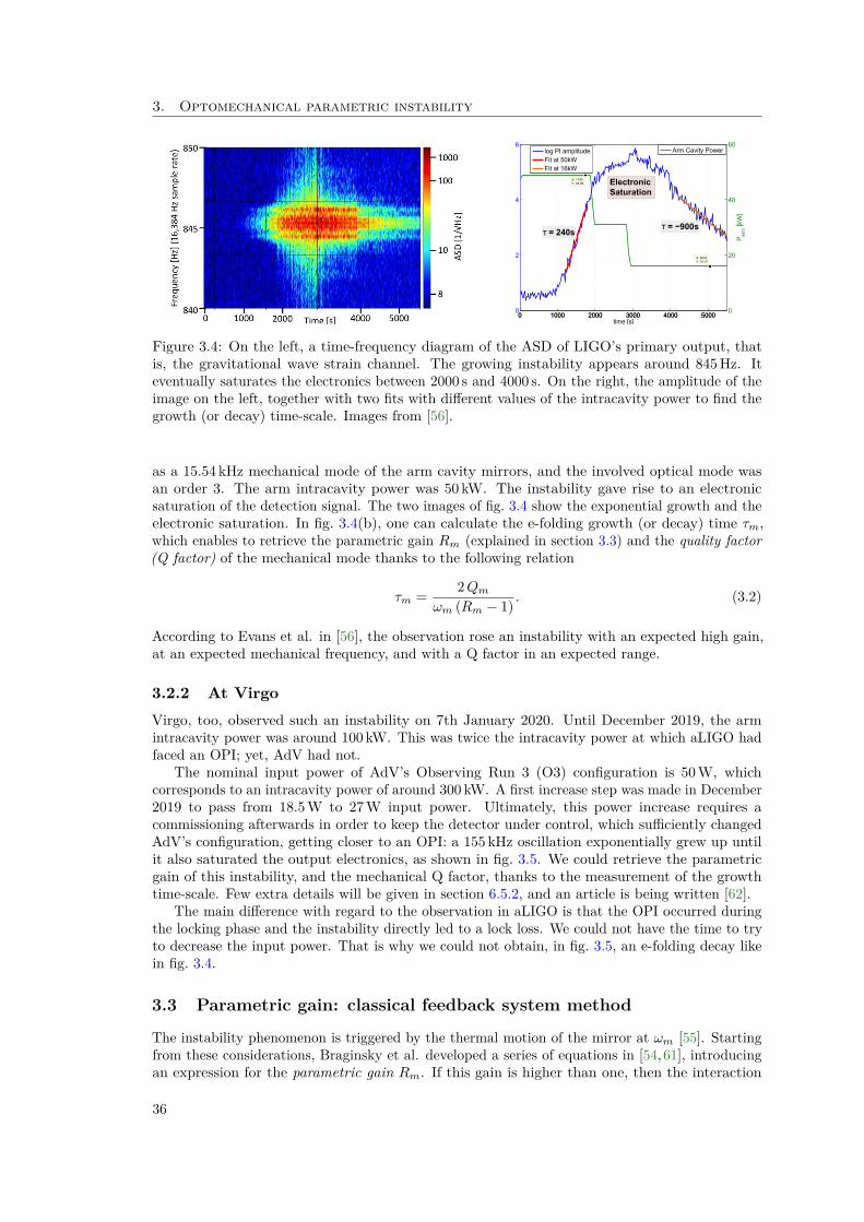
3. Optomechanical parametric instability
0 1000 2000 3000 4000 50000
2
4
6
τ = 240sτ = −900s
0 1000 2000 3000 4000 50000
20
40
60
X: 1740Y: 48.84
time [s]
Pa
rm[k
W]
X: 5040Y: 16.01
Arm Cavity Powerlog PI amplitude
Fit at 50kW
Fit at 16kW
Electronic
Saturation
Figure 3.4: On the left, a time-frequency diagram of the ASD of LIGO’s primary output, thatis, the gravitational wave strain channel. The growing instability appears around 845 Hz. Iteventually saturates the electronics between 2000 s and 4000 s. On the right, the amplitude of theimage on the left, together with two fits with different values of the intracavity power to find thegrowth (or decay) time-scale. Images from [56].
as a 15.54 kHz mechanical mode of the arm cavity mirrors, and the involved optical mode wasan order 3. The arm intracavity power was 50 kW. The instability gave rise to an electronicsaturation of the detection signal. The two images of fig. 3.4 show the exponential growth and theelectronic saturation. In fig. 3.4(b), one can calculate the e-folding growth (or decay) time τm,which enables to retrieve the parametric gain Rm (explained in section 3.3) and the quality factor(Q factor) of the mechanical mode thanks to the following relation
τm = 2Qmωm (Rm − 1) . (3.2)
According to Evans et al. in [56], the observation rose an instability with an expected high gain,at an expected mechanical frequency, and with a Q factor in an expected range.
3.2.2 At VirgoVirgo, too, observed such an instability on 7th January 2020. Until December 2019, the armintracavity power was around 100 kW. This was twice the intracavity power at which aLIGO hadfaced an OPI; yet, AdV had not.
The nominal input power of AdV’s Observing Run 3 (O3) configuration is 50 W, whichcorresponds to an intracavity power of around 300 kW. A first increase step was made in December2019 to pass from 18.5 W to 27 W input power. Ultimately, this power increase requires acommissioning afterwards in order to keep the detector under control, which sufficiently changedAdV’s configuration, getting closer to an OPI: a 155 kHz oscillation exponentially grew up untilit also saturated the output electronics, as shown in fig. 3.5. We could retrieve the parametricgain of this instability, and the mechanical Q factor, thanks to the measurement of the growthtime-scale. Few extra details will be given in section 6.5.2, and an article is being written [62].
The main difference with regard to the observation in aLIGO is that the OPI occurred duringthe locking phase and the instability directly led to a lock loss. We could not have the time to tryto decrease the input power. That is why we could not obtain, in fig. 3.5, an e-folding decay likein fig. 3.4.
3.3 Parametric gain: classical feedback system method
The instability phenomenon is triggered by the thermal motion of the mirror at ωm [55]. Startingfrom these considerations, Braginsky et al. developed a series of equations in [54, 61], introducingan expression for the parametric gain Rm. If this gain is higher than one, then the interaction
36

3.3. Parametric gain: classical feedback system method
Figure 3.5: On the left, a time-frequency diagram of the ASD of Virgo’s primary output, that is,the gravitational wave strain channel. The growing instability appears around 155 kHz, during thelocking phase of the apparatus. It eventually saturates the electronics. On the right, the amplitudeof Virgo’s primary output: the blue curve is the full signal, the red curve is the contribution ofonly the 155 kHz signal. Images done by Paola Puppo (INFN Roma).
between those modes can lead to an OPI. The definition given by Braginsky et al. can also befound in many articles: [63–68]. In [69], this expression is generalised to sum the contributions ofall the transverse optical modes.
However, our computation does not use that expression, as it is not easy to implementnumerically, but rather the one from [55], whose approach is described in the following.
I describe the approach developed by Evans et al. [55] to compute the parametric gain. Inthis framework, the whole interaction between the three implied modes is seen as a classicalfeedback system. This modular approach is very suitable since it can be adapted to many differentinterferometer configurations with the same analytical formulas. The parametric gain of themechanical mode m is given by
Rm = 8πQmP
Mω2mcλ︸ ︷︷ ︸
prefactor
∞∑n=0
Re [Gn]︸ ︷︷ ︸optical transfer coefficient
× B2m,n︸ ︷︷ ︸
spatial overlap parameter
, (3.3)
where Qm is the Q factor of the mechanical mode m and ωm its frequency, P the arm cavity opticalpower, λ the optical wavelength, M the mirror mass, c the velocity of light; Gn is the opticaltransfer coefficient of the nth optical mode and encapsulates the interferometer configuration;finally, Bm,n is the spatial overlap integral between the three involved modes. A mechanicalmode is amplified if Rm > 0 and damped if Rm < 0. It becomes unstable if Rm > 1, that is, ifthe resonant excitation of the mechanical mode by the radiation pressure force overcomes themechanical losses.
3.3.1 The prefactorLet us just recall the linear dependence of the parametric gain on the intracavity power. As well,it is directly proportional to the mechanical mode m’s Q factor. The possibility of damping anOPI by reducing the unstable mechanical mode’s Q factor has been studied in [65]. Indeed, onedoes not design mirrors with low mechanical Q factors, in order not to increase the thermal noise(see eq. (2.19)). Therefore, this is better to keep Q factors as high as possible because the thermalnoise can strongly and continuously deteriorate the detector sensitivity, while the phenomenon ofOPIs happens only for certain configurations.
To lower the parametric gain, trying to build heavier optics seems to be a better solution. Thishas been done from LIGO (11 kg) to aLIGO (40 kg) [70], and from Virgo (21 kg) to AdV (42 kg),as shown in table 2.1. This improvement is first meant to decrease the effect of the radiation
37

3. Optomechanical parametric instability
pressure (improving, thus, the sensitivity), not to lower the odds of encountering an OPI; however,the former leads to the latter.
Note that the parametric gain is inversely proportional to the square of the mechanical modefrequency. However, contrary to what was expected, even a mechanical mode of very high frequencycan lead to an OPI, as experimentally demonstrated in section 3.2.2.
3.3.2 The spatial overlap parameter
The spatial overlap parameter results from the overlap integral of the the three implied modesspatial profiles. It writes
Bm,n =∫∫S
f0fn (um · z) dr⊥, (3.4)
where S is the optic’s coating surface, f0 and fn are the field distributions of respectively thefundamental mode and the nth optical mode, and um is the displacement function of the mechanicalmode. The field distributions are normalised as∫∫
∞
|fn|2 dr⊥ = 1 (3.5)
Figure 3.6 shows various couples of mechanical modes and optical modes, together with theirassociated squared spatial overlap parameters. The two first couples are arbitrarily chosen fortheir weak spatial overlap. The two last couples show very good spatial overlaps. A large overlapparameter is however not a sufficient condition to get an instability, the resonance condition shouldalso be verified. This is the subject of the next paragraph.
3.3.3 The optical transfer coefficient
The optical transfer function encapsulates the cavity response to the optical fields. The two carriersidebands corresponding to the Stokes and anti-Stokes processes have different optical transfercoefficients G−n (lower sideband) and G+
n (upper sideband). The total optical transfer coefficientGn is defined as
Gn = G−n −G+n , (3.6)
where G+n denotes the complex conjugate of G+
n .At low power, the mirror motion due to the radiation pressure is negligible. The propagation
of optical fields at different frequencies are independent and can be treated separately. At highpower, the radiation pressure depends on both sidebands, and the motion induced by the radiationpressure modifies the sidebands. Hence, a classical feedback system; according to Corbitt et al.in [71], the most convenient mathematical framework for this problem is the Caves-Schumakertwo-photon formalism [72, 73].
Evans et al. built their method on this mathematical framework to calculate the scatteringmatrix S±n that contains all the transfer coefficients for the nth optical mode from one port of theoptical system to the next one. Therefore, the scattering matrix is a square matrix whose size isthe number of all considered fields of interest.
From the scattering matrices S±n of the two sidebands, one can derive the optical transfercoefficients
G±n,x = eTx(I − S±n
)−1 ex, (3.7)
where ex is the xth column of the identity matrix I, and eTx its transpose. The index x = 1, 2, ..., 12denotes the fields of interest of figs. 3.7 and 3.8.
38

3.3. Parametric gain: classical feedback system method
-10 0 10cm
-10
0
10
cm
-10 0 10cm
-10
0
10
cm Bm,n2 = 8.2043 X 10⁻¹⁰
-10 0 10cm
-10
0
10
cm
-10 0 10cm
-10
0
10cm Bm,n
2 = 0.1860
-10 0 10cm
-10
0
10
cm
-10 0 10cm
-10
0
10
cm Bm,n2 = 1.2128
-10 0 10cm
-10
0
10
cm
-10 0 10cm
-10
0
10
cm Bm,n2 = 8.1635
Figure 3.6: On the left, the surface displacements of various mechanical modes. In the middle, someoptical modes. On the right, the associated squared spatial overlap parameters B2
m,n. Downwards,the optical modes are respectively the FSMM(5) (order 2), the FSMM(3) (order 1), the FSMM(4)(order 2), and the FSMM(1) (order 0). The FSMM will be introduced in section 5.3.3.
4
21 3
5
IM EM
Figure 3.7: Fields of interest of an arm cavity.
39

3. Optomechanical parametric instability
1
2
8
5
4
12
7
10
WIM
WEM
BS
NIM NEM
Detection photodiode
PRM
SRM
6
3
9
11
Figure 3.8: Fields of interest of a power and signal recycled of a Fabry-Perot interferometer. Thisis the most general configuration, that is, with a PRC, and an SRC cavity. One can ‘suppress’ amirror (and thus its cavity) by setting its transmission to 1.
Single arm cavity
In the case of a single arm cavity of length L, one can use the following simpler formalism wherethe fields of interest are those of fig. 3.7; then, the size of the scattering matrix S±n is 5× 5 andwrites
S±n =
0 0 0 0 0tIM 0 0 0 −rIM0 p±L 0 0 00 0 −rEM 0 00 0 0 p±L 0
, (3.8)
where tIM is the amplitude transmission coefficient of Input Mirror (IM), rIM and rEM theamplitude reflection coefficients of the mirrors, and p±L the propagation operator as
p±L = exp[j
(φn ±
ωmL
c
)]. (3.9)
φn is the phase of the nth HOMφn = φ0 − ψn, (3.10)
where φ0 is the propagation phase of the fundamental mode, and ψn the Gouy phase of the nthoptical mode. Further information on how the Gouy phase is obtained according to the opticalmode basis will be be given in chapter 5.
Full interferometer and losses
Let us now introduce a more general formalism considering a full power- and signal-recycledinterferometer, and the losses.
Figure 3.8 shows the fields of interest for an optical system corresponding to AdV; the size ofthe scattering matrix S±n is then 12× 12. One can write the scattering matrix as the product of
40

3.3. Parametric gain: classical feedback system method
a propagation matrix P±n , which is diagonal, and a mirror matrix Mn containing the amplitudereflection and transmission coefficients, as
S±n = MnP±n , (3.11)
where
P±n =
p±n,1 0 · · ·0 p±n,2... . . .
, (3.12)
withp±n,x = exp
[j
(φn,x ±
ωmLxc
)]. (3.13)
Lx is the propagation distance at the field point x, and φn,x the propagation phase of the nthoptical mode at x. The propagation factor yields constructive interferences when the total phaseis 0 [2π], that is to say when
φ0,x − ψn,x = ωmLxc
+ 2kπ
⇒ φ0,xπ
c
2Lx− ψn,x
π
c
2Lx= νm + 2kπ
⇒ ν0,x − νn,x = νm + 2kπ,
Stokes (3.14)
φ0,x − ψn,x = −ωmLxc
+ 2kπ⇒ νn,x − ν0,x = νm + 2kπ.
}anti-Stokes (3.15)
With these equations, one retrieves the condition for an OPI to occur: the mechanical modefrequency must be close to that of the optical beat note.
Now, if the mirror transmission coefficient is much smaller than one, one can further split themirror matrix into a constant matrix M and a loss matrix Cn, which is diagonal, as
Mn = MCn, (3.16)
where
M =
· −rNEM · · · · · · · · · ·−rNIM · · · · tNIM · · · · · ·· · · −rWEM · · · · · · · ·· · −rWIM · · · · tWIM · · · ·
tNIM · · · · rNIM · · · · · ·· · · · · · · · · tBS · rBS· · tWIM · · · · rWIM · · · ·· · · · · · · · · −rBS · tBS· · · · tBS · −rBS · · · · ·· · · · · · · · −rPRM · · ·· · · · rBS · tBS · · · · ·· · · · · · · · · · −rSRM ·
(3.17)
and
Cn =
tn,1 · · · ·· tn,2... . . .
, (3.18)
were tn,x is the amplitude transmission of the aperture of the each fields of interest, and · standsfor 0.
Now that everything needed to compute the optical transfer coefficient has been presented, letus focus on the role played by this coefficient. By making the mechanical frequency artificiallyvary, one can obtain the optical transfer functions of an optical mode, as well as the parametricgain Rm of a given mechanical mode. The results for AdV’s O3 configuration with the third couple
41

3. Optomechanical parametric instability
35 40 45 50 55 60 650
100
200
300
400
500
-4
-3
-2
-1
0
1
2
20 30 40 50 60 70 80-10
-5
0
5
10102
Figure 3.9: (a) G+n (blue curve), G−n (green curve), and Rm (red curve) of the third couple from
fig. 3.6, while artificially modifying the mechanical frequency. The upper sideband at 37 kHz hasa negative optical transfer coefficient. The lower sideband at 63 kHz has a positive one, but theparametric gain is not high enough to lead to an OPI. (b) Gn of three optical modes of order 1, 2,and 3. The resonant frequencies are set by the optical mode phase, and, therefore, by the cavityGouy phase and the optical mode order. One can also notice that the higher the optical modeorder, the lower its gain, as expected.
of modes from fig. 3.6 are shown in fig. 3.9(a)1; all the optical values used in our simulations aresummarised in table 6.1. One can see that the upper sideband indeed yields a negative parametricgain, while the lower one yields a positive parametric gain.
An interesting point is that although the spatial overlap parameter between those three modesis rather high, the optical transfer coefficient does not lead to an OPI. Hence the critical roles ofthe optical transfer coefficient and the mechanical mode frequency.
Figure 3.9(b) shows the optical transfer coefficient Gn for three optical modes of order 1, 2,and 3. Inasmuch as a cavity Gouy phase is fixed, only the mode order modifies the resonantfrequency. Therefore, the main optical contributors to the parametric gain of a mechanical modeare all of the same order.
3.4 Summary
The OPI in gravitational-wave detectors is a well and long-studied phenomenon since the early2000s. The OPI results from the interaction between two optical modes of the cavity anda mechanical mode of a mirror. The motion of a mirror at ωm can scatter photons from thefundamental mode into two sidebands (ω1 = ω0±ωm), which, in turn, interact with the mechanicalmode via radiation pressure, and so on. This process can either lead to an exponential increase(lower sideband) of the mechanical motion or its damping (upper sideband). The former casecan lead to a loss of the control of the interferometer and becomes more important and likely tohappen if the available energy of the fundamental mode is higher. Indeed, such instabilities havealready been observed at aLIGO and AdV. That is why we study their behaviours for AdV.
The interaction between a mechanical mode m and all the cavity optical modes can bequantified by its parametric gain Rm (eq. (3.3)). The mechanical mode is amplified if Rm > 0,and is damped if Rm < 0. The mechanical mode becomes unstable if Rm > 1. This parametric
1We are always interested to know the parametric gains for fields at mirror locations, that is to say the fieldpoints x = {1, 2, 3, 4}. Therefore, the given results will always be obtained from a mirror field. If the cavity nameor the mirror names matter, then they will be specified.
42

3.4. Summary
gain comprises three terms: the prefactor, the optical transfer coefficient Gn, and the spatialoverlap parameter Bm,n.
• The prefactor depends on the mechanical mode (Q factor and frequency), the mirror mass,the intracavity power, and the laser wavelength.
• The optical transfer function — according to both the fundamental mode (ω0) and the HOM(ω1) — sets the optical resonance (frequency ω0 − ω1, amplitude, and linewidth), whichdepends on both the fundamental mode and the HOM. The optical transfer coefficient (oroptical gain) is the value of the optical transfer function at the mechanical mode frequencyωm.
• The spatial overlap parameter depends on the amplitudes of the fundamental mode, theHOM, and the mechanical mode. This factor is higher if the shapes of the three impliedmodes match.
The optical gain and the overlap parameter are calculated for a specific HOM. The mechanicalmode’s parametric gain sums up the contributions of all the optical modes taken into account.Hence, the OPI study primary requires the computation of the arm cavity mirrors’ mechanicalmodes and the arm cavities’ optical modes. This will be the topic of the two following chapters.
43


Chapter 4
Mechanical modes of Advanced Virgo’sarm cavity mirror
The mechanical modes were computed by means of finite element analysis (FEA) developed forthe actual Input Mirror (IM) of Advanced Virgo (AdV) arm cavities. We used the programAnsys®WorkbenchTM. The IM model includes the high-reflectivity coating of the front face, theflats and the bevels. Moreover the ears and the anchors attached by silicate bonding techniqueare included (see fig. 4.1). In the FEA, the multilayered optical coating is modelled as a solid3D element having the total thickness corresponding to the sum of the thicknesses of the highreflective and low reflective materials and mechanical parameters averaged over the thicknesses ofthe layers. Instead of 3D shell elements, we have used 3D solid elements, for very thin materialsas well, though more CPU time consuming, because they provide the shear deformations andenergies, which are useful for getting the mechanical losses associated to the modes.
Figure 4.1: Geometry used for the FEA, including the ears, the anchors and the magnets attachedon the mirror rear face. The suspension wires are just for sketching but not included in thesimulation as they do not influence the modal frequencies.
45

4. Mechanical modes of Advanced Virgo’s arm cavity mirror
0 10 20 30 40-8
-6
-4
-2
0
2
4
6
810-3
-5 0 5
10-3
0
20
40
60
1 1
151 (99 %)
Figure 4.2: (a) Relative differences of measured frequencies with respect to frequencies obtainedwith the FEA vs the FEA frequencies. The standard deviation σ(νmeas) is 0.15 %. (b) Distributionof the relative differences; the bin width is σ(νmeas)/2. There are 153 data, of which 151 (99 %)are comprised within ±3.5σ(νmeas) ≈ ±0.50 %.
4.1 Finite element analysis simulations results
The flats, the ears, and the anchors play an important role. In particular, since they break thecylindrical symmetry, they lift degeneracies and increase the number of distinct mode frequencies.
To estimate the accuracy of the model, we used a set of frequencies (νmeas) measured fromring-down measurements of the North Input Mirror (NIM) up to 40 kHz. Figure 4.2(a) showsthe relative differences (νmeas − νFEA)/νFEA versus the frequency of the FEA νFEA. The stan-dard deviation is 0.15 %. Figure 4.2(b) shows their distribution: 99 % are comprised within±3.5σ(νmeas) ≈ ±0.50 %.
We estimated the quality factors (Q factors) of the mechanical modes of the IM taking intoaccount several kinds of losses: losses of the fused silica (FS) substrate, anchors and supports ofthe magnets (loss angle φFS); coating losses (loss angle φIMcoating); losses of bonding layers usedto attach the ears, the anchors, and the magnets (loss angle φBonding). The bonding layers havea thickness of 60 nm and are modelled as 3D solid elements. Coating losses of the IM and EndMirror (EM) were recently measured [74]. Note that all the parameters used are given in table 4.1.Each loss contributor is related to the energy fraction stored in the lossy part and to the materialloss angle, through the relationships
φBonding · Etot = φHCB · Ebonds
φIMcoating · Etot = φCIM · ECIM
φFS · Etot = φSuprasil · EFS,
(4.1)
where HCB stands for hydroxide-catalysis bonds. The overall loss angle for the IM is obtained bysumming up all contributors: φIM = φBonding + φIMcoating + φFS. The mechanical Q factor of theIM modes then writes
Qm = 1/φIM. (4.2)Figure 4.3 shows the frequency dependence of the FS substrate loss and the effect of adding
the optical coating and the bonding layers. The influence of the bonding term φBonding is stronglymode shape dependent through the deformation of the ear and anchor bulks, and it is not negligible.In fact, its contribution to Qm is dominant. For this reason, from a set of Q factor measurements,it is possible to infer the value of φHCB by using the energy fractions calculated with the FEA.
Figure 4.4(a) Qm of the IM mass computed by fitting the loss angle φHCB by using the firstset of five modes of the IM of the North arm and supposing that it is does not vary with the
46

4.1. Finite element analysis simulations results
IM Coating1Ta2O5 High index Layer Overall Thickness (tIMH ) 2080 nmSiO2 Low index Layer Overall Thickness (tIML ) 727 nmLoss angle (φCIM) 1.1 · 10−4f0.05
EM Coating1Ta2O5 High index Layer Overall Thickness (tEMH ) 3766 nmSiO2 Low index Layer Overall Thickness (tEML ) 2109 nmLoss angle (φCEM) 2.2 · 10−4f0.01
TM SuprasilYoung modulus 72.251 GPaPoisson ratio 0.166 49Density 2201 kg m−3
Loss angle (φSuprasil) 7.6 · 10−12f0.11
Ear and anchors bonding [75]Young’s modulus 72.9 GPaPoisson ratio 0.17Density 2201 kg m−3
Thickness 60 nmLoss angle 0.1
IM and EM propertiesMass 42 kgThickness 200 mmDiameter 350 mmFlats 50 mm
Table 4.1: Mechanical parameters used in the FEA
1For the FEA, the IM multilayered coating was replaced by one layer having the total thickness corresponding tothe sum of the thicknesses of the high reflective and low reflective materials. The mechanical parameters used arethe average values of this layer [74].
1 2 3 4 5 6 7 8 9 10
Modal Frequencies [Hz] 104
10-9
10-8
10-7
10-6
10-5
10-4
FS+
IM coating+
Bonding
FS+
IM coating
FS
Figure 4.3: Losses present in the FEA model of the IM, computation up to 100 kHz.
47

4. Mechanical modes of Advanced Virgo’s arm cavity mirror
103
104
105
106
107
108
0 20 40 60 80 100 120 140 1600
2000
4000
6000
8000
10000
12000
14000
Figure 4.4: (a) Q factors of the mechanical modes up to 157 kHz. (b) Mechanical mode frequency vsMechanical mode number. The mechanical mode density considerably increase at high frequency.
frequency. At frequencies higher than 10 kHz, the bondings have a strong damping effect, thoughthey have a negligible effect on the the thermal noise of the IM. This is a very important resultfor the parametric gains computation and, consequently, for identification of the unstable modes.
Figure 4.4(b) shows the total number of mechanical modes with respect to their frequencies.We computed 12 750 mechanical modes up to 157 kHz. In chapter 6, I explain that we had firstcomputed only 1600 mechanical modes, up to 70 kHz, but then, we needed to compute muchhigher-frequency modes.
Figure 4.5 shows some mechanical modes, arbitrarily chosen over the whole frequency range.Above each is indicated the measured frequency νmeas.
4.2 Conclusion
The computation of the mechanical modes was done by Paola Puppo (INFN Roma), using 3Dsolid elements FEA simulation. It provided us with the mode shapes, the simulated frequenciesνFEA, and the simulated Q factors QFEA. Paola Puppo also measured, on site the frequenciesνmeas and the Q factors Qmeas of the mechanical modes of the IMs from ring-down measurements.The measured frequencies allowed us to estimate the relative difference between the simulationand the measurements. The measured Q factors allowed us to fit the QFEA up to 157 kHz. Thethree cited parameters obtained by the FEA simulation and the measurements are sufficient to
48

4.2. Conclusion
Figure 4.5: Some arbitrarily chosen mechanical modes.
characterise the mechanical modes that we need to compute the parametric gains in chapter 6.
Figure 4.6: Photograph of a 42 kg AdV’s arm cavity mirror suspended inside the payload by twothin wires of FS. The pink colour is due to a protecting film. Credits: Virgo collaboration.
49


Chapter 5
Optical modes of Advanced Virgo’s armcavities
The previous chapters showed basics of gravitational waves and ground-based interferometricgravitational-wave detection. It was explained how to improve the sensitivity of detectors withvarious techniques. Then, the optomechanical parametric instability (OPI) phenomenon wasintroduced, leading to the computation of the arm cavity mirrors’ mechanical modes and the armcavities’ optical modes. This chapter will focus on the description of arm cavities’ modes.
First is introduced some basic concepts of optical resonators. Then is presented the behaviourof Fabry-Perot resonators (plane-mirror resonators), which will help introduce essential quantitiesrelated to resonators. Then, the case of spherical-mirror cavities is treated. Two different modelsthat can be used to compute optical modes are compared: a model considering the mirrors asinfinite, and another one considering the real finite size of the mirrors. Optical modes of the formercan be computed thanks to well-known and well-studied bases, such as the Hermite-Gaussianmodes (HGM), whereas optical modes of the latter require a numerical computation. I will showthe limits of the HGM with respect to the finite-sized mirror modes (FSMM). Finally, I introducethe effect, on optical modes, of the mirror deformation due to light absorption (sometimes referredto as ‘thermal effects’).
5.1 Wave optics conventions and notation
5.1.1 On light propagation in vacuum
An linearly polarized optical field can be described by a scalar complex wavefuntion E(r, t) ofposition r and time t. E(r, t) must satisfy the wave equation
∇2E(r, t)− 1c2∂2E(r, t)∂t2
= 0, (5.1)
where c is the speed of light in vacuum.In the following, we restrict ourselves to monochromatic waves. For a monochromatic wave
propagating with the wavenumber k = ωc at the instant t, the wavefunction is
E(r, t) = A(r) ej(ωt−k·r), (5.2)
where ω = 2πν is the pulsation, ν the frequency, and A(r) a complex function. Equation (5.2)can be rewritten
E(r, t) = E(r) ejωt, E(r) = A(r) e−jk·r, (5.3)
where E(r) is the complex amplitude and is time independent. In all the following, we will studythe properties of E(r), which is the spatial part of the wavefunction.
51

5. Optical modes of Advanced Virgo’s arm cavities
Substituting eq. (5.3) into eq. (5.1) yields∇2E(r) + k2E(r) = 0 (5.4)
known as the Helmholtz equation.
5.1.2 Incident, reflected, and transmitted wavesAn incident wave reflecting on a mirror undergoes a π phase shift such that a possible conventionfor the scattering matrix is (
Er1
Er2
)=(t −r−r t
)(Ei3Ei4
)(5.5)
where r is the amplitude reflection coefficient, and t the amplitude transmission coefficient(fig. 5.1).
Ei3 Er1
Ei4Er2
r, t
Figure 5.1: Incident, reflected, and transmitted field notations.
In the following, we use these results to calculate the different optical fields of a resonator.
5.1.3 Reflection, transmission, and lossesAn optical element is characterised by three coefficients: its amplitude reflection coefficient r, itsamplitude transmission coefficient t, and its amplitude losses. By squaring these quantities, oneobtains respectively the intensity reflection coefficient (or reflectivity, or reflectance) R = r2, theintensity transmission coefficient (or transmissivity, or transmittance) T = t2, and the intensitylosses L. Hence, the energy conservation of the incident wave reads
R+ T + L = 1. (5.6)Losses can be of various types: absorption in the mirror coatings, scattering on mirrors due toimperfections, and diffraction loss due to the finite size of the mirrors. The diffraction loss will bereferred to as Ld, and all the others losses as1 Lm. Then comes
L = Ld + Lm. (5.7)
5.2 Fabry-Perot resonators
Interferometric gravitational-wave detectors have optical cavities on both of their arms to increasethe sensitivity inasmuch as the phase shift induced by the passage of a gravitational wave ismultiplied by a factor GAFPC, as explained in section 2.2.2. To better understand longitudinalmodes of these cavities, one can use the model of plane-mirror resonators, called Fabry-Perotresonators, which consist in two mirrors M1 and M2 with their associated reflection coefficientsr1, r2, and transmission coefficients t1, t22, separated by a distance L, as shown in fig. 5.2.
1For ‘mirror losses’.2Ideally, the end mirror must be perfectly reflective, whereas the input one should have a non-null transmissivity
such that the light can enter the resonator. In the case of Advanced Virgo, the very small amount of transmittedlight at the end mirror allows to obtain an information about the circulating light field and, thus, to control theFabry-Perot resonator length during the acquisition of the global interferometer working point.
52

5.2. Fabry-Perot resonators
E1
E5
E2 E3 E4
E6E7
L
M1 M2r1, t1 r2, t2
Figure 5.2: Optical fields of a Fabry-Perot resonator.
5.2.1 Optical fields and resonant frequenciesConsidering the complex amplitude of the electromagnetic field entering the resonator Ein = E1,the circulating amplitude Ecirc = E2, the transmitted amplitude Etrans = E4, and the reflectedamplitude Erefl = E7 can be calculated. The circulating field is the sum of all the fields circulatingwithin the resonator (see fig. 5.3) and can then be described as a geometric progression withcommon ratio r1 r2 e
−jk2L. In order that the electromagnetic fields constructively interfere, and,thus, build a mode, they need to be in phase; hence the resonance condition
2kL = q2π ⇐⇒ k = qπ
L⇐⇒ ν = q
c
2L, q ∈ Z. (5.8)
This shows that only certain frequencies can lead to standing waves within the resonator: in thefollowing, these modes will be referred to as longitudinal modes. The electromagnetic fields at
M1 M2r1, t1 r2, t2
E20
E21
E22
Figure 5.3: Travelling waves between both mirrors of a Fabry-Perot resonator.
each point of the resonator are
E2 = t1E1 − r1E6 E5 = −r2E3
E3 = E2 e−jkL E6 = E5 e
−jkL
E4 = t2E3 E7 = −r1E1 + t1E6.
From these equations one can determine the electromagnetic fields inside the resonator of interest:
Ecirc = t11− r1 r2 e−jk2L Ein (5.9)
In practice, the measurable quantity is the intensity (in W m−2), obtained by squaring themodulus of the amplitude:
Icirc = |Ecirc|2 = Ecirc · E∗circ = T11 + r2
1 r22 − 2r1 r2 cos (2kL)Iin, (5.10)
53

5. Optical modes of Advanced Virgo’s arm cavities
0 20 40 60 80 100 120 140 1600
0.2
0.4
0.6
0.8
1
Figure 5.4: Circulating intensity within the resonator. The resonator acts as filter letting only somefrequencies be resonant; these frequencies are separated by the Free Spectral Range representedby the arrow. The circulating intensity is normalised by Icircmax to show that δν increases when Lincreases.
where Iin = |Ein|2. The maximum power is
Icircmax = T1
(1− r1 r2)2 Iin (5.11)
and is reached for cos(2kL) = 1, the resonance condition already expressed by eq. (5.8). Equa-tion (5.10) is called an Airy function (fig. 5.4) and depends on the losses accumulated duringa resonator round trip. This function shows equally separated peaks representing the resonantfrequencies of eq. (5.8) that can travel down the resonator. The frequency difference between twoconsecutive resonances is called Free Spectral Range (FSR), and from eq. (5.8) arises
∆νFSR = c
2L. (5.12)
Advanced Virgo (AdV)’s arms are 3 km long, then their FSR ∆νFSR is
∆νFSR ≈ 50.00 kHz. (5.13)
5.2.2 Effect of resonator lossesMirrors cannot be perfectly reflective and show a non-null transmissivity T and energy losses L.This modifies the travelling fields and relaxes the resonance condition, increasing, in turn, the FullWidth at Half Maximum (FWHM). The FWHM is also known as the linewidth δν. Inasmuch asthe finesse F can be defined as F = ∆νFSR/δν, from eq. (2.20) arises
δν ≈ ∆νFSR1− r1 r2π√r1 r2
. (5.14)
One can notice the dependence to the reflection coefficients: the higher they are (or the lower thelosses), the thinner the linewidth. So, increasing losses broadens resonances (fig. 5.4).
Let us now introduce another more practical definition of the finesse:
F = 2πP, (5.15)
54

5.3. Spherical-mirror resonators
where P = L1 + L2 + T1 + T2 is the resonator total loss, including the mirror transmissions.In summary, the lower the losses, the higher the finesse, the lower the linewidth. AdV’s arm
cavity3 finesse have been measured on site [76]:
FNorth = 464(7)FWest = 455(5)
(5.16)(5.17)
Consequently AdV’s arm cavity linewidths are
δνNorth ≈ 108 HzδνWest ≈ 110 Hz
(5.18)(5.19)
The finesse contains all the information of the resonator losses, and eq. (5.9) can be rewritten
Icirc = Icircmax
1 +G2AFPC sin2 (kL)
, (5.20)
where GAFPC = 2F/π is the optical gain of a Fabry-Perot resonator (see section 2.2.2) and is, forAdV, GAFPC ≈ 300.
5.3 Spherical-mirror resonators
In the previous section, I have derived resonant frequencies of Fabry-Perot longitudinal modes,and discussed the impact of losses on the resonance linewidth. In this section, I substitute planemirrors with spherical mirrors and show their impact on the resonant frequencies and on theresonator stability.
5.3.1 Gaussian beamComplex amplitude and beam properties
Here, I want to obtain a precise description of the complex amplitude E(r). As the field propagatesalong the z direction, we have
E(r) = A(r)e−jkz. (5.21)
Substituting eq. (5.21) into eq. (5.4) yields
∇2A− 2jk ∂A∂z
= 0. (5.22)
Insofar as the longitudinal envelope variation of the beam is very slow within a distance of awavelength λ = 2π/k, one can use the paraxial approximation. It implies that angles to the opticalaxis of the system are rather small. Therefore, a Gaussian beam has its energy confined aboutits axis. The paraxial approximation helps further simplify eq. (5.22) by neglecting the secondderivative in z of the complex envelope, yielding the paraxial Helmholtz equation
∇2TA− 2jk ∂A
∂z= 0, (5.23)
where ∇2T = ∂2/∂x2 + ∂2/∂y2 is the transverse Laplacian operator. In the absence of boundary
conditions, a well-known solution is the so-called Gaussian beam, whose complex amplitudewrites [77]
E(ρ, z) = A0w0w(z) exp
[− ρ2
w2(z)
]exp
[−j(kz + kρ2
2R(z) − ψ(z))], (5.24)
3Here, I speak in terms of cavity because these resonators are stable.
55

5. Optical modes of Advanced Virgo’s arm cavities
ZR
w0
zR(z)
w(z) -r²w²
exp( )
r
0
WavefrontIntensity profileGaussian beam asymptotes
Curvature
2w0
1/e of the maximum amplitude
Figure 5.5: A Gaussian beam profile, together with its Gaussian function transverse projection.Around the beam waist, the wavefronts are approximately planar, afar they are approximatelyspherical. Image by ℵ (Aleph) http://commons.wikimedia.org, modified, under the terms ofthe Creative-Commons-License CC-BY-SA-2.5.
where ρ2 = x2 + y2, w(z) is the beam radius at which the amplitude falls to 1/e (∼ 27%) of themaximum (which is on the axis) at z4, w0 = w(0) is the waist radius, which is the beam radius atits focus, that is, where its radius is minimum, R(z) the wavefront radius of curvature at z, andψ(z) is the Gouy phase, which is an extra phase accumulated along the z-axis.
Figure 5.5 shows a Gaussian beam along the z-axis, together with all parameters defining sucha wave. Its transverse profile is indeed a Gaussian function. Longitudinally, this Gaussian functionpropagates along the z direction, and if one lets the origin of this axis be at the beam waist,the width of the beam becomes larger while increasing |z| due to diffraction. Around the beamwaist, the wavefronts are approximately planar; afar from the beam waist, they are approximatelyspherical. One can then define two approximate regions and a parameter called the Rayleigh rangezR (eq. (5.25)): near field when z � zR and the far field when z � zR.
Let us summarise, here, all parameters defining a Gaussian beam:
• Rayleigh range zR:
zR = πw20
λ(5.25)
• Beam radius w(z):
w(z) = w0
√1 +
(z
zR
)2(5.26)
• Wavefront radius of curvature R(z):
R(z) = z
[1 +
(zRz
)2]
(5.27)
• Gouy phase ψ(z):
ψ(z) = arctan(z
zR
)(5.28)
Equations (5.26) and (5.27) help understand better the longitudinal evolution of the beam radiusand the wavefronts.
4An amplitude drop of 1/e corresponds to an intensity drop of 1/e2 ≈ 0.135; therefore, since the intensitycarried within a circle of radius w(z) represents 86%, it is justified to call w(z) the beam radius.
56

5.3. Spherical-mirror resonators
Regarding the beam radius, as described above, the minimum w0 is at the beam focus andincreases in both directions, linearly with z for z/zR � 1 (eq. (5.26)). Its value at zR is
√2w0.
Regarding the wavefronts, eq. (5.27) shows that limz→0±
R(z) = ±∞, that is, the wavefronts areplanar. While w(z) increases, R(z) first decreases until it reaches its minimum at zR: the beam iscurved the most at the Rayleigh range. Then, R(z) slowly increases, tending towards an R(z) = zasymptote.
Gaussian beam stability in a spherical-mirror resonator
Considering a resonator with two spherical mirrors of different radii of curvature R1 and R2 andseparated by a distance L, one can let the origin of the z-axis be at the beam waist, and the twomirrors be respectively located at z1 and z2. In the following, such a device will be referred to asan optical cavity.
If the wavefront of an incident Gaussian beam has the same radius of curvature than a sphericalmirror, then its reflected beam from that mirror will exactly retrace the incident beam. Thus, abeam within the cavity will be reflected on a mirror and will retrace itself to the second mirror,where the same phenomenon will occur, and, so on, the beam exists self-consistently and can betravelling within the cavity. A Gaussian beam can thus be a stable mode of a spherical-mirrorresonator.
Introducing the g parameters as
gi = 1− L
Ri, i = {1, 2}, (5.29)
and their productg = g1 g2, (5.30)
it can be shown that the stability condition of an optical cavity writes [77]
0 ≤ g ≤ 1. (5.31)
Figure 5.6 shows different optical resonator configurations, which are represented by a doton the diagram. The green area highlights the stable configurations. If R1 = R2, the cavity is asymmetrical resonator and lies on the first bisector in fig. 5.6.
Here are values of AdV’s cavity parameters for both North and West AdV’s arm cavities [36]:
LAFPC = 2999.8 m RIM = 1420 m REM = 1683 m,
yieldinggAFPC = gIM · gEM = 0.8705, (5.32)
with gIM and gEM < 0. The cavities are indeed stable and are not symmetric yet not that far frombeing symmetrical concentric ones, i.e. R1 ≈ R2 ≈ −d/2. In that case, the field is focused at thecentre of the cavity.
Phase and resonant frequencies
From eq. (5.24), one can write the Gaussian beam phase as a function of the radial ρ and theaxial z positions:
φ(ρ, z) = kz + kρ2
2R(z) − ψ(z). (5.33)
The first term is the accumulated phase during the propagation along the z-axis; the second oneis the bending of the wavefront (see eq. (5.27)); and the last one is the Gouy phase: a Gaussianbeam accumulates a delay compare to a planar wave (see eq. (5.28) and fig. 5.7).
From eq. (5.33), one can write the difference in phase on the axis after one round trip
2∆φ(ρ = 0) = 2kL− 2∆ψ (5.34)
57

5. Optical modes of Advanced Virgo’s arm cavities
-2 -1 1 2
-2
-1
1
2
Figure 5.6: Representation of the hyperbola g1 g2 = 1. Each resonator can be represented by adot on this diagram. Given the stability condition 0 < g < 1, any point located in the blueishgreen area represents a stable resonator. Three resonators of interest are highlighted: a representsa planar resonator (Fabry-Perot), b represents a symmetric concentric one, and c represents AdV’sconfiguration, which is a quasi-symmetric-concentric one.
-4zR -2zR 0 2zR 4zR
- /2
- /4
/4
/2
Figure 5.7: Gaussian beam’s Gouy phase, which is the accumulated phase by a Gaussian beamalong the z axis with respect to a planar wave. The farther away from the beam waist, the morephase is accumulated.
where ∆φ(ρ = 0) = φ(0, z2)− φ(0, z1) is the Gouy phase shift accumulated during a single tripand is defined as [78,79],
∆ψ = ψ(z2)− ψ(z1) = arccos (±√g), (5.35)where the plus sign is chosen if g1 and g2 are positive, and the minus sign when g1 and g2 arenegative. The approximate g parameter of AdV has been estimated to 0.8705, so the Gouy phaseshift per single trip of AdV’s arm cavity is
∆ψAFPC = 2.774. (5.36)
Due to the Gouy phase, the resonance condition is modified compared to a planar resonator.The phase accumulated along a cavity round trip must verify
2∆φ(ρ = 0) = q2π, q ∈ Z, (5.37)
which yieldsνq = ∆νFSR
[q + ∆ψ
π
]. (5.38)
58

5.3. Spherical-mirror resonators
5.3.2 Infinite-sized mirror modes: Hermite-Gaussian modes (HGM)The equation satisfied by the wave function is the Helmholtz equation. One can find infinite,countable, and complete orthogonal sets of modes that are solutions of this equation (bases). Thechapter 3 of [77] and the article [78] provide detailed mathematical developments to show thatHGM, Laguerre-Gaussian modes, and Bessel-Gaussian modes are sets of solutions to the paraxialHelmholtz equation, considering infinite-sized mirrors. In the case of perfect spherical mirrors(radial symmetry), the Laguerre-Gaussian basis is a natural basis because these modes, too, havesuch a radial symmetry. Be that as it may, I will focus only on HGM, for they are the simplestand the most commonly used.
Hermite-Gaussian modes: amplitudes and orders
The HGM are an orthogonal set of modes that can be used to decompose a paraxial beam usingCartesian coordinates. The transverse profile is the product of a function in x and one in y, whosereferred index is respectively l and m. The complex amplitudes of HGM are
Elp(ρ, z) =Alpw0w(z) exp
[− ρ2
w2(z)
]×Hl
(√2x
w(z)
)Hp
(√2 y
w(z)
)× exp
[−j(kz + kρ2
2R(z) − (l + p+ 1)ψ(z))],
(5.39)
where Alp is a normalisation constant depending on l and p, Hn are Hermite polynomials.Comparing eqs. (5.24) and (5.39), one can notice that the HGM are waves whose complex
envelope are modulated forms of the Gaussian beam and whose phase is shifted. Both of thesemodifications depend on the values of l and p. A Hermite-Gaussian mode’s profile is determinedby a Hermite polynomial multiplied by a Gaussian profile. One can first study the effect of asingle Hermite-Gaussian function, which is defined by
Gn(u) = Hn(u) exp(−u2
2
). (5.40)
Figure 5.8 shows the shapes of the first Hermite-Gaussian functions. First, note that the indexn is the number of zeros of the polynomial; hence, an odd index yields an odd function, and aneven index yields an even function. Then, a very important piece of information is that the profilebecomes broader when n increases.
The two numbers l and p define the order N of the Hermite-Gaussian mode as
N = l + p, l, p ∈ N (5.41)
and give its name HGlp. There are always N + 1 modes of order N . From eq. (5.39) lettingl = p = 0 arises the same expression as eq. (5.24); therefore the HG00, or the fundamental mode,is described by eq. (5.24) just as the free space Gaussian beam. The other modes are calledhigher-order modes (HOMs). Figure 5.9 shows HGM for l, p ∈ {1, 2}. One can see the zeros ofeach polynomial according to the index values; these zeros correspond to dark fringes on thebeam transverse profiles. Moreover, one can see, as well, the broadening of the beam profiles forincreasing N .
Hermite-Gaussian modes: Gouy phases and resonant frequencies
Another interesting point yielded by eq. (5.39) is that the cavity Gouy phase increases with themode order as
∆ψN = (N + 1) ∆ψ. (5.42)
59

5. Optical modes of Advanced Virgo’s arm cavities
-5 -4 -3 -2 -1 0 1 2 3 4 5-1
-0.5
0
0.5
1
Figure 5.8: Normalised Gn(u) for n = {0, 1, 2, 3}. The profile becomes broader when n increases.
Figure 5.9: HGM intensity profiles for l = 0, 1, 2 and p = 0, 1, 2. One can see the zeros of thepolynomials corresponding to the anti-nodes.
60

5.3. Spherical-mirror resonators
The higher the mode order, the more phase the beam will accumulate along the propagationdirection. In chapter 3, the beat note that can lead to an OPI is defined as the frequency differencebetween the fundamental mode and an HOM; therefore, when it comes to compute the parametricgains, we are only interested in the frequency difference rather than the true frequency of an HOM.That is why we set the fundamental mode frequency to 0 and use ∆ψN = N∆ψ.
From eqs. (5.38) and (5.42) comes the expression of the resonant frequencies:
νlp,q = ∆νFSR[q + (N + 1)∆ψ
π
]. (5.43)
For l = p = 0, this expression yields the same as eq. (5.38). The frequency difference between twoadjacent orders is the Transverse Mode Spacing (TMS) δνTMS and writes
δνTMS = ∆νFSR∆ψπ. (5.44)
The HGM basis is easy to implement as the mode shapes are provided by simple analyticalformulas, but it does not include the effects of the deviations from the spherical shape due tofabrication imperfections or light absorption within the coating. Finally, it does not include finitesize effects such as the diffraction loss, which must be estimated separately.
Hermite-Gaussian modes: diffraction loss estimation
Diffraction loss5 stems from the finite size of the cavity mirrors. We evaluate diffraction lossesfor HGM like in [55], by evaluating the ratio of the light flux within the AdV’s mirrors’ coatingradius Rcoating to the total flux. To do so, we first create a disc mesh larger than the coatingdiameter by a factor C — this is the red circle in fig. 5.10. Secondly, we compute the intensity ofthe mode over this mesh. Then, we truncate the mode at the disc of the coating diameter — thegreen circle in fig. 5.10. Finally, we calculate the energy fraction that is not within the green disc,that is, the energy that is lost, leading to the diffraction loss:
diffraction loss = 1− intensity in small discintensity in large disc (5.45)
Convergence with respect to C The factor C enables an artificial infinite circle. To makethe circle infinite-like, it only needs be large enough so that it comprises most of the energy ofthe larger considered HGM. To find this minimum value of C, we compute the diffraction loss ofthe HG44 for different values of C at a fixed Γ, where Γ is the number of pixels on the coatingdiameter. Γ is set to 3500 (∆x ≈ 10 µm) so that it is high enough to ensure that the results not bebiased. The result is shown in fig. 5.11 (a). A convergence is reached from C = 1.5. We, therefore,endorse that 1.5 times Rcoating is enough to use order-8 modes.
Convergence with respect to the grid size Making Γ vary instead of C, which is now fixedto 1.5, we can perform the same process. Figure 5.11 (b) shows the diffraction loss of the sameHG44 with respect to Γ at a fixed C0 = 1.5. From Γ = 650, a convergence is reached.
Conclusion We can estimate HGM’s diffraction losses as in [55], setting C ≥ 1.5 to mimic aninfinite disc, providing that we compute the HGM with Γ ≥ 650. One can now plot the diffractionlosses of the HGM, shown in fig. 5.12. The diffraction losses do increase while increasing theoptical mode order. The diffraction loss of the HG00 (or TEM00) is 3.23× 10⁻² ppm. The armcavity finesse is determined by the total losses of the arm cavity fundamental mode (eq. (5.15)).The transmissivities of AdV’s Input Mirrors (IMs) are around 13 760 ppm, dominating the totalarm cavity losses and yielding an arm cavity finesse of approximately 455 ; it matches the measuredAdV’s finesses.
5Sometime referred to as clipping loss
61

5. Optical modes of Advanced Virgo’s arm cavities
Figure 5.10: Method to estimate the diffraction losses of the HGM. This one is the HG44. Thegreen circle highlights the coating radius Rcoating of the mirrors of AdV’s arm cavities. Thered circle highlights a larger radius built to mimic an infinite mirror and is C times larger thanRcoating.
0.5 1 1.5 2 2.5 3 3.5 4 4.5 5
3.66
3.68
3.7
3.72
3.74
3.76
3.7810
4
102
103
104
Figure 5.11: Convergence tests for the HG44 diffraction loss. (a) Diffraction loss while making Cvary, with a fixed Γ0 = 3500. A convergence is reached for C = 1.5. (b) Diffraction loss whilemaking Γ vary, with a fixed C0 = 1.5. A convergence is reached from Γ = 650.
62

5.3. Spherical-mirror resonators
10-2
100
102
104
1060 1 2 3 4 5 6 7 8 9
Figure 5.12: Diffraction losses of HGM. The green line shows the IM transmissivity (' 13 760 ppm).The red dashed lines represent the mode orders. Modes are sorted first by order, then, within anorder, by increasing diffraction loss.
5.3.3 Finite-sized mirror modes (FSMM)
The HGM are solutions to the paraxial Helmholtz equation considering infinite-sized-mirrorspherical resonators. In reality, mirrors have a finite size that originates diffraction losses;inasmuch as the transverse beam profile is broadening while increasing the mode order, highorder modes will suffer even more from this effect. Therefore, HGM may not be good enoughapproximations to describe the transverse optical modes of a finite-sized-mirror resonator. In thefollowing, I numerically find solution of the paraxial Helmoltz equation with arbitrary boundaryconditions (arbitrary mirror size and shape).
Amplitudes, Gouy phases, and diffraction losses
Consider the linear system introduced in fig. 5.2, where the input is the optical field to the rightof M1 (that is to say the input wave after its transmission through M1), and the output the samewave after a single round trip; respectively, their complex amplitudes correspond to E20 and E21in fig. 5.3, which will be recalled E1 and E2 here for convenience. The conditions for a wave tobe a mode is that it retraces both its amplitude (to within a constant) and phase (to within aninteger multiple of 2π) after a cavity round trip, i.e.,
E2(x, y) = µE1(x, y), (5.46)arg(µ) = q 2π, (5.47)
where µ is then the multiplicative factor of a single round trip, i.e., r1 r2 ejk2L. On the other hand,
the linear system can be written as [77]
E2(x, y) =+∞∫∫−∞
K12(x, y;x′, y′)E1(x′, y′) dx′dy′, (5.48)
where K12(x, y;x′, y′) represents the contribution of the input at x′ and y′ to the output at xand y. In linear systems theory, such a function is called the impulse-response function, for it isthe output of the system if the input is an impulse signal (Dirac delta function). Substituting
63

5. Optical modes of Advanced Virgo’s arm cavities
eq. (5.46) in eq. (5.48) yields
+∞∫∫−∞
K12(x, y;x′, y′)E1(x′, y′) dx′dy′ = µE1(x, y). (5.49)
This becomes an eigenvalue problem where the eigenfunctions Elp are the transverse optical modes’amplitudes, and the eigenvalues µlp are the associated multiplicative factors, from which canbe extracted the diffraction losses and the Gouy phases. The determination of the transverseoptical modes is not straightforward, but, considering some crucial simplifying assumptions, whichare actually very-well describing this problem, the eigenvalue problem becomes tractable. Theseassumptions are (i) the dimensions of the resonator are much larger than the wavelength (paraxialapproximation), and (ii) the field travelling within the cavity is essentially transverse electromag-netic (TEM) [78]. This eigenvalue problem is solvable insofar as the function K12(x, y;x′, y′) isknown. After a single trip, the contribution of the optical field at x′ and y′ to the optical field atx and y is described by the propagator K12(x, y;x′, y′) as
K12(x, y;x′, y′) = jk
2πexp [−jk ρ(x, y;x′, y′)]
ρ(x, y;x,′ y′) , (5.50)
where ρ(x, y;x,′ y′) is the optical path length between the input position and the output position.However, solving the integral equation is tedious and only yields low-loss modes [80]. That is
why another technique has been developed and is introduced in [80]. The idea is to convert theintegral equation to a matrix equation by kernel expansion. The eigenvalue problem becomes
KE = µE ⇐⇒ (K − µ I) E = 0, (5.51)
where K is the propagator matrix, and I is the identity matrix. The propagator matrix is theoperator for which the eigenfunctions and the eigenvalues need to be found. Using eq. (5.50) ineq. (5.49), one can then identity K from eq. (5.51):
K(x, y;x′, y′) = K12(x, y;x′, y′) dx′dy′, (5.52)
where K(x, y;x′y′) is the value of the matrix K at the indices representing the passage from theposition (x, y) to the position (x′, y′), dx′ and dy′ are the mesh spacing on which the input field iscomputed, towards the x axis and the y axis respectively; in the following dx = dy = dx′ = dy′.
Let us again specify a bit more the problem: what has been called input and output so far,are, in our case of an optical cavity, the mirrors IM and End Mirror (EM) already introduced inchapter 2. Thus, the propagation from the input mirror to the end mirror can be represented bythe propagator matrix KIM→EM, and the propagator of a cavity round trip is
Kround trip = KEM→IMKIM→EM. (5.53)
Once the propagator matrix is known, the eigenvalue problem
Kround tripEIMi = µiE
IMi (5.54)
is tractable: the eigenvector EIMi is the amplitude fields of the ith transverse optical mode at the
input mirror, and from the eigenvalue µi are calculated the diffraction loss Ld,i and the Gouyphase ψi [78], as
Ld,i = 1− |µi|2,ψi = arg (µi).
(5.55)(5.56)
From the Gouy phase, the resonant frequencies in FSR unit νi|FSR are
νi|FSR = ψiπ. (5.57)
64

5.4. Comparison between Hermite-Gaussian modes and finite-sized mirror modes
Then, to obtain the transverse optical modes at the end mirror, it suffices to multiply theeigenvectors of the input mirror by the propagator KIM→EM.
The simplification into a matrix eigenvalue problem allows us to compute the transverse opticalmodes of AdV’s arm cavities. This mode basis will be referred to as ‘FSMM’. For the studyof OPIs in the next chapter, the optical modes of the cavities play an important role and thequestion that arises now is ‘Does the choice between a finite-sized-mirror set of modes and aninfinite-sized-mirror one yield notable different results?’. That is what is going to be studied insection 5.4. But, first, some crucial tests need to be performed: convergence tests.
Required computation mesh size
A numerical computation forces a discretisation of the problem. Hence, the need of choosing aproper mesh on which to compute data: too thin and the computation will be too long or lead toa memory overflow, too wide and the computation will yield erroneous results. In the following,different tests of convergence will be shown for the HGM and the FSMM, and for two of the threequantities characterising a transverse optical mode, namely the diffraction loss, and the Gouyphase.
Notes on computation All of our computations and simulations are implemented in Matlab®
version 9.8.0.1323502 (R2020a) [81]. The diagonalisation of the kernel for the computation of theFSMM is done thanks to the function eigs [82].
Notation of the FSMM Unlike the HGM, the FSMM cannot be labelled with the two indicesp and l. However, we are still able to define what the closest HGM order is (all of this will beshown in section 5.4). I sort the FSMM first by increasing mode order, and then, within an order,by increasing diffraction loss. Hence, the notation FSMM(n), with n starting from 1.
Diffraction losses The diffraction losses of FSMM are directly obtained from the eigenvalues ofthe numerical diagonalisation of the propagation kernel over a cavity round trip (see section 5.3.3);unlike the HGM’s, they need not be estimated separately. To look for a convergence, I computedthe diffraction losses of one hundred FSMM for different mesh sizes, namely for Γ from 30 to 210(see section 5.3.2 for the definition of the grid thinness). The left panel of fig. 5.13 shows thosediffraction losses for some FSMM; ten modes, chosen from low-order modes to high-order ones,representing the behaviour of all the sixty-five computed FSMM. Clearly, the grid thinness mustbe higher than 50. The right panel shows a zoom in of the left panel in order to better discern thesmall variations of non-absurd values; a grid thinness higher than 100 seems preferable; and if onewere to be very picky, one would demand at least 150.
Gouy phase Regarding the FSMM Gouy phases, the same method as for the diffraction lossescan be used. The results are shown in fig. 5.14. The behaviours of the Gouy phases with respectto the grid thinness are similar to those of the diffraction losses. One can do the same conclusions.
Convergence tests: conclusion According to what I have just showed, a grid thinness ofmore than 50 is required, more than 100 is preferable, and more than 150 would be optimal. Inthe following simulations, I use 120.
5.4 Comparison between Hermite-Gaussian modes and finite-sizedmirror modes
A first benefit of the FSMM is that they do consider the finite (or the real) size of the mirrors, whichbetter describes the real problem. Moreover, the diagonalisation of the kernel directly providesone with the diffraction losses of the modes, being more accurate as well. But a second benefit isthat mirror shapes can be chosen arbitrarily, which enables one to introduce any deformation of
65

5. Optical modes of Advanced Virgo’s arm cavities
50 100 150 200
-0.05
0
0.05
0.1
50 100 150 2000
0.2
0.4
50 100 150 2000
0.2
0.4
50 100 150 2000
2
4
50 100 150 2000
50
100
50 100 150 20002468
103
50 100 150 2000
5
10
15103
50 100 150 2000
5
10104
50 100 150 2000
1
2
3105
50 100 150 2000
2
4
6105
60 100 140 180-0.1
0
0.1
60 100 140 1800.3
0.4
0.5
60 100 140 1800.3
0.4
0.5
60 100 140 1804
4.5
60 100 140 1808688909294
60 100 140 1806.5
7
7.5103
60 100 140 18014
14.5
15103
60 100 140 180
9.4
9.6
9.8104
60 100 140 180
2.8
2.85
2.9105
60 100 140 180
5.8
5.85105
Figure 5.13: FSMM diffraction loss convergence tests: diffraction losses of ten FSMM for Γ from30 to 210; the modes are arbitrarily chosen from low to high-order modes, and are representativeof the whole. The right panel is a zoom (Γ from 60 to 210) of the left panel.
50 100 150 2000
1
2
3
50 100 150 2000
1
2
3
50 100 150 2000
1
2
50 100 150 2000
1
2
50 100 150 2000
1
2
50 100 150 2000
0.5
1
50 100 150 2000
1
2
3
50 100 150 2000
1
2
3
50 100 150 2000
1
2
50 100 150 2000
1
2
100 150 2002.7455999
2.7456
2.7456001
100 150 2002.7455999
2.7456
2.7456001
100 150 200
2.3496068
2.349607
100 150 200
2.349607
2.3496072
100 150 2001.953607
1.9536075
100 150 2001.16121
1.16122
1.16123
100 150 200
2.77164
2.77166
2.77168
100 150 200
3.116
3.1161
3.1162
100 150 200
2.7
2.701
100 150 200
2.224
2.226
Figure 5.14: FSMM Gouy phase convergence tests: Gouy phases of ten FSMM for Γ from 30 to210; the modes are arbitrarily chosen from low to high-order modes, and are representative of thewhole. Note that the FSMM(1), which is the HG00, is not shown because we set its Gouy phaseto 0. The right panel is a zoom (Γ from 60 to 210) of the left panel.
66

5.4. Comparison between Hermite-Gaussian modes and finite-sized mirror modes
the mirrors due to thermal effects or fabrication imperfections (genuine mirror maps characterisedat the Laboratoire des Matériaux Avancés, Lyon, France). Note that fabrication imperfectionswere not included in this thesis and will be the subject of future work.
In the following, I analyse the differences in diffraction loss, mode amplitude, and Gouy phasebetween the HGM and FSMM basis sets. To do so, I sort the HGM following the same rule thatI use for sorting the FSMM, that is to say first by increasing mode order, then, within a modeorder, by increasing diffraction loss. Thus, we can use a single index as well (for instance HGM(1)stands for HG00).
All the following results and conclusions on the comparison between these two sets of modesare part of an article submitted to Physical Review A [83].
5.4.1 Diffraction losses
Figure 5.15(a) shows the diffraction losses for both sets of modes. Figure 5.15(b) shows thelinewidth differences between the two sets of modes, in unit of arm cavity linewidth. Except for theHG00, the estimation method depicted in section 5.3.2 underestimates all HGM’s diffraction losses.Note that the total losses of low-order modes are dominated by the input mirror transmittanceTIM ≈ 13 760 ppm [84–87] (green line in fig. 5.15(a)). The mirror losses Lm for a cavity round tripare estimated to be around 75 ppm [62]. Hence, one can write P ≈ TIM (see section 5.1.3), andthe difference in diffraction loss Ld between HGM(1) and FSMM(1) does not cause a significantdifference in P. According to fig. 5.15(a), the difference between the diffraction losses of FSMMand those evaluated for HGM amounts to about 10 % of the input mirror transmittance for modeorders greater than 4. Therefore, the linewidths of all HGM and FSMM of order lower than 5 aredominated by the input mirror transmittance: they are close to the measured cavity linewidth,which is 107 Hz for AdV (see eq. (5.19)). The diffraction losses of HGM and FSMM of ordergreater than 4, however, are no longer negligible compared to the input mirror transmittance;then, diffraction loss discrepancies between the two basis sets will lead to significantly differentlinewidths.
5.4.2 Mode amplitudes
In order to compare the mode amplitudes of FSMM and HGM, we decompose the vectors of onebasis set onto the other, by using the decomposition coefficient cij of any FSMM (index i) withany HGM (index j):
cij =∫∫S
dx dy u∗i (x, y) vj(x, y), (5.58)
where i and j are mode integer indices, ui (resp. vj) are the FSMM (resp. HGM) mode amplitudesand S is the mirror coating surface. Note that the energy of FSMM is distributed over a disc(mirror coating), whereas HGM’s energy is distributed over the whole space such that a linearsuperposition of FSMM will never exactly match a HGM.
In fig. 5.16(a), I represent |cij |2 for i = 2, and j ∈ {1, 2, ..., 36}. This figure is a representationof the decomposition of FSMM(2) on the HGM basis set. We find that FSMM(2) is a linearcombination of the two order-one HGM: the HG01 and the HG10. Additionally, we noticed thatthis is true for all low-order FSMM. It shows that the low-order FSMM amplitudes are alwaysvery close to the HGM ones, as they can always be decomposed within a family of HGM withsame order. Conversely, as shown in fig. 5.16(b), the higher order FSMM(36) (high order modearbitrarily chosen) mode cannot be decomposed on only a single order of HGM. In the presentedcase, it is a mixture of all odd orders from 7 on, though the higher the order, the lower theircontribution.
After plotting the decomposition of all the FSMM up to the ninth order, we notice that thisdeviation initiates after order 6.
67

5. Optical modes of Advanced Virgo’s arm cavities
10-2
100
102
104
106
0 5 10 15 20 25 30 35 40 45 50 5510-8
10-6
10-4
10-2
100
102
0 1 2 3 4 5 6 7 8 9
Figure 5.15: (a) Diffraction losses of FSMM (crosses) and HGM (circles). The green line showsthe IM transmissivity. The red dashed lines represent the mode orders. Modes are sorted firstby order, then, within an order, by increasing diffraction loss. (b) Linewidth difference betweenFSMM and HGM. It is shown in arm cavity linewidth unit, which is around 110 Hz. The greenline highlights a linewidth difference of half an AdV’s cavity linewidth.
5.4.3 Gouy phases
In section 5.4.2, I showed that, unlike low-order modes, high-order FSMM could not be describedby a linear combination of HGM of a single order. Here, I show that unlike the HGM, the FSMMresonant frequencies cannot be determined simply by multiplying the HG00 Gouy phase shift bythe order, as in eqs. (5.42) and (5.43).
Figure 5.17 shows the difference between HGM’s and FSMM’s Gouy phases, expressed inunits of FSR (50 kHz) on the left vertical axis, and in units of cavity linewidth δν (110 Hz) on thevertical right axis. To obtain this curve, the Gouy phases have been wrapped within an interval oflength π, which allows to fold all the modes within a single FSR. The green line splits the graphinto two regions: in the above region, for orders higher than 8, the deviation is more than half acavity linewidth.
In chapter 3, we saw that the Gouy phase is definitely an important parameter, in that it setsthe OPI resonance condition. We expect that, if the Gouy phase shift amounts to a frequencyshift of less than half of the cavity linewidth, it will marginally impact the OPI gains.
68

5.5. Thermal effect
0 5 10 15 20 25 30 350
0.2
0.4
0.6
0.8
1
0 10 20 30 40 50 60 70
0 1 2 3 4 5 6 7 01 2 3 4 5 6 7 8 9 10 11
Figure 5.16: Decomposition of two FSMM on the HGM basis. The blue dots are the values of cij .The red dashed lines demarcate the mode orders. (a) cij of the low-order FSMM(2). Non-nullvalues are all of order 1. (b) cij of the high-order FSMM(36).
0 10 20 30 40 50 60 7010-8
10-6
10-4
10-2
100
10-4
10-2
100
102
0 1 2 3 4 5 6 7 8 9 10 11
Figure 5.17: Frequency differences between the FSMM and their HGM partners. The left axisgives the difference in FSR unit (50 kHz) while the right axis gives it in cavity linewidth unit(110 Hz). The green horizontal line highlights a frequency difference of 0.5 linewidth unit.
5.4.4 Conclusion
For modes of order lower that 5, discrepancies between the two transverse optical mode basis setsdo not lead to any consequence in terms of linewidth, mode shapes, and Gouy phases. Thus, thereshould be no consequences on the OPI gains. For mode orders of at least 5, the HGM basis mightlead to wrong results in the OPI gains calculation. Therefore, we consider that for orders higherthan 4, the more resource-consuming FSMM should be required.
5.5 Thermal effect
The laser energy is partially absorbed both by coatings and in the bulk of mirrors. This causes atemperature gradient, which originates two effects. First, a gradient of refractive index in the bulkof input mirrors modifies the mode matching condition but affects neither the cavity linewidth
69

5. Optical modes of Advanced Virgo’s arm cavities
nor the mode frequencies. Second, a deformation of the mirror surface, which modifies the modeshapes and frequencies. In this section, I evaluate the impact of this second effect on the propertiesof cavity modes by comparing FSMM obtained for purely spherical mirrors with FSMM obtainedfor thermally deformed mirrors.
-15 -10 -5 0 5 10 15
10-8
10-7
10-6
10-5
0 10 20 30 40 50 60 700
0.005
0.01
0.015
0
1
2
3
4
5
6
0 1 2 3 4 5 6 7 8 9 10 11
Figure 5.18: (a) Input mirror profiles with (dashed red line) and without thermal effect (bluesolid line). (b) Frequency difference between FSMM modes with and without thermal effect. It isexpressed in FSR unit (50 kHz) on the left axis, and in cavity linewidth unit (110 Hz) on the rightaxis.
The deformation profile is obtained by solving the linear thermoelastic equations [88]. Fig-ure 5.18(a) shows the purely spherical and thermally deformed profiles of an AdV input mirror6,for an intracavity power of 300 kW7. In the second case, we fit the centre part of the mirror toextract a radius of curvature. The results are shown in table 5.1.
In order to evaluate the incidence of this effect on the optical cavity parameters, we computethe FSMM with and without thermal effect on the two cavity mirrors. Figure 5.18(b) shows thefrequency differences between the two situations. We see that optical modes acquire a differentGouy phase among a similar order, and that the frequency shift starts to be significant alreadyfor very low orders.
6The deformations profiles were obtained thanks to a code provided by Mikhaël Pichot du Mezeray (Artemis,Nice, France).
7This intracavity power is obtained for an input laser power of 50 W, which is the Observing Run 3 (O3)nominal value. Let us recall here eq. (2.35): Pintracavity ≈ 6000Pinput power.
70

5.6. Summary
Table 5.1: Radii of curvature of the NIM and the glsnem, with (blue) and without (red) takinginto account the thermal effects.
No thermal effect With thermal effectNIM 1424.6 m 1432.1 m
North End Mirror (NEM) 1695.0 m 1702.3 m
5.6 Summary
The arm cavities of AdV are built to improve the detector sensitivity by increasing the availableoptical power and effective length. The laser beam injected into the interferometer is a Gaussianbeam, which will continue travelling within the cavities by bouncing back and forth between thetwo mirrors of the cavities, if the cavity is stable (see eq. (5.31)), and if the beam frequency matchesthe resonance condition (see eq. (5.8)). Thus, the circulating field sums up with the constantlyentering field so that the cavity acts as an amplifier for selected frequencies (the different beamfrequencies allowed in the cavity are the longitudinal modes). The optical gain of AdV’s armcavities is about 300.
In reality, the Gaussian mode, or fundamental mode, can scatter to higher-order transversemodes for various reasons, such as imperfections on the mirrors or a possible displacement ofa mirror. The latter will be of interest in the next chapter. The photon energy levels that areauthorised by the cavity are those respecting eq. (5.43). The beams fulfilling this equation canbe calculated by solving the paraxial Helmholtz equation (eq. (5.23)). Considering a perfectspherical-mirror cavity whose mirrors are of infinite size, the HGM is one of the complete, countable,and infinite sets of modes solving the equation. It is a rather simple basis to use and it doesnot consume too much resource in terms of numerical computation. But it does not allow toconsider fabrication imperfections for instance. Moreover, it cannot provide diffraction losses thatmust then be estimated. Here comes the interest of computing the transverse optical modes by anumerical resolution of the paraxial equation with finite-sized mirrors: we refer to this basis asFSMM. This basis has the advantage of better describing the modes of the cavity but is muchmore complex to solve and therefore requires more computing time.
The scattering from the fundamental mode to a higher-order one from the motion of a mirroris the source of the OPI of the next chapter. This instabilities are driven by the interactionbetween these aforementioned optical modes and a mechanical mode. That is why the choiceof the transverse optical mode basis is crucial in our study. Hence, I have compared the twotransverse optical mode bases with respect to three parameters characterising an optical mode:its diffraction loss (losses playing on the resonance linewidth), its amplitude shape, and its Gouyphase (setting the resonant frequency). I have shown that low-order modes (up to 5) HGM andFSMM behave similarly and the choice of the basis does not change anything in terms of resonancelinewidth, nor in terms of Gouy phase. Furthermore, for low-order modes, the passage from abasis to another can be done via a finite matrix: it is possible to decompose a FSMM of low orderinto a linear combination of HGM of the same order. Therefore, any operation on a FSMM canbe transposed onto an operation of a finite linear combination of HGM, and vice versa. However,none of this is true for high-order modes. I have shown that the two bases eventually departfrom each other and the HGM basis is no longer precise enough to describe the transverse opticalmodes of the cavities. That is why we have chosen to use the FSMM basis, although it is muchmore resource-consuming.
71


Chapter 6
Optomechanical parametric instabilitygain computation in the Advanced Virgoconfiguration
In chapter 3 was introduced the phenomenon of optomechanical parametric instability (OPI)within the interferometric gravitational-wave detectors. I defined the mechanical parametric gainthanks to which we can now estimate the potential unstable mechanical modes of Advanced Virgo(AdV) in the Observing Run 3 (O3) and Observing Run 4 (O4) configurations.
This chapter focuses on these computations. First, an introduction on the numerical com-putation that we performed is given: the code and its input parameters, the validation of ourframework, and the various configurations. Second, the impacts and effects on the OPIs of variousparameters, namely the mirrors’ radii of curvature, the diffraction losses, and the optical modebases are discussed. Then, I confront the impact of the arm cavities, the Power Recycling Cavity(PRC), and the Signal Recycling Cavity (SRC). The simulation results are shown in the lastsections of this chapter. They allowed us to track the OPI event observed by AdV in January2020. Then, as O4 has not started yet, the Virgo collaboration needs to know the interferometer’sOPI behaviour considering O4 parameters.
6.1 Numerical computation and its validation
6.1.1 Program and parametersI have written an object-oriented Matlab® program implementing the classical feedback systemmethod that has been introduced in section 3.3. All the results presented in the following areobtained with this program. It requires a few inputs: mechanical modes that are obtained by finiteelement analysis (FEA) simulations combined with quality factor (Q factor) measurements (seesection 4.1); optical modes obtained with different mirror models (see section 5.3). Ultimately, theprogram provides us with the prefactors, the optical transfer coefficients Gn, the spatial overlapparameters Bm,n, from which it derives the parametric gains Rm for all mechanical modes m. Ablock diagram in fig. 6.1 helps visualise the whole OPI computation process.
The parameters that are used are those of table 4.1 and table 6.1. The mechanical Q factorsare those labelled as Qinf in fig. 6.1, which are the QFEA inferred by the Qmeas (see chapter 4).We chose this set of Q factors, for they are the most accurate ones. When the interferometerconfiguration considered is that of O3, the transmittance of Signal Recycling Mirror (SRM) is setto 1 and SRC’s Gouy phase is set to 0 to mimic the absence of SRC.
6.1.2 Comparison with the Finesse softwareTo validate our code, we compared its results with those obtained with the Finesse software [89,90].The parametric gain obtained with Finesse for one mechanical mode and two arm cavity mirrors
73

6. Optomechanical parametric instability gain computation in the AdvancedVirgo configuration
shapes
QFE
A
FEA
AN
SYS
Qin
f
νFE
Aν
meas
estim
atio
n
νm
eas −ν
FEA
νFE
A
Ld
estim
atio
n
HG
MFS
MM
Optica
l modes
Gouy
phase
ssh
apes
shapes
OR
single
cavity
O3
(PR
-recy
cled)
O4
(PR
/SR
-recy
cled)
ring
-dow
n m
easu
rem
ents
on th
e N
orth
Inp
ut M
irror
Qm
eas
Mech
anica
l modes
FSM
Mco
mputa
tion
HG
Mco
mputa
tion
OPI cla
ssical fe
edback
therm
al
effe
ct
spherica
lfin
ite-size
dm
irrors
arb
itrary
shaped
mirro
rs
Gouy
phase
sdiff.
losse
sdiff.
losse
s
`
Figure 6.1: Block diagram summarising the links between computations and their outputs.74

6.2. Some interesting effects on the optomechanical parametric instability
Advanced Virgo’s O3 and O4 optical configuration parametersArm lengths 2999.8 mTransmittance NIM 13 770 ppmTransmittance NEM 4.4 ppmTransmittance WIM 13 750 ppmTransmittance WEM 4.3 ppmTransmittance PRM 48 400 ppmTransmittance SRM 400 000 ppmRound trip loss 75 ppmDistance from BS to NIM (LBS-NIM) 6.0167 mDistance from BS to WIM (LBS-WIM) 5.7856 mDistance from BS to PRM (LBS-PRM) 6.0513 mDistance from BS to SRM (LBS-SRM) 6.015 mIntracavity power 300 kWLaser wavelength 1064 nmGouy phase of PRC 1.8 mradGouy phase of SRC 1.8 mradRadius of curvature of NIM 1424.56 mRadius of curvature of WIM 1424.58 m
Table 6.1: OPI simulation optical parameters. For convenience, all acronyms have been used inthis table. If they are not defined yet, please refer to the acronym table at the end of this thesis.
is shown in fig. 6.2(a). In fig. 6.2(b), I plot the relative difference between the OPI gain obtainedby Finesse and the OPI gain obtained by eq. (3.3), using finite-sized mirror modes (FSMM)and Hermite-Gaussian modes (HGM). We note a difference of a few percent at maximum. Theasymmetry between the blue (North End Mirror (NEM)) and red (West End Mirror (WEM))curve stems from the small parameter differences between the two arm cavities. This comparisonhas been performed with many other mechanical modes and showed similar results. Note thatusing eq. (3.3) is much faster than using Finesse.
6.1.3 Comparison with Evans et al. articleIn [55], Fig. 4 shows the optical gains G±n of a HG11 and the parametric gain Rm,HG11 of amechanical mode (shown in fig. 6.3) with this HG11 optical mode, considering a single arm cavity.The aforementioned figure from [55] is given in fig. 6.4(a), while fig. 6.4(b) shows the outcome ofour program, fed by aLIGO’s input parameters provided in [55]. Note that [55] contains an errorof a factor 2 in the parametric gain (as mentioned in [56]): to obtain this figure, one shall use theerroneous parametric gain formula.
6.2 Some interesting effects on the optomechanical parametricinstability
6.2.1 Effect of the optical lossesIn this section, I demonstrate a counter-intuitive effect of optical losses on the OPI gains. Intuitively,if optical losses increase, the parametric gains become lower since the optical linewidths increaseas well. Here, I show that, if the OPI resonance condition is not exactly fulfilled, broadeningthe optical mode response can increase the gain such that the gain variation does not varymonotonously with the diffraction loss. This is best shown in fig. 6.5(a), where the parametricgain of a mechanical mode is plotted against the optical diffraction losses of the main opticalcontributor. In this example, the gain first increases from around 0.04 below 102 ppm to 0.1 at2× 104 ppm, before decreasing at higher loss values, as expected. This appears also in fig. 6.5(b),
75

6. Optomechanical parametric instability gain computation in the AdvancedVirgo configuration
0
1
2
3
4
5
12.5 12.55 12.6 12.65 12.7 12.75-4
-2
0
2
4
Figure 6.2: (a) OPI gain obtained with Finesse for one mechanical mode on mirror NEM (blue)and WEM (red). (b) Relative difference between (a) and the OPI gain obtained with eq. (3.3)using FSMM (solid lines) and HGM (dashed lines).
Figure 6.3: On the left: surface displacement amplitude normal to the surface um ·z of a mechanicalmode of an aLIGO arm cavity mirror near 30 kHz. On the right: basis function fHG11 of a HG11optical mode. From [55].
76

6.2. Some interesting effects on the optomechanical parametric instability
(a)
20 25 30 35 40 45 500
50
100
150
-2.5
-2
-1.5
-1
-0.5
0
0.5
1
1.5
Figure 6.4: (a) Fig. 4 from [55]: optical gains G+HG11 and G−HG11, and parametric gain Rm,HG11.
m is a LIGO’s mirror mechanical mode shown in Fig. 3 of [55]. (b) Same data obtained by ourprogram.
100
102
104
106
0
0.02
0.04
0.06
0.08
0.1
12.5 12.55 12.6 12.65 12.7 12.75 12.8
101
102
103
Figure 6.5: (a) Rm of a mechanical mode of frequency 12.552 kHz while varying artificially thediffraction losses of optical modes. (b) Optical gain Gn of the 12.552 kHz FSMM mode versusmechanical frequency for two arbitrary diffraction losses: the blue line is for a diffraction loss of0 ppm, and the red one is for 21 540 ppm (red bullet at the peak on (a)). The arrow points theminimum between the two resonances on the blue curve and the disappearance of that minimumon the red curve. The grey-shaded area highlights a frequency band in which Gn is higher whenthe diffraction loss is higher.
where the optical gain Gn of the main optical contributor to the parametric gain of the mechanicalmode of fig. 6.5(a) is represented as a function of the mechanical mode frequency, for two differentvalues of diffraction losses. There exists a whole frequency region where the gain is higher forhigher diffraction losses. At low losses, the two resonance peaks are well separated such thatthere is a minimum in between (black arrow). A loss increase from 0 to 21540 ppm (red bullet atmaximum of fig. 6.5(a)) broadens the peaks and lead to the red curve, which has no minimum anymore (black arrow), and which shows higher values in a whole frequency region (grey-shaded areaon fig. 6.5(b)). Finally, if the losses were increased further, the red curve would start lowering andthe grey-shaded area would vanish.
77

6. Optomechanical parametric instability gain computation in the AdvancedVirgo configuration
33.2 33.4 33.6 33.8 34 34.2 34.4-0.05
0
0.05
0.1
0.15
0.2
0.25
0.3
Figure 6.6: Rm of the 33.750 kHz mechanical mode (see inset) while artificially modifying themechanical frequency, using the two different optical mode basis (red: HGM, blue: FSMM). Thedashed lines point the maximums of the two curves, and emphasise the height and frequencychange.
6.2.2 Impact of the optical mode basisIn this paragraph, I study the impact of the model used to compute the optical modes. I comparethe OPI gains obtained with the HGM and FSMM bases. As explained in section 5.4, the HGMand the FSMM show significant discrepancies from order 5 and should give significantly differentparametric gains at high order. Indeed, a Gouy phase shift causes a resonant frequency shift ofthe optical function transfer; a diffraction loss difference implies different linewidths, and, thus, adifferent optical gain; different shapes lead to different overlap parameters.
As expected, we find that there is only a marginal difference between the two models if opticalmodes of order below 5 are involved. In fig. 6.6, I plot the gain of a mechanical mode versus itsfrequency using the two optical mode basis sets. This mode has been chosen because the mainoptical contributor to the OPI gain is an order 6 mode. There is a factor 3 between the two gainmaximums, and the two peaks are shifted by around 100 Hz, which corresponds to the opticallinewidth. This is in agreement with the conclusions of section 5.4; therefore, the FSMM basisshould be used.
6.2.3 Impact of a radius-of-curvature shiftHere, I study the impact on the gain of the radii of curvature of the optics. This will be useful toestimate how the uncertainty on the radii of curvatures propagates. Within a cavity, the radiiof curvature RIM and REM set the resonant frequency, in that they set the cavity Gouy phase:eqs. (3.10), (5.29), (5.30) and (5.35) for the HGM, and eqs. (3.10) and (5.56) for the FSMM. It isinteresting to quantify the resonant frequency shift with respect to the radius-of-curvature shift.For this purpose, let us restrict to the HGM, since we have analytical formulas.
To do so, we calculate the derivative of the frequency expressed as a function of the radius ofcurvature of the End Mirror (EM). With eqs. (3.10) and (5.42) and setting the fundamental modefrequency to 0, the frequency in unit of Free Spectral Range (FSR) is
νn(REM) = −Nn × arccos
(−√gIMgEM
)π
, (6.1)
and its derivativedνndREM
= Nn LAFPC2πR2
EM
√gIMgEM
1√1− gIMgEM
. (6.2)
78

6.3. Accounting for mechanical frequency and optical working point uncertainties
1650 1660 1670 1680 1690 170024
26
28
30
32
34
61 61.5 62 62.50
2
4
6
8
1667 m
1677 m
1697 m
Figure 6.7: (a): ν′n(REM)/Nn for an arm cavity, in AdV’s configuration (x = {1, 2, 3, 4}, L1,2,3,4 =2999.8 m, and FSR ≈ 50 kHz). (b) parametric gain Rm of the mechanical mode of the third coupleof fig. 3.6 for various radii of curvature. A radius-of-curvature shift ultimately leads to a frequencyshit of the HOM, which, in turn, modifies the beat note, and then the optical resonant frequency.The optical mode is an order 2, then the frequency shift matches the one expected by (a).
Figure 6.7(a) shows the function dνn
dREMfor a Virgo arm cavity, i.e. LAFPC = 2999.8 m and
FSR ≈ 50 kHz. Roughly, the frequency derivative is around 30Nn Hz m−1.Figure 6.7(b) shows the parametric gain of the mechanical mode of the third couple of fig. 3.6
(again) against its frequency for different radii of curvature. There is a shift of around 600 Hzwhen the radius of curvature is shifted by around 10 m. This matches the expected value: themain optical contributor to this mechanical mode is an order 2 (Nn = 2); therefore the expectedfrequency shift is around 30× 2× 10 = 600 Hz for a 10 m-shift of the radii of curvature. However,the resonance not only is shifted, but also the maximum gain is modified. The reason is that aradius-of-curvature shift causes a beam radius shift, and the optical mode shapes are consequentlymodified; therefore, both the optical gain and the overlap parameter are modified.
6.3 Accounting for mechanical frequency and optical working pointuncertainties
In chapter 4, it is shown that the frequency uncertainty standard deviation is σFEA = 0.15 %.This uncertainty is equivalent to an uncertainty on the radii of curvature. We can assume that99 % of the population is included within ±3.5σFEA = 0.5 % (see section 4.1). We have computedmechanical modes up to 157 kHz. Therefore, the highest uncertainty on the mechanical frequenciesis around ±780 Hz, which can be much larger than optical resonance linewidths. Inasmuch as themechanical frequency sets the actual optical gain, those uncertainties can strongly distort the OPIresults.
In the end, we must then take into account both the uncertainty on the radii of curvatures andthe uncertainty on the mechanical mode frequencies. This can be done by doing the simulationfor a range of end mirror radii of curvatures around the nominal values. A frequency shift of780 Hz matches a radius-of-curvature shift of around 25 m for the fundamental mode. Therefore,instead of looking for instabilities close to the estimated radii of curvature, we should compute theparametric gains for a radius-of-curvature range of approximately 50 m centred at the expectedradius of curvature.
Another reason for scanning the radii of curvature of the EMs is that the envisioned OPImitigation technique relies on a system that enables the tuning of the mirrors’ radii of curvature.
79

6. Optomechanical parametric instability gain computation in the AdvancedVirgo configuration
It comprises Ring Heaters (RHs) that are around the mirrors: a surface deformation stemmingfrom induced thermal gradients is used to fine tune the radii of curvature of the arm mirrors.Only the EMs are heated because if the substrate of the Input Mirrors (IMs) is heated, the modematching condition is modified [91].
Note that in the O3 configuration, the designed radii of curvature of EMs are 1683 m [36].However, the last measurement on site estimated it to be around 1667 m [62]. That is why thefollowing OPI simulations will be shown over a range centred at that radius of curvature. Thisworking point will be referred to as ‘estimated working point’.
6.4 Parametric gains for different optical configurations
I study here the impact of the different optical configurations, namely the single arm cavity, thefull interferometer (interferometer with arm cavities), the power-recycled interferometer, and thepower- and signal-recycled interferometer.
Figure 6.8 shows the positive parametric gains of all mechanical modes up to 70 kHz for thefour configurations. The working point is 1669.3 m because it is a working point at which at leasta mechanical mode is unstable in AdV’s O3 and O4 configurations. This mode will be labelled Din the following. This logarithmic representation enables to distinguish some sort of lines on whichmore mechanical modes get higher gains; they are separated by the Transverse Mode Spacing(TMS) of about 6 kHz of AdV’s arm cavities.
The impact of the full interferometer is not relevant compare to the impact of the recyclingcavities, which multiply by more than 10 the parametric gain of the mechanical mode D. This isbetter shown in fig. 6.9, where only the parametric gain of the mechanical mode D is plotted, whileartificially varying its frequency. The peaks of the parametric gain resonances in fig. 6.9 correspondto the parametric gains of fig. 6.8 because the working point corresponds to the resonant frequency(see table 6.5).
6.5 Observing Run 3 (O3): power-recycled interferometer
The O3 configuration is that of fig. 6.10. The O3 was actually split into two sub-runs: ObservingRun 3a (O3a) from 1st April 2019 to 1st October 2019, and Observing Run 3b (O3b) from 1stNovember 2019 to 27th March 2020. In the meantime, AdV was being commissioned to increasethe input laser power from 18.5 W to 27 W, which is still twice less than the AdV’s O3 nominalinput power. The OPI event observed by AdV occurred during O3b, after the input power increase.Until then, Virgo had probably never faced any OPI because its mirror Q factors are very low(< 107).
Prior to that experimental observation of an OPI, we computed 1600 mechanical modes,from 5.7 kHz to 70 kHz. We did not think it would be useful to compute more modes as aLIGOexperienced its instability at 15.54 kHz (fig. 3.4) and as the parametric gain is inversely proportionalto the square of the mechanical frequency (eq. (3.3)). But, an OPI was finally observed around155 kHz; therefore, we expanded the mechanical mode computation up to 157 kHz, adding, thus,11 150 more mechanical modes to the simulation. The mechanical frequency limit at 157 kHzis minorised by the need to include sufficient mechanical modes whose frequencies are around155 kHz, and majorised by the increase of mechanical mode density at high frequency.
6.5.1 O3: up to 70-kHz mechanical modesIn the following, I show two sets of results. Each figure is the result of the same parametric gaincalculation but using a different set of optical modes. Figure 6.11(a) shows the results for FSMM,fig. 6.11(b) for FSMM including thermal effects due to coating absorption (see section 5.5). Theinput power is the nominal one (50 W). NEM and WEM are scanned over a five-meter range,which is within reach of the mirror RH system. In each OPI plot, the colour code is chosensuch that the grey-shaded scale is for gains lower than 1 (no instability), and the colourful scale
80

6.5. Observing Run 3 (O3): power-recycled interferometer
0 10 20 30 40 50 60 7010-8
10-6
10-4
10-2
100
0 10 20 30 40 50 60 7010-8
10-6
10-4
10-2
100
0 10 20 30 40 50 60 7010-8
10-6
10-4
10-2
100
0 10 20 30 40 50 60 7010-8
10-6
10-4
10-2
100
Figure 6.8: Parametric gains Rm for all mechanical modes up to 70 kHz of the IM (blue crosses)and EM (red crosses), at 50 W input power. The red dashed lines highlight Rm = 1. (a)Single arm cavity. (b) Full interferometer. (c) Power-recycled interferometer. (d) Power- andsignal-recycled interferometer.
61 61.05 61.1 61.15 61.2 61.25 61.310-3
10-2
10-1
100
101
Single cavity
Full ITF
ITF+PRC
ITF+PRC+SRC
Figure 6.9: parametric gain Rm of a mechanical mode near 61.15 kHz while artificially modifyingits frequency, for the four different configurations, at 50 W input power.
81

6. Optomechanical parametric instability gain computation in the AdvancedVirgo configuration
LaserLBS-WIM
LW
WIM
WEM
BS NIM NEM
LBS-NIM LN
Detection photodiode
PRM
LBS-PRM
Figure 6.10: AdV’s O3 configuration.
is for Rm > 1 (instability). The involved mechanical modes are indicated by the arrows andcorresponding letters; they are represented together with their main optical modes contributors atthe bottom, in fig. 6.11(c resp. f). Note that the results obtained with HGM are indistinguishablefrom that of fig. 6.11(a); therefore, I did not include the corresponding figure. Indeed, onlylow order optical modes are involved here such that HGM and FSMM give the same result. Infig. 6.11(c resp. f), I plot the number of unstable modes (red solid line) in the range of fig. 6.11(aresp. d) versus the optical power for FSMM without (resp. with) thermal effect. Modes that ringon different mirrors are counted only once; it is referred to as ‘Number of unstable modes’. Theblue curve is the ratio of the area filled by instabilities SRm>1 to the total area Stot in fig. 6.11 (aresp. d) versus the optical power1.
The three unstable mechanical modes without thermal effects are labelled D, E, and L; theirfrequencies are respectively 61.154 kHz, 61.160 kHz, and 66.784 kHz. The mechanical modes Dand E ring with an optical mode of order 2, while the mechanical mode L rings with an order 3.They become unstable from an optical input power of respectively 9 W, 26 W, and 27 W; as theparametric gain is proportional to the input power, one can retrieve the parametric gains at anyinput power from those power values (at which Rm = 1).
Taking into account the thermal effects, three modes are unstable at the nominal input power:they are labelled M , N , and F ; their frequencies are respectively 66.888 kHz, 66.912 kHz, and61.216 kHz. They become unstable from an optical input power of respectively 4.6 W, 35 W, and42 W. Two other mechanical modes, becoming unstable from an input power of respectively 51 Wand 57 W; they are respectively labelled G and L, and their frequencies are respectively 61.231 kHzand 66.784 kHz. The contributions of each optical mode to the cited mechanical modes, togetherwith the input power at which they become unstable (‘critical input power’), are summarised intables 6.2 and 6.3.
These results show that an OPI whose frequency is at most 70 kHz could have been observedat the nominal power of O3a, although it would have been easily escaped with the end mirrorRHs since SRm>1/Stot ' 0.2 at 300 kW intracavity power. They also show that the thermal effectcaused by coating absorption has an important impact on the results at such high optical powers.
These results, too, are part of the article cited in section 5.4 [83].
1The maximum input power of 100 W is twice the nominal power of O4. Note, however, that O4 will have adifferent interferometer configuration.
82

6.5. Observing Run 3 (O3): power-recycled interferometer
1665 1666 1667 1668 1669 16701665
1666
1667
1668
1669
1670
0 1 2 3 4 5
1665 1666 1667 1668 1669 16701665
1666
1667
1668
1669
1670
0 1 2 4 6 8 10
0 100 200 300 400 500 6000
0.05
0.1
0.15
0.2
0.25
0.30 20 40 60 80 100
0
1
2
3
4
0 100 200 300 400 500 6000
0.1
0.2
0.3
0.4
0 20 40 60 80 100
0
1
2
3
4
5
6
7
D
EL
MN
F/L
G
(a)
(b)
(c)
(d)
(e)
(f)
D E L M N F G
Figure 6.11: (a) Rm versus radii of curvature of NEM and WEM, using FSMM without thermaleffect, for an input power of 50 W. The grey-shaded scale highlights the parametric gains lowerthan 1, while the colourful scale highlights the instabilities (Rm > 1). (b) The mechanical modeshapes and associated transverse optical mode contributing the most to the aforementionedinstabilities. (c) The red solid line is the number of unstable modes in the radius of curvaturerange of (a), with respect to the optical input power (top) or intracavity power (bottom). Theblue curve is the ratio of the area filled by instabilities SRm>1 to the total area Stot in fig. 6.11 (aresp. b) versus the optical power. The three dashed green lines highlight the input powers 18.5 W(O3a actual), 27 W (O3b actual), and 50 W (O3 nominal). The figures (d) resp. (e) resp. (f) arethe same than (a) resp. (b) resp. (c), but taking into account the thermal effect.
83

6. Optomechanical parametric instability gain computation in the AdvancedVirgo configuration
α (%) β (%) γ (%) δ (%) Critical inputpower (W)
D 93.3 5.5 9E 77.3 15.2 26L 89.3 10.2 27
Table 6.2: Optical contributions (in %) of O3 unstable mechanical modes, without thermal effect.Last column: input power at which the corresponding mechanical mode becomes unstable (in W).
ε (%) ζ (%) η (%) θ (%) Critical inputpower (W)
M 83.7 16.3 4.6N 24.3 75.7 35F 99.9 42G 99.9 51L 97.1 57
Table 6.3: Optical contributions (in %) of O3 unstable mechanical modes, with thermal effect.Last column: input power at which the corresponding mechanical mode becomes unstable (in W).
6.5.2 O3b: OPI observation at Virgo around 150-kHz mechanical modes
On 7th January 2020 (during the O3b), an instability arose after a tuning of the working pointwith the RHs: the detection electronics saturated due to an exponentially growing up 155.408 kHzoscillation. It was soon identified as an OPI [92, 93] (article being written [62]). The rise timeenables to retrieve both the mechanical Q factor (estimated at around 2× 10⁶) and the parametricgain (estimated as 1.4 < Rm < 10); they will be referred to as respectively the ‘estimatedmechanical Q factor’ and the ‘estimated parametric gain range’.
Furthermore, the optical signal was visible on a phase camera of the arm cavity and let usknow that this instability rang with an optical mode of order 1. This is an interesting pieceof information, in that it enables to check whether an optical order 1 presents a resonance ataround 155.4 kHz at a working point of around 1667 m; indeed, the radius of curvature sets theGouy phase, and, thus, the resonant frequency, which varies according to the optical mode order(eq. (6.1)). Figure 6.12(a) shows the optical gain functions Gn for orders 1, 2, and 3: AdV’s armcavities indeed present an order-1 resonance ringing at around 155.4 kHz. It can be better seenin fig. 6.12(b). These resonances have been obtained numerically for a radius of curvature of1666.25 m, which is pretty close to the measured working point (1667 m).
Then, we can compute the parametric gain of a custom mechanical mode. By custom, I meanthat its Q factor is set to the estimated one (2× 10⁶), and its overlap with the two implied opticalmodes is set to 1, to mimic a good-enough spatial matching. Thus, we can compare this parametricgain to the estimated range (1.4 < Rm < 10). Figure 6.13(a) shows this parametric gain againstthe mechanical frequency; the estimated mechanical Q factor can yield an OPI that is within theestimated range. Should the overlap parameter be even lower, the parametric gain could stillbe within the estimated range. In fig. 6.13(b) is shown the same type of 2D map already shownin the previous section, except this time, only a single mechanical mode is considered, and itsfrequency and Q factor are set to the estimated values. The same conclusion arises as the highestparametric gain on the map is also within the expected range. In addition, it provides a secondverification of the working point yielding a resonance at 155.408 kHz.
Finally, to further investigate, we can plot again fig. 6.13(a) but using the computed mechanicalmodes (and not the custom one). Thus, we can see whether there is at least a computed mechanicalmode that has a parametric gain between 1.4 and 10 ringing with an order-1 optical mode, ata 155.408 kHz beat note (this type of plot allows to dispose of the computed mechanical modefrequency, and, thus, of its uncertainty too). In fig. 6.14, one can see that there are actually
84

6.5. Observing Run 3 (O3): power-recycled interferometer
120 130 140 150 160 170-4
-2
0
2
4103
Order 1Order 2Order 3
155.4 155.405 155.41 155.4150
1000
2000
3000
4000
Figure 6.12: (a) The optical gains Gn of three modes: an order 1, an order 2, and an order 3.The order 1 has indeed a positive resonance around 155 kHz. (b) Zoom centred at the OPI eventfrequency 155.408 kHz. These resonances have been obtained for a working point at 1666.25 m.
155.4 155.405 155.41 155.415Mechanical frequency (kHz)
0
2
4
6
8
10
Par
amet
ric g
ain
Rm
(a)
Max PI gains
1660 1662 1664 1666 1668 1670
NEM RoC (m)
1660
1662
1664
1666
1668
1670
WE
M R
oC (
m)
(b)
0
1
2
3
4
5
6
7
8
Figure 6.13: (a) Parametric gain Rm, while artificially modifying the mechanical frequency, for acustom mechanical mode with a 155.408 kHz frequency, a 2× 10⁶ Q factor, and an overlap of 1with the two optical modes in play. Considering all the measured parameters of the OPI of 7thJanuary 2020, our simulation indeed yields a parametric gain as 1.4 < Rm < 10 (greyed area).(b) The maximum parametric gain of the same custom mechanical mode for different workingpoints. Again, the parametric gain matches that expected, and the resonant Gouy phase is aroundthe measured working point as well.
85

6. Optomechanical parametric instability gain computation in the AdvancedVirgo configuration
155.4 155.405 155.41 155.4150
0.5
1
1.5
2
2.5
3
3.5
TUVWYZ
Figure 6.14: Parametric gain Rm, while artificially modifying the mechanical frequency, for allcomputed mechanical modes whose resonance rings with a gain Rm as 1.4 < Rm < 3.7. Thefrequencies of these computed mechanical modes are comprised from 155.756 kHz to 155.827 kHz,which is roughly 385 Hz away from the measured frequency.
some of them: the frequencies of all these modes are comprised from 155.756 kHz to 155.827 kHz.Therefore, we can estimate the unstable mechanical frequency uncertainty to be around 385 Hz;endorsing the expected uncertainty.
6.5.3 O3: conclusionFrom the simulation of O3a, first, we learn that the AdV’s OPI density is very low; therefore,even though AdV could have experienced an OPI during O3a, it would have been easily mitigatedthanks to the RHs. Also, AdV did not experience any OPI during O3a. The OPI density canbe drastically increased if the mechanical Q factors are 10 to 100 times higher. For example,fig. 6.15 is the same as fig. 6.11(a) except that all mechanical Q factors have been set to 107. Onecan see that the OPI density is much higher: there is almost no working point zone at whichno mechanical mode is unstable. That might explain why Virgo is less likely to face an OPI.Furthermore, we are comparing two interferometers in two different configurations: AdV’s O3configuration has no SRC, whereas aLIGO does. Therefore, it can be understandable that aLIGOfaces OPIs while AdV does not, even with a lower input power. Second, we learn that the thermaleffects have a non-negligible impact at such high powers.
The OPI experimental observation of 7th January 2020 permitted us to compare our codeto genuine data. By setting our simulation parameters to the values measured from these data,we find that we do have mechanical modes that could be good candidates, that is, that have aQ factor around 2× 10⁶, a resonance with an order-1 optical mode at the measured frequencyof 155.408 kHz, around the measured working points of 1667 m, and whose parametric gain isbetween 1.4 and 10. Moreover, it provides us with a good estimation of the unstable mechanicalmode frequency error, confirming that we must perform simulations over a range of at least 30 mfor the EM radii of curvature to take all possible uncertainties into account. So one could say thatwhat was an issue for Virgo, was actually a marvellous opportunity for the OPI team.
6.6 Observing Run 4 (O4): power- and signal-recycled interferometer
After the end of O3, the AdV detector is being upgraded in two different phases, called Advanced-Virgo+ Phase I and Phase II, which will respectively lead to O4 and O5. During the first upgrade,an additional mirror (SRM) will be included in the optical configuration and the input power
86

6.6. Observing Run 4 (O4): power- and signal-recycled interferometer
1665 1666 1667 1668 1669 16701665
1666
1667
1668
1669
1670
0 5 10 15 20 25 30 35 40
Figure 6.15: Rm versus radii of curvature of NEM and WEM, using FSMM without thermaleffects, at 50 W input power (nominal power). All mechanical Q factors are set to 1× 10⁷. Thegrey-shaded scale highlights the parametric gains lower than 1, while the colourful scale highlightsthe instabilities (Rm > 1).
will be doubled. Subsequently, the installation of larger END mirrors will be performed, and theoptical configuration will be redesigned during the AdV+ Phase II. In both cases, the opticalconfiguration of the interferometer will be different with respect to the current one, and a newsimulation campaign is being performed in order to study the possibility that new OPIs couldarise.
The main new feature of O4 is the insertion of the SRM (see section 2.2.2). The AdV’s O4optical scheme is represented in fig. 6.16. As explained in section 2.2.2, the SRC is designed in sucha way that the sidebands are resonant, whereas the arm cavities are designed so that the carrier isresonant. Therefore, intuitively, one can imagine that certain HOMs could ‘live’ longer withinthe interferometer by being resonant in the SRC. Hence, optical modes with lower diffractionlosses, implying thinner resonances but higher gains. Gurkovsky et al. confirmed in [94] that asignal-recycled interferometer is less likely to fall into an OPI trap because its optical linewidthsare smaller.
Figure 6.17, like fig. 6.11, shows the maximum parametric gains while making the END mirrors’radii of curvature vary, considering the same input power, that is to say 50 W. Indeed, althoughthe actual input power will be doubled from O3 to O4, the nominal one is finally the same.But, the main interest lies in the fact that, this way, the only visible impact is that of the SRC;to ensure this, we also take into account the same mechanical modes as in section 6.5.1 in thecomputation. The three unstable mechanical modes are labelled D, E, and L; they are thesame ones as in fig. 6.11, as expected. Their frequencies are respectively 61.164 kHz, 61.160 kHz,and 66.784 kHz. They become unstable from an optical input power of respectively 6.7 W, 17 W,and 24 W. Table 6.4 summarises these critical input powers, together with the optical modecontributions. We do observe what was expected: the maximum parametric gains are higher, andthe resonances are sharper. The former statement can also be verified by noticing that the criticalinput powers are lower than those of O3. The latter causes a lower density of instabilities, whichcan be verified thanks to the ratio SRm>1/Stot in fig. 6.17(b). Note that the instability densityprofile evolution in ‘steps’ is a direct effect of the sharper resonances.
This first study of O4 permitted to endorse our intuitions on the SRC impact, as well as whatwas foreseen in [94]. The next step is to compute the parametric gains of all the mechanical modesthat we have obtained, that is, the 12 750 modes up to 157 kHz. Also, due to the mechanicalfrequency uncertainties, we need to compute for many more working points: an interesting range
87

6. Optomechanical parametric instability gain computation in the AdvancedVirgo configuration
LaserLBS-WIM
LW
WIM
WEM
BS NIM NEM
LBS-NIM LN
Detection photodiode
PRM
LBS-PRM
SRM
LBS-SRM
Figure 6.16: AdV’s O4 configuration.
1665 1666 1667 1668 1669 16701665
1666
1667
1668
1669
1670
0 1 2 3 4 5 6 7
0 100 200 300 400 500 6000
0.05
0.1
0.15
0.2
0.250 20 40 60 80 100
0
1
2
3
4
D
EL
(a) (b)
Figure 6.17: (a) Rm versus radii of curvature of NEM and WEM, using FSMM without thermaleffect, at 50 W input power (nominal power); the mechanical modes are the same 1600 modes upto 70 kHz. The grey-shaded scale highlights the parametric gains lower than 1, while the colourfulscale highlights the instabilities (Rm > 1).(b) The red solid line is the number of unstable modes in the radius of curvature range of (a),with respect to the optical input power (top) or intracavity power (bottom). The blue curve isthe ratio of the area filled by instabilities SRm>1 to the total area Stot in (a) versus the opticalpower. The three dashed green lines highlight the input powers 18.5 W (O3a actual), 27 W (O3bactual), and 50 W (O3 and O4 nominal). The O3 powers are left for comparing with fig. 6.11.
88

6.7. Summary and conclusion
α (%) β (%) γ (%) δ (%) Critical inputpower (W)
D 93.3 5.5 6.7E 77.8 15.3 17L 2.7 96.7 24
Table 6.4: Optical contributions (in %) of O3 unstable mechanical modes. Last column: inputpower at which the corresponding mechanical mode becomes unstable (in W).
would be ±25 m around the expected working point, that is, from 1640 m to 1690 m. However,inasmuch as the computation time is roughly proportional to the number of mechanical modesand the number of working points, such a simulation would be approximately 200 times longerthan the simulation2 for fig. 6.11! Hence fig. 6.18: only five consecutive 5 m× 5 m ranges alongthe diagonal have been chosen to compute the parametric gains of the 12 750 mechanical modes.This should provide enough information, in that the maximum gains (and the minimum ones) aremore or less on the diagonal on the one hand, and the AdV’s working point is usually more or lesson the diagonal on the other hand.
The potential unstable mechanical modes are summarised in table 6.5. This table also showsthe maximum possible deviation due to uncertainties (±0.5 %) from the calculated mechanicalfrequency, together with the associated radius-of-curvature deviation, which takes the opticalcontributor order into account. This allows us to dismiss some mechanical modes if the workingpoint remains the same during O4; these modes are those for which |R|m− 1667| > ∆Rmax (darkblueish green). One can recognise that all of these modes were already in play previously: thosethat ring very close to the measured working point and those among which one, at least, has anfrequency uncertainty making it ring at our measured working point. But, they all have higherparametric gains.
We can conclude that, in O4, the odds that AdV experience another OPI are rather high:the resonances are at the same frequencies than for O3 and their amplitudes are even higher. Ifthe working point remains the same, we will be close to the same instability of January 2020except that the parametric gain will be higher, which decrease the rising time of the OPI eq. (3.2).By the way, due to all the commissioning work in progress, the working point might be prettydifferent once O4 is started. Be that as it may, another interesting conclusion of these simulationsis that, indeed, the resonance linewidths are much sharper, both in terms of frequency or radiusof curvature; therefore, crossing over an instability should even be easier than in O3.
6.7 Summary and conclusion
The study of OPIs within the Virgo Collaboration was made first for O3 configuration; it wasactually mostly performed during the run and had to pass a series of validation tests and others;hence, it could not be used as a prevision of AdV’s OPI behaviour. However, it helps us understandthat if AdV had never faced any OPI, it not only was a lucky strike, but also a behaviour thatseems to be pretty general in the O3 configuration. Regarding the intracavity power of O3(relatively high compare to that of aLIGO when they encountered an OPI for the first time), themain criterion that can explain such low parametric gains is then the fact that mechanical AdV’sQ factors are much lower than aLIGO’s. We did see how the instability density increases when weartificially increase the mechanical Q factors to one or two higher orders.
On 7th January 2020, Virgo, ‘at last’, encountered an OPI following a working point tuning.This event allowed us to confront our code to a real situation and we did find an agreementbetween them. This is how we eventually feel highly confident in our simulations and results.
For the next Observing run (O4), AdV’s configuration will be rather different that the previousone, as the SRC will be installed. This extra cavity, resonant for the sidebands and anti-resonant
2This simulation takes about 2–3 days.
89

6. Optomechanical parametric instability gain computation in the AdvancedVirgo configuration
1655 1660 1665 1670 1675
North END RoC (m)
1655
1660
1665
1670
1675
We
st
EN
D R
oC
(m
)
0 1 5 10 15
Figure 6.18: (a) Rm versus radii of curvature of NEM and WEM, using FSMM without thermaleffect, at 50 W input power (nominal power), for the O4 configuration; the mechanical modesare all the 12 750 modes up to 157 kHz. The grey-shaded scale highlights the parametric gainslower than 1, while the colourful scale highlights the instabilities (Rm > 1). Any mechanicalmode’s resonance can be seen on both arm cavities; however, for a matter of clarity, only a singlearm cavity is pointed for each unstable mechanical mode, and the choice of the pointed axis ismotivated by nothing but clarity.
90

6.7. Summary and conclusion
Label Frequency(kHz)
∆νmax(±102 Hz)
Opticalorder R (m) ∆Rmax
(±m) Rm
A 16.015 0.80 3 1660.8 0.89 1.7344B 23.128 1.2 4 1675.9 1.0 5.3664C 23.258 1.2 4 1676.1 1.0 1.3776D 61.154 3.1 2 1669.3 5.2 7.6253E 61.160 3.1 2 1669.4 5.2 2.9983F 61.216 3.1 2 1670.4 5.2 1.0805G 61.231 3.1 2 1670.6 5.2 1.3914H 61.676 3.1 2 1678.4 5.2 2.5652I 61.705 3.1 2 1679.0 5.2 3.3382J 61.759 3.1 2 1679.9 5.2 2.6389K 66.150 3.3 3 1662.7 3.7 1.1813L 66.784 3.3 3 1669.7 3.7 2.0182M 66.888 3.3 3 1670.9 3.7 14.0449N 66.912 3.3 3 1671.2 3.7 2.4578O 67.567 3.4 3 1678.9 3.8 0.8203P 67.616 3.4 3 1679.5 3.8 2.1297Q 72.971 3.6 4 1674.8 3.0 1.7454R 105.112 5.3 1 1655.6 18 1.4159S 115.812 5.8 3 1659.3 6.4 1.0308T 155.756 7.8 1 1678.4 26 4.4221U 155.765 7.8 1 1678.7 26 3.2889V 155.768 7.8 1 1678.8 26 4.6354W 155.770 7.8 1 1678.9 26 3.9399X 155.780 7.8 1 1679.2 26 1.3523
Table 6.5: All unstable mechanical mode frequencies of O4 over the the chosen range. ∆νmaxis the maximum possible frequency deviation due to uncertainties. R is the radius of curvatureat which the mechanical mode rings. Rm is the maximum parametric gain all over the range.The optical order is the order of the main optical contributor to that OPI, that is to say at thatradius of curvature (or cavity Gouy phase). ∆Rmax is the maximum possible radius-of-curvaturedeviation due to mechanical frequency uncertainties (it takes account of the optical mode order).The dark blueish green rows point the mechanical modes that could be unstable even at themeasure working point of 1667 m. H, I, J , O, P , and Q could be in the vicinity of this workingpoint (in light blueish green); therefore, they might raise an OPI in case of working point tuning.
for the carrier, will trap more HOMs within the interferometer; an HOM living longer means amode with less losses; less losses induce a smaller linewidth; then resonances are much sharperand their maximum gains are much higher. A double-recycled interferometer presents higherinstabilities but that can be crossed over more easily by slightly modifying the radii of curvatureof the EMs. After simulating, this is what we indeed notice. We can give the conclusion thatapproximately 15 mechanical modes can be unstable in O4. We obtain all necessary informationupon these unstable modes, such as their frequencies, radius of curvature at which it rings, theirparametric gains (which can help know what is the minimum power at which the mode becomesunstable), and the order of the main optical contributors.
91


Conclusion
The OPI has now been observed at both Virgo and LIGO. Its study in AdV is of crucial importancefor at least two reasons: first, it is a power-proportional phenomenon and the power will continuebeing increased in the next commissioning phases; second, given the characteristic detection timeof gravitational wave events lasts, at most, a few tens of seconds and the rather low frequency ofthese events, one must try not to encounter any instability, lest one looses the apparatus control.
Within the Virgo Collaboration, a dozen of people work on three aspects of the OPI: the OPIcomputation, the OPI mitigation, and the precursors3. We have seen that this thesis treats of theOPI computation, requiring first the computation of the arm cavity mirrors’ mechanical modesand that of the arm cavities’ optical modes.
Regarding the optical modes, I studied two different bases: one considering the finite size of themirrors (FSMM), and the HGM. The former demands to solve an eigenvalue problem but directlyprovides us with the diffraction losses of the optical modes, while they need to be estimated forthe HGM. We showed that optical modes are significantly distinct from order 5. In all simulationsof chapter 6, we can see that some OPI ring with order-4 optical modes. Then, we consider thatwe should use the FSMM for the OPI computation. Especially given that we also showed that ahigher-diffraction-loss optical mode, that is a higher-order mode, can be more likely to cause anOPI due to its larger linewidth.
Another advantage of the FSMM is that they can be obtained with any custom mirror shape,namely including thermal effect or considering the real maps of the mirrors rather than perfectlyspherical ones. A team of the Laboratoire des Matériaux Avancés (LMA), Lyon, France, mappedthe AdV’s mirrors. I tried to use these maps, but the results were not satisfying; this work is stillto be done.
We4 computed the mechanical modes via a FEA simulation that provided us with the mechanicalQ factors. A series of measurements on site allowed us to estimate a limit for the mechanicalfrequency uncertainties, of which certain happen to be higher than the optical resonance linewidths.We showed to what extent a mechanical frequency uncertainty can be transposed into a workingpoint uncertainty. Hence, we present data taking into account various radii of curvature of bothend mirrors.
Having the optical modes and the mechanical modes enables to calculate the optical gains,which set the optical resonances, and the parametric gain of each mechanical mode thanks to anobject-oriented program that we have implemented. It is a remarkable tool given its flexibility,but the process of computing the overlap parameters and the parametric gain between each coupleof optical and mechanical mode can take a non-negligible CPU time. And this process is all thelonger if we include various working points. That is why, the code is being updated to make itlighter and faster. Also, an interesting technique that we have not used so far is, first, to determinethe optical resonant frequencies up to a certain order, for example 5 or 6, and then to select,beforehand, the mechanical modes whose parametric gains need calculating according to theirfrequencies. This technique would drastically decrease the number of mechanical modes to includein the OPI computation.
Our first preliminary results arrived after O3 started. We performed a simulation using thatconfiguration regardless, for we, thus, could verify whether the results matched the observation; or
3Study of the state of some interferometer variables to try to predict an OPI before it arises.4Here ‘we’ stands for the group, tough I did not participate to this part.
93

Conclusion
I should say, the non-observation. Indeed, the first experimental observation of an OPI at Virgohappened during O3b. We profited from this observation to perform more accurate simulationsthat helped endorse the OPI nature of the observation on the one hand, and that gave even morecredit to our simulations for the future on the other hand.
This assurance permitted me to perform a set of simulations for AdV’s O4 configuration. Thisconfiguration adds an extra optical cavity (SRC) and is foreseen to start in 2022. Therefore, wecan try to make our simulations as predictive as possible. That is why, I try to compute themechanical parametric gains over a larger range of working points. The simulations shows thatthis extra cavity should not noticeably change the potential unstable mechanical modes froman O3 configuration. It also shows, as expected, that the optical resonances are much thinnerbecause losses are lower, and, thus, the peaks of the resonances are higher, which, in turn, makethe parametric gains of already resonant modes higher. In definitive, during O4, AdV is likely toface an OPI whose gain would be higher (increasing the speed of the instability), but it wouldbe easier to mitigate by slightly modifying the radius of curvature of an EM. As a very nearfuture work, a simulation with an even larger range and including the thermal effect could be aninteresting improvement.
The main improvement of Observing Run 5 (O5) will be the modification of the IMs: they willget heavier and larger. The size and the mass of the mirror directly impact its natural modes.Therefore, a new series of FEA simulations is needed; it is ongoing. As well, the optical modeswill be modified; we have not yet started the computation of these new optical modes. Froma parametric gain prospective, the heavier the mirror, the lower the gain. However, we cannotstate anything before computing at least all the modes. Indeed, the mechanical mode density canincrease, so can the optical mode one. Simulations need performing, also including the thermaleffect because the input power will be again increased.
94
Index & List of Acronyms
AdV Advanced Virgo 7, 15, 18–28, 33, 34, 36, 37, 40–42, 45, 49, 52, 54, 55, 57, 58, 61, 62, 65, 67,68, 70, 71, 73, 75, 79, 80, 82, 84, 86–89, 93, 94
AFPC Arm Fabry-Perot Cavity 21
aLIGO Advanced LIGO 15, 29, 30, 33, 34, 36, 37, 42, 75, 76, 80, 86, 89
arm cavity 7, 21–25, 27, 28, 33, 34, 36, 37, 39, 40, 43, 45, 49, 51, 55, 57, 58, 61, 62, 65, 67, 68,71, 73, 75, 76, 79–81, 84, 87, 90, 93
ASD Amplitude Spectral Density 18–21, 36, 37
BBH Binary Black Holes 7, 9, 12, 29, 30
beam radius 27, 56, 57, 79
black hole 11, 12, 29, 30
BNS Binary Neutron Stars 12, 18, 19, 30
BS Beam Splitter 16–18, 20, 25, 27, 75
CB Central Building 18
Chandrasekhar limit 11
CNRS Centre National de la Recherche Scientifique 15, 18
CP Compensation Plate 27
diffraction loss 52, 61–68, 71, 73, 75, 77, 78, 87, 93
EGO European Gravitational Observatory 15, 28
EM End Mirror 18, 23, 24, 27, 46, 64, 78–81, 86, 91, 94
Fabry-Perot 40, 51–53, 55, 58
FEA finite element analysis 45–48, 73, 93, 94
finesse 23, 24, 27, 28, 54, 55, 61
FS fused silica 27, 46, 49
FSMM finite-sized mirror modes 3–5, 39, 51, 65–71, 75–78, 80, 82, 83, 87, 88, 90, 93
FSR Free Spectral Range 34, 54, 64, 68, 70, 78
FWHM Full Width at Half Maximum 54
general relativity 9, 11, 13
95

Index & List of Acronyms
Gouy phase 40, 42, 56–59, 63–71, 73, 75, 78, 84, 85, 91
gravitational wave 7, 9–13, 15–18, 20, 23, 28–31, 36, 37, 51, 52, 93
gravitational-wave detector 7, 12, 15, 18, 21, 33, 34, 42, 52, 73
HCB hydroxide-catalysis bonds 46
HGM Hermite-Gaussian modes 3, 4, 51, 59–63, 65, 67–69, 71, 75, 76, 78, 82, 93
HOM higher-order mode 2–4, 7, 33, 34, 40, 43, 59, 61, 79, 87, 91
IJCLab Laboratoire de Physique des 2 Infinis Irène Joliot-Curie 26
IM Input Mirror 18, 23, 27, 40, 45–48, 61, 63, 64, 68, 80, 81, 94
INFN Istituto Nazionale di Fisica Nucleare 15, 18, 37, 48
intracavity power 25, 33, 36, 37, 43, 70, 75, 82, 83, 88, 89
KAGRA Kamioka Gravitational Wave Detector 28, 29
LHO LIGO Hanford Observatory 28, 30
LIGO Laser Interferometer Gravitational-wave Observatory 1, 3, 7, 9, 15, 29, 30, 36, 37, 93
LLO LIGO Livingston Observatory 28, 30, 34
LMA Laboratoire des Matériaux Avancés 93
LSC LIGO Scientific Collaboration 28
Michelson interferometer 7, 16–18, 20, 22–25
NEM North End Mirror 71, 75, 76, 80, 83, 87, 88, 90
neutron star 11–13, 30
NIM North Input Mirror 46, 71, 75
NS-BH Neutron Star – Black Hole 12
O1 Observing Run 1 3, 12, 29, 30, 33
O2 Observing Run 2 12, 15, 18, 19, 30
O3 Observing Run 3 4, 7, 12, 18, 19, 24, 25, 30, 36, 41, 70, 73, 80, 82–84, 86–89, 93, 94
O3a Observing Run 3a 30, 33, 80, 82, 83, 86, 88
O3b Observing Run 3b 28, 30, 33, 80, 83, 84, 88, 94
O4 Observing Run 4 4–7, 25, 28, 73, 80, 82, 86–91, 94
O5 Observing Run 5 86, 94
OPI optomechanical parametric instability 2–4, 6, 7, 33, 34, 36–38, 41–43, 51, 61, 65, 68, 69, 71,73, 75, 76, 78–80, 82, 84–87, 89, 91, 93, 94
parametric gain 33, 36–38, 41–43, 48, 49, 61, 73, 75, 77–91, 93, 94
PRC Power Recycling Cavity 24, 25, 27, 28, 40, 73, 75
PRM Power Recycling Mirror 18, 24, 25, 75
96
Index & List of Acronyms
Q factor quality factor 20, 21, 36, 37, 43, 46, 48, 73, 80, 84–87, 89, 93
radiation pressure 7, 19–21, 26, 33, 34, 37, 38, 42
radius of curvature 27, 28, 56, 57, 70, 71, 73, 75, 78–80, 83, 84, 86–91, 93, 94
RH Ring Heater 27, 28, 80, 82, 84, 86
SA Superattenuator 20, 21, 27
Schwarzschild radius 11
seismic noise 19, 20
sensitivity 7, 12, 15, 18–21, 23–29, 33, 37, 38, 51, 52, 71
shot noise 19–21, 23, 24, 33
SNR Signal-to-Noise Ratio 12, 13, 19, 29
spacetime 9, 10
squeezing 25, 26
SRC Signal Recycling Cavity 25–27, 40, 73, 75, 86, 87, 89, 94
SRM Signal Recycling Mirror 25, 73, 75, 86, 87
strain amplitude 10, 12, 17, 19, 20, 29
supernova 12
suspension 20, 21, 27, 45
TEM transverse electromagnetic 64
thermal noise 19–21, 26, 37, 48
TMS Transverse Mode Spacing 61, 80
Tolman–Oppenheimer–Volkoff limit 12
Virgo 1, 3, 4, 7, 9, 15, 18–21, 26–30, 36, 37, 49, 73, 79, 80, 86, 89, 93, 94
WEM West End Mirror 75, 76, 80, 83, 87, 88, 90
WIM West Input Mirror 75
97


Bibliography
[1] O. Heaviside. A gravitational and electromagnetic analogy. The Electrician, 31(18):5125–5134,1893. 9
[2] H. Poincaré. Notes de Sur la dynamique de l’électron. Comptes rendus hebdomadaires desséances de l’Académie des sciences, 150:1504–1508, 1906. 9
[3] A. Einstein. Die Grundlage der Allgemeinen Relativitätstheorie. Annalen der Physik,354(7):769–822, 1916. 9
[4] B. P. Abbott et al. (LIGO Scientific Collaboration and Virgo Collaboration). GW150914:First results from the search for binary black hole coalescence with Advanced LIGO. PhysicalReview D, 93(12):122003, 2016. 9
[5] R. A. Hulse and J. H. Taylor. Discovery of a pulsar in a binary system. The AstrophysicalJournal, 195:L51–L53, 1975. 9
[6] B. P. Abbott et al. (LIGO Scientific Collaboration and Virgo Collaboration). GW151226:Observation of Gravitational Waves from a 22-Solar-Mass Binary Black Hole Coalescence.Physical Review Letters, 116(24):241103, 2016. 9
[7] B. P. Abbott et al. (LIGO Scientific Collaboration and Virgo Collaboration). GW170104:Observation of a 50-Solar-Mass Binary Black Hole Coalescence at Redshift 0.2. PhysicalReview Letters, 118(22):221101, 2017. 9, 30
[8] C. W. Misner, K. S. Thorne, and J. A. Wheeler. Gravitation. Macmillan, 1973. 9, 10
[9] R. M. Wald. General Relativity. The University of Chicago Press, 1984. 10
[10] E. D. Black and R. N. Gutenkunst. An introduction to signal extraction in interferometricgravitational wave detectors. American Journal of Physics, 71(4):365–378, 2003. 10, 20
[11] N. Arnaud. Contrôle global de la partie centrale du détecteur d’ondes gravitationnelles Virgo.Recherche de signaux impulsionnels: application aux coincidences entre interféromètres. PhDthesis, Université Paris Sud - Paris XI Orsay, 2002. 10, 11, 20, 23, 24
[12] M. Kasprzack. Thermally Deformable Mirrors: a new Adaptive Optics scheme for AdvancedGravitational Wave Interferometers. PhD thesis, Université Paris-Sud 11, 2014. 10, 11, 20, 23
[13] P. R. Saulson. Fundamentals of Interferometric Gravitational Wave Detectors. WorldScientific, 1994. 11
[14] R. C Tolman. Static Solutions of Einstein’s Field Equations for Spheres of Fluid. PhysicalReview, 55(4):364, 1939. 12
[15] J. R. Oppenheimer and G. M. Volkoff. On massive neutron cores. Physical Review, 55(4):374,1939. 12
[16] I. Bombaci. The maximum mass of a neutron star. Astronomy and Astrophysics, 305:871,1996. 12
99

Bibliography
[17] V. Kalogera and G. Baym. The maximum mass of a neutron star. The Astrophysical JournalLetters, 470(1):L61, 1996. 12
[18] S. Bonazzola and J.-A. Marck. Efficiency of gravitational radiation from axisymmetric and 3d stellar collapse. i-polytropic case. Astronomy and Astrophysics, 267:623–633, 1993. 12
[19] J. Abadie et al. (The LIGO Scientific Collaboration and The Virgo Collaboration). Search forGravitational Waves from low Mass Compact Binary Coalescence in LIGO’s Sixth ScienceRun and Virgo’s Science Runs 2 and 3. Physical Review D, 85(8):082002, 2012. 12
[20] A. Lartaux-Vollard. Beating the standard quantum limit for the gravitational wave detectorAdvanced Virgo. PhD thesis, Université Paris-Saclay, 2020. 12, 26
[21] C. M. Will. Henry Cavendish, Johann von Soldner, and the deflection of light. AmericanJournal of Physics, 56(5):413–415, 1988. 13
[22] J. Soldner. Über die Ablenkung eines Lichtstrahls von seiner geradlinigen Bewegung durchdie Attraktion eines Weltkörpers, an welchem er nahe vorbei geht. Annalen der Physik,370(15):593–604, 1921. 13
[23] F. W. Dyson, A. S. Eddington, and C. Davidson. IX. A determination of the deflection oflight by the Sun’s gravitational field, from observations made at the total eclipse of May29, 1919. Philosophical Transactions of the Royal Society of London. Series A, ContainingPapers of a Mathematical or Physical Character, 220(571-581):291–333, 1920. 13
[24] W. S. Adams. The relativity displacement of the spectral lines in the companion of Sirius.Proceedings of the National Academy of Sciences of the United States of America, 11(7):382,1925. 13
[25] D. M. Popper. Red Shift in the Spectrum of 40 Eridani B. The Astrophysical Journal, 120:316,1954. 13
[26] J. Weber. Detection and Generation of Gravitational Waves. Physical Review, 117(1):306,1960. 15
[27] A. Abramovici, W. E. Althouse, R. W. P. Drever, Y. Gürsel, S. Kawamura, F. J. Raab,D. Shoemaker, L. Sievers, R. E. Spero, K. S. Thorne, et al. LIGO: The Laser InterferometerGravitational-Wave Observatory. Science, 256(5055):325, 1992. 15
[28] J. L. Levine. Early Gravity-Wave Detection Experiments, 1960-1975. Physics in Perspective,6(1):42–75, 2004. 15
[29] V. Fafone. Resonant-mass detectors: status and perspectives. Classical and Quantum Gravity,21(5):S377, 2004. 15
[30] A. De Waard, L. Gottardi, M. Bassan, E. Coccia, V. Fafone, J. Flokstra, A. Karbalai-Sadegh,Y. Minenkov, A. Moleti, G. V. Pallottino, et al. Cooling down MiniGRAIL to milli-Kelvintemperatures. Classical and Quantum Gravity, 21(5):S465, 2004. 15
[31] M. E. Gerstenshteın and V. I. Pustovoıt. On the detection of low frequency gravitationalwaves. Journal of Experimental and Theoretical Physics, 16(2):433–435, 1963. 15
[32] R. Weiss, D. J. Muehlner, R. L. Benford, D. K. Owens, N. A. Pierre, and M. Rosenbluh.Gravitation research. Technical report, 1972. 15
[33] B. Bryson. A short history of nearly everything. 2003. 16
[34] G. Vajente. Interferometer configurations. VESF School on Advanced Gravitationnal WaveDetectors 2012, 2012. 17, 20, 24
100

Bibliography
[35] http://public.virgo-gw.eu/the-virgo-collaboration,https://apps.virgo-gw.eu/vmd/public/institutions. 18
[36] The Virgo Collaboration. Advanced Virgo Technical Design Report. VIR-O128A-12, 2012.https://tds.virgo-gw.eu/ql/?c=8940. 20, 22, 27, 28, 57, 80
[37] R. Bonnand. The Advanced Virgo Gravitational Wave Detector: Study of the optical designand development of the mirrors. PhD thesis, Université de Lyon, 2012. 23
[38] J. Casanueva Diaz. Control of the Gravitational Wave Interferometric Detector AdvancedVirgo. PhD thesis, Université Paris Saclay, 2017. 23, 28
[39] G. Vajente. Analysis of sensitivity and noise sources for the Virgo gravitational wave inter-ferometer. PhD thesis, Scuola Normale Superiore di Pisa, 2008. 24
[40] F. Acernese et al. ((Virgo Collaboration), H. Vahlbruch, M. Mehmet, H. Lück, and K.)Danzmann. Increasing the Astrophysical Reach of the Advanced Virgo Detector via theApplication of Squeezed Vacuum States of Light. Physical Review Letters, 123(23):231108,2019. 26
[41] M. Bawaj, M. Barsuglia, M. Bazzan, E. Calloni, G. Ciani, L. Conti, B. D’Angelo, M. De Lau-rentis, R. De Rosa, S. Di Pace, et al. Study and experiment on the alternative technique offrequency–dependent squeezing generation with EPR entanglement for Virgo. 1468(1):012215,2020. 26
[42] LIGO Scientific Collaboration B. P. Abbott et al. (KAGRA Collaboration and Virgo Collab-oration). Prospects for observing and localizing gravitational-wave transients with AdvancedLIGO, Advanced Virgo and KAGRA. Living Reviews in Relativity, 21(1):3, 2018. 29
[43] B. P. Abbott et al. (LIGO Scientific Collaboration and Virgo Collaboration). Observation ofGravitational Waves from a Binary Black Hole Merger. Physical Review Letters, 116(6):061102,2016. 29
[44] B. P. Abbott et al. (LIGO Scientific Collaboration and Virgo Collaboration). GW170814: AThree-Detector Observation of Gravitational Waves from a Binary Black Hole Coalescence.Physical Review Letters, 119(14):141101, 2017. 30
[45] B. P. Abbott et al. (LIGO Scientific Collaboration and Virgo Collaboration). GW170817:Observation of Gravitational Waves from a Binary Neutron Star Inspiral. Physical ReviewLetters, 119(16):161101, 2017. 30
[46] B. P. Abbott et al. (LIGO Scientific Collaboration and Virgo Collaboration). GWTC-1: AGravitational-Wave Transient Catalog of Compact Binary Mergers Observed by LIGO andVirgo During the First and Second Observing Runs. Physical Review X, 9(3):031040, 2019.30
[47] R. Abbott et al. (The LIGO Scientific Collaboration and the Virgo Collaboration). GWTC-2:Compact Binary Coalescences Observed by LIGO and Virgo During the First Half of theThird Observing Run. arXiv preprint arXiv:2010.14527, 2020. 30
[48] R. Abbott et al. (LIGO Scientific Collaboration and Virgo Collaboration). GW190412:Observation of a binary-black-hole coalescence with asymmetric masses. Physical Review D,102(4):043015, 2020. 30
[49] B. P. Abbott et al. GW190425: Observation of a Compact Binary Coalescence with TotalMass 3.4 Msun. The Astrophysical Journal Letters, 892(1):L3, 2020. 30
[50] R. Abbott et al. (LIGO Scientific Collaboration and Virgo Collaboration). GW190521:A Binary Black Hole Merger with a Total Mass of 150 Msun. Physical Review Letters,125(10):101102, 2020. 30
101

Bibliography
[51] B. P. Abbott et al. (LIGO Scientific Collaboration and Virgo Collaboration). Astrophysicalimplications of the binary black hole merger GW150914. The Astrophysical Journal Letters,818(2):L22, 2016. 30
[52] B. P. Abbott et al. (The LIGO Scientific Collaboration and the Virgo Collaboration). Binaryblack hole population properties inferred from the first and second observing runs of advancedLIGO and advanced Virgo. The Astrophysical Journal Letters, 882(2):L24, 2019. 30
[53] LIGO Scientific Collaboration, Virgo Collaboration, 1M2H Collaboration, Dark EnergyCamera GW-EM Collaboration, DES Collaboration, DLT40 Collaboration, Las Cumbres Ob-servatory Collaboration, VINROUGE Collaboration, MASTER Collaboration, et al. Agravitational-wave standard siren measurement of the hubble constant. Nature, 551(7678):85–88, 2017. 30
[54] V. B. Braginsky, S. E. Strigin, and S. P. Vyatchanin. Parametric oscillatory instability inFabry–Perot interferometer. Physics Letters A, 287(5-6):331–338, 2001. 33, 34, 36
[55] M. Evans, L. Barsotti, and P. Fritschel. A general approach to optomechanical parametricinstabilities. Physics Letters A, 374(4):665–671, 2010. 33, 36, 37, 61, 75, 76, 77
[56] M. Evans, S. Gras, P. Fritschel, J. Miller, L. Barsotti, D. Martynov, A. Brooks, D. Coyne,R. Abbott, R. X. Adhikari, et al. Observation of parametric instability in Advanced LIGO.Physical Review Letters, 114(16):161102, 2015. 33, 34, 36, 75
[57] L. Brillouin. Diffusion de la lumière et des rayons x par un corps transparent homogène.AnPh, 9(17):88–122, 1922. 33
[58] L. I. Mandelstam. Light scattering by inhomogeneous media. Zhurnal Russkogo fiziko-khimicheskogo obshchestva, 58:381, 1926. 33
[59] S. P. Vyatchanin and S. E. Strigin. Parametric oscillatory instability in gravitational wavelaser detectors. Physics-Uspekhi, 55(11):1115, 2012. 34, 35
[60] W. Kells and E. D’Ambrosio. Considerations on parametric instability in Fabry–Perotinterferometer. Physics Letters A, 299(4):326–330, 2002. 34
[61] V. B. Braginsky, S. E. Strigin, and S. P. Vyatchanin. Analysis of parametric oscillatoryinstability in power recycled LIGO interferometer. Physics Letters A, 305(3-4):111–124, 2002.34, 36
[62] A. Allocca, G. Bogaert, D. E. Cohen, T. Jacqmin, and P. Puppo. personal communication.36, 67, 80, 84
[63] C. Zhao, L. Ju, J. Degallaix, S. Gras, and D. G. Blair. Parametric Instabilities and TheirControl in Advanced Interferometer Gravitational-Wave Detectors. Physical Review Letters,94(12):121102, 2005. 37
[64] L. Ju, C. Zhao, S. Gras, J. Degallaix, D. G. Blair, J. Munch, and D. H. Reitze. Comparisonof parametric instabilities for different test mass materials in advanced gravitational waveinterferometers. Physics Letters A, 355(6):419–426, 2006. 37
[65] L. Ju, D. G. Blair, C. Zhao, S. Gras, Z. Zhang, P. Barriga, H. Miao, Y. Fan, and L. Merrill.Strategies for the control of parametric instability in advanced gravitational wave detectors.Classical and Quantum Gravity, 26(1):015002, 2008. 37
[66] F. Liang, C. Zhao, S. Gras, L. Ju, and D. G. Blair. Study of three-mode parametric instability.228(1):012025, 2010. 37
102
Bibliography
[67] C. Zhao, L. Ju, Q. Fang, C. Blair, J. Qin, D. Blair, J. Degallaix, and H. Yamamoto. ParametricInstability in Long Optical Cavities and Suppression by Dynamic Transverse Mode FrequencyModulation. Physical Review D, 91(9):092001, 2015. 37
[68] Y. B. Ma, J. Liu, Y. Q. Ma, C. Zhao, L. Ju, D. G. Blair, and Z. H. Zhu. Thermal modulationfor suppression of parametric instability in advanced gravitational wave detectors. Classicaland Quantum Gravity, 34(13):135001, 2017. 37
[69] H. S. Bantilan and W. P. Kells. Investigating a Parametric Instability in the LIGO TestMasses. LIGO Document: LIGO-T060207-00-Z, 2006. 37
[70] A. V. Cumming, A. S. Bell, L. Barsotti, M. A. Barton, G. Cagnoli, D. Cook, L. Cunningham,M. Evans, G. D. Hammond, G. M. Harry, et al. Design and development of the advancedLIGO monolithic fused silica suspension. Classical and Quantum Gravity, 29(3):035003, 2012.37
[71] T. Corbitt, Y. Chen, and N. Mavalvala. Mathematical framework for simulation of quantumfields in complex interferometers using the two-photon formalism. Physical Review A,72(1):013818, 2005. 38
[72] C. M. Caves and B. L. Schumaker. New formalism for two-photon quantum optics. I.Quadrature phases and squeezed states. Physical Review A, 31(5):3068, 1985. 38
[73] B. L. Schumaker and C. M. Caves. New formalism for two-photon quantum optics. II.Mathematical foundation and compact notation. Physical Review A, 31(5):3093, 1985. 38
[74] M. Granata, A. Amato, L. Balzarini, M. Canepa, J. Degallaix, D. Forest, V. Dolique, L. Mereni,C. Michel, L. Pinard, B. Sassolas, J. Teillon, and G. Cagnoli. Amorphous optical coatings ofpresent gravitational-wave interferometers. Classical and Quantum Gravity, 37(9):095004,2020. 46, 47
[75] L. Cunningham, P. G. Murray, A. Cumming, E. J. Elliffe, G. D. Hammond, K. Haughian,J. Hough, M. Hendry, R. Jones, I. W. Martin, S. Reid, S. Rowan, J. Scott, K. A. Strain,K. Tokmakov, C. Torrie, and A. A. van Veggel. Re-evaluation of the mechanical loss factorof hydroxide-catalysis bonds and its significance for the next generation of gravitational wavedetectors. Physics Letters A, 374(39):3993–3998, 2010. 47
[76] A. Allocca and A. Chiummo. Logbook entry at https://logbook.virgo-gw.eu/virgo/?r=42806. 55
[77] B. E. A. Saleh and M. C. Teich. Fundamentals of Photonics. John Wiley & Sons, 2007. 55,57, 59, 63
[78] H. Kogelnik and T. Li. Laser Beams and Resonators. Applied Optics, 5(10):1550–1567, 1966.58, 59, 64
[79] K. F. Renk. Basics of Laser Physics. Springer, 2012. 58
[80] W. Streifer. Optical Resonator Modes—Rectangular Reflectors of Spherical Curvature.Journal of the Optical Society of America, 55(7):868–875, 1965. 64
[81] The Mathworks, Inc., Natick, Massachusetts. MATLAB® version 9.8.0.1323502 (R2020a),2020. 65
[82] MathWorks. MATLAB®: Function Reference, volume 1, pages 3279–3295. https://fr.mathworks.com/help/pdf_doc/matlab/matlab_ref.pdf. 65
[83] D. E. Cohen, A. Allocca, G. Bogaert, P. Puppo, and T. Jacqmin. Optomechanical parametricinstabilities simulation in advanced virgo. arXiv preprint arXiv:2102.11070, 2021. 67, 82
103

Bibliography
[84] L. Pinard. Advanced Virgo Input Mirror Characterization report- IM02 (coatingsC14081+C14087). Virgo Internal Note, VIR-0543A-14, 2014. https://tds.virgo-gw.eu/ql/?c=10649. 67
[85] L. Pinard. Advanced Virgo Input Mirror Characterization report- IM04 (coatingsC14081+C14087). Virgo Internal Note, VIR-0544A-14, 2014. https://tds.virgo-gw.eu/ql/?c=10650. 67
[86] L. Pinard. Advanced Virgo End mirror Characterization report- EM01 (coatings C14042/10 +C14035/10). Virgo Internal Note, VIR-0269A-15. https://tds.virgo-gw.eu/ql/?c=10990.67
[87] L. Pinard. Advanced Virgo End mirror Characterization report- EM03 (coatings C14042/20+ C14035/20). Virgo Internal Note, VIR-0270A-15, 2015. https://tds.virgo-gw.eu/ql/?c=10991. 67
[88] The Virgo Collaboration. The Virgo Physics Book, vol. II, optics and related topics, 2005. 70
[89] D. D. Brown and A. Freise. Finesse, may 2014. The software and source code is available athttp://www.gwoptics.org/finesse. 73
[90] A. C. Green, D. D. Brown, M. Dovale-Álvarez, C. Collins, H. Miao, C. M. Mow-Lowry, andA. Freise. The influence of dual-recycling on parametric instabilities at Advanced LIGO.Classical and Quantum Gravity, 34(20):205004, 2017. 73
[91] J. Degallaix, C. Zhao, L. Ju, and D. Blair. Thermal tuning of optical cavities for parametricinstability control. Journal of the Optical Society of America B, 24(6):1336–1343, 2007. 80
[92] A. Allocca. ITF (Parametric?) Instability. Virgo Internal Note, VIR-0018A-20, 2020.https://tds.virgo-gw.eu/ql/?c=15132. 84
[93] A. Allocca and P. Puppo. Observation of Parametric Instability in Virgo. Virgo InternalNote, VIR-0287A-20, 2020. https://tds.virgo-gw.eu/ql/?c=15408. 84
[94] A. G. Gurkovsky, S. E. Strigin, and S. P. Vyatchanin. Analysis of parametric oscillatoryinstability in signal recycled LIGO interferometer. Physics Letters A, 362(2-3):91–99, 2007.87
104

Remerciements / Acknowledgements
Voilà arrivé à la fin, quasiment quatre années se sont écoulées. Avant de remercier dignementtoutes les personnes qui m’ont soit permis d’arriver jusqu’ici, ou qui ont simplement rendu ma vieplus belle, je veux changer ici les codes habituels.
Je veux remercier du fond du cœur ma maman qui, paix à son âme, s’est battue contre lecancer pendant les trois années de mon doctorat, mais qui n’a pas pu voir l’aboutissement de cetravail. On se soutenait mutuellement, et on croyait tous les deux à nos réussites respectives. Tuas toujours été une maman formidable, autant pour l’éducation de tes enfants, que dans ta viepersonnelle. Je suis fier que t’avoir vue si forte face à ces difficultés, et que tu aies cru en la viejusqu’au bout. Je ne serais clairement pas où je suis, et, surtout, qui je suis sans toi. Merci pour tout !
À côté de cette épreuve qui a rendu ces dernières années très difficiles pour moi, la vie, commetoujours, a également montré ses plus beaux atours. Et après la mémoire d’évènements tristes, ilest bon de se rappeler les moments joyeux.
Tout d’abord, je tenais à exprimer à quel point je suis reconnaissant que mon parcoursacadémique et professionnel m’ait permis de rencontrer Nicolas Arnaud, mon directeur de thèse.En effet, dès notre premier entretien téléphonique, pour un stage de M2, j’ai senti que tu seraisune personne très intéressante. Et la suite n’a fait que le confirmer. Tu as toujours su être présentou distant comme il le fallait, autant d’un point de vue professionnel que personnel. Et bien qu’onne travaillait pas sur le même projet, tu m’as remis on track lorsqu’il le fallait. Merci de m’avoirfait confiance et de m’avoir soutenu !
À partir du moment où mon intégration au groupe PI a été entérinée, j’ai commencé à travailleren étroite collaboration avec Thibaut Jacqmin, qui, très rapidement, a accepté de jouer le rôled’un encadrant alors que cette tâche ne lui était pas du tout initialement incombée ; et c’est pourcela qu’il m’a paru judicieux de lui proposer de devenir officiellement mon coencadrant de thèse.Donc, je tiens tout particulièrement à te remercier pour ton aide scientifique, et également pourton soutien moral. Je regrette sincèrement que la situation sanitaire ait empêché à chaque fois quel’on puisse travailler réellement ensemble, et pas seulement par email ou visioconférence. Mais cefut tout de même un réel plaisir de collaborer avec toi.
Et petit message commun à tous les deux, je vous remercie pour votre franchise, autant pour« me remonter les bretelles » que pour me féliciter.
Trouver une personne qui accepte de devenir son directeur de thèse est une première étapetrès importante pour commencer un doctorat, mais, également, le laboratoire en question doitêtre d’accord : je remercie Achille Stocchi pour m’avoir accepté au sein de son établissement, leLaboratoire de l’Accélérateur Linéaire (LAL) lorsque j’ai commencé, puis qui est devenu l’Ins-titut de Physique des 2 Infinis Irène Joliot-Curie (IJCLab) suite à la fusion de plusieurs laboratoires.
Mais que serait un doctorat sans École doctorale ? ! Et c’est pour cela que j’aimerais exprimertoute ma gratitude à Patrice Hello, directeur de PHENIICS, qui non seulement a accepté chaqueannée que mon travail se poursuive, mais aussi m’a souvent donné de très bons conseils en ce quiconcerne le déroulement de la thèse. Merci Patrice ! et aussi pour avoir toujours répondu à mes
105

Remerciements / Acknowledgements
innombrables questions lorsque je me perdais si souvent dans les démarches administratives.
I would like to express my heartfelt gratitude to all the members of the jury. I will now switchinto each member’s own native language.
Je tiens à remercier Frédérique Marion qui a accepté de faire partie des rapporteurs, et doncd’avoir pris le temps de lire ma thèse, d’approuver la validité de la soutenance, et pour sescommentaires.
Poi vorrei ringraziare Ettore Majorana per aver letto la mia tesi e per le suoi commentari chel’hanno migliorata. Pure, sono molto grato in generale per la tua disponibilità, le tue risposte, e iltuo supporto.
J’aimerais exprimer une toute particulière attention à Sophie Kazamias, qui, pour cette thèse,a accepté avec plaisir d’être examinatrice de ma soutenance, mais qui m’a surtout permis d’accéderà cet aboutissement en acceptant ma candidature en formation continue au sein de son M2 GrandsInstruments il y a cinq ans, et qui a eu confiance en ma motivation. Je suis vraiment reconnaissantd’avoir eu la chance de participer à votre formation très enrichissante tenue par une personne sidynamique et déterminée dans son travail.
Je remercie très chaleureusement Jérôme Degallaix, pour avoir accepté d’être examinateurde mon jury. Mais également pour tous les échanges qu’on a pu avoir, que ce soit au sujet desOPI ou des lock losses. J’ai particulièrement apprécié ta disponibilité, ta gentillesse, et ta rigueurscientifique.
Et je souhaite exprimer un très grand merci à Sophie Henrot-Versillé pour avoir accepté leposte de présidente du jury, et qui a su parfaitement introduire et animer la soutenance.
Il reste un dernier élément important pour le bon déroulement de soutenance (d’autant plusquand elle se doit d’être principalement en visioconférence) : le garant technique. Et je tiensà remercier Nicolas Leroy pour s’être plus que bien occupé de cette tâche. Mais, en fait, pourtellement d’autres choses aussi. Merci Nicolas pour ta disponibilité sans faille, d’avoir été uneaide et lien direct avec une grande partie des démarches administratives sur place à Orsay (pastoujours facile quand on est quasiment tout le temps à plus de 1000 km), tes conseils scientifiqueset professionnels, et tes encouragements et ton soutien.
Ringrazio molto sinceramente Paola Puppo, responsabile del gruppo PI con cui ho lavorato.Sei sempre stata ascoltando e disponibile quando avevo bisogno. Penso che tu sia una personamolto umana e gentile, ed è stato davvero un piacere lavorare con te.
As well, it was a great pleasure to work with Annalisa Allocca and Gilles Bogaert. Both ofyou were always keen to help me whenever I felt the need. I truly appreciated the conversationsand chats that we shared.
I would also like to thank all the other members of the PI group for our fruitful conversations:Margherita Turconi, Nelson Christensen (thank you also for your encouragement and support formy talk at Les Rencontres de Moriond, and for the organisation of the summer school at École dePhysique des Houches), Walid Chaibi, Thomas Harder, Marco Romanelli, and François Bondu.
Che sarebbe stata la vita a Pisa senza il buon umore e la cordialità sul sito di EGO? Mi èpiaciuto come all’inizio l’atmosfera può sembrare un poco timida (almeno non c’è ipocrisia) pero,in realtà, tutti sono pronti ad aiutarti con la loro area di competenza speciale, e con molto piacere.Alla fine si può imparare tante cose sulla fisica di Virgo. Vi ringrazio voi tutti.
Un grazie speciale per Maddalena Mantovani, Diego Bersanetti, John Brooks, Paolo Ruggi,Antonino Chiumo, Andrea Magazzu, Irene Fiori, Valerio Boschi, Heinrich Heitmann, GaryHemming, e Bas Swinkels per la loro aiuta e le loro risposte dettagliate alle mie domande. Pure,tra di loro sono alcuni che spesso mi hanno portato da Pisa al sito di EGO, vi ringrazio molto perquello. Ovviamente un pensiero particolare per tutti che giocano a ping pong. Non dimenticheròmai tutti questi « - Io gioco! - Sotto il tavolo! Sotto il tavolo! etc. ». Une attention particulièrepour Julia Casanueva-Diaz (muchas gracias por tu ayuda en EGO desde el principio), Camilla De
106

Remerciements / Acknowledgements
Rosi, Matthieu Gosselin, et Gabriel Pillant, pour ce que j’ai déjà énoncé ici, et, également, pourles moments passés ensembles et leur soutien.
I cannot forget all Virgo members who spent some time on site, and with whom we also sharedinteresting scientific talks, car rides, and amazing ping pong matches! A particular thank toFrancesco Di Renzo, Imran Khan, Mattia Boldrini, Neha Singh, Valeria Sequino, Alex Amato.
Je voudrais également exprimer ma gratitude à toute l’équipe Virgo-LAL, devenue Virgo-IJCLab, avec qui je n’ai eu que des contacts et relations sporadiques à cause de ma localisation àPise, mais avec qui j’ai apprécié passer les rares moments où je devais être à Paris/Orsay, autantpour les discussions scientifiques que pour les plus relâchées : Florent Robinet, Valentin Frey,Pierre Gruning, Angelique Lartaux-Vollard et Misha Belahcene (Les Houches était un grandmoment ! Et bravo Misha pour l’escalade !), Sarah Antier, Fabien Cavalier, Marie-Anne Bizouard(super cool organisation de la summer school des Houches !), David Corre (« Mec, ils serventdu Genepi au bar ! » ; et la petite balade dans la neige), Jean-Grégoire Ducoin (« - Eh, ça tedit on va au village ? bien qu’il pleuve comme vache bretonne qui pisse. - Ça part ! ! ! » Couragepour la dernière ligne droite !), et Pierre-Alexandre Duverne. Et ceux qui sont arrivés plus tard etavec qui j’ai eu, malheureusement, peu voire pas d’échange, Marion Pillas et Shaymaa Hussein(bon courage à toutes les deux pour votre PhD !), Tito Dal Canton (loving linguistics at least asmuch as physics, I really appreciated when you pointed out the relation between Dal Canton andDucoin ;) ), et Aymeric van de Walle (merci pour tes conseils et encouragements lors de notrepremière rencontre).
Un grand merci à Manon Paris, Sylvie Prandt, Sylvie Teulet, et Isabelle Vauléon pour leuraide plus que précieuse pour les démarches et problèmes administratifs. D’autant plus que jen’étais probablement pas toujours le cas le plus facile : « Alors, je pars en avion de Pise pour allerà Paris le 15, puis le 18 je prends un train pour Saint-Perdu-l’Église-en-Bauce-sur-Mer, mais le34, je rentrerai de Strasbourg à Pise avec ma voiture, par nationales, ... », « Il faut que je viennesigner un contrat ? ! Mais là je suis à Pise... ».
Had I to point out a single small negative aspect of my PhD, I would say the lack of properPhD student life. Indeed, I was far away from my university, and not in a university lab (thereare few PhD students always on site at EGO). That’s why I fancied so much participating toscientific events that would make me get together with other PhD students (and scientists), likethe Summer School at École de Physique des Houches (Lectures, Beers, Hiking/Climbing, Repeat),Les Rencontres de Moriond, and the JRJC (ou la semaine du karaoké ? et celle où je ne meretrouve pas le seul fumeur du tout...! enfin). I thank all of those I had a lot of fun and interestingconversations with. If you happen to read this thesis, then you’ll recognise yourself. But I’d like togive a special thank to Francesco Cabral, for we met again later, at his, in Sintra, Portugal, andfor the extremely deep talks, muito obrigado; to Nicolas Radulesco, also because we met againlater, for his interesting vision of life, and the love we share with mountains (j’espère pouvoir faireune randonée avec toi).
Je tenais également à remercier tout le staff de l’École de Physique des Houches, avec qui on apassé de très bons moments et délires, et dont j’ai revu certains en repartant des Rencontres deMoriond : Kevin, Julien, Grégoriié, et désolé pour ceux dont je ne me rappelle pas les noms.
Mmhh life in Pisa... how many times can we hear ‘Pisa merdaaa!’ from all of those students?!But how come could Pisa be so shitty if like so many students from Italy and Europe come overthere? OK, it definitely misses concert halls... and proper clubs where we can stamp our feetfrom 120 to more than 200 bpm all the night long... But there’s an emulating street life whereyou can always meet someone you know. Speaking of you guys... you’ve been just awesome! I’dlike to thank all the people from various ‘generations’ that followed each other at La Colmena,the best house ever, as well as those who were part of this nice community: Piero (among somany altre cose, grazie bello per tu hospitalidad en Barcelona!), Irene, Vanessa (ahhh these threedays of peace of mind and techno at Klangtherapie!), Amaro, Mati (longest Colmena flatmate!),
107

Remerciements / Acknowledgements
Davor, Jorge (so cool to see you every now and then!), Kevin, Tamsin, Julia, Leo (so many tough,deep, animated conversations... pronto podremos hacerlas en castillano, estoy mejorando), Ankith(come back to Europe!! ;) we miss you! I’ll come to see you in India bro), Chethan and Ivette(it was so cool to see you in Barcelona and Paris too! where should we meet next?), Christophe,Maxime, Nikos, Ovidiu (‘Ovidiu! Do you wanna watch a video?’), Fabian (the visit of Romewouldn’t’ve been so interesting without you!), Joseph, Juliette, Katherine, Elisa, Laura, Alexander(I’ll miss these parties in Mannheim), and Pauline (thanks for your hospitality in Amsterdam,plus I’d always dreamt to live a bit in these so typical Dutch city houses, and for joining me atthe 7 Chakras festival!). And thanks all of you a lot for all our trips in countryside! (« And if werented a 9-passenger car? »)
And what would’ve been my Pisa life without the craziness and party-lover spirit of hyperdynamic Israeli people?! I mean, whenever I say ’Let’s go the the beach!... to mountains!... tosnow!... to this or that village!... to some sulphuric hot springs!... or even let’s drive more thanthree hours to get to a party or a festival and arrive in the middle of the night... or anything...you’ll be dedicated to do so. (non-Latin scripts force me to break this line)Василий (aka Elevatus Vacuus Castagna the Psychonaut, my beloved братан flatmate!Beemet, che lingua do we speak latekh? and che magical colourful autumnal hiking to MonteForato...!), אלי , Nרו (so many amazing sunsets!), אורי . Thank you for everything, from yourpsychological support to all these crazy and lovely moments. רבה תודה
I’d like to add a special mention to Toby, who was an intern at EGO, and who also alwaysfancied joining any plan for visiting all around, and with whom I had the chance to hike bear-footup to the Gran Sasso and see one of the southernmost European glaciers. As well, thank you verymuch for our exceptionally interesting conversations on linguistics! And another special mentionto Marta, my Berlinerin activist friend, met while hiking in the Cinque Terre with Toby (thanksman for your success in dedicating me while I knew how crowded that place usually is). Dankeschön for your hospitality in Berlin, for our extremely enriching talks on society, you helped meopen my mind on some interesting social aspects.
I’d like to thank Nina, for your psychological support and your kindness.
Thank you Dinesh for your support when things started going wrong in my life. I hope we’llget together again very soon.
Thank you Ákos for meeting in Copenhagen. And thank you Harish you hosting us at yoursin Århus, I was really glad to attend your PhD defence.
Thanks to all teachers who fed my thirst for knowledge in any field, and provided me with thekeys to reach this achievement. And a special thank to Richard Donahue, Vladimir Smakhtin,and Yan Benhammou, who supervised my internships at LBNL and at Weizmann Institute ofScience, and definitely made me want to carry on with a PhD.
Here I thank anyone who’s not been mentioned, and that I shared incredible moments anddeep talks with.
Before thanking longtime friends and relatives, I must here thank two important people to me,as controversial as it might be perceived. First, Alexandra Elbakyan, for her prominent contri-bution to Science. Second, in memory of Albert Hofmann: danke schön für dein Sorgenkind, itreally has helped me go beyond and overcome difficulties, and be more sensitive to the beauty of life.
Je veux maintenant remercier mes amis de longues dates, pour qui je n’aurai pas besoin dem’étendre autant car nous savons déjà tout l’amour que nous nous portons. Wesh si si la famille ! !J’vous kiffe !
Cependant, une petite kass-dédi à Nils et Noémie, ou Noémils, pour leur mariage. Ça a étéplus qu’un honneur pour moi d’être un de tes témoins Nils. Merci à tous les deux pour tout engénéral !
108

Remerciements / Acknowledgements
Et j’ai une pensée particulièrement émue et tendre envers... pleins de gens en fait. Alors, mespotos de la Cité des Sciences : Ludivine, Benoît, Antoine, Luca, et Antonio. Les (ex-)Caennais :Cocococococoooo, Zaki, Fred, Ararat, Boris, Bouba, Raph, Julien F, Julien M, Damien (aka LaP’tite Colle), Seb, Amine, Flo(teub ?). Les cliques d’Elsaß : Mathieu (aka pleins de trucs en -el(le)et même des trucs qui, normalement, ne finissent pas en -el(le), mais du coup... si), Vincent (akaChiss aka Papier aka Pooopiiir aka Ciseaux aka Caillou aka 120sachets aka ............ chaimemepu),Gaetan C’est-Pas-Ro (mais c’est qui alors ?), Alex (B-Boy Rastalex), Alexis (Braumeister), Sophie,Steve, Valérie, Julien et Marianne (c’était vraiment trop d’la balle ce confinement dans les Vosges !).Et également ceux chez qui j’ai obtenu une médaille de sale squatteur de merde : Anna (« Eh, sion parlait encore linguistique, montagnes et déserts ? ! »), Clo, Nino, et Axel. Voilà, je vous aitous « thêmatisés », mais en vrai, VMVC que j’kiffe surtout mélanger les cliques de potes, et c’estdans l’ensemble assez bien réussi.
Merci à vous tous pour tout ce qu’on partage et d’être toujours présent dans le besoin, mêmesans prise de contact forcément fréquente.
J’ai une pensée pour Agnès, la sœur de ma mère, qui nous a également quittés en cette annéetragique. Paix à son âme, et courage à ses enfants, et à son frère.
Et j’aimerais finir par remercier ma famille de tout mon cœur ! Je ne citerai pas tout le monde,ma famille est gigantesque même en n’allant que jusqu’aux cousins.
Premièrement, merci à tous pour votre soutien lors de cette année 2020 toute pourrie, vousavez tous su exprimer les mots qu’il fallait, ou même être présents. Et merci à tous, pour tous lesmoments partagés en famille.
Je remercie tout particulièrement mon père pour tous ses enseignements, son soutien, et d’avoirfait en sorte, avec ma mère, que nous ne manquions jamais de rien ma sœur et moi. Merci beaucoupà ma sœur pour son soutien et tous ces moments marrants. Ou moins marrants... mais on esttoujours là quoi !
109

Titre : Étude des instabilités paramétriques optomécaniques pour le détecteur Advanced Virgo
Mots clés : détecteur Advanced Virgo, instabilités paramétriques optomécaniques (OPI), modes propres de cavités optiques, résonateur optique de Fabry-Perot, cavity à miroirs sphériques
Résumé : Le 14 septembre 2015, la collaboration LIGO-Virgo onde gravitationnelle, produite par la fusion de deux trous noirs. Cette détection a confirmé l'existence des trous noirs et a permis de prouver celle des ondes gravitationnelles. Cela a nécessité de détecter un signal extrêmement faible une amplitude relative
de 10-22 Hz-1/2. Une telle prouesse a été
décennie. Augmenter la puissance du laser entrant dans
encore plus la sensibilité, parce cela diminue l'importance relative du bruit quantique du laser à haute fréquence. Cependant, des instabilités paramétriques optomécaniques limitent l'augmentation de la puissance optique.
Cette thèse présente les simulations que nous avons effectuées de ces instabilités. Nous avons calculé le gain paramétrique de chaque mode mécanique des quatre miroirs suspendus des
pendant la prise de données O3 (04/2019 03/2020). Ce calcul met en jeu les modes mécaniques des miroirs ainsi que les modes optiques des cavités de bras. Nous montrons
paramétriques de la taille finie des miroirs, ainsi
thermique du laser dans les miroirs. Enfin, cette thèse donne également une prédiction sur les modes mécaniques qui seront potentiellement instables dans la configuration d'Advanced Virgo pendant la prochaine prise de données O4 qui devrait démarrer mi-2022.
Title : Study of optomechanical parametric instabilities in the Advanced Virgo detector
Keywords : Advanced Virgo detector, optomechanical parametric instability (OPI), cavity optical modes, Fabry-Perot optical resonator, spherical mirror cavity
Abstract : On 14 September 2015, the LIGO-Virgo collaboration performed the very first direct detection of a gravitational wave, emitted from a binary black hole merger. This detection demonstrated the existence of black holes and that of the gravitational waves. It required to detect an exceptionally weak signal the order of 10-22 Hz-1/2 in terms of strain amplitude. This tour de force was made possible thanks to several detector upgrades for over a decade. Increasing the laser power is a way to improve the sensitivity of interferometric gravitational-wave detectors for it reduces even more the relative quantum shot noise at high frequency. However,
optomechanical parametric instabilities can set a limit to that power. This thesis presents the simulations that we have performed to compute the parametric gain of each mechanical mode of the four suspended 3km-arm-cavity mirrors of Advanced Virgo during the Observing run O3 (04/2019 03/2020). We study the influence of mirror finite size effects, and deformation due to thermal absorption, on optical modes and parametric gains. Finally, this thesis also gives a prediction on the potential unstable mechanical modes in Advanced Virgo's configuration during the next Observing run O4, which is expected to start in mid-2022.
Copyright © 2022 FDOKUMEN