PARAMETRIC STUDY AND HIGHER MODE RESPONSE QUANTIFICATION

OF STEEL SELF-CENTERING CONCENTRICALLY-BRACED FRAMES

A Thesis

Presented to

The Graduate Faculty of The University of Akron

In Partial Fulfillment

of the Requirements for the Degree

Master of Science

M. R. Hasan

December, 2012

ii

PARAMETRIC STUDY AND HIGHER MODE RESPONSE QUANTIFICATION

OF STEEL SELF-CENTERING CONCENTRICALLY-BRACED FRAMES

M. R. Hasan

Thesis Approved:

Accepted:

_____________________________ Advisor Dr. David Roke _____________________________ Committee Co-Chair Dr. Kallol Sett _____________________________ Committee Member Dr. Qindan Huang

_____________________________ Department Chair Dr. Wieslaw Binienda _____________________________ Dean of the College Dr. George K. Haritos _____________________________ Dean of the Graduate School Dr. George R. Newkome _____________________________ Date

iii

ABSTRACT

Conventional concentrically braced frame (CBF) systems have limited drift capacity

prior to structural damage, often leading to brace buckling under moderate earthquake

input, which results in residual drift. Self-centering CBF (SC-CBF) systems have been

developed to maintain the economy and stiffness of the conventional CBFs while

increasing the ductility and drift capacity. SC-CBF systems are designed such that the

columns uplift from the foundation at a specified level of lateral loading, initiating a

rocking (rigid body rotation) of the frame. Vertically aligned post tensioning bars resist

column uplift and provide a restoring force to return the structure to its initial state (i.e.,

self-centering the system). Friction elements are used at the lateral-load bearings (where

lateral load is transferred from the floor diaphragm to the SC-CBF) to dissipate energy

and reduce the peak structural response.

Previous research has identified that the frame geometry is a key design parameter

for SC-CBFs, as frame geometry relates directly to the energy dissipation capacity of the

system. This thesis therefore considered three prototype SC-CBFs with differing frame

geometries for carrying out a comparative study. The prototypes were designed using

previously developed performance based design criteria and modeled in OpenSees to

carry out nonlinear static and dynamic analyses. The design and analysis results were

iv

then thoroughly investigated to study the effect of changing frame geometry on the

behavior of SC-CBF systems.

The rocking response in SC systems introduces large higher mode effects in the

dynamic responses of structure, which, if not properly addressed during design, can result

in seismic demands significantly exceeding the design values and may ultimately lead to

a structural failure. To compare higher mode effects on different frames, proper

quantification of the modal responses by standard measures is therefore essential. This

thesis proposes three normalized quantification measures based on an intensity-based

approach, considering the intensity of the modal responses throughout the ground motion

duration rather than focusing only on the peak responses. The effectiveness of the three

proposed measures and the conventionally used peak-based measure is studied by

applying them on dynamic analysis results from several SC-CBFs. These measures are

then used to compare higher mode effects on frames with varying geometric and friction

properties.

v

ACKNOWLEDGEMENTS

The research presented in this thesis was conducted at the University of Akron,

Department of Civil Engineering, in Akron, Ohio. During the study, the chairmanship of

the department was held by Dr. Wieslaw K. Binienda.

The author would like to thank his research advisor and chair of his thesis

committee, Dr. David Roke, for his constant guidance, support, direction, and advice for

past couple of years. The author would also like to thank his committee member Dr.

Qindan Huang, who has also been co-supervising his research for past few months, for

her guidance, support, direction, and advice. The author also appreciates the time and

contributions of Dr. Kallol Sett, the co-chair of his thesis committee, for his time, advice,

and input.

The author would like to thank the following people for their contributions to his

research: the civil engineering department staff for their support, and fellow researchers,

particularly Brandon Jeffers and Felix Blebo, for their continuous support and guidance.

Most importantly, the author would like to extend his greatest thanks to his friends

and family who have offered help and motivation along the way. The author extends a

special thanks to his parents and his elder sister, who have been his most steady

vi

supporters, all throughout his academic life. The author would also like to thank her little

sister, brother-in-law, mother-in-law and father-in-law for their support and guidance.

Most of all, the author is extremely thankful for the help, support, patience, and love

of his wonderful wife Pushpita. This thesis is for her.

vii

TABLE OF CONTENTS

Page

LIST OF TABLES ............................................................................................................ xii

LIST OF FIGURES ......................................................................................................... xiv

CHAPTER

I. INTRODUCTION ........................................................................................................1

1.1 Overview ............................................................................................................1

1.2 Literature Review...............................................................................................2

1.2.1 Background of Self-Centering Systems ............................................3

1.2.2 SC-CBF Systems ...............................................................................4

1.2.3 Higher Mode Effects on SC Systems ................................................5

1.3 Research Objectives and Scope .........................................................................6

1.4 Organization of Thesis .......................................................................................9

II. FUNDAMENTALS OF SC-CBF BEHAVIOR AND DESIGN ................................11

2.1 Overview ..........................................................................................................11

2.2 System Configuration ......................................................................................12

viii

2.3 System Behavior under Lateral Loading .........................................................12

2.4 Limit States ......................................................................................................14

2.4.1 Column Decompression ..................................................................14

2.4.2 PT Bar Yielding ...............................................................................15

2.4.3 Member Yielding ............................................................................15

2.4.4 Member Failure ...............................................................................15

2.5 Performance Based Design (PBD) ...................................................................16

2.5.1 Performance Levels .........................................................................16

2.5.2 Hazard Levels ..................................................................................18

2.5.3 SC-CBF Performance Objectives ....................................................18

2.6 Design Theory and Procedure ..........................................................................19

2.6.1 Initial Design Phase .........................................................................20

2.6.1.1 Design Response Spectrum................................................20

2.6.1.2 Equivalent Lateral Force Procedure...................................21

2.6.1.3 Initial Member Selection ....................................................22

2.6.1.4 Initial PT Bar Area Selection .............................................23

2.6.1.5 Hysteretic Energy Dissipation Ratio βE .............................26

2.6.2 Structural Member Design Phase ....................................................27

2.6.2.1 Modal Truncation...............................................................27

2.6.2.2 Factored Design Demand ...................................................28

2.6.2.3 Capacity Check ..................................................................30

2.6.3 PT Bar Design Phase .......................................................................31

ix

2.6.3.1 Decompression Roof Drift .................................................31

2.6.3.2 Factored Roof Drift Design Demand .................................32

2.6.3.3 Roof Drift Check................................................................34

2.6.4 Design of the Adjacent Gravity Columns .......................................35

III. DESIGN AND ANALYSIS RESULTS .....................................................................48

3.1 Overview ..........................................................................................................48

3.2 Prototype Buildings .........................................................................................48

3.3 Design Results .................................................................................................50

3.4 Analytical Model .............................................................................................51

3.5 Nonlinear Static Analysis ................................................................................53

3.5.1 Monotonic Pushover Study .............................................................53

3.5.2 Cyclic Pushover Study ....................................................................55

3.6 Nonlinear Dynamic Analysis ...........................................................................55

3.6.1 Ground Motion Records ..................................................................56

3.6.2 Peak Dynamic Responses ................................................................56

3.6.3 Time History Responses ..................................................................59

3.7 Summary ..........................................................................................................62

IV. HIGHER MODE EFFECTS .......................................................................................95

4.1 Overview ..........................................................................................................95

4.2 Higher Mode Contributions in SC-CBF Design ..............................................96

4.3 Prototypes for Higher Mode Quantification Study ..........................................96

4.4 Modal Analysis ................................................................................................97

x

4.5 Modal Decomposition ......................................................................................98

4.5.1 Effective Pseudo Acceleration ........................................................99

4.5.2 Effective Peak Displacement .........................................................100

4.6 Modal Decomposition Results .......................................................................101

4.6.1 Peak Effective Pseudo-Acceleration Response .............................102

4.6.2 Modal Responses ...........................................................................102

4.7 Quantification of Higher Mode Responses ....................................................103

4.7.1 Modal Peak to Total Peak Ratio ....................................................103

4.7.2 Modal Contribution Ratio at Total Peak Response .......................104

4.7.3 Normalized Modal Absolute Area Intensity .................................105

4.7.4 Modified Normalized Modal Absolute Area Intensity ..................105

4.8 Comparison of Quantification Measures .......................................................106

4.9 Modal Response Quantification Results ........................................................108

4.9.1 Effect of Frame Geometry .............................................................108

4.9.2 Effect of Friction ...........................................................................109

4.10 Summary ......................................................................................................110

V. SUMMARY AND CONCLUSIONS .......................................................................123

5.1 Summary ........................................................................................................123

5.1.1 Motivation for Present Research ...................................................123

5.1.2 Research Objectives and Scope .....................................................124

5.2 Findings..........................................................................................................128

5.2.1 SC-CBF Design Results ................................................................128

xi

5.2.2 Nonlinear Static Analysis Results .................................................129

5.2.3 Nonlinear Dynamic Analysis Results ............................................129

5.2.4 Higher Mode Quantification Results .............................................130

5.3 Conclusions ....................................................................................................131

5.4 Original Contributions of Research ...............................................................133

5.5 Future Work ...................................................................................................136

REFERENCES .........................................................................................................138

xii

LIST OF TABLES

Table Page

2.1 Summary of Performance Based Design Objectives ............................................ 37

2.2 Regression coefficients a, b, c, and d for Equations 2.50 and 2.51 (Seo 2005) ... 37

3.1 Design dead loads at each floor level ................................................................... 64

3.2 Design live loads at each floor level ..................................................................... 64

3.3 Summary of gravity loads on each adjacent-gravity column ................................ 64

3.4 Summary of gravity loads on the lean-on columns .............................................. 65

3.5 Summary of gravity column sections and lean-on column areas ......................... 65

3.6 Comparison of design parameters ......................................................................... 65

3.7 Summary of DBE-level ground motion characteristics ........................................ 66

3.8 Summary of gap opening and base shear responses to DBE-level ground motions for frame a ............................................................................................................. 67

3.9 Summary of gap opening and base shear responses to DBE-level ground motions for frame b ............................................................................................................. 68

3.10 Summary of gap opening and base shear responses to DBE-level ground motions for frame c ............................................................................................................. 69

3.11 Mean and standard deviation of gap opening and base shear responses to DBE-level ground motions............................................................................................. 70

3.12 Summary of drift responses to DBE-level ground motions for frame a ............... 71

3.13 Summary of drift responses to DBE-level ground motions for frame b ............... 72

3.14 Summary of drift responses to DBE-level ground motions for frame c ............... 73

xiii

3.15 Mean and standard deviation of drift responses to DBE-level ground motions ... 74

3.16 Summary of peak brace force and PT bar force responses to DBE-level ground motions for frame a ............................................................................................... 75

3.17 Summary of peak brace force and PT bar force responses to DBE-level ground motions for frame b ............................................................................................... 76

3.18 Summary of peak brace force and PT bar force responses to DBE-level ground motions for frame c ............................................................................................... 77

3.19 Brace axial force capacity (kips) ........................................................................... 78

3.20 Mean and standard deviation of peak brace force and PT bar force responses to DBE-level ground motions ................................................................................... 78

4.1 Modal properties of prototypes with varying frame geometries ......................... 111

4.2 Modal properties of prototypes with varying coefficients of friction ................. 111

4.3 Quantification data of modal base shear responses for prototypes with varying frame geometries ................................................................................................. 112

4.4 Quantification data of modal base shear responses for prototypes with varying coefficients of friction ......................................................................................... 112

xiv

LIST OF FIGURES

Figure Page

2.1 Schematic configuration of an SC-CBF system ................................................... 38

2.2 SC-CBF behavior under lateral loading: (a) elastic deformation under low level of forces; (b) column uplifting under high level of forces ........................................ 39

2.3 Typical force distribution at column decompression (Jeffers 2012) .................... 40

2.4 Typical force distribution at PT bar yielding (Jeffers 2012) ................................. 41

2.5 Idealized base shear-roof drift response of an SC-CBF........................................ 42

2.6 Schematic of performance based design criteria .................................................. 43

2.7 Design response spectrum (ASCE 2010) .............................................................. 44

2.8 Hysteretic response of an SC-CBF system with friction-based energy dissipation compared to that of a bilinear elasto-plastic system. (Jeffers 2012) ..................... 45

2.9 Schematic of idealized overturning moment versus roof drift response of an SC-CBF system (Roke 2010) ...................................................................................... 46

2.10 Design cases for the adjacent gravity column: (a) PT bar yielding; (b) unloading after PT bar yielding (Jeffers 2012) ...................................................................... 47

3.1 Prototype buildings used for the parametric study: (a) typical elevation; (b) floor plan for frame a; (c) floor plan for frame b; (d) floor plan for frame c ................ 79

3.2 Member selections for the frame a ........................................................................ 80

3.3 Member selection for the frame b ......................................................................... 81

3.4 Member selections for the frame c ........................................................................ 82

3.5 Monotonic pushover results: (a) pre-decompression response; (b) full range of response................................................................................................................. 83

xv

3.6 Cyclic pushover results: up to 1% roof drift ......................................................... 84

3.7 DBE-level peak roof drift response for all three frames ....................................... 85

3.8 Roof drift response to arl360 ground motion for frame a ..................................... 86

3.9 Roof drift response to arl360 ground motion for frame b ..................................... 86

3.10 Roof drift response to arl360 ground motion for frame c ..................................... 87

3.11 PT bar force response to arl360 ground motion for frame a ................................. 87

3.12 PT bar force response to arl360 ground motion for frame b ................................. 88

3.13 PT bar force response to arl360 ground motion for frame c ................................. 88

3.14 PT bar force and SC-CBF column base gap opening response to arl360 ground motion for frame a ................................................................................................ 89

3.15 PT bar force and SC-CBF column base gap opening response to arl360 ground motion for frame b ................................................................................................ 89

3.16 PT bar force and SC-CBF column base gap opening response to arl360 ground motion for frame c ................................................................................................ 90

3.17 First story brace axial force response to arl360 ground motion for frame a ......... 90

3.18 First story brace axial force response to arl360 ground motion for frame b ......... 91

3.19 First story brace axial force response to arl360 ground motion for frame c ......... 91

3.20 Overturning moment roof drift response to arl360 ground motion for frame a .... 92

3.21 Overturning moment roof drift response to arl360 ground motion for frame b ... 92

3.22 Overturning moment roof drift response to arl360 ground motion for frame c .... 93

3.23 Overturning moment column base gap opening response to arl360 ground motion for frame a ............................................................................................................. 93

3.24 Overturning moment column base gap opening response to arl360 ground motion for frame b ............................................................................................................. 94

3.25 Overturning moment column base gap opening response to arl360 ground motion for frame c ............................................................................................................. 94

xvi

4.1 Normalized displaced shapes of frames a45, b45, and c45 for- (a) 1st mode and rocking displaced shape; (b) 2nd mode; and (c) 3rd mode ................................... 113

4.2 Normalized displaced shapes of frames b30, b45, and b60 for- (a) 1st mode and rocking displaced shape; (b) 2nd mode; and (c) 3rd mode ................................... 113

4.3 Distribution of modal effective pseudo-acceleration responses for frame b45 .. 114

4.4 Base shear response of frame b45 to arl360: total response vs.- (a) 1st mode response; (b) 2nd mode response; and (c) 3rd mode response .............................. 115

4.5 Overturning moment response of frame b45 to arl360: total response vs.- (a) 1st mode response; (b) 2nd mode response; and (c) 3rd mode response .................... 116

4.6 Roof drift response of frame b45 to arl360: total response vs.- (a) 1st mode response; (b) 2nd mode response; and (c) 3rd mode response .............................. 117

4.7 Schematics of total and modal time history responses ....................................... 118

4.8 Normalized modal absolute area intensities for base shear responses of frames a45, b45, and c45 ................................................................................................ 119

4.9 Mean normalized modal absolute area intensities for story shear responses of frames a45, b45, and c45 .................................................................................... 119

4.10 Normalized modal absolute area intensities for roof drift responses of frames a45, b45, and c45 ........................................................................................................ 120

4.11 Mean normalized modal absolute area intensities for story drift responses of frames a45, b45, and c45 .................................................................................... 120

4.12 Normalized modal absolute area intensities for base shear responses of frames b30, b45, and b60 ................................................................................................ 121

4.13 Mean normalized modal absolute area intensities for story shear responses of frames b30, b45, and b60 .................................................................................... 121

4.14 Normalized modal absolute area intensities for roof drift responses of frames b30, b45, and b60 ........................................................................................................ 122

4.15 Mean normalized modal absolute area intensities for story drift responses of frames b30, b45, and b60 .................................................................................... 122

1

CHAPTER I

INTRODUCTION

1.1 Overview

Recent advances in earthquake engineering research have shifted the seismic design

philosophy from strength based design to performance based design. To improve

performance over conventional design, researchers have studied self-centering or base-

rocking structural systems, which have a significant advantage over their conventional

fixed-base counterparts as efficient earthquake resistant systems because of their high

lateral load bearing capacity without any residual drift or structural damage.

The steel self-centering concentrically braced frame (SC-CBF) system is one such

structural system. SC-CBFs have been developed to maintain the economy and stiffness

of conventional concentrically braced frames (CBFs), while increasing the ductility and

drift capacity of the system (Roke et al. 2006). SC-CBF systems are designed such that

the columns uplift from the foundation at a specified level of lateral loading, initiating a

rocking (or rigid body rotation) of the frame. Vertically aligned post tensioning (PT) bars

resist column uplift and provide a restoring force to return the structure to its initial state

(i.e., self-centering the system). Friction elements at the lateral-load bearings (where

2

lateral load is transferred from the floor diaphragm to the SC-CBF) dissipate energy

during cyclic loading (Roke et al. 2010).

Previous research has identified that the energy dissipation capacities of SC-CBF

systems are functions of the coefficient of friction at the lateral-load bearings and the

frame geometry (Roke et al. 2010). In this thesis, prototype SC-CBF structures with

different frame geometries have been designed and analyzed to study the effect of frame

geometry on the overall seismic performance of the system.

Previous research has also identified that the introduction of rocking response in self-

centering structural systems causes higher mode responses to significantly exceed that of

an equivalent fixed-base structure (Roke et al. 2009, Wiebe and Christopoulos 2009). The

presence of higher modes introduces significant uncertainty in the dynamic responses of

structures, which, if not properly addressed during design, can result in seismic responses

significantly exceeding the design demands. To compare higher mode effects on different

frames and determine an optimal SC-CBF configuration, proper quantification of the

higher mode responses for such systems is essential. This thesis proposes several

quantification measures that can be used to study higher mode responses in SC-CBF

systems. The quantification measures are used to compare higher mode contributions for

frames with varying geometric and friction properties.

1.2 Literature Review

This section discusses some of the previous researches on self-centering (SC)

systems. A brief summary of the development of such structural systems has been

3

presented. A brief background on the SC-CBF systems and higher mode effects

quantification research has also been presented.

1.2.1 Background of Self-Centering Systems

Self-centering (SC) systems are recent advancements in earthquake resistant

structural systems. The difference between conventional and SC structural systems is that

critical connections in SC systems are designed to decompress at a specific level of

lateral loading. After decompression, a gap opens between the elements at those

connections, softening the force-deformation response without structural damage. PT

elements are used to provide a restoring force to return the connection to its closed state

after an earthquake (i.e., self-centering the system). Energy dissipation (ED) elements

that are deformed by the gap opening behavior are often included in the system; the ED

elements can typically be replaced following an earthquake.

SC systems were first developed for precast concrete buildings (Priestley et al. 1999,

Kurama et al. 1999). There have been many experimental and analytical studies of SC

systems for concrete, ultimately leading to the design requirements for such systems to be

included in New Zealand building codes (NZS 2006).

The concept of self-centering has also been extended to steel structural systems, and

several innovative solutions have been developed in recent years based on this concept.

SC concepts have been applied to steel structures in the shape of self-centering moment

resisting frame (SC-MRF) or post-tensioned MRF (PT-MRF) systems (e.g., Ricles et al.

2001). SC concepts were then extended to CBFs in the development of SC-CBFs (Roke

4

et al. 2006). Self-centering energy dissipative (SCED) steel brace members have also

been developed (e.g., Christopoulos et al 2008). SCED braces are intended to sustain

large axial deformations without damaging the brace member and to provide stable

energy dissipation without residual drift.

1.2.2 SC-CBF Systems

SC-CBFs with friction based energy dissipation have been developed at Lehigh

University to improve the seismic performance of already popular steel CBF systems.

SC-CBFs were developed to maintain the economy and stiffness of the conventional CBF

systems, while increasing the lateral drift capacity before structural damage initiates and

reducing the potential for residual drift (Roke et al. 2006). Analytical and experimental

studies have been carried out, and a performance based design procedure was developed

for SC-CBF systems. Several frame configurations have been studied with different

arrangements of PT bars and ED elements. Roke et al. (2010) identified energy

dissipation capacity, which is a function of the geometric and friction properties of the

SC-CBF, as a primary parameter for SC-CBF structural systems (Roke et. al 2010).

The study presented in this thesis is an extension of the research carried out by Roke

et al. (2010), who considered only a fixed set of geometric and friction properties of SC-

CBF prototypes. To extend that study, SC-CBFs were designed with different energy

dissipation capacities by varying the frame geometries and friction coefficients at lateral

load bearings to study the effect of these changing properties on the overall seismic

behavior of the system. Jeffers (2012) conducted studies on SC-CBF prototypes with

5

different friction coefficients. The research presented in this thesis involves prototypes

with different frame geometries, which complements the research carried out by Roke et

al. (2010) and Jeffers (2012).

1.2.3 Higher Mode Effects on SC Systems

Higher mode effects may contribute significantly to structural responses, and

therefore must be considered in the calculation of design demands, especially for SC

structural systems. For conventional fixed based structural systems, higher mode effects

are only significant for high rise buildings. However, for self-centering or base-rocking

structural systems, the effects are comparatively much more significant, even for low rise

buildings (e.g., Kurama et al. 1999, Roke et al. 2009, Wiebe and Christopoulos 2009).

For concrete precast wall systems, Kurama et al. (1999) found that the first mode

response alone was inadequate to predict the peak base shear demands from dynamic

analyses. This effect is due to the softening of the lateral force-lateral drift response of the

system, which resulted in period elongation that increased the contribution of the higher

modes to the inertia forces. Aoyama (1987) and Kabeyasawa (1987) incorporated the

higher modes into an estimate of the base shear design demand for concrete structures;

Kurama et al. (1999) demonstrated that this method can also be applied to rocking

concrete wall systems.

Roke et al. (2009) also found that SC-CBF systems are subjected to amplified higher

mode effects due to rocking response, introducing the concept of effective pseudo

acceleration to develop an approximate modal decomposition method for nonlinear

6

response of SC-CBF systems. This modal decomposition method was applied to generate

first mode overturning moment and base shear responses. The study suggested that

overturning moment is primarily a first mode dominated response while base shear

responses had significant contributions from higher modes. For SC-CBF systems, Wiebe

and Christopoulos (2009) proposed the introduction of multiple rocking sections over the

height of the rocking wall system to reduce higher mode effects.

1.3 Research Objectives and Scope

The research presented in this thesis has two primary objectives. The first objective

is to determine how frame geometry affects the seismic performance of the SC-CBF

systems, with the goal of finding an optimal and economic SC-CBF configuration that

maximizes the energy dissipation capacity. The second objective is to study the modal

behavior of SC-CBF systems by determining higher mode effects on the frames with

differing friction and geometric properties.

The research objectives are used to define the tasks within the scope of this thesis.

The specific tasks necessary to achieve the research objectives are the following:

1. Design prototype SC-CBF prototypes with three different frame bay widths

using previously developed performance-based design criteria. Four-story

prototype SC-CBFs, with three different braced bay widths, were designed

using the same floor plan area, friction properties and loading conditions. The

designs of the SC-CBFs followed the PBD procedure developed by Roke et

7

al. (2010). The design results were compared to determine the effects of frame

geometry on various design parameters.

2. Develop analytical models for SC-CBF prototypes. Nonlinear analytical

models were created in OpenSees (Mazzoni et al. 2009) to analyze the

designed SC-CBF systems. For each prototype structure, a single SC-CBF is

modeled and analyzed instead of the entire structure for the sake of simplicity.

The main components of the model are the SC-CBF, the adjacent gravity

columns, and the lean-on column, which accounts for the mass of the structure

and the P-Δ effects on the SC-CBF system.

3. Perform nonlinear static analyses using OpenSees models. Nonlinear static

analyses were performed in OpenSees for the prototype SC-CBFs to

determine the system behavior under static monotonic and cyclic pushovers.

The analysis results were compared to determine the effects of frame

geometry on the SC-CBF behavior under static loading.

4. Perform nonlinear dynamic analyses using a suite of DBE-level ground

motions. Nonlinear dynamic time history analyses of each prototype SC-CBF

were performed in OpenSees using a suite of 30 ground motion records scaled

to DBE-level. The dynamic analysis results were compared to determine the

effects of frame geometry on the seismic response of SC-CBF systems.

5. Perform modal analysis to determine the modal properties of the prototypes.

Eigen value analyses of the prototypes were performed in OpenSees to

8

determine the modal properties of the prototypes. The prototypes considered

for the study of higher mode effects include the three prototype SC-CBFs with

varying frame geometry and two prototype SC-CBFs designed and analyzed

by Jeffers (2012) with varying friction coefficients. The modal properties of

the five prototype SC-CBFs were compared to study the effect on friction and

frame geometry on the modal behavior of SC-CBF systems.

6. Perform modal decomposition of dynamic time history results. For each

prototype SC-CBF, dynamic analysis results of several response quantities

(e.g., base shear, roof drift, and overturning moment) were decomposed into

modal responses. These calculated modal responses were compared against

the total response to observe the relative higher mode effects on different

response quantities for the different prototype SC-CBFs.

7. Develop quantification measures for quantifying and comparing higher mode

contributions to total response. Several quantification measures were

developed, considering conventional peak-based approaches as well as

proposed intensity-based approaches. The effectiveness of these measures was

studied to find the most appropriate measure for quantification of higher mode

effects on SC-CBF systems. This quantification measure is then applied to

dynamic responses to compare and study the effect of frame geometry and

friction on the higher mode response of SC-CBF systems.

9

8. Assess the overall behavior and performance of all SC-CBF prototypes. The

design and analysis results for the SC-CBF prototypes with differing frame

bay widths were compared and studied. The higher mode effects on all five

prototype SC-CBFs are then assessed. Based on these results,

recommendations have been made for an optimal SC-CBF configuration.

1.4 Organization of Thesis

The remaining chapters of this thesis are organized as follows:

• Chapter 2 presents all the fundamentals of SC-CBF systems with friction based

energy based dissipation, including an explanation of SC-CBF behavior under

lateral loading, the PBD criteria, and a detailed description of the SC-CBF design

procedure.

• Chapter 3 describes the design and analysis results for the SC-CBF prototypes

with varying frame geometries. A detailed description of the analytical models

and the analysis results also presented in this chapter. The analysis results include

the nonlinear static pushover responses as well as the nonlinear dynamic time

history responses to a suite of 30 DBE-level ground motions.

• Chapter 4 presents the additional prototype SC-CBFs for the study of modal

response. The mathematical basis for modal decomposition of time history

responses is presented. This chapter also introduces a number of quantification

measures. These measures are compared against each other to determine the most

effective quantification measure for SC-CBF systems, which is then used to

10

compare higher mode effects on frames with varying geometric and friction

properties.

• Chapter 5 summarizes the research program and offers conclusions and

recommendations for future research.

11

CHAPTER II

FUNDAMENTALS OF SC-CBF BEHAVIOR AND DESIGN

2.1 Overview

The conventional concentrically-braced frame (CBF) has been a popular earthquake-

resistant structural system due to its economy and stiffness. However, conventional CBF

systems have limited drift capacity prior to structural damage, often leading to residual

drift under moderate earthquake input. Steel self-centering CBFs (SC-CBFs) with

friction-based energy dissipation have been developed to increase the lateral drift

capacity of CBFs while also reducing the residual drift. Previous research has developed

a performance based design (PBD) framework for such systems and a number of SC-

CBF configurations have been studied (Roke et al. 2010). This chapter discusses the

fundamentals of SC-CBF behavior under lateral loading (including the various limit

states associated with the system), provides a brief presentation of the PBD framework,

and presents the complete PBD procedure and the underlying theories for SC-CBF

design.

12

2.2 System Configuration

A simple SC-CBF configuration is shown schematically in Figure2.1. The frame

geometry is similar to that of a conventional CBF; the SC-CBF consists of structural

members (e.g., beams, columns, and braces) in a conventional arrangement. The

significant difference between SC-CBFs and conventional CBFs is that column base

details for the SC-CBF permit column uplift under a specified level of lateral loading.

Vertically aligned post-tensioning (PT) bars are used to provide the restoring force for the

structure to return to its original position after column uplift. SC-CBF columns do not

carry the structural weight (gravity load); instead, two gravity load bearing columns (the

adjacent gravity columns shown in Figure 2.1) are included with the SC-CBF in a single

bay. The adjacent gravity columns do not uplift. The floor system is supported by these

gravity columns; the floor system is not directly connected to SC-CBF columns, avoiding

the need to detail floor-to-column connections that accommodate the uplift of the SC-

CBF. Lateral load bearings at the floor levels transmit the lateral inertia forces into the

SC-CBF. These lateral load bearings develop friction forces in the vertical direction

which aids in energy dissipation after earthquakes.

2.3 System Behavior under Lateral Loading

Under low levels of lateral load, the SC-CBF undergoes elastic deformation similar

to that of a conventional CBF, as shown in Figure 2.2(a). As the lateral loading is

increased, the SC-CBF columns begin to decompress and uplift from the base, as shown

in Figure 2.2(b). The column uplift induces rigid body rotation (or “rocking”) about the

13

base of the column that is still in contact with the foundation. This rocking response

results in a significantly increased lateral drift capacity of the structure prior to structural

damage by limiting the member deformation demands. Friction forces are developed at

the lateral load bearings in vertically downward direction to oppose the lateral

deformation. The magnitudes of the friction force are equal to the lateral force acting on

the frame (Fi) times the coefficient of friction (μ) at the lateral load bearings. These

friction forces along with the weight of the frame and the force in the PT bars provide the

restoring force for the SC-CBF to return to its undeformed state (i.e., self-centering the

system) after rocking.

The point at which the overturning moment due to the applied lateral loads exceeds

the overturning moment resistance of the frame is called “column decompression,” as the

initial compression in the SC-CBF column is negated by the tension demand from the

base overturning moment. Figure 2.3 shows a typical free body diagram of an SC-CBF at

column decompression subjected to applied loads FD,i at floor i. By definition, the

vertical reaction at the base of the uplifting column is equal to zero. At this point, the PT

force is equal to its initial value (PT0). The friction forces FED,D,i at the lateral load

bearings at each floor i act along the centerline of the adjacent gravity column (Roke et

al. 2010). The weight of the SC-CBF, WSC-CBF, is assumed to act at midbay.

After column decompression, the PT bars elongate as a gap opens between the

uplifting column base and the foundation and develop an increased tensile force. As the

lateral forces continue to increase beyond column decompression, the PT bars will

eventually yield. Figure 2.4 shows a typical free body diagram of an SC-CBF at PT bar

14

yielding. As with the column decompression state shown in Figure 2.3, at PT bar yielding

the vertical reaction at the uplifted column base is zero. At PT bar yielding, the PT force

will be equal to the yield force (PTY). FED,Y,i is assumed to act along the centerline of the

adjacent gravity columns, and WSC-CBF is assumed to act at midbay.

Further increases in lateral loading beyond PT bar yielding will eventually result in

member yielding and finally member failure, which may lead to structural collapse.

2.4 Limit States

There are four limit states associated with the SC-CBF behavior under lateral

loading: 1) column decompression; 2) PT bar yielding; 3) member yielding (e.g., beams,

columns, braces or strut); and 4) member failure. These limit states, and when they are

expected to occur in a pushover analysis, are shown schematically in Figure 2.5.

2.4.1 Column Decompression

Column decompression is the most significant feature of self-centering structural

systems. Column decompression occurs when the tensile force demand due to the base

overturning moment exceeds the initial compressive force in one of the SC-CBF

columns. Column decompression creates a gap at the base of the column and induces

rocking response of the SC-CBF.

Special detailing at the SC-CBF column bases is necessary to permit this column

decompression and the associated rocking to occur without structural damage. As the SC-

CBF rocks, the vertically-oriented PT bars elongate, providing a restoring force that tends

15

to self-center the SC-CBF (i.e., return it to its initial position) after column

decompression and rocking occur.

2.4.2PT Bar Yielding

After column decompression the PT bars elongate, increasing the stress in the bars

beyond the initial stress. As the stress in PT bars reaches the yield value, the PT bars

yield, which is the first occurrence of structural damage. PT bar yielding softens the

lateral force-lateral drift response of the system, as shown in Figure 2.5. After an

earthquake during which the PT bars have yielded, SC-CBFs lose some of their self-

centering capacity, which requires repair; the initial stress in the PT bars can be easily

restored by repeating the post-tensioning operation on the PT bars.

2.4.3 Member Yielding

The introduction of rocking behavior in the SC-CBFs tends to reduce the

deformation demands in the frame members (beams, columns, braces, and strut), as the

deformations are localized into the gap opening response. As the lateral forces increase

beyond PT bar yielding, the members will eventually yield. Member yielding is a form of

structural damage that results in permanent member deformation and residual drift.

2.4.4 Member Failure

Even after the members yield, the structure should not collapse. If the structure is

properly designed and detailed, a certain amount of post-yielding ductility capacity will

be available between member yielding and member failure. Member failure is defined as

16

the loss of force capacity due to excessive deformation (such as member yielding or

buckling). Member failure leads to collapse of the system.

2.5 Performance Based Design (PBD)

Recent advances in earthquake engineering have seen the design philosophy and

focus has shifted from strength based design to performance based design (PBD). In

PBD, the structures are designed to meet certain performance criteria under certain

seismic hazard conditions. Several standardized performance and hazard levels were

developed as guidelines (BSSC 2003) for the design which will be discussed below.

Based on to those performance and hazard levels, some performance objectives for SC-

CBF systems have been set (Roke et al. 2010). The frames are designed such that they

fulfill all the objectives.

2.5.1 Performance Levels

Several performance levels are identified and described in FEMA 450 (BSSC 2003)

for the performance based seismic design of structures. The performance levels are

Operational (O), Immediate Occupancy (IO), Life Safety (LS), and Collapse Prevention

(CP). The hazard levels are defined as Maximum Considered Earthquake (MCE), Design

Based Earthquake (DBE), and Frequently Occurring Earthquake (FOE).

At the O performance level, the structure may undergo negligible structural damage

and minor non-structural damage during an earthquake. No repair is generally required,

and the risk to life safety is almost zero. Column decompression is the only limit state

that is permissible at the O performance level.

17

The IO performance level is similar to the O performance level, except that more

non-structural damage is permitted in the IO performance level. Although the structure

will retain most of its pre-earthquake strength, significant non-structural repair may be

required before normal function of the structure is restored. Column decompression and

minor PT bar yielding are permitted at the IO performance level.

At the LS performance level, the structure will sustain significant structural and non-

structural damage during an earthquake, resulting in a reduction of the original strength

and stiffness. Residual drift, member yielding, and some severe local damage to members

are likely to occur. However, the structure will still have a significant safety margin

against collapse. Repair of the structure at this stage is expected to be feasible, but may

not be an economically viable option. The limit states that are permitted within LS

performance are column decompression, PT bar yielding, and member yielding.

At the CP performance level, the structure will sustain nearly complete damage

during an earthquake. The structure is expected to lose nearly all of its pre-earthquake

stiffness and margin of safety against collapse will be small. Due to the substantial

damage to both structural and non-structural systems, repair of the structure may not be

practically achievable. Column decompression, PT bar yielding, and member yielding are

permitted to occur within this performance level.

18

2.5.2 Hazard Levels

Several hazard levels (earthquake intensities) are identified and described in FEMA

450 (BSSC 2003). The hazard levels are defined as Maximum Considered Earthquake

(MCE), Design Based Earthquake (DBE), and Frequently Occurring Earthquake (FOE).

The MCE hazard level is defined as a ground motion intensity that has a 2%

probability of exceedance in 50 years, corresponding to a 2500-year return period. This

intensity level is intended to be “reasonably representative of the most severe ground

motion ever likely to affect a site” (BSSC 2003).

The DBE hazard level represents a ground motion intensity that is two-thirds of that

of the MCE. The DBE corresponds approximately to a ground motion intensity that has a

return period of several hundred years.

The FOE hazard level, which is also known Maximum Probable Event (MPE), refers

to a ground motion intensity that has a 50% probability of exceedance in 50 years,

corresponding to a 72-year return period.

2.5.3 SC-CBF Performance Objectives

The performance objectives for the SC-CBF system are to achieve IO performance

under DBE-level ground motions and CP performance under MCE-level ground motions.

The performance objectives for conventional seismic-resistant structural systems are to

achieve LS performance under DBE-level ground motions and CP performance under

MCE-level ground motions (BSSC 2003). Therefore, the proposed performance of the

19

SC-CBF system is better than that of conventional systems. Table 2.1 summarizes the

performance objectives in terms of the performance levels, the hazard levels, and the

associated limit states. Figure 2.6 shows the performance based design criteria

schematically in an idealized base shear-roof drift response curve, similar to that shown

in Figure 2.5.

2.6 Design Theory and Procedure

Roke et al. (2010) developed a PBD procedure based on the performance objectives

described in the Section 2.5. The purpose of the SC-CBF design is to determine the

member sizes (e.g., beam, column, brace, and strut sizes), the required PT steel area, and

the initial stress in the PT bars. The design procedure consists of three phases: the

preliminary or initial design phase, the structural member design phase and the PT bar

design phase.

The initial design phase includes constructing a design response spectrum and

executing the equivalent lateral force (ELF) procedure as described in ASCE-7 (ASCE

2010). This phase also includes the selection of the initial arbitrary member sizes and the

determination of initial PT steel area.

The structural members are designed to meet “strength” criteria, and the PT bars are

designed to meet “serviceability” (or drift) criteria. Member force design demands in the

structural members are dictated by applied lateral loads and the PT yield force. The drift

demand for PT steel (and ultimately the total PT bar area and PT yield force) is dictated

by the lateral stiffness of the SC-CBF, which is dependent on the member sizes. Due to

20

this interdependence of member design and PT steel design, an iterative design procedure

has been adopted.

During the structural member design phase, modal lateral forces are applied to the

SC-CBF to determine the modal member force demands. These modal member forces

demands are combined to determine the factored member force design demands for each

member, which are then checked against the member capacity. The member capacities

are determined from bending moment and axial force interaction equations (AISC

2005b).

During the PT bar design phase, a drift check is carried out to determine the required

area of PT steel. The PT bars must be selected such that the factored DBE roof drift

demand is less than or equal to the roof drift capacity of the SC-CBF at PT bar yielding.

The structural member and PT bar design phases may be repeated for several

iterations until a satisfactory design is achieved. Once the final frame members and PT

bar area have been selected, the adjacent gravity columns must be designed. The entire

design procedure is explained in details in following sections.

2.6.1 Initial Design Phase

2.6.1.1 Design Response Spectrum

The first step in the initial design phase is to construct a design response spectrum as

described in ASCE-7 (ASCE 2010). Atypical DBE-level design response spectrum is

shown in Figure 2.7. The design response spectrum is defined as:

21

<⋅

≤<

≤<

≤

⋅+

=

TTT

TS

TTTT

S

TTTS

TTTT..S

)T(SA

LLD

LSD

SDS

DS

21

1

0

00

6040

(2.1)

where,

SDS, SD1 = spectral response acceleration parameters for short periods and a period

of 1 sec., respectively

T0, TS, and TL = transition periods (see ASCE 2010)

2.6.1.2 Equivalent Lateral Force Procedure

The equivalent lateral force (ELF) procedure described in ASCE-7 (2010) is used to

determine the initial yield strength of the SC-CBF system. The ELF procedure, as applied

to SC-CBF systems, is summarized by Jeffers (2012).

The lateral force vector determined using the ELF procedure represents the total

lateral force acting on the building. This vector must therefore be divided by the number

of SC-CBFs in each direction to get ELF force vector acting on each SC-CBF. For

example, the prototype structures that are being used in this study contain four SC-CBFs

in each direction; therefore, each SC-CBF will be designed to carry one quarter of the

total lateral force.

22

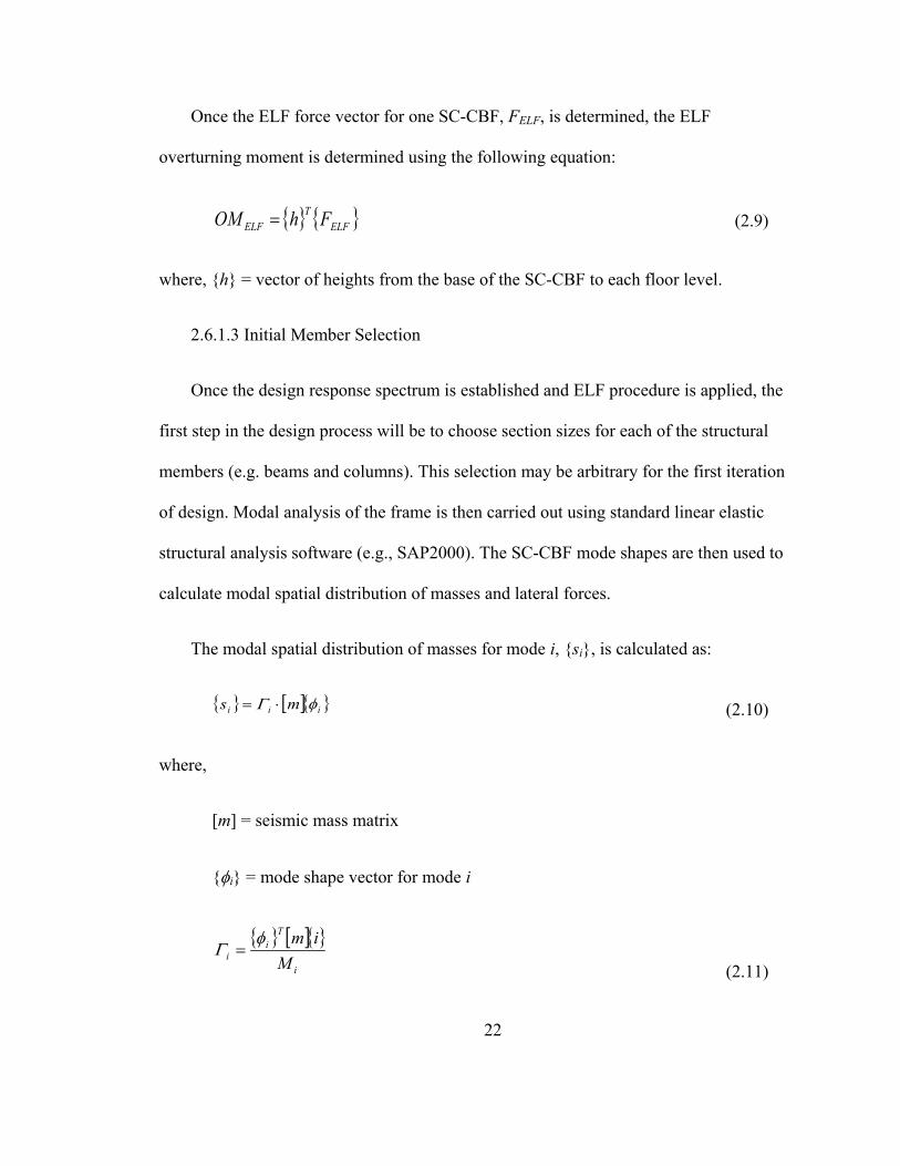
Once the ELF force vector for one SC-CBF, FELF, is determined, the ELF

overturning moment is determined using the following equation:

{ } { }ELFT

ELF FhOM = (2.9)

where, {h} = vector of heights from the base of the SC-CBF to each floor level.

2.6.1.3 Initial Member Selection

Once the design response spectrum is established and ELF procedure is applied, the

first step in the design process will be to choose section sizes for each of the structural

members (e.g. beams and columns). This selection may be arbitrary for the first iteration

of design. Modal analysis of the frame is then carried out using standard linear elastic

structural analysis software (e.g., SAP2000). The SC-CBF mode shapes are then used to

calculate modal spatial distribution of masses and lateral forces.

The modal spatial distribution of masses for mode i, {si}, is calculated as:

{ } [ ]{ }iii ms φΓ ⋅= (2.10)

where,

[m] = seismic mass matrix

{φi} = mode shape vector for mode i

{ } [ ]{ }i

Ti

i Mimφ

Γ = (2.11)

23

{i} = {1 1 1 1}T for a four-story SC-CBF

{ } [ ]{ }iT

ii mM φφ= (2.12)

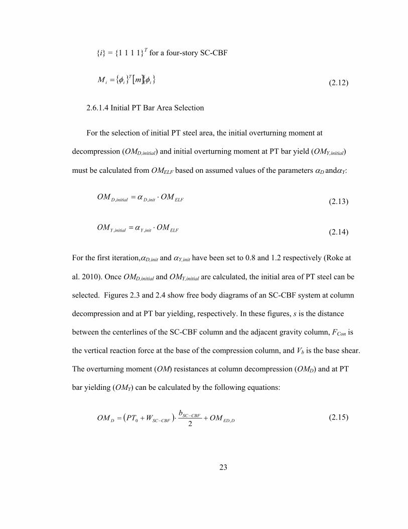
2.6.1.4 Initial PT Bar Area Selection

For the selection of initial PT steel area, the initial overturning moment at

decompression (OMD,initial) and initial overturning moment at PT bar yield (OMY,initial)

must be calculated from OMELF based on assumed values of the parameters αD andαY:

ELFinitDinitialD OMOM ⋅= ,, α (2.13)

ELFinitYinitialY OMOM ⋅= ,, α (2.14)

For the first iteration,αD,init and αY,init have been set to 0.8 and 1.2 respectively (Roke at

al. 2010). Once OMD,initial and OMY,initial are calculated, the initial area of PT steel can be

selected. Figures 2.3 and 2.4 show free body diagrams of an SC-CBF system at column

decompression and at PT bar yielding, respectively. In these figures, s is the distance

between the centerlines of the SC-CBF column and the adjacent gravity column, FCon is

the vertical reaction force at the base of the compression column, and Vb is the base shear.

The overturning moment (OM) resistances at column decompression (OMD) and at PT

bar yielding (OMY) can be calculated by the following equations:

( ) DEDCBFSC

CBFSCD OMb

WPTOM ,0 2+⋅+= −

− (2.15)

24

( ) YEDCBFSC

CBFSCYY OMb

WPTOM ,2+⋅+= −

− (2.16)

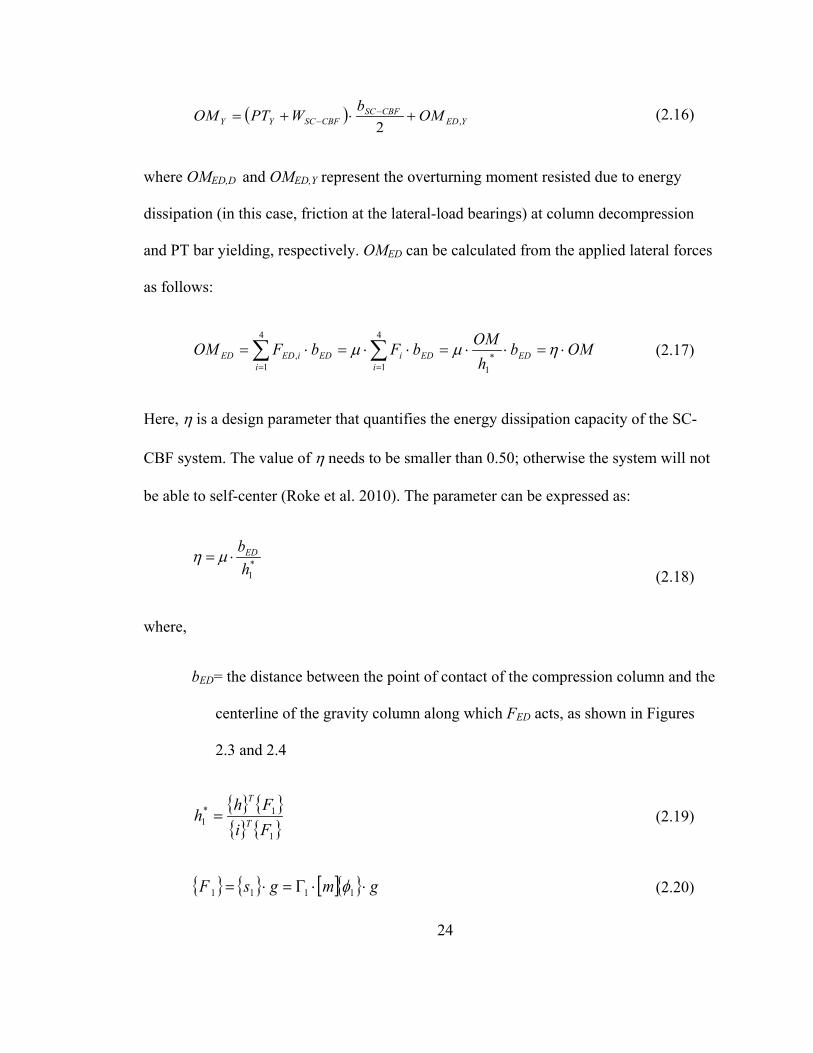
where OMED,D and OMED,Y represent the overturning moment resisted due to energy

dissipation (in this case, friction at the lateral-load bearings) at column decompression

and PT bar yielding, respectively. OMED can be calculated from the applied lateral forces

as follows:

OMbh

OMbFbFOM EDEDi

iEDi

iEDED ⋅=⋅⋅=⋅⋅=⋅= ∑∑==

ηµµ *1

4

1

4

1, (2.17)

Here, η is a design parameter that quantifies the energy dissipation capacity of the SC-

CBF system. The value of η needs to be smaller than 0.50; otherwise the system will not

be able to self-center (Roke et al. 2010). The parameter can be expressed as:

*1h

bED⋅= µη (2.18)

where,

bED= the distance between the point of contact of the compression column and the

centerline of the gravity column along which FED acts, as shown in Figures

2.3 and 2.4

{ } { }{ } { }1

1*1 Fi

Fhh T

T

= (2.19)

{ } { } [ ]{ } gmgsF ⋅⋅Γ=⋅= 1111 φ (2.20)

25

g = acceleration of gravity

Now Equation 2.15 can be rearranged to solve for the required initial PT bar force as

follows:

CBFSCCBFSC

initialDCBFSC

initialDinitial Wb

OMb

OMPT −−−

−

⋅⋅−

⋅=

22,,,0 η

(2.21)

At PT bar yielding, the stresses in the PT bars are equal to the yield stress of the PT bars,

σY. The force in the PT bars at yield can be calculated as follows:

YPTY APT σ⋅= (2.22)

where APT and σY are the area and the yield stress of the PT bars, respectively.

Substituting Equation 2.17 and 2.22 into Equation 2.16 produces an equation to calculate

the initial area of PT steel required:

( )

Y

CBFSCinitialYinitialYCBFSC

initialPT

WOMOMb

Aσ

η −−

−⋅−⋅

=,,

,

2

(2.23)

The PT bars must then be selected such that APT≥APT,initial. The initial stress of the PT

bars, σ0, can then be calculated using the selected APT:

PT

initial

APT ,0

0 =σ (2.24)

Updated values of the OMD and OMY can be calculated as follows:

26

( )

−

⋅+⋅= −−

η11

2 0 CBFSCCBFSC

D WPTbOM (2.25)

( )

−

⋅+⋅= −−

η11

2 CBFSCYCBFSC

Y WPTbOM (2.26)

which are based on the free body diagrams at decompression and PT bar yielding

(Figures 2.3 and 2.4, respectively). The ratio of overturning moment at PT bar yielding

to the overturning moment at decompression, αY, will be used to determine the first mode

forces at PT bar yielding, and is calculated as:

D

YY OM

OM=α

(2.27)

2.6.1.5 Hysteretic Energy Dissipation Ratio βE

The hysteretic energy dissipation ratio (βE) is a key design parameter for self-

centering (SC) structural systems. It is representative of the relative energy dissipation

capacity of a SC system in comparison to a bilinear elasto-plastic system. Figure 2.8

shows schematic hysteresis loops for an SC-CBF system with friction based energy

dissipation and for a bilinear elasto-plastic system.

βE is defined as the ratio of the area of the flag-shaped hysteresis loop of an SC-CBF

system to the area of the hysteresis loop of a bilinear elasto-plastic system (Seo and Sause

2005). Assuming the area of the flag-shaped hysteresis loops to be trapezoidal, βE can be

approximated as:

27

( )D

YEDDED

E OM

OMOM ,,21

+=β

(2.28)

2.6.2 Structural Member Design Phase

2.6.2.1 Modal Truncation

The primary purpose of the structural member design phase is to determine the

member force design demands in the structural members and select member sizes such

that their capacities exceed the design demands. To determine the member force design

demands, modal lateral forces must be applied to the SC-CBF to determine the modal

internal forces and bending moments for each member. However, it may not be necessary

to include all modes. Modal truncation can be applied to reduce the number of modes

used to determine the axial force and bending moment design demands.

The number of modes to be included is determined by comparing the effective modal

masses to the total mass of the system. The effective modal mass of mode i, Mi*, is

calculated as follows:

{ } [ ] { }imM Tiii ⋅⋅⋅Γ= φ*

(2.29)

The total mass of the system is:

{ } [ ] { }imiM Ttotal ⋅⋅= (2.30)

The number of modes to be included is selected such that the sum of the first J modal

masses is greater than or equal to 95% of the total mass (Roke et al. 2010). The rest of the

28

modes can be truncated, as they will have negligible contributions to the member force

design demands.

2.6.2.2 Factored Design Demand

The next step in the structural member design phase is to determine modal member

force design demands for each member (i.e., axial forces and bending moments). Modal

load profiles for each mode to be included (after modal truncation) are determined

through a static analysis on a simple fixed-base analytical model using structural analysis

software (e.g., SAP2000). For the higher modes, the forces applied equal the entries in

the mass distribution matrix si (Equation 2.10) multiplied by g.

However, the first mode is designed at PT bar yielding. Unlike the higher modes,

which are designed using only the lateral forces, the first mode applied loads include the

lateral forces, frame weight, vertical friction forces at the lateral-load bearings, and the

PT bar yield force as shown in Figure 2.4 (Roke et al. 2010). The higher mode load cases

may be conducted using unit accelerations, whereas the lateral forces applied for the first

mode include a factor of αY,1:

{ } { }11,'1 ss Y ⋅= α (2.31)

where,

11, OM

OM YY =α (2.32)

{ } { } gshOM T ⋅⋅= 11 (2.33)

29

The friction forces at PT yield can then be calculated:

{ } { }'1, sF YED ⋅= µ (2.34)

The axial force and bending moment design demands are recorded from the analysis

for each modal load case. As higher mode load cases were conducted using unit

accelerations, higher mode peak member forces must be multiplied by the corresponding

design spectral acceleration (SAn) values. Modal spectral acceleration (SAn) values from

the design spectrum are factored by a safety factor γn, which is introduced to account for

potential bias and dispersion in higher mode responses (Roke et al. 2010). The value of γn

is equal to 1.15 for the first mode and 2.0 for the higher modes. Since study showed that

SC-CBFs are prone to significant amount of higher mode effects, such high conservative

values ofγn are set for higher modes (Roke et al. 2009).

Once the factored modal design demands are determined, the complete quadratic

combination (CQC) method is used to estimate the member factored design demands,

Fx,fdd, for each member. Factored design demands for axial forces and bending moments

are calculated for each member. The CQC method is defined as follows:

21

4

1

4

1,,,,,

⋅⋅= ∑∑

= =i jfddxjfddxiijfddx FFF ρ

(2.35)

where i and j are defined as the number of included modes, and the correlation

coefficients are (Roke et al. 2010):

30

≠=

=jiifjiif

ij 25.00.1

ρ (2.36)

2.6.2.3 Capacity Check

The factored design demands, Fx,fdd, determined using Equation 2.35 are then

compared against the member capacities. Since SC-CBF connections are assumed to

transmit bending moment along with axial forces, these checks were performed using the

following bending moment and axial force interaction equations (AISC 2005b):

2.00.198

≥≤

+⋅+

nc

r

nyb

ry

nxb

rx

nc

r

PPfor

MM

MM

PP

φφφφ (2.37)

2.00.12

<≤

++

⋅ nc

r

nyb

ry

nxb

rx

nc

r

PPfor

MM

MM

PP

φφφφ (2.38)

where,

Pr = factored design axial force demand determined from second-order analysis

(AISC 2005b)

φc = compression resistance reduction factor, equal to 0.9

Pn = nominal compressive strength of the member

Mrx = factored design strong axis bending moment demand determined from

second-order analysis (AISC 2005b)

Mry = factored design weak axis bending moment, assumed to be zero

31

φb = flexural bending resistance reduction factor, equal to 0.9

Mny and Mnx = nominal flexural strength about each cross-sectional axis of the

member

If the interaction equations are not satisfied, the member sizes must be increased, and

another iteration of design is necessary.

2.6.3 PT Bar Design Phase

2.6.3.1 Decompression Roof Drift

The first step in the PT steel design phase is to determine roof drift at column

decompression, θD. As both the factored roof drift design demand, θDBE,fdd, and the roof

drift capacity of the SC-CBF, θY,N, are directly related to θD, this calculation is very

important for the PT bar design phase. A simple analytical fixed-base model is developed

using structural analysis software (e.g., SAP2000) to perform a static analysis of the SC-

CBF at column decompression. The forces to be included in the analysis are the lateral

forces, vertical friction forces, frame self-weight and initial PT force as shown in Figure

2.3. The lateral forces at column decompression are calculated as follows:

{ } { }11, FF DD ⋅= α (2.39)

where,

11, OM

OM DD =α

(2.40)

32

The vertical friction forces at decompression can be calculated by:

{ } { }DDED FF ⋅= µ, (2.41)

The recorded lateral roof displacement is divided by the total height of the frame to

calculate θD.

2.6.3.2 Factored Roof Drift Design Demand

One of the design objectives for SC-CBF is that PT bars should not yield under

median DBE-level seismic inputs, which means the probability of PT bar yielding under

DBE-level seismic input should be less than 50% (Roke et al. 2010). Therefore, the

median DBE roof drift demand is taken as the design demand for the PT bar yielding

limit state. Figure 3.9 shows a schematic of the idealized overturning moment versus roof

drift response of an SC-CBF system. The DBE roof drift demand, θDBE,dd, can be

calculated based on the ductility demand, µDBE and the roof drift at column

decompression, θD:

DDBEddDBE θµθ ⋅=, (2.42)

The ductility demand of the system, µDBE can be calculated from standard

relationships between μ, R, and T determined from single-degree-of-freedom nonlinear

analyses of SC systems (Seo and Sause 2005). The μ-R-T relationship for SC systems is

as follows:

)(,

1TpDADBE R=µ (2.43)

33

where,

( )

=

21

11 exp cT

cTp (2.44)

( )2

1 kbac α−= (2.45)

( )2

2 kdcc α−= (2.46)

The coefficients a, b, c, and d are functions of βE and the site soil conditions (site class)

(Seo 2005). Values of these coefficients are given in Table 2.2. For calculation of µDBE, in

equation 2.42, RA,D is used instead of the code-based response modification coefficient,

R. RA,D is the ratio of the required strength of the structure for it to remain elastic during

median DBE-level response to the actual strength of the structure (Roke et al. 2010). The

coefficient is determined by:

D

elasticDA OM

OMR 1,

, = (2.47)

OMelastic,1 is the required elastic strength of the structure (considering only the first mode

effective modal mass) and it can be determined by (Roke et al. 2010):

elastictotal

elastic OMMMOM ⋅=

*1

1,

(2.48)

where,

34

ELFelastic OMROM ⋅= (2.49)

R = 8 (assumed for SC-CBF systems)

The design demand, θDBE,dd, as calculated by equation 2.42, is factored by γθ to

control the probability of roof drift response under the DBE, θDBE exceeding the design

demand. In this case, γθ is assumed to be equal to 1.0, which indicated a 50% probability

that the PT bars will yield under the median DBE-level earthquake (Roke et al. 2010).

The factored DBE-level design demand is equal to:

DBEfddDBE θγθ θ ⋅=, (2.50)

2.6.3.3 Roof Drift Check

The factored roof drift design demand must be compared to the roof drift capacity at

PT bar yielding, θY,N, which is calculated from the roof drift ductility demand at PT bar

yielding, µY (Roke et al. 2010):

DYNY θµθ ⋅=, (2.51)

µY is determined as follows:

K

KYY α

ααµ

1−+=

(2.52)

αk is the ratio of the elastic and post-decompression stiffness of the frame (Roke et. al.

2010):

35

elastic

pdk k

k=α

(2.53)

Where,

D

Delastic

OMkθ

= (2.54)

−

⋅

⋅

⋅= −

η11

2

2CBFSC

PT

PTPTpd

bL

EAk (2.55)

where LPT and EPT are the length and elastic modulus of the PT bars, respectively.

For PT steel adequacy, θY,N should be greater than θDBE,fdd. If this condition isn’t

satisfied, the PT bar area should be increased and another design iteration should be

performed.

2.6.4 Design of the Adjacent Gravity Columns

The final step in the SC-CBF design procedure is the design of adjacent gravity

columns. The adjacent gravity column is designed to carry all the gravity loads from the

tributary floor area, as well as the vertical friction forces from the lateral load bearings.

The design of the adjacent gravity columns is relatively simple, as these columns have

fixed base and do not uplift like the SC-CBF columns. Three main design cases for the

adjacent gravity columns are considered: (1) loading to PT bar yielding, (2) unloading

after PT bar yielding, and (3) zero lateral loading. Cases (1) and (2) are shown in Figure

2.9(a) and 2.9(b), which show free body diagrams of the adjacent gravity column at PT

36

bar yielding and after PT bar yielding, respectively. At PT bar yielding, the friction

forces from the lateral load bearings act vertically downward on the SC-CBF, resisting

the rocking response, so the opposing forces act upward on the adjacent gravity column.

This reduces the total vertical force on the adjacent gravity column.

However, during unloading after PT bar yielding, the friction forces act upward on

the SC-CBF, resisting column base gap closure, and thus act downward on the adjacent

gravity column. These forces add to the total vertical force on the adjacent gravity

column.

The zero lateral load case consists of only gravity loads; no friction forces are

present in this design case. Unloading after PT bar yielding is typically the governing

load case for design of the adjacent gravity columns. The design demands from this case

are compared to the capacity of the selected members using Equations 2.37 and 2.38,

with the moments in the adjacent gravity columns assumed to be zero (Roke et al. 2010).

37

Table 2.1 – Summary of Performance Based Design Objectives Seismic

Input Level Performance

Level Limit States

Column Decompression

PT Bar Yielding

Member Yielding

Member Failure

DBE IO Permitted Minor Yielding Permitted

Not Permitted

Not Permitted

MCE CP Permitted Permitted Permitted Not Permitted

Table 2.2 – Regression coefficients a, b, c, and d for Equations 2.50 and 2.51 (Seo 2005)

Site Class βE (%) A b c d

C

0.0 0.636 0.306 0.713 0.111 12.5 0.569 0.264 0.769 0.115 25.0 0.515 0.222 0.816 0.113 100.0 0.412 0.498 0.904 -0.415

D

0.0 0.729 0.399 0.624 0.0657 12.5 0.657 0.327 0.678 0.0756 25.0 0.597 0.288 0.728 0.0677 100.0 0.457 0.500 0.872 -0.305

38

Figure 2.1 – Schematic configuration of an SC-CBF system

Lateral-load Bearing

Adjacent gravity column

SC-CBF column

PT bar

Distribution Strut

39

Figure 2.2- SC-CBF behavior under lateral loading: (a) elastic deformation under low level of forces; (b) column uplifting under high level of forces

Applied Force

Column Gap Opening

(a) (b) Roof Drift

40

Figure 2.3- Typical force distribution at column decompression (Jeffers 2012)

PT0

WSC-CBF

FD,1

FD,2

FD,3

FD,4

FCon

Vb,D=∑FD,iss bSC-CBF

bED

Point of contact of compression column

FED,1

FED,3

FED,2

FED,4

Centerline of adjacent gravity column

41

Figure 2.4- Typical force distribution at PT bar yielding (Jeffers 2012)

PTY

WSC-CBF

FY,1

FY,2

FY,3

FY,4

FCon

Vb,Y=∑FY,i s s bSC-CBF

bED

Point of contact of compression column

FED,Y,1

FED,Y,3

FED,Y,2

FED,Y,4

Centerline of gravity column

42

Figure 2.5 – Idealized base shear-roof drift response of an SC-CBF

Base Shear

Roof Drift

Member failure

Member yielding

PT bar yielding

SC-CBF column decompression

43

Figure 2.6 – Schematic of performance based design criteria

Base Shear

Roof Drift

Member failure

Member yielding

PT bar yielding

Column decompression

DBE MCE

IO CP

Limit of Performance Levels

Median Response for Hazard Levels

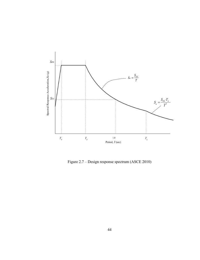
44

Figure 2.7 – Design response spectrum (ASCE 2010)

45

Figure 2.8- Hysteretic response of an SC-CBF system with friction-based energy dissipation compared to that of a bilinear elasto-plastic system. (Jeffers 2012)

OM

θ

OMY

OMD

OMDHysteresis loop for a bilinear elasto-plastic system

Flag-shaped hysteresis loop for an SC-CBF with friction based energy dissipation

2·OMED,D

2·OMED,Y

2·OMED,D

2·OMED,Y

46

Figure 2.9- Schematic of idealized overturning moment versus roof drift response of an SC-CBF system (Roke 2010)

OM

θ

OMY

OMDBE

OMD

θD

θDBE,dd = μDBE∙θD

θY,n = μY∙θD

kpd = αk∙kelastic

kelastic

47

Figure 2.10 – Design cases for the adjacent gravity column: (a) PT bar yielding; (b)

unloading after PT bar yielding (Jeffers 2012)

F1

F2

F3

F4

VED VED

0

(a)

(b)

F1

F2

F3

F4

VED

0

VED

F4

F3

F2

F1

F4

F3

F2

F1

F4

F3

F2

F1

F4

F3

F2

F1

48

CHAPTER III

DESIGN AND ANALYSIS RESULTS

3.1 Overview One of the primary purposes of this research is to study the effect of the frame

geometry on the behavior and performance of SC-CBFs under lateral loading. Three

different SC-CBF prototype structures with varying braced bay widths have therefore

been developed, designed, and numerically analyzed. This chapter first introduces the

prototype buildings and summarizes the designs. Next, the analytical models developed

to run numerical analyses are explained and the analysis results for all three prototypes

are presented. Finally, the design and analysis results are compared and studied to

determine the effect of frame geometry on SC-CBF behavior and performance.

3.2 Prototype Buildings

The prototype buildings considered for this study are assumed to be four story office

buildings located in a stiff soil site (Site Class D (ASCE 2010)) at Van Nuys, California.

SC-CBFs are incorporated in the prototype buildings as the only lateral-load resisting

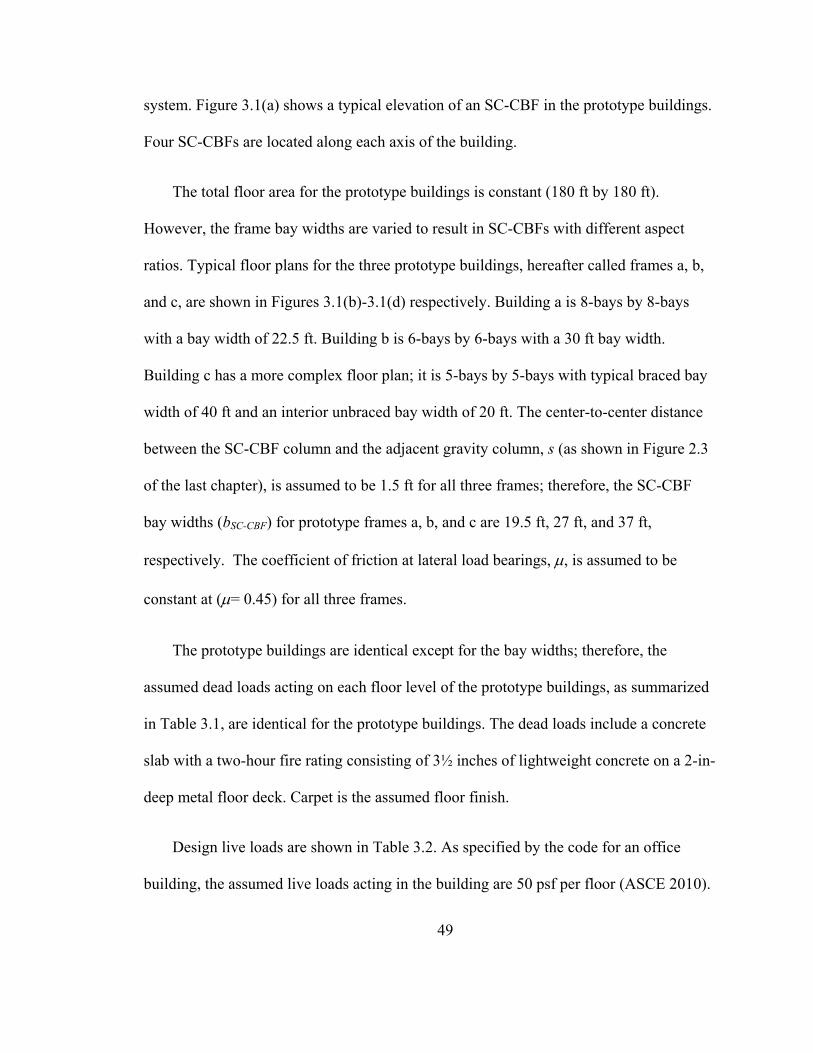
49

system. Figure 3.1(a) shows a typical elevation of an SC-CBF in the prototype buildings.

Four SC-CBFs are located along each axis of the building.

The total floor area for the prototype buildings is constant (180 ft by 180 ft).

However, the frame bay widths are varied to result in SC-CBFs with different aspect

ratios. Typical floor plans for the three prototype buildings, hereafter called frames a, b,

and c, are shown in Figures 3.1(b)-3.1(d) respectively. Building a is 8-bays by 8-bays

with a bay width of 22.5 ft. Building b is 6-bays by 6-bays with a 30 ft bay width.

Building c has a more complex floor plan; it is 5-bays by 5-bays with typical braced bay

width of 40 ft and an interior unbraced bay width of 20 ft. The center-to-center distance

between the SC-CBF column and the adjacent gravity column, s (as shown in Figure 2.3

of the last chapter), is assumed to be 1.5 ft for all three frames; therefore, the SC-CBF

bay widths (bSC-CBF) for prototype frames a, b, and c are 19.5 ft, 27 ft, and 37 ft,

respectively. The coefficient of friction at lateral load bearings, µ, is assumed to be

constant at (µ= 0.45) for all three frames.

The prototype buildings are identical except for the bay widths; therefore, the

assumed dead loads acting on each floor level of the prototype buildings, as summarized

in Table 3.1, are identical for the prototype buildings. The dead loads include a concrete

slab with a two-hour fire rating consisting of 3½ inches of lightweight concrete on a 2-in-

deep metal floor deck. Carpet is the assumed floor finish.

Design live loads are shown in Table 3.2. As specified by the code for an office

building, the assumed live loads acting in the building are 50 psf per floor (ASCE 2010).

50

As specified by the code, the partition load (which is part of the live load) is assumed to

be equal to 15 psf, and the roof live load is assumed to be 20 psf. Gravity loads (live and

dead loads) acting on each adjacent gravity column are summarized in Table 3.3.

In the analytical models developed for this research, a lean-on column is used to

represent the gravity columns in the tributary area of an SC-CBF, except the \ gravity

columns adjacent to the modeled SC-CBF (Roke et al. 2010). Table 3.4 shows the total

gravity loads acting on the lean-on column.

3.3 Design Results

As described in Chapter 2, the primary objectives of an SC-CBF design are to

determine PT steel area and to select the sizes of SC-CBF members (columns, beams,

braces, strut) and gravity columns. All three prototype buildings have been designed

using the PBD procedure for SC-CBF systems.

The SC-CBF member selections are presented in Figures 3.2, 3.3, and 3.4, for frames

a, b, and c, respectively. The member sizes for frame a are typically larger compared to

those of frames b and c. The member sizes for frames b and c are similar, with identical

section sizes for the lower story braces, upper story columns, and beams.

Due to the different floor plans (Figure 3.1), the quantity and tributary area of the

gravity columns is different for the three prototype buildings. As a result, the sizes of the

standard gravity columns and the adjacent gravity columns are also different in three

designs. Table 3.5 presents the gravity column sizes and lean on column areas for all

three prototype buildings.

51

Table 3.6 summarizes the SC-CBF design results. The tabulated values include the

frame width, bSC-CBF; the frame weight; the PT bar area, APT; the hysteretic energy

dissipation ratio, βE; design parameterη; the overturning moment at decompression,

OMD; the overturning moment at PT bar yielding, OMY; pre-decompression or elastic

stiffness, kelastic; and post-decompression stiffness, kpd. The PT steel area decreases with

the increase in SC-CBF bay width: frames a, b, and c have PT bar areas of 15.72 in2, 9.48

in2, and 7.50 in2, respectively. The frame weights exhibit no trend with changing frame

geometry, as the weights of frames a and c are both higher than that of frame b.

βE andη increase with increasing bSC-CBF. Therefore, the SC-CBF with the highest

frame bay width has the highest energy dissipation capacity. However, the magnitudes of

OMD and OMY exhibit no trends with changing frame geometry. The values of OMD and

OMY are nearly equal for frames a and b; but OMD and OMY for frame c are significantly

higher than those of the other frames. Both elastic and pre-decompression stiffness values

increase with the increase of frame bay width.

3.4 Analytical Model

Nonlinear analytical models of the prototype structures have been created in

OpenSees (Mazzoni et al. 2009) for static pushover and dynamic time history analyses.

For each prototype structure, the analytical model represents a single SC-CBF and its

tributary area, as shown in Figure 3.1. The basic components of the models are the SC-

CBF, the PT bars, the adjacent gravity columns, the lean-on column, and the lateral load

bearings.

52

The SC-CBF structural members (beams, columns, braces and strut) are modeled as

linear elastic elements so that the force demands in these members can be determined.

The nodes in the model are located at the working points of the connections between SC-

CBF members, and these connections are assumed to be rigid (Roke et al. 2010). The PT

bars are modeled as nonlinear beam-column elements with negligible flexural and shear

stiffness and a post-yielding axial stiffness equal to 2% of the initial axial stiffness.

Column base decompression is modeled using compression-only gap elements

located at the base of the SC-CBF columns. These elements allow uplift of the column

base, but still provide a linear-elastic compressive resistance when the column base is in

contact with the foundation. Horizontal force (i.e., base shear force) resistance at the

column base is provided only when the column is in contact with the foundation; only the

column that is in contact with the foundation provides base shear force resistance.

Sliding at the base due to slip is not permitted in these SC-CBF models.

The lateral-load bearing elements were modeled as contact friction gap elements

with a defined coefficient of friction, µ. These elements are similar to the gap elements

used at the column bases, though they also develop transverse friction forces under the

action of a compressive force. Initial gaps in these elements were set to 0.02 inches at

each floor level (i.e., these elements provide no compressive resistance until the

compressive deformation exceeds 0.02 inches).

A lean-on column is incorporated into the analytical model to account for P-Δ

effects. The lean-on column represents the strength and stiffness of the standard gravity

53

columns (i.e., not the gravity columns directly adjacent to the SC-CBF columns) in the

tributary area of the modeled SC-CBF. The nodes at the floor levels of the lean-on

column and the adjacent gravity columns are modeled to have the same degree of

freedom in the lateral direction (i.e., each floor has one horizontal degree of freedom).

For static analysis, the lateral loads are applied on the lean-on column.

The analytical models used for dynamic analyses included seismic masses that were

lumped on the lean-on column nodes at each floor level. Damping is incorporated in the

dynamic analytical models through a damping substructure (Roke et al. 2010) that

utilizes Rayleigh damping coefficients. The Rayleigh damping coefficients α and β were

determined using 2% damping in the first mode and 5% damping in the third mode.

3.5 Nonlinear Static Analysis

Nonlinear static analyses were performed on each of the analytical models to verify

that the SC-CBFs exhibited the expected behavior under lateral loading. The static

pushover responses were then compared to study the effect of frame geometry on SC-

CBF behavior. Monotonic and cyclic pushover analyses were performed using OpenSees.

The load profiles used for these analyses are proportional to the first mode forces, which

were calculated based on the elastic mode shape of the fixed-base SC-CBFs. This section

presents the analysis results in detail.

3.5.1 Monotonic Pushover Study

Monotonic pushover analysis was conducted on each SC-CBF up to 3% roof drift,

well beyond the limit state of PT bar yielding (which occurs at around 1% - 1.5% roof

54

drift). The analysis results are presented as overturning moment versus roof drift plots, as

shown in Figure 3.5. Figure 3.5(a) shows the pre-decompression (elastic) response of the

systems, and Figure 3.5(b) shows the full range of response.

The elastic stiffness of each frame is a function of the SC-CBF member size and

member length. The differences in member sizes for different frames are offset by the

differences in member lengths. Even though the member sizes are relatively smaller for

frame c, due to its relatively larger bay width frame c has a slightly greater elastic

stiffness than the other frames as shown in Figure 3.5(a). The frames a and b have almost

identical elastic stiffness. The stiffness values tabulated in Table 3.6 also show that the

differences in stiffness values of frames b and c are much higher compared to those of

frames a and b.

The limit state of column decompression is a function of the initial force in the PT

bars, the weight of the SC-CBF members, and the frame width. As shown in Table 3.6

and Figure 3.5, frame c has the highest value of OMD, whereas the values of OMD for

frames a and b are very close; the difference in initial PT bar force and frame weight for

frames a and b are offset by the difference in frame width. Similarly, frame c has the

highest value of OMY, while the values of OMY for frames a and b are close to one

another.

The roof drift capacity at PT bar yielding, which is a function of initial PT bar stress

and frame geometry, is highest for frame a and lowest for frame c. Therefore, for these

designs with identical initial stresses in the PT bars, the increase in frame width results in

55

a decrease in the roof drift capacity at PT bar yielding. However, the roof drift capacities

at column decompression seem to be somewhat similar for all three frames.

3.5.2 Cyclic Pushover Study

Cyclic pushover analyses were performed on the prototype SC-CBFs to verify and

study the energy dissipation capacity of the systems. As with the monotonic pushovers,

the lateral forces applied to the frames were proportional to the first mode lateral forces.

Loading was incremented until each frame underwent 1% roof drift, at which point the

loading was until the SC-CBF returned to its initial condition.

Figure 3.6 shows the overturning moment-roof drift response for the prototype

frames. The difference in energy dissipation ratio (βE) for the three SC-CBF designs, as

tabulated in Table 3.6, is evident. Frames a and b have almost the same values of OMD;

but the higher “unloading” overturning moment in frame b causes a wider hysteresis loop

and thus a higher βE value for frame b. This is due to the higher post-decompression

stiffness in frame b. Again, frame c has almost similar “unloading” overturning moment

as frame b; but due to higher OMD in frame c results in a higher βE value for frame c.

3.6 Nonlinear Dynamic Analysis

Nonlinear dynamic analyses were conducted in OpenSees on the three prototype SC-

CBFs using a suite of DBE-level ground. This section elaborates the selection of ground

motion records and presents the analysis results to perform an in-depth study on the

seismic response of SC-CBF systems.

56

3.6.1 Ground Motion Records

A suite of 30 DBE-level ground motion records were selected to assess the response

of SC-CBF frames under seismic input. The theory behind the selection of these ground

motion records is beyond the scope of this thesis. This section roughly summarizes the

selection method, which is explained in detail by Roke et al. (2010).

Hazard disaggregation was used to determine the magnitude, M, and distance, D,

combinations for ground motions with a spectral acceleration at the first mode period of

the designed systems, SA(T1), that are banded around the target value, SADBE(T1). A third

parameter,ε, indirectly characterizes the spectral acceleration for a given ground motion

relative to the expected spectral shape: a positive value of ε indicates a high spectral

acceleration at T1 relative to the spectrum away from T1, while a negative value of ε

indicates a low spectral acceleration at T1 relative to the spectrum away from T1. The

ground motions were selected to closely match the disaggregation results for a Van Nuys,

California, site in terms of the parameters M, D, and ε. Table 3.7 lists the values of M,

D,ε, as well as the scale factors used to approximate the DBE, for each ground motion

pair.

3.6.2 Peak Dynamic Responses

Numerical analyses of each of three prototype SC-CBFs were conducted using the

suite of DBE-level ground motions. The peak values of response quantities (e.g., floor

displacements, member forces, PT bar forces etc.) determined from the time history

analyses are used to represent the DBE-level demand for each SC-CBF system. The peak

57

column gap opening responses are considered to determine the degree of rocking in

different frames. The other response quantities that are of major concern for assessing the

seismic behavior of SC-CBF systems are base shear, roof drifts, inter-story drifts, brace

forces and PT bar forces.

Tables 3.8, 3.9, and 3.10 tabulate the gap opening and base shear response data of

frames a, b, and c, respectively. The data presented in these tables are: ∆gap,L, peak gap

opening at the left column; ∆gap,R, peak gap opening at the right column; ∆gap,max,

maximum gap opening for any column; Vb,max, peak base shear. Table 3.11 presents the

mean and standard deviation values of these gap opening and base shear responses for the

three prototype SC-CBFs. As the frame bay width increases, the gap opening response

also increases; that means there will be more rocking response. The base shear response

also increases with the increase of frame bay width.

The data presented in these tables also include vbn, base shear overstrength factor,

which is equal to peak base shear normalized by the design base shear. The design base

shear is equivalent to the ELF base shear determined using ASCE7 (2010), which

specifies an overstrength factor of 2.0 for conventional CBF systems. The data presented

in Table 3.11 show that the value of vbn for SC-CBF systems is greater than the value

specified for conventional CBF systems, indicating that increased system strength

contributes to the performance of SC-CBF systems.

Tables 3.12, 3.13, and 3.14 tabulate the drift response data of frames a, b, and c,

respectively. The data presented in these tables are: θDBE, the maximum roof drift; θs,i, the

58

maximum story drift for story i; and θs,max, the peak story drift in any story. Table 3.15

presents the mean and standard deviation values of these peak drift quantities for the

three prototype SC-CBFs. These values indicate that story drifts are typically larger for

the higher (3rd and 4th) stories than for the lower stories. The story drifts tend to decrease

slightly with the increase of frame bay width. Figure 3.7 shows the distribution of peak

roof drift responses for different ground motions for all three frames. The mean peak roof

drift response decreases with the increase of frame bay width; frame a has the highest

mean peak roof drift values and frame c has the lowest.

Brace forces are the most important member forces, since braces provide the lateral

stiffness of the frame and are susceptible to the most damage while the frame undergoes

lateral drift. Tables 3.16, 3.17, and3.18 present the peak brace force and PT bar force

responses for frames a, b, and c, respectively. The peak brace force response in story i is

represented by Fbri. Table 3.19 shows the brace axial force capacities for each SC-CBF

design. These axial force capacities represent the limit beyond which the braces will start

to exhibit nonlinear behavior. However, all of the structural members (e.g., braces,

beams, and columns) were modeled as linear elastic elements in the OpenSees analytical

model; the analysis results will therefore be meaningless if the value of Fbri exceeds the

corresponding normalized brace axial force capacity tabulated in Table 3.15. Highlighted

values in Tables 3.17 and 3.18show that Fbr1 exceeds the brace axial force capacity in

several ground motion responses for frame b and frame c. Table 3.20 shows the mean and

standard deviation for brace force and PT bar force responses. The mean Fbri results show

that the brace force responses decrease with the increase of the frame bay width.

59

Tables 3.16, 3.17, and 3.18, in addition to showing the Fbri results, also present the

values of peak PT bar force, PTmax, and peak normalized PT bar force, PTmax,norm, which

is equal to peak PT bar force normalized by the PT bar force at yield, PTY. The values of

PTmax,norm exceeding 1.0 indicates that PT bar has yielded for that particular ground

motion record. For frames b and c, PT bar yields on a few occasions. Since SC-CBFs are

designed to allow for minor PT bar yielding under DBE-level earthquake, this is not

going to be a problem. The data presented in Table 3.20 suggest that as the frame bay

width increases, resulting in a decrease in peak PT force responses as well. This is

consistent with the trend in the decrease in PT bar areas with the increase in frame bay

width. However, the normalized PT force response increases with the increase of frame

bay width. Thereby, the probability of PT bar yielding increases with the increase of

frame bay width.

3.6.3 Time History Responses

The previous section summarized the peak dynamic response results, averaged over

all the ground motions; however, a more elaborate look at the time history response is

required to investigate the behavior of SC-CBF systems under DBE-level ground

motions. A representative ground motion response is therefore selected in this section to

study the time history of various response quantities (e.g., roof drift, PT bar force,

overturning moment, and column base gap-opening). The representative ground motion

response was chosen such that it showed the previously mentioned trend in the roof drift

responses with the changing frame bay width.

60

The data presented in Table 3.11 and Figure 3.7 show that the mean peak roof drift

response tends to decrease with the increase in the frame bay width. The roof drift

responses for several ground motions exhibit trends similar to that of the mean values.

Among those records, the arl360 ground motion was selected as the representative

ground motion because the roof drift responses to this ground motion are also close to the

corresponding mean values.

Figures 3.8, 3.9, and 3.10 show the roof drift time history responses of frames a, b,

and c, respectively, subjected to ground motion arl360. The peak roof drift responses are

0.85%, 0.73%, and 0.66% for Frames a, b, and c, respectively. Zero roof drift responses

at the end of ground motion duration show that the structure self-centers following the

earthquake.

Figures 3.11, 3.12, and 3.13 show PT bar force responses of all three SC-CBFs under

arl360. As shown in Table 3.6, the PT bar areas are different for the three frames, with

frame a having the highest area and frame c having the lowest area. Consequently, PT bar

responses in frame a are the highest among the three frames. The initial PT forces in

frames a, b, and c are 755 kips, 455 kips and 360 kips, respectively (i.e., the initial stress

is 40% of the yield stress for each design). The PT yield forces are 1886 kips for frame a,

1138 kips for frame b, and 900 kips for frame c. Under arl360, PT bar force responses are

well below the PT yield force for each SC-CBF; the peak PT force responses for frames

a, b, and c are 1286 kips, 826 kips and 664 kips, respectively. In conclusion, the increase

of frame bay width decreases the PT bar area, thereby decreasing the PT force response

as well. However, if the peak PT force responses are normalized by the corresponding

61

yield forces, the normalized responses for frames a, b, and c will be 0.68, 0.73 and 0.74.

That means, the normalized peak PT force responses increases slightly with the increase

of frame bay width.

Figures 3.14, 3.15, and 3.16 show the PT bar force responses and column gap

opening responses in the same plot. For simplicity, only the column base gap opening at

the left SC-CBF column is shown. Following the expected behavior of SC-CBF systems,

the PT bar force is at its maximum when the column base gap opening is at its maximum.

These points also correspond to the peak roof drift. The magnitudes of the peak column

base gap opening for frame a are 1.14 inches for the left column and 1.78 inches for the

right column. For frame b the peak column base gap openings are 1.36 inches for the left

column and 2.09 inches for the right column. For frame c the peak column base gap

openings are 2.32 inches for the left column and 2.10 inches for the right column. These

results suggest that as the frame bay width increases, the peak column base gap opening

increases, meaning that frames with higher bay width tend to exhibit more significant

rocking behavior.

Figures 3.17, 3.18, and 3.19 show the first story brace axial force response to the

arl360 ground motion. The first story left brace was chosen as the sample member for all

three frames. Figures show that the peak brace force responses are well below their

corresponding design demand values for all three frames. The magnitudes of peak brace

force responses for frames a, b, and c are 880 kips, 811 kips and 765 kips, respectively.

The peak response decreases with the increase in the frame bay width; which is consistent

with the previous observations.

62

Figures 3.20, 3.21, and 3.22 show the overturning moment versus roof drift

hysteretic responses for the prototype SC-CBFs subjected to the arl360 ground motion.

Each SC-CBF exhibits the expected flag-shaped hysteretic behavior. The hysteresis

responses of frames a and b are very similar. Of the three hysteresis loops, the loop for

frame c is the closest to the ideal hysteresis response shown in Figure 2.8. The responses

for frames a and b exhibit many fluctuations from the ideal shape in the post-

decompression region. The causes of this roughness in hysteresis responses are subjects

of ongoing research.

Figures 3.23, 3.24, and 3.25 show the overturning moment versus column gap

opening hysteresis loops for the prototype SC-CBFs subjected to arl360. The loops in

these plots closely resemble the loops formed in Figures 3.20-3.22, demonstrating the

strong correlation between roof drift and column base gap opening of the SC-CBF system

(also shown in Figures 3.14-3.16). Since rocking response drives the roof drift response,

roof drift is at its peak when the column base gap opening is at its maximum. It is to be

noted that the frames a and b have similar responses for overturning moment-gap opening

hysteresis loops, as seen in Figures 3.20-3.22 for the overturning moment-roof drift

hysteresis loops.

3.7 Summary

This chapter introduced the prototypes and presented their design results. The

analytical model for each prototype SC-CBF is described. Nonlinear monotonic and

cyclic pushover analysis was performed for each prototype and the design results were

63

compared against each other to study the effect of frame geometry on the behavior of SC-

CBF systems under static lateral loading. A suite of DBE-level ground motion was used

to carry out nonlinear dynamic analyses for each frame. The peak dynamic responses for

different response quantities (e.g. SC-CBF column gap opening, base shear, roof drift,

story drift, brace force, PT bar force) are presented. The mean values of these responses

are compared for different prototype to determine the effect of frame geometry on these

response quantities. As the frame bay width increases, the base shear increases that

induces a higher SC-CBF column gap opening (i.e. more rocking response). The rocking

response softens the structural responses. Therefore, as the frame bay width increases, the

roof drift, brace force and PT bar force responses decreases due to a higher rocking

response. However, the probability of PT bar yielding increases with the increase of

frame bay width.

64

Table 3.1 – Design dead loads at each floor level

Dead Loads Floor 1 Floor 2 & 3 Roof

(psf) (psf) (psf) Floor/roof slab 43 43 0 Floor/roof deck 3 3 0

Roofing material 0 0 6 Mechanical weight 10 10 20

Ceiling material 5 5 5 Floor finish 2 2 0

Steel fireproofing 2 2 2 Structural steel 15 15 10

Exterior wall (per sq. ft. of floor area) 0 7 8.3

Total 80 87 51.3

Table 3.2– Design live loads at each floor level

Dead Loads Floors 1-3 Roof

(psf) (psf) Office 50 0

Partitions 15 0 Roof live load 0 20

Table 3.3 – Summary of gravity loads on each adjacent-gravity column

Floor Dead Load (kip) Live Load (kip) Frame a Frame b Frame c Frame a Frame b Frame c

1 44.4 78.9 140.2 22.4 36.0 59.0 2 44.0 78.3 139.1 22.4 36.0 59.0 3 44.0 78.3 139.1 22.4 36.0 59.0 4 25.9 46.1 82.0 5.9 9.0 14.0

65

Table 3.4 – Summary of gravity loads on the lean-on columns

Floor Dead Load (kip) Live Load (kip)

Frame a Frame b Frame c Frame a Frame b Frame c 1 621.1 552.1 464.5 78.3 63.0 48.9 2 616.2 547.7 460.8 78.3 63.0 48.9 3 616.2 547.7 460.8 78.3 63.0 48.9 4 363.2 322.9 271.6 20.7 15.8 11.6

Table 3.5 – Summary of gravity column sections and lean-on column areas

Frame Gravity Column

Section Adjacent Gravity Column

Section Lean-on Column Area

(in2) 1st and 2nd

Stories 3rd and 4th

Stories 1st and 2nd

Stories 3rd and 4th

Stories 1st and 2nd

Stories 3rd and 4th

Stories A W8x31 W8x24 W8x48 W8x24 176.4 129.2 B W8x48 W8x24 W10x77 W8x40 161.5 81.8 C W10x77 W8x35 W10x112 W8x58 178.8 85.7

Table 3.6 – Comparison of design parameters

Frame bSC-CBF

(ft) Weight (kips)

APT (in2) βE η

OMD (kip-ft)

OMY (kip-ft)

kelastic

(kip-ft) kpd

(kip-ft) A 19 45.8 15.72 0.43 0.25 10410 25130 1.9x107 1.1x106 B 27 39.1 9.48 0.59 0.35 10200 24290 2.1x107 1.5x106 C 37 45.5 7.50 0.79 0.48 14305 33355 2.8x107 2.8x106

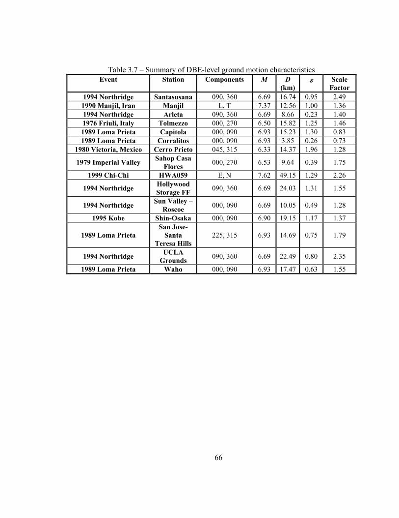
66

Table 3.7 – Summary of DBE-level ground motion characteristics Event Station Components M D

(km) ε Scale

Factor 1994 Northridge Santasusana 090, 360 6.69 16.74 0.95 2.49

1990 Manjil, Iran Manjil L, T 7.37 12.56 1.00 1.36 1994 Northridge Arleta 090, 360 6.69 8.66 0.23 1.40 1976 Friuli, Italy Tolmezzo 000, 270 6.50 15.82 1.25 1.46 1989 Loma Prieta Capitola 000, 090 6.93 15.23 1.30 0.83 1989 Loma Prieta Corralitos 000, 090 6.93 3.85 0.26 0.73

1980 Victoria, Mexico Cerro Prieto 045, 315 6.33 14.37 1.96 1.28

1979 Imperial Valley Sahop Casa Flores 000, 270 6.53 9.64 0.39 1.75

1999 Chi-Chi HWA059 E, N 7.62 49.15 1.29 2.26

1994 Northridge Hollywood Storage FF 090, 360 6.69 24.03 1.31 1.55

1994 Northridge Sun Valley – Roscoe 000, 090 6.69 10.05 0.49 1.28

1995 Kobe Shin-Osaka 000, 090 6.90 19.15 1.17 1.37

1989 Loma Prieta San Jose-

Santa Teresa Hills

225, 315 6.93 14.69 0.75 1.79

1994 Northridge UCLA Grounds 090, 360 6.69 22.49 0.80 2.35

1989 Loma Prieta Waho 000, 090 6.93 17.47 0.63 1.55

67

Table 3.8 – Summary of gap opening and base shear responses to DBE-level ground motions for frame a

Ground Motion

∆gap,L (in)

∆gap,R (in)

∆gap,max (in) Vb,max(kips) vbn

5108-090 2.27 1.83 2.27 1476 4.07 5108-360 1.78 1.57 1.78 1212 3.35 abbar--l 1.11 1.95 1.95 1474 4.07 abbar--t 2.86 3.51 3.51 1475 4.07 arl090 2.54 3.54 3.54 925 2.55 arl360 1.14 1.78 1.78 897 2.48

a-tmz000 1.22 1.19 1.22 829 2.29 a-tmz270 1.77 1.78 1.78 698 1.93 cap000 2.98 2.89 2.98 774 2.14 cap090 1.17 1.15 1.17 707 1.95 cls000 1.45 1.31 1.45 695 1.92 cls090 1.37 1.80 1.80 631 1.74 cpe045 2.89 3.07 3.07 1047 2.89 cpe315 1.10 1.09 1.10 695 1.92

h-shp000 1.26 1.25 1.26 1069 2.95 h-shp270 2.00 1.57 2.00 1312 3.62 hwa059-e 2.02 1.04 2.02 615 1.70 hwa059-n 1.33 1.46 1.46 650 1.79 nr-pel090 1.96 2.04 2.04 662 1.83 nr-pel360 2.45 2.52 2.52 1217 3.36

ro3000 1.08 1.31 1.31 817 2.26 ro3090 2.94 3.57 3.57 979 2.70 shi000 1.92 2.91 2.91 735 2.03 shi090 1.98 2.03 2.03 711 1.96 sjte225 1.30 1.22 1.30 1021 2.82 sjte315 1.93 1.67 1.93 833 2.30 ucl090 2.01 1.09 2.01 1165 3.22 ucl360 2.83 3.25 3.25 1504 4.15

wah000 2.00 2.04 2.04 1173 3.24 wah090 3.08 3.08 3.08 1645 4.54

68

Table 3.9 – Summary of gap opening and base shear responses to DBE-level ground motions for frame b

Ground Motion

∆gap,L (in)

∆gap,R (in)

∆gap,max (in) Vb,max(kips) vbn

5108-090 2.36 2.12 2.36 1150 3.17 5108-360 1.88 1.66 1.88 1297 3.58 abbar--l 1.30 2.47 2.47 1417 3.91 abbar--t 3.29 4.48 4.48 1349 3.72 arl090 2.89 4.55 4.55 1082 2.99 arl360 1.36 2.09 2.09 964 2.66

a-tmz000 1.57 1.49 1.57 828 2.29 a-tmz270 2.28 2.06 2.28 710 1.96 cap000 3.09 2.68 3.09 876 2.42 cap090 1.49 1.61 1.61 600 1.66 cls000 1.95 1.69 1.95 698 1.93 cls090 1.69 2.21 2.21 674 1.86 cpe045 3.41 4.14 4.14 1265 3.49 cpe315 1.41 1.30 1.41 697 1.92

h-shp000 1.65 1.55 1.65 978 2.70 h-shp270 2.72 2.08 2.72 1236 3.41 hwa059-e 2.57 1.23 2.57 540 1.49 hwa059-n 1.86 1.79 1.86 672 1.86 nr-pel090 2.31 2.20 2.31 650 1.79 nr-pel360 2.71 2.82 2.82 1411 3.90

ro3000 1.28 2.23 2.23 773 2.13 ro3090 3.62 4.35 4.35 1052 2.90 shi000 2.20 3.58 3.58 707 1.95 shi090 2.28 2.25 2.28 602 1.66 sjte225 1.73 1.31 1.73 967 2.67 sjte315 2.40 2.06 2.40 867 2.39 ucl090 2.76 1.58 2.76 1443 3.98 ucl360 3.48 3.17 3.48 1727 4.77

wah000 2.28 2.52 2.52 1024 2.83 wah090 3.36 3.56 3.56 1611 4.45

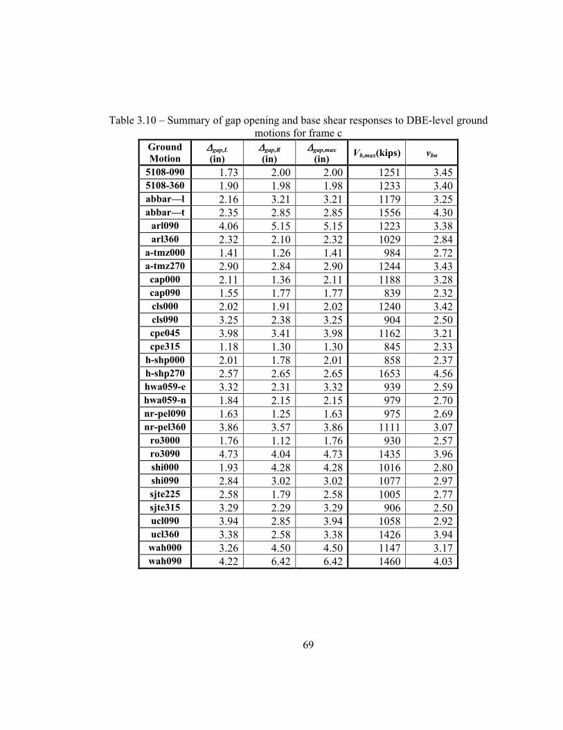
69

Table 3.10 – Summary of gap opening and base shear responses to DBE-level ground

motions for frame c Ground Motion

∆gap,L (in)

∆gap,R (in)

∆gap,max (in) Vb,max(kips) vbn

5108-090 1.73 2.00 2.00 1251 3.45 5108-360 1.90 1.98 1.98 1233 3.40 abbar—l 2.16 3.21 3.21 1179 3.25 abbar—t 2.35 2.85 2.85 1556 4.30

arl090 4.06 5.15 5.15 1223 3.38 arl360 2.32 2.10 2.32 1029 2.84

a-tmz000 1.41 1.26 1.41 984 2.72 a-tmz270 2.90 2.84 2.90 1244 3.43 cap000 2.11 1.36 2.11 1188 3.28 cap090 1.55 1.77 1.77 839 2.32 cls000 2.02 1.91 2.02 1240 3.42 cls090 3.25 2.38 3.25 904 2.50 cpe045 3.98 3.41 3.98 1162 3.21 cpe315 1.18 1.30 1.30 845 2.33

h-shp000 2.01 1.78 2.01 858 2.37 h-shp270 2.57 2.65 2.65 1653 4.56 hwa059-e 3.32 2.31 3.32 939 2.59 hwa059-n 1.84 2.15 2.15 979 2.70 nr-pel090 1.63 1.25 1.63 975 2.69 nr-pel360 3.86 3.57 3.86 1111 3.07

ro3000 1.76 1.12 1.76 930 2.57 ro3090 4.73 4.04 4.73 1435 3.96 shi000 1.93 4.28 4.28 1016 2.80 shi090 2.84 3.02 3.02 1077 2.97 sjte225 2.58 1.79 2.58 1005 2.77 sjte315 3.29 2.29 3.29 906 2.50 ucl090 3.94 2.85 3.94 1058 2.92 ucl360 3.38 2.58 3.38 1426 3.94

wah000 3.26 4.50 4.50 1147 3.17 wah090 4.22 6.42 6.42 1460 4.03

70

Table 3.11 – Mean and standard deviation of gap opening and base shear responses to DBE-level ground motions

∆gap,L (in)

∆gap,R (in)

∆gap,max (in) Vb,max(kips) vbn

Frame a Mean 1.93 2.02 2.14 988 2.73 std. dev. 0.65 0.83 0.76 310 0.86

Frame b Mean 2.31 2.43 2.63 996 2.75 std. dev. 0.71 0.98 0.90 330 0.91

Frame c Mean 2.67 2.67 2.99 1128 3.11 std. dev. 0.96 1.24 1.22 215 0.59

71

Table 3.12 – Summary of drift responses to DBE-level ground motions for frame a Ground Motion

θDBE (% rad)

θs,1 (% rad)

θs,2 (% rad)

θs,3 (% rad)

θs,4 (% rad)

θs,max (% rad)

5108-090 1.06 0.98 1.16 1.13 1.04 1.16 5108-360 0.85 0.91 1.00 0.94 0.89 1.00 abbar--l 0.96 0.64 0.72 0.67 0.66 0.72 abbar--t 1.58 0.87 0.94 0.91 0.85 0.94 arl090 1.58 0.95 1.13 1.08 1.02 1.13 arl360 0.85 1.69 1.70 1.65 1.59 1.70

a-tmz000 0.60 1.60 1.68 1.64 1.53 1.68 a-tmz270 0.84 0.84 0.96 0.92 0.86 0.96 cap000 1.35 1.33 1.37 1.38 1.34 1.38 cap090 0.57 0.57 0.59 0.60 0.55 0.60 cls000 0.71 0.61 0.81 0.80 0.75 0.81 cls090 0.85 0.79 0.89 0.90 0.82 0.90 cpe045 1.40 1.38 1.51 1.48 1.40 1.51 cpe315 0.55 0.57 0.63 0.63 0.57 0.63

h-shp000 0.64 0.73 0.79 0.74 0.73 0.79 h-shp270 0.90 1.11 1.03 1.00 1.05 1.11 hwa059-e 0.94 0.90 0.98 1.00 0.94 1.00 hwa059-n 0.69 0.70 0.74 0.73 0.66 0.74 nr-pel090 0.94 0.96 0.96 0.97 0.92 0.97 nr-pel360 1.17 1.14 1.30 1.25 1.26 1.30

ro3000 0.64 0.64 0.69 0.68 0.65 0.69 ro3090 1.61 1.63 1.65 1.65 1.62 1.65 shi000 1.32 1.29 1.36 1.37 1.30 1.37 shi090 0.94 0.95 0.98 0.97 0.93 0.98 sjte225 0.61 0.69 0.67 0.65 0.68 0.69 sjte315 0.89 0.91 0.91 0.92 0.87 0.92 ucl090 0.92 1.01 1.04 0.96 0.99 1.04 ucl360 1.46 1.55 1.53 1.52 1.49 1.55

wah000 0.97 0.95 1.11 1.05 1.02 1.11 wah090 1.43 1.46 1.54 1.53 1.54 1.54

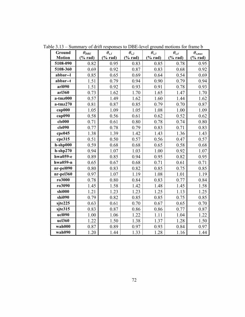
72

Table 3.13 – Summary of drift responses to DBE-level ground motions for frame b Ground Motion

θDBE (% rad)

θs,1 (% rad)

θs,2 (% rad)

θs,3 (% rad)

θs,4 (% rad)

θs,max (% rad)

5108-090 0.82 0.95 0.83 0.85 0.78 0.95 5108-360 0.69 0.92 0.87 0.83 0.68 0.92 abbar--l 0.85 0.65 0.69 0.64 0.54 0.69 abbar--t 1.51 0.79 0.94 0.90 0.79 0.94 arl090 1.51 0.92 0.93 0.91 0.78 0.93 arl360 0.73 1.62 1.70 1.65 1.47 1.70

a-tmz000 0.57 1.49 1.62 1.60 1.44 1.62 a-tmz270 0.81 0.87 0.85 0.79 0.70 0.87 cap000 1.05 1.09 1.05 1.08 1.00 1.09 cap090 0.58 0.56 0.61 0.62 0.52 0.62 cls000 0.71 0.61 0.80 0.78 0.74 0.80 cls090 0.77 0.78 0.79 0.83 0.71 0.83 cpe045 1.38 1.39 1.42 1.43 1.36 1.43 cpe315 0.51 0.50 0.57 0.56 0.47 0.57

h-shp000 0.59 0.68 0.68 0.65 0.58 0.68 h-shp270 0.94 1.07 1.03 1.00 0.92 1.07 hwa059-e 0.89 0.85 0.94 0.95 0.82 0.95 hwa059-n 0.65 0.67 0.68 0.71 0.61 0.71 nr-pel090 0.80 0.83 0.82 0.85 0.75 0.85 nr-pel360 0.97 1.07 1.19 1.08 1.01 1.19

ro3000 0.78 0.80 0.84 0.83 0.77 0.84 ro3090 1.45 1.58 1.42 1.48 1.45 1.58 shi000 1.21 1.23 1.23 1.25 1.13 1.25 shi090 0.79 0.82 0.85 0.85 0.75 0.85 sjte225 0.63 0.61 0.70 0.67 0.65 0.70 sjte315 0.83 0.87 0.86 0.86 0.77 0.87 ucl090 1.00 1.06 1.22 1.11 1.04 1.22 ucl360 1.22 1.50 1.38 1.37 1.28 1.50

wah000 0.87 0.89 0.97 0.93 0.84 0.97 wah090 1.20 1.44 1.33 1.28 1.16 1.44

73

Table 3.14 – Summary of drift responses to DBE-level ground motions for frame c Ground Motion

θDBE (% rad)

θs,1 (% rad)

θs,2 (% rad)

θs,3 (% rad)

θs,4 (% rad)

θs,max (% rad)

5108-090 0.58 0.90 0.66 0.81 0.55 0.90 5108-360 0.61 0.81 0.88 1.08 0.56 1.08 abbar--l 0.88 0.67 0.64 0.78 0.38 0.78 abbar--t 0.79 1.11 1.03 1.15 0.79 1.15 arl090 1.33 1.13 0.92 1.05 0.70 1.13 arl360 0.66 1.03 1.03 1.26 0.68 1.26

a-tmz000 0.45 1.38 1.30 1.45 1.22 1.45 a-tmz270 0.83 0.86 0.67 0.79 0.57 0.86 cap000 0.63 0.90 0.88 1.06 0.56 1.06 cap090 0.53 0.59 0.73 0.81 0.39 0.81 cls000 0.59 1.04 0.74 0.82 0.59 1.04 cls090 0.89 0.87 0.89 1.04 0.82 1.04 cpe045 1.06 1.26 1.16 1.27 0.85 1.27 cpe315 0.41 0.54 0.53 0.60 0.37 0.60

h-shp000 0.58 0.60 0.65 0.73 0.47 0.73 h-shp270 0.75 1.20 1.05 1.30 0.68 1.30 hwa059-e 0.92 0.77 1.03 1.15 0.84 1.15 hwa059-n 0.63 0.81 0.65 0.73 0.55 0.81 nr-pel090 0.48 0.68 0.56 0.60 0.40 0.68 nr-pel360 1.03 1.22 1.06 1.20 0.86 1.22

ro3000 0.53 0.64 0.69 0.75 0.43 0.75 ro3090 1.23 1.34 1.35 1.40 1.06 1.40 shi000 1.14 1.14 1.12 1.28 1.03 1.28 shi090 0.84 0.96 0.83 0.92 0.74 0.96 sjte225 0.73 0.79 0.86 0.95 0.65 0.95 sjte315 0.90 0.83 0.99 1.11 0.76 1.11 ucl090 1.06 1.07 1.18 1.30 1.00 1.30 ucl360 0.94 1.26 1.17 1.39 0.82 1.39

wah000 1.21 1.16 1.32 1.47 1.12 1.47 wah090 1.61 1.67 1.63 1.73 1.44 1.73

74

Table 3.15 – Mean and standard deviation of drift responses to DBE-level ground motions

θDBE

(% rad) θs,1

(% rad) θs,2

(% rad) θs,3

(% rad) θs,4

(% rad) θs,max

(% rad) Frame a Mean 0.99 1.01 1.08 1.06 1.02 1.09

std. dev. 0.33 0.34 0.33 0.33 0.33 0.33 Frame b Mean 0.91 0.97 0.99 0.98 0.88 1.02

std. dev. 0.29 0.32 0.30 0.30 0.29 0.32 Frame c Mean 0.83 0.97 0.94 1.07 0.73 1.09

std. dev. 0.29 0.27 0.27 0.29 0.27 0.27

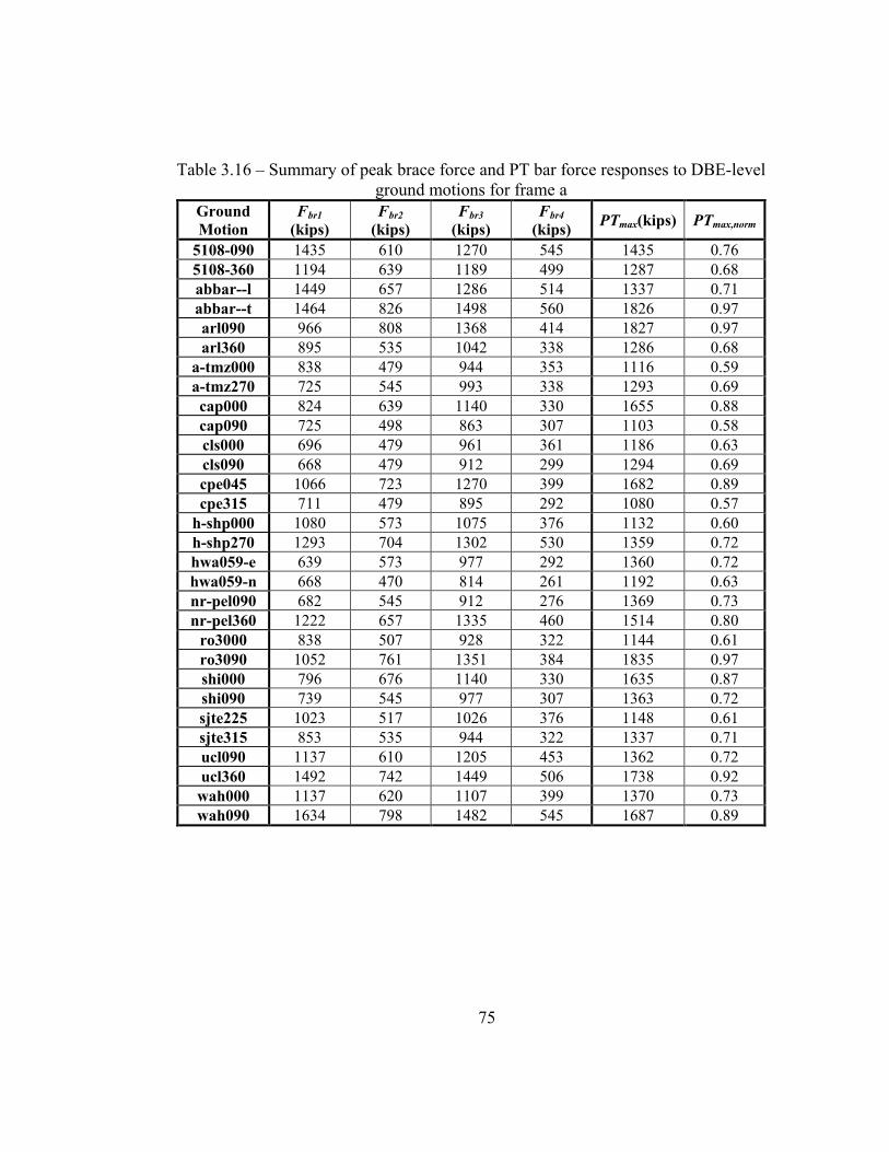
75

Table 3.16 – Summary of peak brace force and PT bar force responses to DBE-level ground motions for frame a

Ground Motion

Fbr1 (kips)

Fbr2 (kips)

Fbr3 (kips)

Fbr4 (kips) PTmax(kips) PTmax,norm

5108-090 1435 610 1270 545 1435 0.76 5108-360 1194 639 1189 499 1287 0.68 abbar--l 1449 657 1286 514 1337 0.71 abbar--t 1464 826 1498 560 1826 0.97 arl090 966 808 1368 414 1827 0.97 arl360 895 535 1042 338 1286 0.68

a-tmz000 838 479 944 353 1116 0.59 a-tmz270 725 545 993 338 1293 0.69 cap000 824 639 1140 330 1655 0.88 cap090 725 498 863 307 1103 0.58 cls000 696 479 961 361 1186 0.63 cls090 668 479 912 299 1294 0.69 cpe045 1066 723 1270 399 1682 0.89 cpe315 711 479 895 292 1080 0.57

h-shp000 1080 573 1075 376 1132 0.60 h-shp270 1293 704 1302 530 1359 0.72 hwa059-e 639 573 977 292 1360 0.72 hwa059-n 668 470 814 261 1192 0.63 nr-pel090 682 545 912 276 1369 0.73 nr-pel360 1222 657 1335 460 1514 0.80

ro3000 838 507 928 322 1144 0.61 ro3090 1052 761 1351 384 1835 0.97 shi000 796 676 1140 330 1635 0.87 shi090 739 545 977 307 1363 0.72 sjte225 1023 517 1026 376 1148 0.61 sjte315 853 535 944 322 1337 0.71 ucl090 1137 610 1205 453 1362 0.72 ucl360 1492 742 1449 506 1738 0.92

wah000 1137 620 1107 399 1370 0.73 wah090 1634 798 1482 545 1687 0.89

76

Table 3.17 – Summary of peak brace force and PT bar force responses to DBE-level ground motions for frame b

Ground Motion

Fbr1 (kips)

Fbr2 (kips)

Fbr3 (kips)

Fbr4 (kips) PTmax(kips) PTmax,norm

5108-090 986 563 877 313 875 0.77 5108-360 1089 465 1021 346 785 0.69 abbar--l 1222 618 973 326 894 0.79 abbar--t 1161 695 1225 385 1154 1.01 arl090 935 653 1093 339 1155 1.02 arl360 811 507 853 294 825 0.73

a-tmz000 709 472 721 267 730 0.64 a-tmz270 616 479 829 287 855 0.75 cap000 750 528 829 267 1006 0.88 cap090 514 382 600 222 738 0.65 cls000 616 465 769 326 795 0.70 cls090 575 410 721 241 847 0.74 cpe045 1078 632 997 333 1146 1.01 cpe315 596 382 636 222 702 0.62

h-shp000 822 465 685 248 745 0.66 h-shp270 1058 604 1057 346 938 0.82 hwa059-e 452 452 781 241 913 0.80 hwa059-n 575 410 636 235 784 0.69 nr-pel090 555 465 721 254 867 0.76 nr-pel360 1212 681 1033 365 957 0.84

ro3000 668 452 757 267 850 0.75 ro3090 924 681 1021 378 1150 1.01 shi000 637 597 913 300 1097 0.96 shi090 514 452 721 254 859 0.76 sjte225 822 438 709 280 759 0.67 sjte315 740 500 745 254 885 0.78 ucl090 1253 764 1141 398 943 0.83 ucl360 1458 716 1261 444 1079 0.95

wah000 873 479 889 300 902 0.79 wah090 1397 813 1261 437 1094 0.96

77

Table 3.18 – Summary of peak brace force and PT bar force responses to DBE-level ground motions for frame c

Ground Motion

Fbr1 (kips)

Fbr2 (kips)

Fbr3 (kips)

Fbr4 (kips) PTmax(kips) PTmax,norm

5108-090 941 539 681 250 621 0.69 5108-360 923 566 864 272 614 0.68 abbar—l 888 600 791 295 786 0.87 abbar—t 1169 675 949 295 740 0.82

arl090 923 620 912 357 920 1.02 arl360 765 532 681 267 664 0.74

a-tmz000 730 470 706 233 544 0.60 a-tmz270 914 634 925 346 740 0.82 cap000 888 491 815 267 635 0.71 cap090 624 430 693 238 586 0.65 cls000 923 566 742 289 624 0.69 cls090 668 498 803 318 790 0.88 cpe045 870 566 900 312 896 1.00 cpe315 624 436 584 210 526 0.58

h-shp000 633 443 633 233 625 0.69 h-shp270 1239 730 949 301 706 0.78 hwa059-e 694 511 876 335 796 0.88 hwa059-n 730 511 657 255 641 0.71 nr-pel090 721 484 584 227 572 0.64 nr-pel360 800 607 876 318 874 0.97

ro3000 686 470 681 255 587 0.65 ro3090 1072 730 1022 391 913 1.01 shi000 747 511 900 352 904 1.00 shi090 800 539 766 295 758 0.84 sjte225 747 525 791 295 697 0.77 sjte315 668 511 839 312 794 0.88 ucl090 765 580 937 363 883 0.98 ucl360 1072 668 1046 352 820 0.91

wah000 844 641 1022 386 908 1.01 wah090 1099 655 1010 346 944 1.05

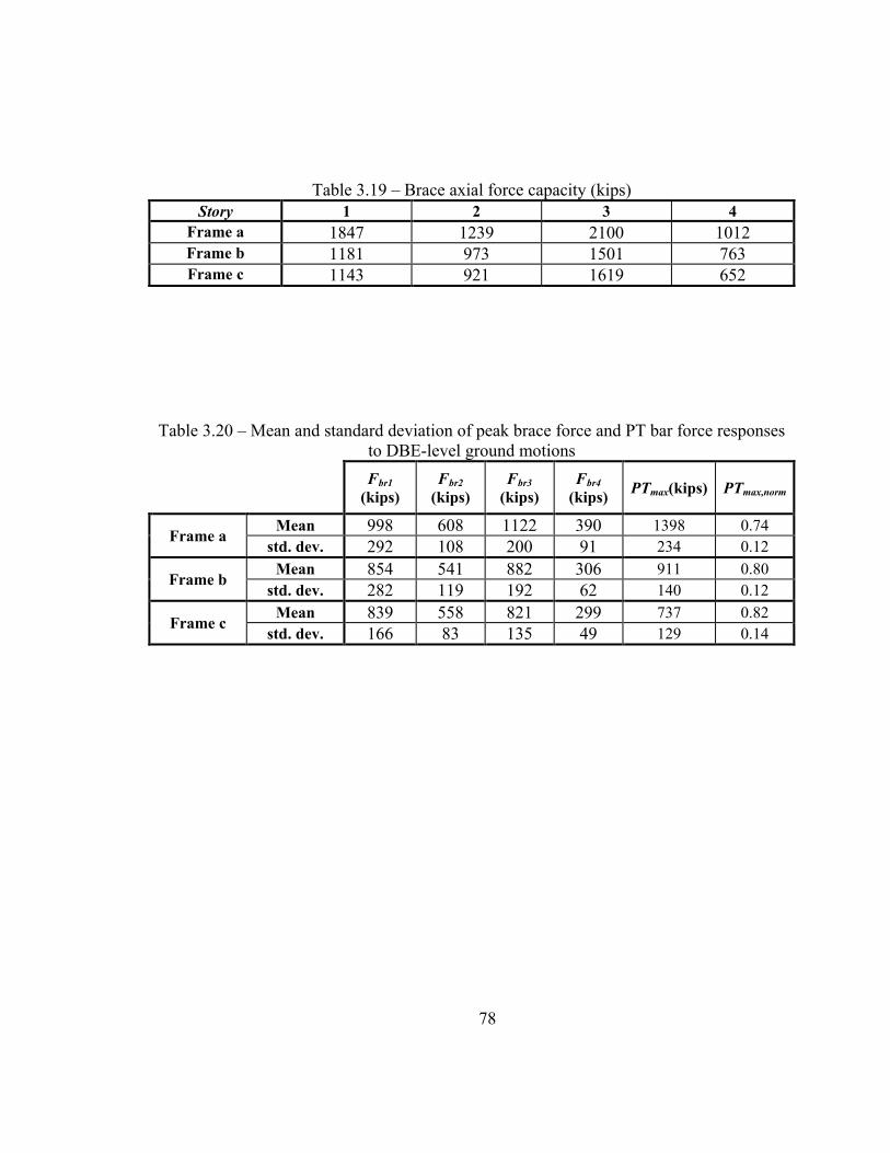
78

Table 3.19 – Brace axial force capacity (kips) Story 1 2 3 4

Frame a 1847 1239 2100 1012 Frame b 1181 973 1501 763 Frame c 1143 921 1619 652

Table 3.20 – Mean and standard deviation of peak brace force and PT bar force responses to DBE-level ground motions

Fbr1 (kips)

Fbr2 (kips)

Fbr3 (kips)

Fbr4 (kips) PTmax(kips) PTmax,norm

Frame a Mean 998 608 1122 390 1398 0.74 std. dev. 292 108 200 91 234 0.12

Frame b Mean 854 541 882 306 911 0.80

std. dev. 282 119 192 62 140 0.12

Frame c Mean 839 558 821 299 737 0.82 std. dev. 166 83 135 49 129 0.14

79

Figure 3.1 – Prototype buildings used for the parametric study: (a) typical elevation; (b) floor plan for frame a; (c) floor plan for frame b; (d) floor plan for frame c

Ground level

h4 = 12.5ft

h3 = 12.5ft

h2 = 12.5ft

h1 = 15.0ft

SC-CBF

Gravity Column

Adjacent Gravity Column

Tributary area for one SC-CBF

(b) (a) 8 @ 22.5ft = 180ft

8 @

22.

5ft =

180

ft

6 @

30f

t = 1

80ft

6 @ 30ft = 180ft

(c) 180ft

2 @ 40ft 2 @ 40ft

(d)

Frame b Frame c

180f

t

Frame a

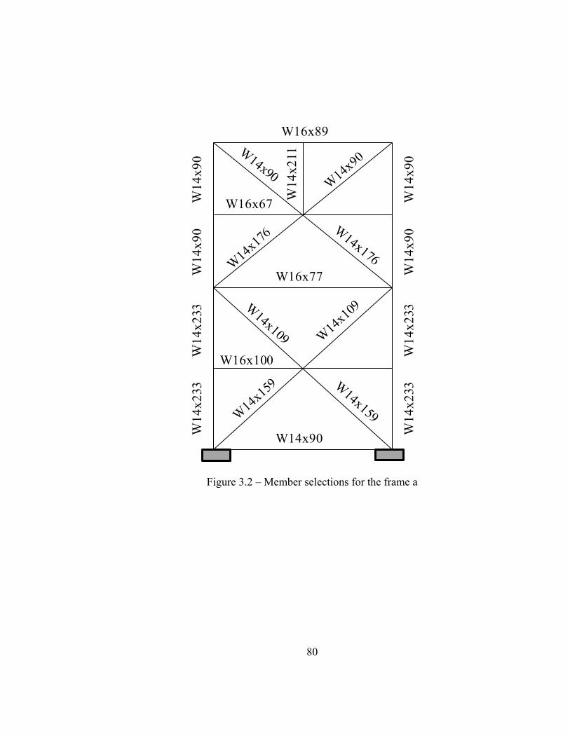
80

Figure 3.2 – Member selections for the frame a

W16x100

W16x77

W16x67

W16x89

W14x90

W14

x211

W14

x233

W14

x233

W14

x233

W14

x233

W14

x90

W14

x90

W14

x90

W14

x90

81

Figure 3.3 – Member selection for the frame b

W16x100

W16x67

W16x67

W16x67

W14x74

W14

x120

W14

x159

W14

x159

W14

x159

W14

x159

W14

x68

W14

x68

W14

x68

W14

x68

82

Figure 3.4 – Member selections for the frame c

W16x100

W16x67

W16x67

W16x67

W14x82

W14

x99

W14

x145

W14

x145

W14

x145

W14

x145

W14

x68

W14

x68

W14

x68

W14

x68

83

Figure 3.5 – Monotonic pushover results: (a) pre-decompression response; (b) full

range of response

0

3000

6000

9000

12000

15000

18000

0.00 0.04 0.08 0.12 0.16 0.20

Ove

rtur

ning

Mom

ent (

Kip

-ft)

Roof Drift (%)

Frame b

Frame a

Frame c

(a)

0

10000

20000

30000

40000

0.0 0.5 1.0 1.5 2.0 2.5 3.0

Ove

rtur

ning

Mom

ent (

Kip

-ft)

Roof Drift (%)

Frame b

Frame a

Frame c

(b)

84

Figure 3.6 - Cyclic pushover results: up to 1% roof drift

0

5000

10000

15000

20000

25000

30000

35000

0.0 0.2 0.4 0.6 0.8 1.0

Ove

rtur

ning

Mom

ent (

kip-

ft)

Roof Drift (%)

Frame c

Frame b

Frame a

85

Figure 3.7 – DBE-level peak roof drift response for all three frames

0.0

0.3

0.6

0.9

1.2

1.5

1.8Pe

ak R

oof D

rift

(%)

Frame a Frame c Frame b

mean (typ.)

arl360

86

Figure 3.8 – Roof drift response to arl360 ground motion for frame a

Figure 3.9 – Roof drift response to arl360 ground motion for frame b

0 5 10 15 20 25 30 35 40 45-1

-0.8

-0.6

-0.4

-0.2

0

0.2

0.4

0.6

0.8

1

Time (s)

Roof

Drif

t (%

rad)

-0.85%

0 5 10 15 20 25 30 35 40 45-1

-0.8

-0.6

-0.4

-0.2

0

0.2

0.4

0.6

0.8

1

Time (s)

Roof

Drif

t (%

rad)

-0.73%

87

Figure 3.10 – Roof drift response to arl360 ground motion for frame c

Figure 3.11 – PT bar force response to arl360 ground motion for frame a

0 5 10 15 20 25 30 35 40 45-1

-0.8

-0.6

-0.4

-0.2

0

0.2

0.4

0.6

0.8

1

Time (s)

Roof

Drif

t (%

rad)

0.66%

0 5 10 15 20 25 30 35 40 45600

800

1000

1200

1400

1600

1800

2000

Time (s)

PT F

orce

Res

pons

e(ki

p)

PT Bar Yield

1286 kips

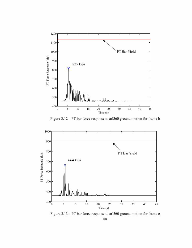
88

Figure 3.12 – PT bar force response to arl360 ground motion for frame b

Figure 3.13 – PT bar force response to arl360 ground motion for frame c

0 5 10 15 20 25 30 35 40 45400

500

600

700

800

900

1000

1100

1200

Time (s)

PT F

orce

Res

pons

e (k

ip)

825 kips

PT Bar Yield

0 5 10 15 20 25 30 35 40 45300

400

500

600

700

800

900

1000

Time (s)

PT F

orce

Res

pons

e (k

ip) PT Bar Yield

664 kips

89

Figure 3.14 – PT bar force and SC-CBF column base gap opening response to arl360 ground motion for frame a

Figure 3.15 – PT bar force and SC-CBF column base gap opening response to arl360

ground motion for frame b

0 5 10 15 20 25 30 35 40 45400

600

800

1000

1200

1400

1600

PT

Forc

e (k

ip)

Time (s)

0 5 10 15 20 25 30 35 40 450

0.5

1

1.5

2

2.5

3

Col

umn

Gap

Ope

ning

(in)

PT ForceLeft Column Gap Opening

0 5 10 15 20 25 30 35 40 450

200

400

600

800

1000

1200

PT

Forc

e (k

ip)

Time (s)

0 5 10 15 20 25 30 35 40 450

0.5

1

1.5

2

2.5

3

Col

umn

Gap

Ope

ning

(in)

PT ForceLeft Column Gap Opening

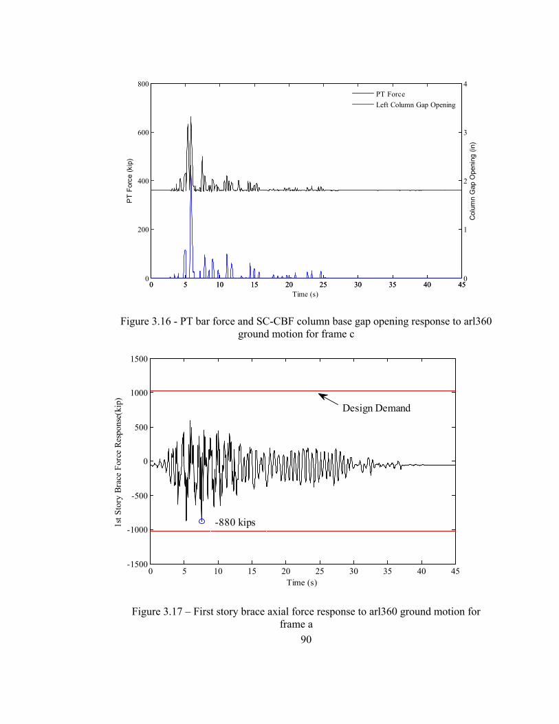
90

Figure 3.16 - PT bar force and SC-CBF column base gap opening response to arl360 ground motion for frame c

Figure 3.17 – First story brace axial force response to arl360 ground motion for frame a

0 5 10 15 20 25 30 35 40 450

200

400

600

800

PT

Forc

e (k

ip)

Time (s)

0 5 10 15 20 25 30 35 40 450

1

2

3

4

Col

umn

Gap

Ope

ning

(in)

PT ForceLeft Column Gap Opening

0 5 10 15 20 25 30 35 40 45-1500

-1000

-500

0

500

1000

1500

Time (s)

1st S

tory

Bra

ce F

orce

Res

pons

e(ki

p)

-880 kips

Design Demand

91

Figure 3.18 - First story brace axial force response to arl360 ground motion for frame

b

Figure 3.19 - First story brace axial force response to arl360 ground motion for frame

c

0 5 10 15 20 25 30 35 40 45-1500

-1000

-500

0

500

1000

1500

Time (s)

1st S

tory

Bra

ce F

orce

Res

pons

e (k

ip)

Design Demand

-812 kips

0 5 10 15 20 25 30 35 40 45-1000

-800

-600

-400

-200

0

200

400

600

800

1000

Time (s)

1st S

tory

Bra

ce F

orce

Res

pons

e (k

ip)

-765 kips

Design Demand

92

Figure 3.20 – Overturning moment roof drift response to arl360 ground motion for frame a

Figure 3.21 – Overturning moment roof drift response to arl360 ground motion for frame b

-1 -0.8 -0.6 -0.4 -0.2 0 0.2 0.4 0.6-2.5

-2

-1.5

-1

-0.5

0

0.5

1

1.5

2x 10

4

Ove

rturn

ing

Mom

ent (

kip-

ft)

Roof Drift (% rad)

-0.8 -0.6 -0.4 -0.2 0 0.2 0.4 0.6-2.5

-2

-1.5

-1

-0.5

0

0.5

1

1.5

2x 10

4

Ove

rturn

ing

Mom

ent (

kip-

ft)

Roof Drift (% rad)

93

Figure 3.22 - Overturning moment roof drift response to arl360 ground motion for

frame c

Figure 3.23 – Overturning moment column base gap opening response to arl360

ground motion for frame a

-0.8 -0.6 -0.4 -0.2 0 0.2 0.4 0.6 0.8-3

-2

-1

0

1

2

3

4x 10

4

Ove

rturn

ing

Mom

ent (

kip-

ft)

Roof Drift (% rad)

0 0.2 0.4 0.6 0.8 1 1.2 1.4 1.6

-2

-1.5

-1

-0.5

0

0.5

1

1.5

x 104

Column Gap Opening (in)

Ove

rturn

ing

Mom

ent (

kip-

ft)

Left Column Gap OpeningRight Column Gap Opening

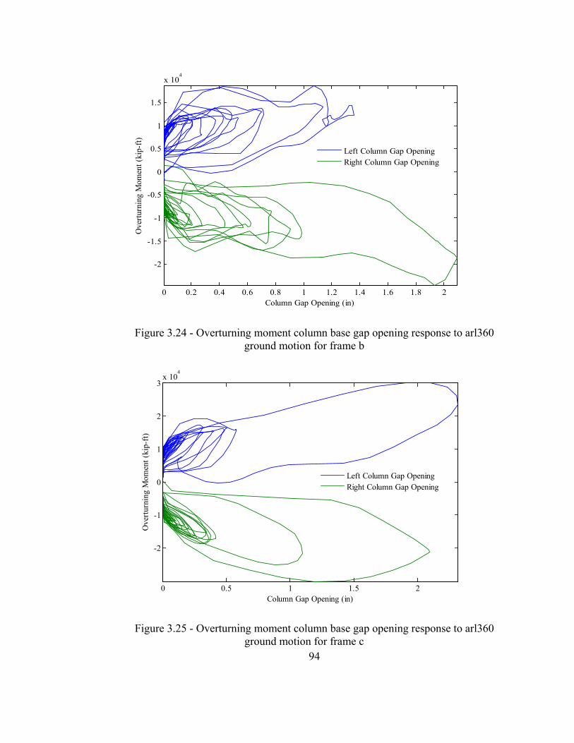
94

Figure 3.24 - Overturning moment column base gap opening response to arl360 ground motion for frame b

Figure 3.25 - Overturning moment column base gap opening response to arl360 ground motion for frame c

0 0.2 0.4 0.6 0.8 1 1.2 1.4 1.6 1.8 2

-2

-1.5

-1

-0.5

0

0.5

1

1.5

x 104

Column Gap Opening (in)

Ove

rturn

ing

Mom

ent (

kip-

ft)

Left Column Gap OpeningRight Column Gap Opening

0 0.5 1 1.5 2

-2

-1

0

1

2

3x 10

4

Column Gap Opening (in)

Ove

rturn

ing

Mom

ent (

kip-

ft)

Left Column Gap OpeningRight Column Gap Opening

95

CHAPTER IV

HIGHER MODE EFFECTS

4.1 Overview

The rocking response of SC-CBF systems tends to cause higher mode response

exceeding that of an equivalent fixed-base structure, which results in a significant

increase in member force demands (Roke et al. 2009, Wiebe and Christopoulos 2009).

This amplification of higher mode response introduces additional uncertainty in the

dynamic response. It is therefore desirable to determine which frame configuration

minimizes the higher mode effects.

To compare modal response for the various SC-CBFs, the modal demands in must be

quantified and normalized by standard measures. In this chapter, several quantification

measures (both intensity-based measures and conventional peak-based measures) are

proposed for quantifying modal responses. The effectiveness of these measures for

quantifying modal responses of SC-CBFs is then studied by applying them to several

prototype frames with varying frame geometries and friction coefficients.

96

4.2 Higher Mode Contributions in SC-CBF Design

Several conservative measures had been taken to account for large higher mode

effects in the development of the SC-CBF design procedure (Roke et al. 2010), which

modifies the conventional response spectrum analysis (RSA) design method. For design

demand calculation, a design pseudo-acceleration spectrum based on the modal

properties of the structure is used to determine the peak modal responses, similar to

conventional RSA. However, the design pseudo-acceleration values are amplified by a

safety factor, γn, as described in Section 2.6.2.2. For higher modes, γn was set equal to

2.0 to account for the significant uncertainty in the higher mode response. Furthermore,

conservative values of modal correlation coefficients (the off-diagonal correlation

coefficients, ρij, were set equal to 0.25) are used while combining the peak modal

responses by complete quadratic combination (CQC) method (as described in Section

2.6.2.2).

4.3 Prototypes for Higher Mode Quantification Study

To demonstrate and compare the modal response of SC-CBF systems, two sets of

prototype SC-CBFs are used: the prototype SC-CBFs described in Section 3.2, and an

additional set of prototypes that were initially studied by Jeffers (2012). The prototype

SC-CBFs described in Section 3.2 were designed using frame geometries a, b, and c and

have coefficients of friction equal to 0.45 at the lateral load bearings; therefore, they will

be referred to as frames a45, b45, and c45, respectively. The prototype SC-CBFs studied

by Jeffers (2012) were designed using frame geometry b and have coefficients of friction

97

equal to 0.30, 0.45, and 0.60 at the lateral load bearings; therefore, these frames will be

referred to as frames b30, b45, and b60. Note that frame b45 was designed once and used

in both studies. Each of the five prototypes was subjected to the DBE-level ground

motions described in Section 3.6.1. The nonlinear dynamic analysis results were then

used to study the modal responses.

4.4 Modal Analysis

Mode shapes for the five prototype SC-CBFs were determined using eigen value

analyses in OpenSees. Tables 4.1 and 4.2 show the modal frequencies and natural periods

of the prototype SC-CBFs. Figures 4.1 and 4.2 show the mode shapes of the prototype

SC-CBFs. Since the masses of the prototype structures are identical, any difference in

modal properties (e.g., mode shapes and frequencies) among the prototype SC-CBFs will

be a function of frame stiffness.

The change in frame geometry between frames a45, b45, and c45 significantly

affects the frame stiffness, effecting changes in the mode shapes (as shown in Figure 4.1)

and natural frequencies (as shown in Table 4.1). The frames with larger frame width

(frame c) are comparatively stiffer than narrower frames (e.g., frame a).

The change in coefficient of friction between frames b30, b45, and b60 do not

significantly affect the frame stiffness. Figure 4.2 shows the first three modes for

prototype SC-CBFs b30, b45, and b60. Although these frames are designed separately

and have member sections with different sizes, the mode shapes are nearly identical.

Since the frame geometries are identical for three frames, the slight differences in frame

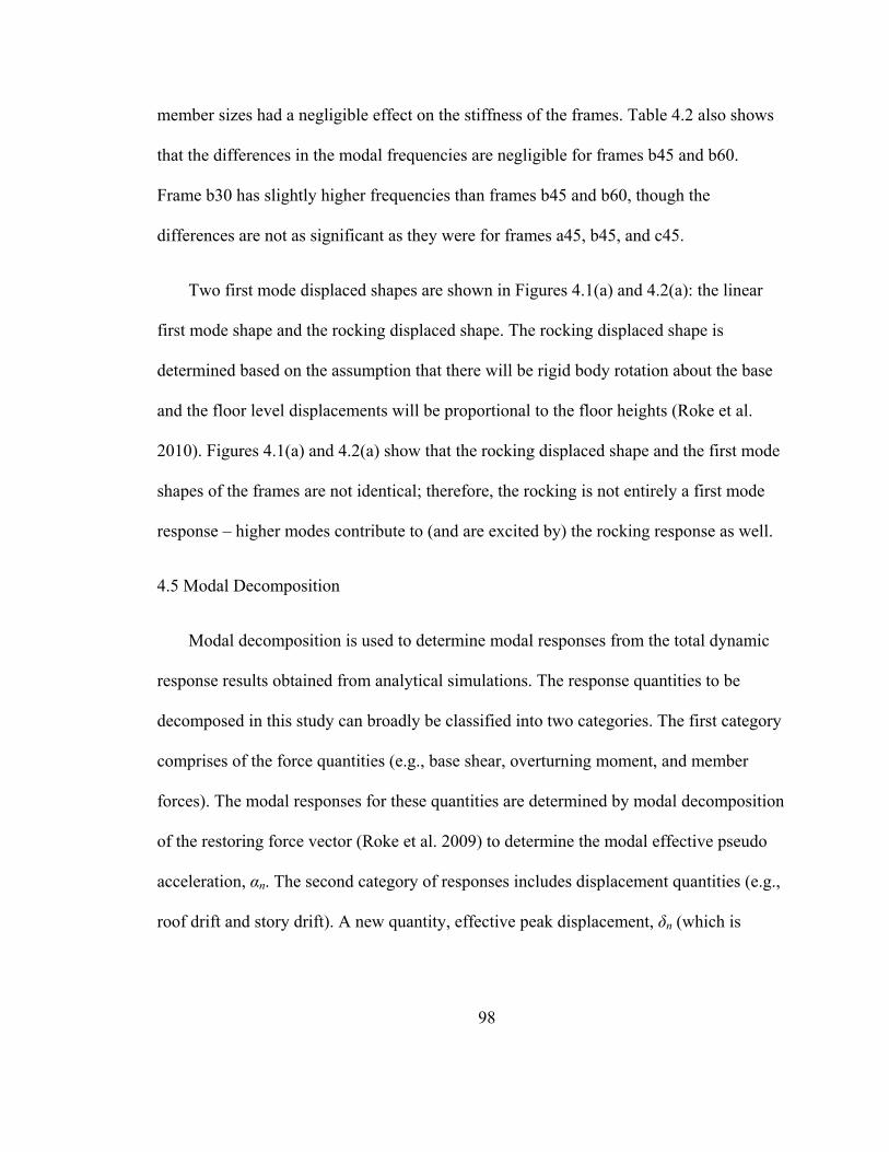
98

member sizes had a negligible effect on the stiffness of the frames. Table 4.2 also shows

that the differences in the modal frequencies are negligible for frames b45 and b60.

Frame b30 has slightly higher frequencies than frames b45 and b60, though the

differences are not as significant as they were for frames a45, b45, and c45.

Two first mode displaced shapes are shown in Figures 4.1(a) and 4.2(a): the linear

first mode shape and the rocking displaced shape. The rocking displaced shape is

determined based on the assumption that there will be rigid body rotation about the base

and the floor level displacements will be proportional to the floor heights (Roke et al.

2010). Figures 4.1(a) and 4.2(a) show that the rocking displaced shape and the first mode

shapes of the frames are not identical; therefore, the rocking is not entirely a first mode

response – higher modes contribute to (and are excited by) the rocking response as well.

4.5 Modal Decomposition

Modal decomposition is used to determine modal responses from the total dynamic

response results obtained from analytical simulations. The response quantities to be

decomposed in this study can broadly be classified into two categories. The first category

comprises of the force quantities (e.g., base shear, overturning moment, and member

forces). The modal responses for these quantities are determined by modal decomposition

of the restoring force vector (Roke et al. 2009) to determine the modal effective pseudo

acceleration, αn. The second category of responses includes displacement quantities (e.g.,

roof drift and story drift). A new quantity, effective peak displacement, δn (which is

99

similar to αn) has been derived to decompose the displacement quantities. The derivation

and definition of these pseudo response quantities are discussed in detail in this section.

4.5.1 Effective Pseudo Acceleration

For linear response, the restoring force vector in the nth mode, {fr,n(t)}, can be

expressed as the modal mass distribution,{sn}, multiplied by the modal pseudo-

acceleration, An(t) (Chopra 2007):

{ } [ ] { } )()(}{)(, tAmtAstf nnnnnnr ⋅⋅⋅Γ=⋅= φ (4.1)

Since the rocking response of SC-CBFs is nonlinear, the conventional modal pseudo-

acceleration, An(t)is replaced by a similar quantity that accounts for this nonlinearity

(Roke et al 2009). This quantity, αn(t), is called the “effective” pseudo-acceleration for

the nth mode. Equation 4.1 can then be rewritten for nonlinear response as follows:

{ } )(}{)(, tstf nnnr α⋅= (4.2)

To determine αn(t), the total restoring force vector, {fr(t)} is written as a summation

of the modal restoring force vectors:

( ){ } ( ){ } [ ] { }∑∑==

⋅⋅⋅Γ==N

nnnn

N

nnrr tmtftf

11, )(αφ (4.3)

Where Γn is the modal participation factor, [m] is the mass matrix, {ϕn} is the nth

mode shape.

100

Due to modal orthogonality, pre-multiplying each side of Equation 4.3 by { nφ }T

gives the effective pseudo acceleration:

( ) { } ( ){ }nn

rT

nn M

tft

⋅Γ=

φα (4.4)

where Mn is the modal mass.

The effective pseudo-acceleration values are then used to determine the modal

restoring force vectors (Equation 4.2). Time history results of these modal restoring

forces are used to determine the modal time history results of force quantities (e.g., base

shear and base overturning moment).

4.5.2 Effective Peak Displacement

As effective pseudo-acceleration is derived from static restoring force vector,

effective peak displacement is determined from the floor displacement vector. For linear

response, the modal floor displacement vectors can be expressed in terms of modal peak

displacement as follows (Chopra 2007):

{ } )(}{)( tDtu nnnn ⋅⋅Γ= φ (4.5)

Equation 4.5 is applicable only to linear response; for nonlinear response, the term

Dn(t) will be replaced by δn(t), the effective peak displacement:

{ } )(}{)( ttu nnnn δφ ⋅⋅Γ= (4.6)

101

The total floor displacement vector, {u(t)}, may be written as the sum of the modal

displacement vectors:

( ){ } ( ){ } { }∑∑==

⋅⋅Γ==N

nnnn

N

nn ttutu

11)(δφ (4.7)

Pre-multiplying each side of the equation 4.3 by { nφ }T.[m] and then applying modal

mass orthogonality, the effective peak displacement can be determined:

( ) { } [ ] ( ){ }nn

Tn

n Mtum

t⋅Γ

⋅⋅=

φδ (4.8)

The time history values of δn(t) are put into Equation 4.6 to calculate the modal floor

displacements, which are then used to determine time history responses of modal

displacement quantities (e.g., roof drift and story drift).

4.6 Modal Decomposition Results

Time history results from OpenSees for the prototype SC-CBFs are decomposed into

modal responses as described in Section 4.5. First, the peak effective pseudo-acceleration

responses are determined and compared against the corresponding design values. The

modal values of quantities such as base shear, overturning moment, and roof drift are

then determined to compare the modal responses against the total responses. Time history

records of modal responses are presented against the corresponding total responses to

demonstrate the higher mode effects on different response quantities.

102

4.6.1 Peak Effective Pseudo-Acceleration Response

Figure 4.3 shows the distribution of peak αn values of the first three modes for the

suite of DBE-level ground motions frame b45. This distribution is typical of the modal

response of the prototype frames. The peak values of effective pseudo-acceleration are

compared against the design spectral acceleration (SAn) and factored spectral acceleration

(γnSAn) values derived from the design response spectrum (as described in Section

2.6.1.1). Figure 4.3 shows that the higher mode responses have very high dispersion

compared to the first mode responses; therefore, a higher value of γn was chosen for the

higher modes (2.0) than the value of γ1 for the first mode (1.15).

4.6.2 Modal Responses

Since ground motion arl360 was used previously for presentation of dynamic

analysis results, the same ground motion record will be used for demonstration of the

modal responses. Figures 4.4, 4.5, and 4.6 show the time history records of the modal

responses (base shear, overturning moment, and roof drift, respectively) compared

against the corresponding total responses for frame b45. Figure 4.4 suggests that the

higher modes contribute significantly to the base shear response. This is only a four-story

structure, so the second mode is the only higher mode that contributes significantly to the

base shear response; however, for taller buildings, the contributions from the third and

fourth modes are expected to increase.

Figures 4.5 and 4.6 show the overturning moment and roof drift responses,

respectively. These figures indicate that the roof drift and overturning moment responses

103

are dominated by the first mode response. The first mode dominance in the roof drift and

overturning moment responses are similar for all of the prototype frames; however, the

degree of the higher mode contribution varies.

4.7 Quantification of Higher Mode Responses

The modal response demonstrated in Section 4.6 shows that higher modes

significantly contribute to SC-CBF dynamic response, especially for base shear. The

modal responses must be quantified using normalized quantification measures so that the

higher mode effects can be compared for different prototype SC-CBFs. Three such

quantification measures are proposed in this study to quantify higher mode effects. They

are compared with the conventional measure, modal peak to total peak ratio. This section

describes all four of the quantification measures (QMs) considered in this study.

4.7.1 Modal Peak to Total Peak Ratio

The first quantification measure discussed in this study is the modal peak to total

peak ratio. For convenience, this quantification parameter will be referred to as QM0.

QM0 is expressed as the ratio of the absolute modal peak response to the absolute total

peak response. Figure 4.7 shows schematic time history plots for total response, rtot(t),

and nth mode response, rn(t), indicating the peak values rtot,max and rn,max, respectively.

QM0 for the nth mode can be expressed as follows:

max

max0 )(

)(trtr

QMtot

nn = (4.9)

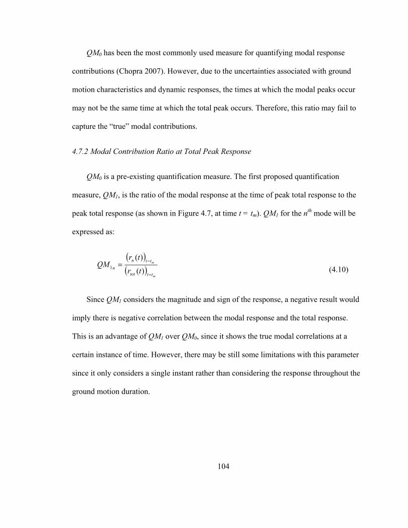
104

QM0 has been the most commonly used measure for quantifying modal response

contributions (Chopra 2007). However, due to the uncertainties associated with ground

motion characteristics and dynamic responses, the times at which the modal peaks occur

may not be the same time at which the total peak occurs. Therefore, this ratio may fail to

capture the “true” modal contributions.

4.7.2 Modal Contribution Ratio at Total Peak Response

QM0 is a pre-existing quantification measure. The first proposed quantification

measure, QM1, is the ratio of the modal response at the time of peak total response to the

peak total response (as shown in Figure 4.7, at time t = tm). QM1 for the nth mode will be

expressed as:

( )( )

m

m

tttot

ttnn tr

trQM

=

==)(

)(1 (4.10)

Since QM1 considers the magnitude and sign of the response, a negative result would

imply there is negative correlation between the modal response and the total response.

This is an advantage of QM1 over QM0, since it shows the true modal correlations at a

certain instance of time. However, there may be still some limitations with this parameter

since it only considers a single instant rather than considering the response throughout the

ground motion duration.

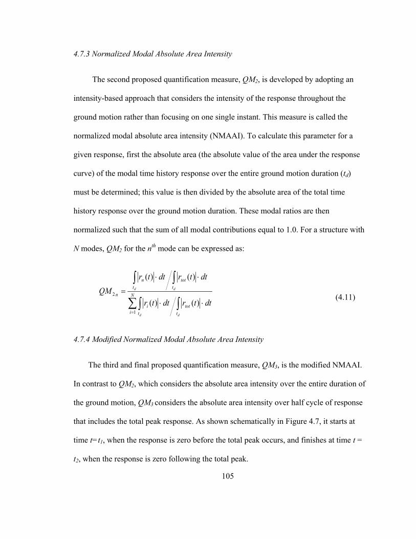
105

4.7.3 Normalized Modal Absolute Area Intensity

The second proposed quantification measure, QM2, is developed by adopting an

intensity-based approach that considers the intensity of the response throughout the

ground motion rather than focusing on one single instant. This measure is called the

normalized modal absolute area intensity (NMAAI). To calculate this parameter for a

given response, first the absolute area (the absolute value of the area under the response

curve) of the modal time history response over the entire ground motion duration (td)

must be determined; this value is then divided by the absolute area of the total time

history response over the ground motion duration. These modal ratios are then

normalized such that the sum of all modal contributions equal to 1.0. For a structure with

N modes, QM2 for the nth mode can be expressed as:

∑ ∫∫

∫∫

=

⋅⋅

⋅⋅

= N

i ttot

ti

ttot

tn

n

dd

dd

dttrdttr

dttrdttrQM

1

2

)()(

)()(

(4.11)

4.7.4 Modified Normalized Modal Absolute Area Intensity

The third and final proposed quantification measure, QM3, is the modified NMAAI.

In contrast to QM2, which considers the absolute area intensity over the entire duration of

the ground motion, QM3 considers the absolute area intensity over half cycle of response

that includes the total peak response. As shown schematically in Figure 4.7, it starts at

time t=t1, when the response is zero before the total peak occurs, and finishes at time t =

t2, when the response is zero following the total peak.

106

The calculation procedure of QM3 is similar to that for QM2; the only difference is in

the range over which the area is integrated. The ratio of the area intensity of the modal

response to the total time response for duration t= t1 to t= t2 is first determined. These

modal ratios are then normalized such that the sum of all modal contributions equal to

1.0. For a structure with N modes, QM3 for the nth mode can be expressed as:

∑ ∫∫

∫∫

=

⋅⋅

⋅⋅

=N

i

t

ttot

t

ti

t

ttot

t

tn

n

dttrdttr

dttrdttrQM

1

3 2

1

2

1

2

1

2

1

)()(

)()(

(4.12)

4.8 Comparison of Quantification Measures

The primary purpose of the introduction of these QMs is to compare the higher mode

contributions of different SC-CBF systems. The most effective measure would therefore

be the one which yields results that are comparable for different frames. The most

effective quantification measure is selected based on two criteria: 1) the sum of the modal

means must be equal to 1; and 2) the coefficient of variation must be small. If the sum of

the modal means is 1, the QM values for each mode will represent the percentage of

modal contribution to the total response. QM2 and QM3are normalized such that the sum

of the modal means is 1. Additionally, it is desirable to have a quantification measure

which produces results with low dispersion, as measured by the coefficient of variation

(COV).

The modal response data for all five prototype SC-CBFs have been used to extract

results as calculated by each of the four QMs. As discussed in Section 4.6.2, the base

107

shear responses have the most significant contributions from higher modes among the

studied response quantities; therefore, the response data for base shear have been used to

study the effectiveness of the proposed quantification measures. Since each frame is

subjected to 30 ground motion records, there will be 30 modal QM responses for each

quantification measure. Modal means and coefficients of variation have been determined

for each measure from these records.

Tables 4.3 and 4.4 show the results of the quantification measures for base shear

response. The modal mean values, the sum of the modal means, and the coefficients of

variation for all four quantification measures have been presented for all five prototype

frames. Table 4.3 shows the data for frames a45, b45, and c45 (i.e., frames with varying

geometry). Table 4.4 shows the data for frames b30, b45, and b60 (i.e., frames with

varying coefficients of friction. These tables show that QM1, QM2, and QM3 fulfill the

first criterion (the sum of the modal means should be 1).

The data in Tables 4.3 and 4.4 also suggest that among the four quantification

measures, QM2 generates results with the least COV. For the first mode responses, the

COV for QM2 is in the range of 4% to 11%, which is significantly lower than that of the

other QMs. For the higher mode responses, the COV of QM2 seemed to be a bit larger

compared to those of first mode responses, though they are lower than those of the other

quantification measures. Therefore, QM2, the Normalized Modal Absolute Area Intensity

(NMAAI) measure, is the best of the proposed quantification measures for modal

response of SC-CBF systems.

108

4.9 Modal Response Quantification Results

As QM2 (NMAAI) was found to be the most effective of the four described

quantification measures, only this measure is used to compare the higher mode responses

in the studied SC-CBFs. Comparisons will be made between the set of prototypes with

varying frame geometries (a45, b45, and c45) as well as prototypes with varying friction

coefficients (b30, b45, b60). In Section 4.8, only the base shear data were considered in

the presentation of the different quantification methods; here, other response quantities

(e.g., roof drift and story shear) will also be discussed.

4.9.1 Effect of Frame Geometry

The modal intensities of frames a45, b45, and c45 have been compared for different

response quantities to determine if there is any trend in the higher mode effects of SC-

CBFs with changing frame geometries. Figure 4.8 shows the distribution of normalized

modal absolute area intensities for base shear responses of frames a45, b45, and c45. By

definition, smaller first mode intensity leads to larger higher mode intensity; it is

therefore convenient to study the intensity values for the first mode rather than looking at

those for the individual higher modes (e.g., the 2nd and 3rd modes). The normalized first

mode base shear intensities are largest for frame c45 and lowest for frame a45,

suggesting that the higher mode contribution to base shear response decreases with an

increase of frame bay width.

Figure 4.9 shows the mean modal intensities of story shear responses for frames a45,

b45, and c45. The trend in the mean story shear intensities in these three frames is similar

109

to that of base shear intensities (except in the fourth story): higher mode effects in the

story shear responses seem to be the least for frame c45.

Figure 4.10 shows the distribution of normalized modal intensities for roof drift

responses for frames a45, b45, and c45. The time history records of modal responses

shown in Section 4.6.2 suggested that the higher mode contribution to roof drift is

negligible. For frames a45 and b45, the mean normalized first mode roof drift intensities

are about 90%, indicating the responses are dominated by the first mode. For frame c45,

the higher mode effects in roof drift response increase as the mean first mode intensity is

reduced to about 84%. The mean modal intensities of story drift responses shown in

Figure 4.11 also show similar trends: the higher mode effects are highest for frame c45,

indicating that higher mode contributions to displacement quantities are increased with

increasing frame bay width.

4.9.2 Effect of Friction

The modal intensities of frames b30, b45, and b60 have been compared for different

response quantities to determine trends in the higher mode contributions for frames with

changing friction coefficients. Figure 4.12 shows the normalized modal intensities for

base shear response of frames b30, b45, and b60. The higher mode effects are similar for

frames b45 and b60, though the higher mode effects for frame b30 are less significant.

Figure 4.13 shows that the trends in the mean story shear intensities are similar except for

the second story shear, which is dominated by first mode response.

110

No trend is observed in the mean modal intensities for roof drift response of frames

b30, b45, and b60 shown in Figure 4.14: the modal intensities are nearly identical for the

three frames. As shown in Figure 4.15, the first mode mean intensities for story drift are

similar for frames b30 and b60, and slightly higher for frame b45, though there is no

definite trend with the change in friction coefficients.

4.10 Summary

This chapter addressed the higher mode effects on SC-CBF systems. Additional

prototypes had been introduced before modal properties of each prototype were

presented. The approximate modal decomposition technique by using “effective” pseudo-

acceleration and “effective” peak displacement was described. This technique was

applied on the dynamic time history analysis results to determine the modal responses.

Three proposed quantification measures along with the conventional peak-based

measure were described in details. These measures were applied on the base shear

responses of each prototype and the results were compared and analyzed to select the

most appropriate and effective measure for the quantification of higher mode effects on

SC-CBF responses. Since the proposed normalized modal absolute area intensity

(NMAAI) was found to be the most effective measure, it was used to quantify and

compare the higher mode effects on prototype sets with varying frame geometries as well

as varying friction properties.

111

Table 4.1 – Modal properties of prototypes with varying frame geometries

Frames Circular Frequency,

ωn (rad/s) Period,

T (s) mode 1 mode 2 mode 3 mode 4 mode 1 mode 2 mode 3 mode 4

a45 10.980 35.520 48.405 64.637 0.572 0.177 0.130 0.097 b45 12.610 35.852 47.959 60.759 0.498 0.175 0.131 0.103 c45 13.794 36.834 46.683 59.342 0.455 0.171 0.135 0.106

Table 4.2 – Modal properties of prototypes with varying coefficients of friction

Frames Circular Frequency,

ωn (rad/s) Period,

T (s) mode 1 mode 2 mode 3 mode 4 mode 1 mode 2 mode 3 mode 4

b30 13.376 38.572 51.089 65.213 0.470 0.163 0.123 0.096 b45 12.610 35.852 47.959 60.759 0.498 0.175 0.131 0.103 b60 12.532 35.690 48.291 59.512 0.501 0.176 0.130 0.106

112

Table 4.3 – Quantification data of modal base shear responses for prototypes with varying frame geometries

Mean Sum of Modal Means

Coefficient of Variation Mode 1 Mode 2 Mode 3 Mode 1 Mode 2 Mode 3

QM1 a45 0.631 0.608 0.058 1.309 0.211 0.204 0.214 b45 0.715 0.507 0.025 1.259 0.177 0.216 0.270 c45 0.783 0.335 0.008 1.127 0.090 0.238 0.209

QM2 a45 0.527 0.448 0.024 1.000 0.328 0.392 0.614 b45 0.662 0.332 0.007 1.000 0.224 0.438 1.355 c45 0.750 0.248 0.003 1.000 0.109 0.322 1.138

QM3 a45 0.725 0.237 0.032 1.000 0.103 0.313 0.085 b45 0.762 0.216 0.016 1.000 0.090 0.317 0.103 c45 0.831 0.164 0.004 1.000 0.052 0.261 0.148

QM4 a45 0.783 0.208 0.008 1.000 0.250 0.912 0.801 b45 0.862 0.134 0.003 1.000 0.169 1.071 0.613 c45 0.912 0.087 0.001 1.000 0.088 0.922 0.723

Table 4.4 – Quantification data of modal base shear responses for prototypes with varying coefficients of friction

Mean Sum of Modal Means

Coefficient of Variation Mode 1 Mode 2 Mode 3 Mode 1 Mode 2 Mode 3

QM1 b30 0.769 0.400 0.023 1.194 0.139 0.280 0.167 b45 0.715 0.507 0.025 1.259 0.177 0.216 0.270 b60 0.739 0.471 0.021 1.236 0.107 0.241 0.227

QM2 b30 0.705 0.289 0.007 1.001 0.155 0.358 1.555 b45 0.662 0.332 0.007 1.000 0.224 0.438 1.355 b60 0.701 0.294 0.006 1.000 0.121 0.280 1.114

QM3 b30 0.829 0.159 0.011 1.000 0.049 0.247 0.154 b45 0.762 0.216 0.016 1.000 0.090 0.317 0.103 b60 0.771 0.214 0.011 1.000 0.070 0.244 0.134

QM4 b30 0.902 0.093 0.004 1.000 0.118 1.115 0.761 b45 0.862 0.134 0.003 1.000 0.169 1.071 0.613 b60 0.869 0.126 0.004 1.000 0.120 0.808 0.738

113

Figure 4.1 – Normalized displaced shapes of frames a45, b45, and c45 for- (a) 1st mode and rocking displaced shape; (b) 2nd mode; and (c) 3rd mode

Figure 4.2 – Normalized displaced shapes of frames b30, b45, and b60 for- (a) 1st mode and rocking displaced shape; (b) 2nd mode; and (c) 3rd mode

0

1

2

3

4

0.0 0.5 1.0

a45

b45

c45

Rocking

Normalized Displacement

Floo

r Lev

el

(a) 1st Mode

0

1

2

3

4

-2.0 -1.0 0.0 1.0 2.0Normalized Displacement

(b) 2nd Mode

0

1

2

3

4

-1.0 -0.5 0.0 0.5 1.0 1.5

(c) 3rd Mode

Normalized Displacement

0

1

2

3

4

0.0 0.5 1.0 1.5

b30b45b60rocking

Normalized Displacement

Floo

r Lev

el

(a) 1st Mode

0

1

2

3

4

-2.0 -1.0 0.0 1.0 2.0Normalized Displacement

(b) 2nd Mode

0

1

2

3

4

-1.0 -0.5 0.0 0.5 1.0 1.5Normalized Displacement

(c) 3rd Mode

114

Figure 4.3 – Distribution of modal effective pseudo-acceleration responses for frame

b45

115

Figure 4.4 – Base shear response of frame b45 to arl360: total response vs.- (a) 1st

mode response; (b) 2nd mode response; and (c) 3rd mode response

0 2 4 6 8 10 12 14 16 18 20

-500

0

500

Bas

e Sh

ear

(kip

)

(a)

Total ResponseModal Response

0 2 4 6 8 10 12 14 16 18 20

-500

0

500

Bas

e Sh

ear

(kip

)

(b)

0 2 4 6 8 10 12 14 16 18 20

-500

0

500

Bas

e Sh

ear

Res

pons

e (k

ip)

Time (s)

(c)

116

Figure 4.5 – Overturning moment response of frame b45 to arl360: total response vs.- (a) 1st mode response; (b) 2nd mode response; and (c) 3rd mode response

0 2 4 6 8 10 12 14 16 18 20

-2

-1

0

1

2x 10

5O

vert

urni

ng M

omen

t (ki

p-ft

)(a)

Total ResponseModal Response

0 2 4 6 8 10 12 14 16 18 20

-2

-1

0

1

2x 10

5

Ove

rtur

ning

Mom

ent (

kip-

ft)

(b)

0 2 4 6 8 10 12 14 16 18 20

-2

-1

0

1

2x 10

5

Ove

rtur

ning

Mom

ent (

kip-

ft)

Time (s)

(c)

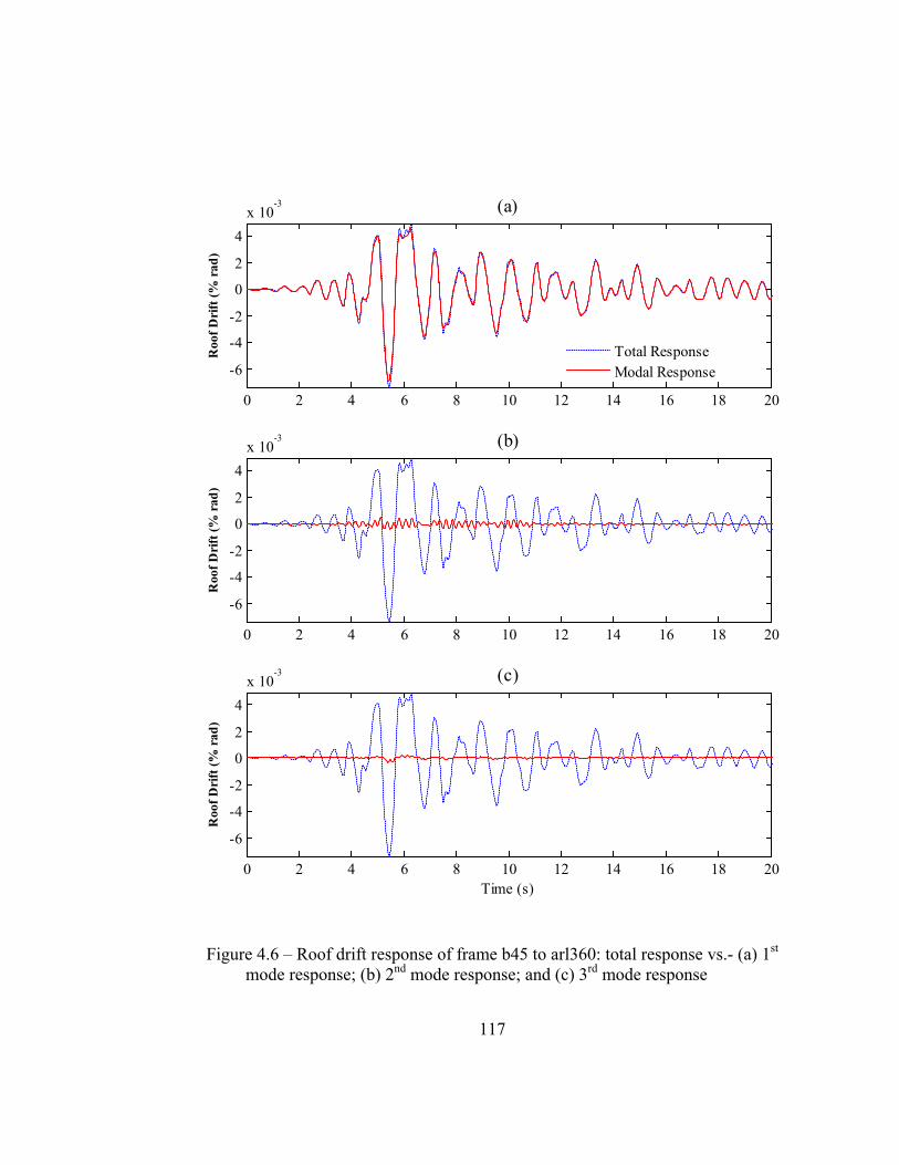
117

Figure 4.6 – Roof drift response of frame b45 to arl360: total response vs.- (a) 1st

mode response; (b) 2nd mode response; and (c) 3rd mode response

0 2 4 6 8 10 12 14 16 18 20

-6

-4

-2

0

2

4x 10

-3R

oof D

rift

(% r

ad)

(a)

Total ResponseModal Response

0 2 4 6 8 10 12 14 16 18 20

-6

-4

-2

0

2

4x 10

-3

Roo

f Dri

ft (%

rad

)

(b)

0 2 4 6 8 10 12 14 16 18 20

-6

-4

-2

0

2

4x 10

-3

Roo

f Dri

ft (%

rad

)

Time (s)

(c)

118

Figure 4.7 – Schematics of total and modal time history responses

119

Figure 4.8 – Normalized modal absolute area intensities for base shear responses of

frames a45, b45, and c45

Figure 4.9 – Mean normalized modal absolute area intensities for story shear

responses of frames a45, b45, and c45

a45 b45 c450

0.1

0.2

0.3

0.4

0.5

0.6

0.7

0.8

0.9

1

Nor

mal

ized

Mod

al A

bsol

ute

Are

a In

tens

ity fo

r Bas

e Sh

ear

Mean

Mean

1st Mode2nd Mode3rd Mode

0 0.2 0.4 0.6 0.8 11

2

3

4

Mean Normalized Modal Absolute Area Intensity for Story Shear

Stor

y

a45 (1st Mode)a45 (2nd Mode)b45 (1st Mode)b45 (2nd Mode)c45 (1st Mode)c45 (2nd Mode)

120

Figure 4.10 – Normalized modal absolute area intensities for roof drift responses of

frames a45, b45, and c45

Figure 4.11 – Mean normalized modal absolute area intensities for story drift

responses of frames a45,b45, and c45

a45 b45 c450

0.1

0.2

0.3

0.4

0.5

0.6

0.7

0.8

0.9

1

Nor

mal

ized

Mod

al A

bsol

ute

Are

a In

tens

ity fo

r Roo

f Drif

t

Mean

Mean

1st Mode2nd Mode3rd Mode

0 0.2 0.4 0.6 0.8 11

2

3

4

Mean Normalized Modal Absolute Area Intensity for Story Drift

Stor

y

a45 (1st Mode)a45 (2nd Mode)b45 (1st Mode)b45 (2nd Mode)c45 (1st Mode)c45 (2nd Mode)

121

Figure 4.12 – Normalized modal absolute area intensities for base shear responses of

frames b30, b45, and b60

Figure 4.13 – Mean normalized modal absolute area intensities for story shear

responses of frames b30, b45, and b60

b30 b45 b600

0.1

0.2

0.3

0.4

0.5

0.6

0.7

0.8

0.9

1

Nor

mal

ized

Mod

al A

bsol

ute

Are

a In

tens

ity fo

r Bas

e Sh

ear

MeanMeanMean

Mean

1st Mode2nd Mode3rd Mode

0 0.2 0.4 0.6 0.8 11

2

3

4

Mean Normalized Modal Absolute Area Intensity for Story Shear

Stor

y

b30 (1st Mode)b30 (2nd Mode)b45 (1st Mode)b45 (2nd Mode)b60 (1st Mode)b60 (2nd Mode)

122

Figure 4.14 – Normalized modal absolute area intensities for roof drift responses of

frames b30, b45, and b60

Figure 4.15 – Mean normalized modal absolute area intensities for story drift

responses of frames b30, b45, and b60

b30 b45 b600

0.1

0.2

0.3

0.4

0.5

0.6

0.7

0.8

0.9

1

Nor

mal

ized

Mod

al A

bsol

ute

Are

a In

tens

ity fo

r Roo

f Drif

t

Mean

Mean

1st Mode2nd Mode3rd Mode

0 0.2 0.4 0.6 0.8 11

2

3

4

Mean Normalized Modal Absolute Area Intensity for Story Drift

Stor

y

b30 (1st Mode)b30 (2nd Mode)b45 (1st Mode)b45 (2nd Mode)b60 (1st Mode)b60 (2nd Mode)

123

CHAPTER V

SUMMARY AND CONCLUSIONS

5.1 Summary

This chapter summarizes the research conducted during the study. First, summaries

of the motivation for the research, the research objectives, and the research scope are

presented. Next, findings from the research are summarized. Finally, recommendations

based on the findings and ideas for further research are presented.

5.1.1 Motivation for Present Research

Conventional concentrically-braced frame (CBF) systems have been a popular lateral

force resisting systems due to their economy and high stiffness. However, the problem

associated with CBFs is that they have limited lateral drift capacity before damage

initiates in the structural members. During earthquakes, CBFs are often subjected to high

drift demands that yield or buckle the brace, which leads to residual lateral drift after the

earthquake.SC-CBF with friction based energy dissipation system had been developed to

enhance the seismic performance of conventional CBF structures. Prior research and

experimental study have seen that such systems performed very well under dynamic

earthquake loading. But further studies on different SC-CBF systems were necessary to

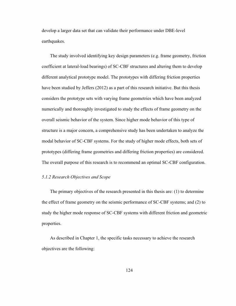
124

develop a larger data set that can validate their performance under DBE-level

earthquakes.

The study involved identifying key design parameters (e.g. frame geometry, friction

coefficient at lateral-load bearings) of SC-CBF structures and altering them to develop

different analytical prototype model. The prototypes with differing friction properties

have been studied by Jeffers (2012) as a part of this research initiative. But this thesis

considers the prototype sets with varying frame geometries which have been analyzed

numerically and thoroughly investigated to study the effects of frame geometry on the

overall seismic behavior of the system. Since higher mode behavior of this type of

structure is a major concern, a comprehensive study has been undertaken to analyze the

modal behavior of SC-CBF systems. For the study of higher mode effects, both sets of

prototypes (differing frame geometries and differing friction properties) are considered.

The overall purpose of this research is to recommend an optimal SC-CBF configuration.

5.1.2 Research Objectives and Scope

The primary objectives of the research presented in this thesis are: (1) to determine

the effect of frame geometry on the seismic performance of SC-CBF systems; and (2) to

study the higher mode response of SC-CBF systems with different friction and geometric

properties.

As described in Chapter 1, the specific tasks necessary to achieve the research

objectives are the following:

125

1. Design prototype SC-CBF prototypes with three different frame bay widths

using previously developed performance-based design criteria.

2. Develop analytical models for SC-CBF prototypes.

3. Perform nonlinear static analyses using OpenSees models.

4. Perform nonlinear dynamic analyses using a suite of DBE-level ground

motions.

5. Perform modal analysis to determine the modal properties of the prototypes.

6. Perform modal decomposition of dynamic time history results.

7. Develop quantification measures for quantifying and comparing higher mode

contributions to total response.

8. Assess the overall behavior and performance of all SC-CBF prototypes.

This research evaluated the seismic performance of SC-CBF systems with friction-

based energy dissipation. The lateral drift capacity before the initiation of structural

damage has been increased in SC-CBFs (in comparison to conventional CBFs) by

softening the lateral force-lateral drift behavior by designing a column base detail which

allows the SC-CBF columns to decompress and uplift at a specified level of lateral force,

initiating a rocking response. This rocking response limits the internal force demands in

the structural members

126

The performance based design criteria developed by Roke et al. (2010) were

implemented in this research. The design procedure is based on specified probabilities of

the responses under earthquake loading exceeding the design demands for selected limit

states. Three four-story prototype buildings with different floor plans were designed for a

site in Van Nuys, California. The design results for the prototype frames were compared

to determine how frame geometry affects SC-CBF design.

Detailed nonlinear analytical models for the prototype SC-CBFs were developed

using OpenSees (Mazzoni et al. 2009). The analytical models included the structural

members (i.e., the beams, columns, braces, and struts) of the SC-CBF, as well as the

adjacent gravity columns and the lean-on column. The lean-on-column accounts for the

stiffness of the gravity columns that are within the tributary area of the SC-CBF and the

P-Δ effects from gravity loads. Nonlinearity was included only in the PT bar elements,

the column base gap opening elements, and the lateral-load bearing elements. Nonlinear

behavior was not modeled in the SC-CBF members; therefore, the model is incapable of

predicting nonlinear behavior of the members.

Monotonic and cyclic static pushovers were conducted on each prototype SC-CBF

system. The results of these analyses were evaluated and compared for each SC-CBF to

determine which frame geometry generated the most desirable behavior under static

lateral loading. Nonlinear response history analyses were performed by subjecting each

prototype to fifteen pairs of DBE-level ground motions. The results of the analyses were

evaluated to verify that the SC-CBF systems exhibited the expected behavior under

seismic loading. The results of the analyses were also compared for each SC-CBF to

127

determine which frame geometry produced the most desirable response to DBE-level

seismic loading.

As determined from the dynamic analysis results, SC-CBFs are prone to significant

higher mode effects. A detailed study was therefore undertaken to investigate the modal

behavior of the SC-CBF systems. The prototype SC-CBFs used in this thesis, as well as

additional prototypes with varying friction properties that were designed and analyzed by

Jeffers (2012), were considered for the study of higher mode effects on the seismic

responses of SC-CBF systems. Modal analyses were carried out for each of five

prototype SC-CBFs and the results were compared to study the effect of frame geometry

and the coefficient of friction at the lateral-load bearings on the modal properties of SC-

CBF systems.

An approximate modal decomposition technique using effective pseudo-acceleration

and effective peak displacement was presented. The modal responses determined using

these decomposition techniques were compared against the total response for several

response quantities. Since base shear was found to be the response quantity that was most

affected by higher-mode response, the modal base shear response results were then used

to quantify the higher mode effects. Three intensity-based measures were proposed for

quantification of higher mode effects. The effectiveness of these proposed measures, as

well as the effectiveness of the conventionally-used peak-based measure, was studied by

applying the measures to the modal base shear responses. The comparative study on these

measures shows that the proposed normalized modal absolute area intensity (NMAAI)

128

modal response quantification measure is the most effective and reliable measure of those

considered in this study.

The NMAAI quantification measure was then applied on several different modal

response quantities (base shear, roof drift, story shear, and story drift) to quantify the

higher mode effects on these response quantities. As expected, the higher mode effects

are different on different response quantities. The NMAAI values for the set of

prototypes with varying frame geometries (frames a45, b45, and c45) are studied to

determine the effect of frame geometry on the higher mode responses of SC-CBF

systems. Similarly, the NMAAI values for the set of prototypes with varying friction

properties (frames b30, b45, and b60) are studied to determine the effect of friction on the

higher mode responses of SC-CBF systems.

5.2 Findings

This section summarizes the results of the research described in this thesis.

5.2.1 SC-CBF Design Results

• As the SC-CBF width bSC-CBF increases, the area of PT steel APT decreases.

• As bSC-CBF increases, the hysteretic energy dissipation ratio βE and design

parameter η increase.

• As bSC-CBF increases, the member sizes tend to decrease. However, the

total SC-CBF weight does not follow the same trend due to the differing

frame width (i.e., beam and brace length) of the prototype SC-CBFs.

129

• As bSC-CBF increases, kelastic and kpd increase.

• The η values for all three SC-CBFs were less than 0.50, so each SC-CBF

was expected to self-center.

5.2.2 Nonlinear Static Analysis Results

• The monotonic pushover results show that there is no trend in the values

of overturning moment at decompression OMD and overturning moment at

PT bar yielding OMY with the change of bSC-CBF.

• The monotonic pushover results show that frames a and b had similar

OMD and OMY values; therefore, the increase in bSC-CBF (i.e., the moment

arm of the frame weight and PT force) for these frames is offset by the

differences in the frame weight and APT.

• The monotonic pushover results show that bSC-CBF does not significantly

affect the roof drift at column decompression. However, the roof drift

capacities at PT bar yielding decreases with the increase of bSC-CBF.

• The cyclic pushover results show that as bSC-CBF increases, the width of the

hysteresis loop increases. This is consistent with the increase in βE.

5.2.3 Nonlinear Dynamic Analysis Results

• Dynamic analysis results for the complete suite of DBE-level ground

motion show that as bSC-CBF increases, the mean values of peak base shear

130

and peak SC-CBF column gap opening increase (i.e., the magnitude of the

rocking response increases).

• Dynamic analysis results for the complete suite of DBE-level ground

motion show that as bSC-CBF increases, the mean value of peak roof drift

response decreases. The results also show that story drifts are typically

larger for higher stories (3rd and 4th stories) than for lower stories (1st and

2nd stories). As bSC-CBF increases, the mean values of story drift tend to

decrease.

• Dynamic analysis results for the complete suite of DBE-level ground

motion show that the mean values of brace force and PT bar force

response decrease as bSC-CBF increases. However, the probability of PT bar

yielding increases with the increase of frame bay width, due in part to the

decreased value of APT.

5.2.4 Higher Mode Quantification Results

• The modal analysis results show that as bSC-CBF increases, modal natural

frequency (e.g., SC-CBF stiffness) increases.

• The modal analysis results show that changing the coefficient of friction

(μ) has negligible effect on the modal properties.

131

• The modal decomposition results show that overturning moment and roof

drift responses are primarily dominated by the first mode, while base shear

responses have large higher mode contributions.

• The comparative study of quantification measures show that the proposed

intensity-based NMAAI (normalized modal absolute area intensity)

quantification measure produces the most consistent and reliable results

with the least dispersion.

• The quantification results using NMAAI show that as bSC-CBF increases,

the higher mode effect on base shear response decreases. The higher mode

effect on story shear also typically decreases with the increase of bSC-CBF.

• The quantification results using NMAAI show that the higher mode effect

on roof drift is very small, but increases with the increase of bSC-CBF. The

trend in the higher mode effects on story drift responses is typically

similar to that of roof drift.

• The quantification results using NMAAI show that there is no definitive

trend in the higher mode effects on the SC-CBF responses with the change

in friction coefficient.

5.3 Conclusions

The major conclusions of the research described in this thesis are:

132

• As the frame unbraced bay width bSC-CBF increases, APT decreases, leading

to more economical designs.

• As bSC-CBF increases, βE and η increase, leading to increased energy

dissipation.

• The η values for all three SC-CBFs were less than 0.50, so each of the

studied SC-CBFs was expected to self-center.

• The frame bay width bSC-CBF does not significantly affect the roof drift at

column decompression; however, the roof drift capacity at PT bar yielding

decreases with the increase of bSC-CBF.

• As the frame bay width bSC-CBF increases, the width of the hysteresis loop

increases. This is consistent with the increase in βE.

• With this specific suite of DBE-level ground motions, as the frame bay

width bSC-CBF increases, the sample means of peak base shear and peak

column base gap opening increase, indicating an increase in the magnitude

of the rocking response.

• The rocking responses soften the structural responses. Therefore, as the

frame bay width bSC-CBF increases, the peak roof drift, the peak PT bar

force response and the peak brace force responses decrease.

133

• The friction coefficient at the lateral-load bearings has a negligible effect

on the mode shapes and frequencies, which are largely driven by frame

geometries.

• The intensity-based NMAAI modal response quantification measure is

better than the conventionally used peak-based measure for quantifications

of higher mode responses of SC-CBF systems.

• The higher mode effects on base shear and story shear responses typically

decrease with an increase of bSC-CBF. The higher mode effects on roof drift

and story drift responses exhibit the opposite trend, though the higher

mode effects on roof drift are typically negligible compared those on base

shear responses.

• There is no definitive trend in the higher mode effects on the response

quantities for SC-CBFs with varying friction properties.

• In general engineering practice, use of a higher frame bay width of the SC-

CBF with any friction coefficient is recommended, as long as η is less than

0.50 to permit the system to self-center, as the higher frame bay width

leads to improved system response and less higher mode effects.

5.4 Original Contributions of Research

This research explored the effects of the frame geometry on the seismic behavior of

SC-CBF systems with friction-based energy dissipation. The research also studied the

134

effects of higher modes on the seismic responses of SC-CBF prototypes with varying

friction and geometric properties. The specific original contributions of this research are:

• Developed analytical models for SC-CBF systems with friction-based

energy dissipation. Detailed nonlinear analytical models of three designed

SC-CBF prototypes with varying frame geometries were constructed in

OpenSees (Mazzoni et al. 2009). The primary components of the model

are the SC-CBF, the adjacent gravity columns, and the lean-on column,

which is introduced to account for P-Δ effects on the SC-CBF system.

• Performed nonlinear static and dynamic analyses using the analytical

models of the designed SC-CBF systems. The nonlinear analytical models

developed for the three SC-CBF systems were subjected to a number of

static and dynamic analyses. Nonlinear static analyses were performed to

determine the response of the prototypes to monotonic and cyclic

pushovers. Nonlinear dynamic analyses were carried out to determine the

responses of the prototypes to a suite of 15 pairs of DBE-level ground

motions.

• Analyzed the results of the static and dynamic numerical simulations. The

results of this parametric study increased the knowledge base of SC-CBF

seismic response and also provided important insight into a major design

parameter for SC-CBF systems.

135

• Performed modal decomposition of dynamic responses of the prototypes

with varying geometric and friction properties. Five prototype SC-CBFs

with varying geometric and friction properties were considered for

studying the higher mode behavior of SC-CBF systems. Modal

decomposition was carried out on the dynamic responses for each of the

prototypes to determine modal responses.

• Proposed three measures for quantification of higher mode responses and

performed a comparative study of the proposed measures and the

conventionally used peak-based measure. Three quantification measures

have been proposed to quantify the modal contributions on the total

responses. The proposed measures and the conventionally used peak-

based measure were applied to the modal base shear responses for each

prototype SC-CBF. The results were studied to find the most effective

measure for quantification of higher mode effects.

• Compared the higher mode effects on frames with varying friction and

geometric properties. The proposed intensity-based measure was applied

to various modal response quantities (e.g., base shear, story shear, roof

drift, and story drift) of each prototype SC-CBF. The results were studied

to determine the effect of friction and geometric properties on the higher

mode responses of SC-CBF systems.

136

5.5 Future Work

This research explored the seismic performance of SC-CBF systems with friction-

based energy dissipation. This section identifies research that can further develop the

knowledge base on SC-CBF systems with friction-based energy dissipation.

• This thesis considered three prototypes to study the effect of frame

geometry. Studying more prototypes would help to make more accurate

prediction about this key design parameter.

• This thesis considered four-story buildings as prototypes for the study of

higher mode effects. Taller buildings should be considered in future

research.

• Only DBE-level dynamic response was included in this research. Further

research of the response of SC-CBF systems under MCE-level ground

motions is needed.

• This thesis did not include experimental research. Further experimental

simulations performed on SC-CBF test structures are necessary to validate

analytical results.

• A detailed investigation of the hysteretic behavior of the SC-CBF systems

should be undertaken to determine the reasons for the fluctuations from

the ideal flag-shaped hysteresis loops.

137

• Research into the behavior of SC-CBFs displaced out of plane is needed

(i.e., three-dimensional studies of buildings with SC-CBFs as the lateral

force resisting system).

• A comparative study of the life-cycle costs of buildings with SC-CBF

systems and the life-cycle costs of buildings with conventional CBF

systems should be undertaken to illustrate the cost-effectiveness of a

damage-free SC-CBF system.

138

REFERENCES

AISC (2005a). Seismic Provisions for Structural Steel Buildings. American Institute of

Steel Construction, Chicago, IL.

AISC (2005b). Specification for Structural Steel Buildings. American Institute of Steel Construction, Chicago, IL.

AISC (2005c). Steel Construction Manual, 13th Edition. American Institute of Steel Construction, Chicago, IL.

ASCE (2010). Minimum Design Loads for Buildings and Other Structures, ASCE7-10.American Society of Civil Engineers (ASCE), Reston, VA.

Aoyama, H. (1987). “Earthquake Resistant Design of Reinforced Concrete Frame Buildings with ‘Flexural’ Walls,” Journal of the Faculty of Engineering, The University of Tokyo, 39(2), pp 87-109.

BSSC (2003). NEHRP Recommended Provisions for Seismic Regulations for New Buildings and Other Structures. FEMA 450.Building Seismic Safety Council, National Institute of Building Sciences, Washington, D.C.

Chopra, A.K. (2007). Dynamics of Structures – Theory and Applications to Earthquake Engineering, 3rd Edition. Prentice Hall, Upper Saddle River, NJ.

Christopoulos, C.; Tremblay, R.; Kim, H.-J.; and Lacerte, M. (2008). “Self-Centering Energy Dissipative Bracing System for the Seismic Resistance of Structures: Development and Validation,” ASCE Journal of Structural Engineering, 134(1),pp 96-107.

Jeffers, B. (2012). “Parametric Study of Self-Centering Concentrically Braced Frames with Friction-Based Energy Dissipation.” M.S. Thesis, Department of Civil and Environmental Engineering, University of Akron, Akron, OH.

Kabeyasawa, T. (1987). “Ultimate-State Design of Reinforced Concrete Wall-Frame Structures,” Proceedings of the 10th Pacific Conference on Earthquake Engineering, Wairakei, New Zealand, August 5-8.

139

Kurama, Y. C.; Pessiki, S.; Sause, R.; and Lu, L.-W. (1999), “Seismic Behavior and Design of Unbonded Post-Tensioned Precast Concrete Wall,” PCI Journal, 44(3), 72-89.

Mazzoni, S.; McKenna, F.; Scott, M.H.; Fenves, G.L.; et al. (2009). Open System for Earthquake Engineering Simulation (OpenSees) User Command-Language Manual. Pacific Earthquake Engineering Research Center, University of California, Berkeley.

New Zealand Standards (NZS) (2006), Appendix B: Special Provisions for the Seismic Design of Ductile Jointed Precast Concrete Structural Systems, NZS 3101:2006, Concrete Standard, Wellington, New Zealand.

Priestley, M. J. N.; Sritharan, S.; Conley, J. R.; and Pampanin, S. (1999). “Preliminary Results and Conclusions from the PRESSS Five-Story Precast Concrete Test Building,’’ PCI Journal 44(6), 42–67.

Ricles, J.M.; Sause, R.; Garlock, M.M.; and Zhao, C. (2001). “Posttensioned Seismic- Resistant Connections for Steel Frames,” ASCE Journal of Structural Engineering, 127(2), pp 113-121.

Roke, D.; Sause, R.; Ricles, J.M.; Seo, C.-Y.; and Lee, K.-S. (2006). “Self-Centering Seismic-Resistant Steel Concentrically-Braced Frames,” Proceedings of the 8th U.S. National Conference on Earthquake Engineering, EERI, San Francisco, April 18-22.

Roke, D.; Sause, R.; Ricles, J.M.; and Gonner, N. (2009). “Damage-Free Seismic-Resistant Self-Centering Steel Concentrically-Braced Frames,” STESSA 2009, Proceedings of the 6th International Conference on Behavior of Steel Structures in Seismic Areas, Philadelphia, August 16-20.

Roke, D.; Sause, R.; Ricles, J.M.; & Chancellor, N.B. (2010). “Damage-Free Seismic-Resistant Self-Centering Concentrically-Braced Frames,” ATLSS Report 10-09, Lehigh University, Bethlehem, PA, USA.

Seo, C.-Y.; and Sause, R. (2005). “Ductility Demands on Self-Centering Systems Under Earthquake Loading,” ACI Structural Journal, 102(2), pp 275-285.

Seo, C.-Y.(2005). “Influence of Ground Motion Characteristics and Structural Parameters on Seismic Responses of SDOF Systems.” Ph.D. Dissertation, Department of Civil and Environmental Engineering, Lehigh University, Bethlehem, PA.

Wiebe, L.; and Christopoulos, C. (2009), “Mitigation of Higher Mode Effects in Base-Rocking Systems by Using Multiple Rocking Sections”, Journal of Earthquake Engineering, 13(S1), pp83-108.