Parametric and non-parametric probabilistic approachesin the mechanics of thin-walled composite curved beams

M.T. Piovan a,n, R. Sampaio b

a Centro de Investigaciones de Mecánica Teórica y Aplicada, Universidad Tecnológica Nacional FRBB, 11 de Abril 461, B8000LMI Bahía Blanca, Argentinab PUC-Rio, Mechanical Engineering Department, Rua Marquês de São Vicente 225, 22451-900 Rio de Janeiro, RJ, Brazil

a r t i c l e i n f o

Article history:Received 8 September 2014Received in revised form20 December 2014Accepted 21 December 2014

Keywords:Uncertainties quantificationComposite curved beamsDynamicsFlexible structures

a b s t r a c t

In this paper we perform a quantification of the uncertainty propagation of the dynamics of slenderinitially curved structures constructed with fiber reinforced composite materials. Depending on themanufacturing process, composite materials may have deviations with respect to the expected response,often called nominal response in a deterministic sense. The manufacturing aspects lead to uncertainty inthe structural response associated with constituent proportions, material and/or geometric parametersamong others. Another aspect of uncertainty that can be sensitive in composite structures is themathematical model that represents the mechanics of the structural member, that is: the assumptionsand type of hypotheses invoked reflect the most relevant aspects of the physics of a structure, howeverin some circumstances these hypotheses are not enough, and cannot represent properly the mechanicsof the structure. Uncertainties should be considered in a structural system in order to improve thepredictability of a given modeling scheme. There are two approaches to evaluate the propagation ofuncertainties in structural models: the parametric probabilistic approach and the non-parametricprobabilistic approach. In the parametric, one quantifies the uncertainty of given parameters (such asvariation of the angles of fiber reinforcement and material constituents) by associating random variablesto them. In the non-parametric, the propagation of uncertainty is quantified by considering uncertainthe matrices of the whole system. In this study a shear deformable model of composite curved thin-walled beams is employed as the mean or expected model. The probabilistic model is constructed byadopting random variables for the uncertain entities (parameters or matrices) of the model. Theprobability density functions of the random entities are derived appealing to the maximum entropyprinciple under given constraints. Once the probabilistic model is discretized in the context of the finiteelement method, the Monte Carlo method is employed to perform the simulations. Then the statistics ofthe simulations is evaluated and the parametric and non-parametric approaches are compared.

& 2014 Elsevier Ltd. All rights reserved.

1. Introduction

Composite materials have such a number of interesting featuresthat impel their use in different industrial devices. Examples ofthese features are high strength and stiffness properties togetherwith a low weight, good corrosion resistance, enhanced fatiguelife, low thermal expansion properties among others [1]. Thevery low machining cost for complex structures is the otherimportant feature of composite materials [2]. Slender compositestructures that can be analyzed by means of curved beam modelsare present in many applications such as bridge segments,

machine parts: such as leaf springs of sport cars or blades ofturbo-propellers, among others.

The development of theoretical and computational methods fordynamic and static analysis of slender thin-walled compositestructures is growing continuously since the early eighties. Thus,one of the first consistent studies about thin-walled composite-beams was introduced by Baud and Tzeng [3], who developed abeam theory to analyze fiber-reinforced members featuring opencross-sections with symmetric laminates invoking Vlasov'shypotheses. Afterwards, Bauchau [4] incorporated some aspectsof shear flexibility in the analysis of thin-walled composite beams.Models of fiber reinforced composite beams that are based onVlasov or Bauld and Tzeng's ideas [3] normally over-predict thevalues of natural frequencies and consequently the dynamicpatterns, specially in the case of shorter beams. In the 1990s,many new models of composite beams were introduced, in which

Contents lists available at ScienceDirect

journal homepage: www.elsevier.com/locate/tws

Thin-Walled Structures

http://dx.doi.org/10.1016/j.tws.2014.12.0180263-8231/& 2014 Elsevier Ltd. All rights reserved.

n Corresponding author.E-mail addresses: mpiovan@frbb.utn.edu.ar,

mtpforever@gmail.com (M.T. Piovan), rsampaio@puc-rio.br (R. Sampaio).

Thin-Walled Structures 90 (2015) 95–106

shear-flexibility as well as warping effects due to non-uniformtwisting were incorporated. These models were based on newtheories for micro/macrostructures of composite materials, newmodeling schemes including selective warping and second-orderdisplacements, etc. The research of Wu and Sun [5], Librescu andcoworkers [6,7], Kim et al. [8] and Cesnik et al. [9] are just a fewexamples of the most representative works in the modeling ofcomposite beams with thin or thick walled cross-sections; howevermost of them were devoted to closed cross-sections as basicapproaches for the analysis of helicopter blades. More recentlyCortínez and Piovan [10] developed a theory of thin walled compo-site beams accounting for full shear flexibility (i.e. shear deformationdue to bending as well as due to warping related to non-uniformtwisting). The scopes and limits of the previous full shear flexiblemodeling conception were extended [11] by incorporating elasticcouplings and the evaluation of general dynamic problems forstraight beams and for curved thin-walled composite beams [12].The model employed in this study was conceived in order to takeinto account the effects of shear deformability that are mandatory inthe mechanics of thin-walled structures specially if they are con-structed with fiber reinforced composite materials [6,8,10,12].

The behavior of composite structures under typical service in civil,aeronautical, aero-spatial or mechanical devices, is constrained to anumber of factors that are stochastic in essence [13,14]. Manyresearchers have focused their attention in the evaluation of thestochastic response of composite structures since the middle 1990s[15,16]. Moreover, there is an increasing interest to quantify thepropagation of uncertainty in the mechanics of composite materialsat the microscale level [13] or for failure analysis [17]. The uncertaintyinvolved in the material properties of the composites can be con-sidered as random fields [18,19] among others. However, there areother ways for studying the dynamic response due to uncertainties incomposite structures, for example by associating random variables togiven entities that define a structural dynamic model. Effectively,when the parameters, such as material properties or reinforcementangles, are considered uncertain, the methodology for studying theuncertainty is called parametric probabilistic approach (PPA). Howeverif the model as a whole is uncertain, the class of uncertainty is calledsystemic uncertainty. In order to analyze this type of uncertainty thereare various approaches, one of them is the so-called non-parametricprobabilistic approach (NPPA). The NPPA implies the introduction ofrandom matrix variables. This approach was formulated by Soize [20]and employed in a variety of structural problems [21–23].

In this paper, the PPA and NPPA are applied in order to evaluatethe uncertainty propagation in the dynamic response of naturallycurved composite thin-walled beams. The theory for curvedcomposite structures introduced by Piovan and Cortínez [12] isbriefly revisited and employed as the nominal response or deter-ministic model in order to compare and quantify the uncertaintypropagation of the stochastic approach. The solution of thedynamics equations is approximated in the context of the finiteelement method. For the PPA case, the parameters correspondingto elastic properties are considered uncertain. For the NPPA thestiffness matrix and the damping matrix are considered uncertain.This is due to the evidence gathered in other work of the authors[23] in which the elastic properties, and hence the stiffness matrix,are the main focus of uncertainty propagation in dynamics ofcomposite thin-walled straight beams. To construct the probabil-istic models, the probability density functions associated with therandom variables are constructed appealing to the maximumentropy principle [24,25]. This principle uses the available infor-mation of the random entities to construct their probabilitydensity functions such that the entropy, in the sense of Shannon[26], is maximum. The use of this scheme allows the maximumpossible propagation of the uncertainty according to the availableinformation about the random variables.

The paper is organized as follows: after the introductorysection where the state-of-the-art in modeling curved thin-walled composite beams is summarized, the deterministic/meanmodel and its finite element discretization are briefly described,then the probabilistic approach is constructed. The parametric andthe non-parametric approaches are described for this problem andthe subsequent section contains the computational studies, theanalysis of the uncertainty propagation in the dynamics of thin-walled composite curved beams and finally concluding remarksare outlined.

2. Deterministic model

2.1. Brief description of the curved beam model

Fig. 1 shows a basic sketch of the structural component, inwhich it is possible to see the basic dimensions and the referencepoints C and A. The principal reference point C is located at thegeometric center of the cross-section, the x-direction is tangent tothe curved axis of the beam, and y and z are the axes of the crosssection, but not necessarily the principal axes of inertia. Thesecondary reference system, located at A, is used to describe shellstresses and strains. The curved axis of the beam, that has constantradius R, is contained in the plane Ξ. The curved beam has anopening angle β and a circumferential length L¼ Rβ. The determi-nistic model of the present study is based on the followingassumptions [11,12]:

1. The cross-section contour is rigid in its own plane (i.e. planeYZ).

2. The radius of curvature at any point of the shell is neglected.3. The warping function is normalized with respect to the

principal reference point C.4. A general laminate stacking sequence for a composite material

is considered.5. The material density is considered constant along the curved

axis beam.6. Stress and strain components are defined according to the

secondary reference system located in A.7. The most representative stresses are σxx, σxs and σxn; and the

most representative strain and curvature components are ϵxx,γxs, γxn, κxx and κxs.

8. The model is derived in the framework of linear elasticity.

Employing assumptions (1)–(7) one can derive the displace-ment field of the point B [12], which can be presented as follows:

~UB ¼ux

uy

uz

8><>:9>=>;¼

uxc�ωΦw

uyc

uzc

8><>:9>=>;þ

0 �Φ3 Φ2

Φ3 0 �Φ1

�Φ2 Φ1 0

264375 0

y

z

8><>:9>=>;; ð1Þ

where Φw, Φ1, Φ2 and Φ3 are defined in terms of rotational and

Fig. 1. Sketch of the thin-walled curved beam with the reference systems.

M.T. Piovan, R. Sampaio / Thin-Walled Structures 90 (2015) 95–10696

warping parameters as follows:

Φ1 ¼ θx; Φ2 ¼ θy; Φ3 ¼ θz�uxc

R; Φw ¼ θwþθy

Rð2Þ

and uxc, uyc, and uzc are the displacements of the reference centerin x-, y-, and z-directions, respectively. θz and θy are bendingrotational parameters. θx is the twisting angle and θw is awarping-intensity parameter. R is the radius of curvature of thebeam. In Eq. (1) the cross-sectional variables y(s) and z(s) of ageneric point are related to the ones of the wall middle line Y(s)and Z(s) by means of Eq. (3) is the warping function normalizedwith respect to the reference center. It is defined in Eq. (4)

yðsÞ ¼ YðsÞ�ndZds

; zðsÞ ¼ ZðsÞþndYds

; ð3Þ

ωðs;nÞ ¼ωpðsÞþωsðs;nÞ: ð4Þ

In Eq. (4), ωpðsÞ is the primary or contour warping functionwhereas ωsðs;nÞ is the secondary or thickness warping. Theseentities are given by

ωpðsÞ ¼ZsrðsÞþψ ðsÞ� �

ds�DC ; ωsðs;nÞ ¼ �nlðsÞ; ð5Þ

where the functions r(s), l(s), ψ ðsÞ and DC are defined in thefollowing form (see Fig. 2):

rðsÞ ¼ ZðsÞdYds

�YðsÞdZds

; lðsÞ ¼ YðsÞdYds

þZðsÞdZds

;

ψ ðsÞ ¼ 1A66ðsÞ

RsrðsÞ dsH

S1

A66ðsÞds

2666437775; DC ¼

HS rðsÞþψ ðsÞ� �

A11ðsÞ dsHSA11ðsÞ ds

: ð6Þ

The functions A11 and A66 are normal and tangential elasticcoefficient of the composite laminates [11] which can vary alongthe section middle line. ψ ðsÞ is a function related to the torsionalshear flow and DC is a constant to normalize the warping functionwith respect to the reference system C [10,12]. The warpingfunction is valid for both open and closed sections (sinceψ ðsÞ ¼ 0 in the case of open sections). Moreover the warpingfunction described in Eq. (4) is conceptually analogous to thehomonym warping function employed by Song and Librescu [7]but for composite straight beams.

The displacement–strain relations can be deduced by substi-tuting Eq. (1) in the well-known expressions of linear straincomponents [1]. As it was shown by [12] the shell strains can bewritten as

~EP ¼R

RþyGk

~D; ð7Þ

where

~ETP ¼ ϵxx; γxs; γxn; κxx; κxs

� �;

~DT ¼ εD1; εD2; εD3; εD4; εD5; εD6; εD7; εD8f g; ð8Þ

Gk ¼

1 Z �Y �ωp 0 0 0 00 0 0 0 dY=ds dZ=ds rðsÞþψ ðsÞ �ψ ðsÞ0 0 0 0 �dZ=ds dY=ds lðsÞ 00 �dY=ds dZ=ds � lðsÞ 0 0 0 00 0 0 0 0 0 1 �2

26666664

37777775:

ð9ÞIn Eq. (8), ϵxx, γxs and γxn are the strain components and κxx and

κxs are the curvatures of the shell that conforms the wall of thecross-section. These strain components are measured according tothe wall reference system in A. The entities εDi, i¼ 1;…;8 may beregarded as generalized deformations. In this context εD1 is theaxial deformation, εD2 and εD3 are bending deformations, εD4 is thedeformation due to non-uniform warping, εD5 and εD6 are thebending shear deformations, εD7 is the warping shear deformationand finally εD8 is the pure torsion shear deformation. Thesegeneralized deformations, which are collected in vector ~D, aredefined in the following form:

~D ¼GDU~U; ð10Þ

where GDU is a matrix operator and ~U is the vector of kinematicvariables which are defined in the following forms, in which ∂xð⋄Þis the spatial derivative operator

GDU ¼

∂xð⋄Þ 1=R 0 0 0 0 00 0 0 0 ∂xð⋄Þ �1=R 0

�∂xð⋄Þ=R 0 ∂xð⋄Þ 0 0 0 00 0 0 0 �∂xð⋄Þ=R 0 ∂xð⋄Þ0 ∂xð⋄Þ �1 0 0 0 00 0 0 ∂xð⋄Þ 1 0 00 0 0 0 0 ∂xð⋄Þ �10 0 0 0 1=R ∂xð⋄Þ 0

2666666666666664

3777777777777775;

ð11Þ

~UT ¼ uxc;uyc;θz;uzc;θy;θx;θW

� �: ð12Þ

The principle of virtual works can be condensed in the follow-ing form:

WT ¼ZLδ ~D

T ~SR

� �dxþ

ZLδ ~U

TMm

€~U dx�ZLδ ~U

T ~PX dxþδ ~UT ~BX

���x ¼ L

x ¼ 0¼ 0;

ð13Þwhere the vector of internal forces or, in other terms, generalizedstress-resultants ~SR is defined as follows:

~STR ¼ Qx;My;Mz;B;Qy;Qz; Tw; Tsv

� �; ð14Þ

whereas for the sake of fluid and clear reading, the matrix of masscoefficients Mm, the vector of external forces ~PX and the vector ofnatural boundaries conditions ~BX are detailed in Appendix A. Qx,My, Mz, and B identify the axial force, the bending moment in they-direction, the bending moment in the z-direction, and the bi-moment, respectively; whereas Qy, Qz, Tw, and Tsv correspond tothe shear force in the y-direction, the shear force in the z-direction, the twisting moment due to warping and the twistingmoment due to pure torsion, respectively. These internal/general-ized forces can be written in terms of the shell-forces as [11]

~SR ¼ZSGTk~NP ds; ð15Þ

Fig. 2. Cross-section of the curved beam with the reference systems.

M.T. Piovan, R. Sampaio / Thin-Walled Structures 90 (2015) 95–106 97

where ~NP is the vector of shell stress resultants or shell forces andmoments defined according to [1,2]

~NTP ¼

ZSσxx;σxs;σxn;nσxx;nσxsf g dn: ð16Þ

The differential equations of motion and corresponding bound-ary conditions are derived by applying variational procedures inEq. (13). The differential equations of motion can be useful forsome numerical methods, e.g. power series method or differentialquadrature. While in the present paper the finite element methodis employed, the derivation of differential equations is not neces-sary. The interested readers may follow in the technical literatureauthors' articles [12,27] devoted to evaluate the differential equa-tions of the thin-walled curved beam model applied to a numberof specific structural problems.

2.2. Constitutive equations in terms of internal forces andgeneralized strains

In order to obtain the relationship between beam stress resul-tants and generalized deformations εDi

, i¼ 1;…;8, one has toselect the constitutive laws for a composite shell and use appro-priate constitutive hypotheses [12] of the shell stress resultants interms of the shell strains. The shell stress resultants can beexpressed in terms of the generalized deformations defined inEq. (10) according to the following matrix form:

~NP ¼MC~EP ; ð17Þ

where MC is the matrix of modified shell stiffness, which dependson the type of constitutive hypotheses involved [12,23,27] and canbe expressed in the following form:

MC ¼

A11 A16 0 B11 B16

A66 0 Bn

16 B66

An

55 0 0

sym D11 D16

D66

266666664

377777775: ð18Þ

The elastic stiffness coefficients A11, B11, D11, etc., are notdescribed in the present paper, however the interested readerscan find their definition and ”in-extenso” expressions in theauthors’ previous works [12,27].

Substituting Eq. (17) into Eq. (15) the curved beam stressresultants can be represented in terms of generalized strains as

~SR ¼Mk~D; ð19Þ

where

Mk ¼ZSGTkMCGk ds: ð20Þ

The matrix Mk of cross-sectional stiffness coefficients leads toconstitutive elastic coupling or not, depending on the stackingsequence of the laminates in a given cross-section. The interestedreader can follow an extended explanation about elastic constitutivecoupling in the books of Barbero [1] and Jones [2]. Moreover for beamapplications the explanation of the constitutive coupling can befollowed in the works of Piovan and Cortínez [12] and Kim et al. [8],among others.

2.3. Finite element approach

In order to perform the calculations, the curved beam model isdiscretized with iso-parametric elements of five nodes per ele-ment, seven degrees-of-freedom per node and shape functions ofquartic order. The formulation of the finite element approach forthis type of curved structural member has been introduced in

previous works [12] in which the interested readers can finddetailed explanations. The assembled finite element equation canbe written in the conventional form as

KWþC _W þM €W ¼ F; ð21Þwhere K and M are the global matrices of elastic stiffness andmass, respectively; whereas W , €W and F are the global vectors ofnodal displacements, nodal accelerations and nodal forces, respec-tively. The damping in Eq. (21) is incorporated as an “a posteriori”procedure after the discretization of the functional given in Eq.(13). Then C identifies the global matrix of structural damping,calculated according to Rayleigh's definition as

C¼ η1Mþη2K: ð22ÞThe coefficients η1 and η2 in Eq. (22) are computed by using thedamping coefficients, ξ1 and ξ2, according to the common meth-odology presented in the bibliography related to finite elementprocedures [28].

The response in the frequency domain of the linear dynamicsystem given by Eq. (21) can be written as

cW ωð Þ ¼ �ω2Mþ iωCþK� ��1bF ωð Þ; ð23Þ

where cW and bF are the Fourier transform of the displacementvector and force vector, respectively; whereas ω is the circularfrequency measured in (rad/s).

2.4. Reduced order model

The calculation of the responses in the frequency domain isnormally quite demanding in terms of computational cost. Then,in order to have a speedup in the calculation process, it ismandatory to construct a reduced model by defining an appro-priate projection basis. Thus, taking advantage of the linearity ofthe present formulation, the projection basis for the reducedmodel can be extracted from the following eigenvalue problem:

ω2i Mvi ¼Kvi; ð24Þ

where ω2i and vi are the square of the ith natural frequency and its

corresponding eigenvector.Now, defining the global vector of kinematic variables W in

terms of the projection basis V and the modal coordinates Q :

W ¼VQ ; ð25Þand using it in Eq. (21) according to the common procedure of modelreduction [29] it is possible to write the following expression:

KrQ þCr_Q þMr

€Q ¼ Fr ; ð26Þand finally

cW ωð Þ ¼V bQ ωð Þ ¼ �ω2Mrþ iωCrþKr� ��1bFr ωð Þ: ð27Þ

In the previous expressions the following definitions have beenused:

Mr ¼VTMV

Cr ¼ VTCV

Kr ¼ VTKV

Fr ¼VTF: ð28ÞNotice that V is a (n�m) matrix whose columns correspond to

the m eigenvectors selected to reduce the model.Models of 12 finite elements (i.e. 343 degrees of freedom) are

employed to do the calculations. This number of elements isenough to reach approximation errors less than 1% up to the 8-th frequency. Moreover with 24 normal modes one reaches amean error less than 0.1% in the frequency response functions. This

M.T. Piovan, R. Sampaio / Thin-Walled Structures 90 (2015) 95–10698

implies a reduction of about 92% in size that was reflected in acalculation procedure, at least, 150 times faster.

3. Description of the probabilistic model

The probabilistic model is constructed by selecting parametersor matrices as uncertain entities and then deducing the appro-priate and corresponding random variables based on the availableinformation. Whether it is employed the PPA or the NPPA, theprobabilistic approach is constructed from the finite elementequation of the deterministic model which is assumed as themean model. The construction of the probabilistic model is quitesensitive in the analysis of uncertainty propagation. This involvesthe deduction of the probability density functions of the randomentities (parameters or matrices depending on the selectedapproach) taking into account the scarce information about therandom entities. According to the authors’ opinion, the use of themaximum entropy principle (MEP) allows the construction of aprobabilistic model despite the lack of information about therandom variables. In this context, the probability density functionsof the random variables can be derived guaranteeing consistencewith the available information and the physics of the problem.

In order to derive the probability density functions of therandom variables, the maximum entropy principle is proposed inthe following form:

pðoptÞV ¼ arg maxpV AP

S pV ð29Þ

where pðoptÞV is the optimal probability density function such thatSðpðoptÞV ÞZSðpV Þ; 8pV AP, and S is the measure of entropy whereasP is a set of admissible probability density functions satisfying theknown data of the random variables and the physical constraints.The measure of the entropy S is defined as [26]

S pV ¼ �

ZSpV ln pV

dv ð30Þ

where S is the support of the probability distributions of the ran-dom variables taken into account in the optimization procedure.

Once the random variables are appropriately defined then thestochastic finite element equation can be written, through Eq. (23),in the following form:

cW ωð Þ ¼ V bQ ωð Þ ¼ �ω2Mrþ iωCrþKr� ��1bFr ωð Þ: ð31Þ

Notice that in Eq. (31) the math-blackboard typeface indicatesstochastic entities, thus the stiffness matrix Kr is stochasticbecause random variables (scalars or matrices) are employed inits construction, and the damping matrix Cr is stochastic throughthe stochastic nature of Kr in Eq. (22), hence cW is stochastic.

The Monte Carlo method is used for the simulation of thestochastic dynamics. This strategy leads to the calculation of adeterministic system for each realization of the random variablesemployed. The convergence of the stochastic response cW can becalculated with the following function:

conv NMSð Þ ¼ffiffiffiffiffiffiffiffiffiffiffiffiffiffiffiffiffiffiffiffiffiffiffiffiffiffiffiffiffiffiffiffiffiffiffiffiffiffiffiffiffiffiffiffiffiffiffiffiffiffiffiffiffiffiffiffiffiffiffiffiffiffiffiffiffiffiffiffiffiffiffi1

NMS

XNMS

j ¼ 1

ZΩJcW j ωð Þ�cW ωð ÞJ2 dω

vuut ; ð32Þ

where NMS is the number of Monte Carlo samplings and Ω is thefrequency band of analysis. Clearly, cW is the response of thestochastic model and cW is the response of the mean model ordeterministic model.

3.1. Parametric approach

The stochastic model according to the PPA is constructedselecting two sets of uncertain parameters and associating random

variables to them. One set for the orientation angles of the fiberreinforcement in the layers of each panel and other set for basicelastic properties of the material. In the present problem randomvariables Vi, i¼ 1;2…NP and Vi, i¼NPþ1;…;NPþ6 are introducedsuch that they represent the angles of NP different plies in a cross-sectional laminate and the basic elastic properties of the material(i.e. elastic moduli: E11, E22 ¼ E33, G12 ¼ G13 and G23, Poissoncoefficients: ν12 ¼ ν13 and ν23), respectively.

The available information to deduce the probability densityfunctions is associated with some information that can be found inthe technical literature [13]. The following conditions are proposedin order to construct the probability density functions with themaximum entropy principle:

� The random variables associated with material properties arepositive and have bounded supports.

� The random variables associated with the reinforcement angleshave bounded supports whose upper and lower limits aredistant Δα from the expected value V i.� The expected values are EfVig ¼ V i, i¼ 1;…NPþ6, i.e. thosecorresponding to the deterministic model.

� The variance of the random variable has to be kept finite inorder to satisfy the physical consistence of the problem.

� There is no information about the correlation between randomvariables.

Consequently, according to the aforementioned background,the probability density functions of the random variables Vi can bewritten as

pVivið Þ ¼S LVi

;UVi

� � við Þ 12Δα

; i¼ 1;…;NP ð33Þ

pVivið Þ ¼S LVi

;UVi

� � við Þ 12ffiffiffi3

pV iδVi

; i¼NPþ1;…;NPþ6 ð34Þ

where S LVi;UVi

� � við Þ is the generic support function, whereas LVi

and UViare the lower and upper bounds of the random variable Vi.

Δα is a gap measured in angular units (radians or degrees),whereas δVi

is the coefficient of variation. The Matlab [30] functionunifrnd V i�Δα;V iþΔα

� �can be used to generate realizations of

the random variables Vi, i¼ 1;2…NP . The Matlab function unifrndV i 1�δVi

ffiffiffi3

p� �;V i 1þδVi

ffiffiffi3

p� �� �can be used to generate realiza-

tions of the random variables Vi, i¼NPþ1;…;NPþ6.

3.2. Non-parametric approach

Under this conception, the matrices of the system are consid-ered uncertain. In particular, there is evidence [23] that theuncertainty in the elastic properties is more sensitive than theuncertainty in the mass properties in the dynamics of beamsconstructed with composite materials. Consequently, the construc-tion of the probability density function of the random stiffnessmatrix K is performed in this section. The procedure explained inthe subsequent lines follows the concepts and ideas elaborated inthe works [31,20,32].

In order to construct the random matrix K, it is necessary thatthe mean value (or the deterministic one) of the positive-definitematrix K to be written according to the Cholesky-decomposition,that is K¼ LTKLK, where LK is an upper triangular matrix. Hence therandom matrix K can be written as follows:

K¼ LTKGLK ð35Þwhere G is a random matrix that has the following constraints:

� Positive-definiteness.� The mean value is the identity matrix: E Gf g ¼ I.

M.T. Piovan, R. Sampaio / Thin-Walled Structures 90 (2015) 95–106 99

� The mean square value of its inverse is finite, i.e E JG�1 J2Fn o

oþ1; this assures that the response of the system is asecond-order random variable.

Then using the maximum entropy principle the probabilitydensity function of G can be written as [31]

pG Gð Þ ¼SMþ Rð Þ Gð ÞCG det Gð Þ nþ1ð Þðð1�δ2KÞ=2δ2KÞexp �nþ1

2δ2Ktr Gð Þ

( )ð36Þ

where SMþ Rð Þ Gð Þ is the support of the random variable, n is thedimension of the random matrix G, the dispersion parameter δKand CG are given as follows:

δK ¼ffiffiffiffiffiffiffiffiffiffiffiffiffiffiffiffiffiffiffiffiffiffiffiffiffiffiffiffiffiffi1nE G�Ik k2Fn or

;CG ¼2πð Þ n�n2ð Þ=4 nþ1

2δ2K

! nþn2ð Þ= 2δ2K

∏nj ¼ 1Γ

nþ1

2δ2Kþ1� j

2

! ð37Þ

The dispersion parameter is such that 0oδKoffiffiffiffiffiffiffiffiffiffiffiffiffiffiffiffiffiffiffiffiffiffiffiffiffiffiffiffiffiffinþ1ð Þ= nþ5ð Þ

p,

where n is the number of degrees of freedom.Thus, for each realization of the randommatrix K, the matrix G

is built by means of a Cholesky decomposition, i.e. G¼ LTL, whereL is an upper triangular positive-definite random matrix subjectedto the following constraints:

� The random variables Ljk; jrk� �

are independent.� For jok, the real-valued random variable Ljk ¼ σVjk, in whichσ ¼ δK

ffiffiffiffiffiffiffiffiffiffiffinþ1

pand Vjk is a real-valued random variable with zero

mean and unit variance.� For j¼k the real-valued random variable Ljk ¼ σ

ffiffiffiffiffiffiffiffi2Vj

p, in which

Vj is a real-valued gamma random variable with probabilitydensity function:

pVjvð Þ ¼SRþ vð Þ v

nþ1

2δ2K�1� j2

!

Γnþ1

2δ2Kþ1� j

2

!exp vð Þ ð38Þ

As it is possible to infer, the random variables Vjk; jak andVjk; j¼ k can be generated by a normal distribution and a gammadistribution respectively. In fact they can be generated in theMonte Carlo simulation procedure by means of the Matlab func-tions normrndð0;1Þ and gamrndðα;βÞ, with α¼ ððnþ1Þ=2δ2Þþ

�ðð1� jÞ=2ÞÞ and β¼ 1.

4. Computational studies

4.1. Definitions and convergence checks

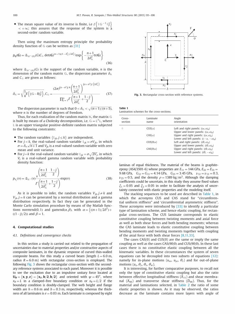
In this section a study is carried out related to the propagation ofuncertainties due to material properties and/or constructive aspects ofcomposite laminates, in the dynamic response of curved thin-walledcomposite beams. For this study a curved beam (length L¼ 6:0 m,radius R¼ 6:0 m) with rectangular cross-section is employed. Thefollowing Fig. 3 shows the rectangular cross-section with the second-ary reference systems associated to each panel. Moreover it is possibleto see the excitation due to an impulsive unitary force located atUB ¼ x; y; z

� �¼ xB;b=2;h=2� �

and oriented with ψ ¼ 45o, wherexB ¼ L in a clamped–free boundary condition or xB ¼ L=2 if theboundary condition is doubly-clamped. The web height and flangewidth are h¼ 0:6 m and b¼ 0:3 m, respectively, whereas the thick-ness of all laminates is e¼ 0:03 m. Each laminate is composed by eight

laminas of equal thickness. The material of the beams is graphite-epoxy (AS4/3501-6) whose properties are E11 ¼ 144 GPa, E22 ¼ E33 ¼9:68 GPa, G12 ¼ G13 ¼ 4:14 GPa, G23 ¼ 3:45 GPa, ν12 ¼ ν13 ¼ 0:3,ν23 ¼ 0:5, and the density ρ¼ 1389 kg=m3. Although the dampingcoefficients could be uncertain, in this study they assume fixed valuesξ1 ¼ 0:05 and ξ2 ¼ 0:05 in order to facilitate the analysis of uncer-tainty connected with elastic properties and the modeling itself.

The stacking sequences to be used are described in Table 1, inwhich the acronyms CUS and CAS stand for “circumferen-tial uniform stiffness” and ‘circumferential asymmetric stiffness”.These acronyms were introduced by [33] to identify a particulartype of lamination scheme, and hence elastic coupling, for rectan-gular cross-sections. The CUS laminate corresponds to elasticconstitutive coupling between twisting moments and axial forceas well as both shear forces and both bending moments; whereasthe CAS laminate leads to elastic constitutive coupling betweenbending moments and twisting moments together with couplingof the axial force with both shear forces [8,11,33].

The cases CAS(0) and CUS(0) are the same or imply the samecoupling as well as the cases CASð90j0Þ and CUSð90j0Þ. In these lastcases there is no constitutive elastic coupling between all thekinematic variables. In these circumstances the system of sevenequations can be decoupled into two subsets of equations [12]:namely for in-plane motions (uxc, uyc, θz) and for out-of-planemotions (uz, θy, θx, θw).

It is interesting, for further comparative purposes, to recall notonly the type of constitutive elastic coupling but also the ratiobetween effective longitudinal stiffness (A11) and shear membra-nal (A66) and transverse shear stiffness (D66). Thus, for thematerial and laminations selected, in Table 2 the ratio of someelastic properties is shown. As it may be observed, the ratiosdecrease as the laminate contains more layers with angle of

Fig. 3. Rectangular cross-section with reference systems.

Table 1Lamination schemes for the cross-sections.

Cross- Laminate Anglesection name orientation

□ CUS(α) Left and right panels: fðα; αÞ4gUpper and lower panels: fðα; αÞ4g

CAS(α) Upper and right panels: fðα;αÞ4gLower and left panels: fð�α; �αÞ4g

CUS(0jα) Left and right panels: fð0; αÞ4gUpper and lower panels: fð0; αÞ4g

CAS(0jα) Upper and right panels: fð0; αÞ4gLower and left panels: fð0; �αÞ4g

M.T. Piovan, R. Sampaio / Thin-Walled Structures 90 (2015) 95–106100

reinforcement away of the orthotropic directions (i.e. at α¼ 01 andα¼ 901). Although the ratios A11=A66 and A11=D66 have the samevalue for CAS and CUS configurations, it is important to recall thatthe global elastic behavior in the structure is quite different as it ismentioned above.

The stochastic analysis of the present study is mainly con-cerned with the evaluation of the uncertainty propagation in thefrequency response function of the composite curved beam sub-jected to a unit force F that perturbs the structure. The response isobserved at the location of the forcing point and evaluated bymeans of the following frequency response function:

HF ωð Þ ¼ J bUB ωð ÞJbF ωð Þ: ð39Þ

In Eq. (39), J bUB J is the norm of the Fourier transform of thedisplacement vector of the point in which the force is applied (seeFig 3) and bF is the Fourier transform of the force applied at thebeam's end. Moreover, the following frequency response functionsare introduced for specific comparative purposes:

H1 ωð Þ ¼ buyc ωð ÞbF y ωð Þ; H2 ωð Þ ¼ buzc ωð ÞbF z ωð Þ

; H3 ωð Þ ¼bθx ωð ÞbT x ωð Þ

; ð40Þ

where buyc, buzc and bθx are the Fourier transforms of lateraldisplacement, vertical displacement and twisting angle, respec-tively, whereas bF y, bF z and bT x ¼ bTwþbT sv are the Fourier transformsof the components of force F and the associated twisting moment.For this problem, the displacements are calculated at the free end.

In the PPA, four random variables are selected to identify theorientation angles of the fiber reinforcement according to thecommon stacking sequences employed in the construction ofcomposite structures. These random variables have the following

expected values: EfV1g ¼ 01, EfV2g ¼ 151, EfV3g ¼ 451 andEfV4g ¼ 901, with ΔαA 21;41½ �. On the other hand the expectedvalues of random variables Vi, i¼ 5;…;10 correspond to thenominal values of the elastic properties indicated above. Theelastic random variables can have dispersion parameters con-tained in δiA 0:04;0:12½ �, i¼ 5;…;10 [13,23].

Recall that the discrete models contain 12 finite elements, andit should be noted that a clamped end restricts the motion of theseven kinematic variables. This implies that depending on the caseof clamped–free or double clamped beam, n¼336 or n¼329should be used in Eq. (37). In the case of the NPPA it is importantto identify the limits of the dispersion parameter that accor-ding to Section 3.2 it should be, for example: 0oδKoffiffiffiffiffiffiffiffiffiffiffiffiffiffiffiffiffiffiffiffiffiffiffiffiffiffiffiffiffiffiffiffiffiffiffiffiffiffiffiffiffi

336þ1ð Þ= 336þ5ð Þp

¼ 0:9941 in the case of a clamped–free beam(and 0oδKo0:9939 in the case of a double-clamped beam).The uncertainty dispersion parameter in the NPPA can take thefollowing values: δKA 0:20;0:50;0:65;0:80;0:95½ �. In fact the lowervalue implies a model with a slight global uncertainty and thehigher value indicates a model with strong uncertainty.

Fig. 4 shows two examples of the convergence in the MonteCarlo simulations performed according to the PPA and NPPA of aclamped–free beam. In both cases the evolutions of the functionconv NMSð Þ is evaluated with respect to the number of simulations.The cross-section has a stacking sequence CAS(15) with thefollowing parameters: Δα ¼ 41 and δi ¼ 0:1; i¼ 1;…;NPþ6 for thePPA and δK ¼ 0:9 for the NPPA. It can be seen that with nearly 300simulations, the conv NMSð Þ function reaches an acceptable level ofconvergence. The convergence has been controlled for eachsimulation performed in the subsequent studies of uncertaintypropagation.

4.2. A brief discussion on the uncertainty in the formulation of shearflexibility

The appropriate way to model the shear flexibility and its effectin the mechanics of slender composite structures was an interest-ing problem that attracted the attention of many researchers[1,7,10,34,35]. The discussion has been focused in the appropriateway of incorporating the thickness shear deformation, i.e. γxn ofEq. (7). In some models (Bauchau [4] and Wu and Sun [5] forexample), γxn has been neglected and in other contemporarymodels it was included (Librescu and Song [6], as the remarkable

Table 2Ratios A11=A66 and A11=D66 for different stacking sequences.

Laminate name A11=A66 A11=D66

CUS(0) or CAS(0) 34.78 417.39CUS(0j90) or CAS(0j90) 18.64 223.74CUS(0j15) or CAS(0j15) 16.20 194.42CUS(15) or CAS(15) 9.82 117.92CUS(0j45) or CAS(0j45) 8.02 96.33CUS(45) or CAS(45) 1.31 15.79

0 100 200 300 400 500 600 700 8005

5.5

6

6.5

7

7.5

8

8.5

9

9.5

10 x 10−5

Frecuency [Hz]

Con

v(N

S)

Con

v(N

S)

0 100 200 300 400 500 600 700 8003.5

4

4.5

5

5.5

6

6.5

7 x 10−5

Frecuency [Hz]

Fig. 4. Convergence of the Monte Carlo simulations for CAS(15). (a) PPA with Δα ¼ 41 and δi ¼ 0:1, (b) NPPA with δK ¼ 0:9.

M.T. Piovan, R. Sampaio / Thin-Walled Structures 90 (2015) 95–106 101

case). The controversy has been discussed [10,34,36] by comparingthe responses of the conventional 1D models with a number ofadvanced models (finite element 2D and 3D formulations or evenenhanced 1D formulations). From these studies, it was clear that,for static problems, the incorporation of thickness shear deforma-tion does not affect the sensitivity of the response. However, fordynamic problems, the response can be seriously affected depend-ing on the case of stacking sequence, ratio thickness to flangeswidth, among others; and the incorporation of the thickness shearis discouraged.

Nevertheless, these aspects may be also evaluated and quanti-fied in the frame of the uncertainty of the model. Thus as a firstcomparative study two classes of stacking sequences are taken intoaccount; one corresponds to an extreme orthotropic laminate, e.g.CAS(0), and the other to a more balanced laminate, but certainly notisotropic, e.g. CAS(45) or CUS(45). The deterministic FRFs of themodels taking into account γxn ¼ 0 and γxna0 are calculated andcontrasted with the bounds of the Monte Carlo simulation per-formed with modeling uncertainty δK based in a deterministicmodel where thickness shear deformation is neglected.

In Fig. 5(a) the FRFs of the clamped–free beams with CAS(45) andCUS(45) with δK ¼ 0:4 are shown. The bounds of the Monte Carlosimulation are also depicted. Now in Fig. 5(b) the FRFs of a clamped–clamped beams with δK ¼ 0:99 are depicted. Notice that, in the case ofa lamination CAS(45) or CUS(45), the FRFs of the deterministic modelsaccounting or not for thickness shear deformation are contained insidethe bounds of the stochastic model with the corresponding level ofuncertainty. However in the case of the stacking sequence CUS(0) neither with the maximum level of uncertainty in the stochasticmodel (i.e. δK ¼ 0:99) both the deterministic approaches can becontained inside the bounds of the Monte Carlo simulations of theprobabilistic model. Moreover the cases of CAS(45) or CUS(45) can beconsidered within the modeling uncertainty of δK ¼ 0:4 until thefourth frequency, and the case of CUS(0)/CAS(0) even in the allowablemaximum level of uncertainty of δK ¼ 0:99 the first frequency can beclearly attainted.

In order to identify bounds of uncertainty in the model due to thethickness shear deformability the following Table 3 is presented. Inthis table it is summarized the value of δK in the NPA whoserealization bounds can cover the 100% of the FRFs of both thedeterministic models (with and without thickness shear deformabil-ity); moreover it is included in the order of the frequency where the

FRFs fall out the simulation bounds. In some cases, e.g. CUS(0)/CAS(0) with double clamped boundary conditions, where there is extremeuncertainty, reaching nearly the maximum level of uncertainty allow-able for the model of finite elements, as it is seen in Fig. 5(b).

As one can see in Table 3 the structures with more orthotropiclaminates and more rigid boundary conditions are more sensitiveto the modeling uncertainty, and the laminates with the lowervalues in the ratios: A11=A66 and A11=D66 are less sensitive touncertainties. In general the stiffness criteria of incorporating thethickness shear deformability leads to a stiffening of the dynamicresponses, shifting the FRFs to the right.

4.3. Uncertainty propagation in the dynamics of curved compositebeams

In this section the propagation of uncertainty in the dynamicsof curved thin-walled composite beams is evaluated in differentcases of stacking sequences and boundary conditions and theparametric and non-parametric approaches are compared as well.Taking into account the conclusions of the previous paragraph andin view of the discussion about the disadvantages in incorporatingthe thickness shear deformation in the transient dynamic analysisof composite structures [34,35], in the subsequent calculations thethickness shear deformation (γxn) is neglected in the constitutiveformulation.

Thus as a first study, a clamped–free curved beam with thelamination scheme CAS(15) is selected. Now, Fig. 6 shows thefrequency response functions of the simulation in which the PPA hasbeen employed. In Fig. 6(a) the dispersion parameter of the elastic

0 10 20 30 40 50 60 70 80−34

−32

−30

−28

−26

−24

−22

−20

Frequency [Hz]

log(

|HF|)

uB (γxn=0) CUS(45)

uB (γxn≠0) CUS(45)

uB (γxn=0) CAS(45)

uB (γxn≠0) CAS(45)

0 50 100 150 200 250−42

−40

−38

−36

−34

−32

−30

Frequency [Hz]

log(

|HF|)

uB (γxn=0)

uB (γxn≠0)

Fig. 5. Responses with and without thickness shear deformation γxn . (a) Clamped–free beam with CAS(45) and CUS(45) and δK ¼ 0:3. (b) Clamped–clamped beam with CUS(0) and δK ¼ 0:99.

Table 3Quantification of the level of uncertainty δK due to thickness shear deformation ofsome stacking sequences and boundary conditions.

Laminate Clamped–free Clamped–clamped

name δK Order freq. δK Order freq.

CUSð0Þ=CASð0Þ 0.80 1 0.99 0CUSð0j90Þ=CASð0j90Þ 0.62 1 0.95 1CUSð0j15Þ 0.60 2 0.85 1CUSð0j45Þ 0.45 2 0.70 1CUSð45Þ=CASð45Þ 0.40 4 0.48 3

M.T. Piovan, R. Sampaio / Thin-Walled Structures 90 (2015) 95–106102

properties has been fixed in its lower value (δi ¼ 0:04, i¼ 5;…;10,and the angular dispersion of reinforcement is prescribed, in turns, inthe minimum (Δα ¼ 21) and maximum (Δα ¼ 41) limits, whereas inthe case of Fig. 6(b) the angular dispersion parameter is settled inΔα ¼ 21 and the dispersion parameters of the elastic properties canhave, in turns, the minimum (δi ¼ 0:04, i¼ 5;…;10) and maximum(δi ¼ 0:12, i¼ 5;…;10) values.

Fig. 7 exemplifies the FRFs calculated from the Monte Carlosimulations in which the NPPA was employed. Effectively in Fig. 7(a) one can see the responses of the deterministic model and themeanresponses for given values of the non-parametric dispersion parameterδK. On the other hand, in Fig. 7(b) one can see the deterministicresponse and the bounds of the 98% confidence intervals for the samevalues of δK. It can be observed that there are some intervals wherethe uncertainty of the model does not affect the sensitivity thedynamic response, for example in the frequency range of 22;48½ �Hz. On the other hand, in the proximities of the peaks there is a stronginfluence of the uncertainty in the model as well as it is observed inthe studies carried out with the PPA.

Fig. 8(a) and (b) presents the histograms of the realizationsperformed at frequencies f ¼ 15:5 Hz and f ¼ 25:0 Hz, respectively.Fig. 8(a) corresponds to an excitation frequency between the first andsecond natural frequencies of the beam, whereas Fig. 8(b) correspondsto an excitation frequency between the second and third naturalfrequencies. It could be observed that the dispersion is larger as theexcitation frequency is near to the peaks of the FRF which is inconsonance with the behavior observed in Figs. 6 and 7 where there isevidence of no strong influence of uncertainty, in both properties ormodels, in the intervals of frequency 22;48½ � Hz and 105;120½ � Hz.

In the subsequent figures, an evaluation of the uncertaintypropagation, for different types of laminates and boundary condi-tions, is shown. All these cases are simulated with the NPA, in whichthe uncertainty measure is settled in δK ¼ 0:6. In Fig. 9 the FRFs fordifferent boundary conditions of the case of lamination CUS(45) areshown. In both cases the deterministic response, the mean stochasticresponse and the 98% confidence interval are depicted. As it ispossible to see, there are some intervals where the response is notthat sensitive to the variability despite the higher value of the

0 50 100 150 200 250−42

−40

−38

−36

−34

−32

−30

−28

−26

−24

−22

−20

Frequency [Hz]

log(

|HF|

)

log(

|HF|

)

0 50 100 150 200 250−42

−40

−38

−36

−34

−32

−30

−28

−26

−24

−22

−20

Frequency [Hz]

Fig. 6. FRFs simulated with the PPA for the lamination CAS(15). (a) with δi ¼ 0:04 and (b) with Δα ¼ 21.

0 50 100 150 200 250−40

−38

−36

−34

−32

−30

−28

−26

−24

−22

−20

Frequency [Hz]

log(

|HF|

)

log(

|HF|

)

0 50 100 150 200 250

−40

−38

−36

−34

−32

−30

−28

−26

−24

−22

Frequency [Hz]

Fig. 7. FRFs simulated with the NPPA for the lamination CAS(15). (a) Mean responses. (b) Confidence intervals.

M.T. Piovan, R. Sampaio / Thin-Walled Structures 90 (2015) 95–106 103

uncertainty assumed in the model. The same information is shown inFig. 10 but for the case of lamination CAS(45).

A way to identify the frames where the FRFs manifest the lowestsensibility to the uncertainty of input (properties or modeling) is bymeans of the calculation of the coefficient of variation (CV) definedas the ratio of standard deviation to the mean. A suitable a limit tothe CV can be imposed and then the frequency bands in which theFRFs have a limit of variability can be found. In Table 4 thefrequency bands, where CVr0:1, are presented for different casesof stacking sequences and boundary conditions.

It is possible to see in Table 4, for the case of the clamped–clamped boundary condition, that the band of frequencies inwhich the CVr0:1 (or in other words: of lower sensitivity touncertainties) is normally narrow or an empty set. Clearly if ahigher CV is accepted, e.g. CVr0:2, the frequency-bounds of lowersensibility to uncertainty will increase. Stacking sequences withfull or partial reinforcement of α¼ 451 are the exception, i.e.the laminates with the lower values of coefficients A11=A66 andA11=D66. On the other hand, for the case of clamped–free boundary

condition, there is evidence of a band of frequencies that has lowsensitivity to uncertainties for the stacking sequences evaluated.

5. Conclusions

In this paper a study about the quantification of uncertainty andits propagation in the dynamics of thin-walled composite-curvedbeams has been carried out. The parametric probabilistic approach(PPA) and the non-parametric probabilistic approach (NPPA) havebeen employed. The later approach allows the analysis of uncer-tainties in the conception of the model as a whole entity. The effectof shear deformation has been revisited and its influence in thecontext of an uncertain model has been evaluated. Both approacheshave been compared and employed and despite the commonprocedural differences, the following remarks can be made:

� The propagation of uncertainty in the dynamic response ofcomposite thin-walled curved beams is more sensitive to the

−27 −26.8 −26.6 −26.4 −26.2 −26 −25.8 −25.6 −25.4 −25.2 −250

50

100

150

log(|HF|)

Num

ber o

f Sam

ples

−30 −29.8 −29.6 −29.4 −29.2 −29 −28.8 −28.6 −28.4 −28.2 −280

10

20

30

40

50

60

70

80

90

100

log(|HF|)

Num

ber o

f Sam

ples

Fig. 8. Histograms at given frequencies of CAS(15). (a) f ¼ 15:5 Hz. (b) f ¼ 25:0 Hz.

0 20 40 60 80 100 120 140 160−38

−36

−34

−32

−30

−28

−26

−24

−22

−20

−18

Frequency [Hz]

log(

|HF|)

log(

|HF|)

0 50 100 150 200 250 300−42

−40

−38

−36

−34

−32

−30

−28

Frequency [Hz]

Fig. 9. FRFs for a CUS(45) lamination. (a) Clamped–free. (b) Clamped–clamped.

M.T. Piovan, R. Sampaio / Thin-Walled Structures 90 (2015) 95–106104

variability of the elastic properties that to the variability ofangular reinforcement.

� The variability of the dynamic response is strongly influencedby the type of elastic coupling inherent to the laminationschemes.

� The non-parametric probabilistic approach can face uncertain-ties in the modeling theories for example the type of shearflexibility theory employed.

� From the viewpoint of the high variability observed in the FRFsof composite curved beams, the incorporation of γxn in theconstitutive equations, as a sum of stiffness, does not offer anenhancement in the mechanics of composite curved beams.

� Although the conclusions of the previous item are known fact,the effects of thickness shear deformation (i.e. γxn) as a part ofmodel uncertainty have been evaluated and, for some cases,quantified.

� There is evidence of the presence of regions that have a lowersensitivity to the uncertainty of the model and/or parameters.Although the width and the location of the frequency-bandsare case dependent on the boundary conditions and dimen-sions of the beam.

Nevertheless, there are other concerns related to the uncer-tainty of the beam model and the parameters themselves thathave not been analyzed, for example, the correlation among elasticproperties as well as other random variables, other types of crosssection, etc. In order to characterize the dynamics of compositebeams with uncertainties, their influence should be quantified.

However these studies are addressed for further extensions to thepresent investigations.

Acknowledgments

The authors recognize the support of Universidad TecnológicaNacional (Project no. AMUTI0002194TC) and CONICET of Argentinaand FAPERJ and CNPq of Brazil.

Appendix A. Definition in-extenso of matrices and vectorsemployed in the principle of virtual works

The vector of external forces ~PX and the matrix of masscoefficients Mm can be calculated in the following form:

~PX ¼ZAXx Xy Xz� �

GmR dy dzRþy

; ðA:1Þ

Mm ¼ZAρ y; zð ÞGT

mGmR dy dzRþy

; ðA:2Þ

where Xx, Xy and Xz are general volume forces, whereas

Gm ¼1þy=R 0 �y 0 z�ω=R 0 �ω

0 1 0 0 0 �z 00 0 0 1 0 y 0

264375; ðA:3Þ

The vector of natural boundary conditions ~BX can be written inthe following subsequent form:

~BX ¼

�Q xþMz=RþQx�Mz=R

�Q yþQy

�MzþMz

�Q zþQz

�MyþB=RþMy�B=R

�T sv�TwþTsvþTw

�BþB

8>>>>>>>>>>>><>>>>>>>>>>>>:

9>>>>>>>>>>>>=>>>>>>>>>>>>;; ðA:4Þ

where Q x, Q y, Q z , My, Mz , Tw and T sv are prescribed forces andmoments applied at the boundaries.

0 20 40 60 80 100 120 140 160−38

−36

−34

−32

−30

−28

−26

−24

−22

−20

−18

Frequency [Hz]

log(

|HF|

)

log(

|HF|

)

0 50 100 150 200 250−40

−38

−36

−34

−32

−30

−28

Frequency [Hz]

Fig. 10. FRFs for a CAS(45) lamination. (a) Clamped–free. (b) Clamped–clamped.

Table 4Frequency-bands where CVr0:1.

Laminate type Clamped–free Clamped–clamped

CUS(45) 15:2;26:5½ � 0:0;18:2½ �⋃ 104:5;133:2½ �CAS(45) 14:4;25:8½ � 0:0;17:5½ �⋃ 110:6;137:8½ �CUS(0j45) 28:4;54:9½ �⋃ 107:1;141:2½ � 0:0;15:3½ �CAS(0j45) 28:2;57:6½ �⋃ 109:5;145:7½ � 0:0;18:5½ �CUS(15) 22:9;47:3½ �⋃ 79:7;106:7½ � ∅CAS(15) 21:6;49:8½ �⋃ 104:1;127:9½ � ∅CUS(0j15) 27:1;55:9½ �⋃ 94:5;118:6½ � ∅CAS(0j15) 23:6;57:5½ �⋃ 101:2;132:1½ � ∅CUS(0j90) 20:6;47:1½ �⋃ 79:1;104:8½ � ∅CUS(0j0) 25:1;51:1½ �⋃ 85:7;110:7½ � ∅

M.T. Piovan, R. Sampaio / Thin-Walled Structures 90 (2015) 95–106 105

References

[1] Barbero E. Introduction to composite material design. New York, USA: Taylorand Francis Inc.; 1999.

[2] Jones R. Mechanics of composite material. New York, USA: Taylor and FrancisInc.; 1999.

[3] Bauld N, Tzeng L. A vlasov theory for fiber-reinforced beams with thin-walledopen cross sections. Int J Solids Struct 1984;20(3):277–97.

[4] Bauchau O. A beam theory for anisotropic materials. J Appl Mech 1985;52(2):416–22.

[5] Wu X, Sun C. Vibration analysis of laminated composite thin walled beamsusing finite elements. AIAA J 1990;29(5):736–42.

[6] Librescu L, Song O. On the aeroelastic tailoring of composite aircraft swept wingsmodeled as thin walled beam structures. Compos Eng 1992;2(5):497–512.

[7] Song O, Librescu L. Free vibration of anisotropic composite thin-walled beamsof closed cross-section contour. J Sound Vib 1993;167(1):129–47.

[8] Kim C, White S. Thick walled composite beam theory including 3d elasticeffects and torsional warping. Int J Solids Struct 1997;34(31):4237–59.

[9] Cesnik C, Sutyrin V, Hodges D. Refined theory of composite beams: the role ofshort-wavelength extrapolation. Int J Solids Struct 1996;33(10):1387–408.

[10] Cortínez V, Piovan M. Vibration and buckling of composite thin-walled beamswith shear deformability. J Sound Vib 2002;258(4):701–23.

[11] Piovan M, Cortínez V. Mechanics of shear deformable thin-walled beams madeof composite materials. Thin-Walled Struct 2007;45:37–62.

[12] Piovan M, Cortínez V. Mechanics of thin-walled curved beams made ofcomposite materials, allowing for shear deformability. Thin Walled Struct2007;45:759–89.

[13] Sriramula S, Chryssantopoulos M. Quantification of uncertainty modelling instochastic analysis of frp composites. Composites: Part A 2009;40:1673–84.

[14] Sampson W. Modelling stochastic fibrous materials with mathematica.Springer-Verlag London Limited; 2009.

[15] Vickenroy G, Wilde W. The use of the Monte Carlo techniques in statistical finiteelement methods for the determination of the structural behavior of compositematerial structural components. Compos Struct 1995;32(1):247–53.

[16] Salim S, Yadav D, Iyengar N. Analysis of composite plates with randommaterial characteristics. Mech Res Commun 1993;20(3):405–14.

[17] Pawar P. On the behavior of thin walled composite beams with stochasticproperties under matrix cracking damage. Thin-Walled Struct 2011;49:1123–31.

[18] Mehrez L, Moens D, Vandepitte D. Stochastic identification of compositematerial properties from limited experimental databases. Part i: experimentaldatabase construction. Mech Syst Signal Process 2012;27:471–83.

[19] Mehrez L, Doostan A, Moens D, Vandepitte D. Stochastic identification of compositematerial properties from limited experimental databases. Part ii: uncertaintymodelling. Mech Syst Signal Process: Uncertaint Model 2012;27:484–98.

[20] Soize C. Random matrix theory and non-parametric model of randomuncertainties in vibration analysis. J Sound Vib 2003;263:893–916.

[21] Sampaio R, Cataldo E. Comparing two strategies to model uncertainties instructural dynamics. Shock Vib 2011;17(2):171–86.

[22] Ritto T, Sampaio R, Cataldo E. Timoshenko beam with uncertainty on theboundary conditions. J Brazil Soc Mech Sci Eng 2008;30(4):295–303.

[23] Piovan M, Ramirez J, Sampaio R. Dynamics of thin-walled composite beams:analysis of parametric uncertainties. Compos Struct 2013;105:14–28.

[24] Jaynes E. Information theory and statistical mechanics. Phys Rev 1957;106(4):1620–30.

[25] Jaynes E. Information theory and statistical mechanics ii. Phys Rev1957;108:171–90.

[26] Shannon C. A mathematical theory of communication. Bell Syst Tech1948;27:379–423.

[27] M. Piovan, Estudio Teórico y Computacional sobre la mecánica de vigas curvasde materiales compuestos con secciones de paredes delgadas considerandoefectos no convencionales [Ph.D. thesis]. Departamento de Ingeniería, Uni-versidad Nacional del Sur; 2003.

[28] Bathe K-J. Finite element procedures in engineering analysis. Englewood Cliffs,NJ, USA: Prentice-Hall; 1996.

[29] Meirovitch L. Principles and techniques of vibrations. Upper Saddle River, NJ:Prentice-Hall; 1997.

[30] Yang W, Cao W, Chung T-S, Morris J. Applied numerical methods using matlab.New Jersey, USA: Wiley and Sons Inc.; 2005.

[31] Soize C. Maximum entropy approach for modeling random uncertainties intransient elasto-dynamics. J Acoust Soc Am 2001;109(5):1979–96.

[32] Soize C. A comprehensive overview of a non-parametric probabilisticapproach of model uncertainties for predictive models in structural dynamics.J Sound Vib 2005;288(3):623–52.

[33] Rehfield L, Atilgan A, Hodges D. Non-classical behavior of thin-walled compositebeams with closed cross sections. J Am Helicopter Soc 1990;35(3):42–50.

[34] Piovan M, Cortínez V. Transverse shear deformability in the dynamics of thin-walled composite beams: consistency of different approaches. J Sound Vib2005;285(3):721–33.

[35] Minghini F, Tullini N, Laudiero F. Vibration analysis with second-order effectsof pultruded frp frames using locking-free elements. Thin-Walled Struct2009;47(2):136–50.

[36] Hodges D. Nonlinear composite beam theory. Reston, VA, USA: AmericanInstitute of Aeronautics and Astronautics Inc.; 2006.

M.T. Piovan, R. Sampaio / Thin-Walled Structures 90 (2015) 95–106106