Field Monitoring of Curved Girder Bridges with Integral Abutments

Final ReportJanuary 2014

Sponsored throughFederal Highway Administration (TPF-5(169)) andTransportation Pooled Fund partners: Iowa (lead agency), Ohio, Pennsylvania, and Wisconsin Departments of Transportation (InTrans Project 08-323)

About the BEC

The mission of the Bridge Engineering Center is to conduct research on bridge technologies to help bridge designers/owners design, build, and maintain long-lasting bridges.

Disclaimer Notice

The contents of this report reflect the views of the authors, who are responsible for the facts and the accuracy of the information presented herein. The opinions, findings and conclusions expressed in this publication are those of the authors and not necessarily those of the sponsors.

The sponsors assume no liability for the contents or use of the information contained in this document. This report does not constitute a standard, specification, or regulation.

The sponsors do not endorse products or manufacturers. Trademarks or manufacturers’ names appear in this report only because they are considered essential to the objective of the document.

Non-Discrimination Statement

Iowa State University does not discriminate on the basis of race, color, age, religion, national origin, sexual orientation, gender identity, genetic information, sex, marital status, disability, or status as a U.S. veteran. Inquiries can be directed to the Director of Equal Opportunity and Compliance, 3280 Beardshear Hall, (515) 294-7612.

Iowa Department of Transportation Statements

Federal and state laws prohibit employment and/or public accommodation discrimination on the basis of age, color, creed, disability, gender identity, national origin, pregnancy, race, religion, sex, sexual orientation or veteran’s status. If you believe you have been discriminated against, please contact the Iowa Civil Rights Commission at 800-457-4416 or Iowa Department of Transportation’s affirmative action officer. If you need accommodations because of a disability to access the Iowa Department of Transportation’s services, contact the agency’s affirmative action officer at 800-262-0003.

The preparation of this report was financed in part through funds provided by the Iowa Department of Transportation through its “Second Revised Agreement for the Management of Research Conducted by Iowa State University for the Iowa Department of Transportation” and its amendments.

The opinions, findings, and conclusions expressed in this publication are those of the authors and not necessarily those of the Iowa Department of Transportation or the U.S. Department of Transportation Federal Highway Administration.

Technical Report Documentation Page

1. Report No. 2. Government Accession No. 3. Recipient’s Catalog No.

InTrans Project 08-323

4. Title and Subtitle 5. Report Date

Field Monitoring of Curved Girder Bridges with Integral Abutments January 2014

6. Performing Organization Code

7. Author(s) 8. Performing Organization Report No.

Lowell Greimann, Brent M. Phares, Yaohua Deng, Gus Shryack, and Jerad Hoffman InTrans Project 08-323

9. Performing Organization Name and Address 10. Work Unit No. (TRAIS)

Bridge Engineering Center

Iowa State University

2711 South Loop Drive, Suite 4700

Ames, IA 50010-8664

11. Contract or Grant No.

12. Sponsoring Organization Name and Address 13. Type of Report and Period Covered

Federal Highway Administration, U.S. Department of Transportation, 1200 New

Jersey Avenue SE, Washington, DC 20590

TPF partners: Ohio DOT, Pennsylvania DOT, Wisconsin DOT, and Iowa DOT (lead

state), 800 Lincoln Way, Ames, IA 50010

Final Report

14. Sponsoring Agency Code

TPF-5(169)

15. Supplementary Notes

Visit www.intrans.iastate.edu for color pdfs of this and other research reports.

16. Abstract

Nationally, there are questions regarding the design, fabrication, and erection of horizontally curved steel girder bridges due to

unpredicted girder displacements, fit-up, and locked-in stresses. One reason for the concerns is that up to one-quarter of steel girder

bridges are being designed with horizontal curvature. There is also an urgent need to reduce bridge maintenance costs by eliminating or

reducing deck joints, which can be achieved by expanding the use of integral abutments to include curved girder bridges. However, the

behavior of horizontally curved bridges with integral abutments during thermal loading is not well known nor understood. The purpose

of this study was to investigate the behavior of horizontal curved bridges with integral abutment and semi-integral abutment bridges

with a specific interest in the response to changing temperatures.

The long-term objective of this effort is to establish guidelines for the use of integral abutments with curved girder bridges. The primary

objective of this work was to monitor and evaluate the behavior of six in-service, horizontally curved, steel-girder bridges with integral

and semi-integral abutments. In addition, the influence of bridge curvature, skew and pier bearing (expansion and fixed) were also part

of the study.

Two monitoring systems were designed and applied to a set of four horizontally curved bridges and two straight bridges at the northeast

corner of Des Moines, Iowa—one system for measuring strains and movement under long term thermal changes and one system for

measuring the behavior under short term, controlled live loading. A finite element model was developed and validated against the

measured strains. The model was then used to investigate the sensitivity of design calculations to curvature, skew and pier joint

conditions. The general conclusions were as follows:

There were no measureable differences in the behavior of the horizontally curved bridges and straight bridges studied in this work

under thermal effects. For preliminary member sizing of curved bridges, thermal stresses and movements in a straight bridge of the

same length are a reasonable first approximation.

Thermal strains in integral abutment and semi-integral abutment bridges were not noticeably different. The choice between IAB and

SIAB should be based on life – cycle costs (e.g., construction and maintenance).

An expansion bearing pier reduces the thermal stresses in the girders of the straight bridge but does not appear to reduce the stresses in

the girders of the curved bridge

An analysis of the bridges predicted a substantial total stress (sum of the vertical bending stress, the lateral bending stress, and the

axial stress) up to 3 ksi due to temperature effects.

For the one curved integral abutment bridge studied at length, the stresses in the girders significantly vary with changes in skew and

curvature. With a 10⁰ skew and 0.06 radians arc span length to radius ratio, the curved and skew integral abutment bridges can be

designed as a straight bridge if an error in estimation of the stresses of 10% is acceptable.

17. Key Words 18. Distribution Statement

bridge thermal stresses—expansion pier bearings—fixed pier bearings—horizontally

curved bridges—integral abutments—semi-integral abutments—steel-girder bridges

No restrictions.

19. Security Classification (of this

report)

20. Security Classification (of this page) 21. No. of Pages 22. Price

Unclassified. Unclassified. 272 NA

FIELD MONITORING OF CURVED GIRDER

BRIDGES WITH INTEGRAL ABUTMENTS

Final Report

January 2014

Principal Investigator

Brent M. Phares, Director

Bridge Engineering Center, Iowa State University

Research Assistants

Jerad Hoffman and Gus Shryack

Authors

Lowell Greimann, Brent M. Phares, Yaohua Deng, Gus Shryack, and Jerad Hoffman

Sponsored by

Federal Highway Administration (FHWA) TPF-5(169) and

Transportation Pooled Fund partners:

Iowa DOT (lead state), Ohio DOT, Pennsylvania DOT, and Wisconsin DOT

Preparation of this report was financed in part

through funds provided by the Iowa Department of Transportation

through its Research Management Agreement with the

Institute for Transportation

(InTrans Project 08-323)

A report from

Bridge Engineering Center

Iowa State University

2711 South Loop Drive, Suite 4700

Ames, IA 50010-8664

Phone: 515-294-8103 Fax: 515-294-0467

www.intrans.iastate.edu

v

TABLE OF CONTENTS

LIST OF VARIABLES................................................................................................................ xiv

ACKNOWLEDGEMENTS ........................................................................................................ xvii

EXECUTIVE SUMMARY ......................................................................................................... xix

CHAPTER 1 INTRODUCTION .....................................................................................................1

1.1 Background ....................................................................................................................1 1.2 Objective and Scope ......................................................................................................1 1.3 Research Plan .................................................................................................................1 1.4 Report Organization .......................................................................................................4

CHAPTER 2 BACKGROUND/LITERATURE REVIEW .............................................................5

2.1 Mechanics and Behavior of Horizontally Curved Girders ............................................5

2.2 Comparing Levels of Analysis for Horizontally Curved Bridges .................................9

2.3 History of the Design Specifications for Horizontally Curved Bridges ......................11 2.4 Load Distributions for Horizontally Curved Bridges ..................................................12 2.5 Framing and Erection of Horizontally Curved Girders ...............................................13

2.6 Integral Abutments and Horizontally Curved Girders .................................................14 2.7 Past Work on Thermal Loading on Horizontally Curved IABs ..................................15

2.8 Select Past Work on Thermal Loading on Straight IABs ............................................15 2.9 Past Work on Thermal Loading on Horizontally Curved Non-IABs ..........................17

CHAPTER 3 SURVEY OF STATES ...........................................................................................19

3.1 Purpose .........................................................................................................................19 3.2 Description of Survey ..................................................................................................19

3.3 Information Gained ......................................................................................................19

CHAPTER 4 IN-SERVICE BRIDGE INSPECTIONS .................................................................22

4.1 Bridge Location and Geometry ....................................................................................22 4.2 Inspection Findings ......................................................................................................22

CHAPTER 5 EXPERIMENTAL PROCEDURE ..........................................................................28

5. 1 Bridge Location and Geometry ...................................................................................28

5.2 Long-Term Instrumentation and Data Collection Protocol .........................................40 5.3 Short-Term Instrumentation and Data Collection Protocol .........................................49 5.4 Live Load Testing ........................................................................................................54

CHAPTER 6 LONG-TERM EXPERIMENTAL PROCEDURE AND RESULTS .....................57

6. 1 Pre-analysis .................................................................................................................57 6.2 Member Strains and Forces .........................................................................................62 6.3 Measured Displacements .............................................................................................95

CHAPTER 7 SHORT-TERM EXPERIMENTAL RESULTS ....................................................131

7.1 Strain Data .................................................................................................................131 7.2 Superstructure Forces.................................................................................................143

vi

CHAPTER 8 ANALYTICAL STUDY .......................................................................................161

8.1 Introduction ................................................................................................................161 8.2 Model Development...................................................................................................161 8.3 Model Validation .......................................................................................................171

8.4 Design Loading ..........................................................................................................180 8.5 Results and Observations ...........................................................................................183

CHAPTER 9 SENSITIVITY STUDY.........................................................................................198

9.1 Curvature and Skew Effects.......................................................................................198 9.2 Pier Fixity Effects ......................................................................................................216

CHAPTER 10 SUMMARY, CONCLUSIONS, AND RECOMMENDATIONS ......................218

10.1 Long-Term Experimental Study ..............................................................................218

10.2 Short-Term Experimental Study ..............................................................................222 10.3 Analytical Study.......................................................................................................224 10.4 Sensitivity Study ......................................................................................................226

REFERENCES ............................................................................................................................231

APPENDIX - QUESTIONNAIRE FOR CURVED INTEGRAL ABUTMENT BRIDGE

PROJECT .........................................................................................................................233

vii

LIST OF FIGURES

Figure 2.1. Three moment components in a single curved girder ...................................................6 Figure 2.2. Normal stress in flanges due to three moment components ..........................................6 Figure 2.3. Normal stress in flanges due to major axis bending and lateral bending ......................7

Figure 2.4. Lateral flange bending (from Figure A-1 Hall et al. 1999) ...........................................7 Figure 2.5. Four normal stress components (from Figure A-5 Hall et al. 1999) .............................8 Figure 2.6. Levels of analysis (from Fig. 1 Kim et al. 2007).........................................................13 Figure 4.1. North abutment hairline crack .....................................................................................23 Figure 4.2. North abutment and bottom flange interface ...............................................................24

Figure 4.3. Off-ramp slab cracking ................................................................................................24 Figure 4.4. Deck transverse cracking .............................................................................................25 Figure 4.5. Guardrail transverse cracking ......................................................................................25 Figure 4.6. Approach slab/bridge joint ..........................................................................................26

Figure 4.7. North abutment and bottom flange interface ...............................................................26 Figure 4.8. Calcium carbonate formation ......................................................................................27

Figure 4.9. Girder-to-diaphragm welded connection .....................................................................27 Figure 5.1. NEMM bridge locations and site layout ......................................................................28

Figure 5.2. Bridge 109 plan view...................................................................................................29 Figure 5.3. Bridge 209 plan view...................................................................................................30 Figure 5.4. Bridge 309 plan view...................................................................................................30

Figure 5.5. Bridge 2208 plan view.................................................................................................31 Figure 5.6. Bridge 2308 plan view.................................................................................................31

Figure 5.7. Bridge 2408 plan view.................................................................................................32 Figure 5.8. Typical bridge cross section ........................................................................................33 Figure 5.9. Local girder coordinate system ...................................................................................35

Figure 5.10. Expansion pier bearing ..............................................................................................36

Figure 5.11. Fixed pier bearing ......................................................................................................37 Figure 5.12. Integral abutment – front elevation ...........................................................................37 Figure 5.13. Integral abutment Section A-A ..................................................................................38

Figure 5.14. Semi-integral abutment – front elevation ..................................................................38 Figure 5.15. Semi-integral abutment Section A-A ........................................................................39

Figure 5.16. Integral Abutment pile coordinate system for Bridge 309 ........................................40 Figure 5.17. Vibrating-wire strain gauge .......................................................................................41

Figure 5.18. Expansion meter ........................................................................................................42 Figure 5.19. Long-range displacement meter ................................................................................43 Figure 5.20. Temperature gauge ....................................................................................................43 Figure 5.21. Bridge 109 instrumentation .......................................................................................44 Figure 5.22. Bridge 209 instrumentation .......................................................................................45

Figure 5.23. Bridge 309 instrumentation .......................................................................................45 Figure 5.24. Bridge 2208 instrumentation .....................................................................................46

Figure 5.25. Bridge 2308 instrumentation .....................................................................................46 Figure 5.26. Reflector instrumentation ..........................................................................................47 Figure 5.27. Survey benchmark .....................................................................................................48 Figure 5.28. Bridge 309 reflector, TS, and BM locations..............................................................49 Figure 5.29. Mounted strain transducer .........................................................................................50 Figure 5.30. Bridge 309 plan view.................................................................................................50

viii

Figure 5.31. Bridge 209 plan view.................................................................................................51

Figure 5.32. Bridge 2208 plan view...............................................................................................51 Figure 5.33 Bridge 2308 plan view................................................................................................52 Figure 5.34. Bridge 109 plan view.................................................................................................52

Figure 5.35. Section 1 strain transducer locations .........................................................................53 Figure 5.36. Section 2 strain transducer locations .........................................................................53 Figure 5.37. I-girder and diaphragm strain transducer detail .........................................................54 Figure 5.38 Truck configuration and loading ................................................................................54 Figure 5.39. (a) Plan view and (b) cross section view of load path placement .............................55

Figure 6.1. Concrete member .........................................................................................................59 Figure 6.2. Steel member ...............................................................................................................59 Figure 6.3. Composite concrete and steel member ........................................................................60 Figure 6.4. Resolved girder forces .................................................................................................64

Figure 6.5. Four equations and four unknowns .............................................................................65 Figure 6.6. Bottom flange east strain gauge reading .....................................................................66

Figure 6.7. Top flange east strain gauge reading ...........................................................................67 Figure 6.8. Top flange west strain gauge reading ..........................................................................67

Figure 6.9. Bottom flange west strain gauge reading ....................................................................68 Figure 6.10. Axial strain versus time .............................................................................................69 Figure 6.11. Major axis bending versus time .................................................................................69

Figure 6.12. Top flange lateral bending versus time .....................................................................70 Figure 6.13. Bottom flange lateral bending versus time ................................................................70

Figure 6.14. Axial strain versus Teff ...............................................................................................71 Figure 6.15. Major axis bending versus Teff ..................................................................................72 Figure 6.16. Top flange lateral bending versus Teff .......................................................................72

Figure 6.17. Bottom flange lateral bending versus Teff ..................................................................73

Figure 6.18. Strain range calculation – axial strain example .........................................................74 Figure 6.19. Bridge 309:2308 axial strain range............................................................................77 Figure 6.20. Bridge 209:2208 axial strain range............................................................................77

Figure 6.21. Bridge 109 axial strain range .....................................................................................77 Figure 6.22. Bridge 309:2308 strong axis bending strain range ....................................................78

Figure 6.23. Bridge 209:2208 strong axis bending strain range ....................................................78 Figure 6.24. Bridge 109 strong axis bending strain range .............................................................78

Figure 6.25. Bridge 309:2308 lateral bending strain top flange ....................................................79 Figure 6.26. Bridge 209:2208 lateral bending strain top flange ....................................................79 Figure 6.27. Bridge 109 lateral bending strain top flange .............................................................79 Figure 6.28. Bridge 309:2308 lateral bending strain bottom flange ..............................................80 Figure 6.29. Bridge 209:2208 lateral bending strain bottom flange ..............................................80

Figure 6.30. Bridge 109 lateral bending strain bottom flange .......................................................80

Figure 6.31. Bridge 309:2308 axial force range ............................................................................81

Figure 6.32. Bridge 209:2208 axial force range ............................................................................81 Figure 6.33. Bridge 109 axial force range .....................................................................................81 Figure 6.34. Bridge 309:2308 strong axis moment range ..............................................................82 Figure 6.35. Bridge 209:2208 strong axis moment range ..............................................................82 Figure 6.36. Bridge 109 strong axis bending moment range .........................................................82 Figure 6.37. Bridge 309:2308 lateral bending moment top flange ................................................83

ix

Figure 6.38. Bridge 209:2208 lateral bending moment top flange ................................................83

Figure 6.39. Bridge 109 lateral bending moment top flange .........................................................83 Figure 6.40. Bridge 309:2308 lateral bending strain bottom flange ..............................................83 Figure 6.41. Bridge 209:2208 lateral bending strain bottom flange ..............................................84

Figure 6.42. Bridge 109 lateral bending strain bottom flange .......................................................84 Figure 6.43. Abutment pile internal forces ....................................................................................85 Figure 6.44. Typical internal axial strain .......................................................................................86 Figure 6.45. Typical internal major axis bending strain ................................................................87 Figure 6.46. Typical internal minor axis bending strain ................................................................88

Figure 6.47. Typical internal torsional-warping strain ..................................................................89 Figure 6.48. Northwest abutment backwall pressure versus effective temperature ......................91 Figure 6.49. Northeast abutment backwall pressure versus effective temperature ........................92 Figure 6.50. Southwest abutment backwall pressure versus effective temperature ......................93

Figure 6.51. Southeast abutment backwall pressure versus effective temperature ........................94 Figure 6.52. Assumed backfill passive stress distribution .............................................................94

Figure 6.53. Local abutment and pier coordinate systems.............................................................96 Figure 6.54. Bridge 309 benchmark three movements ..................................................................97

Figure 6.55. Bridge 109 total change in length ..............................................................................99 Figure 6.56. Bridge 209 total change in length ..............................................................................99 Figure 6.57. Bridge 309 total change in length ............................................................................100

Figure 6.58. Bridge 2208 total change in length ..........................................................................100 Figure 6.59. Bridge 2308 total change in length ..........................................................................101

Figure 6.60. Bridge 2408 total change in length ..........................................................................101 Figure 6.61. Bridge 209 change in length per span .....................................................................103 Figure 6.62. Bridge 309 change in length per span .....................................................................103

Figure 6.63. Bridge 2208 change in length per span ...................................................................103

Figure 6.64. Bridge 2308 change in length per span ...................................................................104 Figure 6.65. Bridge 109 change in length per span .....................................................................104 Figure 6.66. Bridge 2408 change in length per span ...................................................................104

Figure 6.67. Bridge 109 deflected shape .....................................................................................107 Figure 6.68. Bridge 209 deflected shape .....................................................................................108

Figure 6.69. Bridge 309 deflected shape .....................................................................................109 Figure 6.70. Bridge 2208 deflected shape ...................................................................................110

Figure 6.71. Bridge 2308 deflected shape ...................................................................................111 Figure 6.72. Bridge 2408 deflected shape ...................................................................................112 Figure 6.73. Bridge 109 movement at north abutment west and east reflectors ..........................113 Figure 6.74. Bridge 109 movement at north pier west and east reflectors ..................................113 Figure 6.75. Bridge 109 movement at south pier west and east reflectors ..................................114

Figure 6.76. Bridge 109 movement at south abutment west and east reflectors .........................114

Figure 6.77. Bridge 209 movement at north abutment west and east reflectors ..........................115

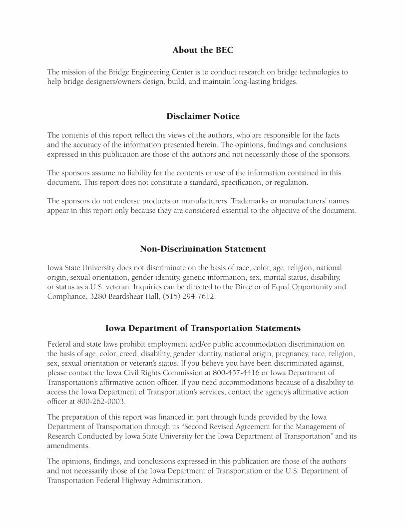
Figure 6.78. Bridge 209 movement at north pier west and east reflectors ..................................115 Figure 6.79. Bridge 209 movement at south pier west and east reflectors ..................................116 Figure 6.80. Bridge 209 movement at south abutment west and east reflectors .........................116 Figure 6.81. Bridge 309 movement at north abutment west and east reflectors ..........................117 Figure 6.82. Bridge 309 movement at north pier west and east reflectors ..................................117 Figure 6.83. Bridge 309 movement at south pier west and east reflectors ..................................118

x

Figure 6.84. Bridge 309 movement at south abutment west and east reflectors .........................118

Figure 6.85. Bridge 2208 movement at north abutment west and east reflectors ........................119 Figure 6.86. Bridge 2208 movement at north pier west and east reflectors ................................119 Figure 6.87. Bridge 2208 movement at south pier west and east reflectors ................................120

Figure 6.88. Bridge 2208 movement at south abutment west and east reflectors .......................120 Figure 6.89. Bridge 2308 movement at north abutment west and east reflectors ........................121 Figure 6.90. Bridge 2308 movement at north pier west and east reflectors ................................121 Figure 6.91. Bridge 2308 movement at south pier west and east reflectors ................................122 Figure 6.92. Bridge 2308 movement at south abutment west and east reflectors .......................122

Figure 6.93. Bridge 2408 movement at north abutment west and east reflectors ........................123 Figure 6.94. Bridge 2408 movement at north pier west and east reflectors ................................123 Figure 6.95. Bridge 2408 movement at south pier west and east reflectors ................................124 Figure 6.96. Bridge 2408 movement at south abutment east and west reflectors .......................124

Figure 6.97. Bridge 109 relative displacement between fixed pier and Girder B .......................125 Figure 6.98. Absolute movement of bottom flange of Girder B at north pier reflector...............125

Figure 6.99. Expansion pier displacement ...................................................................................126 Figure 6.100. Equivalent cantilever pile model ...........................................................................127

Figure 6.101. SAHP1 weak axis bending strain versus displacement .........................................128 Figure 6.102. SAHP4 weak axis bending strain versus displacement .........................................128 Figure 6.103. SAHP6 weak axis bending strain versus displacement .........................................129

Figure 6.104. NAHP1 weak axis bending strain versus displacement ........................................129 Figure 6.105. NAHP4 weak axis bending strain versus displacement ........................................130

Figure 6.106. NAHP6 weak axis bending strain versus displacement ........................................130 Figure 7.1. Bridge 309-S1 Girder A strain (LP2) ........................................................................131 Figure 7.2. Bridge 309-S1 Girder B strain for (LP2) ...................................................................132

Figure 7.3. Bridge 309-S1 Girder C strain (LP2) ........................................................................132

Figure 7.4. Bridge 309-S1 Girder D strain (LP2) ........................................................................133 Figure 7.5. Bridge 309-S2 Girder A strain (LP2) ........................................................................133 Figure 7.6. Bridge 309-S2 Girder B strain (LP2) ........................................................................134

Figure 7.7. Bridge 309-S2 Girder C strain (LP2) ........................................................................134 Figure 7.8. Bridge 309-S2 Girder D strain (LP2) ........................................................................135

Figure 7.9. Bridge 309-S1 Girder A bottom flange strain (LP3) .................................................137 Figure 7.10. Bridge 309-S2 Girder A bottom flange strain (LP3) ...............................................137

Figure 7.11. Bridge 309-S1 Girder B top flange strain (LP3) .....................................................138 Figure 7.12. Girder B-S2 top flange strain (LP3) ........................................................................138 Figure 7.13. Bridge 309 inner diaphragm strain (LP2) ................................................................139 Figure 7.14. Bridge 309 center diaphragm strain (LP2) ..............................................................139 Figure 7.15. Bridge 309 outer diaphragm strain (LP2) ................................................................140

Figure 7.16. Bridge 209-S1 dynamic loading strain in Girder A.................................................141

Figure 7.17. Bridge 209-S1 static loading strain in Girder A ......................................................141

Figure 7.18. Superimposed static and dynamic load strains ........................................................142 Figure 7.19. Diaphragm cross-section .........................................................................................144 Figure 7.20. Two equations and two unknowns ..........................................................................144 Figure 7.21. Bridge 309-S1 strong axis moments in girders (LP1) .............................................145 Figure 7.22. Bridge 309-S1 strong axis moments in girders (LP2) .............................................145 Figure 7.23. Bridge 309-S1 strong axis moments in girders (LP3) .............................................146

xi

Figure 7.24. Bridge 309-S1 lateral bottom flange moments (LP3) .............................................147

Figure 7.25. Bridge 309-S2 lateral bottom flange moments (LP3) .............................................148 Figure 7.26. Bridge 309-S2 lateral top flange moments (LP3)....................................................149 Figure 7.27. Bridge 309-S1 axial forces in girders (LP3)............................................................150

Figure 7.28. Bridge 309-S2 axial forces in girders (LP3)............................................................150 Figure 7.29. Bridge 309 strong axis moments in diaphragms (LP3) ...........................................151 Figure 7.30. Bridge 309 axial forces in diaphragms (LP3) ..........................................................152 Figure 7.31. Bridge 309-S2 (LP1) ...............................................................................................153 Figure 7.32. Bridge 309-S1 single lane moment distributions for three truck lanes ...................154

Figure 7.33. Bridge 309-S2 single lane moment distributions for three truck lanes ...................154 Figure 7.34. Bridge 309-S1 moment distributions versus truck position ....................................155 Figure 7.35. Bridge 309-S2 moment distributions versus truck position ....................................155 Figure 7.36. Bridge 309 maximum moment distribution factors.................................................156

Figure 7.37. Maximum moment distribution factors in bridges ..................................................157 Figure 7.38. Bridge 309 Girder A ratio of Mlb/Mx .......................................................................159

Figure 8.1. Model superstructure cross section ...........................................................................162 Figure 8.2. Plate girder sizes elevation view ...............................................................................163

Figure 8.3. Typical pier geometry................................................................................................164 Figure 8.4. Analytical model elevation view ...............................................................................164 Figure 8.5. Analytical model plan view .......................................................................................165

Figure 8.6. Analytical model end views ......................................................................................165 Figure 8.7. Meshed diaphragms and girders ................................................................................168

Figure 8.8. Meshed changes in girder bottom flange thicknesses ...............................................168 Figure 8.9. Typical meshed cross section with parapets ..............................................................169 Figure 8.10. Meshed girders and abutment ..................................................................................169

Figure 8.11. Meshed pier .............................................................................................................170

Figure 8.12. Simply supported abutment (left) and pier (right) ...................................................171 Figure 8.13. Deflected shape for outer truck position .................................................................172 Figure 8.14. Outside path at Section 2 Girder A ..........................................................................173

Figure 8.15. Center path at Section 1 Girder B............................................................................173 Figure 8.16. Laterally-deflected girders.......................................................................................174

Figure 8.17. Deflected shape for center truck position ................................................................176 Figure 8.18. Composite section presented by consultant .............................................................177

Figure 8.19. FEM center path at Section 1 ..................................................................................178 Figure 8.20. FEM center path at Section 2 ..................................................................................178 Figure 8.21. Girder A center path at Section 1 ............................................................................179 Figure 8.22. Girder C center path at Section 2 ............................................................................179 Figure 8.23. Design truck specifications (from Figure 3.6.1.2.2-1 AASHTO 2010) ..................181

Figure 8.24. Uniform temperature distribution ............................................................................182

Figure 8.25. Temperature gradient...............................................................................................183

Figure 8.26. North pier Service I loads ........................................................................................185 Figure 8.27. Center span Service I loads .....................................................................................186 Figure 8.28. North pier Service I loads ........................................................................................187 Figure 8.29. Center span Service I loads .....................................................................................187 Figure 8.30. Curved member subjected to temperature increase .................................................188 Figure 8.31. Girder A deflected shape due to T(+) ......................................................................188

xii

Figure 8.32. North pier Service I loads ........................................................................................189

Figure 8.33. Center span Service I loads .....................................................................................190 Figure 8.34. North pier load combinations ..................................................................................191 Figure 8.35. Center span load combinations ................................................................................192

Figure 8.36. North pier load combinations ..................................................................................193 Figure 8.37. Center span load combinations ................................................................................193 Figure 8.38. North pier load combinations ..................................................................................194 Figure 8.39. Center span load combinations ................................................................................195 Figure 9.1. Bridge 309 circled locations of extracted results ......................................................199

Figure 9.2. Stress points in girder section ....................................................................................200 Figure 9.3. Critical stresses in Girder A and D at mid-center span with varying skew and

curvature ..........................................................................................................................202 Figure 9.4. Critical stresses in Girder A and D at north pier with varying skew and curvature ..203

Figure 9.5. Total stresses at Points 3 and 4 of Girder A at mid-center span................................205 Figure 9.6. Total and component stresses in Girder A at mid-center span due to DL+LL+T(+) 206

Figure 9.7. Total and component stresses in Girder A at mid-center span due to DL+LL+T(-) .207 Figure 9.8. Total and component stresses in Girder A at mid-center span due to DL .................208

Figure 9.9. Total and component stresses in Girder A at mid-center span due to LL .................209 Figure 9.10. Total and component stresses in Girder A at mid-center span due to T(+) .............210 Figure 9.11. Total and component stresses in Girder D at north pier due to DL+LL+T(+) ........212

Figure 9.12. Total and component stresses in Girder D at north pier due to DL .........................213 Figure 9.13. Total and component stresses in Girder D at north pier due to LL .........................214

Figure 9.14. Total and component stresses in Girder D at north pier due to T(+) .......................215

xiii

LIST OF TABLES

Table 2.1. Levels of analysis (from Table 1 Nevling et al. 2006) .................................................10 Table 5.1. NEMM bridge geometry ...............................................................................................32 Table 5.2. Steel girder dimensions (all dimensions in inches) ......................................................34

Table 5.3. Girder A composite section properties at strain gauge locations ..................................35 Table 5.4. Girder D composite section properties .........................................................................36 Table 6.1. Girder A strain range (in Microstrain) ..........................................................................75 Table 6.2. Girder D strain range (in Microstrain) ..........................................................................75 Table 6.3. Girder A force range (in kip) ........................................................................................76

Table 6.4. Girder D force range (in kip-in.) ...................................................................................76 Table 6.5. Measured pile internal strain ranges .............................................................................87 Table 6.6. Calculated pile internal force ranges ............................................................................89 Table 6.7. Approximation of girder axial force from abutment backwall pressure .......................95

Table 6.8. Total free expansion and measured change in length .................................................102 Table 6.9. Calculated average axial strain versus measured average axial strain ........................102

Table 6.10. Effective thermal length ............................................................................................106

Table 7.1. Maximum strain (μ𝜀) at bottom of web ......................................................................135

Table 7.2. Maximum strain (μ𝜀) at top of web ............................................................................136

Table 7.3. Maximum diaphragm strains (μ𝜀) ...............................................................................140

Table 7.4. Maximum DAF (%) in bottom flange strain ..............................................................142 Table 7.5. Maximum Mx in girder (kip-in.) .................................................................................146 Table 7.6. Maximum Mlb in girders (kip-in.) ...............................................................................148

Table 7.7. Maximum Mlt in girders (kip-in.) ...............................................................................149 Table 7.8. Maximum P in girders (kip)........................................................................................150

Table 7.9. Maximum Mx in diaphragms (kip-in.) ........................................................................151 Table 7.10. Maximum P in diaphragms (kip) ..............................................................................152

Table 7.11. Moment distribution factors for multi-lane live loading ..........................................156 Table 7.12. Results from AASHTO LRFD equation C4.6.1.2.4b-1 ............................................159 Table 7.13 S2: Mlb/Mx (%) from field results ..............................................................................159

Table 7.14. S1: Mlb/Mx (%) from field results .............................................................................160 Table 8.1. ANSYS model concrete material properties ...............................................................166

Table 8.2. ANSYS model steel material properties .....................................................................167

Table 8.3. Center load path average bottom flange strain (μ𝜀) ....................................................174

Table 8.4. Outside load path bottom flange strain (μ𝜀) ...............................................................174

Table 8.5. Inside load path bottom flange strain (μ𝜀) ..................................................................175 Table 8.6. Ranges of measured temperatures and strains in Girders A and D at different spans

and backwall pressure at abutments .................................................................................175

Table 8.7. Strain range comparison between field data and FEM results....................................176

Table 8.8. Uniform temperature values .......................................................................................182

Table 8.9. Girder A unfactored internal forces at north pier .......................................................184 Table 8.10. Girder A unfactored internal forces at center span ...................................................184 Table 8.11. North pier Strength I stresses ....................................................................................196 Table 8.12. Center span Strength I stresses .................................................................................196 Table 9.1. Variable values of the curvature and skew .................................................................198 Table 9.2. Bridge model with a skew of 0 degrees and a curvature radius of 20,950 ft ..............217 Table 9.3. Bridge model with a skew of 15 degrees and a curvature radius of 950 ft .................217

xiv

LIST OF VARIABLES

A, B, and C = gauge specific constants given by manufacturer

Ac = the area of concrete

Ap = cross-sectional area of the pile tips

As = the area of the steel

Babutment = width of the abutment

Be = effective slab width,

D = the depth of the web

DAF = dynamic amplification factor

DC = dead load for structural components

D0 = initial reading

Di = reading at time i

(EA)eff = effective axial rigidity

(EIx)eff = the effective flexural axial rigidity for X-axis bending

Ec = the linear elastic modulus of concrete

Es = the linear elastic modulus of steel

G = correction factor that converts digits to inches (provided by manufacturer)

If = moment of inertia of a flange about its smaller principal axis

Iytb = moment of inertia of the bottom flange of the steel girder for Y-axis bending

Iytf = moment of inertia of the top flange of the steel girder for Y-axis bending

IM = dynamic impact factor for live load

K = a temperature correction coefficient given by the manufacturer (digits/°C)

Kp = the coefficient of passive lateral earth pressure (psi/psi)

Kq = end-bearing soil-spring resistance

Kv = skin-friction soil-spring resistance

L = length of bridge along curve

L = length of the member

Leff = effective thermal length

Lcable = the length of the cable

Lc = the length of the concrete member

Le = equivalent cantilever length

Lg = distance between equivalent Mg moments

Lgauge = the distance from the top of the abutment to the pressure cells

Lmax = the total height of each abutment

Lp = tributary pile length for each soil-skin-friction soil-spring

Ls = the length of the steel member

LL = vehicular live load

M = resulting end moment

M and B = constants for the model 1127 gauges given by the manufacturer

Mf = lateral bending moment acting on the flanges

Mg = resulting moment at location of strain gauges

Mlat = the lateral flange moment in a girder at the brace point due to vertical loading

Mlb = lateral bending moment in the bottom flange

Mlt = lateral bending moment in the top flange

xv

Mx = strong axis bending moment

MDF = moment distribution factors

N = a constant of either 10 or 12 (engineer’s discretion)

P = applied load on composite section

P = the internal axial force

Pc = applied unit load on concrete

Ps = applied unit load on steel

Pgauge = the maximum stress measured at the location of pressure cells

Pmax = the approximated maximum stress at the bottom of the abutment

Ptotal = the total approximate force applied to each abutment

R = the radius of the girder

Ri = the frequency reading produced by the gauge when the vibrating wire is

plucked

TG = force effect due to temperature gradient

TU = force effect due to uniform temperature

Y(NA) = the distance to the neutral axis measured from the center of the bottom flange

Z = depth from top of soil to location of desired stress

Δ = applied lateral end displacement

bfb = bottom flange width

bft = top flange width

d = centerline concrete slab to centerline bottom flange

fbw = tension or compression stress due to warping of the cross-section

hw = web height

tfb = bottom flange thickness

tft = top flange thickness

ts = slab thickness

tw = web thickness

x = distance from center of flange to flange tip

xi = distance from neutral axis to strain gauge i along the X-axis

yi = distance from neutral axis to strain gauge i along the Y-axis

ӯ = distance from the center of the bottom flange to the neutral axis

αc = the thermal expansion of concrete

αcable = the coefficient of thermal expansion of the cable

αeff = the effective thermal expansion coefficient of combined steel and concrete

αs = the thermal expansion of steel

δ = displacement of composite section

δc = displacement of concrete

δs = displacement of steel

εcurrent = the microstrain reading at its respective time

εreference = the microstrain reading on April 28, 2011 at 6 a.m.

εa = internal axial strain

εylt = lateral bending strain in the top flange

εylb = lateral bending strain in the bottom flange

εi = strain reading at gauge i

εx = strong axis bending strain

εt = internal torsional-warping strain

xvi

𝜀s = static strain

𝜀d = dynamic strain

ΔDcable = the correction

ΔDuncorrected = the reading before a temperature correction

∆Lavg = the average bridge expansion computed via instrumentation data during the

surveying time interval

∆Ls = the surveying expansion referenced to April 28, 2011 at 6 a.m.

∆Ls′ = the surveying expansion at the time of the survey on April 28, 2011

ΔTair = the ambient air temperature

ΔTeff = the effective bridge temperature

ΔTc = the change in temperature of the concrete member

ΔTs = the change in temperature of the steel member

Δd = range of longitudinal movement of fixed pier or integral abutment

Δε = difference in microstrain

∆εr = resistance axial strain

σx′ = total horizontal stress

σz′ = total vertical stress

σx = strong axis bending stress

σlb = lateral bending stress in the bottom flange

σa = axial stress

ϕ′ = effective friction angle of the soil

ɣ′ = unit weight of soil

ɣp = design load factor for permanent loads

ɣTG = design load factor for temperature gradients

ɣTU = design load factor for uniform temperature

νc = Poisson’s Ratio for concrete

νs = Poisson’s Ratio for steel

xvii

ACKNOWLEDGEMENTS

The research team would like to acknowledge the Federal Highway Administration for

sponsoring this Transportation Pooled Fund study: TPF-5(169). The authors would also like to

thank the state pooled fund department of transportation (DOT) partners for their support:

Iowa DOT (lead state)

Ohio DOT (ODOT)

Pennsylvania DOT (PennDOT)

Wisconsin DOT (WisDOT)

xix

EXECUTIVE SUMMARY

The National Cooperative Highway Research Program (NCHRP) has shown concerns regarding

the design, fabrication, and erection of horizontally curved steel girder bridges due to

unpredicted girder displacements, fit-up, and locked-in stresses, including thermal stresses.

Because curved steel girder bridges are used in up to one-quarter of the nation’s steel girder

bridges, having a better understanding of actual behavior – and therefore having better design

methodologies – is of notable importance.

The primary objective of this work was to monitor and evaluate the behavior of six in-service,

horizontally curved, steel-girder bridges with integral and semi-integral abutments and to provide

design recommendations.

A national survey was conducted and a literature review was performed to capture the state-of-

the-art regarding these types of structures. Also, a monitoring program was developed and

deployed on six bridges located at the I-35, I-235, and I-80 interchange on the northeast side of

Des Moines, Iowa to obtain strains and movements that result from long term temperature

changes. An additional instrumentation system was installed to measure strains in the girders

under short term loading with known truck weights and paths. The data gathered during the

monitoring period of the project were post-processed to study important behavioral attributes.

The sensitivity of long term thermal loading and short term live loading stresses to curvature,

skew and pier bearing fixity was also studied.

The following general conclusions were made from the results of the study:

There were no measureable differences in the behavior of the horizontally curved bridges and

straight bridges studied in this work under thermal effects. For preliminary member sizing of

curved bridges, thermal stresses and movements in a straight bridge of the same length are a

reasonable first approximation.

Thermal strains in integral abutment and semi-integral abutment bridges were not noticeably

different. The choice between IAB and SIAB should be based on life – cycle costs (e.g.,

construction and maintenance).

The measured internal strain in the abutment piles due to expansion and contraction of the

bridge were generally below 50% of yield stress. The equivalent cantilever method of steel

pile analysis fell short of accurately predicting weak axis bending strain.

The soil pressures on the abutment backwalls were generally below the approximate passive

soil pressures.

Moment distribution factors for the short term live loading were influenced by the amount of

curvature.

An analysis of the bridges predicted a substantial total stress (sum of the vertical bending

stress, the lateral bending stress, and the axial stress) up to 3 ksi due to temperature effects.

For the one curved integral abutment bridge studied at length, the stresses in the girders

significantly vary with changes in skew and curvature. An expansion bearing pier reduces the

thermal stresses in the girders of the straight bridge but does not appear to reduce the stresses

in the girders of the curved bridge.

xx

Since AASHTO requires a three-dimensional analytical model of the bridge and support

conditions to calculate lateral bending stresses for the final design of all curved bridges, this

model should also be used to calculate thermal stresses for final design of the curved bridge.

(However, with a 10⁰ skew and 0.06 radians arc span length to radius ratio (i.e., meeting the

geometrical requirements to ignore curvature for strong axis bending), the curved and skew

integral abutment bridges can be designed as a straight bridge if an error in the estimation of

stress of 10% is acceptable.)

1

CHAPTER 1 INTRODUCTION

This chapter presents the background to the project and the problems it addresses, the objective

and scope of the project, and the research plan undertaken during the project. The final section of

this chapter summarizes the organization of this report.

1.1 Background

A report published by The National Cooperative Highway Research Program (NCHRP) raised

concerns regarding the design, fabrication, and erection of horizontally curved steel girder

bridges. These concerns are centered around difficult-to-predict girder displacements, fit-up

issues, and unintended locked-in stresses. Because curved steel girder bridges are used in up to

one-quarter of the nation’s steel girder bridges, having a better understanding of actual behavior

– and therefore having better design methodologies – is of notable importance. In order to have

these concerns addressed, the NCHRP developed a research problem statement and gave it high

priority for funding.

A major problem facing the nation today is the need to replace large numbers of bridges. Future

engineers will need to utilize cost effective and durable designs in order to meet this challenge.

Bridge joints permit relative movement between bridge deck spans and abutments; however,

they must be continually maintained at a cost to the owner. Therefore, an urgent need exists to

reduce bridge maintenance costs by eliminating or reducing deck joints. One way to achieve this

is by expanding the use of integral abutments to include curved girder bridges.

1.2 Objective and Scope

The combined use of horizontally curved steel girder bridges and integral abutments looks to be

a promising design; however, this combination is relatively new to the nation, and to Iowa. The

purpose of the work summarized herein is to investigate the use of integral abutments on curved

girder bridges through a monitoring and evaluation program of in-service bridges.

1.3 Research Plan

The objective of the research project was to gather information that will assist in the future

design of integral-abutment, curved-girder bridges by monitoring and analyzing the behavior of

curved steel girder bridges with integral abutments. There were three general task groups for this

project, each of which consisted of several related tasks, as described below.

1.3.1 Task Group I: Information Collection

The use of integral abutments in curved girder bridges has either not been tried with great

frequency or is not well documented in the technical literature. As such, the first project task

group involved collection of information on the use of these combined structural systems. The

following tasks were undertaken to fulfill this task group’s objective:

2

Task A – Technical Advisory Committee

A technical advisory committee (TAC) was formed to assist the research team regarding issues

related to curved girders, integral and semi-integral abutments, and fixed and expansion bearings

at piers. The TAC also assisted in establishing performance metrics that could be used to

evaluate the performance of curved-girder, integral-abutment bridges. The TAC was encouraged

to provide other information they deemed useful to the research team.

Task B – Survey of Available Technologies

A survey, which was sent to all the nation’s state DOTs, was conducted to determine if integral

abutments have been used for horizontally curved bridges and, if so, what were the significant

findings, conclusions, or recommendations regarding these types of bridges. The survey also

requested that the state bridge engineers express concerns regarding potential behavioral issues

and to provide any specific information related to instrumentation and monitoring of these types

of bridges.

Task C – Review of Available Engineering Literature

Although a brief literature search and review had been performed before the project officially

began, a more complete review was conducted to determine the past and present use of integral

abutments for horizontally curved bridges and to uncover any concerns or problems associated

with this type of bridge construction. Since significant information on curved-girder, integral-

abutment bridges was not initially found in the literature, two general literature searches were

conducted that individually addressed horizontally curved bridges and integral-abutment bridges

separately in order to formulate potential behavioral issues and to develop a more refined project

scope.

Task D – Inspect Existing Curved and Chorded Girder Bridges

The re-alignment of the intersection of Interstates I-35, I-80 and, I-235 (northeast mix-master)

near Des Moines, Iowa included the demolition of the old bridges and the construction of six

new bridges. Several bridge types were used in the reconstruction including curved girder

bridges with integral or semi-integral abutments. For this task, two I-235 curved girder bridges

were inspected to determine if there was any evidence of problems associated with the use of

integral abutments.

1.3.2 Task Group II: Collect and Analyze Data on the Performance of Six Bridges

The reconstruction of the Northeast Mix-Master, started in 2008, provided the opportunity to

monitor the behavior of curved and straight-steel girder bridges. The interchange design was

planned so that semi-integral abutments were used in two curved-girder bridges, and integral

abutments were used in two essentially identical curved bridges. There were six 26 ft wide

3

roadway bridges included in the research. Bridge characteristics are presented in Chapter 5 of

this report. The following tasks highlight the steps taken by this task group:

Task E – Finalize an Instrumentation Plan

Working with the Iowa DOT Office of Bridges and Structures, the research team developed

preliminary instrumentation schemes for five of the six Northeast Mix-Master bridges. These

schemes are shown in Chapter 5, along with pertinent bridge information. The instrumentation

layouts typically consist of strain gauges on girders and other elements, temperature sensors,

sensors utilized to monitor the differential girder-to-substructure displacement at expansion piers

and semi-integral abutments, and techniques for monitoring the global movement of the

substructure elements. Along with the instrumentation placed on the bridges, each of the six

bridges was outfitted with eight surveying-type reflectors for the purpose of performing monthly

surveys of the bridges. These reflectors were placed on the exterior girders at both abutments and

both piers. The survey procedure is discussed further in Chapter 5.

Task F – Monitor and Analyze the Behavior of the Selected Bridges

The bridges were monitored over a period of approximately 18 months for the long-term health

assessment. During this period, the strains, temperatures, and displacements were recorded under

a variety of loading conditions. In addition, the short-term health assessment was investigated by

conducting a series of live load tests as described in Chapter 5.

Task G – Develop and Validate Simple Analytical Models for the Monitored Bridges

Using the collected data, simple analytical models were developed and validated. These models

may be able to be extrapolated to other design conditions (e.g., geometry, soil conditions, etc.)

that may provide information on other hypothetical situations.

1.3.3 Task Group III. Develop Project Conclusions and Recommendations

The focus of this task group was to summarize the entire project with a goal of developing

recommendations that will assist bridge owners with decisions regarding the combined use of

curved girders and integral abutments.

Task H – Establish a Meeting with the TAC

A final meeting with the TAC was held so that the research team could present the results of the

project and some initial project conclusions. The TAC was then asked to provide detailed input.

4

Task I – Submit Final Report

The Final Report, presented herein, summarizing the results of the research was the final step for

this task group.

1.4 Report Organization

Chapter 1 introduces the project including the project background, the objective and scope of the

project, and the research plan. Chapter 2 presents the literature review, discusses the design of

horizontally curved, steel-girder bridges, summarizes use of integral and semi-integral

abutments, and presents circumstances in which both have been used. Chapter 3 summarizes a

survey conducted of the nation’s transportation departments in regard to their current design

practices for horizontally curved, steel-girder bridges with integral and semi-integral abutments.

Chapter 4 summarizes a bridge inspection conducted on two partially horizontally curved bridges

with integral abutments. Chapter 5 presents the experimental procedure. Chapters 6 and 7 present

the results from the testing described in Chapter 5. Chapter 8 presents an analytical investigation

of design loading conditions. Chapter 9 presents a sensitivity study that was performed to

investigate the influences of the curvature and skew on the stresses in girders of an integral

abutment bridge. Finally, Chapter 10 presents conclusions, recommendations, and suggested

future work with curved-girder, integral-abutment bridges.

5

CHAPTER 2 BACKGROUND/LITERATURE REVIEW

The design and analysis of straight, integral-abutment bridges (IABs) has a long and extensive

history dating back as far as the 1930s. These bridges came about after the introduction of the

Hardy Cross Method, and were considered a viable solution to the drawbacks of expansion joints

and expansion bearings (Tennessee DOT 1996). Although there has been a tremendous amount

of research on the response of straight IABs, less attention has been paid to their horizontally

curved counterparts. Research on the use of integral abutments on horizontally curved bridges is

scarce (Hassiotis 2006). This chapter attempts to summarize completed work on horizontally

curved, integral-abutment bridges. This chapter also presents completed work on straight,

integral-abutment bridges, and on horizontally curved, non-integral-abutment bridges.

2.1 Mechanics and Behavior of Horizontally Curved Girders

A single curved girder has three force components (vertical shear, radial shear, and axial load)

and three moment components (strong axis bending (Mx), weak axis bending (My), and torsion

(T)). For purposes of the following discussion, only the moment components are shown in Figure

2.1. The normal stresses induced in the upper and lower flanges of a wide flange shape by these

three moments are illustrated in Figure 2.2. The stress due to the positive strong axis bending

(Mx) causes tension in lower flange and an equal compression in the top flange and can be

computed by the usual strength of materials approach by assuming plane sections remain plane

(Figure 2.2a). Similarly, the stress due to the weak axis bending (My) causes tension on one side

and compression on the other side of both the top and bottom flanges (Figure 2.2b). Stresses due

to torsion (T) are typically divided into two categories: (1) pure torsion often called Saint-

Venant’s torsion and (2) warping torsion [steel text book reference]. The pure torsion stress is a

shear stress induced into the flanges and, for thin walled open sections, usually neglected. The

warping torsion is resisted by equal and opposite horizontal shears in the upper and lower flanges

so that the upper flange is bent laterally in one direction and the lower flanges is bent laterally in

the opposite direction. Hence, the cross section is warped and is no longer planar, as assumed in

elementary beam theory. The moments that induce this bending are sometimes referred to as the

bi-moments and result in normal stresses in the top and bottom flanges as illustrated in Figure

2.2c.

The total lateral moment in the flanges (Mlt and Mlb in the top and bottom flange, respectively) is

the vector sum of the weak axis bending and the warping torsion bending as illustrated in Figure

2.3 and for one flange in Figure 2.4.

In NCHRP Report 424, Hall et al. (1999) describe that vertical bending is broken down into the

first three components shown in Figure 2.5 all of which induce bending about the major axis, as

in Figure 2.2. Component 1 represents the moment in each girder if all the girders deflected

uniformly. Component 2 is the result of restoring forces in connecting members. Adjacent girder

generally have different stiffnesses and different loads. Connecting members, such as the

diaphragm and deck, shift load from the more flexible girders to the more stiff girders. The sum

of components 1 and 2 are similar to the moments calculated for straight bridges determined by

finding the moment at a bridge cross section from a line girder analysis and multiplying it by a

distribution factor.

6

Component 3 moments occur because the girders have different radii. The outside girder is less

stiff because of its larger radius (and, generally, longer span). If the cross sectional properties are

about the same, the outside girder will develop a higher component 3 stress. According to Hall,

component 4 stress is the lateral bending stress equal to the sum of the warping stress from the

bi-normal moment (Figure 2.2c) and the radial bending stress (Figure 2.2b) as illustrated in

Figure 2.3. Hall describes also describes an amplification effect similar to the P-delta effect in

columns. It is usually a second order effect caused by the increased curvature of a curved girder

due to lateral bending. The amplification effect is not included in first order linear analysis

methods and can be included by considering large deflection theory. An approximation of lateral

flange bending can be addressed through the V-load equation, discussed subsequently.

Figure 2.1. Three moment components in a single curved girder

Figure 2.2. Normal stress in flanges due to three moment components

T Mx

My

M

T

M

(a) (b) (c)

-stress -stress T-stress

y

x

Mx My

7

Figure 2.3. Normal stress in flanges due to major axis bending and lateral bending

Figure 2.4. Lateral flange bending (from Figure A-1 Hall et al. 1999)

M

M

-stress -stress

M

lt

x

lb

Mx Ml

8

Figure 2.5. Four normal stress components (from Figure A-5 Hall et al. 1999)

Miller et al. (2009) state that curved beams create twisting effects, which result in warping out of

plane similar to torsion. This phenomenon is referred to as a bimoment, a product of combined

lateral flange bending and torsional shear. In addition, negligible second order effects, similar to

P-Δ in columns, occur when the curved compression flange bows outwards, increasing the

degree of curvature.

Lydzinski et al. (2008) further explain additional complications that arise when analyzing and

designing I-girders in curved bridges. Complications range from the individual plates to the

constructed girder as a whole. Compared to straight girders, horizontally curved I-girders are

significantly different in the following ways:

Flange local buckling may differ from the outer to the inner side of the web

Local buckling is possible on the inner half of the tension flange

S-shaped bending occurs in the web, causing an increase of stress at the web-flange

connection

Bending and torsion stresses are not decoupled, resulting in lateral bending behavior

Twisting can occur under individual girder self-weight, causing construction issues in

framing

Several levels of analysis can be used to determine girder responses. These include, but are not

limited to, the line girder method, grid method, finite strip method, and finite element modeling

9

(FEM) analysis method. The simplest technique, line-girder method, assumes only vertical loads

applied to a single girder. Engineers must determine the amount of load and location of load

between girders. Component 1 is only considered during the line-girder analysis and Component

3 may be considered if the V-load method is also applied. The grid analysis considers

Components 1, 2, and 3. Warping torsion is not recognized in the grid analysis, since only St.

Venant torsion is used. Again, applying the V-load method indirectly accounts for lateral flange

bending. Finite element analysis is capable of determining Components 1, 2, and 3. If large-

deflection theory is used, then the effects of warping stress may also be accounted for (Hall et al.

1999).

2.2 Comparing Levels of Analysis for Horizontally Curved Bridges

Several levels of analysis can be used to determine girder responses [Hall reference]. These

include, but are not limited to, the line girder method, grid method, finite strip method, and finite

element modeling (FEM) analysis method. The simplest technique, line-girder method, assumes

only vertical loads applied to a single girder. Only Component 1 stresses are determined in the

line-girder analysis. Component 2 stresses are often determined by applying wheel load

distribution factors to the line-girder method results. According to Hall, component 3 and 4

may be considered if the V-load method is also applied with the line-girder method. The grid

analysis considers Components 1, 2, and 3. Warping torsion is not recognized in the grid

analysis. Applying the V-load method indirectly accounts for lateral flange bending. Finite

element analysis is capable of determining Components 1, 2, and 3. Component 4 can be

included in the 3-D finite element analysis if the lateral flange bending degrees of freedom

correspond to the moments in Fig. 2.X3 are incorporated into the model. If large-deflection

theory is used, then the amplification effects may also be accounted for (Hall et al. 1999).

Very few studies have thoroughly compared different methods of analysis with respect to field

test results in horizontally curved bridges. Nevling et al. (2006) attempt to evaluate the level of

accuracy produced for various analysis methods through conducting research on a continuous

three-span bridge. Table 2.1 details the three levels of analysis performed in the study. The

bridge of interest is constructed of five, Grade 50, steel plate I-girders with the outside girder

having a radius of 178.5 m (585.6 ft). The non-integral abutment skews range from 60⁰ to 35⁰.

An American Association of State Highway and Transportation Officials (AASHTO) HS20

design truck was applied as a live load to the bridge at various locations. The single instrumented

radial cross-section focused on in this paper, includes the location of maximum positive moment

at center span. At this location, strain gauges were placed on the four flanges on each of the five

girders to analyze the superstructure’s reaction to live loading.

10

Table 2.1. Levels of analysis (from Table 1 Nevling et al. 2006)

Level Description Analysis Tool

1 Manual AASHTO Guide Specs

V-load Method

2 2D Grillage SAP2000

MDX

DESCUS

3 3D FEM SAP2000

BSDI

The study made conclusions comparing the three methods of analysis against one another, as

well as the methods against field data. Compared to field results, Level 1 analyses predicted

larger major axis bending moments for girders closer to the applied load and smaller major axis

bending moments for girders furthest from the applied load. Correlations between Level 1 and 3

analyses to field results were inconclusive with respect to lateral bottom flange bending

moments. Levels 2 and 3 predicted major axis bending moments similar to the field results.

However, Level 2 predicted more accurate vertical bending moments compared to Level 1. The

study concluded that Level 3 did not provide increased accuracy that was noticeable compared to

Level 2 analyses. Thus, Level 2 analysis would be recommended based on the study findings.

Miller et al. (2009) also conducted a study comparing field testing to FEM. The study focused on

a multi-girder, three-span, steel composite, horizontally curved I-girder bridge. Field testing

consisted of attaching several strain gauges to the steel girders and diaphragms. Static and

dynamic loading, similar to an HS20 truck, was applied and later replicated on a FEM. Results

concluded that the FEM predicted a higher neutral axis location compared to the field results and

composite section theory. The cause may be due to slippage of the shear studs in the haunches.

Comparing the FEM to field results showed that larger diaphragm shear strains were found in the

field than provided by FEM analysis. In addition, including pier flexibility most accurately

compared to the field results. Lastly, the curved girder may require a refined mesh in the FEM to

simulate for the complex strain distribution (Miller et al. 2009).

Another FEM study was performed by Lydzinski et al. (2008). The FEM replicated a continuous

three-span horizontally curved I-girder bridge comparing dynamic and static loading responses.

Dynamic loading concentrated on free vibrations. FEM found that plate elements adequately

represented plate bending behavior and interactions in the cross framing. Refined meshing is

more critical along the longitudinal direction of the bridge versus the transverse direction at a

particular cross-section. Modeling the haunch with plate elements provided negligible

differences compared to using rigid links. The authors further found that the piers can be

modeled using beam elements rather than complicated 3D elements. Finally, the overall

conclusion of the study indicated that including the pier model flexibility is significant in

estimating the behavior of the entire bridge.

Barr et al. (2007) investigated the live-load response of a three span horizontally curved I-girder

bridge. The study pertains to comparing field test data to a FEM analysis, as well as the V-load

method. Conclusions of the study offer suggestions regarding FEM analysis results. These

11

suggestions explore differences between the FEMs and the V-load analysis methods. Their

research focuses on a continuous three-span bridge constructed of five steel I-girders with a

noncomposite deck. A field inspection of the bridge determined that the bearings were severely

deteriorated and were not allowing the degrees of freedom to be released per design. Relevance

of the frozen bearings was explored throughout the FEM.

The study concluded that the detailed FEM produced accurate strain readings under applied live

loading. Replacing the frozen bearings with new bearings proved to be negligible because

accounting for the amount of resistance provided by frozen bearings is challenging. Another

conclusion found that using the V-load for positive moments was 6.8% unconservative for the

exterior girders and 8.3% conservative for interior girders when compared to FEM. For negative

moments, the V-load was 16.1% conservative for interior girders and 12% unconservative for

exterior girders (Barr et al. 2007). These conclusions might indicate that the V-load method

offers a relatively accurate preliminary method of analysis, while FEM analysis would be

recommended for final design.

2.3 History of the Design Specifications for Horizontally Curved Bridges

Through the 1960s, curved steel bridges were increasingly designed and constructed as engineers

realized their advantages. Because of this, a drive began towards developing the scarcely

available specifications and guidelines. This led to the Consortium of University Research

Teams (CURT) project managed by the Federal Highway Association (FHWA). The CURT

project completed analytical and theoretical work, which eventually helped create a preliminary

set of specifications for allowable stress design (ASD) which were later accepted by AASHTO in

1976. Through additional work by AASHTO committees and the American Iron and Steel

Institute, LFD criteria were developed and transformed from the preliminary set of ASD

specifications by CURT. The LFD criteria combined with the ASD criteria formed the 1980

AASHTO Guide Specs. After eight revisions, another edition was published in 1993.

The 1993 Guide Specs concepts were difficult to understand and could be easily misused by

designers. The 2003 Guide Specs offer more details for discussion of the specifications and

include design examples. Design for the 2003 Guide Specs includes general parameters,

preliminary design, preliminary analysis, and refined design as four main categories. General

parameters are broken down into two main divisions of design and construction. The design of

the bridge is subdivided into general bridge geometry and limit states that incorporate: strength,

fatigue, serviceability, and constructability. Criteria for preliminary design are outlined based on

material strengths and girder geometries. Preliminary member sizes and framing can be

calculated in accordance to Articles 5, 6, 9, and 12 of the specifications. As outlined in previous

sections, preliminary analysis of a horizontally curved girder bridge can be much more

sophisticated than a traditional straight girder bridge. A percentage of the applied load is often

transmitted to the girder with the largest radius. Because of this, the entire structure must be

analyzed as a whole, in contrast to only analyzing single girders with distribution factors. Often,

small-deflection theory can be used for most bridges. Second-order analyses are usually

recommended during construction phases and stability checks. If certain requirements are met,

the effects of curvature may be neglected when considering vertical bending moments. Torsion

12

and lateral bending must account for curvature effects. The V-load method is recommended for

simplified cases outlined in the specifications. Finite element theory is recommended for more

refined analysis methods if the criteria for V-load are not met. Finally, design refinement is

performed as an iterative process to ensure that all components meet design requirements such as

strength, serviceability, fatigue, overload, detailing, and constructability.

Linzell et al. (2004) discusses the efforts leading up to the formation of the 2003 Guide

Specifications for Horizontally Curved Highway Bridges by AASHTO, hereafter referred to as

the Guide Specs. The 2003 Guide Specs encompasses load factor design (LFD) criteria, which

has been eliminated by the development of the Load and Resistance Factor Design (LRFD)

design provisions. In 2006, the AASHTO Bridge LRFD Design Specifications combined the

specifications for straight bridges and curved bridges so that straight and horizontally curved

bridges are in one manual.

2.4 Load Distributions for Horizontally Curved Bridges

Kim et al. (2007) studied live load radial moment distribution in horizontally curved girders. As

previously stated, substantial normal stresses are present in horizontally curved girders due to

warping torsion. Cross frames are designed to reduce these warping normal stresses. These

primary members offer an additional load path for induced live loads, which has an effect on

vertical bending of adjacent girders. Because of this, cross frames and diaphragms will have a

significant influence on transferring load from one girder to the next. Transferring of load can be

assessed by calculating girder distribution factors (GDF). The Kim et al. report focuses on

developing GDF equations, which are primarily a function of cross framing details. The research

employed both field studies and analytical models. Three increasing levels of complexity for

modeling of the FEM were utilized and are shown in Figure 2.6. Based upon field measurements,

results showed that Type I was conservative by up to 45%, Type II only differed by 10% and

Type III provided slightly more accurate results than Type III. Due to the added increased effort

for creating a Type III model, the slightly increased accuracy was deemed negligible. Radius,

span length, and cross frames all were found to influence the live load distribution. On the other

hand, the parapets and deck thickness were insignificant with respect to GDFs. Overall, the span

length was found to be the most influential factor.

13

Figure 2.6. Levels of analysis (from Fig. 1 Kim et al. 2007)

A study by Miller et al. (2009), previously mentioned, made conclusions from calculated

dynamic amplification factors (DAF). When comparing the FEM analysis to field data analysis,

the study found that the FEM overestimated the stiffness of the diaphragm to girder connection

as it predicted greater transfer of loads between adjacent girders as compared to field

measurements. Consequently, load distribution was greater for the outermost girders. The field

results indicated that DAF were within the limit of AASHTO recommendations.

In contrast to the research by Miller et al. (2009), Barr et al. (2007) determined that the FEM

distribution factors differed by only 5% from the AASHTO (2003) standard distribution factors.

This discrepancy could be due to varying degrees of complexity in each FEM.

2.5 Framing and Erection of Horizontally Curved Girders

Although steel I girders offer minimal torsional resistance, they are most commonly used in the

construction of horizontally curved bridges. These members are only stable when connected via

diaphragms or cross bracing, which leads to substantial interaction forces in those connecting

members. Consequently, the analysis and design of the superstructure needs to accommodate

these forces (Linzell et al. 2004).

14

In a dissertation from the University of Maryland, Thanasattayawibul addresses the two main

types of curved girder framing, closed and open framing (Thanasattayawibul 2006). Closed

framing resists torsion through the interactions of girders that are connected by diaphragms or

floor beams along with lateral bracing at girder flange locations. In contrast, open bracing does

not include the horizontal bracing of girder flanges. Combinations of closed and open framing

can be used during construction of curved bridges. Cross frames and diaphragms act as

secondary members in straight bridges; however, they act as load-carrying members in curved

bridges. The report also notes that spacing of cross frames has a significant effect on warping

stresses.

In a presentation, associated with HNTB, LaViolette further highlights the importance of

erecting horizontally curved members (LaViolette 2009). He explained that lateral bending is

primarily caused by warping normal stresses along with wind loads, skew, and overhangs of

girders during construction. Throughout construction and erection phases, many calculations

must be made to account for the several stages of construction. Stability of each individual girder

and the multi-girder system as a whole must be met. Often, these calculations and checks are

made by performing a 3D finite element analysis to investigate each sequence of construction.

Structural engineers must account for load capacities and stabilities at all stages of construction.

Notable loadings to be accounted for should include self-weights and attachments, wind loads,

loads induced during lifting and tie downs, girders rolling due to unbalanced loadings, and

several more. Additionally, issues during erection can be prevented by properly noting the

alignment. Such preventions include detailing sufficient cross framing, using falsework, properly

placing holding cranes, and thoroughly following procedures outlined for pinning, bolting and

tightening. A detailed set of erection drawings are extremely important. LaViolette states that

drawings should include work area plans, erection sequences, temporary supports, rigging

details, etc. Neglecting to follow rigorous construction plans have proven to cause catastrophic

failures resulting in injuries and death.

2.6 Integral Abutments and Horizontally Curved Girders

One key factor in general bridge design can be eliminating expansion joints and expansion

bearings throughout a bridge structure. The installation and maintenance of bearing joints can be

problematic due to leaky joints, which result in corrosion and buildup of debris at the bearings..

Eliminating these joints can potentially decrease maintenance costs and ultimately increase the

structure life. In order to eliminate joints and seals, integral abutments were introduced. Integral

abutment bridges are designed without joints in the bridge deck. They are designed to

accommodate thermal movements typically by providing flexibility of the abutment piles.. These

bridges are less expensive to construct, simple to detail in design, and require less maintenance

(Mistry 2000).

However, incorporating integral abutments with horizontally curved girders can be more difficult

to understand and analyze as compared to an equivalent straight girder bridge. Doust (2011)

assessed the effect of introducing integral abutments to horizontally curved bridges. The study

focused on the live-load response of a curved steel I-girder IAB. Abutment pile moments were

found to be approximately 20% larger than an equivalent straight bridge. Direct relationships

15

between abutment pile moments and the bridge radius or length were not apparent, although, the

orientation of the pile with respect to possible bridge skews may be significant and require

further investigation beyond the original Doust study.

2.7 Past Work on Thermal Loading on Horizontally Curved IABs

The most recent study to investigate the thermal behavior of horizontally curved, steel-girder,

integral-abutment bridges was completed by Doust at the University of Nebraska (Doust 2011).

In this study, a detailed investigation was conducted into the behavior of horizontally- curved,

steel-girder, integral-abutment bridges and horizontally curved, concrete slab, integral-abutment

bridges using the finite-element-analysis program SAP 2000. Multiple bridges were modeled

with varying horizontal curvatures and total bridge lengths. The study considered the effect of

different loading conditions applied to the bridges, namely gravity loads, lateral loads

(longitudinal and transverse), temperature effects, concrete shrinkage, and earth pressure. From

the investigation, the author concluded that for bridges longer than a specific length, dependent

mainly upon bridge curvature, the internal forces due to expansion are smaller in a horizontally

curved bridge than in a straight bridge of similar length. Regarding bridge displacement, the

author was able to develop an equation to predict the direction of end displacements of a

horizontally curved, integral-abutment bridge. This was important because the author also

concluded that the abutment piles should be oriented to produce strong-axis pile bending in the

direction of this maximum displacement. Based on this study, orienting the piles in such a

fashion will reduce the maximum bending stress in the piles.

Another study involving curved, integral-abutment bridges was presented in a dissertation by

Thanasattayawibul at the University of Maryland (Thanasattayawibul 2006). This work was a

parametric study performed using a three-dimensional finite-element model to investigate the

effect that different parameters would have on the behavior of horizontally curved, steel-girder,

integral-abutment bridges. Bridge length, temperature, soil profile type, span length, radius, and

pile type were the defining parameters selected in this study. As a result of this study,

conclusions and recommendations were made for the future research and for the design of

horizontally curved, steel-girder, integral-abutment bridges.

2.8 Select Past Work on Thermal Loading on Straight IABs

ABAQUS/CAE 6.5-1 was used to conduct numerical simulations on the response of a three span,

IAB to thermal loads (Shah 2007). The purpose of the study was to investigate the soil-structure

interaction due to temperature changes on IABs with different types of soil behind the abutments

and along the piles. Three different soil conditions, incorporating non-linear soil response and

three different temperature changes, were imposed on a model of the Bermis Road Bridge: F-4-

20, Fitchburg, Massachusetts. The non-linear response of the soil was modeled using linear

springs and an iterative equivalent linear approach. The spring stiffness was determined based on

recommendations by Manuals for Design of Bridge Foundations published by the NCHRP in

1991 (Barker et al. 1991). According to the study, the overall behavior of IABs is significantly

affected by the type of soil surrounding the bridge abutments. As expected, an increase in soil

compaction adjacent to the abutment results in smaller pile tip displacements and smaller pile

16

bending moments. Also, at lower soil compaction levels the abutment translation tends to be

larger and the abutment rotation tends to be smaller; at higher compaction levels the abutment

rotation tends to be larger and the abutment translation tends to be smaller. The author also noted

that vertical thermal gradient in the abutment, although considered a rigid body, produced

bending of the abutment.

Abendroth and Greimann (2005) conducted a thorough investigation into the thermal behavior of

IABs. First, an extensive literature review was conducted on the following topics: performance

of joint-less bridges, bridge field studies, pile tests (field tests and laboratory tests), analytical

studies (thermal analysis and integral-bridge analytical studies), integral-abutment design models

(bridge temperature, coefficient of thermal expansion and contraction for concrete, bridge

displacement, pile design, and approach slabs), and flange local buckling of I-shaped beams.

The thermal load responses of two IABs were monitored by developing a bridge-monitoring

program to obtain long-term air and concrete temperature; pile and girder strain; longitudinal and

transverse abutment displacements; relative, longitudinal displacements between the bridge

girders and their pier caps; pile-head rotation relative to the abutment pile cap; and abutment

rotations in a vertical plane that is parallel to the length of the bridge (1-4).

Next, finite-element models of two integral-abutment bridges were developed. These models

were then calibrated and refined using the experimental results. The measured and predicted

results of abutment displacements and member strains were compared to verify the accuracy of

the finite-element models. Lastly, the authors developed recommendations and design

procedures. The recommendations and procedures covered integral-abutment backwalls, pile

caps, abutment piles, and connections; design examples were provided. Conclusions the authors

drew were as follows: a good correlation exists between longitudinal displacements of the

integral abutments and the recorded changes in the average bridge temperatures, the extrapolated

maximum bending strains at the flange tip of the HP abutment piles exceeded the minimum yield

strain of the steel at one of the bridges and was equal to approximately 73% of the minimum

yield strain of the steel at the other bridge, the measured longitudinal strains in the PC girders

were within acceptable limits for both bridges, and the vertical rotations and longitudinal

displacements of the abutments for both bridges were over estimated by the finite-element

models when compared to the measured experimental results. The authors also made a number

of design recommendations from the results of their study. Please refer to Chapter 10 of

Abendroth and Greimann (2005) for more details on their conclusions.

In 2005, the Federal Highway Administration (FHWA), in conjunction with West Virginia

University, hosted a conference on integral abutment and jointless bridges. The purpose of the

conference was to establish the current practices with regard to design, maintenance and

rehabilitation, and construction of integral abutment and jointless bridges and to present case

studies regarding the use of IABs. Each of the topics had five to seven presentations reporting on

studies completed across the United States. One example was a presentation by Frosch et al.

(2005). In this study the authors, in conjunction with the Indiana DOT, instrumented four bridges

in Indiana to observe the in-service behavior of straight, integral-abutment bridges. Some notable

conclusions were drawn from the study. First, the movement of the abutment can be

conservatively estimated using the theoretical thermal expansion and contraction of the

superstructure by ΔL=α(ΔT)L. Secondly, the primary thermal response of the abutment is to

17

translate longitudinally and that minor abutment rotations can be ignored for analysis. Lastly,

piles integrally connected with the abutment experience double curvature bending but pinned

connections can be detailed to eliminate the double curvature.

2.9 Past Work on Thermal Loading on Horizontally Curved Non-IABs

Hall et al. (1999) established design specifications for horizontally curved, steel-girder bridges.

This report was published by NCHRP and was based upon over one hundred studies. Section 3.4

of this report addresses thermal loads in the bridge superstructure. It states:

According to the Recommended Specifications, curved bridges should be designed for the

assumed uniform temperature change specified in AASHTO Article 3.16. The orientation of

bearing guides and the freedom of bearing movement is extremely important in determining the

magnitude and direction of thermal forces that can be generated. For example, sharply skewed

supports and sharp curvature can cause very large lateral thermal forces at supports if tangential

movements are permitted and radial movements are not permitted. Under a uniform temperature

change, orienting the bearing guides toward a fixed point and allowing the bridge to move freely

along rays emanating from the fixed point will theoretically result in zero thermal forces. Other

load conditions, however, can dictate the bearing orientation. The bearing restraints and

orientation, as well as the lateral stiffness of the substructure, must be considered in a thermal

analysis (15).

Section 3.4 of the Hall et al. report discusses the need, in certain conditions, to consider deck

temperature gradients as specified by the AASHTO LRFD Specifications. If the width of the

deck is less than one-fifth of the longest span, the bridge is considered narrow and uplift can

occur. Section 8.3 of this report addresses thermal induced movements in the bearings and states

“Bearing devices should be designed to accommodate movements due to temperature changes in

the superstructure and to accommodate rotations about the tangential and radial axes of the

girder” (25).

Moorty and Roeder (1992) studied the effect various geometric parameters, orientation of the

bearings, and the stiffness and resistance of the substructure had on the thermal response of

curved bridges. Analytical models of a 600-ft long, three span, horizontally curved, steel-girder

bridge had vertically varying temperature distributions applied to them. The location of the fixed

point, the bearing orientation, the relative stiffness of the bearings, the stiffness of the piers, and

the angle of curvature varied between models. The Sutton Creek Bridge was also used in a field

study conducted by the authors to compare and validate the information provided by their

models. The Sutton Creek Bridge is a 658-ft long, three-span, horizontally curved, steel-girder

bridge in the Kootenai National Forest in Montana. For the field study, the bridge temperature,

the ambient air temperature, and the bridge movements were measured over a three-day period

and the wind speed and cloud cover were estimated from local newspapers and radio stations.

From their work, Moorty and Roeder were able to draw a number of conclusions about the

design of horizontally curved, steel-girder bridges. For example, the authors state that the method

of predicting thermal movements recommended by AASHTO is reasonable for straight

orthogonal bridges, but a more refined analysis may be required for skew and curved bridges.

18

Furthermore, an increase in the curvature of the bridge results in an increase in the radial

movements and stresses in the bridge. The relative stiffness of the bridge, the girder bearings,

and the substructure influence the tangential and radial movements in a horizontally curved

bridge; and the transverse movements and stresses in bridges increase with an increase in the

skew angle and the width of the bridge.

19

CHAPTER 3 SURVEY OF STATES

In March of 2010, a survey of state transportation agencies regarding their experience with

horizontally curved bridges with integral abutments was conducted. This chapter covers the

purpose of the survey, describes the survey, and reports the information obtained by the survey.

3.1 Purpose

The purpose of the survey was to synthesize the state-of-the-practice with regard to the design

and construction of horizontally curved bridges with integral and semi-integral abutments and to

gather available information on the behavior of these types of bridges.

3.2 Description of Survey

For this survey, an online questionnaire was utilized. This format helped with distribution of the

survey and helped minimize response time. The DOTs were sent an email that asked for their

participation in a short questionnaire along with a brief description of the questionnaire and why

the survey as being conducted. The DOTs were also provided with a web page link and a

password that allowed them access to the questionnaire. The survey consisted of ten questions

formulated to assess the agencies experience with horizontally curved steel girder bridges with

integral abutments. Following an initial evaluation of the responses, follow-up phone interviews

were conducted with the states that were deemed to have the most experience. Of the 50 state

agencies, a total of 27 participated, six of which were contacted for the follow-up phone

interview. The survey questionnaire and responses can be found in the APPENDIX.

3.3 Information Gained

3.3.1 Reasons for Construction

Out of the responding agencies, those that construct horizontally curved, steel girder bridges with

integral or semi-integral abutments indicated that they do so for corrosion protection and

elimination of expansion joints/expansion bearings. Some agencies also indicated that they

consider restrained girder ends as a benefit for both uplift and torque. Agencies that do not

construct horizontally curved, steel girder bridges with integral or semi-integral abutments do so

because of poor soil conditions, extreme temperature ranges, unfamiliarity with design, concerns

with additional forces on the girders, and a general lack of need for integral abutment bridges.

One state indicated that, “Integral abutments inhibit movements at bridge ends. This movement

is necessary to dissipate energy during seismic events.”

3.3.2 Published or Unpublished Reports

Agencies were asked if they were aware of any published or unpublished documents that

addressed the design, monitoring, or performance of horizontally curved, integral or semi-

integral abutment, bridges. Pennsylvania, who was the only state that indicated that they knew of

20

any published information, indicated that they had contracted with Penn State University to

monitor four straight integral abutment bridges and to develop a design methodology based on

the monitored behavior of the bridges.

Vermont was the only state that was aware of any current or contemplated research regarding

horizontally curved, integral or semi-integral abutment bridges. In that work a single curved

girder bridge is being monitored. The monitoring began in the early winter of 2009 and, at the

time of this survey, had not yet resulted in published information.

3.3.3 Additional Limitations

For the most part, responding agencies do not have limitations on radius, total length, or material

type for horizontally curved bridges with integral or semi-integral abutments beyond the

limitations that are applicable to straight bridges with integral or semi-integral abutments.

Several agencies place a limit on the skew angle and the span length, such as skew angle is

limited to 30 to 45° and the span length is limited to anywhere between 250 ft to 450 ft.

3.3.4 Common Design Methods

The most commonly indicated analysis method used in the design of horizontally curved bridges

with integral or semi-integral abutments was the grillage method (used by 46% of the

respondents). The grillage method is an analysis technique where the physical deck is idealized

into an equivalent “grid” of structural members (Hall 1999). The next most commonly indicated

analysis method was the finite element method (used by 31% of the respondents). The finite

element method is a numerical technique where the structure is idealized into a mesh of elements

(Hall 1999). The V-load method was cited as the third most common analysis method (used by

27% of the respondents). The V-load method is an approximate solution that assumes a

distribution of radial forces between the girders. The radial forces are a result of the need to

balance axial forces acting on a horizontally curved girder. Diaphragm members are assumed to

resist the radial force and, as a result, cause a moment on the inside and outside girders

(Richardson 1976). Finally the M/R method, an approximate method used for box girder bridges

(Hall 1999), was the least cited analysis method (used by 8% of the respondents). The M/R

method is a technique that follows the logic that the difference in total bending moment between

any two points is the area under the shear diagram except that it utilizes torsional moments. The

total change in total torsional moment between any two points is equal to the change in area

under the (M/R – t) diagram between those two points (Richardson 1976). The percentage of

respondents that used each respective analysis method do not sum to 100% because several

(31%) respondents use more than one analysis method.

3.3.5 Follow-up Interview

Personnel in six states (Missouri, Nebraska, Tennessee, Vermont, Washington, and Wyoming)

were interviewed by telephone to get further clarification on their initial survey responses. Most

of the agencies started using integral abutments in the 1970s. Some agencies started using semi-

21

integral abutments in the 1960s and integral abutments later. None of the agencies have any

evidence of thermal expansion performance issues associated with horizontally curved steel

girder bridges with integral abutments. None of the interviewed agencies use a specific erection

scheme that differs from that for a horizontally curved bridge without integral abutments. All of

the agencies believe that expansion and contraction of the bridge occurs with temperature

changes; however, each agency has their own method to address this matter. Tennessee is the

only state that attempts to fully quantify the thermal movements. All other agencies design

structural components to accommodate the thermal movements. Each of the agencies uses

approach slabs that are tied to horizontally curved integral abutment bridges. Typically,

reinforcing bars are designed to work as a “pin” connection allowing relative rotation but not

translation at the slab/bridge joint. Lastly, none of the interviewed agencies had any specific

limits placed on the design of these bridges. Each state allows their designers to use their

judgment in design of a bridge with suggestions to guide, not limit, their design.

22

CHAPTER 4 IN-SERVICE BRIDGE INSPECTIONS

On July 26, 2010 two members of the research team accompanied an Iowa DOT Bridge

Inspection crew while they inspected two steel girder bridges that were built in 2005 in the Des

Moines, Iowa area. These bridges are partially curved and have integral abutments. This chapter

covers the purpose of the inspection, the location and geometry of the bridges, and the inspection

findings. The purpose of the visit was to identify any evidence of problems associated with the

use of horizontally curved, steel-girder bridges with integral abutments.

4.1 Bridge Location and Geometry

The first bridge inspected was Bridge No. 7707.50235, which carries West 19th Street over I-235

in Des Moines and has a horizontally curved off ramp on the northwest side of the bridge. The

bridge cross section near the north abutment is comprised of ten steel girders with variable cross-

sectional dimensions. The three most easterly girders are straight and the other seven girders are

curved, with the degree of curvature increasing towards the western-most exterior girder. Due to

the increasing degree of curvature, the spacing between the girders also increases as the girders

approach the abutment. At the section near the north abutment the bridge deck is crowned over

the fourth girder from the east side of the bridge. The deck slope varies to the west of the crown,

is constant at 2.5% to the east over the straight girders, and is approximately zero at the sidewalk.

The second bridge inspected was Bridge No. 7708.20235. This bridge carries West 3rd Street

over I-235 in Des Moines and has a horizontally curved off ramp on the northeast side of the

bridge. The bridge cross section near the north abutment has nine steel girders with varying

cross-sectional dimensions. North of the north pier all nine girders have horizontal curvature.

The curvature of the girders increases from the west to the easternmost exterior girder. As with

Bridge 7707.50235 the girder spacing increases from west to east. The bridge deck is horizontal

at the sidewalk then varies while sloping to the east.

4.2 Inspection Findings

4.2.1 19th Street Bridge

While inspecting the 19th Street Bridge, the north abutment and girders were visually inspected

for cracking and other signs of damage. Also, the bridge deck and guard rail were visually

inspected. Figure 4.1 displays a typical hairline crack in the north abutment near its mid-width.

This crack runs vertically along the abutment and extends roughly over about 80% of the visible

height of the abutment. This cracking is typical of hairline cracking observed in the abutment.

However, these cracks could not be specifically attributed to curvature of the bridge girders.

23

Figure 4.1. North abutment hairline crack

Figure 4.2 displays slight cracking near the interface between the steel girders and the north

abutment at the bottom flange of the steel girders. These cracks typically are oriented downward

at a 45° angle from the corners of the bottom flange. These cracks appeared at each of the girder-

to-north abutment connections.

Figure 4.3 displays cracking in the off-ramp slab that runs perpendicular to the expansion joint.

There were multiple cracks found similar to the one shown. It is interesting to note that these

cracks do not follow the curve of the underlying girder.

Figure 4.4 displays transverse cracking in the deck slab. The crack shown is close to the mid-

span of the bridge and runs the full width from side-to-side of the bridge. This crack was not the

only transverse crack found in the slab, but was the longest.

Figure 4.5 displays transverse cracking in the guardrail that divides the roadway and pedestrian

sidewalk. These cracks typically occur at five ft increments along the length of the barrier and

occur on both sides of the bridge.

24

Figure 4.2. North abutment and bottom flange interface

Figure 4.3. Off-ramp slab cracking

25

Figure 4.4. Deck transverse cracking

Figure 4.5. Guardrail transverse cracking

Figure 4.6 shows the joint at the sidewalk between the approach slab and the bridge. Comparing

Figure 4.6 to Figure 4.3 reveals that the joint at the sidewalk is open more than the expansion

joints in the deck.

4.2.2 Third Street Bridge

While inspecting the 3rd

Street Bridge, the north abutment and girders were checked for cracking

and any signs of other types of damage. Despite the similarities in design, the West 3rd Street

Bridge displayed less damage than that of the West 9th Street Bridge. However, there were some

notable discoveries.

26

Figure 4.6. Approach slab/bridge joint

Figure 4.7 displays slight cracking at the joint between the steel girders and the north abutment at

the bottom flange of the steel girders. These cracks run downward at a 45° angle from the

corners of the bottom flange. These cracks appeared at each of the girder-to-north abutment

connections. Most notably about this figure is the oxidation that has occurred around the cracks

and below the girder.

Figure 4.7. North abutment and bottom flange interface

Figure 4.8 is another photograph of cracking occurring in the abutment. This figure shows

evidence of salt water infiltration as indicated by the formation of calcium carbonate crystals

around the cracks.

27

Figure 4.8. Calcium carbonate formation

While on inspection, a possible fatigue crack indication, shown in Figure 4.9, was found in the

girder-to-diaphragm connection of one of the horizontally curved girders. Upon further testing

conducted by the Iowa DOT, the defect identified on the weld toe adjacent to the top flange on

the stiffener to the web weld was the result of a lack of fusion at the weld toe.

Figure 4.9. Girder-to-diaphragm welded connection

28

CHAPTER 5 EXPERIMENTAL PROCEDURE

One of the principal aspects of this project was to monitor the behavior of horizontally curved,

steel girder, integral and semi-integral abutment bridges under changes in temperature and live

load. As such, six bridges constructed by the Iowa DOT were instrumented with various sensors

at various locations. Behaviors under live loads were evaluated using point-in-time testing and

the behaviors under temperature variations were monitored for a period of approximately 18

months.

5. 1 Bridge Location and Geometry

5.1.1 Site Plan View

The intersection of Interstate 80, Interstate 35, and Interstate 235 on the northeast side of Des

Moines, also known as the northeast mix-master (NEMM), was the location for the testing

associated with this work. Overall, there were six 26 ft wide roadway bridges that were included

in the research. The interchange layout was configured such that semi-integral abutments were

used in two of the curved bridges and integral abutments were used in two of the curved bridges.

In general the bridges had geometries that made them essentially mirror-images. Two other ramp

bridges at the NEMM are straight with integral abutments and are generally in this work for

comparison purposes. Figure 5.1 displays the location and site layout of the NEMM.

Figure 5.1. NEMM bridge locations and site layout

29

The six bridges labeled in Figure 5.1 are part of an on ramp or an off ramp at the NEMM

interchange. The Iowa DOT assigned the bridge labels, identifying them as shown in the figure.

The top left bridge, Bridge 109; and the bottom right bridge, Bridge 2408; are the straight, steel-

girder bridges with integral abutments. The remaining four bridges are the horizontally curved,

steel-girder bridges with integral and semi-integral abutments: Bridge 209, 309, 2208, and 2308.

The center of curvature for each of the horizontally curved bridges is the same for all four girders

of the same bridge and therefore the radii for the girders vary.

5.1.2 Bridge Configurations

Bridge 109 is a one lane, three-span bridge with a straight-alignment and spans of 80 ft, 144 ft,

and 80 ft, as shown in Figure 5.2. The spans are measured between the centerline of the

abutments and the piers. The baseline of the bridge, a line that is a base for measurement and for

construction, is located 4 ft – 6 in. east from the west exterior girder and the abutments and piers

are skewed 15°. The bridge abutments are integral abutments, the south pier is an expansion pier

(EP), and the north pier is a fixed pier (FP).

Figure 5.2. Bridge 109 plan view

Bridge 209 is a one lane, three-span, semi-integral abutment bridge with a 1,340 ft horizontal

curvature radius, and spans of 90 ft, 152 ft, and 90 ft, as shown in Figure 5.3. The spans are

measured along the bridge baseline between the centerline of the abutments and the piers. The

baseline is located 4 ft - 6 in. east of the centerline of the west exterior girder (i.e., Girder A).

The abutments and piers are skewed at a 35° right ahead. The radius of the baseline is 1,340 ft.

The abutments are semi-integral abutments, the south pier is an expansion pier, and the north

pier is a fixed pier.

(FP) (IAB)

15° 15°

S. Pier CL Brg. N. Pier CL Brg. N. Abt. CL Brg.

Girder AGirder B

Girder CGirder D

(IAB) (EP)Baseline

26'-

0"

4'-

6"

3'-

2"

80'-0"144'-0"80'-0"

304'-0"

S. Abt. CL Brg.

15° 15°

N

30

Figure 5.3. Bridge 209 plan view

Bridge 309 is a one lane, three span, integral abutment bridge with a 950 ft horizontal baseline

curvature radius, and spans of 85 ft, 149 ft, and 85 ft, as shown in Figure 5.4. The baseline is

located 2 ft – 6 in from the west exterior girder, measured perpendicular to the roadway. The

abutments and piers are skewed at 15° left ahead. The south pier is a fixed pier and the north pier

is a fixed pier.

Figure 5.4. Bridge 309 plan view

Figure 5.5 shows the plan view for Bridge 2208. This bridge is a one lane, three span bridge with

a horizontal radius of 1340 ft and spans of 90 ft, 150 ft and 90 ft. The baseline is located 4 ft –

6 in. west of the east exterior girder, and the abutments and piers are skewed at 35° right ahead.

The abutments are integral abutments, the south pier is an expansion pier, and the north pier is a

fixed pier.

35°

35°35°

35°

90'-0"

332'-0"

152'-0"90'-0"

26'-

0"

4'-6

"3'-2

" S. Pier CL Brg.

Radial Line

N. Pier CL Brg.

N. Abt. CL Brg.S. Abt. CL Brg.

Baseline

Girder AGirder B

Girder DGirder C

0209SADisp

0209NPDisp0209NADisp

(SIAB)(FP)(EP)

(SIAB)

319'-0"

85'-0"149'-0"

85'-0"

15°

Base Line

5'-2

"2'-6

"26'-

0"

Girder A Girder B

Girder CGirder D

15° 15°

15°

S. Abut. CL Brg.

S. Pier CL Brg. N. Pier CL Brg.

N. Abut. CL Brg.

Radial Line

(IAB)

(FP) (FP)

(IAB)

N

N

31

Figure 5.5. Bridge 2208 plan view

Bridge 2308 is a one lane, three span semi-integral abutment bridge with spans of 80 ft, 142 ft

and 80 ft and a horizontal curvature of 950 ft, as shown in Figure 5.6. The baseline is located

2 ft – 6 in. from the east exterior girder, and the abutments and piers are skewed at 35° left

ahead. The north and south piers are fixed piers.

Figure 5.6. Bridge 2308 plan view

Bridge 2408 is a one lane, three span integral abutment bridge with spans of 80 ft, 144 ft and

80 ft, as shown in Figure 5.7. The abutments and piers are skewed at 15° left ahead. The south

pier is a fixed pier and the north pier is an expansion pier.

Geometric similarities and differences for the six bridges become more apparent in a tabular

presentation than with the separate plan views for these bridges that are shown in Figures 5.2

through 5.7. Table 5.1 lists the length, width, skew angle, curve, radius, spans, abutment type,

and pier fixity for each bridge.

(IAB)(EP) (FP)

90'-0"150'-0"

330'-0"

90'-0"

26'-0

"

S. Abt. CL Brg.

Baseline

Girder A

35°35°

35°35°

Girder B

Girder CGirder D

S. Pier CL Brg. N. Pier CL Brg.

N. Abt. CL BrgRadial Line4'-

6"

3'-

2" (IAB)

Baseline

80'-0" 80'-0"142'-0"

(SIAB)(SIAB)

15°

15°15°

15°

26'-

0"

2308NADISP

2'-6

"

(FP) (FP)

302'-0"

Girder CGirder D

Girder BGirder A

S. Abt. CL Brg.

S. Pier CL Brg.N. Pier CL Brg.

N. Abt. CL Brg.

Radial Line

5'-2

"

2308SADISP

N

N

32

Figure 5.7. Bridge 2408 plan view

Table 5.1. NEMM bridge geometry

Design No. 109 209 309 2208 2308 2408

Length (ft) 304 332 319 330 302 304

Width (ft) 26 26 26 26 26 26

Skew (°) 15 35 15 35 15 15

Radius (ft) N/A 1340 950 1340 950 N/A

Spans (ft) 80-144-80 90-152-90 85-149-85 90-150-90 80-142-80 80-144-80

Abut. Type Integral Semi-Integral Integral Integral Semi-Integral Integral

S. Pier

Fixity

Expansion Expansion Fixed Expansion Fixed Fixed

N. Pier

Fixity

Fixed Fixed Fixed Fixed Fixed Expansion

After an examination of Table 5.1, one will notice there are bridge pairings based on general

geometry and restraint conditions. Additionally, all bridges are generally similar in terms of span

lengths and total length. Bridges 109 and 2408 are both straight bridges with the same abutment

type and the same skew angle. The only notable difference between these two bridges is the

geographic location of their expansion and fixed piers. Bridges 209 and 2208 share similar span

lengths, total length, radius of horizontal curvature, pier fixity, and skew angle. The only major

difference between the two bridges is their abutment type. Bridges 309 and 2308 are almost

identical to one another. The only major difference between Bridges 309 and 2308 is the

abutment type.

5.1.3 Bridge Cross Section

Except for the girder dimensions and diaphragm configuration, the cross-sectional properties for

all six bridges are similar. Each of the bridges has a roadway width of 26 ft and a total width of

29 ft-2 in. The horizontally curved bridges have non-composite bent plate diaphragms and the

straight bridges have cross frames with WT horizontal members and angle diagonal members.

The typical bridge cross section is shown in Figure 5.8. The left half of the figure shows the

Baseline Girder BGirder A

Girder CGirder D

(IAB) (IAB)(FP) (EP)

15° 15° 15°

N. Pier CL Brg. S. Pier CL Brg. S. Abt. CL Brg.

26'-

0"

4'-

6"

3'-

2"

80'-0"144'-0"80'-0"

304'-0"

N. Abt. CL Brg.

15°

N

33

diaphragm configuration for the horizontally curved bridges and the right side of the figure

shows the cross frames of the straight bridges.

Figure 5.8. Typical bridge cross section

For the six bridges at the NEMM, the Iowa DOT labeled the west exterior girder as Girder A and

the east exterior girder as Girder D. However, in this work, the exterior girder on the outside of

the curve has been labeled Girder A and the exterior girder on the inside of the curve has been

labeled Girder D. Therefore, for the four horizontally curved bridges, Girder A measures the

longest total length. Similarly, Girder D measures the shortest total length.

5.1.4 Girder Cross Section

All six bridges were constructed with welded, I-shaped, plate girders. Along with the variation

within a span and from span-to-span, field splices and slab haunches change the cross-sectional

properties of the girders. In this work variations in slab haunches were ignored. Table 5.2 lists

the girder dimension at the locations within each span that were monitored with strain gauges.

The gauge locations are discussed in Section 5.2.2.

Girder D Girder A Girder B Girder C

26'-0"

1'-7"

1'-6"

3'-1"

3 Girder Spaces At 7'-8 = 23'-0

Varies

Varies Varies

Varies

34

Table 5.2. Steel girder dimensions (all dimensions in inches)

Bridge Span and Girder Location

North and South Span Girder A Center Span Girder A

tft bft tw hw tfb bfb tft bft tw hw tfb bfb

109 - - - - - - 3/4 16 7/16 54 1 1/8 16

209 1 22 7/16 42 1 22 3/4 18 7/16 42 1 1/4 22

309 1 20 7/16 48 1 20 7/8 20 7/16 48 1 3/8 20

2208 1 22 7/16 42 1 22 3/4 18 7/16 42 1 1/4 22

2308 7/8 18 7/16 48 1 18 3/4 18 7/16 48 1 3/8 18

North and South Span Girder D Center Span Girder D

tft bft tw hw tfb bfb tft bft tw hw tfb bfb

109 - - - - - - 3/4 16 7/16 54 1 1/8 16

209 1 20 7/16 42 1 20 3/4 18 7/16 42 1 1/8 20

309 7/8 18 7/16 48 1 18 3/4 18 7/16 48 1 3/8 18

2208 1 20 7/16 42 1 20 3/4 18 7/16 42 1 1/8 20

2308 7/8 16 7/16 48 7/8 16 3/4 16 7/16 48 1 1/8 16

Note: “-” = location with no strain gauge; tft = top flange thickness; bft = top flange width; tw = web

thickness; hw = web height; tfb = bottom flange thickness; bfb = bottom flange width.

To aid in data analysis, a local coordinate system was established for each girder as shown in

Figure 5.9. In this coordinate system, while facing north, the positive X-axis direction is to the

left and the positive Y-axis direction is downward.

In the positive moment regions the concrete deck was made composite with the steel girders with

welded shear studs. In this work it was assumed that the effective cross-section of each

composite girder was symmetric about their local Y-axis. The effective slab width is considered

twice the distance from the centerline of the girder to the end of the deck overhang for each

bridge. A constant slab thickness of 8 in. was also assumed.

The approximate cross sectional properties of Girder A and Girder D, at the location of strain

gauges, are listed in Table 5.3 and Table 5.4 respectively. For each strain gauge location, Table

5.3 lists (EA)eff, the effective axial rigidity; (EIx)eff, the effective flexural axial rigidity for X-axis

bending; Iytf(steel) and Iytb(steel), the moment of inertia of the top and bottom flange for Y-axis

bending, respectively; and Y(NA), the distance to the neutral axis (in the Y direction) measured

from the center of the bottom flange. These properties were used to calculate internal forces and

moments in the girders from the measured strains.

35

Figure 5.9. Local girder coordinate system

where,

Be = effective slab width,

ts = slab thickness

d = centerline concrete slab to centerline bottom flange, and

ӯ = distance from the center of the bottom flange to the neutral axis.

Table 5.3. Girder A composite section properties at strain gauge locations

North and South Span Girder A

Bridge (EA)eff (k) (EIx)eff (k-in.2) Iytf (Steel) (in.

4) Iybf (Steel) (in.

4) Y (NA) (in.)

209 4.1e6 1.4e

9 8.9 e

2 8.9e

2 3.6e

1

309 4.0e6 1.7e

9 6.7e

2 6.7e

2 4.1e

1

2208 4.1e6 1.4e

9 8.9e

2 8.9e

2 3.6e

1

2308 3.9e6 1.5e

9 4.3e

2 4.9e

2 4.1e

1

Center Span Girder A

Bridge (EA)eff (k) (EIx)eff (k-in.2) Iytf (Steel) (in.

4) Iybf (Steel) (in.

4) Y (NA) (in.)

109 3.7e6 1.7e

9 2.6e

2 3.0e

2 4.6e

1

209 4.0e6 1.5e

9 3.6e

2 11.1e

2 3.4e

1

309 4.2e6 2.0e

9 5.8e

2 9.2e

2 3.9e

1

2208 4.0e6 1.5e

9 3.6e

2 11.1e

2 3.4e

1

2308 4.0e6 1.8e

9 3.6e

2 6.7e

2 3.9e

1

X-axis Neutral Axis

12Be

12Be

ts

d

Y-axis

ӯ

36

Table 5.4. Girder D composite section properties

North and South Span Girder D

Bridge (EA)eff (k) (EIx)eff (k-in.2) Iytf (Steel) (in.

4) Iybf (Steel) (in.

4) Y (NA) (in.)

209 4.0e6 1.3e

9 6.7e

2 6.7e

2 3.6e

1

309 3.9e6 1.5e

9 4.3e

2 4.9e

2 4.1e

1

2208 4.0e6 1.3e

9 6.7e

2 6.7e

2 3.6e

1

2308 3.7e6 1.3e

9 3.0e

2 3.0e

2 4.23

1

Center Span Girder D

Bridge (EA)eff (k) (EIx)eff (k-in.2) Iytf (Steel) (in.

4) Iybf (Steel) (in.

4) Y (NA) (in.)

109 3.7e6 1.7e

9 2.6e

2 3.0e

2 4.6e

1

209 3.8e6 1.3e

9 3.6e

2 7.5e

2 3.5e

1

309 4.0e6 1.8e

9 3.6e

2 6.7e

2 3.9e

1

2208 3.8e6 1.3e

9 3.6e

2 7.5e

2 3.5e

1

2308 3.7e6 1.5e

9 2.6e

2 3.8e

2 4.1e

1

5.1.5 Pier Bearings

Two types of pier bearings were used for the NEMM bridges studied in this work. Figure 5.10

shows an expansion pier bearing. For this pier design a curved sole plate with a pintle is welded

to the girder bottom flange. The curved sole plate sits on a pintel plate which rests on a neoprene

pad, which is on top of the pier cap. An expansion pier is designed to allow rotation about an

axis perpendicular to the longitudinal direction of the girder at the pier location. The pad allows

some rotation about an axis parallel to the longitudinal direction. Translation in the longitudinal

and transverse directions of the girder at the pier location is allowed.

Figure 5.11 shows a fixed pier bearing. For this pier design a curved sole plate with a pintle is

welded to the girder bottom flange. The curved sole plate rests on a masonry plate, which is

attached to the top of the pier cap. A fixed pier is designed to allow only rotation about an axis

perpendicular to the longitudinal direction of the girder at the pier location. Translation in all

directions of the girder is restrained at the pier location.

Figure 5.10. Expansion pier bearing

(a) On Location (b) Schematic

Pintle plate

37

Figure 5.11. Fixed pier bearing

5.1.6 Substructure Description

The research presented in this report involved bridges with differing abutment and pier fixity

conditions, as listed in Table 5.1. Each IAB at the NEMM was 29 ft – 2 in. wide in the radial

direction, the width of each maskwall measured 1 ft – 7 in., and the height of each integral

abutment varied from bridge to bridge. Figure 5.12 shows a typical front elevation of an IAB

used at the NEMM.

Each girder bears on a short length of an S3x7.5, which bears on the abutment pile cap, as shown

in Figure 5.13. The entire abutment is supported by vertical piles, with size and spacing varying

from bridge to bridge. For clarity, the reinforcing steel in the reinforced concrete backwall, mask

wall, and pile cap are not shown. Some of the vertical reinforcing bars extend from the pile cap

into the abutment backwall and mask walls to form a composite section between the pile cap and

the abutment walls.

Figure 5.12. Integral abutment – front elevation

A

A

Pile Cap

Maskwall

(beyond)

varies

29'-2"

1'-7"

1'-7"

# of piles and pile space varies

Backwall

(a) On Location (b) Schematic

38

Figure 5.13. Integral abutment Section A-A

Figure 5.14 shows a typical front elevation of a SIAB used at the NEMM. Each girder bears on a

curved sole plate with a pintle and a laminated neoprene pad, as shown in Figure 5.15.

Figure 5.14. Semi-integral abutment – front elevation

Not shown in these figures are the reinforcing steel in the reinforced concrete backwall, mask

wall, and pile cap. For the SIAB, no vertical reinforcing bars extend from the pile cap into the

backwall. Semi-integral abutments eliminate expansion joints from the bridge deck and their

design is intended to eliminate bending strains in the piles due to bridge expansion and

contraction because horizontal displacement can occur along the interface between the abutment

backwall and pile cap.

Pile Cap

Girder

S 3x2.5

Backwall

HP varies

A

A

Turndown

Pile Cap

Joint Filler

# of piles and pile space varies

29'-5" 1'1'

4'

39

5.1.7 Pile Geometry

Both abutments of Bridge 309 (the only bridge to have instrumented substructure elements) had

eight HP 10 x 57 piles set in predrilled holes filled with bentonite. Figure 5.16 shows the global

coordinate system for the north and south abutment piles of Bridge 309. For these piles, the

positive X-axis direction was chosen to be in the same direction as outward expansion of the

bridge and the positive Y-axis direction follows the right-hand-rule for a Cartesian coordinate

system. For convenience the coordinate system originates at the top of the pile. This coordinate

system facilitates better comparisons between abutment pile bending strains and abutment

displacements.

Figure 5.15. Semi-integral abutment Section A-A

Turndown

Pile Cap

Joint Filler

GirderSteel Reinforced Neoprene PadPintle

Curved Sole Plate

Construction Joint

Bridge Deck

1

4

40

Figure 5.16. Integral Abutment pile coordinate system for Bridge 309

5.2 Long-Term Instrumentation and Data Collection Protocol

5.2.1 Electronic Gauge Instrumentation

Five of the six bridges described previously were instrumented with a variety of electronic

devices for measuring changes in strains, displacements, and temperatures that occurred during

the bridge monitoring period for the project. The most common instrument attached to the

bridges was the Geokon Model 4150 vibrating-wire strain gauge. This gauge is designed to

measure load-induced strain on structural steel members. Strains are measured using the

vibrating-wire principle: as the tension in a wire changes, so does its vibration frequency. A

change in the vibration frequency relates to a change in strain in the wire and, therefore, any

element, to which the gauge is mounted. The tension is measured by plucking the wire and

measuring the resonant frequency of vibration with an electromagnetic coil positioned next to the

wire (Geokon 2009c). Figure 5.17 shows a vibrating strain gauge mounted to a piece of steel

prior to the application of the protective coatings.

S N

X

Y

(a) South Abutment–Elevation View (d) North Abutment–Elevation View

X

Y

Z

X

Z

X

(b) South Abutment-Plan View (c) North Abutment-Plan View

41

Figure 5.17. Vibrating-wire strain gauge

For this work, strain gauges measured strains at mid-span of select girders and spans. Only the

exterior girders (Girder A and Girder D) were monitored. Horizontally curved bridges were

monitored at each span and one straight bridge, Bridge 109, was monitored at mid-span of the

center span.

At the locations monitored, four strain gauges were attached to the inside face of the top and

bottom flanges. The gauges were placed 1 in. from the flange tips and oriented to measure the

longitudinal strains. Four strain gauges were also attached to the inside faces of both flanges of

six piles of Bridge 309. These gauges were placed at a distance of 1 in. from the flange tips. The

gauges were located 9 in. below the abutment pile cap.

The next most common instrumentation attached to the bridges is the Geokon Model 4420

vibrating wire crack meter. This instrument is designed to measure movement across joints. In

the case of this work, the gauge was used to measure the movement between the bridge girders

and piers and/or the bridge girders and abutments, depending on the particular bridge being

monitored. Herein, this gauge is referred to as an expansion meter. The instrument consists of a

vibrating-wire sensing element in series with a spring, which is connected to the wire at one end

and to a connecting rod at the other end. As the connecting rod is pulled out from the gauge

body, the spring is stretched causing an increase in the tension. This increase in tension is sensed

by the vibrating-wire element. Since the tension in the wire is directly proportional to the spring

extension, the opening of the joint can be determined (Geokon 2008). Figure 5.18 shows an

expansion meter attached to the bottom of a steel girder and to the top of a semi-integral

abutment. A similar detail was used to attach an expansion meter at pier locations.

42

Figure 5.18. Expansion meter

An instrument that was used on only Bridge 309 is the Geokon Model 4427 vibrating-wire long-

range displacement meter. This instrument is designed to measure displacements of up to

2 meters. The instrument consists of a spool on which is wound stainless-steel aircraft cable. As

the bridge temperature increases, which will induce bridge expansion, the cable unwinds from

the spool. When the bridge temperature decreases, which will cause the bridge contraction, the

cable is rewound on the spool. The spool is connected to a lead-screw in such a way that the

rotation of the spool is converted into a linear motion of the lead-screw. The lead-screw is

connected to a Model 4450 vibrating-wire displacement transducer, which measures the linear

motion between the two attached objects (Geokon 2009b). Figure 5.19 shows a vibrating-wire

long-range displacement meter attached to the abutment backwall. To permit the measurement of

relative displacements between two points that are far apart, a long steel aircraft cable was

connected to the cable that extends from the reel of the transducer. Bridge 309 was instrumented

with three of these sensors allowing relative movement between each of the substructure

elements to be monitored.

43

Figure 5.19. Long-range displacement meter

Ambient air temperature was measured using the Geokon Model 4700 vibrating-wire

temperature-gauge. Inside the temperature gauge is a tensioned steel wire. The body of the gauge

is stainless steel, while the wire is normal grade steel. As the temperature changes the wire and

the body expand and contract at differing rates, causing a change in tension in the wire. The

change in tension results in a different vibrating frequency for the wire, which is converted into a

temperature change (Geokon 2004). Figure 5.20 shows a gauge on the bottom of one of the

bridge decks.

Figure 5.20. Temperature gauge

There were a few instrumentation devices that were attached to the bridges whose locations

could not be photographed. Geokon thermistors, Model 3800, were placed at mid-depth of the

bridge decks. These gauges are typically used to measure hydration and cooling temperatures in

44

mass concrete (Geokon 2009a). In this work the gauges measured the temperature of the deck

concrete.

On the back side of each abutment pile caps for Bridge 309, two Geokon vibrating-wire pressure

cells, Model 4800, were attached. These gauges measure the pressure of the soil induced on the

abutment backwall. Earth pressure cells are constructed by welding together the periphery of two

stainless-steel plates and leaving a narrow space between them. The hollow space created by the

plates is completely filled with de-aired hydraulic oil. The oil pressure is converted to an

electrical signal by a hydraulically connected pressure transducer. The electrical signal is

transmitted through a signal cable to the readout location (Geokon 2010).

Each of the monitored bridges was instrumented in different ways depending upon individual

configurations and the project goals. As shown in Figure 5.21, Bridge 109 had the least amount

of instrumentation. Four strain gauges were attached at mid-span of the center span on Girder A

and Girder D. Also, an expansion meter 109NPDisp was mounted to the north pier to measure

relative movement between Girder B and the fixed pier to determine what relative movement

occurred.

Figure 5.21. Bridge 109 instrumentation

Figure 5.22 shows the instrumentation that was installed on Bridge 209. Strain gauges were

installed on the flanges of Girder A and Girder D at the mid-length of all three spans. Also,

expansion meters 209SADisp, 209NPDisp, and 209NADisp were mounted to the south

abutment, north pier, and north abutment, respectively. The expansion meters measured the

relative movement in a direction tangential to the horizontal curve for Girder B. Relative

movement was also measured between Girder B, near each end. Also relative movement

between Girder B and the expansion pier was monitored.

-Strain gauge set

45

Figure 5.22. Bridge 209 instrumentation

Bridge 309 was the most heavily instrumented bridge. Figure 5.23 shows the location of these

monitoring devices. Strain gauges were attached to Girder A and Girder D at mid-length of each

span. Not shown on the figure are the strain gauges that were attached to the three piles at each

abutment. Long-range displacement meters 309SAP1Disp, 309P1P2Disp, and 309NAP2Disp

were mounted at the south abutment, south pier, and north abutment, respectively, to measure the

change in the chord length of each span. Two pairs of pressure cells 309SAPrW and 309SAPrE,

and 309NAPrW and 309NAPrE were mounted at the third points of each abutment width and at

the mid-height of the pile cap to measure soil pressure behind the south and north abutments,

respectively. Lastly, temperature gauges 309ETemp and 309WTemp were installed inside the

deck on the east and west side of the north pier to measure the concrete temperature and

temperature gauge 309AirTemp was hung below the deck at the middle of the north pier to

measure ambient air temperature.

Figure 5.23. Bridge 309 instrumentation

As shown in Figure 5.24, the instrumentation for Bridge 2208 was similar to that used on Bridge

209, with the exception that expansion meters were not placed at the abutments. Expansion meter

2208NPDisp was mounted on the south pier to measure relative movement between Girder B

and the pier, an expansion pier.

46

Figure 5.24. Bridge 2208 instrumentation

Figure 5.25 shows that the Instrumentation for Bridge 2308 was similar to that used on Bridge

209, with the exception that expansion meters were not placed at either pier. Expansion meters

2308SADisp and 2308NADisp were mounted on the south and north abutments, respectively, to

measure relative movement between Girder B and the abutments. Also, temperature gauges

2308ETemp and 2308WTemp were cast inside the deck at mid-length of center span to measure

the concrete temperature and temperature gauge 2308AirTemp was hung below the deck mid-

length of center span to measure ambient air temperature surrounding that location of the bridge.

Figure 5.25. Bridge 2308 instrumentation

Along with all the gauges presented in this section, a data collection and storage system for each

bridge was assembled, configured, and installed. The data acquisition system consisted of

Campbell Scientific data loggers and associated components. The system featured solar power so

that line power was not required. Data from each sensor was collected once an hour during the

monitoring period.

5.2.2 Survey Instrumentation

Surveying techniques were used to monitor displacements of each of the previously described six

bridges. Each bridge had prism reflectors that were mounted near the bearing points of Girder A

and Girder D. These reflectors were used as survey targets for monthly surveys of each bridge

during the monitoring period. In total, each bridge had eight reflectors that were located at the

47

abutments and piers. As shown in Figure 5.26, a reflector was bolted to the bottom flange of a

metal channel track that was attached to the girder bottom flange. Each reflector was positioned

directly below the girder web and was aligned for optimal viewing. These reflectors provided a

consistent point to survey each bridge.

Figure 5.26. Reflector instrumentation

Twelve bench marks were installed near the six bridges to establish consistent survey coordinate

systems. These benchmarks (which were assumed to not move) were then used to establish the

X, Y, Z coordinates for each reflector location. The bench marks consisted of a 3 in. dia. by 10 ft

long steel pipe that was embedded 42 in. into the ground. The bottom of the pipe was encased

into a concrete footing that rested on undisturbed soil below the frost depth. Figure 5.27a shows

a bench mark post during construction. A PVC pipe was sleeved over the steel pipe to shield the

steel pipes from direct sunlight that could cause a temperature gradient in the steel pipe and to

shield the post from wind that could cause the post to vibrate. A survey reflector was attached to

the top of each steel pipe. To shield the reflector from direct sunlight and wind, a T-shaped PVC

plumbing fixture was placed over the top of the vertical PVC pipe as shown in Figure 5.27b. The

goal with placing these benchmarks was to establish a set of non-moving points in the vicinity of

each bridge therefore allowing movements of the bridges to be assessed.

Figure 5.28 shows the relative locations of the reflectors (309P01 through 309P08) that were

attached to the Bridge 309 girders, three reflectors (109BM1 though 109BM3) that were

mounted to the top of bench mark posts, and the two relative positions where the surveying

instrumentation was placed (309TS1 and 309TS2) for Bridge 309. Note that the locations shown

in this figure for the total station and for the bench marks were not drawn to scale. Further, this

configuration is representative of that utilized at all bridges. From each total station location, the

48

eight reflectors on the bridge girders and the three reflectors on the bench mark posts were

clearly visible when viewed with the survey instrument.

Figure 5.27. Survey benchmark

The surveyor used a Topcon GPT-7501 Pulse Total Station to monitor the bridges during the

monitoring period of the project. The GPT-7501 Total Station is accurate to 1 in. at 3000 meters

and comes pre-loaded with Windows CE.NET.4.2 and TopSURV 7.2 surveying software

(Topcon 2007).

(a) Construction (b) Operational

49

Figure 5.28. Bridge 309 reflector, TS, and BM locations

5.2.3 Data Collection

Once a month a team traveled to the NEMM. While there, the team retrieved the electronic data

and surveyed the bridges in the following order: 309, 109, 2208, 2308, 2408, and 209. The

survey process at each bridge took approximately one hour. Three survey cycles were completed

in which the surveyor shot and recorded the relative location of the benchmark reflectors and the

bridge reflectors. The data for each point were stored in the total station as slope distance,

horizontal angle, and zenith angle. In all cycles the total station was rotated through 360° such

that any closure error could be accounted for while post-processing the data. After the first three

cycles, the surveyor moved and re-setup the total station and repeated the process used during the

first three cycles. After all six bridges were surveyed the data were transferred from the total

station to a permanent storage location.

The team post processed the data to transform the new survey data into a Cartesian coordinate

system originating at BM1. With the Y-axis oriented from BM1 to BM2 and the X-axis 90°

clockwise from the Y-axis, as shown in Figure 5.28.

5.3 Short-Term Instrumentation and Data Collection Protocol

5.3.1 Strain Transducer Information

Strain transducers were used to test live load, superstructure behavior of one straight bridge and

four horizontally curved bridges. Bridge Diagnostics, Inc. (BDI) strain transducers were used

throughout the testing. These temporarily placed transducers are designed to measure load-

induced strain on structural members. In this testing, the structural members instrumented were

limited to the steel girders of the superstructure of all five bridges. The BDI strain transducers

Girder AGirder B

Girder CGirder D

S. Abut. CL Brg.

S. Pier CL Brg. N. Pier CL Brg.

N. Abut. CL Brg.

Y-axis

X-axis

309TS1

309TS2

309P05

309P04

309P06

309P03

309P07

309P02

309P08

309P01

309BM2309BM1

309BM3

50

are 3 in. reusable gauges that mount directly to the surface of the structure using adhesive. An

example photograph of a mounted transducer is shown in Figure 5.29.

Figure 5.29. Mounted strain transducer

The superstructure of each curved bridge was instrumented with 40 strain transducers. Each of

the four I-girders was outfitted with four transducers at two separate radial cross-sections. In all

cases the first cross-section, Section 1, is located at half the unbraced length between two

diaphragms. Section 2 is located where diaphragms are present. Both sections are parallel to the

radius of curvature and adjacent to one another. The instrumented sections of each bridge are

illustrated in the plan views of Figure 5.30 through Figure 5.34.

Figure 5.30. Bridge 309 plan view

Girder A

Girder B

Girder C

Girder D

North

Pier No. 2

North Abut. Brg.

Section 1Section 2

85'-0" Pier No. 2 to North Abut. Brg.

4 Spa. @ 18'-9 "

Intermediate Diaphragm

Traffic Flow

51

Figure 5.31. Bridge 209 plan view

Figure 5.32. Bridge 2208 plan view

Intermediate Diaphragm

Girder D

Girder C

Girder B

Girder A

North

Section 2 Section 1

4 Spa. @ 17'-2 38"

90'-0" South Abut. Brg. to Pier No.1

South Abut. Brg.

Pier No. 1

Traffic Flow

North Traffic Flow

Section 2 Section 1

90'-0" North Abut. Brg. to Pier No. 1

4 Spa. @ 17'-2 38 "Intermediate Diaphragm

South Abut. Brg.

Pier No. 1

Girder A

Girder B

Girder C

Girder D

52

Figure 5.33 Bridge 2308 plan view

Figure 5.34. Bridge 109 plan view

Four strain transducers were placed on the upper and lower flanges of each girder at both

sections shown in Figure 5.35 and Figure 5.36. In Section 2, the two diaphragms towards the

inside of the curve were instrumented with transducers at mid-length. The diaphragm towards the

outermost of the curve was instrumented with four transducers located at the one-third points as

shown in Figure 5.36. Figure 5.37 displays the detailed placement of the transducers on both the

girder and diaphragm flanges.

80'-0" Pier No. 2 to North Abut. Brg.

4 Spa. @ 18'-3 "

Intermediate Diaphragm

Traffic Flow

North

Section 1Section 2

Pier No. 2

North Abut. Brg.

Girder D

Girder B

Girder C

Girder A

3 Spa. @ 24'-0 "

80'-0" Pier No. 2 to North Abut. Brg.

Girder A

Girder B

Girder C

Girder D

Traffic Flow

North

Section 1Intermediate DiaphragmNorth Abut. Brg.Pier No. 2

53

Only 16 transducers were placed on the only straight bridge tested, Bridge 109. These

transducers were installed only at one section. This section is comparable to Section 1 in the

curved bridges, where the transducers were placed at half the unbraced length between two cross

frame sections as illustrated in Figure 5.34. No Bridge 109 diaphragms or cross frames were

instrumented.

Figure 5.35. Section 1 strain transducer locations

Figure 5.36. Section 2 strain transducer locations

Girder D Girder A Girder B Girder C

Center of Curvature

26'-0"

1'-7"

1'-6"

3'-1"

StrainTransducer

Girder D Girder A Girder B Girder C

Center of Curvature

26'-0"

1'-7"

1'-6"

3'-1"

StrainTransducer

54

Figure 5.37. I-girder and diaphragm strain transducer detail

5.4 Live Load Testing

This section discusses three aspects of live load testing, the test vehicle, load paths, and static

and dynamic test procedures.

5.4.1 Test Vehicle

A three-axle Iowa Department of Transportation dump truck was used for live load testing of all

five bridges. The test vehicle consisted of three axles, one steer axle and two drive axles. Loaded

with gravel, the gross vehicle weight of the truck was approximately 48,700 lb. Individual axle

weights along with the gross vehicle weight were recorded at a Certified Automated Truck Scale

located in Des Moines. Refer to Figure 5.38 for axle spacing and loading.

Figure 5.38 Truck configuration and loading

3'-0

6"

1 12 "

Varies

Strain Transducer

3 "

Strain Transducer

15'-2"4'-5" 16,2

50-lb

GVW=48,700-lb

6'-0

16,2

50-lb

16,2

50-lb

55

5.4.2 Load Paths

Three parallel load paths were pre-defined so as to induce extreme and typical truck positions.

The driver-side wheels were placed 2 ft from the inner barrier rail on Load Path 1 (LP1). Load

Path 2 (LP2) was centered on the bridge deck. The passenger-side wheels were placed 2 ft from

the outer barrier rail on Load Path 3 (LP3). These three paths are outlined in Figure 5.39, which

represents a general horizontally curved bridge.

(a)

(b)

Figure 5.39. (a) Plan view and (b) cross section view of load path placement

5.4.3 Static Load Data Collection

Static load testing was conducted for all three load paths. For each trial, the truck travelled across

the bridge along the individual load path at a crawl, or walking pace. Each load path consisted of

two identical trials to ensure that consistent data were being collected. Hence, six total static load

trials were logged.

NorthDirection of Traffic

Path #3 Path #2Path #1

Skew Angle

Girder D Girder A Girder B Girder C

2'-0" Path #1

Center of Curvature

Path #2 2'-0"Path #3

56

Prior to collecting data on the acquisition software, each individual strain transducer was zeroed

and the sample frequency was set to 20 Hz. Once the testing trials began, longitudinal tracking of

the vehicle occurred at 20 ft intervals.

5.4.4 Dynamic Load

Only two trials were conducted for the dynamic load cases. For this testing, the speed of the

truck was increased to approximately 35-45 mph. Again, two identical trials were performed to

ensure consistent data collection. Load Path 2 was used for both trials. Due to the increased

speed, the truck could not be safely placed at a constant 2 ft from the barrier rails; consequently,

Load Paths 1 and 3 were not used. Data were collected at 100 Hz. Since the truck was moving at

increased speeds, only start and end of bridge truck positions were recorded.

57

CHAPTER 6 LONG-TERM EXPERIMENTAL PROCEDURE AND RESULTS

6. 1 Pre-analysis

6.1.1 Thermal Strains due to Solar Radiation

During initial evaluation of data collected from the strain gauges mounted on the girders an

unusual amount of outliers were noticed. It was found that the cover used to protect the strain

gauges did not provide enough thermal protection when exposed to direct sunlight. The sunlight

raised the temperature of the gauge significantly and resulted in what were determined to be

erroneous readings. To remedy this, only girder strain gauge data collected between 9 p.m. to 6

a.m. were considered in the analysis.

6.1.2 Setting a Reference Date

Because the installed instrumentation measured changes over time a reference date is needed to

be set. The reference date is the date where the sensors were essentially zeroed. The reference

date was selected to be the reading at 6 a.m. April 28, 2011. April 28th was the first date that all

the measured data were believed to be high quality. Prior to this date, the team had

instrumentation issues that resulted in erroneous data.

No April 28th survey data were available at the 6 a.m. reference date since surveys were

performed during the daylight. However, the survey from the April 28th survey was set as the

reference date for the survey data.

All data in this report are presented with respect to the reference date. Therefore, all date

reference data presented here is equal to the difference between the instrument reading at that

date and the instrument readings at the reference date. For example, the difference between the

strain reading at the reference date and the current strain reading would be calculated as:

Δε = εcurrent – ε reference (6.1)

where,

Δε = difference in microstrain,

εcurrent = microstrain reading at its respective time, and

εreference = microstrain reading on April 28, 2011 at 6 a.m.

Since there is a slight difference between the reference date for the instrumentation data and for

the surveying data, to compare instrumentation data and surveying data, the difference between

the reference positions of the two data sets had to be taken into account. Equation 6.3 presents

the proper conversion. Effectively, equation 6.3 aligns the reference date of the survey data and

the instrumentation data when they are displayed together.

∆Ls = ∆Ls′ + ∆Lavg (6.3)

58

where,

∆Ls = adjusted surveying total bridge expansion referenced to April 28, 2010 at 6 a.m.,

∆Ls′ = surveying total bridge expansion at the time of the survey on April 28, 2011; and

∆Lavg = average bridge expansion computed via instrumentation data during the surveying

time interval.

6.1.3 Effective Temperature and Effective Alpha

Since concrete and steel expand and contract at differing rates, it was necessary to formulate an

effective coefficient of thermal expansion, αeff , to simulate the composite behavior of the bridge.

In this section, the following variables will be utilized.

αeff = effective thermal expansion coefficient of combined steel and concrete,

Ac = area of concrete,

As = area of the steel,

Ec = linear elastic modulus of concrete,

Es = linear elastic modulus of steel,

αc = thermal expansion coefficient of concrete,

αs =thermal expansion coefficient of steel,

Lc = length of the concrete member, and

ΔTc = change in temperature of the concrete member,

Ls = length of the steel member,

ΔTs = change in temperature of the steel member,

ΔTeff = effective bridge temperature,

Ps = applied unit load on steel,

Pc = applied unit load on concrete,

P = applied load on composite section,

δs = displacement of steel,

δc = displacement of concrete, and

δ = displacement of composite section.

Equation 6.4 has been used in previous studies and will be used herein to represent the effective

thermal expansion (Abendroth 2005).

( )

( ) (6.4)

To describe the temperature of the entire bridge, an effective temperature, Teff, was derived.

Figure 6.1 displays a rectangular concrete member with an axial tension load, Pc, and the

resulting displacement, δc.

59

Figure 6.1. Concrete member

Equation 6.5 is the governing equation that combines the change in length due to the applied

load and due to a change in temperature of the concrete member.

(6.5)

Figure 6.2 displays a rectangular steel member with an axial tension load, Ps, and the resulting

displacement, δs.

Figure 6.2. Steel member

Equation 6.6 is the governing equation that combines the change in length due to applied load

and due to a change in temperature of the steel member.

(6.6)

Next in a perfectly composite element, it is assumed that the change in length of the concrete

member, δc, is equal to the change in length of the steel member, δs, and the length of both

members, Lc and Ls, are also equal to L. Figure 6.3 displays a composite concrete and steel

rectangular member with an axial tension, P, and a resulting change in length, δ.

Concrete

δc

Pc

Steel

δs

Ps

60

Figure 6.3. Composite concrete and steel member

Considering the assumptions stated in the previous paragraphs and Equations 6.5 and 6.6 and the

equation for the effective thermal expansion coefficient for combined steel and concrete

(Equation 6.4). An effective bridge temperature can be derived as follows:

1. Since δ = δs = δc and L = Ls = Lc

a. (

) (

)

2. If Pc + Ps = P and P = 0 for free expansion

a. Then Ps = -Pc

b. And (

) (

)

c. Re-arranging like terms (

)

d. Lastly (

)

3. Substitute equation from step 2d into eq. 6.5

a. (( )

(

))

b. (( )

(

))

c. ( (

)

(

))

By simplifying step 3c one last time equation 6.7 results. Equation 6.7 gives the free change in

length of the combined concrete and steel member under a uniform temperature change.

(

) (6.7)

In a similar manner:

(

) (

) (6.8)

Concrete

Steel

δ

P

61

Substituting equations 6.4 and 6.7 into equation 6.8 produces the final equation for the effective

bridge temperature, ΔTeff.

( )

( ) (6.9)

Utilizing the temperatures measured from each of the strain gauges, and from the temperatures

gauges embedded in the concrete, an effective temperature could be calculated when all

measurements were taken.

6.1.4 Temperature Correction for Long-Range Distance Meters (LRDM)

Internal Correction

Temperature ranges greater than 50° Fahrenheit impact an LRDM displacement reading (Geokon

2009). Given the expected operational temperature ranges, it was necessary to apply a

temperature correction to the results. Equation 6.10 is the controlling formula for making such

corrections.

∆Dcorrected = ∆Duncorrected +K(Ti-T0)G (6.10)

where,

ΔDuncorrected = reading, in inches, before a temperature correction,

K = a temperature correction coefficient given by the manufacturer (digits/°C),

and

G = correction factor that converts digits to inches (provided by manufacturer).

ΔDuncorrected, and K are calculated by the following equations:

∆Duncorrected = Di – D0 (6.11)

K = MRi + B (6.12)

where,

D0 = initial reading,

Di = reading at time i,

M and B = constants for the model 1127 gauges given by the manufacturer, and

Ri = the frequency reading produced by the gauge when the vibrating wire is

plucked.

To calculate Ri it is necessary to use equation 6.13. The quadratic formula is then solved to

calculate the values of Ri.

Di = ARi2 + BRi + C (6.13)

where,

A, B, and C = gauge specific constants given by manufacturer.

62

External Correction

An external temperature correction was applied to the cable connected to the LRDMs.

Specifically, as the cable temperature rose above the initial temperature, the cable would

naturally lengthen. As a result, the measured value would be smaller than actual. Similarly, as

the cable temperature lowered below the initial temperature, the cable would naturally shorten.

As a result, the measured displacement would be greater than actual displacement. Equation 6.14

shows the appropriate correction that is applied.

ΔDcable = αcableΔTairLcable (6.14)

where,

ΔDcable = the correction,

αcable = the coefficient of thermal expansion of the cable,

ΔTair = the ambient air temperature, and

Lcable = the length the cable.

6.2 Member Strains and Forces

As mentioned previously, five of the six bridges in the study were instrumented with strain

gauges. The data collected from these strain gauges were used to calculate the internal strains

and forces induced in each bridge due to ambient temperature changes. Member strains are

induced as a result of restraining temperature induced expansion and contraction of a bridge.

6.2.1 Superstructure

Girder Resolved Strains and Forces

As discussed previously, a girder coordinate system was established and the important girder

section properties calculated. Figure 6.4 depicts the forces considered in analysis of the

composite section. The forces were chosen to align with the AASHTO codified approach for

calculating lateral forces due to live loading (AASHTO 4-3).

Referencing Figure 6.4, the following describes each of the external forces induced on each

composite section , measured by each strain sensor on the steel cross section, and then resolved

using the subsequently described process: P represents the axial force induced on the composite

cross-section; tension is positive. Mx represents strong axis bending of the composite cross-

section, Mx is positive when the top flange is in compression. Mlt and Mlb represent lateral

bending of the top and bottom steel flange, respectively. As is considered in AASHTO, tension

in the flange tip on the outside of the curve is considered positive. The lateral moment in the

concrete is represented as Mlc so that the total lateral moment would the sum of Mlt, Mlb and Mlc.

According to AASHTO: (1) flange lateral bending is the bending of a flange about an axis

perpendicular to the flange plane due to lateral loads applied to the flange and/or non-uniform

63

torsion in the member (AASHTO 4-3), (2) flange lateral bending stress is the normal stress

caused by flange lateral bending (AASHTO 4-3), and (3) lateral moments Mlt and Mlb are the

moments about the Y-axis in the top and bottom flange, respectively, and replaces combined

weak axis bending plus torsional warping. For reference Equation 6.15 can be found in the

AASHTO Bridge Design Guidelines (Eq. C4.6.1.2.4b-1), and is used to calculate the lateral

flange moment, , in a girder at the brace point due to vertical loading (Note: current

AASHTO specifications contain no codified approach for calculating temperature induced

loadings):

(6.15)

where,

Mx = major axis bending,

L = length of the member,

N = a constant of either 10 or 12 (engineer’s discretion),

R = the radius of the girder, and

D = the depth of the web.

64

Figure 6.4. Resolved girder forces

Utilizing the four measured strains at each steel girder cross section and the specific girder cross

sectional properties (Table 5.4), one is able to calculate the four resolved forces in the composite

section described previously. Figure 6.5 displays a set of matrices that describe the relationship

between the four known internal strains at the strain gauge locations and the four desired internal

strains.

NA x-axis

Mx

y-axis

Mlb

Mlc

ӯ

d

Center of Curvature

2 1

4 3

P

Mlt

65

{

}

[

]

{

( )

( )

}

Figure 6.5. Four equations and four unknowns

where,

εi = strain reading at gauge i,

xi = distance from neutral axis to strain gauge i along the X-axis, and

yi = distance from neutral axis to strain gauge i along the Y-axis.

The relationship between internal axial strain and internal axial force is described by equation

6.16. The relationship between major axis bending strain and major axis bending moment is

described by equation 6.17. The relationship between lateral bending strain and lateral bending

moment in the top and bottom flange in represented by equations 6.18 and 6.19.

𝜀

( ) (6.16)

where,

εa = internal axial strain, and

P = the internal axial force.

𝜀

( ) (6.17)

where,

εx = strong axis bending strain, and

Mx = strong axis bending moment.

𝜀

(6.18)

where,

εylt = lateral bending strain in the top flange, and

Mlt = lateral bending moment in the top flange.

66

𝜀

(6.19)

where,

εylb = lateral bending strain in the bottom flange, and

Mlb = lateral bending moment in the bottom flange.

Typical Girder Strain Data at Gauge versus Time

Figures 6.6 through 6.9 illustrate typical girder strain gauge data versus date. Each of the figures

represents a specific girder flange location and the illustrations represent data from the center

span of Girder D on Bridge 309. (The strains are the strains due to stress, sometimes called load

strain. In this work, the loading is primarily thermal. Vibrating wire gauges measure slowly

changing strain that would filter out most moving live load strains.) (As described in Section 6.1,

all strains are in the time interval from 9 pm to 6 am and the reference (or zero) strain is at 6 am,

April 28, 2011).

Figure 6.6. Bottom flange east strain gauge reading

-200

-150

-100

-50

0

50

100

150

200

1/17/11 3/8/11 4/27/11 6/16/11 8/5/11 9/24/11 11/13/11

Mic

rost

rain

Date

67

Figure 6.7. Top flange east strain gauge reading

Figure 6.8. Top flange west strain gauge reading

-200

-150

-100

-50

0

50

100

150

200

1/17/11 3/8/11 4/27/11 6/16/11 8/5/11 9/24/11 11/13/11

Mic

rost

rain

Date

-200

-150

-100

-50

0

50

100

150

200

1/17/11 3/8/11 4/27/11 6/16/11 8/5/11 9/24/11 11/13/11

Mic

rost

rain

Date

68

Figure 6.9. Bottom flange west strain gauge reading

Typical Girder Strains versus Time

Figure 6.10 though Figure 6.13 show the internal girder component strain measurements versus

time for the four calculated strains at the center span of Girder D of Bridge 309 using Equations

6.16 through 6.19 and the measured strains at the four gauge locations. Figure 6.10 shows

internal axial strain versus time, Figure 6.11 shows strong axis bending strain versus time, Figure

6.12 shows top flange lateral bending versus time, and Figure 6.13 shows bottom flange lateral

bending versus time. In each figure, the light grey data shows the strain from the life of the

project and the black data with white highlights shows the daily strain cycle from specific days

of the project. The data denoted by squares represent a low temperature day, the data denoted by

circles represent a moderate temperature day, and the data denoted by the triangles represent a

high temperature day.

Figure 6.9 through 6.13 show a daily and annual cycle when compared with the date. The annual

cycle range is larger than the daily cycle range for axial strain. In the case of major axis bending

and lateral flange bending in both the top and bottom flanges the daily cycle range is comparable

to the annual cycle range.

-200

-150

-100

-50

0

50

100

150

200

1/17/11 3/8/11 4/27/11 6/16/11 8/5/11 9/24/11 11/13/11

Mic

rost

rain

Date

69

Figure 6.10. Axial strain versus time

Figure 6.11. Major axis bending versus time

-110

-90

-70

-50

-30

-10

10

30

50

70

90

110

1/7/11 2/26/11 4/17/11 6/6/11 7/26/11 9/14/11 11/3/11 12/23/11

Mic

rost

rain

Date

9pm 2-28-11 to 6 am 2-29-11 9pm 4-28-11 to 6am 4-29-11

9pm 7-18-11 to 6am 7-19-11

-60

-50

-40

-30

-20

-10

0

10

20

30

40

50

60

01/07/11 02/26/11 04/17/11 06/06/11 07/26/11 09/14/11 11/03/11 12/23/11

Mic

rost

rain

Date

9pm 2-28-11 to 6 am 2-29-11 9pm 4-28-11 to 6am 4-29-11

9pm 7-18-11 to 6am 7-19-11

70

Figure 6.12. Top flange lateral bending versus time

Figure 6.13. Bottom flange lateral bending versus time

-25

-20

-15

-10

-5

0

5

10

15

20

25

01/07/11 02/26/11 04/17/11 06/06/11 07/26/11 09/14/11 11/03/11 12/23/11

Mic

rost

rain

Date

9pm 2-28-11 to 6 am 2-29-11 9pm 4-28-11 to 6am 4-29-11

9pm 7-18-11 to 6am 7-19-11

-25

-20

-15

-10

-5

0

5

10

15

20

25

1/7/11 2/26/11 4/17/11 6/6/11 7/26/11 9/14/11 11/3/11 12/23/11

Mix

rost

rain

Date

9pm 2-28-11 to 6 am 2-29-11 9pm 4-28-11 to 6am 4-29-11

9pm 7-18-11 to 6am 7-19-11

71

Typical Girder Strains versus Teff

Figure 6.14 though Figure 6.17 show the internal girder strain measurements versus the effective

bridge temperature for the four calculated strains at the center span of Girder D of Bridge 309.

Figure 6.14 shows internal axial strain versus effective bridge temperature, Figure 6.15 shows

strong axis bending strain versus effective bridge temperature, Figure 6.16 shows top flange

lateral bending versus effective bridge temperature, and Figure 6.17 shows bottom flange lateral

bending versus effective bridge temperature. In each figure, the light grey data shows the strain

for the entire effective bridge temperature range, and the black data with white highlights shows

the strain for an effective bridge temperature for single days. As with the previous figures, the

data denoted by squares represent a low temperature day, the data denoted by circles represent a

moderate temperature day, and the data denoted by the triangles represent a high temperature

day.

Figure 6.14. Axial strain versus Teff

-110

-90

-70

-50

-30

-10

10

30

50

70

90

110

0 15 30 45 60 75 90 105

Mic

rost

rain

Teff ( F)

9pm 2-28-11 to 6 am 2-29-11 9pm 4-28-11 to 6am 4-29-11

9pm 7-18-11 to 6am 7-19-11

72

Figure 6.15. Major axis bending versus Teff

Figure 6.16. Top flange lateral bending versus Teff

-60

-50

-40

-30

-20

-10

0

10

20

30

40

50

60

0 15 30 45 60 75 90 105

Mic

rost

rain

Teff ( F)

9pm 2-28-11 to 6 am 2-29-11 9pm 4-28-11 to 6am 4-29-11

9pm 7-18-11 to 6am 7-19-11

-25

-20

-15

-10

-5

0

5

10

15

20

25

0 15 30 45 60 75 90 105

Mic

rost

rain

Teff ( F)

9pm 2-28-11 to 6 am 2-29-11 9pm 4-28-11 to 6am 4-29-11

9pm 7-18-11 to 6am 7-19-11

73

Figure 6.17. Bottom flange lateral bending versus Teff

Each of the internal strains has different relationships with temperature. Axial strain exhibits a

generally linear relationship with the daily and annual effective bridge temperature cycles, and

the daily range for axial strain is small compared to the annual range for axial strain. The

relationship between strong axis bending strain and the annual effective temperature cycle is

very difficult to describe. However, the daily range for strong axis bending strain is comparable

to the annual range and displays a consistent, non-linear, relationship. Top and bottom flange

lateral bending strain display a smaller daily and annual strain range compared to axial and

strong axis bending strains. Top flange lateral bending strain is consistently between 5 and -5

microstrain but with no obvious relationship with temperature. Bottom flange lateral bending

strain shows a somewhat linear relationship with daily effective temperature cycles, the range of

which is proportion to annual effective temperature cycles.

Girder Strain and Force Range

For further data analysis, the research team determined a strain range experienced at each

location over an equivalent temperature change. Over the course of a year, each location

experiences a change in Teff of approximately 100 °F. For each strain type the range was

determined similar to the results displayed in Figure 6.18. In this way, the dashed lines represent

the strain range over an annual effective temperature cycle. Note that this process was completed

with some level of judgment involved and in many cases the upper and lower bounds did not

necessarily capture all data points.

Once the strain range for each internal strain was determined, the ranges were tabulated and

summarized based on strain type, bridge, and span location. Table 6.1 shows the values collected

-25

-20

-15

-10

-5

0

5

10

15

20

25

0 15 30 45 60 75 90 105

Mic

rost

rain

Teff ( F)

9pm 2-28-11 to 6 am 2-29-11 9pm 4-28-11 to 6am 4-29-11

9pm 7-18-11 to 6am 7-19-11

74

for outside girder, Girder A, for each bridge. Table 6.2 shows the values collected for the inside

girder, Girder D, for each bridge. All values displayed are in microstrain.

Once the internal strain ranges were tabulated, the internal force ranges were calculated by

substituting values from Table 6.1 and Table 6.2 and the composite section properties in Table

5.4 into equations 6.16–6.19. Table 6.3 and Table 6.4 display the calculated values based on

force type, bridge, and span location, for their respective girder.

After the internal strain and force ranges were tabulated, the values were represented alongside

their respective locations on representations of the bridges. For ease of interpretation Bridge 309

and Bridge 2308 were placed on the same graphic and Bridge 209 and Bridge 2208 were

similarly compared due to their similar geometries. From the illustration, the research team made

observations about the nature of the results with respect to bridge configuration.

Figure 6.18. Strain range calculation – axial strain example

-110

-90

-70

-50

-30

-10

10

30

50

70

90

110

0 15 30 45 60 75 90 105

Mic

rost

rain

Teff ( F)

75

Table 6.1. Girder A strain range (in Microstrain)

Bridge # S span C span N span Avg.

εa = P/(AE)eff 109 NA 180 NA 180

209 150 155 150 152

309 170 160 170 167

2208 70 85 120 92

2308 130 150 80 120

εx = Mxy3/(EIx)eff 109 NA 70 NA 70

209 80 80 80 80

309 50 40 50 47

2208 110 80 100 97

2308 60 60 100 73

εlt = Mltx1/EsIyt 109 NA 60 NA 60

209 100 25 25 50

309 20 15 15 17

2208 10 40 NA 25

2308 40 10 60 37

εlb = Mlbx3/EsIyb 109 NA NA NA NA

209 NA 20 NA 20

309 NA NA 15 15

2208 20 NA 20 20

2308 30 10 NA 20

Table 6.2. Girder D strain range (in Microstrain)

Bridge # S span C span N span Avg.

εa = P/(AE)eff 109 NA 180 NA 180

209 180 200 180 187

309 130 180 180 163

2208 140 120 80 113

2308 190 220 140 183

εx = Mxy3/(EIx)eff 109 NA 70 NA 70

209 110 20 90 73

309 80 70 80 77

2208 90 70 80 80

2308 60 100 35 65

εlt = Mltx1/EsIyt 109 NA 40 NA 40

209 10 50 20 27

309 30 10 40 27

2208 15 10 20 15

2308 15 20 70 35

εlb = Mlbx3/EsIyb 109 NA 10 NA 10

209 30 35 10 25

309 15 30 25 23

2208 120 NA 15 68

2308 NA 90 60 75

76

Table 6.3. Girder A force range (in kip)

Bridge # S span C span N span Average

P = εa(AE)eff 109 NA 666 NA 666

209 610 618 611 613

309 685 668 686 680

2208 285 339 489 371

2308 500 598 308 469

Mx = εx(EIx)eff/y3 109 NA 2580 NA 2580

209 3070 3630 3070 3260

309 2060 2100 2060 2070

2208 4220 3630 3840 3900

2308 2290 2750 3820 2950

Mlt = εltEsIyt/x1 109 NA 64 NA 64

209 257 33 64 118

309 43 28 32 34

2208 26 53 NA 39

2308 62 13 93 56

Mlb = εlbEsIyb/x3 109 NA NA NA NA

209 NA 64 NA 64

309 NA NA 32 32

2208 52 NA 52 51

2308 53 24 NA 39

Table 6.4. Girder D force range (in kip-in.)

Figures 6.19 through 6.30 display the internal strains for the four curved and the one straight

bridge that has electronic instrumentation mounted to their girder flanges. In the figures, north is

to the right with respect to Bridge 309 and Bridge 209. North is to the left with respect to Bridge

2308 and Bridge 2208. All values are in microstrain.

Bridge # S span C span N span Average

P = εa(AE)eff 109 NA 666 NA 666

209 712 768 712 731

309 501 717 693 637

2208 554 461 317 444

2308 700 823 516 680

Mx = εx(EIx)eff/y3 109 NA 2580 NA 4030

209 3930 776 3220 2640

309 3050 3370 3050 3160

2208 3220 2720 2860 2930

2308 1930 3810 1130 2290

Mlt = εltEsIyt/x1 109 NA 42 NA 42

209 22 66 43 44

309 46 13 62 40

2208 32 13 43 29

2308 19 21 87 42

Mlb = εlbEsIyb/x2 109 NA 12 NA 12

209 64 85 22 57.

309 26 73 44 48

2208 258 NA 32 145

2308 NA 143 74 109

77

Figures 6.19 through 6.21 show the measured internal axial strains, εa, for each of the five

bridges. The results for each of the measured locations are roughly the same (150 to 170 µε). The

strain values are somewhat larger for semi-integral abutments and the center span strain is

somewhat greater when between two fixed piers.

Figures 6.22 through 6.24 show the measured internal strong axis bending strains, εx, for each of

the five bridges. The results for most measured locations all fall in the range of 60 to 90

microstrain. The measured results at the center span of the horizontally curved bridges are

typically very close to the measured results at the center span of the straight bridge.

Figure 6.19. Bridge 309:2308 axial strain range

Figure 6.20. Bridge 209:2208 axial strain range

Figure 6.21. Bridge 109 axial strain range

170:130 160:150

170:80 FP FP

IAB:

SIAB

IAB:

SIAB 180:220 180:190 130:140

Avg 165:152

EP:FP

FP:EP 150:70

200:120

150:120

180:80 Avg 169:103

180:140

SIAB:

IAB

155:85

SIAB:

IAB

180

IAB IAB

EP FP

Avg 180

180

78

Figure 6.22. Bridge 309:2308 strong axis bending strain range

Figure 6.23. Bridge 209:2208 strong axis bending strain range

Figure 6.24. Bridge 109 strong axis bending strain range

Figures 6.25 through 6.27 show the measured internal top flange lateral bending strain, εlt, for

each of the five bridges. The results from the measured values are all roughly equivalent (20—30

µε), with some outliers. There are no notable differences with respect to bridge radius or skew,

and the results from the straight bridge are only slightly higher than the results from the

horizontally curved bridges.

70:100 80:60 80:35

50:60

40:60 50:100

IAB:

SIAB

FP FP

Avg 62:69

IAB:

SIAB

80:100

110:80 20:70

80:80

90:90

80:110

SIAB:

IAB

Avg 77:88

EP:FP FP:EP

SIAB:

IAB

70

70

IAB

EP FP

Avg 70

IAB

79

Figure 6.25. Bridge 309:2308 lateral bending strain top flange

Figure 6.26. Bridge 209:2208 lateral bending strain top flange

Figure 6.27. Bridge 109 lateral bending strain top flange

Figures 6.28 through 6.30 show the measured internal bottom flange lateral bending strain, εlb,

for each of the five bridges. The results from the measured values are similar to the results of top

flange lateral bending strain (typically about 20 to 30 µε). As with top flange lateral bending,

there are no notable differences between the straight and curved bridges and no notable

difference with respect to bridge radius or skew.

15:10

Avg 22:36

20:60

30:70

IAB:

SIAB 10:20

FP 15:40

40:15

FP

IAB:

SIAB

EP:FP

Avg 38:20

100:NA

50:10

25: 40 FP:EP 25:10

20:15

SIAB:

IAB 10:20

SIAB:

IAB

40

60

IAB IAB

EP FP

Avg 50

80

Figure 6.28. Bridge 309:2308 lateral bending strain bottom flange

Figure 6.29. Bridge 209:2208 lateral bending strain bottom flange

Figure 6.30. Bridge 109 lateral bending strain bottom flange

Figures 6.31 through 6.42 show the calculated internal forces for the four curved and the one

straight bridge that had strain gauge instrumentation on their girders. As with the internal strain

figures, north is to the right with respect to Bridge 309 and Bridge 209, and north is to the left

with respect to Bridge 2308 and Bridge 2208.

Figures 6.31 through 6.33 show the internal axial force, P, for each of the five bridges. The

results for the inside girder of bridge 109, the straight bridge, is lower than Bridge 309, 209 and

2308; and is higher than the results for the inside girder of Bridge 2208. The outside girder for

Bridge 109 is close to Bridge 209, 309, and 2308; and is higher than the outside girder of Bridge

2208. All values in the figures are in kip.

FP NA:NA NA:10

30:90

25:NA

FP

IAB:

SIAB 15:60

Avg 19:48

IAB:

SIAB

15:30

NA:20 EP:FP FP:EP

35:NA

10:120 30:15

NA:20

Avg 23:44

10

NA

IAB IAB

EP FP

Avg 10

SIAB:

IAB

SIAB:

IAB

20:NA

81

Figure 6.31. Bridge 309:2308 axial force range

Figure 6.32. Bridge 209:2208 axial force range

Figure 6.33. Bridge 109 axial force range

Figures 6.34 through 6.36 show the internal strong axis bending moment, Mx, for each of the five

bridges. With the exception of one span, the values at the center span of Bridge 309 and Bridge

2308, between two fixed piers, are generally higher than the center span values of the other

bridges. The inside girder results of Bridge 109 are lower than the inside girder results of Bridge

309 and Bridge 2308 and are similar to the results of the inside girder results of Bridge 209 and

Bridge 2208. The outside girder results are lower than the outside girder results of Bridge 209

and Bridge 2208, and are similar to the outside girder results of Bridge 309 and Bridge 2308. All

values in the figures are in kip-in.

Figures 6.37 through 6.42 shows the results of internal lateral flange bending moment in the top

and bottom flanges. Since a number of gauges malfunctioned and their data had to be ignored,

the results of lateral flange bending in both the top and bottom flanges were incomplete for all

the bridges, which made it hard to draw any solid conclusion. However, typically the results

were larger in the bottom flanges, and the lateral flange bending moment was smaller in Bridge

690:500 670:600

690:300 FP FP

IAB:

SIAB IAB:

SIAB 720:820

690:700 500:520 Avg 658:574

EP:FP FP:EP 610:290

620:340

770:460

610:490

710:320

SIAB:

IAB

Avg 672:407

1

710:550

SIAB:

IAB

670

670

IAB IAB

EP FP

Avg 670

82

109, the straight bridge, than in any of the horizontally curved bridges. All values in the figures

are in kip-in.

Figure 6.34. Bridge 309:2308 strong axis moment range

Figure 6.35. Bridge 209:2208 strong axis moment range

Figure 6.36. Bridge 109 strong axis bending moment range

3370:3810 3050:1930 3050:1130

2060:2290 2100:2750

2060:3820

IAB:

SIAB

FP FP

Avg 2616:2619

3070:3840

3930:2860 776:2720

3630:3630

3220:3220

3070:4220

Avg 2948:3413

EP:FP FP:EP

SIAB:

IAB SIAB:

IAB

2580

2580

IA

B

EP FP

Avg 2580

IAB

IAB:

SIAB

83

Figure 6.37. Bridge 309:2308 lateral bending moment top flange

Figure 6.38. Bridge 209:2208 lateral bending moment top flange

Figure 6.39. Bridge 109 lateral bending moment top flange

Figure 6.40. Bridge 309:2308 lateral bending strain bottom flange

28:13

Avg 37:49

43:93

46:87

IAB:

SIAB 13:21

FP 32:62

62:19

FP

IAB:

SIAB

EP:FP

Avg 91:34

260:NA

66:13

33:53 FP:EP 64:26

43:32 22:43

SIAB:

IAB

SIAB:

IAB

42

64

IAB IA

B

EP FP

Avg 53

FP NA:NA NA:24

73:143

44:NA

FP

IAB:

SIAB

26:74

Avg 40:74

32:53

IAB:

SIAB

84

Figure 6.41. Bridge 209:2208 lateral bending strain bottom flange

Figure 6.42. Bridge 109 lateral bending strain bottom flange

6.2.2 Substructure

Pile Resolved Strains

There are six piles cast into each abutment pile cap of Bridge 309. At the north abutment, the

west most pile, outside the curve, was labeled NAHP1, and the labeling continued east with the

east most pile, inside the curve, labeled NAHP6. At the south abutment, the west most pile,

outside the curve, was labeled SAHP1, and the labeling continued east with the east most pile,

inside the curve, labeled SAHP6. At each abutment of Bridge 309 piles HP1, HP4, and HP6 were

instrumented with strain gauges, the results of which are discussed in this section.

As discussed previously, the coordinate system for each set of piling was established so that the

positive X-axis was in the direction of outward expansion and the positive Y-axis was 90 degrees

counter-clockwise from the X-axis. In both the north and south abutment piles, positive minor

axis bending caused tension in the outside flange. The positive direction of the other strains was

different between each abutment and was controlled by the equations used to calculate the

strains. Figure 6.43(a) shows the pile coordinate system and the resultant strains of the south

abutment piles. Figure 6.43(b) shows the pile coordinate system and the resultant strains of the

north abutment piles.

Using the sign conventions shown in Figure 6.43, the total internal strain at all four gage

locations were used to calculate the four resultant strains in the south abutment instrumented

piles. Equations 6.20 through 6.23 are the necessary equations to determine the resultant strains.

Equation 6.22.1 was used to determine the weak axis bending strain in the south abutment piles

64:NA NA:52

EP:FP FP:EP

85:NA

22:258 64:32 Avg 61:98

SIAB:

IAB SIAB:

IAB

12

NA

IAB IAB

EP FP

Avg 12

NA:52

85

while Equation 6.22.2 was used to determine the weak axis bending strain in the north abutment

piles. The rest of the equations are relevant for the piles at either abutment.

Figure 6.43. Abutment pile internal forces

Δεa = ¼(ε1+ε2+ε3+ε4) (6.20)

Δεx = ¼(-ε1+ε2+ε3-ε4) (6.21)

Δεy = ¼(ε1+ε2-ε3-ε4) (6.22.1)

Δεy = ¼(-ε1-ε2+ε3+ε4) (6.22.2)

Δεt = ¼(-ε1+ε2-ε3+ε4) (6.23)

where,

εa = internal axial strain,

εx = internal strong axis bending strain,

εy = internal weak axis bending strain, and

εt = internal torsional-warping strain.

Figures 6.44 through 6.47 show the typical results of internal strains versus effective bridge

temperature. These results are from HP1 of the north abutment. The gray, background data in the

figures are the total data over the length of the monitoring period. Three separate days of data are

also displayed in the figures, separate from the total data. January 28, 2011, a cold day, is

represented by triangles; April 28, 2011, a moderate day, is represented by circles; and July 19,

2011, a hot day, is represented by squares.

Figure 6.44 shows the typical internal axial strain in the piles. A solid description of a

relationship between axial strain and effective temperature is hard to produce. The range due to

the annual effective temperature cycle is large compared to the strain range due to the daily

effective temperature cycle. Internal axial strain is small compared to strong axis bending and

weak axis bending strain but is large compared to torsional-warping strain.

Y

εy

εx

εy

εt εt εx

X X

Y

1

2 3

4 1

2 3

4

(a) South abutment b) North abutment

εa εa

86

Figure 6.44. Typical internal axial strain

Figure 6.45 shows the typical internal strong axis bending strain in the piles. The results show a

strong linear relationship with effective bridge temperature. The range due to the annual effective

temperature cycle is larger compared to the strain range due to the daily effective temperature

cycle. The resulting strong axis bending strain range is larger than the internal axial strain and

torsional-warping strain range but is small compared to the minor axis bending strain.

-100

-80

-60

-40

-20

0

20

40

60

80

100

-10 10 30 50 70 90 110

Mic

rost

rain

Teff

2/28/2011 4/28/2011 7/19/2011

87

Figure 6.45. Typical internal major axis bending strain

Figure 6.46 shows the typical internal weak axis bending strain in the piles. As expected because

the piles are oriented for weak axis bending, the weak axis bending strain range is much large

than the range of any other measured internal strain. The results show a strong linear relationship

with effective bridge temperature. The range due to the annual effective temperature cycle is

large compared to the strain range due to the daily effective temperature cycle.

Figure 6.47 shows the typical internal torsional-warping strain in the piles. Typically the data

tends to hover around a value of zero microstrain. There is no solid relationship between the

strain and the effective bridge temperature, and the ranges due to the annual effective

temperature cycle and the daily effective temperature cycle are both minimal.

As was done with the measured internal girder strain, the measured internal strain ranges at each

instrumented pile location were found and tabulated for comparison. Table 6.5 shows the

measured pile internal strain ranges.

Table 6.5. Measured pile internal strain ranges

Pile/Strain NH1 NH4 NH6 SH1 SH4 SH6

εa(µε) 60 90 60 120 90 80

εx(µε) 220 240 240 140 160 190

εy(µε) 900 800 590 810 710 700

εt(µε) 45 60 30 NA NA 20

-200

-160

-120

-80

-40

0

40

80

120

160

200

-10 10 30 50 70 90 110

Mic

rost

rain

Teff

2/28/2011 4/28/2011 7/19/2011

88

The internal weak axis bending strain showed larger ranges than the other three strains in all six

monitored piles with an average of 751 microstrain. The internal strong axis bending strain

showed the next largest strain ranges in all six monitored piles with an average of 198

microstrain. The average internal axial strain range of all six piles was 83 microstrain. The

smallest of all four strains was the torsional-warping strain with an average of 39 microstrain for

the four piles with available results.

Figure 6.46. Typical internal minor axis bending strain

-500

-400

-300

-200

-100

0

100

200

300

400

500

-10 10 30 50 70 90 110

Mic

rost

rain

Teff

2/28/2011 4/28/2011 7/19/2011

89

Figure 6.47. Typical internal torsional-warping strain

Using the cross-sectional properties of the HP 10x57 abutment piles and the measured pile

internal strain range, the pile internal force ranges were calculated. Table 6.6 shows the

calculated values. In the table axial load, P, strong axis bending, Mx, and weak axis bending,

My, were calculated using familiar strength of materials equations. The lateral bending moment,

Mf, is a lesser known quantity and was calculated using the following equation from Salmon, et

al (2009):

𝜀

(6.24)

where,

fbw = tension or compression stress due to warping of the cross-section

Es = modulus elasticity of the steel

Mf = lateral bending moment acting on the flanges

x = distance from center of flange to flange tip

If = moment of inertia of a flange about its smaller principal axis

Table 6.6. Calculated pile internal force ranges

Pile/Force NH1 NH4 NH6 SH1 SH4 SH6

P(kips) 290 440 290 590 440 390

Mx(kip-in.) 380 410 410 240 270 320

My(kip-in.) 520 460 340 470 410 400

Mf(kip-in.) 12 16 8 NA NA 5

-100

-80

-60

-40

-20

0

20

40

60

80

100

-10 10 30 50 70 90 110

Mic

rost

rain

Teff

2/28/2011 4/28/2011 7/19/2011

90

As shown in Table 6.6, axial load in the South abutment is typically higher than axial load in the

North abutment, although both abutments show similar values. Generally minor axis bending is

larger than major axis bending in all instrumented piles in both the North and South abutments,

and lateral flange bending, where data are available, is very small compared to all other

measured forces.

Abutment Backwall Pressure

The soil pressure on the abutment backwalls of Bridge 309 increases as the bridge expands into

the backfill soil. This condition is called passive soil pressure (Coduto 2001) and was measured

by the pressure cells mounted to the abutment backwalls. If the soil conditions in the abutment

backfill are known, the maximum passive soil pressures can be approximated using the following

equations:

(6.25)

Kp = tan2(45°+ϕ′/2) (6.26)

σz′ = ɣ′Z (6.27)

where,

Kp = the coefficient of passive lateral earth pressure (psi/psi),

σx′ = effective horizontal stress (psi),

σz′ = effective vertical stress (psi),

ϕ′ = effective friction angle of the soil (degree)

ɣ′ = buoyant unit weight of soil (lb/in.3), and

Z = depth from top of soil to location of desired stress (in.)

By making a few assumptions on the backfill soil properties the research team was able to

approximate the range of passive soil stress on the north and south abutments of Bridge 309. The

approximation was calculated at the depth of the pressure cells. According to the bridge plan set,

the backfill soil consists of A-6 soil type, a clayey soil with >35% passing the 0.075mm sieve

(ASTM D3283). Considering the soil classification, the following assumptions were made

following recommendations by Coduto 2011:

ϕ ≈ 30°—40°, and

ɣ≈ 110—135 pcf

By substituting the assumptions for ϕ and ɣ into Equations 6.25 through 6.27 the research team

was able to calculate an approximate range between 10 and 19 psi for passive stress on the

abutment backwalls at the depth of the pressure cells for Bridge 309.

91

Figures 6.48 through 6.51 show the external stress on the north and south abutment pressure cells

attached to Bridge 309, respectively. As expected, the stresses increase as the temperature

increases and drops to zero at lower temperatures. According to the figure, over the life of the

monitoring period of the project, the north abutment experienced higher stresses. Also shown in

the figure are the upper-bound and lower-bound approximations of passive pressure, denoted by

dashed horizontal lines.

Figure 6.48 shows the external stress on the north-west abutment pressure cell on Bridge 309

versus the effective temperature of the bridge. The north-west corner of the bridge is outside of

the horizontal curve and is on the side of the bridge that is elongated due to skew.

Figure 6.49 shows the external stress on the north-east abutment pressure cell on Bridge 309

versus the effective temperature of the bridge. The north-east corner of the bridge is on the inside

of the horizontal curve and is on the side of the bridge that is shortened due to skew. The

measured passive stress range was the greatest at this location, compared to the other three

locations.

Figure 6.48. Northwest abutment backwall pressure versus effective temperature

-25

-20

-15

-10

-5

0

5

-10 0 10 20 30 40 50 60 70 80 90 100 110

Str

ess

(psi

)

Teff ( F)

92

Figure 6.49. Northeast abutment backwall pressure versus effective temperature

Figure 6.50 shows the external stress on the south-west abutment pressure cell on Bridge 309

versus the effective temperature of the bridge. The south-west corner of the bridge is on the

outside of the horizontal curve and is on the side of the bridge that is shortened due to the skew.

-25

-20

-15

-10

-5

0

5

-10 0 10 20 30 40 50 60 70 80 90 100 110

Str

ess

(psi

)

Teff ( F)

93

Figure 6.50. Southwest abutment backwall pressure versus effective temperature

Figure 6.51 shows the external stress on the south-east abutment pressure cell on Bridge 309

versus the effective temperature of the bridge. The south-east corner of the bridge is on the inside

of the horizontal curve and is on the side of the bridge that is elongated due to the skew.

During the monitoring period of the project a critical hardware component had to be replaced. As

a result, six months of data from the south end of Bridge 309 was considered untrustworthy and

had to be disregarded. Losing this period of data could have influenced the stress ranges

measured and could be a reason for higher stress ranges in the north abutment. Additionally, the

soil compaction of the backfill may have varied between the north and south abutment.

From the pressure cell results, an estimation of the axial stresses in the girders due to soil

pressure was calculated, with the purpose of checking the values obtained from the strain gauges.

If the soil behind each abutment was assumed to be homogenous and the stress distribution

increases linearly from zero at the surface downward as shown in Figure 6.52. Soil pressure

ranges from the pressure cells, mounted 10 in. below the abutment corbel, were observed over a

100 °F range. The measured pressure range for the soil pressure at the bottom of the pile cap was

then found by Equation 6.28.

(6.28)

where,

Lmax = the total height of each abutment,

Lgauge = the distance from the top of the abutment to the pressure cells,

-25

-20

-15

-10

-5

0

5

-10 0 10 20 30 40 50 60 70 80 90 100 110

Str

ess

(psi

)

Teff ( F)

94

Pgauge = the maximum stress measured at the location of pressure cells, and

Pmax = the approximated maximum stress at the bottom of the abutment.

Figure 6.51. Southeast abutment backwall pressure versus effective temperature

Figure 6.52. Assumed backfill passive stress distribution

Since the measured values of pgauge were different for the east and west pressure cells of each

abutment, the calculated values of pmax were inconsistent. Therefore, for each abutment an

-25

-20

-15

-10

-5

0

5

-10 0 10 20 30 40 50 60 70 80 90 100 110

Str

ess

(psi

)

Teff ( F)

Lgauge

Lmax

pgauge

pmax

95

average pressure, pavg, was calculated from the two corresponding values of pmax and was

assumed constant across the length of the abutment backwall. For each abutment a total passive

force (kips) applied to the respective abutment backwall was calculated by

Ptotal = (1/2)LmaxpavgBabutment (6.29)

where,

Ptotal = the total approximate force applied to each abutment, and

Babutment = width of the abutment

It was assumed the total force was distributed evenly among each of the four girders, from which

a single girder force, Ppergirder, could be calculated. Table 6.7 shows the results of the

approximation.

Table 6.7. Approximation of girder axial force from abutment backwall pressure

NAPRW (GA) NAPRE (GD) SAPRW (GA) SAPRE (GD)

Papprox. (kip) 134 73

Pmeasured(kip)* 690 690 690 500

The discrepancy between the measured and calculated axial forces can be explained by other

restraining forces, such as forces from the piers, piles, and pavement.

6.3 Measured Displacements

6.3.1 Superstructure Displacement

Coordinate Systems and Coordinate Transformations

The raw survey data for each bridge were initially transformed into global bridge coordinates X

and Y, as described previously. To make the raw data useful, the research team transformed the

data into local coordinate systems. Figure 6.53 shows both of the local coordinate systems and

the global coordinate system. Each abutment and pier has two Cartesian coordinate systems that

originate at their respective interior reflector. The first of the two local coordinate systems is

aligned with the skew of the abutments and piers. The x-axis of the first system is related to the

abutment/pier geometry. The y-axis is 90 degrees counter-clockwise to the x-axis. Displacements

for these systems are labeled u, x-axis displacement, and v, y-axis displacement.

The second of the two local coordinate systems is related to the bridge radius. The r-axis is

aligned with the radial line passing through the same origin. The t-axis is 90 degrees counter-

clockwise to the r-axis and runs tangent to the bridge’s horizontal curve. Displacements for the

radial system are labeled u′, r-axis displacement, and v′, t-axis displacement.

96

Figure 6.53. Local abutment and pier coordinate systems

Bridge 309 Benchmark Three Movements

The surveying results rely upon the assumption that the benchmarks remain stationary

throughout the length of the project and their location can be measured accurately with a total

station. Figure 6.54 shows the average location of benchmark three for Bridge 309, as measured

by the monthly surveys, for each month a survey was conducted. Each month is represented by a

circle and is labeled accordingly. The figure shows that there are errors in either the assumption

that the benchmark remains stationary or that its location can be accurately measured during each

survey. In general, most of the months are within roughly 0.3in. of each other. Two outliers,

August 2011 and November 2011, are roughly 0.6 in apart.

309P05

309P04

309P02 309P01

309P08309P07

309P06

309BM1

309BM2

309BM3

309P03

Y,V

X,U

x,u

y,v

x,u

y,v

x,u

y,v

x,u

y,v

r,u'

t,v'

r,u'

t,v'

r,u'

t,v'

r,u'

t,v'

97

Figure 6.54. Bridge 309 benchmark three movements

June-11

July-11

Aug-11

Sept-11

Oct-11

Nov-11

0.100 in.

July-10

Aug-10

Nov-10

Dec-10

Jan-11Feb-11

Mar-11Apr-11

May-11

98

Total Change in Length

Throughout the project each bridge at the NEMM was surveyed each month. From these data the

research team was able to track the length changes of each bridge. The total change in length for

each bridge was calculated from the displacements in the t-axis direction, v′, at both abutments.

Figures 6.55 through 6.60 show the change in length of bridges 109, 209, 309, 2208, 2308, and

2408 versus effective bridge temperature. In each of the figures, each survey month is

represented by a rectangle where the vertical sides of the rectangle represent the 95% confidence

interval of the results and the horizontal sides of the rectangle represent the change in effective

temperature during the time of the survey. The solid diagonal line represents the change in length

based on free expansion and contraction of the bridge, and the dashed diagonal line represents

the best fit line from the survey results.

Figure 6.55 shows the measured values of the change bridge length versus the effective

temperature for Bridge 109, a straight integral abutment bridge with two fixed piers. The best fit

line of the surveying results shows a linear relationship between the change in length and the

effective temperature of the bridge that is similar to that of the theoretical free expansion line.

Figure 6.56 shows the total change in length of Bridge 209, a semi-integral abutment bridge with

a fixed and expansion pier, as calculated by the surveying as well as by expansion meters

mounted on each abutment. The movements measured by the expansion meters record a

plateauing at both ends of the temperature spectrum, something the research team was unable to

explain.

Figure 6.57 shows the total change in length measurements of Bridge 309 measured by the

monthly survey as well as by long-range distance meters mounted at each abutment and pier.

Bridge 309 is an integral abutment bridge with two fixed piers. For the most part, the measured

results from the survey data and from the long-range distance meters correspond to one another

and both show a linear relationship between the change in length of the bridge and the effective

temperature of the bridge.

Figure 6.58 shows the total change in length versus effective bridge temperature for Bridge 2208,

an integral abutment bridge with a fixed and expansion pier. The best fit of the survey line and

the theoretical free expansion line produce very close results, suggesting less expansion restraint

at this bridge.

Figure 6.59 displays the total change in length of Bridge 2308 by surveying and expansion meter

measurements. As with bridge 209, the expansion meters plateau at high and low temperatures.

Bridge 2308 is a semi-integral abutment bridge with two fixed piers.

Figure 6.60 shows the total change in length of Bridge 2408 versus the effective bridge

temperature. As with Bridge 109, Bridge 2408 is a straight bridge with integral abutments and

two fixed piers.

99

Figure 6.55. Bridge 109 total change in length

Figure 6.56. Bridge 209 total change in length

100

Figure 6.57. Bridge 309 total change in length

Figure 6.58. Bridge 2208 total change in length

101

Figure 6.59. Bridge 2308 total change in length

Figure 6.60. Bridge 2408 total change in length

Table 6.8 shows the total free expansion change in length, ∆Lfree, and the total measured change

in length, ∆Lmeasured, for each bridge, which are equal to the differences between the maximum

and minimum lengths in Figure 6.55 to Figure 6.60.

102

An axial strain as a result of expansion resistance was calculated from the difference between

these two lines by Equation 6.30:

∆εr = (∆Lfree - ∆Lmeasured)/L (6.30)

where,

∆εr = resistance axial strain, and

L = length of bridge along curve.

Table 6.8. Total free expansion and measured change in length

Bridge/Range 109 209 309 2208 2308 2408

∆Lfree 2.14 2.32 2.24 2.24 2.14 2.14

∆Lmeasured 1.54 2.15 1.7 2.00 1.65 1.58

Table 6.9 shows the results from Equation 6.33 as well as the average axial strain in the

respective bridge from the strain gauge data.

Table 6.9. Calculated average axial strain versus measured average axial strain

Bridge/Strain 109 209 309 2208 2308 2408

∆εr(με) 141 43 141 61 135 154

∆εa(με) 180 169 165 108 153 NA

The resistance axial strain, ∆εr, is similar to the strain gauge measured axial strain, ∆εa, for

Bridges 109, 309, and 2308. The resistance axial strain for Bridges 209 and 2208 are much lower

than the strain gauge measured axial strain, and no comparison can be made for Bridge 2408, as

there is no strain gauge data.

Total Change in Span Length

From the survey data, the change in span length was calculated from displacements along the

respective t-axis at the abutments and piers, v′. Figures 6.61 through 6.66 show the change in

span length for Girder A and Girder D of each span of Bridges 109, 209, 309, 2208, 2308, and

2408, respectively. Also shown in the figures are the average of Girder A and Girder D for each

span and the total average of all spans.

103

Figure 6.61. Bridge 209 change in length per span

Figure 6.62. Bridge 309 change in length per span

Figure 6.63. Bridge 2208 change in length per span

0.76 0.47 0.58

0.49 0.71

0.45

0.48 0.735

0.515

Avg: 0.58

EP FP

SIAB SIAB

0.41 0.65

0.40

0.3 0.61

0.40

0.355 0.63

0.40

Avg: 0.46

IAB

FP FP

0.47 0.74

0.51

0.50 0.72

0.41

0.485 0.73

0.46

Avg: 0.56

IAB

FP EP

IAB

IAB

104

Figure 6.64. Bridge 2308 change in length per span

Figure 6.65. Bridge 109 change in length per span

Figure 6.66. Bridge 2408 change in length per span

As shown in Figures 6.60 through 6.66 the change in length of the center span is, as one might

expect, largest for all bridges. With regard to the curved-girder bridges, Figures 6.60 through

6.64, the bridges with one fixed pier and one expansion pier, Bridge 209 and 2208, show higher

values in the change in length of the center span compared to the two bridges with both piers

fixed, Bridge 309 and 2308. With regard to the two straight bridges, Bridge 109 and 2408, the

change in length of both end spans and the center span were similar between the bridges.

Bridge Movements Month to Month

The monthly reflector coordinates calculated from the survey data were input into a commercial

drafting program. This allowed the research team to produce graphical images summarizing the

0.48 0.66 0.41

0.37

0.59 0.41

0.425 0.625

0.41 SIAB

Avg: 0.49

FP FP

0.39

0.31

0.73 0.32

0.74 0.34

0.35 0.735 0.33

Avg: 0.47

IAB IAB

EP FP

0.38

0.36

0.74 0.35

0.72 0.34

Avg: 0.48

IAB IAB 0.37 0.73 0.345

FP EP

SIAB

105

bridge movements with time. Because the movements were very small compared to the geometry

of the bridges, the drawings had to be scaled. In the following the scale is shown in its respective

figure.

Figures 6.67 through 6.72 display the location of the bridge, at the reflectors, for three months

during the monitoring portion of the project life. The three months include February 2011, a cold

month; April 2011, the reference month; and July 2011; a hot month. In the figures, the

respective bridge is shortest during the cold month, at its longest during the hot month, and in the

middle during the reference month.

Figures 6.73 through 6.96 track the monthly location of the abutments and piers reflectors on

each bridge during the monitoring period. The west and east reflectors at each abutment and pier

are positioned next to each other. Also, the figures are ordered starting with the north abutment

and end with the south abutment, for each bridge respectively.

In general the reflector movements documented by Figures 6.73 through 6.96 show much larger

longitudinal movements of the bridge superstructure compared to radial or transverse

movements. As one might expect, the movement ranges of the superstructures near fixed piers

are generally smaller than the movement ranges displayed near an expansion pier. The range of

superstructure movements documented near IABs and SIABs show little difference between the

two abutment configurations. Also, generally there is little noticeable difference between the

movements in both the longitudinal and transverse direction of the two straight bridges and the

four horizontal bridges when considering similar pier and abutment fixities.

Effective Thermal Length

One way to calculate longitudinal forces on piers from thermal expansion of girders is to

establish a design length. The design length is the length of a girder whose expansion contributes

to the development of forces on the pier. From here on, this report refers to this as the effective

thermal length.

Table 6.6.2.12.4.1 of the Iowa DOT LRFD Bridge Design Manual specifies an effective thermal

length based on abutment and pier fixity configuration. The table covers two- to four-span

integral abutment bridges with expansion and fixed piers, and is used with bridges that do not

have large variations in pier stiffness (Iowa DOT 2011). In this report, the research team used the

survey data and Equation 6.31 to calculate an effective thermal length.

(6.31)

where,

Leff = effective thermal length,

Δd = range on longitudinal movement of fixed pier or integral abutment, and

ΔT is a temperature range of 100 F.

106

Table 6.10 shows the effective thermal length calculated by the research team as well as the

effective thermal length given by the Iowa DOT. Iowa DOT values are in parentheses.

Table 6.10. Effective thermal length

Bridge/Location S. Abut (ft) S. Pier (ft) N. Pier (ft) N. Abut (ft) Bearing

109 91 72 105 IAB-EP-FP-IAB

309 95 60 (74.5) 65 (74.5) 116 IAB-FP-FP-IAB

2208 142 113 150 IAB-EP-FP-IAB

209 51 SIAB-FP-EP-SIAB

2308 50 (71) 46 (71) SIAB-FP-FP-SIAB

2408 155 115 101 IAB-FP-EP-IAB

As shown in Table 6.10, the effective thermal length approximation proposed by the Iowa DOT

results in higher effective thermal lengths. As a result, there is a level of conservatism built into

their design. Also, the results of the approach taken by the research team results in values for end

spans that are larger than the actual length of the corresponding span.

Fixed Pier Displacement

The fixed pier of Bridge 109, the north pier, was instrumented with an expansion meter to

measure the relative displacement between the bottom flange of Girder B and the pier cap.

Figure 6.97 shows the displacement results from the expansion meter versus effective bridge

temperature.

Figure 6.97 shows that there is little measurable relative displacement between the pier cap of the

fixed pier and the bottom flange of Girder B. As a result, this figure helps to confirm pier fixity

assumptions.

Along with the relative displacement between the pier cap and the bottom flange of Girder B, the

absolute displacement of the bottom flange of Girder B perpendicular to the pier was calculated

using the survey data. Figure 6.98 shows the results of the absolute movement of Girder B from

the survey.

Combining the results of Figure 6.97 and Figure 6.98 implies that, although there is no relative

movement between the pier cap and the bottom flange of Girder B, there is movement at the pier

location. Thus, there must be flexure in the pier due to thermal girder movement induced forces.

Expansion Pier Displacement

The expansion pier of Bridge 209 and Bridge 2208 was instrumented with an expansion meter.

This meter measured the relative displacement between the bottom flange of Girder B and the

pier cap. Figure 6.99 shows the results of typical relative displacement of the expansion pier

measured by the expansion meter and by the surveying results. Similar to the displacements

measured by the expansion meters mounted on the semi-integral abutments, the expansion

107

meters mounted on the expansion piers start to plateau at the effective bridge approaches the hot

and cold extremes.

Figure 6.67. Bridge 109 deflected shape

1"

North Abutment (IA)

South Abutment(IA)

South Pier (EP)

North Pier (FP)

1"

108

Figure 6.68. Bridge 209 deflected shape

1"

North Abutment (SI)

South Pier (FP)

South Abutment (SI)

1"

North Pier (EP)

109

Figure 6.69. Bridge 309 deflected shape

110

Figure 6.70. Bridge 2208 deflected shape

111

Figure 6.71. Bridge 2308 deflected shape

1"

1"

South Abutment (SI)

South Pier (FP)

North Pier (FP)

North Abutment (FP)

112

Figure 6.72. Bridge 2408 deflected shape

1"

South Abutment (IA)

North Abutment (IA)

North Pier (EP)

South Pier (FP)

1"

113

Figure 6.73. Bridge 109 movement at north abutment west and east reflectors

Figure 6.74. Bridge 109 movement at north pier west and east reflectors

114

Figure 6.75. Bridge 109 movement at south pier west and east reflectors

Figure 6.76. Bridge 109 movement at south abutment west and east reflectors

115

Figure 6.77. Bridge 209 movement at north abutment west and east reflectors

Figure 6.78. Bridge 209 movement at north pier west and east reflectors

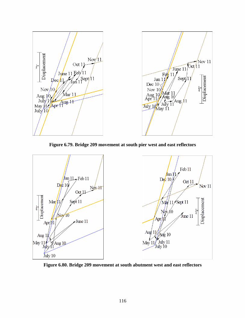
116

Figure 6.79. Bridge 209 movement at south pier west and east reflectors

Figure 6.80. Bridge 209 movement at south abutment west and east reflectors

117

Figure 6.81. Bridge 309 movement at north abutment west and east reflectors

Figure 6.82. Bridge 309 movement at north pier west and east reflectors

118

Figure 6.83. Bridge 309 movement at south pier west and east reflectors

Figure 6.84. Bridge 309 movement at south abutment west and east reflectors

119

Figure 6.85. Bridge 2208 movement at north abutment west and east reflectors

Figure 6.86. Bridge 2208 movement at north pier west and east reflectors

120

Figure 6.87. Bridge 2208 movement at south pier west and east reflectors

Figure 6.88. Bridge 2208 movement at south abutment west and east reflectors

121

Figure 6.89. Bridge 2308 movement at north abutment west and east reflectors

Figure 6.90. Bridge 2308 movement at north pier west and east reflectors

122

Figure 6.91. Bridge 2308 movement at south pier west and east reflectors

Figure 6.92. Bridge 2308 movement at south abutment west and east reflectors

123

Figure 6.93. Bridge 2408 movement at north abutment west and east reflectors

Figure 6.94. Bridge 2408 movement at north pier west and east reflectors

124

Figure 6.95. Bridge 2408 movement at south pier west and east reflectors

Figure 6.96. Bridge 2408 movement at south abutment east and west reflectors

125

Figure 6.97. Bridge 109 relative displacement between fixed pier and Girder B

Figure 6.98. Absolute movement of bottom flange of Girder B at north pier reflector

-0.6

-0.5

-0.4

-0.3

-0.2

-0.1

0

0.1

0.2

0.3

0.4

0.5

0.6

0 10 20 30 40 50 60 70 80 90 100

Dis

pla

cem

ent

(in

.)

Teff

-0.6

-0.5

-0.4

-0.3

-0.2

-0.1

0

0.1

0.2

0.3

0.4

0.5

0.6

0 10 20 30 40 50 60 70 80 90 100

Dis

pla

cem

ent

(in

.)

Teff

126

Figure 6.99. Expansion pier displacement

6.3.2 Steel Pile Behavior

Equivalent Cantilever Model

The equivalent cantilever analytical model shown in Figure 6.100 attempts to estimate the weak

axis bending moment in an integral abutment steel pile (Abendroth 2005). In the model, the steel

pile is idealized as an isolated column with an equivalent length, L, and rotationally fixed ends.

Equation 6.32 describes the relationship between the applied displacement, Δ, and the resulting

end moment, M.

(6.32)

Assuming a linear moment diagram for the pile because no intermediate forces exist, the end

moment M can be calculated from Mg by Equation 6.33.

(6.33)

The relationship between weak axis bending moment at the location of the strain gauges, Mg, and

the weak axis bending strain at the location of the strain gauges, εg, is given by Equation 6.34.

-0.5

-0.4

-0.3

-0.2

-0.1

0

0.1

0.2

0.3

0.4

0.5

0 10 20 30 40 50 60 70 80 90 100

Dis

pla

cmen

et (

in.)

Teff ( F)

127

𝜀

(6.34)

By combining Equations 6.32 through 6.34, the weak axis bending strain at the location of the

strain gauges can be expressed by Equation 6.35.

𝜀

(6.35)

Figure 6.100. Equivalent cantilever pile model

where,

Δ = applied lateral end displacement,

M = resulting end moment,

Mg = resulting moment at location of strain gauges

Le = equivalent cantilever length, and

Lg = distance between equivalent Mg moments

Pile Expansion

Figures 6.101 through 6.106 show the weak axis bending strain versus displacement for the six

instrumented piles of Bridge 309. The data in the figures come from the survey data and from the

pile strain gauge data. Each rectangle in the figures represents a survey date. The horizontal sides

of the rectangle represent the 95% confidence interval of pile displacement, at the top of the pile,

for a given survey date. The vertical sides of the rectangle represent the change in the measured

microstrain in the pile during the life of the respective survey, at the location of the strain gauge.

The solid, diagonal lines represent the theoretical relationship between pile displacement and

microstrain calculated using the analytical cantilever method. Based on the soil conditions shown

M

M

Mg

Lg

Mg

Le

M

M

∆

128

in the bridge plan set and following the work of Abendroth and Greimann, an equivalent

cantilever length of 18 ft was calculated. From there, an approximate relationship between pile

expansion and internal weak axis bending strain was plotted alongside the measured results.

In each of the figures there are a couple of survey months that show conflicting results with the

rest of the data. One of the months has a very large confidence interval and two of the months

show displacement without any resulting strain. These results have been unexplainable except

for errors in the electronic and/or survey data.

Figure 6.101. SAHP1 weak axis bending strain versus displacement

Figure 6.102. SAHP4 weak axis bending strain versus displacement

-300

-200

-100

0

100

200

300

-0.5 -0.4 -0.3 -0.2 -0.1 0 0.1 0.2 0.3 0.4 0.5

Mic

rost

rain

Δx (in.)

-400

-300

-200

-100

0

100

200

300

400

-0.5 -0.4 -0.3 -0.2 -0.1 0 0.1 0.2 0.3 0.4 0.5

Mic

rost

rain

Δx (in.)

129

Figure 6.103. SAHP6 weak axis bending strain versus displacement

Figure 6.104. NAHP1 weak axis bending strain versus displacement

-400

-300

-200

-100

0

100

200

300

400

-0.5 -0.4 -0.3 -0.2 -0.1 0 0.1 0.2 0.3 0.4 0.5

Mic

rost

rain

Δx (in.)

-400

-300

-200

-100

0

100

200

300

400

-0.5 -0.4 -0.3 -0.2 -0.1 0 0.1 0.2 0.3 0.4 0.5

Mic

rost

rain

Δx (in.)

130

Figure 6.105. NAHP4 weak axis bending strain versus displacement

Figure 6.106. NAHP6 weak axis bending strain versus displacement

Based on the figures it appears that the analytical cantilever model was a better predictor of

stress versus displacement for the HP1 piles, the piles closest to the outside curve. The

equivalent length was too large to accurately reflect the measured results of the HP4 and HP6

piles, at both abutments. The equivalent length is directly related to the pre-bored depth of each

pile as well as the soil conditions surrounding the piles. As a result, there are a number of

explanations as to why the equivalent length was artificially large, none of which the research

team could definitely narrow down.

-400

-300

-200

-100

0

100

200

300

400

-0.5 -0.4 -0.3 -0.2 -0.1 0 0.1 0.2 0.3 0.4 0.5

Mic

rost

rain

Δx (in.)

-400

-300

-200

-100

0

100

200

300

400

-0.5 -0.4 -0.3 -0.2 -0.1 0 0.1 0.2 0.3 0.4 0.5

Mic

rost

rain

Δx (in.)

131

CHAPTER 7 SHORT-TERM EXPERIMENTAL RESULTS

This chapter presents the measured strain and resolved superstructure forces from the static and

dynamic live load field described in Chapter 5. The figures in this chapter display typical

behavior of the five bridges and only represent a small amount of the total data evaluated during

the course of the assessment. Section 7.1 briefly introduces the collected strain data that will be

further interpreted in relation to superstructure forces, discussed in Section 7.2. Observations and

conclusions throughout this chapter were based on values summarized in tables that were

generated from analyses not always presented.

7.1 Strain Data

7.1.1 Girder Strains

The four girders in each bridge were one of the main focuses for assessing the superstructure

behavior under live load. Initially, plots similar to Figure 7.1 through Figure 7.8 were produced

for each of the five bridges for each of the three load paths, LP1, LP2, and LP3 (See Figure

5.39). The figures below plot the four strains measured in each girder for Bridge 309 (LP2). The

top and bottom flange tips are designated by inner, for gauges located inside of the curve, and

outer, for gauges located outside of the curve; recall Figure 5.37 for the strain gauge locations.

Figure 7.1. Bridge 309-S1 Girder A strain (LP2)

-30

-20

-10

0

10

20

30

40

50

60

70

0 30 60 90 120 150 180 210 240 270 300 330 360

Mic

rost

rain

Front Axle Position (ft)

Inner Top

Inner Bottom

Outer Bottom

Outer Top

132

Figure 7.2. Bridge 309-S1 Girder B strain for (LP2)

Figure 7.3. Bridge 309-S1 Girder C strain (LP2)

-30

-20

-10

0

10

20

30

40

50

60

70

0 30 60 90 120 150 180 210 240 270 300 330 360

Mic

rost

rain

Front Axle Position (ft)

Inner Top

Inner Bottom

Outer Bottom

Outer Top

-30

-20

-10

0

10

20

30

40

50

60

70

0 30 60 90 120 150 180 210 240 270 300 330 360

Mic

rost

rain

Front Axle Position (ft)

Inner Top

Inner Bottom

Outer Bottom

Outer Top

133

Figure 7.4. Bridge 309-S1 Girder D strain (LP2)

Figure 7.5. Bridge 309-S2 Girder A strain (LP2)

-30

-20

-10

0

10

20

30

40

50

60

70

0 30 60 90 120 150 180 210 240 270 300 330 360

Mic

rost

rain

Front Axle Position (ft)

Inner Top

Inner Bottom

Outer Bottom

Outer Top

-30

-20

-10

0

10

20

30

40

50

60

70

0 30 60 90 120 150 180 210 240 270 300 330 360

Mic

rost

rain

Front Axle Position (ft)

Inner Top

Inner Bottom

Outer Bottom

Outer Top

134

Figure 7.6. Bridge 309-S2 Girder B strain (LP2)

Figure 7.7. Bridge 309-S2 Girder C strain (LP2)

-30

-20

-10

0

10

20

30

40

50

60

70

0 30 60 90 120 150 180 210 240 270 300 330 360

Mic

rost

rain

Front Axle Position (ft)

Inner Top

Inner Bottom

Outer Bottom

Outer Top

-30

-20

-10

0

10

20

30

40

50

60

70

0 30 60 90 120 150 180 210 240 270 300 330 360

Mic

rost

rain

Front Axle Position (ft)

Inner Top

Inner Bottom

Outer Bottom

Outer Top

135

Figure 7.8. Bridge 309-S2 Girder D strain (LP2)

Strain values at the top and bottom of the girder webs were calculated by assuming linear strain

variations through the flange width (equation 7.1).

μ𝜀web = (μ𝜀inner + μ𝜀outer)/ 2 (7.1)

where,

μ𝜀inner = flange strain measured at the gauge located on the inside of the curve

μ𝜀outer = flange strain measured at the gauge located on the outside of the curve

μ𝜀web= flange strain measured at the web

Table 7.1 and Table 7.2 present the maximum strains found in each girder at each section due to

one of the three load paths. Results are separated by girder section located at S1 and S2.

Table 7.1. Maximum strain (μ𝜀) at bottom of web

Bridge Section 1 (S1) Bridge Section 2 (S2)

Girder A B C D A B C D

Bri

dge

# 309 51 48 43 52 45 40 37 47

2308 58 55 49 60 52 48 45 43

2208 48 46 40 43 46 43 41 50

209 53 52 45 52 52 49 41 41

109 43 50 49 51 - - - -

-30

-20

-10

0

10

20

30

40

50

60

70

0 30 60 90 120 150 180 210 240 270 300 330 360

Mic

rost

rain

Front Axle Position (ft)

Inner Top

Inner Bottom

Outer Bottom

Outer Top

136

Table 7.2. Maximum strain (μ𝜀) at top of web

Bridge Section 1 (S1) Bridge Section 2 (S2)

Girder A B C D A B C D

Bri

dge

# 309 5 4 7 9 4 21 9 4

2308 8 9 9 10 10 11 9 21

2208 10 7 8 9 10 9 9 15

209 7 8 6 9 26 9 6 22

109 7 8 6 8 - - - -

In examining the data, several observations were evident for the four curved bridges. First,

maximum strains in the bottom flange typically occurred in the exterior girders, A and D, at S1.

At S2, Bridges 309 and 2208, consisting of IABs, produced strains in Girder D that differed from

Girder A by only 2 μ𝜀 and 4 μ𝜀, respectively. Conversely, Bridges 209 and 2308, consisting of

SIABs, produced slightly larger strains in Girder A than Girder D by 11 μ𝜀 and 9 μ𝜀,

respectively. Although these differences are quite small, they may indicate the distribution of

live load at diaphragm sections may be influenced by the abutment type.

Strain magnitudes in the top flange were less in magnitude and often subject to the localized

effect of the truck wheels crossing the instrumented section at maximum strain locations,

represented by the spikes in strain measurements (Figure 7.6). The largest top flange strains were

produced at S2. A maximum top flange strain was measured in Girder A (Bridge 209) equal to

26 μ𝜀 compared to the largest top flange strain at S1 equal to 10 μ𝜀 (Bridges 2308 and 2208).

Bottom Flange Strain Variations

The most notable trends relate to the variations in bottom and top flanges between the inner and

outer strains. This typical behavior is not found in traditionally straight bridges, such as Bridge

109. Figure 7.9 and Figure 7.10 plot the bottom flange strains for the inner and outer flange tips

for Girder A. The two figures represent the typically larger strain variation at S1 than at S2.

Additionally, the largest strain variations typically occur in the exterior girders, A and D. These

data also indicate that the strain variations reverse from S1 to S2. For example, in Figure 7.9 the

inner strain is larger than the outer strain, while in Figure 7.10, the outer strain is larger than the

inner strain. This illustrates the reversal in direction of lateral bottom flange bending found in

horizontally curved bridges, which is influenced by the diaphragms. This is an important point as

it relates to curved girder design.

137

Figure 7.9. Bridge 309-S1 Girder A bottom flange strain (LP3)

Figure 7.10. Bridge 309-S2 Girder A bottom flange strain (LP3)

Top Flange Strain Variations

Figure 7.11 and Figure 7.12 display the top flange strain variation in S1 and S2 in girder B,

respectively. Conversely to the bottom flange, strains in the top flange typically varied most for

the interior girders, B and C, at S2 for all three load paths. Figure 7.12 shows a maximum strain

variation nearly equal to 30 μ𝜀. This behavior may represent significant girder-diaphragm

interactions transferring live loads to adjacent girders. This again emphasizes the proper

consideration of curvature influences.

-30

-20

-10

0

10

20

30

40

50

60

70

0 30 60 90 120 150 180 210 240 270 300 330 360

Mic

rost

rain

Front Axle Position (ft)

Inner

Outer

-30

-20

-10

0

10

20

30

40

50

60

70

0 30 60 90 120 150 180 210 240 270 300 330 360

Mic

rost

rain

Front Axle Position (ft)

Inner

Outer

138

Figure 7.11. Bridge 309-S1 Girder B top flange strain (LP3)

Figure 7.12. Girder B-S2 top flange strain (LP3)

7.1.2 Diaphragm Strains

Figure 7.13 through Figure 7.15 characterize typical strains recorded in the three diaphragms at

S2 for LP2. As discussed in Chapter 5, strains were measured in the top and bottom flanges at

mid points for the inner and center diaphragms. For the outer diaphragm, strains were measured

in the top and bottom flanges at the one-third points. The letter A or B on the outer diaphragm

designates that the one-third point was nearest to either Girder A or Girder B.

-30

-20

-10

0

10

20

30

40

50

60

70

0 30 60 90 120 150 180 210 240 270 300 330 360

Mic

rost

rain

Front Axle Position (ft)

Inner

Outer

-30

-20

-10

0

10

20

30

40

50

60

70

0 30 60 90 120 150 180 210 240 270 300 330 360

Mic

rost

rain

Front Axle Position (ft)

Inner

Outer

139

Figure 7.13. Bridge 309 inner diaphragm strain (LP2)

Figure 7.14. Bridge 309 center diaphragm strain (LP2)

-30

-20

-10

0

10

20

30

40

50

60

70

0 30 60 90 120 150 180 210 240 270 300 330 360

Mic

rost

rain

Front Axle Position (ft)

Top

Bottom

-30

-20

-10

0

10

20

30

40

50

60

70

0 30 60 90 120 150 180 210 240 270 300 330 360

Mic

rost

rain

Front Axle Position (ft)

Top

Bottom

140

Figure 7.15. Bridge 309 outer diaphragm strain (LP2)

Note that regardless of the diaphragm or the cross-section, the maximum tensile strain exceeds

the maximum compression strain. This indicates that in addition to being subjected to bending,

the diaphragms must also resist a tensile force. These results indicate that the outermost girder is

tending to expand radially more than the innermost girder. This is an important point as it relates

to inner and outer girder design approaches.

Table 7.3 tabulates maximum diaphragm strains recorded for each of the four curved bridges.

The maximum strain was 26 μ𝜀 in the bottom of the center diaphragm (Bridge 209). The

outer diaphragm experienced larger strains in the top and bottom flanges at the section nearest

Girder B compared to the section nearest Girder A.

Table 7.3. Maximum diaphragm strains (μ𝜀)

Inner Center Outer-B Outer-A

Diaphragm Top Bot. Top Bot. Top Bot. Top Bot.

Bri

dge

# 309 -5 11 -6 16 -8 17 6 7

2308 -5 7 -7 15 -6 21 6 3

2208 -4 7 -7 12 -9 10 2 5

209 -5 12 -6 26 -13 12 2 4

7.1.3 Dynamic Load Data

Recall from Chapter 5 that load testing also entailed at least two high speed test trials per bridge

with truck speeds ranging from 35-45 mph using LP2. These speeds are typical of truck traffic

on the bridges as they are located within an interchange. The truck driver monitored and reported

his approximate entrance and exit speeds on the bridge.

-30

-20

-10

0

10

20

30

40

50

60

70

0 30 60 90 120 150 180 210 240 270 300 330 360

Mic

rost

rain

Front Axle Position (ft)

Top-A

Top-B

Bottom-B

Bottom-A

141

Figure 7.16 represents typical dynamic strain measured at a bottom flange gauge location, where

the position of the truck was estimated.

Figure 7.16. Bridge 209-S1 dynamic loading strain in Girder A

Figure 7.17 plots the strain measured during the static load testing, which corresponds to the

same load path and location of measured strain as Figure 7.16. Figure 7.16 is superimposed onto

Figure 7.17 to produce Figure 7.18. The difference between the magnitudes of the two lines in

Figure 7.18 represents the dynamic load contribution to the overall response.

Figure 7.17. Bridge 209-S1 static loading strain in Girder A

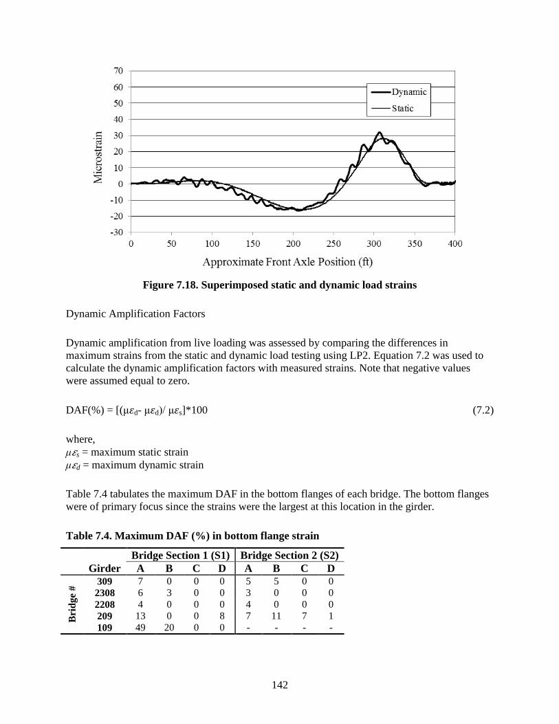
142

Figure 7.18. Superimposed static and dynamic load strains

Dynamic Amplification Factors

Dynamic amplification from live loading was assessed by comparing the differences in

maximum strains from the static and dynamic load testing using LP2. Equation 7.2 was used to

calculate the dynamic amplification factors with measured strains. Note that negative values

were assumed equal to zero.

DAF(%) = [(μ𝜀d- μ𝜀d)/ μ𝜀s]*100 (7.2)

where,

μ𝜀s = maximum static strain

μ𝜀d = maximum dynamic strain

Table 7.4 tabulates the maximum DAF in the bottom flanges of each bridge. The bottom flanges

were of primary focus since the strains were the largest at this location in the girder.

Table 7.4. Maximum DAF (%) in bottom flange strain

Bridge Section 1 (S1) Bridge Section 2 (S2)

Girder A B C D A B C D

Bri

dg

e # 309 7 0 0 0 5 5 0 0

2308 6 3 0 0 3 0 0 0

2208 4 0 0 0 4 0 0 0

209 13 0 0 8 7 11 7 1

109 49 20 0 0 - - - -

143

The most significant dynamic amplification factors were found in Girder A for all bridges at S1.

A maximum of 13% was found in Bridge 209 for the four curved bridges, which was graphically

shown in Figure 7.18. One of the high speed runs on Bridge 109 give a maximum DAF of 49%

respectively. It should be noted that the transverse positioning of the truck during the dynamic

testing was not as accurate as the static testing. This fact could contribute to some experimental

error in the determination of the experimental DAF.

Table 3.6.2.1-1 in the AASHTO LRFD specifications provides a dynamic load allowance factor

of 15% in girders for fatigue and fracture limit states and 33% in girders for limits states other

than fatigue and fracture. The calculated DAFs for the curved bridges in Table 7.4 prove to be

less than values that the AASHTO LRFD specifications used in design.

7.2 Superstructure Forces

This section utilizes the strain data, briefly shown in Section 7.1, to calculate forces in the girders

and diaphragms. Further investigation of lateral flange bending, strong axis bending, axial load,

live load distribution, and diaphragm behavior will be presented. Observations regarding

superstructure results with respect to bridge type and geometry will be made appropriately.

7.2.1 Resolving Member Forces

The composite section girder forces for the live load study are determined using the same

procedure outlined in Section 6.2.1 of this report. Refer to Figure 6.4 for the resolved girder

forces and the matrix described in Figure 6.5 for the four equations and four unknowns

associated with the cross-section. Equations 6.16 through 6.19 represent the relationships

between internal strain components and internal forces calculated within the girder that will be

used in the assessment of the live load girder response.

Similarly, Figure 7.19 depicts the forces considered in the analysis of the diaphragms for the

horizontally curved bridges. P represents the internal axial force (tension is positive). Mx

represents the internal strong axis bending moment in the diaphragm (positive when the top

flange is in compression).

144

Figure 7.19. Diaphragm cross-section

Figure 7.20 shows the matrix used to calculated P and Mx from known diaphragm dimensions

and measured field strains.

{

} [

]

{

( )

( )}

Figure 7.20. Two equations and two unknowns

where,

𝜀 = strain reading at gauge i,

= distance from neutral axis to strain gauge i along the y-axis

P = the internal axial force in the diaphragm.

Mx = strong axis bending moment in the diaphragm.

A = cross-sectional area of the diaphragm (24 in.2)

Ix = strong axis moment of inertia about the NA (3,834 in.4)

E = Young’s modulus of elasticity for steel (29,000 ksi)

7.2.2 Girder Forces

Strong Axis Bending Moment

Figure 7.21 through Figure 7.23 displays typical strong axis moments calculated for each of the

four girders in all bridges. The figures plot the strong axis moments in Bridge 309 versus truck

position for load paths LP1 through LP3, respectively. In general, LP1 typically produced the

145

largest Mx in Girder D. LP2 typically produced the largest Mx in Girders B and C. And LP3

typically produced the largest Mx in Girder A.

Figure 7.21. Bridge 309-S1 strong axis moments in girders (LP1)

Figure 7.22. Bridge 309-S1 strong axis moments in girders (LP2)

-1,100

-800

-500

-200

100

400

700

1,000

1,300

1,600

1,900

0 30 60 90 120 150 180 210 240 270 300 330

Mx

(kip

-in)

Front Axle Position (ft)

Girder A

Girder B

Girder C

Girder D

-1,100

-800

-500

-200

100

400

700

1,000

1,300

1,600

1,900

0 30 60 90 120 150 180 210 240 270 300 330

Mx

(k

ip-i

n)

Front Axle Position (ft)

Girder A

Girder B

Girder C

Girder D

146

Figure 7.23. Bridge 309-S1 strong axis moments in girders (LP3)

Table 7.5 tabulates the maximum strong axis bending moments and the associated load path in

each girder for the five bridges.

Table 7.5. Maximum Mx in girder (kip-in.)

Bridge Section 1 (S1) Bridge Section 2 (S2)

Girder A B C D A B C D

Bri

dg

e # 309 1840[LP3] 1620[LP3] 1400[LP1] 1580[LP1] 1510[LP3] 1680[LP2] 1670[LP2] 1530[LP1]

2308 1870[LP3] 1530[LP3] 1350[LP2] 1570[LP1] 1510[LP3] 1350[LP2] 1240[LP2] 1130[LP1]

2208 1340[LP3] 1340[LP3] 1210[LP2] 1210[LP1] 1300[LP3] 1320[LP2] 1340[LP2] 1180[LP1]

209 1580[LP3] 1600[LP3] 1370[LP2] 1480[LP1] 1090[LP3] 1450[LP3] 1280[LP2] 820[LP1]

109 1310[LP3] 1560[LP3] 1600[LP2] 1530[LP1] - - - -

Results show the largest strong axis moments occurred at S1 in Girder A for the two bridges with

the most severe curvature, Bridges 309 and 2308. Also at S1, Girder C produced the least

moment of all four girders for all curved bridges. For Bridges 209 and 2208, with less curvature,

more uniform moments were produced throughout the four girders at S1.

Additionally, the moment in Girder A was less at S2 compared to S1 for all curved bridges. The

straight bridge, Bridge 109, produced the largest moments in the interior two girders and the

smallest moments in the exterior two girders.

These results indicate noticeable load distribution differences to the girders for various bridge

geometries. The most significant factors influencing the distribution results may relate to bridge

radius and diaphragm location. The effects of these will further be addressed under the live load

distribution section.

-1,100

-800

-500

-200

100

400

700

1,000

1,300

1,600

1,900

0 30 60 90 120 150 180 210 240 270 300 330

Mx

(kip

-in)

Front Axle Position (ft)

Girder A

Girder B

Girder C

Girder D

147

Lateral Flange Bending Moment

Figure 7.24 and Figure 7.25 display the typical lateral bottom flange bending moments in Bridge

309. Note that the reversal in direction for the lateral bottom flange bending is illustrated by

comparing Figure 7.24 to Figure 7.25. Recall from the resolved girder forces diagram (Figure

6.4) that positive lateral flange bending values occur when strain in the flange located on the

outside of the curve is larger than the strain in the flange located towards the inside of the curve.

The apparent direction of lateral bottom flange bending is related to the diaphragm location

along the girder length, further discussed within the V-Load exploration section. A detailed

summary of the maximum lateral bottom flange bending moments and associated load path for

the tested bridges is presented in Table 7.6.

Figure 7.24. Bridge 309-S1 lateral bottom flange moments (LP3)

-20

-15

-10

-5

0

5

10

15

20

0 30 60 90 120 150 180 210 240 270 300 330

Mlb

(kip

-in

)

Front Axle Position (ft)

Girder A

Girder B

Girder C

Girder D

148

Figure 7.25. Bridge 309-S2 lateral bottom flange moments (LP3)

Table 7.6. Maximum Mlb in girders (kip-in.)

Bridge Section 1 (S1) Bridge Section 2 (S2)

Girder A B C D A B C D

Bri

dge

# 309 -15[LP3] -7[LP3] -7[LP2] -19[LP1] 11[LP2] 8[LP2] 8[LP1] 17[LP1]

2308 -8[LP3] 3[LP1] 34[LP1] -17[LP1] 8[LP2] 6[LP2] 10[LP1] 10[LP1]

2208 -8[LP3] -4[LP3] -5[LP1] 18[LP1] 14[LP3] 15[LP2] 6[LP1] -16[LP1]

209 -6[LP3] -6[LP3] -8[LP3] -5[LP2] 9[LP2] -8[LP1] -13[LP1] -7[LP1]

109 -3[LP1] -12[LP3] -5[LP1] 4[LP1] - - - -

As expected, lateral bottom flange bending proved to be more significant in the four curved

bridges compared to the straight bridge. Maximum bottom flange moments ranged from -19 to

34 kip-in. in the curved girders versus only -12 to 4 kip-in. in the straight girders. Furthermore,

the largest results were found in Bridges 309 and 2308, which have the largest curvature. These

results indicate that increased skew and curvature have direct influences on lateral bottom flange

bending.

Typical lateral top flange bending moments are illustrated in Figure 7.26, whereas a more

detailed summary of results is tabulated in Table 7.7.

-20

-15

-10

-5

0

5

10

15

20

0 30 60 90 120 150 180 210 240 270 300 330

Mlb

(kip

-in

)

Front Axle Position (ft)

Girder A

Girder B

Girder C

Girder D

149

Figure 7.26. Bridge 309-S2 lateral top flange moments (LP3)

Table 7.7. Maximum Mlt in girders (kip-in.)

Bridge Section 1 (S1) Bridge Section 2 (S2)

Girder A B C D A B C D

Bri

dge

# 309 7[LP3] 5[LP2] 4[LP1] 3[LP1] 4[LP3] -34[LP2] 20[LP2] -5[LP1]

2308 -4[LP3] -4[LP2] 3[LP1] 4[LP1] 5[LP1] 9[LP3] 8[LP2] 23[LP1]

2208 -7[LP3] 6[LP3] 5[LP1] 8[LP1] -5[LP3] -13[LP2] 23[LP2] 20[LP1]

209 -6[LP3] -4[LP3] -8[LP3] -5[LP2] -50[LP3] 5[LP2] 6[LP2] -40[LP1]

109 3[LP3] -2[LP3] -3[LP3] -2[LP1] - - - -

First, lateral top flange bending moments were much smaller than lateral bottom flange bending

moments for all bridges, particularly at S1. Lateral top flange bending moments increased at S2.

The moments in the exterior girders for Bridge 209 increased by nearly ten times the moment

found at S1 for Girder A. In Bridge 309, the largest increases were found in the interior girders.

These results indicate that lateral top flange bending moments are most significant at diaphragm

sections. However, the AASHTO LRFD Specifications permit lateral top flange bending

moments to be neglected when designing the flexural resistance of a steel girder that has the top

flange continuously braced through shear studs (6-105). Because of the smaller values produced

and the AASHTO LRFD specifications permitting the moments to be neglected, lateral top flange

bending will not be further addressed in this work.

Axial Forces

Figure 7.27 and Figure 7.28 plot the typical axial girder forces for Bridge 309 for a given load

path at S1 and S2, respectively. Note the large increase in axial force found in Girder B when

comparing S1 to S2. The maximum values are tabulated in Table 7.8.

-25

-20

-15

-10

-5

0

5

10

15

20

25

30

0 30 60 90 120 150 180 210 240 270 300 330

Mlt

(kip

-in)

Front Axle Position (ft)

Girder A

Girder B

Girder C

Girder D

150

Figure 7.27. Bridge 309-S1 axial forces in girders (LP3)

Figure 7.28. Bridge 309-S2 axial forces in girders (LP3)

Table 7.8. Maximum P in girders (kip)

Bridge Section 1 (S1) Bridge Section 2 (S2)

Girder A B C D A B C D

Bri

dg

e # 309 45[LP3] 41[LP3] 42[LP1] 57[LP1] 41[LP3] 92[LP3] 49[LP1] 38[LP1]

2308 53[LP3] 54[LP3] 46[LP2] 59[LP1] 58[LP3] 56[LP3] 45[LP1] 101[LP1]

2208 59[LP3] 50[LP3] 47[LP1] 55[LP1] 61[LP3] 54[LP3] 50[LP1] 76[LP1]

209 55[LP3] 55[LP3] 42[LP2] 59[LP1] 122[LP3] 55[LP3] 37[LP2] 95[LP1]

109 43[LP3] 48[LP3] 41[LP1] 50[LP1] - - - -

-40

-20

0

20

40

60

80

100

0 30 60 90 120 150 180 210 240 270 300 330

Ax

ial

Fo

rce

(kip

)

Front Axle Position (ft)

Girder A

Girder B

Girder C

Girder D

-40

-20

0

20

40

60

80

100

0 30 60 90 120 150 180 210 240 270 300 330

Ax

ial

Fo

rce

(kip

)

Front Axle Position (ft)

Girder A

Girder B

Girder C

Girder D

151

Results in Table 7.8 indicate that axial forces for the curved bridges are largest at S2. The forces

produced at S1 for the curved bridges are relatively uniform between adjacent girders, similar to

the straight bridge. Largest increases occurred in the exterior girders for Bridges 2308, 2208, and

209. The axial force in Girder A increased from 55 kips at S1, to 122 kips at S2 (Bridge 209).

7.2.3 Diaphragm Forces

Strong Axis Bending Moment

Figure 7.29 displays typical strong axis bending moments produced in the three diaphragms due

to a particular load path. Note the large difference in values produced in the outer diaphragm

near girder B compared to outer diaphragm near girder A. This trend is also apparent in the

results listed for each curved bridge in Table 7.9.

Figure 7.29. Bridge 309 strong axis moments in diaphragms (LP3)

Table 7.9. Maximum Mx in diaphragms (kip-in.)

Diaphragm Inner Center Outer-B Outer-A

Bri

dge

# 309 50[LP2] 70[LP2] 74[LP2] -18[LP3]

2308 35[LP2] 67[LP2] 82[LP2] -16[LP3]

2208 35[LP2] 55[LP2] 59[LP2] 18[LP2]

209 51[LP2] 96[LP2] 80[LP2] 9[LP2]

The largest strong axis moments were found at the center diaphragm and at the one-third point

nearest Girder B for the outer diaphragm. LP2 produced the maximum strong axis moments for

all bridges. Conversely, the strong axis moments were significantly smaller at the one-third point

nearest Girder A for the outer diaphragm. Overall, diaphragm strong axis moments in Bridge 209

-20

-10

0

10

20

30

40

50

0 30 60 90 120 150 180 210 240 270 300 330

Mx

(kip

-in

)

Front Axle Position (ft)

Inner Diaphragm

Center Diaphragm

Outer Diaphragm-B

Outer Diaphragm-A

152

and 2308, consisting of SIABs, were larger than the strong axis moments in Bridges 309 and

2208, consisting of IABs.

Axial Forces

Figure 7.30 depicts typical axial forces produced in the three diaphragms for the curved bridges

due to a particular load path. Table 7.10 provides a summary of maximum axial forces reported

in the diaphragms for the four curved bridges tested. Results for axial forces in the diaphragms

were all governed by LP2 in all bridges. Bridge 209 produced the largest range of axial forces

from 0.6 to 7.6 kip.

Figure 7.30. Bridge 309 axial forces in diaphragms (LP3)

Table 7.10. Maximum P in diaphragms (kip)

Diaphragm Inner Center Outer-B Outer-A

Bri

dge

# 309 2.3[LP2] 3.8[LP2] 3.3[LP2] 2.7[LP2]

2308 0.9[LP2] 3.1[LP2] 5.5[LP2] 3.0[LP2]

2208 1.3[LP2] 1.9[LP2] 0.9[LP2] 1.8[LP2]

209 2.3[LP2] 7.6[LP2] 0.6[LP2] 1.1[LP2]

7.2.4 Live Load Distribution

Live load distribution to the girders was assessed by calculating moment distribution factors in

the four girders for each bridge. Strong axis moments were used throughout this process. The

moment distribution factors were determined for single lane and multi-lane loadings for LP1,

LP2, and LP3.

-4

-2

0

2

4

6

8

10

0 30 60 90 120 150 180 210 240 270 300 330

Ax

ial

Fo

rce

(kip

)

Front Axle Position (ft)

Inner Diaphragm

Center Diaphragm

Outer Diaphragm-B

Outer Diaphragm-A

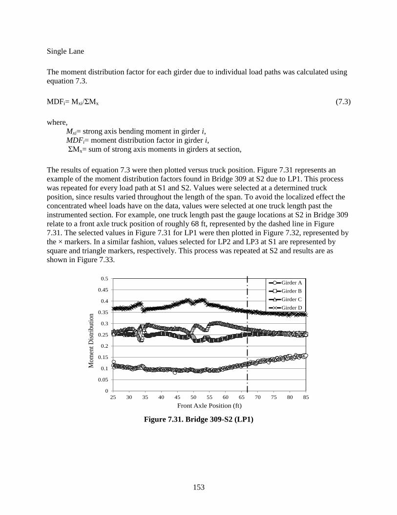
153

Single Lane

The moment distribution factor for each girder due to individual load paths was calculated using

equation 7.3.

MDFi= Mxi/ΣMx (7.3)

where,

Mxi= strong axis bending moment in girder i,

MDFi= moment distribution factor in girder i,

ΣMx= sum of strong axis moments in girders at section,

The results of equation 7.3 were then plotted versus truck position. Figure 7.31 represents an

example of the moment distribution factors found in Bridge 309 at S2 due to LP1. This process

was repeated for every load path at S1 and S2. Values were selected at a determined truck

position, since results varied throughout the length of the span. To avoid the localized effect the

concentrated wheel loads have on the data, values were selected at one truck length past the

instrumented section. For example, one truck length past the gauge locations at S2 in Bridge 309

relate to a front axle truck position of roughly 68 ft, represented by the dashed line in Figure

7.31. The selected values in Figure 7.31 for LP1 were then plotted in Figure 7.32, represented by

the × markers. In a similar fashion, values selected for LP2 and LP3 at S1 are represented by

square and triangle markers, respectively. This process was repeated at S2 and results are as

shown in Figure 7.33.

Figure 7.31. Bridge 309-S2 (LP1)

0

0.05

0.1

0.15

0.2

0.25

0.3

0.35

0.4

0.45

0.5

25 30 35 40 45 50 55 60 65 70 75 80 85

Mom

ent

Dis

trib

uti

on

Front Axle Position (ft)

Girder A

Girder B

Girder C

Girder D

154

Figure 7.32. Bridge 309-S1 single lane moment distributions for three truck lanes

Figure 7.33. Bridge 309-S2 single lane moment distributions for three truck lanes

Multi-Lane

Since the roadway width was a constant 26 ft for all bridges, 12 ft design lane widths allows two

trucks to be placed adjacent to one another. Consequently, multi-lane live load moment

distribution factors were estimated by superimposing the results from LP1 and LP3. Similarly to

the single lane moment distributions, the results from the multi-lane loading were plotted versus

truck position. Figure 7.34 and Figure 7.35 display typical results for each girder for the curved

Bridge 309 at S1 and S2, respectively. Again, individual values were selected at one truck length

beyond the instrumented section. Figure 7.36 represents the selected values for Bridge 309.

0

0.05

0.1

0.15

0.2

0.25

0.3

0.35

0.4

0.45

0.5

A B C D

Mom

ent

Dis

trib

uti

on

Girder

Inside Path

Center Path

Outside Path

0

0.05

0.1

0.15

0.2

0.25

0.3

0.35

0.4

0.45

A B C D

Mom

ent

Dis

trib

uti

on

Girder

Inside Path

Center Path

Outside Path

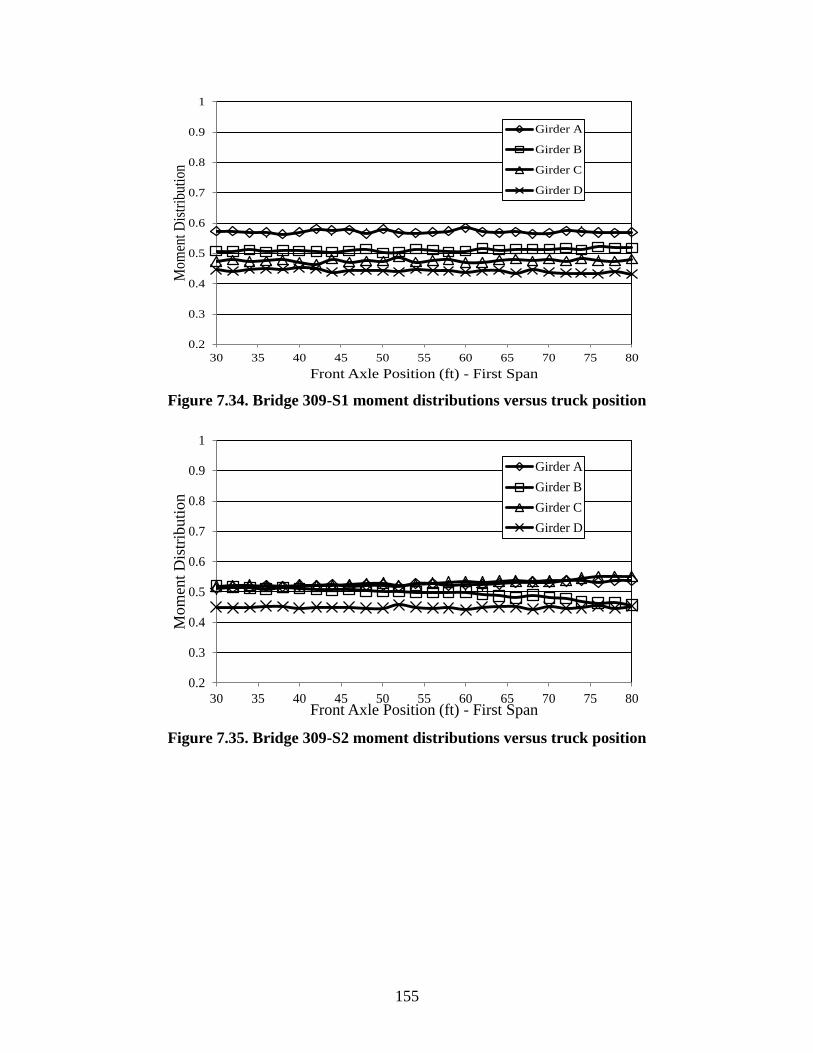
155

Figure 7.34. Bridge 309-S1 moment distributions versus truck position

Figure 7.35. Bridge 309-S2 moment distributions versus truck position

0.2

0.3

0.4

0.5

0.6

0.7

0.8

0.9

1

30 35 40 45 50 55 60 65 70 75 80

Mom

ent

Dis

trib

utio

n

Front Axle Position (ft) - First Span

Girder A

Girder B

Girder C

Girder D

0.2

0.3

0.4

0.5

0.6

0.7

0.8

0.9

1

30 35 40 45 50 55 60 65 70 75 80

Mom

ent

Dis

trib

uti

on

Front Axle Position (ft) - First Span

Girder A

Girder B

Girder C

Girder D

156

Figure 7.36. Bridge 309 maximum moment distribution factors

Tabulated results for multi-lane moment distribution factors are presented in Table 7.11. Results

are separated by their respective section, S1 and S2. The controlling value is in bold for each

girder based on the maximum value at either section and Figure 7.37 graphically represents the

controlling values shown in Table 7.11.

Table 7.11. Moment distribution factors for multi-lane live loading

Bridge Section 1 (S1) Bridge Section 2 (S2)

Girder A B C D A B C D

Bri

dge

# 309 0.57 0.51 0.49 0.43 0.53 0.51 0.52 0.44

2308 0.63 0.47 0.44 0.46 0.58 0.51 0.51 0.40

2208 0.51 0.53 0.53 0.43 0.50 0.54 0.53 0.44

209 0.53 0.52 0.49 0.47 0.46 0.56 0.58 0.40

109 0.42 0.55 0.56 0.47 - - - -

0.00

0.10

0.20

0.30

0.40

0.50

0.60

0.70

A B C D

Mom

ent

Dis

trib

uti

on

Girder

Section 1

Section 2

157

Figure 7.37. Maximum moment distribution factors in bridges

Results in Figure 7.37 indicate the largest MDFs were in Girder A for the two bridges with the

most sever curvature, Bridges 309 and 2308 with values of 0.57 and 0.63, respectively. The

interior girders produced MDF values ranging from 0.51 to 0.52 at S2. Lastly, Girder D

produced the smallest moment distribution factors of 0.44 and 0.46 in Bridges 309 and 2308,

respectively. Results show the bridges will the largest degree of curvature will distribute more

load to the exterior girder located on the outside of the curve and the least amount to the exterior

girder located on the inside of the curve.

For Bridges 2208 and 209, which consist of larger radii and skew angles, produced results more

similar to Bridge 109 than the other two curved bridges. The largest MDF was found in the

interior two girders for Bridges 2208, 209, and 109. Values for Girders B and C ranged from

0.53 to 0.58. The exterior girders in Bridges 2208 and 209 produced smaller MDFs, ranging

from 0.44 in Girder D to 0.53 in Girder A. However, Girder A was found to produce larger

MDFs than Girder D for these two bridges.

As a general comparison, the experimental MDFs were compared to approximate method of

analysis as specified by Section 4.6.2.2.2 in AASHTO. Note that these bridges do not meet the

criteria for applying the approximate level of analysis, because not all girders have the same

stiffness and the degree of curvature exceeds the limits as required in Section 4.6.1.2.4. By

applying appropriate bridge geometry, the multi-lane MDF for Bridge 309 equals 0.582 for

exterior girders and 0.623 for interior girders. These results do not match experimental values, as

the exterior girders do not have the same MDF in the curved bridges, proving in fact that the

approximate method of analysis by AASHTO is not applicable for these curved bridges.

0.3

0.35

0.4

0.45

0.5

0.55

0.6

0.65

A B C D

Mo

men

t D

istr

ibu

tio

n

Girder

Bridge 309Bridge 2308Bridge 2208Bridge 209Bridge 109

158

7.2.5 V-Load Exploration

The application of the V-Load method, which was introduced in Chapter 2 of this report, was

explored for lateral flange bending. According to Section 4.6.1.2.4b-1 in AASHTO, the effect of

curvature when calculating strong axis bending moments may be ignored when the following

criteria are satisfied:

Concentric girders

Skews less than 10⁰ from radial

Equal girder stiffness

Arc span length to radius ratio less than 0.06 radians

If the above criteria are met, then the bridge can be assumed straight and an approximate method

of analysis can be used for the bridge. However, lateral flange bending effects still need to be

considered regardless of the degree of curvature. AASHTO refers to equation 7.4, the V-Load

equation, to adequately determine the lateral flange bending due to curvature for all curvatures.

This method is sometimes used in place of a refined method of analysis. Note that the V-Load

equation does not account for skew effects. This is important, as it has been observed here that

increasing skew may increase lateral flange bending.

Mlb = MxL2/NRD (7.4)

where,

Mx = strong axis bending,

Mlb= lateral flange bending located at the presence of a diaphragm or cross frame,

L= length of the member,

N= a constant of either 10 or 12 (engineer’s discretion),

R= the radius of the girder, and

D= the depth of the web.

Based on their geometry, the four curved bridges in this study fail to satisfy the requirements that

AASHTO specifies for an approximate level of analysis for strong axis bending, because:

Girders do not have equal stiffness

Skew angles range from 15⁰ to 35⁰ Arc length to radius ratios for the end spans range from 0.061 to 0.076 radians

Consequently, AASHTO requires that a refined analysis must be employed. However, the V-

Load method still is applicable in the assessment of lateral flange bending due to curvature. The

remaining results in this section evaluate the V-Load equation with respect to Bridges 309, 2308,

2208, and 209. Equation 7.4 was rearranged as equation 7.5 to produce the ratio of lateral flange

bending to strong axis bending to ease comparison with experimental results. Table 7.12

provides the results in equation 7.5.

159

Mlb/Mx=L2/NRD (7.5)

Table 7.12. Results from AASHTO LRFD equation C4.6.1.2.4b-1

Bridge

#

Radius, R

(ft)

Web Depth, D

(ft)

N

(constant)

Diaphragm

Spacing, L (ft)

Mlb/Mx

(%)

309 950 4.0 10 18.75 0.9

2308 950 4.0 10 18.70 0.9

2208 1340 3.5 10 17.50 0.7

209 1340 3.5 10 17.20 0.6

The experimentally determined lateral bottom flange bending moments and strong axis bending

moment were plotted as ratios. Figure 7.38 shows a typical example of the experimentally

determined ratio.

Figure 7.38. Bridge 309 Girder A ratio of Mlb/Mx

Table 7.13 and Table 7.14 summarize the field results for each girder of each bridge. Values

shown under A-D are when the maximum lateral bottom flange moments occurred due to LP1,

LP2, or LP3. An average value from the four girders is provided in the last column. Note this

equation is only applicable at the diaphragm. Thus, only field results at S2 (Table 7.13) relate to

the V-Load equation results (Table 7.12).

Table 7.13 S2: Mlb/Mx (%) from field results

Girder A B C D Avg.

Bri

dge

#

309 1.3 0.5 0.8 1.2 1.0

2308 0.6 0.4 0.8 1.3 0.8

2208 1.1 1.1 0.6 1.1 1.0

209 0.9 1.2 1.3 0.9 1.1

-3.0

-2.5

-2.0

-1.5

-1.0

-0.5

0.0

0.5

1.0

1.5

2.0

2.5

3.0

20 30 40 50 60 70 80

Mlb

/Mx

(%)

Front Axle Position (ft)

Section 1

Section 2

160

Table 7.14. S1: Mlb/Mx (%) from field results

Girder A B C D Avg.

Bri

dg

e

#

309 0.8 0.5 0.6 1.3 0.8

2308 0.5 0.5 0.4 1.2 0.6

2208 0.7 0.3 0.5 1.5 0.8

209 0.4 0.5 1.0 0.7 0.6

Average results in Table 7.13 and Table 7.14 indicate larger lateral bottom flange moment to

strong axis moment ratios at S2 than ratios at S1. Additionally, results at S2 compare well with

the V-Load equation results (Table 7.12) for Bridges 309 and 2308. These two bridges have

smaller skews of only 15⁰. On the other hand, average values in Bridges 2208 and 209 were

greater than the results in Table 7.12. This increase could be a direct result of the 35⁰ skew in Bridges 2208 and 209. Overall, results indicate that the V-Load equation provides a worthy preliminary assessment for the lateral bottom flange bending moment based on the strong axis moment produced in the girder. Additional analysis would need to be performed in order to address the effects of increased skew angles. In conclusion, the V-Load method may help a designer understand the basic behavior of the diaphragm and lower girder flange, even if the numerical results may not be accurate enough for final design. This fact likely becomes more imperfect for smaller radii and larger skews.

161

CHAPTER 8 ANALYTICAL STUDY

The purpose of the work described in this chapter is to analytically investigate the superstructure

behavior of a horizontally curved bridge under design loading conditions. One bridge from the

empirical field study was modeled using a commercial finite element model (FEM) analysis

software package. The 3D rendering included main components of the superstructure system

along with simplified components for the substructure.

8.1 Introduction

Structural analysis of a bridge, in accordance to the 2010 AASHTO LRFD Specifications,

requires any method that satisfies equilibrium, compatibility, and proper stress-strain

relationships for a given material. Examples of such methods include classical, finite difference,

FEM, folded plate, finite strip, yield line, and grillage methods. Often, a horizontally curved

girder bridge requires a refined method of analysis. Section 4.6.3.3.2 states:

Refined analysis methods should be used for the analysis of curved steel bridges unless the

Engineer ascertains that approximate analysis methods are appropriate according to the provision

of Article 4.6.2.2.4 (4-69).

A refined method of analysis is defined as one that includes the superstructure as an integral

system providing adequate displacements and reactions. An engineer may neglect the horizontal

curvature component and apply approximate methods of analysis if the geometry meets certain

criteria outlined in Article 4.6.2.2.4. These criteria often pertain to limiting bridge skew,

maintaining constant cross sections, and limiting radius to arc span length ratios. Approximate

methods of analysis require significantly less effort as several assumptions are made throughout

the process. Simplifications and assumptions made in the approximate methods greatly reduce

time.

The four curved bridges of focus in this study do not meet the criteria established in Article

4.6.2.2.4 of AASHTO. Consequently, a refined analysis method must be employed. Chapter 2 of

this report categorizes three levels of analysis. Levels 2 and 3 fall under the definition of a

refined level of analysis. Based on the desired outputs from this study and relative accuracy

provided as discussed, a Level 3 analysis was selected. According to Lydzinski et al. (2008), the

finite element method is beneficial for multispan horizontally curved steel girders. Modeling

certain details in order to capture structural behaviors cannot be completed any other way.

Details such as bracing connections and element type combinations can play an important role

when analyzing a complex structure similar to the horizontally curved bridges in this study.

8.2 Model Development

Bridge 309 was selected for a detailed analytical FEM study for a number of reasons. First, this

bridge was equipped with the most instrumentation of the five bridges in the field study. This

would prove beneficial in not only validating the analytical model, but evaluating the behavior of

the structure to the fullest degree. Also, as mentioned in Chapter 5, Bridge 309 is the most

162

restrained bridge, consisting of two integral abutments and two piers fixed to translation. Lastly,

Bridge 309 has the most severe curvature with a 950 ft radius. This section will address how the

FEM attempts to represent the conditions of Bridge 309.

8.2.1 Geometry

Superstructure

Recall the Bridge 309 superstructure detailed in Chapter 5. Figure 8.1 illustrates a cross section

of the simplified dimensions of the superstructure. Steel girder dimensions follow Figure 8.2 to

include all flange thickness changes along the longitudinal length of the bridge. The concrete

deck was assumed to have a constant thickness of 8 in. and was modeled directly on top of the

steel girders. The connection between the deck and the girders is described under Section 8.2.4.

The following notable components of the superstructure were assumed to be insignificant and

were neglected for the scope of this study:

Superelevations

Differential elevation changes

Concrete haunches

Field splices

Plate stiffeners

Figure 8.1. Model superstructure cross section

Diaphragms shown in Figure 8.1 were modeled as the entire 48 in. depth of the girder web. As

indicated, web stiffeners were not included in the model, so the diaphragms were modeled as

being directly connected to the girder. Additionally, parapets models were simplified by

assuming an average constant thickness of 10 in. and directly attaching them to the deck, i.e. a

jointless connection.

4 Girders Spaced @ 7'-8"3'-8"

10"

8"

48"

Diaphragm

37"

CL Girder A CL Girder B CL Girder CCL Girder D

163

Figure 8.2. Plate girder sizes elevation view

Piers

Pier columns and beams were modeled about their centerlines. The pier columns were modeled

using tapered members starting at the base cross section, 51 in. x 53in; and increasing to the top,

51in. x 74 in.. The pier cap heights and widths were 51 in. and 74 in., respectively. Thicknesses

of the members were specified during the meshing process. Figure 8.3 illustrates the simplified

typical frame pier geometry. Since superelevation was neglected, the average distance from the

centerline of the pier cap to the bottom of the girders was determined to equal 37 ½ in..

Connections between the girders and the piers are described in Section 8.2.4.

PL 1x20 PL 2x20 PL 78 x20 PL 2x20 PL 1x20

PL 78 x20 PL 78x20

Span No. 1

23' 17' 13' 13' 17' 22'

Span No. 2 Span No. 3

PL 1 38 x20 PL 1x20PL 2x20PL 2x20PL 1x20

Web PL 716 x48 Web PL 7

16 x48 Web PL 716 x48

Girder A Plate Sizes

Girders B,C,D Plate Sizes

CL S. Abut. CL S. Pier No. 1 CL S. Pier No. 2CL N. Abut.

PL 78 x18 PL 1 78 x18 PL 78 x18 PL 1 78 x18 PL 78 x18

PL 78 x18 PL 78x18

Span No. 1

18' 15' Varies Varies 15' 18'

Span No. 2 Span No. 3

PL 1 38 x18 PL 1x18PL 1 78 x18PL 1 78 x18PL1x18

Web PL 716 x48 Web PL 7

16 x48 Web PL 716 x48

CL S. Abut. CL S. Pier No. 1 CL S. Pier No. 2CL N. Abut.

PL 34 x18 PL78 x18

164

Figure 8.3. Typical pier geometry

Abutments

The analytical abutment model utilized the as-built north/south abutment dimensions. The top

and bottom elevations, pile locations, pile cap, and backwall thicknesses were taken from the

Bridge 309 plan sheets. Abutment piles were modeled using an equivalent cantilever length of 18

ft, previously calculated in Section 6.3.2. Figure 8.4 through Figure 8.6 depict the simplified

geometry of the analytical south abutment. The north abutment geometry is identical.

Figure 8.4. Analytical model elevation view

22'-0"(avg.)

19'-2"

Pier Column

Pier Cap4'-8"

CL Girder BCL Girder A CL Girder C CL Girder D

4 Girders Spaced @ 7'-8"

165

Figure 8.5. Analytical model plan view

Figure 8.6. Analytical model end views

In order to simplify the analytical model, the wingwalls were extended the full height of the

abutment backwall and the thickness of the abutment is a constant 36 in.. Also, the portion of the

wingwall that extends forward, past the backwall was not included in the analytical model.

8.2.2 Elements

Three types of elements were used throughout the FEM, which are described below. The shell

and beam elements used are described accordingly.

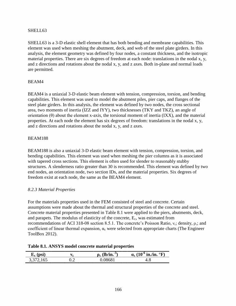
166

SHELL63

SHELL63 is a 3-D elastic shell element that has both bending and membrane capabilities. This

element was used when meshing the abutment, deck, and web of the steel plate girders. In this

analysis, the element geometry was defined by four nodes, a constant thickness, and the isotropic

material properties. There are six degrees of freedom at each node: translations in the nodal x, y,

and z directions and rotations about the nodal x, y, and z axes. Both in-plane and normal loads

are permitted.

BEAM4

BEAM4 is a uniaxial 3-D elastic beam element with tension, compression, torsion, and bending

capabilities. This element was used to model the abutment piles, pier caps, and flanges of the

steel plate girders. In this analysis, the element was defined by two nodes, the cross sectional

area, two moments of inertia (IZZ and IYY), two thicknesses (TKY and TKZ), an angle of

orientation (θ) about the element x-axis, the torsional moment of inertia (IXX), and the material

properties. At each node the element has six degrees of freedom: translations in the nodal x, y,

and z directions and rotations about the nodal x, y, and z axes.

BEAM188

BEAM188 is also a uniaxial 3-D elastic beam element with tension, compression, torsion, and

bending capabilities. This element was used when meshing the pier columns as it is associated

with tapered cross sections. This element is often used for slender to reasonably stubby

structures. A slenderness ratio greater than 30 is recommended. This element was defined by two

end nodes, an orientation node, two section IDs, and the material properties. Six degrees of

freedom exist at each node, the same as the BEAM4 element.

8.2.3 Material Properties

For the materials properties used in the FEM consisted of steel and concrete. Certain

assumptions were made about the thermal and structural properties of the concrete and steel.

Concrete material properties presented in Table 8.1 were applied to the piers, abutments, deck,

and parapets. The modulus of elasticity of the concrete, Ec, was estimated from

recommendations of ACI 318-08 section 8.5.1. The concrete’s Poisson Ratio, νc; density, ρc; and

coefficient of linear thermal expansion, αc were selected from appropriate charts (The Engineer

ToolBox 2012).

Table 8.1. ANSYS model concrete material properties

Ec (psi) νc ρc (lb/in.-3

) αc (10-6

in./in. °F)

3,372,165 0.2 0.08681 4.8

167

Steel material properties were applied to the girders, diaphragms, and abutment piles as listed in

Table 8.2. The steel’s modulus of elasticity, Es; Poisson’s ratio, νs; density, ρs; and coefficient of

linear thermal expansion, αs; were selected from Chapter 17 in the AISC Steel Construction

Manual (AISC 2007).

Table 8.2. ANSYS model steel material properties

Es (psi) νs ρs (lb/in.-3

) αs (10-6

in./in. °F)

29,000,000 0.3 0.2836 6.5

8.2.4 Boundary Conditions and Meshing

Boundary conditions varied throughout the FEM study in order to accomplish specific tasks and

comparisons. Task outlines and reasoning for changes will be noted in appropriate proceeding

sections of Chapter 8. This section discusses all boundary conditions and mesh arrangements

used in the FEM.

Girders and Diaphragms

Considering that the girder and diaphragm responses were the main focus of the FEM study,

much attention to detail went into determining their respective mesh sizes and connecting the

two entities. As previously described, the diaphragms were directly attached to the girders along

their full depth. Directly attaching these components required that girder elements and

diaphragm elements share common nodes. The diaphragms and girders are shown sharing three

common nodes in Figure 8.7. The top shared node is attached to the top flanges of the girder and

diaphragm, as well as the webs of the girder and diaphragm. The middle shared node joins the

webs of the girder and diaphragm. The bottom shared node is attached to the bottom flanges of

the girder and diaphragm, as well as the webs of the girder and diaphragm.

Lydzinski et al. (2008) described that the number of elements per girder cross section has little

influence on results. Conversely, the results are more sensitive to a finer mesh with respect to the

longitudinal length of the bridge. Lydzinski et al. further suggested that the element length

should roughly equal 2% of the span length. This percentage correlates to an element length of

20 in. for the shortest span of 85ft. Approximate element lengths of 12 in. were conservatively

chosen to account for the location of flange thickness changes. Flange thickness changes are

represented by the color changes in Figure 8.8. The web depth consisted of two elements to

produce a desirable aspect ratio near 2:1.

168

Figure 8.7. Meshed diaphragms and girders

Figure 8.8. Meshed changes in girder bottom flange thicknesses

Deck and Parapets

Rigid links connected the girders to the deck. The top flange of the girder contained the master

node, while the slave node was located in the deck. A 4 in. rigid link accounted for the difference

in elevation between the top of the girder and the centerline of the deck.

Dunker (1985) explained that the mesh size of the deck has little effect on stress and deflection

results of the superstructure. Consequently, the mesh size of the deck, shown in Figure 8.9, was

determined based on the locations of the live load and a more sensitive girder mesh size. Point

loads were used during loading, so the transverse locations of the nodes in the deck were critical

in order to properly place the loading because the live loads followed predetermined radial truck

paths. Furthermore, the longitudinal mesh size was determined by aligning nodes in the deck and

the girder. This alignment was necessary in order to align the rigid links vertically.

169

Figure 8.9. Typical meshed cross section with parapets

The parapets shown in Figure 8.9 were directly attached to the deck. Doing so requires equal

mesh sizes along the shared line.

Abutments

Both abutments were directly attached to the girders, deck, and abutment piles. Shown in Figure

8.10, the mesh geometry is irregular. Few undesired tetrahedral element shapes were formed, but

necessary in order to align the shared nodes with the correct geometry. These formations were

deemed insignificant as the superstructure’s response is assumed to be insensitive to the meshing

in the abutment.

More importantly, the abutment piles would provide the rotational restraint of the abutment as a

whole. The effective cantilevered piles were oriented such that their weak axis coincided with

the abutment centerline. All rotation and translation degrees of freedom (DOF) were restrained at

the base of the piles to represent the theorized effective cantilever.

Figure 8.10. Meshed girders and abutment

170

Piers

Rigid links also connected the bottom of the girders to the center line of the pier caps. The rigid

link nodes attached to the pier were restrained to all DOFs, while the nodes on the bottom of the

girders released rotation in the plane tangent to the curvature about the strong axis of the girders.

Releasing such the rotation represented the fixed pier condition, previously described in Chapter

5. Piers were assumed to be fixed at the base of the modeled columns. The piles and footings for

the pier were assumed to be rigid for the scope of this study. Figure 8.11 shows the typical

meshed pier, where the tapered columns can be noted. The sensitivity of the superstructure

behavior to the mesh arraignment in the piers is assumed to be insignificant. Again, nodes were

placed directly below proper girder node locations to ensure the rigid links were vertical.

Figure 8.11. Meshed pier

Simply Supported Model

The simply supported model was constructed in order to validate the FEM results in this study to

results from a consultant’s modeling. Section 8.3.3 discusses the validation. The consultant’s

design model substituted simple supports for the substructure components modeled above.

Additionally, the parapets were excluded in the consultant model, as they are not considered in

design practice; however, the field results showed that they have an influence on the

superstructure response as discussed in Chapter 6.

171

Figure 8.12. Simply supported abutment (left) and pier (right)

Abutments, piers, and parapets were removed for the simply supported FEM model. Boundary

conditions were applied at nodes in the bottom of the girder ends, where the abutments and piers

would be located (Figure 8.12). DOFs at these nodes were fixed for translation and released for

the girder’s x-axis rotation. These supports at the abutments represented classical pinned support

condition. Supports at the piers were idealized as rollers, releasing the translational DOF in the

girder’s y-axis direction and the rotational DOF about the girder’s x-axis.

8.3 Model Validation

Model validation will be achieved by comparing the FEM analysis results to two separate data

sets. First, the FEM will be tailored to compare with the experimental results presented in

Chapter 7, referred to as “field” hereafter. Additionally, a second FEM will be tailored to

compare results provided from a consulting design firm, referred to as “consultant” hereafter.

The consultant completed a 3D finite element analysis of Bridge 309 for design and agreed to

provide their output to further aid this study. The alterations made to the completed FEM will be

discussed in the accompanying subsections. Upon validation of this study’s FEM, further

exploration of design loading effects will be presented in Sections 8.4 and 8.5.

8.3.1 Data Reduction

Section 6.2.1of this report discusses the process of resolving internal composite section strains

and forces from the four measured strains at each girder cross section. The data reduction and

analysis for the analytical model will follow the same procedure outlined in Section 6.2.1. In

order to do so, strains were linearly interpolated from the FEM output for the four strain gauge

locations designated in the experimental field study.

8.3.2 Validation to Field Study

As previously mentioned, the field study comparison required the FEM to contain certain

structural entities in the model for validation. Results from the field study indicate that the

parapets influence the live load response in the superstructure, particularly the exterior girders.

Therefore, parapets were included in the FEM for live load field comparisons. In addition, all

172

substructure entities and boundary conditions described in Section 8.2.4 were incorporated for

the field study validation to simulate the as-is bridge conditions.

Live loading was applied according to the truck dimensions, axle weights, and transverse axle

locations for the static field testing discussed in Chapter 5. Prior to processing data, deflected

shapes of the model were verified at various truck positions. Figure 8.13 shows the deflected

shape for a truck positioned in the first span for the outer load path. The plotted deflections are

not to scale.

Figure 8.13. Deflected shape for outer truck position

Once several deflected shapes were plotted and reviewed, the girder strains were extracted at

Bridge Sections 1 and 2. The FEM strains were then directly compared to the strains in the field.

Directly comparing strains reduced the potential of discrepancies between FEM composite

section calculations and existing field composite sections.

While comparing strains, girder bottom flange strains were of specific interest due to their large

magnitudes relative to the top flange strains. Figure 8.14 and Figure 8.15 are typical graphs

comparing bottom flange strains at Bridge Section 1 or 2, respectively.

173

Figure 8.14. Outside path at Section 2 Girder A

Figure 8.15. Center path at Section 1 Girder B

The comparisons typically shown in Figure 8.14 and Figure 8.15 indicate that the FEM predicted

larger bottom flange strains at all girder locations for all three load paths. Upon summing the

peak bottom flange strains of all girders at a given bridge section, the results produced

174

differences ranging from 12% to 22% between FEM and field strains. The magnitude of

difference was least when the truck was centered and at Bridge Section 1. Since Bridge Section 1

is located between two diaphragm sets, results may indicate that the behavior of the modeled

girder-diaphragm interaction diverges from the actual field condition.

In addition to the increased values presented by the FEM, another key behavior is also shown in

Figure 8.14 and Figure 8.15. The FEM coordinated to the field with respect to outer versus inner

flange tip strain variations. Results from the FEM show the outer and inner flange tips varying in

strain magnitudes. This trend validates that the FEM not only predicted lateral bottom flange

bending behavior that is present in horizontally curved girders, but also the correct direction of

the lateral flange bending as it relates to the field results. Figure 8.16, viewed from the bottom of

the superstructure, plots laterally deflected girders for a centered truck in the first span of Bridge

309.

Figure 8.16. Laterally-deflected girders

A tabular summary is presented in Table 8.3 through Table 8.5, comparing maximum girder

strains averaged across the bottom flange width for the three truck paths.

Table 8.3. Center load path average bottom flange strain (μ𝜀)

Bridge Section 1 Bridge Section 2

Girder A B C D A B C D

FEM 33 44 43 30 34 38 37 29

Field 26 42 42 20 24 36 37 19

% Diff. 21 4 1 33 31 5 7 37

Table 8.4. Outside load path bottom flange strain (μ𝜀)

Bridge Section 1 Bridge Section 2

Girder A B C D A B C D

FEM 63 54 25 8 63 48 28 8

Field 51 48 20 6 45 40 22 7

% Diff. 19 11 18 25 28 15 19 22

175

Table 8.5. Inside load path bottom flange strain (μ𝜀)

Bridge Section 1 Bridge Section 2

Girder A B C D A B C D

FEM 11 25 53 62 12 27 43 57

Field 8 20 44 52 8 20 37 47

% Diff. 33 21 18 18 32 25 12 19

From the results presented in the previous tables, it was concluded analytical values match

experimental field tests reasonably well. Based on these results, the FEM validation is

considered acceptable with respect to the field results.

8.3.3 Validation to Thermal Analysis

Reported in Chapter 6, the field study measured the temperatures in the steel girders and the

concrete deck, the strains in steel girders and backwall pressures at abutments. The measured

field data at two time instants (i.e., 1/21/2011 6:00 and 7/19/2011 6:00) during cold and hot

weathers respectively are selected to validate the FE model as shown in Table 1. The differences

of strains between the two time instants were mainly induced by the change of temperatures in

the concrete deck and steel girders and backwall pressures at abutments in Table 2. The ranges of

temperatures and backwall pressures are calculated in Table 1. As indicated in Table 1, the

temperature ranges are almost the same in all girders A and D at different spans. Thus, a uniform

temperature change of the average value 86.7 ºF is applied to all the steel sections of the

superstructures in the FE model. The temperature change of 89.0 ºF is applied to concrete deck

and parapets. The average backwall pressure of 11.7 psi is applied to both south and north

abutments.

The ranges of axial strains in the sections of girders A and D at mid-center span are calculated

using the FE model and summarized in Table 2. As indicated Table 2, the strains in Girders A

and D at the mid-center span predicted using the FE model compare well with the field data.

Table 8.6. Ranges of measured temperatures and strains in Girders A and D at different

spans and backwall pressure at abutments

Temperature Range (ºF)

Back Wall Pressure

Range (psi)

Mid-

South

Span

Mid-

Center

Span

Mid-

North

Span Concrete

Deck

South

Abutment

North

Abutment A D A D A D

1/21/2011

6:00 -1.5 -1.7 -1.2 -0.4 -0.9 -1.1 -1.6 0.2 0.1

7/19/2011

6:00 85 85.3 85.1 85.8 86.2 85.8 87.4 13.6 10

Differences 86.5 87.0 86.3 86.2 87.1 86.9 89.0 13.4 9.9

Average 86.7 89.0 11.7

Note: A – Girder A; D – Girder D

176

Table 8.7. Strain range comparison between field data and FEM results

Strain Ranges in Mid-Center Span (10

-6)

Girder A Girder D

Field Data -95 -151

FEM Results -122 -133

8.3.4 Validation to Consultant Model

Similar to the field study comparison, changes in the FEM needed to be made to compare with

the consultant model. The goal was to create a FEM that closely resembled the geometry of the

consultant design model for Bridge 309. In practice, designers do not consider the parapets to

contribute to the structural stiffness of the superstructure. Therefore, the parapets were removed

for this stage of validation. Substructure entities were also removed for the consultant

comparison. Simply supported conditions, discussed in Section 8.2.4, were applied in place of

the substructure abutments and piers to correlate with the design practice of the consultant. With

these changes, the only known differences between the consultant model and the FEM pertained

to mesh sizes. The consultant meshed one element through the depth of the girder webs and

diaphragm webs with aspect ratios near 1:1. Also, deck elements were approximately twice the

size in the consultant model, compared to the FEM.

Once geometric model comparisons were finished, live loading was then applied in similar

fashion to the field study model for both the FEM and consultant analyses. Only the center and

outside load paths were considered. In post-processing, deflected shapes of the model were

verified at various truck positions. Figure 8.17 illustrates the deflected shape for a truck

positioned in the first span for the center load path. The simple supports are represented by

triangles at the abutment and first pier. All deflected shapes for the live load positions, similar to

Figure 8.17, agreed with the assumed overall structural behavior of the bridge.

Figure 8.17. Deflected shape for center truck position

177

Next, the FEM output was compared to the supplied output from the consultant design model.

The consultant presented results in terms of strong axis bending moments and lateral bottom

flange bending moments. The consultant determined strong axis bending moments based on

nodal force extractions in the composite section, Figure 8.18. Element nodal forces for the top

and bottom flange, top and bottom node of the web plate, and one nodal force in the deck plate

on each side of the girder were extracted. With the extracted forces and known locations, the

moment of the section could be summed about the section’s neutral axis.

Figure 8.18. Composite section presented by consultant

The consultant’s procedure of determining strong axis bending moments in the composite section

differed from those used in this study. Recall that moments were calculated from internal

composite section forces, described in Section 6.2.1. The results from the consultant’s procedure

would give the opportunity to validate the data reduction procedure in this study.

The validation compared calculated moments at Bridge Sections 1 and 2 for the two indicated

load paths. Typical strong axis moments and lateral bottom flange moments calculated in the

FEM are represented in Figure 8.19 and Figure 8.20, respectively, for all four girders. Each of

the four girders was then directly compared to the consultant’s results. Figure 8.21 and Figure

8.22 represent typical comparisons to lateral flange bending moments and strong axis bending

moments for Girder A.

178

Figure 8.19. FEM center path at Section 1

Figure 8.20. FEM center path at Section 2

179

Figure 8.21. Girder A center path at Section 1

Figure 8.22. Girder C center path at Section 2

180

Strong axis moments differed between the FEM and consultant by an average 6.0% at peak truck

locations in all girder sections. Furthermore, lateral bottom flange moments differed by less than

4.0 kip-in at peak truck locations in all girder sections. The FEM validation is considered

acceptable with respect to the consultant’s design model.

8.4 Design Loading

8.4.1 Load Factors and Combinations

With the validation complete, the study then investigated design loading conditions. The loading

conditions selected were based on the design limit states in accordance with the AASHTO LRFD

specification. For the scope of this study, the Strength I and Service I load combinations from

Table 3.4.1-1 in AASHTO LRFD were assumed to govern the design. These load combinations

included components for dead load, live load, water load, thermal load, wind load, settlement,

and friction load. However, for the scope of this study, only the dead, live, and thermal loads

were considered. In reference to Table 3.4.1-1, the following variables will be used.

DC=dead load of structural components and nonstructural attachments

LL=vehicular live load

IM=vehicular dynamic load allowance

TU=force effect due to uniform temperature

TG=force effect due to temperature gradient

γp=load factor for permanent loads

γTG=load factor for temperature gradient

γTU=load factor for uniform temperature

Equations 8.1 and 8.2 represent the load combinations considered throughout Chapter 8. Values

for the given load factors will be addressed in Sections 8.4.2 through 8.4.4.

Strength I=γpDC+1.75LL(1+IM/100)+ γTUTU+ γTGTG (8.3)

Service I=1.00DC+1.00LL(1+IM/100)+ γTUTU+ γTGTG (8.4)

8.4.2 Dead Load

Dead loads from the structural components included the weights of the deck, steel girders, steel

diaphragms, and parapets. Material densities from Table 8.1 and Table 8.2 were assigned to the

proper structural components in the model. In addition to the self-weight of the modeled

components, the weights of the parapets were calculated based on their average cross sectional

area of 440 in2. A distributed weight of 0.268x10

-2 k/in

2 was applied over the length of the bridge

in place of their footprint on the bridge deck.

181

Maximum and minimum load factors, γp, of 1.25 and 0.90 were applied for the Strength I load

combination. The minimum load factor was used when the force results from the live load were

not additive to the dead load results.

8.4.3 Live Load

Vehicular live loading was designated by the HL-93 load case, consisting of the combination of a

design truck or design tandem in both lanes, and the design lane load. The combination of the

design truck with the design lane load were assumed to govern for this work. Design lanes are

12.0 ft wide and the number of design lanes is based on the roadway width. Bridge 309 has a

26.0 ft roadway width, so the number of design lanes equals two.

The 0.64 klf uniformly distributed design lane load occupies a 10.0 ft transverse width within the

design lane. The load was distributed over the entire length of the bridge and superimposed on

top of the design truck load. Axle spacing and weights for the design truck load are specified in

Figure 8.23. Rear axle spacing varies between 14.0 ft and 30.0 ft to produce maximum force

effects. For the scope of this study, the 14.0 ft axle spacing was assumed to control. Since Bridge

309 has two design lanes, two design trucks were placed side by side at increments of 10.0 ft

along the bridge centerline. Placing the trucks side by side would produce maximum responses

to live load.

Figure 8.23. Design truck specifications (from Figure 3.6.1.2.2-1 AASHTO 2010)

Load factors for Strength I and Service I load combinations were taken as 1.75 and 1.00,

respectively. A vehicular dynamic load allowance of 33% was applied to the static live load

application for both load combinations. Note that only the design truck is subject to the IM.

182

8.4.4 Thermal Load

Design loads also considered two thermal loads, uniform temperature and temperature gradient.

Shown in Figure 8.24, uniform temperature is applied to the entire depth of the superstructure.

Procedure A from Section 3.12.2.1 in AASHTO LRFD was used to determine the maximum and

minimum temperatures for the model. Table 8.8 lists the temperature ranges Bridge 309

experiences. Temperature ranges are based on the classification of the bridge due to material

type and location. Bridge 309 classifies as a steel or aluminum structure located in a cold

climate. A cold climate is defined as having more than 14 days with average temperatures less

than 32⁰F.

Figure 8.24. Uniform temperature distribution

Table 8.8. Uniform temperature values

Temperature Range Lock-in Temperatures +TU -TU

-30 to 120⁰F 40 and 80⁰F 80⁰F -110⁰F

The thermal analysis assumed two lock-in temperatures for a positive (+TU) and negative (-TU)

temperature change. Lock-in temperatures were based on acceptable temperatures for placing

concrete during construction. By choosing the upper and lower bounds for acceptable pouring

temperatures, the positive and negative uniform temperatures changes could then be chosen

accordingly, listed in Table 8.8. For a positive uniform temperature change, the lock-in

temperature was assumed to be 40⁰F; yielding +TU equal to 80⁰F to reach the upper temperature

range of 120⁰F. For a negative uniform temperature change, the lock in temperature was assumed

to be 80⁰F; yielding -TU equal to -110⁰F to reach the lower range of -30⁰F.

183

Figure 8.25 diagrams the temperature gradients applied to the superstructure. Temperature 1 (T1)

and temperature 2 (T2), for the positive temperature gradient, were selected based on the

geographic bridge location in Section 3.12.3 in the AASHTO LRFD specification. Temperature 3

(T3) was calculated from the cross section depth shown in Figure 8.25. For steel superstructures,

A=12.0 in. and the location of T2 is 4.0 in. from the top of the deck. Negative values were

obtained by multiplying the positive values by -0.30 for plain concrete decks with no asphalt

overlay.

Figure 8.25. Temperature gradient

8.5 Results and Observations

In order to narrow the exploration of the design loading conditions, the study focused on results

near approximate maximum positive and maximum negative moment regions. Strains were

extracted for each of the four girders at seven cross sections along Bridge 309. Three mid-span

cross sections representing positive moment regions and four support cross sections for negative

moment regions. The sections located at mid-span are parallel to the bridge radius while the

sections near supports are parallel to the bridge skew. Recall that the supports align with the

bridge skew and intermediate diaphragms align with the radius.

8.5.1 Preliminary Results

A preliminary review of results indicated that typical trends could be characterized by two of the

seven cross sections. The center span cross section represented girder behavior for maximum

positive moment regions. The cross section at the fixed north pier represented girder behavior for

maximum negative moment regions. Initial results concentrated on relative magnitudes of strong

axis bending, lateral bending in the bottom flange, and axial forces for each loading condition.

184

Girder A, the outside girder, typically produced the maximum results at the center span and north

pier cross sections. Table 8.9 and Table 8.10 tabulate the unfactored internal forces for each of

the design loads in Girder A.

Table 8.9. Girder A unfactored internal forces at north pier

N. Pier DL LL T(+) T(-)

Mx (kip-ft) -1730 -745 98.4 -172

Mlb (kip-ft) 8.9 5.7 -23.3 31.0

P (kip) 24.0 10.7 -150.2 328

Table 8.10. Girder A unfactored internal forces at center span

C. Span DL LL T(+) T(-)

Mx (kip-ft) 1480 1030 -78.4 150

Mlb (kip-ft) -6.0 -4.7 1.2 -2.4

P (kip) -72.2 -53.3 -70.2 224

Note that live load results were recorded from peak truck positions for each respective cross

section. Also, thermal results were separated into positive and negative temperature changes.

Each temperature change combined both uniform and gradient temperatures, previously

specified.

Influences of thermal loadings proved to be present upon further assessment of Table 8.9 and

Table 8.10. A negative temperature change produced a strong axis moment nearly one-quarter of

the moment due to live loading at the north pier. Furthermore, lateral flange moments were over

six times greater than the lateral flange moments produced by the live load. Finally, thermal axial

loads were significantly greater than that of dead and live load results for all girder cross

sections.

Even though the contributions of temperature are to be included in Strength I and Service I limit

states according to AASHTO LRFD, bridge designers sometimes neglect the influences of

thermal loadings. The designers may make conservative assumptions for boundary conditions

and degrees of fixity within the structure to offset the omission of possible internal thermal

forces. Increased efforts and uncertainty in thermal analysis leads designers away from assessing

thermal loads because their influence is assumed insignificant. Regarding superstructure design,

temperatures are only taken into account in extreme design cases, deemed necessary by designer

or owner. However, since the above tables suggest that thermal loads may have contributions to

design load conditions, the study further investigated the matter. The proceeding figures in this

chapter help determine the significance of including thermal loading and/ or modeling

substructure entities.

To determine the significance, two different models will be compared in this section. This study

attempted to decide whether that assumption is appropriate by plotting the load effects for the

simply supported model, referred to as the “Simple” model, versus the model that included the

abutments and piers, referred to as the “Full” model. In summary, the models are as follows:

185

Full model: includes abutments, piers, and applies thermal, dead, and live loads (results

represented by solid lines in accompanying figures)

Simple model: assumes simple supports and applies only dead and live loads (results

represented by dashed lines in accompanying figures)

8.5.2 Service I Load Conditions

Strong Axis Bending

Girder responses to individual Service I load conditions were plotted for all four girders at the

north pier and center span cross sections. Figure 8.26 and Figure 8.27 plot the strong axis

moment results for the Service I load cases. Service I strong axis moments due to thermal loads

prove to be noticeable but less influential compared to the dead and live load results. Thermal

strong axis moments contributed a maximum of 8.8% to the total negative moment at the north

pier in Girder C. Temperature had an even less significant influence at the center span where the

maximum contribution to the total moment is 5.8% in Girder A.

Replacing substructure entities with the simply supported model produced negligible differences

in results. Less than a 3% increase in strong axis moments (center span) due to dead load and

live load were present. This slight increase may suggest the simply supported conditions do not

increase results due to dead and live load as assumed by consultant

Figure 8.26. North pier Service I loads

186

Figure 8.27. Center span Service I loads

Lateral Bottom Flange Bending

Figure 8.28 and Figure 8.29 show the lateral bending moment in the bottom flange for factored

Service I level loads. Results indicate that thermal lateral bending moments in the bottom flanges

ranged from -57 kip-ft to 43 kip-ft at the north pier. Lateral bending moments in the bottom

flanges for thermal loads were greater than dead or live loads in Girders A, B, and D at the north

pier. The exterior two girders, A and D, had the largest responses to temperature. After

combining dead, live, and thermal lateral moments in Girder D, a positive temperature increase

contributed to nearly 50% of the sum. Conversely, thermal lateral bending moments were rather

insignificant at the center span.

Replacing the substructure entities with simply supported conditions yielded smaller lateral

bending moments in the bottom flanges for dead and live load conditions. Figure 8.28 and Figure

8.29 illustrate that the simply supported model produced smaller lateral moments in the bottom

flanges in all girders at both negative and positive moment regions. The simply supported

assumption proves to be unconservative with respect to lateral bending in the bottom flange,

particularly at the pier.

187

Figure 8.28. North pier Service I loads

Figure 8.29. Center span Service I loads

Figure 8.30 demonstrates the cause of increased lateral bending in the bottom flanges at support

locations based on simple mechanics of materials. A non-composite undeformed curved member

188

subjected to a constant increase in temperature will uniformly increase in overall length and

radius of curvature. Support conditions at the piers and abutments in Bridge 309, represented in

Figure 8.30, restrain translational movement. Thus, the piers hinder the uniform deformation of

the member, especially the lower flange, which is connected directly to the pier.

Figure 8.30. Curved member subjected to temperature increase

Figure 8.31 plots the FEM deformed shape of Girder A at the north pier due to an increase in

temperature. Restraining the deformation of the horizontally curved member increased lateral

bending, particularly in the bottom flange, at the fixed pier location. The development of Figure

8.30 and the results presented in Figure 8.28 and Figure 8.31 call special attention to lateral

bottom flange bending due to temperature changes at fixed pier locations.

Figure 8.31. Girder A deflected shape due to T(+)

Axial Forces

Figure 8.32 and Figure 8.33 plot the axial forces from Service I loading conditions. Axial forces

due to thermal loads are much greater compared to the dead and live load conditions at both the

north pier and center span. Temperature changes produced average girder axial forces ranging

from -217 to 358 kips and -195 to 326 kips at the north pier and center span, respectively. The

189

axial forces produced at the north pier due to dead and live loads are small in comparison to the

thermal results. At the center span, girder axial forces due to combined dead and live loads had a

greater influence with an average of -141 kips.

Incorporating simply supported conditions had little effect on axial forces at the north pier due to

the negligible results produced from dead and live loads. However, at the center span, girder

axial forces from the simply supported model produced an average -67 kips due to combined

dead and live load. Only 48% of the axial forces produced by incorporating the substructure

model were present in the Simple model. Again, the assumption of replacing substructure entities

with simply supported conditions proves to be unconservative with respect to axial forces

produced from design loads in the superstructure.

Figure 8.32. North pier Service I loads

190

Figure 8.33. Center span Service I loads

Summary

According to the results presented in Figure 8.26 through Figure 8.33, temperature appeared to

influence the substructure behavior for Service I level loading conditions. Axial loads due to

temperature produced the most significant results as they often accounted for most of the total

force at all cross sections along the bridge. Lateral bending moments in the bottom flange proved

to be most influential for temperature changes at fixed pier locations, accounting for up to 50%

of the total lateral moment in bottom flanges. Strong axis bending moments due to temperature

were less influential; however, their presence was still noticeable as they contributed up to 8.8%

of the total moment in the composite section. Lastly, removing substructure entities and

replacing boundary conditions with the simply supported model proved to be unconservative for

the axial forces and lateral bottom flange bending moments.

8.5.3 Load Combinations

Service I level results suggest that thermal loads may be critical in the design of Bridge 309.

However, Strength I load conditions often govern the design of girder members. The

accompanying graphs of this section compare Service I and Strength I load combinations.

Strong Axis Bending

191

Figure 8.34 and Figure 8.35 plot the combinations of Strength I and Service I strong axis

moments in the composite sections. As noted, a thermal analysis was conducted for both

negative and positive temperature changes. The load combinations account for only the thermal

analysis that yielded the critical loading combination. In other words, the thermal load results

were to be additive to the dead and live load results. The solid lines represent the model that

includes the substructure entities and accounts for the thermal loads, referred to as the “Full”

model. The dashed lines represent the simply supported model that does not include thermal

loads, referred to as “Simple” in the associated figures.

Results in Figure 8.34 and Figure 8.35 show that strong axis moment magnitudes were up to

5.6% more for the Strength I Full model at the north pier compared to the Simple model. Overall,

including the substructure and incorporating thermal loads in the analysis provide only slight

variances with regards to strong axis composite section moments.

Strength I load factors produced larger moments over the Service I load factors. Magnitudes of

Strength I moments were on average 35% and 43% larger than Service I moments for each of the

four girders at the north pier and center span, respectively. Therefore, for this case the Strength I

load combination governs over the Service I load combinations for strong axis moments, as

assumed.

Figure 8.34. North pier load combinations

192

Figure 8.35. Center span load combinations

Lateral Bottom Flange Bending

Figure 8.36 and Figure 8.37 plot the combined loads for the lateral bottom flange bending

moments. Again, including thermal loads and substructure entities yield the largest lateral

moments. The impact of temperature loads in the Full model is most profound at the fixed pier

location. Lateral flange bending moments at the center span are negligible for all loading

conditions when compared to the pier locations. Service I produced slightly larger lateral

moments in the exterior girder flanges while Strength I produced larger lateral moments in the

interior girders. Because the relatively large lateral bottom flange moments are not present in the

Simple model, the Full model exemplifies the unique behavior a curved member exhibits from

thermal loads at restrained support locations.

193

Figure 8.36. North pier load combinations

Figure 8.37. Center span load combinations

194

Axial Forces

Figure 8.38 and Figure 8.39 plot the Service I and Strength I axial load combinations. Service I

produced the largest axial forces in all four girders at the north pier and in only Girders A and C

at the center span. More importantly, inclusion of the substructure model and thermal effects

yielded axial load magnitudes up to 12 times greater than the Simple model. This large increase

emphasizes the significance of a thermal analysis for determining axial loads.

Figure 8.38. North pier load combinations

195

Figure 8.39. Center span load combinations

Stresses

Observations from Figure 8.34 through Figure 8.39 indicate that both Strength I and Service I

load combinations are highly dependent on including a thermal analysis to assess strong axis

moments, lateral bottom flange moments, and axial forces in a girder section. Even though the

internal moments and forces, i.e., stress resultants, produced from temperature changes are

noteworthy, it was deemed necessary to study the effects temperature has on the stress levels. So,

for example, even though the effect of temperature on bottom flange bending moment may be

large, the effect of the bottom flange bending stress may be small relative to the major axis

bending stresses produced from dead and live load.

Table 8.11 and Table 8.12 tabulate the Strength I design load stresses at the north pier and center

span cross sections from the Full model. Results are in terms of internal components consisting

of strong axis bending stress, σx; lateral bottom flange bending stress, σlb; and axial stress, σa.

Additionally, the last four rows in Table 8.11 and Table 8.12 provide the total individual girder

stress, Σσtotal, for each loading case as well as the stresses from combined loading.

As previously stated, the stresses presented in Table 8.11 and Table 8.12 represent only two

locations--a small portion of the design stresses that are considered in practice for all cross

sections. The purpose of this portion of the study is to merely evaluate the effect that temperature

changes may have on a horizontally curved steel I-girders. In doing so, the dead and live load

results provide references to assess the relative magnitudes of the thermal results. (For this study,

the dead load stresses are based on the composite section.)

196

Table 8.11. North pier Strength I stresses

Girder DL LL T(+) Combined Loads

σx (ksi)

A -10.2 -6.1 0.3 -16.0

B -11.0 -6.4 -0.2 -17.5

C -10.2 -6.0 -0.5 -16.7

D -9.4 -5.4 -0.1 -14.8

σlb (ksi)

A -0.9 -0.8 -0.9 -2.6

B -1.1 -1.0 -0.5 -2.6

C -2.1 -1.7 -0.2 -4.0

D -3.5 -2.7 -2.0 -8.2

σa (ksi)

A 0.2 0.1 -0.8 -0.5

B -0.1 0.1 -0.9 -0.9

C -0.2 -0.1 -0.8 -1.1

D 0.1 0.3 -0.7 -0.4

Σσtotal (ksi)

A -10.9 -6.8 -1.4 -19.0

B -12.1 -7.3 -1.6 -21.1

C -12.4 -7.8 -1.5 -21.7

D -12.8 -7.8 -2.7 -23.3

Table 8.12. Center span Strength I stresses

Girder DL LL T(-) Combined Loads

σx (ksi)

A 12.4 12.1 0.5 25.1

B 11.9 11.9 0.3 24.0

C 11.3 11.4 0.3 22.9

D 10.6 10.8 0.0 21.4

σlb (ksi)

A 0.8 0.9 0.2 1.9

B 0.9 1.0 0.2 2.0

C 0.9 0.9 0.2 2.0

D 0.9 1.0 0.2 2.0

σa (ksi)

A -0.6 -0.6 1.0 -0.2

B -0.7 -0.7 1.2 -0.1

C -0.7 -0.7 1.2 -0.2

D -0.5 -0.6 1.5 0.4

Σσtotal (ksi)

A 12.7 12.4 1.7 26.8

B 12.1 12.1 1.7 25.9

C 11.5 11.6 1.6 24.7

D 11.0 11.1 1.6 23.8

Notice that Table 8.11 and Table 8.12 only provide results for one thermal load case, T(+) or

T(-). The controlling thermal load at the individual section was selected based on the critical total

stress produced in the section. An increase in temperature, T(+), was found to be the controlling

thermal case at the north pier; while on the other hand, a negative temperature change, T(-),

controlled the thermal loading at the center span in Table 8.12.

The tabulated results indicate that the strong axis bending stresses contribute most to the total

stress (for DL and LL). Strong axis bending from combined loading accounts for an average 92%

and 77% of the total stress from combined loading at the center span and north pier, respectively.

Thermal loads contribute only up to 3% of the combined strong axis bending stress in Girder C

at the north pier.

197

Contrarily, thermal loads had more influence at the fixed pier location for bottom flange bending.

In the most extreme case of Girder D, lateral bending stresses in the bottom flanges were greatest

at the north pier. After applying Strength I load factors, combined loading produced a lateral

bottom flange bending stress magnitude of 8.2 ksi. Thermal loads produced maximum lateral

flange bending stresses of 2.0 ksi. Though this quantity is less than the lateral stress produced

from the dead and live load of 3.5 ksi and 2.7 ksi, respectively, the thermal contribution to the

stress in the flange may be significant enough to account for in design. At the center span, lateral

bending stresses were less at only 2.0 ksi, due to combined loading.

Recall that significantly higher axial loads were present due to the temperature changes.

However, the constant axial force was found to be relatively small for the size of the composite

cross sectional area. Therefore, the stresses yielded less influential results. The maximum axial

stress equaled -1.1 ksi, in compression, for Girder C at the north pier due to combined loading.

Thermal axial stress accounted for -0.8 ksi of the total -1.1 ksi, indicating that temperature does

indeed account for most of the axial effects. However, axial loads only contribute minimal

stresses to the section.

After summing the stresses in individual girders for each load case, thermal loads contribute

average magnitudes of 1.8 ksi and 1.7 ksi to the total combined stress for the north pier and

center span, respectively. For Grade 50 steel, 1.8 ksi correlates to only 4% of the yield stress. As

mentioned, the maximum case existed in Girder D at the north pier. Thermal loads produced a

total stress magnitude of 2.7 ksi, or 5% of the yield stress. In conclusion, thermal stresses for

these curved bridges are small and may only add up to near 3 ksi.

198

CHAPTER 9 SENSITIVITY STUDY

In this chapter, a sensitivity study is described that was performed to investigate the influence of

bridge curvature and skew on the stresses induced in girders of an integral abutment bridge, in

particular Bridge 309. The goal of this sensitivity study is to determine the amount of curvature

that does not result in bridge behaviors significantly different from straight integral abutment

bridges. Further, the impact of having two fixed piers (as opposed to one fixed pier and one

expansion pier) on the design of these curved girder bridges will be investigated.

9.1 Curvature and Skew Effects

9.1.1 Established FE Models

To achieve the study goal, the FE modeling techniques described in Chapter 8 were utilized to

establish the components of the superstructure and substructure systems. Then, different bridge

models were established by systematically changing the degree of curvature and skew. To allow

for comparison, all other parameters of the bridge models - such as the dimensions of bridge

components, spacings of girders and diaphragms, material properties and boundary conditions,

etc. - were kept the same as the Bridge 309 model. Following analysis, the internal stresses in the

girders at different locations were studied to understand how they might be influenced by skew

and curvature.

A total of twelve FE models were established with the range of values for curvature and skew as

tabulated in Table 9.1. Note that Bridge 309 (which was the baseline for this study) has a

curvature radius of 950 ft and a skew of 15 degrees. All bridge models with a curvature radius of

20950 ft (very high curvature radius) are deemed to essentially represent the straight bridge case.

For the entire sensitivity study, the Strength I load combination was considered and included

dead load, live load, and thermal loads associated with the load factors illustrated in Section

8.4.1. Accordingly, the dead load, live load and thermal loads were applied to the bridge models

based on Sections 8.4.2, 8.4.3, and 8.4.4, respectively. Note that an average back wall pressure of

11.7 psi was applied to both the south and north abutments when considering positive

temperature change effects.

Table 9.1. Variable values of the curvature and skew

Skew, degrees Curvature Radius, ft (Curvature, 1/ft)

0 350 (0.00303) 550 (0.00182) 950 (0.00105) 20950 (0.00005)

15 350 (0.00303) 550 (0.00182) 950 (0.00105) 20950 (0.00005)

30 350 (0.00303) 550 (0.00182) 950 (0.00105) 20950 (0.00005)

199

9.1.2 Results and Discussion

Similar to the analytical work described in Chapter 8, this study focused on results near the

approximate maximum positive and negative moment regions. Strains were extracted for each of

the four girders at seven cross sections along the bridge length. Specifically, three mid-span cross

sections representing positive moment regions and four support cross sections representing the

negative moment regions were considered. Given the different curvatures and skew, the mid-

span cross sections were selected to be parallel to the bridge skew so that the cross sections are

all located the same distance from the two piers. Taking the model of Bridge 309 as an example,

the mid-span and support cross sections considered are circled in Figure 9.1. Recall that the

supports align with the bridge skew and that the intermediate diaphragms align with the radius.

Figure 9.1. Bridge 309 circled locations of extracted results

The FE results indicated that the mid-center span section and the north pier section are

representative of the locations where the most critical stresses exist. As was done previously the

stress results for Girders A and D were the focus of the sensitivity study. In the previous

experimental and analytical work, the stresses at four points (i.e., 1, 2, 3, and 4) in the girder

cross-section, as shown in figure 9.2 (similar to Figure 6.4), were discussed. As the stresses at

Points 3 and 4 were larger than Points 1 and 2, Points 3 and 4 are the focus here. Note that Points

3 and 4 are located at the outer and inner curvature of the girders, respectively (See Figure 9.2).

200

Figure 9.2. Stress points in girder section

The critical stresses in the mid-center span and north pier sections of Girders A and D are plotted

in Figure 9.3 and Figure 9.4, respectively. Critical stress in this discussion refers to the largest

sum of stresses (vertical bending plus lateral bending plus axial) in the cross section. Figure 9.3

shows that at the mid-center span section the stress in Girder A increases and the stress in Girder

D decreases with an increase of curvature regardless of the skew; further, the stresses in Girder A

and Girder D both decrease with an increase of skew regardless of the curvature. Figure 9.4

shows that for the north pier section, the stresses in Girder A and Girder D generally increase

with an increase of curvature, except for the girder D at a 0 degree skew; the stresses in Girder A

and Girder D increase with an increase of skew.

According to Section 4.6.1.2.4b-1 in the AASHTO LRFD Bridge Design Code, the effect of

curvature, when calculating strong axis bending moments, may be ignored when the following

criteria are satisfied:

concentric girders;

skews less than 10⁰ from radial;

equal girder stiffness;

arc span length to radius ratio less than 0.06 radians.

In addition to showing the actual critical stresses, Figure 9.3 and Figure 9.4 show the percentage

of the critical stress obtained for the bridge with the zero skew and 20950 ft curvature radius

(i.e., a baseline condition). For the bridge with 10⁰ sk w a d 0.06 radians arc span length to

radius ratio (i.e., a bridge meeting the geometrical requirements to ignore curvature for strong

axis bending), the critical stresses in Girder A at the mid-center span, Girder D at the mid-center

NA

x

y

2 1

4 3

P

Outer of the

curvature

Inner of the

curvature

Girder curvature

201

span, Girder A at the north pier, and Girder D at the north pier are 107%, 97%, 99%, 110% of

those in the straight bridge, respectively, as shown in Figure 9.3(a), Figure 9.3(b), Figure 9.4(a),

and Figure 9.4(a).

Figure 9.3 indicates that the maximum critical stress occurs at the mid-center span section of

Girder A. Additionally, the sensitivity study results indicated that the maximum lateral bending

stress occurs at the north pier section of Girder D (also indicated in Chapter 8). As a result, these

two sections were selected for further, more detailed analysis.

202

(a) Girder A

(b) Girder D

Figure 9.3. Critical stresses in Girder A and D at mid-center span with varying skew and

curvature

203

(a) Girder A

(b) Girder D

Figure 9.4. Critical stresses in Girder A and D at north pier with varying skew and

curvature

204

Stresses in Girder A at Mid-Center Span

Figure 9.5 indicates that the change of the total stress at Point 3 of the girder Mid-Span section is

similar to that of the stress at Point 4. However, the total stress at Point 3 is bigger for skews of 0

and 15 degrees while the total stress at Point 4 is smaller for skews of 0 and 15 degrees. Thus,

the stress at either Point 3 or 4 was selected for further analysis depending on which one is

bigger. Specifically, the stress at Point 3 was selected for Girder A at the mid-center span and the

stress at Point 4 was selected for Girder D at the north pier for further analysis. Further analysis

focused on studying the influence of different loads: dead load (DL), live load (LL), positive

temperature change (T(+)), and negative temperature change (T(-)) and the changes in various

stress components consisting of vertical bending stress, lateral bending stress, and axial stress as

they were specifically influenced by changes in curvature and skew.

The total stress and stress components at Point 3 of the mid-center span section of Girder A due

to the load combination of DL+LL+T(+) are shown in Figure 9.6(a) and Figure 9.6(b),

respectively. The total stress is similar for the 0 and 15 degree skews but the total stress is

significantly smaller for the 30 degree skew case due to the increase in lateral bending stress

shown in Figure 9.6(b). The vertical bending stress does not vary much for different skews and

increases with an increase in curvature as shown in Figure 9.6(b). Overall, the vertical bending

stress is significantly larger than the lateral bending and axial stresses as shown in Figure 9.6(b).

The lateral bending stress tends to increase when the curvature increases for the all skew cases as

shown in Figure 9.6(b). The axial stress maintains a constant value of about 3 ksi regardless of

the curvature and skew as shown in Figure 9.6(b).

The load combination of DL+LL+T(-) induces similar stress change patterns as the

DL+LL+T(+) case except that the sign of the thermal stresses are reversed as shown in Figure

9.7. Thus, future discussion will focus on the positive temperature change effects (T(+)) only.

DL and LL induce similar stress change patterns as DL+LL+T(+) as shown in Figure 9.8 and

Figure 9.9, respectively. However, T(+) induces a different stress change patterns as shown in

Figure 9.10, respectively. The total stress and component stresses at Point 3 of Girder A at the

mid-center span due to T(+) are shown in Figure 9.10(a) and Figure 9.10(b), respectively. The

total stress is generally less than about 3 ksi as shown in Figure 9.10(a). The stress components

vary slightly with skew and the lateral bending stress increases with curvature shown in Figure

9.10(b).

Note that Figure 9.6(b), Figure 9.7(b), Figure 9.8(b), Figure 9.9(b), and Figure 9.10(b) show the

percentage of the vertical bending stress in the secondary vertical axis obtained for the bridge

with the zero skew and 20950 ft curvature radius (i.e., a baseline condition).

205

(a) Point 3

(b) Point 4

Figure 9.5. Total stresses at Points 3 and 4 of Girder A at mid-center span

206

(a) Total Stress

(b) Stress Components

Figure 9.6. Total and component stresses in Girder A at mid-center span due to

DL+LL+T(+)

207

(a) Total Stress

(b) Stress Components

Figure 9.7. Total and component stresses in Girder A at mid-center span due to

DL+LL+T(-)

208

(a) Total Stress

(b) Stress Components

Figure 9.8. Total and component stresses in Girder A at mid-center span due to DL

209

(a) Total Stress

(b) Stress Components

Figure 9.9. Total and component stresses in Girder A at mid-center span due to LL

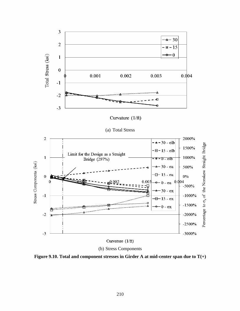
210

(a) Total Stress

(b) Stress Components

Figure 9.10. Total and component stresses in Girder A at mid-center span due to T(+)

211

Stresses in Girder D at North Pier

The total stress and stress components at Point 4 of Girder D due to the load combination

DL+LL+T(+) are shown in Figure 9.11(a) and Figure 9.11(b), respectively. The total stress in

Girder D at the north pier increases for the 15 and 30 degree skews case due, principally, to an

increase in the lateral bending stress as shown in Figure 9.11(a) and Figure 9.11(b). The vertical

bending stress does not change significantly for different skews and decreases with an increase in

curvature. The lateral bending stress increases with curvature especially for the 15 and 30 degree

skew cases as shown in Figure 9.11(b). The vertical bending stress and the lateral bending stress

are significantly larger than the axial stress as shown in Figure 9.11(a). The lateral bending stress

increases when the curvature increases for all skews as shown in Figure 9.11(b).

DL and LL induce similar stress change patterns as DL+LL+T(+) as shown in Figure 9.12 and

Figure 9.13, respectively. However, T(+) induces a different stress change patterns from

DL+LL+T(+); this indicates that the sum seems to be dominated by DL+LL. The total stress and

component stresses at Point 4 of Girder D at the mid-center span due to T(+) are shown in Figure

9.14(a) and Figure 9.14(b) respectively. The total stress is generally less than 2 ksi as shown in

Figure 9.14(a). The stress components vary slightly with skew and the lateral bending stress

decreases with an increase in curvature as shown in Figure 9.14(b).

Note that Figure 9.11(b), Figure 9.12(b), Figure 9.13(b), and Figure 9.14(b) show the percentage

of the vertical bending stress in the secondary vertical axis obtained for the bridge with the zero

skew and 20950 ft curvature radius (i.e., a baseline condition).

212

(a) Total Stress

(b) Stress Components

Figure 9.11. Total and component stresses in Girder D at north pier due to DL+LL+T(+)

213

(a) Total Stress

(b) Stress Components

Figure 9.12. Total and component stresses in Girder D at north pier due to DL

214

(a) Total Stress

(b) Stress Components

Figure 9.13. Total and component stresses in Girder D at north pier due to LL

215

(a) Total Stress

(b) Stress Components

Figure 9.14. Total and component stresses in Girder D at north pier due to T(+)

216

9.2 Pier Fixity Effects

The purpose of using expansion piers is to reduce overall bridge restraint and thereby reduce

thermal stresses. Bridge 309, which was the basis for much of the study in this project, has a

structural system consisting of two fixed piers. As a result, a question was raised regarding the

impact of this particular geometry. To evaluate the impact on thermal restraint a positive

temperature change was introduced to several analytical models. Two bridge models established

for this part of the sensitivity study included (1) a straight bridge with a skew of 0 degree and (2)

a curved and skew bridge (Bridge 309) with a skew of 15 degrees and a curvature radius of 950

ft for evaluating the skew and curvature effects. For each of the two bridge models, two types of

pier fixity (i.e., fixed south pier-fixed north pier (fixed-fixed) and fixed south pier-expansion

north pier (fixed-expansion)) were studied. Note that for the fixed pier case, the girder and pier

tangential, radial and vertical displacements are coupled; for the expansion pier case, only the

vertical displacement is coupled. Similar to Section 9.1, stresses at Point 3 of the mid-center span

section of Girders A and Point 4 of the north pier section of Girder D are used for comparisons

(See Figure 9.2).

The stress results for the straight bridge with two types of pier fixity are tabulated and compared

in Table 9.2. Table 9.2 indicates:

The vertical bending stresses slightly increased and the lateral bending stresses and the

axial stresses decrease in all girder sections when a fixed-expansion pier system is used

compared to those obtained using two fixed-fixed piers.

The critical stresses in all sections (i.e., the bigger thermal stress at Points 3 and 4) also

decrease when using a fixed-expansion pier system.

In short and as expected, using an expansion pier reduced the thermal stresses in the girders of

the straight bridge due to the reduced restraints from the supports.

The stress results for the curved and skew bridge with two types of pier fixity are tabulated and

compared in Table 9.3. Table 9.3 indicates that:

For the fixed-expansion piers, the highest thermal stresses decrease in the mid-center span

section of the girder and increase at the north pier section of the girder as compared to the

fixed-fixed condition.

The vertical bending stresses obtained using the fixed-expansion piers is larger than the

fixed-fixed condition at the mid-center span section of Girder A and the north pier section

of Girder D.

Lateral bending stresses decrease in the two sections when the fixed-expansion piers are

used.

Axial stresses using fixed-expansion piers are larger than a fixed-fixed condition at the

mid-center span section of Girder A and increase in the north pier section of Girder D.

217

Consequently, using an expansion pier does not appear to absolutely reduce the stresses in the

girders of the curved and skew bridge even though the overall restraint is reduced. This is likely

due to the complex interaction of skew, curvature, and restraint.

Table 9.2. Bridge model with a skew of 0 degrees and a curvature radius of 20,950 ft

Girder

Section Pier Fixity Type

Thermal

Stress (ksi)

Vertical

Bending

Stress (ksi)

Lateral

Bending

Stress (ksi)

Axial Stress

(ksi)

3 4 3 4 3 4 3 4

Girder A -

Mid-Center

Span

Fixed-fixed -1.8 --- -0.1 --- 0.0 --- -1.7 ---

Fixed-Expansion -1.5 --- 0.1 --- 0.0 --- -1.6 ---

Girder D -

North Pier

Fixed-fixed --- -2.4 --- 0.2 --- -1.0 --- -1.6

Fixed-Expansion --- -1.2 --- 0.3 --- -0.1 --- -1.4

Note: --- – not used for comparison

Table 9.3. Bridge model with a skew of 15 degrees and a curvature radius of 950 ft

Girder

Section Pier Fixity Type

Thermal

Stress (ksi)

Vertical

Bending

Stress (ksi)

Lateral

Bending

Stress (ksi)

Axial Stress

(ksi)

3 4 3 4 3 4 3 4

Girder A -

Mid-Center

Span

Fixed-fixed -2.2 --- -0.4 --- -0.2 --- -1.6 ---

Fixed-Expansion -1.8 --- -0.5 --- -0.1 --- -1.2 ---

Girder D -

North Pier

Fixed-fixed --- -2.7 --- -0.5 --- -1.5 --- -0.7

Fixed-Expansion --- -4.5 --- -1.0 --- -1.4 --- -2.1

Note: --- – not used for comparison

218

CHAPTER 10 SUMMARY, CONCLUSIONS, AND RECOMMENDATIONS

This chapter presents a summary of the project approach, a discussion of the measured and

analytical results, conclusions drawn from those results, and recommendations developed by the

research team.

10.1 Long-Term Experimental Study

10.1.1 Summary of Procedure

The reconstruction of the NEMM provided the opportunity to monitor the behavior of straight

and horizontally curved, steel-girder, integral-abutment bridges. There were six 26 ft wide

roadway bridges included in this work. The interchange design was such that two straight-girder

bridges were constructed with integral abutments, two curved-girder bridges were constructed

with semi-integral abutments with expansion joints, and two curved-girder bridges were

constructed with integral abutments.

The typical instrumentation plan for each bridge consisted of four girder strain gauges at the

mid-span of exterior girders on select spans, temperature sensors embedded into the concrete

deck, and expansion meters strategically placed between the bottom flange of the girders and the

pier cap and the abutment cap. On Bridge 309, six abutment piles were also instrumented with

strain gauges approximately ten inches below the bottom of the pile cap, long-range

displacement meters were installed at each abutment and pier, and pressure cells were installed

on the back face of the abutment backwalls. The bridges were monitored for a period of

approximately 15 months.

Along with the electronic instrumentation placed on the bridges, each of the six bridges was

outfitted with eight prismatic reflectors for the purpose of performing monthly surveys of the

bridges. These reflectors were placed on the bottom flange of the exterior girders near both

abutments and both piers.

10.1.2 Summary of Results

Composite Girder Strains and Forces

The axial-strain range, Δεa, at measured locations was between 70 µε and 220 µε for all six

bridges, with an average value of 153 µε. Axial thermal strains were somewhat larger for SIAB.

The strong-axis-bending strain range, Δεx, at the monitored girder locations was measured

between 20 µε and 110 µε, with an average value of 73 µε. The monitored lateral-bending strain

range for the top and bottom flanges were measured between 10 µε and100 µε and 10 µε and 120

µε, respectively. The top flange lateral-bending strain range had an average value of 31 µε and

the bottom flange lateral-bending strain range had an average value of 21 µε. Strong axes

bending and lateral bending thermal strains were similar for IAB and SAIB. Thermal axial and

219

major axis bending strains for straight and curved bridges were similar, though inside and

outside girders varied slightly for curved bridges.

The axial-force range, ΔP, for all six bridges ranged from 70 kip to 770 kip with an average

value of 596 kip. Axial forces were somewhat larger for SIAB. The strong-axis-bending moment

ranged from 1200 kip-in. to 6300 kip-in. with an average value of 4400 kip-in. The lateral-

bending strain range for the top and bottom flanges were between 13 kip-in. and 260 kip-in. and

12 kip-in. and 260 kip-in. with an average value of 43 kip-in. and 42 kip-in., respectively. Strong

axes bending and lateral bending thermal moments were similar for IAB and SAIB. Axial forces

and strong axis bending moments for straight and curved bridges were similar, though inside and

outside girder varied slightly for curved bridges

Abutment Steel Pile Strains

The axial-strain range, Δεa, in the six abutment pile instrumented locations was measured

between 60 µε and 120 µε, with an average value of 83 µε. The strong-axis-bending strain range,

Δεx, was measured between 140 µε and 240 µε, with an average value of 198 µε. The weak-axis-

bending strain range, Δεy, was measured between 590 µε and 900 µε, with an average value of

750 µε. The torsional-warping strain range, εt, measured from 20 µε to 60 µε, with an average

value of 39 µε.

The strain ranges in the piles show only a few discernible relationships with the geometry of

Bridge 309. The strong-axis bending-strain ranges are highest for HP6s, closest to Girder D.

HP4s, closest to the interior girders; show the next highest strong-axis-bending strain ranges,

followed by HP1s, closest to Girder A. The weak-axis-bending strain ranges are highest for

HP1s, followed first by HP4s, and then HP6s. This result might be expected since Girder A is

nearly eight feet longer than Girder D.

Abutment Backwall Pressure

The measured backwall soil pressure ranges were higher at the north abutment than those at the

south abutment. For the north abutment the range in the west pressure cell and the east pressure

cell were approximately 10 psi and 20 psi, respectively. For this abutment, the soil pressure

range at the obtuse side of the skewed abutment shows a greater soil pressure range than at the

acute side of the skewed abutment. This result is consistent with work presented in Abendroth

and Greimann (2005). Both the west and east pressure cells on the south abutment measured

approximately 8 psi for the soil pressure range against this abutment backwall.

The estimated axial forces in the girders due to the soil pressures against the abutments were

much lower than these forces that were computed from the measured girder strains. The

discrepancy in the girder axial forces can be explained by other restraining forces, such as forces

from the piers, piles, and pavement. Also, by assuming linear soil pressure on the abutment

backwall and equal girder force distribution made during the calculation can lead to errors in

these results as well.

220

Bridge and Span Change in Length

The measured total change in length, ∆Lmeasured , of the six bridges ranged from 1.54 in. to

2.15 in., with an average value of 1.77 in. The total change in length values by free expansion

theory, ∆Lfree, ranged from 2.14 in. to 2.32 in. The total change in length by free expansion

theory provides a conservative estimate, on average 0.43 in. or 26% higher than the measured

value. The average axial girder strain calculated from the difference between ∆Lfree and

∆Lmeasured, ∆εr, ranged from 43 µε to 154 µε with an average value of 113 µε. This average is

51 µε or 34% lower than the measured value.

For each three span bridge, the center spans experienced the greatest change in length. For all six

bridges, the change in their center span lengths range from 0.59 in. to 0.75 in. with an average

value of 0.70 in. The average difference for the change in the center span length between the

inside and outside girders was 0.03 in. or 5%. The change in length of the center span for the

bridge with an acute skew angle at the outside girder ranged from 0.32 in. to 0.58 in. with an

average value of 0.43 in. The average difference in this span length between the inside and

outside girders was 0.043 in. or 10%. The change in length of the center span for the bridges

with an obtuse skew angle at the outside girder ranged from 0.30 in. to 0.50 in. with an average

value of 0.41 in. The average difference in this span between the inside and outside girders was

0.06 in. or 18%. For all six bridges, the difference in the span length between the two end spans,

for all six bridges, ranged from 0.015 in. to 0.045 in. with an average value of 0.03 in. or 7%.

Abutment and Pier Displacements

As shown in the bridge deflected shape figures presented earlier, the girders typically expanded

during warmer temperatures and contracted during colder temperatures. Generally, longitudinal

bridge displacement at expansion piers would show a larger displacement range than that at fixed

piers. One of the semi-integral abutment bridges, Bridge 209, shows a larger displacement range

at the abutments than that for all of the integral abutments, but the other semi-integral abutment

bridge, Bridge 2309, shows a displacement range similar in value to most of the integral

abutments.

Effective Thermal Length

An effective thermal length was calculated for all fixed bearing locations. The effective thermal

lengths for the integral abutments were all longer than the length of their respective adjoining

span. The effective thermal lengths for the fixed piers were all shorter than the longest adjacent

span. In situations where the center span is between two fixed piers, the Iowa DOT uses half the

length of the center span for the effective thermal length. The effective thermal length used by

the Iowa DOT is conservatively longer when compared to the effective thermal lengths obtained

from this study.

221

Fixed and Expansion Pier Displacement

According to collected data, the maximum range in the girder-to-expansion pier relative

displacements were around 0.6 in. The displacements essentially show a linear relationship with

regard to the effective bridge temperature until the temperatures approached 100 °F and 0 °F at

which point they behave nonlinearly. A correlation between the survey and expansion meter

results varied from month to month. In some cases the two data sets overlap one another and in

some cases they show a difference of up to 0.2 in. This inconsistency most likely stems from

accuracy issues within the survey data.

Abutment Steel Pile Cantilever Model

The results from the abutment steel pile equivalent cantilever model, as described by Abendroth

and Greimann (2005), fell short of accurately predicting the relationship between the weak axis

bending strain in the piles and the pile head displacement. According to the strain gauge data and

the survey results, the measured strain was anywhere between 50 and 150 µε higher than the

values predicted by the model. The accuracy of the survey data could be a possible explanation

for the difference in results, as well as a possible difference between the actual pile pre-bore

depths and the pre-bore depths shown on the plan, effectively shortening the effective length and

increasing the resulting strains.

Abutment Steel Pile Strain versus Expansion

According to the measured strains and displacements, the abutment steel pile strains and the

bridge expansion show a linear relationship. According to the data, the SAHP1 pile shows a

strain range of approximately 470 µε under roughly 0.95 in. displacement, the SAHP4 pile

shows a strain range of approximately 600 µε under 0.75 in. displacement, and the SAHP6 pile

shows a strain range of approximately 620 µε under a 0.75 in. displacement. Also according to

the data, the NAHP1 pile shows a strain range of approximately 650 µε under a 0.95 in.

displacement, the NAHP4 pile shows a strain range of approximately 620 µε under a 0.95 in

displacement, and the NAHP6 pile shows a strain range of approximately 610 µε under a 0.70 in.

displacement.

10.1.3 Conclusions and Recommendations

Instrumentation

All of the electronic instrumentation (vibrating wire strain gauges, vibrating wire displacement

meters, vibrating wire displacement meters, thermistors, and vibrating wire pressure transducers)

performed acceptably with few problems occurring. The displacement data obtaining using

surveying techniques were acceptable for this study but not as accurate as hoped with errors of

the order of 0.3 in.

222

Internal Composite Girder Strains and Forces

The internal axial girder strain showed the largest ranges of all the resulting strains from the

measured girder strain gauge data, with the largest range being 220 µε. For Grade 50 steel the

resulting stress is 6.4 ksi or roughly 13% of the yield stress. By superimposing the four

calculated internal strains, the results can exceed 400 µε, giving 11.6 ksi or 23% of yield stress

for Grade 50 steel. Although the composite girders have substantial resistance to the effects of

thermal loading, this does not consider the effects of other loading conditions.

Abutment Steel Pile Internal Strains

The relationship between abutment steel pile internal axial strain and effective bridge

temperature varied depending on the pile location with respect to the abutment pile cap. The

measured results showed either a proportional, inversely proportional, or erratic relationship

between internal axial strain and effective bridge temperature. This behavior could impact design

and further investigation into the phenomena should be undertaken.

The greatest weak axis bending strain, in fact the greatest of all the measured strains, to be

resisted by any of the monitored abutment piles was the NAHP1 pile at 900 µε. The stress in the

section because of the strain equals 26.1 ksi, which amounts to 52% of the yield stress for Grade

50 steel. When considering just weak axis bending, the HP 10x57 piles used as support for the

integral abutments in this study had appropriate resistance.

By superimposing the four different abutment pile internal strain ranges on one another, the

largest possible strain felt by any of the piles was 1225 µε. The stress in the section equates to 36

ksi or 72% of the yield stress of Grade 50 steel. From the results of this study, the piles used for

support of the integral abutments at the NEMM had sufficient resistance to thermal expansion;

however, this is without considering the effects of other loading conditions. Further investigation

into the behavior of abutment piles of horizontally curved integral abutment bridges is suggested.

10.2 Short-Term Experimental Study

10.2.1 Summary of Procedure

Five of six bridges at the NEMM were selected to be live load tested. Static and dynamic truck

loads were applied to the bridge using varying load paths. Monitoring the response of each

bridge due to the various truck positions was prepared by instrumenting the girders and

diaphragms of the bridge superstructures. Each of the four curved bridges was equipped with 40

strain transducers at two radial cross sections and one straight bridge was equipped with 16 strain

transducers at a single cross section. Four strain transducers were placed on both the top and

bottom flanges of each girder at the instrumented cross section. Strain transducers for the

diaphragms, in the curved bridges, were placed on the top and bottom flanges at mid and one-

third points for the purpose of monitoring girder-diaphragm interactions.

223

10.2.2 Summary of Results

Girder Forces

The largest strong axis moments occurred at S1 in Girder A for the two bridges with the most

severe curvature, Bridges 309 and 2308. Maximum values reached almost 1900 kip-in. The other

two curved bridges produced more uniform strong axis moments and the straight bridge

produced larger strong axis moments in the interior girders compared to the exterior girders.

Additionally, the moment in Girder A was less at S2 compared to at S1 for all curved bridges.

Lateral bottom flange bending moments proved to be more significant in the four curved bridges

compared to the straight bridge as maximums ranged from -19 to 34 kip-in. in the curved

bridges. The reversal in the lateral bending direction for the bottom flange was also noted when

comparing results at S1 to S2. This trend was expected as curved bridges exhibit an S-shaped

bending behavior, which is related to the diaphragm location along the girder.

Lateral top flange bending moments were much smaller than bottom flange bending moments at

S1, ranging from -8 to 7 kip-in. Results at S2 produced outliers as the top flange was subject to

the localized effect of the concentrated wheel loads.

Axial forces for the curved bridges were largest at S2. An axial force increase of 67 kip in Girder

A was produced from S1 to S2 in Bridge 209 under LP3. Similar trends were consistent

throughout the four curved bridges.

Dynamic Amplification Factors

A maximum DAF equal to 13% for the four curved bridges was found in Bridge 209. Bridge

109, the straight bridge, produced a 49% DAF in an exterior girder that may have been due to

experimental errors during the dynamic testing. Overall, the experimental DAFs for the curved

bridges proved to be less than the values specified by the AASHTO LRFD Specifications for all

limit states.

Moment Distribution Factors

Experimental results produced the largest MDFs in Girder A for the bridges with the most severe

curvature, Bridges 309 and 2308, equal to 0.57 and 0.63, respectively. The interior girders,

Girders B and C, ranged from 0.51 to 0.52 and the innermost exterior girder, Girder D, ranged

from 0.44 to 0.46. For Bridges 2208 and 209, the two exterior girders ranged from 0.44 in Girder

D to 0.53 in Girder A.

Calculating MDFs for Bridge 309 using the approximate method of analysis in AASHTO

produced MDFs equal to 0.58 in both exterior girders and 0.62 in both interior girders.

224

V-Load Exploration

The experimental ratios of Mlb/Mx for each girder produced average results ranging from 0.8 to

1.1% for the four curved bridges at S2. These values correspond to ratios calculated from the V-

Load equation. Based on bridge geometry, the V-Load equation produced ratios ranging from 0.6

to 0.8%. Experimental values for Bridges 309 and 2308 matched well with the V-Load equation

results, while experimental values for Bridges 209 and 2208 were larger than the V-Load

equation results.

Diaphragm Forces

The largest strong axis bending in the diaphragms were recorded due to LP2 in the center

diaphragm and the outer diaphragm sections located nearest Girder B for all curved bridges.

Axial forces reached maximums of nearly 8 kips in tension in the center diaphragm in Bridge

209.

10.2.3 Conclusions and Recommendations

Based on the results from the live load field testing and assessment, it was concluded that live

load moment distribution factors were primarily influenced by the degree of curvature. The

largest MDFs were found in Girder A for the two bridges with the most severe curvature,

Bridges 309 and 2308. The MDFs for Girder A in Bridges 2208 and 209, which have less severe

curvature, were in between the results for the straight bridge and the results for the two bridges

with more severe curvature. No conclusions were drawn related to support conditions or skew

angles. Furthermore, the live load field testing results found that the V-Load equation provided a

decent preliminary estimate of Mlb based on the magnitude of Mx and the degree of curvature in

the girder near a diaphragm. However, as the skew increased in Bridges 2208 and 209, the V-

Load equation under predicted the magnitude of Mlb.

Dynamic amplification values were well below specified code values for all curved girders. The

DAFs in Bridge 109 may very well be due to experimental error and contain no amount of

confidence.

Diaphragms were found to be subjected to both bending and tensile axial forces. This indicates

that the outermost girder is tending to expand radially more than the innermost girder, an

important point to note in outer versus inner girder design approaches.

10.3 Analytical Study

10.3.1 Summary of Procedure

A single bridge of the empirical field study at the NEMM was subject to further analytical study.

A FEM static analysis was performed to investigate the superstructure behavior under design

225

loading conditions, particularly the thermal loads. Bridge 309 was selected because it had the

most severe curvature, greatest level of restraints, and it was equipped with the most field

instrumentation. The FEM used a combination of 3-D beam shell elements to model key

superstructure and substructure entities. Once the model was completed, results from the

empirical field study were used to validate the model and increase the confidence of the

analytical output. Finally, design loading conditions were applied to the FEM in order to

complete the investigation.

10.3.2 Summary of Results

FEM Validation

Girder strains were used as a basis for comparison with the measured field results. For the live

load comparison, after summing the peak bottom flange strains of all girders at a given bridge

section, the FEM produced strains 12% to 22% larger than the live load field results. Next, the

FEM was compared with the thermal field results through proportioning effective bridge

temperatures. Axial strains were approximately 18% larger in the outside girder, Girder A, for

the FEM versus thermal field results comparison. Lastly, computed girder forces in the FEM

were compared with the provided consultant FEM results. The FEM in this study produced

strong axis moments that differed by an average 6.0% and lateral bottom flange bending

moments that differed by less than 4.0 kip- in. at peak truck locations in all girder sections when

compared to the consultant’s results.

Strong Axis Bending

Strength I load conditions governed over Service I load conditions, producing larger strong axis

bending moments by up to 43%. When comparing the Full model to the Simple model, Strength

I strong axis bending moments were 5.6% greater for the Full model at the north pier.

With regards to girder stresses, Strength I strong axis bending due to only DL and LL

contributed most to the total stress in the bottom flange. At the center span, the DL and LL

accounted for 92% of the total stress in the bottom flange. The addition of thermal loads

contributed only 3% more stress to the combined strong axis bending stress in a single girder.

Lateral Bottom Flange Bending

Lateral bottom flange bending was most noticeable at the fixed north pier as moments reached

near 90 kip-ft. Service I produced slightly larger lateral moments in the exterior girder flanges

while Strength I produced larger lateral moments in the interior girders. On the other hand, the

simple model produced negligible lateral bottom flange bending results at both the center span

and north pier as moments were less than 20 kip-ft.

Considering that Strength I load combinations produced such dominate strong axis bending

stresses in the Full model, only the Strength I lateral bottom flange bending stresses were

226

calculated. At the north pier, lateral bottom flange bending produced stresses up to 2.0 ksi due to

thermal loads alone.

Axial Forces

Axial forces were much greater in the Full model compared to the Simple model along the entire

length of the bridge. Service I produced the largest axial forces at the center span and similar

forces to Strength I at the North Span. Despite the large axial forces, axial stresses were deemed

less significant. Thermal axial stresses were less than or equal to 1.5 ksi in each girder at both

sections.

10.3.3 Conclusions and Recommendations

Based on analytical analysis results, Strength I lateral bottom flange bending moments were

nearly 10 times greater when including temperature effects at the fixed pier. Moreover, Strength

I axial forces were nearly three times greater when accounting for temperature effects compared

to only DL and LL. These results indicate that temperature is an essential consideration when

addressing member forces. However, in design it is more important to determine the level of

stress produced in the section.

With regards to stresses, thermal-induced stresses in horizontally curved steel I-girder bridges

similar to Bridge 309, with radii greater than 950 ft, are small. Thermal stresses may only add an

additional stress of up to 3 ksi in the bottom flange. However, special attention has been drawn

to translationally-restrained locations, such as fixed piers, for exterior girders as lateral bottom

flange bending has become more prevalent. In conclusion, the findings from this investigation

are not alarming; however, thermal loading may require further consideration in the future design

of horizontally curved bridges that incorporate restrained supports with increasing degrees of

curvature and skew.

10.4 Sensitivity Study

10.4.1 Summary of Procedure

A sensitivity study was performed to investigate the influence of curvature and skew on the

stresses induced in the girders of an integral abutment bridge, in particular Bridge 309. A total of

twelve bridge models were established by changing the degree of curvature and skew and

keeping all other parameters of the bridge models the same as the as-constructed Bridge 309.

Following analysis, the internal stresses in the girders at different locations were studied to

understand how they might be influenced by skew and curvature.

Further, the impact of having two fixed piers (as opposed to one fixed pier and one expansion

pier) on the behavior of these curved girder bridges was investigated. Two pairs of models were

established for this portion of the sensitivity study and included (1) a straight bridge and (2) a

curved plus skewed bridge. For each of the two bridge models, two types of pier fixity (i.e., fixed

227

south pier-fixed north pier (fixed-fixed) and fixed south pier-expansion north pier (fixed-

expansion)) were evaluated.

10.4.2 Summary of Results

Critical Stresses

The FE results indicated that the mid-center span section and the north pier section are

representative of the locations where the most critical stresses exist. For the mid-center span

section, the critical stress in Girder A increases and the critical stress in Girder D decreases with

an increase of curvature regardless of the skew; furthermore, the critical stresses in Girder A and

Girder D both decrease with an increase of skew regardless of the curvature. For the north pier

section, the critical stresses in Girder A and Girder D generally increase with an increase in

curvature, except for girder D at a 0 degree skew; the critical stresses in Girder A and Girder D

both vary with different skews regardless of the curvature. For the bridge with 10⁰ sk w a d a 0.06 radians arc span length to radius ratio (i.e., a bridge meeting the geometrical requirements

allowing curvature to be ignored for determining strong axis bending), the stresses in Girder A at

the mid-center span, Girder D at the mid-center span, Girder A at the north pier, and Girder D at

the north pier are 107%, 97%, 99%, 110% of those in the straight bridge, respectively.

Stresses in Girder A at Mid-Center Span

Due to the load combination of DL+LL+T(+), the total stress is similar for the 0 and 15 degree

skews but the total stress is significantly smaller for the 30 degree skew case due to an increase

in lateral bending. The vertical bending stress does not change significantly for different skews

but increases with an increase in curvature. Overall, the vertical bending stress is significantly

larger than the lateral bending and axial stresses. The lateral bending stress tends to increase

when the curvature increases for all skews. The axial stress maintains a constant value of about 3

ksi regardless of the curvature and skew. The load combination of DL+LL+T(-) induces similar

stress change patterns as the DL+LL+T(+) case except that the sign of the thermal stresses are

reversed.

Stresses in Girder D at North Pier

Under load combination of DL+LL+T(+), the total stress in Girder D at the north pier increases

for the 15 and 30 degree skews due to an increase in the lateral bending stress. The vertical

bending stress does not change much for different skews and decreases with an increase in

curvature. The lateral bending stress increases with curvature especially for the 15 and 30 degree

skew cases. The vertical bending stress and the lateral bending stress are significantly larger than

the axial stress. The lateral bending stress increases when the curvature increases for all skews.

Due to T(+), the total stress, is generally less than 2 ksi and the stress components vary slightly

with skew and the lateral bending stress decreases with an increase in curvature.

228

Pier Fixity Effects

For the straight bridge, the vertical bending stresses slightly increased and the lateral bending

stresses and the axial stresses decrease in all girder sections when a fixed-expansion pier system

is used compared to those obtained using two fixed piers. The critical stresses also decrease

when using a fixed-expansion pier system.

For the curved and skew bridge, the maximum thermal stresses decrease at the mid-center span

section of Girder A and increase in the north pier section of Girder D, respectively, when using

fixed-expansion piers as opposed to fixed-fixed piers. The vertical bending stresses obtained

using the fixed-expansion piers increase in the mid-center span section of Girder A and the north

pier section of Girder D. When the fixed-expansion pier configuration is used, the lateral bending

stresses decrease in the two sections and axial stresses decrease at the mid-center span section of

Girder A and increase at the north pier section of Girder D.

10.4.3 Conclusions and Recommendations

The stresses in the girders of integral abutment bridges significantly vary with changes in skew

and curvature. Due to dead and live loads, the change in pattern of the vertical bending stress and

axial stress are easy to follow and the change in pattern of the lateral bending stress varies

significantly with respect to different skews and curvature. Due to temperature change, the

patterns of all stress components vary significantly with respect to different skews and curvature.

The largest critical stress occurs in the outer girder at mid-center span and the largest lateral

bending stress occurs at the inner girder at the pier. With a 10⁰ sk w a d 0.06 radians arc span

length to radius ratio (i.e., meeting the geometrical requirements to ignore curvature for strong

axis bending), the curved and skew integral abutment bridges can be designed as a straight

bridge if a stress tolerance of 10% is acceptable. If a designer cannot accept an apparent 10%

error in stress estimation (even when meeting the geometrical requirements outlined in

AASHTO), the designer is advised to use a more discretized modeling approach.

Using an expansion pier reduces the thermal stresses in the girders of the straight bridge due to

the reduced restraints from the supports but does not appear to absolutely reduce the stresses in

the girders of the curved and skew bridge even though the overall restraint is reduced.

10.5 Design Suggestions

Thermal stresses should be included in all appropriate load combinations as per the

AASHTO Bridge Design Specifications.

For preliminary member sizing of curved bridges, thermal axial stresses and movements

in a straight bridge of the same length are a reasonable first approximation.

For preliminary member sizing, thermal major axis bending and lateral bending stresses

in curved bridges are about the same as for straight bridges.

229

Stresses for other loadings other than thermal should follow AASHTO recommendations

and guidelines. However, designers should realize that even if AASHTO Specifications

allow simpler bridge models that internal forces may be underestimated.

The choice between IAB and SIAB should be based on life – cycle costs, e.g.,

construction and maintenance. Differences in thermal stresses are not significant for the

bridges studied in this work.

An expansion pier does reduces the thermal stresses in the girders of the straight bridge

but does not appear to absolutely reduce the stresses in the girders of the curved and skew

bridge even though the overall restraint is reduced.

Since AASHTO requires a three-dimensional analytical model of the bridge and support

conditions to calculate lateral bending stresses for the final design of all curved bridges,

this model should also be used to calculate thermal stresses for final design of the curved

bridge. However, with a 10⁰ sk w a d 0.06 radians arc span length to radius ratio (i.e.,

meeting the geometrical requirements to ignore curvature for strong axis bending), the

curved and skew integral abutment bridges can be designed as a straight bridge if a stress

tolerance of 10% is acceptable.

231

REFERENCES

Abendroth, E. R., and L. F. Greimann. 2005. Field Testing of Integral Abutments. Center for

Transportation Research and Education. Iowa State University. Ames, IA.

American Institute of Steel Construction Inc. 2007. Steel Construction Manual Thirteenth

Edition. United States: American Institute of Steel Construction, Inc.

Barker, R. M., J. M. Duncan, K. B. Rojiani, P. S. K. Ooi, C. K. Tan, and S. G. Kim. 1991.

Manuals for the Design of Bridge Foundations. NCHRP Report 343. Washington, DC:

Transportation Research Board, National Research Council.

Barr, P. J., N. Yanadori, M. W. Halling, and K. C. Womack. 2007. “Live-Load Analysis of a

Curved I-Girder Bridge.” Journal of Bridge Engineering. ASCE, 11(2), 160-168.

Coduto, Donald P. 2001. Foundation Design Principles and Practices: Second Edition. New

Jersey: Prentice Hall.

Doust, S. 2011. Extending Integral Concepts to Curved Bridge Systems. PhD dissertation.

University of Nebraska.

Dunker, K. 1985. Strengthening of Simple Span Composite Bridges by Post-Tensioning. PhD

dissertation. Iowa State University.

Geokon 2004. Instruction Manual Model 4700 VW Temperature Gage. Lebanon, NH: Geokon.

Geokon 2008. Instruction Manual Model 4420 VW Crackmeter. Lebanon, NH: Geokon.

Geokon 2009a. Instruction Manual 3800/3810 Thermistors & Thermistor Strings. Lebanon, NH:

Geokon.

Geokon 2009b. Instruction Manual Model 4427 VW Long range Displacement Meter. Lebanon,

NH: Geokon.

Geokon 2009c. Instruction Manual Model VK-4100/4150 Vibrating Wire Strain Gages.

Lebanon, NH: Geokon.

Geokon 2010. Instruction Manual Model 4800, 4810, 4820, and 4830 VW Earth Pressure Cells.

Lebanon, NH: Geokon.

Hall, D. H., M. A. Grubb, and C. H. Yoo. 1999. Improved Design Specifications for Horizontally

Curved Steel Girder Highway Bridges. NCHRP Report 424. Washington, DC:

Transportation Research Board, National Research Council.

Hassiotis, S., Y. Khodair, E. Roman, and Y. Dehne. 2006. Final Report Evaluation of Integral

Abutments. Hoboken, New Jersey Department of Transportation, Division of Research

and Technology.

Iowa DOT. 2011. LRFD Bridge Design Manual. Ames, IA: Iowa Department of Transportation

Office of Bridges and Structures.

Kim, W. S., J. A. Laman, and D. G. Linzell. 2007. “Live Load Radial Moment Distribution for

Horizontally Curved Bridges.” Journal of Bridge Engineering. ASCE, 12(6), 727-736.

LaViolette, M. 2009. Design and Construction of Curved Steel Girder Bridges. Presentation.

Linzell, D., D. Hall, and D. White. 2004. “Historical Perspective on Horizontally Curved I

Girder Bridge Design in the United States.” Journal of Bridge Engineering. ASCE, 9(3),

218-229.

Lydzinski, J. and T. Baber. 2008. Finite Element Analysis of the Wolf Creek Multispan Curved

Girder Bridge. Virginia Transportation Research Council, FHWA/VTRC 08-CR8.

Charlottesville, Virginia.

Miller, J. and T. Baber. 2009. Field Testing of the Wolf Creek Curved Girder Bridge: Part II:

Strain Measurements. Virginia Transportation Research Council, FHWA/ VTRC 09-

CR14. Charlottesville, Virginia.

232

Mistry, Vasant C. Integral Abutment and Jointless Bridges. Conference of High Performance

Steel Bridges. Baltimore, MD. Nov. 30-Dec. 1, 2000. 1-10. Accessed May 2011 at:

http://www.nabro.unl.edu/articles/20002012/download/vasant.pdf.

Moorty, S., and C. W. Roeder. 1992. “Temperature-Dependent Bridge Movements.” Journal of

Structural Engineering 118: 1090-1105.

Nevling, D., D. Linzell, and J. Laman. 2006. “Examination of Level of Analysis Accuracy for

Curved I-Girder Bridges through Comparisons to Field Data.” Journal of Bridge

Engineering. ASCE, 11(2), 160-168.

Priestley, M. J. N., F. Sieble, and G. M. Calvi. 1996. Seismic Design and Retrofit of Bridges.

New York. John Wiley & Sons, Inc.

Richardson, Gordon and Associates. 1976. Curved Girder Workshop. Pittsburgh, PA: Federal

Highway Administration, Office of Research and Development.

Salmon, C., J. Johnson, and F. Malhas. 2009. Steel Structures: Design and Behavior. Fifth

Edition. New Jersey: Prentice Hall.

Shah, B. 2011. 3D Finite Element Analysis of Integral Abutment Bridges Subjected to Thermal

Loading. MS thesis. Kansas State University.

Thanasattayawibul, N. 2006. Curved Integral Abutment Bridges. PhD dissertation. University of

Maryland.

Tennessee Department of Transportation. 1996. Highway Structures Design Handbook. Volume

II, Chapter 5. Integral Abutments for Steel Bridges. U.S.A: American Iron and Steel

Institute, National Steel Bridge Alliance.

The Engineering ToolBox. 2012. Material Properties.

http://www.engineeringtoolbox.com/material-properties-t_24.html.

Topcon Corporation. 2007. Pulse Total Station GPT-7500 Series. Instruction Manual. Tokyo,

Japan.

233

APPENDIX - QUESTIONNAIRE FOR CURVED INTEGRAL ABUTMENT BRIDGE

PROJECT

Questionnaire

234

235

236

237

238

Responses

3. Briefly describe why your agency chooses to construct or not to construct horizontally curved,

integral abutment, bridges.

Summary:

For the most part, the agencies that choose to construct horizontally curved, steel girder

bridges with integral abutments have chosen to do so for joint elimination and the elimination of

expansion joints, expansion bearings, and guides. Some also consider having restrained girder

ends a benefit for both uplift and torque. Those agencies that choose to not construct horizontally

curved, steel girder bridges with integral abutments have a variety of reasons each of which is

unique to the state. These reasons include poor local soil conditions, extreme temperature range,

unfamiliarity with design, additional forces on the girders, and a general lack of need.

~Alaska~

Alaska generally avoids integral abutments because of poor past performance. The

combination of large temperature extremes (-60 to +100 degrees) and pile rotations prevented in

frozen ground results in girders pulling out of the abutment walls.

~Arkansas~

Joint elimination

~Colora

do~

CDOT does not prohibit the use of integral abutments with curved bridges. CDOT

encourages designers to explore the use of integral abutments for all bridges. The issues related

to integral abutments with curved bridges are similar to those that can occur with skewed

bridges, the significant issues being unbalanced earth pressures and direction of movement at

approach slab expansion joints. The severity and certainly the frequency of these issues tend to

be largest for skewed bridges. For the CDOT’s guidance on integral abutments see Subsection

7.2 of the CDOT Bridge Design Manual. Skew is addressed in the second to last paragraph.

Steps to control the affects of earth pressures is also partially addressed in the 3rd

to last

paragraph where using MSE to create a gap at the abutment interface is mentioned.

http://www.dot.state.co.us/Bridge/DesignManual/dm_s07.pdf

~Delaware~

We are a small state and have only a handful of curved girder bridges to begin with. We are

just now getting into designing and constructing integral abutments for straight girder bridges.

~Florida~

Florida does not design integral abutments due to the fact that we do not have de-icing salts.

~Hawaii~

Our goal is to construct bridges that are jointless. The majority of our bridges are being

designed with integral abutments. Generally our bridges are relatively short spans and a few may

be on curves, however, its effect appears to be relatively insignificant compared to the degree of

skew at the abutments.

239

~Idaho~

We do have a few integral abutment bridges on curved alignments. The girders (primarily

prestressed concrete) girders are on chords between the abutments and piers and the concrete

deck is placed on the curve. We have not constructed any steel bridges with the girders

fabricated with a horizontal curve with the abutments placed radial to the curve.

~Iowa~

The answer to Q2 includes mostly chorded bridges, curved bridges made up of straight

prestressed concrete or steel beams. Iowa approves integral abutments for chorded bridges

because they have minimal curvature. Curved bridges with curved steel girders generally are not

approved for integral abutments. The concerns for those bridges are lateral bending of girders

and movements at bearings.

~Kentucky~

Haven't had right foundation conditions. There is shallow rock present at sites.

~Maryland~

We have generally avoided combining horizontally curved superstructures with integral

abutments. This is not necessarily due to any specific technical or performance issue(s).

~Michigan~

Curved or large skewed alignments add out of plane forces not considered in developing the

integral abutment details.

~Minnesota~

We do not restrict their use however but the geometric constraints for IA use (length, skew)

have set limitations.

~Missouri~

We do allow IAB construction for horizontally curved bridges. Typically these are steel

girders. It is preferred to use IAB construction and no expansion joints even for curved systems.

~Nebraska~

We don't have concerns constructing horizontally curved girders on integral abutments since

it's has been established that the bridge will expand radial. But we do have some questions about

skew limitations. Our policy is to limit integral abutment use to 45 degrees based on the

assumption that the pile is in double curvature.

~New York State~

Concerns about additional axial forces from earth pressure being introduced into curved

girders.

~New Hampshire~

NHDOT has a small number of straight integral bridges but we have not extended the use of

integral abutment to the support of curved girders due to unfamiliarity.

240

~North Dakota~

Integral abutment bridges are our first choice for bridge type. They are used unless there is a

reason we cannot use them.

~Ohio~

ODOT chooses to avoid the complex analysis required to resolve the axial loading placed on

the curved superstructure. Typical curved girder analysis software applications do not address

this loading.

~Pennsylvania~

Curved bridges are not permitted to guard against the possibility of flange buckling caused

by the beams trying to expand between the restrained abutments.

~South Dakota~

We have very little, if any, need for curved structures.

~South Carolina~

Decision is based on span arrangement and project geometry.

~Tennessee~

Integral abutments for horizontally curved girders: 1) Provide beneficial restoring torques to

otherwise simple supports; 2) Provide uplift restrain, if needed; 3)Provide protection from water

intrusion; 4) Eliminate the need for expansion joints, expansion bearings and guides.

~Texas~

Texas has very limited soil and foundation conditions that are appropriate for integral

abutments. We use drilled shaft foundations on a majority of or bridge projects so using integral

abutments would be problematic and expensive compared to conventional abutments.

~Vermont~

We constructed one last construction season. We are interested in doing more but are moving

ahead slowly. We have instrumented the one bridge and are awaiting some results on the

seasonal and load responses.

~Virginia~

Not enough information/research in this area.

~Washington State~

Integral abutments inhibit movement at bridge ends. This movement is necessary to dissipate

energy during seismic events.

~Wyoming~

Good past performance, no joints, constrained girder ends, direction of movement due to

expansion and contraction does not appear to be as critical regarding the bearing layout.

241

5. Briefly describe why your agency chooses to construct or not to construct horizontally curved,

semi-integral abutment, bridges.

Summary:

For the most part, the agencies that choose to construct horizontally curved, steel girder

bridges with semi-integral abutments have chosen to do so for joint elimination and corrosion

protection. Washington State also mentions their benefits during seismic events. Those agencies

that choose to not construct horizontally curved, steel girder bridges with semi-integral

abutments have a variety of reasons each of which is unique to the state. As with the responses

regarding integral abutments, these reasons include poor local soil conditions, extreme local

temperature range, additional forces on the girders, and a general lack of need.

~Alaska~

We construct very few horizontally curved bridges to start with. Further, we anticipate poor

performance of a semi-integral abutment due to our large design temperature range.

~Arkansas~

NA

~Colorado~

CDOT does not have any formal guidance for the use of semi-integral abutments, however

their use in Colorado is not uncommon. Integral abutments are preferred over semi-integral

abutments. Curvature typically would not be a significant factor in the decision of whether to use

an integral or semi-integral abutment. The issues with curvature would typically be similar for

both integral and semi-integral abutments.

~Delaware~

We are a small state and have only a handful of curved girder bridges to begin with. We are

just now getting into designing and constructing semi-integral abutments for straight girder

bridges.

~Florida~

Florida does not design semi-integral abutments due to the fact that we do not have de-icing

salts.

~Hawaii~

We prefer integral rather than semi-integral, however, we do not exclude the use of these if

the design justifies this.

~Idaho~

The girders (primarily prestressed concrete girders) are on chords between the abutments and

piers and the concrete deck is placed on the curve. We have not constructed any steel bridges

with the girders fabricated with a horizontal curve with the abutments placed radial to the curve.

~Iowa~

With extensive use of integral abutments there is little need for semi-integral abutments.

242

Iowa has no standard details for semi-integral abutments. Again, there is a concern with

movements at bearings.

~Kentucky~

We want the corrosion protection of the concrete diaphragm/backwall over the steel girders.

~Maryland~

We have generally avoided combining horizontally curved superstructures with semi-integral

abutments. This is not necessarily due to any specific technical or performance issue(s).

~Michigan~

Curved or large skewed alignments add out of plane forces not considered in developing the

integral abutment details.

~Minnesota~

We may in the future but we all has a length limit. Most curved girder bridges use parapet

abutments.

~Missouri~

IAB provides lateral support which could be a concern with SIAB unless detailed with

support. However, we would prefer IAB unless length or severe curvature would indicate

otherwise. We don't have any hard and fast rules on when this would be an issue but it could

come up for consideration.

~Nebraska~

No limitations.

~New York State~

Concerns about additional axial forces from earth pressure being introduced into curved

girders.

~New Hampshire~

NHDOT has a small number of straight semi-integral bridges but we have not extended the

use of integral abutment to the support of curved girders due to unfamiliarity.

~North Dakota~

Our semi-integral bridges have not performed well.

~Ohio~

ODOT chooses to avoid the complex analysis required to resolve the axial loading placed on

the curved superstructure. Typical curved girder analysis software applications do not address

this loading.

~Pennsylvania~

If an integral abutment cannot be used, PennDOT utilizes a stub abutment or conventional

abutment with piles cap and two or more rows of piles. PennDOT does not have details for semi-

integral abutments similar to Iowa DOT.

243

~South Dakota~

Again, very little need for curved structures. If we were to construct a new horizontally

curved bridge, it would most likely be with integral abutments. The one horizontally curved

bridge with a semi-integral abutment that we do have was a rehab. project where an expansion

abutment was made semi-integral.

~South Carolina~

It is difficult to isolate superstructure movement from substructure due to difficulty in

predicting direction of longitudinal movement.

~Tennessee~

The occasion to do so has not arisen. There would be no hesitancy to do so, given the right

circumstances.

~Texas~

Texas has very limited soil and foundation conditions that are appropriate for semi-integral

abutments. We use drilled shaft foundations on a majority of or bridge projects so using semi-

integral abutments would be problematic and expensive compared to conventional abutments.

~Vermont~

I am unsure of the actual number but we have been using semi integral abutment end of

bridge details for a while in bridges less than or equal to about 100 feet in length. This is the

same restriction that we use for straight bridges.

~Virginia~

Not enough information/research in this area.

~Washington State~

1. Semi-integral abutments enable the end expansion joint to be located off the bridge. This

prevents water seepage at the ends that causes damage to bearings. 2. Semi-integral abutments

allow longitudinal bridge movements that dissipate energy during seismic events and lead to

more economical substructure designs.

~Wyoming~

We have not used this type of integral abutment on straight bridges due to good overall

performance of integral abutments.

6. What aspects of the design and performance of horizontally curved, integral or semi-integral

abutment, bridges would your agency like to see addressed if the opportunity existed?

Summary:

For the most part, the participating agencies had varying responses regarding what they

would like to see addressed. However, a number of agencies would like to see general guidelines

with design examples that explain best design practices for horizontally curved, integral and

semi-integral abutment, brides. A number of agencies also show concern for the longitudinal and

244

radial movement of the structure and of the piles. As with other questions, Washington State is

concerned with performance in seismic events.

~Alaska~

None -- Not a common bridge type in Alaska

~Arkansas~

None

~Colorado~

I would like to provide our engineers with some design examples of how to use battered piles

and MSE to control the earth pressures & direction of movement on tall and skewed abutments.

These could be used if needed for issues related to curvature.

~Delaware~

A comprehensive design guide would be helpful. A report on issues confronted on real-life

examples of these types of bridges and how they were addressed would also be helpful.

~Florida~

No needs are required for Florida.

~Hawaii~

Basically general recommendations on limitations on modeling for analysis/design for these

types of bridges. Another aspect is curved bridges with skewed abutments with limitations,

recommendations, etc.

~Idaho~

Not sure

~Iowa~

Does thermal expansion cause significant movements or stresses not accounted for in normal

design procedures? Are there any factors unique to curved integral abutment bridges that should

be addressed in design?

~Kentucky~

Stress importance of showing in the design plans, the steel girders condition/geometry before

the deck is poured, and when girder webs should be plumb. (Whether before or after deck is

poured). Contractors and inspection personnel become concerned when erected steel is out of

plumb before deck is poured, and begin questioning the validity of the design plans, and steel

fabricator's workmanship, and contractor's erection procedures. The group can sometimes take

measures to force steel into an incorrect alignment, without checking with designers.

~Maryland~

How prevalent is this type of design? What has been the experience of owners who have

utilized this type of design, specially long-term? What are the best practices in utilizing this type

of design, especially any limitations on its use?

245

~Michigan~

n

~Minnesota~

With semi-integral, is a lug utilized to keep the lateral movements controlled to a normal

direction. If not doeas lateral movement cause service issues at the supports.

~Missouri~

We generally pour our concrete diaphragms before we pour the deck. On curved systems,

could this be an issue with differential rotation or loading between interior and exterior girders.

Differently skewed abutment than intermediate bents; differential rotations; slab cracking.

Different pile lateral and vertical stresses. Twisting at the abutment. Wing shear or pavement

problems.

~Nebraska~

I would confirm the radial expansion with severe skew and the possibility of uplift affect. I

would also confirm the double curvature bending in the pile.

~New York State~

Guidelines on degree of curvature and length that could be utilized without causing distress

to curved girders.

~New Hampshire~

NHDOT would like to see information on pile response to the radial loads that a curved

structure will generate.

~North Dakota~

None.

~Ohio~

For both integral and semi-integral bridges, a simplified determination of realistic earth

pressures exerted on the abutment would be useful.

~Pennsylvania~

PennDOT would like to have the issue of flange bucking due to beam expansion addressed

for horizontally curved bridges with integral abutments. Another issue may be the potential

variation in cap depth along the abutment length of the integral abutment in regard to twisting

and recommendations for maximum overall cap depth and reinforcement detailing.

~South Dakota~

Limiting skew and lengths, as well as degree of curvature

~South Carolina~

Guidelines for predicting direction of longitudinal movement

~Tennessee~

246

None. The tools in the AASHTO LRFD Bridge Design Specifications already exist.

~Texas~

No opinion, not applicable.

~Vermont~

I am somewhat concerned that bridge with radial integral abutments will exhibit lateral

movement due to unbalanced forces resulting from earth pressure.

~Virginia~

How to deal with the forces and displacments/rotations and good detailing parctices.

~Washington State~

Performance in seismic events. Comparison of force transfer to piles/shafts between intergral

and semi-integral abutments for temperature and seismic loads.

~Wyoming~

None

7. Is your agency aware of any published or unpublished reports or papers that address the

design, monitoring, or performance of horizontally curved, integral or semi-integral

abutment, bridges? If so, please provide contact or other information.

Pennsylvania was the only state whose response to this question wasn’t in some form of

“none.” *Iowa’s response came after original summary

~Pennsylvania~

Yes - PennDOT had contracted with Penn State to monitor 4 integral abutment bridges and to

develop a design methodology based upon the monitored behavior of the integral abutment

bridges. For a copy of the report please contact Beverly Miller at 717-783-4338

bevemiller@state.pa.us. For questions concerning the report, please contact Professor Jeff

Laman of Penn State at Jal@engr.psu.edu

~Iowa~

Books by Martin P. Burke and Brian Pritchard on integral abutments have been noted.

8. Is your agency aware of any current or contemplated research regarding horizontally curved,

integral or semi-integral abutment, bridges? If so, please provide contact or other

information.

Vermont was the only state whose response wasn’t in some form of “none.” *Iowa’s response came after original summary

~Vermont~

We are monitoring the one curved girder bridge. The monitoring began early last winter so

247

we have not yet obtained any information. The project Manager for the monitoring project is

Chad Allen 802 828 6924. chad.allen@state.vt.us

~Iowa~

Possibly there are a couple of projects in the northeastern US

9. What limitations does your agency place on the design of horizontally curved bridges that do

not have integral or semi-integral abutments regarding skew, radius, span length, total

length, steel girders, and prestressed girders?

Summary:

For the most part, the participating agencies did not have additional limitations regarding

horizontally curved brides without integral or semi-integral bridges. However, the agencies that

do have additional limits place a limit on the skew angle and the span length. In general the skew

angle is limited to 30-45° and the span length is limited anywhere between 250 ft. to 450 ft.

~Alaska~

No Response

~Arkansas~

None

~Colorado~

CDOT has no formal limitations. CDOT does have published minimum expectations, see

Subsection 7.2 of the CDOT Bridge Design Manual.

~Delaware~

We base our designs on a case-by-case basis and do not put any limitations on what can and

cannot be used.

~Florida~

N/A

~Hawaii~

We do not have limitations beyond AASHTO specifications and guidelines.

~Idaho~

Beyond the AASHTO LRFD code we have no limitations.

~Iowa~

For prestressed beams the office permits only chorded, curved bridges. Steel girder bridges

may use chorded or horizontally curved girders. For chorded bridges the office prefers that pier

and abutment skews are the same so that all members for a span are the same length. For all

bridges the office prefers that skews not exceed 45 degrees. Horizontal spiral curves are to be

248

moved off a curved bridge to avoid unwarranted complexity.

~Kentucky~

Follow AASHTO Guide Specification for Horizontally Curved Steel Girder Highway

Bridges

~Maryland~

With respect to steel plate or box/tub girders, we have very few specific restrictions on

horizontally curved bridges, but rather try to stay within certain guidelines or rules of thumb. In

general, we would try to limit the length of continuous units (say, < 1500 ft.) such that fairly

conventional joint systems (i.e., finger joints) can be utilized. Excessive skew angles (> 30 to 45

degrees) at end supports are avoided where possible. We try to keep individual span lengths to a

reasonable limit (< 250 ft.) to avoid extremely high loads on bearings. We have limited

experience with curved prestressed girders, so no such guidelines are established.

~Michigan~

No Response

~Minnesota~

We would utilize our same limitation for integral or semi-integral abutments 30 deg skew

300 ft total length

~Missouri~

The minimum radius is limited by the girder section properties per AASHTO LRFD 6.7.7.

~Nebraska~

Our span limitation is 450 ft on 45 degree skew. No limit with a reason without the severe

skew.

~New York State~

No explicit limitations, although we have not used curved prestressed girders.

~New Hampshire~

NHDOT's Bridge Design Manual does not place any limitations on the design of horizontally

curved bridges. To date, we have only curved steel girders, not prestressed girders.

~North Dakota~

Skew must be less that 30 deg. Length must be 400' or less.

~Ohio~

No ODOT imposed limitations.

~Pennsylvania~

AASHTO A 4.6.1.2 is followed to determine if the structure is horizontally curved.

PennDOT's design manual Part 4 Section 6 and Appendix E contain additional requirements.

Design Manual Part 4 is available through PennDOT's web site

249

ftp://ftp.dot.state.pa.us/public/Bureaus/design/PUB15M/DM-

4%202007%20Change%20No.%201.pdf.

~South Dakota~

None

~South Carolina~

None

~Tennessee~

No limitations exist. Use of curved bridges on skewed supports are discouraged

~Texas~

Not applicable.

~Vermont~

No Response

~Virginia~

None for steel beams/girders. Not using curved prestressed concrete beams at this time.

~Washington State~

Follow AASHTO LRFD guidelines for skew and radius limitations. Steel spans are generally

kept below 400 ft. Curved P/S girders have not been constructed yet, although one such bridge is

currently under design.

~Wyoming~

Mainly due to the small number of curved bridge designs, we have no limitations other than

total length of bridge for the use of integral abutments. Our maximum bridge length having an

integral abutment is 380 feet; we try to limit skew to less than 30 with 45 degrees being the

maximum.

10. What AASHTO recommended method(s) does your agency follow for final design of

horizontally curved bridges that do not have integral or semi-integral abutments?

Summary:

The most common method for final design of horizontally curbed brides without integral or

semi-integral abutments is the grillage method at 46.2% of the respondents, followed by the FE

method at 30.8%, the V load method at 26.9%, and finally M/R method at a mere 7.7%. These

percentages do not sum to 100% because 30.8% of the states claim the use of more than one

method. It’s interesting to discover the V load methods use is so high for final design considering

AASHTO recommends its use for only preliminary design.

~Alaska~

V load method

Other (please specify) – For new designs, would used computer methods such as grillage

250

method verified or checked using the V load method.

~Arkansas~

FE method

~Colorado~

The design method used for curved bridges is as determined appropriate for the situation and

is selected by the supervising structure engineer. Over time the V-Load and M/R methods have

been generally replaced with finite element grillage and 3-D methods

~Delaware~

FE method

~Florida~

No Response

~Hawaii~

Other (please specify) - We do not have any defined methodology. This is generally left up to

the responsible designer.

~Idaho~

Grillage method

Other (please specify) – MDX software for curved steel design

~Iowa~

Other (please specify) - With only one known exception in the past 10 years, the DOT bridge

office has not designed curved bridges. At this point the office does not have software that is

usable for curved bridges.

~Kentucky~

Grillage method

Other (please specify) - MDX, SAP2000 , GT STrudl

~Maryland~

Grillage method

~Michigan~

V load method

Grillage method

~Minnesota~

FE method

~Missouri~

V load method

~Nebraska~

251

V load method

~New York State~

Grillage method

~New Hampshire~

Grillage method

FE method

Other (please specify) - It has been over a decade since NHDOT designed a curved girder in-

house. NH consultants designing curved girders seem to be favoring the Descus software

package, which will analyze with either grillage or FE.

~North Dakota~

V load method

~Ohio~

Other (please specify) - ODOT does not list a recommended preference for design

methodology of curved bridges.

~Pennsylvania~

FE method

Other (please specify) - Approved FE programs are listed in DM-4 Appendix

J;ftp://ftp.dot.state.pa.us/public/Bureaus/design/PUB15M/DM-

4%202007%20Change%20No.%201.pdf

~South Dakota~

No Response

~South Carolina~

Grillage method

FE method

~Tennessee~

Grillage method

~Texas~

Grillage method

~Vermont~

M/R method

Grillage method

~Virginia~

Other (please specify) - Using the DESCUS program

~Washington State~

252

FE method

~Wyoming~

V load method