Threshold capillary pressure in capillaries with curved sides
Upload
khangminh22Category
view
0download
0
Relative Equilibria of the Curved N-BodyProblem
Florin DiacuPacific Institute for the Mathematical Sciences
andDepartment of Mathematics and Statistics
University of VictoriaVictoria, B.C., Canada
Email: [email protected]
Copyright c© 2012 by Florin Diacu

ii
Contents
Preface vii
1 Introduction 11.1 Motivation . . . . . . . . . . . . . . . . . . . . . . . . . . . . . . . . . 11.2 The problem . . . . . . . . . . . . . . . . . . . . . . . . . . . . . . . . 31.3 Importance . . . . . . . . . . . . . . . . . . . . . . . . . . . . . . . . 41.4 History . . . . . . . . . . . . . . . . . . . . . . . . . . . . . . . . . . . 51.5 Structure . . . . . . . . . . . . . . . . . . . . . . . . . . . . . . . . . 10
I Background and Equations of Motion 11
2 Preliminary developments 152.1 The hyperbolic sphere . . . . . . . . . . . . . . . . . . . . . . . . . . 162.2 More geometric background . . . . . . . . . . . . . . . . . . . . . . . 192.3 The metric . . . . . . . . . . . . . . . . . . . . . . . . . . . . . . . . . 222.4 Unified trigonometry . . . . . . . . . . . . . . . . . . . . . . . . . . . 25
3 Equations of motion 273.1 The potential . . . . . . . . . . . . . . . . . . . . . . . . . . . . . . . 273.2 Euler’s formula for homogeneous functions . . . . . . . . . . . . . . . 293.3 Constrained Lagrangian dynamics . . . . . . . . . . . . . . . . . . . . 303.4 Derivation of the equations of motion . . . . . . . . . . . . . . . . . . 303.5 Independence of curvature . . . . . . . . . . . . . . . . . . . . . . . . 323.6 Hamiltonian formulation . . . . . . . . . . . . . . . . . . . . . . . . . 343.7 Invariance . . . . . . . . . . . . . . . . . . . . . . . . . . . . . . . . . 353.8 First integrals . . . . . . . . . . . . . . . . . . . . . . . . . . . . . . . 363.9 Singularities . . . . . . . . . . . . . . . . . . . . . . . . . . . . . . . . 393.10 Some physical remarks . . . . . . . . . . . . . . . . . . . . . . . . . . 42
iv CONTENTS
3.11 The curved Kepler problem . . . . . . . . . . . . . . . . . . . . . . . 43
II Isometries and Relative Equilibria 45
4 Isometric rotations 494.1 The principal axis theorems . . . . . . . . . . . . . . . . . . . . . . . 494.2 Invariance of 2-spheres . . . . . . . . . . . . . . . . . . . . . . . . . . 514.3 Invariance of hyperbolic 2-spheres . . . . . . . . . . . . . . . . . . . . 54
5 Relative equilibria (RE) 595.1 Positive elliptic RE . . . . . . . . . . . . . . . . . . . . . . . . . . . . 595.2 Positive elliptic-elliptic RE . . . . . . . . . . . . . . . . . . . . . . . . 605.3 Negative elliptic RE . . . . . . . . . . . . . . . . . . . . . . . . . . . 615.4 Negative hyperbolic RE . . . . . . . . . . . . . . . . . . . . . . . . . 625.5 Negative elliptic-hyperbolic RE . . . . . . . . . . . . . . . . . . . . . 635.6 Negative parabolic RE . . . . . . . . . . . . . . . . . . . . . . . . . . 635.7 Formal expressions of the RE . . . . . . . . . . . . . . . . . . . . . . 64
6 Fixed Points (FP) 676.1 FP in S3 . . . . . . . . . . . . . . . . . . . . . . . . . . . . . . . . . . 676.2 Two examples . . . . . . . . . . . . . . . . . . . . . . . . . . . . . . . 686.3 Cases of nonexistence . . . . . . . . . . . . . . . . . . . . . . . . . . . 69
III Criteria and Qualitative Behavior 71
7 Existence criteria 757.1 Criteria for RE . . . . . . . . . . . . . . . . . . . . . . . . . . . . . . 757.2 Criteria for positive elliptic-elliptic RE . . . . . . . . . . . . . . . . . 787.3 Criterion for negative elliptic RE . . . . . . . . . . . . . . . . . . . . 817.4 Criterion for negative hyperbolic RE . . . . . . . . . . . . . . . . . . 827.5 Criterion for negative elliptic-hyperbolic RE . . . . . . . . . . . . . . 847.6 Nonexistence of negative parabolic RE . . . . . . . . . . . . . . . . . 85
8 Qualitative behavior 878.1 Some geometric topology in S3 . . . . . . . . . . . . . . . . . . . . . . 878.2 RE in S3 . . . . . . . . . . . . . . . . . . . . . . . . . . . . . . . . . . 888.3 RE generated from FP configurations . . . . . . . . . . . . . . . . . . 91
CONTENTS v
8.4 Some geometric topology in H3 . . . . . . . . . . . . . . . . . . . . . 938.5 RE in H3 . . . . . . . . . . . . . . . . . . . . . . . . . . . . . . . . . 94
IV Examples 97
9 Positive elliptic RE 1019.1 Lagrangian RE . . . . . . . . . . . . . . . . . . . . . . . . . . . . . . 1029.2 Scalene triangles . . . . . . . . . . . . . . . . . . . . . . . . . . . . . 1039.3 A regular RE with a fixed subsystem . . . . . . . . . . . . . . . . . . 1049.4 An irregular RE with a fixed subsystem . . . . . . . . . . . . . . . . . 105
10 Positive elliptic-elliptic RE 10910.1 Equilateral triangle with equal frequencies . . . . . . . . . . . . . . . 10910.2 Regular tetrahedron . . . . . . . . . . . . . . . . . . . . . . . . . . . 11110.3 Regular pentatope . . . . . . . . . . . . . . . . . . . . . . . . . . . . 11310.4 Pair of equilateral triangles . . . . . . . . . . . . . . . . . . . . . . . . 11510.5 Pair of scalene triangles . . . . . . . . . . . . . . . . . . . . . . . . . 117
11 Negative RE 11911.1 Negative elliptic RE . . . . . . . . . . . . . . . . . . . . . . . . . . . 11911.2 Negative hyperbolic RE . . . . . . . . . . . . . . . . . . . . . . . . . 12111.3 Negative elliptic-hyperbolic RE . . . . . . . . . . . . . . . . . . . . . 122
V The 2-dimensional case 123
12 Polygonal RE 12712.1 Polygonal RE on geodesics of S2 . . . . . . . . . . . . . . . . . . . . . 12812.2 Polygonal RE on non-great circles of S2 . . . . . . . . . . . . . . . . . 12912.3 Polygonal RE in H2 . . . . . . . . . . . . . . . . . . . . . . . . . . . . 131
13 Lagrangian and Eulerian RE 13313.1 Positive Elliptic Lagrangian RE . . . . . . . . . . . . . . . . . . . . . 13313.2 Negative Elliptic Lagrangian RE . . . . . . . . . . . . . . . . . . . . . 13613.3 Positive Elliptic Eulerian RE . . . . . . . . . . . . . . . . . . . . . . . 13813.4 Negative Elliptic Eulerian RE . . . . . . . . . . . . . . . . . . . . . . 13913.5 Negative Hyperbolic RE . . . . . . . . . . . . . . . . . . . . . . . . . 14013.6 Negative hyperbolic Eulerian RE . . . . . . . . . . . . . . . . . . . . 141
vi CONTENTS
14 Saari’s conjecture 14314.1 Extension of Saari’s conjecture to S2 and H2 . . . . . . . . . . . . . . 14314.2 The proof in the geodesic case . . . . . . . . . . . . . . . . . . . . . . 144
Preface
The guiding light of this monograph is a question easy to understand but difficultto answer: What is the shape of the universe? In other words, how do we measurethe shortest distance between two points of the physical space? Should we follow astraight line, as on a flat table, fly along a great circle of a sphere, as between Parisand New York, or take some other course, and if so, what would that path look like? Ifwe accept the model proposed here, which assumes that a Newtonian gravitationallaw extended to a universe of constant curvature is a good approximation of thephysical reality (and we will later outline a few arguments in favor of this approach),then we can hint at a potential proof to the above question for distances comparableto those of our solar system. More precisely, this monograph provides a first steptowards showing that, for distances of the order of 10AU, space is Euclidean. Even ifrigorously proved, this conclusion won’t surprise astronomers, who accept the small-scale flatness of the universe due to the many observational confirmations they have.But the analysis of some recent spaceship orbits raises questions either about thegeometry of space or our understanding of gravitation, [26].
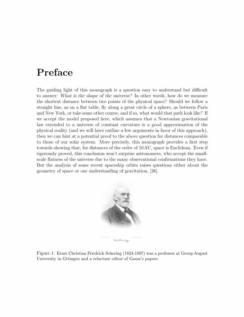
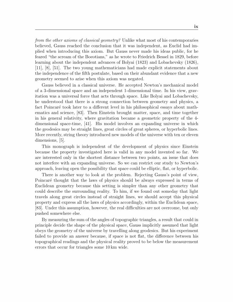
Figure 1: Ernst Christian Friedrich Schering (1824-1897) was a professor at Georg-AugustUniversity in Gttingen and a reluctant editor of Gauss’s papers.
viii Preface
However, we cannot emphasize enough that the main goal of this monograph ismathematical. We aim to shed some light on the dynamics of N point masses thatmove in spaces of nonzero constant curvature according to an attraction law whichextends classical Newtonian gravitation beyond R3. This natural generalization em-ploys the cotangent potential, first introduced in 1870 by Ernst Schering, who ob-tained its analytic expression following the geometric approach of Janos Bolyai andNikolai Lobachevsky for a 2-body problem in hyperbolic space, [87], [8], [70]. AsNewton’s idea of gravitation was to use a force inversely proportional to the areaof a sphere of radius equal in length to the Euclidean distance between the bodies,Bolyai and Lobachevsky thought of a similar definition in terms of the hyperbolicdistance in hyperbolic space. Our generalization of the cotangent potential to anynumber N of bodies led us to the recent discovery of some interesting properties,[35], [36]. These new results reveal certain connections among at least five branchesof mathematics: classical dynamics, non-Euclidean geometry, geometric topology,Lie groups, and the theory of polytopes. But how does the astronomical aspectmentioned above relate to these mathematical endeavors?
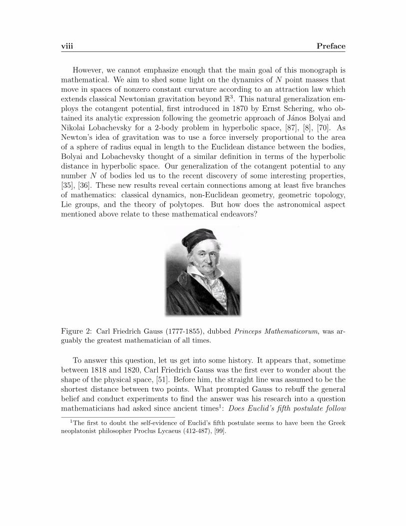
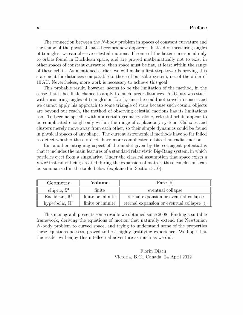
Figure 2: Carl Friedrich Gauss (1777-1855), dubbed Princeps Mathematicorum, was ar-guably the greatest mathematician of all times.
To answer this question, let us get into some history. It appears that, sometimebetween 1818 and 1820, Carl Friedrich Gauss was the first ever to wonder about theshape of the physical space, [51]. Before him, the straight line was assumed to be theshortest distance between two points. What prompted Gauss to rebuff the generalbelief and conduct experiments to find the answer was his research into a questionmathematicians had asked since ancient times1: Does Euclid’s fifth postulate follow
1The first to doubt the self-evidence of Euclid’s fifth postulate seems to have been the Greekneoplatonist philosopher Proclus Lycaeus (412-487), [99].
ix
from the other axioms of classical geometry? Unlike what most of his contemporariesbelieved, Gauss reached the conclusion that it was independent, as Euclid had im-plied when introducing this axiom. But Gauss never made his ideas public, for hefeared “the scream of the Boeotians,” as he wrote to Friedrich Bessel in 1829, beforelearning about the independent advances of Bolyai (1823) and Lobachevsky (1826),[11], [8], [51]. The two young mathematicians had made explicit statements aboutthe independence of the fifth postulate, based on their abundant evidence that a newgeometry seemed to arise when this axiom was negated.
Gauss believed in a classical universe. He accepted Newton’s mechanical modelof a 3-dimensional space and an independent 1-dimensional time. In his view, grav-itation was a universal force that acts through space. Like Bolyai and Lobachevsky,he understood that there is a strong connection between geometry and physics, afact Poincare took later to a different level in his philosophical essays about math-ematics and science, [83]. Then Einstein brought matter, space, and time togetherin his general relativity, where gravitation became a geometric property of the 4-dimensional space-time, [41]. His model involves an expanding universe in whichthe geodesics may be straight lines, great circles of great spheres, or hyperbolic lines.More recently, string theory introduced new models of the universe with ten or elevendimensions, [5].
This monograph is independent of the development of physics since Einsteinbecause the property investigated here is valid in any model invented so far. Weare interested only in the shortest distance between two points, an issue that doesnot interfere with an expanding universe. So we can restrict our study to Newton’sapproach, leaving open the possibility that space could be elliptic, flat, or hyperbolic.
There is another way to look at the problem. Rejecting Gauss’s point of view,Poincare thought that the laws of physics should be always expressed in terms ofEuclidean geometry because this setting is simpler than any other geometry thatcould describe the surrounding reality. To him, if we found out someday that lighttravels along great circles instead of straight lines, we should accept this physicalproperty and express all the laws of physics accordingly, within the Euclidean space,[83]. Under this assumption, however, the real difficulties are not overcome, but onlypushed somewhere else.
By measuring the sum of the angles of topographic triangles, a result that could inprinciple decide the shape of the physical space, Gauss implicitly assumed that lightobeys the geometry of the universe by travelling along geodesics. But his experimentfailed to provide an answer because, if space is not flat, the difference between histopographical readings and the physical reality proved to be below the measurementerrors that occur for triangles some 10 km wide.
x Preface
The connection between the N -body problem in spaces of constant curvature andthe shape of the physical space becomes now apparent. Instead of measuring anglesof triangles, we can observe celestial motions. If some of the latter correspond onlyto orbits found in Euclidean space, and are proved mathematically not to exist inother spaces of constant curvature, then space must be flat, at least within the rangeof these orbits. As mentioned earlier, we will make a first step towards proving thisstatement for distances comparable to those of our solar system, i.e. of the order of10 AU. Nevertheless, more work is necessary to achieve this goal.
This probable result, however, seems to be the limitation of the method, in thesense that it has little chance to apply to much larger distances. As Gauss was stuckwith measuring angles of triangles on Earth, since he could not travel in space, andwe cannot apply his approach to some triangle of stars because such cosmic objectsare beyond our reach, the method of observing celestial motions has its limitationstoo. To become specific within a certain geometry alone, celestial orbits appear tobe complicated enough only within the range of a planetary system. Galaxies andclusters merely move away from each other, so their simple dynamics could be foundin physical spaces of any shape. The current astronomical methods have so far failedto detect whether these objects have more complicated orbits than radial motion.
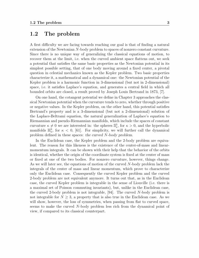
But another intriguing aspect of the model given by the cotangent potential isthat it includes the main features of a standard relativistic Big-Bang system, in whichparticles eject from a singularity. Under the classical assumption that space exists apriori instead of being created during the expansion of matter, these conclusions canbe summarized in the table below (explained in Section 3.10):
Geometry Volume Fate [b]
elliptic, S3 finite eventual collapse
Euclidean, R3 finite or infinite eternal expansion or eventual collapse
hyperbolic, H3 finite or infinite eternal expansion or eventual collapse [t]
This monograph presents some results we obtained since 2008. Finding a suitableframework, deriving the equations of motion that naturally extend the NewtonianN -body problem to curved space, and trying to understand some of the propertiesthese equations possess, proved to be a highly gratifying experience. We hope thatthe reader will enjoy this intellectual adventure as much as we did.
Florin DiacuVictoria, B.C., Canada, 24 April 2012
Chapter 1
Introduction
In this introductory chapter, we provide the motivation that led us to this research,define the problem, explain its importance, outline its history, and present the struc-ture of the monograph.
1.1 Motivation
In the early 1820s, with his recently invented heliotrope1 (see Figure 1.1), Carl Frie-drich Gauss, later dubbed Princeps Mathematicorum, allegedly tried to determinethe nature of the physical space within the framework of classical mechanics, underthe assumption that space and time exist a priori and are independent of each other,[75], [49]. He measured the angles of a triangle formed by three hills near Gottingen(Inselsberg, Brocken, and Hoher Hagen) and computed their sum, S, hoping to learnwhether space is hyperbolic (S < π radians) or elliptic (S > π radians), [99]. But theresults of his measurements did not deviate form π radians beyond the unavoidablemeasurement errors, so his experiment was inconclusive. Since we cannot reachdistant stars to measure all the angles of some cosmic triangle, Gauss’s method is ofno practical use for astronomic distances either.2
1The heliotrope, which Gauss invented in 1820, is an instrument that uses a mirror to reflectsunlight in order to mark the positions of the land surveyors (see “The Gentleman’s magazine,”Volume 92, Part 2, July 1822, p. 358).
2There are other methods, such as cosmic crystallography and the Boomerang experiment,which show strong evidence that if the universe is not flat, its deviation from zero curvature mustbe very small, [98], [6]. But, in spite of their merits, these attempts rely on certain physical models,principles, and interpretations we do not need in the framework of celestial mechanics. Moreover,they do not yet provide a final answer to the question posed in the Preface.

2 Introduction
Figure 1.1: A drawing of a heliotrope designed by William Wurdemann, a German-American optical instrument maker of the 19th century.
But celestial mechanics can help us find a new approach towards establishing thegeometric nature of the physical space. The idea we suggest is to use the connectionbetween geometry and dynamics, and reduce the problem to performing astronomicalobservations instead of taking measurements. To explain this method in more detail,let us recall that, in the 17th century, Isaac Newton derived the equations of motionof the N -body problem in Euclidean space, i.e. obtained the system of differentialequations that describe the gravitational dynamics of N point masses, albeit in ageometric form, very different form how we write these equations today. Physicistsagreed later that a universe of constant Gaussian curvature is a good approximationof the macrocosmic reality, a hypothesis they still accept. So if we succeed to extendNewton’s gravitational law to 3-dimensional spheres and 3-dimensional hyperbolicmanifolds, and also prove the existence of solutions that are specific to only one ofthe negative, zero, or positive constant Gaussian curvature spaces, but not to theother two, then the problem of understanding the geometric nature of the universereduces to finding, through astronomical observations, some of the orbits provedmathematically to exist.
Therefore obtaining a natural extension of the Newtonian N -body problem tospaces of nonzero constant Gaussian curvature, such that the properties of the orig-inal potential are satisfied when taking the Euclidean space as a limit, and studyingthe system of differential equations thus derived, appears to be a worthy endeavortowards comprehending the geometry of the physical space. Additionally, an investi-gation of this system when the curvature tends to zero may help us better understandthe dynamics of the classical Euclidean case, viewed as a particular problem withina more general mathematical framework. This general methodological approach hasbeen useful in many branches of mathematics.
1.2 The problem 3
1.2 The problem
A first difficulty we are facing towards reaching our goal is that of finding a naturalextension of the Newtonian N -body problem to spaces of nonzero constant curvature.Since there is no unique way of generalizing the classical equations of motion, torecover them at the limit, i.e. when the curved ambient space flattens out, we seeka potential that satisfies the same basic properties as the Newtonian potential in itssimplest possible setting, that of one body moving around a fixed center, a pivotalquestion in celestial mechanics known as the Kepler problem. Two basic propertiescharacterize it, a mathematical and a dynamical one: the Newtonian potential of theKepler problem is a harmonic function in 3-dimensional (but not in 2-dimensional)space, i.e. it satisfies Laplace’s equation, and generates a central field in which allbounded orbits are closed, a result proved by Joseph Louis Bertrand in 1873, [7].
On one hand, the cotangent potential we define in Chapter 3 approaches the clas-sical Newtonian potential when the curvature tends to zero, whether through positiveor negative values. In the Kepler problem, on the other hand, this potential satisfiesBertrand’s property and is a 3-dimensional (but not a 2-dimensional) solution ofthe Laplace-Beltrami equation, the natural generalization of Laplace’s equation toRiemannian and pseudo-Riemannian manifolds, which include the spaces of constantcurvature κ 6= 0 we are interested in: the spheres S3
κ, for κ > 0, and the hyperbolicmanifolds H3
κ, for κ < 0, [61]. For simplicity, we will further call the dynamicalproblem defined in these spaces: the curved N -body problem.
In the Euclidean case, the Kepler problem and the 2-body problem are equiva-lent. The reason for this likeness is the existence of the center-of-mass and linear-momentum integrals. It can be shown with their help that the behavior of the orbitsis identical, whether the origin of the coordinate system is fixed at the center of massor fixed at one of the two bodies. For nonzero curvature, however, things change.As we will later see, the equations of motion of the curved N -body problem lack theintegrals of the center of mass and linear momentum, which prove to characterizeonly the Euclidean case. Consequently the curved Kepler problem and the curved2-body problem are not equivalent anymore. It turns out that, as in the Euclideancase, the curved Kepler problem is integrable in the sense of Liouville (i.e. there isa maximal set of Poisson commuting invariants), but, unlike in the Euclidean case,the curved 2-body problem is not integrable, [94]. The curved N -body problem isnot integrable for N ≥ 3, a property that is also true in the Euclidean case. As wewill show, however, the loss of symmetries, when passing from flat to curved space,seems to make the curved N -body problem less rich from the dynamical point ofview, if compared to its classical counterpart.

4 Introduction
As stated in Section 1.1, our main goal is to find solutions that are specific toeach of the spaces corresponding to κ < 0, κ = 0, and κ > 0. We did that in somepreviously published papers, but only in the 2-dimensional case, [28], [37], [35], [36].In this monograph, we will see that the 3-dimensional curved N -body problem putsinto the evidence even more differences between the qualitative behavior of orbits ineach of these spaces.
1.3 Importance
We already mentioned that the study of the curved N -body problem may help usbetter understand the geometry of the universe and put the classical Euclidean casein a broader mathematical perspective. In fact, in [33] and [35], we made a first steptowards proving that space is Euclidean for distances of the order of 10 AU. Thereason is the existence of Lagrangian orbits of unequal masses (e.g., the equilateraltriangles formed by the Sun, Jupiter, and the Trojan/Greek asteroids) in our solarsystem and the fact that, for nonzero curvature, 2-dimensional Lagrangian solutionsexist only if the masses are equal, a fact which makes them unlikely to form in auniverse of nonzero constant curvature. We will present and analyze these aspectsin detail in the last part of this monograph.
These results, however, only hint at the fact that space is Euclidean for solar-system scales. Indeed, the motions of the Trojan and Greek asteroids are not exactlyat the vertices of equilateral triangles but close to them, the physical existence ofthese orbits following from their stability for a certain range of masses. A better wayto approach this issue is through the circular restricted 3-body problem, when theTrojan and Greek asteroids are close to moving on 3-dimensional invariant tori, butthe values of the inclinations are large for most of these little planets. Nonetheless,this approach must also take into account the perturbation from the other planets.Finally, we do not yet exclude the existence of Lagrangian quasiperiodic orbits ofunequal masses in 3-dimensional curved space, motions that might be hard to dis-tinguish in practice from the orbits we observe in our solar system. So a final answerabout the curvature of our local universe still awaits an extensive investigation ofthe differential equations we will derive here.
Another practical aspect that has not been studied so far has to do with motionin the neighborhood of large celestial bodies, such as the Sun. While for distances of1 AU or so, space can be assumed to have constant curvature, light rays are knownto bend near large cosmic objects. These things are explained in terms of generalrelativity, but the ideas that led to the derivation of the curved N -body problemmay be also used to study this bending with classical tools.
1.4 History 5
Apart from these philosophical and applicative aspects, the curved N -body prob-lem lays bridges between the theory of dynamical systems and several other branchesof mathematics: the geometry and topology of 3-dimensional manifolds of constantcurvature, Lie group theory, and the theory of regular polytopes, all of which weuse in this monograph, and with differential geometry and Lie algebras, as alreadyshown in [37] and [81].
As the results we prove here point out, many of which are surprising and non-intuitive, the geometry of the space in which the bodies move strongly influencestheir dynamics, including some important qualitative properties, stability amongthem. Topological concepts, such as the Hopf fibration and the Hopf link; geometricobjects, like the pentatope, the Clifford torus, and the hyperbolic cylinder; or geo-metric properties, such as the Hegaard splitting of genus 1, become essential toolsfor understanding the gravitational motion of the bodies.
Since we provide here only a first study in this direction of research, reduced tothe simplest orbits the equations of motion have, namely the relative equilibria (andthe fixed points in the case of positive curvature), we expect that many more con-nections between dynamics, geometry, topology, and other branches of mathematicswill be discovered in the near future through a deeper exploration of the curved3-dimensional problem.
1.4 History
The first researchers who took the idea of gravitation beyond the Euclidean spacewere Nikolai Lobachevsky and Janos Bolyai, the founders of hyperbolic geometry.In 1835, Lobachevsky proposed a Kepler problem in the 3-dimensional hyperbolicspace, H3, by defining an attractive force proportional to the inverse area of the2-dimensional sphere of radius equal in length to the distance between bodies, [70].Independently of him, and at about the same time, Bolyai came up with a similaridea, [8]. Both of them grasped the intimate connection between geometry and phys-ical laws, a relationship that proved very prolific ever since. Gauss also understoodthat hyperbolic geometry existed independently, but never went as far as Bolyai andLobachevsky, and there is no historical evidence (until now) that he thought of howto extend Newton’s gravitational law beyond the Euclidean space.
These co-discoverers of the first non-Euclidean geometry had no followers in theirpre-relativistic attempts until 1860, when Paul Joseph Serret3 extended the gravi-
3Paul Joseph Serret (1827-1898) should not be mixed up with another French mathematician,Joseph Alfred Serret (1819-1885), known for the Frenet-Serret formulas of vector calculus.
6 Introduction
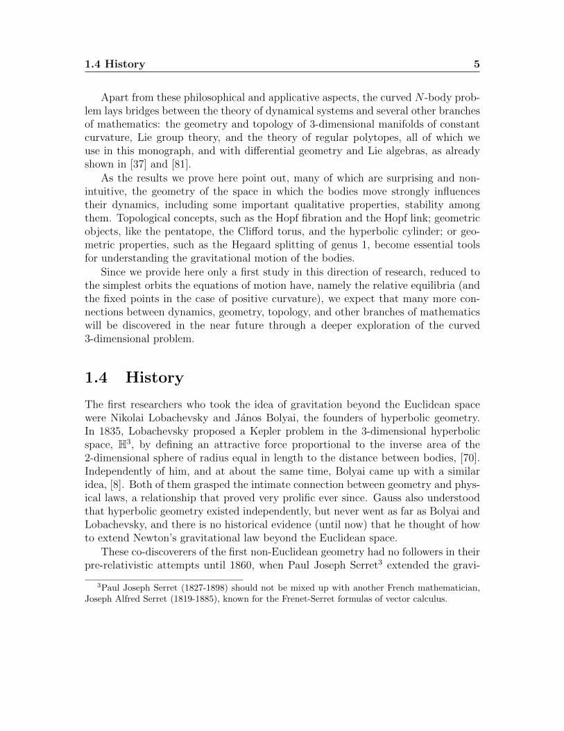
Figure 1.2: Janos Bolyai (1802-1860) was a Hungarian mathematician born in Transylva-nia (then in Hungary, now in Romania), where he spent most of his life. This sculptureon the frontispiece of the Culture Palace in Targu Mures (known in Hungarian as Maros-Vasarhely) seems to be the only true image left of him, [24].
tational force to the sphere S2 and solved the corresponding Kepler problem, [90].Ten years later, Ernst Schering revisited the Bolyai-Lobachevsky law, for which heobtained an analytic expression given by the curved cotangent potential we study inthis paper, [87]. Schering also wrote that Lejeune Dirichlet had told some friends tohave dealt with the same problem during his last years in Berlin4, but Dirichlet neverpublished anything in this direction, and we found no evidence of any unpublishedmanuscripts in which he had studied this particular topic, [88]. In 1873, Rudolph Lip-schitz considered the problem in S3, but defined a potential proportional to 1/ sin r
R,
where r denotes the distance between bodies and R is the curvature radius, [69]. Hesucceeded to obtain the general solution of the corresponding differential equationsonly in terms of elliptic functions, a dead end nobody followed. His failure to providean explicit formula, which could have helped him draw some conclusions about themotion of the bodies, showed the advantage of Schering’s approach.
In 1885, Wilhelm Killing adapted the Bolyai-Lobachevsky gravitational law toS3 and defined an extension of the Newtonian force given by the inverse area of a2-dimensional sphere (in the spirit of Schering), for which he proved a generalizationof Kepler’s three laws, a step which suggested that the cotangent potential was agood way to extend the classical approach, [59]. Then a breakthrough took place. In1902, Heinrich Liebmann5 showed that the orbits of the Kepler problem are conics
4This must have happened around 1852, as claimed by Rudolph Lipschitz, [68].5Although he signed his papers and books as Heinrich Liebmann, his full name was Karl Otto
1.4 History 7
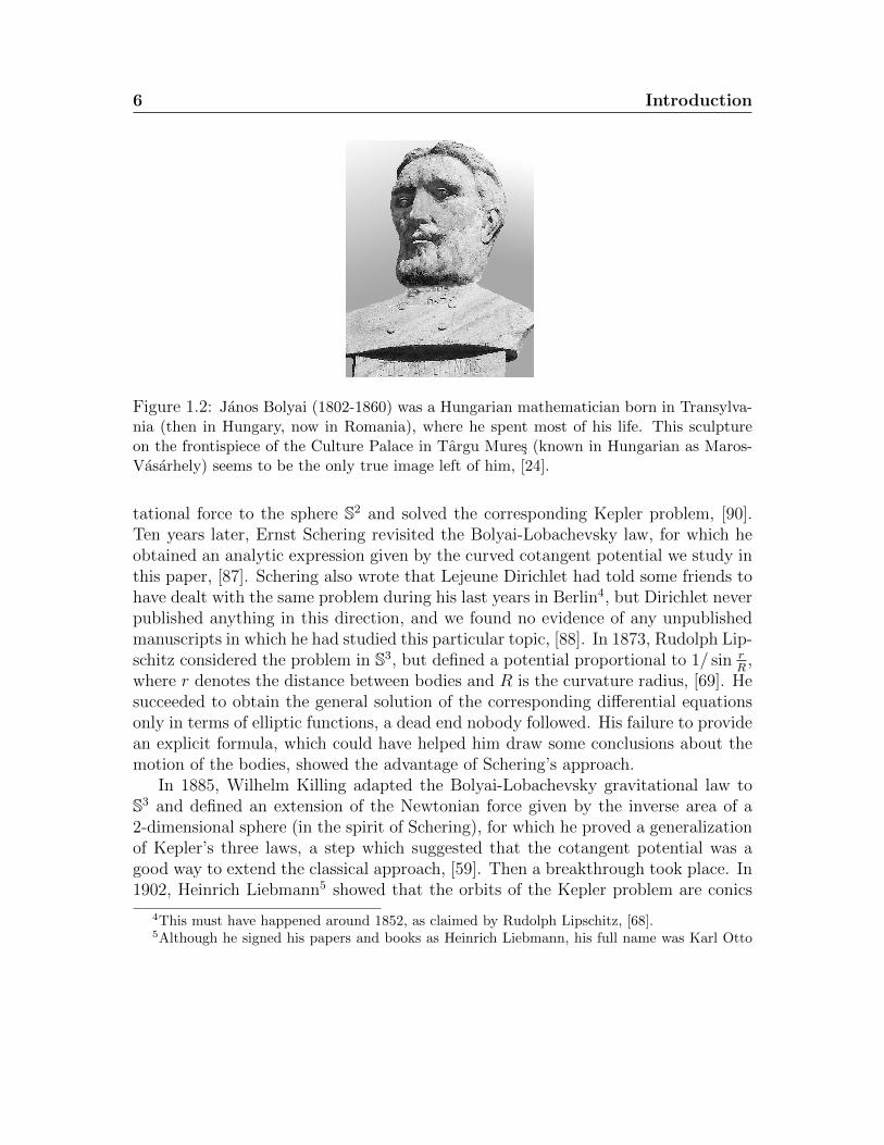
Figure 1.3: Nikolai Ivanovich Lobachevsky (1792-1856) was a Russian mathematician atthe University of Kazan, where he also served as president. As in the case of Bolyai, hismathematical work received little recognition during his life time.
in S3 and H3 and further generalized Kepler’s three laws to κ 6= 0, [65]. One yearlater, he proved S2- and H2-analogues of Bertrand’s theorem, which states that forthe Kepler problem there exist only two analytic central potentials in the Euclideanspace for which all bounded orbits are closed, one of which corresponds to gravitation,[7], [100], [66]. Liebmann also included his results in the last chapter of a book onhyperbolic geometry published in 1905, which saw two more editions, one in 1912and the other in 1923, [67]. Intriguing enough, in the third edition he replaced theconstant-curvature approach with relativistic considerations.
Liebmann’s change of mind about the importance of the constant-curvature ap-proach may explain why this direction of research was ignored in the decades im-mediately following the birth of special and general relativity. The reason for thisneglect was probably connected to the idea that general relativity could allow thestudy of 2-body problems on manifolds with variable Gaussian curvature, so theconstant-curvature case appeared to be outdated. Indeed, although the most im-portant subsequent success of relativity was in cosmology and related fields, therewere attempts to discretize Einstein’s equations and define a gravitational N -bodyproblem. Remarkable in this direction were the contributions of Jean Chazy, [15],
Heinrich Liebmann (1874-1939). He did most of his work in Heidelberg, where he became briefly theuniversity’s president, before the Nazis forced him to retire. A remembrance colloquium was heldin his honor at the University of Heidelberg in 2008. On this occasion, Liebmann’s son, Karl-OttoLiebmann, also and academic, donated to the Faculty of Mathematics an oil portrait of his father,painted by Adelheid Liebmann, [91]. This author had the opportunity to see that portrait on avisit to Heidelberg in 2009, when Willi Jager, his former Ph.D. supervisor, showed it to him.
8 Introduction
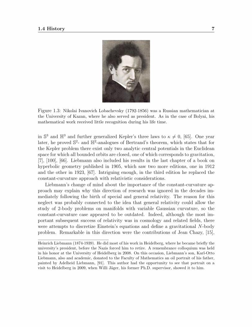
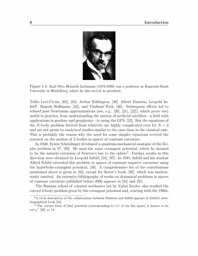
Figure 1.4: Karl Otto Heinrich Liebmann (1874-1939) was a professor at Ruprecht-KarlsUniversity in Heidelberg, where he also served as president.
Tullio Levi-Civita, [62], [63], Arthur Eddington, [40], Albert Einstein, Leopold In-feld6, Banesh Hoffmann, [42], and Vladimir Fock, [46]. Subsequent efforts led torefined post-Newtonian approximations (see, e.g., [20], [21], [22]), which prove veryuseful in practice, from understanding the motion of artificial satellites—a field withapplications in geodesy and geophysics—to using the GPS, [23]. But the equations ofthe N -body problem derived from relativity are highly complicated even for N = 2and are not prone to analytical studies similar to the ones done in the classical case.This is probably the reason why the need for some simpler equations revived theresearch on the motion of 2 bodies in spaces of constant curvature.
In 1940, Erwin Schrodinger developed a quantum-mechanical analogue of the Ke-pler problem in S2, [89]. He used the same cotangent potential, which he deemedto be the natural extension of Newton’s law to the sphere7. Further results in thisdirection were obtained by Leopold Infeld, [54], [97]. In 1945, Infeld and his studentAlfred Schild extended this problem to spaces of constant negative curvature usingthe hyperbolic-cotangent potential, [56]. A comprehensive list of the contributionsmentioned above is given in [92], except for Serret’s book, [90], which was inadver-tently omitted. An extensive bibliography of works on dynamical problems in spacesof constant curvature published before 2006 appears in [94] and [95].
The Russian school of celestial mechanics led by Valeri Kozlov also studied thecurved 2-body problem given by the cotangent potential and, starting with the 1990s,
6A vivid description of the collaboration between Einstein and Infeld appears in Infeld’s auto-biographical book [55].
7“The correct form of [the] potential (corresponding to 1/r of the flat space) is known to becotχ,” [89], p. 14.
1.4 History 9
considered related problems in spaces of constant curvature, [61]. An importantcontribution to the case N = 2 and the Kepler problem belongs to Jose Carinena,Manuel Ranada, and Mariano Santander, who provided a unified approach in theframework of differential geometry with the help of intrinsic coordinates, emphasizingthe dynamics of the cotangent potential in S2 and H2, [13] (see [14] and [50] as well).They also proved that the conic orbits known in Euclidean space extend naturally tospaces of constant curvature, in agreement with the results obtained by Liebmann,[92]. Moreover, the authors used the rich geometry of the hyperbolic plane to searchfor new orbits, whose existence they either proved or conjectured. The study of theirpaper made us look for a way to write down the equations of motion for any numberN ≥ 2 of bodies.
Thus inspired, we proposed a new setting, which allowed us an easy derivation ofthe equations of motion for any N ≥ 2 in terms of extrinsic coordinates, [35]. Thecombination of two main ideas helped us achieve this goal: the use of Weierstrass’smodel of the hyperbolic plane (also known as the Lorentz model on the hyperbolicsphere), which is embedded in the 3-dimensional Minkowski space, and the appli-cation of the variational approach of constrained Lagrangian dynamics, [48]. Theequations we obtained are valid in any finite dimension. In [35] we explored relativeequilibria and solved Saari’s conjecture in the collinear case (see also [34], [31]), in [36]and [27] we studied the singularities of the curved N -body problem, in [33] we gave acomplete classification of the Lagrangian and Eulerian solutions in the 3-body case,and in [28] we obtained some results about polygonal orbits, including a generaliza-tion of the Perko-Walter-Elmabsout theorem to both the case of relative equilibriaand when expansion/contraction takes place, [43], [82]. Ernesto Perez-Chavela andJ. Guadalupe Reyes Victoria derived the equations of motion in intrinsic coordinatesin the case of positive curvature and showed them to be equivalent with the extrinsicequations, [81]. The analysis of the intrinsic equations in the case of negative cur-vature was done in [37]. This study is more complicated than the one for positivecurvature, involving both the Poincare disk and the upper-half-plane model. Somepreliminary results about relative equilibria in the 3-dimensional case occur in [29],out of which many properties will be presented here.
A study of the stability of Lagrangian relative equilibria of the curved 3-bodyproblem in S2 appeared in [73]. Regina Martınez and Carles Simo thus discoveredtwo zones on the sphere in which the orbit is stable. This result is surprising becauseequal-mass Lagrangian orbits are unstable in the Euclidean case. Currently we areperforming a study of the stability of tetrahedral orbits for the curved 4-body problemin S2, [32].
10 Introduction
1.5 Structure
In what follows, we will present some results obtained in the 2- and 3-dimensionalcurved N -body problem in the context of differential equations in extrinsic coordi-nates, as derived in [35]. We are mainly concerned with understanding the motionof the simplest possible orbits, the relative equilibria, which move like rigid bodiesby maintaining constant mutual distances for all time.
The main part of this monograph is structured in five parts. Part I providesthe mathematical background and gives a complete derivation of the equations ofmotion. Part II deals with isometries, whose group representations allow us to mean-ingfully define relative equilibria for spheres and hyperbolic manifolds. Part III isconcerned with finding existence criteria for relative equilibria and describing thequalitative behavior of these orbits. Part IV gives many explicit examples of relativeequilibria, which illustrate each type of dynamical behavior previously described.Finally, Part V focuses on the 2-dimensional case, provides a proof that Lagrangianorbits must have equal masses (the result that throws some light on the shape ofthe physical space), and ends with an extension of Saari’s conjecture to spaces ofconstant curvature, which is proved in the geodesic case.
The parts are divided into chapters, numbered increasingly throughout the text.Each part starts with a preamble that provides a brief idea of what to expect, and thebeginning of each chapter outlines the main properties we found. To avoid repetition,we will not describe those results here. The rest of the text can therefore be readlinearly or by going first to the preambles of the parts and the introductions to thechapters to get a general idea about what results will be proved.
We finally reached the starting point into a mathematical universe that will revealconnections between several branches of mathematics and bring some insight into thegeometry of the physical space. We hope that the above introduction has given thereader enough reasons to explore this new world.
Part I
Background and Equations ofMotion

13
Preamble
The goal of Part I is to lay the mathematical foundations for future developmentsand to obtain the equations of motion of the curved N -body problem together withtheir first integrals. We will also identify the singularities of the equations of motionin order to avoid impossible configurations for the relative equilibria we are going toconstruct in Part V. A basic property we prove, which will simplify our presentation,is that, up to its sign, the curvature can be eliminated from the equations of motionthrough suitable coordinate and time-rescaling transformations. Consequently ourstudy can be reduced to the unit sphere, S3, for positive curvature, and the unithyperbolic sphere, H3, for negative curvature.

14
Chapter 2
Preliminary developments
In this chapter we will introduce some concepts needed for the derivation of theequations of motion of the N -body problem in spaces of constant curvature as wellas for the study of the relative equilibria, which are special classes of orbits that wewill investigate later. We will start by introducing a model for hyperbolic geometry,usually attributed to Hendrik Lorentz, but actually due to Karl Weierstrass.
The 2-sphere is familiar to everybody as a complete and compact surface of con-stant positive Gaussian curvature, κ = 1/R2, where R is the radius. But the under-standing of its dual, the hyperbolic sphere, which has constant negative curvature,κ = −1/R2, needs more imagination. This object is connected to hyperbolic geom-etry. The standard models of 2-dimensional hyperbolic geometry are the Poincaredisk and the Poincare upper-half plane, which are conformal, i.e. maintain the an-gles existing in the hyperbolic plane, as well as the Klein-Beltrami disk, which is notconformal. But we won’t use any of these models here.
In the first part of this chapter, we will introduce a less known model, due toKarl Weierstrass, which geometers call the hyperbolic sphere or, sometimes ambigu-ously, the pseudosphere, whereas physicists refer to it as the Lorentz model. We willfirst present the 2-dimensional case, which can be easily extended to 3 dimensions.This model is more natural than the ones previously mentioned in the sense thatit is analytically similar to the sphere, and will thus be essential in our endeavorsto develop a unified N -body problem in spaces of constant positive and negativecurvature. We will then provide a short history of this model, and introduce somegeometry concepts that are going to be useful later. In the last part of this chapter,we will define the natural metric of the sphere and of the hyperbolic sphere and unifycircular and hyperbolic trigonometry in order to introduce a single potential functionfor both the positive and the negative curvature case.
16 Preliminary developments
2.1 The hyperbolic sphere
Since Weierstrass’s model of hyperbolic geometry is not widely known among non-linear analysts or experts in differential equations and dynamical systems, we willbriefly present it here. We first discuss the 2-dimensional case, which we will thenextend to 3 dimensions. In its 2-dimensional form, this model appeals for at least tworeasons: it allows an obvious comparison with the 2-sphere, both from the geometricand from the algebraic point of view, and emphasizes the difference between the hy-perbolic (Bolyai-Lobachevsky) and the Euclidean plane as clearly as the well-knowndifference between the Euclidean plane and the sphere. From the dynamical pointof view, the equations of motion of the curved N -body problem in S3
κ resemble theequations of motion in H3
κ, with just a few sign changes, as we will show soon. Thedynamical consequences, however, are going to be significant, but we will be ableto use the resemblances between the sphere and the hyperbolic sphere to study thedynamics of the problem.
The 2-dimensional Weierstrass model is built on the hyperbolic sphere, repre-sented by one of the sheets of the hyperboloid of two sheets,
x2 + y2 − z2 = κ−1,
where κ < 0 represents the curvature of the surface in the 3-dimensional Minkowskispace R2,1 := (R3,�), in which
a � b := axbx + ayby − azbz,
defines the Lorentz inner product of the vectors a = (ax, ay, az) and b = (bx, by, bz).We pick for our model the sheet z > 0 of the hyperboloid of two sheets and identifythis connected component with the hyperbolic plane H2
κ. We can think of this surfaceas being a pseudosphere of imaginary radius iR, a case in which the relationshipbetween radius and curvature is given by (iR)2 = κ−1.
A linear transformation T : R2,1 → R2,1 is called orthogonal if it preserves theinner product, i.e.
T (a) � T (a) = a � a
for any a ∈ R2,1. The set of these transformations, together with the Lorentz innerproduct, forms the orthogonal Lie group O(R2,1), given by matrices of determinant±1. Therefore the connected Lie group SO(R2,1) of orthogonal transformations ofdeterminant 1 is a subgroup of O(R2,1). Another subgroup of O(R2,1) is G(R2,1),which is formed by the transformations T that leave H2
κ invariant. Furthermore,G(R2,1) has the closed Lorentz subgroup, Lor(R2,1) := G(R2,1) ∩ SO(R2,1).
2.1 The hyperbolic sphere 17
An important result, with deep consequences in our paper, is the principal axistheorem for Lor(R2,1), [38], [52]. To present it, let us define the Lorentzian rotationsabout an axis as the 1-parameter subgroups of Lor(R2,1) that leave the axis pointwisefixed. Then the principal axis theorem states that every Lorentzian transformationhas one of the matrix representations:
A = P
cos θ − sin θ 0
sin θ cos θ 0
0 0 1
P−1,
B = P
1 0 0
0 cosh s sinh s
0 sinh s cosh s
P−1,or
C = P
1 −t t
t 1− t2/2 t2/2
t −t2/2 1 + t2/2
P−1,where θ ∈ [0, 2π), s, t ∈ R, and P ∈ Lor(R2,1). These transformations are calledelliptic, hyperbolic, and parabolic, respectively. They are all isometries, i.e. preservethe distances in H2
κ.In its standard setting of Einstein’s relativity, the Minkowski space has time and
space coordinates. In our case, however, all coordinates are spatial. Nevertheless,we will use the standard terminology and say that the elliptic transformations arerotations about a timelike axis (the z axis in our case) and act along a circle, likein the spherical case; the hyperbolic rotations are about a spacelike axis (the x axisin this context) and act along a hyperbola; and the parabolic transformations arerotations about a lightlike (or null) axis (represented here by the line x = 0, y = z)and act along a parabola. This result is analogous to Euler’s principal axis theoremfor the sphere, which states that any element of the rotation group SO(3) can bewritten, in some orthonormal basis, as a rotation about the z axis.
The geodesics of H2κ are the hyperbolas obtained by intersecting the hyperbolic
sphere with planes passing through the origin of the coordinate system. For any twodistinct points a and b of H2
κ, there is a unique geodesic that connects them, andthe distance between these points is given by
d(a,b) = (−κ)−1/2 cosh−1(κa � b). (2.1)
In the framework of Weierstrass’s model, the parallels’ postulate of hyperbolicgeometry can be translated as follows. Take a geodesic γ, i.e. a hyperbola obtained
18 Preliminary developments
by intersecting the hyperbolic sphere with a plane through the origin, O, of thecoordinate system. This hyperbola has two asymptotes in its plane: the straightlines a and b, which intersect at O. Take a point, P , on the upper sheet of thehyperboloid but not on the chosen hyperbola. The plane aP produces the geodesichyperbola α, whereas bP produces β. These two hyperbolas intersect at P . Then αand γ are parallel geodesics meeting at infinity along a, while β and γ are parallelgeodesics meeting at infinity along b. All the hyperbolas between α and β (alsoobtained from planes through O) are non-secant with γ.
Like the Euclidean plane, the abstract Bolyai-Lobachevsky plane has no privilegedpoints or geodesics. But the Weierstrass model, given by the hyperbolic sphere, hassome convenient points and geodesics, such as the point (0, 0, |κ|−1/2), namely thevertex of the sheet z > 0 of the hyperboloid, and the geodesics passing throughit. The elements of Lor(R2,1) allow us to move the geodesics of H2
κ to convenientpositions, a property that can be used to simplify certain arguments.
More detailed introductions to the 2-dimensional Weierstrass model can be foundin [45] and [84]. The Lorentz group is treated in some detail in [4] and [84], butthe principal axis theorems for the Lorentz group contained in [4] fails to includeparabolic rotations, and is therefore incomplete.
The generalization of the hyperbolic 2-sphere to 3 dimensions is straightforward.Consider first the 4-dimensional Minkowski space R3,1 = (R4,�), where � is nowdefined as the Lorentz inner product
a � b = awbw + axbx + ayby − azbz,
with a = (aw, ax, ay, az) and b = (bw, bx, by, bz) belonging to R3,1. We further embedin this Minkowski space the connected component with z > 0 of the 3-dimensionalhyperbolic manifold given by the equation
w2 + x2 + y2 − z2 = κ−1, (2.2)
which models the hyperbolic 3-sphere H3κ of constant curvature κ < 0. The distance
is given by the same formula (2.1), where a and b are now points in R4 that lie inthe hyperbolic 3-sphere (2.2) with z > 0.
The next issue to discuss would be that of Lorentzian transformations in H3κ, i.e.
the elements of the corresponding Lorentz group. But we postpone this topic, topresent it in Chapter 4 together with the isometries of the 3-sphere and the groupSO(4) that generates them. There are two good reasons for this postponement. First,we would like to obtain the equations of motion of the curved N -body problem assoon as possible and, second, to present the similarities and the differences betweenthese transformations in a larger geometrical context than the one considered here.
2.2 More geometric background 19
Some historical remarks
The idea of an “imaginary sphere,” at a time when mathematicians were knockingunsuccessfully at the gates of hyperbolic geometry, seems to have first appeared in1766 in the work of Johann Heinrich Lambert, [9]. In 1826, Franz Adolph Taurinusreferred to a “sphere of imaginary radius” in connection with some trigonometricresearch, [9], but was clearly unaware of the work of Bolyai and Lobachevsky, whowere then trying, independently of each other, to make progress in the new universeof the hyperbolic plane. Neither Lambert, nor Taurinus, seem to have viewed theseconcepts as we do today.
The first mathematician who mentioned Karl Weierstrass in connection withthe hyperbolic sphere was Wilhelm Killing. In a paper published in 1880, [58], heused what he called Weierstrass’s coordinates to describe the “exterior hyperbolicplane” as an “ideal region” of the Bolyai-Lobachevsky plane. In 1885, he added thatWeierstrass had introduced these coordinates, in combination with “numerous appli-cations,” during a seminar held in 1872, but also mentioned that Eugenio Beltramihad previously used some related coordinates, [60], pp. 258-259. We found no otherevidence of any written account of the hyperbolic sphere for the Bolyai-Lobachevskyplane prior to the one Killing gave in [60], p. 260. His remarks might have inspiredRichard Faber to name this model after Weierstrass and to dedicate a chapter to itin [45], pp. 247-278.
2.2 More geometric background
Since we are interested in the motion of point particles on 3-dimensional manifolds,the natural background structure for the study of the 3-dimensional curved N -bodyproblem is the Euclidean ambient space, R4, endowed with a specific inner-product,which depends on whether the curvature is positive or negative. For positive constantcurvature, κ > 0, the motion takes place on a 3-sphere embedded in the Euclideanspace R4, endowed with the standard dot product, · , i.e. on the manifold
S3κ = {(w, x, y, z) |w2 + x2 + y2 + z2 = κ−1}.
For negative constant curvature, κ < 0, the motion takes place on the hyperbolicsphere, the manifold introduced in the previous subsection, represented by the upperconnected component of a 3-dimensional hyperboloid of two connected componentsembedded in the Minkowski space R3,1, i.e. on the manifold
H3κ = {(w, x, y, z) |w2 + x2 + y2 − z2 = κ−1, z > 0},
20 Preliminary developments
where R3,1 is R4 endowed with the Lorentz inner product, �. Generically, we willdenote these manifolds by
M3κ = {(w, x, y, z) ∈ R4 |w2 + x2 + y2 + σz2 = κ−1, with z > 0 for κ < 0},
where σ is the signum function,
σ =
{+1, for κ > 0
−1, for κ < 0.(2.3)
In Section 3.7, we will show that, using suitable coordinate and time-rescalingtransformations, we can reduce the mathematical study of the equations of motionto the unit sphere,
S3 = {(w, x, y, z) |w2 + x2 + y2 + z2 = 1},
for positive curvature, and to the unit hyperbolic sphere,
H3 = {(w, x, y, z) |w2 + x2 + y2 − z2 = −1},
for negative curvature. Generically, we will denote these manifolds by
M3 = {(w, x, y, z) ∈ R4 | w2 + x2 + y2 + σz2 = σ, with z > 0 for κ < 0}.
Given the 4-dimensional vectors
a = (aw, ax, ay, az) and b = (bw, bx, by, bz),
we define their inner product as
a� b := awbw + axbx + ayby + σazbz, (2.4)
so M3κ is endowed with the operation �, meaning · for κ > 0 and � for κ < 0.
If R is the radius of the sphere S3κ, then the relationship between κ > 0 and R
is κ−1 = R2. As we already mentioned, to have an analogue interpretation in thecase of negative curvature, H3
κ can be viewed as a hyperbolic 3-sphere of imaginaryradius iR, such that the relationship between κ < 0 and iR is κ−1 = (iR)2.
Let us further define some concepts that will be useful later. Since we are goingto work with them only in the context of S3 and H3, i.e. for κ = 1 and κ = −1,respectively, we will introduce them relative to these manifolds.
Definition 1. A great sphere of S3 is a 2-sphere of radius 1.
2.2 More geometric background 21
Great spheres of S3 are obtained by intersecting S3 with hyperplanes of R4 thatpass through the origin of the coordinate system. Examples of great spheres are:
S2w = {(w, x, y, z) |x2 + y2 + z2 = 1, w = 0} (2.5)
for all possible relabelings of the variables.
Definition 2. A great circle of a great sphere of S3 is a 1-sphere of radius 1.
Definition 2 implies that the curvature of a great circle is the same as the curvatureof S3. Notice that this is not true in general, i.e. for spheres of curvature κ. Thenthe curvature of a great circle is κ = 1/R, where R is the radius of S3
κ and of thegreat circle.
A great circle can be obtained by intersecting a great sphere with a plane passingthrough the origin of the coordinate system. Examples of great circles in S3 are:
S1wx = {(w, x, y, z) | y2 + z2 = 1, w = x = 0} (2.6)
for all possible relabelings of the variables. Notice that S1wx is a great circle for both
the great spheres S2w and S2
x, whereas S1yz is a great circle for the great spheres S2
y
and S2z. Similar remarks can be made about any of the above great circles.
Definition 3. Two great circles, C1 and C2, of two distinct great spheres of S3 arecalled complementary if there is a coordinate system wxyz such that either of thefollowing two conditions is satisfied:
C1 = S1wx and C2 = S1
yz, (2.7)
C1 = S1wy and C2 = S1
xz. (2.8)
The conditions (2.7) and (2.8) for C1 and C2 exhaust all possibilities. Indeed, therepresentation
C1 = S1wz and C2 = S1
xy,
for instance, is the same as (2.7) after we perform a circular permutation of thecoordinates w, x, y, z. For simplicity, and without loss of generality, we will alwaysuse representation (2.7).
In topological terms, the complementary circles C1 and C2 of S3 form a Hopf linkin a Hopf fibration, which is the map
H : S3 → S2, H(w, x, y, z) = (w2 + x2 − y2 − z2, 2(wz + xy), 2(xz − wy))
22 Preliminary developments
that takes circles of S3 to points of S2, [53], [71]. In particular, H takes S1wx to
(1, 0, 0) and S1yz to (−1, 0, 0). Using the stereographic projection, it can be shown
that the circles C1 and C2 are linked (like any adjacent rings in a chain), hence thename of the pair, [71]. Hopf fibrations have important physical applications in fieldssuch as rigid body mechanics, [72], quantum information theory, [77], and magneticmonopoles, [78]. As we will see later, they are also useful in celestial mechanics viathe curved N -body problem.
We will show in the next section that the distance between two points lying oncomplementary great circles is independent of their position. This remarkable geo-metric property turns out to be even more surprising from the dynamical point ofview. Indeed, given the fact that the distance between 2 complementary great circlesis constant, the magnitude of the gravitational interaction (but not the direction ofthe force) between a body lying on a great circle and a body lying on the comple-mentary great circle is the same, no matter where the bodies are on their respectivecircles. This simple observation will help us construct some interesting, nonintuitiveclasses of solutions of the curved N -body problem.
In analogy with great spheres of S3, we will further define great hyperbolic spheresof H3.
Definition 4. A great hyperbolic sphere of H3 is a hyperbolic 2-sphere of curvature−1.
Great hyperbolic spheres of H3 are obtained by intersecting H3 with hyperplanesof R4 that pass through the origin of the coordinate system, whenever this intersec-tion is not empty. Examples of great hyperbolic spheres of H3 are:
H2w = {(w, x, y, z) |x2 + y2 − z2 = −1, w = 0}, (2.9)
and the its analogues obtained by replacing w with x or y.
2.3 The metric
A basic preparatory issue lies with introducing the metric used on the manifolds S3κ
and H3κ, which, according to the corresponding inner products, we naturally define
as
dκ(a,b) :=
κ−1/2 cos−1(κa · b), κ > 0
|a− b|, κ = 0
(−κ)−1/2 cosh−1(κa � b), κ < 0,
(2.10)

2.3 The metric 23
where the vertical bars denote the standard Euclidean norm.
When κ → 0, with either κ > 0 or κ < 0, then R → ∞, where R representsthe radius of the sphere S3
κ or the real factor in the expression iR of the imaginaryradius of the hyperbolic sphere H3
κ. As R→∞, both S3κ and H3
κ become R3, and thevectors a and b become parallel, so the distance between them gets to be measuredin the Euclidean sense, as indicated in (2.10). Therefore, in a way, d is a continuousfunction of κ when the manifolds S3
κ and H3κ are pushed away to infinity relative to
the origin of the coordinate system.
In terms of intrinsic coordinates, as introduced in [37], [81], the plane does notget pushed to infinity, and the transition from S3
κ to R3 to H3κ takes place contin-
uously, since all three manifolds have a common point, as Figure 2.1 shows in the2-dimensional case.
Figure 2.1: The transition from S3κ up to (and from H3κ down to) R3, as κ→ 0, is continuous
since these manifolds have a common point, as suggested here in the 2-dimensional case.
In S3κ, for instance, formula (2.10) is nothing but the well known length of an arc
of a circle (the great circle of the sphere that connects the two points): dκ(a,b) = Rα,where R = κ−1/2 is the radius of the sphere and α = α(a,b) is the angle from thecenter of the circle (sphere) that subtends the arc. When R → ∞, we have α → 0,so the limit of Rα is undetermined. To see that the distance is a finite number,let us denote by ε the length of the chord that subtends the arc. Then, solving theright triangle formed by the vector a, half the chord, and the height of the isoscelestriangle formed by a,b, and the chord, we obtain α = 2 sin−1[ε/(2R)], which meansthat the length of the arc is
dκ(a,b) = Rα = 2R sin−1ε
2R.
If we assume ε constant, then the length of the arc must match the length of the
24 Preliminary developments
chord when R→∞. Indeed, using l’Hopital’s rule, we obtain that
limR→∞
2R sin−1ε
2R= lim
R→∞
ε√1− [ε/(2R)]2
= ε.
To get more insight into the fact that the metrics in S3κ and H3
κ become theEuclidean metric in R3 when κ→ 0, let us use the stereographic projection. Considerthe points of coordinates (w, x, y, z) ∈M3
κ and map them to the points of coordinates(W,X, Y ) of the 3-dimensional hyperplane z = 0 through the bijective transformation
W =Rw
R− σz, X =
Rx
R− σz, Y =
Ry
R− σz, (2.11)
which has the inverse
w =2R2W
R2 + σW 2 + σX2 + σY 2, x =
2R2X
R2 + σW 2 + σX2 + σY 2,
y =2R2Y
R2 + σW 2 + σX2 + σY 2, z =
R(W 2 +X2 + Y 2 − σR2)
R2 + σW 2 + σX2 + σY 2.
From the geometric point of view, the correspondence between a point of M3κ and
a point of the hyperplane z = 0 is made via a straight line through the point(0, 0, 0, σR), called the north pole, for both κ > 0 and κ < 0.
For κ > 0, the projection is the Euclidean space R3, whereas for κ < 0 it is thesolid Poincare 3-ball of radius κ−1/2. The metric in coordinates (W,X, Y ) of thehyperplane z = 0 is given by
ds2 =4R4(dW 2 + dX2 + dY 2)
(R2 + σW 2 + σX2 + σY 2)2,
which can be obtained by substituting the inverse of the stereographic projectioninto the metric
ds2 = dw2 + dx2 + dy2 + σdz2.
The stereographic projection is conformal (angle preserving), but it is neither isomet-ric (distance preserving) nor area preserving. Therefore we cannot expect to recoverthe exact Euclidean metric when κ → 0, i.e. when R → ∞, but hope, nevertheless,to obtain an expression that resembles it. Indeed, we can divide the numerator anddenominator of the right hand side of the above metric by R4 and write it aftersimplification as
ds2 =4(dW 2 + dX2 + dY 2)
(1 + σW 2/R2 + σX2/R2 + σY 2/R2)2.
2.4 Unified trigonometry 25
When R→∞, we have
ds2 = 4(dW 2 + dX2 + dY 2),
which is the Euclidean metric of R3 up to a constant factor.
Remark 1. When κ > 0, we can conclude from (2.10) that if C1 and C2 are twocomplementary great circles, as described in Definition 3, and a ∈ C1,b ∈ C2, thenthe distance between a and b is
dκ(a,b) = κ−1/2π/2.
(In S3, the distance is π/2.) This fact shows that two complementary circles areequidistant, a simple property of essential importance for some of the unexpecteddynamical orbits we will construct in this monograph.
Since, to derive the equations of motion, we will apply a variational principle, weneed to extend the distance from the 3-dimensional manifolds of constant curvatureS3κ and H3
κ to the 4-dimensional ambient space in which they are embedded. Wetherefore redefine the distance between a and b as
dκ(a,b) :=
κ−1/2 cos−1 κa·b√
κa·a√κb·b , κ > 0
|a− b|, κ = 0
(−κ)−1/2 cosh−1 κa�b√κa�a
√κb�b
, κ < 0.
(2.12)
Notice that in S3κ we have
√κa · a =
√κb · b = 1 and in H3
κ we have√κa � a =√
κb � b = 1, which means that the new distance, dκ, reduces to the distance dκdefined in (2.10), when we restrict dκ to the corresponding 3-dimensional manifoldsof constant curvature, i.e. dκ = dκ in M3
κ.
2.4 Unified trigonometry
Following the work of Carinena, Ranada, and Santander, [13], we will further definethe trigonometric κ-functions, which unify circular and hyperbolic trigonometry. Thereason for this step is to obtain the equations of motion of the curvedN -body problemin both constant positive and constant negative curvature spaces. We define the κ-sine, snκ, as
snκ(x) :=
κ−1/2 sin(κ1/2x) if κ > 0
x if κ = 0
(−κ)−1/2 sinh((−κ)1/2x) if κ < 0,
26 Preliminary developments
the κ-cosine, csnκ, as
csnκ(x) :=
cos(κ1/2x) if κ > 0
1 if κ = 0
cosh((−κ)1/2x) if κ < 0,
as well as the κ-tangent, tnκ, and κ-cotangent, ctnκ, as
tnκ(x) :=snκ(x)
csnκ(x)and ctnκ(x) :=
csnκ(x)
snκ(x),
respectively. The entire trigonometry can be rewritten in this unified context, butthe only identity we will further need is the fundamental formula
κ sn2κ(x) + csn2
κ(x) = 1. (2.13)
Notice that all the above trigonometric κ-functions are continuous with respectto κ. In the above formulation of the unified trigonometric κ-functions, we assignedno particular meaning to the real parameter κ. In what follows, however, κ willrepresent the constant curvature of a 3-dimensional manifold. Therefore, with thisnotation, the distance (2.10) on the manifold M3
κ can be written as
dκ(a,b) = csn−1κ (κa� b)
for any a,b ∈M3κ and κ 6= 0. Similarly, we can write that
dκ(a,b) = csn−1κ
(κa� b√
|a� a|√|b� b|
)for any a,b ∈ R4 and κ 6= 0.
Chapter 3
Equations of motion
The main purpose of this chapter is to derive the equations of motion of the curvedN -body problem on the 3-dimensional manifolds M3
κ. To achieve this goal, we willdefine the curved potential function, which also represents the potential of the par-ticle system, introduce and apply Euler’s formula for homogeneous functions to thecurved potential function, describe the variational method of constrained Lagrangiandynamics, and write down the Euler-Lagrange equations with constraints. After de-riving the equations of motion of the curved N -body problem, we will prove thattheir study can be reduced, by suitable coordinate and time-rescaling transforma-tions, to the unit manifold M3. Finally, we will show that the equations of motioncan be put in Hamiltonian form and will find their first integrals.
3.1 The potential
Since the classical Newtonian equations of the N -body problem are expressed interms of a potential function, our next goal is to define such a function that extendsto spaces of constant curvature and reduces to the classical Newtonian potential inthe Euclidean case, i.e. when κ = 0.
Consider the point particles (which we will also call point masses or bodies) ofmasses m1,m2, . . . ,mN > 0 in R4, for κ > 0, and in R3,1, for κ < 0, whose positionsare given by the vectors qi = (wi, xi, yi, zi), i = 1, 2, . . . , N . Let q = (q1,q2, . . . ,qN)be the configuration of the system and p = (p1,p2, . . . ,pN), with pi = miqi, i =1, 2, . . . , N , the momentum of the system. The gradient operator with respect to thevector qi is defined as
∇qi := (∂wi , ∂xi , ∂yi , σ∂zi), i = 1, 2, . . . , N.
28 Equations of motion
From now on we will rescale the units such that the gravitational constant G is1. We thus define the potential of the curved N -body problem, which we will callthe curved potential, as the function −Uκ, where
Uκ(q) :=1
2
N∑i=1
N∑j=1,j 6=i
mimjctnκ(dκ(qi,qj))
stands for the curved force function. Notice that, for κ = 0, we have
ctn0(d0(qi,qj)) = |qi − qj|−1,
which means that the curved potential becomes the classical Newtonian potential inthe Euclidean case, [100]. Moreover, Uκ → U0 as κ → 0, whether through positiveor negative values of κ because, as shown in Section 2.3, dκ → d0 as κ → 0. Itis interesting to notice that Uκ is a homogeneous function of degree 0 for κ 6= 0,but the Newtonian potential, U0, defined in the Euclidean space, is a homogeneousfunction of degree −1. In other words, a bifurcation of Uκ occurs at the transitionfrom κ = 0 to κ 6= 0. Such bifurcations are not unusual. For instance, the functiongα : (0,∞) → R given by gα(x) = αxp, with p a nonzero integer, is homogeneous ofdegree p for α 6= 0, but homogeneous of any degree for α = 0.
Now that we defined a potential that satisfies the basic limit condition we requiredof any extension of the N -body problem beyond the Euclidean space, we emphasizethat this function also satisfies the basic properties the classical Newtonian poten-tial fulfills in the case of the Kepler problem, as mentioned in the Introduction: itobeys Bertrand’s property, according to which every bounded orbit is closed, and is asolution of the Laplace-Beltrami equation (see Section 3.11), the natural generaliza-tion of Laplace’s equation to Riemannian and pseudo-Riemannian manifolds. Theseproperties ensure that the cotangent potential provides us with a natural extensionof Newton’s gravitational law to spaces of constant curvature.
Let us now focus on the case κ 6= 0. A straightforward computation, which usesthe fundamental trigonometric formula (2.13), shows that
Uκ(q) =1
2
N∑i=1
N∑j=1,j 6=i
mimj(σκ)1/2κqi�qj√
κqi�qi√κqj�qj√
σ − σ(
κqi�qj√κqi�qi
√κqj�qj
)2 , κ 6= 0, (3.1)
an expression that is equivalent to
Uκ(q) =∑
1≤i<j≤N
mimj|κ|1/2κqi � qj[σ(κqi � qi)(κqj � qj)− σ(κqi � qj)2]1/2
, κ 6= 0. (3.2)
3.2 Euler’s formula for homogeneous functions 29
In fact, we could simplify Uκ even more by recalling that κqi�qi = 1, i = 1, 2, . . . , N .But since we still need to compute ∇Uκ, which means differentiating Uκ, we will notmake that simplification yet.
3.2 Euler’s formula for homogeneous functions
In 1755, Leonhard Euler proved a beautiful formula related to homogeneous func-tions, [44]. We will further present it and show how it applies to the curved potential.
Definition 5. A function F : Rm → R is called homogeneous of degree α ∈ R if forall η 6= 0 and q ∈ Rm, we have
F (ηq) = ηαF (q).
Euler’s formula shows that, for any homogeneous function of degree α ∈ R, wehave
q · ∇F (q) = αF (q)
for all q ∈ Rm.Notice that Uκ(ηq) = Uκ(q) = η0Uκ(q) for any η 6= 0, which means that the
curved potential is a homogeneous function of degree zero. With our notations, wehave m = 3N , therefore Euler’s formula can be written as
q� ∇F (q) = αF (q).
Since α = 0 for Uκ with κ 6= 0, we conclude that
q� ∇Uκ(q) = 0. (3.3)
We can also write the curved force function as Uκ(q) = 12
∑Ni=1 U
iκ(qi), where
U iκ(qi) :=
N∑j=1,j 6=i
mimj(σκ)1/2κqi�qj√
κqi�qi√κqj�qj√
σ − σ(
κqi�qj√κqi�qi
√κqj�qj
)2 , i = 1, 2, . . . , N,
are also homogeneous functions of degree 0. Applying Euler’s formula for functionsF : R3 → R, we obtain that qi�∇qiU
iκ(q) = 0. Then using the identity ∇qiUκ(q) =
∇qiUiκ(qi), we can conclude that
qi � ∇qiUκ(q) = 0, i = 1, 2, . . . , N. (3.4)
30 Equations of motion
3.3 Constrained Lagrangian dynamics
To obtain the equations of motion of the curved N -body problem, we will use theclassical variational theory of constrained Lagrangian dynamics, [48]. According tothis theory, let
L = T − Vbe the Lagrangian of a system of N particles constrained to move on a manifold,where T is the kinetic energy and V is the potential energy of the system. If the posi-tions and the velocities of the particles are given by the vectors qi, qi, i = 1, 2, . . . , N ,and the constraints are characterized by the equations f i = 0, i = 1, 2, . . . , N , re-spectively, then the motion is described by the Euler-Lagrange equations with con-straints,
d
dt
(∂L
∂qi
)− ∂L
∂qi− λi(t)∂f
i
∂qi= 0, i = 1, 2, . . . , N, (3.5)
where λi, i = 1, 2, . . . , N , are called Lagrange multipliers. For the above equations,the distance is defined in the entire ambient space. Using this classical result, wecan now derive the equations of motion of the curved N -body problem.
3.4 Derivation of the equations of motion
In our case, the potential energy V of Section 3.3 is V = −Uκ, given by the curvedforce function (3.1), and we define the kinetic energy of the system of particles as
Tκ(q, q) :=1
2
N∑i=1
mi(qi � qi)(κqi � qi).
The reason for introducing the factors κqi�qi = 1, i = 1, 2, . . . , N , into the definitionof the kinetic energy will become clear in Section 3.6. Then the Lagrangian of thecurved N -body system has the form
Lκ(q, q) = Tκ(q, q) + Uκ(q).
So, according to the theory of constrained Lagrangian dynamics presented in Section3.3, which requires the use of a distance defined in the ambient space, a conditionwe satisfied when producing formula (2.12), the equations of motion are
d
dt
(∂Lκ∂qi
)− ∂Lκ∂qi− λiκ(t)
∂f iκ∂qi
= 0, i = 1, 2, . . . , N, (3.6)
3.4 Derivation of the equations of motion 31
where f iκ = qi � qi − κ−1 is the function that characterizes the constraints f iκ =0, i = 1, 2, . . . , N . Each constraint keeps the body of mass mi on the surface ofconstant curvature κ, and λiκ is the Lagrange multiplier corresponding to the samebody. Since qi � qi = κ−1 implies that qi � qi = 0, it follows that
d
dt
(∂Lκ∂qi
)= miqi(κqi � qi) + 2mi(κqi � qi) = miqi, i = 1, 2, . . . , N.
This relationship, together with
∂Lκ∂qi
= miκ(qi � qi)qi + ∇qiUκ(q), i = 1, 2, . . . , N,
implies that equations (3.6) are equivalent to
miqi −miκ(qi � qi)qi − ∇qiUκ(q)− 2λiκ(t)qi = 0, i = 1, 2, . . . , N. (3.7)
To determine λiκ, notice that 0 = f iκ = 2qi � qi + 2(qi � qi), so
qi � qi = −qi � qi, i = 1, 2, . . . , N. (3.8)
Let us also remark that�-multiplying equations (3.7) by qi and using Euler’s formula(3.4), we obtain that
mi(qi � qi)−mi(qi � qi)− qi � ∇qiUκ(q) = 2λiκqi � qi = 2κ−1λiκ, i = 1, 2, . . . , N,
which, via (3.8), implies that λiκ = −κmi(qi�qi), i = 1, 2, . . . , N . Substituting thesevalues of the Lagrange multipliers into equations (3.7), the equations of motion andtheir constraints become
miqi = ∇qiUκ(q)−miκ(qi� qi)qi, qi�qi = κ−1, κ 6= 0, i = 1, 2, . . . , N. (3.9)
The qi-gradient of the curved force function, obtained from (3.1), has the form
∇qiUκ(q) =N∑
j=1,j 6=i
mimj(σκ)1/2
(σκqj−σ
κ2qi�qjκqi�qi
qi
)√κqi�qi
√κqj�qj[
σ − σ(
κqi�qj√κqi�qi
√κqj�qj
)2]3/2 , κ 6= 0, i = 1, 2, . . . , N, (3.10)
32 Equations of motion
which is equivalent to
∇qiUκ(q) =N∑j=1j 6=i
mimj|κ|3/2(κqj � qj)[(κqi � qi)qj − (κqi � qj)qi]
[σ(κqi � qi)(κqj � qj)− σ(κqi � qj)2]3/2, i = 1, 2, . . . , N.
(3.11)Using the fact that κqi � qi = 1, i = 1, 2, . . . , N , we can write this gradient as
∇qiUκ(q) =N∑
j=1,j 6=i
mimj|κ|3/2 [qj − (κqi � qj)qi][σ − σ (κqi � qj)
2]3/2 , κ 6= 0, i = 1, 2, . . . , N. (3.12)
We can often use the simpler form (3.12) of the gradient of the force function, butwhenever we need to exploit the homogeneity of the gradient, or have to differentiateit, we must revert to its original form (3.11). Thus equations (3.9) and (3.11) describethe N -body problem on surfaces of constant curvature for κ 6= 0. Though morecomplicated than the equations of motion Newton derived for the Euclidean space,system (3.9) is simple enough to allow an analytic approach.
3.5 Independence of curvature
Recently, Carles Simo pointed to us an important property, which will greatly sim-plify the study of the equations of motion. For S2, he found a change of coordinatesand a rescaling of time that allow the elimination of the parameter κ, up to its sign,from the equations of motion. His idea can be easily generalized to spheres and hy-perbolic manifolds of any dimension. So consider the coordinate and time-rescalingtransformations given by
qi = |κ|−1/2ri, i = 1, 2, . . . , N, and τ = |κ|3/4t. (3.13)
The rescaling of the time variable is equivalent to writing ddt
= |κ|3/4 ddτ
, which is arelationship between differentiation with respect to t and differentiation with respectto τ . Let r′i and r′′i denote the first and second derivative of ri with respect to therescaled time variable τ . Then the equations of motion (3.9) take the form
r′′i =N∑
j=1,j 6=i
mj[rj − σ(ri � rj)ri]
[σ − σ(ri � rj)2]3/2− σ(r′i � r′i)ri, i = 1, 2, . . . , N, (3.14)
where κ does not appear explicitly anymore. They only depend on the sign of κ,given that we must take σ = 1 for κ > 0 and σ = −1 for κ < 0. Moreover, the
3.5 Independence of curvature 33
change of coordinates (3.13) shows that
ri � ri = |κ|qi � qi = |κ|κ−1 = σ.
Consequently, for positive curvature we have ri ∈ S3, i = 1, 2, . . . , N , and for negativecurvature we have ri ∈ H3, i = 1, 2, . . . , N . This means that, from the qualitativepoint of view, the behavior of the orbits is independent of the curvature’s value,and that, without loss of generality, we can restrict our study to the unit sphere,for positive curvature, and the unit hyperbolic sphere, for negative curvature. Ofcourse, for any practical or quantitative purposes, which will not be addressed inthis monograph, we would have to use system (3.9).
Instead of employing the new equations of motion (3.14), in which the ris rep-resent the coordinates, we will use the old notations in the particular cases κ = 1,which stands for positive curvature, and κ = −1, which stands for negative curva-ture. This is as if we would redenote the variables ri by qi, the rescaled time τ by t,and use the upper dots instead of the primes for the derivatives. In other words, forpositive curvature we will use the system
qi =N∑
j=1,j 6=i
mj[qj − (qi · qj)qi][1− (qi · qj)2]3/2
− (qi · qi)qi, qi · qi = 1, i = 1, 2, . . . , N, (3.15)
where · is the standard inner product. The constraints show that the motion takesplace on the unit sphere S3. For negative curvature we will use the system
qi =N∑
j=1,j 6=i
mj[qj + (qi � qj)qi]
[(qi � qj)2 − 1]3/2+(qi� qi)qi, qi�qi = −1, i = 1, 2, . . . , N, (3.16)
where � is the Lorentz inner product. The constraints show that the motion takesplace on the unit hyperbolic manifold H3. When referring to both equations simul-taneously, we will consider the form
qi =N∑
j=1,j 6=i
mj[qj − σ(qi � qj)qi]
[σ − σ(qi � qj)2]3/2−σ(qi�qi)qi, qi�qi = σ, i = 1, 2, . . . , N. (3.17)
The last term in each equation, involving the Lagrange multipliers, occurs due to theconstraints that keep the bodies moving on the manifold. In Euclidean space thoseterms vanish.
The force function and its gradient are then expressed as
U(q) =∑
1≤i<j≤N
σmimjqi � qj[σ(qi � qi)(qj � qj)− σ(qi � qj)2]1/2
, (3.18)
34 Equations of motion
∇qiU(q) =N∑
j=1,j 6=i
mimj [qj − σ(qi � qj)qi][σ − σ (qi � qj)
2]3/2 , (3.19)
respectively, and he kinetic energy is given by
T (q, q) :=1
2
N∑i=1
mi(qi � qi)(σqi � qi). (3.20)
3.6 Hamiltonian formulation
It is always desirable to place any new problem in a more general framework. Thetheory of Hamiltonian systems turns out to be the suitable structure in this case,the same as for the Euclidean N -body problem. In classical mechanics, a Hamilto-nian system is a physical system that is momentum invariant. In mathematics, aHamiltonian system is usually formulated in terms of Hamiltonian vector fields on asymplectic manifold or, more generally, on a Poisson manifold. Hamiltonian systemscover a wide range of applications, and their mathematical properties have been in-tensely investigated in recent times. Consequently the Hamiltonian character of thecurved N -body problem adds another argument in favor of the statement that theseequations naturally extend Newtonian gravitation to spaces of constant curvature.
The Hamiltonian function describing the motion of the curved N -body problemis provided by
H(q,p) = T (q,p)− U(q),
where T is defined in (3.20) and U in (3.18). The Hamiltonian form of the equationsof motion (3.17) is given by the system with constraints
qi = ∇piH(q,p) = m−1i pi,
pi = −∇qiH(q,p) = ∇qiU(q)−m−1i (pi � pi)qi,
qi � qi = σ, qi � pi = 0, i = 1, 2, . . . , N.
(3.21)
The configuration space is the manifold (M3)N , where, recall, M3 denotes S3
or H3. Then (q,p) ∈ T∗(M3)N , where T∗(M3)N is the cotangent bundle, whichrepresents the phase space. The constraints qi�qi = σ, qi�pi = 0, i = 1, 2, . . . , N,keep the bodies on the manifold and show that the position vectors and the momentaof each body are orthogonal to each other. They reduce the 8N -dimensional system(3.21) by 2N dimensions. So, before taking into consideration the first integralsof motion, which we will compute in Section 3.8, the phase space has dimension
3.7 Invariance 35
6N , as it should, given the fact that we are studying the motion of N bodies on3-dimensional manifolds.
3.7 Invariance
In the Euclidean case, planes are invariant sets for the equations of motion. In otherwords, if the initial positions and momenta are contained in a plane, the motion takesplace in that plane for all time for which the solution is defined. We can now provethe natural analogue of this result for the curved N -body problem. More precisely,we will show that, in S3 and H3, the motion can take place on 2-dimensional greatspheres and 2-dimensional great hyperbolic spheres, respectively, if we assign suitableinitial positions and momenta. This result is also true on 1-dimensional manifolds,letting aside that such motions may end up in singularities.
Proposition 1. Let N ≥ 2 and consider the bodies of masses m1,m2, . . . ,mN > 0in M3. Assume that M2 is any 2-dimensional submanifold of M3 having the samecurvature, i.e. a great sphere S2 for S3 or a great hyperbolic sphere H2 for H3. Then,for any nonsingular initial conditions (q(0),p(0)) ∈ (M2)N × (T (M2))N , where ×denotes the cartesian product of two sets and T (M2) is the tangent space of M2, themotion takes place in M2.
Proof. Without loss of generality, it is enough to prove the result for M2w, where
M2w := {(w, x, y, z) |x2 + y2 + σz2 = σ, w = 0}
is the great 2-dimensional sphere S2w, for κ = 1, and the great 2-dimensional hy-
perbolic sphere H2w, for κ = −1, which we defined in (2.5) and (2.9), respectively.
Indeed, we can obviously restrict to this case since any great sphere or great hyper-bolic sphere can be reduced to it by a suitable change of coordinates.
Let us denote the coordinates and the momenta of the body mi, i = 1, 2, . . . , N ,by
qi = (wi, xi, yi, zi) and pi = (ri, si, ui, vi), i = 1, 2, . . . , N,
which, when restricted to M2w and the tangent space T (M2
w), respectively, become
qi = (0, xi, yi, zi) and pi = (0, si, ui, vi), i = 1, 2, . . . , N.
Relative to the first component, w, the equations of motion (3.21) have the formwi = m−1i ri,
ri =∑N
j=1,j 6=imimj [wj−σ(qi�qj)wi]
[σ−σ(qi�qj)2]3/2 − σm−1i (pi � pi)wi,
qi � qi = σ, qi � pi = 0, i = 1, 2, . . . , N.
36 Equations of motion
For our purposes, we can view this first-order system of differential equations aslinear in the variables wi, ri, i = 1, 2, . . . , N . But on M2
w, the initial conditions arewi(0) = ri(0) = 0, i = 1, 2, . . . , N , therefore wi(t) = ri(t) = 0, i = 1, 2, . . . , N , forall t for which the corresponding solutions are defined. Consequently, given initialconditions (q(0),p(0)) ∈ (M2
w)N × (T (M2w))N , the motion is confined to M2
w, aremark that completes the proof.
3.8 First integrals
In this section we will determine the first integrals of the equations of motion. Theseintegrals lie at the foundation of the reduction method, which played an importantrole in the theory of differential equations ever since mathematicians discovered theexistence of functions that remain constant along solutions. The classical N -bodyproblem in R3 has 10 first integrals that are algebraic with respect to q and p, knownalready to Lagrange in the mid 18th century, [100]. In 1887, Heinrich Bruns provedthat there are no other first integrals, algebraic with respect to q and p, [10].
In our case, the existing integrals follow from Noether’s theorem, according towhich differentiable symmetries generated by local actions correspond to a conservedflow. But we can also prove the existence of the first integrals of the curved N -bodyproblem through elementary computations.
The Hamiltonian function provides the integral of energy,
H(q,p) = h, (3.22)
where h is the energy constant. Indeed, �-multiplying system (3.9) by qi, we obtain
N∑i=1
miqi � qi =N∑i=1
[∇qiU(q)]� qi −N∑i=1
σmi(qi � qi)qi � qi =d
dtU(q(t)).
Then equation (3.22) follows by integrating the first and last term in the aboveequation.
Unlike in the classical Euclidean case, there are no integrals of the center of massand the linear momentum (for more details see [30]). This fact is far from surprising,given that N -body problems obtained by discretizing Einstein’s field equations lackthese integrals as well, [42], [46], [62], [63]. Their absence, however, complicates thestudy of the problem since many of the standard methods used in the classical casedon’t apply anymore.
We could, of course, define some artificial center of mass for the particle system,but this move would be to no avail. In general, forces do not cancel each other
3.8 First integrals 37
at such a point, neither do they make it move uniformly along a geodesic, as ithappens in the Euclidean case, so no advantage can be gained from introducing thisconcept. Nevertheless, for particular orbits, most of which have many symmetries,there exist points on the manifold that behave like a center of mass, i.e. where theforces that act on them cancel each other or make the point move uniformly along ageodesic. Unlike in the Euclidean case, this point may not be unique, as it happensfor instance in the case of Lagrangian solutions (equilateral triangles) of the curved3-body problem in S2 (see Chapter 13), when 3 bodies of equal masses rotate alongthe equator. Then both the north pole, (0, 0, 1), and the south pole, (0, 0,−1), actlike centers of mass in the sense that, at those points, forces cancel each other on thesurface of the sphere.
As we will further show, equations (3.21) have 6 angular momentum integrals. Toprove their existence, we need to introduce the notion of bivector, which generalizesthe idea of vector. A scalar has dimension 0, a vector has dimension 1, and a bivectorhas dimension 2. Bivectors are constructed with the help of the wedge product, a∧b,defined below, of two vectors a and b. Its magnitude can be intuitively understoodas the oriented area of the parallelogram with edges a and b. A bivector lies in avector space different from that of the vectors it is generated from, therefore thewedge product is an exterior operation. The space of bivectors together with thewedge product is called a Grassmann algebra.
To make these concepts precise, let
ew = (1, 0, 0, 0), ex = (0, 1, 0, 0), ey = (0, 0, 1, 0), ez = (0, 0, 0, 1)
denote the elements of the canonical basis of R4, and let us consider the vectorsu = (uw, ux, uy, uz) and v = (vw, vx, vy, vz). We define the wedge product (alsocalled outer product or exterior product) of u and v of R4 as
u ∧ v := (uwvx − uxvw)ew ∧ ex + (uwvy − uyvw)ew ∧ ey+(uwvz − uzvw)ew ∧ ez + (uxvy − uyvx)ex ∧ ey+ (3.23)(uxvz − uzvx)ex ∧ ez + (uyvz − uzvy)ey ∧ ez,
where ew ∧ ex, ew ∧ ey, ew ∧ ez, ex ∧ ey, ex ∧ ez, ey ∧ ez represent the bivectors thatform a canonical basis of the exterior Grassmann algebra over R4 (for more details,see, e.g., [39]). In R3, the exterior product is equivalent with the cross product.
Let us define∑N
i=1miqi ∧ qi to be the total angular momentum of the particlesof masses m1,m2, . . . ,mN > 0 in R4. We will further show that the total angularmomentum is conserved for the equations of motion, i.e.
N∑i=1
miqi ∧ qi = c, (3.24)
38 Equations of motion
where c = cwxew ∧ ex + cwyew ∧ ey + cwzew ∧ ez + cxyex ∧ ey + cxzex ∧ ez + cyzey ∧ ez,with the coefficients cwx, cwy, cwz, cxy, cxz, cyz ∈ R. Indeed, relations (3.24) follow byintegrating the identity formed by the first and last term of the equations
N∑i=1
miqi ∧ qi =N∑i=1
N∑j=1,j 6=i
mimjqi ∧ qj[σ − σ(qi � qj)2]3/2
−N∑i=1
[N∑
j=1,j 6=i
σmimjqi � qj[σ − σ(qi � qj)2]3/2
− σmi(qi � qi)
]qi ∧ qi = 0, (3.25)
obtained after ∧-multiplying the equations of motion (3.17) by qi and summing upfrom i = 1 to i = N . The last of the above identities follows from the skew-symmetryof the ∧ operation and the fact that qi ∧ qi = 0, i = 1, 2, . . . , N , as can be easilyseen from the definition (3.23) of the wedge product.
On components, the 6 integrals in (3.24) can be written as
N∑i=1
mi(wixi − wixi) = cwx,N∑i=1
mi(wiyi − wiyi) = cwy, (3.26)
N∑i=1
mi(wizi − wizi) = cwz,N∑i=1
mi(xiyi − xiyi) = cxy, (3.27)
N∑i=1
mi(xizi − xizi) = cxz,N∑i=1
mi(yizi − yizi) = cyz. (3.28)
The physical interpretation of these six integrals is related to the geometry of R4. Thecoordinate axes Ow,Ox,Oy, and Oz determine six orthogonal planes, wx,wy, wz, xy,xz, and yz. We call them basis planes, since they correspond to the bivectors ew∧ex,ew ∧ ey, ew ∧ ez, ex ∧ ey, ex ∧ ez, and ey ∧ ez, respectively, that form a basis of theGrassmann algebra generated from the basis vectors ew, ex, ey, ez of R4. Then theconstants cwx, cwy, cwz, cxy, cxz, cyz measure the rotation of an orbit relative to a pointin the plane their indices define. This reference point is the same for all 6 basis planes,namely the origin of the coordinate system.
To clarify this interpretation of rotations in R4, let us point out that, in R3,rotation is understood as a motion around a pointwise invariant axis orthogonal to abasis plane, which the rotation leaves globally (but not pointwise) invariant. In R4,there are infinitely many axes orthogonal to this plane, and the angular momentumis the same for them all, since each of the 6 equations of the total angular momentumdepends only on the 2 coordinates of the plane and the corresponding velocities. It
3.9 Singularities 39
is, therefore, more convenient to think of these rotations in R4 as taking place arounda point in a plane, in spite of the fact that the rotation moves points outside theplane too.
Whatever sense of rotation a scalar constant of the angular momentum deter-mines, the opposite sign indicates the opposite sense. A zero scalar constant meansthat there is no rotation relative to the origin in that particular plane.
Notice that, after taking into account the integrals of motion described above,the dimension of the phase space can be reduced to 6n− 7.
3.9 Singularities
Before we begin the study of relative equilibria, it is important to know whetherthere are configurations the bodies cannot achieve. It turns out that impossibleconfigurations exist, and they occur when system (3.17) encounters singularities, i.e.if at least one denominator in the sum on the right hand sides of system (3.17)vanishes. So a configuration is singular when
(qi � qj)2 = 1 for some i, j ∈ {1, 2, . . . , N}, i 6= j,
which is the same as saying that
qi � qj = 1 or qi � qj = −1, for some i, j ∈ {1, 2, . . . , N}, i 6= j.
The following result shows that the former case corresponds to collisions, i.e. toconfigurations for which at least two bodies have identical coordinates, whereas thelatter case occurs in S3, but not in H3, and corresponds to antipodal configurations,i.e. when at least two bodies have coordinates of opposite signs. These are impossibleinitial configurations, which we must avoid in the following endeavors.
Proposition 2. (Collision and antipodal configurations) Consider the 3-dimen-sional curved N-body problem, N ≥ 2, with masses m1,m2, . . . ,mN > 0. Then, inS3, if there are i, j ∈ {1, 2, . . . , N}, i 6= j, such that qi ·qj = 1, the bodies mi and mj
form a collision configuration, and if qi�qj = −1, they form an antipodal configura-tion. In H3, if there are i, j ∈ {1, 2, . . . , N}, i 6= j, such that qi�qj = −1, the bodiesmi and mj form a collision configuration, whereas configurations with qi � qj = 1don’t exist.
Proof. Let us first prove the implication related to collision configurations for positivecurvature. Assume that there exist i, j ∈ {1, 2, . . . , N}, i 6= j, such that qi · qj = 1,a relationship that can be written as
wiwj + xixj + yiyj + zizj = 1. (3.29)
40 Equations of motion
But since the bodies are in S3, the coordinates satisfy the conditions
w2i + x2i + y2i + z2i = w2
j + x2j + y2j + z2j = 1.
Consequently we can write that
(wiwj + xixj + yiyj + zizj)2 = (w2
i + x2i + y2i + σz2i )(w2j + x2j + y2j + z2j ),
which is the equality case of the Cauchy-Schwarz inequality. Therefore there is aconstant τ 6= 0 such that wj = τwi, xj = τxi, yj = τyi, and zj = τzi. Substitutingthese values in equation (3.29), we obtain that
τ(wiwj + xixj + yiyj + zizj) = 1. (3.30)
Comparing (3.29) and (3.30), it follows that τ = 1, so wi = wj, xi = xj, yi = yj, andzi = zj, therefore the bodies mi and mj form a collision configuration.
The proof of the implication related to antipodal configurations for positive cur-vature is very similar. Instead of relation (3.29), we have
wiwj + xixj + yiyj + zizj = −1.
Then, following the above steps, we obtain that τ = −1, so wi = −wj, xi = −xj, yi =−yj, and zi = −zj, therefore the bodies mi and mj form an antipodal configuration.
Let us now prove the implication related to collision configurations in the caseof negative curvature. Assume that there exist i, j ∈ {1, 2, . . . , N}, i 6= j, such thatqi � qj = −1, a relationship that can be written as
wiwj + xixj + yiyj − zizj = −1,
which is equivalent towiwj + xixj + yiyj + 1 = zizj. (3.31)
But since the bodies are in H3, the coordinates satisfy the conditions
w2i + x2i + y2i − z2i = w2
j + x2j + y2j − z2j = −1,
which are equivalent to
w2i + x2i + y2i + 1 = z2i and w2
j + x2j + y2j + 1 = z2j . (3.32)
From (3.31) and (3.32), we can conclude that
(wiwj + xixj + yiyj + 1)2 = (w2i + x2i + y2i + 1)(w2
j + x2j + y2j + 1),
3.9 Singularities 41
which is the same as
(wixj − wjxi)2 + (wiyj − wjyi)2 + (xiyj − xjyi)2+
[(wi − wj)2 + (xi − xj)2 + (yi − yj)2] = 0.
It follows from the above relation that wi = wj, xi = xj, and yi = yj. Then relation(3.32) implies that z2i = z2j . But since for negative curvature all z coordinates arepositive, we can conclude that zi = zj, so the bodies mi and mj form a collisionconfiguration.
For negative curvature, we can now prove the non-existence of configurations withqi � qj = 1 with i, j ∈ {1, 2, . . . , N}, i 6= j. Let us assume that they exist. Then
wiwj + xixj + yiyj = zizj + 1. (3.33)
But we also have that
w2i + x2i + y2i = z2i − 1 and w2
j + x2j + y2j = z2j − 1. (3.34)
It then follows from the Cauchy-Schwarz inequality that
(wiwj + xixj + yiyj)2 ≤ (w2
i + x2i + y2i )(w2j + x2j + y2j ),
so, by (3.33) and (3.34), we can conclude that
(zizj + 1)2 ≤ (z2i − 1)(z2j − 1),
which is equivalent to(zi + zj)
2 ≤ 0.
This relationship is satisfied only if zi = −zj, which is impossible because zi, zj > 0,a contradiction that completes the proof.
It is easy to construct solutions ending in collisions. In S3, we can place, forinstance, 3 bodies of equal masses at the vertices of an Euclidean equilateral triangle,not lying on the same great circle, and release them with zero initial velocities. Thebodies will end up in a triple collision. (If the bodies lie initially on a geodesic andhave zero initial velocities, they won’t move in time, a situation that corresponds toa fixed-point solution of the equations of motion, as we will show in Chapter 6.) Thequestion of whether there exist solutions ending in antipodal or hybrid (collision-antipodal) singularities is harder, and it was treated in [36]. But since we are nottouching on this subject when dealing with relative equilibria, we will not discuss itfurther. All we need to worry about in this monograph is to avoid placing the bodiesat singular initial configurations, i.e. at collisions, for any curvature, or at antipodalpositions for positive curvature.
42 Equations of motion
3.10 Some physical remarks
The antipodal and the collision-antipodal singularities seem to obstruct the naturaltranslation of the dynamical properties of the N -body problem from 0 to positivecurvature. To better understand this issue, let us first compare how the force functionand its gradient differ in the Euclidean and in the curved case. For simplicity, wewill restrict to R2, S2 and H2, but all the remarks below can be extended to the3-dimensional case.
Let’s start with N = 2. The Euclidean force function, U0(q) = m1m2/|q1 − q2|,is infinite at collision and tends to zero when the distance between bodies tends toinfinity. The norm of the gradient, |∇U0(q)|, has a similar behavior, which agreeswith our perception that the gravitational force decreases when the distance betweenbodies increases. But the curved force function,
U(q) =σm1m2(q1 � q2)
[σ − σ(q1 � q2)2]1/2,
and the norm of its gradient obtained from (3.11),
|∇U(q)| =[m2
1m22(q2 � q2)|(q1 � q1)q2 − σ(q1 � q2)q1|2
[σ − σ(q1 � q2)2]3
+m2
1m22(q1 � q1)|(q1 � q2)q1 − σ(q1 � q2)q2|2
[σ − σ(q1 � q2)2]3
]1/2,
which stems from a homogeneous function of degree −1, depend on the sign of thecurvature. In H2 the motion behaves qualitatively as in R2. In S2, let’s assume thatone body is fixed at the north pole. Then U ranges from +∞ at collision to −∞at the antipodal configuration, taking the value 0 when the second body is on theequator. The norm of the gradient is +∞ at collision, and becomes smaller whenthe second body lies farther away from collision in the northern hemisphere; it takesa positive minimum value on the equator; and becomes larger the farther the secondbody is from the north pole while lying in the southern hemisphere; finally, the normof the gradient becomes +∞ when the two bodies lie at antipodes.
This behavior of the gradient seems to agree with our understanding of gravitationonly when the second body doesn’t leave the northern hemisphere, but not after itpasses the equator, i.e. only when the arc distance between the two bodies does notexceed π/2. There is cosmological evidence that, in a hypothetical spherical universewith billions of objects ejected from a Big-Bang that took place at the north pole,all the bodies are still close to the origin of the explosion, i.e. far away from the
3.11 The curved Kepler problem 43
equator, [6]. But when the expanding system approaches the equator, many bodiescome close to antipodal singularities, so the potential energy becomes positive, likethe kinetic energy. By the energy integral, the potential energy cannot grow beyondthe value of the energy constant, which, when reached, makes the kinetic energy zeroand stops any motion. (Of course, the larger the initial velocities are, the greaterthe energy constant will be, but finite nevertheless, so the moment when the systemstops moving arrives sooner or later.) The motion then reverses from expansion tocontraction, in agreement with the cosmological scenario of general relativity. So in ahighly populated spherical universe, the motion would be contained in the northernhemisphere, away from the equator, never able to cross into the southern hemisphere.Obviously, all this happens only if all bodies are initially in the northern hemisphere,a restriction we don’t have to take into consideration for a general dynamical studyin S2. When the motion takes place in Euclidean or hyperbolic space, the Big-Bangcould lead to a finite, eventually collapsing, or infinite, eternally expanding universe,depending on the initial velocities taken close to a singularity. These remarks explainthe table presented at the end of the Preface.
3.11 The curved Kepler problem
As mentioned earlier, the Kepler problem describes the motion of a single bodyaround a fixed point. An important property of the Kepler potential in the Euclideancase is that of being a harmonic function in R3, i.e. it satisfies Laplace’s equation,
∂2U(x, y, z)
∂x2+∂2U(x, y, z)
∂y2+∂2U(x, y, z)
∂z2= 0, (3.35)
whereU : R3 → R, U(x, y, z) =
m
(x2 + y2 + z2)1/2
is the force function (recall that −U is the potential) and (x, y, z) are the coordinatesof the body of mass m, which moves around the origin of the coordinate system.Indeed,
∂U(x, y, z)
∂x= − mx
(x2 + y2 + z2)3/2and
∂2U(x, y, z)
∂x2= −m(2x2 − y2 − z2)
(x2 + y2 + z2)5/2,
with the corresponding expressions obtained by circular permutations for ∂2U(x,y,z)∂y2
and ∂2U(x,y,z)∂z2
, which show that U satisfies equation (3.35). It is easy to see that thisproperty is not satisfied if we restrict the Kepler potential to R2.
44 Equations of motion
Similar things happen in curved space. The Laplace-Beltrami equation for somefunction g : M3
κ → R can be written as
∂2f(q)
∂w2+∂2f(q)
∂x2+∂2f(q)
∂y2+ σ
∂2f(q)
∂z2= 0, (3.36)
where q = (w, x, y, z) and f(q) = g(q/√σq� q), see, e.g., [57]. In our case, g is
the force function (3.18) when a single body rotates around a fixed point. To derivethe expression of the curved Kepler force function, U , in this particular case, let uschoose N = (0, 0, 0, 1) to play the role of the fixed point, assumed to act as if havingmass 1. This choice of the fixed point does not restrict generality, but will make ourcomputations easier. Let then q = (w, x, y, z) denote the position vector of the bodyof mass m. A straightforward computation shows that U , given by (3.18), becomes
U(q) = U(w, x, y, z) =mz
(w2 + x2 + y2)1/2.
By computation, or simply invoking the fact that U is a homogeneous function ofdegree 0, we can see that
U(q/√σq� q) = U(q),
which means that U can be taken as the function f in equation (3.36). Notice that
∂U(w, x, y, z)
∂w= − mwz
(x2 + y2 + z2)3/2,
therefore∂2U(w, x, y, z)
∂w2=m(2w2 − x2 − y2)z(x2 + y2 + z2)5/2
,
with similar formulas, obtained by circular permutations, for the partial derivatives∂2U(w,x,y,z)
∂x2and ∂2U(w,x,y,z)
∂y2. Using the fact that
∂U(w, x, y, z)
∂z=
m
(w2 + x2 + y2)1/2and
∂2U(w, x, y, z)
∂z2= 0,
we see that the curved Kepler force function, U , satisfies the Laplace-Beltrami equa-tion (3.36), therefore U is a harmonic function in M3. It is an easy exercise to checkthat, as in the Euclidean case, this property is not satisfied if we restrict U to M2.
So both the classical Kepler potential in Euclidean space and its extension tospaces of constant curvature are harmonic functions in the 3-dimensional, but not inthe 2-dimensional, case. This analogy explains why the extension introduced here forthe Newtonian gravitational law to spaces of constant curvature, originally suggestedby Bolyai and Lobachevsky for hyperbolic space, provides a natural gravitationalmodel within the framework of classical mechanics.
Part II
Isometries and Relative Equilibria

47
Preamble
We will begin now to study the equations of gravitational motion for N point massesin S3 and H3. The goal of Part II is to define the concept of relative equilibrium forthe curved N -body problem. Since for this kind of orbits the mutual distances remainconstant during the motion, we need first to understand the isometric rotations inS3 and H3. Then we will define a natural class of relative equilibria for each possibleisometry. At the end we will study a particular type of relative equilibrium, the fixedpoint, i.e. explore the possibility that the particles don’t move at all. Such orbitsdon’t occur in the classical case, and neither do they show up in H3, but we willprove that they exist in S3.

48
Chapter 4
Isometric rotations
In this chapter we will first introduce the isometries of R4 and R3,1 and connect themwith the corresponding principal axis theorem. Then we aim to understand how theseisometries act in S3 and H3. In fact we will be interested only in the transformationsrepresented by the matrices A and B, defined in (4.1) and (4.2), respectively. As wewill see in Section 7.6, the negative parabolic rotations represented by the matrixC, defined in (4.3), generate no relative equilibria in H3, so we don’t need to worryabout their geometric properties for the purposes of the research presented in thismonograph. Our main reason for investigating these geometrical aspects is that ofunderstanding how some previous research we did on the curved N -body problem inS2 and H2 can be geometrically connected to S3 and H3, respectively. In other words,we would like to see whether the above rotations preserve 2-dimensional spheres inS3 and H3 and 2-dimensional hyperbolic spheres in H3.
4.1 The principal axis theorems
This section introduces the isometric rotations in S3 and H3, since they play anessential role in defining the relative equilibria of the curved N -body problem, andconnects them to the principal axis theorems of R4 and R3,1. There are many waysto express these rotations, but their matrix representations will suit our goals best,as they did in Section 2.1 for the 2-dimensional hyperbolic sphere H2.
For positive curvature, the isometric transformations of S3 are given by the el-ements of the Lie group SO(4) of R4 that keep S3 invariant. They consist of allorthogonal transformations of the Lie group O(4) represented by matrices of deter-
50 Isometric rotations
minant 1, and have the form PAP−1, with P ∈ SO(4) and
A =
cos θ − sin θ 0 0
sin θ cos θ 0 0
0 0 cosφ − sinφ
0 0 sinφ cosφ
, (4.1)
where θ, φ ∈ R. We will call these rotations positive elliptic-elliptic if θ 6= 0 andφ 6= 0, and positive elliptic if θ 6= 0 and φ = 0 (or θ = 0 and φ 6= 0, a possibilitywe ignore since it perfectly resembles the previous case). When θ = φ = 0, A is theidentity matrix, so no rotation takes place. The above description is a generalizationto S3 of Euler’s principle axis theorem for S2. As we will next explain, the referenceto a fixed axis is, from the geometric point of view, far from suggestive in R4.
The form of the matrix A given by (4.1) shows that the positive elliptic-elliptictransformations have two circular rotations, one relative to the origin of the coordi-nate system in the plane wx and the other relative to the same point in the planeyz. In this case, the only fixed point in R4 is the origin of the coordinate system.The positive elliptic transformations have a single rotation around the origin of thecoordinate system that leaves infinitely many axes (in fact, an entire plan) of R4
pointwise fixed.For negative curvature, the isometric transformations of H3 are given by the
elements of the Lorentz group Lor(3, 1), a Lie group in the Minkowski space R3,1.Lor(3, 1) is formed by all orthogonal transformations of determinant 1 that keep H3
invariant. The elements of this group are negative elliptic, negative hyperbolic, andnegative elliptic-hyperbolic transformations, on one hand, and negative parabolictransformations, on the other hand; they can be represented as matrices of the formPBP−1 and PCP−1, respectively, with P ∈ Lor(3, 1),
B =
cos θ − sin θ 0 0
sin θ cos θ 0 0
0 0 cosh s sinh s
0 0 sinh s cosh s
, (4.2)
C =
1 0 0 0
0 1 −ξ ξ
0 ξ 1− ξ2/2 ξ2/2
0 ξ −ξ2/2 1 + ξ2/2
, (4.3)
where θ, s, ξ are some fixed values in R. The negative elliptic, negative hyperbolic,and negative elliptic-hyperbolic transformations correspond to θ 6= 0 and s = 0, to

4.2 Invariance of 2-spheres 51
θ = 0 and s 6= 0, and to θ 6= 0 and s 6= 0, respectively. The above description isa generalization to H3 of the principle axis theorem for H2, which we presented inSection 2.1. Again, as in the case of the group SO(4), the reference to a fixed axishas no real geometric meaning in R3,1.
Indeed, from the geometric point of view, the negative elliptic transformations ofR3,1 are similar to their counterpart, positive elliptic transformations, in R4, namelythey have a single circular rotation around the origin of the coordinate system thatleaves infinitely many axes of R3,1 pointwise invariant. The negative hyperbolictransformations correspond to a single hyperbolic rotation around the origin of thecoordinate system that also leaves infinitely many axes of R3,1 pointwise invariant.The negative elliptic-hyperbolic transformations have two rotations, a circular oneabout the origin of the coordinate system, relative to the wx plane, and a hyperbolicone about the origin of the coordinate system, relative to the yz plane. The onlypoint they leave fixed is the origin of the coordinate system. Finally, parabolictransformations correspond to parabolic rotations about the origin of the coordinatesystem that leave only the w axis pointwise fixed.
4.2 Invariance of 2-spheres
Let us start with the positive elliptic-elliptic rotations in S3 and consider first greatspheres, which can be obtained, for instance, by the intersection of S3 with thehyperplane z = 0. We thus obtain the 2-dimensional great sphere
S2z = {(w, x, y, 0)|w2 + x2 + y2 = 1}, (4.4)
already defined in (2.5). Let (w, x, y, 0) be a point on S2z. Then the positive elliptic-
elliptic transformation (4.1) takes (w, x, y, 0) to the point (w1, x1, y1, z1) given byw1
x1y1z1
=
cos θ − sin θ 0 0
sin θ cos θ 0 0
0 0 cosφ − sinφ
0 0 sinφ cosφ
w
x
y
0
= (4.5)
w cos θ − x sin θ
w sin θ + x cos θ
y cosφ
y sinφ
.
52 Isometric rotations
Since, in general, y is not zero, it follows that z1 = y sinφ = 0 only if φ = 0, acase that corresponds to positive elliptic transformations. For a positive elliptic-elliptic transformation, (w1, x1, y1, z1) does not lie on S2
z because this point is not inthe hyperplane z = 0. Without loss of generality, we can always find a coordinatesystem in which the considered sphere is S2
z. We can therefore draw the followingconclusion.
Remark 2. For every great sphere of S3, there is a suitable system of coordinatessuch that positive elliptic rotations leave the great sphere invariant. However, thereis no system of coordinates for which we can find a positive elliptic-elliptic rotationthat leaves a great sphere invariant.
Let us now see what happens with non-great spheres of S3. Such spheres can beobtained, for instance, by intersecting S3 with a hyperplane z = z0, where |z0| < 1and z0 6= 0. These 2-dimensional spheres are of the form
S2κ0,z0
= {(w, x, y, z)|w2 + x2 + y2 = 1− z20 , z = z0}, (4.6)
where κ0 = (1− z20)−1/2 is the curvature.
Let (w, x, y, z0) be a point on a non-great sphere S2κ0,z0
, given by some z0 as above.Then the positive elliptic-elliptic transformation (4.1) takes the point (w, x, y, z0) tothe point (w2, x2, y2, z2) given by
w2
x2y2z2
=
cos θ − sin θ 0 0
sin θ cos θ 0 0
0 0 cosφ − sinφ
0 0 sinφ cosφ
w
x
y
z0
= (4.7)
w cos θ − x sin θ
w sin θ + x cos θ
y cosφ− z0 sinφ
y sinφ+ z0 cosφ
.
Since, in general, y is not zero, it follows that z2 = y sinφ + z0 cosφ = z0 only ifφ = 0, a case that corresponds to positive elliptic transformations. In the case of apositive elliptic-elliptic transformation, the point (w2, x2, y2, z2) does not lie on S2
κ0,z0
because this point is not in the hyperplane z = z0. Without loss of generality, we canalways reduce the question we posed above to the sphere S2
κ0,z0. We can therefore
draw the following conclusion, which resembles Remark 2.
4.2 Invariance of 2-spheres 53
Remark 3. For every non-great sphere of S3, there is a suitable system of coordinatessuch that positive elliptic rotations leave that non-great sphere invariant. However,there is no system of coordinates for which there exists a positive elliptic-ellipticrotation that leaves a non-great sphere invariant.
Since in H3 we have z > 0, 2-dimensional spheres cannot be centered around theorigin of the coordinate system. We therefore look for 2-dimensional spheres centeredon the z axis, with z > 1, because z = 1 is the smallest possible z coordinate in H3,attained only by the point (0, 0, 0, 1). Such spheres can be obtained by intersectingH3 with a plane z = z0, where z0 > 1, and they are given by
S2,hκ0,z0
= {(w, x, y, z)|w2 + x2 + y2 = z20 − 1, z = z0}, (4.8)
where h indicates that the spheres lie in a 3-dimensional hyperbolic space, and κ0 =(z20 − 1)−1/2 > 0 is the curvature of the sphere.
Let (w, x, y, z0) be a point on the sphere S2,hκ0,z0
. Then the negative elliptic trans-formation B, given by (4.2) with s = 0, takes the point (w, x, y, z0) to the point(w3, x3, y3, z3) given by
w3
x3y3z3
=
cos θ − sin θ 0 0
sin θ cos θ 0 0
0 0 1 0
0 0 0 1
w
x
y
z0
=
w cos θ − x sin θ
w sin θ + x cos θ
y
z0
, (4.9)
which also lies on the sphere S2,hκ0,z0
. Indeed, since z3 = z0 and w23 + x23 + y23 = z20 − 1,
it means that (w3, x3, y3, z3) also lies on the sphere S2,hκ0,z0
.Since for any 2-dimensional sphere of H3 we can find a coordinate system and
suitable values for κ0 and z0 such that the sphere has the form S2,hκ0,z0
, we can drawthe following conclusion.
Remark 4. For every 2-dimensional sphere of H3, there is a system of coordinatessuch that negative elliptic rotations leave the sphere invariant.
Let us further see what happens with negative hyperbolic transformations in H3.Let (w, x, y, z0) be a point on the sphere S2,h
κ0,z0. Then the negative hyperbolic trans-
formation B, given by (4.2) with θ = 0, takes the point (w, x, y, z0) to (w4, x4, y4, z4)given by
w4
x4y4z4
=
1 0 0 0
0 1 0 0
0 0 cosh s sinh s
0 0 sinh s cosh s
w
x
y
z0
= (4.10)
54 Isometric rotations
w
x
y cosh s+ z0 sinh s
y sinh s+ z0 cosh s
,
which does not lie on S2,hκ0,z0
. Indeed, since z3 = y sinh s + z0 cosh s = z0 only fors = 0, a case we exclude because the above transformation is the identity, the point(w4, x4, y4, z4) does not lie on a sphere of radius
√z20 − 1. Therefore we can draw
the following conclusion.
Remark 5. Given a 2-dimensional sphere of curvature κ0 = (z0 − 1)−1/2, withz0 > 1, in H3
κ, there is no coordinate system for which some negative hyperbolictransformation would leave the sphere invariant. Consequently the same holds fornegative elliptic-hyperbolic transformations.
We will further see how the problem of invariance relates to 2-dimensional hy-perbolic spheres in H3.
4.3 Invariance of hyperbolic 2-spheres
Let us first check whether negative elliptic rotations preserve the great 2-dimensionalhyperbolic spheres of H3. For this consider the 2-dimensional hyperbolic sphere
H2y = {(w, x, 0, z) | w2 + x2 − z2 = −1}, (4.11)
already defined in (2.9), and obtained by intersecting H3 with the hyperplane y = 0.Let (w, x, 0, z) be a point on H2
y. Then a negative elliptic rotation takes the point(w, x, 0, z) to the point (w5, x5, y5, z5) given by
w5
x5y5z5
=
cos θ − sin θ 0 0
sin θ cos θ 0 0
0 0 1 0
0 0 0 1
w
x
0
z
= (4.12)
w cos θ − x sin θ
w sin θ + x cos θ
0
z
,
which, obviously, also belongs to H2y. Since for any 2-dimensional hyperbolic sphere
of curvature κ we can find a coordinate system such that the hyperbolic sphere canbe represented as H2
y, we can draw the following conclusion.
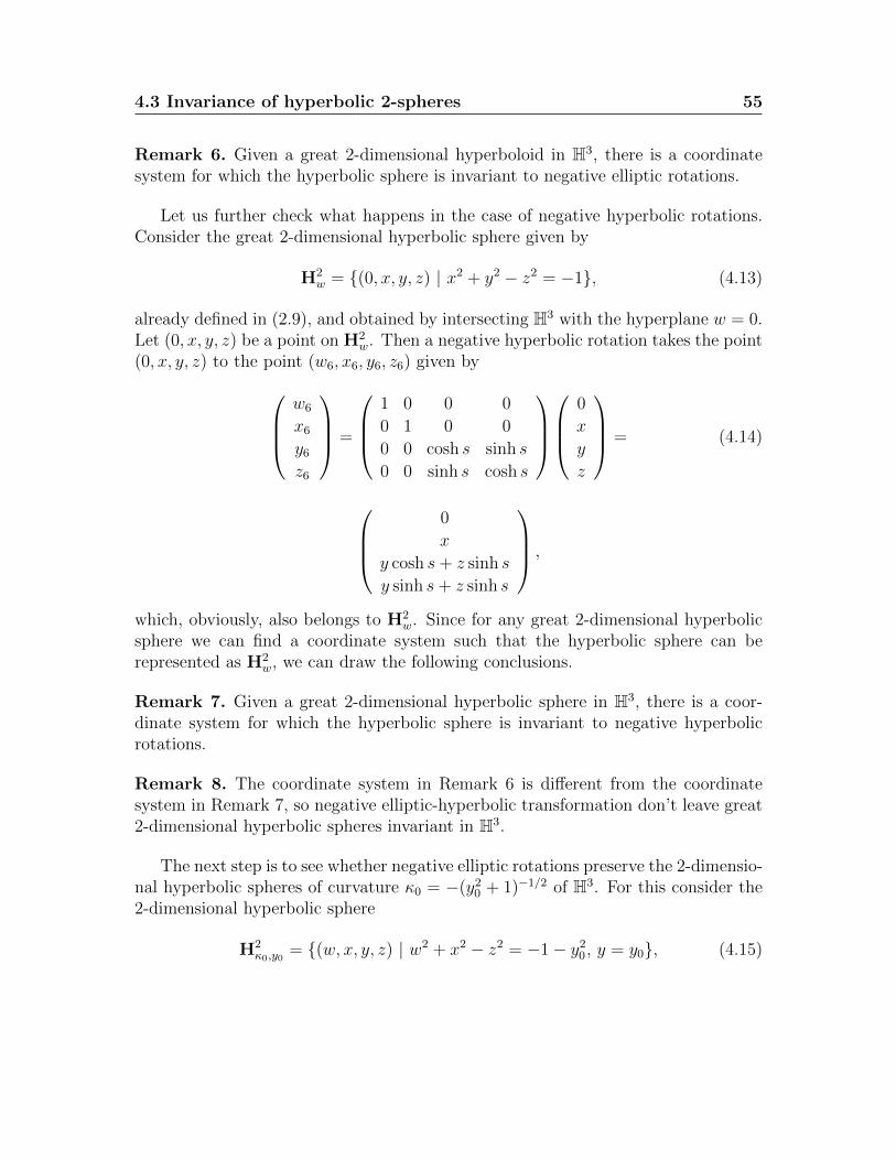
4.3 Invariance of hyperbolic 2-spheres 55
Remark 6. Given a great 2-dimensional hyperboloid in H3, there is a coordinatesystem for which the hyperbolic sphere is invariant to negative elliptic rotations.
Let us further check what happens in the case of negative hyperbolic rotations.Consider the great 2-dimensional hyperbolic sphere given by
H2w = {(0, x, y, z) | x2 + y2 − z2 = −1}, (4.13)
already defined in (2.9), and obtained by intersecting H3 with the hyperplane w = 0.Let (0, x, y, z) be a point on H2
w. Then a negative hyperbolic rotation takes the point(0, x, y, z) to the point (w6, x6, y6, z6) given by
w6
x6y6z6
=
1 0 0 0
0 1 0 0
0 0 cosh s sinh s
0 0 sinh s cosh s
0
x
y
z
= (4.14)
0
x
y cosh s+ z sinh s
y sinh s+ z sinh s
,
which, obviously, also belongs to H2w. Since for any great 2-dimensional hyperbolic
sphere we can find a coordinate system such that the hyperbolic sphere can berepresented as H2
w, we can draw the following conclusions.
Remark 7. Given a great 2-dimensional hyperbolic sphere in H3, there is a coor-dinate system for which the hyperbolic sphere is invariant to negative hyperbolicrotations.
Remark 8. The coordinate system in Remark 6 is different from the coordinatesystem in Remark 7, so negative elliptic-hyperbolic transformation don’t leave great2-dimensional hyperbolic spheres invariant in H3.
The next step is to see whether negative elliptic rotations preserve the 2-dimensio-nal hyperbolic spheres of curvature κ0 = −(y20 + 1)−1/2 of H3. For this consider the2-dimensional hyperbolic sphere
H2κ0,y0
= {(w, x, y, z) | w2 + x2 − z2 = −1− y20, y = y0}, (4.15)
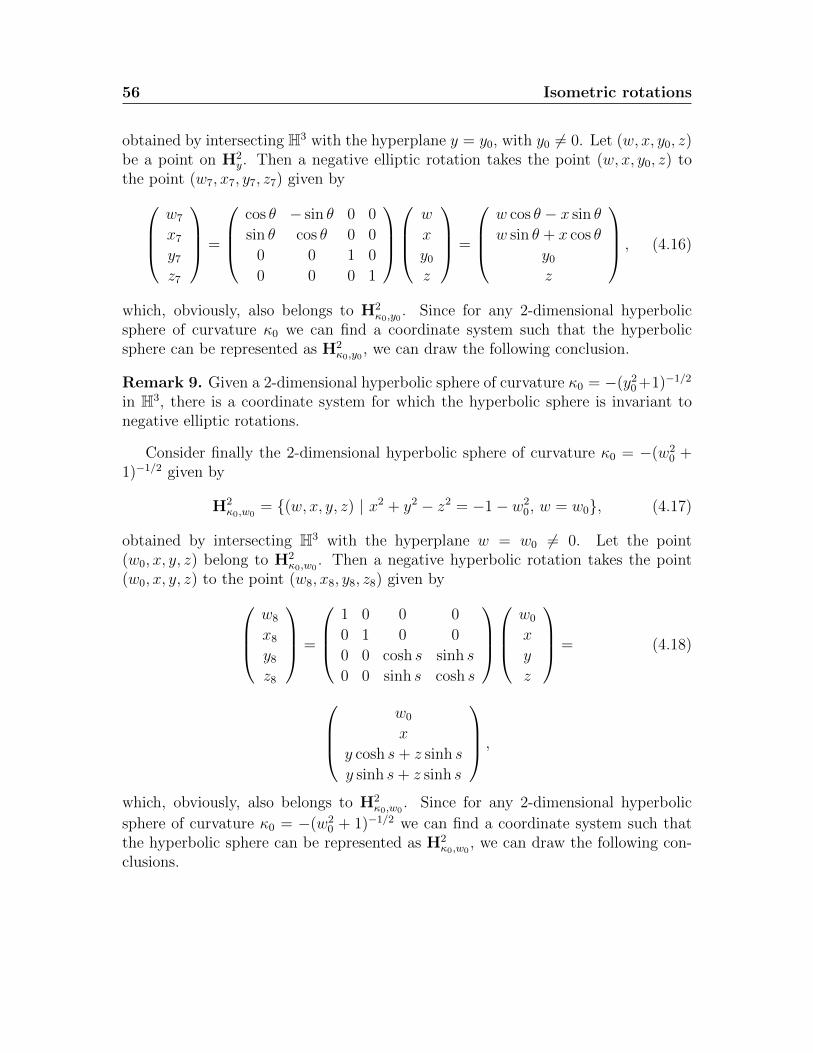
56 Isometric rotations
obtained by intersecting H3 with the hyperplane y = y0, with y0 6= 0. Let (w, x, y0, z)be a point on H2
y. Then a negative elliptic rotation takes the point (w, x, y0, z) tothe point (w7, x7, y7, z7) given by
w7
x7y7z7
=
cos θ − sin θ 0 0
sin θ cos θ 0 0
0 0 1 0
0 0 0 1
w
x
y0z
=
w cos θ − x sin θ
w sin θ + x cos θ
y0z
, (4.16)
which, obviously, also belongs to H2κ0,y0
. Since for any 2-dimensional hyperbolicsphere of curvature κ0 we can find a coordinate system such that the hyperbolicsphere can be represented as H2
κ0,y0, we can draw the following conclusion.
Remark 9. Given a 2-dimensional hyperbolic sphere of curvature κ0 = −(y20+1)−1/2
in H3, there is a coordinate system for which the hyperbolic sphere is invariant tonegative elliptic rotations.
Consider finally the 2-dimensional hyperbolic sphere of curvature κ0 = −(w20 +
1)−1/2 given by
H2κ0,w0
= {(w, x, y, z) | x2 + y2 − z2 = −1− w20, w = w0}, (4.17)
obtained by intersecting H3 with the hyperplane w = w0 6= 0. Let the point(w0, x, y, z) belong to H2
κ0,w0. Then a negative hyperbolic rotation takes the point
(w0, x, y, z) to the point (w8, x8, y8, z8) given byw8
x8y8z8
=
1 0 0 0
0 1 0 0
0 0 cosh s sinh s
0 0 sinh s cosh s
w0
x
y
z
= (4.18)
w0
x
y cosh s+ z sinh s
y sinh s+ z sinh s
,
which, obviously, also belongs to H2κ0,w0
. Since for any 2-dimensional hyperbolic
sphere of curvature κ0 = −(w20 + 1)−1/2 we can find a coordinate system such that
the hyperbolic sphere can be represented as H2κ0,w0
, we can draw the following con-clusions.
4.3 Invariance of hyperbolic 2-spheres 57
Remark 10. Given a 2-dimensional hyperbolic sphere of curvature κ0 = −(w20 +
1)−1/2 in H3, there is a coordinate system for which the hyperbolic sphere is invariantto negative hyperbolic rotations.
Remark 11. Since the coordinate system in Remark 9 is different from the coordi-nate system in Remark 10, negative elliptic-hyperbolic transformations don’t leave2-dimensional hyperbolic spheres of curvature κ0 6= −1 invariant in H3.

58 Isometric rotations
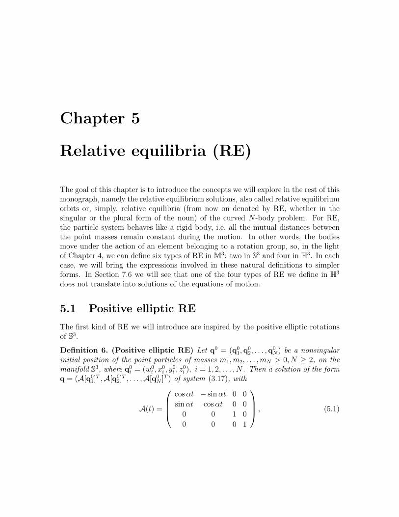
Chapter 5
Relative equilibria (RE)
The goal of this chapter is to introduce the concepts we will explore in the rest of thismonograph, namely the relative equilibrium solutions, also called relative equilibriumorbits or, simply, relative equilibria (from now on denoted by RE, whether in thesingular or the plural form of the noun) of the curved N -body problem. For RE,the particle system behaves like a rigid body, i.e. all the mutual distances betweenthe point masses remain constant during the motion. In other words, the bodiesmove under the action of an element belonging to a rotation group, so, in the lightof Chapter 4, we can define six types of RE in M3: two in S3 and four in H3. In eachcase, we will bring the expressions involved in these natural definitions to simplerforms. In Section 7.6 we will see that one of the four types of RE we define in H3
does not translate into solutions of the equations of motion.
5.1 Positive elliptic RE
The first kind of RE we will introduce are inspired by the positive elliptic rotationsof S3.
Definition 6. (Positive elliptic RE) Let q0 = (q01,q
02, . . . ,q
0N) be a nonsingular
initial position of the point particles of masses m1,m2, . . . ,mN > 0, N ≥ 2, on themanifold S3, where q0
i = (w0i , x
0i , y
0i , z
0i ), i = 1, 2, . . . , N . Then a solution of the form
q = (A[q01]T ,A[q0
2]T , . . . ,A[q0
N ]T ) of system (3.17), with
A(t) =
cosαt − sinαt 0 0
sinαt cosαt 0 0
0 0 1 0
0 0 0 1
, (5.1)
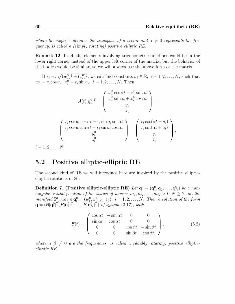
60 Relative equilibria (RE)
where the upper T denotes the transpose of a vector and α 6= 0 represents the fre-quency, is called a (simply rotating) positive elliptic RE.
Remark 12. In A, the elements involving trigonometric functions could be in thelower right corner instead of the upper left corner of the matrix, but the behavior ofthe bodies would be similar, so we will always use the above form of the matrix.
If ri =:√
(w0i )
2 + (x0i )2, we can find constants ai ∈ R, i = 1, 2, . . . , N , such that
w0i = ri cos ai, x
0i = ri sin ai, i = 1, 2, . . . , N . Then
A(t)[q0i ]T =
w0i cosαt− x0i sinαt
w0i sinαt+ x0i cosαt
y0iz0i
=
ri cos ai cosαt− ri sin ai sinαtri cos ai sinαt+ ri sin ai cosαt
y0iz0i
=
ri cos(αt+ ai)
ri sin(αt+ ai)
y0iz0i
,
i = 1, 2, . . . , N.
5.2 Positive elliptic-elliptic RE
The second kind of RE we will introduce here are inspired by the positive elliptic-elliptic rotations of S3.
Definition 7. (Positive elliptic-elliptic RE) Let q0 = (q01,q
02, . . . ,q
0N) be a non-
singular initial position of the bodies of masses m1,m2, . . . ,mN > 0, N ≥ 2, on themanifold S3, where q0
i = (w0i , x
0i , y
0i , z
0i ), i = 1, 2, . . . , N . Then a solution of the form
q = (B[q01]T ,B[q0
2]T , . . . ,B[q0
N ]T ) of system (3.17), with
B(t) =
cosαt − sinαt 0 0
sinαt cosαt 0 0
0 0 cos βt − sin βt
0 0 sin βt cos βt
, (5.2)
where α, β 6= 0 are the frequencies, is called a (doubly rotating) positive elliptic-elliptic RE.
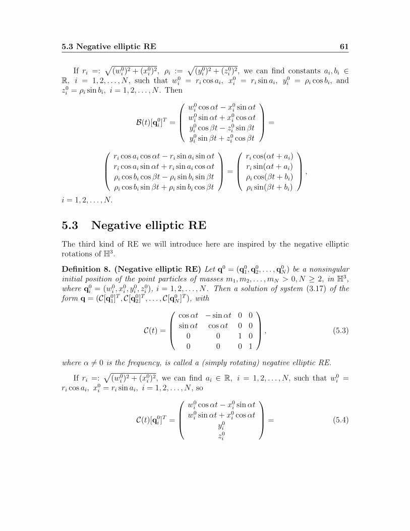
5.3 Negative elliptic RE 61
If ri =:√
(w0i )
2 + (x0i )2, ρi :=
√(y0i )
2 + (z0i )2, we can find constants ai, bi ∈
R, i = 1, 2, . . . , N , such that w0i = ri cos ai, x
0i = ri sin ai, y
0i = ρi cos bi, and
z0i = ρi sin bi, i = 1, 2, . . . , N . Then
B(t)[q0i ]T =
w0i cosαt− x0i sinαt
w0i sinαt+ x0i cosαt
y0i cos βt− z0i sin βt
y0i sin βt+ z0i cos βt
=
ri cos ai cosαt− ri sin ai sinαtri cos ai sinαt+ ri sin ai cosαt
ρi cos bi cos βt− ρi sin bi sin βtρi cos bi sin βt+ ρi sin bi cos βt
=
ri cos(αt+ ai)
ri sin(αt+ ai)
ρi cos(βt+ bi)
ρi sin(βt+ bi)
,
i = 1, 2, . . . , N.
5.3 Negative elliptic RE
The third kind of RE we will introduce here are inspired by the negative ellipticrotations of H3.
Definition 8. (Negative elliptic RE) Let q0 = (q01,q
02, . . . ,q
0N) be a nonsingular
initial position of the point particles of masses m1,m2, . . . ,mN > 0, N ≥ 2, in H3,where q0
i = (w0i , x
0i , y
0i , z
0i ), i = 1, 2, . . . , N . Then a solution of system (3.17) of the
form q = (C[q01]T , C[q0
2]T , . . . , C[q0
N ]T ), with
C(t) =
cosαt − sinαt 0 0
sinαt cosαt 0 0
0 0 1 0
0 0 0 1
, (5.3)
where α 6= 0 is the frequency, is called a (simply rotating) negative elliptic RE.
If ri =:√
(w0i )
2 + (x0i )2, we can find ai ∈ R, i = 1, 2, . . . , N, such that w0
i =ri cos ai, x
0i = ri sin ai, i = 1, 2, . . . , N , so
C(t)[q0i ]T =
w0i cosαt− x0i sinαt
w0i sinαt+ x0i cosαt
y0iz0i
= (5.4)
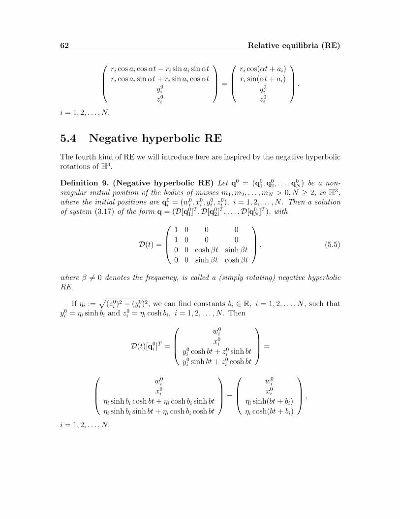
62 Relative equilibria (RE)
ri cos ai cosαt− ri sin ai sinαtri cos ai sinαt+ ri sin ai cosαt
y0iz0i
=
ri cos(αt+ ai)
ri sin(αt+ ai)
y0iz0i
,
i = 1, 2, . . . , N.
5.4 Negative hyperbolic RE
The fourth kind of RE we will introduce here are inspired by the negative hyperbolicrotations of H3.
Definition 9. (Negative hyperbolic RE) Let q0 = (q01,q
02, . . . ,q
0N) be a non-
singular initial position of the bodies of masses m1,m2, . . . ,mN > 0, N ≥ 2, in H3,where the initial positions are q0
i = (w0i , x
0i , y
0i , z
0i ), i = 1, 2, . . . , N . Then a solution
of system (3.17) of the form q = (D[q01]T ,D[q0
2]T , . . . ,D[q0
N ]T ), with
D(t) =
1 0 0 0
1 0 0 0
0 0 cosh βt sinh βt
0 0 sinh βt cosh βt
, (5.5)
where β 6= 0 denotes the frequency, is called a (simply rotating) negative hyperbolicRE.
If ηi :=√
(z0i )2 − (y0i )
2, we can find constants bi ∈ R, i = 1, 2, . . . , N , such thaty0i = ηi sinh bi and z0i = ηi cosh bi, i = 1, 2, . . . , N . Then
D(t)[q0i ]T =
w0i
x0iy0i cosh bt+ z0i sinh bt
y0i sinh bt+ z0i cosh bt
=
w0i
x0iηi sinh bi cosh bt+ ηi cosh bi sinh bt
ηi sinh bi sinh bt+ ηi cosh bi cosh bt
=
w0i
x0iηi sinh(bt+ bi)
ηi cosh(bt+ bi)
,
i = 1, 2, . . . , N.
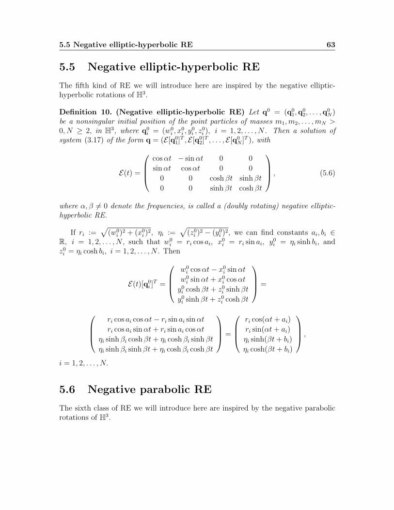
5.5 Negative elliptic-hyperbolic RE 63
5.5 Negative elliptic-hyperbolic RE
The fifth kind of RE we will introduce here are inspired by the negative elliptic-hyperbolic rotations of H3.
Definition 10. (Negative elliptic-hyperbolic RE) Let q0 = (q01,q
02, . . . ,q
0N)
be a nonsingular initial position of the point particles of masses m1,m2, . . . ,mN >0, N ≥ 2, in H3, where q0
i = (w0i , x
0i , y
0i , z
0i ), i = 1, 2, . . . , N . Then a solution of
system (3.17) of the form q = (E [q01]T , E [q0
2]T , . . . , E [q0
N ]T ), with
E(t) =
cosαt − sinαt 0 0
sinαt cosαt 0 0
0 0 cosh βt sinh βt
0 0 sinh βt cosh βt
, (5.6)
where α, β 6= 0 denote the frequencies, is called a (doubly rotating) negative elliptic-hyperbolic RE.
If ri :=√
(w0i )
2 + (x0i )2, ηi :=
√(z0i )
2 − (y0i )2, we can find constants ai, bi ∈
R, i = 1, 2, . . . , N , such that w0i = ri cos ai, x
0i = ri sin ai, y
0i = ηi sinh bi, and
z0i = ηi cosh bi, i = 1, 2, . . . , N . Then
E(t)[q0i ]T =
w0i cosαt− x0i sinαt
w0i sinαt+ x0i cosαt
y0i cosh βt+ z0i sinh βt
y0i sinh βt+ z0i cosh βt
=
ri cos ai cosαt− ri sin ai sinαtri cos ai sinαt+ ri sin ai cosαt
ηi sinh βi cosh βt+ ηi cosh βi sinh βt
ηi sinh βi sinh βt+ ηi cosh βi cosh βt
=
ri cos(αt+ ai)
ri sin(αt+ ai)
ηi sinh(βt+ bi)
ηi cosh(βt+ bi)
,
i = 1, 2, . . . , N.
5.6 Negative parabolic RE
The sixth class of RE we will introduce here are inspired by the negative parabolicrotations of H3.
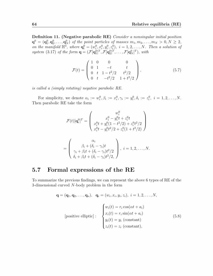
64 Relative equilibria (RE)
Definition 11. (Negative parabolic RE) Consider a nonsingular initial positionq0 = (q0
1,q02, . . . ,q
0N) of the point particles of masses m1,m2, . . . ,mN > 0, N ≥ 2,
on the manifold H3, where q0i = (w0
i , x0i , y
0i , z
0i ), i = 1, 2, . . . , N . Then a solution of
system (3.17) of the form q = (F [q01]T ,F [q0
2]T , . . . ,F [q0
N ]T ), with
F(t) =
1 0 0 0
0 1 −t t
0 t 1− t2/2 t2/2
0 t −t2/2 1 + t2/2
, (5.7)
is called a (simply rotating) negative parabolic RE.
For simplicity, we denote αi := w0i , βi := x0i , γi := y0i , δi := z0i , i = 1, 2, . . . , N .
Then parabolic RE take the form
F(t)[q0i ]T =
w0i
x0i − y0i t+ z0i t
x0i t+ y0i (1− t2/2) + z0i t2/2
x0i t− y0i t2/2 + z0i (1 + t2/2)
=
αi
βi + (δi − γi)tγi + βit+ (δi − γi)t2/2δi + βit+ (δi − γi)t2/2,
, i = 1, 2, . . . , N.
5.7 Formal expressions of the RE
To summarize the previous findings, we can represent the above 6 types of RE of the3-dimensional curved N -body problem in the form
q = (q1,q2, . . . ,qn), qi = (wi, xi, yi, zi), i = 1, 2, . . . , N,
[positive elliptic] :
wi(t) = ri cos(αt+ ai)
xi(t) = ri sin(αt+ ai)
yi(t) = yi (constant)
zi(t) = zi (constant),
(5.8)
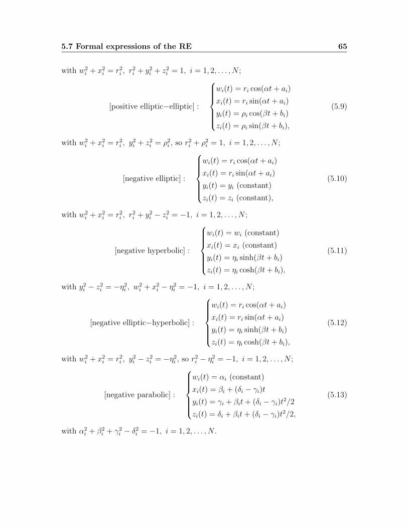
5.7 Formal expressions of the RE 65
with w2i + x2i = r2i , r
2i + y2i + z2i = 1, i = 1, 2, . . . , N ;
[positive elliptic−elliptic] :
wi(t) = ri cos(αt+ ai)
xi(t) = ri sin(αt+ ai)
yi(t) = ρi cos(βt+ bi)
zi(t) = ρi sin(βt+ bi),
(5.9)
with w2i + x2i = r2i , y
2i + z2i = ρ2i , so r2i + ρ2i = 1, i = 1, 2, . . . , N ;
[negative elliptic] :
wi(t) = ri cos(αt+ ai)
xi(t) = ri sin(αt+ ai)
yi(t) = yi (constant)
zi(t) = zi (constant),
(5.10)
with w2i + x2i = r2i , r
2i + y2i − z2i = −1, i = 1, 2, . . . , N ;
[negative hyperbolic] :
wi(t) = wi (constant)
xi(t) = xi (constant)
yi(t) = ηi sinh(βt+ bi)
zi(t) = ηi cosh(βt+ bi),
(5.11)
with y2i − z2i = −η2i , w2i + x2i − η2i = −1, i = 1, 2, . . . , N ;
[negative elliptic−hyperbolic] :
wi(t) = ri cos(αt+ ai)
xi(t) = ri sin(αt+ ai)
yi(t) = ηi sinh(βt+ bi)
zi(t) = ηi cosh(βt+ bi),
(5.12)
with w2i + x2i = r2i , y
2i − z2i = −η2i , so r2i − η2i = −1, i = 1, 2, . . . , N ;
[negative parabolic] :
wi(t) = αi (constant)
xi(t) = βi + (δi − γi)tyi(t) = γi + βit+ (δi − γi)t2/2zi(t) = δi + βit+ (δi − γi)t2/2,
(5.13)
with α2i + β2
i + γ2i − δ2i = −1, i = 1, 2, . . . , N .

66 Relative equilibria (RE)
Chapter 6
Fixed Points (FP)
In this chapter we will introduce the concept of fixed-point solution, also simply calledfixed point (from now on denoted by FP, whether in the singular or the plural formof the noun) of the equations of motion, show that FP exist in S3, provide a coupleof examples, and finally prove that they don’t show up in H3 and in hemispheres ofS3, provided that at least one body is not on the boundary of the hemisphere.
6.1 FP in S3
Although the goal of this monograph is to study RE of the curved N -body prob-lem, some of these orbits can be generated from FP configurations by imposing onthe initial positions of the bodies suitable nonzero initial velocities. It is thereforenecessary to discuss FP as well. Let us start with their definition.
Definition 12. A solution of system (3.21) is called a fixed point if it is a zero of
the vector field, i.e. pi(t) = ∇qiU(q(t)) = 0 for all t ∈ R, i = 1, 2, . . . , N .
In [33] and [35], we showed that FP exist in S2, but don’t exist in H2. Examplesof FP are the equilateral triangle, and in general any regular N -gon of equal masses,N odd, lying on any great circle of S2, and the regular tetrahedron of equal massesinscribed in S2 in the 4-body case. There are also examples of FP of unequal masses.We showed in [28] that, for any acute triangle inscribed in a great circle of thesphere S2, there exist masses m1,m2,m3 > 0 that can be placed at the vertices ofthe triangle such that they form a FP, and therefore can generate RE in the curved3-body problem. The problem of the existence of N -gons with unequal masses isopen, though very likely to be true, for N > 3.
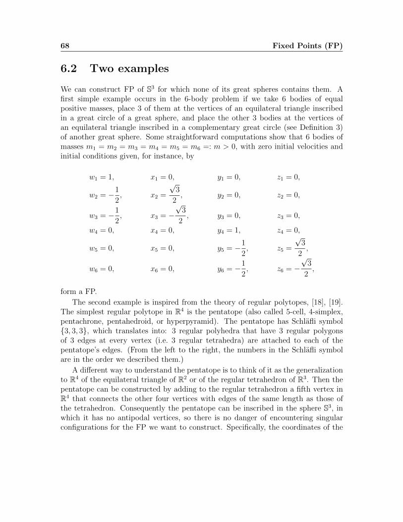
68 Fixed Points (FP)
6.2 Two examples
We can construct FP of S3 for which none of its great spheres contains them. Afirst simple example occurs in the 6-body problem if we take 6 bodies of equalpositive masses, place 3 of them at the vertices of an equilateral triangle inscribedin a great circle of a great sphere, and place the other 3 bodies at the vertices ofan equilateral triangle inscribed in a complementary great circle (see Definition 3)of another great sphere. Some straightforward computations show that 6 bodies ofmasses m1 = m2 = m3 = m4 = m5 = m6 =: m > 0, with zero initial velocities andinitial conditions given, for instance, by
w1 = 1, x1 = 0, y1 = 0, z1 = 0,
w2 = −1
2, x2 =
√3
2, y2 = 0, z2 = 0,
w3 = −1
2, x3 = −
√3
2, y3 = 0, z3 = 0,
w4 = 0, x4 = 0, y4 = 1, z4 = 0,
w5 = 0, x5 = 0, y5 = −1
2, z5 =
√3
2,
w6 = 0, x6 = 0, y6 = −1
2, z6 = −
√3
2,
form a FP.
The second example is inspired from the theory of regular polytopes, [18], [19].The simplest regular polytope in R4 is the pentatope (also called 5-cell, 4-simplex,pentachrone, pentahedroid, or hyperpyramid). The pentatope has Schlafli symbol{3, 3, 3}, which translates into: 3 regular polyhedra that have 3 regular polygonsof 3 edges at every vertex (i.e. 3 regular tetrahedra) are attached to each of thepentatope’s edges. (From the left to the right, the numbers in the Schlafli symbolare in the order we described them.)
A different way to understand the pentatope is to think of it as the generalizationto R4 of the equilateral triangle of R2 or of the regular tetrahedron of R3. Then thepentatope can be constructed by adding to the regular tetrahedron a fifth vertex inR4 that connects the other four vertices with edges of the same length as those ofthe tetrahedron. Consequently the pentatope can be inscribed in the sphere S3, inwhich it has no antipodal vertices, so there is no danger of encountering singularconfigurations for the FP we want to construct. Specifically, the coordinates of the
6.3 Cases of nonexistence 69
5 vertices of a pentatope inscribed in the sphere S3 can be taken, for example, as
w1 = 1, x1 = 0, y1 = 0, z1 = 0,
w2 = −1
4, x2 =
√15
4, y2 = 0, z2 = 0,
w3 = −1
4, x3 = −
√5
4√
3, y3 =
√5√6, z3 = 0,
w4 = −1
4, x4 = −
√5
4√
3, y4 = −
√5
2√
6, z4 =
√5
2√
2,
w5 = −1
4, x5 = −
√5
4√
3, y5 = −
√5
2√
6, z5 = −
√5
2√
2.
Straightforward computations show that the distance from the origin of the coordi-nate system to each of the 5 vertices is 1 and that, for equal masses, m1 = m2 =m3 = m4 = m5 =: m > 0, this configuration produces a FP of system (3.15). Likein the previous example, the FP lying at the vertices of the pentatope is specific toS3 in the sense that there is no 2-dimensional sphere that contains it.
It is natural to ask whether other convex regular polytopes of R4 can form FPsin S3 if we place equal masses at their vertices. Apart from the pentatope, there arefive other such geometrical objects: the tesseract (also called 8-cell, hypercube, or4-cube, with 16 vertices), the orthoplex (also called 16-cell or hyperoctahedron, with8 vertices), the octaplex (also called 24-cell or polyoctahedron, with 24 vertices), thedodecaplex (also called 120-cell, hyperdodecahedron, or polydodecahedron, with 600vertices), and the tetraplex (also called 600-cell, hypericosahedron, or polytetrahe-dron, with 120 vertices). All these polytopes, however, are centrally symmetric, sothey have antipodal vertices. Therefore, if we place bodies of equal masses at theirvertices, we encounter singularities. Consequently the only convex regular polytopeof R4 that can form a FP if we place equal masses at its vertices is the pentatope.
6.3 Cases of nonexistence
We will show further that there are no FP in H3 or in any hemisphere of S3. In thelatter case, for FP not to exist it is necessary that at least one body is not on theboundary of the hemisphere.
Proposition 3. (No FP in H3) There are no masses m1,m2, . . . ,mN > 0, N ≥ 2,that can form FP in H3.
70 Fixed Points (FP)
Proof. Consider N bodies of masses m1,m2, . . . ,mN > 0, N ≥ 2, lying in H3, ina nonsingular configuration (i.e. without collisions) and with zero initial velocities.Then one or more bodies, say, m1,m2, . . . ,mk with k ≤ N , have the largest z co-ordinate. Consequently each of the bodies mk+1, . . . ,mN will attract each of thebodies m1,m2, . . . ,mk along a geodesic hyperbola towards lowering the z coordinateof the latter. For any 2 bodies with the same largest z coordinate, the segment ofhyperbola connecting them has points with lower z coordinates. Therefore these 2bodies attract each other towards lowering their z coordinates as well. So each ofthe bodies m1,m2, . . . ,mk will move towards lowering their z coordinate, thereforethe initial configuration of the bodies is not fixed.
Proposition 4. (No FP in hemispheres of S3) There are no masses m1,m2, . . . ,mN > 0, N ≥ 2, that can form FP in any closed hemisphere of S3 (i.e. a hemispherethat contains its boundary), as long as at least one body doesn’t lie on the boundary.
Proof. The idea of the proof is similar to the idea of the proof we gave for Proposition3. Let us assume, without loss of generality, that the bodies are in the hemispherez ≤ 0 and they form a nonsingular initial configuration (i.e. without collisions orantipodal positions), with at least one of the bodies not on the boundary z = 0, andwith zero initial velocities. Then one or more bodies, say, m1,m2, . . . ,mk, with k < N(a strict inequality is essential to the proof), have the largest z coordinate, whichcan be at most 0. Consequently the bodies mk+1, . . . ,mN have lower z coordinates.Each of the bodies mk+1, . . . ,mN attract each of the bodies m1,m2, . . . ,mk along ageodesic arc of a great circle towards lowering the z coordinate of the latter.
The attraction between any 2 bodies among m1,m2, . . . ,mk is either towardslowering each other’s z coordinate, when z < 0 or along the geodesic z = 0, whenthey are on that geodesic. In both cases, however, composing all the forces thatact on each of the bodies m1,m2, . . . ,mk will make them move towards a lower zcoordinate, which means that the initial configuration is not fixed. This remarkcompletes the proof.
Part III
Criteria and Qualitative Behavior

73
Preamble
Now that we found natural definitions for the RE of the curved N -body problem, wemust understand under what circumstances they may exist. So the goal of Part IIIis to provide existence criteria for each type of RE previously defined and to obtainsome results that describe their qualitative behavior. For this purpose, we will alsoreview some aspects of geometric topology related to S3 and H3, building on certainproperties proved in Part I. Our results are exhaustive in the sense that no othertype of dynamical behavior can occur for these orbits, but we don’t deal here withproving their actual existence, an issue we will address in Part IV.

74
Chapter 7
Existence criteria
In this chapter we establish criteria for the existence of positive elliptic and elliptic-elliptic as well as negative elliptic, hyperbolic, and elliptic-hyperbolic RE. Thesecriteria will be employed in later chapters to obtain concrete examples of such orbits.The proofs are similar in spirit, but for completeness and future reference we describethem all since the specifics differ in each case. We close this chapter by showing thatnegative parabolic RE do not exist in the curved N -body problem.
7.1 Criteria for RE
We will next provide a criterion for the existence of (simply rotating) positive ellipticRE and then prove a corollary that shows under what conditions such solutions canbe generated from FP configurations.
Criterion 1. (Positive elliptic RE) Let m1,m2, . . . ,mN > 0 represent the massesof N ≥ 2 point particles moving in S3. Then system (3.15) admits a solution of theform
q = (q1,q2, . . . ,qn), qi = (wi, xi, yi, zi), i = 1, 2, . . . , N,
wi(t) = ri cos(αt+ ai), xi(t) = ri sin(αt+ ai), yi(t) = yi, zi(t) = zi,
with w2i + x2i = r2i , r
2i + y2i + z2i = 1, and yi, zi constant, i = 1, 2, . . . , N , i.e. a (sim-
ply rotating) positive elliptic RE, if and only if there are constants ri, ai, yi, zi, i =1, 2, . . . , N, and α 6= 0, such that the following 4N conditions are satisfied:
N∑j=1
j 6=i
mj(rj cos aj − νijri cos ai)
(1− ν2ij)3/2= (r2i − 1)α2ri cos ai, (7.1)
76 Existence criteria
N∑j=1
j 6=i
mj(rj sin aj − νijri sin ai)(1− ν2ij)3/2
= (r2i − 1)α2ri sin ai, (7.2)
N∑j=1
j 6=i
mj(yj − νijyi)(1− ν2ij)3/2
= α2r2i yi, (7.3)
N∑j=1
j 6=i
mj(zj − νijzi)(1− ν2ij)3/2
= α2r2i zi, (7.4)
i = 1, 2, . . . , N, where νij = rirj cos(ai − aj) + yiyj + zizj, i, j = 1, 2 . . . , N, i 6= j.
Proof. Consider a candidate, as described above, for a solution q of system (3.15).Some straightforward computations show that
νij := qi � qj = rirj cos(ai − aj) + yiyj + zizj, i, j = 1, 2 . . . , n, i 6= j,
qi � qi = α2r2i , i = 1, 2, . . . , N,
wi = −α2ri cos(αt+ ai), xi = −α2ri sin(αt+ ai),
yi = zi = 0, i = 1, 2, . . . , N.
Substituting the suggested solution and the above expressions into system (3.15),for the w coordinates we obtain conditions involving cos(αt + ai), whereas for thex coordinates we obtain conditions involving sin(αt + ai). In the former case, usingthe fact that cos(αt+ ai) = cosαt cos ai − sinαt sin ai, we can split each equation intwo, one involving cosαt and the other sinαt as factors. The same thing happensin the latter case if we use the formula sin(αt + ai) = sinαt cos ai + cosαt sin ai.Each of these equations are satisfied if and only if conditions (7.1) and (7.2) takeplace. Conditions (7.3) and (7.4) follow directly from the equations involving thecoordinates y and z. This remark completes the proof.
Criterion 2. (Positive elliptic RE generated from FP configurations) Con-sider the point particles of masses m1,m2, . . . ,mN > 0, N ≥ 2, in S3. Then, for anyα 6= 0, system (3.15) admits a solution of the form (5.8):
q = (q1,q2, . . . ,qn),qi = (wi, xi, yi, zi), i = 1, 2, . . . , N,
wi(t) = ri cos(αt+ ai), xi(t) = ri sin(αt+ ai), yi(t) = yi, zi(t) = zi,
7.1 Criteria for RE 77
with w2i +x2i = r2i , r
2i +y2i +z2i = 1, and yi, zi constant, i = 1, 2, . . . , N , generated from
a FP configuration, i.e. a (simply rotating) positive elliptic RE generated from thesame initial positions that would form a FP for zero initial velocities, if and only ifthere are constants ri, ai, yi, zi, i = 1, 2, . . . , N, such that the following 4N conditionsare satisfied:
N∑j=1
j 6=i
mj(rj cos aj − νijri cos ai)
(1− ν2ij)3/2= 0, (7.5)
N∑j=1
j 6=i
mj(rj sin aj − νijri sin ai)(1− ν2ij)3/2
= 0, (7.6)
N∑j=1
j 6=i
mj(yj − νijyi)(1− ν2ij)3/2
= 0, (7.7)
N∑j=1
j 6=i
mj(zj − νijzi)(1− ν2ij)3/2
= 0, (7.8)
i = 1, 2, . . . , N , where νij = rirj cos(ai − aj) + yiyj + zizj, i, j = 1, 2, . . . , N, i 6= j,and one of the following two properties takes place:
(i) ri = 1 for all i ∈ {1, 2 . . . , N},(ii) there is a proper subset I ⊂ {1, 2, . . . , N} such that ri = 0 for all i ∈ I and
rj = 1 for all j ∈ {1, 2, . . . , N} \ I.
Proof. We are seeking a (simply rotating) elliptic RE, as in Criterion 1, that is validfor any α 6= 0. But the solution is also generated from a FP configuration, so the lefthand sides of equations (7.1), (7.2), (7.3), and (7.4) necessarily vanish, thus leadingto conditions (7.5), (7.6), (7.7), and (7.8). However, the right hand sides of equations(7.1), (7.2), (7.3), and (7.4) must also vanish, so we have the 4N conditions:
(r2i − 1)α2ri cos ai = 0, i = 1, 2, . . . , N,
(r2i − 1)α2ri sin ai = 0, i = 1, 2, . . . , N,
α2r2i yi = 0, i = 1, 2, . . . , N,
α2r2i zi = 0, i = 1, 2, . . . , N.
Since α 6= 0 and there is no γ ∈ R such that the quantities sin γ and cos γ vanishsimultaneously, the above 4N conditions are satisfied in each of the following cases:
78 Existence criteria
(a) ri = 0 (consequently wi = xi = 0 and y2i + z2i = 1) for all i ∈ {1, 2, . . . , N},(b) ri = 1 (consequently w2
i + x2i = 1 and yi = zi = 0) for all i ∈ {1, 2 . . . , N},(c) there is a proper subset I ⊂ {1, 2, . . . , N} such that ri = 0 (and consequently
y2i + z2i = 1) for all i ∈ I and rj = 1 (and consequently yj = zj = 0) for allj ∈ {1, 2, . . . , N} \ I.
In case (a), we recover the FP, so there is no rotation of any kind, thereforethis case does not lead to any simply rotating positive elliptic RE. As we will seein Theorem 2, case (b), which corresponds to (i) in the above statement, and case(c), which corresponds to (ii), lead to RE of this kind. This remark completes theproof.
7.2 Criteria for positive elliptic-elliptic RE
We can now provide a criterion for the existence of (doubly rotating) positive elliptic-elliptic RE and a criterion about how such orbits can be obtained from FP configu-rations.
Criterion 3. (Positive elliptic-elliptic RE) Let m1,m2, . . . ,mN > 0 representthe masses of N ≥ 2 point particles moving in S3. Then system (3.15) admits asolution of the form (5.9):
q = (q1,q2, . . . ,qn),qi = (wi, xi, yi, zi), i = 1, 2, . . . , N,
wi(t) = ri cos(αt+ ai), xi(t) = ri sin(αt+ ai),
yi(t) = ρi cos(βt+ bi), zi(t) = ρi sin(βt+ bi),
with w2i + x2i = r2i , y
2i + z2i = ρ2i , r
2i + ρ2i = 1, i = 1, 2, . . . , N , i.e. a (doubly
rotating) positive elliptic-elliptic RE, if and only if there are constants ri, ρi, ai, bi, i =1, 2, . . . , N , and α, β 6= 0, such that the following 4N conditions are satisfied
N∑j=1
j 6=i
mj(rj cos aj − ωijri cos ai)
(1− ω2ij)
3/2= (α2r2i + β2ρ2i − α2)ri cos ai, (7.9)
N∑j=1
j 6=i
mj(rj sin aj − ωijri sin ai)(1− ω2
ij)3/2
= (α2r2i + β2ρ2i − α2)ri sin ai, (7.10)
7.2 Criteria for positive elliptic-elliptic RE 79
N∑j=1
j 6=i
mj(ρj cos bj − ωijρi cos bi)
(1− ω2ij)
3/2= (α2r2i + β2ρ2i − β2)ρi cos bi, (7.11)
N∑j=1
j 6=i
mj(ρj sin bj − ωijρi sin bi)(1− ω2
ij)3/2
= (α2r2i + β2ρ2i − β2)ρi sin bi, (7.12)
i = 1, 2, . . . , N , where ωij = rirj cos(ai−aj)+ρiρj cos(bi−bj), i, j = 1, 2, . . . , N, i 6= j.
Proof. Consider a candidate q as above for a solution of system (3.15). Some straight-forward computations show that
ωij := qi � qj = rirj cos(ai − aj) + ρiρj cos(bi − bj), i, j = 1, 2 . . . , N, i 6= j,
qi � qi = α2r2i + β2ρ2i , i = 1, 2, . . . , N,
wi = −α2ri cos(αt+ ai), xi = −α2ri sin(αt+ ai),
yi = −β2ρi cos(βt+ bi), zi = −β2ρi sin(βt+ bi), i = 1, 2, . . . , N.
Substituting q and the above expressions into system (3.15), for the w coordinateswe obtain conditions involving cos(αt+ ai), whereas for the x coordinates we obtainconditions involving sin(αt+ai). In the former case, using the fact that cos(αt+ai) =cosαt cos ai−sinαt sin ai, we can split each equation in two, one involving cosαt andthe other sinαt as factors. The same thing happens in the latter case if we use theformula sin(αt+ai) = sinαt cos ai+cosαt sin ai. Each of these equations are satisfiedif and only if conditions (7.9) and (7.10) take place.
For the y coordinate, the substitution of the above solution leads to conditionsinvolving cos(βt+bi), whereas for z coordinate it leads to conditions involving sin(βt+bi). Then we proceed as we did for the w and x coordinates and obtain conditions(7.11) and (7.12). This remark completes the proof.
Criterion 4. (Positive elliptic-elliptic RE generated from FP configura-tions) Consider the point particles of masses m1,m2, . . . , mN > 0, N ≥ 2, movingin S3. Then, for any α, β 6= 0, system (3.15) admits a solution of the form (5.9):
q = (q1,q2, . . . ,qn),qi = (wi, xi, yi, zi), i = 1, 2, . . . , N,
wi(t) = ri cos(αt+ ai), xi(t) = ri sin(αt+ ai),
yi(t) = ρi cos(βt+ bi), zi(t) = ρi sin(βt+ bi),
80 Existence criteria
with w2i + x2i = r2i , y
2i + z2i = ρ2i , r
2i + ρ2i = 1, i = 1, 2, . . . , N , generated from a FP
configuration, i.e. a (doubly rotating) positive elliptic-elliptic RE generated from thesame initial positions that would form a FP for zero initial velocities, if and only ifthere are constants ri, ρi, ai, bi, i = 1, 2, . . . , N , such that the 4N relationships beloware satisfied:
N∑j=1
j 6=i
mj(rj cos aj − ωijri cos ai)
(1− ω2ij)
3/2= 0, (7.13)
N∑j=1
j 6=i
mj(rj sin aj − ωijri sin ai)(1− ω2
ij)3/2
= 0, (7.14)
N∑j=1
j 6=i
mj(ρj cos bj − ωijρi cos bi)
(1− ω2ij)
3/2= 0, (7.15)
N∑j=1
j 6=i
mj(ρj sin bj − ωijρi sin bi)(1− ω2
ij)3/2
= 0, (7.16)
i = 1, 2, . . . , N , where ωij = rirj cos(ai−aj)+ρiρj cos(bi− bj), i, j = 1, 2, . . . , N, i 6=j, and, additionally, one of the following properties takes place:
(i) there is a proper subset J ⊂ {1, 2, . . . , N} such that ri = 0 for all i ∈ J andρj = 0 for all j ∈ {1, 2, . . . , N} \ J ,
(ii) the frequencies α, β 6= 0 satisfy the condition |α| = |β|.
Proof. A FP configuration requires that the left hand sides of equations (7.9), (7.10),(7.11), and (7.12) vanish, so we obtain the conditions (7.13), (7.14), (7.15), and(7.16). A RE can be generated from a FP configuration if and only if the right handsides of (7.9), (7.10), (7.11), and (7.12) vanish as well, i.e.
(α2r2i + β2ρ2i − α2)ri cos ai = 0,
(α2r2i + β2ρ2i − α2)ri sin ai = 0,
(α2r2i + β2ρ2i − β2)ρi cos bi = 0,
(α2r2i + β2ρ2i − β2)ρi sin bi = 0,
where r2i + ρ2i = 1, i = 1, 2, . . . , N . Since there is no γ ∈ R such that sin γ andcos γ vanish simultaneously, the above expressions are zero in each of the followingcircumstances:
7.3 Criterion for negative elliptic RE 81
(a) ri = 0, and consequently ρi = 1, for all i ∈ {1, 2, . . . , N};(b) ρi = 0, and consequently ri = 1, for all i ∈ {1, 2, . . . , N};(c) there is a proper subset J ⊂ {1, 2, . . . , N} such that ri = 0 (consequently
ρi = 1) for all i ∈ J and ρj = 0 (consequently rj = 1) for all j ∈ {1, 2, . . . , N} \ J ;
(d) α2r2i + β2ρ2i − α2 = α2r2i + β2ρ2i − β2 = 0, i ∈ {1, 2, . . . , N}.Cases (a) and (b) correspond to (simply rotating) positive elliptic RE, thus recov-
ering condition (i) in Criterion 2. Case (c) corresponds to (i) in the above statement.Since, from Definition 6, it follows that α, β 6= 0, the identities in case (d) can obvi-ously take place only if α2 = β2, i.e. |α| = |β| 6= 0, so (d) corresponds to condition(ii) in the above statement. This remark completes the proof.
7.3 Criterion for negative elliptic RE
We further consider the motion of point masses in H3 and start with proving acriterion for the existence of simply rotating negative elliptic RE.
Criterion 5. (Negative elliptic RE) Consider the point particles of masses m1,m2,. . . ,mN > 0, N ≥ 2, moving in H3. Then system (3.16) admits solutions of the form(5.10):
q = (q1,q2, . . . ,qn), qi = (wi, xi, yi, zi), i = 1, 2, . . . , N,
wi(t) = ri cos(αt+ ai), xi(t) = ri sin(αt+ ai), yi(t) = yi, zi(t) = zi,
with w2i +x2i = r2i , r
2i +y2i −z2i = −1, and yi, zi constant, i = 1, 2, . . . , N , i.e. (simply
rotating) negative elliptic RE, if and only if there are constants ri, ai, yi, zi, i =1, 2, . . . , N , and α 6= 0, such that the following 4N conditions are satisfied:
N∑j=1
j 6=i
mj(rj cos aj + εijri cos ai)
(ε2ij − 1)3/2= −(r2i + 1)α2ri cos ai, (7.17)
N∑j=1
j 6=i
mj(rj sin aj + εijri sin ai)
(ε2ij − 1)3/2= −(r2i + 1)α2ri sin ai, (7.18)
N∑j=1
j 6=i
mj(yj + εijyi)
(ε2ij − 1)3/2= −α2r2i yi, (7.19)

82 Existence criteria
N∑j=1
j 6=i
mj(zj + εijzi)
(ε2ij − 1)3/2= −α2r2i zi, (7.20)
i = 1, 2, . . . , N , where εij = rirj cos(ai − aj) + yiyj − zizj, i, j = 1, 2, . . . , N, i 6= j.
Proof. Consider a candidate q as above for a solution of system (3.16). Some straight-forward computations show that
εij := qi � qj = rirj cos(ai − aj) + yiyj − zizj, i, j = 1, 2 . . . , N, i 6= j,
qi � qi = α2r2i , i = 1, 2, . . . , N,
wi = −α2ri cos(αt+ ai), xi = −α2ri sin(αt+ ai),
yi = zi = 0, i = 1, 2, . . . , N.
Substituting q and the above expressions into the equations of motion (3.16), forthe w coordinates we obtain conditions involving cos(αt + ai), whereas for the xcoordinates we obtain conditions involving sin(αt + ai). In the former case, usingthe fact that cos(αt+ ai) = cosαt cos ai − sinαt sin ai, we can split each equation intwo, one involving cosαt and the other sinαt as factors. The same thing happensin the latter case if we use the formula sin(αt + ai) = sinαt cos ai + cosαt sin ai.Each of these equations are satisfied if and only if conditions (7.17) and (7.18) takeplace. Conditions (7.19) and (7.20) follow directly from the equations involving thecoordinates y and z. This remark completes the proof.
7.4 Criterion for negative hyperbolic RE
We continue our study of the hyperbolic space with proving a criterion that showsunder what conditions (simply rotating) negative hyperbolic RE exist.
Criterion 6. (Negative hyperbolic RE) Consider the point particles of massesm1,m2, . . . ,mN > 0, N ≥ 2, moving in H3. Then system (3.16) admits solutions ofthe form (5.11):
q = (q1,q2, . . . ,qn), qi = (wi, xi, yi, zi), i = 1, 2, . . . , N,
wi(t) = wi (constant), xi(t) = xi (constant),
yi(t) = ηi sinh(βt+ bi), zi(t) = ηi cosh(βt+ bi),
7.4 Criterion for negative hyperbolic RE 83
with y2i − z2i = −η2i , w2i + x2i − η2i = −1, i = 1, 2, . . . , N , i.e. (simply rotating)
negative hyperbolic RE, if and only if there are constants ηi, wi, xi, i = 1, 2, . . . , N ,and β 6= 0, such that the following 4N conditions are satisfied:
N∑j=1
j 6=i
mj(wj + µijwi)
(µ2ij − 1)3/2
= −β2η2iwi, (7.21)
N∑j=1
j 6=i
mj(xj + µijxi)
(µ2ij − 1)3/2
= −β2η2i xi, (7.22)
N∑j=1
j 6=i
mj(ηj sinh bj + µijηi sinh bi)
(µ2ij − 1)3/2
= (1− η2i )β2ηi sinh bi, (7.23)
N∑j=1
j 6=i
mj(ηj cosh bj + µijηi cosh bi)
(µ2ij − 1)3/2
= (1− η2i )β2ηi cosh bi, (7.24)
i = 1, 2, . . . , N , where µij = wiwj +xixj− ηiηj cosh(bi− bj), i, j = 1, 2, . . . , N, i 6= j.
Proof. Consider a candidate q as above for a solution of system (3.16). Some straight-forward computations show that
µij := qi � qj = wiwj + xixj − ηiηj cosh(bi − bj), i, j = 1, 2, . . . , N, i 6= j,
qi � qi = β2η2i , i = 1, 2, . . . , N,
wi = xi = 0,
yi = β2ηi sinh(βt+ bi), zi = β2ηi cosh(βi+ bi), i = 1, 2, . . . , N.
Substituting q and the above expressions into the equations of motion (3.16), we areled for the w and x coordinates to the equations (7.21) and (7.22), respectively. Forthe y and z coordinates we obtain conditions involving sinh(βt+bi) and cosh(βt+bi),respectively. In the former case, using the fact that sinh(βt+ bi) = sinh βt cosh bi +cosh βt sinh bi, we can split each equation in two, one involving sinh βt and the othercosh βt as factors. The same thing happens in the later case if we use the formulacosh(βt+ bi) = cosh βt cosh bi + sinh βt sinh bi. Each of these conditions are satisfiedif and only of conditions (7.23) and (7.24) take place. This remark completes theproof.

84 Existence criteria
7.5 Criterion for negative elliptic-hyperbolic RE
We end our study of existence criteria for RE in hyperbolic space with a result thatshows under what conditions (doubly rotating) negative elliptic-hyperbolic RE exist.
Criterion 7. (Negative elliptic-hyperbolic RE) Consider the point particles ofmasses m1,m2, . . . ,mN > 0, N ≥ 2, moving in H3. Then system (3.16) admitssolutions of the form (5.12):
q = (q1,q2, . . . ,qn),qi = (wi, xi, yi, zi), i = 1, 2, . . . , N,
wi(t) = ri cos(αt+ ai), xi(t) = ri sin(αt+ ai),
yi(t) = ηi sinh(βt+ bi), zi(t) = ηi cosh(βt+ bi),
with w2i + x2i = r2i , y
2i − z2i = −η2i , r2i − η2i = −1, i.e. (doubly rotating) negative
elliptic-hyperbolic RE, if and only if there are constants ri, ηi, ai, bi, i = 1, 2 . . . , N ,and α, β 6= 0, such that the following 4N conditions are satisfied:
N∑j=1
j 6=i
mj(rj cos aj + γijri cos ai)
(γ2ij − 1)3/2= −(α2r2i + β2η2i + α2)ri cos ai, (7.25)
N∑j=1
j 6=i
mj(rj sin aj + γijri sin ai)
(γ2ij − 1)3/2= −(α2r2i + β2η2i + α2)ri sin ai, (7.26)
N∑j=1
j 6=i
mj(ηj sinh bj + γijηi sinh bi)
(γ2ij − 1)3/2= (β2 − α2r2i − β2η2i )ηi sinh bi, (7.27)
N∑j=1
j 6=i
mj(ηj cosh bj + γijηi cosh bi)
(γ2ij − 1)3/2= (β2 − α2r2i − β2η2i )ηi cosh bi, (7.28)
i = 1, 2, . . . , N , where γij = rirj cos(ai−aj)−ηiηj cosh(bi−bj), i, j = 1, 2, . . . , N, i 6= j.
Proof. Consider a candidate q as above for a solution of system (3.16). Some straight-forward computations show that
γij := qi � qj = rirj cos(ai − aj)− ηiηj cosh(bi − bj), i, j = 1, 2, . . . , N, i 6= j,

7.6 Nonexistence of negative parabolic RE 85
qi � qi = α2r2i + β2η2i , i = 1, 2, . . . , N,
wi = −α2ri cos(αt+ ai), xi = −α2ri sin(αt+ ai),
yi = β2ηi sinh(βt+ bi), zi = β2ηi cosh(βi+ bi), i = 1, 2, . . . , N.
Substituting these expression and those that define q into the equations of motion(3.16), we obtain for the w and x coordinates conditions involving cos(αt + ai) andsin(αt + ai), respectively. In the former case, using the fact that cos(αt + ai) =cosαt cos ai − sinαt sin ai, we can split each equation in two, one involving cosαtand the other sinαt as factors. The same thing happens in the latter case if we usethe formula sin(αt + ai) = sinαt cos ai + cosαt sin ai. Each of these equations aresatisfied if and only if conditions (7.25) and (7.26) take place.
For the y and z coordinates we obtain conditions involving sinh(βt + bi) andcosh(βt + bi), respectively. In the former case, using the fact that sinh(βt + bi) =sinh βt cosh bi+cosh βt sinh bi, we can split each equation in two, one involving sinh βtand the other cosh βt as factors. The same thing happens in the latter case if we usethe formula cosh(βt+ bi) = cosh βt cosh bi + sinh βt sinh bi. Each of these conditionsare satisfied if and only of conditions (7.27) and (7.28) take place. These remarkscomplete the proof.
7.6 Nonexistence of negative parabolic RE
As in the curved N -body problem restricted to H2, negative parabolic RE do notexist in H3. The idea of the proof exploits the fact that a RE of parabolic type wouldviolate the conservation law of the angular momentum. Here are a formal statementand a proof of this result.
Proposition 5. (Nonexistence of negative parabolic RE) Consider the pointparticles of masses m1,m2, . . . ,mN > 0, N ≥ 2, in H3. Then system (3.16) does notadmit solutions of the form (5.13), which means that negative parabolic RE do notexist in the 3-dimensional curved N-body problem.
Proof. Checking a solution of the form (5.13) into the last integral of (3.28), weobtain that
cyz =N∑i=1
mi(yizi − yizi) =N∑i=1
mi
[γi + βit+ (δi − γi)
t2
2
][βi + (δi − γi)t]
−N∑i=1
mi
[δi + βit+ (δi − γi)
t2
2
][βi + (δi − γi)t]
86 Existence criteria
=N∑i=1
miβi(γi − δi)−N∑i=1
mi(γi − δi)2t, i = 1, 2, . . . , N.
Since cyz is constant, it follows that γi = δi, i = 1, 2, . . . , N . But from (5.13) weobtain that α2
i + β2i = −1, a contradiction which proves that negative parabolic RE
cannot exist. This remark completes the proof.
Chapter 8
Qualitative behavior
In this chapter we will describe some qualitative dynamical properties for the posi-tive elliptic, positive elliptic-elliptic, negative elliptic, negative hyperbolic, and neg-ative elliptic-hyperbolic RE, under the assumption that they exist. (Examples ofsuch solutions will be given in Part IV for various values of N and of the massesm1,m2, . . . ,mN > 0.) For this purpose we will also provide some geometric-topologicconsiderations about S3 and H3.
8.1 Some geometric topology in S3
Consider the circle of radius r in the wx plane of R4 and the circle of radius ρ in theyz plane of R4, with r2 + ρ2 = 1. Then T2
rρ is the cartesian product of these twocircles, i.e. a 2-dimensional surface of genus 1, called a Clifford torus. Since thesetwo circles are submanifolds embedded in R2, T2
rρ is embedded in R4. But T2rρ also
belongs to the sphere S3. Indeed, we can represent this torus as
T2rρ = {(w, x, y, z) | r2 + ρ2 = 1, 0 ≤ θ, φ < 2π}, (8.1)
where w = r cos θ, x = r sin θ, y = ρ cosφ, and z = ρ sinφ, so the distance from theorigin of the coordinate system to any point of the Clifford torus is
(r2 cos2 θ + r2 sin2 θ + ρ2 cos2 φ+ ρ2 sin2 φ)1/2 = (r2 + ρ2)1/2 = 1.
When r (and, consequently, ρ) takes all the values between 0 and 1, the family ofClifford tori such defined foliates S3 (see Figure 8.1). Each Clifford torus splits S3
into two solid tori and forms the boundary between them. The two solid tori are
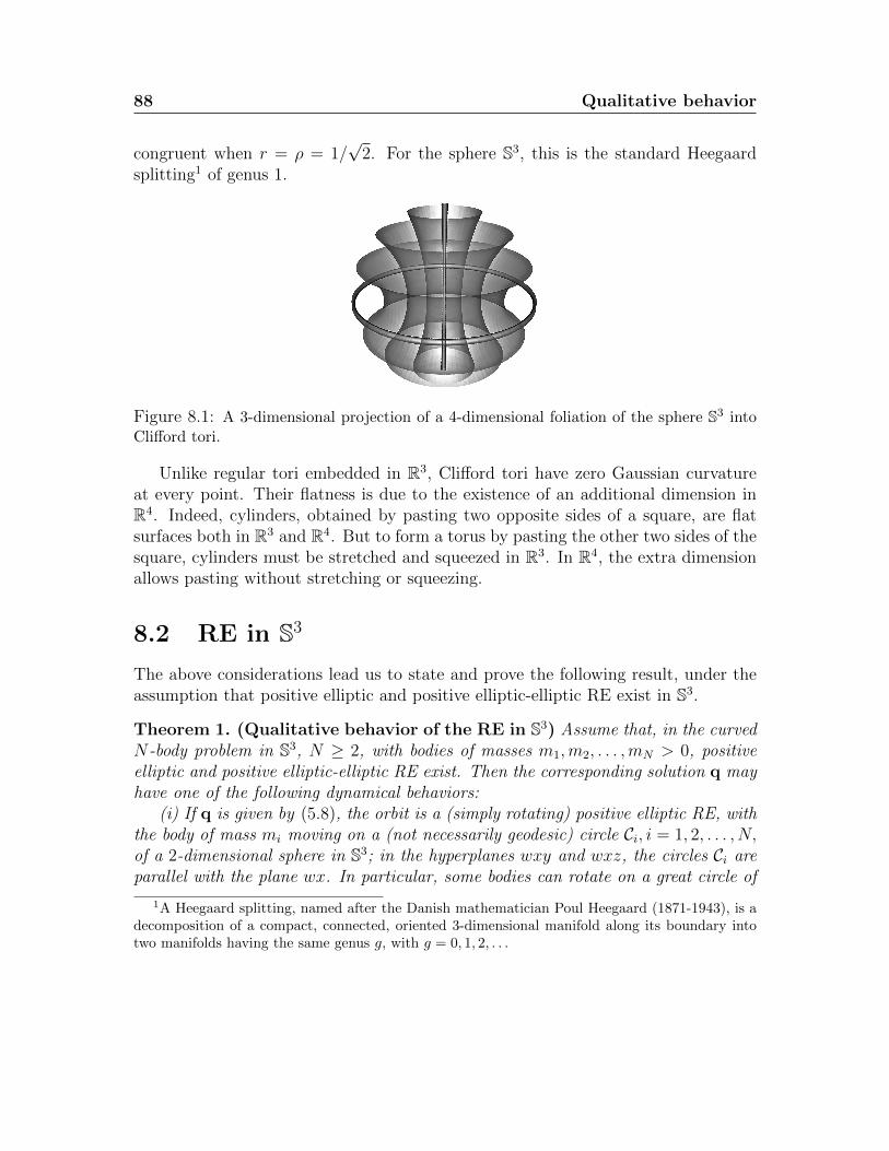
88 Qualitative behavior
congruent when r = ρ = 1/√
2. For the sphere S3, this is the standard Heegaardsplitting1 of genus 1.
Figure 8.1: A 3-dimensional projection of a 4-dimensional foliation of the sphere S3 intoClifford tori.
Unlike regular tori embedded in R3, Clifford tori have zero Gaussian curvatureat every point. Their flatness is due to the existence of an additional dimension inR4. Indeed, cylinders, obtained by pasting two opposite sides of a square, are flatsurfaces both in R3 and R4. But to form a torus by pasting the other two sides of thesquare, cylinders must be stretched and squeezed in R3. In R4, the extra dimensionallows pasting without stretching or squeezing.
8.2 RE in S3
The above considerations lead us to state and prove the following result, under theassumption that positive elliptic and positive elliptic-elliptic RE exist in S3.
Theorem 1. (Qualitative behavior of the RE in S3) Assume that, in the curvedN-body problem in S3, N ≥ 2, with bodies of masses m1,m2, . . . ,mN > 0, positiveelliptic and positive elliptic-elliptic RE exist. Then the corresponding solution q mayhave one of the following dynamical behaviors:
(i) If q is given by (5.8), the orbit is a (simply rotating) positive elliptic RE, withthe body of mass mi moving on a (not necessarily geodesic) circle Ci, i = 1, 2, . . . , N,of a 2-dimensional sphere in S3; in the hyperplanes wxy and wxz, the circles Ci areparallel with the plane wx. In particular, some bodies can rotate on a great circle of
1A Heegaard splitting, named after the Danish mathematician Poul Heegaard (1871-1943), is adecomposition of a compact, connected, oriented 3-dimensional manifold along its boundary intotwo manifolds having the same genus g, with g = 0, 1, 2, . . .
8.2 RE in S3 89
a great sphere, while the other bodies stay fixed on a complementary great circle ofanother great sphere.
(ii) If q is given by (5.9), the orbit is a (doubly rotating) positive elliptic-ellipticRE, with each body mi moving on the Clifford torus T2
riρi, i = 1, 2, . . . , N . In partic-
ular, some bodies can rotate on a great circle of a great sphere, while the other bodiesrotate on a complementary great circle of another great sphere.
Proof. (i) The bodies move on circles Ci, i = 1, 2, . . . , N , because, by (5.8), theanalytic expression of the orbit is given by
q = (q1,q2, . . . ,qn), qi = (wi, xi, yi, zi), i = 1, 2, . . . , N,
wi(t) = ri cos(αt+ ai), xi(t) = ri sin(αt+ ai), yi(t) = yi, zi(t) = zi,
with w2i + x2i = r2i , r
2i + y2i + z2i = 1, and yi, zi constant, i = 1, 2, . . . , N . This proves
the first part of (i), except for the statements about parallelism.In particular, if some bodies are on the circle
S1wx = {(0, 0, y, z) | y2 + z2 = 1},
with yi(t) = yi = constant and zi(t) = zi = constant, then the elliptic rotation,which changes the coordinates w and x, does not act on the bodies, therefore theydon’t move. This remark proves the second part of statement (i).
To prove the parallelism statement from the first part of (i), let us first remarkthat, as the concept of two parallel lines makes sense only if the lines are containedin the same plane, the concept of two parallel planes has meaning only if the planesare contained in the same 3-dimensional space. This explains our formulation of thestatement. Towards proving it, notice first that
cwx =N∑i=1
mi(wixi − wixi) = αN∑i=1
mir2i
and
cyz =N∑i=1
mi(yizi − yizi) = 0.
These constants are independent of the bodies’ position, a fact that confirms thatthey result from first integrals. To determine the values of the constants cwy, cwz, cxy,and cxz, we first compute that
cwy =N∑i=1
mi(wiyi − wiyi) = αN∑i=1
miriyi sin(αt+ ai),

90 Qualitative behavior
cwz =N∑i=1
mi(wizi − wizi) = α
N∑i=1
mirizi sin(αt+ ai),
cxy =N∑i=1
mi(xiyi − xiyi) = α
N∑i=1
miriyi cos(αt+ ai),
cxz =N∑i=1
mi(xizi − xizi) = α
N∑i=1
mirizi cos(αt+ ai).
Since they are constant, the first integrals must take the same value for the argumentst = 0 and t = π/α. But at t = 0, we obtain
cwy = αN∑i=1
miriyi sin ai, cwz = αN∑i=1
mirizi sin ai,
cxy = αN∑i=1
miriyi cos ai, cxz = αN∑i=1
mirizi cos ai,
whereas at t = π/α, we obtain
cwy = −αN∑i=1
miriyi sin ai, cwz = −αN∑i=1
mirizi sin ai,
cxy = −αN∑i=1
miriyi cos ai, cxz = −αN∑i=1
mirizi cos ai.
Consequently, cwy = cwz = cxy = cxz = 0. Since, as we already showed, cyz = 0, itfollows that the only nonzero constant of the total angular momentum is cwx. Thismeans that the particle system has nonzero total rotation with respect to the originonly in the wx plane.
To prove that the circles Ci, i = 1, 2, . . . , N, are parallel with the plane wx inthe hyperplanes wxy and wxz, assume that one circle, say C1, does not satisfy thisproperty. Then some orthogonal projection of C1 (within either of the hyperplaneswxy and wxz) in at least one of the other base planes, say xy, is an ellipse, not asegment—as it would be otherwise. Then the angular momentum of the body ofmass m1 relative to the plane xy is nonzero. Should other circles have an ellipticprojection in the plane xy, the angular momentum of the corresponding bodies wouldbe nonzero as well. Moreover, all angular momenta would have the same sign because
8.3 RE generated from FP configurations 91
all bodies move in the same direction on the original circles. Consequently cxy 6= 0,in contradiction with our previous findings. Therefore the circles Ci, i = 1, 2, . . . , N ,must be parallel, as stated.
(ii) When a positive elliptic-elliptic (double) rotation acts on a system, if somebodies are on a great circle of a great sphere of S3, while other are on a complementarygreat circle of another great sphere, then the former bodies move only because ofone rotation, while the latter bodies move only because of the other rotation. Thespecial geometric properties of complementary circles leads to this kind of qualitativebehavior.
To prove the general qualitative behavior, namely that the body of mass mi of the(doubly rotating) positive elliptic-elliptic RE moves on the Clifford torus T2
riρi, i =
1, 2, . . . , N , of which the situation described above is a notable particular case, itis enough to compare the form of the orbit given in (5.9) with the characterization(8.1) of a Clifford torus. This remark completes the proof.
8.3 RE generated from FP configurations
We will further outline the dynamical consequences of Criterion 2 and Criterion 4,under the assumption that positive elliptic and positive elliptic-elliptic RE, bothgenerated from FP configurations, exist in S3. This theorem deals with a subclass ofthe orbits whose qualitative behavior we have just described.
Theorem 2. (Qualitative behavior of the RE generated from FP configu-rations in S3) Consider the bodies of masses m1,m2, . . . ,mN > 0, N ≥ 2, moving inS3. Then a RE q generated from a FP configuration may have one of the followingcharacteristics:
(i) q is a (simply rotating) positive elliptic RE for which all bodies rotate on thesame great circle of a great sphere of S3;
(ii) q is a (simply rotating) positive elliptic RE for which some bodies rotate ona great circle of a great sphere, while the other bodies are fixed on a complementarygreat circle of a different great sphere;
(iii) q is a (doubly rotating) positive elliptic-elliptic RE for which some bodiesrotate with frequency α 6= 0 on a great circle of a great sphere, while the other bodiesrotate with frequency β 6= 0 on a complementary great circle of a different sphere;the frequencies may be different in size, i.e. |α| 6= |β|;
(iv) q is a (doubly rotating) positive elliptic-elliptic RE that does not rotate oncomplementary circles, a case in which the frequencies α, β 6= 0 are equal in size, i.e.|α| = |β|.
92 Qualitative behavior
Proof. (i) From conclusion (i) of Criterion 2, a (simply rotating) positive elliptic REof the form
q = (q1,q2, . . . ,qn),qi = (wi, xi, yi, zi), i = 1, 2, . . . , N,
wi = ri cos(αt+ ai), xi(t) = ri sin(αt+ ai), yi(t) = yi, zi(t) = zi,
with w2i + x2i = r2i , r
2i + y2i + z2i = 1 and yi, zi constant, i = 1, 2, . . . , N , generated
from a FP configuration, must satisfy one of two additional conditions (besides theinitial 4N equations), the first of which translates into
ri = 1, i = 1, 2, . . . , N.
This property implies that yi = zi = 0, i = 1, 2, . . . , N , so all bodies rotate along thesame great circle of radius 1, namely S1
yz, thus proving the statement in this case.(ii) From conclusion (ii) of Criterion 2, there is a proper subset I ⊂ {1, 2, . . . , N}
such that ri = 0 for all i ∈ I and rj = 1 for all j ∈ {1, 2, . . . , N} \ I.The bodies for which ri = 0 must have wi = xi = 0 and y2i + z2i = 1, so they are
fixed on the great circle S1wx, since yi and zi are constant, i ∈ I, and no rotation acts
on the coordinates w and x.As in the proof of (i) above, it follows that the bodies with rj = 1, j ∈
{1, 2, . . . , N}\I rotate on the circle S1yz, which is complementary to S1
wx, so statement(ii) is also proved.
(iii) From conclusion (i) of Criterion 4, a (doubly rotating) positive elliptic-ellipticRE of the form
q = (q1,q2, . . . ,qn),qi = (wi, xi, yi, zi), i = 1, 2, . . . , N,
wi(t) = ri cos(αt+ ai), xi(t) = ri sin(αt+ ai),
yi(t) = ρi cos(βt+ bi), zi(t) = ρi sin(βt+ bi),
with w2i + x2i = r2i , y
2i + z2i = ρ2i , r
2i + ρ2i = 1, i = 1, 2, . . . , N , generated from a FP
configuration, must satisfy one of two additional conditions (besides the initial 4Nequations), the first of which says that there is a proper subset J ⊂ {1, 2, . . . , N}such that ri = 0 for all i ∈ J and ρj = 0 for all j ∈ {1, 2, . . . , N}\J . But this meansthat the bodies mi with i ∈ J have wi = xi = 0 and y2i + z2i = ρ2i , so one rotationacts along the great circle S1
wx, while the bodies with mi, i ∈ {1, 2, . . . , N}\J satisfythe conditions w2
i + x2i = r2i and yi = zi = 0, so the other rotation acts on themalong the great circle S1
yz, which is complementary to S1wx. Moreover, since the
8.4 Some geometric topology in H3 93
bodies are distributed on two complementary circles, there are no constraints on thefrequencies α, β 6= 0, which can be independent of each other, a remark that provesthe statement.
(iv) From statement (d) in the proof of Criterion 4, a (doubly rotating) positiveelliptic-elliptic RE may exist also when the bodies are not necessarily on complemen-tary circles but the frequencies satisfy the condition |α| = |β|, a case that concludesthe last statement of this result.
8.4 Some geometric topology in H3
Usually, compact higher-dimensional manifolds have a richer geometry than noncom-pact manifolds of the same dimension. This fact is also true about S3 if comparedto H3. Nevertheless, we will be able to characterize the relative equilibria of H3 ingeometric-topologic terms.
The surface we are introducing in this section, which will play for our dynamicalanalysis in H3 the same role the Clifford torus played in S3, is homeomorphic to acylinder. Consider a circle of radius r in the wx plane of R4 and the upper branchof the hyperbola r2 − η2 = −1 in the yz plane of R4. Then we will call the surfaceC2rη obtained by taking the cartesian product between the circle and the hyperbola a
hyperbolic cylinder since it equidistantly surrounds a branch of a geodesic hyperbolain H3. Indeed, we can represent this cylinder as
C2rη = {(w, x, y, z) | r2 − η2 = −1, 0 ≤ θ < 2π, ξ ∈ R}, (8.2)
where w = r cos θ, x = r sin θ, y = η sinh ξ, z = η cosh ξ. But the hyperbolic cylinderC2rη also lies in H3 because the coordinates w, x, y, z, endowed with the Lorentz inner
product, satisfy the equations
w2 + x2 + y2 − z2 = r2 − η2 = −1.
As in the case of S3, which is foliated by a family of Clifford tori, H3 can be foliatedby a family of hyperbolic cylinders. The foliation is, of course, not unique. Butunlike the Clifford tori of R4, the hyperbolic cylinders of R3,1 are not flat surfaces. Ingeneral, they have constant positive Gaussian curvature, which varies with the sizeof the cylinder, becoming zero only when the cylinder degenerates into a geodesichyperbola.
94 Qualitative behavior
8.5 RE in H3
The above considerations allow us to state and prove the following result, underthe assumption that negative elliptic, hyperbolic, and elliptic-hyperbolic RE exist.Notice that, on one hand, due to the absence of complementary circles, and, on theother hand, the absence of FP in H3, the dynamical behavior of RE is less complicatedthan in S3.
Theorem 3. (Qualitative behavior of the RE in H3) In the curved N-bodyproblem in H3, N ≥ 2, with bodies of masses m1,m2, . . . ,mN > 0, every RE q hasone of the following potential behaviors:
(i) if q is given by (5.10), the orbit is a (simply rotating) negative elliptic RE,with the body of mass mi moving on a circle Ci, i = 1, 2, . . . , N , of a 2-dimensionalhyperbolic sphere in H3; in the hyperplanes wxy and wxz, the planes of the circlesCi are parallel with the plane wx;
(ii) if q is given by (5.11), the orbit is a (simply rotating) negative hyperbolicRE, with the body of mass mi moving on some (not necessarily geodesic) hyperbolaHi of a 2-dimensional hyperbolic sphere in H3, i = 1, 2, . . . , N ; in the hyperplaneswyz and xyz, the planes of the hyperbolas Hi are parallel with the plane yz;
(iii) if q is given by (5.12), the orbit is a (doubly rotating) negative elliptic-hyperbolic RE, with the body of mass mi moving on the hyperbolic cylinder C2
riηi, i =
1, 2, . . . , N .
Proof. (i) The bodies move on circles, Ci, i = 1, 2, . . . , N, because, by (5.10), theanalytic expression of the orbit is given by
q = (q1,q2, . . . ,qn), qi = (wi, xi, yi, zi), i = 1, 2, . . . , N,
wi(t) = ri cos(αt+ ai), xi(t) = ri sin(αt+ ai), yi(t) = yi, zi(t) = zi,
with w2i + x2i = r2i , r
2i + y2i − z2i = −1, and yi, zi constant, i = 1, 2, . . . , N . The
parallelism of the planes of the circles in the hyperplanes wxy and wxz followsexactly as in the proof of part (i) in Theorem 1, using the integrals of the totalangular momentum.
(ii) The bodies move on hyperbolas, Hi, i = 1, 2, . . . , N , because, by (5.11), theanalytic expression of the orbit is given by
q = (q1,q2, . . . ,qn),qi = (wi, xi, yi, zi), i = 1, 2, . . . , N,
wi(t) = wi (constant), xi(t) = xi (constant),
yi(t) = ηi sinh(βt+ bi), zi(t) = ηi cosh(βt+ bi),
8.5 RE in H3 95
with y2i − z2i = −η2i , w2i + x2i − η2i = −1, i = 1, 2, . . . , N .
Let us now prove the parallelism statement for the planes containing the hyper-bolas Hi. For this purpose, notice that
cwx =N∑i=1
mi(wixi − wixi) = 0
and
cyz =N∑i=1
mi(yizi − yizi) = −βN∑i=1
miη2i .
These constants are independent of the bodies’ position, a fact which confirms thatthey result from first integrals. To determine the values of the constants cwy, cwz, cxy,and cxz, we first compute that
cwy =N∑i=1
mi(wiyi − wiyi) = βN∑i=1
miwiηi cosh(βt+ bi),
cwz =N∑i=1
mi(wizi − wizi) = βN∑i=1
miwiηi sinh(βt+ bi),
cxy =N∑i=1
mi(xiyi − xiyi) = βN∑i=1
mixiηi cosh(βt+ bi),
cxz =N∑i=1
mi(xizi − xizi) = βN∑i=1
mixiηi sinh(βt+ bi).
We next show that cwy = 0. For this, notice first that, using the formula cosh(βt+bi) = cosh bi cosh βt+ sinh bi sinh βt, we can write
cwy = β[A(t) +B(t)], (8.3)
where
A(t) =N∑i=1
miwiηi cosh bi cosh βt and B(t) =N∑i=1
miwiηi sinh bi sinh βt.
But the function cosh is even, whereas sinh is odd. Therefore A is even and B isodd. Since cwy is constant, we also have
cwy = β[A(−t) +B(−t)] = β[A(t)−B(t)]. (8.4)
96 Qualitative behavior
From (8.3) and (8.4) and the fact that β 6= 0, we can conclude that
cwy = βA(t) and B(t) = 0,
so ddtB(t) = 0. However, d
dtB(t) = βA(t), which proves that cwy = 0.
The fact that cxy = 0 can be proved exactly the same way. The only differencewhen showing that cwz = 0 and cxz = 0 is the use of the corresponding hyperbolicformula, sinh(βt+ bi) = sinh βt cosh bi + cosh βt sinh bi. In conclusion,
cwx = cwy = cwz = cxy = cxz = 0 and cyz 6= 0,
which means that the hyperbolic rotation takes place relative to the origin of thecoordinate system solely with respect to the plane yz.
Using a similar reasoning as in the proof of (i) for Theorem 1, it can be shown thatthe above conclusion proves the parallelism of the planes that contain the hyperbolasHi in the 3-dimensional hyperplanes wyz and xyz.
(iii) To prove that (doubly rotating) negative elliptic-hyperbolic RE move onhyperbolic cylinders, it is enough to compare the form of the orbit given in (5.11)with the characterization (8.2) of a hyperbolic cylinder.
Part IV
Examples

99
Preamble
The goal of Part IV is to provide examples of RE for each type of qualitative be-havior described in Part III. The dynamics appear to be richer and more interestingin S3 than in H3, probably because, unlike the latter, the former is a compact man-ifold. Nevertheless, the curved N -body problem in H3 exhibits certain specific, aswell as unexpected, RE as well, a fact we will use in Part V to make a first steptowards proving that, for distances comparable to those of our solar system, spaceis Euclidean.

100
Chapter 9
Positive elliptic RE
Since Theorems 1, 2, and 3 provide us with the qualitative behavior of all the fiveclasses of RE that we expect to find in S3 and H3, we know what kind of rigid-body-type orbits to look for in the curved N -body problem for various values ofN ≥ 3. Ideal, of course, would be to find them all, but this problem appears to bevery difficult, and it might never be completely solved. As a first step towards this(perhaps unreachable) goal, we will show that each type of orbit described in theabove criteria and theorems exists for some values of N ≥ 3 and m1,m2, . . . ,mN > 0.
To appreciate the difficulty of the above mentioned question, we remark thatits Euclidean analogue is that of finding all central configurations for the New-tonian potential. The notoriety of this problem has been recognized for at leastseven decades, [100]. In fact, we don’t even know whether, for some given massesm1,m2, . . . ,mN > 0, with N ≥ 5, the number of classes of central configurations(after we factorize the central configurations by size and rotation) is finite or not1
and, should it be infinite, whether the set of classes of central configurations is dis-crete or contains a continuum. The finiteness of the number of classes of centralconfigurations is Problem 6 on Steven Smale’s list of mathematics problems for the21st century, [96]. Its analogue in our case would be that of deciding whether, forgiven masses, m1,m2, . . . ,mN > 0, the number of classes of RE of the 3-dimensionalcurved N -body problem is finite or not.
In this chapter, we will provide specific examples of positive elliptic RE, i.e. orbitson the sphere S3 that have a single rotation. The first example is a RE in a 3-bodyproblem in which 3 equal masses are at the vertices of an equilateral triangle that
1Alain Albouy and Vadim Kaloshin have recently reported to have proved the finiteness of centralconfigurations in the planar Euclidean 5-body problem for any given positive masses, except perhapsfor a codimension 2 submanifold of the mass space, [3].
102 Positive elliptic RE
rotates along a not necessarily great circle of a great or non-great sphere. The secondexample is a RE of a 3-body problem in which 3 unequal masses move at the verticesof an acute scalene triangle along a great circle of a great sphere. The third exampleis a RE generated from a FP configuration in a 6-body problem of equal massesfor which 3 bodies move along a great circle of a great sphere at the vertices of anequilateral triangle, while the other 3 masses are fixed on a complementary greatcircle of another great sphere at the vertices of an equilateral triangle. The fourth,and last example of this chapter, generalizes the third example to the case of acutescalene, not necessarily congruent, triangles and unequal masses.
9.1 Lagrangian RE
In the light of Remark 2, we expect to find solutions in S3 that move on 2-dimensionalspheres. A simple example is that of the Lagrangian RE (i.e. equilateral triangles)of equal masses in the curved 3-body problem. Their existence in S2, and the factthat they occur only when the masses are equal, was first proved in [35]. This proofwill also be presented in Part V. So, in this case, we have N = 3 and m1 = m2 =m3 =: m > 0. The solution of the corresponding system (3.15) we are seeking is ofthe form
q = (q1,q2,q3), qi = (wi, xi, yi, zi), i = 1, 2, 3, (9.1)
w1(t) = r cosωt, x1(t) = r sinωt,
y1(t) = y (constant), z1(t) = z (constant),
w2(t) = r cos(ωt+ 2π/3), x2(t) = r sin(ωt+ 2π/3),
y2(t) = y (constant), z2(t) = z (constant),
w3(t) = r cos(ωt+ 4π/3), x3(t) = r sin(ωt+ 4π/3),
y3(t) = y (constant), z3(t) = z (constant),
with r2 + y2 + z2 = 1. Consequently, for the equations occurring in Criterion 1, wehave
r1 = r2 = r3 =: r, a1 = 0, a2 = 2π/3, a3 = 4π/3,
y1 = y2 = y3 =: y (constant), z1 = z2 = z3 =: z (constant).
Substituting these values into the equations (7.1), (7.2), (7.3), (7.4), we obtain eitheridentities or the equation
ω2 =8m√
3r3(4− 3r2)3/2.
9.2 Scalene triangles 103
Therefore, given m > 0, r ∈ (0, 1), and y, z with r2 + y2 + z2 = 1, we can alwaysfind two frequencies,
ω1 =2
r
√2m√
3r(4− 3r2)3/2and ω2 = −2
r
√2m√
3r(4− 3r2)3/2,
such that system (3.17) has a solution of the form (9.1). The positive frequencycorresponds to one sense of rotation, whereas the negative frequency corresponds tothe opposite sense.
Notice that if r = 1, i.e. when the bodies move along a great circle of a greatsphere, equations (7.1), (7.2), (7.3), (7.4) are identities for any ω ∈ R, so any fre-quency leads to a solution. This phenomenon happens because, under those circum-stances, the motion is generated from a FP configuration, a case in which we canapply Criterion 2, whose statement is independent of the frequency.
The bodies move on the great circle S1yz of a great sphere only if y = z = 0.
Otherwise they move on non-great circles of great or non-great spheres. So we canalso interpret this example as existing in the light of Remark 3, which says that thereare positive elliptic rotations that leave non-great spheres invariant.
The constants of the angular momentum are
cwx = 3mω 6= 0 and cwy = cwz = cxy = cxz = cyz = 0,
which means that the rotation takes place around the origin of the coordinate systemonly relative to the plane wx.
9.2 Scalene triangles
It is natural to ask whether solutions such as the one in the previous example also ex-ist for unequal masses. The answer is positive, and it was first answered in [28], wherewe proved that, given a 2-dimensional sphere and any triangle inscribed in a greatcircle of it (for instance inside the equator z = 0), there are masses, m1,m2,m3 > 0,such that the bodies form a relative equilibrium that rotates around the z axis.
We will consider a similar solution here in S3, which moves on the great circleS1yz of the great sphere S2
y or S2z. The expected analytic expression of the solution
depends on the shape of the triangle, i.e. it has the form
q = (q1,q2,q3), qi = (wi, xi, yi, zi), i = 1, 2, 3, (9.2)
104 Positive elliptic RE
w1(t) = cos(ωt+ a1), x1(t) = sin(ωt+ a1),
y1(t) = 0, z1(t) = 0,
w2(t) = cos(ωt+ a2), x2(t) = sin(ωt+ a2),
y2(t) = 0, z2(t) = 0,
w3(t) = cos(ωt+ a3), x3(t) = sin(ωt+ a3),
y3(t) = 0, z3(t) = 0,
where the constants a1, a2, a3, with 0 ≤ a1 < a2 < a3 < 2π, determine the triangle’sshape. The other constants involved in the description of this orbit are
r1 = r2 = r3 = 1. (9.3)
We can use now Criterion 2 to prove that (9.2) is a positive elliptic RE for anyfrequency ω 6= 0. Indeed, we know from [28] that, for any shape of the triangle, thereexist masses that yield a FP on the great circle S1
yz, so the corresponding equations(7.5), (7.6), (7.7), (7.8) are satisfied. Since conditions (9.3) are also satisfied, theproof that (9.2) is a solution of (3.15) is complete.
The constants of the angular momentum integrals are
cwx = (m1 +m2 +m3)ω 6= 0 and cwy = cwz = cxy = cxz = cyz = 0,
which means that the bodies rotate in R4 around the origin of the coordinate systemonly relative to the plane wx.
9.3 A regular RE with a fixed subsystem
The following example of a (simply rotating) positive elliptic RE in the curved 6-bodyproblem corresponds to the second type of orbit described in part (i) of Theorem1, and it is interesting from two points of view. First, it is an orbit that is specificto S3 in the sense that it cannot exist on any 2-dimensional sphere. Second, 3bodies of equal masses move on a great circle of a great sphere at the vertices of anequilateral triangle, while the other 3 bodies of masses equal to the first stay fixed ona complementary great circle of another great sphere at the vertices of an equilateraltriangle. So consider the equal masses
m1 = m2 = m3 = m4 = m5 = m6 =: m > 0.
Then a solution as described above has the form
q = (q1,q2,q3,q4,q5,q6), qi = (wi, xi, yi, zi), i = 1, 2, . . . , 6,
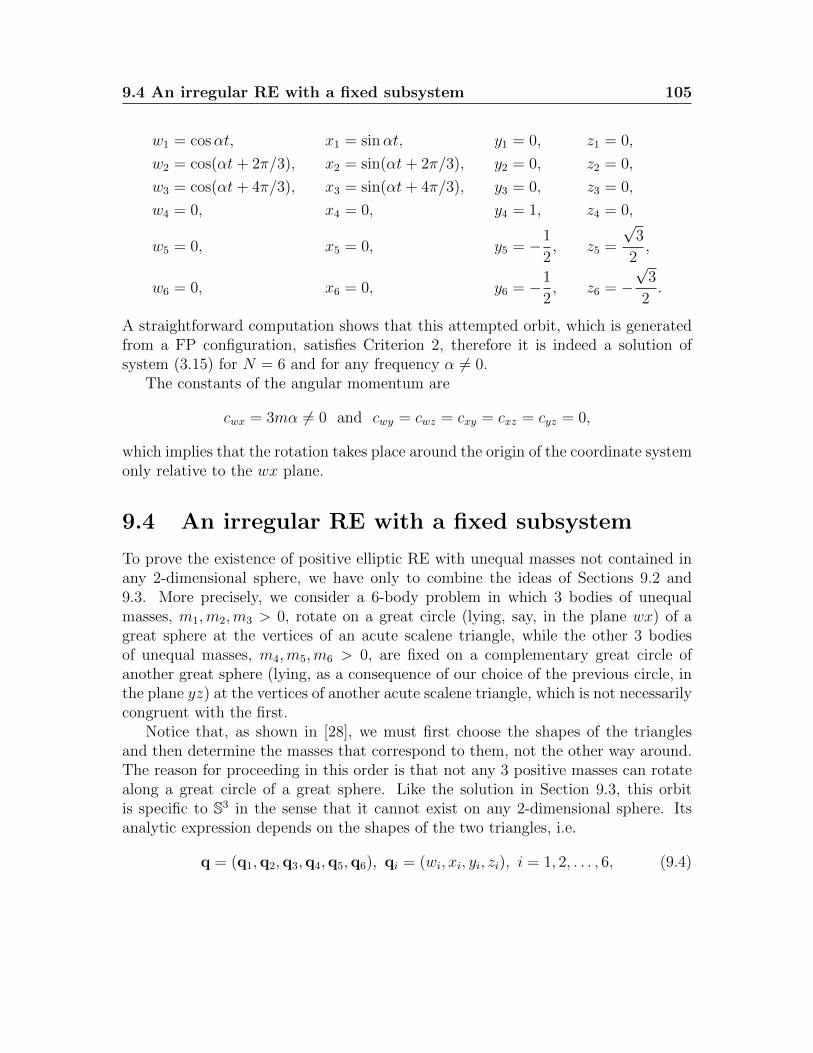
9.4 An irregular RE with a fixed subsystem 105
w1 = cosαt, x1 = sinαt, y1 = 0, z1 = 0,
w2 = cos(αt+ 2π/3), x2 = sin(αt+ 2π/3), y2 = 0, z2 = 0,
w3 = cos(αt+ 4π/3), x3 = sin(αt+ 4π/3), y3 = 0, z3 = 0,
w4 = 0, x4 = 0, y4 = 1, z4 = 0,
w5 = 0, x5 = 0, y5 = −1
2, z5 =
√3
2,
w6 = 0, x6 = 0, y6 = −1
2, z6 = −
√3
2.
A straightforward computation shows that this attempted orbit, which is generatedfrom a FP configuration, satisfies Criterion 2, therefore it is indeed a solution ofsystem (3.15) for N = 6 and for any frequency α 6= 0.
The constants of the angular momentum are
cwx = 3mα 6= 0 and cwy = cwz = cxy = cxz = cyz = 0,
which implies that the rotation takes place around the origin of the coordinate systemonly relative to the wx plane.
9.4 An irregular RE with a fixed subsystem
To prove the existence of positive elliptic RE with unequal masses not contained inany 2-dimensional sphere, we have only to combine the ideas of Sections 9.2 and9.3. More precisely, we consider a 6-body problem in which 3 bodies of unequalmasses, m1,m2,m3 > 0, rotate on a great circle (lying, say, in the plane wx) of agreat sphere at the vertices of an acute scalene triangle, while the other 3 bodiesof unequal masses, m4,m5,m6 > 0, are fixed on a complementary great circle ofanother great sphere (lying, as a consequence of our choice of the previous circle, inthe plane yz) at the vertices of another acute scalene triangle, which is not necessarilycongruent with the first.
Notice that, as shown in [28], we must first choose the shapes of the trianglesand then determine the masses that correspond to them, not the other way around.The reason for proceeding in this order is that not any 3 positive masses can rotatealong a great circle of a great sphere. Like the solution in Section 9.3, this orbitis specific to S3 in the sense that it cannot exist on any 2-dimensional sphere. Itsanalytic expression depends on the shapes of the two triangles, i.e.
q = (q1,q2,q3,q4,q5,q6), qi = (wi, xi, yi, zi), i = 1, 2, . . . , 6, (9.4)
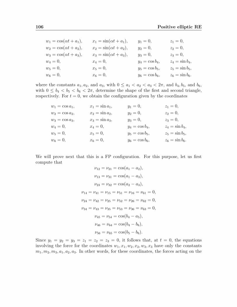
106 Positive elliptic RE
w1 = cos(αt+ a1), x1 = sin(αt+ a1), y1 = 0, z1 = 0,
w2 = cos(αt+ a2), x2 = sin(αt+ a2), y2 = 0, z2 = 0,
w3 = cos(αt+ a3), x3 = sin(αt+ a3), y3 = 0, z3 = 0,
w4 = 0, x4 = 0, y4 = cos b4, z4 = sin b4,
w5 = 0, x5 = 0, y5 = cos b5, z5 = sin b5,
w6 = 0, x6 = 0, y6 = cos b6, z6 = sin b6.
where the constants a1, a2, and a3, with 0 ≤ a1 < a2 < a3 < 2π, and b4, b5, and b6,with 0 ≤ b4 < b5 < b6 < 2π, determine the shape of the first and second triangle,respectively. For t = 0, we obtain the configuration given by the coordinates
w1 = cos a1, x1 = sin a1, y1 = 0, z1 = 0,
w2 = cos a2, x2 = sin a2, y2 = 0, z2 = 0,
w3 = cos a3, x3 = sin a3, y3 = 0, z3 = 0,
w4 = 0, x4 = 0, y4 = cos b4, z4 = sin b4,
w5 = 0, x5 = 0, y5 = cos b5, z5 = sin b5,
w6 = 0, x6 = 0, y6 = cos b6, z6 = sin b6.
We will prove next that this is a FP configuration. For this purpose, let us firstcompute that
ν12 = ν21 = cos(a1 − a2),
ν13 = ν31 = cos(a1 − a3),
ν23 = ν32 = cos(a2 − a3),
ν14 = ν41 = ν15 = ν51 = ν16 = ν61 = 0,
ν24 = ν42 = ν25 = ν52 = ν26 = ν62 = 0,
ν34 = ν43 = ν35 = ν53 = ν36 = ν63 = 0,
ν45 = ν54 = cos(b4 − a5),
ν46 = ν64 = cos(b4 − b6),
ν56 = ν65 = cos(b5 − b6).
Since y1 = y2 = y3 = z1 = z2 = z3 = 0, it follows that, at t = 0, the equationsinvolving the force for the coordinates w1, x1, w2, x2, w3, x3 have only the constantsm1,m2,m3, a1, a2, a3. In other words, for these coordinates, the forces acting on the
9.4 An irregular RE with a fixed subsystem 107
masses m1,m2, and m3 do not involve the masses m4,m5, and m6. But the bodiesm1,m2, and m3 are on the great circle S1
yz, which can be seen as lying on the greatsphere S2
z. This means that, by applying the result of [28], the bodies m1,m2, andm3 form an independent FP configuration. Similarly, we can show that the massesm4,m5, and m6 form an independent FP configuration. Therefore all 6 bodies forma FP configuration.
Consequently, we can now use Criterion 2 to check whether q given by (9.4)is a positive elliptic RE generated from a FP configuration. We can approachthis problem in two ways. One is computational, and it consists of using the factthat the positions at t = 0 form a FP configuration to determine the relationshipsbetween the constants m1,m2,m3, a1, a2, and a3, on one hand, and the constantsm4,m5,m6, b4, b5, and b6, on the other hand. It turns out that these relationshipsreduce to conditions (7.5), (7.6), (7.7), and (7.8). Then we only need to remark that
r1 = r2 = r3 = 1 and r4 = r5 = r6 = 0,
which means that condition (ii) of Criterion 2 is satisfied. The other approach is toinvoke again the result of [28] and a reasoning similar to the one we used to showthat the position at t = 0 is a FP configuration. Each approach helps us concludethat q given by (9.4) is a solution of system (3.15) for any α 6= 0.
The constants of the angular momentum are
cwx = (m1 +m2 +m3)α 6= 0 and cwy = cwz = cxy = cxz = cyz = 0,
which means, as expected, that the bodies rotate in R4 around the origin of thecoordinate system only relative to the plane wx.

108 Positive elliptic RE
Chapter 10
Positive elliptic-elliptic RE
In this chapter we will construct examples of positive elliptic-elliptic RE, i.e. orbitswith two elliptic rotations on the sphere S3. The first example is that of a 3-bodyproblem in which 3 bodies of equal masses are at the vertices of an equilateral triangle,which has two rotations of the same frequency. The second example is that of a 4-body problem in which 4 equal masses are at the vertices of a regular tetrahedron,which has two rotations of the same frequency. The third example is that of a 5-body problem in which 5 equal masses lying at the vertices of a pentatope have tworotations of same-size frequencies. This is the only regular polytope that allows RE,because the five other existing regular polytopes of R4 have antipodal vertices, sothey introduce singularities. As in the previous example, this motion cannot takeplace on any 2-dimensional sphere. The fourth example is that of a 6-body problem,with 3 bodies of equal masses rotating at the vertices of an equilateral triangle alonga great circle of a great sphere, while the other 3 bodies, of the same mass as theothers, rotate at the vertices of an equilateral triangle along a complementary greatcircle of another great sphere. In general, the frequencies of the two rotations aredistinct. The fifth example generalizes the fourth example in the sense that thetriangles are scalene, acute, not necessarily congruent, and the masses as well as thefrequencies of the rotations are distinct, in general.
10.1 Equilateral triangle with equal frequencies
The example we will now construct is that of a (doubly rotating) positive elliptic-elliptic equilateral triangle of equal masses in the curved 3-body problem in S3 forwhich the rotations have the same frequency. Such solutions cannot be found on2-dimensional spheres. So we consider the masses m1 = m2 = m3 =: m > 0 in S3.
110 Positive elliptic-elliptic RE
Then the solution we check for system (3.15) with N = 3 has the form:
q = (q1,q2,q3), qi = (wi, xi, yi, zi), i = 1, 2, 3, (10.1)
w1 = r cosαt, x1 = r sinαt,
y1 = ρ cosαt, z1 = ρ sinαt,
w2 = r cos (αt+ 2π/3) , x2 = r sin (αt+ 2π/3) ,
y2 = ρ cos(αt+ 2π/3), z2 = ρ sin(αt+ 2π/3),
w3 = r cos (αt+ 4π/3) , x3 = r sin (αt+ 4π/3) ,
y3 = ρ cos(αt+ 4π/3), z3 = ρ sin(αt+ 4π/3),
with r2 + ρ2 = 1. For t = 0, the above attempted solution gives for the 3 bodies thecoordinates
w1 = r, x1 = 0, y1 = ρ, z1 = 0,
w2 = −r2, x2 =
r√
3
2, y2 = −ρ
2, z2 =
ρ√
3
2,
w3 = −r2, x3 = −r
√3
2, y3 = −ρ
2, z3 = −ρ
√3
2,
which is a FP configuration, since the bodies have equal masses and are at the verticesof an equilateral triangle inscribed in a great circle of a great sphere. Consequently,we can use Criterion 4 to check whether a solution of the form (10.1) satisfies sys-tem (3.15) for any α 6= 0. A straightforward computation shows that the first 4Nconditions are satisfied. Moreover, since the two rotations have the same frequency,it follows that condition (ii) of Criterion 4 is verified, therefore (10.1) is indeed asolution of system (3.15) for any α 6= 0.
The angular momentum constants are
cwx = 3mαr2, cwy = 0, cwz = 3mαrρ,
cxy = −3mαrρ, cxz = 0, cyz = 3mαρ2,
which show that rotations around the origin of the coordinate system take placerelative to 4 planes: wx,wz, xy, and yz. Consequently the bodies don’t move oncircles, but on the same Clifford torus, namely T2
rρ, a case that agrees with thequalitative result described in part (ii) of Theorem 1.
Notice that for r = 1 and ρ = 0, the orbit becomes a (simply rotating) positiveelliptic RE that rotates along a great circle of a great sphere in S3, i.e. an orbit suchas the one we described in Section 9.1.
10.2 Regular tetrahedron 111
10.2 Regular tetrahedron
We will further construct a (doubly rotating) positive elliptic-elliptic RE of the 4-body problem in S3, in which 4 equal masses are at the vertices of a regular tetrahe-dron that has rotations of equal frequencies. So let us fix m1 = m2 = m3 = m4 =:m > 0 and consider the initial position of the 4 bodies to be given as in the firstexample of Section 6.2, i.e. by the coordinates
w01 = 0, x01 = 0, y01 = 0, z01 = 1,
w02 = 0, x02 = 0, y02 =
2√
2
3, z02 = −1
3,
w03 = 0, x03 = −
√6
3, y03 = −
√2
3, z03 = −1
3,
w04 = 0, x04 =
√6
3, y04 = −
√2
3, z04 = −1
3,
which is a FP configuration. Indeed, the masses are equal and the bodies are at thevertices of a regular tetrahedron inscribed in a great sphere of S3.
For this choice of initial positions, we can compute that
r1 = r2 = 0, ρ1 = ρ2 = 1, r3 = r4 =
√6
3, ρ3 = ρ4 =
√3
3,
which means that m1 and m2 move on the Clifford torus with r = 0 and ρ = 1 (i.e.one of the two Clifford tori, within the class of a given foliation of S3, which is also agreat circle of S3, see Figure 8.1, the other corresponding to r = 1 and ρ = 0), while
we expect m3 and m4 to move on the Clifford torus with r =√63
and ρ =√33
.These considerations allow us to obtain the constants that determine the angles.
Indeed, a1 and a2 can take any values,
a3 = 3π/2, a4 = π/2, b1 = π/2,
and b2, b3, b4 are such that
sin b2 = −1/3, cos b2 = 2√
2/3,
cos b3 = −√
6/3, sin b3 = −√
3/3
cos b4 = −√
6/3, sin b4 = −√
3/3,
which means that b3 = b4.
112 Positive elliptic-elliptic RE
We can now compute the form of the candidate for a solution generated from theabove FP configuration. Using the above values of ri, ρi, ai and bi, i = 1, 2, 3, 4, weobtain from the equations
w0i = ri cos ai, x
0i = ri sin ai, y
0i = ρi cos bi, z
0i = ρi sin bi, i = 1, 2, 3, 4,
that the candidate for a solution is given by
q = (q1,q2,q3,q4), qi = (wi, xi, yi, zi), i = 1, 2, 3, 4, (10.2)
w1 = 0, x1 = 0,
y1 = cos(αt+ π/2), z1 = sin(αt+ π/2),
w2 = 0, x2 = 0,
y2 = cos(αt+ b2), z2 = sin(αt+ b2),
w3 =
√6
3cos(βt+ 3π/2), x3 =
√6
3sin(βt+ 3π/2),
y3 =
√3
3cos(βt+ b3), z3 =
√3
3sin(βt+ b3),
w4 =
√6
3cos(βt+ π/2), x4 =
√6
3sin(βt+ π/2),
y4 =
√3
3cos(βt+ b4), z4 =
√3
3sin(βt+ b4).
If we invoke Criterion 4, do a straightforward computation, and use the fact that thefrequencies of the two rotations have the same size, i.e. are equal in absolute value,we can conclude that q, given by (10.2), satisfies system (3.15), so it is indeed asolution of the curved 4-body problem in S3.
Straightforward computations lead us to the following values of the angular mo-mentum constants:
cwx =4
3mα, cwy = cwz = cxy = cxz = 0, cyz =
8
3mα,
for β = α, and
cwx =4
3mα, cwy = cwz = cxy = cxz = 0, cyz = −8
3mα,
for β = −α, a fact which shows that rotations around the origin of the coordinatesystem takes place only relative to the planes wx and yz.
10.3 Regular pentatope 113
10.3 Regular pentatope
We will next construct a (doubly rotating) positive elliptic-elliptic RE of the 5-bodyproblem in S3, in which 5 equal masses are at the vertices of a regular pentatopethat has two rotations of equal-size frequencies. So let us fix m1 = m2 = m3 = m4 =m5 =: m > 0 and consider the initial position of the 5 bodies to be given as in thesecond example of Section 6.2, i.e. by the coordinates
w01 = 1, x01 = 0, y01 = 0, z01 = 0,
w02 = −1
4, x02 =
√15
4, y02 = 0, z02 = 0,
w03 = −1
4, x03 = −
√5
4√
3, y03 =
√5√6, z03 = 0,
w04 = −1
4, x04 = −
√5
4√
3, y04 = −
√5
2√
6, z04 =
√5
2√
2,
w05 = −1
4, x05 = −
√5
4√
3, y05 = −
√5
2√
6, z05 = −
√5
2√
2,
which is a FP configuration because the masses are equal and the bodies are at thevertices of a regular pentatope inscribed in S3.
For this choice of initial positions, we can compute that
r1 = r2 = 1, ρ1 = ρ2 = 0,
r3 = r4 = r5 = 1/√
6, ρ3 = ρ4 = ρ5 =√
5/√
6,
which means that m1 and m2 move on the Clifford torus with r = 1 and ρ = 0 (i.e.one of the two Clifford tori, in a class of a given foliation of S3, which is also a greatcircle of S3, the other corresponding to r = 0 and ρ = 1), while we expect m3,m4,
and m5 to move on the Clifford torus with r = 1√6
and ρ =√5√6.
These considerations allow us to compute the constants that determine the angles.We obtain that
a1 = 0,
a2 is such thatcos a2 = −1/4, sin a2 = −
√15/4
and a3, a4, a5 are such that
cos a3 = −√
6/4, sin a3 = −√
10/4,
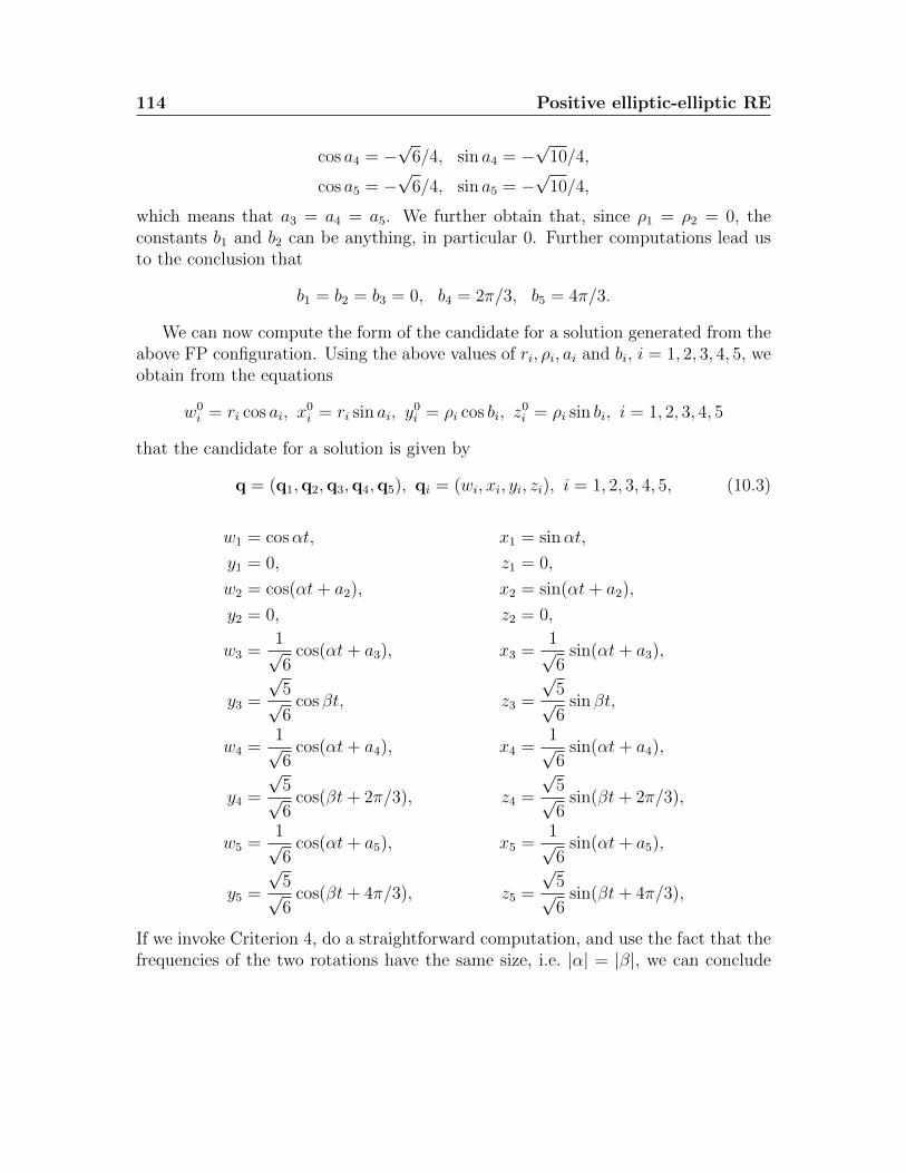
114 Positive elliptic-elliptic RE
cos a4 = −√
6/4, sin a4 = −√
10/4,
cos a5 = −√
6/4, sin a5 = −√
10/4,
which means that a3 = a4 = a5. We further obtain that, since ρ1 = ρ2 = 0, theconstants b1 and b2 can be anything, in particular 0. Further computations lead usto the conclusion that
b1 = b2 = b3 = 0, b4 = 2π/3, b5 = 4π/3.
We can now compute the form of the candidate for a solution generated from theabove FP configuration. Using the above values of ri, ρi, ai and bi, i = 1, 2, 3, 4, 5, weobtain from the equations
w0i = ri cos ai, x
0i = ri sin ai, y
0i = ρi cos bi, z
0i = ρi sin bi, i = 1, 2, 3, 4, 5
that the candidate for a solution is given by
q = (q1,q2,q3,q4,q5), qi = (wi, xi, yi, zi), i = 1, 2, 3, 4, 5, (10.3)
w1 = cosαt, x1 = sinαt,
y1 = 0, z1 = 0,
w2 = cos(αt+ a2), x2 = sin(αt+ a2),
y2 = 0, z2 = 0,
w3 =1√6
cos(αt+ a3), x3 =1√6
sin(αt+ a3),
y3 =
√5√6
cos βt, z3 =
√5√6
sin βt,
w4 =1√6
cos(αt+ a4), x4 =1√6
sin(αt+ a4),
y4 =
√5√6
cos(βt+ 2π/3), z4 =
√5√6
sin(βt+ 2π/3),
w5 =1√6
cos(αt+ a5), x5 =1√6
sin(αt+ a5),
y5 =
√5√6
cos(βt+ 4π/3), z5 =
√5√6
sin(βt+ 4π/3),
If we invoke Criterion 4, do a straightforward computation, and use the fact that thefrequencies of the two rotations have the same size, i.e. |α| = |β|, we can conclude
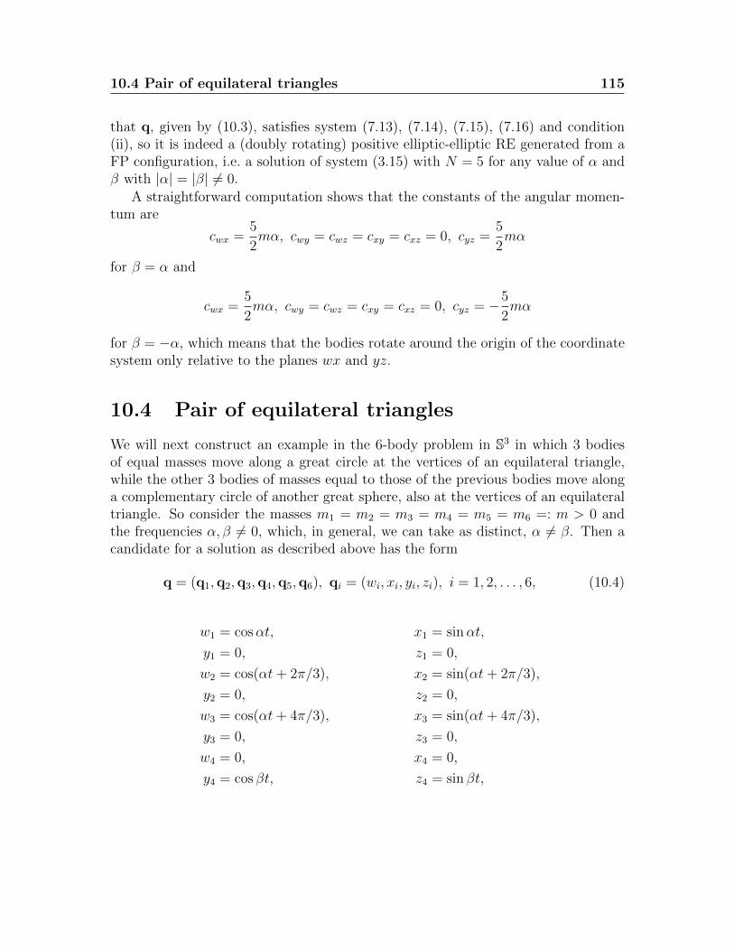
10.4 Pair of equilateral triangles 115
that q, given by (10.3), satisfies system (7.13), (7.14), (7.15), (7.16) and condition(ii), so it is indeed a (doubly rotating) positive elliptic-elliptic RE generated from aFP configuration, i.e. a solution of system (3.15) with N = 5 for any value of α andβ with |α| = |β| 6= 0.
A straightforward computation shows that the constants of the angular momen-tum are
cwx =5
2mα, cwy = cwz = cxy = cxz = 0, cyz =
5
2mα
for β = α and
cwx =5
2mα, cwy = cwz = cxy = cxz = 0, cyz = −5
2mα
for β = −α, which means that the bodies rotate around the origin of the coordinatesystem only relative to the planes wx and yz.
10.4 Pair of equilateral triangles
We will next construct an example in the 6-body problem in S3 in which 3 bodiesof equal masses move along a great circle at the vertices of an equilateral triangle,while the other 3 bodies of masses equal to those of the previous bodies move alonga complementary circle of another great sphere, also at the vertices of an equilateraltriangle. So consider the masses m1 = m2 = m3 = m4 = m5 = m6 =: m > 0 andthe frequencies α, β 6= 0, which, in general, we can take as distinct, α 6= β. Then acandidate for a solution as described above has the form
q = (q1,q2,q3,q4,q5,q6), qi = (wi, xi, yi, zi), i = 1, 2, . . . , 6, (10.4)
w1 = cosαt, x1 = sinαt,
y1 = 0, z1 = 0,
w2 = cos(αt+ 2π/3), x2 = sin(αt+ 2π/3),
y2 = 0, z2 = 0,
w3 = cos(αt+ 4π/3), x3 = sin(αt+ 4π/3),
y3 = 0, z3 = 0,
w4 = 0, x4 = 0,
y4 = cos βt, z4 = sin βt,
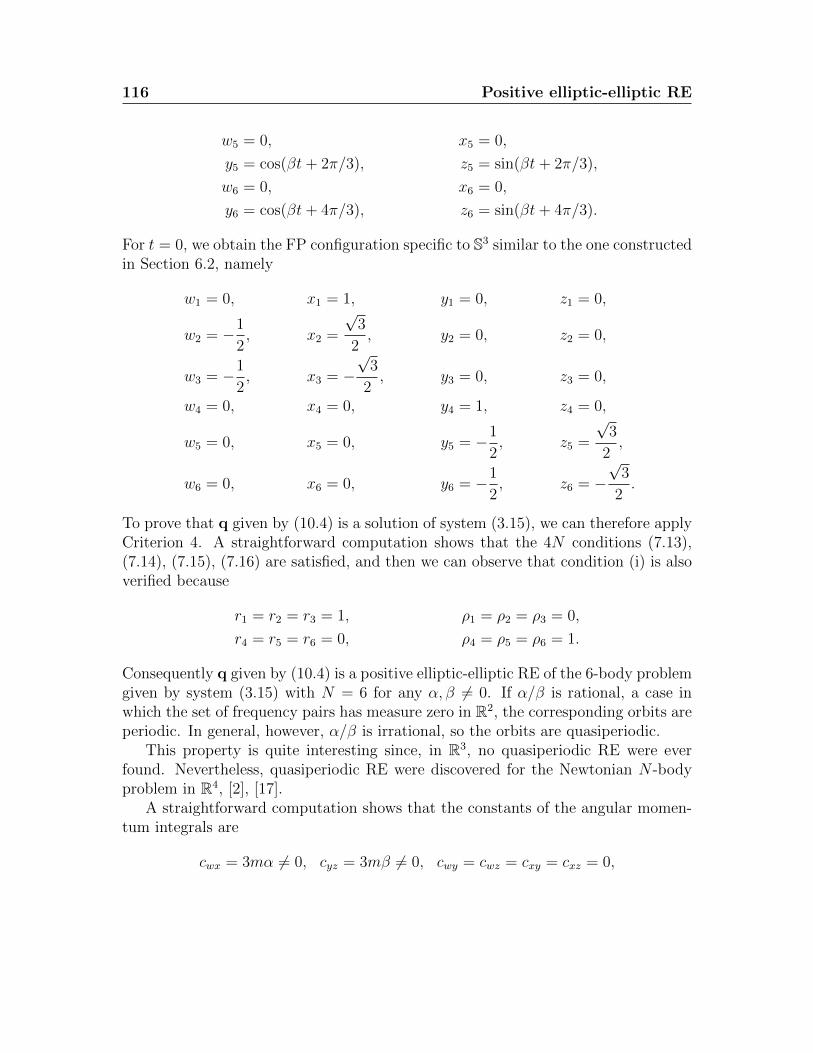
116 Positive elliptic-elliptic RE
w5 = 0, x5 = 0,
y5 = cos(βt+ 2π/3), z5 = sin(βt+ 2π/3),
w6 = 0, x6 = 0,
y6 = cos(βt+ 4π/3), z6 = sin(βt+ 4π/3).
For t = 0, we obtain the FP configuration specific to S3 similar to the one constructedin Section 6.2, namely
w1 = 0, x1 = 1, y1 = 0, z1 = 0,
w2 = −1
2, x2 =
√3
2, y2 = 0, z2 = 0,
w3 = −1
2, x3 = −
√3
2, y3 = 0, z3 = 0,
w4 = 0, x4 = 0, y4 = 1, z4 = 0,
w5 = 0, x5 = 0, y5 = −1
2, z5 =
√3
2,
w6 = 0, x6 = 0, y6 = −1
2, z6 = −
√3
2.
To prove that q given by (10.4) is a solution of system (3.15), we can therefore applyCriterion 4. A straightforward computation shows that the 4N conditions (7.13),(7.14), (7.15), (7.16) are satisfied, and then we can observe that condition (i) is alsoverified because
r1 = r2 = r3 = 1, ρ1 = ρ2 = ρ3 = 0,
r4 = r5 = r6 = 0, ρ4 = ρ5 = ρ6 = 1.
Consequently q given by (10.4) is a positive elliptic-elliptic RE of the 6-body problemgiven by system (3.15) with N = 6 for any α, β 6= 0. If α/β is rational, a case inwhich the set of frequency pairs has measure zero in R2, the corresponding orbits areperiodic. In general, however, α/β is irrational, so the orbits are quasiperiodic.
This property is quite interesting since, in R3, no quasiperiodic RE were everfound. Nevertheless, quasiperiodic RE were discovered for the Newtonian N -bodyproblem in R4, [2], [17].
A straightforward computation shows that the constants of the angular momen-tum integrals are
cwx = 3mα 6= 0, cyz = 3mβ 6= 0, cwy = cwz = cxy = cxz = 0,
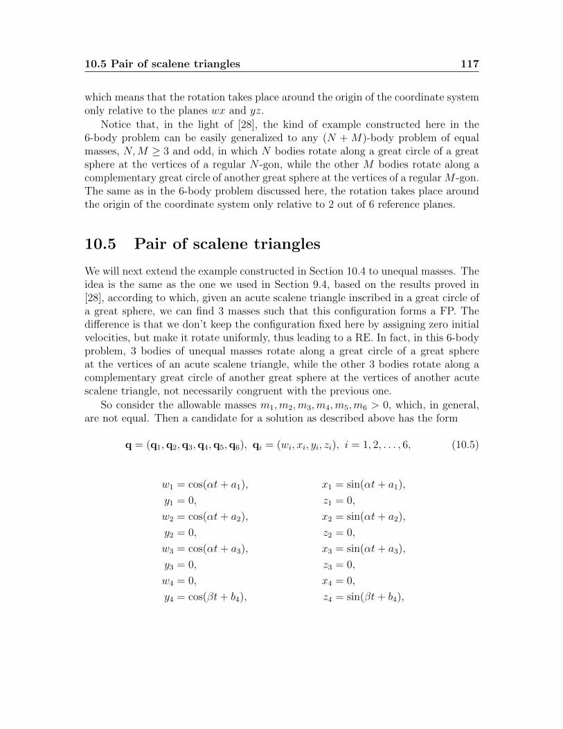
10.5 Pair of scalene triangles 117
which means that the rotation takes place around the origin of the coordinate systemonly relative to the planes wx and yz.
Notice that, in the light of [28], the kind of example constructed here in the6-body problem can be easily generalized to any (N + M)-body problem of equalmasses, N,M ≥ 3 and odd, in which N bodies rotate along a great circle of a greatsphere at the vertices of a regular N -gon, while the other M bodies rotate along acomplementary great circle of another great sphere at the vertices of a regular M -gon.The same as in the 6-body problem discussed here, the rotation takes place aroundthe origin of the coordinate system only relative to 2 out of 6 reference planes.
10.5 Pair of scalene triangles
We will next extend the example constructed in Section 10.4 to unequal masses. Theidea is the same as the one we used in Section 9.4, based on the results proved in[28], according to which, given an acute scalene triangle inscribed in a great circle ofa great sphere, we can find 3 masses such that this configuration forms a FP. Thedifference is that we don’t keep the configuration fixed here by assigning zero initialvelocities, but make it rotate uniformly, thus leading to a RE. In fact, in this 6-bodyproblem, 3 bodies of unequal masses rotate along a great circle of a great sphereat the vertices of an acute scalene triangle, while the other 3 bodies rotate along acomplementary great circle of another great sphere at the vertices of another acutescalene triangle, not necessarily congruent with the previous one.
So consider the allowable masses m1,m2,m3,m4,m5,m6 > 0, which, in general,are not equal. Then a candidate for a solution as described above has the form
q = (q1,q2,q3,q4,q5,q6), qi = (wi, xi, yi, zi), i = 1, 2, . . . , 6, (10.5)
w1 = cos(αt+ a1), x1 = sin(αt+ a1),
y1 = 0, z1 = 0,
w2 = cos(αt+ a2), x2 = sin(αt+ a2),
y2 = 0, z2 = 0,
w3 = cos(αt+ a3), x3 = sin(αt+ a3),
y3 = 0, z3 = 0,
w4 = 0, x4 = 0,
y4 = cos(βt+ b4), z4 = sin(βt+ b4),
118 Positive elliptic-elliptic RE
w5 = 0, x5 = 0,
y5 = cos(βt+ b5), z5 = sin(βt+ b5),
w6 = 0, x6 = 0,
y6 = cos(βt+ b6), z6 = sin(βt+ b6),
where the constants a1, a2, and a3, with 0 ≤ a1 < a2 < a3 < 2π, and b1, b2, and b3,with 0 ≤ b4 < b5 < b6 < 2π, determine the shape of the first and second triangle,respectively, in agreement with the values of the masses.
Notice that for t = 0, the position of the bodies is the FP configuration describedand proved to be as such in Section 9.4. Therefore we can apply Criterion 4 to checkwhether q given in (10.5) is a positive elliptic-elliptic RE. Again, as in Section 9.4,we can approach this problem in two ways. One is computational, and it consists ofusing the fact that the positions at t = 0 form a FP configuration to determine therelationships between the constants m1,m2,m3, a1, a2, and a3, on one hand, and theconstants m4,m5,m6, b4, b5, and b6, on the other hand. It turns out that they reduceto conditions (7.13), (7.14), (7.15), and (7.16). Then we only need to remark that
r1 = r2 = r3 = 1 and r4 = r5 = r6 = 0,
which means that condition (i) of Criterion 4 is satisfied. The other approach is toinvoke again the result of [28] and a reasoning similar to the one we used to show thatthe position at t = 0 is a FP configuration. Both help us conclude that q given by(10.5) is a solution of system (3.15) for any α, β 6= 0. Again, when α/β is rational, acase that corresponds to a negligible set of frequency pairs, the solutions are periodic.In the generic case, when α/β is irrational, the solutions are quasiperiodic.
A straightforward computation shows that the constants of the total angularmomentum integrals are
cwx = (m1 +m2 +m3)α 6= 0, cyz = (m1 +m2 +m3)β 6= 0,
cwy = cwz = cxy = cxz = 0,
which means that the rotation takes place around the origin of the coordinate systemonly relative to the planes wx and yz.
Chapter 11
Negative RE
In this chapter we will provide examples of negative RE, one for each type of orbitof this kind: elliptic, hyperbolic, and elliptic-hyperbolic. The first is the LagrangianRE of equal masses, which is a negative elliptic RE of the 3-body problem in H3, thesecond is the Eulerian orbit of equal masses, which is a negative hyperbolic RE ofthe 3-body problem in H3, and the third is an elliptic-hyperbolic orbit that combinesthe previous two examples in the sense that it inherits their rotations.
11.1 Negative elliptic RE
The class of examples we construct here is the analogue of the one presented inSection 9.1 in the case of the sphere, namely Lagrangian solutions (i.e. equilateraltriangles) of equal masses in H3. In the light of Remark 9, we expect that the bodiesmove on a 2-dimensional hyperbolic sphere, whose curvature is not necessarily thesame as the one of H3. The existence of these orbits in H2, and the fact that theyoccur only when the masses are equal, was first proved in [35]. So, in this case, wehave N = 3 and m1 = m2 = m3 =: m > 0. The solution of the corresponding system(3.16) we are seeking is of the form
q = (q1,q2,q3), qi = (wi, xi, yi, zi), i = 1, 2, 3, (11.1)
w1(t) = r cosωt, x1(t) = r sinωt,
y1(t) = y (constant), z1(t) = z (constant),
w2(t) = r cos(ωt+ 2π/3), x2(t) = r sin(ωt+ 2π/3),
y2(t) = y (constant), z2(t) = z (constant),
120 Negative RE
w3(t) = r cos(ωt+ 4π/3), x3(t) = r sin(ωt+ 4π/3),
y3(t) = y (constant), z3(t) = z (constant),
with r2 + y2− z2 = −1. Consequently, for the equations occurring in Criterion 5, wehave
r1 = r2 = r3 =: r, a1 = 0, a2 = 2π/3, a3 = 4π/3,
y1 = y2 = y3 =: y (constant), z1 = z2 = z3 =: z (constant).
Substituting these values into the equations (7.17), (7.18), (7.19), (7.20), we obtaineither identities or the same equation as in Section 9.1, namely
α2 =8m√
3r3(4− 3r2)3/2.
Consequently, given m > 0, r > 0, and y, z with r2 + y2 − z2 = −1 and z > 1, wecan always find two frequencies,
α1 =2
r
√2m√
3r(4− 3r2)3/2and α2 = −2
r
√2m√
3r(4− 3r2)3/2,
such that system (3.16) has a solution of the form (11.1). The positive frequencycorresponds to one sense of rotation, whereas the negative frequency corresponds tothe opposite sense.
Notice that the bodies move on the 2-dimensional hyperbolic sphere
H2κ0,y0
= {(w, x, y0, z) |w2 + x2 − z2 = −1− y20, y0 = constant, z > 0},
which has curvature κ0 = −(1+y20)−1/2. When y0 = 0, we have a great 2-dimensionalhyperbolic sphere, i.e. its curvature is 1, so the motion is in agreement with Remark6.
A straightforward computation shows that the constants of the angular momen-tum are
cwx = 3mα 6= 0 and cwy = cwz = cxy = cxz = cyz = 0,
which means that the rotation takes place around the origin of the coordinate systemonly relative to the plane wx.
11.2 Negative hyperbolic RE 121
11.2 Negative hyperbolic RE
In this section we will construct a class of negative hyperbolic RE for which, inagreement with Remark 7, the bodies rotate on a 2-dimensional hyperbolic sphere ofthe same curvature as H3. In the 2-dimensional case, the existence of a similar orbitwas already pointed out in [33], where we have also proved it to be unstable. So letus check a solution of the form
q = (q1,q2,q3), qi = (wi, xi, yi, zi), i = 1, 2, 3, (11.2)
w1 = 0, x1 = 0, y1 = sinh βt, z1 = cosh βt,
w2 = 0, x2 = x (constant), y2 = η sinh βt, z2 = η cosh βt,
w3 = 0, x3 = −x (constant), y3 = η sinh βt, z3 = η cosh βt,
with x2 − η2 = −1. Consequently
η1 = 1, η2 = η3 =: η (constant), b1 = b2 = b3 = 0.
We then compute that
µ12 = µ21 = µ13 = µ23 = −η, µ23 = µ32 = 1− 2η2.
We can now use Criterion 6 to determine whether a candidate q given by (11.2) isa (simply rotating) negative hyperbolic RE. Straightforward computations lead usfrom equations (7.21), (7.22), (7.23), and (7.24) either to identities or to the equation
β2 =1 + 4η2
4η3(η2 − 1)3/2.
Therefore, given m,x, η > 0 with x2 − η2 = −1, there exist two nonzero frequencies,
β1 =1
2η
√1 + 4η2
η(η2 − 1)3/2and β2 = − 1
2η
√1 + 4η2
η(η2 − 1)3/2,
such that q given by (11.2) is a (simply rotating) positive hyperbolic relative equi-librium. Notice that the motion takes place on the 2-dimensional hyperbolic sphere
H2w = {(0, x, y, z) |x2 + y2 − z2 = −1, z > 0}.
These orbits are neither periodic nor quasiperiodic. A straightforward computationshows that the constants of the angular momentum are
cwx = cwy = cwz = cxy = cxz = 0, cyz = mβ(1− 2η2),
which means that the rotation takes place about the origin of the coordinate systemonly relative to the yz plane.

122 Negative RE
11.3 Negative elliptic-hyperbolic RE
In this section we will construct a class of (doubly rotating) negative elliptic-hyperbo-lic RE. In the light of Remark 11, we expect that the motion cannot take place onany 2-dimensional hyperboloid of H3. In fact, as we know from Theorem 3, relativeequilibria of this type may rotate on hyperbolic cylinders, which is also the case withthe solution we introduce here.
Consider the masses m1 = m2 = m3 =: m > 0. We will check a solution of theform
q = (q1,q2,q3), qi = (wi, xi, yi, zi), i = 1, 2, 3, (11.3)
w1 = 0, x1 = 0, y1 = sinh βt, z1 = cosh βt,
w2 = r cosαt, x2 = r sinαt, y2 = η sinh βt, z2 = η cosh βt,
w3 = −r cosαt, x3 = −r sinαt, y3 = η sinh βt, z3 = η cosh βt.
In terms of the form (5.12) of an elliptic-hyperbolic RE, (11.3) is realized when
r1 = 0, r2 = r3 =: r, η1 = 1, η2 = η3 =: η,
a1 = a2 = 0, a3 = π, b1 = b2 = b3 = 0.
Substituting these values into the equations (7.25), (7.26), (7.27), (7.28) of Criterion7 and using the fact that r2 − η2 = −1, we obtain the equation
α2 + β2 =m(4η2 + 1)
4η3(η2 − 1)3/2,
which is satisfied for infinitely many values of α and β. Therefore, for any massesm1 = m2 = m3 =: m > 0, and r, η with r2 − η2 = −1, there are infinitely manyfrequencies α and β that correspond to negative elliptic-hyperbolic RE of the form(11.3). These orbits are neither periodic nor quasiperiodic.
The bodies m2 and m3 move on the same hyperbolic cylinder, namely C2rη, which
has constant positive curvature, while m1 moves on the degenerate hyperbolic cylin-der C2
01, which is a geodesic hyperbola, therefore has zero curvature.A straightforward computation shows that the constants of the angular momen-
tum arecwx = 2mαr2, cyz = −1− 2βη2, cwy = cwz = cxy = cxz = 0,
which means that the rotation takes place around the origin of the coordinate systemonly relative to the wx and yz planes.

Part V
The 2-dimensional case

125
Preamble
The goal of Part V is to study some properties of the curved N -body problem onthe surfaces S2 and H2, which are invariant for the equations of motion. We willfocus on polygonal RE for N ≥ 3 as well as on Lagrangian and Eulerian RE forN = 3. The Lagrangian RE are behind a modest first step towards proving thatspace is Euclidean for distances comparable to those of our solar system. We willshow that such orbits exist in the curved case only if the masses are equal. InEuclidean space they also occur for unequal masses, both in theory and in nature,such as the approximate equilateral triangles formed by the Sun, Jupiter, and theTrojan/Greek asteroids. We will end this monograph with extending the formulationof Saari’s conjecture to the curved N -body problem in the 2-dimensional case andproving it when the motion of the bodies is restricted to a rotating geodesic.

126
Chapter 12
Polygonal RE
The goal of this chapter is to study polygonal RE in S2 and H2. Since these manifoldsare embedded in R3, we will drop the w coordinate from now on and use an xyzframe. Given the fact that the dimension is reduced by one, we will not encounterpositive elliptic-elliptic and negative elliptic-hyperbolic RE anymore. So the onlyorbits we will deal with from now on are the positive and negative elliptic as well asthe negative hyperbolic RE.
We will first show that FP configurations lying on geodesics of S2 can generateRE for any nonzero value of the angular frequency. Then we will prove that if thebodies’ initial configuration is on a great circle of S2, then a RE can be generatedonly along that great circle. We will further show that RE formed by regular N -gonshaving equal masses at their vertices can also move on non-great circles. Finally wewill prove that this result is also true in H2.
Both in the classical and the curved N -body problem, given the size of a con-figuration, a RE exists for it, if at all, only for certain angular frequencies, i.e. fortwo angular velocities of equal size and opposite signs. The exception from this ruleoccurs for RE generated from some FP configurations. Let us prove this fact in S2.
Theorem 4. Consider a nonsingular FP configuration given by the bodies of massesm1,m2, . . . ,mN > 0, N ≥ 2, that initially lie on a great circle of S2. Then, for everynonzero angular velocity applied in the plane of the circle, this FP configurationgenerates a positive elliptic RE that rotates along that great circle.
Proof. Without loss of generality, we assume that the great circle is the equatorz = 0 and that for some given masses m1,m2, . . . ,mN > 0 there exist α1, α2, . . . , αNsuch that
q = (q1,q2, . . . ,qN), qi = (xi, yi, 0), (12.1)
128 Polygonal RE
xi = cos(ωt+ αi), yi = sin(ωt+ αi), i = 1, 2, . . . , N,
is a FP for ω = 0. This configuration can also be interpreted as being q(0), i.e. thesolution q at t = 0 for any ω 6= 0. So we can conclude that
∇qiU(q(0)) = 0, i = 1, 2, . . . , N.
But then, for t = 0, the equations of motion (3.15) reduce to{xi = −(x2i + y2i )xi
yi = −(x2i + y2i )yi,(12.2)
i = 1, 2, . . . , N. Notice, however, that
xi = −ω sin(ωt+ αi), xi = −ω2 cos(ωt+ αi),
yi = −ω cos(ωt+ αi), yi = −ω2 sin(ωt+ αi),
therefore x2i + y2i = ω2. Using these expressions, it is easy to see that q given by(12.1) is a solution of (12.2) for every t. Since ∇qiU(q(0)) = 0, i = 1, 2, . . . , N , itfollows that the gravitational forces are in equilibrium at the initial moment, so nogravitational forces act on the bodies. Consequently, the rotation imposed by ω 6= 0makes the system move like a rigid body, so the gravitational forces further remainin equilibrium, consequently ∇qiU(q(t)) = 0, i = 1, 2, . . . , N , for all t. Therefore qgiven by (12.1) satisfies equations (3.15), so it is a positive elliptic RE. This remarkcompletes the proof.
12.1 Polygonal RE on geodesics of S2
The following result shows that positive elliptic RE generated from FP configurationsgiven by regular N -gons of equal masses on a great circle of S2 can occur only ifcertain conditions are satisfied.
Theorem 5. Consider an odd number of equal bodies, initially at the vertices of aregular N-gon inscribed in a great circle of S2. Then the only positive elliptic REthat can be generated from this configuration are the ones that rotate in the plane ofthe original great circle.
Proof. Without loss of generality, we can prove this result for the equator z = 0.Consider therefore a potential positive elliptic RE of the form
q = (q1,q2, . . . ,qN), qi = (xi, yi, zi), (12.3)
12.2 Polygonal RE on non-great circles of S2 129
xi = ri cos(ωt+ αi), yi = ri sin(ωt+ αi), zi = ±(1− r2i )1/2,
i = 1, 2, . . . , N, with + taken for zi > 0 and − for zi < 0. The only condition weimpose on this solution is that ri and αi, i = 1, 2, . . . , N , are chosen such that, atall times, the configuration is a regular N -gon inscribed in a moving great circle ofS2. Therefore the plane of the N -gon can have any angle with, say, the z-axis. Thissolution has the derivatives
xi = −riω sin(ωt+ αi), yi = riω cos(ωt+ αi), zi = 0, i = 1, 2, . . . , N,
xi = −riω2 cos(ωt+ αi), yi = −riω2 sin(ωt+ αi), zi = 0, i = 1, 2, . . . , N.
Thenx2i + y2i + z2i = r2iω
2, i = 1, 2, . . . , N.
Since any N -gon solution with N odd satisfies the conditions
∇qiU(q) = 0, i = 1, 2, . . . , N,
system (3.15) reduces toxi = −(x2i + y2i + z2i )xi,
yi = −(x2i + y2i + z2i )yi,
zi = −(x2i + y2i + z2i )zi, i = 1, 2, . . . , N.
Then the substitution of (12.3) into the above system leads to:{ri(1− r2i )ω2 cos(ωt+ αi) = 0,
ri(1− r2i )ω2 sin(ωt+ αi) = 0, i = 1, 2, . . . , N.
But assuming ω 6= 0, this system is nontrivially satisfied if and only if ri = 0 forsome i ∈ {1, 2, . . . , N} and ri = 1 for the rest of the indices. But given the fact thatthe configuration is an N -gon, the former possibility cannot take place, so we obtainthat zi = 0, i = 1, 2, . . . , N. Therefore the bodies must rotate along the equatorz = 0.
12.2 Polygonal RE on non-great circles of S2
Theorem 5 raises the question whether positive elliptic RE given by regular polygonscan rotate on other curves than geodesics. The answer is positive and is given by
130 Polygonal RE
the following result, which we prove in the case of equal masses and N odd, to avoidsingular configurations. However, we expect that the result is true in general forany nonsingular shape of the polygon and the masses that correspond to such aconfiguration.
Theorem 6. Consider the curved N-body problem with equal masses, m1 = m2 =· · · = mN =: m > 0 in S2. Then, for any N odd, m > 0, and z ∈ (−1, 1), there area positive and a negative ω that produce positive elliptic RE for which the bodies areat the vertices of a regular N-gon rotating in the plane z = constant. If N is even,this property is still true if we exclude the case when the motion takes place alongthe equator z = 0.
Proof. The proof could be presented in general, but for the transparency of theexposition we will discuss the two possible cases: (i) N odd and (ii) N even.
(i) To simplify the presentation, we further denote the bodies by mi, i = −s,−s+1, . . . ,−1, 0, 1, . . . , s − 1, s, where s is a positive integer. Without loss of generalitywe can further check into system (3.15) a solution candidate of the form (12.3) withi as above, α−s = − 4sπ
2s+1, . . . , α−1 = − 2π
2s+1, α0 = 0, α1 = 2π
2s+1, . . . , αs = 4sπ
2s+1,
r := ri, z := zi, and consider only the equations for i = 0. The study of this casesuffices due to the involved symmetry, which yields the same conclusions for anyother value of i.
The equation corresponding to the z0 coordinate takes the form
s∑j=−s,j 6=0
m(z − k0jz)
(1− k20j)3/2− r2ω2z = 0,
where k0j = x0xj+y0yj+z0zj = cosαj−z2 cosαj+z2. Using the fact that r2+z2 = 1,
cosαj = cosα−j, and k0j = k0(−j), this equation becomes
s∑j=1
2(1− cosαj)
(1− k20j)3/2=ω2
m. (12.4)
Now we need to check whether the equations corresponding to x0 and y0 lead to thesame relationship. In fact, checking for x0, and ignoring y0, suffices due to the samesymmetry reasons invoked earlier or the duality of the trigonometric functions sinand cos. The substitution of the the above functions into the first equation of (3.15)leads us to
(r2 − 1)ω2 cosωt =s∑
j=−s,j 6=0
m[cos(ωt+ αj)− k0j cosωt]
(1− k20j)3/2.
12.3 Polygonal RE in H2 131
A straightforward computation, which uses the fact that r2 + z2 = 1, sinαj =− sinα−j, cosαj = cosα−j, and k0j = k0(−j), yields the same equation (12.4). Writingthe denominator of equation (12.4) explicitly, we are led to
s∑j=1
2
(1− cosαj)1/2(1− z2)3/2[2− (1− cosαj)(1− z2)]3/2=ω2
m. (12.5)
The left hand side is always positive, so for any m > 0 and z ∈ (−1, 1) fixed, thereare a positive and a negative ω that satisfy the equation. Therefore the N -gon withan odd number of sides is a positive elliptic RE.
(ii) To simplify the presentation when n is even, we denote the bodies by mi, i =−s+ 1, . . . ,−1, 0, 1, . . . , s− 1, s, where s is a positive integer. Without loss of gener-ality, we can substitute into equations (3.15) a solution candidate of the form (12.3)
with i as above, α−s+1 = (−s+1)πs
, . . . , α−1 = −πs, α0 = 0, α1 = π
s, . . . , αs−1 = (s−1)π
s,
αs = π, r := ri, z := zi, and consider as in the previous case only the equations fori = 0. Then using the fact that k0j = k0(−j), cosαj = cosα−j, and cosπ = −1, astraightforward computation brings the equation corresponding to z0 to the form
s−1∑j=1
2(1− cosαj)
(1− k20j)3/2+
2
(1− k20s)3/2=ω2
m. (12.6)
Using additionally the relations sinαj = − sinα−j and sinπ = 0, we obtain for theequation corresponding to x0 the same form (12.6), which—for k0j and k0s writtenexplicitly—becomes
s−1∑j=1
2
(1− cosαj)1/2(1− z2)3/2[2− (1− cosαj)(1− z2)]3/2
+1
4z2|z|(1− z2)3/2=ω2
m.
Since the left hand side of this equations is positive and finite, given any m > 0 andz ∈ (−1, 0) ∪ (0, 1), there are a positive and a negative ω that satisfy it. So exceptfor the case z = 0, which introduces antipodal singularities, the rotating N -gon withan even number of sides is a positive elliptic RE.
12.3 Polygonal RE in H2
We will further show that negative elliptic RE, similar to the ones proved in Theorem6, also exist in H2.
132 Polygonal RE
Theorem 7. Consider the curved N-body problem with equal masses, m1 = m2 =· · · = mN =: m > 0 in H2. Then, for any m > 0 and z > 1, there are a positive anda negative ω that produce negative elliptic RE in which the bodies are at the verticesof a regular N-gon rotating in the plane z = constant.
Proof. The proof works in the same way as for Theorem 6, by considering the casesN odd and even separately. The only differences are that we replace r with ρ, therelation r2+z2 = 1 with z2 = ρ2+1, and the denominator (1−k20j)3/2 with (c20j−1)3/2,wherever it appears, where c0j = −k0j replaces k0j. Unlike in S2, the case N even issatisfied for all admissible values of z.

Chapter 13
Lagrangian and Eulerian RE
The caseN = 3 presents particular interest in Euclidean space because the equilateraltriangle is a RE for any values of the masses, a property discovered by Joseph LouisLagrange in 1772, [100]. We will further show that this is not the case in S2 andH2, where the positive and negative elliptic Lagrangian RE exist only if the massesare equal. This conclusion provides a first step towards understanding with the helpof these equations whether space is Euclidean for distances of the order of 10 AUbecause Lagrangian orbits of unequal masses show up in our solar system, as forexample the approximate equilateral triangle formed by the Sun, Jupiter, and theTrojan/Greek asteroids. Following this result, we will prove the existence of positiveelliptic Eulerian RE in S2 and negative elliptic Eulerian RE in H2, i.e. orbits formedby 3 bodies lying on a rotating geodesic. In the end we will show that the curved3-body problem in H2 also exhibits negative hyperbolic Eulerian RE, i.e. orbits thatlie on a geodesic that rotates hyperbolically.
13.1 Positive Elliptic Lagrangian RE
We start with a result that refines Theorem 6 in the case N = 3 in S2 by clarifyingexactly when the equilateral triangle of equal masses is a Lagrangian RE.
Proposition 6. Consider the 3-body problem with equal masses, m1 = m2 = m3 =:m, in S2. Then for any m > 0 and z ∈ (−1, 1), there are a positive and a negativeω that produce positive elliptic RE in which the bodies are at the vertices of anequilateral triangle that rotates in the plane z = constant. Moreover, for every ω2/mthere are two values of z that lead to relative equilibria if ω2/m ∈ (8/
√3,∞) ∪ {3},
three values if ω2/m = 8/√
3, and four values if ω2/m ∈ (3, 8/√
3).
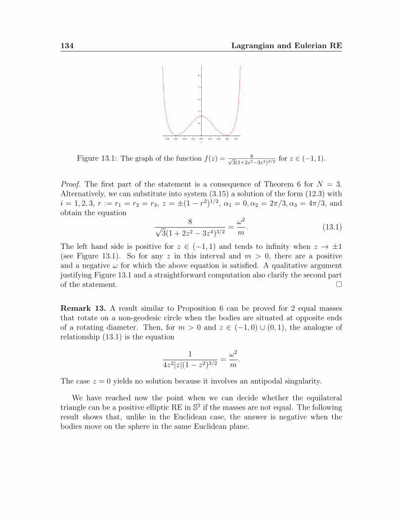
134 Lagrangian and Eulerian RE
Figure 13.1: The graph of the function f(z) = 8√3(1+2z2−3z4)3/2 for z ∈ (−1, 1).
Proof. The first part of the statement is a consequence of Theorem 6 for N = 3.Alternatively, we can substitute into system (3.15) a solution of the form (12.3) withi = 1, 2, 3, r := r1 = r2 = r3, z = ±(1 − r2)1/2, α1 = 0, α2 = 2π/3, α3 = 4π/3, andobtain the equation
8√3(1 + 2z2 − 3z4)3/2
=ω2
m. (13.1)
The left hand side is positive for z ∈ (−1, 1) and tends to infinity when z → ±1(see Figure 13.1). So for any z in this interval and m > 0, there are a positiveand a negative ω for which the above equation is satisfied. A qualitative argumentjustifying Figure 13.1 and a straightforward computation also clarify the second partof the statement.
Remark 13. A result similar to Proposition 6 can be proved for 2 equal massesthat rotate on a non-geodesic circle when the bodies are situated at opposite endsof a rotating diameter. Then, for m > 0 and z ∈ (−1, 0) ∪ (0, 1), the analogue ofrelationship (13.1) is the equation
1
4z2|z|(1− z2)3/2=ω2
m.
The case z = 0 yields no solution because it involves an antipodal singularity.
We have reached now the point when we can decide whether the equilateraltriangle can be a positive elliptic RE in S2 if the masses are not equal. The followingresult shows that, unlike in the Euclidean case, the answer is negative when thebodies move on the sphere in the same Euclidean plane.
13.1 Positive Elliptic Lagrangian RE 135
Proposition 7. In the 3-body problem in S2, if the bodies m1,m2,m3 > 0 are initiallyat the vertices of an equilateral triangle in the plane z = constant for some z ∈(−1, 1), then there are initial velocities that lead to a positive elliptic RE in whichthe triangle rotates in its own plane if and only if m1 = m2 = m3.
Proof. The implication which shows that if m1 = m2 = m3, the rotating equilateraltriangle is a RE, follows from Proposition 6. To prove the other implication, wesubstitute into equations (3.15) a solution of the form (12.3) with i = 1, 2, 3, r :=r1, r2, r3, z := z1 = z2 = z3 = ±(1− r2)1/2, and α1 = 0, α2 = 2π/3, α3 = 4π/3. Thecomputations then lead to the system
m1 +m2 = γω2
m2 +m3 = γω2
m3 +m1 = γω2,
(13.2)
where γ =√
3(1 + 2z2 − 3z4)3/2/4. But for any z = constant in the interval (−1, 1),the above system has a solution only for m1 = m2 = m3 = γω2/2. Therefore themasses must be equal.
The next result leads to the conclusion that Lagrangian solutions in S2 can takeplace only in Euclidean planes of R3. This property is known to be true in theEuclidean case for all RE, [100], but Wintner’s proof doesn’t work in our case becauseit uses the integral of the center of mass. Most importantly, our result also impliesthat Lagrangian orbits with unequal masses cannot exist in S2.
Theorem 8. For all positive elliptic Lagrangian RE of the curved 3-body problem inS2, the masses m1,m2,m3 > 0 have to rotate on the same circle, whose plane mustbe orthogonal to the rotation axis, and therefore m1 = m2 = m3.
Proof. Consider a positive elliptic Lagrangian RE in S2 with bodies m1,m2,m3 > 0.This means that the solution must have the form
x1 = r1 cosωt, y1 = r1 sinωt, z1 = (1− r21)1/2,x2 = r2 cos(ωt+ a), y2 = r2 sin(ωt+ a), z2 = (1− r22)1/2,x3 = r3 cos(ωt+ b), y3 = r3 sin(ωt+ b), z3 = (1− r23)1/2,
with b > a > 0. In other words, we assume that this equilateral triangle forms aconstant angle with the rotation axis, z, such that each body describes its own circleon S2. But for such a solution to exist, the total angular momentum must be either
136 Lagrangian and Eulerian RE
zero or is given by a constant vector parallel with the z axis. Otherwise this vectorrotates around the z axis, in violation of the total angular-momentum integrals. Thismeans that at least the first two components of the vector
∑3i=1miqi × qi must be
zero, where × represents the cross product. A straightforward computation showsthis constraint to lead to the condition
m1r1z1 sinωt+m2r2z2 sin(ωt+ a) +m3r3z3 sin(ωt+ b) = 0,
assuming that ω 6= 0. For t = 0, this equation becomes
m2r2z2 sin a = −m3r3z3 sin b. (13.3)
Using now the fact that
α := x1x2 + y1y2 + z1z2 = x1x3 + y1y3 + z1z3 = x3x2 + y3y2 + z3z2
is constant because the triangle is equilateral, the equation of the system of motioncorresponding to y1 takes the form
Kr1(r21 − 1)ω2 sinωt = m2r2 sin(ωt+ a) +m3r3 sin(ωt+ b),
where K is a nonzero constant. For t = 0, this equation becomes
m2r2 sin a = −m3r3 sin b. (13.4)
Dividing (13.3) by (13.4), we obtain that z2 = z3. Similarly, we can show that z1 =z2 = z3, therefore the motion must take place in the same Euclidean plane on a circleorthogonal to the rotation axis. Proposition 7 then implies that m1 = m2 = m3.
13.2 Negative Elliptic Lagrangian RE
Our next result is the analogue in H2 of Proposition 6.
Proposition 8. Consider the curved 3-body problem with equal masses, m1 = m2 =m3 =: m, in H2. Then for any m > 0 and z > 1, there are a positive and anegative ω that produce negative elliptic RE in which the bodies are at the verticesof an equilateral triangle that rotates in the plane z = constant. Moreover, for everyω2/m > 0 there is a unique z > 1 that satisfies this property.
13.2 Negative Elliptic Lagrangian RE 137
Proof. Substituting in system (3.16) a solution of the form
xi = ρ cos(ωt+ αi), yi = ρ sin(ωt+ αi), zi = z, (13.5)
with z =√ρ2 + 1, α1 = 0, α2 = 2π/3, α3 = 4π/3, we are led to the equation
8√3(3z4 − 2z2 − 1)3/2
=ω2
m. (13.6)
The left hand side is positive for z > 1, tends to infinity when z → 1, and tends tozero when z →∞. So for any z in this interval and m > 0, there are a positive anda negative ω for which the above equation is satisfied.
As we previously proved, an equilateral triangle rotating in its own plane formsa positive elliptic RE in S2 only if the 3 masses lying at its vertices are equal. Thesame result is true in H2, as we will further show.
Proposition 9. In the curved 3-body problem in H2, if the bodies m1,m2,m3 > 0are initially at the vertices of an equilateral triangle in the plane z = constant forsome z > 1, then there are initial velocities that lead to a negative elliptic RE inwhich the triangle rotates in its own plane if and only if m1 = m2 = m3.
Proof. The implication which shows that if m1 = m2 = m3, the rotating equilat-eral triangle is a negative elliptic RE, follows from Theorem 7. To prove the otherimplication, we substitute into equations (3.16) a solution of the form (13.5) withi = 1, 2, 3, ρ := ρ1, ρ2, ρ3, z := z1 = z2 = z3 = (ρ2 + 1)1/2, and α1 = 0, α2 =2π/3, α3 = 4π/3. The computations then lead to the system
m1 +m2 = ζω2
m2 +m3 = ζω2
m3 +m1 = ζω2,
(13.7)
where ζ =√
3(3z4 − 2z2 − 1)3/2/4. But for any z = constant with z > 1, the abovesystem has a solution only for m1 = m2 = m3 = ζω2/2. Therefore the masses mustbe equal.
The following result perfectly resembles Theorem 8. The proof works the sameway, by just replacing the circular trigonometric functions with hyperbolic ones andchanging the signs to reflect the equations of motion in H2. This result finalizesour argument that space is Euclidean for distances comparable to those of our solarsystem.
138 Lagrangian and Eulerian RE
Theorem 9. For all negative elliptic Lagrangian RE of the curved 3-body problem inH2, the masses m1,m2,m3 > 0 have to rotate on the same circle, whose plane mustbe orthogonal to the rotation axis, and therefore m1 = m2 = m3.
13.3 Positive Elliptic Eulerian RE
It is now natural to ask whether positive elliptic RE in which the bodies lie on arotating geodesic exist in S2, since—as Theorem 5 shows—they cannot be generatedfrom regular N -gons. The answer in the case N = 3 of equal masses is given by thefollowing result.
Theorem 10. Consider the curved 3-body problem in S2 with equal masses, m1 =m2 = m3 =: m. Fix the body m1 at (0, 0, 1) and the bodies m2 and m3 at theopposite ends of a diameter on the circle z = constant. Then, for any m > 0 andz ∈ (−0.5, 0) ∪ (0, 1), there are a positive and a negative ω that produce positiveelliptic Eulerian RE.
Proof. Substituting into the equations of motion (3.15) a solution of the form
x1 = 0, y1 = 0, z1 = 1,
x2 = r cosωt, y2 = r sinωt, z2 = z,
x3 = r cos(ωt+ π), y3 = r sin(ωt+ π), z3 = z,
with r ≥ 0 and z constants satisfying r2 + z2 = 1, leads either to identities or to thealgebraic equation
4z + |z|−1
4z2(1− z2)3/2=ω2
m. (13.8)
The function on the left hand side is negative for z ∈ (−1,−0.5), takes the value 0at z = −0.5, is positive for z ∈ (−0.5, 0)∪ (0, 1), and undefined at z = 0. Therefore,for every m > 0 and z ∈ (−0.5, 0)∪ (0, 1), there are a positive and a negative ω thatlead to an Eulerian RE. For z = −0.5, we recover the equilateral FP. The sign of ωdetermines the sense of rotation.
Remark 14. A qualitative argument shows that for every ω2/m ∈ (0, 64√
15/45),there are three values of z that satisfy relation (13.8): one in the interval (−0.5, 0)and two in the interval (0, 1) (see Figure 13.2).
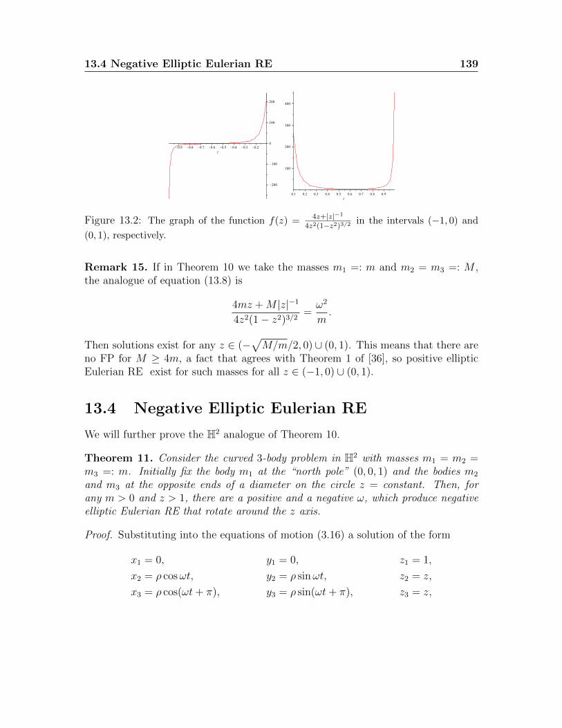
13.4 Negative Elliptic Eulerian RE 139
Figure 13.2: The graph of the function f(z) = 4z+|z|−1
4z2(1−z2)3/2 in the intervals (−1, 0) and
(0, 1), respectively.
Remark 15. If in Theorem 10 we take the masses m1 =: m and m2 = m3 =: M ,the analogue of equation (13.8) is
4mz +M |z|−1
4z2(1− z2)3/2=ω2
m.
Then solutions exist for any z ∈ (−√M/m/2, 0)∪ (0, 1). This means that there are
no FP for M ≥ 4m, a fact that agrees with Theorem 1 of [36], so positive ellipticEulerian RE exist for such masses for all z ∈ (−1, 0) ∪ (0, 1).
13.4 Negative Elliptic Eulerian RE
We will further prove the H2 analogue of Theorem 10.
Theorem 11. Consider the curved 3-body problem in H2 with masses m1 = m2 =m3 =: m. Initially fix the body m1 at the “north pole” (0, 0, 1) and the bodies m2
and m3 at the opposite ends of a diameter on the circle z = constant. Then, forany m > 0 and z > 1, there are a positive and a negative ω, which produce negativeelliptic Eulerian RE that rotate around the z axis.
Proof. Substituting into the equations of motion (3.16) a solution of the form
x1 = 0, y1 = 0, z1 = 1,
x2 = ρ cosωt, y2 = ρ sinωt, z2 = z,
x3 = ρ cos(ωt+ π), y3 = ρ sin(ωt+ π), z3 = z,
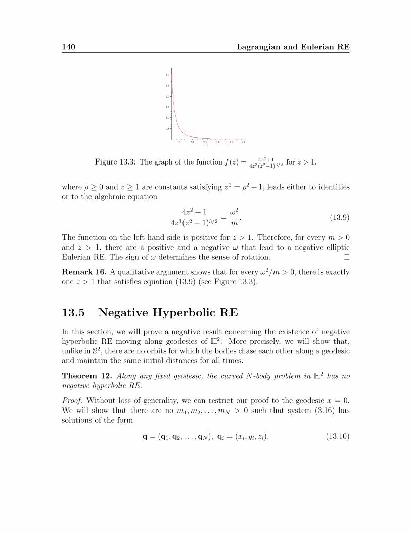
140 Lagrangian and Eulerian RE
Figure 13.3: The graph of the function f(z) = 4z2+14z3(z2−1)3/2 for z > 1.
where ρ ≥ 0 and z ≥ 1 are constants satisfying z2 = ρ2 + 1, leads either to identitiesor to the algebraic equation
4z2 + 1
4z3(z2 − 1)3/2=ω2
m. (13.9)
The function on the left hand side is positive for z > 1. Therefore, for every m > 0and z > 1, there are a positive and a negative ω that lead to a negative ellipticEulerian RE. The sign of ω determines the sense of rotation.
Remark 16. A qualitative argument shows that for every ω2/m > 0, there is exactlyone z > 1 that satisfies equation (13.9) (see Figure 13.3).
13.5 Negative Hyperbolic RE
In this section, we will prove a negative result concerning the existence of negativehyperbolic RE moving along geodesics of H2. More precisely, we will show that,unlike in S2, there are no orbits for which the bodies chase each other along a geodesicand maintain the same initial distances for all times.
Theorem 12. Along any fixed geodesic, the curved N-body problem in H2 has nonegative hyperbolic RE.
Proof. Without loss of generality, we can restrict our proof to the geodesic x = 0.We will show that there are no m1,m2, . . . ,mN > 0 such that system (3.16) hassolutions of the form
q = (q1,q2, . . . ,qN), qi = (xi, yi, zi), (13.10)
13.6 Negative hyperbolic Eulerian RE 141
xi = 0, yi = sinh(ωt+ αi), zi = cosh(ωt+ αi), αi ∈ R, i = 1, 2, . . . , N.
After substitution, the equation corresponding to the yi coordinate becomes
n∑j=1,j 6=i
mj[sinh(ωt+ αj)− cosh(αi − αj) sinh(ωt+ αi)]
| sinh(αi − αj)|3= 0. (13.11)
Assume that αi > αj for all j 6= i and ω > 0. Let αM(i) be the maximum of all αjwith j 6= i. Then for t ∈ (−αM(i)/ω,−αi/ω), we have that sinh(αt + αj) < 0 forall j 6= i and sinh(αt + αi) > 0. Therefore the left hand side of equation (13.11) isnegative in this interval, so the identity cannot take place for all t ∈ R. It followsthat a necessary condition to satisfy equation (13.11) is that αM(i) ≥ αi. But thisinequality must be verified for all i = 1, 2, . . . , N , a fact that can be written as:
α1 ≥ α2 or α1 ≥ α3 or . . . or α1 ≥ αN ,
α2 ≥ α1 or α2 ≥ α3 or . . . or α2 ≥ αN ,
. . .
αN ≥ α1 or αN ≥ α2 or . . . or αN ≥ αN−1.
The constants α1, α2, . . . , αN must satisfy one inequality from each of the above lines.But every possible choice implies the existence of at least one i and one j with i 6= jand αi = αj. For those i and j, we have sinh(αi − αj) = 0, so equation (13.11)is undefined, therefore equations (3.16) cannot have solutions of the form (13.10).Consequently, negative hyperbolic RE do not exist along the geodesic x = 0.
13.6 Negative hyperbolic Eulerian RE
Theorem 12 raises the question whether negative hyperbolic RE do exist at all in H2
(their existence in H3 was proved in Chapter 11). For 3 equal masses, the answeris given by the following result, which shows that, in H2, 3 bodies can move alonghyperbolas lying in parallel planes of R3, maintaining the initial distances amongthemselves and remaining on the same geodesic (which rotates hyperbolically). Suchorbits resemble fighter planes flying in formation, rather than celestial bodies movingunder the action of gravity alone.
Theorem 13. In the curved 3-body problem of equal masses, m1 = m2 = m3 =: m,in H2, for any given m > 0 and x 6= 0, there exist a positive and a negative ω thatlead to negative hyperbolic Eulerian RE.
142 Lagrangian and Eulerian RE
Proof. We will show that qi(t) = (xi(t), yi(t), zi(t)), i = 1, 2, 3, is a negative hyper-bolic RE of system (3.16) for
x1 = 0, y1 = sinhωt, z1 = coshωt,
x2 = x, y2 = ρ sinhωt, z2 = ρ coshωt,
x3 = −x, y3 = ρ sinhωt, z3 = ρ coshωt,
where ρ = (1 + x2)1/2. Notice first that
x1x2 + y1y2 − z1z2 = x1x3 + y1y3 − z1z3 = −ρ,
x2x3 + y2y3 − z2z3 = −2x2 − 1,
x21 + y21 − z21 = ω2, x22 + y22 − z22 = x23 + y23 − z23 = ρ2ω2.
Substituting the above coordinates and expressions into equations (3.16), we are ledeither to identities or to the equation
4x2 + 5
4x2|x|(x2 + 1)3/2=ω2
m, (13.12)
from which the statement of the theorem follows.
Remark 17. The left hand side of equation (13.12) is undefined for x = 0, but ittends to infinity when x → 0 and to 0 when x → ±∞. This means that for eachω2/m > 0 there are exactly one positive and one negative x (equal in absolute value),which satisfy the equation.
Remark 18. Theorem 13 is also true if, say, m1 =: m > 0 and m2 = m3 =: M > 0,with m 6= M . Then the analogue of equation (13.12) is
m
x2|x|(x2 + 1)1/2+
M
4x2|x|(x2 + 1)3/2= ω2,
and it is obvious that for any m,M > 0 and x 6= 0, there are a positive and negativeω satisfying the above equation.
Remark 19. Theorem 13 also works for 2 bodies of equal masses, m1 = m2 =: m >0, of coordinates
x1 = −x2 = x, y1 = y2 = ρ sinhωt, z1 = z2 = ρ coshωt,
where x is a positive constant and ρ = (x2 + 1)3/2. Then the analogue of equation(13.12) is
1
4x2|x|(x2 + 1)3/2=ω2
m,
which obviously supports a statement similar to the one in Theorem 13.
Chapter 14
Saari’s conjecture
In 1970, Don Saari conjectured that solutions of the classical N -body problem withconstant moment of inertia are relative equilibria, [85], [86]. This statement is sur-prising since one does not expect that such a weak constraint would force the bodiesto maintain constant mutual distances all along the motion. Perhaps this is also thereason why the conjecture led to several wrong attempts at proving it, some of whichwere even published, [79], [80].
The case N = 3 was finally solved by Rick Moeckel in 2005, [76], and the collinearcase, when all the bodies are on a rotating line, for any potential that depends onlyon the mutual distances, was settled in [34] in 2006. The problem is open in general.A homographic version of the conjecture was also stated, part of which was solvedin the case N = 3, [31]. A complete proof for N = 3 in the case of equal masses wasrecently announced, [47].
14.1 Extension of Saari’s conjecture to S2 and H2
The moment of inertia is defined in classical Newtonian celestial mechanics as
1
2
N∑i=1
miqi · qi,
a function that gives a crude measure of the bodies’ distribution in space. Butthis definition makes little sense in S2 and H2 because σqi � qi = 1 for every i =1, 2, . . . , N . To avoid this problem, we adopt the standard point of view used inphysics, and define the moment of inertia in S2 and H2 about the direction of theangular momentum. But while fixing an axis in S2 does not restrain generality, thesymmetries of H2 makes us distinguish between two cases.
144 Saari’s conjecture
Indeed, in S2 we can assume that the rotation takes place around the z axis, andthus define the moment of inertia as
I :=N∑i=1
mi(x2i + y2i ). (14.1)
In H2, all possibilities can be reduced via suitable isometric transformations to:(i) the symmetry about the z axis, when the moment of inertia takes the same
form (14.1), and(ii) the symmetry about the x axis, which corresponds to hyperbolic rotations,
when—in agreement with the definition of the Lorentz product—we define the mo-ment of inertia as
J :=N∑i=1
mi(y2i − z2i ). (14.2)
The case of the negative parabolic rotations will not be considered because there areno such RE.
These definitions allow us to formulate the following conjecture:
Saari’s conjecture in S2 and H2. For the curved N-body problem in S2 and H2,every solution that has a constant moment of inertia about the direction of the angularmomentum is either an elliptic relative equilibrium, in S2 or H2, or a hyperbolicrelative equilibrium in H2.
14.2 The proof in the geodesic case
By generalizing an idea we used in the Euclidean case, we can now settle this con-jecture when the bodies undergo another constraint. More precisely, we will provethe following result.
Theorem 14. For the curved N-body problem in S2 and H2, every solution withconstant moment of inertia about the direction of the angular momentum for whichthe bodies remain aligned along a geodesic that rotates elliptically in S2 or H2, orhyperbolically in H2, is either an elliptic relative equilibrium, in S2 or H2, or ahyperbolic relative equilibrium in H2.
Proof. Let us first prove the case in which I is constant in S2 and H2, i.e. when thegeodesic rotates elliptically. According to the above definition of I, we can assumewithout loss of generality that the geodesic passes through the point (0, 0, 1) and

14.2 The proof in the geodesic case 145
rotates about the z-axis with angular velocity ω(t) 6= 0. The angular momentum ofeach body is Li = miqi ⊗ qi, so its derivative with respect to t takes the form
Li = miqi ⊗ qi +miqi ⊗ qi = miqi ⊗ ∇qiU(q)−miq2iqi ⊗ qi =
miqi ⊗ ∇qiU(q),
with κ = 1 in S2 and κ = −1 in H2. Here⊗ is a general notation for the cross product,which means the standard cross product in R3, for positive curvature, and the crossproduct of the Minkowski space R2,1 (i.e. the third component having the oppositesign of the standard cross product’s third component), for negative curvature. Since
qi�∇qiU(q) = 0, it follows that ∇qiUκ(q) is either zero or orthogonal to qi. (Recallthat orthogonality here is meant in terms of the standard inner product because,both in S2 and H2, qi � ∇qiU(q) = qi · ∇qiU(q).) If ∇qiU(q) = 0, then Li = 0, soLzi = 0.
Assume now that ∇qiU(q) is orthogonal to qi. Since all the particles are on ageodesic, their corresponding position vectors are in the same plane, therefore anylinear combination of them is in this plane, so ∇qiU(q) is in the same plane. Thus
∇qiU(q) and qi are in a plane orthogonal to the xy plane. It follows that Li isparallel to the xy plane and orthogonal to the z axis. Thus the z component, Lzi , of
Li is 0, the same conclusion we obtained in the case ∇qiU(q) = 0. Consequently,Lzi = ci, where ci is a constant.
Let us also remark that since the angular momentum and angular velocity vectorsare parallel to the z axis, Lzi = Iiω(t), where Ii = mi(x
2i +y2i ) is the moment of inertia
of the body mi about the z-axis. Since the total moment of inertia, I, is constant,and ω(t) is the same for all bodies because they belong to the same rotating geodesic,it follows that
N∑i=1
Iiω(t) = Iω(t) = c,
where c is a constant. Consequently, ω is a constant vector.Moreover, since Lzi = ci, it follows that Iiω(t) = ci. Then every Ii is constant,
and so is every zi, i = 1, 2, . . . , N . Hence each body of mass mi has a constantzi-coordinate, and all bodies rotate with the same constant angular velocity aroundthe z-axis, properties that agree with our definition of an elliptic RE.
We now prove the case J = constant, i.e. when the geodesic rotates hyperbolicallyin H2. According to the definition of J, we can assume that the bodies are on amoving geodesic whose plane contains the x axis for all time and whose vertex slidesalong the geodesic hyperbola x = 0. (This moving geodesic hyperbola can be also
146 Saari’s conjecture
visualized as the intersection between the sheet z > 0 of the hyperbolic sphere andthe plane containing the x axis and rotating about it. For an instant, this plane alsocontains the z axis.)
The angular momentum of each body is Li = miqi�qi, where � denotes the crossproduct in the Minkowski space R2,1, so we can show as before that its derivativetakes the form Li = miqi � ∇qiU(q), where ∇ = (∂x, ∂y,−∂z). Again, ∇qiU(q) iseither zero or orthogonal to qi. In the former case we can draw the same conclusionas earlier, that Li = 0, so in particular Lxi = 0. In the latter case, qi and ∇qiU(q)are in the plane of the moving hyperbola, so their cross product, qi � ∇qiU(q), isorthogonal to the x axis, and therefore Lxi = 0. Thus Lxi = 0 in either case.
From here the proof proceeds as before by replacing I with J and the z axis withthe x axis, and noticing that Lxi = Jiω(t), to show that every mi has a constant xicoordinate. In other words, each body is moving along a (in general non-geodesic)hyperbola given by the intersection of the hyperboloid with a plane orthogonal to thex axis. These facts, in combination with the sliding of the moving geodesic hyperbolaalong the fixed geodesic hyperbola x = 0, are in agreement with our definition of ahyperbolic relative equilibrium.
Acknowledgments. The author would like to thank Boris Hasselblatt of TuftsUniversity, the editor of the Atlantis Monographs in Dynamical Systems, for theinvitation to write this book for the first volume of this new imprint, and to HenkBroer of the University of Groningen for endorsing this invitation as co-editor ofthe series. Many thanks also go to the anonymous referee, whose excellent remarkshelped the author bring the text to a higher level of rigor and presentation. Lastbut not least, the author acknowledges the research support of the Discovery Grant122045 from NSERC of Canada.
Bibliography
[1] R. Abraham and J.E. Marsden, Foundations of Mechanics, 2nd ed., Benjamin-Cummings, Reading MA, 1978.
[2] A. Albouy and A. Chenciner, Le probleme des N corps et les distancesmutuelles, Inventiones math. 131 (1998), 151-184.
[3] A. Albouy and V. Kaloshin, Finiteness of central configurations for five bodiesin the plane, Ann. of Math. 176 (2012), 535-588.
[4] A. Baker, Matrix Groups: An Introduction to Lie Group Theory, SpringerVerlag, London, 2002.
[5] K. Becker, M. Becker, and J.H. Schwarz, String Theory and M-Theory: AModern Introduction, Cambridge University Press, 2007.
[6] P. de Bernardis et. al., A flat Universe from high-resolution maps of the cosmicmicrowave background radiation, Nature 404, 6781 (2000), 955-959.
[7] J. Bertrand, Theoreme relatif au mouvement d’un point attire vers un centerfixe, C. R. Acad. Sci. 77 (1873), 849-853.
[8] W. Bolyai and J. Bolyai, Geometrische Untersuchungen, Hrsg. P. Stackel,Teubner, Leipzig-Berlin, 1913.
[9] R. Bonola, Non-Euclidean Geometry, Dover, New York, 1955.
[10] H. Bruns, Uber die Integrale des Vielkorper-Problems, Acta Math. 11 (1887),25-96.
[11] D.M. Burton, The History of Mathematics, an Introduction, Allyn and Bacon,Inc., Newton, Massachusetts, 1985.
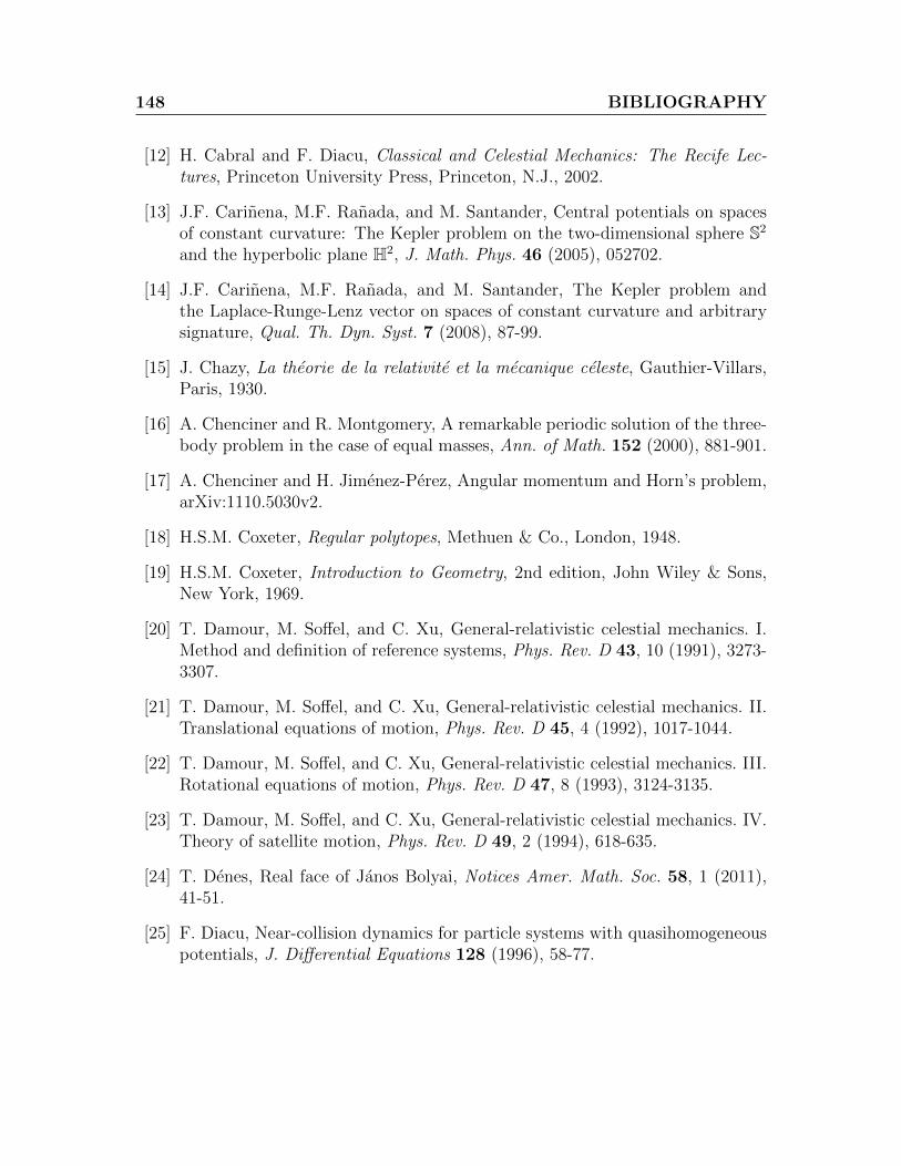
148 BIBLIOGRAPHY
[12] H. Cabral and F. Diacu, Classical and Celestial Mechanics: The Recife Lec-tures, Princeton University Press, Princeton, N.J., 2002.
[13] J.F. Carinena, M.F. Ranada, and M. Santander, Central potentials on spacesof constant curvature: The Kepler problem on the two-dimensional sphere S2
and the hyperbolic plane H2, J. Math. Phys. 46 (2005), 052702.
[14] J.F. Carinena, M.F. Ranada, and M. Santander, The Kepler problem andthe Laplace-Runge-Lenz vector on spaces of constant curvature and arbitrarysignature, Qual. Th. Dyn. Syst. 7 (2008), 87-99.
[15] J. Chazy, La theorie de la relativite et la mecanique celeste, Gauthier-Villars,Paris, 1930.
[16] A. Chenciner and R. Montgomery, A remarkable periodic solution of the three-body problem in the case of equal masses, Ann. of Math. 152 (2000), 881-901.
[17] A. Chenciner and H. Jimenez-Perez, Angular momentum and Horn’s problem,arXiv:1110.5030v2.
[18] H.S.M. Coxeter, Regular polytopes, Methuen & Co., London, 1948.
[19] H.S.M. Coxeter, Introduction to Geometry, 2nd edition, John Wiley & Sons,New York, 1969.
[20] T. Damour, M. Soffel, and C. Xu, General-relativistic celestial mechanics. I.Method and definition of reference systems, Phys. Rev. D 43, 10 (1991), 3273-3307.
[21] T. Damour, M. Soffel, and C. Xu, General-relativistic celestial mechanics. II.Translational equations of motion, Phys. Rev. D 45, 4 (1992), 1017-1044.
[22] T. Damour, M. Soffel, and C. Xu, General-relativistic celestial mechanics. III.Rotational equations of motion, Phys. Rev. D 47, 8 (1993), 3124-3135.
[23] T. Damour, M. Soffel, and C. Xu, General-relativistic celestial mechanics. IV.Theory of satellite motion, Phys. Rev. D 49, 2 (1994), 618-635.
[24] T. Denes, Real face of Janos Bolyai, Notices Amer. Math. Soc. 58, 1 (2011),41-51.
[25] F. Diacu, Near-collision dynamics for particle systems with quasihomogeneouspotentials, J. Differential Equations 128 (1996), 58-77.
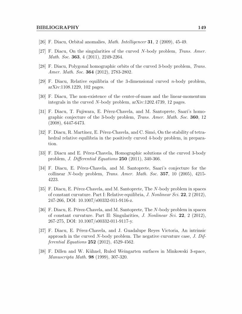
BIBLIOGRAPHY 149
[26] F. Diacu, Orbital anomalies, Math. Intelligencer 31, 2 (2009), 45-49.
[27] F. Diacu, On the singularities of the curved N -body problem, Trans. Amer.Math. Soc. 363, 4 (2011), 2249-2264.
[28] F. Diacu, Polygonal homographic orbits of the curved 3-body problem, Trans.Amer. Math. Soc. 364 (2012), 2783-2802.
[29] F. Diacu, Relative equilibria of the 3-dimensional curved n-body problem,arXiv:1108.1229, 102 pages.
[30] F. Diacu, The non-existence of the center-of-mass and the linear-momentumintegrals in the curved N -body problem, arXiv:1202.4739, 12 pages.
[31] F. Diacu, T. Fujiwara, E. Perez-Chavela, and M. Santoprete, Saari’s homo-graphic conjecture of the 3-body problem, Trans. Amer. Math. Soc. 360, 12(2008), 6447-6473.
[32] F. Diacu, R. Martınez, E. Perez-Chavela, and C. Simo, On the stability of tetra-hedral relative equilibria in the positively curved 4-body problem, in prepara-tion.
[33] F. Diacu and E. Perez-Chavela, Homographic solutions of the curved 3-bodyproblem, J. Differential Equations 250 (2011), 340-366.
[34] F. Diacu, E. Perez-Chavela, and M. Santoprete, Saari’s conjecture for thecollinear N -body problem, Trans. Amer. Math. Soc. 357, 10 (2005), 4215-4223.
[35] F. Diacu, E. Perez-Chavela, and M. Santoprete, The N -body problem in spacesof constant curvature. Part I: Relative equilibria, J. Nonlinear Sci. 22, 2 (2012),247-266, DOI: 10.1007/s00332-011-9116-z.
[36] F. Diacu, E. Perez-Chavela, and M. Santoprete, The N -body problem in spacesof constant curvature. Part II: Singularities, J. Nonlinear Sci. 22, 2 (2012),267-275, DOI: 10.1007/s00332-011-9117-y.
[37] F. Diacu, E. Perez-Chavela, and J. Guadalupe Reyes Victoria, An intrinsicapproach in the curved N -body problem. The negative curvature case, J. Dif-ferential Equations 252 (2012), 4529-4562.
[38] F. Dillen and W. Kuhnel, Ruled Weingarten surfaces in Minkowski 3-space,Manuscripta Math. 98 (1999), 307-320.
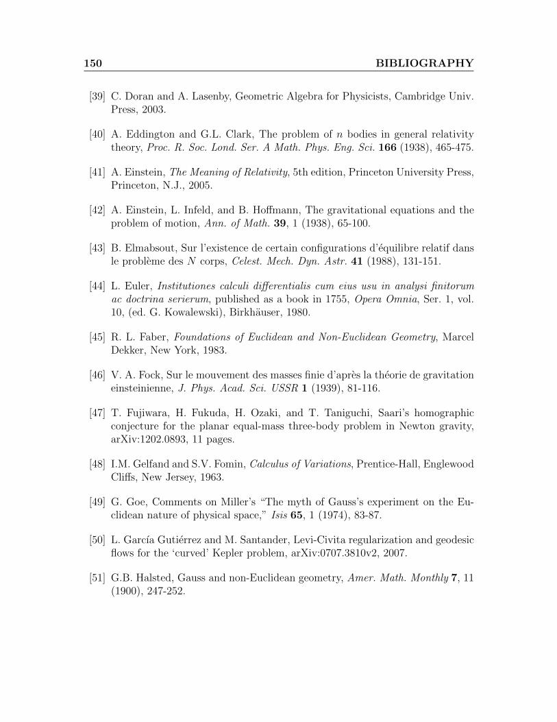
150 BIBLIOGRAPHY
[39] C. Doran and A. Lasenby, Geometric Algebra for Physicists, Cambridge Univ.Press, 2003.
[40] A. Eddington and G.L. Clark, The problem of n bodies in general relativitytheory, Proc. R. Soc. Lond. Ser. A Math. Phys. Eng. Sci. 166 (1938), 465-475.
[41] A. Einstein, The Meaning of Relativity, 5th edition, Princeton University Press,Princeton, N.J., 2005.
[42] A. Einstein, L. Infeld, and B. Hoffmann, The gravitational equations and theproblem of motion, Ann. of Math. 39, 1 (1938), 65-100.
[43] B. Elmabsout, Sur l’existence de certain configurations d’equilibre relatif dansle probleme des N corps, Celest. Mech. Dyn. Astr. 41 (1988), 131-151.
[44] L. Euler, Institutiones calculi differentialis cum eius usu in analysi finitorumac doctrina serierum, published as a book in 1755, Opera Omnia, Ser. 1, vol.10, (ed. G. Kowalewski), Birkhauser, 1980.
[45] R. L. Faber, Foundations of Euclidean and Non-Euclidean Geometry, MarcelDekker, New York, 1983.
[46] V. A. Fock, Sur le mouvement des masses finie d’apres la theorie de gravitationeinsteinienne, J. Phys. Acad. Sci. USSR 1 (1939), 81-116.
[47] T. Fujiwara, H. Fukuda, H. Ozaki, and T. Taniguchi, Saari’s homographicconjecture for the planar equal-mass three-body problem in Newton gravity,arXiv:1202.0893, 11 pages.
[48] I.M. Gelfand and S.V. Fomin, Calculus of Variations, Prentice-Hall, EnglewoodCliffs, New Jersey, 1963.
[49] G. Goe, Comments on Miller’s “The myth of Gauss’s experiment on the Eu-clidean nature of physical space,” Isis 65, 1 (1974), 83-87.
[50] L. Garcıa Gutierrez and M. Santander, Levi-Civita regularization and geodesicflows for the ‘curved’ Kepler problem, arXiv:0707.3810v2, 2007.
[51] G.B. Halsted, Gauss and non-Euclidean geometry, Amer. Math. Monthly 7, 11(1900), 247-252.
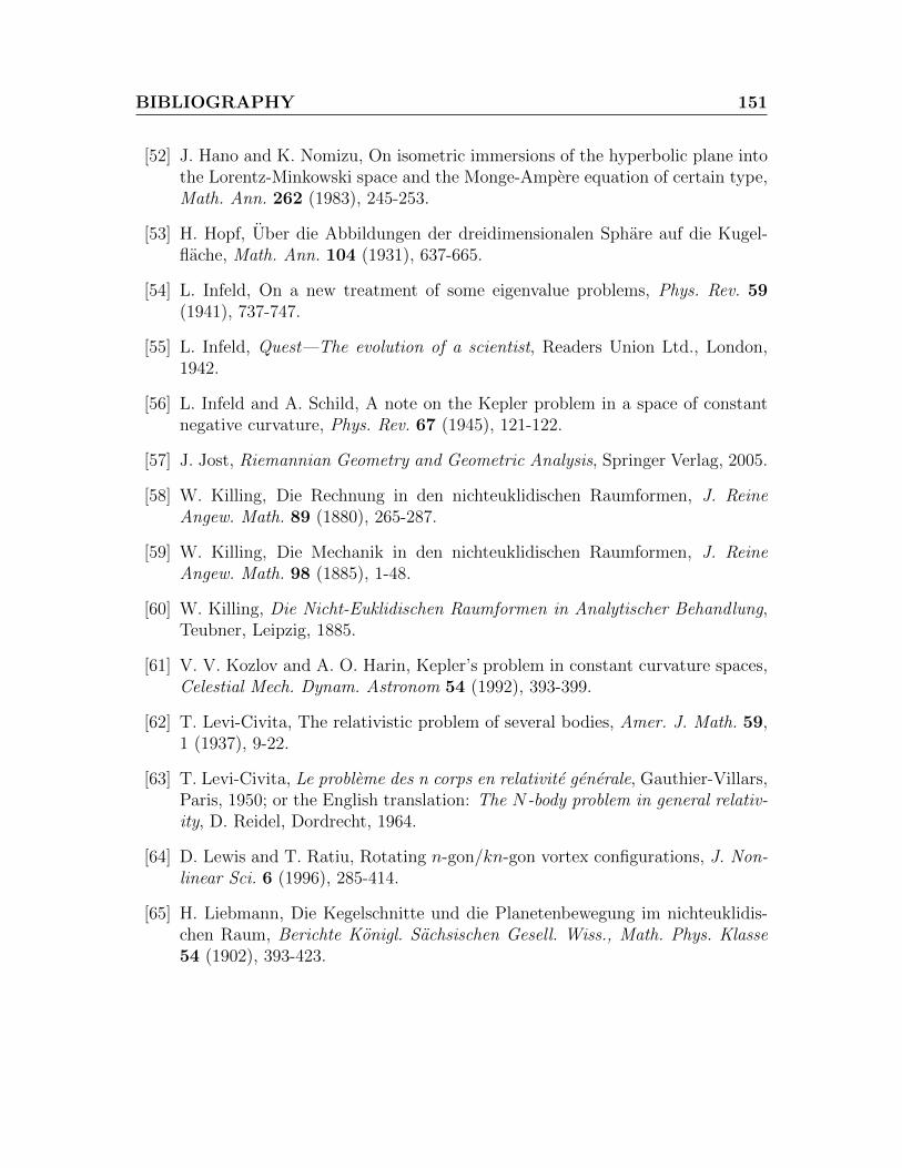
BIBLIOGRAPHY 151
[52] J. Hano and K. Nomizu, On isometric immersions of the hyperbolic plane intothe Lorentz-Minkowski space and the Monge-Ampere equation of certain type,Math. Ann. 262 (1983), 245-253.
[53] H. Hopf, Uber die Abbildungen der dreidimensionalen Sphare auf die Kugel-flache, Math. Ann. 104 (1931), 637-665.
[54] L. Infeld, On a new treatment of some eigenvalue problems, Phys. Rev. 59(1941), 737-747.
[55] L. Infeld, Quest—The evolution of a scientist, Readers Union Ltd., London,1942.
[56] L. Infeld and A. Schild, A note on the Kepler problem in a space of constantnegative curvature, Phys. Rev. 67 (1945), 121-122.
[57] J. Jost, Riemannian Geometry and Geometric Analysis, Springer Verlag, 2005.
[58] W. Killing, Die Rechnung in den nichteuklidischen Raumformen, J. ReineAngew. Math. 89 (1880), 265-287.
[59] W. Killing, Die Mechanik in den nichteuklidischen Raumformen, J. ReineAngew. Math. 98 (1885), 1-48.
[60] W. Killing, Die Nicht-Euklidischen Raumformen in Analytischer Behandlung,Teubner, Leipzig, 1885.
[61] V. V. Kozlov and A. O. Harin, Kepler’s problem in constant curvature spaces,Celestial Mech. Dynam. Astronom 54 (1992), 393-399.
[62] T. Levi-Civita, The relativistic problem of several bodies, Amer. J. Math. 59,1 (1937), 9-22.
[63] T. Levi-Civita, Le probleme des n corps en relativite generale, Gauthier-Villars,Paris, 1950; or the English translation: The N-body problem in general relativ-ity, D. Reidel, Dordrecht, 1964.
[64] D. Lewis and T. Ratiu, Rotating n-gon/kn-gon vortex configurations, J. Non-linear Sci. 6 (1996), 285-414.
[65] H. Liebmann, Die Kegelschnitte und die Planetenbewegung im nichteuklidis-chen Raum, Berichte Konigl. Sachsischen Gesell. Wiss., Math. Phys. Klasse54 (1902), 393-423.

152 BIBLIOGRAPHY
[66] H. Liebmann, Uber die Zentralbewegung in der nichteuklidische Geometrie,Berichte Konigl. Sachsischen Gesell. Wiss., Math. Phys. Klasse 55 (1903),146-153.
[67] H. Liebmann, Nichteuklidische Geometrie, G. J. Goschen, Leipzig, 1905; 2nded. 1912; 3rd ed. Walter de Gruyter, Berlin, Leipzig, 1923.
[68] R. Lipschitz, Untersuchung eines Problems der Variationsrechnung, in welchemdas Problem der Mechanik enthalten ist, J. Reine Angew. Math. 74 (1872),116-149.
[69] R. Lipschitz, Extension of the planet-problem to a space of n dimensions andconstant integral curvature, Quart. J. Pure Appl. Math. 12 (1873), 349-370.
[70] N. I. Lobachevsky, The new foundations of geometry with full theory of paral-lels [in Russian], 1835-1838, In Collected Works, V. 2, GITTL, Moscow, 1949,p. 159.
[71] D.W. Lyons, An elementary introduction to the Hopf fibration, Math. Mag.76, 2 (2003), 87-98.
[72] J.E. Marsden and T.S. Ratiu, Introduction to Mechanics and Symmetry, (2nded.) Springer Verlag, 1999.
[73] R. Martınez and C. Simo, On the stability of the Lagrangian homographicsolutions in a curved three-body problem on S2, Discrete Contin. Dyn. Syst.Ser. B (to appear).
[74] R. McGehee, Triple collision in the collinear three-body problem, Inventionesmath. 27 (1974), 191-227.
[75] A. I. Miller, The myth of Gauss’s experiment on the Euclidean nature of phys-ical space, Isis 63, 3 (1972), 345-348.
[76] R. Moeckel, A computer-assisted proof of Saari’s conjecture for the planarthree-body problem, Trans. Amer. Math. Soc. 357, (2005) 3105-3117.
[77] R. Mosseri and R. Dandoloff, Geometry of entangled states, Bloch spheres andHopf fibrations, J. Phys. A 34 (2001), 10243-10252.
[78] M. Nakahara, Geometry, Topology and Physics, Institute of Physics Publishing,Philadelphia, 1990.
BIBLIOGRAPHY 153
[79] J.I. Palmore, Relative equilibria and the virial theorem, Celestial Mech. 19(1979), 167-171.
[80] J.I. Palmore, Saari’s conjecture revisited, Celestial Mech. 25 (1981), 79-80.
[81] E. Perez-Chavela and J.G. Reyes Victoria, An intrinsic approach in the curvedN -body problem. The positive curvature case, Trans. Amer. Math. Soc. 364,7 (2012), 3805-3827.
[82] L. Perko and E. Walter, Regular polygon solutions of the N -body problem,Proc. Amer. Math. Soc. 94 (1985), 301-309.
[83] H. Poincare, The Value of Science: Essential Writings of Henri Poincare, TheModern Library, New York, 2001.
[84] W.F. Reynolds, Hyperbolic geometry on a hyperboloid, Amer. Math. Monthly100, 5 (1993), 442-455.
[85] D. Saari, On bounded solutions of the n-body problem, in Periodic Orbits,Stability and Resonances, G.E.O. Gicaglia, ed., pp. 76-81, D. Reidel, Dordrecht,1970.
[86] D. Saari, Collisions, Rings, and Other Newtonian N-body Problems, AmericanMathematical Society, Regional Conference Series in Mathematics, No. 104,Providence, RI, 2005.
[87] E. Schering, Die Schwerkraft im Gaussischen Raume, Nachr. Konigl. Gesell.Wiss. Gottingen 13 July, 15 (1870), 311-321.
[88] E. Schering, Die Schwerkraft in mehrfach ausgedehnten Gaussischen und rie-mannschen Raumen, Nachr. Konigl. Gesell. Wiss. Gottingen 26 Febr., 6(1873), 149-159.
[89] E. Schrodinger, A method for determining quantum-mechanical eigenvaluesand eigenfunctions, Proc. Royal Irish Acad., Sect. A 46 (1940), 9-16.
[90] P.J. Serret, Theorie nouvelle geometrique et mecanique des lignes a doublecourbure, Mallet-Bachelier, Paris, 1860.
[91] S. Sgries, Erinnerung an “dunkle Seiten,” Gedenkkolloquium fur den judischenMathematiker Heinrich Liebmann, Heidelberger Nachrichten, June 19, 2008.
154 BIBLIOGRAPHY
[92] A.V. Shchepetilov, Comment on “Central potentials on spaces of constant cur-vature: The Kepler problem on the two-dimensional sphere S2 and the hyper-bolic plane H2,” [J. Math. Phys. 46 (2005), 052702], J. Math. Phys. 46 (2005),114101.
[93] A.V. Shchepetilov, Reduction of the two-body problem with central interac-tion on simply connected spaces of constant sectional curvature, J. Phys. A:Math. Gen. 31 (1998), 6279-6291.
[94] A.V. Shchepetilov, Nonintegrability of the two-body problem in constant cur-vature spaces, J. Phys. A: Math. Gen. V. 39 (2006), 5787-5806; correctedversion at math.DS/0601382.
[95] A.V. Shchepetilov, Calculus and mechanics on two-point homogenous Rieman-nian spaces, Lecture notes in physics, vol. 707, Springer Verlag, 2006.
[96] S. Smale, Mathematical problems for the next century, Mathematics: frontiersand perspectives, Amer. Math. Society, Providence, RI, pp. 271-294.
[97] A. F. Stevenson, Note on the Kepler problem in a spherical space, and thefactorization method for solving eigenvalue problems, Phys. Rev. 59 (1941),842-843.
[98] J.R. Weeks, The Shape of Space, Marcel Dekker, New York, 2002.
[99] H. Weyl, Space, Time, Matter, 4th ed., Methuen & comp., London, 1952.
[100] A. Wintner, The Analytical Foundations of Celestial Mechanics, Princeton Uni-versity Press, Princeton, N.J., 1941.
[101] H.E. Wolfe, Introduction to Non-Euclidean Geometry, Holt, Rineheart andWinston, New York, 1945.

Index
κ-cosine, see unified trigonometryκ-cotangent, see unified trigonometryκ-sine, see unified trigonometryκ-tangent, see unified trigonometry120-cell, 6916-cell, 692-body problem, viii, 3, 7, 824-cell, 694-cube, 69600-cell, 698-cell, 69
angular momentum, 38, 90, 135, 143, 145,146
conservation law, 85constant, 39, 90, 103, 105, 107, 110,
112, 115, 120–122angular velocity, 127, 145astronomical unit, vii
Berlin, 6Bertrand’s theorem, 28Bertrand, Joseph Louis, 3, 7, 28Bessel, Friedrich, ixBetrand’s theorem, 7Boeotians, ixBolyai, Janos, viii, ix, 5–7, 16, 18, 19, 44Boomerang experiment, 1Brocken, 1
cartesian product, 35, 87, 93celestial mechanics, 2, 3, 8, 22, 143
centre of mass, 3, 36, 37Chazy, Jean, 8Clifford torus, 5, 87–89, 91, 93, 96, 110,
111, 113complementary circles, 21, 22, 25, 68, 89,
91–94, 102, 104, 105, 109, 115,117
constant curvature, see curvatureconstrained Lagrangian dynamics, 9, 27,
30coordinates
extrinsic, 9, 10intrinsic, 9, 23
cosmic crystallography, 1cotangent bundle, 34cotangent potential, viii, 3, 6, 8, 9, 28cross product, 37, 146curvature
constant, 4, 5, 7–9, 15, 18, 19, 25, 93Gaussian, 2, 7, 15, 88negative, 8, 9, 13, 15, 20, 25, 33, 40,
41, 50nonzero, 4positive, 5, 9, 13, 20, 33, 39–42, 49,
93, 122zero, 1, 3, 122
Dirichlet, Lejeune, 6distance, vii–x, 1, 4–6, 10, 17, 18, 22, 23,
25, 140, 141Euclidean, viii, 23
156 INDEX
dodecaplex, 69dynamics, viii, x, 2, 5, 9, 16, 27, 30, 99
Eddington, Arthur, 8Einstein’s field equations, 7, 36Einstein, Albert, ix, 8, 17energy constant, 36, 43Euclid, viiiEuclidean geometry, viii, ixEuclidean metric, 24, 25Euclidean norm, 23Euclidean space, vii–x, 2–5, 7, 9, 16, 18,
19, 24, 27, 28, 32, 35–37, 41–44,101, 133–135, 144
Euler’s formula, see homogeneous func-tion
Euler-Lagrange equations, 27, 30exterior product, see wedge product
fixed point, 67–69, 78fixed point configuration, 91Fock, Vladimir, 8foliation, 88, 93, 111, 113force function, 28–33, 42–44Frenet-Serret formulas, 5frequency, 60–63, 80, 91, 93, 103
Gottingen, vii, 1Gauss, Carl Friedrich, viii–x, 1, 5Gaussian curvature, see curvaturegeneral relativity, ixgenus, 88geodesic, ix, 17, 18, 37, 41, 70, 88, 93,
94, 122, 127–129, 133, 140, 141,144–146, 158
geometric topology, viii, 87, 93Grassmann algebra, 37great hyperbolic sphere, 22, 35great sphere, 20–22, 35, 51–53, 68, 89, 91,
102–105, 107, 109–111, 115, 117
Hamiltonian function, 34, 36Hamiltonian system, 27, 34Hamiltonian vector field, 34harmonic function, 3, 43, 44Heegaard splitting, 88Heegaard, Poul, 88Heidelberg, 7heliotrope, 1, 2history, viii, 1, 5, 15Hoffmann, Banesh, 8Hoher Hagen, 1homogeneous function, 27, 29
Euler’s formula, 27, 29, 31Hungary, 6hyperbolic cylinder, 5, 93, 94, 96, 122hyperbolic geometry, 5, 7, 9, 15–17, 19
Klein-Beltrami disk, 15Poincare 3-ball, 24Poincare disk, 15Poincare upper-half plane, 15Weierstrass’s model, 9, 16–18
hyperbolic sphere, 13, 15–20, 22, 23, 33,35, 49, 121
hypercube, 69hyperdodecahedron, 69hypericosahedron, 69hyperoctahedron, 69
Infeld, Leopold, 8inner product, 16, 19, 20, 22
Lorentz, 16, 18, 20, 33, 93, 144standard, 19, 33, 145
integrable system, 3integral
angular momentum, 37, 104, 116, 118centre of mass, 3, 36energy, 36, 43linear momentum, 3, 36
invariance, 35, 51, 54
INDEX 157
isometry, 17, 18, 47, 49
Jupiter, 4, 133
Kazan, 7Kepler problem, 3, 5–9, 28, 43Kepler’s force function, 44Kepler’s laws, 6, 7Kepler’s potential, 43, 44Killing, Wilhelm, 6, 19kinetic energy, 30, 34, 43
Lagrange multipliers, 30, 31Lagrange, Joseph Louis, 133Lagrangian function, 30Laplace’s equation, 3, 28, 43Laplace-Beltrami equation, 3, 28, 44Levi-Civita, Tullio, 8Lie group, viii, 5, 16, 49, 50Liebmann, Adelheid, 7Liebmann, Karl Otto Heinrich, 6, 7Liebmann, Karl-Otto, 7Lipschitz, Rudolph, 6Lobachevsky, Nikolai, viii, ix, 5–7, 16, 18,
19, 44Lorentz product, see inner productLorentz, Hendrik, 15
manifold, 19, 20, 22, 23, 26, 27, 30, 32–35,37, 59, 60, 64, 87, 88, 93
compact, 88connected, 88decomposition, 88hyperbolic, 2, 3, 18of constant curvature, 5, 25of variable curvature, 7oriented, 88pseudo-Riemannian, 3, 28Riemannian, 3, 28
Minkowski space, 9, 16–19, 50, 145, 146
negative curvature, see curvatureNew York, viiNewton, Isaac, ix, 2Newtonian N -body problem, 2, 3, 27Newtonian force, 6Newtonian law, vii, viii, 44Newtonian potential, 3, 27, 28, 101non-Euclidean geometry, 5nonzero curvature, see curvature
octaplex, 69orthoplex, 69outer product, see wedge product
Paris, viipentatope, 5, 68, 69, 109, 113planetary system, xPoincare, Henri, ixpolydodecahedron, 69polyoctahedron, 69polytetrahedron, 69polytope, 69positive curvature, see curvaturepost-Newtonian approximations, 8potential energy, 27, 30, 43preface, viiProclus Lycaeus, viii
RE, see relative equilibriumrelative equilibrium, 59
Eulerian, 119, 133, 138–140Lagrangian, 4, 37, 102, 119, 133, 135,
136, 138negative elliptic, 61, 75, 81, 94, 119negative elliptic-hyperbolic, 63, 84, 94,
96, 122negative hyperbolic, 62, 82, 83, 94,
119, 121negative parabolic, 63, 64, 75, 85, 86
158 INDEX
positive elliptic, 50, 59, 60, 75–78, 87,88, 91, 92, 101, 104, 105, 107, 110,139
positive elliptic-elliptic, 60, 78–80, 87–89, 91–93, 109, 111, 113, 115, 116,118
Romania, 6rotation, see transformation
Saari’s conjecture, 143, 144Saari’s geodesic conjecture, 144Saari, Donald, 143Schering, Ernst Christian Friedrich, vii,
viii, 6Schild, Alfred, 8Schlafli symbol, 68Schrodinger, Erwin, 8Serret, Joseph Alfred, 5Serret, Paul Joseph, 5solar system, vii, xstring theory, ixSun, 4, 133sunlight, 1symmetry, 3, 36–38, 69, 130, 143, 144
Targu Mures (Maros-Vasarhely), 6tesseract, 69tetraplex, 69transformation
negative elliptic, 50, 51, 53, 61negative elliptic-hyperbolic, 50, 51, 55,
63negative hyperbolic, 50, 51, 53–56, 62negative parabolic, 50, 63, 144positive elliptic, 50–52, 59, 103positive elliptic-elliptic, 50–53, 60, 91
Transylvania, 6triangle
acute, 67, 102, 105, 109
equilateral, 4, 37, 41, 67, 68, 101, 102,104, 109, 110, 115, 119, 133–138
scalene, 102, 103, 105, 109, 117Trojan asteroids, 4, 133
unified trigonometry, 25κ-cosine, 26κ-cotangent, 26κ-sine, 25κ-tangent, 26
universe, vii, ix, 1, 2, 4, 42, 43
vertex, 18, 68, 145
Wurdemann, William, 2wedge product, 37, 38Weierstrass’s coordinates, 19Weierstrass, Karl, 15, 19
zero curvature, see curvature
Copyright © 2022 FDOKUMEN