
Nonlinear weakly curved rod by Gamma convergence
27
arXiv:1102.2648v1 [math.AP] 14 Feb 2011 Noname manuscript No. (will be inserted by the editor) Nonlinear weakly curved rod by Γ -convergence Igor Velˇ ci´ c the date of receipt and acceptance should be inserted later Abstract We present a nonlinear model of weakly curved rod, namely the type of curved rod where the curvature is of the order of the diameter of the cross-section. We use the approach analogous to the one for rods and curved rods and start from the strain energy functional of three dimensional nonlinear elasticity and do not presuppose any constitutional behavior. To derive the model, by means of Γ -convergence, we need to propose how is the order of strain energy related to the thickness of the body h. We analyze the situation when the strain energy (divided by the order of volume) is of the order h 4 . That is the same approach as the one when F¨oppl-von K´ arm´an model for plates and the analogous model for rods are obtained. The obtained model is analogous to Marguerre-von K´ arm´anfor shallow shells and its linearization is the linear shallow arch model which can be found in the literature. Keywords weaky curved rod · Gamma convergence · shallow arch · asymptotic analysis Mathematics Subject Classification (2000) 74K20 · 74K25 1 Introduction The study of thin structures is the subject of numerous works in the theory of elasticity. There is a vast literature on the subject of rods, plates and shells (see [5,8,9]). The derivation and justification of the lower dimensional models, equilib- rium and dynamic, of rods, curved rods, weakly curved rods, plates and shells Igor Velˇ ci´ c Faculty of Electrical Engineering and Computer Science, University of Zagreb, Unska 3, 10000 Zagreb, Croatia Tel: +385-1-6129965 Fax:+385-1-6170007 E-mail: [email protected]
Transcript of Nonlinear weakly curved rod by Gamma convergence

arX
iv:1
102.
2648
v1 [
mat
h.A
P] 1
4 Fe
b 20
11
Noname manuscript No.(will be inserted by the editor)
Nonlinear weakly curved rod by Γ -convergence
Igor Velcic
the date of receipt and acceptance should be inserted later
Abstract We present a nonlinear model of weakly curved rod, namely thetype of curved rod where the curvature is of the order of the diameter of thecross-section. We use the approach analogous to the one for rods and curvedrods and start from the strain energy functional of three dimensional nonlinearelasticity and do not presuppose any constitutional behavior. To derive themodel, by means of Γ -convergence, we need to propose how is the order ofstrain energy related to the thickness of the body h. We analyze the situationwhen the strain energy (divided by the order of volume) is of the order h4.That is the same approach as the one when Foppl-von Karman model forplates and the analogous model for rods are obtained. The obtained model isanalogous to Marguerre-von Karman for shallow shells and its linearization isthe linear shallow arch model which can be found in the literature.
Keywords weaky curved rod · Gamma convergence · shallow arch ·asymptotic analysis
Mathematics Subject Classification (2000) 74K20 · 74K25
1 Introduction
The study of thin structures is the subject of numerous works in the theoryof elasticity. There is a vast literature on the subject of rods, plates and shells(see [5,8,9]).
The derivation and justification of the lower dimensional models, equilib-rium and dynamic, of rods, curved rods, weakly curved rods, plates and shells
Igor VelcicFaculty of Electrical Engineering and Computer Science, University of Zagreb, Unska 3,10000 Zagreb, CroatiaTel: +385-1-6129965Fax:+385-1-6170007E-mail: [email protected]
2 Igor Velcic
in linearized elasticity, by using formal asymptotic expansion, is well estab-lished (see [8,9] and the references therein). In all these approaches one startsfrom the equations of three-dimensional linearized elasticity and then via for-mal asymptotic expansion justify the lower dimensional models. One can alsoobtain the convergence results. In [3,4] the linear model of weakly curved rod(or as it is called shallow arch) is derived and the convergence result is ob-tained. We call weakly curved rods or shallow arches those characterized bythe fact that the curvature of their centerline should has the same order ofmagnitude as the diameter of the cross section, both being much smaller thantheir length.
Formal asymptotic expansion is also applied to derive non linear models ofrods, plates and shells (see [8,9,22] and the references therein), starting fromthree-dimensional isotropic elasticity (usually Saint-Venant-Kirchoff material).Hierarchy of the models is obtained, depending on the the order of the externalloads related to the thickness of the body h (see also [11] for plates).
However, formal asymptotic expansion does not provide us a convergenceresult. The first convergence result, in deriving lower dimensional models fromthree-dimensional non linear elasticity, is obtained applying Γ -convergence,very powerful tool introduced by Degiorgi (see [6,10]). Using Γ -convergence,elastic string models, membrane plate and membrane shell models are obtained(see [1,16,17]). It is assumed that the external loads are of order h0. The ob-tained models are different from those ones obtained by the formal asymptoticexpansion in the sense that additional relaxation of the energy functional isdone.
Recently, hierarchy of models of rods, curved rods, plates and shells isobtained via Γ - convergence (see [12,13,14,15,19,24,25,30,31]). Influence ofthe boundary conditions and the order and the type of the external loads islargely discussed for plates (see [13,18]). Let us mention that Γ -convergenceresults provide us the convergence of the global minimizers of the total energyfunctional. Recently, compensated compactness arguments are used to obtainthe convergence of the stationary points of the energy functional (see [23,28]).
Here we apply the tools developed for rods, plates and shells to obtainweakly curved rod model by Γ -convergence. It is assumed that we have freeboundary conditions and that the strain energy (divided by the order of vol-ume) is of the order h4, where h is the thickness of the rod. This correspondsto the situation when external transversal dead loads are of order h3 (see Re-mark 8). The order h4 of the strain energy gives Foppl-von Karman model forplates, Marguerre-von Karman model for shallow shells the analogous modelfor rods (see [14,25,32]). The obtained model is non linear model of the lowestorder in the hierarchy of models and its linearization is shallow arch model,obtained in [3,4] for isotropic, homogenous case (see for comparison Remark7 d)). Here we do not presuppose any constitutional behavior and thus workin a more general framework. The main result is stated in Theorem 5.
Throughout the paper A or A− denotes the closure of the set. By adomain we call a bounded open set with Lipschitz boundary. I denotes theidentity matrix, by SO(3) we denote the rotations in R
3, by so(3) the set of
Nonlinear weakly curved rod by Γ -convergence 3
antisymmetric matrices 3×3 and R3×3sym denotes the set of symmetric matrices.
By symA we denote the symmetric part of the matrix, symA = 12 (A+AT ).
e1, e2, e3 are the vectors of the canonical base in R3. By ∇h we denote ∇h =
∇e1+ 1
h∇e2,e3. ‖f‖C1(Ω) stands for C1 norm of the function f : Ω ⊂ R
n →R i.e. ‖f‖C1(Ω) = maxx∈Ω |f | +
∑ni=1 maxx∈Ω |∂if |. → denotes the strong
convergence and the weak convergence.
2 Setting up the problem
Let ω ⊂ R2 be an open set having area equal to A and Lipschitz boundary.
For all h such that 0 < h ≤ 1 and for given L we define
ωh = hω, Ωh = (0, L)× hω. (2.1)
We shall leave out superscript when h = 1, i.e. Ω = Ω1, ω = ω1. Let us byµ(ω) denote
µ(ω) =
ˆ
ω
(x22 + x2
3)dx2dx3. (2.2)
Let us choose coordinate axis such thatˆ
ω
x2dx2dx3 =
ˆ
ω
x3dx2dx3 =
ˆ
ω
x2x3dx2dx3 = 0. (2.3)
For every h we define the curve Ch of the form
Ch = θh(x1) = (x1, θh2 (x1), θ
h3 (x1)) ∈ R
3 : x1 ∈ (0, L). (2.4)
where θhk (x1), for k = 2, 3, are given functions satisfying θhk ∈ C3(0, L). Let
(th,nh, bh) be the Frenet trihedron associated with the curve Ch
th =1√
1 + ((θh2 )′)2 + ((θh3 )
′)2(1, (θh2 )
′, (θh3 )′), (2.5)
nh =(th)′
‖(th)′‖, (2.6)
bh = th × nh. (2.7)
We suppose nh ∈ C1(0, L) which is satisfied if (θh2 )′′, (θh3 )
′′ do not vanish atthe same time (which is equivalent to the fact that the curvature of Ch isstrictly positive for any x1 ∈ (0, L)). The case where Ch has null curvaturepoints can be treated in the same fashion, provided that we suppose that alongthese points we have the same degree of smoothness as before with th, nh andbh appropriately chosen (see Remark 3). We define the map Θh : Ωh →Θh(Ωh) = Ωh− ⊂ R
3, where Ωh := Θh(Ωh), in the following manner:
Θh(xh) = (x1, θh2 (x1), θ
h3 (x1)) + xh
2nh(x1) + xh
3bh(x1) (2.8)

4 Igor Velcic
and we assume that Θh is a C1 diffeomorphism which can be proved if h issmall enough and θhk , for k = 2, 3, are of the form considered here. Namely, wetake θh2 = hθ2, θ
h3 = hθ3 where θk ∈ C3(0, L). Let us suppose
((θ1)′′)2(x1) + ((θ2)
′′)2(x1) 6= 0, (2.9)
for all x1 ∈ (0, L). A generic point in Ωh or Ωh− will be denoted by xh =(x1, x
h2 , x
h3 ).
Like in [24,25,12,13,14,15,19] we start from three dimensional non linearelasticity functional of strain energy (see [7] for an introduction to non linearelasticity)
Ih(y) :=1
h2
ˆ
Ωh
Wh(xh,∇y)dxh. (2.10)
It is natural to divide the strain energy with h2, since the volume is vanishingwith the order of h2. We are interested in finding Γ -limit (in some sense i.e.in characterizing the limits of minimizers) of the functionals 1
h4 Ih. The reason
why we divide with h4 is that we want to obtain theory analogous to Foppl-vonKarman for plates and rods (see [13,14,25]) and Marguerre-von Karman forshallow shells (see [32]). We do not look the total energy functional because thepart with the strain energy contains the highest order derivatives (at least forthe external dead loads) and thus makes the most difficult part of the analysis(see Remarks 8 and 10). We shall not impose Dirichlet boundary conditionand assume that the body is free at the boundary. The consideration of theother boundary conditions is also possible. We rewrite the functional Ih onthe domain Ω, i.e. we conclude
Ih(y) :=
ˆ
Ω
Wh(Θh P h(x), (∇y) Θh P h) det((∇Θh) P h(x))dx, (2.11)
where by P h : R3 → R3 we denote the mapping P h(x1, x2, x3) = (x1, hx2, hx3).
(∇y) Θh P h denotes ∇y evaluated at the point Θh(P h(x)). We assumethat for each h it is valid
det((∇Θh) P h(x))Wh(Θh P h(x),F) = W (x,F), ∀x ∈ Ω, ∀F ∈ R3×3,
(2.12)where the stored energy function W is independent of h and satisfies thefollowing assumptions (the same ones as in [25]):
i) W : Ω × R3×3 → [0,+∞] is a Caratheodory function; for some δ > 0 the
function F 7→ W (x,F) is of class C2 for dist(F, SO(3)) < δ and for a.e.x ∈ Ω;
ii) the second derivative ∂2W∂F2 is a Caratheodory function on the set Ω×F ∈
R3×3 : dist(F, SO(3)) < δ and there exists a constant γ > 0 such that
∣∣∣∣∣∂2W
∂F2(x,F)[G,G]
∣∣∣∣∣ ≤ γ|G|2 if dist(F, SO(3)) < δ and G ∈ R3×3sym;

Nonlinear weakly curved rod by Γ -convergence 5
iii) W is frame-indifferent, i.e. W (x,F) = W (x,RF) for a.e. x ∈ Ω and everyF ∈ R
3×3,R ∈ SO(3);iv) W (x,F) = 0 if F ∈ SO(3); W (x,F) ≥ C dist2(F, SO(3)) for every F ∈
R3×3, where the constant C > 0 is independent of x.
Under these assumptions we first show the compactness result (Theorem 3)i.e. we take the sequence yh ∈ W 1,2(Ωh;R3) such that
lim suph → 01
h4Ih < +∞
and conclude how that fact affects the limit displacement. In Lemma 2 weprove the lower bound, in Theorem 4 we prove the upper bound and thatenables us to identify limit functional (Theorem 5). First we start with somebasic properties of the mappings Θh which are necessary for further analysis.
3 Properties of the mappings Θh
We introduce for k = 2, 3,
pk(x1) =θ′′k (x1)√
(θ′′2 )2(x1) + (θ′′3 )
2(x1). (3.1)
Notice thatp22 + p23 = 1, p2p
′2 + p3p
′3 = 0. (3.2)
Let us denote p = p2p′3 − p′2p3.
Theorem 1 Let the functions θhk be such that
θhk (x1) = hθk(x1), for all x1 ∈ (0, L), k = 2, 3.
where θk ∈ C3(0, L) is independent of h. Then there exists h0 = h0(θ) > 0such that the Jacobian matrix ∇Θh(xh), where the mappings Θh are definedwith (2.8), is invertible for all xh ∈ Ωh and all h ≤ h0. Also there exists C > 0such that for h ≤ h0 we have
det∇Θh = 1 + hδh(xh), (3.3)
and
th(x1) = e1 + hθ′2(x1)e2 + hθ′3(x1)e3 + h2o1(x1), (3.4)
nh(x1) = p2(x1)e2 + p3(x1)e3 − h(θ′2p2 + θ′3p3)(x1)e1
+h2o2(x1), (3.5)
bh(x1) = −p3(x1)e2 + p2(x1)e3 + h(θ′2p3 − θ′3p2)(x1)e1
+h2o3(x1), (3.6)
∇Θh(xh) = Re(x1) + hC(x1) + xh2D(x1) + xh
3E(x1)
+h2Oh1 (x
h), (3.7)
(∇Θh(xh))−1 = RTe (x1)− hC1(x1)− xh
2D1(x1)− xh3E1(x1)
+h2Oh2 (x
h), (3.8)

6 Igor Velcic
∥∥∥(∇Θh)−Re
∥∥∥L∞(Ωh;R3×3)
< Ch, (3.9)
∥∥∥(∇Θh)−1 −RTe
∥∥∥L∞(Ωh;R3×3)
< Ch, (3.10)
where
Re =
(1 0
0 R
), R =
(p2 −p3p3 p2
), (3.11)
C =
0 −(θ′2p2 + θ′3p3) −(θ′3p2 − θ′2p3)θ′2 0 0θ′3 0 0
, (3.12)
D =
0 0 0p′2 0 0p′3 0 0
, E =
0 0 0−p′3 0 0p′2 0 0
, (3.13)
C1 =
0 −θ′2 −θ′3θ′2p2 + θ′3p3 0 0θ′3p2 − θ′2p3 0 0
, (3.14)
D1 =
0 0 00 0 0p 0 0
, E1 =
0 0 0−p 0 00 0 0
, (3.15)
and δh : Ωh → R, oi : (0, L) → R3, i = 1, 2, 3, Oh
k : Ωh → R3×3, k = 1, 2 are
functions which satisfy
sup0<h≤h0
maxxh∈Ωh
|δh(xh)| ≤ C0,
sup0<h≤h0
maxx1∈(0,L)
‖ohi (x1)‖ ≤ C0, sup
0<h≤h0
maxx1∈(0,L)
‖(ohi )
′(x1)‖ ≤ C0
sup0<h≤h0
maxi,j
maxxh∈Ωh
‖Ohk,ij(x
h)‖ ≤ C0, k = 1, 2,
for some constant C0 > 0.
Proof. It can be easily seen
th(x1) = e1+hθ′2(x1)e2+hθ′3(x1)e3−h2
2((θ′2)
2+(θ′3)2)e1+h3oh
4 (xh), (3.16)
where ‖o4‖C2(0,L) ≤ C. The relations (3.5) and (3.6) are the direct conse-
quences of the relation (3.16). Let us by uh : (0, L) → R3 denote the function
uh = (1, hθ′2, hθ′3)
T . (3.17)
It is easy to see
∇Θh(xh) = (uh(x1) + xh2 (n
h)′(x1) + xh3 (b
h)′(x1) | nh(x1) | b
h(x1)). (3.18)
Nonlinear weakly curved rod by Γ -convergence 7
The relations (3.3), (3.7), (3.9), (3.10) are the direct consequences of the rela-tions (3.4-(3.6) and (3.18). The relation (3.8) is the direct consequence of thefact that, for a regular matrix A and arbitrary B, which satisfies ‖A−1B‖ < 1(‖ · ‖ is the operational norm), the matrix A+B is invertible and
‖(A+B)−1 − (A−1 −A−1BA−1)‖ ≤‖A−1B‖2‖A‖−1
1− ‖A−1B‖.
To end the proof observe that
C1 = RTe CRT
e , D1 = RTe DRT
e , E1 = RTe ERT
e .
Remark 1 By a careful computation it can be seen that oh2 , o
h3 and oh
4 (definedin the relation (3.16)) are dominantly in e2, e3 plane i.e. that we have fori = 2, 3, 4:
ohi (x1) = f2
i (x1)e2 + f3i (x1)e3 + hrhi (x1), (3.19)
where f2i , f3
i ∈ C1(0, L), sup0<h≤h0‖rhi ‖C1(0,L) ≤ C, for some C > 0.
Remark 2 By a further inspection it can be seen that
f24 = −
1
2θ′2((θ
′2)
2 + (θ′3)2), f3
4 = −1
2θ′3((θ
′2)
2 + (θ′3)2), (3.20)
f22 = p2
(f2(θ
′, θ′′)−1
2((θ′2)
2 + (θ′3)2))− θ′2(θ
′2p2 + θ′3p3), (3.21)
f32 = p3
(f2(θ
′, θ′′)−1
2((θ′2)
2 + (θ′3)2))− θ′3(θ
′2p2 + θ′3p3), (3.22)
f23 = p3((θ
′2)
2 + (θ′3)2)− p3f2(θ
′, θ′′), (3.23)
f33 = −p2((θ
′2)
2 + (θ′3)2) + p2f2(θ
′, θ′′), (3.24)
where f2(θ′, θ′′) ∈ C1(0, L) is the expression that includes θ′, θ′′:
f2(θ′, θ′′) =
1
2
((p2 + p3)((θ
′2)
2 + (θ′3)2) + 2(θ′2 + θ′3)(θ
′2p2 + θ′3p3)
−√(θ′′2 )
2 + (θ′′3 )2(θ′2p2 + θ′3p3)
2)
Remark 3 It is not necessary to impose the condition (2.9). All we need isthe existence of the expansions given by (3.4)-(3.6), where p2, p3 ∈ C1(0, L),including the statement of Remark 1.
Remark 4 Although Θh makes the small perturbation of the central line,(x1, 0, 0), for x1 ∈ [0, L], it is not true that ∇Θh is close to the identity (like inthe shallow shell model, see [32]). In fact, there are torsional effects of order 0on every cross section. This is the main reason why is the change of coordinatesintroduced in the next chapter useful.

8 Igor Velcic
4 Γ -convergence
We shall need the following theorem which can be found in [12].
Theorem 2 (on geometric rigidity) Let U ⊂ Rm be a bounded Lipschitz
domain, m ≥ 2. Then there exists a constant C(U) with the following property:for every v ∈ W 1,2(U ;Rm) there is an associated rotation R ∈ SO(m) suchthat
‖∇v −R‖L2(U) ≤ C(U)‖ dist(∇v, SO(m)‖L2(U). (4.1)
The constant C(U) can be chosen uniformly for a family of domains which areBilipschitz equivalent with controlled Lipschitz constants. The constant C(U)is invariant under dilatations.
The following version of the Korn’s inequality is needed.
Lemma 1 Let ω ⊂ R2 with Lipschitz boundary and u ∈ L2(ω;R2). Let us by
eij(u) denote eij(u) =12 (∂iu + ∂ju). Let us suppose that for every i, j = 1, 2
we have that eij(u) ∈ L2(ω). Then we have that u ∈ W 1,2(ω;R2). Also thereexists constant C(ω), depending only on the domain ω, such that we have
‖u‖W 1,2(ω;R2) ≤ C(ω)(|
ˆ
ω
udx1dx2|+ |
ˆ
ω
(x1u2 − x2u1)dx1dx2|
+∑
i,j=1,2
‖eij(u)‖L2(ω)
). (4.2)
Let us suppose that the domains ωs are changing in the sense that they areequal to ωs = Asω, where As ∈ R
2×2, and there exists a constant C such that‖As‖, ‖A
−1s ‖ ≤ C. Then the constant in the inequality (4.2) can be chosen
independently of s.
Proof. The first part of the lemma (the fixed domain) is a version of theKorn’s inequality (see e.g. [29]). The last part we shall prove by a contradiction.Let us suppose the contrary that for each n ∈ N there exists sn and un ∈W 1,2(ωsn ;R
2) such that we have
|
ˆ
ωsn
undx1dx2|+ |
ˆ
ωsn
(x1un2 − x2u
n1 )dx1dx2|
+∑
i,j=1,2
‖esn
ij (un)‖L2(ωsn) ≤
1
n‖un‖W 1,2(ωsn ;R2), (4.3)
where we have by esn
ij (·) denoted the symmetrized gradient on the domain ωsn .Without any loss of generality we can suppose that ‖un‖W 1,2(ωsn ;R2) = 1. Letus take the subsequence of (sn) (still denoted by (sn)) such that Asn → Aand A−1
sn → A−1 in R2×2.
Let us look the sequence unc = un Asn A−1. It is clear that there exist
C1, C2 > 0 such that
C1 ≤ ‖unc ‖W 1,2(ω∞;R2) ≤ C2, (4.4)
Nonlinear weakly curved rod by Γ -convergence 9
where we have put ω∞ := Aω. Thus there exists u ∈ W 1,2(ω∞;R2) suchthat un
c u weakly in W 1,2(ω∞;R2). Specially, by the compactness of theembedding L2 → W 1,2 (see e.g. [2]), we also conclude the strong convergenceunc → u in L2(ω∞;R2). Since it is validAsnA
−1 → I, it can be easily seen that,from the weak convergence, it follows es
n
ij (un) (Asn A
−1) e∞ij (u), weakly
in L2(ω∞;R2), where we have by e∞ij (·) denoted the symmetrized gradient onthe domain ω∞. From the weak convergence we can conclude that
‖e∞ij (u)‖L2(ω∞) ≤ lim infn→∞
‖esn
ij (un) (Asn A−1)‖L2(ω∞) = 0, (4.5)
for every i, j = 1, 2. We can also from (4.3) conclude thatˆ
ω∞
udx1dx2 = 0,
ˆ
ω∞
(x1u2 − x2u1)dx1dx2 = 0. (4.6)
Applying the standard Korn’s inequality on the domain ω∞, i.e.
‖u− unc ‖W 1,2(ω∞;R2) ≤ C(ω∞)
(‖u− un
c ‖L2(ω∞;R2)
+∑
i,j=1,2
‖eij(u)− eij(unc )‖L2(ω∞;R2)
),
we conclude that unc → u strongly in W 1,2(ω∞;R2). But then (4.4), (4.5),
(4.6) make a contradiction with the version of the Korn’s inequality (4.2) onthe domain ω∞.
Remark 5 The same proof can be done under the assumption that ωs = Fs(ω),where Fs is the family of Bilipschitz mappings whose Bilipschitz constants wecan control (i.e. the Lipschitz constants of Fs and F−1
s are bounded by a univer-sal constant), provided that the family Fs is strongly compact in W 1,∞(ω;R2).It would require more analysis to conclude the same result only for Bilipschitzmappings whose Bilipschitz constants we can control.
Let us by x′ : R3 → R3 denote the change of coordinates
(x′1, x
′2, x
′3) = x′(x1, x2, x3) := Re(x1)
x1
x2
x3
. (4.7)
By Ω′ we denote x′(Ω) and ω′(x1) ⊂ R2 denotes x′(x1×ω), for x1 ∈ [0, L].
The generic point in Ω′ is denoted with x′ = (x′1, x
′2, x
′3). Let us observe that
by (2.2) and (2.3)ˆ
ω′(x1)
x′2dx
′2dx
′3 =
ˆ
ω′(x1)
x′3dx
′2dx
′3 = 0, (4.8)
ˆ
ω′(x1)
x′2x
′3dx
′2dx
′3 = p2p3
ˆ
ω
(x22 − x2
3)dx2dx3, (4.9)
µ(ω) =
ˆ
ω
(x22 + x2
3)dx2dx3 =
ˆ
ω′(x1)
((x′2)
2 + (x′3)
2)dx′2dx
′3, (4.10)

10 Igor Velcic
for all x1 ∈ [0, L]. By (∂iyj) Θh P h) we denote ∂iyj evaluated at the point
Θh(P h(x)).In the sequel we suppose h0 ≥ 1 (see Theorem 1). If this was not the
case, what follows could be easily adapted. Using theorem 2 we can prove thefollowing theorem
Theorem 3 Let yh ∈ W 1,2(Ωh;R3) and let
Eh =1
h2
ˆ
Ωh
dist2(∇yh, SO(3))dx.
Let us suppose that
lim suph→0
Eh
h4< +∞. (4.11)
Then there exist maps Rh : [0, L] → SO(3) and Rh : [0, L] → R3×3, with
|R| ≤ C, R ∈ W 1,2([0, L],R3×3) and constants Rh∈ SO(3), ch ∈ R
3 such
that the functions yh := (R
h)Tyh − ch satisfy
‖(∇yh) Θh P h −Rh‖L2(Ω) ≤ Ch2, (4.12)
‖Rh − Rh‖L2([0,L]) ≤ Ch2, ‖(Rh)′‖L2([0,L]) ≤ Ch, (4.13)
‖Rh − I‖L∞([0,L]) ≤ Ch. (4.14)
Moreover if we define
uh =1
A
ˆ
ω
yh1 Θh P h − x1
h2dx2dx3, (4.15)
vhk =1
A
ˆ
ω
yhk Θh P h − hθk
hdx2dx3, for k = 2, 3, (4.16)
wh =1
Aµ(ω)
ˆ
ω
x′2(y3 Θ
h P h)− x′3(y2 Θ
h P h)
h2dx2dx3 (4.17)
then, up to subsequences, the following properties are satisfied
(a) uh u in W 1,2(0, L);(b) vhk → vk in W 1,2(0, L), where vk ∈ W 2,2(0, L) for k = 2, 3.(c) wh w weakly in W 1,2(0, L);
(d) (∇yh)ΘhPh−I
h → A, in L2(Ω), where A ∈ W 1,2(0, L) is given by
A =
0 −v′2 −v′3v′2 0 −w
v′3 w 0
. (4.18)
(e) sym Rh−I
h2 → A2
2 uniformly on (0, L);
Nonlinear weakly curved rod by Γ -convergence 11
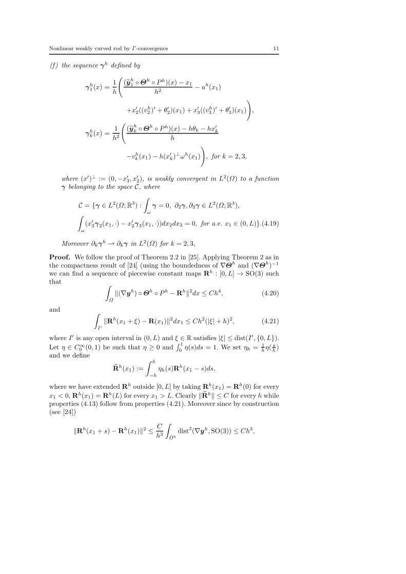
(f) the sequence γh defined by
γh1 (x) =
1
h
((yh
1 Θh P h)(x) − x1
h2− uh(x1)
+x′2((v
h2 )
′ + θ′2)(x1) + x′3((v
h3 )
′ + θ′3)(x1)
),
γhk(x) =
1
h2
((yh
k Θh P h)(x) − hθk − hx′k
h
−vhk (x1)− h(x′k)
⊥ωh(x1)
), for k = 2, 3,
where (x′)⊥ := (0,−x′3, x
′2), is weakly convergent in L2(Ω) to a function
γ belonging to the space C, where
C = γ ∈ L2(Ω;R3) :
ˆ
ω
γ = 0, ∂2γ, ∂3γ ∈ L2(Ω;R3),
ˆ
ω
(x′3γ2(x1, ·)− x′
2γ3(x1, ·))dx2dx3 = 0, for a.e. x1 ∈ (0, L).(4.19)
Moreover ∂kγh ∂kγ in L2(Ω) for k = 2, 3,
Proof. We follow the proof of Theorem 2.2 in [25]. Applying Theorem 2 as inthe compactness result of [24] (using the boundedness of ∇Θh and (∇Θh)−1
we can find a sequence of piecewise constant maps Rh : [0, L] → SO(3) suchthat
ˆ
Ω
‖(∇yh) Θh P h −Rh‖2dx ≤ Ch4, (4.20)
andˆ
I′
‖Rh(x1 + ξ)−R(x1)‖2dx1 ≤ Ch2(|ξ|+ h)2, (4.21)
where I ′ is any open interval in (0, L) and ξ ∈ R satisfies |ξ| ≤ dist(I ′, 0, L).
Let η ∈ C∞0 (0, 1) be such that η ≥ 0 and
´ 1
0 η(s)ds = 1. We set ηh = 1hη(
sh )
and we define
Rh(x1) :=
ˆ h
−h
ηh(s)Rh(x1 − s)ds,
where we have extended Rh outside [0, L] by taking Rh(x1) = Rh(0) for every
x1 < 0, Rh(x1) = Rh(L) for every x1 > L. Clearly ‖Rh‖ ≤ C for every h whileproperties (4.13) follow from properties (4.21). Moreover since by construction(see [24])
‖Rh(x1 + s)−Rh(x1)‖2 ≤
C
h3
ˆ
Ωh
dist2(∇yh, SO(3)) ≤ Ch3,

12 Igor Velcic
for every |s| ≤ h we have by Jensen’s inequality that
‖Rh −Rh‖2L∞([0,L];R3×3 ≤ Ch3 (4.22)
By the Sobolev-Poincare inequality and the second inequality in (4.13), there
exist constants Qh ∈ R3×3 such that ‖Rh −Qh‖L∞([0,L];R3×3) ≤ Ch. Combin-
ing this inequality with (4.22), we have that ‖Rh −Qh‖L∞([0,L];R3×3) ≤ Ch.
This implies that dist(Qh, SO(3)) ≤ Ch; thus, we may assume that Qh belongs
to SO(3) and by modifying Qh by order h, if needed. Now choosing Rh= Qh
and replacing Rh by (Qh)TRh and Rh by (Qh)T Rh, we obtain (4.14). Bysuitable choice of constants ch ∈ R
3 we may assume thatˆ
Ω
(yh1 Θ
hP h−x1) = 0,
ˆ
Ω
(yhk Θ
hP h−hθk) = 0, for k = 2, 3. (4.23)
Let Ah = Rh−I
h . By (4.14) there exists A ∈ L∞((0, L);R3×3) such that, up tosubsequences,
Ah A weakly * in L∞((0, L);R3×3). (4.24)
On the other hand it follows from (4.13) and (4.14) that
Rh − I
h A weakly in W 1,2((0, L);R3×3). (4.25)
In particular, A ∈ W 1,2((0, L);R3×3) and h−1(Rh − I) also converges uni-formly. Using (4.22) we deduce that
Ah → A uniformly. (4.26)
In view of (4.12) this clearly implies the convergence property in (d). SinceRh ∈ SO(3) we have
Ah + (Ah)T = −hAh(Ah)T .
Hence, A+AT = 0. Moreover, after division by 2h we obtain property (e) by(4.26). For adapting the proof to the proof of Theorem 2.2 in [25] it is essentialto see
(∇yh) Θh P h = (∇(yh Θh) P h)((∇Θh)−1 P h)
= ∇h(yh Θh P h)((∇Θh)−1 P h). (4.27)
From (4.27) it follows
((∇yh) Θh P h)((∇Θh) P h) = ∇h(y
h Θh P h). (4.28)
and
(∇yh) Θh P h − I = (∇h(y
h Θh P h −Θh P h))((∇Θh)−1 P h −RTe )
+(∇h(yh Θh P h −Θh P h))RT
e . (4.29)
Nonlinear weakly curved rod by Γ -convergence 13
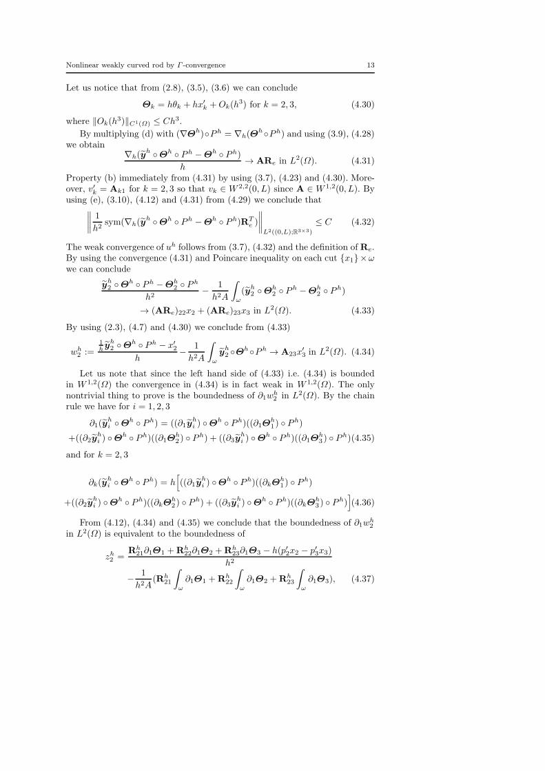
Let us notice that from (2.8), (3.5), (3.6) we can conclude
Θk = hθk + hx′k +Ok(h
3) for k = 2, 3, (4.30)
where ‖Ok(h3)‖C1(Ω) ≤ Ch3.
By multiplying (d) with (∇Θh)P h = ∇h(ΘhP h) and using (3.9), (4.28)
we obtain∇h(y
h Θh P h −Θh P h)
h→ ARe in L2(Ω). (4.31)
Property (b) immediately from (4.31) by using (3.7), (4.23) and (4.30). More-over, v′k = Ak1 for k = 2, 3 so that vk ∈ W 2,2(0, L) since A ∈ W 1,2(0, L). Byusing (e), (3.10), (4.12) and (4.31) from (4.29) we conclude that
∥∥∥∥1
h2sym(∇h(y
h Θh P h −Θh P h)RTe )
∥∥∥∥L2((0,L);R3×3)
≤ C (4.32)
The weak convergence of uh follows from (3.7), (4.32) and the definition of Re.By using the convergence (4.31) and Poincare inequality on each cut x1×ω
we can conclude
yh2 Θh P h −Θh
2 P h
h2−
1
h2A
ˆ
ω
(yh2 Θh
2 P h −Θh2 P h)
→ (ARe)22x2 + (ARe)23x3 in L2(Ω). (4.33)
By using (2.3), (4.7) and (4.30) we conclude from (4.33)
wh2 :=
1h y
h2 Θh P h − x′
2
h−
1
h2A
ˆ
ω
yh2 Θ
hP h → A23x′3 in L2(Ω). (4.34)
Let us note that since the left hand side of (4.33) i.e. (4.34) is boundedin W 1,2(Ω) the convergence in (4.34) is in fact weak in W 1,2(Ω). The onlynontrivial thing to prove is the boundedness of ∂1w
h2 in L2(Ω). By the chain
rule we have for i = 1, 2, 3
∂1(yhi Θh P h) = ((∂1y
hi ) Θ
h P h)((∂1Θh1 ) P
h)
+((∂2yhi ) Θ
h P h)((∂1Θh2 ) P
h) + ((∂3yhi ) Θ
h P h)((∂1Θh3 ) P
h)(4.35)
and for k = 2, 3
∂k(yhi Θh P h) = h
[((∂1y
hi ) Θ
h P h)((∂kΘh1 ) P
h)
+((∂2yhi ) Θ
h P h)((∂kΘh2 ) P
h) + ((∂3yhi ) Θ
h P h)((∂kΘh3 ) P
h)](4.36)
From (4.12), (4.34) and (4.35) we conclude that the boundedness of ∂1wh2
in L2(Ω) is equivalent to the boundedness of
zh2 =Rh
21∂1Θ1 +Rh22∂1Θ2 +Rh
23∂1Θ3 − h(p′2x2 − p′3x3)
h2
−1
h2A(Rh
21
ˆ
ω
∂1Θ1 +Rh22
ˆ
ω
∂1Θ2 +Rh23
ˆ
ω
∂1Θ3), (4.37)

14 Igor Velcic
in L2(Ω). By using (2.3) and (3.18) we conclude
zh2 =Rh
21(x2(nh1 )
′ + x3(bh1 )
′) +Rh22(x2(n
h2 )
′ + x3(bh2 )
′)
h
+Rh
23(x2(nh3 )
′ + x3(bh3 )
′)− (p′2x2 − p′3x3)
h. (4.38)
The boundedness of zh2 in L2(Ω) is the consequence of (3.5), (3.6) and (4.14).Now we have proved wh
2 A23x′3 weakly in W 1,2(Ω).
Analogously we conclude
wh3 :=
1h y
h3 Θh P h − x′
3
h−
1
h2A
ˆ
ω
yh3 Θh P h −A23x
′2, . (4.39)
weakly in W 1,2(Ω). Now, since wh can be written as
wh(x1) =1
Aµ(ω)
ˆ
ω
(x′2w
h3 − x′
3wh2 )dx2dx3, (4.40)
it is clear that wh converges weakly to the function w = −A23 = A32 inW 1,2(0, L). Let us define for βh : Ω′ → R
3, βh = γ x′−1. By the chain rulewe have
∂1βhi = (∂1γ
hi ) (x
′)−1 + (p′2x′2 + p′3x
′3)(∂2γ
hi ) (x
′)−1
+(−p′3x′2 + p′2x
′3)(∂3γ
hi ) (x
′)−1,
∂2βhi = p2(∂2γ
hi ) (x
′)−1 − p3(∂3γhi ) (x
′)−1,
∂3βhi = p3(∂2γ
hi ) (x
′)−1 + p2(∂3γhi ) (x
′)−1. (4.41)
By differentiating β1 with respect to x′k, with k=2,3, we have
∂2βh1 =
1
h3∂2(y
h1 Θh P h (x′)−1) +
1
h((vh2 )
′ + θ′2), (4.42)
∂3βh1 =
1
h3∂3(y
h1 Θh P h (x′)−1) +
1
h((vh3 )
′ + θ′3)). (4.43)
Let us analyze only ∂2βh1 . We have by (3.18), (4.36) and the chain rule
∂2βh1 =
((∂1yh1 ) Θ
h P h (x′)−1)(p2nh1 − p3b
h1 )
h2
+((∂2y
h1 ) Θ
h P h (x′)−1)(p2nh2 − p3b
h2 )
h2
+((∂3y
h1 ) Θ
h P h (x′)−1)(p2nh3 − p3b
h3 )
h2
+1
h((vh2 )
′ + θ′2). (4.44)

Nonlinear weakly curved rod by Γ -convergence 15
By using (3.5), (3.6), (3.18), (4.12), (4.14), (4.35) and the definition of vhk we
can conclude that for proving the boundedness of ∂2βh1 it is enough to prove
the boundedness of δh1,2 in L2(Ω) where
δh1,2 :=−hRh
11θ′2 +Rh
12
h2+
Rh21 + hθ′2h2
=1−Rh
11
hθ′2 +
Rh12 +Rh
21
h2. (4.45)
The boundedness of δh1,2 in L∞(Ω) is then the consequence of the property (e).
In the same way we can prove the boundedness of ∂3βh1 . Using the Poincare
inequality and the fact that´
ω′(x1)βh1dx2, dx
′3 = 0, we deduce that there exists
a constant C > 0 such thatˆ
ω′(x1)
(βh1 (x))
2dx2dx3 ≤ C
ˆ
ω′(x1)
[(∂2βh1 (x))
2 + (∂3βh1 (x))
2]dx2dx3
for a.e. x1 ∈ (0, L) and for every h. Although the constant C depends on thedomain, since all domains are translations and rotations of the domain ω, theconstant C can be chosen uniformly. Integrating both sides with respect to x1,we obtain that the sequence (βh
1 ) is bounded in L2(Ω′) so, up to subsequencesβh1 β1 and ∂kβ
h1 ∂kβ1 weakly in L2(Ω′), for k = 2, 3. From the relations
(4.41) it can be concluded that γh1 γ1 and ∂kγ
h1 ∂kγ1 weakly in L2(Ω),
for k = 2, 3, where γ = β x′. For the sequences (βh2 ), (β
h3 ), we have by
differentiation that for j, k = 2, 3
∂jβhk =
1
h2
(1
h∂j(y
hk Θ
h P h (x′)−1)−hδjk −hwh(1− δjk)(−1)k
). (4.46)
By using the chain rule we see that for k = 2, 3,
∂2(yhk Θh P h (x′)−1) = h
(((∂1y
hk) Θ
h P h (x′)−1)(p2nh1 − p3b
h1 )
+ ((∂2yhk) Θ
h P h (x′)−1)(p2nh2 − p3b
h2 )
+ ((∂3yhk) Θ
h P h (x′)−1)(p2nh3 − p3b
h3 )),
∂3(yhk Θh P h (x′)−1) = h
(((∂1y
hk) Θ
h P h (x′)−1)(p3nh1 + p2b
h1 )
+ ((∂2yhk) Θ
h P h (x′)−1)(p3nh2 + p2b
h2 )
+ ((∂3yhk) Θ
h P h (x′)−1)(p3nh3 + p2b
h3 )).
Now we want to check that for j, k = 2, 3
ejk(βh) :=
1
2(∂jβ
hk + ∂kβ
hj ). (4.47)
is bounded in L2(Ω′). In the similar way as for β1 (relations (4.44) and (4.45))we can using (3.5), (3.6), (4.12), (4.14) and the property (e) conclude that for

16 Igor Velcic
every j, k = 2, 3, ejk(βh) ∈ L2(Ω′). By using Korn’s inequality (Lemma 1) we
have that there exists C > 0 such that
‖βh2‖
2W 1,2(ω′(x1))
+ ‖βh3‖
2W 1,2(ω′(x1))
≤ C(|
ˆ
ω′(x1)
βh2dx
′2dx
′3|
+|
ˆ
ω′(x1)
βh3dx
′2dx
′3|+ |
ˆ
ω′(x1)
(x′3β
h2 − x′
2βh3 )dx
′2dx
′3|
+∑
j,k=1,2
‖ejk(βh)‖L2(ω′(x1))
), (4.48)
for a.e. x1 ∈ (0, L). From the definition of vhk and wh we see that the functions
(βh2 (x1, ·), β
h3 (x1, ·)) belong to the space
Bx1= β = (β2,β3) ∈ W 1,2(ω′(x1);R
2) :
ˆ
ω′(x1)
βdx′2dx
′3 = 0,
ˆ
ω′(x1)
(x′2β3 − x′
3β2)dx′2dx
′3 = 0 (4.49)
for every x1. By integrating (4.48) with respect to x1 we conclude that βh2 ,β
h3
are bounded in L2(Ω′) as well as their derivatives with respect to x2, x3. Fromthis we can conclude the same fact about γh
2 , γh3 . The fact that the weak limit
belongs to the space C can be concluded from the fact that for every h anda.e. x1 (βh
2 (x1, ·),βh3 (x1, ·)) ∈ Bx1
. This finishes the proof of (f).
4.1 Lower bound
Lemma 2 Let yh, yh, Eh, Rh, uh, vh, wh, γh, βh = γh (x′)−1, γ, β =γ (x′)−1, A be as in Theorem 3 and let us suppose that the condition (4.11)is satisfied and that γh γ, ∂2γ
h ∂2γ, ∂3γh ∂3γ weakly in L2(Ω) i.e.
βh β, ∂2βh ∂2β, ∂3β
h ∂3β weakly in L2(Ω′). Let us define
ηh1 (x) =
1
h
((yh
1 Θh P h)(x) −Θh1 P h
h2− uh(x1)
+x′2(v
h2 )
′(x1) + x′3(v
h3 )
′(x1)
), (4.50)
ηhk(x) =
1
h2
((yh
k Θh P h)(x) −Θhk P h
h
−vhk (x1)− h(x′k)
⊥ωh(x1)
), for k = 2, 3, (4.51)
and κh = ηh (x′)−1. Then we have that ηh η weakly in L2(Ω) and∂kη
h ∂kη weakly in L2(Ω) i.e. κh κ, ∂2κh ∂2κ, ∂3κ
h ∂3κ weakly
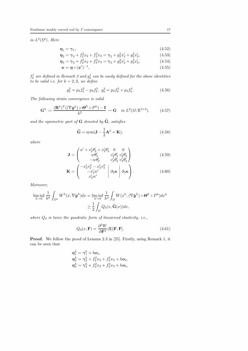
Nonlinear weakly curved rod by Γ -convergence 17
in L2(Ω′). Here
η1 = γ1, (4.52)
η2 = γ2 + f22x2 + f3
2x3 = γ2 + g22x′2 + g32x
′3, (4.53)
η3 = γ3 + f23x2 + f3
3x3 = γ3 + g23x′2 + g33x
′3, (4.54)
κ = η (x′)−1, (4.55)
fjk are defined in Remark 2 and g
jk can be easily defined for the above identities
to be valid i.e. for k = 2, 3, we define
g2k = p2f2k − p3f
3k , g3k = p3f
2k + p2f
3k . (4.56)
The following strain convergence is valid
Gh :=(Rh)T ((∇yh) Θh P h)− I
h2 G in L2(Ω;R3×3). (4.57)
and the symmetric part of G denoted by G, satisfies
G = sym(J−1
2A2 +K), (4.58)
where
J =
u′ + v′2θ′2 + v′3θ
′3 0 0
wθ′3 v′2θ′2 v′2θ
′3
−wθ′2 v′3θ′2 v′3θ
′3
(4.59)
K =
−x′
2v′′2 − x′
3v′′3
−x′3w
′
x′2w
′
∣∣∣∣∣ ∂2κ∣∣∣∣∣ ∂3κ
. (4.60)
Moreover,
lim infh→0
1
h6
ˆ
Ωh
Wh(x,∇yh)dx = lim inf
h→0
1
h4
ˆ
Ω
W (xh, (∇yh) Θh P h)dxh
≥1
2
ˆ
Ω
Q3(x, G(x))dx,
where Q3 is twice the quadratic form of linearized elasticity, i.e.,
Q3(x,F) =∂2W
∂F2(I)[F,F]. (4.61)
Proof. We follow the proof of Lemma 2.3 in [25]. Firstly, using Remark 1, itcan be seen that
ηh1 = γh
1 + ho1,
ηh2 = γh
2 + f22x2 + f3
2x3 + ho2,
ηh3 = γh
3 + f23x2 + f3
3x3 + ho3,
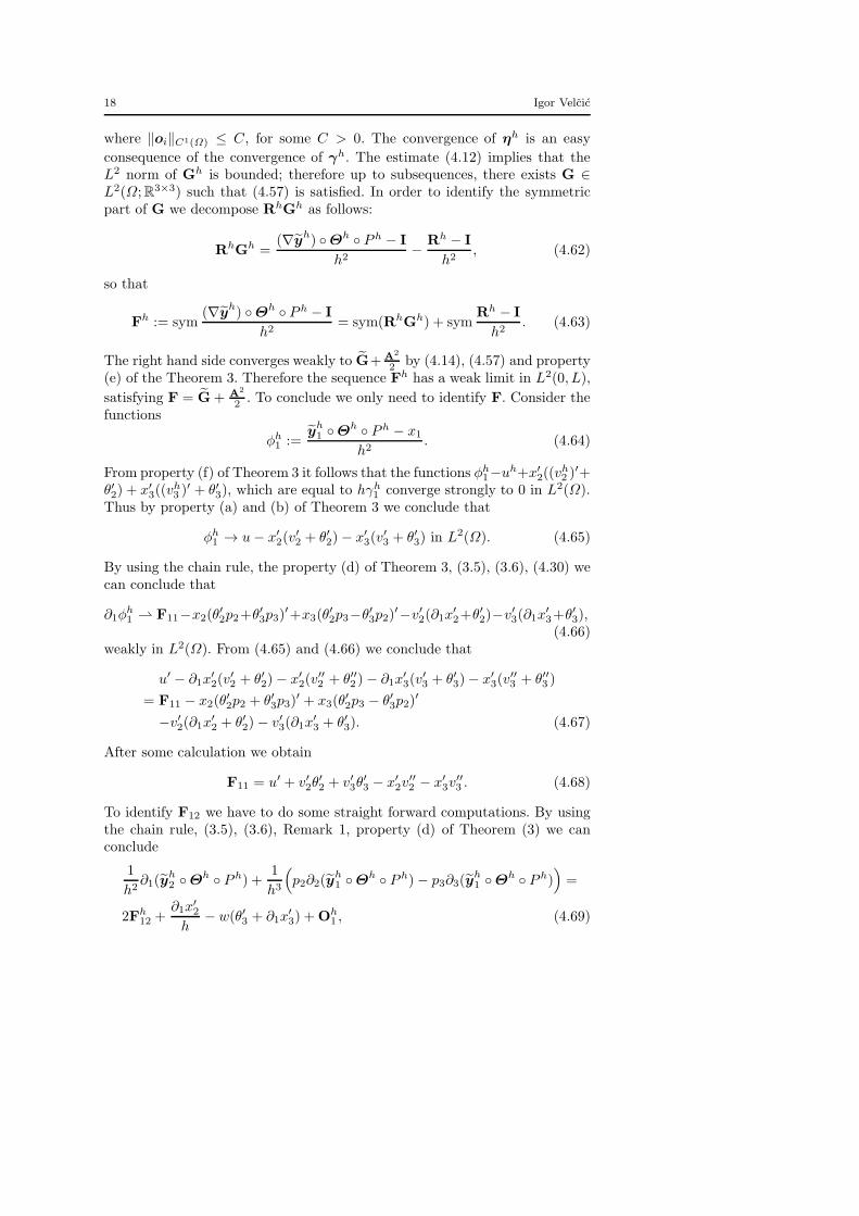
18 Igor Velcic
where ‖oi‖C1(Ω) ≤ C, for some C > 0. The convergence of ηh is an easy
consequence of the convergence of γh. The estimate (4.12) implies that theL2 norm of Gh is bounded; therefore up to subsequences, there exists G ∈L2(Ω;R3×3) such that (4.57) is satisfied. In order to identify the symmetricpart of G we decompose RhGh as follows:
RhGh =(∇y
h) Θh P h − I
h2−
Rh − I
h2, (4.62)
so that
Fh := sym(∇y
h) Θh P h − I
h2= sym(RhGh) + sym
Rh − I
h2. (4.63)
The right hand side converges weakly to G+A2
2 by (4.14), (4.57) and property(e) of the Theorem 3. Therefore the sequence Fh has a weak limit in L2(0, L),
satisfying F = G+ A2
2 . To conclude we only need to identify F. Consider thefunctions
φh1 :=
yh1 Θh P h − x1
h2. (4.64)
From property (f) of Theorem 3 it follows that the functions φh1−uh+x′
2((vh2 )
′+θ′2) + x′
3((vh3 )
′ + θ′3), which are equal to hγh1 converge strongly to 0 in L2(Ω).
Thus by property (a) and (b) of Theorem 3 we conclude that
φh1 → u− x′
2(v′2 + θ′2)− x′
3(v′3 + θ′3) in L2(Ω). (4.65)
By using the chain rule, the property (d) of Theorem 3, (3.5), (3.6), (4.30) wecan conclude that
∂1φh1 F11−x2(θ
′2p2+θ′3p3)
′+x3(θ′2p3−θ′3p2)
′−v′2(∂1x′2+θ′2)−v′3(∂1x
′3+θ′3),(4.66)
weakly in L2(Ω). From (4.65) and (4.66) we conclude that
u′ − ∂1x′2(v
′2 + θ′2)− x′
2(v′′2 + θ′′2 )− ∂1x
′3(v
′3 + θ′3)− x′
3(v′′3 + θ′′3 )
= F11 − x2(θ′2p2 + θ′3p3)
′ + x3(θ′2p3 − θ′3p2)
′
−v′2(∂1x′2 + θ′2)− v′3(∂1x
′3 + θ′3). (4.67)
After some calculation we obtain
F11 = u′ + v′2θ′2 + v′3θ
′3 − x′
2v′′2 − x′
3v′′3 . (4.68)
To identify F12 we have to do some straight forward computations. By usingthe chain rule, (3.5), (3.6), Remark 1, property (d) of Theorem (3) we canconclude
1
h2∂1(y
h2 Θh P h) +
1
h3
(p2∂2(y
h1 Θh P h)− p3∂3(y
h1 Θh P h)
)=
2Fh12 +
∂1x′2
h− w(θ′3 + ∂1x
′3) +Oh
1 , (4.69)

Nonlinear weakly curved rod by Γ -convergence 19
where limh→0 ‖Oh1‖L2(Ω;R3×3) = 0. On the other hand it can be easily seen
that
∂2βh1 = p2∂2γ
h1 − p3∂3γ
h1
=1
h3
(p2∂2(y
h1 Θh P h)− p3∂3(y
h1 Θh P h)
)
+1
h((vh2 )
′ + θ′2). (4.70)
From (4.34), (4.69), (4.70) we conclude
2Fh12 =
1
h2∂1(y
h2 Θh P h − hx′
2)−1
h((vh2 )
′ + θ′2)
+∂2βh1 + wθ′3 + w∂1x
′3 −Oh
1
= ∂1wh2 + ∂2β
h1 + wθ′3 + w∂1x
′3 −Oh
1 . (4.71)
By using (4.34) we conclude that the right hand side of (4.71) converges inW−1,2(Ω) to
∂1(−wx′3) + ∂2β1 + wθ′3 + w∂1x
′3 = −x′
3w′ + wθ′3 + ∂2κ1, (4.72)
since β1 = κ1. On the other hand we know that the left hand side of (4.71)converges strongly in L2(Ω) to 2F12 and thus we can conclude
F12 =1
2(−x′
3w′ + wθ′3 + ∂2κ1). (4.73)
In the same way one can prove
F13 =1
2(x′
2w′ − wθ′2 + ∂3κ1). (4.74)
To identify F22 let us observe that by the chain rule, (3.5), (3.6) and theproperty (d) of Theorem (3) we have
1
h3
(p2∂2(y
h2 Θh P h −Θ2 P
h)− p3∂3(yh2 Θh P h −Θ2 P
h))=
Fh22 − v′2θ
′2 +Oh
2 , (4.75)
where limh→0 ‖Oh2‖L2(Ω;R3×3) = 0. On the other hand we can conclude
∂2κh2 = p2∂2η
h2 − p3∂3η
h3
=1
h3
(p2∂2(y
h2 Θh P h −Θ2 P
h)− p3∂3(yh2 Θh P h −Θ2 P
h)).
(4.76)
In the same way as before we conclude that
F22 = v′2θ′2 + ∂2κ2. (4.77)
20 Igor Velcic
Analogously we can conclude
F33 = v′3θ′3 + ∂3κ3. (4.78)
To identify F23 = F32 we, by using the chain rule, (3.5), (3.6) and the property(d) of Theorem (3), can conclude:
1
h3
(p2∂2(y
h3 Θh P h −Θ2 P
h)− p3∂2(yh3 Θh P h −Θ2 P
h))=
1
h2(∂2y
h3 ) Θ
h P h − v′2θ′3 +Oh
3 , (4.79)
where limh→0 ‖Oh3‖L2(Ω;R3×3) = 0. In the same way we conclude
1
h3
(p3∂2(y
h2 Θh P h −Θ2 P
h) + p2∂3(yh2 Θh P h −Θ2 P
h))=
1
h2(∂2y
h3 ) Θ
h P h − v′3θ′2 +Oh
4 , (4.80)
where limh→0 ‖Oh4‖L2(Ω;R3×3) = 0. It can be also concluded
p2∂2ηh3 − p3∂3η
h3 =
1
h3
(p2∂2(y
h3 Θh P h −Θ2 P
h)
−p3∂2(yh3 Θh P h −Θ2 P
h))+
1
h2wh, (4.81)
p3∂2ηh2 + p2∂3η
h2 =
1
h3
(p3∂2(y
h2 Θh P h −Θ2 P
h)
+p2∂2(yh3 Θh P h −Θ2 P
h))−
1
h2wh. (4.82)
By summing the relations (4.79)-(4.82) and letting h → 0 it can be concludedthat
2F23 = v′2θ′3 + v′3θ
′2 + ∂2κ3 + ∂3κ2. (4.83)
To prove the lower bound we can continue in the same way as in the proofof Lemma 2.3 in [25], by using the Taylor expansion, the cutting and Scorza-Dragoni theorem.
4.2 Upper bound
Theorem 4 (optimality of lower bound) Let u,w ∈ W 1,2(0, L) and vk ∈W 2,2(0, L) for k = 2, 3. Let γ be a function in C where
C = γ ∈ L2(Ω;R3) :
ˆ
ω
γ = 0, ∂2γ, ∂3γ ∈ L2(Ω;R3),
ˆ
ω
(x′3γ2(x1, ·)− x′
2γ3(x1, ·))dx2dx3 = 0, ∀x1 ∈ (0, L). (4.84)
Set
G = sym(J−1
2A2 +K). (4.85)
Nonlinear weakly curved rod by Γ -convergence 21
Here A, J, K are defined by the expressions (4.18), (4.59) and (4.60) and η,κ are defined by the expressions (4.52)-(4.55).
Then there exists a sequence (yh) ⊂ W 1,2(Ωh,R3) such that for uh, vhk , w
defined by the expressions (4.15)-(4.17) the properties (a)-(d) of Theorem 3are valid. Also we have that the property (f) of Theorem 3 is valid (whichis equivalent that for ηh defined by the expressions (4.50)-(4.51) it is validηh η weakly in L2(Ω) and ∂kη
h ∂kη weakly in L2(Ω)). Also the followingconvergence is valid
limh→0
1
h6
ˆ
Ωh
Wh(xh,∇yh)dxh =
1
2
ˆ
Ω
Q3(x,G(x))dx (4.86)
Proof. Let us first assume that u,w, vk,η are smooth. Then we define for(x1, x
h2 , x
h3 ) ∈ Ωh:
yh(Θh(x1, x
h2 , x
h3 )) = Θh(x1, x
h2 , x
h3 ) +
h2u(x1)hv2(x1)hv3(x1)
+h2
−x2(v′2p2 + v′3p3)(x1)− x3(v
′3p2 − v′2p3)(x1)
−x2(p3w)(x1)− x3(p2w)(x1)x2(p2w)(x1)− x3(p3w)(x1)
+h3η(x1,xh2
h,xh3
h), (4.87)
where η : Ω → R3 is going to be chosen later. The convergence (a)-(d) and
that ηh η weakly in L2(Ω) and ∂kηh ∂kη weakly in L2(Ω) can easily
seen to be valid for this sequence. We also have
∇yh∇Θh = ∇Θh +
h2u′ −h(v′2p2 + v′3p3) −h(v′3p2 − v′2p3)hv′2 −hp3w −hp2w
hv′3 hp2w −hp3w
+h2
−x2(v′2p2 + v′3p3)
′ + x3(v′2p3 − v′3p2)
′
−x2(p3w)′ − x3(p2w)
′
x2(p2w)′ − x3(p3w)
′
∣∣∣∣∣ ∂2η∣∣∣∣∣ ∂3η
+O(h3). (4.88)
From (4.88), by using (3.8), we conclude
∇yh = I+ h
0 −v′2 −v′3v′2 0 −w
v′3 w 0
+h2
u′ + v′2θ
′2 + v′3θ
′3 0 0
wθ′3 v′2θ′2 v′2θ
′3
−wθ′2 v′3θ′2 v′3θ
′3
+h2
−x2(v′′2 p2 + v′′3 p3) + x3(v
′′2 p3 − v′′3p2)
−x2(p3w′)− x3(p2w
′)x2(p2w
′)− x3(p3w′)
∣∣∣∣∣ ∂2κ∣∣∣∣∣ ∂3κ
+O(h3). (4.89)
22 Igor Velcic
Using the identity (I+M)T (I+M) = I+ 2 symM +MTM we obtain
(∇yh)T (∇yh) = I+ 2h2 symJ+ 2h2 symK+ h2ATA+O(h3),
where ‖O(h3)‖L∞(Ω;R3×3) ≤ Ch3, for some C > 0.Taking the square root we obtain
[(∇yh)T (∇yh)]1/2 = I+ h2G+O(h3). (4.90)
We have det(∇yh) > 0 for sufficiently small h. Hence by frame-indifferenceW (x, (∇yh) Θh P h) = W (x, [∇yh)T (∇yh)]1/2 Θh P h); thus by (4.90)and Taylor expansion we obtain:
1
h4W (x, (∇yh) Θh P h) →
1
2Q3(x, G(x)) a.e
and by the property ii) of W for h small enough
1
h4W (x, (∇yh) Θh P h) ≤
1
2C(‖J‖2 + ‖K‖2 + ‖A‖4) + Ch.
The equality (4.86) follows by the dominated convergence theorem. Namely,we have
1
h6
ˆ
Ωh
Wh(x,∇yh)dx =1
h4
ˆ
Ω
W (x, (∇yh) Θh P h)dx
→1
2
ˆ
Ω
Q3(x, G)dx.
In the general case, it is enough to smoothly approximate u,w in the strongtopology of W 1,2, vk in the strong topology of W 2,2, and η, ∂kη in the strongtopology of L2 and to use the continuity of the right hand side of (4.86) withrespect to these convergences.
Remark 6 Notice that
K =
A′
0x′2
x′3
| ∂2κ | ∂3κ
= L+
A′
0x′2
x′3
| ∂2β | ∂3β
.
Here β = γ (x′)−1 and
L =
0 0 00 g22 g320 g23 g33
. (4.91)
From the fact that γ ∈ C we can conclude β ∈ B, where
B = β ∈ L2(Ω′;R3) :
ˆ
ω
β = 0, ∂2β, ∂3β ∈ L2(Ω′;R3),
ˆ
ω′(x1)
(x′3β2(x1, ·)− x′
2β3(x1, ·)dx′2dx
′3 = 0, for a.e. x1 ∈ (0, L).(4.92)

Nonlinear weakly curved rod by Γ -convergence 23
4.3 Identification of the Γ -limit
Let Q : (0, L)× R× so(3) → [0,+∞) be defined as
Q(x1, t,F) =
minα∈W 1,2(ω′(x1);R3)
ˆ
ω′(x1)
Q3
x,
F
0x′2
x′3
+ te1
∣∣∣∣∣∂2α∣∣∣∣∣∂3α
dx′2dx
′3,
(4.93)
where Q3 is the quadratic form defined in (4.61). For u,w ∈ W 1,2(0, L) andv2, v3 ∈ W 2,2(0, L) we introduce the functional
I0(u, v2, v3, w) :=1
2
ˆ L
0
Q(x1, u′ + v′2θ
′2 + v′3θ
′3 +
1
2((v′2)
2 + (v′3)2), ∂1A)dx1,
(4.94)where A ∈ W 1,2((0, L); so(3)) is defined by (4.18). We shall state the resultof Γ -convergence of the functionals 1
h4 Ih to I0. Before stating the theorem we
analyze some properties of the limit density Q.
Remark 7 By using the remarks in the beginning of chapter 4 in [25] thefollowing facts can be concluded:
a) The functional Q3(x,G) is coercive on symmetric matrices i.e. there existsa constant C > 0, independent of x, such that Q3(x,G) ≥ C‖ symG‖2,for every G (this is the direct consequence of the assumption iv) on W ).The minimum in (4.93) is attained. Since the functional Q3(x,G) dependsonly on the symmetric part of G, it is invariant under transformation α 7→α+c1+c2(x
′)⊥ and hence the minimum can be computed on the subspace
Vx1:=
α ∈ W 1,2(ω′(x1),R
3) :
ˆ
ω′(x1)
α = 0,
ˆ
ω′(x1)
(x′3α2 − x′
2α3)dx′2dx
′3 = 0
.
Strict convexity of Q3(x, ·) on symmetric matrices ensures that the mini-mizer is unique in V .
b) Fix x1 ∈ (0, L), t ∈ R andF ∈ so(3). Letαmin ∈ V be the unique minimizerof the problem (4.93). We set
g(x′2, x
′3) = F
0x′2
x′3
+ te1, bhkij =
∂2W
∂Fih∂Fjk(x, I),
and we call Bhk the matrix in R3×3 whose elements are given by (Bhk)ij =
bhkij . Then αmin satisfies the following Euler-Lagrange equation:ˆ
ω′(x1)
∑
h,k=2,3
(Bhk∂kαmin, ∂hϕ)dx
′2dx
′3 = −
ˆ
ω′(x1)
∑
h=2,3
(Bh1g, ∂hϕ)dx′2dx
′3,
(4.95)

24 Igor Velcic
for every ϕ ∈ W 1,2(ω′(x1);R3×3). From this equation it is clear that αmin
depends linearly on (t,F). Moreover Q is uniformly positive definite, i.e.
Q(x1, t,F) ≥ C(t2 + ‖F‖2), ∀t ∈ R, ∀F ∈ so(3), (4.96)
and the constant C does not depend on x1.c) By mimicking the proof of Remark 4.3 in [25] it can be seen that there
exists a constant C′ (independent of x1, t and F) such that
‖∂2αmin‖L2(ω′(x1);R3×3) + ‖∂3α
min‖L2(ω′(x1);R3×3) ≤ C′‖g‖2L2(ω′(x1);R3×3),
(4.97)for a.e. x1 ∈ (0, L). To adapt the proof we only need to have that theconstant in the Korn’s inequalityˆ
ω′(x1)
∑
j,k=2,3
|∂kαminj |2dx′
2dx′3 ≤ C1
ˆ
ω′(x1)
∑
j,k=2,3
|ejk(αmin)|2dx′
2dx′3
(4.98)can be chosen independently of x1. This is proved in Lemma 1.
d) When Q3 does not depend on x2, x3 we can find a more explicit repre-sentation for Q. More precisely Q can be decomposed into the sum of twoquadratic forms
Q(x1, t,F) = Q1(x1, t) +Q2(x1,F),
where
Q1(x1, t) := mina,b∈R3
Q3(x1, (te1|a|b)), (4.99)
Q2(x1, 0,F) := Q(x1, 0,F). (4.100)
The relations (4.8) are only needed for this. If we assume the isotropic andhomogenous case i.e.
Q3(F) = 2µ∣∣∣F+ FT
2
∣∣∣2
+ λ(traceF)2,
then after some calculation (see Remark 3.5 in [24]) it can be shown that
Q1(t) =µ(3λ+ 2µ)
λ+ µt2
Q2(x1,F) =µ(3λ+ 2µ)
λ+ µ
(F12
ˆ
ω′(x1)
(x′2)
2dx′2dx
′3
+2F12F13
ˆ
ω′(x1)
x′2x
′3dx
′2dx
′3 + F13
ˆ
ω′(x1)
(x′3)
2dx′2dx
′3
)
+µτF23,
where the constant τ is so-called torsional rigidity, defined as
τ(ω′(x1)) = τ(ω) =
ˆ
ω
(x22 + x2
3 − x2∂3ϕ+ x3∂2ϕ)dx2dx3,

Nonlinear weakly curved rod by Γ -convergence 25
and ϕ is the torsion function i.e. the solution of the Neumann problem∇ϕ = 0 in ω
∂νϕ = −(x3,−x2) · ν on ∂ω
The following theorem can be proved in the same way as Theorem 4.5 in [23](we need Theorem 3, Lemma 2, Theorem 4, Remark 6 and Remark 7).
Theorem 5 As h → 0, the functionals 1h4 I
h are Γ -convergent to the func-tional I0 given in (4.94), in the following sense:
i) (compactness and liminf inequality) if lim suph→0 h−4Ih < +∞ then
there exists constants Rh∈ SO(3), ch ∈ R
3 such that (up to subsequences)
Rh→ R and the functions defined by
yh := (R
h)Tyh − ch, uh =
1
A
ˆ
ω
yh1 Θh P h − x1
h2dx2dx3
vhk =1
A
ˆ
ω
yhk Θh P h − hθk
hdx2dx3
wh =1
Aµ(ω)
ˆ
ω
x′2(y3 Θ
h P h)− x′3(y2 Θ
h P h)
h2dx2dx3
satisfy(a) (∇y
h) Θh P h → I in L2(Ω).(b) there exist u,w ∈ W 1,2(0, L) such that uh u and wh w weakly in
W 1,2(0, L).(c) there exists vk ∈ W 2,2(0, L) such that vhk → vk strongly in W 1,2(0, L)
for k = 2, 3.Moreover we have
lim infh→0
1
h4Ih(yh) ≥ I0(u, v2, v3, w). (4.101)
ii) (limsup inequality) for every v, w ∈ W 1,2(0, L), v2, v3 ∈ W 2,2(0, L) there
exists (yh) such that (a)-(c) hold (with yh replaced by yh) and
limh→0
1
h4Ih(yh) = I0(u, v2, v3, w) (4.102)
Remark 8 Let f2, f3 ∈ L2(0, L). We introduce the functional
J0 = I0(u, v2, v3, w)−
ˆ L
0
∑
k=2,3
fkvk, (4.103)
for every u ∈ W 1,2(0, L), v2, v3 ∈ W 2,2(0, L), and w ∈ W 1,2(0, L). The func-tional J0 can be obtained as Γ -limit of the energies 1
h4 Ih by adding a term
describing transversal body forces of order h3 (see [13], see also [32]). For lon-gitudinal body forces see [18]. The problem for longitudinal body forces arisesbecause the longitudinal forces should be of order h2, the same order as for
26 Igor Velcic
the model in [24]. One needs to impose certain stability condition to see whichmodel describes the behavior of the body for the longitudinal forces of orderh2.
Remark 9 The term u′ + v′2θ′2 + v′3θ
′3 +
12 ((v
′2)
2 +(v′3)2) in the strain measures
the extension of the central line (which is of the second order). Namely, if weapproximate the deformation of the weakly curved rod by:
ϕ1(x1, x2, x3) = x1 + h2u+ h2x′2(v
′2 + θ′2) + h2x′
3(v′3 + θ′3) (4.104)
ϕk(x1, x2, x3) = hθk + hx′k + hvk + h2(x′
k)⊥w, for k = 2, 3, (4.105)
we see, that it is valid
‖∂1ϕ(x1, 0, 0)‖2 − ‖∂1Θ
h(x1, 0, 0)‖2 = h2
(2u′ + 2v′2θ
′2 + 2v′3θ
′3
+(v′2)2 + (v′3)
2).
Remark 10 The existence of the solution for the functional J0 under theDirichlet boundary condition for vk at both ends of the rod can be proveddirectly. It is also enough that we impose v2, v
′2, v3, v
′3 at the one end. The
existence can also be proved for the free boundary condition under the hy-
pothesis that´ L
0 fkdx1 = 0,´ L
0 x1fkdx1 = 0 for k = 2, 3. It can be done inthe same way as the proof of Lemma 5 in [32].
References
1. Acerbi, E., Butazzo, G., Percivale, D.: A variational definition of the strain energy foran elastic string, Journal of Elasticity, 25, 137–148 (1991)
2. Adams, R.A.: Sobolev spaces, Academic press, New York 1975.3. Alvarez-Dios, J.A. , Viano, J.M.: A bending and stretching asymptotic theory for
general elastic shallow arches, ESAIM: Proc., Vol. 2, 145–152 (1997)4. Alvarez-Dios, J.A. , Viano, J.M.: Mathematical Justication of a One-dimensional Model
for General Elastic Shallow Arches, Mathematical Methods in the Applied Sciences,Volume 21, Issue 4, 281–325 (1998)
5. S.S. Antman, Nonlinear problems of elasticity. Second edition, Applied MathematicalSciences, 107, Springer, New York, 2005.
6. A. Braides: Γ -convergence for Beginners, Oxford University Press, Oxford, 2002.7. Ciarlet, P.G.: Mathematical elasticity. Vol. I, Three-dimensional elasticity, North-
Holland Publishing Co., Amsterdam, 1988.8. Ciarlet, P.G.: Mathematical elasticity. Vol. II. Theory of plates. Studies in Mathematics
and its Applications, 27. North-Holland Publishing Co., Amsterdam (1997).9. Ciarlet, P.G.: Mathematical elasticity. Vol. III. Theory of shells. Studies in Mathemat-
ics and its Applications, 29. North-Holland Publishing Co., Amsterdam (2000).10. Dal Maso, G.: An introduction to Γ -convergence, Progress in Nonlinear Differential
Equations and Their Applications, Birkauser, Basel (1993).11. Fox, D.D., Raoult A., Simo, J.C.: A justification of nonlinear properly invariant plate
theories, Arch. Rational Mech. Anal., 124, p. 157199 (1993).12. Friesecke, G., James R.D., Muler, S.: A theorem on geometric rigidity and the deriva-
tion of nonlinear plate theory from three-dimensional elasticity, Comm. Pure Appl.Math. 55, 1461–1506 (2002).
Nonlinear weakly curved rod by Γ -convergence 27
13. Friesecke, G., James R.D., Muler, S.: A Hierarchy of Plate Models Derived from Non-linear Elasticity by Γ -Convergence, Archive for Rational Mechanics and Analysis 180,no.2, 183–236 (2006).
14. Friesecke, G., James R.D., Muler, S.: The Foppl-von Karman plate theory as a lowenergy Γ -limit of nonlinear elasticity, Comptes Rendus Mathematique 335, no. 2, 201–206 (2002).
15. Friesecke, G., James R., Mora, M.G., Muller, S.: Derivation of nonlinear bending theoryfor shells from three-dimensional nonlinear elasticity by Γ -convergence, C. R. Math.Acad. Sci. Paris, 336, no. 8, 697–702 (2003).
16. Le Dret, H., Raoult, A.: The nonlinear membrane model as a variational limit ofnonlinear three-dimensional elasticity, Journal de Mathematiques Pures et Appliquees74, 549–578 (1995).
17. Le Dret, H., Raoult, A.: The membrane shell model in nonlinear elasticity: A variationalasymptotic derivation, Journal of Nonlinear Science 6, Number 1, 59–84 (1996).
18. Lecumberry, M., Muller, S.: Stability of slender bodies under compression and validityof the von Karman theory, Archive for Rational Mechanics and Analysis, Volume 193,Number 2, 255–310 (2009).
19. Lewicka, M., Mora, M.G., Pakzad, M.: Shell theories arising as low energy Γ -limit of3d nonlinear elasticity , Ann. Scuola Norm. Sup. Pisa Cl. Sci. 5, Vol. IX, 1–43 (2010).
20. Lewicka, M., Mora, M.G., Pakzad, M.: The matching property of infinitesimal isome-tries on elliptic surfaces and elasticity of thin shells, accepted in Arch. Rational Mech.Anal.
21. Lewicka, M., Pakzad, M.: The infinite hierarchy of elastic shell models: some recentresults and a conjecture , accepted in Fields Institute Communications (2010).
22. Marigo, J.J., Meunier, N.: Hierarchy of One-Dimensional Models in Nonlinear Elastic-ity, Journal of Elasticity, 83, 1–28 (2006)
23. Mora, M.G., Scardia, L.: Convergence of equilibria of thin elastic plates under physicalgrowth conditions for the energy density, submitted paper.
24. Mora, M.G., Muller, S.: Derivation of the nonlinear bending-torsion theory for inex-tensible rods by Gamma-convergence, Calc. Var., 18, 287–305 (2003)
25. Mora, M.G., Muller, S.: A nonlinear model for inextensible rods as a low energyGamma-limit of three-dimensional nonlinear elasticity, Ann. Inst. H. Poincar Anal.Nonlin., 21, 271–293 (2004)
26. Mora, M.G., Muller, S., Schultz, M.G.: Convergence of equilibria of planar thin elasticbeams, Indiana Univ. Math. J., 56, 2413-2438 (2007)
27. Mora, M.G., Muller, S.: Convergence of equilibria of three-dimensional thin elasticbeams, Proc. Roy. Soc. Edinburgh Sect. A 138, 873–896 (2008)
28. Muller, S., Packzad, M.R.: Convergence of equilibria of thin elastic plates : the vonKarman case, Communications in Partial Differential Equations 33, Number 6, 1018–1032 (2008).
29. Oleinik, O.A., Shamaev, A.S., Yosifian, G.A.: Mathematical problems in elasticity andhomogenization, North-Holland, 1992.
30. Scardia, L.: The nonlinear bending-torsion theory for curved rods as Gamma-limit ofthree-dimensional elasticity, Asymptot. Anal., 47, 317–343 (2006)
31. Scardia, L.: Asymptotic models for curved rods derived from nonlinear elasticity byΓ -convergence, submitted paper.
32. Velcic, I.: Shallow shell models by Γ -convergence, submitted paper. Preprinthttp://web.math.hr/∼ivelcic
33. Ziemer, W.: Weakly Differentiable Functions, Springer-Verlag: New York (1989).