Theoretical Computer Science 412 (2011) 4297–4311

Contents lists available at ScienceDirect

Theoretical Computer Science

journal homepage: www.elsevier.com/locate/tcs

Fault containment in weakly stabilizing systemsAnurag Dasgupta, Sukumar Ghosh ∗, Xin XiaoDepartment of Computer Science, The University of Iowa, United States

a r t i c l e i n f o

Keywords:Fault containmentWeak stabilizationPersistent bitLeader electionFault gap

a b s t r a c t

Research on fine tuning stabilization properties has received attention for more thana decade. This paper presents probabilistic algorithms for fault containment. Wedemonstrate two exercises in fault containment in a weakly stabilizing system, whichexpedite recovery from single failures, and confine the effect of any single fault to theconstant-distance neighborhood of the faulty process. The most significant aspect of thealgorithms is that the fault gap, defined as the smallest interval after which the system isready tohandle thenext single faultwith the sameefficiency, is independent of thenetworksize. We argue that a small fault gap increases the availability of the fault-free system.

© 2011 Elsevier B.V. All rights reserved.

1. Introduction

A distributed system is weakly stabilizing [14,6], when its legitimate configuration is reachable from any startingconfiguration, and the legitimate configuration is closed under the given system actions. Arbitrary configurations maybe caused by transient failures that can corrupt the system state. Due to the weakening of the stabilization property,it is not possible to bound the stabilization time under a deterministic scheduler, and randomized scheduling becomesnecessary to guarantee eventual recovery. Furthermore, in well-designed systems, and with improved reliability of thesystem components, the possibility of a massive failure is quite low, and single failures are much more likely to occur.To increase the efficiency of fault tolerance, it is important to guarantee a fast recovery from all single failures, while alsoguaranteeing eventual recovery from more major failures. This motivated the current work. The problem of containing theeffect of minor failures is becoming important not only due to the improved reliability of system components, but also dueto the dramatic growth of network sizes. Such limited transient faults are likely to give rise to states that are almost legal,rather than states that are arbitrary. Hence, it is desirable that the system should recover quickly from such limited transientfaults. Moreover, to ensure that non-faulty processes largely remain unaffected by such minor level failures, only a smallpart of the network around the faulty components should be allowed to make observable state changes.

The tight containment of the effect of single failures depends on the context: containment in time implies that allobservable variables of the system recover to their legal values in O(1) time, whereas containment in space means thatthe processes at O(1) distance from the faulty process make observable changes. For optimal performance, both of theseproperties should hold.

An important issue in system design is the mean time between failures, commonly termed the MTBF. Once a fault-containing system recovers from a single failure in constant time, how much time will elapse before the system becomesready to recover from the next single failurewith the same efficiency is an importantmetric, and it is called the fault gap [17].If the next failure hits the system sooner than this period, then the guarantee ofO(1) time recovery falls apart. Thus, the faultgap determines the availability of the fault-free system, and a low fault gap reflects better availability. The dramatic growthof network size increases the probability of failures, andmost solutions to fault containment that we know of achieve a fault

∗ Corresponding author. Tel.: +1 319 335 0738.E-mail addresses: adasgupt@cs.uiowa.edu (A. Dasgupta), ghosh@cs.uiowa.edu (S. Ghosh), xinxiao@cs.uiowa.edu (X. Xiao).

0304-3975/$ – see front matter© 2011 Elsevier B.V. All rights reserved.doi:10.1016/j.tcs.2011.02.039

4298 A. Dasgupta et al. / Theoretical Computer Science 412 (2011) 4297–4311

gap of O(n) or worse. As a result, when two single faults occur relatively quickly, the system fails to provide the guaranteeof efficient recovery, and in fact the second single failure may sometimes require O(n) (or higher) time for recovery. Thisseriously undermines the availability of the fault-free system. So a scale-free fault gap is an important design goal.

1.1. Contributions

We show how fault containment can be added to weakly stabilizing distributed systems. We present solutions using arandomized scheduler, and illustrate techniques to bias the random schedules so that the system recovers from all singlefaults in a time independent of the size n = |V | of the system, and the effect of the failure is contained within O(1) distancefrom the faulty node with high probability (this probability can be controlled by a user-defined tuning parameter). Usingthis technique, we solve two problems: one is the persistent-bit problem on an arbitrary connected topology, and the otheris a leader election problem on a line topology. Our solutions exhibit a low fault gap, and guarantee high system availability;once the output variables of the system recover to a legal configuration, the system is immediately ready to handle the nextsingle fault with the same degree of efficiency [4,5]. Our solutions guarantee that the fault gap depends only on the degree ofthe nodes, and is independent of the size of the network. This significantly increases the availability of the fault-free system.

For the persistent-bit problem, our solution contains a single fault in O(∆3) expected number of steps, where ∆ is thehighest degree of a node in the network. For the leader election problem on a line topology, our algorithm confines the effectof any single fault to the constant-distance neighborhood of the faulty process. We show that the contamination number(maximum number of processes that change the primary part of their local states during recovery from any single-faultconfiguration) is at most 4 with high probability. Also, the expected recovery time from a single fault is independent of thenetwork size.

1.2. Related work

Kutten and Peleg [7] introduced a protocol for fault mending that corrects a system from minor failures, but providesno guarantee for stabilization. Subsequently, for specific problems, fault containment has been added to self-stabilization.In [16], Ghosh and Gupta solved the leader election problem on an oriented ring, and presented a simple self-stabilizingleader election protocol that recovers in O(1) time from a 1-fault configuration. Only the faulty node and its two neighborschange their states during convergence to a stable state. In [18], Ghosh et al. presented a fault-containing self-stabilizingprotocol for constructing a spanning tree of an arbitrary network. In [13], the same authors demonstrated a fault-containingself-stabilizing protocol for BFS – Breadth First Search tree construction in an arbitrary network. Ghosh et al. [17,8] andGupta [19] demonstrated a general technique of adding fault containment to self-stabilization, and analyzed the cost of it.Dolev and Herman introduced superstabilizing protocols [12] that, in addition to being stabilizing, guarantee that, duringconvergence from configurations arising from legal states by small-scale topology changes, certain passage predicates aresatisfied. Herman’s self-stabilizing protocol [15] for mutual exclusion investigates the possibility of superstabilizing proto-cols for mutual exclusion in a ring of processors, where a local fault consists of any transient fault at a single processor, andthe passage predicate for mutual exclusion specifies that there be at most one token in the ring, with the single exceptionof a spurious token co-located with the transient fault. Kutten and Patt-Shamir [3] proposed an asynchronous stabilizingalgorithm for the persistent-bit problem. Their solution leads to recovery in O(k) time from any k-faulty configuration. Asimilar protocol for the problem of token passing was addressed by Beauquier et al. [9], where up to k faults hit nodes bycorrupting their state undetectably. Beauquier et al. also investigated k-strong self-stabilizing systems [10], which satisfythe properties of strong confinement and of k-linear time adaptivity. Strong confinement means that a non-faulty processorhas the same behavior with or without the presence of faults elsewhere in the system. k-linear time adaptivity means thatafter k or fewer faults hitting the system in a correct state, recovery takes a number of rounds linear in k. Other approachesfor fault containment can be found in [1,2].

1.3. Organization of the paper

This paper has five sections. Section 2 describes the models and notation. Section 3 presents the algorithms and theresults for the persistent-bit protocol. Section 4 describes the algorithms and the results for the leader election problem.Finally, Section 5 contains some concluding remarks.

2. Models and notation

Let G = (V , E) denote the topology of a distributed system, where V denotes the set of nodes {0, 1, . . . , n − 1}representing processes, and E ⊆ (V × V ) represents the set of edges. Each edge (i, j) ∈ E represents a bidirectional linkbetween processes i and j. We use the notation N(i) to represent the neighbors of i: thus (i, j) ∈ E ⇔ j ∈ N(i). Processescommunicate with their immediate neighbors (also called the distance-1 neighbors) using the shared memory model. Theexecution of the protocols is organized in steps. In each step, a process i executes one ormore guarded actions g → A, whereg is a predicate involving the variables of i and N(i), and A is an action that updates one or more variables of i. The global

A. Dasgupta et al. / Theoretical Computer Science 412 (2011) 4297–4311 4299

state or configuration S of the system is a tuple consisting of the local states of all the processes. Unless otherwise stated,a central scheduler (also called a central demon) serializes all guarded actions. We assume a randomized scheduler, wherethe central demon randomly chooses an action with an enabled guard with uniform probability. The scheduler is weakly fair.A computation of the system is a finite or infinite sequence of global states that satisfies two properties: (a) if S and S ′ aretwo consecutive states in the sequence, then there exists a process i such that i has an enabled guard in S and execution ofthe corresponding action results in the state S ′, and (b) if the sequence is finite, then, in the last state of the sequence, noprocess has an enabled guard.

Definition 1 (Weak Stabilization). Weak stabilization [14] guarantees that, starting from an arbitrary configuration, thereexists at least one computation that leads the system to a legal configuration.

A stabilizing system converges to a legal configuration LC that is traditionally defined in terms of the observable orprimary variables. However, in most cases, fault containment requires the use of auxiliary or secondary variables too. Wedefine the local state of each process i as an ordered pair ⟨pi, si⟩, where pi denotes the primary variables, and si denotesthe secondary variables. Correspondingly, we write the global state as an ordered pair ⟨p, s⟩, where p is the collection of allprimary variables and s is the collection of all secondary variables. For any global state ⟨p, s⟩, ⟨p, s⟩ ∈ LC ⇒ p ∈ LCp ands ∈ LCs. The following are some important definitions relevant to the fault-containment problem [18].

Definition 2 (Stabilization Time). The stabilization time is themaximum time needed to establish LC from an arbitrary initialconfiguration.

Though LC ⇒ p ∈ LCp and s ∈ LCs, in most cases, it is adequate to establish LCp only, since the application is not affectedby the secondary variables.

Definition 3 (Fault Containment in Time). Fault containment in timemeans that, starting from any single-fault configuration,LCp is restored in O(1) time.

This definition may appear strict in some cases. So we define the notion of weak fault containment.

Definition 4 (Weak Fault Containment). A system is said to beweakly fault containing if the containment time of the systemis independent of n, i.e., the size of the network.

Note that, for weak fault containment, LCp does not necessarily have to be restored in O(1) time.

Definition 5 (Fault Containment in Space). Fault containment in spacemeans that, starting from a single-fault configuration,the primary variables of the processes at O(1) distance from the faulty process make observable changes.

One can also define aweaker version of fault containment in space, where the distance up towhich the primary variablesare affected is independent of n.

Ideally, attemptsmust bemade to restrict the effect of the fault within the immediate neighborhood of the original faultynode, which is the notion of tight containment. This way, the rest of the system can still perform its normal operation. Thefault should not contaminate a large portion of the network.

Definition 6 (Contamination Number). The contamination number is the maximum number of processes that change theprimary part of their local states during recovery from any single-fault configuration.

Ideally, the contamination number should be as small as possible.

Definition 7 (Fault gap). Starting from any single-fault configuration, the fault gap is the maximum time required to reacha state in LC .

The fault gap determines the availability of the fault-free system, and a low fault gap reflects better availability. If thenext failure hits the system sooner than the time duration of the fault gap, then the guarantee of constant time recoverydoes not hold anymore.

In a probabilistic setting, the definitions of stabilization time and contamination numberwill beweakened to reflect theirexpected values only.

3. Persistent-bit protocol

For the sake of exposition, we consider the case of persistent-bit protocol, in which a set of processes maintains the valueof a replicated bit v ∈ {0, 1} across a connected network. There are two distinct legal configurations: all 0s and all 1s. Theprotocol in Algorithm 1 is weakly stabilizing.

Algorithm 1 Persistent-bit protocol: Program for process iA1. do ∃j ∈ N(i) : v(j) = v(i)→ v(i) := v(j) od

4300 A. Dasgupta et al. / Theoretical Computer Science 412 (2011) 4297–4311

Lemma 1. The persistent-bit protocol is not fault containing with a randomized demon.Proof. Consider a linear array of processes numbered 0, 1, . . . , n−1 from left to right, and assume that initially∀i : v(i) = 1holds. Let a failure of process 0 change v(0) to 0. With this as the starting state, the computation can be reduced to a run ofgambler’s ruin1: whenever a process with v = 0 executes an action, the boundary between the dissimilar values of v shiftsto the left, and whenever a process with v = 1 executes an action, the boundary moves to the right. The game is over whenthe system reaches LC , and per [11] the expected number of moves needed is (1× n− 1), i.e., O(n). Thus, the protocol is notfault containing. �

In view of Lemma 1, we present a fault-containing version of the persistent-bit protocol.

3.1. Fault-containing persistent-bit protocol

To make the protocol fault containing, we add to each process i a secondary variable x(i) ∈ Z∗ (the set of non-negativeintegers). In a way, x(i) will reflect the priority of process i in executing an action to update v(i). Process i will update v(i),when the following three conditions hold.1. The randomized scheduler chooses i,2. ∃j ∈ N(i) : v(j) = v(i), and3. ∀j ∈ N(i) : x(i) ≥ x(j).

After updating v(i), process i will increase x(i) to max{x(j) : j ∈ N(i)} + m, where m is a constant positive integer.When only the first two conditions hold, but not the third, then process iwill increment the value of x(i) by 1, and leave v(i)unchanged. Algorithm 2 shows the modified protocol.

Algorithm 2 Probabilistic fault-containing algorithm: Program for process iA1. ∃j ∈ N(i) : v(j) = v(i) ∧ ∀k ∈ N(i) : x(i) ≥ x(k)→ v(i) := v(j); x(i) := max{x(k) : k ∈ N(i)} +mA2. ∃j ∈ N(i) : v(j) = v(i) ∧ ∃ k ∈ N(i) : x(i) < x(k)→ x(i) := x(i)+ 1A3. ∀j ∈ N(i) : v(j) = v(i)→ v(i) := v(j)

Observe that once a process i updates v(i), it becomes difficult for its neighbors to change their v-values, since their x-values will lag behind that of i. The larger is the value ofm, the greater is the difficulty. A neighbor j of iwill be able to updatev(j) only if it is chosen by the random schedulerm times, without choosing i even once. On the other hand, it becomes easierfor i to update v(i) again in the near future.

Failures can not only corrupt v, but also corrupt x. Assume that LC ≡ ∀j : v(j) = 1, and that a single failure at processi changes v(i) to 0 and x(i) to some unknown value. If ∀j ∈ N(i) : x(i) > x(j), then process i is likely to change its v(i)soon again, before its neighbors get a chance to do so. As a result, the fault is contained in a small number of steps, and thecontamination number is 1. However, a smart adversary injecting the failure at process i is likely to set x(i) to the smallestvalue (i.e., 0). Thismakes the neighbors of process i better candidates for changing their v, before process i executes amove tocomplete the recovery. However, it also raises the x-values of these neighbors of i above those of their neighbors. In order thatthe fault percolates to a node at distance 2 from the faulty process i, such a distance-2 node has to be chosen by the schedulerat least m times, without choosing its neighboring distance-1 node even once. With a large value of m, the probability ofsuch an event is very low. This explains the mechanism of containment. In the meantime, the condition ∀j ∈ N(i) : v(j) = 1is likely to hold several times. If on one such occasion the faulty process is chosen by the random scheduler (action A3; notethat its guard does not depend on x), then v(i) will change to 1, and the recovery will be complete.

3.2. Results

Webeginwith an analysis of the spatial containment. Assume that all nodes have a degree∆. Then the following theoremholds.Theorem 1. As m→∞, the effect of a single failure is restricted to only the immediate neighbors of the faulty process.Proof. Suppose that the faulty process has n1 distance-1 neighbors and n2 distance-2 neighbors. The probability that adistance-2 neighbor is contaminated is largest, when only one distance-1 process is contaminated, and only one neighbor ofthat contaminated distance-1 process (which is a distance-2 neighbor of the faulty process) is contaminated. The probabilityof one distance-1 neighbor being contaminated is n1

n1+1. To contaminate a distance-2 neighbor, the scheduler must select

the specific process m times. So the probability of one distance-2 neighbor being contaminated is 1(n1+n2+1)m

. Therefore,after a node becomes faulty, the probability that some distance-2 neighbor of the faulty process becomes contaminated isn1

n1+1× n2 ×

1(n1+n2+1)m

. By choosing a large value ofm, this probability can be made as small as possible. �

1 The original study is by Coolidge [11] in 1909, where he showed that if two gamblers start with capitals of x and N − x, and each fair coin toss transfersa dollar from one to the other depending on the outcome of the toss, then the expected number of steps to finish the game is x · (N − x).

A. Dasgupta et al. / Theoretical Computer Science 412 (2011) 4297–4311 4301

Theorem 2. If ∆ << m, then the expected number of steps needed to contain a single fault is O(∆3).

Proof. Sincem is very large, per Theorem 1, the effect of the fault is unlikely to propagate to the distance-2 neighbors of thefaulty process. It is therefore sufficient to consider the case when the fault propagates to the immediate neighbors of faultyprocess.

Since there are at most ∆ neighbors of the faulty process, the system can have at most ∆ + 1 faults. Let pi,j denote theprobability that the number of the faults changes from i to j due to the action taken by some process. Below, we list suchprobabilities for various possible values of i and j:

p1,0 =1

∆+ 1(1)

p2,1 =12∆

(2)

p2,2 =∆

2∆(3)

p1,2 =1

∆+ 1(4)

and for 3 ≤ i ≤ ∆− 1

pi,i+1 =i

(∆+ 1)+ i(∆− 1)(5)

pi+1,i+1 =1+ i(∆− 1)

(∆+ 1)+ i(∆− 1)(6)

pi+1,i+2 =∆− 1

(∆+ 1)+ i(∆− 1)(7)

and

p∆+1,∆ =∆− 1

(∆+ 1)+∆(∆− 1)(8)

p∆+1,∆+1 =1+∆(∆− 1)

(∆+ 1)+∆(∆− 1). (9)

We use P[X] to denote the probability that the system recovers using X moves. The expected number of moves needed is

E = 1× P[1] + 2× P[2] + 3× P[3] + · · ·

=

∞−x=1

XP[X].

Starting from a 1-fault configuration, during a recovery phase, the number of faulty processes may initially grow, but musteventually shrink. Accordingly, we first calculate P[X] using (1), (2), and (4), as follows:

P[1] = p1,0 =1

∆+ 1(10)

P[2] = 0 (11)

P[3] = p1,2p2,1p1,0 =1

∆+ 112∆

1∆+ 1

=1

2∆(∆+ 1)2(12)

P[4] = p1,2p2,2p2,1p1,0 =1

∆+ 1∆

2∆12∆

1∆+ 1

, (13)

and, for n ≥ 1, we get the following recursive function of P[2n+ 2] using P[2n+ 1]:

P[2n+ 2] = 2m−j=2

pj,jP[2n+ 1]. (14)

(Note: m and n used here are variable parameters only, and should not be confused with the scheduler bias or the size ofthe system.) If n + 1 < ∆ + 1, then m = n. If n + 1 > ∆ + 1, then m = ∆ + 1. This is because, if n + 1 < ∆ + 1, using2n+ 2 steps, the system can reach at most the n+ 1-th state. So the repeated moves can occur in any state within the n-thstate. But if n+ 1 > ∆+ 1, the system can move through all the states, so the repeated moves can occur anywhere withinthe ∆+ 1 states.

4302 A. Dasgupta et al. / Theoretical Computer Science 412 (2011) 4297–4311

We can also write P[2n+ 3] using P[2n+ 1] as

P[2n+ 3] = 2m−j=2

m−i=2

pj,jpi,iP[2n+ 1] + 2m′−k=2

pi,i+1pi+1,iP[2n+ 1]. (15)

The values of m and m′ are the same as in (14). The system can have either two additional moves that do not change thecurrent state, or the system can first reach a state in one step and come back in the next step. We now substitute forP[1], P[2], P[3], andP[4] using (10)–(15) in (10), and let pmax = max{pi,j,∀i,∀j}:

E = 1× P[1] + 2× P[2] + 3× P[3] + 4× P[4]

+

∞−n=2

{(2n+ 1)P[2n+ 1] + (2n+ 2)P[2n+ 2] + (2n+ 3)P[2n+ 3]}

= 1×1

∆+ 1+ 2× 0+ 3×

12∆(∆+ 1)2

+ 4×1

4∆(∆+ 1)2

+

∞−n=2

(2n+ 1)+ 2(2n+ 2)

m−j=2

m−i=2

pi,ipj,j + (2n+ 3)

2

m′−i=2

pi,i+1pi+1,i + 2m′′−j=2

m′′−i=2

pi,ipj,j

× P[2n+ 1]

< O

1∆2

+

∞−n=2

{(2n+ 1)p2n+1max + 2(2n+ 2)∆2p2n+2max + (2n+ 3)(2∆+ 2∆2)p2n+3max }

=

∞−n=2

(2n+ 1)p2n+1max + 2∆2∞−n=2

(2n+ 2)p2n+2max + (2∆+ 2∆2)

∞−n=2

(2n+ 3)p2n+3max + O

1∆2

.

Let T1 =∑∞

n=2(2n + 1)p2n+1max , T2 = 2∆2∑∞n=2(2n + 2)p2n+2max , T3 = (2∆ + 2∆2)

∑∞

n=2(2n + 3)p2n+3max . As the order of T3is the same as that of T2 and larger than that of T1, we just need to calculate T3.

T3 = (2∆+ 2∆2)

∞−n=2

(2n+ 3)p2n+3max

= (2∆+ 2∆2)

2p3max

∞−n=2

np2nmax + 3pmax

∞−n=2

p2nmax

= (2∆+ 2∆2)

[2p3max

2p4max

1− p2max+ p6max

+ 3p3max

11− p2max

]= (2∆+ 2∆2)

4p7max + 2p3maxp6max(1− p2max)+ 3p3max

1− p2max.

Let pmax =a

∆+a , a = 1+∆(∆− 1):

T3 = (2∆+ 2∆2)4a7(∆+ a)2 + 2a9 + 3a3(∆+ a)6

(∆2 + 2∆a)(∆+ a7)

= O(∆2)×O(a9)

O(∆3)O(a7)

=O(a2)O(∆)

= O(∆3).

So we get

E = O

1∆2

+ O(∆3) = O(∆3). � (16)

When the graph is dense, i.e., ∆ = O(n), the containment time is not independent of the size of the network anymore.However, the spatial containment property still holds. Themore dense the graph is, the smaller is the contamination number.As m → ∞, contamination number tends to 1. Below, we separately analyze the extreme case of a dense topology: acompletely connected graph.

Theorem 3. For a completely connected graph, the contamination number approaches 1 as m→∞.

A. Dasgupta et al. / Theoretical Computer Science 412 (2011) 4297–4311 4303

Proof. Let i be the faulty process. At least one neighbor j of the faulty process i is likely to update v(j), and raise x(j) at leastmsteps above the x-values of the rest. The contamination number can increase beyond 1 only if a second neighbor k updatesv(k) (instead of the system recovering to its legal configuration). This requires the scheduler to choose the neighbor k atleast m times, without choosing i or j even once.

Let P{n0, n1, n2, . . . , ni, ni+1, . . . , n∆−1} denote the probability that, ∀i, 1 ≤ i ≤ ∆, node i is chosen ni times. So theprobability of node k being chosenm times before j being chosen even once is

P{n0, n1, n2, . . . , nj−1, nj = 0, nj+1, . . . , nk = m, . . . , n∆−1} ∀i, 0 ≤ i ≤ ∆− 1 ∧ i = j, ni ≤ m. (17)

With increasing ni, 1 ≤ i ≤ ∆∧ i = j, (17) is decreasing (see Lemma 2 for the proof). So the above probability is maximumwhen node k is consecutively chosenm times, and other nodes are never chosen. The maximum probability is

P{0, 0, . . . , 0,m, 0, . . . , 0, 0} =1

∆m. (18)

Since ni, 0 ≤ i ≤ ∆− 1∧ i = j can be any value between 0 andm, and there are in totalm∆−2 possible situations, we applythe maximum estimate to each such case. As a result, the probability of the system having two contaminated processes isno larger than m∆−2

∆m , which approaches 0 asm approaches∞. �

Lemma 2. For a completely connected graph, where i is a faulty node, the probability that node k is chosen m times before nodej is chosen once is maximum when node k is consecutively chosen m times and other nodes are never chosen.

Proof. The probability that node k is chosenm times before node j is chosen once is

P{nk = m, nj = 0} =∆−

i=1∧i=j∧i=k

m−ni=0

P{n1, n2, . . . , nj = 0, . . . , nk = m, . . . , n∆}

=

∑∆

i=1 nin1

∑∆

i=2 nin2

. . .

∑∆

i=j ni0

. . .

∑∆

i=k nim

. . .

∑∆

i=∆ nin∆

1∆

∑∆i=1 ni

= l×

1∆

q

,

where l =∑∆

i=1 nin1

· · ·

∑∆

i=∆ nin∆

, q =

∑∆

i=1 ni. If we increase any ni, 1 ≤ i ≤ ∆ ∧ i = j ∧ i = k to ni + 1, we can see

this selection process as follows: first do the selection in the same way as before we increase ni, then choose any one of theeligible processes. There are in all ∆− 1 processes that can be chosen for the last step, and the probability of choosing anyone of them is 1

∆, so the probability will be l× (∆− 1)×

1∆

q+1, and this is smaller than l×

1∆

q. So the probability that

node k is chosenm times before choosing node j chosen once will decrease as ni increases. �

The above mechanism reveals that a high clustering coefficient limits the probability of contamination to only a smallfraction of the distance-1 neighbors. The completely connected graph exhibits an extreme form of this property.

3.3. Computing the availability

An interesting aspect of the proposed algorithm is that LCs = true; thus there is no overhead for stabilizing the secondaryvariables. So LC holds as soon as LCp holds. This leads to the following theorem.

Theorem 4. For single failures, the fault gap equals the containment time.

As a consequence of this, within an expected time of O(∆3) after each single failure, the system is ready to withstand thenext single failure with the same efficiency. Furthermore, since only the distance-1 neighbors are contaminated with highprobability, the proposed algorithm enables the system to recover from all concurrent failures of nodes that are distance3 or more apart with the same efficiency. This significantly increases the availability of the system compared to existingsolutions that we know of.

A drawback of the proposed solution is that the values of the x-variables grow in an unbounded manner, and this affectsthe implementability of the protocol. One way of overcoming this problem is transforming the solution into one that relieson bounded variables only [4].

Theorem 5. Algorithm 2 is weakly stabilizing.

3.4. Experimental results

We ran simulation experiments on random graph topologies G(n, p) with n = 1000 nodes and edge probability p set to0.5 for various values of m ranging from 2 to 32. The initial values of x were randomly chosen. The fraction of cases where

4304 A. Dasgupta et al. / Theoretical Computer Science 412 (2011) 4297–4311

number of moves required for convergence

frac

tion

of c

onve

rged

inst

ance

s

m=2m=4m=8m=16m=32

number of moves required for convergence

frac

tion

of c

onve

rged

inst

ance

s

p=0.02p=0.8p=0.5p=0.3

0 2 4 6 8 10 12degree0

1000

2000

3000

4000

5000containment time

0 2000 4000 6000 8000 100000

0.1

0.2

0.3

0.4

0.5

0.6

0.7

0.8

0.9

1

0 1000 2000 3000 4000 5000 6000 7000 8000 9000 100000

0.1

0.2

0.3

0.4

0.5

0.6

0.7

0.8

0.9

1

m = 15

m = 7

m = 5

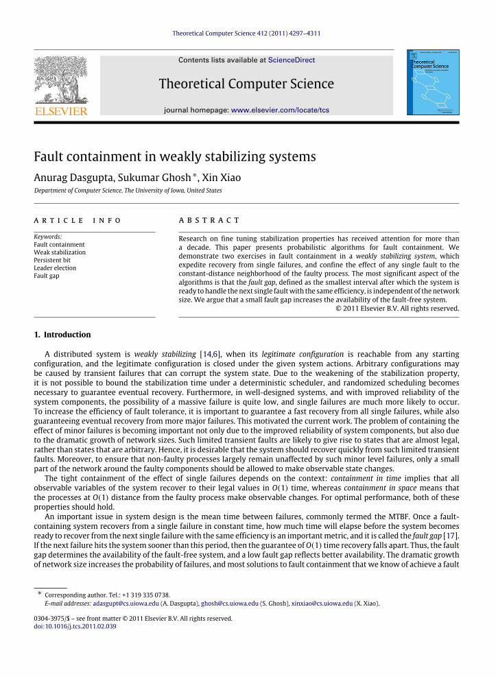
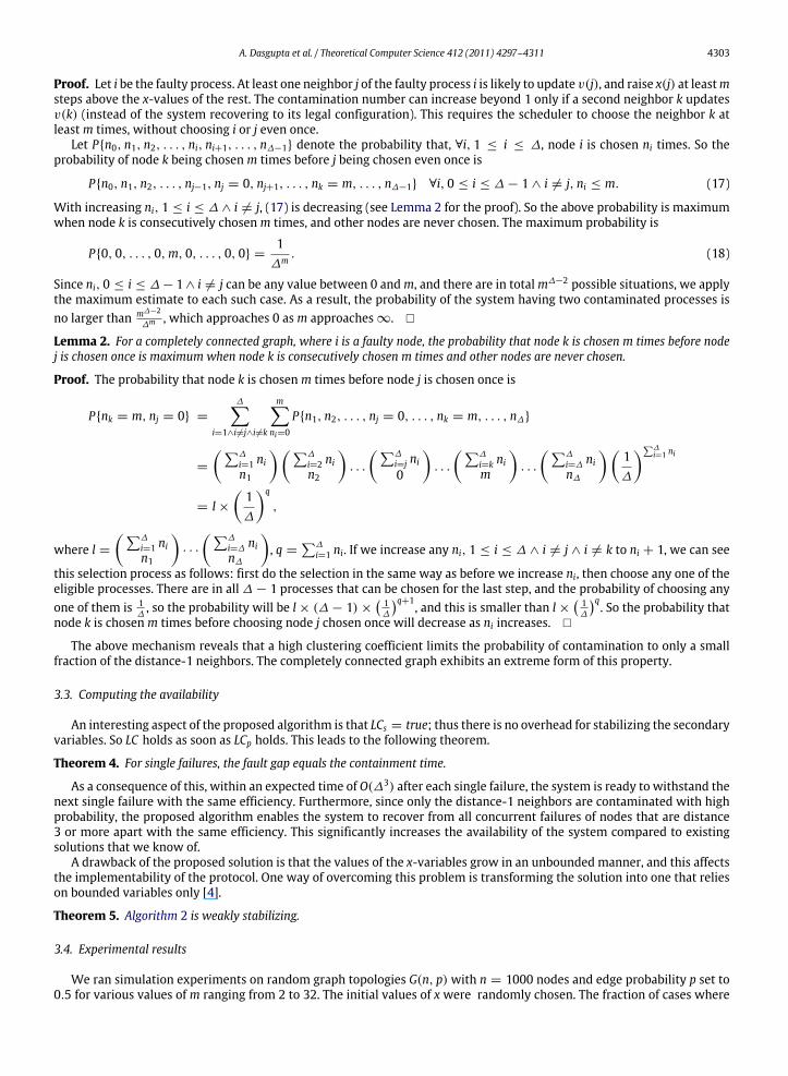
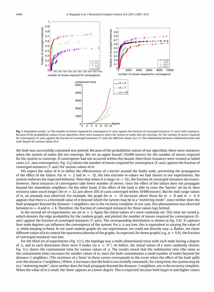
Fig. 1. Simulation results. (a) The number of moves required for convergence (X-axis) against the fraction of converged instances (Y -axis) with varyingm.Because of the probabilistic nature of our algorithm, there were instances when the system of nodes did not converge. (b) The number of moves requiredfor convergence (X-axis) against the fraction of converged instances (Y -axis) for different values of p. (c) The relationship between stabilization time andnode degree for various values ofm.

the fault was successfully contained was plotted. Because of the probabilistic nature of our algorithm, there were instanceswhen the system of nodes did not converge. We set an upper bound (10,000 moves) for the number of moves requiredfor the system to converge. If convergence had not occurred within this bound, then those instances were treated as failedcases (i.e., non-convergence). Fig. 1(a) shows the number of moves required for convergence (X-axis) against the fraction ofconverged instances (Y -axis) for various values ofm.

We expect the value of m to define the effectiveness of a barrier around the faulty node, preventing the propagationof the effect of the failure. For m = 2 and m = 32, the two extreme m-values we had chosen in our experiments, thesystem endorses the expected behavior. Note that whenm is large (m = 32), the fraction of converged instances decreases;however, these instances of convergence take fewer number of moves, since the effect of the failure does not propagatebeyond the immediate neighbors. On the other hand, if the effect of the fault is able to cross the ‘barrier’ set by m, thenrecovery takes much longer (form = 32, just above 20% of cases converged within 10000moves). But for mid-range valuesof m, an anomaly was observed. For example, the graph for m = 16 increases above those for m = 8 and m = 4. Itappears that there is a threshold value ofm beyond which the systemmay be in a ‘‘stuttering mode’’, since neither does thefault propagate beyond the distance-1 neighbors, nor is the recovery complete. In our case, this phenomenon was observedbetweenm = 4 andm = 8. Therefore, the fraction of converged instances for those values lags behind.

In the second set of experiments, we set m = 2. Again the initial values of x were randomly set. This time we varied p,which denotes the edge probability for the random graph, and plotted the number of moves required for convergence (X-axis) against the fraction of converged instances (Y -axis). The corresponding distribution is shown in Fig. 1(b). It captureshow node degrees can influence the convergence of the system. For a ∆-ary tree, this is equivalent to varying the value of∆, while keeping m fixed. As we used random graphs for our experiments, we could not directly vary ∆. Rather, we chosedifferent values of p to control the sparseness/density of the graphs. As expected, for dense graphs (e.g., p = 0.8), the fractionof converged instances was low.

For the third set of experiments (Fig. 1(c)), the topology was a multi-dimensional torus with each node having a degreeof ∆, and in each dimension there were 9 nodes (so n = 9∆). As before, the initial values of x were randomly chosen.Fig. 1(c) shows the containment time for various values of ∆. The results reveal that the stabilization time (the same asthe containment time) increases for smaller values of m, since the fault contaminates a small number of nodes beyond thedistance-1 neighbors. (The existence of a ‘knee’ in these curves corresponds to the event when the effect of the fault spillsover the distance-1 neighbors.)When∆ increases (but the fault is successfully contained), for a long time, the systemmay bein a ‘‘stutteringmode’’, since neither does the fault propagate beyond the distance-1 neighbors, nor is the recovery complete.When the value ofm is small, the ‘knee’ appears at a lower degree. This is expected, because both largerm and higher values

A. Dasgupta et al. / Theoretical Computer Science 412 (2011) 4297–4311 4305

of ∆ adversely affect fault propagation as well as convergence. An additional experiment conducted on a (30 × 30) gridrevealed that, when m = 5, the fault is successfully contained within a neighborhood of size 3 in 96% of the cases, but form = 10 this number exceeds 99%.

4. Algorithm for leader election

We now extend our technique to design a probabilistic solution to fault containment for a different problem, that ofleader election. Let A = (V , E) denote an array of a distributed system, where V = {0, 1, . . . , n − 1} represents the set ofprocesses, and each edge (i, j) ∈ E represents a link between processes i and j. Each process i has a parent variable P(i),where P(i) ∈ N(i) ∪ ⊥, and a secondary variable x(i) ∈ Z+. The purpose of the secondary variable is to contain the fault.∀j ∈ N(i) : P(j) = i ∧ P(i) = ⊥ implies that i is the leader. In a legal configuration, there can only be a single leader inthe system. Processes communicate with their immediate neighbors (also called the distance-1 neighbors) using the sharedmemory model.

Our starting point is the weakly stabilizing leader election algorithm on a tree network presented by Devismes et al. [6].An array is a special case of a tree where each node except the end nodes has a degree of 2. Therefore we disregard thenotation ∆ from [6], and just consider the two neighbors (or the neighbor if it is an end node) of a particular process. Theoriginal algorithm has three rules. In Algorithm 3, we reproduce the algorithm of Devismes et al. adapted to a line topology.

Algorithm 3Weakly stabilizing leader election algorithm of Devismes et al.: Program for process i• Variable: P(i) ∈ N(i) ∪ {⊥}.• Macro: C(i) = {q ∈ N(i)|P(q) = i}• Predicates: Leader(i) ≡ (P(i) = ⊥) ∧ (∀j ∈ N(i) : P(j) = i)• Actions:

R1. (P(i) = ⊥) ∧ (|C(i)| = |N(i)|) −→ P(i)←⊥R2. (P(i) = ⊥) ∧ (∃k ∈ N(i) \ {C(i) ∪ P(i)}) −→ P(i)← kR3. (P(i) = ⊥) ∧ (|C(i)| < |N(i)|) −→ P(i)← (N(i) \ C(i))

We directly use R1 and R3 from [6] in our new algorithm (R1 and R2 in Algorithm 3), but, for the fault-containment part,we need to add new rules, consistent with the basic approach used in the persistent-bit protocol and also described in [4].Therefore, R2 of [6] is extended to multiple rules in Algorithm 4 (R3, R4, and R5). To make the protocol fault containing, weadd to each process i a secondary variable x(i) ∈ Z+. In a way, x(i) will reflect the priority of process i in executing an actionto update P(i). Our fault-containing algorithm is shown in Algorithm 4. Process iwill update P(i) and increase its x(i)-valuewith respect to its neighbors when the following conditions hold.1. The randomized scheduler chooses i,2. {(∃j ∈ N(i) : P(i) = j)},3. {(∃k ∈ N(i) : P(k) = l = i)},4. {x(i) ≥ x(k)}.

After updating P(i), process iwill increase its x(i)-value accordingly: {x(i)← maxq∈N(i) x(q)+m},m ∈ Z+. For simplicityof exposition, we use unboundedm.

If the first three conditions hold, but not the fourth one, process i increases its xi-value by 1, and leaves P(i) unchanged.Process i also increases its x(i)-value by 1, and leaves P(i) unchanged when the following conditions hold.1. The randomized scheduler chooses i,2. {(∃j ∈ N(i) : P(i) = j)},3. {(∃k ∈ N(i) : P(k) = ⊥)},4. {x(i) < x(k)}.

Observe that, once a process i updates x(i), it becomes difficult for its neighbors to change their P-values, since theirx-values will lag behind that of i. The larger the value of m is, the greater is the difficulty. A neighbor j of i will be able toupdate P(j) if it is chosen by the random schedulerm times, without choosing i even once (except case R5, where the updatetakes place immediately when recovery is in sight within a single future move). On the other hand, it becomes easier for ito update P(i) again in the near future. With a large value ofm, the probability of j changing its parent pointer compared toi is very low. This explains the mechanism of containment.

In Algorithm 4:1. R1 describes the situation when a process i has a parent but all its neighbor(s) consider(s) i as its(their) parent. So i sets

its parent pointer to null and start considering itself as the leader.2. R2 describes the situationwhen a process ihas no parent and one of its neighbors qdoes not satisfy the condition P(q) = i.

Note that for a single-fault scenario it cannot be the case that both of i’s neighbors do not satisfy the same condition. Thismeans that i is not unanimously selected as the leader by its neighbors. As a consequence, i stops considering itself as aleader by setting its parent pointer to q, i.e., P(i) = q.

4306 A. Dasgupta et al. / Theoretical Computer Science 412 (2011) 4297–4311

Algorithm 4 Probabilistic fault-containing leader election algorithm: Program for process i• Variable: P(i) ∈ N(i) ∪ {⊥}.• Macro: C(i) = {q ∈ N(i)|P(q) = i}• Predicates: Leader(i) ≡ (P(i) = ⊥) ∧ (∀j ∈ N(i) : P(j) = i)• Actions:

R1. (P(i) = ⊥) ∧ (|C(i)| = |N(i)|) −→ P(i)←⊥R2. (P(i) = ⊥) ∧ (|C(i)| < |N(i)|) −→ P(i)← (N(i) \ C(i))R3. (a) (∃j ∈ N(i) : P(i) = j) ∧ (P(j) = ⊥) ∧ (∃k ∈ N(i) : P(k) = l = i or⊥) ∧ (x(i) ≥ x(k)) −→ (P(i)← k) ∧

x(i)← maxq∈N(i) x(q)+m,m ∈ N

(b)(∃j ∈ N(i) : P(i) = j) ∧ (P(j) = ⊥) ∧ (∃k ∈ N(i) : P(k) = l = i) ∧ (x(i) < x(k)) −→ x(i)← x(i)+ 1R4. (a) (∃j ∈ N(i) : P(i) = j) ∧ (∃k ∈ N(i) : P(k) = ⊥) ∧ (x(i) ≥ x(k)) −→ P(i)← k

(b)(∃j ∈ N(i) : P(i) = j) ∧ (∃k ∈ N(i) : P(k) = ⊥) ∧ (x(i) < x(k)) −→ x(i)← x(i)+ 1R5. (∃j ∈ N(i) : P(i) = j) ∧ (P(j) = ⊥) ∧ (∃k ∈ N(i) : P(k) = l = i or⊥) −→ P(i)← k

v0 v1 v2 v3

⋆

v4

⋆

v5 v6

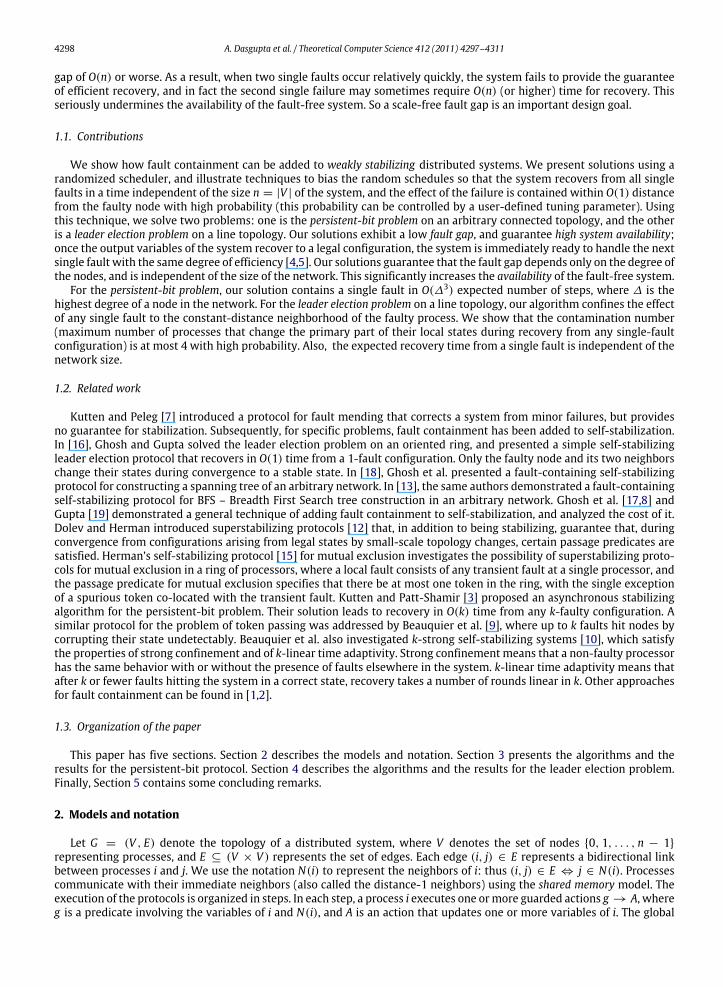
Fig. 2. Fault at leader v4 . Due to the fault, v3 becomes v4 ’s parent.

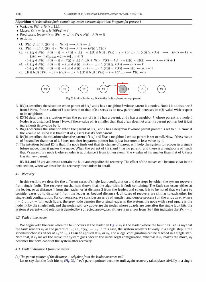
3. R3(a) describes the situation when parent of i is j, and i has a neighbor k whose parent is a node l. Node l is at distance 2from i. Now, if the x-value of i is no less than that of k, i sets k as its new parent and increases its x(i)-value with respectto its neighbors.

4. R3(b) describes the situation when the parent of i is j, j has a parent, and i has a neighbor k whose parent is a node l.Node l is at distance 2 from i. Now, if the x-value of i is smaller than that of k, i does not alter its parent pointer but it justincrements its x-value by 1.

5. R4(a) describes the situation when the parent of i is j, and i has a neighbor k whose parent pointer is set to null. Now, ifthe x-value of i is no less than that of k, i sets k as its new parent.

6. R4(b) describes the situationwhen the parent of i is j, and i has a neighbor kwhose parent is set to null. Now, if the x-valueof i is smaller than that of k, i does not alter its parent pointer but it just increments its x-value by 1.

7. The intuition behind R5 is that, if a node finds out that its change of parent will help the system to recover in a singlefuture move, then it makes the move. When the parent of i is j, and j has no parent, and there is a neighbor k of i suchthat k’s parent is a node l, where node l is at distance 2 from i, then even if the x-value of i is smaller than that of k, i setsk as its new parent.

R3, R4, and R5 are actions to contain the fault and expedite the recovery. The effect of the moves will become clear in thenext section, when we describe the recovery mechanism in detail.

4.1. Recovery

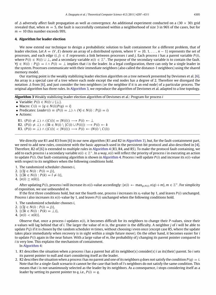
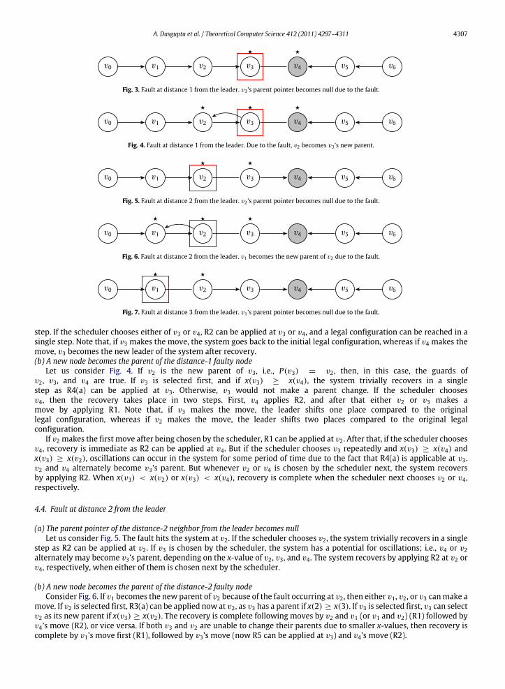
In this section, we describe the different cases of single-fault configuration and the steps by which the system recoversfrom single faults. The recovery mechanism shows that the algorithm is fault containing. The fault can occur either atthe leader, or at distance 1 from the leader, or at distance 2 from the leader, and so on. It is to be noted that we have toconsider cases up to distance 4 from the leader as, beyond distance 4, all cases of recovery are similar to each other forsingle-fault configuration. For convenience, we consider an array of length n and denote process i on the array as vi, wherei = 0, . . . , n − 1. In each figure, the grey node denotes the original leader in the system, the node with a red square is thenode hit by the single fault, and the nodes with a ⋆ above are the nodes whose guards are true after the single fault hits thesystem. A parent–child relation is denoted by a directed arrow;, i.e., if there is an arrow from i to j, this indicates that P(i) = j.

4.2. Fault at the leader

We begin with the case when the fault occurs at the leader. In Fig. 2, v4 is the leader where the fault hits. Let us say thatthe fault renders v3 as the parent of v4; i.e., P(v4) = v3. In this case, the system recovers trivially in a single step. If thescheduler chooses either of v3 or v4, R1 can be applied at v3 or v4, and a legal configuration can be reached in a single step.Note that, if v4 makes the move, the system goes back to the initial legal configuration, whereas if v3 makes the move, v3becomes the new leader of the system after recovery.

4.3. Fault at distance 1 from the leader

(a) The parent pointer of the distance-1 neighbor from the leader becomes nullLet us say that the fault hits v3 (Fig. 3). If v3’s parent pointer becomes null, again recovery takes place trivially in a single

A. Dasgupta et al. / Theoretical Computer Science 412 (2011) 4297–4311 4307

v0 v1 v2 v3

⋆

v4

⋆

v5 v6

Fig. 3. Fault at distance 1 from the leader. v3 ’s parent pointer becomes null due to the fault.

v0 v1 v2

⋆

v3

⋆

v4

⋆

v5 v6

Fig. 4. Fault at distance 1 from the leader. Due to the fault, v2 becomes v3 ’s new parent.

v0 v1 v2

⋆

v3

⋆

v4 v5 v6

Fig. 5. Fault at distance 2 from the leader. v2 ’s parent pointer becomes null due to the fault.

v0 v1

⋆

v2

⋆

v3

⋆

v4 v5 v6

Fig. 6. Fault at distance 2 from the leader. v1 becomes the new parent of v2 due to the fault.

v0 v1

⋆

v2

⋆

v3 v4 v5 v6

Fig. 7. Fault at distance 3 from the leader. v1 ’s parent pointer becomes null due to the fault.

step. If the scheduler chooses either of v3 or v4, R2 can be applied at v3 or v4, and a legal configuration can be reached in asingle step. Note that, if v3 makes the move, the system goes back to the initial legal configuration, whereas if v4 makes themove, v3 becomes the new leader of the system after recovery.(b) A new node becomes the parent of the distance-1 faulty node

Let us consider Fig. 4. If v2 is the new parent of v3, i.e., P(v3) = v2, then, in this case, the guards ofv2, v3, and v4 are true. If v3 is selected first, and if x(v3) ≥ x(v4), the system trivially recovers in a singlestep as R4(a) can be applied at v3. Otherwise, v3 would not make a parent change. If the scheduler choosesv4, then the recovery takes place in two steps. First, v4 applies R2, and after that either v2 or v3 makes amove by applying R1. Note that, if v3 makes the move, the leader shifts one place compared to the originallegal configuration, whereas if v2 makes the move, the leader shifts two places compared to the original legalconfiguration.

If v2 makes the first move after being chosen by the scheduler, R1 can be applied at v2. After that, if the scheduler choosesv4, recovery is immediate as R2 can be applied at v4. But if the scheduler chooses v3 repeatedly and x(v3) ≥ x(v4) andx(v3) ≥ x(v2), oscillations can occur in the system for some period of time due to the fact that R4(a) is applicable at v3.v2 and v4 alternately become v3’s parent. But whenever v2 or v4 is chosen by the scheduler next, the system recoversby applying R2. When x(v3) < x(v2) or x(v3) < x(v4), recovery is complete when the scheduler next chooses v2 or v4,respectively.

4.4. Fault at distance 2 from the leader

(a) The parent pointer of the distance-2 neighbor from the leader becomes nullLet us consider Fig. 5. The fault hits the system at v2. If the scheduler chooses v2, the system trivially recovers in a single

step as R2 can be applied at v2. If v3 is chosen by the scheduler, the system has a potential for oscillations; i.e., v4 or v2alternately may become v3’s parent, depending on the x-value of v2, v3, and v4. The system recovers by applying R2 at v2 orv4, respectively, when either of them is chosen next by the scheduler.

(b) A new node becomes the parent of the distance-2 faulty nodeConsider Fig. 6. If v1 becomes the new parent of v2 because of the fault occurring at v2, then either v1, v2, or v3 canmake a

move. If v2 is selected first, R3(a) can be applied now at v2, as v3 has a parent if x(2) ≥ x(3). If v3 is selected first, v3 can selectv2 as its new parent if x(v3) ≥ x(v2). The recovery is complete following moves by v2 and v1 (or v1 and v2) (R1) followed byv4’s move (R2), or vice versa. If both v3 and v2 are unable to change their parents due to smaller x-values, then recovery iscomplete by v1’s move first (R1), followed by v3’s move (now R5 can be applied at v3) and v4’s move (R2).

4308 A. Dasgupta et al. / Theoretical Computer Science 412 (2011) 4297–4311

v0

⋆

v1

⋆

v2

⋆

v3 v4 v5 v6

Fig. 8. Fault at distance 3 from the leader. v0 becomes the new parent of v1 .

v0 v1

⋆

v2

⋆

v3 v4 v5 v6

Fig. 9. Fault at distance 4 from the leader. v1 ’s parent pointer becomes null.

v0

⋆

v1

⋆

v2

⋆

v3 v4 v5 v6

Fig. 10. Fault at distance 4 from the leader. v0 becomes the new parent of v1 .

4.5. Fault at distance 3 from the leader

(a) The parent pointer of a distance-3 neighbor from the leader becomes nullConsider Fig. 7. If v2 is chosen tomake the firstmove, then it can alternately choose v1 or v3 as its parent for awhile, if its x-

value is greater than that of both v1 and v3. Recovery is completedwhen v1 is selected by the scheduler tomake amove (R2).

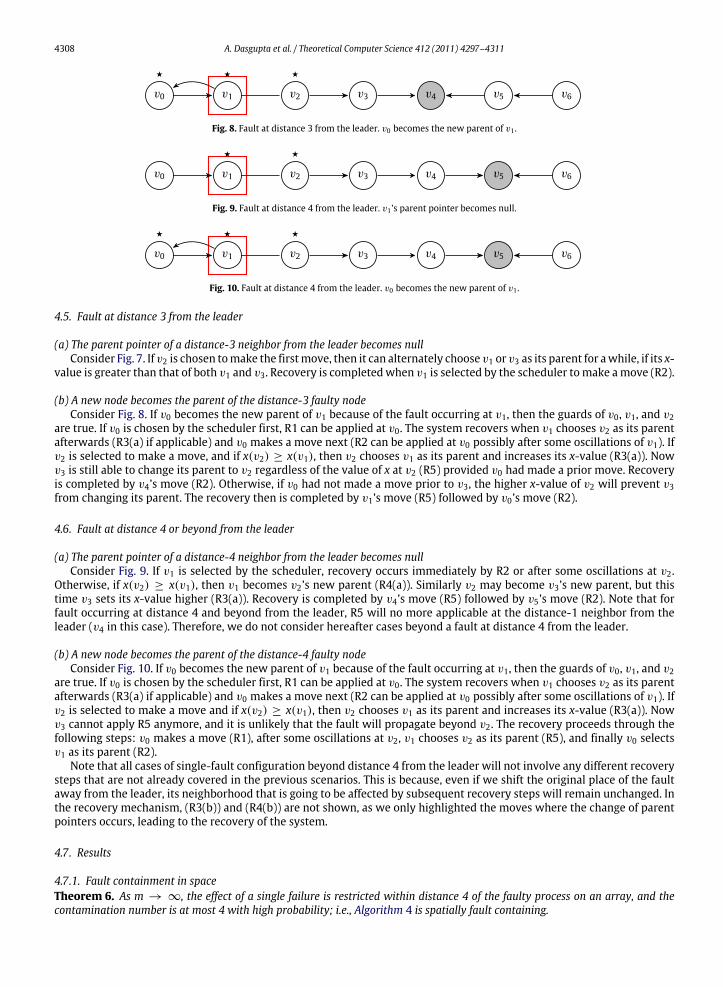
(b) A new node becomes the parent of the distance-3 faulty nodeConsider Fig. 8. If v0 becomes the new parent of v1 because of the fault occurring at v1, then the guards of v0, v1, and v2

are true. If v0 is chosen by the scheduler first, R1 can be applied at v0. The system recovers when v1 chooses v2 as its parentafterwards (R3(a) if applicable) and v0 makes a move next (R2 can be applied at v0 possibly after some oscillations of v1). Ifv2 is selected to make a move, and if x(v2) ≥ x(v1), then v2 chooses v1 as its parent and increases its x-value (R3(a)). Nowv3 is still able to change its parent to v2 regardless of the value of x at v2 (R5) provided v0 had made a prior move. Recoveryis completed by v4’s move (R2). Otherwise, if v0 had not made a move prior to v3, the higher x-value of v2 will prevent v3from changing its parent. The recovery then is completed by v1’s move (R5) followed by v0’s move (R2).

4.6. Fault at distance 4 or beyond from the leader

(a) The parent pointer of a distance-4 neighbor from the leader becomes nullConsider Fig. 9. If v1 is selected by the scheduler, recovery occurs immediately by R2 or after some oscillations at v2.

Otherwise, if x(v2) ≥ x(v1), then v1 becomes v2’s new parent (R4(a)). Similarly v2 may become v3’s new parent, but thistime v3 sets its x-value higher (R3(a)). Recovery is completed by v4’s move (R5) followed by v5’s move (R2). Note that forfault occurring at distance 4 and beyond from the leader, R5 will no more applicable at the distance-1 neighbor from theleader (v4 in this case). Therefore, we do not consider hereafter cases beyond a fault at distance 4 from the leader.

(b) A new node becomes the parent of the distance-4 faulty nodeConsider Fig. 10. If v0 becomes the new parent of v1 because of the fault occurring at v1, then the guards of v0, v1, and v2

are true. If v0 is chosen by the scheduler first, R1 can be applied at v0. The system recovers when v1 chooses v2 as its parentafterwards (R3(a) if applicable) and v0 makes a move next (R2 can be applied at v0 possibly after some oscillations of v1). Ifv2 is selected to make a move and if x(v2) ≥ x(v1), then v2 chooses v1 as its parent and increases its x-value (R3(a)). Nowv3 cannot apply R5 anymore, and it is unlikely that the fault will propagate beyond v2. The recovery proceeds through thefollowing steps: v0 makes a move (R1), after some oscillations at v2, v1 chooses v2 as its parent (R5), and finally v0 selectsv1 as its parent (R2).

Note that all cases of single-fault configuration beyond distance 4 from the leader will not involve any different recoverysteps that are not already covered in the previous scenarios. This is because, even if we shift the original place of the faultaway from the leader, its neighborhood that is going to be affected by subsequent recovery steps will remain unchanged. Inthe recovery mechanism, (R3(b)) and (R4(b)) are not shown, as we only highlighted the moves where the change of parentpointers occurs, leading to the recovery of the system.

4.7. Results

4.7.1. Fault containment in spaceTheorem 6. As m → ∞, the effect of a single failure is restricted within distance 4 of the faulty process on an array, and thecontamination number is at most 4 with high probability; i.e., Algorithm 4 is spatially fault containing.

A. Dasgupta et al. / Theoretical Computer Science 412 (2011) 4297–4311 4309

To prove the result of spatial containment, we need to find out how far the observable variables change from the faulty node.We consider all the subcases of the recovery mechanism.

1. Fault at leader: The fault propagates to at most distance 1.2. Fault at distance 1 from the leader:

(a) The parent pointer of the distance-1 neighbor becomes null: The fault propagates to at most distance 1.(b) A new node becomes the parent of the distance-1 faulty node: In the recovery steps, we showed that, in Fig. 4, at

most v2’s parent or v4’s parent might change. Thus, the fault propagates to at most distance 1.3. Fault at distance 2 from the leader:

(a) The parent pointer of the distance-2 neighbor becomes null: Consider Fig. 5. If v2 is selected, the system recoversimmediately. Another possible recovery is through the sequence of moves of v3 followed by v4. In the latter case,contamination occurs up to distance 2 from the original faulty node.

(b) A new node becomes the parent of the distance-2 faulty node: Consider Fig. 6. The worst-case scenario happenswhen v3 makes a move and after that v4 completes the recovery. Contamination occurs up to distance 2 from theoriginal faulty node in this case.

4. Fault at distance 3 from the leader:(a) The parent pointer of the distance-3 neighbor becomes null: Consider Fig. 7. The worst-case scenario happens when

v4 has to change its parent. The fault propagates to at most distance 3.(b) A new node becomes the parent of the distance-3 faulty node: Consider Fig. 8. The worst-case scenario happens

when v4 has to change its parent. The fault propagates to at most distance 3.5. Fault at distance 4 from the leader:

(a) The parent pointer of the distance-4 neighbor becomes null: This is the scenario in which the highest spatialcontamination occurs. Consider Fig. 9. In theworst case, a distance-4 node from the faulty nodemight have to changeits parent pointer. In Fig. 9, v5 is this node.

(b) A new node becomes the parent of the distance-4 faulty node: Consider Fig. 10. The fault propagates up to distance1 with high probability. The probability of the fault contaminating beyond distance 1 is (1 − 1/2m) × 1/2m, andlimm→∞(1− 1/2m)× 1/2m

= 0.

Note that for a fault occurring at distance 4 and beyond from the leader, R5 will no longer be applicable at the distance-1 neighbor from the leader. Therefore, we do not consider the cases beyond a fault at distance 4 from the leader. HenceAlgorithm 4 is spatially fault containing, and the highest contamination number is 4 with high probability. �

4.7.2. Fault containment in timeTheorem 7. The expected number of steps needed to contain a single fault is independent of n, i.e., the number of nodes in thearray. Hence Algorithm 4 is fault containing in time.

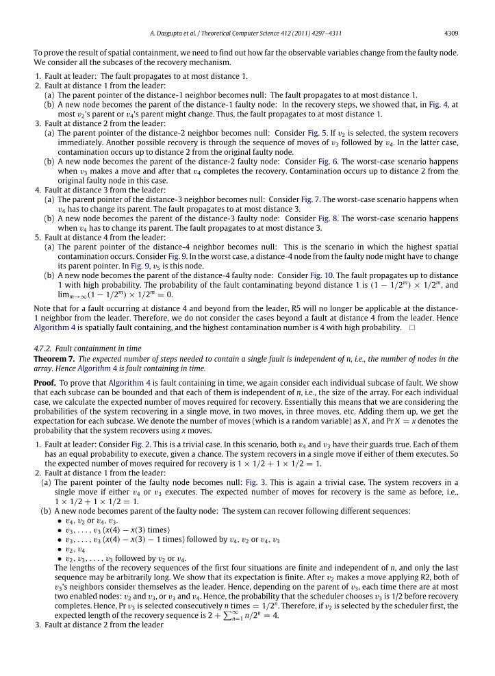
Proof. To prove that Algorithm 4 is fault containing in time, we again consider each individual subcase of fault. We showthat each subcase can be bounded and that each of them is independent of n, i.e., the size of the array. For each individualcase, we calculate the expected number of moves required for recovery. Essentially this means that we are considering theprobabilities of the system recovering in a single move, in two moves, in three moves, etc. Adding them up, we get theexpectation for each subcase. We denote the number of moves (which is a random variable) as X , and Pr X = x denotes theprobability that the system recovers using xmoves.

1. Fault at leader: Consider Fig. 2. This is a trivial case. In this scenario, both v4 and v3 have their guards true. Each of themhas an equal probability to execute, given a chance. The system recovers in a single move if either of them executes. Sothe expected number of moves required for recovery is 1× 1/2+ 1× 1/2 = 1.

2. Fault at distance 1 from the leader:(a) The parent pointer of the faulty node becomes null: Fig. 3. This is again a trivial case. The system recovers in a

single move if either v4 or v3 executes. The expected number of moves for recovery is the same as before, i.e.,1× 1/2+ 1× 1/2 = 1.

(b) A new node becomes parent of the faulty node: The system can recover following different sequences:• v4, v2 or v4, v3.• v3, . . . , v3 (x(4)− x(3) times)• v3, . . . , v3 (x(4)− x(3)− 1 times) followed by v4, v2 or v4, v3• v2, v4• v2, v3, . . . , v3 followed by v2 or v4.The lengths of the recovery sequences of the first four situations are finite and independent of n, and only the lastsequence may be arbitrarily long. We show that its expectation is finite. After v2 makes a move applying R2, both ofv3’s neighbors consider themselves as the leader. Hence, depending on the parent of v3, each time there are at mosttwo enabled nodes: v2 and v3, or v3 and v4. Hence, the probability that the scheduler chooses v3 is 1/2 before recoverycompletes. Hence, Pr v3 is selected consecutively n times = 1/2n. Therefore, if v2 is selected by the scheduler first, theexpected length of the recovery sequence is 2+

∑∞

n=1 n/2n= 4.

3. Fault at distance 2 from the leader

4310 A. Dasgupta et al. / Theoretical Computer Science 412 (2011) 4297–4311

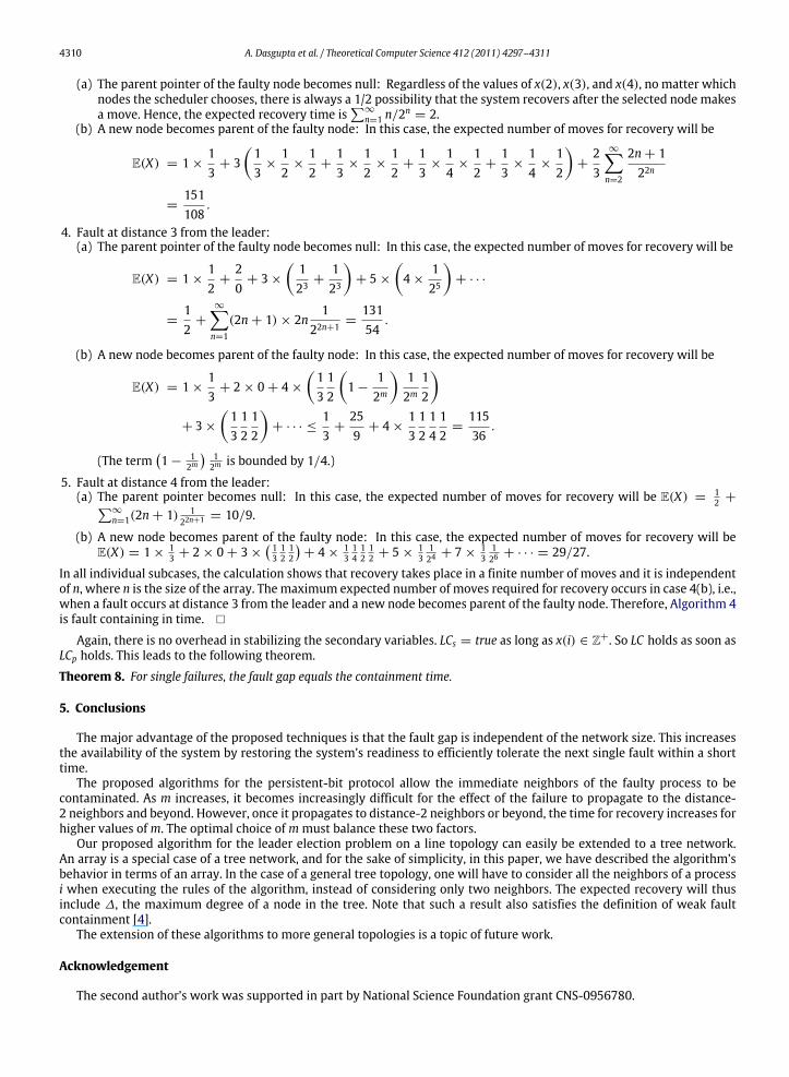
(a) The parent pointer of the faulty node becomes null: Regardless of the values of x(2), x(3), and x(4), no matter whichnodes the scheduler chooses, there is always a 1/2 possibility that the system recovers after the selected node makesa move. Hence, the expected recovery time is

∑∞

n=1 n/2n= 2.

(b) A new node becomes parent of the faulty node: In this case, the expected number of moves for recovery will be

E(X) = 1×13+ 3

13×

12×

12+

13×

12×

12+

13×

14×

12+

13×

14×

12

+

23

∞−n=2

2n+ 122n

=151108

.

4. Fault at distance 3 from the leader:(a) The parent pointer of the faulty node becomes null: In this case, the expected number of moves for recovery will be

E(X) = 1×12+

20+ 3×

123+

123

+ 5×

4×

125

+ · · ·

=12+

∞−n=1

(2n+ 1)× 2n1

22n+1=

13154

.

(b) A new node becomes parent of the faulty node: In this case, the expected number of moves for recovery will be

E(X) = 1×13+ 2× 0+ 4×

1312

1−

12m

12m

12

+ 3×

131212

+ · · · ≤

13+

259+ 4×

13121412=

11536

.

(The term1− 1

2m 1

2m is bounded by 1/4.)

5. Fault at distance 4 from the leader:(a) The parent pointer becomes null: In this case, the expected number of moves for recovery will be E(X) = 1

2 +∑∞

n=1(2n+ 1) 122n+1= 10/9.

(b) A new node becomes parent of the faulty node: In this case, the expected number of moves for recovery will beE(X) = 1× 1

3 + 2× 0+ 3× 131212

+ 4× 1

3141212 + 5× 1

3124+ 7× 1

3126+ · · · = 29/27.

In all individual subcases, the calculation shows that recovery takes place in a finite number of moves and it is independentof n, where n is the size of the array. Themaximum expected number of moves required for recovery occurs in case 4(b), i.e.,when a fault occurs at distance 3 from the leader and a new node becomes parent of the faulty node. Therefore, Algorithm 4is fault containing in time. �

Again, there is no overhead in stabilizing the secondary variables. LCs = true as long as x(i) ∈ Z+. So LC holds as soon asLCp holds. This leads to the following theorem.

Theorem 8. For single failures, the fault gap equals the containment time.

5. Conclusions

The major advantage of the proposed techniques is that the fault gap is independent of the network size. This increasesthe availability of the system by restoring the system’s readiness to efficiently tolerate the next single fault within a shorttime.

The proposed algorithms for the persistent-bit protocol allow the immediate neighbors of the faulty process to becontaminated. As m increases, it becomes increasingly difficult for the effect of the failure to propagate to the distance-2 neighbors and beyond. However, once it propagates to distance-2 neighbors or beyond, the time for recovery increases forhigher values ofm. The optimal choice ofm must balance these two factors.

Our proposed algorithm for the leader election problem on a line topology can easily be extended to a tree network.An array is a special case of a tree network, and for the sake of simplicity, in this paper, we have described the algorithm’sbehavior in terms of an array. In the case of a general tree topology, one will have to consider all the neighbors of a processi when executing the rules of the algorithm, instead of considering only two neighbors. The expected recovery will thusinclude ∆, the maximum degree of a node in the tree. Note that such a result also satisfies the definition of weak faultcontainment [4].

The extension of these algorithms to more general topologies is a topic of future work.

Acknowledgement

The second author’s work was supported in part by National Science Foundation grant CNS-0956780.

A. Dasgupta et al. / Theoretical Computer Science 412 (2011) 4297–4311 4311

References

[1] Y. Azar, S. Kutten, B. Patt-Shamir, Distributed error confinement, ACM Trans. Algorithms 6 (3) (2010).[2] Y. Afek, S. Dolev, Local stabilizer, J. Parallel Distrib. Comput. 62 (5) (2002) 745–765.[3] S. Kutten, B. Patt-Shamir, Stabilizing time-adaptive protocols, Theoret. Comput. Sci. 220 (1999) 93–111.[4] A. Dasgupta, S. Ghosh, X. Xiao, Probabilistic fault-containment, in: 9th International Symposium on Stabilization, Safety, and Security of Distributed

Systems, Paris, France, 2007.[5] A. Dasgupta, S. Ghosh, X. Xiao, Fault containment inweakly stabilizing systems, in: 11th International Symposiumon Stabilization, Safety, and Security

of Distributed Systems, Lyon, France, 2009.[6] S. Devismes, S. Tixeuil, M. Yamashita, Weak vs. Self vs. Probabilistic Stabilization, Distributed Computing Systems, International Conference, vol. 0,

2008. pp. 681–688, Los Alamitos, CA, USA.[7] S. Kutten, D. Peleg, Fault-local distributed mending, in: Proceedings of the 14th Annual ACM Symposium on Principles of Distributed Computing,

1995, pp. 20–27.[8] S. Ghosh, A. Gupta, T. Herman, S.V. Pemmaraju, Fault-containing self-stabilizing distributed algorithms, in: Proceedings of the 15th Annual ACM

Symposium on Principles of Distributed Computing, 1996, pp. 45–54.[9] J. Beauquier, C. Genolini, S. Kutten, Optimal reactive k-stabilization: the case of mutual exclusion, in: Proceedings of the 18th Annual ACM Symposium

on Principles of Distributed Computing, 1999, pp. 209–218.[10] J. Beauquier, S. Delaet, S. Haddad, A 1-strong self-stabilizing transformer, in: Proceedings of the Eighth Symposium on Self-Stabilizing Systems, 2006.[11] J.L. Coolidge, The Gambler’s ruin, Ann. of Math. 10 (4) (1909) 181–192.[12] S. Dolev, T. Herman, Superstabilizing protocols for dynamic distributed systems, in: Proceedings of the SecondWorkshop on Self-Stabilizing Systems,

1995, pp. 3.1–3.15.[13] S. Ghosh, A. Gupta, S.V. Pemmaraju, Fault-containing network protocols, in: Proceedings of 12th Annual ACM Symposium on Applied Computing,

1997.[14] M.G. Gouda, The theory of weak stabilization, in: Proceedings of WSS, in: LNCS, vol. 2194, 2001, pp. 114–123.[15] T. Herman, Superstabilizing mutual exclusion, in: Proceedings of 1st International Conference on Parallel and Distributed Processing: Techniques and

Applications, 1995.[16] S. Ghosh, A. Gupta, An exercise in fault-containment: self-stabilizing leader election, Informat. Process. Lett. 5 (59) (1996) 281–288.[17] S. Ghosh, A. Gupta, T. Herman, S.V. Pemmaraju, Fault-containing self-stabilizing distributed protocols, Distrib. Comput. (2007).[18] S. Ghosh, A. Gupta, S.V. Pemmaraju, A fault-containing self-stabilizing algorithm for spanning trees, J. Comput. Informat. 2 (1996) 322–338.[19] A. Gupta, Fault-containment in self-stabilizing distributed systems, Ph.D. thesis. Department of Computer Science, The University of Iowa, Iowa City,

IA, USA, 1997.