
The Stabilizing Role of Government Size
25
The Stabilizing Role of Government Size Javier Andrés a , Rafael Doménech a and Antonio Fatás b a University of Valencia b INSEAD January, 2007 Abstract This paper presents an analysis of how alternative models of the business cycle can replicate the stylized fact that large governments are associated with less volatile economies. Our analysis shows that adding nominal rigidities and costs of capital adjustment to an otherwise standard RBC model can generate a negative correlation between government size and the volatility of output. However, in the model, we find that the stabilizing effect is only due to a composition effect and it is not present when we look at the volatility of private output. Given that empirically we also observe a negative correlation between government size and the volatility of consumption, we modify the model by introducing rule-of-thumb consumers. In this modified version of our initial model we observe that consumption volatility is also reduced when government size increases in similar way to the observed pattern in OECD economies over the last 45 years. Keywords: Government size, output volatility, automatic stabilizers. JEL Classification: E32, E52, E63. 1. Introduction This paper provides a study of how alternative models of the business cycle can replicate the stylized fact that across countries and even across U.S. states large governments are associated with less volatile economies. There is substantial evidence that countries or re- gions with large governments display less volatile economies, as shown in Galí (1994) and Fatás and Mihov (2001). This is not only an intriguing fact for macroeconomists, but also one that has implications regarding the models we use to analyze economic fluctuations. As it is the case that most macroeconomic theories incorporate governments in one form We would like to thank the comments by two anonymous referees and the editor, Wouter den Haan, as well as by C. Leith and participants at the ESWC (London, 2005), the 61st annual congress of the IIPF (Ko- rea, 2005), the XXX SAE, and seminars at different institutions. Financial support by CICYT grants SEC2002- 0026 and SEJ2005-01365, Fundación Rafael del Pino and EFRD is gratefully acknowledged. e-mails for comments: [email protected], [email protected] and [email protected].
-
Upload
independent -
Category
Documents
-
view
1 -
download
0
Transcript of The Stabilizing Role of Government Size
The Stabilizing Role of Government Size
Javier Andrésa, Rafael Doménecha and Antonio Fatásb
a University of Valencia
b INSEAD
January, 2007
Abstract
This paper presents an analysis of how alternative models of the business cycle can replicate thestylized fact that large governments are associated with less volatile economies. Our analysis showsthat adding nominal rigidities and costs of capital adjustment to an otherwise standard RBC modelcan generate a negative correlation between government size and the volatility of output. However,in the model, we find that the stabilizing effect is only due to a composition effect and it is notpresent when we look at the volatility of private output. Given that empirically we also observea negative correlation between government size and the volatility of consumption, we modify themodel by introducing rule-of-thumb consumers. In this modified version of our initial model weobserve that consumption volatility is also reduced when government size increases in similar wayto the observed pattern in OECD economies over the last 45 years.
Keywords: Government size, output volatility, automatic stabilizers.JEL Classification: E32, E52, E63.
1. IntroductionThis paper provides a study of how alternative models of the business cycle can replicatethe stylized fact that across countries and even across U.S. states large governments areassociated with less volatile economies. There is substantial evidence that countries or re-gions with large governments display less volatile economies, as shown in Galí (1994) andFatás and Mihov (2001). This is not only an intriguing fact for macroeconomists, but alsoone that has implications regarding the models we use to analyze economic fluctuations.As it is the case that most macroeconomic theories incorporate governments in one form
We would like to thank the comments by two anonymous referees and the editor, Wouter den Haan, aswell as by C. Leith and participants at the ESWC (London, 2005), the 61st annual congress of the IIPF (Ko-rea, 2005), the XXX SAE, and seminars at different institutions. Financial support by CICYT grants SEC2002-0026 and SEJ2005-01365, Fundación Rafael del Pino and EFRD is gratefully acknowledged. e-mails for comments:[email protected], [email protected] and [email protected].
THE STABILIZING ROLE OF GOVERNMENT SIZE 2
or another (expenditures, transfers or taxes), understanding this correlation is crucial toimprove the ability of models to replicate the stylized facts of the business cycle.
The approach of this paper is to explore alternative theories and probe into thedifferent mechanisms that may explain why government size can have an effect on thevolatility of output fluctuations. Although we replicate and present some of the evidenceprovided by previous papers in the literature, our goal is not to challenge or qualify thisempirical fact. We take as given that the size of governments is inversely correlated withthe volatility of business cycles and we look for an explanation. Finding this explanationis a challenging task given that, as shown by Galí (1994), there is no clear connection be-tween government size and volatility in the context of a standard RBC model. In fact,under some reasonable assumptions, that model produces a positive correlation.
Our paper, by clearly illustrating the mechanisms behind the effects of taxes andgovernment spending on macroeconomic outcomes under different theoretical assump-tions, can be useful in discriminating among different business cycle models. We comparethe predictions of a standard RBC model to those of models that incorporate nominalrigidities, costs of adjustment for capital and rule-of-thumb consumers. There are severalreasons why we consider a framework in which several frictions are present. First, theseare models that are more likely to generate the type of Keynesian effects observed in thedata. For example, adding costs of adjustment to capital is a way of making investmentless reactive to technology shocks and, as a result, replicate better the behavior in the data.A second reason for looking into this class of models is that they are increasingly beingused by researchers who struggle to explain other puzzles also related to fiscal policy. Forexample, there is evidence that consumption increases in response to exogenous increasesin government spending (see Fatás and Mihov, 2002, or Perotti, 2002). This fact, which isagain at odds with the standard RBC model, has been partially accounted for in a recentpaper by Galí, López-Salido and Vallés (2003) using a model with similar features to theones we explore in our paper.
From an empirical point of view, understanding the implications of the correlationbetween government size and output volatility is important for the design of stabilizingfiscal policies. The fact that larger governments are associated with lower volatilities canlead to the easy temptation of arguing that this is the result of automatic stabilizers but tobe able to make that assertion one first needs to understand the stabilizing properties oflarge governments in a dynamic stochastic general equilibrium model.
Our main findings are the following. First, our analysis shows that adding nominalrigidities and costs of capital adjustment to an otherwise standard RBC model can generatea negative correlation between government size and the volatility of output. However,in the model, we find that the stabilizing effect is only present because of a composition
THE STABILIZING ROLE OF GOVERNMENT SIZE 3
effect, given that larger governments are not associated, in the calibrated model, with morestable private consumption or investment. In fact, as government size increases, these twocomponents of aggregate expenditure become more volatile. There is still an interestinginteraction between the degree of rigidities and the volatility of these two components ofGDP. As we increase the degree of rigidities in the model, the increase in the volatility ofconsumption and investment as government size increases is smaller. This interaction is,nonetheless, of second order importance since we observe a negative correlation betweengovernment size and the volatility of both components.
Given that empirically we observe that consumption volatility is also negatively cor-related with government size, we explore and additional variation of the initial model inwhich we introduce rule-of-thumb consumers in an attempt to have consumption closelymimic the response of GDP. In this modified version of our initial model we indeed ob-serve that consumption volatility is also reduced when government size increases.
The structure of this paper is as follows. In section 2 we present the basic empiricalevidence about the negative correlation between government size and output and con-sumption volatility. In the third section we describe our model with nominal and realrigidities. Its main implications in terms of the relationship between government size andmacroeconomic volatility are explored in Section 4, where we also extend our basic modelto the inclusion of rule-of-thumb consumers to better account for the empirical evidence.Finally, section 5 concludes.
2. Empirical evidenceWe first present evidence of the negative correlation between government size and busi-ness cycle volatility for a sample of 20 OECD countries over the period 1960 to 2004.This correlation has been documented by, among others, Galí (1994) and Fatás and Mihov(2001). We measure government size by the GDP share of total government expenditures(G/Y).1 When it comes to output volatility, we follow an eclectic approach and use fouralternative measures that use different detrending methods. Besides government size wehave considered the effect of some additional variables such as openness, the average logof GDP per capita, the average log of GDP over the sample period and the average rateof growth of GDP per capita. Only the average log of GDP (ln Y) turns out to be statis-tically significant in all regressions and hence we include it in the regressions in Table 1as a proxy for the size of the economy. Column (1) uses the log of the standard deviation
1 All the data come from various issues of the Economic Ourlook dataset in the OECD Statistical Compendiumby DSI Data Service and Information, with the exception of the GDP share of total government expenditures forTurkey that comes from the IMF International Financial Statistics. The dataset as well as the technical appendixwith the model solution, the equilibrium, the steady state and the dynamic system can be downloaded from:http://iei.uv.es/rdomenec/ADFatas/ADFatas.html
THE STABILIZING ROLE OF GOVERNMENT SIZE 4
of GDP growth rates (∆ ln Y) as a measure of output volatility, whereas in column (2) weare using the standard deviation of the GDP per capita growth rates (∆ ln y); both thesevolatilities are negatively correlated with the variable G/Y.2
The reduced-form approach of columns (1) and (2) has a difficult interpretation be-cause of the possibility of misspecifications in the regression. For example, it could bethat differences in volatility across OECD countries are not driven by business cycle phe-nomenon but by transitional growth dynamics that become part of the measured volatilitybecause we are looking at deviations around a flat trend (when using growth rates). A wayof dealing with the influence of transitional dynamics in our measure of volatility is to usethe cyclical component of the GDP (in logs), obtained with the HP filter and a smoothingparameter equal to 10 since we are using annual data (see Baxter and King, 1999, and Mar-avall and del Rio, 2001). In column (3) the dependent variable is the log of the standarddeviation of the output gap (Yc), whereas in column (4) is the log of the standard devia-tion of the cyclical component of GDP per capita (yc). We need to stress that in all cases,the coefficient of G/Y is negative and very significant.
There is also the possibility of reverse causation in this regression. The reverse cau-sation can bias our results in many directions. For example, it could be that economiesthat are very volatile (for example because they are very open) will have larger govern-ments that serve as an insurance against cyclical shocks (see Rodrik, 1998). If this were thecase, the coefficient in the regressions above would be biased towards zero. The possibil-ity of endogeneity in this specification is dealt with in detail in Fatás and Mihov (2001),who show that after controlling for endogeneity, the negative correlation is still presentand, in some cases, becomes more significant (from both an economic and statistical pointof view).
In columns (5) and (6) we present the correlation between the log of the standarddeviation of the cyclical component of private consumption (both in levels, Cc, and in percapita terms, cc) and government size. As it is clear from both columns, there is also anegative and significant correlation between both variables, suggesting that the resultsof columns (1) to (4) cannot be explained solely by the composition effect of aggregatedemand as the share of public consumption becomes larger. The magnitude of the semi-elasticity of the standard deviation of consumption to government size is similar to the
2 Notice that we use ∂ ln σ/∂(G/Y) as a measure of the effects of the changes in government size on the stan-dard deviation (σ) of the different variable considered in Table 1. There are several reasons for this choice. First,G/Y has been the standard regressor in the previous literature. Second, in the model presented in the next sectionthe simulations indicate that ∂ ln σ/∂(G/Y) is not affected by changes in G/Y within the range usually observedin the data. Finally, since for any given value of G/Y the simulations in Tables 3 to 5 show that the standarddeviation of output and consumption are very sensitive to nominal and real rigidities, which means that usingthe log transformation (ln σ) provides a more reliable measure of how the effects of government size change fordifferent degrees of rigidities.
THE STABILIZING ROLE OF GOVERNMENT SIZE 5
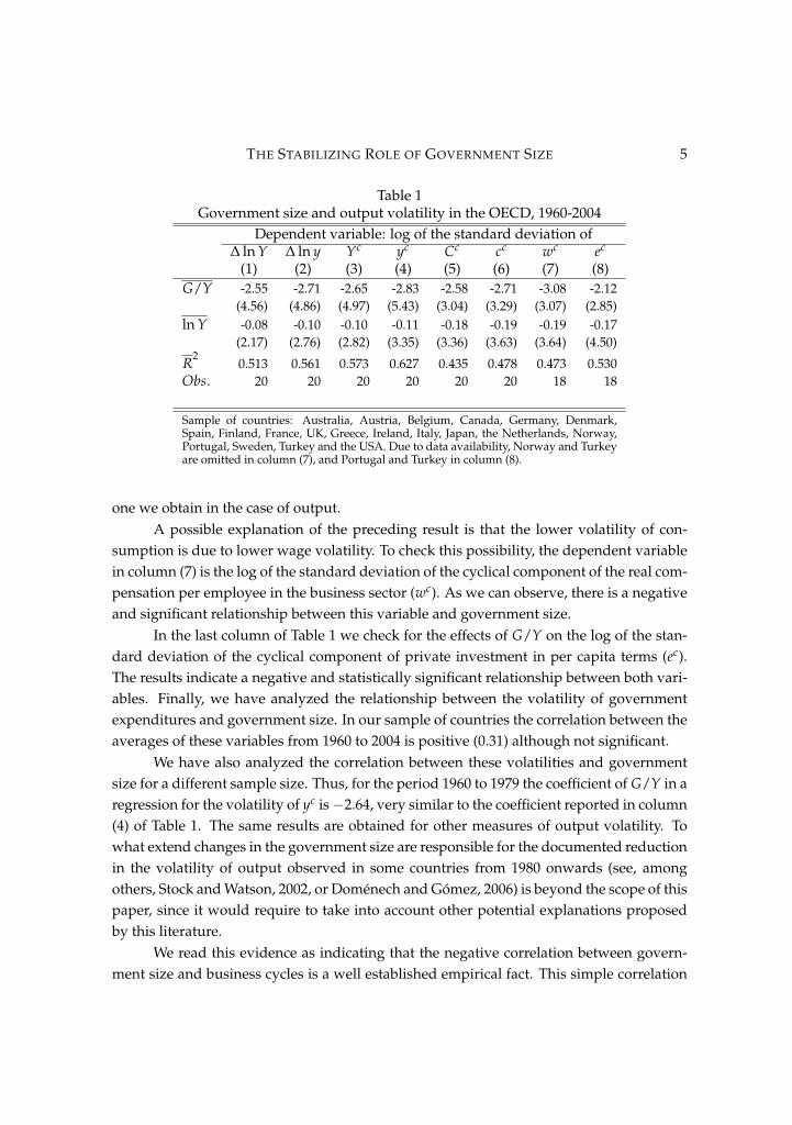
Table 1Government size and output volatility in the OECD, 1960-2004
Dependent variable: log of the standard deviation of∆ ln Y ∆ ln y Yc yc Cc cc wc ec
(1) (2) (3) (4) (5) (6) (7) (8)G/Y -2.55 -2.71 -2.65 -2.83 -2.58 -2.71 -3.08 -2.12
(4.56) (4.86) (4.97) (5.43) (3.04) (3.29) (3.07) (2.85)ln Y -0.08 -0.10 -0.10 -0.11 -0.18 -0.19 -0.19 -0.17
(2.17) (2.76) (2.82) (3.35) (3.36) (3.63) (3.64) (4.50)
R20.513 0.561 0.573 0.627 0.435 0.478 0.473 0.530
Obs. 20 20 20 20 20 20 18 18
Sample of countries: Australia, Austria, Belgium, Canada, Germany, Denmark,Spain, Finland, France, UK, Greece, Ireland, Italy, Japan, the Netherlands, Norway,Portugal, Sweden, Turkey and the USA. Due to data availability, Norway and Turkeyare omitted in column (7), and Portugal and Turkey in column (8).
one we obtain in the case of output.A possible explanation of the preceding result is that the lower volatility of con-
sumption is due to lower wage volatility. To check this possibility, the dependent variablein column (7) is the log of the standard deviation of the cyclical component of the real com-pensation per employee in the business sector (wc). As we can observe, there is a negativeand significant relationship between this variable and government size.
In the last column of Table 1 we check for the effects of G/Y on the log of the stan-dard deviation of the cyclical component of private investment in per capita terms (ec).The results indicate a negative and statistically significant relationship between both vari-ables. Finally, we have analyzed the relationship between the volatility of governmentexpenditures and government size. In our sample of countries the correlation between theaverages of these variables from 1960 to 2004 is positive (0.31) although not significant.
We have also analyzed the correlation between these volatilities and governmentsize for a different sample size. Thus, for the period 1960 to 1979 the coefficient of G/Y in aregression for the volatility of yc is2.64, very similar to the coefficient reported in column(4) of Table 1. The same results are obtained for other measures of output volatility. Towhat extend changes in the government size are responsible for the documented reductionin the volatility of output observed in some countries from 1980 onwards (see, amongothers, Stock and Watson, 2002, or Doménech and Gómez, 2006) is beyond the scope of thispaper, since it would require to take into account other potential explanations proposedby this literature.
We read this evidence as indicating that the negative correlation between govern-ment size and business cycles is a well established empirical fact. This simple correlation
THE STABILIZING ROLE OF GOVERNMENT SIZE 6
between government size and volatility has been refined by several recent studies. Therehave been attempts to clarify the origin of this correlation. For example, Martinez-Mongay(2002) and Martinez-Mongay and Sekkat (2003) have looked at which measure of gov-ernment size captures this correlation better (e.g., personal versus indirect taxes). Othershave looked at the possibility that the correlation of Table 1 is not linear and can be re-versed for large government size (Silgoner, Reitschuler, Crespo-Cuaresma, 2003). We willignore these refinements and simply postulate a model that can account for the negativecorrelation observed in Table 1.
3. The modelAs mentioned in the introduction, the fact that government size is negatively correlatedwith the size of the business cycle is difficult to reconcile within a standard RBC model(Galí, 1994). The failure of the RBC framework to replicate some basic features of the busi-ness cycle with respect to fiscal policy is not unique to this stylized fact. For example, inthe recent literature that looks at the dynamic effects of fiscal policy changes (Blanchardand Perotti, 2002, Fatás and Mihov, 2002, or Perotti, 2002) there is evidence that consump-tion tends to respond positively to increases in government spending, a result that doesnot square well with the predictions of the RBC model.
Both of these facts are easily explained by a simple textbook IS-LM model. Thissimple static model predicts both that larger governments (if associated to stronger auto-matic stabilizers) dampen the response of output to exogenous technology shocks and thatconsumption increases when government spending increases. In that sense, these resultshave a Keynesian flavor that speaks in favor of the stabilizing role of government spend-ing. This effect is also present in large scale macroeconometric models (see van den Noord,2000, and Buti and van den Noord, 2004). Thus, our search for an explanation starts witha basic dynamic general equilibrium model to which we add some Keynesian features:nominal inertia and adjustments to investment costs. Our model is very similar to the oneproposed by Andrés and Doménech (2006) and Linnemann and Schabert (2003), and alsodisplays many features of the analysis of Galí, López-Salido and Vallés (2003), who attemptto provide a theoretical explanation for the observed positive response of consumption togovernment spending changes.
We now describe the main building blocks of the model, emphasizing the assump-tions that should help us account for the empirical results of Table 1.
THE STABILIZING ROLE OF GOVERNMENT SIZE 7
3.1. Firms and households
Price setting: nominal inertia
We consider a cashless economy that is populated by an infinite number of firms. Eachfirm (indexed by i) faces a downward sloping demand curve for its product (yi) withfinite elasticity ε
yit = yt
PitPt
ε
(1)
wherehR 1
0 (yit)ε1
ε dii ε
ε1= yt and Pt =
hR 10 (Pit)
1ε dii 1
1ε . We follow Woodford (2004and 2005) and Christiano (2004), who have proposed a generalization to Calvo’s (1983)model when capital and labour are firm-specific. Each period a measure 1 φ of firms settheir prices, ePit, to maximize the present value of future profits,
maxePit
Et
∞
∑j=0
ρit,t+j(βφ)jh ePitπ
jyit+j Pt+jmcit,t+j(yit+j + κ)i
(2)
subject to
yit+j =ePitπ
εPε
t+jyt+j (3)
where ρt,t+j is a price kernel representing the marginal utility value to the representativehousehold of an additional unit of profits accrued in period t + j, β the discount factor,mct,t+j the marginal cost at t + j of the firm changing prices at t and κ a fixed cost ofproduction. The remaining (φ per cent) firms set Pit = πPit1 where π is the steady-staterate of inflation. We shall further assume that capital cannot be instantaneously reallocatedacross firms, so that, the marginal cost of firms adjusting prices (mcit,t) differs from theaverage marginal cost at time t (mct). In this case, the coefficient which measures theresponse of inflation (bπt, in deviations from steady state) to changes in marginal costs(cmct, also in deviations) departs from the one in the standard Calvo model since now itincludes a new multiplicative term, that is decreasing in the elasticity of demand ε:3
bπt = βEtbπt+1 +(1 βφ)(1 φ)
φ
1 φβκ1
(1+ ε α1α )(1 φβκ1) +
α1α φβκ2
cmct (4)
3 A good intuition of why this happens is given by Eichenbaum and Fisher (2004) and Sbordone (2002). Withcostly adjustment of capital the marginal cost of a firm is increasing in output. When there is an economy-wideshock that increases marginal costs the firm will tend to raise prices and to reduce output. But the reduction ofoutput has a counteracting effect on marginal costs and then on prices. This dampens the response of prices toan aggregate shock for a given value of the parameter φ.
THE STABILIZING ROLE OF GOVERNMENT SIZE 8
where κ1 and κ2 are non-linear functions of the elasticity of output to capital (α), β, φ, ε
and the capital adjusments costs we consider below, as in Christiano (2004).
Capital and labor demand
The profit maximization problem of the ith intermediate good firm is given by
maxeit+j ,kit+j+1,lit+1
Et
∞
∑j=0
ρt,t+jβj
(1 τk
t+j)
"Pit+j
Pt+jyit+j wit+jlit+j
# eit+j
!(5)
subject to
kit+j+1 = Φ
eit+j
kit+j
!kit+j + (1 δ)kit+j (6)
yit = Atkαitl
1αit κ (7)
where τk is the tax rate over the firm’s profit, w is the wage, l is the amount of specificlabour hired by the firm and e the investment which accumulates into the firm-specificcapital, k. It is assumed that the variable At, which stands for the total factor productivity,follows the process.
ln At = ρa ln At1 + εat (8)
where εat is white noise and 0 < ρa < 1.
The accumulation of capital results from the firms’ investment decisions. Due toinstallation costs Φ (eit/kit) only a proportion of investment spending goes to increase thecapital stockwhere δ is the constant depreciation rate. For the installation costs we use thesame function as Bernanke, Gertler and Gilchrist (1999).4
From the first order conditions we have that
wit = (1 α)mcit Atkαitlαit (9)
and
qit = Et
"β
ρt,t+1
ρt,t
(1 τk
t+1)rit+1 + qit+1
Φ
eit+1
kit+1
+ (1 δ)Φ0
eit+1
kit+1
eit+1
kit+1
#(10)
where qit is the Tobin’s q and rit is defined as
rit mcitαAtkα1i l1α
i (11)
4 In particular, Φ
ek
= δ, Φ0
ek
= 1 and Θ = Φ
00
ek
< 0.
THE STABILIZING ROLE OF GOVERNMENT SIZE 9
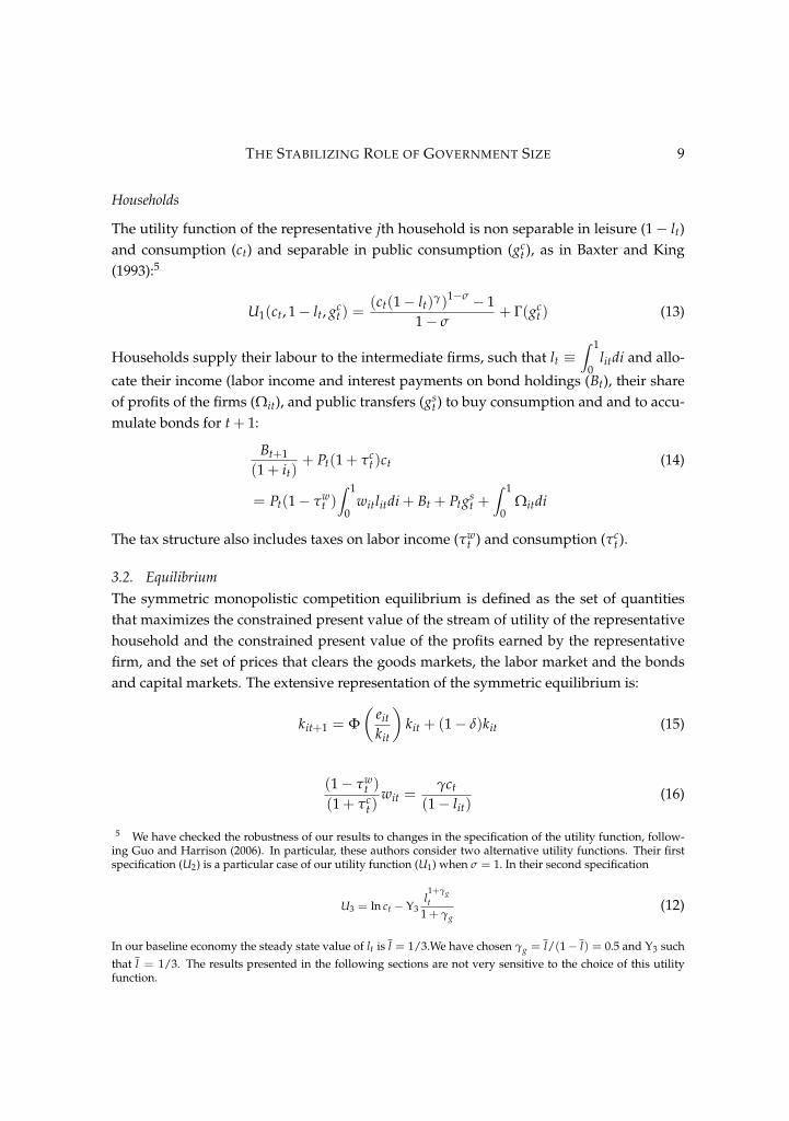
Households
The utility function of the representative jth household is non separable in leisure (1 lt)and consumption (ct) and separable in public consumption (gc
t ), as in Baxter and King(1993):5
U1(ct, 1 lt, gct ) =
(ct(1 lt)γ)1σ 1
1 σ+ Γ(gc
t ) (13)
Households supply their labour to the intermediate firms, such that lt Z 1
0litdi and allo-
cate their income (labor income and interest payments on bond holdings (Bt), their shareof profits of the firms (Ωit), and public transfers (gs
t ) to buy consumption and and to accu-mulate bonds for t+ 1:
Bt+1
(1+ it)+ Pt(1+ τc
t )ct (14)
= Pt(1 τwt )Z 1
0witlitdi+ Bt + Ptgs
t +Z 1
0Ωitdi
The tax structure also includes taxes on labor income (τwt ) and consumption (τc
t ).
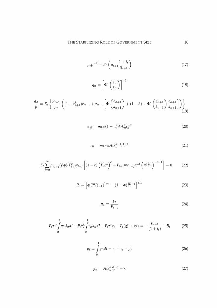
3.2. EquilibriumThe symmetric monopolistic competition equilibrium is defined as the set of quantitiesthat maximizes the constrained present value of the stream of utility of the representativehousehold and the constrained present value of the profits earned by the representativefirm, and the set of prices that clears the goods markets, the labor market and the bondsand capital markets. The extensive representation of the symmetric equilibrium is:
kit+1 = Φ
eitkit
kit + (1 δ)kit (15)
(1 τwt )
(1+ τct )
wit =γct
(1 lit)(16)
5 We have checked the robustness of our results to changes in the specification of the utility function, follow-ing Guo and Harrison (2006). In particular, these authors consider two alternative utility functions. Their firstspecification (U2) is a particular case of our utility function (U1) when σ = 1. In their second specification
U3 = ln ct Υ3l1+γgt
1+ γg(12)
In our baseline economy the steady state value of lt is l = 1/3.We have chosen γg = l/(1 l) = 0.5 and Υ3 suchthat l = 1/3. The results presented in the following sections are not very sensitive to the choice of this utilityfunction.
THE STABILIZING ROLE OF GOVERNMENT SIZE 10
µtβ1 = Et
µt+1
1+ it
πt+1
(17)
qit =
Φ0
eitkit
1(18)
qitβ= Et
µt+1
µt
(1 τk
t+1)rit+1 + qit+1
Φ
eit+1
kit+1
+ (1 δ)Φ0
eit+1
kit+1
eit+1
kit+1
(19)
wit = mcit(1 α)Atkαitlαit (20)
rit = mcitαAtkα1it l1α
it (21)
Et
∞
∑j=0
ρt,t+j(βφ)jPεt+jyt+j
(1 ε)
ePitπε+ Pt+jmcit+jεπ j
π j ePit
ε1= 0 (22)
Pt =hφ (πPt1)
1ε + (1 φ)eP1εt
i 11ε (23)
πt Pt
Pt1(24)
Ptτwt
1Z0
witlitdi+ Ptτkt
1Z0
ritkitdi+ Ptτct ct Pt(gc
t + gst ) =
Bt+1
(1+ it)+ Bt (25)
yt 1Z
0
yitdi = ct + et + gct (26)
yit = Atkαitl
1αit κ (27)
THE STABILIZING ROLE OF GOVERNMENT SIZE 11
Etρt,t+j+1
Etρt,t+j=
Etµt+j+1
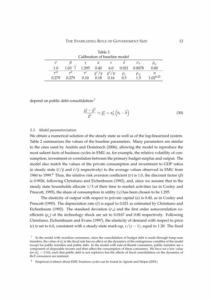
Etµt+j(28)
plus the equation relating the marginal costs of the price-adjusting firm (mcit,t+j) with theaverage marginal costs (mct+j), and where µt in equation (28) is the Lagrange multiplierof the intertemporal decision problem of the household.
The model is completed with the description of how the policy instruments are set.The fiscal rules determine the path of gc
t and gst . All τw
t , τkt and τc
t will be assumed constantfor all t unless said otherwise. Monetary policy is represented by a standard Taylor rule:
it = ρrit1 + (1 ρr)i+ (1 ρr)ρπ(πt π) + (1 ρr)ρy(byt byNt ) + zi
t (29)
in which the monetary authority sets the interest rate (it) to prevent inflation deviatingfrom its steady-state level (πt π) and to counteract movements in the output gap (byt byN
t ) where byNt represents frictionless output (in deviations from the steady-state); i is the
steady-state interest rate and the current rate moves smoothly (0 < ρr < 1) and has anunexpected component, zi
t.Provided that ρπ is above certain threshold value, fiscal policy must be designed
to satisfy the present value budget constraint of the public sector for any price level inorder to obtain a unique monetary equilibrium (Leeper, 1991, Woodford, 1997, Leith andWren-Lewis, 2001). A simple way of making this requirement operational is to assume thateither taxes or public spending respond sufficiently to the level of debt (Canzoneri, Cumbyand Diba, 2001). These feedback rules also represent the quantitative deficit and/or debttargets made explicit in most developed countries’ fiscal systems nowadays (Corsetti andRoubini, 1996, Bohn, 1998, and Ballabriga and Martinez-Mongay, 2002). The theoreticalrequirements of a Ricardian policy can be satisfied with a feedback behavior of either rev-enues or expenditures, but the empirical evidence indicates that successful consolidationsin industrialized countries have been based on spending cuts (see von Hagen, Hallet andStrauch, 2001, Alesina and Perotti, 1997).6 For simplicity, in our baseline economy we as-sume that gc
t remains constant over the business cycle and we use a fiscal rule in lump-sumtransfers (gs) as a function of the absolute deviations of public debt bt Bt/Pt from itssteady-state value b = 0 and, therefore, in the basic model private agents decisions do not
6 Cyclical changes in tax rates are not very realistic and may, under some circumstances, lead to multiple(sunspot) equilibria, thus inducing additional instability (Schmitt-Grohé and Uribe, 1997).
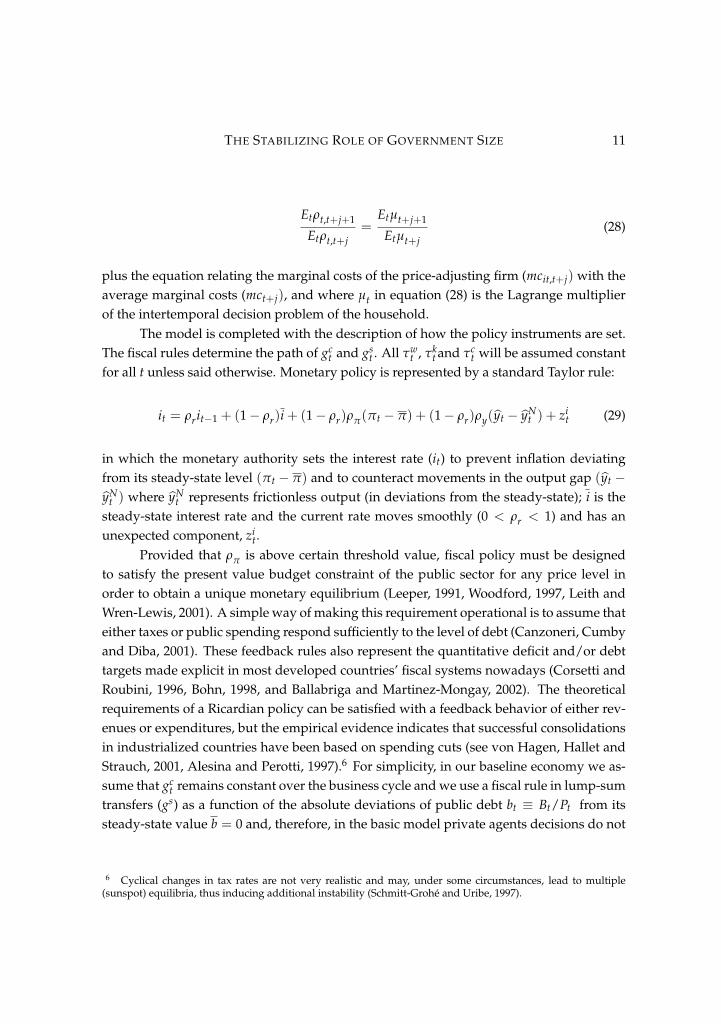
THE STABILIZING ROLE OF GOVERNMENT SIZE 12
Table 2Calibration of baseline model
σ β γ α ε δ σa ρa1.0 1.03
14 1.295 0.40 6.0 0.021 0.0078 0.80
τw τk τc gc/y gs/y ρr ρπ π0.279 0.279 0.10 0.18 0.16 0.5 1.5 1.020.25
depend on public debt consolidation:7
gst gs
gs ' bgst = αs
b
bt b
(30)
3.3. Model parameterizationWe obtain a numerical solution of the steady state as well as of the log-linearized system.Table 2 summarizes the values of the baseline parameters. Many parameters are similarto the ones used by Andrés and Doménech (2006), allowing the model to reproduce themost salient facts of business cycles in EMU as, for example, the relative volatility of con-sumption, investment or correlation between the primary budget surplus and output. Themodel also match the values of the private consumption and investment to GDP ratiosin steady state (c/y and e/y respectively) to the average values observed in EMU from1960 to 1999.8 Thus, the relative risk aversion coefficient (σ) is 1.0, the discount factor (β)is 0.9926, following Christiano and Eichenbaum (1992), and, since we assume that in thesteady state households allocate 1/3 of their time to market activities (as in Cooley andPrescott, 1995), the share of consumption in utility (γ) has been chosen to be 1.295.
The elasticity of output with respect to private capital (α) is 0.40, as in Cooley andPrescott (1995). The depreciation rate (δ) is equal to 0.021 as estimated by Christiano andEichenbaum (1992). The standard deviation (σa) and the first order autocorrelation co-efficient (ρa) of the technology shock are set to 0.0167 and 0.80 respectively. FollowingChristiano, Eichembaum and Evans (1997), the elasticity of demand with respect to price(ε) is set to 6.0, consistent with a steady-state mark-up, ε/(ε 1), equal to 1.20. The fixed
7 In the model with ricardian consumers, since the consolidation of budget debt is made through lump-sumtransfers, the value of αs
b in the fiscal rule has no effect on the dynamics of the endogenous variables of the modelexcept for public transfers and public debt. In the model with rule-of-thumb consumers, public transfers are acomponent of disposable income and then affect the consumption of these consumers. We have set a low valuefor (αs
b = 0.10), such that public debt is not explosive but the effects of fiscal consolidation on the dynamics ofRoT consumers are minimal.8 Empirical evidence about EMU business cycles can be found in Agresti and Mojon (2001).
THE STABILIZING ROLE OF GOVERNMENT SIZE 13
cost in production (κ) is then solved as a function of y and ε to produce zero profits in thesteady-state:
κ =y
ε 1(31)
Fiscal policy parameters have been set after computing the tax rates for OECD coun-tries using the method proposed by Mendoza, Razin and Tesar (1994). Given these num-bers, we assume for simplicity that there is a unique income tax (τk = τw = 0.279) whereasconsumption taxes (τc) are equal to 0.10. For the same sample of countries and years, gov-ernment consumption over GDP (gc/y) is 0.18 and transfers (gs/y) are 0.16. This calibra-tion yields no public debt in steady state, whereas the response of transfers to absolutedeviations of debt from its steady state is set at 0.1.
The last set of parameters refers to the interest rate rule. In the baseline model, weset the autocorrelation coefficient of the interest rate (ρr) equal to 0.5 and the responseto inflation deviations from target (ρπ) equal to 1.5. These values imply a response of theinterest rate to inflation slightly quicker and less aggressive than the one usually estimatedfor EMU countries (see, Doménech, Ledo and Taguas, 2002). The steady-state level of grossinflation (π) is set to 1.020.25, that is, the target level of the ECB. The model with supplyshocks has been simulated 100 times, producing 200 observations. We take the last 100observations and compute the steady-sate value (x) and the standard deviation of eachendogenous variable (σx). To avoid spurious correlation, we do not filter the simulateddata (see Cogley and Nason, 1995).
4. Government size and output volatility.We have simulated the model under different configurations of parameters to assess howthe size of the government affects the volatility of output. Government size will be cap-tured by a parameter η that will scale both expenditures and revenues so that the steadystate budget remains balanced. In other words, we will start with a baseline economy (b)and we will then look at transformations (j) in which government expenditures and taxrates are proportional to those of the benchmark model (τi
b and gib respectively):
τij = ητi
b
gij/yj = ηgi
b/yb
where 0.5 η 1.5, implying that the output share of total government expenditureschanges from 0.17 to 0.51.
The first three columns of Table 3 present the standard deviation of output as well
THE STABILIZING ROLE OF GOVERNMENT SIZE 14
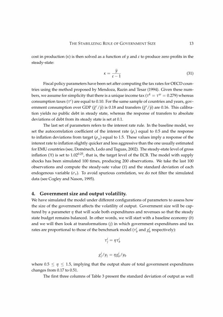
Table 3Government size and output and consumption volatility
Output Consumptionσy σy
∂ ln σy∂(G/Y) σc σc
∂ ln σc∂(G/Y)
η = 0.5 η = 1.5 η = 0.5 η = 1.5Θ = φ = 0 4.658 4.582 -0.049 1.986 2.802 1.012Θ = 0, φ = 0.75 4.952 4.735 -0.132 2.071 2.856 0.944Θ = 0.25, φ = 0 3.496 3.133 -0.323 2.502 3.036 0.568Θ = 0.25, φ = 0.75 1.709 1.337 -0.723 1.386 1.446 0.124
as its semi-elasticity, ∂ ln σy/∂(G/Y), as we change government size for different configu-rations of parameters. We present this semi-elasticity to be able to do a quick comparisonwith the results of Table 1 where the coefficients of the first row can be read also as semi-elasticities.9
The four economies of Table 3 differ in their degree of price rigidities (φ) and in thesize of the adjustment costs to capital (that is, parameter Θ which is the second derivativeof the installation costs function). In the case where Θ = φ = 0.0 we have a standard RBCmodel with no price rigidities or adjustment costs to investment. In this case we obtainresults which are similar to the findings of Galí (1994). As government size increases,output volatility barely changes.
We now introduce nominal rigidities and costs of adjustment to investment to addKeynesian features to the economy. As expected, adding rigidities to the model makes theeconomy less volatile. This effect is mainly driven by the adjustment costs to capital, as canbe seen by comparing rows 1 and 3 in Table 3. A comparison of rows 1 and 2 shows that therigidity of prices can make the economy more volatile by itself. We are not interested in theoverall volatility of output but on how this volatility changes as we change governmentsize. We can see this effect by either comparing columns 1 and 2, which are calculatedby two different sizes of government, or by looking at the next column that contains thesemi-elasticity of output volatility with respect to government size.
What can be seen as we move down through rows 2 to 4, is that, with rigidities,the volatility of output decreases as we increase government size. In other words, addingrigidities to the RBC economy allows us to generate important stabilizing effects from
9 It is important to notice that in the linear approximation of the model the semielasticity of output and con-sumption volatilities to government size are invariant to the choice of the standard deviation of technologyshocks (σz). Additionally, our simulations indicate that ∂ ln σ/∂(G/Y) is not affected by changes in G/Y withinthe range usually observed in the data, that is, the response of ln σ to changes in G/Y is linear.
THE STABILIZING ROLE OF GOVERNMENT SIZE 15
government size. And these stabilizing effects are directly linked to the degree of rigiditiespresent in the economy: as these rigidities increase this correlation becomes even morenegative (i.e., larger in absolute size). For example, in the case where Θ = 0.25, a valuewhich reproduce the relative volatility of investment to output in EMU, and φ = 0.75,in line with the estimates of Gali, Gertler and Lopez-Salido (2001) for the euro area, thesemi-elasticity of output volatility to government size is 0.25, approximately half of theestimated semi-elasticity in Table 1.
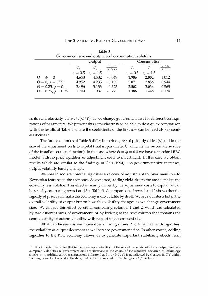
In Figure 1 we generalize the results of Table 1 by displaying this semi-elasticityas a function of the values for two key parameters: the degree of nominal rigidities (φ)and capital adjustment costs (Θ). We observe a monotonic negative relationship betweenthis semi-elasticity and the degree of rigidities in the model. As rigidities increase, thissemi-elasticity decreases.
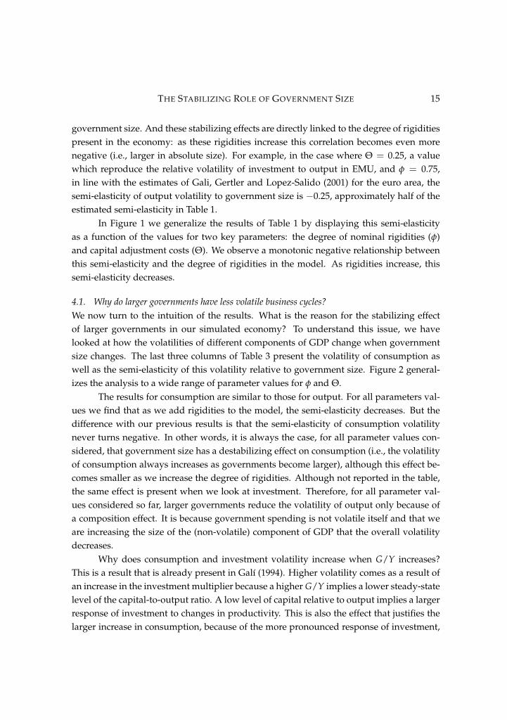
4.1. Why do larger governments have less volatile business cycles?We now turn to the intuition of the results. What is the reason for the stabilizing effectof larger governments in our simulated economy? To understand this issue, we havelooked at how the volatilities of different components of GDP change when governmentsize changes. The last three columns of Table 3 present the volatility of consumption aswell as the semi-elasticity of this volatility relative to government size. Figure 2 general-izes the analysis to a wide range of parameter values for φ and Θ.
The results for consumption are similar to those for output. For all parameters val-ues we find that as we add rigidities to the model, the semi-elasticity decreases. But thedifference with our previous results is that the semi-elasticity of consumption volatilitynever turns negative. In other words, it is always the case, for all parameter values con-sidered, that government size has a destabilizing effect on consumption (i.e., the volatilityof consumption always increases as governments become larger), although this effect be-comes smaller as we increase the degree of rigidities. Although not reported in the table,the same effect is present when we look at investment. Therefore, for all parameter val-ues considered so far, larger governments reduce the volatility of output only because ofa composition effect. It is because government spending is not volatile itself and that weare increasing the size of the (non-volatile) component of GDP that the overall volatilitydecreases.
Why does consumption and investment volatility increase when G/Y increases?This is a result that is already present in Galí (1994). Higher volatility comes as a result ofan increase in the investment multiplier because a higher G/Y implies a lower steady-statelevel of the capital-to-output ratio. A low level of capital relative to output implies a largerresponse of investment to changes in productivity. This is also the effect that justifies thelarger increase in consumption, because of the more pronounced response of investment,
THE STABILIZING ROLE OF GOVERNMENT SIZE 16
0.350.3
0.250.2
0.150.1
0.050
0
0.2
0.4
0.6
0.8
0.8
0.7
0.6
0.5
0.4
0.3
0.2
0.1
0
Capital adjustment costsφ
Out
put
sem
iela
stic
ity
Fig. 1: The semielasticity of output volatility to government size (∂ ln σ/∂(G/Y)) as a function of nominaland real rigidities when public consumption is acyclical.
0.30.25
0.20.15
0.10.05
0
0
0.2
0.4
0.6
0.8
0
0.2
0.4
0.6
0.8
1
Capital adjustment costsφ
Con
sum
ptio
n se
mie
last
icit
y
Fig. 2: The semielasticity of consumption volatility to government size (∂ ln σ/∂(G/Y)) as a function ofnominal and real rigidities when public consumption is acyclical.
THE STABILIZING ROLE OF GOVERNMENT SIZE 17
the associated increase in wealth leads to a larger response of consumption.As regards hours and wages, the empirical response of these two variables to pro-
ductivity shocks is a much debated issue in the literature. Some of the recent empiricalwork in this area has established the result that hours tend to fall on impact followinga positive technology shock (see, for example, Rotemberg, 2003, or Galí, 1999).10 Whilethis result is at odds with a standard RBC model, it can easily be accommodated withina model with significant nominal rigidities as discussed by Gali (1999). The intuition issimple. With the money supply being fixed (or not too accommodative), and sticky pricesfirms face constant demand and this means, for a higher level of productivity, that employ-ment has to go down. In economies with substantial rigidities, real wages fall on impactfor very much the same reasons as employment does in the presence of technology shocks.The response of real wages is the standard one as labor demand temporarily falls alongan upward sloping labor supply curve. Despite this short-run fall on labor income con-sumption should not fall if consumers are forward looking since permanent income risesas a result of the technology shock. This is what we observe in our calibrations as well. Inthe absence of rigidities, hours and real wages increase after a productivity shock. Witha high-enough degree of nominal rigidities the response of wages and hours becomes theopposite as in Gali (1999). But, still, consumption increases as long as forward lookingconsumers anticipate increases in income. Automatic stabilizers associated to large gov-ernments smooth disposable income in the periods that follow the productivity shock, butthey have very little effect on the dynamics of consumption.
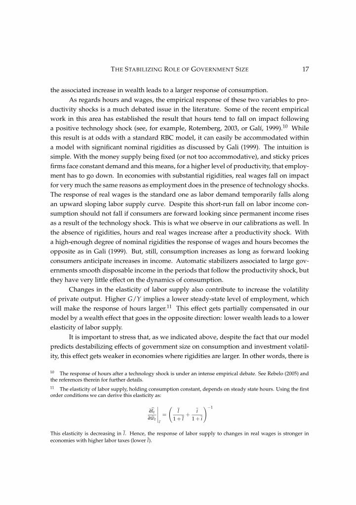
Changes in the elasticity of labor supply also contribute to increase the volatilityof private output. Higher G/Y implies a lower steady-state level of employment, whichwill make the response of hours larger.11 This effect gets partially compensated in ourmodel by a wealth effect that goes in the opposite direction: lower wealth leads to a lowerelasticity of labor supply.
It is important to stress that, as we indicated above, despite the fact that our modelpredicts destabilizing effects of government size on consumption and investment volatil-ity, this effect gets weaker in economies where rigidities are larger. In other words, there is
10 The response of hours after a technology shock is under an intense empirical debate. See Rebelo (2005) andthe references therein for further details.11 The elasticity of labor supply, holding consumption constant, depends on steady state hours. Using the firstorder conditions we can derive this elasticity as:
∂blt∂ bwt
c
=
l
1+ l+
i1+ i
!1
This elasticity is decreasing in l. Hence, the response of labor supply to changes in real wages is stronger ineconomies with higher labor taxes (lower l).
THE STABILIZING ROLE OF GOVERNMENT SIZE 18
Table 4Sensitivity to parameter changes
Output Consumptionσy σy
∂ ln σy∂(G/Y) σc σc
∂ ln σc∂(G/Y)
η = 0.5 η = 1.5 η = 0.5 η = 1.5σ = 2 1.399 1.066 -0.800 0.734 0.722 -0.050γ = 0.63 2.014 1.619 -0.643 1.637 1.759 0.211α
yg = 1.0 1.613 1.111 -1.095 1.441 1.557 0.227
σ = 2, γ = 2.0,α
yg = 1.0
1.206 0.804 -1.191 0.712 0.697 -0.062
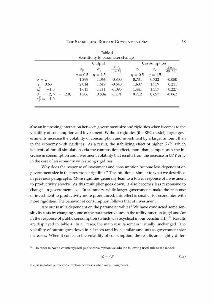
also an interesting interaction between government size and rigidities when it comes to thevolatility of consumption and investment. Without rigidities (the RBC model) larger gov-ernments increase the volatility of consumption and investment by a larger amount thanin the economy with rigidities. As a result, the stabilizing effect of higher G/Y, whichis identical for all simulations via the composition effect, more than compensates the in-crease in consumption and investment volatility that results from the increase in G/Y onlyin the case of an economy with strong rigidities.
Why does the response of investment and consumption become less dependent ongovernment size in the presence of rigidities? The intuition is similar to what we describedin previous paragraphs. More rigidities generally lead to a lower response of investmentto productivity shocks. As this multiplier goes down, it also becomes less responsive tochanges in government size. In summary, while larger governments make the responseof investment to productivity more pronounced, this effect is smaller for economies withmore rigidities. The behavior of consumption follows that of investment.
Are our results dependent on the parameter values? We have conducted some sen-sitivity tests by changing some of the parameter values in the utility function (σ, γ) and/orin the response of public consumption (which was acyclical in our benchmark).12 Resultsare displayed in Table 4. In all cases, the main results remain virtually unchanged. Thevolatility of output goes down in all cases (and by a similar amount) as government sizeincreases. When it comes to the volatility of consumption, the results are slightly differ-
12 In order to have a countercyclical public consumption we add the following fiscal rule to the model:
bgct = αc
ybyt (32)
If αcy is negative public consumption decreases when output augments.
THE STABILIZING ROLE OF GOVERNMENT SIZE 19
ent as, under some parameter values, the volatility of consumption also goes down whengovernment size increases. But this decline is still smaller than what we observed in thedata.
In summary, these preliminary results show that the model with real and nominalrigidities is partially able to account for the empirical evidence about volatility and gov-ernment size. While it can account for some of the stabilizing effects on output volatility, itcannot justify the stabilizing effect that we also observe empirically on consumption. Wenow explore an extension of the model that can help us match this behavior.
4.2. Introducing rule-of-thumb consumersWe now consider that only a proportion of consumers can borrow and lend in the finan-cial markets, whereas others are restricted in the sense that they choose consumption andleisure to maximize utility on a period-by-period basis.13 By looking at this class of con-sumers that cannot borrow or lend but simply spend all their current income, we hope touncouple the dynamics of investment and wealth from that of consumption. In that sense,the response of consumption for those individuals should closer mimic that of GDP.
A proportion (λ) of consumers will spend all of their current income as consumptionwhile the rest will follow the same optimizing behavior as in the previous version of themodel. Representing by crt, lrt and cot, lot consumption and labor supply of restricted andoptimizing consumers respectively, rule-of-thumb consumers face the following budgetrestriction,
Pt(1+ τct )crt = Pt(1 τw
t )Z 1
0witlrit + Ptλgs
t
Solving now the model, after the aggregation of the optimality conditions for both typesof consumer, the equilibrium described by the previous equations (15) to (28) includes twonew conditions
ct =λ
(1+ τct )
(1 τw
t )wt
1+ γ+
λgst
1+ γ
+ (1 λ)cot (33)
lt =λ
1+ γ
1 γλgs
t(1 τw
t )wt
+ (1 λ)lot (34)
whereas the Euler equation (17) now changes to
1 = βEt
(1+ τc
t )cσot+1(1 lot+1)
γ(1σ)
(1+ τct+1)c
σot (1 lot)γ(1σ)
1+ itπt+1
!(35)
13 These are ’rule-of-thumb’ consumers in Galí, López-Salido and Vallés (2003) terminology.
THE STABILIZING ROLE OF GOVERNMENT SIZE 20
Table 5Government size and volatility with λ = 0.65
Output Consumptionσy σy
∂ ln σy∂(G/Y) σc σc
∂ ln σc∂(G/Y)
η = 0.5 η = 1.5 η = 0.5 η = 1.5Θ = φ = 0.0 4.046 4.104 0.042 2.169 2.812 0.763Θ = 0.0, φ = 0.75 4.348 4.284 -0.044 2.488 2.947 0.498Θ = 0.25, φ = 0.0 3.372 3.001 -0.343 2.608 3.118 0.525Θ = 0.25, φ = 0.75 1.852 1.062 -1.636 2.934 1.028 -3.084
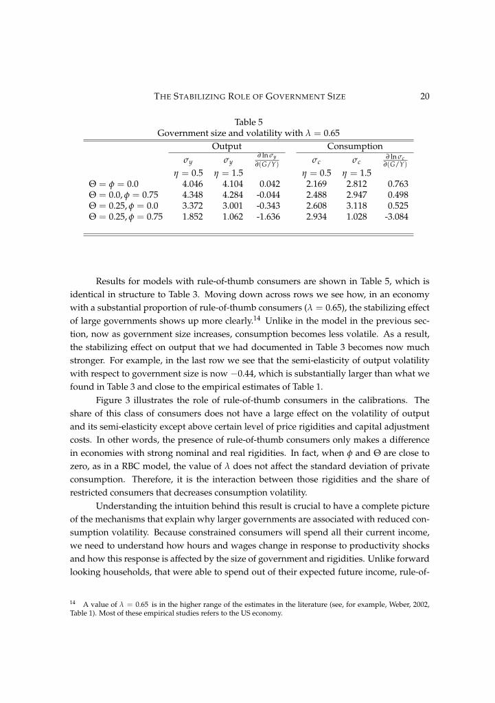
Results for models with rule-of-thumb consumers are shown in Table 5, which isidentical in structure to Table 3. Moving down across rows we see how, in an economywith a substantial proportion of rule-of-thumb consumers (λ = 0.65), the stabilizing effectof large governments shows up more clearly.14 Unlike in the model in the previous sec-tion, now as government size increases, consumption becomes less volatile. As a result,the stabilizing effect on output that we had documented in Table 3 becomes now muchstronger. For example, in the last row we see that the semi-elasticity of output volatilitywith respect to government size is now 0.44, which is substantially larger than what wefound in Table 3 and close to the empirical estimates of Table 1.
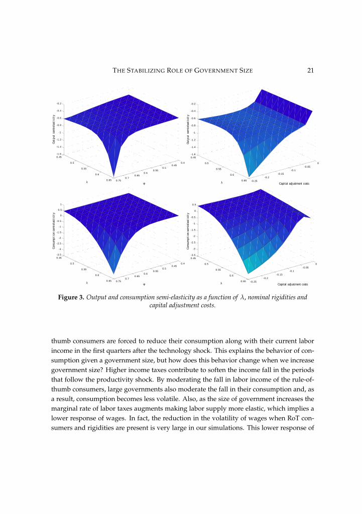
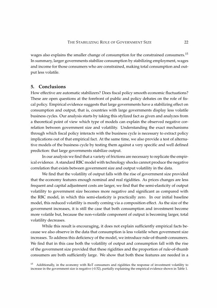
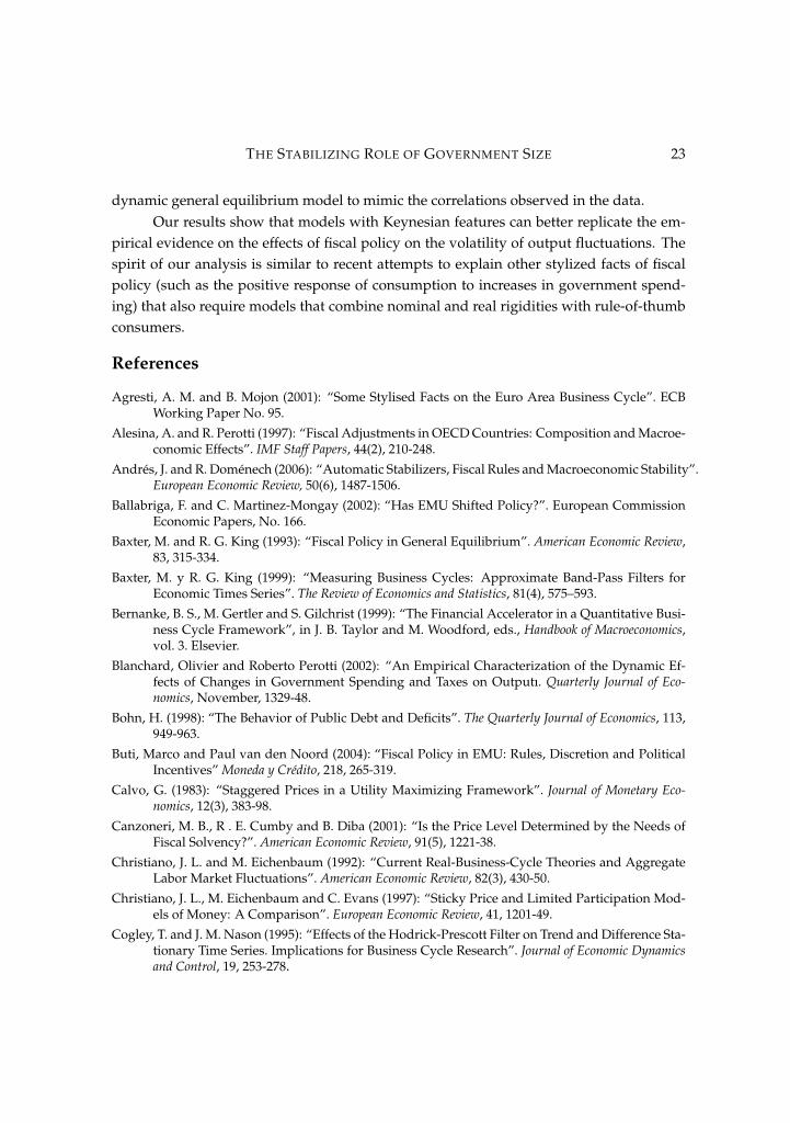
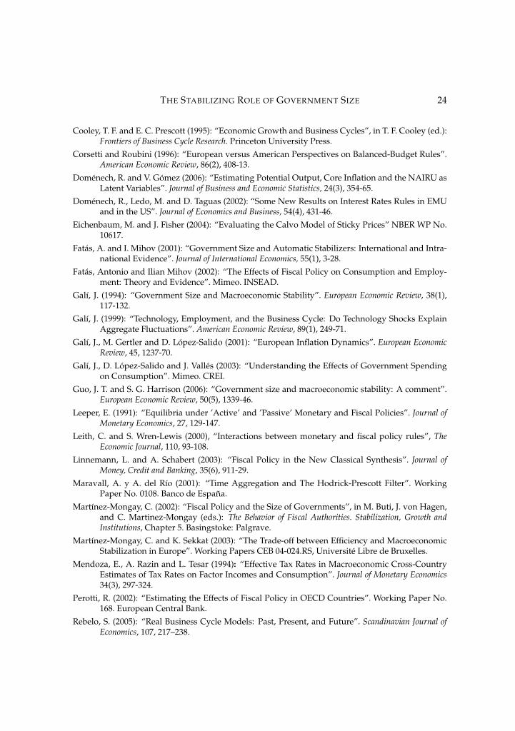
Figure 3 illustrates the role of rule-of-thumb consumers in the calibrations. Theshare of this class of consumers does not have a large effect on the volatility of outputand its semi-elasticity except above certain level of price rigidities and capital adjustmentcosts. In other words, the presence of rule-of-thumb consumers only makes a differencein economies with strong nominal and real rigidities. In fact, when φ and Θ are close tozero, as in a RBC model, the value of λ does not affect the standard deviation of privateconsumption. Therefore, it is the interaction between those rigidities and the share ofrestricted consumers that decreases consumption volatility.
Understanding the intuition behind this result is crucial to have a complete pictureof the mechanisms that explain why larger governments are associated with reduced con-sumption volatility. Because constrained consumers will spend all their current income,we need to understand how hours and wages change in response to productivity shocksand how this response is affected by the size of government and rigidities. Unlike forwardlooking households, that were able to spend out of their expected future income, rule-of-
14 A value of λ = 0.65 is in the higher range of the estimates in the literature (see, for example, Weber, 2002,Table 1). Most of these empirical studies refers to the US economy.
THE STABILIZING ROLE OF GOVERNMENT SIZE 21
0.40.45
0.50.55
0.60.65
0.70.75
0.45
0.5
0.55
0.6
0.65
1.6
1.4
1.2
1
0.8
0.6
0.4
0.2
φλ
Out
put
sem
iela
stic
ity
0.250.2
0.150.1
0.050
0.45
0.5
0.55
0.6
0.65
1.6
1.4
1.2
1
0.8
0.6
0.4
0.2
Capital adjustment costsλ
Out
put
sem
iela
stic
ity
0.40.45
0.50.55
0.60.65
0.70.75
0.45
0.5
0.55
0.6
0.65
3.5
3
2.5
2
1.5
1
0.5
0
0.5
1
φλ
Con
sum
pti
on s
emie
last
icit
y
0.250.2
0.150.1
0.050
0.45
0.5
0.55
0.6
0.65
3.5
3
2.5
2
1.5
1
0.5
0
0.5
Capital adjustment costsλ
Con
sum
pti
on s
emie
last
icit
y
Figure 3. Output and consumption semi-elasticity as a function of λ, nominal rigidities andcapital adjustment costs.
thumb consumers are forced to reduce their consumption along with their current laborincome in the first quarters after the technology shock. This explains the behavior of con-sumption given a government size, but how does this behavior change when we increasegovernment size? Higher income taxes contribute to soften the income fall in the periodsthat follow the productivity shock. By moderating the fall in labor income of the rule-of-thumb consumers, large governments also moderate the fall in their consumption and, asa result, consumption becomes less volatile. Also, as the size of government increases themarginal rate of labor taxes augments making labor supply more elastic, which implies alower response of wages. In fact, the reduction in the volatility of wages when RoT con-sumers and rigidities are present is very large in our simulations. This lower response of
THE STABILIZING ROLE OF GOVERNMENT SIZE 22
wages also explains the smaller change of consumption for the constrained consumers.15
In summary, larger governments stabilize consumption by stabilizing employment, wagesand income for those consumers who are constrained, making total consumption and out-put less volatile.
5. ConclusionsHow effective are automatic stabilizers? Does fiscal policy smooth economic fluctuations?These are open questions at the forefront of public and policy debates on the role of fis-cal policy. Empirical evidence suggests that large governments have a stabilizing effect onconsumption and output, that is, countries with large governments display less volatilebusiness cycles. Our analysis starts by taking this stylized fact as given and analyzes froma theoretical point of view which type of models can explain the observed negative cor-relation between government size and volatility. Understanding the exact mechanismsthrough which fiscal policy interacts with the business cycle is necessary to extract policyimplications out of that empirical fact. At the same time, we also provide a test of alterna-tive models of the business cycle by testing them against a very specific and well definedprediction: that large governments stabilize output.
In our analysis we find that a variety of frictions are necessary to replicate the empir-ical evidence. A standard RBC model with technology shocks cannot produce the negativecorrelation that exists between government size and output volatility in the data.
We find that the volatility of output falls with the rise of government size providedthat the economy features enough nominal and real rigidities. As prices changes are lessfrequent and capital adjustment costs are larger, we find that the semi-elasticity of outputvolatility to government size becomes more negative and significant as compared withthe RBC model, in which this semi-elasticity is practically zero. In our initial baselinemodel, this reduced volatility is mostly coming via a composition effect. As the size of thegovernment increases, it is still the case that both consumption and investment becomemore volatile but, because the non-volatile component of output is becoming larger, totalvolatility decreases.
While this result is encouraging, it does not explain sufficiently empirical facts be-cause we also observe in the data that consumption is less volatile when government sizeincreases. To address this deficiency of the model, we introduce rule-of-thumb consumers.We find that in this case both the volatility of output and consumption fall with the riseof the government size provided that these rigidities and the proportion of rule-of-thumbconsumers are both sufficiently large. We show that both these features are needed in a
15 Additionally, in the economy with RoT consumers and rigidities the response of investment volatility toincrease in the government size is negative (-0.52), partially explaining the empirical evidence shown in Table 1.
THE STABILIZING ROLE OF GOVERNMENT SIZE 23
dynamic general equilibrium model to mimic the correlations observed in the data.Our results show that models with Keynesian features can better replicate the em-
pirical evidence on the effects of fiscal policy on the volatility of output fluctuations. Thespirit of our analysis is similar to recent attempts to explain other stylized facts of fiscalpolicy (such as the positive response of consumption to increases in government spend-ing) that also require models that combine nominal and real rigidities with rule-of-thumbconsumers.
References
Agresti, A. M. and B. Mojon (2001): “Some Stylised Facts on the Euro Area Business Cycle”. ECBWorking Paper No. 95.
Alesina, A. and R. Perotti (1997): “Fiscal Adjustments in OECD Countries: Composition and Macroe-conomic Effects”. IMF Staff Papers, 44(2), 210-248.
Andrés, J. and R. Doménech (2006): “Automatic Stabilizers, Fiscal Rules and Macroeconomic Stability”.European Economic Review, 50(6), 1487-1506.
Ballabriga, F. and C. Martinez-Mongay (2002): “Has EMU Shifted Policy?”. European CommissionEconomic Papers, No. 166.
Baxter, M. and R. G. King (1993): “Fiscal Policy in General Equilibrium”. American Economic Review,83, 315-334.
Baxter, M. y R. G. King (1999): “Measuring Business Cycles: Approximate Band-Pass Filters forEconomic Times Series”. The Review of Economics and Statistics, 81(4), 575–593.
Bernanke, B. S., M. Gertler and S. Gilchrist (1999): “The Financial Accelerator in a Quantitative Busi-ness Cycle Framework”, in J. B. Taylor and M. Woodford, eds., Handbook of Macroeconomics,vol. 3. Elsevier.
Blanchard, Olivier and Roberto Perotti (2002): “An Empirical Characterization of the Dynamic Ef-fects of Changes in Government Spending and Taxes on Outputı. Quarterly Journal of Eco-nomics, November, 1329-48.
Bohn, H. (1998): “The Behavior of Public Debt and Deficits”. The Quarterly Journal of Economics, 113,949-963.
Buti, Marco and Paul van den Noord (2004): “Fiscal Policy in EMU: Rules, Discretion and PoliticalIncentives” Moneda y Crédito, 218, 265-319.
Calvo, G. (1983): “Staggered Prices in a Utility Maximizing Framework”. Journal of Monetary Eco-nomics, 12(3), 383-98.
Canzoneri, M. B., R . E. Cumby and B. Diba (2001): “Is the Price Level Determined by the Needs ofFiscal Solvency?”. American Economic Review, 91(5), 1221-38.
Christiano, J. L. and M. Eichenbaum (1992): “Current Real-Business-Cycle Theories and AggregateLabor Market Fluctuations”. American Economic Review, 82(3), 430-50.
Christiano, J. L., M. Eichenbaum and C. Evans (1997): “Sticky Price and Limited Participation Mod-els of Money: A Comparison”. European Economic Review, 41, 1201-49.
Cogley, T. and J. M. Nason (1995): “Effects of the Hodrick-Prescott Filter on Trend and Difference Sta-tionary Time Series. Implications for Business Cycle Research”. Journal of Economic Dynamicsand Control, 19, 253-278.
THE STABILIZING ROLE OF GOVERNMENT SIZE 24
Cooley, T. F. and E. C. Prescott (1995): “Economic Growth and Business Cycles”, in T. F. Cooley (ed.):Frontiers of Business Cycle Research. Princeton University Press.
Corsetti and Roubini (1996): “European versus American Perspectives on Balanced-Budget Rules”.American Economic Review, 86(2), 408-13.
Doménech, R. and V. Gómez (2006): “Estimating Potential Output, Core Inflation and the NAIRU asLatent Variables”. Journal of Business and Economic Statistics, 24(3), 354-65.
Doménech, R., Ledo, M. and D. Taguas (2002): “Some New Results on Interest Rates Rules in EMUand in the US”. Journal of Economics and Business, 54(4), 431-46.
Eichenbaum, M. and J. Fisher (2004): “Evaluating the Calvo Model of Sticky Prices” NBER WP No.10617.
Fatás, A. and I. Mihov (2001): “Government Size and Automatic Stabilizers: International and Intra-national Evidence”. Journal of International Economics, 55(1), 3-28.
Fatás, Antonio and Ilian Mihov (2002): “The Effects of Fiscal Policy on Consumption and Employ-ment: Theory and Evidence”. Mimeo. INSEAD.
Galí, J. (1994): “Government Size and Macroeconomic Stability”. European Economic Review, 38(1),117-132.
Galí, J. (1999): “Technology, Employment, and the Business Cycle: Do Technology Shocks ExplainAggregate Fluctuations”. American Economic Review, 89(1), 249-71.
Galí, J., M. Gertler and D. López-Salido (2001): “European Inflation Dynamics”. European EconomicReview, 45, 1237-70.
Galí, J., D. López-Salido and J. Vallés (2003): “Understanding the Effects of Government Spendingon Consumption”. Mimeo. CREI.
Guo, J. T. and S. G. Harrison (2006): “Government size and macroeconomic stability: A comment”.European Economic Review, 50(5), 1339-46.
Leeper, E. (1991): “Equilibria under ’Active’ and ’Passive’ Monetary and Fiscal Policies”. Journal ofMonetary Economics, 27, 129-147.
Leith, C. and S. Wren-Lewis (2000), “Interactions between monetary and fiscal policy rules”, TheEconomic Journal, 110, 93-108.
Linnemann, L. and A. Schabert (2003): “Fiscal Policy in the New Classical Synthesis”. Journal ofMoney, Credit and Banking, 35(6), 911-29.
Maravall, A. y A. del Río (2001): “Time Aggregation and The Hodrick-Prescott Filter”. WorkingPaper No. 0108. Banco de España.
Martínez-Mongay, C. (2002): “Fiscal Policy and the Size of Governments”, in M. Buti, J. von Hagen,and C. Martinez-Mongay (eds.): The Behavior of Fiscal Authorities. Stabilization, Growth andInstitutions, Chapter 5. Basingstoke: Palgrave.
Martínez-Mongay, C. and K. Sekkat (2003): “The Trade-off between Efficiency and MacroeconomicStabilization in Europe”. Working Papers CEB 04-024.RS, Université Libre de Bruxelles.
Mendoza, E., A. Razin and L. Tesar (1994): “Effective Tax Rates in Macroeconomic Cross-CountryEstimates of Tax Rates on Factor Incomes and Consumption”. Journal of Monetary Economics34(3), 297-324.
Perotti, R. (2002): “Estimating the Effects of Fiscal Policy in OECD Countries”. Working Paper No.168. European Central Bank.
Rebelo, S. (2005): “Real Business Cycle Models: Past, Present, and Future”. Scandinavian Journal ofEconomics, 107, 217–238.
THE STABILIZING ROLE OF GOVERNMENT SIZE 25
Rotemberg, J. J. (2003): “Stochastic Technical Progress, Smooth Trends, and Nearly Distinct BusinessCycles”. American Economic Review, 1543-1559.
Sbordone, A. (2002): “Prices and Unit Labor Costs: A New Test of Price Stickiness”. Journal of Mone-tary Economics, 49, 265-292.
Schmitt-Grohé, S. and M. Uribe (1997): “Balanced-Budget Rules, Distortionary Taxes and AggregateInstability”. Journal of Political Economy, 105 (5), 976-1000.
Silgoner, M.A., G. Reitschuler and Crespo-Cuaresma (2003): “Assessing the Smoothing Impact ofAutomatic Stabilizers: Evidence from Europe”, in Tumpel-Gugerell and Mooslechner (eds.),Structural Challenges for Europe, Edward Elgar.
Stock, J. H. and Watson, Mark W. (2002): “Has the Business Cycle Changed and Why?ı. NBERMacroeconomics Annual, 159–218.
van den Noord, P. (2000): “The Size and Role of Automatic Fiscal Stabilizers in the1990s and Beyond”.OECD Economics Department Working Papers, No. 230.
von Hagen, J., A.C. Hallet and R. Strauch (2001): “Budgetary Consolidation in EMU”. EconomicPapers, No. 148. European Communities.
Weber, C. E. (2002): "Intertemporal non-separability and rule-of-thumb consumption". Journal ofMonetary Economics, 49 (2002) 293–308.
Woodford, M. (1997): “Control of the Public Debt: A Requirement for Price Stability?” in G. Calvoand M. King, eds., The Debt Burden and Monetary Policy, London, MacMillan.
Woodford, M. (2003): Interest and Prices, Foundations of a Theory of Monetary Policy. Princeton Univer-sity Press.
Woodford, M. (2005): “Firm-Specific Capital and the New-Keynesian Philips Curve”. InternationalJournal of Central Banking, 1(2), p. 1-46.