Wolves adapt territory size, not pack size to local habitat quality

Acc

epte

d A

rtic

le

This article has been accepted for publication and undergone full peer review but has not been through the copyediting, typesetting, pagination and proofreading process, which may lead to differences between this version and the Version of Record. Please cite this article as doi: 10.1111/1365-2656.12366 This article is protected by copyright. All rights reserved.

Received Date : 03-Jul-2014

Revised Date : 21-Nov-2014

Accepted Date : 25-Feb-2015

Article type : Standard Paper

Wolves adapt territory size, not pack size to local habitat quality

Andrew M. Kittle*1, Morgan Anderson1, Tal Avgar1,a, James A. Baker1, Glen S. Brown2, Jevon Hagens3, Ed Iwachewski3, Scott Moffatt1, Anna Mosser1,b, Brent R. Patterson4, Douglas E.B. Reid3, Arthur R. Rodgers3, Jen Shuter3, Garrett M. Street1, Ian D. Thompson5, Lucas M. Vander Vennen1, and John M. Fryxell1

1 Department of Integrative Biology, University of Guelph, 50 Stone Road E., Guelph, ON, Canada, N1G 2W1

2 Ontario Ministry of Natural Resources, 1235 Queen Street East, Sault Ste. Marie, ON, Canada P6A 2E5

3 Ontario Ministry of Natural Resources, Centre for Northern Forest Ecosystem Research, Thunder Bay, ON, Canada P7B 5E1

4 Ontario Ministry of Natural Resources, Wildlife Research and Development Section, Trent University, DNA Building, 2140 East Bank Drive, Peterborough, ON, Canada K9J 7B8

5 Canadian Forest Service, 1219 Queen Street East, Sault Ste. Marie, ON, Canada, P6A 2E5

a Current address: Department of Biological Sciences, University of Alberta, Edmonton, AB, Canada

b Current address: College of Biological Sciences, University of Minnesota Twin Cities, St Paul, MN, USA

*corresponding author: [email protected]

Acc

epte

d A

rtic

le

This article is protected by copyright. All rights reserved.

Running headline: Wolves adapt territory size to local habitat quality

Summary

1. Although local variation in territorial predator density is often correlated with habitat quality,

the causal mechanism underlying this frequently observed association is poorly understood and

could stem from facultative adjustment in either group size or territory size.

2. To test between these alternative hypotheses we used a novel statistical framework to

construct a winter population-level utilization distribution for wolves (Canis lupus) in northern

Ontario, which we then linked to a suite of environmental variables to determine factors

influencing wolf space use. Next we compared habitat quality metrics emerging from this

analysis as well as an independent measure of prey abundance, with pack size and territory size

to investigate which hypothesis was most supported by the data.

3. We show that wolf space use patterns were concentrated near deciduous, mixed

deciduous/coniferous and disturbed forest stands favoured by moose (Alces alces), the

predominant prey species in the diet of wolves in northern Ontario, and in proximity to linear

corridors, including shorelines and road networks remaining from commercial forestry activities.

4. We then demonstrate that landscape metrics of wolf habitat quality – projected wolf use,

probability of moose occupancy and proportion of preferred land cover classes - were inversely

related to territory size but unrelated to pack size.

5. These results suggest that wolves in boreal ecosystems alter territory size, but not pack size,

in response to local variation in habitat quality. This could be an adaptive strategy to balance

tradeoffs between territorial defense costs and energetic gains due to resource acquisition. That

Acc

epte

d A

rtic

le


pack size was not responsive to habitat quality suggests that variation in group size is influenced

by other factors such as intra-specific competition between wolf packs.

Keywords: anthropogenic disturbance, boreal forest, Brownian bridge, generalized least squares,

optimal group size, predator density, repeated measures, rubber disc hypothesis, spatial

autocorrelation, territoriality

Introduction

For carnivores there is often a strong positive relationship between density and habitat

quality as defined by available prey biomass (Miquelle et al. 1999; Carbone & Gittleman 2002;

Fuller, Mech & Cochrane 2003; Markar & Dickman 2005). Local density for a gregarious

territorial species can be defined as the average territory size divided by average group size

(Mosser et al. 2009), so higher densities could result from either metric.

Territory size is expected to be inversely related to habitat quality since the energetic

costs associated with maintaining territories typically ensures they are as large as necessary, but

as small as possible (Macdonald 1983). This implies a flexible approach to territoriality, the so-

called rubber disc hypothesis first described by Huxley (1934). This has been observed in

multiple carnivore species. For example, coyote (Canis latrans) group territory sizes contract

with increasing hare and deer densities in Eastern Canada (Patterson & Messier 2001), leopard

(Panthera pardus) home range sizes throughout Africa and Asia are inversely related to

available prey biomass (Markar & Dickman 2005) and female lion (Panthera leo) home range

sizes similarly decrease with increasing prey biomass in Zimbabwe, after accounting for pride

biomass (Loveridge et al. 2009).

Acc

epte

d A

rtic

le


Alternately, if fitness is linked to habitat quality one might expect groups holding the best

habitat to exhibit higher rates of reproduction and recruitment, logically contributing to greater

potential for large group size, as seen in Serengeti lions (Mosser et al. 2009). Large lion prides

out-compete smaller prides for high quality habitat (Mosser 2008) and patch richness has been

demonstrated to determine maximum lion group biomass (Valeix, Loveridge & Macdonald

2012). European badger (Meles meles) group size has also been shown to positively correlate

with patch quality, as measured by earthworm abundance (Kruuk & Parish 1982). Furthermore,

the rate of emigration from social groups can be inversely related to resource availability as

mediated by intra-specific competition (Bowler & Benton 2005; VanderWaal, Mosser & Packer

2009). This potentially results in lower emigration rates from better quality habitat (Stacey &

Ligon 1987; Pasinelli & Walters 2002) leading to increased group sizes therein. Although habitat

quality is most often, and directly, expressed as food availability (Carbone & Gittleman 2002)

other measures of quality include available shelter (Sprent & Nicol 2012), level of disturbance

(Kapfer et al. 2010), vegetative cover (McLoughlin et al. 2003) and proportion of open water

(Fortin, Blouin-Demers & Dubois 2012).

Here we use GPS radio-telemetry for 34 wolf packs in northern Ontario to determine

which environmental factors most influence winter wolf space use across a boreal forest

ecosystem. We then employ the projected wolf use probabilities, habitat attributes identified as

disproportionately utilized by wolves and an independent prey abundance measure, as quality

metrics to test whether local variation in wolf population density results from adaptive changes

in pack size or territory size. If wolves respond to changes in habitat quality behaviourally by

adjusting their pack size to match local environmental conditions at the pack level, then we

would expect to see habitat quality metrics positively related to pack size, whereas if wolves are

Acc

epte

d A

rtic

le


adjusting their territory size to match these conditions we would expect to see an inverse

relationship between quality metrics and territory size.

Materials and Methods

Study area

Research was conducted in the boreal forest of Northern Ontario’s Shield Ecozone

between 92°1’W, 52° 6’N and 86°32’W, 49°49’N (Crins et al. 2009). Common trees include

black spruce (Picea mariana), jack pine (Pinus banksiana), white spruce (Picea glauca), balsam

fir (Abies balsamea), white birch (Betula papyrifera) and trembling aspen (Populus

tremuloides).Tamarack (Larix larcinia) and white cedar (Thuja occidentalis) are restricted to

lowland sites (Crins et al. 2009).

The study area straddles the northern boundary of the Ontario Ministry of Natural

Resources’ Area of the Undertaking (AOU), where timber extraction is licensed. Subsequently

there is a marked southeast to northwest transition from high to low levels of anthropogenic

disturbance, accompanied by a similar gradient in predator and prey densities. Wolf density

estimates, derived from the total number of known individuals within the minimum convex

polygon (MCP) of all telemetry re-locations, were 5.1/1000km² in the southeast and 3.1/1000km²

in the northwest. Moose density, estimated from fixed-wing aerial surveys, was 46/1000km² in

the southeast and 24/1000km² in the northwest. The spatial distribution of moose and wolves

were sampled across this gradient, centred on the townships of Pickle Lake in the northwest and

Nakina in the southeast.

Acc

epte

d A

rtic

le


Wolf resource utilization

Between February 2010 and January 2013 52 wolves were tracked using GPS telemetry

collars (Lotek 7000MA, 7000SAW, Lotek Inc, Newmarket, Ontario); 37 individuals representing

23 packs in the southeast and 15 from 11 packs in the northwest (Fig. 1). Wolves were captured

using padded leg-hold traps (#7 EZ grip, Livestock Protection Co., Alpine, Texas, USA) in

summer (2010 – 12) and helicopter net-gunning in winter (2010-12). Summer captures were

immobilized with a xylazine hydrochloride (2 mg/kg) and Telazol (4 mg/kg) combination with a

Yohimbine (0.15 mg/kg) antagonist. Winter captures were physically restrained but not

chemically immobilized during collaring. Wolf re-locations were recorded every 2.5- 5 hours

with fix rate success averaging 91% (range 77-99%, n=17, Anderson 2012) allowing for

unbiased resource utilization analyses (Frair et al. 2004).

Instead of averaging un-standardized coefficients from individual-level resource

utilization functions to infer population-level processes (Marzluff et al. 2004, Long et al. 2009)

we developed population-level utilization distributions (UDs) for winter (1 November – 30

April) which were linked directly to landscape characteristics. This allows for population-level

patterns to be detected directly. Furthermore, because population-level UDs were created by

amalgamating individual pack-level UDs, this method permits the effective incorporation of

territoriality as well as individual variation in selection (Bolnick et al. 2003)

Pack-level utilization distribution

Utilization distributions were determined (cell size = 100x100m) for each

individual/winter using kernel Brownian bridge (kbb) home range estimation (Calenge 2006).

This is conditioned on the start and end spatial coordinates of each move, time between points

Acc

epte

d A

rtic

le


and the individual’s speed of movement (Bullard 1999; Horne et al. 2007). Two smoothing

parameters incorporated into the kbb model relate to each individual animal’s mobility (σ1) and

relocation imprecision (σ2). The R function liker (Horne et al. 2007) was used to estimate σ1,

with σ2 defined as 30m (Frair et al. 2010). Given the number and frequency of relocations used

here, it is unlikely that utilization estimates substantially differ from those obtained using fixed

kernel density estimation (Horne et al. 2007 Fig. 3). However an advantage of the kbb method,

given its mechanistic basis, is that frequently used areas of an animal’s range are more likely to

be connected via pathways (Horne et al. 2007). For wide ranging species like wolves, selected

movement paths influence prey availability and encounter rates (McPhee et al. 2012). Therefore

it is useful to probabilistically estimate movements between observed locations, and objectively

quantify and incorporate into estimates uncertainty resulting from the time and distance between

these observations (Horne et al. 2007). This provides a more accurate assessment of the areas an

individual actually used (Horne et al. 2007) and provisions greater allowance for unused areas of

potential biological significance. It is important to note that this method is informative only when

successive locations are autocorrelated (Kie et al. 2010) since as the relocation interval increases,

the inherent assumption of a conditioned random walk with constant movement rate between

relocations becomes less realistic (Horne et al. 2007). Autocorrelation is typical of fine scale

temporal data generated by GPS telemetry and incorporating it into range utilization estimates

instead of accounting for it by sub-sampling data is appealing.

Wolves move widely and rapidly through their ranges, often utilizing movement

corridors along linear features (Whittington, Cassady St.Clair & Mercer 2005; Latham et al.

2011). This allows them to visit all parts of their range within 1-3 weeks (Weaver 1994;

Acc

epte

d A

rtic

le


Jedrejewski et al. 2001) and results in “holes” of low use within territories. Brownian bridge

UDs were therefore determined for all individuals with data covering >10% of the winter (18.4

days). Average coverage was 105 days (57.2%; N=62). A linear regression conducted with

pooled data showed no relationship between number of fixes and range size (P > 0.15). If two

pack-related individuals were tracked in a single winter but exhibited no temporal overlap, we

calculated kbb UDs for each and combined them with cell values weighted by relative temporal

coverage (i.e. if wolf A was tracked for 25% of winter and wolf B 50%, wolf A’s values were

weighted half those of wolf B’s in the combined UD (i.e. 0.33 and 0.67)). If two pack-related

wolves overlapped in time, only the individual with the longer tracking duration was retained.

Landscape-level utilization distribution

Kernel Brownian bridge UDs were converted to volume UDs (vUDs) for which the value

of a pixel equals the percentage of the smallest home range containing it (Calenge 2006),

therefore ascribing low values to high use areas (i.e. the vUD value is 10 for a pixel included in

an animal’s 10% territory and 95 for a pixel included only in the 95% territory). The study area

was overlaid with a grid of hexagonal cells, with 500m between centroids. Within each resulting

0.22km2 hexagonal cell the average pack vUD value was extracted. Volume UDs were subtracted

from 100 to arrive at more intuitive measures for each cell (i.e. a cell with vUD of 95 was valued

as 100 - 95 = 5). Only hexagons with values > 5 were retained to mimic the 95% territory.

Individual pack use values were integrated to 1 to remove bias imposed by differing territory

sizes. If multiple pack ranges overlapped single cells, values were summed to determine the

cumulative use of cells. This was repeated to create 4 landscape-level winter wolf UDs (2009-10

Acc

epte

d A

rtic

le


to 2012-13). The final population-level UDs were based on 60,196 relocations from 23 southeast

and 11 northwest packs.

Statistical modeling of wolf UD

Each hexagon/year was associated with wolf use estimates from the relevant population

level UD and with temporally appropriate habitat and landscape covariates. Relative elevation

reflects the effect of localized topographical differences (i.e. highlands vs. lowlands) which

influence dominant vegetation and can be meaningful to animal space use patterns (Kittle et al.

2008). We therefore calculated elevation at each pixel’s centroid relative to the average elevation

within a 500m radius buffer calculated from a digital elevation map (NASA Land Processes

Distributed Active Archive Centre (LP DAAC) 2009). Current and preceding seasons’ average

normalized difference vegetation indexes (NDVI) were also calculated, indicating vegetation

growth across the landscape (NASA Land Processes Distributed Active Archive Centre (LP

DAAC) 2013). These were determined by averaging the 250m resolution, 16-day windows that

cover the relevant season’s 4-month core (June-September for summer and December-March for

winter). This provides a generic measure of vegetation growth, as opposed to standing biomass

(Pettorelli et al. 2005), that complements individual land cover classes and may be used as a cue

by wolves in their search for prey (Courbin et al. 2014). Independent variables also included

Boolean measures of proximity to dump (<1km=1; >1km=0), settlement (<1km=1; >1km=0),

primary (paved and primary classes) roads (<500m=1; >500m=0) and secondary roads

(secondary, tertiary, rail and utility classes) (<500m=1; >500m=0). Dumps provide a spatially

fixed and consistent food source for wolves to exploit (Ciucci et al. 1997; Lesmerises, Dussault

Acc

epte

d A

rtic

le


& St-Laurent 2012) whereas settlements can represent heightened risk and have been used as

spatial refugia by herbivores to avoid wolves (Hebblewhite et al. 2005). Roads, which can

increase mobility and lead to improved hunting efficiency (James & Stuart-Smith 2000;

Whittington et al. 2011), are selectively used as travel corridors where vehicle traffic is sparse

(Hebblewhite & Merrill 2008). Similarly, shorelines can provide increased mobility for wolves

and may provision increased encounters with prey (Latham et al. 2011), so distances (km) to

shorelines of rivers or large lakes (>500m in diameter) were also included. Unlike roads, dumps

and settlements, these features are widely distributed across the landscape so Boolean conversion

was unnecessary.

Land cover proportions were calculated for each cell using the 30m² resolution Far North

Land Cover map (OMNR 2013). This map does not extend south of ~50° N latitude so was

merged with an earlier Ontario Land Cover map (Spectranalysis Inc. 2004) where necessary.

Maps included updated disturbances (fire and harvest) for each year of the study. Land cover

classes were amalgamated into 9 categories. These included water (open and turbid classes)

which offers the possibility of increased prey vulnerability in winter (Kunkel & Pletscher 2001).

Lowland classes, typically avoided by wolves in winter (McLoughlin et al. 2003), were defined

as open lowland (open fen, open bog and freshwater marsh classes), treed lowland (treed

peatland, treed fen, treed bog and coniferous swamp classes) and deciduous lowland (thicket

swamp and deciduous swamp classes). Deciduous (deciduous treed class) and mixed upland (25-

75% deciduous and 25-75% coniferous; mixed treed class) classes represent preferred moose

forage (Peek 2007) whereas sparse forest (sparse treed class) is preferred by woodland caribou

(Rangifer tarandus caribou), the secondary prey species of wolves in this system (O’Brien et al.

Acc

epte

d A

rtic

le


2006). Disturbed (disturbed treed/shrub and disturbed non/sparse classes representing natural

and anthropogenic disturbances) classes, typically preferred by moose for forage (Brown 2011),

were differentiated from newly disturbed (< 1 year from fire or forestry disturbance) classes. A

10th category, coniferous forest, considered the default of the boreal and highly correlated with

the other land cover classes (Dormann et al. 2013), was withheld from the model as the reference

class in comparison to which other classes were interpreted (Hosmer & Lemeshow 2000).

A total of 169,738 hexagonal cells were thus characterized. Due to computational

constraints a single analysis of the dataset was impossible so hexagons were systematically sub-

sampled at every 50th location from west to east starting from the NW corner (Long et al. 2009).

This was repeated 49 times with the second sub-sample starting from the 2nd hexagon from the

NW corner, then from the 3rd, then the 4th until all hexagons were sampled. This ensured no

hexagons were repeated in any of the 50 sub-samples. After conducting correlation analysis to

ensure independent variables were not highly correlated (r < 0.7; Dormann et al. 2013), 50

generalized least squares (GLS) mixed effect regression models (gls in R package nlme), one for

each sub-sample, were used to link wolf use to the full suite of predictor variables. The natural

logarithm of the wolf use value was used to better fit model assumptions. GLS models allow

spatial autocorrelation in the response variable to be explicitly accounted for as random effects

(Zuur et al. 2009). Using GLS two additional parameters, the spatial autocorrelation range and

nugget, are estimated. The range is a distance measure indicating the point on the x-axis of a

variogram at which autocorrelation between points disappears, whereas the nugget is the y-value

when the distance between points is 0, and represents the variable discontinuity imposed by the

spatial structures at distances less than the actual minimum distance between points (Zuur et al.

Acc

epte

d A

rtic

le


2009). These random effects are meant to improve parameter estimate precision by separately

modelling the dependence structure between measurements which otherwise gets incorporated

into parameter estimates (Zuur et al. 2009). Semi-variograms of normalized residuals were

employed to initially detect autocorrelation and inform initial range and nugget estimates

(Crawley 2007). Rational quadratic spatial correlation (corRatio in nlme) dealt most effectively

with the spatial autocorrelation in response variables, determined by comparing various

correlation structures using AIC and visualizing output with semi-variograms of normalized

residuals (Crawley 2007). Plots of normalized residuals against fitted values and normal plots

were used to verify model fit (Crawley 2007).

Output model coefficients were averaged among the 50 models and all predictor variables

retained. This method includes the uncertainty inherent in the models based on the logic that

effects that vary substantially in direction among the 50 subsamples should average out to ~0

(Harrell 2001; John Fieberg, University of Minnesota, personal communication). An additional

benefit of running 50 separate models was that it allowed for the empirical estimation of

confidence intervals. The averaged coefficients from the model output were then used to project

wolf use values across the landscape.

Mean confidence intervals were determined for each model-averaged coefficient using:

± (zα/2)*(σ/ )

Acc

epte

d A

rtic

le


where = model averaged coefficient estimate, zα/2 = 95% critical value of the normal

distribution, σ = standard deviation of coefficient estimates (β) across all models and =

square root of total number of coefficient estimates (β).

Comparing quality metrics to individual pack characteristics

Pack size was enumerated during winter/spring helicopter captures when most wolves

were collared and packs typically range as a cohesive unit (Mech & Boitani 2003). Pack size was

further monitored during winter kill site investigation and collar retrieval when numbers were

estimated from the number of beds around kills and backtracking to open areas (e.g. frozen

lakes) where packs fanned out and individual tracks could be counted. This often allowed

multiple pack size estimates which were averaged to provide a single mean seasonal estimate.

Range attributes of collared individuals travelling alone were excluded from analysis. These

“satellites” tend to be motivated by different factors than pack living animals, such as searching

for mates or territory, and display different spatial patterns as a result, typically roaming widely

across the landscape (Mech & Boitani 2003). Using only packs >1 with pack size directly

determined in the field in the same winter as data collection resulted in 42 winters of data from

26 different packs.

The size of each pack’s 95% territory and 50% core area were determined from the

Brownian bridge kernels and, using known pack sizes, local density of each was determined.

Measures of habitat quality were then determined for these same 95% territories and 50% core

Acc

epte

d A

rtic

le


areas (Table S1, Supporting material). These were the average projected wolf use value, the

probability of moose occupancy of each pixel (Lele et al. 2013) as projected from an

independent resource selection probability function analysis (Street et al. unpublished

manuscript; a description of the resource selection modelling procedure is detailed in Appendix

S1, Supporting material), and the proportion of individual land cover variables selected or

avoided by wolves in the population-level model. These were considered measures of habitat

quality because areas of higher projected wolf use, which emerged from the population-level

resource utilization analysis described above, reflects population-level wolf habitat selection that

over evolutionary time, should maximize fitness (Morris 2003). Following this logic, specific

habitat classes selected at the population level were defined as high quality and those avoided as

low quality. Areas of higher probability of moose occupancy reflect better habitat in that it is

more likely to hold prey resources, a key factor influencing predator distribution and abundance

(Carbone & Gittleman 2002). Since individual pack characteristics were measured across

multiple years, repeated measures linear mixed effects modeling was employed to investigate the

link between these quality measures and local wolf density, pack sizes and territory sizes. The

influence of pack size on territory size was similarly assessed at both 95% and 50% levels. Pack

size, territory size and wolf density were each log transformed to better meet modeling

assumptions.

Statistical and spatial analysis was undertaken using R software version 2.15.1, R

Development Core Team 2012, ArcMap 10.1 (ESRI Inc.) and Geospatial Modeling Environment

0.7.2.0.

Acc

epte

d A

rtic

le


Results

Wolves tended to use lower elevation areas relative to the immediate surroundings but

also avoided both open and treed lowlands (Fig. 2). Deciduous, mixed and disturbed forest areas

were preferentially utilized whereas recently disturbed areas were avoided. Open water was

similarly avoided whereas areas close to shorelines were strongly selected (negative coefficient

for increasing distance). Associations with anthropogenic features were mostly positive, with

dumps strongly selected, settlements eliciting no strong response and areas close to roads,

particularly secondary roads, preferentially used. Vegetation growth, as measured by NDVI, was

influential and associations indicated use of areas with low winter growth (negative β) but high

summer growth (positive β).

Wolf densities within the 95% and 50% territories exhibited consistently positive

associations with habitat quality metrics (Table 1). Local wolf density was strongly correlated

with wolf use as projected from the GLS model and was also positively associated with average

probability of moose occupancy (Fig. 3). Mixed forest proportion was also positively associated

with local wolf density (95%: R² = 0.26, P < 0.01; 50%: R² = 0.18, P < 0.05). The proportion of

disturbed forest showed a similar trend but the relationship was marginally significant only at the

95% range (R² = 0.04, P < 0.1). Conversely the open lowland proportion was negatively

associated with wolf density, weakly so within the core range (95%: R² = 0.21, P < 0.01; 50%:

R² = 0.14, P < 0.1).

Territory size was also consistently associated with most measures of habitat quality

(Table 1). Larger 95% and 50% territories had lower average projected wolf use values and also

had lower average moose occupancy probabilities (Fig. 4). Larger ranges also included lower

Acc

epte

d A

rtic

le


mixed forest proportions at both scales (Table 1; 95%: R² = 0.14, P < 0.05; 50%: R² = 0.09, P <

0.1) as well as lower proportions of disturbed forest (95%: R² = 0.17, P < 0.01; 50%: R² = 0.03,

P ≤ 0.1) although in both instances associations with core territories were weak. Open lowland

was positively associated with the 95% range size (R² = 0.22, P < 0.01) indicating that larger

ranges include proportionally more of this poor quality habitat. The proportion of deciduous

forest (high quality) was not associated with local density or territory size (P > 0.1). In

comparison, there was no significant relationship between pack size and any of the habitat

quality variables tested (Table 1). We found no significant relationship between territory size and

pack size at the 95% level (P = 0.17) and a marginally positive relationship at the 50% core (P

=0.09).

Discussion

Wolf resource utilization across this broad, heterogeneous landscape was influenced by a

variety of landscape modifiers and habitat attributes. Wolves made disproportionate use of

deciduous, mixed and disturbed forest, corresponding to high quality moose habitat (Peek 2007;

Brown 2011; Street et al. unpublished manuscript). Conversely, lowland habitat was avoided

here, as in other boreal sites elsewhere in Canada (McLoughlin et al. 2003), as were frozen lakes.

However, wolves heavily used shorelines, which are typically preferred as travel corridors

(Latham et al. 2011). Anthropogenic disturbances were generally exploited. Dump sites were

disproportionately utilized as expected given that they were situated away from settlements and

therefore represent a consistent and largely risk-free food source (Murray et al. 2010). Areas

close to roads were also preferred. Like shorelines, sparsely used transport corridors provide a

Acc

epte

d A

rtic

le


convenient means for wolves to move quickly through the landscape (Hebblewhite & Merrill

2008; Latham et al. 2011). This increase in velocity across the landscape has been linked in this

system to higher kill rates of moose by wolves (Moffatt 2012). Such linear features can also be

important for territorial behaviour, used as territorial boundaries via scent marking (Peters &

Mech 1975).

Direct fitness measures such as demographic vital rates should be ideal indicators of

habitat quality (Van Horne 1983) but such basic measures as reproductive rate are often density-

dependent, complicating habitat assessment for a population near its ecological carrying capacity

(Mitchell & Hebblewhite 2012). More problematic is that accurate fitness measures are difficult

to attain (Silk 2007). As a result density is often used as an indicator of quality given its intuitive

link with fitness (McLoughlin et al. 2010). For territorial species where social restrictions on

access to prime habitat increases the chances of subdominant individuals or social groups

utilizing suboptimal habitat (Fretwell & Lucas 1969), the putative relationship between habitat

quality and density may be obscured (Van Horne 1983; Mosser et al. 2009; DeCesare et al.

2014). However, even in species not under ideal free distribution, density can provide a better

short term measure of habitat quality than demographic vital rates due to environmental and

demographic stochasticity (Mosser et al. 2009). Given these complications, demonstrating a

clear link between density and habitat quality is particularly useful for population management.

Here local wolf density was positively related to probability of moose use, consistent with

observations that the main factor driving obligate carnivore densities is the density or availability

of prey (Fuller & Sievert 2001; Carbone & Gittleman 2002; Fuller, Mech & Cochrane 2003;

Karanth et al. 2004). Consistent relationships between pack-level density and the other habitat

Acc

epte

d A

rtic

le


quality metrics here further suggests that local density may be a reasonable metric of short-term

habitat quality in this system (Mosser et al. 2009, van Beest et al. 2014).

In a seminal paper Macdonald (1983) demonstrated a strong positive correlation between

wolf pack and territory sizes, as well as a similar relationship between coyote, lion and spotted

hyena (Crocuta crocuta) groups and their territories. However more recent studies have typically

failed to find such a relationship for coyotes (Patterson & Messier 2001) or wolves (Potvin 1988;

Fuller 1989; Mech et al. 1998) and in Montana, wolf territory sizes were inversely correlated

with pack size (Rich et al. 2012). Lions in the Selous showed no relationship between group and

territory size (Sprong 2002) whereas Serengeti lions did, albeit only when partitioned by habitat

type (Mosser & Packer 2009). Large spotted hyena clans in Ngorongoro Crater held larger

territories than did smaller clans (Höner et al. 2005). The relationship between group and

territory size can be nuanced such as for Ethiopian wolves (Canis simensis) for which territory

size is primarily determined by the number of adult males plus the dominant female in a group,

not the group size as a whole (Tallents et al. 2012).

Maintaining a territory requires considerable energy expenditure to enable perimeter

patrol, scent marking and occasional direct aggression against transgressors, so it should

therefore be big enough to encompass essential resources, but small as possible to ensure

energetic efficiency (Macdonald 1983). This results in the oft-observed inverse relationship

between territory size and habitat quality (Gass, Angehr & Centa 1976; Village 1982; Smith &

Shugart 1987; Mills & Knowlton 1991; Patterson & Messier 2001; McLoughlin et al. 2003;

Acc

epte

d A

rtic

le


Markar & Dickman 2005; but see Tallents et al. 2012). This pattern was also detected in our

study suggesting that wolves here employ an adaptive approach to territoriality, whereby the

extent of the defended core shifts as a function of resource quality, consistent with the elastic

disc hypothesis (Huxley 1934; Potts, Harris & Giuggioli 2013). This strategy allows wolves to

optimize the trade-off between the costs of territorial defense and gains from resource acquisition

(Hixon 1980; Schoener 1983).

Pack size was not linked with any available metrics of habitat quality at either scale,

including prey habitat preference, indicating that wolf group size is regulated by other factors.

Optimal group size theory indicates that territorial animals should strive to best compromise the

potential advantages of shared costs vs. disadvantages arising from resource depletion (Brown

1982). Larger foraging groups often have improved attack success and are able to subdue larger

prey, broadening their available prey base (Creel & Creel 1995). However large groups do not

necessarily confer foraging advantages (Schmidt & Mech 1997) because the cost of sharing the

spoils (Packer, Scheel & Pusey 1990), tendency to “free ride” (MacNulty et al. 2012) and

reduced efficiency of group search can outweigh any potential benefit (Caro 1994; Fryxell et al.

2007). The optimal foraging group size for wolves based on per capita intake has been estimated

at ~2 (Thurber & Peterson 1993; Hayes et al. 2000) although offsetting the impact of scavenging

by ravens (Corvus corax) might promote formation of larger groups (Vucetich et al. 2002).

Similarly, small group size was predicted for African wild dogs (Lycaon pictus) until variation in

foraging costs were incorporated into the determination of energetics of cooperative hunting,

which increased the pack size predicted by peak per capita food intake rate (12-14) such that it

closely matched the modal observed adult pack size (10) (Creel & Creel, 1995).

Acc

epte

d A

rtic

le


An alternative mechanism promoting increased pack size is intra-specific competition,

including protection of young from con-specific predation (Packer, Scheel & Pusey 1990).

Larger lion prides dominate smaller ones (McComb, Packer & Pusey 1994; Heinsohn & Packer

1995) and are significantly more able to control disputed areas and improve their territory quality

through acquisition of additional area (Mosser & Packer 2009). In highly competitive

environments, retaining group members might be even more important (Heinsohn 1997). For

example, where overall lion density was high, females were less likely to disperse from prides

surrounded by large numbers of unrelated females than would be predicted based on the habitat’s

ability to sustain them (VanderWaal, Mosser & Packer 2009). Similarly, Rich et al. (2012) found

an inverse relationship between wolf territory size and both pack size and intra-specific

competition as measured by density of packs (not wolves), indicating a positive correlation

between pack size and competition. However an inverse relationship between territory size and

forest cover, indicating habitat quality, was also observed so whether larger pack size was a

response to increased pack density (i.e. competiton) or whether both factors were by-products of

higher quality habitat is uncertain. These uncertainties expose the gaps that exist in the chain of

evidence linking social behaviour in mammals to fitness outcomes (Silk 2007). Our results

exhibit no direct support for the hypothesis that wolf group size is influenced by intra-specific

competition, but the absence of any correlation with habitat quality elevates the potential of this

hypothesis by eliminating one alternative (response to habitat quality).

Acc

epte

d A

rtic

le


Acknowledgements

Two referees and an associate editor provided valuable feedback which considerably

improved this manuscript. Research funding was provided by the Forest Ecosystem Science

Cooperative, Inc., Natural Sciences and Engineering Research Council of Canada, Ontario

Ministry of Natural Resources, and National Research Council of Canada. We thank Blake

Laporte, Phil Wiebe, and Lyle Walton for assistance with GIS development and coordination of

fieldwork. Animal utilization protocols were approved by Ontario Ministry of Natural Resources

(permits 10/11/12-218).

Data Accessibility

Relevant data is accessible as Table S1 and Appendix S1 in Supporting material. Table S1 is also

archived in the Dryad Digital Repository http://dx.doi.org/10.5061/dryad.b21q1 (Kittle et al.

2015).

References

Anderson, M. (2012) Wolf responses to spatial variation in moose density in northern Ontario. MSc

thesis, University of Guelph, Guelph.

Beyer, H.L. (2012) Geospatial Modelling Environment (Version 0.7.2.1) (software). URL:

http://www.spatialecology.com/gme.

Acc

epte

d A

rtic

le


Bolnick, D.I., Svanbäck, R., Fordyce, J.A., Yang, L.H., Davis, J.M., Hulsey, C.D. & Forister, M.L.

(2003) The ecology of individuals: incidence and implications of individual specialization. The American

Naturalist, 161, 1–28.

Bowler, D.E. & Benton, T.G. (2005) Causes and consequences of animal dispersal strategies: relating

individual behaviour to spatial dynamics. Biological Reviews, 80, 205-225.

Brown, G. S. (2011) Patterns and causes of demographic variation in a harvested moose population:

evidence for the effects of climate and density-dependent drivers. Journal of Animal Ecology, 80, 1288–

1298.

Brown, J. L. (1982) Optimal group size in territorial animals. Journal of Theoretical Biology, 95, 793–

810.

Bullard, F. (1999) Estimating the home range of an animal: a Brownian bridge approach. MSc thesis,

University of North Carolina, Chapel Hill.

Calenge, C. (2006) The package adehabitat for the R software: a tool for the analysis of space and habitat

use by animals. Ecological Modelling, 197, 516-519.

Carbone, C. & Gittleman, J.L. (2002) A common rule for the scaling of carnivore density. Science, 295,

2273–2276.

Caro, T.M. (2004) Cheetahs of the Serengeti Plains. University of Chicago Press, Chicago.

Ciucci, P., Boitani, L., Francisci, F. & Andreoli, G. (1997) Home range, activity and movements of a wolf

pack in central Italy. Journal of Zoology (London), 243, 803-819.

Courbin, N., Fortin, D., Dussault, C. & Courtois, R. (2014) Logging-induced changes in habitat network

connectivity shape behavioral interactions in the wolf-caribou-moose system. Ecological Monographs,

84, 265-285.

Acc

epte

d A

rtic

le


Crawley, M. (2007) The R Book. John Wiley & Sons, Ltd., Chichester.

Creel, S. & Creel, N.M. (1995) Communal hunting and pack size in African wild dogs, Lycaon pictus.

Animal Behaviour, 50, 1325-1339.

Crins, W.J., Gray, P.A., Uhlig, P.W.C. & Wester, M.C. (2009) The Ecosystems of Ontario, Part 1:

Ecozones and Ecoregions. Ontario Ministry of Natural Resources, Peterborough, Ontario, Inventory,

Monitoring and Assessment, SIB TER IMA TR-01

DeCesare, N.J., Hebblewhite, M., Bradley, M., Hervieux, D., Neufeld, L. & Musiani, M. (2014) Linking

habitat selection and predation risk to spatial variation in survival. Journal of Animal Ecology, 83, 343–

352.

Dormann, C.F., Elith, J., Bacher, S., Buchmann, C., Carl, G., Carré, G., Marquéz, J.R.G., Gruber, B.,

Lafourcade, B., Leitão, P.J., Münkemüller, T., McClean, C., Osborne, P.E., Reineking, B., Schröder, B.,

Skidmore, A.K., Zurell, D. & Lautenbach, S. (2013) Collinearity: a review of methods to deal with it and

a simulation study evaluating their performance. Ecography, 36, 27–46.

Fortin, G., Blouin-Demers, G. & Dubois, Y. (2012) Landscape composition weakly affects home range

size in Blanding’s turtles (Emydoidea blandingii). Ecoscience, 19, 191–197.

Frair, J.L., Nielsen, S.E., Merrill, E.H., Lele, S.R., Boyce, M.S., Munro, R.H.M., Stenhouse, G.B. &

Beyer, H.L. (2004) Removing GPS collar bias in habitat selection studies. Journal of Applied Ecology,

41, 201–212.

Frair, J.L., Fieberg, J., Hebblewhite, M., Cagnacci, F., DeCesare, N.J. & Pedrotti, L. (2010) Resolving

issues of imprecise and habitat-biased locations in ecological analyses using GPS telemetry data.

Philosophical Transactions of the Royal Society of London B, Biological Sciences, 365, 2187–2200.

Acc

epte

d A

rtic

le


Fretwell, S.D. & Lucas, H.L.J. (1969) On territorial behavior and other factors influencing habitat

distribution in birds. Acta Biotheoretica, XIX, 1–21.

Fryxell, J.M., Mosser, A., Sinclair, A.R.E. & Packer, C. (2007) Group formation stabilizes predator-prey

dynamics. Nature, 449, 1041-1044.

Fuller, T.K. (1989) Population dynamics of wolves in north-central Minnesota. Wildlife Monographs,

105, 1-41.

Fuller, T.K. & Sievert, P.R. (2001) Carnivore demography and the consequences of changes in prey

availability. Carnivore Conservation (eds J.L. Gittleman, S.M. Funk, D. Macdonald & R.K. Wayne) pp.

163-178. Cambridge University Press, Cambridge.

Fuller, T.K., Mech, L.D. & Cochrane, J.F. (2003) Wolf population dynamics. Wolves: Behavior, Ecology

and Conservation (eds L.D. Mech & L. Boitani) pp. 161-190. University of Chicago Press, Chicago.

Gass, C.L., Angehr, G. & Centa, J. (1976) Regulation of food supply by feeding territoriality in the

Rufous Hummingbird. Canadian Journal of Zoology, 54, 2046–54.

Harrell, F.E. (2001) Regression Modeling Strategies. Springer-Verlag, New York.

Hayes, R., Baer, A., Wotschikowsky, U. & Harestad, A.S. (2000) Kill rate by wolves on moose in the

Yukon. Canadian Journal of Zoology, 78, 49–59.

Hebblewhite, M., White, C.A., Nietvelt, C.G., McKenzie, J.A., Hurd, T.E., Fryxell, J.M., Bayley, S.E. &

Paquet, P. (2005) Human activity mediates a trophic cascade caused by wolves. Ecology, 86, 2135-2144.

Hebblewhite, M. & Merrill, E.H. (2008) Modelling wildlife-human relationships for social species with

mixed –effects resource selection models. Journal of Applied Ecology, 45, 834-844.

Heinsohn, R. (1997) Group territoriality in two populations of African lions. Animal Behaviour, 53, 1143-

1147.

Acc

epte

d A

rtic

le


Heinsohn, R. & Packer, C. (1995) Complex cooperative strategies in group-territorial African lions.

Science, 269, 1260-1262.

Hixon, M.A. (1980) Food production and competitor density as the determinants of feeding territory size.

American Naturalist, 115, 510–530

Höner, O.P., Wachter, B., East, M.L, Runyoro, A. & Hofer, H. (2005) The effect of prey abundance and

foraging tactics on the population dynamics of a social, territorial carnivore, the spotted hyena. Oikos,

108, 544-554.

Horne, J.S., Garton, E.O., Krone, S.M. & Lewis, J.S. (2007) Analyzing animal movements using

Brownian bridges. Ecology, 88, 2354–2363.

Hosmer, D.W. & Lemeshow, S. (2000) Applied Logistic Regression. John Wiley & Sons, Inc., New York.

Huxley, J.S. (1934) A natural experiment on the territorial instinct. British Birds, 27, 270-277.

James, A.R.C. & Stuart-Smith, A.K. (2000) Distribution of caribou and wolves in relation to linear

corridors. Journal of Wildlife Management, 64, 154-159.

Jedrzejewski, W., Schmidt, K., Theuerkauf, J., Jedrzejewska, B. & Okarma, H. (2001) Daily movements

and territory use by radio-collared wolves (Canis lupus) in Bialowieza Primeval Forest in Poland.

Canadian Journal of Zoology, 79, 1993–2004.

Kapfer, J.M., Peckar, C.W., Reineke, D.M., Coggins, J.R. & Hay, R. (2010) Modeling the relationship

between habitat preferences and home range size: A case study on a large mobile colubrid snake from

North America. Journal of Zoology, 282, 13-20.

Karanth, K.U., Nichols, J.D., Kumar, N.S., Link, W.A. & Hines, J.E. (2004) Tigers and their prey:

predicting carnivore densities from prey abundance. Proceedings of the National Academy of Sciences of

the United States of America, 101, 4854-4858.

Acc

epte

d A

rtic

le


Kittle, A.M., Fryxell, J.M., Desy, G.E. & Hamr, J. (2008) The scale-dependent impact of wolf predation

risk on resource selection by three sympatric ungulates. Oecologia, 157, 163-175.

Kittle, A.M., Anderson, M., Avgar, T., Baker, J.A., Brown, G.S., Hagens, J., Iwachewski, E.,

Moffatt, S., Mosser, A., Patterson, B.R., Reid, D.E.B., Rodgers, A.R., Shuter, J., Street, G.M.,

Thompson, I.D., Vander Vennen, L.M. & Fryxell, J.M. (2015) Data From: Wolves adapt

territory size, not pack size to local habitat quality. Dryad Digital Repository,

http://dx.doi.org/10.5061/dryad.b21q1

Kruuk, H.H. & Parish, T. (1982) Factors affecting population density, group size and territory size of the

European badger, Meles meles. Journal of Zoology, 184, 1-19.

Kunkel, K. & Pletscher, D.H. (2001) Winter hunting patterns of wolves in and near Glacier National Park,

Montana. Journal of Wildlife Management, 65, 520-530.

Latham, A.D.M, Latham, M.C., Boyce, M.S. & Boutin, S. (2011) Movement responses by wolves to

industrial linear features and their effect on woodland caribou in northeastern Alberta. Ecological

Applications, 21, 2854–2865.

Lele, S.R., Merrill, E.H., Keim, J. & Boyce, M.S. (2013) Selection, use, choice and occupancy: clarifying

concepts in resource selection studies. Journal of Animal Ecology, 82, 1183-1191.

Lesmerises, F., Dussault, C. & St-Laurent, M-H. (2012) Wolf habitat selection is shaped by human

activities in a highly managed boreal forest. Forest Ecology and Management, 276, 125-131.

Long, R.A., Muir, J.D., Rachlow, J.L. & Kie, J.G. (2009) A comparison of two modeling approaches for

evaluating wildlife–habitat relationships. Journal of Wildlife Management, 73, 294–302.

Acc

epte

d A

rtic

le


Loveridge, A.J., Valeix, M., Davidson, Z., Murindagomo, F., Fritz, H. & Macdonald, D.W. (2009)

Changes in home range size of African lions in relation to pride size and prey biomass in a semi-arid

savanna. Ecography, 32, 953-962.

MacNulty, D.R., Smith, D.W., Mech, L.D., Vucetich, J.A. & Packer, C. (2012) Nonlinear effects of group

size on the success of wolves hunting elk. Behavioral Ecology, 23,75-82.

Manly, B.F.J., McDonald, L.L., Thomas, D.L., McDonald, T.L. & Erickson, W.P. (2002) Resource

Selection by Animals, 2nd edn. Kluwer Academic Publishers, Dordrecht.

Marker, L. & Dickman, A. (2005) Factors affecting leopard (Panthera pardus) spatial ecology, with

particular reference to Namibian farmlands. South African Journal of Wildlife, 35, 105–115.

Marzluff, J., Millspaugh, J., Hurvitz, P. & Handcock, M. (2004) Relating resources to a probabilistic

measure of space use: forest fragments and Steller’s jays. Ecology, 85, 1411–1427.

Macdonald, D.W. (1983) The ecology of carnivore social behaviour. Nature, 301, 379–384.

McComb, K.E., Packer, C. & Pusey, A.E. (1994) Roaring and numerical assessment in contests between

groups of female lions, Panthera leo. Animal Behaviour, 47, 379-387.

McLoughlin, P.D., Cluff, H.D., Gau, R.J., Mulders, R., Case, R.L. & Messier, F. (2003) Effect of spatial

differences in habitat on home ranges of grizzly bears. Ecoscience, 10, 11-16.

McLoughlin, P.D., Morris, D.W., Fortin, D., Vander Wal, E. & Contasti, A.L. (2010) Considering

ecological dynamics in resource selection functions. Journal of Animal Ecology, 79, 4–12.

Mech, L.D., Adams, L.G., Meier, T.J., Burch, J.W. & Dale, B.W. (1998) The Wolves of Denali.

University of Minnesota Press. Minneapolis.

Mech, L.D. & Boitani, L. (2003) Wolf social ecology. Wolves: Behavior, Ecology and Conservation (eds

L.D. Mech & L. Boitani), pp. 1-34. University of Chicago Press, Chicago.

Acc

epte

d A

rtic

le


Mills, L.S. & Knowlton, F.F. (1991) Coyote space use in relation to prey abundance. Canadian Journal of

Zoology, 69, 1516-1521.

Miquelle, D.G., Smirnov, E.N., Merrill, T.W., Myslenkov, A.E., Quigley, H.B., Hornocker, M.G. &

Schleyer, B. (1999) Hierarchical spatial analysis of Amur tiger relationships to habitat and prey. Riding

the Tiger: Tiger Conservation in Human-dominated Landscapes (eds P.J. Seidensticker, S. Christie, P.

Jackson), Cambridge University Press, Cambridge.

Mitchell M.S. & Hebblewhite, M. (2012) Carnivore habitat ecology: integrating theory and application.

Carnivore Ecology and Conservation (eds L. Boitani & R.A. Powell) pp 218-255, Oxford University

Press, Oxford.

Moffatt, S. (2012) Time to event modelling: Wolf search efficiency in Northern Ontario. MSc thesis,

University of Guelph, Guelph.

Morris, D.W. (2003) Toward an ecological synthesis: a case for habitat selection. Oecologia, 136, 1–13.

Mosser, A. (2008) Group territoriality of the African lion: behavioral adaptation in a heterogeneous

landscape. PhD thesis, University of Minnesota, Minneapolis.

Mosser, A., Fryxell, J.M., Eberly, L. & Packer, C. (2009) Serengeti real estate: density vs. fitness-based

indicators of lion habitat quality. Ecology Letters, 12, 1050–1060.

Mosser, A. & Packer, C. (2009) Group territoriality and the benefits of sociality in the African lion,

Panthera leo. Animal Behaviour, 78, 359–370.

Murray, D.L., Smith, D.W., Bangs, E.E., Mack, C., Oakleaf, J.K., Fontaine, J., Boyd, D., Jiminez, M.,

Niemeyer, C., Meier, T.J., Stahler, D., Holyan, J. & Asher, V.J. (2010) Death from anthropogenic causes

is partially compensatory in recovering wolf populations. Biological Conservation, 143, 2514-2524.

Acc

epte

d A

rtic

le


NASA Land Processes Distributed Active Archive Centre (LP DAAC). (2009) ASTER Global Digital

Elevation Model GDEM DEM. Earth Observing System Data and Information System (EOSDIS),

Goddard Space Flight Centre (GSFC), Greenbelt, MD.

NASA Land Processes Distributed Active Archive Centre (LP DAAC). (2013) MODIS Vegetation

Indices. USGS/Earth Resources Observation and Science (EROS) Center, Sioux Falls, SD.

O’Brien, D., Manseau, M., Fall, A. & Fortin, M-J. (2006) Testing the importance of spatial configuration

of winter habitat for woodland caribou: An application of graph theory. Biological Conservation, 130, 70-

83.

OMNR (2013) Far North Land Cover Data Specifications Version 1.3; May 2013. Inventory, Monitoring

and Assessment section Technical Report (Unpublished) 30p.

Packer, C., Scheel, D. & Pusey, A. (1990) Why lions form groups: food is not enough. American

Naturalist, 136, 1-19.

Pasinelli G. & Walters, G.R. (1987) Social and environmental factors effect natal dispersal and philopatry

of male red-cockaded woodpeckers. Ecology, 83, 2229-2239.

Patterson, B.R. & Messier, F. (2001) Social organization and space use of coyotes in Eastern Canada

relative to prey distribution and abundance. Journal of Mammalogy, 82, 463-477.

Peek, J.M. (2007). Habitat relationships. Ecology and management of the North American moose (eds

A.W. Franzmann and C.C. Schwartz) pp 351-375, University Press of Colorado, Boulder

Peters, R.P. & Mech, L.D. (1975) Scent-marking in wolves: A field study. American Scientist, 63, 628-

637.

Acc

epte

d A

rtic

le


Pettorelli, N., Weladji, R.B., Holand, O., Mysterud, A., Breie, H. & Stenseth, N.C. (2005) The relative

role of winter and spring conditions: linking climate and landscape-scale plant phenology to alpine

reindeer body mass. Biology Letters, 1, 24-26.

Potts, J.R., Harris, S. & Giuggioli, L. (2013) Quantifying behavioral changes in territorial animals caused

by sudden population declines. American Naturalist, 182, E73–82.

Potvin, F. (1988) Wolf movements and population dynamics in Papineau-Labelle reserve, Quebec.

Canadian Journal of Zoology, 66, 1266-1273.

R Core Team (2012) R: A language and environment for statistical computing. R Foundation for

Statistical Computing, Vienna, Austria. ISBN 3-900051-07-0, URL http://www.R-project.org/.

Rich, L.N., Mitchell, M.S., Gude, J.A. & Sime, C.A. (2012) Anthropogenic mortality, intraspecific

competition, and prey availability influence territory sizes of wolves in Montana. Journal of Mammalogy,

93, 722-731.

Ripple, W.J., Estes, J.A., Beschta, R.L., Wilmers, C.C., Ritchie, E.G., Hebblewhite, M., Berger, J.,

Elmhagen, B., Letnic, M., Nelson, M.P., Schmitz, O.J., Smith, D.W., Wallach, A.D. & Wirsing, A.J.

(2014) Status and ecological effects of the world’s largest carnivores. Science, 343, 1241-1248.

Schmidt, P.A. & Mech, L.D. (1997) Wolf pack size and food acquisition. American Naturalist, 150, 513-

517.

Schoener, T.W. (1983) Simple models of optimal-territory size– a reconciliation. American Naturalist,

121, 608–629.

Silk, J.B. (2007) The adaptive value of sociality in mammalian groups. Philosophical Transactions of the

Royal Society B, Biological Sciences, 362, 539-559.

Acc

epte

d A

rtic

le


Smith, T.M. & Shugart, H.H. (1987) Territory size variation in the ovenbird: the role of habitat structure.

Ecology, 68, 695–704.

Spectranalysis Inc. (2004) Introduction to the Ontario Land Cover Database, Second edition (2000):

Outline of Production Methodology and Description of 27 Land Cover Classes.

http://lioapp.lrc.gov.on.ca/edwin/EDWINCGI.exe?IHID=4711&AgencyID=1&Theme=All_Themes

Sprent, J. & Nicol, S.C. (2012) Influence of habitat on home-range size in the short-beaked echidna.

Australian Journal of Zoology, 60, 46-53.

Sprong, G. (2002) Space use in lions in the Selous Game Reserve: social and ecological factors.

Behavioural and Ecological Sociobiology, 52, 303-307.

Stacey, P.B. & Ligon, J.D. (1987) Territory quality and dispersal options in the acorn woodpecker, and a

challenge to the habitat-saturation model of cooperative breeding. American Naturalist, 120, 654-676.

Tallents, L.A., Randall, D.A., Williams, S.D. & Macdonald, D.W. (2012) Territory quality determines

social group composition in Ethiopian wolves Canis simensis. Journal of Animal Ecology, 81, 24-35.

Thurber, J. & Peterson, R.O. (1993) Effects of population density and pack size on the foraging ecology

of gray wolves. Journal of Mammalogy, 74, 879–889.

Valeix, M., Loveridge, A.J. & Macdonald, D.W. (2012) Influence of prey dispersion on territory and

group size of African lions: a test of the resource dispersion hypothesis. Ecology, 93, 2490-2496.

van Beest, F.M., Uzal, A., Vander Wal, E., Laforge, M.P., Contasti, A.L., Colville, D. & McLoughlin,

P.D. (2014) Increasing density leads to generalization in both coarse-grained habitat selection and fine-

grained resource selection in a large mammal. Journal of Animal Ecology, 83, 147–156.

VanderWaal, K.L., Mosser, A. & Packer, C. (2009) Optimal group size, dispersal decisions and

postdispersal relationships in female African lions. Animal Behaviour, 77, 949-954.

Acc

epte

d A

rtic

le


Van Horne, B. (1983) Density as a misleading indicator of habitat quality. Journal of Wildlife

Management, 47, 893–901.

Village, A. (1982) The home range and density of kestrels in relation to vole abundance. Journal of

Animal Ecology, 51, 413–428.

Vucetich, J.A., Peterson, R.O. & Waite, T.A. (2004) Raven scavenging favours group foraging in wolves.

Animal Behaviour, 67, 1117–1126.

Weaver, J. L. (1994). Ecology of wolf predation amidst high ungulate diversity in Jasper National Park,

Alberta. PhD thesis, University of Montana, Missoula.

Whittington, J., Cassady St.Clair, C. & Mercer, G. (2005) Spatial responses of wolves to roads and trails

in mountain valleys. Ecological Applications, 15, 543-553.

Whittington, J., Hebblewhite, M., DeCesare, N.J., Neufeld, L., Bradley, M., Wilmshurst, J. & Musiani,

M. (2011) Caribou encounters with wolves increase near roads and trails: a time-to-event approach.

Journal of Applied Ecology, 48, 1535-1542.

Zuur, A.F., Ieno, E.N., Walker, N.J., Saveliev, A.A. & Smith, G.M. (2009) Mixed Effects Models and

Extensions in Ecology with R. Springer-Verlag, New York.

Acc

epte

d A

rtic

le


Tables

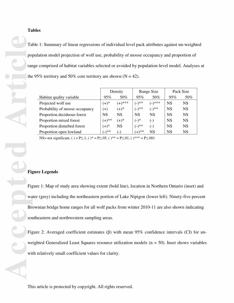
Table 1: Summary of linear regressions of individual level pack attributes against un-weighted

population model projection of wolf use, probability of moose occupancy and proportion of

range comprised of habitat variables selected or avoided by population-level model. Analyses at

the 95% territory and 50% core territory are shown (N = 42).

Density Range Size Pack Size Habitat quality variable 95% 50% 95% 50% 95% 50%

Projected wolf use (+)* (+)*** (-)** (-)*** NS NS Probability of moose occupancy (+) (+)* (-)** (-)** NS NS Proportion deciduous forest NS NS NS NS NS NS Proportion mixed forest (+)** (+)* (-)* (-) NS NS Proportion disturbed forest (+)* NS (-)** (-) NS NS Proportion open lowland (-)** (-) (+)** NS NS NS

NS= not significant, ( ) = P≤.1, ( )* = P≤.05, ( )** = P≤.01, ( )*** = P≤.001

Figure Legends

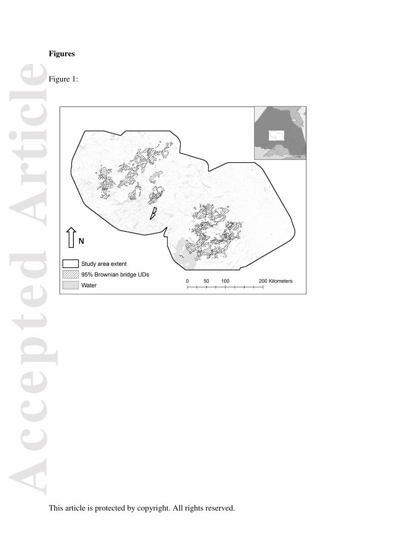
Figure 1: Map of study area showing extent (bold line), location in Northern Ontario (inset) and

water (grey) including the northeastern portion of Lake Nipigon (lower left). Ninety-five percent

Brownian bridge home ranges for all wolf packs from winter 2010-11 are also shown indicating

southeastern and northwestern sampling areas.

Figure 2: Averaged coefficient estimates (β) with mean 95% confidence intervals (CI) for un-

weighted Generalized Least Squares resource utilization models (n = 50). Inset shows variables

with relatively small coefficient values for clarity.

Acc

epte

d A

rtic

le


Figure 3: From 42 pack winters of 26 separate wolf packs, the 95% territory and 50% core area

plots of log(wolf density) as a function of projected wolf use from un-weighted population level

resource utilization model (95%: R² = 0.43, P < 0.05; 50%: R² = 0.57, P < 0.001), and as a

function of probability of moose occupancy (“moose use”) from resource selection probability

function (95%: R² = 0.14, P < 0.1; 50%: R² = 0.18, P < 0.05). Regression lines are shown (solid:

P < 0.05; dotted: 0.1 < P > 0.05).

Figure 4: From 42 pack winters of 26 separate wolf packs, the 95% territory and 50% core area

plots of log(territory size) as a function of projected wolf use from un-weighted population level

resource utilization model (95%: R² = 0.50, P < 0.01; 50%: R² = 0.56, P < 0.001), and as a

function of probability of moose occupancy (“moose use”) from resource selection probability

function (95%: R² = 0.27, P < 0.01; 50%: R² = 0.22, P < 0.01). Regression lines are shown.

Acc

epte

d A

rtic

le


Figures

Figure 1:

Acc

epte

d A

rtic

le


Figure 2:

Acc

epte

d A

rtic

le


Figure 3

Acc

epte

d A

rtic

le


Figure 4

Wolves adapt territory size, not pack size to local habitat quality

Documents

Transcript of Wolves adapt territory size, not pack size to local habitat quality