ISA TRANSACTIONS$

ISA Transactions 44 (2005) 213-223

Computation of stabilizing PI and PID controllers for processes with time delay

Nusret Tan* lnonu University. Engineering Faculty. Dept. of Electrical and Electronics Engineering. 44280. Malatya. Turkey

(Received 6 February 2004; accepted 2 August 2004)

Abstract

In this paper, a new method for the computation of all stabilizing PI controllers for processes with time delay is given. The proposed method is based on plotting the stability boundary locus in the (kp ,k;) plane and then computing the stabilizing values of the parameters of a PI controller for a given time delay system. The technique presented does not need to use Pade approximation and does not require sweeping over the parameters and also does not use linear programming to solve a set of inequalities. Thus it offers several important advantages over existing results obtained in this direction. Beyond stabilization, the method is used to compute stabilizing PI controllers which achieve user specified gain and phase margins. The proposed method is also used to design PID controllers for control systems with time delay. The limiting values of a PID controller which stabilize a given system with time delay are obtained in the (kp ,k/) plane, (kp ,kd) plane, and (k/ ,kd) plane. Examples are given to show the benefits of the method presented. © 2004 ISA-The Instrumentation, Systems, and Automation Society.

Keywords; Stabilization; PI control; PID control; Time delay; Gain and phase margins

1. Introduction

This paper concerns the problem of designing PI and PIO controllers for systems with time delay. Design of controllers for control systems with time delay is very important since most real pro­cesses are represented by time delay models. De­signing stabilizing PI and PIO controllers are of great importance for industrial applications since these controllers are used extensively in the pro­cess industries because of their robust perfor­mance and simplicity. Indeed, more than 90% of the control loops are PIO and most loops are infact PI since derivative action is not used very often [1]. Several methods (see Refs. [1-3], and refer­ences therein) for detennining parameters of these controllers have been developed during past 60

!/IE·mail address: ntan@inonu.edu.tr

years. Some of the most popular methods, are the Ziegler-Nichols tuning method, the Cohen-Coon rules. the Astrom-Hagglund autotuning method, and other methods based on integral perfonnance criteria. However, many important results have been recently reported on computation of all sta­bilizing P, PI, and PIO controllers after the publi­cation of the work by Ho et al. [4 - 7] which is based on the generalized version of the Hermite­Biehler theorem [4]. This new approach has re­vealed important structural properties of PI and PIO controllers. For example, it was shown that for a fixed proportional gain, the set of all stabi­lizing integral and derivative gains lie in a convex set. This method is very important since it can cope with systems that are open loop stable or unstable, minimum, or nonminimum phase. How­ever, the computation time for this approach in­creases in an exponential manner with the order of

0019·0578120051$ • see front matter 0 2005 ISA-The Instrumentation. Systems. and Automation Society.

214 Nusret Tan I ISA Transactions 44 (2005) 213-223

the system being considered. It also needs sweep­ing over the proportional gain to find all stabiliz­ing PI and PID controllers which is a disadvantage of the method. An alternative fast approach to this problem based on the use of the Nyquist plot has been given in Refs. [8-9]. An extension of the method proposed in Ref. [5] to the lagllead con­troller structure has been given in Ref. [to]. A pa­rameter space approach using the singular fre­quency concept has been proposed in Ref. [11] for design of robust PID controllers. More direct graphical approaches to this problem based on fre­quency response plots have been reported in Refs. [12,13]. Computation of the stability region using the stability boundary locus has been given in Ref. [14]. All of these methods, however, have been applied to the systems which do not have time delay. Although these methods can be used to find all the stabilizing values of the parameters of PI and PID controllers for control systems with time delay using the Pade approximation, the results will be inaccurate due to the approximate nature of the Pade approximation as shown in the next sec­tion.

In this paper,. a new approach is given for com­putation of stabilizing PI controllers for processes with time delay in the parameter plane, (kp ,k;) plane. Using the stability boundary locus, a very fast way of calculating the stabilizing values of PI controllers for a given single-input single-output (SISO) control system with time delay is given. The proposed method is also used for computation of PI controllers for achieving user specified gain and phase margins for time delay systems. An ex­tension of the method to find all stabilizing values of the parameters of a PID controller, namely, kp ,

k;, and kd in the (kp ,k;) plane, (kp ,kd) plane, and (k; ,kd ) plane is also given. It is shown that the stability boundary of the convex polygon in the (k; ,kd) plane for a fixed value of kp can be gen­erated from straight lines. The equations of these. straight lines can be easily derived using the sta­bility boundary of the stabilizing regions obtained in the (kp ,k;) plane for fixed values of kd and (kp ,kd) plane for fixed values of k/. The proposed method provides several important advantages such as it can be applied to the control systems with time delay of any order including unstable time delay systems and the method is very simple to use for computation of stability region.

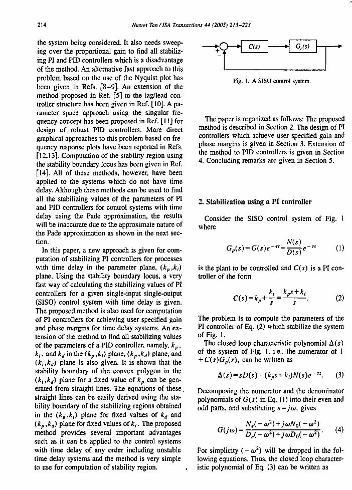
Fig. 1. A SISO control system.

The paper is organized as follows: The proposed method is described in Section 2. The design of PI controllers which achieve user specified gain and phase margins is given in Section 3. Extension of the method to PID controllers is given in Section 4. Concluding remarks are given in Section 5.

2. Stabilization using a PI controller

Consider the SISO control system of Fig. where

N(s) G (s)= G(s)e-rs=--e- rs (1) p L>(s)

is the plant to be controlled and C(s) is a PI con­troller of the form

The problem is to compute the parameters of the PI controller of Eq. (2) which stabilize the system of Fig. 1.

The closed loop characteristic polynomial A(s) of the system of Fig. I, i.e., the numerator of 1 + C(s)Gp(s), can be written as

A(s)=sL>(s)+(kps+ki)N(s)e- rs . (3)

Decomposing the numerator and the denominator polynomials of G(s) in Eq. (1) into their even and odd parts, and substituting s = j w, gives

. Ne( - w2) + jwNo( - w2)

G{jw)= L>,,(-w2)+jwL>O(-w2)" (4)

For simplicity ( - w2) will be dropped in the fol­lowing equations. Thus, the closed loop character­istic polynomial of Eq. (3) can be written as

· Nusret Tan I [SA Transactions 44 (2005) 2/3-223 215

A(jw) = [(k;Ne- kpw2No)coS(WT) + w(k;No

+ kpNe)sin( WT) - w2DO] + j[ w(kiNo

+ kpNe)cos( WT) - (kiNe

- w2kpNo)sin(wT) + wDe]

=R~+jl~=O. (5)

Then, equating the real and imaginary parts of A (j w) to zero, one obtains

kp[ - w2No COS(WT) + wNe sine WT)]

and

+ k;[Ne cos( WT) + wNo sine WT)]= w2Do

(6)

kp[wNe cos( WT) + w2No sine WT)]

+ k;[wNoCOS(WT) -Ne sin(wT)]= - wDe.

(7)

Let us define

Q(w)= wNe sin(wT) - w2NocoS(WT),

and

R( w) =Ne COS(WT) + wNo sine WT),

X(w)= w2Do (8)

and

S(w)= wNe COS(WT) + w2No sin(wT),

U(w)= wNOCOS(WT)- Ne sin(wT),

Y(w)=-wDe· (9)

Then, Eqs. (6) and (7) can be written as

kpQ( w) + k;R(w) =X( w),

kpS(w)+k;U(w)= Yew). (I 0)

Solving Eq. (10), one can obtain

X(w)U(w)- Y(w)R(w) (ll) k = p Q(w)U(w)-R(w)S(w)

and

Y(w)Q(w)- X(w)S(w) (12) k·=

I Q(w)U(w)-R(w)S(w)'

Substituting Eqs. (8) and (9) into Eqs. (11) and (12), it can be found that

(13)

w2(N oD e - N eDO)cos( WT) - weN tP e + w2N oDo)sin( WT) k;= _(N;+w2N~) (14)

It can be seen that if the numerator of Eqs. (13) and (14) Ne(-w2)+w2No(-w2)=I=O then the stability boundary locus, /(kp ,k; ,w), can be con­structed in the (kp ,k/) plane. Once the stability boundary locus has been obtained then it is neces­sary to test whether stabilizing controllers exist or not since the stability boundary locus, /(kp ,k/,w), and the line k;=O may divide the parameter plane [(kp ,k/) plane] into stable and unstable regions. Here, the line k; = 0 is the boundary line obtained from substituting w=o into Eq. (3) and equating it to zero since a real root of A(s) of Eq. (3) can cross over the imaginary axis at s = o.

It can be seen that the stability boundary locus is dependent on the frequency w which varies from 0 to 00. However, one can consider the frequency below the critical frequency, We' or the ultimate frequency since the controller operates in this fre­quency range. Thus, the critical frequency can be used to obtain the stability boundary locus over a possible smaller range of frequency such as w E [O,we]' Since the phase of GpCs) at s= jWe is equal to - 1800

, one can write

( WNo) (WDo) tan- 1 -- -tan- 1 -- -WT=-7T Nt. De

(15)

216 Nusret Tanl/SA Transactions 44 (2005) 213-223

.li

or

~5 ·20 ·15 ·10 o kp

5 10

Fig. 2. Stability boundary locus.

15 20 25

Thus, we is the solution of Eq. (16) in the interval (0, 7T). By plotting tan(wT) and f( w) vs w, it can be seen that We is the smallest value of W at which plots of tan( WT) and f( w) intersect with each other.

Example 1: Consider the control system of Fig. 1 with transfer function

I Gp(s)= S+ 1 e- s

, (17)

which is a stable first order plus time delay pro­cess transfer function where T= I. The aim is to compute all the stabilizing values of kp and k; which make the characteristic polynomial of Eq. (3) Hurwitz stable. From Eqs. (13) and (14)

k p = W sine w) - cos( w),

k;=wsin(w)+w2 cos(w). (I 8)

For WE [0,25], the stability boundary locus is shown in Fig. 2. However, in order to find the stabilizing values of kp and k;, it is only necessary to obtain stability boundary locus for W below the critical frequency We' From Eq. (16), tan(w) =-w=f(w) and the plots of tan(w) and f(w) = - w are shown in Fig. 3 where it has been com­puted that the value of the critical frequency, We'

is equal to 2.0288 rad/s. The region enclosed by the stability boundary locus for WE [0,2.0288] •

.(l.5,----r---....---..----.-----.------.-_

·1

.4, '::-B---:l:-'::9-~2~<IJ~c ~2 7-, --:2-':-2 ---c2..L.3----'-2.4---J2.5 OJ

Fig. 3. Computation of We'

and k; = 0 is the stability region which is the shaded region shown in Fig. 4.

Using the Pade approximation and other results such as Ref. [5] where a new method based on the generalized version of the Hermite Biehler theo­rem has been presented for computation of all sta­bilizing PI and PID controllers, the stabilizing k p

and k; values can be computed. However, the re­sult will not be correct as shown in Fig. 4. The stability region shown in Fig. 4 is obtained taking first order Pade approximation for e - S in Eq. (17) and then using other methods such as Ref. [5]. From Fig. 4, it can be seen that the stability region obtained for the first order Pade approximation en­closes the shaded region which is the correct sta­bility region. For example, for kp =2.5 and k/ = 0.5, using the Nyquist plot or Bode diagram it

Stabllrty Region Ullng FilII 2 Order Pad. Approximation

15

05

.()5 0 05 1 15 2 25 kp

Fig. 4. Stability region.

Nusret Tan liSA Transactions 44 (2005) 213-223 217

can be seen that the system is not stable. However, from Fig. 4, it can be seen that the system after taking the first order Pade approximation is stable for these values of kp and kj • When the order of the Pade approximation is increased, the results obtained using other methods approach to the shaded region. However, in this case, the compu­tation of the stability region will be difficult since the order of the system increases and also the re­sult may still not be exact. It has been observed that when the second order Pade approximation is used the stability region is almost equal to the shaded region. However, the stability region may still include unstable parameters. For example, the point which corresponds to kp = 1.8 and k i = 1.35 is outside of the shaded region but inside the sta­bility region obtained using second order Pade ap­proximation. Thus, the approach presented in this paper have advantages over existing results since it gives exact stability region and it is easy to use for the computation of the stability region.

Furthermore, the method presented can be ap­plied for the case of uncertain parameters. It is well known that the mathematical representations of real physical systems suffer from parametric uncertainty due to modeling errors, nonlinearities, manufacturing tolerances, and operating condi­tions. Therefore, it is very important to take para­metric variation into account while analyzing and designing control systems. Fig. 5 shows the stabil-

-~1!---7-0 -~----:2!---7-3 -~----:5!------:!6

kp

Fig. 5. Stability regions for different values of T.

ity regions for 7'= 0.3, 7'= 0.5, 7'= 1, 7'= 1.2, and 7'= 1.5 in example 1 where it can be seen that the time delay has an important affect on the stability region.

Example 2: Consider a high order unstable sys­tem with time delay

27 Gp(s)= (s_0.I)(s+2.8)3 e -

O.5S

, (19)

which has been studied in Ref. [12]. From Eqs. (13) and (14):

(27w4 -612.36w2 - 59.2704)cos(0.5w) - (- 224.1w3+ 529.2w)sin(0.5w) kp = -729 (20)

and

(- 224.1w4+ 529.2w2)cos(0.5w) + (27w S - 612.36w3 - 59.2704w)sin(0.5w) k,= 729 (21)

Using Eq. (16), it has been computed that We

= 0.9571 radls. The region enclosed by the line k, = 0 and the stability boundary locus, l(kp ,k, ,w), when w varies within w e [0,0.9571] is the stability region. Thus, all the stabilizing values of kp and k j are in the shaded region shown in Fig. 6.

Example 3: Consider

which is a seventh order oscillatory process. It is generally difficult to design controllers which pro-

218 Nusret TanllSA Transactions 44 (2005) 213-223

Fig. 6. Stability region.

vide good performance for oscillatory systems since the transfer functions of such systems have resonant poles. It can be seen that the transfer function of Eq. (22) has six resonant poles. How­ever, the proposed approach can be easily used to compute all stabilizing PI controller for the system of Eq. (22) as follows: From Eqs. (13) and (14),

kp = (Sw2- 2)cos(O.lw) + (- w3

+ lOw)sin(O.1w) (23)

and

kj = (- w4 + lOw2)cos(O.lw) + (- Sw3

+ 2w )sin(O.l w). (24)

Using Eq. (16), it has been computed that We = 2.S983 rad/s. All the stabilizing values of k p

and k j are in the shaded region shown in Fig. 7.

o 5 10 15 20 25 Il 35 kp

Fig. 7. Stability region.

3. Stabilization for specified gain and phase margins

Phase and gain margins are two important fre­quency domain performance measures which are widely used in classical control theory for control­ler design. Consider Fig. 1 with a gain-phase mar­gin tester [IS], Ge(s)=Ae-N , which is con­nected in the feed forward path. Then Eqs. (8) and (9) can be written as

Q( w) =A[wNe( - w2)sin(h)

- w2No( - w2)cos(h)],

R( w) =A[Ne( - w2)cos(h) + wNo( - w2)sin(h)],

S( w) =A[ wNe( - w2)cos(h)

+ w2No( - w2)sin(h)],

U( w) =A[ wNo( - w2)cos(h) - NA - w2)sin(h)]

X(w)=w2Do(-w2), Y(w)=-wDe(-w2), (2S),

where h = wr+ cP. From Eqs. (13) and (14),

(w2 N oDo + NeD e)cos(h) + w(N oD e - NeDo)sin( h)

kp = -A(N;+W2N~) (26)

and

(27)

Nusret Tan/ [SA Transactions 44 (2005) 213-223 219

1.2 r----.----.----.--.....--...---.-----.---,

-05 0 05 1 25 3 kp

Fig. 8. Stability region for cP~45° and A ~ 2.5.

To obtain the stability boundary locus for a given value of gain margin A, one needs to set cfJ=O in Eqs. (26) and (27). On the other hand, setting A == 1 in Eqs. (26) and (27), one can obtain the sta­bility boundary locus for a given phase margin cfJ.

Example 4: Consider

1 Gp(s)= (s+ 1)2 e - s

• (28)

The aim is to find all stabilizing PI controllers which satisfy the conditions that the phase margin of the system is greater than 45° and the gain mar­gin is greater than 2.5. First, let us compute the stability boundary locus. Using Eqs. (13) and (14),

kp= 2w sin(w) - (- w2+ 1 )cos( w),

k;= w( - w2+ l)sin(w) +2w2 cos(w). (29)

The stabilizing region is shown in Fig. 8. To find all stabilizing PI controllers for which the phase margin of the system is greater than 45°, it is re­quired to set A = 1 and cfJ=45° in Eqs. (26) and (27). Using Eqs. (26) and (27) for these values of A and cfJ gives

kp=2w sin(h)- (- w2+ l)cos(h),

k/= w( - w2+ l)sin(h) + 2w2 cos(h), (30)

where h = w+ 'Tr/4. The stability boundary locus for cfJ= 45° with w varying within WE (0,0.895) is shown in Fig. 8. Similarly, setting cfJ = 0 and A == 2.5 in Eqs. (26) and (27):

1.5 r--.....-----.---r----r--..-----.,

0.5

O~-~--~~~----~-~

·2

·25 ·15 ·1 .(1.5 o

Real 05

Fig. 9. Nyquist plot.

1.5

kp = 0.8w sin( w) - 0.4( - w2 + 1 )cos( w),

k;=0.8w2 cos( w) +O.4w( - w2+ 1 )sin( w). (31)

The stability boundary locus for A = 2.5 can be obtained for w E (0,1.307) as shown in Fig. 8. The region obtained from the intersections of these re­gions includes the stabilizing values of kp and k; which make the phase margin of the system

12 kp-O 8 Ind k~.4

08

108 r--- kp· -0.015 .nd k~.27

.0.20 5 10 15 20 25 30 35 40 45 50 Tim.(ltc)

Fig. to. Step responses for different values of kp and kj •

220 Nusret Tan /ISA Transactions 44 (2005) 2/3-223

greater than 4So and the gain margin greater than 2.S. For example, the Nyquist plot of G/jw) C(jw) for kp=0.S2 and k j=0.46 which are com­puted from Fig. 8 at the intersection of the stabil­ity boundary locus for c/>=4So and the stability boundary locus for A = 2.S is shown in Fig. 9 where it can be seen that the gain margin is equal to 2.S and the phase margin is equal to 4So. Step responses for different values of k p and k j within the stability region for A;;;:,2.S and c/>;;;:,45° are shown in Fig. 10.

4. Design of PID controllers

This section deals with the design of PID con­troller. The method proposed in Section 2 is fur­ther developed for computation of stabilizing PID controllers. Consider that C(s) of Fig. 1 is an ideal PID controller of the form

Using the procedure given in Section 2, the stabil­ity boundary locus in the (kp ,kj ) plane can be obtained for a fixed value of kd or in the (kp ,kd) plane for a fixed value of k j • However, it is not possible to obtain the stability boundary locus in the (k j ,kd) plane for a fixed value of kp since Q( w) U( w) - R( w )S( w) will be equal to zero for this case. However, it has been shown in Ref. [S] using the generalized version of the Hermite­Biehler theorem that the stability boundary in the (k j ,kd) plane for a fixed value of kp is a convex polygon. Therefore, it is possible to obtain the sta­bility region in the (k; ,kd ) plane for a fixed value ' of kp using the stability regions obtained in the (kp ,k j) plane and (kp ,kd) plane. To obtain the stability boundary locus in the (kp ,k;) plane in terms of kd' it has been found that kp is the same as Eq. (13) and k; has been computed as

For the computation of the stability boundary locus in the (kp ,kd) plane in terms of k;, it has been calculated that kp is again the same as Eq. (13) and

w2(NoDe- NeDo)cos(wr)- w(NeDe+ w2NoDo)sin(wT)+kj(N;+ w2N~) kd= w2(N;+ w2N~) (34)

Thus, using Eqs. (13), (33), and (34) the stability regions in the (kp ,k j) plane and (kp ,kd) plane can be obtained. Using these stability regions, a new approach for computation of all the stabilizing kp, k;, and kd values is given as illustrated in the following example.

Example 5: Consider a system with the transfer function

_ - O.Ss + 1 -O.6s

Gp(s)-(s+1)(2s+l)e , (35)

which is a process with a right half plane zero. The aim is to find the limiting values of the parameters of a PID controller such that the resulting closed lo~p system is stable. To obtain the stability region in the (k p ,k;) plane in terms of kd' it can be found using Eqs. (13) and (33) that

(3.5w- w3)sin(0.6w) + (3.5w2-1 )cos(0.6w) kp= 0.25w2+ 1 (36)

and

(3.Sw2- w4 )cos(0.6w) + (w- 3.5w3)sin(0.6w) + kd(0.2Sw4 + w2) k j = 0.,25w2+ I (37)

Nusret Tan / [SA Transactions 44 (2005) 2/3-223 221

The stability regions for kd=O and kd=0.5 are shown in Fig. 11. For the computation of the stabilizing regions in the (kp ,kd) plane for fixed k;, it has been calculated that kp is the same as Eq. (36) and from Eq. (34), one can obtain

(w4 - 3.5(2)cos(0.6w) + (3.5w3 - w)sin(0.6w)+ k;(0.25w2+ 1) kd=------------------0-.~25~w-4T+--w~2--------~-------- (38)

The stability regions for k;=O.1 and k;=0.5 are shown in Fig. 12. Since it is known that the sta­bility region in the (k; ,kd ) plane for a fixed value of kp is a convex polygon [5], it is possible to obtain this polygon using Figs. 11 and 12. From Fig. 11 it can be seen that there are two stability regions in the (k p , k;) plane obtained for k d = 0 and kd= 0.5, therefore, one can obtain equations of two straight lines which contribute to the boundary of the stability region for each value of k p. For example, it is clear from Fig. 11 that the line k p = 1 intersect with the boundary of the sta­bility region for kd=O when k;=O and k;=0.96. Similarly, the line k p = 1 intersect with the bound­ary of the stability region for kd= 0.5 when k; =0 and k;= 1.162. So, one straight line passes through the points (k; ,kd ) = (0.96,0) and (k; ,kd )

= (1.162,0.5) and the other straight line passes through the points (k; ,kd) = (0,0) and (k; ,kd) = (0,0.5) for k p = 1. Thus the equations of these two straight lines are

• II:' kd=2.5k j-2.4 and 12 : kj=O. (39)

Similarly, from Fig. 12, it is also clear that one straight line going through the points (k; ,kd )

·0 2,·L--:.(I~5--~O---:-'0'-5 --l--1:-':5'---~2----::-2'::-5 -~--,J3 5

kp

Fig. II. Stability region in the (kp .k;) plane for kd=O and kd=O.5.

=(0.1,3.29) and (k; ,kd) = (0.5,3.38) and the other one going through (k;,kd)=(0.1,-2.15) and (k;,kd)=(0.5,-1.14) for kp= 1. The equa­tions of these two straight lines are

13: kd=0.225k;+ 3.2675,

14: kd=2.525k;-2.4. (40)

These four lines are shown in Fig. 13 where the shaded region is the stability region in the (k; ,kd )

plane for k p = 1. Repeating the procedure for dif­ferent values of proportional gain, kp , the stabiliz­ing kp , k;, and kd values can be shown in the three-dimensional plot of Fig. 14. The step re­sponses of the system for different values of k p ,

k;, and kd , which are obtained from the stability domain of Fig. 14, using Simulink are shown in Fig. 15.

It can be seen that all stabilizing PID controllers can be computed graphically with the proposed approach once the stability regions in the (kp ,k;) plane and (k p ,kd ) plane have been plotted. Since a graphical approach is adopted, generating the set of stabilizing PID controllers without human inter­actions seems to be difficult. However, one can

:ll 0

.,

., ·3 ., .(15 0 05 15 25 3 35

kp

Fig. 12. Stability region in the (kp.kd) plane for k;=O.l and k{=O.5.

222 Nusret Tan I [SA Transactions 44 (2005) 2/3-223

~1 .0.5 o 05 15 kl

2 25

Fig. 13. Stability region for kp = I.

35

easily overcome this difficulty with the aid of spe­cialized software programs such as MATLAB. It is also clear that to ~btain the complete stability do­main, one must resort to a grid on k p' However, the range of k p over which gridding needs to be done can be reduced using Figs. 11 and 12. It will be a very good result to obtain the complete sta­bility domain without gridding but this seems im­possible for PID.

5. Conclusions

In this paper, a new approach has been presented for the computation of the boundaries of the lim­iting values of PI and PID controller parameters that guarantee stability of control systems with time delay. The approach is based on the stability

.' . 4 ••••

.. -"~ 3 ••••

2 •••••

kp 1 •• ,

·1 o

6 -5

-"

.. .. r"'"'· ...... , ,

......... ~ .......... -,

Fig. 14. Stabilizing kp, k" and kd values.

5

16 kp-3, k,.o 6 and kd=1 8

1.4

12

r-"--I--+ kp-1, kl"ll4 Ind kd-l

/--_ kp&{l25, kP'O 1 and kdLl

5 10 15 20 25 :lJ 35 40 45 50 TIm.(I.c)

Fig. 15. Step responses for different values of kp' k" and kd •

boundary locus which can be easily obtained by equating the real and the imaginary parts of the characteristic equation to zero. The computation of PI compensator parameters for achieving user specified gain and phase margins has also been studied. The method presented does not require sweeping over the parameters for the computation of stabilizing PI controllers. Also, it does not need linear programming to solve a set of inequalities as other methods [5] requires. Although it needs a grid on proportional gain for computation of all stabilizing PID controllers, it provides a graphical feature which facilitates computation of stabilizing convex polygon. Therefore, the proposed method has advantages over existing results such as Refs. [5] and [9]. The examples given clearly show the value of the method presented for the analysis and design of time delay systems. .

References

[1] Astrom, K. J. and Hagglund, T., The future of PID control. Control Eng. Pract. 9, 1163-1175 (2001).

[2] Zhuang, M. and Atherton, D. P., Automatic tuning of optimum PID controllers. IEE Proc.-D: Control Theory Appl. 140,216-224 (1993) .

[3] Astrom, K. J. and Hagglund, T., PIO Controllers: Theory, Design, and Tuning. Instrument Society of America, Research Triangle Park, NC, 1995.

[4] Ho, M. T., Datta, A., and Bhattacharyya, S. P., A new approach to feedback stabilization. Proc. of the 35th CDC, 1996, pp. 4643-4648.

[5] Ho, M. T., Datta, A., and Bhattacharyya, S. P., A linear programming characterization of all stabilizing PID controllers. Proc. of Amer. Contr. Conf., 1997.

[6] Ho, M. T., Datta, A., and Bhattacharyya, S. P., A new

NLisret Tan / ISA Transactions 44 (2005) 213-223 223

approach to feedback des ign Part I: Genera lized inter­lacing and proportional contro l. Dept. of Electrical Eng., Texas A&M Uni v., College Station, TX, Tech. Report TAMU-ECE97-00 I-A, 1997.

[7] Ho, M. T. , Datta, A., and 8hattacharyya, S. P., A new approach to feedback des ign Part II : PI and PID con­trollers. Dept. of Electri cal Eng., Texa A&M Uni v .. College Station, TX, Tech: Report TAMU-ECE97-001 -8 , 1997.

[8] Munro, N. and Soylemez, M. T. , Fa t calculation of stabilizing PID controllers for uncertain parameter systems. Proc. Sympos ium on Robu t Control, Prague, 2000.

[9] Soylemez, M. T. , Munro, N., and 8 aki, H., Fast calcu­lation of stabilizing PID controllers. Automatica 39. 121- 126 (2003).

[ 10] Tan, N., Computation of stabil ization lag/lead control­ler parameters. Compul. Electr. Eng. 29. 835- 849 (2003).

[II] Ackermann. J. and Kaesbauer, D .. Design of robust PID controllers. European Control Conference, 527, 2001 , pp. 522-527.

[1 2] Shafi ei, Z. and Shenton, A. T. , Frequency domain de­sign of Pro controller for stable and unstable y terns with time delay. Automatica 33, 2223- 2232 (1997) .

[13] Huang. Y. J. and Wang, Y. 1.. Robu t PID tuning strat­egy for uncertain plants based on the Kharitonov theo­rem. ISA Trans. 39. 419-43 1 (2000).

[ 14] Tan, N., Kaya, I., and Atherton, D. P., Computation of stabil izing Pl and PID controllers. Proc. of the 2003 IEEE Intern . Conf. on the Control Appl ications (CCA2003), Istanbul , Turkey. 2003.

[15] Argoun, M. 8 . and 8 ayoumi, M. M., Robust gain and phase margins fo r interval uncertai n system . 1993 Canadi an Conf. on Electrical and Computer Eng., 1993, pp. 73-78.

Nusrel Tan was born in Malatya. Turkey. in 1971. He received his B.Sc. degree in electrical and electronics engi­neering from Hacettepe Uni­versity. Ankara. Turkey. in 1994. He received hi Ph.D. degree in control engineeri ng from Universi ty of Su sex. Brighton. UK. in 2000. He is currenl ly working as an as aci­ate profe sor in the department of electrical and electronics en­gineering at Inonu Univer i!y,

Malatya. Turkey. His primary research interest lies in the area of sys­tems and control.